mass extinctions and the structure and function of … · mass extinctions profoundly influence the...
TRANSCRIPT

MASS EXTINCTIONS AND THE STRUCTURE AND FUNCTION OF ECOSYSTEMS
PINCELLI M. HULL AND SIMON A. F. DARROCH
Department of Geology & Geophysics, Yale University, PO Box 208109, New Haven, CT 06520-8109 USA
ABSTRACT.–Mass extinctions shape the history of life and can be used to inform understanding of the current biodiversity crisis. In this paper, a general introduction is provided to the methods used to investigate the ecosystem effects of mass extinctions (Part I) and to explore major patterns and outstanding research questions in the field (Part II). The five largest mass extinctions of the Phanerozoic had profoundly different effects on the structure and function of ecosystems, although the causes of these differences are currently unclear. Outstanding questions and knowledge gaps are identified that need to be addressed if the fossil record is to be used as a means of informing the dynamics of future biodiversity loss and ecosystem change.
INTRODUCTION
Mass extinctions profoundly influence the history of life. Although they are defined by their impacts on taxonomic diversity (e.g., Raup and Sepkoski, 1982; Sepkoski, 1986), their effects extend far beyond the loss of species richness. Mass extinctions have shaped the history of Phanerozoic biodiversity, sparked innovations in morphology, life history, and ecology, and led to the construction of entirely new ecosystems in their aftermath (e.g., Sepkoski, 1981; Bambach et al., 2002; Wagner et al., 2006; Erwin, 2008). For example, the Permo–Triassic extinction event permanently altered the composition of marine ecosystems from one dominated by brachiopods and crinoids to one dominated by mollusks and echinoderms (Gould and Calloway, 1980; Sepkoski, 1981; Erwin, 1990; Greene et al., 2011). Similarly, the Cretaceous–Paleogene mass extinction reset open-ocean food webs, with two groups of top marine predators in late Cretaceous food webs, non-acanthomorph fishes and marine repti les, replaced in the Paleogene by acanthomorph fishes and marine mammals, respectively (Friedman, 2010; Uhen, 2010). More broadly, the ecological effects of mass extinctions include the flourishing of unusual ecosystems in their immediate aftermath, feedbacks within and between the geosphere and biosphere, and long-term changes in the structure and function of earth’s ecosystems.
A paleontological perspective on the history of life, particularly regarding past biotic crises, is now in demand (Erwin, 2009; Barnosky et al., 2011; Harnik et al., 2012; Hönisch et al., 2012). The cumulative effects of humanity on the earth, ocean, atmosphere, and biosphere arguably are driving the sixth major mass extinction (Myers, 1990; Leaky and Lewin, 1992). While this classification is still debated (Barnosky et al., 2011), the potential for anthropogenic activity to change the biosphere is not. Anthropogenic influences detrimental to ecosystems include extensive habitat modification and fragmentation, the introduction of nonnative and invasive species, overexploitation of natural resources, pollution, global climate change, and ocean acidification, among many others (IUCN; Hassan et al., 2005; Fischlin et al., 2007; Halpern et al., 2008). Past ecosystem dynamics may help inform the present diversity crisis by revealing how the interaction between environmental perturbations, species diversity, and ecosystem structure influence species extinction and ecosystem change. This includes understanding the potential importance of ecosystems in mitigating or enhancing the effects of environmental disturbance on the loss of species, the rate of rediversification, or the change in ecosystem function across mass-extinction events (Erwin, 2001; Jackson and Erwin, 2006; Barnosky et al., 2011).
In Ecosystem Paleobiology and Geobiology, The Paleontological Society Short Course, October 26, 2013. The Paleontological Society Papers, Volume 19, Andrew M. Bush, Sara B. Pruss, and Jonathan L. Payne (eds.). Copyright © 2013 The Paleontological Society.
Advances in the understanding of mass extinctions and the structure and function of ecosystems have the potential to be utilized in predicting the course of the modern biodiversity crisis. This paper aims to give an overview of this interdisciplinary field by providing a general introduction alongside a discussion of outstanding questions and issues. Specifically, Part I introduces key concepts in ecosystems ecology, background on the largest five mass extinction events in the Phanerozoic, and an overview of major ecosystem proxies. Readers who are well-versed in these topics are encouraged to skip through this section to Part II. In Part II, four major open questions with modern implications are explored: 1) What evidence exists for changes in ecosystem structure and function across mass extinctions? Does the ecosystem response scale with the magnitude of the mass extinction? 2) Do trophic structure, food web interactions, or extinction selectivity play a role in determining the overall severity of species loss or the rate of subsequent rediversification? How are these effects distinguished from those of an exogenous disturbance? 3) Do interactions among major biomes (e.g., terrestrial, shallow marine, open ocean) influence the pattern or rate of extinction and recovery? 4) What are the major issues with scaling the ecosystem lessons of past biodiversity crises to the modern world? These questions reflect a current emphasis within paleontology on the interactions and feedbacks between the history of earth and life. By directly measuring, modeling, and testing the dynamics of the integrated system, this focus on ecosystems paleobiology promises to move paleontology toward a more mechanistic understanding of the past and future world. We hope to encourage further research with this introduction to the concepts and outstanding questions regarding ecosystems and mass extinctions. Note that this paper focuses largely on marine rather than terrestrial environments because of limits of space and our primary areas of expertise, rather than a lack of information regarding terrestrial environments. For similar reasons, there is an emphasis on empirical over modeling approaches, and discussion of only the five largest mass extinction events.
PART I: ECOSYSTEMS, EXTINCTIONS, AND PROXIES
Part I is designed to serve as a brief primer in the necessary terminology, background, and tools needed to conduct research on the effects of mass extinctions on the structure and function of ecosystems. For those who are well acquainted with this field, reading the section ‘Ecosystem structure and function’ for terminology definitions and usage may be useful before skipping ahead to the open questions of Part II.
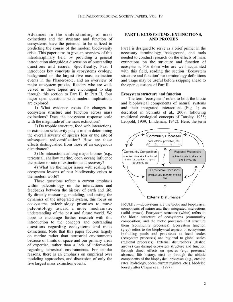
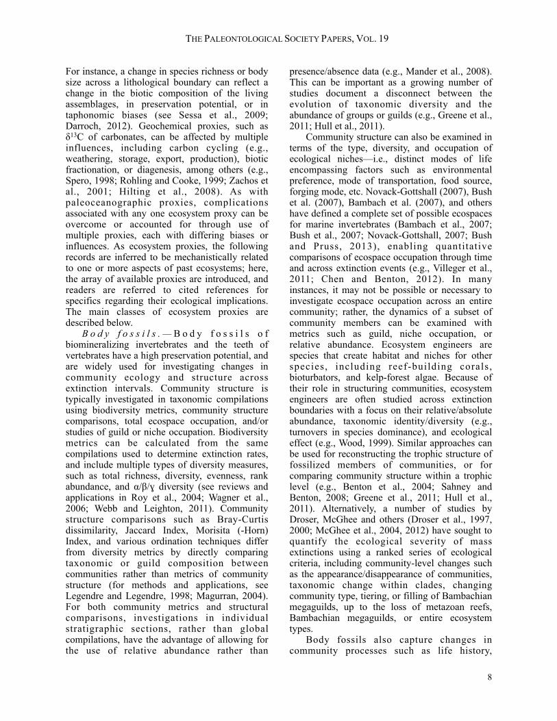
Ecosystem structure and function The term ‘ecosystem’ refers to both the biotic and biophysical components of natural systems and their integrated interactions (Fig. 1; as described in Schmitz et al., 2008, following traditional ecological concepts of Tansley, 1935; Leopold, 1939; Lindeman, 1942). Here, the term
THE PALEONTOLOGICAL SOCIETY PAPERS, VOL. 19
2
FIGURE 1.—Ecosystems are the biotic and biophysical components of nature and their integrated interactions (solid arrows). Ecosystem structure (white) refers to the biotic structure of ecosystems (community composition) and the biotic processes that structure them (community processes). Ecosystem function (grey) refers to the biophysical aspects of ecosystems including pools and processes at local scales (ecosystem processes) and regional to global scales (regional processes). External disturbances (dashed arrows) can disrupt ecosystem structure and function through direct effects on species (e.g., presence/absence, life history, etc.) or through the abiotic components of the biophysical processes (e.g., erosion rates, hydrology, ocean current regimes, etc.). Modeled loosely after Chapin et al. (1997).

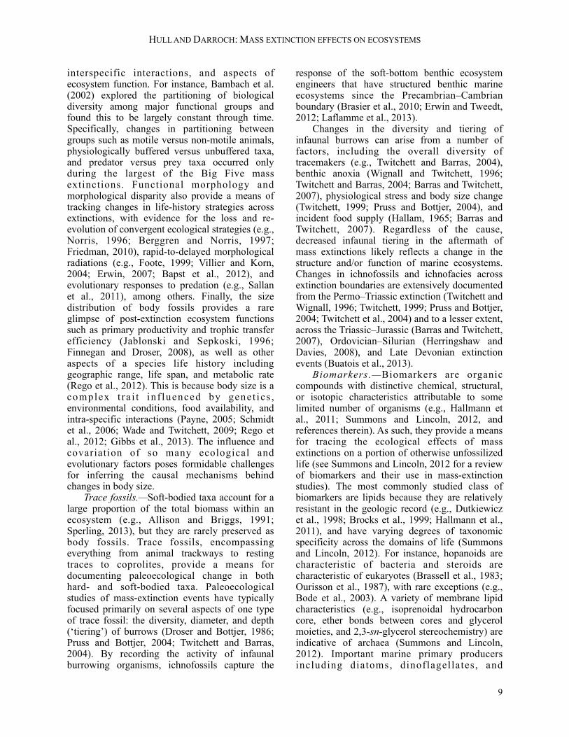
‘ecosystem structure’ is used mainly in reference to the biotic structure of ecosystems, including the distribution and abundance of species, or of individuals within and across trophic levels, or by functional traits (i.e., guilds or ecological niches), or by interactions with one another (e.g., predation, competition, and mutualism) (Chapin et al., 1997; Hooper et al., 2005; Schmitz et al., 2008). In contrast, the term ‘ecosystem function’ is used to refer to the biophysical aspects of ecosystems, including the reservoirs and processes involved in nutrient cycling, productivity, and trophic transfer efficiency (after Hooper et al., 2005; Schmitz et al., 2008). Ecosystem structure and function encapsulate factors and processes acting over multiple spatial scales, across a range of timescales, and at substantially different rates (e.g., Levin, 1992; Chapin et al., 1997; Carpenter et al., 2006). On local to regional scales, ecosystem functions can include formation of soils, accumulation of biomineralized calcium carbonate, and export of organic matter from the ocean surface to the deep ocean. For example, these functions can influence silicate weathering, dust flux to the open ocean, s t r e am nu t r i en t l oads t o nea r- coas t a l e n v i r o n m e n t s , a n d a t m o s p h e r i c p C O 2 concentrations on regional to global scales. Ecosystem structure is similarly scale-dependent. For example, the field of macroecology focuses on understanding the determinants of species distributions and community structure from local to global scales (Brown, 1995). In time, important biotic and biophysical processes on short t imescales include interactions such as competition, predation, the uptake of nutrients from the surface ocean, and seasonal peaks in productivity. Longer timescale processes include population differentiation, speciation, weathering, and organic carbon burial. Ecologists have struggled to account for this vast range of interactions in forecasting the response of modern ecosystems to unprecedented environmental change (Levin, 1992; Chapin et al., 1997; Carpenter and Turner, 2000). The fossil record has perhaps its greatest potential in this area, as it can reveal the role and importance of slow or infrequent ecological processes to the structure and function of current and future ecosystems. Mass-extinction events have a relatively long history of investigation regarding their effects on biodiversity. As a result, a distinct nomenclature has arisen describing the various phases and taxa present across extinction intervals (Fig. 2). A mass
extinction can be divided into four main intervals: pre-extinction, extinction, recovery, and post-extinction. There has been the tendency to adopt the same terminology to describe ecosystems across extinction intervals as well. This may not be a good practice for two reasons. First, a growing body of evidence suggests that the timing of ecological and evolutionary changes across extinction boundaries can be decoupled (e.g., Greene et al., 2011; Hull et al., 2011). For instance, after an extinction event, some ecosystem functions can match those of pre-extinction ecosystems long before taxonomic diversity recovers. Thus, the use of the same
HULL AND DARROCH: MASS EXTINCTION EFFECTS ON ECOSYSTEMS
3
FIGURE 2.—Proposed nomenclature for discrete phases of (top) purely taxonomic richness dynamics, and (bottom) all other ecological changes in response to an extinction-causing perturbation. The ecological transition interval coincides with the extinction-causing perturbation, a period that may or may not coincide with the extinction interval (top), depending on the importance of ecosystem feedbacks on taxonomic loss. This is followed by the ecological flux interval, defined by the presence of short-lived, often uniquely structured, ecosystems. Flux ecosystems are subsequently replaced by stable, post-extinction communities typical of the geological interval that follows. One advantage of separating the terminology between the loss and gain of taxa and all other changes in ecosystem structure and function is that it allows for possible differences in the timing of phases. Note that the ecosystem metric can hypothetically correspond to any aspect of ecosystem structure or function.

extinction and recovery terminology for both taxonomic and ecological change can be confusing. Shared terminology also implies a known mechanistic link between diversity and ecology following extinctions, effectively hiding an important set of questions. Second, although the term ‘recovery’ makes sense in the context of recovering levels of taxonomic diversity similar to pre-extinction levels of diversity, this is not necessarily true for the various aspects of ecosystem structure and function because of the potential for long-term shifts in environmental state (e.g., Wagner, 2006) and a lack of inherent directionality in ecological change. How can an ecosystem before or after an extinction event be determined to be ‘recovered’ or more or less ‘stressed’? For example, comparing a community of crinoids in pre-extinction, well-ventilated oceans with microbial reefs thriving in post-extinction euxinic conditions is problematic, as both may represent climax communities that were well adapted to local environmental conditions. To avo id these p rob lems , a separa te , nondirectional set of terms is used herein to describe ecosystems across extinction boundaries: the pre-extinction, transition, flux, and post-ecosystem intervals (Fig. 2). In this terminology, the ecosystem transition interval coincides with the presence of the ext inct ion-causing perturbation, and the ecosystem flux interval coincides with the subsequent presence of short-lived, often uniquely structured, ecosystems (Fig. 2).
The Big Five Phanerozoic mass-extinction events During mass-extinction intervals, a large proportion of Earth’s species are lost in a geologically brief time interval (Sepkoski, 1986; Hallam and Wignall, 1997). Modern interest in mass extinctions and their effects arose from examining compilations of marine diversity through time (Schindewolf, 1954; Beurlen, 1956; Newell, 1962; 1967; Raup and Sepkoski, 1982). What are now known as the ‘Big Five’ mass extinctions were identified by Raup and Sepkoski (1982) based on what they perceived as unusually large proportional losses of marine families. This paper focuses on the ecological dynamics of the Big Five mass extinction events. Whereas a comprehensive understanding of the effects of extinctions on ecosystems would require investigating events at a wide range of spatial, temporal, and taxonomic scales and
resolutions, the aim here is to introduce emergent patterns and outstanding questions and issues in the field. A brief review of the current research regarding each of the Big Five is provided below as context for later discussions. For each of the discussions of the Big Five mass extinctions, extinction age is listed as the age of initial extinction pulse (as in Bambach, 2006) rounded to the nearest million year. Three estimates of genus-level extinction intensity are then listed, with differences among estimates reflecting ongoing methodological developments regarding the incorporation of sampling biases into calculations of past diversity: 1) S.89 (Sepkoski, 1989; S.89* values reported in Jablonski, 1991 citing Sepkoski, 1989). 2) B.06 (Bambach, 2006; % extinction rather than % diversity loss). 3) A.08 (Alroy et al., 2008). Descriptions follow and expand on overviews by Hallam and Wignall (1997), Bambach (2006), Barnosky et al. (2011), and Harnik et al. (2012). Late Ordovician extinction (~447 Mya) % extinction: 61S.89*–57B.06 .—The Ordovician–Silurian (O–S) mass extinction occurred in two distinct pulses approximately at the start and end of the latest Ordovician Hirnantian stage, coinciding with an interval of global cooling following the uplift and weathering of the Appalachians and subsequent CO2 drawdown (Kump et al., 1999; Sheehan, 2001; Brenchley et al., 2003). The O–S extinction is also referred to in the literature as the mid–late Ashgillian extinction (see Bambach, 2006). The first global pulse of extinction is associated with the onset or intensification of glaciation, which lead to a ~100 m sea-level fall and cooler temperatures (6 °C cooling) in the Hirnantian (Brenchley et al., 1994; Sheehan, 2001; Finnegan et al., 2011). Extinction was likely driven by some combination of habitat loss in shallow epicontinental seaways, the thermal stress of cooling from after the extreme Late Ordovician greenhouse, and increased deep-water anoxia and euxinia (Berner, 2006; Finnegan et al., 2011, 2012; Hammarlund et al., 2012). The second pulse of extinction was apparently more regional, such that the timing of recovery varies between paleocontinents (Krug and Patzkowsky, 2007). Extinction mechanisms for the second pulse are less clear (Finnegan et al., 2012). However, the termination of peak glaciation, warming, and regional anoxia also point towards a changing depth distribution of anoxic bottom
THE PALEONTOLOGICAL SOCIETY PAPERS, VOL. 19
4
waters as a possible kill mechanism (Sheehan, 2001; Bambach, 2006; Zhang et al., 2009; Hammarlund et al., 2012). In terms of overall ecological effects, post-extinction ecosystems largely resemble those of the pre-extinction interval (Droser et al., 1997, 2000; Sheehan, 2001; McGhee et al., 2012), although Silurian ecosystems did not exhibit pre-extinction levels of complexity until five Ma after the initial extinction pulse (Brenchley et al., 2001). Late Devonian (~378 Mya) % extinction: 55S.89*–35B.06 .—The Late Devonian extinction, like the Late Ordovician extinction, was associated with an episode of global cooling followed by g l o b a l w a r m i n g , a l t h o u g h t h e a c t u a l mechanism(s) of extinction is debated (McGhee, 1996; House, 2002; Joachimski et al., 2002; Bambach, 2006). The Late Devonian extinction is traditionally placed among the ‘Big Five’ and is also referred to as the Frasnian/Famennian (F/F), late Frasnian, or Upper Kellwasser Event (House, 2002; Bambach, 2006). In contrast to the rest of the Big Five, the loss of biodiversity in the Late Devonian seems to have been driven primarily by decreased speciation rates, rather than increased extinction (Bambach et al., 2004). Accordingly, Bambach et al. (2004) reclassified the F/F as a ‘mass depletion’ event rather than a mass extinction. In addition, the F/F does not supersede other mid-to-late Devonian events by much in terms of magnitude, with extinction intensities of 31% and 28.5% for the latest Devonian late Famennian event (a.k.a. Hangenberg event), and Middle Devonian late Givetian event, respectively (Bambach et al., 2004; Bambach, 2006). More recent biodiversity compilations suggest that the relative magnitude of biodiversity loss is higher in the late Famennian and late Givetian events than in the Frasnian/Famennian event (House, 2002). The F/F may be a two-pulse extinction, with the first pulse coinciding with sea-level fall, and the second with sea-level rise (Chen and Tucker, 2003). Habitat fragmentation through repeated regressions/transgressions (e.g., anoxia in the Kellwasser events) and temperature change is the primary hypothesized driver of the extinction (Copper, 2002; Chen and Tucker, 2003; Bambach, 2006). Ultimately, the diversification of land plants may have caused the extinction event by increasing weathering, leading to CO2 drawdown and cooling, increased nutrient flux, and increased anoxia in the marine realm (Algeo and Scheckler, 1998; Copper, 2002; Godderis and Joachimski, 2004; Malkowski and Racki, 2009). The F/F mass
depletion had a devastating impact on reefs, likely due to the marine regression (Copper, 2002; Wood, 2004). The reestablishment of reef ecosystems following the extinction tracked the availability of favorable environmental conditions (Wood, 2004). Overall, the Late Devonian extinction had relatively minimal long-lasting ecological effects; post-extinction ecosystems largely resembled those of the pre-extinction interval (Droser et al., 1997, 2000). Late Permian (~252 Mya) % extinction: 84S.89 – 56B.06–78A.08 .—The Permo–Triassic (Late Permian, Changhsingian, Permian–Triassic, or P–T) mass extinction was the most severe of the Phanerozoic, with approximately ~90% of biomineralizing marine species estimated as having gone extinct (Knoll et al., 2007; Chen and Benton, 2012). Recent work has affirmed the high genus-level extinctions of the late Permian event (79%) compared to the relatively minor (24%) end middle Permian event (Clapham et al., 2009; Payne and Clapham, 2012), mitigating earlier concerns about distinguishing the cause and effects of the two events. The main extinction pulse of end-Permian occurred over an extremely short period (Shen et al., 2011) and has been linked to the release of volatiles associated with the onset of Siberian flood-basalt volcanism into carbon- and sulfur-rich sediments (Ganino and Arndt, 2009; Black et al., 2012). Volcanism caused extinction through some combination of global warming, widespread shallow-water anoxia and euxinia, ocean acidification, and elevated atmospheric H2S and CO2 (Wignall and Twitchett, 1996; Berner, 2002; Grice et al., 2005; Erwin, 2006; Knoll et al., 2007; Payne and Clapham, 2012). Associated with the end-Permian mass extinction are a number of pronounced geochemical changes, including multiple excursions in δ13C, δ44/40Ca, and δ15N, and positive shifts in δ34S and 87Sr/86Sr, suggesting, respectively, carbon injection, ocean acidification, regional increase in nitrogen fixation, changing ocean stratification or pyrite burial, and enhanced weathering (Erwin et al., 2002; Korte et al., 2004; Meyer et al., 2011; Payne and Clapham, 2012). The extinction selected against physiologically unbuffered taxa (i.e. those with carbonate skeletons) and reef organisms (Erwin, 1994; Knoll et al., 1996; Knoll et al., 2007; Clapham and Payne, 2011). Ecosystem structure was profoundly altered during the transition and flux interval, particularly for the duration of Siberian
HULL AND DARROCH: MASS EXTINCTION EFFECTS ON ECOSYSTEMS
5
volcanism, with the growth of microbialite reefs and anachronistic carbonate facies (e.g., Kershaw et al., 2012), collapse of ecological infaunal and epifaunal tiering (Twichett, 2006), widespread dwarfing of taxa (‘Lilliput effect’), high oceanic productivity, near-absence of calcareous algae, and altered balance of life-history strategies (Erwin et al., 2002; Chen and Benton, 2012; Payne and Clapham, 2012). Late Triassic (~201 Mya) % extinction: 47S.89–47B06–63A08 .—Similar to the P–T, the Late Triassic (Triassic–Jurassic, or T–J) extinction is tightly linked to the onset of flood-basalt volcanism (Hesselbo et al., 2007; Whiteside et al., 2010; Blackburn et al., 2013). Central Atlantic Flood Basalt (CAMP) volcanism led to elevated atmospheric CO2 levels (among other gases), causing brief global warming, ocean acidification, enhanced weathering, longer term global cooling, and atmospheric pollution (Beerling, 2002; van de Schootbrugge et al., 2009; Schaller et al., 2011, 2012; Martindale et al., 2012). The magnitude and duration of this extinction is debated (see discussion in Bambach, 2006), including the relative importance of decreased origination versus elevated extinction rates (Bambach et al., 2004). However, the extinction clearly selected against calcified reef organisms (Bambach, 2006; Martindale et al., 2012). In fact, the T–J and P–T mass extinctions represent the two largest reef crises of the Phanerozoic (Kiessling and Simpson, 2011). Chronic environmental disturbance across the T–J is suggested by δ13C, biomarkers, δ15N, and δ34S, and is linked to the timing and pattern of post-extinction evolution and ecological change in marine and terrestrial systems (Hesselbo et al., 2007; van de Schootbrugge et al., 2007, 2008; Williford et al., 2009; Whiteside and Ward, 2011; Bachan et al., 2012; Bartolini et al., 2012; Richoz et al., 2012). In the terrestrial realm, climate change and elevated CO2 across the end-Triassic extinction predominately affected community structure among plants (McElwain et al., 2007, 2009; Mander et al., 2010; Bonis and Kurschner, 2012), and it also ranks as the third largest tetrapod extinction (Benton, 1989; 1995). End-Cretaceous (~65 Mya) % extinction: 47S.89–40B06–55A08 .—The end-Cretaceous mass extinction (Cretaceous–Paleogene, or K–Pg) is the only one of the Big Five extinction events directly triggered by a bolide impact (D'Hondt, 2005; Schulte et al., 2010). The impact structure is the largest known in the Phanerozoic, and likely involved an impactor of >10 km diameter
(Hildebrand et al., 1991; Morgan et al., 1997). The exis tence of an impact s t ructure , simultaneous global deposition of impact markers such as shocked quartz, tecktites, and iridium, and the coincident mass extinction of abundant planktonic animals, all support the original hypothesis of Alvarez et al. (1980) for an impact-triggered extinction (Smit and Hertogen, 1980; Smit, 1999; Mukhopadhyay et al., 2001; Claeys et al., 2002; Renne et al., 2013). The exact kill mechanisms may have varied among affected taxonomic groups, but include global darkness leading to starvation, acid rain, extreme surface heating, and subsequent impact winter (Toon et al., 1997; Alegret et al., 2012). Extinction was apparently geologically instantaneous after accounting for Signor-Lipps effects among rare taxa (e.g., Sheehan et al., 1991), and selectively affected some taxa, including those with small geographic ranges (Jablonski and Raup, 1995; Longrich et al., 2012), calcareous plankton (D'Hondt, 2005), and top predators (Sheehan and Hansen, 1986; Friedman, 2009). The relative influence of the Deccan volcanism in altering pre-impact communities continues to be debated (e.g., Chenet et al., 2009; Archibald et al., 2010; Keller et al., 2010), although a more compelling argument may be made for volcanism in structuring post-impact communities (see discussion below). Associated with the end-Cretaceous mass extinction are a number of pronounced geochemical changes, including declines/excursions in δ13C, δ7Li, Li/Ca, 187/186Os, and an inflection point in 87Sr/86Sr, all suggesting changes in global carbon cycling and terrestrial weathering (e.g., D'Hondt, 2005; Misra and Froelich, 2012). As with the P–T, the structure of flux ecosystems was profoundly altered relative to pre-extinction communities (e.g., Aberhan et al., 2007), with dwarfing of taxa (Longrich et al., 2012), a change in the dominant oceanic primary producers (Hull and Norris, 2011), enhanced inter-ocean basin differences in community structure (Hull et al., 2011), altered balance in l i fe-history strategies, and turnover in evolutionary faunas (Droser et al., 2000; Bambach et al., 2002). Although each of the Big Five extinctions is unique in both cause and effect (see Wang, 2003; Bambach et al., 2004), there are shared characteristics across events. Notably, both the Late Ordovician and the Late Devonian extinctions are two-pulse events associated with
THE PALEONTOLOGICAL SOCIETY PAPERS, VOL. 19
6
global cooling and marine regression, followed by global warming. Both the end-Permian and Late Triassic extinctions may have been precipitated by flood basalts, are associated with ocean acidification, and are followed by lengthy recovery intervals as a result of ongoing perturbation. Additional commonalities and contrasts among the Big Five will be discussed throughout the remainder of the paper in the context of associated ecological change.
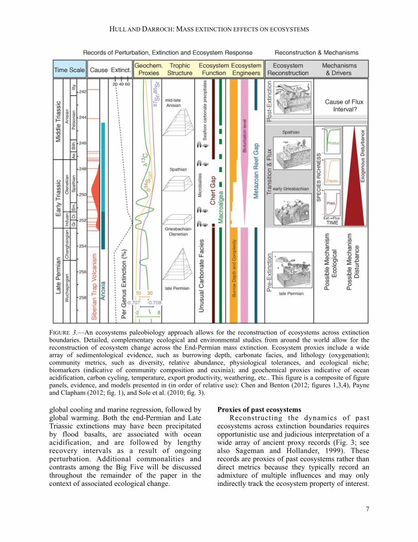
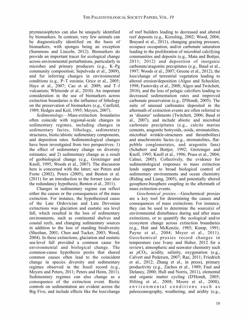
Proxies of past ecosystems Reconstructing the dynamics of past ecosystems across extinction boundaries requires opportunistic use and judicious interpretation of a wide array of ancient proxy records (Fig. 3; see also Sageman and Hollander, 1999). These records are proxies of past ecosystems rather than direct metrics because they typically record an admixture of multiple influences and may only indirectly track the ecosystem property of interest.
HULL AND DARROCH: MASS EXTINCTION EFFECTS ON ECOSYSTEMS
7
FIGURE 3.—An ecosystems paleobiology approach allows for the reconstruction of ecosystems across extinction boundaries. Detailed, complementary ecological and environmental studies from around the world allow for the reconstruction of ecosystem change across the End-Permian mass extinction. Ecosystem proxies include a wide array of sedimentological evidence, such as burrowing depth, carbonate facies, and lithology (oxygenation); community metrics, such as diversity, relative abundance, physiological tolerances, and ecological niche; biomarkers (indicative of community composition and euxinia); and geochemical proxies indicative of ocean acidification, carbon cycling, temperature, export productivity, weathering, etc.. This figure is a composite of figure panels, evidence, and models presented in (in order of relative use): Chen and Benton (2012; figures 1,3,4), Payne and Clapham (2012; fig. 1), and Sole et al. (2010; fig. 3).
For instance, a change in species richness or body size across a lithological boundary can reflect a change in the biotic composition of the living assemblages, in preservation potential, or in taphonomic biases (see Sessa et al., 2009; Darroch, 2012). Geochemical proxies, such as δ13C of carbonates, can be affected by multiple influences, including carbon cycling (e.g., weathering, storage, export, production), biotic fractionation, or diagenesis, among others (e.g., Spero, 1998; Rohling and Cooke, 1999; Zachos et al., 2001; Hilting et al., 2008). As with paleoceanographic proxies, complications associated with any one ecosystem proxy can be overcome or accounted for through use of multiple proxies, each with differing biases or influences. As ecosystem proxies, the following records are inferred to be mechanistically related to one or more aspects of past ecosystems; here, the array of available proxies are introduced, and readers are referred to cited references for specifics regarding their ecological implications. The main classes of ecosystem proxies are described below. B o d y f o s s i l s . — B o d y f o s s i l s o f biomineralizing invertebrates and the teeth of vertebrates have a high preservation potential, and are widely used for investigating changes in community ecology and structure across extinction intervals. Community structure is typically investigated in taxonomic compilations using biodiversity metrics, community structure comparisons, total ecospace occupation, and/or studies of guild or niche occupation. Biodiversity metrics can be calculated from the same compilations used to determine extinction rates, and include multiple types of diversity measures, such as total richness, diversity, evenness, rank abundance, and α/β/ɣ diversity (see reviews and applications in Roy et al., 2004; Wagner et al., 2006; Webb and Leighton, 2011). Community structure comparisons such as Bray-Curtis dissimilarity, Jaccard Index, Morisita (-Horn) Index, and various ordination techniques differ from diversity metrics by directly comparing taxonomic or guild composition between communities rather than metrics of community structure (for methods and applications, see Legendre and Legendre, 1998; Magurran, 2004). For both community metrics and structural comparisons, investigations in individual stratigraphic sections, rather than global compilations, have the advantage of allowing for the use of relative abundance rather than
presence/absence data (e.g., Mander et al., 2008). This can be important as a growing number of studies document a disconnect between the evolution of taxonomic diversity and the abundance of groups or guilds (e.g., Greene et al., 2011; Hull et al., 2011). Community structure can also be examined in terms of the type, diversity, and occupation of ecological niches—i.e., distinct modes of life encompassing factors such as environmental preference, mode of transportation, food source, forging mode, etc. Novack-Gottshall (2007), Bush et al. (2007), Bambach et al. (2007), and others have defined a complete set of possible ecospaces for marine invertebrates (Bambach et al., 2007; Bush et al., 2007; Novack-Gottshall, 2007; Bush and Pruss, 2013), enabling quantitative comparisons of ecospace occupation through time and across extinction events (e.g., Villeger et al., 2011; Chen and Benton, 2012). In many instances, it may not be possible or necessary to investigate ecospace occupation across an entire community; rather, the dynamics of a subset of community members can be examined with metrics such as guild, niche occupation, or relative abundance. Ecosystem engineers are species that create habitat and niches for other species, including reef-building corals, bioturbators, and kelp-forest algae. Because of their role in structuring communities, ecosystem engineers are often studied across extinction boundaries with a focus on their relative/absolute abundance, taxonomic identity/diversity (e.g., turnovers in species dominance), and ecological effect (e.g., Wood, 1999). Similar approaches can be used for reconstructing the trophic structure of fossilized members of communities, or for comparing community structure within a trophic level (e.g., Benton et al., 2004; Sahney and Benton, 2008; Greene et al., 2011; Hull et al., 2011). Alternatively, a number of studies by Droser, McGhee and others (Droser et al., 1997, 2000; McGhee et al., 2004, 2012) have sought to quantify the ecological severity of mass extinctions using a ranked series of ecological criteria, including community-level changes such as the appearance/disappearance of communities, taxonomic change within clades, changing community type, tiering, or filling of Bambachian megaguilds, up to the loss of metazoan reefs, Bambachian megaguilds, or entire ecosystem types. Body fossils also capture changes in community processes such as life history,
THE PALEONTOLOGICAL SOCIETY PAPERS, VOL. 19
8
interspecific interactions, and aspects of ecosystem function. For instance, Bambach et al. (2002) explored the partitioning of biological diversity among major functional groups and found this to be largely constant through time. Specifically, changes in partitioning between groups such as motile versus non-motile animals, physiologically buffered versus unbuffered taxa, and predator versus prey taxa occurred only during the largest of the Big Five mass extinctions. Functional morphology and morphological disparity also provide a means of tracking changes in life-history strategies across extinctions, with evidence for the loss and re-evolution of convergent ecological strategies (e.g., Norris, 1996; Berggren and Norris, 1997; Friedman, 2010), rapid-to-delayed morphological radiations (e.g., Foote, 1999; Villier and Korn, 2004; Erwin, 2007; Bapst et al., 2012), and evolutionary responses to predation (e.g., Sallan et al., 2011), among others. Finally, the size distribution of body fossils provides a rare glimpse of post-extinction ecosystem functions such as primary productivity and trophic transfer efficiency (Jablonski and Sepkoski, 1996; Finnegan and Droser, 2008), as well as other aspects of a species life history including geographic range, life span, and metabolic rate (Rego et al., 2012). This is because body size is a complex t ra i t in f luenced by gene t ics , environmental conditions, food availability, and intra-specific interactions (Payne, 2005; Schmidt et al., 2006; Wade and Twitchett, 2009; Rego et al., 2012; Gibbs et al., 2013). The influence and covariation of so many ecological and evolutionary factors poses formidable challenges for inferring the causal mechanisms behind changes in body size. Trace fossils.—Soft-bodied taxa account for a large proportion of the total biomass within an ecosystem (e.g., Allison and Briggs, 1991; Sperling, 2013), but they are rarely preserved as body fossils. Trace fossils, encompassing everything from animal trackways to resting traces to coprolites, provide a means for documenting paleoecological change in both hard- and soft-bodied taxa. Paleoecological studies of mass-extinction events have typically focused primarily on several aspects of one type of trace fossil: the diversity, diameter, and depth (‘tiering’) of burrows (Droser and Bottjer, 1986; Pruss and Bottjer, 2004; Twitchett and Barras, 2004). By recording the activity of infaunal burrowing organisms, ichnofossils capture the
response of the soft-bottom benthic ecosystem engineers that have structured benthic marine ecosystems since the Precambrian–Cambrian boundary (Brasier et al., 2010; Erwin and Tweedt, 2012; Laflamme et al., 2013). Changes in the diversity and tiering of infaunal burrows can arise from a number of factors, including the overall diversity of tracemakers (e.g., Twitchett and Barras, 2004), benthic anoxia (Wignall and Twitchett, 1996; Twitchett and Barras, 2004; Barras and Twitchett, 2007), physiological stress and body size change (Twitchett, 1999; Pruss and Bottjer, 2004), and incident food supply (Hallam, 1965; Barras and Twitchett, 2007). Regardless of the cause, decreased infaunal tiering in the aftermath of mass extinctions likely reflects a change in the structure and/or function of marine ecosystems. Changes in ichnofossils and ichnofacies across extinction boundaries are extensively documented from the Permo–Triassic extinction (Twitchett and Wignall, 1996; Twitchett, 1999; Pruss and Bottjer, 2004; Twitchett et al., 2004) and to a lesser extent, across the Triassic–Jurassic (Barras and Twitchett, 2007), Ordovician–Silurian (Herringshaw and Davies, 2008), and Late Devonian extinction events (Buatois et al., 2013). Biomarkers.—Biomarkers are organic compounds with distinctive chemical, structural, or isotopic characteristics attributable to some limited number of organisms (e.g., Hallmann et al., 2011; Summons and Lincoln, 2012, and references therein). As such, they provide a means for tracing the ecological effects of mass extinctions on a portion of otherwise unfossilized life (see Summons and Lincoln, 2012 for a review of biomarkers and their use in mass-extinction studies). The most commonly studied class of biomarkers are lipids because they are relatively resistant in the geologic record (e.g., Dutkiewicz et al., 1998; Brocks et al., 1999; Hallmann et al., 2011), and have varying degrees of taxonomic specificity across the domains of life (Summons and Lincoln, 2012). For instance, hopanoids are characteristic of bacteria and steroids are characteristic of eukaryotes (Brassell et al., 1983; Ourisson et al., 1987), with rare exceptions (e.g., Bode et al., 2003). A variety of membrane lipid characteristics (e.g., isoprenoidal hydrocarbon core, ether bonds between cores and glycerol moieties, and 2,3-sn-glycerol stereochemistry) are indicative of archaea (Summons and Lincoln, 2012). Important marine primary producers including diatoms, dinoflagellates, and
HULL AND DARROCH: MASS EXTINCTION EFFECTS ON ECOSYSTEMS
9
prymnesiophytes can also be uniquely identified by biomarkers. In contrast, very few animals can be diagnostically identified on the basis of biomarkers, with sponges being an exception (Summons and Lincoln, 2012). Biomarkers do provide an important tracer for ecological change across environmental perturbations, particularly in microbes and primary producers (e.g., K–Pg community composition; Sepulveda et al., 2009), and for inferring changes in environmental conditions (e.g., P–T euxinia; Grice et al., 2005; Hays et al., 2007; Cao et al. 2009; and T–J vulcanism; Whiteside et al., 2010). An important consideration in the use of biomarkers across extinction boundaries is the influence of lithology on the preservation of biomarkers (e.g., Canfield, 1989; Hedges and Keil, 1995; Meyers, 2007). Sedimentology.—Mass-extinction boundaries often coincide with regional-scale changes in sedimentary regimes, including changes in sedimentary facies, lithology, sedimentary structures, biotic/abiotic sedimentary components, and deposition rates. Sedimentological changes have been investigated from two perspectives: 1) the effect of sedimentary change on diversity estimates; and 2) sedimentary change as a result of geobiological change (e.g., Grotzinger and Knoll, 1995; Woods et al., 2007). The discussion here is concerned with the latter; see Peters and Foote (2002), Peters (2005), and Benton et al. (2011) for an introduction to the former (see also the redundancy hypothesis; Benton et al., 2011). Changes in sedimentary regime can reflect either the causes or the consequences of the mass extinction. For instance, the hypothesized cause of the Late Ordovician and Late Devonian extinctions was glaciation and eustatic sea level fall, which resulted in the loss of sedimentary environments, such as continental shelves and coastal reefs, and changing sedimentary sources in addition to the loss of standing biodiversity (Sheehan, 2001; Chen and Tucker, 2003; Wood, 2004). In these extinctions, glaciation and eustatic sea-level fall provided a common cause for environmental and biological change. The common-cause hypothesis posits that shared common causes often lead to the coincident change in species diversity and sedimentary regimes observed in the fossil record (e.g., Meyers and Peters, 2011; Peters and Heim, 2011). Sedimentary regimes can also change as a consequence of the extinction event. Biotic controls on sedimentation are evident across the Big Five, and include effects like the loss/change
of reef builders leading to decreased and altered reef deposits (e.g., Kiessling, 2002; Wood, 2004; Brayard et al., 2011), changing grazing pressure, ecospace occupation, and/or carbonate saturation leading to the proliferation of microbial calcifying communities and deposits (e.g., Mata and Bottjer, 2011; 2012) and deposition of inorganic carbonate/aragonite precipitates (e.g., Baud et al., 1997; Woods et al., 2007; Greene et al., 2012), the loss/change of terrestrial vegetation leading to altered erosion/deposition (Algeo and Scheckler, 1998; Fastovsky et al., 2008; Algeo and Twitchett, 2010), and the loss of pelagic calcifiers leading to decreased sedimentation rates and improved carbonate preservation (e.g., D'Hondt, 2005). The suite of unusual carbonates deposited in the aftermath of extinction events are often referred to as ‘disaster’ sediments (Twitchett, 2006; Baud et al., 2007), and include abiotic and microbial carbonate precipitates (e.g., calcite marine cements, aragonite botryoids, ooids, stromatolites, microbial wrinkle-structures and thrombolites) and anachronistic facies (e.g., stromatolites, flat-pebble conglomerates, and aragonite fans) (Schubert and Bottjer, 1992; Grotzinger and Knoll, 1995; Knoll et al., 1996; Pruss et al., 2004; Calner, 2005). Collectively, the evidence for sedimentological responses to mass extinction lends support to broad biological control of sedimentary environments and ocean chemistry (Riding and Liang, 2005), and potentially altered geosphere-biosphere coupling in the aftermath of mass extinction events. Geochemical proxies.—Geochemical proxies are a key tool for determining the causes and consequences of mass extinctions. For instance, they can be used to determine the source(s) of environmental disturbance during and after mass extinctions, or to quantify the ecological and/or ecosystem change across extinction boundaries (e.g., Hsü and McKenzie, 1985; Kump, 1991; Payne et al., 2004; Meyer et al., 2011). Geochemical proxies record changes in temperature (see Ivany and Huber, 2012 for a review), atmospheric and seawater chemistry such as pCO2, acidity, salinity, oxygenation (e.g., Calvert and Pedersen, 2007; Rae, 2011; Friedrich et al., 2012; Zhang et al., in press), primary productivity (e.g., Zachos et al., 1989; Faul and Delaney, 2000; Hull and Norris, 2011), elemental and organic matter cycling (D'Hondt, 2005; Hilting et al., 2008; Moore et al., 2008), e n v i r o n m e n t a l c o n d i t i o n s s u c h a s paleoceanography, weathering, and aridity (e.g.,
THE PALEONTOLOGICAL SOCIETY PAPERS, VOL. 19
10
Mukhopadhyay and Kreycik, 2008; Cramer et al., 2009; Misra and Froelich, 2012), and the occurrence of large-scale Earth system events such as meteor impacts, glacial/interglacials, and flood-basalt volcanism (Hays et al., 1976; Alvarez et al., 1980; Ravizza and Peucker-Ehrenbrink, 2003). Proxies include isotopic measures (e.g., δ18O, δ13C, δ34S, δ7Li, δ44/40Ca, δ11B, δ15N, including biomarker-specific isotopes), elemental ratios (e.g., B/Ca, Ba/Ti, Li/Ca), absolute abundance per unit time such as mass accumulation rates (MAR) of 4He, opal accumulation, total organic carbon (TOC), and many others. These can be examined in bulk sediments or in specific organisms, with the tradeoff generally being the speed and availability of bulk-sediment proxies over the specificity and time involved in collecting species-specific proxies. Although geochemical proxies offer powerful tools for tracking changes in environmental conditions, each proxy is influenced by multiple environmental and biological factors, with important controls exerted during diagenesis (e.g., Sexton et al., 2006; Katz et al., 2010; Friedrich et al., 2012). Geochemical proxies are thus most powerful when multiple proxies are applied to the same problem, allowing for a careful examination of potential biasing factors. Ecosystem proxies in concert.—As a result of proxy developments and refinements, the opportunity to document ecosystem dynamics over mass extinction events in unparalleled detail (Fig. 3) is now available. Integrative, highly resolved records across individual events are critically important for documenting the causes and consequences of mass-extinction events in Earth history. For instance, Figure 3 illustrates the increasingly resolved ecosystems paleobiology view of the Permo–Triassic extinction that has resulted from concerted efforts in paleontology, geobiology, geochronology, geochemistry, and ecological and Earth systems modeling. However, understanding the progression of individual extinction events, even in great detail, does not translate into understanding or predicting the progression of other events. This is because each mass-extinction event is influenced by factors such as the background conditions of Earth systems, the structure and composition of ecosystems, and the extinction mechanism and timing. To untangle these factors in the search general mechanisms or patterns, a comparative, cross-extinction approach is needed.
PART II: ECOSYSTEMS AND MASS EXTINCTIONS
Part II is designed to highlight some of the outstanding questions and issues regarding the responses of ecosystems to mass extinctions, as well as outlining some implications for modern ecosystems, by reviewing the available evidence across the five largest extinctions of the Phanerozoic.
Q1) Collapsing and resetting: ecosystem response to mass extinctions What evidence exists for changes in ecosystem structure and function across mass extinctions? Does ecosystem response scale with the magnitude of the mass extinction?
Extinction boundaries often coincide with profound changes in ecosystems. Although this relationship is widely recognized, how biodiversity and ecosystem structure and function interact over geologic time to influence the pattern and rate of biotic change during extinction events remains an open question. Here, the few ecosystem proxies that are readily available and comparable across the Big Five are synthesized to examine the relationship between biodiversity and ecosystem change (Fig. 4). For the purpose of discussion, these proxies are loosely grouped in terms of their broad ecosystem role, although some proxies may be applicable to multiple categories (see Proxies of Past Ecosystems, above). These categories are: 1) ecosystem structure, 2) ecosystem function, and 3) ecosystem engineers. In addition to recording a different aspect of past ecosystems, each proxy captures past change at a different temporal scale. Some proxies reflect ecosystems during or in the immediate aftermath of extinctions (i.e., the transient-to-flux intervals), others record the difference between pre- and post-extinction ecosystems, and some reflect a mixed signal of both timescales. Ecosys tem s t ruc ture .—Two proxies , ecological ranking and life history strategy, illustrate the complexities of measuring and interpreting ecosystem structure in the fossil record (Fig. 4). These two proxies suggest a different rank order for ecosystem structure change across the Big Five mass extinctions. For life-history strategy, the three prominent step-
HULL AND DARROCH: MASS EXTINCTION EFFECTS ON ECOSYSTEMS
11

THE PALEONTOLOGICAL SOCIETY PAPERS, VOL. 19
12
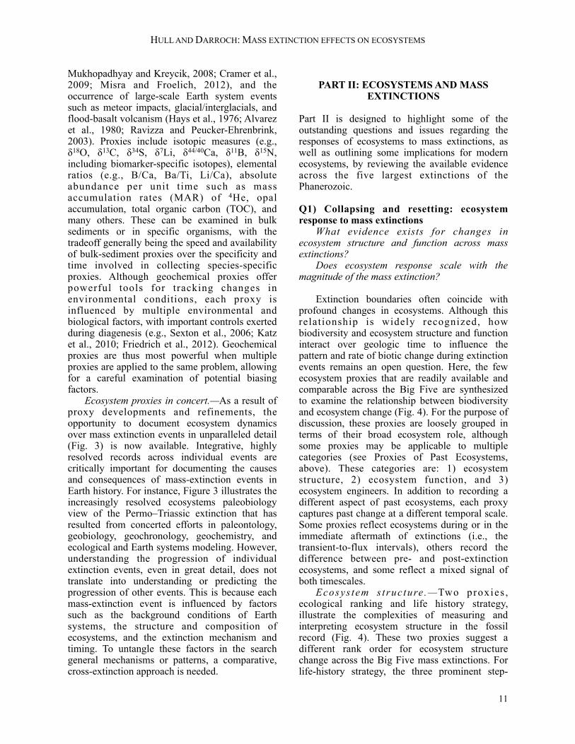
FIGURE 4.—A Phanerozoic compilation of effects of mass extinctions on the structure and function of ecosystems using available proxies, categorized as relating to ecosystem structure, function, or engineering (right). Estimates of extinction taxonomic severity (Sepkoski, 1989; Bambach, 2006; Alroy et al., 2008) are plotted at the top for comparative purposes and the Big Five mass extinction events are highlighted in light gray across all panels. Compilations are replotted from: Ecological ranking –McGhee et al. (2004); Life strategy (predation and motility)–Bambach et al. (2002); CaCO3 production –Flügel and Kiessling (2002); Sedimentary packages –Meyers and Peters (2011); Infaunal tiering –compiled from Web of Science and superimposed on tiering curves of Ausich and Bottjer (1982, 1986); and Reef crises –Flügel and Kiessling (2002). The positions of reef crises as defined by Flügel and Kiessling (2002) have been superimposed on the curves for carbonate production and reef crises as dark grey bars. These data demonstrate the different effects of the Big Five mass extinction events on various measures of ecosystem structure and function. Of the five events, the Permian–Triassic had the most severe ecological effects (i.e. perturbed the largest proportion of the chosen proxies), and resulted in permanent restructuring of marine ecosystems.
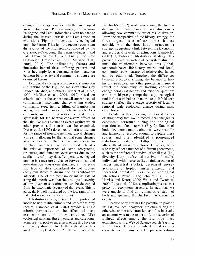
changes in strategy coincide with the three largest mass extinctions (Permo–Triassic, Cretaceous–Paleogene, and Late Ordovician), with no change during the Triassic–Jurassic and Late Devonian extinctions (Fig. 4). In contrast, by ecological rank, the Permo–Triassic is the greatest ecosystem disturbance of the Phanerozoic, followed by the Cretaceous–Paleogene, the Triassic–Jurassic and Late Devonian events, and finally, the Late Ordovician (Droser et al., 2000; McGhee et al., 2004, 2012). The influencing factors and timescales behind these differing patterns and what they imply for understanding the interaction between biodiversity and community structure are examined herein. Ecological ranking is a categorical summation and ranking of the Big Five mass extinctions by Droser, McGhee, and others (Droser et al., 1997, 2000; McGhee et al., 2004, 2012) based on criteria such as the appearance/disappearance of communities, taxonomic change within clades, community type, tiering, filling of Bambachian megaguilds, and changes in metazoan reefs. As a composite metric, it provides the best single hypothesis for the relative ecosystem effects of the Big Five mass extinction events against which other proxies and metrics can be examined. Droser et al. (1997) developed criteria to account for the range of possible nonhierarchical changes while still allowing for the fact that some changes have a greater relative impact on ecosystem structure than others. Even so, this model elevates the relative importance of some ecosystems, structures, and functions over others due to the availability of proxy data. Temporally, ecological ranking is a measure of change between post- and pre-extinction ecosystem structure, as the scale and type of data considered do not capture ecosystem structure during the transient-to-flux intervals. One of the most important insights of using this metric was that the ecological severity of any given mass extinction can be decoupled from the taxonomic severity of that event. This is particularly well illustrated by the low rank of the Late Ordovician extinction (Fig. 4). Life-history strategies (i.e., the proportion of motile to non-motile animals and predator to prey species; Bambach et al. 2002) provide a single criteria perspective on the effects of mass extinction on community structure. Like ecological ranking, these measures indicate long-term, pre- vs. post-event effects of the Big Five on community structure due to the scale of the data used (i.e., Sepkoski’s 2002 database). As such,
Bambach’s (2002) work was among the first to demonstrate the importance of mass extinctions in allowing new community structures to develop. From the perspective of life-history strategy, the three largest losses of taxonomic richness coincide with the three largest turnovers in strategy, suggesting a link between the taxonomic and ecological severity of extinctions. Bambach’s (2002) global-scale life-history strategy data provide a tentative metric of ecosystem structure until the relationship between this global, taxonomic-based life-history metric and local, community-scale measures of relative abundances can be established. Together, the differences between ecological ranking, the balance of life-history strategies, and other proxies in Figure 4 reveal the complexity of tracking ecosystem change across extinctions and raise the question: can a multi-proxy composite (e.g., ecological ranking) or a global-scale metric (e.g., life-history strategy) reflect the average severity of local to regional scale ecological change during mass extinctions? To address this question, we looked for an existing proxy that would record local changes in ecosystem structure during the ecological transition and flux intervals (Fig. 2). Studies of body size across mass extinctions were spatially and temporally resolved enough to capture these scales, and often identified a pronounced reduction in body size (Lilliput effect) in the aftermath of mass extinctions. However, body size may reflect a number of different phenomena, such as the preferential survival of small taxa (i.e., diversity loss), preferential survival of smaller individuals within species (i.e., miniaturization of larger ancestral stocks), decreased energy availability or trophic transfer efficiency, and increased predation pressure or ecological interactions (Payne, 2005; Schmidt et al., 2006; Harries and Knorr, 2009; Wade and Twitchett, 2009; Rego et al., 2012), complicating its use as a proxy of ecosystem structure. In addition, we were unable to find any comparative study of body size spanning the Big Five mass-extinction events. Because body size has the potential to provide insight into local ecosystem structure during the otherwise unmeasured transient and flux intervals, an attempt was made to quantify the severity of Lilliput effects among the Big Five mass extinctions with a Web of Science search (see Fig. 5 for details). This search indicated that a strong correlate for the number of Lilliput observations
HULL AND DARROCH: MASS EXTINCTION EFFECTS ON ECOSYSTEMS
13
per extinction was the intensity of research on that extinction event, and, in particular, on body size change across the boundary (Fig. 5). These patterns suggest that the Web of Science proxy is
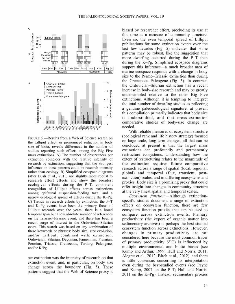
biased by researcher effort, precluding its use at this time as a measure of community structure. Even so, the even temporal spread of Lilliput publications for some extinction events over the last few decades (Fig. 5) indicates that some patterns may be robust, like the suggestion that more dwarfing occurred during the P–T than during the K–Pg. Simplified ecospace diagrams support this inference—a much broader area of marine ecospace responds with a change in body size to the Permo–Triassic extinction than during the Cretaceous–Paleogene (Fig. 5). In contrast, the Ordovician–Silurian extinction has a recent increase in body-size research and may be greatly undersampled relative to the other Big Five extinctions. Although it is tempting to interpret the total number of dwarfing studies as reflecting a genuine paleoecological signature, at present this compilation primarily indicates that body size is understudied, and that cross-extinction comparative studies of body-size change are needed. With reliable measures of ecosystem structure (ecological rank and life history strategy) focused on large-scale, long-term changes, all that can be concluded at present is that the largest mass extinctions can profoundly and permanently restructure ecosystems. Understanding how the extent of restructuring relates to the magnitude of the extinction requires future comparative research across a range of spatial (local, regional, global) and temporal (flux, transient, post-extinction) scales, and in differing ecosystems and proxies. Body size is a promising proxy that could offer insight into changes in community structure at the very finest spatial and temporal scales. Ecosystem function.—Although extinction-specific studies document a range of extinction effects on ecosystem function, there are few ecosystem function proxies that can be used to compare across extinction events. Primary productivity (the export of organic matter into sedimentary archives) is perhaps the best-studied ecosystem function across extinctions. However, changes in primary productivity are not considered here because the most common tracer of primary productivity δ13C) is influenced by multiple environmental and biotic biases (see Kump and Arthur, 1999; Hull and Norris, 2011; Alegret et al., 2012; Birch et al., 2012), and there is little consensus concerning its interpretation even during the best-studied events (see Payne and Kump, 2007 on the P–T; Hull and Norris, 2011 on the K–Pg). Instead, sedimentary proxies
THE PALEONTOLOGICAL SOCIETY PAPERS, VOL. 19
14
FIGURE 5.—Results from a Web of Science search on the Lilliput effect, or pronounced reduction in body size of biota, reveals differences in the number of studies reporting such effects among the Big Five mass extinctions. A) The number of observances per extinction coincides with the relative intensity of research by extinction, suggesting that the strongest influence on these patterns could be research intensity rather than ecology. B) Simplified ecospace diagrams (after Bush et al., 2011) are slightly more robust to research effort effects and show the broadest ecological effects during the P–T, consistent recognition of Lilliput effects across extinctions among epifaunal suspension-feeding taxa, and a narrow ecological spread of effects during the K–Pg. C) Trends in research efforts by extinction: the P–T and K–Pg events have been the primary focus of Lilliput research over the years; there is a broad temporal span but a low absolute number of references on the Triassic–Jurassic event; and there has been a recent surge of interest in the Ordovician–Silurian event. This search was based on any combination of these keywords or phrases: body size, size evolution, and/or Lilliput; combined with: extinction, Ordovician, Silurian, Devonian, Famennian, Frasnian, Permian, Triassic, Cretaceous, Tertiary, Paleogene, and/or K/Pg.

—sedimentary package truncation/initiation and the gross accumulation of reef CaCO3—are examined to ask whether extinction-related changes in ecosystem function generally scale with changes in ecosystem structure or species loss. Sedimentary package initiation and truncation rate (Fig. 4; replotted from Meyers and Peters, 2011), records the onset and end of sedimentary package deposition in marine and terrestrial environments across North America. Meyers and Peters (2011) attribute long-term oscillations (~56 Ma) in these data to tectonic or mantle processes, but note that two of the three highest package turnover rates are at mass-extinction boundaries: the Cretaceous–Paleogene, followed by the Permo–Triassic. The third interval of high turnover, the middle Ordovician, appears to occur well before the end-Ordovician extinction. Although the Cretaceous–Paleogene has a greater aggregate turnover rate, the Permo–Triassic has a greater package t runcat ion rate across depositional environments (Peters, 2008). In both the Cretaceous–Paleogene and Permian–Triassic extinctions, high package turnover rates are driven by a peak in truncation (indicative of increased erosion or non-deposition) followed by a peak in initiation (Meyers and Peters, 2011). This is the pattern that is expected from a biotic control on ecosystem function when both extinctions are marked by the loss and turnover of terrestrial floral communities (Looy et al., 2001; Twitchett et al., 2001; Wilf and Johnson, 2004), followed by increased terrestrial erosion (Sephton et al., 2005; Fastovsky et al., 2008). The loss of reefs provides an additional, marine source of non-deposition at the Permian–Triassic, but not at the Cretaceous–Paleogene (Flügel and Kiessling, 2002; Peters, 2008; Kiessling and Simpson, 2011). With the reestablishment of terrestrial floras and marine faunas in post-extinction communities, sediment package deposition (i.e., normal ecosystem function) resumed, perhaps driving a peak in package initiation. Peters (2008) attributed the coincidence of package turnover and extinctions during mass extinctions to a common environmental cause, such as sea level change. However, the evidence is compelling for an additional mechanism wherein the extinction itself, through the loss of species and their ecological roles can result in a change in ecosystem function. Admittedly, evidence against this alternative and in support of the common-cause hypothesis
abounds. For instance, abundant Permo–Triassic evidence links an environmental perturbation to both the extinction and lithological change (see review of the Permo–Triassic in Part I). In addition, only two of the Big Five mass extinctions have a global effect on sedimentary package initiation and truncation. For these, targeted outcrop-scale studies would be needed to determine the relative importance of common-cause versus ecological function mechanisms. This mechanistic uncertainty aside, both life-history strategy and the sedimentary package metric of ecosystem function rank the Permian–Triassic and Cretaceous–Paleogene mass extinctions as the greatest disruptors of ecosystem structure and function. Reef CaCO3 is considered using Flügel and Kiessling’s (2002) global analysis of the PaleoReefs database. Gross carbonate production can be a measure of the health of reef ecosystems in any time interval (Flügel and Kiessling, 2002), and of reef functions, including a providing a carbonate sink, coastal buffer, and marine habitat, among others. The gross carbonate record is interesting because its dynamics are unrelated to mass-extinction intervals, with the exception of the end-Devonian (Fig. 4). This largely independent pattern indicates great stability of at least one ecosystem function—carbonate deposition—to the causes and consequences of mass extinctions. The potential reasons for the independence of this function from extinctions are numerous and include factors such as the replacement of metazoan reef builders by algal, protozoan, and bacterial reef builders, or the deposition of inorganic calcite precipitates in the transition-to-flux intervals (e.g., Baud et al., 1997; Woods et al., 2007; Mata and Bottjer, 2011; 2012) Ecosystem engineers.—Ecosystem engineers play a structuring role in their ecosystems. Reef-building corals and coralline algae construct three-dimensional habitat that supports the extensive diversity of coral-reef ecosystems. As such, these community members should have an outsized role in mitigating, propagating, or amplifying the effect of species loss on the structure and function of ecosystems. Here two groups of ecosystems engineers are considered: carbonate reef builders (diversity) and soft-bottom benthic bioturbators (depth). Both ecosystem engineers reveal a similar ranking of extinctions by their ecological impact: the Permo–Triassic and the Triassic–Jurassic have the greatest effects, followed by the Late
HULL AND DARROCH: MASS EXTINCTION EFFECTS ON ECOSYSTEMS
15

Ordovician and the Late Devonian events. Infaunal tiering depth was quantified by superimposing the minimum depth of tiering reached during the Big Five (based on a literature search of depth of tiering and ichnofabric index) on top of Ausich and Bottjer’s (1982, 1986) curve of the maximum depth of Phanerozoic infaunal tiering. The limitations of this approach include superimposing minimum tiering depths after mass extinctions on top of maximum tiering depths through time, ignoring recent literature on variation in tiering depths over other geological time intervals, and ignoring rare localities with unaltered tiering depth in the aftermath of extinctions (see list of references used below). However, these data highlight major trends: a stepwise colonization of deeper infaunal tiers over the Phanerozoic and the apparent, profound effect of most mass extinctions on infaunal ecosystem structure. With respect to specific events, reductions in infaunal tiering and ichnofabric index have been recorded after the Ordovician–Silurian (Herringshaw and Davies, 2008), Late Devonian (Wang, 2004; Morrow and Hasiotis, 2007; Buatois et al., 2013), Permian–Triassic (Pruss and Bottjer, 2004; Chen et al., 2012), and Triassic–Jurassic (Twitchett and Barras, 2004; Barras and Twitchett, 2007) extinctions, but not the Cretaceous–Paleogene event. Generally, mass extinctions result in relatively shallow tiering depths and reduced complexity relative to adjacent time intervals. Reef diversity (in terms of raw species richness of reef builders; Kiessling et al. 1999, 2000; Kiessling and Flügel 2002) responds to most of the Big Five, although the dominant dynamics are not associated with extinction boundaries. The responses of reefs and perhaps infaunal tiering depth may highlight the issue of extinction selectivity. Reefs are not taxonomically defined by a specific set of organisms, but rather are a spatial association of animals with similar ecological requirements (Wood, 1999). To highlight the importance of the specific type of disturbance in driving periodic collapses of reef ecosystems on geologic time scales, several authors have noted the lack of response of reefs to the K–Pg extinction (e.g., Flügel and Kiessling, 2002; Kiessling and Simpson, 2011). Kiessling and Simpson (2011) assessed reef dynamics through time and argued for a link between ocean acidification and reef collapse, with calcareous reef-builders responding dramatically to decreased oceanic pH, but seemingly not to other
sources of ecological disturbance. If ocean acidification is absent or relatively minor (as is the case with many of the Big Five mass extinction events), then reefs persist across the boundary (Flügel and Kiessling, 2002; Kiessling, 2009; Kiessling and Simpson, 2011). On an ecosystem-by-ecosystem scale, the mechanism or selectivity of the extinction may be of critical importance for the magnitude of ecological change. As a result, metrics that include specific ecosystem engineers may convolute the selectivity of the extinction with its global, ecological impact. Synthesis: collapsing & resetting ecosystems.—These observations highlight several points with respect to the responses of ecosystems to extinction: 1) The Big Five extinction events affected a variety of aspects of ecosystem structure and function. 2) There is some semblance of scaling between aspects of ecological structure and function and extinction magnitude. The largest three mass extinctions in terms of biodiversity (P–T, O–S, and K–Pg) also have the greatest effects on some metrics of ecosystem structure (life history) and function (sedimentary package initiation and truncation rate). Within this group, the K–Pg typically ranks above the O–S in effect size, possibly due to differences in the rate of biodiversity loss between these two events. 3) The ecosystem response of any given extinction likely reflects some combination of total species loss, extinction selectivity, geographic extent and temporal duration of the environmental disturbance, relative robustness of certain species and (perhaps) ecosystems to perturbation, and ecosystem feedbacks and dynamics. Differences in these factors among habitats and across space may partly account for the apparent disconnect between some metrics of ecosystem structure (i.e., ecological ranking) and global biodiversity loss. 4) Many ecosystem metrics measure the sustained effects of mass extinctions on ecosystem structure and function by focusing on data from the pre- and post-extinction intervals. How the magnitude of ecosystem change during the transition-to-flux interval affects the scale of turnover between pre- and post-extinction communities is an open question. Targeting these three intervals (pre-, transition/flux, and post-extinction) is a promising area of research for understanding the role of extinctions in resetting
THE PALEONTOLOGICAL SOCIETY PAPERS, VOL. 19
16
ecosystem structure and function. 5) Extinction events have the potential to profoundly and permanently restructure ecosystems, possibly as a result of novel interactions among surviving taxa.
Q2) Ecological feedbacks during mass extinctions: Does ecology (e.g., trophic structure, food-web interactions, community assembly, etc.) play a role in determining the overall severity of species loss or the rate of subsequent rediversification? How do are these effects distinguished from those of an exogenous disturbance?
There are many reasons why ecological factors such as trophic structure and food web interactions should play a role in determining species loss and ecosystem change at extinction boundaries. Ecological theory and modern ecosystem dynamics both suggest an important role for ecological feedbacks in determining extinction severity (via secondary extinctions), the pattern and rate of rediversification (via species interactions, community assembly, etc), and the change (or lack thereof) in ecological function during extinction events of all magnitudes. The most compelling evidence for ecological interactions driving an episode of global faunal turnover in the fossil record comes from the Ediacaran–Cambrian transition, where the Ediacaran biota were progressively outcompeted by new clades, particularly ecosystem engineers such as bilaterian epifaunal grazers, burrowers, and filter feeders (e.g., Laflamme et al., 2013). These groups had a profound effect in modifying physical and chemical aspects of the environment, including the removal of microbial-bound substrates, aerating and mixing sediments, and repackaging dissolved organic carbon (DOC) as larger particulate matter inaccessible to the (largely) osmotrophic Ediacara fauna (Erwin and Tweedt, 2012; Laflamme et al., 2013). Ultimately, these environmental changes both created and destroyed ecological niches in a way that was detrimental to Ediacaran organisms (Erwin and Tweedt, 2012). However, besides the Ediacaran–Cambrian transition, there are few intervals in the fossil record where biotic interactions and innovations can be held unequivocally responsible for driving global extinction or for driving changes in diversity or ecosystem function (for a
rare exception, see Ezard et al., 2011). During mass-extinction intervals, the evidence is less clear, at least in part because of the difficulty in separating the effects of ongoing, exogenous disturbances from ecological interactions, and the potential for multiple coincident changes in species’ life history, community structure and dynamics, and environmental boundary conditions. Here, the theoretical importance of ecological interactions in modern and ancient systems is briefly considered before turning to the evidence for ecological feedbacks during extinctions and subsequent recoveries in a series of case studies. In section Q1, multiple mass extinctions characterized by the coincident alteration of ecosystem proxies (e.g., changes in community composition and ecosystem function) and the loss of species richness were discussed. However, ruling out abiotic drivers of these patterns is generally difficult, given the presence of profound environmental disturbance both during and after mass extinctions. A discussion of the type of study designs best suited for disentangling the relative importance of ecological feedbacks and external disturbance in the pattern and timing of extinction and recovery are put forth as well. Theory: Ecology and biodiversity in modern and ancient systems.—In theory, the structure and function of ecosystems can act as a positive or negative feedback on taxonomic diversity and ecosystem changes across extinction boundaries. Ecological stability generally refers to the ability of ecosystems to either resist or quickly rebound from change, although there are many definitions of the term (Ives and Carpenter, 2007; Donohue et al., 2013). Putting aside these differences, increasing diversity generally increases the stability of the systems; for instance, more diverse communities tend to be more resistant to invasions and to change, and more likely to maintain ecosystem functions even with the loss of some species (see reviews such as Ives and Carpenter, 2007 for examples). Biodiversity acts to increase the stability of ecosystems in a number of ways, including through ecological redundancy (i.e., multiple species with the same niche) and food-web structure (Srinivasan et al., 2007; Dunne and Williams, 2009). During extinctions and their recoveries, the loss (or subsequent gain) of biodiversity can form feedbacks with and between the structure and function of ecosystems in a number of ways. At the onset of a mass extinction, ecological
HULL AND DARROCH: MASS EXTINCTION EFFECTS ON ECOSYSTEMS
17

interactions should initially confer systemwide stability in the face of environmental change. Once species are lost, ecological interactions can act to amplify the extinction perturbation over those directly caused by the environment, leading to secondary extinctions. For instance, Lotze et al. (2011) demonstrated that the historical and largely anthropogenic removal of consumers and predators in the Mediterranean has shifted diversity toward smaller and lower trophic level species. As a result, the overall food-web structure has become simplified, with a decrease in the number of links in food chains, trophic path lengths, and the hypothesized loss of robustness to extinction. After a mass extinction, the net effect of extinction selectively can determine which species thrive during the ecosystem flux interval and how communities are restructured during this and subsequent time periods. Feedbacks between biodiversity, ecosystem structure and function, and the environment likely played a key role in the Big Five mass extinctions (Vermeij, 2004). Three main approaches have been used to investigate this problem in fossil communities. First, empirical patterns and associations have been identified and considered based on modern ecological and paleoecological theory. Second, food-web models have been used to quantify the effects of extinctions on ancient ecosystems, and to compare these patterns with the fossil record (Angielczyk et al., 2005; Roopnarine, 2009; Mitchell et al., 2012). Third, quantitative hypotheses of specific ecological mechanisms have been generated using simplified ecological models and tested against the fossil record (Sole et al., 2002; Sole et al., 2010). However, in all cases, the interpretation of past ecological mechanisms relies heavily on assumptions about the presence or absence of external environmental disturbances and interactions beyond the scope of any given study. These complications, and how to address them, are the focus of the subsequent discussion in this section. Before moving on, it is useful to distinguish between two types (or directions) of ecological feedbacks within communities: bottom-up versus top-down. At the K–Pg boundary, for instance, ejecta from the impact crater are modeled to have blocked out the sun for several months, leading to the collapse of photosynthetic primary production (Toon et al., 1997). The extinction of primary producers would be considered a direct effect of the impact. In contrast, the extinction of species
higher in the food web, herbivores and consumers (e.g., Sheehan and Fastovsky, 1992; Fastovsky and Sheehan, 2005), is considered to be a secondary extinction forced from the bottom up. Primary production-driven secondary extinctions are widely considered to play a role in extinction severity and, at times, recovery patterns during mass extinctions. Bottom-up forcing is comparatively straightforward to detect and model (Roopnarine, 2006). Vermeij (2004) even took the provocative view that bottom-up forcing was the primary mechanism of extinction across most mass extinctions. In contrast to bottom-up forcing, clear evidence for top-down forcing, i.e., consumer-driven changes in food web or community stability, are difficult to find between the Ediacaran–Cambrian transition (Erwin and Tweedt, 2012; Laflamme et al., 2013) and recent Quaternary extinctions (e.g., Lopes dos Santos et al., 2013). This may be because, as Vermeij (2004) argued, they are simply less important drivers of mass extinctions and their ecological aftermaths, or this may be due to the current way of investigating and interpreting patterns in the fossil record. Case studies: testing for ecological feedbacks in extinction and recovery.—The difficulty of quantifying the importance of ecological feedbacks is highlighted in two case studies. The first examines the role of ecosystem structure in extinction susceptibility (the problem of assumptions), and the second tests for ecological feedbacks in the timing and pattern of species recovery (the problem of exogenous disturbance). Case I: Mitchell et al. (2012) recently argued that changes in the food-web structure of terrestrial communities over the last two stages of the Cretaceous may have amplified the effects of the bolide impact (at least in North America), thereby contributing to the severity of the mass extinction among dinosaurs. To make this assessment, Mitchell et al. (2012) constructed food-web models of Campanian and later Maastrichtian communities by assigning taxa to guilds on the basis of broad trophic niche and body-size category. These guild assignments set the basic topology, or structure, of the food web. To assess the stability of the resulting webs, Mitchell et al. (2012) used an approach called Cascading Extinction on Graphs (CEG, a paleo-food-web reconstruction approach: Roopnarine 2006, 2009, 2010) to randomly assign interaction strengths among guilds given constant assumptions for unknown parameters or scaling
THE PALEONTOLOGICAL SOCIETY PAPERS, VOL. 19
18
relationships (e.g., primary productivity, species specific effects or interactions, population size by guild, trophic transfer efficiency, etc). Although Mitchell et al.’s (2012) data strongly argues for differences between Campanian and Maastrichtian food web structure (topology), the inference of lower late Maastrichtian food-web stability to perturbation depends on a number of model and ecological assumptions. Food-web topology is only one of many factors determining the stability of communities to environmental perturbations (Ives and Carpenter, 2007; Donohue et al., 2013). In addition, the changing nature of other ecologically relevant, but unfossilized, parameters impose well-recognized limits on paleo-inferences (e.g., Olszewski and Erwin, 2004; Roopnarine, 2006). For instance, interactions between species can change under differing environmental conditions (Burkepile and Hay, 2006), food-web structures (Brose et al., 2005), or with the presence/absence of specific predators (Schmitz et al., 2008)—all with the possibility of cascading effects on ecosystem dynamics and functions (Schmitz et al., 2010). Beyond community structure, community stability can depend on the behavior of species (Schmitz and Booth, 1997; Valdovinos et al., 2010) or keystone species interactions (i.e., species with disproportionately large ecological effects relative to their abundance; Estes et al., 1998), among others. In one study of intertidal communities, the interactions between specific species determined resilience to environmental perturbation (Wootton, 2004). In another study, the differing physiological susceptibility of species to a change in pH resulted (in some communities) in compensatory dynamics in lake plankton, increasing community-wide stability (Klug et al., 2000). Food-web structure can also change on long evolutionary time scales (Hironaga and Yamamura, 2010). Given the long geological duration of the Campanian and Maastrichtian, the turnover in species between the two intervals, and changing environmental conditions, any number of ecosystem changes could have made Maastrichtian communities more, rather than less, stable than their Campanian counterparts. Below, cross-ecosystem (and cross-extinction) comparative approaches are discussed that could be used to partially constrain the effects of unknown parameters like those discussed here to further test the consequences of ecological interactions in past communities. Case II: The recovery of diversity and, at
times, ecosystem structure from mass extinctions often occurs in a series of steps beginning long (~1 Ma or more) after the extinction itself (Erwin, 1998; D'Hondt, 2005; Coxall et al., 2006; Chen and Benton, 2012). This empirical observation led to the hypothesis that the delay in recovery and the stepped rediversification patterns resulted from the mechanisms of evolutionary community reassembly. Sole et al. (2002; 2010) formalized this hypothesis by a simple mechanistic model, and showed that upper trophic levels should exhibit delayed recoveries if diversity scaled with the standing abundance of individuals. Thus, primary producers would recover their diversity and abundance first, supporting the subsequent diversification of herbivores, followed by predators. Detailed records from the K–Pg boundary suggest that the recovery of open-ocean taxa fit model expectations (Sole et al., 2002), given the assumption of diversity-abundance scaling. Hull et al. (2011) revisited the recovery of open ocean ecosystems from the K–Pg boundary and the model of Sole et al. (2002), using paired records of abundance and taxonomic diversity within two trophic levels (primary producers and low-level consumers). These records revealed a surprising disconnect between species abundance and diversity in the aftermath of the K–Pg mass extinction. The numerical abundance of consumers (i.e., planktonic foraminifera) in one oceanic site was higher in the immediate aftermath of the K–Pg mass extinction than during the preceding or following higher diversity time periods (Hull et al., 2011). A decoupling of population abundance, diversity, and ecosystem function during ecosystem flux intervals was also found in digital models of extinction and recovery (Yedid et al., 2009), leading Hull et al. (2011) to hypothesize that food-web relationships during evolutionary recoveries could be highly sensitive to initial conditions (i.e., contingent). Recent studies have found similar patterns during other mass extinctions as well: Greene et al. (2011) found decoupling between taxonomic richness and abundance in bioclastic accumulations of post P–T flux communities; and Payne et al. (2011) recorded the recovery of diversity among higher trophic level predators (ammonites and conodonts) before lower trophic level primary consumers (foraminifera) following the P–T mass extinction. In many studies of post-extinction dynamics following the K–Pg mass extinction (e.g.,
HULL AND DARROCH: MASS EXTINCTION EFFECTS ON ECOSYSTEMS
19

D'Hondt et al., 1998; Coxall et al., 2006; Jiang et al., 2010; Hull et al., 2011, and others), changes in primary productivity (and its deep sea export) have been attributed to community membership, ecosystem structure, diversity, and to the ecological dynamics of the ocean ecosystem itself. What about an exogenous disturbance? Although the K–Pg mass extinction is clearly tied to Chicxulub impact and its severe, geologically instantaneous environmental consequences (Toon et al., 1982,1997; Schulte et al., 2010; Alegret et al., 2012), the second phase of Deccan volcanism roughly coincides with the existence of the uniquely structured, ‘disaster fauna’ found after the impact (Chenet et al., 2009; Hull et al., 2011). Rather than food web interactions, or contingent patterns of ecosystem reassembly, might Deccan volcanism have acted not as a cause of the extinction but rather as a persistent, low-grade perturbation to the environment (i.e., a changed selective regime) during the ecosystem flux interval? Geographic patterns (heterogeneity, often scaling with distance from the impactor) in the recovery of oceanic food webs, near-coastal mollusks, and terrestrial plant communities, all provide at least some evidence against this hypothesis of a globally acting exogenous disturbance (Jablonski, 1998; Wappler et al., 2009; Jiang et al., 2010; Hull and Norris, 2011; Hull et al., 2011). Cross-ecosystem and spatially explicit approaches for quantifying the effects of environmental disturbances like these below are explored next. Disentangling ecological feedbacks.—Although it is difficult to separate the effects of ecological feedbacks from ongoing disturbances and other factors, advances are being made in understanding the influence of ecology in extinctions and their aftermath. Three approaches are discussed that may be helpful to this end. I. Cross-ecosystem comparisons.—Cross-ecosystem comparisons provide a means of controlling for persistent perturbations and/or poorly quantified ecosystem feedbacks. These include comparing the same ecosystem type (e.g., carbonate reefs) in multiple locations, or comparing between different ecosystem types ( e . g . , c a r b o n a t e - r e e f a n d s o f t - b o t t o m communities) in the same location. For instance, after the P–T extinction, the persistence of anoxic conditions was geographically heterogeneous (Twitchett et al., 2004), with benthic infaunal recovery following immediately after the return of well-oxygenated conditions.
Different ecosystems are characterized by different food-web structures, species, and interaction strengths, among other factors, and can provide a means of testing for top-down control on the stability and/or reassembly of ecosystems in deep time. The contrast between reef and benthic soft-bottom ecosystems is particularly illustrative because the ecological effects of extinction are similar in both habitats during some extinctions and different during others. Both reef and non-reef benthic ecosystems were heavily affected by Permian–Triassic extinction (see section Q1). Complex late Permian metazoan reefs were replaced by early Triassic reefs composed largely of calcifying microbes in stromatolitic and thrombolitic mounds (e.g., Schubert and Bottjer, 1992; Sano and Nakashima, 1997)—a turnover attributed to the extinction of incumbents and the removal of grazing and burrowing metazoans. The effects of extinction on non-reef communities were similarly severe. Post-extinction communities were typified by low diversity and low evenness; dominated by a few, morphologically conservative, cosmopolitan taxa (ecological opportunists of Harries et al., 1996); exhibited dwarfing (Lilliput effect) in a wide range of ecological guilds (Payne, 2005); and had reduced levels of infaunal and epifaunal tiering (e.g., Twitchett, 2006). In contrast, the Ordovician–Silurian transition shows a large mismatch in the ecological effects of extinction on reef and non-reef ecosystems. Non-reef communities show patterns similar to those of P–T (although much less severe) including low abundance, diversity and evenness (see McGhee et al., 2004; Rasmussen and Harper, 2011) and Lilliput faunas in the immediate aftermath (Huang et al., 2010; Borths and Ausich, 2011). However, the ecological effects on reefs were minor (Copper, 1994; 2002): early Silurian reefs were composed of the same families of rugose and tabulate corals and stromatoporoid sponges that made up late Ordovician reefs (Droser et al., 2000). Complex reefs are hypothesized by some to be relatively stable ecosystems to global extinction crises due to their structure (i.e., a top down effect; Cooper 1988, 2002). Reef crises in the fossil record are often not associated with mass-extinction events (e.g., Wood 1999; Flügel and Kiessling 2002) or with the magnitude of ecological disturbance in other ecosystems (e.g., Fig. 4). Modern reef ecosystems are highly diverse, with complex, ecologically redundant
THE PALEONTOLOGICAL SOCIETY PAPERS, VOL. 19
20
food webs (e.g. Wood, 1999), characteristics generally correlated with greater stability to ecological perturbations (e.g., Loreau et al., 2001; Elmqvist et al., 2003; Worm et al., 2006). This diversity could lead, in part, to their greater stability as compared to benthic soft-bottom communities during mass-extinction events. This is not to imply that reefs are stable through time –reef crises exist throughout the Phanerozoic and are strongly correlated with habitat loss/sea level fall (Wood, 1999; see also Peters, 2008) and ocean acidification (Kiessling and Simpson, 2011). Rather, reefs may simply differ in the sensitivities and dynamics as compared to other ecosystems. Cross-ecosystem approaches would provide the most compelling test of top-down (and other) ecological consequences of mass extinctions if compared within a single extinction event, across spatial scales (i.e., within and across locations), and with known similarities in environmental conditions. Although bottom-up and top-down effects might be expected a priori to be important in all ecosystems, differing extinction selectivity, food-web structure, and environmental change among differing habitats could help untangle the roles played by these factors. To the best of our knowledge, cross-ecosystem comparisons are rare (for one such example, see Aberhan et al. 2007). Such comparisons are complicated by differing environmental disturbance regimes across space and habitats (Thomas, 2007; Onue et al., 2012ß), preservational differences, and facies change (e.g. Smith et al., 2001; Payne, 2007, Sessa, 2009; Darroch, 2012). More local scale, outcrop or core-based studies are needed that explicitly test the links between species richness and ecosystem complexity, with patterns of ecological collapse over individual mass-extinction events and within and between facies and ecosystems. II. Cross-model comparisons.—Simple ecological and food-web models provide quantitative hypotheses against which to test empirical data, and some food web and ecosystems models have been developed (Sole et al., 2002; Roopnarine, 2006; Dunne et al., 2007; Roopnarine, 2009; Sole et al., 2010). However, there is a lack of a full set of simple models that cover and differentiate the range of ecological mechanisms thought to be important in ecosystem stability, collapse, and assembly over evolutionary time. For instance, body size is a factor that often changes across extinctions (Fig. 5), and theoretical models have shown that the
distribution of body size can affect the stability of food webs (e.g., Riede et al., 2011), but this interaction has yet to be modeled and tested across the Big Five. Other observations have shown that interspecific interactions can change in response to the environment (Harmon et al., 2009; He et al., 2013), with such changes modifying subsequent community dynamics. Including evolving interactions in theoretical models could be particularly important over geological time scales, as it is on these scales that mass extinctions are commonly studied. A robust set of null expectations covering the different classes of ecological models is also needed. For instance, a set of null models to contrast with the Sole et al. (2002, 2010) model might allow each trophic level to independently evolve diversity as bounded random-walk with step-frequency per trophic level parameterized by average life span. To date, the application of models has been piecemeal, with each group testing a subset of ava i lab le models and mechanisms. To complement the call for collection of paired, highly resolved empirical datasets, the need for a full and standard set of ecological model tests that can be appl ied across ext inct ions and environments in the quest for a general understanding of the mechanisms structuring extinctions and recoveries is highlighted. III. Cross-extinction comparisons.—Global compilations consistently show an increase in genus richness among marine invertebrates since the Cambrian, particularly during the Mesozoic and Cenozoic (Alroy et al., 2008). Ecosystem structure has also changed; both evenness (Powell and Kowalewski, 2002; Alroy et al., 2008) and the number of ecological guilds (e.g., Powell and Kowalewski, 2002; Bambach et al., 2002) have increased through the Phanerozoic. In modern and ancient communities, biological diversity and ecosystem structure have been linked with resilience to extinction (e.g. Srinivasan et al., 2007; Roopnarine, 2009; Lotze et al., 2011). For example, Kiessling (2006) demonstrated an inverse relationship between taxonomic richness and ecological change in a global Phanerozoic compilation of fossil reefs. Thus, with the observation that both overall biodiversity and ecosystem complexity have increased over the last ~540 million years (in some cases, via a step-change; Wagner et al., 2006), the question is: are modern ecosystems more or less robust to extinctions than ancient ones? There is some evidence to suggest that early
HULL AND DARROCH: MASS EXTINCTION EFFECTS ON ECOSYSTEMS
21
Paleozoic ecosystems were unusually prone to extinction. Bambach et al. (2004) found that turnover rates were anomalously high throughout the Cambrian and Early Ordovician, a pattern they attributed to the lower diversity of communities during this time. Roopnarine (2006) used models to compare the stability of Cambrian food webs with Paleozoic and Mesozoic food webs and also found a greater propensity toward secondary extinctions in Cambrian communities. Dunne et al. (2008) later provided opposing evidence, suggesting that Cambrian food webs were similar in terms of topology and inferred complexity to those of the present day. However, as previously discussed, food-web topology and complexity are just two of the factors that dictate community stability. The basic organization and taxonomic composition of marine ecosystems has changed profoundly over the Phanerozoic. Bambach (2002) identified a global increase in the proportion of secondary consumers (i.e., heterotrophs) coincident with the P–T transition. Subsequently, Wagner et al. (2006) demonstrated that both alpha diversity and ecological complexity also increased across the P–T boundary. Together, these studies suggest the P–T may have had lasting implications for overall ecosystem stability in the marine realm. More recently, Sobolev et al. (2011) used a compilation of genus-level extinctions and flood basalts to argue for greater stability of marine communities to volcanism since the Triassic. Sobolev et al. (2011) attributed this pattern to the geochemistry of the ocean (the switch from Neritan to Cretan seas), but this is ultimately driven by biota—the evolution and ecological rise of marine calcifying plankton (Ridgwell, 2005). If Mesozoic and Cenozoic ecosystems are more robust to extinction than Paleozoic ecosystems, then in theory, the ecological effects of an extinction-causing perturbation should be lower in the latter part of the Phanerozoic. However, there are (as yet) no universally accepted ways of quantifying the ecological impacts of extinction or of normalizing ecological changes to the magnitude of environmental perturbation so that they can be reasonably compared. Synthesis: ecological feedbacks and mass extinction.—Much work remains to be done in causally linking the mechanisms and effects of extinctions. This discussion has highlighted areas for more focused research. At present: 1) Ecological factors should play an important
role in determining species loss and ecosystem change during and after extinctions. 2) In looking for evidence of ecological feedbacks, it is difficult to rule out abiotic factors such as persistent environmental perturbations during the transition and flux interval. 3) There is evidence that bottom-up forcing (i.e., extinction of primary producers or other low trophic levels) is an important driver of biodiversity loss during transition intervals. 4) Unambiguous evidence for top-down forcing (e.g., changing abundance of consumers or food web structure) as a driver of extinction or of ecosystem change is rare or even lacking, perhaps due to (#2) above. 5) Addressing the gap between theory (#1) and current evidence (#4) is an important, difficult, and fascinating problem, best tackled by comparative approaches: cross-ecosystem, multi-model, and cross-extinction.
Q3) Cross-biome pacing of ecosystem change during mass extinctions: Do interactions among major biomes (i.e., terrestrial, shallow-marine, and open-ocean ecosystems) influence the pattern or rate of extinction and recovery?
Arguably, two or three of the Big Five Phanerozoic biodiversity crises exhibit evidence for significant marine-terrestrial feedbacks. For the Late Ordovician and the Late Devonian extinction, it has been hypothesized that evolutionary innovations in terrestrial land plants precipitated the extinction-causing glaciations (Berner, 1997; Algeo and Scheckler, 1998; Lenton et al., 2012). In the absence of the terrestrial plant hypothesis, these glacial events are surprising, as both occur in extreme greenhouse worlds. Prior to the events of the latest Ordovician, proxies and earth system models estimate pCO2 levels of 12-22 times present-day atmospheric levels (PAL)(Yapp and Poths, 1996; Berner, 1997; Tobin and Bergstrom, 2002; Tobin et al., 2005). As a result of lower solar insulation in the Ordovician (and despite high levels of CO2), ocean temperatures may have been comparable to present day (Vandenbroucke et al., 2010), although recent clumped isotopes suggest warmer values of 32-37°C (Finnegan et al., 2011). The Early-Middle Devonian similarly is a warm, high CO2 world (~3-10 PAL; Algeo and Scheckler, 1998; Royer et al., 2001; Godderis and Joachimski, 2004). In both cases, evolutionary innovations in
THE PALEONTOLOGICAL SOCIETY PAPERS, VOL. 19
22
terrestrial vegetation (the spread of non-vascular land plants in the Ordovician, and the rise of complex, vascular land plant communities in the Devonian) have been cited as key innovations leading to a fundamental shift in the terrestrial biosphere (Berner, 1997; Retallack, 1997; Elick et al., 1998), and short-term perturbations to global weathering and nutrient cycles (Algeo and Scheckler, 1998; Lenton et al., 2012). By increasing global weathering and nutrient fluxes, these innovations in terrestrial vegetation are thought to have drawn down pCO2 (Algeo and Scheckler, 1998; Godderis and Joachimski, 2004; Lenton et al., 2012), leading to cascading effects including glaciation (and glacial-interglacial cycles), global cooling, and marine regressions (Herrmann et al., 2003; Finnegan et al., 2012). A geologically short-term perturbation, rather than a persistent change in the biosphere, is predicted as new plant taxa rapidly invade open habitat, increase the depth of rock weathering, release easily accessed nutrients, and then, quickly, reach a new equilibrium (Algeo and Scheckler, 1998; Lenton et al., 2012). What is striking about the Late Ordovician and Late Devonian extinctions is that an evolutionary innovation in terrestrial vegetation cover could cause an environmental change (i.e., CO2 drawdown), large enough to drive two of the five largest marine biodiversity crises of the Phanerozoic. It is important to note, however, that there are other hypothesized triggers for both glacial periods (Kump et al., 1999; Ellwood et al., 2003; Young et al., 2009; Buggisch et al., 2010). Timing and ecological dominance can severely limit the effect terrestrial plants exert on the earth system (e.g., Boyce and Lee, 2011). Thus, additional sedimentological, geochemical, and paleontological evidence, integrated with earth system modeling, is needed to test these compelling (yet tenuous) drivers of the Paleozoic mass extinctions. Regardless, together the weight of the evidence for these two events provides compelling support for the potential of life to act as a geological force on global, realm-crossing scales (Westbroek, 1991). This possibility that terrestrial vegetation can dramatically influence marine life is readily countered by the lack of unequivocal evidence for marine-terrestrial coupling in two of the Big Five: the Permo–Triassic and the Triassic-Jurassic. The direct effects of flood-basalt volcanism are thought to have led to both of these extinction events (Erwin, 2006; Ganino and Arndt, 2009; Whiteside et al., 2010; Black et al., 2012;
Blackburn et al., 2013) through some combination of factors l ike global warming, ocean acidification, anoxia, euxinia, and others (Wignall and Twitchett, 1996; Beerling, 2002; Berner, 2002; Grice et al., 2005; Knoll et al., 2007; van de Schootbrugge et al., 2009; Schaller et al., 2011; Martindale et al., 2012; Payne and Clapham, 2012; Schaller et al., 2012). In the aftermath of the P–T, the timing of marine and terrestrial rediversif icat ion appears to be largely synchronous with the stabilization of global δ13C curves (Chen and Benton, 2012; Irmis and Whiteside, 2012; Schneebeli-Hermann et al., 2012; Meyer et al., 2013; Romano et al., 2013). The boundary oscillations in global δ13C during the Early Triassic have been attributed to multiple episodes of CO2 release due to Siberian Trap volcanism (Payne and Kump, 2007), with biotic recovery across realms following on the cessation of this external perturbation. Other alternative explanations for the δ13C oscillations evoke other abiotic drivers (e.g., ocean overturning, methane clathrate destabilization, or coal metamorphism) or biotic causes (oceanic export productivity, organic carbon burial, increased organic-carbon weathering; as discussed in Payne and Kump, 2007). The high-amplitude oscillations (up to 8‰ δ13C) make a biotic driver unlikely. However, if the drivers were somehow biotic then this too would provide support for biotic pacing across the marine-terrestrial divide in the P–T recovery. In the T-J, the pattern of marine and terrestrial environmental change is also tied directly to volcanism, rather than cross-realm interactions. On land, there is a coincidence between the perturbation of flood basalt volcanism (in this case, deposition of toxic aerosols) and transient t e r r e s t r i a l e c o s y s t e m c h a n g e ( v a n d e Schootbrugge et al., 2009). In the sea, coral reef deposits recovered at a different pace (Martindale et al., 2012), but this pattern too is attributed to the cessat ion of the extinct ion-driving perturbation (i.e., ocean acidification due to flood basalt volcanism). The Cretaceous–Paleogene mass extinction contains several lines of evidence suggesting some role for the terrestrial biosphere in the pattern and timing of marine recovery. Following the impact at the K–Pg boundary, there is globally distributed evidence for increase in terrestrial erosion (Fastovsky et al., 2008), possibly due to the widespread loss of land plants. This includes sedimentological evidence for high-energy streams, increased coal deposits in swampy
HULL AND DARROCH: MASS EXTINCTION EFFECTS ON ECOSYSTEMS
23
lowlands, regional coastal anoxia, the largest turnover rate in sedimentary packages in the Phanerozoic, and changes in geochemical weathering proxies (δ7Li and 87Sr/86Sr) (Martin and Macdougall, 1991; MacLeod et al., 2001; Fastovsky et al., 2008; Meyers and Peters, 2011; Misra and Froelich, 2012). At sea, there is a striking unexplained environmental pattern in post-extinction export productivity (Hull and Norris, 2011)–depressed export productivity is prolonged in the Atlantic but not the in the Pacific. Rather, Pacific records even provide some evidence for an export productivity boom following the extinction (e.g., Hollis et al., 1995; Alegret and Thomas, 2009). One highly speculative mechanism for this pattern is that the loss (or change) of terrestrial vegetation altered the hydrological cycle to the extent that water column stratification was increased in the Atlantic (a narrow, restricted basin at the time), depressing regional productivity (suggested by P.J.S. Franks [pers. comm.] and promulgated by P.M. Hull). Direct interpretations across the K–Pg are impeded, however, by the need to disentangle the relative effects of the impact, flood basalt volcanism, and potential terrestrial-marine feedbacks. At present, although there is growing evidence for terrestrial vegetation-related changes in weathering and near coastal deposits, it is unclear if these were of a large enough scale to influence open ocean ecosystem function. Alternatively, the impact winter could have temporarily changed oceanic overturning circulation, increasing Atlantic stratification, and resulting in the regional suppression of primary productivity (pers. comm., R.D. Norris). A final possibility is that Deccan volcanism (Chenet et al., 2009; Robinson et al., 2009)–which was relatively unimportant as a driver of the extinction itself (Schulte et al., 2010)– acted as a post-extinction disturbance influencing the pattern and timing of ecosystem change. In the long view, the history of life in marine and terrestrial environments shows a general concordance between marine and terrestrial mass extinction events (Benton, 1995). This coordinated pattern of marine and terrestrial turnovers led to our initial question: do the interactions between life on land and life at sea lead, in part, to these parallel signals? The alternative hypothesis is that extinction dynamics in both marine and terrestrial settings is driven entirely by the same, exogenous processes. At present, the bulk of existing evidence (see above)
h a s s u p p o r t e d a c o r r e l a t i o n b e t w e e n environmental drivers of the extinction events and the post-extinction dynamics (Peters, 2008; Peters and Heim, 2011), with the drivers of extinction (with the possible exception of the Late Ordovician and Late Devonian) arising from a geological process like volcanism, orogenic processes, and tectonics (i.e., paleogeography, oceanic seaways). However, the history of life is peppered with examples of biotic processes shaping both short-term dynamics and large-scale patterns in the earth system (e.g., Zimov et al., 1995; Algeo and Scheckler, 1998; Ridgwell, 2005) and biotic interactions continue to be invoked to explain biotic dynamics across geological boundaries. However, when it comes to inferring terrestrial, marine, and earth system feedbacks, the relative timing and magnitude of change is critically important for assigning causality, as recently argued by Boyce and Lee (2011). Synthesis: cross-biome interactions.– To sum up, why and how the biosphere is (and is not) the dominant influence on earth system evolution during certain intervals or on certain time scales remains an open and important question for understanding ecosystem dynamics across mass extinctions, and in the history of life more generally (Jablonski, 2008; Benton, 2009; Benton, 2010; Sahney et al., 2010). At present: 1) There is some evidence for cross-biome interactions during the End Ordovician and End Devonian extinctions driven by evolutionary innovations in terrestrial plants. 2) Similar evidence is generally lacking from the other three of the Big Five extinctions.In all cases, confidently linking cross-biome interactions requires excellent time control, multi-proxy and multi-site empirical evidence, and model testing, thus leaving much room for future work.
Q4) Ecosystem lessons from past crises: What are the major issues with scaling the ecosystem lessons of past biodiversity crises to the modern?
In practice, although the deep-time record of past mass and minor extinctions is studied in the context of the present biodiversity crisis (e.g., Erwin, 2009; Barnosky et al., 2011; Dawson et al., 2011; Harnik et al., 2012), it remains difficult to use the past to generate direct predictions of how the present crisis will unfold. This can be
THE PALEONTOLOGICAL SOCIETY PAPERS, VOL. 19
24
largely attributed to three factors: First, few extinction events are sufficiently well-described in terms of cause, timing, duration, and ecosystem responses to mechanistically relate biodiversity to ecosystem structure and function in deep time. The systems paleobiology approach is a recent one, and efforts in this field have largely focused on two extinction events: the End Permian and the End Cretaceous (see discussion in section Q1). Current understanding of ecosystem dynamics across both events has advanced dramatically as a result (e.g., Hull et al., 2011; Alegret et al., 2012; Chen and Benton, 2012; Payne and Clapham, 2012). However, comparative cross-extinction studies are needed to test the link between biodiversity and ecosystem structure and function while accounting for the unique aspects of each extinction event. In the absence of direct environmental perturbation (i.e., acidification or sea-level change), how robust are the structure and function of benthic reef versus benthic soft-bottom ecosystems to the removal of species? How robust are pelagic ecosystems? Both empirical and model-based studies on modern systems are investigating the roles played by overall taxonomic richness and trophic complexity (see section Q2). However, few studies using fossil data have been successful in unequivocally identifying these sorts of ecological interactions and feedbacks. Among those that do, most take advantage of the high-resolution stratigraphic and fossil records preserved across the P–T and K–Pg boundaries. According to Bambach (2006), there are eighteen mass extinctions in the Phanerozoic; P–T and K–Pg type ecosystem records are needed for these events as well if general lessons from the post-extinction dynamics of the past are to be extracted. Second, there is a lack of a mechanistic understanding of the feedbacks between the structure and function of ecosystems, and the loss and re-evolution of biodiversity during mass extinctions (see discussion in Q2). If the goal is to better understand the future of the modern oceans, research is needed to address the following questions: 1) Are the ecosystem-biodiversity relationships observed in modern ecosystems (e.g., Hooper at al. 2005) maintained across extinction events in the fossil record? (Table 1); 2) Do relatively slow-acting processes such as speciation, weathering, and evolving food-web structure become important factors during extinctions and their aftermath? Or, do the same
processes dominate on short and long timescales? and; 3) Do these inferences hold across realms? This last question is particularly relevant because terrestrial ecosystems form the basis for understanding the interaction between ecosystem structure, function, and diversity (e.g., Hopper et al., 2005). In contrast, benthic marine ecosystems dominate the understanding of community dynamics in deep time, and pelagic marine ecosystems the understanding of past ecosystem function. Third, there are large differences in resolution and scaling between the modern diversity crisis and past extinctions. These include differences in taxonomic resolution, assemblage coverage, environmental data types, spatial coverage, and temporal resolution. The challenge of comparing modern and ancient rates of extinction has been considered in detail (most recently in Barnosky et al., 2011), but similar problems exist for understanding ecosystem dynamics. Broadly, these issues relate to the patchy geographic and taxonomic resolution in terms of fossilized/unfossilized taxa and the taxonomic level of identification of the modern and fossil record, and to differences in temporal resolution of modern and fossil ecosystems (Bennington et al., 2009). The issue of temporal resolution is exacerbated for ancient ecosystems as compared to ancient biodiversity estimates because different ecosystem proxies may reflect biotic and environmental changes acting at dramatically different timescales. For example, within benthic marine ecosystems, the composition of fossil shell assemblages may capture changes in community structure on scales of 102–103 years (e.g., Flessa et al., 1993; Kidwell and Flessa, 1995; Roy et al., 1996; Kidwell, 2013), whereas strontium or carbon-isotope studies from the same sections might reflect earth system processes operating on 104–106 years (Hillaire-Marcel and De Vernal, 2007). Four main study angles can be used to address this problem of scaling. First, target mechanisms or dynamics can be compared across scales to test whether the processes differ in modern and ancient systems (as in Harnik et al., 2012). Second, the problem of scaling and biasing can be directly investigated in the fossil record (see recent community scale applications in Tomasovych and Kidwell, 2010a, b, 2011). Third, more recent historical, sub-fossil, and fossil communities can be used to bridge across the modern-ancient divide as they have the resolution and the temporal duration to capture processes
HULL AND DARROCH: MASS EXTINCTION EFFECTS ON ECOSYSTEMS
25
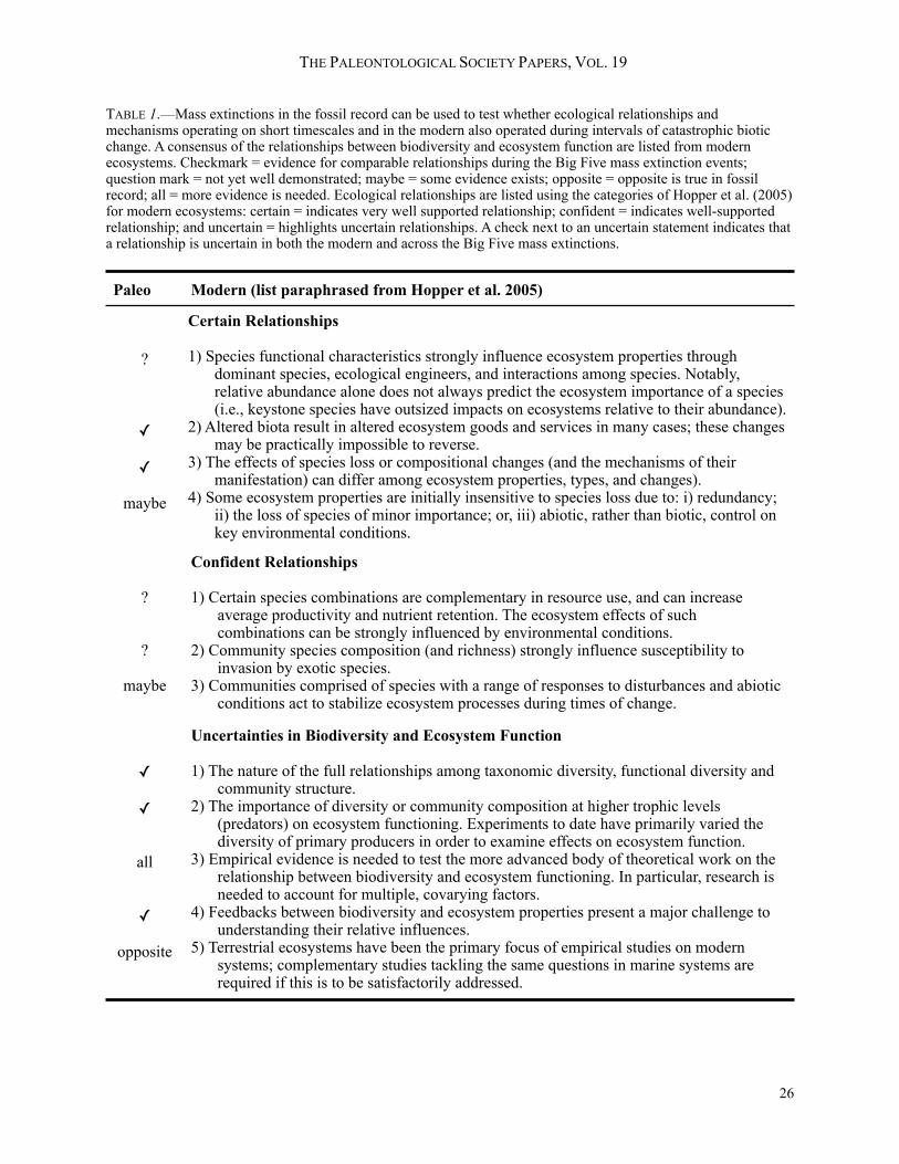
THE PALEONTOLOGICAL SOCIETY PAPERS, VOL. 19
26
TABLE 1.—Mass extinctions in the fossil record can be used to test whether ecological relationships and mechanisms operating on short timescales and in the modern also operated during intervals of catastrophic biotic change. A consensus of the relationships between biodiversity and ecosystem function are listed from modern ecosystems. Checkmark = evidence for comparable relationships during the Big Five mass extinction events; question mark = not yet well demonstrated; maybe = some evidence exists; opposite = opposite is true in fossil record; all = more evidence is needed. Ecological relationships are listed using the categories of Hopper et al. (2005) for modern ecosystems: certain = indicates very well supported relationship; confident = indicates well-supported relationship; and uncertain = highlights uncertain relationships. A check next to an uncertain statement indicates that a relationship is uncertain in both the modern and across the Big Five mass extinctions.
Paleo Modern (list paraphrased from Hopper et al. 2005)
?
✓
✓
maybe
Certain Relationships
1) Species functional characteristics strongly influence ecosystem properties through dominant species, ecological engineers, and interactions among species. Notably, relative abundance alone does not always predict the ecosystem importance of a species (i.e., keystone species have outsized impacts on ecosystems relative to their abundance).
2) Altered biota result in altered ecosystem goods and services in many cases; these changes may be practically impossible to reverse.
3) The effects of species loss or compositional changes (and the mechanisms of their manifestation) can differ among ecosystem properties, types, and changes).
4) Some ecosystem properties are initially insensitive to species loss due to: i) redundancy; ii) the loss of species of minor importance; or, iii) abiotic, rather than biotic, control on key environmental conditions.
?
?
maybe
Confident Relationships
1) Certain species combinations are complementary in resource use, and can increase average productivity and nutrient retention. The ecosystem effects of such combinations can be strongly influenced by environmental conditions.
2) Community species composition (and richness) strongly influence susceptibility to invasion by exotic species.
3) Communities comprised of species with a range of responses to disturbances and abiotic conditions act to stabilize ecosystem processes during times of change.
✓
✓
all
✓
opposite
Uncertainties in Biodiversity and Ecosystem Function
1) The nature of the full relationships among taxonomic diversity, functional diversity and community structure.
2) The importance of diversity or community composition at higher trophic levels (predators) on ecosystem functioning. Experiments to date have primarily varied the diversity of primary producers in order to examine effects on ecosystem function.
3) Empirical evidence is needed to test the more advanced body of theoretical work on the relationship between biodiversity and ecosystem functioning. In particular, research is needed to account for multiple, covarying factors.
4) Feedbacks between biodiversity and ecosystem properties present a major challenge to understanding their relative influences.
5) Terrestrial ecosystems have been the primary focus of empirical studies on modern systems; complementary studies tackling the same questions in marine systems are required if this is to be satisfactorily addressed.
working across scales (e.g., Zimov et al., 1995; Jackson et al., 2001; Pandolfi et al., 2003; Field et al., 2006; Blois et al., 2010). Fourth, Earth system models such as GENIE can be used and modified to test mechanisms, generate fossil record-like data (e.g., time averaged, geographically and depth specific values, etc.), and to compare with empirical records (e.g., Ridgwell, 2005, 2007; Ridgwell and Schmidt, 2010). Synthesis: lessons from past crises.—There are many questions that need to be addressed to translate evidence from past global crises into lessons for the future. They include: 1) Across the ~18 mass extinctions of the Phanerozoic, what ecological mechanisms are generally important in the loss and recovery of biological diversity, or in the extent, direction, and type of ecosystem change? 2) Do these ecological factors change between minor and mass extinctions, or as a result of changing background conditions (e.g., environment, taxonomic, ecosystem structure, etc)? 3 ) A r e t h e e c o s y s t e m - b i o d i v e r s i t y relationships observed in modern ecosystems maintained across mass-extinction events? 4) Are there certain slow-acting mechanisms (i.e., speciation, weathering, evolving food-web structure, etc) that become important factors during extinctions and their aftermath, or do the same processes dominate regardless of time scale or event magnitude? 5) How does scaling affect the importance of mechanisms identified in fossil and modern systems? How can we best translate across these gaps?
SUMMARY
The Big Five mass extinctions profoundly altered the structure and function of ecosystems, albeit in markedly different ways. In some cases, the ecosystem effects of the extinction were confined largely to the evolutionary recovery period (e.g., the Late Ordovician). In others, ecosystem structure and function were altered permanently (i.e., the late Permian and End Cretaceous) by removing ecological incumbents and resetting the balance of alternative life-history strategies (Fig. 4). The differing severities of effects on ecosystem structure and function among the Big Five mass extinctions is likely linked, in part, to the ultimate source(s) of the disturbance. For instance, reefs are strongly affected by direct
physical and physiological disturbances (sea level fall and ocean acidification), but are relatively robust with regard to elevated rates of species extinction (Dunne et al., 2004), perhaps due to the high levels of ecological redundancy in reef ecosystems. As an example, the bolide impact at the Cretaceous–Paleogene boundary restructured pelagic and terrestrial ecosystems, but left reef ecosystems relatively unperturbed (Flügel and Kiessling, 2002; Kiessling and Simpson, 2011). In contrast to previous studies, by considering the ecosystem as a whole, some evidence for a link between the magnitude of the ecological and the evolutionary turnover for the Big Five mass extinction events is found. However, our chosen proxies of ecosystem structure and function influence these findings, and until it is possible to rule out local or ecosystem specific responses, it will be difficult to argue for global decoupling (or coupling) between biodiversity and ecosystem structure and function. A systems paleobiology approach, in which multiple ecosystem proxies are used in concert to understand the integrated evolution of the earth and biosphere, has the potential to address fundamental questions regarding the interaction of species extinctions and the structure and function of ecosystems. However, to use the fossil record to inform the future, a number of key questions need to be addressed: 1) How do ecosystem attributes mitigate (or exacerbate) the magnitude of species loss during mass extinctions? 2) How do environmental perturbation, ecosystem change, taxonomic diversity, and ecological interactions affect the extent of change in ecosystem function across extinction crises? 3) How do ecological processes affect the rate at which standing diversity recovers, or the establishment and structure of post-extinction ecosystems? An underlying problem involves the effective scaling of inferences from the geological record to modern ecosystems, which we seek to predict on relatively short (<100 yr.) timescales. Bridging this scaling gap is important because ecosystem processes that play a relatively minor role on short time scales, such as land-sea interactions, may be important regulators of post-extinction dynamics. This is an exciting time as the tools, methods, approaches, and questions needed to address these outstanding issues are now readily available. If the next ten years are as productive as the last ten
HULL AND DARROCH: MASS EXTINCTION EFFECTS ON ECOSYSTEMS
27

have been, the mechanisms at work during the largest biotic mass-extinction events known on Earth may finally be understood.
ACKNOWLEDGMENTS
The clarity, content, and structure of this manuscript were greatly improved by insightful comments from our editor (J. L. Payne), our reviewers (P. M. Novack-Gottshall and one anonymous), and colleagues (R.D. Norris, Y. G. Zhang, and W. Jetz); any remaining errors or oversights are ours alone. We thank the editors of this volume (A. M. Bush, S. B. Pruss, and J. L. Payne) for inviting our contribution and supporting our efforts along the way.
REFERENCES
ABERHAN, M., S. WEIDEMEYER, W. KIESSLING, R. A. SCASSO, AND F. A. MEDINA. 2007. Faunal evidence for reduced product iv i ty and uncoordinated recovery in Southern Hemisphere Cretaceous–Paleogene boundary sections. Geology, 35:227–230.
ALEGRET, L., AND E. THOMAS. 2009. Food supply to the seafloor in the Pacific Ocean after the Cretaceous/Paleogene boundary event. Marine Micropaleontology, 73:105–116.
ALEGRET, L., E. THOMAS, AND K. C. LOHMANN. 2012. End-Cretaceous marine mass extinction not caused by productivity collapse. Proceedings of the National Academy of Sciences of the United States of America, 109:728–732.
ALGEO, T. J., AND S. E. SCHECKLER. 1998. Terrestrial-marine teleconnections in the Devonian: Links between the evolution of land plants, weathering p r o c e s s e s , a n d m a r i n e a n o x i c e v e n t s . Philosophical Transactions of the Royal Society B-Biological Sciences, 353:113–128.
ALGEO, T. J., AND R. J. TWITCHETT. 2010. Anomalous Early Triassic sediment fluxes due to elevated w e a t h e r i n g r a t e s a n d t h e i r b i o l o g i c a l consequences. Geology, 38:1023–1026.
ALLISON, P. A., AND D. E. G. BRIGGS. 1991. Taphonomy of non-mineralized tissues, p. 25–69. In P. A. Allison and D. E. G. Briggs (eds.), Taphonomy: Releasing the Data Locked in the Fossil Record. Plenum Press, New York.
ALROY, J., M. ABERHAN, D. J. BOTTJER, M. FOOTE, F. T. FURSICH, P. J. HARRIES, A. J. W. HENDY, S. M. HOLLAND, L. C. IVANY, W. KIESSLING, M. A. KOSNIK, C. R. MARSHALL, A. J. MCGOWAN, A. I. MILLER, T. D. OLSZEWSKI, M. E. PATZKOWSKY, S. E. PETERS, L. VILLIER, P. J. WAGNER, N. BONUSO, P. S. BORKOW, B. BRENNEIS, M. E. CLAPHAM, L.
M. FALL, C. A. FERGUSON, V. L. HANSON, A. Z. KRUG , K. M. LAYOU , E. H. LECKEY , S. NURNBERG, C. M. POWERS, J. A. SESSA, C. SIMPSON, A. TOMASOVYCH, AND C. C. VISAGGI. 2008. Phanerozoic trends in the global diversity of marine invertebrates. Science, 321:97–100.
ALVAREZ, L. W., W. ALVAREZ, F. ASARO, AND H. V. MICHEL. 1980. Extraterrestrial cause for the Cretaceous–Tertiary extinction—experimental results and theoretical interpretation. Science, 208:1095–1108.
ANGIELCZYK, K. D., P. D. ROOPNARINE, AND S. C. WANG. 2005. Modeling the role of primary product ivi ty disrupt ion in end-Permian extinctions, Karoo Basin, South Africa, p. 16–23. In S. G. Lucas and K. E. Ziegler (eds), The Nonmarine Permian. New Mexico Museum of Natural History and Science Bulletin 30. Albuquerque, New Mexico.
ARCHIBALD, J. D., W. A. CLEMENS, K. PADIAN, T. ROWE, N. MACLEOD, P. M. BARRETT, A. GALE, P. HOLROYD, H. D. SUES, N. C. ARENS, J. R. HORNER, G. P. WILSON, M. B. GOODWIN, C. A. BROCHU, D. L. LOFGREN, S. H. HURLBERT, J. H. HARTMAN, D. A. EBERTH, P. B. WIGNALL, P. J. CURRIE, A. WEIL, G. V. R. PRASAD, L. DINGUS, V. COURTILLOT, A. MILNER, A. MILNER, S. BAJPAI, D. J. WARD, AND A. SAHNI. 2010. Cretaceous extinctions: Multiple causes. Science, 328:973–973.
AUSICH, W. I., AND D. J. BOTTJER. 1982. Tiering in suspension-feeding communities on soft substrata throughout the Phanerozoic. Science, 216:173–174.
BACHAN, A., B. VAN DE SCHOOTBRUGGE, J. FIEBIG, C. A. MCROBERTS, G. CIARAPICA, AND J. L. PAYNE. 2012. Carbon cycle dynamics following the end-Triassic mass extinction: Constraints from paired δ13Ccarb and δ13Corg records. Geochemistry Geophysics Geosystems, 13:Q09008. doi:10.1029/2012GC004150
BAMBACH, R. K. 2006. Phanerozoic biodiversity mass extinctions. Annual Review of Earth and Planetary Sciences, 34:127–155.
BAMBACH, R. K., A. M. BUSH, AND D. H. ERWIN. 2007. Autecology and the filling of ecospace: Key metazoan radiations. Palaeontology, 50:1–22.
BAMBACH, R. K., A. H. KNOLL, AND J. J. SEPKOSKI. 2002. Anatomical and ecological constraints on Phanerozoic animal diversity in the marine realm. Proceedings of the National Academy of Sciences of the United States of America, 99:6854–6859.
BAMBACH, R. K., A. H. KNOLL, AND S. C. WANG. 2004. Origination, extinction, and mass depletions of marine diversity. Paleobiology, 30:522–542.
BAPST, D. W., P. C. BULLOCK, M. J. MELCHIN, H. D. SHEETS, AND C. E. MITCHELL. 2012. Graptoloid diversity and disparity became decoupled during
THE PALEONTOLOGICAL SOCIETY PAPERS, VOL. 19
28
the Ordovician mass extinction. Proceedings of the National Academy of Sciences of the United States of America, 109:3428–3433.
BARNOSKY, A. D., N. MATZKE, S. TOMIYA, G. O. U. WOGAN , B. SWARTZ , T. B. QUENTAL , C. MARSHALL, J. L. MCGUIRE, E. L. LINDSEY, K. C. MAGUIRE, B. MERSEY, AND E. A. FERRER. 2011. Has the Earth's sixth mass extinction already arrived? Nature, 471:51–57.
BARRAS, C. G., AND R. J. TWITCHETT. 2007. Response of the marine infauna to Triassic–Jurassic environmental change: Ichnological data from s o u t h e r n E n g l a n d . P a l a e o g e o g r a p h y, Palaeoclimatology, Palaeoecology, 244:223–241.
BARTOLINI, A., J. GUEX, J. E. SPANGENBERG, B. SCHOENE, D. G. TAYLOR, U. SCHALTEGGER, AND V. ATUDOREI. 2012. Disentangling the Hettangian carbon isotope record: Implications for the aftermath of the end-Triassic mass extinction. Geochemis t ry Geophys ics Geosys tems , 13:Q01007, doi:10.1029/2011GC003807
BAUD, A., S. CIRILLI, AND J. MARCOUX. 1997. Biotic response to mass extinction: The lowermost Triassic microbialites. Facies, 36:238–242.
BAUD, A., S. RICHOZ, AND S. PRUSS. 2007. The lower Triassic anachronistic carbonate facies in space and time. Global and Planetary Change, 55:81–89.
BEERLING, D. 2002. Palaeoclimatology—CO2 and the end-Triassic mass extinction. Nature, 415:386–387.
BENNINGTON, J. B., W. A. DIMICHELE, C. BADGLEY, R. K . B A M B A C H , P. M . B A R R E T T , A . K . BEHRENSMEYER, R. BOBE, R. J. BURNHAM, E. B. DAESCHLER, J. VAN DAM, J. T. ERONEN, D. H. ERWIN, S. FINNEGAN, S. M. HOLLAND, G. HUNT, D. JABLONSKI, S. T. JACKSON, B. E. JACOBS, S. M. KIDWELL, P. L. KOCH, M. J. KOWALEWSKI, C. C. LABANDEIRA, C. V. LOOY, S. K. LYONS, P. M. N O VA C K - G O T T S H A L L , R . P O T T S , P. D . ROOPNARINE, C. A. E. STROMBERG, H. D. SUES, P. J. WAGNER, P. WILF, AND S. L. WING. 2009. Critical issues of scale in paleoecology. PALAIOS, 24:1–4.
BENTON, M. J. 1989. Patterns of evolution and extinction in vertebrates, p. 218–241. In K. C. a. B. In Allen, D. E. G. (eds.), Evolution and the Fossil Record. John Wiley & Sons Ltd Belhaven, London.
BENTON, M. J. 1995. Diversification and extinction in the history of life. Science, 268:52–58.
BENTON, M. J. 2009. The red queen and the court jester: species diversity and the role of biotic and abiotic factors through time. Science, 323:728–732.
BENTON, M. J. 2010. The origins of modern biodiversity on land. Philosophical Transactions of the Royal Society B-Biological Sciences, 365:3667–3679.
BENTON, M. J., A. M. DUNHILL, G. T. LLOYD, AND F. G. MARX. 2011. Assessing the quality of the fossil record: insights from vertebrates, p. 63–94. In A. J. McGowan and A. B. Smith (eds.), Comparing the Geological and Fossil Records: Implications for Biodiversity Studies. Geological Society Special Publications 358, Geological Society of London, London.
BENTON, M. J., V. P. TVERDOKHLEBOV, AND M. V. SURKOV. 2004. Ecosystem remodelling among vertebrates at the Permian–Triassic boundary in Russia. Nature, 432:97–100.
BERGGREN, W. A., AND R. D. NORRIS. 1997. Biostratigraphy, phylogeny and systematics of Paleocene trochospiral planktic foraminifera. Micropaleontology, 43:1–116.
BERNER, R. A. 1997. The rise of plants and their effect on weathering and atmospheric CO2. Science, 276:544–546.
BERNER, R. A. 2002. Examination of hypotheses for the Permo–Triassic boundary extinction by carbon cycle modeling. Proceedings of the National Academy of Sciences of the United States of America, 99:4172–4177.
BERNER, R. A. 2006. GEOCARBSULF: A combined model for Phanerozoic atmospheric O2 and CO2. Geochimica Et Cosmochimica Acta, 70:5653–5664.
BEURLEN, K. 1956. Der Faunenschnitt an der Perm–Trias Grenze. Zeitschrift der Deutschen Geologischen Gesellschaft, 108:88–99.
BIRCH, H. S., H. K. COXALL, AND P. N. PEARSON. 2012. Evolutionary ecology of Early Paleocene planktonic foraminifera: Size, depth habitat and symbiosis. Paleobiology, 38:374–390.
BLACK, B. A., L. T. ELKINS-TANTON, M. C. ROWE, AND I. U. PEATE. 2012. Magnitude and consequences of volatile release from the Siberian Traps. Earth and Planetary Science Letters, 317:363–373.
BLACKBURN, T. J., P. E. OLSEN, S. A. BOWRING, N. M. MCLEAN, D. V. KENT, J. PUFFER, G. MCHONE, E. T. RASBURY, AND M. ET-TOUHAMI. 2013. Zircon U-Pb geochronology links the end-Triassic extinction with the Central Atlantic Magmatic Province. Science, 340:941–945.
BLOIS, J. L., J. L. MCGUIRE, AND E. A. HADLY. 2010. Small mammal diversity loss in response to late-Pleistocene climatic change. Nature, 465:771–775.
BODE, H. B., B. ZEGGEL, B. SILAKOWSKI, S. C. WENZEL, H. REICHENBACH, AND R. MULLER. 2003. Steroid biosynthesis in prokaryotes: identification of myxobacterial steroids and cloning of the first bacterial 2,3(S)-oxidosqualene cyclase from the myxobacterium Stigmatella aurantiaca. Molecular Microbiology, 47:471–481.
BONIS, N. R., AND W. M. KURSCHNER. 2012. Vegetation history, diversity patterns, and climate change across the Triassic/Jurassic boundary.
HULL AND DARROCH: MASS EXTINCTION EFFECTS ON ECOSYSTEMS
29
Paleobiology, 38:240–264.BORTHS, M. R., AND W. I. AUSICH. 2011. Ordovician–
Silurian Lilliput crinoids during the end-Ordovician biotic crisis. Swiss Journal of Paleontology, 130:7–18.
BOTTJER, D. J., AND W. I. AUSICH. 1986. Phanerozoic development of tiering in soft substrata suspension-feeding communities. Paleobiology, 12:400–420.
BOYCE, C. K., AND J. E. LEE. 2011. Could land plant evolution have fed the marine revolution? Paleontological Research, 15:100–105.
BRASIER, M. D., J. B. ANTCLIFFE, AND R. H. T. CALLOW. 2010. Evolutionary trends in remarkable fossil preservation across the Edicaran–Cambrian transition and the impact of metazoan mixing, p. 519–567. In P. A. Allison and D. J. Bottjer (eds.), Taphonomy: Process and Bias Through Time: Topics in Geobiology, 32.
BRASSELL, S. C., G. EGLINTON, AND J. R. MAXWELL. 1983. The geochemistry of terpenoids and steroids. Biochemical Society Transactions, 11:575–586.
BRAYARD, A., E. VENNIN, N. OLIVIER, K. G. BYLUND, J. JENKS, D. A. STEPHEN, H. BUCHER, R. HOFMANN, N. GOUDEMAND, AND G. ESCARGUEL. 2011. Transient metazoan reefs in the aftermath of the end-Permian mass extinction. Nature Geoscience, 4:693–697.
BRENCHLEY, P. J., G. A. CARDEN, L. HINTS, D. KALJO, J. D. MARSHALL, T. MARTMA, T. MEIDLA, AND J. NOLVAK. 2003. High-resolution stable isotope stratigraphy of Upper Ordovician sequences: Constraints on the timing of bioevents and environmental changes associated with mass extinction and glaciation. Geological Society of America Bulletin, 115:89–104.
BRENCHLEY, P. J., J. D. MARSHALL, G. A. F. CARDEN, D. B. R. ROBERTSON, D. G. F. LONG, T. MEIDLA, L. HINTS, AND T. F. ANDERSON. 1994. Bathymetric and isotopic evidence for a short-lived Late Ordovician glaciation in a greenhouse period. Geology, 22:295–298.
BRENCHLEY, P. J., J. D. MARSHALL, AND C. J. UNDERWOOD. 2001. Do all mass extinctions represent an ecological crisis? Evidence from the Late Ordovician. Geological Journal, 36:329–340.
BROCKS, J. J., G. A. LOGAN, R. BUICK, AND R. E. SUMMONS. 1999. Archean molecular fossils and the early rise of eukaryotes. Science, 285:1033–1036.
BROSE, U., E. L. BERLOW, AND N. D. MARTINEZ. 2005. Scaling up keystone effects from simple to complex ecological networks. Ecology Letters, 8:1317–1325.
BROWN, J. H. 1995. Macroecology. The University of Chicago Press, Chicago.
BUATOIS, L. A., A. SOLANGE, AND M. G. MANGANO.
2013. Onshore expansion of benthic communities after the Late Devonian mass extinction. Lethaia, 46: 251–261.
BUGGISCH, W., M. M. JOACHIMSKI, O. LEHNERT, L. BERGSTROM, J. E. REPETSKI, AND G. F. WEBERS. 2010. Did intense volcanism trigger the first Late Ordovician icehouse? Geology, 38:327–330.
BURKEPILE, D. E., AND M. E. HAY. 2006. Herbivore vs. nutrient control of marine primary producers: Context-dependent effects. Ecology, 87:3128–3139.
BUSH, A. M., R. K. BAMBACH, AND G. M. DALEY. 2007. Changes in theoretical ecospace utilization in marine fossil assemblages between the mid-Paleozoic and late Cenozoic. Paleobiology, 33:76–97.
*BUSH, A. M. AND S. B. PRUSS. 2013. Theoretical ecospace for ecosystem paleobiology: energy, nutrients, biominerals, and macroevolution, p. xxx-xxx. xx–xxx. In A. M. Bush, S. B. Pruss, and J. L. Payne (eds.), Ecosystem Paleobiology and Geobiology, The Paleontological Society Papers 19. Yale Press, New Haven.
CALNER, M. 2005. A Late Silurian extinction event and anachronistic period. Geology, 33:305–308.
CALVERT, S. E., AND T. F. PEDERSEN. 2007. Elemental proxies for palaeoclimatic and palaeoceanographic variability in marine sediments: interpretation and application, p. 567–644. In C. Hillaire-Marcel and A. de Vernal (eds.), Proxies in late Cenozoic paleoceanography. Elsevier, Oxford.
CANFIELD, D. E. 1989. Sulfate reduction and oxic respiration in marine sediments - Implications for organic-carbon preservat ion in euxinic environments. Deep-Sea Research Part A-Oceanographic Research Papers, 36:121–138.
CAO, C. Q., G. D. LOVE, L. E. HAYS, W. WANG, S. Z. SHEN, AND R. E. SUMMONS. 2009. Biogeochemical evidence for euxinic oceans and ecological disturbance presaging the end-Permian mass extinction event. Earth and Planetary Science Letters, 281:188–201.
CARPENTER, S. R., R. DEFRIES, T. DIETZ, H. A. MOONEY, S. POLASKY, W. V. REID, AND R. J. SCHOLES . 2006. Mi l lennium ecosys tem assessment: Research needs. Science, 314:257–258.
CARPENTER, S. R., AND M. G. TURNER. 2000. Hares and tortoises: Interactions of fast and slow variables in ecosystems. Ecosystems, 3:495–497.
CHAPIN, F. S., B. H. WALKER, R. J. HOBBS, D. U. HOOPER, J. H. LAWTON, O. E. SALA, AND D. TILMAN. 1997. Biotic control over the functioning of ecosystems. Science, 277:500–504.
CHEN, D. Z., AND M. E. TUCKER. 2003. The Frasnian–Famennian mass extinction: insights from high-r e s o l u t i o n s e q u e n c e s t r a t i g r a p h y a n d c y c l o s t r a t i g r a p h y i n S o u t h C h i n a .
THE PALEONTOLOGICAL SOCIETY PAPERS, VOL. 19
30
P a l a e o g e o g r a p h y, P a l a e o c l i m a t o l o g y, Palaeoecology, 193:87–111.
CHEN, Z.-Q., AND M. J. BENTON. 2012. The timing and pattern of biotic recovery following the end-Permian mass extinction. Nature Geoscience, 5:375–383.
CHENET, A. L., V. COURTILLOT, F. FLUTEAU, M. GERARD, X. QUIDELLEUR, S. F. R. KHADRI, K. V. SUBBARAO , AND T. THORDARSON . 2009 . Determination of rapid Deccan eruptions across the Cretaceous–Tertiary boundary using paleomagnetic secular variation: 2. Constraints from analysis of eight new sections and synthesis for a 3500-m-thick composite section. Journal of Geophysical Research-Solid Earth, 114:B06103, doi:10.1029/2008JB005644
CLAEYS, P., W. KIESSLING, AND W. ALVAREZ. 2002. Distribution of Chicxulub ejecta at the Cretaceous–Tertiary boundary, p. 55–69. In C. Koeberl and K. G. MacLeod (eds.), Catastrophic Events and Mass Extinctions: Impacts and Beyond. Geological Society of America Special Paper 356, Geological Society of America, Boulder, CO.
CLAPHAM, M. E., AND J. L. PAYNE. 2011. Acidification, anoxia, and extinction: A multiple logistic regression analysis of extinction selectivity during the Middle and Late Permian. Geology, 39:1059–1062.
CLAPHAM, M. E., S. Z. SHEN, AND D. J. BOTTJER. 2009. The double mass extinction revisited: reassessing the severity, selectivity, and causes of the end-Guadalupian biotic crisis (Late Permian). Paleobiology, 35:32–50.
COPPER, P. 1988. Ecological succession in Phanerozoic reef ecosystems: is it real? Palaios, 3: 136–151.
COPPER, P. 1994. Ancient Reef Ecosystem Expansion and Collapse. Coral Reefs, 13:3–11.
COPPER, P. 2002. Reef development at the Frasnian/F a m e n n i a n m a s s e x t i n c t i o n b o u n d a r y. P a l a e o g e o g r a p h y, P a l a e o c l i m a t o l o g y, Palaeoecology, 181:27–65.
COXALL, H. K., S. D'HONDT, AND J. C. ZACHOS. 2006. Pelagic evolution and environmental recovery after the Cretaceous–Paleogene mass extinction. Geology, 34:297–300.
CRAMER, B. S., J. R. TOGGWEILER, J. D. WRIGHT, M. E. KATZ , AND K. G. M ILLER . 2009. Ocean overturning since the Late Cretaceous: Inferences from a new benthic foraminiferal isotope compilation. Paleoceanography, 24: PA4216, doi:10.1029/2008PA001683
D'HONDT, S. 2005. Consequences of the Cretaceous/Paleogene mass extinction for marine ecosystems. Annual Review of Ecology Evolution and Systematics, 36:295–317.
D'HONDT, S., P. DONAGHAY, J. C. ZACHOS, D. LUTTENBERG, AND M. LINDINGER. 1998. Organic
carbon fluxes and ecological recovery from the Cretaceous–Tertiary mass extinction. Science, 282:276–279.
DARROCH, S. A. F. 2012. Carbonate facies control on the fidelity of surface-subsurface agreement in benthic foraminiferal assemblages: Implications for index-based paleoecology. PALAIOS, 27:137–150.
DAWSON, T. P., S. T. JACKSON, J. I. HOUSE, I. C. PRENTICE, AND G. M. MACE. 2011. Beyond predictions: Biodiversity conservation in a changing climate. Science, 332:53–58.
DONOHUE, I., O. L. PETCHEY, J. M. MONTOYA, A. L. JACKSON, L. MCNALLY, M. VIANA, K. HEALY, M. LURGI, N. E. O’CONNOR, AND M. C. EMMERSON. 2013. On the dimensionality of ecological stability. Ecology Letters, 16:421–429.
DROSER, M. L., AND D. J. BOTTJER. 1986. A semiquantitative field classification of ichnofabric. Journal of Sedimentary Petrology, 56:558–559.
DROSER, M. L., D. J. BOTTJER, AND P. M. SHEEHAN. 1997. Evaluating the ecological architecture of major events in the Phanerozoic history of marine invertebrate life. Geology, 25:167–170.
DROSER, M. L., D. J. BOTTJER, P. M. SHEEHAN, AND G. R. MCGHEE. 2000. Decoupling of taxonomic and ecologic severity of Phanerozoic marine mass extinctions. Geology, 28:675–678.
DUNNE, J. A., AND R. J. WILLIAMS. 2009. Cascading extinctions and community collapse in model food webs. Philosophical Transactions of the Royal Society B-Biological Sciences, 364:1711–1723.
DUNNE, J. A., R. J. WILLIAMS, AND N. D. MARTINEZ. 2004. Network structure and robustness of marine food webs. Marine Ecology-Progress Series, 273:291–302.
DUNNE, J. A., R. J. WILLIAMS, N. D. MARTINEZ, R. A. WOOD, AND D. H. ERWIN. 2008. Compilation and network analyses of Cambrian food webs. PLoS Biology, 6:693–708.
DUTKIEWICZ, A., B. RASMUSSEN, AND R. BUICK. 1998. Oil preserved in fluid inclusions in Archaean sandstones. Nature, 395:885–888.
ELICK, J. M., S. G. DRIESE, AND C. I. MORA. 1998. Very large plant and root traces from the Early to Middle Devonian: Implications for early terrestrial ecosystems and atmospheric pCO2. Geology, 26:143–146.
ELLWOOD, B. B., S. L. BENOIST, A. EL HASSANI, C. WHEELER, AND R. E. CRICK. 2003. Impact ejecta layer from the mid-Devonian: Possible connection to global mass extinctions. Science, 300:1734–1737.
ELMQVIST, T., C. FOLKE, M. NYSTROM, G. PETERSON, J. BENGTSSON, B. WALKER, AND J. NORBERG. 2003. Response diversity, ecosystem change, and resilience. Frontiers in Ecology and the Environment, 1:488–494.
HULL AND DARROCH: MASS EXTINCTION EFFECTS ON ECOSYSTEMS
31
ERWIN, D. H. 1990. The end-Permian mass extinction. Annual Review of Ecology and Systematics, 21:69–91.
ERWIN, D. H. 1994. The Permo–Triassic extinction. Nature, 367:231–236.
ERWIN, D. H. 1998. The end and the beginning: recoveries from mass extinctions. Trends in Ecology & Evolution, 13:344–349.
ERWIN, D. H. 2001. Lessons from the past: biotic recoveries from mass extinctions. Proceedings of the National Academy of Sciences of the United States of America, 98:5399–5403.
ERWIN, D. H. 2006. Extinction: how life on earth nearly ended 250 million years ago. Princeton University Press, Princeton, NJ.
ERWIN, D. H. 2007. Disparity: Morphological pattern and developmental context. Palaeontology, 50:57–73.
ERWIN, D. H. 2008. Extinction as the loss of evolutionary history. Proceedings of the National Academy of Sciences of the United States of America, 105:11520–11527.
ERWIN, D. H. 2009. A call to the custodians of deep time. Nature, 462:282–283.
ERWIN, D. H., S. A. BOWRING, AND J. YUGAN. 2002. End-Permian mass extinctions: A review, p. 363–383. In C. Köberl and K. G. MacLeod. Catastrophic events and mass extinctions: Impacts and beyond. Geological Society of America Special Paper 356, Geological Society of America, Boulder, CO
ERWIN, D. H., AND S. M. TWEEDT. 2012. Ecological drivers of the Ediacaran–Cambrian diversification of Metazoa. Evolutionary Ecology, 26:417–433.
ESTES, J. A., M. T. TINKER, T. M. WILLIAMS, AND D. F. DOAK. 1998. Killer whale predation on sea otters linking oceanic and nearshore ecosystems. Science, 282:473–476.
EZARD, T. H. G., T. AZE, P. N. PEARSON, AND A. PURVIS. 2011. Interplay between changing climate and species' ecology drives macroevolutionary dynamics. Science, 332:349–351.
FASTOVSKY, D. E., AND P. M. SHEEHAN. 2005. The extinction of the dinosaurs in North America. GSA Today, 15:4–10.
*FASTOVSKY, D. E., P. M. SHEEHAN, J. L. ISBELL, AND R. GRANDPRE. 2008. Anomalous, temporary terrestrial sedimentary environments following Cretaceous–Tertiary ecosystems disruptions: North America, Asia, and Europe [Abstract], Geological Society of America Joint Annual Meeting, Houston, Texas.
FAUL, K. L., AND M. L. DELANEY. 2000. Nutrient and paleoproductivity dynamics in the early P a l e o g e n e . G F F , 1 2 2 : 4 6 – 4 7 , d o i : 10.1080/11035890001221046
FIELD, D. B., T. R. BAUMGARTNER, C. D. CHARLES, V. FERREIRA-BARTRINA, AND M. D. OHMAN. 2006.
Planktonic foraminifera of the California Current reflect 20th Century warming. Science, 311:63–66.
FINNEGAN, S., K. BERGMANN, J. M. EILER, D. S. JONES, D. A. FIKE, I. EISENMAN, N. C. HUGHES, A. K. TRIPATI, AND W. W. FISCHER. 2011. The magnitude and duration of Late Ordovician–Early Silurian glaciation. Science, 331:903–906.
FINNEGAN, S., AND M. L. DROSER. 2008. Body size, energetics, and the Ordovician restructuring of marine ecosystems. Paleobiology, 34:342–359.
FINNEGAN, S., N. A. HEIM, S. E. PETERS, AND W. W. FISCHER. 2012. Climate change and the selective signature of the Late Ordovician mass extinction. Proceedings of the National Academy of Sciences of the United States of America, 109:6829–6834.
FISCHLIN, A., G. F. MIDGLEY, J. T. PRICE, R. LEEMANS, B. GOPAL, C. TURLEY, M. D. A. ROUNSEVELL, O. P. DUBE, J. TARAZONA, AND A. A. VELICHKO. 2007. Ecosystems, their properties, goods, and services, p. 211–272. In M. L. Parry, O. F. Canziani, J. P. Palutikof, P. J. van der Linden, and C. E. Hanson (eds.), Climate Change 2007: Impacts , Adapta t ion and Vulnerabi l i ty. Contribution of Working Group II to the Fourth Assessment Report of the Intergovernmental Panel on Climate Change. Cambridge University Press, Cambridge.
FLESSA, K. W., A. H. CUTLER, AND K. H. MELDAHL. 1993. Time and taphonomy: Quantitative estimates of time-averaging and stratigraphic disorder in a shallow marine habitat. Paleobiology, 19:266–286.
FLÜGEL, E., AND W. KIESSLING. 2002. Patterns of Phanerozoic reef crises, p. 691–723. In W. Kiessling, E. Flügel, and J. Golonka (eds.), Phanerozoic Reef Patterns. SEPM Special Publication 72, Tulsa, OK.
FOOTE, M. 1999. Morphological diversity in the evolutionary radiation of Paleozoic and post-Paleozoic crinoids. Paleobiology, 25:1–115.
Friedman, M. 2009. Ecomorphological selectivity among marine teleost fishes during the end-Cretaceous extinction. Proceedings of the National Academy of Sciences of the United States of America, 106:5218–5223.
FRIEDMAN, M. 2010. Explosive morphological diversification of spiny-finned teleost fishes in the aftermath of the end-Cretaceous extinction. Proceedings of the Royal Society B Biological Sciences, 277:1675–1683.
FRIEDRICH, O., R. SCHIEBEL, P. A. WILSON, S. WELDEAB, C. J. BEER, M. J. COOPER, AND J. FIEBIG. 2012. Influence of test size, water depth, and ecology on Mg/Ca, Sr/Ca, δO18 and δC13 in nine modern species of planktic foraminifers. Earth and Planetary Science Letters, 319:133–145.
GANINO, C., AND N. T. ARNDT. 2009. Climate changes
THE PALEONTOLOGICAL SOCIETY PAPERS, VOL. 19
32
caused by degassing of sediments during the emplacement of large igneous provinces. Geology, 37:323–326.
GIBBS, S. J., A. J. POULTIN, P. R. BOWN, C. J. DANIELS, J. HOPKINS, J. R. YOUNG, H. L. JONES, G. J. THIEMANN, S. A. O'DEA, AND C. NEWSAM. 2013. S p e c i e s - s p e c i f i c g r o w t h r e s p o n s e o f coccol i thophores to Palaeocene–Eocene environmental change. Nature Geoscience, 6:218–222.
GODDERIS, Y., AND M. M. JOACHIMSKI. 2004. Global change in the Late Devonian: Modelling the Frasnian–Famennian short-term carbon isotope excursions. Palaeogeography, Palaeoclimatology, Palaeoecology, 202:309–329.
GOULD, S. J., AND C. B. CALLOWAY. 1980. Clams and brachiopods: ships that pass in the night. Paleobiology, 6:383–396.
GREENE, S. E., D. J. BOTTJER, F. A. CORSETTI, W. M. BERELSON, AND J.-P. ZONNEVELD. 2012. A subseafloor carboante factory across the Triassic–Jurrasic transition. Geology, 40:1043–1046.
GREENE, S. E., D. J. BOTTJER, H. HAGDORN, AND J.-P. ZONNEVELD. 2011. The Mesozoic return of Paleozoic faunal constituents: A decoupling of taxonomic and ecological dominance during the recovery from the end-Permian mass extinction. P a l a e o g e o g r a p h y, P a l a e o c l i m a t o l o g y, Palaeoecology, 308:224–232.
GRICE, K., C. Q. CAO, G. D. LOVE, M. E. BOTTCHER, R. J. TWITCHETT, E. GROSJEAN, R. E. SUMMONS, S. C. TURGEON, W. DUNNING, AND Y. G. Jin. 2005. Photic zone euxinia during the Permian–Triassic superanoxic event. Science, 307:706–709.
GROTZINGER, J. P., AND A. H. KNOLL. 1995. Anomalous carbonate precipitates: Is the precambrian the key to the Permian? Palaios, 10:578–596.
HALLAM, A. 1965. Environmental causes of stunting in living and fossil marine benthonic invertebrates. Palaeontology, 8:132–155.
HALLAM, A., AND P. B. WIGNALL. 1997. Mass extinctions and their aftermath. Oxford University Press, Oxford.
HALLMANN, C., A. E. KELLY, S. NEAL GUPTA, AND R. E. SUMMONS. 2011. Reconstructing deeP–Time biology with molecular fossils, p. 355–401. In M. Laflamme, J. D. Schiffbauer, and S. Q. Dornbos (eds.), Quantifying the Evolution of Early life: Numerical Approaches to the Evaluation of Fossils and Ancient Ecosystems. Springer, Dordrecht.
HALPERN, B. S., S. WALBRIDGE, K. A. SELKOE, C. V. KAPPEL, F. MICHELI, C. D'AGROSA, J. F. BRUNO, K. S. CASEY, C. EBERT, H. E. FOX, R. FUJITA, D. HEINEMANN, H. S. LENIHAN, E. M. P. MADIN, M. T. PERRY, E. R. SELIG, M. SPALDING, R. STENECK, AND R. WATSON. 2008. A global map of human impact on marine ecosystems. Science, 319:948–
952.HAMMARLUND, E. U., T. W. DAHL, D. A. T. HARPER, D.
P. G. BOND, A. T. NIELSEN, C. J. BJERRUM, N. H. SCHOVSBO, H. P. SCHONLAUB, J. A. ZALASIEWICZ, AND D. E. CANFIELD. 2012. A sulfidic driver for the end-Ordovician mass extinction. Earth and Planetary Science Letters, 331:128–139.
HARMON, J. P., N. A. MORAN, AND A. R. IVES. 2009. Species response to environmental change: Impacts of food web interactions and evolution. Science, 323:1347–1350.
HARNIK, P. G., H. K. LOTZE, S. C. ANDERSON, Z. V. FINKEL, S. FINNEGAN, D. R. LINDBERG, L. H. LIOW, R. LOCKWOOD, C. R. MCCLAIN, J. L. MCGUIRE, A. O’DEA, J. M. PANDOLFI, C. SIMPSON, AND D. P. TITTENSOR. 2012. Extinctions in ancient and modern seas. Trends in Ecology & Evolution, 27:608–617.
HARRIES, P. J., E. G. KAUFFMAN, AND T. A. HANSEN. 1996. Models for biotic survival following mass extinction, p. 41–60. In M. B. Hart (ed.), Biotic Recovery from Mass Extinction Events. Geological Society of London Special Publication, 102.
HARRIES, P. J., AND P. O. KNORR. 2009. What does the 'Lilliput Effect' mean? Palaeogeography, Palaeoclimatology, Palaeoecology, 284:4–10.
HASSAN, R., R. SCHOLES, AND N. ASH. 2005. Ecosystems and human well-being: current state and trends. The Millennium Ecosystem Assessment Series, 1. Island Press, Washington.
HAYS, J. D., J. IMBRIE, AND N. J. SHACKLETON. 1976. Variations in Earth’s orbit: pacemaker of ice ages. Science, 194:1121–1132.
HAYS, L., T. BEATTY, C. M. HENDERSON, G. D. LOVE, AND R. E. SUMMONS. 2007. Evidence for photic zone euxinia through the end-Permian mass extinction in the Panthalassic Ocean (Peace River Basin, Western Canada). Palaeoworld, 16:39–50.
HE, Q., M. D. BERTNESS, AND A. H. ALTIERI. 2013. Global shifts towards positive species interactions with increasing environmental stress. Ecology Letters, 16:695–706.
HEDGES, J. I., AND R. G. KEIL. 1995. Sedimentary organic-matter preservation: An assessment and speculative synthesis. Marine Chemistry, 49:81–115.
HERRINGSHAW, L. G., AND N. S. DAVIES. 2008. Bioturbation levels during the end-Ordovician extinction event: a case study of shallow marine strata from the Welsh Basin. Aquatic Biology, 2:279–287.
HERRMANN, A. D., M. E. PATZKOWSKY, AND D. POLLARD. 2003. Obliquity forcing with 8–12 times preindustrial levels of atmospheric pCO2 during the Late Ordovician glaciation. Geology, 31:485–488.
HESSELBO, S. P., C. A. MCROBERTS, AND J. PALFY.
HULL AND DARROCH: MASS EXTINCTION EFFECTS ON ECOSYSTEMS
33

2007. Triassic–Jurassic boundary events: P r o b l e m s , p r o g r e s s , p o s s i b i l i t i e s . P a l a e o g e o g r a p h y, P a l a e o c l i m a t o l o g y, Palaeoecology, 244:1–10.
HILDEBRAND, A. R., G. T. PENFIELD, D. A. KRING, M. PILKINGTON, A. CAMARGO, S. B. JACOBSEN, AND W. V. BOYNTON. 1991. Chicxulub crater: a possible Cretaceous–Tertiary Boundary impact crater on the Yucatan Peninsula, Mexico. Geology, 19:867–871.
HILLAIRE-MARCEL, C., AND A. DE VERNAL. 2007. Proxies in Late Cenozoic Paleoceanography. Elsevier, Amsterdam.
HILTING, A. K., L. R. KUMP, AND T. J. BRALOWER. 2008. Variations in the oceanic vertical carbon isotope gradient and their implications for the P a l e o c e n e – E o c e n e b i o l o g i c a l p u m p . P a l e o c e a n o g r a p h y , 2 3 : PA 3 2 2 2 , d o i :10.1029/2007PA001458
HIRONAGA, R., AND N. YAMAMURA. 2010. Effects of extinction on food web structures on an evolutionary time scale. Journal of Theoretical Biology, 263:161–168.
HÖNISCH, B., A. RIDGWELL, D. N. SCHMIDT, E. THOMAS, S. GIBBS, A. SLUIJS, R. E. ZEEBE, L. KUMP, R. C. MARTINDALE, S. E. GREENE, W. KIESSLING, J. RIES, J. C. ZACHOS, D. L. ROYER, S. BARKER, T. M. MARCHITTO JR., R. MOYER, C. PELEJERO, P. ZIVERI, G. L. FOSTER, AND B. WILLIAMS. 2012. The geological record of ocean acidification. Science, 335:1058–1063.
HOOPER, D. U., F. S. CHAPIN, J. J. EWEL, A. HECTOR, P. INCHAUSTI, S. LAVOREL, J. H. LAWTON, D. M. LODGE, M. LOREAU, S. NAEEM, B. SCHMID, H. SETALA, A. J. SYMSTAD, J. VANDERMEER, AND D. A. WARDLE. 2005. Effects of biodiversity on ecosystem functioning: A consensus of current knowledge. Ecological Monographs, 75:3–35.
HOUSE, M. R. 2002. Strength, timing, setting and cause of mid-Palaeozoic extinctions. Palaeogeography, Palaeoclimatology, Palaeoecology, 181:5–25.
HSÜ, K. J., AND A. MCKENZIE. 1985. A ‘‘Strangelove’’ ocean in the earliest Tertiary, p. 487– 492. In E. T. Sundquist and W. S. Broecker (eds.), The carbon cycle and atmospheric CO2: Natural variations Archean to Present. American Geophysical Union, Washington, D. C.
HUANG, B., D. A. T. HARPER, R. B. ZHAN, AND J. Y. RONG. 2010. Can the Lilliput Effect be detected in the brachiopod faunas of South China following the terminal Ordovician mass extinction? P a l a e o g e o g r a p h y, P a l a e o c l i m a t o l o g y, Palaeoecology, 285:277–286.
HULL, P. M., AND R. D. NORRIS. 2011. Diverse patterns of ocean export productivity change across the Cretaceous-Paleogene boundary: New insights from biogenic barium. Paleoceanography, 26: PA3205, doi:10.1029/2010PA002082
HULL, P. M., R. D. NORRIS, T. J. BRALOWER, AND J. D. SCHUETH. 2011. A role for chance in marine recovery from the end-Cretaceous extinction. Nature Geoscience, 4:856–860.
IRMIS, R. B., AND J. H. WHITESIDE. 2012. Delayed recovery of non-marine tetrapods after the end-Permian mass extinction tracks global carbon cycle. Proceedings of the Royal Society B-Biological Sciences, 279:1310–1318.
*IUCN. International Union for Conservation of Nature Red List of Threatened Species. www.iucnredlist.org
IVANY , L. C. , AND B. HUBER ( eds ) . 2012 . Reconstructing Earth's DeeP–Time Climate. The Paleontological Society Papers 18. Yale Press, New Haven, 262 p.
Ives, A. R., and S. R. Carpenter. 2007. Stability and diversity of ecosystems. Science, 317:58–62.
JABLONSKI, D. 1991. Extinctions: a paleontological perspective. Science, 253:754–757.
JABLONSKI, D. 1998. Geographic variation in the molluscan recovery from the end-Cretaceous extinction. Science, 279:1327–1330.
JABLONSKI, D. 2008. Biotic interactions and macroevolution: Extensions and mismatches across scales and levels. Evolution, 62:715–739.
JABLONSKI, D., AND D. M. RAUP. 1995. Selectivity of End-Cretaceous marine bivalve extinctions. Science, 268:389–391.
JABLONSKI, D., AND J. J. SEPKOSKI. 1996. Paleobiology, community ecology, and scales of ecological pattern. Ecology, 77:1367–1378.
JACKSON, J. B. C., AND D. H. ERWIN. 2006. What can we learn about ecology and evolution from the fossil record? Trends in Ecology & Evolution, 21:322–328.
JACKSON, J. B. C., M. X. KIRBY, W. H. BERGER, K. A. BJORNDAL, L. W. BOTSFORD, B. J. BOURQUE, R. H. BRADBURY, R. COOKE, J. ERLANDSON, J. A. ESTES, T. P. HUGHES, S. KIDWELL, C. B. LANGE, H. S. LENIHAN, J. M. PANDOLFI, C. H. PETERSON, R. S. STENECK, M. J. TEGNER, AND R. R. WARNER. 2001. Historical overfishing and the recent collapse of coastal ecosystems. Science, 293:629–638.
JIANG, S. J., T. J. BRALOWER, M. E. PATZKOWSKY, L. R. KUMP, AND J. D. SCHUETH. 2010. Geographic controls on nannoplankton extinction across the Cretaceous/Palaeogene boundary. Nature Geoscience, 3:280–285.
JOACHIMSKI, M. M., R. D. PANCOST, K. H. FREEMAN, C. OSTERTAG-HENNING, AND W. BUGGISCH. 2002. Carbon isotope geochemistry of the Frasnian–Famennian t ransi t ion. Palaeogeography, Palaeoclimatology, Palaeoecology, 181:91–109.
KATZ, M. E., B. S. CRAMER, A. FRANZESE, B. HONISCH, K. G. MILLER, Y. ROSENTHAL, AND J. D. WRIGHT. 2010. Traditional and emerging geochemical
THE PALEONTOLOGICAL SOCIETY PAPERS, VOL. 19
34
proxies in foraminifera. Journal of Foraminiferal Research, 40:165–192.
KELLER, G., T. ADATTE, A. PARDO, S. BAJPAI, A. KHOSLA, AND B. SAMANT. 2010. Cretaceous extinctions: Evidence overlooked. Science, 328:974–975.
KERSHAW, S., S. CRASQUIN, Y. LI, P. Y. COLLIN, M. B. FOREL, X. MU, A. BAUD, Y. WANG, S. XIE, F. MAURER, AND L. GUO. 2012. Microbialites and global environmental change across the Permian–Triassic boundary: a synthesis. Geobiology, 10:25–47.
KIDWELL, S. M. 2013. Time-averaging and fidelity of modern death assemblages: Building a taphonomic foundation for conservation palaeobiology. Palaeontology, 56:487–522.
KIDWELL, S. M., AND K. W. FLESSA. 1995. The quality of the fossil record: populations, species, and communities. Annual Review of Ecology and Systematics, 26:269–299.
KIESSLING, W. 2002. Secular variations in the Phanerozoic reef ecosystem, p. 625–690. In W. Kiessling, E. Flügel, and J. Golonka (eds.), Phanerozoic Reef Patterns. SEPM Special Publication 72, Tulsa, OK.
KIESSLING, W. 2006. Towards an unbiased estimate of fluctuations in reef abundance and volume during the Phanerozoic. Biogeosciences, 3:15–27.
KIESSLING, W. 2009. Geologic and biologic controls on the evolution of reefs. Annual Review of Ecology Evolution and Systematics, 40:173–192.
KIESSLING, W., AND E. FLÜGEL. 2002. Paleoreefs: a database on Phanerozoic reefs, p. 77–95. In W. Kiessling, E. Flügel, and J. Golonka (eds.), Phanerozoic Reef Patterns. SEPM Special Publication 72, Tulsa, OK.
KIESSLING, W., E. FLUGEL, AND J. GOLONKA. 1999. Paleoreef maps: Evaluation of a comprehensive database on Phanerozoic reefs. AAPG Bulletin, 83:1552–1587.
KIESSLING, W., E. FLUGEL, AND J. GOLONKA. 2000. Fluctuations in the carbonate production of Phanerozoic reefs. Carbonate platform systems: Components and Interactions, 178:191–215.
KIESSLING, W., AND C. SIMPSON. 2011. On the potential for ocean acidification to be a general cause of ancient reef crises. Global Change Biology, 17:56–67.
KLUG, J. L., J. M. FISCHER, A. R. IVES, AND B. DENNIS. 2000. Compensatory dynamics in planktonic community responses to pH perturbations. Ecology, 81:387–398.
KNOLL, A. H., R. K. BAMBACH, D. E. CANFIELD, AND J. P. GROTZINGER. 1996. Comparative earth history and Late Permian mass extinction. Science, 273:452–457.
KNOLL, A. H., R. K. BARNBACH, J. L. PAYNE, S. PRUSS, AND W. W. FISCHER. 2007. Paleophysiology and
end-Permian mass extinction. Earth and Planetary Science Letters, 256:295–313.
KORTE, C., H. W. KOZUR, M. M. JOACHIMSKI, H. STRAUSS, J. VEIZER, AND L. SCHWARK. 2004. Carbon, sulfur, oxygen and strontium isotope records, organic geochemistry and biostratigraphy across the Permian/Triassic boundary in Abadeh, Iran. International Journal of Earth Sciences, 93:565–581.
KRUG, A. Z., AND M. E. PATZKOWSKY. 2007. Geographic variation in turnover and recovery from the Late Ordovician mass extinction. Paleobiology, 33:435–454.
KUMP, L. R. 1991. Interpreting carbon-isotope excursions: Strangelove Oceans. Geology, 19:299–302.
KUMP, L. R., AND M. A. ARTHUR. 1999. Interpreting carbon-isotope excursions: carbonates and organic matter. Chemical Geology, 161:181–198.
KUMP, L. R., M. A. ARTHUR, M. E. PATZKOWSKY, M. T. GIBBS, D. S. PINKUS, AND P. M. SHEEHAN. 1999. A weathering hypothesis for glaciation at high atmospheric pCO2 during the Late Ordovician. P a l a e o g e o g r a p h y, P a l a e o c l i m a t o l o g y, Palaeoecology, 152:173–187.
LAFLAMME, M., S. A. F. DARROCH, S. M. TWEEDT, K. J. PETERSON, AND D. H. ERWIN. 2013. The end of the Ediacara biota: extinction, biotic replacement, or Cheshire Cat? Gondwana Research, 23:558–573.
LEAKY, R., AND R. LEWIN. 1992. The sixth extinction: patterns of life and the future of humankind. Doubleday.
LEGENDRE, P., AND L. LEGENDRE. 1998. Numerical Ecology. Elsevier Science B.V., Amsterdam.
LENTON, T. M., M. CROUCH, M. JOHNSON, N. PIRES, AND L. DOLAN. 2012. First plants cooled the Ordovician. Nature Geoscience, 5:86–89.
LEOPOLD, A. 1939. A biotic view of the land. Journal of Forestry, 37:727–730.
LEVIN, S. A. 1992. The problem of pattern and scale in ecology. Ecology, 73:1943–1967.
LINDEMAN, R. L. 1942. The trophic-dynamic aspect of ecology. Ecology, 23:399–418.
LONGRICH, N. R., B. A. S. BHULLAR, AND J. A. GAUTHIER. 2012. Mass extinction of lizards and snakes at the Cretaceous–Paleogene boundary. Proceedings of the National Academy of Sciences of the United States of America, 109:21396–21401.
LOOY, C. V., R. J. TWITCHETT, D. L. DILCHER, J. H. A. KONIJNENBURG-VAN CITTERT, AND H. VISSCHER. 2001. Life in the end-Permian dead zone. Proceedings of the National Academy of Sciences of the United States of America, 98:7879–7883.
LOPES DOS SANTOS, R. A., P. DE DECKKER, E. C. HOPMANS, J. W. MAGEE, A. METS, J. S. SINNIGHE DAMSTÉ, AND S. SCHOUTEN. 2013. Abrupt
HULL AND DARROCH: MASS EXTINCTION EFFECTS ON ECOSYSTEMS
35
vegetation change after the Late Quaternary megafaunal extinction in southeastern Australia. Nature Geoscience, 6: 627–631.
LOREAU, M., S. NAEEM, P. INCHAUSTI, J. BENGTSSON, J. P. GRIME, A. HECTOR, D. U. HOOPER, M. A. HUSTON, D. RAFFAELLI, B. SCHMID, D. TILMAN, AND D. A. WARDLE. 2001. Biodiversity and ecosystem functioning: Current knowledge and future challenges. Science, 294:804–808.
LOTZE, H. K., M. COLL, AND J. A. DUNNE. 2011. Historical Changes in Marine Resources, Food-web Structure and Ecosystem Functioning in the Adriatic Sea, Mediterranean. Ecosystems, 14:198–222.
MACLEOD, K. G., B. T. HUBER, AND P. D. FULLAGAR. 2001. Evidence for a small (~0.000030) but resolvable increase in seawater Sr87/Sr86 ratios across the Cretaceous–Tertiary boundary. Geology, 29:303–306.
Magurran, A. E. 2004. Measuring Biological Diversity. Blackwell Publishing, Oxford.
MALKOWSKI, K., AND G. RACKI. 2009. A global biogeochemical perturbation across the Silurian–Devonian boundary: Ocean-continent-biosphere feedbacks. Palaeogeography, Palaeoclimatology, Palaeoecology, 276:244–254.
MANDER, L., W. M. KURSCHNER, AND J. C. MCELWAIN. 2010. An explanation for conflicting records of Triassic–Jurassic plant diversity. Proceedings of the National Academy of Sciences of the United States of America, 107:15351–15356.
MANDER, L., R. J. TWITCHETT, AND M. J. BENTON. 2008. Palaeoecology of the Late Triassic extinction event in the SW UK. Journal of the Geological Society, 165:319–332.
MARTIN, E. E., AND J. D. MACDOUGALL. 1991. Seawater Sr Isotopes at the Cretaceous Tertiary Boundary. Earth and Planetary Science Letters, 104:166–180.
MARTINDALE, R. C., W. M. BERELSON, F. A. CORSETTI, D. J . BOTTJER , AND A. J . WEST . 2012 . Constraining carbonate chemistry at a potential ocean acidification event (the Triassic–Jurassic boundary) using the presence of corals and coral reefs in the fossil record. Palaeogeography, Palaeoclimatology, Palaeoecology, 350:114–123.
MATA, S. A., AND D. J. BOTTJER. 2011. Origin of Lower Triassic microbialites in mixed carbonate-siliciclastic successions: Ichnology, applied stratigraphy, and the end-Permian mass extinction. P a l a e o g e o g r a p h y, P a l a e o c l i m a t o l o g y, Palaeoecology, 300:158–178.
MATA, S. A., AND D. J. BOTTJER. 2012. Microbes and mass extinctions: paleoenvironmental distribution of microbialites during times of biotic crisis. Geobiology, 10:3–24.
MCELWAIN, J. C., M. E. POPA, S. P. HESSELBO, M. HAWORTH, AND F. SURLYK. 2007. Macroecological
responses of terrestrial vegetation to climatic and atmospheric change across the Triassic/Jurassic boundary in East Greenland. Paleobiology, 33:547–573.
MCELWAIN, J. C., P. J. WAGNER, AND S. P. HESSELBO. 2009. Fossil plant relative abundances indicate sudden loss of Late Triassic biodiversity in East Greenland. Science, 324:1554–1556.
MCGHEE, G. R., JR., 1996. The Late Devonian mass extinction: the Frasnian/Famennian crisis. Columbia University Press, New York.
MCGHEE, G. R., JR., P. M. SHEEHAN, D. J. BOTTJER, AND M. L. DROSER. 2004. Ecological ranking of Phanerozoic biodiversity crises: ecological and taxonomic severities are decoupled.
MCGHEE, G. R., P. M. SHEEHAN, D. J. BOTTJER, AND M. L. DROSER. 2012. Ecological ranking of Phanerozoic biodiversity crises: The Serpukhovian (early Carboniferous) crisis had a greater ecological impact than the end-Ordovician. Geology, 40:147–150.
MEYER, K. M., M. YU, A. B. JOST, B. M. KELLEY, AND J. L. PAYNE. 2011. ™13C evidence that high primary productivity delayed recovery from the end-Permian mass extinction. Earth and Planetary Science Letters, 302:378–384.
MEYER, K. M., M. YU, D. LEHRMANN, B. VAN DE SCHOOTBRUGGE , AND J. L. PAYNE . 2013. Constraints on Early Triassic carbon cycle dynamics from paired organic and inorganic carbon isotope records. Earth and Planetary Science Letters, 361:429–435.
MEYERS, S. R. 2007. Production and preservation of organic matter: The significance of iron. P a l e o c e a n o g r a p h y , 2 2 : PA 4 2 1 1 , d o i :10.1029/2006PA001332
MEYERS, S. R., AND S. E. PETERS. 2011. A 56 million year rhythm in North American sedimentation during the Phanerozoic. Earth and Planetary Science Letters, 303:174–180.
MISRA, S., AND P. N. FROELICH. 2012. Lithium isotope history of Cenozoic seawater: Changes in silicate weathering and reverse weathering. Science, 335:818–823.
MITCHELL, J. S., P. D. ROOPNARINE, AND K. D. ANGIELCZYK. 2012. Late Cretaceous restructuring of terrestrial communities facilitated the end-Cretaceous mass extinction in North America. Proceedings of the National Academy of Sciences of the United States of America, 109:18857–18861.
MOORE, T. C., JR., R. D. JARRARD, A. OLIVAREZ LYLE, AND M. LYLE. 2008. Eocene biogenic silica accumulation rates at the Pacific equatorial divergence zone. Paleoceanography, 23: PA2202, doi:10.1029/2007PA001514
MORGAN, J., M. WARNER, J. BRITTAN, R. BUFFLER, A. CAMARGO, G. CHRISTESON, P. DENTON, A.
THE PALEONTOLOGICAL SOCIETY PAPERS, VOL. 19
36
HILDEBRAND, R. HOBBS, H. MACINTYRE, G. MACKENZIE , P. MAGUIRE , L. MARIN , Y. NAKAMURA, M. PILKINGTON, V. SHARPTON, D. SNYDER, G. SUAREZ, AND A. TREJO. 1997. Size and morphology of the Chicxulub impact crater. Nature, 390:472–476.
MORROW , J. R., AND S. T. HASIOTIS . 2007. Endobenthic response through mass extinction episodes: predictive models and observed patterns, p. 575–611. In W. I. Miller (ed.), Trace Fossils: Concepts, Problems, Prospects. Elsevier, Amsterdam.
MUKHOPADHYAY , S. , K. A. FARLEY , AND A. MONTANARI. 2001. A short duration of the Cretaceous–Tertiary boundary event: Evidence from extraterrestrial helium-3. Science, 291:1952–1955.
MUKHOPADHYAY, S., AND P. KREYCIK. 2008. Dust generation and drought patterns in Africa from helium-4 in a modern Cape Verde coral. Geophysical Research Letters, 35:L20820, doi:10.1029/2008GL035722
MYERS, N. 1990. Mass extinctions:what can the past tell us about the present and the future? Global and Planetary Change, 82:175–185.
NEWELL, N. D. 1962. Paleontological gaps and geochronology. Journal of Paleontology, 36:592–610.
NEWELL, N. D. 1967. Revolutions in the history of life. Geological Society of America Special Paper, 89:63–91.
NORRIS, R. D. 1996. Symbiosis as an evolutionary innovation in the radiation of Paleocene planktic foraminifera. Paleobiology, 22:461–480.
NOVACK-GOTTSHALL, P. M. 2007. Using a theoretical ecospace to quantify the ecological diversity of P a l e o z o i c a n d m o d e r n m a r i n e b i o t a s . Paleobiology, 33:273–294.
OLSZEWSKI, T. D., AND D. H. ERWIN. 2004. Dynamic response of Permian brachiopod communities to long-term environmental change. Nature, 428:738–741.
ONOUE, T., H. SATO, T. NAKAMURA, T. NOGUCHI, Y. HIDAKA, N. SHIRAI, M. EBIHARA, T. OSAWA, Y. HATSUKAWA, Y. TOH, M. KOIZUMI, H. HARADA, M. ORCHARD, AND M. NEDACHI. 2010. Deep-sea record of impact apparently unrelated to mass extinction in the Late Triassic. Proceedings of the National Academy of Sciences,109:19134–19139.
OURISSON, G., M. ROHMER, AND K. PORALLA. 1987. Prokaryotic hopanoids and other polyterpenoid sterol surrogates. Annual Review of Microbiology, 41:301–333.
PANDOLFI, J. M., R. H. BRADBURY, E. SALA, T. P. HUGHES, K. A. BJORNDAL, R. G. COOKE, D. MCARDLE, L. MCCLENACHAN, M. J. H. NEWMAN, G. PAREDES, R. R. WARNER, AND J. B. C. JACKSON. 2003. Global trajectories of the long-
term decline of coral reef ecosystems. Science, 301:955–958.
PAYNE, J. L. 2005. Evolutionary dynamics of gastropod size across the end-Permian extinction and through the Triassic recovery interval . Paleobiology, 31:269–290.
PAYNE, J. L., AND M. E. CLAPHAM. 2012. End-Permian mass extinction in the oceans: An ancient analog for the Twenty-first Century? Annual Review of Earth and Planetary Sciences, 40:89–111.
PAYNE, J. L., AND L. R. KUMP. 2007. Evidence for recurrent Early Triassic massive volcanism from quantitative interpretation of carbon isotope fluctuations. Earth and Planetary Science Letters, 256:264–277.
PAYNE, J. L., D. J. LEHRMANN, J. Y. WEI, M. J. ORCHARD, D. P. SCHRAG, AND A. H. KNOLL. 2004. Large perturbations of the carbon cycle during recovery from the end-Permian extinction. Science, 305:506–509.
PAYNE, J. L., M. SUMMERS, B. L. REGO, D. ALTINER, J. Y. WEI, M. Y. YU, AND D. J. LEHRMANN. 2011. Early and Middle Triassic trends in diversity, evenness, and size of foraminifers on a carbonate platform in south China: implications for tempo and mode of biotic recovery from the end-Permian mass extinction. Paleobiology, 37:409–425.
PETERS, S. E. 2005. Geologic constraints on the macroevolutionary history of marine animals. Proceedings of the National Academy of Sciences of the United States of America, 102:12326–12331.
PETERS, S. E. 2008. Environmental determinants of extinction selectivity in the fossil record. Nature, 454:626–629.
PETERS, S. E., AND M. FOOTE. 2002. Determinants of extinction in the fossil record. Nature, 416:420–424.
P E T E R S , S . E . , A N D N . A . H E I M . 2 0 1 1 . Macrostratigraphy and macroevolution in marine environments: testing the common-cause hypothesis, p. 95–104. In A. J. McGowan and A. B. Smith (eds.), Comparing the Geological and Fossil Records: Implications for Biodiversity Studies. Geological Society Special Publication 358, The Geological Society of London.
POWELL, M. G., AND M. KOWALEWSKI. 2002. Increase in evenness and sampled alpha diversity through the Phanerozoic: Comparison of early Paleozoic and Cenozoic marine fossil assemblages. Geology, 30:331–334.
PRUSS, S. B., AND D. J. BOTTJER. 2004. Early Triassic trace fossils of the western United States and their implications for prolonged environmental stress from the end-Permian mass extinction. PALAIOS, 19:551–564.
PRUSS, S., M. FRAISER, AND D. J. BOTTJER. 2004. Proliferation of Early Triassic wrinkle structures:
HULL AND DARROCH: MASS EXTINCTION EFFECTS ON ECOSYSTEMS
37
Implications for environmental stress following the end-Permian mass extinction. Geology, 32:461–464.
RAE, J. W. B. 2011. Boron isotopes and B/Ca in benthic foraminifera: proxies for the deep ocean carbonate system. Earth and Planetary Science Letters, 302:403–413.
RASMUSSEN, C. M. O., AND D. A. T. HARPER. 2011. Did the amalgamation of continents drive the end Ordovician mass extinctions? Palaeogeography, Palaeoclimatology, Palaeoecology, 311:48–62.
RAUP, D. M., AND J. J. SEPKOSKI. 1982. Mass extinctions in the marine fossil record. Science, 215:1501–1503.
RAVIZZA, G., AND B. PEUCKER-EHRENBRINK. 2003. Chemostratigraphic evidence of Deccan volcanism from the marine osmium isotope record. Science, 302:1392–1395.
REGO, B. L., S. C. WANG, D. ALTINER, AND J. L. PAYNE. 2012. Within- and among-genus components of size evolution during mass extinction, recovery, and background intervals: a case study of Late Permian through Late Triassic foraminifera. Paleobiology, 38:627–643.
RENNE, P. R., A. L. DEINO, F. J. HILGEN, K. F. KUIPER, D. F. MARK, W. S. MITCHELL, L. E. MORGAN, R. MUNDIL, AND J. SMIT. 2013. Time scales of critical events around the Cretaceous–Paleogene boundary. Science, 339:684–687.
RETALLACK, G. J. 1997. Early forest soils and their role in Devonian global change. Science, 276:583–585.
RICHOZ, S., B. VAN DE SCHOOTBRUGGE, J. PROSS, W. PUTTMANN, T. M. QUAN, S. LINDSTROM, C. HEUNISCH, J. FIEBIG, R. MAQUIL, S. SCHOUTEN, C. A. HAUZENBERGER, AND P. B. WIGNALL. 2012. Hydrogen sulphide poisoning of shallow seas following the end-Triassic extinction. Nature Geoscience, 5:662–667.
RIDGWELL, A. 2005. A Mid Mesozoic Revolution in the regulation of ocean chemistry. Marine Geology, 217:339–357.
RIDGWELL, A. 2007. Application of sediment core modelling to interpreting the glacial-interglacial record of Southern Ocean silica cycling. Climate of the Past, 3:387–396.
RIDGWELL, A., AND D. N. SCHMIDT. 2010. Past constraints on the vulnerability of marine calcifiers to massive carbon dioxide release. Nature Geoscience, 3:196–200.
RIDING, R., AND L. Y. LIANG. 2005. Geobiology of microbial carbonates: metazoan and seawater saturation state influences on secular trends during t h e P h a n e r o z o i c . P a l a e o g e o g r a p h y , Palaeoclimatology, Palaeoecology, 219:101–115.
RIEDE, J. O., A. BINZER, U. BROSE, F. DE CASTRO, A. CURTSDOTTER, B. C. RALL, AND A. EKLOF. 2011. Size-based food web characteristics govern the response to species extinctions. Basic and Applied
Ecology, 12:581–589.ROBINSON, N., G. RAVIZZA, R. COCCIONI, B. PEUCKER-
EHRENBRINK, AND R. NORRIS. 2009. A high-resolution marine Os187/Os188 record for the late Maastrichtian: Distinguishing the chemical fingerprints of Deccan volcanism and the K–P impact event. Earth and Planetary Science Letters, 281:159–168.
ROHLING, E. J., AND S. COOKE. 1999. Stable oxygen and carbon isotopes in foraminiferal carbonate shells, p. 239–258. In B. K. Sen Gupta (ed.), Modern Foraminifera. Kluwer Academic Publishers, Great Britain.
ROMANO, C., N. GOUDEMAND, T. W. VENNEMANN, D. WARE, E. SCHNEEBELI-HERMANN, P. A. HOCHULI, T. BRUHWILER, W. BRINKMANN, AND H. BUCHER. 2013. Climatic and biotic upheavals following the end-Permian mass extinction. Nature Geoscience, 6:57–60.
ROOPNARINE, P. D. 2006. Extinction cascades and catastrophe in ancient food webs. Paleobiology, 32:1–19.
ROOPNARINE, P. D. 2009. Ecological modeling of paleocommunity food webs, p. 195–220. In G. P. Dietl and K. W. Flessa (eds.), Conservation Paleobiology: Using the Past to Manage for the Future. The Paleontology Society Papers 18, Yale Press, New Haven.
ROOPNARINE, P. D. 2010. Networks, extinction, and paleocommunity food webs, p. 143–161. In J. Alroy and G. Hunt (eds.), Quantitative Methods in Paleobiology. Paleontological Society Short Course. The Paleontology Society Papers 16, Yale Press, New Haven.
ROY, K., D. JABLONSKI, AND J. W. VALENTINE. 2004. Beyond species richness: Biogeographic patterns and biodiversity dynamics using other metrics of diversity, p. 151–170. In M. V. Lomolino and L. R. Heaney (eds.), Frontiers of Biogeography: New Directions in the Geography of Nature. Sinauer, Sunderland, MA.
ROY, K., J. W. VALENTINE, D. JABLONSKI, AND S. M. KIDWELL. 1996. Scales of climatic variability and time averaging in Pleistocene biotas: Implications for ecology and evolution. Trends in Ecology & Evolution, 11:458–463.
ROYER, D. L., R. A. BERNER, AND D. J. BEERLING. 2001. Phanerozoic atmospheric CO2 change: evaluating geochemical and paleobiological approaches. Earth-Science Reviews, 54:349–392.
SAGEMAN, B. B., AND D. J. HOLLANDER. 1999. Cross correlation of paleoecological and geochemical proxies: a holistic approach to the study of past global change, p. 365–384. In E. Barrera and C. C. Johnson (eds.), Evolution of the Cretaceous Ocean-Climate System. Geological Society of America Special Papers 332:.
SAHNEY, S., AND M. J. BENTON. 2008. Recovery from
THE PALEONTOLOGICAL SOCIETY PAPERS, VOL. 19
38
the most profound mass extinction of all time. Proceedings of the Royal Society B-Biological Sciences, 275:759–765.
SAHNEY, S., M. J. BENTON, AND P. A. FERRY. 2010. Links between global taxonomic diversity, ecological diversity and the expansion of vertebrates on land. Biology Letters, 6:544–547.
SALLAN, L. C., T. W. KAMMER, W. I. AUSICH, AND L. A. COOK. 2011. Persistent predator-prey dynamics revealed by mass extinction. Proceedings of the National Academy of Sciences of the United States of America, 108:8335–8338.
SANO, H., AND K. NAKASHIMA. 1997. Lowermost Triassic (Griesbachian) microbial bindstone-cementstone facies, southwest Japan. Facies, 36:1–24.
SCHALLER, M. F., J. D. WRIGHT, AND D. V. KENT. 2011. Atmospheric pCO2 perturbations associated with the Central Atlantic Magmatic Province. Science, 331:1404–1409.
SCHALLER, M. F., J. D. WRIGHT, D. V. KENT, AND P. E. OLSEN. 2012. Rapid emplacement of the Central Atlantic Magmatic Province as a net sink for CO2. Earth and Planetary Science Letters, 323:27–39.
SCHINDEWOLF, O. H. 1954. Über die möglichen Ursachen der grossen erdgeschichtlichen Faunenschnitte. Neues Jahrbuch fur Geologie und Palaontologie Monatshefte:457–465.
SCHMIDT, D. N., D. LAZARUS, J. R. YOUNG, AND M. KUCERA. 2006. Biogeography and evolution of body size in marine plankton. Earth-Science Reviews, 78:239–266.
SCHMITZ, O. J., AND G. BOOTH. 1997. Modelling food web complexity: The consequences of individual-based, spatially explicit behavioural ecology on trophic interactions. Evolutionary Ecology, 11:379–398.
SCHMITZ, O. J., J. H. GRABOWSKI, B. L. PECKARSKY, E. L. PREISSER, G. C. TRUSSELL, AND J. R. VONESH. 2008. From individuals to ecosystem function: Toward an integration of evolutionary and ecosystem ecology. Ecology, 89:2436–2445.
SCHMITZ, O. J., D. HAWLENA, AND G. C. TRUSSELL. 2010. Predator control of ecosystem nutrient dynamics. Ecology Letters, 13:1199–1209.
SCHNEEBELI-HERMANN, E., P. A. HOCHULI, H. BUCHER, N. GOUDEMAND, T. BRUHWILER, AND T. GALFETTI. 2012. Palynology of the Lower Triassic succession of Tulong, South Tibet—Evidence for early recovery of gymnosperms. Palaeogeography, Palaeoclimatology, Palaeoecology, 339:12–24.
SCHUBERT, J. K., AND D. J. BOTTJER. 1992. Early Triassic Stromatolites as post mass extinction disaster forms. Geology, 20:883–886.
SCHULTE, P., L. ALEGRET, I. ARENILLAS, J. A. ARZ, P. J. BARTON, P. R. BOWN, T. J. BRALOWER, G. L. CHRISTESON, P. CLAEYS, C. S. COCKELL, G. S. COLLINS, A. DEUTSCH, T. J. GOLDIN, K. GOTO, J.
M. GRAJALES-NISHIMURA, R. A. F. GRIEVE, S. P. S. GULICK, K. R. JOHNSON, W. KIESSLING, C. KOEBERL, D. A. KRING, K. G. MACLEOD, T. MATSUI, J. MELOSH, A. MONTANARI, J. V. MORGAN, C. R. NEAL, D. J. NICHOLS, R. D. N O R R I S , E . P I E R A Z Z O , G . R AV I Z Z A , M . REBOLLEDO-VIEYRA, W. U. REIMOLD, E. ROBIN, T. SALGE, R. P. SPEIJER, A. R. SWEET, J. URRUTIA-FUCUGAUCHI, V. VAJDA, M. T. WHALEN, AND P. S. WILLUMSEN. 2010. The Chicxulub asteroid impact and mass extinction at the Cretaceous–Paleogene Boundary. Science, 327:1214–1218.
SEPHTON, M. A., C. V. LOOY, H. BRINKHUIS, P. B. WIGNALL, J. W. DE LEEUW, AND H. VISSCHER. 2005. Catastrophic soil erosion during the end-Permian biotic crisis. Geology, 33:941–944.
SEPKOSKI, J. J., JR. 1981. A factor analytic description of the Phanerozoic marine fossil record. Paleobiology, 7:36–53.
SEPKOSKI, J. J., Jr. 1986. Phanerozoic overview of mass extinction, p. 277–295. In D. M. Raup and D. Jablonski (eds.), Patterns and Processes in the History of Life. Springer-Verlag, Berlin.
SEPKOSKI, J. J., JR. 1989. Periodicity in extinction and the problem of catastrophism in the history of life. Journal of the Geological Society of London, 146:7–19.
SEPULVEDA, J., J. E. WENDLER, R. E. SUMMONS, AND K. U. HINRICHS. 2009. Rapid resurgence of marine productivity after the Cretaceous–Paleogene mass extinction. Science, 326:129–132.
SESSA, J. A., M. E. PATZKOWSKY, AND T. BRALOWER. 2009. The impact of lithification on the diversity, size distribution, and recovery dynamics of marine invertebrate assemblages. Geology, 37:115–118.
SEXTON, P. F., P. A. WILSON, AND P. N. PEARSON. 2006. Microstructural and geochemical perspectives on planktic foraminiferal preservation: "Glassy'' versus "Frosty.'' Geochemistry, Geophysics, G e o s y s t e m s , 7 : Q 1 2 P 1 9 , d o i :10.1029/2006GC001291
SHEEHAN, P. M. 2001. The Late Ordovician mass extinction. Annual Review of Earth and Planetary Sciences, 29:331–364.
SHEEHAN, P. M., AND D. E. FASTOVSKY. 1992. Major extinctions of land-dwelling vertebrates at the Cretaceous–Tertiary boundary, Eastern Montana. Geology, 20:556–560.
SHEEHAN, P. M., AND T. A. HANSEN. 1986. Detritus feeding as a buffer to extinction at the end of the Cretaceous. Geology, 14:868–870.
SHEN, S. Z., J. L. CROWLEY, Y. WANG, S. A. BOWRING, D. H. ERWIN, P. M. SADLER, C. Q. CAO, D. H. ROTHMAN, C. M. HENDERSON, J. RAMEZANI, H. ZHANG, Y. N. SHEN, X. D. WANG, W. WANG, L. MU, W. Z. LI, Y. G. TANG, X. L. LIU, L. J. LIU, Y. ZENG, Y. F. JIANG, AND Y. G. JIN. 2011. Calibrating the end-Permian mass extinction. Science,
HULL AND DARROCH: MASS EXTINCTION EFFECTS ON ECOSYSTEMS
39
334:1367–1372.SMIT, J. 1999. The global stratigraphy of the
Cretaceous–Tertiary boundary impact ejecta. Annual Review of Earth and Planetary Sciences, 27:75–113.
SMIT, J., AND J. HERTOGEN. 1980. An extraterrestrial event at the Cretaceous–Tertiary boundary. Nature, 285:198–200.
SMITH, A. B., A. S. GALE, AND N. E. A. MONKS. 2001. Sea-level change and rock-record bias in the Cretaceous: a problem for extinction and biodiversity studies. Paleobiology, 27:241–253.
SOBOLEV, S. V., A. V. SOBOLEV, D. V. KUZMIN, N. A. KRIVOLUTSKAYA, A. G. PETRUNIN, N. T. ARNDT, V. A. RADKO, AND Y. R. VASILIEV. 2011. Linking mantle plumes, large igneous provinces and environmental catastrophes. Nature, 477:312–U380.
SOLE, R. V., J. M. MONTOYA, AND D. H. ERWIN. 2002. Recovery after mass extinction: evolutionary assembly in large-scale biosphere dynamics. Philosophical Transactions of the Royal Society of London Series B-Biological Sciences, 357:697–707.
SOLE, R. V., J. SALDANA, J. M. MONTOYA, AND D. H. ERWIN. 2010. Simple model of recovery dynamics after mass extinction. Journal of Theoretical Biology, 267:193–200.
*SPERLING, E. A. 2013. Tackling the 99%: can we begin to understand the paleoecology of the small and sof-bodied animal majority? xxx–xxx. In A. Bush, S. Pruss, and J. Payne (eds.), Ecosystem Paleobiology and Geobiology, The Paleontological Society Papers 19. Yale Press, New Haven.
SPERO, H. J. 1998. Life history and stable isotope geochemistry of planktonic foraminifera. In R. D. Norris and R. M. Corfield (eds.), Isotope Paleobiology and Paleoecology. Paleontological Society Papers 4, The Paleontological Society, Pittsburgh, PA.
SRINIVASAN, U. T., J. A. DUNNE, J. HARTE, AND N. D. MARTINEZ. 2007. Response of complex food webs to realistic extinction sequences. Ecology, 88:671–682.
SUMMONS, R. E., AND S. A. LINCOLN. 2012. Biomarkers: informative molecules for studies in geobiology, p. 269–296. In A. H. Knoll, D. E. Canfield, and K. O. Konhauser (eds.) , Fundamentals of Geobiology. Wiley-Blackwell Publishing Ltd., Oxford.
TANSLEY, A. G. 1935. The use and abuse of vegetational concepts and terms. Ecology, 16:284–307.
THOMAS, E. 2007. Cenozoic mass extinctions in the deep sea: What perturbs the largest habitat on Earth?, p. 1–23. In S. Monechi, R. Coccioni, and M. R. Rampino (eds.), Large Ecosystem Perturbations: Causes and Consequences:
Geological Society of America Special Paper, 424.TOBIN, K. J., AND S. M. BERGSTROM. 2002.
Implications of Ordovician (~460 Myr) marine cement for constraining seawater temperature and a t m o s p h e r i c p C O 2 . P a l a e o g e o g r a p h y, Palaeoclimatology, Palaeoecology, 181:399–417.
TOBIN, K. J., S. M. BERGSTROM, AND P. DE LA GARZA. 2005. A mid-Caradocian (453 Ma) drawdown in atmospheric pCO2 without ice sheet development? P a l a e o g e o g r a p h y, P a l a e o c l i m a t o l o g y, Palaeoecology, 226:187–204.
TOMASOVYCH, A., AND S. M. KIDWELL. 2010a. The effects of temporal resolution on species turnover and on testing metacommunity models. American Naturalist, 175:587–606.
TOMASOVYCH, A., AND S. M. KIDWELL. 2010b. Predicting the effects of increasing temporal scale on species composition, diversity, and rank-abundance distributions. Paleobiology, 36:672–695.
TOMASOVYCH, A., AND S. M. KIDWELL. 2011. Accounting for the effects of biological variability and temporal autocorrelation in assessing the preservation of species abundance. Paleobiology, 37:332–354.
TOON, O. B., J. B. POLLACK, T. P. ACKERMAN, R. P. TURCO, C. P. MCKAY, AND M. S. LIU. 1982. Evolution of an impact-generated dust cloud and its effects on the atmosphere, p. 187–200. In L. T. Silver and P. H. Schultz (eds.), Geological Implications of Impacts of Large Asteroids and Comets on the Earth: Geological Society of America Special Paper 190, Geological Society of America, Boulder, CO.
TOON, O. B., K. ZAHNLE, D. MORRISON, R. P. TURCO, AND C. COVEY. 1997. Environmental perturbations caused by the impacts of asteroids and comets. Reviews of Geophysics, 35:41–78.
TWITCHETT, R. J. 1999. Palaeoenvironments and faunal recovery after the end-Permian mass extinction. P a l a e o g e o g r a p h y, P a l a e o c l i m a t o l o g y, Palaeoecology, 154:27–37.
TWITCHETT, R. J. 2006. The palaeoclimatology, palaeoecology and palaeoenvironmental analysis of mass extinction events. Palaeogeography, Palaeoclimatology, Palaeoecology, 232:190–213.
TWITCHETT, R. J., AND C. G. BARRAS. 2004. Trace fossils in the aftermath of mass extinction events. Application of Ichnology to Palaeoenvironmental and Stratigraphic Analysis, 228:397–418.
TWITCHETT, R. J., L. KRYSTYN, A. BAUD, J. R. WHEELEY, AND S. RICHOZ. 2004. Rapid marine recovery after the end-Permian mass-extinction event in the absence of marine anoxia. Geology, 32:805–808.
TWITCHETT, R. J., C. V. LOOY, R. MORANTE, H. VISSCHER, AND P. B. WIGNALL. 2001. Rapid and synchronous collapse of marine and terrestrial
THE PALEONTOLOGICAL SOCIETY PAPERS, VOL. 19
40
ecosystems during the end-Permian biotic crisis. Geology, 29:351–354.
TWITCHETT, R. J., AND P. B. WIGNALL. 1996. Trace fossils and the aftermath of the Permo–Triassic mass extinction: Evidence from northern Italy. P a l a e o g e o g r a p h y, P a l a e o c l i m a t o l o g y, Palaeoecology, 124:137–151.
UHEN, M. D. 2010. The Origin(s) of Whales. Annual Review of Earth and Planetary Sciences, 38:189–219.
VALDOVINOS, F. S., R. RAMOS-JILIBERTO, L. GARAY-NARVAEZ, P. URBANI, AND J. A. DUNNE. 2010. Consequences of adaptive behaviour for the structure and dynamics of food webs. Ecology Letters, 13:1546–1559.
VAN DE SCHOOTBRUGGE, B., J. L. PAYNE, A. T O M A S O V Y C H , J . P R O S S , J . F I E B I G , M . BENBRAHIM, K. B. FOLLMI, AND T. M. QUAN. 2008. Carbon cycle perturbation and stabilization in the wake of the Triassic–Jurassic boundary mass-extinction event. Geochemistry Geophysics G e o s y s t e m s , 9 : Q 0 4 0 2 8 , d o i : 10.1029/2007gc001914
VAN DE SCHOOTBRUGGE, B., T. M. QUAN, S. LINDSTROM, W. PUTTMANN, C. HEUNISCH, J. PROSS, J. FIEBIG, R. PETSCHICK, H. G. ROHLING, S. RICHOZ, Y. ROSENTHAL, AND P. G. FALKOWSKI. 2009. Floral changes across the Triassic/Jurassic boundary linked to flood basalt volcanism. Nature Geoscience, 2:589–594.
VAN DE SCHOOTBRUGGE, B., F. TREMOLADA, Y. ROSENTHAL, T. R. BAILEY, S. FEIST-BURKHARDT, H. BRINKHUIS, J. PROSS, D. V. KENT, AND P. G. FALKOWSKI. 2007. End-Triassic calcification crisis and blooms of organic-walled 'disaster species'. P a l a e o g e o g r a p h y, P a l a e o c l i m a t o l o g y, Palaeoecology, 244:126–141.
VANDENBROUCKE, T. R. A., H. A. ARMSTRONG, M. WILLIAMS, F. PARIS, J. A. ZALASIEWICZ, K. SABBE, J. NOLVAK, T. J. CHALLANDSA, J. VERNIERS, AND T. SERVAIS. 2010. Polar front shift and atmospheric CO2 during the glacial maximum of the Early Paleozoic Icehouse. Proceedings of the National Academy of Sciences of the United States of America, 107:14983–14986.
VERMEIJ, G. J. 2004. Ecological avalanches and the two kinds of extinction. Evolutionary Ecology Research, 6:315–337.
VILLEGER, S., P. M. NOVACK-GOTTSHALL, AND D. MOUILLOT. 2011. The multidimensionality of the niche reveals functional diversity changes in benthic marine biotas across geological time. Ecology Letters, 14:561–568.
VILLIER, L., AND D. KORN. 2004. Morphological disparity of ammonoids and the mark of Permian mass extinctions. Science, 306:264–266.
WADE, B. S., AND R. J. TWITCHETT. 2009. Extinction, dwarfing and the Lilliput effect Preface.
P a l a e o g e o g r a p h y, P a l a e o c l i m a t o l o g y, Palaeoecology, 284:1–3.
WAGNER, P. J., M. A. KOSNIK, AND S. LIDGARD. 2006. Abundance distr ibutions imply elevated complexity of post-Paleozoic marine ecosystems. Science, 314:1289–1292.
WANG, S. C. 2003. On the continuity of background and mass extinction. Paleobiology, 29:455–467.
WANG, Y. 2004. Some trace fossils after the Frasnian–Famennian extinction in Dushan area, southern Guizhou Province, China. Acta Palaeontologica Sinica, 43:132–141.
WAPPLER, T., E. D. CURRANO, P. WILF, J. RUST, AND C. C. LABANDEIRA. 2009. No post-Cretaceous ecosystem depression in European forests? Rich insect-feeding damage on diverse middle Palaeocene plants, Menat, France. Proceedings of the Royal Society of London B: Biological Sciences, 276:4271–4277.
*WEBB, A. E., AND L. R. LEIGHTON. 2011. Exploring the ecological dynamics of extinction, p. 185–220. In M. LaFlamme, J. D. Schiffbauer, and S. Q. Dornbos (eds.), Quantifying the Evolution of Early Life. Topics in Geology 36.
WESTBROEK, P. 1991. Life as a Geological Force: Dynamics of the Earth. W.W. Norton & Company, New York.
WHITESIDE, J. H., P. E. OLSEN, T. EGLINTON, M. E. BROOKFIELD, AND R. N. SAMBROTTO. 2010. Compound-specific carbon isotopes from Earth's largest flood basalt eruptions directly linked to the end-Triassic mass extinction. Proceedings of the National Academy of Sciences of the United States of America, 107:6721–6725.
WHITESIDE, J. H., AND P. D. WARD. 2011. Ammonoid diversity and disparity track episodes of chaotic carbon cycling during the early Mesozoic. Geology, 39:99–102.
WIGNALL, P. B., AND R. J. TWITCHETT. 1996. Oceanic anoxia and the end Permian mass extinction. Science, 272:1155–1158.
WILF, P., AND K. R. JOHNSON. 2004. Land plant extinction at the end of the Cretaceous: A quantitative analysis of the North Dakota megafloral record. Paleobiology, 30:347–368.
WILLIFORD, K. H., J. FORIEL, P. D. WARD, AND E. J. STEIG. 2009. Major perturbation in sulfur cycling at the Triassic–Jurassic boundary. Geology, 37:835–838.
WOOD, R. 1999. Reef Evolution. Oxford University Press, Oxford.
WOOD, R. 2004. Palaeoecology of a post-extinction reef: Famennian (Late Devonian) of the Canning Basin, north-western Australia. Palaeontology, 47:415–445.
WOODS, A. D., D. J. BOTTJER, AND F. A. CORSETTI. 2007. Calcium carbonate seafloor precipitates from the outer shelf to slope facies of the Lower
HULL AND DARROCH: MASS EXTINCTION EFFECTS ON ECOSYSTEMS
41
Triassic (Smithian–Spathian) Union Wash Formation, California, USA: Sedimentology and palaeobiologic significance. Palaeogeography, Palaeoclimatology, Palaeoecology, 252:281–290.
WOOTTON, J. T. 2004. Markov chain models predict the consequences of experimental extinctions. Ecology Letters, 7:653–660.
WORM, B., E. B. BARBIER, N. BEAUMONT, J. E. DUFFY, C. FOLKE, B. S. HALPERN, J. B. C. JACKSON, H. K. LOTZE, F. MICHELI, S. R. PALUMBI, E. SALA, K. A. SELKOE, J. J. STACHOWICZ, AND R. WATSON. 2006. Impacts of biodiversity loss on ocean ecosystem services. Science, 314:787–790.
YAPP, C. J., AND H. POTHS. 1996. Carbon isotopes in continental weathering environments and variations in ancient atmospheric CO2 pressure. Earth and Planetary Science Letters, 137:71–82.
YEDID, G., C. A. OFRIA, AND R. E. LENSKI. 2009. Selective press extinctions, but not random pulse extinction cause delayed ecological recovery in communities of digital organisms. American Naturalist, 173:139–154.
YOUNG, S. A., M. R. SALTZMAN, K. A. FOLAND, J. S. LINDER, AND L. R. KUMP. 2009. A major drop in seawater 87Sr/86Sr during the Middle Ordovician (Darriwilian): Links to volcanism and climate? Geology, 37:951–954.
ZACHOS, J., M. PAGANI, L. SLOAN, E. THOMAS, AND K. BILLUPS. 2001. Trends, rhythms, and aberrations in global climate 65 Ma to present. Science, 292:686–693.
ZACHOS, J. C., M. A. ARTHUR, AND W. E. DEAN. 1989. Geochemical evidence for suppression of pelagic marine productivity at the Cretaceous/Tertiary boundary. Nature, 337:61–64.
ZHANG, T. G., Y. N. SHEN, R. B. ZHAN, S. Z. SHEN, AND X. CHEN. 2009. Large perturbations of the carbon and sulfur cycle associated with the Late Ordovician mass extinction in South China. Geology, 37:299–302.
*ZHANG, Y. G., M. PAGANI, Z. LIU, S. M. BOHATY, AND R. DECONTO. in press. A 40-million year history of atmospheric CO2. Philosophical Transactions of the Royal Society of London A-Mathematical Physical and Engineering Sciences.
ZIMOV, S. A., V. I. CHUPRYNIN, A. P. ORESHKO, F. S. CHAPIN, J. F. REYNOLDS, AND M. C. CHAPIN. 1995. Steppe-Tundra transition: A herbivore-driven biome shift at the end of the Pleistocene. American Naturalist, 146:765–794.
THE PALEONTOLOGICAL SOCIETY PAPERS, VOL. 19
42