Mass Normalized Mode Shapes Using Impact Excitation and Continuous-Scan Laser Doppler Vibrometry

Shifei Yang, Michael W. Sracic and Matthew S. Allen1

Department of Engineering Physics, University of Wisconsin-Madison 535 Engineering Research Building, 1500 Engineering Drive, Madison, WI 53706

1Email: msallen@engr.wisc.edu

ABSTRACT:

Continuous-scan laser Doppler vibrometry (CSLDV), a concept where a vibrometer measures the motion of a structure as the laser measurement point sweeps over the structure, has proven to be an effective method for rapidly obtaining mode shape measurements with very high spatial detail using a completely non-contact approach. Existing CSLDV methods obtain only the operating shapes or arbitrarily scaled modes of a structure, but the mass-normalized modes are sought in many applications, for example when the experimental modal model is to be used for substructuring predictions or to predict the effect of structural modifications. This paper extends an approach based on impact excitation and CSLDV, presenting a new least squares algorithm that can be used to estimate the mass-normalized modes of a structure from CSLDV measurements. Two formulations are derived; one based on real-modes that is appropriate when the structure is proportionally damped, and a second that accommodates a complex-mode description. The latter approach also gives the algorithm further latitude to accommodate time-synchronization errors in the data acquisition system. The method is demonstrated on a free-free beam, where both CSLDV and a conventional test using an accelerometer and a roving-hammer are used to find its first seven mass normalized modes. The scale factors produced by both methods are found to agree with a tuned analytical model for the beam to within about ten percent. The results are further verified by attaching a small mass to the beam and using the model to predict the change in the structure’s natural frequencies and mode shapes due to the added mass.

1. INTRODUCTION Continuous-Scan Laser Doppler Vibrometry (CSLDV) is a novel method of operating a laser vibrometer in which the laser spot scans continuously over a surface while recording the vibration at the moving measurement point. Since the mode shapes of the structure are functions of position, they appear to change as the laser spot moves, so the measurement appears to be that of a time varying system. Several methods have been proposed for analyzing this type of measurement so that one can estimate the structure’s mode shapes with very high spatial detail, and often in a fraction of the time required to measure at each point individually. Furthermore, since the mode shape is measured all along a path or over an area using a single time record, the accuracy can be much better than one would obtain with conventional methods, so CSLDV may be very attractive when the properties of the structure of interest might change over the course of a conventional test or if the input forces are difficult to replicate such as explosive or impact forces.

The first published papers on CSLDV date to the early 90’s, [1-3], although the method was first made practical by Stanbridge, Martarelli and Ewins, who coined the term Continuous-Scan Laser Doppler Vibrometry (CSLDV). They developed a number of novel methods of extracting one and two-dimensional operating deflection shapes from CSLDV measurements, focusing primarily on harmonically excited structures [4-7]. Vanlanduit et al. [8] presented a CSLDV method that works in conjunction with multi-sine excitation so long as the scan pattern is periodic, although their method required fairly long time records.

This work focuses on a different technique that uses CSLDV to identify the modes of a structure from its free or impulsively excited response. This is particularly attractive because hammer tests are easy to set up and because one can identify a number of modes, including mode shapes with high spatial resolution, all from a single free-response. Stanbridge and his associates were the first to apply CSLDV to impact excitation [5, 9, 10], and have revisited the technique recently [11]. They scan the LDV spot sinusoidally while measuring the free-response of the structure, in which case the spectrum of the CSLDV measurement contains clusters of peaks near each of the natural frequencies of the structure. The amplitudes of those peaks can be used to reconstruct a series expansion of each of the mode shapes. Their recent work shows very promising results, especially when the structure of interest is lightly damped, its modes have widely spaced natural frequencies and when the natural frequencies are high relative to the mirror scan frequency.

The authors recently presented an alternative approach [12] that is advantageous when the structure of interest has natural frequencies that are low relative to the mirror scan frequency (typically < 200 Hz, limited by mirror inertia and laser speckle noise [13-15]). That approach is the focus of this work. It requires that the laser scan pattern be limited to a periodic, closed path, in which case a technique called lifting [16] can be used to reorganize the measured response into a collection of responses that fixed sensors would have measured at various points along the laser scan path. Each pseudo response may be aliased since the effective sample rate is equal to the laser scan frequency, and the phase delays between the measurements must be accounted for, but all of these issues are readily addressed [12]. One advantage of this approach is the fact that one can use virtually any modal parameter identification routine (for linear time invariant structures) in order to extract the mode shapes, natural frequencies and damping ratios from the measurements, and tools such as the complex mode indicator function [17] can be used to interrogate the measurements, just as one does in conventional modal analysis.

The CSLDV method presented in [12], and all others based on impact testing utilize only the free response of the structure, so the mode shapes obtained have an unknown scaling. However, one must obtain mass-normalized mode shapes in order to predict the effects of structural modifications [18], or for substructuring predictions where one wishes to couple the experimentally derived model to other substructures in order to predict the modes or response of the built-up system [19-23]. Furthermore, if the modes identified by CSLDV were mass-normalized, one could more easily stitch together mode shapes measured in multiple tests, for example from different views of the structure, to characterize the three-dimensional motion in each mode. This work presents an algorithm by which one can obtain mass normalized mode shapes with CSLDV and impact testing. The same approach presented in [12] is used to find the arbitrarily scaled mode shapes, and then the measured force is used in a new linear least squares process to solve for the scale factor for each mode. The method is demonstrated on a free-free aluminum beam whose modes are well characterized, and the scale factors derived using the proposed method are found to agree well with those obtained using conventional methods. The mode scale factors are validated by adding small masses to the structure and comparing the measured shift in each natural frequency with those predicted based on the scaled mode vectors.

The following section reviews some aspects of the CSLDV method presented in [12] and presents the proposed mode vector scaling routine. Two different algorithms are presented, one that assumes that the modes of the structure are real corresponding to a proportionally damped structure, and the other which is valid for arbitrary damping. Section 3 applies these methods to a free-free beam in a laboratory setup, and conclusions are presented in Section 4.

2. THEORY The CSLDV method presented in [12] presumed that the structure of interest had been excited impulsively and then derived an expression for the free response of the structure when the measurement point was moving over a known path periodically in time. Subsequent experience has revealed that one can sometimes reduce leakage by considering the entire response of the structure, including the portion during which the impulse happens, so long as the impulse spectrum is sufficiently flat. The resulting measurements may have a significant phase delay relative to usual impulse response, but this can be corrected by multiplying the fast Fourier transforms (FFTs) of the responses by exp(iωTd), where ω is the frequency and Td is the time elapsed between the beginning of the time record and the instant when the impulse was applied.

Before the lifting technique can be employed, the response measured by the scanning laser is resampled such that there are an integer number of samples, NA, per scan period, TA, using, for example, the FFT expansion algorithm described in [12] and [24]. A collection of lifted responses, yp, are then created from the signal measured by the vibrometer, yCSLDV(t), according to

( )CSLDVp Ay y p t mT= Δ + (1)

where p = 1…NA, and m = 1... Nt is an integer that ranges over the time extent of the measurement. Since TA is typically larger than the period of the highest frequency mode in the system, this aliases each of the modes of the system to the frequency band [0,ωA/2]. Using this procedure, one can create NA lifted measurements, each of which has the same (aliased) natural frequencies since the mode shape, denoted ( )ex

r tφ , is constant in each of the lifted responses. The lifted responses are collected into a vector of length NA and the collection can be used to identify the aliased natural frequencies and damping ratios of the system. The authors have accomplished this by treating the lifted measurements as a single-input-multi-output (SIMO) set of measurements and processing them with a global modal parameter identification routine [25]. The residue vectors of the lifted system are found in this process and the algorithm in [12] is used to extract the arbitrarily-scaled mode shapes from them. The mode shapes ( )ex

r tφ at the NA sampling instants are collected into vectors{ }exrφ . When the system is

lightly damped so that its modes are predominantly real, then the procedure described in [12] can be used to determine the true, unaliased natural frequencies from the identified ones. If the mode vectors are significantly complex then one can supplement the CSLDV measurements with a few point measurements to determine the unaliased frequencies.

When traditional impact tests are performed using a fixed sensor and roving hammer, a few impacts are typically performed at each measurement point in order to reduce noise in the measurements. Since the response sensor is fixed, linear time-invariant system theory holds and one can use the H1 estimator to find the FRFs from the system from the auto and cross spectra of the force and response. The same cannot be done with CSLDV since the moving sensor violates the time-invariant assumption of the theory. However, relatively few hammer inputs are required with CSLDV, since one typically obtains measurements at hundreds of pseudo-response points for each input. Whether the inputs are applied different points on the structure, or merely replicates of the same point, one can treat each record as an additional input and process the resulting multi-input-multi-output (MIMO) data set to determine the best estimate for the modal parameters of the system. In effect, one relies on the modal parameter identification routine to perform the averaging to arrive at the best estimate for the modal parameters rather than averaging the measurements directly. The authors have had good success with this procedure using typically fewer than 10 replicates at each of 3-5 input points (see, e.g. [26]), although for the system studied in this work only one measurement at each input point was needed.

2.1 Mode Scaling with Real Modes

This section shows how one can mass normalize the mode shapes using the measurement of the impulse that excited the structure. The standard procedure when employing hammer excitation is to trigger based on the hammer signal and record the response of the system from just before the start of the hammer impulse until the response signal decays to a negligible level. We shall presume that this has been done and that the continuous-scan vibrometer signal and the associated hammer signal have both been measured.

The underlying structure is presumed to be linear and time-invariant, so if the measurement point were actually fixed then one could use the FRF for the structure to relate the response at all of the pseudo-output points, {YFS}, to a single input, U, at the impact location. The subscript ‘FS’ is used to emphasize that {YFS} is the vector of responses that would be measured with a fixed sensor at each of the pseudo measurement points.

{ } { }FS1 1) ) )

A AN NY (ω H(ω U(ω

× ×

= (2)

If the structure is lightly damped or proportionally damped, then its mode vectors are well approximated as real [18, 27] and the frequency response function takes the following form

{ } { } ,2 2

1

( )2

Nr r dp

r r r r

Hi

φ φω

ω ω ωζ ω=

=− −∑ (3)

where { }rφ is the rth mass normalized mode vector at the NA pseudo-output points, ,r dpφ is the mode shape at the drive point, and N is the number of modes needed to represent the response in the frequency band of interest. The scale factor between the experimentally identified mode shapes and the mass normalized mode shapes is denoted Cr, so each mass normalized mode shape is related to the experimentally measured mode shape as follows.

{ } { }exr r rCφ φ= (4)

The objective is to use the measurements to estimate Cr so that the mass normalized mode shape, { }rφ , can be computed using eq. (4).

Before one can proceed, the mode shape at the drive point location must be estimated. The mode shapes identified by CSLDV are defined at a series of points along a specific scan pattern, so the mode shape can be found at the drive point as long as the drive point location was traversed during the scan and its position is known. Now one can obtain an expression relating the input and output in terms of the known mode shapes by substituting eq. (4) into (3) resulting in the following.

{ } { }2 ex ex,dp

FS 2 21

( ))

2

Nr r r

r r r r

C UY (ω

iφ φ ω

ω ω ωζ ω=

=− −∑ (5)

The only unknowns in the equation above are the squared scale factors Cr2, which appear linearly. The input and output are

known at many frequencies, so a linear least squares problem can be formulated to find the unknown squared scale factors. However, the equation above is for traditional measurements where the response is measured at all of the output points simultaneously, but in CSLDV the laser spot is moving continuously visiting each response point in turn during each scan cycle. Equation (5) must be modified slightly to account for this. We begin by taking the inverse Fourier transform of the equation above to obtain the response at each time instant tk = kΔt. The left hand side gives a vector of time responses

{yFS(tk)}, while the right hand side can be written as follows in terms of the scale factors, the mode shapes and the modal amplitudes qr(tk) as follows.

{ } { } ( )2 exFS

ex,dp 2 2

( )

( )IDFT2

N

k r r r kr

r rr r r

y t C q t

Uqi

φ

ωφω ω ωζ ω

=

⎛ ⎞= ⎜ ⎟− −⎝ ⎠

∑ (6)

The response of the rth modal coordinate to the input at the kth time instant is denoted qr(tk), and is found by dividing the input spectrum by the familiar denominator, which is constructed from the unaliased modal natural frequency and damping ratio, and then performing an inverse Discrete Fourier Transform. When CSLDV is used, the measurement begins at the first pseudo-point and progresses sequentially through each point over the first NA time instants. At the time instant (NA+1)Δt, the response has returned to the first pseudo point and the pattern repeats. So, the CSLDV signal can be written as follows, where p is k modulo NA (or p = k - NAfloor(k/NA) with floor() rounding down).

( ) ( )2 exCSLDV ( )

N

k r r r kpr

y t C q tφ=∑ (7)

The computations can be simplified somewhat if the signals on both sides of this equation are lifted according to eq. (1), resulting in a set of lifted CSLDV responses yp(m) for p = 1 … NA and m = 1…Nt. Each modal response is also lifted forming qr,p(m), for each mode r and each pseudo-output p. The pth of the lifted CSLDV responses is then related to the corresponding modal responses as follows, resulting in a linear least squares problem for the unknown Cr

2 values.

( )( )

( )

( )( )

( )

1, , 21

1, ,ex ex1, ,

2

1, ,

(1) 1 1(2) 2 2

( )

p p N p

p p N pp N p

Np t p t N p t

y q qC

y q q

Cy N q N q N

φ φ

⎡ ⎤⎧ ⎫ ⎧ ⎫⎧ ⎫⎧ ⎫⎢ ⎥⎪ ⎪ ⎪ ⎪⎪ ⎪⎪ ⎪⎪ ⎪ ⎪ ⎪ ⎪ ⎪⎢ ⎥=⎨ ⎬ ⎨ ⎬ ⎨ ⎬ ⎨ ⎬⎢ ⎥⎪ ⎪ ⎪ ⎪ ⎪ ⎪ ⎪ ⎪⎢ ⎥ ⎩ ⎭⎪ ⎪ ⎪ ⎪ ⎪ ⎪⎢ ⎥⎩ ⎭ ⎩ ⎭ ⎩ ⎭⎣ ⎦

(8)

It is more convenient to solve this least squares problem in the frequency domain so one has the option of excluding any frequency bands that are dominated by noise, especially narrow-band noise speckle noise [13-15]. Let ( )pY ω denote the

FFT of the pth lifted response at frequency ω. All of the frequencies of interest are collected forming a vector of FFT values

for each lifted response, { } T

1( ) ( )fp p p NY Y Yω ω⎡ ⎤= ⎣ ⎦ . In this work, only the FFT frequency lines near each of the

natural frequencies of the system are used to form { }pY , so Nf is relatively small. The FFT of the modal responses is also

found and arranged similarly forming { },r pQ , so each of the p lifted responses is stacked resulting in the complete

frequency-domain least squares problem shown below.

{ }

{ }

( ){ } ( ){ }

( ){ } ( ){ }

ex ex 21 1 1,1 1 ,11 1

2ex ex1 1, ,A A A A A

N N

NN N N N N N N

t Q t QY C

CY t Q t Q

φ φ

φ φ

⎡ ⎤ ⎡ ⎤ ⎧ ⎫⎢ ⎥ ⎢ ⎥ ⎪ ⎪=⎢ ⎥ ⎢ ⎥ ⎨ ⎬⎢ ⎥ ⎢ ⎥ ⎪ ⎪

⎩ ⎭⎢ ⎥ ⎢ ⎥⎣ ⎦ ⎣ ⎦

(9)

The size of the first matrix in the right hand side of the least squares problem is (NANf) by N. The scale factors for each mode are real numbers, so the problem can be separated into real and imaginary components in order to enforce this. Hence, the final least squares problem includes 2(NANf) real equations. If measurements from additional inputs are available, one can extend the least squares problem further to find the set of scale factors that best fits the entire MIMO data set. The matrix on the right hand side is 2(NANf) by N for each SIMO test, so if Ni different inputs are used, the matrix for the MIMO least squares problem is 2(NANfNi) by N.

This method will be evaluated in Section 3 by comparing the experimentally estimated mass-normalized mode vectors with analytically generated vectors. In doing so, it is convenient to use the Modal Scale Factor (MSF) [28]. Denoting the analytical mode vectors { }an

rφ , the MSF between the experimentally estimated vectors { }rφ , and the analytical ones is:

{ } { }{ } { }

,

, ,

T

r r anr T

r an r an

MSFφ φ

φ φ= (10)

The MSF gives a value of one if the Modal Assurance Criterion (MAC) between the two vectors is unity and if the norm of the vectors is the same. If the MAC between two vectors is close to one, then the MSF gives values above or below unity if the scale of the experimental vector is, respectively, larger or smaller than that of the analytical vector.

2.2 Mode Scaling with State Space Modes

When the structure is not proportionally damped, complex mode vectors must be used to uncouple the equations of motion. One interpretation of the resulting complex mode vectors is that they allow each point on a structure to reach its maximum at different instants within a vibration cycle. Experience has shown, that even if a structure is proportionally damped, the complex mode description often fits a set of measurements more accurately than a real mode description because instrumentation may induce small phase delays that give the appearance of complex modal motion (see [29, 30], for example). The mode scaling procedure just presented can be readily extended to accommodate a description in terms of complex modes. In this case one would estimate a complex experimental mode vector { }ex

rψ from the measurements. (One might also use

the same real mode vector used in the previous section but use the following procedure to find a complex mode scale factor since that would accommodate a phase delay between the hammer and vibrometer signals.) The transfer function can be written as follows in terms of the complex mode vectors,

{ } { } { }** *,dp ,dp

*1

( )N

r r r r r r

r r r

Hi i

λ ψ ψ λ ψ ψω

ω λ ω λ=

⎛ ⎞⎜ ⎟= +⎜ ⎟− −⎝ ⎠

∑ (11)

where rλ is the complex eigenvalue, 21r r r r riλ ζ ω ω ζ= − + − and the definition of the residue vectors comes from the ‘S’ normalization in the text by Ginsberg [27]. If the structure is proportionally damped, then the complex mode vectors are related to the mass-normalized real mode vectors by

{ } { }2 2r r r rφ λ ω ψ= − (12)

The measured complex mode vectors, { }exrψ , are assumed to be related to { }rψ by an unknown scale factor Cr, only now

that scale factor is complex. Following the same procedure that was used for real modes, the CSLDV response can be written as

( ) ( ) ( ) ( )( )

( )

*2 ex *2 ex

1

ex,dp

** ex,dp *

( )

( )

( )

N

CSLDV k r r r k r r r kp pr

r r rr

r r rr

y t C q t C p t

Uq IDFTi

Up IDFTi

ψ ψ

ωλψω λ

ωλ ψω λ

=

= +

⎛ ⎞= ⎜ ⎟−⎝ ⎠

⎛ ⎞= ⎜ ⎟−⎝ ⎠

∑

(13)

Again it is convenient to lift each of the time signals and then to take the FFT of each, so the lifted CSLDV signal ( )pY ω

again appears, as well as two new signals , ( )r pQ ω , and , ( )r pP ω , all of which can be stacked at the desired frequencies

resulting in { }pY { },r pQ , and { },r pP . In order to obtain a linear least squares problem, the complex, squared scale factor

must be broken into real and imaginary parts,

2

*2r r r

r r r

C a ib

C a ib

= +

= − (14)

And then one can form a least squares problem as in eq. (9) to find the unknown real constants ar and br from { }pY { },r pQ ,

and { },r pP . The scale factors Cr can then be found via eq. (14) and used to estimate the scaled state space modes { }rψ or

the mass-normalized mode vectors{ }rφ using eq. (12).

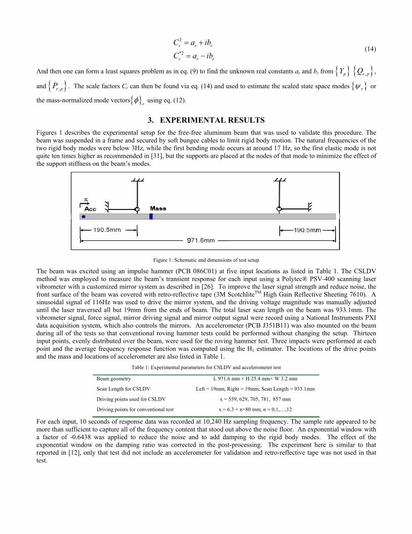
3. EXPERIMENTAL RESULTS Figures 1 describes the experimental setup for the free-free aluminum beam that was used to validate this procedure. The beam was suspended in a frame and secured by soft bungee cables to limit rigid body motion. The natural frequencies of the two rigid body modes were below 3Hz, while the first bending mode occurs at around 17 Hz, so the first elastic mode is not quite ten times higher as recommended in [31], but the supports are placed at the nodes of that mode to minimize the effect of the support stiffness on the beam’s modes.

Figure 1: Schematic and dimensions of test setup

The beam was excited using an impulse hammer (PCB 086C01) at five input locations as listed in Table 1. The CSLDV method was employed to measure the beam’s transient response for each input using a Polytec® PSV-400 scanning laser vibrometer with a customized mirror system as described in [26]. To improve the laser signal strength and reduce noise, the front surface of the beam was covered with retro-reflective tape (3M ScotchliteTM High Gain Reflective Sheeting 7610). A sinusoidal signal of 116Hz was used to drive the mirror system, and the driving voltage magnitude was manually adjusted until the laser traversed all but 19mm from the ends of beam. The total laser scan length on the beam was 933.1mm. The vibrometer signal, force signal, mirror driving signal and mirror output signal were record using a National Instruments PXI data acquisition system, which also controls the mirrors. An accelerometer (PCB J351B11) was also mounted on the beam during all of the tests so that conventional roving hammer tests could be performed without changing the setup. Thirteen input points, evenly distributed over the beam, were used for the roving hammer test. Three impacts were performed at each point and the average frequency response function was computed using the H1 estimator. The locations of the drive points and the mass and locations of accelerometer are also listed in Table 1.

Table 1: Experimental parameters for CSLDV and accelerometer test

Beam geometry

Scan Length for CSLDV

Driving points used for CSLDV

Driving points for conventional test

L 971.6 mm × H 25.4 mm× W 3.2 mm

Left = 19mm, Right = 19mm; Scan Length = 933.1mm

x = 559, 629, 705, 781, 857 mm

x = 6.3 + n×80 mm, n = 0,1,…,12

For each input, 10 seconds of response data was recorded at 10,240 Hz sampling frequency. The sample rate appeared to be more than sufficient to capture all of the frequency content that stood out above the noise floor. An exponential window with a factor of -0.6438 was applied to reduce the noise and to add damping to the rigid body modes. The effect of the exponential window on the damping ratio was corrected in the post-processing. The experiment here is similar to that reported in [12], only that test did not include an accelerometer for validation and retro-reflective tape was not used in that test.

3.1 Experimental CSLDV Results Using MDTS Method

Figure 2 shows the frequency domain spectrum of one of the CSLDV measurements up to 800 Hz, where peaks are evident in the response near each of the natural frequencies plus or minus integer multiples of the 116 Hz scan frequency. This occurs because each time-varying mode shape modulates the response of each mode as was explained in [6, 12]. The CSLDV measurement is easier to interpret after it has been lifted, as discussed in [12]. To do this, one must first obtain a very accurate estimate of the mirror drive frequency. This was done by fitting a Fourier series to the measured mirror position signal and using an optimization routine to find the best fundamental frequency for the series. This was found to be 116.0090 Hz using a tolerance of 1e-6. The phase of the drive signal was used to align each of the responses. Then the response and its corresponding force and mirror output signals were resampled so that they had an integer number of samples per scanning period.

0 100 200 300 400 500 600 700 80010-6

10-5

10-4

10-3

10-2

10-1

100

Frequency (Hz)

FFT

of V

eloc

ity (m

/s)

Spectrum of 116Hz CSLDV Signal

Figure 2: Expanded view of CSLDV signal of beam with accelerometer attached

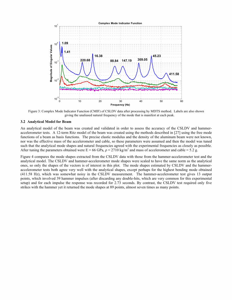
Initially, the portion of the signals before and during the force input pulse were deleted to give a Ni = 5 input and NA = 89 response points, 1157 frequency line pseudo-FRF matrix. (That information was subsequently restored in order to use the scaling routine, as described later.) The complex mode indicator function (CMIF), shown in Figure 3, was formed for the 5-input set of lifted responses, to see whether any repeated natural frequencies exist. The second singular value trace in the CMIF (green) always has a considerably lower magnitude than the first, suggesting that none of the (aliased) frequencies in the pseudo-FRFs are repeated, which is why the 116 Hz scan frequency was chosen for this analysis. Comparing Figures 2 and 3, one can see that the lifting procedure has resulted in a much simpler spectrum, as discussed in detail in [12]. The lifted spectrum was used to identify the modes of the beam, and the frequencies and damping ratios obtained are shown in Table 3. The frequencies and damping ratios obtained by the conventional hammer-accelerometer test are also shown. Both methods gave very similar results; the differences of natural frequency are less than 1%, and the differences between the damping ratios are less than 3%.

0 10 20 30 40 50 60

10-3

10-2

10-1

100

101

Frequency (Hz)

Mag

nitu

de o

f Sin

gula

r Val

ues

Complex Mode Indicator Function

1.09

1.4116.38

411.58

147.1988.84220.6845.23

309.05

Figure 3: Complex Mode Indicator Function (CMIF) of CSLDV data after processing by MDTS method. Labels are also shown

giving the unaliased natural frequency of the mode that is manifest at each peak.

3.2 Analytical Model for Beam

An analytical model of the beam was created and validated in order to assess the accuracy of the CSLDV and hammer-accelerometer tests. A 12-term Ritz model of the beam was created using the methods described in [27] using the free mode functions of a beam as basis functions. The precise elastic modulus and the density of the aluminum beam were not known, nor was the effective mass of the accelerometer and cable, so these parameters were assumed and then the model was tuned such that the analytical mode shapes and natural frequencies agreed with the experimental frequencies as closely as possible. After tuning the parameters obtained were E = 66 GPa, ρ = 2710 kg/m3 and mass of accelerometer and cable = 5.2 g.

Figure 4 compares the mode shapes extracted from the CSLDV data with those from the hammer-accelerometer test and the analytical model. The CSLDV and hammer-accelerometer mode shapes were scaled to have the same norm as the analytical ones, so only the shapes of the vectors is of interest in this plot. The mode shapes estimated by CSLDV and the hammer-accelerometer tests both agree very well with the analytical shapes, except perhaps for the highest bending mode obtained (411.58 Hz), which was somewhat noisy in the CSLDV measurement. The hammer-accelerometer test gives 13 output points, which involved 39 hammer impulses (after discarding any double-hits, which are very common for this experimental setup) and for each impulse the response was recorded for 2.73 seconds. By contrast, the CSLDV test required only five strikes with the hammer yet it returned the mode shapes at 89 points, almost seven times as many points.

0 100 200 300 400 500 600 700 800 900 1000-4

-2

0

2

4

6Elastic Mode Shapes

Mode 1Mode 2Mode 3

0 100 200 300 400 500 600 700 800 900 1000-4

-2

0

2

4

6

Mode 4Mode 5

0 100 200 300 400 500 600 700 800 900 1000-4

-2

0

2

4

6

Position (mm)

Mode 6Mode 7

Figure 4: Mode shapes for free-free beam with an accelerometer attached at x=6.4 mm. Solid black lines denote the analytical shapes estimated

by Ritz method; dots show the CSLDV shapes at each pseudo-measurement point; triangles give the results of a hammer - accelerometer test.

Careful inspection of the mode shapes in Fig. 4 reveals that each mode shape has slightly lower amplitude at the left edge of the beam than the right edge. CSLDV was applied to a bare beam without an accelerometer in [12], and the mode shapes were found to agree very well with the analytical mode functions for a free-free beam. Here the shapes are considerably different, apparently due to the small mass loading effect of the accelerometer.

To verify the mass-scaling in the analytical model, an additional test was performed with a 58.5g mass added at x = 246mm (see Fig. 1). The same procedure was used for this with an exponential window factor of -0.8158. Fig. 5 gives the normalized analytical and experimental mode shapes of the beam with both the accelerometer and the 58.5g mass attached. The shapes have changed substantially due to the attached mass, especially near the point where it was attached (x = 246mm). Both the CSLDV and hammer-accelerometer measurements capture this change, and it agrees well with that predicted by the Ritz model.

0 100 200 300 400 500 600 700 800 900 1000-5

0

5Elastic Mode Shapes

Mode 1Mode 2Mode 3

0 100 200 300 400 500 600 700 800 900 1000-5

0

5

Mode 4Mode 5

0 100 200 300 400 500 600 700 800 900 1000-5

0

5

Position (mm)

Mode 6Mode 7

Figure 5: Mode shapes for the free-free beam with an accelerometer at 6.4mm and a mass added at 246mm. Solid black lines denote the

analytical shapes estimated by Ritz method; dots show the CSLDV shapes at each pseudo-measurement point; triangles give the results of the hammer-accelerometer test.

Table 2 compares the natural frequencies of the analytical model with those measured by CSLDV. The first two columns compare the baseline model consisting of the free-beam and the accelerometer with the corresponding measurements. It can be seen that the Ritz model predicts the actual measured frequencies well for all of the modes, the largest error being less than 1% (for the 7th mode). The 3rd and 4th columns compare the analytical and experimental frequencies with the added mass. For convenience, the difference between each of the frequencies was also computed and is shown in the 5th and 6th columns. According to theory, the frequency shift is proportional to the scale of the mode vectors [18]. The measured frequency shifts agree very well with those predicted by the analytical model, although the errors become larger for some of the higher modes. The rotatory inertia of the block was not included in the Ritz model, but it does have a more significant effect as frequency increases so this might explain the discrepancy. Also, the point where the block was attached is very near a node of the beam for the 4th and 5th modes, so this might explain why those frequency shifts were predicted less accurately than the others. In any event, these results suggest that the Ritz model is quite accurate and accurately scaled, so it should serve as a good standard against which to compare the scaled mode shapes that were obtained experimentally.

Table 2. Comparison of analytical and CSLDV natural frequencies in Hz with and without the added mass

Accelerometer Accelerometer and mass Frequency shift

Mode Analytical Experimental Analytical Experimental Analytical Experimental

1 16.38 16.38 16.21 16.20 0.17 0.18

2 45.35 45.23 39.62 39.59 5.73 5.64

3 89.23 88.84 82.05 81.69 7.18 7.15

4 147.99 147.19 147.33 145.86 0.66 1.33

5 221.71 220.70 211.02 208.38 10.69 12.32

6 310.49 309.04 280.55 279.07 29.94 29.97

7 414.37 411.58 395.57 390.28 18.8 21.3

3.3 Experimental Mass Normalization

The mode shapes shown in Figure 4 were used in the procedure described in Section 2 to find the unknown scale factors Cr relating the identified mode shapes to the mass-normalized mode vectors. In order to do this, the part of the measurement that occurred before and during the force pulse was restored so that the full set of input-output data could be used in the normalization procedure. All of the 5 inputs were considered simultaneously, resulting in an overdetermined system of linear equations, which were solved to find the scale factors that best satisfied the entire data set, so the mode scale factors found are denoted “MIMO MSFs” in Table 3. The scale factors were found using each of the two methods described in Section 2 based on both real and complex modes. The mode scale factors were then computed between the analytical modes and the scaled experimental modes, and are reported in the table. For the state space modes, the scaled state space modes were computed and then the best real-mode approximation to each was found and used to compute the MSF. The MAC values between the experimentally derived mode shapes and the analytical ones are also reported, most of which are above 0.98 so any discrepancy in the MSFs should be attributable to the scale of the modes.

It should be noted that the algorithm based on classical modes sometimes returned negative squared scale factors, which is not reasonable since the scale factors are real numbers. The spectra near these natural frequencies were carefully inspected, revealing that the negative scale factor was needed to adequately reconstruct the measurements. The reason for this is not known, but it could simply be a phase error in the data and so it was ignored and the absolute value of the squared scale factors was used in the results that are reported. When the state space algorithm was used, this was not an issue since the state space description allows the mode vectors to be scaled by any complex constant.

Table 3. Summary of results of CSLDV and hammer-accelerometer tests

Hammer - CSLDV Hammer - Accelerometer

Mode Frequency (Hz) Damping MAC Classical

MIMO MSF State Space MIMO MSF

Frequency (Hz) Damping MAC Classical

SIMO MSF 1 16.38 0.52% 1.00 0.96 0.96 16.38 0.52% 1.00 0.97

2 45.23 0.31% 1.00 0.93 0.94 45.23 0.32% 1.00 1.03

3 88.84 0.59% 1.00 0.96 0.96 88.85 0.60% 1.00 0.99

4 147.19 0.43% 0.98 0.95 0.94 147.19 0.44% 0.99 1.03

5 220.70 0.12% 0.99 0.93 0.94 220.69 0.12% 0.99 1.02

6 309.04 0.08% 0.99 0.90 0.90 309.06 0.08% 0.99 1.05

7 411.58 0.17% 0.95 0.92 0.90

411.55 0.17% 0.99 1.16

The MSFs show that the procedure proposed in this work scales the CSLDV mode vectors quite accurately; the discrepancy between them and the analytical model is always between -4 and -10%. The higher modes showed larger deviations from the analytical model. This might be caused by measurement noise since those modes are somewhat weak relative to the noise. The hammer-accelerometer test yielded a similar level of uncertainty, ranging from -3% to +16%. There seems to be a systematic difference between the CSLDV and hammer-accelerometer MSFs; the former seem to always under predict the mode scaling while the latter more often over predict it. The reason for this is not known, but one should note that there is potentially a good deal of uncertainty associated with the direction and location of the hammer blows, which may contribute to the variation in the MSFs. Uncertainty in the damping ratio of the each mode may also contribute to the variability. Finally, we note that accurate mode scaling requires that all of the sensors and data acquisition hardware be correctly calibrated, but the uncertainty in the accelerometer calibration alone is a few percent, so these types of errors could explain much of the discrepancy.

4. CONCLUSIONS This work presented a new procedure whereby mass-normalized mode shapes can be identified from continuous-scan laser vibrometer measurements, potentially at hundreds of points simultaneously on a structure. The method builds on a CSLDV technique that was previously presented by two of the authors [12] where the response of the structure is recorded as a laser vibrometer scans rapidly over the structure. The mode scaling procedure presented here uses the measured response and the input force to compute the scale factor between the CSLDV computed vectors and the underlying mass-normalized modes of the system.

The proposed mode scaling method was evaluated by using it to compute the first seven mass normalized modes of a free-free aluminum beam from a multi-input set of CSLDV measurements. Although the true mass-normalized modes of a real

structure such as this are not known, the CSLDV results were validated in two ways. First, an accelerometer was mounted on one end of the beam and a traditional roving hammer test was performed to estimate the mass-normalized modes at 13 points. Second, an analytical model of the beam was created using the Ritz method, and tuned to accurately reproduce the natural frequencies of the beam. In this effort, it was necessary to model the mass of a small accelerometer that was mounted on one end of the beam in order to obtain accurate results, and the model was verified by checking that the mode shapes obtained by CSLDV agreed well with those predicted by the model. The model was also checked by verifying that it correctly predicted the amount that the first seven natural frequencies shifted when a small mass was attached to the beam. The mass-loaded mode shapes predicted by the model were also compared with the experimentally measured mode shapes and found to agree very well.

The mass-normalized mode shapes predicted by CSLDV were compared with those from the analytical model using the modal scale factor. The MSFs between the CSLDV mode shapes and the analytical were above 0.90, indicating no more than 10% disagreement in scale and many of the modes agreed to within 5%. The mode shapes found using the traditional accelerometer / roving hammer test showed a similar level of disagreement with the analytical model. It was also informative to compare the time required to perform CSLDV relative to the traditional roving hammer test. The traditional test required almost eight times as many impacts with the hammer, yet the spatial resolution obtained by that method was seven times lower than that obtained by CSLDV.

The spatially detailed, mass-normalized modes identified using this method can be used to predict the effect of structural modifications (see, e.g. [32]), or the modes can be used in substructuring predictions, where the structure’s modal model is coupled to models for other subcomponents in order to predict the response of the built-up structure [19]. This possibility is especially intriguing since one can reliably estimate the rotation of the structure thanks to the high spatial detail afforded by CSLDV. Rotations must be accurately captured at the interfaces between subcomponents in order to obtain accurate substructuring predictions, but this has proven challenging and many researchers have explored methods for doing this [20, 33-37].

5. REFERENCES [1] P. Sriram, J. I. Craig, and S. Hanagud, "Scanning laser Doppler vibrometer for modal testing," International Journal

of Analytical and Experimental Modal Analysis, vol. 5, pp. 155-167, 1990. [2] P. Sriram, S. Hanagud, and J. I. Craig, "Mode shape measurement using a scanning laser doppler vibrometer,"

International Journal of Analytical and Experimental Modal Analysis, vol. 7, pp. 169-178, 1992. [3] P. Sriram, S. Hanagud, and J. I. Craig, "Mode shape measurement using a scanning laser doppler vibrometer." vol. 1

Florence, Italy: Publ by Union Coll, Schenectady, NY, USA, 1991, pp. 176-181. [4] C. W. Schwingshackl, A. B. Stanbridge, C. Zang, and D. J. Ewins, "Full-Field Vibration Measurement of

Cylindrical Structures using a Continuous Scanning LDV Technique," in 25th International Modal Analysis Confernce (IMAC XXV) Orlando, Florida, 2007.

[5] A. B. Stanbridge and D. J. Ewins, "Modal testing using a scanning laser Doppler vibrometer," Mechanical Systems and Signal Processing, vol. 13, pp. 255-70, 1999.

[6] A. B. Stanbridge, M. Martarelli, and D. J. Ewins, "Measuring area vibration mode shapes with a continuous-scan LDV," Measurement, vol. 35, pp. 181-9, 2004.

[7] M. Martarelli, "Exploiting the Laser Scanning Facility for Vibration Measurements," Ph.D. Thesis, Imperial College of Science, Technology & Medicine, London: Imperial College, 2001.

[8] S. Vanlanduit, P. Guillaume, and J. Schoukens, "Broadband vibration measurements using a continuously scanning laser vibrometer," Measurement Science &amp; Technology, vol. 13, pp. 1574-82, 2002.

[9] A. B. Stanbridge, A. Z. Khan, and D. J. Ewins, "Modal testing using impact excitation and a scanning LDV," Shock and Vibration, vol. 7, pp. 91-100, 2000.

[10] A. B. Stanbridge, M. Martarelli, and D. J. Ewins, "Scanning laser Doppler vibrometer applied to impact modal testing," in 17th International Modal Analysis Conference - IMAC XVII. vol. 1 Kissimmee, FL, USA: SEM, Bethel, CT, USA, 1999, pp. 986-991.

[11] R. Ribichini, D. Di Maio, A. B. Stanbridge, and D. J. Ewins, "Impact Testing With a Continuously-Scanning LDV," in 26th International Modal Analysis Conference (IMAC XXVI) Orlando, Florida, 2008.

[12] M. S. Allen and M. W. Sracic, "A New Method for Processing Impact Excited Continuous-Scan Laser Doppler Vibrometer Measurements," Mechanical Systems and Signal Processing, vol. 24, pp. 721–735, 2010.

[13] S. Rothberg, "Numerical simulation of speckle noise in laser vibrometry," Applied Optics, vol. 45, pp. 4523-33, 2006.

[14] S. J. Rothberg, "Laser vibrometry. Pseudo-vibrations," Journal of Sound and Vibration, vol. 135, pp. 516-522, 1989. [15] S. J. Rothberg and B. J. Halkon, "Laser vibrometry meets laser speckle," 1 ed. vol. 5503 Ancona, Italy: SPIE-Int.

Soc. Opt. Eng, 2004, pp. 280-91.

[16] M. S. Allen, "Frequency-Domain Identification of Linear Time-Periodic Systems using LTI Techniques," Journal of Computational and Nonlinear Dynamics vol. 4, 24 Aug. 2009.

[17] R. J. Allemang and D. L. Brown, "A Unified Matrix Polynomial Approach to Modal Identification," Journal of Sound and Vibration, vol. 211, pp. 301-322, 1998.

[18] D. J. Ewins, Modal Testing: Theory, Practice and Application. Baldock, England: Research Studies Press, 2000. [19] D. de Klerk, D. J. Rixen, and S. N. Voormeeren, "General framework for dynamic substructuring: History, review,

and classification of techniques," AIAA Journal, vol. 46, pp. 1169-1181, 2008. [20] M. S. Allen, R. L. Mayes, and E. J. Bergman, "Experimental Modal Substructuring to Couple and Uncouple

Substructures with Flexible Fixtures and Multi-point Connections," Journal of Sound and Vibration, vol. Submitted Aug 2009, 2010.

[21] M. Imregun, D. A. Robb, and D. J. Ewins, "Structural Modification and Coupling Dynamic Analysis Using Measured FRF Data," in 5th International Modal Analysis Conference (IMAC V) London, England, 1987.

[22] D. R. Martinez, A. K. Miller, and T. G. Carne, "Combined Experimental and Analytical Modeling of Shell/Payload Structures," in The Joint ASCE/ASME Mechanics Conference, D. R. M. a. A. K. Miller, Ed. Albuquerque, NM, 1985, pp. 167-194.

[23] M. Corus, E. Balmes, and O. Nicolas, "Using model reduction and data expansion techniques to improve SDM," Mechanical Systems and Signal Processing, vol. 20, pp. 1067-89, 2006.

[24] S. D. Stearns, Digital Signal Processing with Examples in Matlab. New York: CRC Press, 2003. [25] M. S. Allen and J. H. Ginsberg, "A Global, Single-Input-Multi-Output (SIMO) Implementation of The Algorithm of

Mode Isolation and Applications to Analytical and Experimental Data," Mechanical Systems and Signal Processing, vol. 20, pp. 1090–1111, 2006.

[26] A. Gasparoni, M. S. Allen, S. Yang, M. W. Sracic, P. Castellini, and E. P. Tomasini, "Experimental Modal Analysis on a Rotating Fan Using Tracking-CSLDV," in 9th International Conference on Vibration Measurements by Laser and Noncontact Techniques Ancona, Italy, 2010.

[27] J. H. Ginsberg, Mechanical and Structural Vibrations, First ed. New York: John Wiley and Sons, 2001. [28] R. J. Allemang, Vibrations Course Notes. Cincinnati: http://www.sdrl.uc.edu/, 1999. [29] M. S. Allen and T. G. Carne, "Comparison of Inverse Structural Filter (ISF) and Sum of Weighted Accelerations

Technique (SWAT) Time Domain Force Identification Methods," in 47th AIAA-ASME-ASCE-AHS-ASC Structures, Structural Dynamics, and Materials Conference Newport, RI, 2006.

[30] M. S. Allen and T. G. Carne, "Delayed, Multi-step Inverse Structural Filter for Robust Force Identification and comparison with the Sum of Weighted Accelerations Technique," Mechanical Systems and Signal Processing, vol. 22, pp. 1036–1054, 2008.

[31] T. G. Carne, D. Todd Griffith, and M. E. Casias, "Support conditions for experimental modal analysis," Sound and Vibration, vol. 41, pp. 10-16, 2007.

[32] J. E. Mottershead, M. G. Tehrani, D. Stancioiu, S. James, and H. Shahverdi, "Structural modification of a helicopter tailcone," Journal of Sound and Vibration, vol. 298, pp. 366-84, 2006.

[33] P. Avitabile, J. O'Callahan, C. M. Chou, and V. Kalkunte, "Expansion of rotational degrees of freedom for structural dynamic modification," in 5th International Modal Analysis Conference (IMAC V) London, England, 1987.

[34] H. Kanda, M. L. Wei, R. J. Allemang, and D. L. Brown, "Structural Dynamic Modification Using Mass Additive Technique," in 4th International Modal Analysis Conference (IMAC IV) Los Angeles, California, 1986.

[35] J. E. Mottershead, A. Kyprianou, and H. Ouyang, "Structural modification. Part 1: rotational receptances," Journal of Sound and Vibration, vol. 284, pp. 249-65, 2005.

[36] D. de Klerk, D. J. Rixen, S. N. Voormeeren, and F. Pasteuning, "Solving the RDoF Problem in Experimental Dynamic Substructuring," in 26th International Modal Analysis Conference (IMAC XXVI) Orlando, Florida, 2008.

[37] D. R. Martinez, T. G. Carne, D. L. Gregory, and A. K. Miller, "Combined Experimental/Analytical Modeling Using Component Mode Synthesis," in AIAA/ASME/ASCE/AHS Structures, Structural Dynamics & Materials Conference Palm Springs, CA, USA, 1984, pp. 140-152.