massive mimo for high-accuracy target localization and

2327-4662 (c) 2020 IEEE. Personal use is permitted, but republication/redistribution requires IEEE permission. See http://www.ieee.org/publications_standards/publications/rights/index.html for more information.

This article has been accepted for publication in a future issue of this journal, but has not been fully edited. Content may change prior to final publication. Citation information: DOI 10.1109/JIOT.2021.3050720, IEEE Internet ofThings Journal

1

Massive MIMO for High-Accuracy TargetLocalization and Tracking

Xiaolu Zeng, Feng Zhang, Beibei Wang, Senior Member, IEEE and K. J. Ray Liu, Fellow, IEEE

Abstract—High-accuracy target localization and tracking havebeen widely used in the modern navigation system. However,most of the methods such as GPS are highly dependent ontime measurement accuracy, which prevents them from achievinghigh accuracy in practice. Time-reversal (TR) based techniquehas been shown to be able to achieve centimeter accuracylocalization by fully utilizing the focusing effect brought bythe massive multipaths naturally existing in a rich scatteringenvironment such as indoor scenarios. By investigating a similarstatistical property, this paper develops a novel high-accuracytarget localization method by using massive MIMO to providemassive signal components. We first observe that the statisticalautocorrelation of the received energy physically focuses into abeam around the receiver exhibiting a sinc-like distribution infar-field scenario. By leveraging such a distribution of the focus-ing beam, an effective way to estimate the relative moving speedof the target with respect to a single base station is proposed.We also obtain the absolute moving speed and subsequently trackthe target accurately by associating the speed estimation resultsand geometrical relationship of multiple stations. The theoreticalanalysis on the error in the speed and localization estimationvalidated by numerical simulation results show that the proposedsystem can achieve decimeter accuracy for target localization andtracking.

Index Terms—Statistical electromagnetic, MIMO, target local-ization and tracking, centimeter accuracy.

I. INTRODUCTION

TARGET localization and tracking have been of greatinterest over several decades because of their wide appli-

cations in navigation and many location-based services suchas autonomous drivings [1], [2]. Furthermore, most of theselocalization requests emerge in urban areas where the globalpositioning system (GPS) [3] cannot offer good performancebecause the line-of-sight (LOS) signal between the GPS satel-lite and the terminal is easily to be blocked by obstaclessuch as tall buildings. As a result, it is imperative to seek fortechnologies which can provide high-accuracy localization incomplex environments such as dense urban areas under non-line-of-sight (NLOS) and multipath conditions [4].

Based on their principle, localization techniques can beclassified into two categories, i.e., triangulation-based meth-ods and fingerprinting-based methods. Triangulation-basedmethods consist of two steps. First, model-based parameters

X. Zeng is with the Department of Electrical and Computer En-gineering, University of Maryland at College Park, USA (e-mail: [email protected]). During this work, he was also a visiting student fromXidian University, Xi’an, 71007, China.

F. Zhang, B. Wang and K. J. R. Liu are with Origin Wireless Inc.,Greenbelt, MD 20770 USA, and also with the Department of Electrical andComputer Engineering, University of Maryland, College Park, MD 20742USA (e-mail: fzhang15, bebewang, [email protected]).

such as the angle-of-arrivals (AOAs) [5], [6], time-of-arrivals(TOAs) [7], [8] or time-difference-of-arrival (TDOAs) of LOSsignals [9] are measured at all access points (APs) or basestations (BSs). Then, the target location can be estimatedby using triangulation/trilateration among all APs/BSs [10].However, these methods cannot work well under the multi-path effect and NLOS because of the unreliable parameterestimation. Fingerprinting-based methods first construct anoffline database by collecting location related features suchas received signal strength (RSS) [11]–[13] and channel stateinformation (CSI) [14]–[16] in the area of interest. Then,the same features are extracted from the online signals andcompared with the offline database to obtain the location esti-mations. However, the overhead of establishing and updatingthe offline database also prevents these methods from beingwidely adopted [2].

More recently, massive MIMO has been gaining popularityin target localization because of its high angular resolution anddegree of freedom [17]. This mainly benefits from the hun-dreds of antennas on the BS, which can enable narrow, highly-directional and high-gain beams by beamforming [18]. Similarto the localization methods without using massive MIMO, theexisting massive MIMO-based localization methods can alsobe classified into the same two categories. The first is thetriangulation-based methods in which many techniques suchas beamforming [19], multiple signal classification (MUSIC)[20], 2-D rotational invariance technique [21] and compres-sive sensing [22], [23] are explored on the base of massiveMIMO systems. To reduce the prohibitive energy consumptionand complexity increment caused by the massive antennas,high-efficient beam allocation/switching schemes [24], [25],AOAs estimations in beamspace [26], pre-energy detections[27] as well as the combination of digital beamforming andanalog techniques [28]–[30] have been considered. In thefingerprinting-based methods with massive MIMO [31]–[36],different matching techniques have been studied in comparingthe online phase with the offline phase to estimate the targetlocation such as model-based similarity comparison [31],similarity learning by neural network (NNs) [32], [33], supportvector machines (SVMs) [35] and Kernel-based methods [36].Even though the localization accuracy is improved by lever-aging the high range/angular resolution provided by massiveantennas, most of existing massive MIMO-based localizationmethods still entail the same challenges as the traditionalmethods which do not use massive MIMO antennas, that is,the NLOS distortions and performance degradation in rich-scattering environment. This motivates us to design a high-accuracy localization system that is robust to environment

Authorized licensed use limited to: University of Maryland College Park. Downloaded on March 11,2021 at 18:06:56 UTC from IEEE Xplore. Restrictions apply.



2

dynamics while with good performance under multipath andNLOS conditions.

Inspired by the recent research on decimeter-accuracy in-door tracking [37]–[40] using time reversal focusing effect[41], [42], in this paper, we propose a massive MIMO-basedhigh-accuracy localization and tracking system by utilizing thefocusing effect brought by the massive number of antennas.We first propose the definition of an important statistical vari-able, the strength of the autocorrelation function (ACFS) of thereceived signal in a massive MIMO system, to characterize theenergy distribution of the focusing effect around a location ofinterest. Because the received signal in a massive MIMO sys-tem contains a large number of components due to the massivenumber of antenna elements and further reflections/scattering,it can be shown that the distribution of the ACFS exhibitsa stationary sinc-like focusing beam1 around the receiver inspatial domain regardless of the environment.

By leveraging the ACFS, we then develop an approachwhich can estimate the relative speed of the target withrespect to a single BS. The absolute moving speed, movingdirection/orientation and location of the target can be furtherderived by jointly considering the relative speed estimationand geometrical relationship among multiple BSs. Differentfrom [42] which needs an extra inertial sensor to estimatethe moving direction because the energy distribution of thetime reversal focusing effect shows the same trend along allthe directions, the proposed system can estimate the movingspeed/distance and direction simultaneously only based on theACFS focusing beam which exhibits different distributionsalong different directions. This is because that in the proposedsystem the massive number of the incident signal componentsreach the receiver from the antennas/BS side, resulting in adirectional focusing beam rather than a symmetrical focusingball as shown in [42].

Based on the derivation of the ACFS and how it can be usedfor speed and location estimation, we derive the theoreticalexpectation of the speed and location estimation errors, whichare further verified by extensive simulations. It is shown thatthe proposed system can achieve decimeter-level accuracy fortarget localization and tracking in various scenarios, whichoutperforms three latest massive MIMO-based localizationtechniques [23] [31] [32].

In summary, the main contributions of this work are asfollows:• We observed and proved that the statistical distribution

of the ACFS of the received signal in a massive MIMOsystem exhibits a sinc-like beam pattern, because thereceived signal usually contains a large number of LOSand NLOS signal components.

• Based on the distribution of the ACFS, we developed atarget localization and tracking system which has robustperformance in rich-scattering urban areas with NLOS.Because the proposed system only needs to calculate the

1We use the term focusing beam rather than beamforming because weutilize the ACFS, a specific function of the received signal for positioning atarget, and the distribution of the ACFS happens to exhibit a beam-shapedpattern. There is no ”physical beamforming” that explicitly focuses a signaltowards a receiver.

ACFS of the received signal on the user side while thespeed and location estimations are very straightforwardaccording to the derived close-form expressions, the sys-tem enjoys a very low computation complexity and thuscan be widely applied in real-time tracking and navigationapplications with a stringent requirement on the latency.

• We further derived the theoretical speed and localizationerror expectations of the proposed system and validatedthe theoretical performance analysis using extensive sim-ulations.

The rest of the paper is organized as follows. In Section II,we elaborate on the signal model for massive MIMO systemfollowed by the derivation of the focusing beam. Then, SectionIII proposes a speed estimation method by using the focus-ing beam of multiple distributed BSs. Section IV introducethe target localization system while Section V derives thetheoretical speed and location estimation error expectations.Extensive numerical simulations are conducted to validate theperformance of the proposed approach in Section VI. Finally,Section VII concludes this paper.

II. FOCUSING BEAM IN MASSIVE MIMO

In this section, we first introduce the background knowledgeabout the system model. Then, we elaborate on the signalmodel and derive the analytical distribution of the ACFSfocusing beam in 5G massive MIMO communication systems.

A. Background Knowledge

Ultra-dense 5G BS deployment: The 5G cellular networkwill be an ultra-dense cellular network, e.g., with a density of40− 50 BS/km2, because that a massive number of antennaswill be deployed on the BS [43], which means that everyantenna’s transmission power has to be greatly decreasedcompared to that of a 4G BS, leading to a smaller coveragearea. Second, mmWave transmission is very likely to beadopted in 5G cellular networks and the signal decays muchfaster at mmWave frequency which again will reduce thecell coverage and thus denser BS deployment is needed. Forexample, the Federal Communications Commission (FCC) inthe USA issued a declaratory ruling which indicates that mostof the 5G BSs are about 30 feet tall while the service range ofeach BS is about 400-500 feet or less in large crowded areas[44].Far-field condition: As shown in Fig. 1, let HB and LBR de-note the altitude of the BS and the horizontal distance betweenthe BS and the receiver. Ae is the aperture of the antenna arrayA. Due to the Ultra-dense 5G BS deployment, LBR is about 80-200m in practice [43]. In addition, Ae is less than 2m and HB isabout 10m because of the antenna fabrication and installationrequirements [44]. As a consequence, LBR ≥ 10HB Ae isthe condition of the far-field scenario in this paper and usuallyholds in the 5G networks [45], [46]. This is different fromthe conventional far-field condition in which Lf = 2A2

e/λ isthe boundary between the Fresnel region and the Fraunhoferregion [47] with λ as the wavelength of the signal.




3

tr

1

M

Transmitting antenna

x

z

yO

BH

BRL

B

A

AeB( 2,0,H )m mdxThe mth antenna

Receiver at

Scatter n

Scatter 1

Scatter N

NLOSLOS

Scatter

n

Fig. 1: The set-up for a BS with massive MIMO antennas.

B. Signal Model

As shown in Fig. 1, “B” denotes a BS equipped with Mantennas which communicate with the receiver “r” simulta-neously. Note that practical measurements in [48]–[50] havevalidated that the LOS signal matches with the free spacepropagation model while the NLOS signal follow the Raleighfading [51] in 5G massive MIMO system. As a result, in urbanareas, the received signal consisting of both LOS and NLOSparts at baseband can be expressed as

y(t) = yL(t) + yN(t) + n(t),

yL(t) =√KL

M∑m=1

exp(j(k|xmrt|+ φm))

4π|xmrt|,

yN(t) =√KN

N∑n=1

exp[j(ωdtcosαn + φn)],

(1)

where yL(t) and yN(t) denote the LOS and NLOS componentsand KL and KN are their corresponding power, k = 2π/λ isthe wave number, λ is the wave length, ωd is the maximumradian Doppler frequency, xm and rt are the coordinates ofthe m-th antenna and the receiver at time t, respectively,|xmrt| denotes the Euclidean spatial distance between them-th antenna and the receiver, n(t) represents the additiveGaussian noise, φm is the phase distortion of the m-th LOSpath signal, and αn and φn are the AOA and phase distortionof the n-th NLOS signal component.

In general, φm is caused by hardware imperfections, het-erogeneity of the propagation medium and channel attenua-tions, etc. αn and φn are mainly introduced by the reflec-tion/absorption of the randomly distributed scatterers in a rich-scattering urban area. As a result, φm, αn and φn are notdeterministic and can be assumed as i.i.d uniform distributionsover [−π, π) for m = 1, 2, . . . ,M and n = 1, 2, . . . , N[51], [52], where N is the total number of NLOS signalcomponents. In practice, the number of multipath N can varyfrom 10 to 100 in urban areas according to the practicalmeasurements in New York City [45], [46].

C. Massive MIMO Focusing Beam

In the following, we explore the distribution of the focusingeffect of massive MIMO in far-field scenario by first derivingthe ACF of the received signal and then the ACFS, which isinspired by the TRRS in [42], [53] but more robust to therandomness of signal distortions.

As shown in Fig. 2, a target moves from r0 at time t0 tors at time ts on the ground (xOy plane). Then, the ACF ofthe received signal between r0 and rs is defined as

ηy(r0, rs) = E[y(t0)y∗(ts)] (2)≈ ηyL + ηyN + ηn. (3)

where ηn = E[n(t0)n∗(ts)] = σ2I, σ2 is the power spectraldensity of the Gaussian noise n(t). ηyL , ηyN and ηn denotesthe ACF of the LOS signal component yL(t), NLOS signalcomponent yN(t) and the noise term n(t), respectively.

Note that the independence among yL(t), yN(t) and n(t)is assumed to obtain (3). Detailed derivations can be found inAppendix. Next, we will derive ηyN and then ηyL , respectively.

1) ACF of NLOS signal: According to [42], [51], ηyN canbe written as

ηyN = E[yN(t0)y∗N(ts)]

= KN

N∑n=1

N∑i=1

Eφ,α exp[j(ωdtcosαn + φn)

·exp[j(ωd(t+ τ)cosαi + φi)= KNNJ0(ωdτ) = KNNJ0(kp),

(4)

where τ = ts− t0, Eφ,α means taking expectation over φ andα, J0(·) is the 0-order Bessel function, and p is the Euclideandistance between r0 to rs and as shown in Fig. 2. We omitthe details about the derivation of (4) because they are similarto that in [42], [51].

2) ACF of LOS signal: Similar to (4), the ACF of the LOSsignal yL(t) between r0 and rs is given by

ηyL = ηyL(r0, rs) = E[yL(t0)y∗L(ts)] = KL·M∑i=1

M∑m=1

Eφ

exp[j(k(|xir0| − |xmrs|) + φi − φm)]

(4π)2|xir0||xmrs|

.

(5)

In the far-field scenario where |xir0|, |xmrs| > LBR Aeholds, |xir0| and |xmrs| in the denominator of (5) can beapproximated as the same for all elements, i.e., |xir0| ≈ |x0r0|and |xmrs| ≈ |x0rs| because (|xir0| − |xmrs|) is usuallymagnitudes smaller than |xir0| and |xmrs|. We omit thedenominator of (5) in the derivation for simplicity.

Next, we decompose (5) into two different cases, i.e., a)i = m and b) i 6= m. Considering i = m, we have

η1styL

= KL

M∑m=1

exp(jk(|xmr0| − |xmrs|)). (6)

To compute |xmr0| − |xmrs| in Fig. 2, the angle symbolsare defined as ∠rsr0r

′

s = γ′

m,∠rsr0r′

0 = γm,∠r′

sr0r′′

0 =β1,∠r

′′

0 r0r′

0 = β, where r′

0 lies in the extension line of lxmr0

satisfying that lxmr′0⊥ lrsr′0

. And r′′

0 is the projection of r′

0

on the xOy plane. From the cosine theory, we have

|xmrs|2 = (|xmr0| − pcosγm)2 + psinγ2m, (7)

cosγm = cosβ · cos(β1 + γ′

m), cosγ′

m = ε/p,

cosβ =

√L2

BR + x2m√

L2BR + H2

B + x2m

, cosβ1 =LBR√

L2BR + x2

m

.(8)




4

B

0r

1

M

x

O

BH

BRL

sr

''

sr'

0r

pL

y

z

Transmitting antennas A

''

0r

'

mx

'

sr

LOS

1β

m

'

m

The m-th antennamx

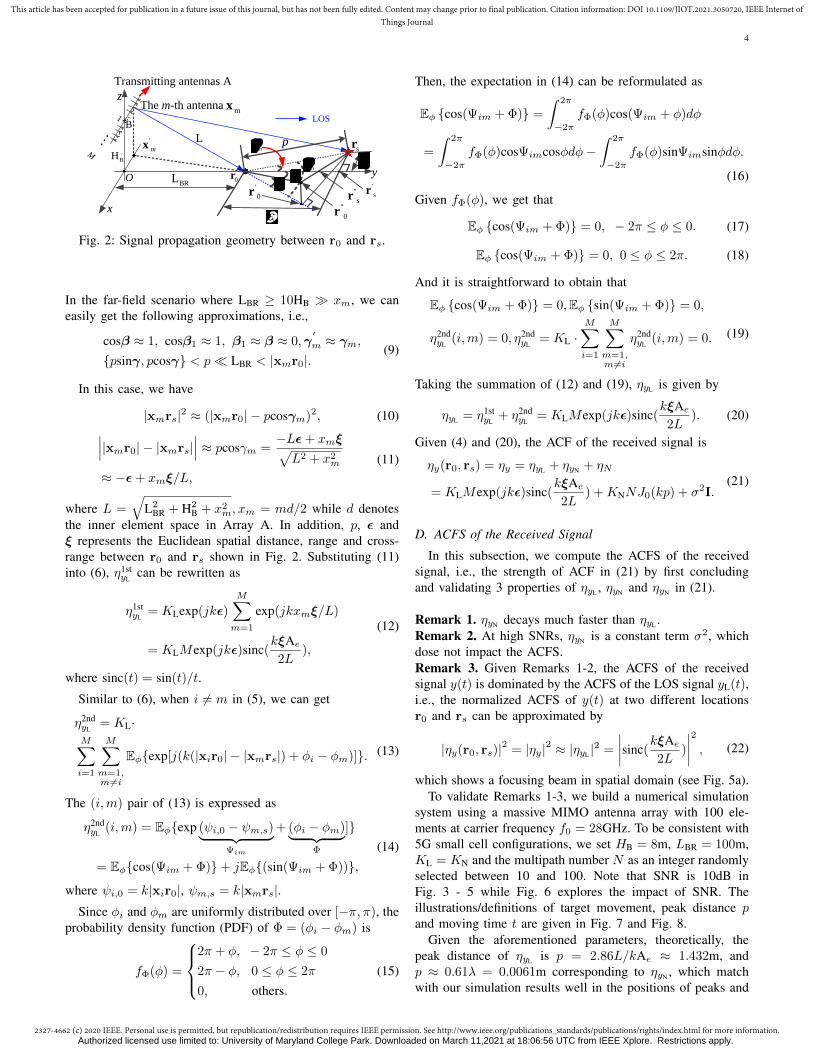
Fig. 2: Signal propagation geometry between r0 and rs.

In the far-field scenario where LBR ≥ 10HB xm, we caneasily get the following approximations, i.e.,

cosβ ≈ 1, cosβ1 ≈ 1, β1 ≈ β ≈ 0,γ′

m ≈ γm,

psinγ, pcosγ < p LBR < |xmr0|.(9)

In this case, we have

|xmrs|2 ≈ (|xmr0| − pcosγm)2, (10)∣∣∣|xmr0| − |xmrs|∣∣∣ ≈ pcosγm =

−Lε + xmξ√L2 + x2

m

≈ −ε + xmξ/L,

(11)

where L =√

L2BR + H2

B + x2m, xm = md/2 while d denotes

the inner element space in Array A. In addition, p, ε andξ represents the Euclidean spatial distance, range and cross-range between r0 and rs shown in Fig. 2. Substituting (11)into (6), η1st

yLcan be rewritten as

η1styL

= KLexp(jkε)M∑m=1

exp(jkxmξ/L)

= KLMexp(jkε)sinc(kξAe2L

),

(12)

where sinc(t) = sin(t)/t.

Similar to (6), when i 6= m in (5), we can get

η2ndyL

= KL·M∑i=1

M∑m=1,m6=i

Eφexp[j(k(|xir0| − |xmrs|) + φi − φm)]. (13)

The (i,m) pair of (13) is expressed as

η2ndyL

(i,m) = Eφexp (ψi,0 − ψm,s)︸︷︷︸Ψim

+ (φi − φm)︸︷︷︸Φ

]

= Eφcos(Ψim + Φ)+ jEφ(sin(Ψim + Φ)),(14)

where ψi,0 = k|xir0|, ψm,s = k|xmrs|.Since φi and φm are uniformly distributed over [−π, π), the

probability density function (PDF) of Φ = (φi − φm) is

fΦ(φ) =

2π + φ, − 2π ≤ φ ≤ 0

2π − φ, 0 ≤ φ ≤ 2π

0, others.(15)

Then, the expectation in (14) can be reformulated as

Eφ cos(Ψim + Φ) =

∫ 2π

−2π

fΦ(φ)cos(Ψim + φ)dφ

=

∫ 2π

−2π

fΦ(φ)cosΨimcosφdφ−∫ 2π

−2π

fΦ(φ)sinΨimsinφdφ.

(16)

Given fΦ(φ), we get that

Eφ cos(Ψim + Φ) = 0, − 2π ≤ φ ≤ 0. (17)

Eφ cos(Ψim + Φ) = 0, 0 ≤ φ ≤ 2π. (18)

And it is straightforward to obtain that

Eφ cos(Ψim + Φ) = 0,Eφ sin(Ψim + Φ) = 0,

η2ndyL

(i,m) = 0, η2ndyL

= KL ·M∑i=1

M∑m=1,m6=i

η2ndyL

(i,m) = 0. (19)

Taking the summation of (12) and (19), ηyL is given by

ηyL = η1styL

+ η2ndyL


). (20)

Given (4) and (20), the ACF of the received signal is

ηy(r0, rs) = ηy = ηyL + ηyN + ηN


) +KNNJ0(kp) + σ2I.(21)

D. ACFS of the Received Signal

In this subsection, we compute the ACFS of the receivedsignal, i.e., the strength of ACF in (21) by first concludingand validating 3 properties of ηyL , ηyN and ηyN in (21).

Remark 1. ηyN decays much faster than ηyL .Remark 2. At high SNRs, ηyN is a constant term σ2, whichdose not impact the ACFS.Remark 3. Given Remarks 1-2, the ACFS of the receivedsignal y(t) is dominated by the ACFS of the LOS signal yL(t),i.e., the normalized ACFS of y(t) at two different locationsr0 and rs can be approximated by

|ηy(r0, rs)|2 = |ηy|2 ≈ |ηyL |2 =

∣∣∣∣sinc(kξAe2L

)

∣∣∣∣2 , (22)

which shows a focusing beam in spatial domain (see Fig. 5a).To validate Remarks 1-3, we build a numerical simulation

system using a massive MIMO antenna array with 100 ele-ments at carrier frequency f0 = 28GHz. To be consistent with5G small cell configurations, we set HB = 8m, LBR = 100m,KL = KN and the multipath number N as an integer randomlyselected between 10 and 100. Note that SNR is 10dB inFig. 3 - 5 while Fig. 6 explores the impact of SNR. Theillustrations/definitions of target movement, peak distance pand moving time t are given in Fig. 7 and Fig. 8.

Given the aforementioned parameters, theoretically, thepeak distance of ηyL is p = 2.86L/kAe ≈ 1.432m, andp ≈ 0.61λ = 0.0061m corresponding to ηyN , which matchwith our simulation results well in the positions of peaks and




5

-2 0 2

Range (m)

-3

-2

-1

0

1

2

3C

ross-r

an

ge

(

m)

-30

-25

-20

-15

-10

-5

0(dB)

(a) 2-dimensional ACFS

-3 -2 -1 0 1 2 3

Cross-range (m)

-30

-25

-20

-15

-10

-5

0

AC

FS

(d

B)

LOS only

Raw ACFS

Smoothed ACFS

(b) 1-dimensional ACFS

Fig. 3: ACFS distribution of LOS.

-0.02 -0.01 0 0.01 0.02

Range (m)

-0.02

-0.01

0

0.01

0.02

Cro

ss-r

an

ge

(

m)

-25

-20

-15

-10

-5

0(dB)


-0.02 -0.01 0 0.01 0.02

Cross-range (m)

-25

-20

-15

-10

-5

0

AC

FS

(dB

)

NLOS only

Raw ACFS

Smoothed ACFS


Fig. 4: ACFS distribution of NLOS.

-2 0 2

Range (m)

-3

-2

-1

0

1

2

3

Cro

ss-r

an

ge

(

m)

-30

-25

-20

-15

-10

-5

0(dB)


-3 -2 -1 0 1 2 3

Cross-range (m)

-30

-25

-20

-15

-10

-5

0

AC

FS

(d

B)

LOS + NLOS

Raw ACFS

Smoothed ACFS


Fig. 5: ACFS distribution with both LOS and NLOS.Fig. 6: ACFS distribution at different SNRs. (Theoretical ACFSis computed by (22) while others are simulated by (2).)

v

sr

0r

pv

prInitial location

Peak locationpr

Fig. 7: Target moving illustration.

Peak distance

pd

… …

Moving time

pt

v

st0t 1t 1st pt

Peak location

…

prsr

0r

Fig. 8: Speed estimation illustration.

O: Center of station

L

Ae

…

0r

1r

sr

O

x

y

Fig. 9: Geometrical relationship betweenthen target and the BS when the targetmoves from r0 to rs.

valleys as shown in Fig. 3b and Fig. 4b. Moreover, Fig. 3 andFig. 4 clearly shows that the ACFS of the NLOS signal decaysmuch faster than that of LOS, which validates Remark 1.

Equation (21) indicates that the constant term ηn = σ2Idoes not impact ηy much at high SNR (i,e., σ2 is much smallercompared with KL and KN). In Fig. 6, the theoretical ACFSaccording to (22) matches the ACFS directly computed byE[y(t0)y∗(ts)]) when SNR ≥ 5dB while it deviates a lotwhen SNR ≤ 0dB. As a result, Remark 2 is verified. GivenRemarks 1-2 and (21), it is straightforward to conclude thatthe ACFS of the received signal y(t) is mainly dominated bythe ACFS of the LOS signal especially when KLOS ≥ KNLOSin 5G massive MIMO system 1. Thus, Remark 3 and (22)are verified. Fig. 5 shows the result when KLOS = KNLOS andSNR = 10dB, which also validates (22).

Note that when the target keeps moving, the line betweenthe antenna center and r0 (i.e.,

−−→Or0) may not be perpendicular

1Practical measurements in [49] show that NLOS usually suffers an over10dB additional path loss than LOS signal in 5G massive MIMO system dueto the greater traveling distance and absorption of corresponding scatterers.

to the line along which the antennas are deployed (i.e.,−→Ox).

As shown in Fig. 9,−−→Or0 ⊥

−→Ox does not hold when the

target is moving. In this case, the effective aperture Ae in(22) should be replaced with Aecosβ. Correspondingly, thedistance L should be replaced by L/cosβ [47].

III. MOVING SPEED AND DIRECTION ESTIMATION

In this section, we first provide an overview of the ACFSbased tracking system. Then, we present a novel ACFS match-ing method to estimate the moving speed and direction simul-taneously by leveraging the RF signals only. For descriptionclarity, we define the range- and cross-range direction in Fig. 7while the peak distance dp and moving time tp are illustratedin Fig. 8.

A. Overview of the ACFS Based Tracking System

Consider that a target moves at a speed of v along the linejoining r0 and rs as shown in Fig. 7. The receiver is fixedon the target and keeps recording signals transmitted from the




6

time index (t) -30

-25

-20

-15

-10

-5

0N

orm

aliz

ed

en

err

gy (

dB

)

false peak

True peak

estimated

peak

ACFS of pure singal

ACFS of corrupted signal

ACFS of corrupted signal

after local regression

Fig. 10: Curve fitting by local regression.

…

Station 11

2v

,1ˆ

pv,2

ˆpv1

M

Initial location 0r

pr

Range direction of BS1

Ran

ge d

irec

tion

of B

S2

12

Station 2

1

M

1B

2B

sr

…

Peak location

Fig. 11: Example scenario of two base stations.

BS with a sample rate fs. The proposed method estimatesthe moving trajectory of the receiver, i.e., the location of thereceiver at time ts can be estimated by

rs = rs−1 + ∆rs = rs−1 + v∆t = rs−1 + vp∆t/sinθ, (23)

where rs−1 denotes the location of the receiver at ts−1,while ∆t = 1/fs denotes the sample period. The proposedsystem continuously searches for the peak location rp of thecomputed ACFS, i.e., |E[y(t)y∗(t + τ)|2, t = t0, t1, · · · . Itthen estimates the consecutive vp and θ, thus yielding thereal-time tracking of a moving target 1. In Fig. 7, we namev as the absolute speed while vp = vsinθ is the projectedspeed which represents the projection of v along the cross-

range direction (i.e.,−−→r′

prp).

B. Projected Speed EstimationAs shown in (22), a moving target keeps receiving signals

transmitted from the massive MIMO antennas on the BS.Then, the computed ACFS of the measured signal y(t) atthe receiver side is a sampled version of the theoretical ACFS∣∣∣sinc(kξAe

2L )∣∣∣2, where ξ is the cross-range between r0 and

rs (see Fig. 2 and Fig. 7). As a result, we extract the first

local peak of the theoretical ACFS (∣∣∣sinc(kξAe

2L )∣∣∣2). The peak

distance dp in Fig.8 is given by

dp = 2.86L/kAe. (24)

Note that L denotes the distance between the BS center andthe initial location. Similarly, we look for the first local peakof the computed ACFS of y(t). Then, the moving time tp canbe estimated by

tp = argFindPeakτ∈0,∆t,2∆t,··· ,TACFS

|E[y(t0)y∗(t0 + τ)|2, (25)

where operation FindPeak• means looking for the firstpeak and TACFS is the time window length within which the

1In case of outliers, popular smoothing techniques such as moving aver-age and local regression [54] can be further used to improve the robustness.

first peak may fall in. Given dp and tp, the projected speedestimation is expressed as vp = dp/tp.

Note that in practice, we first apply a local regression [54]on the ACFS distribution curve to get rid of the spikes causedby noise or other distortions. Numerical simulation in Fig.10 shows that when the signal is corrupted, it is difficult tofind the true peak directly. However, after local regression,we can get a very good estimation of the true peak. Fig. 10also shows that a false peak very close to the reference point(t = 0) may mislead the peak finding and thus induce largeerrors. However, this can be eliminated by using peak distancedp at the previous time (which is known) as a new constraint.Specifically, the distance L between the BS center and receivercannot change much during two adjacent measurements due tothe high sample rate and limited moving velocity. As a result,dp which is determined by L in (22) cannot change very muchas well.

C. Absolute Speed and Moving Direction Estimation

In addition to the projected speed estimation vp, this sectionintroduces how to estimate the absolute speed and movingdirection of the target in order to track a moving targetcontinuously. We consider a practical multiple-BS case withone user/receiver and Q based stations. For notation purpose,let vp,q denote the projected speed estimated from BS q. Notethat the absolute moving speed v of a moving target is uniqueand can be estimated by

v =vp,q

sinθq, q = 1, 2, · · · , Q,

s.t. θq + θl = 180− Ωql, q 6= l, q, l ∈ 1, 2, · · · , Q,(26)

where θq represents the angle between the moving direction(−−→r0rs) and the range direction (

−−→Bqr0) corresponding to station

q centered at Bq (see Fig. 11). In (26), Ωql is the angle amongthe initial location r0, station Bl and station Bq with vertex r0,which is known a priori since the location of the base stationsand the initial location are easy to get in communication




7

Moving time estimation

2pt

pQt

...

11 BB : ( )y t

22 BB : ( )y t

BB : ( )QQ y t

1ptACFS

ACFS

ACFS

...

...

2ˆ

pv

ˆpQv

1ˆ

pv

...

pˆˆ /q

pq pqv d t

Projected speed estimation

By Eq. 26-29

Moving direction

and absolute speed

estimation:

v1 2, ,..., Q

New location

Location estimation

and fusion

1 2

New New New

BR B R B R, ,...Q

L L L

Update the distance

between the station

and target

By Eq. 33

Peak distance estimation

By Eq. 24

B R

p

2.86

A

qq

e

Ld

k

(Only be used at the

first time once)

1 2

0 0 0

B R B R B R, ,...Q

L L L

Initial distance

between the station

and targetBy Eq. 30-32

2pd

pQd

1pd

...

Received

signal ( )y t2B

BQ...

1B

Fig. 12: Flow chart of the proposed target location system.

systems. Fig. 11 gives an example of two base stations, i.e.,Q = 2. Then, (26) becomes

v =vp,1

sinθ1=

vp,2sinθ2

,

s.t. θ1 + θ2 = 180− Ω12.(27)

In (27), vp,1 and vp,2 can be estimated by using the ACFSof the received signal as shown in Section III-B and Ω12 isknown a priori. Thus the moving direction θ1 and θ2 can beestimated by

θ1 = arctan(

vp,1sinΩ12

vp,2 + vp,1cosΩ12

),

θ2 = arctan(

vp,2sinΩ12

vp,1 + vp,2cosΩ12

).

(28)

To improve the robustness and accuracy, we explore thedifferent combining pairs of the BSs (Bq,Bl, l 6= q), ifany. Similar to the (B1,B2) pair shown in Fig. 11, we canfurther get corresponding projected speed estimations (vq, vl)and moving direction estimations (θq, θl). Then, the absolutespeed can be estimated by

v =1

Q

Q∑q=1

vp,qsinθq

, q = 1, 2, · · · , Q. (29)

IV. TARGET LOCALIZATION

In this section, the location estimation is first calculated byintegrating the consecutive moving speed and moving directionestimations. Then, the location estimations from different BSpairs (Bq,Bl, l 6= q) are fused to improve the robustness andaccuracy. To have a high-level understanding of the algorithm,the architecture and main steps are summarized in Fig. 12.

Recalling the estimations of the absolute speed v andmoving directions θq(q = 1, 2, · · · , Q) from (28) and (29), asshown in Fig. 13, the new location rBq

TMestimated by station q

in the local coordinate system xBqOyBq can be expressed asrTM,xBq

= r0,xBq− dTM cosθq

rTM,yBq= r0,yBq

+ dTM sinθq, q = 1, 2, · · · , Q . (30)

where dTM = vTM, TM is the updating window length,meaning that we update the location estimation every TM sec-onds. (r0,xBq

, r0,yBq) and (rTM,xBq

, rTM,yBq) are the coordinates

of the initial location r0 and the new location rBq

TMat the

local coordinate system xBqOyBq

shown in Fig. 13. We thentransform the local coordinates of rBq

TMinto the global Cartesian

coordinate system xOy, which is denotes as rqTMshown in

the magenta color in Fig. 14. As a result, the coordinaterqTM

= (rqTMx, rqTMy

) can be calculated by[rqTMx

rqTMy

]=

[rTM,xBq

rTM,yBq

rTM,yBq− rTM,xBq

][cosζqsinζq

], (31)

where ζq is the angle between the global Cartesian coordi-nate system xOy and the local Cartesian coordinate systemxBq

OyBq, and is known a priori in modern communication

systems. Furthermore, we fuse the location estimations fromdifferent BSs, i.e.,

rTM =1

Q

Q∑q=1

rqTM, q = 1, 2, · · · , Q. (32)

where rqTM= (rqTMx

, rqTMy).

Once we get the global coordinates of the new locationrTM = (rTMx, rTMy), the distance between the qth station andthe receiver/target can be updated by

LnewBqR =

√(rTMx −Oxq

)2 + (rTMy −Oyq )2, (33)

where (Oxq , Oyq ) are the coordinates of the qth station centerBq at the global coordinate system. As a consequence, accord-ing to (22), the new peak distance dqpNew

corresponding to theqth BS can be updated by

dqpNew= 2.86Lnew

BqR/kAe. (34)




8

Station q

ˆq

M

B

, , Mˆq

p T p qd v T

Initial location

Bq

xB B

( , )qq

x yO OBq

B

B B0 0 0( , )q

q qx yr rr

pr

…

1r2r

srBq

y

……

M Mˆ

Td vT

B B

B

, ,( , )q

M M Mq qT T x T yr rr

1

M

…

New location

Fig. 13: Target localization at station q.

…Station q

q

Initial location Bq

x

x

0 0( , )x yO O

q

0 00 ( , )x yr rr

qB

B B0 0 0( , )q q

x yr rr

…

sr

B B

B( , )q

M M Mq qT T x T yr rr

New location

( , )M M M

q q q

T T x T yr rr

y

O

…

1

M

Bq

y

B B( , )

qqx yO O

Fig. 14: Coordinates transformation.

In the next step, we take rTM as the new starting point torepeat the ACFS computation (based on the data measure-ments starting at the time-stamp corresponding to rTM ), speedestimation and localization process, thus getting a locationestimation sequence rTM(t) representing the trajectory of themoving target.

V. PERFORMANCE ANALYSIS

In this section, we perform theoretical analysis about theexpected error of the speed and location estimation usingthe proposed algorithm. Since the system estimates the timetp corresponding to the first local peak of the computedACFS (as in Section III-B), we first derive the distributionof the peak-location-error (PLE) measured by the distancethat the estimated peak deviates from the true peak. Theexpected-error-of-speed-estimation (EES) and the expected-error-of-localization (EEL) are further derived on the base ofthe PLE distribution.

A. Peak Location Error Distribution

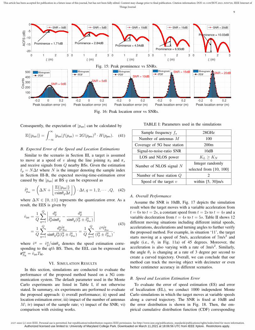
To derive the PLE, we first introduce an intermediatevariable peak prominence [55] as shown in Fig. 15, whichindicates the relative height of a peak. In general, a largerprominence corresponds to a sharper peak and thus the peakcan be localized more accurately. Recalling (21) and SectionII-D, the ACFS is given by

|ηy|2 =

∣∣∣∣KLMsinc(kξAe/2L) +KNNJ0(kp) + σ2

KLM +KNN + σ2

∣∣∣∣2 . (35)

The height ph of the first local peak and height pv of first localvalley of (35) (see Fig. 15) can be expressed as

ph =

∣∣∣∣0.22KLM + 0.01KNN + σ2

KLM +KNN + σ2

∣∣∣∣2 .pv =

∣∣∣∣ σ2

KLM +KNN + σ2

∣∣∣∣2 .(36)

where we have sinc(kξ0Ae/2L) = 0.22 and J0(kp) = 0.01while ξ0 is the first local peak location of (35) and p =√

ξ20 + ε2 ≥ ξ0 = vtsinθ (see Fig. 7). Then, the prominence

ppro of the first local peak of (35) in the unit of decibel (dB)can be expressed as

ppro = 10log10[ph − pv]

= 10log10

∣∣∣∣0.22KLM + 0.01KNN + σ2

σ2

∣∣∣∣2 . (37)

Note that SNR is defined as SNR = 20log10(KLM/σ2).Consequently, the prominence ppro can be rewritten as

ppro =

10log10

∣∣∣∣∣0.21KLM + 0.01KNN +KLM · 10−SNR20

KLM · 10−SNR20

∣∣∣∣∣2

.(38)

To have a better standing, Fig. 15 shows the peak prominenceversus difference SNRs. It is clear that the prominence pproincreases monotonically with the increment of SNR, thusimproving the peak localization accuracy. Note that the systemneeds to estimate the moving distance of the target every TMseconds as introduced in (30). As a result, we have to repeatthe peak finding process for a large number of times to track amoving target. Then, by using the Central Limit Theorem [56],the expectation of the PLE denoted by perr can be assumed tofollow a Gaussian distribution, i.e., the PDF of the perr can beexpressed as

f(perr) = H(ppro)exp(− p2err

2G(ppro)2), (39)

where H(ppro) is the coefficient function while G(ppro) de-notes the standard deviation function (SDF). Since perr de-creases with the increment of SNR, H(ppro) is a monotonicallyincreasing function while G(ppro) is a decreasing function. Itis preferable that H(ppro) grows slowly and G(ppro) decreasesslowly as their arguments increase. Here we propose a pair ofempirical approximations about H(ppro) and G(ppro) by 5000Monte Carlo experiments, i.e.,

H(ppro) = 186√

10log10(ppro),

G(ppro) =1

10√

10log10(ppro).

(40)

Fig. 16 shows that the PDF f(perr) with H(ppro) and G(ppro)given in (40) can well approximate the distribution of the PLE.




9

0 1 2 3

(m)

-20

-15

-10

-5

0A

CF

S (

dB

)

Prominence = 1.71dB

SNR = 0dB

0 1 2 3

(m)

Prominence = 2.84dB

SNR = 5dB

0 1 2 3

(m)

Prominence = 4.54dB

SNR = 10dB

0 1 2 3

(m)

Prominence = 6.93dB

SNR = 15dB

0 1 2 3

(m)

Prominence = 10.03dB

SNR = 20dB

Fig. 15: Peak prominence vs SNRs.

SNR = 0dB

-0.2 0 0.2

Peak location error (m)

0

100

200

300

400

500

Co

un

ts

Histogram

PDF

SNR = 5dB

-0.2 0 0.2


Histogram

PDFSNR = 10dB

-0.2 0 0.2


Histogram

PDFSNR = 15dB

-0.2 0 0.2


Histogram

PDF SNR = 20dB

-0.2 0 0.2


Histogram

PDF

Fig. 16: Peak location error vs SNRs.

Consequently, the expectation of |perr| can be calculated by

E|perr| =

∫ ∞−∞|perr|f(perr) = 2G(ppro)2 ·H(ppro). (41)

B. Expected Error of the Speed and Location Estimations

Similar to the scenario in Section III, a target is assumedto move at a speed of v along the line joining r0 and rsand receive signals from Q nearby BSs. Given the estimationtp = N∆t where N is the integer denoting the sample indexin Section III-B, the expected moving-time-estimation errorcaused by the |perr| at BS q can be expressed as

tqperr=

(∆N +

⌊E|perr|vsinθq∆t

⌋)·∆t, q = 1, 2, · · · , Q, (42)

where ∆N ∈ 0,±1 represents the quantization error. As aresult, the EES is given by

verr =1

Q

Q∑q=1

∣∣∣∣ dqp

tqpsinθq−

dqp

sinθq(tqp ± tqperr)

∣∣∣∣=

1

Q

Q∑q=1

dqptqperr

sinθq tqp(t

qp ± tqperr)

=1

Q

Q∑q=1

vq tqperr

(tqp ± tqperr),

(43)

where vq = vqp/

sinθq denotes the speed estimation corre-sponding to the qth BS. Then, the EEL can be expressed asrerrTM

= verrTM.

VI. SIMULATION RESULTS

In this section, simulations are conducted to evaluate theperformance of the proposed method based on a 5G com-munication system. The default parameter used in the MonteCarlo experiments are listed in Table I, if not otherwisestated. In summary, six experiments are performed to evaluatethe proposed approach: i) overall performance; ii) speed andlocation estimation error; iii) impact of the number of antennasM ; iv) impact of the sample rate; v) impact of the SNR; vi)comparison with existing works.

TABLE I: Parameters used in the simulations

Sample frequency fs 28GHzNumber of antennas M 100

Coverage of 5G base station 200mSignal-to-noise-ratio SNR 10dB

LOS and NLOS power KL ≥ KN

Number of NLOS signal NInteger randomly

selected from [10, 100]Number of base station Q 2

Speed of the target v within [5, 30]m/s

A. Overall Performance

Assume the SNR is 10dB, Fig. 17 depicts the simulationresult when the target moves with a variable acceleration fromt = 0s to t = 2s, a constant speed from t = 2s to t = 4s and avariable deceleration from t = 4s to t = 5s. Table II shows 12different moving situations including different initial speeds,accelerations, decelerations and turning angles to further verifythe proposed method. For example, in situation ‘11’, the targetstarts moving at a speed of 5m/s, acceleration of 7m/s2 andangle (i.e., θ1 in Fig. 11a) of 45 degrees. Moreover, theacceleration is also varying with a rate of 3m/s2. Similarly,the angle θ1 is changing at a rate of 3 degree per second tocreate a curved trajectory. Overall, we can conclude that ourmethod can track the moving object with decimeter or evenbetter centimeter accuracy in different scenarios.

B. Speed and Location Estimation Error

To evaluate the error of speed estimation (ES) and errorof localization (EL), we conduct 1000 independent MonteCarlo simulations in which the target moves at variable speedsalong a curved trajectory. The SNR is fixed at 10dB andthe error distribution is shown in Fig. 18. Then, the em-pirical cumulative distribution function (CDF) corresponding




10

0 1 2 3 4 5

Moving Time (/s)

5

10

15

20

25

30S

pe

ed

(m

/s)

Real speed

Speed estimation

(a) Speed estimation

0 1 2 3 4 5

Moving Time (/s)

-2

0

2

4

Sp

ee

d e

rro

r (m

/s)

Speed estimation error

(b) Speed estimation error

100 110 120 130 140 150

Distance to BS, y-axis (m)

0

20

40

60

Dis

tance to B

S, x-a

xis

(m

)

Real location

Estimated location

(c) Location estimation

100 110 120 130 140 150 160 170

Distance to BS (m)

0

0.1

0.2

0.3

0.4

Location e

rror

(m) Location estimation error

(d) Location estimation error

Fig. 17: Speed and location estimation results with variable speeds (directions of x-axis and y-axis are shown in Fig. 2).

TABLE II: Mean velocity and location estimation error in different situations

SituationVelocity Angle RMSE of velocity RMSE of location

Initial Acceleration Initial Acceleration estimation error estimation error(m/s) (m/s2) () (/s2) (cm/s) (cm)

1 10 0 1 40 0 2 44.32 5.452 10 0 45 2 2 45.61 10.363 10 0 50 6 40.67 9.444 20 0 45 0 57.89 18.815 20 0 60 6 69.63 11.286 30 0 40 0 78.21 19.337 30 0 65 3 81.41 15.238 5 6 1 45 0 47.93 14.219 5 6 (2) 3 40 0 44.04 10.6610 5 6 (2) 3 50 2 35.47 24.8911 5 7 (3) 3 45 3 47.87 13.77

1 Acceleration of the velocity being 0 means the velocity is constant while nonzero means it is changing as the target is moving.2 Acceleration of the angle being 0 means direction angle is constant, i.e., the trajectory is a straight while nonzero means the

direction is changing, which indicates a curved trajectory.3 The number in the bracket () means the acceleration is also changing during the process.

to different velocities (v = 10m/s, 20m/s, 30m/s) is givenin Fig. 19. As illustrated in Fig. 18, our method achieveshigh-accuracy speed estimation results with a median errorof 0.4m/s. Fig. 19 indicates that the median speed estimationerrors are about 0.18m/s, 0.26m/s and 0.45m/s while the cor-responding location errors are about 0.06m, 0.12m and 0.53m.Moreover, when v ≤ 20m/s(45mph), the 80 percentile of thespeed estimation error is within 0.25m/s while the locationestimation error is less than 0.2m. Therefore, our method hasa promising performance in urban areas where v ≤ 20m/sgenerally holds and there are strong NLOS. Moreover, Fig.18b shows that the location estimation error accumulates ata moderate rate as the object moves continuously. This ismainly because the estimation of the next location is highlydependent on the previous location estimation result, whichcauses accumulative errors. Another possible reason is thatSNR of the received signal drops with the target movingtowards cell boundary. In the future, locations of the nearbyBSs may be used to mitigate the accumulative error, whichwe leave for future work.

C. Impact of the Number of Antennas

Fig. 20 shows the root mean square error (RMSE) of thespeed and location estimation versus different antenna numberM. Evidently, both the speed and location estimation accuracyare improved with the increment of M. Specifically, when Mis less than 100, it may not work well when the velocity istoo high (e.g., v =30m/s). However, our system can localizethe target within 0.3m error when M is no less than 100. Thisis because that as M increases, we can harvest more signalcomponents and thus get more accurate ACFS estimation. Andthe performance starts to saturate when M ≥ 200. Note thatwhen M approaches to 400, the location estimation error canbe as low as 8cm.

D. Impact of the Sample Rate

Fig. 21 further explores impacts of the sample rate on ourmethod. In general, higher sample rate improves the estimationaccuracy. For a fixed sample rate, the object moving at a higherspeed suffers from a worse location accuracy than that movingat a lower speed, which is consistent with (42). Moreover, Fig.21 demonstrates that the minimum sample rate is a moderate




11

10 16 23 24 24 24 21

Speed (m/s)

0

0.2

0.4

0.6

0.8

1

1.2S

pe

ed

err

or

(m/s

) Speed estimation error

(a) Speed estimation error

6 15 29 46 63 80 96

Moving distance (m)

0

0.2

0.4

0.6

0.8

1

1.2

Location e

rror

(m)

Location estimation error

(b) Location estimation error

Fig. 18: Estimation error distribution.

0 0.2 0.4 0.6 0.8 1 1.2 1.4 1.6

Speed estimation error (m/s)

0

0.2

0.4

0.6

0.8

1

CD

F

ES, v=10m/s

ES, v=20m/s

ES, v=30m/s


0 0.2 0.4 0.6 0.8 1 1.2 1.4

Location estimation error (m)

0

0.2

0.4

0.6

0.8

1

CD

F EL, v=10m/s

EL, v=20m/s

EL, v=30m/s


Fig. 19: CDF of estimation error.

50 100 150 200 250 300 350 400

Antenna number

00.10.20.30.40.50.60.70.80.9

1

RM

SE

(m

/s)

ES, v=10m/s

ES, v=20m/s

ES, v=30m/s


50 100 150 200 250 300 350 400

Antenna number

0

0.1

0.2

0.3

0.4

0.5

0.6

RM

SE

(m

)

EL, v=10m/s

EL, v=20m/s

EL, v=30m/s


Fig. 20: Estimation error versus antenna number.

200 500 1000 1500 2000 2500 3000

Sample rate

0

0.2

0.4

0.6

0.8

1

RM

SE

(m

/s)

ES, v=10m/s

ES, v=20m/s

ES, v=30m/s


200 500 1000 1500 2000 2500 3000

Sample rate

0.05

0.1

0.15

0.2

0.25

RM

SE

(m

)

EL, v=10m/s

EL, v=20m/s

EL, v=30m/s


Fig. 21: Estimation error versus sample rate.

0 5 10 15 20 25 30 35 40

SNR(dB)

0

0.3

0.6

0.9

1.2

RM

SE

(m

/s)

ES, v=10m/s

ES, v=20m/s

ES, v=30m/s

EES, v=10m/s

EES, v=20m/s

EES, v=30m/s


0 5 10 15 20 25 30 35 40

SNR(dB)

0

0.1

0.2

0.3

0.4

0.5

0.6

0.7

RM

SE

(m

)

EL, v=10m/s

EL, v=20m/s

EL, v=30m/s

EEL, v=10m/s

EEL, v=20m/s

EEL, v=30m/s


Fig. 22: Estimation error versus SNRs.

v = 10m/s v = 20m/s v = 30m/s0

0.2

0.4

0.6

0.8

1

1.2

1.4

1.6Location e

rror

(m)

2-stations

3-stations

4-stations

Fig. 23: Location error versus the number of stations.

value about 500Hz. Further reducing the sample rate may leadto worse speed estimation error or even failure especially forhigh-speed objects, e.g., v =30m/s. When the sample ratefurther increases, such as 3000Hz, the speed estimation error isno greater than 0.6m/s while the minimum location estimationerror is about 10.8cm.

E. Impact of SNR and the Number of Stations

Fig. 22 explores the system performance versus differentSNRs with M = 100 and a sample rate 1000Hz. The EES andEEL are shown in dotted lines with corresponding markers.Clearly, the system is seriously impacted by noise when SNRis less than 10dB and does not work when the target moves at30m/s if SNR further decreases to 0dB. Moreover, the objectwith a higher speed shows a worse estimation error than thatwith a lower speed. However, in all the scenarios, our methodworks well when SNR is no less than 10dB, which is easy tomeet in a typical communication system.

F. Impact the Number of Stations

A unique feature of the proposed method is that it jointlyexplores the directional ACFS distribution of the receivedsignal and the geometric relationship among multiple basestations to estimate the moving direction of a target withoutany further information. We investigate how the performancewould change with the number of base stations. As shown inFig. 23, the performance is improved by fusing the informa-tion from more surrounding stations. However, the proposedsystem can achieve very good location accuracy with only2 stations. In practice, users can flexibly select the numberof stations according to the requirements of system latency,complexity and accuracy for real applications.

G. Comparison with Existing Works

In this section, we compare the proposed method withcorresponding existing works in the aspect of speed, direction,location estimation accuracy and complexity. To simulatea typical localization and tracking scenario, we assume amoving target which continues recording signals transmitted




12

0 0.2 0.4 0.6 0.8 1 1.2 1.4 1.6 1.8 2

Speed error (m/s)

0

0.2

0.4

0.6

0.8

1C

DF

SenSpeed

GPS

WiFiDetect

The proposed


-5 0 5 10 15 20 25 30 35 40

SNR(dB)

0

2

4

6

8

10

12

14

16

18

20

RM

SE

of direction e

stim

ation (°)

Capon

ESPRIT

MUSIC

Proposed

(b) Direction estimation error

0 0.2 0.4 0.6 0.8 1 1.2 1.4 1.6 1.8 2

Position estimation error (m)

0

0.1

0.2

0.3

0.4

0.5

0.6

0.7

0.8

0.9

1

CD

F

The proposed

DiSouL

Conv-fingerprint

DNN-fingerprint

(c) Location estimation error

Fig. 24: Performance comparison.

from 2 surrounding 5G massive MIMO base stations. The 2stations are 200m away from each other and equipped withM = 100 antennas on each station. Considering the rich-scattering urban environment, we randomly choose N (within10 to 100) NLOS components1 while the impinging anglesfollow uniform distributions over (−π, π]. The target starts tomove at a speed of 5m/s, accelerates 2s, then keeps constantspeed for 2s and finally decelerates until end. In total, thetarget moves 80ms away from the starting point 2.Speed estimation: Fig. 24a compares the speed estimationperformance of the proposed system with the existing Sen-Speed [57], WiFiDetect [58] and GPS [59] methods. Clearly,our method outperforms the benchmark algorithms in accu-racy. Specifically, SenSpeed estimates the speed by assum-ing that the error of the integrated acceleration accumulateslinearly over time, which dose not always hold in practice.WiFiDetect considers only 1 dominant NLOS signal and GPSmethod relies on the LOS signal greatly, which is vulnerableto NLOS distortions in urban rich-scattering environments.However, by exploring the ACFS of the received signal,the proposed method treats all the LOS and NLOS signalcomponents as a whole and thus improves the accuracy.Direction estimation: Fig. 24b shows that the proposedsystem can achieve 1.8 direction estimation accuracy, withimprovement than the existing DOA approaches, i.e., Capon[60], ESPRIT [21] and MUSIC [20]. This mainly benefitsfrom the ACFS which has been proved to be tolerable toNLOS distortions. On the contrary, most DOA approachesare highly dependent on the time measurement accuracy ofthe LOS signal, which is easily to be distorted/impacted byNLOS signals in practice.Location estimation: Fig. 24c demonstrates the locationaccuracy of the proposed method and the state-of-the-arttechniques including DiSouL [23], Conv-fingerprint [31] andDNN-fingerprint [32]. From Fig. 24c, the proposed methodcan achieve less than 0.2m error with the percentile ≥ 95%.However, the 95% percentile estimation error of the DNN-fingerprint is 1.2m while both Conv-fingerprint and DiSouLcannot offer ≥ 95% confidence with less than 2m error.

1Many practical measurements in New York City [45], [46] validated thatthe number of dominate NLOS signal usually varies from 10 to 100.

2After moving 80m, the target is about 180m from one of the two stations,which is close to the cell boundary of the station. In this case, we need toswitch to closer base stations, and detailed cell switching procedure is out ofthe scope of this paper.

TABLE III: Computational complexity comparisons

Algorithms Computational complexityDiSouL Of2

s /TM(QL+∑q Nq)

3.5Proposed O(Qfs + fs +Q2 + 7Q)fs/TM

New notationsTM output estimated location every TM seconds.L number of location grid in candidate areaNq number of NLOS components at station q

Overall, our method is more robust because it explores thestatistical ACFS of the received signal which is very stablein 5G massive MIMO systems regardless of the environment.However, fingerprint-based methods may suffer from finger-print mismatch issue due to the change of the wireless propa-gation environment, thus degrading the accuracy. In dynamicenvironments, DiSouL works even worse because there aretwo hyperparameters in the model, which are sensitive to theenvironment changes.Complexity: Considering that complexity is very importantfor real-time tracking and navigation applications with astringent requirement on the latency, Table III compares thecomplexity between our algorithm and the state-of-the-artDiSouL [23] approach. In DiSouL, the main computationcomes from solving the second-order cone program (SOCP)problem, which is about (QL+

∑q Nq)

3.5 in a single snapshot[23]. Our computation is mainly caused by ACFS computa-tion, 1-dimension peak searching in Eq.(25) and the locationcomputation from Eq.(28) to Eq.(32), which are Qfs, fs, andQ2 + 7Q respectively. Since L ≥ Q, our method is muchcheaper than DiSouL.

Note that we do not compare with Conv-fingerprint [31]and DNN-fingerprint [32] here because they are all trainingbased methods in which the overhead in map constructionstage is hard to be quantified. To improve accuracy, fingerprint-based methods usually require a lot of training and updatingto construct the offline map, which leads to a prohibitiveoverhead especially in a dynamic environment.

VII. CONCLUSION

This paper proposes a high-accuracy target location methodbased on the 5G massive MIMO system. We first prove the




13

existence of a sinc-like focusing beam in a massive MIMOsystem by computing the statistical autocorrelation of thereceived signal in far-filed scenario. Based on the focusingbeam, a speed estimation algorithm is then proposed by jointlyusing the relative speed estimations with respect to multipleBSs. Give an initial point, we develop a target localizationmethod by further using the geometrical relationships betweenmultiple BSs. Theoretical error analysis and extensive numer-ical simulations show that our method can achieve decimeterlocalization accuracy by computing ACFS of the receivedsignal, which outperforms many prior works in accuracy andcost.

APPENDIX

In this appendix, we prove (3), i.e., ηy(r0, rs) =E[y(t0)y∗(ts)] ≈ ηyL + ηyN + ηn. Mathematically, the ACFof the received signal y(t) given by

ηy(r0, rs) = E[y(t0)y∗(ts)] = ηLL∗ + ηLN∗ + ηLn∗

+ ηNL∗ + ηNN∗ + ηNn∗ + ηnL∗ + ηnN∗ + ηnn∗

ηLL∗ = E[yL(t0)y∗L(ts)], ηLN∗ = E[yL(t0)y∗N(ts)],

ηLn∗ = E[yL(t0)n∗(ts)], ηNL∗ = E[yN(t0)y∗L(ts)],

ηNN∗ = E[yN(t0)y∗N(ts)], ηNn∗ = E[yN(t0)n∗(ts)],

ηnL∗ = E[n(t0)y∗L(ts)], ηnN∗ = E[n(t0)y∗N(ts)],

ηnn∗ = E[n(t0)n∗(ts)] = σ2I.

(44)

Referring to our derivations from (14) to (19), it is easy toobtain

ηLN∗ =M∑i=1

N∑n=1

ηy(LN∗)i,n =M∑i=1

N∑n=1

Eφ exp[j(ψi,0 − ωdtscosαn + φi − φn)] = 0,

ηy(Ln∗) = E[yLOS]E[n∗(ts)] = 0,

(45)

given the fact that φi and φn are assumed to be uniformdistribution over (−π, π] and the signal components yL and yNare independent with noise. Similarly, we can get ηy(NL∗) =0, ηy(Nn∗) = 0, ηy(nL∗) = 0, ηy(nN∗) = 0. As a conse-quence, ηy(r0, rs) can be simplified as

ηy(r0, rs) =ηy(LL∗) + ηy(NN∗) + ηy(nn∗).= ηyL + ηyN + ηn

(46)

Thus, the proof is completed.

REFERENCES

[1] H. Wang, L. Wan, M. Dong, K. Ota, and X. Wang, “Assistant vehiclelocalization based on three collaborative base stations via sbl-basedrobust doa estimation,” IEEE Internet of Things Journal, vol. 6, no.3, pp. 5766–5777, 2019.

[2] S. Kuutti, S. Fallah, K. Katsaros, M. Dianati, F. Mccullough, andA. Mouzakitis, “A survey of the state-of-the-art localization techniquesand their potentials for autonomous vehicle applications,” IEEE Internetof Things Journal, vol. 5, no. 2, pp. 829–846, 2018.

[3] J. G. McNeff, “The global positioning system,” IEEE Transactions onMicrowave Theory and Techniques, vol. 50, no. 3, pp. 645–652, March2002.

[4] J. Wang, J. Luo, S. J. Pan, and A. Sun, “Learning-based outdoorlocalization exploiting crowd-labeled WiFi hotspots,” IEEE Transactionson Mobile Computing, vol. 18, no. 4, pp. 896–909, April 2019.

[5] X. Zeng, M. Yang, B. Chen, and Y. Jin, “Estimation of direction ofarrival by time reversal for low-angle targets,” IEEE Transactions onAerospace and Electronic Systems, vol. 54, no. 6, pp. 2675–2694, Dec2018.

[6] M. Guo, Y. D. Zhang, and T. Chen, “Doa estimation using compressedsparse array,” IEEE Transactions on Signal Processing, vol. 66, no. 15,pp. 4133–4146, 2018.

[7] A. Alessandrini, F. Mazzarella, and M. Vespe, “Estimated time of arrivalusing historical vessel tracking data,” IEEE Transactions on IntelligentTransportation Systems, vol. 20, no. 1, pp. 7–15, Jan 2019.

[8] F. Shang, B. Champagne, and I. N. Psaromiligkos, “A ml-basedframework for joint toa/aoa estimation of uwb pulses in dense multipathenvironments,” IEEE Transactions on Wireless Communications, vol. 13,no. 10, pp. 5305–5318, 2014.

[9] G. Wang, W. Zhu, and N. Ansari, “Robust TDOA-based localizationfor IoT via joint source position and NLOS error estimation,” IEEEInternet of Things Journal, vol. 6, no. 5, pp. 8529–8541, Oct 2019.

[10] Yihong Qi, H. Kobayashi, and H. Suda, “Analysis of wireless geoloca-tion in a non-line-of-sight environment,” IEEE Transactions on WirelessCommunications, vol. 5, no. 3, pp. 672–681, 2006.

[11] N. Patwari, A. O. Hero, M. Perkins, N. S. Correal, and R. J. O’Dea,“Relative location estimation in wireless sensor networks,” IEEETransactions on Signal Processing, vol. 51, no. 8, pp. 2137–2148, 2003.

[12] H. C. So and L. Lin, “Linear least squares approach for accurate receivedsignal strength based source localization,” IEEE Transactions on SignalProcessing, vol. 59, no. 8, pp. 4035–4040, 2011.

[13] R. W. Ouyang, A. K. Wong, and C. Lea, “Received signal strength-basedwireless localization via semidefinite programming: Noncooperative andcooperative schemes,” IEEE Transactions on Vehicular Technology, vol.59, no. 3, pp. 1307–1318, 2010.

[14] X. Tian, S. Zhu, S. Xiong, B. Jiang, Y. Yang, and X. Wang, “Per-formance analysis of Wi-Fi indoor localization with channel stateinformation,” IEEE Transactions on Mobile Computing, vol. 18, no.8, pp. 1870–1884, 2019.

[15] Q. Song, S. Guo, X. Liu, and Y. Yang, “CSI amplitude fingerprinting-based NB-IoT indoor localization,” IEEE Internet of Things Journal,vol. 5, no. 3, pp. 1494–1504, 2018.

[16] C. Hsieh, J. Chen, and B. Nien, “Deep learning-based indoor localizationusing received signal strength and channel state information,” IEEEAccess, vol. 7, pp. 33256–33267, 2019.

[17] A. Shahmansoori, G. E. Garcia, G. Destino, G. Seco-Granados, andH. Wymeersch, “Position and orientation estimation through millimeter-wave MIMO in 5G systems,” IEEE Transactions on Wireless Commu-nications, vol. 17, no. 3, pp. 1822–1835, March 2018.

[18] X. Xia, K. Xu, D. Zhang, Y. Xu, and Y. Wang, “Beam-domainfull-duplex massive mimo: Realizing co-time co-frequency uplink anddownlink transmission in the cellular system,” IEEE Transactions onVehicular Technology, vol. 66, no. 10, pp. 8845–8862, 2017.

[19] A. Guerra, F. Guidi, and D. Dardari, “Single-anchor localiza-tion and orientation performance limits using massive arrays: MIMOvs.beamforming,” IEEE Transactions on Wireless Communications, vol.17, no. 8, pp. 5241–5255, Aug 2018.

[20] L. Hachad, O. Cherrak, H. Ghennioui, F. Mrabti, and M. Zouak, “Doaestimation based on time-frequency music application to massive mimosystems,” in 2017 International Conference on Advanced Technologiesfor Signal and Image Processing (ATSIP), 2017, pp. 1–5.

[21] A. Hu, T. Lv, H. Gao, Z. Zhang, and S. Yang, “An ESPRIT-basedapproach for 2-D localization of incoherently distributed sources inmassive MIMO systems,” IEEE Journal of Selected Topics in SignalProcessing, vol. 8, no. 5, pp. 996–1011, Oct 2014.

[22] Z. Marzi, D. Ramasamy, and U. Madhow, “Compressive channelestimation and tracking for large arrays in mm-wave picocells,” IEEEJournal of Selected Topics in Signal Processing, vol. 10, no. 3, pp. 514–527, April 2016.

[23] N. Garcia, H. Wymeersch, E. G. Larsson, A. M. Haimovich, andM. Coulon, “Direct localization for massive MIMO,” IEEE Transactionson Signal Processing, vol. 65, no. 10, pp. 2475–2487, May 2017.

[24] J. Wang, H. Zhu, L. Dai, N. J. Gomes, and J. Wang, “Low-complexitybeam allocation for switched-beam based multiuser massive mimosystems,” IEEE Transactions on Wireless Communications, vol. 15, no.12, pp. 8236–8248, 2016.

[25] W. Wu, D. Liu, X. Hou, and M. Liu, “Low-complexity beam trainingfor 5g millimeter-wave massive mimo systems,” IEEE Transactions onVehicular Technology, vol. 69, no. 1, pp. 361–376, 2020.

[26] T. Lv, F. Tan, H. Gao, and S. Yang, “A beamspace approach for 2-D localization of incoherently distributed sources in massive MIMOsystems,” Signal Processing, vol. 121, pp. 30–45, 2016.




14

[27] F. Guidi, A. Guerra, D. Dardari, A. Clemente, and R. D’Errico, “Jointenergy detection and massive array design for localization and mapping,”IEEE Transactions on Wireless Communications, vol. 16, no. 3, pp.1359–1371, 2017.

[28] K. Wu, W. Ni, T. Su, R. P. Liu, and Y. J. Guo, “Robust unambiguousestimation of angle-of-arrival in hybrid array with localized analogsubarrays,” IEEE Transactions on Wireless Communications, vol. 17,no. 5, pp. 2987–3002, 2018.

[29] X. Liu, Q. Zhang, W. Chen, H. Feng, L. Chen, F. M. Ghannouchi, andZ. Feng, “Beam-oriented digital predistortion for 5G massive MIMOhybrid beamforming transmitters,” IEEE Transactions on MicrowaveTheory and Techniques, vol. 66, no. 7, pp. 3419–3432, July 2018.

[30] S. A. Shaikh and A. M. Tonello, “Localization based on angle of arrivalin em lens-focusing massive mimo,” in 2016 IEEE 6th InternationalConference on Consumer Electronics - Berlin (ICCE-Berlin), 2016, pp.124–128.

[31] X. Sun, X. Gao, G. Y. Li, and W. Han, “Single-site localization basedon a new type of fingerprint for massive MIMO-OFDM systems,” IEEETransactions on Vehicular Technology, vol. 67, no. 7, pp. 6134–6145,July 2018.

[32] X. Sun, C. Wu, X. Gao, and G. Y. Li, “Fingerprint-based localization formassive mimo-ofdm system with deep convolutional neural networks,”IEEE Transactions on Vehicular Technology, vol. 68, no. 11, pp. 10846–10857, 2019.

[33] J. Vieira, E. Leitinger, M. Sarajlic, X. Li, and F. Tufvesson, “Deepconvolutional neural networks for massive MIMO fingerprint-basedpositioning,” in 2017 IEEE 28th Annual International Symposium onPersonal, Indoor, and Mobile Radio Communications (PIMRC), Oct2017, pp. 1–6.

[34] V. Savic and E. G. Larsson, “Fingerprinting-based positioning indistributed massive MIMO systems,” in 2015 IEEE 82nd VehicularTechnology Conference (VTC2015-Fall), Sep. 2015, pp. 1–5.

[35] A. Chriki, H. Touati, and H. Snoussi, “SVM-based indoor localizationin wireless sensor networks,” in 2017 13th International WirelessCommunications and Mobile Computing Conference (IWCMC), June2017, pp. 1144–1149.

[36] J. Yan, L. Zhao, J. Tang, Y. Chen, R. Chen, and L. Chen, “Hybrid kernelbased machine learning using received signal strength measurements forindoor localization,” IEEE Transactions on Vehicular Technology, vol.67, no. 3, pp. 2824–2829, March 2018.

[37] C. Chen, Y. Chen, Y. Han, H. Lai, F. Zhang, and K. J. R. Liu, “Achievingcentimeter-accuracy indoor localization on WiFi platforms: A multi-antenna approach,” IEEE Internet of Things Journal, vol. 4, no. 1,pp. 122–134, Feb 2017.

[38] K. J. R. Liu and B. Wang, Wireless AI: Wireless Sensing, Positioning,IoT, and Communications, Cambridge University Press, 2019.

[39] B. Wang, Q. Xu, C. Chen, F. Zhang, and K. J. R. Liu, “The promise ofradio analytics: A future paradigm of wireless positioning, tracking, andsensing,” IEEE Signal Processing Magazine, vol. 35, no. 3, pp. 59–80,May 2018.

[40] C. Wu, F. Zhang, B. Wang, and K. J. R. Liu, “Easitrack: Decimeter-level indoor tracking with graph-based particle filtering,” IEEE Internetof Things Journal, vol. 7, no. 3, pp. 2397–2411, 2020.

[41] Z. Wu, Y. Han, Y. Chen, and K. J. R. Liu, “A time-reversal paradigm forindoor positioning system,” IEEE Transactions on Vehicular Technology,vol. 64, no. 4, pp. 1331–1339, April 2015.

[42] F. Zhang, C. Chen, B. Wang, H. Lai, Y. Han, and K. J. R. Liu, “Wiball:A time-reversal focusing ball method for decimeter-accuracy indoortracking,” IEEE Internet of Things Journal, vol. 5, no. 5, pp. 4031–4041, Oct 2018.

[43] X. Ge, S. Tu, G. Mao, C. Wang, and T. Han, “5g ultra-dense cellularnetworks,” IEEE Wireless Communications, vol. 23, no. 1, pp. 72–79,February 2016.

[44] Federal Communications Commission (FCC), “Citycommission agenda memo/5G small cell infrastructure inmanhattan,” https://cityofmhk.com/DocumentCenter/View/53891/Item-7B-Local-Standards-for-Small-Cell-Infrastructure, March 12,2019.

[45] Y. Azar, G. N. Wong, K. Wang, R. Mayzus, J. K. Schulz, H. Zhao,F. Gutierrez, D. Hwang, and T. S. Rappaport, “28 GHz propagationmeasurements for outdoor cellular communications using steerable beamantennas in new york city,” in 2013 IEEE International Conference onCommunications (ICC), June 2013, pp. 5143–5147.

[46] A. I. Sulyman, A. T. Nassar, M. K. Samimi, G. R. Maccartney, T. S.Rappaport, and A. Alsanie, “Radio propagation path loss models for 5Gcellular networks in the 28 GHZ and 38 GHZ millimeter-wave bands,”IEEE Communications Magazine, vol. 52, no. 9, pp. 78–86, Sep. 2014.

[47] W. Croswell, Antenna Theory, Analysis, and Design, Harper and Row,1982.

[48] A. Taira, H. Iura, K. Nakagawa, S. Uchida, K. Ishioka, A. Okazaki,S. Suyama, T. Obara, Y. Okumura, and A. Okamura, “Performanceevaluation of 44GHz band massive mimo based on channel measure-ment,” in 2015 IEEE Globecom Workshops (GC Wkshps), 2015, pp.1–6.

[49] A. O. Martınez, J. Ø. Nielsen, E. De Carvalho, and P. Popovski, “Anexperimental study of massive mimo properties in 5g scenarios,” IEEETransactions on Antennas and Propagation, vol. 66, no. 12, pp. 7206–7215, 2018.

[50] J. Chen, X. Yin, X. Cai, and S. Wang, “Measurement-based massivemimo channel modeling for outdoor los and nlos environments,” IEEEAccess, vol. 5, pp. 2126–2140, 2017.

[51] C. Xiao, Y. R. Zheng, and N. C. Beaulieu, “Novel sum-of-sinusoidssimulation models for rayleigh and rician fading channels,” IEEETransactions on Wireless Communications, vol. 5, no. 12, pp. 3667–3679, December 2006.

[52] C. Chen, Y. Chen, Y. Han, H. Lai, and K. J. R. Liu, “Achievingcentimeter-accuracy indoor localization on WiFi platforms: A frequencyhopping approach,” IEEE Internet of Things Journal, vol. 4, no. 1, pp.111–121, Feb 2017.

[53] F. Zhang, C. Chen, B. Wang, and K. J. R. Liu, “Wispeed: A statisticalelectromagnetic approach for device-free indoor speed estimation,” IEEEInternet of Things Journal, vol. 5, no. 3, pp. 2163–2177, June 2018.

[54] C. William, “Robust locally weighted regression and smoothing scatter-plots,” Journal of the American statistical association, vol. 74, no. 368,pp. 829–836, 1979.

[55] Manhattan local news, “Topographic prominence,” https://en.wikipedia.org/wiki/Topographic prominence, Accessed August 25, 2020.

[56] GA. Brosamler, “An almost everywhere central limit theorem,” inMathematical Proceedings of the Cambridge Philosophical Society.Cambridge University Press, 1988, vol. 104, pp. 561–574.

[57] J. Yu, H. Zhu, H. Han, Y. J. Chen, J. Yang, Y. Zhu, Z. Chen, G. Xue, andM. Li, “Senspeed: Sensing driving conditions to estimate vehicle speedin urban environments,” IEEE Transactions on Mobile Computing, vol.15, no. 1, pp. 202–216, Jan 2016.

[58] J. Wang, J. Tong, Q. Gao, Z. Wu, S. Bi, and H. Wang, “Device-freevehicle speed estimation with wifi,” IEEE Transactions on VehicularTechnology, vol. 67, no. 9, pp. 8205–8214, 2018.

[59] A. Gorski, “Understanding gps performance in urban environments”,”2011.

[60] J. Li, P. Stoica, and Z. Wang, “On robust Capon beamforming anddiagonal loading,” IEEE Transactions on Signal Processing, vol. 51,no. 7, pp. 1702–1715, July 2003.

Xiaolu Zeng received his B.S. degree from theHarbin Institute of Technology (HIT), China, in2014. He received Ph.D. degree at the School ofElectronic Engineering, Xidian University, China,in 2020. From Sept. 2017 to Jun. 2020, he is avisiting student at the Department of Electrical andComputer Engineering, University of Maryland atCollege Park, USA. He is now a Postdoc ResearchAssociate in the Department of Electrical and Com-puter Engineering University of Maryland, CollegePark. His research interests include target detection,

tracking and localization, wireless sensing, 5G millimeter wave communi-cation and applications, intelligent recognition and classification, AdvancedDriver Assistance Systems (ADAS).

Powered by TCPDF (www.tcpdf.org)

Feng Zhang (S’12-M’19) received his B.S. andM.S. degrees from the Department of ElectronicEngineering and Information Science, University ofScience and Technology of China, Hefei, in 2011and 2014, respectively. He received his Ph.D. degreefrom the Department of Electrical and ComputerEngineering, University of Maryland, College Parkin Dec. 2018. He was with Origin Wireless, Inc.as a principal scientist between 2018 and 2020 andHe is currently with Amazon.com, Inc. His researchinterests include wireless sensing, statistical signal

processing, and wireless indoor localization. He was the recipient of 2020IEEE Internet of Things Journal best paper award.




15

Beibei Wang. (SM’15) received the B.S. degree inelectrical engineering (Hons.) from the Universityof Science and Technology of China in 2004, andthe Ph.D. degree in electrical engineering from theUniversity of Maryland, College Park in 2009. Shewas with the University of Maryland as a researchassociate in 2009-2010, and with Qualcomm Re-search and Development in 2010- 2014. Since 2015,she has been with Origin Wireless Inc., where sheis currently the Vice President of Research. Sheis also affiliated with the University of Maryland,

College Park. Dr. Wang is the recipient of the 2020 IEEE Internet ofThings Journal Best Paper Award, 2015 IEEE Signal Processing SocietyOverview Paper Award and several research and invention awards from theUniversity of Maryland. She is a co-author of Cognitive Radio Networkingand Security: A Game-Theoretic View (Cambridge University Press, 2010)and Wireless AI: Wireless Sensing, Positioning, IoT, and Communications(Cambridge University Press, 2019). She has served on the editorial board ofIEEE Signal Processing Letters, IEEE Internet of Things Journal, and IEEEJournal on Selected Areas in Communications. Her research interests includeInternet of Things, mobile computing, wireless sensing and positioning, andcommunications and networking. She is a senior member of IEEE.

K. J. Ray Liu. (F’03) is a Distinguished UniversityProfessor and a Distinguished Scholar-Teach of Uni-versity of Maryland, College Park, where he is alsoChristine Kim Eminent Professor of InformationTechnology. He leads the Maryland Signals andInformation Group conducting research encompass-ing broad areas of information and communicationstechnology with recent focus on wireless AI forindoor tracking and wireless sensing.

Dr. Liu was the recipient of two IEEE TechnicalField Awards: the 2021 IEEE Fourier Award for

Signal Processing and the 2016 IEEE Leon K. Kirchmayer Graduate TeachingAward, IEEE Signal Processing Society 2009 Technical Achievement Award,IEEE Signal Processing Society 2014 Society Award, and over a dozen ofbest paper/invention awards. Recognized by Web of Science as a Highly CitedResearcher, Dr. Liu is a fellow of IEEE, AAAS, and U.S. National Academyof Inventors. As the founder of Origin Wireless, his inventions won the 2017CEATEC Grand Prix and three CES Innovation Awards, including CES Bestof Innovation in 2021.

Dr. Liu is 2021 IEEE President-Elect. He was IEEE Vice President,Technical Activities, and a member of IEEE Board of Director as Division IXDirector. He has also served as President of IEEE Signal Processing Society,where he was Vice President – Publications and Editor-in-Chief of IEEESignal Processing Magazine.

He also received teaching and research recognitions from University ofMaryland including university-level Invention of the Year Award; and college-level Poole and Kent Senior Faculty Teaching Award, Outstanding FacultyResearch Award, and Outstanding Faculty Service Award, all from A. JamesClark School of Engineering.


massive mimo for high-accuracy target localization and

Documents