master recherche iac tc2: apprentissage …sebag/slides/cours_aso_intro.pdfmaster recherche iac tc2:...
TRANSCRIPT

Master Recherche IACTC2: Apprentissage Statistique & Optimisation
Alexandre Allauzen − Anne Auger − Michele SebagLIMSI − LRI
Oct. 1st, 2012

Where we are
Ast. series Pierre de Rosette
Maths.
World
Data / Principles
Naturalphenomenons
Modelling
Human−relatedphenomenons
You are here
CommonSense

Where we are
Sc. data
Maths.
World
Data / Principles
Naturalphenomenons
Modelling
Human−relatedphenomenons
You are here
CommonSense

Harnessing Big Data
Watson (IBM) defeats human champions at the quiz game Jeopardy (Feb. 11)
i 1 2 3 4 5 6 7 81000i kilo mega giga tera peta exa zetta yotta bytes
I Google: 24 petabytes/dayI Facebook: 10 terabytes/day; Twitter: 7 terabytes/dayI Large Hadron Collider: 40 terabytes/seconds

Machine Learning and Optimization
Machine Learning
World → instance xi →Oracle↓yi
Optimization
ML and Optimization
I ML is an optimization problem: find the best model
I Smart optimization requires learning about the optimizationlandscape

Types of Machine Learning problems
WORLD − DATA − USER
Observations
UnderstandCode
UnsupervisedLEARNING
+ Target
PredictClassification/Regression
SupervisedLEARNING
+ Rewards
DecideAction Policy/Strategy
ReinforcementLEARNING

The module
1. Introduction. Decision trees. Validation.
2. Neural Nets
3. Statistics
4. Learning from sequences
5. Unsupervised learning
6. Representation changes
7. Bayesian learning
8. Optimisation

Pointers
I Slides of this module:http://tao.lri.fr/tiki-index.php?page=Courseshttp://www.limsi.fr/Individu/allauzen/wiki/index.php/
I Andrew Ng courseshttp://ai.stanford.edu/∼ang/courses.html
I PASCAL videoshttp://videolectures.net/pascal/
I Tutorials NIPS Neuro Information Processing Systemshttp://nips.cc/Conferences/2006/Media/
I About ML/DMhttp://hunch.net/

Today
1. Part 1. Generalities
2. Part 2. Decision trees
3. Part 3. Validation

Overview
Examples
Introduction to Supervised Machine Learning
Decision trees
Empirical validationPerformance indicatorsEstimating an indicator

Examples
I Vision
I Control
I Netflix
I Spam
I Playing Go
I Google
http://ai.stanford.edu/∼ang/courses.html

Reading cheques
LeCun et al. 1990

MNIST: The drosophila of ML
Classification

Detecting faces

The 2005-2012 Visual Object Challenges
A. Zisserman, C. Williams, M. Everingham, L. v.d. Gool

The supervised learning setting
Input: set of (x, y)
I An instance x e.g. set of pixels, x ∈ IRD
I A label y in {1,−1} or {1, . . . ,K} or IR
Pattern recognition
I Classification Does the image contain the targetconcept ?
h : { Images} 7→ {1,−1}
I Detection Does the pixel belong to the img of targetconcept?
h : { Pixels in an image} 7→ {1,−1}
I SegmentationFind contours of all instances of target concept in image

The 2005 Darpa Challenge
Thrun, Burgard and Fox 2005
Autonomous vehicle Stanley − Terrains

The Darpa challenge and the AI agenda
What remains to be done Thrun 2005
I Reasoning 10%
I Dialogue 60%
I Perception 90%

Robots
Ng, Russell, Veloso, Abbeel, Peters, Schaal, ...
Reinforcement learning Classification

Robots, 2
Toussaint et al. 2010
(a) Factor graph modelling the variable interactions
(b) Behaviour of the 39-DOF Humanoid:Reaching goal under Balance and Collision constraints
Bayesian Inference for Motion Control and Planning

Go as AI Challenge
Gelly Wang 07; Teytaud et al. 2008-2011
Reinforcement Learning, Monte-Carlo Tree Search

Energy policy
ClaimMany problems can be phrased as optimization in front of theuncertainty.
Adversarial setting 2 two-player gameuniform setting a single player game
Management of energy stocks under uncertainty

States and Decisions
States
I Amount of stock (60 nuclear, 20 hydro.)
I Varying: price, weather alea or archive
I Decision: release water from one reservoir to another
I Assessment: meet the demand, otherwise buy energy
Reservoir 1
Reservoir2
Reservoir 3
Reservoir 4
Lost water
PLANT
NUCLEAR PLANT
DEMAND
PRICE

Netflix Challenge 2007-2008
Collaborative Filtering

Collaborative filtering
Input
I A set of users nu, ca 500,000
I A set of movies nm, ca 18,000
I A nm × nu matrix: person, movie, ratingVery sparse matrix: less than 1% filled...
Output
I Filling the matrix !
Criterion
I (relative) mean square error
I ranking error

Collaborative filtering
Input
I A set of users nu, ca 500,000
I A set of movies nm, ca 18,000
I A nm × nu matrix: person, movie, ratingVery sparse matrix: less than 1% filled...
Output
I Filling the matrix !
Criterion
I (relative) mean square error
I ranking error

Spam − Phishing − Scam
Classification, Outlier detection

The power of big data
I Now-casting outbreak of flu
I Public relations >> Advertizing

Mc Luhan and Google
We shape our tools and afterwards our tools shape usMarshall McLuhan, 1964
First time ever a tool is observed to modify human cognition thatfast.
Sparrow et al., Science 2011

Types of application
Domain But : Modelling
Physical phenomenons analysis & controlmanufacturing, experimental sciences, numerical engineering
Vision, speech, robotics..
Social phenomenons + privacyHealth, Insurance, Banks ...
Individual phenomenons + dynamicsConsumer Relationship Management, User Modelling
Social networks, games...
PASCAL : http://pascallin2.ecs.soton.ac.uk/

Banks, Telecom, CRN
Ex: KDD 2009 − Orange
1. Churn
2. Appetency
3. Up-selling
Objectives
1. Ads. efficiency
2. Less fraud

Health, bio-informatics
Ex: Risk factors
1. Cardio-vascular diseases
2. Carcinogenic Molecules
3. Obesity genes ...
Objectives
1. Diagnostic
2. Personalized care
3. Identification

Scientific Social Network
Questions
1. Who does what ?2. Good conferences ?3. Hot/emerging topics ?4. Is Mr Q. Lee same as Mr Quoc N. Lee ?
[tr. Jiawei Han, 2010]

e-Science, Design
Numerical Engineering
I Codes
I Computationally heavy
I Expertise demanding
Fusion based on inertial confinement, ICF

e-Science, Design (2)
Objectives
I Approximate answer
I .. in tenth of seconds
I Speed up the design cycle
I Optimal design More is Different

Autonomous robotics
Complexe, monde ferme simple, randomDesign
[tr. Hod Lipson, 2010]

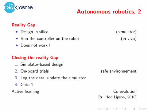
Autonomous robotics, 2
Reality Gap
I Design in silico (simulator)
I Run the controller on the robot (in vivo)
I Does not work !
Closing the reality Gap
1. Simulator-based design
2. On-board trials safe environnement
3. Log the data, update the simulator
4. Goto 1
Active learning Co-evolution[tr. Hod Lipson, 2010]

Overview
Examples
Introduction to Supervised Machine Learning
Decision trees
Empirical validationPerformance indicatorsEstimating an indicator

Types of Machine Learning problems
WORLD − DATA − USER
Observations
UnderstandCode
UnsupervisedLEARNING
+ Target
PredictClassification/Regression
SupervisedLEARNING
+ Rewards
DecidePolicy
ReinforcementLEARNING

Data
Example
I row : example/ case
I column : feature/variable/ attribute
I attribute : class/label
Instance space XI Propositionnal :X ≡ IRd
I Structured :sequential,spatio-temporal,relational.
aminoacid

Data / Applications
I Propositionnal data 80% des applis.
I Spatio-temporal data alarms, mines, accidents
I Relationnal data chemistry, biology
I Semi-structured data text, Web
I Multi-media images, music, movies,..

Difficulty factors
Quality of data / of representation
− Noise; missing data
+ Relevant attributes Feature extraction
− Structured data: spatio-temporal, relational, text, videos,..
Data distribution
+ Independants, identically distributed examples
− Other: robotics; data streams; heterogeneous data
Prior knowledge
+ Goals, interestingness criteria
+ Constraints on target hypotheses

Difficulty factors, 2
Learning criterion
+ Convex optimization problem
↘ Complexity : n, nlogn, n2 Scalability
− Combinatorial optimization
H. Simon, 1958:In complex real-world situations, optimization becomesapproximate optimization since the description of the real-world isradically simplified until reduced to a degree of complication thatthe decision maker can handle.Satisficing seeks simplification in a somewhat different direction,retaining more of the detail of the real-world situation, but settlingfor a satisfactory, rather than approximate-best, decision.

Learning criteria, 2
The user’s criteria
I Relevance, causality,
I INTELLIGIBILITY
I Simplicity
I Stability
I Interactive processing, visualisation
I ... Preference learning

Difficulty factors, 3
Crossing the chasm
I No killer algorithm
I Little expertise about algorithm selection
How to assess an algorithm
I Consistency
When number n of examples goes to infinityand target concept h∗ is in H
h∗ is found:
limn→∞hn = h∗
I Speed of convergence
||h∗ − hn|| = O(1/n),O(1/√
n),O(1/ ln n)

Context
Disciplines et criteres
I Data bases, Data MiningScalability
I Statistics, data analysisPredefined models
I Machine learningPrior knowledge; complex data/hypotheses
I Optimisationwell / ill posed problems
I Computer Human InteractionNo final solution: a process
I High performance computingDistributed processing; safety

Supervised Learning, notationsContext
World → Instance xi →Oracle↓yi
INPUT ∼ P(x, y)
E = {(xi , yi ), xi ∈ X , yi ∈ Y, i = 1 . . . n}HYPOTHESIS SPACE
H h : X 7→ YLOSS FUNCTION
` : Y × Y 7→ IR
OUTPUTh∗ = arg max{score(h), h ∈ H}

Classification and criteriaSupervised learning
I Y = True/False classificationI Y = {1, . . . k} multi-class discriminationI Y = IR regression
Generalization Error
Err(h) = E [`(y , h(x))] =
∫`(y , h(x))dP(x , y)
Empirical Error
Erre(h) =1
n
n∑i=1
`(yi , h(xi ))
Bound structural risk
Err(h) < Erre(h) + F(n, d(H))
d(H) = Vapnik Cervonenkis dimension of H, see later

The Bias-Variance Trade-off
Biais Bias (H): error of the best hypothesis h∗ de H
Variance Variance of hn as a function of E
h*
h
h
Variance
h
H
Bias
target concept
Function Space
Overfitting
Test error
Training error
Complexity of H

The Bias-Variance Trade-off
Biais Bias (H): error of the best hypothesis h∗ de H
Variance Variance of hn as a function of E
h*
h
h
Variance
h
H
Bias
target concept
Function Space
Overfitting
Test error
Training error
Complexity of H

Key notions
I The main issue regarding supervised learning is overfitting.
I How to tackle overfitting:I Before learning: use a sound criterion regularizationI After learning: cross-validation Case studies
Summary
I Learning is a search problem
I What is the space ? What are the navigation operators ?

Hypothesis Spaces
Logical Spaces
Concept ←∨∧
Literal,Condition
I Conditions = [color = blue]; [age < 18]
I Condition f : X 7→ {True,False}I Find: disjunction of conjunctions of conditions
I Ex: (unions of) rectangles of the 2D-planeX .

Hypothesis Spaces
Numerical Spaces
Concept = (h() > 0)
I h(x) = polynomial, neural network, . . .
I h : X 7→ IR
I Find: (structure and) parameters of h

Hypothesis Space H
Logical Space
I h covers one example x iff h(x) = True.
I H is structured by a partial order relation
h ≺ h′ iff ∀x , h(x)→ h′(x)
Numerical Space HI h(x) is a real value (more or less far from 0)
I we can define `(h(x), y)
I H is structured by a partial order relation
h ≺ h′ iff E [`(h(x), y)] < E [`(h′(x), y)]

Hypothesis Space H / Navigation
H navigation operators
Version Space Logical spec / genDecision Trees Logical specialisation
Neural Networks Numerical gradientSupport Vector Machines Numerical quadratic opt.
Ensemble Methods − adaptation E

Overview
Examples
Introduction to Supervised Machine Learning
Decision trees
Empirical validationPerformance indicatorsEstimating an indicator

Decision Trees
C4.5 (Quinlan 86)
I Among the most widelyused algorithms
I EasyI to understandI to implelementI to useI and cheap in CPU time
I J48, Weka, SciKit
NORMAL
>= 55 < 55
Age
Smoker
no yes
Sport
RISK
NORMAL
highlow
RISK
Tension
yesno
Diabete
yes
RISK PATH.
no

Decision Trees

Decision Trees (2)
Procedure DecisionTree(E)
1. Assume E = {(xi , yi )ni=1, xi ∈ IRD , yi ∈ {0, 1}}
• If E single-class (i.e., ∀i , j ∈ [1, n]; yi = yj), return• If n too small (i.e., < threshold), return• Else, find the most informative attribute att
2. Forall value val of att• Set Eval = E ∩ [att = val ].• Call DecisionTree(Eval)
Criterion: information gain
p = Pr(Class = 1|att = val)I ([att = val ]) = −p log p − (1− p) log (1− p)
I (att) =∑
i Pr(att = vali ).I ([att = vali ])

Decision Trees (3)
Contingency TableQuantity of Information (QI)
p
QI
0.1 0.3 0.5 0.7 0.9
0.1
0.3
0.5
0.7 Quantity of Information
Computationvalue p(value) p(poor | value) QI (value) p(value) * QI (value)[0,10[ 0.051 0.999 0.00924 0.000474
[10,20[ 0.25 0.938 0.232 0.0570323[20,30[ 0.26 0.732 0.581 0.153715

Decision Trees (4)
Limitations
I XOR-like attributes
I Attributes with many values
I Numerical attributes
I Overfitting
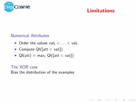
Limitations
Numerical Attributes
I Order the values val1 < . . . < valtI Compute QI([att < vali ])
I QI(att) = maxi QI([att < vali ])
The XOR caseBias the distribution of the examples

Complexity
Quantity of information of an attribute
n ln n
Adding a node
D × n ln n

Tackling Overfitting
Penalize the selection of an already used variable
I Limits the tree depth.
Do not split subsets below a given minimal size
I Limits the tree depth.
Pruning
I Each leaf, one conjunction;
I Generalization by pruning litterals;
I Greedy optimization, QI criterion.

Decision Trees, Summary
Still around after all these years
I Robust against noise and irrelevant attributes
I Good results, both in quality and complexity
Random Forests Breiman 00

Overview
Examples
Introduction to Supervised Machine Learning
Decision trees
Empirical validationPerformance indicatorsEstimating an indicator

Validation issues
1. What is the result ?
2. My results look good. Are they ?
3. Does my system outperform yours ?
4. How to set up my system ?

Validation: Three questions
Define a good indicator of quality
I Misclassification cost
I Area under the ROC curve
Computing an estimate thereof
I Validation set
I Cross-Validation
I Leave one out
I Bootstrap
Compare estimates: Tests and confidence levels

Which indicator, which estimate: depends.
Settings
I Large/few data
Data distribution
I Dependent/independent examples
I balanced/imbalanced classes

Overview
Examples
Introduction to Supervised Machine Learning
Decision trees
Empirical validationPerformance indicatorsEstimating an indicator

Performance indicators
Binary class
I h∗ the truth
I h the learned hypothesis
Confusion matrix
h / h∗ 1 0
1 a b a + b0 c d c+d
a+c b+d a + b + c + d

Performance indicators, 2
h / h∗ 1 0
1 a b a + b0 c d c+d
a+c b+d a + b + c + d
I Misclassification rate b+ca+b+c+d
I Sensitivity, True positive rate (TP) aa+c
I Specificity, False negative rate (FN) bb+d
I Recall aa+c
I Precision aa+b
Note: always compare to random guessing / baseline alg.

Performance indicators, 3
The Area under the ROC curve
I ROC: Receiver Operating Characteristics
I Origin: Signal Processing, Medicine
Principle
h : X 7→ IR h(x) measures the risk of patient x
h leads to order the examples:+ + +−+−+ + + +−−−+−−−+−−−−−−−−−−−−
Given a threshold θ, h yields a classifier: Yes iff h(x) > θ.+ + +−+−+ + ++ | − − −+−−−+−−−−−−−−−−−−
Here, TP (θ)= .8; FN (θ) = .1

ROC

The ROC curve
θ 7→ IR2 : M(θ) = (1− TNR,FPR)
Ideal classifier: (0 False negative,1 True positive)Diagonal (True Positive = False negative) ≡ nothing learned.

ROC Curve, Properties
PropertiesROC depicts the trade-off True Positive / False Negative.
Standard: misclassification cost (Domingos, KDD 99)
Error = # false positive + c × # false negative
In a multi-objective perspective, ROC = Pareto front.
Best solution: intersection of Pareto front with ∆(−c ,−1)

ROC Curve, Properties, foll’dUsed to compare learners Bradley 97
multi-objective-likeinsensitive to imbalanced distributionsshows sensitivity to error cost.

Area Under the ROC Curve
Often used to select a learnerDon’t ever do this ! Hand, 09
Sometimes used as learning criterion Mann Whitney
Wilcoxon
AUC = Pr(h(x) > h(x ′)|y > y ′)
WHY Rosset, 04
I More stable O(n2) vs O(n)
I With a probabilistic interpretation Clemencon et al. 08
HOW
I SVM-Ranking Joachims 05; Usunier et al. 08, 09
I Stochastic optimization

Overview
Examples
Introduction to Supervised Machine Learning
Decision trees
Empirical validationPerformance indicatorsEstimating an indicator

Validation, principle
Desired: performance on further instances
Further examples
WORLD
h
Quality
Dataset
Assumption: Dataset is to World, like Training set is to Dataset.
Training set
h
Quality
Test examples
DATASET

Validation, 2
Training set
hTest examples Learning parameters
DATASET
perf(h)
Unbiased Assessment of Learning Algorithms
T. Scheffer and R. Herbrich, 97

Validation, 2
Training set
hTest examples Learning parameters
DATASET
parameter*, h*, perf (h*)
perf(h)
Unbiased Assessment of Learning Algorithms
T. Scheffer and R. Herbrich, 97

Validation, 2
Training set
hTest examples Learning parameters
DATASET
Validation set
True performance
parameter*, h*, perf (h*)
perf(h)
Unbiased Assessment of Learning Algorithms
T. Scheffer and R. Herbrich, 97

Overview
Examples
Introduction to Supervised Machine Learning
Decision trees
Empirical validationPerformance indicatorsEstimating an indicator

Confidence intervalsDefinitionGiven a random variable X on IR, a p%-confidence interval isI ⊂ IR such that
Pr(X ∈ I ) > p
Binary variable with probability εProbability of r events out of n trials:
Pn(r) =n!
r !(n − r)!εr (1− ε)n−r
I Mean: nε
I Variance: σ2 = nε(1− ε)Gaussian approximation
P(x) =1√
2πσ2exp−
12x−µσ
2

Confidence intervals
Bounds on (true value, empirical value) for n trials, n > 30
Pr(|xn − x∗| > 1.96√
xn.(1−xn)n ) < .05
z ε
Tablez .67 1. 1.28 1.64 1.96 2.33 2.58ε 50 32 20 10 5 2 1

Empirical estimates
When data abound (MNIST)
Training Test Validation
Cross validationFold
2 31
Run
N
2
1
N
Error = Average (error on
N−fold Cross Validation
of h
learned from )

Empirical estimates, foll’d
Cross validation → Leave one out
2 31
Run 2
1
Fold
n
n
Leave one out
Same as N-fold CV, with N = number of examples.
PropertiesLow bias; high variance; underestimate error if data notindependent

Empirical estimates, foll’d
Bootstrap
Dataset
Training set
Test set.
rest of examples
with replacement
uniform sampling
Average indicator over all (Training set, Test set) samplings.

Beware
Multiple hypothesis testing
I If you test many hypotheses on the same dataset
I one of them will appear confidently true...
More
I Tutorial slides:http://www.lri.fr/ sebag/Slides/Validation Tutorial 11.pdf
I Video and slides (soon): ICML 2012, Videolectures, TutorialJapkowicz & Shahhttp://www.mohakshah.com/tutorials/icml2012/

Validation, summary
What is the performance criterion
I Cost function
I Account for class imbalance
I Account for data correlations
Assessing a result
I Compute confidence intervals
I Consider baselines
I Use a validation set
If the result looks too good, don’t believe it