POLITECNICO DI TORINO

MASTER’S DEGREE IN AEROSPACE ENGINEERING

MASTER THESIS

Concurrent Engineering Methodologies applied to LISA satellite sizing through System and Sub-System trade off

analyses and System Budgets definition

2018-2019

Supervisors

Prof. Paolo Maggiore

Ing. Gino Bruno Amata

Dott. Valter Basso

Candidate

Francisco Javier Hernández González

2

3

ABSTRACT The aim of this Master thesis work is apply Concurrent Engineering methodologies in the Phase A study of LISA (Laser Interferometer Space Antenna) mission carried out in Thales Alenia Space, in order to provide support to the project engineers in the system analysis by carrying out trade-off analysis as well as generating complete Budgets regarding the main performance fields of the mission. The mission in the study belongs to the Cosmic Vision programme of the European Space Agency, and its purpose is to detect and study gravitational waves in space.

The thesis is focused on studying the LISA mission through the utilization of the software IDM-CIC (Integrated Design Model), which is a collaborative engineering tool used by the company. Particularly, the features of the software were tested by making use of it, and the advantages and disadvantages were understood, in order to find proposals and solutions to make the work procedure more efficient. Therefore, several Microsoft Excel interfaces between the IDM-CIC information and the final Budgets presented in the technical reports have been developed.

In addition, the second part of the thesis covered a technical trade-off regarding the calculi of the propellant masses of the diverse manoeuvres of the mission during the transfer and science stages, carrying out a detailed analysis taking into account the system requirements. Moreover, a simplified model of the current baseline configuration was implemented in IDM-CIC, in order to obtain a first estimation of the centre of gravity and inertia matrix of the spacecraft and then to compare the results with the more complete and detailed CAD model.

To conclude, the results obtained from this master thesis have really been quantitatively and also qualitatively satisfying, as the proposed solutions for the trade-off fulfil the requirements of launch mass and power consumptions. In addition, the continuous evolution of the budgets was also satisfied, thanks especially to the interaction with the concurrent engineering methodologies that in these days are more and more utilised in company contexts.

4

SOMMARIO Lo scopo di questo lavoro di tesi di Master è applicare metodologie di Ingengeria Collaborativa nello studio di Fase A della missione LISA (Laser Interferometer Space Antenna) svolta in Thales Alenia Space, al fine di fornire supporto ai progettisti nell'analisi dei sistemi svolgendo analisi di trade-off oltre a generare Budgets completi riguardanti i principali campi di prestazione della missione. La missione nello studio appartiene al programma Cosmic Vision dell'Agenzia Spaziale Europea ed il suo scopo è rilevare e studiare le onde gravitazionali nello spazio.

La tesi è incentrata sullo studio della missione LISA attraverso l'utilizzo del software IDM-CIC (Integrated Design Model), uno strumento di Ingegneria Collaborativa utilizzato dall'azienda. In particolare, le funzionalità del software sono state testate facendo uso di esso, e sono stati compresi i vantaggi e gli svantaggi, con il fine di trovare proposte e soluzioni per rendere più efficiente la procedura di lavoro. Pertanto, sono state sviluppate diverse interfacce Microsoft Excel tra le informazioni IDM-CIC ed i Budgets finali presentati nei report tecnici.

Inoltre, la seconda parte della tesi ingloba uno studio di trade-off relativo ai calcoli delle masse di propellente delle diverse manovre della missione durante le fasi di trasferimento e di scienza, effettuando un'analisi dettagliato avendo in conto conto i requisiti del sistema. Oltretutto, in IDM-CIC è stato implementato un modello semplificato dell'attuale configurazione baseline dello spacecraft, con il fine di ottenere una prima stima del baricentro e della matrice di inerzia del velivolo spaziale e poi confrontare i risultati con il modello CAD più completo e dettagliato.

Per concludere, i risultati ottenuti da questa tesi sono chiaramente stati quantitativamente e anche qualitativamente soddisfacenti, in quanto le soluzioni proposte per il trade-off soddisfano i requisiti di lancio di massa e consumi energetici. Inoltre, è stata soddisfatta anche la continua evoluzione dei Budgets, grazie soprattutto all'interazione con le metodologie di Ingegneria Concorrente che in questi giorni sono più utilizzate in contesti aziendali.

5

TABLE OF CONTENTS CHAPTER 1 INTRODUCTION ............................................................................................ 14

1.1 Aim of the thesis .......................................................................................................................... 14

1.2 LISA ............................................................................................................................................. 14 1.2.1 Background ................................................................................................................................... 14 1.2.2 Gravitational Wave spectrum ........................................................................................................ 14 1.2.3 Concept mission of LISA .............................................................................................................. 16

1.3 State of art of the mission ........................................................................................................... 17 1.3.1 LISA phase A study ...................................................................................................................... 17 1.3.2 Current State of art of LISA phase A ............................................................................................ 18

1.4 Description of the LISA status ................................................................................................... 19 1.4.1 Spacecraft Structure ...................................................................................................................... 19 1.4.2 Launcher Structure ........................................................................................................................ 20 1.4.3 Communication Subsystems ......................................................................................................... 21 1.4.4 Data Handling ............................................................................................................................... 21 1.4.5 AOCS/DFACS .............................................................................................................................. 21 1.4.6 Electrical Power ............................................................................................................................ 21 1.4.7 Propulsion subsystems .................................................................................................................. 22 1.4.8 Payload Module ............................................................................................................................ 23

1.5 Participation in LISA project design ......................................................................................... 24

CHAPTER 2 CONCURRENT ENGINEERING ................................................................... 25

2.1 Aim of the Concurrent Engineering .......................................................................................... 25

2.2 Traditional Engineering & Concurrent Engineering ............................................................... 25

2.3 Concurrent Design Facility ......................................................................................................... 27

2.4 Integrated Design Model (IDM) ................................................................................................. 28

2.5 Concurrent Engineering at Thales Alenia Space ...................................................................... 30

CHAPTER 3 IDM-CIC ............................................................................................................ 32

3.1 IDM-CIC characteristics ............................................................................................................ 32

3.2 Structure of an IDM workbook.................................................................................................. 33 3.2.1 System Management ..................................................................................................................... 33 3.2.2 User Management ......................................................................................................................... 34

3.3 Subsystem Worksheets................................................................................................................ 35 3.3.1 Shapes ........................................................................................................................................... 37 3.3.2 Power and dissipation ................................................................................................................... 38

6

3.3.3 Mass .............................................................................................................................................. 39 3.3.4 Centre of Gravity / Inertia Matrix ................................................................................................. 39 3.3.5 Tank Data ...................................................................................................................................... 40 3.3.6 Risk/TRL ....................................................................................................................................... 40

3.4 Summary worksheets .................................................................................................................. 40 3.4.1 System Mass ................................................................................................................................. 41 3.4.2 System Power ................................................................................................................................ 42 3.4.3 System Configuration.................................................................................................................... 45

3.5 Visualization tool: IDM View ..................................................................................................... 48

3.6 IDM-CIC working procedure .................................................................................................... 50 3.6.1 Guidelines for a work session directly from IDM-CIC ................................................................. 50 3.6.2 Guidelines for a work session using the xslm files ....................................................................... 51

3.7 Pros and cons of IDM-CIC ......................................................................................................... 52 3.7.1 Advantages .................................................................................................................................... 53 3.7.2 Disadvantages ............................................................................................................................... 53

CHAPTER 4 TRADE-OFF STUDIES .................................................................................. 54

4.1 Trade-off concept ........................................................................................................................ 54

4.2 Working method .......................................................................................................................... 54

4.3 System trade-offs status and suitable future trades ................................................................. 56

4.4 Propellant Trade-off.................................................................................................................... 59 4.4.1 Trade-off Variables ....................................................................................................................... 59 4.4.2 Decision Criteria ........................................................................................................................... 63 4.4.3 Working methodology .................................................................................................................. 64 4.4.4 Launch mass evaluation ................................................................................................................ 66

4.5 Trade-off Results ......................................................................................................................... 68 4.5.1 Launch mass criteria ..................................................................................................................... 68 4.5.2 Power consumption criteria ........................................................................................................... 70

CHAPTER 5 LISA BASELINE DEFINITION FOR THE UPCOMING PHASES ........... 72

5.1 Road to the mission baseline identification ............................................................................... 72

5.2 Propulsion systems ...................................................................................................................... 72 5.2.1 De-tumbling and AOCS Propulsions ............................................................................................ 72 5.2.2 Transfer Propulsion ....................................................................................................................... 73 5.2.3 DFACS Propulsion ....................................................................................................................... 74

5.3 Electrical Power System ............................................................................................................. 76 5.3.2 Battery ........................................................................................................................................... 77 5.3.3 Solar Array .................................................................................................................................... 77

5.4 Spacecraft Configuration ............................................................................................................ 79 5.4.1 Guidelines to shape the spacecraft configuration with IDM-CIC ................................................. 80

7

5.4.2 Comparison between CAD and IDM models ................................................................................ 82

5.5 Test Masses Self-Gravity ............................................................................................................ 83 5.5.1 Self-Gravity model ........................................................................................................................ 85

5.6 Updating working process with IDM-CIC ................................................................................ 88 5.6.1 Guidelines for updating the budgets .............................................................................................. 89

5.7 Final Budgets ............................................................................................................................... 90

CHAPTER 6 CONCLUSIONS ................................................................................................ 94

6.1 To sum up… ................................................................................................................................. 94

6.2 Future steps .................................................................................................................................. 95

8

LIST OF FIGURES FIGURE 1.1: THE GRAVITATIONAL WAVE SPECTRUM, INCLUDING THE TECHNOLOGIES

CAPABLE OF DETECTING THEM (NASA, 2011). ...................................................................... 15

FIGURE 1.2: THE LISA FORMATION IN ITS YEARLY MOTION AROUND THE SUN. ................. 16

FIGURE 1.3: LISA PATHFINDER MISSION RESULTS. THE PRELIMINARY RESULTS ARE

SHOWN IN BLUE, AND THE FINAL ONES IN RED................................................................... 17

FIGURE 1.4: FLOW CHART OF THE LISA PHASE A1 STUDY PLAN. ............................................. 19

FIGURE 1.5: STRUCTURE DESIGNS FOR THE “PRISM” (LEFT) AND “PIE” (RIGHT)

CONFIGURATIONS. ....................................................................................................................... 20

FIGURE 1.6: ACCOMMODATION CONFIGURATION OPTIONS OF THE SATELLITES IN THE

LAUNCHER. .................................................................................................................................... 20

FIGURE 1.7: LISA PROPULSION CONFIGURATIONS. ...................................................................... 23

FIGURE 2.1: COMPARISON BETWEEN SEQUENTIAL AND INTEGRATED PRODUCT DESIGN

LIFE CYCLE. .................................................................................................................................... 25

FIGURE 2.2: CONCURRENT ENGINEERING METHODOLOGY. ...................................................... 26

FIGURE 2.3: COMPARISON BETWEEN TRADITIONAL AND CONCURRENT ENGINEERING

TIME COSTS. ................................................................................................................................... 27

FIGURE 2.4: CONCURRENT DESIGN FACILITY STANDARD AEROSPACE LAYOUT. ............... 28

FIGURE 2.5: IDM ARCHITECTURE. ..................................................................................................... 29

FIGURE 2.6: EARLY ESA IDM WORK PROCEDURE. ........................................................................ 30

FIGURE 2.7: SYNCHRONOUS CE VS. ASYNCHRONOUS CE APPROACHES. ............................... 31

FIGURE 3.1: MAIN TOOLS OF THE IDM-CIC WINDOW. .................................................................. 32

FIGURE 3.2: SYSTEM STRUCTURE CHART LOCATED ON THE SYSTEM MANAGEMENT

WINDOW. ......................................................................................................................................... 33

FIGURE 3.3: SYSTEM PROPERTIES CHART. ...................................................................................... 34

FIGURE 3.4: USERS AND ROLES MANAGEMENT TOOL. ................................................................ 35

FIGURE 3.5: SUBSYSTEM CHART AT UNIT LEVEL. ........................................................................ 36

FIGURE 3.6: DISPLAY OPTIONS TOOL ON IDM-CIC WINDOW. ..................................................... 36

FIGURE 3.7: GEOMETRY DEFINITION HELPER. ............................................................................... 37

FIGURE 3.8: THE SHAPE DISPLAY OPTION, SHOWING THE TOPOLOGY OPTION BESIDES

THE POSITION AND MASS OF THE GEOMETRY. .................................................................... 38

FIGURE 3.9: POWER DISPLAY OPTIONS AND ITS FEATURES. ..................................................... 38

FIGURE 3.10: MASS DISPLAY OPTION AND ITS FEATURES. ......................................................... 39

FIGURE 3.11: INERTIA MATRIX AND COG DISPLAY OPTIONS. ................................................... 39

FIGURE 3.12: TANK DATA DISPLAY OPTION. .................................................................................. 40

FIGURE 3.13: MASS BUDGET. .............................................................................................................. 41

FIGURE 3.14: STRUCTURE OF THE SYSTEM POWER ROLE. .......................................................... 42

FIGURE 3.15: EXAMPLE OF THE ELEMENT POWER BUDGET. HIGHLIGHTED IN RED, THE

MAPPING MENU............................................................................................................................. 43

9

FIGURE 3.16: SYSTEM POWER BUDGET. ........................................................................................... 44

FIGURE 3.17: SYSTEM DISSIPATION BUDGET. ................................................................................ 45

FIGURE 3.18: CONFIGURATION MANAGEMENT OF THE UNITS. ................................................. 46

FIGURE 3.19: SAVED CONFIGURATIONS WORKSHEET. ................................................................ 47

FIGURE 3.20: MCI BUDGET WITHOUT MATURITY MARGIN (LEFT) AND WITH MATURITY

MARGIN (RIGHT). .......................................................................................................................... 48

FIGURE 3.21: VISUALIZATION TOOL WINDOW. .............................................................................. 49

FIGURE 3.22: IDM VIEW WITH THE EQUIPMENT SUMMARY MENU (RIGHT) AND THE

HIERARCHICAL STRUCTURE MENU (LEFT). ........................................................................... 49

FIGURE 3.23: CONCURRENT ENGINEERING WORK PROCEDURE USING IDM-CIC WITH

(RIGHT) AND WITHOUT (LEFT) .XSLM FILES. ........................................................................ 50

FIGURE 3.24: IDM-CIC ARCHITECTURE. ............................................................................................ 51

FIGURE 3.25: FLOW CHART BETWEEN IDM AND XLSM FILES. ................................................... 52

FIGURE 4.1: DECISION ANALYSIS FLOW CHART. ........................................................................... 55

FIGURE 4.2: LISA CURRENT BASELINE CONFIGURATION (1). ..................................................... 57

FIGURE 4.3: LISA CURRENT BASELINE CONFIGURATION (2). ..................................................... 57

FIGURE 4.4: TANKS PLACEMENT IN THE SPACECRAFT. XENON TANKS ARE HIGHLIGHTED

IN GREEN, NITROGEN TANKS IN TURQUOISE. EXTRA TANKS FOR THE EXTENDED

MISSION OUTLINED IN RED. ....................................................................................................... 60

FIGURE 4.5: MISSION ANALYSIS FOR AN SPECIFIC IMPULSE OF 1650S. VARIATION OF THE

FINAL MASS (LEFT) AND DELTA-V REQUIRED (RIGHT) FOR EACH SATELLITE IN 2034.

........................................................................................................................................................... 62

FIGURE 4.6: PROPELLANT TRADE-OFF TREE. ................................................................................. 65

FIGURE 4.7: LAUNCH MASS MARGIN FOR ALL CONFIGURATIONS. IN BLUE, RESULTS FOR

THE NOMINAL MISSION, WHILE IN RED ARE SHOWN THE RESULTS FOR THE

EXTENDED MISSION. .................................................................................................................... 69

FIGURE 5.1: DFACS DAILY THRUSTS FOR 1 YEAR. ........................................................................ 75

FIGURE 5.2: VARIATION OF THE SPECIFIC IMPULSE WITH THE THRUST, DFACS

PROPULSION. .................................................................................................................................. 75

FIGURE 5.3: ENERGY BATTERY BUDGET. ASCENT WITH A ∆𝑉 = 5 𝑚/𝑠 (LEFT) AND

WITHOUT THE INCREMENT (RIGHT). ....................................................................................... 77

FIGURE 5.4: SOLAR PANEL RADIUS (LEFT) AND CUT-OFFS FOR THE STACKING

MECHANISM (RIGHT). .................................................................................................................. 78

FIGURE 5.5:CAD MODEL OF LISA CURRENT BASELINE CONFIGURATION. ............................. 80

FIGURE 5.6: IDM MODEL OF LISA CURRENT BASELINE CONFIGURATION. ............................ 81

FIGURE 5.7: REFERENCE AXIS OF THE IDM MODEL. X AXIS HIGHLIGHTED IN RED, Y AXIS

IN GREEN AND Z AXIS IN BLUE. INERTIA AXES AND COG POSITION REMARKED IN

BLACK. ............................................................................................................................................. 83

FIGURE 5.8: LISA TEST MASSES CONFIGURATION IN EACH SPACECRAFT. ............................ 84

FIGURE 5.9: DFACS ACTUATION CONCEPT. .................................................................................... 84

10

FIGURE 5.10: TEST MASS DRAFT. ....................................................................................................... 85

FIGURE 5.12: SPACECRAFT AND TEST MASSES REFERENCE SYSTEMS. .................................. 87

FIGURE 5.13: BUDGETS UPDATE PROCEDURE. ............................................................................... 89

11

LIST OF TABLES TABLE 4-1: BASELINE PROPULSION ALTERNATIVES PROPOSED. ............................................. 58

TABLE 4-2: PRELIMINARY MAIN FEATURES OF HYBRID AND ALL ELECTRIC PROPULSION.

........................................................................................................................................................... 58

TABLE 4-3: DFACS TANK MASS VALUES FOR NOMINAL AND EXTENDED

CONFIGURATIONS. ....................................................................................................................... 60

TABLE 4-4: OPERATING HET ALTERNATIVES. ................................................................................ 61

TABLE 4-5: ∆𝑣 VALUES FOR EACH S/C DEPENDING ON THE LAUNCH WINDOW. .................. 63

TABLE 4-6: TRADE-OFF VARIABLES CHART. .................................................................................. 63

TABLE 4-7: MASS ESTIMATED VALUES OF THE DIFFERENT ELEMENTS. ................................ 66

TABLE 4-8: PROPELLANT MASSES VALUES FOR THE IMPULSIVE MANOEUVRES. ............... 67

TABLE 4-9: PROPELLANT MASS CALCULATION CHART FOR THE NOMINAL LIFETIME, FW

AND REFERENCE CASE. HIGHLIGHTED THE S/C DRY MASS AND THE TRANSFER

PROPELLANT MASS. ..................................................................................................................... 67

TABLE 4-10: PROPELLANT TRANSFER MASSES FOR THE NOMINAL MISSION

CONFIGURATION. ......................................................................................................................... 67

TABLE 4-11: PROPELLANT TRANSFER MASSES FOR THE EXTENDED MISSION

CONFIGURATION. ......................................................................................................................... 67

TABLE 4-12: TOTAL WET MASSES FOR THE NOMINAL MISSION CONFIGURATION.............. 68

TABLE 4-13: TOTAL WET MASSES FOR THE EXTENDED MISSION CONFIGURATION. .......... 68

TABLE 4-14: LAUNCH MASS MARGIN CALCULATION PROCESS FOR THE NOMINAL

LIFETIME, FW AND REFERENCE CASE. HIGHLIGHTED THE TOTAL LAUNCH MASS

AND THE LAUNCH MASS MARGIN. .......................................................................................... 68

TABLE 4-15: LAUNCH MASS MARGIN FOR THE NOMINAL MISSION CONFIGURATION. ...... 69

TABLE 4-16: LAUNCH MASS MARGIN FOR THE EXTENDED MISSION CONFIGURATION. .... 69

TABLE 4-17: POWER CONSUMPTION VALUES DURING THE TRANSFER MANOEUVRE. ....... 70

TABLE 5-1: CURRENT DE-TUMBLING AND AOCS THRUSTERS CHARACTERISTICS.............. 72

TABLE 5-2: CURRENT TRANSFER PROPULSION THRUSTERS CHARACTERISTICS. ............... 74

TABLE 5-3: CURRENT DFACS PROPULSION THRUSTER CHARACTERISTICS .......................... 74

TABLE 5-4: POWER GENERATED BY SOLAR PANEL. ..................................................................... 79

TABLE 5-5: MCI BUDGETS, INCLUDING MARGINS, FROM THE IDM MODEL. RESULTS FOR

THE NOMINAL (LEFT) AND EXTENDED (RIGHT) BASELINE CONFIGURATIONS. .......... 82

TABLE 5-7: GRAVITATIONAL ACCELERATION VALUES PER UNIT MASS EXERTED ON THE

TEST MASSES. ................................................................................................................................ 88

TABLE 5-8: GRAVITATIONAL ANGULAR ACCELERATION VALUES PER UNIT MASS

EXERTED ON THE TEST MASSES. .............................................................................................. 88

TABLE 5-9: DRY MASS BUDGET FOR THE NOMINAL BASELINE CONFIGURATION. ............. 91

TABLE 5-10: DRY MASS BUDGET FOR THE EXTENDED BASELINE CONFIGURATION. ......... 91

12

TABLE 5-11: POWER BUDGET FOR THE BASELINE CONFIGURATION. THE REFERENCE

TRANSFER MODE REFERS TO THE SPECIFIC IMPULSE OF 1650 S WHILE THE

ALTERNATIVE TRANSFER MODE TO THE 2000 S. ................................................................. 92

TABLE 5-12: LAUNCH BUDGET FOR THE NOMINAL CONFIGURATIONS. ................................. 93

TABLE 5-13: LAUNCH BUDGET FOR THE EXTENDED CONFIGURATIONS. ............................... 93

13

14

CHAPTER 1 INTRODUCTION

1.1 Aim of the thesis The present Master thesis work, carried out during a six months stay in a top-level aerospace company, Thales Alenia Space, aims to apply Concurrent Engineering tools in an early phase mission study in order to support the project engineers in the system analysis by carrying out trade-off analysis as well as generating complete performance reports, called also as Budgets.

1.2 LISA The project LISA, acronym for Laser Interferometer Space Antenna, carried out by the European Space Agency, is a planned mission that belongs to the Cosmic Vision programme and whose purpose is to measure and detect gravitational waves in a frequency window below 1 Hz, which actually is inaccessible from ground, through laser interferometry.

1.2.1 Background Over the last century, the knowledge obtained regarding the Universe has experienced a huge increment. Principally, the main tool used to observe the Universe is the electromagnetic radiation, or electromagnetic waves. These waves are synchronized variations of magnetic and electric fields which propagate at the speed of light charged of electromagnetic energy.

Thanks to the electromagnetic waves (EW), remarkable information has been found out in relation to the formation of the Universe. Therefore, it has been discovered that the formation of the different cosmic structures that give shape to the Universe have been caused by fluctuations at early eras. However, there are also significant features of the Universe completely unknown yet, like the origin of the formation of the first black holes. This information can be obtained by observing its gravitational action on the luminous matter, through the gravitational waves (GW).

Gravitational waves, predicted by Albert Einstein in his general theory of relativity back in 1916, are small waves in the fabric of space-time caused by massive accelerating objects, following the concept of the formation of electromagnetic waves, produced by electrical charges undergoing acceleration. However, the weakness of these fluctuations provoke that the unique disturbances that could be measured are the ones caused by massive bodies.

The first actual evidence of the existence of GW was founded in 1974, when two astronomers working at the Radio Observatory of Arecibo discovered a type of system that, after the extensive study, was demonstrated that radiate gravitational waves. This system consisted in a binary pulsar with two extremely dense and heavy stars in orbit around each other: The “Hulse-Taylor Binary”. But the fact which revolutionised the current astronomy was the measurement of gravitational waves by the ground-based Laser Interferometric Gravitational-Wave Observatory, LIGO, where it was announced that the distortions in space-time caused by the merging of two black holes were sensed.

1.2.2 Gravitational Wave spectrum As it has been exposed, the gravitational radiation can be sensed by measuring the variation of the distance between two massive bodies, by making use of the laser interferometry technology.

15

Nowadays, there are two main ground based missions provided with the laser interferometers technique in operation: the previously mentioned LIGO, placed in the United States, and VIRGO, in Italy. Nonetheless, as the range of frequency of the gravitational radiation is really wide, it can be implied that logically the ground observatories cannot cover all the frequency range of the GW. Currently, LIGO and VIRGO are able to sense high frequency gravitational waves (from 10 Hz to 10 kHz, approximately), while the very high frequency and very low frequency gravitational waves are at these days non feasible or impossible to study.

Figure 1.1: The Gravitational Wave Spectrum, including the technologies capable of detecting them (NASA, 2011).

On Figure 1.1 the Gravitational Wave Spectrum can be visualised. From the diagram it can be deduced that there is a specific range of frequencies, in which diverse and significant phenomena occur and produce gravitational radiation that can only be measured by the use of space interferometers: the low frequency range (from 10-4 Hz to 1Hz), in which LISA will operate. Therefore, and focusing again on the spectrum, the LISA mission will be capable to detect and study objects captured by supermassive black holes, compact binary systems and supermassive black holes in galactic nucleus, between others.

Although the low frequency waves could be also measured, there are several motives that require the use of LISA, and in general the space-based laser interferometry missions, which are the own earth noise sources that interfere with the low frequency GW. Among others, the most important ones are the thermal noises, as well as the seismic activity (earthquakes, eruptions). Therefore, due to the difficulty to cut off the gravitational radiation have provoked the beginning of the space interferometers.

16

1.2.3 Concept mission of LISA LISA is going to be the first space-based gravitational wave observatory. With an estimated launch date, it consists in a three spacecraft constellation that will follow geodesic trajectories inside three spacecraft trailing the Earth in a triangular formation with 2.5 million km side length.

LISA will detect gravitational waves in a window below 1 Hz, inaccessible from ground-based gravitational wave observatories as previously mentioned, by laser interferometers measuring pm-level distance variations between pairs of test masses (TM). The main features of the orbit and placement of the constellation (i.e. distance from the sun, elevation angle) can be seen on the figure below:

Figure 1.2: The LISA formation in its yearly motion around the Sun.

Hence, LISA will detect the gravitational waves by measuring, with the laser interferometry technology, the distance variation induced between the pairs of test masses kept in “free fall”

condition inside the three spacecraft. Every spacecraft has, besides the two test masses, two optical assemblies that point to the other two spacecraft. Therefore, the tiny displacements caused by the gravitational waves will be distinguished when the measurements of the distances between the spacecraft do not coincide with the expected values.

In addition, each satellite is designed as a zero-drag spacecraft in order to avoid the non-gravitational forces. In fact, the test masses float in a certain position in the spacecraft, and their position is controlled by accurate very-low thrusters in order to maintain them centred. This system, called DFACS, will be lately commented extensively.

In order to verify the possibility of detecting the gravitational radiation, the European Space Agency launched in 2015 the LISA pathfinder mission (LPF) with the aim of confirming the isolation of noise of the “free-fall” test masses located in the satellite in the outer space, according to the requirements (Armano, 2018).

Thus, the pathfinder had several goals. The major one, as explained, was to detect gravitational radiation by tracking two test masses, in the conditions explained before, using the laser interferometry technology with a resolution of picometres (pm). Hence, the accuracy of the interferometers was also analysed, in order to confirm the viability of this technology on LISA. Besides, the DFACS system was also tested, onto a single spacecraft with the two TMs.

S/C 2

S/C 1

S/C 3

17

The operations of the explorer started in March 2016, when the first results were taken. After an improvement of the instrument of the pathfinder, the final results were obtained in 2017, before the end of the operations in June 2017. The data received can be seen on Figure 1.3.

Figure 1.3: LISA Pathfinder mission results. The preliminary results are shown in blue, and the final ones in red.

On the above figure, the requirements needed for the correct performance of both LISA and LPF can be seen in the form of shaded areas. The results obtained relate the residual relative acceleration of the test masses with the frequency. After analysing the data, not only the final ones but also the preliminary ones verified the feasibility of LISA, and it fulfilled by far the original requirements, as the accuracy of the laser interferometers were about five times better than expected.

1.3 State of art of the mission

1.3.1 LISA phase A study In order to launch the LISA mission in the early 2030s, the ESA signed a contract with Thales Alenia Space to develop the Phase A study. According to the definition of Thales Alenia Space:

“Phase A includes the identification of a feasible mission design, the definition of a baseline for the spacecraft and its subsystems, including payload interfaces, the evaluation of achievable science based on extensive analyses, and the definition of a development road map”. (Thales Alenia Space, 2018)

The Phase A study will be split into two studies: Part A1 (the identification of the baseline configuration) and Part A2 (the consolidation of the architecture of the mission).

The Phase A1 study aims to identify a mission and system baseline, so the cores of this stage are the different trade-offs analyses. The main trade-offs developed on this phase are:

The spacecraft configuration trade, in order to obtain the baseline configuration that will serve for the following phase A2 study.

18

The launch/spacecraft configuration trade, in order to reach the optimal configurations that will be further developed.

The DFACS propulsion trade.

The development of the Phase A1 will be followed by certain scheduled meetings, called Progress Meetings (PM), and the final result will be presented in the Mission Consolidation Review, which will be the income for the Phase A2. The Part A2 shall fulfil the achievement of the Phase A aims, which are the following:

Define, for LISA; a mission architecture as well as a satellite design in order to demonstrate the compliance of the pertinent requirements.

Prove the consistency of the equipment with the Launcher interfaces Define the mission Assembly Integration and Verification (AIV) approach. Verify the consistency with the L3 mission programmatic constraints.

Therefore, the Phase A2 will consolidate the chosen baseline mission architecture and model with its performance budget, perfecting all the trade-off designs and studies at satellite level as well as at subsystem level developed in Phase A2. In addition, in this face the laser architecture and the telescope design selected will be integrated.

Finally, the overall outcome of the Phase A will presented on the Mission Formulation Review (MFR), and then submitted to the European Space Agency.

1.3.2 Current State of art of LISA phase A As it has been commented at the beginning of the document, the role of the student is to follow the development of the mission LISA by giving support during his stay on Thales Alenia Space to the assigned system engineer of the company. Therefore, although that on the upcoming chapters the progress the project has undergone will be detailed, a general description of the situation of LISA at the beginning of the stage must be given. Thus, the advances made during his participation in the project will be reflected on this document.

In addition, it must be highlighted at this point that this Master Thesis is the second one regarding LISA mission, following the one made by the students Rabagliati and Di Giorgio. Therefore, the beginning of this Master Thesis coincides with the situation of the study at the end of the first Master Thesis done, situation that will be detailed next.

Their stay covered principally the first five months of the LISA Phase A, that is, the identification of the Baseline configuration, as explained before on the Part A1 definition. They participation lasted until the second scheduled meeting, the PM2, and it covered the spacecraft configuration trade-off, as well as the DFACS propulsion trade, with the possible propellant options analysed.

The start of the participation coincides after the PM2, and lasts almost to the Progress Meeting 6, the last meeting scheduled before the Manual Consolidation Review, so the whole work done during this thesis belongs to the Phase A1. The flow chart of the Part A1 of the Phase A study can be seen on Figure 1.4.

19

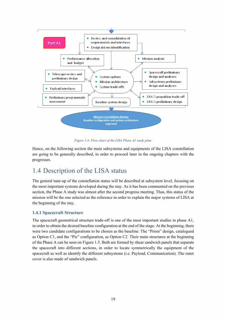
Figure 1.4: Flow chart of the LISA Phase A1 study plan.

Hence, on the following section the main subsystems and equipments of the LISA constellation are going to be generally described, in order to proceed later in the ongoing chapters with the progresses.

1.4 Description of the LISA status The general tune-up of the constellation status will be described at subsystem level, focusing on the most important systems developed during the stay. As it has been commented on the previous section, the Phase A study was almost after the second progress meeting. Thus, this status of the mission will be the one selected as the reference in order to explain the major systems of LISA at the beginning of the stay.

1.4.1 Spacecraft Structure The spacecraft geometrical structure trade-off is one of the most important studies in phase A1, in order to obtain the desired baseline configuration at the end of the stage. At the beginning, there were two candidate configurations to be chosen as the baseline: The “Prism” design, catalogued

as Option C1, and the “Pie” configuration, as Option C2. Their main structures at the beginning

of the Phase A can be seen on Figure 1.5. Both are formed by shear sandwich panels that separate the spacecraft into different sections, in order to locate symmetrically the equipment of the spacecraft as well as identify the different subsystems (i.e. Payload, Communication). The outer cover is also made of sandwich panels.

20

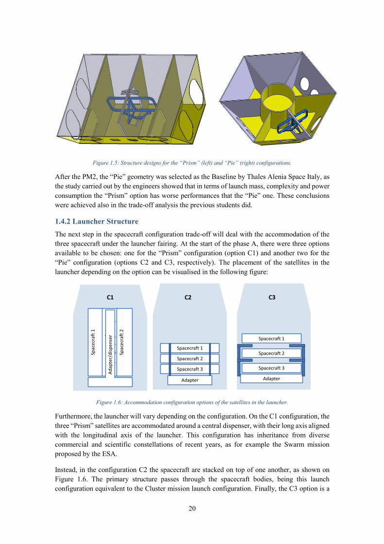
Figure 1.5: Structure designs for the “Prism” (left) and “Pie” (right) configurations.

After the PM2, the “Pie” geometry was selected as the Baseline by Thales Alenia Space Italy, as the study carried out by the engineers showed that in terms of launch mass, complexity and power consumption the “Prism” option has worse performances that the “Pie” one. These conclusions were achieved also in the trade-off analysis the previous students did.

1.4.2 Launcher Structure The next step in the spacecraft configuration trade-off will deal with the accommodation of the three spacecraft under the launcher fairing. At the start of the phase A, there were three options available to be chosen: one for the “Prism” configuration (option C1) and another two for the “Pie” configuration (options C2 and C3, respectively). The placement of the satellites in the launcher depending on the option can be visualised in the following figure:

Figure 1.6: Accommodation configuration options of the satellites in the launcher.

Furthermore, the launcher will vary depending on the configuration. On the C1 configuration, the three “Prism” satellites are accommodated around a central dispenser, with their long axis aligned with the longitudinal axis of the launcher. This configuration has inheritance from diverse commercial and scientific constellations of recent years, as for example the Swarm mission proposed by the ESA.

Instead, in the configuration C2 the spacecraft are stacked on top of one another, as shown on Figure 1.6. The primary structure passes through the spacecraft bodies, being this launch configuration equivalent to the Cluster mission launch configuration. Finally, the C3 option is a

Spac

ecra

ft 1

Spac

ecra

ft 3

(in

tegr

al p

rop

uls

ion

)

Spac

ecra

ft 2

Spacecraft 1

Spacecraft 2

Spacecraft 3

Adapter

Ad

apte

r/d

isp

ense

r

Spacecraft 2

Spacecraft 1

Adapter

C1 C3C2

Spacecraft 3

21

variant in which an external support holds the three satellites, making the adapter qualified for a triple launch.

The dismiss of the “Prism” configuration as the baseline option in favour of the “Pie” geometrical

option after the second progress meeting entailed the discard of the C1 accommodation configuration automatically. On the other hand, the option C3 was even before eliminated due to penalisations regarding the mass and feasibility compared to the C2 option. Thus, the C2 accommodation configuration will be selected as the baseline for the upcoming phases.

1.4.3 Communication Subsystems The communication system can be divided into two subsystems: The Telemetry, Tracking and Command system (TT&C) and the Radio Frequency Inter-satellite link (RF ISL). Both subsystems architectures are aligned with the ones elaborated by the European Space Agency and reported on the Concurrent Design Facility report (ESA, 2017), while the mass and power values have suffered variations as consequence of the design process.

1.4.4 Data Handling The data handling subsystem, as well as the communication systems, are also consistent with the CDF report. Its architecture is formed by the following elements:

On-Board Computer & Mass Memory. Remote Terminal Unit. Ultra-Stable Oscillator.

1.4.5 AOCS/DFACS The AOCS/DFACS subsystem is the one responsible for the correct Guidance, Navigation and Control (GNC) of the three satellites in each mission stages of the spacecraft (launch, transfer, etc.), by making use of the pertinent fuel. The system must be able to control the relative position of the test masses as well, and the orientation of the telescope. There are two main modes which cover all the mission modes of the constellation. According to their functionality, these modes are distinguished as AOCS and DFACS.

The Attitude and Orbit Control System (AOCS) is the one responsible for controlling all the modes from the launch release to the commissioning in final orbit. Therefore, it covers the de-tumbling after launch separation as well as the transfer till the reach of the science orbit.

The other mode that covers the remaining mission phases, that is, from the commissioning in final orbit to the scientific measurement phase is called Drag-Free Attitude Control System (DFACS).

The AOCS/DFACS system is formed by the items listed below:

Four star trackers. Eight sun sensors. Two Inertial Measurement Units.

1.4.6 Electrical Power The electrical power subsystem architecture consists in:

A Power Control and Distribution Unit (PCDU). A Battery.

22

A Solar Array, the main component of the electrical power system (EPS).

The EPS requirements are driven in different ways by the early orbit operations, in particular the transfer stage and the science orbit. Hence, the solar array will be restricted by the needs of both phases.

Thus, the requirements of power demand of the solar array are ruled by the needs of the electric propulsion during the transfer. On the other hand, the dimensional and temperature stability requirements of the electrical power system will be ruled by the requirements of the science phase.

1.4.7 Propulsion subsystems LISA requires propulsion with widely varying characteristics for reaction control in support of post-separation attitude acquisition, attitude control, orbit maintenance and orbit transfer; as well as DFACS and end-of-life disposal. These functions are performed by three propulsion systems:

Xenon propulsion for Orbit Transfer, formed by 2 Hall Effect Thrusters (HET) PPS-1350G which are responsible of the transfer of each spacecraft to the science orbit. The thrusters are also compatible with the power received by the solar array during the Transfer Phase. At the beginning, the option of using chemical propulsion during the transfer was also considered. Nonetheless, TAS-I as well as the ESA CDF reached the conclusion that the chemical propulsion is not feasible due to unreasonable mass constrains.

Nitrogen propulsion for the de-tumbling and Attitude Control manoeuvres. Propulsion for DFACS during the science phase. The Technical Proposal of LISA

gathered a trade-off that included the possible propulsion candidates for the drag-free control manoeuvre (see section 1.3.1): Nitrogen Cold Gas Thrusters (CGT), Mini Radio-frequency Ion Thrusters (mRIT), Indium Field Emission Electric Propulsion (In-FEEP) and Colloid Thrusters.

However, before entering into details of the status of the DFACS trade-off, the propulsion module architecture in the spacecraft must be clarified. There were three different options considered at the beginning that not only regarded the propulsion but also the launching of the constellation. These can be seen on Figure 1.7, and have the following features:

The option named as A is formed by a common Propulsion Module (PM) that supplies the propellant needed to transfer the satellites to the centre of the formation and then each spacecraft reaches its final position using its own propulsion.

The option B proposes a Propulsion Module for each satellite that lets the transfer to its final destination and after that is jettisoned.

The last configuration C suggest the integration of the propulsion systems into the spacecraft.

23

Figure 1.7: LISA propulsion configurations.

After the studies carried out by the engineers, in the Technical Proposal of LISA was included that the option C (Integral propulsion) is chosen as the Baseline configuration, as the option A requires to carry an extra amount of propulsion on the transfer, and the option B lows the system reliability.

On the other hand, the DFACS trade-off was really advanced after the second progress meeting, as the In-FEEP and Colloid Thrusters were already discarded, due to their huge requirements of power consumption. Besides, the technology regarding these two alternatives is not really advanced in comparison with the CGT and mRIT options. The remaining options, CGT and mRIT, make reference to the two main propulsion trade-off configurations, Hybrid and All Electric, respectively.

As it will be explained with more extension in Chapter 4, before the PM3 the DFACS CGT propulsion was selected as the baseline. Hence, the principal features of all propulsion systems as well as the studies made during the stay will be detailed on the fourth chapter.

1.4.8 Payload Module The Payload Module (PLM) is not being designed in Thales Alenia Space Italy. Nevertheless, it is important to study the Payload features as the system engineer has to gather the information of the diverse systems and modules that form the spacecraft, as well as obtaining the report budgets. Therefore, the main components of the Payload are going to be described.

The most important element of the PLM of each spacecraft is the LISA Core Assembly, LCA, which is formed by:

Two Moving Optical Sub-Assembly (MOSA). Each MOSA include: 1. A Telescope for transmitting and receiving the laser beam to/from the other

spacecraft, working with a magnification of 135x. 2. An Optical Bench which implements the local and long arm interferometers. 3. The Gravitational Reference Sensor (GRS), divided into the GRS Head, which

contains the test masses, and the GRS Electronics. Two MOSA Support Structure and two MOSA Thermal Control. An Optical Assembly Tracking Mechanism (OATM), which is the responsible of aligning

the MOSAs towards the remote satellite.

In addition, there are another several components that should be mentioned:

Sciencecraft 1

Sciencecraft 2

Sciencecraft 3

Common Propulsion Module

Adapter / Dispenser

Sciencecraft 1

Propulsion Module 1

Adapter / Dispenser

Sciencecraft 2

Propulsion Module 2

Sciencecraft 3

Propulsion Module 3

Spacecraft 1(integral propulsion)

Adapter / Dispenser

Spacecraft 2(integral propulsion)

Spacecraft 3(integral propulsion)

A B C

24

The LCA structure, which is the mounting structure that connects the two MOSAs of each spacecraft and interfaces them to the satellite, and the LCA Thermal Control.

The Payload Processing Unit (PPU), the Phasemeter System and the Diagnostic System. Two Laser systems, one for each MOSA, as well as the MOSA Control Electronics.

1.5 Participation in LISA project design At the start of the thesis period in Thales Alenia Space, the LISA mission was in the beginning of the Phase A1. During the six months stay in the company, the Phase A1 study will continue in order to consolidate the baseline configuration. Therefore, this master thesis will reflect the advances in the Part 1 studies carried out during the six-month period. In order to support the work done by the project engineers, several functions have been asked to be carried out:

Getting accustomed to the software used in the company to store all the information of LISA, IDM-CIC (will be detailed in Chapter 3).

Optimise the method used to obtain the data stored in the database (IDM-CIC) in the customised report Budgets made by the lean project engineer. This has been carried out by creating several Microsoft Excel interfaces between the IDM-CIC information and these final Budgets mentioned (the complete process will be detailed in Chapter 5).

Carry out an extended trade-off study regarding the propellant mass for the transfer manoeuvre, according to several variables and criteria selected by the domain experts, in order to consolidate the baseline configuration (detailed in Chapter 4).

Develop a simplified model of the current baseline configuration in IDM-CIC, in order to obtain a first estimation of the centre of gravity and inertia matrix of the spacecraft and then to compare the results with the more complete and detailed CAD model (see Chapter 5).

All this tasks done have been carried out in a collaborative engineering environment. Hence, first of describing the processes and estimations made during the thesis period, the Concurrent Engineering concept will be introduced.

25

CHAPTER 2 CONCURRENT ENGINEERING

2.1 Aim of the Concurrent Engineering The Concurrent Engineering (CE), called also simultaneous engineering, is a product designing and developing method which has the purpose of decreasing the time and money used to design a new product. According to this method, the different stages are run simultaneously, instead of being done consecutively. Therefore, concurrent engineering provides a cooperative and collaborative engineering working environment.

The CE term was first introduced by the Institute for Defense Analyses Report R-338 in 1986:

“Concurrent Engineering is a systematic approach to the integrated, concurrent design of

products and their related processes, including manufacturing and support. This approach is intended to cause the developers from the very outset to consider all elements of the product life cycle, from conception to disposal, including quality, cost, schedule and user requirements.” (Winner, 1988)

In addition, the ESA’s Concurrent Design Facility (CDF) uses the following definition:

“Concurrent Engineering (CE) is a systematic approach to integrated product development that

emphasizes the response to customer expectations. It embodies team values of co-operation, trust and sharing in such a manner that decision making is by consensus, involving all perspectives in parallel, form the beginning of the product life cycle.” (ESA; ESTEC, 1999)

Thus, both definitions explain that the Concurrent Engineering replaces the classical Sequential Product Development (SPD) methodology by merging all the product design tasks already in development (IPD – Integrated Product Development).

Figure 2.1: Comparison between Sequential and Integrated Product Design life cycle.

2.2 Traditional Engineering & Concurrent Engineering The classic product design model approaches the product development as a stage-by-stage project. Therefore, the involvement of the different engineers and experts from the different areas of the project on the other tasks is really poor. Usually the design team does not have all the skills and information from the other sectors (engineering, marketing, maintenance) and will eventually

26

design a product which will not reach the quality, functionality, manufacturing and economics levels desired.

Furthermore, once the design stage is done, the upon stages will work based on the product design given; so a lack of design quality will succeed to an overall lack of quality on the following stages. And even worse, may lead to several projects modifications in advances stages of the project development, which turns in reaching non optimal objectives for the product as well as a significant increment of time and money.

This lack of cooperation between the different teams is why the Concurrent Engineering was born. The CE focuses on the involvement of the different teams. Therefore, a first draft made by the design team will be submitted to the CE team, so then the experts of the different sectors will be able to improve the design of the product, as they will work simultaneously with the design team.

Figure 2.2: Concurrent Engineering methodology.

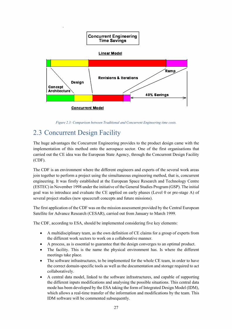
The following Figure 2.3 reflects the time difference between the Concurrent Engineering and the traditional one. It can be seen that, although the design time (including also the Architecture Concept stage) is really similar in both models, the Revision phase is significantly reduced on the Concurrent model, which results not only in a quicker complete process but also in a cheaper product.

27

Figure 2.3: Comparison between Traditional and Concurrent Engineering time costs.

2.3 Concurrent Design Facility The huge advantages the Concurrent Engineering provides to the product design came with the implementation of this method onto the aerospace sector. One of the first organisations that carried out the CE idea was the European State Agency, through the Concurrent Design Facility (CDF).

The CDF is an environment where the different engineers and experts of the several work areas join together to perform a project using the simultaneous engineering method, that is, concurrent engineering. It was firstly established at the European Space Research and Technology Centre (ESTEC) in November 1998 under the initiative of the General Studies Program (GSP). The initial goal was to introduce and evaluate the CE applied on early phases (Level 0 or pre-stage A) of several project studies (new spacecraft concepts and future missions).

The first application of the CDF was on the mission assessment provided by the Central European Satellite for Advance Research (CESAR), carried out from January to March 1999.

The CDF, according to ESA, should be implemented considering five key elements:

A multidisciplinary team, as the own definition of CE claims for a group of experts from the different work sectors to work on a collaborative manner.

A process, as is essential to guarantee that the design converges to an optimal product. The facility. This is the name the physical environment has. Is where the different

meetings take place. The software infrastructures, to be implemented for the whole CE team, in order to have

the correct domain-specific tools as well as the documentation and storage required to act collaboratively.

A central data model, linked to the software infrastructures, and capable of supporting the different inputs modifications and analysing the possible situations. This central data mode has been developed by the ESA taking the form of Integrated Design Model (IDM), which allows a real-time transfer of the information and modifications by the team. This IDM software will be commented subsequently.

28

Focusing on the facility environment, a sketch of the typical CFD layout can be seen on Figure 2.4. As it can be seen, the positioning of the different specialist is made in order to facilitate the cooperation between them, and also to surround correctly the customers.

Figure 2.4: Concurrent Design Facility standard aerospace layout.

2.4 Integrated Design Model (IDM) The centralized database model developed by the ESA is called Integrated Design Model (IDM). It is a Microsoft Excel based software created to make viability studies of spacecraft configurations and missions following the concurrent engineering guidelines. Since its birth, it has supported more than one hundred ESA studies.

The database’s template has been used to support, principally, the different data obtained during

the Phase-A level in order to make an interactive revision of the model, that is, operates as an interface for the CDF review.

The IDM’s format was provided to the principal partners of the ESA; not only companies to test

the software, but also important universities like TU Delft or Politecnico di Milano and European agencies as CNES (in French, Centre National d’Etudes Spatiales) or the Italian Space Agency in

order to obtain feedbacks or improvements about the IDM use. The results obtained shown the significant improvement on the review phase, therefore an increment of the efficiency when it comes to the analysis of the product design.

Focusing now on the software, the IDM model is an Excel file workbook in which the different sheets are reserved for the several sectors of the spacecraft so the team engineers are able to edit or work on the project simultaneously. Thus, these worksheets, that can be referred to a whole system or a single subsystem as well as issues like the risk calculation, will be modified in real time by the appropriate specialist.

29

Figure 2.5: IDM architecture.

Therefore, the several workbooks, schematised on Figure 2.5, encompass four different types of sheets:

Input: Asks for the necessary parameters the workbook needs for calculating and obtaining the output worksheet.

Calculation: The interface between the input and the output sheets. Output: Shows the lists of parameters calculated by the sheet and also provides to the

other workbooks. Presentation: A summary of all the information obtained, in order to be presented to the

other members of the team.

The information obtained from these sheets in the different workbooks is shared with the other ones. This exchange of information requires the figure of a session leader, which is able to control and enable the different outputs obtained thanks to a central network share in which all the workbooks are located. This control is done by the leader on a Data-Exchange workbook, as it can be seen on Figure 2.5.

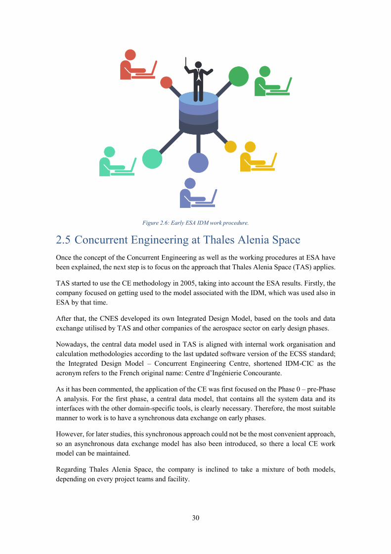
To sum up, the work procedure using the IDM database model is shown on Figure 2.6. The experts of the different areas work collaboratively, sharing their information which is controlled by the system engineer or leader.

30

Figure 2.6: Early ESA IDM work procedure.

2.5 Concurrent Engineering at Thales Alenia Space Once the concept of the Concurrent Engineering as well as the working procedures at ESA have been explained, the next step is to focus on the approach that Thales Alenia Space (TAS) applies.

TAS started to use the CE methodology in 2005, taking into account the ESA results. Firstly, the company focused on getting used to the model associated with the IDM, which was used also in ESA by that time.

After that, the CNES developed its own Integrated Design Model, based on the tools and data exchange utilised by TAS and other companies of the aerospace sector on early design phases.

Nowadays, the central data model used in TAS is aligned with internal work organisation and calculation methodologies according to the last updated software version of the ECSS standard; the Integrated Design Model – Concurrent Engineering Centre, shortened IDM-CIC as the acronym refers to the French original name: Centre d’Ingénierie Concourante.

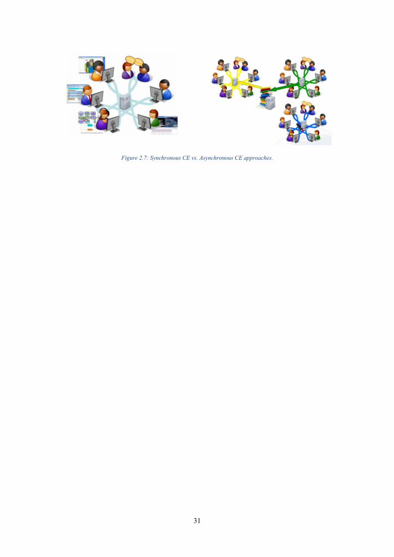
As it has been commented, the application of the CE was first focused on the Phase 0 – pre-Phase A analysis. For the first phase, a central data model, that contains all the system data and its interfaces with the other domain-specific tools, is clearly necessary. Therefore, the most suitable manner to work is to have a synchronous data exchange on early phases.

However, for later studies, this synchronous approach could not be the most convenient approach, so an asynchronous data exchange model has also been introduced, so there a local CE work model can be maintained.

Regarding Thales Alenia Space, the company is inclined to take a mixture of both models, depending on every project teams and facility.

31

Figure 2.7: Synchronous CE vs. Asynchronous CE approaches.

32

CHAPTER 3 IDM-CIC

As it has been commented on the previous chapter, the Integrated Design Model is the main tool used to apply the CE in the different studies. The software IDM-CIC, an Excel central database model, was developed by CNES and later taken by the ESA as the standard programme for CE approaches on Phase A studies.

Thales Alenia Space has been using IDM-CIC since then, having an important contribution on the Phase A study of the latest missions developed such as NGGM, IXV, XIPE, and now LISA. However, is with the LISA mission where the CE techniques have gone a step further, as it is the first time that the application of an integrated design model (working collaboratively) is the main tool used to obtain the mass and power budgets while the study is in Phase A.

The purpose of IDM-CIC is to storage all the important information related to the spacecraft design and to manage it on a structural way. This structure results in the several budgets (mass, power, inertia) that the software provides as outputs, both for element-level and mission-level.

Over the following section, the features of IDM-CIC will be explained. Then, the utilisation of the software will be discussed, as well as the use in a real concurrent engineering session. Finally, the advantages and disadvantages of using IDM-CIC will be detailed.

3.1 IDM-CIC characteristics IDM-CIC (version 3.2.1.7) is a Microsoft Excel Macro-Enabled based software created to allow fast data exchange between the engineering teams plus having a control of the information during the project development.

Therefore, once the software is launched, as it is a MS Excel based, a new window on the main bar of Excel can be founded, which refers to the IDM-CIC tool.

Figure 3.1: Main tools of the IDM-CIC window.

The first thing the software ask is to “Join Study” or to create a “New Study”. At this point, it should be remembered that if a new study is created, the idm file must be located in a shared directory so all the collaborative engineers are able to accede to the file.

After the selection of the study, the IDM-CIC window can be seen. The tools that the plug-in has are highlighted on the Figure 3.1, where three different main commands can be distinguished:

Update and commit processes: These are the commands which support the CE approach on the software. There are several buttons which allow the updating, saving and exporting of the files. Further details will be given over the chapter.

33

Visualization tool: Permits the option of seeing the spacecraft developed, depending on its different configurations.

Users management: Handles the different users the project has, usually associated to the roles (i.e. AOCS, Communication, Thermal). There is a principal user, called “System”,

which responds to the figure of the session leader previously mentioned.

3.2 Structure of an IDM workbook

3.2.1 System Management Starting with a new study, a first window will be automatically generated on the workbook. It is called “System Management”, and it contains the structure of the Spacecraft. The organization of the structure can be seen on Figure 3.2. On it, it can be distinguished:

Elements: The main modules (Platform, Payload, Miscellanea, etc.). Subsystems: For example: AOCS, Electrical Power, Structure, Thermal Control, etc. Equipments: The different Units the Subsystem has (i.e., Tanks, Remote Terminal Unit,

Solar Panel, etc.). Spacecraft Modes or Mission Phases: Science Mode, Transfer Mode, etc.

Figure 3.2: System Structure chart located on the System Management window.

The different subsystems, selected consequently by the project lean manager, are then associated to the different modules, where the green cells mean that the subsystem belongs to the module, and the red ones imply that the subsystem is not included.

All four categories (Elements, Subsystems, Equipments and Mission Phases) can be either created from the beginning or imported (see Figure 3.2) from another project workbook. This means that not only the correspondent unit will be imported but also its own features as the mass, geometry or the element power modes. This last statement shows one of the biggest advantages the IDM-CIC has in relation to a normal Excel workbook.

At this point, it must be pointed out that, as it has been explained on section 2.4, there are four types of sheets, where one of those are the input ones. In the worksheets, the input cells are clearly distinguished from the other ones as are the only modifiable cells in which the user can introduce data. These cells are highlighted in Orange, as it can be seen, for example, on Figure 3.3).

34

Above the system structure, on the System Management Window the system properties chart can also be found. In this table the main information regarding the project is summed up (name of the mission, launcher or launch date as examples).

Figure 3.3: System properties chart.

3.2.2 User Management After the structure is defined, the different Users must be declared. As it has been mentioned, the users created usually tend to be assigned to a “Role”, for example by designating the users to the

different subsystems of the spacecraft. Therefore, when a user launches the idm file, he would be asked for selecting the appropriate “User”, so it assures that every role created has its own competences on the subsystem (or subsystems) assigned.

By default, when a new study is created, there is a unique user called “System”. To create other

users and assign subsystems, the “User Management” command (highlighted in green on Figure 3.1) must be used.

35

Figure 3.4: Users and Roles management tool.

Following the previous figure, the designation of the different users can be seen. As it was commented before, the users created are normally associated to the different subsystems gathered on the system structure (see Figure 3.2), as it happens on the LISA idm file. Regarding the roles, besides the Units roles, which are associated to corresponding users, there are the summary worksheets (“System configuration”, “System mass”, “System power”, “Mission” and

“Propulsion”) where the main calculus and outputs are shown (i.e. mass budget, power budget).

These last sheets usually are part of the System User role, and they will be extensively detailed

To sum up, when the domain expert enters in the idm file and selects the pertinent user, the pertinent worksheets he is responsible for will be opened, and he will be able to work and update all the information related to his area. On the other hand, the “System” user will be able to manage and control the roles, as well as the summary sheets. At this point, it must be highlighted that the assignation of roles is not an irreversible process, as the System engineer (User) can always take back the roles and manage them from his own session. Therefore, this means that the system users and engineers/experts are able to work simultaneously in the same product.

3.3 Subsystem Worksheets Firstly, the sheets regarding the different subsystems are going to be analysed. Every subsystem is formed by the several units the pertinent domain expert considers. As mentioned before, every unit can be imported from another idm file or be created from the beginning. Hence, in order to create the Units, the subsystem sheet offers different commands to fulfil its complete designation.

36

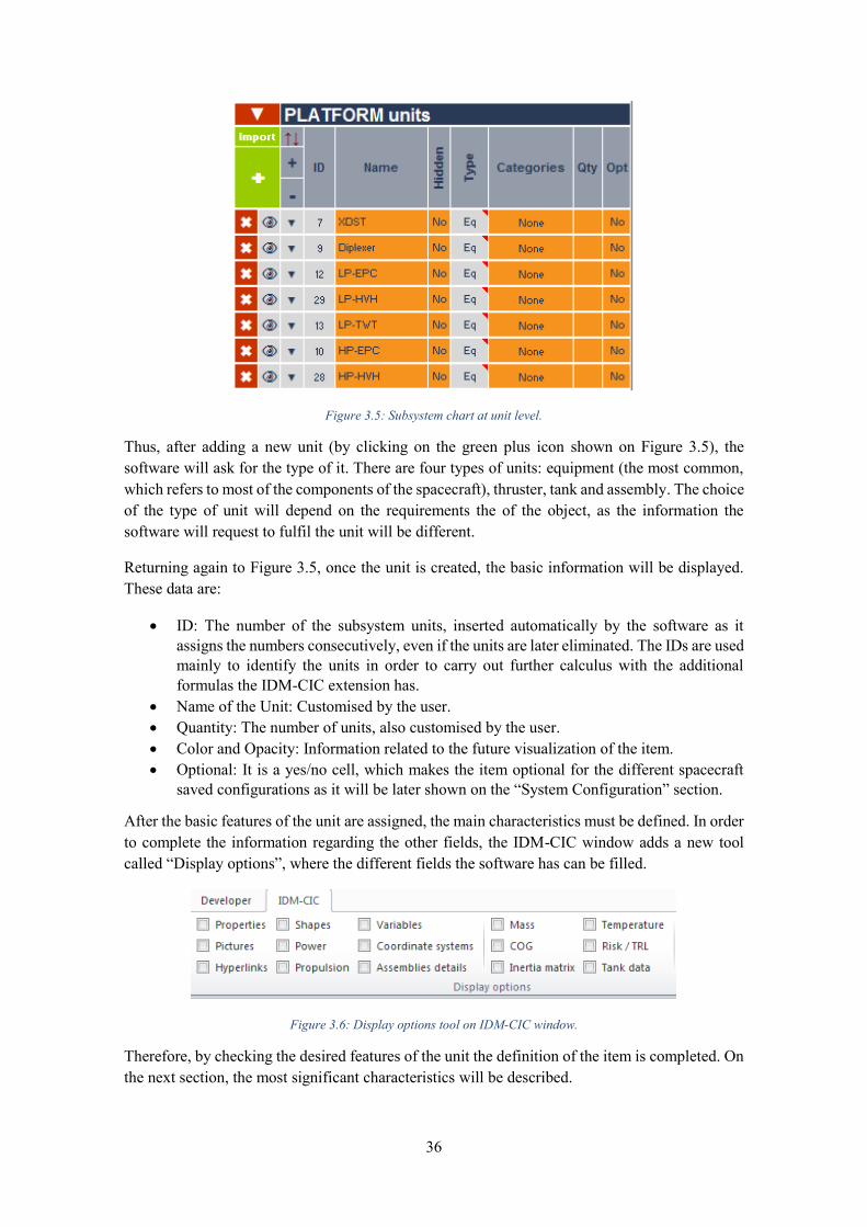
Figure 3.5: Subsystem chart at unit level.

Thus, after adding a new unit (by clicking on the green plus icon shown on Figure 3.5), the software will ask for the type of it. There are four types of units: equipment (the most common, which refers to most of the components of the spacecraft), thruster, tank and assembly. The choice of the type of unit will depend on the requirements the of the object, as the information the software will request to fulfil the unit will be different.

Returning again to Figure 3.5, once the unit is created, the basic information will be displayed. These data are:

ID: The number of the subsystem units, inserted automatically by the software as it assigns the numbers consecutively, even if the units are later eliminated. The IDs are used mainly to identify the units in order to carry out further calculus with the additional formulas the IDM-CIC extension has.

Name of the Unit: Customised by the user. Quantity: The number of units, also customised by the user. Color and Opacity: Information related to the future visualization of the item. Optional: It is a yes/no cell, which makes the item optional for the different spacecraft

saved configurations as it will be later shown on the “System Configuration” section.

After the basic features of the unit are assigned, the main characteristics must be defined. In order to complete the information regarding the other fields, the IDM-CIC window adds a new tool called “Display options”, where the different fields the software has can be filled.

Figure 3.6: Display options tool on IDM-CIC window.

Therefore, by checking the desired features of the unit the definition of the item is completed. On the next section, the most significant characteristics will be described.

37

3.3.1 Shapes IDM, though is not a complete design tool such as the diverse CAD software, lets the creation of complex geometries through the commands this display options has.

Therefore, after selecting the green plus icon the software will request for the type of geometry from a list of different options, i.e. cylinder, parallelepiped, extruded triangle or hollow truncated cone. Then, the own tool will facilitate to complete the definition of the shape (see Figure 3.7 as example) and also will provide the location of the centre of reference of the own shape.

Figure 3.7: Geometry definition helper.

This reference centre (inserted by default by IDM-CIC) can be placed around the three coordinates x, y, z and also rotated around these axes, in order to locate correctly the geometry (for example if one piece is formed by the union of several shapes). However, the final location of the item can be later changed on the “System Configuration” sheet, that will be later explained.

In addition, several options regarding the shape selection should be mentioned, besides the fact that it can also be imported a considered shape from another idm file. The first one is the “Topology” option, from which complex forms can be created as a combination of different

geometries that, selecting the appropriate command, can result in the union, intersection or elimination of shapes (see Figure 3.8).

38

Figure 3.8: The shape display option, showing the Topology option besides the position and mass of the geometry.

As it can be seen on the above picture, the mass can also be inserted on the geometry (only if the Mass Display option is also selected). This option will be discussed with the Mass and Inertia Display options explanation, but gains importance when it comes to the MCI (Mass, Centre of Gravity, Inertia) budget calculation.

Finally, the last option significant to mention is the step one. By selecting this option, the user is able to import a step file (and hence the geometry) on IDM, which shows another huge advantage IDM-CIC possesses: the integration of design models from complex CAD designs.

3.3.2 Power and dissipation The power feature is one of the most important information that has to be added on IDM-CIC, so then the system engineer will be able to obtain the power budget and the dissipation budget. In this tool, the user can add the power consumption and dissipation of the items he is responsible for. As it can be implied, the power consumption is not a constant, so IDM comes up with a solution that consists in create the different element power modes during the mission of the spacecraft.

Thus, the user adds (creating or importing it) all the operative modes and rename them, inserting their mean or peak values (usually the last one is inserted, as the study on this phases tends to obtain the power consumed on the worst case) as well as the dissipation. After that, the system engineer associates the element power modes to the mission phases the study has and obtains the final power budget and dissipation budget.

Figure 3.9: Power display options and its features.

39

3.3.3 Mass The other main feature along with the power definition is the Mass. This option lets the engineer to insert the mass numeric value in the correspondent cell. Furthermore, the cell directly next to the mass value allows the inclusion of a determined maturity margin (which is related to the TRL, mentioned below). This margin can be “0%”, “Fully developed (5%)”, “To be modified (10%)”,

“15%” and “To be developed (20%)”, as well as an own custom margin, chosen by the user. These margins make reference to the Margin philosophy document carried out by ESA, in particular to the requirement R-M2-4, which states (ESA; ESTEC, 2012):

“At equipment level, the following design maturity mass margins shall be applied:

R-M2-41: ≥5 % for “Off-The-Shelf” items (…). R-M2-42: ≥10 % for “Off-The-Shelf” items requiring minor modifications (…). R-M2-43: ≥20 % for new designed/developed items, or items requiring major

modifications or re-design (…).”

Figure 3.10: Mass display option and its features.

The last cell that can be seen on Figure 3.10 shows the option of inserting the mass “Manually”

or “From Geometry”, which is related to the MCI information, discussed on the following section.

3.3.4 Centre of Gravity / Inertia Matrix These options are, logically, directly associated with the mass characteristic. Once inserted the mass, the software would let the manual insertion of the coordinates of the Centre of Gravity of the shape, as well as the inertial moments of the geometry designed. This will allow the user to introduce more accurate values obtained from other software, i.e. Catia. Additionally, if the option “From Geometry” is selected, IDM will automatically obtain the Mass from the shape, and also

will calculate the CoG of the geometry and its inertial matrix according to the orientation and position given on the previous definition.

Figure 3.11: Inertia Matrix and CoG display options.

40

On the above image the two different options of data origin for the MCI information can be seen. As it was said before, the “Manual” option lets the user introduce the values calculated externally, as the orange input cells can be seen on Figure 3.11. On the other hand, the “Geometry” option

will calculate the MCI data according to the shape placement and dimensions (the data now appear automatically on grey).

Furthermore, it must be highlighted that, when the MCI data is taken from the geometry, the mass of the item is introduced homogeneously on the shape. This fact implies that the IDM-CIC precision when it calculates the MCI budget is not as accurate as desired, as it does not consider complex elements formed by diverse materials.

3.3.5 Tank Data The correspondent option to add all the information regarding the tanks of the spacecraft, which are the Capacity and the percentage of filling. This information is really important in order to later insert the fuel mass on IDM, as it will be shown with more details on the System Configuration section (see section 3.4.3).

Figure 3.12: Tank Data Display option.

3.3.6 Risk/TRL The last feature analysed is the TRL. This acronym stands for Technology Readiness Levels, which are a systematic measurement system that supports assessments regarding the maturity of a technology and the relation between the maturity of different types of technology. The TRL values respond to a scale of numbers whose range comes from 1, defined as “Basic principles

observed and reported” to 9, defined as “Actual system “flight proven” through successful

mission operations”. (Mankins, 1995)

3.4 Summary worksheets As the subsystems worksheets are being completed by the pertinent team groups/engineers the session leader is able to obtain the summary worksheets, that is, the output budgets the IDM-CIC provides in order to support the mission phase A study. So, the main worksheets which the system engineer works with are going to be detailed.

41

3.4.1 System Mass By picking the System mass worksheet shown on Figure 3.4, IDM opens a window called “Mass

Budget”, which shows, as the own name implies, a structured mass summary of the spacecraft.

The mass budget is structured in the different layers the software lets to organize. Therefore, from minor to major details, the mass budget can be obtained at Element (or system) level, then at subsystem level and finally at unit level, by selecting the different arrows that can expand the budget. An example of the mass budget created by IDM-CIC can be seen on Figure 3.13.

Figure 3.13: Mass Budget.

In this chart, several information can be obtained. From the several columns the summary has, the mass with and without the maturity margin (explained on section 3.3.3), the percentage of the maturity margin and the value (in kilograms) of the mass added by the margin. The sum of the mass of the different units define the mass and margin of the subsystem, and the same happens

42

with the values at element level, summed up at the end of every element chart. Besides, at element level another margin can be introduced, the system margin.

Finally, the total Dry Mass is obtained, with the possibility to obtain the total wet mass by introducing the correspondent mass on the tanks. This option will be explained later, on the “system configuration” section, as previously mentioned.

3.4.2 System Power The same methodology explained to obtaining the mass budget could be implied in order to obtain the power budget. However, the necessary process needed to achieve a power summary is more complicated, as it requires an extra work from the system engineer.

Figure 3.14: Structure of the System Power Role.

The Figure 3.14 schematises the structure which appears when the Role “System Power” is

selected. Thus, it can be seen that, in order to obtain the Power and Dissipation Budgets, the session leader needs to take an intermediary step, on the windows “Element Power Budget” and

“Element Dissipation Budget”.

In these two sheets, the system engineer has to map the power mode of every unit by selecting the power values defined previously on the power display option (as explained on section 3.3.2). Hence, on the “Element Power Budget” and “Element Dissipation Budget” worksheets, the system engineer selects and maps the appropriate power modes for each item according to the diverse element power modes that are defined. These element modes are related to the operational power values during the mission (i.e. Launch Mode, Science Mode).

43

Figure 3.15: Example of the Element Power Budget. Highlighted in red, the mapping menu.

Once fulfilled the “Element” sheets, and after committing, the system engineer can accede to the

Power and Dissipation Budgets, where the charts result pretty similar to the ones mapped on the Element windows but are no longer modifiable.

The diagram of the Power Budget follows the template of the Mass Budget, in which the power consumed by Units, Subsystems and Elements can be seen, with also the capability of adding a system power margin at the end of every Element. The same procedures are applied to the Dissipation Budget.

44

Figure 3.16: System Power Budget.

45

Figure 3.17: System Dissipation Budget.

3.4.3 System Configuration The last important role designed to the system engineer is the “System Configuration” one. Once

selected it, the user will be able to manage two worksheets: “Configuration” and “Saved

Configurations”. Moreover, there is an extra window whose link is located on the “Saved

Configurations” worksheets, the “MCI budget” which will also be analysed.

Configuration

This worksheet is one of the most important ones of the software. It is the one used to assemble all the items that shape the spacecraft. In order to do the assembly, the first part of the sheet lets the user to create the different coordinate systems the domain expert considers appropriate. These coordinate systems can be placed, with three different rotations and also three positions, from the main system called “System”, which can also be editable.

Once defined the coordinate systems, the position of the different items is adjusted, using not only the previous coordinate systems created but also the six degrees of freedom mentioned.

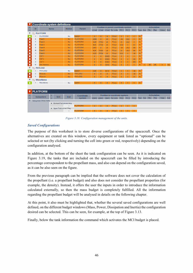
46

Figure 3.18: Configuration management of the units.

Saved Configurations

The purpose of this worksheet is to store diverse configurations of the spacecraft. Once the alternatives are created on this window, every equipment or tank listed as “optional” can be

selected or not (by clicking and turning the cell into green or red, respectively) depending on the configuration analysed.

In addition, at the bottom of the sheet the tank configuration can be seen. As it is indicated on Figure 3.19, the tanks that are included on the spacecraft can be filled by introducing the percentage correspondent to the propellant mass, and also can depend on the configuration saved, as it can be also seen on the figure.

From the previous paragraph can be implied that the software does not cover the calculation of the propellant (i.e. a propellant budget) and also does not consider the propellant properties (for example, the density). Instead, it offers the user the inputs in order to introduce the information calculated externally, so then the mass budget is completely fulfilled. All the information regarding the propellant budget will be analysed in details on the following chapter.

At this point, it also must be highlighted that, whether the several saved configurations are well defined, on the different budget windows (Mass, Power, Dissipation and Inertia) the configuration desired can be selected. This can be seen, for example, at the top of Figure 3.13.

Finally, below the tank information the command which activates the MCI budget is placed.

47

Figure 3.19: Saved Configurations worksheet.

MCI Budget

The last sheet that is going to be analysed is the Mass, Centre of Gravity and Inertia Budget. This chart is a summary of the positions and inertia of the spacecraft at Unit, Subsystem and Element Level.

On this worksheet, the software has an extra display options on the IDM-CIC window, which lets the user select to include in the chart the CoG and the Mass with and without margins. Regarding the inertia, besides including it with and without margins, also shows the coordinate system from which the inertia has been calculated: From the CoG or from the “System” coordinate system. An

example can be seen below:

48

Figure 3.20: MCI Budget without maturity margin (left) and with maturity margin (right).

This budget, however is not as accurate as the other ones. There are several factors that influence the summary chart: First of all, the lack of complexity on the shape definition of the elements of the spacecraft provokes that the mass distribution is not as precise as desired. In addition, on this phases of early analyses there are equipment that does not have linked a shape, therefore their CoG and mass distribution is not well positioned.

Despite these issues, the inertia budget results useful in this stage, as it can provide the engineering group a preliminary estimate of the Inertia distribution, and even so, as in the case of LISA, obtaining an Inertia Budget before the calculation made by the design team (which in TAS-I is done with Catia V5) as the detailed CAD model is not perfected yet.

3.5 Visualization tool: IDM View The last main feature the IDM-CIC window provides is the visualization tool. Whether a determined configuration is defined, with all its optional components and shapes placement, the software lets the visualization of the spacecraft configuration by the integrated tool developed: the IDM View.

Therefore, once the command of the visualization tool is selected (see Figure 3.6 to locate the tool) a new window will appear. In it, the user is able to select or not the components he wants to be shown on IDM view; from single equipments or tanks to an overall view of the whole spacecraft. Besides, the tool also is capable of include the system axis of all the coordinate systems created, as well as the position of the CoG.

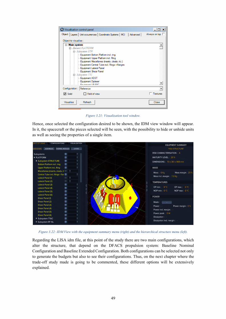
49

Figure 3.21: Visualization tool window.

Hence, once selected the configuration desired to be shown, the IDM view window will appear. In it, the spacecraft or the pieces selected will be seen, with the possibility to hide or unhide units as well as seeing the properties of a single item.

Figure 3.22: IDM View with the equipment summary menu (right) and the hierarchical structure menu (left).

Regarding the LISA idm file, at this point of the study there are two main configurations, which alter the structure, that depend on the DFACS propulsion system: Baseline Nominal Configuration and Baseline Extended Configuration. Both configurations can be selected not only to generate the budgets but also to see their configurations. Thus, on the next chapter where the trade-off study made is going to be commented, these different options will be extensively explained.

50

3.6 IDM-CIC working procedure Over the different sections of this chapter, the features of the software, as well as its purposes on the spacecraft design have been explained. Nevertheless, IDM-CIC must be used following certain procedures during a concurrent engineering work session, or on the contrary significant information and work advances could be lost during the session.

Thus, there are two principal procedures to perform properly a CE work session. The first one is that every domain expert works directly form the idm file, by entering on his role assigned. The other one requires an intermediary step, in which from the idm file several .xlsm files are generated, one for every user, so each engineer works on his own file which refers to the central IDM-CIC file.

Figure 3.23: Concurrent Engineering work procedure using IDM-CIC with (right) and without (left) .xslm files.

3.6.1 Guidelines for a work session directly from IDM-CIC All the members of the team work simultaneously on one only idm file, which includes the spacecraft model. It must be implied that the file must be placed on a shared directory so all the experts have access to it.

Therefore, each expert opens the file and selects the pertinent role the system engineer has associated to him, so then the user works only on his own responsibilities, as it has been explained previously.

The working methodology the different “editors” follow is schematized on Figure 3.24. It can be seen that, from the IDM central data file several users can work simultaneously, though they cannot notice in real time the modifications of the other engineers. When a certain team member finishes his job, he uses the command “Commit” (see the IDM-CIC toolbar on Figure 3.1) to automatically save the changes made on the idm file on the shared directory. On the other hand, the other users which initially do not see the modifications, have to select the command “Update”

to retrieve the updated information from the central database.

Once all the users associated to the different roles have ended their works, the session leader can update his main file and refresh all the budgets. After the refreshing, the system engineer makes the last commit and states the conclusion of the working session.

51

Figure 3.24: IDM-CIC architecture.

3.6.2 Guidelines for a work session using the xslm files The easiest way to implement the use of IDM-CIC in a working session is by introducing the “xlsm” files. Although the global architecture introducing these files seems to be more complex, the use of the xlsm files entail several advantages than working directly from the idm file. The most important benefit the xlsm files provide is the capability to add new sheets. In them, the user can create tool and personalization (macros or references to the correspondent worksheet) that, instead of a working session on an idm file, where all the new sheets created during the update are deleted once the working session is concluded and the idm file closed, these worksheets will not be erased.

These individual files can work with users (hence, the different roles), so there is not the risk of altering the part of the project that are not competences of the user. Moreover, each user is able only to read and link data regarding other subsystems by using the command “Read-only reports” located on the IDM-CIC toolbar. Besides, the opening time of the xlsm files is much lower than the idm file opening time. This is because on the second case, when the role is selected, Excel has to generate a temporary xlsm file, whilst the own xlsm file is immediately ready to be opened.

Finally, the last advantage is that when another user modifies data in the idm file, the owner of the xlsm file is always able to overwrite these changes by using its own file (xlsm) and then using the “Commit” command. In order to create a xlsm file, these steps must be followed:

Open the interested idm file. Login with the own role. Clicking on “Save with name” and save the excel file as a new one in a dedicated

directory, selecting the file type “Excel Macro-Enabled Workbook”.

Therefore, the new flow chart which represents the working procedure is shown below. In order to send all changes that one has made, the user has to “Commit” from his xlsm and, in this way, this Macro will refresh the idm file with the changes done. Moreover, in order to see the changes that another user has done, it is necessary to “Update” on the own “xlsm” file, so the “Read-only reports” will be updated with the modifications made by the other domain experts.

52

Figure 3.25: Flow chart between idm and xlsm files.

At this point, it must be highlighted that the IDM-CIC command “Revert”, which is useful to

recover the data of the previous working session, does not work yet on the current IDM-CIC version, so creating a backup file before any working session is highly recommended.

It also must be pointed out the difference between the common “Save” function of Excel and the “Commit” of IDM. Regarding the working session on an idm file, it must never be saved the Excel session on the exit otherwise the template will be compromised. Therefore, the commit command is the correct tool to save the progresses made.

However, the save on exit is allowed if the working session is done through the xlsm files, as the changes made are saved locally on the file of the user avoiding the alteration of the template. In fact, in order to update the central data mode with the xlsm files the tool used is the “Commit”

Button, as it is shown on Figure 3.25. However, if the user closes the xlsm without saving, although all the modifications made are already saved on the idm file, the information added, including the extra sheets the user could have developed, will be lost. This problem can be solved by exporting another xlsm file from the original idm file updated, but the extra sheets created will not be recuperated.

For all these reasons, before a CDF session is advisable to create a backup of the idm file as well as for all the xlsm files created, according to the following guidelines:

Create a backup directory and export there the idm file, usually adding references like the version number (so finally the backup results a version control).

From this idm file, create the related xlsm files through the function “Save with name”. On these xlsm files, copy all the extra worksheets developed locally from the original

ones.

Thus, the xlsm file will be aligned with the idm one inside the version control folder.

3.7 Pros and cons of IDM-CIC The most used tool during the work period in TAS-I was IDM-CIC, so a high level of knowledge and confidence with the software has been reached. Therefore, and as a kind of summary of this chapter, a list of pros and cons the IDM-CIC tool provides a Concurrent Engineering approach are going to be enumerated.

53

3.7.1 Advantages

The software is a Microsoft Excel extension, so that makes IDM-CIC really easy learning. The facility to recover and re-utilise information of other spacecraft projects already

designed, through the import functions the software has. The introduction of the different roles as well as the session leader, which approaches

more to the real time design. In addition, the possibility to work simultaneously either through the xslm files or directly from the idm file causes a more productive working sessions.

The capability to analyse on the same idm file several configurations, through the definition of optional units, not only regarding the budgets, but also the geometrical configurations that can be seen on the IDM view.

3.7.2 Disadvantages

The lack of integration of the software with another engineering tools, as the only useful implementation IDM has is the import or export of step files to/from CAD programmes.

The impossibility of return to the previous version of the file IDM once the user has committed, having to use a more articulated version control procedure while the “Revert”

command continues to be inoperative. The difficulty to, once there are more than one configuration available on the file,

compare simultaneously the configurations, having to make this comparison externally through the exportation of the reports from the file idm. Besides, the software requires a significant amount of time in order to selecting the desired configurations, obtaining the correspondent budgets and exporting them to xlsx files.

In relation to the MCI budget, the IDM-CIC does not consider the system margin in Inertia and CoG calculations, as it is detailed in Chapter 5, so in order to include the system margin it must be included equipment by equipment in IDM.

54

CHAPTER 4 TRADE-OFF STUDIES

4.1 Trade-off concept In the first chapter, the current status of the ongoing LISA phase A1 study were commented. As it has been also mentioned, the outcome of the stage A1 is the baseline configuration identification, as well as the mission definition.

Therefore, in order to obtain a final configuration, the engineering teams select a wide variety of possibilities and considerations that should be taken into account in order to obtain an optimal product, by taking into consideration their knowledge besides their experiences in other mission studies. This range of features and configurations are analysed on the preliminary phase (phase 0) and are gathered in a document that Thales Alenia Space sends to the client (European Space Agency) in response to their Invitation to Tender (ITT).

The main candidate configurations are exhaustively examined, by analysing the advantages and disadvantages each option provides. For example, an item can have a minor power consumption than other choices, but its dry mass or dimensions can be bigger. The study that gathers all different configuration possibilities and analyses them according to different criteria is called trade-off. Hence, a trade-off is a decision that means diminishing or losing one quality or property of a product design in favour of an increment on other qualities; therefore, a compromise solution.

4.2 Working method The response of the Invitation to Tender made by the company is the Technical Proposal, a document that includes not only the aims for which the mission has been planned, but also the list of requirements the project has to fulfil as well as the diverse proposals selected to reach these objectives.

Once the Technical Proposal is approved, the beginning of the Phase A study can be launched, and with that the trade-off analyses. However, the engineering teams must follow certain guidelines in order to make a correct approach of the trade-off studies. There are several decision analysis models, most of them really similar, that illustrate these rules. On the Figure 4.1 is schematised a basic flow chart of the stages that should be taken into account at the start of the trade-off (Hirshorn, Voss, & Bromley, 2017):

55

Figure 4.1: Decision Analysis Flow Chart.

On the figure above the main phases for an appropriate analysis after being made the decision of develop a trade-off study are outlined. From them, several remarks can be made, which will be listed below.

Frame the decision

The first step that must be made is the definition of the diverse criteria from which the analysis will stand, that is, the parameters or qualities that will be evaluated in order to judge the alternatives. Typically, these set of criteria are mission performances, manufacturing, time or costs.

Identify the alternatives

Then, the work teams strive to obtain the different alternatives that could fulfil the requirements established previously. The alternatives can vary from the design concept to other more technical features like the mass and power performances.

Evaluate the decision

According to the solution desired to have, the variety of alternatives selected are evaluated in order to obtain the best solution that satisfies the criteria previously chosen. There are several manners of evaluating the decisions, starting by working sessions by the members of the team where they discuss and work among the possible alternatives. Besides, there are also more complex evaluation models that can be really useful if the difficulty of the decision as well as its

56

complexity are higher. These models are called Multi-Criteria Decision Making models (MCDM).

Once decided the method with which the approach will be done, the examination of the alternatives starts. Each possibility is evaluated according to the criteria and classified respect to the other alternatives.

Select the alternative

After the evaluation phase is finished, the following step is to analyse the results obtained, according again to the criteria chosen. Hence, the different alternatives are classified (whether or not with a sort of numerical rankings, depending on the decision method analysis) from the most suitable to the worst one, and then reported to the team leader or decision maker.

Conduct sensitivity analysis

With the report of the ranking of the alternatives usually is included a sensitivity analysis focused on this ranking. A sensitivity analysis is how the uncertainty or risk in the outcome of the study developed is assigned to the inputs (criteria utilised). According to (Parnell, 2013), the sensitivity analysis is introduced as:

“Analysis that assesses the impact of changes in a parameter on value of an alternative, or on

difference of value between two alternatives.”

Hence, the sensitivity analysis shows how much has to change the effect of a certain criteria so it introduces a change in the ranking.

After this stage, if the decision maker checks and approves the recommended option the implementation of it begins.

4.3 System trade-offs status and suitable future trades In the Chapter 1 the main trade-off for the Phase A1 were also introduced. This three analysis were:

The launch/spacecraft configuration trade, in order to reach the optimal configurations that will be further developed.

The spacecraft configuration trade, in order to obtain the baseline configuration that will serve for the following phase A2 study.

The DFACS propulsion trade.

In relation to the first trade-off listed, the spacecraft candidate propulsion configurations listed were three, shown on Figure 1.7. The preliminary analysis carried out by Thales Alenia Space stated the option with integral propulsion (named as C) as the most feasible and hence, declared as the Baseline configuration. In addition, the trade-off study carried out by the previous students corroborated the baseline option as the most recommended one.

Instead, the spacecraft alternatives resulted to be two geometrical configurations, the “Pie” and

the “Prism” geometries (see Figure 1.5); while the launch configurations selected were three, two for the “Pie” geometry and the last one for the “Prism” configuration (see Figure 1.6). As with the propulsion configurations, by the end of the second progress meeting the baseline options

57

were selected, being the “Pie” geometry and the “C2” launch option the current baseline for the

upcoming phases of the project.

Therefore, it can be stated that the spacecraft geometrical, propulsion and launch baseline configurations have been decided, so the first trade-off listed is already completed. The baseline configuration is shown in the figures below:

Figure 4.2: LISA current baseline configuration (1).

Figure 4.3: LISA current baseline configuration (2).

58

In relation to the DFACS propulsion trade-off, in the first chapter was commented that the viable alternatives introduced in the Technical proposal of LISA were two:

Hybrid Option: Formed by Hall Effect Thrusters (HET) fed with Xe for the transfer and Cold-Gas Thrusters (CGT) for De-tumbling & AOCS and DFACS.

All-Electric Option: The De-tumbling and AOCS CGT are now fed with Xenon. while the DFACS operations are propelled by miniRIT, fed also with Xe.

AOCS & Detumbling Transfer DFACS

Hybrid 6+6 Cold Gas (N2) 50 mN

1+1 HET (Xe) ≤90 mN

9+9 Cold Gas (N2) 1-1000 µN

All-Electric 6+6 Cold Gas (Xe) 50 mN

1+1 HET (Xe) ≤90 mN

9+9 miniRIT (Xe) 50-500 µN

Table 4-1: Baseline propulsion alternatives proposed.

Nevertheless, as it has been commented in section 1.4.7, an extensive trade-off was carried out by TAS-I in order to find the most suitable option. Several criteria were selected in order to choose the correct alternative, including the launch mass, complexity, technology level and power consumption. The following table shows a summary in which the estimated values at the beginning of Phase A of mass, power, and other significant features are included.

Hybrid All Electric Propellant Mass (Only DFACS, Nominal Mission) [kg] 46 9

Power consumption (peak) [W] 43 215 Specific Impulse [s] 55 830

TRL 9 5 Table 4-2: Preliminary main features of Hybrid and All Electric propulsion.

After the analysis it was concluded that, the All Electric option provides a higher launch mass margin as well as a bigger specific impulse than the Hybrid option. However, the superior power consumption, the elevated degree of complexity of the option and the lack of technology knowledge in comparison with the Hybrid one provoked the selection of the Hybrid propulsion configuration as the current Baseline, having therefore the All Electric option as the backup alternative.

Therefore, after seeing the results of both trade-offs, it could be implied that the trade-offs are already finished and so the Part A1 ended. Nonetheless, although two of the main trade analysis might be consolidated, the baseline configuration is far from being completed, as there still are significant features pending to be finalised.

After the third progress meeting, where TAS-I reported the consolidation of the two trade-offs, one of these features was requested to the system engineer (and hence, to the student) to be analysed: the study of the propellant mass necessary to fulfil the LISA requirements in each of the mission phases. In particular, the analysis will be focused principally in the propellant during the transfer phase.

Thus, the analysis requested has been developed as a propellant trade-off. On the following sections, the main characteristics and criteria utilised will be defined, in order to proceed then to its study.

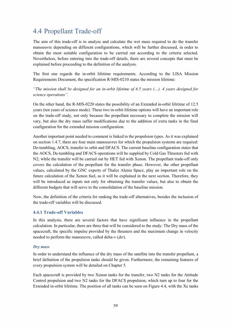
59

4.4 Propellant Trade-off The aim of this trade-off is to analyse and calculate the wet mass required to do the transfer manoeuvre depending on different configurations, which will be further discussed, in order to obtain the most suitable configuration to be carried out according to the criteria selected. Nevertheless, before entering into the trade-off details, there are several concepts that must be explained before proceeding to the definition of the analysis.

The first one regards the in-orbit lifetime requirements. According to the LISA Mission Requirements Document, the specification R-MIS-0210 states the mission lifetime:

“The mission shall be designed for an in-orbit lifetime of 6.5 years (…). 4 years designed for

science operations”.

On the other hand, the R-MIS-0220 states the possibility of an Extended in-orbit lifetime of 12.5 years (ten years of science mode). These two in-orbit lifetime options will have an important role on the trade-off study, not only because the propellant necessary to complete the mission will vary, but also the dry mass suffer modifications due to the addition of extra tanks in the final configuration for the extended mission configuration.

Another important point needed to comment is linked to the propulsion types. As it was explained on section 1.4.7, there are four main manoeuvres for which the propulsion systems are required: De-tumbling, AOCS, transfer to orbit and DFACS. The current baseline configuration states that the AOCS, De-tumbling and DFACS operations will be supplied by Cold Gas Thrusters fed with N2; while the transfer will be carried out by HET fed with Xenon. The propellant trade-off only covers the calculation of the propellant for the transfer phase. However, the other propellant values, calculated by the GNC experts of Thales Alenia Space, play an important role on the future calculation of the Xenon fuel, as it will be explained in the next section. Therefore, they will be introduced as inputs not only for obtaining the transfer values, but also to obtain the different budgets that will serve to the consolidation of the baseline mission.

Now, the definition of the criteria for ranking the trade-off alternatives, besides the inclusion of the trade-off variables will be discussed.

4.4.1 Trade-off Variables In this analysis, there are several factors that have significant influence in the propellant calculation. In particular, there are three that will be considered to the study: The Dry mass of the spacecraft, the specific impulse provided by the thrusters and the maximum change in velocity needed to perform the manoeuvre, called delta-v (𝛥𝑣).

Dry mass

In order to understand the influence of the dry mass of the satellite into the transfer propellant, a brief definition of the propulsion tanks should be given. Furthermore, the remaining features of every propulsion system will be detailed on Chapter 5.

Each spacecraft is provided by two Xenon tanks for the transfer, two N2 tanks for the Attitude Control propulsion and two N2 tanks for the DFACS propulsion, which turn up to four for the Extended in-orbit lifetime. The position of all tanks can be seen on Figure 4.4, with the Xe tanks

60

highlighted in green and the N2 ones, in light blue. In addition, the two extra DFACS tanks developed for the extended mission are outlined in red.

Figure 4.4: Tanks placement in the spacecraft. Xenon tanks are highlighted in green, Nitrogen tanks in turquoise. Extra tanks for the extended mission outlined in red.

Therefore, it can be implied that the dry mass of the satellite will not be equal for the Nominal and Extended Mission designs. Since the rest of the subsystems remain unaltered, the mass difference between Nominal and Extended configurations will be the one caused by the addition of the two extra tanks. In addition, the difference between both DFACS tank mass is shown below:

In-orbit lifetime DFACS tank mass (with margins) [kg]

Nominal (6.5 years) 49 Extended (12.5 years) 99

Table 4-3: DFACS tank mass values for Nominal and Extended configurations.

The reason the dry mass variation is important for the trade is because of the method used to calculate the transfer propellant. The dry mass corresponds to the final mass of the last manoeuvre the spacecraft has to do, that is, the DFACS control during the science operations. So, knowing (as it has been mentioned before), the DFACS propellant mass as well as the final mass (dry mass), the initial mass for this manoeuvre is obtained, which is equal to the final mass of the previous manoeuvre (AOCS control). After doing this process of reverse engineering, the value of the initial, final and propellant mass of the transfer are obtained. Thus, the final dry mass acquires an important role in the study. The complete process of the propellant calculation will be detailed on section 4.4.3.

61

Hence, for the upcoming trade-off analysis, the propellant mass for the transfer stage will be calculated for two configurations, named as Nominal Baseline configuration and Extended Baseline configuration.

Hall Effect Thrusters Operating point

As it was commented in the introduction, the Xenon propulsion during the transfer is going to be carried out by 1+1 Hall Effect Thrusters PPS-1350G. However, the thruster set point has not been decided yet. Three were the possible operating points alternatives, listed on the table below:

1 2 3 Thrust [mN] 88 60 60 Voltage [V] 350 350 500 Intensity [A] 4.3 2.8 2.3 Power [W] 1500 1015 1150

Specific Impulse [s] 1650 1600-1700 1900-2000 Table 4-4: Operating HET alternatives.

The specific impulse, listed in the last row of the previous table, can be obtained from the relation between power and thrust for orbital manoeuvres:

𝑃 =1

2· 𝑇 · 𝑣𝑒 (4.1)

where 𝑇 is the thrust applied and 𝑣𝑒 the velocity of the exhaust gas in rocket frame. This speed is defined as 𝑣𝑒 = 𝑔0 · 𝐼𝑠𝑝, with 𝑔0 as the standard gravity and 𝐼𝑠𝑝 the mentioned specific impulse.

The selection of an optimal solution turns up to be important for the baseline design, as the solution desired to found has to provide a certain specific impulse not only to fulfil the manoeuvre but to reduce as possible the propellant mass to carry out the operation, which is strongly related to the specific impulse value as it is stated in the Tsiolkovsky rocket Equation:

∆𝑣 = 𝑔0 · 𝐼𝑠𝑝 · ln (𝑚0

𝑚𝑓) (4.2)

where 𝑚0 is the initial wet mass that includes the propellant consumed during the operation, and 𝑚𝑓 the final dry mass.

On the other hand, another important aspect to be considered is the power consumption, which is desired to be as low as possible.

Once stated these arguments, the decision process carried out by the mission analysis experts discarded the operating point at 88 mN, due to the high peak of power consumption required. Instead, for the other two, the company concluded that the most suitable option was the one operated at 350 V and 1015 W, not only because the performance criteria but also because feasibility factors. However, it was requested for the trade-off analysis to study both operating points, that is, the reference one, established at 1650 s of specific impulse (fed at 350 V), and the alternative operating point, with 2000s of specific impulse (fed at 500 V). From this stated two of the criteria used for the decision analysis can be implied: the power consumption and the launch mass.

62

∆𝒗 required for transfer

Although the propellant calculation as well as the mass and power budgets are competence of TAS-I, the LISA mission Analysis belongs to Thales Alenia Space France. Hence, the Delta-v values that will be used for the propellant estimations will be inputs taken from the TAS-F estimations.

Nevertheless, before introducing the Delta-v values taken the mission analysis done will be briefly explained. The mission study was developed with the scope of finding the best operating point for doing the transfer manoeuvre. The analysis was carried out taking into account the maximum mass optimisation criterion, therefore aiming to obtain the maximum mass at the end of the transfer. Besides, the obtaining of the lowest possible ∆𝑣 will be also considered for the study.

The Delta-v taken for the dimensioning of the propellant mass correspond to the worst case of all the ones studied by TAS-F, that is, the case subjected to the hardest constrains. Thus, the considerations made for the analysis were the following:

Since the launch of the constellation is scheduled in 2034, there mission study will cover the twelve months of this year, in order to obtain the best and worst launch windows.

The maximum transfer duration has been fixed to 540 days (1.5 years). Therefore, the months that require a higher amount of days for the transfer would not be considered.

The most restrictive case introduces a cone constraint of 90º±30º on the angle between the Sun and the thrust direction (SAA).

Both HET operating points described in the previous section are considered in this analysis. This means that the mission calculi have been done for both specific impulse (1650 s, reference and 2000 s, alternative).

An example of the outcomes of this study can be seen on Figure 4.5 (the tendency for both specific impulses is equivalent). There, the variation of the final mass and the ∆𝑣 required is shown in function of the month as well as the number of the spacecraft (each satellites achieves a certain position in order to arrive to the final triangle configuration – see section 1.2.1 for further details).

Figure 4.5: Mission analysis for an specific impulse of 1650s. Variation of the final mass (left) and Delta-v required (right) for each satellite in 2034.

From the figure above, it can be implied that the best launch window appears to be around August 2034, while the worst one, over December 2034.

After the arrival of the mission analysis results, the upcoming decision was to select the pertinent Delta-v for the trade-off study. The lean manager of LISA, Stefano Cesare, basing on the results

63

obtained as well as in his vast experience from previous programmes, introduced two different ∆𝑣:

∆𝑣𝑚𝑎𝑥: Correspondent to the Extended launch window, the impulse required for each spacecraft seeking a launch from April to December 2034.

∆𝑣𝑚𝑖𝑛: Correspondent to the Restricted launch window, the necessary impulse for planning a launch from June to August 2034.

Finally, the following table shows the values utilised for the trade-off. There will be analysed hence two conditions: the propellant needed for the manoeuvre for the Extended launch window, and the one for the Restricted launch window.

Launch Window ∆𝑣 (with margins) Spacecraft 1 Spacecraft 2 Spacecraft 3

Extended window [m/s] 1229 1304 1225 Restricted window [m/s] 876 747 798

Table 4-5: ∆𝑣 values for each S/C depending on the launch window.

4.4.2 Decision Criteria On the previous section the selected parameters for the trade-off study have been extensively detailed. The following table sums these variables:

Trade-off Variables Dry Mass (with margins) Nominal (2 DFACS tanks) Extended (4 DFACS tanks)

DFACS tank mass [kg] 49 99 HET Operating Point Reference Alternative

Specific Impulse [s] 1650 2000 ΔV with 5% margin [m/s] Full Launch Window Restricted Launch Window

Spacecraft 1 1229 876 Spacecraft 2 1304 747 Spacecraft 3 1225 798

Table 4-6: Trade-off variables chart.

Hence, the study will gather two mass configurations (Nominal and Extended) in which the propellant will be calculated depending on the operating point of the thrusters, as well as on the launch window of the constellation.

Now, the next step is to define the criteria utilised for evaluating the alternative solutions. Since the main trade-offs are practically consolidated, this trade-off study will not be approached with the same level of study. This means that the number of criteria with which the alternatives will be evaluated will be significantly reduced, as for example performance criteria like the stability of the test masses or the complexity are no longer appropriate for this analysis. In addition, criteria from other fields like the cost, although they have an important weighting in the analysis, will not be introduced because of the restriction policies of the company.

Therefore, there only will remain two main criteria for this propellant trade-off decision: the minimisation of the total launch mass, and the power consumption. In fact, this last one will only act as a filter in order to dismiss or not the option.

64

4.4.3 Working methodology Analysing the trade exposed, the complexity level of the study is inferior to other trade-offs studies of LISA also mentioned on the first chapter, as the decision criteria as well as the systems involved in the study are less (in fact, the main criteria is only one, the launch mass). Due to this, and also by recommendations of the system engineer, the development of a complex MCMD model in order to evaluate the decision has been discarded. Instead, the different options will be evaluated according to the criteria exposed on the previous section, and will be listed from the most recommended to the least.

Nevertheless, first of enumerating the ranking of the different alternatives, the procedure made to achieve to the results will be explained. The first step is to identify the options that are going to be studied. This can be done by taking into account the trade-off variables, from which diverse combinations can be chosen and hence analysed. Thus, the combinations can be classified according to:

The mission in-orbit lifetime (Nominal or Extended). The specific impulse of the Ion thruster (Reference or Alternative). The Delta-v needed for the transfer (Full Window or Restricted Window).

Therefore, from the trade-off variables, a list of possible candidate options can be made. As the only feature that varies the dry mass of the spacecraft is the mission lifetime, this will be the main trade-off variable in the trade-off tree. Therefore, the configurations listed will be the Nominal configuration and the Extended configurations. Then, from each one four different alternatives will be analysed, as the other two trade variables will be taken into account to make the remaining combinations (for example, for the Nominal mission, the Full window Delta-v with a Reference specific impulse). Thus, there will be eight possible alternatives to be the baseline option, that will be analysed according to the criteria exposed.

In addition, it must be highlighted that, as the Delta-v selected for the calculi are unique for each spacecraft, the trade-off will be done at a spacecraft level, so each satellite will have eight combinations. This is important to be remarked as the criteria analysed is the launch mass, which as it has been defined includes the whole constellation. Therefore, the results of the three spacecraft alternatives will be added in order to test the launch mass criteria, according to the eight possible options listed. This means that, for example, the Nominal Full Window Reference Option includes the results of S/C1, S/C2 and S/C3 of this combination.

Finally, the following figure shows the trade-off tree in study, where the alternatives proposed are gathered:

65

Figure 4.6: Propellant trade-off tree.

66

4.4.4Launch mass evaluation Once defined the combinations that are going to be analysed, the launch mass evaluation can be started. First, the mass features of the launch will be defined. Then, the propellant mass estimations in order to obtain the wet mass will be detailed.

Launch characteristics

Talking into maximum terms, the max launch mass, also called max launcher performance, is the maximum capacity of the launcher which contains the maximum separated mass (that is, the wet mass of the constellation) and the launcher adapter mass. According to the Technical Proposal of LISA, “The three spacecraft will be launched with a single Ariane 6.4 launch”. Hence, the LISA launch will be based on the Ariane 6.4, with a maximum launcher mass of 7000kg. Therefore, the launch mass criteria will state that the total wet mass of the three spacecraft plus the adapter does not exceed the maximum launcher performance. In the following table, the values of the launcher performance, launcher adapter and the two dry masses in study (Nominal and Extended) are gathered:

Element Mass with margins[kg] Maximum launcher performance 7000

Launcher adapter 110 S/C Dry mass, Nominal case 2027 S/C Dry mass, Extended case 2087

Table 4-7: Mass estimated values of the different elements.

Propellant mass estimations

In this section the propellant needed for the transfer manoeuvre will be finally estimated. As it has been commented previously, the xenon propellant mass will be calculated by using the relationship between initial and final masses after an impulsive manoeuvre; the Tsiolkovsky rocket equation. Rewriting the expression (4.2) and introducing the propellant mass: 𝑚𝑝 = 𝑚0 +

𝑚𝑓, the equation turns into:

𝑚𝑝 = 𝑚𝑓 · (𝑒∆𝑣

𝐼𝑠𝑝·𝑔0 − 1) (4.3)

where the relationship between the propellant mass and the final mass, can be seen, and hence, the influence of the dry mass of the satellite on the propellant mass (as it has been previously mentioned on the dry mass part on section 4.4.1). However, the dry mass only enters on the calculation on the propellant mass of the last impulsive manoeuvre, the DFACS. So, in order to obtain the propellant for the transfer phase, it is necessary to calculate the final mass after the transfer is done. The order of the impulsive manoeuvres starts with the de-tumbling, then the transfer to the orbit of science operation is done, followed by the AOCS operations and finally by the DFACS ones. Therefore, the final mass of the DFACS coincides with the dry mass, while the final transfer mass with the AOCS wet mass.

Thus, this is the reason why, although the DFACS, AOCS and de-tumbling propellants have not been calculated, are necessary as they influence the transfer propellant mass. On the following table the values of the propellant masses of the three manoeuvres mentioned are gathered, including the propellant mass margins as it is stated on (ESA; ESTEC, 2012): “A 2% of propellant

residuals shall be added to the propellant calculated”.

67

Impulsive manoeuvre Mass with margins [kg] De-tumbling 1,43

AOCS 36,58 DFACS (Nominal) 56,62 DFACS (Extended) 126,98

Table 4-8: Propellant masses values for the Impulsive manoeuvres.

Furthermore, observing the equation (4.3), it can be also seen the influence of the specific impulse and the Delta-v in the propellant mass, reason for which these two variables are included in the trade-off.

The procedure for the xenon mass calculation proceed as commented, on the basis of the dry mass, the propellant mass for the certain manoeuvre (DFACS) is added, so then the initial mass is reached, which coincides with the final mass of the previous manoeuvre. This process is repeated backwards until the transfer manoeuvre is reached, where the equation (4.3) is used to calculate the transfer propellant, as it is unknown. Finally, after repeating the process with the de-tumbling manoeuvre, the final wet mass of the spacecraft is obtained, which will be used to evaluate the certain alternative. An example of the propellant calculation can be seen below:

Full Window DV, Reference ISP=1650s Nominal lifetime DETUMB TRANSF AOCS DFACS

Specific impulse [s] 65 1650 65 50 - 63 S/C dry mass [kg] 2285,86 2118,79 2082,93 2027,42

DV with margins [m/s] - 1228,50 - - Propellant mass [kg] 1,40 167,07 35,87 55,51 S/C wet mass [kg] 2287,26 2285,86 2118,79 2082,93

Table 4-9: Propellant mass calculation chart for the Nominal lifetime, FW and Reference case. Highlighted the S/C dry mass and the transfer propellant mass.

This process is repeated for each of the eight configurations for each spacecraft so the propellant required for the transfer manoeuvre is finally reached. The results, with the propellant margin included, can be seen on Table 4-10 and on Table 4-11. It must be highlighted that the values shown are an average of the obtained from the three spacecraft, in order to make the study easier and didactic to see and hence avoiding the inclusion of a table for each spacecraft results.

Nominal in-orbit lifetime (6.5 years) Option Transfer propellant mass with margins [kg]

Full Window, Reference ISP 173.9 Restricted Window, Reference ISP 110.5

Full Window, Alternative ISP 142.5 Restricted Window, Alternative ISP 90.7

Table 4-10: Propellant transfer masses for the nominal mission configuration.

Extended in-orbit lifetime (12.5 years) Option Transfer propellant mass with margins [kg]

Full Window, Reference ISP 184.4 Restricted Window, Reference ISP 117.1

Full Window, Alternative ISP 151.1 Restricted Window, Alternative ISP 96.21

Table 4-11: Propellant transfer masses for the extended mission configuration.

68

4.5 Trade-off Results Over the last section, the definition of the trade-off, the criteria selected as well as the trade variables, and the calculation of the results needed to do the analysis have been exposed. In this final section, the results obtained will be studied according to the criteria selected, and the most suitable alternatives will be remarked.

4.5.1 Launch mass criteria After the propellant for the transfer has been calculated, the total wet mass of the spacecraft can be obtained. Following the same structure of Table 4-10 and Table 4-11, on the upcoming two tables the wet masses values according to the alternative are gathered (as before, the wet mass is an average of the three satellites of the constellation):

Nominal in-orbit lifetime (6.5 years) Option Total wet mass with margins [kg]

Full Window, Reference ISP 2295.9 Restricted Window, Reference ISP 2232.5

Full Window, Alternative ISP 2264.5 Restricted Window, Alternative ISP 2212.8

Table 4-12: Total wet masses for the nominal mission configuration.

Extended in-orbit lifetime (12.5 years) Option Total wet mass with margins [kg]

Full Window, Reference ISP 2436 Restricted Window, Reference ISP 2368.8

Full Window, Alternative ISP 2402.7 Restricted Window, Alternative ISP 2347.8

Table 4-13: Total wet masses for the extended mission configuration.

Once the wet masses are obtained, the total launch mass of LISA depending on the different alternatives can be compared with the maximum launcher performance included in Table 4-7. The final mass of the constellation is reached as the sum of the three wet satellites and the adapter of the launcher. The result of the subtraction between the launcher performance and the launch mass is the launch mass margin, value that will be used to rank all the alternatives exposed. Thus, the process carried out to obtain the launch margin can be seen below:

Mass with margins[kg]

Spacecraft dry mass 2027.4 Average propellant mass (N2+Xe) 268.5

Average Spacecraft wet mass 2295.9 Launch composite wet 6887.8

Launcher adapter 109.8 Total launch mass 6997.6

Launcher performance 7000.0

Margin with regard to launcher performance 2.4 Table 4-14: Launch mass margin calculation process for the Nominal lifetime, FW and Reference case. Highlighted

the total launch mass and the launch mass margin.

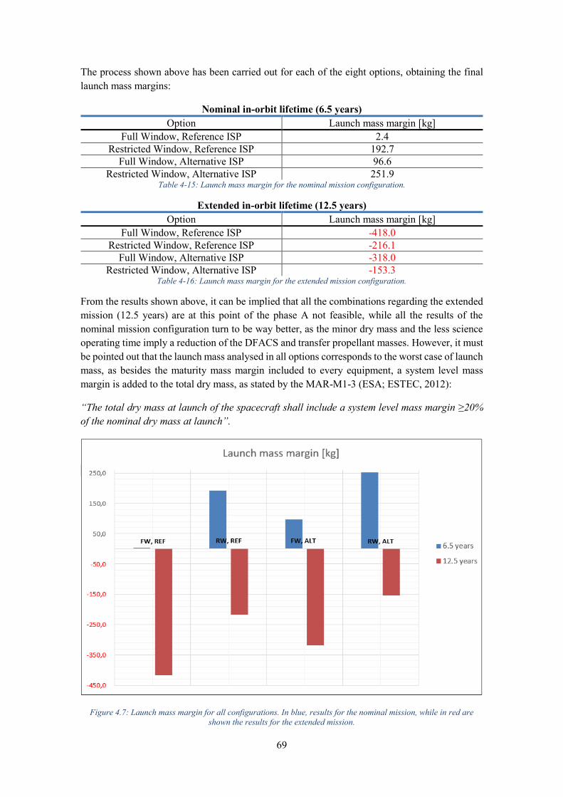
69

The process shown above has been carried out for each of the eight options, obtaining the final launch mass margins:

Nominal in-orbit lifetime (6.5 years) Option Launch mass margin [kg]

Full Window, Reference ISP 2.4 Restricted Window, Reference ISP 192.7

Full Window, Alternative ISP 96.6 Restricted Window, Alternative ISP 251.9

Table 4-15: Launch mass margin for the nominal mission configuration.

Extended in-orbit lifetime (12.5 years) Option Launch mass margin [kg]

Full Window, Reference ISP -418.0 Restricted Window, Reference ISP -216.1

Full Window, Alternative ISP -318.0 Restricted Window, Alternative ISP -153.3

Table 4-16: Launch mass margin for the extended mission configuration.

From the results shown above, it can be implied that all the combinations regarding the extended mission (12.5 years) are at this point of the phase A not feasible, while all the results of the nominal mission configuration turn to be way better, as the minor dry mass and the less science operating time imply a reduction of the DFACS and transfer propellant masses. However, it must be pointed out that the launch mass analysed in all options corresponds to the worst case of launch mass, as besides the maturity mass margin included to every equipment, a system level mass margin is added to the total dry mass, as stated by the MAR-M1-3 (ESA; ESTEC, 2012):

“The total dry mass at launch of the spacecraft shall include a system level mass margin ≥20% of the nominal dry mass at launch”.

Figure 4.7: Launch mass margin for all configurations. In blue, results for the nominal mission, while in red are shown the results for the extended mission.

70

Among the results obtained for the nominal mission, it can be affirmed that the alternatives launched in the restricted window provide a major launch margin than the ones launched in the extended (or full) window, due to the minor Delta-v required to carry out the impulsive manoeuvre. Furthermore, the bigger alternative impulse causes an increment of the launch margin with respect to the reference one. Nevertheless, as it can be seen on Figure 4.7, the influence of the launch window is more important than the specific impulse given.

Therefore, according to the launch mass criteria, the most suitable option will be the Nominal lifetime, Restricted launch window, Alternative specific impulse option, followed by the Nominal, Restricted launch, Reference specific impulse combination.

4.5.2 Power consumption criteria Although the majority of the trade-off analysis is focused into the launch mass, the power consumption of the spacecraft is also important and influences the final trade-off decision.

As it has been detailed in section 4.4.1, the specific impulse provided by the thrusters depends on the power consumed by them (see equation (4.1)). Thus, although the alternative impulse of 2000s provides a major launch mass margin, its power consumption is bigger than in the case of the reference impulse of 1650s. Therefore, it must be checked that the total (peak) power consumption during the transfer manoeuvre, including margins, does not exceed the maximum power the solar panel can provides, also during the transfer.

The solar panel geometrical and power features will be detailed in the following chapter. Besides, the final power budget will also be included and commented in Chapter 5, so in order to not repeat information and avoid the extension of this section, the power margins between the power consumed and the power provided by the solar panel in the transfer phase will be directly introduced, so then the power criteria can be evaluated in the feasible options. Thus, these values are gathered in the Table 4-17: Power consumption values during the transfer manoeuvre.. It must be highlighted that the power produced by the solar panel shown is the minimum power computed for the worst solar distance and illumination angle.

Power with margins [W] Reference ISP Alternative ISP Power consumption during transfer 2377 2580

Power produced by solar panel 2380 2380 Margin with regard to available

power 3 -200

Table 4-17: Power consumption values during the transfer manoeuvre.

As it can be seen above, the power consumption during the transfer by the alternative thruster operating point exceeds by far the maximum power value provided by the solar panel. Therefore, although the best possible configuration according to the launch mass included the alternative specific impulse, the huge negative power margin obtained causes that the combinations that involve the alternative impulse (2000s) will be discarded.

Thus, after the trade-off analysis, it can be concluded that:

The extended in-orbit lifetime missions are, at this point of the study, not feasible due to the big negative launch mass margin. However, as the study of an extended mission is a requirement of the CDF report (ESA, 2017), it will continue to be studied until the end of the phase A.

71

The alternative HET operating point provides the biggest launch mass margins. However, due to the awful power margin obtained, this operating point will be discarded in favour of the reference one: 350 V and 1015 W of power, providing an impulse of 1650 s.

A launch during the Restricted Window decreases the Delta-v needed for the transfer and hence increases the launch margin.

Finally, from all this exposed, the Nominal lifetime, Reference Specific Impulse and Restricted Launch window is suggested as the Baseline configuration, followed by the Nominal lifetime, Reference Specific Impulse and Full Launch window, suggested as the backup option.

72

CHAPTER 5 LISA BASELINE DEFINITION

FOR THE UPCOMING PHASES

5.1 Road to the mission baseline identification Over the different chapters of the document, the mission in study and the aim and scope of the project have been described, besides the state of the Phase A study at the beginning of the stay in TAS. Then, the concurrent engineering methodologies as well as the software (IDM-CIC) under which the study has been carried out were introduced. Hence, in this final chapter the current status of LISA at the end of the stay will be defined, detailing all the updates or advances in the subsystems and features where the support to the engineers has been done.

After that, the way in which it has been worked using the IDM-CIC to obtain the different inputs for the calculation and update the budgets will be described, in order to present then the final budgets obtained that will be useful to continue the pathway to the Phase A2.

5.2 Propulsion systems

5.2.1 De-tumbling and AOCS Propulsions

De-tumbling

The de-tumbling defined as the manoeuvre used to prevent the spinning of a spacecraft after the launch separation. The thrusters that carry out this task are the ones selected also for the Attitude and Orbit Control Propulsion, the Moog SVT01. Initially, as it has been exposed in Table 4-1, the CFD report gathers 6+6 SVT01 thrusters fed with Nitrogen. However, later power estimations made by the propulsion engineers suggested to increment the number of SVT01 thrusters to 8+8. Its main characteristics are shown on the following table:

Propellant Thruster Thrust [mN] Isp [s] GN2 SVT01 (8+8) 120 65

Table 5-1: Current de-tumbling and AOCS thrusters characteristics.

The CFD establishes a requirement for the de-tumbling manoeuvre, the R-MEC-010, which states that “The maximum tumbling rate of the spacecraft, after separation from the launcher, shall be

less than 5º/s”. Hence, making use of the fundamental dynamics law of Newton, the relationship between the torque and the rotational acceleration can be reached:

∑𝑇 = 𝐼 · 𝛼 (5.1)

where the I stands for the inertial moment of the pertinent axis. The torque instead is obtained from the thrust supplied by the SVT01 thrusters:

𝑇 = 𝐹𝑆𝑉𝑇01 × 𝑟𝑆𝑉𝑇01 (5.2)

73

Therefore, introducing equation (5.2) into (5.1), the rotational acceleration is obtained. Assuming the worst possible chase, in which the rotational speed is 5º/s, these two equations refer to the maximum torque, that is, the minimum angular acceleration. Thus, the de-tumbling time is:

∆𝑡𝐷𝑒𝑡𝑢𝑚𝑏𝑙𝑖𝑛𝑔 =5º/𝑠

𝛼𝑚𝑖𝑛 (5.3)

So finally, the propellant mass shown on Table 4-8 can be obtained:

𝑚𝑝𝐷𝑒𝑡𝑢𝑚𝑏𝑙𝑖𝑛𝑔=

𝐹𝑆𝑉𝑇01,𝑀𝐴𝑋

𝐼𝑠𝑝,𝑆𝑉𝑇01 · 𝑔0· ∆𝑡𝐷𝑒𝑡𝑢𝑚𝑏𝑙𝑖𝑛𝑔 (5.4)

Attitude Control Propulsion

The de-tumbling operation is just the first of the group of operations that the AOCS propulsion covers. As it was introduced in the first chapter, the AOCS is the responsible to control the spacecraft attitude during the transfer phase, that is, from the separation of the launcher until the arrival to the science orbit. Besides the de-tumbling, the Attitude Control System performs the following operations:

Sun acquisition and attitude control with respect to the Sun. HET torque compensation during transfer. The thrust generated during the transfer phase

in order to produce an increment of velocity (Δv) to reach the science orbit produces a misalignment between this thrust and the centre of gravity of the spacecraft. This misalignment is compensated by the SVT01 thrusters.

Solar radiation pressure compensation during transfer. Spacecraft orientation for the High Gain Antenna pointing during transfer.

In relation to the second operation listed above, the propellant mass needed can be calculated by introducing the concept of the angular impulse, the impulse regarding the angular momentum. In order to avoid the misalignment during the transfer, the angular momentum of the satellite must remain constant. Therefore, the angular impulse of the misalignment produced by the HET is compensated with the angular impulse generated by the SVT01 thrusters:

𝑇𝑚𝑖𝑠 · ∆𝑡𝐻𝐸𝑇 = 𝑇𝑐𝑜𝑚𝑝 · ∆𝑡𝑆𝑉𝑇01 (5.5)

Isolating the ∆𝑡𝑆𝑉𝑇01, the propellant mass required to compensate the torque can be obtained:

𝑚𝑝𝑐𝑜𝑚𝑝=

𝐹𝑆𝑉𝑇01

𝐼𝑠𝑝,𝑆𝑉𝑇01 · 𝑔0· ∆𝑡𝑆𝑉𝑇01 =

𝐹𝑆𝑉𝑇01

𝐼𝑠𝑝,𝑆𝑉𝑇01 · 𝑔0·𝑇𝑚𝑖𝑠 · ∆𝑡𝐻𝐸𝑇

𝑇𝑐𝑜𝑚𝑝 (5.6)

The propellant mass of this operations can be also seen in Table 4-8. The sum of the AOCS and de-tumbling propellant masses define the total propellant mas of the Attitude Control propulsion, included in the spacecraft in the correspondent N2 tanks (see Figure 4.4). It must be pointed out that these propellant masses, as well as the propellant for the DFACS include the propellant residual margins, consistent with the margin philosophy requirement MAR-M1-7 (ESA; ESTEC, 2012).

5.2.2 Transfer Propulsion The transfer propulsion, as it has been defined before, consists in 1+1 Hall Effect Thrusters PPS-1350G fed with Xenon propellant which drives the spacecraft to the science orbit. All the details

74

regarding the transfer propellant, as well as the thruster features have been extensively exposed in Chapter 4. Therefore, to sum up, a table with the thruster characteristics can be seen below, were the features regarding the baseline HET operating point have been included:

Propellant Thruster Thrust [mN] Isp [s] Xe HET (1+1) 60 1650

Table 5-2: Current Transfer Propulsion thrusters characteristics.

5.2.3 DFACS Propulsion As it has been exposed in Chapter 1, the Drag-Free Attitude Control System (DFACS) is the responsible to control the spacecraft during the science phase, that is, from the arrival of the satellite to the science operations orbit until the spacecraft de-commissioning at the graveyard orbit. The main operations the DFACS will control are listed below:

Attitude control of the spacecraft using the DFACS propulsion system with the test masses caught.

Attitude control of the satellite during any eventual orbit correction and de-commissioning manoeuvres.

Constellation acquisition: successful acquisition of laser pointing and bidirectional laser links between all spacecraft in the constellation.

Electrostatic capture of the test masses during their initial or any subsequent release, while controlling the attitude of the spacecraft and telescopes to point the laser links.

Simultaneous attitude control of the telescopes and satellites in order to hold the constellation links, and electrostatic attitude control of the test masses.

Drag-free control of the necessary test mass degrees of freedom (DoF), like the compensation of the disturbance forces and torques on those degrees of freedom, while the remaining test mass DoF are controlled as well as the satellite attitude and telescope pointing in order to maintain the constellation bidirectional laser links.

Control the spacecraft and telescope attitude compensating the disturbances forces and torques while the repointing of the High Gain Antenna is being done.

The DFACS trade-off carried out by TAS-I finished with the selection of the 9+9 Cold Gas Thrusters fed by Nitrogen in order to perform a complete control during the science operations. Its main features are shown below:

Propellant Thruster Thrust [mN] Isp [s] GN2 CGT (9+9) 1-1000 50-63

Table 5-3: Current DFACS propulsion thruster characteristics

where the range of thrust and hence the range of specific impulses reflects the variation needed to compensate all the daily disturbances during the mission.

As it can be implied, the in-orbit lifetime of the mission influences the DFACS propellant mass, as it can be seen in Table 4-8, as the science operations last more in the extended mission than in the nominal. The drag-free operations that requires most of the propellant are logically the ones that compensates the disturbance forces and torques during the science phase, which are principally two: The solar radiation pressure (SRP) compensation, and the Self-gravity of the Test Masses compensation.

In order to calculate the propellant needed to supply to the thrusters during the whole mission to compensate these forces and momentums, the propulsion engineers estimated the thrust needed to compensate the daily disturbances, by making simulations with each of the nine thrusters (that

75

will be continuously operating during the mission). An example of outcome of this study can be seen below:

Figure 5.1: DFACS daily thrusts for 1 year.

From the required thrust, the specific impulse is obtained as a function of it, as it is shown in the following figure:

Figure 5.2: Variation of the specific impulse with the thrust, DFACS propulsion.

Thus, using the expression (5.4) but introducing the DFACS thrust and specific impulse values, the propellant required is obtained:

𝑚𝑝𝐶𝐺𝑇 (𝑁𝑜𝑚𝑖𝑛𝑎𝑙 𝑜𝑟 𝐸𝑥𝑡𝑒𝑛𝑑𝑒𝑑)=

𝐹𝐶𝐺𝑇

𝐼𝐶𝐺𝑇 · 𝑔0· ∆𝑡𝐶𝐺𝑇 (5.7)

76

The propellant values obtained, together with the other propellant required for the remaining operation (i.e. compensation during repointing of the antenna, constellation acquisition) define the DFACS propellant mass gathered in Table 4-8.

5.3 Electrical Power System The Electrical Power System (EPS) is the responsible of providing the satellites with the necessary electrical power in all phases of the mission. As it has been introduced in section 1.4.6, the EPS is formed by the following elements:

A Power Control and Distribution Unit (PCDU). A Battery. A Solar Array.

The mass, power consumed and dimensions of the PCDU, which have been estimated from other recent missions like Galileo IOV, have not been modified yet from the original values of the CDF report, so further details will not be given as it has not been analysed during the stay. However, it does not occur the same with the Battery and Solar Panel, where the modifications in the dimensions and power consumption have been followed and will be detailed in this section.

Nevertheless, before starting with the characteristics of the EPS elements, the power modes identified for the LISA mission are going to be detailed, in order to clarify not only the requirements for the Battery and Solar Panel but also the structure of the Power Budget.

Launch and Early Operations (LEOP) mode

The LEOP power mode covers the power requirements from the pre-lift off until the acquisition of a stable sun-pointing attitude. During this phase, the Electrical Power System must provide the spacecraft electrical load necessities without any solar generation, that is, using the power supplied by the battery. Three different phases can be distinguished from the LEOP:

Pre Lift-off phase: The moment in which the satellite must be powered by its own batteries to lift-off.

Ascent phase: From the lift-off of the spacecraft until the separation from the launch composite.

Sun acquisition mode: From separation until the acquisition of a stable sun-pointing attitude. This mode covers also the de-tumbling, as it is the previous step of the starting of the acquisition.

Transfer mode

The EPS must be on during the transfer towards the operational orbit, as the electrical thruster that carries out the transfer manoeuvre (Hall Effect Thruster) requires a large amount of power. The reason is that the thruster, as it has been mentioned before, needs to be pointed correctly constantly in order to not produce a misalignment with the CoG of the spacecraft. As the spacecraft has acquired a stable sun point, the aspect angle of the solar panel does not need to be optimised, and can reach up to 40º from normal incidence in the worst case. During this phase the spacecraft will not notice eclipses, so the battery power will not be necessary.

Science mode

The power mode related to the science operations of the spacecraft. When each spacecraft of the constellation is in the correspondent science orbit, the plane of the triangle made by the union of

77

the arms of the three satellites should be at 60º to the ecliptic plane. Besides, if the spacecraft achieves a top-mounted solar panel and sunshield configuration, the aspect angle of the solar angle results 30º from nominal incidence. In this phase the satellites will not suffer eclipse periods, so the battery will also not be utilised.

Safe mode

The last mode is a recovery operation like the sun acquisition mode, but includes redundant configuration set-up. It includes the power necessary by the spacecraft required to let it survive in case of a misfortune until ground operation.

5.3.2 Battery The battery must produce and supply energy during the LEOP mode as the solar panel does not provides energy yet. Therefore, its energy requirements will be dimensioned from the necessary power the satellite needs from the pre lift-off until the sun acquisition.

According to the estimations of the TAS-I teams, the Pre Lift-off phase will last 10 minutes, moment in which the LEOP Ascent phase will start. The ascent phase is divided into two steps: the first one is the duration of the ascent, estimated from other similar missions as the Ariane 64, which will last 30 minutes. The second one, is the time interval needed to achieve a “safe” distance

of 500 m between a satellite already released and the rest of the launch composite before releasing the successive spacecraft, with or without a ∆𝑉 = 5 𝑚/𝑠 applied to the composite by the upper stage after each release. Depending of the necessity or not of the Delta-v the complete operation will last 39 or 66 minutes respectively.

Finally, the LEOP Sun acquisition phase is estimated to last 36 minutes, in which the de-tumbling operation time is also included.

To sum up, in the following table, the different power modes with which the battery will be dimensioned are listed, including the duration of the operation as well as the maximum power consumption.

Mission Phase Duration [minutes] Power [W] Energy

[Wh] Duration [minutes] Power [W] Energy

[Wh]

Pre Lift-off 10 93,9 15,6 10 93,9 15,6 Ascent 39 283,2 184,0 66,3 283,2 312,9

Sun Acquisition 36 613,6 368,2 36 613,6 368,2 Total 567,9 Total 696,7

Figure 5.3: Energy Battery Budget. Ascent with a ∆𝑉 = 5 𝑚/𝑠 (left) and without the increment (right).

In relation to the other characteristics of the battery, there are several requirements in order to size the battery. The battery must be dimensioned for a 60% DoD after five hours of the LEOP mode consumption. In addition, the failure of one string (for each satellite) must be taken into account for the sizing. The current geometrical dimensions and mass are 100×380×230mm and 10kg including margins.

5.3.3 Solar Array The solar panel is placed at the base of the spacecraft and it has a circular geometry. As the launcher used to guide the constellation into the space is based in the Ariane 64, the dimensions

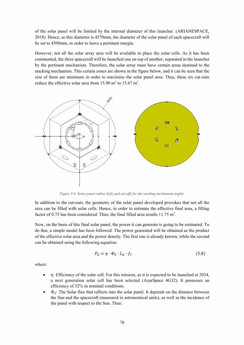
78

of the solar panel will be limited by the internal diameter of this launcher. (ARIANESPACE, 2018). Hence, as this diameter is 4570mm, the diameter of the solar panel of each spacecraft will be set to 4500mm, in order to leave a pertinent margin.

However, not all the solar array area will be available to place the solar cells. As it has been commented, the three spacecraft will be launched one on top of another, separated in the launcher by the pertinent mechanism. Therefore, the solar array must have certain areas destined to the stacking mechanism. This certain zones are shown in the figure below, and it can be seen that the size of them are minimum in order to maximise the solar panel area. Thus, these six cut-outs reduce the effective solar area from 15.90 m2 to 15.67 m2.

Figure 5.4: Solar panel radius (left) and cut-offs for the stacking mechanism (right).

In addition to the cut-outs, the geometry of the solar panel developed provokes that not all the area can be filled with solar cells. Hence, in order to estimate the effective final area, a filling factor of 0.75 has been considered. Thus, the final filled area results 11.75 m2.

Now, on the basis of this final solar panel, the power it can generate is going to be estimated. To do that, a simple model has been followed. The power generated will be obtained as the product of the effective solar area and the power density. The first one is already known, while the second can be obtained using the following equation:

𝑃𝑑 = 𝜂 · Φ𝑆 · 𝐿𝑑 · 𝑓𝑇 (5.8)

where:

𝜂: Efficiency of the solar cell. For this mission, as it is expected to be launched at 2034, a next generation solar cell has been selected (AzurSpace 4G32). It possesses an efficiency of 32% in nominal conditions.

Φ𝑆: The Solar flux that reflects into the solar panel. It depends on the distance between the Sun and the spacecraft (measured in astronomical units), as well as the incidence of the panel with respect to the Sun. Thus:

79

Φ𝑆 = Φ𝑆𝐶 · (1

𝑟2) · 𝑐𝑜𝑠𝜃 (5.9)

𝐿𝑑: The degradation lifetime factor 𝑓𝑇: The temperature factor. Analyses the solar panel performances under the temperature

of the own panel.

Once introduced the guidelines for the calculation of the power of the solar panel, the results for the power modes in which the solar panel is utilised to generate energy (Transfer and Science mode) can be calculated. Its main characteristics are:

Transfer Mode: In this case, the power supplied by the solar panel during the transfer phase is assessed for the worst case combination of the parameters mentioned above. Besides, the calculation is done at the Beginning of Life (BOL). Hence, the minimum power for a filling factor of 0.75 is reached with a Solar Aspect Angle (SAA) of 30º, a temperature of the panel of 70ºC and a heliocentric distance of 1.07 astronomical units (AU).

Science mode: The power generated, calculated at the End of Life (EOL), has been estimated with the same filling factor and SAA, a heliocentric distance of 1.05 AU and 80ºC of solar panel temperature.

Introducing these parameters into the expressions of the model, the power generated by the solar panel is obtained:

Transfer Mode Science Mode

Power produced by solar panel [W] 2380 2454 Table 5-4: Power generated by solar panel.

At this point, it must be highlighted that from the solar panel power available shown above, the power system margin established by the margin philosophy has been subtracted, according to the MAR-P-7 statement of the margin philosophy requirements:

“Solar arrays shall be sized to provide the spacecraft required power, including all specified

margins, at EOL, and taking into account one string failure”.

Finally, the comparison of the available power with the requested power will be discussed at the end of the chapter, when the whole power budget will be presented, though that for the transfer case the check has already been done, as it was one of the decision criteria for the propellant trade-off.

5.4 Spacecraft Configuration The closing of the geometrical configuration trade of the spacecraft (the “Pie” configuration was

selected) entailed the development of the spacecraft configuration. Besides the pertinent modifications (i.e. performances, dimensions) obtained from the engineering teams regarding the systems of the spacecraft (where most of them have been detailed over the document), another important issue has been carried out in parallel by the design engineers: the assembly of the spacecraft.

80

Through the CAD modelling software Catia, all the elements that form the spacecraft are included. As the LISA project is in a phase of constant development, all the modifications regarding the mass and geometrical dimensions of the elements are constantly being updated in Catia.

Figure 5.5:CAD model of LISA current baseline configuration.

Therefore, the implementation of the spacecraft configuration in Catia permits to obtain the Centre of Gravity of the spacecraft as well as the momentums of inertia of it, information that is clearly important for the perfection of the baseline configurations. For example, the estimation of the thrust required for the different manoeuvres depends of the main axis inertia momentums, and the position of the CoG will be necessary to analyse the self-gravity of the test masses.

Although that it has not been worked with the Catia files, the functionality of IDM-CIC permits to develop a simplified model of the current baseline configuration, in order to obtain a first estimation of the centre of gravity and inertia matrix of the spacecraft and then to compare the results with the more complete and detailed CAD model.

5.4.1 Guidelines to shape the spacecraft configuration with IDM-CIC In Chapter 3, all the methodology needed to be carried out in order to define the equipments, subsystems and elements of the spacecraft in IDM-CIC was extensively detailed. Hence, in this section a brief summary of the guidelines needed to follow to shape the spacecraft configuration will be given, before entering into the MCI details.

Defining mass and dimensions of the equipments

As explained in sections 3.3.1 and 3.3.3, using the appropriate commands in the IDM software at equipment level, the mass and dimensions can be defined. It must be pointed out that, in order to

81

introduce the mass into the geometry, it must be selected the option “From Geometry” instead of

the “Manual” option in the command “MCI data origin”, otherwise the mass will be located at the default position (the origin of IDM-CIC) and considered as point, so the CoG and Inertia information will be mistaken.

Special attention must be given to certain subsystems, the Service Module (SVM) Harness and the thermal subsystem, whose shapes have been copied from the structure subsystem, as both are included into the structure of the spacecraft. Hence, the structure of the satellite will be redundant in this model.

Placing the elements in the correct position

After the definition of the element properties, it is proceeded with the placement with respect to the absolute reference system of IDM. To do that, the software provides the pertinent commands that let the modification of the three coordinates (x,y,z) and three possible rotations along the three axis, as well as to define secondary reference systems in order to help with the correct placement, as it has been explained in section 3.4.3.

Furthermore, in order to consider the wet mass into the CoG and Inertia estimations, the correspondent percentage of tank filling shall be included in the Saved Configurations worksheet.

Finally, using the “Visualization tool” of IDM, the spacecraft configuration can be seen. In

addition, extra components such as the reference axis can also be displayed.

Figure 5.6: IDM model of LISA current baseline configuration.

At this point, it must be highlighted that the spacecraft configuration has been, together with the propellant trade-off and budget reports, one of the tasks which has covered an important part of

82

the time during the internship. Although in this master thesis only the final configuration at the end of the stay is shown, the constant updates and modifications in the configuration imply an important work load, as this task is a really delicate work.

After the configuration is completed, selecting the command “Show MCI budget” (see Figure 3.19) the information regarding the Inertia and Centre of Mass is obtained.

5.4.2 Comparison between CAD and IDM models From the MCI budget of IDM, the main information regarding Mass and Inertia can be obtained. In the table below, the MCI budgets of the Nominal and Extended baseline configurations can be seen:

Nominal Configuration Extended Configuration Total dry mass [kg] 2027 2087

𝐺𝑥 [mm] -150 -125 𝐺𝑦 [mm] 31 30 𝐺𝑧 [mm] 530 532

𝐼𝑥𝑥 [kg·m2] 1870 1982 𝐼𝑦𝑦 [kg·m2] 1538 1630 𝐼𝑧𝑧 [kg·m2] 2786 2776 𝐼𝑥𝑦 [kg·m2] -13 -11 𝐼𝑥𝑧 [kg·m2] 1 -3 𝐼𝑦𝑧 [kg·m2] 54 54

Table 5-5: MCI budgets, including margins, from the IDM model. Results for the Nominal (left) and Extended (right) baseline configurations.

Therefore, the results can be compared with the ones obtained by the CAD model, in order to see the validity of the IDM model. However, due to the restriction policies of the company, the CAD values are not included. Nonetheless, there are several considerations that influence the calculation in the IDM model with respect the CAD model that can be mentioned:

The IDM model is a simplified version of the detailed CAD model, and it considers the mass of each equipment as homogeneous, so the equipments formed by diverse materials with logically diverse density are not considered on IDM, and therefore neither its variation on the CoG.

Although most of the elements included on the CAD model are included in the IDM, there are elements that do not possess their own shape and their MCI data origin is placed in the base of the spacecraft, so the Z coordinate of the Centre of Mass tends to decrease with respect to the CAD result.

On the other hand, the redundant subsystems introduced in IDM (Harness and Thermal module) are not included on the CAD model, so it influences not only the CoG but also the final dry mass in both models.

Finally, IDM-CIC also lets the possibility of adding the Inertia Axes as well as the CoG to the IDM view, in order to compare them with respect to the reference system:

83

Figure 5.7: Reference axis of the IDM model. X axis highlighted in red, Y axis in green and Z axis in blue. Inertia axes and CoG position remarked in black.

In addition, it must be pointed out that the MCI budget that IDM-CIC provides only consider the equipment margin, so the estimations of CoG and Inertia obtained do not include the system margin (20% of the total mass). In order to consider the system margin to the calculi, a new IDM file had to be created where the system margin was included equipment by equipment, fact that significantly increased the work time for this task.

Thus, it can be concluded that the IDM features regarding the MCI budget can be really useful in the early stages of the Phase A study, when the CAD model of the configuration is not defined yet. For later studies, where the CAD model is consolidated, the tool should be improved in order to consider it a feasible tool to support the CAD studies.

5.5 Test Masses Self-Gravity In the first Chapter, the aim and scope of the LISA mission were presented. To sum up, LISA will detect gravitational waves with an interferometric measurement of differential optical path length modulation along three spacecraft placed in a triangular configuration defined by two free-falling test masses for spacecraft. The distance changes produced by the GW between the test masses (really small distances, order of picometres) will be detected, as the links created by the laser interferometry technology between the three spacecraft (see Figure 1.2) will measure the differential acceleration among the test masses.

84

Figure 5.8: LISA test masses configuration in each spacecraft.

In order to let the test masses “free-falling”, the TMs must not suffer any kind of force along the

measurement axes. Therefore, the spacecraft must be “drag-free controlled”, and this control is

achieved, as it has been mentioned previously, with the Drag-Free and Attitude Control System, the DFACS. The DFACS shields the test masses from all disturbances as well as maintains the links between the arms of the constellation that detect the differential acceleration between the TMs. Hence, the Drag-free system of every satellite must be able to control sixteen of the nineteen Degrees of Freedom (DoF) in the system.

In the figure below the DFACS actuation is illustrated. If one test mass moves in the spacecraft (left draft on Figure 5.9), the DFACS propulsion system will shift the satellite with regard to the test mass displaced in order to centre again inside the electrode housing (centre draft on Figure 5.9). Furthermore, an electrostatic actuation will also shift the test mass to centre it in the electrode housing (right draft on Figure 5.9). Thus, the DFACS ensures the self-gravity of the TMs using its propulsion besides electrostatic actuation electrodes.

Figure 5.9: DFACS actuation concept.

However, despite the test masses are controlled by the DFACS to avoid the contact with the rest of the elements of the spacecraft, these elements produce a certain force and torque on the test masses that must be calculated before the launching, in order to verify that the interactions do not

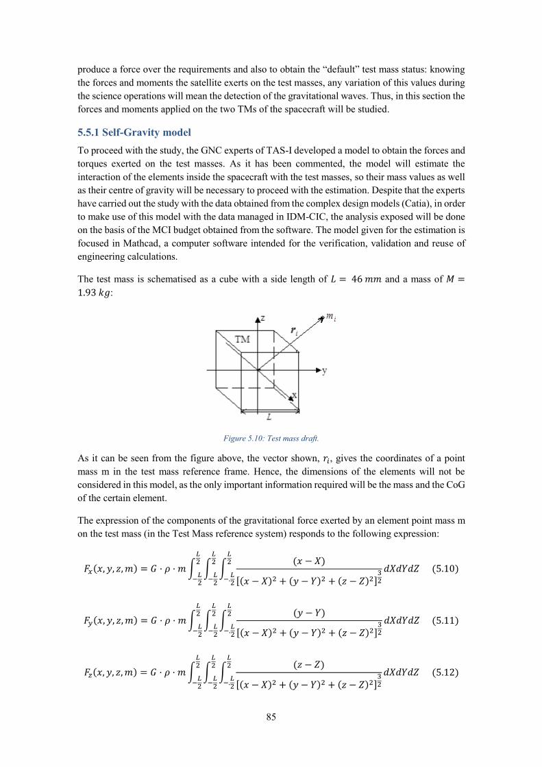
85

produce a force over the requirements and also to obtain the “default” test mass status: knowing

the forces and moments the satellite exerts on the test masses, any variation of this values during the science operations will mean the detection of the gravitational waves. Thus, in this section the forces and moments applied on the two TMs of the spacecraft will be studied.

5.5.1 Self-Gravity model To proceed with the study, the GNC experts of TAS-I developed a model to obtain the forces and torques exerted on the test masses. As it has been commented, the model will estimate the interaction of the elements inside the spacecraft with the test masses, so their mass values as well as their centre of gravity will be necessary to proceed with the estimation. Despite that the experts have carried out the study with the data obtained from the complex design models (Catia), in order to make use of this model with the data managed in IDM-CIC, the analysis exposed will be done on the basis of the MCI budget obtained from the software. The model given for the estimation is focused in Mathcad, a computer software intended for the verification, validation and reuse of engineering calculations.

The test mass is schematised as a cube with a side length of 𝐿 = 46 𝑚𝑚 and a mass of 𝑀 =

1.93 𝑘𝑔:

Figure 5.10: Test mass draft.

As it can be seen from the figure above, the vector shown, 𝑟𝑖, gives the coordinates of a point mass m in the test mass reference frame. Hence, the dimensions of the elements will not be considered in this model, as the only important information required will be the mass and the CoG of the certain element.

The expression of the components of the gravitational force exerted by an element point mass m on the test mass (in the Test Mass reference system) responds to the following expression:

𝐹𝑥(𝑥, 𝑦, 𝑧,𝑚) = 𝐺 · 𝜌 · 𝑚 ∫ ∫ ∫(𝑥 − 𝑋)

[(𝑥 − 𝑋)2 + (𝑦 − 𝑌)2 + (𝑧 − 𝑍)2]32

𝑑𝑋𝑑𝑌𝑑𝑍

𝐿2

−.𝐿2

𝐿2

−𝐿2

𝐿2

−𝐿2

(5.10)

𝐹𝑦(𝑥, 𝑦, 𝑧,𝑚) = 𝐺 · 𝜌 · 𝑚∫ ∫ ∫(𝑦 − 𝑌)

[(𝑥 − 𝑋)2 + (𝑦 − 𝑌)2 + (𝑧 − 𝑍)2]32

𝑑𝑋𝑑𝑌𝑑𝑍

𝐿2

−.𝐿2

𝐿2

−𝐿2

𝐿2

−𝐿2

(5.11)

𝐹𝑧(𝑥, 𝑦, 𝑧,𝑚) = 𝐺 · 𝜌 · 𝑚 ∫ ∫ ∫(𝑧 − 𝑍)

[(𝑥 − 𝑋)2 + (𝑦 − 𝑌)2 + (𝑧 − 𝑍)2]32

𝑑𝑋𝑑𝑌𝑑𝑍

𝐿2

−.𝐿2

𝐿2

−𝐿2

𝐿2

−𝐿2

(5.12)

86

where G is the gravitational constant (𝐺 = 6.674 · 10−11 𝑚3

𝑠2𝑘𝑔), m is the point mass of the element

and 𝜌 =𝑀

𝐿3, the density of the test mass.

Hence, the gravitational acceleration components produced by an element point mass can be obtained by dividing the forces by the test mass:

𝑎𝑥,𝑦,𝑧(𝑥, 𝑦, 𝑧,𝑚) =𝐹𝑥,𝑦,𝑧(𝑥, 𝑦, 𝑧, 𝑚)

𝑀 (5.13)

The same discourse can be utilised for the calculation of the torques exerted on the test masses:

𝑇𝑥(𝑥, 𝑦, 𝑧,𝑚) = 𝐺 · 𝜌 · 𝑚 ∫ ∫ ∫𝑍 · (𝑌 − 𝑦) − 𝑌 · (𝑍 − 𝑧)

[(𝑥 − 𝑋)2 + (𝑦 − 𝑌)2 + (𝑧 − 𝑍)2]32

𝑑𝑋𝑑𝑌𝑑𝑍

𝐿2

−.𝐿2

𝐿2

−𝐿2

𝐿2

−𝐿2

(5.14)

𝑇𝑦(𝑥, 𝑦, 𝑧,𝑚) = 𝐺 · 𝜌 · 𝑚∫ ∫ ∫𝑋 · (𝑍 − 𝑧) − 𝑍 · (𝑋 − 𝑥)

[(𝑥 − 𝑋)2 + (𝑦 − 𝑌)2 + (𝑧 − 𝑍)2]32

𝑑𝑋𝑑𝑌𝑑𝑍

𝐿2

−.𝐿2

𝐿2

−𝐿2

𝐿2

−𝐿2

(5.15)

𝑇𝑧(𝑥, 𝑦, 𝑧,𝑚) = 𝐺 · 𝜌 · 𝑚 ∫ ∫ ∫𝑌 · (𝑋 − 𝑥) − 𝑋 · (𝑌 − 𝑦)

[(𝑥 − 𝑋)2 + (𝑦 − 𝑌)2 + (𝑧 − 𝑍)2]32

𝑑𝑋𝑑𝑌𝑑𝑍

𝐿2

−.𝐿2

𝐿2

−𝐿2

𝐿2

−𝐿2

(5.16)

And therefore, the gravitational angular acceleration around the three axes is obtained:

𝛼𝑥,𝑦,𝑧(𝑥, 𝑦, 𝑧,𝑚) =𝑇𝑥,𝑦,𝑧(𝑥, 𝑦, 𝑧,𝑚)

𝐼 (5.17)

where I is the inertia moment of the test mass, equal for all axes in the test mass frame, 𝐼 =

1

6𝑀𝐿2.

Although the calculi seem to be really elaborated, Mathcad obtains the outputs requested practically at the instant. Therefore, the next step is to introduce the mass and coordinates of the elements into the software. However, first of proceed to the calculation, a change of the reference system of the inputs introduced must be given, as the coordinates of the TMs are given in the spacecraft reference frame of the CAD model (see Figure 5.7). The change from the IDM reference system to the S/C is given by the following transformation:

𝑅𝑆𝑆/𝐶 = [−1 0 00 1 00 0 −1

]𝑅𝑆𝐼𝐷𝑀 + (00

1.352) (5.18)

where the z coordinate of the vector in equation (5.18) is the z-distance between the CAD and the IDM reference system origins.

On the other hand, the coordinates of the test masses in the spacecraft reference frame are shown below:

87

𝑇𝑀1 = (154220911

) ·1

1000 ; 𝑇𝑀2 = (−

154220911

) ·1

1000 (5.19)

Thus, once obtained the coordinates of the elements in the satellite reference system, the relative positions of them with respect of the two test masses (always in the S/C reference system) can be obtained (for the further calculi). After the obtaining of the position vectors of the point masses, a final transformation of axes must be done, as the test masses forces and torques formulas exposed are framed in the TM reference system.

The transformation can be done taking into account the diagram shown in Figure 5.11. At the beginning of the section, it was commented that the arms of the constellation form an equilateral triangle, therefore the angle between the two test masses is 60º. Once known this, the transformation matrix results simple:

𝑅𝑆𝑆𝐶 𝑇𝑀1

=

[ cos (

60º

2) − sin (

60º

2) 0

sin (60º

2) cos (

60º

2) 0

0 0 1]

(5.20)

𝑅𝑆𝑆𝐶 𝑇𝑀2

=

[ cos (

60º

2) − sin (

−60º

2) 0

sin (60º

2) cos (

60º

2) 0

0 0 1]

(5.21)

Figure 5.11: Spacecraft and test masses reference systems.

88

Thus, finally the computation of the self-gravity is done, taking into account that the analysis is being done at the Beginning of Life (BOL) and with all tanks full of propellant. Introducing the point mass vectors expressed in the TM reference frame into the equations (5.10), (5.13), (5.14) and (5.17), the values of the gravitational acceleration as well as the angular gravitational acceleration are obtained as the sum of all the forces generated by all the elements included.

Finally, doing at the inverse the transformation from TM reference system to S/C reference frame, the final forces and torques the Test Masses suffer by the elements of the spacecraft are obtained:

Test Mass 1 Test Mass 2 𝑎𝑥 [nm/s2] -57 -55 𝑎𝑦 [nm/s2] -190 185 𝑎𝑧 [nm/s2] -33 -31

Table 5-6: Gravitational acceleration values per unit mass exerted on the test masses.

Test Mass 1 Test Mass 2 𝛼𝑥 [nrad/s2] -0.815 0.736 𝛼𝑦 [nrad/s2] 0.869 0.753 𝛼𝑧 [nrad/s2] 1.044 -1.217

Table 5-7: Gravitational angular acceleration values per unit mass exerted on the test masses.

Therefore, once the spacecraft is in the science orbit and the operations have begun, a variation of the gravitational accelerations from the values shown in the figures above will mean that the gravitational waves will be detected and measured.

The results should be compared to the ones calculated by the domain experts. However, due to the restriction policies of the company, the estimations have not been included. Nevertheless, several points can be commented. As the CoG and mass data from the elements inside the spacecraft have been taken from the IDM database, the estimations will suffer the same issues stated in section 5.4.2, where the significant differences from the MCI information obtained by IDM-CIC with respect to the CAD model were detailed. Hence, the gravitational accelerations calculated will eventually suffer these differences. Thus, for further advances in the self-gravity model studies should logically made a comparison with the complex models developed in the company, in order to see the feasibility of these estimations.

5.6 Updating working process with IDM-CIC In the Chapter 3, the IDM-CIC software was introduced as the software that will store the characteristics of all the elements that form the LISA spacecraft. Over the document, the guidelines in order to define the elements, as well as to visualise the report Budgets (i.e. Mass Budget) that will serve to the progress meetings and eventually to the future mission documentation. The point is, how can it be accessed to the information stored?

Logically, the option of a manual exportation of the data stored in IDM has been dismissed, as it implies a huge computational time, besides the possibility of missing relevant data modifications when the users update the database. Hence, an automation of the exportations from the IDM-CIC files was sought. The solution founded in Thales Alenia Space entailed the creation of intermediate intermediary files or interfaces between the final Budgets gathered in the presentations and the data stored in IDM-CIC. Therefore, there are several possible methods that can be followed in order to generate these interfaces:

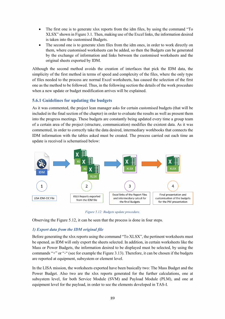
89

The first one is to generate xlsx reports from the idm files, by using the command “To

XLSX” shown in Figure 3.1. Then, making use of the Excel links, the information desired is taken into the customised Budgets.

The second one is to generate xlsm files from the idm ones, in order to work directly on them, where customised worksheets can be added, so then the Budgets can be generated by the exchange of information and links between the customised worksheets and the original sheets exported by IDM.

Although the second method avoids the creation of interfaces that pick the IDM data, the simplicity of the first method in terms of speed and complexity of the files, where the only type of files needed to the process are normal Excel worksheets, has caused the selection of the first one as the method to be followed. Thus, in the following section the details of the work procedure when a new update or budget modification arrives will be explained.

5.6.1 Guidelines for updating the budgets As it was commented, the project lean manager asks for certain customised budgets (that will be included in the final section of the chapter) in order to evaluate the results as well as present them into the progress meetings. These budgets are constantly being updated every time a group team of a certain area of the project (structure, communication) modifies the existent data. As it was commented, in order to correctly take the data desired, intermediary workbooks that connects the IDM information with the tables asked must be created. The process carried out each time an update is received is schematised below:

Figure 5.12: Budgets update procedure.

Observing the Figure 5.12, it can be seen that the process is done in four steps.

1) Export data from the IDM original file

Before generating the xlsx reports using the command “To XLSX”, the pertinent worksheets must

be opened, as IDM will only export the sheets selected. In addition, in certain worksheets like the Mass or Power Budgets, the information desired to be displayed must be selected, by using the commands “+” or “-“ (see for example the Figure 3.13). Therefore, it can be chosen if the budgets are reported at equipment, subsystem or element level.

In the LISA mission, the worksheets exported have been basically two: The Mass Budget and the Power Budget. Also two are the xlsx reports generated for the further calculations, one at subsystem level, for both Service Module (SVM) and Payload Module (PLM), and one at equipment level for the payload, in order to see the elements developed in TAS-I.

90

2) XLSX reports

The xlsx reports generated will only include the sheets mentioned. If an update regarding certain mass or power consumption of any subsystem arrives, these files are re-generated with the idm file and hence will be overwritten. As the process is being done at subsystem level, if in the idm file extra equipments are generated, the subsystems will not change, so the links created between the report files and the interfaces will not be altered. However, if an extra subsystem or element is added, the disposition of the budgets will change, so when the update of the reports is carried out, the links will be lost. This is the main issue the method faces, so special attention must be taken in order to not provoke mistakes in the budgets.

3) Interface Excel workbook

Once obtained the xlsx reports, an intermediary workbook is created, in order to organise and select the information for the Mass and Power Budgets. Furthermore, there are certain values, like the dry mass, that not only will be links for the budgets, but also inputs for further calculations. In the example shown, the dry mass taken from the reports will be used in this file for the propellant trade-off detailed in Chapter 4.

4) Final Budgets workbook

Finally, the last Excel file works as a summary file where all the Budgets requested, previously customised as desired, are included by inserting the correspondent links from the interface workbook. Therefore, not only the Mass and Power budgets will be included in this file, but also other important charts like the Launch Budget or the Propellant Budget.

5.7 Final Budgets After all the estimations, calculations and procedures that have been deeply detailed over the document, finally the most important budgets of the LISA mission can be presented. Therefore, in this final section of the chapter, the main final budgets are going to be included and commented.

It will be started with the dry mass budgets. The Table 5-8 and Table 5-9 reflect the composition of the complete Mass Budgets for the Nominal mission and Extended mission. As it was mentioned in section 4.4, the only difference between both configurations is the addition of the two DFACS propulsion tanks for the extended configuration, as it can be seen in the tables.

91

Dry mass Budget (Nominal)

Without margin [kg] Margin Including margin [kg] Payload 571,4 33% 758,2

Structure 235,0 20% 282,0 TT&C 52,5 14% 59,9

RF Inter-Satellite Link 38,9 17% 45,5 Data Handling 29,2 11% 32,3

DFACS/AOCS sensors 33,8 5% 35,5 Electrical Power 95,8 16% 111,5 Thermal Control 48,7 20% 58,4

Mechanisms 73,6 19% 87,7 Attitude Control Propulsion 34,3 5% 36,1

DFACS Propulsion 63,6 6% 67,5 Electric Propulsion 65,6 8% 70,5

Harness 44,3 0% 44,3 TOTAL DRY MASS 1386,8 22% 1689,5

System margin 20% 337,9 TOTAL MASS 2027,4

Table 5-8: Dry mass budget for the Nominal Baseline Configuration.

The final system margin is also included at the end of the charts, which according to the margin philosophy stated by ESA, turns to be a 20% (requirement MAR-M1-3).

Dry mass Budget (Extended) Without margin [kg] Margin Including margin [kg]

Payload 571,4 33% 758,2 Structure 235,0 20% 282,0

TT&C 52,5 14% 59,9 RF Inter-Satellite Link 38,9 17% 45,5

Data Handling 29,2 11% 32,3 DFACS/AOCS sensors 33,8 5% 35,5

Electrical Power 95,8 16% 111,5 Thermal Control 48,7 20% 58,4

Mechanisms 73,6 19% 87,7 Attitude Control Propulsion 34,3 5% 36,1

DFACS Propulsion 110,0 6% 116,9 Electric Propulsion 65,6 8% 70,5

Harness 44,3 0% 44,3 TOTAL DRY MASS 1433,2 21% 1738,9

System margin 20% 347,8 TOTAL MASS 2086,6

Table 5-9: Dry mass budget for the Extended Baseline Configuration.

Then, the power budget is introduced. In it, the main operating modes of the spacecraft are detailed, where it can be outlined the two transfer modes for the two HET operating points: Reference (1650 s and 1015 W) and Alternative (2000 s and 1150 W).

92

System Mode Launch Mode

Transfer Mode - Reference

Transfer Mode - Alternative

Science Mode

Safe Mode

Payload 0 0 0 683 0 TT&C 105 132 132 355 343

RF Inter-Satellite Link 0 0 0 434 0

Data handling 66 66 66 70 66 DFACS/AOCS

sensors 34 49 49 65 34

Electrical Power 0 60 60 60 60 Thermal Control 223 300 300 147 300 Attitude Control

propulsion 44 46 46 0 44

DFACS propulsion 0 1 1 69 1

Electric propulsion 0 1175 1330 0 0

TOTAL 472 1829 1985 1882 848 TOTAL WITH

MARGIN (30%) 614 2377 2580 2447 1102

Power produced by solar panel - 2380 2380 2453 -

Margin w.r.t. available power - 3 -200 6 - Table 5-10: Power Budget for the Baseline Configuration. The reference transfer mode refers to the specific impulse

of 1650 s while the alternative transfer mode to the 2000 s.

The system margin according to the margin philosophy is also included in this chart, which is stated in the MAR-P-4:

“The total power budget of the spacecraft shall include a system level power margin of 30% of

the nominal power requirements of the spacecraft” (ESA; ESTEC, 2012).

Finally, the power produced by the solar panel in the Transfer and Science mode is also included, in order to see if the panel produces the necessary power, as it was also commented in section 4.5.2.

The last budgets included are the launch mass budgets, gathered in Table 5-11 and Table 5-12. As these budgets include the wet mass, eight diverse launch budgets are displayed, following the same methodology of Table 4-14.

93

Mass including all margins [kg] - Extended launch window ∆V Isp Value Reference (1650 s) Alternative (2000 s)

In-orbit lifetime Extended window

Restricted Window

Extended window

Restricted window

Spacecraft dry mass 2027,4 2027,4 2027,4 2027,4 N2 propellant 94,6 94,6 94,6 94,6

Xe propellant S/C1 170,4 120,1 139,6 98,6 Xe propellant S/C2 181,3 102,0 148,5 83,8 Xe propellant S/C3 170,0 109,2 139,3 89,7

Spacecraft 1 wet 2292,5 2242,2 2261,7 2220,7 Spacecraft 2 wet 2303,4 2224,1 2270,6 2205,9 Spacecraft 3 wet 2292,0 2231,3 2261,3 2211,8

Launch composite wet 6887,8 6697,5 6793,6 6638,3 Launcher adapter 109,8 109,8 109,8 109,8

Total launch mass 6997,6 6807,3 6903,4 6748,1 Launcher performance 7000,0 7000,0 7000,0 7000,0

Margin w.r.t. launcher performance

2,4 192,7 96,6 251,9

Table 5-11: Launch Budget for the Nominal Configurations.

The results obtained have been already discussed in Chapter 4, where it was suggested the Nominal dry mass, Reference specific impulse and Restricted Launch Window option as the baseline configuration.

Mass including all margins [kg] - Restricted launch window ∆V Isp Value Reference (1650 s) Alternative (2000 s)

In-orbit lifetime Extended window

Restricted Window

Extended window

Restricted Window

Spacecraft dry mass 2086,6 2086,6 2086,6 2086,6 N2 propellant 165,0 165,0 165,0 165,0

Xe propellant S/C1 180,7 127,4 148,1 104,6 Xe propellant S/C2 192,3 108,2 157,5 88,9 Xe propellant S/C3 180,2 115,8 147,7 95,1

Spacecraft 1 wet 2432,4 2379,0 2399,7 2356,2 Spacecraft 2 wet 2443,9 2359,8 2409,1 2340,5

Spacecraft 3 wet 2431,9 2367,5 2399,3 2346,8

Launch composite wet 7308,1 7106,3 7208,2 7043,5 Launcher adapter 109,8 109,8 109,8 109,8

Total launch mass 7418,0 7216,1 7318,0 7153,3 Launcher performance 7000,0 7000,0 7000,0 7000,0

Margin w.r.t. launcher performance -418,0 -216,1 -318,0 -153,3

Table 5-12: Launch Budget for the Extended Configurations.

94

CHAPTER 6 CONCLUSIONS

6.1 To sum up… This master thesis has been carried out in a top leading space company, Thales Alenia Space. During the six-month period, it has been possible to attend to several meetings with the engineers of the project, where the exchange of data, ideas possible solutions and future steps for the consolidation of the Phase A were supported. Hence, the opportunity to develop the final dissertation in a company and being involved in a work environment has been really stimulant.

In addition, the application of the Concurrent Engineering methodologies in the project have been also tested, as the differences between the classic system engineering approach and the new collaborative engineering approach implemented in the company have been studied. This engineering approach, detailed in Chapter 2, lets the cooperation between the engineers of the project during the Concurrent Design Facility meetings, which turns up in a clear advantage in order to build a prosperous environment. Hence, the results of the application in the company were also satisfying.

The software used in Thales Alenia Space to implement the Collaborative Engineering is IDM-CIC, which is used as a central database in which all the members of the project can accede in order to exchange or update data regarding the project design. Its advantages and disadvantages have been discussed in Chapter 3, and although the software has been actively used during the stay in the company in order to export the Mass and Power Budgets, the use of it is not optimised yet. An example of this is detailed in section 5.6, where the articulated process used to obtain the data stored in IDM-CIC was introduced. Besides, another issue that came up is that most of the engineers of the project are not used to the software, so it would be interesting to assist them with personnel of the company skilled with IDM-CIC, in order to train the experts and introduce more the software in the company.

Furthermore, the software is only being used in LISA as a database, while other functions of the software like the spacecraft configuration and the Mass, Centre of Gravity and Inertia Budget are not as exploited and utilised as desired. Hence, besides some updates that can be made in order to optimise the interface model, an improvement of the software must be made in order to make it more useful during Phase A study of a project design.

Nevertheless, since the IDM-CIC has the possibility of introducing geometrical shapes, it has been possible to implement a simplified model of the current baseline configuration, in order to obtain a first estimation of the centre of gravity and inertia matrix of the spacecraft and then to compare these calculations with the more complete and detailed CAD model developed by the experts. The results obtained suggest that the model can be really useful in the first steps of the Phase A project, when the CAD model is not well defined yet and hence the inertia data can be used for further estimations at the beginning of the Phase A. In addition, the data obtained from the model developed in IDM-CIC have been useful to estimate the self-gravity of the Test Masses in the spacecraft, as the CoG values of the elements inside of the satellite will enter as inputs in the self-gravity model described in Chapter 5.

95

Finally, apart from the work done with IDM-CIC, an extensive study regarding the propellant mass during the transfer manoeuvre was elaborated. In particular, several configurations were studied, according to the different criteria and variables mentioned in Chapter 4. Therefore, a trade-off analysis of the propellant configurations listed was developed, in order to obtain the most optimal configuration of the spacecraft in terms of launch mass and power consumption. The outcome of the study corroborated the analysis made by the company and the selection of the baseline configuration: The Nominal in-orbit lifetime, Reference Hall Effect Thruster operating point and the Restricted Launch window combination.

6.2 Future steps In order to improve the work elaborated for the ongoing study, several suggestions can be made for the upcoming students that will carry out the Master Thesis in the company:

Optimise the interfaces between the data stored in IDM-CIC and the final Budget Reports, in order to obtain a cleaner and more elegant model, by making use of the Excel Macros as well as the advantages of the xslm files.

Improve the IDM configuration model to obtain more accurate self-gravity results. Consolidate the baseline configuration in order to continue with the Part A2 of the LISA

study.

96

LIST OF ACRONYMS AE All-Electric

AIV Assembly Integration and Verification

ALT Alternative Specific Impulse

AOCS Attitude and Orbit Control System

AU Astronomical Units

BOL Beginning of Life

CAD Computer Aided Design

CDF Concurrent Design Facility

CE Concurrent Engineering

CESAR Central European Satellite for Advance Research

CGT Cold Gas Thruster

CNES Centre National d’Etudes Spatiales

CoG Centre of Gravity

DFACS Drag-Free and Attitude Control System

DoD Depth of Discharge

DoF Degree of Freedom

DST Domain Specific Tools

EOL End of Life

EW Electromagnetic Waves

EPS Electrical Power System

ESA European Space Agency

ESTEC European Space Research and Technology Centre

FW Full or Extended Launch Window

GNC Guidance Navigation and Control

GRS Gravitational Reference Sensor

GSP General Studies Program

GW Gravitational Waver

HET Hall Effect Thruster

HGA High Gain Antenna

HY Hybrid

IDM Integrated Design Model

IDM-CIC Integrated Design Model – Centre d’Ingénierie Concourante

97

In-FEEP Indium Field Emission Electric Propulsion

IPD Integrated Product Development

ISP Specific Impulse

ITT Invitation to Tender

IXV Intermediate eXperimental Vehicle

LCA LISA Core Assembly

LEOP Launch and Early Operations

LIGO Laser Interferometer Gravitational-Wave Observatory

LISA Laser Interferometer Space Antenna

LPF LISA Pathfinder

MCDM Multiple Criteria Decision Making

MCI Mass, Centre of Gravity and Inertia Matrix

MCR Mission Consolidation Review

MFR Mission Formulation Review

MOSA Moving Optical Sub-Assembly

mRIT Mini Radio-frequency Ion Thrusters

NASA National Aeronautics and Space Administration

NGGM Next Generation Gravity Mission

OATM Optical Assembly Tracking Mechanism

PCDU Power Control & Distribution Unit

PLM Payload Module

PM Progress Meeting or Propulsion module

PPU Power Processing Unit

REF Reference Specific Impulse

RF ISL Radio Frequency Inter-Satellite Link

RW Restricted Launch Window

S/C Spacecraft

SA Solar Array

SAA Solar Aspect Angle

SPD Sequential Product Development

SRP Solar Radiation Pressure

SVM Service Module

TAS Thales Alenia Space

TAS-F Thales Alenia Space France

TAS-I Thales Alenia Space Italy

98

TM Test Mass

TRL Technology Readiness Level

TT&C Telemetry Tracking & Commands

XIPE X-RAY Imaging Polarimetry Explorer

99

BIBLIOGRAPHY [1] ARIANESPACE. (2018). Ariane 6 User's Manual.

[2] Armano, M. (2018). Beyond the Required LISA Free-Fall Performance: New LISA Pathfinder Results down to 20µHz. Physical review letters.

[3] Bandecchi, B., & Melton. (2000). The ESA/ESTEC Concurrent Design Facility.

[4] Braukhane, A. (2015). Evolution of the European Concurrent Design Tool for Space-based System-of-system studies.

[5] ESA. (2008). ESA Requirements and Standards DIvision.

[6] ESA. (2017). Cosmic Vision L3 Assessment of Laser Interferometer Space Antenna Mission, CDF Study Report: CDF-172(C).

[7] ESA; ESTEC. (1999). Concurrent Engineering Applied to Space Mission Assessment and Design.

[8] ESA; ESTEC. (2012). Margin philosophy for science assessment studies.

[9] Fortescue, G., & Stark, J. (2003). Spacecraft Systems Engineering. Wiley.

[10] Ganesan, S. (1997). Advances in Concurrent Engineering. Technomic Pub.Company.

[11] Hirshorn, S., Voss, L., & Bromley, L. K. (2017). NASA Systems Engineering Handbook.

[12] Hollington, D. (2011). The Charge Management System for LISA and LISA Pathfinder.

[13] Larson, W. (1992). Space Mission Analysis and Design. Space Technology Library.

[14] Le Gal, J.-L., & Rocha, P. (2016). Tools implemented at CIC (Centre d'Ingènierie Concourante).

[15] Mankins, J. C. (1995). Technology Readiness Levels. Office of Space Access and Technology NASA.

[16] Parnell, G. S. (2013). Handbook of decision analysis. John Wiley & Sons.

[17] Pitkin, M. (2011). Gravitational wave detection by interferometry (ground and space). Living reviews in relativity.

[18] Schumann, H. (2010). Concurrent systems engineering in aerospace: From excel-based to model driven design.

[19] Thales Alenia Space. (2018). Discovering tthe mysteries of gravitational waves and black holes. Cannes.

100

[20] Winner, R. I. (1988). The role of concurrent engineering in weapons system acquisition. Alexandria VA: Institute for Defense Analyses.