MASTER THESIS IN FINANCE

COUNTERPARTY CREDIT RISK IN ENERGY-COMMODITY FORWARDS

by

Maierdan Halifu

Graduate School of Business, Economics and Law University ofGothenburg

UNIVERSITY OF GOTHENBURG SCHOOL OF BUSINESS, ECONOMICS AND LAWSE 405 30 GÖTEBORG, SWEDEN

Center for Finance

Master thesis in Finance

Date:1st June 2011

Project name:COUNTERPARTY CREDIT RISK IN ENERGY-COMMODITY FORWARDS

Author(s):Maierdan Halifu

Supervisor(s):Alexander Herbertsson

Examiner:Alexander Herbertsson

Comprising:30 ECTS

Acknowledgements

I am heartily thankful to my supervisor, Alexander Herbertsson, whose encouragement, su-pervision and support from the preliminary to the concluding level enabled me to develop anunderstanding of the subject. A special thanks to Robin Chang who helped and inspired meduring my work. I would also like to thank my family members for their consideration andmotivation.

2

Abstract

At present, the energy commodity market is an important component of financial markets. Thecommodities that are trading at an exchange via clearing houses are considered as risk-free,but not the OTC (over-the-counter) derivatives. For example, forward contracts within OTCmarkets face the risk of a default of one of the counterparty. Recent reports have establishedevidence that OTC derivative-trading has increased tremendously within commodity markets.As a result, counterparty default risk is an important subject for commodities. In this paper, wehave used a hybrid commodity-credit model to compute the so-called credit value adjustment(CVA) and analyzed the impact of counterparty risk for an oil forward. We assume that onlyone counterparty can default in the oil forward. The implied default probabilities which areused in CVA calculations are bootstrapped from the CDS term structure of the risky counter-party in the oil forward. Finally, we re-computed the CVA value in a fictive stressed marketscenario and comparing the results with the calmer CVA values.

Contents

1 Introduction 5

2 Financial Risks 72.1 Market Risk . . . . . . . . . . . . . . . . . . . . . . . . . . . . . . . . . . . 82.2 Credit Risk . . . . . . . . . . . . . . . . . . . . . . . . . . . . . . . . . . . 82.3 Liquidity Risk . . . . . . . . . . . . . . . . . . . . . . . . . . . . . . . . . . 82.4 Operational Risk . . . . . . . . . . . . . . . . . . . . . . . . . . . . . . . . 82.5 Counterparty Risk . . . . . . . . . . . . . . . . . . . . . . . . . . . . . . . . 9

3 OTC Derivatives and Energy Markets 103.1 Energy Commodity Markets . . . . . . . . . . . . . . . . . . . . . . . . . . 113.2 Energy Over-The-Counter Derivative Markets . . . . . . . . . . . . . . . . . 13

3.2.1 Forward Contracts . . . . . . . . . . . . . . . . . . . . . . . . . . . 133.2.2 Value of Forwards . . . . . . . . . . . . . . . . . . . . . . . . . . . 133.2.3 Swaps . . . . . . . . . . . . . . . . . . . . . . . . . . . . . . . . . . 143.2.4 Value of Swaps . . . . . . . . . . . . . . . . . . . . . . . . . . . . . 153.2.5 Credit Default Swaps . . . . . . . . . . . . . . . . . . . . . . . . . . 163.2.6 Value of Credit Default Swaps . . . . . . . . . . . . . . . . . . . . . 17

4 Credit Risk Model 204.1 Merton Model . . . . . . . . . . . . . . . . . . . . . . . . . . . . . . . . . . 204.2 Intensity Default Model . . . . . . . . . . . . . . . . . . . . . . . . . . . . . 224.3 Bootstrapping . . . . . . . . . . . . . . . . . . . . . . . . . . . . . . . . . . 24

5 Commodity Model 26

6 Counterparty Credit Risk and Credit Value Adjustment 286.1 General Valuation of Counterparty Risk . . . . . . . . . . . . . . . . . . . . 286.2 Counterparty Risk Valuation for Oil Forwards . . . . . . . . . . . . . . . . . 306.3 Counterparty Risk Valuation for Swaps . . . . . . . . . . . . . . . . . . . . 31

7 Numerical Studies 33

8 Conclusion 40

2

List of Figures

2.1 The different components of financial risks . . . . . . . . . . . . . . . . . . 7

3.1 Notional amount of outstanding of OTC derivatives, source: [Bed] . . . . . . 103.2 Swap . . . . . . . . . . . . . . . . . . . . . . . . . . . . . . . . . . . . . . 153.3 CDS cash flow, source: [Ale10] . . . . . . . . . . . . . . . . . . . . . . . . . 173.4 CDS cash flows when τ < T , source: [Ale10] . . . . . . . . . . . . . . . . . 183.5 CDS cash flows when τ > T , source: [Ale10] . . . . . . . . . . . . . . . . . 18

7.1 Default intensities λ bootstrapped from CDS term structure . . . . . . . . . 347.2 Implied survival probabilities bootstrapped from CDS term structure by using

a piecewise constant default intensity . . . . . . . . . . . . . . . . . . . . . 357.3 Credit Value Adjustment for The Forward . . . . . . . . . . . . . . . . . . . 367.4 Price difference between counterparty risk free price and price after credit

value adjustment . . . . . . . . . . . . . . . . . . . . . . . . . . . . . . . . 377.5 Default intensities λ bootstrapped from the stressed CDS term structure . . . 387.6 Forwards value difference among different situations . . . . . . . . . . . . . 39

3

List of Tables

3.1 Commodity Markets: [The11] . . . . . . . . . . . . . . . . . . . . . . . . . 12

7.1 Calibrated Parameters . . . . . . . . . . . . . . . . . . . . . . . . . . . . . . 337.2 CDS spreads for the airline . . . . . . . . . . . . . . . . . . . . . . . . . . . 347.3 Light Sweet crude Oil WTI Future Prices . . . . . . . . . . . . . . . . . . . 357.4 Counterparty risk free prices for oil forwards with different maturities and

corresponding CVA values, where T means time to maturity in terms of years,K represents the delivery prices. Also Fwd p, and Fwd pD are the same as inEquation (6.10) . . . . . . . . . . . . . . . . . . . . . . . . . . . . . . . . . 36

7.5 Stressed CDS spreads for the airline . . . . . . . . . . . . . . . . . . . . . . 377.6 Counterparty risk free prices for oil forwards with different maturities and

corresponding CVA values under the stressed CDS term structure, where Tmeans time to maturity in terms of years, Fwd p, and Fwd pD are the same asin Equation (6.10) . . . . . . . . . . . . . . . . . . . . . . . . . . . . . . . 38

4

Chapter 1

Introduction

The trading of commodities have witnessed a huge growth on exchanges in recent years.Between 2005 and 2008, the notional value outstanding of OTC (over-the-counter) commod-ities has risen by nearly 500%. In the aftermath of the financial crisis that began in the autumnof 2008, commodity shares of the overall notional value outstanding of OTC derivatives haveplummeted from 2% to 0.5%, see [The11]. OTC derivatives on energy and commodities arevery important for both producers and purchasers due to its unique characteristics of custom-izability and negotiability. Furthermore, OTC derivatives can also be used to hedge potentialmarket risks. On the contrary, there are also downsides associated with OTC derivative trad-ing, where both parties of the contract are exposed to counterparty credit risk.

OTC derivative prices are usually calculated under certain assumptions. Up to the recentfinancial crisis one of the more common assumptions of OTC derivative was that they werefree of counterparty credit risk (CCR). In reality, this assumption is not true with OTC deriv-ative trading, which was clearly demonstrated in the autumn of 2008. Most financial groupsincurred considerable CCR losses due to their trading of OTC derivatives and repo-style trans-actions during the tumultuous economic upheaval of 2008 to 2009. A typical example wouldbe the Lehman default and its wake that strengthened the focus of market participants on theissue of CCR. Derivatives that trade through an exchange are backed by a clearing housingand can be considered as risk-free, since trades executed on regulated future exchanges areguaranteed by the clearing house. As such, the CCR is minimized to traders, and thereforetraders trading OTC derivatives should take into consideration CCR. Therefore, CCR riskmanagement became a crucial issue for financial institutions after financial crisis and valu-ation and management of CCR have been practiced seriously by financial institutions eversince, see [GT10].

In December 2009 The Basel Committee on Banking Supervision (BCBS) issued a reportthat points out in the Committee’s point of view the Base II framework does not fully addresscertain issues. For instance, a potential loss from CCR at financial institutions is one of suchissues. In responds to this Basel III, a new global regulatory standard on bank capital adequacyand liquidity agreed by the member of the Basel committee of banking Supervision was an-nounced on April 2010. Basel III puts a lot of emphasize on CCR, it incentivizes banks toactively manage counterparty risk by increasing the capital charges for Credit Value Adjust-ment (CVA) noticeably. Many larger financial institutions already hedge a significant portion

5

of counterparty risk through central CVA desks. A common agreement and trend towards thismodel starts coming in the industry, Basel III accelerates this process. see [GT10] and [Dav11]

In this paper, we will focus primarily on the counterparty risk from a pricing perspective.Chapter 2 discuss the definition of counterparty risk and its relationship with other commonfinancial risks. Chapter 3 will briefly touch on the OTC and energy commodity markets. Thissection will also investigate the most popular OTC derivatives in the energy commodity mar-kets such as forwards and swaps as well their corresponding pricing formulas. Chapter 4 willdiscuss two different methods of modeling the default time of a company. This chapter willalso demonstrate the methods of bootstrapping the survival probabilities from the CDS (CreditDefault Swaps) term structure of a company. Here, the CDS for the company is considered asa liquid source of market default probabilities. Although there are different models that can beused to bootstrap the survival probabilities from CDS spreads, we shall use a piecewise con-stant default intensity model for it, due to the fact that the piecewise constant default intensitymodel is accepted and widely used in the industry. Chapter 6 will look at the general valuationof counterparty risk termed CVA (Credit Value Adjustment), and we will closely follow thecounterparty risk framework presented by Brigo and Chourdakis (2008) together with com-modity model, which will be discussed in chapter 5, where we will present the closed formulaof CVA calculation for the oil forward contract. For the commodity model, we have adopteda two-factor model to shape both short-term and long-term deviations in prices, as mentionedin Smith and Schwartz (2000). Finally, in chapter 7 we will analyze through numerical casestudies, the impact of CVA on the value of an oil forward contract.

6

Chapter 2

Financial Risks

Financial institutions are facing a variety of risks at present. In the last 20 years, the markethas experienced the default of many huge financial institutions due to bad risk management.Examples of such were Barings in 1995, Long Term Capital Management in 1998, Enron in2001, and Lehman Brothers in 2008. Therefore, corporations have to scrutinize and managefinancial risk carefully, see [Gre10].

Financial risk is a broad concept that relates to any form of financing. It can be brokendown into four main categories, namely; market risk, credit risk, liquidity risk, and operationalrisk, visualized in Figure 2.1. The boundaries surrounding these forms of risks are not alwaysclearly defined.

Figure 2.1: The different components of financial risks

7

2.1 Market RiskMarket risk is defined as the risk of losses in both on and off-balance sheet positions that arisefrom movements in market prices, see [Gal03]. In a nutshell, it is the risk of change in thefinancial market prices and interest rates that reduce the value of a security or a portfolio. Manyunderlying variables like stock price, interest rates, foreign exchange rates, and commodityprices are affected by market risks. Market risk is also strongly influenced by fluctuations inmarket volatility, especially for the hedge positions, [Gre10].

2.2 Credit RiskCredit risk is defined as the risk of loss arising from nonpayment of installments due by adebtor to a creditor under a contract, see [BC06]. Credit risk can be classified into Defaultrisk and Creditworthiness risk as follows:

• Default risk corresponds to the risk that the debtor fails to meet his contractual financialagreement towards his creditor, whether by payment of the interest or the principle ofthe loan contracted, see [BC06].

• Creditworthiness risk is defined as the risk that the perceived creditworthiness of theborrower or the counterparty might deteriorate, without default being a certainty. Forexample, when a credit rating agency downgrades a company’s credit rating, this almostalways lead to an increase in the risk premium for the company and the credit spread ofthe borrower, see [BC06].

2.3 Liquidity RiskIt is not a norm for financial institutions to hold large amount of assets that could be easilysold in the secondary markets. Thus, they would have to borrow funds when there is a needto. Liquidity risk is the risk that the financial institution cannot possibly avoid, or it may bepossible to do so only at great inconveniences and costs in terms of money and time. Thegreater the uncertainty about the time elements, concession, and transaction cost, the greaterthe liquidity risks, see [Mad08].

2.4 Operational RiskGenerally speaking, operational risk is the risk that does not belong to market risk and creditrisk but can create deviation from expected or planned level of losses. The two different typesof operational risks are, see [Gre10]:

• Business Risk: The risk that mainly arises when market conditions worsen. For ex-ample, price competition and reputation changes for financial institutions.

8

• Event Risk: The risk that arises as a result of surprises due to human activities, error injudgments, which also includes regulatory and political changes, see [BL00]

According to the Basel Committee, the operational risk is the risk of a direct or indirectloss resulting from inadequate or failed internal processes, people and system, or from externalevents, see [Com01].

2.5 Counterparty RiskCounterparty risk is a type of risk that does not exactly fall under any of the above-mentionedrisk categories. It is rather a combination of various types of risks, and is included in the com-plex financial derivatives and instruments. Hence, counterparty risk should be understood inthe context of different categories of financial risks, see [Gre10]. Counterparty risk is closelyrelated to market risk in such a way that the changes in the market can possibly alter the po-tential value of the contract or the credit quality of the counterparty, see [Gre10]. Meanwhile,counterparty risk can be associated with operational risk, since netting and collateralizationgive rise to operational risk. Nevertheless, collateralization of counterparty risk may lead toliquidity risk if the collateral needs to be sold at some point due to a credit event, see [Gre10].As we can see that counterparty risk is rather complex and we will discuss this topic furtherin chapter 6.

9

Chapter 3

OTC Derivatives and Energy Markets

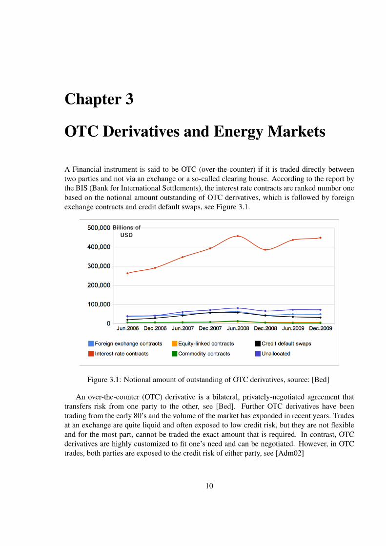
A Financial instrument is said to be OTC (over-the-counter) if it is traded directly betweentwo parties and not via an exchange or a so-called clearing house. According to the report bythe BIS (Bank for International Settlements), the interest rate contracts are ranked number onebased on the notional amount outstanding of OTC derivatives, which is followed by foreignexchange contracts and credit default swaps, see Figure 3.1.

Figure 3.1: Notional amount of outstanding of OTC derivatives, source: [Bed]

An over-the-counter (OTC) derivative is a bilateral, privately-negotiated agreement thattransfers risk from one party to the other, see [Bed]. Further OTC derivatives have beentrading from the early 80’s and the volume of the market has expanded in recent years. Tradesat an exchange are quite liquid and often exposed to low credit risk, but they are not flexibleand for the most part, cannot be traded the exact amount that is required. In contrast, OTCderivatives are highly customized to fit one’s need and can be negotiated. However, in OTCtrades, both parties are exposed to the credit risk of either party, see [Adm02]

10

3.1 Energy Commodity MarketsCommodity markets originated from the U.S. in the 19th century. In the beginning, it wasthe market where agriculture products such as wheat, corn etc., were traded. As time wentby, the commodities that were trading in the commodity markets expanded rapidly and werenot only restricted to agriculture products. Other commodities started to trade in this market,such as metals and oil. The commodity market began to transform into a global market overthe past several decades. Currently, global markets where commodities are being traded canbe classified into markets for energy, metals, minerals, agriculture commodities, and othermiscellaneous commodities. Many of these markets are organized exchanges, while the restare OTC markets, see [Cla02].

Energy commodities refer to crude and refined oil, kerosene, naphtha, liquefied petroleumgas, natural gas, and coal. Even emissions and pure electricity have also become traded com-modities. Energy markets can be farther divided into three separate markets based on the timethe markets were opened, see [EW03].

1. Oil, gas, coal, their derivatives and by-products

2. Electricity

3. Weather, emissions, pulp, paper, and forced outage insurance

Energy trading is more complex compared to trade of other commodities, because of thenature of energy commodities. For instance, some energy commodities like natural gas cannotbe transported conveniently, and some other energy commodities like electricity are hard tostore. If the trading requires a physical delivery of the commodity, it is termed as a physicaltrade. When only a transaction of cash without physical delivery is involved, it is defined as afinancial trade.

Commodities traded on an exchange have seen an exponential rise in global trading volumesince the turn of the 21st century. This increase was largely due to the growing popularityamong commodities as an asset class and the mass introduction of investment options, whichhas result in easier access to markets. The three years leading up to the end of 2010 saw afall in the global physical exports of commodities by 2%, while the outstanding value of OTCderivatives fell by 67%. Exchange trading in China has gained significance in recent times dueto their emergence as commodity consumers and producers, with China encompassing 60% oftraded commodities in 2009, a rise from 40% in 2008. Managed commodity assets increasedby more than twice its amount between 2008 and 2010, to approximately USD 380 billion.Cash inflows into this sector amounted to more than USD 60 billion in 2010, a decline fromUSD 72 billion designated to commodities funds in 2009. A major portion of these funds wereassigned to precious metals and energy products, see [The11].

Trading of commodities consists of direct physical trading and derivatives trading, seeTable3.1. Physical Trading - OTC commodities markets are basically wholesale marketswhere customized contracts are traded. A large portion of OTC commodities’ trading is donebetween producers, refiners, and wholesalers in the spot market. Trading is delivery-based

11

and usually carried out through intermediaries. For a majority of commodities that are phys-ically traded, there is no trading hub and it usually only encompasses a small percentage oftotal trade. Derivatives Trading - The notional value outstanding of banks’ OTC commodities’derivatives contracts dropped 3% in the 6 months leading to June 2010 amounting to $2.9trillion. Commodities’ share of the aggregate notional value outstanding of OTC derivativesdeclined within this period from approximately 2% till 0.5% as investors withdrew from thismarket as a result of lackluster global economic activity. Precious metals constituted 19% ofthe total trade in 2010, a far cry from their 41% share 10 years ago when trading in energyderivatives spiked. [The11]

Table 3.1: Commodity Markets: [The11]Exchange trading (stand-ardized and maturitydates)

OTC trading (individu-ally tailored)

Physical trading Accounts for a small pro-portion of trading on ex-changes. It is typicallyused to balance out an ex-cess of demand or supplyon the physical market

Accounts for most OTCtrading. Participants in-clude farmers, refiners,wholesalers. Trading isdone on the spot and for-wards market and is de-livery based

Derivatives trading Accounts for most oftrading on exchanges.Traders include hedgers,speculators and arbit-ragers. Dominates softcommodities’ trading.

Precious metals andmore recently energycontracts are oftentraded through OTCderivatives markets.

Due to the unique characteristics of energy commodities mentioned above, energy marketscan categorized into both the spot and forward markets. A spot market is a collection of smalllocal markets concerned with today’s activity, while a forward market is a separate marketconcerned with national expectations of the future. Unlike the stock or bond market, theenergy spot and forward markets are not closely linked. This is because it is impossible topurchase certain energy commodities at one point in time, store it, and then deliver it at a laterpoint in time. The major spot markets for oil products are in Amsterdam, Antwerp, Rotterdam,New York and Singapore. Derivatives are also traded on the London’s ICF Futures (formerlythe London International Petroleum Exchange (IPE)) and New York Mercantile Exchange(NYMEX/-COMEX). Derivatives are not only traded in the exchange markets, but also inthe OTC markets. The OTC markets is specific to the non-standardized price swap and OTCoptions, see [Cla02] and [EW03].

12

3.2 Energy Over-The-Counter Derivative MarketsOTC derivatives play an important role for oil companies, refineries, trading firms and otherintermediaries that are engaged in the physical trading of energy commodities. Profit structureof these kinds of companies are rather unstable due to the fact that their profit are heavilydepending on the market price volatility. As the result, OTC derivatives satisfy their needs andcan reduce the risk and stabilize earnings, see [EW03].

3.2.1 Forward ContractsA forward is similar to a future contract, as it is an agreement between a seller and a buyeron certain commodities in a future time. The price that the buyer has to pay is specified whenthe is made. The delivery price may be fixed at the inception of the contract and the formulaof the delivery price should be agreed by both parties. This formula can be based on theexpiration dates of the future prices or an average of the future prices during the week beforethe expiration date. Like a future contract, the following characteristics must be specified inthe forward , see [EW03].

• Delivery details (total quantity, per day/hour quantity, firm/non-firm, etc.)

• Delivery price or formula for computing delivery price

• Delivery period and time of delivery during period

• Delivery location

The main differences between a future and a forward contract are as follows:

• A forward contract is an OTC product in which both parties of the contract can negotiate,and thus it is fairly customized and flexible compared to a future contract. At the sametime, a forward contract is subjected to credit risk because there is no guarantee fromthe clearing house, there is counterparty credit risk.

• A forward contract can be physically or financially settled.

• A forward is not settled daily, and so the contract holder does not have to worry aboutthe daily access to cash to meet the margin requirements from the exchanges.

3.2.2 Value of ForwardsThe value of a forward with fixed price for future delivery of a unit of commodity is expressedby, see also [EW03]

Vf (t,Ft,T ) = e−r(T−t)(Ft,T −X) (3.1)

where

• t is the time that is evaluated

13

• X is a strike price which is a contractual fixed price to be paid for one unit of the de-livered commodity

• Ft,T is the price at time t future settled at the same time as the forward

In practical application the above formula is often written in a more complicated way asfollows

Vf (t,Ft,T ) = N · e−r(t,Tpay)(Tpay−t) · (Ft,T −X) (3.2)

where, t, X , Ft,T , defined as above.

• Tpay is the payment time

• r(t,Tpay) is an annualized and continuously compounded discount rate from t to Tpay

• e−r(t,Tpay)(Tpay−t) is the correspondent discount factor

• N is the number of commodity units to be delivered under the contract

• Vf (t,Ft,T ) is the value of a fixed-price the forward contract at the time t.

3.2.3 SwapsThe swap market began in the US from 1981. A swap is a contractual agreement where twoparties accept to exchange fixed payments against floating payments, see [Fus07]. Accordingto BIS at the end of 2006 the notional amount outstanding of swap in the OTC derivativemarket was $415.2 trillion, more than 8.5 times the 2006 gross world product. The mostcommon swap contracts are currency swaps, interest rate swaps, commodity swaps, equityswaps, and credit default swaps. A swap contract is very popular in the energy market as well.The reasons are as follows, see [EW03]:

• Swaps are flexible and customized.

• Swaps are financially settled (no physical delivery) and are non-regulated.

• Swaps are uniquely suited for hedging applications.

Swaps in the energy market are quite similar to swaps in the financial market and can beviewed as a portfolio of generalized forward s. The most common case is a fixed price swap fora period of time. A party pays a fixed payment and in exchange, receives a floating paymentlinked to a certain index from a counterparty. For instance, in order to hedge price exposure tooil price fluctuation, an oil producer enters an oil swap contract to lock the oil price (WTI crudeoil) with another party. The counterparty is a risk profile of the oil consumer who wants to lockin a fixed price for oil purchases for a certain period of time. "Both parties agree to exchangecash, whereby the oil producer receives a fixed price on a pre-agreed volume of oil and agreesto pay a floating price index (WTI index) on an identical volume of oil (100,000 barrels ofcrude WTI to be delivered each month for a specific period of time, i.e. 6 months). The oilconsumer enters the reverse part of the same transaction." see [Fus07]. The counterparty (the

14

consumer) on the other hand, agrees that settlement will be in cash based on WTI prices ona monthly basis. This transaction allows both counterparties to lock in a price on an agreedvolume of oil off the WTI Price index, see [Fus07] and [EW03].

Figure 3.2: Swap

3.2.4 Value of SwapsAs discussed above swap can be considered as a portfolio of generalized forward contract,so it is not hard to derive the formula for value of the swap based of the formula (3.1), see[EW03]

PVswap(t) = ∑i

Ni · [ fi ·DF(t,T f loati,pay )−X ·DF(t,T f ixed

i,pay )] (3.3)

where

• Ni is volume

• fi = Ft,T is the forward price at the valuation time

• t of the commodity for delivery in the i-th month

• DF(t,T f loati,pay )–is the discount factor from t to T f loat

i,pay , the time of payment for the com-modity delivered during the i-th month.

• DF(t,T f loati,pay ) = e−ri(t,Tt)(Tt−t) is the discount factor from t to time T f loat

i,pay .

• DF(t,T f ixedi,pay ) is the discount factor from t to the fixed price payment.

15

• PV (t) is the present value of the swap at time t.

Now, by using Equation (3.3) we can derive an expression for the fair value of the fixedpayment X , which makes the present value of the swap contract to zero at the inception time(which means t = 0). This value is called a swap price. As the result, letting the left hand sideof the Equation (3.3) to be zero and solve for X , we get the expression as follows, see [EW03]:

SP(t) =∑i Ni · fi ·DF(t,T f loat

i,pay )

∑i Ni ·DF(t,T f ixedi,pay )

(3.4)

Since the Formula (3.3) assumes the frequency of fixed and floating payments to be thesame, which is a quite realistic assumption when it comes to energy swaps.(Financial swapsmay have different payment frequencies). So Equation (3.4) can be considered as the generalformula for swap price in the energy market, see [EW03].

3.2.5 Credit Default Swaps

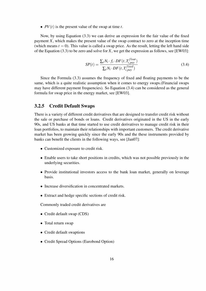
There is a variety of different credit derivatives that are designed to transfer credit risk withoutthe sale or purchase of bonds or loans. Credit derivatives originated in the US in the early90s, and US banks at that time started to use credit derivatives to manage credit risk in theirloan portfolios, to maintain their relationships with important customers. The credit derivativemarket has been growing quickly since the early 90s and the these instruments provided bybanks can benefit the clients in the following ways, see [Jan07]:

• Customized exposure to credit risk.

• Enable users to take short positions in credits, which was not possible previously in theunderlying securities.

• Provide institutional investors access to the bank loan market, generally on leveragebasis.

• Increase diversification in concentrated markets.

• Extract and hedge specific sections of credit risk.

Commonly traded credit derivatives are

• Credit default swap (CDS)

• Total return swap

• Credit default swaptions

• Credit Spread Options (Eurobond Option)

16

A credit default swap (CDS) is a product within the credit derivative assets class, consti-tuting a type of OTC derivative. It consists of a buyer and a seller. The buyer agrees to paya periodic fee (premium) and/or upfront in exchange for a payment by the protection sellerin the event such as bankruptcy affecting a reference entity or a portfolio of reference entitiessuch as a CDS index. As a result, the market price of the premium is an indication of theperceived risk related to the reference entity, see [Ban09].

For default swap transactions, the credit default payment must be clearly defined. Thecontingent payment is usually settled in cash and equals to the total value of loss incurred bythe protection buyer on the reference assets. Other than cash settlements, physical delivery ofthe reference asset for its par value also exists but not often used, see [Jan07].

3.2.6 Value of Credit Default SwapsLet us consider a case where company C have issued bonds and C defaults at time τ . Here τ isa random variable modeling the future potential default of company C. The protection buyerA buys protection from the protection seller B, on credit-losses inferred by C, for the next Tyears, see [Ale10].

Figure 3.3: CDS cash flow, source: [Ale10]

For this protection, A pays a quarterly fee to B given by R(T )N4 , where N is protected value.

The quantity R(T ) is called the CDS-premium, or CDS-spread, on obligor C, for the periodup to time T . Moreover if company C defaults before time T , that is, if τ < T , then B pays Athe credit loss suffered by A at time τ which is N · `. Here ` is the credit loss in percentage forthe nominal value N, see Figure 3.3.

17

Figure 3.4 and Figure 3.5 displays the cash flow between A and B in two different scen-arios, when τ < T and when τ ≥ T respectively, see [Ale10]

Figure 3.4: CDS cash flows when τ < T , source: [Ale10]

Figure 3.5: CDS cash flows when τ > T , source: [Ale10]

The CDS spread R(t) is determined as that the expected discounted cash flow between Aand B are equal at time t = 0, that is

R(T ) =E[1τ≤tnD(τ)l]

∑4Tn=1E[D(tn)1

41τ>tn+D(τ)(τ− tn−1)1tn−1<τ≤tn](3.5)

where tn = n4 , D(t) = exp(−

∫ t0 rs ds) and rs is risk-free interest rate at time t. If τ and rt

are independent and ` is deterministic then Equation (3.5) reduced to:

R(T ) =`∫ t

0 Bs dF(s)

∑4Tn=1(Btn

14(1−F(tn))+

∫ tn−1tn Bs(s− tn−1)dF(s)

) . (3.6)

18

If we assume that the interest rate rt is a deterministic function of time t, then τ and rt are in-dependent and Bt = D(t) = exp(−

∫ t0 r(s)ds). Additionally let F(t) be the default distribution

of τ , that is F(t) = P[τ ≤ t] and let fτ(t) be the density of τ , so that fτ(t) =dF(t)

dt which hisnotation the default leg can be written as, see Equation (3.7):

E[1τ<TD(τ)(1−φ)] =∫

∞

01τ<TD(t)(1−φ) fτ(t)dt = (1−φ)

∫ T

0D(t) fτ(t)dt (3.7)

where φ is the so called recovery defined as φ = 1−` when ` is the loss. Further, note that

E[D(tn)

14

1τ>tn]= D(tn)

14E[1τ>tn] = D(tn)

14P[τ > tn] = D(tn)

14(1−F(tn)) (3.8)

and the accrued premium is given by:

E[D(τ)(τ− tn−1)1tn−1<τ<tn

]=∫ tn

tn−1

D(t)(t− tn−1) fτ(t)dt. (3.9)

So inserting Equation (3.7), (3.8) and (3.9) into Equation (3.6) we get that the CDS-spreadR(t) is given by:

R(t) =(1−φ)

∫ T0 D(t) ft(t)dt

∑4Tn=1(D(tn)1

4(1−F(tn))+∫ tn

tn−1D(s)(s− tn−1) fτ(s)ds

) . (3.10)

Therefore, we see that in order to find CDS-spread R(t) we need to find F(t) = P[τ < t]and the density fτ(t) of the default time τ . Furthermore, Equation (3.10) can be simplifiedeven more by using the following assumptions:

• Ignore the accrued premium term

• At a default τ in the period [n−14 , n

4 ], the loss is paid at time tn = n4 . e.i. at the end of the

quarter, instead of immediately at τ .

Hence, using the above assumptions inspired by Lando, see [Lan04] the original formula(3.10) will be simplified as follows together with the assumption of deterministic interest rateand recovery rate

R(T ) =(1−φ)∑

4Tn=1 D(tn)(F(tn)−F(tn−1))

∑4Tn=1 D(tn)(1−F(tn))1

4

. (3.11)

Thus, in the view of Equation (3.11) we conclude that finding the CDS spread R(t) is inpractice equivalent with finding the default distribution F(t) = P[τ ≤ t]. By using so-calledintensity based models (that we will discuss in Section 4.2) we can find convenient formulasfor the survival probability P[τ > t], see [Ale10]

19

Chapter 4

Credit Risk Model

As we have witnessed in the previous chapter, an essential step when modeling dynamic creditrisk and specifically, when pricing CDS spreads, is to model the default time τ for the com-pany. In particular, we would like to acertain a convenient expression for the default distribu-tion F(t) = P[τ ≤ t].

In general, there are two main approaches to determine the default probabilities for a com-pany. One such approach is to calibrate the default probabilities from market data. The mostfamous method from this approach is termed the AVM (Asset Value Model), which is in-spired by Merton, Black, and Scholes, see [BOW03]. An alternative method in this approachfor calibrating the default probabilities from market data is based on credit spreads of tradedproducts that bear credit risks (for example, CDS). Another approach to find default prob-abilities is to calibrate the default probabilities form ratings. There are some credit ratingagencies that estimate a company’s real-world default probability. Unfortunately, credit ratingis not frequently revised most of the time, and as a result, this leads some analysts to arguethat equity prices can provide more updated information to estimate the default probabilities,see [BOW03].

In this chapter we briefly discuss two different methods to model default times. First, inSection 4.1 we provide a short outline of so-called firm-value models for the default time τ .Then in Section 4.2 we introduce the intensity based model for modeling default time τ .

4.1 Merton ModelIn 1974, Merton proposed a model where a company’s equity is an option on the asset of thecompany, [Mer74]. Merton’s model that was developed by the KMV corporation, which werefer to as the KMV-Merton model that is well known model in the industry, see [BOW03].

Let us consider a firm whose value of assets follow a Geometric Brownian Motion (GBM):

dVt = µVt dt +σVt dWt . (4.1)

where Wt is a standard Brownian motion. By using Ito’s lemma, we have

Vt =V0e(µ−12 σ2)t+σWt (4.2)

20

where V0 is the value of a company’s asset today and VT is the value of the assets at timeT . Let us denote E0 and ET as the values of the company’s equity at time t and time Trespectively, D being the debt repayment due at time T , σV and σE being the volatility ofasset and instantaneous volatility of equity respectively, see [HNW04].

If VT < D, the equity owners will declare bankruptcy. This means that the firm is handedover to the debt-holders. They will recover VT instead of D because of the bankruptcy, and thedebt-holder loses the amount D−VT > 0. The equity value then becomes 0, see [HNW04].

If VT > D, the value of the firm’s assets exceeds the liabilities. In this case, the debt-holders receive D, the share holders receive the residual value ST =VT −D, and there will beno default, see [HNW04].

Hence, based on the above reasoning a default occur when VT < D. It is our interest tocompute the default probability in Merton model, both under the real probability measure Pand the pricing measure Q, see [Ale10].

Let us start with the default probability under the real measure, i.e P[VT < D]. Under P itholds that VT = V0e(µ−

12 σ2)T+σWT and since ln(x) is an strictly increasing function, the event

VT < D is therefore equivalent with the event:

ln(V0e(µ−12 σ2)T+σWT )≤ lnD. (4.3)

Since ln(V0e(µ−12 σ2)T+σWT ) = lnV0 +(µ− 1

2σ2)T +µWT , a simple calculation show thatthe event (4.3) is equivalent with the event

WT ≤ln D

V0− (µ− 1

2σ2)T

σ. (4.4)

Since WT ∼ N(0,T ), Hence, if X ∼ N(0,1), the WT has the same distribution as√

T X .As a result, P[WT ≤ x] = P[

√T X ≤ x] = P[X ≤ x√

T] = N( x√

T), which together with Equation

(4.4) yields that:

P[VT < D] = N(ln D

V0− (µ− 1

2σ2)T

σ√

T).

Furthermore, by defining the default time τ as the first time the asset value falls below the debtthat is

τ = in ft > 0 : Vt ≤ D (4.5)

we have that P[τ ≤ t] = P[Vt ≤ D]. Hence, (4.1) implies that:

P[τ ≤ t] = Φ(ln D

V0− (µ− 1

2σ2)T

σ√

T).

Meanwhile, based on discussion above, we can also come up with the following equationsas in the original Merton model:

ST = max(VT −D,0) = (VT −D)+ (4.6)

21

DT = min(D,VT ) = D−max(D−VT ,0) = D− (D−VT )+

According to the equations above, we can say that the debt, i.e. zero coupon bonds, incurredby the company can be viewed as the difference between a risk-free bond (with face valueD) and a put option on the asset with strike price D. The equity i.e. St can be viewed as acall-option on the asset with strike price D.

Under the Black-Scholes setting and with equation (4.1) and (4.2), we can conclude thatin the Merton model, equity St and debt Bt are given by (for 0≤ t ≤ T )

St =CBS(Vt ,D,T − t,σ ,r)

Bt = De−r(T−t)−PBS(Vt ,D,T − t,σ ,r)

whereCBS(Vt ,D,T − t,σ ,r) =VtN(d1)−De−r(T−t)N(d2)

d1 =ln(Vt

D )+(r+ 12σ2)(T − t)

σ√

T − t

d2 = d1−σ√

T − t

N(x) =∫ x

−∞

1√2π

e−y2

2 dy.

4.2 Intensity Default ModelIn this section we present the so-called intensity based model for modeling default times τ . Inorder to understand the intensity default model better, we have to first bear in mind that thereis a direct connection between hazard rates and conditional default probabilities. Consider asingle obligor with default time τ , and the basic assumption is, see [Lan04]

P[τ ∈ [t, t +∆t) |Ft ] = λt∆t i f τ > t (4.7)

where

• Ft–is the market information available at time t.

• λ – is the intensity for τ , with respect to the information Ft

The intuition behind Equation (4.7) is that given the market information Ft at time t, andgiven that the default time τ has not yet occurred before t, then the conditional probability ofa default in the small time period [t, t +∆t] is approximately equal to λt∆t.

22

As we have mentioned above, in order to calculate CDS spreads R(T ), we need to findF(t) = P[τ ≤ t], which is the survival probability and the density fτ(t) of τ . Since we havethat

F(t) = P[τ ≤ t] = 1−P[τ ≥ t]

So it is enough to find P[τ ≥ t], if τ has the default-intensity λ (Xt) with respect to the inform-ation (Ft)t≥0 we have the following

P[τ ≥ t] = E[exp(−∫ t

0λ (Xt)ds

)](4.8)

and

fτ(t) = E[λ (Xt)exp

(−∫ t

0λ (Xt)ds

)]We can now consider three special case of the intensity

1. The intensity λ (X) is a deterministic constant.

2. The intensity λ (Xt) is a deterministic function of time t, λ (t).

3. The intensity λ (Xt) is a stochastic process and this case will not be studied in this paper.

• When the intensity λ is a deterministic constant, we have that λ (Xs) = λ , and Equation(4.8) reduces to:

P[τ ≥ t] = E[

exp(−∫ t

0λ (Xt)ds

)]= E

[e−λ t]= e−λ t (4.9)

and fτ(t) = λe−λ t .

• When the intensity λ is a deterministic function of time t (non-constant), we have

P[τ ≥ t] = E[

exp(−∫ t

0λ (s)ds

)]= exp

(−∫ t

0λ (s)ds

)(4.10)

and fτ(t) = λ (t)exp(−∫ t

0 λ (s)ds). One of the most important case of deterministic

default intensity λ (t) is called piecewise constant default intensity. Let T ∈ T, whereT =

T1, T2, . . . , Tj

, for example, T = 3,5,7,10. If we assume that the default in-

tensity for the company λ (t) is piecewise constant, then

λ (t) =

λ1 if 0≤ t ≤ T1λ2 if T1 ≤ t ≤ T2...λ j−1 if Tj−2 ≤ t ≤ Tj−1λ j if Tj−1 ≤ t ≤ t.

(4.11)

23

In this case with piecewise constant default intensity we can find an easy formula forthe survival probability P[τ > t]. We just need to integrate the function λ (t), which isgiven by the equation (4.11) , and this yields that:

P[τ > t] =

exp(−λ1t) if 0≤ t ≤ T1exp(−λ1T1− (t− T1)λ2)

)if T1 ≤ t < T2

...exp(−∑

J−2j=1 λ j(Tj− Tj−1)− (t− TJ−2)λJ

)if Tj−2 ≤ t < Tj−1

exp(−∑

J−1j=1 λ j(Tj− Tj−1)− (t− TJ−1)λJ

)if Tj−1 < t

(4.12)where we define T0 as T0 = 0.

• If λ (Xs) = λt is a Vasicek-process, independent of the interest rate,

dλt = α(µ−λt)dt +σ dWt (4.13)

where Wt is a brownian motion under the risk-neutral measure P, we then concludedthat

P[τ > t] = exp(A(t)−B(t)λ0)

for

B(t) =1− e−αt

α(4.14)

A(t) = (B(t)− t)(

µ− σ2

2α2

)−σ2

4αB(t)2 (4.15)

Furthermore, because we know that fτ(t) =−P[τ>t]dt we can show that

fτ(t) =[

e−αt(

σ2

2α+λ0

)−(e−αt−1)

(µ− σ2

2α2

)]eA(t)−B(t)λ0 (4.16)

4.3 BootstrappingAs we have studied in the previous sections, we need to first determine the survival probabil-ities in order to calculate the CDS spreads. By using piecewise constant default intensity aspresented in Equation (4.11) and Equation (4.12), it is possible to calibrate the default distri-bution perfectly against the CDS-term structure RM(Tj) for Tj ∈ T1, T2, . . . , Tj. This methodis called bootstrapping.

Let us assume that the default intensity for the company is deterministic and the intensityλ (t) is piecewise constant, see Equation (4.11). Then, the way to compute the survival prob-ability is straightforward and already presented in Equation (4.12). The basic procedure aboutbootstrapping to find λ = (λ1,λ2, . . . ,λ j) is as follows:

• Find λ1 so that R(T1;λ1)=RM(T1). Note that RM(T1) here does not depend on (λ2, . . . ,λ j)since the CDS contract stops at T1. Here we can use the approximation formula R(T )≈(1−φ)λ .

24

• Given λ1, find λ2 so that RM(T2;λ1,λ2) = RM(T2). RM(T2) here does not depend onλ3, . . . ,λ j since the CDS contract stops at T2.

• . . .

• Given λn−1,λn−2, . . . ,λ1 from steps above, find λn, so that RM(Tn;λ1,λ2, . . . ,λn) =RM(Tn). RM(Tn;λ1,λ2, . . . ,λn) does not depend on λn+1, . . . ,λ j since the CDS contractsstops at Tn.

• Continue the procedure until the final step n = j.

25

Chapter 5

Commodity Model

There are many different types of price models for energy and commodities. Depending onthe characteristics of the underlying commodities, different pricing models are applied. In thischapter we closely follow the outline presented in section 4 of Brigo’s paper, see [BCB08].Let us focus on one such model, which is similar to one of the most famous pricing modelin this field; the mean/reverting model, or the two-factor model that captures both the shortterm deviations in prices and the equilibrium price level developed by Smith and Schwartz(2000). Let the oil price at time t be denoted by St . Then the log price process can be writtenas follows, see [BCB08] and [SS00]

ln(St) = x(t)+L(t)+ϕ(t) (5.1)

where x(t) represents the short-term deviation from the prices that refers to temporarychanges in the price, and L(t) refers to equilibrium level of the price. Here ϕ is a deterministicshift that we will need when it comes to the calibration of quoted prices. Under the risk neutralmeasure, the dynamics for x(t) and L(t) is given by:

dx(t) =−κx dt +σx dZx (5.2)

dL(t) = µL dt +σL dZL, dZxdZL = ρx,L dt (5.3)

For the two factors model we have a joint Gaussian transition.[x(t)L(t)

]∣∣∣∣x(s),L(s)

∼N

([x(s)exp(−κx(t− s))

L(s)+µt(t− s)

],

[σ2

2κx(1− exp(−2κx(t− s)) Covx,L(s,t)

Covx,L(s,t) σ2(t− s)

])

where Covx,L(s,t) = ρx,L(s,t)σxσL

κx(1− exp(−κx(t− s))). According to what we have above

and the rule of sum of two Gaussian random variables is still Gaussian, we have the following:

ln(S(t)) = x(t)+L(t)+ϕ(t)|x(s),L(s) ∼N (m(t,s),V (s, t))

m(t,s) = x(s)exp(−κx(t− s))+L(s)+µL(t− s)+ϕ(t)

26

V (s, t) =σ2

2κx(1− exp(−2κx(t− s))+σ

2(t− s)+2Covx,L(s,t)

from which we get

E[S(t)|x(s),L(s)] = exp(x(s)exp(−κx(t− s))+L(s)+µL(t− s)+ϕ(t)+V (s, t)/2)

Hence the forward price E[S(t)|x(s),L(s)] at time t of the commodity at maturity T whencounterparty risk is not taken into consideration and under deterministic interest rates is:

F(t,T ) = exp(x(t)exp(−κx(T − t))+L(t)+µL(T − s)+ϕ(T )+V (T, t)/2) (5.4)

27

Chapter 6

Counterparty Credit Risk and CreditValue Adjustment

Counterparty credit risk is the risk that one of the counterparties in a financial contract willdefault prior to the expiration of the contract and will not make all the payments required bythe contract. In exchange-traded contracts, all trades can be considered as free from counter-party credit risk, since they are backed by the guarantee of a clearing house or an exchange.However, unlike exchange-traded contracts, all the OTC derivatives are subjected to counter-party risk, due to a default by one of the counterparties before maturity of the contract. Asa result, only the contracts privately negotiated between counterparties - OTC derivatives andSecurities Financing Transactions (SFT) - are subjected to counterparty risk, see [ZP07] and[Gre09].

As seen from the definition, counterparty risk is related to the other forms of credit risk thatcause economics loss, often due to the obligor’s default. There is still a difference betweencounterparty risks and traditional credit risks. Firstly, the counterparty credit risk exposure isuncertain, as well as the market risk in the underlying contract. Secondly, the counterparty riskis a bilateral risk, where both parties are subjected to the counterparty risk of either party. Acommon way to measure counterparty risk is to compute the so-called credit value adjustment(CVA).

Credit value adjustment (CVA) is by definition the difference between the risk-free portfo-lio value and the true portfolio value, and which takes into account counterparty default risk.The counterparty credit quality of derivative portfolios has not been considered the standardpractice in the industry for years. All cash flows were discounted by LIBOR and the resultswere considered as risk-free values. However, counterparty risks exist in real life and cannotbe omitted. Hence, counterparty risk must be included when calculating the true portfoliovalue and CVA is the market value of counterparty credit risk.

6.1 General Valuation of Counterparty Risk

In this section we introduce a general formula to compute the counterparty credit risk. Ourpresentation follows the outline of Brigo and Chourdakis (2008), see [BCB08]. We first de-

28

note τ to be the default time for the counterparty and we further assume that the investors whoentered the contract with the counterparty is default free. We then place ourselves in a probab-ility space (Ω, G , Gt , Q), where the filtration models the information about defaults and creditof the entire market, and Q is the risk neutral measure. This space is also endowed with a rightcontinuous and complete sub-filtration Ft , representing all the observable market quantities,excluding the default event (hence Ft ⊆ Gt : Ft ∨Ht where Ht = σ(τ ≤ u : u ≤ t) is theright-continuous filtration generated by the default event).

Let us denote the final maturity of the payoff we need to evaluate to be T . If τ > T , thenthere is no default of the counterparty during the life time of the products. However, if τ < T ,the counterparty can not fulfill his obligations, and the following events will occur:

At time τ , the Net Present Value (NPV) of the residual payoff until maturity is computed:If this NPV value is negative for the investor, it is completely paid by the investor. If the NPVvalue is positive for the investor, only a recovery fraction of REC of the NPV is exchanged.

We term ΠD(t,T ) as the discounted payoff of a general claim at t under counterparty risk.This is the sum of all cash flows from t to T and each of them is discounted back to time t.This payoff is stochastic and the payoff price is given by risk neutral expectations. Now, wedenote Π(t,T ) as the payoff without taking into consideration of counterparty risk. From theinvestor who is facing counterparty risk, his point of view would be:

ΠD(t,T ) = 1τ>TΠ(t,T )+

1t<τ≤T[Π(t,τ)+D(t,τ)

(REC(NPV(τ))+− (−NPV(τ))+

)]The last expression is the general price of the payoff under counterparty risk. If there is noearly counterparty default this expression will be reduced to the risk neutral payoff, which isthe first term in the right hand-side of the above equation.

ΠD(t,T ) = Π(t,T )

In case of early default of counterparty, the valuation of payoff is as follows:

ΠD(t,τ) = Π(t,τ)+D(t,τ)

(REC(NPV(τ))+− (−NPV(τ))+

)The first term above represents that the payment due before default occurs are received, and ifthe residual NPV is positive, only a recovery of it is received i.e., the second term in the aboveequation. On the other hand, if residual NPV is negative, then payment is paid in full, whichis the last term the in above equation.

In the paper [BCB08] it is proved that the general counterparty-risk credit-valuation ad-justment (CR-CVA) formula at valuation time t, and on τ > t, is given by, see [BCB08]

EΠD(t)= EtΠ(t)−LGDE1t<τ≤TD(t,τ)(NPV(τ))+︸ ︷︷ ︸Positive CR-CVA

(6.1)

where LGD = 1−REC is the Loss Given Default and the recovery fraction REC is assumedto be deterministic. The formula (6.1) can be approximated in the following manner: Takingt = 0 for simplicity and write, on a discretization time grid T0 = 0,T1, . . . ,Tb = T ,

29

E[ΠD(0,Tb)] = E[Π(0,Tb)]−LGD

b

∑j=1

E[1Tj−1<τ≤TjD(0,τ)(EτΠ(τ,Tb))+]. (6.2)

Furthermore, under the assumption of postponing the default time τ to the first Ti, followingτ , we can then approximate the formula further as follows:

E[ΠD(0,Tb)]≈ E[Π(0,Tb)]−LGD

b

∑j=1

E[1Tj−1<τ≤TjD(0,Tj)(EτΠ(Tj,Tb))+]︸ ︷︷ ︸

approximated (positive adjustment)

(6.3)

6.2 Counterparty Risk Valuation for Oil ForwardsIn this section we derive the closed-formulas for the counterparty risk valuation of oil for-wards. We follow the outline of Brigo and Chourdakis, see [BCB08]. Let us consider aforward contract with time t representing the valuation time, and time T representing the ma-turity time in the future. In this contract, a party agrees to buy from another party a certainamount of commodities at the strike price K, which is fixed today. Alternatively, we can as-sume that the first party has entered a payer forward rate agreement, and the second party inthis case has agreed to enter a receiver forward rate agreement. The value of the contract atmaturity time T for both of the parties in this agreement are as follows: [BCB08]

ST −K and K−ST (6.4)

For the payer, the price of the contract is given by:

Et [D(t,T )(ST −K)] = D(t,T )(Et [ST −K]) = D(t,T )(F(t,T )−K). (6.5)

Note that the quantity Et [·] in Equation (6.5) is defined as Et = E[·|G ]. With the above model,in order to calculate the forward contract price, we can insert Equation (5.4) into Equation(6.5) As a result, we have a forward contract price, which is denoted by Fwdp(t,T; K), for thepayer at time t as follows:

Fwdp(t,T ;K)=D(t,T )(exp(x(t)exp(−κx(T−t))+L(t)+µL(T−s)+ϕ(T )+V (T, t)/2)−K)(6.6)

Now we can apply the counterparty risk framework to the forward contract, where Π(t,T ) =D(t,T )(ST −K), and NPV (t) = Fwdp(t,T ;K). We get the price of the payer forward contractunder counterparty risk from Equation (6.1):

FwdpD(t,T ;K) = Fwdp(t,T ;K)−LGDEt1t<τ≤TD(t,T )(NPV (τ))+︸ ︷︷ ︸Positive counterparty risk adjustment

. (6.7)

30

according to the bucketing approximation given by Equation (6.3) we have:

FwdpD(t,T ;K) = Fwdp(t,T ;K)−LGD

b

∑j=1

D(t,Tj)Et [1Tj−1<τ≤Tj(Fwdp(Tj,T ;K))+] (6.8)

If one assumes independence between the underlying commodity and the counterpartydefault, one may factor the above expectation and obtain: see [BCB08]

FwdpD(t,T ;K)= Fwdp(t,T ;K)−LGD

b

∑j=1

Qt(Tj−1 < τ ≤ Tj)E[D(t,Tj)(Fwdp(Tj,T ;K))+].

(6.9)Where Q[·] = Q[·|G ]. The last term in above equation is the price of an option on a for-ward price, which is known as the closed f orm in the Schwartz and Smith Model, see alsoin [BCB08] and [SS00]

Et [D(t,Tj)(Fwdp(Tj,T ;K))+] = D(t,T )expM(t,T,Tj;xt ,Lt)

+V (t,T,Tj/2)Φ(

M(t,T,Tj;xt ,Lt)+V (t,T,Tj− lnK√v(t,T,Tj)

)−D(t,T )KΦ

(M(t,T,Tj− lnK√

V (t,T,Tj)

)(6.10)

where

M(t,T,Tj;xt ,Lt) = xt exp−κx(T − t)+Lt +ϕ(T )+V (T,Tj/2)

and

V (t,T,Tj) = exp(−2κ(T −Tj))σ2

2κx(1− exp(−2κ(Tj− t)))

+σ2L(Tj− t)+ exp(−κx(T −Tj))2ρx,L

σxσL

κx(1− exp(−κx(Tj− t))).

Here Φ is the cumulative distribution function of standard Gaussian. Based on the formulaabove, we have the adjustment as a stream of options on forwards weighted by the defaultprobabilities, see [BCB08]. In chapter 7 we will use Equation (6.10) in the case when t = 0.

6.3 Counterparty Risk Valuation for SwapsRecall the swap contract discussed in subsection 3.2.4. In this section we study the coun-terparty risk valuation for oil swaps, and we closely follow section 4 in Brigo’s paper, see[BCB08]. The typical swap can be considered as a portfolio of forwards with different matur-ities, and agreeing on the following:

31

The valuation time is t. At the future time(s) Ti in Ta+1, Ta+2, . . . , Tb, a party agrees tobuy a commodity at the K, on a notional amount of αi. The valuation of the payer commodityswap (CS) contract to second party at time t, will be:

PCSa,b(t,K)=Et

b

∑i=a+1

D(t,Ti)αi(STi)=b

∑i=a+1

αiD(t,Ti)(F(t,Ti)−K)=b

∑i=a+1

αiFwdp(t,Ti;K)

(6.11)As we have discussed in the earlier sections, the price of the swap contract is computed

with this formula (3.4). We will once again repeat the same procedure to compute the valueof a swap contract. We look for the value of K by setting the contract price to zero, i.e. theforward swap commodity price Sa,b(t), and we have:

Sa,b(t) =∑

bi=a αiD(t,Ti)F(t,Ti)

∑bi=a αiD(t,Ti)

The payer of commodity swap price at a general strike K by using the above expressioncan be written as:

PCSa,b(t,K) = (Sa,b−K)b

∑i=a+1

αiD(t,Ti)

where the receiver commodity swap would be:

RCSa,b(t,K) = (K−Sa,b)b

∑i=a+1

αiD(t,Ti)

These formulas here represent the values of swap contracts when a clearinghouse or mar-gining agreements are in place. When it is traded over-the-counter, then both parties of thecontract are faced with counterparty credit risk. By taking counterparty risk into consideration,the payer for the commodity swap by using our general formula generates:

PCSDa,b(t,K) = PCSa,b(t,K)−LGDEt1t<τ≤TbD(t,τ)(PCSa,b(τ,K))+︸ ︷︷ ︸

Positive counterparty-risk adjustment

and it can be written as

PCSDa,b(t,K) = PCSa,b(t,K)−LGDEt

1t<τ≤TbD(t,τ)

( b

∑i=a+1

αiFwdp(τ,Ti;K))+ (6.12)

Since the formula for forwards are known in our model, then the swap case counterpartyrisk adjustment can be approached in a similar fashion like the forward case. However to thebest of our knowledge there are no closed formula for the Equation (6.12). Thus simulationhave to be used, even when t = 0. Recall that in a forward contract there are closed formula tocompute, see Equation (6.10). Thus in this paper we calculate CVA just for forward contracts.

32

Chapter 7

Numerical Studies

In this chapter, we consider counterparty credit risk in an oil forward contracts. Let us assumethere is an airline who needs to buy oil in the future exchange market and is concerned aboutthe possible fluctuations in oil prices. In order to hedge these price movements, the airlinerequests a bank to enter a oil forward contract, where at the maturity date of the forward T ,the airline pays the pre-agreed price to the bank. The reason for the airline not requisitioningcrude oil directly via the future exchange market is because a forward contract is trading inthe OTC market and it is more flexible, negotiable, and customized. Hence, the airline prefersto requisition crude oil via the forward market. The future price is merely a reference for thestrike price in the contract.

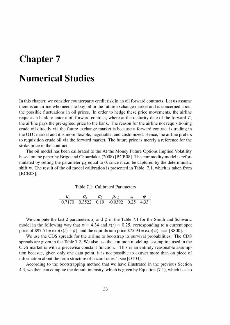
The oil model has been calibrated to the At the Money Future Options Implied Volatilitybased on the paper by Brigo and Chourdakis (2008) [BCB08]. The commodity model is refor-mulated by setting the parameter µL equal to 0, since it can be captured by the deterministicshift ϕ . The result of the oil model calibration is presented in Table 7.1, which is taken from[BCB08].

Table 7.1: Calibrated Parameters

κx σx σL ρx,L xt ϕ

0.7170 0.3522 0.19 -0.0392 0.25 4.33

We compute the last 2 parameters xt and ϕ in the Table 7.1 for the Smith and Schwartzmodel in the following way that ϕ = 4.34 and x(t) = 0.25, corresponding to a current spotprice of $97.51 = exp(x(t)+φ), and the equilibrium price $75.94 = exp(ϕ), see [SS00].

We use the CDS spreads for the airline to bootstrap its survival probabilities. The CDSspreads are given in the Table 7.2. We also use the common modeling assumption used in theCDS market is with a piecewise constant function. "This is an entirely reasonable assump-tion becasue, given only one data point, it is not possible to extract more than on piece ofinformation about the term structure of hazard rates.", see [OT03].

According to the bootstrapping method that we have illustrated in the previous Section4.3, we then can compute the default intensity, which is given by Equation (7.1), which is also

33

Table 7.2: CDS spreads for the airline

maturities (years) 0.5 1 2 3 4 5CDS spreads (bps) 76 82 104 122 139 154

Figure 7.1: Default intensities λ bootstrapped from CDS term structure

visualized in Figure7.1.

λ (t) =

λ1 = 0.0126 if 0 < t ≤ 0.5λ2 = 0.0147 if 0.5 < t ≤ 1λ3 = 0.0211 if 1 < t ≤ 2λ4 = 0.0268 if 2 < t ≤ 3λ5 = 0.0328 if 3 < t ≤ 4λ6 = 0.0374 if 4 < t ≤ 5

(7.1)

Since we got the default intensities from bootstrapping the CDS term structure, we cannow calculate the survival probabilities of the airline according to the Equation (4.12) for thedifferent maturities. The results are as follows:

P[τ > t] =

99.37% when t = 0.598.64% when t = 196.58% when t = 294.02% when t = 390.99% when t = 487.65% when t = 5

(7.2)

We have also displayed P[τ > t] for t = 0.5,1, . . . ,5 in Figure 7.2The delivery prices we can reference via future prices from the Light Sweet Crude Oil

WTI (West Texas Intermediate), which are the world’s most actively traded energy product,

34

Figure 7.2: Implied survival probabilities bootstrapped from CDS term structure by using apiecewise constant default intensity

see [WTI]. We took prices for oil future from WTI with different maturities, and these futureprices will be used as delivery prices in the forward contract. The future prices are displayedin Table 7.3.

Table 7.3: Light Sweet crude Oil WTI Future PricesDates Number of years Future Pirce

2011-Dec 0.5 $98.952012-June 1 $98.902013-June 2 $96.462014-June 3 $95.992015-June 4 $95.252016-June 5 $95.45

As we have mentioned earlier, the airline enters a forward contract with the bank based onthe oil future’s prices (presented in the above table) as delivery prices for the forward contracts.At the same time, the bank knows that forward contracts are trading over-the-counter and areexposed to counterparty risk. As a result, the bank has to consider counterparty risk. Here,the credit value adjustment (CVA) is calculated from the bank’s point of view by the formuladiscussed in the previous sections. Now we assume the market recovery rate for the airlineis 40% i.e. LGD = 40% and the value of the other parameters are known from above. TheCVA value and forward prices after considering the counterparty risk are shown in Table7.4. Furthermore, Figure 7.3 displays the CVA values for the forwards with different timeto maturities and Figure 7.4 illustrates the differences between counterparty risk free forwardprice and forwards price with counterparty risk.

35

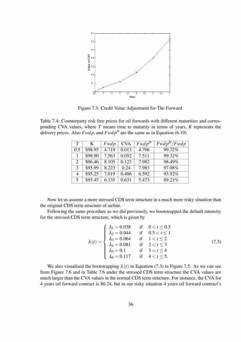
Figure 7.3: Credit Value Adjustment for The Forward

Table 7.4: Counterparty risk free prices for oil forwards with different maturities and corres-ponding CVA values, where T means time to maturity in terms of years, K represents thedelivery prices. Also Fwd p, and Fwd pD are the same as in Equation (6.10)

T K Fwd p CVA Fwd pD Fwd pD/Fwd p0.5 $98.95 4.719 0.013 4.706 99.72%1 $98.90 7.563 0.052 7.511 99.32%2 $96.46 8.105 0.123 7.982 98.49%3 $95.99 8.223 0.24 7.983 97.08%4 $95.25 7.019 0.406 6.592 93.92%5 $95.45 6.135 0.631 5.473 89.21%

Now let us assume a more stressed CDS term structure in a much more risky situation thanthe original CDS term structure of airline.

Following the same procedure as we did previously, we bootstrapped the default intensityfor the stressed CDS term structure, which is given by

λ (t) =

λ1 = 0.038 if 0 < t ≤ 0.5λ2 = 0.044 if 0.5 < t ≤ 1λ3 = 0.064 if 1 < t ≤ 2λ4 = 0.081 if 2 < t ≤ 3λ5 = 0.1 if 3 < t ≤ 4λ6 = 0.117 if 4 < t ≤ 5.

(7.3)

We also visualized the bootstrapping λ (t) in Equation (7.3) in Figure 7.5. As we can seefrom Figure 7.6 and in Table 7.6 under the stressed CDS term structure the CVA values aremuch larger than the CVA values in the normal CDS term structure. For instance, the CVA for4 years oil forward contract is $0.24, but in our risky situation 4 years oil forward contract’s

36

Figure 7.4: Price difference between counterparty risk free price and price after credit valueadjustment

Table 7.5: Stressed CDS spreads for the airline

maturities (years) 0.5 1 2 3 4 5CDS spreads (bps) 228 246 312 366 417 462

CVA value is $0.62. We can conclude that in the OTC trading when a company’s CDS spreadsincreases the counterparty of the financial contract should reevaluate the CVA.

37

Figure 7.5: Default intensities λ bootstrapped from the stressed CDS term structure

Table 7.6: Counterparty risk free prices for oil forwards with different maturities and corres-ponding CVA values under the stressed CDS term structure, where T means time to maturityin terms of years, Fwd p, and Fwd pD are the same as in Equation (6.10)

T K Fwd p CVA Fwd pD Fwd pD/Fwd p0.5 $98.95 4.719 0.041 4.678 99.13%1 $98.90 7.563 0.091 7.472 98.80%2 $96.46 8.105 0.298 7.807 96.23%3 $95.99 8.223 0.623 7.602 92.42%4 $95.25 7.019 1.116 5.903 84.1%5 $95.45 6.135 1.705 4.430 72.2%

38

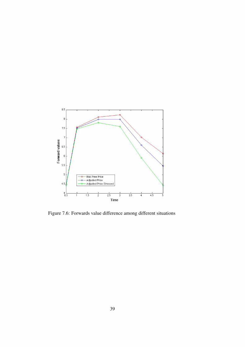
Figure 7.6: Forwards value difference among different situations

39

Chapter 8

Conclusion

In this paper we have computed the CVA for an oil forward. The default probability werebootstrapped from a CDS term structure by using a piecewise constant default intensity model.According to the results, there exists a significant positive correlation between the piecewiseconstant default intensity and the CDS term structure. As we can see from the CVA calcula-tions, the CVA has a considerable impact on the forward price. The longer the time to maturityT , the higher the CVA value. Hence, when a company enters an OTC derivative contract withanother party, it should consider the counterparty default risk. Moreover, with a longer timeto maturity, the company is exposed to greater counterparty risk that may strongly influencethe derivatives’ actual prices. We have discussed the CVA impact on forward prices for theairline example under the assumption that the commodity price and the counterparty defaulttime are independent. For future research, we could perhaps look at the CVA impact on for-ward prices if we do not assume that independence exists between underlying commodity andcounterparty default.

40

Bibliography

[Adm02] Energy Information Administration. Derivatives and risk management in the pet-roleum, natural gas, and electricity industries. October 2002.

[Ale10] Herbertsson Alexander. Credit risk modeling: Lecture notes. Gothenburg Univer-sity, December 2010.

[Ban09] European Central Bank. Credit default swap and counterparty risk. (9-11), August2009.

[BC06] R. Bruyère and R. Cont. Credit derivatives and structured credit: a guide forinvestors. Wiley, 2006.

[BCB08] D. Brigo, K. Chourdakis, and I. Bakkar. Counterparty risk valuation for energy-commodities swaps. 2008.

[Bed] Denise Bedell. Outstanding otc derivatives volumes 2006-2009.

[BL00] L. Borodovsky and M. Lore. The Professional’s Handbook of Financial Risk Man-agement. Butterworth-Heinemann, 2000.

[BOW03] C. Bluhm, L. Overbeck, and C. Wagner. An introduction to credit risk modeling.CRC Press, 2003.

[Cla02] E. Clark. International finance. Cengage Learning, 2002.

[Com01] Basel Committee. Operational risk. Basel Committee on Banking Supervision,page 2, May 2001.

[Dav11] Kelly David. The impact of basel iii on systemic risk and counterparty risk, 2011.

[EW03] A. Eydeland and K. Wolyniec. Energy and power risk management. Wiley, 2003.

[Fus07] P.C. Fusaro. The Professional Risk Managers’ Guide to the Energy Market.McGraw-Hill Professional, 2007.

[Gal03] R.R. Gallati. Risk management and capital adequacy. McGraw-Hill Companies,2003.

41

[Gre09] J. Gregory. Being two-faced over counterparty credit risk. Risk Magazine,22(2):86–90, 2009.

[Gre10] J. Gregory. Counterparty credit risk: the new challenge for global financial mar-kets. Wiley, 2010.

[GT10] Bugie Scott Grunspan Thierry, Kam Simon. Basel iii proposal to inscrease cap-ital requirements for counterparty credit risk may significantly affect derivativestrading. Global Credit Portal RatingDirec, Apirl 2010.

[HNW04] J. Hull, I. Nelken, and A. White. Merton’s model, credit risk, and volatility skews.Journal of Credit Risk Volume, 1(1):05, 2004.

[Jan07] Roman M Jan. Lecture notes in analytical finance ii. August 2007.

[Lan04] D. Lando. Credit risk modeling: theory and applications. Princeton Univ Pr, 2004.

[Mad08] J. Madura. Financial institutions and markets. South-Western Pub, 2008.

[Mer74] R.C. Merton. On the pricing of corporate debt: The risk structure of interest rates.The Journal of Finance, 29(2):449–470, 1974.

[OT03] D. O’Kane and S. Turnbull. Valuation of credit default swaps. Lehman BrothersQuantitative Credit Research Quarterly, 2003, 2003.

[SS00] E. Schwartz and J.E. Smith. Short-term variations and long-term dynamics incommodity prices. Management Science, pages 893–911, 2000.

[The11] TheCityUK. Commodities trading. Financial Market Series, March 2011.

[WTI] http://www.cmegroup.com/trading/energy/crude-oil/light-sweet-crude.html.

[ZP07] S. Zhu and M. Pykhtin. A guide to modeling counterparty credit risk. GARP RiskReview, 37:16–22, 2007.

42