master thesis - technische universität münchen · nese calligraphy. considering the existing...

TU Dortmund University and TU Munchen UniversityComputational Intelligence Research GroupDynamic Human Robot Interaction Group

Prof. Dr. Gunter RudolphProf. Dongheui Lee

Master Thesis

Robotic Calligraphy: Learning From Character Images

by

Omair Ali

Supervisors: Affan Pervez, M.Sc.

Internal Examiner: Prof. Dr. Gunter Rudolph

External Examiner: Prof. Dongheui Lee

Dortmund, October 06, 2015

DECLARATION

I hereby declare and confirm that the master thesis

Robotic Calligraphy: Learning From Character Images

is entirely the result of my own work except where otherwise indicated.

On the next page of this document, I have acknowledged the supervision,guidance and help I received from Prof. Dongheui Lee, Ph.D, M.Sc. AffanPervez and Prof. Dr. Gunter Rudolph.


Omair Ali

ACKNOWLEDGMENTS

This work was done in the department of Dynamische Mensch-Roboter-Interaktion fur Automatisierungstechnik, Technische Universitat Munchen andComputational Intelligence Research Group, Technische Universitat Dortmund.

I would like to thank Prof. Dongheui Lee, Ph.D. for giving me the op-portunity to work in this field of research. A special thanks to M.Sc. AffanPervez, without whom, this work would not have been possible. His constanthelp and guidance was vital in completion of this work. I would further liketo thank Prof. Dr. Gunter Rudolph for his constant support and suggestionsof improvement. Their recommendations and ideas helped me to compile thework in the best possible way.

In the end, I would like to thank my family for their constant support andencouragement.


Omair Ali

ABSTRACT

Known as the ”art of combining strokes to form complex letters”, Chi-nese and Korean Calligraphy has always been of vital significance through-out the history of these ancient civilizations. Its exquisite epitome of ele-gance is depicted through the strokes. A calligrapher assimilates the skillof drawing these strokes. Once this dexterity is mastered, it can be used tocompose a calligraphic letter afterwards. The very notion of calligraphy isendeavored to be implemented on robots in this research. Korean calligra-phy is the nucleus of this research work and the image of the calligraphiccharacter is used as an input. Unlike humans or calligraphers, the robotsare unacquainted with combination of various strokes used to draw a calli-graphic letter. Hence it is quite cardinal and arduous to fragment the calli-graphic letter into diverse strokes used to draw it. A novel approach ensu-ing the concept of Gaussian Mixture Model (GMM) is proposed to segregatethe input image into assorted strokes. Once the image is partitioned into dif-ferent strokes, the character is reproduced by blending the strokes in rightorder and right position using Gaussian Mixture Regression (GMR). Whencharacter is redrawn, Dynamic Movement Primitive (DMP) is applied to ac-quire the scale and temporal in-variance in the stroke trajectory. The param-eters learned through DMP are iteratively streamlined using ReinforcementLearning until they converge or don’t revamp any further.

I

CONTENTS

List of Figures III

1. Introduction 11.1. Highlights and Layout of the Report . . . . . . . . . . . . . . . 3

2. Theoretical Prerequisites 52.1. Gaussian Mixture Model (GMM) . . . . . . . . . . . . . . . . . 52.2. Expectation Maximization (EM) . . . . . . . . . . . . . . . . . . 82.3. Learning GMM Using EM . . . . . . . . . . . . . . . . . . . . . 9

2.3.1. Estimating the Optimal Number of Components . . . . . 102.4. Gaussian Mixture Regression (GMR) . . . . . . . . . . . . . . . 112.5. Dynamic Moment Primitives (DMPs) . . . . . . . . . . . . . . . 122.6. Reinforcement Learning (RL) . . . . . . . . . . . . . . . . . . . 14

3. Stroke Extraction 153.1. Thinning . . . . . . . . . . . . . . . . . . . . . . . . . . . . . . . 153.2. Image to Data Points . . . . . . . . . . . . . . . . . . . . . . . . 173.3. Gaussian Mixture Model on Data set . . . . . . . . . . . . . . . 183.4. Extracting End points of Stroke . . . . . . . . . . . . . . . . . . 203.5. Stroke Retrieval . . . . . . . . . . . . . . . . . . . . . . . . . . . 27

4. Character Reproduction 294.1. Thickness of Character . . . . . . . . . . . . . . . . . . . . . . . 29

5. Results 33

A. Eidesstattliche Versicherung iii

III

LIST OF FIGURES

1.1. (a)Input character and (b)Extraction result [17] . . . . . . . . . 2

2.1. Exemplification of the Bias and Variance. The higher the Biasis, the lower the accuracy from target is. With high variance,the target might be acquired but it can increase the variance inthe data resulting in over-fitting of the model. The best modelhas low unexplained variance and the bias. [onl] . . . . . . . . 9

2.2. Trade-off between bias and variance [onl] . . . . . . . . . . . . 10

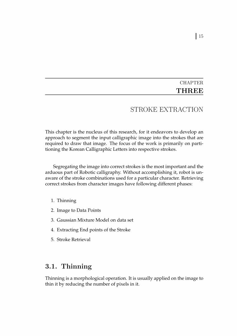
3.1. It has two parallel overlapping Gaussian Components on ex-treme left side of the character. . . . . . . . . . . . . . . . . . . 16

3.2. It has no parallel Gaussian Components . . . . . . . . . . . . . 173.3. It shows the conversion of input image into data points . . . . 183.4. GMM starting with high number of components . . . . . . . . 193.5. GMM with only one component . . . . . . . . . . . . . . . . . 193.6. GMM with optimal number of components. For this character

it is 9. . . . . . . . . . . . . . . . . . . . . . . . . . . . . . . . . 203.7. GMM with major axes of all the Gaussian Components, shown

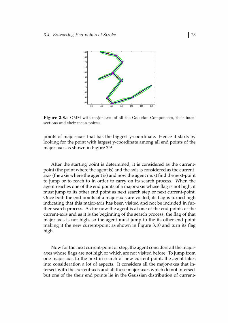
in blue color . . . . . . . . . . . . . . . . . . . . . . . . . . . . 223.8. GMM with major axes of all the Gaussian Components, their

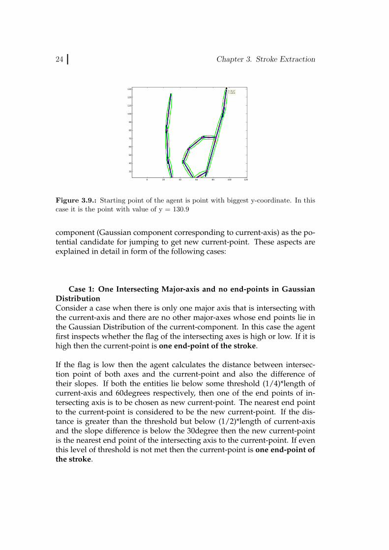
intersections and their mean points . . . . . . . . . . . . . . . . 233.9. Starting point of the agent is point with biggest y-coordinate.

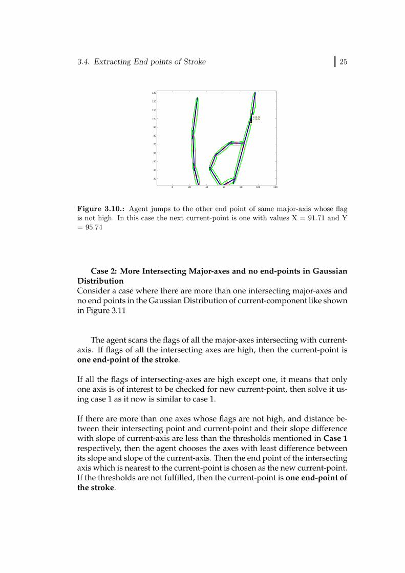
In this case it is the point with value of y = 130.9 . . . . . . . 243.10. Agent jumps to the other end point of same major-axis whose

flag is not high. In this case the next current-point is one withvalues X = 91.71 and Y = 95.74 . . . . . . . . . . . . . . . . . 25

3.11. A figure indicating more than one intersecting major-axes . . . 263.12. (a) A fully extracted Stroke in two strokes Character , (b)

Trajectory generated by GMR . . . . . . . . . . . . . . . . . . 283.13. Extracted Strokes of two stroke character . . . . . . . . . . . . 28

4.1. Thickness of the stroke by drawing circles. . . . . . . . . . . . . 294.2. Calligraphy letter drawn using drop model. . . . . . . . . . . . 30

5.1. (a),(b),(c),(d) Show the original images of the calligraphic char-acters. . . . . . . . . . . . . . . . . . . . . . . . . . . . . . . . 34

5.2. (a) Shows the character before reinforcement learning, (b) Showsthe character after 3 iterations, (c) Shows the character after7 iterations . . . . . . . . . . . . . . . . . . . . . . . . . . . . 35

5.3. (a) Shows the original Character, (b) Shows the character be-fore reinforcement learning, (c) Shows the character after 3iterations, (d) Shows the character after 7 iterations . . . . . . 35

5.4. (a) Shows the original Character, (b) Shows the character be-fore reinforcement learning, (c) Shows the character after 3iterations, (d) Shows the character after 7 iterations. . . . . . . 36

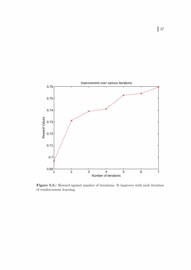
5.5. Reward against number of iterations. It improves with eachiteration of reinforcement learning. . . . . . . . . . . . . . . . . 37

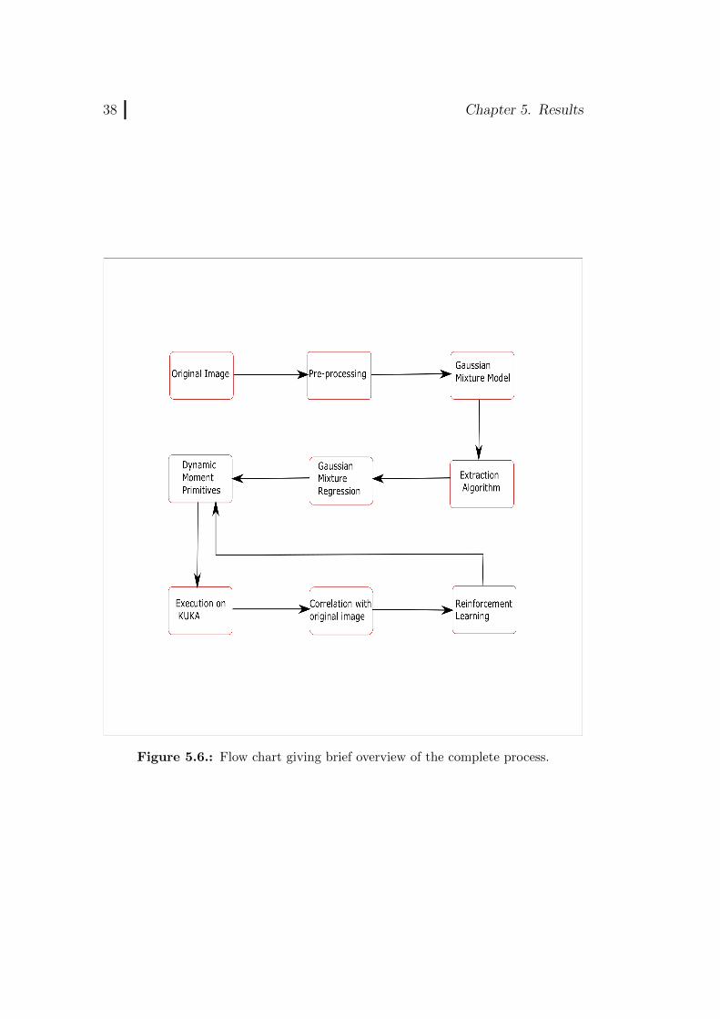
5.6. Flow chart giving brief overview of the complete process. . . . . 385.7. Complete overview of the stroke extraction and reproduction

of a character. . . . . . . . . . . . . . . . . . . . . . . . . . . . 39

1

CHAPTER

ONE

INTRODUCTION

In the contemporary era, extensive research work in field of robotics is ma-terializing to give birth to an artificial being, intelligent enough to competewith human counterparts. Without the aptitude of learning and transform-ing, no artificial entity is entitled to be intelligent. To inculcate these twobasic traits of intelligent agent in artificial body, the outlook must be in-spired from the most intelligent network on the face of the earth, the hu-man’s. Studies reveal that three strategies opted in Organic world to learnand transform are; Unsupervised Learning, Supervised Learning and Re-inforcement Learning. The abstract ideas of all these three schemes are ex-ploited in this research work for it is intrinsically quite captivating.

Unsupervised Learning pivots on retrieving some useful informationfrom the data under observation rather than us explicitly stipulating thesource or use of the data. It strives for finding pattern and structure in the in-complete data. Where as in Supervised Learning, labeled data is employedfor learning. Reinforcement learning can be defined as optimizing the per-formance of a system by trial and error

The cornerstone of this research work is to traverse the idea of KoreanCalligraphy on robots. Korean Calligraphy is an art of combining strokesto form complex letters. A calligrapher learns the skill of drawing thesestrokes rather than explicitly drawing the complete letter itself. The learnedstrokes can be used to draw complex letters afterwards.

The idea is to use the image of the calligraphic character and segregateit into different strokes used to form the letter. As stroke is the basic unitof a symbolic language, thus the basis of character analysis is stroke extrac-

2 Chapter 1. Introduction

tion. But unlike humans or calligraphers, the robots are unacquainted withcombination of various strokes used to draw a calligraphic letter. As it isquite predominant, fundamental and strenuous in calligraphy to identifythe strokes, it has been the area of interest for many researchers in recenttime.

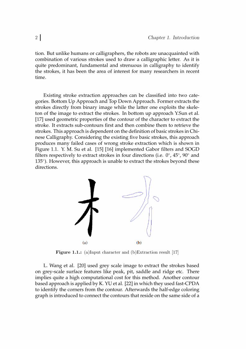
Existing stroke extraction approaches can be classified into two cate-gories. Bottom Up Approach and Top Down Approach. Former extracts thestrokes directly from binary image while the latter one exploits the skele-ton of the image to extract the strokes. In bottom up approach Y.Sun et al.[17] used geometric properties of the contour of the character to extract thestroke. It extracts sub-contours first and then combine them to retrieve thestrokes. This approach is dependent on the definition of basic strokes in Chi-nese Calligraphy. Considering the existing five basic strokes, this approachproduces many failed cases of wrong stroke extraction which is shown inFigure 1.1. Y. M. Su et al. [15] [16] implemented Gabor filters and SOGDfilters respectively to extract strokes in four directions (i.e. 0◦, 45◦, 90◦ and135◦). However, this approach is unable to extract the strokes beyond thesedirections.

Figure 1.1.: (a)Input character and (b)Extraction result [17]

L. Wang et al. [20] used grey scale image to extract the strokes basedon grey-scale surface features like peak, pit, saddle and ridge etc. Thereimplies quite a high computational cost for this method. Another contourbased approach is applied by K. YU et al. [22] in which they used fast-CPDAto identify the corners from the contour. Afterwards the half-edge coloringgraph is introduced to connect the contours that reside on the same side of a

1.1. Highlights and Layout of the Report 3

stroke. Matching contours on both sides of stroke finally results in completestroke.

In this research work we have proposed a novel idea of extracting strokesfrom Korean Calligraphic letters based on the Gaussian Mixture Model (GMM).Given the image of calligraphic letter as an input, it is first thinned and thenconverted into data points. Afterwards, GMM is applied to cluster the datapoints. Expectation Maximization algorithm is then implemented to learnthe parameters of GMM. Bayesian information criteria (BIC) is employed todetermine the number of components required by GMM to represent thedata. Once GMM is learned, the strokes are retrieved by combining respec-tive components(gaussians) based on proposed algorithm that represent thestroke and then Gaussian Mixture Regression (GMR) is applied to get thesmooth trajectory for the extracted strokes. As soon as strokes are retrieved,the trajectories encoded by GMM are re-encoded using Dynamic movementprimitives (DMPs) to reduce the number of parameters to learn during rein-forcement learning. The calligraphic brush is modeled as droplet to redrawthe character as a proof of concept. Then the learned dexterity is imple-mented on KUKA LWR robot. The reinforcement learning is brought intoservice to improve iteratively the reproduction of the drawn letter.

1.1. Highlights and Layout of the Report

Chapter 2 spans the theoretical prerequisites required to follow the proceed-ings of the report. In Chapter 3 the proposed idea for extracting strokes isbriefly described. Chapter 4 elaborates the complete work with help of ex-amples and results. The conclusion is presented in last chapter 5.

5

CHAPTER

TWO

THEORETICAL PREREQUISITES

In this chapter, the theoretical framework needed to fully understand thisresearch work are elaborated. First, a general summary of basic conceptscoupled with the modeling of Gaussian Mixture Model (GMM) is provided.The abstraction which entails to fully comprehend the modeling of GMMare:

1. Gaussian Mixture Model (GMM)

2. Expectation Maximization Algorithm (EM Algorithm)

3. Gaussian Mixture Regression (GMR)

Afterwards, an insight regarding Dynamic Movement Primitives is given.Then basics of Reinforcement Learning are briefly touched at the end of thischapter.

2.1. Gaussian Mixture Model (GMM)

A Gaussian Mixture Model [12], [4] is considered to be a simple linear su-perposition of K Gaussian components, which are combined to provide amultimodal density. It is quite beneficial for modeling data that is obtainedfrom one of several groups e.g. they can be utilized to implement a colorbased segmentation of an image or for clustering purpose. It is assumed tobe like kernel density estimates with components much less than total num-ber of data points

6 Chapter 2. Theoretical Prerequisites

A GMM is a probability based model. It presumes that all the datapoints are originated from a mixture of a finite number of Gaussian dis-tributions with known parameters. A GMM can be written as a linear su-perposition of these finite number of Gaussian distributions as:

p(y) =K∑k=1

πkN (y|µk,Σk) (2.1)

Where:K = fixed number of componentsπk = probability of kth componentµk = mean of the kth componentΣk = variance of the kth component

The parameters πk, µk and Σk of the Equation (2.1) are approximatedby maximizing the expected value of incomplete data log-likelihood. Toacquire the estimation of these parameters, first Latent Variables Z are pre-sented which is quite significant in providing the deeper insight into thedistribution and EM algorithm. Assume Z to be a K dimensional variablewith one of the K representations in which a particular element zk is oneand rest of the elements are equal to zero. The value of zk therefore fulfills∑K

k=1 zk = 1 and zk ∈ {0, 1}. Hence, the total number of representations ofthe latent variable are K where each representation relates to a certain classor basis function in the GMM. Mixing probabilities πk specify the marginaldistribution over Z such that:

p(z) =K∏k=1

πzkk

The conditional probability of data point x provided a particular valueof Z is Gaussian distributed and is given by:

p(y|z) =K∏k=1

(N (y|µk,Σk))zk (2.2)

The joint probability distribution is obtained by p(Z)p(y|Z), and themarginal distribution of x is then evaluated by adding the joint probabil-ity distribution over all possible states of Z which is written as:

2.1. Gaussian Mixture Model (GMM) 7

p(y) =∑Z

p(Z)p(y|Z) =K∑k=1


The equation achieved in (2.3) is the equivalent representation of a GMMby explicitly involving a latent variable Z. Let y = {y1, y2, ...yn} be the givenset of observations and data is to be modeled using a mixture of K Gaussiancomponents. The log-likelihood function of the data on the approximatedmodel is acquired as:

lnL(π, µ,Σ|y) = lnp(y|π, µ,Σ) =n∑

i=1

ln

{K∑k=1

πkN (yi|µk,Σk)

}(2.4)

The model corresponding to the values of parameters π,µ and Σ thatmaximize the function (2.4) for i.i.d dataset y best represents the data. Themaximization of (2.4) is very arduous because of the involvement of addi-tion terms inside the function of log. In fact, no closed form solution of theabove equation can be found if its gradient is put equal to zero. Hence asubstitute view of the likelihood, known as the completed log likelihood ofthe data is introduced. Assume that in addition to the observed data y, la-tent variables also known as hidden variables Z or the class labels are alsogiven. Considering the likelihood of the complete dataset {y, Z}, the likeli-hood function can be written as:

lnp(y, Z|π, µ,Σ) =n∑

i=1

K∑k=1

zki {lnπk + lnN (yi|µk,Σk)} (2.5)

Where, zki shows the responsibility of the kthcomponent in producingthe ithdata. Its value is known before hand in case of completed data. Whilecomparing the Equation (2.5) with Equation (2.4), it can be seen that sum-mation over K term is interchanged with logarithmic term, making the equa-tion a viable closed form solution. The completed likelihood and the incom-plete data likelihood can be related using the following identity:

L(π, µ,Σ|y, Z) = L(π, µ,Σ|y) +n∑

i=1

K∑k=1

zkilogwki

πk(2.6)


2.2. Expectation Maximization (EM)

Expectation Maximization (EM) [7] is a strong tool that, with the help oflatent variables, is employed to find the maximum likelihood solution formodels. It is purely an iteration based method for finding the maximumlikelihood, which implies that the means, co-variances and mixing coeffi-cients of the model are initialized with some appropriate initial values andthen iteratively refined through two steps namely:

1. Expectation Step (E-Step)

2. Maximization Step (M-Step)

E StepIn this step, the most recent values of parameters are used to calculate thePosterior probabilities for the data. Posterior probability or responsibilitycan be considered as the probability of ith data produced by kth componenti.e. p(zki = 1). It is mathematically formulated as:

wki =πkN (yi|µk,Σk)∑Kj=1 πjN (yi|µj,Σj)

(2.7)

M StepIn M step, the parameters that include mean, mixing coefficient and co-variance are updated or re-estimated based on Posterior probabilities cal-culated in E-Step by using:

µk =1

Nk

n∑i=1

wkiyi (2.8)

Σk =1

Nk

n∑i=1

wki(yi − µk)(yi − µk)T (2.9)

πk =Nk

n(2.10)

where

Nk =n∑

i=1

wki

2.3. Learning GMM Using EM 9

The above mentioned two steps are repeated until the Likelihood func-tion converges or there is not further significant change.

2.3. Learning GMM Using EM

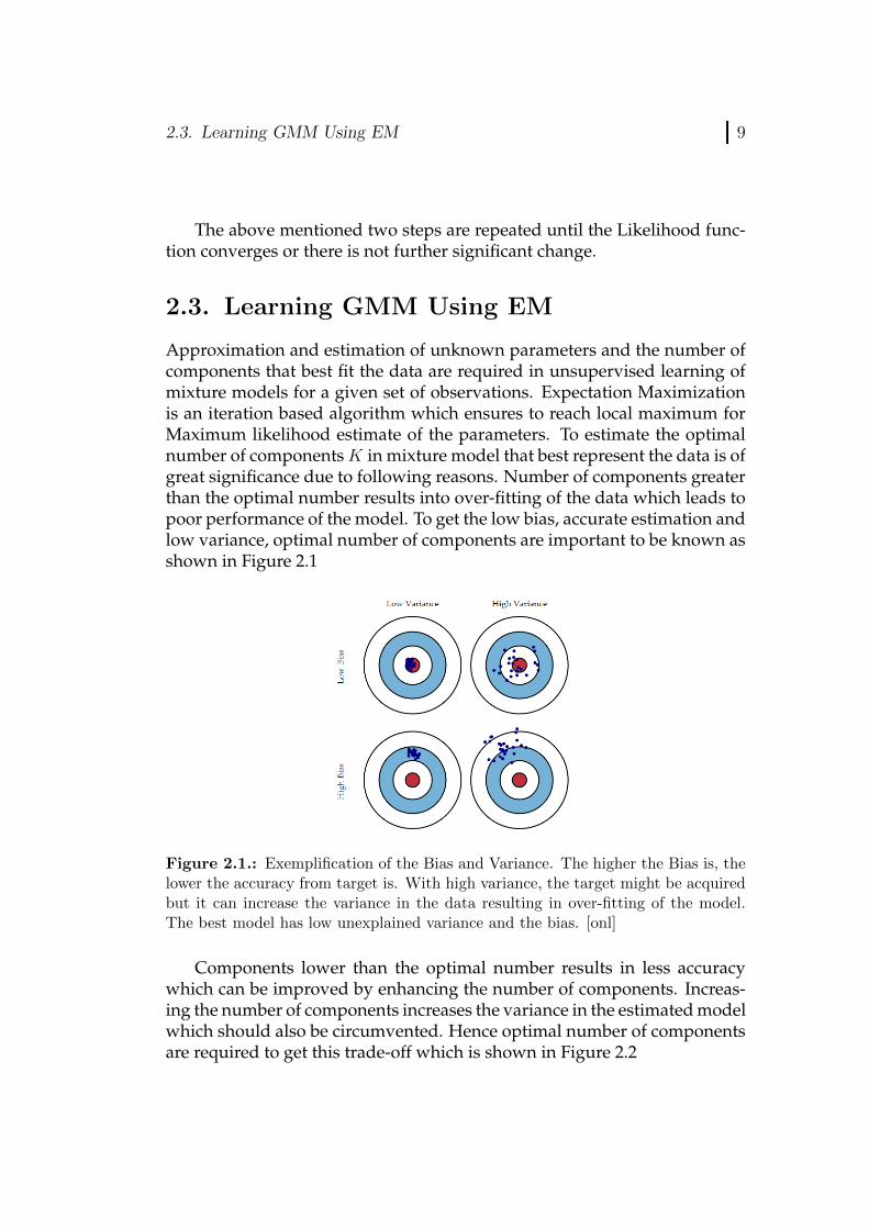
Approximation and estimation of unknown parameters and the number ofcomponents that best fit the data are required in unsupervised learning ofmixture models for a given set of observations. Expectation Maximizationis an iteration based algorithm which ensures to reach local maximum forMaximum likelihood estimate of the parameters. To estimate the optimalnumber of componentsK in mixture model that best represent the data is ofgreat significance due to following reasons. Number of components greaterthan the optimal number results into over-fitting of the data which leads topoor performance of the model. To get the low bias, accurate estimation andlow variance, optimal number of components are important to be known asshown in Figure 2.1

Figure 2.1.: Exemplification of the Bias and Variance. The higher the Bias is, thelower the accuracy from target is. With high variance, the target might be acquiredbut it can increase the variance in the data resulting in over-fitting of the model.The best model has low unexplained variance and the bias. [onl]

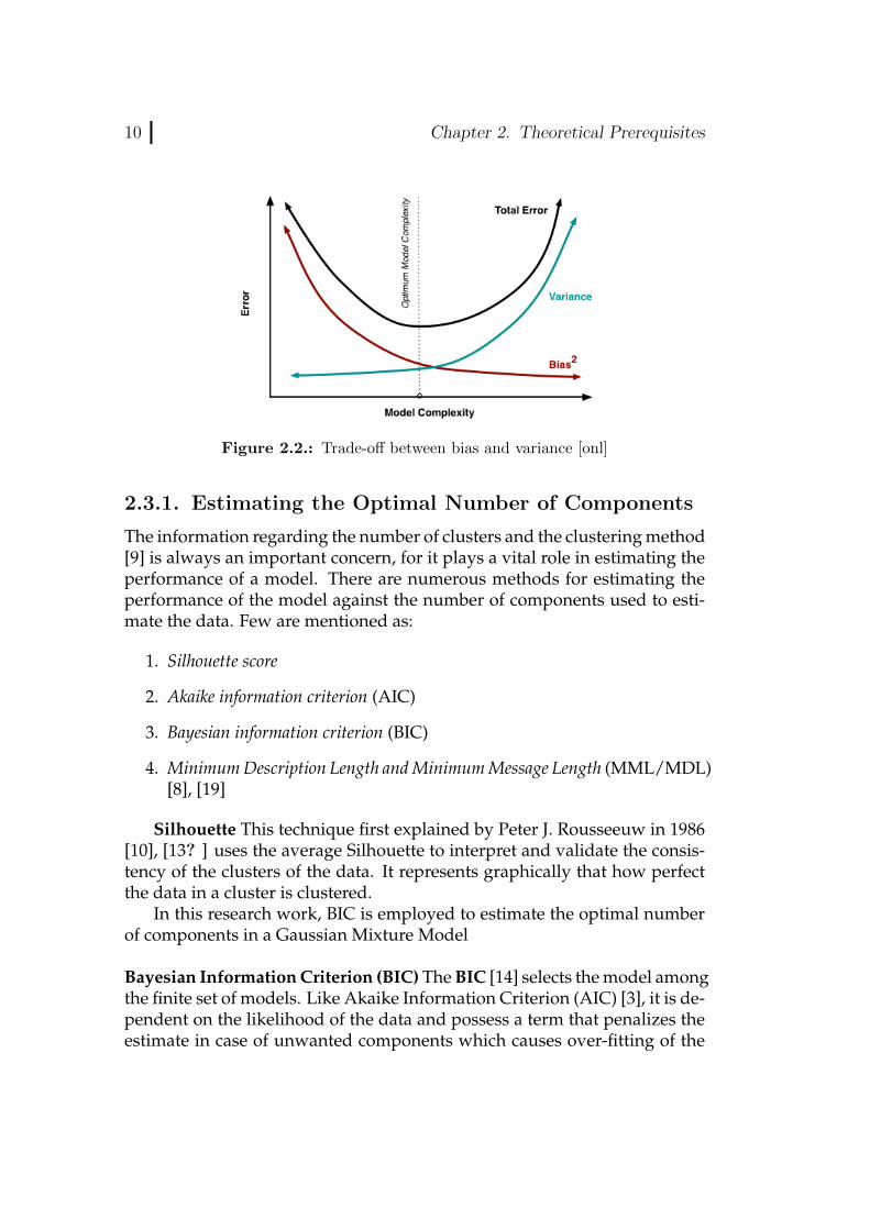
Components lower than the optimal number results in less accuracywhich can be improved by enhancing the number of components. Increas-ing the number of components increases the variance in the estimated modelwhich should also be circumvented. Hence optimal number of componentsare required to get this trade-off which is shown in Figure 2.2


Figure 2.2.: Trade-off between bias and variance [onl]

2.3.1. Estimating the Optimal Number of Components

The information regarding the number of clusters and the clustering method[9] is always an important concern, for it plays a vital role in estimating theperformance of a model. There are numerous methods for estimating theperformance of the model against the number of components used to esti-mate the data. Few are mentioned as:

1. Silhouette score

2. Akaike information criterion (AIC)

3. Bayesian information criterion (BIC)

4. Minimum Description Length and Minimum Message Length (MML/MDL)[8], [19]

Silhouette This technique first explained by Peter J. Rousseeuw in 1986[10], [13? ] uses the average Silhouette to interpret and validate the consis-tency of the clusters of the data. It represents graphically that how perfectthe data in a cluster is clustered.

In this research work, BIC is employed to estimate the optimal numberof components in a Gaussian Mixture Model

Bayesian Information Criterion (BIC) The BIC [14] selects the model amongthe finite set of models. Like Akaike Information Criterion (AIC) [3], it is de-pendent on the likelihood of the data and possess a term that penalizes theestimate in case of unwanted components which causes over-fitting of the

2.4. Gaussian Mixture Regression (GMR) 11

data. The penalty term is non-linear and take into consideration the samplesize and total number of observations that estimated the model. It is math-ematically written as:

BIC = Dkln(n)− 2lnL (2.11)

where,

Dk = number of parameters in K-component model L = likelihood of thedata on estimated model

In other words, it is a trade-off between complexity and the likelihoodof the model. For number of components K for which BIC is lowest, are theoptimal number of components.

2.4. Gaussian Mixture Regression (GMR)

Linear combination of Gaussian and conditional Gaussian densities are thebasis of GMR [5]. Once, the input data is modeled by GMM, Gaussian Mix-ture Regression gives a quick and analytic way to get smooth output tra-jectories in addition to covariance matrices that explain the change and cor-relation among various variables. At the time of fitting GMM on dataset,there is no difference between input and output variables. In a special caseof trajectory learning, time can be referred to as an Input variable yI and po-sition can be considered as output variable yO and the goal is to reproducethe trajectory (yO) or part of it provided a time step yI . The data y modeledusing GMM can be segregated into input yI and output variables yO.

The probability of a data point y = [yI , yO] that corresponds to GMM dis-tribution is shown as.

p(y) =K∑k=1


where the parameters: means µk and co-variance matrices Σk are com-posed of input and output components and are represented as:

µk =

[µIk

µOk

],

[ΣI

k ΣIOk

ΣOIk ΣI

k

](2.13)


The distribution of output variable yO given the corresponding inputvariable yI and Component k is written as:

p(yO|yI , k

)= N (ζk, ςk)

where

ζk = µOk + ΣOI

k

(ΣI

k

)−1 (yI − µI

k

)ς = ΣO

k − ΣOIk

(ΣI

k

)−1ΣIO

k

(2.14)

Taking into consideration the whole Gaussian Mixture model, the prob-ability distribution of yO given yI is written as:

p(yO|yI

)≈ ΣK

k=1hkN (ζk, ςk)

where :

hk =πkp(y

I |k)

ΣKj=1πjp(y

I |j)

(2.15)

Hence, Gaussian Mixture Regression can be used to regenerate the skill,once an optimal Gaussian Mixture Model is at hand.

2.5. Dynamic Moment Primitives (DMPs)

Dynamic Movement Primitives [11] are utilized to encode a trajectory. Theywere first proposed by Stefan Schaal’s Lab in 2002. Trajectories encoded us-ing GMM have high number of free parameters to update in reinforcementlearning. So to reduce the number of free parameters while applying rein-forcement learning, DMPs are introduced and the trajectories encoded us-ing GMM are now encoded using DMPs. The motion generated using themare highly stable and it can be used to encode both discrete and rhythmicmotions. In this research work, DMPs were used only for discrete move-ments.

It has a hidden system known as canonical system

z = u(z)

which drives the transformed system

x = v(x, z, g, θ)

2.5. Dynamic Moment Primitives (DMPs) 13

for all degrees of freedom (DoFs) i, where θ is the parameter to be learned.Desired positions x1 and the velocities q = τx2 of the robot either in jointspace or in the task space are used as the states x = [x1,x2] of the transformedsystem. Accelerations are calculated by q = τ x2. These are converted intotorques or forces required by the robot using a controller. It ensures the sta-bility of the movement. As only discrete movements are considered in thisresearch work hence only the corresponding policies of DMPs are provided.In case of only single discrete movement the canonical form u can be rep-resented as: z = −ταzz. Here τ = 1/T time constant where T is the totalduration of a MP. The value of the parameter αz is selected such that it en-sures the safe termination of the movement. It is chosen such that value ofz approaches zero at T. The transformed function v is shown in the form:

x2 = ταx(βx(g − x1)− x2) + τAf(z)

x1 = τx2

Here the value of τ is same as that of the canonical system. The values ofthe parameters αx and βx are chosen so that the system is critically dampedat A = 0. g is goal and f is a transformation function and A is a diagonalmatrix that modify the amplitude. The matrix A ensures linear re-scalingwhen the the goal is varied. The transformation function varies the outputof the transformed system and is given by:

f(z) =N∑

n=1

ψn(z)θnz

Here θn contains the nth set of adjustable parameters for all DoFs. N is thenumber of parameters per DoF. z is the value of canonical system. ψn(z) arethe corresponding weights which are given by:

f(z) =exp(−h−2

n (z − cn)2)∑Nm=1 exp(−h−2

m (z − cm)2)

Each DoF has a separate DMP and the parameters for each DoF arelearned separately. The cost function that needs to be minimized for all pa-rameters θn is given in form of weighted squared error: e2n =

∑Tt=1 ψ

nt (f ref

t −ztθ

n)2.The error written in matrix form is given as:

e2n = (f ref − Zθn)Tψ(f ref − Zθn)

Here θn is given by:


θn = (ZTψZ)−1ZTψf ref

Here f ref contains the values of f reft for all samples.

2.6. Reinforcement Learning (RL)

Reinforcement learning can be defined as optimizing the performance of asystem by trial and error. In this research EM based RL mentioned in [6] isemployed. In this RL the update policy is given by:

θ(n) = θ(n−1) +

∑Mm r(θm)[θm − θ(n−1)]∑M

m r(θm)(2.16)

where:θ(n) = Learned parameters of DMP.θ(n−1) = Old parameters of DMP.r(θm) = Reward.θm = Perturbed parameters of DMP.The difference between perturbed and old parameters of DMP [11] θm −θ(n−1) are Exploration terms and give relative exploration between parame-ters in mth iteration and current parameters. In this research, reward (r(θm))is the correlation between original image and image produced by robot.The exploration terms are weighted by the respective correlation r(θm) andnormalized by the sum of other correlations. They are sampled from normaldistribution. It is expressed as co-variance matrix and updated as:

∑n=

∑Mm r(θm)[θm − θ(n−1)][θm − θ(n−1)]T∑M

m r(θm)+∑

0(2.17)

where:∑0 = is a regularization term corresponding to a minimum exploration

noise used to avoid premature convergence to poor local optima.The equations mentioned form a multivariate normal distribution at eachiteration. The covariance can guide the exploration and it also provides in-formation about the neighborhood of the policy solutions.

15

CHAPTER

THREE

STROKE EXTRACTION

This chapter is the nucleus of this research, for it endeavors to develop anapproach to segment the input calligraphic image into the strokes that arerequired to draw that image. The focus of the work is primarily on parti-tioning the Korean Calligraphic Letters into respective strokes.

Segregating the image into correct strokes is the most important and thearduous part of Robotic calligraphy. Without accomplishing it, robot is un-aware of the stroke combinations used for a particular character. Retrievingcorrect strokes from character images have following different phases:

1. Thinning

2. Image to Data Points

3. Gaussian Mixture Model on data set

4. Extracting End points of the Stroke

5. Stroke Retrieval

3.1. Thinning

Thinning is a morphological operation. It is usually applied on the image tothin it by reducing the number of pixels in it.

16 Chapter 3. Stroke Extraction

40 60 80 100 120 140

50

60

70

80

90

100

110

120

130

Figure 3.1.: It has two parallel overlapping Gaussian Components on extreme leftside of the character.

In this phase, the image is thinned or in other words the data points arereduced to get a thinned image. This is quite an important phase in the pro-cess because it ensures in the later stage that when Gaussian Mixture Modelis applied on the data points, it does not model the thickness of the charac-ter and there are no parallel or random Gaussian Components. Presence ofparallel Gaussian components as shown in Figure 3.1 make it quite difficultto extract the strokes and also the thinning is helpful in reducing the com-putation time because it does not contain all the data points.

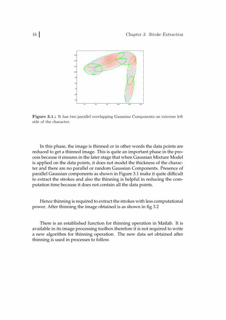
Hence thinning is required to extract the strokes with less computationalpower. After thinning the image obtained is as shown in fig 3.2

There is an established function for thinning operation in Matlab. It isavailable in its image processing toolbox therefore it is not required to writea new algorithm for thinning operation. The new data set obtained afterthinning is used in processes to follow.

3.2. Image to Data Points 17

40 50 60 70 80 90 100 110 120 130

50

60

70

80

90

100

110

120

Figure 3.2.: It has no parallel Gaussian Components

3.2. Image to Data Points

This is the second phase in stroke extraction process. In this phase the inputimage is converted into data points so as to make the image compatible forapplying Gaussian Mixture Model later on.

It is the most basic step in the process and is shown in fig3.3

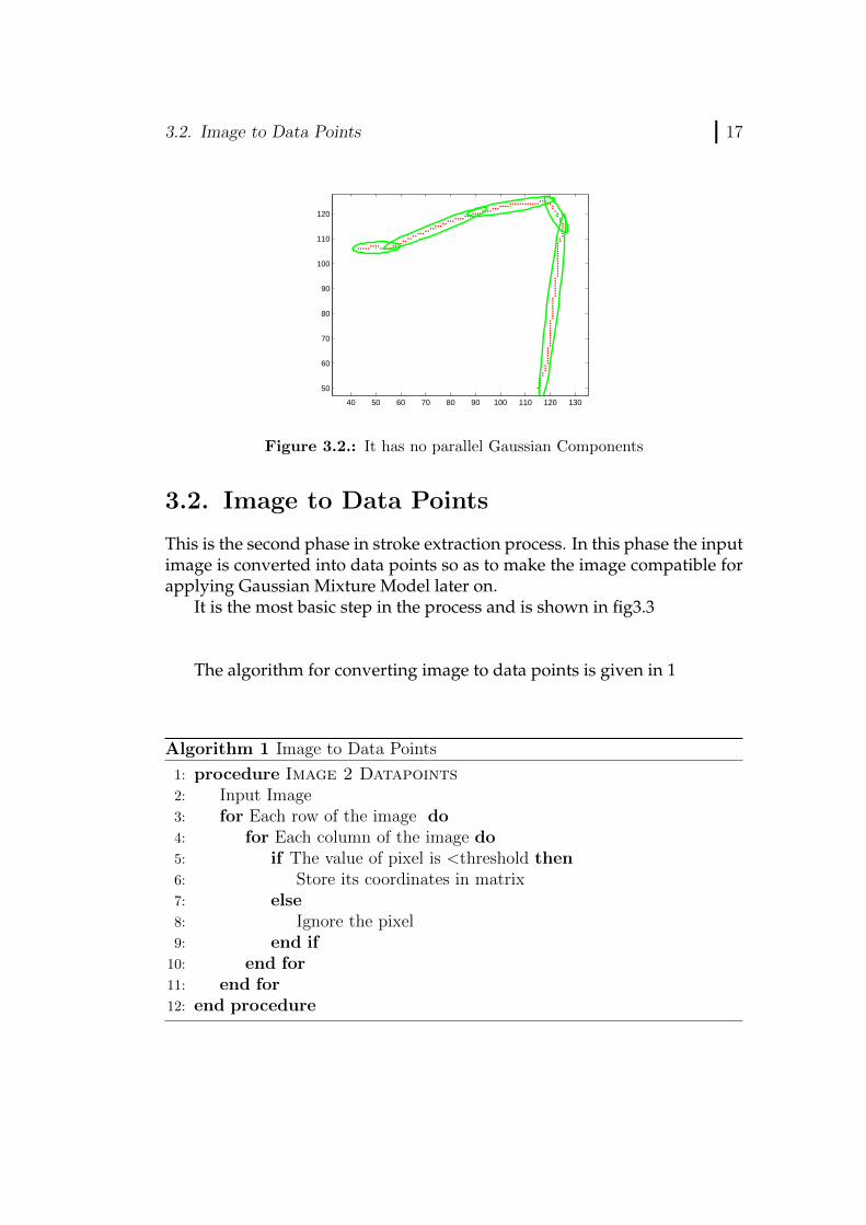
The algorithm for converting image to data points is given in 1

Algorithm 1 Image to Data Points

1: procedure Image 2 Datapoints2: Input Image3: for Each row of the image do4: for Each column of the image do5: if The value of pixel is <threshold then6: Store its coordinates in matrix7: else8: Ignore the pixel9: end if

10: end for11: end for12: end procedure


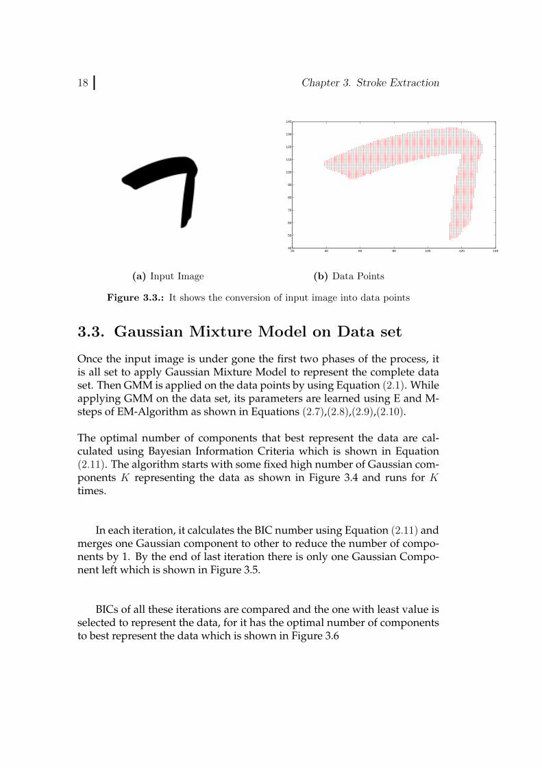
(a) Input Image

20 40 60 80 100 120 14040

50

60

70

80

90

100

110

120

130

140

(b) Data Points

Figure 3.3.: It shows the conversion of input image into data points

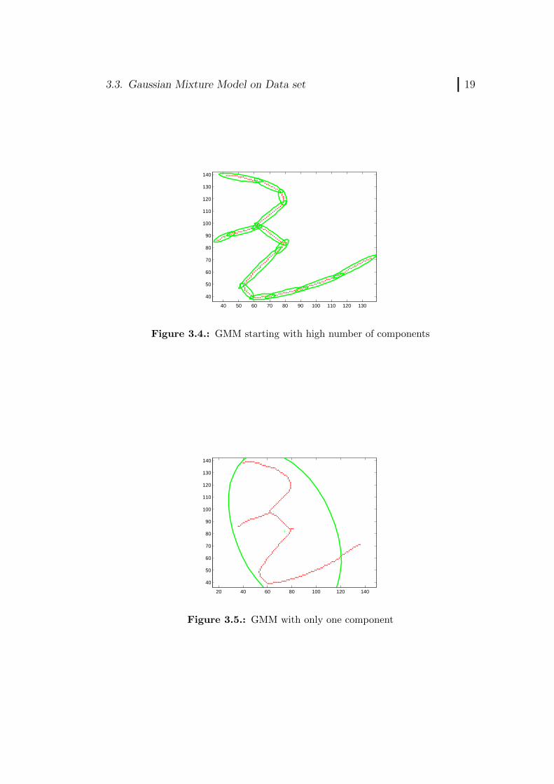
3.3. Gaussian Mixture Model on Data set

Once the input image is under gone the first two phases of the process, itis all set to apply Gaussian Mixture Model to represent the complete dataset. Then GMM is applied on the data points by using Equation (2.1). Whileapplying GMM on the data set, its parameters are learned using E and M-steps of EM-Algorithm as shown in Equations (2.7),(2.8),(2.9),(2.10).

The optimal number of components that best represent the data are cal-culated using Bayesian Information Criteria which is shown in Equation(2.11). The algorithm starts with some fixed high number of Gaussian com-ponents K representing the data as shown in Figure 3.4 and runs for Ktimes.

In each iteration, it calculates the BIC number using Equation (2.11) andmerges one Gaussian component to other to reduce the number of compo-nents by 1. By the end of last iteration there is only one Gaussian Compo-nent left which is shown in Figure 3.5.

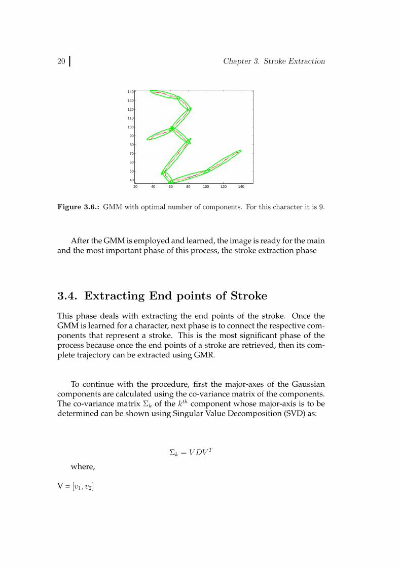
BICs of all these iterations are compared and the one with least value isselected to represent the data, for it has the optimal number of componentsto best represent the data which is shown in Figure 3.6

3.3. Gaussian Mixture Model on Data set 19

40 50 60 70 80 90 100 110 120 130

40

50

60

70

80

90

100

110

120

130

140

Figure 3.4.: GMM starting with high number of components

20 40 60 80 100 120 140

40

50

60

70

80

90

100

110

120

130

140

Figure 3.5.: GMM with only one component


20 40 60 80 100 120 140

40

50

60

70

80

90

100

110

120

130

140

Figure 3.6.: GMM with optimal number of components. For this character it is 9.

After the GMM is employed and learned, the image is ready for the mainand the most important phase of this process, the stroke extraction phase

3.4. Extracting End points of Stroke

This phase deals with extracting the end points of the stroke. Once theGMM is learned for a character, next phase is to connect the respective com-ponents that represent a stroke. This is the most significant phase of theprocess because once the end points of a stroke are retrieved, then its com-plete trajectory can be extracted using GMR.

To continue with the procedure, first the major-axes of the Gaussiancomponents are calculated using the co-variance matrix of the components.The co-variance matrix Σk of the kth component whose major-axis is to bedetermined can be shown using Singular Value Decomposition (SVD) as:

Σk = V DV T

where,

V = [v1, v2]

3.4. Extracting End points of Stroke 21

Matrix whose columns are eigenvectors of Σk and it satisfies Σ*V = D*V

D = Diagonal matrix that contains the eigenvalues of Σk along the maindiagonal and for 2x2 square matrix, it is written as:

[λ211 00 λ222

]Here values of λ are calculated by solving det(Σk − λI) = 0

For each eigenvalue, its corresponding eigenvector is calculated by solvingthe following equation:

Σk ∗ v1 = λ11 ∗ v1,Σk ∗ v2 = λ22 ∗ v2Once the eigenvalues matrix D and eigenvectors matrix V are calculated,

arrange them in such an order that vector v1 is major eigenvector and λ11 isthe corresponding biggest eigenvalue. Then the two end points of the majoraxes of the Gaussian components are calculated by using the Equation (3.1)

endpoint1 = µk + 2 ∗ λ11 ∗ v1endpoint2 = µk − 2 ∗ λ11 ∗ v1

(3.1)

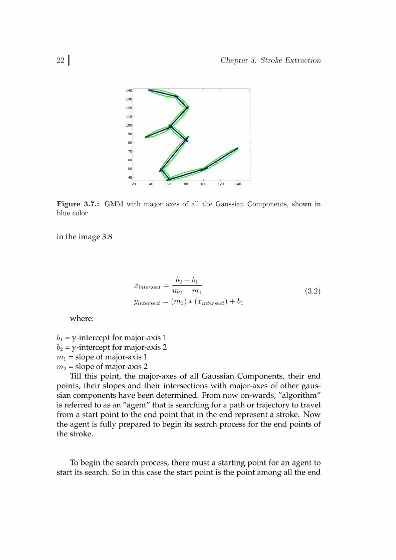
Here µk is the mean of gaussian component k whose major axis is beingdetermined. As most of the points lie in 2σ standard deviation, thereforefactor of 2 is multiplied with eigenvalues and eigenvectors in the Equation(3.1). Now by joining the two endpoints calculated above, major axis of thegaussian component is obtained. This procedure is done as many time asnumber of components K in GMM are and store the endpoints of all themajor-axes . Once the major axes of all the components are found, they aredrawn on the GMM as shown in Figure 3.7

After the major axes have been retrieved, their slopes are calculated us-ing the basic slope formula. Intersection of major axes of two components(say major-axes 1 and 2) are calculated using the Equation 3.2. After calcu-lating all the intersection points, they are also drawn on the GMM as shown


20 40 60 80 100 120 140

40

50

60

70

80

90

100

110

120

130

140

Figure 3.7.: GMM with major axes of all the Gaussian Components, shown inblue color

in the image 3.8

xintersect =b2 − b1m2 −m1

yintersect = (m1) ∗ (xintersect) + b1

(3.2)

where:

b1 = y-intercept for major-axis 1b2 = y-intercept for major-axis 2m1 = slope of major-axis 1m2 = slope of major-axis 2

Till this point, the major-axes of all Gaussian Components, their endpoints, their slopes and their intersections with major-axes of other gaus-sian components have been determined. From now on-wards, ”algorithm”is referred to as an ”agent” that is searching for a path or trajectory to travelfrom a start point to the end point that in the end represent a stroke. Nowthe agent is fully prepared to begin its search process for the end points ofthe stroke.

To begin the search process, there must a starting point for an agent tostart its search. So in this case the start point is the point among all the end


20 40 60 80 100 120 140

40

50

60

70

80

90

100

110

120

130

140

Figure 3.8.: GMM with major axes of all the Gaussian Components, their inter-sections and their mean points

points of major-axes that has the biggest y-coordinate. Hence it starts bylooking for the point with largest y-coordinate among all end points of themajor-axes as shown in Figure 3.9

After the starting point is determined, it is considered as the current-point (the point where the agent is) and the axis is considered as the current-axis (the axis where the agent is) and now the agent must find the next-pointto jump or to reach to in order to carry on its search process. When theagent reaches one of the end points of a major-axis whose flag is not high, itmust jump to its other end point as next search step or next current-point.Once both the end points of a major-axis are visited, its flag is turned highindicating that this major-axis has been visited and not be included in fur-ther search process. As for now the agent is at one of the end points of thecurrent-axis and as it is the beginning of the search process, the flag of thatmajor-axis is not high, so the agent must jump to the its other end pointmaking it the new current-point as shown in Figure 3.10 and turn its flaghigh.

Now for the next current-point or step, the agent considers all the major-axes whose flags are not high or which are not visited before. To jump fromone major-axis to the next in search of new current-point, the agent takesinto consideration a lot of aspects. It considers all the major-axes that in-tersect with the current-axis and all those major-axes which do not intersectbut one of the their end points lie in the Gaussian distribution of current-


0 20 40 60 80 100 120

30

40

50

60

70

80

90

100

110

120

130X: 96.27Y: 130.9

Figure 3.9.: Starting point of the agent is point with biggest y-coordinate. In thiscase it is the point with value of y = 130.9

component (Gaussian component corresponding to current-axis) as the po-tential candidate for jumping to get new current-point. These aspects areexplained in detail in form of the following cases:

Case 1: One Intersecting Major-axis and no end-points in GaussianDistributionConsider a case when there is only one major axis that is intersecting withthe current-axis and there are no other major-axes whose end points lie inthe Gaussian Distribution of the current-component. In this case the agentfirst inspects whether the flag of the intersecting axes is high or low. If it ishigh then the current-point is one end-point of the stroke.

If the flag is low then the agent calculates the distance between intersec-tion point of both axes and the current-point and also the difference oftheir slopes. If both the entities lie below some threshold (1/4)*length ofcurrent-axis and 60degrees respectively, then one of the end points of in-tersecting axis is to be chosen as new current-point. The nearest end pointto the current-point is considered to be the new current-point. If the dis-tance is greater than the threshold but below (1/2)*length of current-axisand the slope difference is below the 30degree then the new current-pointis the nearest end point of the intersecting axis to the current-point. If eventhis level of threshold is not met then the current-point is one end-point ofthe stroke.


0 20 40 60 80 100 120

30

40

50

60

70

80

90

100

110

120

130

X: 91.71Y: 95.74

Figure 3.10.: Agent jumps to the other end point of same major-axis whose flagis not high. In this case the next current-point is one with values X = 91.71 and Y= 95.74

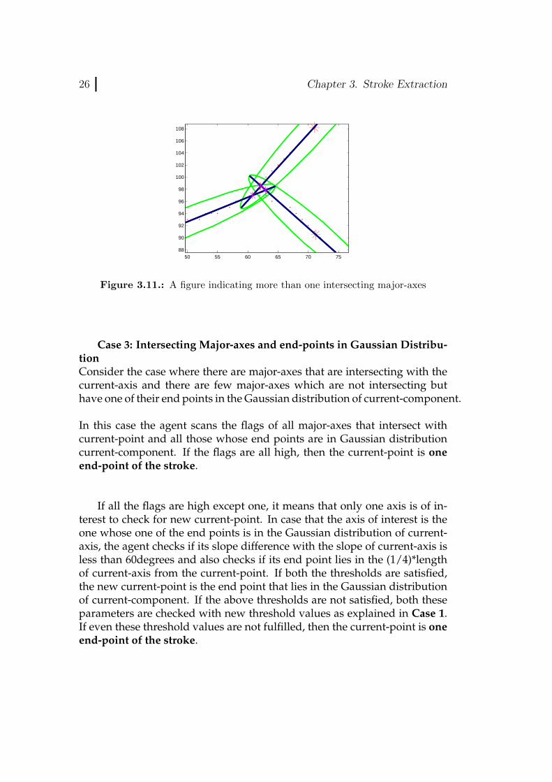
Case 2: More Intersecting Major-axes and no end-points in GaussianDistributionConsider a case where there are more than one intersecting major-axes andno end points in the Gaussian Distribution of current-component like shownin Figure 3.11

The agent scans the flags of all the major-axes intersecting with current-axis. If flags of all the intersecting axes are high, then the current-point isone end-point of the stroke.

If all the flags of intersecting-axes are high except one, it means that onlyone axis is of interest to be checked for new current-point, then solve it us-ing case 1 as it now is similar to case 1.

If there are more than one axes whose flags are not high, and distance be-tween their intersecting point and current-point and their slope differencewith slope of current-axis are less than the thresholds mentioned in Case 1respectively, then the agent chooses the axes with least difference betweenits slope and slope of the current-axis. Then the end point of the intersectingaxis which is nearest to the current-point is chosen as the new current-point.If the thresholds are not fulfilled, then the current-point is one end-point ofthe stroke.


50 55 60 65 70 7588

90

92

94

96

98

100

102

104

106

108

Figure 3.11.: A figure indicating more than one intersecting major-axes

Case 3: Intersecting Major-axes and end-points in Gaussian Distribu-tionConsider the case where there are major-axes that are intersecting with thecurrent-axis and there are few major-axes which are not intersecting buthave one of their end points in the Gaussian distribution of current-component.

In this case the agent scans the flags of all major-axes that intersect withcurrent-point and all those whose end points are in Gaussian distributioncurrent-component. If the flags are all high, then the current-point is oneend-point of the stroke.

If all the flags are high except one, it means that only one axis is of in-terest to check for new current-point. In case that the axis of interest is theone whose one of the end points is in the Gaussian distribution of current-axis, the agent checks if its slope difference with the slope of current-axis isless than 60degrees and also checks if its end point lies in the (1/4)*lengthof current-axis from the current-point. If both the thresholds are satisfied,the new current-point is the end point that lies in the Gaussian distributionof current-component. If the above thresholds are not satisfied, both theseparameters are checked with new threshold values as explained in Case 1.If even these threshold values are not fulfilled, then the current-point is oneend-point of the stroke.

3.5. Stroke Retrieval 27

If there are more than one axes whose flags are not high, use the conceptmentioned in Case 2 to determine the new current-point or one end-pointof the stroke. The agent repeats the above method based on the case en-countered till one of the end points of the stroke are determined.

By now one of the end points of the stroke has been found by the agent.Agent uses this determined end point of the stroke as a starting point orstarting current-point to find the other end point of the same stroke by em-ploying the same method (the flags are reset) as mentioned above based onthe case encountered by it during its search policy. It also stores the order inwhich the major-axes are visited to get the trajectory of the stroke.

Once both end points of the same stroke are determined, these are storedand the flags of major-axes used in this process are permanently turned highand not used in finding the end points of other stroke. This process is re-peated till end points of all the strokes are determined.

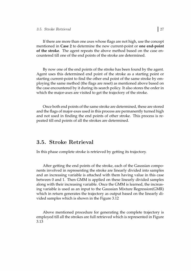
3.5. Stroke Retrieval

In this phase complete stroke is retrieved by getting its trajectory.

After getting the end points of the stroke, each of the Gaussian compo-nents involved in representing the stroke are linearly divided into samplesand an increasing variable is attached with them having value in this casebetween 0 and 1. Then GMM is applied on these linearly divided samplesalong with their increasing variable. Once the GMM is learned, the increas-ing variable is used as an input to the Gaussian Mixture Regression(GMR)which in return generates the trajectory as output based on the linearly di-vided samples which is shown in the Figure 3.12

Above mentioned procedure for generating the complete trajectory isemployed till all the strokes are full retrieved which is represented in Figure3.13


0 20 40 60 80 100 12020

30

40

50

60

70

80

90

100

110

120

130

(a)

0

20

40

60

80

100

2040

6080

100120

0

50

100

(b)

Figure 3.12.: (a) A fully extracted Stroke in two strokes Character , (b) Trajectorygenerated by GMR

20 40 60 80 100 120

20

30

40

50

60

70

80

90

100

110

Figure 3.13.: Extracted Strokes of two stroke character

Once all the strokes are extracted, the character can be reproduced bythe robot by drawing the extracted strokes in order. A stroke encoded us-ing GMM has a high number of free parameters which become problematicwhen applying RL. Hence, to reduce the number of parameters, the trajecto-ries extracted using GMR are re-encoded using DMPs before reproduction.The reproduction phase is discussed in following chapter.

29

CHAPTER

FOUR

CHARACTER REPRODUCTION

This chapter describes the reproduction phase of the character. Accurate re-production of the character is possible only when its thickness informationis known before hand.

4.1. Thickness of Character

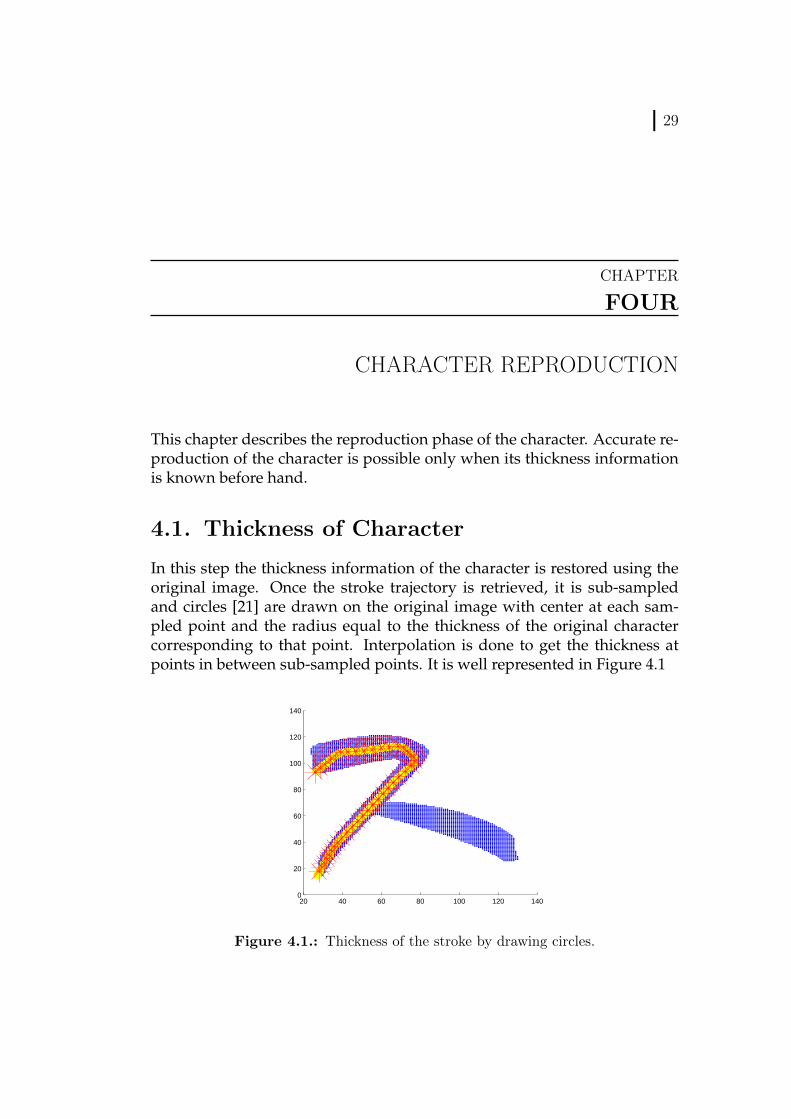
In this step the thickness information of the character is restored using theoriginal image. Once the stroke trajectory is retrieved, it is sub-sampledand circles [21] are drawn on the original image with center at each sam-pled point and the radius equal to the thickness of the original charactercorresponding to that point. Interpolation is done to get the thickness atpoints in between sub-sampled points. It is well represented in Figure 4.1

20 40 60 80 100 120 1400

20

40

60

80

100

120

140

Figure 4.1.: Thickness of the stroke by drawing circles.

30 Chapter 4. Character Reproduction

The thickness information is quite crucial in correct reproduction of thecharacter.

The reproduction phase can further be partitioned into following partsnamely:

1. Trajectory encoding by DMPs

2. Reproduction of Trajectory

3. Iterative Improvement of trajectory using Reinforcement Learning

Trajectory encoding by DMPs In order to improve the learned skill, theparameters of the extracted trajectory must be updated iteratively. A strokeencoded using GMM has high number of free parameters which becomeproblematic when applying reinforcement learning because the number offree parameters to update increase tremendously which results in high com-putational cost and time to converge to better result. Hence, to reduce thenumber of parameters, the trajectories extracted using GMR are re-encodedusing DMPs. Each stroke in the character has an individual DMP.

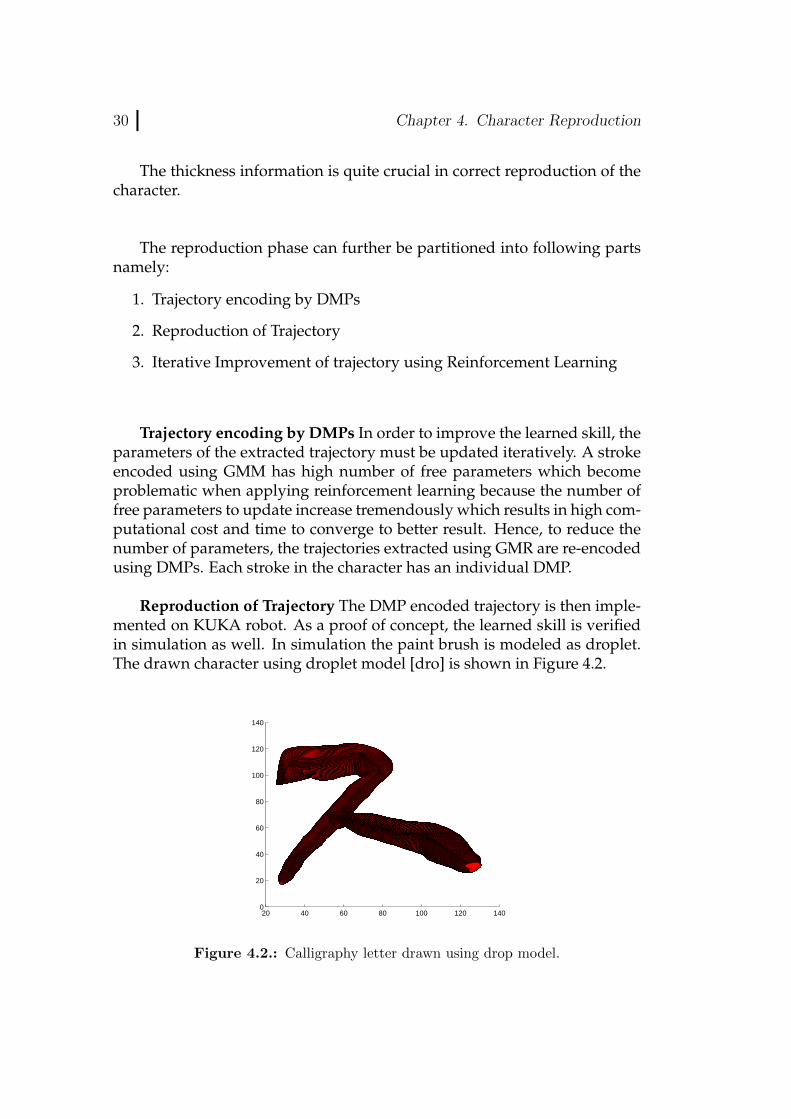
Reproduction of Trajectory The DMP encoded trajectory is then imple-mented on KUKA robot. As a proof of concept, the learned skill is verifiedin simulation as well. In simulation the paint brush is modeled as droplet.The drawn character using droplet model [dro] is shown in Figure 4.2.

20 40 60 80 100 120 1400

20

40

60

80

100

120

140

Figure 4.2.: Calligraphy letter drawn using drop model.

4.1. Thickness of Character 31

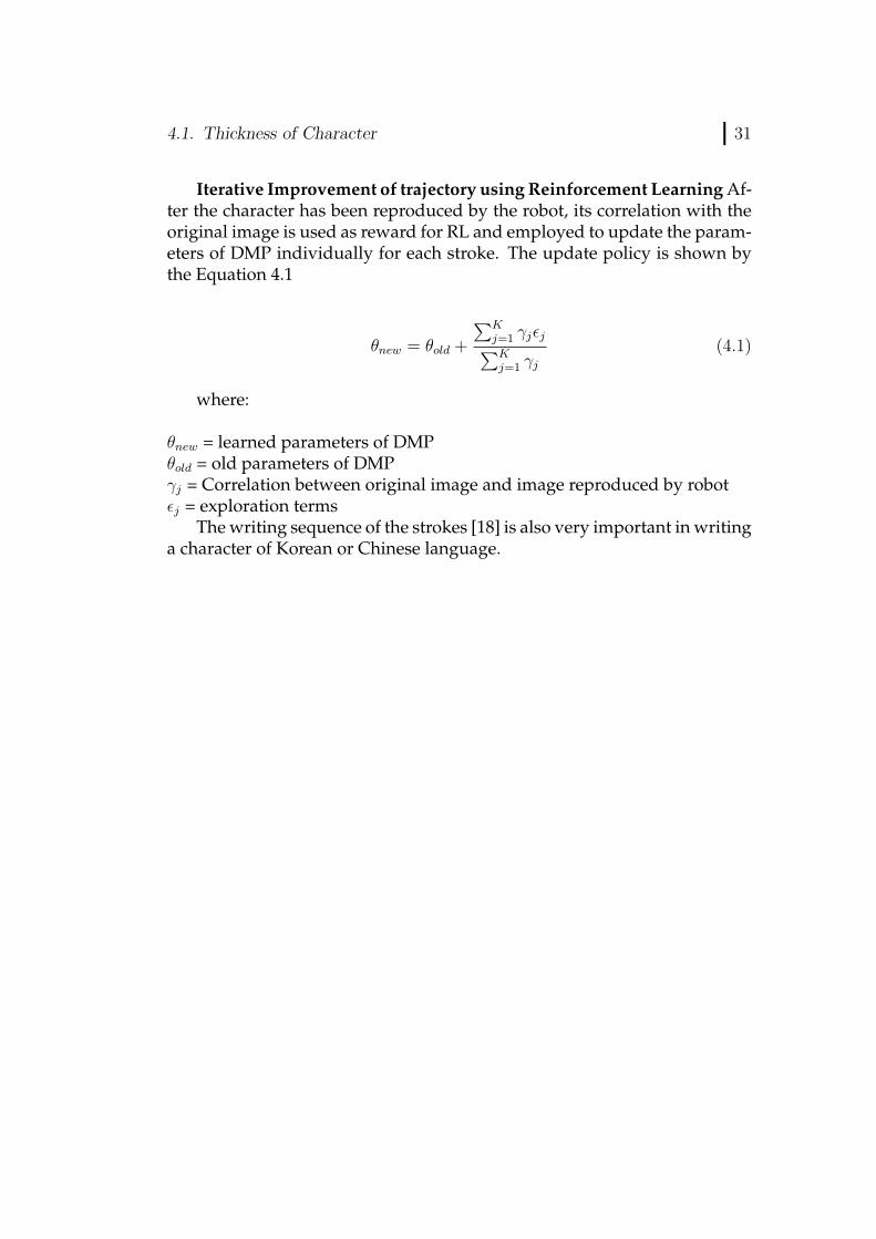
Iterative Improvement of trajectory using Reinforcement Learning Af-ter the character has been reproduced by the robot, its correlation with theoriginal image is used as reward for RL and employed to update the param-eters of DMP individually for each stroke. The update policy is shown bythe Equation 4.1

θnew = θold +

∑Kj=1 γjεj∑Kj=1 γj

(4.1)

where:

θnew = learned parameters of DMPθold = old parameters of DMPγj = Correlation between original image and image reproduced by robotεj = exploration terms

The writing sequence of the strokes [18] is also very important in writinga character of Korean or Chinese language.

33

CHAPTER

FIVE

RESULTS

This chapter includes all the results of the research. The hardware usedto acquire the results is KUKA Light weight robot which is operated usingRobot Operating System. The software used in this research is MATLAB.

As a proof of concept the extracted strokes are also drawn in simulation.The paint brush is modeled as droplet [dro] which is given as:

x = thicknessi(1− cos(2πt))sin(2πt)

y = thicknessicos(2πt)

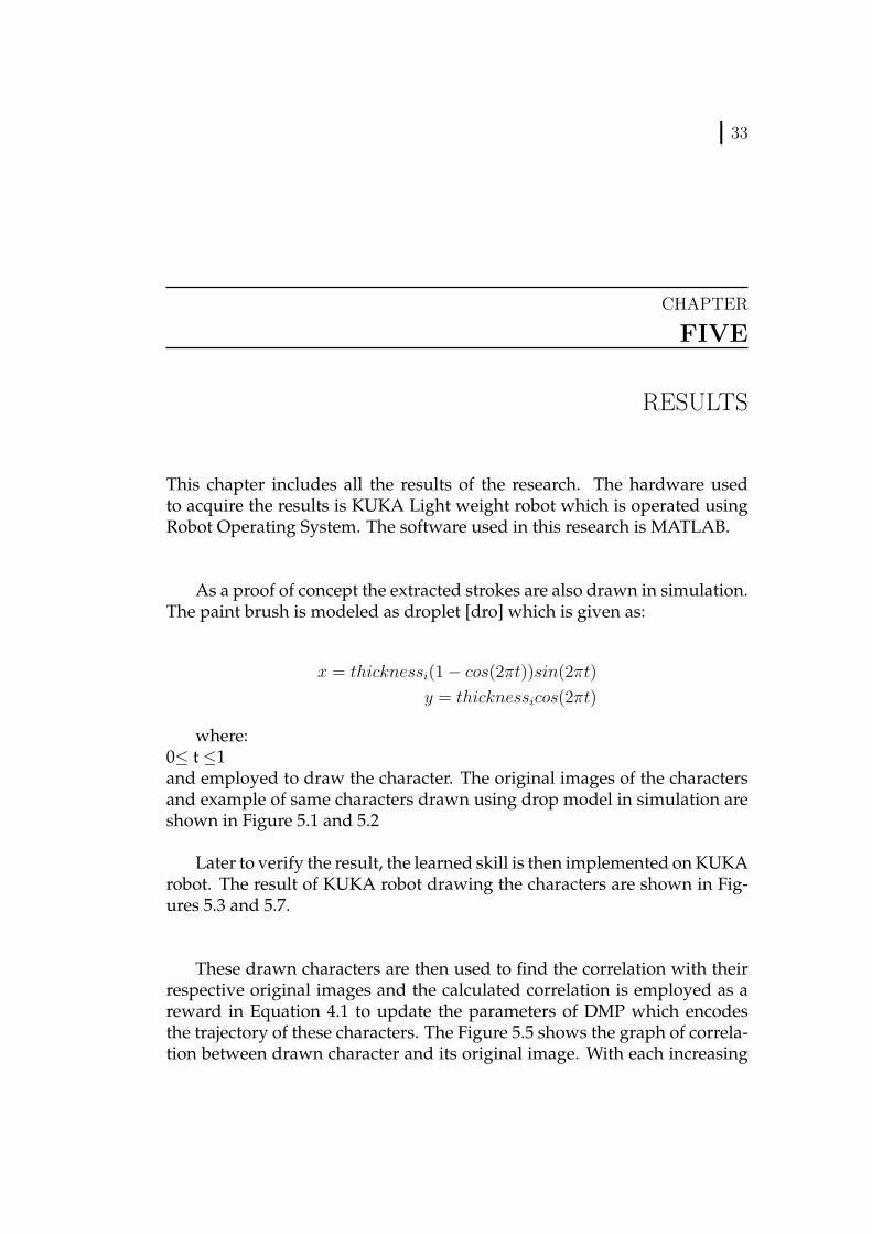
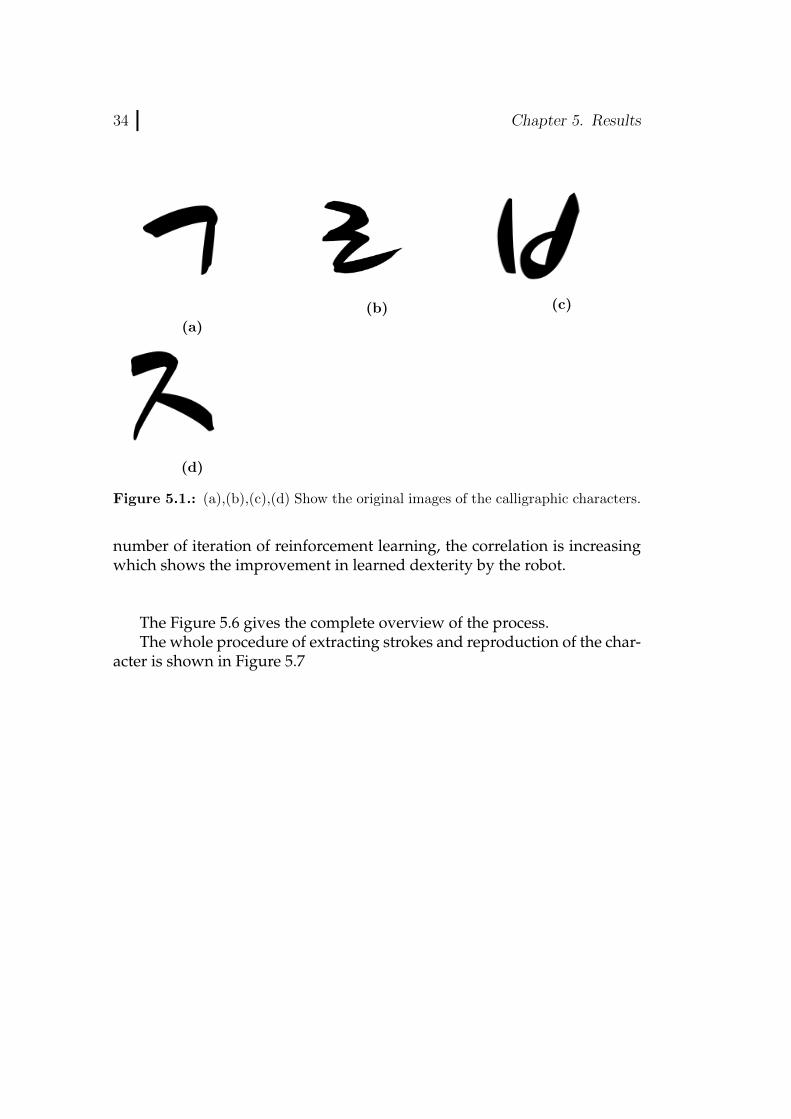
where:0≤ t ≤1and employed to draw the character. The original images of the charactersand example of same characters drawn using drop model in simulation areshown in Figure 5.1 and 5.2

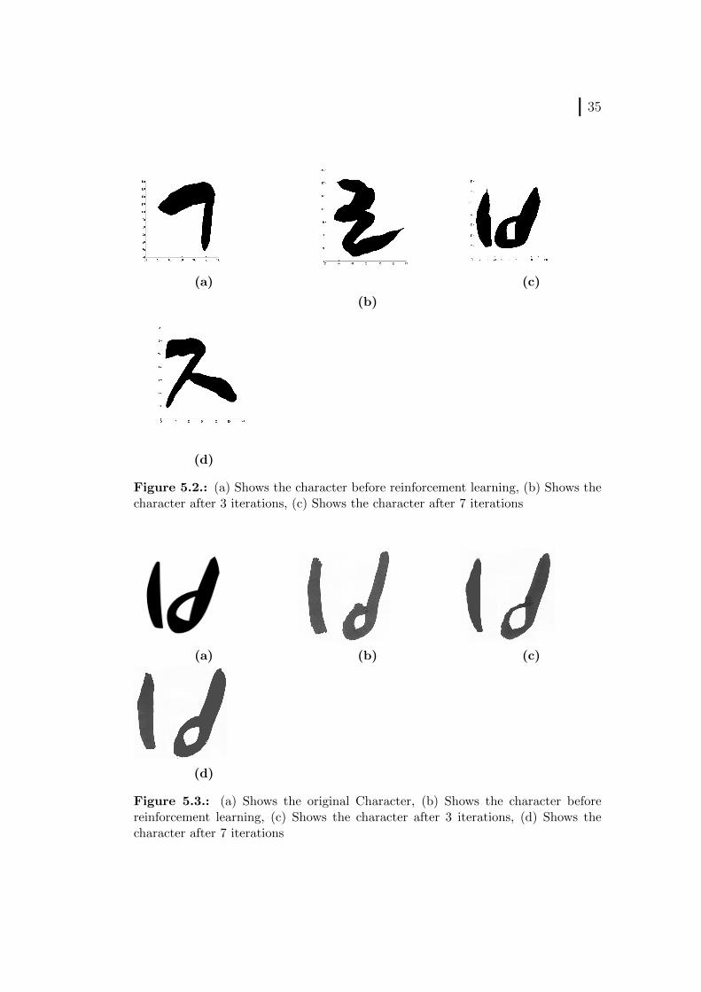
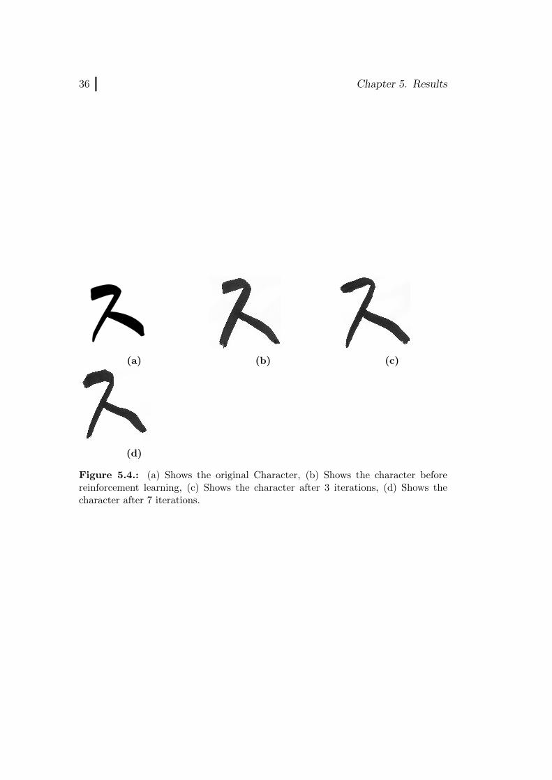
Later to verify the result, the learned skill is then implemented on KUKArobot. The result of KUKA robot drawing the characters are shown in Fig-ures 5.3 and 5.7.

These drawn characters are then used to find the correlation with theirrespective original images and the calculated correlation is employed as areward in Equation 4.1 to update the parameters of DMP which encodesthe trajectory of these characters. The Figure 5.5 shows the graph of correla-tion between drawn character and its original image. With each increasing

34 Chapter 5. Results

(a)

(b) (c)

(d)

Figure 5.1.: (a),(b),(c),(d) Show the original images of the calligraphic characters.

number of iteration of reinforcement learning, the correlation is increasingwhich shows the improvement in learned dexterity by the robot.

The Figure 5.6 gives the complete overview of the process.The whole procedure of extracting strokes and reproduction of the char-

acter is shown in Figure 5.7

35

(a)

(b)

(c)

(d)

Figure 5.2.: (a) Shows the character before reinforcement learning, (b) Shows thecharacter after 3 iterations, (c) Shows the character after 7 iterations

(a) (b) (c)

(d)

Figure 5.3.: (a) Shows the original Character, (b) Shows the character beforereinforcement learning, (c) Shows the character after 3 iterations, (d) Shows thecharacter after 7 iterations


(a) (b) (c)

(d)

Figure 5.4.: (a) Shows the original Character, (b) Shows the character beforereinforcement learning, (c) Shows the character after 3 iterations, (d) Shows thecharacter after 7 iterations.

37

1 2 3 4 5 6 70.69

0.7

0.71

0.72

0.73

0.74

0.75

0.76

Number of iterations

Rew

ard

Val

ues

Improvement over various iterations

Figure 5.5.: Reward against number of iterations. It improves with each iterationof reinforcement learning.


Figure 5.6.: Flow chart giving brief overview of the complete process.

39

Figure 5.7.: Complete overview of the stroke extraction and reproduction of acharacter.

i

BIBLIOGRAPHY

[dro] A math function that draws water droplet shape?http://math.stackexchange.com/questions/51539/

a-math-function-that-draws-water-droplet-shapel.

[onl] Understanding the bias-variance tradeoff. http://scott.

fortmann-roe.com/docs/BiasVariance.html.

[3] Akaike, H. (1974). A new look at the statistical model identification. Au-tomatic Control, IEEE Transactions on, 19(6):716–723.

[4] Bishop, C. M. (2006). Pattern recognition and machine learning. springer.

[5] Calinon, S., Guenter, F., and Billard, A. (2007). On learning, representing,and generalizing a task in a humanoid robot. Systems, Man, and Cybernet-ics, Part B: Cybernetics, IEEE Transactions on, 37(2):286–298.

[6] Calinon, S., Pervez, A., and Caldwell, D. G. (2012). Multi-optima ex-ploration with adaptive gaussian mixture model. In Proc. Intl Conf. onDevelopment and Learning (ICDL-EpiRob), pages 1–6, San Diego, USA.

[7] Dempster, A. P., Laird, N. M., and Rubin, D. B. (1977). Maximum like-lihood from incomplete data via the em algorithm. Journal of the royalstatistical society. Series B (methodological), pages 1–38.

[8] Fitzgibbon, L. J., Allison, L., and Dowe, D. L. (2000). Minimum messagelength grouping of ordered data. In Algorithmic Learning Theory, pages56–70. Springer.

[9] Fraley, C. and Raftery, A. E. (1998). How many clusters? which clusteringmethod? answers via model-based cluster analysis. The computer journal,41(8):578–588.

[10] Kaufman, L. and Rousseeuw, P. J. (2009). Finding groups in data: anintroduction to cluster analysis, volume 344. John Wiley & Sons.

http://math.stackexchange.com/questions/51539/a-math-function-that-draws-water-droplet-shapel

http://math.stackexchange.com/questions/51539/a-math-function-that-draws-water-droplet-shapel

http://scott.fortmann-roe.com/docs/BiasVariance.html

http://scott.fortmann-roe.com/docs/BiasVariance.html

ii Bibliography

[11] Kober, J. and Peters, J. (2010). Imitation and reinforcement learning.Robotics & Automation Magazine, IEEE, 17(2):55–62.

[12] Pervez, A. and Lee, D. (2015). A componentwise simulated annealingEM algorithm for mixtures. In KI 2015: Advances in Artificial Intelligence,pages 287–294. Springer.

[13] Pollard, K. S. and Van Der Laan, M. J. (2002). A method to identifysignificant clusters in gene expression data.

[14] Schwarz, G. et al. (1978). Estimating the dimension of a model. Theannals of statistics, 6(2):461–464.

[15] Su, Y.-M. and Wang, J.-F. (2003). A novel stroke extraction method forchinese characters using gabor filters. Pattern Recognition, 36(3):635–647.

[16] Su, Y.-M. and Wang, J.-F. (2004). Decomposing chinese characters intostroke segments using sogd filters and orientation normalization. In Pat-tern Recognition, 2004. ICPR 2004. Proceedings of the 17th InternationalConference on, volume 2, pages 351–354. IEEE.

[17] Sun, Y., Qian, H., and Xu, Y. (2014). A geometric approach to strokeextraction for the chinese calligraphy robot. In Robotics and Automation(ICRA), 2014 IEEE International Conference on, pages 3207–3212. IEEE.

[18] Tang, K.-t. and Leung, H. (2007). Reconstructing strokes and writingsequences from chinese character images. In Machine Learning and Cyber-netics, 2007 International Conference on, volume 1, pages 160–165. IEEE.

[19] Wallace, C. S. and Dowe, D. L. (1999). Refinements of mdl and mmlcoding. The Computer Journal, 42(4):330–337.

[20] Wang, L. and Pavlidis, T. (1993). Direct gray-scale extraction of featuresfor character recognition. Pattern Analysis and Machine Intelligence, IEEETransactions on, 15(10):1053–1067.

[21] Wong, S. T., Leung, H., and Ip, H.-S. (2006). Fitting ellipses to a regionwith application in calligraphic stroke reconstruction. In Image Processing,2006 IEEE International Conference on, pages 397–400. IEEE.

[22] YU, K., WU, J., and YUAN, Z. (2012). Stroke extraction for chinesecalligraphy characters. Journal of Computational Information Systems.

iii

APPENDIX

A

EIDESSTATTLICHE VERSICHERUNG

Eidesstattliche Versicherung

______________________________ ____________________

Name, Vorname Matr.-Nr.

Ich versichere hiermit an Eides statt, dass ich die vorliegende Bachelorarbeit/Masterarbeit* mit

dem Titel

____________________________________________________________________________

____________________________________________________________________________

____________________________________________________________________________

selbstständig und ohne unzulässige fremde Hilfe erbracht habe. Ich habe keine anderen als die

angegebenen Quellen und Hilfsmittel benutzt sowie wörtliche und sinngemäße Zitate kenntlich

gemacht. Die Arbeit hat in gleicher oder ähnlicher Form noch keiner Prüfungsbehörde

vorgelegen.

__________________________ _______________________

Ort, Datum Unterschrift

*Nichtzutreffendes bitte streichen

Belehrung:

Wer vorsätzlich gegen eine die Täuschung über Prüfungsleistungen betreffende Regelung einer

Hochschulprüfungsordnung verstößt, handelt ordnungswidrig. Die Ordnungswidrigkeit kann mit

einer Geldbuße von bis zu 50.000,00 € geahndet werden. Zuständige Verwaltungsbehörde für

die Verfolgung und Ahndung von Ordnungswidrigkeiten ist der Kanzler/die Kanzlerin der

Technischen Universität Dortmund. Im Falle eines mehrfachen oder sonstigen schwerwiegenden

Täuschungsversuches kann der Prüfling zudem exmatrikuliert werden. (§ 63 Abs. 5

Hochschulgesetz - HG - )

Die Abgabe einer falschen Versicherung an Eides statt wird mit Freiheitsstrafe bis zu 3 Jahren

oder mit Geldstrafe bestraft.

Die Technische Universität Dortmund wird gfls. elektronische Vergleichswerkzeuge (wie z.B. die

Software „turnitin“) zur Überprüfung von Ordnungswidrigkeiten in Prüfungsverfahren nutzen.

Die oben stehende Belehrung habe ich zur Kenntnis genommen:

_____________________________ _________________________ Ort, Datum Unterschrift

master thesis - technische universität münchen · nese calligraphy. considering the existing...

Documents