mastering financial mathematics in microsoft excel a ...krisuti/fs/ind darbai/14.pdf · add excess...

207

Valuation

Valuation methods

Assets

Market methods

Multi-period dividend discount models

Free cash flow valuation

Adjusted present value

Economic profit

Exercise

Summary

14

File: MFME2_14.xls

14 · Valuation

209

VALUATION METHODS

Valuation models use time value of money principles or simpler market

principles to value assets, stock and shares or the perceived value of future

benefits. Valuation by different methods does not necessarily produce the

same answers and the market employs a wide variety of methods. The

purpose of this chapter is to set out some of the basic mathematics for valu-

ation. Methods fall into these main categories:

■ asset and adjusted asset valuations;

■ dividend models;

■ market methods;

■ free cash valuation.

Companies can be valued from several different perspectives: for example, a

liquidation value can be very different from a going concern. Alternatively,

a stream of dividends is very different from cash flow although a long-term

investor may view a company purely for its income potential. Similarly it

depends on whether you are buying or selling. Since a flow of future ben-

efits represents a forecast, the financial model has to show all the inputs to

enable risk analysis of the key variables. The valuation is very likely a range

rather than a single point which should be compared by method and with

other companies within a peer group.

The print-outs in Figures 14.1 and 14.2 show the base data for the model

as an abridged income statement and balance sheet with supplementary

information. The methods require information about earnings, dividends

and cash flows and this can be extracted from the data. Period zero is the

last historic data and there are five forecast periods.

Figure 14.1Income statement

Other variables used in the model are below.

Tax rate % 30.00

Loan % 8.00

Bank loan % 8.00

Risk free % 5.00

Risk premium % 6.00

Growth rate % 5.00

Future debentures discount rate % 8.00

Dividend payout rate % 25.00

ASSETS

A glance at the accounts shows a current equity value of 100.0 based on

the shareholders’ funds or equity. This is simply the accounting net worth,

which does take account of many factors which could be important in deter-

mining value. Here is a selection of issues:

■ Not based on replacement cost of assets, but on historic cost.

■ Uses historic data and says nothing about the future and the organiza-

tion’s future earning power.

■ Ignores the value of information and non-financial capital such as

knowledge and patents which do not appear on the balance sheet. Non-

210

Figure 14.2 Balance sheet

Mastering Financial Mathematics in Microsoft® Excel

14 · Valuation

211

financial assets in areas such as legal, healthcare, information, consulting

and personal services could be more valuable than traditional fixed assets.

■ Accounting approach is based on a range of standards and conventions

which can be applied differently and affect value. For example, the choice

of depreciation method can enhance or reduce earnings merely by select-

ing periods or switching from accelerated to straight line methods.

■ There are a number of items which are ‘off-balance sheet’ and can mask

the true level of borrowings or enhance earnings and therefore net worth.

Examples include factoring, operating leases, joint ventures, contracted

capital expenditure, contingent liabilities (e.g. asbestos), pensions deficits,

derivatives and financial instruments, and current and future litigation.

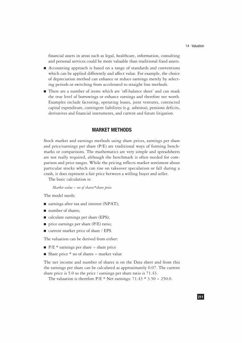
MARKET METHODS

Stock market and earnings methods using share prices, earnings per share

and price/earnings per share (P/E) are traditional ways of forming bench-

marks or comparisons. The mathematics are very simple and spreadsheets

are not really required, although the benchmark is often needed for com-

parison and price ranges. While the pricing reflects market sentiment about

particular stocks which can rise on takeover speculation or fall during a

crash, it does represent a fair price between a willing buyer and seller.

The basic calculation is:

Market value = no of shares*share price

The model needs:

■ earnings after tax and interest (NPAT);

■ number of shares;

■ calculate earnings per share (EPS);

■ price earnings per share (P/E) ratio;

■ current market price of share / EPS.

The valuation can be derived from either:

■ P/E * earnings per share = share price

■ Share price * no of shares = market value

The net income and number of shares is on the Data sheet and from this

the earnings per share can be calculated as approximately 0.07. The current

share price is 5.0 so the price / earnings per share ratio is 71.43.

The valuation is therefore P/E * Net earnings: 71.43 * 3.50 = 250.0.

212

The data table in Figure 14.3 shows the sensitivity to the P/E ratio. The

formula is:

Value of equity = sustainable earnings * approx P/E ratio + value of non-operating

assets

The model perhaps would benefit from some adjustments since you need to

identify sustainable earnings:

■ historic and forecast growth pattern which may not match;

■ resilience (‘quality’) of earnings;

■ accounting adjustments and their effect on valuation;

■ adjustments for external factors beyond the control of the company;

■ quoted/unquoted adjustment since private companies are often valued as

a percentage of the peer group to reflect the non-tradability.

This method also suffers from weaknesses such as:

■ A high P/E denotes a share with growth prospects, but this is also

dependent on market sentiment for the sector and the market, for ex-

ample the technology boom of the late 1990s.

■ Not based on time value money concepts or real future prospects.

■ Companies invest now for returns in future periods and this is not

included in the method. Earnings can be depressed by heavy investment

which could generate enhanced cash flow in the future.

■ Company may issue shares at any time and optimism may overvalue

shares and stock market sectors.

■ No account is taken of different accounting methods or changes in stand-

ards which affect earnings but do not alter the underlying cash flow.

Figure 14.3 Market methods


14 · Valuation

213

Nevertheless, market methods reflect value that people are prepared to

pay for a specific stock and in an efficient market, news and other negative

information should translate quickly into share price losses.

MULTI-PERIOD DIVIDEND DISCOUNT MODELS

When you buy shares, you are essentially buying into the dividend stream.

Unless you sell the shares, the only income is the dividend and therefore the

value could be viewed as the present value of the expected future dividends.

The simple perpetuity formula is the Gordon’s growth model as a shortcut

to present valuing an infinite stream of cash flows. The simple formula is:

D1P

1 = –––––––––

E(R1) – g

D1 = Dividend for next period i.e. Do * (1 + g)

E(R1) = Desired return

g = Implied growth = Cost of equity – Dividend yield / (1+Dividend yield)

In Figure 14.4, the dividend is 0.018 and the growth rate is 8.5 per cent.

Therefore:

Value = [ (0.018 * ( + 8.5%) ] / (9.25% – 8.5%)

Figure 14.4Dividend model


214

The simple dividend model assumes a constant rate of growth in perpetuity.

It is possible to construct multi-stage models using forecast dividends and

different rates of discounting. In the model above, the company forecasts

a period of rapid growth over the next five years before dropping back to

more modest growth. The dividend rate is 25.0 per cent and the income

and dividends are shown on the Data sheet.

The forecast dividends are discounted at the cost of equity and then the

final dividend is subjected to the perpetuity formula. The terminal value is:

Cell I22: =I17/(C7–C5)

The share value is:

Cell D25: =NPV(C7,D17:H17)+PV(C7,H9,0,–I22)

The valuation by this method is 4.355 per share or 217.75 in total. The

model is based on stable growth or dividends which last to infinity. This

is a simplification: for example, dividends cannot grow faster than earnings

since it is unsustainable that dividends would become greater than earnings

over a sufficient number of periods.

The model is also extremely sensitive to the growth rate. As the growth

rate converges on the discount rate, the value increases rapidly and will

become negative if the growth rate exceeds the discount rate. The chart

in Figure 14.5 shows a rapid increase in value followed by a dramatic fall

above the growth rate of 8.5 per cent.

Figure 14.5 Sensitivity to growth rate

14 · Valuation

215

FREE CASH FLOW VALUATION

Free cash methods focus on the forecast cash to be produced by the com-

pany and discount the cash flows at a risk-adjusted rate to reflect the mix

and relative cost of debt and equity. Given the weaknesses of other methods

in using time value of money or including future prospects, the reasoning

behind cash flow is the focus on tangible future benefits which are not mod-

ified by accounting methods or standards. The methodology is:

■ Forecast operating cash flows and prepare related financial statements as

in the Data sheet.

■ Calculate a suitable discount rate (cost of capital using a weighted aver-

age cost of capital formula for each source of capital).

■ Determine a suitable residual value (continuing value using the perpetu-

ity – Gordon’s Growth Model) or some other suitable multiple such as

the enterprise value (EV) to the earnings before interest, tax, depreciation

and amortization (EBITDA).

■ Calculate the present value of the cash flows and terminal value above at

the weighted average cost of capital.

■ Add excess cash and cash equivalents and subtract market value of debt.

■ Enterprise value less debt plus cash is the equity value.

■ Interpret and test results of calculations and assumptions using sensitiv-

ity analysis to form a range of potential valuations.

Cost of capital

The model generates the forecast cash flows over five years that belong to all

providers of capital. Therefore the discount rate or cost of capital needs to

reflect systematic risk and cost of each form of capital. This is the weighted

average cost of capital. Equity is calculated using the standard Capital Asset

Pricing Model as an extension of Portfolio Theory. The formula is:

E(R1) = Rf + β

i [E(R

m) – R

f]

where:

E(Ri) = Expected return on share i

Rf = Risk-free rate

E(Rm) = Expected return on the market

βI = Beta of share i

The risk-free rate is a suitable almost risk-free rate such as ten-year govern-

ment bond. This is currently in the range of 4 to 5 per cent in the UK and

the model uses 5 per cent. The risk premium is a measure of the return


216

that investors should demand for investing in shares and thereby accepting

a risk rather than investing in a risk-free asset. While returns have varied

in individual years over the last 50 years, the range has fluctuated between

10 and 12 per cent on the London Stock Market. Standard deviation is also

substantial which reflects the volatility of shares over government bonds.

The model uses a premium of 6 per cent from the Data sheet.

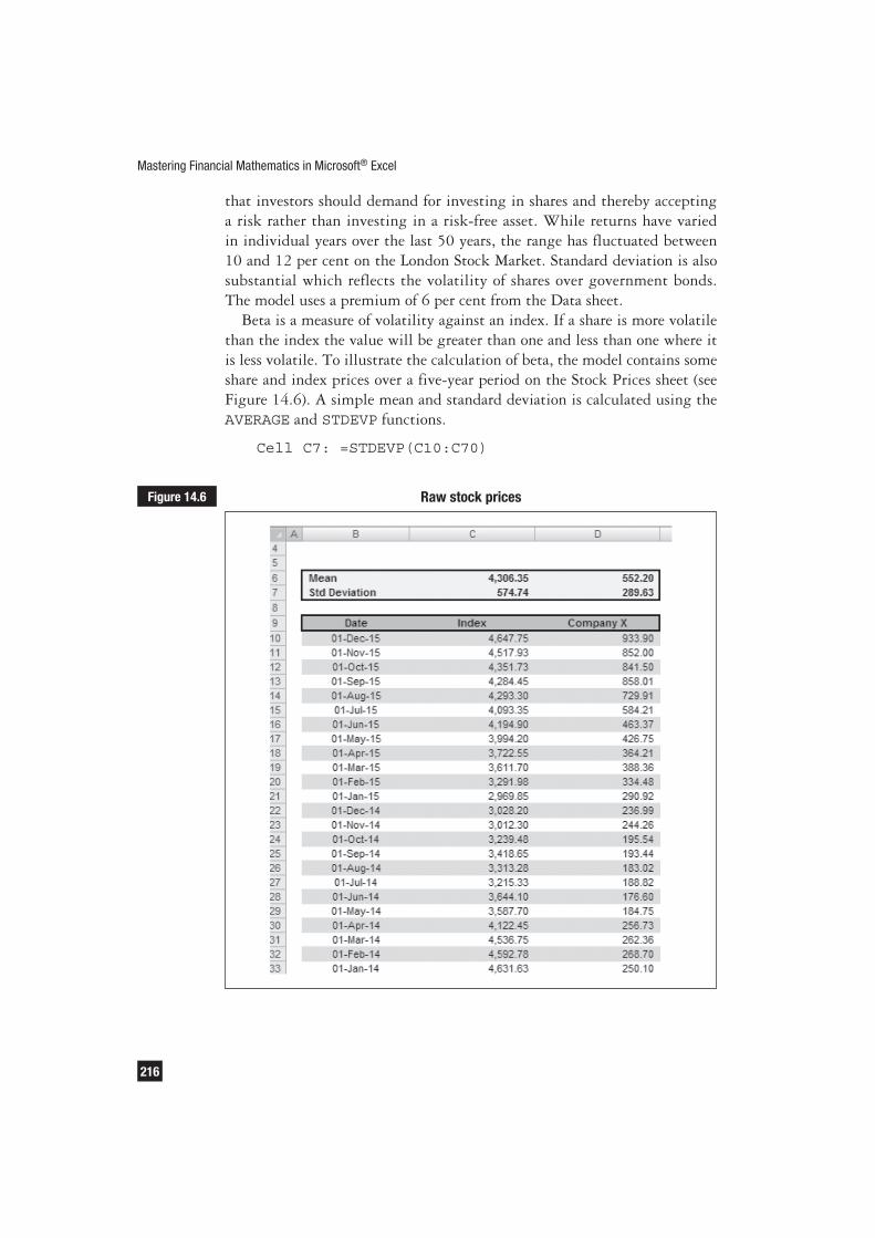
Beta is a measure of volatility against an index. If a share is more volatile

than the index the value will be greater than one and less than one where it

is less volatile. To illustrate the calculation of beta, the model contains some

share and index prices over a five-year period on the Stock Prices sheet (see

Figure 14.6). A simple mean and standard deviation is calculated using the

AVERAGE and STDEVP functions.

Cell C7: =STDEVP(C10:C70)

Figure 14.6 Raw stock prices

14 · Valuation

217

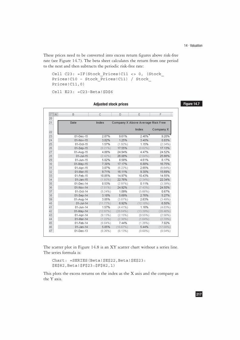
These prices need to be converted into excess return figures above risk-free

rate (see Figure 14.7). The beta sheet calculates the return from one period

to the next and then subtracts the periodic risk-free rate:

Cell C23: =IF(Stock_Prices!C11 <> 0, (Stock_

Prices!C10 – Stock_Prices!C11) / Stock_

Prices!C11,0)

Cell E23: =C23-Beta!$D$6

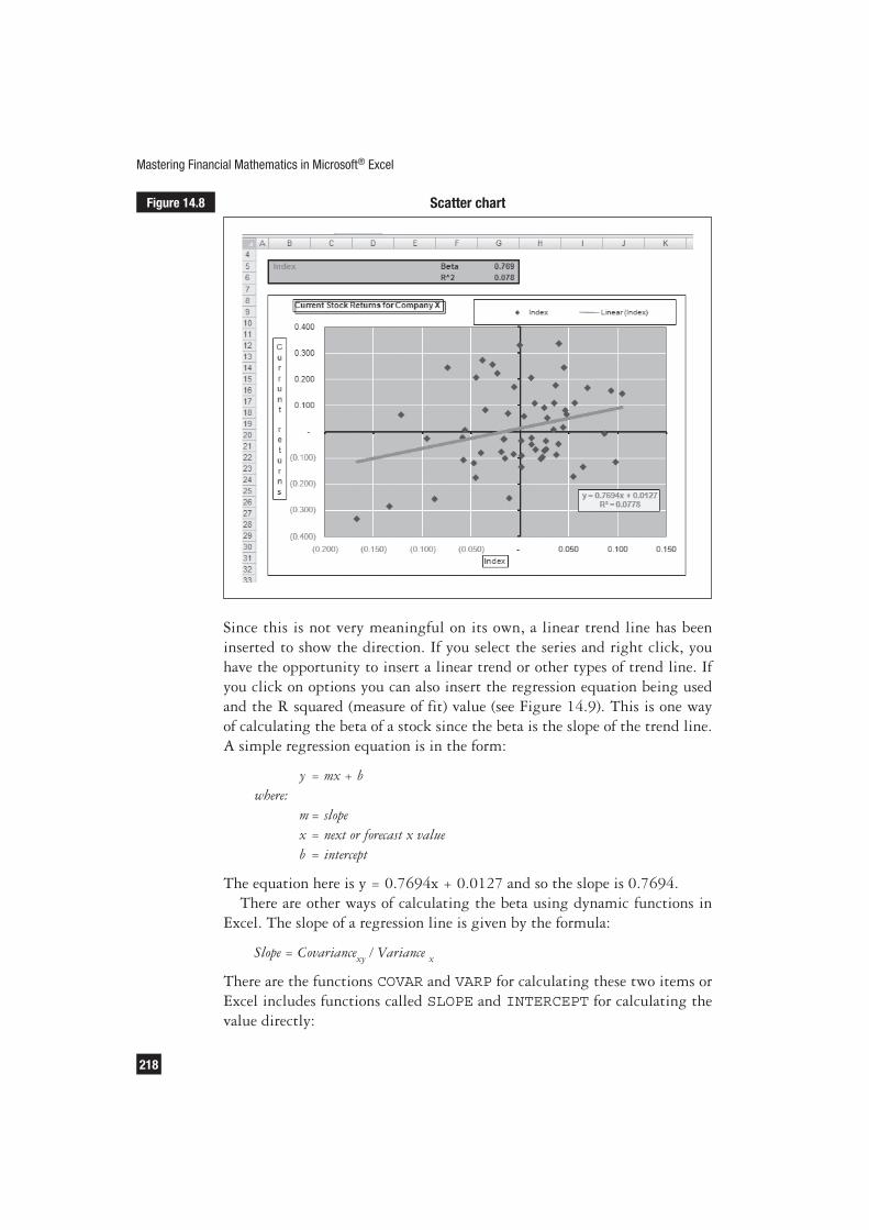
The scatter plot in Figure 14.8 is an XY scatter chart without a series line.

The series formula is:

Chart: =SERIES(Beta!$E$22,Beta!$E$23:

$E$82,Beta!$F$23:$F$82,1)

This plots the excess returns on the index as the X axis and the company as

the Y axis.

Figure 14.7Adjusted stock prices

218

Since this is not very meaningful on its own, a linear trend line has been

inserted to show the direction. If you select the series and right click, you

have the opportunity to insert a linear trend or other types of trend line. If

you click on options you can also insert the regression equation being used

and the R squared (measure of fit) value (see Figure 14.9). This is one way

of calculating the beta of a stock since the beta is the slope of the trend line.

A simple regression equation is in the form:

y = mx + b

where:

m = slope

x = next or forecast x value

b = intercept

The equation here is y = 0.7694x + 0.0127 and so the slope is 0.7694.

There are other ways of calculating the beta using dynamic functions in

Excel. The slope of a regression line is given by the formula:

Slope = Covariancexy

/ Variance x

There are the functions COVAR and VARP for calculating these two items or

Excel includes functions called SLOPE and INTERCEPT for calculating the

value directly:

Figure 14.8 Scatter chart


14 · Valuation

219

Covariance cell D11: =COVAR($E$23:$E$82,

$F$23:$F$82)

Variance cell D12: =VARP(E23:E82)

Slope cell D14: =SLOPE($F$23:$F$82,$E$23:$E$82)

These methods all achieve the same value of 0.7694. There is also an

advanced array function called LINEST whereby you can calculate the inter-

cept and slope together.

Cell D9: =LINEST(Beta!$F$23:$F$82,Beta!$E$23:

$E$82,,TRUE)

Figure 14.9Trend line options


220

To insert the function, the entries to cell D9 are as in Figure 14.10. All

the entries are locked using F4 so that the formula can be dragged to the

right into cell D10. With both cells selected, you go to the formula bar

and insert the function with Control, Shift, Enter in order to enter the two

cells as an array or block. Together the two cells calculate the intercept and

slope dynamically. The cell on the right is the intercept. Again the answer

is 0.7694.

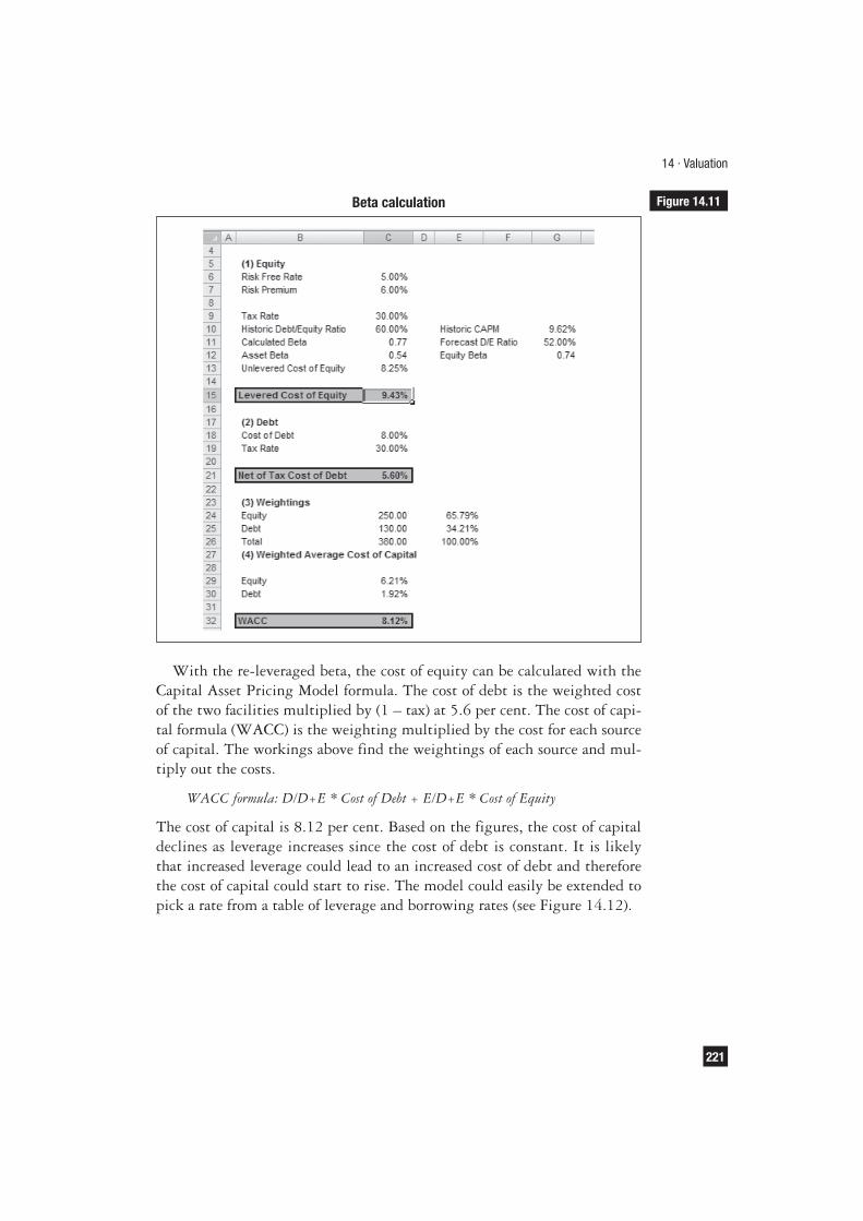
This provides all the information for the beta calculation bearing in mind

that beta is affected both by volatility and the company’s financial leverage.

Since the data is backward-looking, the effect of the historic debt/equity

needs to be stripped out and then reinserted as a forward debt/equity ratio.

The formulas for leveraging are:

■ Asset (un-leveraged) beta: BetaU

= BetaL / [1+(1–tax) * (D/E)]

■ Equity (leveraged) beta: BetaL = Beta

U * [1+(1–tax) * (D/E)]

Cell C12: =($C$11/(1+(1-$C$9)*$C$10))

Cell G12: =(C12*(1+(1-$C$9)*G10))

The formulas above un-leverage the beta based on the tax rate of 30.0 per

cent and a debt/equity ratio of 60.0 per cent. The forecast debt/equity ratio

is 52 per cent and therefore the forward beta is slightly lower than the his-

toric beta (see Figure 14.11).

Figure 14.10 Beta calculation

14 · Valuation

221

With the re-leveraged beta, the cost of equity can be calculated with the

Capital Asset Pricing Model formula. The cost of debt is the weighted cost

of the two facilities multiplied by (1 – tax) at 5.6 per cent. The cost of capi-

tal formula (WACC) is the weighting multiplied by the cost for each source

of capital. The workings above find the weightings of each source and mul-

tiply out the costs.

WACC formula: D/D+E * Cost of Debt + E/D+E * Cost of Equity

The cost of capital is 8.12 per cent. Based on the figures, the cost of capital

declines as leverage increases since the cost of debt is constant. It is likely

that increased leverage could lead to an increased cost of debt and therefore

the cost of capital could start to rise. The model could easily be extended to

pick a rate from a table of leverage and borrowing rates (see Figure 14.12).

Figure 14.11Beta calculation

222

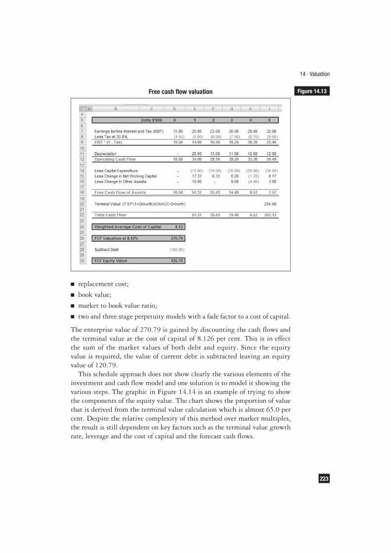
Free cash valuation

The FCF sheet brings together the cash flows, cost of capital and terminal

value. The schedule looks up values from the Data sheet and generates a free

cash flow (see Figure 14.13). This is the cash available to pay dividends to

shareholders and interest to debt or bond holders. The terminal value is cal-

culated in cell I20 using the perpetuity formula:

7.57 *(1+Growth))/(WACC-Growth)

Other possible methods for calculating the terminal value (which could all

yield different answers) include:

■ EV/EBITDA or other multiple;

■ P/E ratio;

■ liquidation value;

Figure 14.12 Sensitivity to debt ratio


14 · Valuation

223

■ replacement cost;

■ book value;

■ market to book value ratio;

■ two and three stage perpetuity models with a fade factor to a cost of capital.

The enterprise value of 270.79 is gained by discounting the cash flows and

the terminal value at the cost of capital of 8.126 per cent. This is in effect

the sum of the market values of both debt and equity. Since the equity

value is required, the value of current debt is subtracted leaving an equity

value of 120.79.

This schedule approach does not show clearly the various elements of the

investment and cash flow model and one solution is to model it showing the

various steps. The graphic in Figure 14.14 is an example of trying to show

the components of the equity value. The chart shows the proportion of value

that is derived from the terminal value calculation which is almost 65.0 per

cent. Despite the relative complexity of this method over market multiples,

the result is still dependent on key factors such as the terminal value growth

rate, leverage and the cost of capital and the forecast cash flows.

Figure 14.13Free cash flow valuation

224

ADJUSTED PRESENT VALUE

The adjusted present value method is a variant on free cash flows. Instead of

deriving a composite value, this pieces together value from different segments

to try to show where the value comes from. The free cash method above does

not tell how much leverage or cost improvements are worth and for risk ana-

lysis this could help to show the potential risks in achieving a suitable return.

Examples of layers are:

■ margin improvement;

■ plant closures or cost reductions;

■ synergies;

■ working capital improvements;

■ asset sales;

■ high terminal value growth.

In Figure 14.15, the base case valuation is 1.0 per share and further ‘layers’

show a potential value of 1.60 if all the plans are realized. The model there-

fore needs to split out each of these components.

The steps as in Figure 14.16 are:

■ Develop the free cash forecast as in the last section using discounted cash

flow methodology.

■ Discount the cash flows using a cost of equity derived from the un-

leveraged beta.

Figure 14.14 Free cash flow valuation graphic


14 · Valuation

225

■ Calculate actual interest tax shield gained from the leverage and discount

at the cost of debt.

■ Develop free cash flows for all other synergies and benefits of the transac-

tion. These cash flows need to be adjusted for tax.

■ Discount each layer using its own appropriate cost of capital to form a

series of net present values for each of the revenue gains and costs.

■ Add together all elements to obtain the adjusted present value which is

equivalent to the firm’s enterprise value.

■ Subtract the debt to form the equity value as in free cash flow methodology.

The cash flow in Figure 14.17 uses the cost of equity with an un-leveraged

beta. This was calculated on the WACC sheet:

Figure 14.15Valuation gains

Figure 14.16APV framework


226

Risk-free rate 5.00%

Risk premium 6.00%

Asset beta 0.54

Un-levered cost of equity 8.25%

The terminal value calculation also uses the same cost of equity (see Figure

14.18). The result is the present value as the company were fully equity

funded. This is the base case before any financial engineering or leverage.

Figure 14.17 APV base case

Figure 14.18 Interest shield

14 · Valuation

227

The next stage is to plot out the interest tax shield. This is the interest

paid on line 18 of the Data sheet multiplied by the tax rate. The terminal

value is also calculated to form a total cash flow which can be discounted

at the cost of debt. This procedure can be repeated for other layers of cost

or revenue gain. The adjusted present value is then the sum of each of the

components as above. This procedure could also be applied to other types

of cash model such as investment or project finance where the model needs

more flexibility than a single output.

ECONOMIC PROFIT

Economic profit is an alternative way of looking at the returns made by

the company. Traditional return on capital measures calculate the return

on invested capital, assets or equity. Since the level of capital can be altered

by off-balance sheet financing or the level of profit enhanced by switching

accounting methods, this method seeks to look at real value generation.

Drawbacks with accounting methods include:

■ income recognition, not cash;

■ creative accounting and presentation;

■ drawbacks with selecting projects/transactions on income/capital ratios.

The formula used in the model is:

EVA = Opening capital + (Cost of capital * Capital employed)

This will provide a cost of employing capital during the period and any

increase must derive from a return on the capital rather than profit. Thus a

company increases value by earning over and above the cost of capital and

should give rise to:

■ growing by investing in new projects whose return more than compen-

sates for risks taken;

■ curtailing investment in and diverting capital from uneconomic activities.

Capital in a complete model is calculated as the sum of:

■ ordinary equity value;

■ unusual losses/(gains) on balance sheet;

■ preferred stock and minority interests;

■ all debt (book, not market value);

■ present value of non-capitalized leases, less marketable securities;

■ other adjustments to LIFO reserve, goodwill, accounting reserves, capi-

talized value of marketing and research and development.


228

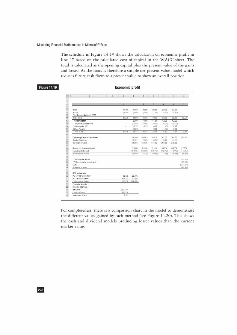
The schedule in Figure 14.19 shows the calculation on economic profit in

line 27 based on the calculated cost of capital in the WACC sheet. The

total is calculated as the opening capital plus the present value of the gains

and losses. At the roots is therefore a simple net present value model which

reduces future cash flows to a present value to show an overall position.

For completeness, there is a comparison chart in the model to demonstrate

the different values gained by each method (see Figure 14.20). This shows

the cash and dividend models producing lower values than the current

market value.

Figure 14.19 Economic profit

14 · Valuation

229

EXERCISE

You have the data below on a company. Write an Excel model to value the

cash flows together with two sensitivity tables: a one-dimensional table to

WACC and a two-way table to the WACC and growth rate.

WACC 10.00

Growth 1.00

Debt 250.00

Minority Interests 100.00

The annual cash flow forecast begins in one year’s time. The final cash flow

can be used for a terminal value growth calculation.

Year 1 2 3 4 5 6 7

Cash Flow 100.00 125.00 150.00 175.00 200.00 225.00 250.00

Figure 14.20Comparison of values


230

There are many ways of valuing companies and this section introduces

the basic mathematics for using accounting values, dividends, multiples

and cash methods. Using perpetuity and discounted cash flow methods,

the techniques can be applied to value dividends or cash over initial fore-

cast and longer periods.

SUMMARY

mastering financial mathematics in microsoft excel a ...krisuti/fs/ind darbai/14.pdf · add excess...

Documents