master’s degree in chemical engineering - … · master’s degree in chemical engineering...

Master’s Degree in Chemical Engineering

Simulation of Contaminant Concentrations in Drinking-Water Distribution Systems

Master Thesis

Developed in the ambit of the subject

Development Project

Diogo Moreira da Costa

Department of Chemical Engineering

Supervisor: Prof. Fernando Gomes Martins

July of 2008


Acknowledgements

I would like to express my great gratitude to my supervisor, Professor Fernando Martins,

whose support and guidance were determinants for the success of this work. His dedication

and hard work have set an example that I hope to match some day. I would also like to thank

Professor Luís Melo for the assistance he provided in all levels of this research work.

A special thanks goes out to all my family, in particular to my parents for all the support and

guidance they provided me through my entire life. I would also like to acknowledge Ricardo

for being such a great brother.

Finally, I must thank to my friends, whose support helped me to achieve my graduation and,

at the same time, living the best time of my live.


Abstract

The main objective of this work is the development of software tools to perform the

evaluation of contaminant concentrations in drinking-water distribution systems.

A software application was created coupling the EPANET software with visual basic code

developed in Visual Basic for Applications. The EPANET was used to compute the hydraulic

calculations and to establish the calculation sequence for the evaluation of contaminant

concentrations along the network.

The application allows the user to analyse the behaviour of the network after several types of

multiple perturbations at any node/nodes of the network.

The analytical and numerical approaches for solving the problem of advective transport in

pipes with reaction in the bulk flow presented identical results.

Keywords: drinking-water distribution systems, deliberate contamination, concentration

profiles along the network


Resumo

Este trabalho tem como principal objectivo o desenvolvimento de ferramentas informáticas

capazes de realizar a análise da qualidade da água em sistemas de distribuição de água.

Foi criada uma aplicação informática conjugando a aplicação informática EPANET com código

visual basic desenvolvido em Visual Basic for Applications. O EPANET foi utilizado para

realizar os cálculos hidráulicos e para estabelecer a sequência de cálculo para a determinação

das concentrações de contaminante ao longo da rede.

A aplicação permite ao utilizador analisar o comportamento da rede em resposta a vários

tipos de perturbações, realizados em qualquer ponto/ pontos da rede. Podem ser definidas

várias perturbações em simultâneo.

A abordagem analítica da resolução do problema do transporte advectivo em tubos com

reacção apresentou resultados idênticos aos resultados obtidos pela abordagem numérica

presente na aplicação desenvolvida.

Palavras Chave: sistemas de distribuição de água, contaminação deliberada, perfis de

concentração ao longo da rede


i

Contents

Contents ......................................................................................................i

List of figures.............................................................................................. iii

List of tables............................................................................................... iv

Nomenclature and glossary .............................................................................. v

1 Introduction...........................................................................................1

1.1 Project overview...............................................................................1

1.2 Work contribution .............................................................................1

1.3 Thesis outline...................................................................................2

2 State of the art .......................................................................................4

3 Models and software tools..........................................................................6

3.1 Models............................................................................................6

3.1.1 Numerical approach ......................................................................................6

3.1.2 Analytical approach ......................................................................................7

3.2 The EPANET software ....................................................................... 10

3.3 The software tool ............................................................................ 11

3.3.1 Algorithm and program development ............................................................... 13

4 Results and discussion ............................................................................ 16

4.1 EPANET’s network definition and hydraulic analysis ................................. 16

4.2 EPANET’s water quality solver ............................................................ 19

4.3 Comparison between EPANET and author’s application.............................. 21

4.4 Demonstration of other potentialities of the software tool ......................... 23

4.4.1 Simulation with other kinetic model ................................................................ 23

4.4.2 Simulation of multiple perturbations................................................................ 25

4.5 Comparison between analytical and numerical solutions ............................ 29

5 Conclusions ......................................................................................... 32

6 Work assessment................................................................................... 33

6.1 Results accomplished ....................................................................... 33


ii

6.2 Future work................................................................................... 33

7 References .......................................................................................... 34


iii

List of figures

Figure 1 – Interaction between EPANET software and Visual Basic for Applications. ...................... 12

Figure 2 – The drinking-water distribution system................................................................ 16

Figure 3– EPANET table with results computed for nodes. ...................................................... 18

Figure 4 – EPANET table with results computed for links........................................................ 18

Figure 5 – EPANET series plot for the contaminant concentration at Node7 ................................. 19

Figure 6 – EPANET series plot for the contaminant concentration at Node11 ............................... 20

Figure 7 – EPANET series plot for the Contaminant concentration at Nodes1 and 2........................ 20

Figure 8 -Contaminant concentration at perturbation point (Node 1) – Section 4.3........................ 21

Figure 9 - Contaminant concentration at node 7 – Section 4.3. ................................................ 22

Figure 10 - Contaminant concentration at node 11 – Section 4.3. ............................................. 22

Figure 11 - Comparison between contaminant concentration at node 7...................................... 22

Figure 12 - Comparison between contaminant concentration profiles at node 11. ......................... 23

Figure 13 - Contaminant concentration at perturbation point (Node 1) – Section 4.4.1................... 24

Figure 14 - Contaminant concentration at node 7 – Section 4.4.1. ............................................ 25

Figure 15 – Contaminant concentration at node 11 – Section 4.4.1. ........................................... 25

Figure 16- Represention of the perturbations of example presented in Section 4.4.2..................... 27

Figure 17 - Contaminant concentration at node 7 – Section 4.4.2. ............................................ 27

Figure 18 - Contaminant concentration at node 11 – Section 4.4.2. ........................................... 28

Figure 19 - Contaminant concentration at each length step of pipe 2 – Section 4.4.2. .................... 28

Figure 20 - Comparision between the analytical and the numerical solution for pipe 1 concentration

profiles – t= 10 s. ........................................................................................................ 30


profiles – t= 50 s. ........................................................................................................ 30


profiles – t= 100 s........................................................................................................ 30

Figure 23 - Contaminant concentration at several point locations of pipe 1 ................................ 31


iv

List of tables

Table 1 – Network nodes characteristics. ........................................................................... 16

Table 2 – Network pipes characteristics............................................................................. 17

Table 3 - Data supplied to the software tool ...................................................................... 21

Table 4 - Information supplied as simulation parameters in Section 4.4.1. ................................. 24

Table 5 – Information supplied for the case of reaction rate defined by Equation 3.2. ................... 24

Table 6 - Information supplied for the case of reaction rate defined by Equation 4.2. ................... 24

Table 7 - Information supplied as simulation parameters in Section 4.4.2. ................................. 26

Table 8 - Information supplied for the perturbations definition in Section 4.4.2. ......................... 26

Table 9 - Information supplied for the demonstration in Section 4.5. ........................................ 29

Table 10 - Information necessary to perform the analytical solution. ........................................ 29


v

Nomenclature and glossary

A Perturbation amplitude defined in analytical approach g/m3

r Reaction rate g/(m3/s)

k Kinetic coefficient g/(m3/s) or s-1

n Reaction order

t Time s

s Laplace domain variable

x Distance along the pipe m

il Length of pipe i m

iu Flow velocity in pipe i m/s

iQ Volumetric flow rate in pipe i m3/s

( )txCi , Concentration at position x of pipe i in instant equal to t g/m3

( )tC p Concentration at node p in instant equal to t g/m3

pi Set of the incoming links to the node p

( )tV Storage tank volume in instant t m3

Greek Letters

∆ interval

Index

p node i link

Symbol List

THM Trihalomethanes


Introduction 1

1 Introduction

1.1 Project overview

Contamination of critical infrastructures, such as drinking-water distribution systems, by

chemical, biological or radiological agents can have major public health, economical and

psychosocial consequences. Vulnerability of drinking-water distribution systems to deliberate

attacks is one of the main issues of concern to regulatory agencies and water utilities.

The response to these vulnerabilities is a great challenge, in which protection and

surveillance represent only one of the aspects to take attention. The detection of water

quality deterioration in drinking-water distribution systems calls for the development of new,

sensitive and rapid methodologies.

In case of a deliberate contamination of the drinking-water distribution systems, it is very

important to know the localization of the point sources of contamination and subsequently

the contaminated area allowing the specification of delimitation areas to perform corrective

actions. One possible approach for solving this problem is the inverse simulation which allows

estimating the localization of the point sources contamination by analysing the concentration

profiles in several check points along the network. So, before applying this methodology, it is

necessary to have information about the evolution of the contaminant concentrations along

the network after deliberate contamination in specific points. This information is very

difficult to be obtained in real situations, but can be generated through simulation.

Therefore, the main objectives of this work are:

1. To evaluate the potentialities of the EPANET software to study the contaminant

concentrations along the networks of drinking-water distribution systems;

2. To develop a software tool able to estimate the contaminant concentrations along the

networks after perturbations of several types defined by the user.

1.2 Work contribution

The work, here reported, has as main objective the development of a software application

that performs the evaluation of contaminant concentrations in drinking-water distribution

systems. The software application was developed coupling the EPANET software with visual

basic code developed in Visual Basic for Applications. The EPANET is used to compute the

hydraulic calculations and to establish the calculation sequence for the evaluation of


Introduction 2

contaminant concentrations. This application allows the user to analyse the behaviour of the

network for several types of perturbations at any node of the network.

This software is a useful tool for performing simulations to build a database that will be

necessary for solving the inverse problem of prediction the localization of the point sources

after deliberate contamination.

1.3 Thesis outline

This thesis is divided in 6 chapters.

Chapter 1 has three sections. In Section 1.1, it is introduced the problem studied in this work,

presenting an overview and the objectives of the project. Section 1.2 exposes the work

contributions and Section 1.3 presents the thesis outline.

Chapter 2 describes the state of the art about the research in the field of modelling and

simulation of contamination of drinking-water distribution systems. This chapter resumes

some published scientific works concerning this subject.

Chapter 3 is divided in three main sections. Section 3.1 presents the models that were the

basis for the evaluation of contaminant concentrations in the work reported. This section also

shows two different approaches for solving the equations for study the evaluation of

contaminant concentrations. Section 3.2 describes the main potentialities of the EPANET

software, in terms of hydraulic and evaluation of contaminant concentrations, and lists the

information that user has necessarily to define to run a hydraulic analysis. The method used

by EPANET to solve the equations that characterise de hydraulic state of a pipe network at a

given point in time is presented, as well as the list of phenomena that are involved in

EPANET’s water quality solver. Finally, it is resumed several ways of presenting results

available in EPANET. In Section 3.3, it is explained the list of tasks performed by the

application developed by the author. It is reported the relation between the EPANET

hydraulic analysis and models exposed in Section 3.1, and the integration in Visual Basic for

Applications. It is also presented the main steps that constitute the algorithm for the

application.

Chapter 4 is the chapter where the results are presented and the different methods and

applications are compared. It starts with Section 4.1 in which is shown the definition of a

drinking-water distribution system. Results of EPANET’s hydraulic analysis are reported here.

The system (network) described in this section is used in the rest of the chapter, for all

simulations. Section 4.2 explains the process of defining a perturbation in EPANET, which

simulates the deliberate contamination, and exposes the results obtained for the evaluation


Introduction 3

of contaminant concentrations. Section 4.3 presents the results computed by the developed

application for the same perturbation that was defined in Section 4.2 and compare the results

obtained with the results achieved by EPANET software. Section 4.4 has the aim of exposing

other potentialities of the developed application. In Section 4.4.1, it is shown the comparison

between the simulations of two different kinetic models. In Section 4.4.2, it is run a

simulation with the definition of several perturbations at different points of the network. The

influence of reaction is also exposed with the representation of results for different values for

the kinetic coefficient. Section 4.5 presents the comparison between the results obtained

using the numerical approach – explained in Section 3.1.1 – and the analytical approach –

Section 3.1.2.

Chapter 5 presents the conclusions of this work after the analysis of the results obtained.

Chapter 6 is divided in two sections. The objectives achieved in this work are listed in the

Section 6.1. Future works that would enhance the results already obtained are indicated in

Section 6.2.


State of the art 4

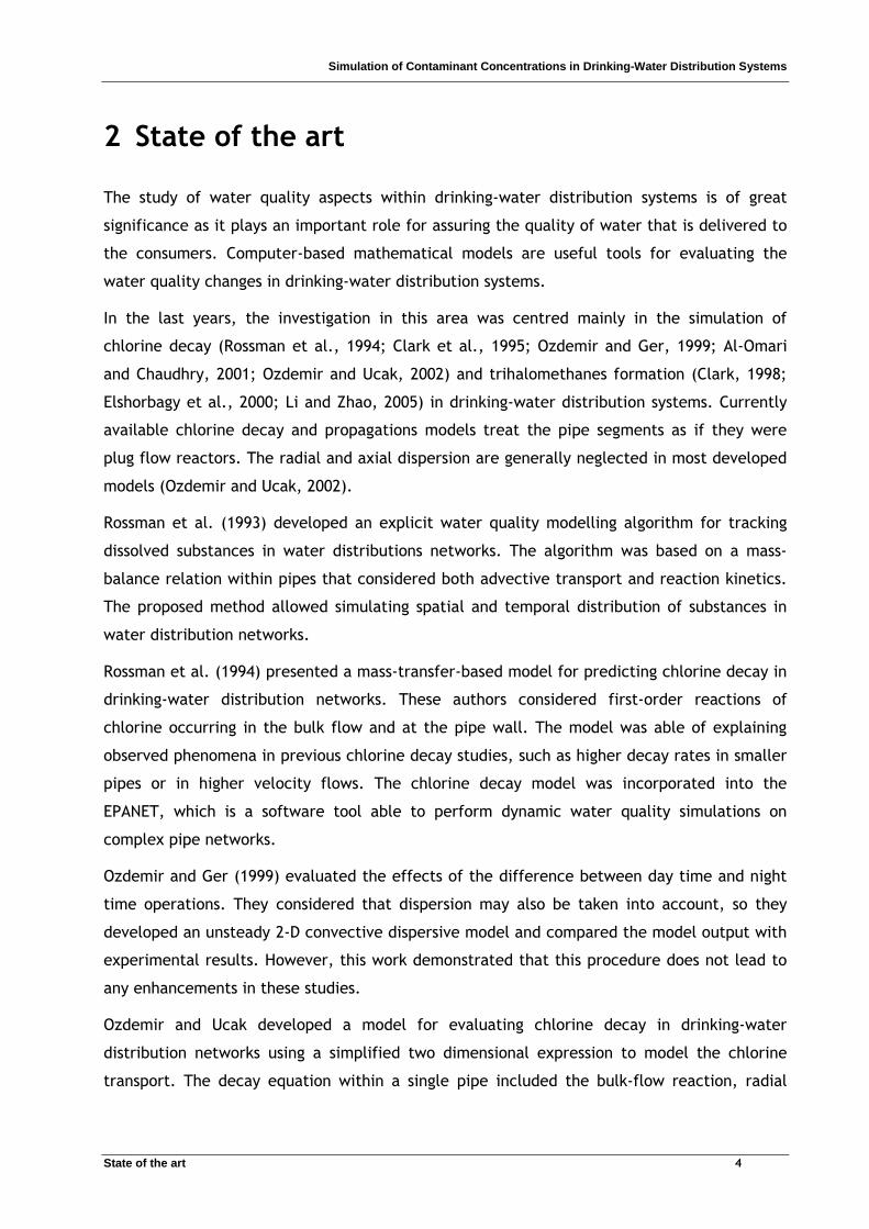
2 State of the art

The study of water quality aspects within drinking-water distribution systems is of great

significance as it plays an important role for assuring the quality of water that is delivered to

the consumers. Computer-based mathematical models are useful tools for evaluating the

water quality changes in drinking-water distribution systems.

In the last years, the investigation in this area was centred mainly in the simulation of

chlorine decay (Rossman et al., 1994; Clark et al., 1995; Ozdemir and Ger, 1999; Al-Omari

and Chaudhry, 2001; Ozdemir and Ucak, 2002) and trihalomethanes formation (Clark, 1998;

Elshorbagy et al., 2000; Li and Zhao, 2005) in drinking-water distribution systems. Currently

available chlorine decay and propagations models treat the pipe segments as if they were

plug flow reactors. The radial and axial dispersion are generally neglected in most developed

models (Ozdemir and Ucak, 2002).

Rossman et al. (1993) developed an explicit water quality modelling algorithm for tracking

dissolved substances in water distributions networks. The algorithm was based on a mass-

balance relation within pipes that considered both advective transport and reaction kinetics.

The proposed method allowed simulating spatial and temporal distribution of substances in

water distribution networks.

Rossman et al. (1994) presented a mass-transfer-based model for predicting chlorine decay in

drinking-water distribution networks. These authors considered first-order reactions of

chlorine occurring in the bulk flow and at the pipe wall. The model was able of explaining

observed phenomena in previous chlorine decay studies, such as higher decay rates in smaller

pipes or in higher velocity flows. The chlorine decay model was incorporated into the

EPANET, which is a software tool able to perform dynamic water quality simulations on

complex pipe networks.

Ozdemir and Ger (1999) evaluated the effects of the difference between day time and night

time operations. They considered that dispersion may also be taken into account, so they

developed an unsteady 2-D convective dispersive model and compared the model output with

experimental results. However, this work demonstrated that this procedure does not lead to

any enhancements in these studies.

Ozdemir and Ucak developed a model for evaluating chlorine decay in drinking-water

distribution networks using a simplified two dimensional expression to model the chlorine

transport. The decay equation within a single pipe included the bulk-flow reaction, radial


State of the art 5

diffusion and pipe wall reaction of chlorine. Good agreements were achieved between

experimental observations and the outputs of the developed application.

As far as author of this thesis know, there aren’t published works directly related with the

study of deliberate contaminations in drinking-water distribution systems. So, this work tries

to apply the available knowledge in the study of chlorine decay and trihalomethanes

formation to the propagation of contaminants through the networks after deliberate

contaminations.


Models and software tools 6

3 Models and software tools

3.1 Models

The model used in the evaluation of contaminant concentrations was based on the

phenomena of advective transport and reaction in the pipes. This model considers that a

dissolved substance will travel down the length of a pipe with the same average velocity as

the carrier fluid at the same time reacting at some given rate. Longitudinal dispersion is

usually not an important transport mechanism under most operating conditions. So, the

advective transport within a pipe is represented with the following equation:

( ) ( ) ( )( )txCrx

txCu

t

txCi

ii

i ,,, +

∂∂−=

∂∂

(3.1)

where ( )txCi , is the concentration (mass/volume) in pipe i as a function of distance x and

time t , iu is the flow velocity (length/time) in pipe i and r is the rate of reaction

(mass/volume/time) that is function of concentration (Rossman et al., 1993).

3.1.1 Numerical approach

The numerical solution is achieved applying a finite differences method for solving the

Equation 3.3. Equation 3.3 is obtained by substituting the reaction rate in Equation 3.1 by

Equation 3.2, which is a generic equation for the decay reaction rate:

( )( ) ( )txCktxCr nii ,, −= (3.2)

where k is the rate kinetic coefficient and n is the reaction order.

( ) ( ) ( )txCkx

txCu

t

txC ni

ii

i ,,,

−∂

∂−=

∂∂

(3.3)

Methods involving finite differences for solving boundary value problems replace each of

derivatives in the differential equation with an appropriate difference-quotient

approximation. In this case, for derivative of the function ( )txCi , in order to x , the

procedure used was to consider the average between the difference-quotient approximation

for t and tt ∆+ .



( ) ( ) ( )t

txCttxC

t

txC iii

∆−∆+

=∂

∂ ,,, (3.4)

( ) ( ) ( ) ( ) ( )

∆∆−−

+∆

∆+∆−−∆+=

∂∂

x

txxCtxC

x

ttxxCttxC

x

txC iiiii ,,,,

2

1, (3.5)

Replacing the derivatives in order to t and to x with the Equation 3.4 and Equation 3.5

respectively, Equation 3.6 is obtained:

( ) ( ) ( ) ( ) ( ) ( ) ( )txCkx

txxCtxC

x

ttxxCttxCu

t

txCttxC ni

iiiiiii ,,,,,

2

,, −

∆∆−−+

∆∆+∆−−∆+−=

∆−∆+ (3.6)

Rewriting the Equation 3.6, it is possible to deduce an explicit equation for ( )ttxCi ∆+, :

( )( ) ( ) ( ) ( )( )

x

u

t

txxCttxxCx

utxCtxCk

x

u

tttxC

i

iii

in

ii

i

∆+

∆

∆−+∆+∆−

∆+

−

∆−

∆=∆+

−

2

1

,,2

,,2

1

,

1

(3.7)

3.1.2 Analytical approach

To try to validate the results computed by the software tool developed in this work, an

analytical solution was obtained for the partial differential equation given by Equation 3.1. It

is assumed that a first order reaction rate is able to simulate the decay of contaminant:

( )( ) ( )txCktxCr ii ,, −= (3.8)

Equation 3.9 is obtained by the substitution of the Equation 3.8 in Equation 3.1:

( ) ( ) ( )txCk

x

txCu

t

txCi

ii

i ,,, −

∂∂−=

∂∂

(3.9)

Applying the Laplace Transform to the variable t , Equation 3.9 is transformed in Equation

3.10:

( ) ( ) ( ) ( )sxCkx

sxCuxCsxCs i

iiii ,

,0,, −

∂∂−=− (3.10)

The next step is to define the boundary conditions. It is assumed that the initial contaminant

concentration is 0 for all the length of the pipe.

( ) 00, =xCi (3.11)

In Laplace domain is:



( ) 00, =xCi (3.12)

Substituting this initial condition in Equation 3.10, Equation 3.13 is obtained:

( ) ( ) ( )sxCkx

sxCusxCs i

iii ,

,, −

∂∂−= (3.13)

Equation 3.13 is a differential equation which can be solved by direct integration:

( ) ( )( ) ( )∫∫ +∂=+∂−

kssxC

sxCsfx

u i

i

i ,

,1 (3.14)

The integration is performed without integration limits. A function ( )sf is added as a

constant of integration, not dependent of the variable x , but as a function of the other

independent variable s .

Integrating the Equation 3.14 and rewriting the same equation, it is possible to obtain an

explicit form for ( )sxCi , :

( ) ( ) ( )

+−+

+= sf

u

xks

kssxC

ii exp

1, (3.15)

Considering ( ) ( ) ( )[ ]sfkssg += exp , the Equation 3.16 is obtained:

( ) ( ) ( )sgu

xks

kssxC

ii

−+

+= exp

1, (3.16)

It is still impossible to invert Equation 3.16 for time domain because ( )sg is an unknown

function. This function can be determined by applying a second boundary condition. This

boundary condition must be the contaminant concentration at the point 0=x along the time.

As example, Equation 3.17 describes a pulse with amplitude A that occurs between the times

1t and 2t .

( ) ( ) ( )[ ]21,0 ttHttHAtCi −−−= (3.17)

The transformation of this equation to Laplace domain is:

( ) ( ) ( )

−−−=s

st

s

stAsCi

21 expexp,0 (3.18)

Applying this boundary condition to Equation 3.16 allows the evaluation of ( )sg , i.e.:



( ) ( ) ( ) ( )

−−−=

−+

+ s

st

s

stAsg

uks

ks i

21 expexp0exp

1 (3.19)

( ) ( ) ( ) ( )

−−−+=s

st

s

stksAsg 21 expexp

(3.20)

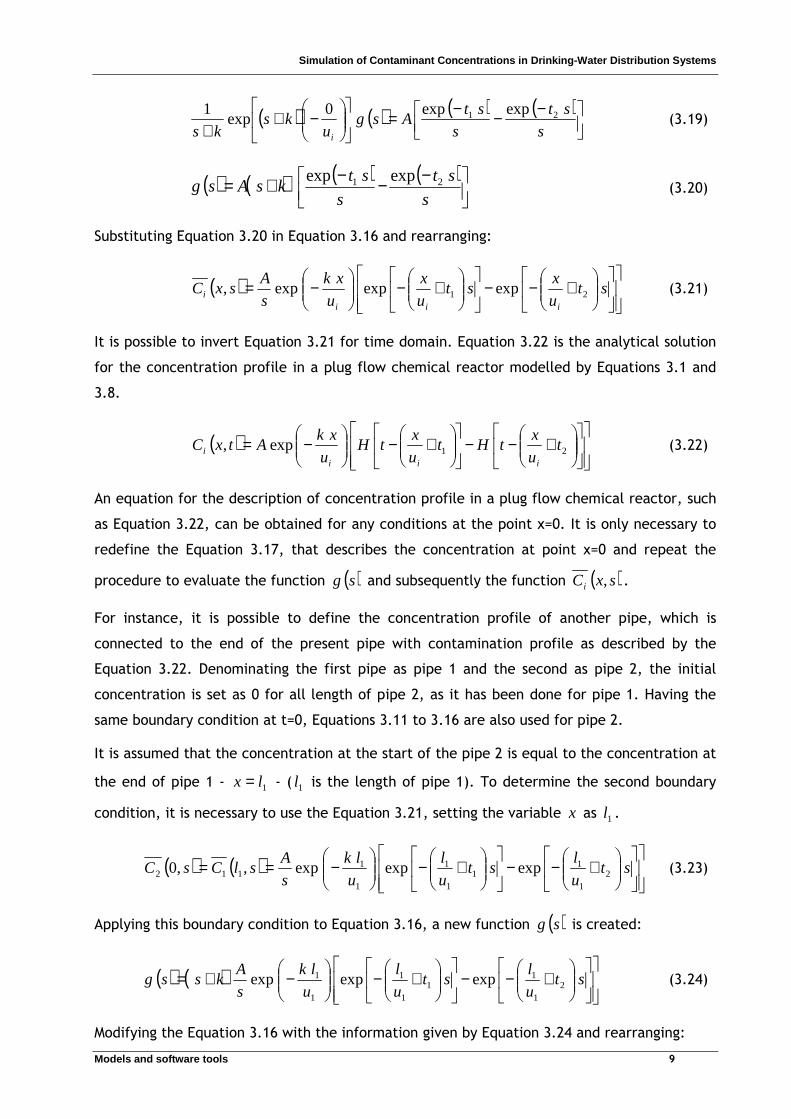
Substituting Equation 3.20 in Equation 3.16 and rearranging:

( )

+−−

+−

−= st

u

xst

u

x

u

xk

s

AsxC

iiii 21 expexpexp, (3.21)

It is possible to invert Equation 3.21 for time domain. Equation 3.22 is the analytical solution

for the concentration profile in a plug flow chemical reactor modelled by Equations 3.1 and

3.8.

( )

+−−

+−

−= 21exp, t

u

xtHt

u

xtH

u

xkAtxC

iiii (3.22)

An equation for the description of concentration profile in a plug flow chemical reactor, such

as Equation 3.22, can be obtained for any conditions at the point x=0. It is only necessary to

redefine the Equation 3.17, that describes the concentration at point x=0 and repeat the

procedure to evaluate the function ( )sg and subsequently the function ( )sxCi , .

For instance, it is possible to define the concentration profile of another pipe, which is

connected to the end of the present pipe with contamination profile as described by the

Equation 3.22. Denominating the first pipe as pipe 1 and the second as pipe 2, the initial

concentration is set as 0 for all length of pipe 2, as it has been done for pipe 1. Having the

same boundary condition at t=0, Equations 3.11 to 3.16 are also used for pipe 2.

It is assumed that the concentration at the start of the pipe 2 is equal to the concentration at

the end of pipe 1 - 1lx = - ( 1l is the length of pipe 1). To determine the second boundary

condition, it is necessary to use the Equation 3.21, setting the variable x as 1l .

( ) ( )

+−−

+−

−== st

u

lst

u

l

u

lk

s

AslCsC 2

1

11

1

1

1

1112 expexpexp,,0 (3.23)

Applying this boundary condition to Equation 3.16, a new function ( )sg is created:

( ) ( )

+−−

+−

−+= st

u

lst

u

l

u

lk

s

Akssg 2

1

11

1

1

1

1 expexpexp (3.24)

Modifying the Equation 3.16 with the information given by Equation 3.24 and rearranging:



( )

++−−

++−

+−= st

u

x

u

lst

u

x

u

l

u

xk

u

lk

s

AsxC 2

21

11

21

1

21

12 expexpexp, (3.25)

The inverse of the Equation 3.25 allows to evaluate the concentration profile for the pipe 2.

( )

++−−

++−

+−= 2

21

11

21

1

21

12 exp, t

u

x

u

ltHt

u

x

u

ltH

u

xk

u

lkAtxC (3.26)

3.2 The EPANET software

This software performs extended period simulation of hydraulic and water quality behaviour

in drinking-water distribution systems. These systems are built by pipes, nodes, pumps,

valves, reservoirs and tanks (Rossman, 2000).

EPANET can model systems of any size, computes friction head loss using different equations -

Hazen-Williams, Darcy-Weisbach or Chezy-Manning - (Rossman, 2000), allows minor head

losses for bends or fittings and computes pumping energy and cost. EPANET models constant

or variable speed pumps, various types of valves including shutoff valves, check valves,

pressure regulating valves and flow control valves, storage tanks of any shape and allows

multiple demand categories at nodes, each with its own pattern of time variation.

The basic data to be introduced in EPANET software are:

� For reservoirs:

• hydraulic head (equal to the water surface elevation if the reservoir is not

under pressure;

� For junctions:

• elevation above some reference (usually mean sea level);

• water demand (rate of withdrawal from the network);

� For tanks:

• bottom elevation (where water level is zero);

• diameter (or shape if non-cylindrical);

• initial, minimum and maximum levels;

� For pipes:

• start and end nodes;

• diameter;

• length;

• roughness coefficient;

• status (open close, or contains a check valve);



� For pumps:

• start and end nodes;

• pump curve (the combination of heads and flows that the pump can produce).

In addition to hydraulic modelling, EPANET provides water quality modelling capabilities. The

quality models allow evaluating the movement of a non reactive tracer material through the

network over time and the movement and the fate of a reactive material along the network.

This software models the reaction mechanisms, both in the bulk flow and in the pipe wall,

using several order kinetics to model reactions in the bulk flow and zero or first order kinetics

for reaction at the pipe wall. The global reaction rate coefficients can be specific for each

pipe and the wall reaction rate coefficients can be correlated with pipe roughness. It is also

possible to determine the effects of concentration or mass input at any location in the

network. The models available for storage tanks can simulate different behaviours, such as,

complete mixing, plug flow and as two compartment reactors.

Todini’s approach to a hydraulic node-loop system, also known as Gradient Method, is used by

EPANET to solve the flow continuity and headloss equations which characterize the hydraulic

state of the pipe network at a given point in time. The hydraulic head lost by water flowing in

a pipe due to friction with the pipe walls can be computed using one of the following

formulas: Hazen-Williams, Darcy-Weisbach and Chezy-Manning (Rossman, 2000).

The governing equations for EPANET’s water quality solver are based on the principles of

conservation of mass conjugated with reaction kinetics. The equations involve:

• Advective transport in pipes;

• Mixing in storage facilities;

• Bulk flow reactions;

• Pipe wall reactions;

• System of equations;

• Lagrangian transport algorithm;

EPANET also provides an integrated set of conditions for editing network input data, running

hydraulic and water quality simulations, and viewing the results in a variety of formats, such

as colour-coded network maps, data tables, time series graphs and contour plots.

3.3 The software tool

The software was developed in Visual Basic for Applications, incorporating the hydraulic

analysis performed by EPANET software with models for the evaluation of contaminant

concentrations solved using numerical approaches as described in the Section 3.1.



The application is divided in the following tasks:

1. Network design: The network is designed with the EPANET software, introducing the

characteristics and the information associated to the equipments. For example, it is

necessary to define pump curves in EPANET.

2. Setting the necessary data to characterize the reaction within the pipes and to

perform the integration in the evaluation of contaminant concentrations.

3. Definition of the perturbations, providing the information needed to fully characterize

the perturbations.

4. Run hydraulics analysis using the EPANET Programmer’s Toolkit, which is a dynamic

link library that allows the developers to incorporate EPANET’s functions in their own

applications.

5. Perform the evaluation of contaminant concentrations, based on the equations

described before for the advective transport in pipes. The hydraulic data needed to

run the evaluation of contaminant concentrations is provided by EPANET results

computed previously.

The Figure 1 shows a diagram that explains the interaction between Visual Basic for

Applications and EPANET software, during the execution of steps listed above.

Figure 1 – Interaction between EPANET software and Visual Basic for Applications.

Visual Basic for Applications tasks:

• Import EPANET’s dynamic library.

• Open the input file supplied by EPANET.

• Perform hydraulic analysis using EPANET’s

dynamic library.

• Perform quality analysis.

EPANET tasks:

• Network design.

• Introduction the characteristics

associated to the equipments.

• Export the network to a file with

format inp.



3.3.1 Algorithm and program development

Input information:

Network scheme designed by EPANET software in a file with the format inp;

Simulation time;

Integration steps for space and time variables;

Reaction rate coefficient and order of reaction;

Nodes where perturbations occur;

Start time and duration of each perturbation;

Amount of contaminant introduced at network per time unit.

Output:

Concentration profiles for each physical component of the network.

Step 1. Import the EPANET Programmer’s Toolkit, EPANET’s dynamic link library.

Step 2. Open the input file that provides the description of the network in study and run a

complete extended period analysis.

Step 3. Get the information related with nodes (node type, hydraulic head and water

demand) and links (length, velocity, diameter, start and end nodes).

Step 4. Define the start and the end nodes for each link by evaluating the difference of

hydraulic head between the nodes connected. The EPANET software defines the start and the

end nodes based on the order of the drawing process. The direction defined from the start

node to the end node has to be the same as the direction of fluid movement. So, the start

node has to have a higher hydraulic head then end node, with the exception of a link of the

type pump.

Step 5. Sort the links for decreasing order of hydraulic head at the start node (if there were

nodes with the same hydraulic head at the start node, sort those nodes for decreasing order

of hydraulic head at the end node), with exception links which have a reservoir as start node

that have to be placed first in the order of resolution.

Step 6. Set the concentration at each node and in all length of each pipe as 0, for 0=t .



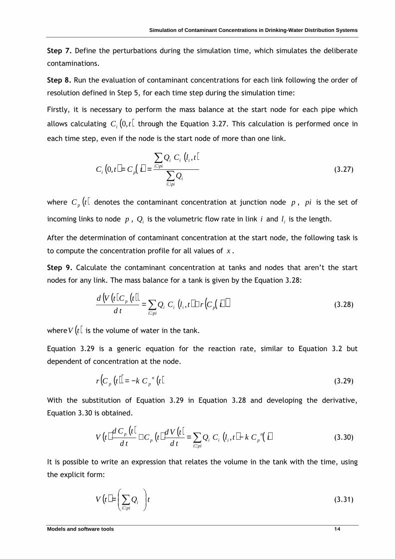
Step 7. Define the perturbations during the simulation time, which simulates the deliberate

contaminations.

Step 8. Run the evaluation of contaminant concentrations for each link following the order of

resolution defined in Step 5, for each time step during the simulation time:

Firstly, it is necessary to perform the mass balance at the start node for each pipe which

allows calculating ( )tCi ,0 through the Equation 3.27. This calculation is performed once in

each time step, even if the node is the start node of more than one link.

( ) ( )( )

∑

∑

∈

∈==

piii

piiiii

pi Q

tlCQ

tCtC

,

,0 (3.27)

where ( )tC p denotes the contaminant concentration at junction node p , pi is the set of

incoming links to node p , iQ is the volumetric flow rate in link i and il is the length.

After the determination of contaminant concentration at the start node, the following task is

to compute the concentration profile for all values of x .

Step 9. Calculate the contaminant concentration at tanks and nodes that aren’t the start

nodes for any link. The mass balance for a tank is given by the Equation 3.28:

( ) ( )( ) ( ) ( )( )tCrtlCQtd

tCtVdp

piiiii

p +=∑∈

, (3.28)

where ( )tV is the volume of water in the tank.

Equation 3.29 is a generic equation for the reaction rate, similar to Equation 3.2 but

dependent of concentration at the node.

( )( ) ( )tCktCr npp −= (3.29)

With the substitution of Equation 3.29 in Equation 3.28 and developing the derivative,

Equation 3.30 is obtained.

( ) ( ) ( ) ( ) ( ) ( )∑∈

−=+pii

npiiip

p tCktlCQtd

tVdtC

td

tCdtV , (3.30)

It is possible to write an expression that relates the volume in the tank with the time, using

the explicit form:

( ) tQtVpii

i

= ∑

∈ (3.31)



Using the Equation 3.31, the derivative of volume is obtained by:

( )∑∈

=pii

iQtd

tVd (3.32)

The derivative of the concentration at the node p in order to time can be rewrite using the

finite difference method, as it has been done at Section 3.1.1. Using this approximation,

Equation 3.33 is obtained:

( ) ( ) ( )t

tCttC

td

tCd ppp

∆−∆+

= (3.33)

The substitution of the Equations 3.32 and 3.33 in Equation 3.30 leads to:

( ) ( ) ( ) ( ) ( ) ( )tCktlCQQtCt

tCttCttV n

ppii

iiipii

ippp −=+

∆−∆+

∆+ ∑∑∈∈

, (3.34)

It is also possible to obtain a equation in an explicit form in relation to ( )ttC p ∆+ ,

rearranging the Equation 3.34:

( ) ( ) ( ) ( ) ( ) ( )

−−

∆+∆+=∆+ ∑ ∑

∈ ∈pii piiip

npiiipp QtCtCktlCQ

ttV

ttCttC , (3.35)

These 9 steps allow performing the evaluation of contaminant concentrations, presenting

results for the contaminant concentration at each node or pipe length step in the network.


Results and discussion 16

4 Results and discussion

4.1 EPANET’s network definition and hydraulic analysis

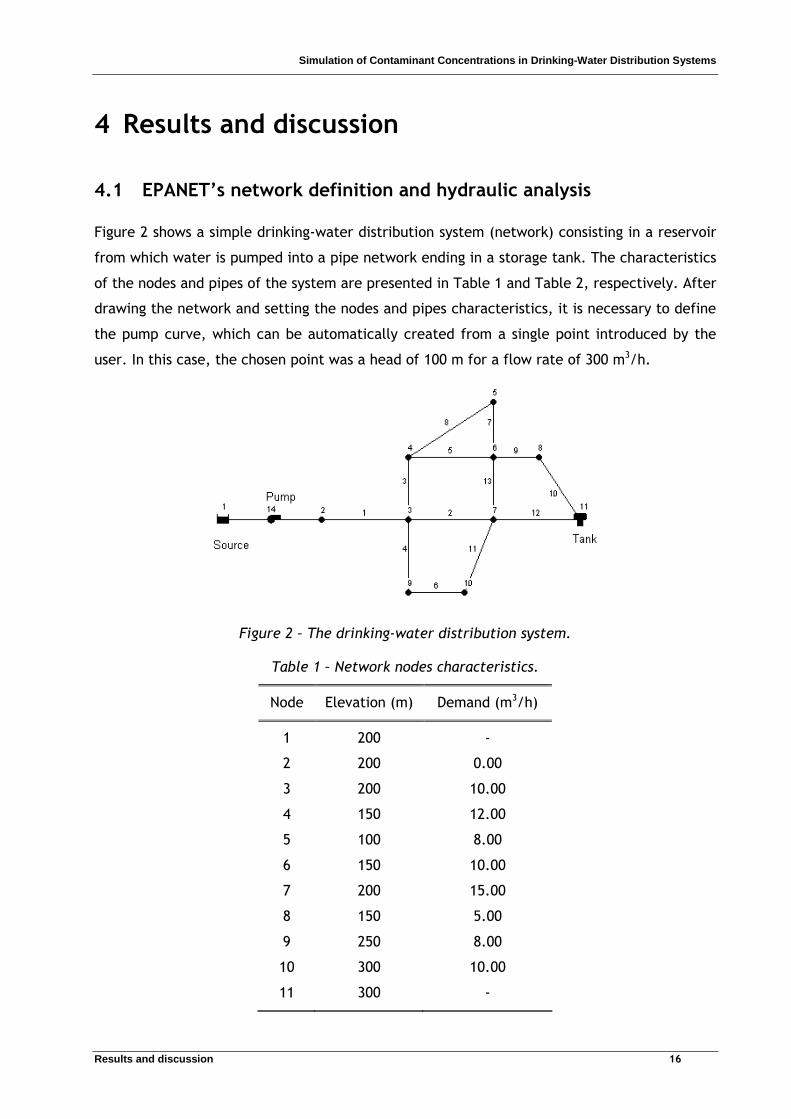
Figure 2 shows a simple drinking-water distribution system (network) consisting in a reservoir

from which water is pumped into a pipe network ending in a storage tank. The characteristics

of the nodes and pipes of the system are presented in Table 1 and Table 2, respectively. After

drawing the network and setting the nodes and pipes characteristics, it is necessary to define

the pump curve, which can be automatically created from a single point introduced by the

user. In this case, the chosen point was a head of 100 m for a flow rate of 300 m3/h.

Figure 2 – The drinking-water distribution system.

Table 1 – Network nodes characteristics.

Node Elevation (m) Demand (m3/h)

1 200 -

2 200 0.00

3 200 10.00

4 150 12.00

5 100 8.00

6 150 10.00

7 200 15.00

8 150 5.00

9 250 8.00

10 300 10.00

11 300 -



The elevation column refers to the nodes’ elevations above some reference point and demand

values are related to the withdrawal rates from the network. Reservoirs and tanks don’t need

input data of demands. The reservoir is the node that represent infinite external source of

water to the network; the water flow supplied by the reservoir has to be sufficient to satisfy

the demands for all nodes. The pump must supply hydraulic head enough to avoid low

pressures along the network and to set a relative pressure of 0 meter of water column at the

tank. The tank is the node with storage capacity to receive the water that was supplied by

the reservoir and was not used in the other nodes demands.

Table 2 – Network pipes characteristics.

Link Length (m) Diameter (m) C-Factor

1 100 0.300 100

2 200 0.250 100

3 100 0.175 100

4 100 0.175 100

5 200 0.175 100

6 150 0.175 100

7 100 0.150 100

8 150 0.150 100

9 100 0.175 100

10 150 0.100 100

11 150 0.150 100

12 200 0.200 100

13 100 0.175 100

14 - - -

C-Factor is the parameter used in Hazen-Williams Formula to calculate the friction headloss

(C-Factor equal to 100, assuming pipes made of galvanized iron).

With this information, EPANET is able to run a single period hydraulic analysis. It’s possible to

create tables with the computed hydraulic results for each link and node (Figures 3 and 4).



Figure 3– EPANET table with results computed for nodes.

Figure 4 – EPANET table with results computed for links.



4.2 EPANET’s water quality solver

The study of deliberate contaminations in EPANET was performed by using the EPANET’s

water quality solver. Therefore, a perturbation was defined at the reservoir. This was

performed creating a pattern by selecting the Patterns category in the Browser. After

defining the time pattern, the user has to edit the Source Quality parameter in Reservoir

Properties. In this example, and considering the simulation time equal to 1 hour, the

contaminant concentration in the reservoir was set as 1 mg/l during the first 6 minutes and 0

mg/l for the rest of time.

The definition of the perturbations is a great limitation of the EPANET software, because this

application doesn’t allow introducing a perturbation through a function. This means that the

concentration must be defined for each pattern step in simulation time.

With this information, EPANET was ready to perform the evaluation of contaminant

concentrations, computing the water quality - in this case, contaminant concentration - for

all nodes and average concentration for pipes. For instance, Figures 5 and 6 represent the

variation of the contaminant concentration at the Nodes 7 and 11 (storage tank),

respectively, during the simulation time.

Figure 5 – EPANET series plot for the contaminant concentration at Node7



Figure 6 – EPANET series plot for the contaminant concentration at Node11

Figure 7 shows the contaminant concentrations at Nodes 1 and 2 along the time. The

difference between the representations at Node 1 and Node 2 weren’t expected. Those nodes

are connected by a pump, which is assumed that has a residence time approximately equal to

0 but EPANET’s results show a delay of 1 minute between these nodes.

Figure 7 – EPANET series plot for the Contaminant concentration at Nodes1 and 2.



4.3 Comparison between EPANET and author’s application

It was performed a evaluation of contaminant concentrations to the same network, with the

same conditions, using the software tool described before to compare the results computed

by EPANET with the results computed by the application developed in this work. Table 3 lists

all the information that had to be supplied to the application. In the application, the user has

to set the amount of contaminant that is introduced in the network per second, instead of

setting the concentration at the point of perturbation as in EPANET. To have a concentration

of 1 mg/l (equal to 1 g/m3), the amount of contaminant was calculated by Equation 4.1.

Figure 8 shows the variation of concentration in the reservoir along the time.

( ) ( ) ( ) ( )sgsmmgsgm antcounta /076452.0/3600

23.275/1/ 33

min =×= (4.1)

Table 3 - Data supplied to the software tool

Simulation time (s) 3600

Reporting step (s) 60

Integration step for time (s) 0.1

Integration step for position (m) 1

Kinetic coefficient (g/m3/s) 0

Reaction order 0

Number of perturbations 1

Point of perturbation (Node) 1

Start time (s) 0

Duration of perturbation (s) 360

Amount of contaminant (g/s) 0.076452

Figure 8 -Contaminant concentration at perturbation point (Node 1) – Section 4.3.



Figures 9 and 10 show the concentration at nodes 7 and 11, respectively, during the

simulation time.

Figure 9 - Contaminant concentration at node 7 – Section 4.3.

Figure 10 - Contaminant concentration at node 11 – Section 4.3.

Figures 11 and 12 show the comparison between the results obtained using EPANET (line and

points in red colour) and the results computed by the author’s application (line and points in

blue colour).

Figure 11 - Comparison between contaminant concentration at node 7.



Figure 12 - Comparison between contaminant concentration profiles at node 11.

It is observed a slight discrepancy between the results obtained using EPANET and the

author’s application. This delay can be explained by the different approach used in the

definition of water residence time inside the pump. Figure 7, which presents the contaminant

concentration at nodes 1 and 2 - nodes that are connected by a pump – suggests that EPANET

considers a delay of 1 minute associated to the passage through the pump. In author’s

application, it was considered that the water have a residence time inside the pump

approximately equal to 0.

4.4 Demonstration of other potentialities of the software tool

4.4.1 Simulation with other kinetic model

This application is able to simulate other types of kinetic models. In this section, it is

compared the results obtained for a network with a reaction rate defined by Equation 3.2

with the results obtained for the same network with a reaction rate given by Equation 4.2:

( )( ) ( )( )txCkk

txCktxCr

ni

ni

i,

,,

32

1

+−

= (4.2)

where 1k , 2k and 3k are kinetic coefficients. In this case, Equation 3.7 has to be

manipulated to include the Equation 4.2 obtaining Equation 4.3:

( )

( )( )

( ) ( ) ( )( )

x

u

t

txxCttxxCx

utxC

txCkk

txCk

x

u

tttxC

i

iii

ini

nii

i

∆+

∆

∆−+∆+∆−

∆+

+−

∆−

∆=∆+

−

2

1

,,2

,,

,

2

1

,32

11

(4.3)



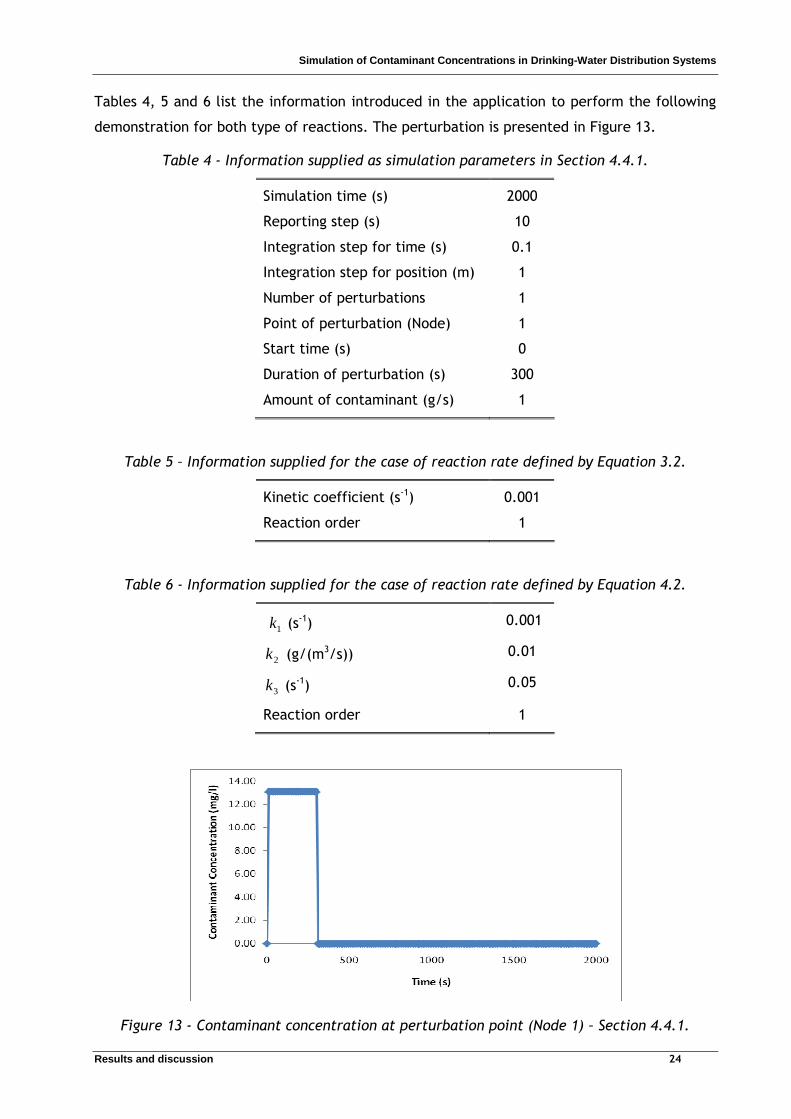
Tables 4, 5 and 6 list the information introduced in the application to perform the following

demonstration for both type of reactions. The perturbation is presented in Figure 13.

Table 4 - Information supplied as simulation parameters in Section 4.4.1.







Start time (s) 0


Amount of contaminant (g/s) 1

Table 5 – Information supplied for the case of reaction rate defined by Equation 3.2.

Kinetic coefficient (s-1) 0.001

Reaction order 1

Table 6 - Information supplied for the case of reaction rate defined by Equation 4.2.

1k (s-1) 0.001

2k (g/(m3/s)) 0.01

3k (s-1) 0.05

Reaction order 1

Figure 13 - Contaminant concentration at perturbation point (Node 1) – Section 4.4.1.



Figures 14 and 15 show the results computed for the contaminant concentration at node 7

and node 11, respectively. The results obtained for the reaction rate defined by the Equation

3.2 are presented by line and points in red colour; the results obtained with Equation 4.2 are

presented by line and points in blue colour.

Figure 14 - Contaminant concentration at node 7 – Section 4.4.1.

Figure 15 – Contaminant concentration at node 11 – Section 4.4.1.

As can be seen from Figures 14 and 15, different concentrations are achieved with the

different kinetic models.

4.4.2 Simulation of multiple perturbations

Another feature of the application is the possibility of defining more than one perturbation,

at different nodes. In this case, three perturbations at three different locations were defined



and are characterized in Tables 7 and 8. This simulation was run with three different values

of kinetic coefficient, 0 g/(m3/s) , 0.001 s-1 and 0.01 s-1.

Table 7 - Information supplied as simulation parameters in Section 4.4.2.





Kinetic coefficient 1 (g/(m3/s)) 0

Kinetic coefficient 2 (s-1) 0.001

Kinetic coefficient 3 (s-1) 0.01

Reaction order 1


Table 8 - Information supplied for the perturbations definition in Section 4.4.2.

Perturbation 1


Start time (s) 0



Perturbation 2


Start time (s) 500



Perturbation 3


Start time (s) 1000



The perturbations are represented in the Figure 16. The perturbation 1 is drawn in blue

colour, 2 in red and 3 in green.



Figure 16- Represention of the perturbations of example presented in Section 4.4.2

Figures 17 and 18 show the contaminant concentration at nodes 7 and 11, respectively.

Analysing Figure 17, three peaks can be observed for each kinetic coefficient, with increasing

amplitude as it is also observed in Figure 16. Figure 18 doesn’t present peaks – Node 11 is a

storage tank – but it is possible to observe an abrupt increase of concentration after each

perturbation.





The response to the different perturbations is also present in the results computed for the

pipes. Figure 19 represents the contaminant concentration at each length step of pipe 2 for

the simulation without reaction ( 0=k ). Similarly to the representation of the contaminant

concentration at Node 7 (Figure 17), it is possibly to distinguish the influence of each

perturbation by the amplitude of the curves.

Figure 19 - Contaminant concentration at each length step of pipe 2 – Section 4.4.2.



4.5 Comparison between analytical and numerical solutions

It was performed a comparison between the numerical approach used by the software tool,

explained in the Section 3.1.1 and the analytical approach described in the Section 3.1.2, in

the analysis of contamination profiles of the pipe 1. Table 9 lists the information supplied to

the application for this demonstration. Once again, the amount of contaminant was defined

using Equation 4.1, ensuring that the concentration at the reservoir is 1 mg/l.

Table 9 - Information supplied for the demonstration in Section 4.5.





Kinetic coefficient (g/m3/s) 0.1

Reaction order 1



Start time (s) 0


Amount of contaminant (g/s) 0.076452

The analytical solution was performed applying the Equation 3.22 using the parameters listed

in Table 10.

Table 10 - Information necessary to perform the analytical solution.

A (mg/l) 1

Kinetic coefficient (g/m3/s) 0.1

1u (m/s) 1.0816

1t (s) 0

2t (s) 100

Figures 20, 21 and 22 show the comparison between the concentration profiles computed the

analytical approach and the numerical approach, for time equal to 0 s, 50 s and 100 s,

respectively. The blue colour line refers to the results obtained with the analytical approach

and red colour points refer to the numerical approach results.



Figure 20 - Comparision between the analytical and the numerical solution for pipe 1

concentration profiles – t= 10 s.







Good agreements were observed between the results calculated by numerical and analytical

approaches, especially for t=100 s. Figures 20 and 21 show some discrepancies, caused by the

definition of the Heaviside used in the analytical approach.

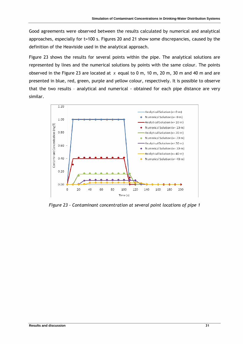
Figure 23 shows the results for several points within the pipe. The analytical solutions are

represented by lines and the numerical solutions by points with the same colour. The points

observed in the Figure 23 are located at x equal to 0 m, 10 m, 20 m, 30 m and 40 m and are

presented in blue, red, green, purple and yellow colour, respectively. It is possible to observe

that the two results – analytical and numerical - obtained for each pipe distance are very

similar.

Figure 23 - Contaminant concentration at several point locations of pipe 1


Conclusions 32

5 Conclusions

The EPANET software was able to evaluate the hydraulic calculation for drinking-water

distribution systems; however this application presented several limitations concerning the

evaluation of concentration profiles along the network. The limitations are related mainly

with the specification of perturbations and with the definition of kinetic models in EPANET

software, which simulates the deliberate contaminations.

The application developed overcame some of these limitations as it was demonstrated by the

simulations presented. As example, the study of different kinetic models performed by the

developed application is impossible to be performed by EPANET.

The application allows the user to analyse the behaviour of the network after several types of

multiple perturbations at any node/nodes of the network.

The analytical and numerical approaches for solving the problem of advective transport in

pipes with reaction in the bulk flow presented identical results.


Work assessment 33

6 Work assessment

6.1 Results accomplished

The main objectives of this work were:

1. To evaluate the potentialities of the EPANET software to study the contaminant

concentrations along the networks of drinking-water distribution systems;

2. To develop a software tool able to estimate the contaminant concentrations along the

networks after perturbations of several types defined by the user.

Relatively to the first objective, it was completely accomplished. It was done a detailed study

about the potentialities of the EPANET software and it was concluded that there are some

limitations established in the perturbation definition. These limitations constitute a great

disadvantage of this software tool for the study of contaminant concentrations along the

networks of drinking-water distribution systems.

Despite of having an unsatisfactory evaluation of concentration profiles, the hydraulic

simulation performed by EPANET was considered useful and suitable to be incorporated in the

developed application. This application is able to perform the study of deliberate

contaminations with more flexible perturbation definitions using the hydraulic data supplied

by EPANET. During this work, it was developed an application capable of managing the

hydraulic simulation performed by EPANET and the evaluation of contaminant concentrations

programmed in Visual Basic for Applications.

6.2 Future work

The work developed allowed to create a software application to perform the evaluation of

contaminants concentration after deliberate contaminations. Other types of perturbations

could be analysed without any additional effort.

The model used was very simple but can be easily redefined to account other aspects of

transport mechanism such as axial dispersion and reaction at the pipe wall.

New integration methods could be implemented to decrease the computing time of

simulations.


References 34

7 References

• Al-Omari, A. S., Chaudhry, M. H. Unsteady-state inverse chlorine modeling in pipe

networks. Journal of Hydraulic Engineering, 127, 669-677 (2001).

• Clark, R. M., Rossman, L. A., Wymer, L. J. Modeling distribution system water quality:

regulatory implications. Journal of Water Resources Planning and Management, 121,

423-428 (1995).

• Clark, R. M. Chlorine demand and TTHM formation kinetics: a second-order model.

Journal of Environmental Engineering, 124, 16-24 (1998).

• Elshorbagy, W. E., Abu-Qdais, H., Elsheamy, M. K., Simulation of THM species in water

distribution systems. Water Research, 34, 3431-3439 (2000).

• Li, X., Zhao, H., Development of a model for predicting trihalomethanes propagation

in water distribution systems. Chemosphere, 62, 1028-1032 (2005).

• Ozdemir, O. N., Ger, A. M., Unsteady 2-D chlorine transport in water supply pipes.

Water Research, 33, 3637-3645 (1999).

• Ozdemir, O., N., Ucak, A., Simulation of chlorine decay in drinking-water distribution

systems. Journal of Environmental Engineering, 128, 31-39 (2002).

• Rossman, L. A., Boulos, P. F., Altman, T., Discrete volume-element method for

network water-quality models. Journal of Water Resources Planning and Management,

119, 505-517 (1993).

• Rossman, L.A., Clark, R., M., Grayman, W. M., Modeling chlorine residuals in drinking-

water distribution systems. Journal of Environmental Engineering, 120, 803-820

(1994).

• Rossman, L. A., EPANET Users Manual. National Risk Management Research Laboratory,

Office of Research and Development, United States Environmental Protection Agency,

Cincinnati, Ohio (2000).

master’s degree in chemical engineering - … · master’s degree in chemical engineering...

Documents