master’s thesissterg.sun.ac.za/wp-content/uploads/2010/11/giglmayr_masterthesis1.pdfmaster’s...
TRANSCRIPT
MASTER’S THESIS
Thesis submitted in partial fulfilment of the requirements for the degree of Master of Science in Engineering
At the University of Applied Sciences – Technikum Wien, Vienna, Austria
Course of studies: Renewable Urban Energy Systems
At the University of Stellenbosch, Stellenbosch, Republic of South Africa
Research centre: Centre for Renewable and Sustainable Energy Studies
Development of a Renewable Energy Power
Supply Outlook 2015 for the Republic of South
Africa
Achieved by Sebastian Giglmayr, BSc
Registration number: 1110578003
Supervisors
Alan C. Brent, PhD
DI Hubert Fechner, MAS, MSc
Stellenbosch, South Africa, 27/03/2013

I

II
Declaration
I, Sebastian GIGLMAYR, hereby declare on oath that this master’s thesis is a presentation of my
original research work and that it has not been submitted anywhere for any award. Wherever
external contribution and other sources were implied, every attempt was made to emphasise this
clearly by indicating references to the literature.
____________________ ____________________
Place, Date Signature

III
IV
Abstract
South Africa’s electricity supply is characterised by outdated structures that cannot meet
contemporary requirements. The distribution is centralised and mostly unidirectional, while the
generation is based on the use of such fossil fuels as coal. A current substantial backlog of
electricity supply occurred, since the demand rose faster than the generation capacities increased.
During the last decade, the government has implemented a variety of mid- and long-term
programmes to enable further capacities, and to ensure onward sustainable development. A
meaningful part thereof is a subsidy mechanism for large-scale and grid-connected renewable
energy systems to promote an increase of installed capacities by independent power producers.
The framework of the thesis includes a literature research to highlight the current challenges and to
justify the need for a sufficient forecast method regarding an increased amount of renewable
energies. A 2015 annual time series simulation of every approved project until mid-2013 is
undertaken, assuming that every plant will be on grid by the end of 2014. The model’s
methodology is split into four different approaches regarding four different technologies, including
solar photovoltaic, wind, hydropower, and concentrated solar power. Hourly based annual load
behaviour results throughout in the achievement of a prospective amount of electricity contribution.
As a consequence, knowledge about system loads behaviour, such as evaluations regarding high-
demand scenarios and fluctuation bandwidths, is developed. The result contains a variety of
information about the prospective supply, which might serve for trendsetting decision-making.
Keywords
Renewable energy in South Africa, policy framework, forecast, time series simulation

V
VI
Kurzfassung
Die Infrastruktur zur Stromerzeugung bzw. zur Verteilung in Südafrika ist veraltet und wird die
zukünftigen Anforderungen nicht erfüllen können. Das System ist stark zentralisiert, unflexibel und
hat einen außergewöhnlich hohen Anteil an fossilen Energieträgern. Angesichts des stetig
anwachsenden Verbrauchs und des Mangels an zusätzlichen Versorgungskapazitäten, erhöht sich
die Wahrscheinlichkeit einer Unterversorgung. Um den zukünftigen Aufgaben gerecht werden zu
können, wurden innerhalb der letzten Jahre lang- und mittelfristige Programme geschaffen, die
unter Anderem dazu dienen, erneuerbare Energieträger zu unterstützen.
Die Arbeit beinhaltet eine ausführliche Literaturrecherche, welche aktuelle Problematiken im
Bereich der Stromerzeugung bzw. Verteilung aufzeigt und begründet. Das Hauptaugenmerk gilt
jedoch der Erstellung einer Zukunftsprognose für 2015 in welcher alle genehmigten und
geförderten Projekte mit einer Anschlussleistung größer 1MW bis 2013 berücksichtigt werden. Ein
auf Zeitserien basierendes Modell beinhaltet vier verschiedene Vorgehensweisen, entsprechend
der eingesetzten Technologien.
Das Resultat umfasst eine jährliche Menge an eingespeistem Strom, das Lastverhalten der
Kraftwerke und eine Bewertung des Beitrags zur Verbrauchsspitzen bzw.
Fluktuationseigenschaften um Entscheidungsträgern einen Ausblick der erneuerbaren
Stromversorgung zu gewährleisten.
Schlagwörter
Erneuerbare Energien in Südafrika, politische Rahmenbedingungen, Prognose,
Zeitseriensimulation

VII

VIII
Acknowledgement
The success of my thesis largely depended on the encouragement of various key role-players.
I wish to express my sincere gratitude to Paul Gauché, Director of the Solar Thermal Energy
Research Group, for his valuable advice. I, further, would like to acknowledge, with appreciation,
the supervision of Alan Brent, Director at the Centre for Renewable and Sustainable Energy
Studies in Stellenbosch and that of Hubert Fechner, Head of Department at the University of
Applied Science, Vienna.
My family and my parents, Ulli and Burkhard, are the recipients of my heartfelt gratitude for their
continuous devotion during the entire period of my studies. Their unfailing support constitutes the
basis of my success.
I, further, largely appreciate the scholarship ‘TOP-Stipendium NÖ’, provided by the federal state
‘Niederösterreich’ in the form of financial assistance.
Thank you to my friends, especially to Alexander, Nikolaus and Jakob, who have been there
continuously for me, and to everyone who has contributed to my progress during my studies.

IX

X
Table of contents
Declaration......................................................................................................................................I
Abstract..........................................................................................................................................II
Acknowledgement.........................................................................................................................IV
List of tables.................................................................................................................................VI
List of figures...............................................................................................................................VII
Acronyms and abbreviations..........................................................................................................IX
1 Description of the objective of the thesis .......................................................................... 2
2 Relevance of results ........................................................................................................ 2
3 Methodology .................................................................................................................... 5
3.1 Definition of the objective of the project ........................................................................... 5
3.2 Information procurement .................................................................................................. 5
3.3 Quality assurance ............................................................................................................ 6
3.4 Implementation of present resources ............................................................................... 6
3.5 Development of the model ............................................................................................... 7
4 Introduction to issues relating to electricity supply and demand ....................................... 8
4.1 Local renewable energy resource analysis ...................................................................... 9
4.1.1 Solar irradiance ............................................................................................................... 9
4.1.2 Wind power ................................................................................................................... 10
4.2 National energy consumption and allocation .................................................................. 11
4.3 Electricity supply and demand ....................................................................................... 11
4.3.1 National electricity supply .............................................................................................. 12
4.3.2 Sector-specific electricity demand ................................................................................. 13
4.3.3 Present lack of supply ................................................................................................... 13
4.3.4 Prospective development .............................................................................................. 14
4.4 Power distribution .......................................................................................................... 14
4.5 Chapter summary .......................................................................................................... 15
5 Policy guidelines and legal framework ........................................................................... 18
5.1 IRP for electricity – IRP 2010 ......................................................................................... 18
5.1.1 IRP 2010 – content ........................................................................................................ 19
5.1.2 The Medium-Term Risk Mitigation Plan ......................................................................... 21
5.2 The Renewable Energy Feed-In Tariffs (REFIT) programme ......................................... 22
5.3 The REIPPPP ................................................................................................................ 23

XI
6 Involved renewable energy projects............................................................................... 30
6.1 Approved facilities prior to 2011 ..................................................................................... 30
6.1.1 Existing wind resources ................................................................................................. 30
6.1.2 REIPPPP-approved projects ......................................................................................... 31
7 Modelling the prospective load contribution ................................................................... 34
7.1 Introduction .................................................................................................................... 34
7.2 Input parameters ........................................................................................................... 35
7.3 Wind simulation ............................................................................................................. 35
7.3.1 Data verification ............................................................................................................. 36
7.3.2 Height-related extrapolation ........................................................................................... 38
7.3.3 Power conversion .......................................................................................................... 40
7.3.4 Method 1 – assorted approach ...................................................................................... 42
7.3.5 Method 2 – single approach .......................................................................................... 43
7.3.6 Validation – assorted and single approach .................................................................... 44
7.3.7 Results .......................................................................................................................... 44
7.4 Solar PV simulation ....................................................................................................... 46
7.4.1 Data verification ............................................................................................................. 46
7.4.2 Methodology .................................................................................................................. 47
7.4.3 The making of assumptions ........................................................................................... 48
7.4.4 Results .......................................................................................................................... 49
7.5 Concentrated solar power simulation ............................................................................. 50
7.5.1 Methodology and assumptions ...................................................................................... 50
7.5.2 Results .......................................................................................................................... 52
7.6 Hydropower simulation .................................................................................................. 53
7.6.1 Methodology and assumptions ...................................................................................... 53
7.6.2 Results .......................................................................................................................... 54
8 Simulation results .......................................................................................................... 56
8.1 Cumulated output .......................................................................................................... 56
8.1.1 Overview of general results ........................................................................................... 56
8.1.2 Contribution to winter demand peak .............................................................................. 58
8.1.3 Fluctuation characteristics ............................................................................................. 60
8.2 Conclusion..................................................................................................................... 63
9 Reference list ................................................................................................................ 66

XII

XIII
List of tables
Table 1: The premier CO2-emitting power utilities worldwide (Gross, 2012, p. 5) ............................ 8
Table 2: List of power capacities (Nersa 2006, p. 42) .................................................................... 12
Table 3: Final development of the IRP 2010 (IRP 2011, p. 6 sqq.) ................................................ 19
Table 4: Policy-adjusted IRP – intended capacities (IRP 2011, p. 7) ............................................. 20
Table 5: Trend in REFIT tariffs (Nersa 2008, 2011) ....................................................................... 23
Table 6: Overview of the REIPPPP (DoE 2011b, p. 2) .................................................................. 24
Table 7: Bidding approach of the REIPPPP (DoE 2013a) ............................................................. 25
Table 8: Tariff cap and recent subsidy tariffs (DoE 2012a; Greyling A. 2012, p. 14) ...................... 26
Table 9: Facilities committed prior to 2011 .................................................................................... 30
Table 10: Wind facilities approved for R1 and R2.......................................................................... 31
Table 11: Solar PV facilities approved for R1 and R2 .................................................................... 31
Table 12: CSP and hydropower facilities approved for R1 and R2 ................................................ 32
Table 13: Comparison of GeoModel data at WM sites and WM measurements ............................ 37
Table 14: Error evaluation between GeoModel data and WM measurements ............................... 37
Table 15: Friction coefficient and roughness lengths (Tong 2010; Patel 2006) .............................. 39
Table 16: Wind speed extrapolation – verification. Units in GWh. ................................................. 42
Table 17: Seasonal characteristics of wind generation .................................................................. 46
Table 18: Solar CPV properties, type 3C40, Azur Space Solar Power Ltd, under STC ................. 49
Table 19: Seasonal characteristics of solar PV generation ............................................................ 50
Table 20: CSP SAM – input parameters (CSP World 2013) .......................................................... 51
Table 21: Verification of CSP simulation results ............................................................................ 52
Table 22: Hydropower input parameters ....................................................................................... 54
Table 23: Technology-specific annual energy yield ....................................................................... 57
Table 24: System duration curve – classification into quartiles ...................................................... 58
Table 25: Fluctuation duration curve – classification into quartiles ................................................ 61
Table 26:Coal sales by sector, 2000 (King N.A., Blignaut J.N., 2002, p. 6 sqq.) ............................ 73
Table 27: Comparison of five solar PV modules ............................................................................ 94
Table 28: CSP, SAM – additional input parameters (CSP World, 2013) ........................................ 96

XIV

XV
List of figures
Figure 1: Wind Atlas of South Africa (WASA 2012, p. 4) ............................................................... 10
Figure 2: South African map for GHI, left and DNI, right (GeoSun Africa 2008) ............................. 11
Figure 3: Transmission and distribution network; units in TWh (Nersa 2006, p. 54) ...................... 15
Figure 4: Eskom and IPP price adjustment/forecast 2006–2018 (Nersa 2013, 2013a) .................. 27
Figure 5: REIPPPP approach for an Independent Power Producer (Siepelmeyer N. 2013) .......... 28
Figure 6: Location of IPP projects countrywide, featured by way of Google Maps. ........................ 33
Figure 7: Mean wind distribution curve – wind mast measurement and GeoModel simulation ...... 38
Figure 8: Comparison of the data according to the Hellmann exponential law and the logarithmic
wind profile law ............................................................................................................................. 40
Figure 9: Approximation of the wind power curve .......................................................................... 41
Figure 10: Capacity factors of wind facilities – model and assimilation .......................................... 44
Figure 11: Exemplary wind power course in January .................................................................... 46
Figure 12: Exemplary cumulative solar PV generation in January ................................................. 50
Figure 13: Khi Solar One – seasonal course with 3h storage ........................................................ 52
Figure 14: Bokpoort CSP – seasonal course with 3h storage ........................................................ 53
Figure 15: Neusberg hydropower − annual course ........................................................................ 54
Figure 16: System duration curve ................................................................................................. 58
Figure 17: Winter and summer firm capacity – 19:00 to 01:00 ...................................................... 59
Figure 18: Frequency distribution during summer and winter (A) .................................................. 60
Figure 19: Mean power distribution during winter and summer – 19:00 to 24:00 ........................... 60
Figure 20: Fluctuation duration curve ............................................................................................ 61
Figure 21: Exemplary single and cumulative power course – 01/01/2010–11/01/2010 .................. 62
Figure 22: Final consumption, 2006 (DoE 2009, Statistics Austria 2013) ...................................... 72
Figure 23: Correlation between the electricity- and the GDP growth rate (Mashao 2012) .............. 76
Figure 24: Electricity intensity (Mashao 2012, p. 19 sqq.) ............................................................. 77
Figure 25: Electricity available for distribution (SSA 2013, World Bank 2013, Nersa 2006) ........... 78
Figure 26: Electricity demand, by sector (Nersa 2006, p. 58) ........................................................ 78
Figure 27: Exemplary weekday demand during summer and winter in 2010 (Eskom 2012) .......... 79
Figure 28: Expected annual energy simulation (DoE 2010, IRP 2010b) ........................................ 81
Figure 29: High-voltage grid map – South Africa (CRSES 2013) ................................................... 82
Figure 30: Wind – annual load duration curve (assorted and single approach) ............................. 92
Figure 31: Wind – seasonal load duration curve ........................................................................... 92
Figure 32: Validation of contemporaneous power increase and wind speeds at WMs (60m) ........ 93
Figure 33: Optimum PV tilt for maximising annual energy yield (Suri, Cebecauer 2012, p. 5) ....... 94
Figure 34: Solar PV model verification (Gauché 2011, NREL 2005) ............................................. 95
Figure 35: Cumulative CSP course in January .............................................................................. 96
Figure 36: Khi Solar One – seasonal, temporal distribution ........................................................... 97
Figure 37: Bokpoort CSP – seasonal, temporal distribution .......................................................... 98

XVI
Figure 38: Frequency distribution during summer and winter (B) ................................................ 100
Figure 39: Distribution share, winter 19:00–22:00 ....................................................................... 101
Figure 40: Distribution share, summer 19:00–22:00 .................................................................... 102

XVII
Acronyms and abbreviations
ANC African National Congress
CCGT closed-cycle gas turbine
CF capacity factor
CORDIS Community Research and Development Information Service
CPV concentrated photovoltaic
CR central receiver
CRSES Centre for Renewable and Sustainable Energy Studies
CSIR Council for Scientific and Industrial Research
CSP concentrated solar power
DEA Department of Environmental Affairs
DHI diffuse horizontal irradiance
DME Department of Minerals and Energy
DNI direct normal irradiance
DoE Department of Energy
DR demand response
DSM demand-side management
DWA Department of Water Affairs
EAF energy availability factor
ECS energy conservation scheme
EIA environmental impact assessment
ESKOM Elektrisiteitsvoorsienings-kommissie (prev. ESCOM Electricity Supply Commission)
GDP gross domestic product
GHI global horizontal irradiance
GTI global tilted irradiance
IEP Integrated Energy Plan
IPP independent power producer
IRP Integrated Resource Plan
ISMO Independent System and Market Operator MAE mean absolute error
MAPE mean absolute percentage error
ME mean error
MTPPP medium-term power purchase programme
MTRM Medium Term Risk Mitigation
MYPD Multi-Year Price Determination
NEA National Energy Act
NERSA National Energy Regulator of South Africa

XVIII
NREL National Renewable Energy Laboratory
OCGT open-cycle gas turbine
PFMA Public Finance Management Act
PPA power purchase agreement
RBS Revised Balanced Scenario REBID Renewable Energy Bid
REFIT Renewable Energy Feed-In Tariff
REIPPPP Renewable Energy Independent Power Producer Procurement Programme
RFP Request for Proposal
RMSE root mean square error
RoD Record of Decision
SAM System Advisor Model
SANEDI South African National Energy Development Institute
SAPIA South African Petroleum Industry Association
SAPVIA South African Photovoltaic Industry Association
SAWEA South African Wind Energy Association
SBO Single Buyer Office
SD standard deviation
SESSA Sustainable Energy Society of Southern Africa
SO system operator
SSA Statistics South Africa
STC standard test conditions
STERG Solar Thermal Energy Research Group
SVC static VAR compensator
SWH solar water heater
TES thermal energy storage UCT University of Cape Town
WASA Wind Atlas for South Africa
WaSP Wind Atlas Analysis and Application Programme
WM weather mast

Description of the objective of the thesis

Description of the objective of the thesis
2
1 Description of the objective of the thesis
The objective of the thesis was to develop a plausible supply scenario for every submitted,
commercial, grid-connected and approved renewable energy generation project in South
Africa until 9 May 2013, once the financial closure of the Renewable Energy Independent
Power Producer Procurement Programme (REIPPPP) had taken place. This closure
constitutes a proper public landmark for a national implementation of renewable sources,
and should result in the grid commissioning of all participants by the end of 2014.
In terms of the above, a time series simulation was developed containing a consolidation of
accurate simulated weather data, a localisation of all related projects, and the technical
correlations among them, to compute an estimated annual power output for the
subsequent year, 2015.
The result delivers insight into the entire annual countrywide share of renewable energies
for 2015, represented by weather data of 2010, as well as by the load behaviour, in certain
load cases. The study will make it possible to do more accurate forecasting as soon as all
the necessary suppliers are commissioned, and will allow a further road map development
to advise policymakers and other representatives, mostly at the national level, to consider
decisions regarding the future energy mix. Based on the fact that a variety of renewable
energy projects in South Africa are planned, and that some of them are currently in
progress, it has become necessary to reflect the prospective situation in detail.
The research question is as follows:
What will be the supposed annual trend and the summarised amount of renewable
energies in South Africa that are fed into the electricity grid by 2015, since policies
encourage increased implementation? How will power loads such as PV, CSP, wind
power and small scale hydro power contribute to supply stability during full-load demand
cases, and what are the characteristics likely to be in terms of generation volatility
based on an hourly time series simulation?
2 Relevance of results
South Africa seems to possess an extraordinary amount of energy resources. The primary
energy carrier, coal, which is the major fossil resource, is mainly used for national
electricity production, for liquefaction and for exportation. Despite the fact that the majority
of produced electricity is generated by fossil fuels, the country’s potential of renewable
energy sources is vast, whereas solar irradiance and wind offer considerable commercial
potential.

Relevance of results
3
Within the last decade, the national approach to renewable energies issues has changed
according to rising prices for fossil fuels and the increasing awareness of the their
countrywide potential. As a consequence, increasingly more international lenders, funds
and other sponsoring bodies have been lured to invest in alternative energy projects
(Record Conference 2013). For the purposes of this study, national policy guidelines such
as the Integrated Resource Plan 2010 (IRP 2010) were assembled, and incorporated with
different lobbies to determine a legal framework and a specific road map for South Africa.
Currently, South Africa sets a high standard with specialised engineering departments
such as the Centre for Renewable and Sustainable Energy Studies (CRSES); the Solar
Thermal Energy Research Group (STERG); GeoSUN; that of the University of Cape Town
(UCT); and Eskom. Despite said departments being focused on conducting scientific
research in the fields of concentrated solar power (CSP), deterministic model mapping,
and sustainable development, among others, a backlog exists in satisfying the demand for
reliable forecasting of the total renewable energy contribution that is to be made within the
next decade. Although previously released forecasts and guidelines take capacities into
account, they do not take into consideration the temporal and technology-dependent
energy distribution of renewable generation.
The purpose of the current thesis is to address this problem, and to overcome the present
backlog.
Hence, the CRSES and UCT will cooperate in developing a proper, more explicit study,
which will be based on the results of this thesis, which, in addition, specifies the
prospective renewable energy contribution to be made in South Africa.

Relevance of results
4

Methodology
5
3 Methodology
The methodology of this study entailed the adoption of a comprehensive and wide-ranging
approach. The present chapter describes the scientific character of the thesis, which
required specific methods of research and legal proceedings. The approach was based on
the bottom-up principle of obtaining results from a large quantity of information. The
research was undertaken in chronological order to enable entire conformability with the set
requirements.
This chapter outlines the objectives, the data assessments, the quality assurance
concerns, and the model development in this study.
3.1 Definition of the objective of the project
The objective of the project was predefined by the CRSES Department, and it was derived
according to the present institutional requirements. The structure of the project was
discussed at the initial meeting. The objective of said Department was to advise the
policymakers concerned through providing them with reliable information on which to base
their decisions. The intended purpose of the thesis was established and well-defined, with
the evolution of the framework being considered an integral part of the consistent progress
made in terms of the project, which strongly depended on the availability of the appropriate
data.
3.2 Information procurement
The first step in the procedure comprised data mining with regard to the surrounding
conditions to substantiate the present need for the analysis. The main sources of required
information were scientific papers, the publications of linked and relevant departments, ,
and the contents of scientific databases.
The following scientific databases were considered to obtain some of the required
information:
The Library and Information Service of Stellenbosch University
The Community Research and Development Information Service (CORDIS)
The Austrian Library Composite of the Österreichischer Bibliothekenverbund GmbH
The library of the FH Technikum Wien/ the University of Applied Science Vienna
The library of the TU Vienna
The library of Science Direct

Methodology
6
With regard to expenditure on the project, the layout was mainly on desk and literature
research, with some hard copy literature but mostly online media being utilised. For further
information, interviews, phone calls, electronic mail, and attendance at lectures and
scientific congresses, which allowed for networking with fellow professionals, were used.
3.3 Quality assurance
The approach that was adopted to ensure the quality of work is stated as follows:
Mutual control existed between the author, his supervisors, and the project team,
with the conclusions, calculations, assumptions, and adoptions being validated.
The reliability of the data that were obtained was compared with that of data that
were obtained from other sources.
In order to ensure the reliability of the data source, information was obtained only
from government, institutional and scientific sources.
3.4 Implementation of present resources
This section deals with the utilisation of available auxiliary means, such as simulation tools
and information-providing applications, which contributed to the completion of the analysis.
Simulation programmes
Beside the development of a particular model, several tools were used for simulation and
verification purposes. The tools reflect the connection between the raw weather data and
the corresponding power loads. The following applications were used:
The basic PV model by P. Gauché (2011), which is a time series simulation for
solar PV issues
The System Advisor Model (SAM), by the National Renewable Energy Laboratory
(NREL 2005), for CSP and solar PV applications
Data procurement
The following sources were applied to access the necessary records of data for simulation
and/or validation purposes:
The Wind Atlas of South Africa (WASA), for the weather mast (WM) measurements
The GeoModel Solar Ltd (SolarGIS)
The South African Department of Water Affairs (DWA 2013)

Methodology
7
All utilised data were validated in terms of the origin, the reliability, the error margin, and
the existing evaluations of the data provided by the other scientists. Cases of irregularity
were considered and clearly identified, so as to be able to evaluate the probability of
recurrence of an error.
3.5 Development of the model
The quasistatic nature of the model was obtained by using basic physical correlations and
external time series simulated data records from specific project sites.
The model’s methodology was composed of different approaches for each modelling
technology used, depending on the availability of existing simulation programmes. If an
already developed tool was consulted, it was necessarily validated. Such validation
contains analogies to other simulation approaches, a comparison to the expectations of the
project developers, and a plausibility check by project members. For a single developed
method, such as the wind power analysis, a validation, as described above, had to be
achieved.
For simulation concerns, certain boundary conditions and assumptions had to be met.
Each assumption was clearly specified and technically justified to ensure transparency and
clarity. Furthermore, every uncertainty and possibility of error was stated.
The simulation approach for every technology (whether wind, solar photovoltaic (PV), CSP,
or hydropower) is described in detail in each corresponding chapter.
Introduction to issues relating to electricity supply and demand
8
4 Introduction to issues relating to electricity
supply and demand
The South African economy strongly depends on the consumption of fossil fuels such as
coal as the primary energy source countrywide. Although other renewable potential, such
as that which is possessed by hydropower and solar irradiance, as well as by wind power,
is vast, it is, as yet, almost untapped.
The present and prospective countrywide power supply is subject to the following three
main constraints:
Lack of reliability: One of the key roles of a reliable power supply is to ensure the
maintenance of a reserve margin that allows for periods of both planned and
unplanned unavailability, such as for maintenance and for outages. The reserve
margin in South Africa declined from 25% in 2002 to 10% in 2008, as a result of the
robust economic growth experienced, as well as a coincidental missed strategy to
align the demand, thus drastically limiting the scope of action (RSA Government
2008, p. 4).
Lack of sustainability: In 2007, 92% of the electricity generation made use of coal,
which led to extraordinary CO2 equivalent (eqt.) emissions. In 2012, Eskom was the
second highest CO2-emitting power utility company worldwide. The average CO2
eqt of South Africa is 1.015tCO2 – eqt/MWhel (Letete, M. Guma, 2009), whereas the
mean European CO2 eqt is 0.578tCO2 – eqt/MWhel, which is almost 45% less than
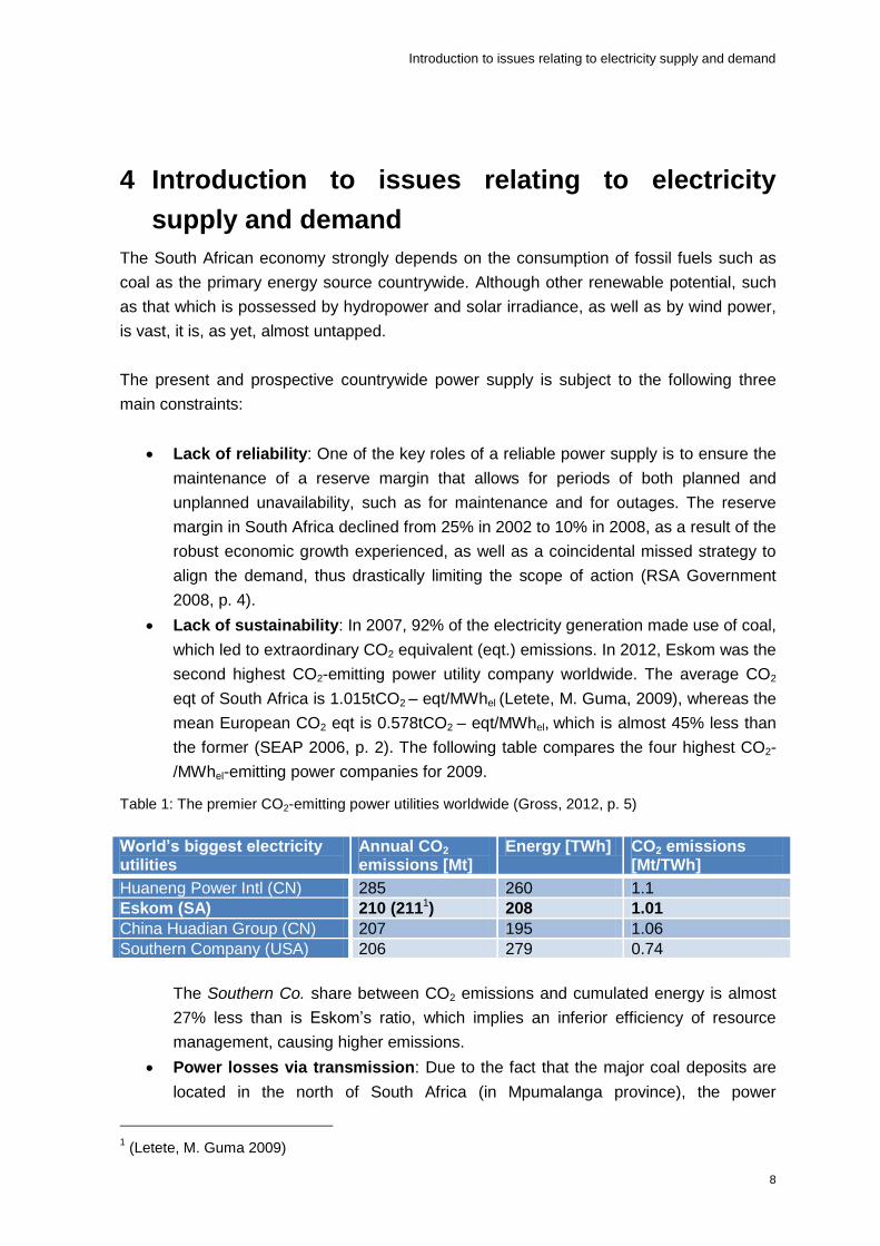
the former (SEAP 2006, p. 2). The following table compares the four highest CO2-
/MWhel-emitting power companies for 2009.
Table 1: The premier CO2-emitting power utilities worldwide (Gross, 2012, p. 5)
World’s biggest electricity utilities
Annual CO2 emissions [Mt]
Energy [TWh] CO2 emissions [Mt/TWh]
Huaneng Power Intl (CN) 285 260 1.1
Eskom (SA) 210 (2111) 208 1.01
China Huadian Group (CN) 207 195 1.06
Southern Company (USA) 206 279 0.74
The Southern Co. share between CO2 emissions and cumulated energy is almost
27% less than is Eskom’s ratio, which implies an inferior efficiency of resource
management, causing higher emissions.
Power losses via transmission: Due to the fact that the major coal deposits are
located in the north of South Africa (in Mpumalanga province), the power
1 (Letete, M. Guma 2009)

Introduction to issues relating to electricity supply and demand
9
generation is situated in this region. A transmission grid connects the north of the
country to the south. The vast distances involved resulted in losses of 9.5% in 2010
(World Bank 2013). Scientists such as Prof. Ernst Uken (2013) estimate the actual
amount of loss to be as much as 15%.
The probability of a feasible prospective scenario, with a high integrity of renewable
sources, requires an increase in supply capacity, and a concurrent specific decrease in
demand through improvements in efficiency, and other methods.
Notice should be taken that the current thesis refers to the commitment of a renewable
supply only.
4.1 Local renewable energy resource analysis
Establishing the potential of renewable sources in South Africa is focused on wind energy
and solar irradiance. Whereas the highest measured values for solar irradiation are in the
north-western part of the country, the wind potential mainly exists on the coastline, which
stretches from the Atlantic to the Indian Ocean.
Other renewable resources, such as biomass and ocean energy, do not play a decisive
role. Until 2006, 10 river power stations were built up with an annual yield of 1.3% to the
gross sent out electricity and an installed capacity of 668MW (Nersa 2006).
4.1.1 Solar irradiance
The solar irradiance is mostly represented by the global horizontal irradiance (GHI) and/or
the direct normal irradiance (DNI).
The GHI (kWh/m²/a or W/m²) is the total amount of irradiation, consisting of a direct
(beam) and a diffuse (scattered) proportion that is relayed onto a particular
horizontal area. The inclined GHI (global tilted irradiance – GTI) is primarily used for
power estimation purposes related to a solar PV or a solar water heater (SWH) with
a fixed inclined angle.
The DNI value (kWh/m²/a or W/m²) represents the direct, perpendicular on a
predefined surface, beaming component of the sun only and is measured by
tracking the measuring instrument. Diffuse irradiation is totally excluded from such
a calculation. The DNI is utilised for CSP and concentrated photovoltaic (CPV)
purposes.
In South Africa, the ceiling value for GHI can be as high as 2 300 kWh/m²/a, whereas the
DNI value attains a maximum of 2 900 kWh/m²/a, which is significantly higher than it is in

Introduction to issues relating to electricity supply and demand
10
other regions worldwide. The solar GHI and the DNI data for the country, which are well
documented, are available from GeoSUN Africa, SolarGIS. Figure 2 on p. 11 depicts the
national differences between DNI and GHI.
4.1.2 Wind power
The South African wind potential is situated along the coastline that is stretched along the
southern and north-east regions. A partnership between, inter alia, the South African
National Energy Development Institute (SANEDI), the South African Weather Services
(SAWS), UCT and the Risø Danish Research Institute (DTU), which was financially
supported by a consortium, led by the Department of Energy (DoE), developed a numerical
wind atlas to enable the planning of large-scale exploitation of wind power in South Africa.
The result is an extensive Wind Atlas of South Africa (WASA), which offers specified wind
data for all regions in the country. The wind model is based on a measured time series of
wind speeds, direction and terrain topography (in terms of elevation, roughness and
obstacles), and which illustrates the countrywide wind speeds.
Figure 1 below consists of a map of generalised annual mean wind speeds (over a period
of 30 years) in an area that is 100m above ground level, with flat terrain and a 3cm
roughness class. The series of numbers (1–10) featured represents the installed WMs.
Figure 1: Wind Atlas of South Africa (WASA 2012, p. 4)

Introduction to issues relating to electricity supply and demand
11
Figure 2: South African map for GHI, left and DNI, right (GeoSun Africa 2008)
4.2 National energy consumption and allocation
Most of the nationwide primary energy consumption-related publications by governmental
sources are both inconsistent and no longer up to date.
The total determined primary energy supply in 2006 by the Energy Department of South
Africa was 5 644 436TJ (DoE 2009, p. 4 sqq.), whereas 65.9% of such supply was
provided by the use of coal, followed by crude oil (21.5%), and such renewable sources as
biomass and natural processes (7.6%). In contrast to the Energy Department of South
Africa, Statistics South Africa (SSA 2012) estimates a total, since 2002, decreasing primary
energy supply for 2006 of 7 742 673 TJ, excluding the accumulation of imported energy.
Hence, energy is a substantial key driver of the South African economy.
The three major final energy consumers in the country are the industry, which consumes
about 40%, followed by the transportation sector, and the residential sector, as is illustrated
in Annexure I, Part A, Figure 22, p. 72. Further information, such as a digest of the national
coal and petrol allocation, is specified in Annexure I, Part.
4.3 Electricity supply and demand
An overview of the present lack of electricity supply in South Africa is supplied below,
followed by a description of the prospective development of such a supply in the country.
The following additional information is elaborated on in Annexure I, Part B:
The history of supply and demand
The key drivers of electricity growth rates
The development of electricity intensity
Introduction to issues relating to electricity supply and demand
12
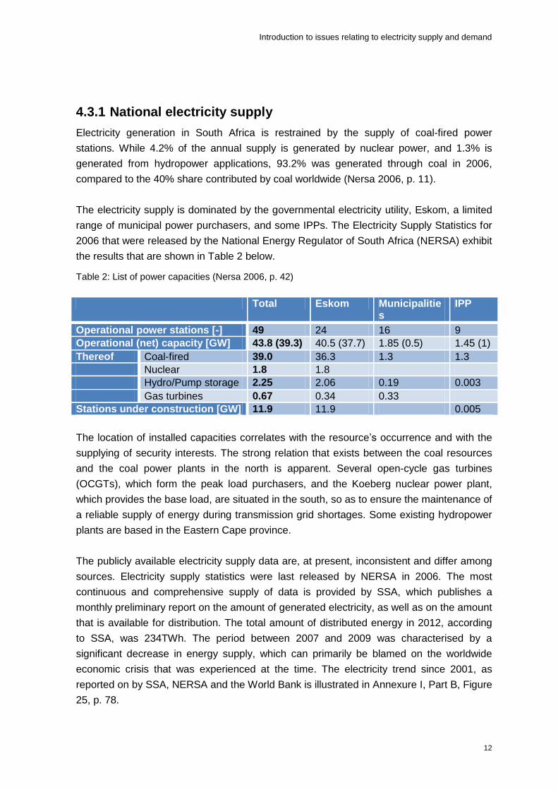
4.3.1 National electricity supply
Electricity generation in South Africa is restrained by the supply of coal-fired power
stations. While 4.2% of the annual supply is generated by nuclear power, and 1.3% is
generated from hydropower applications, 93.2% was generated through coal in 2006,
compared to the 40% share contributed by coal worldwide (Nersa 2006, p. 11).
The electricity supply is dominated by the governmental electricity utility, Eskom, a limited
range of municipal power purchasers, and some IPPs. The Electricity Supply Statistics for
2006 that were released by the National Energy Regulator of South Africa (NERSA) exhibit
the results that are shown in Table 2 below.
Table 2: List of power capacities (Nersa 2006, p. 42)
Total Eskom Municipalities
IPP
Operational power stations [-] 49 24 16 9
Operational (net) capacity [GW] 43.8 (39.3) 40.5 (37.7) 1.85 (0.5) 1.45 (1)
Thereof Coal-fired 39.0 36.3 1.3 1.3
Nuclear 1.8 1.8
Hydro/Pump storage 2.25 2.06 0.19 0.003
Gas turbines 0.67 0.34 0.33
Stations under construction [GW] 11.9 11.9 0.005
The location of installed capacities correlates with the resource’s occurrence and with the
supplying of security interests. The strong relation that exists between the coal resources
and the coal power plants in the north is apparent. Several open-cycle gas turbines
(OCGTs), which form the peak load purchasers, and the Koeberg nuclear power plant,
which provides the base load, are situated in the south, so as to ensure the maintenance of
a reliable supply of energy during transmission grid shortages. Some existing hydropower
plants are based in the Eastern Cape province.
The publicly available electricity supply data are, at present, inconsistent and differ among
sources. Electricity supply statistics were last released by NERSA in 2006. The most
continuous and comprehensive supply of data is provided by SSA, which publishes a
monthly preliminary report on the amount of generated electricity, as well as on the amount
that is available for distribution. The total amount of distributed energy in 2012, according
to SSA, was 234TWh. The period between 2007 and 2009 was characterised by a
significant decrease in energy supply, which can primarily be blamed on the worldwide
economic crisis that was experienced at the time. The electricity trend since 2001, as
reported on by SSA, NERSA and the World Bank is illustrated in Annexure I, Part B, Figure
25, p. 78.

Introduction to issues relating to electricity supply and demand
13
The power supply system load factor determines the share between the average load over
the set period of time (i.e. a year) and the maximum load during the specified time period
as being 68.9%. The load factor ought to be as high as possible to achieve a worthwhile
degree of capacity utilisation for the base-load plants. The average load factor for coal (in
terms of Eskom power generation) is 73.3%, with a variation of +15% and −57%, which
implies a high fault rate, which was caused by maintenance, defects, and other related
factors (Nersa 2006, p. 45).
4.3.2 Sector-specific electricity demand
In 2006, the entire South African demand was 205TWh, with a strong emphasis on the
primary and secondary sector (of which 60% was industry), including manufacturing,
mining and agriculture. The gap between the amount of electricity available for the
distribution of 233TWh, and the amount of energy sold, with an end use of 205TWh,
constituted the distribution losses that are outlined in Chapter 4.4.
Although approximately 94% of the customers were situated in the domestic sector, their
accurate consumption was only 19%. The mean specific retail price for electricity
acquisition in 2006 was 37.5R/kWh for domestic consumers, while the average price for
the mining industry was only 16.9R/kWh (Nersa 2006, p. 60). The sector-specific electricity
demand is described in detail in Annexure I, Part B, Figure 26, p. 78.
4.3.3 Present lack of supply
In South Africa, since the reserve margin steadily decreases at a significant rate, the
stability of the power system is exposed to a relatively high risk of outages. The demand
for power has increased by 230% since 1987, while the power supply has increased by
only190%. During the last decade, the reserve margin has steadily declined. As a result,
the number of low-frequency incidents that have occurred during a period of under supply
has increased from twice in 2002 to 15 times in 2006, and the transmission system
interruption time over a minute has significantly amplified as well (Nersa 2006, p. 37).
Between 2006 and 2009, the outage duration curve of Eskom steadily increased, entailing
a decreasing energy availability factor (EAF). More than 8000MW of capacity was
unavailable for about 700 h per year. The related trigger was the bad coal quality, which
resulted in a need for high rates of maintenance (MTRM 2010, p. 4).
The various causes of the incipient energy crisis are characterised in Annexure 1, Part B.
The DoE launched an initiative named the Medium Term Risk Mitigation Project (MTRM) in
the context of the IRP 2010 (see section 5.1), when South Africa was seen to be facing
electricity constraints in terms of the security of supply. While the IRP addresses the long-
term outlook for the generation mix in South Africa, the MTRM’s focus is on identifying

Introduction to issues relating to electricity supply and demand
14
supply and demand options for addressing the short-term risk for outages from 2011 to
2016 (IRP 2011, p. 60). The report forecasts a high likelihood of occurring energy shortfalls
until 2015, as long as the new coal power plants, Medupi and Kusile (with a gradual
commissioning of 9.5GW from 2015 to 2018), are not yet on stream. The balance between
supply and demand was bound to be tight between 2011 and 2012, with a gap for the
mitigation of 15TWh. The MTRM involves all stakeholders, such as the government,
business, labour, civil society, Eskom, and others, and proposes options for closing the
gap, as shown in Annexure 1, Part B.
4.3.4 Prospective development
A prospective South African electricity supply scenario was calculated in 2010, in line with
the assessment procedure of the IRP 2010 that entailed the setting of major boundary
conditions for the taking of further steps (DoE 2010). In terms of accuracy, two
independent forecasts were developed, which are outlined in Annexure 1, Part B.
The forecast’s trends drift apart until 2034 is caused by many uncertain assumptions that
still essentially had to be set at the time of publication. The simulation was done between
2008 and 2010, following on shortly from the economic crisis, and the coincidental
decrease in demand (according to Figure 25, p. 78). At the time, the deviation concerned
was not conceivable, accounting for the observed gap between recent demand and
forecast that was reflected from 2010 to 2012.
In terms of the current thesis, the total accurate energy demand for 2015 is expected to be
between 275TWh and 315TWh, as depicted in Annexure 1, Part B, Figure 28, p. 81.
Pursuant to Eskom’s contribution, the power demand for 2015 should be approximately
47GW (Eskom 2013).
4.4 Power distribution
The power grid is subdivided into transmission and distribution applications. The urban
areas are well tapped, whereas the rural regions are commonly used for power
transmission applications, as is illustrated in Annexure I, Part C, Figure 29, p. 82. The
image illustrates the South African high-voltage power grid integration stretching from the
north to the south.
In 2006, the amount of electricity generated was 233TWh, whereas the end usage was
205TWh. Taking both imports and exports into account, a system loss of 10.9% was found
to have occurred. Figure 3 below is a Sankey diagram that depicts the energy flow from
generation to consumption in TWh, rounded.

Introduction to issues relating to electricity supply and demand
15
Figure 3: Transmission and distribution network; units in TWh (Nersa 2006, p. 54)
Almost 97% of generation and 100% of electricity transmission were achieved by Eskom,
with the distribution being partly managed by the municipalities and the private distributors.
The South African electricity grid faces a particular challenge in having to ensure a reliable
prospective supply. As long as the power consumption in the southern regions increases,
and the supply is still centrally provided, the distribution distances and the imbalance in
power supply will increase, which might result in power failures. Further details about the
future expectations of transmission, respectively via distribution lines and the power grid,
are noted in Annexure I, Part C.
4.5 Chapter summary
This introduction to issues relating to electricity supply and demand has elaborated on the
essential background information to justify an increased implementation of renewable
energy sources. This chapter summarises and highlights the significant impacts that were
described in the previous sections:
Although the potential for sustainable energy generation countrywide is vast, it is
almost unexploited.

Introduction to issues relating to electricity supply and demand
16
South Africa’s electricity generation strongly depends on the supply of such fossil
fuels as coal. Even though the resource is depleted nationally, and is competitively
available on the international market, its cost has substantially increased over the
last decade.
The specific CO2 emissions for electricity generation in South Africa are of the
highest worldwide, which implies a lack of efficiency and the likelihood of much
environmental pollution.
The electricity distribution is accomplished centrally. The power is transmitted from
the north to the south of the country, over a long distance, which results in
substantial transmission/distribution losses, and a high vulnerability to failure.
The electricity demand has increased faster than the generation availability has
done in the past. As a consequence, new capacities have become indispensable
for meeting the demand, and for increasing the reserve margin. Eskom, the only
national electricity utility, will be incapable of achieving the requirements on its own.
Within the last few years, the occurrence of outages in South Africa has increased.
Scientists further expect capacity shortages for the next decade. Therefore,
preventive measures to provide further capacity are required.
Based on the mentioned difficulties, policy frameworks were set up in line with the intention
to solve the existing problems. The most influential frameworks are discussed in the
following chapter in terms of renewable generation.

Introduction to issues relating to electricity supply and demand
17
Policy guidelines and legal framework
18
5 Policy guidelines and legal framework
Within the last decade, the South African government has pursued a policy that provides
legal frameworks to regulate a cumulative implementation of large-scale (>5MWel), grid-
connected renewable energy sources, due to the fact that the electricity demand of the
country is increasing beyond its generation capacity (see subsection 4.3.3). The
government has realised that the private sector should be given the opportunity to take part
in the process of ensuring energy security. The government has announced its plans to
procure renewable energy from the private sector, in order to relieve the current energy
limitations that it is experiencing. The road map is divided into such long-term guidelines as
the IRP 2010 until 2030, and such short-term policies as the REIPPPP, to achieve
objectives in the short term. The leading stakeholders are the DoE, the National Energy
Regulator (NERSA), Eskom and all involved project developers (IPP).
The policy guidelines require a quantity of installed capacity to be generated by means of
renewable resources. The current thesis explores a forecast demonstrating the results of
decisions that are taken on occasion, by displaying the ensuing amount of energy there
from.
5.1 IRP for electricity – IRP 2010
The IRP 2010, initiated by the DoE, lays out the proposed generation new-build fleet for
South Africa between 2010 and 2030. Said IRP lays out a strategy for determining how the
future demand can be met to ensure sustainable development, considering the given
technical, economic and social constraints. It constitutes a preliminary framework for
promotional programmes supporting IPPs, which are part works simulation. The objective
of the IRP 2010 is to develop a sustainable electricity investment strategy for the
generation of capacity and for the transmission of infrastructure for South Africa for the
future (DoE 2009a). The IRP content covers demand-side management (DSM) and pricing
concerns, and proposes further capacities, such as those which are available from
sustainable sources. The process takes into consideration political interests, technical
expertise, and public participation rounds to ensure a high level of agreement is obtained
among all the participants.
The content of the IRP is based on a number of legal references, such as on White
Papers, strategy plans, Acts, and other sources that are elaborated on in Annexure II.
Final processing
To ensure the involvement of all stakeholders, two public hearings were held to modify the
draft versions. The developer and lobbyists in all sectors participated to represent their
interests. Related to the purposes of renewable energy, the South African Wind Energy

Policy guidelines and legal framework
19
Association (SAWEA), the Sustainable Energy Society of Southern Africa (SESSA), the
South African Photovoltaic Industry Association (SAPVIA), and other concerned bodies
took an active part in the hearings.
The resulting Policy-Adjusted IRP was recommended for adoption by the Cabinet, and for
subsequent promulgation as the final IRP 2010 (IRP 2011, p. 6). Table 3 below reflects the
formation of the paper.
Table 3: Final development of the IRP 2010 (IRP 2011, p. 6 sqq.)
Timeline Version Content
Sept. 2009 IRP 2009 Preliminary Report
June 2010 IRP 2010 Adapted – draft version
– First round of participation Public hearings held countrywide, with all parties focused on input parameter
Oct. 2010 RBS – Revised Balanced Scenario
Scenario based on a cost-optimal solution for new build options, in accordance with qualitative measures (job creation, etc.)
Nov./Dec.2010 Second round of participation
Public hearings for interested parties and individuals to submit written comments
Mar. 2011 Policy-Adjusted IRP (final IRP 2010)
Disaggregation of renewable energy technologies (PV, CSP, wind); inclusion of learning rates; adjustment of investment costs for nuclear units
5.1.1 IRP 2010 – content
The IRP 2010 is a living plan that has to be revised and updated at least biennially, in line
with changing circumstances, by the DoE. The input yield resulting from public participation
was embedded in the multi-criteria decision-making process that took place in the form of
the government’s represented working groups to ensure the representation of all relevant
interests. The first iteration, which resulted in the Revised Balanced Scenario (RBS),
implied a backlog for short-time capacities until 2013. A second round of public
participation emphasised the need to reduce carbon emissions by increasing the use of
renewable energy sources, and the implementation of efficiency measures.
The final IRP 2010 adjustment considered the re-evaluation of renewable sources, learning
rates and a disaggregation of previous renewable grouping into constituent technologies,
such as wind, CSP and solar PV, were included to allow for the establishment of specific
subsidy mechanisms. Particularly the inclusion of learning rates (implicating a rising
competitiveness) caused an increase in the number of regenerative sources considered
during the re-evaluation. In addition, the nuclear costs were increased by 40%, which
constituted a correlative and considerable disadvantage.

Policy guidelines and legal framework
20
The resolved new capacities were recommended for firm commitment for a certain length
of time (in the case of wind and PV until 2015, and in the case of CSP 2016) to quell
concerns regarding security of supply, which further indicated the need for the Renewable
Energy Bid (REBID) Programme. The REBID succeeded from the Renewable Energy
Feed-In Tariff (REFIT), as is specified in section 5.2.
In addition, firm commitments were made regarding the installation of coal fluidised-bed
combustion, nuclear power, OCGT / closed-cycle gas turbine (CCGT) plants, and others
were decided upon. The IRP 2010 tentatively anticipates final commitments for prospective
IRP iteration processes for unit 2030 as well.
The formal results of the policy-adjusted IRP imply a total energy consumption of 454TWh
by the end of 2030, which correlates with the system operator (SO) modified scenario (see
the trend in Figure 28, p. 81). The prospective share of the annual amount of generated
electricity in 2030 is expected to be as follows:
9% of renewable energies (excluding large-scale hydropower)
65% generation through coal (90% in 2010)
20% of nuclear power
5% large-scale hydropower and 1% CCGT
The capacity contribution is split up in an entirely different way. Besides the existing fleet
and the already committed power plants, the IRP 2010 anticipates the following new build
capacity options:
Table 4: Policy-adjusted IRP – intended capacities (IRP 2011, p. 7)
New capacity [GW] Committed capacity [GW]
Renewable resources 17.8 (42%) 1
Thereof Wind power 8.4 0.8
Solar PV 8.4 −
CSP 1 0.2
Nuclear 9.6 (23%)
Coal 6.3 (15%) 10
Others (CCGT/OCGT, imported hydropower)
8.9 (20%) 1
Total 42.6 13
The final IRP suggests a replacement of nuclear generation by means of renewable
capacities if the nuclear scheme cannot be met. As a consequence, an extensive range of
prospective capacities (9.6 GW) might be disengaged (IRP 2011, p. 10).

Policy guidelines and legal framework
21
In addition, the IRP 2010 estimates that the committed supply capacities until 2020 will be as follows:
A ‘return to service capacity’ for Eskom: ~1 500MW coal-fired
The DoE’s OCGT programme: 1 020MW
The new coal plants Medupi and Kusile: ~8 700MW
Cogeneration and own build, announced in terms of Eskom’s medium-term power
purchase programme (MTPPP): ~390MW
Assumed renewable generation, facilitated by REFIT: 1 025MW
Pump storage: ~1 300MW and Eskom’s Sere wind farm: 100MW
The IRP forecasts a decrease in specific CO2 emissions from 912g/kWh to 600g/kWh,
which implies a reduction of 34%. In terms of the IRP, nuclear energy is considered
emission-free. The share of renewable generation, including hydropower (5%), is expected
to be 14%.
5.1.2 The Medium-Term Risk Mitigation Plan
The Medium-Term Risk Mitigation (MTRM) Plan for Electricity 2010 to 2016, which was
published in 2011, forms an integral part of the IRP 2010. It is a medium-term national plan
that is intended to avoid urgent predicted outages until 2016, by assessing options to
mitigate the risk. The MTRM developers (the government, the business partner, The
National Economic Development and Labour Council, and Eskom) emphasise that rolling
blackouts are anticipated unless extraordinary steps are taken to accelerate the realisation
of non‐Eskom generation and such energy-efficiency projects as DSM.
The key risks that might lead to a power shortage are summarised below (MTRM 2010, p.
2):
A missed EAF of at least 85% by Eskom’s plant fleet
Delays in the new coal power plants Medupi and Kusile
The lack of appropriate procedures related to enabling policy, regulatory
instruments, bureaucratic red tape, and other issues
The mitigation plan earmarks a legal framework for IPPs as well. Such a non-conflicting
entity as the Independent System and Market Operator (ISMO) was proposed to mitigate
the conflicting interests between Eskom and the IPPs. Up until the current moment, Eskom
still represented the single electricity buyer, and the only contracting party.
In terms of the evaluation of the different scenarios by the MTRM, a total shortfall of
42GWh is likely to occur between 2011 and 2016. To alleviate the short-term constraints,

Policy guidelines and legal framework
22
an additional implemented risk mitigation scheme, allowing for a further 3 500MW, has
been scheduled, even though a supply gap will remain from 2012 to 2013.
The risk mitigation scheme includes such enterprises as:
Demand market participation (DMP)
DSM
IPP
Increasing Eskom’s existing generator fleet performance
The Energy Conservation Scheme (ECS) – see subsection 4.3.3
The remaining gap will be addressed through a mandatory ECS that limits the amount of
energy that a consumer uses in a month before a penalty rate is charged. This method is
only required as a last step prior to load-shedding.
The MTRM suggested that the contribution of IPPs, with a renewable capacity of 1
025MW, be brought into operation from 2012 onwards. Therefore, the Multi-Year Price
Determination (MYPD Application No. 2) might approve funds for tendering the capacity at
REFIT tariffs (MTRM 2010, p. 11 sqq.).
5.2 The Renewable Energy Feed-In Tariffs (REFIT)
programme
Based on the Electricity Regulation Act 4 of 2006, which is hereinafter referred to as the
‘Electricity Regulation Act’ (DoE 2011), the White Paper on Renewable Energies (2003a),
and the above-mentioned sources, the National Energy Regulator (NERSA) has a
mandate to set electricity tariffs (in accordance with section 15, ERA, 2006).
Accordingly, NERSA developed such an appropriate market mechanism as the REFIT to
stimulate the implementation of renewable generation, in order to achieve the aspiration
set out in the White Paper on Renewable Energies 2003 of the supply of 10 000GWh by
2013 which has not been achieved by now. The tariffs guarantee certain prices for
electricity that cover the cost of generation, and that should attract developers to invest in
the scheme. The tariffs and some qualifying technologies were coincidentally adapted year
by year alongside the development of the IRP 2010 to attain 1 025MW in the first step.
The subsequent low demand made by IPPs to utilise feed-in tariffs in 2008 initiated a large
increase in the amount of appropriation, and an extension of the contract period from 15 to
20 years. Table 5 below gives insight into the tariff structure (in R/kWh) decided upon.

Policy guidelines and legal framework
23
While the first REFIT draft of 2008 did not specify CSP and excluded solar PV, the 2009
wind power tariff was doubled, and the CSP tariff was tripled. The REFIT 2009 and 2011
included the biomass solid and the biogas funding as well.
Table 5: Trend in REFIT tariffs (Nersa 2008, 2011)
Prices in R/kWh REFIT 2008
REFIT 2009 – 1
REFIT 2009 – 2
Revised REFIT 2011
Wind 0.65 1.25 1.25 0.94
CSP – not specified 0.60 – – –
CSP – trough with storage (6h) – 2.10 2.10 1.84
CSP – trough without storage – – 3.14 1.94
CSP – tower with storage (6h) – – 2.31 1.40
Large-scale PV ≥ 1 MW – – 3.94 2.31
Small hydropower < 10 MW 0.74 0.94 0.94 0.67
Landfill gas 0.43 0.90 0.90 0.54
Until 2011, two years after the first announcement, no power purchase agreement (PPA)
had been made, although the precise enhancement of tariffs implied a high level of interest
from investors. Some participants designated the period as being that of a ‘false start’
(Kernan A. 2013), whereas blamed the failing on the undue amount of bureaucracy and
red tape involved (Fritz W. 2012). As a result of the failure to meet expectations, the
conveying system was changed to that of an allocation-based bidding process in 2011
since the current Act did not provide the necessary requirements for implementing a
REFIT. A media release made on 31 August 2011 by the DoE announced the change from
a REFIT to a REBID as follows: “The current legal framework governing the electricity
sector in South Africa does not allow REFIT in the guise that had been anticipated; hence
a revised procurement process in line with the existing regime had to be developed” (DoE
2011a).
5.3 The REIPPPP
The REBID is a part of the REIPPPP. The procurement documents, which were
proclaimed by the DoE, were released on 3 August 2011, with an adjacent bidder’s
conference being held in September 2011. The DoE determined that the approach did not
amount to a replacement of REFIT, but rather to its extension. Still, a REFIT process is
aimed at procuring small IPPs to give the local communities an opportunity to initiate their
own generation.
The government then admitted that the 10 000GWh target could not be met by 2013, but
by 2015. Therefore, the target was expanded. Instead of advertising a certain amount of
energy, a capacity of 3 725MW has been announced. As the government expected that it
had surpassed the intended 10 000GWh, the allocation was capped to keep up demand
Policy guidelines and legal framework
24
during the bidding process. The determination provides a capacity for large-scale
renewable projects of 3 625MW, and of 100MW for small-scale projects with a capacity
range between 1 and 5MW (DoE 2011g). The total capacity was then used in calling for
tenders in certain bidding rounds.
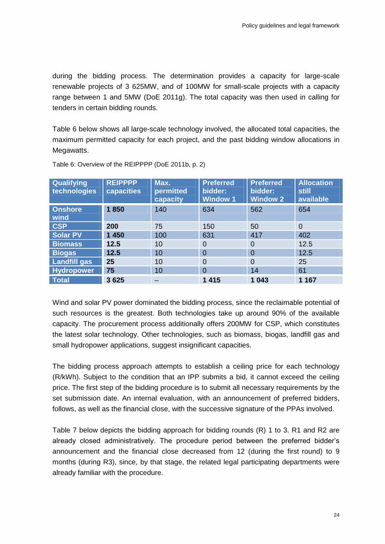
Table 6 below shows all large-scale technology involved, the allocated total capacities, the
maximum permitted capacity for each project, and the past bidding window allocations in
Megawatts.
Table 6: Overview of the REIPPPP (DoE 2011b, p. 2)
Qualifying technologies
REIPPPP capacities
Max. permitted capacity
Preferred bidder: Window 1
Preferred bidder: Window 2
Allocation still available
Onshore wind
1 850 140 634 562 654
CSP 200 75 150 50 0
Solar PV 1 450 100 631 417 402
Biomass 12.5 10 0 0 12.5
Biogas 12.5 10 0 0 12.5
Landfill gas 25 10 0 0 25
Hydropower 75 10 0 14 61
Total 3 625 – 1 415 1 043 1 167
Wind and solar PV power dominated the bidding process, since the reclaimable potential of
such resources is the greatest. Both technologies take up around 90% of the available
capacity. The procurement process additionally offers 200MW for CSP, which constitutes
the latest solar technology. Other technologies, such as biomass, biogas, landfill gas and
small hydropower applications, suggest insignificant capacities.
The bidding process approach attempts to establish a ceiling price for each technology
(R/kWh). Subject to the condition that an IPP submits a bid, it cannot exceed the ceiling
price. The first step of the bidding procedure is to submit all necessary requirements by the
set submission date. An internal evaluation, with an announcement of preferred bidders,
follows, as well as the financial close, with the successive signature of the PPAs involved.
Table 7 below depicts the bidding approach for bidding rounds (R) 1 to 3. R1 and R2 are
already closed administratively. The procedure period between the preferred bidder’s
announcement and the financial close decreased from 12 (during the first round) to 9
months (during R3), since, by that stage, the related legal participating departments were
already familiar with the procedure.

Policy guidelines and legal framework
25
Table 7: Bidding approach of the REIPPPP (DoE 2013a)
R1 R2 R3
Bid submission date 4 Nov. 2011 5 Mar. 2012 19 Aug. 2013
Announcement of preferred bidders
7 Dec. 2011 21 May 2012 29 Oct. 2013
Financial close – signature of PPA
5 Nov. 2012 9 May 2013 30 Jul. 2014
The thesis accruement period lasted from the financial close of bidding for R2 to the
submission date for R3 (which is marked in bold in Table 7 above). Therefore, 9 May 2013
(the date of financial closure of R2) is the appointed day for the assessment of the
renewable energy forecast, as referred to in Chapter 0 of the current thesis. The third
bidding round will not be included, since only the residual power of 1 176MW is known, and
too many assumptions would otherwise have to be set.
Primarily up to five bidding windows were estimated to award the specified capacity (DoE
2011c, p. 43). The trend distinctly shows, in spite of a decrease from bidding R1 to R2, that
R3, with an available capacity of 1 167MW, is likely almost to achieve the total desired
amount of 3 625MW. The DoE determined, in consultation with NERSA, by December
2012 (DoE 2012) to amplify the generation capacity from 2017 to 2020. Acting under the
ERA 2006, a supplementary renewable capacity of 3 200MW has been stated in order for
one or more tendering procedures to contribute towards energy security achievements,
and to facilitate the IRP 2010 targets, whereas 100MW have once more been dedicated for
small projects. The portions between the particular technologies remain similar, in keeping
with the previous determination, except for CSP, where the share rises from 5.5% to
12.5%, with a total amount of 400MW.
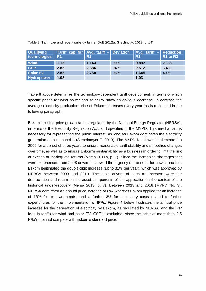
The first bidding round cumulated the greatest amount of capacity and subsidy tariffs. This
phenomenon was based on the fact that the IPPs had been aware of reduced competition
for the first bidding window, thus the number of submitted projects (with their respective
capacities) was less than the government had previously announced. The additional
present urgency of new capacities related to the MTRM prospects led to an average
resulted sales price that was close to the ceiling price. Such progress depicted the crude
market launch, and led to a distortion. A further reduction rate of 21.5% for wind and of
40% for solar PV from bidding in R1 to R2 underlined an overestimation of subsidy tariffs
(Siepelmeyer T. 2013). Table 8 below allows for insight to be gained into the tariff caps and
into the fully indexed actual subsidy tariffs in R/kWh.
Policy guidelines and legal framework
26
Table 8: Tariff cap and recent subsidy tariffs (DoE 2012a; Greyling A. 2012, p. 14)
Qualifying technologies
Tariff cap for R1
Avg. tariff – R1
Deviation Avg. tariff – R2
Reduction R1 to R2
Wind 1.15 1.143 99% 0.897 21.5%
CSP 2.85 2.686 94% 2.512 6.4%
Solar PV 2.85 2.758 96% 1.645 40%
Hydropower 1.03 – – 1.03 –
Table 8 above determines the technology-dependent tariff development, in terms of which
specific prices for wind power and solar PV show an obvious decrease. In contrast, the
average electricity production price of Eskom increases every year, as is described in the
following paragraph.
Eskom’s ceiling price growth rate is regulated by the National Energy Regulator (NERSA),
in terms of the Electricity Regulation Act, and specified in the MYPD. This mechanism is
necessary for representing the public interest, as long as Eskom dominates the electricity
generation as a monopolist (Siepelmeyer T. 2013). The MYPD No. 1 was implemented in
2006 for a period of three years to ensure reasonable tariff stability and smoothed changes
over time, as well as to ensure Eskom’s sustainability as a business in order to limit the risk
of excess or inadequate returns (Nersa 2011a, p. 7). Since the increasing shortages that
were experienced from 2008 onwards showed the urgency of the need for new capacities,
Eskom legitimated the double-digit increase (up to 31% per year), which was approved by
NERSA between 2009 and 2010. The main drivers of such an increase were the
depreciation and return on the asset components of the application, in the context of the
historical under-recovery (Nersa 2013, p. 7). Between 2013 and 2018 (MYPD No. 3),
NERSA confirmed an annual price increase of 8%, whereas Eskom applied for an increase
of 13% for its own needs, and a further 3% for accessory costs related to further
expenditures for the implementation of IPPs. Figure 4 below illustrates the annual price
increase for the generation of electricity by Eskom, as regulated by NERSA, and the IPP
feed-in tariffs for wind and solar PV. CSP is excluded, since the price of more than 2.5
R/kWh cannot compete with Eskom’s standard price.

Policy guidelines and legal framework
27
Figure 4: Eskom and IPP price adjustment/forecast 2006–2018 (Nersa 2013, 2013a)
According to NERSA, the generation price of Eskom for 2015/16 will be 0.76 R/kWh,
increasing up to 0.89 R/kWh in 2017/18. As long as Eskom’s price rises and the wind
power and solar PV price decreases, contemplated renewable energy facilities will be able
to compete over the next 5 to 10 years. They might not depend on subsidies as a
consequence, regardless of the volatile power production not being of great significance,
since it is not able to contribute fully to basic or peak load power generation.
The first two price levels of wind and solar PV are average values that resulted after the
financial close of bidding R1 and R2, assuming that the plants will be on grid by 2013/14
and 2014/15. The average wind price for 2015/16 was estimated by N. Siepelmeyer
(2013), the CEO of IPD Power Ltd, whereas the solar PV value was derived from the same
decrease rate as that of the preceding year.
The REIPP Procedure Programme assumes a standardised approach for all submitted
renewable energy projects. Every developer has to follow this procedure to be admitted to
any bidding process.
The procedure is subdivided into three major, hierarchically ordered categories that are
described in detail in Annexure II, in terms of Request for Qualification and Proposal
(RFP), the bidding process, and financial closure.
Figure 5 below depicts a simplified approach to the REIPPPP and the contractual
expiration of the cash and electricity flow.

Policy guidelines and legal framework
Figure 5: REIPPPP approach for an Independent Power Producer (Siepelmeyer N. 2013)

Policy guidelines and legal framework

Involved renewable energy projects
30
6 Involved renewable energy projects
This chapter reviews all renewable energy projects that were announced in REIPPPP
bidding R1 and R2, and provides a brief overview of the already installed renewable
capacities, besides the large-scale hydropower stations and the off-grid applications, which
are not part of the works content. Based on the objectives of the current thesis in regard to
the assessment of a time series simulation for all relevant, confirmed on-grid renewable
energies, certain information, such as specific project positions, capacities, deployed
technologies, and other details have to be known.
6.1 Approved facilities prior to 2011
The number of already installed or approved on-grid renewable energy power plants before
2011 was rare, since there were no legal policy guidelines to stimulate demand, such as
the REBID has constituted from 2011 onwards. Although some mid-range solar PV plants,
such as the 542kWp Vodacom rooftop application (Cloete K. 2013), were built up, they
were intended to be off-grid, based on the lack of technical, legal and financial constraints
available. Further programmes (e.g. Eskom’s small-scale Renewable Energy Programme
2012) that support the integration of small-scale, grid-integrated plants that are less than 1
MW were excluded from the analysis.
6.1.1 Existing wind resources
Up until the current moment, the following three on-grid wind farms have come into being,
but, so far, no solar PV, hydropower, biomass, biogas power plant, or other plants have
been built. Two out of the three above-mentioned facilities were constructed by Eskom,
which facilitates the grid connection as well. Accordingly, the number of PPA participants is
limited, since the transmission grid is run by Eskom, which facilitates the grid connection
procedure. Darling Wind Farm has been the first confirmed on-grid wind energy facility that
is developed and run by an IPP, even though no policy guideline was developed in time.
The Klipheuwel Wind Energy Facility was constructed in 2003 under the pretext of it being
research-related.
The following table gives an overview of the three already committed wind farms.
Table 9: Facilities committed prior to 2011
Developer Capacity per turbine [MW]
Nominal capacity [MW]
Commissioning date
Sere Wind Farm Eskom 2 100 Oct. 2013
Klipheuwel Wind Energy Facility
Eskom 0.6 – 1.75 (3 units)
3.16 2003
Darling Wind Farm IPP 1.3 5.2 2008
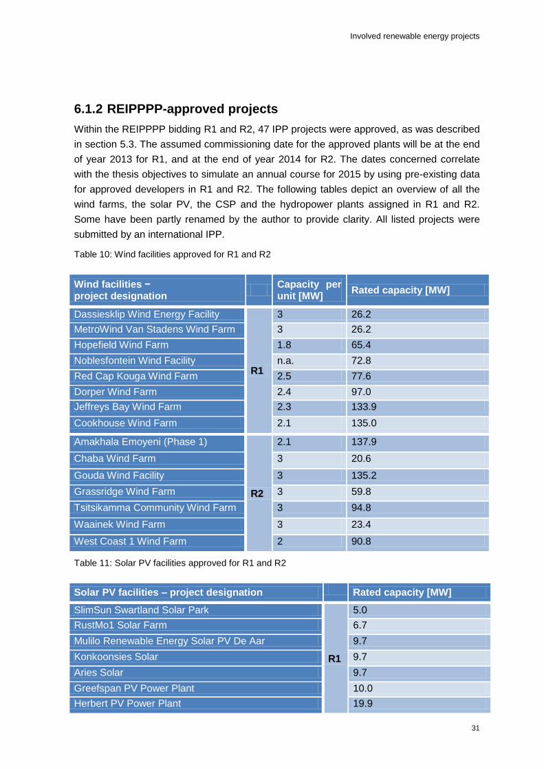
Involved renewable energy projects
31
6.1.2 REIPPPP-approved projects
Within the REIPPPP bidding R1 and R2, 47 IPP projects were approved, as was described
in section 5.3. The assumed commissioning date for the approved plants will be at the end
of year 2013 for R1, and at the end of year 2014 for R2. The dates concerned correlate
with the thesis objectives to simulate an annual course for 2015 by using pre-existing data
for approved developers in R1 and R2. The following tables depict an overview of all the
wind farms, the solar PV, the CSP and the hydropower plants assigned in R1 and R2.
Some have been partly renamed by the author to provide clarity. All listed projects were
submitted by an international IPP.
Table 10: Wind facilities approved for R1 and R2
Wind facilities − project designation
Capacity per unit [MW]
Rated capacity [MW]
Dassiesklip Wind Energy Facility
R1
3 26.2
MetroWind Van Stadens Wind Farm 3 26.2
Hopefield Wind Farm 1.8 65.4
Noblesfontein Wind Facility n.a. 72.8
Red Cap Kouga Wind Farm 2.5 77.6
Dorper Wind Farm 2.4 97.0
Jeffreys Bay Wind Farm 2.3 133.9
Cookhouse Wind Farm 2.1 135.0
Amakhala Emoyeni (Phase 1)
R2
2.1 137.9
Chaba Wind Farm 3 20.6
Gouda Wind Facility 3 135.2
Grassridge Wind Farm 3 59.8
Tsitsikamma Community Wind Farm 3 94.8
Waainek Wind Farm 3 23.4
West Coast 1 Wind Farm 2 90.8
Table 11: Solar PV facilities approved for R1 and R2
Solar PV facilities – project designation Rated capacity [MW]
SlimSun Swartland Solar Park
R1
5.0
RustMo1 Solar Farm 6.7
Mulilo Renewable Energy Solar PV De Aar 9.7
Konkoonsies Solar 9.7
Aries Solar 9.7
Greefspan PV Power Plant 10.0
Herbert PV Power Plant 19.9

Involved renewable energy projects
32
Mulilo Renewable Energy Solar PV Prieska 19.9
Soutpan Solar Park 28.0
Witkop Solar Park 30.0
Touwsrivier Project (CPV) 36.0
De Aar Solar PV 48.3
SA Mainstream Renewable Power Droogfontein 48.3
Letsatsi Power Company 64.0
Lesedi Power Company 64.0
Kalkbult Solar PV 72.5
Kathu Solar Energy Facility 75.0
Solar Capital De Aar (Pty) Ltd 75.0
Solar Capital De Aar 3
R2
75.0
Sishen Solar Facility 74.0
Aurora Solar Park 9.0
Vredendal Solar Park 8.8
Linde (Scatec Solar Linde) 36.8
Dreunberg Solar PV 69.6
Jasper Power Company 75.0
Boshoff Solar Park 60.0
Upington Solar PV 8.9
Table 12: CSP and hydropower facilities approved for R1 and R2
CSP & hydropower – project designation
Technology Rated capacity [MW]
CSP – Khi Solar One R1
Central receiver – heat storage 50.0
CSP – KaXu Solar One Parabolic trough – heat storage 100.0
CSP – Bokpoort
R2
Parabolic trough – heat storage 50.0
Hydropower – Stortemelk Hydro
Run-of-river power plant 4.3
Hydropower – Neusberg Hydropower
Run-of-river power plant 10.0
The cumulative capacities of all the above tables are summarised in Table 6, p. 24. The
registered capacities for R1 and R2 were obtained from the DoE’s ‘REIPP Announcement’,
and from the ‘Window Two Preferred Bidders’ announcement (DoE 2012b, DoE 2011f).
The nominal capacities that have been published by the developers state a slightly higher
value than do the registered capacities. The registered capacity for wind, CSP and
hydropower facilities can be assumed to represent the total power output at the grid

Involved renewable energy projects
33
connection port under full load (deducting losses) and the peak power for solar PV under
standard test conditions (STC).
The map in Figure 6 below pictures the spatial distribution of all approved IPP projects. It is
evident that the projects are located according to the resource potentials that were
reported in the local resource analysis, in section 4.1.
Figure 6: Location of IPP projects countrywide, featured by way of Google Maps.
Modelling the prospective load contribution
34
7 Modelling the prospective load contribution
The model consists of four different approaches that were taken all the above-mentioned
technologies used. This chapter constitutes an introduction to the model’s objectives, the
data assessment, the methodology, and other aspects, and describes each specific
procedure in detail.
7.1 Introduction
The government’s future supply ambitions are mostly linked to determined technology
classifications and its single capacities. Especially renewable sources, such as wind and
solar irradiation, are highly volatile. Facing the capacity for future expectations only will
cause a high rate of uncertainty, which is based on the short-term fluctuation for peak load
supply and the mostly unknown annual energy output of each technology. Therefore, the
developed model represents a method of how to achieve load curves to be able to observe
the load behaviour of all supplying, approved renewable technologies, and to enable the
determination of the minimal−maximal fluctuation during different seasons. The results
provide information about countrywide weather simultaneities, as well as about the fed
amount of electricity by renewable energies after such stimulating measures as REIPPPP
have been applied.
The model’s objective is to develop a method with default input parameter thatrepresents
the results in a reproducible and reliable way. Therefore, physical laws and mathematical
correlations are implemented. To measure an occurring deviation, such reference values
are gathered as predicted values, by independent developers, and/or calculated values, by
means of using other comprehensible methods. The model uses annual input data from
2010, and approved renewable capacities from bidding R1 and R2 to process an
exemplary load course for the year 2015.
For time series simulation purposes in every specific approach, various boundary
conditions/ assumptions have had to be met. The assumptions will be scientifically justified
and clearly specified.
The simulation requires such necessary tools as:
Microsoft Excel by Windows Microsoft
The solar PV model developed by the Solar Thermal Energy Research Institute
The SAM developed by the NREL – US DoE
The Wind Atlas Analysis and Application Programme (WAsP), developed by the
Technical University of Denmark

Modelling the prospective load contribution
35
7.2 Input parameters
The default input parameters for simulation issues were provided by GeoModel Solar Ltd
and its solar GIS database. The simulated time series records were averaged on hourly
based values (8 760), and represent the annual period of 2010 (1 January to 31 December
2010). The solar GIS data specification document (Solar GIS 2013) provides detailed
information about the data acquisition, as well as about the related method and its
occurrence.
The four data records used for research purposes are discussed below.
GHI and DNI [W/m²]
The solar radiation primary parameters, such as GHI and DNI, are derived by advanced
and scientifically validated models that use satellite data and outputs from atmospheric
models. The solar database input parameters are based on, inter alia, the cloud index, the
water vapour database, the atmospheric optical depth, the elevation, the horizontal profile,
and other factors. The spatial resolution of GHI and DNI is specified with a raster of 3 arc
seconds (which corresponds to a cluster of about 90m at the Equator, and which
decreases towards the Poles).
According to solar GIS, the quality assessment in South Africa shows a low bias within a
range of ± 2.5% and an hourly root mean square error (RMSE) between 16 and 22%.
Ambient temperature [°C]
The spatial resolution of simulated air temperature is 1km, at an elevation of 2 meters
above surface.
Wind velocity [m/s]
According to the solar GIS, the wind speeds are intended to be used as ancillary
parameters only. Such meteor parameters as wind speeds, directions and humidities are
derived from the numerical weather model output. In terms of said output, the spatial
resolution is lower and might not represent the site-specific conditions, as does the solar
resource data. Likewise, the wind’s velocity data has to be verified before it can be used for
further calculations to be sure about any possible deviation (see section 7.3.1). The spatial
resolution of wind speeds is 900km² (30 × 30km) at a height of 10 m above surface.
7.3 Wind simulation
The purpose of the wind simulation is to calculate a power output for 18 wind farms by
means of the use of individual wind conditions. Therefore, the hourly average wind speed
in m/s has to be converted to an hourly average amount of energy in Wh, as generated by

Modelling the prospective load contribution
36
a certain number of wind turbines. Regarding the uncertainties of the GeoModel wind
speeds, the data set values have to be analysed and verified, assumptions have to be set,
and a reliable method for extrapolation has to be developed.
7.3.1 Data verification
To ensure certain accuracy of the GeoModel wind speeds at a height of 10m, GeoModel’s
data is compared with free available wind measurement data records. As part of the
numerical Wind Atlas of South Africa (WASA), as described in subsection 4.1.2, ten WMs
were sited countrywide to assist with developing, and to gauge their own model.
The WM’s records are site specific for a certain spot, in comparison to the GeoModel
simulation, which represents an average spatial resolution of 900km². The GeoModel data
is expected to be more damped, which might imply higher maximum amplitudes of wind
speeds. Nonetheless, juxtaposing both sets of data is necessary for verification purposes,
as well as for subsequent adjustments.
The WM sites were not placed in areas that were expected to be windy. The placement
was done in line with the following criteria (Otto. A 2013):
Spaced out evenly across the project area (respecting the numerical wind atlas)
At a distance from complex terrain
In areas uniform in terms of roughness and topography
Within such different climatological regions as coastal and inland low-/high-lying
The WMs provide 10 minutes mean, maximum and minimum wind speed values at an
elevation of 10m, 20m, 40m, 60m and 62m; accurate wind directions; temperatures;
barometric pressures; and relative humidity. WASA initiated the recording of data from
August 2010 onwards, which limited the comparison period to 5 months. As a result,
seasonal deviations cannot be taken into account. Since the wind potential in W/m²
depends on the velocity power of three, cubed average hourly values for all WASA records
are calculated to be able to compare both data sets.
Individual record assessment
An evaluation with regard to the standard deviation (SD) of each record at five relevant
chosen sites confirmed the above-mentioned expectations. The WM’s average SD was
found to be 24% higher than the GeoModel deviation (2.1 to 2.8m/s).

Modelling the prospective load contribution
37
Assessment of the analogy
To compare both data records, different methods were used. The utilisation of such
formulas as the mean error (ME), the root mean squared error (RMSE), the mean absolute
error (MAE), and others which are described in Annexure III.
A comparison of mean wind speed values and a relative influence of the wind power
potential ((Σvi3)/1000) are depicted in the table below. WM 09 and 10 measurements were
excluded, since the deviation was implausible.
Table 13: Comparison of GeoModel data at WM sites and WM measurements
Site Vmean GM [m/s]
Vmean WM [m/s]
Deviation [%]
GM (Σvi
3)/1000 WM (Σvi
3)/1000 Deviation [%]
WM01 3.9 5 130 372 987 265
WM02 3.1 5 159 238 679 285
WM03 3.4 5.7 169 225 1069 475
WM04 4.2 4.8 116 484 718 148
WM05 5.3 7.3 138 855 2251 263
WM06 3.7 5.6 151 298 773 259
WM07 3.6 5.8 161 341 1064 312
WM08 4.7 5.8 123 709 1345 190
The WM measurements were higher than the GeoModel values throughout. The aberration
between the WM and the GeoModel mean wind speeds was between 116 and 169%, while
the deviation of the summarised, single-cubed values (representing theoretical wind energy
potential) extended from 148 to 475%. For the error examination, only proper geographical
WM sites were evaluated.
The following five WMs were the nearest to the related 17 wind farms.
Table 14: Error evaluation between GeoModel data and WM measurements
Site ME [m/s] RMSE [m/s] MAE [m/s] MAPE [%]
WM01 1.1 2.9 2.1 49
WM03 2.3 3.4 2.7 46
WM04 0.7 2.5 2.0 50
WM05 2.0 2.9 2.3 34
WM08 1.1 2.4 1.9 39
The error evaluation shows that the deviation was substantial. The mean absolute
percentage error (MAPE) exhibited a significant gap. An analysis of the monthly mean
absolute percentage error (MMAPE) resulted in slight monthly differences, but since only

Modelling the prospective load contribution
38
five months of comparable data were available at the time of the study, further examination
was not possible.
Figure 7 below represents the averaged distribution curve of the sites mentioned above.
Although the distribution of the lower GeoModel simulation was higher in the ranges
between 0.5 and 6m/s, the higher wind speeds above 7m/s influenced the apparent gap.
Figure 7: Mean wind distribution curve – wind mast measurement and GeoModel simulation
Visual assessment
The trend of both data records was found to be similar and consistent, even though the
absolute values differed, as is described above. The relative values, such as tendency,
could be used for further computing, although a difference existed in the SD, indicating the
mean relative error.
A further use of GeoModel data records is not recommended without a projection being
related to the results above. An approximation should be comprehensible, single-value
based, and evenly distributed to adhere to the trend in the records. A multiplication of each
value using the factor 1.4 as representing the vmean average deviation might prove to be the
probable method.
7.3.2 Height-related extrapolation
The GeoModel data at a height of 10m above ground had to be extrapolated to an
accurate operation elevation. A commercial wind turbine typically operates at an
appropriate height, since the wind speeds are more consistent and increase, depending on
the height above surface. The wind’s potential depends on the third power of the velocity,
as the following derived formula describes:

Modelling the prospective load contribution
39
(1)
The most influential parameters are the velocity (corresponding to the height) and the
diameter of the wind stream. The hub height of a wind turbine usually depends on the
surface roughness, and on the vertical wind distribution. For simplified simulation
purposes, a standard wind turbine hub height of 100m was assumed.
The Hellmann exponential law and the logarithmic wind profile law are empirical
determined relations between the wind’s velocity and the hub height. Both laws were
simplified and empirically verified. Another method, such as the more precise Monin-
Obukov relation, could not be taken into account, based on a lack of further input
parameters, such as temperature differences, friction lengths, and others (Banuelos,
Camacho 2011).
The following formulas represent the Hellmann exponential law (2) and the logarithmic
wind profile law (3).
(2)
(3)
In terms of the above, v is the velocity to the height H, and v0 is the velocity to H0. The
Hellmann exponent, or friction coefficient, is α, and z0 represents the roughness length in
m. The values of both parameters corresponded to a certain terrain class, as the following
table shows.
Table 15: Friction coefficient and roughness lengths (Tong 2010; Patel 2006)
Landscape type Friction coefficient α Roughness length [m]
Offshore, hard ground 0.10 0.0002
Grassland, open areas 0.15 0.03
Tall crops, hedges, farmland 0.20 0.1
Urban districts, small town 0.30 0.4
City areas, forest areas 0.40 1.6
In this case, both laws were validated by existing, randomly chosen data samples from the
WASA WMs, taken at a height of 10 and 60m. Therefore, α and z0 were calculated by
means of the transformed equations above ((2),(3)) for each dataset, and averaged by
means of the use of the mean and median value. The two homogenised coefficients for

Modelling the prospective load contribution
40
each data set were utilised to extrapolate new sample wind speeds for a height of 60m, to
be able to compare them with the according true wind speeds.
The following graphs were drawn using the determined mean/median coefficients α and z0
at a sample wind speed of 8m/s. The comparison showed similar results as long as the
aberration of the single calculated coefficients was not too high.
As a result, the Hellman exponential law was chosen for extrapolation purposes.
Figure 8: Comparison of the data according to the Hellmann exponential law and the logarithmic
wind profile law
To be able to extrapolate each wind record at all project site using a single method, a
homogenised α coefficient was calculated by using all WM data, following the same
method described above.
The calculated α coefficient was 0.126, which corresponded to the sites ranging from hard
ground to grassland/ open areas (see Table 15, p. 39). The less the exponential coefficient
was, the smaller was the relative increase of the extrapolated value. Such an approach is
based on the assumption that wind farms tend to be located on a similarly flat terrain as the
wind measurement stations are, to avoid having to have excessively tall wind turbine
masts.
The projection was made up to a generalised hub height of 100m, although the coefficient
was calculated between 10 and 60m. The increase was expected to match an
approximately realistic result.
7.3.3 Power conversion
The power conversion from an accurate extrapolated wind speed at a height of 100 m to a
power output was approximated by the specific power curves of certain wind turbines. Two

Modelling the prospective load contribution
41
turbines of different performance categories were chosen to cover the bandwidth of utilised
turbines at all the approved wind farms (see Table 11: Solar PV facilities approved for R1
and R2
The load behaviour of different turbines at the same performance category was found to be
similar, which could lead back to such physical limits as Betz’ law, component efficiencies,
and others.
The approximation was based on a logarithmic conversion between 6 and 10m/s, and on
linear relationships above/below that. It was made in terms of two developed wind turbines,
with a capacity of 2.35 and 3MW, as manufactured by Enercon Ltd. The minimum
operation wind speed was 2m/s. Above 13m/s the power output was limited due to a stall
in the wings.
The graph in Figure 9 below illustrates the mathematical approximation to the real power
curves involved.
Figure 9: Approximation of the wind power curve
The course of both power curves was almost equal, up to a wind speed of 9m/s. Assuming
a wind farm with a capacity of 50MW at a site with a mean wind speed of less than 9m/s,
the technically exploitable energy output of a wind farm with smaller turbines at a certain
constant hub height would be greater than if bigger windmills were to be used, since the
number of turbines would be higher. Although the technical potential can be higher with the
installation of smaller turbines, the decision criterion in terms of which turbines are chosen
is based on an economic viability (e.g. on the specific cost of each wind turbine). The

Modelling the prospective load contribution
42
turbine size in the case of individual projects assumes the selection of the approximated
load curve.
7.3.4 Method 1 – assorted approach
The approach adopted in the simulation can be summarised as follows:
GeoModel 10m data projection to compensate for WM 10m deviation
Height extrapolation – 10 to 100m
Power conversion
The assessed simulation approach was performed for the following five wind farms, in
terms of which the developers published an annual expected energy output to verify the
developed methodology. The results in GWh below show an explicit overvaluation of four
out of five projects with the developed methodology.
An extrapolation without a GM 10m data projection surprisingly meets the expected output.
Table 16: Wind speed extrapolation – verification. Units in GWh.
Wind farms Expected energy output
Including GM 10 m alignment
Excluding GM 10 m alignment
MetroWind Van Stadens Wind Farm
80 126 74
Hopefield Wind Farm 190 198 101
Red Cap Kouga Wind Farm 290 426 283
Jeffreys Bay Wind Farm 362 627 380
West Coast 1 Wind Farm 290 440 273
This fundamental finding, and a further verification of the capacity factors (CF) of all the
projects as a comparative analysis tool, led to the conclusion that the developed method
was not reliable enough for a further straight forward proceeding. The CF differed greatly
from the realistic bandwidth. The CF is defined as follows:
(4)
A further step was contained an assorted approach for different groups of projects
regarding to available IPP information. The proceeding is described below:
The calculation without a ‘GM to WM – 10m projection’ led to an approximate result
compared to the IPPs’ expectations, or fell within a plausible CF bandwidth (in the
case of seven projects).

Modelling the prospective load contribution
43
An IPP expectation in GWh or an estimated CF was available (in the case of five
projects):
o Iterative adjustment of the ‘GM to WM – 10m projection’ factor was done to
achieve the expected results.
No specific project information was available (in the case of six projects):
o The resulting CF fell below the expectancy range after calculation without a
‘GM to WM – 10m projection’.
o Relative adjustment into a plausible CF range resulted in a subsequent
energy output.
o Iterative adjustment of the ‘GM to WM – 10m projection’ factor achieved the
expected output.
The plausible CF range was defined by means of the above results, and then verified by
means of consulting literature references. For the purpose of the current study, the range
was set between 27 and 42% (Siepelmeyer N. 2013; Soni 2012, p. 34; Stanley Cons.
2009). Although the CF bandwidth contained the highest assumption uncertainty, the
fluctuation margin in the high wind records allowed for no other possibility than to
implement such an approach.
7.3.5 Method 2 – single approach
In order to accomplish a single and comprehensible approach for all cases, and to simulate
consistently, the following approach was derived in terms of the methodology discussed
above:
1. GeoModel 10m records were used directly for height extrapolation from 10 to
100m.
2. The CF’s of the IPP projects were adjusted into the defined bandwidth.
3. The ‘GM to WM – 10m projection’ factor was iteratively adjusted to achieve the
cumulated energy output (which was derived by the adjustment of the CF, in
accordance with the above-mentioned step).
4. A power conversion and cumulative display was performed.
Figure 10 below demonstrates the CF adjustments in a bandwidth of 27 to 42%. The blue
spots describe the origin CFs, following the simulation method. The red spots represent the
CFs after the assimilation.

Modelling the prospective load contribution
44
Figure 10: Capacity factors of wind facilities – model and assimilation
7.3.6 Validation – assorted and single approach
The grouped approach’s output was 3 598GWh, whereas the output for the single
approach was 3 685GWh. The mean deviation of 13MW corresponded to 1% of the
installed capacity. The maximum deviation amounted to 60MW.
The advantage of adopting the assorted approach is that the result might be more
accurate, based on the individual project information, while the single approach does not
take such information into account. The disadvantage of the assorted approach lies in the
lack of standardisation, which impedes replication, and also in the references not being
confirmed and independent. Based on the fact that the hourly trend and the annual yield of
both methodologies were very close, the single approach (Method 2) was be chosen for
further study.
It must be borne in mind that the assorted approach serves as a verification model for the
single approach.
7.3.7 Results
The main boundary conditions influencing the simulation must be stated to allow for
evaluation of the existing uncertainties before any result can be analysed. The most
important assumptions that were set are summarised below:
A CF bandwidth of between 27 and 42%
The usage of 10m GeoModel records, even though the deviation to measured
values records was high
A general turbine hub height of 100m
The Hellman exponential law for 10 to 100m extrapolation

Modelling the prospective load contribution
45
The generalisation of the exponential coefficient α = 0.126 (determination taken
from a WM 10m and 60m in height)
Load curves approximated by Enercon Ltd
The following influences could not be fully taken into account, based on the lack of
information, and, to some degree, the limited extent of the thesis:
The seasonal evaluation of WM and GeoModel data
The wind farm’s specific simultaneities
Probable deviation from a standard wind year
The lack of available data in a range that was less than hourly based
Regarding the simulation, the total annual generated energy yield would be 3 685GWh.
The maximum available power was 1 302MW, which almost corresponded to the total
installed capacity. The least amount of available power was 8.3MW, emphasised that it
represents one single value only. Such a result indicates the presence of a spatially
consistent, but temporal, fluctuating wind resource. On the one hand, every wind farm will
run at its ceiling capacity at certain hours, but, on the other hand, the firm capacity was
found to be almost zero (~0.6%), which is a negative aspect regarding the contribution that
can be made by a wind-powered base load. Whereas the annual mean was found to be
421MW, the seasonal fluctuation was considerable. Table 17 below characterises the
seasonal behaviour of wind power generation.
The knowledge of the wind power contribution to satisfying the winter peak demand must
be examined, since such political instruments as the IRP 2010 – MTRM require a
substantial contribution from each generation unit to supply stability. About 15% of the wind
distribution tends to occur between 19 and 22h, which corresponds to an appropriate time
distribution of 16.7% (= 4h / 24h). The according firm capacity was 23.5MW, whereas the
annual firm capacity during that period was 26MW. Further analysis of this issue
demonstrated that 40.4% of the winter’s distribution tends to occur between 8 and 15h,
which is proportionally higher than the accurate time distribution. It can be asserted that the
wind power in 2010 slightly contributes to the morning peaking hours, and nearly provides
its own amount of time distribution-related energy.
Further analysis, such as an annual load duration curve, which is shown in Figure 30, and
a seasonal separated duration curve, which is shown in Figure 31, are included in
Annexure IV. Autumn is indicated as being a wind-rich exposed time period.

Modelling the prospective load contribution
46
Table 17: Seasonal characteristics of wind generation
Power [MW] Energy [GWh]
Spring (21/09–20/12)
Summer (21/12–20/03)
Autumn (21/03–20/06)
Winter (21/06–20/09)
Deliv. energy 843 926 1000 916
Min. power 8.3 20.3 12.4 20
Max. power 1285 1215 1302 1284
The cumulative wind power shows concurrent increases and decreases within a few hours.
As a result, the spatial distribution does not imply an upper simultaneity, as is illustrated by
the exemplary wind power course that is pictured in Figure 11 below.
Figure 11: Exemplary wind power course in January
Figure 32 (Annexure IV) verifies the rapid wind speed changes, with locally relevant WM
records taken at a height of 60m.
7.4 Solar PV simulation
The simulation covers 27 solar PV plants, which were approved in bidding R1 and R2. The
purpose in doing so was to utilise a standardised approach to calculating an hourly load
curve by using, inter alia, local solar irradiance data records. Therefore, an already
developed method by Paul Gauché, is applied (Gauché 2011). One project, as has already
been mentioned in Table 12: CSP and hydropower facilities approved for R1 and R2
is provided with CPVs, which require the adoption of such a method as is described in
subsection 7.4.3.
The following sections deal with the description of the PV simulation approach.
7.4.1 Data verification
The data provided by GeoModel consists of 2010 annual GHI and DNI, ambient
temperature and wind speed data for every single project site. The properties of the data
Day 1 Day 2 Day 3 Day 4

Modelling the prospective load contribution
47
records are defined in section 7.2. The temperature and the wind speeds are intended to
be used as ancillary parameters. The STERG and its director, Paul Gauché, have already
published papers regarding the mentioned GeoModel data. In terms of said data, the
quality of the irradiance values is stated as being reliable (Gauché, Pfenninger 2012;
Gauché, Heller 2012). The cooperation with GeoSun Africa©, which is a spin-off company
of CRSES, and with the representatives of GeoModel in South Africa verifies the reliability
of the data obtained. Based on such quality references, GeoModel data will be used for
further processing.
7.4.2 Methodology
The simulation approach was conducted by means of a modified Microsoft Excel tool
devised by Paul Gauché. It has been developed to simulate a central receiver (CR) CSP
plant, with a solar PV model having also been derived, in addition (Gauché 2011).
The tool in question calculates the hourly position of the sun (in terms of an equation of
time, altitude, azimuth, etc.), including several derived, generally valid coefficients (Stine,
Geyer 2001, Chapter 5), and taking mutual module shading into account. The model can
be adapted for different solar PV applications, such as for tracking types (e.g. fixed tilt,
periodic adjustment, azimuth tracking, full tracking, etc.).
For solar PV purposes, the tool processes the following input parameter:
Net aperture size [m²]
Length, width [m²]
Pitch of modules [m]
Site’s coordinates – longitude, latitude [deg]
GHI, DNI, diffuse horizontal irradiance [W/m²]
Ambient temperature [°C]
Ground-level wind speeds [m/s]
Aperture tilt angle [°]
Cell efficiency [%]
Inverter efficiency [%]
o Coefficients
o Temperature efficiency [% per °C above 25°C]
o Irradiance efficiency [% per W/m² below 1000W/m²]
o Temperature rise coefficient [°C per W/m²]
and computes, among others, the following values:
Maximum actual power output [Wmax]
Modelling the prospective load contribution
48
Time series load behaviour [Wh]
Annual amount of energy [Wh]
Maximum cell temperature [°C]
The results are validated by means of single projects that are conducted on a random
basis by means of the SAM of the US NREL in efforts to confirm the model’s reliability.
7.4.3 The making of assumptions
The solar PV simulation requires the following modifications/assumptions in terms of a
consistent approach:
25 of 27 solar PV systems were mounted in a fixed position on a rack facing north.
o A location-dependent optimum tilt (between 24 and 32°) for a maximum
annual energy yield has been developed by GeoModel, and has been
adopted for simulation approaches (Suri, Cebecauer 2012, p. 5).
A conversion factor from a peak power to a certain aperture plain was
implemented, since the model requires a PV size, and the developers published
only the peak power of each plant. Five appropriate modules of different
manufactures from 240 to 250Wp were chosen, and a mean specific peak capacity
of 167Wp/m² was determined (see Annexure V).
The module efficiency was generalised to 15.1%, corresponding to an average
value for the five chosen modules described above.
The panels did not cast shadows on each other.
Since the required DHI was not available from GeoModel, it was derived by means
of the following formula. Theta represents the zenith angle in the following equation:
Some DHI values, which were negative at the beginning of the day, were replaced
by 0. This incident can be blamed on DNI/GHI simulation inaccuracy. For validation
purposes, solar irradiance data at the measurement station at Stellenbosch
University was examined, where it was found that the same effect occurred.
The following coefficients were derived by Gauché (2011) and received from Stine
and Geyer (2001).
o Temperature efficiency −0.5% per °C
o Irradiance efficiency 0.0125% per W/m²
o Temperature rise coefficient 0.03°C per W/m²
For the 36MW CPV plant, a simplified and reproducible methodology was
developed.
(5)

Modelling the prospective load contribution
49
The concentration lenses focused only on the DNI, which was multiplied by the
efficiency and the net module size, as the following formula describes:
The efficiency was derived by means of a concentrator triple-junction solar cell,
type 3C40, made by Azur Space Solar Power Ltd.
Table 18: Solar CPV properties, type 3C40, Azur Space Solar Power Ltd, under STC
Specifications Type 3C40
Sun concentration × 1000
ηcell 36.3%
WMPP/m²gross 362
Temperature coefficient (25 – 80°C) -0 035%/ΔT
Based on the lack of temperature rise coefficients that could have designated the cell
temperatures, the cell efficiency was reduced by means of a mean alternation between 25
and 80°C, and yielded 35.3%.
Based on the above assumptions, the simulation was done for each project.
7.4.4 Results
The annual cumulative energy from solar PV summarised the single output rating of 25
solar PV plants with a fixed tilt, one plant with a one-axis tracker system, and one CPV
plant that was fully tracked. The total amount of delivered energy was 1 906GWh. The
cumulative maximum power was almost 900MW, which was 14.2% less than the
registered capacity of 1 049MWp. The gap of 149MW was based on the fact that the peak
power corresponded to the STC, which did not represent an appropriate irradiance and cell
temperature course per day.
The CF’s bandwidth for the fixed tilt plants ranged between 18 and 22%, which implied
consistent specific results. The one-axis tracker CF achieved almost 25% and the CPV CF
was 28.5%. Eleven determined IPP expectations (annual energy generation and/or CF)
and a SAM simulation output for a 75MWp plant (Kalkbult Solar PV) confirmed the results
obtained. The deviation was insignificant (see Annexure V).
The seasonal characteristics appeared as follows: The spring delivered the highest amount
of energy, which was almost 26% more than the autumnal contribution. The mean
delivered energy per day was 5.9GWh during spring, and 4.7GWh during autumn.
(6)

Modelling the prospective load contribution
50
Table 19: Seasonal characteristics of solar PV generation
Power [MW] Energy [GWh]
Spring (21/09–20/12)
Summer (21/12–20/03)
Autumn (21/03–20/06)
Winter (21/06–20/09)
Max. power 900 852 830 856
Delivered energy 533 485 429 459
Min. peak power 265 291 270 257
The cumulative, delivered solar PV energy visibly runs synchronically with the solar
irradiance, influenced, as it is, by local weather conditions. Solar PV without energy
storage basically contributes to the higher demand during daytime, but a base-load firm
capacity contribution cannot be ensured. During winter, the total output decreases, based
on the limited irradiance, resulting in a further lack of contribution to evening peak loads.
Figure 12 below depicts two days of an exemplary cumulative generation course during
January.
Figure 12: Exemplary cumulative solar PV generation in January
7.5 Concentrated solar power simulation
The CSP simulation contained three approved projects, with a net capacity of 200MW.
They were located in the Northern Cape, where the highest solar irradiance potential
occurs, especially in terms of DNI. In contrast to solar PV, which directly exhibited the PV
effect, the CSP technology mirrored/concentrated the direct solar irradiance onto a small
area, where the uprising thermal energy was used to run a heat engine. Two parabolic
troughs and one CR plant were deployed, with energy storages ranging from 2.5 to 9h. The
simulation was based on hourly specific site GeoModel weather data, such as the GHI and
the DNI records, and was computed by means of SAM. The results were verified by means
of expected energy outputs that had been released by the developers of the project.
7.5.1 Methodology and assumptions
The SAM offered a variety of different possible input parameters. A projects-related
literature research revealed a number of specific boundary conditions that were

Modelling the prospective load contribution
51
implemented. The residual number of unknown parameters was set at default values.
Business concerns were not taken into account. Besides the individual underlying weather
data for each project, Table 20 below specifies some modified input parameters.
Table 20: CSP SAM – input parameters (CSP World 2013)
KaXu Solar One Bokpoort CSP Khi Solar One
Technology Parabolic trough Parabolic trough CR
Net capacity [MW] 100 50 50
Storage 2.5h/ molten salt 9h/ molten salt 3h/ saturated steam
Cooling Dry Wet Dry
Reflecting area [m²] 800 000 588 600 580 000
Annexure VI reports the remaining boundary conditions. Some further parameters were
plausibly adapted to obtain the hypothesised input values.
The thermal storage dispatch control was consistently defined as follows (Gilman 2012),
with no specified approach being required by the Single Buyer Office (SBO):
The turbine was operated at nameplate capacity, as long as sufficient energy was
available from the solar field, or from thermal energy storage (TES).
The plant-generated electricity operated at nameplate capacity, using solar field
energy with TES to cover low sunlight conditions.
If there were no sunlight, the TES would dispatch energy, as long as there was
some thermal energy in storage.
The backup boiler does not operate, except for in response to thermal oil freezing
protection issues.
The model further required ambient air (TA), dew bulb temperature (Tdb), relative humidity
(RH), and wind speeds. The provided GeoModel record contained data relating to ambient
air temperatures and wind speeds only, from which no dew bulb or relative humidity
information could be derived. Based on this lack of information, the closest WM data
(WM02 – see subsection 7.3.1) were gathered for all three projects. Although the WM’s
mean ambient temperature was less than the appropriate site temperatures, the decision
rested on the assumption that TA, Tdb and RH influenced only the re-cooling process, which
changed the result in a manageable way. The dew point temperature calculation is
described in Annexure VI.
After the completion of the input parameter, the output of each plant was calculated by
means of SAM. The output offered a range of parameters, of which a net sent-out load was
required.

Modelling the prospective load contribution
52
7.5.2 Results
The specific annual sent-out energy matched the expectations of the developers. The
relative deviation was between −0.8% and +4.1%. The CF was found to be significantly
higher than was the CF of the solar PV, since storage capacities were available and the
solar multiple is higher than 1. A solar multiple of 1 is the aperture area required to deliver
sufficient thermal energy to the power cycle to drive it at its nameplate capacity under
design conditions. Table 21 below shows the results obtained.
Table 21: Verification of CSP simulation results
Energy in GWh KaXu Solar One Bokpoort CSP Khi Solar One
Annual output 325 228 197
Expected output 320 230 190
CF [%] 37.2 52.1 45.2
The cumulative annual delivered amount of energy was 752GWh, and the maximum
calculated power was 217MW. The storage dispatch differed strongly, relative to the
storage size and to the season-dependent irradiance densities. KaXu and Khi Solar One,
with 2.5 to 3h capability of nameplate storage capacity, rarely contribute to the winter
evening peak, although the generation can be shifted towards evening.
Khi Solar One’s annual energy share constantly decreased from 18:00 onwards, while the
number of days without any generation increased from 7% (16:00 to 17:00) to 34% (19:00
to 20:00). If the plant were to deliver energy from 19:00 to 20:00, the minimum power
would be 18.5MW out of 50MW nameplate capacity. Although Khi Solar One could not
provide a certain quantity of firm capacity during a period of time, contribution probabilities
(see Annexure VI) distinguish the difference involved from other fluctuating technologies.
Figure 13 below illustrates the seasonal energy share.
Figure 13: Khi Solar One – seasonal course with 3h storage
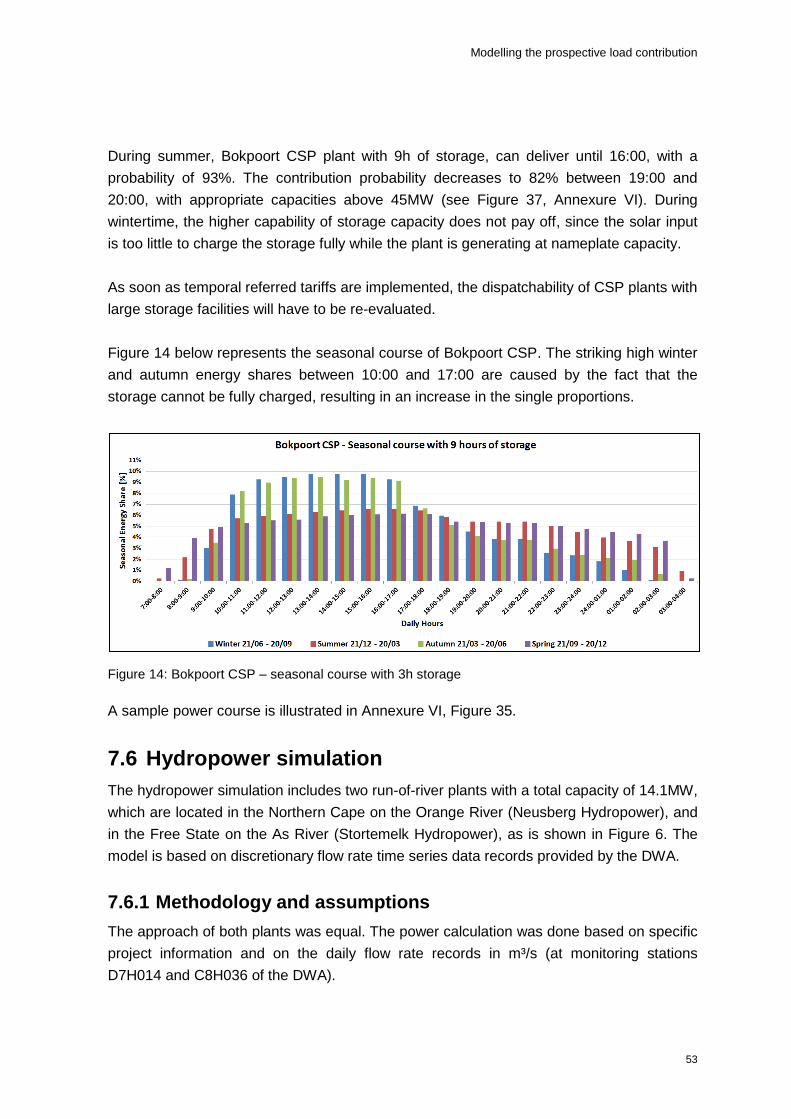
Modelling the prospective load contribution
53
During summer, Bokpoort CSP plant with 9h of storage, can deliver until 16:00, with a
probability of 93%. The contribution probability decreases to 82% between 19:00 and
20:00, with appropriate capacities above 45MW (see Figure 37, Annexure VI). During
wintertime, the higher capability of storage capacity does not pay off, since the solar input
is too little to charge the storage fully while the plant is generating at nameplate capacity.
As soon as temporal referred tariffs are implemented, the dispatchability of CSP plants with
large storage facilities will have to be re-evaluated.
Figure 14 below represents the seasonal course of Bokpoort CSP. The striking high winter
and autumn energy shares between 10:00 and 17:00 are caused by the fact that the
storage cannot be fully charged, resulting in an increase in the single proportions.
Figure 14: Bokpoort CSP – seasonal course with 3h storage
A sample power course is illustrated in Annexure VI, Figure 35.
7.6 Hydropower simulation
The hydropower simulation includes two run-of-river plants with a total capacity of 14.1MW,
which are located in the Northern Cape on the Orange River (Neusberg Hydropower), and
in the Free State on the As River (Stortemelk Hydropower), as is shown in Figure 6. The
model is based on discretionary flow rate time series data records provided by the DWA.
7.6.1 Methodology and assumptions
The approach of both plants was equal. The power calculation was done based on specific
project information and on the daily flow rate records in m³/s (at monitoring stations
D7H014 and C8H036 of the DWA).

Modelling the prospective load contribution
54
The following formula was used for the power calculation, with ρH2O standing for density, g
for gravity, h for height difference, and ηsystem for the total system efficiency:
The required input parameters are shown below. The numbers given in bold were not
available, but were approximated or assumed.
Table 22: Hydropower input parameters
Neusberg Hydropower Stortemelk Hydropower
Registered capacity [MW] 10 4.1
Max./Min. flow rate [m³/s] through turbine
60/5 30/5
System efficiency 93% 93%
Rated head [m] 18.7 14
The released maximum flow rate of Neusberg Hydropower was contradictory, due to it
having been derived from formula (7), taking the registered capacity into account. The
minimum flow rate and the system efficiency of Stortemelk Hydropower was adopted by
Neusberg Hydropower.
7.6.2 Results
A validation of the expected annual output by the developer yielded reliable results. The
deviation was −0.5% for Neusberg, and +8 % for Stortemelk Hydropower, with a CF of 82
and 76%, and an output of 71.5 and 27.2GWh. The annual course of Stortemelk
Hydropower was consistent, since the design flow rate was mostly surpassed. The flow
rate course of Neusberg (on the Orange River) showed a surplus during summer and
autumn, including flooding, and an inferior discharge rate during winter and spring, as is
illustrated in Figure 15 below.
Figure 15: Neusberg hydropower − annual course
(7)

Modelling the prospective load contribution
55
The two approved hydropower plants yielded a maximum capacity of 14.1MW and a
minimum of 5.4 MW. The base-load contribution was superior, unlike with solar PV, wind,
and CSP, since the CF showed the highest values by far, and the full load hours exceeded
7 000h/a.

Simulation results
56
8 Simulation results
The results include an evaluation of the cumulative output load behaviour to obtain
information about the future electricity contribution for South Africa, and an assessment of
the contribution made by each technology to the security of supply. The evaluation was
done to identify the strengths and weaknesses of each technology utilised.
The results are based on the weather data records for 2010 only, including irregularities
caused by single weather phenomenon. Hence, the simulation output does not represent
standard yearly conditions over a long period of time.
8.1 Cumulated output
The cumulative energy yield consists of an hourly addition of every source to gain a mutual
energy output. It generalises the individual contribution, to allow for the evaluation of the
systems output. In addition to a system assessment, an individual evaluation is done as
well.
8.1.1 Overview of general results
The model forecasts an annual energy yield of 6 442GWh (including 319GWh of Sere,
Klipheuwel and Darling wind farms, which are not part of the REIPPPPP), with the
following limit values:
A maximum occurring power of 2 302MW (27/03, 13:00–14:00), which constitutes
95% of the maximum possible capacity of 2 433MW
A firm capacity – representing the minimum occurring power of 27.2MW (20/10,
15:00–16:00), which is 1.1% of the maximum possible capacity. It is essential to
point out that the firm capacity represents one single value only. Further analysis
has to be done to assess the systems quality of minimum contribution.
Regarding to the IRP 2010 prediction analysis (see subsection 4.3.4 and Annexure 1, Part
B), which forecasts a demand between 275TWh (low scenario) and 315TWh (high
scenario) for 2015, the annual renewable energy distribution will range between 2.05% and
2.34%. The installed capacity will be 4.9% of 47GW of expected maximum demand load
for 2015.

Simulation results
57
A breakdown of the different technologies is shown in Table 23 below.
Table 23: Technology-specific annual energy yield
Wind power Solar PV CSP Hydropower
Delivered energy [GWh] 3 685 1 906 752 99
Share of total occurring output 57% 30% 12% 1.5%
Max. occurring power [MW] 1 302 900 217 14
Share of max. possible capacity 54% 37% 9% 0.6%
Average full load h [h/a] 2 830 2 119 3 456 7 016
About 57% of the annual output is delivered by means of wind power. The share between
the maximum occurring and the total installed power was found to be relatively low (54%),
which corresponds to the higher wind power full load hours rather than to the system’s
average. Related to the dispatchability of CSP and the continuity of hydropower, the
contribution that is made to the annual yield is remarkably higher than the capacity share
(ranging from 133%, in the case of CSP, to 250%, in the case of hydropower).
The 2011 adjusted target stated in the White Paper on Renewable Energy 2003 of more
than 10 000GWh in 2015 cannot temporarily be met. The government’s estimation
included the entire tendered capacity. An according linear extrapolation of the results
reveals an annual yield of 9 124GWh, assuming that biomass and biogas applications
operate with similar full load hours as does hydropower. The announced capacity of
bidding in R3 will presumably be online by 2016.
To be able to evaluate the frequency occurrence of system loads, a duration curve was
calculated. Every value was sorted according to size, and depicted over time (8 760
values). The duration curve in Figure 16 represents the total system load and the
contribution that was made by each technology.
The total duration curve does not reflect the sum of the specific curves, because the time-
related occurrence of the maximum values differed. The hydropower and wind power
graphs are the most constant, which indicates the highest mean power contribution during
the period of a year.

Simulation results
58
Figure 16: System duration curve
As derived from the table above, a classification into time-related quartiles (Qi) was done.
The interquartile range covered 50% of the distribution (4 380h) and was between 325 and
1 103MW. The results are illustrated below.
Table 24: System duration curve – classification into quartiles
Q 0.25 Q 0.5 Q 0.75
No. of h [h/a] 2 190 4 380 6 570
Power < hXY [MW] 1 103 632 (= median) 325
Share of maximum power 48% 27% 14%
The duration curve exhibits a high-power bandwidth regarding the fluctuation of the wind
power and the solar PV. The power was less than 632MW for 6 months each year.
The seasonal distribution was almost equal, with the share during wintertime being 24%,
whereas the summertime contributory share was 25.6%. The wind occurrence was
focused on autumn, which supplied 27% of the annual yield, whereas the solar PV
contribution that was made during spring achieved 28%.
8.1.2 Contribution to winter demand peak
The main difficulties that were encountered in terms of supply security occurred during
winter at around 20:00 (see Annexure 1, Part B, Figure 27). Therefore, an availability
evaluation of the results between 19:00 and 24:00 was done.
The supply system’s firm capacity during the time period differed seasonally, with it being
explicitly greater during summer, based on the availability of the higher wind speeds, on
the hydropower contribution, and on the dispatchability of the CSP. Solar PV made no
contribution, besides from 19:00 to 20:00 during summertime. Figure 17 below constitutes
the firm capacities, which showed a definite trend between 19:00 and 01:00.
Interquartile Range
Q 0.25
Q 0.5
Q 0.75

Simulation results
59
Figure 17: Winter and summer firm capacity – 19:00 to 01:00
The firm capacity represents a single value only. Although it can be used to evaluate the
merest temporal contribution, it does not provide information about the probability of
occurrence.
To be able to compare the results with those of other fluctuating power systems, a
frequency scale for use during certain hours, such as is shown in Table 27 below, might be
helpful. The frequency range between winter and summer differed. The gap obviously
decreased from 19:00 to 24:00, related to a minor contribution that was made by CSP. In
summertime, from 19:00 to 20:00, only 3% of the occurring power loads were less than
350MW, while almost 40% were so during wintertime. On the one hand, such an
occurrence indicates the gap existing between summertime and wintertime, but, on the
other hand, such an occurrence indicates a deficient wintertime contribution in terms of
systems performance.
The gap between summertime and wintertime decreases temporally until both graphs are
almost equal (supplementary information in Annexure VII).

Simulation results
60
Figure 18: Frequency distribution during summer and winter (A)
To understand the technologically dependent contribution, an average seasonal share is
depicted in Figure 19 below. The majority of contributed load is provided by wind power.
The decrease in the amount of CSP is based on the limited storage capabilities, since only
one out of the three plants was appointed with storage larger than that of 3h of nameplate
capacity.
Figure 19: Mean power distribution during winter and summer – 19:00 to 24:00
The amount of energy delivered between 19:00 and 24:00 decreased from 235 during
summer to 187GWh during winter. The share between wind power and CSP changed as
well. The yellow band represents the limited contribution that was made by solar PV.
8.1.3 Fluctuation characteristics
Based on the high volatility of renewable energy sources, the system tends to fluctuate,
with the power output changing within short periods of time. This chapter examines the
hourly fluctuation susceptibility, to obtain an impression of generation volatility properties.

Simulation results
61
The fluctuation can be defined as the derivative of the power change per time. According to
an annual, hourly calculated power course, 8 760 alternations occurred. The maximum
number of alterations was +960MW and −1 073MW. A determination of the seasonal
variation obtained by using the SD yielded a slight difference. The winter SD was 199 MW,
whereas the deviation during spring was 182 MW.
A repeated classification into quartiles showed a distinct result. A number of extreme
values occurred since the ratio of the lower quartile power (Q0.25) to the maximum power
was only 18% (see Table 25: Fluctuation duration curve – classification into quartiles Table
25 below). The median was proportionally low (10%) in comparison to the ceiling power
change, which confirmed that the majority of the values fell within a limited bandwidth.
Figure 20 depicts the systems absolute- and a real fluctuation duration curve.
Figure 20: Fluctuation duration curve
Table 25: Fluctuation duration curve – classification into quartiles
Q0.25 Q0.5 Q0.75
No. of h [h/a] 2 190 4 380 6 570
Power < hXY [MW] 208 108 (= median) 43
Share to maximum power 18% 10% 1%
An exemplary power course is illustrated in Figure 16 below.

Simulation results
Exemplary power course − 01/01/2010–11/01/2010 (representing 01/01/2015–11/01/2015)
Figure 21: Exemplary single and cumulative power course – 01/01/2010–11/01/2010

Simulation results
8.2 Conclusion
The current thesis consists of an annual renewable energy output, a load behaviour, an
evaluation of the contribution to the winter peak demand, and a fluctuation assessment. In
terms of such, the scientific question asked can be answered clearly.
The work represents a variety of different, technology-dependent approaches that have
been adopted to gain an entire annual load for 2015, by taking 2010 data into account. It
simulates every approved IPP project until the financial close of REIPPPP bidding R2 (9
May 2013), as well as three further, already authorised renewable energy projects.
Conclusions drawn from the work
The conclusion of the thesis is split into the following aspects that summarise the most
important findings of the work:
The annual delivered energy was 6 442GWh, which corresponded to from 2.05 to
2.34% of the expected electricity demand in 2015. An inclusion of a linear
extrapolation from the results of bidding R1 and R2 to bidding R3 yielded an
amount of 9 124GWh. In terms of such figures, the government’s ambition to
surpass the 10 000GWh level cannot be met.
Although the wind farms are spread countrywide, the wind speeds were found to be
spatially consistent, but temporally fluctuating. Despite the vast variation, almost no
(less than 1%) firm capacities can be guaranteed. Further analysis in that field has
to be done.
Solar PV does not make a perceptible contribution to any evening peaking demand.
The actual capacity of installed solar PV is 14% less than the registered capacity,
which is based on a specification of peak capacity, in accordance with STC.
The retail prices per kWh for solar PV and for wind power generation are the most
favourable by far, which justifies the highest economic feasibilities.
CSP offers the greatest degrees of freedom regarding security of supply.
Depending on the storage size involved, it could contribute to the evening peak
demand. The CF’s were almost 2.5 times higher than solar PV exhibits. The
insertion of an increased amount of technical implementation into the supply mix
would cause a higher individual availability of renewable generated electricity.
The difference between the summer and winter contribution was found to deviate
strongly, especially in terms of frequency distribution from 19:00 to 24:00. The
contribution that was made during the winter season was found to be 20% less than
in summer.
The more volatile are the sources that feed into the public grid, the higher the
power hub and the burden are. As soon as a regulatory strategic electricity plan

Simulation results
64
requires an upper share of peaking distribution, storage capabilities have to be
taken into account.
The shock rate of the system that expresses fluctuation in behaviour demonstrated
high, but temporally rare, amplitudes. The median was 10 times less, which implies
a smoothed course.
It is essential to mention that the entire methodology included many uncertainties and
assumptions that strongly influenced the results. Every assumption for each approach has
been clearly stated and scientifically justified. The focus in each approach was on
developing a single applicable method, by means of using external, reliable information
sources, such as the expectations of developers, for validation purposes only.
During the development process, a number of new perspectives and problems arose that
could not be processed within the precisely structured framework of the thesis. To examine
the open questions, further research would have to be undertaken, which has already
scheduled for the next time period by the CRSES.
Contribution to knowledge
The thesis provides a first step towards an ongoing forecast prospective method. The
researcher involved assembled tendered capacities into annual energies to figure out the
strengths and the weaknesses of the evolving renewable energy mix. The results of the
thesis might contribute to advising policymakers to take further decisions in this regard,
since a detailed annual projection is now available in the public domain.
Prospect of future research
The thesis determines a first step in forecasting South Africa’s industrial renewable energy
supply. It forms part of an ongoing approach to keep the results up to date, to take
additional guidelines into account, and to which to append prospective projects.
Research in the following fields is required:
A focus on the contribution that is made by each technology, to gain a more
detailed forecast and to take such technologies as landfill gas, biomass, and others
into account
An improved method of evaluating the simulated results for every single approach
The models susceptibility of aberrations depends on uncertain assumptions. An
assessment of every met boundary value causes an error minimization by coeval
adjustments. Each aberration could be quantified in terms of error bandwidths
A closer collaboration than at present with the weather records, enabling GeoModel
to increase the reliability of wind data sets

Simulation results
65
An additional examination of the weather data in terms of long period records would
reduce the dependency on unforeseen weather phenomenon, and provide an
ordinary annual output
A prospective, ongoing evaluation of the model’s results, according to real values
from 2015 onwards
Reference list
9 Reference list
Banuelos Ruedas, F., Camacho, C.A., Rios-Marcuello, S., 2011. Methodologies Used in the Extrapolation of
Wind Speed Data at Different Heights and Its Impact in the Wind Energy Resource Assessment in a Region.
Wind Farm - Technical Regulations, Potential Estimation and Siting Assessment, 97 – 114. Orlando Suvire
(Ed.), ISBN: 978-953-307-483-2.
BP Statistical Review, 2012. British Petrol Statistical Review of World Energy, June 2012. United Kingdom.
Available from: http://www.bp.com/content/dam/bp/pdf/Statistical-Review-
2012/statistical_review_of_world_energy_2012.pdf [Accessed 11/07/2013]
Centre for Renewable and Sustainable Energy Studies (CRSES), 2013. AcrMap 2010 – electricity grid image.
Stellenbosch, South Africa.
Chamber of Mines of South Africa, 2007. Annual Report 2006 – 2007. Mining together. Available from:
http://www.bullion.org.za/documents/text%20compressed.pdf [Accessed 11/07/2013]
Cloete K., March 2013. Vodacom shows off its solar rooftop – the largest in Africa, Engineering News Online,
Creamer Media (Pty) LTD. Germiston, South Africa. Available from:
http://www.engineeringnews.co.za/article/vodacom-shows-off-its-solar-rooftop-the-largest-in-africa-2013-03-06
[Accessed 12/06/2013]
CSP World – World News about Concentrated Solar Power, 2013. Servicios Avanzados de Comunicación y
Marketing SL (SACM). Spain. Available from: http://www.csp-world.com [Accessed 20/06/2013]
Department of Energy (DoE), 2009. Digest of South African Energy Statistics 2009. Directorate. Pretoria, South
Africa. Available from:
http://www.energy.gov.za/files/media/explained/2009%20Digest%20PDF%20version.pdf. [Accessed
15/04/2013]
Department of Energy (DoE), 2010. Annual Demand forecast 2010. Forecast - IRP 2010 Parameter, Overview
sheet. Pretoria, South Africa. Available from: http://www.energy.gov.za/IRP/factsheet.html [Accessed
29/04/2013]
Department of Energy (DoE), 2013. Formal homepage, Available from:
http://www.energy.gov.za/files/petroleum_frame.html [Accessed 22/04/2013]
Department of Energy (DoE), 2013a. Renewable Energy Independent Power Producer Procurement
Programme, formal homepage 2013. South Africa. Available from: http://www.ipprenewables.co.za/#site/index
[Accessed 13/05/2013]
Department of Energy (DoE), Aug 2011a. Question and Answer for IPP Briefing session 31. Media &
Publications., South Africa. Available from:
http://www.energy.gov.za/files/media/pr/media_pressreleases2011.html, [Accessed 10/05/2013]
Department of Energy (DoE), Aug 2011g. Media Statement, Renewable Energy Independent Power Producer
Programme, Media & Publications. South Africa. Available from:
http://www.energy.gov.za/files/media/pr/media_pressreleases2011.html [Accessed 12/05/2013]

Reference list
67
Department of Energy (DoE), August 2011b. Fact sheet for the media briefing session on 31 August 2011.
Renewable Energy Independent Power Producer (IPP) Programme. South Africa.
Department of Energy (DoE), August 2011c. Request for qualification and proposals for new generation
capacity under the IPP procurement programme, Part A – general requirements, rules and provisions. Tender
No.: DOE/001/2011/2012. South Africa.
Department of Energy (DoE), August 2011d. Request for qualification and proposals for new generation
capacity under the IPP Procurement Programme, Part B – Qualification Criteria. Tender No.:
DOE/001/2011/2012. South Africa.
Department of Energy (DoE), August 2011e. Request for Qualification and Proposals for New Generation
Capacity under the IPP Procurement Programme, Volume 5: Economic Development Requirements. Tender
No: DOE/001/2011/2012. South Africa.
Department of Energy (DoE), December 2011f. Renewable Energy Independent Power Producer
Announcement 2011 − Summary of Evaluation Findings. Renewable Energy Independent Power Producer
Procurement Programme. South Africa
Department of Energy (DoE), December 2012. IPP Procurement Programme 2012. Determination under
Section 34(!) of the Electricity Regulation Act 4 of 2006 No. 1074. South Africa.
Department of Energy (DoE), May 2011. Electricity Regulation Act (ERA) No.4 of 2006, Electricity Regulations
on New Generation Capacity. Government Notice. Pretoria, South Africa.
Department of Energy (DoE), May 2012a. Renewable Energy IPP Procurement Programme, Window Two
Preferred Bidders Announcement 21 May 2012. South Africa
Department of Energy (DoE), May 2012b. Window Two Preferred Bidders’ Announcement 2012, Renewable
Energy Independent Power Producer Procurement Programme. South Africa
Department of Energy (DoE), September 2009a. Integrated Resource Plan for Electricity 2009 (IRP 2009).
Preliminary Report. South Africa.
Department of Minerals and Energy (DME), December 1998. White Paper on the Energy Policy of the Republic
of South Africa. ISBN: 0-9584235-8-X. Pretoria, South Africa.
Department of Minerals and Energy (DME), July 2003. Free Basic Electricity Policy. Electricity Basic Services
Support Tariff. Government Gazette No. 25088, Pretoria, South Africa.
Department of Minerals and Energy (DME), March 2003a. Integrated Energy Plan for the Republic of South
Africa 2003 (IEP), South Africa.
Department of Minerals and Energy (DME), May 2002. Energy Outlook for South Africa: 2002, Eskom Holding,
Energy Research Institute – University of Cape Town, South Africa.
Department of Minerals and Energy (DME), November 2003b. White Paper on Renewable Energy 2003. South
Africa.
Reference list
68
Department of Water Affairs (DWA), 2013. Hydrological Services, Republic of South Africa. Available from:
http://www.dwaf.gov.za/Hydrology/ [Accessed 27/06/2013]
Eskom, 2012. Annual demand, hourly based – featured by MS Excel. Provided by Paul Gauché. Source:
Eskom Holding. South Africa.
Eskom, 2013. Transmission Ten Year Development Plan 2013 – 2022. Eskom Transmission Division, Eskom
Holding, Johannesburg, South Africa. Available from: www.eskom.co.za[Accessed 29/04/2013]
Fritz W., October 2012. Renewable Energy Feed in Tariffs, REBID, SASGI and the Smart Grid. Cape
Peninsula University of Technology. Journal: Energize, p. 80. Stellenbosch, South Africa.
Gauché, P., 2011. [Microsoft Excel tool]. Stellenbosch. South Africa, Conn.: Solar Thermal Energy Research
Group.
Gauché, P., Pfenninger, S., Meyer, A.J., Von Backström, T.W and Brent, A.C., 2012. Modeling Dispatchability
Potential of CSP in South Africa. South African Solar Energy Conference (SASEC). Stellenbosch, South Africa.
GeoSun Africa, 2008. South Africa Maps, Spin-off company of the Centre for Renewable and Sustainable
Energy Studies. Stellenbosch, South Africa, Available from: http://geosun.co.za/solar-maps/ [Accessed
12/04/2013]
Gilman, P., 2012. Thermal Storage Dispatch Control for Physical Trough Model. System Advisor Model −
National Renewable Energy Laboratory, US Department of Energy, USA. Available from:
https://sam.nrel.gov/webfm_send/252 [Accessed 20/06/2013]
Greyling A., July 2012. Renewable Energy Independent Power Producer Procurement Programme – An Eskom
perspective. Eskom. South Africa. Available from: http://alive2green.com/conference-
presentations/SES2012/Adele_Greyling.pdf [Accessed 13/07/2013]
Gross, C., March 2012. Electricity Generation Options considered by Eskom, Presentation at the Energy
Planning Colloquium, Eskom, Available from:
http://www.energy.gov.za/files/IEP/presentations/ElectricityGenerationOptionsConsidered_30March2012.pdf
[Accessed 09/04/2013]
Heller, L., Gauché, P., 2012. Rock Bed Storage Based Simulation of a 5MWel Combined Cycle Solar Power
Plant. South African Solar Energy Conference (SASEC). Stellenbosch, South Africa.
Inglesi R., Pouris A., A critique of Eskom’s projections, University of Pretoria, ‘Forecasting Electricity Demand
in South Africa’, Article #16 of South African Journal of Science, Pretoria, South Africa.
IRP 2010, March 2011. Integrated Resource Plan for Electricity 2010−2030, Department of Energy, Revision 2,
Final Report, South Africa.
IRP 2010a Energy Forecast Revision 2 Report, July 2010. Systems Operations and Planning 2010. Available
from:
http://www.energy.gov.za/IRP/irp%20files/SO_IRP%202010%20Energy%20Forecast%20Final%20Report.pdf
[Accessed 28/04/2013]

Reference list
69
IRP, 2010b. Demand Forecast - IRP 2010 Input Parameter, Department of Energy, Republic South Africa.
South Africa
Kernan A., 2013. From REFIT to REBID: South Africa’s Renewable Energy Auctions, Clean Energy Solution
Center – Assisting countries with clean energy policy, Kernan Aedan, Greenwell Consulting. Available from:
https://cleanenergysolutions.org/users/aedan-kernan, [Accessed 10/05/2013]
King N.A., Blignaut J.N., 2002. The Externality Costs of Coal Combustion in South Africa, Forum for Economics
and Environment. University of Pretoria, Department of Economics. South Africa.
Letete, T., Guma, M., Marquard, A., 2009. Carbon accounting for South Africa, Information on climate change
in South Africa: Greenhouse gas emissions and mitigation options, Topic 3. University of Cape Town. South
Africa. Available from: http://www.erc.uct.ac.za/Information/Climate%20change/Climate_change_info3-
Carbon_accounting.pdf [Accessed 08/04/2013]
Mashao M., March 2012. Trends in the consumption of electricity in the Industr. Eskom Holding. Available from:
http://www.energy.gov.za/files/IEP/presentations/TrendsInTheConsumptionOfElectricityInTheIndustry_30March
2012.pdf [Accessed 22/04/2013]
Medium Term Risk Mitigation Plan for Electricity in South Africa 2010 to 2016 (MTRM), September 2010.
Phase 1 Report, Department of Energy. South Africa.
National Energy Regulator of South Africa (Nersa), 2006. Statistics 2006 - Electricity Supply Statistics for South
Africa, South Africa. Available from: www.nersa.org.za[Accessed 24/04/2013]
National Energy Regulator of South Africa (Nersa), December 2008. Renewable Energy Feed-In Tariff (REFIT),
Consultation Paper, South Africa.
National Energy Regulator of South Africa (Nersa), March 2011. Review of Renewable Energy Feed - In
Tariffs, Consultation Paper. South Africa.
National Energy Regulator South Africa (Nersa), February 2013a. Revenue Application - Multi Year Price
Determination 2013/14 to 2017/18 (MYPD3). South Africa.
National Energy Regulator South Africa (Nersa), January 2013. MYPD3 Application 2014 -2018, Eskom
Holding. Gauteng, South Africa. Available from:
http://www.eskom.co.za/content/MYPDPresentationGauteng29Jan_20h00.pdf [Accessed 23/05/2013]
National Energy Regulator South Africa (Nersa), October 2011a. Nersa Consultation Paper: Eskom Multi-Year
Price Determination Methodology. South Africa
National Renewable Energy Laboratory, NREL, 2005. System Advisor Model (SAM). [SamUL scripting
simulation tool]. United States of America. Available from: https://sam.nrel.gov/ [Accessed 01/05/2013]
Otto A., 30/05/2013. Project manager, South African Wind Energy Programme (SAWEP), e-mail
correspondence. South Africa
Patel, M.R., 2006. Wind and solar power systems: design analysis, and operation. 2nd ed. CRC Press. ISBN
0849315700. USA

Reference list
70
Renewable Energy Centre of Research and Development (Record), South African National Energy
Development Institute (Sanedi), Deutsche Gesellschaft für Internationale Zusammenarbeit (Giz). 11/03/2013.
Wind energy and defence radar discussion workshop: challenges and possible solutions. Mount Nelson Hotel.
Cape Town. South Africa.
RSA Government, January 2008. National Response to South Africa’s Electricity Shortage - Interventions to
address electricity shortages. South Africa Government Online. Available from:
http://www.info.gov.za/otherdocs/2008/nationalresponse_sa_electricity1.pdf [Accessed 08/04/2013]
Siepelmeyer N., Interview 18/05/2013. Managing Director, IPD Power Ltd., [email protected]. Cape
Town. South Africa.
Siepelmeyer T., Interview 20/04/2013. CEO, IPD Power Ltd., [email protected]. Cape Town. South Africa.
SolarGIS, March 2013. SolarGIS version 1.8: Specifications of solar radiation and meteo database. SolarGis,
GeoModel Solar s.r.o. Bratislava, Slovakia. Available from:
http://solargis.info/doc/_docs/SolarGIS_data_specification.pdf [Accessed 13/06/2013]
South African Petroleum Industry Association (SAPIA), March 2012. 2011 Annual Report. Sandton, South
Africa. Available from: www.sapia.co.za [Accessed 11/07/2013]
Stanley Consultants INC, June 2009. Wind and Hydropower Feasibility Study. Final Report June 2, U.S.
Department of Energy (U.S. DoE). USA. Available from:
https://www.wapa.gov/ugp/powermarketing/WindHydro/Final%20WHFS%20Ver%20Mar-2010%205b.pdf
[Accessed 30/05/2013]
Statistics Austria, 2013. Geamtenergiebilanz 1970 – 2011. Bundesanstalt Statistik Österreich. Vienna, Austria.
Available from: http://www.statistik.at/web_de/suchergebnisse/index.html [Accessed 21/04/2013]
Statistics South Africa (SSA), 2012. January 2012. Energy Accounts for South Africa 2002 – 2009. Pretoria,
South Africa. Available from: http://www.statssa.gov.za/ [Accessed 20/04/2013]
Statistics South Africa (SSA), 2013. Statistical Release 2013, Electricity generated and available for distribution
(Preliminary), monthly released. Ref. Nr. P4141. Pretoria, South Africa.
Stine, W., Geyer, M., 2001. Power from The Sun. Available from: http://www.powerfromthesun.net/book.html
[Accessed 18/06/2013]
Suri M., Cebecauer T., Skoczek A., Betak J., May 2012. Solar electricity production from fixed-inclined and
sun-tracking C-Si photovoltaic modules in South Africa. GeoModel Solar. South African Solar Energy
Conference 21-23/05/2012. South Africa.
Sustainable Energy Action Plans (SEAP), 2006. The Emission Factors 2006, Technical annex to the
Sustainable Energy Action Plan template instructions document. Available from:
http://www.eumayors.eu/IMG/pdf/technical_annex_en.pdf [Accessed 09/04/2013]
System Operator for Northern Ireland (SONI), EirGrid Plc, 2012. All-Island Generation Capacity Statement
2013-2022, Ireland. Available from: http://www.eirgrid.com/media/All-Island_GCS_2013-2022.pdf [Accessed
30.05.2013]
Reference list
71
The National Energy Act 2008 (NEA), Nov 2008. No. 34 of 2008, Vol. 521, Government Gazette No. 31638.
Republic of South Africa. Cape Town, South Africa.
The World Bank Group, April 2013. Data by Countries. Represented via Google Public Data, Google
Incorporated. Available from: http://www.google.at/publicdata/directory [Accessed 10/04/2013]
Tong, W., 2010. Fundamentals of wind energy. WindPower Generation and Wind Turbine Design. 3 – 89. WIT
Press. ISBN: 978-1-84564-205-1. USA
Uken, E., 2013. German South African Research Lecture Series: Energy Sciences. Focus on Solar Power and
the Energy Supply of the Future, German Academic Exchange Service (DAAD), German-South African Year of
Science 2012/13, 17/03/2013. Bellville Campus CPUT. Cape West, South Africa.
Wind Atlas for South Africa (WASA). March 2012. Overview of Wind Atlas for South Africa (WASA) project.
Cape Town, South Africa. Available from: http://www.wasaproject.info/docs/Launch.pdf [Accessed 12/04/2013]

Reference list
72
Annexure I, Part A – Energy consumption
Primary energy consumption
Oil and gas explorations, which are rare, are mostly imported from the Middle East and
from other African countries than South Africa, as well as being provided by means of the
liquefaction of coal. The annual primary energy proportions differ, due to the fact that the
majority of the consumed energy depends on the mining and industrial production of a few
crucial players who rely on the changing worldwide economic growth.
The primary energy intensity, as a ratio between primary energy consumption and the
gross domestic product (GDP), decreased from almost 7MJ/R in 2002 to 4.2MJ/R in 2009
(SSA 2012, p. 42). Such a key performance indicator has to be considered controversial,
since the structure of the economy, the energy sector intensities, the technological
development, the sustainability of energy use, and the social indicators strongly influence
the value. The Integrated Energy Plan (IEP 2003, p. 4 sqq.) signifies that the industrial
policy has shifted towards a greater focus on knowledge-intensive sectors and human
resource development than in the past. Such primary production as agriculture and mining
with high energy intensities currently contributes less to the economy than does the tertiary
or services sector, which might have caused the significant decrease in primary energy
intensities experienced.
Final energy consumption
The three major consumers are the industry, of almost 40%, and the transportation and the
residential sector, as are illustrated in Figure 22 below. The category ‘Other’ represents
such energy carriers as petroleum product solvents, lubricants and bitumen.
Figure 22: Final consumption, 2006 (DoE 2009, Statistics Austria 2013)

Reference list
73
The South African mining industry is characterised by a traditional mining history that
currently covers 7.5% of total consumption, while Austria’s proportion is only 0.58%.
Although the total energy consumption in Austria is 41% less than it is in South Africa, the
ratio between GDP per capita is 712% higher, which leads to the conclusion that the
economy of South Africa is not as adequately developed and per capita intensive as the
Austrian economy is (DoE 2009, World Bank 2013).
Coal industry
Due to the fact that the national mining industry is well established, coal and other mining
goods are traded at a more favourable price than the international standards assume. A
supply of coal is usually available, with about 53% being facilitated by means of
inexpensive opencast mining operations (Chamber of Mines 2007, p. 17).
The expected South African coal reserves are estimated to be about 30 000 Mio tons,
which corresponds to 3.5% of the world’s proven reserves. South Africa provided 3.6% of
the annual worldwide produced coal in 2011, of which the country consumed 2.5%. As a
result, about 30% of the country’s annually produced coal was exported (BP 2012). In
2000, approximately 41% of the overall coal depletion was used for electricity generation,
whereas 98% of it was utilised by Eskom (King N.A., Blignaut J.N. 2002, p. 6).
Table 26 below displays that the share between the total coal revenue and the traded
mass deviates from the norm. While 31% of the exported coal earns 56% of the revenue
(price to the mass share of 181%), the price that Eskom disburses is 50% lower.
Table 26:Coal sales by sector, 2000 (King N.A., Blignaut J.N., 2002, p. 6 sqq.)
Sectors Mass rel. share [%] Price rel. share [%] Price to mass share [%]
Electricity (non-Eskom)
0.7 0.5 70
Eskom 41 20.6 50
Exports 31 56.1 181
Synthetic fuel (Sasol)
20.7 14.2 69
Others 6.7 8.5 127
The countrywide coal resources are exclusively depleted in the north-eastern part of the
country, leading to disparities in the contribution that is made by power generation.
Petrol industry
According to the South African Petroleum Industry Association (SAPIA 2012), the total
consumption of petroleum products in 2010 was 25 300 Mio litres. Of the liquid fuel
demand in 2005, 36% was synthesised from locally depleted coal by Sasol (30%) and from
natural gas by PetroS (6%), whereas the total installed refinery capacities were lower

Reference list
74
(being 27.5% in 2007). This development implied a greater degree of capacity utilisation
from synthesised fuels than from refined crude oil. The remaining 64% of the liquid fuel
demand was refined by means of imported crude oil (DoE 2013).
Petroleum fuels (except for the liquefied coal products) and other chemicals for industry,
transport, heating, and other uses were provided by such national and international energy
utilities as Caltex (Chevref – Chevron Cooperation), Sapref (which is a joint venture
between Shell SA Refining and BP Southern Africa), Engen, and others.

Reference list
75

Reference list
76
Annexure 1, Part B – Electricity supply and demand
History
South African electricity consumption increased almost steadily, from 75TWh in 1975 to
260.5TWh in 2007. The major uncertainties in more recent years have been based on the
unbanning of the African National Congress (ANC) in 1990, with a subsequent
extraordinary increase of consumption, the Asian and emerging market crisis in 1997/98,
and the economic crisis after 2007 (Mashao M. 2012, p. 4).
In 2010, 58% of the African continent’s electricity utilisation was owned by South Africa (in
comparison to 60.5% in 1975), underlining the country’s primacy in Africa (World Bank
2013).
Key drivers of electricity growth
An assessment of key drivers of electricity growth was performed by Eskom (taking
historical impacts into account), to figure out the most influential correlations. Various
interrelations are enumerated below (Mashao M. 2012, p. 3):
Economic growth
The relationship between the GDP and the growth rate, as well as the relationship
between the electricity sales and the sales growth rate has shown a correlation
since 1920. The chart in Figure 18 below illustrates the fact that the electricity sales
grew to a similar extent as did the GDP. While the average electricity sales growth
rate dropped between 1950/75 and 1975/2007 from 7.5 to 3%, the GDP growth
decreased by a similar amount (from 5 to 2%).
Figure 23: Correlation between the electricity- and the GDP growth rate (Mashao 2012)
Weather – seasonal temperatures
Due to the fact that the majority of the installed heating devices are driven by
electricity, and due to the fact that the insulation of buildings is insufficient, heating

Reference list
77
during wintertime influences the daily consumption load curve significantly more
than does air conditioning during summer (see Figure 27, p. 79)
Large industrial projects
The larger the industrial sector is, the higher is the influence on electricity
consumption. South Africa’s heavy industry and mining sector exhibits vast energy
expenditures (see section 4.2)
Electricity intensity development
The electricity intensity (i.e. the share of electricity sales and the GDP) steadily increased
until 1997, due to the increased efficiencies of power production units, the heightened
efficiency of the transmission system, and favourable resource prices. The growth of
electricity demand was higher than was the GDP growth. In later years, the electricity
intensity started to decline, since the South African economy had matured, and the prices
of fossil fuels had increased. The future development forecast by Eskom anticipates a
distinct downturn in the electricity intensity, since the electricity demand growth is expected
to be less than the GDP growth (Mashao 2012, p. 19 sqq.). Figure 19 below illustrates the
past course and future trend of the electricity intensity in kWh/R.
Figure 24: Electricity intensity (Mashao 2012, p. 19 sqq.)
The electricity intensity in 2009 was 0.12kWh/R, whereas the primary energy intensity in
2009 was 1.17kWh/R (= 4.2MJ/R), as was noted in Annexure I, Part A. The difference can
be explained in simplified form as being due to the intermediate reduction factors that are
involved in converting primary energy to electricity (such as conversion losses, power
efficiency, transportation, and other related factors).

Reference list
78
Electricity supply progression
Figure 20 below refers to the contents of subsection 4.3.1, covering the National electricity
supply.
Figure 25: Electricity available for distribution (SSA 2013, World Bank 2013, Nersa 2006)
Sector-specific electricity demand
Figure 21 below illustrates the share of customer categories referred in subsection 4.3.2.
Figure 26: Electricity demand, by sector (Nersa 2006, p. 58)

Reference list
79
Weekday electricity demand
To understand the meaningful implementation of fluctuating renewable generation in the
electricity supply, the daily consumption trend has to be considered, since the demand
precisely determines the supply. The generic South African weekly load curve changes,
depending on the time of day, and varies markedly between the lower summer and the
greater winter demand. Two major peaks typically occur during a winter’s day: at 09:00,
and at 19:00. The higher consumption during wintertime is caused by electrical heating
devices. Figure 27 below depicts the daily demand during a week in winter and one in
summer. The difference in the consumption of power between summer and winter can
increase by as much as 15%.
Figure 27: Exemplary weekday demand during summer and winter in 2010 (Eskom 2012)
Causes of the incipient energy crisis
This subsection refers to subsection 4.3.3 – ‘Present lack of supply’. The causes of the
incipient energy crisis are controversial, due to the different interests of all the stakeholders
involved. Eskom blamed the energy crisis that was experienced in 2007/08, and the
shortages that are anticipated until 2016, on the following contributory factors (Inglesi R.,
Pouris A., p. 2):
The exceptional increase of 50% from 1994 to 2007 was based on (World Bank
2013):
o A strong, unexpected upturn in the economy occurred after sanctions were
lifted in the early 1990s.
o The implementation of the Free Basic Electricity Policy in 2003 prescribed
the allocation of an allowance of 50kWh electricity per month to poor
households, executed by the individual provinces (DME 2003).

Reference list
80
The government’s decision in 2004 to fund new capacities was delayed.
A countrywide lack of research into energy in general (with only 0.34% of the
international research publications reporting on energy-related topics, with South
Africa contributing 0.5% of academic research papers in all scientific disciplines
internationally).
MTRM – recommendation for closing the supply/demand gap
The recommendations discussed below are directed by the IRP 2010 (2011, p. 66).
Supply-side options
Implementation of the REFIT programme, which was modified to form the REBID
programme (see section 5.3)
Implementation of co- and own generation
Increased generation availability from existing fleet, by means of enhancing the
outage rate (with 1% improvement by 2012 corresponding to about 2.5TWh per
year)
Demand-side options
Meeting the government’s target to roll out 1 million SWHs to cut down power
demand
DSM: the addition of 25% on existing commitments, with a vast forecast reduction
potential
Supplying of demand response (DR) to small, commercial and industrial
applications
The IRP 2010 (2011, p. 69) determined that a gap would still remain during 2011 and
2012, even if every identified potential could be captured. Therefore, three further options
were added to avoid load-shedding in future:
ECS: A reduction target could be established for the 500 largest power consumers
during peak loads, which would include penalties if specifications are not met. The
estimated saving potential is 6 TWh.
Compulsory DR: Consumption during peak hours could be limited for certain
residential users.
Increasing OCGT load factor: By increasing the OCGT operation by 5%, about 1
TWh of supplementary energy output could be provided.

Reference list
81
IRP demand forecast
As part of the IRP, two demand forecasts were assessed. They varied widely, since
different methods were applied, although the same input parameters were utilised to keep
the result comparable. Such input parameters as economic growth (in terms of the GDP),
changes in energy intensity, international sales, system losses, load profiles for customer
sectors, and others were utilised (IRP 2010b):
The two forecasting methods can be abstracted as follows (IRP 2010a, p. 4):
SO forecast: “The model is a combination of statistical analysis, tracking of
historical trends and applying expert knowledge.”
Council for Scientific and Industrial Research (CSIR) forecast:
“The model is basically a multiple regression model forecasting technique used to
forecast the annual consumption within the individual electricity sectors by relating
various conditions (or ‘drivers’) to the demand in each sector.”
For both methodologies, a sensitivity analysis was undertaken during the IRP process to
ensure a reliable generation forecast. A high and low forecast scenario was allocated as
well, with the intention that it should not be breached.
Figure 23 below illustrates the trend experienced in both methods, and the actual
generation that occurred until 2012, according to the SSA, as well as a power demand
forecast by Eskom.
Figure 28: Expected annual energy simulation (DoE 2010, IRP 2010b)
The results of the above were discussed in subsection 4.3.4 – ‘Prospective development’.

Reference list
82
Annexure I, Part C – Electricity distribution
High-voltage grid map
Figure 29: High-voltage grid map – South Africa (CRSES 2013)
Transmission and distribution line specifications
The last released electricity supply bulletin of the SSA (Nersa 2006) determined the total
number of transmission and distribution lines for 2006.
The transmission grid, which is carried and owned by Eskom, consists of 765, 400, 275,
220 and 132kV lines, whereof 56% are 400kV lines. An additional 533kV high-voltage
direct current (HVDC) line connects Johannesburg with Sonogo (Mozambique), for
international power transfers. The total transmission line length is 27 770km.
The distribution network can be differentiated into lines and cables, and is subdivided into
high-voltage (44 to 132kV), medium-voltage (1 to below 44kV) and low-voltage (below
1kV). While 78% of the distribution lines are carried by Eskom, the majority (96%) of the
distribution cables are owned by municipalities and a private provider. The total distribution
length is 608 000km, of which almost 47% consists of medium-voltage lines managed by
Eskom, and 24% of low-voltage cables run by municipalities and a private provider. The
total transformer capacity in 2006 was 403GVA.
Reference list
83
Future expectations
A further, intended installation of renewable energies will cause decentralisation of the
power supply, which will basically bring relief to the transmission grids, but which will strain
the local grids during full-load times. A bidirectional current flow has to be technically
feasible, which implies the need for further applications, such as dynamic transformers and
static VAR compensators (SVCs), to reduce the reactive power that is required for voltage
stability and variation.
Under the prospective ‘Transmission Ten-Year Development Plan 2013–2022’ (Eskom
2013, p. 11), the following investments are provided until 2022:
3 700 km of 765 kV lines and 8 631 km of 400 kV lines
A total installed transformer capacity of about 84 000 MVA, including the
transformation capacity that is required to integrate the fluctuating generation
A capacitor power of 2 600 Mvar, which is required to support areas of the network
under contingency conditions, to ensure that the required voltage levels are
maintained
A reactor power of 9 200 MVA, which is a consequence related to the extensive distance that the transmission system has to cover
Reference list
84
Annexure II – Legal Framework
IRP Accruement
The development of such a future-orientated plan as the IRP 2010 requires extensive
preliminary work. Various policy and legal guidelines, such as a legal framework and
certain resolutions, have to be set before standards and other technical specifications can
be implemented. The following guidelines and decrees strongly contributed to the
development of the IRP 2010.
White Paper, 1998
The ‘White Paper on the Energy Policy of the Republic of South Africa’ was published in
December 1998 by the DME. South Africa’s external and internal environments, including
the lifted, apartheid-induced embargos had experienced fundamental shifts, which resulted
in significant changes occurring in the context of the energy policy. The White Paper’s
objective constitutes a major re-evaluation of the sector’s policies that are aimed at
providing policy stability for energy suppliers, investors and consumers.
The energy policy objectives were spelled out as follows:
Increasing access to affordable energy services
Improving energy governance
Stimulating economic development
Managing energy-related environmental impacts
Securing supply through diversity
The White Paper further covers the major topics of the demand sector, the supply sector,
and cross-cutting issues. The White Paper, which takes integrated energy planning as part
of the cross-cutting issues, promotes a development of standards, guidelines and codes of
practice for the correct use of renewable energy sources as part of the supply diversity that
can be facilitated by the DME, but which must, in addition, include facilitation by the
standard authorities and the renewable energy industry (DME 1998).
IEP, 2003
The IEP 2003 was published by the DME. The integrated energy planning process was
based on the results of Energy Outlook 2002 (DME 2002), which was developed by DME,
Eskom, and UCT, with its Energy Research Institute (ERI). The IEP 2003 is not a precise
blueprint for the energy sector, but it is a framework within which specific energy
development decisions can be made.
Amongst derived, valuable conclusions regarding the integrated planning process, the IEP
accentuates that historically driven energy sector decisions were mostly made by
Reference list
85
maintaining supply security. The economic, environmental and social impacts of such
alternatives as renewable energies were, by and large, not considered, which amounted to
a large-scale, capital-intensive supply, instead of to a more cost-effective, long-term
alternative (DME 2003a, p. 4 sqq.).
White Paper on Renewable Energy, 2003
As well as the IEP, the White Paper on Renewable Energy 2003, published by the DME,
strongly facilitates the commitment of sustainable resources. It requires essential elements
of renewable energy implementation, such as suggestions for financial, legal and
regulatory instruments, as well as explaining policy principles. One of the White Paper’s
objectives was to develop an appropriate legal and regulatory framework for pricing and
tariff structures to support the integration of renewable energy and to attract investment.
The government’s medium-term (10-year) target of 10 000GWh to be attained by 2013 was
set (DME 2003b).
South Africa has two Acts that have directed the planning and development of the
country’s electricity sector, including a strategy for renewable energy power supply as well.
The Electricity Regulation Act, 2006
A part of the Electricity Regulation Act (ERA), No. 4 of 2006, named ‘Electricity Regulation
on New Generation Capacity’, and gazetted by the DoE in May 2011, established rules and
guidelines for the implementation of an IPP Bid Programme and for the procurement of an
IPP for new generation capacity. The Act regulates simple access for the buyer, as well as
for the purchaser, and all necessary requirements, into a PPA. Since the subsidy scheme
for IPPs was changed from a feed-In tariff to a bidding approach in 2011, the Act has since
been adapted, as was explained in section 5.2 (DoE 2011).
The National Energy Act (NEA), 2008
The NEA, assented to by the president in November 2008, has been established by the
Ministry of Energy with the main intention of developing an IRP, in terms of which the IRP
2010 was developed. The Government Gazette No. 31638 of 2008 (NEA 2008) contains a
variety of objectives that are more detailed than are those contained in the White Paper
2003. Some of the former are listed below:
To ensure an uninterrupted supply of energy to the country
To promote diversity in the supply of energy and its sources
To promote energy research
To promote appropriate standards and specifications for the equipment, systems
and processes used for producing, supplying and consuming energy
The Act further established the SANEDI as a regulatory body for guaranteeing energy
efficiency and research, as well as development matters.

Reference list
86
Standardised approach for the Renewable Independent Power Producer
Purchase Programme (REIPPPP)
This section is referred to in section 5.3, p. 23, ‘The REIPPPP’.
1. Request for proposal (RFP)
The ‘Request for Qualification and Proposal for New Generation Capacity’ under the IPP
Procurement Programme (DoE 2011c) assumes a number of requirements for developers
and authorities that have to be conformed to in order to be admitted for the further steps.
The RFP’s content comprises general requirements (Part A); sets qualification criteria for
each bidder (Part B); and defines evaluation criteria after the submission (Part C). Six
different further volumes determine the detailed legal, technical, financial and economic
development requirements, as well as government policies, in terms of guidelines and
templates.
The first step for an IPP to access the RFP requires a non-refundable fee of R15 000,
whereupon the government provides the necessary briefing notes for the full approach. As
Figure 5, p. 28 illustrates, the RFP consists of the three parts discussed below.
Part A – General requirements, rules and provisions
Part A addresses all legal requirements, rules and provisions for the bidders in order to
guarantee a suitable bidding process. It states the DoE’s rights, the RFP structure, and a
timetable that has to be met by all involved parties. A bid response must include, inter alia,
a payment confirmation of a 1% development fee of the total project expenses (to cover
DoE costs incurred), as soon as the project achieves the ‘Preferred Bidder’ status and a
bid guarantee of R100 000/MW for submission, and R200 000/MW after being selected as
a ‘Preferred Bidder’. The bidder has to confirm a binding offer to the DoE. The bid
response must remain valid and binding for 300 days, from the submission date on.
Part B – Qualification criteria
The qualification criteria constitute the major integral part of the RFP process. They
determine legal, environmental, financial, technical and economic development criteria,
and prevalently refer to volumes 1 to 6. In any case, a project developer has to fulfil all
consent criteria to be permitted as a preferred bidder.
During the final submission procedures, the fulfilment of environmental and financial
criteria emerged as one of the main challenges for IPPs during the submission process.
Especially the long duration and the high expenditure involved have been key challenges
to the process (Siepelmeyer N. 2013):

Reference list
87
The following monetary requirements imply difficulties for IPPs:
Whereas the investors principally postulate a preferred bidder’s status in relation to
a submitted project before they confirm an investment, the DoE requires funds and
bank guarantees as a submission condition, without any legal consent.
An IPP is bound to allocate 40 to 45% of the project funds by a national lender,
which limits broader options. The share depends on which renewable technology is
acquired.
The RFP’s environmental criteria consent by the DoE depends on a successfully
completed environmental impact assessment (EIA), as confirmed by the Department of
Environmental Affairs (DEA).
According to the RFP, Part B – ‘Environmental Consent Criteria and Evaluation’ (DoE
2011d, p. 18), each bidder has to fulfil the following requirement in its own bid response:
“Provide evidence [...], in its sole distinction, that all the requisite Environmental Consents
[...] for the relevant Technology have been obtained and identify all other Environmental
Consents that are required [...] and not listed in [...] the General Overview of Environmental
and Land Use Consents.”
The EIA is executed by the DEA, which represents the interests of diverse public,
environmental concerned authorities. It is an interdisciplinary procedure that is related to
various qualification criteria in Part B of the RFP. The assessment’s emphasis mainly
focuses on such environmental issues as, inter alia, a geotechnical and agricultural report,
and a botanical, faunal and paleontological impact assessment. It is further adapted to
various power production technologies which, among others, include birds, bats, and
shadowing reports, and a Civil Aviation Assessment (CAA) for wind turbine purposes. The
evaluation process further considers different subjects, such as a social and a visual
impact assessment. The accumulation of all related reports and assessments represents
an entire EIA.
The EIA procurement, as illustrated in Figure 5, p. 28, is a public, ongoing and iterative
process that includes all participating parties, including abutting neighbours, lobbyists,
authorities, and others. A developer has to publish all comissioned specialist reports
related to every contemplated concern. A public participation meeting follows, with
comments and appeals submitted by the participants. The developer is committed to
providing a timely responding statement, and is responsible for resolving all complaints
until the time of that all parties concerned give their consent. It is the developer’s duty to
appoint an independent, accredited consultant to assess the reports before they can be
approved by the DEA. Such consultancies as Terramanzi Environmental Consulting,
EcoAfrica, and Aurecon Group Ltd, as well as others, commonly release their results for

Reference list
88
public perusal. Provided that all concerns are perceived and resolved in the Final Scoping
Report, a Record of Decision (RoD) confirms the closure of the EIA process.
The RoD grants a projects permit to construct a full-scale power plant, which is a
requirement for an REIPPPP bid response.
Part C – Evaluation criteria
The purpose of the evaluation criteria is to determine the relative rankings of all received
bid responses. The project’s evaluation criteria are based on the equivalent annual tariffs in
R/kWh, and the coincidental economic development, with a split of 70% financial and 30%
social issues. Whereas the economic development assessment includes a multipart social
environment analysis, the tariff assessment is set with the following principle in mind: the
lower the bid price is, the better the likelihood is of it being accepted. The economic
development should guarantee a national/regional benefit, since international power
producers have entered the market. The accurate evaluation methods are depicted in the
RFP Volume 5 – ‘Economic Development Requirements’ (DoE 2011e, p.12,13).
According to the 30% contribution of economic development (social concerns), the
following weightings were allocated:
Job creation (25%)
Local content (25%)
Ownership (15%)
Socio-economic development (15%)
Preferential procurement (10%)
Enterprise development (5%)
Management control (5%)
2. The bidding procedure and the financial close
As soon as the bid submission is completed by the applicants at a certain appointed date
(see Figure 5, p. 28), an assessment, which is based on the evaluation criteria of Part C,
can be done. The evaluation team consists of international reviewers, and a legal, a
technical, and a financial team, drawn up by external and governmental consultants. The
different evaluation streams are shown in Figure 5. The result is a ranking of all bidders,
which is published in the form of an official announcement in respect to the bid submission
date. The DoE appoints as many preferred bidders as are required to provide the
maximum allocation of Megawatt for a technology.
Once an IPP is declared as a preferred bidder, the final contracts of shareholders can be
prepared. After an appropriate-to-every-technology announced PPA is comprehensively
concluded, a Direct, Transmission, Distribution, Implementation, and Connection Direct
Agreement is signed between the SBO, NERSA, and the DoE in terms of the Public
Finance Management Act (PFMA), with the contract involved being valid for 20 years. So
far, the SBO has been managed by Eskom.

Reference list
89
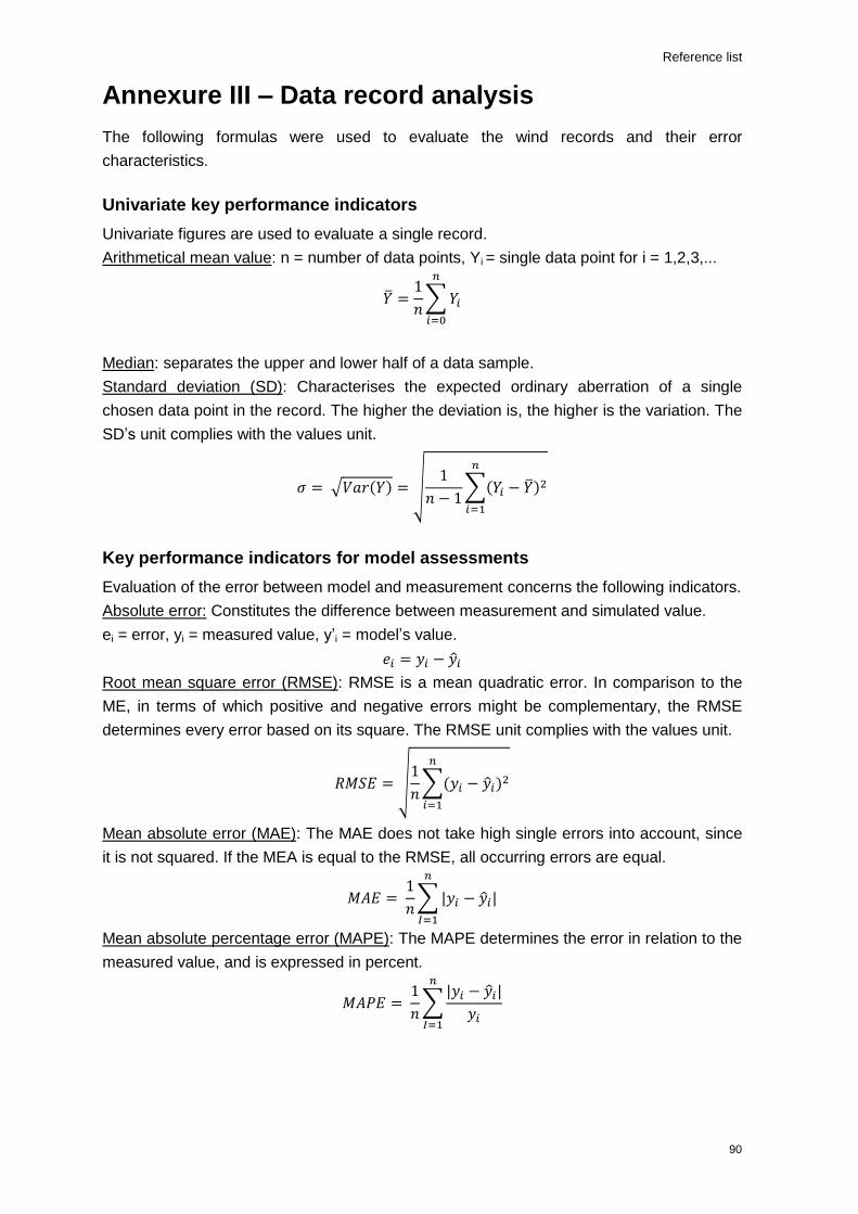
Reference list
90
Annexure III – Data record analysis
The following formulas were used to evaluate the wind records and their error
characteristics.
Univariate key performance indicators
Univariate figures are used to evaluate a single record.
Arithmetical mean value: n = number of data points, Yi = single data point for i = 1,2,3,...
Median: separates the upper and lower half of a data sample.
Standard deviation (SD): Characterises the expected ordinary aberration of a single
chosen data point in the record. The higher the deviation is, the higher is the variation. The
SD’s unit complies with the values unit.
Key performance indicators for model assessments
Evaluation of the error between model and measurement concerns the following indicators.
Absolute error: Constitutes the difference between measurement and simulated value.
ei = error, yi = measured value, y’i = model’s value.
Root mean square error (RMSE): RMSE is a mean quadratic error. In comparison to the
ME, in terms of which positive and negative errors might be complementary, the RMSE
determines every error based on its square. The RMSE unit complies with the values unit.
Mean absolute error (MAE): The MAE does not take high single errors into account, since
it is not squared. If the MEA is equal to the RMSE, all occurring errors are equal.
Mean absolute percentage error (MAPE): The MAPE determines the error in relation to the
measured value, and is expressed in percent.

Reference list
91
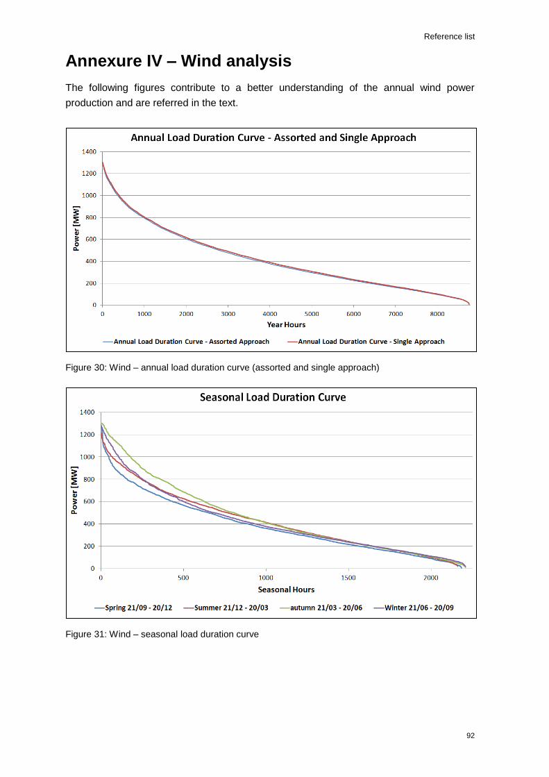
Reference list
92
Annexure IV – Wind analysis
The following figures contribute to a better understanding of the annual wind power
production and are referred in the text.
Figure 30: Wind – annual load duration curve (assorted and single approach)
Figure 31: Wind – seasonal load duration curve

Reference list
Figure 32: Validation of contemporaneous power increase and wind speeds at WMs (60m)

Annexure V – Solar PV analysis
Annexure V – Solar PV analysis
Determination of conversion factor and cell efficiency of five panels
Table 27: Comparison of five solar PV modules
PMPP peak power [WP]
Size net [m²]
Specific power [WP/m²]
Cell efficiency
Schüco MPE PG04 250Wp 250 1.46 171 15.1%
BYD P6-30 250Wp 250 1.50 167 15.4%
BLD SOLAR 240-60P 240 1.51 159 14.7%
Sharp Solar NU-E245 (J5) 245 1.46 168 14.9%
TSolar TSM-250 PC/PA05 250 1.46 171 15.3%
Mean - 1.47 167 15.1%
Optimum tilt for maximising annual energy yield of solar PV systems,
mounted in a fixed position in a rack facing north
Figure 33: Optimum PV tilt for maximising annual energy yield (Suri, Cebecauer 2012, p. 5)

Annexure V – Solar PV analysis
95
Verification of applied methodology by ENREL’s SAM
The verification was done for a project called ‘Kalkbult Solar PV’, with a registered capacity
of 72.5 MWP (in bidding R1). Despite the fact that SAM offered a higher possibility of input
parameter (including various default values), the boundary conditions were equally set.
The difference in annual distributed energy was immaterial, and the time series course was
similar.
Figure 34: Solar PV model verification (Gauché 2011, NREL 2005)

Annexure VI – CSP Analysis
96
Annexure VI – CSP Analysis
Simulation boundary conditions
Table 28: CSP, SAM – additional input parameters (CSP World, 2013)
KaXu Solar One Bokpoort CSP Khi Solar One
Turbine steam temp. [°C] 375
Turbine steam pres. [bar] 100
Working fluid VP-1 Dowtherm D VP-1
No. of loops [–] 300 180 –
No. of collectors/loops [–] 4 5 −
Tower height [m] – – 200
Heliostat aperture [m²] – – 120 × 4 500
Dew point temperature calculation
The dew point temperature calculation is derived by means of the function of relative
humidity to ambient temperature and the Magnus formula. It is valid for a temperature
range between −45 and +60°C.
ϑd(φ,ϑ) is the dew point temperature in the dependency of relative humidity (φ) and
ambient temperature (ϑ).
Sample, cumulative CSP course in January
The relatively large storage capacity of Bokpoort CSP is apparent.
Figure 35: Cumulative CSP course in January
( 8 )

Annexure VI – CSP Analysis
Khi Solar One seasonal and mean temporal distribution
The minimum power defines the firm capacity as soon as the plant generates electricity. The generation distribution in % is expressed by
means of the red bar. The blue bar describes the hourly average energy share in each season.
Figure 36: Khi Solar One – seasonal, temporal distribution
Bokpoort CSP − seasonal and mean temporal distribution
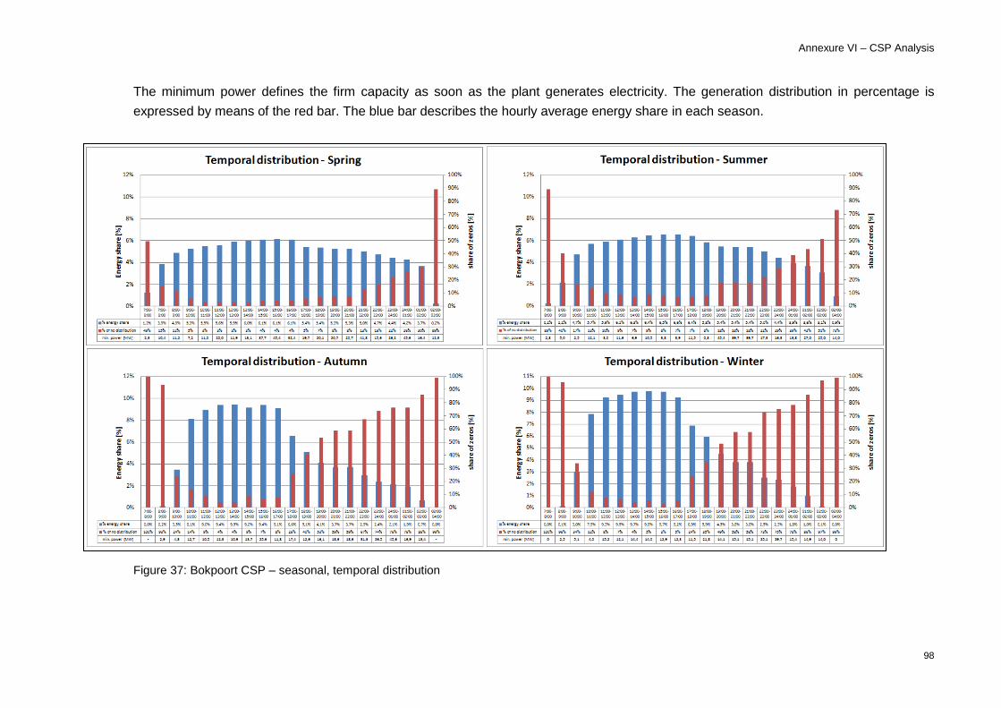
Annexure VI – CSP Analysis
98
The minimum power defines the firm capacity as soon as the plant generates electricity. The generation distribution in percentage is
expressed by means of the red bar. The blue bar describes the hourly average energy share in each season.
Figure 37: Bokpoort CSP – seasonal, temporal distribution

Annexure VI – CSP Analysis

Annexure VII – Results
100
Annexure VII – Results
Supplement to the frequency distribution from 20:00 to 22:00
Figure 38: Frequency distribution during summer and winter (B)

Annexure VII – Results
Systems distribution share between 19:00 and 22:00 during winter
Figure 39: Distribution share, winter 19:00–22:00

Annexure VII – Results
102
Systems distribution share between 19:00 and 22:00 during summer
Figure 40: Distribution share, summer 19:00–22:00