master’s thesis - bibsys · master’s thesis study program ... i would like to first express my...

Faculty of Science and Technology

MASTER’S THESIS

Study program/Specialization: Petroleum Geosciences Engineering

Spring semester, 2016

Open

Writer: Yichen Yang

(Writer’s signature)

Faculty supervisor: Reidar B. Bratvold External supervisor(s): Title of thesis: A Reduced Order Model for Fast Production Prediction from an Oil Reservoir with a Gas Cap Credits (ECTS): 30 Keywords: Production prediction

Gas cap field

Material balance equation

Uncertainty assessment

Monte Carlo simulation

Pages: 82 +enclosure: CD Stavanger, June 15th 2016

Copyright

by

Yichen Yang

2016

A Reduced Order Model for Fast Production Prediction from an Oil

Reservoir with a Gas Cap

by

Yichen Yang, B.Sc.

Thesis

Presented to the Faculty of Science and Technology

The University of Stavanger

The University of Stavanger

June 2016

iv

Acknowledgements

I would like to first express my sincere gratitude to my thesis supervisor Prof. Reidar B.

Bratvold for his kind help and suggestions throughout the process of researching and writing

this thesis. This accomplishment would not have been possible without you.

Besides my supervisor, I would like to particularly thank Philip Thomas, Aojie Hong,

Kanokwan Kullawan and Camilo Malagon for their insightful comments and encouragement

during my research.

Finally, I must express my very profound gratitude to my parents for providing me with

consistent support and encouragement throughout my years of study.

v

Abstract

A Reduced Order Model for Fast Production Prediction from an Oil

Reservoir with a Gas Cap

Yichen Yang, M.Sc.

The University of Stavanger, 2016

Supervisor: Reidar B. Bratvold

Economic evaluations are essential inputs for oil and gas field development decisions.

These evaluations are critically dependent on the unbiased assessment of uncertainty in the

future oil and gas production from wells. However, many production prediction techniques

come at significant computational costs as they often require a very large number of highly

detailed grid based reservoir simulations.

In this study, we present an alternative compelling and efficient approach to assess the

impact of reserves uncertainty on the oil and gas production from an oil reservoir with a gas

cap. The justification for using the reduced order (less detailed) model to assess possible future

production is that, for many decisions, it is more important to capture the uncertainties in the

production than the production impact of the detailed characteristics of the reservoir in

question. The computational costs of the reduced order model presented in this work is small

relative to a typical grid based simulator which makes it possible to assess production

uncertainties by using Monte Carlo simulation with a large number of iterations.

The model developed in this work combines the use of inflow performance relationship

(IPR), tubing performance relationship (TPR) curves with the material balance equation. By

balancing the dynamic material balance equation at each time period, the reservoir average

pressure decline curve and the oil and gas production profiles can be obtained. The impact of

vi

reserves uncertainty on oil and gas production can be assessed by combing this approach with

the Monte Carlo simulation method.

We apply the approach to a gas cap field to investigate the impact of reserves

uncertainty on oil and gas production. The result shows that the relationship between oil in

place, gas cap-to-oil volume ratio and oil production can be expressed in a functional form.

One conclusion from this study is that the oil in place uncertainty has a larger impact on oil

production than the gas in place uncertainty.

The approach in this study is developed in MATLAB and easy to modify and extend,

so it can be applied to other gas cap fields and combined with cash flow model to help the

decision maker design specific development and production plans and maximize the overall

value of the field.

vii

Table of Contents

Acknowledgements .............................................................................................. iv

Abstract ...................................................................................................................v

Table of Contents ................................................................................................ vii

List of Tables ...................................................................................................... viii

List of Figures ....................................................................................................... ix

Nomenclature ....................................................................................................... xi

1. Introduction ........................................................................................................1

2. PVT Properties Analysis ...................................................................................4

3. Well Production Model....................................................................................10

3.1 Inflow Performance Relationship (IPR) ..........................................................10

3.2 Future IPR Prediction ......................................................................................12

3.3 Tubing Performance Relationship (TPR) ........................................................13

3.4 Natural Flow ....................................................................................................24

3.5 Application of Material Balance Equation ......................................................26

3.6 Model Test and Verification ............................................................................27

4. Uncertainty Analysis ........................................................................................36

4.1 Reserves Uncertainty .......................................................................................36

4.2 Monte Carlo Simulation ...................................................................................37

4.3 A Case Study....................................................................................................39

5. Discussion and Conclusion ..............................................................................51

References .............................................................................................................53

Appendices ............................................................................................................55

viii

List of Tables

Table 1 Basic input parameters for model test .......................................................28

Table 2 Distribution of initial hydrocarbon in place in X gas cap field ................39

Table 3 Basic input parameters in the X gas cap field ...........................................40

ix

List of Figures

Figure 1 A typical gas cap drive reservoir (Dake, 1983) .........................................1

Figure 2 The typical production history of a gas cap drive reservoir (Selley and

Sonnenberg, 2014) ..............................................................................1

Figure 3 The linear IPR curve (Golan and Whitson, 1991) ...................................10

Figure 4 The IPR curve for the saturated oil and gas wells (Golan and Whitson, 1991)

...........................................................................................................11

Figure 5 An example of current and future IPR curves .........................................13

Figure 6 Computer flow diagram for the Beggs and Brill method ........................16

Figure 7 Horizontal flow pattern map ....................................................................20

Figure 8 An example of typical TPR curve ...........................................................23

Figure 9 Natural flow rate condition (Golan and Whitson, 1991) .........................24

Figure 10 Influence of wellhead pressure on natural flow rate .............................25

Figure 11 Influence of gas liquid ratio on natural flow rate ..................................25

Figure 12 Influence of tubing inner diameter on natural flow rate ........................26

Figure 13 The general form of material balance equation .....................................26

Figure 14 Solution gas oil ratio comparison ..........................................................28

Figure 15 Oil formation volume factor comparison ..............................................29

Figure 16 Gas formation volume factor comparison .............................................29

Figure 17 Gas viscosity comparison ......................................................................30

Figure 18 Oil viscosity comparison .......................................................................30

Figure 19 IPR curve comparison ...........................................................................31

Figure 20 TPR curve comparison ..........................................................................31

Figure 21 Oil production profile comparison (without gas reinjection) ................32

Figure 22 Gas production profile comparison (without gas reinjection) ...............32

Figure 23 Reservoir pressure declination comparison (without gas reinjection) ..33

Figure 24 Oil production profile comparison (with gas reinjection) .....................33

Figure 25 Gas production profile comparison (with gas reinjection) ....................34

x

Figure 26 Reservoir pressure declination comparison (with gas reinjection) ........34

Figure 27 Three PERT distributions with different input parameters ...................37

Figure 28 The general procedures of Monte Carlo simulation (Bratvold and Begg, 2010)

...........................................................................................................38

Figure 29 The procedures of Monte Carlo simulation in this study ......................38

Figure 30 The probability distribution of oil in place ............................................40

Figure 31 The probability distribution of gas cap-to-oil volume ratio ..................40

Figure 32 Running average of samples from oil in place distribution ...................41

Figure 33 Running standard deviation of samples from oil in place distribution ..42

Figure 34 The number of iterations and its corresponding computational time ....42

Figure 35 Oil production profiles generated from 1000 iterations and its mean production

profile ................................................................................................43

Figure 36 The relationship between oil and gas in place and oil production at four different

years ..................................................................................................43

Figure 37 The trend surface analysis for oil production at the 30th year ...............44




Figure 41 The shifted and original distributions of oil in place .............................47

Figure 42 The shifted and original distributions of gas cap-to-oil volume ratio ...47

Figure 43 The tornado chart to identify the main uncertainty driver .....................48

Figure 44 The relationship between oil in place and recovery efficiency .............49

Figure 45 The relationship between gas cap-to-oil volume ratio and recovery efficiency

...........................................................................................................50

xi

Nomenclature

English

area

gas formation volume factor

oil formation volume factor

water formation volume factor

liquid holdup inclination

correction factor

isothermal compressibility

pore compressibility

flow coefficient

tubing diameter

exponential

friction factor

Moody friction factor

two-phase friction

no-slip friction factor

water cut

local acceleration due to gravity

gravitational constant

weight flux rate

oil zone thickness

0 horizontal liquid holdup

liquid holdup

productivity index

length

∆ length increment

ratio of the initial hydrocarbon

pore volume of the gas cap to

that of the oil

gas molecular weight

total number of moles

flow exponent

net-to-gross thickness ratio

stock tank oil initially in place

Froude number

liquid velocity number

cumulative oil production

Reynolds number

pressure

average pressure

pseudocritical pressure

pseudoreduced pressure

reservoir pressure

∆ pressure drop

production rate

gas constant

production gas oil ratio

solution gas oil ratio

saturation

connate water saturation

absolute temperature

average temperature

pseudocritical temperature

pseudoreduced temperature

reservoir temperature

velocity

volume

cumulative natural water influx

xii

cumulative natural water

production

z-factor

Greek

liquid holdup inclination

correction factor coefficient

specific gravity

absolute pipe roughness

no-slip liquid holdup

pipe inclination angle

viscosity

density

surface tension

porosity

Subscripts

acc acceleration

av average

b bubble point

c constant

el elevation

f friction

g gas

i initial

L liquid

n no-slip

o oil

od dead oil

os saturated oil

ou undersaturated oil

p production

sc standard condition

SG superficial gas

SL Superficial liquid

t mixture

tp two-phase

w water

wh wellhead

wf bottomhole flowing

1

1. Introduction

A gas cap field is an oil reservoir with a segregated free gas zone overlying an oil zone. In such

reservoirs, the main producing mechanism is the expansion of the gas cap gas and solution gas,

which pushes the oil downward to the production wells. For a typical gas cap field (Figure 1),

the exploration well is drilled to identify the gas oil contact. Then all production wells are

placed further down-dip since the purpose is not to produce gas but rather to allow its expansion

to push the oil towards the production wells.

Figure 1 A typical gas cap drive reservoir (Dake, 1983)

It is known that reservoir pressure declines with production. Figure 2 shows the production

history of a typical gas cap drive reservoir. The reservoir pressure and oil production drop

steadily, while the gas oil ratio increases naturally.

Figure 2 The typical production history of a gas cap drive reservoir (Selley and Sonnenberg, 2014)

2

One common method for improving the oil recovery in a gas cap field is to reinject a portion

of the produced gas, if the economics are favorable. The reinjected gas helps maintaining the

reservoir pressure. The theory behind this method is that gas reinjection will maximize the oil

production and thus maximize the overall value of the reservoir. But in consideration of the

uncertainty in future oil and gas prices, the method above may eventually not maximize the

overall value of the reservoir (Thomas and Bratvold, 2015). In this case, an optimal time point

can be identified when the gas should be lifted and sold rather than being reinjected. Switching

from injecting to a depressurization of the gas cap reservoir is called gas cap blowdown.

The common way to identify the optimal blowdown time is to generate oil and gas production

profiles for each possible blowdown time and compare the resulting values. The blowdown

time with the highest value is optimal. However, many of the production prediction techniques

come at significant computational costs, as they require a very large number of grid based

reservoir simulations. This makes it difficult to identify the optimal blowdown time, not to

mention to assess the impact of reserves uncertainty on oil and gas production.

The purpose of this thesis is to identify a compelling and efficient approach to assess the impact

of reserves uncertainty on oil and gas production. Such an approach can be useful to identify

production uncertainties for several different decision contexts including the blowdown

decision with the goal of maximizing the overall value of the field. The specific objectives of

this work are to:

Develop a material balance based production model which can be used to generate

cogent oil and gas production profiles at a relatively low computational expense

Illustrate and assess the impact of reserves uncertainty on oil and gas production

In order to achieve these objectives, a six-step approach has been implemented:

1) Develop the production model by constructing inflow performance relationship (IPR)

and tubing performance relationship (TPR)

2) Calculate the oil and gas production over a selected time period based on the production

model

3) Select the appropriate oil PVT properties (e.g., Bo, Bg, Rs) to balance the material

balance equation (MBE) based on the oil and gas reserves and production data

4) Identify the corresponding reservoir pressure based on the oil PVT properties used

above

5) Generate the oil and gas production profiles by repeating steps 2 through 4 at each

selected time period

3

6) Apply Monte Carlo simulation (MCS) to assess the impact of reserves uncertainty on

oil and gas production

4

2. PVT Properties Analysis

The goal of pressure-volume-temperature (PVT) analysis is to determine the relationship

between observed surface volumes of hydrocarbon production and the corresponding volume

in the reservoir. A good knowledge of PVT properties will be helpful to the reserves calculation

and its economic evaluation. Ideally, these properties are determined from laboratory studies

on samples collected at an early stage in the reservoir’s production life. There are usually two

ways of collecting such samples, either by directing subsurface sampling or by surface

recombination of oil and gas phases. However, such laboratory data are not always available

because of cost saving and the strict measurement environment. In that situation, PVT

properties can be approximated by using empirical correlations.

The three main PVT parameters measured from PVT analysis are solution gas oil ratio (Rs), oil

formation volume factor (Bo) and gas formation volume factor (Bg), all of which are of primary

importance in material balance calculation and well performance analysis.

The solution gas oil ratio (Rs) is the amount of surface gas that can be dissolved in one stock

tank barrel of oil when both are at a specific reservoir pressure and temperature (units-scf/stb).

The oil formation volume factor (Bo) is the ratio of the volume of oil at reservoir conditions to

that at surface conditions (units-rb/stb). The gas formation volume factor (Bg) is the ratio of the

volume of gas at reservoir conditions to that at surface conditions (units-rb/scf).

Many correlations have been developed in the petroleum industry to estimate the solution gas

oil ratio (Rs), oil formation volume factor (Bo) and gas formation volume factor (Bg). Examples

of such PVT correlations are given by Standing (1947), Lasater (1958), Glaso (1980), Al-

Marhoun (1988), Petrosky and Farshad (1993). Each of these correlations seems to be

applicable and reliable only for a specific set of reservoir fluid characteristics. This is due to

the fact that each correlation has been developed by using samples from a restricted

geographical area.

In this work, the Standing correlation is applied to calculate the solution gas oil ratio (Rs) and

the oil formation volume factor (Bo). For a gas cap field, the oil is saturated and the reservoir

pressure is equal to the bubble point pressure. Standing used 105 experimentally determined

data points obtained from 22 different California crude oils to develop the correlations. In 1947,

he published the equations to estimate the solution gas oil ratio (Rs) and the oil formation

volume factor (Bo) when the reservoir pressure is equal to the bubble point pressure.

Solution gas oil ratio

5

1.4 /18.2 . 10 . . . (1)

Oil formation volume factor

0.972 1.47 10 1.25 ⁄

/ . (2)

Standing used flash liberation tests to obtain the experimental data and he stated that, for the

given data set, the average error in using equations (1) and (2) are 4.8% and 1.2%, respectively.

The oil samples used during the experimental process were free of nitrogen (N2) and hydrogen

sulfide (H2S), with CO2 less than 1 mole percent. In this work, it is also assumed that the gas

in the gas cap field doesn’t contain the nitrogen (N2), hydrogen sulfide (H2S) and carbon

dioxide (CO2).

Gas formation volume factor

The gas formation volume factor (Bg) can be deduced by the simple equation of state

(3)

in which Z is called the Z-factor and is the ratio of the real volume to the ideal volume, which

defines the departure from the ideal gas behavior. R is the gas constant.

By applying equation (3) at both standard and reservoir conditions, the gas formation volume

factor becomes

∙ ∙ (4)

For the standard condition of 14.7pisa, 460 60 520° and 1 ,

equation (4) can be reduced to

0.00503676 (5)

Before equation (5) can be used for gas formation volume factor calculation, the Z-factor

should be measured. Z-factors can be determined through several steps, starting with the

estimation of the pseudocritical temperature and pseudocritical pressure of gas

mixtures. Based on the definition, the pseudocritical temperature and pseudocritical

pressure can normally be calculated by the mole average of critical temperature and

6

pressure of the mixture components. There are different correlations available for

pseudocritical property estimation. One correlation is developed by Sutton (1985) based on

264 different gas samples, which is used in this work.

Pseudocritical temperature

169.2 349.5 74.0 (6)

Pseudocritical pressure

756.8 131.07 3.6 (7)

After the pseudocritical properties are obtained, the next step is to calculate the pseudoreduced

temperature and pressure by using the following equations.

(8)

Then the Z-factor can be determined by using the Standing-Katz correlation chart (1942),

which has shown itself to be very reliable and is considered as the industry standard. Several

best-fit equations for the Standing-Katz correlation chart have been developed, such as Hall

and Yarborough (1973), Dranchuk and Abou-Kassem (1975) and Beggs and Brill (1973),

which are more convenient for estimating the Z-factor in computer programs and spreadsheets.

In this work, the Beggs and Brill equation is used for the Z-factor calculation.

Beggs and Brill correlation for Z-factor

Z A 1 ⁄ (9)

where

A 1.39 0.92 . 0.36 0.101 (10)

B 0.62 0.23

0.0660.86

0.0370.32

10 (11)

C 0.132 0.32 log (12)

D 10 . . . (13)

7

Some useful correlations for other PVT parameters are introduced here to help to build the well

production model in the following chapters.

Gas viscosity

For gas viscosity, Lee et al (1966) presented a useful empirical equation for most natural gas

viscosity estimations, which is convenient for computer programming. The method uses the

temperature, pressure, Z-factor, and molecular weight.

(14)

where

0.00149406 (15)

0.00094 2 10 .

209 19 (16)

3.5

9860.01 (17)

2.4 0.2 (18)

28.967 (19)

is gas viscosity, cP. is gas density, g/cm3. is pressure, psia. is temperature, R.

is gas molecular weight.

Saturated oil viscosity

Beggs and Robinson (1975) developed a correlation which can be used for both dead and

saturated oil viscosity.

(20)

where

8

10 1.0 (21)

. 6.9824 0.04658 (22)

A 10.715 100 . (23)

B 5.440 150 . (24)

is saturated oil viscosity, cP. is dead oil viscosity, cP. is temperature, F. is

oil API gravity, API. is solution gas oil ratio, scf/stb.

Undersaturated oil viscosity

Undersaturated oil viscosity can be calculated by applying Vazquez and Beggs (1980)

correlation.

(25)

where

exp (26)

2.6, 1.187 , 11.513 8.98 10 (27)

is undersaturated oil viscosity at , cP. is saturated oil viscosity at , cP.

is pressure, psia. is bubble-point pressure, psia.

Water viscosity

Brill and Beggs (1973) developed one simple relationship between water viscosity and

temperature

1.003 0.01479 1.982 10 (28)

Where is temperature, F.

9

Oil-gas interfacial tension

Abdul-Majeed and Al-Soof (2000) provided one equation to estimate the oil-gas surface

tension

1.17013 1.694 10 38.085 0.259 (29)

Where is temperature, F. is oil API gravity, API.

Water-oil interfacial tension

Water-oil interfacial tension can be calculated using the following correlation proposed by

Hough et al. (1951)

75 1.108 . , 74 (30)

53 0.1048 . , 280 (31)

74206

, 74 280 (32)

Where is temperature, F . is pressure, psia.

There are constrains and limitations in all of these empirical equations, but the results obtained

by using these correlations are useful to estimate the impact of reserves uncertainty on oil and

gas production. By using the correlations presented above, the PVT parameters can be

estimated, which can be applied to build the well production model and material balance

calculation in next steps.

10

3. Well Production Model

This chapter discusses a common method to build one well production model by using the

inflow performance relationship (IPR) and tubing performance relationship (TPR). The model

provides the relationship between the pressure and the flow rate and, will be used to predict the

production rate.

3.1 Inflow Performance Relationship (IPR)

The inflow performance relationship (IPR) is the relationship between the surface flow rate

and the bottomhole flowing pressure at a given reservoir pressure . It describes that

the flow rate of fluids from the reservoir into the well is a function of the bottomhole flowing

pressure (Guo et al., 2011). For an oil production well, the IPR equation is linear when the oil

is undersaturated or slightly compressible (Golan and Whitson, 1991). It means that the fluid

inflow rate is proportional to the difference between reservoir pressure and the bottomhole

flowing pressure (Figure 3). When the bottomhole flowing pressure is equal to zero, the flow

rate is the maximum rate , which is called absolute open flow (AOF).

Figure 3 The linear IPR curve (Golan and Whitson, 1991)

The linear IPR can be represented by the following equation (Golan and Whitson, 1991)

(33)

where J is the productivity index (units – STB/D/psi), defined as the ratio of the flow rate to

pressure drop in the reservoir. is the average reservoir pressure.

11

For saturated oil and gas wells, the linear IPR is not suitable due to the effect of highly

compressible gas and two-phase flow on IPR. Instead of a linear flow rate increase with

pressure drop, it has been observed that larger-than-linear pressure drops are required to

increase the rate at higher rates (Golan and Whitson, 1991). The IPR shows the curvature

pronounced (Figure 4).

Figure 4 The IPR curve for the saturated oil and gas wells (Golan and Whitson, 1991)

Vogel (1968) proposed the following equation to describe the IPR curve for saturated oil wells:

,1 0.2 0.8 (34)

where , is the maximum oil rate when bottomhole flowing pressure equals zero.

Besides Vogel there are other correlations which describe two-phase inflow performance

relationships, such as the equation presented by Fetkovich (1973). Vogel’s equation is a best-

fit approximation of numerous simulated well performance calculations. In this work, Vogel’s

equation is used to describe the IPR for saturated oil in gas cap reservoirs.

For gas well performance, the backpressure equation (Rawlins and Schellhardt, 1935) is widely

accepted as a simple and accurate expression of the production:

(35)

where the exponent n ranges in value from 0.5 to 1.0 depending on flow characteristics and C

is the flow coefficient.

12

The C and n can be determined by using a two or three point flow test and the following

equation:

nlog

log

C (36)

Where is the flow rate at bottomhole flowing pressure, , and is the flow rate at

bottomhole flowing pressure, .

3.2 Future IPR Prediction

The future IPR prediction is key to forecast the future well production. Several methods exist

to estimate the future maximum flow rate , . Usually these methods provide an equation

relating changes in the productivity index J to the average reservoir pressure. Fetkovich (1973)

presented the following equations to predict the maximum future flow rate:

and ⁄ (37)

where the flow exponent, n, is assumed to be constant throughout the entire production life of

the reservoir. is the flow constant at current reservoir pressure, , and is the flow

constant at a future reservoir pressure, .

When n and are determined by a few flow test points, then any future maximum flow rate

, can be estimated by

, (38)

Based on Fetkovich’s work, Eickmeier (1968) proposed a simple equation to estimate the

maximum flow rate , . Instead of using multipoint test data, only one single flow test

point is need to estimate the maximum flow rate , . Eickmeier (1968) set the flow

exponent to a fixed value of 1 to arrive at

, , ⁄ (39)

After this relationship between the maximum flow rate and the reservoir pressure is established,

for any future pressure, the corresponding maximum flow rate can be predicted. Then both

values can be used in Vogel’s IPR equation to generate a set of future IPR curves (Figure 5).

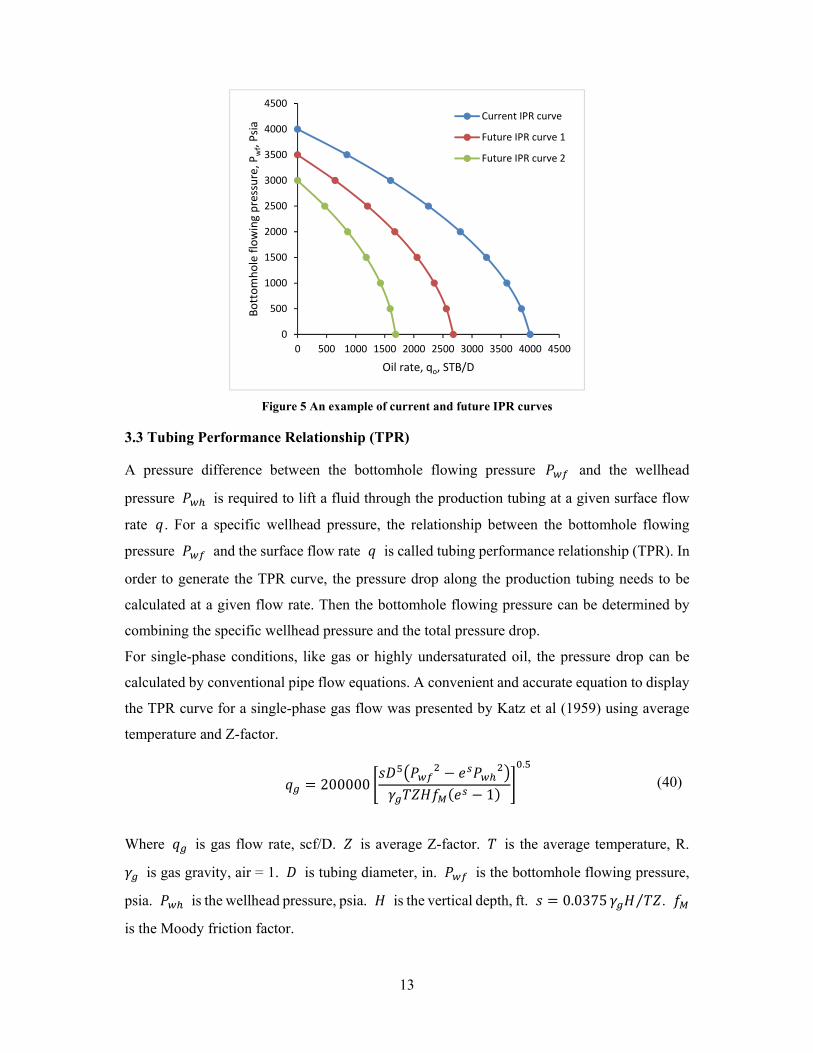
13

Figure 5 An example of current and future IPR curves

3.3 Tubing Performance Relationship (TPR)

A pressure difference between the bottomhole flowing pressure and the wellhead

pressure is required to lift a fluid through the production tubing at a given surface flow

rate . For a specific wellhead pressure, the relationship between the bottomhole flowing

pressure and the surface flow rate is called tubing performance relationship (TPR). In

order to generate the TPR curve, the pressure drop along the production tubing needs to be

calculated at a given flow rate. Then the bottomhole flowing pressure can be determined by

combining the specific wellhead pressure and the total pressure drop.

For single-phase conditions, like gas or highly undersaturated oil, the pressure drop can be

calculated by conventional pipe flow equations. A convenient and accurate equation to display

the TPR curve for a single-phase gas flow was presented by Katz et al (1959) using average

temperature and Z-factor.

200000

1

.

(40)

Where is gas flow rate, scf/D. is average Z-factor. is the average temperature, R.

is gas gravity, air = 1. is tubing diameter, in. is the bottomhole flowing pressure,

psia. is the wellhead pressure, psia. is the vertical depth, ft. 0.0375 ⁄ .

is the Moody friction factor.

0

500

1000

1500

2000

2500

3000

3500

4000

4500

0 500 1000 1500 2000 2500 3000 3500 4000 4500

Bottomhole flowing pressure, P

wf, Psia

Oil rate, qo, STB/D

Current IPR curve

Future IPR curve 1

Future IPR curve 2

14

A best-fit equation to estimate for gas wells is the following expression, which is

sufficiently accurate for most engineering calculations.

2 log 3.71 ⁄⁄ (41)

Where is the absolute pipe roughness for most commercial pipes and equal to 0.0006 in.

For multiphase conditions, the tubing performance relationship is more complicated. This is

due to the fact that the properties of each fluid and the interactions between each phase must

be taken into account. The TPR curve can only be described approximately by the empirical

equations. The theoretical basis for the pressure drop calculation is the mechanical balance

equation. It is an expression for the balance of energy between two points in a system, which

is composed of three distinct components.

The general differential form can be written as

(42)

Where is the component due to hydrostatic pressure loss, is the component due

to friction pressure loss, and is the component due to kinetic pressure loss or

convective acceleration.

For most applications, the kinetic pressure loss is very small and can be ignored. Thus, the

equation that describes the overall pressure loss can be expressed as the sum of two terms:

(43)

The hydrostatic pressure loss calculation can be calculated by using a mixture density :

sin (44)

Where is the local acceleration due to gravity, and is the gravitational constant 32.174

ft/s2. is the inclination angle of the pipe from horizontal.

Based on the definition, the friction pressure loss can be estimated by the following equation:

15

2

(45)

Where is the two-phase friction, is the mixture weight flux rate, and is the mixture

velocity. is the tubing diameter.

Some correlations have been presented to predict these pressure losses (Beggs and Brill, 1973;

Duns and Ros, 1963; Hagedorn and Brown, 1965; Hasan and Kabir, 1992; Orkiszewski, 1967).

In this study, the Beggs and Brill correlation is chosen to generate the TPR curve, based on the

fact that it is relatively easily implemented in MATLAB or Excel VBA and perform as well as

any of the other correlations. This method requires an iterative procedure for the two-phase

pressure drop calculation. In the calculation, the pipe line is divided into a number of pressure

increments, then the fluid properties and pressure gradient are evaluated at average pressure

and temperature condition in each increment.

The procedure for segmenting the pipe line by pressure increment (Beggs and Brill, 1973) is:

Step 1: Starting with the known pressure, , at location , select a length increment ∆ , at

least 10% of total .

Step 2: Estimate the incremental pressure change, ∆ , corresponding to the length increment

∆ .

Step 3: Calculate the average pressure and temperature in the increment.

Step 4: Using empirical equations, determine the necessary PVT properties at average pressure

and temperature in the increment.

Step 5: Calculate the pressure gradient, ∆ /∆ , in the increment at average pressure and

temperature condition.

Step 6: Determine the total incremental pressure change corresponding to the selected length

increment, ∆ ∆ ∗ ⁄ .

Step 7: Compare the estimated and calculated values of ∆ obtained in step 2 and 6. If they

are not close enough, use the calculated incremental pressure and return to step 2. Repeat step

3 through step 7 until the estimated and calculated values are sufficiently close.

Step 8: Continue iteration until ∑∆ (total length), the bottomhole flowing pressure

∑∆ .

Based on the procedure above, a computer flow diagram (Figure 6) is developed for calculating

the two-phase pressure drop in a well.

16

Figure 6 Computer flow diagram for the Beggs and Brill method

17

A detailed procedure for this two-phase pressure drop calculation is following:

1. Start with the known pressure, , at location , select a length increment ∆ , at least

10% of total .

2. Estimate the incremental pressure change, ∆ , corresponding to the length increment

∆ .

3. Calculate the average pressure between the two points:

∆2

4. Determine the average temperature at the average depth, based on the temperature

versus depth plot.

5. From PVT analysis or appropriate correlations, calculate solution gas oil ratio , oil

formation volume factor , Z-factor and gas formation volume factor .

6. Calculate gas, oil and water viscosity ( , , , oil-gas interfacial tension and

water-oil interfacial tension .

7. Calculate the oil gravity from API gravity:

141.5131.5

8. Calculate the gas ,oil and liquid densities at the average conditions of pressure and

temperature:

28.97

350 0.07645.615

1

1

18

9. Calculate the gas and liquid flowrate:

86400

1 5.61586400

10. Calculate sectional area of pipe and the superficial gas, liquid and mixture velocity:

/2

⁄

⁄

11. Calculate the gas, liquid and mixture weight flux rates:

12. Calculate the no-slip liquid holdup:

13. Calculate the Froude number:

19

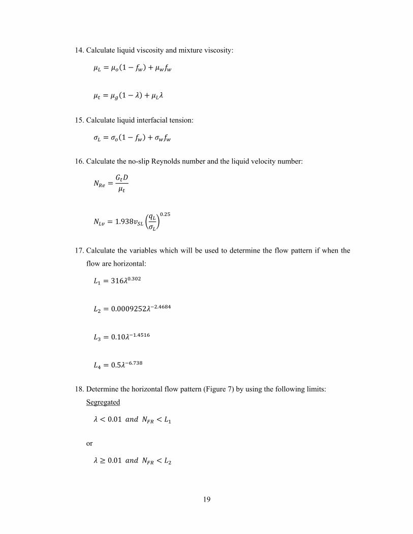
14. Calculate liquid viscosity and mixture viscosity:

1

1

15. Calculate liquid interfacial tension:

1

16. Calculate the no-slip Reynolds number and the liquid velocity number:

1.938.

17. Calculate the variables which will be used to determine the flow pattern if when the

flow are horizontal:

316 .

0.0009252 .

0.10 .

0.5 .

18. Determine the horizontal flow pattern (Figure 7) by using the following limits:

Segregated

0.01

or

0.01

20

Transition

0.01

Intermittent

0.01 0.4

or

0.4

Distributed

0.4

or

0.4

Figure 7 Horizontal flow pattern map

19. Calculate the horizontal liquid holdup:

0

21

where a, b and c are determined for different flow pattern from the following table:

Flow pattern a b c

Segregated 0.98 0.4846 0.0868

Intermittent 0.845 0.5351 0.0173

Distributed 1.065 0.5824 0.0609

20. Calculate the liquid holdup inclination correction factor coefficient:

1 ln

where d, e, f and g are determined for different flow pattern from the following table:

Flow pattern d e f g

Segregated 0.011 -3.768 3.539 -1.614

Intermittent 2.96 0.305 -0.4473 0.0978

Distributed No correlation β 0

21. Calculate the liquid holdup inclination correction factor:

1 sin 1.8 1 3⁄ sin 1.8

For vertical well, 90° and becomes:

1 0.3

22. Calculate the liquid holdup:

0

When the flow pattern is transition, the transition horizontal holdup should be

determined by using both segregated horizontal holdup and intermittent horizontal

holdup with following equations:

where

22

1

23. Calculate the two-phase density:

1

24. Calculate the pressure gradient due to the hydrostatic pressure loss:

sin

25. Calculate the ratio of two-phase to no-slip friction factor:

where

ln 0.0523 3.182 ln 0.8725 ln 0.01853 ln⁄

and

If is in the interval 1 1.2, the value of S is calculated from:

ln 2.2 1.2

26. Calculate no-slip friction factor from Darcy-Weisbach friction factor :

/4

where can be obtained from Colebrook White equation:

12 log

3.72.51

23

The Colebrook White equation can be solved by iteration using the Newton-Raphson

method.

27. Calculate the two-phase friction factor

28. Calculate the pressure gradient due to the friction pressure loss

2

29. Calculate the overall pressure gradient:

30. Calculate the overall pressure loss in this length increment ∆ :

∆ ∆

By repeating the procedure above at different oil rates, a TPR curve can be generated. The

figure below shows a typical TPR curve (Figure 8).

Figure 8 An example of typical TPR curve

0

1000

2000

3000

4000

5000

6000

7000

0 1000 2000 3000 4000 5000 6000

Bottomhole flowing pressure, P

wf, Psia

Oil rate, qo, STB/D

TPR curve

24

3.4 Natural Flow

After the IPR curve and TPR curve are generated, the natural flow rate can easily be found. For

a typical case, when at a specific rate the bottomhole flowing pressures of two curves are equal,

the flow system is in equilibrium and the flow is stable (Golan and Whitson, 1991). This

specific rate is called natural flow rate. Figure 9 illustrates the natural flow rate condition.

Figure 9 Natural flow rate condition (Golan and Whitson, 1991)

The natural flow rate will change with time, due to the changes of the IPR and TPR curves

caused by the pressure change in reservoir. The other major factors influencing the natural flow

rate are the well parameters, which have a great impact on the TPR curve based on the equations

introduced in the previous section. The influence on the TPR curve of changing some of the

main well parameters are described below.

Changing wellhead pressure

The influence of changing wellhead pressure is quite straightforward. Decreasing the wellhead

pressure will shift the TPR curve downward, resulting in a decrease in rate (Figure 10).

Changing gas liquid ratio

Increasing the gas liquid ratio reduces the hydrostatic pressure loss and increases the friction

pressure loss. An increase in the gas liquid ratio will shift the TPR curve upwards and to the

right. The result is that the natural flow rate increases first, when it reaches a certain gas liquid

ratio, the rate decrease afterwards (Figure 11).

25

Changing tubing inner diameter

Increasing the inner diameter increases the rate of natural flow rate until a critical diameter is

reached. For higher diameters, the rate will decrease. Figure 12 shows the general effect of the

tubing inner diameter on the natural flow rate.

Figure 10 Influence of wellhead pressure on natural flow rate

Figure 11 Influence of gas liquid ratio on natural flow rate

26

Figure 12 Influence of tubing inner diameter on natural flow rate

Knowing the influence of the well parameters on the natural flow rate will be helpful to take

the measures and maintain the excepted natural flow rate in the future.

3.5 Application of Material Balance Equation

Once the natural flow rate is obtained, it can be combined with reserves to predict the future

reservoir performance by using the material balance equation. The material balance equation

was first presented by Schilthuis (1936) and is now one of the fundamental equations used by

reservoir engineers for predicting the behavior of hydrocarbon reservoirs. The basic theory of

the equation is that if the total observed surface production of oil and gas can be expressed as

an underground withdrawal, then this underground withdrawal is equal to the expansion of the

fluids in the reservoir resulting from a finite pressure drop. Figure 13 shows the general form

of material balance equation.

Figure 13 The general form of material balance equation

27

The equation postulates that the underground withdrawal should be equivalent to the total

volume change from the expansion of oil and dissolved gas, the expansion of gas cap, the

reduction in hydrocarbon pore volume of the reservoir (HCPV) and the net water influx into

the reservoir. The mathematical form of the material balance equation is:

1 1

1∆ (46)

For a gas cap field, it is assumed that the natural water influx is negligible ( 0) and,

because of the high gas compressibility, the effect of water and pore compressibility is also

negligible (Dake, 1983). In this case, the material balance equation can be simplified to:

1 (47)

Based on parameters in the equation above, it is easy to see that and can be derived

from the IPR and TPR plots, , and can be estimated from PVT correlations at the

initial reservoir pressure, and and are related to the initial oil and gas in place. Hence,

the only thing needed to balance the equation is to find a new reservoir pressure for the ,

and calculation. Once the new reservoir pressure is obtained, it can be used to generate

the new natural flow rate which can be used for balance calculation in the next round. By

repeating the processes above, oil and gas production profiles can be generated.

3.6 Model Test and Verification

In the previous sections, the procedures to build the well production model and generate the oil

and gas profiles are introduced and discussed in detail. In this section, the model is tested to

verify the validity of the well production model and its implementation. The Petroleum Experts

software (MBAL, PROSPER and GAP) is used for comparison purposes. The same input

parameters are given for both the well production model developed in this work and the

Petroleum Experts software.

Initial reservoir pressure 4350 psig

Average reservoir temperature 160

28

Oil API gravity 40°API

Gas gravity 0.7

Oil in place 100MMSTB

Gas cap volume 107.3BSCF

Wellhead pressure 200psig

Wellhead temperature 120

Bottomhole temperature 160

Well depth 7500ft

Tubing inner diameter 1.995in

Pipe roughness 0.0006in

Table 1 Basic input parameters for model test

We set the production gas-oil ratio equal to the solution gas-oil ratio and the water cut to 0%.

The PVT parameters, IPR and TPR curves and the production profiles are generated from both

the well production model and the Petroleum Experts software (MBAL, PROSPER, GAP) and

the resulting profiles are compared.

PVT parameters verification

Figure 14 Solution gas oil ratio comparison

0

200

400

600

800

1000

1200

1400

0 1000 2000 3000 4000 5000

Rs(scf/stb)

pressure (psig)

MBAL software

Well production model

29

Figure 15 Oil formation volume factor comparison

Figure 16 Gas formation volume factor comparison

1

1,1

1,2

1,3

1,4

1,5

1,6

1,7

1,8

0 1000 2000 3000 4000 5000

Bo(rb/stb)

pressure (psig)

MBAL software


0

0,002

0,004

0,006

0,008

0,01

0,012

0,014

0,016

0,018

0 1000 2000 3000 4000 5000

Bg(ft3/scf)

pressure (psig)

MBAL software


30

Figure 17 Gas viscosity comparison

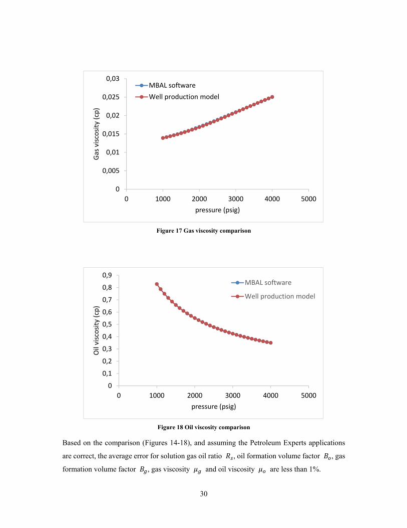
Figure 18 Oil viscosity comparison

Based on the comparison (Figures 14-18), and assuming the Petroleum Experts applications

are correct, the average error for solution gas oil ratio , oil formation volume factor , gas

formation volume factor , gas viscosity and oil viscosity are less than 1%.

0

0,005

0,01

0,015

0,02

0,025

0,03

0 1000 2000 3000 4000 5000

Gas viscosity (cp)

pressure (psig)

MBAL software


0

0,1

0,2

0,3

0,4

0,5

0,6

0,7

0,8

0,9

0 1000 2000 3000 4000 5000

Oil viscosity (cp)

pressure (psig)

MBAL software


31

IPR and TPR curve verification

Figure 19 IPR curve comparison

Figure 20 TPR curve comparison

Figures 19 and 20 show IPR and TPR curves calculated from both MBAL software and well

production model, the results are quite similar. The average error of IPR and TPR curves is

0.01% and 2.1% respectively.

0

500

1000

1500

2000

2500

3000

3500

4000

4500

5000

0 2000 4000 6000 8000 10000 12000

Pressure (psig)

Liquid rate (STB/Day)

PROSPER software


0

2000

4000

6000

8000

10000

12000

0 2000 4000 6000 8000 10000 12000

Pressure (psig)

Liquid rate (STB/Day)

PROSPER software


32

Production profile verification

The production profile comparison is conducted in two parts. The first part is the oil and gas

production profile comparison and the reservoir pressure comparison when the production gas

is not reinjected. The second comparison part is the case when the production gas is reinjected

to the reservoir.

Figure 21 Oil production profile comparison (without gas reinjection)

Figure 22 Gas production profile comparison (without gas reinjection)

0

0,2

0,4

0,6

0,8

1

1,2

0 5 10 15 20 25 30 35 40 45 50 55 60

Oil production(M

MSTB)

Year

GAP software


0

0,2

0,4

0,6

0,8

1

1,2

1,4

1,6

1,8

0 5 10 15 20 25 30 35 40 45 50 55 60

Gas production(BSCF)

Year

GAP software


33

Figure 23 Reservoir pressure declination comparison (without gas reinjection)

Figures above show the oil production profile, gas production profile and reservoir pressure

declination respectively when production gas is not reinjected (Figures 21-23). The average

error of both oil production and gas production are around 3.1%. The average error of the

reservoir pressure is less than 1%.

Figure 24 Oil production profile comparison (with gas reinjection)

0

500

1000

1500

2000

2500

3000

3500

4000

4500

5000

0 5 10 15 20 25 30 35 40 45 50 55 60

Reservoir pressure (psig)

Year

GAP software


0

0,2

0,4

0,6

0,8

1

1,2

0 5 10 15 20 25 30 35 40 45 50 55 60

Oil prodcution (MMSTB)

Year

GAP software


34

Figure 25 Gas production profile comparison (with gas reinjection)

Figure 26 Reservoir pressure declination comparison (with gas reinjection)

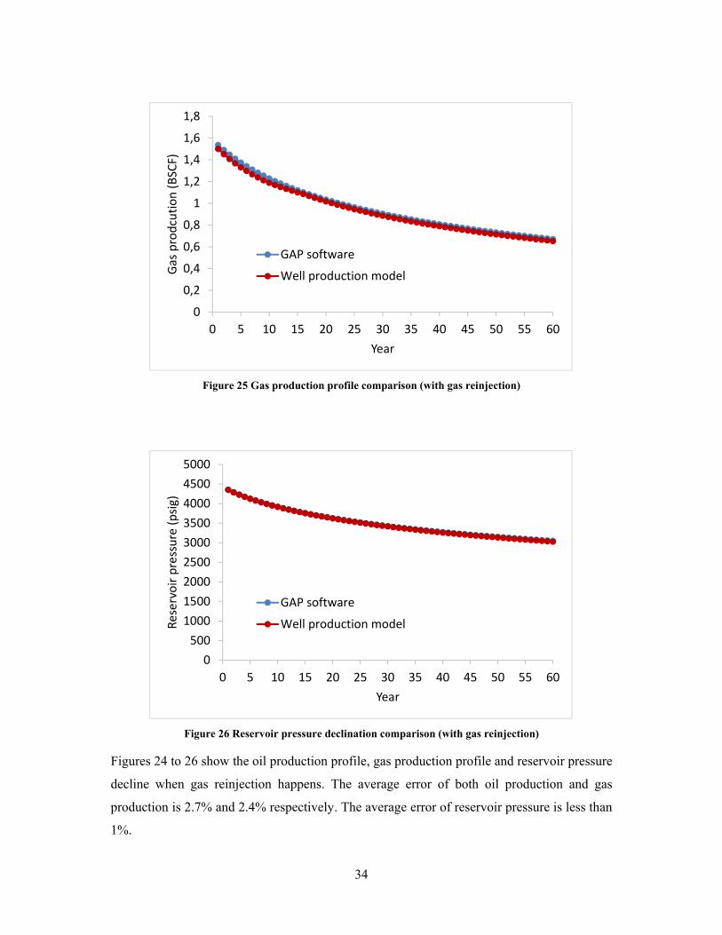
Figures 24 to 26 show the oil production profile, gas production profile and reservoir pressure

decline when gas reinjection happens. The average error of both oil production and gas

production is 2.7% and 2.4% respectively. The average error of reservoir pressure is less than

1%.

0

0,2

0,4

0,6

0,8

1

1,2

1,4

1,6

1,8

0 5 10 15 20 25 30 35 40 45 50 55 60

Gas prodcution (BSCF)

Year

GAP software


0

500

1000

1500

2000

2500

3000

3500

4000

4500

5000

0 5 10 15 20 25 30 35 40 45 50 55 60

Reservoir pressure (psig)

Year

GAP software


35

Based on the comparisons above, the same trends for the reservoir pressure, oil production and

gas production are resulting from both Petroleum Experts software and well production model

developed here. The small difference between the results above occur because of different

choices of empirical equations for some intermediate variable calculations and the fact that the

well production model developed here is not a fully detailed model which can represent the

accurate future production. In this study, the goal is to provide sufficient insight to make the

best choice clear and not to build the best possible representation of the actual future

production. The well production model developed here includes the main characteristics of the

production from an oil field with a gas cap and is useful to assess the impact of reserves

uncertainty on the oil and gas production.

36

4. Uncertainty Analysis

In this chapter, the reserves uncertainty and its influence on the oil and gas production will be

discussed. The discussion is divided into two parts: 1) the reason why uncertainty occurs and

its corresponding distribution; 2) a method to investigate the impact of reserves uncertainty on

the oil and gas production.

4.1 Reserves Uncertainty

The reserves estimation in all oil and gas fields includes uncertainty because the evaluation

team do never have complete information about the reservoir or of the input parameters

required for assessing the oil initially in place and recovery efficiency (RE). A common method

to estimate the oil reserves is the volumetric method, it can be expressed as follows:

∙ ∙ ∙ ∙ 1 / ∙ (48)

From this equation, we see that the porosity is one of the input parameters. But the porosities

determined from the well data do not provide perfect information of the porosity of the entire

field. Hence, geologists have to estimate the distribution of the porosity for the whole field by

their expert knowledge and experience. The same situation applies to the assessment of other

parameters. Once the experts have assessed the uncertainty for each of the input parameters,

the reserves uncertainty can be calculated by repeatedly sampling these distributions and

calculating the reserves. By central limit theorem, the product of independent random variable

approaches a lognormal distribution. Therefore, the distribution of oil and gas reserves

calculated by equation (48) with uncertain input parameters will be lognormal regardless of the

distribution used for the input variables (Demirmen, 2007). In this study, the PERT distribution

is chosen to represent the reserves, because it provides a reasonable approximation of the

lognormal distribution and because the parameters required to specify the PERT distribution

often are easier to assess than the mean and standard deviation required for the lognormal

distribution. The PERT distribution can be defined by different sets of three points. It could be

the minimum (a), mode (b) and maximum (c) or, say, the P10, P50 and P90. If the min, mode

and max are used, it is easy to calculate mean and standard deviation of this distribution.

mean

46

(49)

37

Standard deviation6

(50)

The flexibility of the PERT distribution is demonstrated in Figure 27 with three distributions

with different minima (a), modes (b) and maxima (c). The flexibility in choosing input

parameters for which the expert has some intuition, such as the percentiles, makes it easy to

update the distribution as new knowledge is obtained.

Figure 27 Three PERT distributions with different input parameters

4.2 Monte Carlo Simulation

Monte Carlo simulation (MCS) is a mathematical technique that makes it practical and

relatively easy to aggregate and quantify uncertainty and to investigate the impact of

uncertainty on decision alternatives. The result of a MCS is a range of possibilities with

associated probabilities; i.e., a probability distribution of the variable of interest. MCS is

commonly used in the oil and gas industry, for example to estimate the hydrocarbon reserves

in place (Bratvold and Begg, 2010). In this work, MCS is combined with the well production

model to assess the impact of reserves uncertainty on oil and gas production.

Figure 28 illustrates the general procedure of MCS with two input parameters. First, for each

input variable, MCS samples from the probability distribution. Then, the samples are used in

the model or function to calculate the output variables. The result is stored and the previous

steps are repeated a large number of times. The result of a MCS are distributions of the variables

of interest (OOIP, GIIP, reserves, production, NPV, etc.).

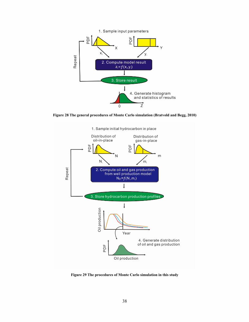
38

Figure 28 The general procedures of Monte Carlo simulation (Bratvold and Begg, 2010)

Figure 29 The procedures of Monte Carlo simulation in this study

39

In this study, we apply MCS to assess the impact of the reserves uncertainty on the oil and gas

production. Figure 29 shows the MCS procedure for this specific case. First, the probability

distributions for oil and gas in place are being sampled. Then the sampled oil and gas in place

are used in the well production model to generate a single realization of oil and gas production

profiles. The oil and gas production profiles are stored and the input distributions are sampled

and used to generate for new realizations of the production profiles. All the realizations of the

production profiles are stored and the end result is a distribution of possible oil and gas

productions at a given point in time. Not only does the procedure provide the range of

possibilities, it also furnish probabilities of all the possibilities.

4.3 A Case Study

In order to understand how the oil and gas reserves influence the oil and gas production, a case

study was developed for the X gas cap field. The estimated distribution of initial hydrocarbon

in place in the X are listed below (Table 2). 20 production wells have been drilled to produce

oil, and the produced solution gas is reinjected into the reservoir. Due to limitations in the

capabilities of installed infrastructure and pipelines, the oil production is constrained to a

maximum rate of 360,000 STB/Day. The maximum oil production rate is expected to be

achieved in 6th year after production is started.

Minimum (a) Mode (b) Maximum (c)

Initial oil in place (N) 2000 MMSTB 4000 MMSTB 15000 MMSTB

gas cap-to-oil volume ratio (m) 0.2 0.4 1.2

Table 2 Distribution of initial hydrocarbon in place in X gas cap field

The required input parameters for predicting oil and gas production are listed below (Table 3).

Initial reservoir pressure 4263psig

Average reservoir temperature 180

Oil API gravity 38.5°API

Gas gravity 0.62

Wellhead pressure 650psig

Wellhead temperature 120

Bottomhole temperature 180

Well depth 8200ft

40

Tubing inner diameter 5.5in

Pipe roughness 0.0006in

Table 3 Basic input parameters in the X gas cap field

Figure 30 The probability distribution of oil in place

Figure 31 The probability distribution of gas cap-to-oil volume ratio

41

PERT distributions for oil in place and gas cap-to-oil volume ratio were generated using

minimum, mode and maximum values supplied by the geoscientists (Figures 30 and 31). Once

the input uncertainties have been assessed, the MCS procedure is used to generate the oil and

gas production profiles.

Before running Monte Carlo simulation, an important question which needs to be addressed is

the number of iterations to use in the MCS. By the law of large numbers, the errors in a MCS

goes to zero as the number of iterations goes to infinity. Thus, in deciding on the number of

iterations there are two opposing considerations: 1) too few iterations leads to inaccurate

outputs and 2) too many iterations leads to large computational costs and long simulation times.

As a rule of thumb, the following order-of-magnitude guidelines for the number of iterations

are listed by Yoe (2011):

Determining the mean of results - 102

Estimating outcome probabilities - 103

Defining tails of output distribution - 104

In this study, some plots are generated to help to decide on the number of iterations. Figure 32

and 33 show the comparison of the mean and standard deviation from original oil in place

distribution and the samples. It can be observed that the mean and standard deviation of the

samples are fluctuant when the number of iteration are less than 1000, but both values become

stable and are close to the values calculated from the original oil in place distribution when the

number of iteration are equal to or larger than 1000. In this case, the mean of oil in place

distribution is 5500 MMSTB and the standard deviation of oil in place distribution is 2166.7.

Figure 32 Running average of samples from oil in place distribution

3000

3500

4000

4500

5000

5500

6000

1 1001 2001 3001 4001 5001

Mean

Number of iterations

Mean of the samples

Mean of the oil in place distribution

42

Figure 33 Running standard deviation of samples from oil in place distribution

The computational time for different number of iterations in this simulation are also tested to

help make this decision (Figure 34). A linear relationship between the number of iterations and

its corresponding computational time can be observed. It takes 8-9 hours to run 1000 iterations,

so it can be speculated that it may take 80-90 hours to run 10000 iterations. Hence, considering

the guidelines above, the observations from plots and the time limitation, 1000 iterations are

performed to estimate the influence of reserves uncertainty on oil and gas production in this

study.

Figure 34 The number of iterations and its corresponding computational time

With 1000 iterations, 1000 possible oil and gas production profiles are generated (Figure 35).

The thick black line in Figure 35 is the mean production of these 1000 oil production profiles.

We can now examine how the oil and gas reserves influence the oil and gas production.

0

500

1000

1500

2000

2500

1 1001 2001 3001 4001 5001

Standard deviation

Number of inerations

SD of the samples

SD of the oil in place distribution

y = 0,0088x + 0,1641

0

2

4

6

8

10

0 200 400 600 800 1000 1200

Computitional tim

e (hour)

Number of iterations

43

Figure 35 Oil production profiles generated from 1000 iterations and its mean production profile

Since both the oil in place and gas cap-to-oil volume ratio have an effect on the oil and gas

production, 3D plots are generated to show the relationship between oil and gas in place and

oil production for different production years (Figure 36). It can be observed that the oil

production data can be divided into two parts. The first part is the data with zero production

the “floor” in the graph, which means that the production wells stop producing oil at that

specific year as a function of the corresponding oil and gas in place. The other part is the

production data with values larger than zero which means that the wells are producing. The

data from the producing part fall on surfaces in the 3D plot. Hence, the surface trend analysis

is performed to look for this relationship.

Figure 36 The relationship between oil and gas in place and oil production at four different years

Mean production

44

Figure 37 The trend surface analysis for oil production at the 30th year


Adjusted R-square: 0.9834


45




Adjust R-square: 0.9866

46

Trend surface analysis is a global surface-fitting technique. The mapped data are approximated

by a polynomial expansion. Figures 37-40 display the surface trends based on oil in place, gas

cap-to-oil volume ratio and oil production at four different production years. The goodness of

fit of the multiple regression model can be assessed by the adjusted R-square. The adjusted R-

square can take on any value less than or equal to 1, with a value closer to 1 indicating a better

fit. The adjusted R-square values above are all larger than 0.98 which indicate a good fit.

Therefore, a mathematical expression could be used to describe the relationship between oil in

place, gas cap-to-oil volume ratio and oil production and predict the oil production at each

production year. For example, the oil production for the 70th year in this case can be predicted

by the following equation:

124.8 0.01866 140.5 5.769 ∗ 10 0.001038 47.19 (51)

where x is the initial oil in place, y is the initial gas cap-to-oil volume ratio and z is the

corresponding oil production at the 70th year. Hence, this equation can be used to predict oil

production at the 70th year in this specific case with any combination of the initial oil in place

(x) and the initial gas cap-to-oil volume ratio (y). At another production year, another

mathematical equation can be constructed based on the oil production profiles generated from

iterative computation and used for oil production prediction at that specific year.

In order to further study the influence of oil and gas in place on oil and gas production, the oil

and gas production profiles generated from the new distributions of hydrocarbon in place are

compared with the previous oil and gas production profiles. The new distributions of

hydrocarbon in place are obtained by shifting the mode of previous distributions 25% to the

left and right respectively (Figure 41 and 42). The middle distributions with red color in the

following graphs are the previous distributions for oil in place and gas cap-to oil volume ratio.

The same procedures of MCS are used for the new distributions to generate the oil and gas

production profiles. In order to compare the difference, the average oil production is selected

as the decision criterion. Then the average oil productions at the specific years resulting from

the new oil production profiles are calculated and used to perform a sensitivity analysis. In the

tornado charts below (Figure 43), the vertical black line close to the middle of each chart

represents the average oil production from the original distributions of oil in place and gas cap-

to-oil volume ratio. The green and red areas represent the average oil production from the

shifted distribution of oil in place and gas cap-to-oil volume ratio. The green areas indicate the

25% left shift from the mode value of the original distributions and the red areas indicate the

47

25% right shift from the mode value of the original distributions. The tornado charts show that

the oil production is more sensitive to changes in oil in place than gas cap-to-oil volume ratio.

Figure 41 The shifted and original distributions of oil in place

Figure 42 The shifted and original distributions of gas cap-to-oil volume ratio

48

Figure 43 The tornado chart to identify the main uncertainty driver

49

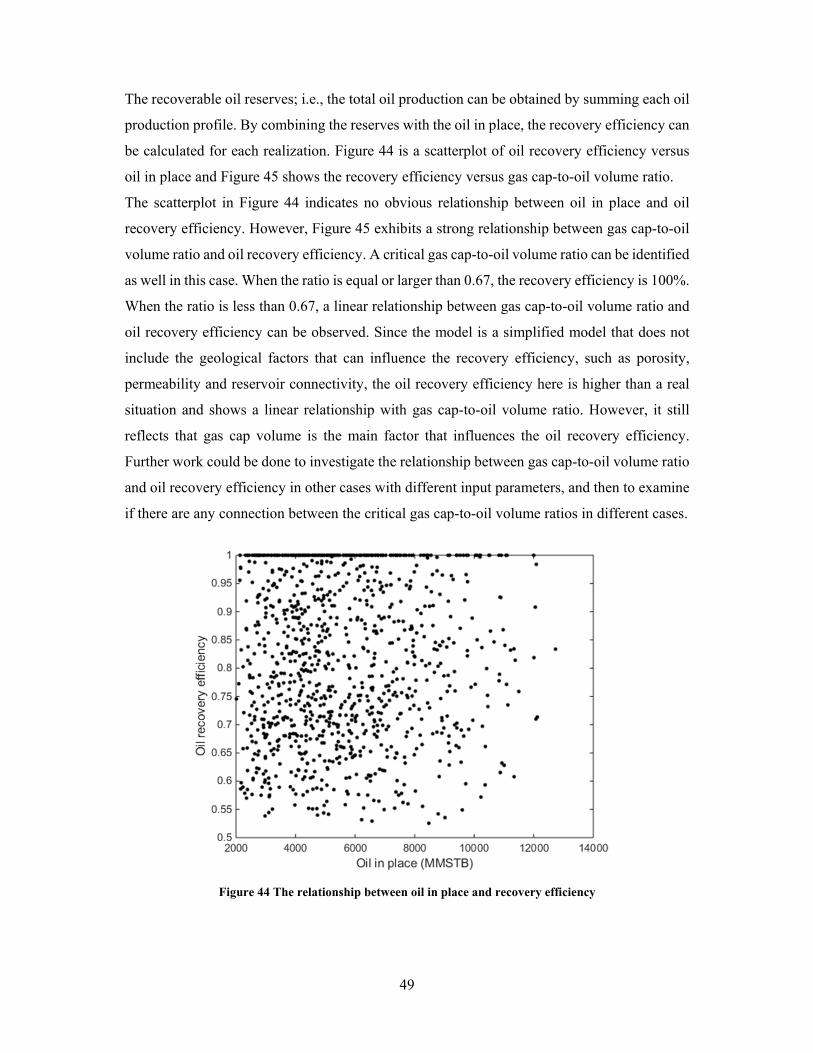
The recoverable oil reserves; i.e., the total oil production can be obtained by summing each oil

production profile. By combining the reserves with the oil in place, the recovery efficiency can

be calculated for each realization. Figure 44 is a scatterplot of oil recovery efficiency versus

oil in place and Figure 45 shows the recovery efficiency versus gas cap-to-oil volume ratio.

The scatterplot in Figure 44 indicates no obvious relationship between oil in place and oil

recovery efficiency. However, Figure 45 exhibits a strong relationship between gas cap-to-oil

volume ratio and oil recovery efficiency. A critical gas cap-to-oil volume ratio can be identified

as well in this case. When the ratio is equal or larger than 0.67, the recovery efficiency is 100%.

When the ratio is less than 0.67, a linear relationship between gas cap-to-oil volume ratio and

oil recovery efficiency can be observed. Since the model is a simplified model that does not

include the geological factors that can influence the recovery efficiency, such as porosity,

permeability and reservoir connectivity, the oil recovery efficiency here is higher than a real

situation and shows a linear relationship with gas cap-to-oil volume ratio. However, it still

reflects that gas cap volume is the main factor that influences the oil recovery efficiency.

Further work could be done to investigate the relationship between gas cap-to-oil volume ratio

and oil recovery efficiency in other cases with different input parameters, and then to examine

if there are any connection between the critical gas cap-to-oil volume ratios in different cases.

Figure 44 The relationship between oil in place and recovery efficiency

50

Figure 45 The relationship between gas cap-to-oil volume ratio and recovery efficiency

51

5. Discussion and Conclusion

In this study, an approach to assess the impact of reserves uncertainty on oil and gas production

for gas cap fields has been introduced, implemented and discussed. The inflow performance

relationship (IPR) and tubing performance relationship (TPR) curves used to generate the

natural flow rate. The natural flow rate is combined with the material balance equation to

construct a well production model to generate oil and gas production profiles, which is the core

of this approach.

The conventional methods to predict the oil and gas production are computationally expensive

as the production models often are based on a highly detailed model utilizing a large number

of grid cells. The high computational cost makes these production models unfeasible for

probabilistic analysis and decision support under uncertainty.

Unlike conventional methods, the approach discussed here provides a compelling and efficient

way to generate oil and gas production profiles that encapsulates the uncertainty, or lack of

knowledge, of the geoscientists and reservoir engineers. Using Monte Carlo simulation,

volumetric and reserves uncertainties can be combined with the production model to (1)

generate production time-series with uncertainties and (2) to assess the impact of reserves

uncertainties on the oil and gas production profiles. The end purpose of such assessing and

quantifying these uncertainties is to support reservoir management decisions.

The modeling approach is applied to X gas cap field to assess the impact of reserves uncertainty

on oil and gas production. Some general conclusions can be reached based on the case results.

First, a simple functional form can be used as a good approximation for the relationship

between oil in place, gas cap-to-oil volume ratio and oil production at each production year.

This functional form can then be used to predict the oil production. Second, the uncertainty in

oil in place has a larger impact on the oil production than the uncertainty in gas in place. Thus,

if it is important to reduce the uncertainty in the oil production, the main effort should be

reducing uncertainty in oil in place. Finally, the gas cap volume is the main factor which

impacts the oil recovery efficiency.

In addition to the application of the discussed production model in this thesis, it has also applied

to another, parallel, master thesis project “Depressurization of Oil Fields with Gas Injection”.

In that project, we have applied the approach to an example gas cap field to generate oil and

gas production profiles at different blowdown (depressurization) times, which provides

insights to the decision situation concerning optimal timing for blowdown.

52

Though this approach has advantages, it is not a general replacement of traditional production

prediction techniques. The purpose of developing the production model discussed in this thesis

is to provide decision makers with a cogent and tractable means of predicting future oil and gas

production with uncertain reserves and support reservoir management decisions.

53

References

Abdul-Majeed, G.H., Al-Soof, N.B.A., 2000. Estimation of gas–oil surface tension. Journal of Petroleum Science and Engineering, 27(3): 197-200.

Al-Marhoun, M.A., 1988. PVT correlations for Middle East crude oils. Journal of Petroleum Technology, 40(05): 650-666.

Beggs, D.H., Brill, J.P., 1973. A study of two-phase flow in inclined pipes. Journal of Petroleum technology, 25(05): 607-617.

Beggs, H.D., Robinson, J., 1975. Estimating the viscosity of crude oil systems. Journal of Petroleum technology, 27(09): 140-141.

Bratvold, R., Begg, S., 2010. Making good decisions. Society of Petroleum Engineers. Dake, L.P., 1983. Fundamentals of reservoir engineering, 8. Elsevier. Demirmen, F., 2007. Reserves estimation: the challenge for the industry. Journal of Petroleum

Technology, 59(05): 80-89. Dranchuk, P., Abou-Kassem, H., 1975. Calculation of Z factors for natural gases using

equations of state. Journal of Canadian Petroleum Technology, 14(03). Duns, H., Ros, N., 1963. Vertical flow of gas and liquid mixtures in wells, 6th World Petroleum

Congress. World Petroleum Congress. Eickmeier, J.R., 1968. How to Accurately Predict Future Well Productivities. World Oil, 99. Fetkovich, M., 1973. The isochronal testing of oil wells, Fall Meeting of the Society of

Petroleum Engineers of AIME. Society of Petroleum Engineers. Glaso, O., 1980. Generalized pressure-volume-temperature correlations. Journal of Petroleum

Technology, 32(05): 785-795. Golan, M., Whitson, C.H., 1991. Well performance. Prentice Hall. Guo, B., Lyons, W.C., Ghalambor, A., 2011. Petroleum production engineering, a computer-

assisted approach. Gulf Professional Publishing. Hagedorn, A.R., Brown, K.E., 1965. Experimental study of pressure gradients occurring during

continuous two-phase flow in small-diameter vertical conduits. Journal of Petroleum Technology, 17(04): 475-484.

Hall, K.R., Yarborough, L., 1973. A new equation of state for Z-factor calculations. Oil and Gas journal, 71(25): 82-92.

Hasan, A., Kabir, C., 1992. Two-phase flow in vertical and inclined annuli. International Journal of Multiphase Flow, 18(2): 279-293.

Hough, E., Rzasa, M., Wood, B., 1951. Interfacial tensions at reservoir pressures and temperatures; apparatus and the water-methane system. Journal of Petroleum Technology, 3(02): 57-60.

Katz, D.L.V., 1959. Handbook of natural gas engineering. McGraw-Hill. Lasater, J., 1958. Bubble point pressure correlation. Journal of Petroleum Technology, 10(05):

65-67. Lee, A.L., Gonzalez, M.H., Eakin, B.E., 1966. The viscosity of natural gases. Journal of

Petroleum Technology, 18(08): 997-1,000. Orkiszewski, J., 1967. Predicting two-phase pressure drops in vertical pipe. Journal of

Petroleum Technology, 19(06): 829-838. Petrosky Jr, G., Farshad, F., 1993. Pressure-volume-temperature correlations for Gulf of

Mexico crude oils, SPE annual technical conference and exhibition. Society of Petroleum Engineers.

Rawlins, E.L., Schellhardt, M.A., 1935. Back-pressure data on natural-gas wells and their application to production practices, Bureau of Mines, Bartlesville, Okla.(USA).

Schilthuis, R.J., 1936. Active oil and reservoir energy. Transactions of the AIME, 118(01): 33-52.

54

Selley, R.C., Sonnenberg, S.A., 2014. Elements of petroleum geology. Academic Press. Standing, M., 1947. A pressure-volume-temperature correlation for mixtures of California oils

and gases, Drilling and Production Practice. American Petroleum Institute. Standing, M.B., Katz, D.L., 1942. Density of natural gases. Transactions of the AIME, 146(01):

140-149. Sutton, R., 1985. Compressibility factors for high-molecular-weight reservoir gases, SPE

Annual Technical Conference and Exhibition. Society of Petroleum Engineers. Thomas, P., Bratvold, R.B., 2015. A Real Options Approach to the Gas Blowdown Decision,

SPE Annual Technical Conference and Exhibition. Society of Petroleum Engineers. Vazquez, M., Beggs, H.D., 1980. Correlations for fluid physical property prediction. Journal

of Petroleum Technology, 32(06): 968-970. Vogel, J., 1968. Inflow performance relationships for solution-gas drive wells. Journal of

petroleum technology, 20(01): 83-92. Yoe, C., 2011. Principles of risk analysis: decision making under uncertainty. CRC press.

55

Appendices

Appendix A: MATLAB code for pressure drop calculation

function [ PDTrue ] = PressureDroptest(RP,OilR,InsD,WHP,PD)% Pressure Drop

Calculation

% Summary of this function goes here

% To calculate the pressure drop along the production tubing by using Beggs and

Brill correlation

% Detailed explanation goes here

% Input parameters in this function:

% IRP Initial Reservoir Pressure (Psig)

% RP Reservoir Pressure (Psig)

% OilR Oil Rate (STB/day)

% InsD Instant Well Depth (ft)

% WHP Wellhead Pressure (Psig)

% PD Estimated Pressure Drop (Psig)

% Output parameters in this function:

% PDTrue True Pressure Drop (Psig)

% Basic Input Parameters

IRT = 180; %Intial Reservoir Temperature (F)

WHT = 120; %Wellhead Temperature (F)

BHT = 180; %Bottomhole Temperature (F)

TD = 8200; %Total Depth (ft)

Dia = 5.5; %Inner Diameter (in)

Rough = 0.0006; %Pipe Roughness (in)

Angle = 90; %Pipe Inclination Angle with Horizontal

GasG = 0.62; %Gas Gravity

OilAPI = 38.5; %Oil API

OilG = 141.5/(131.5+OilAPI);%Oil Gravity

% Basic Input Parameters End

SD = TD/12;% Step Distance (ft)

BHP = PD+WHP; %Bottomhole Pressure (Psig)

AVP = (WHP+BHP)/2;%Average Pressure (Psig)

AVT = ((WHT + (BHT-WHT)/TD*InsD)+(WHT + (BHT-WHT)/TD*(InsD+SD)))/2;%Average

Temperature (F)

IIGOR = GasG*(((RP+14.7)/18.2 + 1.4)*10^(0.0125* OilAPI-

0.00091*IRT))^(1/0.83);%Instant Intial GOR (scf/STB)

if GasG*(((AVP+14.7)/18.2 + 1.4)*10^(0.0125* OilAPI-

0.00091*AVT))^(1/0.83)>IIGOR

GOR = IIGOR;% Solution GOR (scf/STB)

else

GOR = GasG*(((AVP+14.7)/18.2 + 1.4)*10^(0.0125* OilAPI-

0.00091*AVT))^(1/0.83);% Solution GOR (scf/STB)

56

end

if GOR<IIGOR

Bo = 0.972+1.47*10^(-4)*(1.25*AVT+GOR*(GasG/OilG)^0.5)^1.175;% Oil

Formation Volume Factor (bbl/STB)

else

OilC = 10^(-5)*(-1433+5*IIGOR+17.2*AVT-

1180*GasG+12.61*OilAPI)/(RP+14.7); %Oil Compressibility

Bo = (0.972+1.47*10^(-

4)*(1.25*AVT+GOR*(GasG/OilG)^0.5)^1.175)*exp(OilC*(RP-AVP));% Oil Formation Volume

Factor (bbl/STB)

end

%Z factor and Gas Formation Volume Factor Calculation

Ppc = 756.8-131.07*GasG-3.6*GasG^2;%Pseudocritical Pressure

Tpc = 169.2+349.5*GasG-74*GasG^2; %Pseudocritical Temperature

Pr = (AVP+14.7)/Ppc; %Pseudoreduced Pressure

Tr = (AVT+460)/Tpc; %Pseudoreduced Temperature

A = 1.39*(Tr-0.92)^0.5-0.36*Tr-0.101;

B =(0.62-0.23*Tr)*Pr+(0.066/(Tr-0.86)-0.037)*Pr^2+0.32/10^(9*(Tr-1))*Pr^6;

C = 0.132-0.32*log10(Tr);

D = 10^(0.3106-0.49*Tr+0.1824*(Tr^2));

Z = A+(1-A)/exp(B)+C*Pr^D;% Z Factor

Bg = 0.0282793*(AVT+460)*Z/(AVP+14.7);% Gas Formation Volume Factor

(rcf/scf)

GasD = 28.97*GasG*(AVP+14.7)/Z/10.73/(460+AVT);% Gas Density (lb/ft3)


0.00091*AVT))^(1/0.83)>IIGOR

OilC = 10^(-5)*(-1433+5*IIGOR+17.2*AVT-1180*GasG+12.61*OilAPI)/(RP+14.7);

OilD = (350*OilG+0.0764*GasG*GOR)/5.615/Bo*exp(OilC*(AVP-RP));% Oil

Density (lb/ft3)

else

OilD = (350*OilG+0.0764*GasG*GOR)/5.615/Bo;% Oil Density (lb/ft3)

end

LiqD = OilD;%Liquid Density (lb/ft3)

GasFR = (IIGOR-GOR)* OilR * Bg/86400;% Gas Flowrate (ft3/s)

LiqFR = OilR*Bo*5.615/86400;% Liquid Flowrate (ft3/s)

Area = pi*(Dia/2*0.0833333)^2;% Pipe Sectional Area (ft2)

SfGasFR = GasFR/Area;% Superficial Gas Flowrate (ft/s)

SfLiqFR = LiqFR/Area;% Superficial Liquid Flowrate (ft/s)

SfMixFR = SfGasFR + SfLiqFR;% Superficial Mix Flowrate (ft/s)

GasWFR = GasD * SfGasFR;% Gas Weight Flux Rate (lb/ (ft2.s))

LiqWFR = LiqD * SfLiqFR;% Liquid Weight Flux Rate (lb/ (ft2.s))

MixWFR = GasWFR + LiqWFR;% Mix Weight Flux Rate (lb/ (ft2.s))

57

NoSlipHUp = LiqFR/(LiqFR + GasFR);% No-slip Holdup

Nfr = SfMixFR^2/32.174/(Dia*0.0833333);% Froude Number

%Gas Viscosity

Mg = 28.967 * GasG;% Mole weight

K1 = (0.00094+2*10^(-6)*Mg)*(AVT+460)^1.5/(209+19*Mg+(AVT+460));

X = 3.5+986/(460+AVT)+0.01*Mg;

Y = 2.4-0.2*X;

GasVisc = K1*exp(X*(GasD/62.4)^Y); %Gas Viscosity (cp)

DeadOilVisc = 10^(AVT^-1.163*exp(6.9824-0.04658*OilAPI))-1;% Dead Oil

Viscosity (cp)

A1 = 10.715*(GOR+100)^-0.515;

B1 = 5.44*(GOR+150)^-0.338;


0.00091*AVT))^(1/0.83)>IIGOR

C1 =2.6*AVP^1.187*exp(-11.513+(-8.98*10^-5*AVP));

OilVisc = A1* DeadOilVisc^B1*(AVP/RP)^C1; % Bubblepoint Oil Viscosity

(cp)

else

OilVisc = A1* DeadOilVisc^B1; % Bubblepoint Oil Viscosity (cp)

end

LiqVisc = OilVisc;

OilIntT = (1.17013-1.694*10^(-3)*AVT)*(38.085-0.259*OilAPI);% Oil

Interfacial Tension (dynes/cm)

LiqIntT = OilIntT;% Liquid Interfacial Tension (dynes/cm)

MixVisc = 6.72*10^(-4)*(LiqVisc*NoSlipHUp + GasVisc*(1-NoSlipHUp));% Mix

Viscosity (lb/ft/s)

Nre = MixWFR*Dia*0.0833333/MixVisc;% No Slip Reynold Number

Nlv = 1.938*SfLiqFR*(LiqD/LiqIntT)^0.25;% Liquid Velocity Number

%Determine the flow patten

L1 = 316*NoSlipHUp^0.302;

L2 = 0.0009252*NoSlipHUp^-2.4684;

L3 = 0.1*NoSlipHUp^-1.4516;

L4 = 0.5*NoSlipHUp^-6.738;

if (NoSlipHUp<0.01 && Nfr<L1) || (NoSlipHUp>=0.01 && Nfr<L2)

Flow = 'Segregated';

elseif (NoSlipHUp>=0.01 && NoSlipHUp<0.4 && Nfr>L3 && Nfr<=L1) ||

(NoSlipHUp>=0.4 && Nfr>L3 && Nfr<=L4)

Flow = 'Intermittent';

elseif (NoSlipHUp<0.4 && Nfr>=L4) || (NoSlipHUp>=0.4 && Nfr>L4)

Flow = 'Distributed';

58

elseif (Nfr>L2 && Nfr<L3)

Flow = 'Transition';

else

Flow = ' ';

end

%Liquid Holdup for Horizontal Flow

SegHup0 = 0.98*NoSlipHUp^0.4846/Nfr^0.0868; % Segregated

InterHup0 = 0.845*NoSlipHUp^0.5351/Nfr^0.0173; % Intermittent

DisHup0 = 1.065*NoSlipHUp^0.5824/Nfr^0.0609; % Distributed

% Selected Liquid Holdup

if strcmp(Flow,'Segregated')

Sel_Hup0 = SegHup0;

elseif strcmp(Flow,'Intermittent')

Sel_Hup0 = InterHup0;

elseif strcmp(Flow,'Distributed')

Sel_Hup0 = DisHup0;

else

Sel_Hup0 = 1;

end

% Final Selected Liquid Holdup

if Sel_Hup0 > NoSlipHUp

FSel_Hup0 = Sel_Hup0;

else

FSel_Hup0 = NoSlipHUp;

end

% Correction Factor Coefficient

SegCF = (1-NoSlipHUp)*log(0.011*NoSlipHUp^(-3.768)*Nlv^3.539*Nfr^(-

1.614)); % Segregated Flow

InterCF = (1-NoSlipHUp)*log(2.96*NoSlipHUp^(0.305)*Nlv^(-

0.4473)*Nfr^(0.0978)); % Intermittent Flow

DisCF = 0; % Distributed Flow

% Selected Correction Factor Coefficient

if strcmp(Flow,'Segregated')

Sel_CF = SegCF;

elseif strcmp(Flow,'Intermittent')

Sel_CF = InterCF;

else

Sel_CF = DisCF;

end

% Final Selected Correction Factor Coefficient

if Sel_CF <= 0

FSel_CF = 0;

59

else

FSel_CF = Sel_CF;

end

Rad_Angle = Angle*pi/180; % Pipe Inclination Angle with Horizontal

B_Angle = 1+FSel_CF*(sin(1.8*Rad_Angle)-(1/3)*sin(1.8*Rad_Angle)^3); %

Correction Factor

%Liquid Holdup for Transition Flow

AA = (L3-Nfr)/(L3-L2);

BB = 1-AA;

SegB_Angle = 1+SegCF*(sin(1.8*Rad_Angle)-(1/3)*sin(1.8*Rad_Angle)^3); %

Correction Factor For Segregated Flow

InterB_Angle = 1+InterCF*(sin(1.8*Rad_Angle)-(1/3)*sin(1.8*Rad_Angle)^3); %

Correction Factor For Intermittent Flow

if SegB_Angle<=1

SegHup1 = SegHup0;

else

SegHup1 = SegHup0 * SegB_Angle;

end

if InterB_Angle<=1

InterHup1 = InterHup0;

else

InterHup1 = InterHup0 * InterB_Angle;

end

TransHup1 = AA* SegHup1 + BB* InterHup1;

% Selected Liquid Holdup for Transition Flow

if TransHup1<=NoSlipHUp

Sel_TransHup1 = NoSlipHUp;

else

Sel_TransHup1 = TransHup1;

end

% Final Liquid Holdup For Next Calculation

if strcmp(Flow,'Transition')

Final_LiqHup = Sel_TransHup1;

elseif B_Angle<=1

Final_LiqHup = FSel_Hup0;

else

Final_LiqHup = FSel_Hup0 * B_Angle;

end

TwoPhaseD = Final_LiqHup * LiqD + (1- Final_LiqHup)*GasD; % two-phase

density

PressDropG = TwoPhaseD * sin(Rad_Angle)/144; % hydrostatic pressure gradient

% Pressure drop due to friction loss

% Ratio of two-phase to no-slip friction factor calculation

60

Y = NoSlipHUp/Final_LiqHup^2;

In_Y = log(Y);

S = In_Y/(-0.0523+3.182*In_Y-0.8725*In_Y^2+0.01853*In_Y^4);

if Y == 0

S_Final = 0;

elseif Y>1 && Y<1.2

S_Final = log(2.2*Y-1.2);

else

S_Final = S;

end

FrictionFR = exp(S_Final); % Ratio of two-phase to no-slip friction factor

% No-slip friction factor calculation/ Fanning friction factor calculation

Epsilon_D = Rough/Dia;

FF1 = 64/Nre;

FF2 = 1/(-2*log10(Epsilon_D/3.7+2.51/(Nre*sqrt(FF1))))^2;














if Nre<=2100

FannFriF = FF1 /4; % Fanning friction factor

else

FannFriF = FF15 /4;

end

TwoPhaseFriF = FrictionFR * FannFriF; % Two-phase friction factor

PressDropF = 2*TwoPhaseFriF*SfMixFR*MixWFR/144/32.174/(Dia*0.0833333); %

pressure gradient due to the friction pressure loss

PressDropT = PressDropG + PressDropF; % Total pressure gradient

PDTrue = SD*PressDropT; % Ture pressure drop in the length increment

end

61

Appendix B: MATLAB code for natural oil rate calculation

function [NOR] = NaturalOilFlow(RP,MaxOilR)


% To calculate natural oil flowrate by using IPR and TPR curves




% MaxOilR Max Oil Rate (STB/day)


% NOR Natural Oil Rate (STB/day)

TD = 8200; %Total Depth (ft)

i= 0;

Oilrate = zeros(1,20);

TPR = zeros(1,20);

IPR = zeros(1,20);

Dif = zeros(1,20);

k =1;

while i< 20

OilR = 10 + MaxOilR/20*i; % Oil rate

Oilrate(k) = OilR;

InsD = 0;% Instant Well Depth (ft)

WHP = 650; % Wellhead Pressure (Psig)

L = WHP;

j = 1;

% Construct TPR curve

while InsD < TD

PressureDropF = @(PD)(PressureDroptest(RP,OilR,InsD,WHP,PD)-PD)^2;

lb = 0;

ub = RP;

x0 = RP/2;

A = [];

b = [];

Aeq = [];

beq = [];

nonlcon = [];

opt = optimoptions('fmincon','Display','off','Algorithm','sqp');

PDTrue = fmincon(PressureDropF,x0,A,b,Aeq,beq,lb,ub,nonlcon,opt);

InsD = j*TD/12;

L = L+PDTrue;

WHP = L;

j=j+1;

end

TPR(k) = L;

62

IPR(k) = (-0.2+sqrt(0.2^2-4*0.8*(OilR/MaxOilR-1)))/(2*0.8)*RP; % Construct IPR

curve

Dif(k) = IPR(k)-TPR(k); % Pressure difference between IPR and TPR curves

if k>=2

if Dif(k-1)>0 && Dif(k)<0

x1 = [Oilrate(k-1),Oilrate(k)];

y1 = [TPR(k-1),TPR(k)];

p = polyfit(x1,y1,1);

func = @(x)((p(1)*x+p(2))-((-0.2+sqrt(0.2^2-4*0.8*(x/MaxOilR-

1)))/(2*0.8)*RP))^2;

lb = Oilrate(k-1);

ub = Oilrate(k);

x0 = Oilrate(k-1);

A = [];

b = [];

Aeq = [];

beq = [];

nonlcon = [];

opt1 = optimoptions('fmincon','Display','off','Algorithm','sqp');

NOR = fmincon(func,x0,A,b,Aeq,beq,lb,ub,nonlcon,opt1); % Natural Oil

Rate Calculation

return

end

end

k = k+1;

i = i+1;

end

NOR = 0;

63

Appendix C: MATLAB code for natural gas rate calculation

function [NGR] = NaturalGasFlow(RP)


% To calculate natural gas flowrate by using IPR and TPR curves





% NGR Natural Gas Rate (MMscf/day)

c = 0.5;% IPR parameter (backpressure equation)

n = 0.7;% IPR parameter (backpressure equation)

WHP = 650; %Wellhead Pressure (Psig)

func1= @(BHPgas)(PressureGasFlow(BHPgas) - (c*(RP^2-BHPgas^2)^n /10^3))^2;

lb = WHP;

ub = RP;

x0 = (WHP+RP)/2;

A = [];

b = [];

Aeq = [];

beq = [];

nonlcon = [];

opt1 = optimoptions('fmincon','Display','off','Algorithm','sqp');

BHPgas = fmincon(func1,x0,A,b,Aeq,beq,lb,ub,nonlcon,opt1);

NGR = c*(RP^2-BHPgas^2)^n /10^3; % Natural Gas Rate Calculation

end

64

Appendix D: MATLAB code for PVT properties calculation

function [GOR,Bo,Bg] = PVTproperties(RP)


% To calculate PVT properties





% GOR Solution Gas Oil Ratio (scf/STB)

% Bo Oil Formation Volume Factor (bbl/STB)

% Bg Gas Formation Volume Factor (bbl/scf)

GasG = 0.62; %Gas Gravity

OilAPI = 38.5; %Oil API

IRT = 180; %Intial Reservoir Temperature (F)

OilG = 141.5/(131.5+OilAPI);%Oil Gravity

Ppc = 756.8-131.07*GasG-3.6*GasG^2;%Pseudocritical Pressure

Tpc = 169.2+349.5*GasG-74*GasG^2; %Pseudocritical Temperature

Tr = (IRT+460)/Tpc; %Pseudoreduced Temperature

GOR = GasG*(((RP+14.7)/18.2 + 1.4)*10^(0.0125* OilAPI-0.00091*IRT))^(1/0.83);%

Solution GOR (scf/STB)

Bo = 0.972+1.47*10^(-4)*(1.25*IRT+GOR*(GasG/OilG)^0.5)^1.175;% Oil Formation Volume

Factor (bbl/STB)

Pr = (RP+14.7)/Ppc; %Pseudoreduced Pressure

A = 1.39*(Tr-0.92)^0.5-0.36*Tr-0.101;

B =(0.62-0.23*Tr)*Pr+(0.066/(Tr-0.86)-0.037)*Pr^2+0.32/10^(9*(Tr-1))*Pr^6;

C = 0.132-0.32*log10(Tr);

D = 10^(0.3106-0.49*Tr+0.1824*(Tr^2));

Z = A+(1-A)/exp(B)+C*Pr^D;% Z Factor

Bg = 0.00503676*(IRT+460)*Z/(RP+14.7);% Gas Formation Volume Factor (bbl/scf)

end

65

Appendix E: MATLAB code for the material balance equation

function [output] = MBE(N,m,SCNp,SINg,TGOR,Boi,Bgi,GORi,RP)


% To construct a function about Material Balance Equation



% N Initial oil in place (STB)

% m Initial gas cap-to-oil volume ratio

% SCNp Culmulative Oil Production (STB)

% SINg Culmulative Gas Injection (MMscf)

% Boi Initial Oil Formation Volume Factor (bbl/STB)

% Bgi Gas Formation Volume Factor (bbl/scf)

% GORi Solution Gas Oil Ratio (scf/STB)


[GOR,Bo,Bg] = PVTproperties(RP); % calculate the Bo, Bg, and solution GOR at each

reservoir pressure

output = ((SCNp*(Bo +(TGOR-GOR)*Bg))-(N*Boi*(((Bo-Boi)+(GORi-GOR)*Bg)/Boi)+

(N*m*Boi/Bgi + SINg*10^6)*Bg - N*m*Boi))^2;

end

66

Appendix F: MATLAB code for oil and gas production profiles generation

function [Y,Newpressure,Np,Ngp] = UnderGWithdraw(N,m)


% To calculate the reservoir pressure decline curve and oil and gas production

profiles



% N Initial oil in place (STB)

% m Initial gas cap-to-oil volume ratio


% Y Years

% Newpressure Reservoir Pressure (Psig)

% Np Oil Production (STB/Y)

% Ngp Gas Production (MMscf/Y)


Numberofwells = 20; % Number of wells

MaxOilCap = 18000*365*20; % Maximum Oil Capicity (STB/Y)

Y2MaxOilR = 5.5; % Years to reach the Maxmium Oil Rate

MaxGasCap = 21.1*365*20;% Maximum Gas Capicity (MMscf/Y)

Pgy = 1000;% The year to start to produce free gas

Y2MaxGasR = 4; % Years to reach the Maxmium Gas Rate

IRP = 4263; % Initial Reservoir Pressure (Psig)

MaxOilR = 50000; % Maximum Oil Rate (STB/Y)

%Basic Input Parameters End

[GORi,Boi,Bgi] = PVTproperties(IRP); % Initial Bo, Bg, and Solution GOR calculation

Newpressure = zeros(200,1); Newpressure(1)= IRP;

Y = zeros(200,1); Y(1) = 0; % Year

Nr = zeros(200,1); Nr(1) = N;% Remaining Oil Volume

Np = zeros(200,1);Np(1) = 0; % Real Oil Production

Ngp = zeros(200,1);Ngp(1) = 0; % Real Gas Production

CNp = zeros(200,1);CNp(1) = 0;% Real Culmulative Oil Production

Nsgp = zeros(200,1);Nsgp(1)= 0;% Real Solution Gas Production

CNsgp = zeros(200,1);CNsgp(1)=0;% Real Culmulative Solution Gas Production

INg = zeros(200,1);INg(1) = 0;% Culmulative Gas injection

Nfgp = zeros(200,1);Nfgp(1) = 0;% Real Free Gas Production

GasCapNgp = zeros(200,1);% Gas Production due to the capacity influence

CNtgp = zeros(200,1); % Real Culmulative total Gas Production

Ngr = zeros(200,1); Ngr(1)=N*m*Boi/Bgi/10^6;% Remaining gas volume

Py =1;

RPj = IRP;

67

MaxOilRj = MaxOilR;

gy =1;

while Nr(Py) >0

Y(Py+1) = Py;

if Py >2 && Np(Py) == 0

OilR_Year = 0;

else

OilR_Day = NaturalOilFlow(RPj,MaxOilRj);

OilR_Year = OilR_Day*365*Numberofwells;% Oil production in one year (STB/Year)

end

if Py < Y2MaxOilR

OilCap = MaxOilCap/Y2MaxOilR * Py;

else

OilCap = MaxOilCap;

end

SmaP = [OilCap, OilR_Year, Nr(Py)];

Np(Py+1) = min(SmaP);

CNp(Py+1) = CNp(Py)+min(SmaP);

Nr(Py+1) = Nr(1)-CNp(Py+1);

Nsgp(Py+1) = Np(Py+1)* PVTproperties(RPj)/10^6;

CNsgp(Py+1) = CNsgp(Py)+ Nsgp(Py+1);

INg(Py+1) = CNsgp(Py+1);

if Py < Pgy

Ngr(Py+1) = Ngr(1) + INg(Py+1);

TGOR = CNsgp(Py+1)/CNp(Py+1)*10^6;

SCNp = CNp(Py+1);

SINg = INg(Py+1);

AAA = @(RP) MBE(N,m,SCNp,SINg,TGOR,Boi,Bgi,GORi,RP);

opt = optimoptions(@fminunc,'Display','off','Algorithm','quasi-newton');

Newpressure(Py+1) = fminunc(AAA,Newpressure(Py),opt);

else

Nfgp(Py+1) = NaturalGasFlow(RPj)*365*Numberofwells;

if gy < Y2MaxGasR

if (Nsgp(Py+1)+ Nfgp(Py+1)) > MaxGasCap

INg(Py+1) = MaxGasCap*(1-gy/Y2MaxGasR)+ INg(Py);

CNsgp(Py+1) = MaxGasCap + CNsgp(Py);

GasCapNgp(Py+1) = MaxGasCap*gy/Y2MaxGasR;

Fgi = INg(Py+1);

else

INg(Py+1) = (Nsgp(Py+1)+ Nfgp(Py+1))*(1-gy/Y2MaxGasR)+ INg(Py);

CNsgp(Py+1) = (Nsgp(Py+1)+ Nfgp(Py+1))+ CNsgp(Py);

GasCapNgp(Py+1) = (Nsgp(Py+1)+ Nfgp(Py+1))*gy/Y2MaxGasR;

68

Fgi = INg(Py+1);

end

else

if (Nsgp(Py+1)+ Nfgp(Py+1)) > MaxGasCap

INg(Py+1) = Fgi;

CNsgp(Py+1) = MaxGasCap + CNsgp(Py);

GasCapNgp(Py+1) = MaxGasCap;

else

INg(Py+1) = Fgi;

CNsgp(Py+1) = (Nsgp(Py+1)+ Nfgp(Py+1))+ CNsgp(Py);

GasCapNgp(Py+1) = (Nsgp(Py+1)+ Nfgp(Py+1));

end

end

gy = gy +1;

SmaGP = [GasCapNgp(Py+1),Ngr(Py)];

Ngp(Py+1) = min(SmaGP);

CNtgp(Py+1) = CNtgp(Py)+ min(SmaGP);

Ngr(Py+1) = Ngr(1)+ INg(Py+1)- CNtgp(Py+1);

TGOR = CNsgp(Py+1)/CNp(Py+1)*10^6;

SCNp = CNp(Py+1);

SINg = INg(Py+1);

AAA = @(RP) MBE(N,m,SCNp,SINg,TGOR,Boi,Bgi,GORi,RP);

opt = optimoptions(@fminunc,'Display','off','Algorithm','quasi-newton');

Newpressure(Py+1) = fminunc(AAA,Newpressure(Py),opt);

end

MaxOilRj = Newpressure(Py+1)/IRP*MaxOilR;

RPj = Newpressure(Py+1);

if Np(Py+1) == 0 && Ngp(Py+1)== 0

return

end

if Py >198

return

end

Py = Py+1;

end

end

69

Appendix G: MATLAB code for the PERT distribution

function [OilV,GasV,OilVmean,OilVstd,GasVmean,GasVstd] = PERTdistribution()


% To generate the PERT distribution for oil in place and gas cap-to-oil volume

ratio



% OilV Oil in place (MMSTB)

% GasV Gas cap-to-oil volume ratio

% OilVmean Mean of oil in place distribution

% OilVstd Standard deviation of oil in place distribution

% GasVmean Mean of gas cap-to-oil volume ratio distribution

% GasVstd Standard deviation of gas cap-to-oil volume ratio distribution


OilVmin = 2000; % minimum value of oil in place (MMSTB)

OilVmode = 4000; % mode of oil in place (MMSTB)

OilVmax = 15000; % maximum value of oil in place (MMSTB)

GasVmin = 0.2; % minimum value of gas cap-to-oil volume ratio

GasVmode = 0.4; % mode of gas cap-to-oil volume ratio

GasVmax = 1.2;% maximum value of gas cap-to-oil volume ratio

% Basic Input Parameters End

N_samples = 1000; % number of samples

OilVmean = (OilVmin+4*OilVmode+OilVmax)/6;

OilVstd = (OilVmax-OilVmin)/6;

Oilw1 = (OilVmean-OilVmin)*(2*OilVmode-OilVmin-OilVmax)/(OilVmode-

OilVmean)/(OilVmax-OilVmin);

Oilw2 = Oilw1*(OilVmax-OilVmean)/(OilVmean-OilVmin);

OilVdist = makedist('Beta','a',Oilw1,'b',Oilw2);

rng('shuffle');y1 = rand(N_samples,1);

OilVbeta = icdf(OilVdist,y1);

OilV= OilVbeta * (OilVmax-OilVmin) + OilVmin;

GasVmean = (GasVmin+4*GasVmode+GasVmax)/6;

GasVstd = (GasVmax-GasVmin)/6;

Gasw1 = (GasVmean-GasVmin)*(2*GasVmode-GasVmin-GasVmax)/(GasVmode-

GasVmean)/(GasVmax-GasVmin);

Gasw2 = Gasw1*(GasVmax-GasVmean)/(GasVmean-GasVmin);

GasVdist = makedist('Beta','a',Gasw1,'b',Gasw2);

rng('shuffle');y2 = rand(N_samples,1);

GasVbeta = icdf(GasVdist,y2);

GasV= GasVbeta * (GasVmax-GasVmin) + GasVmin;

end

70

Appendix H: MATLAB code for Monte Carlo simulation


% Monte Carlo simulation appliaction and parallel computing

[OilV,GasV,OilVmean,OilVstd,GasVmean,GasVstd] = PERTdistribution() ;

Np = zeros(200,length(OilV));

Ngp = zeros(200,length(OilV));

Newpressure = zeros(200,length(OilV));

Year = transpose(0:1:199);

parfor i = 1:length(OilV)

[Y,Newpressure(:,i),Np(:,i),Ngp(:,i)] = UnderGWithdraw(OilV(i)*10^6,GasV(i));

end

master’s thesis - bibsys · master’s thesis study program ... i would like to first express my...

Documents