Improving landfill monitoring programswith the aid of geoelectrical - imaging techniquesand geographical information systems Master’s Thesis in the Master Degree Programme, Civil Engineering

KEVIN HINE

Department of Civil and Environmental Engineering Division of GeoEngineering Engineering Geology Research GroupCHALMERS UNIVERSITY OF TECHNOLOGYGöteborg, Sweden 2005Master’s Thesis 2005:22

Design of an Autonomous Office GuideMaster’s Thesis in Systems, Control and Mechatronics

GUSTAF AGRENIUS

Department of Signals and SystemsChalmers University of TechnologyGothenburg, Sweden 2012Master’s Thesis EX081/2012

Abstract

In this master thesis a guiding software for an autonomous robot was developed. Thepurpose was to enable a preexisting robot to guide visitors to the right office space insideof Aros Electronics. The guiding software have four major parts; path planning, pathfollowing, collision avoidance and localization. The A* algorithm is used on a map of theoffice to get the path to the destination. The path following is done by driving the robottowards a waypoint located on the path ahead of the robot. The collision avoidancechecks that the path is clear and if not the robot is not allowed to continue. Two ways oflocalization is tested in combination with odometry. First an Xbox kinect camera is usedto spot landmarks and the distance and angle to this landmark is used in a probabilisticmethod called particle filter to estimate the pose. Secondly a wall following method isdeveloped where ultrasonic proximity sensors are used to sense the walls of the office.Both localization methods greatly improves the pose estimation compared to using onlyodometry but the wall following method shows better performance compared to particlefilter method. The main reason for this is that the update frequency is much higher.

Keywords: Autonomous robot, autonomous guiding, path planning, path following,collision avoidance, localization, landmark, kinect camera, particle filter, A* algorithm,wall following.

I

Acknowledgment

This master thesis was made at the Department of Signal and Systems in cooperationwith Aros Electronics. I would like to thank every one at Aros Electronics for all theirsupport. I especially want to thank my two advisors Henrik Gulven and Andreas Pet-terson for helping me with ideas and motivation when needed. Also a special thanks toDaniel Chadstrom for helping me understand the inner workings of Glenn and to HenrikNeugebauer for helping me save money at lunch time. At Chalmers I would like to thankmy examiner Jonas Fredriksson for ideas and input. At last I want to thank Lena forproofreading this text and for always being there.

Gustaf Agrenius, Gothenburg 12/11/28

II

Contents

Variables 1

1 Introduction 31.1 Autonomous Guiding . . . . . . . . . . . . . . . . . . . . . . . . . . . . . . 31.2 Related Work . . . . . . . . . . . . . . . . . . . . . . . . . . . . . . . . . . 31.3 Glenn . . . . . . . . . . . . . . . . . . . . . . . . . . . . . . . . . . . . . . 4

1.3.1 CAN Communication . . . . . . . . . . . . . . . . . . . . . . . . . 61.3.2 Sensor Board . . . . . . . . . . . . . . . . . . . . . . . . . . . . . . 61.3.3 Control Board . . . . . . . . . . . . . . . . . . . . . . . . . . . . . 6

1.4 Software Structure . . . . . . . . . . . . . . . . . . . . . . . . . . . . . . . 61.5 Outline of the Report . . . . . . . . . . . . . . . . . . . . . . . . . . . . . 7

2 Path Planning 82.1 Contracted Map . . . . . . . . . . . . . . . . . . . . . . . . . . . . . . . . 82.2 A∗ Algorithm . . . . . . . . . . . . . . . . . . . . . . . . . . . . . . . . . . 9

3 Path Following 113.1 Collision Avoidance . . . . . . . . . . . . . . . . . . . . . . . . . . . . . . 11

4 Localization 134.1 Odometry . . . . . . . . . . . . . . . . . . . . . . . . . . . . . . . . . . . . 13

4.1.1 Odometric Errors . . . . . . . . . . . . . . . . . . . . . . . . . . . . 144.2 Kinect . . . . . . . . . . . . . . . . . . . . . . . . . . . . . . . . . . . . . . 154.3 Particle Filter . . . . . . . . . . . . . . . . . . . . . . . . . . . . . . . . . . 174.4 Wall Following . . . . . . . . . . . . . . . . . . . . . . . . . . . . . . . . . 20

5 Result 215.1 Localization Results . . . . . . . . . . . . . . . . . . . . . . . . . . . . . . 215.2 Guiding Results . . . . . . . . . . . . . . . . . . . . . . . . . . . . . . . . . 25

6 Conclusion 266.1 Future Work . . . . . . . . . . . . . . . . . . . . . . . . . . . . . . . . . . 26

Bibliography 28

A The Parts of Glenn 29

B A∗ Algorithm 30

III

Variables

A list of variables and abrevations used.

PFL particle filter localization

CAN Controller Area Network

dCAN distance traveled by Glenn

αCAN angle of Glenn

RWpos angular position of right wheel

LWpos angular position of left wheel

p edge of the map polygon

Pa and Pb vertices of p

c vector defining the movement of the map polygon edges

µ the distance to move the map polygon edges

Ω the direction of c

d vector orthogonal to p

Qa and Qb points on the contracted map

f(n) the cost of the path through n

g(n) the cost to the current node n

h(n) the heuristic cost from the current node n to the goal

(xp,yp) the position of the current waypoint p

dp distance to the current waypoint p

αp angle to the current waypoint p

xk = [xk,yk,θk]T the pose of Glenn at time k

xk = [xk,yk,θk]T the pose estimate of Glenn at time k

δθk the change in heading since the last time step

δdk the change in distance since the last time step

δrk the distance traveled by the right wheel since the last time step

δlk the distance traveled by the left wheel since the last time step

W wheelbase of Glenn

Dw wheel diameter

edrift, etrans and erot odometric error correction

αk azimuth angle to the current landmark

Lk the distance to the current landmark

resX horizontal resolution of the kinect RGB camera

FOV field of view of the kinect RGB camera

Zkinect kinect depth measurement

XL the x position of center pixel of the current landmark

1

Wi weight of particle i

δLi the difference of the actual kinect depth readings and the expectedkinect depth readings for particle i

δαi the difference of the actual kinect angle readings and the expectedkinect angle readings for particle i

(xM ,yM ) the position of the current landmark M

xi = (xi,yi,θi) the pose of particle i

σL and σα tuning parameters for the particle filter

S the difference between measured distance and expected distanceto the wall

ϕ the angle error of Glenn

Di mean deviation in Y direction of Glenn at position i

Ti mean deviation in X direction of Glenn at position i

Gi distance traveled at position i

Ri mean angle deviation at angle i

Ai actual angle i

2

Chapter 1

Introduction

This thesis describe the development of an autonomous guiding functionality in a preex-isting robot, called Glenn. The desired behavior of Glenn is to get user input in the formof a desired position, where to guide someone, and then drive to that position. After thetask is complete Glenn should return back to the starting position. This thesis is madetogether with Aros Electronics and it is in their office Glenn should be able to guidepeople.

1.1 Autonomous Guiding

Autonomous robots are an increasingly common part of our every day life. They existin both the industry, as unmanned trucks, and in our homes, as autonomous vacuumcleaners or lawnmowers. Autonomous guiding robots are not very common today but ina near future they will probably be a well known sight at many museums.

To achieve a guiding functionality in an autonomous robot four tasks have beenidentified that need to be performed. First the path must to be planed (task 1: pathplanning) between the current position and the desired goal and for this the robot needto have a map of the environment. When the path is obtained the robot must be ableto follow it (task 2: path following) without any collisions (task 3: collision avoidance).For any of this to work the robot must know where it is located in the environment (task4: localization).

1.2 Related Work

A lot of work exists in the area of autonomous robots. One example is RHINO, a guidingrobot that was tested for six days in the Deutsches Museum Bonn [1]. RHINO wasequipped with many different sensors, infrared, sonar, lasers and tactile. As a map theyused an probabilistic occupancy grid and planned the robots path with value iteration,this is a good way in a dynamically changing environment like a museum with a lot

3

1.3. GLENN CHAPTER 1. INTRODUCTION

of visitors. They used markov localization to estimate the pose which is a probabilisticapproach. They achieved a success rate of 99,75% during the time RHINO was deployed.

Another good example is [2] where the authors develop a differential steered robotthat have a map available of the environment and plan its path using the dijkstra’salgorithm. They use a laser range finder for localization and to avoid obstacles. Theyshow good results at long term navigation but suggests improvements that would beable to handle failures of the robot.

In [3] and [4] two similar ways of path following and collision avoidance are described.The robot drives towards a point located on the path some distance ahead of the robot.When an obstacle is detected a reactive control makes the robot follow the edge of theobstacle until it reaches the path on the other side and can continue.

Landmark localization is a common way to estimate a robots pose. [5] and [6] bothdescribes ways to estimate a pose by spotting landmarks in the environment. For thecalculations to work at least three known landmarks are needed. The idea to use a parti-cle filter localization (PFL) is from [7] where a kinect camera is used to spot landmarks.They test two ways to fuse the kinect and odometric meassurements, extended Kalmanfilter and particle filter. They reach the conclusion that the particle filter gives the bestlocalization. This approach have the advantage that only one landmark needs to berecognized to estimate the pose.

Particle filter localization is also known as Monte Carlo localization and is a way ofprobabilistically estimate the pose of a robot. Some different but similar algorithms forthe PFL are described in [8], [9] and [10].

1.3 Glenn

The robot used in this project is called Glenn (see figure 1.1). It was developed atAROS Electronics and is used as a demo at fairs. Glenn is an autonomous two wheeledself-balancing robot, much like a Segway, but without a driver.

The robot Glenn mainly consists of parts that are designed and produced by ArosElectronics. The balance control is performed in the control board and uses a Gyro(ADXRS610) and an Accelerometer (ADXL203EB) to sense the angle. The motors arecontrolled by two motor drives and each wheel axis is equipped with an encoder to beable to sense the wheel position and speed. There are 6 ultrasonic proximity sensors(Devantech SRF01) fitted at the front of Glenn that are used for collision avoidance andwall following, these are controlled by the sensor board. To be able to spot landmarksthere is an Xbox 360 kinect camera. The guiding software is run on a PC (Zotac) whichis equipped with a touchscreen, speakers and a keyboard. Glenn is powered by twoLi-Po battery packs and the power board and PC power board are used to distribute thepower. The communication between the different parts is done over a CAN bus with aUSB/CAN converter to connect the PC. In figure 1.2 a diagram over the different partsof Glenn is shown and in appendix A there is a detailed list of the different parts.

4

1.3. GLENN CHAPTER 1. INTRODUCTION

Figure 1.1: The robot Glenn

Figure 1.2: Diagram of the different parts for the robot Glenn

5

1.4. SOFTWARE STRUCTURE CHAPTER 1. INTRODUCTION

1.3.1 CAN Communication

CAN stands for Controller Area Network and was developed for the automotive industryin the mid-1980s. It is a serial communication protocol that enables for the differentnodes in a system to communicate. For further reading see [11].

1.3.2 Sensor Board

The sensor board continuously fires the ultrasonic sensors and update the measureddistance. To get the sensor readings a request is sent to the sensor board over the CANbus and a response is returned with the latest reading for each sensor in cm.

1.3.3 Control Board

To move Glenn, a desired distance, dCAN , and angle, αCAN , are sent over the CAN busand a response with the current distance and angle is returned. This position and angleis measured from the original wheel position when Glenn is powered up according to

dCAN =RWpos + LWpos

2

αCAN =RWpos − LWpos

2

(1.1)

Where RWpos and LWpos is the angular position of the right and left wheel respectively.

1.4 Software Structure

The structure of the guiding software in Glenn is presented in a flow chart in figure 1.3.When the software is started it initializes Glenn with a known starting pose and startthe localization process. In this project two different ways of localization is developedand used together with odometry. The first based on landmark detection using an Xboxkinect camera to spot the landmarks and a particle filter to estimate the pose. The otheris a wall following approach that uses ultrasonic sensor to sense the walls and from thatestimate the pose.

After the software is initialized it waits for a user input in the form of a desired goal.When a desired goal is given the path planning first creates the path. Then the pathfollowing process is started which drives Glenn to the desired goal. The path followingprocess also performs the collision avoidance. When the goal is reached Glenn checks ifit should return, which is possible to decide beforehand. If yes then the starting point isset as the desired goal and sent to the path planning and the process is repeated. Thedifferent tasks are described in more detail in the following chapters.

6

1.5. OUTLINE OF THE REPORT CHAPTER 1. INTRODUCTION

Figure 1.3: The flowchart of the software structure

1.5 Outline of the Report

In this chapter the main goal and the different tasks where described together withrelated work studies. Also the robot Glenn and the software structure was introduced.The following chapters describes the different tasks needed for autonomous guiding.Chapter 2 describes the path planning algorithm. In chapter 3 the path following andcollision avoidance are described. The localization of Glenn is covered in chapter 4 wheretwo different alternatives are described. First particle filter localization (PFL) and thenwall following. Chapter 5 shows the results of the guiding and localization and in chapter6 the results are discussed and future work and improvements are suggested.

7

Chapter 2

Path Planning

For path planning the A* Algorithm is used which is a heuristic best-first search algo-rithm [12]. The path planning also requires a map of the environment to define whereGlenn is allowed to travel.

2.1 Contracted Map

The map is represented by the corner points in the office which defines a polygon wherethe inside is the allowed space. This area is in reality to big because the position of Glennis a single point located in the middle of the wheel axis and therefore can not be closerthen half of Glenns width to a wall i.e the polygons sides. To handle this a contractedmap is created where all the sides is moved inwards. This is done by using a methodfrom [2] where for each side of the polygon p = (px,py) = Pb −Pa = (xb − xa,yb − ya),where Pa and Pb are the vertices’s of that side, a vector c is defined as

c = µΩ(−py,px)√p2x + p2y

(2.1)

where µ is the desired length with which to move the sides and Ω = sgn((p × d) · z)defines the inwards direction by either -1 or 1 given the unit vector d orthogonal to pand pointing towards the allowed space. The sign of Ω depends on which direction thepolygon sides are defined, either clockwise or counterclockwise. Now two points on thecontracted map side can be defined as

Qa = Pa + c

Qb = Pb + c(2.2)

These points are not necessarily corner points of the contracted map. Instead the in-tersections of each neighboring line defined by these new points are taken as the cornerpoints for the contracted map. In figure 2.1 an example of how a contracted map is

8

2.2. A∗ ALGORITHM CHAPTER 2. PATH PLANNING

created can be seen. The solid line represents the original polygon and the dashed linesare the new lines after equation 2.2 is applied. The black dots shows the corner pointsof the new contracted polygon. The map of the office can be seen in figure 2.2 wherethe solid line is the original map and the dotted line is the contracted map.

Figure 2.1: An example of the creation of a contracted map. The solid line is the originalmap and the dashed lines are the lines after they are moved. The black dots is the newcorner points of the contracted map.

2.2 A∗ Algorithm

A* is a widely used best first search algorithm which uses the function f(n) = g(n)+h(n)where g(n) is the cost, in this case the distance, to reach the current node n and h(n) isthe estimated cost of reaching the goal from the current node. f(n) then becomes theestimated cost of the cheapest solution through n [12]. The A* algorithm operates bytaking the neighboring nodes of the node with the lowest f(n) and after checking thatthey are inside the constricted map, calculate their f(n) values, add them to the set ofnodes to be evaluated and remove the current one. Each node has eight neighboringnodes that are created in each iteration by adding or subtracting 100 mm to the X andY position. This is repeated until the goal point is reached.

Then a recursive function recreates the path taken by the algorithm and returns it.h(n) is called a heuristic and can be estimated in different ways. Here it is taken asthe shortest straight line distance to the goal. The pseudo code for the A* algorithm isdisplayed in algorithm 1 in appendix B.

9

2.2. A∗ ALGORITHM CHAPTER 2. PATH PLANNING

Figure 2.2: The map of the office with the original map (solid line) and the contractedmap (dotted line)

10

Chapter 3

Path Following

The A* algorithm returns a path consisting of discrete points. Glenn follows this pathby driving towards a waypoint (xp,yp) located a certain distance in front of the currentposition (xk,yk) as displayed in figure 3.1. The drive commands controlling Glenn is anangle and a distance according to equation 3.2. The distance, dp, and angle, αp, between(xk,yk) and (xp,yp) is added to the current distance and angle of Glenn and sent as thenew desired distance and angle

dCAN = d−CAN + dp

αCAN = α−CAN + αp

(3.1)

where

dp =√

(xk − xp)2 + (yk − yp)2

αp = θk − atan2((yp − yk),(xp − xk))(3.2)

Here θk is the heading of Glenn with respect to the X-axis as seen in figure 4.1 and atan2is a function that returns the angle from the X-axis to a vector in this case the vectorbetween (xk,yk) and (xp,yp) [13].

The reason to look at a point ahead of Glenn is that this gives smoother cornersand avoids an overshoot when turning. This way on the other hand makes Glenn cutcorners. To avoid colliding when turning a corner the map is adjusted by moving all theconvex corners further in.

3.1 Collision Avoidance

Collision avoidance is very important for all kinds of autonomous robots to avoid thoseobstacles that are not known before hand such as people or things placed temporarily inthe robots way. So far only a simple solution is implemented which makes Glenn stop

11

3.1. COLLISION AVOIDANCE CHAPTER 3. PATH FOLLOWING

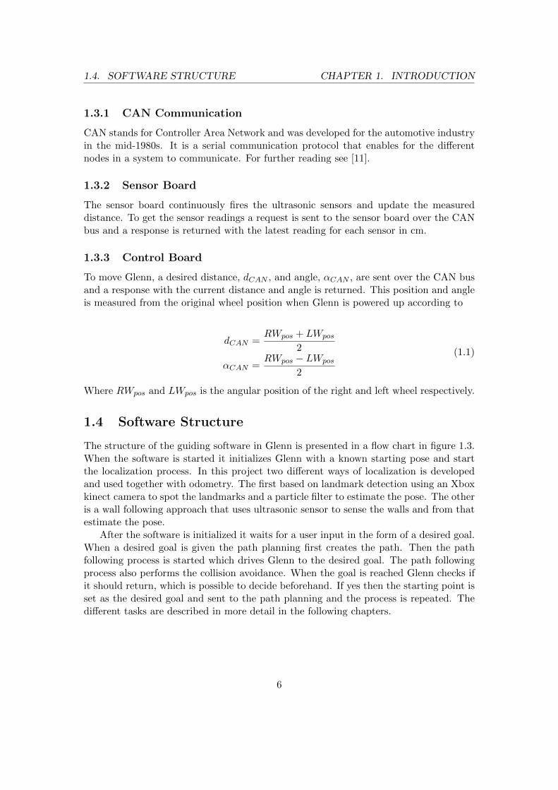
Figure 3.1: The path following algorithm where the crosses are the way points and thedotted arrows indicates which one Glenn drives towards at the given positions

if the ultrasonic sensors senses something getting to close. This solution works to keepGlenn from colliding but it is possible for Glenn to get stuck in front of an obstacle unableto continue. Therefore future improvements is needed in this area to enable Glenn todrive around obstacles. There are many ways to achieve this. For example in [4] sixproximity sensors (IR) is used to adjust the speed and angle to avoid obstacles and in[3] a laser is used to spot the closest point on an obstacle and from this recalculate thenext way point.

12

Chapter 4

Localization

A prerequisite for the autonomous guiding to work is that Glenn can locate in a globalcoordinate system (figure 4.1). To achieve this odometric calculations is used on theinformation about wheel rotation received from Glenn. Odometry is subjected to alocalization error that grows with the distance traveled. To compensate for these er-rors two different ways are implemented. First particle filter localization (PFL) withmeasurements from the kinect camera. Then a wall following algorithm that uses theultrasonic sensors.

4.1 Odometry

Odometry also known as dead reckoning is the use of odometers, sensors that measuresdistance traveled (in this case encoders), to estimate the pose, xk = [xkykθk]

T , of amobile robot at time step k. Where xk and yk is the position of the robot in the globalcoordinate system in figure 4.1 and θk is the angle relative the global X axis. For smallvalues of δθk the pose can be estimated as

xk = xk−1 +

δdk cos(θk−1 + δθk2 )

δdk sin(θk−1 + δθk2 )

δθk

(4.1)

δdk =δrk + δlk

2δθk =

δrk − δlkW

where W is the wheelbase, xk−1 = [xk−1yk−1θk−1]T is the previous pose estimation and

δrk and δlk is the distance traveled by the right and left wheel respectively since thelast time step [7]. The guiding program does not have access to the individual wheeldistances so δrk and δlk instead becomes

13

4.1. ODOMETRY CHAPTER 4. LOCALIZATION

Figure 4.1: The coordinate system of Glenn

δdk = Dwπ(dCAN − d−CAN )

δθk = 2Dwπ(αCAN − α−

CAN )

W

(4.2)

where Dw is the wheel diameter and dCAN and αCAN is from equation 3.2.

4.1.1 Odometric Errors

Because odometry uses the previous pose to estimate the current one errors will ac-cumulate over time. There are two types of odometric errors, systematic errors andnon-systematic errors [14]. Examples of these error sources are:

• Systematic errors

1. unequal wheel diameter, for example caused by unequal air pressure in thewheels.

2. uncertain wheelbase, because the wheels contact the floor over an area not ina single point. Therefore the wheelbase is difficult to measure correct.

14

4.2. KINECT CHAPTER 4. LOCALIZATION

3. misalignment of wheels

• Non-systematic errors

1. uneven floors

2. objects in the way

3. wheel slippage

Non-systematic errors are different each run and can not be predicted beforehand butdo not contribute as much as systematic errors when traveling in a smooth indoor en-vironment. Systematic errors are vehicle specific and easier to predict beforehand andcan thus be compensated for [14]. One widely used procedure to correct systematic odo-metric errors are the UMBmark procedure [15]. The UMBmark procedure corrects theerrors in the wheelbase and the wheel diameter for each wheel respectively. In this casethis is not useful because the guiding program does not have access to the individualwheels. Instead an error correction is added to the pose prediction which becomes

xk = xk−1 +

δdk cos(θk−1 + δθk2 ) + edriftδdk sin(θk) + etransδdk cos(θk)

δdk sin(θk−1 + δθk2 ) + edriftδdk cos(θk) + etransδdk sin(θk)

δθk + erotδθk

(4.3)

where edrift, etrans and erot are derived experimentally (see chapter 5).

4.2 Kinect

The Microsoft Kinect sensor is a low cost RGB camera and depth sensor that was releasedin 2010 [16]. The Kinect camera is used to recognize the landmarks and measure thedistance Lk and azimuth angle αk as shown in figure 4.1. The landmarks are detectedby first creating a threshold image of the kinect RGB image where one color (in thiscase red) is white and everything else is black. Then contours over a certain size isanalyzed as potential landmarks. The different landmarks are identified by letters. Thisprocedure is shown in figure 4.2.

The kinect sensor measures distance to the plane parallel to the sensor where theobject is located as shown in figure 4.3 [16]. This means if a landmark is not in themiddle of the image the distance returned from the kinect is to small. Therefore theazimuth angle αk needs to be taken into account when measuring the distance Lk. αkand Lk becomes

αk =resX/2−XL

FOV/resX

Lk =Zkinectcos(αk)

(4.4)

15

4.2. KINECT CHAPTER 4. LOCALIZATION

Figure 4.2: The RGB image (left) from the kinect and the threshold image (right). Theblue rectangle represent the detected landmark. In the threshold we can see that smallercontours are ignored

Figure 4.3: The kinect camera measures the distance to a plane parallel to the sensor(dashed line)

16

4.3. PARTICLE FILTER CHAPTER 4. LOCALIZATION

where resX is the horizontal resolution of the kinect RGB camera, XL is the x positionof the landmarks center pixel, FOV is the Field Of View for the kinect RGB cameraand Zkinect is the returned depth measurement from the kinect sensor. According to[17] resX = 640 pixels and FOV = 62.7 deg. After some experiments the FOV wasadjusted to 63 deg which gave better results. Figure 4.4 displays the kinect measurementscompared to the real values. This shows a precision for the angle within 0.6 deg and forthe distance within 1 cm up to 2 m. After 2 m the distance error grows but it is stillwithin 3-4 cm.

Figure 4.4: Test of the kinect cameras depth and angle measurements

4.3 Particle Filter

The kinect angle and distance measurements from one landmark is not enough to de-termine the pose of Glenn. Therefore particle filter localization (PFL, also known asMonte Carlo localization [7]) is used. The PFL estimates the pose by keeping multiple”guesses” of the pose called particles and each particle has a weight that signifies theprobability of that particle being the current pose of Glenn. The PFL works in twophases a prediction phase and an update phase [8]. During the prediction phase eachparticle is moved according to the odometry model (equation 4.1) with an added randomnoise to represent the odometric errors. This results in a distribution of particles overan area around the current pose which grows with the distance. When a landmark isdetected the particle filter performs the update phase where the kinect readings is usedto calculate the weight of each particle as

Wi =1

σLe

−δL2i

2σ2L

1

σαe

−δα2i2σ2α (4.5)

which is an adaption from the approach in [8]. δLi and δαi is the difference of the actualkinect readings and the expected kinect readings for particle i according to

17

4.3. PARTICLE FILTER CHAPTER 4. LOCALIZATION

δLi = Lk −√

(xM − xi)2 + (yM − yi)2

δαi = αk − tan−1(yM − yixM − xi

)− θi(4.6)

where xi = (xi,yi,θi) is the pose of particle i and (xM ,yM ) is the position of the spottedlandmark [7]. σL and σα determines which kinect measurement effects the weight mostand are derived experimentally.

After the weights are calculated they are normalized. This results in a pdf (prob-ability density function) of the random pose, X, of Glenn. After that a process calledre-sampling is performed which probabilistically multiplies the particles according totheir weights. This means particles with small weights have a small chance of multiply-ing while particles with high weights have a big chance. In practice this removes theparticles with small weights and multiplying the ones with higher weights. Then theparticle filter is run again from the prediction phase and repeated until a good pose esti-mation can be obtained. To get the final estimate of the pose three ways are suggested,[8]:

• Best particlemax(W )

• Weighted meanx =

∑Wixi

• Robust mean

The best particle solution is simply to take the particle with the highest weight. Thissolution is subjected to discretization errors when the actual pose is not represented bya particle. The weighted mean solution adds all particles multiplied with its respectiveweight. This fails when the pdf is multi-modal, have multiple local maxima. The bestsolution is robust mean which is a combination of the above, the weighted mean is takenin an small area around the best particle [8].

To be able to run the PFL, Glenn needs to stand still. This is because the imageprocessing involved in getting the kinect measurements is not fast enough. If Glenn ismoving the measurements is from an old position when the particle filter calculates theweights resulting in a faulty pose estimate. Instead Glenn stops each time a landmark isdetected. Then two iterations of the filter is performed with re-sampling after which therobust mean is taken as the estimated pose. Glenn standing still results in a problem withthe prediction phase. After the first iteration there are no new movements of Glenn touse for predicting new particles so instead each particle are disturbed randomly aroundits current pose. Figure 4.5 shows the particles after the four steps used. In A theparticles from the prediction phase is shown. B shows the particles left after the firstiteration. C shows the particles after the third iteration where the particles from B wheredisturbed. Then D shows the final step where the robust mean has been calculated. Theblack particle is the actual pose and the red in D is the estimated pose which is difficultto see because it is situated underneath the actual pose.

18

4.3. PARTICLE FILTER CHAPTER 4. LOCALIZATION

Figure 4.5: A: The particles after the prediction phase. B: The particles after the firstiteration. C: The particles after the second iteration. D: The particles and estimated pose(red) after the robust mean has been calculated. The black particle represent the actualpose and the red rectangle is the landmark used

19

4.4. WALL FOLLOWING CHAPTER 4. LOCALIZATION

4.4 Wall Following

As an alternative to the PFL a wall following algorithm is developed. First the map isdivided into zones depending on which side of Glenn the best wall to follow is located.A smooth and straight wall is preferred. Then several measurements from the ultrasonicsensor on that side is recorded together with the estimated pose of Glenn on the axisparallel to the wall. The difference S between the recorded distance to the wall andthe distance it should be depending on the estimated pose is calculated. Then the leastsquare method is used to approximate a line corresponding to the path Glenn actuallytravels related to its estimated path. The angle ϕ between this line and its x-axis thenbecomes the angle error of Glenn. This angle together with the last sensor measurementis then used to update the pose of Glenn, figure 4.6 shows a graphic representation ofthe algorithm.

Figure 4.6: The wall following algorithm

This approach has some limitations. First, a smooth and straight wall is needed, if thewall is to uneven it does not work. This is the case in some parts of the office, herethe pose is just updated with the distance from the wall at regular intervals. This doesnot correct the heading but keeps Glenn away from the wall. Second, the ultrasonicsensor used are not located at the turning axis of Glenn. This results in to large sensorreadings when Glenn is not parallel to the wall. This is solved by limiting the angle ϕ sothat large values has a limited effect. Third, only the position to the side is corrected,so when Glenn approached a corner it could turn to soon or to late. This is solved bystopping before a turn and using the kinect camera to update the distance to the corner.

20

Chapter 5

Result

To see how well Glenn performs, first the localization is tested. Then Glenn is set toperform different guiding tests to see how all the parts work together.

5.1 Localization Results

Two steps where taken to improve the localization. First the systematic errors wherecorrected using equation 4.3 then the PFL and wall following was implemented. Thelocalization tests where performed by leading Glenn by hand along a predefined pathand logging the pose, +, at certain positions, . 20 runs were performed for each setting.In figure 5.1 the localization of Glenn when using uncorrected odomerty is shown. Herewe clearly see the problems with odometry as the uncertainty of the pose grows by thedistance traveled. There is also a big systematic error as seen from the mean error thatdeviates more and more from the path.

Figure 5.1: Localization test using odometry

21

5.1. LOCALIZATION RESULTS CHAPTER 5. RESULT

To correct the systematic errors edrift and etrans where obtained from the meassurementsfrom figure 5.1 according to

edrift =1

n

n∑i=1

Di

Gi

etrans =1

n

n∑i=1

TiGi

(5.1)

Where n = 4 is the first four test positions not including the start position, Di and Tiis the mean deviation from the actual position i in the Y and X direction respectivelyand Gi is the actual distance traveled. To obtain erot an additional test where neededwhere Glenn was standing in a fixed position and turned around its axis and the anglewas logged every 90 degrees. The result of the angle measurements of the uncorrectedodometry is seen in figure 5.2, where the arrow indicates the measurements after a 360degree turn.

Figure 5.2: Angle test using odometry

Here it is also obvious there is a systematic error because the angle measurements is notcentered around the actual angles but concentrated a certain angle away. Also this anglegrows at every step which suggests a systematic error. erot is obtained as

erot =1

m

m∑i=1

RiAi

(5.2)

22

5.1. LOCALIZATION RESULTS CHAPTER 5. RESULT

Where m = 4 represents the test angles, Ri is the mean deviation from the actual angleat angle i and Ai is the actual angle. In figure 5.3 the localization test for the correctedodometry is shown. The localization is clearly improved. The errors still grows withoutbounds with the distance but the systematic errors are reduced. This does not removethe systematic errors and over a large enough distance they would increase more andmore. This will be enough in this case because the pose of Glenn will be updated atregular intervals.

Figure 5.3: Localization test using corrected odometry

Figure 5.4 and 5.5 shows the result of the same test performed with PFL and wallfollowing respectively. Both solutions shows a significant improvement. To decide thetuning parameters, σL and σα, for the PFL first δαi and δLi were set to similar sizeby taking δLi

100 before inserting in to equation 4.5. Then different settings of σL and σαwhere tested. The best localization was found for σL = 0.05 and σα = 0.07.

Figure 5.4: Localization test using PFL

23

5.1. LOCALIZATION RESULTS CHAPTER 5. RESULT

Figure 5.5: Localization test using wall following

To compare the different results the RMSE (Root Mean Square Error) for each positionis plotted in figure 5.6. This clearly shows that PFL and wall following are the mostaccurate methods for positioning. Wall following even shows better results after the 90degree turn. It is also evident that great improvements can be made by calibrating theodometric calculations.

Figure 5.6: RMSE for the positioning. The dotted line marks the 90 degree turn

Localization for an autonomous robot does not only include positioning but also heading.In figure 5.7 the RMSE for the heading at each position is displayed. Here the PFL isnot that much better than only using odometry, it even becomes worse after the 90degree turn performed between the last two positions. The angle errors are small, θ < 5deg, but angle errors effects on the positioning grows with the distance traveled. Sosmall errors can have big effects. The wall following on the other hand does improvethe heading. Here only the last two measurements are of interest because the first three

24

5.2. GUIDING RESULTS CHAPTER 5. RESULT

positions is in a zone with a uneven wall and therefore no heading update are performedhere.

Figure 5.7: RMSE for the heading. The dotted line marks the 90 degree turn

5.2 Guiding Results

When testing the full guiding functionality of Glenn it becomes obvious that the local-ization is not robust enough when using PFL. The path planning with the A* algorithmworks perfectly. Glenn always finds a path when there is a possible one. The path fol-lowing control also works well, if we consider the pose Glenn thinks it has. The problemarises when the estimated pose do not coincide with the real pose, with other words thelocalization. The problem lies with the heading as the results in figure 5.7 indicates. Ifthe heading is wrong after an update phase then Glenn will go in the wrong directionand because it is some meters between the landmarks Glenn will get to close to a walland stop before being able to update the position again. Another problem is that Glennsometimes misses to spot a landmark.

When using wall following the movement of Glenn becomes more jerky because ofthe constant updating of the pose but this approach works much better.

In table 5.1 the results of 10 guiding tests together with how many was successful isdisplayed. Here it is clear that the PFL is not robust enough and that the wall followingworks.

Mode Used Performed Tests Successful Tests Success Rate [%]

Particle Filter 10 5 50

Wall Following 10 10 100Table 5.1: The results of 10 guiding tests for each mode

25

Chapter 6

Conclusion

The result of this project is straight forward. Using a particle filter together with akinect camera greatly improves the positioning of an autonomous robot which agreeswith the results in [7]. The heading on the other hand is not improved as much. Theheading is not explored in [7] so there are no research to compare with. It can not beexcluded that it is possible of improving the PFL to also give a more accurate heading.On the other hand I do not believe that would solve the problem for the guiding. ThePFL developed in this project is not robust enough for an indoor guiding functionalityas can be seen in table 5.1, it worked only 50% of the times. The wall following methodshows a better localization according to figure 5.6 and 5.7, especially when consideringthe heading. The guiding test presented in table 5.1 shows that it works 100% of thetimes. Better localization is not the only reason the guiding works so well. The mainreason is it gets readings and update the position at a much higher frequency. If afterone update the pose is wrong a new update occurs before Glenn has gotten to muchoff course to not be able to continue. This also suggests that the PFL also would workbetter if Glenn could update its pose at a higher frequency through more landmarks,and I believe it would. Still the wall following would be preferred, because Glenn wouldneed to stop at every landmark and would travel very slow which would not be optimalfor guiding visitors.

6.1 Future Work

To make Glenn work as a guiding robot my suggestions is to skip localization withthe kinect camera and instead focus on developing better wall following. Adding moreultrasonic sensors or using a laser for proximity sensing would be an advantage andwould probably result in smoother movements. Also the collision avoidance should beimproved to make Glenn able to go around obstacles and continue following the path.With some more work I believe Glenn could become an awesome office guide.

26

Bibliography

[1] Wolfram Burgard, Armin B. Cremers, Dieter Fox, Dirk Hahnel, Gerhard Lakemey-ery, Dirk Schulz, Walter Steiner, and Sebastian Thrunz, “The Interactive MuseumTour-Guide Robot,” AAAI-98 Proceedings, 1998.

[2] D. S. Mattias Wahde and K. Wolff, “Reliable Long-Term Navigation in IndoorEnvironments,” Recent Advances in Mobile Robotics, 2011.

[3] J. L. Martinez, A. Pozo-Ruz, S . Pedraza and R. Fernhdez, “Object Following andObstacle Avoidance Using a Laser Scanner in the Outdoor Mobile Robot Auriga-α,” Proceedings of the 1998 IEEE/RSJ Intl. Conference on Intelligent Robots andSystems, 1998.

[4] X. Hu, D. Fuentes Alarcon and T. Gustavi, “Sensor-Based Navigation Coordinationfor Mobile Robots,” 42nd IEEE Conference on Decision and Control, 2006.

[5] Margrit Betke and Leonid Gurvits, “Mobile Robot Localization Using Landmarks,”IEEE TRANSACTIONS ON ROBOTICS AND AUTOMATION, VOL. 13, NO. 2,1997.

[6] Kimihiro Okuyama, Tohru Kawasaki, and Valeri Kroumov, “Localization and Posi-tion Correction for Mobile Robot Using Artificial Visual Landmarks,” Proceedings ofthe 2011 International Conference on Advanced Mechatronic Systems, Zhengzhou,China, 2011.

[7] N. Ganganath and H. Leung,“MOBILE ROBOT LOCALIZATION USING ODOM-ETRY AND KINECT SENSOR,” 2012.

[8] Ioannis M. Rekleitis, “A Particle Filter Tutorial for Mobile Robot Localization,”2003.

[9] P. Hiemstra, and A. Nederveen, “Monte Carlo Localization,” 2007.

[10] S. Thrun, D. Fox, W. Burgard, and F. Dellaert, “Robust Monte Carlo Localizationfor Mobile Robots,” 2001.

27

BIBLIOGRAPHY

[11] K. Pazul, “Controller Area Network (CAN) Basics,” Microchip Technology Inc.,Tech. Rep., 1999.

[12] S. Russel, P. Norvig, Artificial Intelligence - A Modern Approach, 2nd ed., 2003.

[13] Microsoft, “Math.Atan2 Method,” 2012. [Online]. Available: http://msdn.microsoft.com/en-us/library/system.math.atan2.aspx

[14] Johann Borenstein and Liqiang Feng, “Maesurement and Correction of System-atic Odometry Errors in Mobile Robots,” IEEE TRANSACTIONS ON ROBOTICSAND AUTOMATION, VOL. 12, NO. 6, 1996.

[15] ——, “UMBmark: A Benchmark Test for Measuring Odometry Errors in MobileRobots ,” SPIE Conference on Mobile Robots, Philadelphia, October 22-26, 1995.

[16] K. Khoshelham, “ACCURACY ANALYSIS OF KINECT DEPTH DATA,” 2011.

[17] ROS.org, 2012. [Online]. Available: http://www.ros.org/wiki/kinect calibration/technical#Focal lengths

28

Appendix A

The Parts of Glenn

• 2 Motor drives, from an existing Aros product.

• 2 Permanent magnet synchronous motors, designed and produced by Aros.

• 1 Control board where the balance control is performed, designed and producedby Aros.

• 1 Gyro sensor, 1 axis, ADXRS610.

• 1 Accelerometer, 2 axis, ADXL203EB.

• 2 Encoders one for each motor, Tamagawa 1024 pulses/rev.

• 6 Devantech SRF01 ultrasonic sensors that measures distance used for collisionavoidance and wall following.

• 1 Sensor board controlling the ultrasonic sensors over a single pin serial interface,designed and produced by Aros.

• 1 Zotac PC with a 1.6 GHz Intel Atom processor and Nvidia graphics equippedwith a touchscreen, speakers and a keyboard.

• 2 Li-Po battery packs, 22.2 V and 6000 mAh.

• 1 Power board for distributing the power.

• 1 PC power board for transforming the voltage for the PC.

• 1 PC with attached keyboard, speakers and touchscreen.

• 1 Xbox 360 Kinect camera to make Glenn able to see.

• 1 USB to CAN converter designed and produced by Aros.

• 1 Candy bowl.

29

Appendix B

A∗ Algorithm

input : Start and Goal Pointoutput: List of points along the closest path

openSet = startPoint ; // The set of points to be tested

closedSet = ∅; // The set of points already tested

g(startPoint) = 0;f(startPoint) = g(startPoint) + ShortestDistance(startPoint,goalPoint);while openSet 6= ∅ do

currentPoint = Point with lowest f;if currentPoint = goalPoint then

return ReconstructPath(cameFrom,goalPoint)endRemove currentPoint from openSet;Add currentPoint to closedSet;foreach neighbourPoint to currentPoint do

if ( neighbourPoint ∈ closedSet) ∨ ( neighbourPoint /∈ map) thencontinue;

endtentativeGScore = g(currentPoint) +ShortestDistance(currentPoint,neighbourPoint);if ( neighbourPoint /∈ openSet) ∨ ( tentativeGScore <g(neighbourPoint)) then

Add neighbourPoint to openSet;cameFrom(neighbourPoint) = currentPoint;g(neighbourPoint) = tentativeGScore;f(neighbourPoint) = g(neighbourPoint) +ShortestDistance(neighbourPoint,goalPoint);

end

end

endfunction ReconstructPath(cameFrom,point)

if cameFrom(point) 6= startPoint thenreturn ReconstructPath(cameFrom,cameFrom(point))

elsereturn point

end

Algorithm 1: A* Algorithm

30