masters thesis: design of an electric servo controlled rudder pedal
TRANSCRIPT

HAN Control and Systems Engineering
Design of an Electric Servo con-trolled Rudder pedal for an air-plane simulatorOptimize the servo controller for the system
A. Damman B.Sc.
Master
Thesis

Design of an Electric Servo controlledRudder pedal for an airplane simulator
Optimize the servo controller for the system
Master Thesis
For the degree of Master in Mechatronics at HAN University of Applied
Science
A. Damman B.Sc.
August 16, 2013
Faculty of Technic and Life Science · HAN University of Applied Science

The work in this thesis was supported by Yaskawa. Their cooperation is hereby gratefullyacknowledged.
Copyright c© Control and Systems EngineeringAll rights reserved.
Summary
A Servo controlled control loading system for a fixed based simulator is converted from hy-draulic to electric. In this thesis is explained how a high performed hydraulic servo system isexchanged for an electrical servo motor via EtherCAT.
The first reason is the advantage in maintenance costs and safety items when using an elec-trical servo motor. The second reason is noise influence on the analog signal to the servocontroller. This is an advantage in comparison to the old situation. The disadvantage is thehigh volume-power-ratio of an electrical servo motor in comparison with a hydraulic servosystem.
To reduce the load torque at the motor side, a gearing is necessary. For selecting the correctgearing, the load inertia is taken into account, that the inertia is lower than 2 times of theselected motor inertia. A backlash free gearbox will improve the results, but is this the bestsolution? The maximum acceleration rate of the specific motor will take effect on the totalacceleration time to reach the maximum speed of the motor. A trapezium test profile iscommonly used, but in our system not useful. A sinusoidal test signal is a useful solution toavoid hitting the hard end stops.
The control loop can be made in several ways, explained are: position, velocity and force(torque) control loop. The best simulated results are obtained by the force (torque) controlloop. However force prediction is a problem in this situation. From a practical point of view,the signal-noise-ratio is a problem for the servo controller certainly in an extreme field ofelectromagnetic compatibility. Best possible grounding and shielding of the power and thesensor cables is a guidance for a reliable signal-noise-ratio.
In this specific arrangement, the signal-noise-ratio is low for the torque sensor, however thevelocity control loop is a sufficient signal. Therefore a control loop based on velocity is thebest practical solution to reduce the jerky effects of the system. An additional reliable torquesensor to assist the actual value is the best improvement. For now the best option is toimplement the servo controller in a digital EtherCAT environment.
The implementation of a synchronized Distributed Clock will improve the results. Somedisturbance in the timing during the validation tests is noticed.
The bandwidth necessary for aircraft simulation (FCS) goes up till 2 Hz or 12.6 rad/s. TheFCS is commonly modeled as a second order system. For good simulation, the cut-off fre-quency of the actuator needs preferable 10 times higher. For an admissible simulation ofhard-end stops, a cut-off frequency of 50 Hz or higher is preferable at the desired position.
Master Thesis A. Damman B.Sc.
ii Summary
The cut-off frequency of the ideal simulated hydraulic actuator (velocity loop) is 5550 rad/sor 883 Hz. The cut-off frequency of the electrical servo system is 14.7 Hz at the maximumvelocity.
The signal-noise-ratio of the torque sensor is very poor. The single ended torque signal doeshave a signal-noise-ratio of 500/18, and this is useless for torque control loop. The differentialsignal has an improved signal-noise-ratio of 500/3. The accuracy is of the attached HBMtorque sensor is 0.2% and the overall accuracy is 0.5%. The disappointing signal-noise-ratioof the torque sensor and the open control loop in cyclic torque mode, makes the decision tochoose for a decent velocity inner loop and a torque (force) outer loop.
The mass and added mass of a human body cannot be accounted very accurate because yousimply do not know anything of the reaction force of the subject in the time domain and thisis far from constant in time domain. The accuracy of the position and velocity encoder is1.9 · 10−7% (within a window of 5 steps at nominal velocity) much higher than the accuracyof the torque level 0.1% of the rated torque. This torque is calculated in the servo pack as aresult of the forward current to the motor. The accuracy of the servo pack torque level is 3%at the pedal side when the gear ratio is applied.
The implemented control loop meets the requirements. A simple second order mass-spring-damper system converts the required force into a velocity. The inner loop is based on velocityand the outer loop is a torque control loop. A graphical presentation is obtained from theresults of the evaluation experiment.
The safety environment in the old hydraulic situation is less sufficient. In the new electricservo drive system, there is full control over the behavior of the pedals. This is satisfactorybetter compared to the hydraulic situation. The safety is grouped in several layers: a hardwarelayer (mechanical end stops), Hardware Base Block (HBB) in the servo pack and a softwareenvironment layer. In the old situation there was only a software environment layer what wasactually taken care of the safety of the subject.
Please don’t hesitate to contact me if you have any further questions: [email protected].
A. Damman B.Sc. Master Thesis
Preface
This document is part of my Master graduation thesis. The idea of doing my thesis onthis subject came after a discussion about maintenance costs of hydraulic systems with mycolleagues F.N. Postema and H. Lindenburg.
I am very grateful that Mr. H. Lindenburg and prof. M. Mulder gave me the possibility toexchange a reliable hydraulic actuator for an unfamiliar technique with electrical servo drivesystem. This has never been done before in our group. The scientific staff in our work teamare not so enthusiastic about electrical servo drive systems in performance respect. Hydraulicservo actuators are excellent in that respect. The high force and small volume relationis very powerful for a wide range of applications. In most cases, a hydraulic servo motorimplementation is not necessary. The choice of a hydraulic servo system over an electricalservo drive system is made because of lack of space. In most cases the dimensions of anelectrical drive system are in conflict with the construction environment.
In high performance point of view, a solution with a high torque motor is the ultimate solution.Due to financial restrictions, it was not possible to implement such a high torque motor forthis first attempt of electrifying the system. In other situations it is preferable to select aservo drive where the inertia of the motor is at least 1/5 of the total load inertia. The systemfeels a little nervous when the inertia of the selected motor is more than five times of theinertia of the load. When using a backlash free gearbox, the high performance can be reachedwith a smaller size motor. To optimize the system, I did select the smallest motor, so thatspeed and torque both can be reached continuously. The challenge is to tune the system ina way that both aspects can be reached. And most important in all situations the systemshould "feel" smooth like a real airplane. Another challenge is to tune the system for a genericconfigurable airplane.
The first reason to write this report is of course a report of my master thesis in control andsystem engineering. The second less important reason is to order the steps that are followedto develop the rudder pedals system and this documentation is a good start for furtherimprovement for this system. The project oriented information is moved to the appendixas much as possible. To understand these information it is recommended to read the thesisreport first.
Master Thesis A. Damman B.Sc.

iv Preface
A. Damman B.Sc. Master Thesis
Acknowledgments
I would like to thank my HAN University of Applied Sciences (HAN University) supervisorir. P.A.C. Ypma at the department CSE for his assistance during the writing of this thesis.Also his general and global knowledge to setup this master thesis. His knowledge about LATEXto make this document is really an eye opener for now and the future. I can recommendeveryone using LATEX . For more information read [1]. The next person, I would like to thankis my company supervisor from the department CS at the TU Delft dr.ir. M.M. van Paassenfor his assistance during the writing of this thesis, his control knowledge and the knowledgeabout the set up of the specifications [2].
My colleague ir. F.N. Postema was very helpful with assisting me selecting and installing theservo system. His enormous experience in building servo systems helped detailing the systemstep by step.
Two people who had made this thesis project possible in financial and administrating respectsare Prof.dr.ir. M. Mulder and ing. H. Lindenburg. Ing. A. Muis and ing. E.H.H. Thung madethe communication possible to get the drive system running via Linux Etherlab.
Last but not least, my girlfriend G.M. Fontijn. I really appreciate her incredible supportduring my thesis. She made a lot of improvements on the first draft of this thesis. I love youGyselle, it’s you and me together forever and never apart, maybe in distance, but never inheart.
Arnhem, HAN University of Applied Science A. Damman B.Sc.August 16, 2013
Master Thesis A. Damman B.Sc.

vi Acknowledgments
A. Damman B.Sc. Master Thesis

Glossary
List of Acronyms
CSE Control and Systems Engineering
TU Delft Technical University of Delft
TU Twente Technical University of Twente
HAN University HAN University of Applied Sciences
DUECA Delft University Environment for Communication and Activation
LQR Linear-Quadratic Regulator
EtherCAT Ethernet for Control Automation Technology
LaTeX Leslie Lamport TEX typesetting language
FCS Flight Control System
HBM Hottinger Baldwin Messtechnik
EtherLab open source toolkit for real time Linux using EtherCAT-Technology
IgH Ingenieurgemeinschaft Hydraulik
AC Alternating Current
DC Direct Current
EMF Electromagnetic Field
EMI Electromagnetic Interference
EMC Electromagnetic Compatibility
CANopen open Controller Area Network
HF High Frequency
Master Thesis A. Damman B.Sc.

viii Glossary
EMP Electromagnetic Pulse
PDO Process Data Object
SDO Service Data Object
Linux open source operating system
SGDV electric servo amplifier of brand Yaskawa
CS Control and Simulation department at the TU
NASA National Aeronautics and Space Administration
FBW Fly-By-Wire
MIL United States Military Standard
Compax3 electic servo controller type of brand Parker
RS422 Differential signaling protocol
AISI American Iron and Steel Institute
DAQ Data Acquisition
NEN NEderlandse Norm
SGMGV electric servo motor type of brand Yaskawa
SGMCS electric servo motor type of brand Yaskawa
RPM Revolutions Per Minute
RPS Revolutions Per Second
RMS Root Mean Square
FFT Fast Fourier Transfer function
Twincat Communication protocol which correspond with EtherCAT
A/D Analog to Digital Conversion
D/A Digital to Analog Conversion
IEEE Institute of Electrical and Electronics Engineers
UDP User Datagram Protocol
IP Internet Protocol
I/O Input / Output
MAC Media Access Control
IEC International Engineering Consortium
A. Damman B.Sc. Master Thesis

ix
FTP File Transfer Protocol
FPGA Field-Programmable Gate Array
ASIC Application-Specific Integrated Circuit
Sercos SErial Real-time COmmunication System
OSI Open Systems Interconnection
List of Symbols
Abbreviations
α acceleration rate [rad/s2]
∆p pressure difference over piston [N/m2]
δ skin depth is the depth below the surface of the conductor at which the currentdensity has fallen to 1/e of JS [m]
η efficiency [-]
µ absolute magnetic permeability of the conductor [Wb/(A · m)]
ω angular frequency of current [rad/s]
ω0
√
4·E·Ap
meffp·Sp[-]
ωm motor speed [rad/s]
ρr resistivity of the conductor [Ω· m]
ζe damping of the electric servo [-]
ζh damping of the hydraulic servo [-]
Ap area of the piston [m2]
bsim effective damping of the simulated system [Ns/m]
csim effective stiffness of the simulated system [N/m]
ct coefficient of rigid mechanical construction of the system [Nm/rad]
d depth [m]
E bulk modulus of the oil [N/m]
EMFb back EMF [mV/rpm/phase]
Fa force connection rod [N]
Fb force hydraulic actuator [N]
Fpd force at pedal side [N]
fres resonance frequency of the electric servo drive system [Hz]
g standard gravity [m/s2]
i1 gear ratio of the first force lever of at the rudder pedals [-]
i2 gear ratio of the second force lever of at the rudder pedals [-]
iT total gear ratio of the force levers of at the rudder pedals [-]
Master Thesis A. Damman B.Sc.
x Glossary
Ii motor instantaneous peak current RMS [A]
imax maximum value electrical input signal [A]
Ir motor rated current [A]
JS current density at the surface [A · m2]
JAC AC current density [A · m2]
Jl load inertia of the electric servo drive system [kg ·m2]
Jm motor inertia of the electric servo drive system [kg ·m2]
Jr reflected load inertia [kg ·m2]
Jt total inertia of the electric servo drive system [kg ·m2]
Kv specific velocity gain of the servo [-]
K1 = qmax/imax gain between electrical input signal and oil flow [-]
K2 =(
2·ζω0
− Lc·meffp
Ap2
)
· Ap
K1gain of acceleration feedback of the servo [-]
K3 = Kv ·Ap
K1gain between physical input and the electrical servo input [-]
Kb back EMF constants [V/(rad/s)]
Kff feedforward gain [-]
Km motor torque constants [Nm/A]
Lc leakage coefficient [m5/Ns]
Lhp inductance [mH/phase]
Lh motor inductance constants [H]
li2Lever arm length from Fa to the second pedal shaft axis [m]
li2Lever arm length from Fa to the second pedal shaft axis [m]
meffp effective mass at the piston [kg]
Momd mass above measurement device [kg]
msim effective mass of the simulated system [kg]
Np number of poles or phase [-]
Pr motor power rated output [kW]
ql oil flow due to leakage [m3/s]
qc oil flow due to compression [m3/s]
qmax maximum oil flow generated by the servo [m3/s]
qs oil flow generated by the hydraulic servo [m3/s]
qxp oil flow due to piston movement [m3/s]
R motor winding resistance [Ohm]
Rp resistance per phase [Ohm/phase]
Rg gear ratio of the control device [-]
Ri inertia ratio [-]
RAa motor rated angular acceleration [rad/s2]
RPr motor rated power rate [kW/s]
sActuatorMax maximal displacement of the hydraulic actuator [m]
Sm motor maximal speed [RPM]
Sp stroke of the piston [m]
A. Damman B.Sc. Master Thesis

xi
sRudderMax maximal displacement of the pedal [m]
Sr motor rated speed [RPM]
T2 Torque at the pedal shaft [Nm]
T2 Torque at the pedal shaft [Nm]
Ta acceleration torque [Nm]
Ti motor instantaneous peak torque [Nm]
Tr motor rated torque [Nm]
Ts settling time [s]
Va supply voltage to the DC motor [VDC]
Vbs supply voltage to the brushless DC motor [DC Volt]
Vclass voltage rated class between two phases RMS [VAC]
Xc displacement of control device [m]
xd desired position [m]
’B’ breakout force [’lbs’]
’M’ force at maximum travel [’lbs’]
’X’ maximum travel [’in’]
Master Thesis A. Damman B.Sc.

xii Glossary
A. Damman B.Sc. Master Thesis
Table of Contents
Summary i
Preface iii
Acknowledgments v
Glossary vii
List of Acronyms . . . . . . . . . . . . . . . . . . . . . . . . . . . . . . . . . . . viiList of Symbols . . . . . . . . . . . . . . . . . . . . . . . . . . . . . . . . . . . ix
1 Introduction 11-1 Background Rudder pedals HMI-Laboratory . . . . . . . . . . . . . . . . . . . . 11-2 Process Description Rudder pedals Setup . . . . . . . . . . . . . . . . . . . . . . 1
1-2-1 Objectives . . . . . . . . . . . . . . . . . . . . . . . . . . . . . . . . . . 21-3 Sizing and Design . . . . . . . . . . . . . . . . . . . . . . . . . . . . . . . . . . 31-4 Approach . . . . . . . . . . . . . . . . . . . . . . . . . . . . . . . . . . . . . . . 41-5 Chapter summary . . . . . . . . . . . . . . . . . . . . . . . . . . . . . . . . . . 5
2 Flight Control System 7
2-1 Aircraft Flight Control System . . . . . . . . . . . . . . . . . . . . . . . . . . . 72-1-1 Primary controls . . . . . . . . . . . . . . . . . . . . . . . . . . . . . . . 72-1-2 Secondary controls . . . . . . . . . . . . . . . . . . . . . . . . . . . . . 8
2-2 Mechanical Flight Control System . . . . . . . . . . . . . . . . . . . . . . . . . 82-3 Hydraulic-mechanical Flight Control System . . . . . . . . . . . . . . . . . . . . 82-4 Fly-by-wire control systems . . . . . . . . . . . . . . . . . . . . . . . . . . . . . 102-5 Comparison the rudder performance of 6 different vehicles . . . . . . . . . . . . 10
2-6 Dynamic Force/Feel System Considerations . . . . . . . . . . . . . . . . . . . . 13
2-7 Other Dynamic Effect acting on Force/Feel System . . . . . . . . . . . . . . . . 14
2-8 Chapter summary . . . . . . . . . . . . . . . . . . . . . . . . . . . . . . . . . . 15
Master Thesis A. Damman B.Sc.
xiv Table of Contents
3 Performed Solution 17
3-1 Performed Solution . . . . . . . . . . . . . . . . . . . . . . . . . . . . . . . . . 173-2 Mechanical Identification . . . . . . . . . . . . . . . . . . . . . . . . . . . . . . 173-3 Inertia of the drive system . . . . . . . . . . . . . . . . . . . . . . . . . . . . . . 20
3-3-1 Mechanical analyses . . . . . . . . . . . . . . . . . . . . . . . . . . . . . 22
3-3-2 Acceleration torque . . . . . . . . . . . . . . . . . . . . . . . . . . . . . 23
3-4 Chapter summary . . . . . . . . . . . . . . . . . . . . . . . . . . . . . . . . . . 23
4 Performance of the analytical models 25
4-1 Hydraulic Servo Simulation . . . . . . . . . . . . . . . . . . . . . . . . . . . . . 27
4-2 Comparison of Position, Velocity and Force loop based Control Loading Architectures 28
4-2-1 Basics for Control Loading Simulation . . . . . . . . . . . . . . . . . . . 28
4-2-2 Subsystems . . . . . . . . . . . . . . . . . . . . . . . . . . . . . . . . . 28
4-3 Hydraulic Servo Identification . . . . . . . . . . . . . . . . . . . . . . . . . . . . 32
4-3-1 Analytical performance evaluation . . . . . . . . . . . . . . . . . . . . . 35
4-3-2 Choice Type of Control Loop . . . . . . . . . . . . . . . . . . . . . . . . 37
4-4 Electrical Servo Simulation . . . . . . . . . . . . . . . . . . . . . . . . . . . . . 374-4-1 Matlab/Simulink model . . . . . . . . . . . . . . . . . . . . . . . . . . . 38
4-4-2 Feedforward value for simulation . . . . . . . . . . . . . . . . . . . . . . 414-4-3 Simplified synchronous brushless servomotor model . . . . . . . . . . . . 47
4-4-4 Simulated Acceleration Bandwidth . . . . . . . . . . . . . . . . . . . . . 484-5 Comparison Hydraulic and Electrical Servo Simulation . . . . . . . . . . . . . . . 50
4-6 Implementation possibilities for the selected servo drive . . . . . . . . . . . . . . 52
4-7 Chapter summary . . . . . . . . . . . . . . . . . . . . . . . . . . . . . . . . . . 52
5 Performance evaluation experiment 53
5-1 Rudder pedal Impression . . . . . . . . . . . . . . . . . . . . . . . . . . . . . . 53
5-2 Results of the velocity control loop . . . . . . . . . . . . . . . . . . . . . . . . . 56
5-2-1 Start stop input response . . . . . . . . . . . . . . . . . . . . . . . . . . 57
5-2-2 Sinusoidal cyclic signal . . . . . . . . . . . . . . . . . . . . . . . . . . . 58
5-2-3 Noise on torque signal . . . . . . . . . . . . . . . . . . . . . . . . . . . . 60
5-2-4 Added mass on rudder pedal . . . . . . . . . . . . . . . . . . . . . . . . 61
5-2-5 Bode plot velocity control loop . . . . . . . . . . . . . . . . . . . . . . . 64
5-3 Chapter summary . . . . . . . . . . . . . . . . . . . . . . . . . . . . . . . . . . 68
6 Discussion 69
6-1 Discussion . . . . . . . . . . . . . . . . . . . . . . . . . . . . . . . . . . . . . . 69
7 Conclusions 71
7-1 Conclusions . . . . . . . . . . . . . . . . . . . . . . . . . . . . . . . . . . . . . 71
A. Damman B.Sc. Master Thesis
Table of Contents xv
A Alternative Solutions 73A-1 Alternative Solution 1 . . . . . . . . . . . . . . . . . . . . . . . . . . . . . . . . 73
A-1-1 Mechanical solution . . . . . . . . . . . . . . . . . . . . . . . . . . . . . 74A-2 Alternative Solution 2 . . . . . . . . . . . . . . . . . . . . . . . . . . . . . . . . 75A-3 Alternative Solution 3 . . . . . . . . . . . . . . . . . . . . . . . . . . . . . . . . 76A-4 Alternative Solution 4 . . . . . . . . . . . . . . . . . . . . . . . . . . . . . . . . 76A-5 Cost Analysis . . . . . . . . . . . . . . . . . . . . . . . . . . . . . . . . . . . . 78A-6 Compare 4 Alternative Solutions . . . . . . . . . . . . . . . . . . . . . . . . . . 79
A-6-1 Energy Balance . . . . . . . . . . . . . . . . . . . . . . . . . . . . . . . 79A-6-2 Supposed Solution . . . . . . . . . . . . . . . . . . . . . . . . . . . . . . 79
B Installation Yaskawa Servo Drive 81B-1 Overview Components . . . . . . . . . . . . . . . . . . . . . . . . . . . . . . . . 82B-2 Overview Wiring . . . . . . . . . . . . . . . . . . . . . . . . . . . . . . . . . . . 85B-3 EtherCAT State flow . . . . . . . . . . . . . . . . . . . . . . . . . . . . . . . . 86B-4 Yaskawa Drive State flow . . . . . . . . . . . . . . . . . . . . . . . . . . . . . . 87B-5 Modes of operation SGDV servopack . . . . . . . . . . . . . . . . . . . . . . . . 87
B-5-1 Profile Position mode . . . . . . . . . . . . . . . . . . . . . . . . . . . . 88B-5-2 Interpolated Position mode . . . . . . . . . . . . . . . . . . . . . . . . . 89B-5-3 Cyclic Synchronous Position mode . . . . . . . . . . . . . . . . . . . . . 89B-5-4 Homing mode . . . . . . . . . . . . . . . . . . . . . . . . . . . . . . . . 90B-5-5 Profile Velocity mode . . . . . . . . . . . . . . . . . . . . . . . . . . . . 90B-5-6 Cyclic Synchronous Velocity mode . . . . . . . . . . . . . . . . . . . . . 91B-5-7 Torque Profile mode . . . . . . . . . . . . . . . . . . . . . . . . . . . . . 91B-5-8 Cyclic Synchronous Torque mode . . . . . . . . . . . . . . . . . . . . . . 92
C Practical Implementation 93
C-1 EMC . . . . . . . . . . . . . . . . . . . . . . . . . . . . . . . . . . . . . . . . . 93C-1-1 Coupling mechanisms . . . . . . . . . . . . . . . . . . . . . . . . . . . . 94C-1-2 EMC control . . . . . . . . . . . . . . . . . . . . . . . . . . . . . . . . . 95
C-2 Skin effect . . . . . . . . . . . . . . . . . . . . . . . . . . . . . . . . . . . . . . 96C-3 Results Signal-Noise-Ratio after alleviation Skin effect . . . . . . . . . . . . . . . 98C-4 Data Acquisition . . . . . . . . . . . . . . . . . . . . . . . . . . . . . . . . . . . 100
C-4-1 Oversampling factor . . . . . . . . . . . . . . . . . . . . . . . . . . . . . 100C-5 EtherCAT Implementation . . . . . . . . . . . . . . . . . . . . . . . . . . . . . 101
C-5-1 CANopen over Ethernet (CoE) in the Yaskawa drive . . . . . . . . . . . 105
C-5-2 Linux Etherlab Communication . . . . . . . . . . . . . . . . . . . . . . . 105C-6 CANopen . . . . . . . . . . . . . . . . . . . . . . . . . . . . . . . . . . . . . . 106
C-6-1 Service Data Object (SDO) protocol . . . . . . . . . . . . . . . . . . . . 108
C-6-2 Process Data Object (PDO) protocol . . . . . . . . . . . . . . . . . . . 108
C-7 Safety Rudder Pedal System . . . . . . . . . . . . . . . . . . . . . . . . . . . . 109C-7-1 Hardware layer . . . . . . . . . . . . . . . . . . . . . . . . . . . . . . . . 109C-7-2 Servo pack layer . . . . . . . . . . . . . . . . . . . . . . . . . . . . . . . 109C-7-3 Software environment layer . . . . . . . . . . . . . . . . . . . . . . . . . 109
Master Thesis A. Damman B.Sc.

xvi Table of Contents
D Calibration 111
D-1 Calibration setup torque transducer . . . . . . . . . . . . . . . . . . . . . . . . . 111
D-2 Calibration torque transducer . . . . . . . . . . . . . . . . . . . . . . . . . . . . 113
Bibliography 115
A. Damman B.Sc. Master Thesis
Chapter 1
Introduction
1-1 Background Rudder pedals HMI-Laboratory
When flying an aircraft, the feel of the rudder pedals provides feedback to the pilot aboutthe yaw state of the aircraft. In a flight simulator this feeling needs to be simulated by thecontrol loading device. The simulators at the Control and Simulation division are equippedwith a hydraulic control loader.
At this moment a hydraulic driven controlled rudder system is installed in the research simu-lator Human Machine Interface Laboratory at the Delft University of Technology. The reasonwhy this configuration does not fulfill the requirements at this moment, is the many man-hours to keep the system running. In maintenance respect this is not acceptable. The bigadvantage for a hydraulic driven actuator is the compact building method, the force/volumeratio for hydraulic is excellent. However it could be done electrical. This is the opinionof some colleagues working at the Faculty Aerospace Engineering, department Control andSystems.
The already installed electric servo driven motors for the side stick and also for the helicoptercontrol do have an excellent performance. This was installed by the company Fokker ControlSystems nowadays known as Moog Netherlands. To design a robust servo controller is acomplicated task and a great challenge for a graduation project.
It is not an ordinary system with a fixed set-point for position or velocity, because the systemshould behave the same as in an airplane. Also the parameters of the mass-spring-dampersystem of a certain airplane are adjustable for simulation. The difficult aspect of this controlmodel is the large operating bandwidth without oscillations.
1-2 Process Description Rudder pedals Setup
In our HMI-laboratory, there is a setup for a generic airplane simulator with side stick on theright hand side. For the rudder pedals on the right hand side, an used Fokker 50 rudder is
Master Thesis A. Damman B.Sc.
2 Introduction
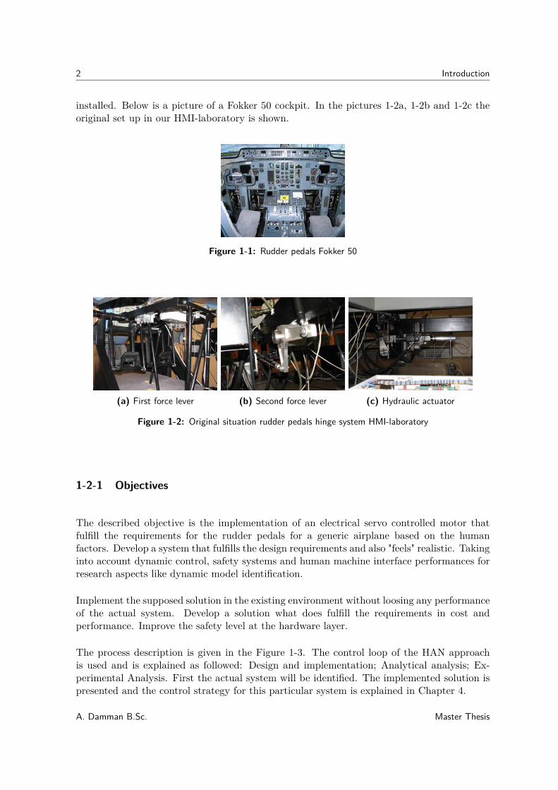
installed. Below is a picture of a Fokker 50 cockpit. In the pictures 1-2a, 1-2b and 1-2c theoriginal set up in our HMI-laboratory is shown.
Figure 1-1: Rudder pedals Fokker 50
(a) First force lever (b) Second force lever (c) Hydraulic actuator
Figure 1-2: Original situation rudder pedals hinge system HMI-laboratory
1-2-1 Objectives
The described objective is the implementation of an electrical servo controlled motor thatfulfill the requirements for the rudder pedals for a generic airplane based on the humanfactors. Develop a system that fulfills the design requirements and also "feels" realistic. Takinginto account dynamic control, safety systems and human machine interface performances forresearch aspects like dynamic model identification.
Implement the supposed solution in the existing environment without loosing any performanceof the actual system. Develop a solution what does fulfill the requirements in cost andperformance. Improve the safety level at the hardware layer.
The process description is given in the Figure 1-3. The control loop of the HAN approachis used and is explained as followed: Design and implementation; Analytical analysis; Ex-perimental Analysis. First the actual system will be identified. The implemented solution ispresented and the control strategy for this particular system is explained in Chapter 4.
A. Damman B.Sc. Master Thesis

1-3 Sizing and Design 3
Figure 1-3: Control loop HAN
Several objectives have been defined for this graduation project:
• Literature study regarding the produced forces on the rudder. The limitations of theseforces must be investigated together with the characteristics of speed of the movements.
• Human factor aspects only for the sizing of the control range.
• Research on airplane rudder pedals like damping and delay.
• Literature study regarding the defined controller. A closer look at the past might revealsimilar problems and possible solutions to implement the controller well.
• Implementing developed controllers in existing hardware at HMI-laboratory to validatethe conclusions drawn in this project.
• Develop a solution what does fulfill the requirements in cost and performance.
• Select the best option in consultation with the stakeholder.
• Comparison of the hydraulic system and electric system in bandwidth aspect.
• Develop a maintenance free system.
1-3 Sizing and Design
Some considerations for sizing and design of control loading devices are made by M.M. vanPaassen, January 13, 2011. The units in aviation is normally expressed in US imperial units,therefore these imperial units are converted to metric units. The original literature quantitiesare expressed in US imperial units.
The following considerations need to be taken into account:
• Maximum force/moment level exerted by human. Pedals 150 lbf ≈ 667.23 N [3].
• Travel, Pedals 4 inches (measured from neutral, total travel 8 inches) ≈ 100 mm [3].
• Velocity, Max 2 Hz sinusoidal cycling at maximum travel of 4 inches. For a pedal; (2 ·2 · π) · 4 (in) ≈ 50 (in/s) ≈ 1.3 m/s.
Master Thesis A. Damman B.Sc.
4 Introduction
• Position bandwidth, When the simulator is configured as a position servo (simulatinghard stops etc.), the maintain bandwidth is preferably 50 Hz or higher. Bandwidthshould be at least 25 Hz.
• Force/moment from bandwidth, necessary for simulating hard stops. Consider effectivemass of the device and add effective limb mass (some guesses: arm side stick roll 1 kg,arm side stick pitch 4 kg, arms column pitch 8 kg, arms column roll 3 kg, legs pedals15 kg). Consider a ramp and hold input signal with half of the maximum velocity, andfeed to a 2nd order system, ζe = 0.7 , ωn as per the desired bandwidth. Calculatethe acceleration at the start of the hold phase from that simulation (sufficient ramp tohave achieved a constant velocity) and multiply by effective mass + limb mass to obtainrequired torque/force levels.
These particular values are obtained by keeping the NASA report [3] about the force/feelcharacteristics in mind. These conservative assumptions are taken to avoid possible com-pliance during the project that decrease the performance of the rudder pedal system. Therequired characteristic for the velocity is calculated for 2 Hz sinusoidal cycling at maximumtravel. For example in an extreme situation, a human person can follow a 1 Hz cycling sig-nal what is demanded on a sidestick. To follow such a signal by foot is not a very realisticsituation.
1-4 Approach
The purpose of this thesis report is for two reasons. The first and most important goal is todocument the scientific thesis information and the second reason is more relevant for furtherimprovement in the future and report practical obstructions during the thesis process. Thepractical relevant implementation is moved to the appendices.
To understand the control challenge of the rudder system, some basic information is required.To tackle the control challenge, it is necessary to get a scope in a very large aspect to avoiddifficulties during the engineering process. The performance of a generic rudder pedal isinvestigated especially for the Flight Control System.
The design specifications are set up and several options are developed to make the rightdecision. In total 4 alternative solutions are checked to make a decision and can be foundin the Appendix A. The decision for the performed solution is based on several aspects like:costs, energy loss and performance.
An analytical performance check is executed before ordering the hardware. The accelerationrate is the most important item to predict the performance in comparison with a originalhydraulic actuator.
After designing and ordering the parts, the parts are assembled properly to get the systemup and running. This operation action of the motor and controller is made in 3 steps. Firstlets operate the motor in Windows mode, later in Linux mode and finally in the DUECAmode via EtherCAT. The second step was not easy due to different software versions insidethe controller of Yaskawa.
A. Damman B.Sc. Master Thesis
1-5 Chapter summary 5
Safety items are taken into account and are inside the controller on hardwired base block likeproximity switches. Maximum torque rate, maximum velocity rate and limited positioningare also in the controller. In software there is also a limited range for these parameters toavoid emergency stops.
A performance evaluation test is executed to compare the analytical model with the realizedinstallation.
At the end of the project, there is solved some minor difficulties concerning the adjustmentof the rudder pedals in length for the well-known 95 percentile indicated human. Some EMCcomplications are solved to assure the robustness of the system and the quality of the acquiredsignal data.
The installation of an inclination transducer is used for correcting the adjustment range.The final step to use the system is the implementation into the DUECA environment. DelftUniversity Environment for Communication and Activation (DUECA) is a middle layer real-time software package, developed in house by dr.ir. M.M. van Paassen. This software packagemakes it relatively easy to stream data into channels and hardware modules.
1-5 Chapter summary
Hydraulic control loading has to be changed by an electric servo controller without any loss onthe performance of the bandwidth. A bandwidth check of the hydraulic model is performedto identify the bandwidth of the hydraulic actuator. The HAN approach is followed duringthis project. Design an electrical drive system what can meet the requirements.
• displacement 100 mm.
• velocity 1.3 m/s.
• force 667 N.
• 2 Hz sinusoidal cycling at desired velocity and desired displacement, ζ = 0.7.
• hard-end stop simulation: start-up ramp to stationary velocity of 0.5 times the minimalvelocity and stop immediately.
• The obtained bandwidth should be at 50 Hz or at least 25 Hz.
Additional project related information is available in the appendix for further improvementin the near future.
Master Thesis A. Damman B.Sc.

6 Introduction
A. Damman B.Sc. Master Thesis
Chapter 2
Flight Control System
2-1 Aircraft Flight Control System
Aircraft flight control systems are classified as primary and secondary. The primary controlsystems consist of those that are required to safely control an airplane during flight. These in-clude the ailerons, elevator (or stabilizer) and rudder. Secondary control systems improve theperformance characteristics of the airplane, or relieve the pilot of excessive control forces.[4]Examples of secondary control systems are wing flaps and trim systems.
2-1-1 Primary controls
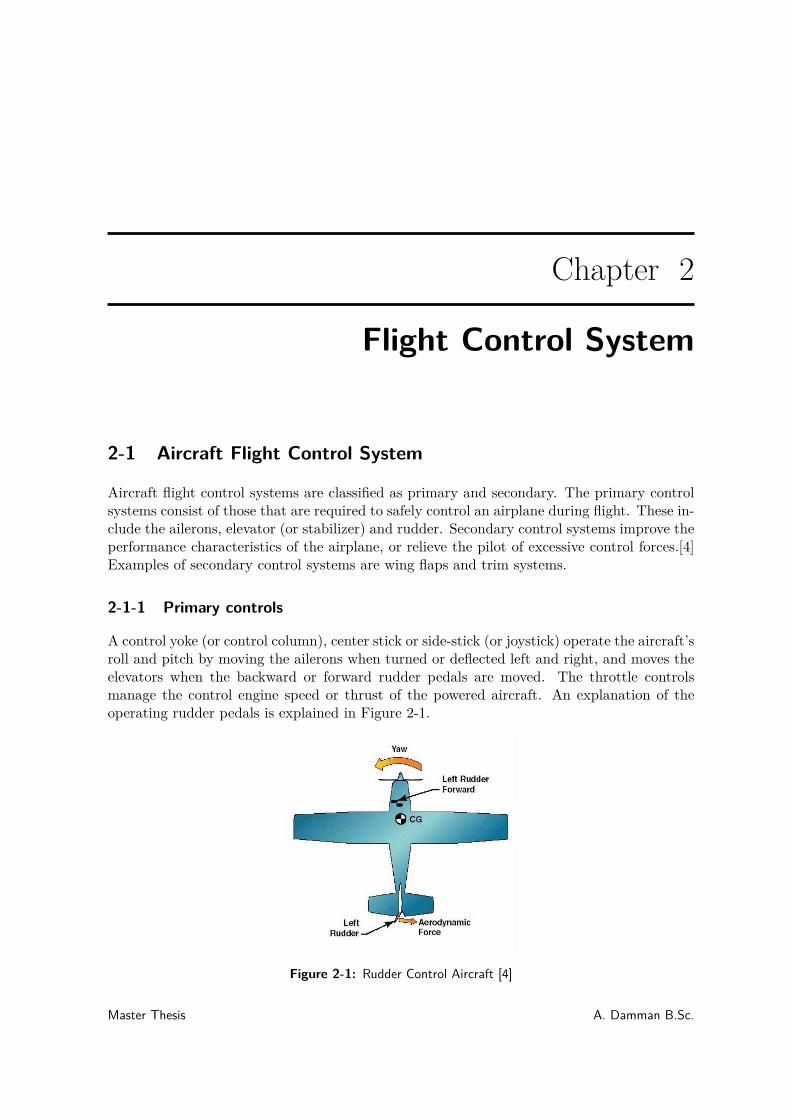
A control yoke (or control column), center stick or side-stick (or joystick) operate the aircraft’sroll and pitch by moving the ailerons when turned or deflected left and right, and moves theelevators when the backward or forward rudder pedals are moved. The throttle controlsmanage the control engine speed or thrust of the powered aircraft. An explanation of theoperating rudder pedals is explained in Figure 2-1.
Figure 2-1: Rudder Control Aircraft [4]
Master Thesis A. Damman B.Sc.
8 Flight Control System
2-1-2 Secondary controls
In addition to the primary flight controls for roll, pitch and yaw, there are often secondarycontrols available to give the pilot a more refined control over the aircraft or to ease theworkload. The most commonly available control is a wheel or other device to control theelevator trim, so that the pilot does not have to maintain constant backward or forwardpressure to hold a specific pitch attitude. Many aircrafts have wing flaps controlled by aswitch or a mechanical lever. In some cases they are fully automatically computer controlled,which alter the shape of the wing for improved control at the slower speed used for take-off and landing. Other secondary flight control systems may be available, including slats,spoilers, air brakes and variable-sweep wings.
2-2 Mechanical Flight Control System
Mechanical or manually operated flight control systems are the most basic methods of con-trolling an aircraft. They were used in older aircrafts and are currently used in small aircraftswhere the aerodynamic forces are not excessive.
A manual flight control system uses a collection of mechanical parts such as push rods, tensioncables, pulleys, counterweights, and sometimes chains to transmit the forces applied to thecockpit controls directly to the control surfaces. Turnbuckles are often used to adjust controlcable tension.
Increases in the control surface area, required by large aircraft or higher loads caused by highairspeed in small aircraft, lead to a large increase in the forces needed to move them. Con-sequently complicated mechanical gearing arrangements were developed to extract maximummechanical advantage in order to reduce the forces required from the pilots. This arrangementcan be found on bigger or higher performance propeller aircrafts such as the Fokker 50.
2-3 Hydraulic-mechanical Flight Control System
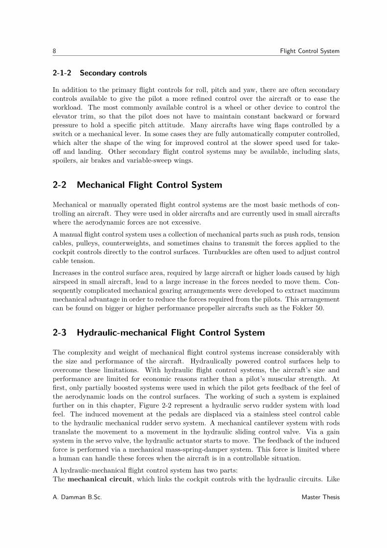
The complexity and weight of mechanical flight control systems increase considerably withthe size and performance of the aircraft. Hydraulically powered control surfaces help toovercome these limitations. With hydraulic flight control systems, the aircraft’s size andperformance are limited for economic reasons rather than a pilot’s muscular strength. Atfirst, only partially boosted systems were used in which the pilot gets feedback of the feel ofthe aerodynamic loads on the control surfaces. The working of such a system is explainedfurther on in this chapter, Figure 2-2 represent a hydraulic servo rudder system with loadfeel. The induced movement at the pedals are displaced via a stainless steel control cableto the hydraulic mechanical rudder servo system. A mechanical cantilever system with rodstranslate the movement to a movement in the hydraulic sliding control valve. Via a gainsystem in the servo valve, the hydraulic actuator starts to move. The feedback of the inducedforce is performed via a mechanical mass-spring-damper system. This force is limited wherea human can handle these forces when the aircraft is in a controllable situation.
A hydraulic-mechanical flight control system has two parts:The mechanical circuit, which links the cockpit controls with the hydraulic circuits. Like
A. Damman B.Sc. Master Thesis
2-3 Hydraulic-mechanical Flight Control System 9
the mechanical flight control system, it consists of rods, cables, pulleys, and sometimes chains.The hydraulic circuit, which has hydraulic pumps, reservoirs, filters, pipes, valves and ac-tuators. The actuators are powered by the hydraulic pressure generated by the pumps in thehydraulic circuit. The actuators convert hydraulic pressure into control surface movements.The electro-hydraulic servo valves control the movement of the actuators.
The pilot’s movement of a control causes the mechanical circuit to open the matching servovalve in the hydraulic circuit. The hydraulic circuit powers the actuators which then move thecontrol surfaces. As the actuator moves, the servo valve is closed by a mechanical feedbacklinkage.
With purely mechanical flight control systems, the aerodynamic forces on the control surfacesare transmitted through the mechanisms and are felt directly by the pilot. With hydraulicmechanical flight control systems, however, the load on the surfaces cannot be felt and there isa risk of over stressing the aircraft through excessive control surface movement. To overcomethis problem, artificial feel systems can be used.
Figure 2-2: Hydraulic Servo Rudder Control Aircraft [5]
Master Thesis A. Damman B.Sc.
10 Flight Control System
2-4 Fly-by-wire control systems
A fly-by-wire (FBW) system replaces the manual flight control of an aircraft with an electronicinterface. The movements of flight controls are converted into electronic signals transmittedby wires (hence the fly-by-wire term), and flight control computers determine how to movethe actuators at each control surface to provide the expected response. Commands from thecomputers are also input without the pilot’s knowledge to stabilize the aircraft and performother tasks. Electronics for aircraft flight control systems are part of the field known asavionics.
2-5 Comparison the rudder performance of 6 different vehicles
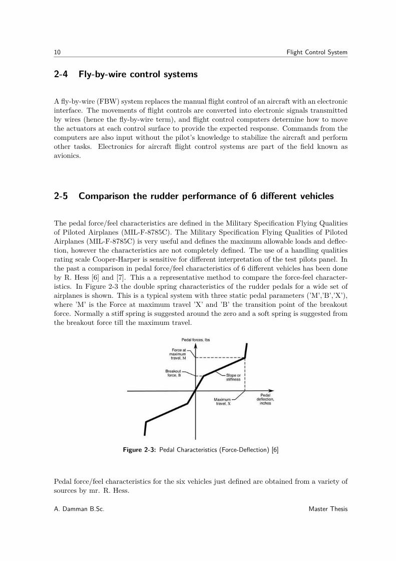
The pedal force/feel characteristics are defined in the Military Specification Flying Qualitiesof Piloted Airplanes (MIL-F-8785C). The Military Specification Flying Qualities of PilotedAirplanes (MIL-F-8785C) is very useful and defines the maximum allowable loads and deflec-tion, however the characteristics are not completely defined. The use of a handling qualitiesrating scale Cooper-Harper is sensitive for different interpretation of the test pilots panel. Inthe past a comparison in pedal force/feel characteristics of 6 different vehicles has been doneby R. Hess [6] and [7]. This a a representative method to compare the force-feel character-istics. In Figure 2-3 the double spring characteristics of the rudder pedals for a wide set ofairplanes is shown. This is a typical system with three static pedal parameters (’M’,’B’,’X’),where ’M’ is the Force at maximum travel ’X’ and ’B’ the transition point of the breakoutforce. Normally a stiff spring is suggested around the zero and a soft spring is suggested fromthe breakout force till the maximum travel.
Figure 2-3: Pedal Characteristics (Force-Deflection) [6]
Pedal force/feel characteristics for the six vehicles just defined are obtained from a variety ofsources by mr. R. Hess.
A. Damman B.Sc. Master Thesis
2-5 Comparison the rudder performance of 6 different vehicles 11
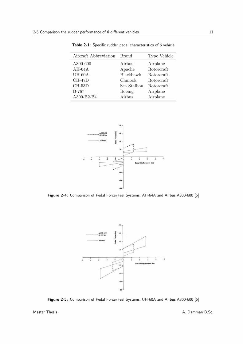
Table 2-1: Specific rudder pedal characteristics of 6 vehicle
Aircraft Abbreviation Brand Type Vehicle
A300-600 Airbus AirplaneAH-64A Apache RotorcraftUH-60A Blackhawk RotorcraftCH-47D Chinook RotorcraftCH-53D Sea Stallion RotorcraftB-767 Boeing AirplaneA300-B2-B4 Airbus Airplane
Figure 2-4: Comparison of Pedal Force/Feel Systems, AH-64A and Airbus A300-600 [6]
Figure 2-5: Comparison of Pedal Force/Feel Systems, UH-60A and Airbus A300-600 [6]
Master Thesis A. Damman B.Sc.
12 Flight Control System
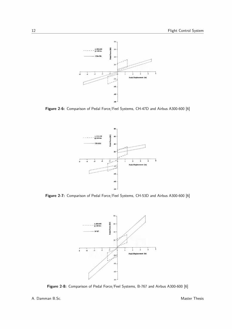
Figure 2-6: Comparison of Pedal Force/Feel Systems, CH-47D and Airbus A300-600 [6]
Figure 2-7: Comparison of Pedal Force/Feel Systems, CH-53D and Airbus A300-600 [6]
Figure 2-8: Comparison of Pedal Force/Feel Systems, B-767 and Airbus A300-600 [6]
A. Damman B.Sc. Master Thesis
2-6 Dynamic Force/Feel System Considerations 13
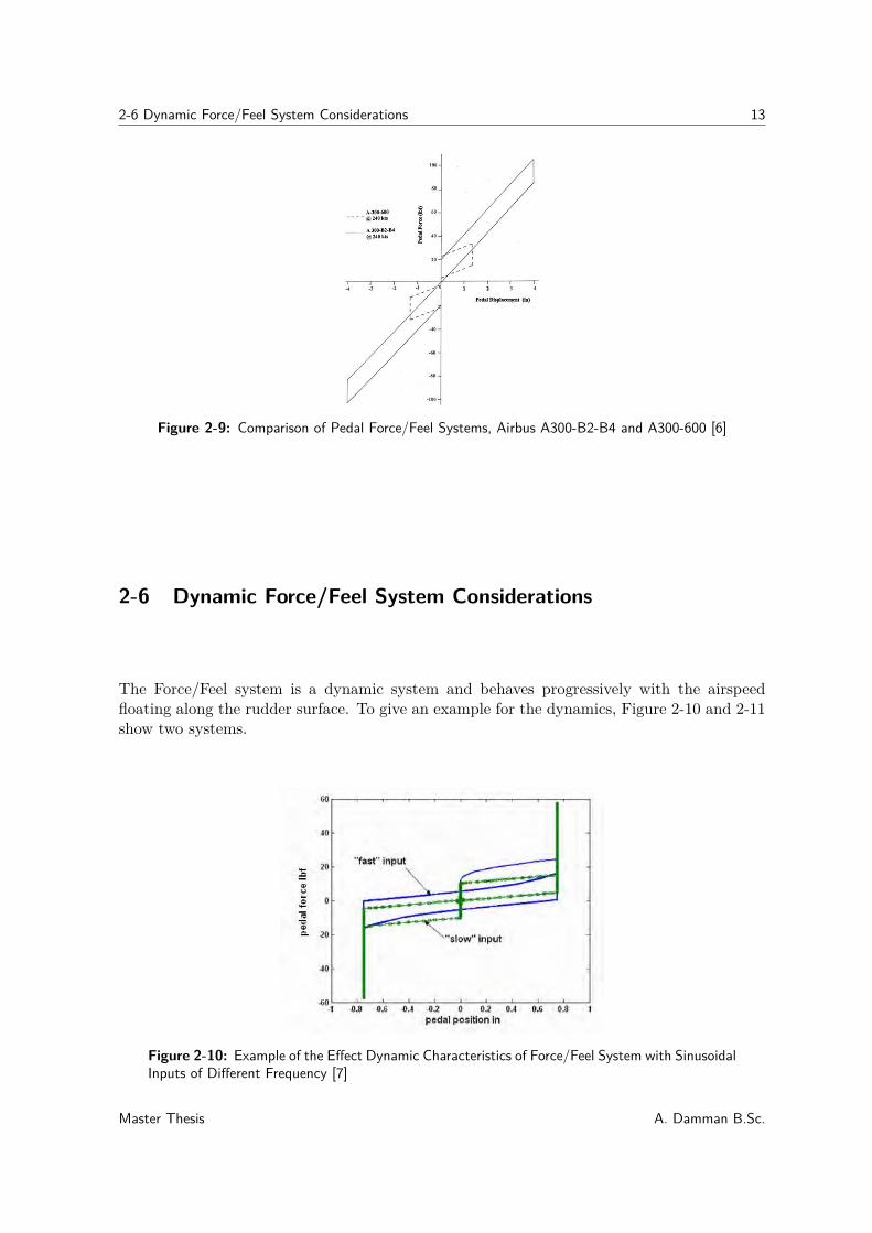
Figure 2-9: Comparison of Pedal Force/Feel Systems, Airbus A300-B2-B4 and A300-600 [6]
2-6 Dynamic Force/Feel System Considerations
The Force/Feel system is a dynamic system and behaves progressively with the airspeedfloating along the rudder surface. To give an example for the dynamics, Figure 2-10 and 2-11show two systems.
Figure 2-10: Example of the Effect Dynamic Characteristics of Force/Feel System with SinusoidalInputs of Different Frequency [7]
Master Thesis A. Damman B.Sc.
14 Flight Control System
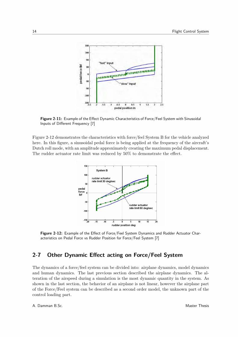
Figure 2-11: Example of the Effect Dynamic Characteristics of Force/Feel System with SinusoidalInputs of Different Frequency [7]
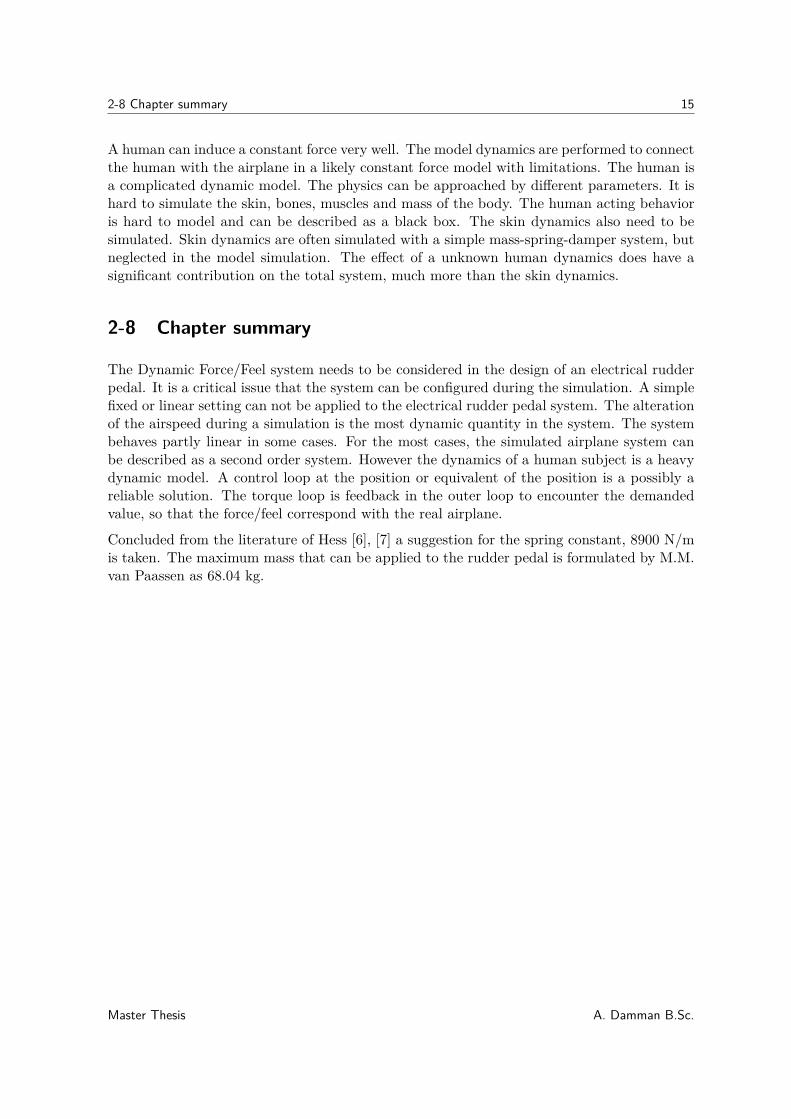
Figure 2-12 demonstrates the characteristics with force/feel System B for the vehicle analyzedhere. In this figure, a sinusoidal pedal force is being applied at the frequency of the aircraft’sDutch roll mode, with an amplitude approximately creating the maximum pedal displacement.The rudder actuator rate limit was reduced by 50% to demonstrate the effect.
Figure 2-12: Example of the Effect of Force/Feel System Dynamics and Rudder Actuator Char-acteristics on Pedal Force vs Rudder Position for Force/Feel System [7]
2-7 Other Dynamic Effect acting on Force/Feel System
The dynamics of a force/feel system can be divided into: airplane dynamics, model dynamicsand human dynamics. The last previous section described the airplane dynamics. The al-teration of the airspeed during a simulation is the most dynamic quantity in the system. Asshown in the last section, the behavior of an airplane is not linear, however the airplane partof the Force/Feel system can be described as a second order model, the unknown part of thecontrol loading part.
A. Damman B.Sc. Master Thesis
2-8 Chapter summary 15
A human can induce a constant force very well. The model dynamics are performed to connectthe human with the airplane in a likely constant force model with limitations. The human isa complicated dynamic model. The physics can be approached by different parameters. It ishard to simulate the skin, bones, muscles and mass of the body. The human acting behavioris hard to model and can be described as a black box. The skin dynamics also need to besimulated. Skin dynamics are often simulated with a simple mass-spring-damper system, butneglected in the model simulation. The effect of a unknown human dynamics does have asignificant contribution on the total system, much more than the skin dynamics.
2-8 Chapter summary
The Dynamic Force/Feel system needs to be considered in the design of an electrical rudderpedal. It is a critical issue that the system can be configured during the simulation. A simplefixed or linear setting can not be applied to the electrical rudder pedal system. The alterationof the airspeed during a simulation is the most dynamic quantity in the system. The systembehaves partly linear in some cases. For the most cases, the simulated airplane system canbe described as a second order system. However the dynamics of a human subject is a heavydynamic model. A control loop at the position or equivalent of the position is a possibly areliable solution. The torque loop is feedback in the outer loop to encounter the demandedvalue, so that the force/feel correspond with the real airplane.
Concluded from the literature of Hess [6], [7] a suggestion for the spring constant, 8900 N/mis taken. The maximum mass that can be applied to the rudder pedal is formulated by M.M.van Paassen as 68.04 kg.
Master Thesis A. Damman B.Sc.

16 Flight Control System
A. Damman B.Sc. Master Thesis
Chapter 3
Performed Solution
3-1 Performed Solution
To get to the performed solution, four alternative solutions have been obtained. The fouralternative solutions could be implemented in terms of torque and velocity specifications,however the following criteria have to be taken into account in order to make the decisionof the preformed solution: communication speed, encoder accuracy, backlash, inertia, inrushcurrent induced by the servo pack, energy consumption and costs. The implemented solution(alternative solution 4) is presented in this Chapter. For more information about the otherelaborated alternative solutions, please refer to the Appendix A.
The most important difference between the three other alternative solutions and the performedsolution is the gearbox which results in a reduced torque and more important a reduced inertiaat the pedal side. In the formula the gear ratio is to the second power. [8] Preferred is the threephase model of the drive system, because of the experience with inrush current by switchingthe controller on, in one of our other laboratory. In fact the 20 bit alternative solution ismaybe not really necessary, but is however very useful for accurate data to implement inthe control system. The gearbox is the part that can cause some problems in our systemperformance. For your understanding the backlash in other parts of the rudder pedals ishigher than the standard backlash in the gearbox, so this can be neglected. Furthermore,the backlash in the rudder pedals is behind the motor, and this has no consequences forour control loop. The selected motor can operate in all required conditions within the ratedtorque characteristics.
3-2 Mechanical Identification
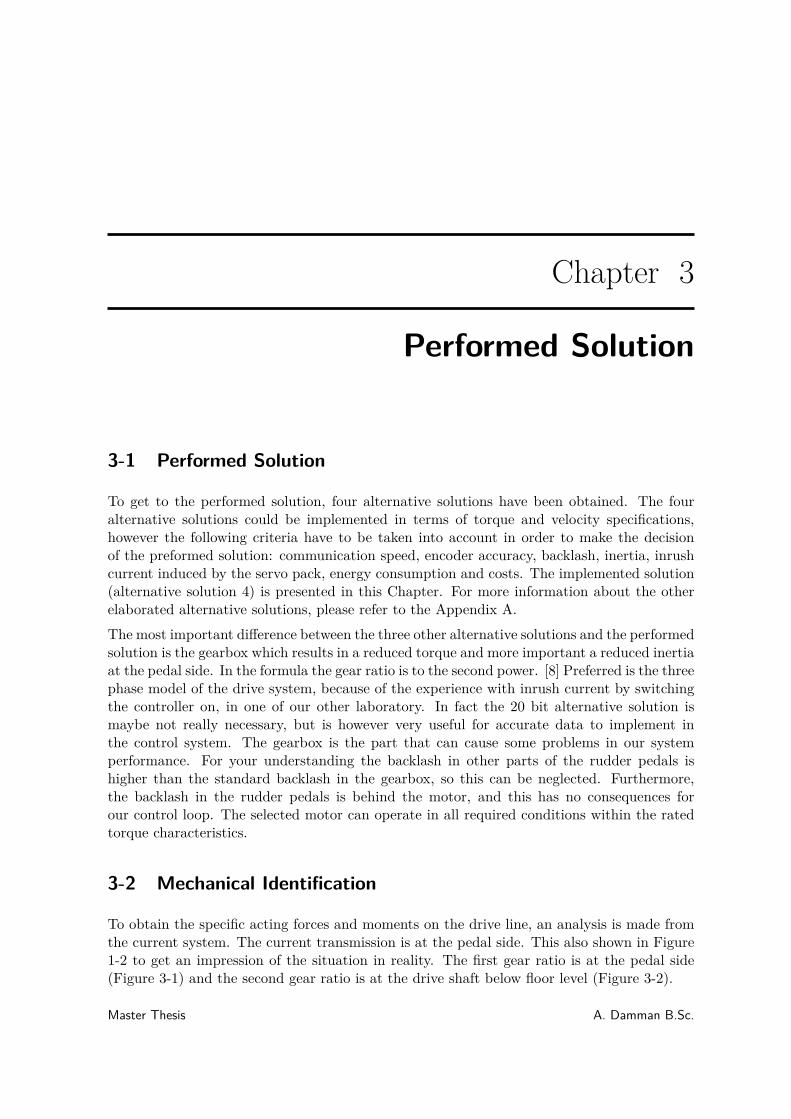
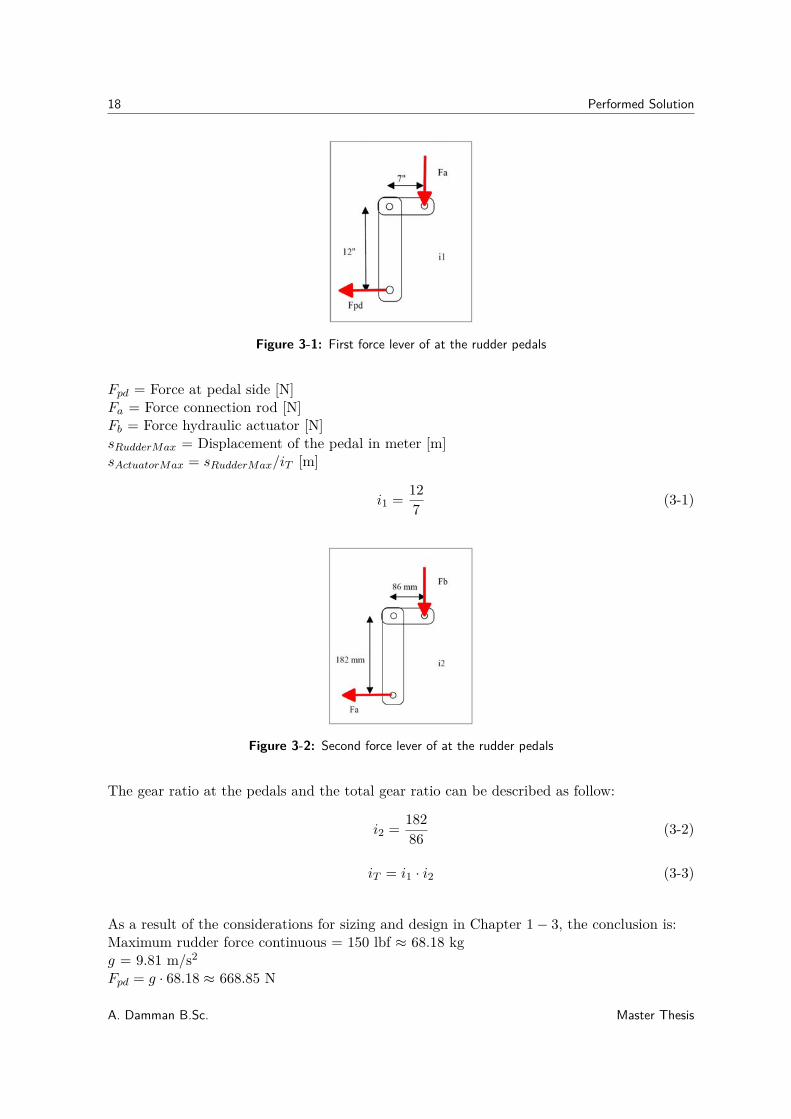
To obtain the specific acting forces and moments on the drive line, an analysis is made fromthe current system. The current transmission is at the pedal side. This also shown in Figure1-2 to get an impression of the situation in reality. The first gear ratio is at the pedal side(Figure 3-1) and the second gear ratio is at the drive shaft below floor level (Figure 3-2).
Master Thesis A. Damman B.Sc.
18 Performed Solution
Figure 3-1: First force lever of at the rudder pedals
Fpd = Force at pedal side [N]Fa = Force connection rod [N]Fb = Force hydraulic actuator [N]sRudderMax = Displacement of the pedal in meter [m]sActuatorMax = sRudderMax/iT [m]
i1 =127
(3-1)
Figure 3-2: Second force lever of at the rudder pedals
The gear ratio at the pedals and the total gear ratio can be described as follow:
i2 =18286
(3-2)
iT = i1 · i2 (3-3)
As a result of the considerations for sizing and design in Chapter 1 − 3, the conclusion is:Maximum rudder force continuous = 150 lbf ≈ 68.18 kgg = 9.81 m/s2
Fpd = g · 68.18 ≈ 668.85 N
A. Damman B.Sc. Master Thesis
3-2 Mechanical Identification 19
Fa = i1 · Fpd ≈ 1146.59 NFb = i2 · Fa ≈ 2456.51 NsRudderMax = 0.2 msActuatorMax = sRudderMax/iT ≈ 0.055 m
The torque at the drive shaft is:
T2 =Fpd · i2
li2
= 208 (3-4)
li2= lever arm length from Fa to the second pedal shaft axis.
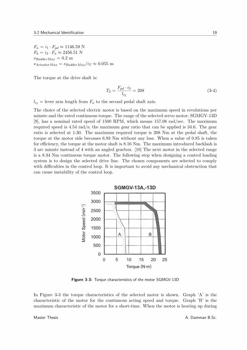
The choice of the selected electric motor is based on the maximum speed in revolutions perminute and the rated continuous torque. The range of the selected servo motor; SGMGV-13D[9], has a nominal rated speed of 1500 RPM, which means 157.08 rad/sec. The maximumrequired speed is 4.54 rad/s; the maximum gear ratio that can be applied is 34.6. The gearratio is selected at 1:30. The maximum required torque is 208 Nm at the pedal shaft, thetorque at the motor side becomes 6.93 Nm without any loss. When a value of 0.85 is takenfor efficiency, the torque at the motor shaft is 8.16 Nm. The maximum introduced backlash is3 arc minute instead of 4 with an angled gearbox. [10] The next motor in the selected rangeis a 8.34 Nm continuous torque motor. The following step when designing a control loadingsystem is to design the selected drive line. The chosen components are selected to complywith difficulties in the control loop. It is important to avoid any mechanical obstruction thatcan cause instability of the control loop.
Figure 3-3: Torque characteristics of the motor SGMGV-13D
In Figure 3-3 the torque characteristics of the selected motor is shown. Graph ’A’ is thecharacteristic of the motor for the continuous acting speed and torque. Graph ’B’ is themaximum characteristic of the motor for a short-time. When the motor is heating up during
Master Thesis A. Damman B.Sc.

20 Performed Solution
operation the characteristics increase. A dwell time can lower the ambient temperature ofthe motor. The maximum continuous torque and speed is 1500 RPM (or 157 rad/s) withoutany loss of torque. The graph is suggested as a vertical line in this situation. In Figure A-4an artist impression of the performed solution is shown. The particular views are presentedin Figure A-5.
Figure 3-4: Alternative solution 4 proposed gearing via planetary gearbox on an electric servodirect drive
Figure 3-5: Drawing alternative solution 4
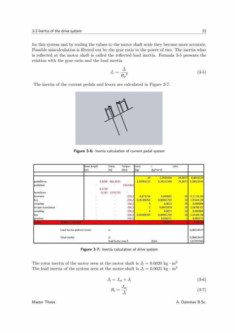
3-3 Inertia of the drive system
For higher performance of the rudder pedal system, it is important to take into account theinertia of the system. To estimate the inertia of the actual rudder pedals with levers, a soliddesign analysis is made by the design software Solidworks. The derived values are considerable
A. Damman B.Sc. Master Thesis
3-3 Inertia of the drive system 21
for this system and by scaling the values to the motor shaft scale they become more accurate.Possible miscalculation is filtered out by the gear ratio to the power of two. The inertia whatis reflected at the motor shaft is called the reflected load inertia. Formula 3-5 presents therelation with the gear ratio and the load inertia.
Jr =Jl
Rg2
(3-5)
The inertia of the current pedals and levers are calculated in Figure 3-7.
Figure 3-6: Inertia calculation of current pedal system
Figure 3-7: Inertia calculation of drive system
The rotor inertia of the motor seen at the motor shaft is Jl = 0.0020 kg · m2
The load inertia of the system seen at the motor shaft is Jl = 0.0021 kg · m2
Jt = Jm + Jl (3-6)
Ri =Jm
Jl(3-7)
Master Thesis A. Damman B.Sc.
22 Performed Solution
The calculated inertia ratio (Ri) is 1.08 and this a good result for the expected performanceof the system. A ratio till 5 is allowed for high performance, above 5 the stability of thecontrol loop will decrease in comparison to a very low value for the ratio.
The total inertia of the system as seen at the motor shaft is Jt = 0.0041 kg · m2
A check for the resonance frequency is important to avoid oscillations. This can be calculatedwhen the inertia value of the load and motor are available. The most common way to checkthe resonance frequency is as followed. [9]:
f res ≈ 12 · π
·√
ct · Jm + J l
Jm · J l
[9] (3-8)
ct = 288.6 [kNm/rad]. The result is 2661 Hz as a theoretical expected mechanical resonancefrequency.
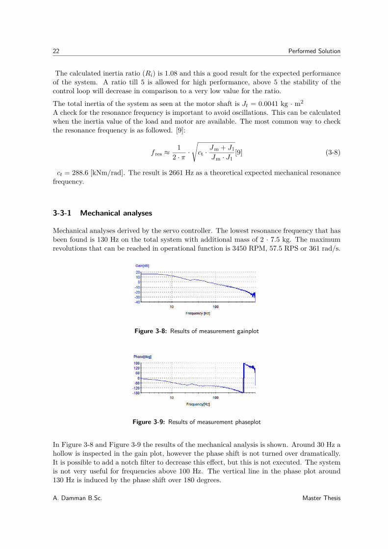
3-3-1 Mechanical analyses
Mechanical analyses derived by the servo controller. The lowest resonance frequency that hasbeen found is 130 Hz on the total system with additional mass of 2 · 7.5 kg. The maximumrevolutions that can be reached in operational function is 3450 RPM, 57.5 RPS or 361 rad/s.
Figure 3-8: Results of measurement gainplot
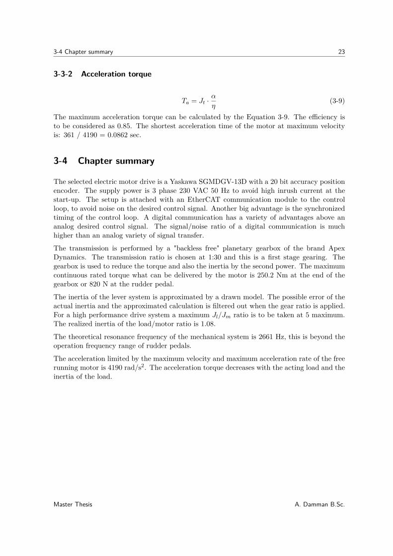
Figure 3-9: Results of measurement phaseplot
In Figure 3-8 and Figure 3-9 the results of the mechanical analysis is shown. Around 30 Hz ahollow is inspected in the gain plot, however the phase shift is not turned over dramatically.It is possible to add a notch filter to decrease this effect, but this is not executed. The systemis not very useful for frequencies above 100 Hz. The vertical line in the phase plot around130 Hz is induced by the phase shift over 180 degrees.
A. Damman B.Sc. Master Thesis
3-4 Chapter summary 23
3-3-2 Acceleration torque
Ta = Jt · α
η(3-9)
The maximum acceleration torque can be calculated by the Equation 3-9. The efficiency isto be considered as 0.85. The shortest acceleration time of the motor at maximum velocityis: 361 / 4190 = 0.0862 sec.
3-4 Chapter summary
The selected electric motor drive is a Yaskawa SGMDGV-13D with a 20 bit accuracy positionencoder. The supply power is 3 phase 230 VAC 50 Hz to avoid high inrush current at thestart-up. The setup is attached with an EtherCAT communication module to the controlloop, to avoid noise on the desired control signal. Another big advantage is the synchronizedtiming of the control loop. A digital communication has a variety of advantages above ananalog desired control signal. The signal/noise ratio of a digital communication is muchhigher than an analog variety of signal transfer.
The transmission is performed by a "backless free" planetary gearbox of the brand ApexDynamics. The transmission ratio is chosen at 1:30 and this is a first stage gearing. Thegearbox is used to reduce the torque and also the inertia by the second power. The maximumcontinuous rated torque what can be delivered by the motor is 250.2 Nm at the end of thegearbox or 820 N at the rudder pedal.
The inertia of the lever system is approximated by a drawn model. The possible error of theactual inertia and the approximated calculation is filtered out when the gear ratio is applied.For a high performance drive system a maximum Jl/Jm ratio is to be taken at 5 maximum.The realized inertia of the load/motor ratio is 1.08.
The theoretical resonance frequency of the mechanical system is 2661 Hz, this is beyond theoperation frequency range of rudder pedals.
The acceleration limited by the maximum velocity and maximum acceleration rate of the freerunning motor is 4190 rad/s2. The acceleration torque decreases with the acting load and theinertia of the load.
Master Thesis A. Damman B.Sc.

24 Performed Solution
A. Damman B.Sc. Master Thesis
Chapter 4
Performance of the analytical models
In this chapter the modeling of the original hydraulic driven actuators in three differentcontrol loops is first explained . The second simulation is an electric driven actuator in thecontrol loop. This is decided for several reasons. The simulation of the electric servo motor isdifficult to establish with the lag of information of the servo pack. This has to be seen moreas an estimation of the limitations of the servo system.
The input signal for the system identification is a sinus profile in the stationary part of theoscillation. The start up and stop of the oscillation is not acquainted with the simulation. Thereason is the interference at the inrush oscillation and the abrupt stopping of the oscillation.
A sinusoidal input signal is achieved to inspect the response, the reason why there is beenchosen for a sinusoidal input signal is the limitation on the travel and the mechanical system.It is not really a good solution to run a step profile or a trapezium pattern where the angleis less steep as in a step response. The jerk will have effect on the system like vibrating therigid frame construction and so on. A sinus is maybe not the ideal identification method interms of workload, however it is a smooth method for identification.
In the Chapter Flight Control System the dynamic behavior of the system is described. Thecomponents that are used for simulation is supposed as a linear system. The most importantelements of the simulated model can be described as a second order mass-spring-dampersystem. In the Figure 4-1 the different elements of the mass-spring-damper system what ismodel for the simulation is shown. The ζ is supposed as a value of 0.7.
As concluded in Chapter 2, the value from experience of the literature of Hess [6], [7] a sug-gested spring constant of 8900 N/m has been taken. The maximum mass that can be appliedto the rudder pedal is formulated by M.M. van Paassen as 68.04 kg. The ζ is formulated as0.7, which mean a damping value of 886 Ns/m when the Formula 4-1 is applied.
ζ =bsim
2√
msim · csim(4-1)
ω0 =
√
k
m(4-2)
Master Thesis A. Damman B.Sc.
26 Performance of the analytical models
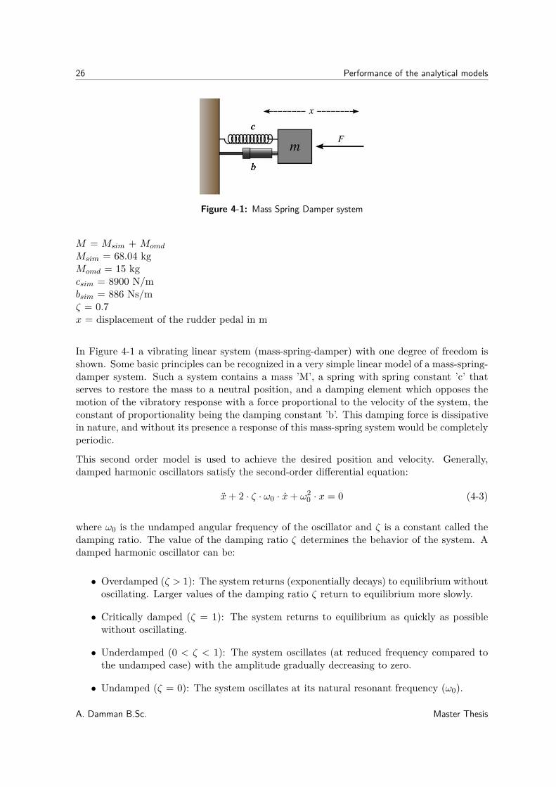
Figure 4-1: Mass Spring Damper system
M = Msim + Momd
Msim = 68.04 kgMomd = 15 kgcsim = 8900 N/mbsim = 886 Ns/mζ = 0.7x = displacement of the rudder pedal in m
In Figure 4-1 a vibrating linear system (mass-spring-damper) with one degree of freedom isshown. Some basic principles can be recognized in a very simple linear model of a mass-spring-damper system. Such a system contains a mass ’M’, a spring with spring constant ’c’ thatserves to restore the mass to a neutral position, and a damping element which opposes themotion of the vibratory response with a force proportional to the velocity of the system, theconstant of proportionality being the damping constant ’b’. This damping force is dissipativein nature, and without its presence a response of this mass-spring system would be completelyperiodic.
This second order model is used to achieve the desired position and velocity. Generally,damped harmonic oscillators satisfy the second-order differential equation:
x + 2 · ζ · ω0 · x + ω20 · x = 0 (4-3)
where ω0 is the undamped angular frequency of the oscillator and ζ is a constant called thedamping ratio. The value of the damping ratio ζ determines the behavior of the system. Adamped harmonic oscillator can be:
• Overdamped (ζ > 1): The system returns (exponentially decays) to equilibrium withoutoscillating. Larger values of the damping ratio ζ return to equilibrium more slowly.
• Critically damped (ζ = 1): The system returns to equilibrium as quickly as possiblewithout oscillating.
• Underdamped (0 < ζ < 1): The system oscillates (at reduced frequency compared tothe undamped case) with the amplitude gradually decreasing to zero.
• Undamped (ζ = 0): The system oscillates at its natural resonant frequency (ω0).
A. Damman B.Sc. Master Thesis
4-1 Hydraulic Servo Simulation 27
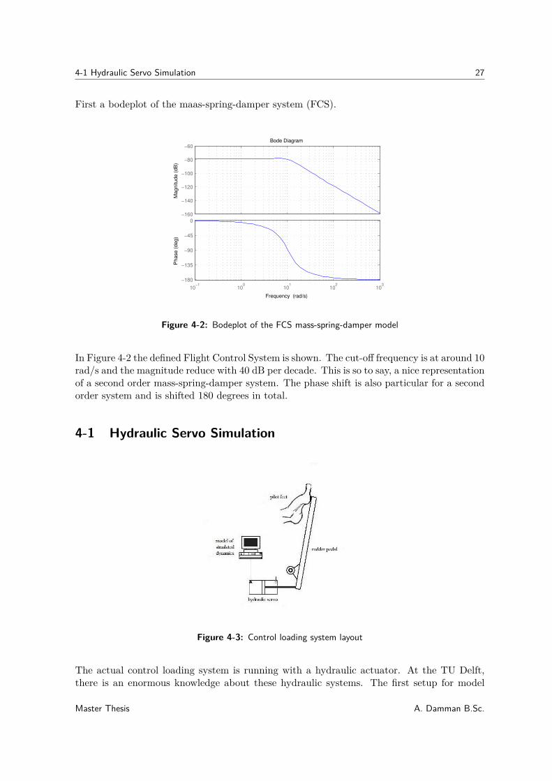
First a bodeplot of the maas-spring-damper system (FCS).
Bode Diagram
Frequency (rad/s)
10−1
100
101
102
103
−180
−135
−90
−45
0
Phase (
deg)
−160
−140
−120
−100
−80
−60
Magnitude (
dB
)
Figure 4-2: Bodeplot of the FCS mass-spring-damper model
In Figure 4-2 the defined Flight Control System is shown. The cut-off frequency is at around 10rad/s and the magnitude reduce with 40 dB per decade. This is so to say, a nice representationof a second order mass-spring-damper system. The phase shift is also particular for a secondorder system and is shifted 180 degrees in total.
4-1 Hydraulic Servo Simulation
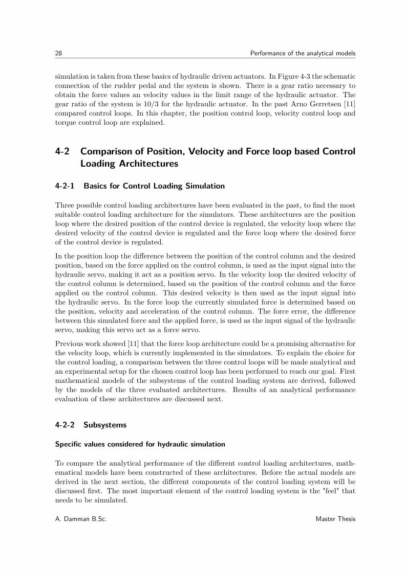
Figure 4-3: Control loading system layout
The actual control loading system is running with a hydraulic actuator. At the TU Delft,there is an enormous knowledge about these hydraulic systems. The first setup for model
Master Thesis A. Damman B.Sc.
28 Performance of the analytical models
simulation is taken from these basics of hydraulic driven actuators. In Figure 4-3 the schematicconnection of the rudder pedal and the system is shown. There is a gear ratio necessary toobtain the force values an velocity values in the limit range of the hydraulic actuator. Thegear ratio of the system is 10/3 for the hydraulic actuator. In the past Arno Gerretsen [11]compared control loops. In this chapter, the position control loop, velocity control loop andtorque control loop are explained.
4-2 Comparison of Position, Velocity and Force loop based Control
Loading Architectures
4-2-1 Basics for Control Loading Simulation
Three possible control loading architectures have been evaluated in the past, to find the mostsuitable control loading architecture for the simulators. These architectures are the positionloop where the desired position of the control device is regulated, the velocity loop where thedesired velocity of the control device is regulated and the force loop where the desired forceof the control device is regulated.
In the position loop the difference between the position of the control column and the desiredposition, based on the force applied on the control column, is used as the input signal into thehydraulic servo, making it act as a position servo. In the velocity loop the desired velocity ofthe control column is determined, based on the position of the control column and the forceapplied on the control column. This desired velocity is then used as the input signal intothe hydraulic servo. In the force loop the currently simulated force is determined based onthe position, velocity and acceleration of the control column. The force error, the differencebetween this simulated force and the applied force, is used as the input signal of the hydraulicservo, making this servo act as a force servo.
Previous work showed [11] that the force loop architecture could be a promising alternative forthe velocity loop, which is currently implemented in the simulators. To explain the choice forthe control loading, a comparison between the three control loops will be made analytical andan experimental setup for the chosen control loop has been performed to reach our goal. Firstmathematical models of the subsystems of the control loading system are derived, followedby the models of the three evaluated architectures. Results of an analytical performanceevaluation of these architectures are discussed next.
4-2-2 Subsystems
Specific values considered for hydraulic simulation
To compare the analytical performance of the different control loading architectures, math-ematical models have been constructed of these architectures. Before the actual models arederived in the next section, the different components of the control loading system will bediscussed first. The most important element of the control loading system is the "feel" thatneeds to be simulated.
A. Damman B.Sc. Master Thesis
4-2 Comparison of Position, Velocity and Force loop based Control Loading Architectures 29
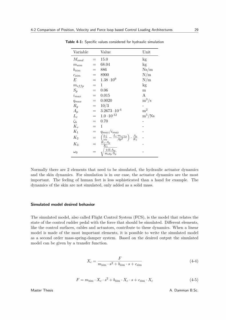
Table 4-1: Specific values considered for hydraulic simulation
Variable Value Unit
Momd = 15.0 kgmsim = 68.04 kgbsim = 886 Ns/mcsim = 8900 N/mE = 1.38 ·109 N/mmeffp = 1 kgSp = 0.06 mimax = 0.015 Aqmax = 0.0020 m3/sRg = 10/3 -Ap = 3.2673 ·10-4 m2
Lc = 1.0 ·10-12 m5/Nsζh = 0.70 -Kv = 1 -K1 = qmax/imax -
K2 =(
2·ζω0
− Lc·meffp
Ap2
)
· Ap
K1-
K3 = Kv ·Ap
K1-
ω0 =√
4·E·Ap
meffp·Sp-
Normally there are 2 elements that need to be simulated, the hydraulic actuator dynamicsand the skin dynamics. For simulation is in our case, the actuator dynamics are the mostimportant. The feeling of human feet is less sophisticated than a hand for example. Thedynamics of the skin are not simulated, only added as a solid mass.
Simulated model desired behavior
The simulated model, also called Flight Control System (FCS), is the model that relates thestate of the control rudder pedal with the force that should be simulated. Different elements,like the control surfaces, cables and actuators, contribute to these dynamics. When a linearmodel is made of the most important elements, it is possible to write the simulated modelas a second order mass-spring-damper system. Based on the desired output the simulatedmodel can be given by a transfer function.
Xc =F
msim · s2 + bsim · s + csim
(4-4)
F = msim · Xc · s2 + bsim · Xc · s + csim · Xc (4-5)
Master Thesis A. Damman B.Sc.
30 Performance of the analytical models
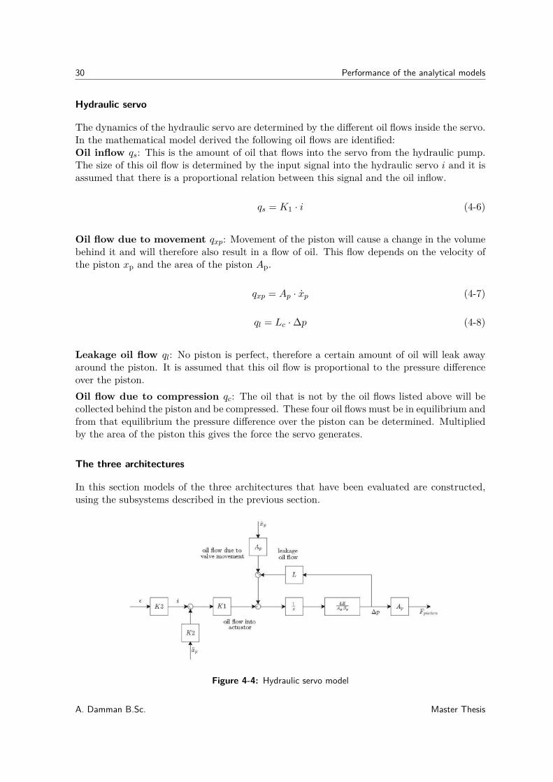
Hydraulic servo
The dynamics of the hydraulic servo are determined by the different oil flows inside the servo.In the mathematical model derived the following oil flows are identified:Oil inflow qs: This is the amount of oil that flows into the servo from the hydraulic pump.The size of this oil flow is determined by the input signal into the hydraulic servo i and it isassumed that there is a proportional relation between this signal and the oil inflow.
qs = K1 · i (4-6)
Oil flow due to movement qxp: Movement of the piston will cause a change in the volumebehind it and will therefore also result in a flow of oil. This flow depends on the velocity ofthe piston xp and the area of the piston Ap.
qxp = Ap · xp (4-7)
ql = Lc · ∆p (4-8)
Leakage oil flow ql: No piston is perfect, therefore a certain amount of oil will leak awayaround the piston. It is assumed that this oil flow is proportional to the pressure differenceover the piston.
Oil flow due to compression qc: The oil that is not by the oil flows listed above will becollected behind the piston and be compressed. These four oil flows must be in equilibrium andfrom that equilibrium the pressure difference over the piston can be determined. Multipliedby the area of the piston this gives the force the servo generates.
The three architectures
In this section models of the three architectures that have been evaluated are constructed,using the subsystems described in the previous section.
Figure 4-4: Hydraulic servo model
A. Damman B.Sc. Master Thesis
4-2 Comparison of Position, Velocity and Force loop based Control Loading Architectures 31
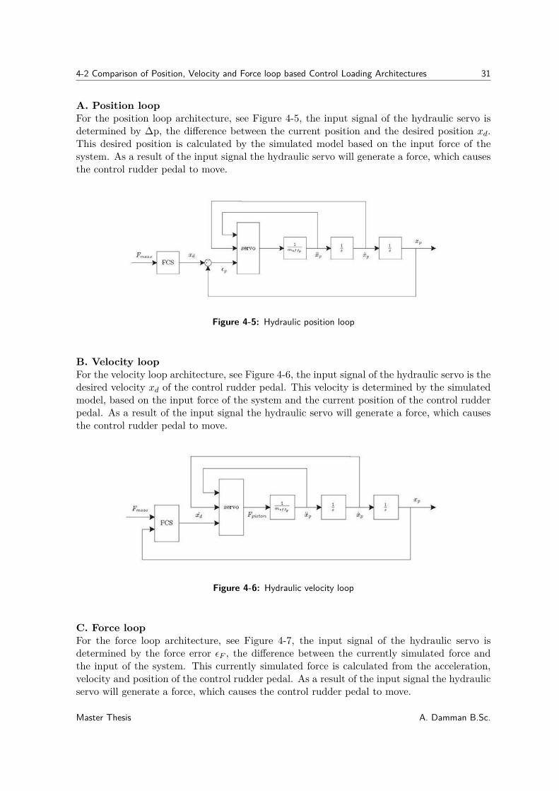
A. Position loop
For the position loop architecture, see Figure 4-5, the input signal of the hydraulic servo isdetermined by ∆p, the difference between the current position and the desired position xd.This desired position is calculated by the simulated model based on the input force of thesystem. As a result of the input signal the hydraulic servo will generate a force, which causesthe control rudder pedal to move.
Figure 4-5: Hydraulic position loop
B. Velocity loop
For the velocity loop architecture, see Figure 4-6, the input signal of the hydraulic servo is thedesired velocity xd of the control rudder pedal. This velocity is determined by the simulatedmodel, based on the input force of the system and the current position of the control rudderpedal. As a result of the input signal the hydraulic servo will generate a force, which causesthe control rudder pedal to move.
Figure 4-6: Hydraulic velocity loop
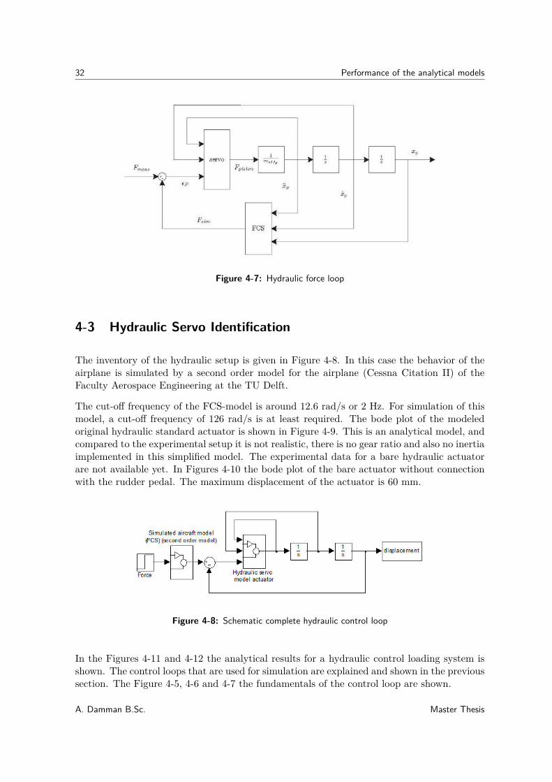
C. Force loop
For the force loop architecture, see Figure 4-7, the input signal of the hydraulic servo isdetermined by the force error ǫF , the difference between the currently simulated force andthe input of the system. This currently simulated force is calculated from the acceleration,velocity and position of the control rudder pedal. As a result of the input signal the hydraulicservo will generate a force, which causes the control rudder pedal to move.
Master Thesis A. Damman B.Sc.
32 Performance of the analytical models
Figure 4-7: Hydraulic force loop
4-3 Hydraulic Servo Identification
The inventory of the hydraulic setup is given in Figure 4-8. In this case the behavior of theairplane is simulated by a second order model for the airplane (Cessna Citation II) of theFaculty Aerospace Engineering at the TU Delft.
The cut-off frequency of the FCS-model is around 12.6 rad/s or 2 Hz. For simulation of thismodel, a cut-off frequency of 126 rad/s is at least required. The bode plot of the modeledoriginal hydraulic standard actuator is shown in Figure 4-9. This is an analytical model, andcompared to the experimental setup it is not realistic, there is no gear ratio and also no inertiaimplemented in this simplified model. The experimental data for a bare hydraulic actuatorare not available yet. In Figures 4-10 the bode plot of the bare actuator without connectionwith the rudder pedal. The maximum displacement of the actuator is 60 mm.
Figure 4-8: Schematic complete hydraulic control loop
In the Figures 4-11 and 4-12 the analytical results for a hydraulic control loading system isshown. The control loops that are used for simulation are explained and shown in the previoussection. The Figure 4-5, 4-6 and 4-7 the fundamentals of the control loop are shown.
A. Damman B.Sc. Master Thesis
4-3 Hydraulic Servo Identification 33
Bode Diagram
Frequency (rad/s)10−1
100
101
102
103
104
−135
−90
−45
0
Ph
ase
(d
eg
)
−12
−10
−8
−6
−4
−2
0
2
Ma
gn
itu
de
(d
B)
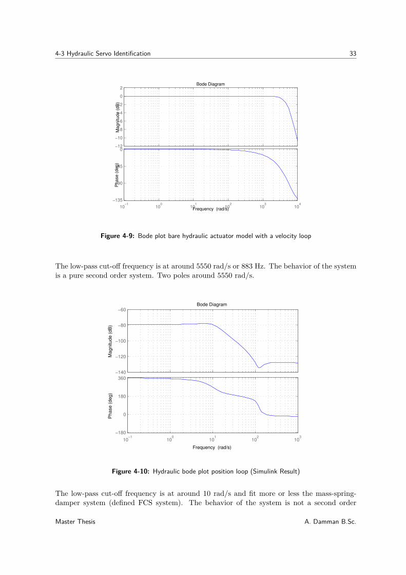
Figure 4-9: Bode plot bare hydraulic actuator model with a velocity loop
The low-pass cut-off frequency is at around 5550 rad/s or 883 Hz. The behavior of the systemis a pure second order system. Two poles around 5550 rad/s.
Bode Diagram
Frequency (rad/s)
10−1
100
101
102
103
−180
0
180
360
Phase (
deg)
−140
−120
−100
−80
−60
Magnitude (
dB
)
Figure 4-10: Hydraulic bode plot position loop (Simulink Result)
The low-pass cut-off frequency is at around 10 rad/s and fit more or less the mass-spring-damper system (defined FCS system). The behavior of the system is not a second order
Master Thesis A. Damman B.Sc.
34 Performance of the analytical models
system. It seems to be a system with two poles around 10 rad/s and two additional zeroaround 110 rad/s.
Bode Diagram
Frequency (rad/s)
10−1
100
101
102
103
−180
−135
−90
−45
0
Phase (
deg)
−140
−120
−100
−80
−60
Magnitude (
dB
)
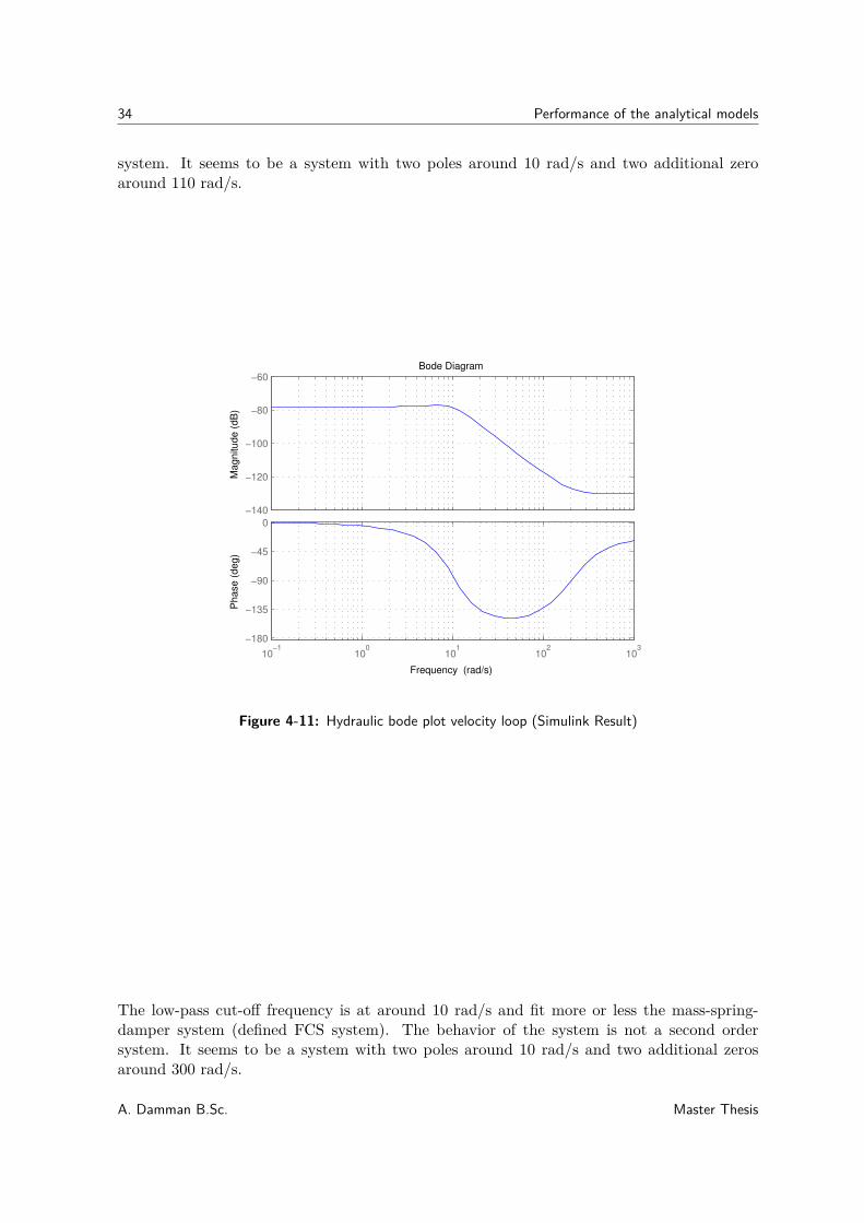
Figure 4-11: Hydraulic bode plot velocity loop (Simulink Result)
The low-pass cut-off frequency is at around 10 rad/s and fit more or less the mass-spring-damper system (defined FCS system). The behavior of the system is not a second ordersystem. It seems to be a system with two poles around 10 rad/s and two additional zerosaround 300 rad/s.
A. Damman B.Sc. Master Thesis
4-3 Hydraulic Servo Identification 35
Bode Diagram
Frequency (rad/s)
10−1
100
101
102
103
−180
−135
−90
−45
0
Phase (
deg)
−200
−150
−100
−50
Magnitude (
dB
)
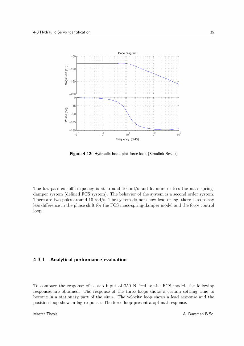
Figure 4-12: Hydraulic bode plot force loop (Simulink Result)
The low-pass cut-off frequency is at around 10 rad/s and fit more or less the mass-spring-damper system (defined FCS system). The behavior of the system is a second order system.There are two poles around 10 rad/s. The system do not show lead or lag, there is so to sayless difference in the phase shift for the FCS mass-spring-damper model and the force controlloop.
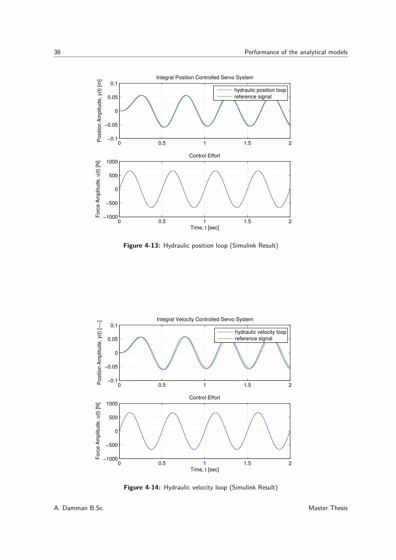
4-3-1 Analytical performance evaluation
To compare the response of a step input of 750 N feed to the FCS model, the followingresponses are obtained. The response of the three loops shows a certain settling time tobecome in a stationary part of the sinus. The velocity loop shows a lead response and theposition loop shows a lag response. The force loop present a optimal response.
Master Thesis A. Damman B.Sc.
36 Performance of the analytical models
0 0.5 1 1.5 2−0.1
−0.05
0
0.05
0.1Integral Position Controlled Servo System
Positio
n A
mplit
ude, y(t
) [m
]
hydraulic position loop
reference signal
0 0.5 1 1.5 2−1000
−500
0
500
1000Control Effort
Time, t [sec]
Forc
e A
mplit
ude, u(t
) [N
]
Figure 4-13: Hydraulic position loop (Simulink Result)
0 0.5 1 1.5 2−0.1
−0.05
0
0.05
0.1Integral Velocity Controlled Servo System
Positio
n A
mplit
ude, y(t
) [−
−]
hydraulic velocity loop
reference signal
0 0.5 1 1.5 2−1000
−500
0
500
1000Control Effort
Time, t [sec]
Forc
e A
mplit
ude, u(t
) [N
]
Figure 4-14: Hydraulic velocity loop (Simulink Result)
A. Damman B.Sc. Master Thesis
4-4 Electrical Servo Simulation 37
0 0.5 1 1.5 2−0.1
−0.05
0
0.05
0.1Integral Force Controlled Servo System
Positio
n A
mplit
ude, y(t
) [m
]
hydraulic force loop
reference signal
0 0.5 1 1.5 2−1000
−500
0
500
1000Control Effort
Time, t [sec]
Forc
e, A
mplit
ude, u(t
) [N
]
Figure 4-15: Hydraulic force loop (Simulink Result)
4-3-2 Choice Type of Control Loop
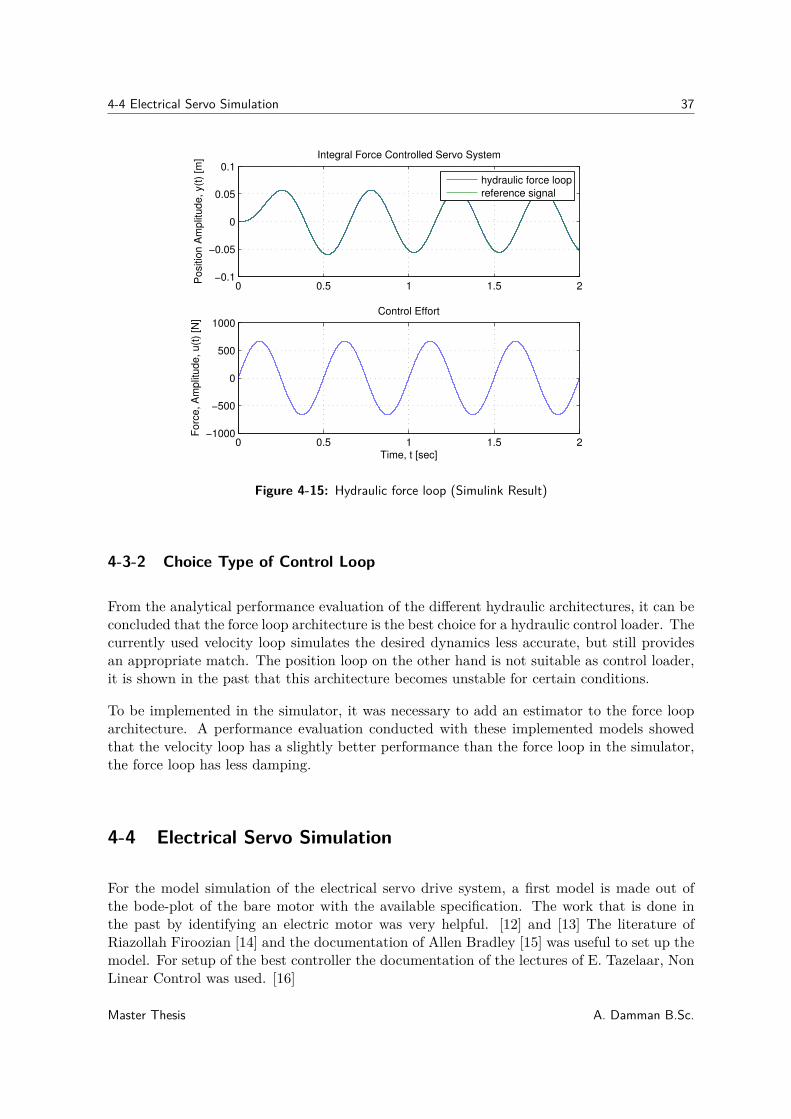
From the analytical performance evaluation of the different hydraulic architectures, it can beconcluded that the force loop architecture is the best choice for a hydraulic control loader. Thecurrently used velocity loop simulates the desired dynamics less accurate, but still providesan appropriate match. The position loop on the other hand is not suitable as control loader,it is shown in the past that this architecture becomes unstable for certain conditions.
To be implemented in the simulator, it was necessary to add an estimator to the force looparchitecture. A performance evaluation conducted with these implemented models showedthat the velocity loop has a slightly better performance than the force loop in the simulator,the force loop has less damping.
4-4 Electrical Servo Simulation
For the model simulation of the electrical servo drive system, a first model is made out ofthe bode-plot of the bare motor with the available specification. The work that is done inthe past by identifying an electric motor was very helpful. [12] and [13] The literature ofRiazollah Firoozian [14] and the documentation of Allen Bradley [15] was useful to set up themodel. For setup of the best controller the documentation of the lectures of E. Tazelaar, NonLinear Control was used. [16]
Master Thesis A. Damman B.Sc.
38 Performance of the analytical models
4-4-1 Matlab/Simulink model
Simulink model
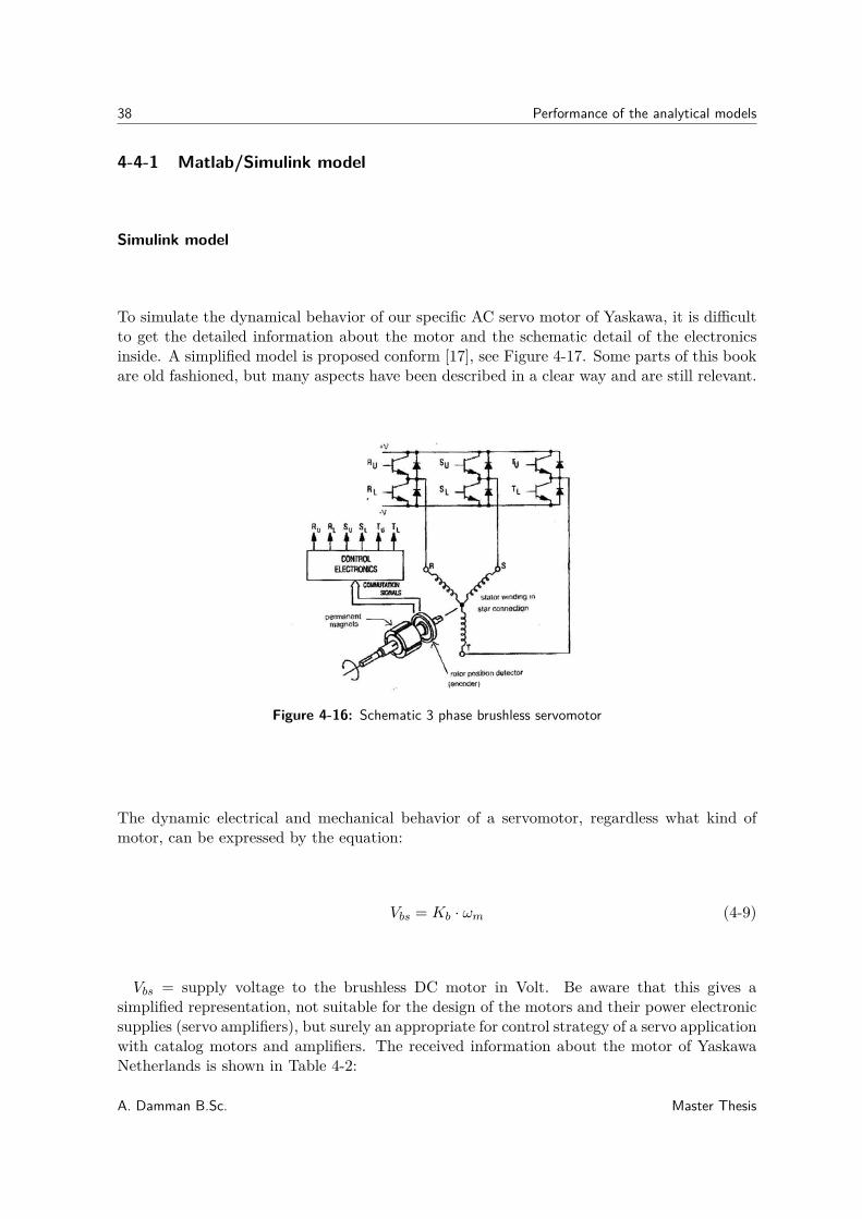
To simulate the dynamical behavior of our specific AC servo motor of Yaskawa, it is difficultto get the detailed information about the motor and the schematic detail of the electronicsinside. A simplified model is proposed conform [17], see Figure 4-17. Some parts of this bookare old fashioned, but many aspects have been described in a clear way and are still relevant.
Figure 4-16: Schematic 3 phase brushless servomotor
The dynamic electrical and mechanical behavior of a servomotor, regardless what kind ofmotor, can be expressed by the equation:
Vbs = Kb · ωm (4-9)
Vbs = supply voltage to the brushless DC motor in Volt. Be aware that this gives asimplified representation, not suitable for the design of the motors and their power electronicsupplies (servo amplifiers), but surely an appropriate for control strategy of a servo applicationwith catalog motors and amplifiers. The received information about the motor of YaskawaNetherlands is shown in Table 4-2:
A. Damman B.Sc. Master Thesis
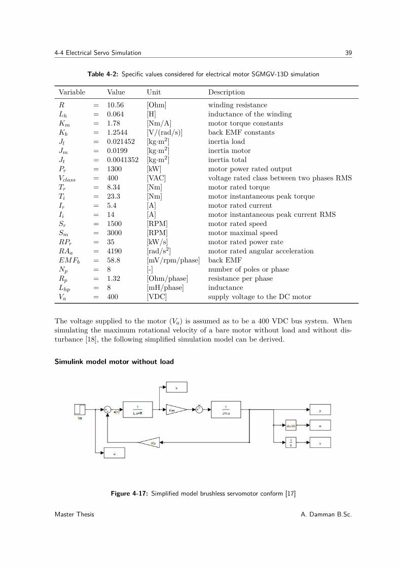
4-4 Electrical Servo Simulation 39
Table 4-2: Specific values considered for electrical motor SGMGV-13D simulation
Variable Value Unit Description
R = 10.56 [Ohm] winding resistanceLh = 0.064 [H] inductance of the windingKm = 1.78 [Nm/A] motor torque constantsKb = 1.2544 [V/(rad/s)] back EMF constantsJl = 0.021452 [kg·m2] inertia loadJm = 0.0199 [kg·m2] inertia motorJt = 0.0041352 [kg·m2] inertia totalPr = 1300 [kW] motor power rated outputVclass = 400 [VAC] voltage rated class between two phases RMSTr = 8.34 [Nm] motor rated torqueTi = 23.3 [Nm] motor instantaneous peak torqueIr = 5.4 [A] motor rated currentIi = 14 [A] motor instantaneous peak current RMSSr = 1500 [RPM] motor rated speedSm = 3000 [RPM] motor maximal speedRPr = 35 [kW/s] motor rated power rateRAa = 4190 [rad/s2] motor rated angular accelerationEMFb = 58.8 [mV/rpm/phase] back EMFNp = 8 [-] number of poles or phaseRp = 1.32 [Ohm/phase] resistance per phaseLhp = 8 [mH/phase] inductanceVa = 400 [VDC] supply voltage to the DC motor
The voltage supplied to the motor (Va) is assumed as to be a 400 VDC bus system. Whensimulating the maximum rotational velocity of a bare motor without load and without dis-turbance [18], the following simplified simulation model can be derived.
Simulink model motor without load
Figure 4-17: Simplified model brushless servomotor conform [17]
Master Thesis A. Damman B.Sc.
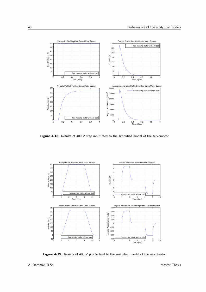
40 Performance of the analytical models
0 0.2 0.4 0.6 0.8 10
50
100
150
200
250
300
350Velocity Profile Simplified Servo Motor System
Ve
locity,
[ra
d/s
]
free running motor without load
0 0.2 0.4 0.6 0.8 10
50
100
150
200
250
300
350
400Voltage Profile Simplified Servo Motor System
Time, t [sec]
Fe
ed
Vo
lta
ge
, [V
]
free running motor without load
0 0.2 0.4 0.6 0.8 10
500
1000
1500
2000
2500
3000Angular Acceleration Profile Simplified Servo Motor System
Time, t [sec]
An
gu
lar
Acce
lera
tio
n,
[ra
d/s
2]
free running motor without load
0 0.2 0.4 0.6 0.8 10
5
10
15
20
25
30
35Current Profile Simplified Servo Motor System
Time, t [sec]
Cu
rre
nt,
[A
]
free running motor without load
Figure 4-18: Results of 400 V step input feed to the simplified model of the servomotor
0 1 2 3 4 5 6−50
0
50
100
150
200
250
300
350Velocity Profile Simplified Servo Motor System
Velo
city, [r
ad/s
]
free running motor without load
0 1 2 3 4 5 60
50
100
150
200
250
300
350
400Voltage Profile Simplified Servo Motor System
Time, t [sec]
Feed V
oltage, [V
]
free running motor without load
0 1 2 3 4 5 6−400
−300
−200
−100
0
100
200
300
400Angular Acceleration Profile Simplified Servo Motor System
Time, t [sec]
Angula
r A
ccele
ration, [r
ad/s
2]
free running motor without load
0 1 2 3 4 5 6−4
−3
−2
−1
0
1
2
3
4Current Profile Simplified Servo Motor System
Time, t [sec]
Curr
ent, [A
]
free running motor without load
Figure 4-19: Results of 400 V profile feed to the simplified model of the servomotor
A. Damman B.Sc. Master Thesis
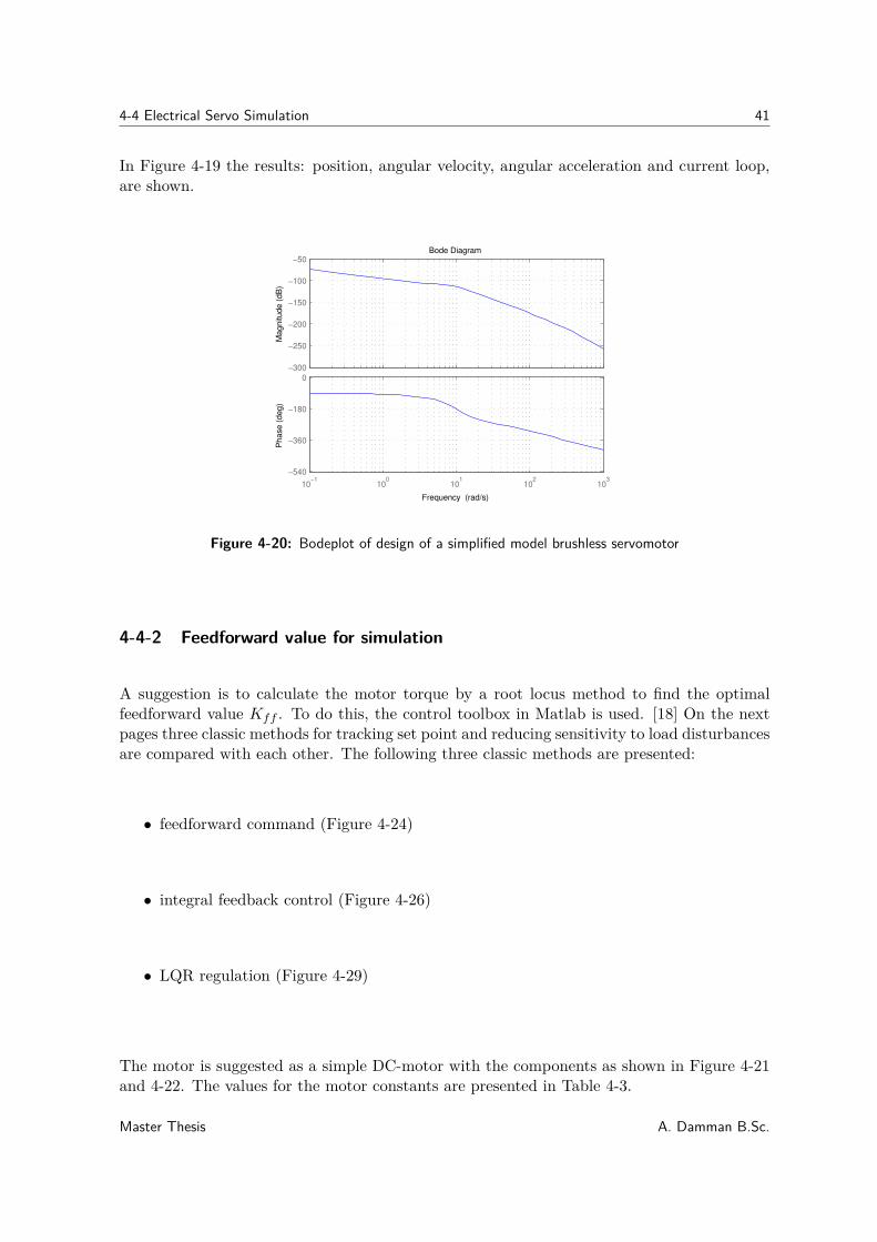
4-4 Electrical Servo Simulation 41
In Figure 4-19 the results: position, angular velocity, angular acceleration and current loop,are shown.
Bode Diagram
Frequency (rad/s)
10−1
100
101
102
103
−540
−360
−180
0
Phase (
deg)
−300
−250
−200
−150
−100
−50
Magnitude (
dB
)
Figure 4-20: Bodeplot of design of a simplified model brushless servomotor
4-4-2 Feedforward value for simulation
A suggestion is to calculate the motor torque by a root locus method to find the optimalfeedforward value Kff . To do this, the control toolbox in Matlab is used. [18] On the nextpages three classic methods for tracking set point and reducing sensitivity to load disturbancesare compared with each other. The following three classic methods are presented:
• feedforward command (Figure 4-24)
• integral feedback control (Figure 4-26)
• LQR regulation (Figure 4-29)
The motor is suggested as a simple DC-motor with the components as shown in Figure 4-21and 4-22. The values for the motor constants are presented in Table 4-3.
Master Thesis A. Damman B.Sc.
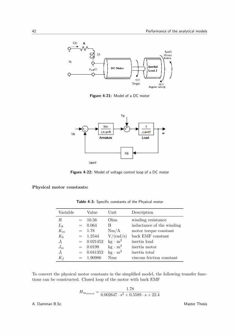
42 Performance of the analytical models
Figure 4-21: Model of a DC motor
Figure 4-22: Model of voltage control loop of a DC motor
Physical motor constants:
Table 4-3: Specific constants of the Physical motor
Variable Value Unit Description
R = 10.56 Ohm winding resistanceLh = 0.064 H inductance of the windingKm = 1.78 Nm/A motor torque constantKb = 1.2544 V/(rad/s) back EMF constantJl = 0.021452 kg · m2 inertia loadJm = 0.0199 kg · m2 inertia motorJt = 0.041352 kg · m2 inertia totalKf = 1.90986 Nms viscous friction constant
To convert the physical motor constants in the simplified model, the following transfer func-tions can be constructed. Closed loop of the motor with back EMF
Hmclosed=
1.780.002647 · s2 + 0.5589 · s + 22.4
A. Damman B.Sc. Master Thesis
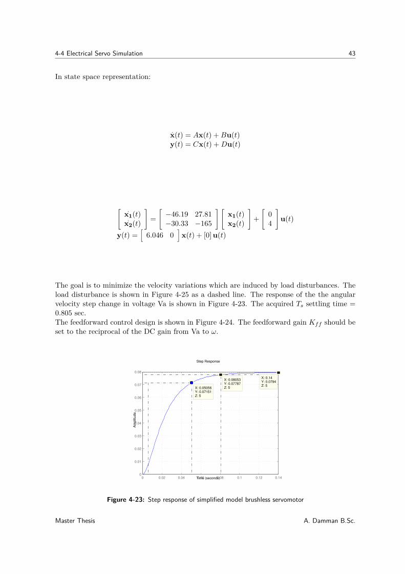
4-4 Electrical Servo Simulation 43
In state space representation:
.x(t) = Ax(t) + Bu(t)y(t) = Cx(t) + Du(t)
[ .x1(t)
.x2(t)
]
=
[
−46.19 27.81−30.33 −165
] [
x1(t)x2(t)
]
+
[
04
]
u(t)
y(t) =[
6.046 0]
x(t) + [0] u(t)
The goal is to minimize the velocity variations which are induced by load disturbances. Theload disturbance is shown in Figure 4-25 as a dashed line. The response of the the angularvelocity step change in voltage Va is shown in Figure 4-23. The acquired Ts settling time =0.805 sec.The feedforward control design is shown in Figure 4-24. The feedforward gain Kff should beset to the reciprocal of the DC gain from Va to ω.
Step Response
Time (seconds)
Am
plit
ud
e
0 0.02 0.04 0.06 0.08 0.1 0.12 0.140
0.01
0.02
0.03
0.04
0.05
0.06
0.07
0.08
X: 0.05056Y: 0.07151Z: 5
X: 0.08053Y: 0.07787Z: 5
X: 0.14Y: 0.0794Z: 5
Figure 4-23: Step response of simplified model brushless servomotor
Master Thesis A. Damman B.Sc.
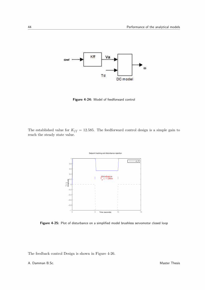
44 Performance of the analytical models
Figure 4-24: Model of feedforward control
The established value for Kff = 12.585. The feedforward control design is a simple gain toreach the steady state value.
0 5 10 15−1
−0.8
−0.6
−0.4
−0.2
0
0.2
0.4
0.6
0.8
1
To
: w
disturbanceT
d = −1.0Nm
Setpoint tracking and disturbance rejection
Time (seconds)
Am
plit
ud
e
cl_ff
Figure 4-25: Plot of disturbance on a simplified model brushless servomotor closed loop
The feedback control Design is shown in Figure 4-26.
A. Damman B.Sc. Master Thesis
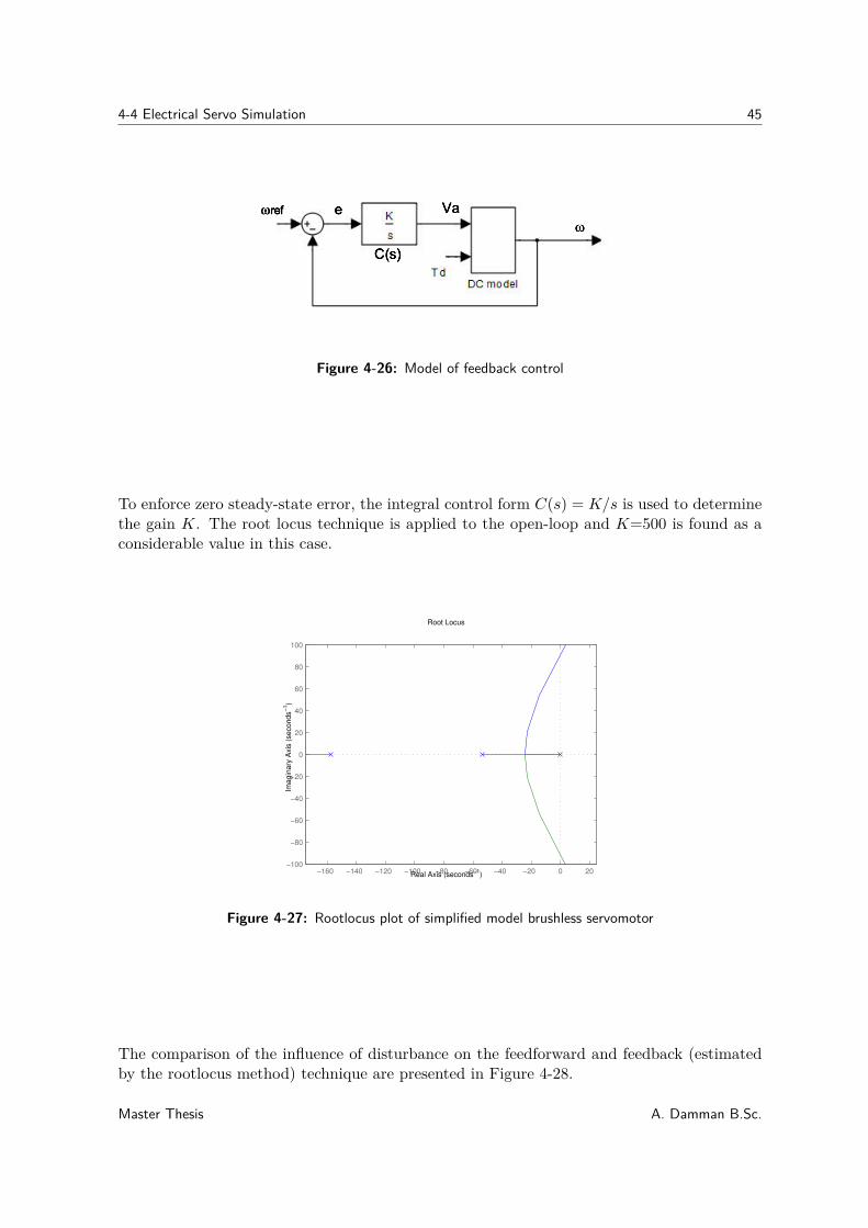
4-4 Electrical Servo Simulation 45
Figure 4-26: Model of feedback control
To enforce zero steady-state error, the integral control form C(s) = K/s is used to determinethe gain K. The root locus technique is applied to the open-loop and K=500 is found as aconsiderable value in this case.
−160 −140 −120 −100 −80 −60 −40 −20 0 20−100
−80
−60
−40
−20
0
20
40
60
80
100
Root Locus
Real Axis (seconds−1
)
Ima
gin
ary
Axis
(se
co
nd
s−
1)
Figure 4-27: Rootlocus plot of simplified model brushless servomotor
The comparison of the influence of disturbance on the feedforward and feedback (estimatedby the rootlocus method) technique are presented in Figure 4-28.
Master Thesis A. Damman B.Sc.
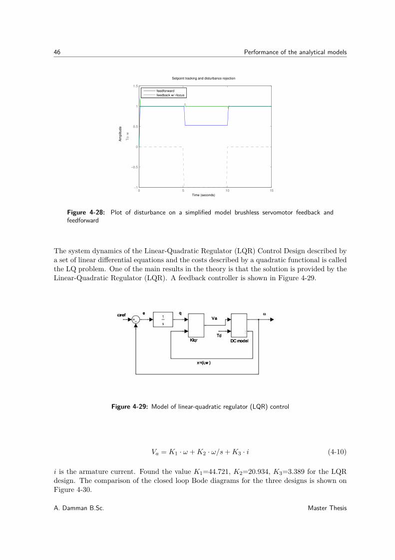
46 Performance of the analytical models
0 5 10 15−1
−0.5
0
0.5
1
1.5
To
: w
Setpoint tracking and disturbance rejection
Time (seconds)
Am
plit
ud
e
feedforward
feedback w/ rlocus
Figure 4-28: Plot of disturbance on a simplified model brushless servomotor feedback andfeedforward
The system dynamics of the Linear-Quadratic Regulator (LQR) Control Design described bya set of linear differential equations and the costs described by a quadratic functional is calledthe LQ problem. One of the main results in the theory is that the solution is provided by theLinear-Quadratic Regulator (LQR). A feedback controller is shown in Figure 4-29.
Figure 4-29: Model of linear-quadratic regulator (LQR) control
Va = K1 · ω + K2 · ω/s + K3 · i (4-10)
i is the armature current. Found the value K1=44.721, K2=20.934, K3=3.389 for the LQRdesign. The comparison of the closed loop Bode diagrams for the three designs is shown onFigure 4-30.
A. Damman B.Sc. Master Thesis
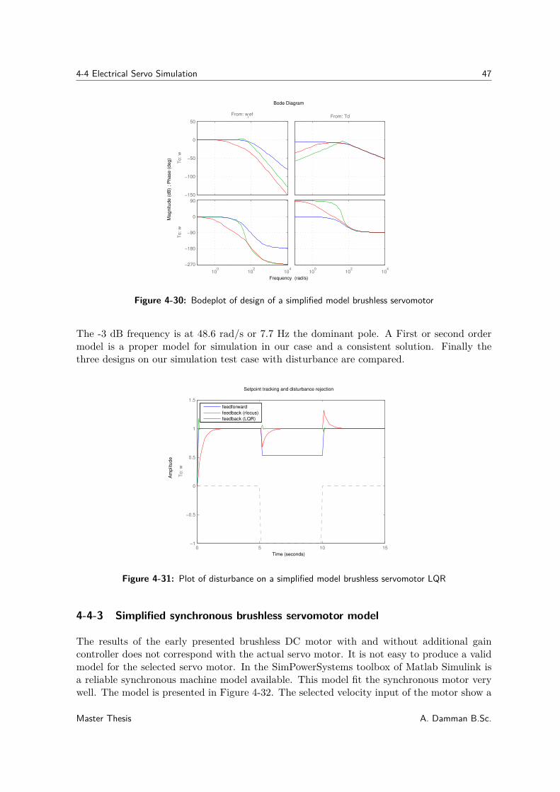
4-4 Electrical Servo Simulation 47
−150
−100
−50
0
50
From: wref
To
: w
100
102
104
−270
−180
−90
0
90
To
: w
From: Td
100
102
104
Bode Diagram
Frequency (rad/s)
Ma
gn
itu
de
(d
B)
; P
ha
se
(d
eg
)
Figure 4-30: Bodeplot of design of a simplified model brushless servomotor
The -3 dB frequency is at 48.6 rad/s or 7.7 Hz the dominant pole. A First or second ordermodel is a proper model for simulation in our case and a consistent solution. Finally thethree designs on our simulation test case with disturbance are compared.
0 5 10 15−1
−0.5
0
0.5
1
1.5
To
: w
Setpoint tracking and disturbance rejection
Time (seconds)
Am
plit
ud
e
feedforward
feedback (rlocus)
feedback (LQR)
Figure 4-31: Plot of disturbance on a simplified model brushless servomotor LQR
4-4-3 Simplified synchronous brushless servomotor model
The results of the early presented brushless DC motor with and without additional gaincontroller does not correspond with the actual servo motor. It is not easy to produce a validmodel for the selected servo motor. In the SimPowerSystems toolbox of Matlab Simulink isa reliable synchronous machine model available. This model fit the synchronous motor verywell. The model is presented in Figure 4-32. The selected velocity input of the motor show a
Master Thesis A. Damman B.Sc.
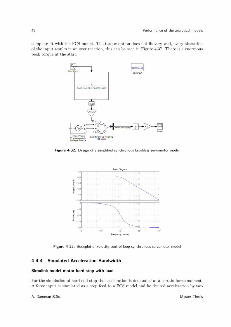
48 Performance of the analytical models
complete fit with the FCS model. The torque option does not fit very well, every alterationof the input results in an over reaction, this can be seen in Figure 4-37. There is a enormouspeak torque at the start.
Figure 4-32: Design of a simplified synchronous brushless servomotor model
Bode Diagram
Frequency (rad/s)
10−1
100
101
102
103
−180
−135
−90
−45
0
Phase (
deg)
−160
−140
−120
−100
−80
−60
Magnitude (
dB
)
Figure 4-33: Bodeplot of velocity control loop synchronous servomotor model
4-4-4 Simulated Acceleration Bandwidth
Simulink model motor hard stop with load
For the simulation of hard end stop the acceleration is demanded at a certain force/moment.A force input is simulated as a step feed to a FCS model and he desired acceleration by two
A. Damman B.Sc. Master Thesis
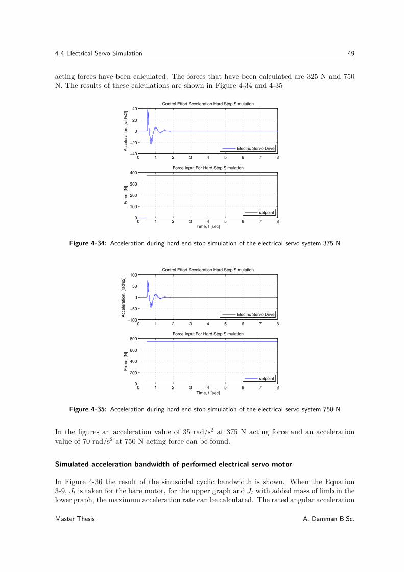
4-4 Electrical Servo Simulation 49
acting forces have been calculated. The forces that have been calculated are 325 N and 750N. The results of these calculations are shown in Figure 4-34 and 4-35
0 1 2 3 4 5 6 7 8−40
−20
0
20
40Control Effort Acceleration Hard Stop Simulation
Accele
ration, [r
ad/s
2]
Electric Servo Drive
0 1 2 3 4 5 6 7 80
100
200
300
400Force Input For Hard Stop Simulation
Time, t [sec]
Forc
e, [N
]
setpoint
Figure 4-34: Acceleration during hard end stop simulation of the electrical servo system 375 N
0 1 2 3 4 5 6 7 8−100
−50
0
50
100Control Effort Acceleration Hard Stop Simulation
Accele
ration, [r
ad/s
2]
Electric Servo Drive
0 1 2 3 4 5 6 7 80
200
400
600
800Force Input For Hard Stop Simulation
Time, t [sec]
Forc
e, [N
]
setpoint
Figure 4-35: Acceleration during hard end stop simulation of the electrical servo system 750 N
In the figures an acceleration value of 35 rad/s2 at 375 N acting force and an accelerationvalue of 70 rad/s2 at 750 N acting force can be found.
Simulated acceleration bandwidth of performed electrical servo motor
In Figure 4-36 the result of the sinusoidal cyclic bandwidth is shown. When the Equation3-9, Jt is taken for the bare motor, for the upper graph and Jt with added mass of limb in thelower graph, the maximum acceleration rate can be calculated. The rated angular acceleration
Master Thesis A. Damman B.Sc.
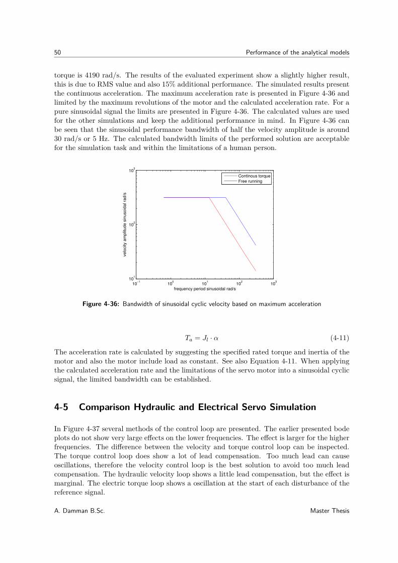
50 Performance of the analytical models
torque is 4190 rad/s. The results of the evaluated experiment show a slightly higher result,this is due to RMS value and also 15% additional performance. The simulated results presentthe continuous acceleration. The maximum acceleration rate is presented in Figure 4-36 andlimited by the maximum revolutions of the motor and the calculated acceleration rate. For apure sinusoidal signal the limits are presented in Figure 4-36. The calculated values are usedfor the other simulations and keep the additional performance in mind. In Figure 4-36 canbe seen that the sinusoidal performance bandwidth of half the velocity amplitude is around30 rad/s or 5 Hz. The calculated bandwidth limits of the performed solution are acceptablefor the simulation task and within the limitations of a human person.
10−1
100
101
102
103
101
102
103
frequency period sinusoidal rad/s
velo
city a
mplit
ude s
inusoid
al ra
d/s
Continous torque
Free running
Figure 4-36: Bandwidth of sinusoidal cyclic velocity based on maximum acceleration
Ta = Jl · α (4-11)
The acceleration rate is calculated by suggesting the specified rated torque and inertia of themotor and also the motor include load as constant. See also Equation 4-11. When applyingthe calculated acceleration rate and the limitations of the servo motor into a sinusoidal cyclicsignal, the limited bandwidth can be established.
4-5 Comparison Hydraulic and Electrical Servo Simulation
In Figure 4-37 several methods of the control loop are presented. The earlier presented bodeplots do not show very large effects on the lower frequencies. The effect is larger for the higherfrequencies. The difference between the velocity and torque control loop can be inspected.The torque control loop does show a lot of lead compensation. Too much lead can causeoscillations, therefore the velocity control loop is the best solution to avoid too much leadcompensation. The hydraulic velocity loop shows a little lead compensation, but the effect ismarginal. The electric torque loop shows a oscillation at the start of each disturbance of thereference signal.
A. Damman B.Sc. Master Thesis
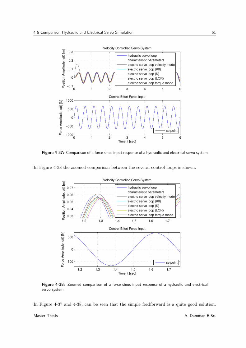
4-5 Comparison Hydraulic and Electrical Servo Simulation 51
0 1 2 3 4 5 6−0.1
0
0.1
0.2
0.3Velocity Controlled Servo System
Positio
n A
mplit
ude, y(t
) [m
]
hydraulic servo loop
characteristic parameters
electric servo loop velocity mode
electric servo loop (Kff)
electric servo loop (K)
electric servo loop (LQR)
electric servo loop torque mode
0 1 2 3 4 5 6−1000
−500
0
500
1000Control Effort Force Input
Time, t [sec]
Forc
e A
mplit
ude, u(t
) [N
]
setpoint
Figure 4-37: Comparison of a force sinus input response of a hydraulic and electrical servo system
In Figure 4-38 the zoomed comparison between the several control loops is shown.
1.2 1.3 1.4 1.5 1.6 1.7
0.03
0.04
0.05
0.06
0.07
Velocity Controlled Servo System
Positio
n A
mplit
ude, y(t
) [m
]
hydraulic servo loop
characteristic parameters
electric servo loop velocity mode
electric servo loop (Kff)
electric servo loop (K)
electric servo loop (LQR)
electric servo loop torque mode
1.2 1.3 1.4 1.5 1.6 1.7
−500
0
500
Control Effort Force Input
Time, t [sec]
Forc
e A
mplit
ude, u(t
) [N
]
setpoint
Figure 4-38: Zoomed comparison of a force sinus input response of a hydraulic and electricalservo system
In Figure 4-37 and 4-38, can be seen that the simple feedforward is a quite good solution.
Master Thesis A. Damman B.Sc.
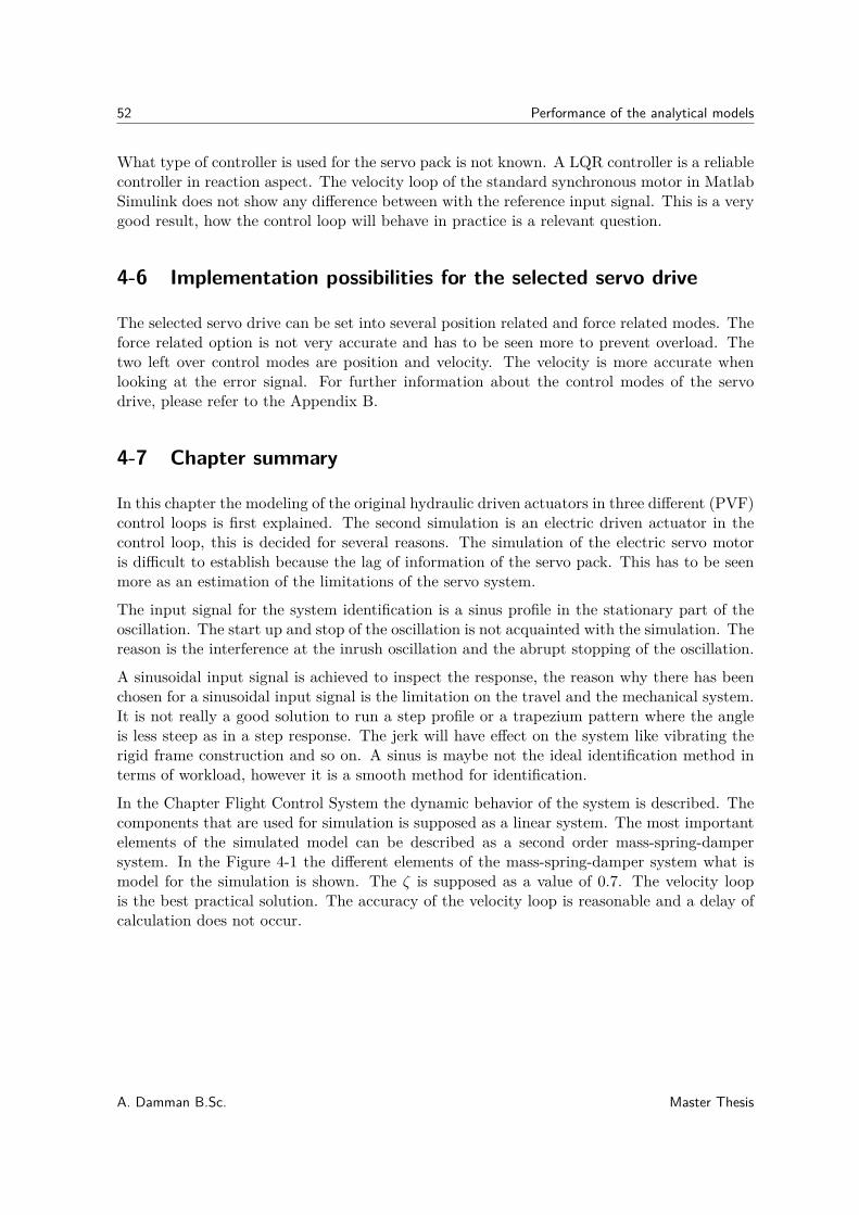
52 Performance of the analytical models
What type of controller is used for the servo pack is not known. A LQR controller is a reliablecontroller in reaction aspect. The velocity loop of the standard synchronous motor in MatlabSimulink does not show any difference between with the reference input signal. This is a verygood result, how the control loop will behave in practice is a relevant question.
4-6 Implementation possibilities for the selected servo drive
The selected servo drive can be set into several position related and force related modes. Theforce related option is not very accurate and has to be seen more to prevent overload. Thetwo left over control modes are position and velocity. The velocity is more accurate whenlooking at the error signal. For further information about the control modes of the servodrive, please refer to the Appendix B.
4-7 Chapter summary
In this chapter the modeling of the original hydraulic driven actuators in three different (PVF)control loops is first explained. The second simulation is an electric driven actuator in thecontrol loop, this is decided for several reasons. The simulation of the electric servo motoris difficult to establish because the lag of information of the servo pack. This has to be seenmore as an estimation of the limitations of the servo system.
The input signal for the system identification is a sinus profile in the stationary part of theoscillation. The start up and stop of the oscillation is not acquainted with the simulation. Thereason is the interference at the inrush oscillation and the abrupt stopping of the oscillation.
A sinusoidal input signal is achieved to inspect the response, the reason why there has beenchosen for a sinusoidal input signal is the limitation on the travel and the mechanical system.It is not really a good solution to run a step profile or a trapezium pattern where the angleis less steep as in a step response. The jerk will have effect on the system like vibrating therigid frame construction and so on. A sinus is maybe not the ideal identification method interms of workload, however it is a smooth method for identification.
In the Chapter Flight Control System the dynamic behavior of the system is described. Thecomponents that are used for simulation is supposed as a linear system. The most importantelements of the simulated model can be described as a second order mass-spring-dampersystem. In the Figure 4-1 the different elements of the mass-spring-damper system what ismodel for the simulation is shown. The ζ is supposed as a value of 0.7. The velocity loopis the best practical solution. The accuracy of the velocity loop is reasonable and a delay ofcalculation does not occur.
A. Damman B.Sc. Master Thesis
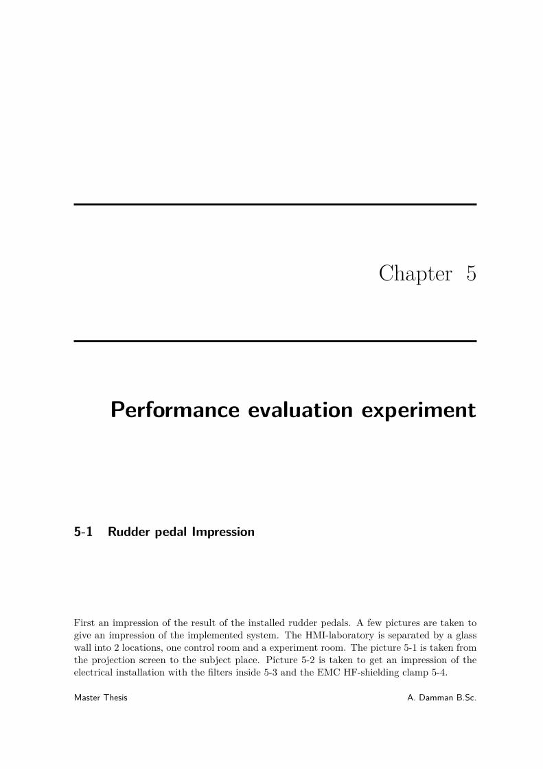
Chapter 5
Performance evaluation experiment
5-1 Rudder pedal Impression
First an impression of the result of the installed rudder pedals. A few pictures are taken togive an impression of the implemented system. The HMI-laboratory is separated by a glasswall into 2 locations, one control room and a experiment room. The picture 5-1 is taken fromthe projection screen to the subject place. Picture 5-2 is taken to get an impression of theelectrical installation with the filters inside 5-3 and the EMC HF-shielding clamp 5-4.
Master Thesis A. Damman B.Sc.
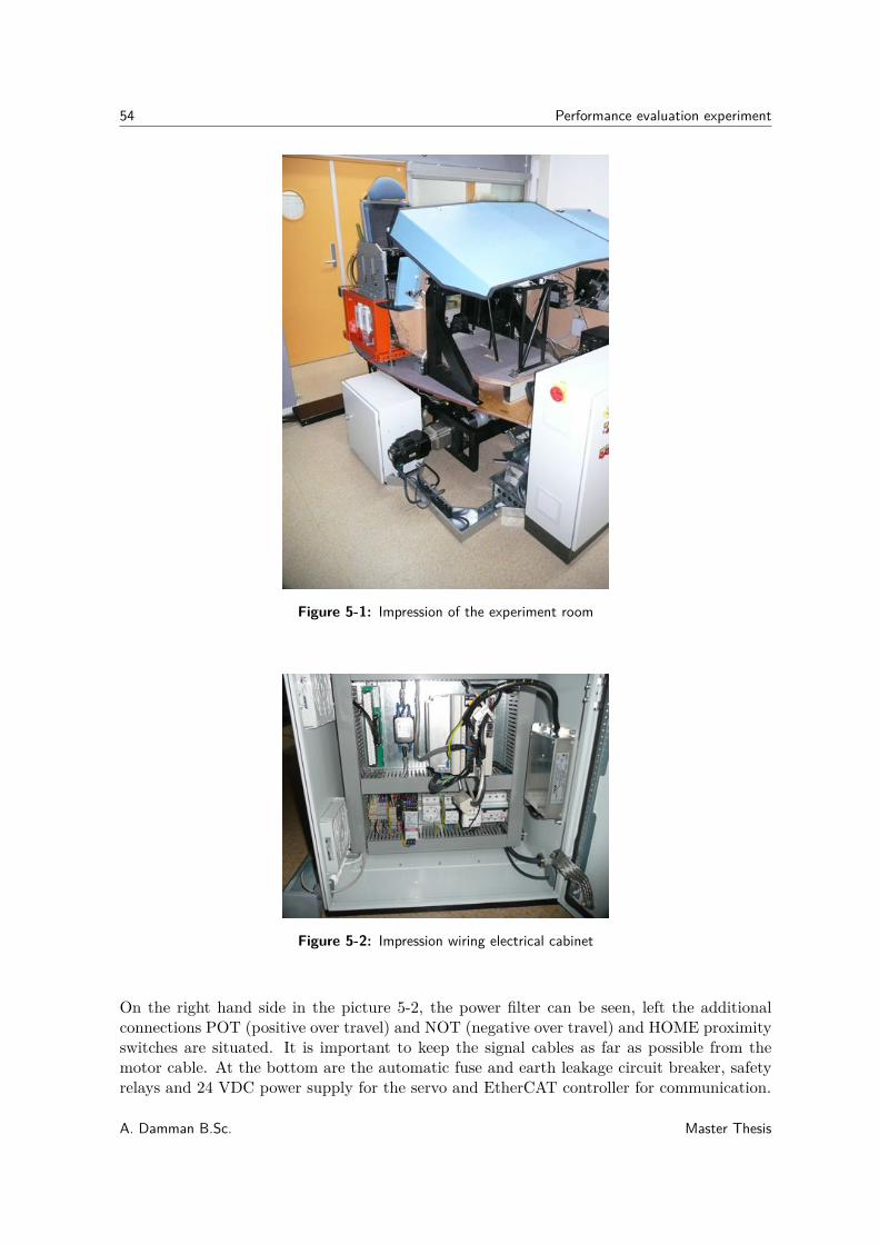
54 Performance evaluation experiment
Figure 5-1: Impression of the experiment room
Figure 5-2: Impression wiring electrical cabinet
On the right hand side in the picture 5-2, the power filter can be seen, left the additionalconnections POT (positive over travel) and NOT (negative over travel) and HOME proximityswitches are situated. It is important to keep the signal cables as far as possible from themotor cable. At the bottom are the automatic fuse and earth leakage circuit breaker, safetyrelays and 24 VDC power supply for the servo and EtherCAT controller for communication.
A. Damman B.Sc. Master Thesis
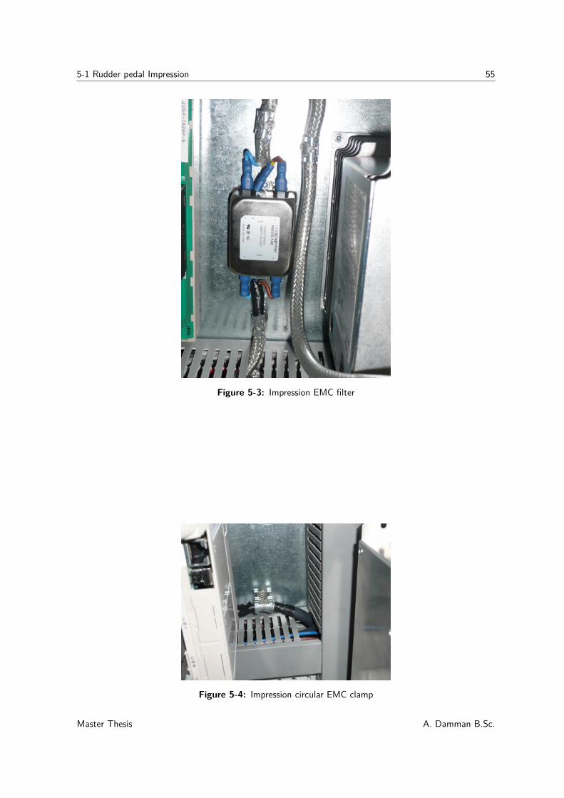
5-1 Rudder pedal Impression 55
Figure 5-3: Impression EMC filter
Figure 5-4: Impression circular EMC clamp
Master Thesis A. Damman B.Sc.
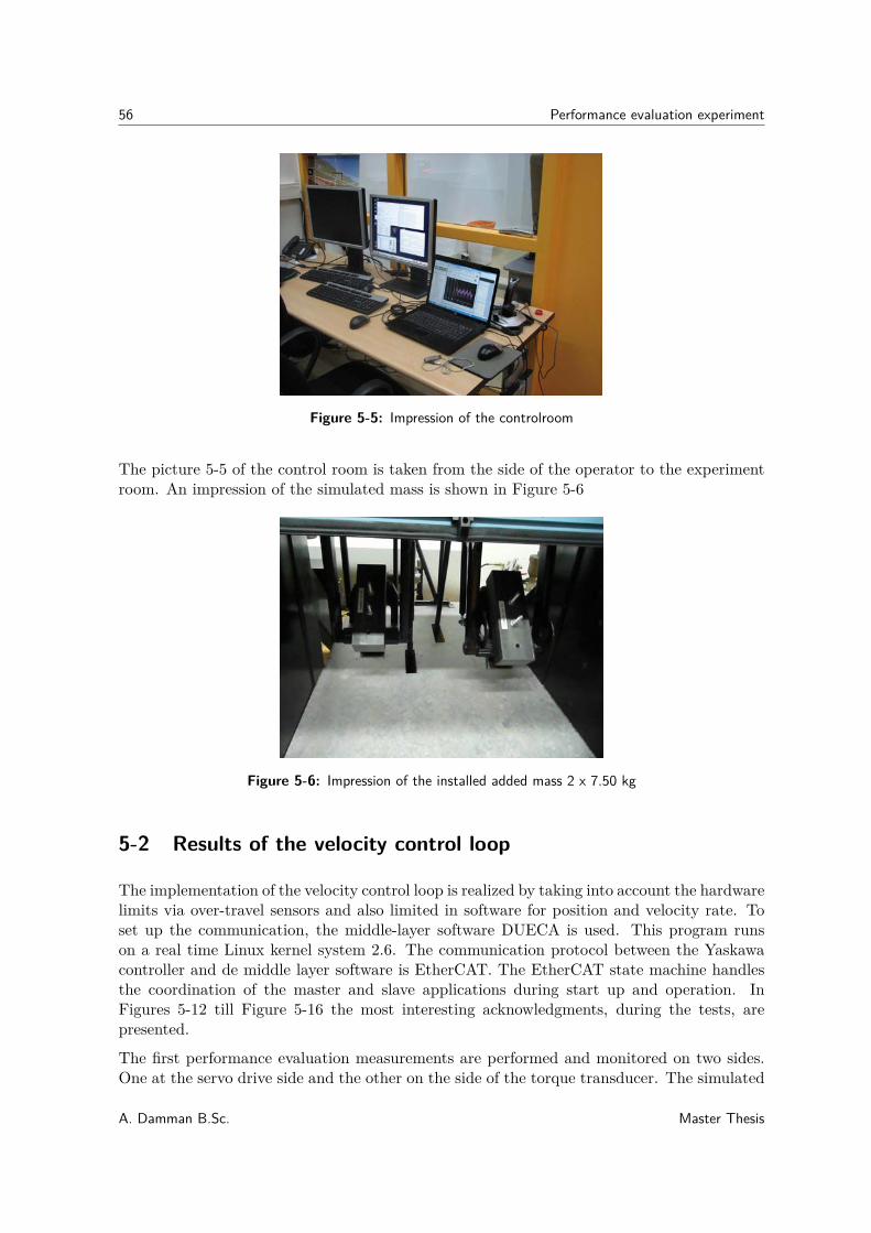
56 Performance evaluation experiment
Figure 5-5: Impression of the controlroom
The picture 5-5 of the control room is taken from the side of the operator to the experimentroom. An impression of the simulated mass is shown in Figure 5-6
Figure 5-6: Impression of the installed added mass 2 x 7.50 kg
5-2 Results of the velocity control loop
The implementation of the velocity control loop is realized by taking into account the hardwarelimits via over-travel sensors and also limited in software for position and velocity rate. Toset up the communication, the middle-layer software DUECA is used. This program runson a real time Linux kernel system 2.6. The communication protocol between the Yaskawacontroller and de middle layer software is EtherCAT. The EtherCAT state machine handlesthe coordination of the master and slave applications during start up and operation. InFigures 5-12 till Figure 5-16 the most interesting acknowledgments, during the tests, arepresented.
The first performance evaluation measurements are performed and monitored on two sides.One at the servo drive side and the other on the side of the torque transducer. The simulated
A. Damman B.Sc. Master Thesis
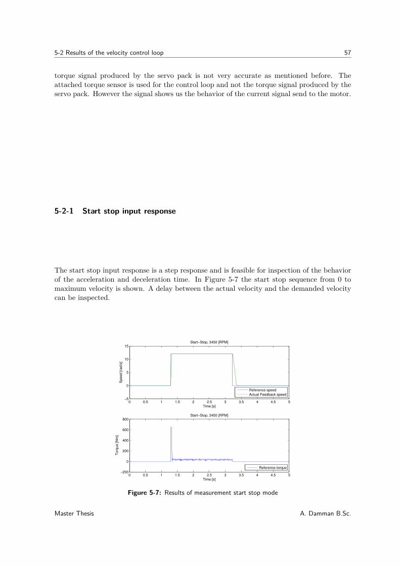
5-2 Results of the velocity control loop 57
torque signal produced by the servo pack is not very accurate as mentioned before. Theattached torque sensor is used for the control loop and not the torque signal produced by theservo pack. However the signal shows us the behavior of the current signal send to the motor.
5-2-1 Start stop input response
The start stop input response is a step response and is feasible for inspection of the behaviorof the acceleration and deceleration time. In Figure 5-7 the start stop sequence from 0 tomaximum velocity is shown. A delay between the actual velocity and the demanded velocitycan be inspected.
0 0.5 1 1.5 2 2.5 3 3.5 4 4.5 5−5
0
5
10
15Start−Stop, 3450 [RPM]
Time [s]
Sp
ee
d [
rad
/s]
Reference speed
Actual Feedback speed
0 0.5 1 1.5 2 2.5 3 3.5 4 4.5 5−200
0
200
400
600
800Start−Stop, 3450 [RPM]
Time [s]
To
rqu
e [
Nm
]
Reference torque
Figure 5-7: Results of measurement start stop mode
Master Thesis A. Damman B.Sc.
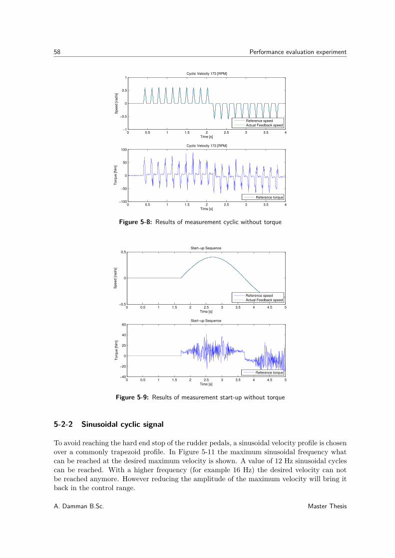
58 Performance evaluation experiment
0 0.5 1 1.5 2 2.5 3 3.5 4−1
−0.5
0
0.5
1Cyclic Velocity 173 [RPM]
Time [s]
Sp
ee
d [ra
d/s
]
Reference speed
Actual Feedback speed
0 0.5 1 1.5 2 2.5 3 3.5 4−100
−50
0
50
100Cyclic Velocity 173 [RPM]
Time [s]
To
rqu
e [N
m]
Reference torque
Figure 5-8: Results of measurement cyclic without torque
0 0.5 1 1.5 2 2.5 3 3.5 4 4.5 5−0.5
0
0.5Start−up Sequence
Time [s]
Speed [ra
d/s
]
Reference speed
Actual Feedback speed
0 0.5 1 1.5 2 2.5 3 3.5 4 4.5 5−40
−20
0
20
40
60Start−up Sequence
Time [s]
Torq
ue [N
m]
Reference torque
Figure 5-9: Results of measurement start-up without torque
5-2-2 Sinusoidal cyclic signal
To avoid reaching the hard end stop of the rudder pedals, a sinusoidal velocity profile is chosenover a commonly trapezoid profile. In Figure 5-11 the maximum sinusoidal frequency whatcan be reached at the desired maximum velocity is shown. A value of 12 Hz sinusoidal cyclescan be reached. With a higher frequency (for example 16 Hz) the desired velocity can notbe reached anymore. However reducing the amplitude of the maximum velocity will bring itback in the control range.
A. Damman B.Sc. Master Thesis
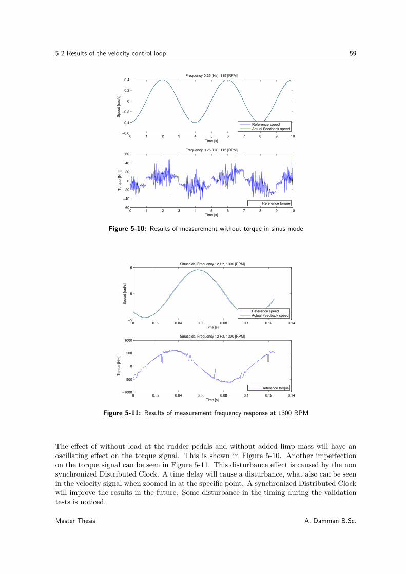
5-2 Results of the velocity control loop 59
0 1 2 3 4 5 6 7 8 9 10−0.6
−0.4
−0.2
0
0.2
0.4Frequency 0.25 [Hz], 115 [RPM]
Time [s]
Sp
ee
d [
rad
/s]
Reference speed
Actual Feedback speed
0 1 2 3 4 5 6 7 8 9 10−60
−40
−20
0
20
40
60Frequency 0.25 [Hz], 115 [RPM]
Time [s]
To
rqu
e [
Nm
]
Reference torque
Figure 5-10: Results of measurement without torque in sinus mode
0 0.02 0.04 0.06 0.08 0.1 0.12 0.14−5
0
5Sinusoidal Frequency 12 Hz, 1300 [RPM]
Time [s]
Speed [ra
d/s
]
Reference speed
Actual Feedback speed
0 0.02 0.04 0.06 0.08 0.1 0.12 0.14−1000
−500
0
500
1000Sinusoidal Frequency 12 Hz, 1300 [RPM]
Time [s]
Torq
ue [N
m]
Reference torque
Figure 5-11: Results of measurement frequency response at 1300 RPM
The effect of without load at the rudder pedals and without added limp mass will have anoscillating effect on the torque signal. This is shown in Figure 5-10. Another imperfectionon the torque signal can be seen in Figure 5-11. This disturbance effect is caused by the nonsynchronized Distributed Clock. A time delay will cause a disturbance, what also can be seenin the velocity signal when zoomed in at the specific point. A synchronized Distributed Clockwill improve the results in the future. Some disturbance in the timing during the validationtests is noticed.
Master Thesis A. Damman B.Sc.
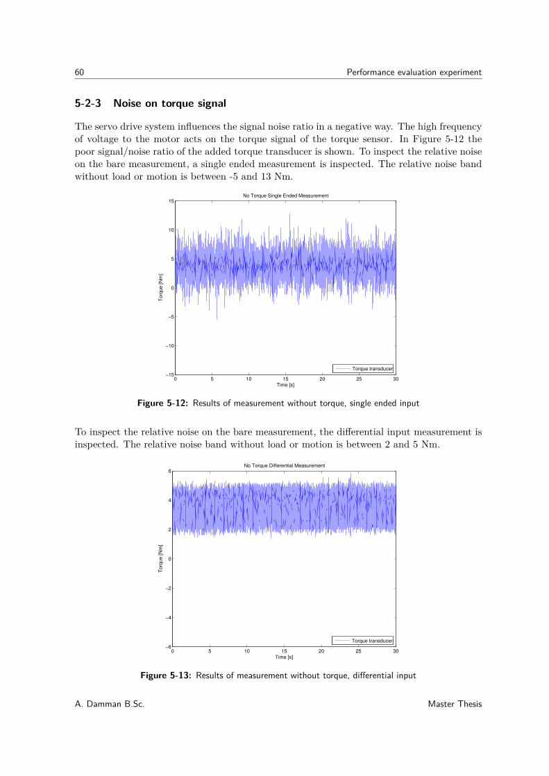
60 Performance evaluation experiment
5-2-3 Noise on torque signal
The servo drive system influences the signal noise ratio in a negative way. The high frequencyof voltage to the motor acts on the torque signal of the torque sensor. In Figure 5-12 thepoor signal/noise ratio of the added torque transducer is shown. To inspect the relative noiseon the bare measurement, a single ended measurement is inspected. The relative noise bandwithout load or motion is between -5 and 13 Nm.
0 5 10 15 20 25 30−15
−10
−5
0
5
10
15No Torque Single Ended Measurement
Time [s]
Torq
ue [N
m]
Torque transducer
Figure 5-12: Results of measurement without torque, single ended input
To inspect the relative noise on the bare measurement, the differential input measurement isinspected. The relative noise band without load or motion is between 2 and 5 Nm.
0 5 10 15 20 25 30−6
−4
−2
0
2
4
6No Torque Differential Measurement
Time [s]
Torq
ue [N
m]
Torque transducer
Figure 5-13: Results of measurement without torque, differential input
A. Damman B.Sc. Master Thesis
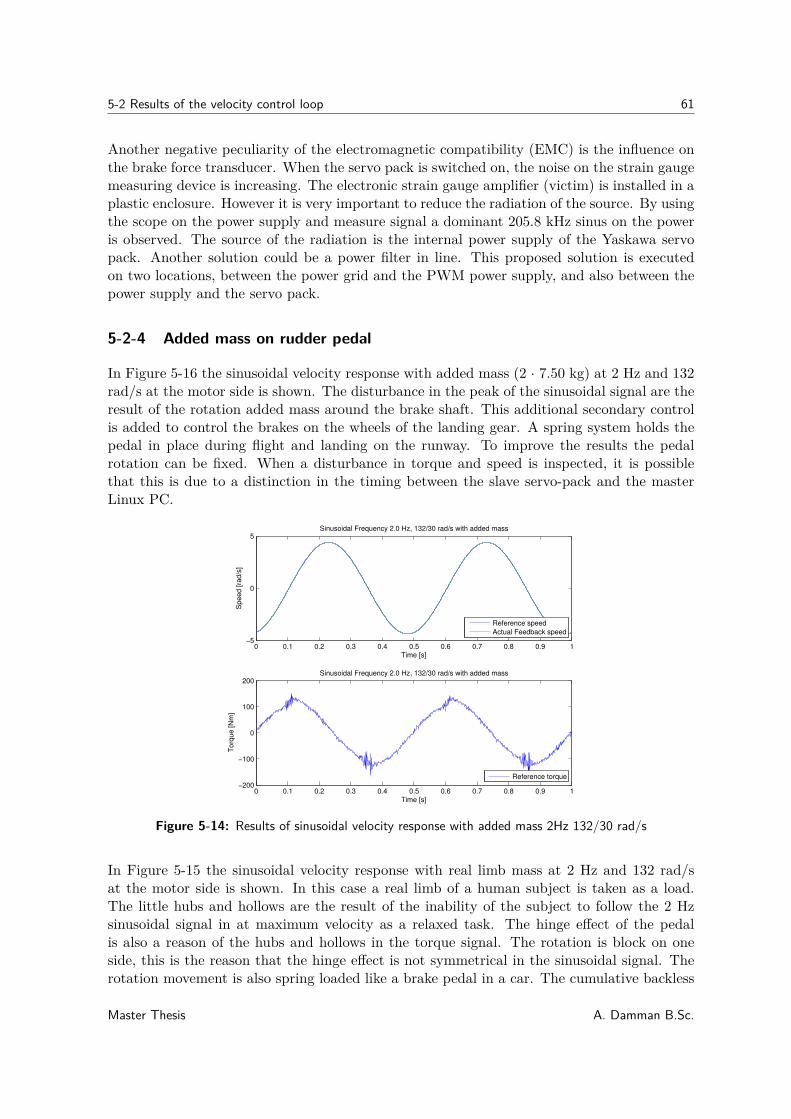
5-2 Results of the velocity control loop 61
Another negative peculiarity of the electromagnetic compatibility (EMC) is the influence onthe brake force transducer. When the servo pack is switched on, the noise on the strain gaugemeasuring device is increasing. The electronic strain gauge amplifier (victim) is installed in aplastic enclosure. However it is very important to reduce the radiation of the source. By usingthe scope on the power supply and measure signal a dominant 205.8 kHz sinus on the poweris observed. The source of the radiation is the internal power supply of the Yaskawa servopack. Another solution could be a power filter in line. This proposed solution is executedon two locations, between the power grid and the PWM power supply, and also between thepower supply and the servo pack.
5-2-4 Added mass on rudder pedal
In Figure 5-16 the sinusoidal velocity response with added mass (2 · 7.50 kg) at 2 Hz and 132rad/s at the motor side is shown. The disturbance in the peak of the sinusoidal signal are theresult of the rotation added mass around the brake shaft. This additional secondary controlis added to control the brakes on the wheels of the landing gear. A spring system holds thepedal in place during flight and landing on the runway. To improve the results the pedalrotation can be fixed. When a disturbance in torque and speed is inspected, it is possiblethat this is due to a distinction in the timing between the slave servo-pack and the masterLinux PC.
0 0.1 0.2 0.3 0.4 0.5 0.6 0.7 0.8 0.9 1−5
0
5Sinusoidal Frequency 2.0 Hz, 132/30 rad/s with added mass
Time [s]
Sp
ee
d [
rad
/s]
Reference speed
Actual Feedback speed
0 0.1 0.2 0.3 0.4 0.5 0.6 0.7 0.8 0.9 1−200
−100
0
100
200Sinusoidal Frequency 2.0 Hz, 132/30 rad/s with added mass
Time [s]
To
rqu
e [
Nm
]
Reference torque
Figure 5-14: Results of sinusoidal velocity response with added mass 2Hz 132/30 rad/s
In Figure 5-15 the sinusoidal velocity response with real limb mass at 2 Hz and 132 rad/sat the motor side is shown. In this case a real limb of a human subject is taken as a load.The little hubs and hollows are the result of the inability of the subject to follow the 2 Hzsinusoidal signal in at maximum velocity as a relaxed task. The hinge effect of the pedalis also a reason of the hubs and hollows in the torque signal. The rotation is block on oneside, this is the reason that the hinge effect is not symmetrical in the sinusoidal signal. Therotation movement is also spring loaded like a brake pedal in a car. The cumulative backless
Master Thesis A. Damman B.Sc.
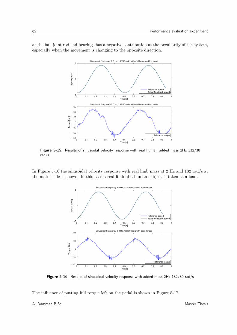
62 Performance evaluation experiment
at the ball joint rod end bearings has a negative contribution at the peculiarity of the system,especially when the movement is changing to the opposite direction.
0 0.1 0.2 0.3 0.4 0.5 0.6 0.7 0.8 0.9 1−5
0
5Sinusoidal Frequency 2.0 Hz, 132/30 rad/s with real human added mass
Time [s]
Sp
ee
d [ra
d/s
]
Reference speed
Actual Feedback speed
0 0.1 0.2 0.3 0.4 0.5 0.6 0.7 0.8 0.9 1−150
−100
−50
0
50
100
150Sinusoidal Frequency 2.0 Hz, 132/30 rad/s with real human added mass
Time [s]
To
rqu
e [N
m]
Reference torque
Figure 5-15: Results of sinusoidal velocity response with real human added mass 2Hz 132/30rad/s
In Figure 5-16 the sinusoidal velocity response with real limb mass at 2 Hz and 132 rad/s atthe motor side is shown. In this case a real limb of a human subject is taken as a load.
0 0.1 0.2 0.3 0.4 0.5 0.6 0.7 0.8 0.9 1−5
0
5Sinusoidal Frequency 2.0 Hz, 132/30 rad/s with added mass
Time [s]
Sp
ee
d [
rad
/s]
Reference speed
Actual Feedback speed
0 0.1 0.2 0.3 0.4 0.5 0.6 0.7 0.8 0.9 1−200
−100
0
100
200Sinusoidal Frequency 2.0 Hz, 132/30 rad/s with added mass
Time [s]
To
rqu
e [
Nm
]
Reference torque
Figure 5-16: Results of sinusoidal velocity response with added mass 2Hz 132/30 rad/s
The influence of putting full torque left on the pedal is shown in Figure 5-17.
A. Damman B.Sc. Master Thesis
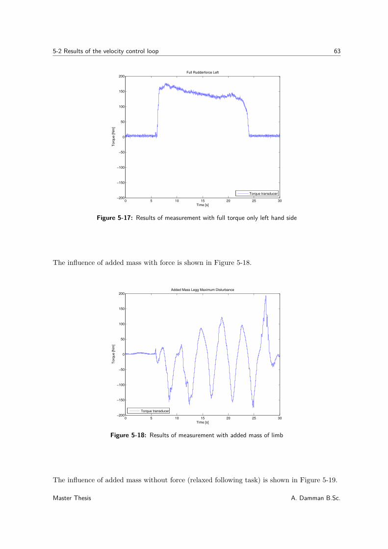
5-2 Results of the velocity control loop 63
0 5 10 15 20 25 30−200
−150
−100
−50
0
50
100
150
200Full Rudderforce Left
Time [s]
To
rqu
e [
Nm
]
Torque transducer
Figure 5-17: Results of measurement with full torque only left hand side
The influence of added mass with force is shown in Figure 5-18.
0 5 10 15 20 25 30−200
−150
−100
−50
0
50
100
150
200Added Mass Legg Maximum Disturbance
Time [s]
To
rqu
e [
Nm
]
Torque transducer
Figure 5-18: Results of measurement with added mass of limb
The influence of added mass without force (relaxed following task) is shown in Figure 5-19.
Master Thesis A. Damman B.Sc.
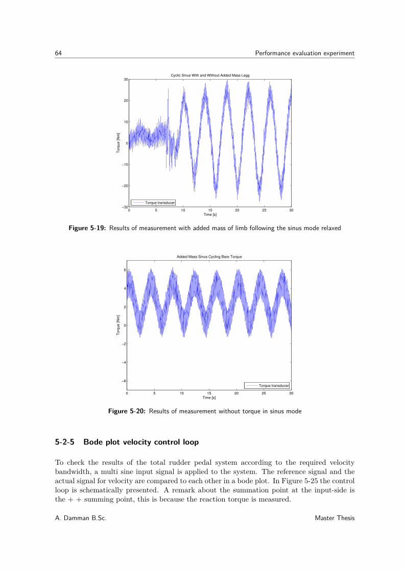
64 Performance evaluation experiment
0 5 10 15 20 25 30−30
−20
−10
0
10
20
30Cyclic Sinus With and Without Added Mass Legg
Time [s]
Torq
ue [N
m]
Torque transducer
Figure 5-19: Results of measurement with added mass of limb following the sinus mode relaxed
0 5 10 15 20 25 30
−6
−4
−2
0
2
4
6
Added Mass Sinus Cycling Bare Torque
Time [s]
Torq
ue [N
m]
Torque transducer
Figure 5-20: Results of measurement without torque in sinus mode
5-2-5 Bode plot velocity control loop
To check the results of the total rudder pedal system according to the required velocitybandwidth, a multi sine input signal is applied to the system. The reference signal and theactual signal for velocity are compared to each other in a bode plot. In Figure 5-25 the controlloop is schematically presented. A remark about the summation point at the input-side isthe + + summing point, this is because the reaction torque is measured.
A. Damman B.Sc. Master Thesis
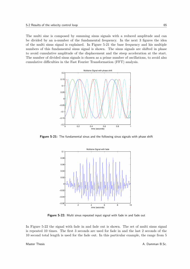
5-2 Results of the velocity control loop 65
The multi sine is composed by summing sinus signals with a reduced amplitude and canbe divided by an n-number of the fundamental frequency. In the next 3 figures the ideaof the multi sinus signal is explained. In Figure 5-21 the base frequency and his multiplenumbers of this fundamental sinus signal is shown. The sinus signals are shifted in phaseto avoid cumulative amplitude of the displacement and the steep acceleration at the start.The number of divided sinus signals is chosen as a prime number of oscillations, to avoid alsocumulative difficulties in the Fast Fourier Transformation (FFT) analysis.
0 0.2 0.4 0.6 0.8 1−0.2
−0.15
−0.1
−0.05
0
0.05
0.1
0.15
0.2Multisine Signal with phase shift
time (seconds)
Figure 5-21: The fundamental sinus and the following sinus signals with phase shift
0 2 4 6 8 10−0.06
−0.04
−0.02
0
0.02
0.04
0.06
0.08
0.1Multisine Signal with fade
time (seconds)
Figure 5-22: Multi sinus repeated input signal with fade in and fade out
In Figure 5-22 the signal with fade in and fade out is shown. The set of multi sinus signalis repeated 10 times. The first 3 seconds are used for fade in and the last 2 seconds of the10 second total length is used for the fade out. In this particular example, the range from 5
Master Thesis A. Damman B.Sc.
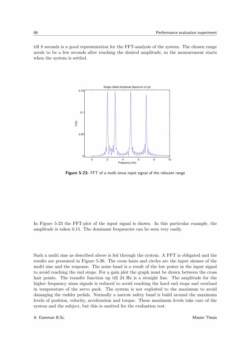
66 Performance evaluation experiment
till 8 seconds is a good representation for the FFT-analysis of the system. The chosen rangeneeds to be a few seconds after reaching the desired amplitude, so the measurement startswhen the system is settled.
0 2 4 6 8 10
0
0.05
0.1
0.15
Single−Sided Amplitude Spectrum of y(t)
Frequency (Hz)
|Y(f
)|
Figure 5-23: FFT of a multi sinus input signal of the relevant range
In Figure 5-23 the FFT-plot of the input signal is shown. In this particular example, theamplitude is taken 0.15. The dominant frequencies can be seen very easily.
Such a multi sine as described above is fed through the system. A FFT is obligated and theresults are presented in Figure 5-26. The cross hairs and circles are the input sinuses of themulti sine and the response. The noise band is a result of the low power in the input signalto avoid reaching the end stops. For a gain plot the graph must be drawn between the crosshair points. The transfer function up till 24 Hz is a straight line. The amplitude for thehigher frequency sinus signals is reduced to avoid reaching the hard end stops and overloadin temperature of the servo pack. The system is not exploited to the maximum to avoiddamaging the rudder pedals. Normally a narrow safety band is build around the maximumlevels of position, velocity, acceleration and torque. These maximum levels take care of thesystem and the subject, but this is omitted for the evaluation test.
A. Damman B.Sc. Master Thesis
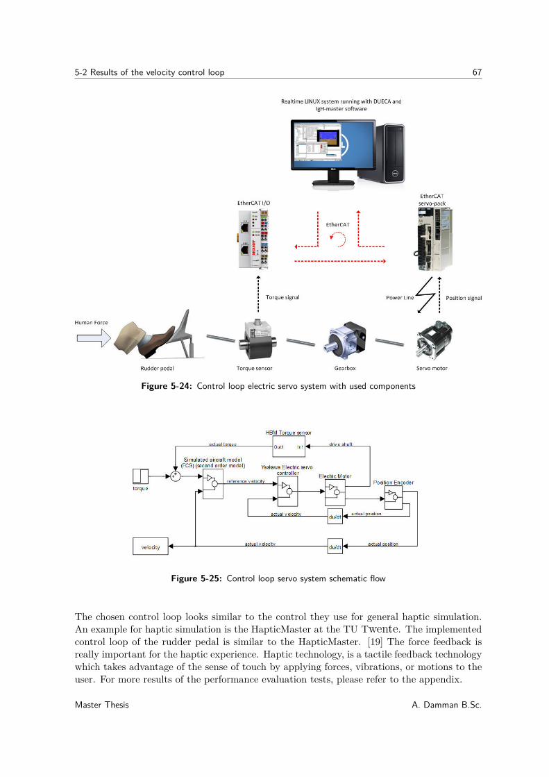
5-2 Results of the velocity control loop 67
Figure 5-24: Control loop electric servo system with used components
Figure 5-25: Control loop servo system schematic flow
The chosen control loop looks similar to the control they use for general haptic simulation.An example for haptic simulation is the HapticMaster at the TU Twente. The implementedcontrol loop of the rudder pedal is similar to the HapticMaster. [19] The force feedback isreally important for the haptic experience. Haptic technology, is a tactile feedback technologywhich takes advantage of the sense of touch by applying forces, vibrations, or motions to theuser. For more results of the performance evaluation tests, please refer to the appendix.
Master Thesis A. Damman B.Sc.
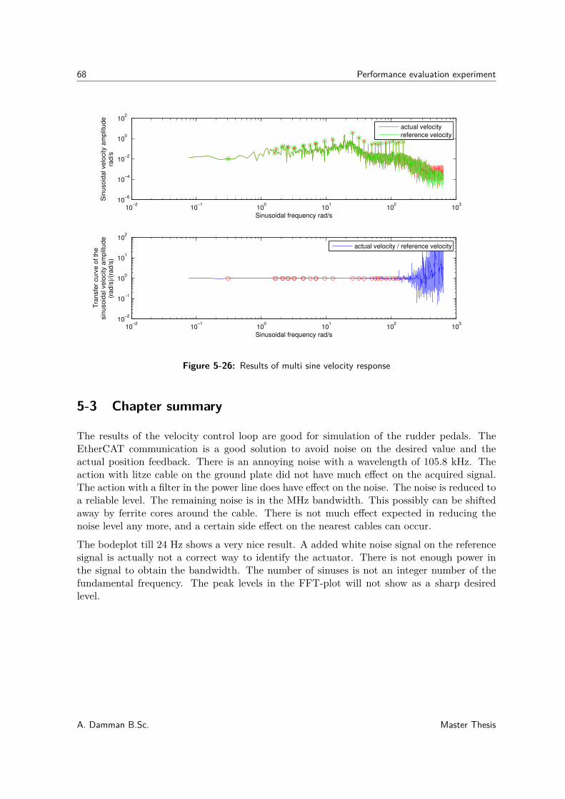
68 Performance evaluation experiment
10−2
10−1
100
101
102
103
10−6
10−4
10−2
100
102
Sinusoidal frequency rad/s
Sin
uso
ida
l ve
locity a
mp
litu
de
rad
/s
actual velocity
reference velocity
10−2
10−1
100
101
102
103
10−2
10−1
100
101
102
Sinusoidal frequency rad/s
Tra
nsfe
r cu
rve
of
the
sin
uso
ida
l ve
locity a
mp
litu
de
(ra
d/s
)/(r
ad
/s)
actual velocity / reference velocity
Figure 5-26: Results of multi sine velocity response
5-3 Chapter summary
The results of the velocity control loop are good for simulation of the rudder pedals. TheEtherCAT communication is a good solution to avoid noise on the desired value and theactual position feedback. There is an annoying noise with a wavelength of 105.8 kHz. Theaction with litze cable on the ground plate did not have much effect on the acquired signal.The action with a filter in the power line does have effect on the noise. The noise is reduced toa reliable level. The remaining noise is in the MHz bandwidth. This possibly can be shiftedaway by ferrite cores around the cable. There is not much effect expected in reducing thenoise level any more, and a certain side effect on the nearest cables can occur.
The bodeplot till 24 Hz shows a very nice result. A added white noise signal on the referencesignal is actually not a correct way to identify the actuator. There is not enough power inthe signal to obtain the bandwidth. The number of sinuses is not an integer number of thefundamental frequency. The peak levels in the FFT-plot will not show as a sharp desiredlevel.
A. Damman B.Sc. Master Thesis
Chapter 6
Discussion
6-1 Discussion
When the results of the simulated model and the evaluation experiment are inspected, Itcan be noticed that the simulated results are optimistic in comparison to the evaluationmeasurements. The many (estimated) unknown variables do have influence on the totalsystem. The proposed solution to design the system completely in the continuous range ofthe motor is a proper solution in this case.
The required 25 Hz bandwidth at maximum velocity can not be reached unfortunately. 14 Hzis reachable at maximum velocity. An additional brake resistor can enlarge the bandwidth. Ata sinusoidal mode at 25 Hz, the maximum velocity of 26 rad/s can be reached at a maximumcontinuous torque of 208 Nm at the drive shaft of the gearbox. The maximum accelerationof 4190 rad/s2 is the limited value in this particular situation.
The force control loop is better but not realistic to implement. The preferred control loopis the velocity control loop, there are several reason for it, the most important reason is theunsatisfying force signal and second, the difficulties to implement a force estimation model inthe FCS.
The force signal with added mass seems more realistic for the motor controller inside and thecurrent to the motor. The attached torque transducer reproduces a reliable signal, howeverthe noise / signal ratio is poor.
The difference in the three hydraulic models (velocity, position and force) can be seen by thedifference in settling time. A bode plot is obtained to inspect the differences. The influenceof the system inertia has a relevant effect on the results and this can not be scaled by only again factor.
Master Thesis A. Damman B.Sc.

70 Discussion
A. Damman B.Sc. Master Thesis
Chapter 7
Conclusions
7-1 Conclusions
When the requirements with the validation results are checked we could answer the researchquestion sizing and designs as followed:
The choice of a gear ratio of 1:30 is a good opportunity, speed and torque requirement can bemet. By reducing the torque via a gearbox, the inertia can also be reduced. For the inertiaratio of the drive system J l/Jm maximum 5 is preferred. Our gear ratio is in the rangeof 1/5 of the motor inertia and gives a safety factor to compensate for possible mechanicalconstruction complaints in the system.
Check with requirements:
Maximum force/moment is 250.2 Nm or 801.9 Nm. For a short period of 5 seconds by naturalheat convection, the motor can produce 3 times the continuous value. The continuous valueis already in specification and a safety factor is build in.
The travel range has not changed and a adjustment sensor is attached for correction
Velocity of 2 Hz sinusoidal cycling is possible and also at the maximum velocity of 1.3 m/s.The maximum frequency at maximum velocity is around 12 Hz. Lower velocity of the sinu-soidal cyclic bandwidth of 24 Hz is validated and reachable. An additional brake resistor canenlarge the bandwidth, however is not necessary in this case.
The inertia ratio of the drive system 1.08 is reached in this case and for high performance themaximum value of 2 is allowed.
Chosen control loop:
The implemented velocity control loop works very well for this system. The force control loopis for several reason not the best solution for this situation. The lead compensation is toomuch and an oscillation can arise. The practical obstacle is the low accuracy of the derivedtorque value by the servo pack. This 0.1 % of the rated torque value and 0.25 Nm at the pedalshaft. The derived torque value of the servo is reliable for overload indication and safety, butis not useful as control signal. The translated current signal is oscillating heavily.
Master Thesis A. Damman B.Sc.
72 Conclusions
The position and velocity loop are feasible for implementation. The choice is made for thevelocity loop, so to translate the signal to acceleration takes one integration an one derivationto the position.
The preferred control loop is velocity, there are several reason for it. The most importantreason is the unsatisfied force signal and second the difficulties to implement a force estimationmodel in the FCS. The force signal with added mass seems more realistic for the motorcontroller inside and the current to the motor. The attached torque transducer reproduces areliable signal, however the signal / noise ratio is poor.
There is no need to implement an additional control loop between the actual velocity and thereference (target) velocity. The build in controller of the Yaskawa drive is sufficient enoughto control the velocity of the rudder pedals.
The requirements can be reached in a proper way with an electrical servo drive, this is provenby the validation tests. The safety environment is improved in comparison with the hydraulicactuator.
A. Damman B.Sc. Master Thesis

Appendix A
Alternative Solutions
A-1 Alternative Solution 1
A proposed solution is to exchange the hydraulic actuator for an electric servo direct drive asshown in the figure below.
Figure A-1: Alternative solution 1 proposed exchange hydraulic motor directly for an electricservo direct drive
The experience we have acquired with one of our electric servo drive systems results in apreferred direct drive solution with a high torque motor of Parker Hannifin combined with aCompax3 servo controller. The documentation and specifications of the controller Compax3of Parker [20] is examined. The direct drive motor type ST series [21] is a suitable solutionfor this matter. There are two types of drives that are suitable for installation. Type of drive300STK4M and 300STK6M, delivers continuous 170 and 235 Nm at 11.8 and 16.3 Amps.Peak torque is 774 and 1161 Nm for a short time of 5 seconds by natural heat convection.The velocity of 4.656 m/s is acceptable, however this is not the speed the system will reach in
Master Thesis A. Damman B.Sc.
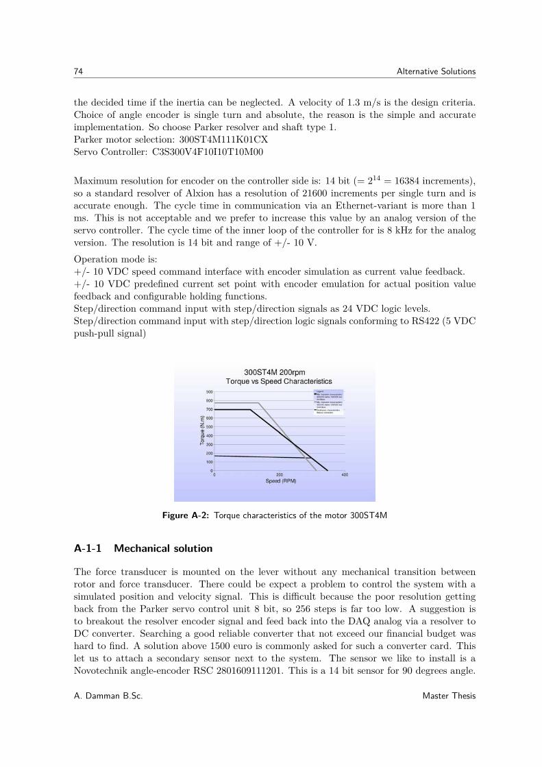
74 Alternative Solutions
the decided time if the inertia can be neglected. A velocity of 1.3 m/s is the design criteria.Choice of angle encoder is single turn and absolute, the reason is the simple and accurateimplementation. So choose Parker resolver and shaft type 1.Parker motor selection: 300ST4M111K01CXServo Controller: C3S300V4F10I10T10M00
Maximum resolution for encoder on the controller side is: 14 bit (= 214 = 16384 increments),so a standard resolver of Alxion has a resolution of 21600 increments per single turn and isaccurate enough. The cycle time in communication via an Ethernet-variant is more than 1ms. This is not acceptable and we prefer to increase this value by an analog version of theservo controller. The cycle time of the inner loop of the controller for is 8 kHz for the analogversion. The resolution is 14 bit and range of +/- 10 V.
Operation mode is:+/- 10 VDC speed command interface with encoder simulation as current value feedback.+/- 10 VDC predefined current set point with encoder emulation for actual position valuefeedback and configurable holding functions.Step/direction command input with step/direction signals as 24 VDC logic levels.Step/direction command input with step/direction logic signals conforming to RS422 (5 VDCpush-pull signal)
Figure A-2: Torque characteristics of the motor 300ST4M
A-1-1 Mechanical solution
The force transducer is mounted on the lever without any mechanical transition betweenrotor and force transducer. There could be expect a problem to control the system with asimulated position and velocity signal. This is difficult because the poor resolution gettingback from the Parker servo control unit 8 bit, so 256 steps is far too low. A suggestion isto breakout the resolver encoder signal and feed back into the DAQ analog via a resolver toDC converter. Searching a good reliable converter that not exceed our financial budget washard to find. A solution above 1500 euro is commonly asked for such a converter card. Thislet us to attach a secondary sensor next to the system. The sensor we like to install is aNovotechnik angle-encoder RSC 2801609111201. This is a 14 bit sensor for 90 degrees angle.
A. Damman B.Sc. Master Thesis

A-2 Alternative Solution 2 75
A-2 Alternative Solution 2
Suggest another transmission system and another servo drive from Yaskawa or Panason-ic/Omron. By selecting another servo drive, the direct drive and a linear drive seems to bea reasonable solution. [22] A linear drive is an expensive solution due to the fact that youhave 2 linear motors and also 2 servo controllers. Also the hardware setup for the rudderpedals have to be redesigned. This is not a suitable solution for our laboratory. Proposed isa solution with a direct drive. The companies Panasonic and Omron do not deliver a directdrive motor in their own product line. Of course it is possible to select a servo controller fromanother company, but this is not preferred to select the motor and the controller from thesame supplier to avoid exchange difficulties in encoder communication. A suitable place toconnect the direct drive motor on the rudder pedals is at the shaft of the second lever withthe lever length of 182 mm. Now calculate back from the maximum speed what kind of motoris selectable in the torque range. T2 is the required torque at the second pedal shaft:
Fpd = 150lbf ≈ 667N
T2 = Fpd·i2
li2
= 208Nm(A-1)
li2= lever arm length from Fa to the second pedal shaft axis.
The selected servomotor could be a direct drive of Yaskawa SGMCS-80M with a continuousrated torque of 80 Nm, it is the first servo drive that fulfills the requirement on velocity andtorque. The smallest transmission ratio for this motor is a transmission ratio of 2.6. Thisis a proper range for a cable transmission. The minimum drum-size is 18 times the cablediameter. With the selected motor of the 80M it is possible to reach the specified velocity of1.3 m/s at a maximum continuous rated torque of 80 Nm and a peak torque of 240 Nm fora short time of 3 seconds by natural convection of heat. The accuracy of the absolute motorencoder is a resolution of 20 bit.
Figure A-3: Alternative solution 2 proposed gearing via a cable quadrant to an electric servodirect drive
The next step in selecting the drive is to define the servo controller. The preferred servopack is the 15AE, which is 3 phase 230 voltage AC powered. We prefer the sigma V series ifpossible, because of the high bandwidth of 1.6 kHz instead of 400 Hz for the older Sigma IIseries. The cable size for the quadrant is calculated in according to the regulations NEN3508.[23]. Tension in the cable is around 200 kg at continuous torque, so take a work and safety
Master Thesis A. Damman B.Sc.
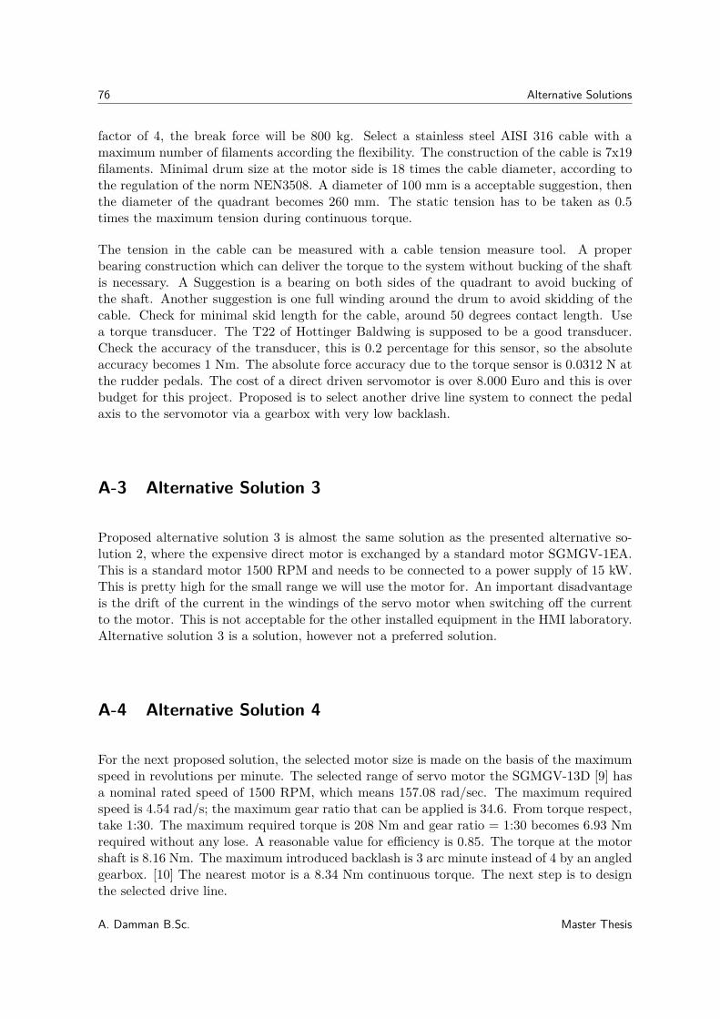
76 Alternative Solutions
factor of 4, the break force will be 800 kg. Select a stainless steel AISI 316 cable with amaximum number of filaments according the flexibility. The construction of the cable is 7x19filaments. Minimal drum size at the motor side is 18 times the cable diameter, according tothe regulation of the norm NEN3508. A diameter of 100 mm is a acceptable suggestion, thenthe diameter of the quadrant becomes 260 mm. The static tension has to be taken as 0.5times the maximum tension during continuous torque.
The tension in the cable can be measured with a cable tension measure tool. A properbearing construction which can deliver the torque to the system without bucking of the shaftis necessary. A Suggestion is a bearing on both sides of the quadrant to avoid bucking ofthe shaft. Another suggestion is one full winding around the drum to avoid skidding of thecable. Check for minimal skid length for the cable, around 50 degrees contact length. Usea torque transducer. The T22 of Hottinger Baldwing is supposed to be a good transducer.Check the accuracy of the transducer, this is 0.2 percentage for this sensor, so the absoluteaccuracy becomes 1 Nm. The absolute force accuracy due to the torque sensor is 0.0312 N atthe rudder pedals. The cost of a direct driven servomotor is over 8.000 Euro and this is overbudget for this project. Proposed is to select another drive line system to connect the pedalaxis to the servomotor via a gearbox with very low backlash.
A-3 Alternative Solution 3
Proposed alternative solution 3 is almost the same solution as the presented alternative so-lution 2, where the expensive direct motor is exchanged by a standard motor SGMGV-1EA.This is a standard motor 1500 RPM and needs to be connected to a power supply of 15 kW.This is pretty high for the small range we will use the motor for. An important disadvantageis the drift of the current in the windings of the servo motor when switching off the currentto the motor. This is not acceptable for the other installed equipment in the HMI laboratory.Alternative solution 3 is a solution, however not a preferred solution.
A-4 Alternative Solution 4
For the next proposed solution, the selected motor size is made on the basis of the maximumspeed in revolutions per minute. The selected range of servo motor the SGMGV-13D [9] hasa nominal rated speed of 1500 RPM, which means 157.08 rad/sec. The maximum requiredspeed is 4.54 rad/s; the maximum gear ratio that can be applied is 34.6. From torque respect,take 1:30. The maximum required torque is 208 Nm and gear ratio = 1:30 becomes 6.93 Nmrequired without any lose. A reasonable value for efficiency is 0.85. The torque at the motorshaft is 8.16 Nm. The maximum introduced backlash is 3 arc minute instead of 4 by an angledgearbox. [10] The nearest motor is a 8.34 Nm continuous torque. The next step is to designthe selected drive line.
A. Damman B.Sc. Master Thesis
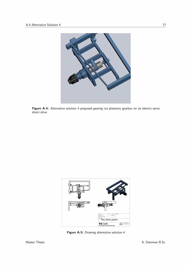
A-4 Alternative Solution 4 77
Figure A-4: Alternative solution 4 proposed gearing via planetary gearbox on an electric servodirect drive
Figure A-5: Drawing alternative solution 4
Master Thesis A. Damman B.Sc.
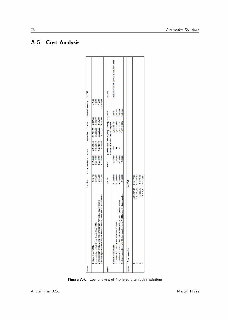
78 Alternative Solutions
A-5 Cost Analysis
Figure A-6: Cost analysis of 4 offered alternative solutions
A. Damman B.Sc. Master Thesis
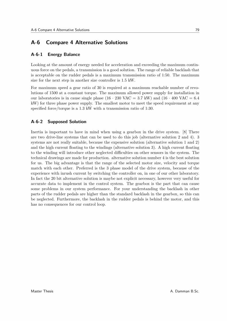
A-6 Compare 4 Alternative Solutions 79
A-6 Compare 4 Alternative Solutions
A-6-1 Energy Balance
Looking at the amount of energy needed for acceleration and exceeding the maximum contin-uous force on the pedals, a transmission is a good solution. The range of reliable backlash thatis acceptable on the rudder pedals is a maximum transmission ratio of 1:50. The maximumsize for the next step in another size controller is 1.5 kW.
For maximum speed a gear ratio of 30 is required at a maximum reachable number of revo-lutions of 1500 at a constant torque. The maximum allowed power supply for installation inour laboratories is in cause single phase (16 · 230 VAC = 3.7 kW) and (16 · 400 VAC = 6.4kW) for three phase power supply. The smallest motor to meet the speed requirement at anyspecified force/torque is a 1.3 kW with a transmission ratio of 1:30.
A-6-2 Supposed Solution
Inertia is important to have in mind when using a gearbox in the drive system. [8] Thereare two drive-line systems that can be used to do this job (alternative solution 2 and 4). 3systems are not really suitable, because the expensive solution (alternative solution 1 and 2)and the high current floating to the windings (alternative solution 3). A high current floatingto the winding will introduce other neglected difficulties on other sensors in the system. Thetechnical drawings are made for production. alternative solution number 4 is the best solutionfor us. The big advantage is that the range of the selected motor size, velocity and torquematch with each other. Preferred is the 3 phase model of the drive system, because of theexperience with inrush current by switching the controller on, in one of our other laboratory.In fact the 20 bit alternative solution is maybe not explicit necessary, however very useful foraccurate data to implement in the control system. The gearbox is the part that can causesome problems in our system performance. For your understanding the backlash in otherparts of the rudder pedals are higher than the standard backlash in the gearbox, so this canbe neglected. Furthermore, the backlash in the rudder pedals is behind the motor, and thishas no consequences for our control loop.
Master Thesis A. Damman B.Sc.

80 Alternative Solutions
A. Damman B.Sc. Master Thesis

Appendix B
Installation Yaskawa Servo Drive
The servo pack installation is given on the next page, our system works without break resistor.It could possibly be added at any given time.
Master Thesis A. Damman B.Sc.
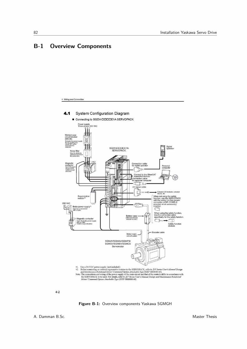
82 Installation Yaskawa Servo Drive
B-1 Overview Components
Figure B-1: Overview components Yaskawa SGMGH
A. Damman B.Sc. Master Thesis
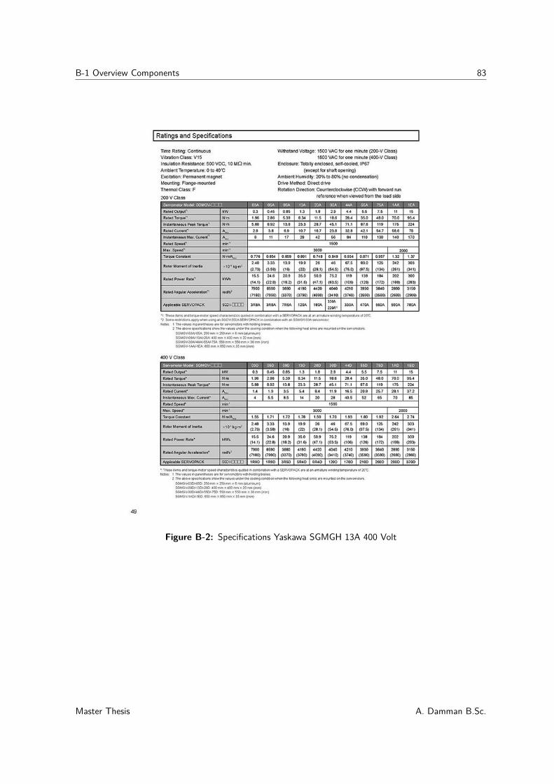
B-1 Overview Components 83
Figure B-2: Specifications Yaskawa SGMGH 13A 400 Volt
Master Thesis A. Damman B.Sc.
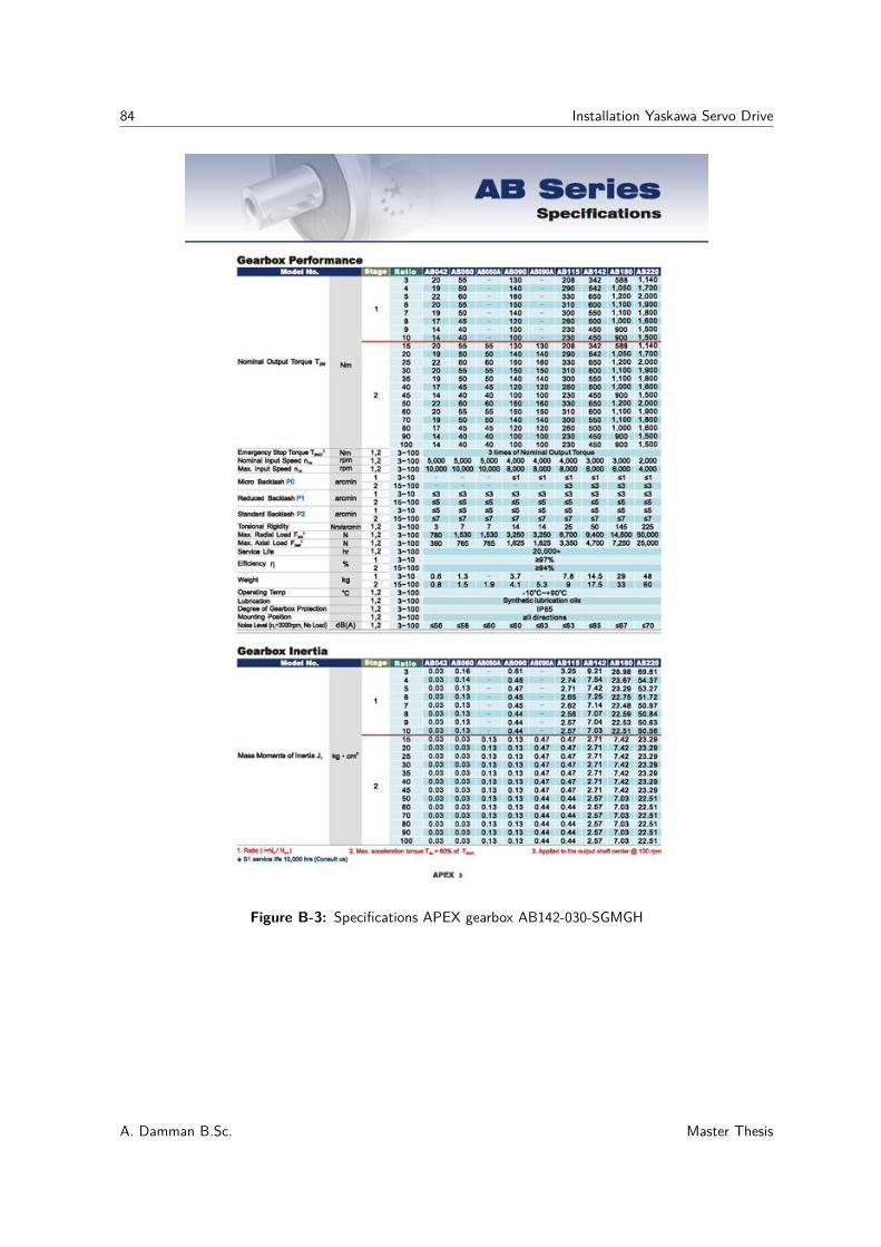
84 Installation Yaskawa Servo Drive
Figure B-3: Specifications APEX gearbox AB142-030-SGMGH
A. Damman B.Sc. Master Thesis
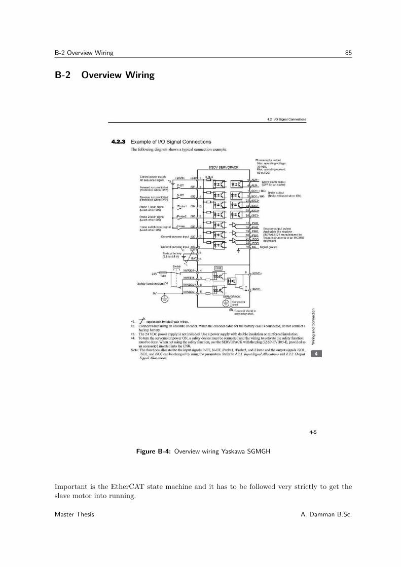
B-2 Overview Wiring 85
B-2 Overview Wiring
Figure B-4: Overview wiring Yaskawa SGMGH
Important is the EtherCAT state machine and it has to be followed very strictly to get theslave motor into running.
Master Thesis A. Damman B.Sc.
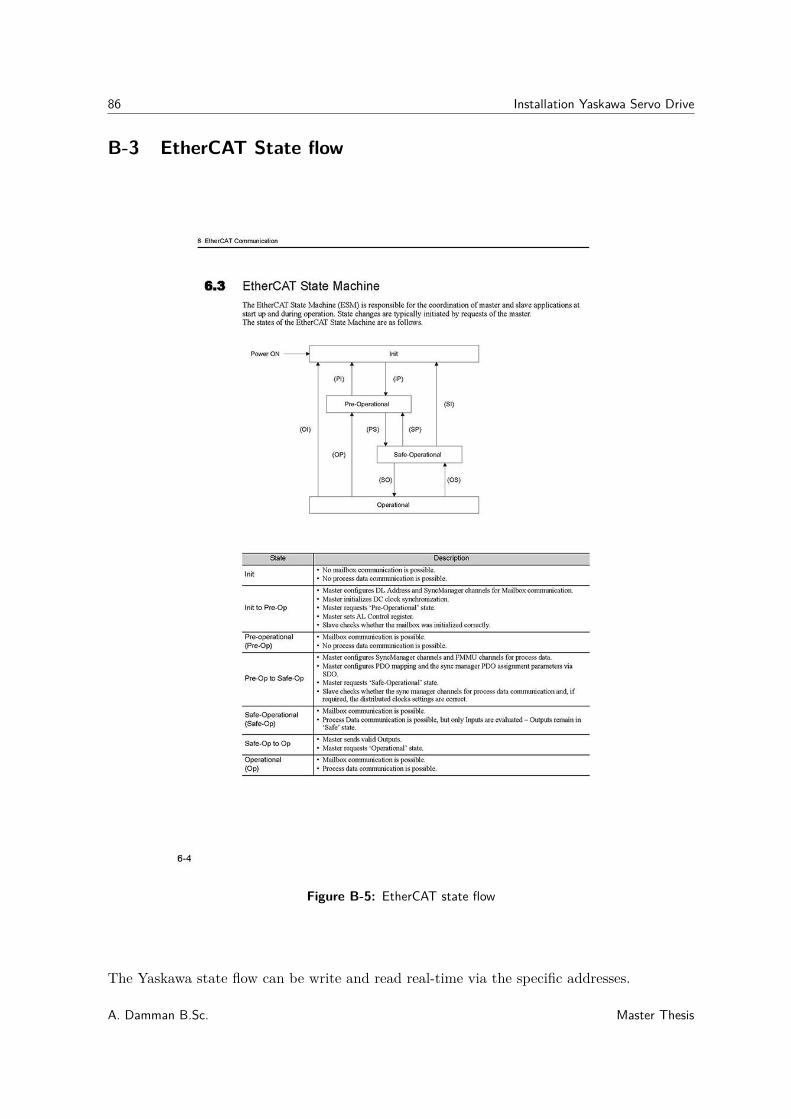
86 Installation Yaskawa Servo Drive
B-3 EtherCAT State flow
Figure B-5: EtherCAT state flow
The Yaskawa state flow can be write and read real-time via the specific addresses.
A. Damman B.Sc. Master Thesis
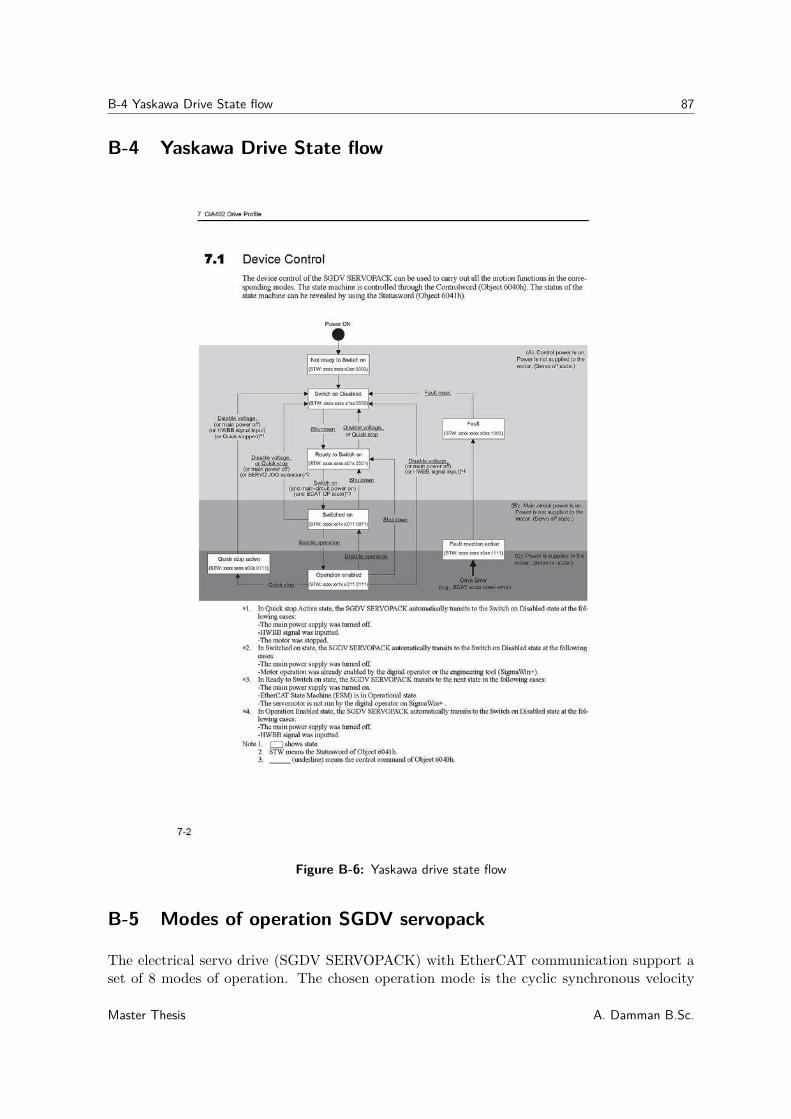
B-4 Yaskawa Drive State flow 87
B-4 Yaskawa Drive State flow
Figure B-6: Yaskawa drive state flow
B-5 Modes of operation SGDV servopack
The electrical servo drive (SGDV SERVOPACK) with EtherCAT communication support aset of 8 modes of operation. The chosen operation mode is the cyclic synchronous velocity
Master Thesis A. Damman B.Sc.
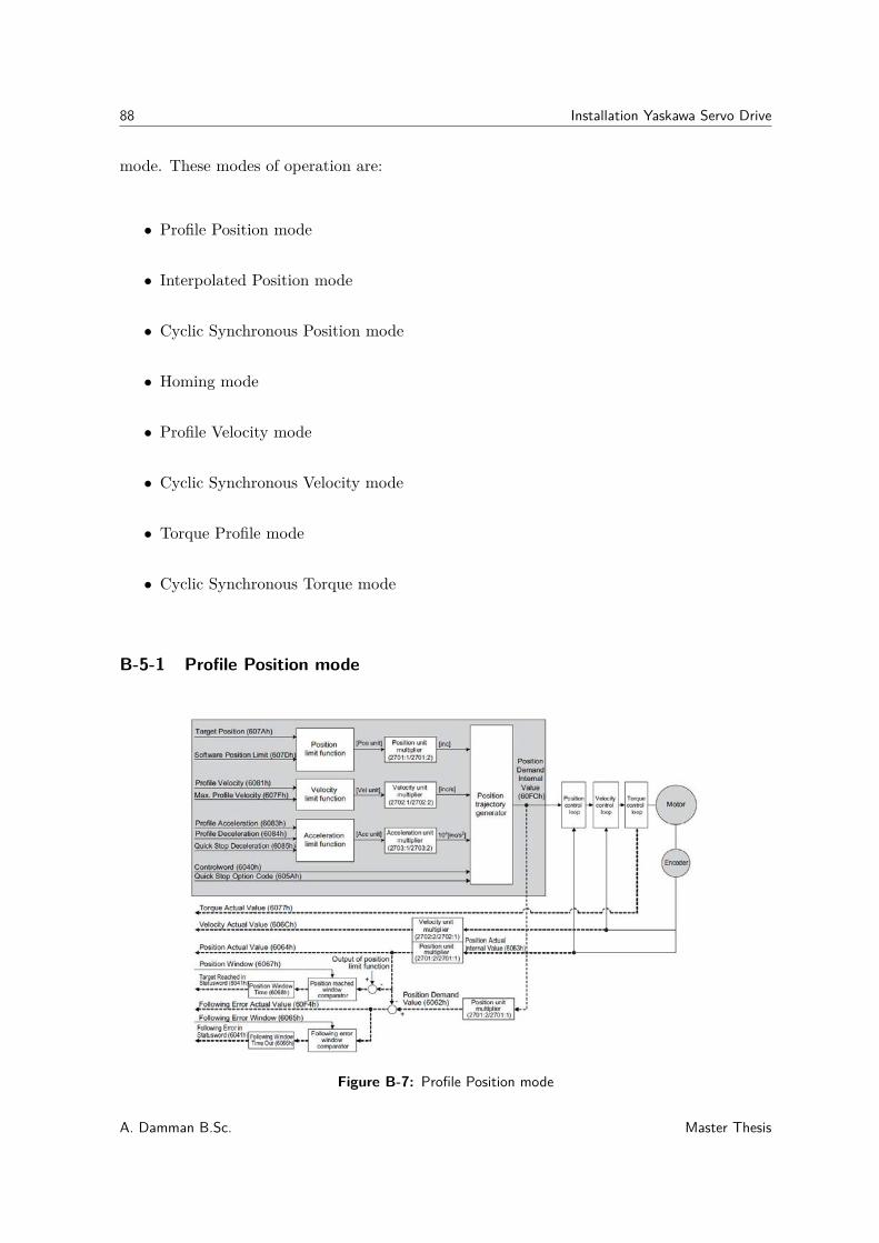
88 Installation Yaskawa Servo Drive
mode. These modes of operation are:
• Profile Position mode
• Interpolated Position mode
• Cyclic Synchronous Position mode
• Homing mode
• Profile Velocity mode
• Cyclic Synchronous Velocity mode
• Torque Profile mode
• Cyclic Synchronous Torque mode
B-5-1 Profile Position mode
Figure B-7: Profile Position mode
A. Damman B.Sc. Master Thesis
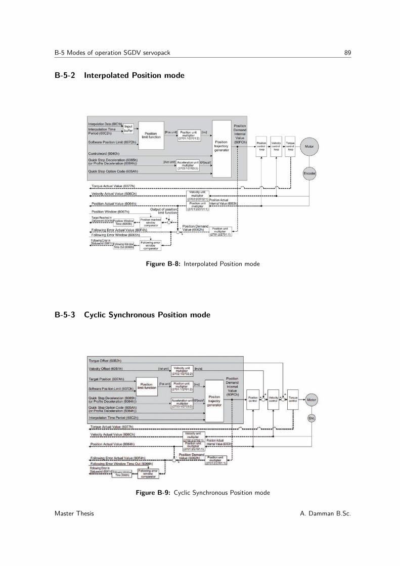
B-5 Modes of operation SGDV servopack 89
B-5-2 Interpolated Position mode
Figure B-8: Interpolated Position mode
B-5-3 Cyclic Synchronous Position mode
Figure B-9: Cyclic Synchronous Position mode
Master Thesis A. Damman B.Sc.
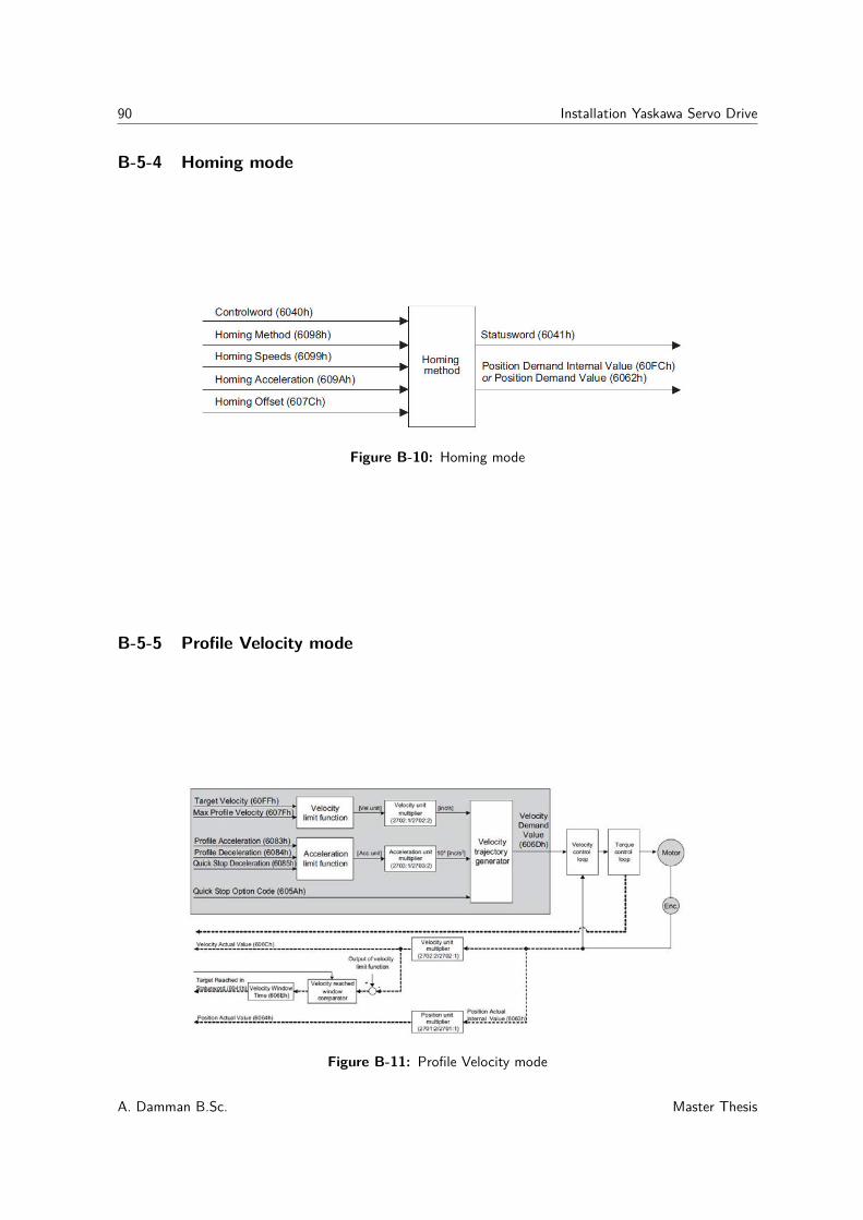
90 Installation Yaskawa Servo Drive
B-5-4 Homing mode
Figure B-10: Homing mode
B-5-5 Profile Velocity mode
Figure B-11: Profile Velocity mode
A. Damman B.Sc. Master Thesis
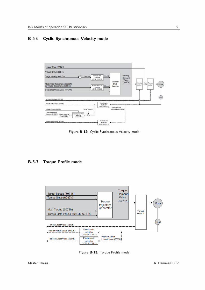
B-5 Modes of operation SGDV servopack 91
B-5-6 Cyclic Synchronous Velocity mode
Figure B-12: Cyclic Synchronous Velocity mode
B-5-7 Torque Profile mode
Figure B-13: Torque Profile mode
Master Thesis A. Damman B.Sc.
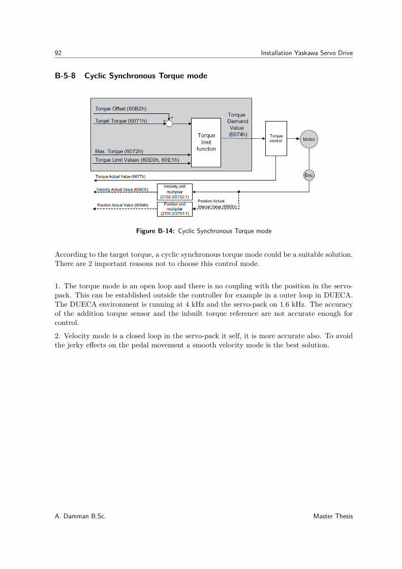
92 Installation Yaskawa Servo Drive
B-5-8 Cyclic Synchronous Torque mode
Figure B-14: Cyclic Synchronous Torque mode
According to the target torque, a cyclic synchronous torque mode could be a suitable solution.There are 2 important reasons not to choose this control mode.
1. The torque mode is an open loop and there is no coupling with the position in the servo-pack. This can be established outside the controller for example in a outer loop in DUECA.The DUECA environment is running at 4 kHz and the servo-pack on 1.6 kHz. The accuracyof the addition torque sensor and the inbuilt torque reference are not accurate enough forcontrol.
2. Velocity mode is a closed loop in the servo-pack it self, it is more accurate also. To avoidthe jerky effects on the pedal movement a smooth velocity mode is the best solution.
A. Damman B.Sc. Master Thesis
Appendix C
Practical Implementation
C-1 EMC
Electromagnetic compatibility EMC is the branch of electrical sciences which studies theaccidental generation of electromagnetic energy with reference to the unwanted effects (Elec-tromagnetic interference, or EMI) that such energy may induce.
EMC aims to ensure that equipment items or systems will not interfere with or prevent eachother’s correct operation through false emission and absorption of EMI. EMC is sometimesreferred to as EMI Control, and in practice EMC and EMI are frequently referred to as acombined term "EMC/EMI". [24]
Electromagnetic interference divides several categories according to the source and signalcharacteristics. There are two types of interferences:
Continuous interference
Continuous, or Continuous Wave interference arises where the source continuously emits ata given range of frequencies. This type is naturally divided into sub-categories according tofrequency range: Audio Frequency, Radio Frequency and Broadband noise.
Pulse or transient interference
Electromagnetic Pulse (EMP), also sometimes called Transient disturbance, arises where thesource emits a short-duration pulse of energy. The energy is usually broadband by nature,although it often excites a relatively narrow-band damped sine wave response in the victim.Sources divide broadly into isolated and repetitive events.
In the servo motor situation this can be interpreted as:Sources of isolated EMP events Switching action of electrical circuitry, including induc-tive loads such as relays, solenoids or electric motors power line surges/pulsesSources of repetitive EMP events Regular pulse trains in a Electric Motor.
Master Thesis A. Damman B.Sc.
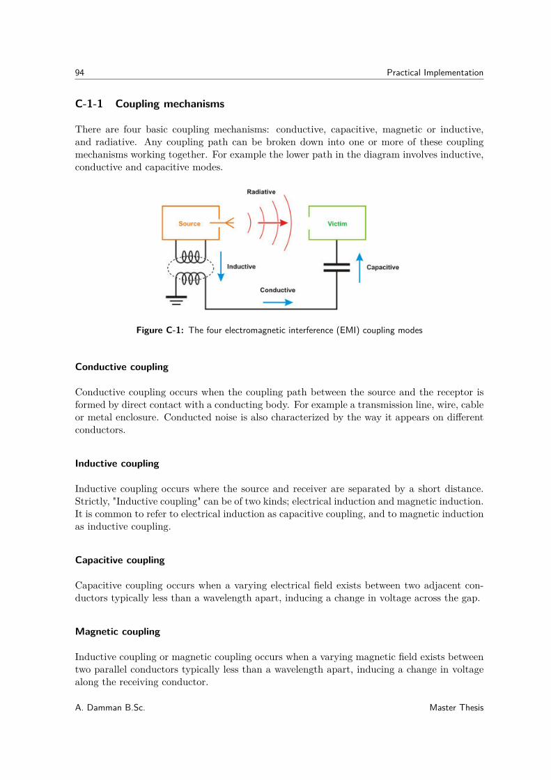
94 Practical Implementation
C-1-1 Coupling mechanisms
There are four basic coupling mechanisms: conductive, capacitive, magnetic or inductive,and radiative. Any coupling path can be broken down into one or more of these couplingmechanisms working together. For example the lower path in the diagram involves inductive,conductive and capacitive modes.
Figure C-1: The four electromagnetic interference (EMI) coupling modes
Conductive coupling
Conductive coupling occurs when the coupling path between the source and the receptor isformed by direct contact with a conducting body. For example a transmission line, wire, cableor metal enclosure. Conducted noise is also characterized by the way it appears on differentconductors.
Inductive coupling
Inductive coupling occurs where the source and receiver are separated by a short distance.Strictly, "Inductive coupling" can be of two kinds; electrical induction and magnetic induction.It is common to refer to electrical induction as capacitive coupling, and to magnetic inductionas inductive coupling.
Capacitive coupling
Capacitive coupling occurs when a varying electrical field exists between two adjacent con-ductors typically less than a wavelength apart, inducing a change in voltage across the gap.
Magnetic coupling
Inductive coupling or magnetic coupling occurs when a varying magnetic field exists betweentwo parallel conductors typically less than a wavelength apart, inducing a change in voltagealong the receiving conductor.
A. Damman B.Sc. Master Thesis
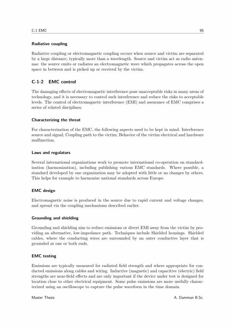
C-1 EMC 95
Radiative coupling
Radiative coupling or electromagnetic coupling occurs when source and victim are separatedby a large distance, typically more than a wavelength. Source and victim act as radio anten-nas: the source emits or radiates an electromagnetic wave which propagates across the openspace in between and is picked up or received by the victim.
C-1-2 EMC control
The damaging effects of electromagnetic interference pose unacceptable risks in many areas oftechnology, and it is necessary to control such interference and reduce the risks to acceptablelevels. The control of electromagnetic interference (EMI) and assurance of EMC comprises aseries of related disciplines.
Characterizing the threat
For characterization of the EMC, the following aspects need to be kept in mind: Interferencesource and signal; Coupling path to the victim; Behavior of the victim electrical and hardwaremalfunction.
Laws and regulators
Several international organizations work to promote international co-operation on standard-ization (harmonization), including publishing various EMC standards. Where possible, astandard developed by one organization may be adopted with little or no changes by others.This helps for example to harmonize national standards across Europe.
EMC design
Electromagnetic noise is produced in the source due to rapid current and voltage changes,and spread via the coupling mechanisms described earlier.
Grounding and shielding
Grounding and shielding aim to reduce emissions or divert EMI away from the victim by pro-viding an alternative, low-impedance path. Techniques include Shielded housings. Shieldedcables, where the conducting wires are surrounded by an outer conductive layer that isgrounded at one or both ends.
EMC testing
Emissions are typically measured for radiated field strength and where appropriate for con-ducted emissions along cables and wiring. Inductive (magnetic) and capacitive (electric) fieldstrengths are near-field effects and are only important if the device under test is designed forlocation close to other electrical equipment. Some pulse emissions are more usefully charac-terized using an oscilloscope to capture the pulse waveform in the time domain.
Master Thesis A. Damman B.Sc.

96 Practical Implementation
C-2 Skin effect
The skin effect is the phenomenon of the flow of an alternating current in a cylindricalconductor, the current density increase from inside to the outside of the conductor.
Figure C-2: Skin depth of the conductor
Distribution of current flow in a cylindrical conductor is shownn in cross sectionin FigureC-3. For alternating current, most (63%) of the electrical current flows between the surfaceand the skin depth, δ, which depends on the frequency of the current and the electrical andmagnetic properties of the conductor. [25] Skin depth is due to the circulating eddy currentscancelling the current flow in the center of a conductor and reinforcing it in the skin.
Figure C-3: Skin depth due to the circulating eddy currents
The skin effect therefore plays a particularly important role in radio frequency (RF) alter-nating currents, see the following figures. At a frequency of 50 Hz, the penetration depthof copper is approximately 1 cm, at 10 kHz less than 1 mm, and 10 MHz only 20 microns,this means that the current is actually run only at the surface in this latter frequency. Theconsequence of the skin effect is that the resistance of a conductor increases strongly at higherfrequencies. Therefore it is better to work in HF technology with hollow conductors.
A. Damman B.Sc. Master Thesis
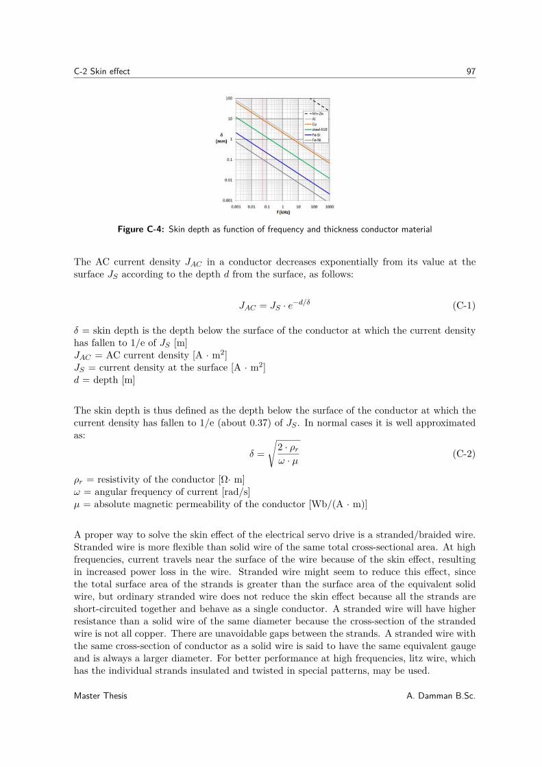
C-2 Skin effect 97
Figure C-4: Skin depth as function of frequency and thickness conductor material
The AC current density JAC in a conductor decreases exponentially from its value at thesurface JS according to the depth d from the surface, as follows:
JAC = JS · e−d/δ (C-1)
δ = skin depth is the depth below the surface of the conductor at which the current densityhas fallen to 1/e of JS [m]JAC = AC current density [A · m2]JS = current density at the surface [A · m2]d = depth [m]
The skin depth is thus defined as the depth below the surface of the conductor at which thecurrent density has fallen to 1/e (about 0.37) of JS . In normal cases it is well approximatedas:
δ =
√
2 · ρr
ω · µ(C-2)
ρr = resistivity of the conductor [Ω· m]ω = angular frequency of current [rad/s]µ = absolute magnetic permeability of the conductor [Wb/(A · m)]
A proper way to solve the skin effect of the electrical servo drive is a stranded/braided wire.Stranded wire is more flexible than solid wire of the same total cross-sectional area. At highfrequencies, current travels near the surface of the wire because of the skin effect, resultingin increased power loss in the wire. Stranded wire might seem to reduce this effect, sincethe total surface area of the strands is greater than the surface area of the equivalent solidwire, but ordinary stranded wire does not reduce the skin effect because all the strands areshort-circuited together and behave as a single conductor. A stranded wire will have higherresistance than a solid wire of the same diameter because the cross-section of the strandedwire is not all copper. There are unavoidable gaps between the strands. A stranded wire withthe same cross-section of conductor as a solid wire is said to have the same equivalent gaugeand is always a larger diameter. For better performance at high frequencies, litz wire, whichhas the individual strands insulated and twisted in special patterns, may be used.
Master Thesis A. Damman B.Sc.
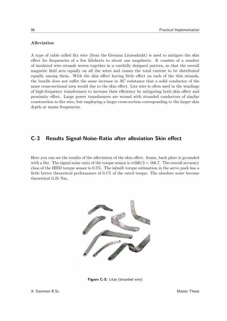
98 Practical Implementation
Alleviation
A type of cable called litz wire (from the German Litzendraht) is used to mitigate the skineffect for frequencies of a few kilohertz to about one megahertz. It consists of a numberof insulated wire strands woven together in a carefully designed pattern, so that the overallmagnetic field acts equally on all the wires and causes the total current to be distributedequally among them. With the skin effect having little effect on each of the thin strands,the bundle does not suffer the same increase in AC resistance that a solid conductor of thesame cross-sectional area would due to the skin effect. Litz wire is often used in the windingsof high-frequency transformers to increase their efficiency by mitigating both skin effect andproximity effect. Large power transformers are wound with stranded conductors of similarconstruction to litz wire, but employing a larger cross-section corresponding to the larger skindepth at mains frequencies.
C-3 Results Signal-Noise-Ratio after alleviation Skin effect
Here you can see the results of the alleviation of the skin effect. frame, back plate is groundedwith a litz. The signal noise ratio of the torque sensor is ≈500/3 = 166.7. The overall accuracyclass of the HBM torque sensor is 0.5%. The inbuilt torque estimation in the servo pack has alittle better theoretical performance of 0.1% of the rated torque. The absolute noise becometheoretical 0.25 Nm.
Figure C-5: Litze (stranded wire)
A. Damman B.Sc. Master Thesis
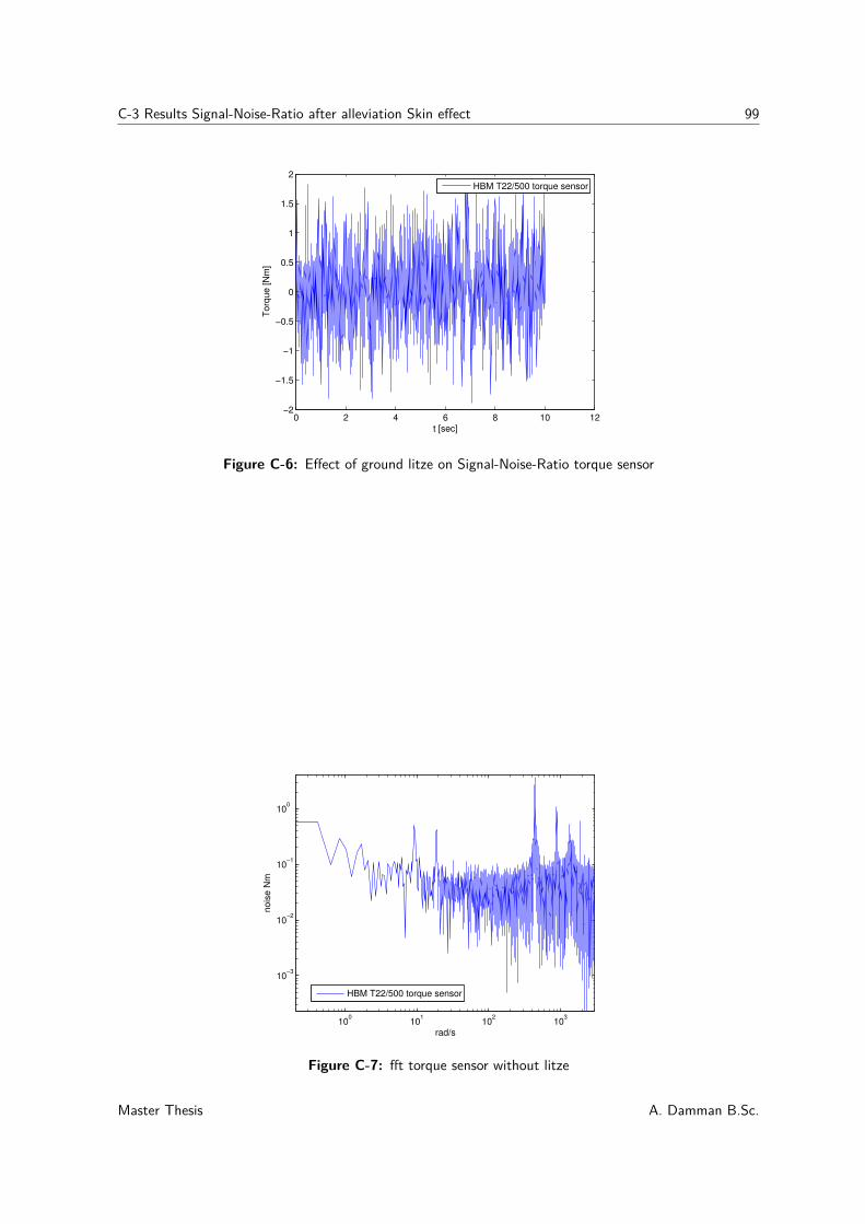
C-3 Results Signal-Noise-Ratio after alleviation Skin effect 99
0 2 4 6 8 10 12−2
−1.5
−1
−0.5
0
0.5
1
1.5
2
t [sec]
Torq
ue [N
m]
HBM T22/500 torque sensor
Figure C-6: Effect of ground litze on Signal-Noise-Ratio torque sensor
100
101
102
103
10−3
10−2
10−1
100
rad/s
nois
e N
m
HBM T22/500 torque sensor
Figure C-7: fft torque sensor without litze
Master Thesis A. Damman B.Sc.
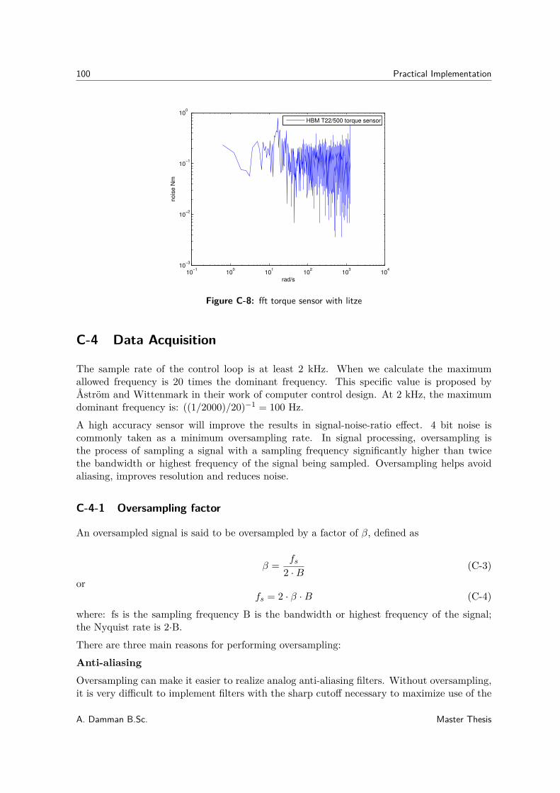
100 Practical Implementation
10−1
100
101
102
103
104
10−3
10−2
10−1
100
rad/s
nois
e N
m
HBM T22/500 torque sensor
Figure C-8: fft torque sensor with litze
C-4 Data Acquisition
The sample rate of the control loop is at least 2 kHz. When we calculate the maximumallowed frequency is 20 times the dominant frequency. This specific value is proposed byÅström and Wittenmark in their work of computer control design. At 2 kHz, the maximumdominant frequency is: ((1/2000)/20)−1 = 100 Hz.
A high accuracy sensor will improve the results in signal-noise-ratio effect. 4 bit noise iscommonly taken as a minimum oversampling rate. In signal processing, oversampling isthe process of sampling a signal with a sampling frequency significantly higher than twicethe bandwidth or highest frequency of the signal being sampled. Oversampling helps avoidaliasing, improves resolution and reduces noise.
C-4-1 Oversampling factor
An oversampled signal is said to be oversampled by a factor of β, defined as
β =fs
2 · B(C-3)
orfs = 2 · β · B (C-4)
where: fs is the sampling frequency B is the bandwidth or highest frequency of the signal;the Nyquist rate is 2·B.
There are three main reasons for performing oversampling:
Anti-aliasing
Oversampling can make it easier to realize analog anti-aliasing filters. Without oversampling,it is very difficult to implement filters with the sharp cutoff necessary to maximize use of the
A. Damman B.Sc. Master Thesis
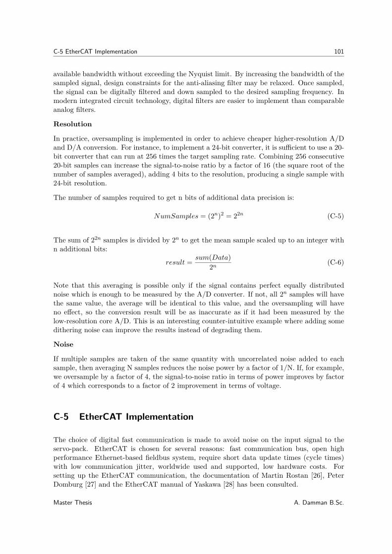
C-5 EtherCAT Implementation 101
available bandwidth without exceeding the Nyquist limit. By increasing the bandwidth of thesampled signal, design constraints for the anti-aliasing filter may be relaxed. Once sampled,the signal can be digitally filtered and down sampled to the desired sampling frequency. Inmodern integrated circuit technology, digital filters are easier to implement than comparableanalog filters.
Resolution
In practice, oversampling is implemented in order to achieve cheaper higher-resolution A/Dand D/A conversion. For instance, to implement a 24-bit converter, it is sufficient to use a 20-bit converter that can run at 256 times the target sampling rate. Combining 256 consecutive20-bit samples can increase the signal-to-noise ratio by a factor of 16 (the square root of thenumber of samples averaged), adding 4 bits to the resolution, producing a single sample with24-bit resolution.
The number of samples required to get n bits of additional data precision is:
NumSamples = (2n)2 = 22n (C-5)
The sum of 22n samples is divided by 2n to get the mean sample scaled up to an integer withn additional bits:
result =sum(Data)
2n(C-6)
Note that this averaging is possible only if the signal contains perfect equally distributednoise which is enough to be measured by the A/D converter. If not, all 2n samples will havethe same value, the average will be identical to this value, and the oversampling will haveno effect, so the conversion result will be as inaccurate as if it had been measured by thelow-resolution core A/D. This is an interesting counter-intuitive example where adding somedithering noise can improve the results instead of degrading them.
Noise
If multiple samples are taken of the same quantity with uncorrelated noise added to eachsample, then averaging N samples reduces the noise power by a factor of 1/N. If, for example,we oversample by a factor of 4, the signal-to-noise ratio in terms of power improves by factorof 4 which corresponds to a factor of 2 improvement in terms of voltage.
C-5 EtherCAT Implementation
The choice of digital fast communication is made to avoid noise on the input signal to theservo-pack. EtherCAT is chosen for several reasons: fast communication bus, open highperformance Ethernet-based fieldbus system, require short data update times (cycle times)with low communication jitter, worldwide used and supported, low hardware costs. Forsetting up the EtherCAT communication, the documentation of Martin Rostan [26], PeterDomburg [27] and the EtherCAT manual of Yaskawa [28] has been consulted.
Master Thesis A. Damman B.Sc.
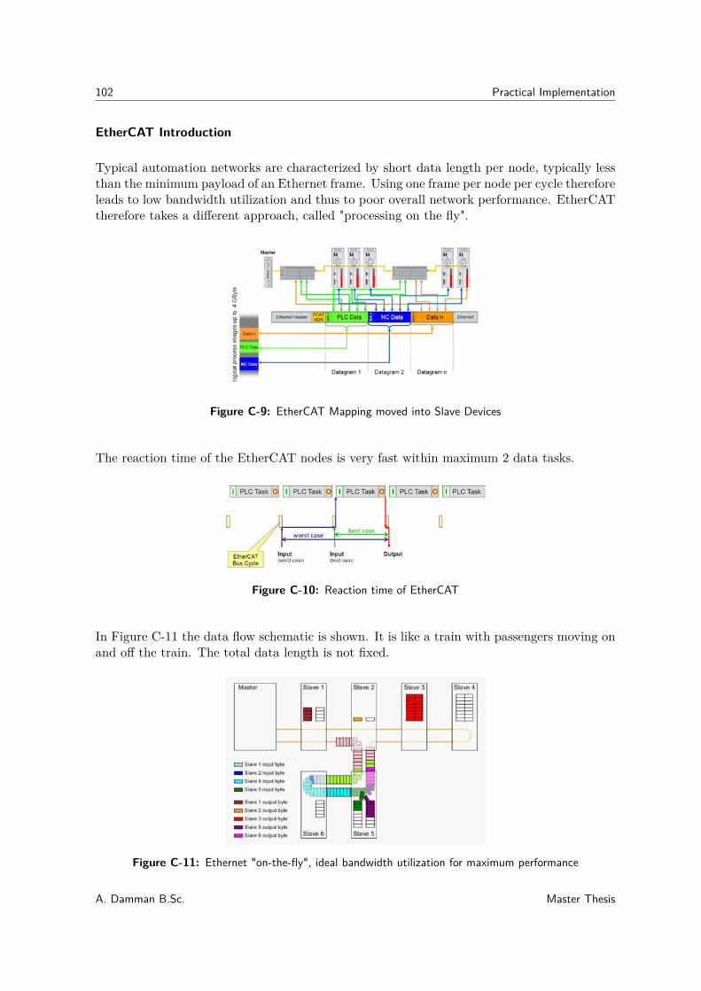
102 Practical Implementation
EtherCAT Introduction
Typical automation networks are characterized by short data length per node, typically lessthan the minimum payload of an Ethernet frame. Using one frame per node per cycle thereforeleads to low bandwidth utilization and thus to poor overall network performance. EtherCATtherefore takes a different approach, called "processing on the fly".
Figure C-9: EtherCAT Mapping moved into Slave Devices
The reaction time of the EtherCAT nodes is very fast within maximum 2 data tasks.
Figure C-10: Reaction time of EtherCAT
In Figure C-11 the data flow schematic is shown. It is like a train with passengers moving onand off the train. The total data length is not fixed.
Figure C-11: Ethernet "on-the-fly", ideal bandwidth utilization for maximum performance
A. Damman B.Sc. Master Thesis
C-5 EtherCAT Implementation 103
Functional Principle
With EtherCAT, the Ethernet packet or frame is no longer received, then interpreted andcopied as process data at every node. The EtherCAT slave devices read the data addressed tothem while the telegram passes through the device. Similarly, input data are inserted whilethe telegram passes through. The frames are only delayed by a fraction of a microsecond ineach node, and many nodes - typically the entire network - can be addressed with just oneframe.
EtherCAT Protocol
The EtherCAT protocol is optimized for process data and is transported directly within thestandard IEEE 802.3 Ethernet frame using Ethertype 0x88a4. It may consist of several sub-telegrams, each serving a particular memory area of the logical process images that can beup to 4 gigabytes in size. The data sequence is independent of the physical order of the nodesin the network; addressing can be in any order. Broadcast, multicast and communicationbetween slaves are possible and must be done by the master device. If IP routing is required,the EtherCAT protocol can be inserted into UDP/IP datagrams. This also enables any controlwith Ethernet protocol stack to address EtherCAT systems.
Performance
Short cycle times can be achieved since the host microprocessors in the slave devices arenot involved in the processing of the Ethernet packets to transfer the process images. Allprocess data communication is handled in the slave controller hardware. Combined with thefunctional principle this makes EtherCAT a high performance distributed I/O system.
Topology
Using full-duplex Ethernet physical layers, the EtherCAT slave controllers close an open portautomatically and return the Ethernet frame if no downstream device is detected. Slavedevices may have two or more ports. Due to these features EtherCAT can support almostany physical topology such as line, tree or star. The bus or line structure known from thefieldbusses thus also becomes available for Ethernet.
Synchronization
For synchronization a distributed clock mechanism is applied, which leads to very low jittersof significantly less than 1 micro second, even if the communication cycle jitters, which isequivalent to the IEEE 1588 Precision Time Protocol standard. Therefore EtherCAT doesnot require a special hardware in the master device and can be implemented in software onany standard Ethernet MAC, even without dedicated communication coprocessor. To keepthe clocks synchronized after initialization, the master or slave must regularly send out thebroadcast again to counter any effects of speed difference between the internal clocks of eachslave. Each slave should adjust the speed of their internal clock or implement an internal
Master Thesis A. Damman B.Sc.
104 Practical Implementation
correction mechanism whenever they have to adjust. The system clock is specified as a 64 bitcounter with a base unit of 1 ns starting at January 1, 2000, 0:00.
Device profiles
The device profiles describe the application parameters and the functional behavior of thedevices including the device class-specific state machines. For many device classes, fieldbustechnology already offers reliable device profiles, for example for I/O devices, drives or valves.EtherCAT supports both the CANopen device profile family as well as the drive profile knownas the Sercos drive profile. Since the application view does not change when migrating fromCANopen or Sercos, this assists users and device manufacturers alike.
Functional safety
The protocol enhancement called Safety over EtherCAT enables safety-related communica-tion and control communication on the same network. The safety protocol is based on theapplication layer of EtherCAT, without influencing the lower layers. It is certified accordingto IEC 61508 and meets the requirements of Safety Integrity Level (SIL). Certified productsusing the Safety over EtherCAT protocol have been available since 2005.
Gateways
For integration of existing fieldbus components (e.g., CANopen, DeviceNet, Profibus) intoEtherCAT networks gateway devices are available. Also other Ethernet protocols can beused in conjunction with EtherCAT: The Ethernet frames are tunneled via the EtherCATprotocol, which is the standard approach for internet applications (e.g. VPN, PPPoE (DSL)etc.). The EtherCAT network is fully transparent for the Ethernet device, and the real-timecharacteristics are not impaired since the master dictates exactly when the tunneled transfersare to occur and how much capacity of the 100Mbit/s media the tunneled protocols can use.All internet technologies can therefore also be used in the EtherCAT environment: integratedweb server, e-mail, FTP transfer etc.
Implementation
Master can be implemented in software on any standard Ethernet MAC. Several vendorssupply code for different operating systems. There are also several open and shared sourceimplementations. For slave devices special EtherCAT slave controller chips are required inorder to perform the "processing on the fly" principle. EtherCAT slave controllers are availableas code for different FPGA types and are also available as ASIC implementations.
EtherCAT Technology Group
The EtherCAT Technology Group (ETG) is international user and vendor organization head-quartered in Nuremberg (Germany). It was founded in November 2003 and has offices in
A. Damman B.Sc. Master Thesis
C-5 EtherCAT Implementation 105
Tokyo (Japan), Beijing (China), Seoul (Korea), and Austin, Tx (USA). As of June 2010,it has over 1350 member companies from 50 countries. The ETG considers itself to be aforum for end users from different sectors, and for machine manufacturers and suppliers ofcontrol technology with the aim of supporting and promoting EtherCAT. The ETG pro-vides information about EtherCAT and its application, organizes technical training classes,has technical and marketing committees, and promotes EtherCAT on trade shows in majorindustrial markets.
International standardization
The EtherCAT Technology Group is an official liaison partner of the IEC (InternationalElectrotechnical Commission) working groups for digital communication. The EtherCATspecification was published as IEC/PAS 62407 in 2005, which was removed end of 2007 sinceEtherCAT had been integrated into the international fieldbus standards IEC 61158 and IEC61784-2 as well as into the drive profile standard IEC 61800-7.
C-5-1 CANopen over Ethernet (CoE) in the Yaskawa drive
CANopen is the standardization in the Yaskawa drive, the figure below show the OSI layerstructure.
C-5-2 Linux Etherlab Communication
The procedure to install EtherLab has to be followed very thoroughly to be able to use forOS Linux kernel 2.6. The manual of IgH is very helpful. [29] [30]
Master Thesis A. Damman B.Sc.
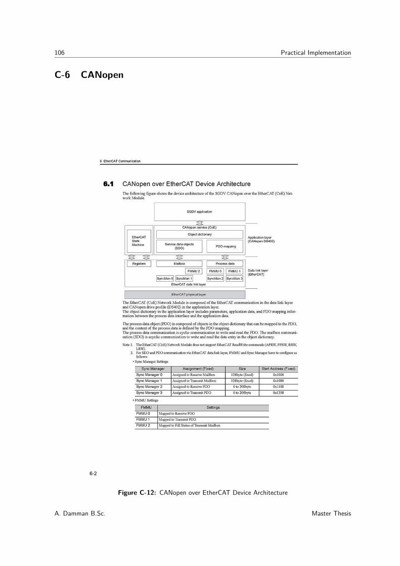
106 Practical Implementation
C-6 CANopen
Figure C-12: CANopen over EtherCAT Device Architecture
A. Damman B.Sc. Master Thesis
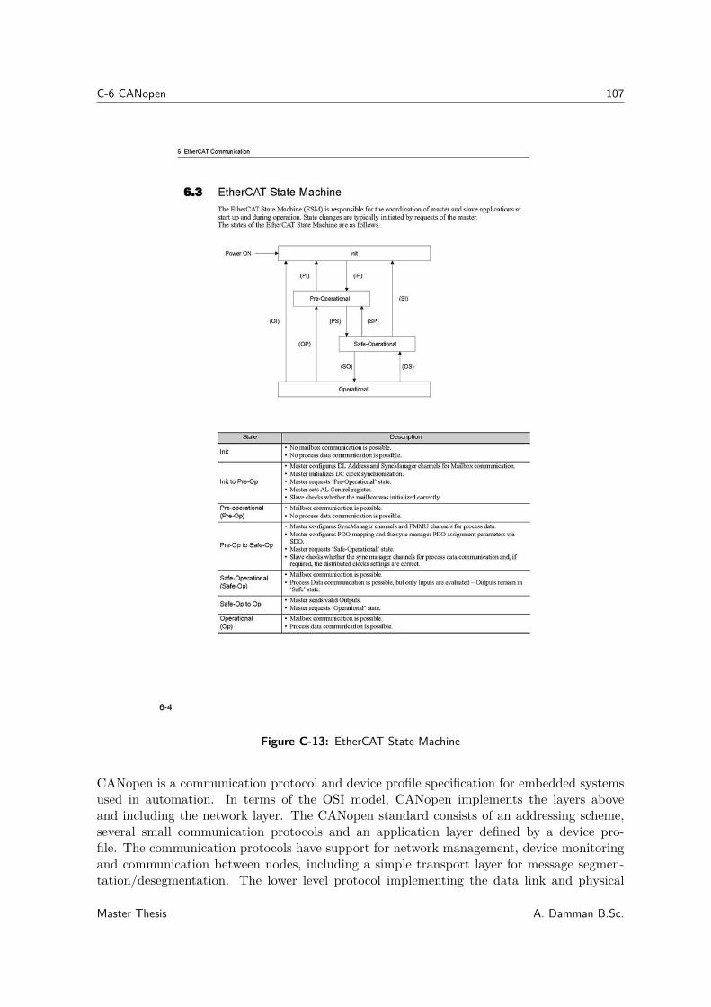
C-6 CANopen 107
Figure C-13: EtherCAT State Machine
CANopen is a communication protocol and device profile specification for embedded systemsused in automation. In terms of the OSI model, CANopen implements the layers aboveand including the network layer. The CANopen standard consists of an addressing scheme,several small communication protocols and an application layer defined by a device pro-file. The communication protocols have support for network management, device monitoringand communication between nodes, including a simple transport layer for message segmen-tation/desegmentation. The lower level protocol implementing the data link and physical
Master Thesis A. Damman B.Sc.
108 Practical Implementation
layers is usually Controller Area Network (CAN), although devices using some other meansof communication (such as Ethernet Powerlink, EtherCAT) can also implement the CANopendevice profile.
The basic CANopen device and communication profiles are given in the CiA 301 specificationreleased by CAN in Automation. Profiles for more specialized devices are built on top of thisbasic profile, and are specified in numerous other standards released by CAN in Automation,such as CiA 401 for I/O-modules and CiA 402 for motion control.
Device Model
Every CANopen device has to implement certain standard features in its controlling software.
• A communication unit implements the protocols for messaging with the other nodesin the network
• Starting and resetting the device is controlled via a state machine. It must containthe states Initialization, Pre-operational, Operational and Stopped. The transitionsbetween states are made by issuing a network management (NMT) communicationobject to the device.
• The object dictionary is an array of variables with a 16-bit index. Additionally, eachvariable can have an 8-bit subindex. The variables can be used to configure the deviceand reflect its environment, i.e. contain measurement data.
• The application part of the device actually performs the desired function of the device,after the state machine is set to the operational state. The application is configuredby variables in the object dictionary and the data are sent and received through thecommunication layer.
C-6-1 Service Data Object (SDO) protocol
The SDO protocol is used to set and read values from the object dictionary of a remote device.The device whose object dictionary is accessed is the SDO server and the device accessing theremote device is the SDO client. The communication is always initiated by the SDO client.In CANopen terminology, communication is viewed from the SDO server, so that a read froman object dictionary results in an SDO upload and a write to dictionary is an SDO download.
C-6-2 Process Data Object (PDO) protocol
Too check the settings of the controller, the program Twincat is very useful. [31] The ProcessData Object protocol is used to process real time data among various nodes. You can transferup to 8 bytes (64 bits) of data per one PDO either from or to the device. One PDO cancontain multiple object dictionary entries and the objects within one PDO are configurableusing the mapping and parameter object dictionary entries. There are two kinds of PDOs:transmit and receive PDOs (TPDO and RPDO). In the pre-defined connection set there areidentifiers for four TPDOs and four RPDOs available. With configuration 512 PDOs arepossible. PDOs can be sent synchronously or asynchronously.
A. Damman B.Sc. Master Thesis
C-7 Safety Rudder Pedal System 109
C-7 Safety Rudder Pedal System
The safety environment is built around the drive system. Where in the old hydraulic situationa less sufficient safety environment is taking care of the subject during the experiment, thenew electric servo drive system has full control over the behavior of the pedals. This is moresatisfying than the hydraulic situation. In the worst case scenario, a broken signal cable tothe hydraulic valve will cause a maximal displacement in one direction at full accelerationand at maximum power. A fault in the input signal to the servo drive will cause an errordetected by at least the servo pack and will result in a soft emergency stop by switching offthe power to the motor directly. After the emergency stop, the mechanical system can bemoved in both directions forward and backward without any motor resistance. To get anoverview of the safety environment, the safety is grouped in several layers.
C-7-1 Hardware layer
First the basal, basic safety is secured by mechanical soft end bumps at the drive shaft. Onthe electric power side, the emergency button switches off the power contactor of the motordirectly via a safety contacter. The feedback contacts (open or closed) of the power contactorprovides the status of the contactor to the safety contactor. Communication with the servopack is possible to be able to provide information of the rudder system.
C-7-2 Servo pack layer
Second by two normally open proximity end switches. When one of both switches are opened,the Hardware Base Block (HBB) in the servo pack becomes active. The servo pack inbuiltpower contactor of the power line to the motor will be opened. Without any reset commandto the servo pack it is not possible to change the position of the motor.
C-7-3 Software environment layer
Third, several software limitations are realized. There are software end stops at position, arate limitation on acceleration, a maximum torque limit and so on. The last added safetyfunction that is added is a maximum energy difference. In a moving time window, the energyof the reference signal and the actual output are compared to avoid any oppression.
Master Thesis A. Damman B.Sc.

110 Practical Implementation
A. Damman B.Sc. Master Thesis
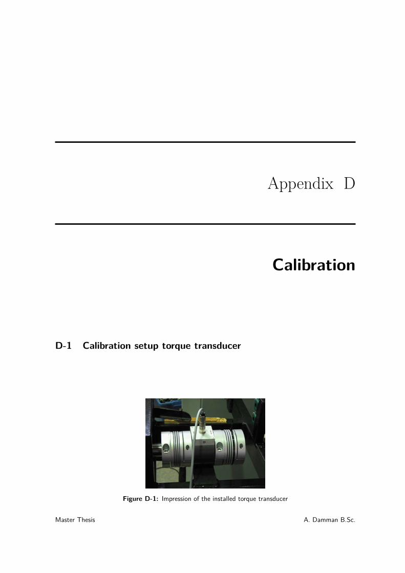
Appendix D
Calibration
D-1 Calibration setup torque transducer
Figure D-1: Impression of the installed torque transducer
Master Thesis A. Damman B.Sc.
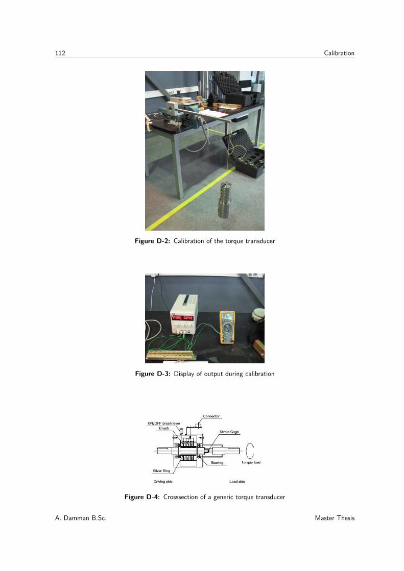
112 Calibration
Figure D-2: Calibration of the torque transducer
Figure D-3: Display of output during calibration
Figure D-4: Crosssection of a generic torque transducer
A. Damman B.Sc. Master Thesis
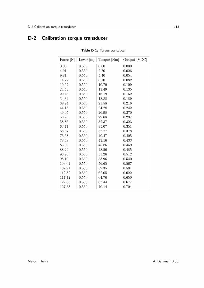
D-2 Calibration torque transducer 113
D-2 Calibration torque transducer
Table D-1: Torque transducer
Force [N] Lever [m] Torque [Nm] Output [VDC]
0.00 0.550 0.00 0.0004.91 0.550 2.70 0.0269.81 0.550 5.40 0.05414.72 0.550 8.10 0.08219.62 0.550 10.79 0.10924.53 0.550 13.49 0.13529.43 0.550 16.19 0.16234.34 0.550 18.88 0.18939.24 0.550 21.58 0.21644.15 0.550 24.28 0.24249.05 0.550 26.98 0.27053.96 0.550 29.68 0.29758.86 0.550 32.37 0.32363.77 0.550 35.07 0.35168.67 0.550 37.77 0.37873.58 0.550 40.47 0.40578.48 0.550 43.16 0.43383.39 0.550 45.86 0.45988.29 0.550 48.56 0.48593.20 0.550 51.26 0.51298.10 0.550 53.96 0.540103.01 0.550 56.65 0.567107.91 0.550 59.35 0.594112.82 0.550 62.05 0.622117.72 0.550 64.76 0.650122.63 0.550 67.44 0.677127.53 0.550 70.14 0.704
Master Thesis A. Damman B.Sc.

114 Calibration
A. Damman B.Sc. Master Thesis
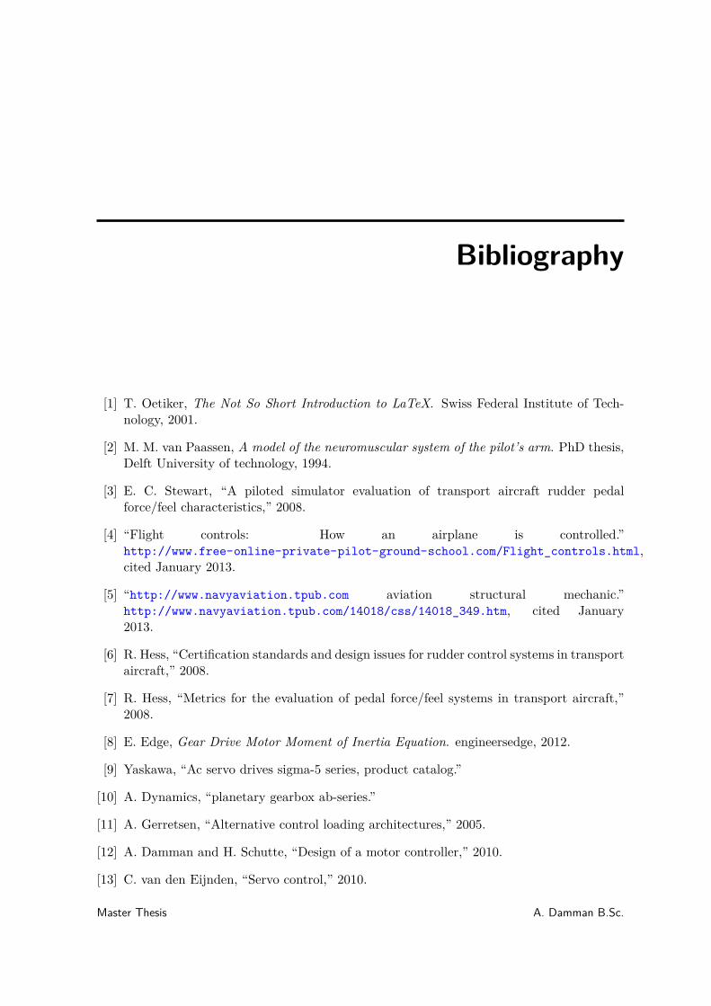
Bibliography
[1] T. Oetiker, The Not So Short Introduction to LaTeX. Swiss Federal Institute of Tech-nology, 2001.
[2] M. M. van Paassen, A model of the neuromuscular system of the pilot’s arm. PhD thesis,Delft University of technology, 1994.
[3] E. C. Stewart, “A piloted simulator evaluation of transport aircraft rudder pedalforce/feel characteristics,” 2008.
[4] “Flight controls: How an airplane is controlled.”http://www.free-online-private-pilot-ground-school.com/Flight_controls.html,cited January 2013.
[5] “http://www.navyaviation.tpub.com aviation structural mechanic.”http://www.navyaviation.tpub.com/14018/css/14018_349.htm, cited January2013.
[6] R. Hess, “Certification standards and design issues for rudder control systems in transportaircraft,” 2008.
[7] R. Hess, “Metrics for the evaluation of pedal force/feel systems in transport aircraft,”2008.
[8] E. Edge, Gear Drive Motor Moment of Inertia Equation. engineersedge, 2012.
[9] Yaskawa, “Ac servo drives sigma-5 series, product catalog.”
[10] A. Dynamics, “planetary gearbox ab-series.”
[11] A. Gerretsen, “Alternative control loading architectures,” 2005.
[12] A. Damman and H. Schutte, “Design of a motor controller,” 2010.
[13] C. van den Eijnden, “Servo control,” 2010.
Master Thesis A. Damman B.Sc.
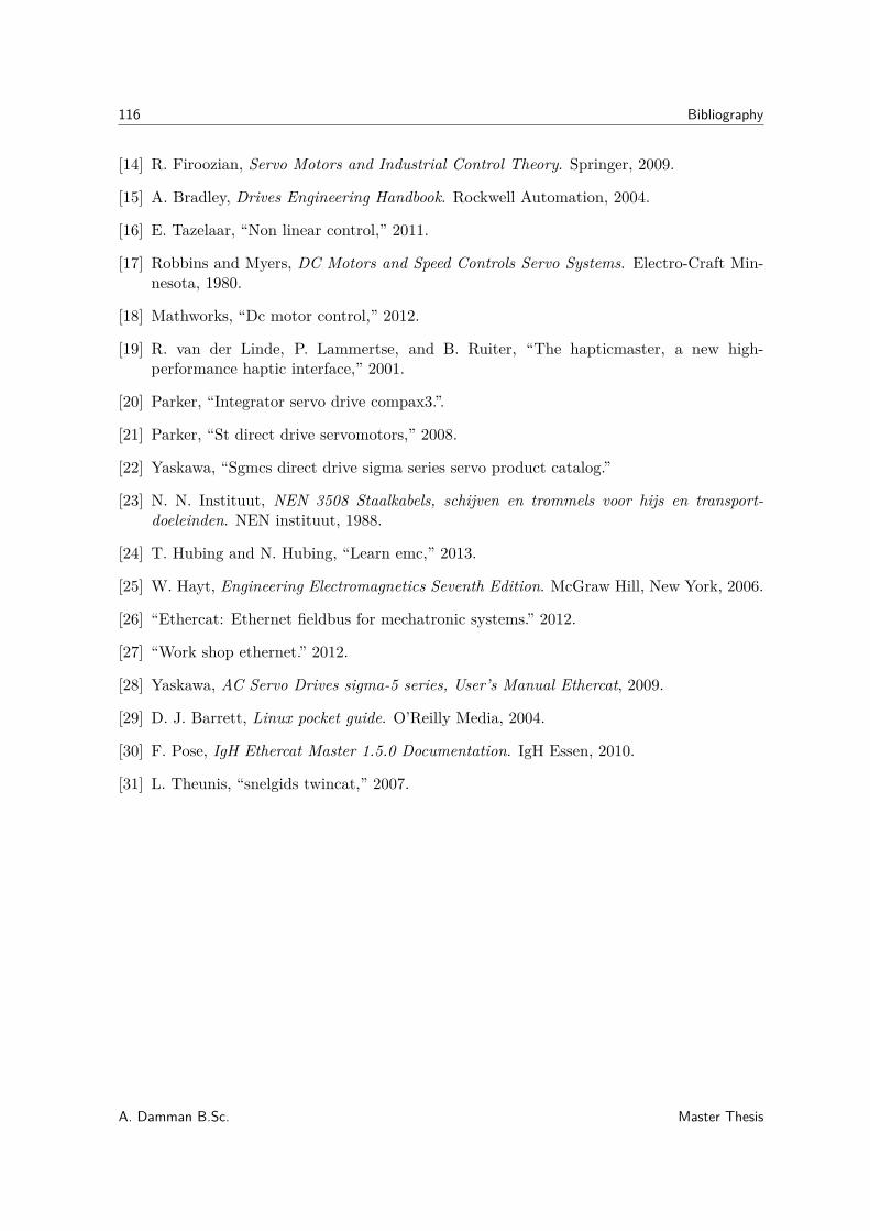
116 Bibliography
[14] R. Firoozian, Servo Motors and Industrial Control Theory. Springer, 2009.
[15] A. Bradley, Drives Engineering Handbook. Rockwell Automation, 2004.
[16] E. Tazelaar, “Non linear control,” 2011.
[17] Robbins and Myers, DC Motors and Speed Controls Servo Systems. Electro-Craft Min-nesota, 1980.
[18] Mathworks, “Dc motor control,” 2012.
[19] R. van der Linde, P. Lammertse, and B. Ruiter, “The hapticmaster, a new high-performance haptic interface,” 2001.
[20] Parker, “Integrator servo drive compax3.”.
[21] Parker, “St direct drive servomotors,” 2008.
[22] Yaskawa, “Sgmcs direct drive sigma series servo product catalog.”
[23] N. N. Instituut, NEN 3508 Staalkabels, schijven en trommels voor hijs en transport-
doeleinden. NEN instituut, 1988.
[24] T. Hubing and N. Hubing, “Learn emc,” 2013.
[25] W. Hayt, Engineering Electromagnetics Seventh Edition. McGraw Hill, New York, 2006.
[26] “Ethercat: Ethernet fieldbus for mechatronic systems.” 2012.
[27] “Work shop ethernet.” 2012.
[28] Yaskawa, AC Servo Drives sigma-5 series, User’s Manual Ethercat, 2009.
[29] D. J. Barrett, Linux pocket guide. O’Reilly Media, 2004.
[30] F. Pose, IgH Ethercat Master 1.5.0 Documentation. IgH Essen, 2010.
[31] L. Theunis, “snelgids twincat,” 2007.
A. Damman B.Sc. Master Thesis
List of Figures
1-1 Rudder pedals Fokker 50 . . . . . . . . . . . . . . . . . . . . . . . . . . . . . . 2
1-2 Original situation rudder pedals hinge system HMI-laboratory . . . . . . . . . . . 2
1-3 Control loop HAN . . . . . . . . . . . . . . . . . . . . . . . . . . . . . . . . . . 3
2-1 Rudder Control Aircraft [4] . . . . . . . . . . . . . . . . . . . . . . . . . . . . . 7
2-2 Hydraulic Servo Rudder Control Aircraft [5] . . . . . . . . . . . . . . . . . . . . 9
2-3 Pedal Characteristics (Force-Deflection) [6] . . . . . . . . . . . . . . . . . . . . 10
2-4 Comparison of Pedal Force/Feel Systems, AH-64A and Airbus A300-600 [6] . . . 11
2-5 Comparison of Pedal Force/Feel Systems, UH-60A and Airbus A300-600 [6] . . . 11
2-6 Comparison of Pedal Force/Feel Systems, CH-47D and Airbus A300-600 [6] . . . 12
2-7 Comparison of Pedal Force/Feel Systems, CH-53D and Airbus A300-600 [6] . . . 12
2-8 Comparison of Pedal Force/Feel Systems, B-767 and Airbus A300-600 [6] . . . . 12
2-9 Comparison of Pedal Force/Feel Systems, Airbus A300-B2-B4 and A300-600 [6] . 13
2-10 Example of the Effect Dynamic Characteristics of Force/Feel System with Sinu-soidal Inputs of Different Frequency [7] . . . . . . . . . . . . . . . . . . . . . . . 13
2-11 Example of the Effect Dynamic Characteristics of Force/Feel System with Sinu-soidal Inputs of Different Frequency [7] . . . . . . . . . . . . . . . . . . . . . . . 14
2-12 Example of the Effect of Force/Feel System Dynamics and Rudder Actuator Char-acteristics on Pedal Force vs Rudder Position for Force/Feel System [7] . . . . . 14
3-1 First force lever of at the rudder pedals . . . . . . . . . . . . . . . . . . . . . . 18
3-2 Second force lever of at the rudder pedals . . . . . . . . . . . . . . . . . . . . . 18
3-3 Torque characteristics of the motor SGMGV-13D . . . . . . . . . . . . . . . . . 19
Master Thesis A. Damman B.Sc.
118 List of Figures
3-4 Alternative solution 4 proposed gearing via planetary gearbox on an electric servodirect drive . . . . . . . . . . . . . . . . . . . . . . . . . . . . . . . . . . . . . . 20
3-5 Drawing alternative solution 4 . . . . . . . . . . . . . . . . . . . . . . . . . . . 20
3-6 Inertia calculation of current pedal system . . . . . . . . . . . . . . . . . . . . . 21
3-7 Inertia calculation of drive system . . . . . . . . . . . . . . . . . . . . . . . . . 21
3-8 Results of measurement gainplot . . . . . . . . . . . . . . . . . . . . . . . . . . 22
3-9 Results of measurement phaseplot . . . . . . . . . . . . . . . . . . . . . . . . . 22
4-1 Mass Spring Damper system . . . . . . . . . . . . . . . . . . . . . . . . . . . . 26
4-2 Bodeplot of the FCS mass-spring-damper model . . . . . . . . . . . . . . . . . . 27
4-3 Control loading system layout . . . . . . . . . . . . . . . . . . . . . . . . . . . . 27
4-4 Hydraulic servo model . . . . . . . . . . . . . . . . . . . . . . . . . . . . . . . . 30
4-5 Hydraulic position loop . . . . . . . . . . . . . . . . . . . . . . . . . . . . . . . 31
4-6 Hydraulic velocity loop . . . . . . . . . . . . . . . . . . . . . . . . . . . . . . . 31
4-7 Hydraulic force loop . . . . . . . . . . . . . . . . . . . . . . . . . . . . . . . . . 32
4-8 Schematic complete hydraulic control loop . . . . . . . . . . . . . . . . . . . . . 32
4-9 Bode plot bare hydraulic actuator model with a velocity loop . . . . . . . . . . . 33
4-10 Hydraulic bode plot position loop (Simulink Result) . . . . . . . . . . . . . . . . 33
4-11 Hydraulic bode plot velocity loop (Simulink Result) . . . . . . . . . . . . . . . . 34
4-12 Hydraulic bode plot force loop (Simulink Result) . . . . . . . . . . . . . . . . . 35
4-13 Hydraulic position loop (Simulink Result) . . . . . . . . . . . . . . . . . . . . . 36
4-14 Hydraulic velocity loop (Simulink Result) . . . . . . . . . . . . . . . . . . . . . . 36
4-15 Hydraulic force loop (Simulink Result) . . . . . . . . . . . . . . . . . . . . . . . 37
4-16 Schematic 3 phase brushless servomotor . . . . . . . . . . . . . . . . . . . . . . 38
4-17 Simplified model brushless servomotor conform [17] . . . . . . . . . . . . . . . . 39
4-18 Results of 400 V step input feed to the simplified model of the servomotor . . . . 40
4-19 Results of 400 V profile feed to the simplified model of the servomotor . . . . . . 40
4-20 Bodeplot of design of a simplified model brushless servomotor . . . . . . . . . . 41
4-21 Model of a DC motor . . . . . . . . . . . . . . . . . . . . . . . . . . . . . . . . 42
4-22 Model of voltage control loop of a DC motor . . . . . . . . . . . . . . . . . . . 42
4-23 Step response of simplified model brushless servomotor . . . . . . . . . . . . . . 43
4-24 Model of feedforward control . . . . . . . . . . . . . . . . . . . . . . . . . . . . 44
4-25 Plot of disturbance on a simplified model brushless servomotor closed loop . . . . 44
4-26 Model of feedback control . . . . . . . . . . . . . . . . . . . . . . . . . . . . . . 45
A. Damman B.Sc. Master Thesis
List of Figures 119
4-27 Rootlocus plot of simplified model brushless servomotor . . . . . . . . . . . . . . 45
4-28 Plot of disturbance on a simplified model brushless servomotor feedback and feed-forward . . . . . . . . . . . . . . . . . . . . . . . . . . . . . . . . . . . . . . . . 46
4-29 Model of linear-quadratic regulator (LQR) control . . . . . . . . . . . . . . . . . 46
4-30 Bodeplot of design of a simplified model brushless servomotor . . . . . . . . . . 47
4-31 Plot of disturbance on a simplified model brushless servomotor LQR . . . . . . . 47
4-32 Design of a simplified synchronous brushless servomotor model . . . . . . . . . . 48
4-33 Bodeplot of velocity control loop synchronous servomotor model . . . . . . . . . 48
4-34 Acceleration during hard end stop simulation of the electrical servo system 375 N 49
4-35 Acceleration during hard end stop simulation of the electrical servo system 750 N 49
4-36 Bandwidth of sinusoidal cyclic velocity based on maximum acceleration . . . . . 50
4-37 Comparison of a force sinus input response of a hydraulic and electrical servo system 51
4-38 Zoomed comparison of a force sinus input response of a hydraulic and electricalservo system . . . . . . . . . . . . . . . . . . . . . . . . . . . . . . . . . . . . . 51
5-1 Impression of the experiment room . . . . . . . . . . . . . . . . . . . . . . . . . 54
5-2 Impression wiring electrical cabinet . . . . . . . . . . . . . . . . . . . . . . . . . 54
5-3 Impression EMC filter . . . . . . . . . . . . . . . . . . . . . . . . . . . . . . . . 55
5-4 Impression circular EMC clamp . . . . . . . . . . . . . . . . . . . . . . . . . . . 55
5-5 Impression of the controlroom . . . . . . . . . . . . . . . . . . . . . . . . . . . 56
5-6 Impression of the installed added mass 2 x 7.50 kg . . . . . . . . . . . . . . . . 56
5-7 Results of measurement start stop mode . . . . . . . . . . . . . . . . . . . . . . 57
5-8 Results of measurement cyclic without torque . . . . . . . . . . . . . . . . . . . 58
5-9 Results of measurement start-up without torque . . . . . . . . . . . . . . . . . . 58
5-10 Results of measurement without torque in sinus mode . . . . . . . . . . . . . . . 59
5-11 Results of measurement frequency response at 1300 RPM . . . . . . . . . . . . . 59
5-12 Results of measurement without torque, single ended input . . . . . . . . . . . . 60
5-13 Results of measurement without torque, differential input . . . . . . . . . . . . . 60
5-14 Results of sinusoidal velocity response with added mass 2Hz 132/30 rad/s . . . . 61
5-15 Results of sinusoidal velocity response with real human added mass 2Hz 132/30rad/s . . . . . . . . . . . . . . . . . . . . . . . . . . . . . . . . . . . . . . . . . 62
5-16 Results of sinusoidal velocity response with added mass 2Hz 132/30 rad/s . . . . 62
5-17 Results of measurement with full torque only left hand side . . . . . . . . . . . . 63
5-18 Results of measurement with added mass of limb . . . . . . . . . . . . . . . . . 63
Master Thesis A. Damman B.Sc.
120 List of Figures
5-19 Results of measurement with added mass of limb following the sinus mode relaxed 64
5-20 Results of measurement without torque in sinus mode . . . . . . . . . . . . . . . 64
5-21 The fundamental sinus and the following sinus signals with phase shift . . . . . . 65
5-22 Multi sinus repeated input signal with fade in and fade out . . . . . . . . . . . . 65
5-23 FFT of a multi sinus input signal of the relevant range . . . . . . . . . . . . . . 66
5-24 Control loop electric servo system with used components . . . . . . . . . . . . . 67
5-25 Control loop servo system schematic flow . . . . . . . . . . . . . . . . . . . . . 67
5-26 Results of multi sine velocity response . . . . . . . . . . . . . . . . . . . . . . . 68
A-1 Alternative solution 1 proposed exchange hydraulic motor directly for an electricservo direct drive . . . . . . . . . . . . . . . . . . . . . . . . . . . . . . . . . . 73
A-2 Torque characteristics of the motor 300ST4M . . . . . . . . . . . . . . . . . . . 74
A-3 Alternative solution 2 proposed gearing via a cable quadrant to an electric servodirect drive . . . . . . . . . . . . . . . . . . . . . . . . . . . . . . . . . . . . . . 75
A-4 Alternative solution 4 proposed gearing via planetary gearbox on an electric servodirect drive . . . . . . . . . . . . . . . . . . . . . . . . . . . . . . . . . . . . . . 77
A-5 Drawing alternative solution 4 . . . . . . . . . . . . . . . . . . . . . . . . . . . 77
A-6 Cost analysis of 4 offered alternative solutions . . . . . . . . . . . . . . . . . . . 78
B-1 Overview components Yaskawa SGMGH . . . . . . . . . . . . . . . . . . . . . . 82
B-2 Specifications Yaskawa SGMGH 13A 400 Volt . . . . . . . . . . . . . . . . . . . 83
B-3 Specifications APEX gearbox AB142-030-SGMGH . . . . . . . . . . . . . . . . . 84
B-4 Overview wiring Yaskawa SGMGH . . . . . . . . . . . . . . . . . . . . . . . . . 85
B-5 EtherCAT state flow . . . . . . . . . . . . . . . . . . . . . . . . . . . . . . . . . 86
B-6 Yaskawa drive state flow . . . . . . . . . . . . . . . . . . . . . . . . . . . . . . 87
B-7 Profile Position mode . . . . . . . . . . . . . . . . . . . . . . . . . . . . . . . . 88
B-8 Interpolated Position mode . . . . . . . . . . . . . . . . . . . . . . . . . . . . . 89
B-9 Cyclic Synchronous Position mode . . . . . . . . . . . . . . . . . . . . . . . . . 89
B-10 Homing mode . . . . . . . . . . . . . . . . . . . . . . . . . . . . . . . . . . . . 90
B-11 Profile Velocity mode . . . . . . . . . . . . . . . . . . . . . . . . . . . . . . . . 90
B-12 Cyclic Synchronous Velocity mode . . . . . . . . . . . . . . . . . . . . . . . . . 91
B-13 Torque Profile mode . . . . . . . . . . . . . . . . . . . . . . . . . . . . . . . . . 91
B-14 Cyclic Synchronous Torque mode . . . . . . . . . . . . . . . . . . . . . . . . . . 92
C-1 The four electromagnetic interference (EMI) coupling modes . . . . . . . . . . . 94
A. Damman B.Sc. Master Thesis
List of Figures 121
C-2 Skin depth of the conductor . . . . . . . . . . . . . . . . . . . . . . . . . . . . . 96
C-3 Skin depth due to the circulating eddy currents . . . . . . . . . . . . . . . . . . 96
C-4 Skin depth as function of frequency and thickness conductor material . . . . . . 97
C-5 Litze (stranded wire) . . . . . . . . . . . . . . . . . . . . . . . . . . . . . . . . 98
C-6 Effect of ground litze on Signal-Noise-Ratio torque sensor . . . . . . . . . . . . . 99
C-7 fft torque sensor without litze . . . . . . . . . . . . . . . . . . . . . . . . . . . . 99
C-8 fft torque sensor with litze . . . . . . . . . . . . . . . . . . . . . . . . . . . . . 100
C-9 EtherCAT Mapping moved into Slave Devices . . . . . . . . . . . . . . . . . . . 102
C-10 Reaction time of EtherCAT . . . . . . . . . . . . . . . . . . . . . . . . . . . . . 102
C-11 Ethernet "on-the-fly", ideal bandwidth utilization for maximum performance . . . 102
C-12 CANopen over EtherCAT Device Architecture . . . . . . . . . . . . . . . . . . . 106
C-13 EtherCAT State Machine . . . . . . . . . . . . . . . . . . . . . . . . . . . . . . 107
D-1 Impression of the installed torque transducer . . . . . . . . . . . . . . . . . . . . 111
D-2 Calibration of the torque transducer . . . . . . . . . . . . . . . . . . . . . . . . 112
D-3 Display of output during calibration . . . . . . . . . . . . . . . . . . . . . . . . 112
D-4 Crosssection of a generic torque transducer . . . . . . . . . . . . . . . . . . . . 112
Master Thesis A. Damman B.Sc.

122 List of Figures
A. Damman B.Sc. Master Thesis
List of Tables
2-1 Specific rudder pedal characteristics of 6 vehicle . . . . . . . . . . . . . . . . . . 11
4-1 Specific values considered for hydraulic simulation . . . . . . . . . . . . . . . . . 29
4-2 Specific values considered for electrical motor SGMGV-13D simulation . . . . . . 39
4-3 Specific constants of the Physical motor . . . . . . . . . . . . . . . . . . . . . . 42
D-1 Torque transducer . . . . . . . . . . . . . . . . . . . . . . . . . . . . . . . . . . 113
Master Thesis A. Damman B.Sc.

124 List of Tables
A. Damman B.Sc. Master Thesis