master's thesis: potential future engine cycles for...
TRANSCRIPT
Potential Future Engine Cycles forImproved Thermal EfficiencyAnalysis of Various Internal Waste Heat Recovery Cycles withMinimal Deviation From Common Engine Architectures
MICHAEL J. DENNY
Department of Applied MechanicsCombustion DivisionChalmers University of TechnologyGothenburg, Sweden 2014Master’s Thesis 2014:32
Potential Future Engine Cycles for Improved Thermal EfficiencyAnalysis of Various Internal Waste Heat Recovery Cycles with Minimal DeviationFrom Common Engine ArchitecturesMICHAEL J. DENNY
© MICHAEL J. DENNY, 2014
Master’s Thesis 2014:32ISSN 1652-8557Department of Applied MechanicsCombustion DivisionChalmers University of TechnologySE-412 96 GoteborgSwedenTelephone: + 46 (0)31-772 1000
Thesis performed at:Volvo Car CorporationAdvanced Engine Engineering Dept. 97624PO Box PV4BSE-405 31 GoteborgSweden
Printed by:Chalmers ReposerviceGoteborg, Sweden 2014
Abstract
A comparative 1-D analysis is undertaken between a baseline internal combustion engine(ICE) and several ICE operating cycle concepts which are intended to produce higherbrake efficiencies than the baseline which runs on an Otto cycle. The baseline is aspark ignition gasoline engine representative of modern naturally aspirated automotiveengines in its architecture and implemented technologies. Engine models are created andcompared in the 1-D engine simulation software program GT-Power created by GammaTechnologies. After calibrating the performance of each model with the same resolutionand tuning strategies, the result is that all of the concepts are less efficient than the base-line engine. Each engine concept requires additional hardware to separate the processesof the cycle within the engine. These components add to the mechanical friction, flow,and heat losses within the engine, and in some cases manage only to transfer exergy intodifferent forms, not reduce it in a positive way. While the processes of these cycles areintended to improve the brake efficiency of an ICE through internal waste heat recoveryor reduction, they first have to overcome the detrimental effects imposed by the archi-tectures they require. This challenge proved too big to overcome and a net decrease inbrake efficiency is realized.
Keywords: thermal efficiency, improved thermal efficiency, engine concept, GT-Power,fuel conversion efficiency, future engine cycles, future engines


Acknowledgements
I would like to thank Volvo Cars for sponsoring the thesis, my supervisors Fredrik Ek-strom and Soren Eriksson and my examiner Ingemar Denbratt for their ideas and criticalfeedback, Dominik Rether of FKFS for support of the combustion modelling, and thevarious persons in the support team at Gamma Technologies who proved to be invaluablein helping me construct some of the more difficult engine concepts in GT-Power.
Michael J. Denny

Contents
1 Introduction 11.1 Purpose . . . . . . . . . . . . . . . . . . . . . . . . . . . . . . . . . . . . . 31.2 Scope . . . . . . . . . . . . . . . . . . . . . . . . . . . . . . . . . . . . . . 3
2 Concept Review 42.1 History’s Lessons . . . . . . . . . . . . . . . . . . . . . . . . . . . . . . . . 4
2.1.1 Compound Engines . . . . . . . . . . . . . . . . . . . . . . . . . . 42.1.2 Cam and Axial Engines . . . . . . . . . . . . . . . . . . . . . . . . 62.1.3 Combined Cycle . . . . . . . . . . . . . . . . . . . . . . . . . . . . 72.1.4 Regeneration . . . . . . . . . . . . . . . . . . . . . . . . . . . . . . 9
2.2 Today’s Ambitions . . . . . . . . . . . . . . . . . . . . . . . . . . . . . . . 92.2.1 Idealizing the Otto Cycle . . . . . . . . . . . . . . . . . . . . . . . 102.2.2 Differential-Stroke Cycle . . . . . . . . . . . . . . . . . . . . . . . . 112.2.3 Revetec . . . . . . . . . . . . . . . . . . . . . . . . . . . . . . . . . 122.2.4 Over-Expansion Cycle . . . . . . . . . . . . . . . . . . . . . . . . . 132.2.5 Recombustion Cycle . . . . . . . . . . . . . . . . . . . . . . . . . . 132.2.6 4-Stroke Regenerative Split-Cycle . . . . . . . . . . . . . . . . . . . 142.2.7 2-Stroke Regenerative Split-Cycle . . . . . . . . . . . . . . . . . . . 152.2.8 6-Stroke Otto-Steam . . . . . . . . . . . . . . . . . . . . . . . . . . 16
2.3 Selected Concepts . . . . . . . . . . . . . . . . . . . . . . . . . . . . . . . 18
3 Method 193.1 Simulation . . . . . . . . . . . . . . . . . . . . . . . . . . . . . . . . . . . . 19
3.1.1 GT-Power . . . . . . . . . . . . . . . . . . . . . . . . . . . . . . . . 203.1.2 FKFS Cylinder Object . . . . . . . . . . . . . . . . . . . . . . . . . 21
3.2 Model Standards . . . . . . . . . . . . . . . . . . . . . . . . . . . . . . . . 213.2.1 Flow . . . . . . . . . . . . . . . . . . . . . . . . . . . . . . . . . . . 213.2.2 Cylinder . . . . . . . . . . . . . . . . . . . . . . . . . . . . . . . . . 223.2.3 Valves . . . . . . . . . . . . . . . . . . . . . . . . . . . . . . . . . . 223.2.4 FMEP . . . . . . . . . . . . . . . . . . . . . . . . . . . . . . . . . . 23
i
CONTENTS
3.3 Baseline . . . . . . . . . . . . . . . . . . . . . . . . . . . . . . . . . . . . . 233.4 Over-Expansion . . . . . . . . . . . . . . . . . . . . . . . . . . . . . . . . . 243.5 Recombustion Cycle . . . . . . . . . . . . . . . . . . . . . . . . . . . . . . 243.6 4-Stroke Regenerative Split-Cycle . . . . . . . . . . . . . . . . . . . . . . . 263.7 2-Stroke Regenerative Split-Cycle . . . . . . . . . . . . . . . . . . . . . . . 293.8 6-Stroke Otto-Steam . . . . . . . . . . . . . . . . . . . . . . . . . . . . . . 30
4 Results and Discussion 334.1 Baseline . . . . . . . . . . . . . . . . . . . . . . . . . . . . . . . . . . . . . 33
4.1.1 Results . . . . . . . . . . . . . . . . . . . . . . . . . . . . . . . . . 334.1.2 Discussion . . . . . . . . . . . . . . . . . . . . . . . . . . . . . . . . 34
4.2 Over-Expansion . . . . . . . . . . . . . . . . . . . . . . . . . . . . . . . . . 354.2.1 Results . . . . . . . . . . . . . . . . . . . . . . . . . . . . . . . . . 354.2.2 Discussion . . . . . . . . . . . . . . . . . . . . . . . . . . . . . . . . 38
4.3 Recombustion . . . . . . . . . . . . . . . . . . . . . . . . . . . . . . . . . . 394.3.1 Results . . . . . . . . . . . . . . . . . . . . . . . . . . . . . . . . . 394.3.2 Discussion . . . . . . . . . . . . . . . . . . . . . . . . . . . . . . . . 40
4.4 4-Stroke RegenerativeSplit-Cycle . . . . . . . . . . . . . . . . . . . . . . . . . . . . . . . . . . . 434.4.1 Results . . . . . . . . . . . . . . . . . . . . . . . . . . . . . . . . . 434.4.2 Discussion . . . . . . . . . . . . . . . . . . . . . . . . . . . . . . . . 44
4.5 2-Stroke RegenerativeSplit-Cycle . . . . . . . . . . . . . . . . . . . . . . . . . . . . . . . . . . . 484.5.1 Results . . . . . . . . . . . . . . . . . . . . . . . . . . . . . . . . . 484.5.2 Discussion . . . . . . . . . . . . . . . . . . . . . . . . . . . . . . . . 49
4.6 Summary . . . . . . . . . . . . . . . . . . . . . . . . . . . . . . . . . . . . 494.6.1 Closing Remarks . . . . . . . . . . . . . . . . . . . . . . . . . . . . 49
4.7 Suggestions for Future Work . . . . . . . . . . . . . . . . . . . . . . . . . 50
Bibliography 53
A Appendix 54A.1 Model Verification . . . . . . . . . . . . . . . . . . . . . . . . . . . . . . . 54
ii
List of Figures
2.1 Parital drawing of Rudolf Diesel’s compound engine. From The DieselEngine, Cummings, p185. . . . . . . . . . . . . . . . . . . . . . . . . . . . 6
2.2 Examples of cam and axial engines. . . . . . . . . . . . . . . . . . . . . . . 72.3 Functional diagram of the Still-Diesel Engine.[1] . . . . . . . . . . . . . . 82.4 Fluctuation in the ratio of cylinder surface area to volume over a four-
stroke cycle with a compression ratio of 12.5:1 with 5 mm of clearance atTDC. TDC first occurs at 0 multiples of pi. . . . . . . . . . . . . . . . . . 11
2.5 Simplified representation of the Over-Expansion concept. The circles rep-resent the cylinders and the arrows represent the direction of the airflowthrough the engine. Blue is intake air and red is combustion and exhaust. 13
2.6 Simplified representation of the Recombustion concept. The circles rep-resent the cylinders and the arrows represent the direction of the airflowthrough the engine. Blue is intake air, black is the transferred air, andred is exhaust. . . . . . . . . . . . . . . . . . . . . . . . . . . . . . . . . . 14
2.7 Simplified representation of the 4SRSC concept. The circles represent thecylinders, the boxes labelled HX represent the heat exchangers, and thearrows represent the direction of the airflow through the engine. Blue isintake air, orange is heated intake and cooled exhaust, and red is exhaust. 15
2.8 Simplified representation of the 2SRSC concept. The circles represent thecylinders, the box labelled HX represents the heat exchanger, and thearrows represent the direction of the airflow through the engine. Blue isintake air, orange is heated intake and cooled exhaust, and red is exhaust. 16
4.1 BSFC for the baseline engine throughout its entire load map. . . . . . . . 344.2 Maximum brake power and torque, and volumetric efficiency for the base-
line engine. . . . . . . . . . . . . . . . . . . . . . . . . . . . . . . . . . . . 354.3 BSFC for the Over-Expansion engine throughout its entire load map. . . . 364.4 Percent difference in BSFC between the baseline and Over-Expansion en-
gines. Positive values represent an increase in fuel consumption over thebaseline engine, negative values a decrease. . . . . . . . . . . . . . . . . . 37
iii
LIST OF FIGURES
4.5 Maximum brake power and torque, and VE for the Over-Expansion en-gine. The VE is measured for the firing cylinders since they take in theair from the atmosphere. . . . . . . . . . . . . . . . . . . . . . . . . . . . . 38
4.6 BSFC for the Recombustion engine throughout its entire load map. . . . . 394.7 Percent difference in BSFC between the baseline and Recombusiton en-
gines. Positive values represent an increase in fuel consumption over thebaseline engine, negative values a decrease. . . . . . . . . . . . . . . . . . 40
4.8 Maximum brake power and torque, and VE for the Recombustion engine.The VE is measured for the stratified charge cylinders since they take inthe air from the atmosphere. . . . . . . . . . . . . . . . . . . . . . . . . . 41
4.9 Shared cylinder volume between two connected cylinders which have crankpins phased 180° apart. Connecting port volume is not included since itis constant. 0, 2, and 4π are TDC for the exhausting cylinder. . . . . . . . 42
4.10 BSFC for the 1:1 initial compression ratio version of the 4SRSC enginethroughout its entire load map. . . . . . . . . . . . . . . . . . . . . . . . . 44
4.11 Percent difference in BSFC between the baseline and 1:1 4SRSC engines.Positive values represent an increase in fuel consumption over the baselineengine, negative values a decrease. . . . . . . . . . . . . . . . . . . . . . . 45
4.12 Maximum brake power and torque, and VE for the 1:1 4SRSC engine.The VE is measured for the compression cylinder since it takes in the airfrom the atmosphere. . . . . . . . . . . . . . . . . . . . . . . . . . . . . . . 46
4.13 Percent difference in BSFC between the baseline and 4SRSC 2.17:1 versionof the engine. Positive values represent an increase in fuel consumptionover the baseline engine, negative values a decrease. . . . . . . . . . . . . 47
4.14 Maximum BMEP for the 2-Stroke Regenerative Split-Cycle Engine. . . . 48
A.1 Exhaust gas temperature in the exhaust port of the baseline engine through-out its entire load map. The criteria of less than 1223 K has been metat all but one load point, 1 bar at 6000 rpm. This load point is veryuncommon in operation and is easily fixed with further simulation time. . 54
A.2 Burned residuals trapped at the start of the next cycle of the baselineengine throughout its entire load map. The criteria of less than 25% hasbeen met. . . . . . . . . . . . . . . . . . . . . . . . . . . . . . . . . . . . . 55
A.3 Exhaust gas temperature in the exhaust port of the Over-Expansion en-gine throughout its entire load map. The criteria of less than 1223 K hasbeen met without any fuel enrichment. . . . . . . . . . . . . . . . . . . . . 55
A.4 Combustion gas temperature in the transfer port of the Over-Expansionengine throughout its entire load map. This does not come close to stayingbelow 1223 K in the majority of the load map, but this was realized fromthe start since it is intended to transfer recently combusted gases. . . . . . 56
A.5 Burned residuals trapped at the start of the next cycle in the firing cylinderof the Over-Expansion engine throughout its entire load map. The criteriaof less than 25% has been met. . . . . . . . . . . . . . . . . . . . . . . . . 56
iv
LIST OF FIGURES
A.6 Exhaust gas temperature in the exhaust port of the Recombustion enginethroughout its entire load map. The criteria of less than 1223 K has beenmet without any fuel enrichment. . . . . . . . . . . . . . . . . . . . . . . . 57
A.7 Exhaust gas temperature in the transfer port of the Recombustion enginethroughout its entire load map. The criteria of less than 1223 K has beenmet without any fuel enrichment. . . . . . . . . . . . . . . . . . . . . . . . 57
A.8 Burned residuals trapped at the start of the next cycle in the stratifiedcharge cylinder of the Recombustion engine throughout its entire loadmap. The criteria of less than 25% has been met. . . . . . . . . . . . . . . 58
A.9 Exhaust gas temperature for the 4-Stroke Regenerative Split-Cycle enginethroughout its entire load map. The criteria of less than 1223 K has farbeen exceeded at nearly all load points. This is with fuel enrichment downto a minimum lambda of 0.82 (AFR of 12:1). . . . . . . . . . . . . . . . . 58
A.10 Burned residuals trapped at the start of the next cycle in the firing cylinderof the 4-Stroke Regenerative Split-Cycle engine throughout its entire loadmap. The criteria of less than 25% has been met. . . . . . . . . . . . . . . 59
v

List of Tables
3.1 Selected standard characteristics maintained between all engines unlessotherwise stated. . . . . . . . . . . . . . . . . . . . . . . . . . . . . . . . . 32
4.1 A summary of the performance of the baseline plus all evaluated concepts. 50
vi

List of Abbreviations andSymbols
ηf,b brake fuel conversion efficiency
K Kelvin
4SRSC 4-Stroke Regenerative Split-Cycle
a after
b before
BDC Bottom Dead Center
BMEP Brake Mean Effective Pressure
BSFC Brake Specific Fuel Consumption
CAD Crank Angle Degrees
CFD Computational Fluid Dynamics
EGR Exhaust Gas Recirculation
FMEP Friction Mean Effective Pressure
HCCI Homogeneous Charge Compression Ignition
HX Heat Exchanger
ICE Internal Combustion Engine
ISFC Indicated Specific Fuel Consumption
MBT Maximum Brake Torque
MFB Mass Fraction Burned
vii

LIST OF TABLES
NVH Noise, Vibration, and Harshness
PHEV Plug-in Hybrid Electric Vehicle
SOI Start of Injection
TDC Top Dead Center
VE Volumetric Efficiency
VVT Variable Valve Timing
WOT Wide Open Throttle
viii
1Introduction
Legislation in 2020 requires that the fleet-average fuel consumption be 40% lowerthan the 2007 regulations. It is unclear if current gasoline engine technologiessuch as direct injection, variable valve timing and lift, and strategies such as
downsizing and start-stop operation will be able to achieve these future requirements forpassenger cars. It follows then, that unconventional engine cycles and architectures maybe necessary to achieve the required significant improvement in fuel efficiency.
But why focus on improving the engine? Won’t hybridization allow these vehiclesto meet these goals? The trivial answer is that even if the requirements can be metwith conventional engines in hybrid powertrains, it would consume even less fuel with amore efficient ICE. The non-trivial answer depends on the application, the cost for theconsumer and manufacturer, and also on more complex questions not considered here,such as the impact of mining and processing the materials for the batteries vs. drillingfor oil or harvesting biofuels. Here these questions are addressed from the perspective ofapplication, cost, and complexity. The application targeted here is long distance driv-ing. On city cycles where total distances are short and there are many acceleration anddeceleration phases, PHEV’s benefit from reusing the energy recovered during regener-ative braking to help accelerate the vehicle again. In long distance (several hundreds ofkilometers), near steady state driving, that energy storage will either be saved and notcontribute to the tractive force or be drained long before the end of the trip. In thissituation the hybrid system only serves to add weight to the vehicle which increases therolling resistance. From other perspectives it adds more than just weight, it also addscost for both the consumer and manufacturer as well as complexity. Hybrids have thecost disadvantage of requiring two powertrains. Another drawback is the inevitabilityof the expiration of the battery pack, which will be a large expense to the consumer. Ahigher degree of complexity will increase the likelihood of a failure which the manufac-turer will see in warranty costs early in the vehicle’s life, and the consumer will see asrepair costs later in the vehicle’s life.
1
CHAPTER 1. INTRODUCTION
One type of energy recovery system which has shown to be useful for improving steadystate efficiency is a bottoming cycle, more commonly referred to as external waste heatrecovery. These typically consist of a closed loop Rankine cycle where the working fluidis heated with the engine’s cooling and exhaust systems and expanded with a devicethat takes work from the fluid. The drawback with these systems, however, is that in anautomotive application the work they produce is often used to create electrical energy.This obviously requires the vehicle to have a hybrid system, so now it would be composedof three different work producing systems, increasing the vehicle cost and complexity evenfurther. Also, the maximum potential of an external system is below that of an internalwaste heat recovery/reduction process. There could be exergy destruction between theICE and the closed loop system, and the system’s efficiency decreases with every numberof energy conversion stages in the electrical system from generation, to storage, to output.It may be possible to generate mechanical work directly from the expansion process, butthis would incur the efficiency loss of additional transmission components.
Because of these reasons, it would therefore be quite an elegant solution to be ableto meet the 2020 legislation without the addition of a second or third powertrain inthe same vehicle frame and still benefit from the cost and range advantage of a fairlyconventional powertrain operating on non-conventional cycles.
Still, cost remains a concern within this study. The flexibility of the factories wherethese engines are to be produced must also be considered. For example, the engine blockis cast from moulds produced by dies which are very expensive to manufacture, thus achange in the die must be very highly motivated. Likewise, the machining equipmentthat carry out the final processes can be very resistant to change. A simple changein cylinder bore spacing (which has already changed the casting dies) is not adjustedfor at the machining process by the turn of a screw drive as if it were a 3-axis mill.The machines are rigid to maintain high precision, reduce complexity and also wearso the tool spacing is often not adjustable. I was told a story of such a case, basedon inside knowledge, in regard to Buick’s early V6 engine. The cylinder bank anglewas maintained at 90°, the same as the V8 engines, because changing the angle of themachining equipment was too expensive to justify at the time. It also had a crankshaftwhere cylinders directly across from each other shared crank pins, another V8 attribute.This caused an uneven firing order between the cylinders resulting in poor NVH, but thiswas deemed as an acceptable compromise. After the V6 architecture proved its value,dedicated manufacturing lines were created for these engines.
Conversely, some components are made from blanks which can remain unchanged inraw form while being manufactured into physically different components with virtuallyno change in cost. One example here can be cam shafts, provided that the blank lobes arecylindrical. A change in profile may only incur the manufacturing cost of reprogrammingthe cutting and grinding machines. Therefore, a balance must be found between theexpected benefit from a new engine and its deviations from current production.
2
1.1. PURPOSE CHAPTER 1. INTRODUCTION
1.1 Purpose
The purpose of this thesis is to investigate non-conventional engine cycles and archi-tectures which show promise of improving the thermal efficiency of automotive-stylegasoline ICEs while avoiding the cost of a completely retooled engine factory.
1.2 Scope
In order to ensure this investigation is limited to a manageable size the following scopeis defined:
• Create a baseline engine model in GT-Power, an engine simulation software pro-gram, to which the concepts will be compared. The engine should be as represen-tative to a production engine as possible. It and all the concepts will be naturallyaspirated.
• Develop models of the concept engines in GT-Power and compare them to thebaseline, tracking down the reasoning behind any differences in performance andefficiency.
• The detailed mechanical form will not be created. This means no computer aidedsolid modelling or multi-dimensional CFD. Only the dimensions necessary for the1-D analysis the simulation program will perform are developed.
• A detailed analysis of the exhaust gas composition is not considered. Only air-fuelratios will be targeted and monitored.
This paper is written for an audience of engineers with a thermodynamic and me-chanical background who are familiar with power generation cycles and devices includingOtto, Diesel, and steam engines. Therefore it is assumed the reader has a certain level ofknowledge in these and related topics. Readers not familiar with these subjects shouldrefer to textbooks on thermodynamics and ICE’s. The books by Cengel, Heywood, andMoran referenced in the bibliography are suggested. From here on out the efficiency ofthe engines will not be the thermal efficiency as defined by the ideal gas processes ofthe engines but the brake fuel conversion efficiency, ηf,b, which is the ratio of the brakepower produced to the chemical power of the added fuel, using the lower heating valueof the fuel. The fuel used in this study is gasoline.
3
2Concept Review
There are have been, and still are, many claims of technologies which will rev-olutionize internal combustion engines. Sorting through them to find the oneswith true potential can be difficult. Some engines which claim to provide a re-
duction in fuel consumption have the same fuel conversion efficiency of a conventionalengine. Some examples are the cam-style engines discussed later. The difference is thatthey have various clever ways of packaging the engine’s components which increase thepower density in terms of mass. The fuel reductions they claim then are gained in urbandriving cycles and are a result of the change of energy required to accelerate a lightervehicle at the same rate. The steady state fuel consumption will remain unaffected withthese engines (since the mass difference is on the order of tens of kilograms, the differ-ence in the absolute value of rolling resistance will be small). The goal is to identify andevaluate designs whose characteristics reduce the thermal losses from an engine. Thisenergy is most notably lost to the cooling and exhaust systems as well as the mechanicalfriction, or perhaps more properly described as viscous dissipation due to the nature ofmost “contact” joints in engines.
2.1 History’s Lessons
Previous engine architectures which are no longer around may have failed for reasonswhich are easily remedied today, had their funding pulled, or maybe were just unpopularat the time and were simply forgotten about. Therefore it is possible that a good enginedesign from the past could be applicable today.
2.1.1 Compound Engines
In the late 19th and early 20th centuries there were several physical examples, as well assome designs and patents that did not make it to fruition, which focused on compoundexpansion to decrease the exergy of the exhaust gases. Compound expansion means
4
2.1. HISTORY’S LESSONS CHAPTER 2. CONCEPT REVIEW
that the expansion process is broken up into a series of stages. For internal combustionengines two stages were typically used. Compound expansion showed up earlier in steamengines to improve their efficiency, and then three or more stages were often used. Thereason for the increase in efficiency was due to the lower temperature fluctuation in anygiven cylinder. If complete expansion was to take place in a single cylinder, the heatflux of that cylinder would be higher. Every transition from a high temperature to alow temperature is irreversible (unless work is added). Therefore, a smaller difference intemperature between the faces inside the cylinder after the exhaust stroke and the hotincoming steam meant less heat lost to the structure of the engine.[2]
With ICE’s, however, the main advantage comes from obtaining complete expansionof the exhaust gases in the first place. Recalling an ideal Otto cycle, the expandedpressure and temperature is not equal to that at the start of the compression stroke. Inorder for complete expansion of the combustion products to be achieved, the expansionratio needs to be greater than the compression ratio. In this sense a compound internalcombustion engine is similar in thermodynamic operation to an ideal Atkinson cycle.
The early compound engines were large stationary engines. Most of them had aninline three cylinder configuration with the two outer cylinders firing on a four strokecycle and the center cylinder operating (but not firing) on a two-stroke cycle. The centercylinder is, among the engines studied, unanimously of larger bore and 180° out of phaseof the two in-phase outer cylinders. The outer cylinders fire 360° apart and alternatelytransfer their exhaust gasses to the center cylinder where they are expanded further.The firing and expansion cylinders are connected via a port with valves and this createsa pressure drop between them during the gas transfer. Therefore, additional work isgained from the additional force in the expansion cylinder due to the difference in borearea between the two. Some examples also exhibited a longer stroke for the expansioncylinder which also would have provided a torque advantage from the difference in crankthrow radii, albeit continuously varying throughout every revolution.
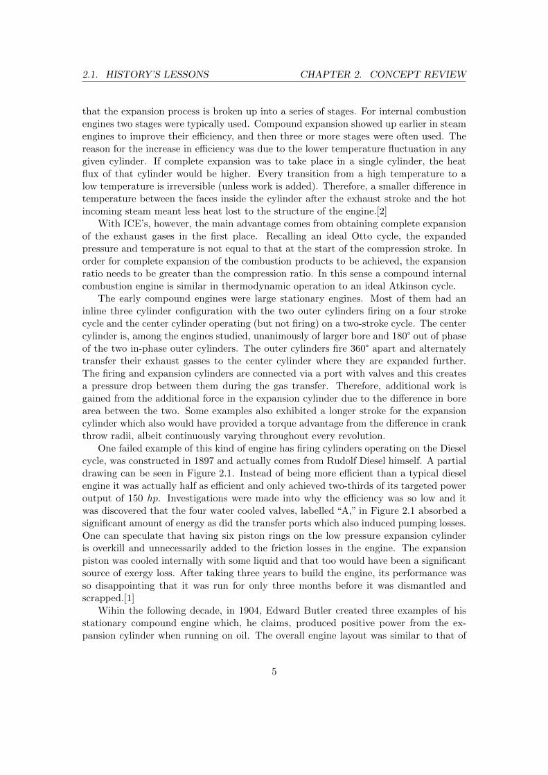
One failed example of this kind of engine has firing cylinders operating on the Dieselcycle, was constructed in 1897 and actually comes from Rudolf Diesel himself. A partialdrawing can be seen in Figure 2.1. Instead of being more efficient than a typical dieselengine it was actually half as efficient and only achieved two-thirds of its targeted poweroutput of 150 hp. Investigations were made into why the efficiency was so low and itwas discovered that the four water cooled valves, labelled “A,” in Figure 2.1 absorbed asignificant amount of energy as did the transfer ports which also induced pumping losses.One can speculate that having six piston rings on the low pressure expansion cylinderis overkill and unnecessarily added to the friction losses in the engine. The expansionpiston was cooled internally with some liquid and that too would have been a significantsource of exergy loss. After taking three years to build the engine, its performance wasso disappointing that it was run for only three months before it was dismantled andscrapped.[1]
Wihin the following decade, in 1904, Edward Butler created three examples of hisstationary compound engine which, he claims, produced positive power from the ex-pansion cylinder when running on oil. The overall engine layout was similar to that of
5
2.1. HISTORY’S LESSONS CHAPTER 2. CONCEPT REVIEW
Figure 2.1: Parital drawing of Rudolf Diesel’s compound engine. From The Diesel Engine,Cummings, p185.
Diesel’s design, but there are no detailed drawings to present. Total power output ofthe engine was 80 hp, and 20 hp was said to be produced by the expansion cylinder.[1]Fifty percent of the firing cylinder’s BMEP seems quite high as does the 25% increase inηf,b. Unfortunately no independent measurements are mentioned. A more likely storyis that of the Duetz engine from 1879. Like the Diesel-compound, it too suffered fromhigh thermal losses to cooled transfer valves and the expansion cylinder barely generatedenough power to cancel out its own friction.[1]
2.1.2 Cam and Axial Engines
Cam engines are different from axial engines in this context in the way that the pistonstransfer their force to the output shaft. They are similar in their flexibility of cylinderarrangement and therefore power density in terms of mass. They all run on conventionalengine cycles, however. They are mentioned here briefly because it is in this flexible
6
2.1. HISTORY’S LESSONS CHAPTER 2. CONCEPT REVIEW
arrangement that they are able to have different instantaneous torque profiles comparedto crankshaft engines. In some cases, piston side-forces can be cancelled out which isattractive for reducing friction, but often comes at the expense of increased complexityand inertia (i.e. the addition of roller bearings).
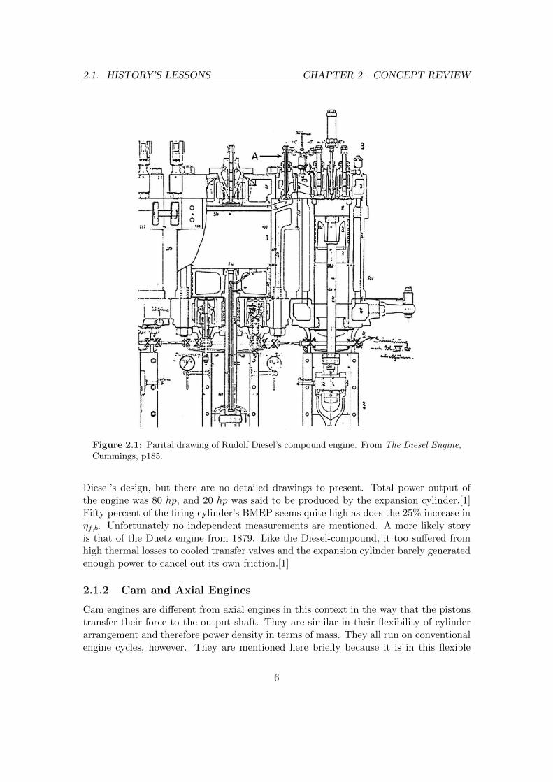
Cam engines tend to have a flat profile with their cylinders arranged radially ina plane. The pistons ride on a symmetric cam profile, often with roller bearings. Thelinkage can take many forms, but one example called the Fairchild-Caminez Cam Enginefrom 1926 is pictured in Figure 2.2a. Axial engines have their cylinders arranged parallelto each other and the output shaft (sometimes the engine block is the take-off point). Thecylinders are arranged in a circular pattern and therefore cylinder counts above threeoccupy nearly the same amount of space. This is due to the diameter of the wobbleor swash plate that the cylinders ride on. To avoid extreme angles to get the sameamount of cylinder stroke the cylinders must have adequate spacing from the engine’saxis. One example of an axial engine is the Macomber Axial Engine from 1911 picturedin Figure 2.2b. Axial engines were actually quite popular in the early 20th century asairplane engines and showed up on several models.[1]
(a) A drawing of the Fairchild-Caminez Cam Engine from 1926.[1]
(b) A drawing of the Macomber AxialEngine from 1911. The engine actu-ally has 7 pistons arranged in a circularpattern.[1]
Figure 2.2: Examples of cam and axial engines.
2.1.3 Combined Cycle
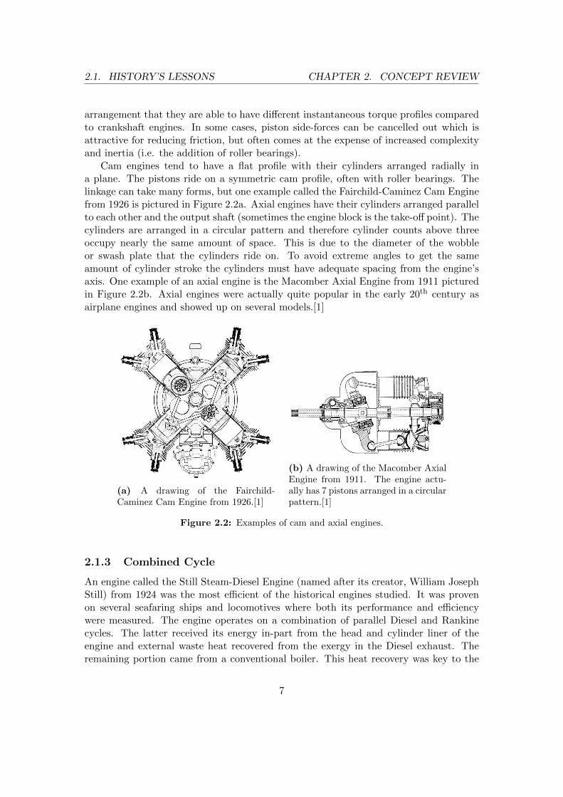
An engine called the Still Steam-Diesel Engine (named after its creator, William JosephStill) from 1924 was the most efficient of the historical engines studied. It was provenon several seafaring ships and locomotives where both its performance and efficiencywere measured. The engine operates on a combination of parallel Diesel and Rankinecycles. The latter received its energy in-part from the head and cylinder liner of theengine and external waste heat recovered from the exergy in the Diesel exhaust. Theremaining portion came from a conventional boiler. This heat recovery was key to the
7
2.1. HISTORY’S LESSONS CHAPTER 2. CONCEPT REVIEW
engine’s high efficiency of 41% (all fuel sources). This compares to a maximum Dieselengine efficiency of 36% and steam turbine efficiency of 20% for that era, according to anarticle from Captain Frank Acland in 1920.[3] The first expansion process of the Rankinecycle acted on the bottom side of the Diesel piston. Any left over steam exergy after thepiston expansion went on to power a small turbine which was connected via a shaft toan air compressor for the Diesel side of the engine, and generate electricity if there wasstill enough exergy in the steam to do so. The electric generator would act as a motorfor the compressor when the steam could not power the turbine. This type of enginearrangement can be seen in Figure 2.3. It was most efficient in its second form, powering
Figure 2.3: Functional diagram of the Still-Diesel Engine.[1]
the cargo liner Eurybates, where instead of all the cylinders having double acting pistons,four cylinders operated on the Diesel cycle, and two cylinders were used for the steamexpansion. This eliminated two problems, both related to contamination. The oil fromthe cylinder liner would no longer mix with the steam and contaminate the boiler, whichreduces its efficiency, and the steam would no longer contaminate the lubricating oil forthe Diesel engine, which reduces its lubricity.
One reason its popularity did not catch on, despite its high efficiency, was apparentlydue to a lack of workforce specialization. These engines required the ships to have SeniorEngineering Officers who were qualified for both steam power units as well as Dieselengines. Apparently at the time, people with both these qualifications were drawn moretowards jobs located on land.[1] Another drawback of this engine, and as we will see,
8
2.2. TODAY’S AMBITIONS CHAPTER 2. CONCEPT REVIEW
many engines which have methods to increase the fuel conversion efficiency, will have alower power density in terms of total cylinder volume than their standard versions. Laterin the ship’s life in 1948, efficiency was traded for power and the two steam cylinderswere converted into Diesel cylinders.
2.1.4 Regeneration
The Stirling engine is a very well known example of incorporating regeneration, the act ofstoring heat from a heat rejection process in the current cycle to use it in a heat additionprocess during the next cycle. This increases the efficiency of the engine because lessheat is rejected to the atmosphere. There are drawbacks to regeneration in practice,however. The first is a problem of time. Due to the fact that the mass which willbe absorbing and releasing the heat energy cannot change temperature instantaneously,a reduction in time between cycles also correlates to a reduction in the regenerator’seffectiveness (ability to absorb and release all the heat energy possible). This limits themaximum engine speed where high efficiencies can still be reached. Another detrimentis the structure of the regenerator itself. If it is to transfer heat quickly, it must havea very high surface area. In a limited volume, this means that the flow areas withinthe regenerator will be very small. Steel wool is one example of what the regenerator issometimes made of, and this or any similar substrate with a very high surface area tovolume ratio adds significantly to the pumping work of the engine.
The Ericsson engine is similar to a Stirling engine with the differences being the con-stant volume processes are instead constant pressure processes and the Ericsson engineruns on an open cycle. Their connection to the Carnot cycle is they all share the sameideal efficiency. Both the Stirling and Ericsson engines get their heat through externalcombustion which means that the transient response will be on the order of seconds (ormore for very large examples) due to the cylinder’s heat capacity. An internal combus-tion engine has a massive advantage in this respect as load can be varied from one cycleto the next. Another disadvantage of these two engines is their low specific output interms of both volume and mass. It’s clear that these engines are not well suited forpersonal vehicle applications but the take-away is understanding why they are efficient.The recycling of heat is the main cause for their efficiency, but as stated earlier, carryingout this process quickly is countered by reduced regenerator effectiveness and higher flowlosses.
2.2 Today’s Ambitions
Not seeing any directly applicable concept or example from the past for today’s vehicles,the search continues. There are several engine concepts which have been created in thelast couple decades which aim to improve the efficiency of ICE’s. Some remember thetriumphs of the past and try to incorporate their processes in a modern package.
9
2.2. TODAY’S AMBITIONS CHAPTER 2. CONCEPT REVIEW
2.2.1 Idealizing the Otto Cycle
In practice, it is not possible to have a truly constant-volume (isochoric) heat addition inan ICE. As a result, the sharp corners at the end of the compression stroke and beginningof the expansion stroke of an ideal Otto cycle P-v diagram end up becoming fillets,reducing the indicated work of the engine. Therefore, it logically follows that creating amechanical linkage which allows the cylinder volume to remain nearly constant duringthe finite combustion duration would generate a more ideal engine cycle in practice.Masatoshi Suzuki (from Honda Motor Corp.) et al. investigated this possibility. Butfirst, a quick review of instantaneous piston velocity. Since the piston in a typical engineis not directly pinned to the crankshaft and the connecting rod used to join the twois not of infinite length, the piston’s velocity is not sinusoidal. The piston’s speed ishigher during the upper 180° of motion and lower during the bottom 180° comparedto a true sine wave. So, taking advantage of this knowledge, Suzuki et al. arranged anengine where the crankshaft was above the combustion chamber and two connecting rodsreached down, one on either “side” of the cylinder, to connect to the bottom end of thepiston. By doing this, the piston now exhibited a velocity profile around TDC identicalto what normally occurs around BDC. While this still does not provide an absolutelyisochoric heat addition, it gives insight into the trend the actual pressure trace takes thenearer it gets to an isochoric process.
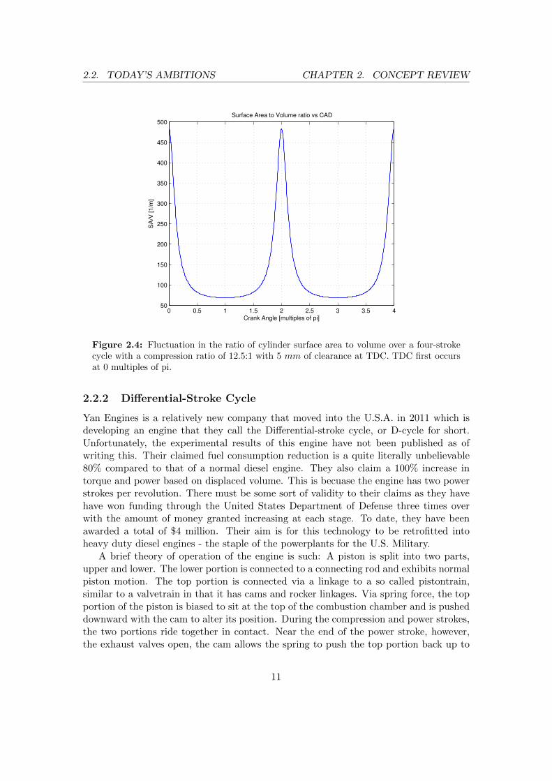
What they discovered is that despite an increase of 15% in maximum cylinder pres-sure, ISFC increased by 5% compared to the base engine. Shortly after the spike, thein-cylinder pressure trace falls slightly below that of the base engine for the remain-der of the expansion stroke. They found that the reason for this was due to increasedheat losses to the combustion chamber walls. The increased dwell time of the gases attheir hottest point during the period where the surface area to volume ratios are theirhighest were more detrimental to the efficiency than the increased peak pressure wasbeneficial.[4] As a visual aid to help appreciate this phenomenon, the fluctuation in theratio of cylinder surface area vs. volume over a four-stroke cycle with a compressionratio of 12.5:1 is shown in Figure 2.4. Not only is the magnitude of the ratio at TDCover 7 times that occurring at BDC, but the upper 84% of that fluctuation occurs in justthe first quarter revolution before and after TDC - the portions of the stroke that Suzukihad slowed down. Trying a different strategy, they created engines with a conventionalpiston-crankshaft placement but with high connecting rod length to crank radius ratios.This still causes the piston speed near TDC to be faster than a true sine wave, but closerto it with higher and higher ratios. For homogeneous charge combustion they found thesame trend; a drop in fuel conversion efficiency. However, with stratified charge combus-tion they saw a 1% improvement between the connecting rod length to crank radius ratioof 3.34:1 and 8:1. They attributed this to the insulating properties of the air surroundingthe combustion and the slow flame speed near the lean regions of the mixture. A sidebenefit they discovered as a part of this investigation is that for homogeneous charges,faster piston speeds near TDC lower the propensity for knock since a larger volume nearthe end of combustion means lower pressures and temperatures.[4]
10
2.2. TODAY’S AMBITIONS CHAPTER 2. CONCEPT REVIEW
0 0.5 1 1.5 2 2.5 3 3.5 450
100
150
200
250
300
350
400
450
500
Crank Angle [multiples of pi]
SA
/V [
1/m
]
Surface Area to Volume ratio vs CAD
Figure 2.4: Fluctuation in the ratio of cylinder surface area to volume over a four-strokecycle with a compression ratio of 12.5:1 with 5 mm of clearance at TDC. TDC first occursat 0 multiples of pi.
2.2.2 Differential-Stroke Cycle
Yan Engines is a relatively new company that moved into the U.S.A. in 2011 which isdeveloping an engine that they call the Differential-stroke cycle, or D-cycle for short.Unfortunately, the experimental results of this engine have not been published as ofwriting this. Their claimed fuel consumption reduction is a quite literally unbelievable80% compared to that of a normal diesel engine. They also claim a 100% increase intorque and power based on displaced volume. This is becuase the engine has two powerstrokes per revolution. There must be some sort of validity to their claims as they havehave won funding through the United States Department of Defense three times overwith the amount of money granted increasing at each stage. To date, they have beenawarded a total of $4 million. Their aim is for this technology to be retrofitted intoheavy duty diesel engines - the staple of the powerplants for the U.S. Military.
A brief theory of operation of the engine is such: A piston is split into two parts,upper and lower. The lower portion is connected to a connecting rod and exhibits normalpiston motion. The top portion is connected via a linkage to a so called pistontrain,similar to a valvetrain in that it has cams and rocker linkages. Via spring force, the topportion of the piston is biased to sit at the top of the combustion chamber and is pusheddownward with the cam to alter its position. During the compression and power strokes,the two portions ride together in contact. Near the end of the power stroke, however,the exhaust valves open, the cam allows the spring to push the top portion back up to
11
2.2. TODAY’S AMBITIONS CHAPTER 2. CONCEPT REVIEW
the top of the cylinder, exhausting the gases. The exhaust valves close, the intake valvesopen, and the piston’s cam then pushes the top portion back down and air is drawn intothe cylinder. After this process the piston portions meet back up for the compressionprocess. The piston splits apart for roughly 140° centered around what is BDC for thelower portion of the piston. Some things they point out is that with the same strokethe displaced volume is decreased, but can be compensated for with supercharging insome way. They also point out that the same technologies applied to valvetrains such asvariable timing and lift can be applied to the pistontrain as well.[5]
Some drawbacks to this engine architecture are mostly due to its kinematics, and it isclear why whey are focusing on low speed heavy duty diesel engines. Since the actuatingrod for the top portion of the piston runs through the center of a split connecting rodthat supports the bottom end of the piston there are a lot of stress concentrationsin both which do not lend themselves to durability at high mean piston speeds. Onthat same subject, the maximum mean piston speed for the engine is that of the topportion during the gas exchange process. The top portion’s acceleration at TDC is justcountered by a slender rod as opposed to the entire connecting rod. It also seems likethe efficiency for this engine would decrease at high loads where the blowdown pressuremay be significantly higher than in a conventional 4-stroke engine. This would be dueto the lower expansion ratio for the same crank radius.
2.2.3 Revetec
This engine was on the verge of omission since it still operates on a typical Otto cycleand just appeared to be another method for increasing power density. What earnedits recognition here, however, is its measured maximum ηf,b of 39.5%. The engine hasopposed pistons which are connected to each other and have separate combustion cham-bers on opposing sides of the engine. Using roller bearings, they ride on two co-axialtri-lobe cams located between the pistons which actuate in a scissoring pattern as theycounter-rotate. This eliminates piston side-forces but puts a twisting moment in theconnecting structure that joins the pistons. These cams are geared to the output shaftand are the means by which the engine turns cylinder pressure into rotational motion.
Recall what was discussed earlier about isochoric heat addition. In slowing the pistondown near TDC, the peak pressure was increased, but the mean pressure was decreaseddue to the higher degree of heat transfer. With a cam engine, the piston’s velocity is freeto be altered at any point in the cycle. It would be possible to truly stop the piston forsome duration at TDC, and allow it to quickly accelerate downward after combustionhad at least mostly been completed. Remember, the piston’s velocity in Suzuki’s enginewas slower during the first 90° of the expansion stroke, a significant duration. HaveRevetec achieved a more favorable piston motion with the cam? Without knowing thecam profiles, it is not possible to say for sure. It may be that the only advantage theirengine has over a conventional one is the reduced friction through fewer journal bearingsand elimination of the piston side-forces.
12
2.2. TODAY’S AMBITIONS CHAPTER 2. CONCEPT REVIEW
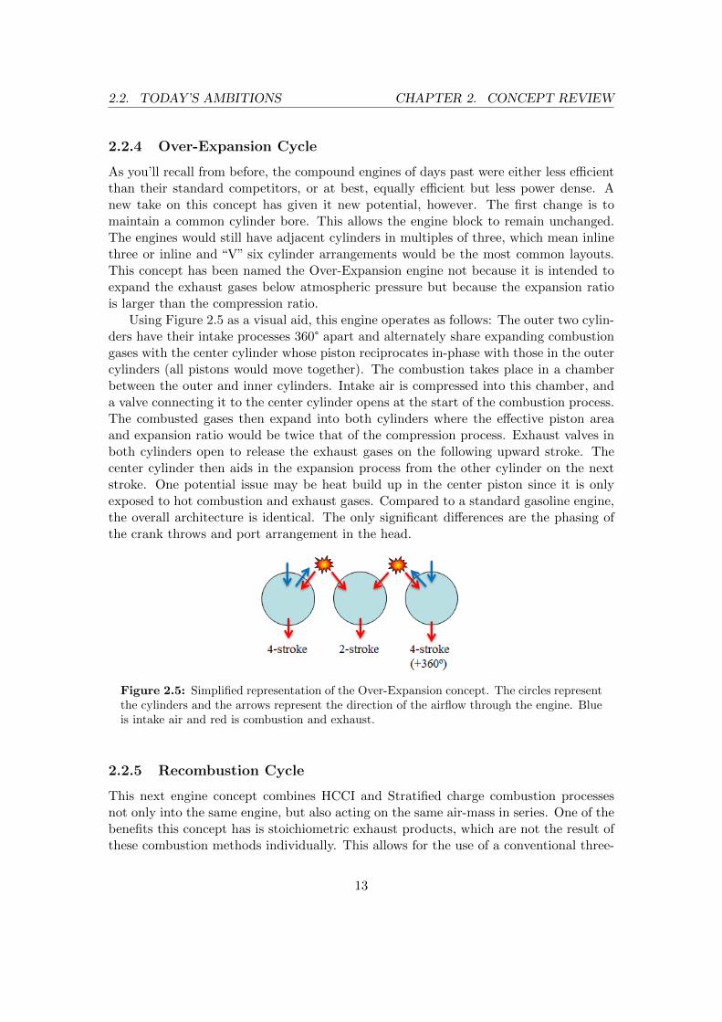
2.2.4 Over-Expansion Cycle
As you’ll recall from before, the compound engines of days past were either less efficientthan their standard competitors, or at best, equally efficient but less power dense. Anew take on this concept has given it new potential, however. The first change is tomaintain a common cylinder bore. This allows the engine block to remain unchanged.The engines would still have adjacent cylinders in multiples of three, which mean inlinethree or inline and “V” six cylinder arrangements would be the most common layouts.This concept has been named the Over-Expansion engine not because it is intended toexpand the exhaust gases below atmospheric pressure but because the expansion ratiois larger than the compression ratio.
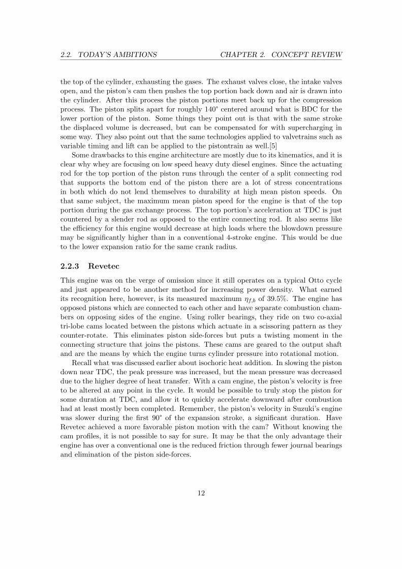
Using Figure 2.5 as a visual aid, this engine operates as follows: The outer two cylin-ders have their intake processes 360° apart and alternately share expanding combustiongases with the center cylinder whose piston reciprocates in-phase with those in the outercylinders (all pistons would move together). The combustion takes place in a chamberbetween the outer and inner cylinders. Intake air is compressed into this chamber, anda valve connecting it to the center cylinder opens at the start of the combustion process.The combusted gases then expand into both cylinders where the effective piston areaand expansion ratio would be twice that of the compression process. Exhaust valves inboth cylinders open to release the exhaust gases on the following upward stroke. Thecenter cylinder then aids in the expansion process from the other cylinder on the nextstroke. One potential issue may be heat build up in the center piston since it is onlyexposed to hot combustion and exhaust gases. Compared to a standard gasoline engine,the overall architecture is identical. The only significant differences are the phasing ofthe crank throws and port arrangement in the head.
Figure 2.5: Simplified representation of the Over-Expansion concept. The circles representthe cylinders and the arrows represent the direction of the airflow through the engine. Blueis intake air and red is combustion and exhaust.
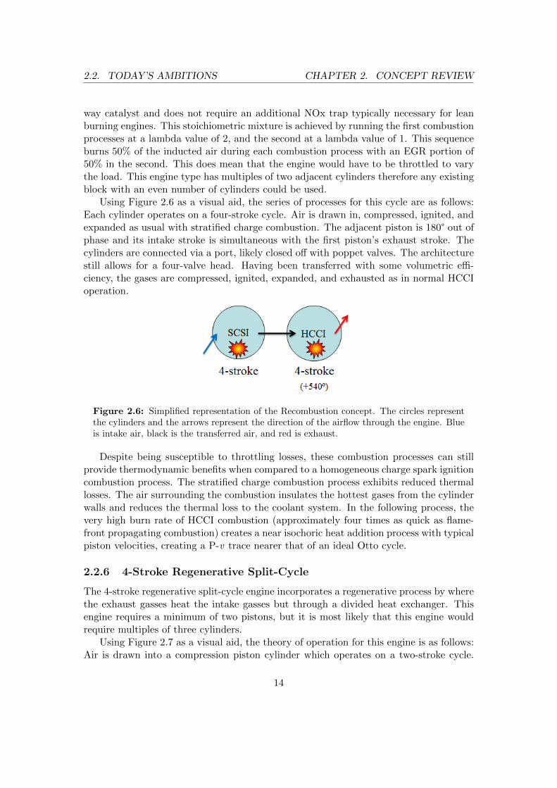
2.2.5 Recombustion Cycle
This next engine concept combines HCCI and Stratified charge combustion processesnot only into the same engine, but also acting on the same air-mass in series. One of thebenefits this concept has is stoichiometric exhaust products, which are not the result ofthese combustion methods individually. This allows for the use of a conventional three-
13
2.2. TODAY’S AMBITIONS CHAPTER 2. CONCEPT REVIEW
way catalyst and does not require an additional NOx trap typically necessary for leanburning engines. This stoichiometric mixture is achieved by running the first combustionprocesses at a lambda value of 2, and the second at a lambda value of 1. This sequenceburns 50% of the inducted air during each combustion process with an EGR portion of50% in the second. This does mean that the engine would have to be throttled to varythe load. This engine type has multiples of two adjacent cylinders therefore any existingblock with an even number of cylinders could be used.
Using Figure 2.6 as a visual aid, the series of processes for this cycle are as follows:Each cylinder operates on a four-stroke cycle. Air is drawn in, compressed, ignited, andexpanded as usual with stratified charge combustion. The adjacent piston is 180° out ofphase and its intake stroke is simultaneous with the first piston’s exhaust stroke. Thecylinders are connected via a port, likely closed off with poppet valves. The architecturestill allows for a four-valve head. Having been transferred with some volumetric effi-ciency, the gases are compressed, ignited, expanded, and exhausted as in normal HCCIoperation.
Figure 2.6: Simplified representation of the Recombustion concept. The circles representthe cylinders and the arrows represent the direction of the airflow through the engine. Blueis intake air, black is the transferred air, and red is exhaust.
Despite being susceptible to throttling losses, these combustion processes can stillprovide thermodynamic benefits when compared to a homogeneous charge spark ignitioncombustion process. The stratified charge combustion process exhibits reduced thermallosses. The air surrounding the combustion insulates the hottest gases from the cylinderwalls and reduces the thermal loss to the coolant system. In the following process, thevery high burn rate of HCCI combustion (approximately four times as quick as flame-front propagating combustion) creates a near isochoric heat addition process with typicalpiston velocities, creating a P-v trace nearer that of an ideal Otto cycle.
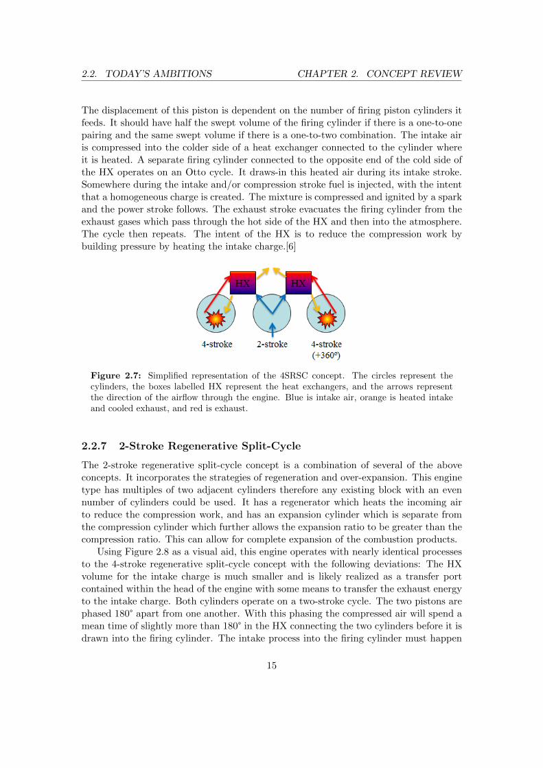
2.2.6 4-Stroke Regenerative Split-Cycle
The 4-stroke regenerative split-cycle engine incorporates a regenerative process by wherethe exhaust gasses heat the intake gasses but through a divided heat exchanger. Thisengine requires a minimum of two pistons, but it is most likely that this engine wouldrequire multiples of three cylinders.
Using Figure 2.7 as a visual aid, the theory of operation for this engine is as follows:Air is drawn into a compression piston cylinder which operates on a two-stroke cycle.
14
2.2. TODAY’S AMBITIONS CHAPTER 2. CONCEPT REVIEW
The displacement of this piston is dependent on the number of firing piston cylinders itfeeds. It should have half the swept volume of the firing cylinder if there is a one-to-onepairing and the same swept volume if there is a one-to-two combination. The intake airis compressed into the colder side of a heat exchanger connected to the cylinder whereit is heated. A separate firing cylinder connected to the opposite end of the cold side ofthe HX operates on an Otto cycle. It draws-in this heated air during its intake stroke.Somewhere during the intake and/or compression stroke fuel is injected, with the intentthat a homogeneous charge is created. The mixture is compressed and ignited by a sparkand the power stroke follows. The exhaust stroke evacuates the firing cylinder from theexhaust gases which pass through the hot side of the HX and then into the atmosphere.The cycle then repeats. The intent of the HX is to reduce the compression work bybuilding pressure by heating the intake charge.[6]
Figure 2.7: Simplified representation of the 4SRSC concept. The circles represent thecylinders, the boxes labelled HX represent the heat exchangers, and the arrows representthe direction of the airflow through the engine. Blue is intake air, orange is heated intakeand cooled exhaust, and red is exhaust.
2.2.7 2-Stroke Regenerative Split-Cycle
The 2-stroke regenerative split-cycle concept is a combination of several of the aboveconcepts. It incorporates the strategies of regeneration and over-expansion. This enginetype has multiples of two adjacent cylinders therefore any existing block with an evennumber of cylinders could be used. It has a regenerator which heats the incoming airto reduce the compression work, and has an expansion cylinder which is separate fromthe compression cylinder which further allows the expansion ratio to be greater than thecompression ratio. This can allow for complete expansion of the combustion products.
Using Figure 2.8 as a visual aid, this engine operates with nearly identical processesto the 4-stroke regenerative split-cycle concept with the following deviations: The HXvolume for the intake charge is much smaller and is likely realized as a transfer portcontained within the head of the engine with some means to transfer the exhaust energyto the intake charge. Both cylinders operate on a two-stroke cycle. The two pistons arephased 180° apart from one another. With this phasing the compressed air will spend amean time of slightly more than 180° in the HX connecting the two cylinders before it isdrawn into the firing cylinder. The intake process into the firing cylinder must happen
15

2.2. TODAY’S AMBITIONS CHAPTER 2. CONCEPT REVIEW
quickly since this process can only begin after the exhaust valve is effectively closed.If not, the compressed and heated intake mixture will short circuit through the firingcylinder. Unless high amounts of EGR are desired, this means the intake process canonly start after TDC, and that combustion can only start after the transfer valve hasclosed since expanding into the port volume causes a reduction in work. This pushes the50% burn point late in the expansion stroke compared to a standard engine. The intentis that in the end the reduced compression work combined with the difference betweenthe compression and expansion ratio will overcome the greatly reduced peak cylinderpressure as a result of combusting the mixture so late in the expansion stroke.
Figure 2.8: Simplified representation of the 2SRSC concept. The circles represent thecylinders, the box labelled HX represents the heat exchanger, and the arrows represent thedirection of the airflow through the engine. Blue is intake air, orange is heated intake andcooled exhaust, and red is exhaust.
2.2.8 6-Stroke Otto-Steam
The final modern concept runs on an Otto cycle followed by a steam expansion and ex-haust stroke, hence its name, 6-Stroke Otto-Steam. In less developed variants, unheatedwater can be injected into the cylinder with the hope it will vaporize and expand. Thismethod only reduces the cooling system’s exergy as it will obtain the heat energy onlyfrom the components in the cylinder. In more advanced variants, the water would bepreheated, reducing the exergy of the cooling and exhaust systems. The first preheat-ing stage would take energy from the cooling system, then from the higher temperatureexhaust system. If necessary, a heating element could add additional energy when theexhaust exergy is insufficient to reach the desired water temperature. The exhaustedsteam could be released to the atmosphere, where the cycle couldn’t really be called anopen Rankine cycle since there would be no condenser. If the steam were captured ina closed loop system, however, the overall cycle becomes a combination of an Otto andRankine cycle in parallel, with their expansion and exhaust processes occurring in series(it should be noted the exhaust process isn’t an official process of the Rankine cycle, butstill required in practical applications as there is some distance between the expanderand condenser).
16
2.2. TODAY’S AMBITIONS CHAPTER 2. CONCEPT REVIEW
There have been several theoretical investigations into this concept, and one physicalprototype. The prototype was created by Bruce Crower, the owner of Crower Cams &Equipment Co., Inc. It was run, but not tested on a dynamometer as of 2006, which isalso the latest date information can be found for this project. He had modified a singlecylinder Diesel engine by using the fuel injector as the water injector. The engine wascarbureted and ran on gasoline fuel. The cams were run at a speed of 3:1, as is necessarywith a six-stroke engine, but the exhaust cam had two lobes on it which opened theexhaust valve at the proper times. His claims were a 40% reduction in fuel consumptionand the ability to eliminate the need for a cooling system, but these are unsubstantiated.It is not clear if all of the exhaust gases were evacuated from the cylinder before thesteam expansion stroke.[7]
One of the theoretical studies done through calculation and engine simulation wasdone by James Conklin and James Szybist of the Oak Ridge National Laboratory. Fear-ing that repeated thermal shocks to the hot surfaces of the combustion chamber maycause cracks over time with liquid water impingement, they focused on using the en-ergy from recompressed exhaust gases to supply the heat energy for water vaporization.Their assumptions were that the water injection, vaporization, and homogeneity occurinstantaneously and that there was no heat transfer from the walls to steam mixture. Aminimum cylinder pressure of 1 bar absolute and minimum mixture temperature equalto the saturation temperature of the steam were limits for the conditions at the endof the steam expansion stroke. This was to avoid negative work from sub-atmosphericpressure and to avoid condensation buildup in the cylinder. They found that due tothe work required to recompress hot exhaust gases, the most efficient results were foundwhen only a portion of the exhaust was recompressed. Since they only used the coolingsystem’s exergy to heat the injected water, a temperature of only 100°C was achieved.Without pumping or friction losses, the maximum IMEP they were able to achieve fromthe exhaust compression and steam expansion process was 2.5 bar, or a 25% increaseover just the Otto cycle. This would represent a 25% reduction in indicated fuel con-sumption. They noted in the conclusions that had the injected water temperature beenraised to 175°C, the IMEP of the steam process could be raised by 40% to 3.5 bar. [8]
Another study on the potential of this concept was conducted by Bernard Johnsonand Chris Edwards of Stanford University. It went away from the six-stroke conventionbut retained the idea of combining the Otto and Rankine cycles. In this variationthe engine operates on an Otto cycle with the steam expansion and exhaust strokesoccurring simultaneously with those of the Otto cycle. The steam is injected duringthe combustion process. They had also incorporated low heat rejection strategies toreduce the thermal losses to the cooling system. However, focusing just on the gainsfrom the steam expansion process they found a 4.7% improvement in efficiency afterthey had imposed a 5% combustion efficiency penalty since steam is injected duringthe combustion process. This penalty is unmotivated, however. This is a relativelysmall improvement in efficiency, but it is on top of the improvements gained through thehigh compression ratio of 17:1 they assumed could be feasible and a low heat rejectioncylinder.[9]
17
2.3. SELECTED CONCEPTS CHAPTER 2. CONCEPT REVIEW
2.3 Selected Concepts
The concepts which will be studied in detail are the:
• Over-Expansion Engine
• Recombustion Engine
• 4-Stroke Regenerative Split-Cycle Engine
• 2-Stroke Regenerative Split-Cycle Engine
• 6-Stroke Otto-Steam Engine
I must state that I did not create these concepts myself. They were either presented tome for investigation, discovered through research, or developed jointly through discussionwith other powertrain engineers.
18
3Method
In order to create a fair comparison between the different concepts, severalcharacteristics are kept constant between them. Operating limits in the mechan-ics and thermodynamics of the concepts are also imposed with practical limits in
mind so that they are representative of what could be achieved in a physical representa-tion. The engine concepts will be compared to a baseline engine which is also created inGT-Power and adheres to the same limits. This minimizes the possibility for misleadingresults and conclusions to be drawn from the simulated performance of the concepts.
3.1 Simulation
Since ideal cycles are well understood in the engineering community and the resultsthey predict are very dependent on the assumptions made in their calculation, a moreaccurate, predictive method of analysis is used to obtain results. This provides a more re-alistic approximation of the performance these engine concepts would exhibit in physicalform.
In order to achieve this, the software package GT-Power by Gamma Technologiesis used for all engine performance calculations. The predictive combustion model cre-ated by the Forschungsinstitut fur Kraftfahrwesen und Fahrzeugmotoren, Stuttgart akaFKFS (translates in English to the Research Institute of Automotive Engineering andVehicle Engines, Stuttgart) is an add-on to GT-Power and is the default method used tocalculate the combustion process. The exception is in cases where the intended combus-tion process is outside the capabilities of the model. In these situations the combustionprocess is modelled based on the works of various researchers who were able to drawconclusions from physical testing. More information on how combustion was modelledin those cases will be covered in their respective sections. While GT-Power has the capa-bility to incorporate multi-dimensional flows, in these analyses it is used as a 1-D enginesimulation program. Taking advantage of its multi-dimensional capabilities requires cre-
19
3.1. SIMULATION CHAPTER 3. METHOD
ating detailed 3-D models of the engines to be studied and is far beyond the scope of thisthesis and not even something pursued extensively in the industry. In practice, identicalor similar component testing is performed along with separate 3-D CFD simulations andthe characteristics of these 1-D components and mechanical models are scaled to matchthe results of the more detailed analyses. By this measure, there is minimal loss in accu-racy by using a calibrated 1-D simulation program. This is, infact, the method by whichseveral models that calculate the performance of the studied concepts are developed.
3.1.1 GT-Power
For those unfamiliar with GT-Power, a brief description of what this program is usedfor, and why, in the scope of this thesis is provided here. GT-Power is a specialized typeof CFD program which solves the compressible Navier-Stokes equation in one dimension.It calculates an array of properties of the working fluid (typically air) and has built-incalculations to provide common metrics by which the user can analyze the performanceof the engine or subsystem. The user is also free to add equations to the simulationto provide other metrics. The user constructs the layout of the gas exchange systemby connecting a series of pipe, volume, and valve elements to represent the intake andexhaust systems connected to cylinder elements by defining diameters, lengths, etc. Itcalculates the properties at CAD intervals within one complete engine cycle. The CADintervals are based off of the current engine speed and time intervals determined bythe time it takes for a pressure wave to travel the distance of the characteristic lengthset by the user. There are other factors in this equation, but the strongest correlationis to the speed of sound. Since they suggest that the characteristic length be set atapproximately 40% of the bore diameter, at low engine speeds the CAD interval is veryshort - a fraction of 1° - and there can be thousands of time steps for even a two-strokecycle. At maximum engine speed, however, the intervals are on the order of 3-4° whichsignificantly reduces the simulation time for a cycle. The results from one cycle are usedas inital values for the next and the solver continues to iterate through complete cyclesuntil the convergence criteria are met. The properties in the different flow elements ateach interval can be displayed as instantaneous values throughout the cycle or integratedover the cycle for a single value. For example, the user can view the pressure trace fromthe cylinder, or the IMEP for the cycle, respectively.[10]
The strongest benefit this program provides over even the most detailed hand cal-culations is capturing the impact on volumetric efficiency from pulsatile flow, the flowlosses caused by the geometries of the engine (valves, orifices, flow areas, wall friction,etc), the heat transfer between the gases and engine components, and the friction in theengine (usually modelled, not calculated). With the FKFS model add-on, the benefitis that an assumed burn duration (i.e. Wiebe curve) can be replaced with a predictivecombustion calculation. If enough testing has been done on a similar engine to calibratea base model with, there are enough input parameters available that almost nothingabout the engine’s operation has to be assumed, and this is what makes it such a valu-able tool for engine engineers; to understand how even just changing one characteristicaffects the various performance metrics of an engine.
20
3.2. MODEL STANDARDS CHAPTER 3. METHOD
3.1.2 FKFS Cylinder Object
The FKFS cylinder object provides several benefits to the end user which greatly reducethe amount of control parameters the end user needs to impose in order to simulatea properly running engine. The first is its ability to phase combustion automaticallyto avoid knock. In-cylinder turbulence coefficients and knock limit coefficients are firstfound through CFD and/or experimentation. By using these, the dwell time of the fuelin the air, its temperature, and other factors, it predicts the onset of knock based offof the Worret knock model. If the calculated values are above the set knock limits itretards the desired mass fraction burned anchor (in this case 50% MFB) in steps untilthe probability of knock is below the limit. It does this within the same cycle thatGT-Power is calculating. The other benefit it provides is calculating the burn duration,which varies with load and speed, which the user otherwise has no good motivation fordefining other than through experimentation.
If the cylinder object did not do this, the engine load map would have to be generated,knock probabilities checked, and MFB anchors phased to values assumed to be correct,and iteratively run through this process. The optimizer in GT-Power can also be usedto find these values, but it also a very lengthy process due to the simulation time. Then,if any parameter is changed and it affects the volumetric efficiency or gas temperatures,the process needs to be repeated to ensure knock does not occur. This process easilyadds hours of simulation time and it is still without the benefit of calculated combustionduration.
FKFS created and verified their model by comparing its results to experimental datagathered from several different engines.[11]
3.2 Model Standards
In order to provide a fair and accurate comparison, several model standards were setboth on the operational and geometric characteristics of the engine. A selection of thosewith the greatest impact can be seen in Table 3.1. There are also some characteristicswhich are better stated than listed.
3.2.1 Flow
In general for the flow components, the diameters are always rounded to the next largestwhole mm if the calculated value is more than 0.1 mm over. The motivation behindthis rounding is that pipes are typically manufactured at whole number intervals. Theexception to this is for partially out of phase flow splits where the expansion diameter nolonger has a strong physical meaning. Flow splits are special cases in that respect sincethe diameters that define them are used to calculate a flow area rather than a physicaldiameter. For example, if a “Y” flow split has a flow direction from the branches tothe single outlet and the flow in each branch occurs simultaneously (in-phase) the areaone branch can effectively “expand” into is half the actual area of the outlet. If theflows are completely out of phase, the expansion diameter would be the full physical
21
3.2. MODEL STANDARDS CHAPTER 3. METHOD
diameter of the single outlet.[10] For this reason, rounding can no longer be motivatedfor out-of-phase flow split diameters.
The displaced volume of the engines is an important point to specify since normalconventions no longer apply. It is no longer based on all of the cylinders in the engine.The displaced volume of these engines is defined as the total swept cylinder volume ofall intake strokes from the atmosphere in one cycle. This means that for engine conceptswhich transfer the gases from one cylinder to the next, only the displaced volume of thecylinder that took the air from the atmosphere counts. This still lies in convention withnormal Otto cycle engines. In these concepts the device which takes work from the gasesa second time just happens to be a piston cylinder. If it were a turbine with a shaftproviding mechanical work, it becomes clear that trying to add a displaced volume forthe second expansion device has no meaning as the flow into it is based on the displacedvolume of the cylinder taking air from the atmosphere.
3.2.2 Cylinder
Concepts allowing the use of FKFS cylinder objects all had identical values for the in-cylinder turbulence coefficients and knock targets. This is due to the fact that these val-ues either have to be experimentally measured or predicted with three dimensional CFD.Refinement of combustion chamber, port, and valve geometries is extremely resource in-tensive in terms of manpower, simulation methods, and simulation time. For this reason,in all respects other than compression ratio, the characteristics remain identical betweenthe engines using the FKFS cylinder object. In special cases, the compression ratio wasonly lowered and only in order to avoid extreme predetonation or knocking at full loadthroughout the majority of its speed range. In cases where either the combustion methodor engine architecture required the use of a general cylinder object, as many properties ascould be carried over, were. Fuel is directly injected into the cylinder unless the conceptrequires otherwise. Deviations will be discussed in their respective sections.
3.2.3 Valves
The valve flow coefficients vs. lift profiles are also left untouched between all engines.The lift profiles are unchanged in their general shape (i.e. the order of the polynomialthat defines the lift curve is untouched), but are allowed to be scaled in terms of bothlift and duration. Due to the varied nature of the gas exchange processes in each of theseconcepts, proper valve timing has a very large impact on their very theory of operation.Forcing them to operate with valve durations and lifts optimized for a conventional four-stroke engine is unreasonable. VVT is implemented in all engines on all poppet valves.These parameters are calibrated with equal resolution and vary with both speed andload throughout each engine’s entire operating range. At all loads below the maximum,the valve timing which reduces the BSFC to a minimum while still allowing for fewerthan 25% burned residuals in the cylinder is selected. At full load the valve timing whichmaximizes engine output is selected.
22
3.3. BASELINE CHAPTER 3. METHOD
3.2.4 FMEP
The FMEP of each engine is dependant on its architecture. This is modelled in GT-Powerusing the Fischer-FMEP object which calculates the values based on the engine’s cycleaveraged coolant and oil temperatures, speed, and BMEP. The user inputs known FMEPvalues at 0 bar BMEP at a low and a high engine speed. The object then calculateswhat the values should be depending on the current engine operating conditions. Thefirst obstacle was how to scale the FMEP for each engine. According to Figure 13-8 inHeywood[12], FMEP is strongly correlated to engine speed, loosely correlated to stroketo bore ratio, and not correlated to displaced volume. Since the stroke to bore ratio isthe same for all of the engine concepts, this just leaves their FMEPs to be scaled basedupon their architecture, that is, the quantity of each component type it has.
A friction breakdown study from a production engine provided measured FMEPvalues from the piston assembly, crankshaft, valvetrain, water pump and alternator(unloaded), oil pump, and fuel injection pump. The scaling is done by calculating aweighted ratio for the concept’s FMEP compared to that of the measured engine. Theratio is weighted based off of the proportion of components from each category betweenthe concept and measured engine and the contribution those components provided tothe overall friction. The number of strokes between the two engine types for one cycleis also used as a scaling factor. For example, if the concept has twice as many of eachengine component but half the number of strokes, the FMEP remained unchanged fromthe measured engine’s value.
3.3 Baseline
The baseline engine is the standard to which all the concept engines are compared. It iscreated with the intent that it should be representative of a production engine in terms ofits performance. Therefore its torque curve is designed to have a smooth transition fromlow to high engine speed with peak torque occurring in the middle of the speed range.It is an inline two-cylinder, four-stroke engine with four poppet valves per cylinder. Thecylinders fire with 360° of separation. This layout allows for a direct comparison ofexpected fuel consumption in a vehicle since it shares the same displaced volume, 0.984L, of all the engine concepts. MEPs are very useful for comparing engines to each other,but in terms of application into the same vehicle, the engine’s performance at a certaintorque and speed is what is important. By having the same displaced volume, both ofthese comparisons can be made with just a single MEP plot. This configuration alsoshares the same instantaneous torque profile of the firing cylinders per cycle. The onlyexception to this is the Recombusiton engine which has twice as many. Since the engineis forced to run at a constant speed, negating any inertial effects, this can be scaled induration for comparison.
23
3.4. OVER-EXPANSION CHAPTER 3. METHOD
3.4 Over-Expansion
Due to the limitations in GT-Power, the ideal theory of operation as described in Sec-tion 2.2.4 has to be modified. The FKFS object cannot predict combustion in a precham-ber. Non-predictive combustion with a quasi-steady cylinder volume with ports connet-ing it to other cylinder objects is also not possible. No matter the imposed combustion,GT-Power is hard coded to terminate combustion the instant any exiting valves open.Since the valves between the prechamber and cylinders would have to be open duringthe entire combustion duration, it is clearly not possible to simulate this engine in itsintended form. The compromise, then, is to simulate it in a form as similar as possible.This means that the transfer and sharing of the combustion gases must start after themajority of the combustion process is completed. Not only does this mean the transfervalve opening needs to be retarded, but the expansion cylinder must lag by the sameoffset, so as to minimize the initial volume the gases expand into. With this timingconvention, the expansion cylinder will be at TDC when the transfer valve opens whichoccurs after the majority of the fuel (MFB>90%) has been completed.
The two outer firing cylinders operate on a four-stroke cycle and have four poppetvalves per cylinder. One of those is a transfer port which connects to the two-strokeexpansion cylinder. The transfer port valves leading into the expansion cylinder arecheck valves actuated via a pressure differential between the two volumes. The averagepressure drop across the similar sized poppet valves was measured on the baseline engineand to that pressure drop, the maximum flow coefficient of the poppet valve was assigned.This gives the two valve types similar maximum flow properties. Values between 0 andthe maximum pressure drop are calculated internally by linear interpolation. Checkvalves were used leading into the expansion cylinder since GT-Power does not allow afour-stroke valve actuation schedule attached to a two-stroke cylinder. The expansioncylinder has one poppet exhaust valve which brings the total to two check valves andone poppet valve.
3.5 Recombustion Cycle
Due to the nature of the combustion processes, the FKFS cylinder object cannot beused since it supports neither HCCI nor stratified charge combustion. Therefore theburn durations and anchors are modelled with a Wiebe curve based on measured data.Thomas Johansson et al. investigated this very relationship in a joint study betweenLund University, in Lund, Sweden and the late car manufacturer, SAAB AutomobilePowertrain AB. They tested a four-cylinder turbocharged engine modified to run withHCCI combustion. Their cylinder geometry is similar to that used in the baseline engine,but the in-cylinder turbulence and knock tolerance is unknown. They calibrated theoperating map for MBT between 1000 to 3000 rpm and 1 to 6 bar IMEP. In terms of the10-90% MFB duration, they found that above 2000 rpm it was fairly constant in terms oftime vs. engine speed, as follows, the duration in CAD increased with engine speed. Thissuggests that the degree of in-cylinder turbulence is fairly constant for that speed range.
24
3.5. RECOMBUSTION CYCLE CHAPTER 3. METHOD
Burn duration did increase below 2000 rpm which suggests that the engine was relyingmore on spark assist to ensure combustion at low engine speeds. They generated a curvefit for the MBT point of the 50% MFB anchor. They found that the relationship waslinear with respect to IMEP and independent of speed. The final aspect they investigatedwas the Wiebe exponent and how that was affected throughout the operating range. Itwas discovered that this too was only dependent on IMEP in a linear fashion which led toanother curve fit being generated.[13] The tabular burn durations and curve fit equationsthey generated are entered into GT-Power to model these phenomena. Since the burnduration varied non-linearly with load and that variation was also different at differentengine speeds, the values throughout the load range at 3000 rpm were extrapolated tohigher engine speeds, sticking to the convention of constant burn duration in terms oftime, therefore increasing in terms of CAD. This is an assumption, but a more accurateassumption than just “smearing” the burn duration values at 3000 rpm to all higherengine speeds.
The stratified charge combustion process also has to be modelled based on valuesthat have motivations behind them. The first is the heat transfer to the walls. One ofthe benefits of stratified charge combustion is that the combustion is insulated from thecylinder walls by the surrounding air. This reduces the temperature losses to the coolingsystem which would have lowered the IMEP. Otherwise, the heat transfer throughout thecycle is identical as in a homogeneous charge spark ignition engine. Unfortunately, noscientific papers could be found which investigated the topic of heat transfer modellingfor stratified charge gasoline engines. Investigations into papers on heat transfer fromDiesel engines were not considered since their combustion process is quite different fromspark ignition engines. Therefore, a logical thought process is used to motivate the valuesset.
The crank angle duration during this reduced heat transfer benefit must be con-sidered. It does not seem reasonable that a lower heat transfer coefficient should beimposed for the entire combustion process or expansion stroke. The flame growth in ahomogeneous mixture is also insulated from the walls for a portion of the flame propaga-tion. Those engines do, however, have a high degree of turbulence and mixing to spreadthe flame throughout the combustion chamber quickly. The convention chosen for thisconcept was that the heat transfer coefficient for the stratified charge cylinders wouldbe lowered from 1 to 0.7 from the 50% MFB angle to 90° aTDC where it goes back upto 1 for the remainder of the cycle. The reason the span ends at 90° aTDC is because itis assumed that after this angle, in-cylinder turbulence will have transported the com-busted gases to the cylinder walls. If this is not true, the error from this assumptionis minimized by the nature of the surface area to volume ratio relationship displayed inFigure 2.4.
Searching for information about how one might model the combustion process itselfonly produced one paper from GM Corp. where they studied one single point in anengine’s operating map. It’s better than nothing, but disappointingly lacking comparedto the depth of research devoted to the HCCI combustion process. Their engine alsoexhibited cylinder geometries similar to that used in this investigation. Their engine was
25
3.6. 4-STROKE REGENERATIVE SPLIT-CYCLE CHAPTER 3. METHOD
a naturally aspirated four-stroke with spray-guided stratification. The intake manifoldpressure was maintained at 95 kPa absolute at 2000 rpm running a lambda of 1.95.They calibrated the engine for MBT and this resulted in an end of fuel injection angle of37° bTDC. The shortest 10-90% MFB combustion duration they achieved was 48°.[14]This is roughly twice as long as what is seen in a modern, high-turbulence engine.This makes sense, since in order to maintain the stratification the turbulence mustbe low, and typically with lower turbulence comes slower flame propagation. A linearextrapolation of combustion duration as with HCCI combustion is not realistic, however,since turbulence increases with engine speed and therefore the flame propagation in termsof time is not constant (in real HCCI combustion the flame initiates at several locationsalmost simultaneously so the dependence on turbulence is much lower). So, the ratioof burn durations at minimum and maximum engine speed compared to that at 2000rpm is taken from the baseline engine where FKFS predicts the burn duration. Theduration drops off by 23% from 2000 to 1000 rpm and increases by 33% between 2000and 7000 rpm. Values in between these points are found through linear interpolation.Since the burn duration is approximately twice that for the baseline engine, the nextquestion posed was if 8° aTDC was still the ideal 50% MFB angle. An optimization runat 7000 rpm (where the CAD duration is the longest) found that, somewhat surprisingly,8° aTDC is still the ideal angle.
The architecture is a four-cylinder, four-stroke engine with four poppet valves percylinder. This configuration is twice its basic form in order to have the same displacedvolume as all the other engines. Firing intervals for the engine are every 180°. Thestratified charge cylinders intake the air from the atmosphere and transfer it to theHCCI cylinders through two parallel transfer ports. The firing interval between thepaired cylinders is 540° and their crank throws are phased 180° apart. After TDC in thestratified cylinder, there is one stroke for the expansion, another for the shared exhaustand intake process, and another for the compression in the HCCI cylinder (which alignswith the intake stroke of the stratified cylinder).
3.6 4-Stroke Regenerative Split-Cycle
Since the HX in this engine concept must withstand high temperatures and large pressuredifferences between the hot and cold sides, it is determined that a shell and tube styleHX would handle this pressure ratio best. It is believed that other heat exchangerswith better surface area to volume ratios, such as those with a corrugated cross-flowconfiguration, would have difficulties with mechanical strength and leakage between thesides due to their construction – the layers are usually tack welded together and anypressure differential acts to separate the layers from one-another. Two versions of thisHX are created to investigate the effect the initial compression ratio has on the engine’scharacteristics. One where the compression ratio between the displaced compressioncylinder volume during one intake stroke vs. the HX volume is 1:1, and another whereit is 2.17:1. This was the highest initial compression ratio that could be achieved withtube diameters that still allowed for no more than a 10 kPa pressure drop over the hot
26
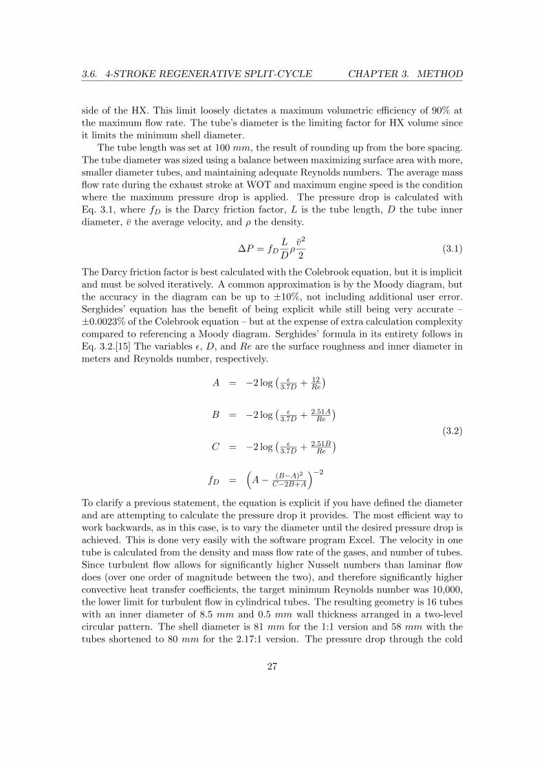
3.6. 4-STROKE REGENERATIVE SPLIT-CYCLE CHAPTER 3. METHOD
side of the HX. This limit loosely dictates a maximum volumetric efficiency of 90% atthe maximum flow rate. The tube’s diameter is the limiting factor for HX volume sinceit limits the minimum shell diameter.
The tube length was set at 100 mm, the result of rounding up from the bore spacing.The tube diameter was sized using a balance between maximizing surface area with more,smaller diameter tubes, and maintaining adequate Reynolds numbers. The average massflow rate during the exhaust stroke at WOT and maximum engine speed is the conditionwhere the maximum pressure drop is applied. The pressure drop is calculated withEq. 3.1, where fD is the Darcy friction factor, L is the tube length, D the tube innerdiameter, v the average velocity, and ρ the density.
∆P = fDL
Dρv2
2(3.1)
The Darcy friction factor is best calculated with the Colebrook equation, but it is implicitand must be solved iteratively. A common approximation is by the Moody diagram, butthe accuracy in the diagram can be up to ±10%, not including additional user error.Serghides’ equation has the benefit of being explicit while still being very accurate –±0.0023% of the Colebrook equation – but at the expense of extra calculation complexitycompared to referencing a Moody diagram. Serghides’ formula in its entirety follows inEq. 3.2.[15] The variables ε, D, and Re are the surface roughness and inner diameter inmeters and Reynolds number, respectively.
A = −2 log(
ε3.7D + 12
Re
)B = −2 log
(ε
3.7D + 2.51ARe
)C = −2 log
(ε
3.7D + 2.51BRe
)fD =
(A− (B−A)2
C−2B+A
)−2
(3.2)
To clarify a previous statement, the equation is explicit if you have defined the diameterand are attempting to calculate the pressure drop it provides. The most efficient way towork backwards, as in this case, is to vary the diameter until the desired pressure drop isachieved. This is done very easily with the software program Excel. The velocity in onetube is calculated from the density and mass flow rate of the gases, and number of tubes.Since turbulent flow allows for significantly higher Nusselt numbers than laminar flowdoes (over one order of magnitude between the two), and therefore significantly higherconvective heat transfer coefficients, the target minimum Reynolds number was 10,000,the lower limit for turbulent flow in cylindrical tubes. The resulting geometry is 16 tubeswith an inner diameter of 8.5 mm and 0.5 mm wall thickness arranged in a two-levelcircular pattern. The shell diameter is 81 mm for the 1:1 version and 58 mm with thetubes shortened to 80 mm for the 2.17:1 version. The pressure drop through the cold
27
3.6. 4-STROKE REGENERATIVE SPLIT-CYCLE CHAPTER 3. METHOD
side of the HX is modelled based off of the relationships from Eq. 7-48 and Figure 7-27from Cengel.[16] On this side of the HX, the pressure drop was a result of the geometriesgenerated from the above requirements as opposed to a target value being set. This sidealso contains one baffle which directs the intake air to pass perpendicular to the tubestwice before it exits into the firing cylinder.
The Nusselt numbers which drive the heat transfer in the hot side of the HX aremodelled off of empirically derived formulas found in Cengel. GT-Power requires acontinuous function and only allows the user to set the exponent, m, of the Colburnequation (Eq. 3.3) for laminar, transient, and turbulent regions and the turbulent coef-ficient, C. This is unfortunate since it is the least accurate of all the internal Nusselt(Nu) correlations.
Nu = C ·RemPr1/3 (3.3)
Nu = C ·RemPr1/3(µ
µs
)(0.14)
(3.4)
To improve the correlation, the Nusselt numbers calculated by the more accurate Sieder-Tate equation (Eq. 3.4) are used to find the exponents and coefficients which should beimposed on the Colburn equation. By this manipulation, the Colburn equation usedin GT-Power will now produce results with the accuracy of the Sieder-Tate equation,so long as a constant µ/µs ratio is assumed. In this equation, µ is the free streamdensity and µs is the density near the surface of the tube. These values are differentdue to the temperature gradient of the fluid. If one would so desire, they could correlatethe Colburn equation based off of the predictions from the Gnielinski equation, which iseven more accurate, ±10% vs. ±25%. This equation requires a friction factor correlationfor non-smooth tubes, and since one is not suggested in the text, this approach is nottaken. Lastly, since these equations are really only valid for the turbulent region, theexponent for the transient region is manipulated until a continuous relationship betweenthe laminar Nusselt number (which is a constant) and the Nusselt number at the lowerturbulent limit is achieved.
On the cold side of the HX, the Nusselt numbers are not so conveniently predictedsince the flow over tube banks is much more complex. Therefore, the values are basedoff of the empirical relationships created by Zukauskas and presented in Table 7-2 inCengel. The coefficient and exponents are again calibrated so that the Colburn equationmatches the accuracy of, this time, Zukauskas, which is ±15%.
As you can see, there are fairly broad accuracies involved in each calculation to eitherover or underestimate the true Nusselt number. They cannot add to each other, however,since each governs one side of the HX and the heat transfer on one side must be equalto that in the other. Short of performing physical testing on an identical HX, this is themost robust method of predicting the Nusselt numbers in the HX within GT-Power.
The compression ratio in the firing cylinder using each size of HX is found by run-ning the engine at wide open throttle and selecting the highest ratio which avoids pre-detonation and allows knock to be controlled by phasing ignition timing down to anengine speed of approximately 3000 rpm.
28
3.7. 2-STROKE REGENERATIVE SPLIT-CYCLE CHAPTER 3. METHOD
The architecture is an inline three-cylinder engine with the compression piston lyingbetween the two firing cylinders. The compression cylinder has two intake poppet valveswith two check valves, one distributing air to each heat exchanger which lay betweenthe compression and two firing cylinders. The firing cylinders have one intake and twoexhaust poppet valves. Only one intake valve was used to achieve the desired initialcompression ratio. The firing cylinder’s crank pins are in-phase with each other but thecylinders fire 360° apart. The crankpin of the compression cylinder is offset from themby 180°.
3.7 2-Stroke Regenerative Split-Cycle
Since the 2-Stroke Regenerative Split-Cycle concept only has one mechanical compres-sion stage, it is critical that the transfer port in this case is small so that adequately highcompression ratios can be achieved. Because of what was learned in the 4-Stroke Re-generative Split-Cycle modelling phase, the transfer port is not modelled as a shell andtube HX. To investigate the potential of this concept, a quicker, less modelling intensiveapproach is adopted. A heat transfer rate is imposed on the transfer port. From thisperspective it provides results based on the assumption that a HX of some architecturecould achieve a certain effectiveness. To understand the impact of the HX’s effectivenesson the performance of the engine, several values are used. The heat transfer rate iscalculated at every timestep with the equation Q = εQmax where ε is the effectiveness.Qmax is calculated through Qmax = hAs∆T where h is the convective heat transfer coef-ficient, As is the surface area of the transfer port, and ∆T is the difference between theexhaust gases in the exhaust port and the air in the transfer port. The convective heattransfer coefficient is determined from a Nusselt number in the middle of the transientflow region since the pulsatile motion and turbulence from the gas transfer process isbelieved to maintain non-laminar flow until the next gas transfer process.
Since the firing cylinders operate on a two-stroke cycle with poppet valves in the head,the exhaust stroke must be completed before the transfer valve can open, otherwisethe risk for short circuiting the fuel is very high due to the large pressure differencebetween the transfer and exhaust ports. In order to minimize trapped residuals and avoidcompressing hot gases, this also means that the exhaust valve must close around TDC,leaving the transfer valve to open around the same time. The air must be transferredvery quickly since the transfer valve must be closed before combustion begins both forGT-Power to function properly and to minimize the initial volume the combustion canexpand into. Having a long transfer valve duration pushes the 50% MFB point to verylate CADs which results in very low peak cylinder pressures and reduces the degree ofexpansion the combusted gases experience. A preliminary transfer valve duration is setat 20° and a maximum lift of half that of the normal profile, since it must provide this liftwhen the piston is near the top of its stroke. Since detailed geometries are not createdfor these engines it is assumed that this relationship is mechanically possible.
Due to unknown difficulties, possibly inherent to the timing conventions, the FKFScylinder object could not be implemented in this model. Instead, a Wiebe curve is
29
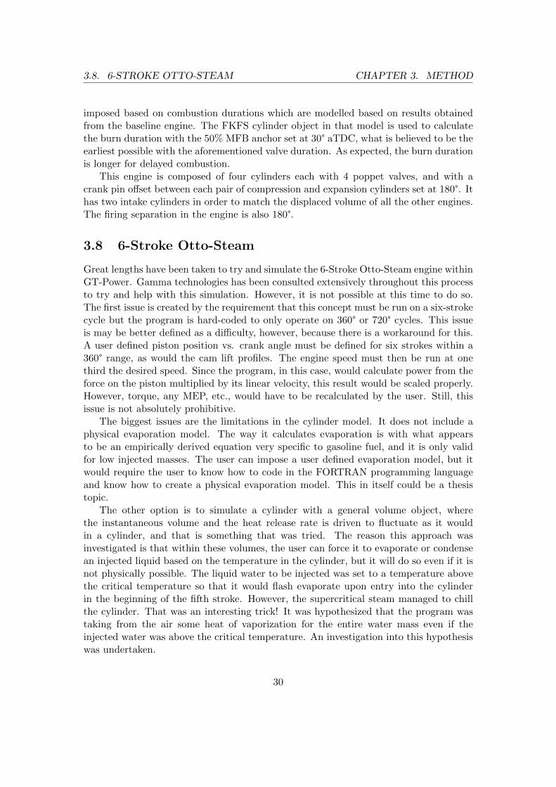
3.8. 6-STROKE OTTO-STEAM CHAPTER 3. METHOD
imposed based on combustion durations which are modelled based on results obtainedfrom the baseline engine. The FKFS cylinder object in that model is used to calculatethe burn duration with the 50% MFB anchor set at 30° aTDC, what is believed to be theearliest possible with the aforementioned valve duration. As expected, the burn durationis longer for delayed combustion.
This engine is composed of four cylinders each with 4 poppet valves, and with acrank pin offset between each pair of compression and expansion cylinders set at 180°. Ithas two intake cylinders in order to match the displaced volume of all the other engines.The firing separation in the engine is also 180°.
3.8 6-Stroke Otto-Steam
Great lengths have been taken to try and simulate the 6-Stroke Otto-Steam engine withinGT-Power. Gamma technologies has been consulted extensively throughout this processto try and help with this simulation. However, it is not possible at this time to do so.The first issue is created by the requirement that this concept must be run on a six-strokecycle but the program is hard-coded to only operate on 360° or 720° cycles. This issueis may be better defined as a difficulty, however, because there is a workaround for this.A user defined piston position vs. crank angle must be defined for six strokes within a360° range, as would the cam lift profiles. The engine speed must then be run at onethird the desired speed. Since the program, in this case, would calculate power from theforce on the piston multiplied by its linear velocity, this result would be scaled properly.However, torque, any MEP, etc., would have to be recalculated by the user. Still, thisissue is not absolutely prohibitive.
The biggest issues are the limitations in the cylinder model. It does not include aphysical evaporation model. The way it calculates evaporation is with what appearsto be an empirically derived equation very specific to gasoline fuel, and it is only validfor low injected masses. The user can impose a user defined evaporation model, but itwould require the user to know how to code in the FORTRAN programming languageand know how to create a physical evaporation model. This in itself could be a thesistopic.
The other option is to simulate a cylinder with a general volume object, wherethe instantaneous volume and the heat release rate is driven to fluctuate as it wouldin a cylinder, and that is something that was tried. The reason this approach wasinvestigated is that within these volumes, the user can force it to evaporate or condensean injected liquid based on the temperature in the cylinder, but it will do so even if it isnot physically possible. The liquid water to be injected was set to a temperature abovethe critical temperature so that it would flash evaporate upon entry into the cylinderin the beginning of the fifth stroke. However, the supercritical steam managed to chillthe cylinder. That was an interesting trick! It was hypothesized that the program wastaking from the air some heat of vaporization for the entire water mass even if theinjected water was above the critical temperature. An investigation into this hypothesiswas undertaken.
30
3.8. 6-STROKE OTTO-STEAM CHAPTER 3. METHOD
For the same injection mass flow rate of 100 g/s, and a defined initial vaporized fluidfraction of 0.5 and 0.99 (assigning either 50% or 1% of the mass a non-instantaneous va-porization), the exact same temperature drop at SOI of 648.5K occurred over 1.1° (CAD).For a fluid fraction of 0.5 and 0.99 and an injection rate of 50 g/s, the temperature dropin both cases was 579.2 K over 1.1°. These results suggested that while the vaporizedfraction does not have an influence on the results, the amount of water injected does,with less mass relating to a smaller decrease in temperature. This was the first red flag,since the initial degree of vaporization should have a direct effect on the temperaturechange in the cylinder. Calculating the change in energy during this period was the nextstep. Short hand calculations show that the change in work and heat for the cylinderare very near zero for these 1.1° and therefore can be ignored without much error. It wasthen just required to calculate the change in enthalpy. Just before 130°, there was 16.6mg of air in the cylinder (as determined by instantaneous density and volume). Withcp = 1.075 kJ/(kg · K), ∆Hair = −11.6 J after the temperature drop. At 1500 rpm,100 g/s of water, there were 36.6 mg of water injected in 1.1°. With a ∆Hw = −11.6 J ,this predicted an evaporation enthalpy of −316.9 kJ/kg. It should be noted that volumeincreases by ˜11% and pressure increases by ˜11% in this duration, so treating it asa constant pressure process isn’t absolutely accurate. That inaccuracy doesn’t mattermuch, however, since 773 K (the injection temperature) is beyond the critical tempera-ture of water, which means that there was no evaporation enthalpy to be crossed for achange in pressure. Furthermore, the air is initially at an even higher temperature than773 K, so it should have had no reason whatsoever to chill the water and dip it into thetwo-phase vapor region.
An inquiry was made to Gamma Technologies and they agreed that it was likelyan evaporation enthalpy was being taken from the air. It turns out that the steamproperties in GT-Power are not found via a lookup table, but instead with a high orderpolynomial curve fit. The one they provide is not valid in the supercritical region. Thisis why whenever water was injected, it forced the entire air mass to chill. Yet anotherlimitation is that the user is forced to specify that only the air or only the cylinder wallsare the thermal sink/source for the evaporation/condensation process. This makes sensefor a 1D simulation, but an improvement would be to allow the user to blend them witha ratio.
So to summarize, GT-Power would need to be modified somewhat significantly bythe user in order to be able to simulate this type of engine cycle with any amount ofaccuracy. As an aside, due to the extremely short time each stroke takes even at modestengine speeds, it was determined that the best way to produce power and capture thecoolant and exhaust exergy was to raise the water to a temperature where it would flashboil on injection, not requiring it to absorb heat from the gases or walls which takestime. The exergy in the cooling system would have first been used to raise the watertemperature to near 373 K. The exergy in the combustion exhaust gases would then beused to raise it beyond the critical temperature, 647.14 K, and higher, depending on theavailable amount of exhaust exergy and temperature difference.
31
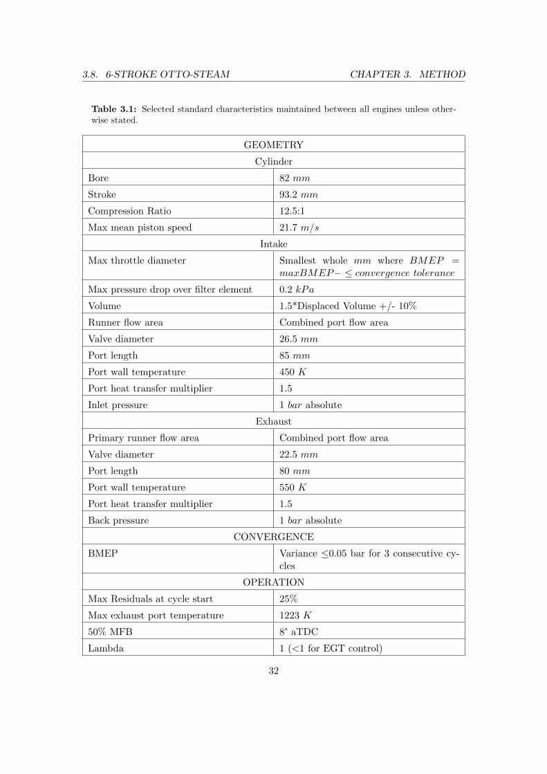
3.8. 6-STROKE OTTO-STEAM CHAPTER 3. METHOD
Table 3.1: Selected standard characteristics maintained between all engines unless other-wise stated.
GEOMETRY
Cylinder
Bore 82 mm
Stroke 93.2 mm
Compression Ratio 12.5:1
Max mean piston speed 21.7 m/s
Intake
Max throttle diameter Smallest whole mm where BMEP =maxBMEP− ≤ convergence tolerance
Max pressure drop over filter element 0.2 kPa
Volume 1.5*Displaced Volume +/- 10%
Runner flow area Combined port flow area
Valve diameter 26.5 mm
Port length 85 mm
Port wall temperature 450 K
Port heat transfer multiplier 1.5
Inlet pressure 1 bar absolute
Exhaust
Primary runner flow area Combined port flow area
Valve diameter 22.5 mm
Port length 80 mm
Port wall temperature 550 K
Port heat transfer multiplier 1.5
Back pressure 1 bar absolute
CONVERGENCE
BMEP Variance ≤0.05 bar for 3 consecutive cy-cles
OPERATION
Max Residuals at cycle start 25%
Max exhaust port temperature 1223 K
50% MFB 8° aTDC
Lambda 1 (<1 for EGT control)
32
4Results and Discussion
Since there are a number of engine concepts, the discussion for each will di-rectly follow the presentation of the results so that the outcome of the investigationis still fresh in the reader’s memory. All line plots have an x-axis resolution of 500
rpm with an exact placement of y-values. All non-comparative contour plots have aresolution of 0.5 bar BMEP and 500 rpm. The exception are the uppermost values ofBMEP which may lie at intermediate values as determined by the maximum capabilitiesof the engine at that speed. All comparative contour plots will have a constant resolutionequal to that stated above, and at exact BMEP locations equal to that determined bythe baseline engine. This is because when the concept’s performance is compared to thebaseline’s, if the BMEP value of the concept engine varies more than 0.25 bar (half theresolution) from that of the baseline, the two engines are deemed to not be running atthe same load point and no data is shown for that point in the map. Where this occursonly the white background will appear.
4.1 Baseline
4.1.1 Results
Figure 4.1 shows the baseline engine’s BSFC throughout its entire load map. It has aminimum value of 201.5 g/(kW ·h) at 13 bar BMEP, 3000 rpm. The peak BMEP of theengine is 13.14 bar at 3500 rpm. The rise and plateau of values at and below 4 bar andabove 4000 rpm is due to the fuel enrichment necessary to maintain adequate EGTs. Aslight leveling off of values above this engine load can be seen for the same reason. Thistrend shows that the BSFC is more strongly tied to the enriched fuel-air mixture than theincreasing FMEP that comes from increasing engine speed. Figure A.1 and A.2 in theappendix show the conformance of the engine to the maximum EGT and residual BMFvalues, respectively. The EGT is too high at one load point; 1 bar at 6000 rpm. Thisload point is very uncommon in operation and is easily fixed by further enriching the
33
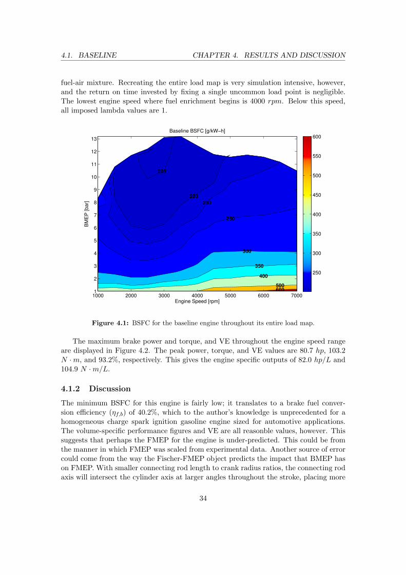
4.1. BASELINE CHAPTER 4. RESULTS AND DISCUSSION
fuel-air mixture. Recreating the entire load map is very simulation intensive, however,and the return on time invested by fixing a single uncommon load point is negligible.The lowest engine speed where fuel enrichment begins is 4000 rpm. Below this speed,all imposed lambda values are 1.
Engine Speed [rpm]
BM
EP
[bar]
Baseline BSFC [g/kW−h]
205
220
230
250
300
350
400
500600
1000 2000 3000 4000 5000 6000 70001
2
3
4
5
6
7
8
9
10
11
12
13
250
300
350
400
450
500
550
600
Figure 4.1: BSFC for the baseline engine throughout its entire load map.
The maximum brake power and torque, and VE throughout the engine speed rangeare displayed in Figure 4.2. The peak power, torque, and VE values are 80.7 hp, 103.2N ·m, and 93.2%, respectively. This gives the engine specific outputs of 82.0 hp/L and104.9 N ·m/L.
4.1.2 Discussion
The minimum BSFC for this engine is fairly low; it translates to a brake fuel conver-sion efficiency (ηf,b) of 40.2%, which to the author’s knowledge is unprecedented for ahomogeneous charge spark ignition gasoline engine sized for automotive applications.The volume-specific performance figures and VE are all reasonble values, however. Thissuggests that perhaps the FMEP for the engine is under-predicted. This could be fromthe manner in which FMEP was scaled from experimental data. Another source of errorcould come from the way the Fischer-FMEP object predicts the impact that BMEP hason FMEP. With smaller connecting rod length to crank radius ratios, the connecting rodaxis will intersect the cylinder axis at larger angles throughout the stroke, placing more
34
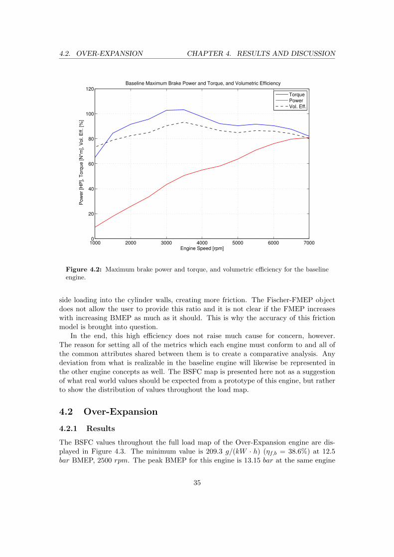
4.2. OVER-EXPANSION CHAPTER 4. RESULTS AND DISCUSSION
1000 2000 3000 4000 5000 6000 70000
20
40
60
80
100
120Baseline Maximum Brake Power and Torque, and Volumetric Efficiency
Engine Speed [rpm]
Pow
er
[HP
], T
orq
ue [N
*m], V
ol. E
ff. [%
]
Torque
Power
Vol. Eff.
Figure 4.2: Maximum brake power and torque, and volumetric efficiency for the baselineengine.
side loading into the cylinder walls, creating more friction. The Fischer-FMEP objectdoes not allow the user to provide this ratio and it is not clear if the FMEP increaseswith increasing BMEP as much as it should. This is why the accuracy of this frictionmodel is brought into question.
In the end, this high efficiency does not raise much cause for concern, however.The reason for setting all of the metrics which each engine must conform to and all ofthe common attributes shared between them is to create a comparative analysis. Anydeviation from what is realizable in the baseline engine will likewise be represented inthe other engine concepts as well. The BSFC map is presented here not as a suggestionof what real world values should be expected from a prototype of this engine, but ratherto show the distribution of values throughout the load map.
4.2 Over-Expansion
4.2.1 Results
The BSFC values throughout the full load map of the Over-Expansion engine are dis-played in Figure 4.3. The minimum value is 209.3 g/(kW · h) (ηf,b = 38.6%) at 12.5bar BMEP, 2500 rpm. The peak BMEP for this engine is 13.15 bar at the same engine
35
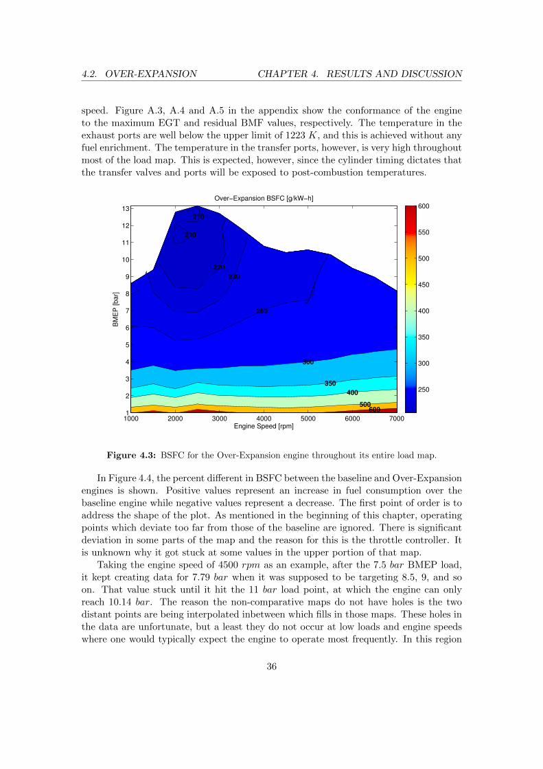
4.2. OVER-EXPANSION CHAPTER 4. RESULTS AND DISCUSSION
speed. Figure A.3, A.4 and A.5 in the appendix show the conformance of the engineto the maximum EGT and residual BMF values, respectively. The temperature in theexhaust ports are well below the upper limit of 1223 K, and this is achieved without anyfuel enrichment. The temperature in the transfer ports, however, is very high throughoutmost of the load map. This is expected, however, since the cylinder timing dictates thatthe transfer valves and ports will be exposed to post-combustion temperatures.
Engine Speed [rpm]
BM
EP
[bar]
Over−Expansion BSFC [g/kW−h]
600
210
210
220
230
250
300
350
400
500
1000 2000 3000 4000 5000 6000 70001
2
3
4
5
6
7
8
9
10
11
12
13
250
300
350
400
450
500
550
600
Figure 4.3: BSFC for the Over-Expansion engine throughout its entire load map.
In Figure 4.4, the percent different in BSFC between the baseline and Over-Expansionengines is shown. Positive values represent an increase in fuel consumption over thebaseline engine while negative values represent a decrease. The first point of order is toaddress the shape of the plot. As mentioned in the beginning of this chapter, operatingpoints which deviate too far from those of the baseline are ignored. There is significantdeviation in some parts of the map and the reason for this is the throttle controller. Itis unknown why it got stuck at some values in the upper portion of that map.
Taking the engine speed of 4500 rpm as an example, after the 7.5 bar BMEP load,it kept creating data for 7.79 bar when it was supposed to be targeting 8.5, 9, and soon. That value stuck until it hit the 11 bar load point, at which the engine can onlyreach 10.14 bar. The reason the non-comparative maps do not have holes is the twodistant points are being interpolated inbetween which fills in those maps. These holes inthe data are unfortunate, but a least they do not occur at low loads and engine speedswhere one would typically expect the engine to operate most frequently. In this region
36
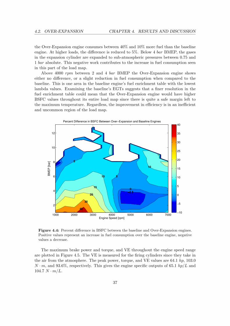
4.2. OVER-EXPANSION CHAPTER 4. RESULTS AND DISCUSSION
the Over-Expansion engine consumes between 40% and 10% more fuel than the baselineengine. At higher loads, the difference is reduced to 5%. Below 4 bar BMEP, the gasesin the expansion cylinder are expanded to sub-atmospheric pressures between 0.75 and1 bar absolute. This negative work contributes to the increase in fuel consumption seenin this part of the load map.
Above 4000 rpm between 2 and 4 bar BMEP the Over-Expansion engine showseither no difference, or a slight reduction in fuel consumption when compared to thebaseline. This is one area in the baseline engine’s fuel enrichment table with the lowestlambda values. Examining the baseline’s EGTs suggests that a finer resolution in thefuel enrichment table could mean that the Over-Expansion engine would have higherBSFC values throughout its entire load map since there is quite a safe margin left tothe maximum temperature. Regardless, the improvement in efficiency is in an inefficientand uncommon region of the load map.
Engine Speed [rpm]
BM
EP
[bar]
Percent Difference in BSFC Between Over−Expansion and Baseline Engines
40
30
20
15
10 5
0
−2.5
10
5
1000 2000 3000 4000 5000 6000 7000
2
4
6
8
10
12
−10
−5
0
5
10
15
20
25
30
35
40
Figure 4.4: Percent difference in BSFC between the baseline and Over-Expansion engines.Positive values represent an increase in fuel consumption over the baseline engine, negativevalues a decrease.
The maximum brake power and torque, and VE throughout the engine speed rangeare plotted in Figure 4.5. The VE is measured for the firing cylinders since they take inthe air from the atmosphere. The peak power, torque, and VE values are 64.1 hp, 103.0N ·m, and 93.6%, respectively. This gives the engine specific outputs of 65.1 hp/L and104.7 N ·m/L.
37
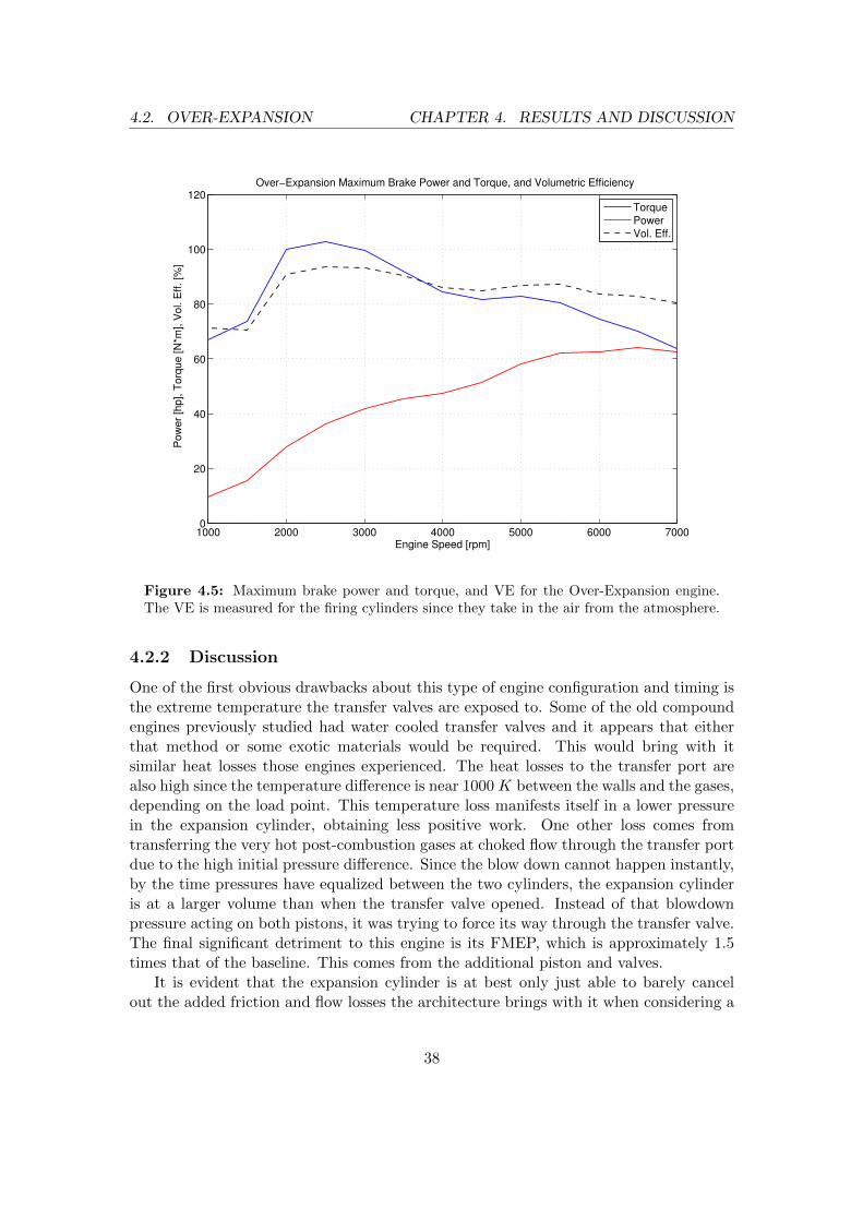
4.2. OVER-EXPANSION CHAPTER 4. RESULTS AND DISCUSSION
1000 2000 3000 4000 5000 6000 70000
20
40
60
80
100
120Over−Expansion Maximum Brake Power and Torque, and Volumetric Efficiency
Engine Speed [rpm]
Pow
er
[hp], T
orq
ue [N
*m], V
ol. E
ff. [%
]
Torque
Power
Vol. Eff.
Figure 4.5: Maximum brake power and torque, and VE for the Over-Expansion engine.The VE is measured for the firing cylinders since they take in the air from the atmosphere.
4.2.2 Discussion
One of the first obvious drawbacks about this type of engine configuration and timing isthe extreme temperature the transfer valves are exposed to. Some of the old compoundengines previously studied had water cooled transfer valves and it appears that eitherthat method or some exotic materials would be required. This would bring with itsimilar heat losses those engines experienced. The heat losses to the transfer port arealso high since the temperature difference is near 1000 K between the walls and the gases,depending on the load point. This temperature loss manifests itself in a lower pressurein the expansion cylinder, obtaining less positive work. One other loss comes fromtransferring the very hot post-combustion gases at choked flow through the transfer portdue to the high initial pressure difference. Since the blow down cannot happen instantly,by the time pressures have equalized between the two cylinders, the expansion cylinderis at a larger volume than when the transfer valve opened. Instead of that blowdownpressure acting on both pistons, it was trying to force its way through the transfer valve.The final significant detriment to this engine is its FMEP, which is approximately 1.5times that of the baseline. This comes from the additional piston and valves.
It is evident that the expansion cylinder is at best only just able to barely cancelout the added friction and flow losses the architecture brings with it when considering a
38
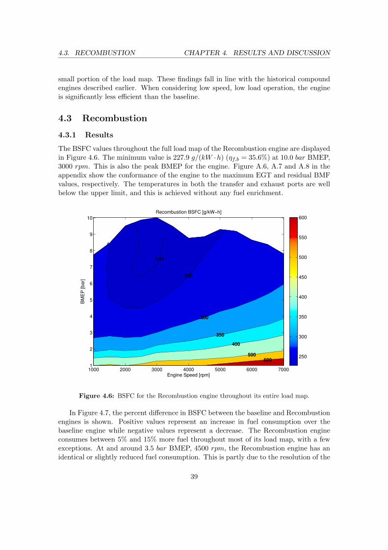
4.3. RECOMBUSTION CHAPTER 4. RESULTS AND DISCUSSION
small portion of the load map. These findings fall in line with the historical compoundengines described earlier. When considering low speed, low load operation, the engineis significantly less efficient than the baseline.
4.3 Recombustion
4.3.1 Results
The BSFC values throughout the full load map of the Recombustion engine are displayedin Figure 4.6. The minimum value is 227.9 g/(kW ·h) (ηf,b = 35.6%) at 10.0 bar BMEP,3000 rpm. This is also the peak BMEP for the engine. Figure A.6, A.7 and A.8 in theappendix show the conformance of the engine to the maximum EGT and residual BMFvalues, respectively. The temperatures in both the transfer and exhaust ports are wellbelow the upper limit, and this is achieved without any fuel enrichment.
Engine Speed [rpm]
BM
EP
[bar]
Recombustion BSFC [g/kW−h]
230
250
300
350
400
500
600
1000 2000 3000 4000 5000 6000 70001
2
3
4
5
6
7
8
9
10
250
300
350
400
450
500
550
600
Figure 4.6: BSFC for the Recombustion engine throughout its entire load map.
In Figure 4.7, the percent difference in BSFC between the baseline and Recombustionengines is shown. Positive values represent an increase in fuel consumption over thebaseline engine while negative values represent a decrease. The Recombustion engineconsumes between 5% and 15% more fuel throughout most of its load map, with a fewexceptions. At and around 3.5 bar BMEP, 4500 rpm, the Recombustion engine has anidentical or slightly reduced fuel consumption. This is partly due to the resolution of the
39
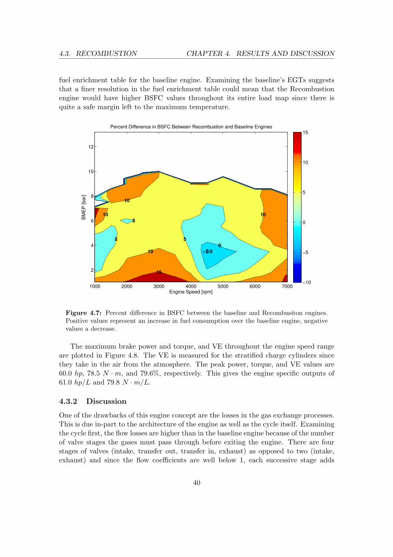
4.3. RECOMBUSTION CHAPTER 4. RESULTS AND DISCUSSION
fuel enrichment table for the baseline engine. Examining the baseline’s EGTs suggeststhat a finer resolution in the fuel enrichment table could mean that the Recombustionengine would have higher BSFC values throughout its entire load map since there isquite a safe margin left to the maximum temperature.
Engine Speed [rpm]
BM
EP
[bar]
Percent Difference in BSFC Between Recombustion and Baseline Engines
5
5
10
15
−2.5
0
5
10
10
10
1000 2000 3000 4000 5000 6000 7000
2
4
6
8
10
12
−10
−5
0
5
10
15
Figure 4.7: Percent difference in BSFC between the baseline and Recombusiton engines.Positive values represent an increase in fuel consumption over the baseline engine, negativevalues a decrease.
The maximum brake power and torque, and VE throughout the engine speed rangeare plotted in Figure 4.8. The VE is measured for the stratified charge cylinders sincethey take in the air from the atmosphere. The peak power, torque, and VE values are60.0 hp, 78.5 N ·m, and 79.6%, respectively. This gives the engine specific outputs of61.0 hp/L and 79.8 N ·m/L.
4.3.2 Discussion
One of the drawbacks of this engine concept are the losses in the gas exchange processes.This is due in-part to the architecture of the engine as well as the cycle itself. Examiningthe cycle first, the flow losses are higher than in the baseline engine because of the numberof valve stages the gases must pass through before exiting the engine. There are fourstages of valves (intake, transfer out, transfer in, exhaust) as opposed to two (intake,exhaust) and since the flow coefficients are well below 1, each successive stage adds
40
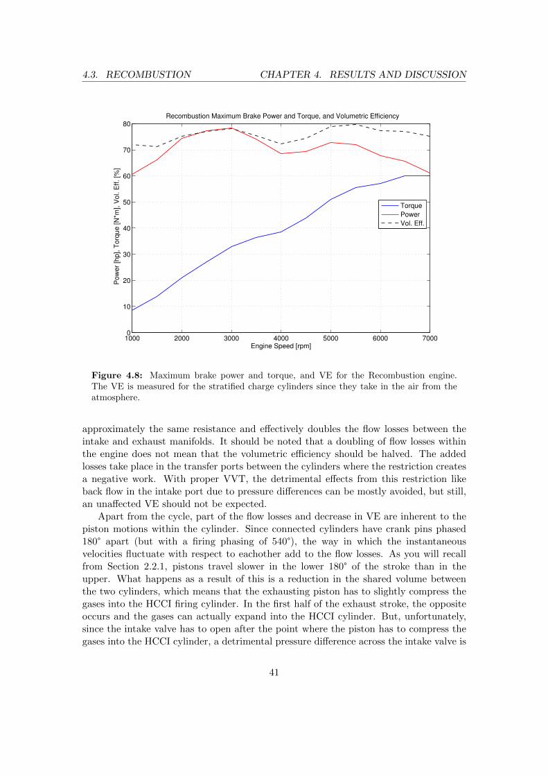
4.3. RECOMBUSTION CHAPTER 4. RESULTS AND DISCUSSION
1000 2000 3000 4000 5000 6000 70000
10
20
30
40
50
60
70
80Recombustion Maximum Brake Power and Torque, and Volumetric Efficiency
Engine Speed [rpm]
Pow
er
[hp], T
orq
ue [N
*m], V
ol. E
ff. [%
]
Torque
Power
Vol. Eff.
Figure 4.8: Maximum brake power and torque, and VE for the Recombustion engine.The VE is measured for the stratified charge cylinders since they take in the air from theatmosphere.
approximately the same resistance and effectively doubles the flow losses between theintake and exhaust manifolds. It should be noted that a doubling of flow losses withinthe engine does not mean that the volumetric efficiency should be halved. The addedlosses take place in the transfer ports between the cylinders where the restriction createsa negative work. With proper VVT, the detrimental effects from this restriction likeback flow in the intake port due to pressure differences can be mostly avoided, but still,an unaffected VE should not be expected.
Apart from the cycle, part of the flow losses and decrease in VE are inherent to thepiston motions within the cylinder. Since connected cylinders have crank pins phased180° apart (but with a firing phasing of 540°), the way in which the instantaneousvelocities fluctuate with respect to eachother add to the flow losses. As you will recallfrom Section 2.2.1, pistons travel slower in the lower 180° of the stroke than in theupper. What happens as a result of this is a reduction in the shared volume betweenthe two cylinders, which means that the exhausting piston has to slightly compress thegases into the HCCI firing cylinder. In the first half of the exhaust stroke, the oppositeoccurs and the gases can actually expand into the HCCI cylinder. But, unfortunately,since the intake valve has to open after the point where the piston has to compress thegases into the HCCI cylinder, a detrimental pressure difference across the intake valve is
41
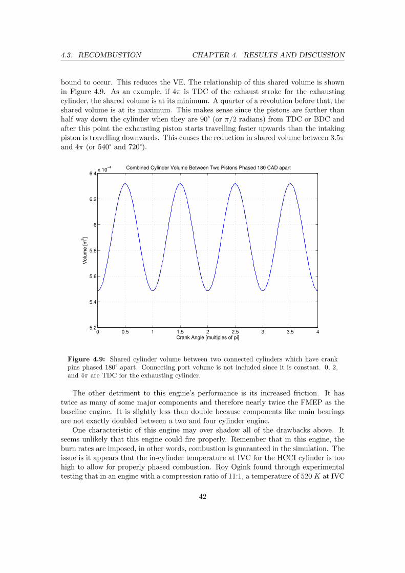
4.3. RECOMBUSTION CHAPTER 4. RESULTS AND DISCUSSION
bound to occur. This reduces the VE. The relationship of this shared volume is shownin Figure 4.9. As an example, if 4π is TDC of the exhaust stroke for the exhaustingcylinder, the shared volume is at its minimum. A quarter of a revolution before that, theshared volume is at its maximum. This makes sense since the pistons are farther thanhalf way down the cylinder when they are 90° (or π/2 radians) from TDC or BDC andafter this point the exhausting piston starts travelling faster upwards than the intakingpiston is travelling downwards. This causes the reduction in shared volume between 3.5πand 4π (or 540° and 720°).
0 0.5 1 1.5 2 2.5 3 3.5 45.2
5.4
5.6
5.8
6
6.2
6.4x 10
−4
Crank Angle [multiples of pi]
Volu
me [m
3]
Combined Cylinder Volume Between Two Pistons Phased 180 CAD apart
Figure 4.9: Shared cylinder volume between two connected cylinders which have crankpins phased 180° apart. Connecting port volume is not included since it is constant. 0, 2,and 4π are TDC for the exhausting cylinder.
The other detriment to this engine’s performance is its increased friction. It hastwice as many of some major components and therefore nearly twice the FMEP as thebaseline engine. It is slightly less than double because components like main bearingsare not exactly doubled between a two and four cylinder engine.
One characteristic of this engine may over shadow all of the drawbacks above. Itseems unlikely that this engine could fire properly. Remember that in this engine, theburn rates are imposed, in other words, combustion is guaranteed in the simulation. Theissue is it appears that the in-cylinder temperature at IVC for the HCCI cylinder is toohigh to allow for properly phased combustion. Roy Ogink found through experimentaltesting that in an engine with a compression ratio of 11:1, a temperature of 520 K at IVC
42
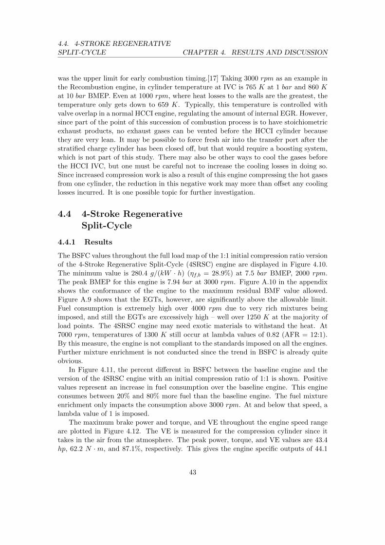
4.4. 4-STROKE REGENERATIVESPLIT-CYCLE CHAPTER 4. RESULTS AND DISCUSSION
was the upper limit for early combustion timing.[17] Taking 3000 rpm as an example inthe Recombustion engine, in cylinder temperature at IVC is 765 K at 1 bar and 860 Kat 10 bar BMEP. Even at 1000 rpm, where heat losses to the walls are the greatest, thetemperature only gets down to 659 K. Typically, this temperature is controlled withvalve overlap in a normal HCCI engine, regulating the amount of internal EGR. However,since part of the point of this succession of combustion process is to have stoichiometricexhaust products, no exhaust gases can be vented before the HCCI cylinder becausethey are very lean. It may be possible to force fresh air into the transfer port after thestratified charge cylinder has been closed off, but that would require a boosting system,which is not part of this study. There may also be other ways to cool the gases beforethe HCCI IVC, but one must be careful not to increase the cooling losses in doing so.Since increased compression work is also a result of this engine compressing the hot gasesfrom one cylinder, the reduction in this negative work may more than offset any coolinglosses incurred. It is one possible topic for further investigation.
4.4 4-Stroke RegenerativeSplit-Cycle
4.4.1 Results
The BSFC values throughout the full load map of the 1:1 initial compression ratio versionof the 4-Stroke Regenerative Split-Cycle (4SRSC) engine are displayed in Figure 4.10.The minimum value is 280.4 g/(kW · h) (ηf,b = 28.9%) at 7.5 bar BMEP, 2000 rpm.The peak BMEP for this engine is 7.94 bar at 3000 rpm. Figure A.10 in the appendixshows the conformance of the engine to the maximum residual BMF value allowed.Figure A.9 shows that the EGTs, however, are significantly above the allowable limit.Fuel consumption is extremely high over 4000 rpm due to very rich mixtures beingimposed, and still the EGTs are excessively high – well over 1250 K at the majority ofload points. The 4SRSC engine may need exotic materials to withstand the heat. At7000 rpm, temperatures of 1300 K still occur at lambda values of 0.82 (AFR = 12:1).By this measure, the engine is not compliant to the standards imposed on all the engines.Further mixture enrichment is not conducted since the trend in BSFC is already quiteobvious.
In Figure 4.11, the percent different in BSFC between the baseline engine and theversion of the 4SRSC engine with an initial compression ratio of 1:1 is shown. Positivevalues represent an increase in fuel consumption over the baseline engine. This engineconsumes between 20% and 80% more fuel than the baseline engine. The fuel mixtureenrichment only impacts the consumption above 3000 rpm. At and below that speed, alambda value of 1 is imposed.
The maximum brake power and torque, and VE throughout the engine speed rangeare plotted in Figure 4.12. The VE is measured for the compression cylinder since ittakes in the air from the atmosphere. The peak power, torque, and VE values are 43.4hp, 62.2 N ·m, and 87.1%, respectively. This gives the engine specific outputs of 44.1
43
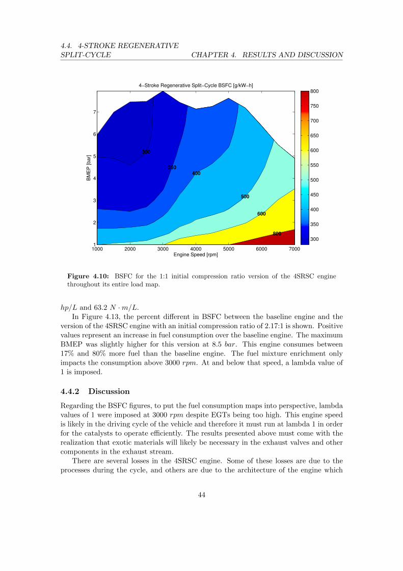
4.4. 4-STROKE REGENERATIVESPLIT-CYCLE CHAPTER 4. RESULTS AND DISCUSSION
Engine Speed [rpm]
BM
EP
[bar]
4−Stroke Regenerative Split−Cycle BSFC [g/kW−h]
300
350
400
500
600
800
1000 2000 3000 4000 5000 6000 70001
2
3
4
5
6
7
300
350
400
450
500
550
600
650
700
750
800
Figure 4.10: BSFC for the 1:1 initial compression ratio version of the 4SRSC enginethroughout its entire load map.
hp/L and 63.2 N ·m/L.In Figure 4.13, the percent different in BSFC between the baseline engine and the
version of the 4SRSC engine with an initial compression ratio of 2.17:1 is shown. Positivevalues represent an increase in fuel consumption over the baseline engine. The maximumBMEP was slightly higher for this version at 8.5 bar. This engine consumes between17% and 80% more fuel than the baseline engine. The fuel mixture enrichment onlyimpacts the consumption above 3000 rpm. At and below that speed, a lambda value of1 is imposed.
4.4.2 Discussion
Regarding the BSFC figures, to put the fuel consumption maps into perspective, lambdavalues of 1 were imposed at 3000 rpm despite EGTs being too high. This engine speedis likely in the driving cycle of the vehicle and therefore it must run at lambda 1 in orderfor the catalysts to operate efficiently. The results presented above must come with therealization that exotic materials will likely be necessary in the exhaust valves and othercomponents in the exhaust stream.
There are several losses in the 4SRSC engine. Some of these losses are due to theprocesses during the cycle, and others are due to the architecture of the engine which
44
4.4. 4-STROKE REGENERATIVESPLIT-CYCLE CHAPTER 4. RESULTS AND DISCUSSION
Engine Speed [rpm]
BM
EP
[bar]
Percent Difference in BSFC Between 4−Stroke Regenerative Split−Cycle and Baseline Engines
20
30
4040
60
80
1000 2000 3000 4000 5000 6000 7000
2
4
6
8
10
12
−10
0
10
20
30
40
50
60
70
80
90
100
Figure 4.11: Percent difference in BSFC between the baseline and 1:1 4SRSC engines.Positive values represent an increase in fuel consumption over the baseline engine, negativevalues a decrease.
increases flow losses and friction.Focusing first on the processes: The air which is pressurized and heated in the HX
is expanded during the firing cylinder’s intake stroke, exposing the air to the full surfacearea of the cylinder, where the coolant jackets in the head and cylinder walls along withthe piston will absorb some of its heat. This effectively transfers some exhaust exergy tothe coolant system where it is then lost to the atmosphere. The air is then recompressed,and since the air is still quite hot, it takes extra work to compress this hot air mass whencompared to the compression process of a normal Otto cycle engine since the specificheat ratio of the air is higher. Another drawback is the very short ignition delay ofthe fuel caused by the high average intake and compression temperatures. End of fuelinjection had to be phased to 90° before top dead center to avoid extreme knocking.It is not clear if it is still possible to create a truly homogeneous mixture with theinjection ending this late. Setting 90° as the limit to the end of injection, the onlyother way to avoid knock is to reduce the compression ratio in the firing cylinder. Thiscauses a somewhat self-exacerbation of knocking. As the compression ratio is reduced,the exhaust gas temperatures rise since they are not expanded as fully as with highcompression ratios. These even hotter exhaust gases increase the intake temperaturesfurther via the HX. This requires a further reduction in compression ratio which again
45
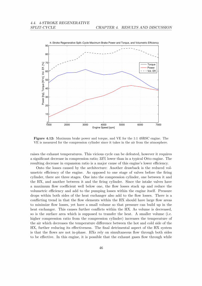
4.4. 4-STROKE REGENERATIVESPLIT-CYCLE CHAPTER 4. RESULTS AND DISCUSSION
1000 2000 3000 4000 5000 6000 70000
10
20
30
40
50
60
70
80
904−Stroke Regenerative Split−Cycle Maximum Brake Power and Torque, and Volumetric Efficiency
Engine Speed [rpm]
Pow
er
[hp], T
orq
ue [N
*m], V
ol. E
ff. [%
]
Torque
Power
Vol. Eff.
Figure 4.12: Maximum brake power and torque, and VE for the 1:1 4SRSC engine. TheVE is measured for the compression cylinder since it takes in the air from the atmosphere.
raises the exhaust temperatures. This vicious cycle can be defeated, however it requiresa significant decrease in compression ratio; 33% lower than in a typical Otto engine. Theresulting decrease in expansion ratio is a major cause of this engine’s lower efficiency.
Onto the losses caused by the architecture: Another drawback is the reduced vol-umetric efficiency of the engine. As opposed to one stage of valves before the firingcylinder, there are three stages. One into the compression cylinder, one between it andthe HX, and another between it and the firing cylinder. Since the intake valves havea maximum flow coefficient well below one, the flow losses stack up and reduce thevolumetric efficiency and add to the pumping losses within the engine itself. Pressuredrops within both sides of the heat exchanger also add to the flow losses. There is aconflicting trend in that the flow elements within the HX should have large flow areasto minimize flow losses, yet have a small volume so that pressure can build up in theheat exchanger. This causes further conflicts within the HX. As volume is decreased,so is the surface area which is supposed to transfer the heat. A smaller volume (i.e.higher compression ratio from the compression cylinder) increases the temperature ofthe air which decreases the temperature difference between the hot and cold side of theHX, further reducing its effectiveness. The final detrimental aspect of the HX systemis that the flows are not in-phase. HXs rely on simultaneous flow through both sidesto be effective. In this engine, it is possible that the exhaust gases flow through while
46
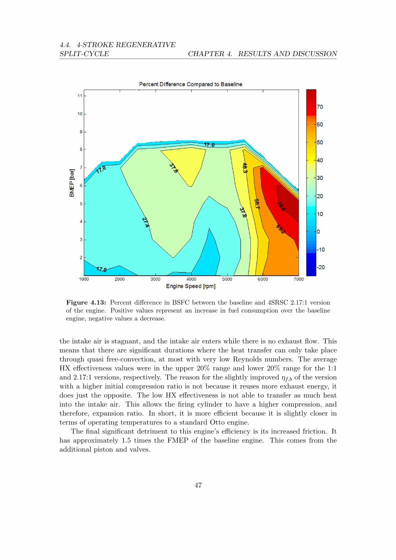
4.4. 4-STROKE REGENERATIVESPLIT-CYCLE CHAPTER 4. RESULTS AND DISCUSSION
Figure 4.13: Percent difference in BSFC between the baseline and 4SRSC 2.17:1 versionof the engine. Positive values represent an increase in fuel consumption over the baselineengine, negative values a decrease.
the intake air is stagnant, and the intake air enters while there is no exhaust flow. Thismeans that there are significant durations where the heat transfer can only take placethrough quasi free-convection, at most with very low Reynolds numbers. The averageHX effectiveness values were in the upper 20% range and lower 20% range for the 1:1and 2.17:1 versions, respectively. The reason for the slightly improved ηf,b of the versionwith a higher initial compression ratio is not because it reuses more exhaust energy, itdoes just the opposite. The low HX effectiveness is not able to transfer as much heatinto the intake air. This allows the firing cylinder to have a higher compression, andtherefore, expansion ratio. In short, it is more efficient because it is slightly closer interms of operating temperatures to a standard Otto engine.
The final significant detriment to this engine’s efficiency is its increased friction. Ithas approximately 1.5 times the FMEP of the baseline engine. This comes from theadditional piston and valves.
47
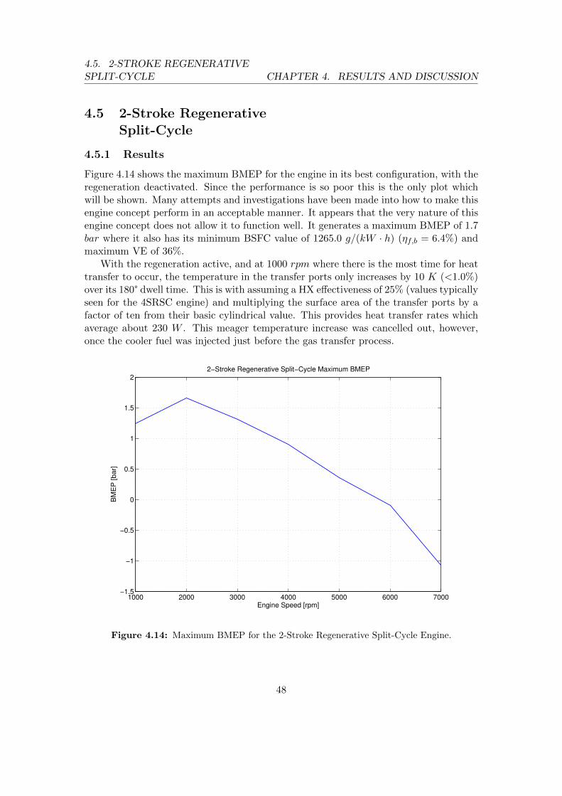
4.5. 2-STROKE REGENERATIVESPLIT-CYCLE CHAPTER 4. RESULTS AND DISCUSSION
4.5 2-Stroke RegenerativeSplit-Cycle
4.5.1 Results
Figure 4.14 shows the maximum BMEP for the engine in its best configuration, with theregeneration deactivated. Since the performance is so poor this is the only plot whichwill be shown. Many attempts and investigations have been made into how to make thisengine concept perform in an acceptable manner. It appears that the very nature of thisengine concept does not allow it to function well. It generates a maximum BMEP of 1.7bar where it also has its minimum BSFC value of 1265.0 g/(kW · h) (ηf,b = 6.4%) andmaximum VE of 36%.
With the regeneration active, and at 1000 rpm where there is the most time for heattransfer to occur, the temperature in the transfer ports only increases by 10 K (<1.0%)over its 180° dwell time. This is with assuming a HX effectiveness of 25% (values typicallyseen for the 4SRSC engine) and multiplying the surface area of the transfer ports by afactor of ten from their basic cylindrical value. This provides heat transfer rates whichaverage about 230 W . This meager temperature increase was cancelled out, however,once the cooler fuel was injected just before the gas transfer process.
1000 2000 3000 4000 5000 6000 7000−1.5
−1
−0.5
0
0.5
1
1.5
22−Stroke Regenerative Split−Cycle Maximum BMEP
Engine Speed [rpm]
BM
EP
[bar]
Figure 4.14: Maximum BMEP for the 2-Stroke Regenerative Split-Cycle Engine.
48
4.6. SUMMARY CHAPTER 4. RESULTS AND DISCUSSION
4.5.2 Discussion
The biggest enemies of this engine are time, limited surface area, and timing. The issuesof little time and surface area mean that the required mechanical compression workremains unaffected. There is no net temperature or pressure increase by the time thetransfer valve opens. Interestingly, the engine operates slightly better when regenerationis inactivated and the temperatures in the transfer port cooled slightly. Had even decentperformance resulted, this phenomenon would have been investigated further.
The timing issues lie primarily in the induction process to the firing cylinder. Thegases are supposed to transfer into the cylinder after the piston has already started tomove down for its expansion stroke. Since combustion can only begin after the intakevalve has closed, this pushes the 50% MFB point very late into the cylinder; 45°. This isexacerbated by the fact that the burn duration increases for delayed 50% MFB points.It was discovered that the peak cylinder pressure came from the release of the air fromthe transfer port, and not the combustion pressure that followed. Where the BMEPfalls below zero, the combustion duration is so long that the valve cannot close in timeand combustion does not take place. Combustion phasing could have been varied withengine speed, but the poor results at low engine speed did not warrant the additionalcalibration this would require.
This engine exhibited no change in friction compared to the baseline engine. This isbecause while it had twice as many components, it operates completely on a two-strokecycle.
4.6 Summary
After comparing all of the studied concept engines to the baseline, it was determinedthat in the low engine speed range where peak efficiency is found, between 1500 and3000 rpm, all of the concepts had a higher BSFC than the baseline engine. The Over-Expansion and Recombustion engines matched and bettered the BSFC of the baselineengine in some areas of the load map, but they were at higher engine speeds and fairlylow loads – inefficient areas of the load map to begin with. It is also possible that witha finer resolution of the baseline’s fuel enrichment table, those two concepts would havea higher fuel consumption in all points of the load map as well. The results of the keymetrics of all the engines analyzed are summarized in Table 4.1. An addition to thistable which was not presented before is a comparison between the engines at a commonload point. An engine load of 4 bar (31.3 N · m for these engines) at 2000 rpm wasselected as an example. By this comparison the Recombustion engine is now slightlymore efficient than the Over-Expansion engine which had previously been the best ofthe selected concepts. Still, the baseline is the most efficient engine.
4.6.1 Closing Remarks
In order to separate the processes of these engine concepts spatially, additional hardwarewas needed. In some cases these components contributed to the FMEP, in others flow
49
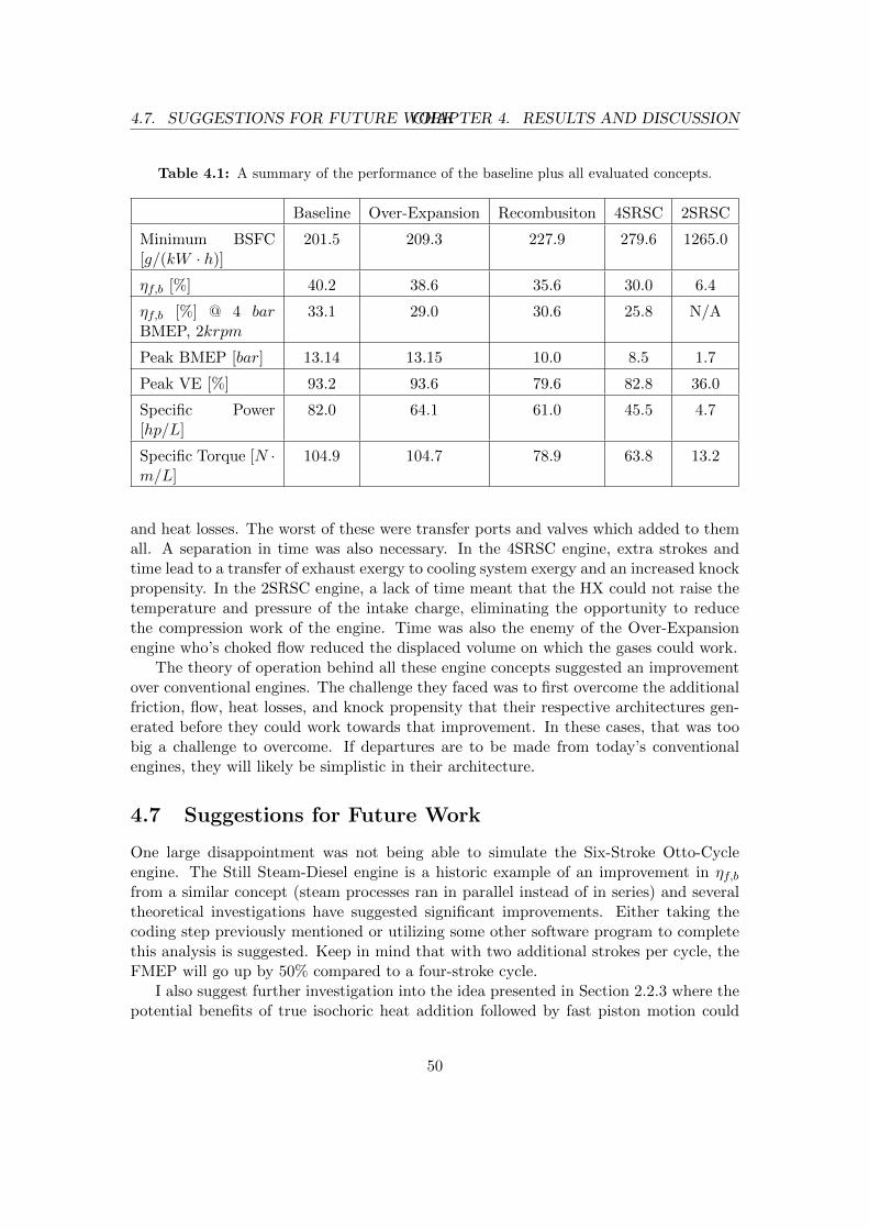
4.7. SUGGESTIONS FOR FUTURE WORKCHAPTER 4. RESULTS AND DISCUSSION
Table 4.1: A summary of the performance of the baseline plus all evaluated concepts.
Baseline Over-Expansion Recombusiton 4SRSC 2SRSC
Minimum BSFC[g/(kW · h)]
201.5 209.3 227.9 279.6 1265.0
ηf,b [%] 40.2 38.6 35.6 30.0 6.4
ηf,b [%] @ 4 barBMEP, 2krpm
33.1 29.0 30.6 25.8 N/A
Peak BMEP [bar] 13.14 13.15 10.0 8.5 1.7
Peak VE [%] 93.2 93.6 79.6 82.8 36.0
Specific Power[hp/L]
82.0 64.1 61.0 45.5 4.7
Specific Torque [N ·m/L]
104.9 104.7 78.9 63.8 13.2
and heat losses. The worst of these were transfer ports and valves which added to themall. A separation in time was also necessary. In the 4SRSC engine, extra strokes andtime lead to a transfer of exhaust exergy to cooling system exergy and an increased knockpropensity. In the 2SRSC engine, a lack of time meant that the HX could not raise thetemperature and pressure of the intake charge, eliminating the opportunity to reducethe compression work of the engine. Time was also the enemy of the Over-Expansionengine who’s choked flow reduced the displaced volume on which the gases could work.
The theory of operation behind all these engine concepts suggested an improvementover conventional engines. The challenge they faced was to first overcome the additionalfriction, flow, heat losses, and knock propensity that their respective architectures gen-erated before they could work towards that improvement. In these cases, that was toobig a challenge to overcome. If departures are to be made from today’s conventionalengines, they will likely be simplistic in their architecture.
4.7 Suggestions for Future Work
One large disappointment was not being able to simulate the Six-Stroke Otto-Cycleengine. The Still Steam-Diesel engine is a historic example of an improvement in ηf,bfrom a similar concept (steam processes ran in parallel instead of in series) and severaltheoretical investigations have suggested significant improvements. Either taking thecoding step previously mentioned or utilizing some other software program to completethis analysis is suggested. Keep in mind that with two additional strokes per cycle, theFMEP will go up by 50% compared to a four-stroke cycle.
I also suggest further investigation into the idea presented in Section 2.2.3 where thepotential benefits of true isochoric heat addition followed by fast piston motion could
50

4.7. SUGGESTIONS FOR FUTURE WORKCHAPTER 4. RESULTS AND DISCUSSION
minimize the heat losses seen by Suzuki et al. while improving the realization of an idealOtto-cycle. Care must be taken to understand and properly model FMEP, along withrealizable instantaneous piston velocities.
51
Bibliography
[1] Douglas. The Museum of Retrotechnology. http://www.douglas-self.com/
MUSEUM/museum.htm, April 2014.
[2] R. K. Raiput. Thermal Engineering. Laxim Publications, Bangalore, 5 edition,2005.
[3] Capt. J. Aclund. (unknown title). Technical report, The Journal of the Society ofAutomotive Engineers, June 1920.
[4] Masatoshi Suzuki, Satoshi Iijima, Hayato Maehara, and Yasuo Moriyoshi. Effectof the ratio between connecting-rod length and crank radius on thermal efficiency.Technical Report 2006-32-0098, SAE International, 11 2006.
[5] Miin Jang Yan. Differential-stroke internal combustion engine. PatentUS20130014713A1, USPTO, January 2013.
[6] Dulob AB. Dulob AB Vatne-Cycle and Thermocompression-Cycle. http://www.
dulob.com/, 2014.
[7] Pete Lyons. Inside Bruce Crower’s Six-Stroke Engine. Auto Week, February 2006.http://www.autoweek.com/article/20060227/free/302270007.
[8] James C. Conklin and James P. Szybist. A highly efficient six-stroke internal com-bustion engine cycle with water injection for in-cylinder exhaust heat recovery. En-ergy by Elsevier, 35:1658–1664, 2010.
[9] Bernard Johnson and Chris Edwards. Exploring the pathway to high efficiencyIC engines through exergy analysis of heat transfer reduction. Technical Report2013-01-0278, SAE International, January 2013.
[10] Gamma Technologies Inc. Various software manuals and tutorials. Version 7.3.
[11] Michael Grill, T. Billinger, and Michael Bargende. Quasi-dimensional modelingof spark ignition engine combustion with variable valve train. Technical Report2006-01-1107, SAE International, January 2006.
52
BIBLIOGRAPHY
[12] John B. Heywood. Internal Combustion Engine Fundamentals. McGraw-Hill, NewYork, 1988.
[13] Thomas Johansson, Patrick Borgqvist, Bengt Johansson, Per Tunestal, and HansAulin. HCCI heat release data for combustion simulation, based on results from aturbocharged multi cylinder engine. Technical Report 2010-01-1490, SAE Interna-tional, May 2010.
[14] Gerald A. Szekely and Alex C. Alkidas. Combustion characteristics of a spray-guided direct-injection stratified-charge engine with a high-squish piston. TechnicalReport 2005-01-1937, SAE International, January 2005.
[15] Wikipedia. Darcy friction factor formulae. http://en.wikipedia.org/wiki/
Darcy_friction_factor_formulae, May 2014.
[16] Janus A. Cengel. Heat and Mass Transfer A Practical Approach. McGraw-Hill,New York, 3 edition, 2007.
[17] Roy Ogink. Approximation of detailed-chemistry modeling by a simplified HCCIcombustion model. Technical Report 2005-24-037, SAE International, September2005.
53
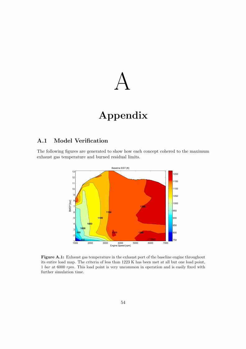
AAppendix
A.1 Model Verification
The following figures are generated to show how each concept cohered to the maximumexhaust gas temperature and burned residual limits.
Engine Speed [rpm]
BM
EP
[b
ar]
Baseline EGT [K]
950
1000
1050
1100
1150
1200
1200 1200
1223900
1000 2000 3000 4000 5000 6000 70001
2
3
4
5
6
7
8
9
10
11
12
13
750
800
850
900
950
1000
1050
1100
1150
1200
Figure A.1: Exhaust gas temperature in the exhaust port of the baseline engine throughoutits entire load map. The criteria of less than 1223 K has been met at all but one load point,1 bar at 6000 rpm. This load point is very uncommon in operation and is easily fixed withfurther simulation time.
54
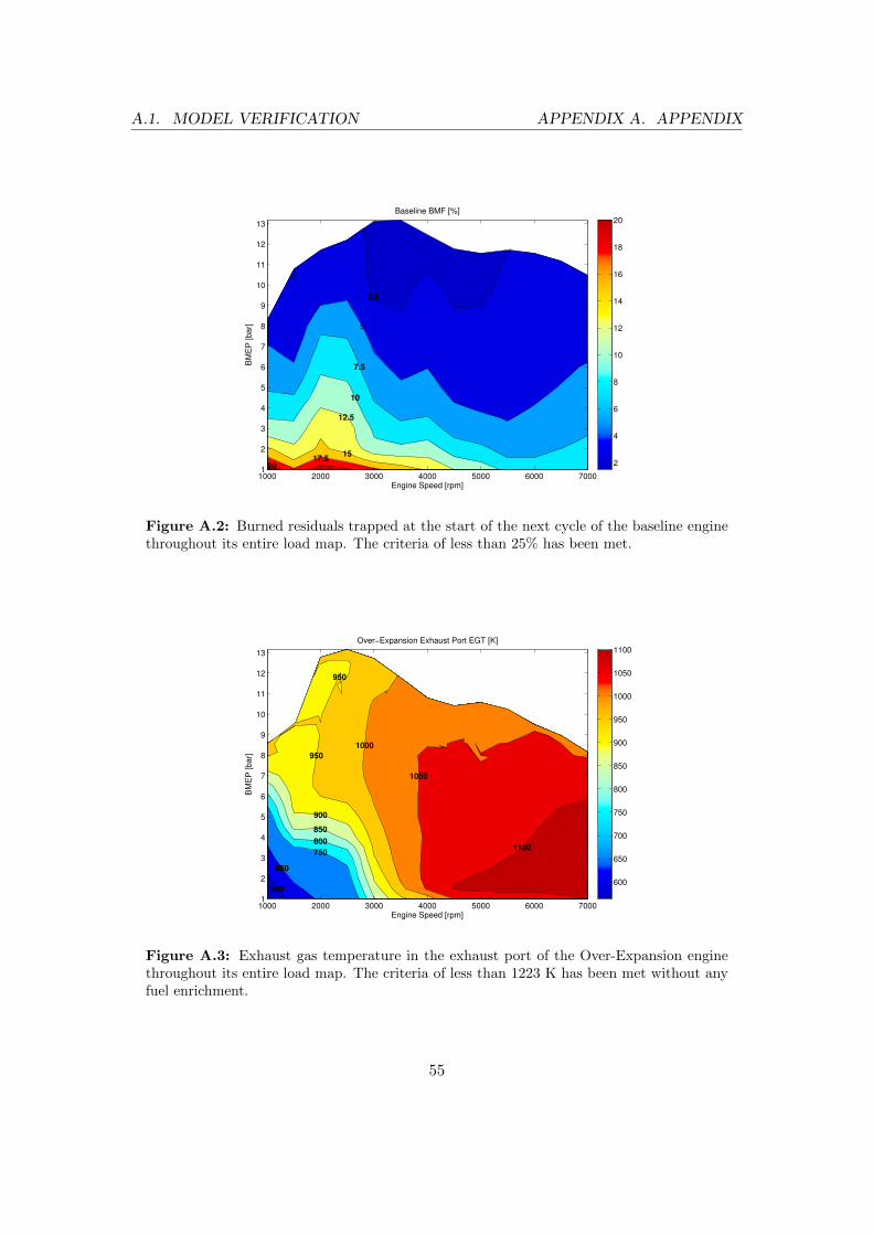
A.1. MODEL VERIFICATION APPENDIX A. APPENDIX
Engine Speed [rpm]
BM
EP
[b
ar]
Baseline BMF [%]
2017.5
15
12.5
10
7.5
5
2.5
1000 2000 3000 4000 5000 6000 70001
2
3
4
5
6
7
8
9
10
11
12
13
2
4
6
8
10
12
14
16
18
20
Figure A.2: Burned residuals trapped at the start of the next cycle of the baseline enginethroughout its entire load map. The criteria of less than 25% has been met.
Engine Speed [rpm]
BM
EP
[b
ar]
Over−Expansion Exhaust Port EGT [K]
600
650
750
800
850
900
950
950
1000
1050
1100
1000 2000 3000 4000 5000 6000 70001
2
3
4
5
6
7
8
9
10
11
12
13
600
650
700
750
800
850
900
950
1000
1050
1100
Figure A.3: Exhaust gas temperature in the exhaust port of the Over-Expansion enginethroughout its entire load map. The criteria of less than 1223 K has been met without anyfuel enrichment.
55
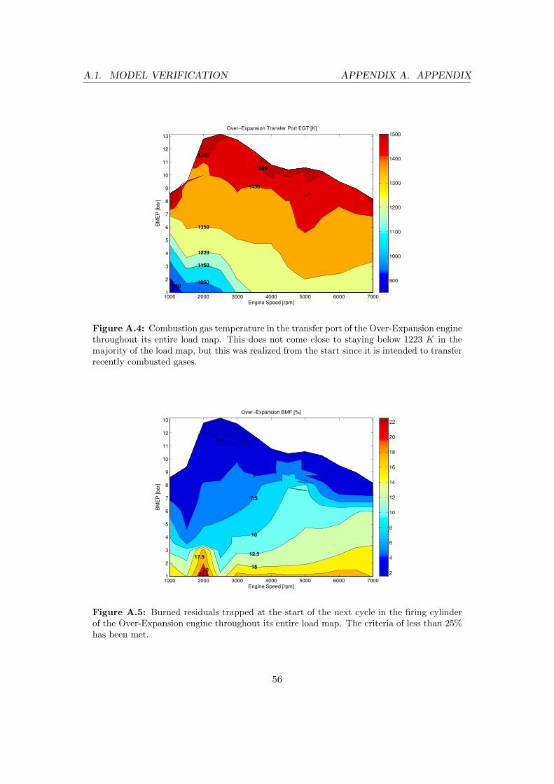
A.1. MODEL VERIFICATION APPENDIX A. APPENDIX
Engine Speed [rpm]
BM
EP
[b
ar]
Over−Expansion Transfer Port EGT [K]
9501050
1150
1223
1350
1450
1500
1500
1000 2000 3000 4000 5000 6000 70001
2
3
4
5
6
7
8
9
10
11
12
13
900
1000
1100
1200
1300
1400
1500
Figure A.4: Combustion gas temperature in the transfer port of the Over-Expansion enginethroughout its entire load map. This does not come close to staying below 1223 K in themajority of the load map, but this was realized from the start since it is intended to transferrecently combusted gases.
Engine Speed [rpm]
BM
EP
[b
ar]
Over−Expansion BMF [%]
22.520
17.512.5
10
7.5
5
2.5
15
1000 2000 3000 4000 5000 6000 70001
2
3
4
5
6
7
8
9
10
11
12
13
2
4
6
8
10
12
14
16
18
20
22
Figure A.5: Burned residuals trapped at the start of the next cycle in the firing cylinderof the Over-Expansion engine throughout its entire load map. The criteria of less than 25%has been met.
56
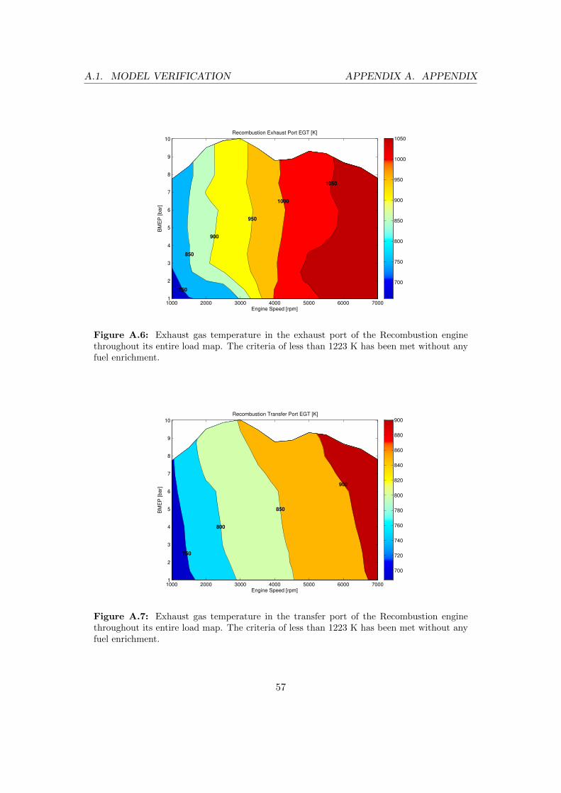
A.1. MODEL VERIFICATION APPENDIX A. APPENDIX
Engine Speed [rpm]
BM
EP
[b
ar]
Recombustion Exhaust Port EGT [K]
750
850
900
950
1000
1050
1000 2000 3000 4000 5000 6000 70001
2
3
4
5
6
7
8
9
10
700
750
800
850
900
950
1000
1050
Figure A.6: Exhaust gas temperature in the exhaust port of the Recombustion enginethroughout its entire load map. The criteria of less than 1223 K has been met without anyfuel enrichment.
Engine Speed [rpm]
BM
EP
[b
ar]
Recombustion Transfer Port EGT [K]
750
800
850
900
1000 2000 3000 4000 5000 6000 70001
2
3
4
5
6
7
8
9
10
700
720
740
760
780
800
820
840
860
880
900
Figure A.7: Exhaust gas temperature in the transfer port of the Recombustion enginethroughout its entire load map. The criteria of less than 1223 K has been met without anyfuel enrichment.
57
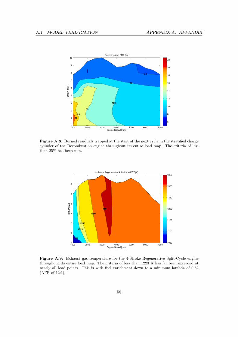
A.1. MODEL VERIFICATION APPENDIX A. APPENDIX
Engine Speed [rpm]
BM
EP
[b
ar]
Recombustion BMF [%]
20
17.5
15
12.5
10
7.5
1000 2000 3000 4000 5000 6000 70001
2
3
4
5
6
7
8
9
10
6
8
10
12
14
16
18
20
22
Figure A.8: Burned residuals trapped at the start of the next cycle in the stratified chargecylinder of the Recombustion engine throughout its entire load map. The criteria of lessthan 25% has been met.
Engine Speed [rpm]
BM
EP
[b
ar]
4−Stroke Regenerative Split−Cycle EGT [K]
1150
1223
1250
1300
1350
1000 2000 3000 4000 5000 6000 70001
2
3
4
5
6
7
1050
1100
1150
1200
1250
1300
1350
Figure A.9: Exhaust gas temperature for the 4-Stroke Regenerative Split-Cycle enginethroughout its entire load map. The criteria of less than 1223 K has far been exceeded atnearly all load points. This is with fuel enrichment down to a minimum lambda of 0.82(AFR of 12:1).
58
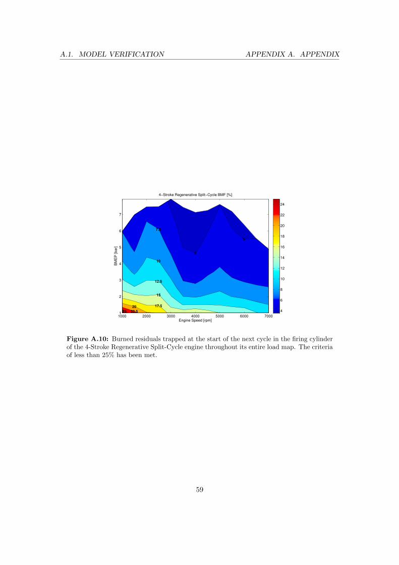
A.1. MODEL VERIFICATION APPENDIX A. APPENDIX
Engine Speed [rpm]
BM
EP
[b
ar]
4−Stroke Regenerative Split−Cycle BMF [%]
25 22.5
20 17.5
15
12.5
10
7.5
5
5
1000 2000 3000 4000 5000 6000 70001
2
3
4
5
6
7
4
6
8
10
12
14
16
18
20
22
24
Figure A.10: Burned residuals trapped at the start of the next cycle in the firing cylinderof the 4-Stroke Regenerative Split-Cycle engine throughout its entire load map. The criteriaof less than 25% has been met.
59