MAT 295: Calculus I — Course Overview Fall 2018

Limits

Definition

• limx→a

f (x): Means what happens to the values of f (x) when x is ‘close’ to a. So limx→a

f (x) = L

means that when x is ‘close’ to a, the values of f (x) are ‘close’ to L.

But there are also left/right limits.

• limx→a−

f (x): Means what happens to the values of f (x) when x is ‘close’ to a but ‘from the left’,

i.e. x is always less than a. So limx→a−

f (x) = L means that when x is ‘close’ to a on the left, the

values of f (x) are ‘close’ to L.

• limx→a+

f (x): Means what happens to the values of f (x) when x is ‘close’ to a but ‘from the

right’, i.e. x is always greater than a. So limx→a+

f (x) = L means that when x is ‘close’ to a on

the right, the values of f (x) are ‘close’ to L.

Because limx→a

f (x) = L means that when x is ‘close’ to a, no matter x is to the left or right of a,

the values of f (x) are ‘close’ to L, this implies if limx→a

f (x) = L, then limx→a−

f (x) = limx→a+

f (x) = L and

that if limx→a−

f (x) = limx→a+

f (x) = L then limx→a

f (x) = L.

Graphical Limits

We can compute limits graphically.

Example. Use the graph of f (x) below to evaluate the following:

−6 −4 −2 2 4 6

−6

−4

−2

2

4

6

x

y

1 of 21

(a) limx→−2−

f (x) = 3

(b) limx→−2+

f (x) = 2

(c) limx→−2

f (x) = D.N.E

(d) f (−2) = 3

(e) limx→1−

f (x) = 2

(f) limx→1+

f (x) = 2

(g) limx→1

f (x) = 2

(h) f (1) = 0

Computing Limits

We also compute limits algebraically, using a number of tricks:

• Plug-in: If one can ‘plug-in’ the limiting value, then the limit is that value (since the functionswe give you are often continuous).

Example. limx→0

sin xx + 1

=sin00+ 1

=01= 0

Example. limx→1

x2 + 2x + 1x − 3

=1+ 2+ 1−2

=4−2= −2

Example. limx→2+

x2 + 3x − 2

=4+ 3+0

=∞

• Expanding/Factoring/Combining: When one obtains00

, often expanding or factoring will can-

cel the terms causing the ‘problem.’ [Note: When allowed, one could use l’Hôpital’s rule, seethat section.]

Example. limx→0

(3+ x)2 − 9x

= limx→0

(x2 + 6x + 9)− 9x

= limx→0

x2 + 6xx

= limx→0(x + 6) = 6

Example. limx→1

x2 + 3x − 4x2 − 5x + 4

= limx→1

(x + 4)����(x − 1)(x − 4)����(x − 1)

= limx→1

x + 4x − 4

= −53

Example. limx→5

15−

1x

5− x= lim

x→5

x − 55x

5− x= lim

x→5

x − 5(5− x)(5x)

= limx→5

���x − 5−����(x − 5)(5x)

= limx→5

−15x= −

125

• Conjugate: When doing limits involving roots, often multiplication by 1 using the conjugateis the trick, i.e. change the sign on the radical or constant and multiply by 1 using this form.

Example. limx→0

px − 3

x − 9·p

x + 3p

x + 3= lim

x→0

���x − 9

����(x − 9)(p

x + 3)= lim

x→9

1p

x + 3=

16

Example. limh→0

3−p

h+ 9h

·3+p

h+ 9

3+p

h+ 9= lim

h→0

−�h

�h(3+p

h+ 9)= lim

h→0

−1

3+p

h+ 9= −

16

• Multiplication by One: In special limits, one can multiply by 1 in a special form (possible usingan identity, such as sin2 x + cos2 x = 1) to compute the limit.

2 of 21

Example.

limx→0

sin2 xcos x − 1

·cos x + 1cos x + 1

= limx→0

sin2(cos x + 1)cos2 x − 1

= limx→0

���sin2 x(cos x + 1)−���sin2 x

= limx→0−(cos x+1) = −2

• Absolute Value Limits: When computing limits with absolute values, often the trick is writingout the definition of the argument.

Example. limx→8−

|x − 8|x − 8

|x − 8|x − 8

=

x − 8x − 8

= 1, x > 8

−(x − 8)x − 8

= −1, x < 8

Therefore, limx→8−

|x − 8|x − 8

= limx→8−

(−1) = −1.

Example. limx→2

x − 2|x − 2

x − 2|x − 2|

=

x − 2x − 2

= 1, x > 2

−(x − 2)x − 2

= −1, x < 2

limx→2+

x − 2|x − 2|

= limx→2+

1= 1

limx→2−

x − 2|x − 2|

= limx→2−

(−1) = −1

Since limx→2+

x − 2|x − 2|

6= limx→2−

x − 2|x − 2|

, limx→2

x − 2|x − 2

D.N.E..

• Special Limits: Some limits could involve previously memorized limits along with multiplica-tion by one. The three most common special memorized limits are

limx→0

sin xx= 1 lim

x→0

1− cos xx

= 0 limx→∞

�

1+1x

�x

= e

Example. limx→0

sin(4x)x

= limx→0

sin(4x)x

·44= lim

x→0

sin(4x)4x

· 4= 1 · 4= 4

Example. limx→0

sin(3x)sin(5x)

·xx= lim

x→0

sin(3x)x

·x

sin(5x)= lim

x→0

sin(3x)3x

·5x

sin(5x)·

35= 1 · 1 ·

35=

35

Example.

limx→0

4xtan(6x)

= limx→0

4xsin6xcos 6x

= limx→0

4xsin6x

· cos6x = limx→0

6xsin6x

·16· 4cos 6x = 1 ·

16· 4=

23

Example.

limx→∞

�

1−2x

�3x

= limx→∞

1+1x−2

3x

= limx→∞

1+1x−2

x−2 ·(−2)·3

=

lim

x→∞

1+1x−2

x−2

−6

= e−6

3 of 21

• Squeeze Theorem: If g(x)≤ f (x)≤ h(x) and limx→a

g(x) = limx→a

h(x) = L, then limx→a

f (x) = L.

Example. Find limx→0

x sin�

1x

�

.

We know that −1≤ sin y ≤ 1, but then −1≤ sin�

1x

�

≤ 1. Then −x ≤ x sin�

1x

�

≤ x . Notice

that limx→0(−x) = lim

x→0x = 0. Therefore by Squeeze Theorem, lim

x→0x sin

�

1x

�

= 0.

Example. If 3≤ f (x)≤ x2 − 2x + 3 for all x , what is limx→2

f (x)?

We know that limx→2

3 = 3 and limx→2(x2 − 2x + 3) = (4 − 4 + 3) = 3. Therefore by Squeeze

Theorem, limx→2

f (x) = 3.

Limits with Infinity

• limx→∞

f (x): Means what happens to the values of f (x) when x gets larger and larger. So

limx→∞

f (x) = L means that when x is ‘very large’, the values of f (x) are ‘close’ to L. Similarly,

limx→−∞

f (x) = L means that when x is ‘very negative’, the values of f (x) are ‘close’ to L.

Again, we can do this graphically.

Example.

−4 −2 2 4

−10

−8

−6

−4

−2

2

4

6

8

10

x

y

(a) limx→−2−

f (x) = −∞

(b) limx→−2+

f (x) =∞

(c) limx→−2

f (x) = D.N.E

(d) limx→1−

f (x) =∞4 of 21

(e) limx→1+

f (x) =∞

(f) limx→1

f (x) =∞

(g) limx→−∞

= 1

(h) limx→∞

f (x) = −∞

We also compute these algebraically.

Example. limx→∞

(x2 + 3) =∞

Example. limx→−∞

ex = limx→∞

e−x = limx→∞

1ex= 0

There are special tricks with rational limits at infinity, i.e. limits at infinity of polynomials over

polynomials, or functions that are ‘close’ to being rational. For these, you multiply by1/xdeg den

1/xdeg den.

[Note: Often one can use l’Hôpital’s with these, but one would have to use it many times. For oneswith roots, l’Hôpital’s rule will often fail because it ‘loops.’]

Example. limx→∞

x2 + 2x + 13x2 − x + 5

·1/x2

1/x2= lim

x→∞

1+2x+

1x2

3−1x+

5x2

=1+ 0+ 03− 0+ 0

=13

Example. limx→∞

x4 − 2x + 1−2x5 + 3x4 + 5

·1/x5

1/x5= lim

x→∞

1x−

2x4+

1x5

−2+3x+

5x5

=0− 0+ 0−2+ 0+ 0

= 0

Example.

limx→∞

x + 1p

2x + 1= lim

x→∞

x + 1p

2x + 1·

1/p

x1/p

x

= limx→∞

px + 1/

px

p2x + 1p

x

= limx→∞

px + 1/

px

s

2x + 1x

= limx→∞

px + 1/

px

2+ 1/x=∞

5 of 21

Example.

limx→∞

x2 + 2x + 2p

x6 + 4x2 + 1= lim

x→∞

x2 + 2x + 2p

x6 + 4x2 + 1·

1/x3

1/x3

= limx→∞

1x+

2x2+

2x3

p

x6 + 4x2 + 1x3

= limx→∞

1/x + 2/x2 + 2/x3

√

√ x6 + 4x2 + 1x6

= limx→∞

1/x + 2/x2 + 2/x3

p

1+ 4/x4 + 1/x6

=0+ 0+ 0p

1+ 0+ 0= 0

These infinite limits are also used to find horizontal asymptotes. If limx→∞

f (x) = L, then f (x)has horizontal asymptote y = L and if lim

x→−∞f (x) = L, then f (x) has horizontal asymptote y = L.

To find vertical asymptotes, look for where the function has an infinite limit. Usually this is wherethe denominator is 0—so long as the number is not also zero for otherwise this may be a removablediscontinuity.

Example. Find the horizontal and vertical asymptotes of the curve given by f (x) =x2 − 4

x2 + x − 6.

For horizontal asymptotes, we look at limx→∞

f (x) and limx→−∞

f (x).

limx→∞

x2 − 4x2 + x − 6

·1/x2

1/x2= lim

x→∞

1−4x2

1+1x−

6x2

=1− 0

1+ 0− 0= 1

limx→−∞

x2 − 4x2 + x − 6

·1/x2

1/x2= lim

x→−∞

1−4x2

1+1x−

6x2

=1− 0

1+ 0− 0= 1

So y = 1 is a horizontal asymptote. For vertical asymptotes, we look for values where the denomi-nator is 0 but the numerator is not.

x2 − 4x2 + x − 6

=����(x − 2)(x + 2)(x + 3)����(x − 2)

=x + 2x + 3

so that we have

limx→−3+

x2 − 4x2 + x − 6

= limx→−3+

x + 2x + 3

=∞

limx→−3−

x2 − 4x2 + x − 6

= limx→−3−

x + 2x + 3

= −∞

so that x = −3 is a vertical asymptote (but x = 2 is not).

6 of 21

Continuity

• We say that f (x) is continuous at x = a if f (a) = limx→a

f (x). This says two important things

(that one has to check):

(i) f (x) is defined at a (because we can plug in x = a)

(ii) limx→a

f (x) exists, which means limx→a+

f (x) and limx→a−

f (x) exist and are equal.

• Constant functions, polynomials, exponential functions, and sin/ cos are all continuous. Sumsand products of continuous functions are continuous, and so are quotients of continuous func-tions continuous (wherever they are defined).

Example. Let a be constant, and define

f (x) =

(

x + a, x ≤ 0sin x

x, x > 0

What values of a make the function f (x) continuous at all x-values?

The function x+a is continuous for all values of a because it is a polynomial. The functionsin x

xis continuous for x > 0 because it is a quotient of continuous functions and is defined for x > 0. Sof (x) is continuous for all values of x except for perhaps x = 0. But

f (0) = 0+ a = a

limx→0+

f (x) = limx→0+

sin xx= 1

limx→0−

f (x) = limx→0−

(x + a) = 0+ a = a

For f (x) to be continuous at x = 0, we need f (0) = limx→0+

f (x) = limx→0−

f (x). But then a = 1= a. So

we must have a = 1.

Intermediate Value Theorem

• Intermediate Value Theorem (IVT): If f (x) is continuous on [a, b] and M is a number betweenf (a) and f (b), then there is a c ∈ [a, b] such that f (c) = M .

• This can be used to show a function has a root, because if f (x) is continuous and f (a) > 0while f (b)< 0 (or vice versa) then f (x) has a zero between x = a and x = b.

• One only really needs to know to use this to find roots of a function. Why? If one wants to useIVT to prove that f (x) = g(x) has a solution, you can just use IVT to show that f (x)− g(x)has a root, say x = c, since then f (c)− g(c) = 0 which means f (c) = g(c).

1. Explain why f (x) is continuous.

2. Find values where f (x)> 0 and f (x)< 0.

3. Explain how IVT applies.

7 of 21

Example. Show that x5 − 2x3 − 2= 0 has a root between x = 0 and x = 2.

We know that f (x) = x5 − 2x3 − 2 is continuous because it is a polynomial. Observe thatf (0) = −2 < 0 and f (2) = 14 > 0. Therefore by IVT, there is a c ∈ [0,2] so that f (c) = 0, i.e.c5 − 2c3 − 2= 0; that is, f (x) has a root between x = 0 and x = 2.

Differentiability

• f ′(a) gives the rate of change of f (x) at x = a. The function f ′(x) gives the rate of changeof f (x) at various values x . Also, f ′(a) is the slope of the tangent line of f (x) at x = a.

• If f ′(x) > 0, then f (x) is increasing; if f ′(x) < 0, then f (x) is decreasing. But if f ′(x) = 0,then f (x) is neither increasing nor decreasing.

• Values x where f ′(x) = 0 are called critical values for f (x).

• The second derivative is denoted f ′′(x) ord2 fd x2

and is the derivative of the derivative. Higher

derivatives are defined and denoted similarly.

• f ′′(x) gives the concavity of f (x). If f ′′(x) > 0 then the function is concave up, while iff ′′(x) < 0 then f (x) is concave down. If f ′′(c) = 0 and f ′′ ‘changes sign’ at x = c, then(c, f (c)) is a point of inflection for f (x).

Derivative Definition

• The derivative is defined as

f ′(a) := limh→0

f (a+ h)− f (a)h

f ′(x) := limh→0

f (x + h)− f (x)h

• Note that f ′(x) can also be denoted as Dx f .

• If a function is differentiable, then it is continuous. But if a function is continuous, then itis not necessarily differentiable. For example, f (x) = |x | is continuous but not differentiable

at x = 0. An extreme example is f (x) =∞∑

k=1

sin(πk2 x)πk2

(the Weierstrass function), which is

everywhere continuous but nowhere differentiable.

Example. Use the limit definition of f ′(a) to compute f ′(1), where f (x) = x2 + 3x .

8 of 21

We know f (1) = 1+ 3= 4 so that

f ′(1) := limh→0

[(1+ h)2 + 3(1+ h)]− 4h

= limh→0

h2 + 5h+ 4− 4h

= limh→0

h2 + 5hh

= limh→0(h+ 5) = 5

Example. Use the limit definition to find the derivative of f (x) = x2 + 3x − 2.

f ′(x) := limh→0

[(x + h)2 + 3(x + h)− 2]− (x2 + 3x − 2)h

:= limh→0

x2 + 2hx + h2 + 3x + 3h− 2− x2 − 3x + 2h

:= limh→0

2hx + h2 + 3hh

:= limh→0(2x + h+ 3) = 2x + 3

Graphical Derivatives

You should also know how to use graphical information about f ′(x) to make inferences about thefunction f (x).

Example. The graph of f ′(x) for some function f (x) is plotted in the figure below. Based on thisgraph, complete the questions below.

−4 −2 2 4 6

−10

−8

−6

−4

−2

2

4

6

8

10

f ′(x)

x

y

9 of 21

(a) Find all the intervals on which f (x) is increasing: f (x) is increasing when f ′(x) > 0, so f (x)is increasing on (−∞,−4)∪ (5,∞).

(b) Find all the intervals on which f (x) is decreasing: f (x) is decreasing when f ′(x)< 0, so f (x)is decreasing on (−4,2)∪ (2, 5).

(c) Find all critical points for f (x). Using the First or Second Derivative Test, classify these x-valuesas locations of maximums, minimums, or neither.

+ − − +

−4 2 5f ′

The critical values are where f ′(x) = 0. We then classify these using the First Derivative Test.Therefore, x = −4 is a maxima, x = 5 is a minimum, and x = 2 is neither.

(d) Find the intervals on which f (x) is concave down (or concave): f (x) is concave down whenf ′′(x) < 0, but then f ′(x) is decreasing. Therefore, f (x) is concave down on (−∞,−1.5) ∪(2,4.2).

(e) Find the intervals on which f (x) is concave up (or convex): f (x) is concave up when f ′′(x)> 0,but then f ′(x) is increasing. Therefore, f (x) is concave down on (−1.5,2)∪ (4.2,∞)

(f) Find the x-values of any points of inflection on f (x): f (x) has a point of inflection whenf ′′(x) = 0 and changes sign. But then f ′(x) has a maximum or minimum. Therefore, x = −1.5,x = 2, and x = 4.2 are the values.

Derivative Rules & Computing Derivatives

There are a number of derivatives you should have memorized:

(a)d

d xconstant= 0

(b)d

d xxn = nxn−1

(c)d

d xsin x = cos x

(d)d

d xcos x = − sin x

(e)d

d xtan x = sec2 x

(f)d

d xsec x = sec x tan x

(g)d

d xcot x = − csc2 x

(h)d

d xcsc x = − csc x cot x

(i)d

d xex = ex

(j)d

d xax = ax ln a

(k)d

d xln x =

1x

(l)d

d xlogb x =

1x ln b

(m)d

d xarctan x =

11+ x2

(n)d

d xarcsin x =

1p

1− x2

(o)d

d xarccos x =

−1p

1− x2

10 of 21

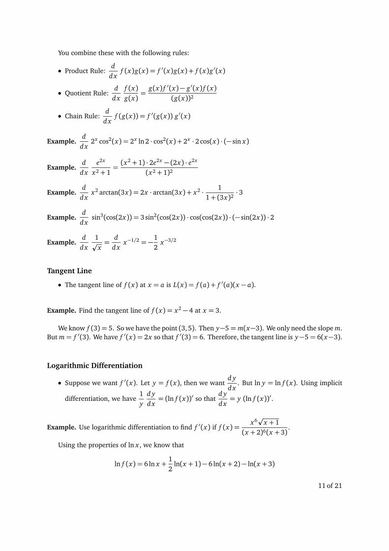
You combine these with the following rules:

• Product Rule:d

d xf (x)g(x) = f ′(x)g(x) + f (x)g ′(x)

• Quotient Rule:d

d xf (x)g(x)

=g(x) f ′(x)− g ′(x) f (x)

(g(x))2

• Chain Rule:d

d xf (g(x)) = f ′(g(x)) g ′(x)

Example.d

d x2x cos2(x) = 2x ln 2 · cos2(x) + 2x · 2 cos(x) · (− sin x)

Example.d

d xe2x

x2 + 1=(x2 + 1) · 2e2x − (2x) · e2x

(x2 + 1)2

Example.d

d xx2 arctan(3x) = 2x · arctan(3x) + x2 ·

11+ (3x)2

· 3

Example.d

d xsin3(cos(2x)) = 3sin2(cos(2x)) · cos(cos(2x)) · (− sin(2x)) · 2

Example.d

d x1p

x=

dd x

x−1/2 = −12

x−3/2

Tangent Line

• The tangent line of f (x) at x = a is L(x) = f (a) + f ′(a)(x − a).

Example. Find the tangent line of f (x) = x2 − 4 at x = 3.

We know f (3) = 5. So we have the point (3,5). Then y−5= m(x−3). We only need the slope m.But m= f ′(3). We have f ′(x) = 2x so that f ′(3) = 6. Therefore, the tangent line is y−5= 6(x−3).

Logarithmic Differentiation

• Suppose we want f ′(x). Let y = f (x), then we wantd yd x

. But ln y = ln f (x). Using implicit

differentiation, we have1y

d yd x= (ln f (x))′ so that

d yd x= y (ln f (x))′.

Example. Use logarithmic differentiation to find f ′(x) if f (x) =x6px + 1

(x + 2)6(x + 3).

Using the properties of ln x , we know that

ln f (x) = 6 ln x +12

ln(x + 1)− 6 ln(x + 2)− ln(x + 3)

11 of 21

But then

dd x

ln f (x) =d

d x

�

6 ln x +12

ln(x + 1)− 6 ln(x + 2)− ln(x + 3)�

1f (x)

f ′(x) =6x+

12(x + 1)

−6

x + 2−

1x + 3

f ′(x) = f (x)�

6x+

12(x + 1)

−6

x + 2−

1x + 3

�

f ′(x) =x6px + 1

(x + 2)6(x + 3)

�

6x+

12(x + 1)

−6

x + 2−

1x + 3

�

Special Derivatives

• To compute derivatives of functions like f (x)g(x), e.g. x sin x , you need logarithmic differenti-ation.

Example.d

d xx sin x

Let y = x sin x . Then

y = x sin x

ln y = ln x sin x

ln y = sin x ln xd

d xln y =

dd x

sin x ln x

1y

d yd x= cos x ln x +

sin xx

d yd x= y

�

cos x ln x +sin x

x

�

d yd x= x sin x

�

cos x ln x +sin x

x

�

One can also memorize that derivatives of f (x)g(x) are like power and exponential rules forderivatives combined, i.e. take their sum:

dd x

f (x)g(x) = g(x) f (x)g(x)−1 · f ′(x)︸ ︷︷ ︸

‘Power Rule’

+ f (x)g(x) ln f (x) · g ′(x)︸ ︷︷ ︸

‘Exponential Rule’

Example.d

d x(tan x)2x = 2x(tan x)2x−1 · sec2 x + (tan x)2x ln(tan x) · 2

Finding Max/Mins on Intervals

• Find and classify the critical values for f (x). Ignore those that are not in the interval you areconsidering. Evaluate f (x) at the endpoints. Then compare the values at the endpoints withthe max/mins you found before.

12 of 21

Example. Find the absolute maximum and minimum of the function f (x) = 3t2 − 2t + 1 on theinterval [−2,2].

We have g(t) = 3t2−2t+1 and g ′(t) = 6t−2. Setting 6t−2= 0, we see the only critical valueis t = 1

3 .

g ′(t)13

− +

so that t = 1/3 is a minimum. Now g(−2) = 17, g(2) = 9, g(1/3) = 2/3. Therefore, the absoluteminimum is 2/3 and occurs at x = 1/3, and the absolute maximum is 17 and occurs at x = −2.

Linear Approximation

• The linearization of f (x) at x = a is simply the tangent line of f (x) at x = a, i.e. thelinearization L (x) for f (x) at x = a is L (x) := f (a) + f ′(a)(x − a). This can be used toapproximate the values of f (x) ‘near’ x = a.

Example. Find the linearization of f (x) =p

x at x = 82 and use this to approximate the value ofp85.

We have f (x) =p

x so f (81) =p

81= 9. We know also f ′(x) =1

2p

xso that f ′(81) =

1

2p

81=

118

. Then we have L (x) = f (81) + f ′(81)(x − 81) = 9+118(x − 81).

To approximatep

82, note that 82 is ‘close’ to 81. Then we have

p82= f (82)≈L (82) = 9+

118(82− 81) = 9+

118=

16318≈ 9.0556.

Implicit Differentiation

• Implicit differentiation works ‘the same’ as normal differentiation, except when computing

things liked

d xy , one needs to ‘tack on’ a

d yd x

term.

Example. Given y2 = x3 + 3x2 − 24x , findd yd x

.

y2 = x3 + 3x2 − 24xd

d xy2 =

dd x

�

x3 + 3x2 − 24x�

2yd yd x= 3x2 + 6x − 24

d yd x=

3x2 + 6x − 242y

13 of 21

Example. Findd yd x

given sin(x y) = 4.

sin(x y) = 4

dd x

sin(x y) =d

d x4

cos(x y)�

y + xd yd x

�

= 0

d yd x= −

yx

Example. Find the tangent line to the curve y4 = y2 − x2 at the point (p

3/4, 1/2).

y −12= m

�

x −p

34

�

dd x

y4 =d

d x(y2 − x2)

4y3 d yd x= 2y

d yd x− 2x

But we have x =p

34

, y =12

so

4�

12

�3 d yd x= 2

�

12

�

d yd x− 2

�p3

4

�

12

d yd x=

d yd x−p

32

d yd x=p

3

y −12=p

3

�

x −p

34

�

Related Rates

• This is an application of implicit differentiation.

1. Draw a picture.

2. Write down the desired quantity.

3. Write down all the knowns.

4. Write down an equation, call this (*), which relates the quantities of interest. [Plug in any valueswhich are always constant.]

5. Implicit differentiate, plug in the known values, and solve.

Example. When the angle of the camera with the ground is π3 and the observer increases this angleat a rate of 1

5 rad/min to keep the ballon centered in the frame. What rate is the balloon rising atthat moment?

14 of 21

θ

d

h

θ =π

3dθd t=

15

d = 200

Want:dhd t

tanθ =hd

tanθ =h

200dd t

tanθ =dd t

h200

sec2 θ ·dθd t=

1200

dhd t

dhd t= 200 sec2 θ

dθd t

dhd t= 200(sec(π/3))2 ·

15

dhd t= 200 · (2)2 ·

15

dhd t= 200 · 4 ·

15

dhd t= 160 ft/min

Example. A conical tank (with the tip at the floor) is 4 ft across at the top and 3 ft tall. If the tank is

being filled with water at a rate of8

27ft3/min, what is the rate of change of the depth of the water

when the tank is filled to a depth of 1 ft?

V =13πr2h

h

r

2

Want:dhd t

rh=

23⇒ r =

23

h and if h=14⇒ r =

23·

14=

16

15 of 21

V =13πr2h

V =13π

�

23

h�2

h

V =4π27

h3

dd t

V =dd t

4π27

h3

dVd t=

4π9

h2 dhd t

827=

4π9· 12 ·

dhd t

dhd t=

827·

94π

dhd t=

23π

ft3/min

Optimization

• This is an application of finding max/mins (on intervals).

1. Draw a picture.

2. Write down what you want to optimize and any constraint equations.

3. Write down your known values.

4. Use your constraint equation to get your optimization equation into one variable.

5. Maximize or minimize this new equation using derivative methods.

Example. A rectangular box has a square bottom and an open top. If only 2,700 cm2 of material isavailable to construct the box, what dimensions maximize the volume of the box? Be sure to drawa picture and justify completely that these dimensions are optimal.

s

s

h

Maximize V = lwh

Constraint 2700= Surface Area= 4sh+ s2

We want to optimize V = lwh= s · s · h= s2h. But we know that

Surface Area= 2,700 cm2

Surface Area= 4sh+ s2

16 of 21

But then we have

4sh+ s2 = 2700

4sh= 2700− s2

h=2700− s2

4s

But then V = s2h = s2

�

2700− s2

4s

�

=2700s− s3

4. Clearly, s ∈ [0,

p2700], where in each case the

box has V = 0. We have V ′ =2700− 3s2

4. Now setting V ′ = 0, we have

2700− 3s2

4= 0

2700− 3s2 = 0

3s2 = 2700

s2 = 900

s = ±p

900= ±p

9 · 100

s = ±30

But then we must have s = 30 cm2. Then h =2700− 900

120=

800120

= 15. The dimensions then are

30× 30× 15. We confirm this is a maximum,

V ′(s)30

+ −

Mean Value Theorem

• Mean Value Theorem (MVT): If f (x) is continuous on [a, b] and differentiable on (a, b), thenthere is c ∈ (a, b) so that f (b)− f (a) = f ′(c)(b− a).

Example. Verify that f (x) = x3 + x − 1 satisfies the hypotheses of the Mean Value Theorem on[0, 3]. Find all numbers c satisfying the conclusions of the Mean Value Theorem on this interval.

Observe f (x) = x3 + x − 1 is continuous on [0,3]. Because f ′(x) = 3x2 + 1 is defined on[0, 3], f (x) is differentiable on (0,3). By the Mean Value Theorem, there exists c ∈ (0,3) such thatf (3)− f (0) = f ′(c)(3− 0). But then we have

f (3)− f (0) = f ′(c)(3− 0)

29− (−1) = 3(3c2 + 1)

30= 3(3c2 + 1)

10= 3c2 + 1

9= 3c2

c2 = 3

c = ±p

317 of 21

Therefore, c =p

3 satisfies the hypothesis of the Mean Value Theorem on [0, 3].

Example. Use the Mean Value Theorem to prove that if f ′(x) = 0 for all x ∈ [a, b], then f (x) isconstant on [a, b]. [Hint: Show f (x0) = f (a) for all a ≤ x0 ≤ b.]

Since f ′(x) exists on [a, b], f (x) is differentiable (hence continuous) on [a, b]. Therefore, f (x)satisfies the Mean Value Theorem on [a, x0] for any x0 ≤ b. Then by the Mean Value Theorem,f (x0)− f (a) = f ′(c)(x0 − a) for some c ∈ [a, x0]. But f ′(x) = 0 for all x ∈ [a, b]. Therefore,

f (x0)− f (a) = f ′(c)(x0 − a)

f (x0)− f (a) = 0

f (x0) = f (a)

This shows f (x) = f (a) for all x ∈ [a, b]. But then f (x) is constant on [a, b].

l’Hôpital’s Rule

• l’Hôpital’s Rule: If limx→a

f (x)g(x)

is an indeterminate form, and limx→a

f ′(x)g ′(x)

exists, then limx→a

f (x)g(x)

=

limx→a

f ′(x)g ′(x)

.

• This is used to calculate limits of indeterminate forms, i.e.00

, ±∞∞

, 0 ·∞,∞−∞, 1∞, 00,

∞0. Each one is handled differently.

(i)00

, ±∞∞

: Handled ‘normally.’

(ii) 0 ·∞: Move either the 0 or ∞ term into the denominator to obtain one of the aboveforms.

(iii) ∞−∞: Combine terms or factor out something to obtain one of the forms above.

(iv) 0·∞,∞−∞, 1∞, 00,∞0: Use logarithms, i.e. set L = lim f (x)g(x), take logs to obtainlim g(x) ln f (x). Then compute this limit, which is now one of the above indeterminateforms above. If this limit is W , then the original limit is eW .

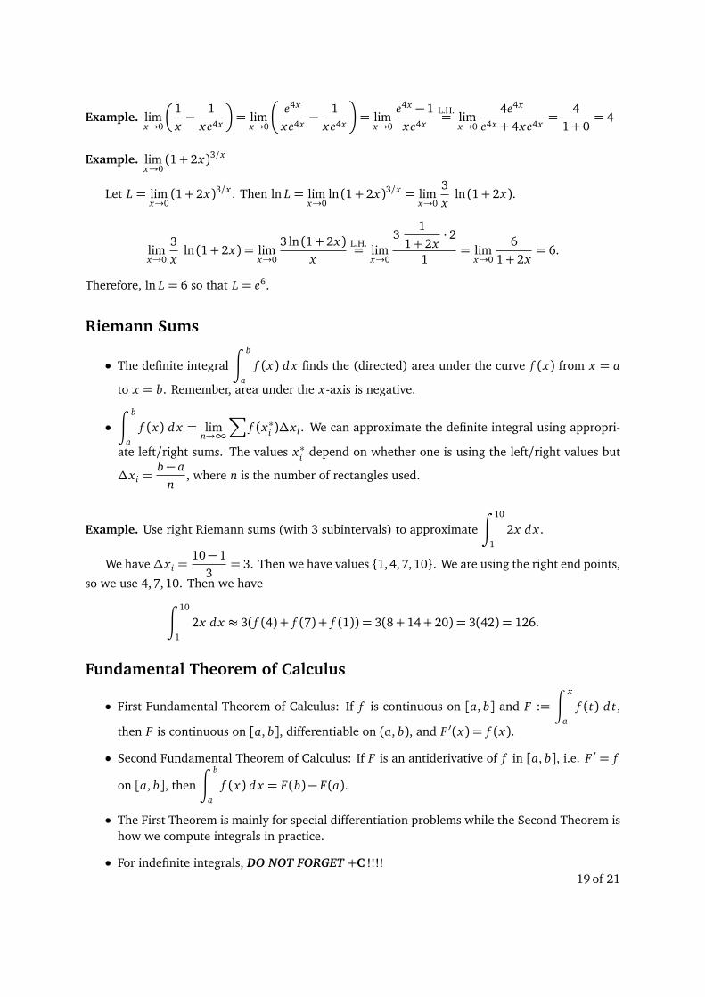
Example. limx→0

ex − 1− xx2

L.H.= lim

x→0

ex − 12x

L.H.= lim

x→0

ex

2=

12

Example.

limx→∞

ln(1+ e6x)5x

L.H.= lim

x→∞

11+ e6x

· 6e6x

5= lim

x→∞

6e6x

5(1+ e6x)L.H.= lim

x→∞

36e6x

5(6e6x)= lim

x→∞

365(6)

=65

Example. limx→0+

3px ln x = limx→0+

ln xx−1/3

L.H.= lim

x→0+

1x

−13

x−4/3= lim

x→0+−

3x4/3

x= lim

x→0+−3x1/3 = 0

18 of 21

Example. limx→0

�

1x−

1xe4x

�

= limx→0

�

e4x

xe4x−

1xe4x

�

= limx→0

e4x − 1xe4x

L.H.= lim

x→0

4e4x

e4x + 4xe4x=

41+ 0

= 4

Example. limx→0(1+ 2x)3/x

Let L = limx→0(1+ 2x)3/x . Then ln L = lim

x→0ln (1+ 2x)3/x = lim

x→0

3x

ln (1+ 2x).

limx→0

3x

ln (1+ 2x) = limx→0

3 ln (1+ 2x)x

L.H.= lim

x→0

31

1+ 2x· 2

1= lim

x→0

61+ 2x

= 6.

Therefore, ln L = 6 so that L = e6.

Riemann Sums

• The definite integral

∫ b

af (x) d x finds the (directed) area under the curve f (x) from x = a

to x = b. Remember, area under the x-axis is negative.

•∫ b

af (x) d x = lim

n→∞

∑

f (x∗i )∆x i . We can approximate the definite integral using appropri-

ate left/right sums. The values x∗i depend on whether one is using the left/right values but

∆x i =b− a

n, where n is the number of rectangles used.

Example. Use right Riemann sums (with 3 subintervals) to approximate

∫ 10

1

2x d x .

We have∆x i =10− 1

3= 3. Then we have values {1,4, 7,10}. We are using the right end points,

so we use 4,7, 10. Then we have

∫ 10

1

2x d x ≈ 3( f (4) + f (7) + f (1)) = 3(8+ 14+ 20) = 3(42) = 126.

Fundamental Theorem of Calculus

• First Fundamental Theorem of Calculus: If f is continuous on [a, b] and F :=

∫ x

af (t) d t,

then F is continuous on [a, b], differentiable on (a, b), and F ′(x) = f (x).

• Second Fundamental Theorem of Calculus: If F is an antiderivative of f in [a, b], i.e. F ′ = f

on [a, b], then

∫ b

af (x) d x = F(b)− F(a).

• The First Theorem is mainly for special differentiation problems while the Second Theorem ishow we compute integrals in practice.

• For indefinite integrals, DO NOT FORGET +C !!!!19 of 21

• For all intents and purposes, antiderivative = integral.

Example.d

d x

∫ 2x

2

sin(t2) d t = sin[(2x)2] · 2

Example.d

d x

∫ 1

x1/2

t(2+ t2)1/2 d t = −d

d x

∫ x1/2

1

t(2+ t2)1/2 d t = −x1/2(2+ (x1/2)2) ·1

2p

x

Example.

dd x

∫ 3x

2xsin2 t d t =

dd x

∫ 0

2xsin2 t d t +

dd x

∫ 3x

0

sin2 t d t

= −d

d x

∫ 2x

0

sin2 t d t +d

d x

∫ 3x

0

sin2 t d t

= − sin2(2x) · 2+ sin2(3x) · 3

Example.

∫ 1

0

(2x + 1) d x =

�

2x2

2+ x

��

�

�

�

1

0=�

x2 + x�

�

�

�

�

1

0= (1+ 1)− (0+ 0) = 1− 0= 1

Example. If f ′(x) = 2x + 1 and f (1) = 3, find f (x).

f (x) =

∫

f ′(x) d x =

∫

(2x + 1) d x =2x2

2+ x + C = x2 + x + C .

But 1= f (1) = 1+ 1+ C so that C = −1. Therefore, f (x) = x2 + x − 1.

u-Substitution

• Used to compute integrals you could not otherwise compute. Specifically, it can computeintegrals where there is a function and its derivative in the integrand.

• When compute indefinite integrals using u-sub, do not forget to go back to the original variableat the end.

• When computing definite integrals using u-sub, do not forget to change the limits of integration!

Example.

∫

ep

x

px

d x

Let u=p

x , then du=1

2p

xso that d x = 2

px du. Then

∫

ep

x

px

d x =

∫

eu

��px

2��px du= 2

∫

eu du= 2eu + C = 2ep

x + C

20 of 21

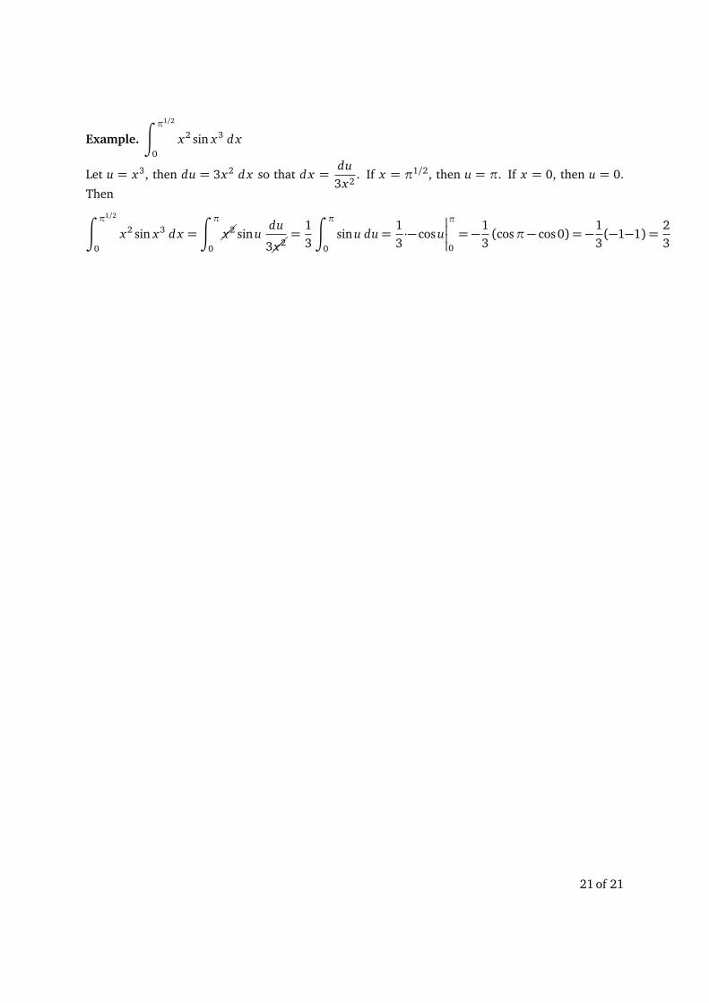
Example.

∫ π1/2

0

x2 sin x3 d x

Let u = x3, then du = 3x2 d x so that d x =du3x2

. If x = π1/2, then u = π. If x = 0, then u = 0.

Then

∫ π1/2

0

x2 sin x3 d x =

∫ π

0��x

2 sin udu

3��x2=

13

∫ π

0

sin u du=13·− cos u

�

�

�

�

π

0= −

13(cosπ− cos0) = −

13(−1−1) =

23

21 of 21