mathschoolinternational.commathschoolinternational.com/math-books/.../schaums-business-statistics... ·...
TRANSCRIPT


SCHAUM’SOUTLINE OF
Theory and Problems of
BUSINESSSTATISTICS
Fourth Edition
LEONARD J. KAZMIER
W. P. Carey School of Business
Arizona State University
Schaum’s Outline SeriesMcGRAW-HILL
New York Chicago San Francisco Lisbon
London Madrid Mexico City Milan New Delhi
San Juan Seoul Singapore Sydney Toronto

Copyright © 2004, 1996, 1988, 1976 by The McGraw-Hill Companies, Inc. All rights reserved. Manufactured in the UnitedStates of America. Except as permitted under the United States Copyright Act of 1976, no part of this publication may be repro-duced or distributed in any form or by any means, or stored in a database or retrieval system, without the prior written permis-sion of the publisher.
0-07-143099-7
The material in this eBook also appears in the print version of this title: 0-07-141080-5
All trademarks are trademarks of their respective owners. Rather than put a trademark symbol after every occurrence of atrademarked name, we use names in an editorial fashion only, and to the benefit of the trademark owner, with no intentionof infringement of the trademark. Where such designations appear in this book, they have been printed with initial caps.
McGraw-Hill eBooks are available at special quantity discounts to use as premiums and sales promotions, or for use in cor-porate training programs. For more information, please contact George Hoare, Special Sales, at [email protected] or (212) 904-4069.
TERMS OF USEThis is a copyrighted work and The McGraw-Hill Companies, Inc. (“McGraw-Hill”) and its licensors reserve all rights inand to the work. Use of this work is subject to these terms. Except as permitted under the Copyright Act of 1976 and theright to store and retrieve one copy of the work, you may not decompile, disassemble, reverse engineer, reproduce, modify,create derivative works based upon, transmit, distribute, disseminate, sell, publish or sublicense the work or any part of itwithout McGraw-Hill’s prior consent. You may use the work for your own noncommercial and personal use; any other useof the work is strictly prohibited. Your right to use the work may be terminated if you fail to comply with these terms.
THE WORK IS PROVIDED “AS IS”. McGRAW-HILL AND ITS LICENSORS MAKE NO GUARANTEES OR WAR-RANTIES AS TO THE ACCURACY, ADEQUACY OR COMPLETENESS OF OR RESULTS TO BE OBTAINED FROMUSING THE WORK, INCLUDING ANY INFORMATION THAT CAN BE ACCESSED THROUGH THE WORK VIAHYPERLINK OR OTHERWISE, AND EXPRESSLY DISCLAIM ANY WARRANTY, EXPRESS OR IMPLIED,INCLUDING BUT NOT LIMITED TO IMPLIED WARRANTIES OF MERCHANTABILITY OR FITNESS FOR A PAR-TICULAR PURPOSE. McGraw-Hill and its licensors do not warrant or guarantee that the functions contained in the workwill meet your requirements or that its operation will be uninterrupted or error free. Neither McGraw-Hill nor its licensorsshall be liable to you or anyone else for any inaccuracy, error or omission, regardless of cause, in the work or for any dam-ages resulting therefrom. McGraw-Hill has no responsibility for the content of any information accessed through the work.Under no circumstances shall McGraw-Hill and/or its licensors be liable for any indirect, incidental, special, punitive, con-sequential or similar damages that result from the use of or inability to use the work, even if any of them has been advisedof the possibility of such damages. This limitation of liability shall apply to any claim or cause whatsoever whether suchclaim or cause arises in contract, tort or otherwise.
DOI: 10.1036/0071430997

CHAPTER 7 Probability Distributions for Continuous RandomVariables: Normal and Exponential 1227.1 Continuous Random Variables 122
7.2 The Normal Probability Distribution 123
7.3 Percentile Points for Normally Distributed Variables 125
7.4 Normal Approximation of Binomial Probabilities 126
7.5 Normal Approximation of Poisson Probabilities 128
7.6 The Exponential Probability Distribution 128
7.7 Using Excel and Minitab 129
CHAPTER 8 Sampling Distributions and Confidence Intervalsfor the Mean 1428.1 Point Estimation of a Population or Process Parameter 142
8.2 The Concept of a Sampling Distribution 143
8.3 Sampling Distribution of the Mean 143
8.4 The Central Limit Theorem 145
8.5 Determining Probability Values for the Sample Mean 145
8.6 Confidence Intervals for the Mean Using the Normal
Distribution 146
8.7 Determining the Required Sample Size for Estimating the
Mean 147
8.8 The t Distribution and Confidence Intervals for the Mean 148
8.9 Summary Table for Interval Estimation of the Population
Mean 149
8.10 Using Excel and Minitab 149
CHAPTER 9 Other Confidence Intervals 1609.1 Confidence Intervals for the Difference Between Two Means
Using the Normal Distribution 160
9.2 The t Distribution and Confidence Intervals for the Difference
Between Two Means 161
9.3 Confidence Intervals for the Population Proportion 162
9.4 Determining the Required Sample Size for Estimating the
Proportion 163
9.5 Confidence Intervals for the Difference Between Two
Proportions 163
9.6 The Chi-Square Distribution and Confidence Intervals for the
Variance and Standard Deviation 164
9.7 Using Excel and Minitab 165
CHAPTER 10 Testing Hypotheses Concerning the Value of thePopulation Mean 17410.1 Introduction 174
CONTENTS ix

PREFACE
This book covers the basic methods of statistical description, statistical inference,decision analysis, and process control that are included in introductory andintermediate-level courses in business statistics.
The concepts and methods are presented in a clear and concise manner, andlengthy explanations have been minimized in favor of presenting concrete examples.Because this book has been developed particularly for those whose interest is theapplication of statistical techniques, mathematical derivations are omitted.
When used as a supplement to a course text, the numerous examples and solvedproblems will help to clarify the mathematical explanations included in such books.This Outline can also serve as an excellent reference book because the concisemanner of coverage makes it easier to find required procedures. Finally, this book iscomplete enough in its coverage that it can in fact be used as the course textbook.
This edition of the Outline has been thoroughly updated, and now includescomputer-based solutions using Excel (copyright Microsoft, Inc.), Minitab (copy-right Minitab, Inc.), and Execustat (copyright PWS-Kent Publishing Co.).
LEONARD J. KAZMIER
v


CONTENTS
CHAPTER 1 Analyzing Business Data 11.1 Definition of Business Statistics 1
1.2 Descriptive and Inferential Statistics 1
1.3 Types of Applications in Business 2
1.4 Discrete and Continuous Variables 2
1.5 Obtaining Data Through Direct Observation vs. Surveys 2
1.6 Methods of Random Sampling 3
1.7 Other Sampling Methods 4
1.8 Using Excel and Minitab to Generate Random Numbers 4
CHAPTER 2 Statistical Presentations and Graphical Displays 102.1 Frequency Distributions 10
2.2 Class Intervals 11
2.3 Histograms and Frequency Polygons 12
2.4 Frequency Curves 12
2.5 Cumulative Frequency Distributions 13
2.6 Relative Frequency Distributions 14
2.7 The ‘‘And-Under’’ Type of Frequency Distribution 15
2.8 Stem-and-Leaf Diagrams 15
2.9 Dotplots 16
2.10 Pareto Charts 16
2.11 Bar Charts and Line Graphs 16
2.12 Run Charts 18
2.13 Pie Charts 19
2.14 Using Excel and Minitab 19
CHAPTER 3 Describing Business Data: Measures of Location 44
3.1 Measures of Location in Data Sets 44
3.2 The Arithmetic Mean 44
3.3 The Weighted Mean 45
3.4 The Median 45
3.5 The Mode 46
3.6 Relationship Between the Mean and the Median 46
3.7 Mathematical Criteria Satisfied by the Median and the Mean 46
3.8 Use of the Mean, Median, and Mode 47
3.9 Use of the Mean in Statistical Process Control 48
viiCopyright 2004, 1996, 1988, 1976 by The McGraw-Hill Companies, Inc. Click Here for Terms of Use.
For more information about this title, click here.

3.10 Quartiles, Deciles, and Percentiles 48
3.11 Using Excel and Minitab 48
CHAPTER 4 Describing Business Data: Measures of Dispersion 574.1 Measures of Variability in Data Sets 57
4.2 The Range 57
4.3 Modified Ranges 58
4.4 Box Plots 58
4.5 The Mean Absolute Deviation 59
4.6 The Variance and Standard Deviation 60
4.7 Simplified Calculations for the Variance and Standard Deviation 61
4.8 The Mathematical Criterion Associated with the Variance
and Standard Deviation 62
4.9 Use of the Standard Deviation in Data Description 62
4.10 Use of the Range and Standard Deviation in Statistical Process
Control 62
4.11 The Coefficient of Variation 63
4.12 Pearson’s Coefficient of Skewness 64
4.13 Using Excel and Minitab 64
CHAPTER 5 Probability 745.1 Basic Definitions of Probability 74
5.2 Expressing Probability 75
5.3 Mutually Exclusive and Nonexclusive Events 76
5.4 The Rules of Addition 76
5.5 Independent Events, Dependent Events, and Conditional
Probability 77
5.6 The Rules of Multiplication 78
5.7 Bayes’ Theorem 80
5.8 Joint Probability Tables 81
5.9 Permutations 82
5.10 Combinations 83
CHAPTER 6 Probability Distributions for Discrete RandomVariables: Binomial, Hypergeometric, and Poission 996.1 What Is a Random Variable? 99
6.2 Describing a Discrete Random Variable 100
6.3 The Binomial Distribution 102
6.4 The Binomial Variable Expressed by Proportions 103
6.5 The Hypergeometric Distribution 104
6.6 The Poisson Distribution 104
6.7 Poisson Approximation of Binomial Probabilities 106
6.8 Using Excel and Minitab 107
viii CONTENTS
10.2 Basic Steps in Hypothesis Testing by the Critical Value
Approach 175
10.3 Testing a Hypothesis Concerning the Mean by Use of the
Normal Distribution 176
10.4 Type I and Type II Errors in Hypothesis Testing 179
10.5 Determining the Required Sample Size for Testing the Mean 181
10.6 Testing a Hypothesis Concerning the Mean by Use of the t
Distribution 182
10.7 The P-Value Approach to Testing Hypotheses Concerning
the Population Mean 182
10.8 The Confidence Interval Approach to Testing Hypotheses
Concerning the Mean 183
10.9 Testing with Respect to the Process Mean in Statistical
Process Control 184
10.10 Summary Table for Testing a Hypothesized Value of the
Mean 184
10.11 Using Excel and Minitab 185
CHAPTER 11 Testing Other Hypotheses 19711.1 Testing the Difference Between Two Means Using the
Normal Distribution 197
11.2 Testing the Difference Between Means Using the t
Distribution 199
11.3 Testing the Difference Between Means Based on Paired
Observations 200
11.4 Testing a Hypothesis Concerning the Value of the Population
Proportion 201
11.5 Determining the Required Sample Size for Testing the
Proportion 202
11.6 Testing with Respect to the Process Proportion in Statistical
Process Control 203
11.7 Testing the Difference Between Two Population Proportions 203
11.8 Testing a Hypothesized Value of the Variance Using the
Chi-Square Distribution 204
11.9 Testing with Respect to Process Variability in Statistical
Process Control 204
11.10 The F Distribution and Testing the Equality of Two
Population Variances 205
11.11 Alternative Approaches to Testing Null Hypotheses 206
11.12 Using Excel and Minitab 207
CHAPTER 12 The Chi-Square Test for the Analysis ofQualitative Data 21912.1 General Purpose of the Chi-Square Test 219
12.2 Goodness of Fit Tests 219
x CONTENTS

12.3 Tests for the Independence of Two Categorical Variables
(Contingency Table Tests) 222
12.4 Testing Hypotheses Concerning Proportions 223
12.5 Using Computer Software 226
CHAPTER 13 Analysis of Variance 24113.1 Basic Rationale Associated with Testing the Differences
Among Several Population Means 241
13.2 One-Factor Completely Randomized Design (One-Way
ANOVA) 242
13.3 Two-Way Analysis of Variance (Two-Way ANOVA) 243
13.4 The Randomized Block Design (Two-Way ANOVA, One
Observation per Cell) 243
13.5 Two-Factor Completely Randomized Design (Two-Way
ANOVA, n Observations per Cell) 244
13.6 Additional Considerations 245
13.7 Using Excel and Minitab 246
CHAPTER 14 Linear Regression and Correlation Analysis 26314.1 Objectives and Assumptions of Regression Analysis 263
14.2 The Scatter Plot 264
14.3 The Method of Least Squares for Fitting a Regression Line 265
14.4 Residuals and Residual Plots 265
14.5 The Standard Error of Estimate 266
14.6 Inferences Concerning the Slope 266
14.7 Confidence Intervals for the Conditional Mean 267
14.8 Prediction Intervals for Individual Values of the Dependent
Variable 267
14.9 Objectives and Assumptions of Correlation Analysis 268
14.10 The Coefficient of Determination 268
14.11 The Coefficient of Correlation 269
14.12 The Covariance Approach to Understanding the Correlation
Coefficient 270
14.13 Significance Testing with Respect to the Correlation
Coefficient 271
14.14 Pitfalls and Limitations Associated with Regression and
Correlation Analysis 271
14.15 Using Excel and Minitab 271
CHAPTER 15 Multiple Regression and Correlation 28315.1 Objectives and Assumptions of Multiple Regression Analysis 283
15.2 Additional Concepts in Multiple Regression Analysis 284
15.3 The Use of Indicator (Dummy) Variables 284
15.4 Residuals and Residual Plots 285
CONTENTS xi
15.5 Analysis of Variance in Linear Regression Analysis 285
15.6 Objectives and Assumptions of Multiple Correlation Analysis 287
15.7 Additional Concepts in Multiple Correlation Analysis 287
15.8 Pitfalls and Limitations Associated with Multiple Regression
and Multiple Correlation Analysis 288
15.9 Using Excel and Minitab 288
CHAPTER 16 Time Series Analysis and Business Forecasting 29616.1 The Classical Time Series Model 296
16.2 Trend Analysis 297
16.3 Analysis of Cyclical Variations 298
16.4 Measurement of Seasonal Variations 299
16.5 Applying Seasonal Adjustments 299
16.6 Forecasting Based on Trend and Seasonal Factors 300
16.7 Cyclical Forecasting and Business Indicators 301
16.8 Forecasting Based on Moving Averages 301
16.9 Exponential Smoothing as a Forecasting Method 301
16.10 Other Forecasting Methods That Incorporate Smoothing 302
16.11 Using Computer Software 303
CHAPTER 17 Nonparametric Statistics 31817.1 Scales of Measurement 318
17.2 Parametric vs. Nonparametric Statistical Methods 319
17.3 The Runs Test for Randomness 319
17.4 One Sample: The Sign Test 320
17.5 One Sample: The Wilcoxon Test 320
17.6 Two Independent Samples: The Mann–Whitney Test 321
17.7 Paired Observations: The Sign Test 322
17.8 Paired Observations: The Wilcoxon Test 322
17.9 Several Independent Samples: The Kruskal–Wallis Test 322
17.10 Using Minitab 323
CHAPTER 18 Decision Analysis: Payoff Tables and DecisionTrees 33618.1 The Structure of Payoff Tables 336
18.2 Decision Making Based upon Probabilities Alone 337
18.3 Decision Making Based upon Economic Consequences Alone 338
18.4 Decision Making Based upon Both Probabilities and
Economic Consequences: The Expected Payoff Criterion 340
18.5 Decision Tree Analysis 342
18.6 Expected Utility as the Decision Criterion 342
xii CONTENTS
CHAPTER 19 Statistical Process Control 35619.1 Total Quality Management 356
19.2 Statistical Quality Control 357
19.3 Types of Variation in Processes 358
19.4 Control Charts 358
19.5 Control Charts for the Process Mean: �XX Charts 359
19.6 Standard Tests Used for Interpreting �XX Charts 360
19.7 Control Charts for the Process Standard Deviation: s Charts 362
19.8 Control Charts for the Process Range: R Charts 362
19.9 Control Charts for the Process Proportion: p Charts 363
19.10 Using Minitab 364
APPENDIX 1 Table of Random Numbers 377
APPENDIX 2 Binomial Probabilities 378
APPENDIX 3 Values of e�l 382
APPENDIX 4 Poission Probabilities 383
APPENDIX 5 Proportions of Area for the Standard NormalDistribution 388
APPENDIX 6 Proportions of Area for the t Distribution 390
APPENDIX 7 Proportions of Area for the x2 Distribution 391
APPENDIX 8 Values of F Exceeded with Probabilities of 5%and 1% 393
APPENDIX 9 Factors for Control Charts 397
APPENDIX 10 Critical Values of T in the Wilcoxon Test 398
INDEX 401
CONTENTS xiii


CHAPTER 1
Analyzing BusinessData
1.1 DEFINITION OF BUSINESS STATISTICS
Statistics refers to the body of techniques used for collecting, organizing, analyzing, and interpreting data.
The data may be quantitative, with values expressed numerically, or they may be qualitative, with
characteristics such as consumer preferences being tabulated. Statistics is used in business to help make
better decisions by understanding the sources of variation and by uncovering patterns and relationships in
business data.
1.2 DESCRIPTIVE AND INFERENTIAL STATISTICS
Descriptive statistics include the techniques that are used to summarize and describe numerical data for the
purpose of easier interpretation. These methods can either be graphical or involve computational analysis (see
Chapters 2, 3, and 4).
EXAMPLE 1. The monthly sales volume for a product during the past year can be described and made meaningful by
preparing a bar chart or a line graph (as described in Section 2.11). The relative sales by month can be highlighted by
calculating an index number for each month such that the deviation from 100 for any given month indicates the percentage
deviation of sales in that month as compared with average monthly sales during the entire year.
Inferential statistics include those techniques by which decisions about a statistical population or process
are made based only on a sample having been observed. Because such decisions are made under conditions of
uncertainty, the use of probability concepts is required. Whereas the measured characteristics of a sample are
called sample statistics, the measured characteristics of a statistical population, or universe, are called
population parameters. The procedure by which the characteristics of all the members of a defined population
are measured is called a census. When statistical inference is used in process control, the sampling is concerned
particularly with uncovering and controlling the sources of variation in the quality of the output. Chapters 5
through 7 cover probability concepts, and most of the chapters after that are concerned with the application of
these concepts in statistical inference.
1
Copyright 2004, 1996, 1988, 1976 by The McGraw-Hill Companies, Inc. Click Here for Terms of Use.

EXAMPLE 2. In order to estimate the voltage required to cause an electrical device to fail, a sample of such devices can
be subjected to increasingly higher voltages until each device fails. Based on these sample results, the probability of failure
at various voltage levels for the other devices in the sampled population can be estimated.
1.3 TYPES OF APPLICATIONS IN BUSINESS
The methods of classical statistics were developed for the analysis of sampled (objective) data, and for the
purpose of inference about the population from which the sample was selected. There is explicit exclusion of
personal judgments about the data, and there is an implicit assumption that sampling is done from a static
(stable) population. The methods of decision analysis focus on incorporating managerial judgments into
statistical analysis (see Chapter 18). The methods of statistical process control are used with the premise that
the output of a process may not be stable. Rather, the process may be dynamic, with assignable causes
associated with variation in the quality of the output over time (see Chapter 19).
EXAMPLE 3. Using the classical approach to statistical inference, the uncertain level of sales for a new product would be
estimated on the basis of market studies done in accordance with the requirements of scientific sampling. In the decision-
analysis approach, the judgments of managers would be quantified and incorporated into the analysis. Statistical process
control would focus particularly on the pattern of sales in a sequence of time periods during test marketing of the product.
1.4 DISCRETE AND CONTINUOUS VARIABLES
A discrete variable can have observed values only at isolated points along a scale of values. In business
statistics, such data typically occur through the process of counting; hence, the values generally are expressed as
integers (whole numbers). A continuous variable can assume a value at any fractional point along a specified
interval of values. Continuous data are generated by the process of measuring.
EXAMPLE 4. Examples of discrete data are the number of persons per household, the units of an item in inventory, and
the number of assembled components that are found to be defective. Examples of continuous data are the weight of a
shipment, the length of time before the first failure of a device, and the average number of persons per household in a large
community. Note that an average number of persons can be a fractional value and is thus a continuous variable, even though
the number per household is a discrete variable.
1.5 OBTAINING DATA THROUGH DIRECT OBSERVATION VS. SURVEYS
One way data can be obtained is by direct observation. This is the basis for the actions that are taken in
statistical process control, in which samples of output are systematically assessed. Another form of direct
observation is a statistical experiment, in which there is overt control over some or all of the factors that may
influence the variable being studied, so that possible causes can be identified.
EXAMPLE 5. Two methods of assembling a component could be compared by having one group of employees use one of
the methods and a second group of employees use the other method. The members of the first group are carefully matched
to the members of the second group in terms of such factors as age and experience.
In some situations it is not possible to collect data directly but, rather, the information has to be obtained
from individual respondents. A statistical survey is the process of collecting data by asking individuals to
provide the data. The data may be obtained through such methods as personal interviews, telephone interviews,
or written questionnaires.
EXAMPLE 6. An analyst in a state’s Department of Economic Security may need to determine what increases or
decreases in the employment level are planned by business firms located in that state. A standard method by which such data
can be obtained is to conduct a survey of the business firms.
2 ANALYZING BUSINESS DATA [CHAP. 1

1.6 METHODS OF RANDOM SAMPLING
Random sampling is a type of sampling in which every item in a population of interest, or target
population, has a known, and usually equal, chance of being chosen for inclusion in the sample. Having such a
sample ensures that the sample items are chosen without bias and provides the statistical basis for determining
the confidence that can be associated with the inferences (see Chapters 8 and 9). A random sample is also called
a probability sample, or scientific sample. The four principal methods of random sampling are the simple,
systematic, stratified, and cluster sampling methods.
A simple random sample is one in which individual items are chosen from the target population on the basis
of chance. Such chance selection is similar to the random drawing of numbers in a lottery. However, in
statistical sampling a table of random numbers or a random-number generator computer program generally is
used to identify the numbered items in the population that are to be selected for the sample.
EXAMPLE 7. Appendix 1 is an abbreviated table of random numbers. Suppose we wish to take a simple random
sample of 10 accounts receivable from a population of 90 such accounts, with the accounts being numbered 01 to 90. We
would enter the table of random numbers “blindly” by literally closing our eyes and pointing to a starting position. Then
we would read the digits in groups of two in any direction to choose the accounts for our sample. Suppose we begin
reading numbers (as pairs) starting from the number on line 6, column 1. The 10 account numbers for the sample would
be 66, 06, 59, 94, 78, 70, 08, 67, 12, and 65. However, since there are only 90 accounts, the number 94 cannot be
included. Instead, the next number (11) is included in the sample. If any of the selected numbers are repeated, they are
included only once in the sample.
A systematic sample is a random sample in which the items are selected from the population at a uniform
interval of a listed order, such as choosing every tenth account receivable for the sample. The first account of the
10 accounts to be included in the sample would be chosen randomly (perhaps by reference to a table of random
numbers). A particular concern with systematic sampling is the existence of any periodic, or cyclical, factor in
the population listing that could lead to a systematic error in the sample results.
EXAMPLE 8. If every twelfth house is at a corner location in a neighborhood surveyed for adequate street lighting, a
systematic sample would include a systematic bias if every twelfth household were included in the survey. In this case, either
all or none of the surveyed households would be at a corner location.
In stratified sampling the items in the population are first classified into separate subgroups, or strata,
by the researcher on the basis of one or more important characteristics. Then a simple random or systematic
sample is taken separately from each stratum. Such a sampling plan can be used to ensure proportionate
representation of various population subgroups in the sample. Further, the required sample size to achieve a
given level of precision typically is smaller than it is with simple random sampling, thereby reducing
sampling cost.
EXAMPLE 9. In a study of student attitudes toward on-campus housing, we have reason to believe that important
differences may exist between undergraduate and graduate students, and between men and women students. Therefore, a
stratified sampling plan should be considered in which a simple random sample is taken separately from the four strata: male
undergraduate, female undergraduate, male graduate, and female graduate.
Cluster sampling is a type of random sampling in which the population items occur naturally in subgroups.
Entire subgroups, or clusters, are then randomly sampled.
EXAMPLE 10. If an analyst in a state’s Department of Economic Security needs to study the hourly wage rates being
paid in a metropolitan area, it would be difficult to obtain a listing of all the wage earners in the target population.
However, a listing of the firms in that area can be obtained much more easily. The analyst then can take a simple
random sample of the identified firms, which represent clusters of employees, and obtain the wage rates being paid to
the employees of these firms.
CHAP. 1] ANALYZING BUSINESS DATA 3

1.7 OTHER SAMPLING METHODS
Although a nonrandom sample can turn out to be representative of the population, there is difficulty in
assuming beforehand that it will be unbiased, or in expressing statistically the confidence that can be associated
with inferences from such a sample.
A judgment sample is one in which an individual selects the items to be included in the sample. The extent
to which such a sample is representative of the population then depends on the judgment of that individual and
cannot be statistically assessed.
EXAMPLE 11. Rather than choosing the records that are to be audited on some random basis, an accountant chooses the
records for a sample audit based on the judgment that these particular types of records are likely to be representative of the
records in general. There is no way of assessing statistically whether such a sample is likely to be biased, or how closely
the sample result approximates the population.
A convenience sample includes the most easily accessible measurements, or observations, as is implied by
the word convenience.
EXAMPLE 12. A community development office undertakes a study of the public attitude toward a new downtown
shopping plaza by taking an opinion poll at one of the entrances to the plaza. The survey results certainly are not likely to
reflect the attitude of people who have not been at the plaza, of people who were at the plaza but chose not to participate in
the poll, or of people in parts of the plaza that were not sampled.
A strict random sample is not usually feasible in statistical process control, since only readily available
items or transactions can easily be inspected. In order to capture changes that are taking place in the quality of
process output, small samples are taken at regular intervals of time. Such a sampling scheme is called the
method of rational subgroups. Such sample data are treated as if random samples were taken at each point in
time, with the understanding that one should be alert to any known reasons why such a sampling scheme could
lead to biased results.
EXAMPLE 13. Groups of four packages of potato chips are sampled and weighed at regular intervals of time in a
packaging process in order to determine conformance to minimum weight specifications. These rational subgroups provide
the statistical basis for determining whether the process is stable and in control, or whether unusual variation in the sequence
of sample weights exists for which an assignable cause needs to be identified and corrected.
1.8 USING EXCEL AND MINITAB TO GENERATE RANDOM NUMBERS
Computer software is widely available to generate randomly selected digits within any specified range of
values. Solved Problems 1.10 and 1.11 illustrate the use of Excel and Minitab, respectively, for selecting simple
random samples.
Solved Problems
DESCRIPTIVE AND INFERENTIAL STATISTICS
1.1. Indicate which of the following terms or operations are concerned with a sample or sampling (S), and
which are concerned with a population (P): (a) Group measures called parameters, (b) use of inferential
statistics, (c) taking a census, (d) judging the quality of an incoming shipment of fruit by inspecting
several crates of the large number included in the shipment.
(a) P, (b) S, (c) P, (d) S
4 ANALYZING BUSINESS DATA [CHAP. 1

TYPES OF APPLICATIONS IN BUSINESS
1.2. Indicate which of the following types of information could be usedmost readily in either classical statistical
inference (CI), decision analysis (DA), or statistical process control (PC): (a) Managerial judgments about
the likely level of sales for a new product, (b) subjecting every fiftieth car assembled to a comprehensive
quality evaluation, (c) survey results for a simple random sample of people who purchased a particular
automobile model, (d) verification of bank account balances for a systematic random sample of accounts.
(a) DA, (b) PC, (c) CI, (d) CI
DISCRETE AND CONTINUOUS VARIABLES
1.3. For the following types of values, designate discrete variables (D) and continuous variables (C):
(a) Weight of the contents of a package of cereal, (b) diameter of a bearing, (c) number of defective
items produced, (d) number of individuals in a geographic area who are collecting unemployment
benefits, (e) the average number of prospective customers contacted per sales representative during the
past month, ( f) dollar amount of sales.
(a) C, (b) C, (c) D, (d) D, (e) C, ( f) D (Note: Although monetary amounts are discrete, when the amounts are large
relative to the one-cent discrete units, they generally are treated as continuous data.)
OBTAINING DATA THROUGH DIRECT OBSERVATION VS. SURVEYS
1.4. Indicate which of the following data-gathering procedures would be considered an experiment (E), and
which would be considered a survey (S): (a) A political poll of how individuals intend to vote in
an upcoming election, (b) customers in a shopping mall interviewed about why they shop there,
(c) comparing two approaches to marketing an annuity policy by having each approach used in
comparable geographic areas.
(a) S, (b) S, (c) E
1.5. In the area of statistical measurements, such as questionnaires, reliability refers to the consistency of
the measuring instrument and validity refers to the accuracy of the instrument. Thus, if a questionnaire
yields similar results when completed by two equivalent groups of respondents, then the questionnaire can
be described as being reliable. Does the fact that an instrument is reliable thereby guarantee that it is valid?
The reliability of a measuring instrument does not guarantee that it is valid for a particular purpose. An
instrument that is reliable is consistent in the repeated measurements that are produced, but the measurements may
all include a common error, or bias, component. (See the next Solved Problem.)
1.6. Refer to Solved Problem 1.5, above. Can a survey instrument that is not reliable have validity for a
particular purpose?
An instrument that is not reliable cannot be valid for any particular purpose. In the absence of reliability, there
is no consistency in the results that are obtained. An analogy to a rifle range can illustrate this concept. Bullet holes
that are closely clustered on a target are indicative of the reliability (consistency) in firing the rifle. In such a case the
validity (accuracy) may be improved by adjusting the sights so that the bullet holes subsequently will be centered at
the bull’s-eye of the target. But widely dispersed bullet holes would indicate a lack of reliability, and under such a
condition no adjustment in the sights can lead to a high score.
METHODS OF RANDOM SAMPLING
1.7. For the purpose of statistical inference a representative sample is desired. Yet, the methods of statistical
inference require only that a random sample be obtained. Why?
CHAP. 1] ANALYZING BUSINESS DATA 5

There is no sampling method that can guarantee a representative sample. The best we can do is to void any
consistent or systematic bias by the use of random (probability) sampling. While a random sample rarely will be
exactly representative of the target population from which it was obtained, use of this procedure does guarantee that
only chance factors underlie the amount of difference between the sample and the population.
1.8. An oil company wants to determine the factors affecting consumer choice of gasoline service stations in
a test area, and therefore has obtained the names and addresses of and available personal information for
all the registered car owners residing in that area. Describe how a sample of this list could be obtained
using each of the four methods of random sampling described in this chapter.
For a simple random sample, the listed names could be numbered sequentially, and then the individuals to be
sampled could be selected by using a table of random numbers. For a systematic sample, every nth (such as 5th)
person on the list could be contacted, starting randomly within the first five names. For a stratified sample, we can
classify the owners by their type of car, the value of their car, sex, or age, and then take a simple random or
systematic sample from each defined stratum. For a cluster sample, we could choose to interview all the registered
car owners residing in randomly selected blocks in the test area. Having a geographic basis, this type of cluster
sample can also be called an area sample.
OTHER SAMPLING METHODS
1.9. Indicate which of the following types of samples best exemplify or would be concerned with either a
judgment sample (J), a convenience sample (C), or the method of rational subgroups (R): (a) Samples of
five light bulbs each are taken every 20 minutes in a production process to determine their resistance to
high voltage, (b) a beverage company assesses consumer response to the taste of a proposed alcohol-free
beer by taste tests in taverns located in the city where the corporate offices are located, (c) an opinion
poller working for a political candidate talks to people at various locations in the district based on the
assessment that the individuals appear representative of the district’s voters.
(a) R, (b) C, (c) J
USING EXCEL AND MINITAB TO GENERATE RANDOM NUMBERS
1.10. A state economist wishes to obtain a simple random sample of 30 business firms from the 435
that are located in a particular part of the state. For convenience, the firms are identified by the ID
numbers 1 through 435. Use Excel to obtain the 30 ID numbers of the sampled firms to be included in
the study.
Figure 1-1 presents the Excel output that lists the sampled firms in rows 1 through 30 of the second column. By
the very nature of a random sample, your sampled firms will be different. The Excel instructions for selecting the
simple random sample of size n ¼ 30 for this example are as follows:
(1) Open Excel. Place the integers from 1 to 435 in column A of the worksheet by first entering the number 1 in
cell A1. With cell A1 active (by clicking away from and back to A1, for instance), click Edit ! Fill ! Series
and open the Series dialog box.
(2) Select the Series in Columns button with Step value of 1 and Stop value of 435. Click OK, and the integers
1 to 435 will appear in column A.
(3) To identify the 30 firms to be sampled, click Tools ! Data Analysis ! Sampling. Designate the Input
Range as $A$1:$A$435, the Sampling Method as Random, the number of samples as 30, and the Output
Range as $B$1. Click OK, and the IDs of the randomly selected firms will appear in rows 1 through 30 of
column B.
6 ANALYZING BUSINESS DATA [CHAP. 1

1.11. A state economist wishes to obtain a simple random sample of 30 business firms from the 435 that are
located in a particular part of the state. For convenience, the firms are identified by the ID numbers 1
through 435. Use Minitab to obtain the 30 ID numbers of the sampled firms to be included in the study.
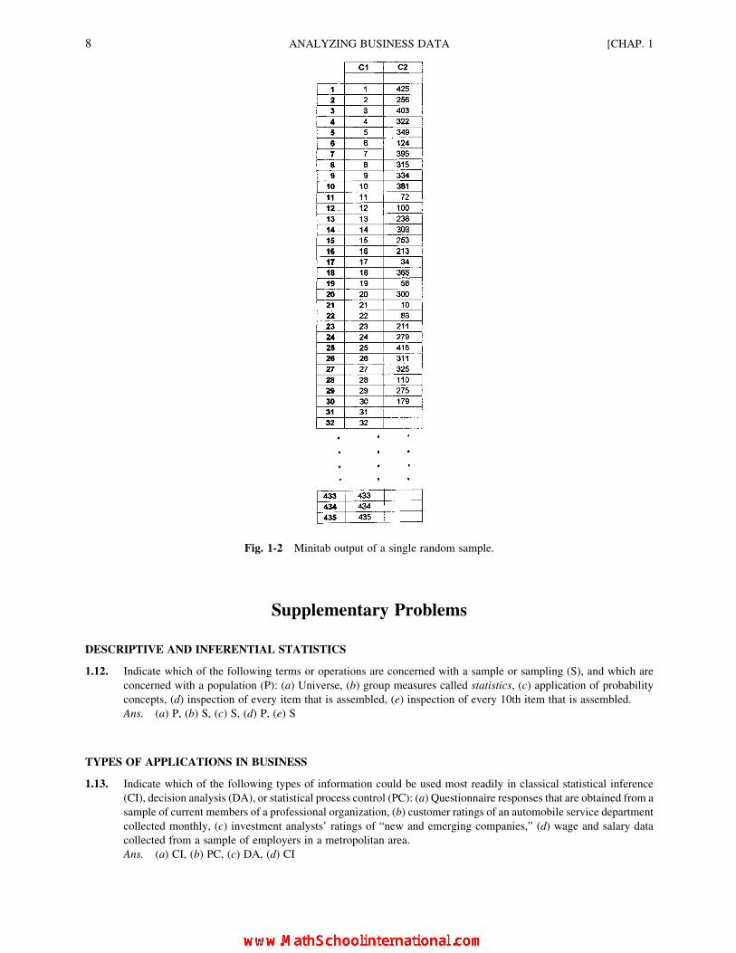
Figure 1-2 presents the Minitab output that lists the sampled firms in rows 1 through 30 of column C2. By the
very nature of a random sample, your sampled firms will be different. The Minitab instructions for selecting the
simple random sample of size n ¼ 30 for this example are as follows:
(1) Open Minitab. Place the integers from 1 to 435 in column C1 as follows. Click Calc ! Make Patterned
Data ! Simple Set of Numbers. Then select Store patterned data in: C1 From first value: 1 To last
value: 435 In steps of: 1. Click OK, and the integers 1 to 435 will appear in column C1.
(2) To identify the 30 firms to be sampled, click Calc ! Random Data ! Samples from Columns. Then select
Sample 30 from column[s]: C1 and Store samples in: C2. Click OK, and the IDs of the randomly selected
firms will appear in rows 1 through 30 of column C2.
Fig. 1-1 Excel output of a simple random sample.
CHAP. 1] ANALYZING BUSINESS DATA 7
Supplementary Problems
DESCRIPTIVE AND INFERENTIAL STATISTICS
1.12. Indicate which of the following terms or operations are concerned with a sample or sampling (S), and which are
concerned with a population (P): (a) Universe, (b) group measures called statistics, (c) application of probability
concepts, (d) inspection of every item that is assembled, (e) inspection of every 10th item that is assembled.
Ans. (a) P, (b) S, (c) S, (d) P, (e) S
TYPES OF APPLICATIONS IN BUSINESS
1.13. Indicate which of the following types of information could be used most readily in classical statistical inference
(CI), decision analysis (DA), or statistical process control (PC): (a) Questionnaire responses that are obtained from a
sample of current members of a professional organization, (b) customer ratings of an automobile service department
collected monthly, (c) investment analysts’ ratings of “new and emerging companies,” (d) wage and salary data
collected from a sample of employers in a metropolitan area.
Ans. (a) CI, (b) PC, (c) DA, (d) CI
Fig. 1-2 Minitab output of a single random sample.
8 ANALYZING BUSINESS DATA [CHAP. 1

DISCRETE AND CONTINUOUS VARIABLES
1.14. For the following types of values, designate discrete variables (D) and continuous variables (C): (a) Number of units
of an item held in stock, (b) ratio of current assets to current liabilities, (c) total tonnage shipped, (d) quantity
shipped, in units, (e) volume of traffic on a toll road, ( f ) attendance at the company’s annual meeting.
Ans. (a) D, (b) C, (c) C, (d) D, (e) D, ( f ) D
OBTAINING DATA THROUGH DIRECT OBSERVATION VS. SURVEYS
1.15. Indicate which of the following data-gathering procedures would be considered an experiment (E), and which
would be considered a survey (S): (a) Comparing the results of a new approach to training airline ticket agents to
those of the traditional approach, (b) evaluating two different sets of assembly instructions for a toy by having two
comparable groups of children assemble the toy using the different instructions, (c) having a product-evaluation
magazine send subscribers a questionnaire asking them to rate the products that they have recently purchased.
Ans. (a) E, (b) E, (c) S
METHODS OF RANDOM SAMPLING
1.16. Identify whether the simple random (R) or the systematic (S) sampling method is used in the following: (a) Using a
table of random numbers to select a sample of people entering an amusement park and (b) interviewing every 100th
person entering an amusement park, randomly starting at the 55th person to enter the park.
Ans. (a) R, (b) S
1.17. For the following group-oriented sampling situations, identify whether the stratified (St) or the cluster (C) sampling
method would be used: (a) Estimating the voting preferences of people who live in various neighborhoods and
(b) studying consumer attitudes with the belief that there are important differences according to age and sex.
Ans. (a) C, (b) St
OTHER SAMPLING METHODS
1.18. Indicate which of the following types of samples best exemplify or would be concerned with a judgment sample (J),
a convenience sample (C), or the method of rational subgroups (R): (a) A real estate appraiser selects a sample of
homes sold in a neighborhood, which seem representative of homes located there, in order to arrive at an estimate of
the level of home values in that neighborhood, (b) in a battery-manufacturing plant, battery life is monitored every
half hour to assure that the output satisfies specifications, (c) a fast-food outlet has company employees evaluate a
new chicken-combo sandwich in terms of taste and perceived value.
Ans. (a) J, (b) R, (c) C
USING COMPUTER SOFTWARE TO GENERATE RANDOM NUMBERS
1.19. An auditor wishes to take a simple random sample of 50 accounts from the 5,250 accounts receivable in a large firm.
The accounts are sequentially numbered from 0001 to 5250. Use available computer software to obtain a listing
of the required 50 random numbers.
CHAP. 1] ANALYZING BUSINESS DATA 9
CHAPTER 2
StatisticalPresentations andGraphical Displays
2.1 FREQUENCY DISTRIBUTIONS
A frequency distribution is a table in which possible values for a variable are grouped into classes, and the
number of observed values which fall into each class is recorded. Data organized in a frequency distribution are
called grouped data. In contrast, for ungrouped data every observed value of the random variable is listed.
EXAMPLE 1. A frequency distribution of weekly wages is shown in Table 2.1. Note that the amounts are reported to the
nearest dollar. When a remainder that is to be rounded is “exactly 0.5” (exactly $0.50 in this case), the convention is to round
to the nearest even number. Thus a weekly wage of $259.50 would have been rounded to $260 as part of the data-grouping
process.
Table 2.1 A Frequency Distribution of
Weekly Wages for 100 Entry-
Level Workers
Weekly wage Number of workers ( f )
$240–259 7
260–279 20
280–299 33
300–319 25
320–339 11
340–359 4
Total 100
10
Copyright 2004, 1996, 1988, 1976 by The McGraw-Hill Companies, Inc. Click Here for Terms of Use.
2.2 CLASS INTERVALS
For each class in a frequency distribution, the lower and upper stated class limits indicate the values
included within the class. (See the first column of Table 2.1.) In contrast, the exact class limits, or class
boundaries, are the specific points that serve to separate adjoining classes along a measurement scale for
continuous variables. Exact class limits can be determined by identifying the points that are halfway between
the upper and lower stated class limits, respectively, of adjoining classes. The class interval identifies the range
of values included within a class and can be determined by subtracting the lower exact class limit from the
upper exact class limit for the class. When exact limits are not identified, the class interval can be determined by
subtracting the lower stated limit for a class from the lower stated limit of the adjoining next-higher class.
Finally, for certain purposes the values in a class often are represented by the class midpoint, which can be
determined by adding one-half of the class interval to the lower exact limit of the class.
EXAMPLE 2. Table 2.2 presents the exact class limits and the class midpoints for the frequency distribution in Table 2.1.
Table 2.2 Weekly Wages for 100 Entry-Level Workers
Weekly wage
(class limits) Exact class limits* Class midpoint Number of workers
$240–259 $239.50–259.50 $249.50 7
260–279 259.50–279.50 269.50 20
280–299 279.50–299.50 289.50 33
300–319 299.50–319.50 309.50 25
320–339 319.50–339.50 329.50 11
340–359 339.50–359.50 349.50 4
Total 100
* In general, only one additional significant digit is expressed in exact class limits as compared with
stated class limits. However, because with monetary units the next more precise unit of measurement
after “nearest dollar” is usually defined as “nearest cent,” in this case two additional digits are
expressed.
EXAMPLE 3. Calculated by the two approaches, the class interval for the first class in Table 2.2 is
$259.50 2 $239.50 ¼ $20 (subtraction of the lower exact class limit from the upper exact class limit of the class)
$260 2 $240 ¼ $20 (subtraction of the lower stated class limit of the class from the lower stated class limit of the adjoining
next-higher class).
Computationally, it is generally desirable that all class intervals in a given frequency distribution be equal.
A formula which can be used to determine the approximate class interval to be used is
Approximate interval ¼largest value inungrouped data
� �� smallest value in
ungrouped data
� �number of classes desired
(2:1)
EXAMPLE 4. For the original, ungrouped data that were grouped in Table 2.1, suppose the highest observed wage was
$358 and the lowest observed wage was $242. Given the objective of having six classes with equal class intervals,
Approximate interval ¼ 358� 242
6¼ $19:33
The closest convenient class size is thus $20.
For data that are distributed in a highly nonuniform way, such as annual salary data for a variety of
occupations, unequal class intervals may be desirable. In such a case, the larger class intervals are used for the
ranges of values in which there are relatively few observations.
CHAP. 2] STATISTICAL PRESENTATIONS AND GRAPHICAL DISPLAYS 11
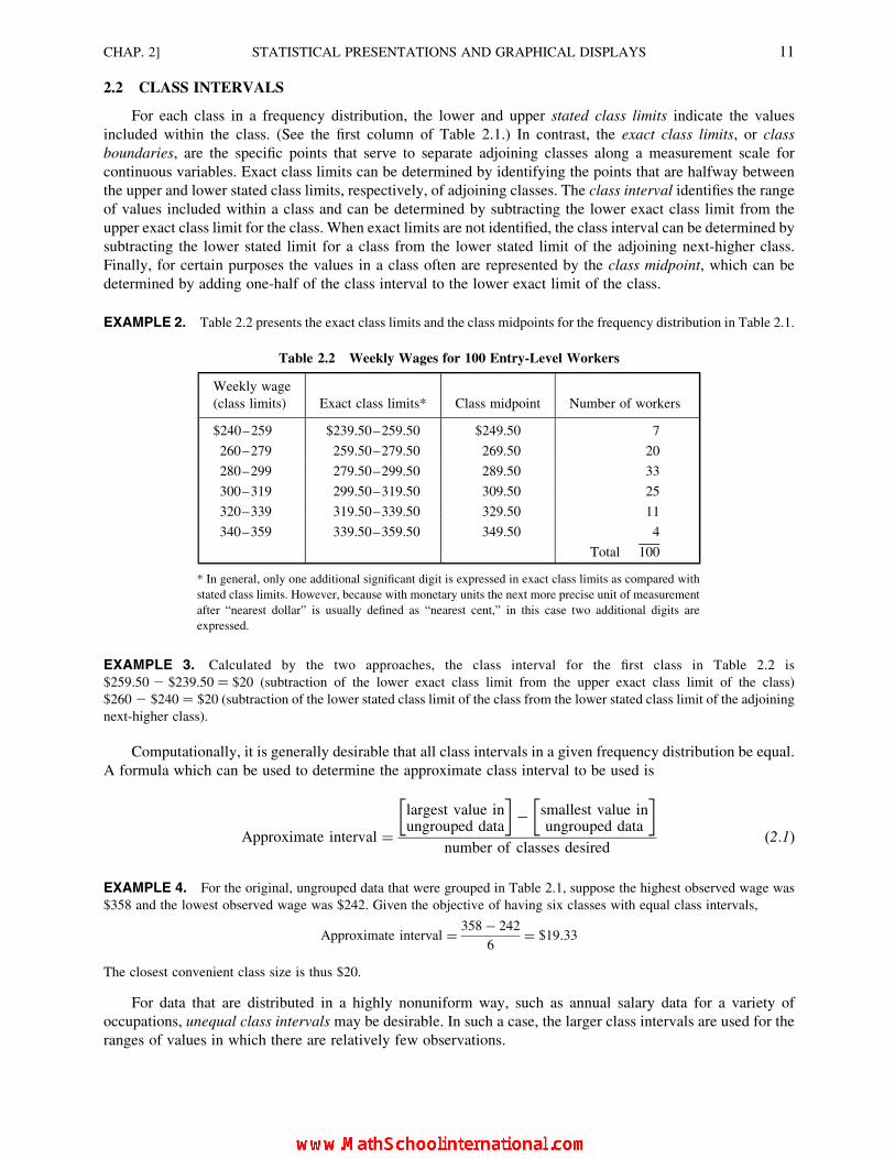
2.3 HISTOGRAMS AND FREQUENCY POLYGONS
A histogram is a bar graph of a frequency distribution. As indicated in Fig. 2-1, typically the exact class
limits are entered along the horizontal axis of the graph while the numbers of observations are listed along the
vertical axis. However, class midpoints instead of class limits also are used to identify the classes.
Fig. 2-1
EXAMPLE 5. A histogram for the frequency distribution of weekly wages in Table 2.2 is shown in Fig. 2-1.
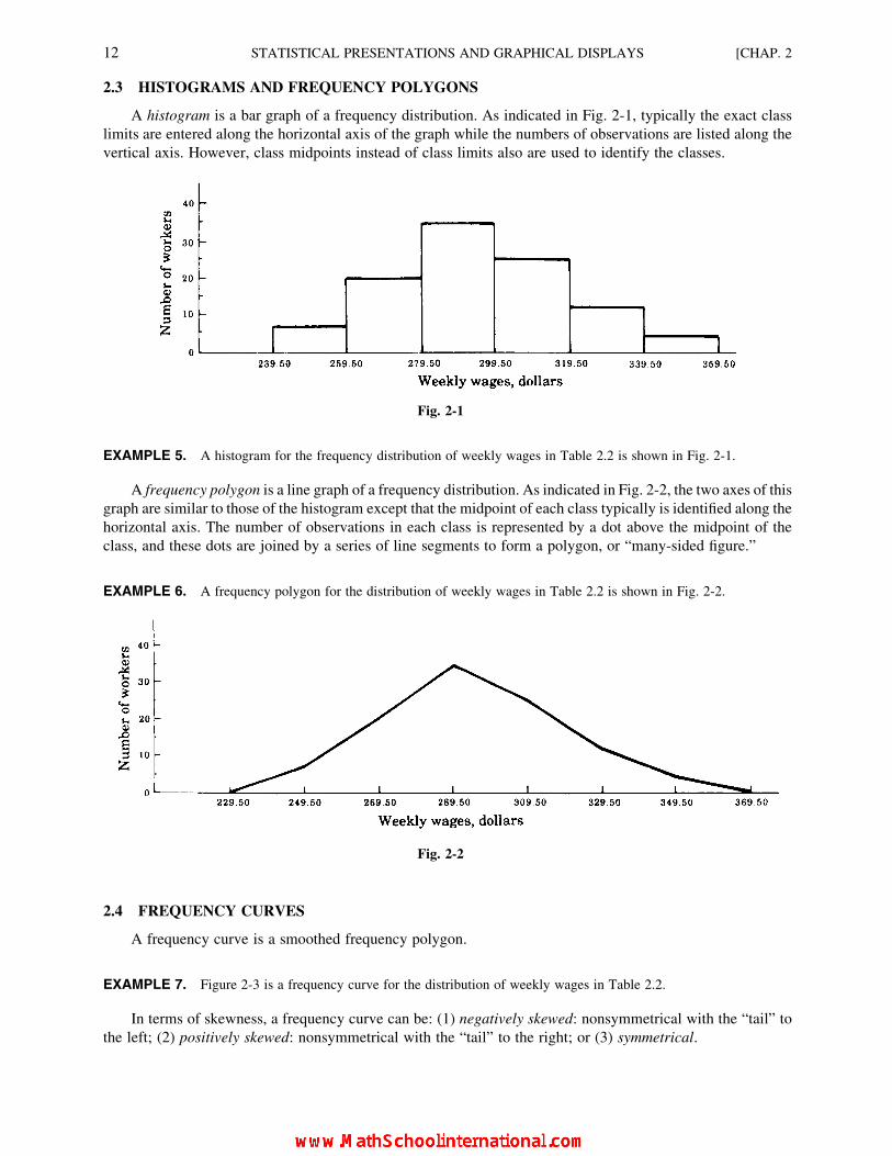
A frequency polygon is a line graph of a frequency distribution. As indicated in Fig. 2-2, the two axes of this
graph are similar to those of the histogram except that the midpoint of each class typically is identified along the
horizontal axis. The number of observations in each class is represented by a dot above the midpoint of the
class, and these dots are joined by a series of line segments to form a polygon, or “many-sided figure.”
EXAMPLE 6. A frequency polygon for the distribution of weekly wages in Table 2.2 is shown in Fig. 2-2.
Fig. 2-2
2.4 FREQUENCY CURVES
A frequency curve is a smoothed frequency polygon.
EXAMPLE 7. Figure 2-3 is a frequency curve for the distribution of weekly wages in Table 2.2.
In terms of skewness, a frequency curve can be: (1) negatively skewed: nonsymmetrical with the “tail” to
the left; (2) positively skewed: nonsymmetrical with the “tail” to the right; or (3) symmetrical.
12 STATISTICAL PRESENTATIONS AND GRAPHICAL DISPLAYS [CHAP. 2
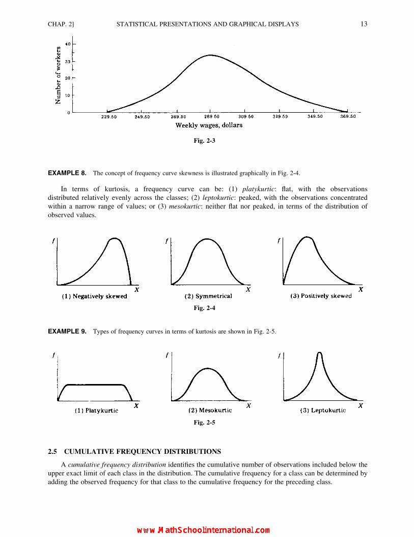
EXAMPLE 8. The concept of frequency curve skewness is illustrated graphically in Fig. 2-4.
In terms of kurtosis, a frequency curve can be: (1) platykurtic: flat, with the observations
distributed relatively evenly across the classes; (2) leptokurtic: peaked, with the observations concentrated
within a narrow range of values; or (3) mesokurtic: neither flat nor peaked, in terms of the distribution of
observed values.
Fig. 2-4
EXAMPLE 9. Types of frequency curves in terms of kurtosis are shown in Fig. 2-5.
Fig. 2-5
2.5 CUMULATIVE FREQUENCY DISTRIBUTIONS
A cumulative frequency distribution identifies the cumulative number of observations included below the
upper exact limit of each class in the distribution. The cumulative frequency for a class can be determined by
adding the observed frequency for that class to the cumulative frequency for the preceding class.
Fig. 2-3
CHAP. 2] STATISTICAL PRESENTATIONS AND GRAPHICAL DISPLAYS 13
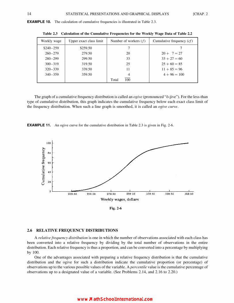
EXAMPLE 10. The calculation of cumulative frequencies is illustrated in Table 2.3.
Table 2.3 Calculation of the Cumulative Frequencies for the Weekly Wage Data of Table 2.2
Weekly wage Upper exact class limit Number of workers ( f ) Cumulative frequency (cf )
$240–259 $259.50 7 7
260–279 279.50 20 20 þ 7 ¼ 27
280–299 299.50 33 33 þ 27 ¼ 60
300–319 319.50 25 25 þ 60 ¼ 85
320–339 339.50 11 11 þ 85 ¼ 96
340–359 359.50 4 4 þ 96 ¼ 100
Total 100
The graph of a cumulative frequency distribution is called an ogive (pronounced “o-jive”). For the less-than
type of cumulative distribution, this graph indicates the cumulative frequency below each exact class limit of
the frequency distribution. When such a line graph is smoothed, it is called an ogive curve.
EXAMPLE 11. An ogive curve for the cumulative distribution in Table 2.3 is given in Fig. 2-6.
Fig. 2-6
2.6 RELATIVE FREQUENCY DISTRIBUTIONS
A relative frequency distribution is one in which the number of observations associated with each class has
been converted into a relative frequency by dividing by the total number of observations in the entire
distribution. Each relative frequency is thus a proportion, and can be converted into a percentage by multiplying
by 100.
One of the advantages associated with preparing a relative frequency distribution is that the cumulative
distribution and the ogive for such a distribution indicate the cumulative proportion (or percentage) of
observations up to the various possible values of the variable. A percentile value is the cumulative percentage of
observations up to a designated value of a variable. (See Problems 2.14, and 2.16 to 2.20.)
14 STATISTICAL PRESENTATIONS AND GRAPHICAL DISPLAYS [CHAP. 2

2.7 THE “AND-UNDER” TYPE OF FREQUENCY DISTRIBUTION
The class limits that are given in computer-generated frequency distributions usually are “and-under” types
of limits. For such limits, the stated class limits are also the exact limits that define the class. The values that are
grouped in any one class are equal to or greater than the lower class limit, and up to but not including the value
of the upper class limit. A descriptive way of presenting such class limits is
5 and under 8
8 and under 11
In addition to this type of distribution being more convenient to implement for computer software, it
sometimes also reflects a more “natural” way of collecting the data in the first place. For instance, people’s ages
generally are reported as the age at the last birthday, rather than the age at the nearest birthday. Thus, to be 24 years
old is to be at least 24 but less than 25 years old. Solved Problems 2.21 and 2.22 concern an and-under frequency
distribution. Problems 2.28 to 2.31 present Excel and Minitab output that include and-under distributions.
2.8 STEM-AND-LEAF DIAGRAMS
A stem-and-leaf diagram is a relatively simple way of organizing and presenting measurements in a rank-
ordered bar chart format. This is a popular technique in exploratory data analysis. As the name implies,
exploratory data analysis is concerned with techniques for preliminary analyses of data in order to gain insights
about patterns and relationships. Frequency distributions and the associated graphic techniques covered in the
previous sections of this chapter are also often used for this purpose. In contrast, confirmatory data analysis
includes the principal methods of statistical inference that constitute most of this book, beginning with Chapter 8
on statistical estimation. Confirmatory data analysis is concerned with coming to final statistical conclusions
about patterns and relationships in data.
A stem-and-leaf diagram is similar to a histogram, except that it is easier to construct and shows the actual
data values, rather than having the specific values lost by being grouped into defined classes. However, the
technique is most readily applicable and meaningful only if the first digit of the measurement, or possibly the
first two digits, provides a good basis for separating data into groups. Each group then is analogous to a class or
category in a frequency distribution. Where the first digit alone is used to group the measurements, the name
stem-and-leaf refers to the fact that the first digit is the stem, and each of the measurements with that first-digit
value becomes a leaf in the display.
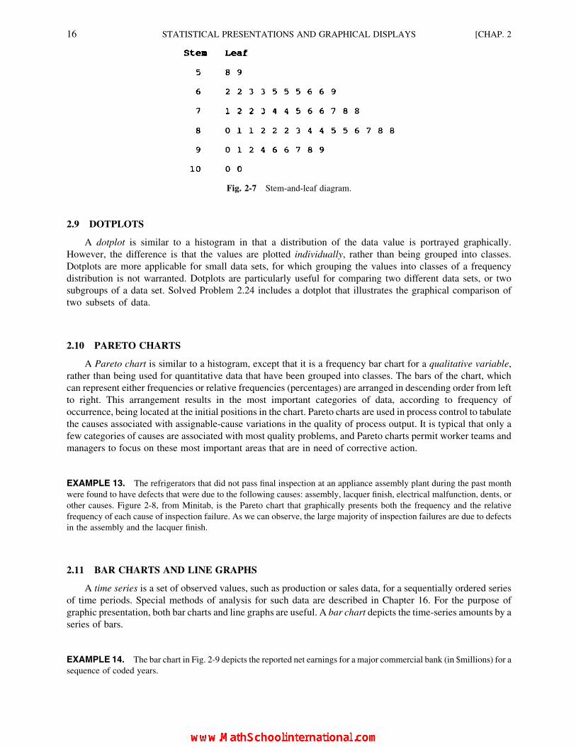
EXAMPLE 12. Table 2.4 presents the scores earned by 50 students in a 100-point exam in financial accounting. Figure 2-7
is the stem-and-leaf diagram for these scores. Notice that in addition to being able to observe the overall pattern of scores,
the individual scores can also be seen. For instance, on the line with the stem of 6, the two posted leaf values of 2 represent
the two scores of 62 that are included in Table 2.4.
Table 2.4 Scores Earned by 50
Students in an Exam in
Financial Accounting
58 88 65 96 85
74 69 63 88 65
85 91 81 80 90
65 66 81 92 71
82 98 86 100 82
72 94 72 84 73
76 78 78 77 74
83 82 66 76 63
62 62 59 87 97
100 75 84 96 99
CHAP. 2] STATISTICAL PRESENTATIONS AND GRAPHICAL DISPLAYS 15
2.9 DOTPLOTS
A dotplot is similar to a histogram in that a distribution of the data value is portrayed graphically.
However, the difference is that the values are plotted individually, rather than being grouped into classes.
Dotplots are more applicable for small data sets, for which grouping the values into classes of a frequency
distribution is not warranted. Dotplots are particularly useful for comparing two different data sets, or two
subgroups of a data set. Solved Problem 2.24 includes a dotplot that illustrates the graphical comparison of
two subsets of data.
2.10 PARETO CHARTS
A Pareto chart is similar to a histogram, except that it is a frequency bar chart for a qualitative variable,
rather than being used for quantitative data that have been grouped into classes. The bars of the chart, which
can represent either frequencies or relative frequencies (percentages) are arranged in descending order from left
to right. This arrangement results in the most important categories of data, according to frequency of
occurrence, being located at the initial positions in the chart. Pareto charts are used in process control to tabulate
the causes associated with assignable-cause variations in the quality of process output. It is typical that only a
few categories of causes are associated with most quality problems, and Pareto charts permit worker teams and
managers to focus on these most important areas that are in need of corrective action.
EXAMPLE 13. The refrigerators that did not pass final inspection at an appliance assembly plant during the past month
were found to have defects that were due to the following causes: assembly, lacquer finish, electrical malfunction, dents, or
other causes. Figure 2-8, from Minitab, is the Pareto chart that graphically presents both the frequency and the relative
frequency of each cause of inspection failure. As we can observe, the large majority of inspection failures are due to defects
in the assembly and the lacquer finish.
2.11 BAR CHARTS AND LINE GRAPHS
A time series is a set of observed values, such as production or sales data, for a sequentially ordered series
of time periods. Special methods of analysis for such data are described in Chapter 16. For the purpose of
graphic presentation, both bar charts and line graphs are useful. A bar chart depicts the time-series amounts by a
series of bars.
EXAMPLE 14. The bar chart in Fig. 2-9 depicts the reported net earnings for a major commercial bank (in $millions) for a
sequence of coded years.
Fig. 2-7 Stem-and-leaf diagram.
16 STATISTICAL PRESENTATIONS AND GRAPHICAL DISPLAYS [CHAP. 2

A component bar chart portrays subdivisions within the bars on the chart. For example, each bar in Fig. 2-9
could be subdivided into separate parts (and perhaps color-coded) to indicate the relative contribution of each
segment of the business to the net earnings for each year. (See Solved Problem 2.26.) The use of Excel and
Minitab to obtain bar charts is illustrated in Problems 2.32 and 2.33.
A line graph portrays time-series amounts by a connected series of line segments.
Fig. 2-8
Fig. 2-9 Bar chart.
CHAP. 2] STATISTICAL PRESENTATIONS AND GRAPHICAL DISPLAYS 17
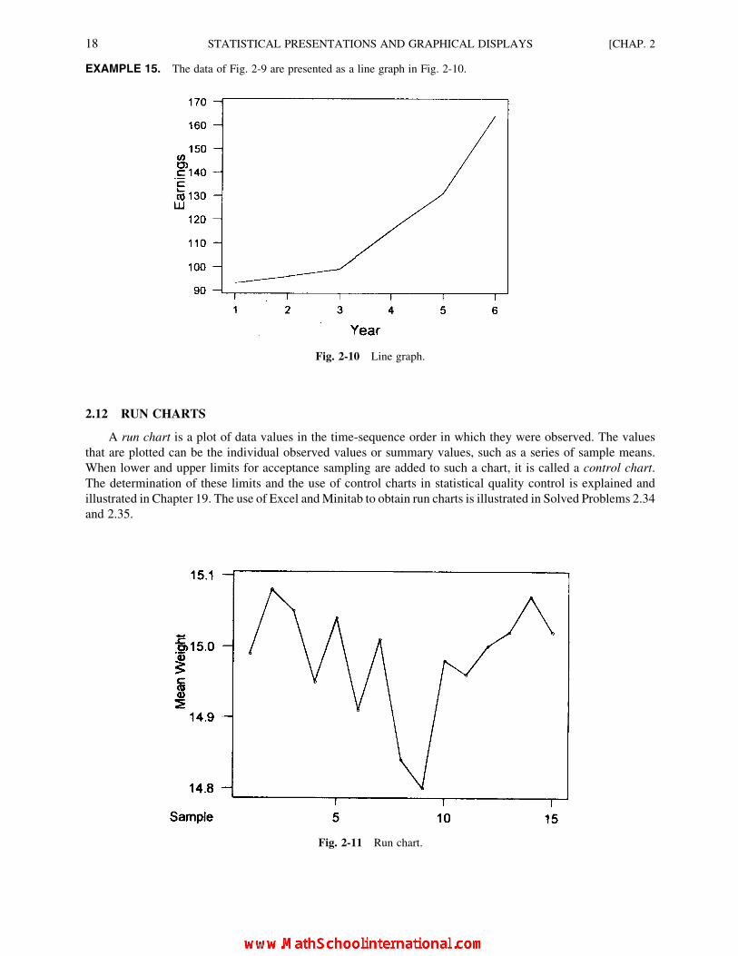
EXAMPLE 15. The data of Fig. 2-9 are presented as a line graph in Fig. 2-10.
2.12 RUN CHARTS
A run chart is a plot of data values in the time-sequence order in which they were observed. The values
that are plotted can be the individual observed values or summary values, such as a series of sample means.
When lower and upper limits for acceptance sampling are added to such a chart, it is called a control chart.
The determination of these limits and the use of control charts in statistical quality control is explained and
illustrated in Chapter 19. The use of Excel andMinitab to obtain run charts is illustrated in Solved Problems 2.34
and 2.35.
Fig. 2-10 Line graph.
Fig. 2-11 Run chart.
18 STATISTICAL PRESENTATIONS AND GRAPHICAL DISPLAYS [CHAP. 2
EXAMPLE 16. Figure 2-11 portrays a run chart for the sequence of mean weights for samples of four packages of potato
chips taken at 15 different times using the sampling method of rational subgroups (see Chapter 1, Example 13). The
sequence of mean weights for the samples was found to be: 14.99, 15.08, 15.05, 14.95, 15.04, 14.91, 15.01, 14.84, 14.80,
14.98, 14.96, 15.00, 15.02, 15.07, and 15.02 oz. The specification for the average net weight to be packaged in the process is
15.00 oz. Whether any of the deviations of these sample means from the specified weight standard can be considered a
meaningful deviation is discussed fully in Chapter 19.
2.13 PIE CHARTS
A pie chart is a pie-shaped figure in which the pieces of the pie represent divisions of a total amount, such
as the distribution of a company’s sales dollar.
A percentage pie chart is one in which the values have been converted into percentages in order to make
them easier to compare. The use of Excel and Minitab to obtain pie charts is illustrated in Solved Problems 2.36
and 2.37.
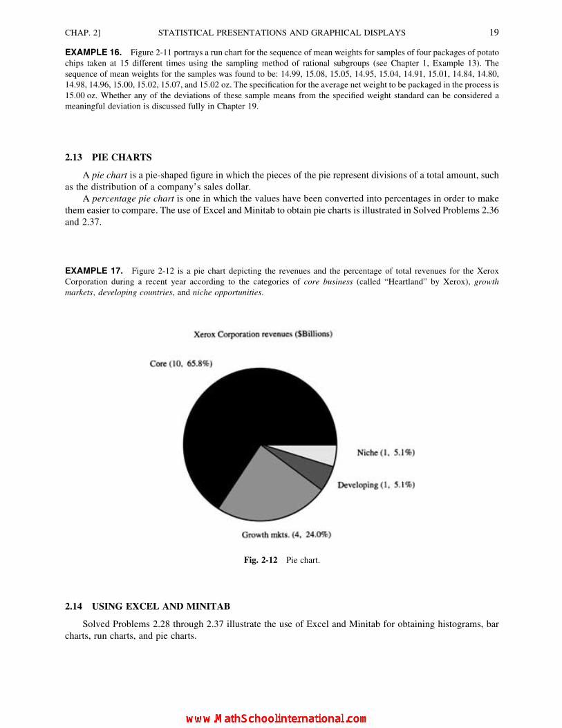
EXAMPLE 17. Figure 2-12 is a pie chart depicting the revenues and the percentage of total revenues for the Xerox
Corporation during a recent year according to the categories of core business (called “Heartland” by Xerox), growth
markets; developing countries, and niche opportunities.
Fig. 2-12 Pie chart.
2.14 USING EXCEL AND MINITAB
Solved Problems 2.28 through 2.37 illustrate the use of Excel and Minitab for obtaining histograms, bar
charts, run charts, and pie charts.
CHAP. 2] STATISTICAL PRESENTATIONS AND GRAPHICAL DISPLAYS 19

Solved Problems
FREQUENCY DISTRIBUTIONS, CLASS INTERVALS, AND RELATED GRAPHIC METHODS
2.1. With reference to Table 2.5,
(a) what are the lower and upper stated limits of the first class?
(b) what are the lower and upper exact limits of the first class?
(c) the class interval used is the same for all classes of the distribution. What is the interval size?
(d) what is the midpoint of the first class?
(e) what are the lower and upper exact limits of the class in which the largest number of apartment rental rates was
tabulated?
( f ) suppose a monthly rental rate of $439.50 were reported. Identify the lower and upper stated limits of the class
in which this observation would be tallied.
(a) $350 and $379
(b) $340.50 and $379.50 (Note: As in Example 2, two additional digits are expressed in this case instead of the
usual one additional digit in exact class limits as compared with stated class limits.)
(c) Focusing on the interval of values in the first class,
$379.50 2 $349.50 ¼ $30 (subtraction of the lower exact class limit from the upper exact class limit of the
class)
$380 2 $350 ¼ $30 (subtraction of the lower stated class limit of the class from the lower stated class limit of
the next-higher adjoining class)
(d) $349.50 þ 30/2 ¼ $349.50 þ $15.00 ¼ $364.50
(e) $499.50 and $529.50
( f ) $440 and $469 (Note: $439.50 is first rounded to $440 as the nearest dollar using the even-number rule
described in Section 2.1.)
Table 2.5 Frequency Distribution of
Monthly Apartment Rental
Rates for 200 Studio
Apartments
Rental rate Number of apartments
$350–379 3
380–409 8
410–439 10
440–469 13
470–499 33
500–529 40
530–559 35
560–589 30
590–619 16
620–649 12
Total 200
20 STATISTICAL PRESENTATIONS AND GRAPHICAL DISPLAYS [CHAP. 2

2.2. Prepare a histogram for the data in Table 2.5.
A histogram for the data in Table 2.5 appears in Fig. 2-13.
Fig. 2-13
2.3. Prepare a frequency polygon and a frequency curve for the data in Table 2.5.
Figure 2-14 is a graphic presentation of the frequency polygon and frequency curve for the data in Table 2.5.
Fig. 2-14
2.4. Describe the frequency curve in Fig. 2-14 from the standpoint of skewness.
The frequency curve appears to be somewhat negatively skewed.
2.5. Prepare a cumulative frequency distribution for the data in Table 2.5.
See Table 2.6.
CHAP. 2] STATISTICAL PRESENTATIONS AND GRAPHICAL DISPLAYS 21

Table 2.6 Cumulative Frequency Distribution of Apartment Rental Rates
Rental rate Class boundaries Number of apartments Cumulative frequency (cf )
$350–379 $349.50–379.50 3 3
380–409 379.50–409.50 8 11
410–439 409.50–439.50 10 21
440–469 439.50–469.50 13 34
470–499 469.50–499.50 33 67
500–529 499.50–529.50 40 107
530–559 529.50–559.50 35 142
560–589 559.50–589.50 30 172
590–619 589.50–619.50 16 188
620–649 619.50–649.50 12 200
Total 200
2.6 Present the cumulative frequency distribution in Table 2.6 graphically by means of an ogive curve.
The ogive curve for the data in Table 2.6 is shown in Fig. 2-15.
2.7 Listed in Table 2.7 are the required times to complete a sample assembly task for 30 employees
who have applied for a promotional transfer to a job requiring precision assembly. Suppose we
Fig. 2-15
Table 2.7 Assembly Times for 30 Employees,
min
10 14 15 13 17
16 12 14 11 13
15 18 9 14 14
9 15 11 13 11
12 10 17 16 12
11 16 12 14 15
22 STATISTICAL PRESENTATIONS AND GRAPHICAL DISPLAYS [CHAP. 2

wish to organize these data into five classes with equal class sizes. Determine the convenient
interval size.
Approximate interval ¼largest value inungrouped data
� �� smallest value in
ungrouped data
� �number of classes desired
¼ 18� 9
5¼ 1:80
In this case, it is convenient to round the interval to 2.0.
2.8. Prepare a frequency distribution for the data in Table 2.7 using a class interval of 2.0 for all classes and
setting the lower stated limit of the first class at 9 min.
The required construction appears in Table 2.8.
2.9. In Table 2.8 refer to the class with the lowest number of employees and identify (a) its exact limits,
(b) its interval, (c) its midpoint.
(a) 16.5–18.5, (b) 18.5 2 16.5 ¼ 2.0, (c) 16.5 þ 2.0/2 ¼ 17.5.
2.10. Prepare a histogram for the frequency distribution in Table 2.8.
The histogram is presented in Fig. 2-16.
Fig. 2-16
Table 2.8 Frequency Distribution for
the Assembly Times
Time, min Number of employees
9–10 4
11–12 8
13–14 8
15–16 7
17–18 3
Total 30
CHAP. 2] STATISTICAL PRESENTATIONS AND GRAPHICAL DISPLAYS 23
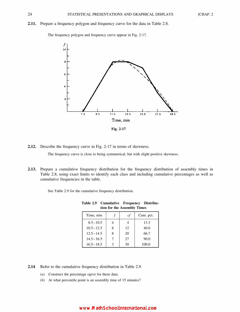
2.11. Prepare a frequency polygon and frequency curve for the data in Table 2.8.
The frequency polygon and frequency curve appear in Fig. 2-17.
Fig. 2-17
2.12. Describe the frequency curve in Fig. 2-17 in terms of skewness.
The frequency curve is close to being symmetrical, but with slight positive skewness.
2.13. Prepare a cumulative frequency distribution for the frequency distribution of assembly times in
Table 2.8, using exact limits to identify each class and including cumulative percentages as well as
cumulative frequencies in the table.
See Table 2.9 for the cumulative frequency distribution.
Table 2.9 Cumulative Frequency Distribu-
tion for the Assembly Times
Time, min f cf Cum. pct.
8.5–10.5 4 4 13.3
10.5–12.5 8 12 40.0
12.5–14.5 8 20 66.7
14.5–16.5 7 27 90.0
16.5–18.5 3 30 100.0
2.14 Refer to the cumulative frequency distribution in Table 2.9.
(a) Construct the percentage ogive for these data.
(b) At what percentile point is an assembly time of 15 minutes?
24 STATISTICAL PRESENTATIONS AND GRAPHICAL DISPLAYS [CHAP. 2
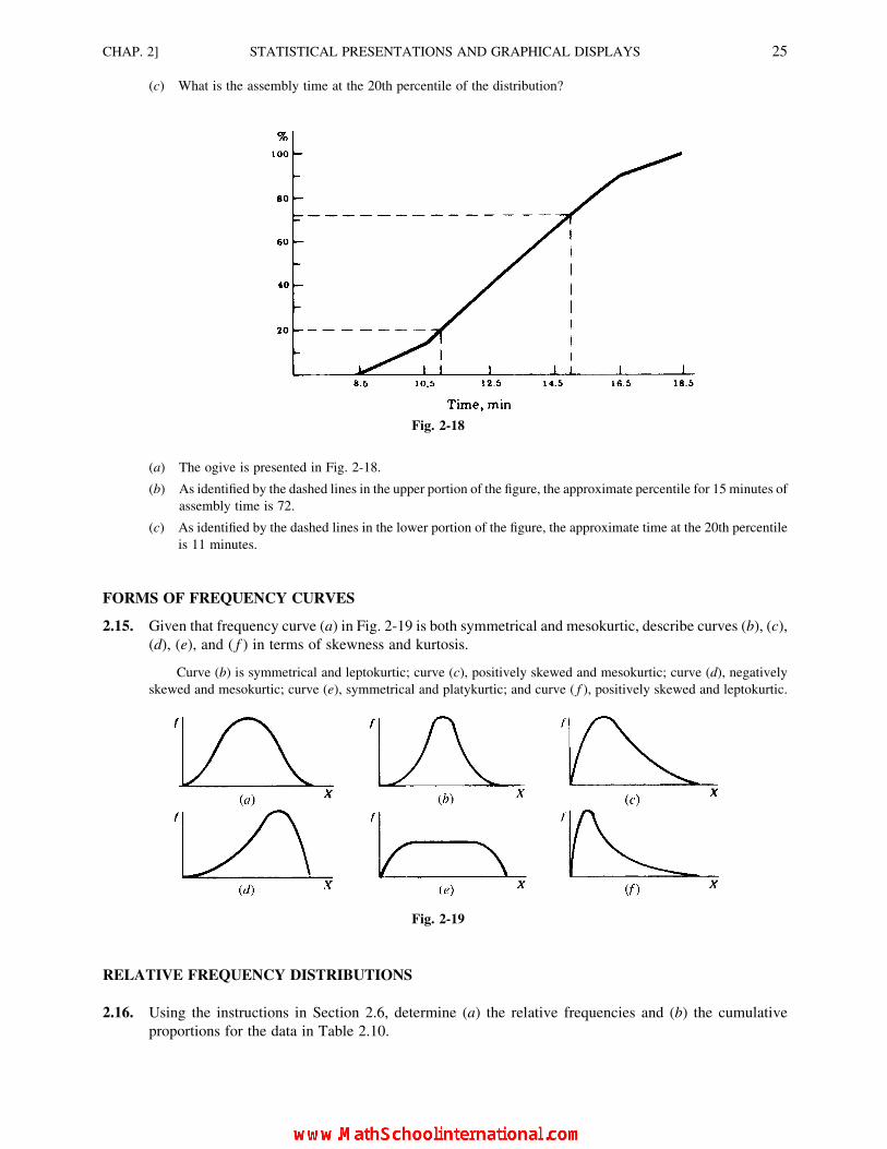
(c) What is the assembly time at the 20th percentile of the distribution?
Fig. 2-18
(a) The ogive is presented in Fig. 2-18.
(b) As identified by the dashed lines in the upper portion of the figure, the approximate percentile for 15 minutes of
assembly time is 72.
(c) As identified by the dashed lines in the lower portion of the figure, the approximate time at the 20th percentile
is 11 minutes.
FORMS OF FREQUENCY CURVES
2.15. Given that frequency curve (a) in Fig. 2-19 is both symmetrical and mesokurtic, describe curves (b), (c),
(d), (e), and ( f ) in terms of skewness and kurtosis.
Curve (b) is symmetrical and leptokurtic; curve (c), positively skewed and mesokurtic; curve (d), negatively
skewed and mesokurtic; curve (e), symmetrical and platykurtic; and curve ( f ), positively skewed and leptokurtic.
RELATIVE FREQUENCY DISTRIBUTIONS
2.16. Using the instructions in Section 2.6, determine (a) the relative frequencies and (b) the cumulative
proportions for the data in Table 2.10.
Fig. 2-19
CHAP. 2] STATISTICAL PRESENTATIONS AND GRAPHICAL DISPLAYS 25

The relative frequencies and cumulative proportions for the data in Table 2.10 are given in Table 2.11.
2.17. With reference to Table 2.11, construct (a) a histogram for the relative frequency distribution and (b) an
ogive for the cumulative proportions.
(a) See Fig. 2-20.
Fig. 2-20
Table 2.10 Average Number of Injuries per
Thousand Worker-Hours in a
Particular Industry
Average number of injuries per
thousand worker-hours
Number of
firms
1.5–1.7 3
1.8–2.0 12
2.1–2.3 14
2.4–2.6 9
2.7–2.9 7
3.0–3.2 5
Total 50
Table 2.11 Relative Frequencies and Cumulative Proportions for Average Number of
Injuries
Average number of injuries
per thousand worker-hours
Number of
firms
(a) Relative
frequency
(b) Cumulative
proportion
1.5–1.7 3 0.06 0.06
1.8–2.0 12 0.24 0.30
2.1–2.3 14 0.28 0.58
2.4–2.6 9 0.18 0.76
2.7–2.9 7 0.14 0.90
3.0–3.2 5 0.10 1.00
Total 50 Total 1.00
26 STATISTICAL PRESENTATIONS AND GRAPHICAL DISPLAYS [CHAP. 2

(b) See Fig. 2-21.
Fig. 2-21
2.18. (a) Referring to Table 2.11, what proportion of firms are in the category of having had an average of at
least 3.0 injuries per thousand worker-hours? (b) What percentage or firms were at or below an average
of 2.0 injuries per thousand worker-hours?
(a) 0.10, (b) 6% þ 24% ¼ 30%
2.19. (a) Referring to Table 2.11, what is the percentile value associated with an average of 2.95
(approximately 3.0) injuries per thousand worker-hours? (b) What is the average number of accidents at
the 58th percentile?
(a) 90th percentile, (b) 2.35.
2.20. By graphic interpolation on an ogive curve, we can determine the approximate percentiles for various
values of the variable, and vice versa. Referring to Fig. 2-21, (a) What is the approximate percentile
associated with an average of 2.5 accidents? (b) What is the approximate average number of accidents at
the 50th percentile?
(a) 65th percentile (This is the approximate height of the ogive corresponding to 2.50 along the horizontal axis.)
(b) 2.25 (This is the approximate point along the horizontal axis which corresponds to the 0.50 height of the ogive.)
THE “AND-UNDER” TYPE OF FREQUENCY DISTRIBUTION
2.21. Identify the exact class limits for the data in Table 2.12.
Table 2.12 Time Required to Process and
Prepare Mail Orders
Time, min Number of orders
5 and under 8 10
8 and under 11 17
11 and under 14 12
14 and under 17 6
17 and under 20 2
Total 47
From Table 2.12,
CHAP. 2] STATISTICAL PRESENTATIONS AND GRAPHICAL DISPLAYS 27
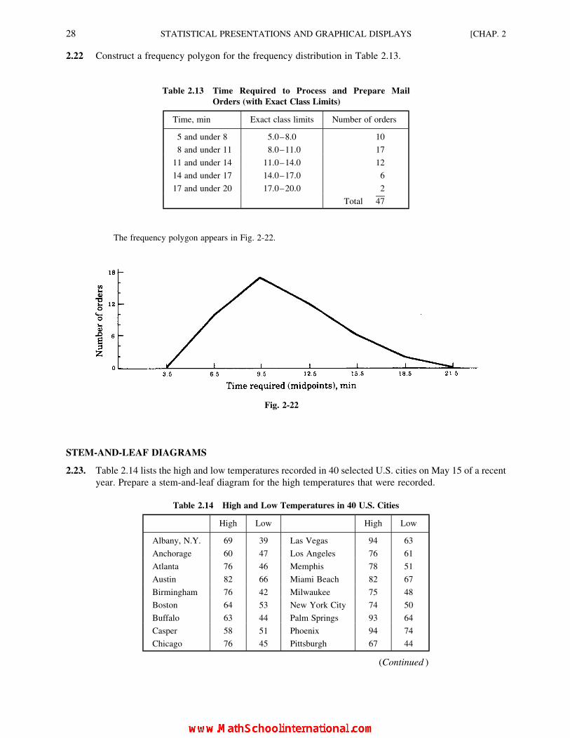
2.22 Construct a frequency polygon for the frequency distribution in Table 2.13.
Table 2.13 Time Required to Process and Prepare Mail
Orders (with Exact Class Limits)
Time, min Exact class limits Number of orders
5 and under 8 5.0–8.0 10
8 and under 11 8.0–11.0 17
11 and under 14 11.0–14.0 12
14 and under 17 14.0–17.0 6
17 and under 20 17.0–20.0 2
Total 47
The frequency polygon appears in Fig. 2-22.
Fig. 2-22
STEM-AND-LEAF DIAGRAMS
2.23. Table 2.14 lists the high and low temperatures recorded in 40 selected U.S. cities on May 15 of a recent
year. Prepare a stem-and-leaf diagram for the high temperatures that were recorded.
Table 2.14 High and Low Temperatures in 40 U.S. Cities
High Low High Low
Albany, N.Y. 69 39 Las Vegas 94 63
Anchorage 60 47 Los Angeles 76 61
Atlanta 76 46 Memphis 78 51
Austin 82 66 Miami Beach 82 67
Birmingham 76 42 Milwaukee 75 48
Boston 64 53 New York City 74 50
Buffalo 63 44 Palm Springs 93 64
Casper 58 51 Phoenix 94 74
Chicago 76 45 Pittsburgh 67 44
(Continued )
28 STATISTICAL PRESENTATIONS AND GRAPHICAL DISPLAYS [CHAP. 2

The stem-and-leaf diagram appears in Fig. 2-23.
Fig. 2-23 Stem-and-leaf diagram for temperature data.
DOTPLOTS
2.24. Table 2.15 presents resting pulse rates for a sample of 40 adults, half of whom do not smoke (code 0) and
half of whom are regular smokers (code 1). Use computer software to prepare a dotplot that will
facilitate the comparison of the pulse rates for the nonsmokers vs. the smokers in this sample. Interpret
the dotplot that is obtained.
Figure 2-24 presents a dotplot in which the two subgroups of people are plotted separately, but using the same scale
in order to facilitate comparison. As we can observe by the centering of the respective distributions, the sample of
habitual smokers shows they have a somewhat higher pulse rate than the nonsmokers. As indicated by the spread of
each subset of data, the smokers are more variable in their pulse rates than are the nonsmokers. Whether such
sample differences can be interpreted as representing actual differences in the population will be considered in
Chapters 9 and 11, which cover, respectively, estimating the difference between population parameters and testing
for difference in population parameters.
Fig. 2-24 Dotplot for pulse rates.
Table 2.14 (Continued )
High Low High Low
Cleveland 70 40 Portland, Ore. 70 53
Columbia, S.C. 74 47 Richmond 70 46
Columbus, Oh. 71 40 Rochester, N.Y. 62 42
Dallas 86 68 St. Louis 76 58
Detroit 71 43 San Antonio 81 69
Forth Wayne 76 37 San Diego 69 62
Green Bay 75 38 San Francisco 78 55
Honolulu 84 65 Seattle 67 50
Houston 84 67 Syracuse 63 43
Jacksonville 77 50 Tampa 85 59
Kansas City 72 59 Washington, D.C. 69 52
CHAP. 2] STATISTICAL PRESENTATIONS AND GRAPHICAL DISPLAYS 29

Table 2.15 Resting Pulse Rates for
a Sample of Adults, Ages
30–35
Habitual smoker?
Pulse rate (0 ¼ no; 1 ¼ yes)
82 0
68 0
78 0
80 0
62 0
60 0
62 0
76 0
74 0
74 0
68 0
68 0
64 0
76 0
88 0
70 0
78 0
80 0
74 0
82 0
80 1
90 1
64 1
74 1
70 1
74 1
84 1
72 1
92 1
64 1
94 1
80 1
78 1
88 1
60 1
68 1
90 1
89 1
68 1
72 1
30 STATISTICAL PRESENTATIONS AND GRAPHICAL DISPLAYS [CHAP. 2

BAR CHARTS AND LINE GRAPHS
2.25. Table 2.16 includes some of the financial results that were reported by an electric power company for six
consecutive years. Prepare a vertical bar chart portraying the per-share annual earnings of the company
for the coded years.
The bar chart appears in Fig. 2-25.
Fig. 2-25 Bar chart.
2.26. Prepare a component bar chart for the data in Table 2.16 such that the division of per-share earnings
between dividends (D) and retained earnings (R) is indicated for each year.
Table 2.16 Per-share Earnings from Continuing
Operations, Dividends, and Retained
Earnings for an Electric Power Company
Year Earnings Dividends Retained earnings
1 $1.61 $1.52 $0.09
2 2.17 1.72 0.45
3 2.48 1.92 0.56
4 3.09 2.20 0.89
5 4.02 2.60 1.42
6 4.35 3.00 1.35
CHAP. 2] STATISTICAL PRESENTATIONS AND GRAPHICAL DISPLAYS 31
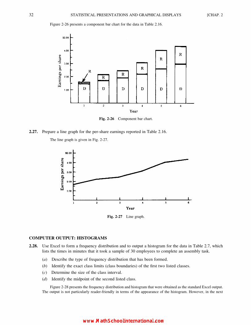
Figure 2-26 presents a component bar chart for the data in Table 2.16.
Fig. 2-26 Component bar chart.
2.27. Prepare a line graph for the per-share earnings reported in Table 2.16.
The line graph is given in Fig. 2-27.
Fig. 2-27 Line graph.
COMPUTER OUTPUT: HISTOGRAMS
2.28. Use Excel to form a frequency distribution and to output a histogram for the data in Table 2.7, which
lists the times in minutes that it took a sample of 30 employees to complete an assembly task.
(a) Describe the type of frequency distribution that has been formed.
(b) Identify the exact class limits (class boundaries) of the first two listed classes.
(c) Determine the size of the class interval.
(d) Identify the midpoint of the second listed class.
Figure 2-28 presents the frequency distribution and histogram that were obtained as the standard Excel output.
The output is not particularly reader-friendly in terms of the appearance of the histogram. However, in the next
32 STATISTICAL PRESENTATIONS AND GRAPHICAL DISPLAYS [CHAP. 2

Solved Problem, 2.29, we will modify the output so that it is more useful. The measurement listed for each bin of the
frequency distribution and associated histogram is the upper boundary of the respective class interval, even though
it is printed at the middle of each bar of the histogram.
(a) As explained in the paragraph above, the style of output is different from historically standard types of output,
with upper-class boundaries serving to identify each class.
(b) The first listed class includes all listed measurements of 9 minutes or less. The second listed class includes all
measurements greater than 9 minutes and less than or equal to 10.8 minutes. Note that this style of output is not
the same as the “and-under” type described in Section 2.7. If the second class were of the “and-under” type, the
class would include all values at or above 9 minutes but less than 10.8 minutes.
(c) For convenience we refer to the second listed class, for which both class limits are specified. The class interval
is: 10.8 2 9.0 ¼ 1.8.
(d) The midpoint is the lower exact limit plus one-half the interval size: 9.0 þ (1.8/2) ¼ 9.9.
The Excel instructions that result in the output presented in Fig. 2-28 are as follows:
(1) Open Excel. Enter the data from Table 2.7 into column A of the worksheet.
(2) Click Tools ! Data Analysis ! Histogram and open the Histogram dialog box. Designate the Input
Range as $A$1:$A$30 and the Output Range as $C$1 (to provide for one column of space between the input
and the output).
(3) Click the checkbox for Chart Output. Click OK and the output will appear as shown in Fig. 2-28.
2.29. Improve the histogram given in Fig. 2-28 by (a) increasing the height of the bars, (b) substituting
“Time,min” for “Bin” as the label for the horizontal axis, (c) inserting the specific bin label for the last
listed class in place of the default “More,” and (d) delete the gaps between the vertical bars, since a
histogram (as contrasted to the bar chart described in Section 2.11) should have no gaps.
Figure 2-29 presents the improved histogram and associated frequency distribution. The Excel instructions that
result in this output are as follows:
(a) Increase the height of the chart as follows. Click anywhere on the chart and “handles” appear on the sides and
corners. Click on the bottom handle and drag it down to increase the height of the bars.
(b) Click on the “Bin” label and type “Time, min” as the replacement.
(c) To determine the upper limit of the last class, we note (from Problem 2.28) that the class interval is 1.8. So the
upper limit is 16.2 þ 1.8 ¼ 18. Click on the cell of the worksheet that contains the “More” and insert “18.”
(d) To remove the gaps, double-click on any histogram bar, and the Format Data Series dialog box appears. Then
click Option and in the text box for Gap width insert: 0.
2.30. Use Minitab to form a frequency distribution and to output a histogram for the data in Table 2.7, which
lists the times in minutes that it took a sample of 30 employees to complete an assembly task.
Fig. 2-28 Frequency distribution and histogram from Excel.
CHAP. 2] STATISTICAL PRESENTATIONS AND GRAPHICAL DISPLAYS 33

(a) Identify the midpoint of the first class.
(b) Determine the size of the class interval.
Figure 2-30 presents the histogram that was obtained as the standard Minitab output. As implied by the
positions of the values for the horizontal axis, the printed values are midpoints.
(a) As explained in the paragraph above, the values printed along the horizontal axis are midpoints. Therefore, the
midpoint of the first listed class is 9.0.
(b) By reference to the midpoints of two adjoining classes: 10 2 9 ¼ 1.
The Minitab instructions that result in the output presented in Fig. 2-30 are as follows:
(1) Open Minitab. Enter the data from Table 2.7 into column C1 of the worksheet.
(2) Click Graph ! Histogram. Under Graph variables, on line 1 insert: C1.
(3) Click OK.
Fig. 2-30 Histogram from Minitab.
Fig. 2-29 Improved histogram from Excel.
34 STATISTICAL PRESENTATIONS AND GRAPHICAL DISPLAYS [CHAP. 2

2.31. Change the analysis done in Problem 2.30, above, by substituting “Time,min” for C1 as the label for the
horizontal axis and by specifying that the midpoint of the first class interval should be set at 10 with a
class interval of 2.
(a) Identify the lower- and upper-class limits for the first class.
(b) Describe the type of frequency distribution that has been formed.
Figure 2-31 presents the required histogram. As is true in Fig. 2-30, the values listed along the horizontal axis
are class midpoints. Unlike the Excel output given in Figs. 2-28 and 2-29, the class limits are of the “and-under”
type, as described in Section 2.7.
(a) The class limits are at the midpoint plus-and-minus one-half the interval: 10+ 12(2) ¼ 9:0 and 11.0.
(b) As explained in the paragraph above, the classes reported are the “and-under” type. Thus, the first listed class
contains all measured times between 9 minutes and under 11 minutes. By reference to the original data table,
we see that the four values in the first class are 9, 9, 10, and 10; the two 11-minute values are not included in the
tally for this class.
The Minitab instructions that result in the output presented in Fig. 2-31 are as follows:
(1) Open Minitab. Enter the data from Table 2.7 into column C1 of the worksheet.
(2) Click the column-name cell located directly below the C1 column label. Type: Time,min.
(3) Click Graph ! Histogram. Under Graph variables, on line 1 insert: C1.
(4) Click Options . . . and in the resulting dialog box insert 10:18/2 for Midpoint/cutpoint positions.
The meaning of this specification is that the midpoints for the histogram should range from 10 to 18 with an
interval of 2.
(5) Click OK.
(6) Upon returning to the original dialog box, click OK.
Fig. 2-31 Modified histogram from Minitab.
COMPUTER OUTPUT: BAR CHARTS
2.32. Use Excel to prepare a vertical bar chart portraying the per-share annual earnings of an electric power
company for the coded years, as reported in Table 2.16.
Figure 2-32 is the bar chart obtained using Excel. The instructions that result in the output are as follows:
CHAP. 2] STATISTICAL PRESENTATIONS AND GRAPHICAL DISPLAYS 35

(1) Open Excel. In cell A1 enter: Year. In B1 enter: Earnings per share.
(2) Enter the coded year and associated values below the respective headings.
(3) Select Insert ! Chart. Then select Column as the Chart type and select the first chart subtype (Clustered
Column). Click Next.
(4) Specify the Data Range as $B$1:$B$7 and select Series in Columns. Click Next.
(5) For Chart title enter: Earnings per Share by Year. For Category (X) axis enter: Year. For Value (Y) axis
enter: Earnings per share. Click Next.
(6) For Place chart select As new sheet. Click Finish.
Fig. 2-32 Vertical bar chart from Excel.
2.33. Use Minitab to prepare a vertical bar chart portraying the per-share annual earnings of an electric power
company for the coded years, as reported in Table 2.16.
Fig. 2-33 Vertical bar chart from Minitab.
36 STATISTICAL PRESENTATIONS AND GRAPHICAL DISPLAYS [CHAP. 2
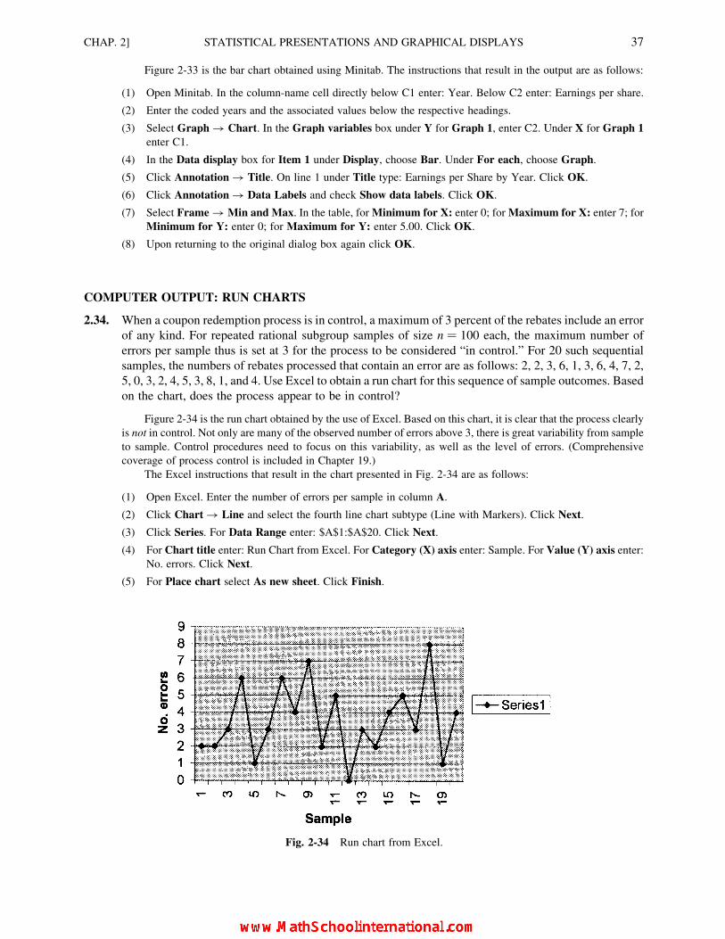
Figure 2-33 is the bar chart obtained using Minitab. The instructions that result in the output are as follows:
(1) Open Minitab. In the column-name cell directly below C1 enter: Year. Below C2 enter: Earnings per share.
(2) Enter the coded years and the associated values below the respective headings.
(3) Select Graph ! Chart. In the Graph variables box under Y for Graph 1, enter C2. Under X for Graph 1
enter C1.
(4) In the Data display box for Item 1 under Display, choose Bar. Under For each, choose Graph.
(5) Click Annotation ! Title. On line 1 under Title type: Earnings per Share by Year. Click OK.
(6) Click Annotation ! Data Labels and check Show data labels. Click OK.
(7) Select Frame ! Min and Max. In the table, for Minimum for X: enter 0; for Maximum for X: enter 7; for
Minimum for Y: enter 0; for Maximum for Y: enter 5.00. Click OK.
(8) Upon returning to the original dialog box again click OK.
COMPUTER OUTPUT: RUN CHARTS
2.34. When a coupon redemption process is in control, a maximum of 3 percent of the rebates include an error
of any kind. For repeated rational subgroup samples of size n ¼ 100 each, the maximum number of
errors per sample thus is set at 3 for the process to be considered “in control.” For 20 such sequential
samples, the numbers of rebates processed that contain an error are as follows: 2, 2, 3, 6, 1, 3, 6, 4, 7, 2,
5, 0, 3, 2, 4, 5, 3, 8, 1, and 4. Use Excel to obtain a run chart for this sequence of sample outcomes. Based
on the chart, does the process appear to be in control?
Figure 2-34 is the run chart obtained by the use of Excel. Based on this chart, it is clear that the process clearly
is not in control. Not only are many of the observed number of errors above 3, there is great variability from sample
to sample. Control procedures need to focus on this variability, as well as the level of errors. (Comprehensive
coverage of process control is included in Chapter 19.)
The Excel instructions that result in the chart presented in Fig. 2-34 are as follows:
(1) Open Excel. Enter the number of errors per sample in column A.
(2) Click Chart ! Line and select the fourth line chart subtype (Line with Markers). Click Next.
(3) Click Series. For Data Range enter: $A$1:$A$20. Click Next.
(4) For Chart title enter: Run Chart from Excel. For Category (X) axis enter: Sample. For Value (Y) axis enter:
No. errors. Click Next.
(5) For Place chart select As new sheet. Click Finish.
Fig. 2-34 Run chart from Excel.
CHAP. 2] STATISTICAL PRESENTATIONS AND GRAPHICAL DISPLAYS 37

2.35. Refer to Problem 2.34, above. Use Minitab to obtain a run chart for the sequence of sample outcomes.
Based on the chart, does the process appear to be in control?
Figure 2-35 is the run chart obtained by the use of Minitab. Based on this chart, it is clear that the process
clearly is not in control. Not only are many of the observed number of errors above 3, there is great variability from
sample to sample. Control procedures need to focus on this variability, as well as the level of errors.
(Comprehensive coverage of process control is included in Chapter 19.)
The Minitab instructions that result in the chart presented in Fig. 2-35 are as follows:
(1) Open Minitab. In the column-name cell directly below C1 enter: No. errors. Then enter the data for the 20
samples below the column name.
(2) Select Graph ! Time Series Plot. In the Graph variables box under Y for Graph 1 enter C1.
(3) In the Data display box for Item 1 under Display, choose Connect. Under For each, choose Graph.
(4) Click Annotation ! Title. On line 1 under Title enter: Run Chart from Minitab. Click OK.
(5) Click Annotation ! Data Labels and check Show data labels. Click OK.
(6) Upon returning to the original dialog box again click OK.
Fig. 2-35 Run chart from Minitab.
COMPUTER OUTPUT: PIE CHARTS
2.36. Table 2.17 reports the portfolio amounts invested in various geographic regions by a global equities
mutual fund. Prepare a percentage pie chart to convey this information graphically by the use of Excel.
Table 2.17 Distribution of Investments:
Global Equities Fund (in
$millions)
U.S. & North America $231
Japan & Far East 158
Continental Europe 84
United Kingdom 53
Total $526
38 STATISTICAL PRESENTATIONS AND GRAPHICAL DISPLAYS [CHAP. 2

The pie chart is presented in Fig. 2-36. The Excel instructions that were used to obtain this output are as follows:
(1) Open Excel. Enter the abbreviated names of the four geographic regions in cells A1–A4 and the respective
investment amounts in cells B1–B4.
(2) Select Insert ! Chart. Select Pie as the Chart type and select the first subtype. Click Next.
(3) For Data Range specify $A$1:$B$4. Click Next.
(4) For Chart title insert: Pie Chart from Excel. For Data Labels select Show label and percent as the only
selection in the dialog box. Click Next.
(5) For Place chart select As new sheet. Click Finish.
Fig. 2-36 Pie chart from Excel.
2.37. Table 2.17 reports the portfolio amounts invested in various geographic regions by a global equities
mutual find. Prepare a percentage pie chart to convey this information graphically by the use of Minitab.
The pie chart is presented in Fig. 2-37. TheMinitab instructions that were used to obtain this output are as follows:
(1) Open Minitab. In the column-name cell below C1 enter: Investments, Below C2 enter: $millions.
(2) Enter the abbreviated names of the geographic regions in column C1 and the respective investments amounts
in column C2.
(3) Select Graph ! Pie Chart.
(4) Check Chart table. For Categories in enter: C1 and for Frequencies enter C2.
(5) For Title enter: Pie Chart from Minitab. Click OK.
CHAP. 2] STATISTICAL PRESENTATIONS AND GRAPHICAL DISPLAYS 39
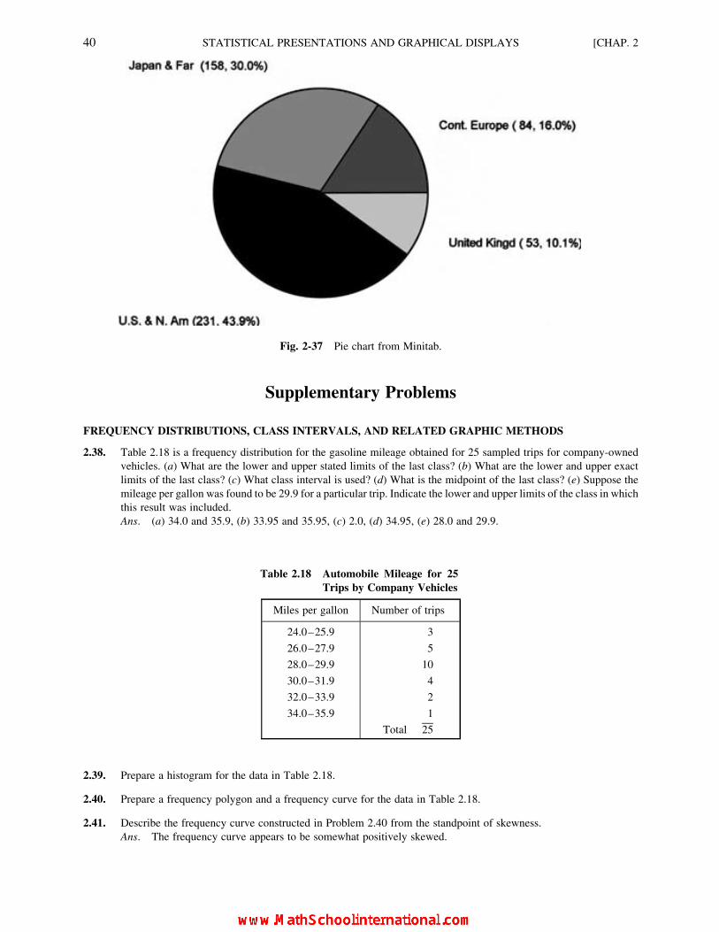
Supplementary Problems
FREQUENCY DISTRIBUTIONS, CLASS INTERVALS, AND RELATED GRAPHIC METHODS
2.38. Table 2.18 is a frequency distribution for the gasoline mileage obtained for 25 sampled trips for company-owned
vehicles. (a) What are the lower and upper stated limits of the last class? (b) What are the lower and upper exact
limits of the last class? (c) What class interval is used? (d) What is the midpoint of the last class? (e) Suppose the
mileage per gallon was found to be 29.9 for a particular trip. Indicate the lower and upper limits of the class in which
this result was included.
Ans. (a) 34.0 and 35.9, (b) 33.95 and 35.95, (c) 2.0, (d) 34.95, (e) 28.0 and 29.9.
2.39. Prepare a histogram for the data in Table 2.18.
2.40. Prepare a frequency polygon and a frequency curve for the data in Table 2.18.
2.41. Describe the frequency curve constructed in Problem 2.40 from the standpoint of skewness.
Ans. The frequency curve appears to be somewhat positively skewed.
Fig. 2-37 Pie chart from Minitab.
Table 2.18 Automobile Mileage for 25
Trips by Company Vehicles
Miles per gallon Number of trips
24.0–25.9 3
26.0–27.9 5
28.0–29.9 10
30.0–31.9 4
32.0–33.9 2
34.0–35.9 1
Total 25
40 STATISTICAL PRESENTATIONS AND GRAPHICAL DISPLAYS [CHAP. 2

2.42. Form a cumulative frequency distribution for the data in Table 2.18 and prepare an ogive to present this distribution
graphically.
2.43. Table 2.19 presents the amounts of 40 personal loans used to finance appliance and furniture purchases. Suppose we
wish to arrange the loan amounts in a frequency distribution with a total of seven classes. Assuming equal class
intervals, what would be a convenient class interval for this frequency distribution?
Ans. $400
2.44. Prepare a frequency distribution for the data in Table 2.19, beginning the first class at a lower class limit of $300 and
using a class interval of $400.
2.45. Prepare a histogram for the frequency distribution formed in Problem 2.44.
2.46. Prepare a frequency polygon and frequency curve for the frequency distribution formed in Problem 2.44.
2.47. Describe the frequency curve constructed in Problem 2.46 in terms of skewness.
Ans. The frequency curve is clearly positively skewed.
2.48. Prepare a cumulative frequency distribution for the frequency distribution formed in Problem 2.44 and prepare an
ogive curve for these data.
FORMS OF FREQUENCY CURVES
2.49. Describe the following curves in terms of skewness or kurtosis, as appropriate: (a) A frequency curve with a tail to
the right, (b) a frequency curve that is relatively peaked, (c) a frequency curve that is relatively flat, (d) a frequency
curve with a tail to the left.
Ans. (a) Positively skewed, (b) leptokurtic, (c) platykurtic, (d ) negatively skewed
RELATIVE FREQUENCY DISTRIBUTIONS
2.50. Prepare a relative frequency table for the frequency distribution presented in Table 2.20.
2.51. Construct a histogram for the relative frequency distribution in Problem 2.50.
2.52. Referring to Table 2.20, (a) What percentage of cutting tools lasted at least 125 hr? (b) What percentage of cutting
tools had a lifetime of at least 100 hr?
Ans. (a) 6%, (b) 31%
2.53 Prepare a table of cumulative proportions for the frequency distribution in Table 2.20.
Table 2.19 The Amounts of 40 Personal
Loans
$ 932 $1,000 $ 356 $2,227
515 554 1,190 954
452 973 300 2,112
1,900 660 1,610 445
1,200 720 1,525 784
1,278 1,388 1,000 870
2,540 851 1,890 630
586 329 935 3,000
1,650 1,423 592 334
1,219 727 655 1,590
CHAP. 2] STATISTICAL PRESENTATIONS AND GRAPHICAL DISPLAYS 41
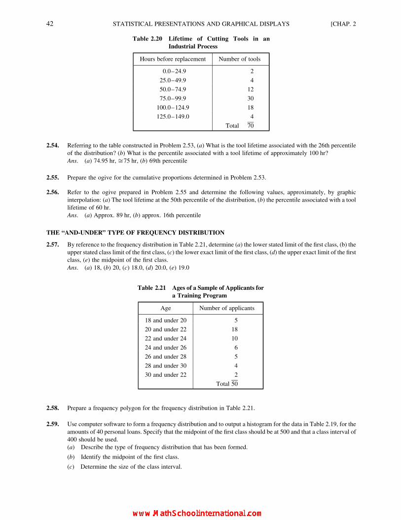
2.54. Referring to the table constructed in Problem 2.53, (a) What is the tool lifetime associated with the 26th percentile
of the distribution? (b) What is the percentile associated with a tool lifetime of approximately 100 hr?
Ans. (a) 74.95 hr, ffi75 hr, (b) 69th percentile
2.55. Prepare the ogive for the cumulative proportions determined in Problem 2.53.
2.56. Refer to the ogive prepared in Problem 2.55 and determine the following values, approximately, by graphic
interpolation: (a) The tool lifetime at the 50th percentile of the distribution, (b) the percentile associated with a tool
lifetime of 60 hr.
Ans. (a) Approx. 89 hr, (b) approx. 16th percentile
THE “AND-UNDER” TYPE OF FREQUENCY DISTRIBUTION
2.57. By reference to the frequency distribution in Table 2.21, determine (a) the lower stated limit of the first class, (b) the
upper stated class limit of the first class, (c) the lower exact limit of the first class, (d) the upper exact limit of the first
class, (e) the midpoint of the first class.
Ans. (a) 18, (b) 20, (c) 18.0, (d) 20.0, (e) 19.0
2.58. Prepare a frequency polygon for the frequency distribution in Table 2.21.
2.59. Use computer software to form a frequency distribution and to output a histogram for the data in Table 2.19, for the
amounts of 40 personal loans. Specify that the midpoint of the first class should be at 500 and that a class interval of
400 should be used.
(a) Describe the type of frequency distribution that has been formed.
(b) Identify the midpoint of the first class.
(c) Determine the size of the class interval.
Table 2.20 Lifetime of Cutting Tools in an
Industrial Process
Hours before replacement Number of tools
0.0–24.9 2
25.0–49.9 4
50.0–74.9 12
75.0–99.9 30
100.0–124.9 18
125.0–149.0 4
Total 70
Table 2.21 Ages of a Sample of Applicants for
a Training Program
Age Number of applicants
18 and under 20 5
20 and under 22 18
22 and under 24 10
24 and under 26 6
26 and under 28 5
28 and under 30 4
30 and under 22 2
Total 50
42 STATISTICAL PRESENTATIONS AND GRAPHICAL DISPLAYS [CHAP. 2

(d) Identify the lower and upper stated class limits for the first class.
(e) Determine the lower and upper exact class limits for the first class.
Ans. (a) and-under frequency distribution, (b) 500.0, (c) 400.0, (d) 200 and 600, (e) 200.0 and 600.0
STEM-AND-LEAF DIAGRAMS
2.60. Prepare a stem-and-leaf diagram for the daily low temperatures that are reported in Table 2.14, for Problem 2.23.
Compare the form of the distribution of daily lows with that of the daily highs, for which the stem-and-leaf diagram
is given in Fig. 2-23.
DOTPLOTS
2.61. Refer to Table 2.15, presented with Problem 2.24, for the resting pulse rates for a sample of 40 adults. Use computer
software to obtain a dotplot similar to the one presented in Fig. 2-24.
BAR CHARTS AND LINE GRAPHS
2.62 Table 2.22 presents the annual investment in R&D (research and development) for a sequence of five years by a
major aerospace company. Construct a vertical bar chart for these data.
2.63. Construct a line graph for the R&D expenditures in the preceding problem.
RUN CHARTS
2.64. When the manufacturing process for AA batteries is in control, the average battery life is 7.5 hours, or 450 minutes.
For 10 sequential samples of nine batteries each that were placed in a rack that systematically drains the batteries to
simulate everyday battery usage, the sample battery life averages are found to be: 460, 450, 440, 470, 460, 450, 420,
430, 440, and 430 minutes. Prepare a run chart for these sample results.
PIE CHARTS
2.65 The foreign sales for a particular year for a major aerospace company are given in Table 2.23. Construct a
percentage pie chart for the revenue from foreign sales according to geographic area.
Table 2.22 Annual Expenditures on
Research and Development
by an Aerospace Company
(in $millions)
Year Amount
1 $751
2 754
3 827
4 1,417
5 1,846
Table 2.23 Foreign Sales for an Aerospace
Company (in $millions)
Europe $7,175
Asia 7,108
Oceania 1,911
Western Hemisphere 872
Africa 430
Total $17,496
CHAP. 2] STATISTICAL PRESENTATIONS AND GRAPHICAL DISPLAYS 43
CHAPTER 3
Describing BusinessData: Measuresof Location
3.1 MEASURES OF LOCATION IN DATA SETS
A measure of location is a value that is calculated for a group of data and that is used to describe the data in
some way. Typically, we wish the value to be representative of all of the values in the group, and thus some kind
of average is desired. In the statistical sense an average is a measure of central tendency for a collection of
values. This chapter covers the various statistical procedures concerned with measures of location.
3.2 THE ARITHMETIC MEAN
The arithmetic mean, or arithmetic average, is defined as the sum of the values in the data group divided by
the number of values.
In statistics, a descriptive measure of a population, or a population parameter, is typically represented by a
Greek letter, whereas a descriptive measure of a sample, or a sample statistic, is represented by a Roman letter.
Thus, the arithmetic mean for a population of values is represented by the symbol m (read “mew”), while the
arithmetic mean for a sample of values is represented by the symbol �XX (read “X bar”). The formulas for the
population mean and the sample mean are
m ¼ SX
N(3:1)
�XX ¼ SX
n(3:2)
Operationally, the two formulas are identical; in both cases, one sums all of the values (SX) and then
divides by the number of values. However, the distinction in the denominators is that in statistical analysis the
uppercase N typically indicates the number of items in the population, while the lowercase n indicates the
number of items in the sample.
44
Copyright 2004, 1996, 1988, 1976 by The McGraw-Hill Companies, Inc. Click Here for Terms of Use.

EXAMPLE 1. During a particular summer month, the eight salespeople in a heating and air-conditioning firm sold the
following number of central air-conditioning units: 8, 11, 5, 14, 8, 11, 16, 11. Considering this month as the statistical
population of interest, the mean number of units sold is
m ¼ SX
N¼ 84
8¼ 10:5 units
Note: For reporting purposes, one generally reports the measures of location to one additional digit beyond the
original level of measurement.
3.3 THE WEIGHTED MEAN
The weighted mean or weighted average is an arithmetic mean in which each value is weighted according
to its importance in the overall group. The formulas for the population, and sample weighted means are
identical:
mw or �XXw ¼ S(wX)
Sw(3:3)
Operationally, each value in the group (X) is multiplied by the appropriate weight factor (w), and the
products are then summed and divided by the sum of the weights.
EXAMPLE 2. In a multiproduct company, the profit margins for the company’s four product lines during the past fiscal
year were: line A, 4.2 percent; line B, 5.5 percent; line C, 7.4 percent; and line D, 10.1 percent. The unweighted mean profit
margin is
m ¼ SX
N¼ 27:2
4¼ 6:8%
However, unless the four products are equal in sales, this unweighted average is incorrect. Assuming the sales totals in
Table 3.1, the weighted mean correctly describes the overall average.
mw ¼ S(wX)
Sw¼ $3,033,000
$58,000,000¼ 5:2%
3.4 THE MEDIAN
The median of a group of items is the value of the middle item when all the items in the group are arranged
in either ascending or descending order, in terms of value. For a group with an even number of items, the
median is assumed to be midway between the two values adjacent to the middle. When a large number of values
is contained in the group, the following formula to determine the position of the median in the ordered group is
useful:
Med ¼ X[(n=2)þ (1=2)] (3:4)
Table 3.1 Profit Margin and Sales Volume for Four Product Lines
Product line Profit margin (X) Sales (w) wX
A 4.2% $30,000,000 $1,260,000
B 5.5 20,000,000 1,100,000
C 7.4 5,000,000 370,000
D 10.1 3,000,000 303,000
Sw ¼ $58,000,000 S(wX) ¼ $3,033,000
CHAP. 3] DESCRIBING BUSINESS DATA: MEASURES OF LOCATION 45
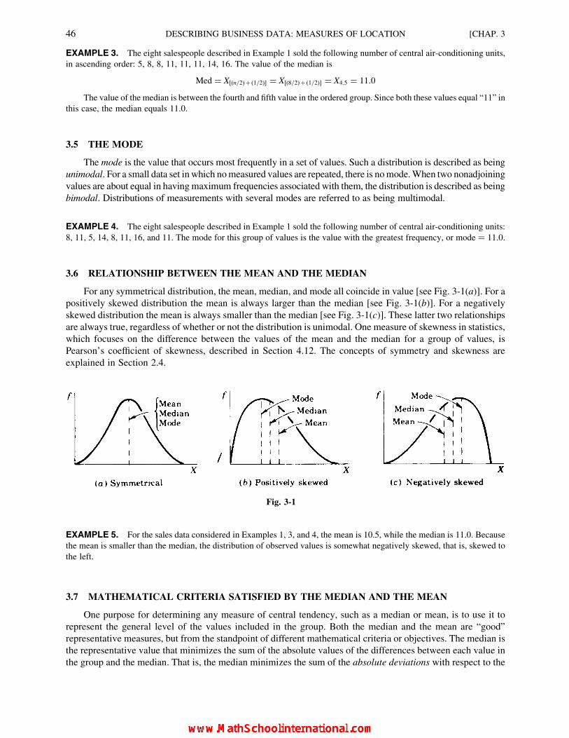
EXAMPLE 3. The eight salespeople described in Example 1 sold the following number of central air-conditioning units,
in ascending order: 5, 8, 8, 11, 11, 11, 14, 16. The value of the median is
Med ¼ X[(n=2)þ (1=2)] ¼ X[(8=2)þ (1=2)] ¼ X4:5 ¼ 11:0
The value of the median is between the fourth and fifth value in the ordered group. Since both these values equal “11” in
this case, the median equals 11.0.
3.5 THE MODE
The mode is the value that occurs most frequently in a set of values. Such a distribution is described as being
unimodal. For a small data set in which nomeasured values are repeated, there is nomode.When two nonadjoining
values are about equal in havingmaximum frequencies associated with them, the distribution is described as being
bimodal. Distributions of measurements with several modes are referred to as being multimodal.
EXAMPLE 4. The eight salespeople described in Example 1 sold the following number of central air-conditioning units:
8, 11, 5, 14, 8, 11, 16, and 11. The mode for this group of values is the value with the greatest frequency, or mode ¼ 11.0.
3.6 RELATIONSHIP BETWEEN THE MEAN AND THE MEDIAN
For any symmetrical distribution, the mean, median, and mode all coincide in value [see Fig. 3-1(a)]. For a
positively skewed distribution the mean is always larger than the median [see Fig. 3-1(b)]. For a negatively
skewed distribution the mean is always smaller than the median [see Fig. 3-1(c)]. These latter two relationships
are always true, regardless of whether or not the distribution is unimodal. One measure of skewness in statistics,
which focuses on the difference between the values of the mean and the median for a group of values, is
Pearson’s coefficient of skewness, described in Section 4.12. The concepts of symmetry and skewness are
explained in Section 2.4.
EXAMPLE 5. For the sales data considered in Examples 1, 3, and 4, the mean is 10.5, while the median is 11.0. Because
the mean is smaller than the median, the distribution of observed values is somewhat negatively skewed, that is, skewed to
the left.
3.7 MATHEMATICAL CRITERIA SATISFIED BY THE MEDIAN AND THE MEAN
One purpose for determining any measure of central tendency, such as a median or mean, is to use it to
represent the general level of the values included in the group. Both the median and the mean are “good”
representative measures, but from the standpoint of different mathematical criteria or objectives. The median is
the representative value that minimizes the sum of the absolute values of the differences between each value in
the group and the median. That is, the median minimizes the sum of the absolute deviations with respect to the
Fig. 3-1
46 DESCRIBING BUSINESS DATA: MEASURES OF LOCATION [CHAP. 3

individual values being represented. In contrast, the arithmetic mean focuses on minimizing the sum of the
squared deviations with respect to the individual values in the group. The criterion by which the objective is that
of minimizing the sum of the squared deviations associated with a representative value is called the least-
squares criterion. This criterion is the one that is most important in statistical inference based on sample data, as
discussed further in the following section.
EXAMPLE 6. For the sales data that we have considered in the previous examples, the median is 11.0 and the mean is
10.5. The ordered sales amounts are presented in the first column of Table 3.2. The other columns of this table are concerned
with determining the sum of the absolute deviations and of the squared deviations of the individual values with respect to
both the median and the mean. Note that the sum of the absolute deviations for the median, 20, is lower than the
corresponding sum of 21.0 for the mean. On the other hand, for the least-squares criterion, the sum of the squared deviations
for the mean, 86.00, is lower than the corresponding sum of 88 for the median. No value that is different from the mean can
have a lower sum of squared deviations than the mean.
3.8 USE OF THE MEAN, MEDIAN, AND MODE
We first consider the use of these measures of average for representing population data. The value of the
mode indicates where most of the observed values, such as hourly wage rates in a company, are located. It can
be useful as a descriptive measure for a population group, but only if there is one clear mode. On the other hand,
the median is always an excellent measure by which to represent the “typical” level of observed values, such as
wage rates, in a population. This is true regardless of whether there is more than one mode or whether the
population distribution is skewed or symmetrical. The lack of symmetry is no special problem because the
median wage rate, for example, is always the wage rate of the “middle person” when the wage rates are listed in
order of magnitude. The arithmetic mean is also an excellent representative value for a population, but only if
the population is fairly symmetrical. For nonsymmetrical data, the extreme values (for instance, a few very high
wage rates for technical specialists) will serve to distort the value of the mean as a representative value. Thus,
the median is generally the best measure of data location for describing population data.
We now consider the use of the three measures of location with respect to sample data. Recall from Chapter 1
that the purpose of statistical inference with sample data is to make probability statements about the population
from which the sample was selected. The mode is not a good measure of location with respect to sample data
because its value can vary greatly from sample to sample. The median is better than the mode because its value is
more stable from sample to sample. However, the value of the mean is the most stable of the three measures. As
will be introduced further in Section 4.9 and explained fully in Chapter 8, the reason for the relative stability of the
sample mean from sample to sample is because it is the measure of location that satisfies the least-squares
criterion. Thus, for sample data, the best measure of location generally is the arithmetic mean.
Table 3.2 Mathematical Criteria Satisfied by the Median and the Mean
(Med 5 11.0; Mean 5 10.5)
X jX 2 Medj jX 2 Meanj (X 2 Med)2 (X 2 Mean)2
5 6 5.5 36 30.25
8 3 2.5 9 6.25
8 3 2.5 9 6.25
11 0 0.5 0 0.25
11 0 0.5 0 0.25
11 0 0.5 0 0.25
14 3 3.5 9 12.25
16 5 5.5 25 30.25
Sum 20 21.0 88 86.00
CHAP. 3] DESCRIBING BUSINESS DATA: MEASURES OF LOCATION 47

EXAMPLE 7. The wage rates of all 650 hourly employees in a manufacturing firm have been compiled. The best
representative measure of the typical wage rate is the median, because a population is involved and the median is relatively
unaffected by any lack of symmetry in the wage rates. In fact, such data as wage rates and salary amounts are likely to be
positively skewed, with relatively few wage or salary amounts being exceptionally high and in the right tail of the distribution.
EXAMPLE 8. A random sample of n ¼ 100 wage rates is obtained in a company having several thousand hourly
employees. The best representative wage rate for the several thousand employees is the sample mean. Although the sample
mean is unlikely to be exactly equal to the mean wage rate for the entire population, it will generally be much closer to the
population mean than the sample median would be as an estimator of the population median wage rate.
3.9 USE OF THE MEAN IN STATISTICAL PROCESS CONTROL
In Section 2.12 we observed that a run chart is a plot of data values in the time-sequence order in which they
were observed, and that the values plotted can be individual values or averages of sequential samples. We prefer
to plot averages rather than individual values because any average generally will be more stable (less variable)
from sample to sample than are the individual observations. As we observed in the preceding section, the
sample mean is more stable than either the median or the mode. For this reason, the focus of run charts
concerned with sample averages is to plot the sample means. Such a chart is called an �XX chart, and serves as the
basis for determining whether a process is stable, or whether there is process variation with an assignable cause
that should be corrected.
EXAMPLE 9. Refer to the run chart in Fig. 2-11 (page 18) of the preceding chapter. This run chart for the sequence of
mean weights for samples of n ¼ 4 packages of potato chips is typical of the kinds of charts that are prepared for the purpose
of statistical process control, as explained and illustrated in Chapter 19.
3.10 QUARTILES, DECILES, AND PERCENTILES
Quartiles, deciles, and percentiles are similar to the median in that they also subdivide a distribution of
measurements according to the proportion of frequencies observed. Whereas the median divides a distribution
into halves, quartiles divide it into quarters, deciles divide it into tenths, and percentile points divide it into 100
parts. Formula (3.4) for the median is modified according to the fraction point of interest. For example,
Q1(first quartile) ¼ X[(n=4)þ (1=2)] (3:5)
D3(third decile) ¼ X[(3n=10)þ (1=2)] (3:6)
P70(seventieth percentile) ¼ X[(70n=100)þ (1=2)] (3:7)
EXAMPLE 10. The eight salespeople described in Example 1 sold the following number of central air-conditioning units,
in ascending order: 5, 8, 8, 11, 11, 11, 14, 16. Find the positions of the first quartile and third quartile for this distribution.
Q1 ¼ X[(n=4)þ (1=2)] ¼ X[(8=4)þ (1=2)] ¼ X2:5 ¼ 8:0
Q3 ¼ X[(3n=4)þ (1=2)] ¼ X[(24=4)þ (1=2)] ¼ X6:5 ¼ 12:5
The position of the first quartile is midway between the second and third values in the ordered array. Since both of these
values are 8, the value at the first quartile is 8.0. The value of the third quartile is midway between the sixth and seventh
values in the array, or midway between 11 and 14, which is 12.5.
3.11 USING EXCEL AND MINITAB
Computer software is available to determine a variety of measures of average. Solved Problems 3.17 and
3.18 illustrate the use of Excel and Minitab to determine the values of the mean and median for a sample of
product assembly times.
48 DESCRIBING BUSINESS DATA: MEASURES OF LOCATION [CHAP. 3
Solved Problems
THE MEAN, MEDIAN, AND MODE
3.1. For a sample of 15 students at an elementary-school snack bar, the following sales amounts arranged in
ascending order of magnitude are observed: $0.10, 0.10, 0.25, 0.25, 0.25, 0.35, 0.40, 0.53, 0.90, 1.25,
1.35, 2.45, 2.71, 3.09, 4.10. Determine the (a) mean, (b) median, and (c) mode for these sales amounts.
(a) �XX ¼ SX
n¼ 18:08
15¼ $1:21
(b) Med ¼ X[(n=2)þ (1=2)] ¼ X[(15=2)þ (1=2)] ¼ X8 ¼ $0:53
(c) Mode ¼ most frequent value ¼ $0.25
3.2. How would you describe the distribution in Problem 3.1 from the standpoint of skewness?
With the mean being substantially larger than the median, the distribution of values is clearly positively
skewed, or skewed to the right.
3.3. For the data in Problem 3.1, suppose that you are asked to determine the typical purchase amount only
for this particular group of students. Which measure of average would you report? Why?
Note that once we decide to focus only on this particular group, we are treating this group as our population of
interest. Therefore, the best choice is to report the median as being the typical value; this is the eighth value in the
array, or $0.53.
3.4. Refer to Problem 3.3 above. Suppose we wish to estimate the typical amount of purchase in the
population from which the sample was taken. Which measure of average would you report? Why?
Because statistical inference for a population is involved, our main concern is to report an average that is the most
stable and has the least variability from sample to sample. The average that satisfied this requirement is the mean,
because it satisfies the least-squares criterion. Therefore, the value reported should be the sample mean, or $1.21.
3.5. A sample of 20 production workers in a company earned the following net pay amounts after all
deductions for a given week, rounded to the nearest dollar and arranged in ascending order: $240, 240,
240, 240, 240, 240, 240, 240, 255, 255, 265, 265, 280, 280, 290, 300, 305, 325, 330, 340. Calculate the
(a) mean, (b) median, and (c) mode for this group of wages.
(a) �XX ¼ SX
n¼ 5,410
20¼ $270:50
(b) Median ¼ X[(n=2)þ (1=2)] ¼ X[(20=2)þ (1=2)] ¼ X10:5 ¼ $260:00
(c) Mode ¼ most frequent value ¼ $240.00
3.6. For the wage data in Problem 3.5, describe the distribution in terms of skewness.
With the mean being larger than the median, the distribution can be described as being positively skewed, or
skewed to the right.
3.7. With respect to the data in Problem 3.5, suppose you are the vice president in charge of collective
bargaining for the company. What measure of average net pay would you report as being representative
of all the company workers in general?
Because the sample mean is the highest of the three averages, your inclination might be to report this value.
Using this value is highly defensible, given that statistical inference is involved and that the sample mean is the most
stable of the estimators that might be used.
CHAP. 3] DESCRIBING BUSINESS DATA: MEASURES OF LOCATION 49
3.8. With respect to the data in Problem 3.5, suppose you are the elected president of the employee bargaining
unit. What measure of average would you report as being representative of workers in general?
In terms of your bargaining position, you might be inclined to report the mode, or at least the median, rather
than the mean. Defense of your choice would rest on identifying the net pay amounts for most people in the sample
(for the mode) or on the observation that the sample mean is affected by a few high wage amounts. However, both
the median and mode have more variability from sample to sample, and therefore are less stable population
estimators than is the mean.
3.9. A work-standards expert observes the amount of time required to prepare a sample of 10 business letters
in an office, with the following results listed in ascending order to the nearest minute: 5, 5, 5, 7, 9, 14, 15,
15, 16, 18. Determine the (a) mean, (b) median, and (c) mode for this group of values.
(a) �XX ¼ SX
n¼ 109
10¼ 10:9min
(b) Med ¼ X[(n=2)þ (1=2)] ¼ X[(10=2)þ (1=2)] ¼ X5:5 ¼ 11:5min
(c) Mode ¼ most frequent value ¼ 5.0
3.10. Compare the values of the mean and median in Problem 3.9 and comment on the form of the
distribution.
Because the mean is smaller than the median, the distribution is somewhat negatively skewed.
THE WEIGHTED MEAN
3.11. Suppose that the per-gallon prices of unleaded regular gasoline are listed for 22 metropolitan areas
varying considerably in size and in gasoline sales. The (a) median and (b) arithmetic mean are computed
for these data. Describe the meaning that each of these values would have.
(a) The median would indicate the average, or typical, price in the sense that half the metropolitan areas would
have gasoline prices below this value and half would have prices above this value.
(b) The meaning of the arithmetic mean as an unweighted value is questionable at best. Clearly, it would not
indicate the mean gasoline prices being paid by all the gasoline purchasers living in the 22 metropolitan areas,
because the small metropolitan areas would be represented equally with the large areas in such an average. In
order to determine a suitable mean for all purchasers in these metropolitan areas, a weighted mean (using
gasoline sales as weights) would have to be computed.
3.12. Referring to Table 3.3, determine the overall percentage defective of all items assembled during the
sampled week.
Using formula (3.3),
�XXw ¼ S(wX)
Sw¼ 526:0
380¼ 1:4% defective
Table 3.3 Percentage of Defective Items in an Assembly Department in a Sampled Week
Shift Percentage defective (X)
Number of items, in thousands
(w) wX
1 1.1 210 231.0
2 1.5 120 180.0
3 2.3 50 115.0
Sw ¼ 380 S(wX) ¼ 526.0
50 DESCRIBING BUSINESS DATA: MEASURES OF LOCATION [CHAP. 3

MATHEMATICAL CRITERIA SATISFIED BY THE MEDIAN AND THE MEAN
3.13. Refer to the sample data in Problem 3.5 and demonstrate that the sum of the absolute values of the
deviations is a smaller sum for the median than it is for the mean. Also demonstrate that the sum of the
squared deviations is smaller for the mean than it is for the median.
By reference to Table 3.4, we see that the sum of the absolute deviations for the median is 550, which is less
than the corresponding sum of 572.00 for the mean. Also, as expected, the sum of the squared deviations of
21,945.00 for the mean is less than the corresponding sum of 24,150 for the median.
3.14. Refer to the sum of the squared deviations for the mean as determined in Problem 3.13 above.
Demonstrate that no other “typical” value for the group has a lower sum of squared deviations by
choosing trial averages of $270 and of $271. Note that each of these trial values is equally and just
fractionally different from the sample mean of $270.50, but in opposite directions.
By reference to Table 3.5, we see that these two trial averages have the same sum of squared deviations,
21,950, which is greater than the corresponding sum of 21,945.00 for the sample mean. Any other trial value
that has a greater difference from the sample mean, in either direction, would have a still-higher sum of squared
deviations.
Table 3.4 Mathematical Criteria Satisfied for the Pay Data in Problem 3.5
(Med 5 $260.00; Mean 5 $270.50)
X jX 2 Medj jX 2 Meanj (X 2 Med)2 (X 2 Mean)2
240 20 30.50 400 930.25
240 20 30.50 400 930.25
240 20 30.50 400 930.25
240 20 30.50 400 930.25
240 20 30.50 400 930.25
240 20 30.50 400 930.25
240 20 30.50 400 930.25
240 20 30.50 400 930.25
255 5 15.50 25 240.25
255 5 15.50 25 240.25
265 5 5.50 25 30.25
265 5 5.50 25 30.25
280 20 9.50 400 90.25
280 20 9.50 400 90.25
290 30 19.50 900 380.25
300 40 29.50 1,600 870.25
305 45 34.50 2,025 1,190.25
325 65 54.50 4,225 2,970.25
330 70 59.50 4,900 3,540.25
340 80 69.50 6,400 4,830.25
Sum 550 572.00 24,150 21,945.00
CHAP. 3] DESCRIBING BUSINESS DATA: MEASURES OF LOCATION 51

QUARTILES, DECILES, AND PERCENTILES
3.15. For the data in Problem 3.1, determine the values at the (a) second quartile, (b) second decile, and (c)
40th percentile point for these sales amounts.
(a) Q2 ¼ X[(2n=4)þ (1=2)] ¼ X(7:5þ 0:5) ¼ X8 ¼ $0:53
(Note: By definition, the second quartile is always at the same point as the median.)
(b) D2 ¼ X[(2n=10)þ (1=2)] ¼ X(3:0þ 0:5) ¼ X3:5 ¼ $0:25
(Note: This is the value midway between the third and fourth sales amounts, arranged in ascending order.)
(c) P40 ¼ X[(40n=100)þ (1=2)] ¼ X(6:0þ 0:5) ¼ X6:5 ¼ 0:375 ffi $0:38
3.16. For the measurements in Problem 3.5, determine the values at the (a) third quartile, (b) ninth decile, (c)
50th percentile point, and (d) 84th percentile point for this group of wages.
(a) Q3 ¼ X[(3n=4)þ (1=2)] ¼ X15:5 ¼ $295:00
(Note: This is the value midway between the 15th and 16th wage amounts, arranged in ascending order.)
(b) D9 ¼ X[(9n=10)þ (1=2)] ¼ X18:5 ¼ $327:50
(c) P50 ¼ X[(50n=100)þ (1=2)] ¼ X10:5 ¼ $260:00
(Note: By definition the 50th percentile point is always at the same point as the median.)
(d ) P84 ¼ X[(84n=100)þ (1=2)] ¼ X(16:8þ 0:5) ¼ X17:3 ¼ $311:00
(Note: This is the value which is three-tenths of the way between the 17th and 18th wage amounts arranged
in ascending order.)
Table 3.5 Alternative Values Used in Lieu of the Mean in Table 3.4
X jX 2 270j jX 2 271j (X 2 270)2 (X 2 271)2
240 30 31 900 961
240 30 31 900 961
240 30 31 900 961
240 30 31 900 961
240 30 31 900 961
240 30 31 900 961
240 30 31 900 961
240 30 31 900 961
255 15 16 225 256
255 15 16 225 256
265 5 6 25 36
265 5 6 25 36
280 10 9 100 81
280 10 9 100 81
290 20 19 400 361
300 30 19 900 841
305 35 34 1,225 1,156
325 55 54 3,025 2,916
330 60 59 3,600 3,481
340 70 69 4,900 4,761
Sum 570 564 21,950 21,950
52 DESCRIBING BUSINESS DATA: MEASURES OF LOCATION [CHAP. 3
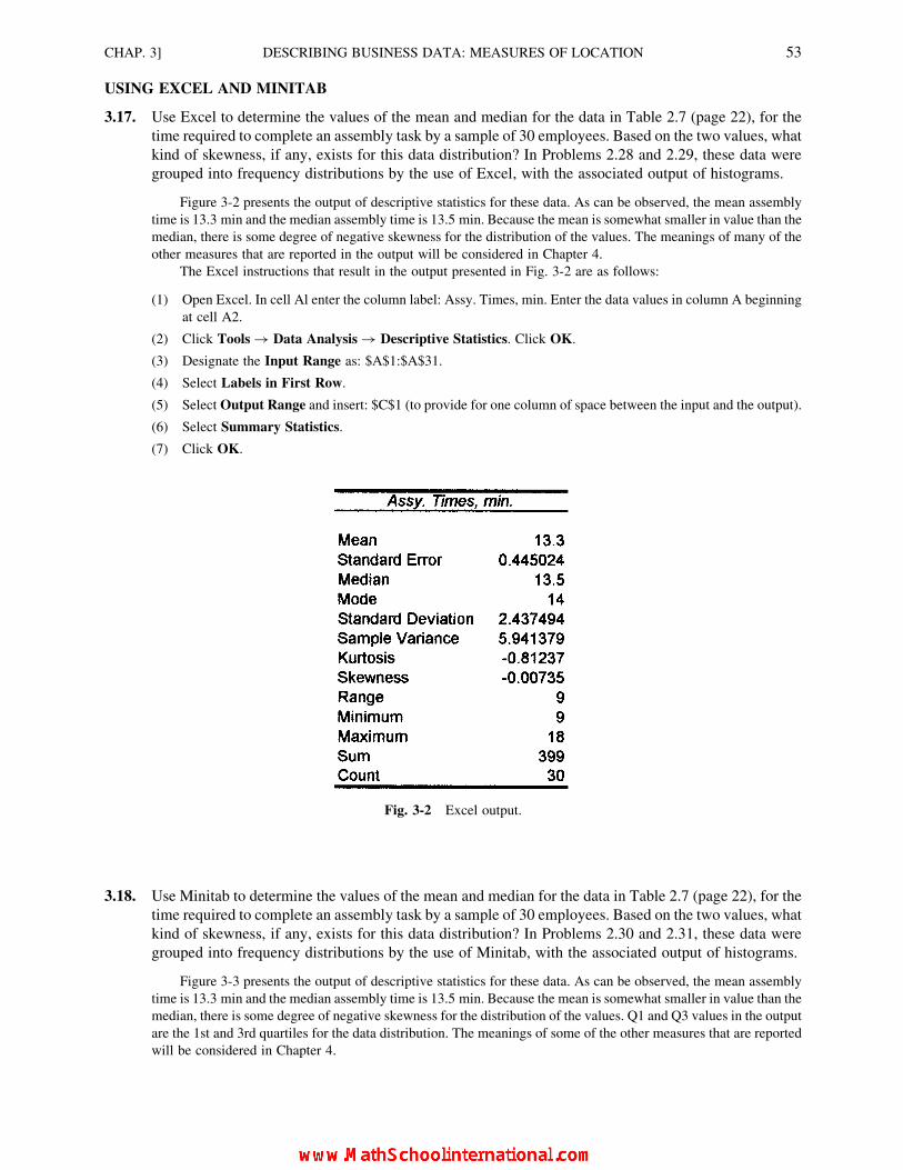
USING EXCEL AND MINITAB
3.17. Use Excel to determine the values of the mean and median for the data in Table 2.7 (page 22), for the
time required to complete an assembly task by a sample of 30 employees. Based on the two values, what
kind of skewness, if any, exists for this data distribution? In Problems 2.28 and 2.29, these data were
grouped into frequency distributions by the use of Excel, with the associated output of histograms.
Figure 3-2 presents the output of descriptive statistics for these data. As can be observed, the mean assembly
time is 13.3 min and the median assembly time is 13.5 min. Because the mean is somewhat smaller in value than the
median, there is some degree of negative skewness for the distribution of the values. The meanings of many of the
other measures that are reported in the output will be considered in Chapter 4.
The Excel instructions that result in the output presented in Fig. 3-2 are as follows:
(1) Open Excel. In cell Al enter the column label: Assy. Times, min. Enter the data values in column A beginning
at cell A2.
(2) Click Tools ! Data Analysis ! Descriptive Statistics. Click OK.
(3) Designate the Input Range as: $A$1:$A$31.
(4) Select Labels in First Row.
(5) Select Output Range and insert: $C$1 (to provide for one column of space between the input and the output).
(6) Select Summary Statistics.
(7) Click OK.
3.18. Use Minitab to determine the values of the mean and median for the data in Table 2.7 (page 22), for the
time required to complete an assembly task by a sample of 30 employees. Based on the two values, what
kind of skewness, if any, exists for this data distribution? In Problems 2.30 and 2.31, these data were
grouped into frequency distributions by the use of Minitab, with the associated output of histograms.
Figure 3-3 presents the output of descriptive statistics for these data. As can be observed, the mean assembly
time is 13.3 min and the median assembly time is 13.5 min. Because the mean is somewhat smaller in value than the
median, there is some degree of negative skewness for the distribution of the values. Q1 and Q3 values in the output
are the 1st and 3rd quartiles for the data distribution. The meanings of some of the other measures that are reported
will be considered in Chapter 4.
Fig. 3-2 Excel output.
CHAP. 3] DESCRIBING BUSINESS DATA: MEASURES OF LOCATION 53

The Minitab instructions that result in the output presented in Fig. 3-2 are as follows:
(1) Open Minitab. In the column-name cell for column C1 enter: Assy. Times, min. Then enter the sample data in
column C1.
(2) Click Stat ! Basic Statistics ! Display Descriptive Statistics.
(3) For Variables enter: C1.
(4) Click OK.
Supplementary Problems
THE MEAN, MEDIAN, AND MODE
3.19. The number of cars sold by each of the 10 salespeople in an automobile dealership during a particular month,
arranged in ascending order, is: 2, 4, 7, 10, 10, 10, 12, 12, 14, 15. Determine the population (a) mean, (b) median,
and (c) mode for the number of cars sold.
Ans. (a) 9.6, (b) 10.0, (c) 10.0
3.20. Which value in Problem 3.19 best describes the “typical” sales volume per salesperson?
Ans. 10.0
3.21. Describe the distribution of the sales data in Problem 3.19 in terms of skewness.
Ans. Positively skewed.
3.22. The weights of a sample of outgoing packages in a mailroom, weighed to the nearest ounce, are found to be: 21, 18,
30, 12, 14, 17, 28, 10, 16, 25 oz. Determine the (a) mean, (b) median, and (c) mode for these weights.
Ans. (a) 19.1, (b) 17.5, (c) there is no mode
3.23. Describe the distribution of the weights in Problem 3.22 in terms of skewness.
Ans. Positively skewed.
3.24. As indicated by the wording in Problem 3.22, the packages that were weighed are a random sample of all such
packages handled in the mailroom. What is the best estimate of the typical weight of all packages handled in the
mailroom?
Ans. 19.1 oz
3.25. For the weights reported in Problem 3.22, suppose we wish to describe only the weights of the selected group of
packages. What is the best representative value for the group?
Ans. 17.5 oz
3.26. The following examination scores, arranged in ascending order, were achieved by 20 students enrolled in a decision
analysis course: 39, 46, 57, 65, 70, 72, 72, 75, 77, 79, 81, 81, 84, 84, 84, 87, 93, 94, 97, 97. Determine the (a) mean,
(b) median, and (c) mode for these scores.
Ans. (a) 76.7, (b) 80.0, (c) 84.0
Fig. 3-3 Minitab output.
54 DESCRIBING BUSINESS DATA: MEASURES OF LOCATION [CHAP. 3

3.27. Describe the distribution of test scores in ProbIem 3.26 in terms of skewness.
Ans. Negatively skewed.
3.28. The number of accidents which occurred during a given month in the 13 manufacturing departments of an industrial
plant was: 2, 0, 0, 3, 3, 12, 1, 0, 8, 1, 0, 5, 1. Calculate the (a) mean, (b) median, and (c) mode for the number of
accidents per department.
Ans. (a) 2.8, (b) 1.0, (c) 0
3.29. Describe the distribution of accident rates reported in Problem 3.28 in terms of skewness.
Ans. Positively skewed.
THE WEIGHTED MEAN
3.30. Suppose the retail prices of the selected items have changed as indicated in Table 3.6. Determine the mean
percentage change in retail prices without reference to the average expenditures included in the table.
Ans. 4.0%
3.31. Referring to Table 3.6, determine the mean percentage change by weighting the percent increase for each item by
the average amount per month spent on that item before the increase.
Ans. 6.0%
3.32. Is the mean percentage price change calculated in Problem 3.30 or 3.31 more appropriate as a measure of the impact
of the price changes on this particular consumer? Why?
Ans. The weighted mean in Problem 3.31 is more appropriate (see Example 2 for an explanation).
QUARTILES, DECILES, AND PERCENTILES
3.33. Determine the values at the (a) first quartile, (b) second decile, and (c) 30th percentile point for the sales amounts in
Problem 3.19.
Ans. (a) 7.0, (b) 5.5, (c) 8.5
3.34. From Problem 3.22, determine the weights at the (a) third quartile, (b) third decile, and (c) 70th percentile point.
Ans. (a) 25.0 oz, (b) 15.0 oz, (c) 23.0 oz
3.35. Determine the (a) second quartile, (b) ninth decile, and (c) 50th percentile point for the examination scores in
Problem 3.26
Ans. (a) 80.0, (b) 95.5, (c) 80.0
Table 3.6 Changes in the Retail Prices of Selected Items During a
Particular Year
Item Percent increase
Average expenditure per month
(before increase)
Milk 10% $20.00
Ground beef 26 30.00
Apparel 28 30.00
Gasoline 20 50.00
CHAP. 3] DESCRIBING BUSINESS DATA: MEASURES OF LOCATION 55

3.36. In general, which quartile, decile, and percentile point, respectively, are equivalent to the median?
Ans. Second quartile, fifth decile, and 50th percentile point.
COMPUTER OUTPUT
3.37. Use computer software to determine the mean and the median for the data in Table 2.19 (page 41), for the amounts
of 40 personal loans.
Ans. The mean loan amount is $1,097.40 and the median is $944.50.
56 DESCRIBING BUSINESS DATA: MEASURES OF LOCATION [CHAP. 3
CHAPTER 4
Describing BusinessData: Measures
of Dispersion
4.1 MEASURES OF DISPERSION IN DATA SETS
The measures of central tendency described in Chapter 3 are useful for identifying the “typical” value in a
group of values. In contrast, measures of dispersion, or variability, are concerned with describing the variability
among the values. Several techniques are available for measuring the extent of variability in data sets. The ones
which are described in this chapter are the range, modified ranges, average deviation, variance, standard
deviation, and coefficient of variation.
EXAMPLE 1. Suppose that two different packaging machines result in a mean weight of 10.0 oz of cereal being
packaged, but that in one case all packages are within 0.10 oz of this weight while in the other case the weights may vary by
as much as 1.0 oz in either direction. Measuring the variability, or dispersion, of the amounts being packaged would be every
bit as important as measuring the average in this case.
The concept of skewness has been described in Section 2.4 and 3.6. Pearson’s coefficient of skewness is
described in Section 4.12.
4.2 THE RANGE
The range, or R, is the difference between highest and lowest values included in a data set. Thus, when H
represents the highest value in the group and L represents the lowest value, the range for ungrouped data is
R ¼ H � L (4:1)
57
Copyright 2004, 1996, 1988, 1976 by The McGraw-Hill Companies, Inc. Click Here for Terms of Use.

EXAMPLE 2. During a particular summer month, the eight salespeople in a heating and air-conditioning firm sold the
following numbers of central air-conditioning units: 8, 11, 5, 14, 8, 11, 16, 11. The range of the number of units sold is
R ¼ H � L ¼ 16� 5 ¼ 11:0 units
Note: For purposes of comparison, we generally report the measures of variability to one additional digit beyond the
original level of measurement.
4.3 MODIFIED RANGES
A modified range is a range for which some of the extreme values at each end of the distribution are
eliminated from consideration. The middle 50 percent is the range between the values at the 25th percentile
point and the 75th percentile point of the distribution. As such, it is also the range between the first and third
quartiles of the distribution. For this reason, the middle 50 percent range is usually designated as the
interquartile range (IQR). Thus,
IQR ¼ Q3 � Q1 (4:2)
Other modified ranges that are sometimes used are the middle 80 percent, middle 90 percent, and middle
95 percent.
EXAMPLE 3. The data for the sales of central air-conditioning units presented in Example 2, in ascending order, are: 5, 8, 8,
11, 11, 11, 14, 16. Thus the number of observations is N ¼ 8 for these population data. To compute the interquartile range, we
first must determine the values atQ3 (the 75th percentile point) and Q1 (the 25th percentile point) and then subtractQ1 fromQ3:
Q3 ¼ X[(75N=100)þ (1=2)] ¼ X[6þ (1=2)] ¼ X6:5 ¼ 12:5
Q1 ¼ X[(25N=100)þ (1=2)] ¼ X[2þ (1=2)] ¼ X2:5 ¼ 8:0
IQR ¼ Q3 � Q1 ¼ 12:5� 8:0 ¼ 4:5 units
4.4 BOX PLOTS
A box plot is a graph that portrays the distribution of a data set by reference to the values at the quartiles as
location measures and the value of the interquartile range as the reference measure of variability. A box plot is a
relatively easy way of graphing data and observing the extent of skewness in the distribution. As such, it is an
easier alternative to forming a frequency distribution and plotting a histogram, as described in Sections 2.1 to
2.3. The box plot is also called a box-and-whisker plot, for reasons that will be obvious in Example 4, below.
Because of its relative ease of use, the box plot is a principal technique of exploratory data analysis, as
described in Section 2.8 on stem-and-leaf displays.
EXAMPLE 4. Figure 4-1 presents the box plot for the unit sales data in Example 3. The lower and upper boundary points of
the rectangular box in the graph are called hinges and generally are located at Q1 and Q3. Thus, based on the quartile values
determined in Example 3, the lower hinge is at 8.0 and the upper hinge is at 12.5. The vertical line within the box indicates the
position of the median (or Q2), which is at 11.0. The dashed horizontal lines to the left and right of the box are called whiskers
and extend to the “inner fences,” which are 1.5 units of the interquartile range in each direction. Thus, the whiskers extend to:
Q1 � (1:5� IQR) ¼ 8:0� (1:5)(4:5) ¼ 1:25
Q3 þ (1:5� IQR) ¼ 12:5þ (1:5)(4:5) ¼ 19:25
The “outer fences” in Fig. 4-1 extend to 3.0 units of the interquartile range in each direction fromQ1 andQ3, or to25.5 and
25.5 for the lower and upper outer fences, respectively. For this example note that the lower outer fence is at the value of 0 for
practical purposes, since negative units of sale are not possible. Any values lying between the inner and outer fences are
considered to be mild outliers, while values located beyond the outer fences are extreme outliers. For any outliers, we would
investigate whether such values were collected under the same circumstances as the other values, andwhether anymeasurement
errors may have occurred. There are clearly no outliers for our small group of eight values, since all the sales values listed in
Example 3 are within the inner fences.
58 DESCRIBING BUSINESS DATA: MEASURES OF DISPERSION [CHAP. 4
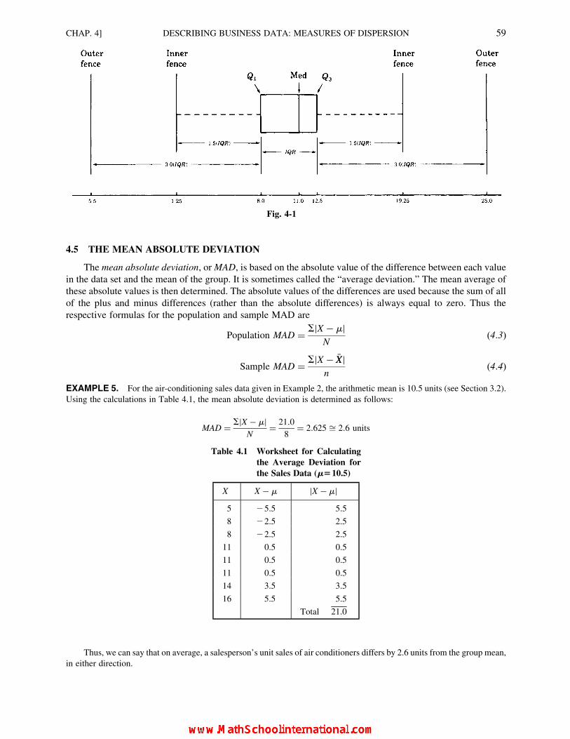
4.5 THE MEAN ABSOLUTE DEVIATION
The mean absolute deviation, or MAD, is based on the absolute value of the difference between each value
in the data set and the mean of the group. It is sometimes called the “average deviation.” The mean average of
these absolute values is then determined. The absolute values of the differences are used because the sum of all
of the plus and minus differences (rather than the absolute differences) is always equal to zero. Thus the
respective formulas for the population and sample MAD are
Population MAD ¼ SjX � mjN
(4:3)
Sample MAD ¼ SjX � �XXjn
(4:4)
EXAMPLE 5. For the air-conditioning sales data given in Example 2, the arithmetic mean is 10.5 units (see Section 3.2).
Using the calculations in Table 4.1, the mean absolute deviation is determined as follows:
MAD ¼ SjX � mjN
¼ 21:0
8¼ 2:625 ffi 2:6 units
Table 4.1 Worksheet for Calculating
the Average Deviation for
the Sales Data (m510.5)
X X � m jX � mj5 25.5 5.5
8 22.5 2.5
8 22.5 2.5
11 0.5 0.5
11 0.5 0.5
11 0.5 0.5
14 3.5 3.5
16 5.5 5.5
Total 21.0
Thus, we can say that on average, a salesperson’s unit sales of air conditioners differs by 2.6 units from the group mean,
in either direction.
Fig. 4-1
CHAP. 4] DESCRIBING BUSINESS DATA: MEASURES OF DISPERSION 59

4.6 THE VARIANCE AND STANDARD DEVIATION
The variance is similar to the mean absolute deviation in that it is based on the difference between each
value in the data set and the mean of the group. It differs in one very important way: each difference is squared
before being summed. For a population, the variance is represented by V(X) or, more typically, by the lowercase
Greek s 2 (read “sigma squared”). The formula is
V(X) ¼ s 2 ¼ S(X � m)2
N(4:5)
Unlike the situation for other sample statistics we have discussed, the variance for a sample is not
computationally exactly equivalent to the variance for a population. Rather, the denominator in the sample
variance formula is slightly different. Essentially, a correction factor is included in this formula, so that the
sample variance is an unbiased estimator of the population variance (see Section 8.1). The sample variance is
represented by s2; its formula is
s2 ¼ S(X � �XX)2
n � 1(4:6)
In general, it is difficult to interpret the meaning of the value of a variance because the units in which it is
expressed are squared values. Partly for this reason, the square root of the variance, represented by Greek s (or s
for a sample) and called the standard deviation is more frequently used. The formulas are
Population standard deviation: s ¼ffiffiffiffiffiffiffiffiffiffiffiffiffiffiffiffiffiffiffiffiffiS(X � m)2
N
s(4:7)
Sample standard deviation: s ¼ffiffiffiffiffiffiffiffiffiffiffiffiffiffiffiffiffiffiffiffiffiS(X � �XX)2
n � 1
s(4:8)
The standard deviation is particularly useful in conjunction with the so-called normal distribution (see
Section 4.9).
EXAMPLE 6. For the air-conditioning sales data given in Example 2 the arithmetic mean is 10.5 units (see Section 3.2).
Considering these monthly sales data to be the statistical population of interest, the standard deviation is determined from
the calculations in Table 4.2 as follows:
s ¼ffiffiffiffiffiffiffiffiffiffiffiffiffiffiffiffiffiffiffiffiffiS(X � m)2
N
s¼
ffiffiffiffiffi86
8
r¼
ffiffiffiffiffiffiffiffiffiffiffi10:75
p¼ 3:3
Table 4.2 Worksheet for Calculating the
Population Standard Deviation
for the Sales Data (m510.5)
X X � m (X � m)2
5 25.5 30.25
8 22.5 6.25
8 22.5 6.25
11 0.5 0.25
11 0.5 0.25
11 0.5 0.25
14 3.5 12.25
16 5.5 30.25
Total 86.00
60 DESCRIBING BUSINESS DATA: MEASURES OF DISPERSION [CHAP. 4

4.7 SIMPLIFIED CALCULATIONS FOR THE VARIANCE
AND STANDARD DEVIATION
The formulas in Section 4.6 are called deviations formulas, because in each case the specific deviations of
individual values from the mean must be determined. Alternative formulas, which are mathematically
equivalent but which do not require the determination of each deviation, have been derived. Because these
formulas are generally easier to use for computations, they are called computational formulas.
The computational formulas are
Population variance: s 2 ¼ SX2 � Nm2
N(4:9)
Population standard deviation: s ¼ffiffiffiffiffiffiffiffiffiffiffiffiffiffiffiffiffiffiffiffiffiffiffiSX2 � Nm2
N
r(4:10)
Sample variance: s2 ¼ SX2 � n �XX2
n � 1(4:11)
Sample standard deviation: s ¼ffiffiffiffiffiffiffiffiffiffiffiffiffiffiffiffiffiffiffiffiffiffiSX2 � n �XX
2
n � 1
s(4:12)
EXAMPLE 7. For the air-conditioning sales data presented in Example 2, we calculate the population standard deviation
below by the use of the alternative computational formula and Table 4.3 to demonstrate that the answer is the same as the
answer obtained with the deviation formula in Example 6. The mean for these data is 10.5 units.
s ¼ffiffiffiffiffiffiffiffiffiffiffiffiffiffiffiffiffiffiffiffiffiffiffiSX2 � Nm2
N
r¼
ffiffiffiffiffiffiffiffiffiffiffiffiffiffiffiffiffiffiffiffiffiffiffiffiffiffiffiffiffi968� 8(10:5)2
8
s¼
ffiffiffiffiffiffiffiffiffiffiffi10:75
p¼ 3:3 units
Table 4.3 Worksheet for Calcu-
lating the Population
Standard Deviation
for the Sales Data
X X2
5 25
8 64
8 64
11 121
11 121
11 121
14 196
16 256
Total 968
CHAP. 4] DESCRIBING BUSINESS DATA: MEASURES OF DISPERSION 61
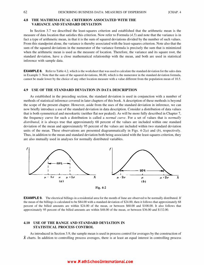
4.8 THE MATHEMATICAL CRITERION ASSOCIATED WITH THE
VARIANCE AND STANDARD DEVIATION
In Section 3.7 we described the least-squares criterion and established that the arithmetic mean is the
measure of data location that satisfies this criterion. Now refer to Formula (4.5) and note that the variance is in
fact a type of arithmetic mean, in that it is the sum of squared deviations divided by the number of such values.
From this standpoint alone, the variance is thereby associated with the least-squares criterion. Note also that the
sum of the squared deviations in the numerator of the variance formula is precisely the sum that is minimized
when the arithmetic mean is used as the measure of location. Therefore, the variance and its square root, the
standard deviation, have a close mathematical relationship with the mean, and both are used in statistical
inference with sample data.
EXAMPLE 8. Refer to Table 4.2, which is the worksheet that was used to calculate the standard deviation for the sales data
in Example 3. Note that the sum of the squared deviations, 86.00, which is the numerator in the standard deviation formula,
cannot be made lower by the choice of any other location measure with a value different from the population mean of 10.5.
4.9 USE OF THE STANDARD DEVIATION IN DATA DESCRIPTION
As established in the preceding section, the standard deviation is used in conjunction with a number of
methods of statistical inference covered in later chapters of this book. A description of these methods is beyond
the scope of the present chapter. However, aside from the uses of the standard deviation in inference, we can
now briefly introduce a use of the standard deviation in data description. Consider a distribution of data values
that is both symmetrical and mesokurtic (neither flat nor peaked). As will be more fully described in Chapter 7,
the frequency curve for such a distribution is called a normal curve. For a set of values that is normally
distributed, it is always true that approximately 68 percent of the values are included within one standard
deviation of the mean and approximately 95 percent of the values are included within two standard deviation
units of the mean. These observations are presented diagrammatically in Figs. 4-2(a) and (b), respectively.
Thus, in addition to the mean and standard deviation both being associated with the least-squares criterion, they
are also mutually used in analyses for normally distributed variables.
Fig. 4-2
EXAMPLE 9. The electrical billings in a residential area for the month of June are observed to be normally distributed. If
the mean of the billings is calculated to be $84.00 with a standard deviation of $24.00, then it follows that approximately 68
percent of the billed amounts are within $24.00 of the mean, or between $60.00 and $108.00. It also follows that
approximately 95 percent of the billed amounts are within $48.00 of the mean, or between $36.00 and $132.00.
4.10 USE OF THE RANGE AND STANDARD DEVIATION IN
STATISTICAL PROCESS CONTROL
As introduced in Section 3.9, the sample mean is used in process control for averages by the construction of�XX charts. In addition to controlling process averages, there is at least an equal interest in controlling process
62 DESCRIBING BUSINESS DATA: MEASURES OF DISPERSION [CHAP. 4
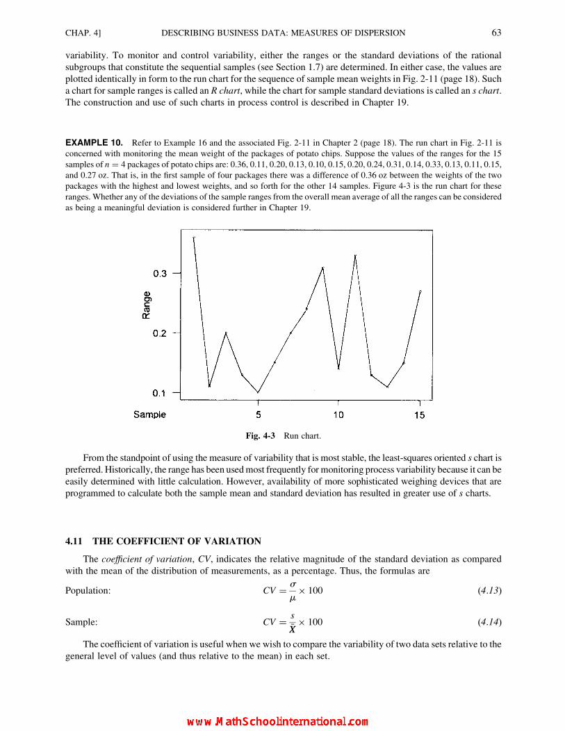
variability. To monitor and control variability, either the ranges or the standard deviations of the rational
subgroups that constitute the sequential samples (see Section 1.7) are determined. In either case, the values are
plotted identically in form to the run chart for the sequence of sample mean weights in Fig. 2-11 (page 18). Such
a chart for sample ranges is called an R chart, while the chart for sample standard deviations is called an s chart.
The construction and use of such charts in process control is described in Chapter 19.
EXAMPLE 10. Refer to Example 16 and the associated Fig. 2-11 in Chapter 2 (page 18). The run chart in Fig. 2-11 is
concerned with monitoring the mean weight of the packages of potato chips. Suppose the values of the ranges for the 15
samples of n ¼ 4 packages of potato chips are: 0.36, 0.11, 0.20, 0.13, 0.10, 0.15, 0.20, 0.24, 0.31, 0.14, 0.33, 0.13, 0.11, 0.15,
and 0.27 oz. That is, in the first sample of four packages there was a difference of 0.36 oz between the weights of the two
packages with the highest and lowest weights, and so forth for the other 14 samples. Figure 4-3 is the run chart for these
ranges. Whether any of the deviations of the sample ranges from the overall mean average of all the ranges can be considered
as being a meaningful deviation is considered further in Chapter 19.
Fig. 4-3 Run chart.
From the standpoint of using the measure of variability that is most stable, the least-squares oriented s chart is
preferred. Historically, the range has been usedmost frequently for monitoring process variability because it can be
easily determined with little calculation. However, availability of more sophisticated weighing devices that are
programmed to calculate both the sample mean and standard deviation has resulted in greater use of s charts.
4.11 THE COEFFICIENT OF VARIATION
The coefficient of variation, CV, indicates the relative magnitude of the standard deviation as compared
with the mean of the distribution of measurements, as a percentage. Thus, the formulas are
Population: CV ¼ s
m� 100 (4:13)
Sample: CV ¼ s
�XX� 100 (4:14)
The coefficient of variation is useful when we wish to compare the variability of two data sets relative to the
general level of values (and thus relative to the mean) in each set.
CHAP. 4] DESCRIBING BUSINESS DATA: MEASURES OF DISPERSION 63
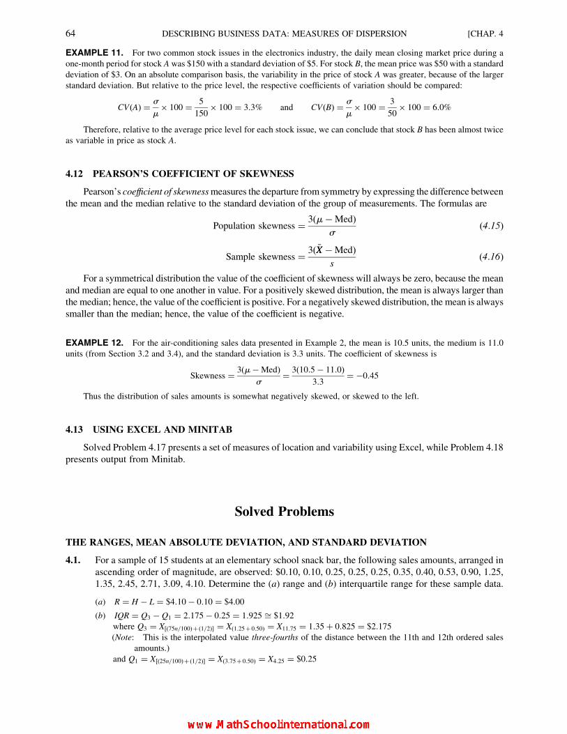
EXAMPLE 11. For two common stock issues in the electronics industry, the daily mean closing market price during a
one-month period for stock A was $150 with a standard deviation of $5. For stock B, the mean price was $50 with a standard
deviation of $3. On an absolute comparison basis, the variability in the price of stock A was greater, because of the larger
standard deviation. But relative to the price level, the respective coefficients of variation should be compared:
CV(A) ¼ s
m� 100 ¼ 5
150� 100 ¼ 3:3% and CV(B) ¼ s
m� 100 ¼ 3
50� 100 ¼ 6:0%
Therefore, relative to the average price level for each stock issue, we can conclude that stock B has been almost twice
as variable in price as stock A.
4.12 PEARSON’S COEFFICIENT OF SKEWNESS
Pearson’s coefficient of skewnessmeasures the departure from symmetry by expressing the difference between
the mean and the median relative to the standard deviation of the group of measurements. The formulas are
Population skewness ¼ 3(m�Med)
s(4:15)
Sample skewness ¼ 3( �XX �Med)
s(4:16)
For a symmetrical distribution the value of the coefficient of skewness will always be zero, because the mean
and median are equal to one another in value. For a positively skewed distribution, the mean is always larger than
the median; hence, the value of the coefficient is positive. For a negatively skewed distribution, the mean is always
smaller than the median; hence, the value of the coefficient is negative.
EXAMPLE 12. For the air-conditioning sales data presented in Example 2, the mean is 10.5 units, the medium is 11.0
units (from Section 3.2 and 3.4), and the standard deviation is 3.3 units. The coefficient of skewness is
Skewness ¼ 3(m�Med)
s¼ 3(10:5� 11:0)
3:3¼ �0:45
Thus the distribution of sales amounts is somewhat negatively skewed, or skewed to the left.
4.13 USING EXCEL AND MINITAB
Solved Problem 4.17 presents a set of measures of location and variability using Excel, while Problem 4.18
presents output from Minitab.
Solved Problems
THE RANGES, MEAN ABSOLUTE DEVIATION, AND STANDARD DEVIATION
4.1. For a sample of 15 students at an elementary school snack bar, the following sales amounts, arranged in
ascending order of magnitude, are observed: $0.10, 0.10, 0.25, 0.25, 0.25, 0.35, 0.40, 0.53, 0.90, 1.25,
1.35, 2.45, 2.71, 3.09, 4.10. Determine the (a) range and (b) interquartile range for these sample data.
(a) R ¼ H � L ¼ $4:10� 0:10 ¼ $4.00
(b) IQR ¼ Q3 � Q1 ¼ 2:175� 0:25 ¼ 1:925 ffi $1:92where Q3 ¼ X[(75n=100)þ (1=2)] ¼ X(1:25þ 0:50) ¼ X11:75 ¼ 1:35þ 0:825 ¼ $2:175(Note: This is the interpolated value three-fourths of the distance between the 11th and 12th ordered sales
amounts.)
and Q1 ¼ X[(25n=100)þ (1=2)] ¼ X(3:75þ 0:50) ¼ X4:25 ¼ $0:25
64 DESCRIBING BUSINESS DATA: MEASURES OF DISPERSION [CHAP. 4
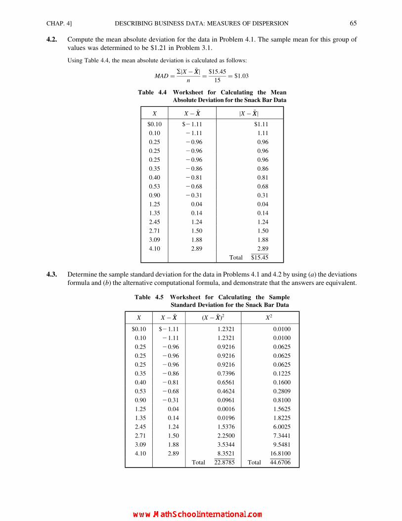
4.2. Compute the mean absolute deviation for the data in Problem 4.1. The sample mean for this group of
values was determined to be $1.21 in Problem 3.1.
Using Table 4.4, the mean absolute deviation is calculated as follows:
MAD ¼ SjX � �XXjn
¼ $15:45
15¼ $1:03
4.3. Determine the sample standard deviation for the data in Problems 4.1 and 4.2 by using (a) the deviations
formula and (b) the alternative computational formula, and demonstrate that the answers are equivalent.
Table 4.4 Worksheet for Calculating the Mean
Absolute Deviation for the Snack Bar Data
X X � �XX jX � �XXj$0.10 $21.11 $1.11
0.10 21.11 1.11
0.25 20.96 0.96
0.25 20.96 0.96
0.25 20.96 0.96
0.35 20.86 0.86
0.40 20.81 0.81
0.53 20.68 0.68
0.90 20.31 0.31
1.25 0.04 0.04
1.35 0.14 0.14
2.45 1.24 1.24
2.71 1.50 1.50
3.09 1.88 1.88
4.10 2.89 2.89
Total $15.45
Table 4.5 Worksheet for Calculating the Sample
Standard Deviation for the Snack Bar Data
X X � �XX (X � �XX)2 X2
$0.10 $21.11 1.2321 0.0100
0.10 21.11 1.2321 0.0100
0.25 20.96 0.9216 0.0625
0.25 20.96 0.9216 0.0625
0.25 20.96 0.9216 0.0625
0.35 20.86 0.7396 0.1225
0.40 20.81 0.6561 0.1600
0.53 20.68 0.4624 0.2809
0.90 20.31 0.0961 0.8100
1.25 0.04 0.0016 1.5625
1.35 0.14 0.0196 1.8225
2.45 1.24 1.5376 6.0025
2.71 1.50 2.2500 7.3441
3.09 1.88 3.5344 9.5481
4.10 2.89 8.3521 16.8100
Total 22.8785 Total 44.6706
CHAP. 4] DESCRIBING BUSINESS DATA: MEASURES OF DISPERSION 65

From Table 4.5,
(a) s ¼ffiffiffiffiffiffiffiffiffiffiffiffiffiffiffiffiffiffiffiffiffiS(X � �XX)2
n � 1
s¼
ffiffiffiffiffiffiffiffiffiffiffiffiffiffiffiffi22:8785
15� 1
r¼
ffiffiffiffiffiffiffiffiffiffiffiffiffiffi1:6342
pffi $1:28
(b) s ¼ffiffiffiffiffiffiffiffiffiffiffiffiffiffiffiffiffiffiffiffiffiffiSX2 � n �XX
2
n � 1
s¼
ffiffiffiffiffiffiffiffiffiffiffiffiffiffiffiffiffiffiffiffiffiffiffiffiffiffiffiffiffiffiffiffiffiffiffiffiffiffiffiffi44:6706� 15(1:21)2
15� 1
s¼
ffiffiffiffiffiffiffiffiffiffiffiffiffiffi1:6221
pffi $1:27
The answers are slightly different because of rounding error associated with the fact that the sample mean was
rounded to two places.
4.4. A sample of 20 production workers in a small company earned the following wages for a given week,
rounded to the nearest dollar and arranged in ascending order: $240, 240, 240, 240, 240, 240, 240, 240,
255, 255, 265, 265, 280, 280, 290, 300, 305, 325, 330, 340. Determine the (a) range and (b) middle 80
percent range for this sample.
(a) R ¼ H � L ¼ $340� $240 ¼ $100
(b) Middle 80% R ¼ P90 � P10 ¼ $327:50� $240:00 ¼ $87:50where P90 ¼ X[(90n=100)þ (1=2)] ¼ X[18þ (1=2)] ¼ X18:5 ¼ $325þ $2:50 ¼ $327:50
P10 ¼ X[(10n=100)þ (1=2)] ¼ X[2þ (1=2)] ¼ X2:5 ¼ $240:00
4.5. Compute the mean absolute deviation for the wages in Problem 4.4. The sample mean for these wages
was determined to be $270:50 in Problem 3.5.
From Table 4.6, the average deviation is
MAD ¼ SjX � �XXjn
¼ $572:00
20¼ $28:60
Table 4.6 Worksheet for Calculating the Mean
Absolute Deviation for the Wage Data
X X � �XX jX � �XXj$240 $230.50 $30.50
240 230.50 30.50
240 230.50 30.50
240 230.50 30.50
240 230.50 30.50
240 230.50 30.50
240 230.50 30.50
240 230.50 30.50
255 215.50 15.50
255 215.50 15.50
265 25.50 5.50
265 25.50 5.50
280 9.50 9.50
280 9.50 9.50
290 19.50 19.50
300 29.50 29.50
305 34.50 34.50
325 54.50 54.50
330 59.50 59.50
340 69.50 69.50
Total $572.00
66 DESCRIBING BUSINESS DATA: MEASURES OF DISPERSION [CHAP. 4

4.6. Determine the (a) sample variance and (b) sample standard deviation for the data in Problems 4.4 and
4.5, using the deviations formulas.
With reference to Table 4.7,
(a) s2 ¼ S(X � �XX)2
n � 1¼ 21,945:00
20� 1¼ 1,155:00
(b) s ¼ffiffiffiffiffiffiffiffiffiffiffiffiffiffiffiffiffiffiffiffiffiS(X � �XX)2
n � 1
s¼
ffiffiffiffiffiffiffiffiffiffiffiffiffiffiffiffiffi1,155:00
pffi $33:99
4.7. A work-standards expert observes the amount of time required to prepare a sample of 10 business letters
in an office with the following results listed in ascending order to the nearest minute: 5, 5, 5, 7, 9, 14, 15,
15, 16, 18. Determine the (a) range and (b) middle 70 percent for the sample.
(a) R ¼ H � L ¼ 18� 5 ¼ 13min
(b) Middle 70% R ¼ P85 � P15 ¼ 16:0� 5:0 ¼ 11:0min
where P85 ¼ X[(85n=100)þ (1=2)] ¼ X(8:5þ 0:5) ¼ X9 ¼ 16:0min
P15 ¼ X[(15n=100)þ (1=2)] ¼ X(1:5þ 0:5) ¼ X2 ¼ 5:0min
4.8. Compute the mean absolute deviation for the preparation time in Problem 4.7. The sample mean was
determined to be 10.9min in Problem 3.9.
Table 4.7 Worksheet for Calculating the
Sample Variance and Standard
Deviation for the Wage Data
X X � �XX (X � �XX)2
$240 $230.50 $930.25
240 230.50 930.25
240 230.50 930.25
240 230.50 930.25
240 230.50 930.25
240 230.50 930.25
240 230.50 930.25
240 230.50 930.25
255 215.50 240.25
255 215.50 240.25
265 25.50 30.25
265 25.50 30.25
280 9.50 90.25
280 9.50 90.25
290 19.50 380.25
300 29.50 870.25
305 34.50 1,190.25
325 56.50 2,970.25
330 59.50 3,540.25
340 69.50 4,830.25
Total $21,945.00
CHAP. 4] DESCRIBING BUSINESS DATA: MEASURES OF DISPERSION 67

From Table 4.8,
MAD ¼ SjX � �XXjn
¼ 47:0
10¼ 4:7min
4.9 Determine the (a) sample variance and (b) sample standard deviation for the preparation-time data in
Problems 4.7 and 4.8, using the alternative computational formulas.
With reference to Table 4.9,
(a) s2 ¼ SX2 � n �XX2
n � 1¼ 1,431� 10 (10:9)2
10� 1¼ 26:99
(b) s ¼ffiffiffiffiffiffiffiffiffiffiffiffiffiffiffiffiffiffiffiffiffiffiSX2 � n �XX
2
n � 1
s¼
ffiffiffiffiffiffiffiffiffiffiffi26:99
pffi 5:2min
Table 4.8 Worksheet for Calculating
the Mean Absolute Devi-
ation for the Preparation-
Time Data
X X � �XX jX � �XXj5 25.9 5.9
5 25.9 5.9
5 25.9 5.9
7 23.9 3.9
9 21.9 1.9
14 3.1 3.1
15 4.1 4.1
15 4.1 4.1
16 5.1 5.1
18 7.1 7.1
Total 47.0
Table 4.9 Worksheet for Calcu-
lating the Sample Var-
iance and Standard
Deviation for the Prep-
aration-Time Data
X X2
5 25
5 25
5 25
7 49
9 81
14 196
15 225
15 225
16 256
18 324
Total 1,431
68 DESCRIBING BUSINESS DATA: MEASURES OF DISPERSION [CHAP. 4

USE OF THE STANDARD DEVIATION
4.10. Many national academic achievement and aptitude tests, such as the SAT, report standardized test
scores with the mean for the normative group used to establish scoring standards converted to 500 with a
standard deviation of 100. Suppose that the distribution of scores for such a test is known to be
approximately normally distributed. Determine the approximate percentage of reported scores that
would be between (a) 400 and 600 and (b) between 500 and 700.
(a) 68% (since these limits are within one standard deviation of the mean)
(b) 47.5% (i.e., one-half of the middle 95 percent)
4.11. Referring to the standardized achievement test in Problem 4.10, what are the percentile values that
would be reported for scores of (a) 400, (b) 500, (c) 600, and (d) 700?
(a) 16 (Since 68 percent of the scores are between 400 and 600, one-half of the remaining 32 percent, or 16
percent, would be below 400, while the other 16 percent would be above 600.)
(b) 50 (Since the mean for a normally distributed variable is at the 50th percentile point of the distribution.)
(c) 84 (As explained in (a), above, since 16 percent are above a score of 600, this leaves 84 percent at or below a
score of 600.)
(d) 97.5 (Because 95 percent of the scores are between 300 and 700, and one-half of 5 percent, or 2.5 percent, are
below 300, the total percentage at or below 700 is 97.5 percent.)
THE COEFFICIENT OF VARIATION
4.12. Determine the coefficient of variation for the wage data analyzed in Problems 4.4 to 4.6.
Since �XX ¼ $270:50 and s ¼ $33:99,
CV ¼ s
�XX� 100 ¼ 33:99
270:50� 100 ¼ 12:6%
4.13. For the same industrial firm as in Problem 4.12, above, the mean weekly salary for a sample of supervisory
employees is �XX ¼ $730:75, with s ¼ $45:52. Determine the coefficient of variation for these salary
amounts.
CV ¼ s
�XX� 100 ¼ 45:52
730:75� 100 ¼ 6:2%
4.14. Compare the variability of the production workers’ wages in Problem 4.12 with the supervisory salaries in
Problem 4.13 (a) on an absolute basis and (b) relative to the mean level of weekly income for the two
groups of employees.
(a) On an absolute basis, there is more variability among the supervisors’ salaries (s ¼ $45:52) than there is
among the production workers’ weekly wages (s ¼ $33:99).(b) On a basis relative to the respective means, the two coefficients of variation are compared. Referring to the
solutions to Problems 4.12 and 4.13, we can observe that the coefficient of variation for the hourly wage data
(0.126) is about twice as large as the respective coefficient for the weekly salaries (0.062), thereby indicating
greater relative variability for the wage data.
PEARSON’S COEFFICIENT OF SKEWNESS
4.15. Compute the coefficient of skewness for the snack-bar data that were analyzed in Problems 4.1
to 4.3.
CHAP. 4] DESCRIBING BUSINESS DATA: MEASURES OF DISPERSION 69

Since �XX ¼ $1:21, Med ¼ $0:53 (from Problem 3.1), and s ¼ $1:27,
Skewness ¼ 3( �XX �Med)
s¼ 3(1:21� 0:53)
1:27¼ 1:61
Therefore the distribution of sales amounts is positively skewed, or skewed to the right.
4.16. Compute the coefficient of skewness for the wage data analyzed in Problems 4.4 to 4.6.
Since �XX ¼ $270:50, Med ¼ $260:00 (from Problem 3.5), and s ¼ $33:99,
Skewness ¼ 3( �XX �Med)
s¼ 3(270:50� 260:00)
33:99¼ 0:93
Therefore the distribution of the wage amounts is slightly positively skewed.
USING EXCEL AND MINITAB
4.17. Use Excel to determine the range, standard deviation, and variance for the data in Table 2.7 (page 22),
for the time required to complete an assembly task by a sample of 30 employees. In Problem 3.17 we
determined the values of the mean and median for these data by the use of Excel.
Figure 4-4 presents the output of descriptive statistics for these data, which is the same output as obtained in the solution
for Problem 3.17. As can be observed, the value of the range is 9min (which is the difference between the maximum
value of 18 and the minimum of 9min that are reported), the standard deviation is 2.437494, or more simply, 2.4min,
and the variance is 5.941379, or more simply, 5.9. As always, the variance is the squared value of the standard
deviation, and thus is expressed in squared units. Note that in Excel, as is true for most software, it is the sample
standard deviation that is reported in the standard output. The reason for this is that this measure of variability typically
is used in conjunction with statistical inference, rather than simply statistical description. Therefore, the data that are
analyzed are usually sample data taken from some defined population.
The Excel instructions that result in the output presented in Fig. 4-4 are
(1) Open Excel. In cell A1 enter the column label: Assy. Times, min. Enter the data values in column A beginning
at cell A2.
(2) Click Tools ! Data Analysis ! Descriptive Statistics. Click OK.
(3) Designate the Input Range as: $$A$1:$A$31.
(4) Select Labels in First Row.
(5) Select Summary Statistics. Click OK.
Fig. 4-4 Excel output.
70 DESCRIBING BUSINESS DATA: MEASURES OF DISPERSION [CHAP. 4
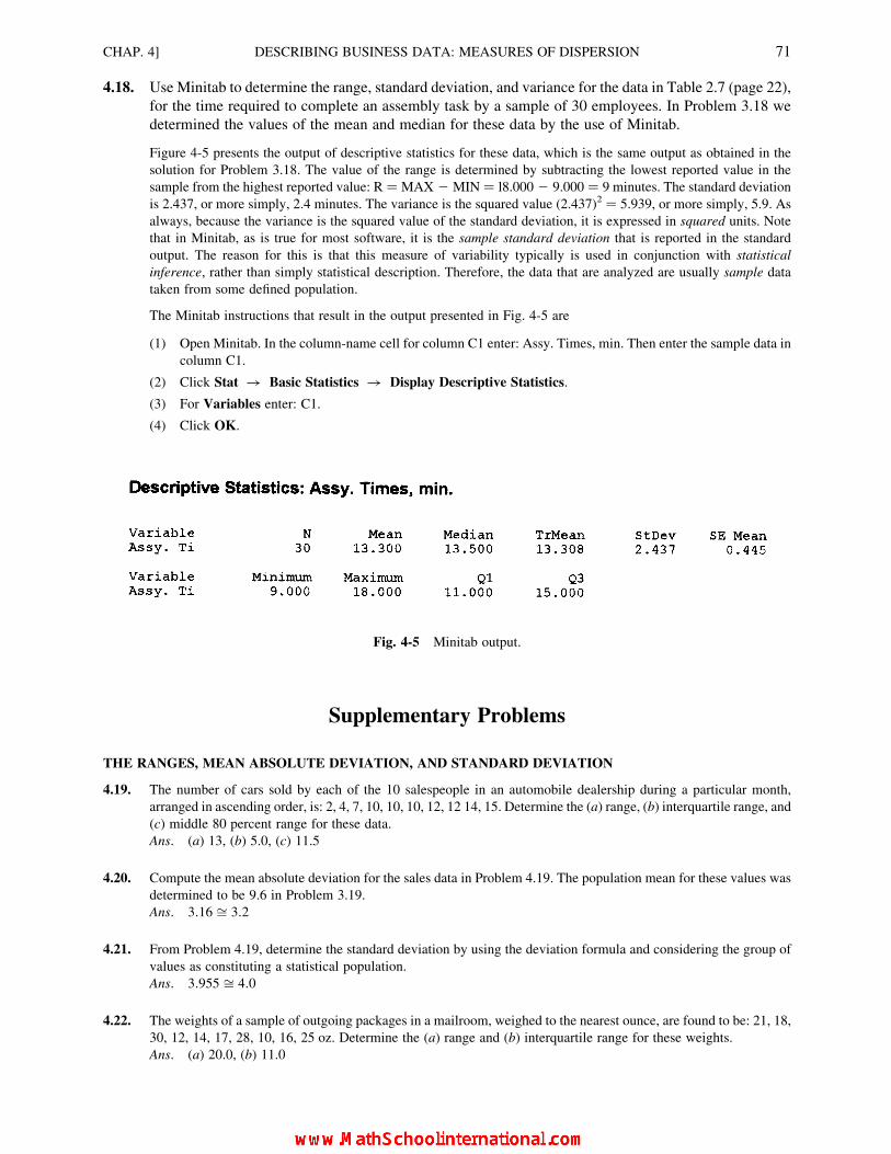
4.18. Use Minitab to determine the range, standard deviation, and variance for the data in Table 2.7 (page 22),
for the time required to complete an assembly task by a sample of 30 employees. In Problem 3.18 we
determined the values of the mean and median for these data by the use of Minitab.
Figure 4-5 presents the output of descriptive statistics for these data, which is the same output as obtained in the
solution for Problem 3.18. The value of the range is determined by subtracting the lowest reported value in the
sample from the highest reported value: R ¼ MAX 2 MIN ¼ l8.000 2 9.000 ¼ 9 minutes. The standard deviation
is 2.437, or more simply, 2.4 minutes. The variance is the squared value (2.437)2 ¼ 5.939, or more simply, 5.9. As
always, because the variance is the squared value of the standard deviation, it is expressed in squared units. Note
that in Minitab, as is true for most software, it is the sample standard deviation that is reported in the standard
output. The reason for this is that this measure of variability typically is used in conjunction with statistical
inference, rather than simply statistical description. Therefore, the data that are analyzed are usually sample data
taken from some defined population.
The Minitab instructions that result in the output presented in Fig. 4-5 are
(1) Open Minitab. In the column-name cell for column C1 enter: Assy. Times, min. Then enter the sample data in
column C1.
(2) Click Stat ! Basic Statistics ! Display Descriptive Statistics.
(3) For Variables enter: C1.
(4) Click OK.
Fig. 4-5 Minitab output.
Supplementary Problems
THE RANGES, MEAN ABSOLUTE DEVIATION, AND STANDARD DEVIATION
4.19. The number of cars sold by each of the 10 salespeople in an automobile dealership during a particular month,
arranged in ascending order, is: 2, 4, 7, 10, 10, 10, 12, 12 14, 15. Determine the (a) range, (b) interquartile range, and
(c) middle 80 percent range for these data.
Ans. (a) 13, (b) 5.0, (c) 11.5
4.20. Compute the mean absolute deviation for the sales data in Problem 4.19. The population mean for these values was
determined to be 9.6 in Problem 3.19.
Ans. 3:16 ffi 3:2
4.21. From Problem 4.19, determine the standard deviation by using the deviation formula and considering the group of
values as constituting a statistical population.
Ans. 3:955 ffi 4:0
4.22. The weights of a sample of outgoing packages in a mailroom, weighed to the nearest ounce, are found to be: 21, 18,
30, 12, 14, 17, 28, 10, 16, 25 oz. Determine the (a) range and (b) interquartile range for these weights.
Ans. (a) 20.0, (b) 11.0
CHAP. 4] DESCRIBING BUSINESS DATA: MEASURES OF DISPERSION 71

4.23. Compute the mean absolute deviation for the sampled packages in Problem 4.22. The sample mean was determined
to be 19.1 oz in Problem 3.22.
Ans. 5:52 ffi 5:5
4.24. Determine the (a) sample variance and (b) sample standard deviation for the data in Problem 4.22, by use of the
computational version of the respective formulas.
Ans. (a) 45.7, (b) 6.8
4.25. The following examination scores, arranged in ascending order, were achieved by 20 students enrolled in a decision
analysis course: 39, 46, 57, 65, 70, 72, 72, 75, 77, 79, 81, 81, 84, 84, 84, 87, 93, 94, 97, 97. Determine the (a) range
and (b) middle 90 percent range for these data.
Ans. (a) 58.0, (b) 54.5
4.26. Compute the mean absolute deviation for the examination scores in Problem 4.25. The mean examination score was
determined to be 76.7 in Problem 3.26.
Ans. 11:76 ffi 11:8
4.27. Considering the examination scores in Problem 4.25 to be a statistical population, determine the standard deviation
by use of (a) the deviations formula and (b) the alternative computational formula.
Ans. (a) 15:294 ffi 15:3, (b) 15:294 ffi 15:3
4.28. The number of accidents which occurred during a given month in the 13 manufacturing departments of an industrial
plant was: 2, 0, 0, 3, 3, 12, 1, 0, 8, 1, 0, 5, 1. Determine the (a) range and (b) interquartile range for the number of
accidents.
Ans. (a) 12.0, (b) 3.5
4.29. Compute the mean absolute deviation for the data in Problem 4.28. The mean number of accidents was determined
to be 2.8 in Problem 3.28.
Ans. 2:646 ffi 2:6
4.30. Considering the accident data in Problem 4.28 to be a statistical population, compute the standard deviation by using
the alternative computational formula.
Ans. 3:465 ffi 3:5
USE OF THE STANDARD DEVIATION
4.31. Packages of a certain brand of cereal are known to be normally distributed, with a mean weight of 13.0 oz and a
standard deviation of 0.1 oz, with the weights being normally distributed. Determine the approximate percentage of
packages that would have weights between (a) 12.9 and 13.1oz and (b) 12.9 and 13.2oz.
Ans. (a) 68%, (b) 81.5%
4.32. Refer to the distribution of cereal weights in Problem 4.31. What percentile values correspond to weights of (a) 13.0,
(b) 13.1, and (c) 13,2 oz?
Ans. (a) 50, (b) 84, (c) 97.5
THE COEFFICIENT OF VARIATION
4.33. Determine the coefficient of variation for the car-sales data analyzed in Problems 4.19 through 4.21.
Ans. CV ¼ 41:7%
4.34. Refer to Problem 4.33. In another (larger) dealership, the mean number of cars sold per salesperson during a
particular month was m ¼ 17:6, with a standard deviation of s ¼ 6:5. Compare the variability of car sales per
salesperson (a) on an absolute basis and (b) relative to the mean level of car sales at the two dealerships.
72 DESCRIBING BUSINESS DATA: MEASURES OF DISPERSION [CHAP. 4

Ans. (a) The standard deviation in the first dealership (4.0) is smaller than the standard deviation in the second
dealership (6.5). (b) The coefficient of variation in the first dealership (41.7%) is larger than the coefficient of
variation in the second dealership (36.9%).
PEARSON’S COEFFICIENT OF SKEWNESS
4.35. Compute the coefficient of skewness for the car-sales data analyzed in Problems 4.19 through 4.21. The median for
these data was determined to be 10.0 in Problem 3.19.
Ans. Skewness ¼ 20.30 (Thus, the distribution of car sales is slightly negatively skewed, or skewed to the left.)
4.36. Compute the coefficient of skewness for the accident data analyzed in Problems 4.28 through 4.30. The median for
these data was determined to be 1.0 in Problem 3.28.
Ans. Skewness ¼ 1.54 (Thus, the distribution of accidents is positively skewed.)
COMPUTER OUTPUT
4.37. Use computer software to determine the (a) mean, (b) median, (c) range, (d) interquartile range, and (e) standard
deviation for the sample of 40 loan amounts in Table 2.19 (page 41).
Ans. (a) $1,097; (b) $945; (c) $2,700; (d) $897; (e) $642
CHAP. 4] DESCRIBING BUSINESS DATA: MEASURES OF DISPERSION 73

CHAPTER 5
Probability
5.1 BASIC DEFINITIONS OF PROBABILITY
Historically, three different conceptual approaches have been developed for defining probability and for
determining probability values: the classical, relative frequency, and subjective approaches.
By the classical approach to probability, if N(A) possible elementary outcomes are favorable to event A,
N(S) possible outcomes are included in the sample space, and all the elementary outcomes are equally likely and
mutually exclusive, then the probability that event A will occur is
P(A) ¼ N(A)
N(S)(5:1)
Note that the classical approach to probability is based on the assumption that each outcome is equally
likely. Because this approach (when it is applicable) permits determination of probability values before any
sample events are observed, it has also been called a priori approach.
EXAMPLE 1. In a well-shuffled deck of cards which contains 4 aces and 48 other cards, the probability of an ace (A)
being obtained on a single draw is
P(A) ¼ N(A)
N(S)¼ 4
52¼ 1
13
By the relative frequency approach, the probability is determined on the basis of the proportion of times
that a favorable outcome occurs in a number of observations or experiments. No prior assumption of equal
likelihood is involved. Because determination of the probability values is based on observation and collection
of data, this approach has also been called the empirical approach. The probability that event A will occur by
the relative frequency approach is
P(A) ¼ no. of observations of A
sample size¼ n(A)
n(5:2)
EXAMPLE 2. Before including coverage for certain types of dental problems in health insurance policies for employed
adults, an insurance company wishes to determine the probability of occurrence of such problems, so that the insurance rate
can be set accordingly. Therefore, the statistician collects data for 10,000 adults in the appropriate age categories and finds
that 100 people have experienced the particular dental problem during the past year. The probability of occurrence is thus
P(A) ¼ n(A)
n¼ 100
10,000¼ 0:01, or 1%
74
Copyright 2004, 1996, 1988, 1976 by The McGraw-Hill Companies, Inc. Click Here for Terms of Use.
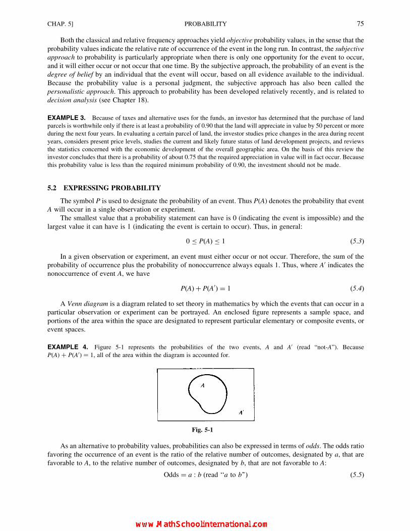
Both the classical and relative frequency approaches yield objective probability values, in the sense that the
probability values indicate the relative rate of occurrence of the event in the long run. In contrast, the subjective
approach to probability is particularly appropriate when there is only one opportunity for the event to occur,
and it will either occur or not occur that one time. By the subjective approach, the probability of an event is the
degree of belief by an individual that the event will occur, based on all evidence available to the individual.
Because the probability value is a personal judgment, the subjective approach has also been called the
personalistic approach. This approach to probability has been developed relatively recently, and is related to
decision analysis (see Chapter 18).
EXAMPLE 3. Because of taxes and alternative uses for the funds, an investor has determined that the purchase of land
parcels is worthwhile only if there is at least a probability of 0.90 that the land will appreciate in value by 50 percent or more
during the next four years. In evaluating a certain parcel of land, the investor studies price changes in the area during recent
years, considers present price levels, studies the current and likely future status of land development projects, and reviews
the statistics concerned with the economic development of the overall geographic area. On the basis of this review the
investor concludes that there is a probability of about 0.75 that the required appreciation in value will in fact occur. Because
this probability value is less than the required minimum probability of 0.90, the investment should not be made.
5.2 EXPRESSING PROBABILITY
The symbol P is used to designate the probability of an event. Thus P(A) denotes the probability that event
A will occur in a single observation or experiment.
The smallest value that a probability statement can have is 0 (indicating the event is impossible) and the
largest value it can have is 1 (indicating the event is certain to occur). Thus, in general:
0 P(A) 1 (5:3)
In a given observation or experiment, an event must either occur or not occur. Therefore, the sum of the
probability of occurrence plus the probability of nonoccurrence always equals 1. Thus, where A0 indicates thenonoccurrence of event A, we have
P(A)þ P(A0) ¼ 1 (5:4)
A Venn diagram is a diagram related to set theory in mathematics by which the events that can occur in a
particular observation or experiment can be portrayed. An enclosed figure represents a sample space, and
portions of the area within the space are designated to represent particular elementary or composite events, or
event spaces.
EXAMPLE 4. Figure 5-1 represents the probabilities of the two events, A and A0 (read “not-A”). Because
P(A) þ P(A0) ¼ 1, all of the area within the diagram is accounted for.
Fig. 5-1
As an alternative to probability values, probabilities can also be expressed in terms of odds. The odds ratio
favoring the occurrence of an event is the ratio of the relative number of outcomes, designated by a, that are
favorable to A, to the relative number of outcomes, designated by b, that are not favorable to A:
Odds ¼ a : b (read ‘‘a to b’’) (5:5)
CHAP. 5] PROBABILITY 75
Odds of 5 : 2 (read “5 to 2”) indicate that for every five elementary events constituting success there are
two elementary events constituting failure. Note that by the classical approach to probability discussed in
Section 5.1 the probability value equivalent to an odds ratio of 5 : 2 is
P(A) ¼ N(A)
N(S)¼ a
a þ b¼ 5
5þ 2¼ 5
7
EXAMPLE 5. Suppose success is defined as drawing any face card or an ace from a well-shuffled deck of 52
cards. Because 16 cards out of 52 are either the jack, queen, king, or ace, the odds associated with success are 16 : 36, or
4 : 9. The probability of success is 16/(16 þ 36) ¼ 16/52 ¼ 4/13.
5.3 MUTUALLY EXCLUSIVE AND NONEXCLUSIVE EVENTS
Two or more events are mutually exclusive, or disjoint, if they cannot occur together. That is, the occurrence
of one event automatically precludes the occurrence of the other event (or events). For instance, suppose we
consider the two possible events “ace” and “king” with respect to a card being drawn from a deck of playing
cards. These two events are mutually exclusive, because any given card cannot be both an ace and a king.
Two or more events are nonexclusive when it is possible for them to occur together. Note that this definition
does not indicate that such events must necessarily always occur jointly. For instance, suppose we consider the
two possible events “ace” and “spade.” These events are not mutually exclusive, because a given card can be
both an ace and a spade; however, it does not follow that every ace is a spade or every spade is an ace.
EXAMPLE 6. In a study of consumer behavior, an analyst classifies the people who enter a clothing store according to sex
(“male” or “female”) and according to age (“under 30” or “30 and over”). The two events, or classifications, “male” and
“female” are mutually exclusive, since any given person would be classified in one category or the other. Similarly, the
events “under 30” and “30 and over” are also mutually exclusive. However, the events “male” and “under 30” are not
mutually exclusive, because a randomly chosen person could have both characteristics.
5.4 THE RULES OF ADDITION
The rules of addition are used when we wish to determine the probability of one event or another (or both)
occurring in a single observation. Symbolically, we can represent the probability of event A or event B
occurring by P(A or B). In the language of set theory this is called the union of A and B and the probability
is designated by P(A < B) (read “probability of A union B”).
There are two variations of the rule of addition, depending on whether or not the two events are mutually
exclusive. The rule of addition for mutually exclusive events is
P(A or B) ¼ P(A < B) ¼ P(A)þ P(B) (5:6)
EXAMPLE 7. When drawing a card from a deck of playing cards, the events “ace” (A) and “king” (K) are mutually
exclusive. The probability of drawing either an ace or a king in a single draw is
P(A or K) ¼ P(A)þ P(K) ¼ 4
52þ 4
52¼ 8
52¼ 2
13
(Note: Problem 5.4 extends the application of this rule to three events.)
For events that are not mutually exclusive, the probability of the joint occurrence of the two events is
subtracted from the sum of the simple probabilities of the two events. We can represent the probability of joint
occurrence by P(A and B). In the language of set theory this is called the intersection of A and B and the
probability is designated by P(A > B) (read “probability of A intersect B”). See Fig. 5-2(b) on the following
page. Thus, the rule of addition for events that are not mutually exclusive is
P(A or B) ¼ P(A)þ P(B)� P(A and B) (5:7)
76 PROBABILITY [CHAP. 5

Formula (5.7) is also often called the general rule of addition, because for events that are mutually
exclusive the last term would always be equal to zero, resulting in formula (5.7) then being equivalent to
formula (5.6) for mutually exclusive events.
EXAMPLE 8. When drawing a card from a deck of playing cards, the events “ace” and “spade” are not mutually
exclusive. The probability of drawing an ace (A) or spade (S) (or both) in a single draw is
P(A or S) ¼ P(A)þ P(S)� P(A and S) ¼ 4
52þ 13
52� 1
52¼ 16
52¼ 4
13
Venn diagrams can be used to portray the rationale underlying the two rules of addition. In Fig. 5-2(a), note
that the probability of A or B occurring is conceptually equivalent to adding the proportion of area included in A
and B. In Fig. 5-2(b), for events that are not mutually exclusive, some elementary events are included in both A
and B; thus, there is overlap between these event sets. When the areas included in A and B are added together for
events that are not mutually exclusive, the area of overlap is essentially added in twice. Thus, the rationale of
subtracting P(A and B) in the rule of addition for nonexclusive events is to correct the sum for the duplicate
addition of the intersect area.
Fig. 5-2
5.5 INDEPENDENT EVENTS, DEPENDENT EVENTS, AND CONDITIONAL PROBABILITY
Two events are independent when the occurrence or nonoccurrence of one event has no effect on the
probability of occurrence of the other event. Two events are dependent when the occurrence or nonoccurrence
of one event does affect the probability of occurrence of the other event.
EXAMPLE 9. The outcomes associated with tossing a fair coin twice in succession are considered to be independent
events, because the outcome of the first toss has no effect on the respective probabilities of a head or tail occurring on the
second toss. The drawing of two cards without replacement from a deck of playing cards are dependent events, because
the probabilities associated with the second draw are dependent on the outcome of the first draw. Specifically, if an
“ace” occurred on the first draw, then the probability of an “ace” occurring on the second draw is the ratio of the number
of aces still remaining in the deck to the total number of cards remaining in the deck, or 3/51.
When two events are dependent, the concept of conditional probability is employed to designate the
probability of occurrence of the related event. The expression P(BjA) indicates the probability of event B
occurring given that event A has occurred. Note that BjA is not a fraction.
Conditional probability expressions are not required for independent events because by definition there is
no relationship between the occurrence of such events. Therefore, if events A and B are independent, the
conditional probability P(BjA) is always equal to the simple (unconditional) probability P(B). Therefore, one
approach by which the independence of two events A and B can be tested is by comparing
P(BjA) ¼? P(B) (5:8)
or P(AjB) ¼? P(A) (5:9)
(See Problems 5.8 through 5.10.)
CHAP. 5] PROBABILITY 77

If the simple (unconditional) probability of a first event A and the joint probability of two events A and B are
known, then the conditional probability P(BjA) can be determined by
P(BjA) ¼ P(A and B)
P(A)(5:10)
(See Problems 5.8 through 5.10.)
There is often some confusion regarding the distinction between mutually exclusive and nonexclusive
events on the one hand, and the concepts of independence and dependence on the other hand. Particularly, note
the difference between events that are mutually exclusive and events that are independent. Mutual
exclusiveness indicates that two events cannot both occur, whereas independence indicates that the probability
of occurrence of one event is not affected by the occurrence of the other event. Therefore it follows that if two
events are mutually exclusive, this is a particular example of highly dependent events, because the probability
of one event given that the other has occurred would always be equal to zero. See Problem 5.10.
5.6 THE RULES OF MULTIPLICATION
The rules of multiplication are concerned with determining the probability of the joint occurrence of A and
B. As explained in Section 5.4, this concerns the intersection of A and B: P(A > B). There are two variations of
the rule of multiplication, according to whether the two events are independent or dependent. The rule of
multiplication for independent events is
P(A and B) ¼ P(A > B) ¼ P(A)P(B) (5:11)
EXAMPLE 10. By formula (5.11), if a fair coin is tossed twice the probability that both outcomes will be “heads” is
( 12)� ( 1
2) ¼ ( 1
4).
(Note: Problem 5.11 extends the application of this rule to three events.)
The tree diagram is particularly useful as a method of portraying the possible events associated with
sequential observations, or sequential trials. Figure 5-3 is an example of such a diagram for the events
associated with tossing a coin twice, and identifies the outcomes that are possible and the probability at each
point in the sequence.
Fig. 5-3
78 PROBABILITY [CHAP. 5
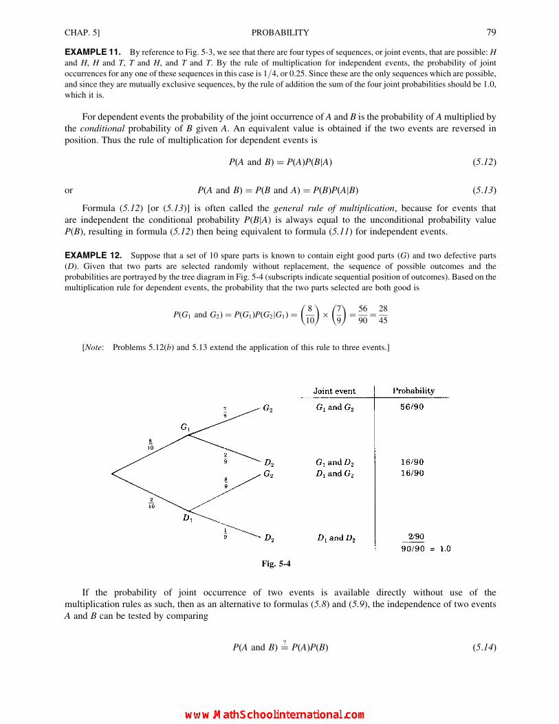
EXAMPLE 11. By reference to Fig. 5-3, we see that there are four types of sequences, or joint events, that are possible: H
and H, H and T, T and H, and T and T. By the rule of multiplication for independent events, the probability of joint
occurrences for any one of these sequences in this case is 1/4, or 0.25. Since these are the only sequences which are possible,and since they are mutually exclusive sequences, by the rule of addition the sum of the four joint probabilities should be 1.0,
which it is.
For dependent events the probability of the joint occurrence of A and B is the probability of A multiplied by
the conditional probability of B given A. An equivalent value is obtained if the two events are reversed in
position. Thus the rule of multiplication for dependent events is
P(A and B) ¼ P(A)P(BjA) (5:12)
or P(A and B) ¼ P(B and A) ¼ P(B)P(AjB) (5:13)
Formula (5.12) [or (5.13)] is often called the general rule of multiplication, because for events that
are independent the conditional probability P(BjA) is always equal to the unconditional probability value
P(B), resulting in formula (5.12) then being equivalent to formula (5.11) for independent events.
EXAMPLE 12. Suppose that a set of 10 spare parts is known to contain eight good parts (G) and two defective parts
(D). Given that two parts are selected randomly without replacement, the sequence of possible outcomes and the
probabilities are portrayed by the tree diagram in Fig. 5-4 (subscripts indicate sequential position of outcomes). Based on the
multiplication rule for dependent events, the probability that the two parts selected are both good is
P(G1 and G2) ¼ P(G1)P(G2jG1) ¼ 8
10
� �� 7
9
� �¼ 56
90¼ 28
45
[Note: Problems 5.12(b) and 5.13 extend the application of this rule to three events.]
Fig. 5-4
If the probability of joint occurrence of two events is available directly without use of the
multiplication rules as such, then as an alternative to formulas (5.8) and (5.9), the independence of two events
A and B can be tested by comparing
P(A and B) ¼? P(A)P(B) (5:14)
CHAP. 5] PROBABILITY 79

EXAMPLE 13. By our knowledge of a playing deck of 52 cards, we know that only one card is both an ace (A) and a
spade (S), and thus that P(A and S) ¼ 1/52. We also know that the probability of drawing any ace is 4/52 and the probabilityof drawing any spade is 13/52. We thus can verify that the events “ace” and “spade” are independent events, as follows:
P(A and S) ¼? P(A)P(S)
1
52¼? 4
52� 13
52
1
52¼ 1
52(therefore the events are independent)
5.7 BAYES’ THEOREM
In its simplest algebraic form, Bayes’ theorem is concerned with determining the conditional probability of
event A given that event B has occurred. The general form of Bayes’ theorem is
P(AjB) ¼ P(A and B)
P(B)(5:15)
Formula (5.15) is simply a particular application of the general formula for conditional probability
presented in Section 5.5. However, the special importance of Bayes’ theorem is that it is applied in the context
of sequential events, and further, that the computational version of the formula provides the basis for
determining the conditional probability of an event having occurred in the first sequential position given that a
particular event has been observed in the second sequential position. The computational form of Bayes’
theorem is
P(AjB) ¼ P(A)P(BjA)P(A)P(BjA)þ P(A0)P(BjA0)
(5:16)
As illustrated in Problem 5.20(c), the denominator above is the overall (unconditional) probability of the event
in the second sequential position; P(B) for the formula above.
EXAMPLE 14. Suppose there are two urns U1 and U2. Urn 1 has eight red balls and two green balls, while urn 2 has
four red balls and six green balls. If an urn is selected randomly, and a ball is then selected randomly from that urn, the
sequential process and probabilities can be represented by the tree diagram in Fig. 5-5. The tree diagram indicates that the
probability of choosing either urn is 0.50. and then the conditional probabilities of a red (R) or a green (G) ball being drawn
are indicated according to the urn involved. Now, suppose we observe a green ball in Step 2 without knowing which urn was
selected in Step 1. What is the probability that urn 1 was selected in Step 1? Symbolically, what is P(U1jG)? Substituting U1
and G for A and B, respectively, in the computational form of Bayes’ theorem:
P(U1jG) ¼ P(U1)P(GjU1)
P(U1)P(GjU1)þ P(U2)P(GjU2)¼ (0:50)(0:20)
(0:50)(0:20)þ (0:50)(0:60) ¼0:10
0:40¼ 0:25
Fig. 5-5
In Example 14, note that Bayes’ theorem presents the basis for obtaining what might be called a “backward
conditional” probability value, since we can determine the probability that a particular urn was selected in Step
1 given the observation of a sampled item from that urn in Step 2.
80 PROBABILITY [CHAP. 5
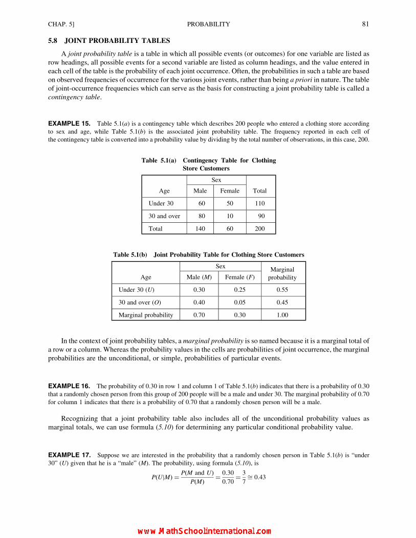
5.8 JOINT PROBABILITY TABLES
A joint probability table is a table in which all possible events (or outcomes) for one variable are listed as
row headings, all possible events for a second variable are listed as column headings, and the value entered in
each cell of the table is the probability of each joint occurrence. Often, the probabilities in such a table are based
on observed frequencies of occurrence for the various joint events, rather than being a priori in nature. The table
of joint-occurrence frequencies which can serve as the basis for constructing a joint probability table is called a
contingency table.
EXAMPLE 15. Table 5.1(a) is a contingency table which describes 200 people who entered a clothing store according
to sex and age, while Table 5.1(b) is the associated joint probability table. The frequency reported in each cell of
the contingency table is converted into a probability value by dividing by the total number of observations, in this case, 200.
Table 5.1(a) Contingency Table for Clothing
Store Customers
Sex
Age Male Female Total
Under 30 60 50 110
30 and over 80 10 90
Total 140 60 200
Table 5.1(b) Joint Probability Table for Clothing Store Customers
SexMarginal
probabilityAge Male (M) Female (F)
Under 30 (U) 0.30 0.25 0.55
30 and over (O) 0.40 0.05 0.45
Marginal probability 0.70 0.30 1.00
In the context of joint probability tables, a marginal probability is so named because it is a marginal total of
a row or a column. Whereas the probability values in the cells are probabilities of joint occurrence, the marginal
probabilities are the unconditional, or simple, probabilities of particular events.
EXAMPLE 16. The probability of 0.30 in row 1 and column 1 of Table 5.1(b) indicates that there is a probability of 0.30
that a randomly chosen person from this group of 200 people will be a male and under 30. The marginal probability of 0.70
for column 1 indicates that there is a probability of 0.70 that a randomly chosen person will be a male.
Recognizing that a joint probability table also includes all of the unconditional probability values as
marginal totals, we can use formula (5.10) for determining any particular conditional probability value.
EXAMPLE 17. Suppose we are interested in the probability that a randomly chosen person in Table 5.1(b) is “under
30” (U) given that he is a “male” (M). The probability, using formula (5.10), is
P(UjM) ¼ P(M and U)
P(M)¼ 0:30
0:70¼ 3
7ffi 0:43
CHAP. 5] PROBABILITY 81

5.9 PERMUTATIONS
By the classical approach to determining probabilities presented in Section 5.1, the probability value is
based on the ratio of the number of equally likely elementary outcomes that are favorable to the total number of
outcomes in the sample space. When the problems are simple, the number of elementary outcomes can be
counted directly. However, for more complex problems the methods of permutations and combinations are
required to determine the number of possible elementary outcomes.
The number of permutations of n objects is the number of ways in which the objects can be arranged in
terms of order:
Permutations of n objects ¼ n! ¼ (n)� (n � 1)� � � � � (2)� (1) (5:17)
The symbol n! is read “n factorial.” In permutations and combinations problems, n is always positive.
Also, note that by definition 0! ¼ 1 in mathematics.
EXAMPLE 18. Three members of a social organization have volunteered to serve as officers for the following year, to
take positions as President, Treasurer, and Secretary. The number of ways (permutations) in which the three can assume the
positions is
n! ¼ 3! ¼ (3)(2)(1) ¼ 6 ways
This result can be portrayed by a sequential diagram. Suppose that the three people are designated as A, B, and C. The
number of possible arrangements, or permutations, is presented in Fig. 5-6.
Fig. 5-6
Typically, we are concerned about the number of permutations of some subgroup of the n objects, rather
than all n objects as such. That is, we are interested in the number of permutations of n objects taken r at a time,
where r is less than n:
nPr ¼ n!
(n � r)!(5:18)
EXAMPLE 19. In Example 18, suppose there are 10 members in the social organization and no nominations have yet
been presented for the offices of President, Treasurer, and Secretary. The number of different arrangements of three officers
elected from the 10 club members is
nPr ¼ 10P3 ¼ 10!
(10� 3)!¼ 10!
7!¼ (10)(9)(8)(7!)
7!¼ (10)(9)(8) ¼ 720
82 PROBABILITY [CHAP. 5

5.10 COMBINATIONS
In the case of permutations, the order in which the objects are arranged is important. In the case of
combinations, we are concerned with the number of different groupings of objects that can occur without regard
to their order. Therefore, an interest in combinations always concerns the number of different subgroups that
can be taken from n objects. The number of combinations of n objects taken r at a time is
nCr ¼ n!
r!(n � r)!(5:19)
In many textbooks, the combination of n objects taken r at a time is represented byn
r
� �. Note that this
is not a fraction.
EXAMPLE 20. Suppose that three members from a small social organization containing a total of 10 members are to be
chosen to form a committee. The number of different groups of three people which can be chosen, without regard to the
different orders in which each group might be chosen, is
nCr ¼ 10C3 ¼ 10!
3!(10� 3)!¼ (10)(9)(8)(7!)
3!(7!)¼ (10)(9)(8)
(3)(2)¼ 720
6¼ 120
As indicated in Section 5.9, the methods of permutations and combinations provide a basis for counting the possible
outcomes in relatively complex situations. In terms of combinations, we can frequently determine the probability of an event
by determining the number of combinations of outcomes which include that event as compared with the total number of
combinations that are possible. Of course, this again represents the classical approach to probability and is based on the
assumption that all combinations are equally likely.
EXAMPLE 21. Continuing with Example 20, if the group contains six women and four men, what is the probability that a
random choice of the committee members will result in two women and one man being selected? The basic approach is to
determine the number of combinations of outcomes that contain exactly two women (of the six women) and one man (of the
four men) and then to take the ratio of this number to the total number of possible combinations:
Number of committees with 2W and 1M ¼ 6C2 � 4C1 (see explanatory note below)
¼ 6!
2!4!� 4!
1!3!¼ 15� 4 ¼ 60
Total number of possible combinations ¼ 10C3
¼ 10!
3!7!¼ (10)(9)(8)(3)(2)(1)
¼ 720
6¼ 120
P(2W and 1M) ¼ 6C2 � 4C1
10C3
¼ 60
120¼ 0:50
Note: In Example 21, above, the so-called method of multiplication is used. In general, if one event can occur in n1ways and second event can occur in n2 ways, then
Total number of ways two events can occur in combination ¼ n1 � n2 (5:20)
The value of 60 in the solution in Example 21 is based on multiplying the number of ways that two women
can be chosen from the six available women (15) by the number of ways that one man can be chosen from the
four available men (4).
CHAP. 5] PROBABILITY 83

Solved Problems
DETERMINING PROBABILITY VALUES
5.1. For each of the following situations, indicate whether the classical, relative frequency, or subjective
approach would be most useful for determining the required probability value.
(a) Probability that there will be a recession next year.
(b) Probability that a six-sided die will show either a 1 or 6 on a single toss.
(c) Probability that from a shipment of 20 parts known to contain one defective part, one randomly
chosen part will turn out to be defective.
(d) Probability that a randomly chosen part taken from a large shipment of parts will turn out to be
defective.
(e) Probability that a randomly chosen person who enters a large department store will make a
purchase in that store.
( f ) Probability that the Dow Jones Industrial Average will increase by at least 50 points during the
next six months.
(a) Subjective, (b) classical, (c) classical, (d) relative frequency (Since there is no information about the overall
proportion of the defective parts, the proportion of defective parts in a sample would be used as the basis for
estimating the probability value.), (e) relative frequency, ( f ) subjective.
5.2. Determine the probability value applicable in each of the following situations.
(a) Probability of industrial injury in a particular industry on an annual basis. A random sample of 10
firms, employing a total of 8,000 people, reported that 400 industrial injuries occurred during a
recent 12-month period.
(b) Probability of betting on a winning number in the game of roulette. The numbers on the wheel
include a 0, 00, and 1 through 36.
(c) Probability that a fast-food franchise outlet will be financially successful. The prospective investor
obtains data for other units in the franchise system, studies the development of the residential area
in which the outlet is to be located, and considers the sales volume required for financial success
based on the required capital investment and operational costs. Overall, it is the investor’s
judgment that there is an 80 percent chance that the outlet will be financially successful and a 20
percent chance that it will not.
(a) By the relative frequency approach, P ¼ 400/8,000 ¼ 0.05. Because this probability value is based on a
sample, it is an estimate of the unknown true value. Also, the implicit assumption is made that safety standards
have not changed since the 12-month sampled period.
(b) By the classical approach, P ¼ 1/38. This value is based on the assumption that all numbers are equally likely,
and therefore a well-balanced wheel is assumed.
(c) Based on the subjective approach, the value arrived at through the prospective investor’s judgment is
P ¼ 0.80. Note that such a judgment should be based on knowledge of all available information within the
scope of the time which is available to collect such information.
5.3. For each of the following reported odds ratios determine the equivalent probability value, and for each
of the reported probability values determine the equivalent odds ratio.
(a) A puchasing agent estimates that the odds are 2 : 1 that a shipment will arrive on schedule.
(b) The probability that a new component will not function properly when assembled is assessed as
being P ¼ 1/5.
(c) The odds that a new product will succeed are estimated as being 3 : 1.
84 PROBABILITY [CHAP. 5

(d) The probability that the home teamwill win the opening game of the season is assessed as being 1/3.
(a) The probability that the shipment will arrive on schedule is P ¼ 2/(2 þ 1) ¼ 2/3 ffi 0.67.
(b) The odds that it will not function properly are 1 : 4.
(c) The probability that the product will succeed is P ¼ 3/(3 þ 1) ¼ 3/4 ¼ 0.75.
(d) The odds that the team will win are 1 : 2.
APPLYING THE RULES OF ADDITION
5.4. Determine the probability of obtaining an ace (A), king (K), or a deuce (D) when one card is drawn from
a well-shuffled deck of 52 playing cards.
From formula (5.6),
P(A or K or D) ¼ P(A)þ P(K)þ P(D) ¼ 4
52þ 4
52þ 4
52¼ 12
52¼ 3
13
(Note: The events are mutually exclusive.)
5.5. With reference to Table 5.2, what is the probability that a randomly chosen family will have household
income (a) between $20,000 and $40,000, (b) less than $40,000, (c) at one of the two extremes of being
either less than $20,000 or at least $100,000?
Table 5.2 Annual Household Income for 500 Families
Category Income range
Number of
families
1 Less than $20,000 60
2 $20,000–$40,000 100
3 $40,000–$60,000 160
4 $60,000–$100,000 140
5 $100,000 and above 40
Total 500
(a) P(2) ¼ 100
500¼ 1
5¼ 0:20
(b) P(1 or 2) ¼ 60
500þ 100
500¼ 160
500¼ 8
25¼ 0:32
(c) P(1 or 5) ¼ 60
500þ 40
500¼ 100
500¼ 1
5¼ 0:20
(Note: The events are mutually exclusive.)
5.6. Of 300 business students, 100 are currently enrolled in accounting and 80 are currently enrolled in
business statistics. These enrollment figures include 30 students who are in fact enrolled in both courses.
What is the probability that a randomly chosen student will be enrolled in either accounting (A) or
business statistics (B)?
From formula (5.6),
P(A or B) ¼ P(A)þ P(B)� P(A and B) ¼ 100
300þ 80
300� 30
300¼ 150
300¼ 1
2¼ 0:50
(Note: The events are not mutually exclusive.)
CHAP. 5] PROBABILITY 85

5.7. Of 100 individuals who applied for systems analyst positions with a large firm during the past year, 40
had some prior work experience (W), and 30 had a professional certificate (C). However, 20 of the
applicants had both work experience and a certificate, and thus are included in both of the counts.
(a) Construct a Venn diagram to portray these events.
(b) What is the probability that a randomly chosen applicant had either work experience or a certificate
(or both)?
(c) What is the probability that a random chosen applicant had either work experience or a certificate
but not both?
(a) See Fig. 5-7.
(b) P(W or C) ¼ P(W)þ P(C)� P(W and C) ¼ 0:40þ 0:30� 0:20 ¼ 0:50(Note: The events are not mutually exclusive.)
(c) P(W or C, but not both) ¼ P(W or C) 2 P(W and C) ¼ 0.50 2 0.20 ¼ 0.30
Fig. 5-7
INDEPENDENT EVENTS, DEPENDENT EVENTS, AND CONDITIONAL PROBABILITY
5.8. For Problem 5.7, (a) determine the conditional probability that a randomly chosen applicant has a
certificate given that he has some previous work experience. (b) Apply an appropriate test to determine
if work experience and certification are independent events.
(a) P(CjW) ¼ P(C and W)
P(W)¼ 0:20
0:40¼ 0:50
(b) P(CjW) ¼? P(C). Since 0.50 = 0.30, events W and C are dependent. Independence could also be tested by
applying the multiplication rule for independent events—see Problem 5.14(a).
5.9. Two separate product divisions included in a large firm are Marine Products (M) and Office Equipment
(O). The probability that the Marine Products division will have a profit margin of at least 10 percent this
fiscal year is estimated to be 0.30, the probability that the Office Equipment division will have a profit
margin of at least 10 percent is 0.20, and the probability that both divisions will have a profit margin of
at least 10 percent is 0.06.
(a) Determine the probability that the Office Equipment division will have at least a 10 percent profit
margin given that the Marine Products division achieved this profit criterion.
(b) Apply an appropriate test to determine if achievement of the profit goal in the two divisions is
statistically independent.
(a) P(OjM) ¼ P(O and M)
P(M)¼ 0:06
0:30¼ 0:20
(b) P(OjM) ¼? P(O). Since 0.20 ¼ 0.20, the two events are independent. [Independence could also be tested by
applying the multiplication rule for independent events—see Problem 5.14(b).]
86 PROBABILITY [CHAP. 5

5.10. Suppose an optimist estimates that the probability of earning a final grade of A in the business statistics
course is 0.60 and the probability of a B is 0.40. Of course, it is not possible to earn both grades as final
grades, since they are mutually exclusive.
(a) Determine the conditional probability of earning a B given that, in fact, the final grade of A has
been received, by use of the appropriate computational formula.
(b) Apply an appropriate test to demonstrate that such mutually exclusive events are dependent events.
(a) P(BjA) ¼ P(B and A)
P(A)¼ 0
0:60¼ 0
(b) P(BjA) ¼? P(B). Since 0 = 0.40, the events are dependent. See Section 5.5.
APPLYING THE RULES OF MULTIPLICATION
5.11. In general, the probability that a prospect will make a purchase after being contacted by a salesperson is
P ¼ 0.40. If a salesperson selects three prospects randomly from a file and makes contact with them,
what is the probability that all three prospects will make a purchase?
Since the actions of the prospects are assumed to be independent of one another, the rule of multiplication for
independent events is applied.
P(all three are purchasers) ¼P(first is a purchaser)� P(second is a purchaser)� P(third is a purchaser)
¼ (0:40)� (0:40)� (0:40) ¼ 0:064
5.12. Of 12 accounts held in a file, four contain a procedural error in posting account balances.
(a) If an auditor randomly selects two of these accounts (without replacement), what is the probability
that neither account will contain a procedural error? Construct a tree diagram to represent this
sequential sampling process.
(b) If the auditor samples three accounts, what is the probability that none of the accounts includes the
procedural error?
(a) In this example the events are dependent, because the outcome on the first sampled account affects the
probabilities which apply to the second sampled account. Where E 01 means no error in the first sampled
account and E 02 means no error in the second sampled account
P(E 01 and E 0
2) ¼ P(E 01)P(E
02jE 0
1) ¼8
12� 7
11¼ 56
132¼ 14
33ffi 0:42
Note: In Fig. 5-8, E stands for an account with the procedural error, E0 stands for an account with no
procedural error, and the subscript indicates the sequential position of the sampled account.
Fig. 5-8
CHAP. 5] PROBABILITY 87
ðbÞ P(E 01 and E 0
2 and E 03) ¼ P(E 0
1)P(E02jE 0
1)P(E03jP 0
1 and E 02)
¼ 8
12� 7
11� 6
10¼ 336
1,320¼ 42
165ffi 0:25
5.13. When sampling without replacement from a finite population, the probability values associated with
various events are dependent on what events (sampled items) have already occurred. On the other hand,
when sampling is done with replacement, the events are always independent.
(a) Suppose that three cards are chosen randomly and without replacement from a playing deck of 52
cards. What is the probability that all three cards are aces?
(b) Suppose that three cards are chosen randomly from a playing deck of 52 cards, but that after each
selection the card is replaced and the deck is shuffled before the next selection of a card. What is
the probability that all three cards are aces?
(a) The rule of multiplication for dependent events applies in this case:
P(A1 and A2 and A3) ¼ P(A1)P(A2jA1)P(A3jA1 and A2)
¼ 4
52� 3
51� 2
50¼ 24
132,600¼ 1
5,525ffi 0:0002
(b) The rule of multiplication for independent events applies in this case:
P(A1 and A2 and A3) ¼ P(A)P(A)P(A)
¼ 4
52� 4
52� 4
52¼ 64
140,608¼ 1
2,197ffi 0:0005
5.14. Test the independence (a) of the two events described in Problems 5.7 and 5.8, and (b) for the two events
described in Problem 5.9, using the rule of multiplication for independent events.
ðaÞ P(W and C) ¼? P(W)P(C)
0:20 ¼? (0:40)� (0:30)0:20 = 0:12
Therefore, events W and C are dependent events. This corresponds with the answer to Problem 5.8(b).
ðbÞ P(M and O) ¼? P(M)P(O)
0:06 ¼? (0:30)� (0:20)0:06 ¼ 0:06
Therefore, events M and O are independent. This corresponds with the answer to Problem 5.9(b).
5.15. From Problem 5.7, what is the probability that a randomly chosen applicant has neither work experience
nor a certificate? Are these events independent?
Symbolically, what is required is P(W 0 and C 0) for these events that are not mutually exclusive but are
possibly dependent events. However, in this case neither P(W 0jC 0) nor P(C 0jW 0) is available, and therefore the ruleof multiplication for dependent events cannot be used. Instead, the answer can be obtained by subtraction, as
follows:
P(W 0 and C0) ¼ 1� P(W or C) ¼ 1� 0:50 ¼ 0:50
(The logic of this can most easily be understood by drawing a Venn diagram.)
88 PROBABILITY [CHAP. 5

We can now also demonstrate that the events are dependent rather than independent:
P(W 0 and C 0) ¼? P(W 0)P(C 0)
0:50 ¼? [1� P(W)][1� P(C)]
0:50 ¼? (0:60)(0:70)0:50 = 0:42
The conclusion that the events are dependent coincides with the answer to Problem 5.14(a), which is directed
to the complement of each of these two events.
5.16. Refer to Problem 5.11. (a) Construct a tree diagram to portray the sequence of three contacts, using S for
sale and S0 for no sale. (b) What is the probability that the salesperson will make at least two sales?
(c) What is the probability that the salesperson will make at least one sale?
(a) See Fig. 5-9.
Fig. 5-9
(b) “At least” two sales includes either two or three sales. Further, by reference to Fig. 5-9 we note that the two
sales can occur in any of three different sequences. Therefore, we use the rule of multiplication for independent
events to determine the probability of each sequence and the rule of addition to indicate that any of these
sequences constitutes “success”:
P(at least 2 sales) ¼P(S and S and S )þ P(S and S and S 0)
þ P(S and S 0 and S)þ P(S 0 and S and S )
¼ (0:064)þ (0:096)þ (0:096)þ (0:096) ¼ 0:352
CHAP. 5] PROBABILITY 89

(c) Instead of following the approach in part (b), it is easier to obtain the answer to this question by subtraction:
P(at least 1 sale) ¼ 1� P(no S)
¼ 1� P(S 0 and S 0 and S 0)¼ 1� 0:216 ¼ 0:784
5.17. In Problem 5.12 it was established that four of 12 accounts contain a procedural error.
(a) If an auditor samples one account randomly, what is the probability that it will contain the error?
(b) If an auditor samples two accounts randomly, what is the probability that at least one will contain
the error?
(c) If an auditor samples three accounts randomly, what is the probability that at least one will contain
the error?
(a) P(E) ¼ number of accts. with error
total number of accts.¼ 4
12¼ 1
3ffi 0:33
ðbÞ P(at least one E) ¼ P(E1 and E2)þ P(E1 and E 02)þ P(E 0
1 and E2)
¼ P(E1)P(E2jE1)þ P(E1)P(E02jE1)þ P(E 0
1)P(E2jE 01)
¼ 4
12
� �3
11
� �þ 4
12
� �8
11
� �þ 8
12
� �4
11
� �
¼ 12
132þ 32
132þ 32
132¼ 76
132¼ 19
33ffi 0:58
or
P(at least one E) ¼ 1� P(no E)
¼ 1� P(E 01 and E 0
2)
¼ 1� P(E 01)P(E
02)P(E
02jE 0
1)
¼ 1� 8
12
� �7
11
� �
¼ 1� 56
132¼ 76
132¼ 19
33ffi 0:58
ðcÞ P(at least one E) ¼ 1� P(no E)
¼ 1� P(E 01 and E 0
2 and E 03)
¼ 1� P(E 01)P(E
02jE 0
1)P(E03jE 0
1 and E 02)
¼ 1� 8
12
� �7
11
� �6
10
� �
¼ 1� 336
1,320¼ 984
1,320¼ 123
165ffi 0:75
BAYES’ THEOREM
5.18. Box A is known to contain one penny (P) and one dime (D), while box B contains two dimes. A box is
chosen randomly and then a coin is randomly selected from the box. (a) Construct a tree diagram to
portray this situation involving sequential events. (b) If box A is selected in the first step, what is the
probability that a dime (D) will be selected in the second step? (c) If a dime (D) is selected in the second
step, what is the probability that it came from box A? (d) If a penny (P) is selected in the second step,
what is the probability that it came from box A?
90 PROBABILITY [CHAP. 5

(a) See Fig. 5-10.
Fig. 5-10
(b) P(DjA) ¼ 12¼ 0:50
ðcÞ P(AjD) ¼ P(A and D)
P(D)¼ P(A)P(DjA)
P(A)P(DjA)þ P(B)P(DjB)
¼ (12)(12)
(12)(12)þ (1
2)(1)
¼14
14þ 1
2
¼ 1
3ffi 0:33
ðdÞ P(AjP) ¼ P(A and P)
P(P)¼ P(A)P(PjA)
P(A)P(PjA)þ P(B)P(PjB)
¼ (12)(12)
(12)(12)þ (1
2)(0)
¼1414
¼ 1
Thus, if a penny is obtained it must have come from box A.
5.19. An analyst in a telecommunications firm estimates that the probability is 0.30 that a new company plans
to offer competitive services within the next three years, and 0.70 that the firm does not. If the new firm
has such plans, a new manufacturing facility would definitely be built. If the new firm does not have
such plans, there is still a 60 percent chance that a new manufacturing facility would be built for other
reasons.
(a) Using T for the decision of the new firm to offer the telecommunications services and M for the
addition of a new manufacturing facility, portray the possible events by means of a tree diagram.
(b) Suppose we observe that the new firm has in fact begun work on a new manufacturing facility.
Given this information, what is the probability that the firm has decided to offer competitive
telecommunications services?
(a) See Fig. 5-11.
Fig. 5-11
ðbÞ P(TjM) ¼ P(T and M)
P(M)¼ P(T)P(MjT)
P(T)P(MjT)þ P(T 0)P(MjT 0)
¼ (0:30)(1)
(0:30)(1)þ (0:70)(0:60) ¼0:30
0:72ffi 0:42
CHAP. 5] PROBABILITY 91

5.20. If there is an increase in capital investment next year, the probability that structural steel will increase in
price is 0.90. If there is no increase in such investment, the probability of an increase is 0.40. Overall, we
estimate that there is a 60 percent chance that capital investment will increase next year.
(a) Using I and I 0 for capital investment increasing and not increasing and using R and R0 for a rise andnonrise in structural steel prices, construct a tree diagram for this situation involving dependent
events.
(b) What is the probability that structural steel prices will not increase even though there is an increase
in capital investment?
(c) What is the overall (unconditional) probability of an increase in structural steel prices next year?
(d) Suppose that during the next year structural steel prices in fact increase. What is the probability
that there was an increase in capital investment?
(a) See Fig. 5-12.
Fig. 5-12
(b) P(R0jI) ¼ 0.10
(c) This is the denominator in Bayes’ formula:
P(R) ¼ P(I and R) or P(I0 and R) ¼ P(I)P(RjI)þ P(I 0)P(RjI 0)¼ (0:60)(0:90)þ (0:40)(0:40) ¼ 0:70
(d) By Bayes’ formula:
P(IjR) ¼ P(I and R)
P(R)¼ P(I)P(RjI)
P(I)P(RjI)þ P(I0)P(RjI0)
¼ (0:60)(0:90)
(0:60)(0:90)þ (0:40)(0:40) ¼0:54
0:70ffi 0:77:
JOINT PROBABILITY TABLES
5.21. Table 5.3 is a contingency table which presents voter reactions to a new property tax plan according to
party affiliation. (a) Prepare the joint probability table for these data. (b) Determine the marginal
probabilities and indicate what they mean.
Table 5.3 Contingency Table for Voter Reactions to a New
Property Tax Plan
Party
affiliation
Reaction
In favor Neutral Opposed Total
Democratic 120 20 20 160
Republican 50 30 60 140
Independent 50 10 40 100
Total 220 60 120 400
92 PROBABILITY [CHAP. 5

(a) See Table 5.4.
Table 5.4 Joint Probability Table for Voter Reactions to a New Property Tax Plan
Party
affiliation
ReactionMarginal
probabilityIn favor (F) Neutral (N) Opposed (O)
Democratic (D) 0.30 0.05 0.05 0.40
Republican (R) 0.125 0.075 0.15 0.35
Independent (I) 0.125 0.025 0.10 0.25
Marginal probability 0.55 0.15 0.30 1.00
(b) Each marginal probability value indicates the unconditional probability of the event identified as the column or
row heading. For example, if a person is chosen randomly from this group of 400 voters, the probability that
the person will be in favor of the tax plan is P(F) ¼ 0.55. If a voter is chosen randomly, the probability that the
voter is a Republican is P(R) ¼ 0.35.
5.22. Referring to Table 5.4, determine the following probabilities: (a) P(O), (b) P(R and O), (c) P(I),
(d) P(I and F), (e) P(OjR), (f) P(RjO), (g) P(R or D), (h) P(D or F).
(a) P(O) ¼ 0.30 (the marginal probability)
(b) P(R and O) ¼ 0.15 (the joint probability in the table)
(c) P(I) ¼ 0.25 (the marginal probability)
(d ) P(I and F) ¼ 0.125 (the joint probability in the table)
(e) P(OjR) ¼ P(O and R)
P(R)¼ 0:15
0:35¼ 3
7ffi 0:43 (the probability that the voter is opposed to the plan given that the
voter is a Republican)
( f ) P(RjO) ¼ P(R and O)
P(O)¼ 0:15
0:30¼ 0:50 (the probability that the voter is a Republican given that the person is
opposed to the plan)
(g) P(R or D) ¼ P(R) þ P(D) ¼ 0.35 þ 0.40 ¼ 0.75 (the probability that the voter is either a Democrat or a
Republican, which are mutually exclusive events)
(h) P(D or F) ¼ P(D) þ P(F) 2 P(D and F) ¼ 0.40 þ 0.55 2 0.30 ¼ 0.65 (the probability that the voter is either
a Democrat or in favor of the proposal, which are not mutually exclusive events)
PERMUTATIONS AND COMBINATIONS
5.23. The five individuals constituting the top management of a small manufacturing firm are to be seated
together at a banquet table. (a) Determine the number of different seating arrangements that are possible
for the five individuals. (b) Suppose that only three of the five officers will be asked to represent the
company at the banquet. How many different arrangements at the banquet table are possible,
considering that any three of the five individuals may be chosen?
(a) nPn ¼ n! ¼ (5)(4)(3)(2)(1) ¼ 120
(b) nPr ¼ n!
(n � r)!¼ 5!
(5� 3Þ! ¼ð5Þð4Þð3Þð2Þð1Þ
ð2Þð1Þ ¼ 60
5.24. For Problem 5.23(b) suppose we are not concerned about the number of different possible seating
arrangements but, rather, about the number of different groupings of three officers (out of the five) who
might attend the banquet. How many different groupings are there?
CHAP. 5] PROBABILITY 93
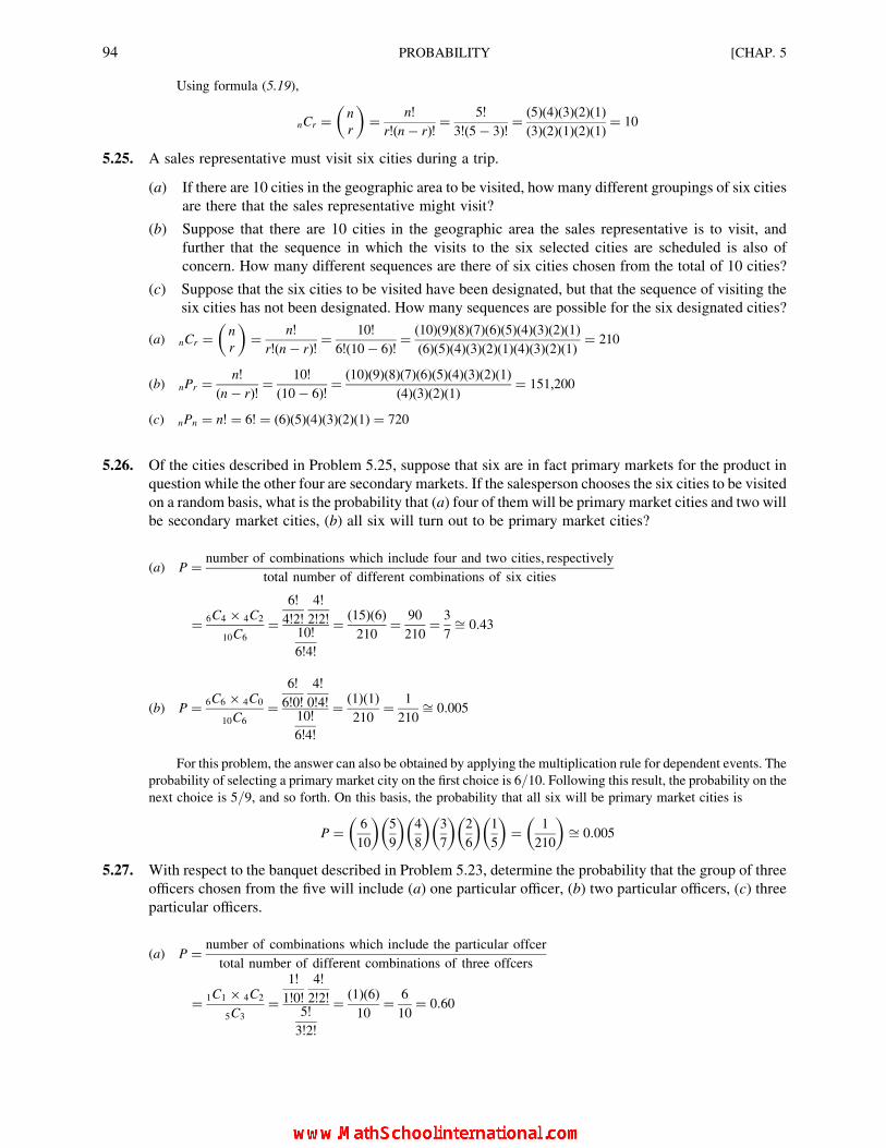
Using formula (5.19),
nCr ¼ n
r
� �¼ n!
r!(n � r)!¼ 5!
3!(5� 3)!¼ (5)(4)(3)(2)(1)(3)(2)(1)(2)(1)
¼ 10
5.25. A sales representative must visit six cities during a trip.
(a) If there are 10 cities in the geographic area to be visited, how many different groupings of six cities
are there that the sales representative might visit?
(b) Suppose that there are 10 cities in the geographic area the sales representative is to visit, and
further that the sequence in which the visits to the six selected cities are scheduled is also of
concern. How many different sequences are there of six cities chosen from the total of 10 cities?
(c) Suppose that the six cities to be visited have been designated, but that the sequence of visiting the
six cities has not been designated. How many sequences are possible for the six designated cities?
(a) nCr ¼ n
r
� �¼ n!
r!(n � r)!¼ 10!
6!(10� 6)!¼ (10)(9)(8)(7)(6)(5)(4)(3)(2)(1)(6)(5)(4)(3)(2)(1)(4)(3)(2)(1)
¼ 210
(b) nPr ¼ n!
(n � r)!¼ 10!
(10� 6)!¼ (10)(9)(8)(7)(6)(5)(4)(3)(2)(1)
(4)(3)(2)(1)¼ 151,200
(c) nPn ¼ n! ¼ 6! ¼ (6)(5)(4)(3)(2)(1) ¼ 720
5.26. Of the cities described in Problem 5.25, suppose that six are in fact primary markets for the product in
question while the other four are secondary markets. If the salesperson chooses the six cities to be visited
on a random basis, what is the probability that (a) four of them will be primary market cities and two will
be secondary market cities, (b) all six will turn out to be primary market cities?
(a) P ¼ number of combinations which include four and two cities, respectively
total number of different combinations of six cities
¼ 6C4 � 4C2
10C6
¼6!
4!2!
4!
2!2!10!
6!4!
¼ (15)(6)210
¼ 90
210¼ 3
7ffi 0:43
(b) P ¼ 6C6 � 4C0
10C6
¼6!
6!0!
4!
0!4!10!
6!4!
¼ ð1Þð1Þ210
¼ 1
210ffi 0:005
For this problem, the answer can also be obtained by applying the multiplication rule for dependent events. The
probability of selecting a primary market city on the first choice is 6/10. Following this result, the probability on thenext choice is 5/9, and so forth. On this basis, the probability that all six will be primary market cities is
P ¼ 6
10
� �5
9
� �4
8
� �3
7
� �2
6
� �1
5
� �¼ 1
210
� �ffi 0:005
5.27. With respect to the banquet described in Problem 5.23, determine the probability that the group of three
officers chosen from the five will include (a) one particular officer, (b) two particular officers, (c) three
particular officers.
(a) P ¼ number of combinations which include the particular offcer
total number of different combinations of three offcers
¼ 1C1 � 4C2
5C3
¼1!
1!0!
4!
2!2!5!
3!2!
¼ (1)(6)10
¼ 6
10¼ 0:60
94 PROBABILITY [CHAP. 5

In this case, this probability value is equivalent simply to observing that 3/5 of the officers will be chosen, andthus that the probability that any given individual will be chosen is 3/5, or 0.60.
ðbÞ P ¼ 2C2 � 3C1
5C3
¼2!
2!0!
3!
1!2!5!
3!2!
¼ ð1Þð3Þ10
¼ 3
10¼ 0:30
(c) P ¼ 3C3 � 2C0
5C3
¼3!
3!0!
2!
0!2!5!
3!2!
¼ ð1Þð1Þ10
¼ 1
10¼ 0:10
Supplementary Problems
DETERMINING PROBABILITY VALUES
5.28. Determine the probability value for each of the following events.
(a) Probability of randomly selecting one account receivable which is delinquent, given that 5 percent of the
accounts are delinquent.
(b) Probability that a land investment will be successful. In the given area, only half of such investments are
generally successful, but the particular investors’ decision methods have resulted in their having a 30 percent
better record than the average investor in the area.
(c) Probability that the sum of the dots showing on the face of two dice after they are tossed is seven.
Ans. (a) 0.05, (b) 0.65, (c) 1/6
5.29. For each of the following reported odds ratios determine the equivalent probability value, and for each of the
reported probability values determine the equivalent odds ratio.
(a) Probability of P ¼ 2/3 that a target delivery date will be met.
(b) Probability of P ¼ 9/10 that a new product will exceed the breakeven sales level.
(c) Odds of 1 : 2 that a competitor will achieve the technological breakthrough.
(d) Odds of 5 : 1 that a new product will be profitable.
Ans. (a) 2 : 1, (b) 9 : 1, (c) P ¼ 1/3, (d) P ¼ 5/6
APPLYING THE RULES OF ADDITION
5.30. During a given week the probability that a particular common stock issue will increase (I) in price, remain
unchanged (U), or decline (D) in price is estimated to be 0.30, 0.20, and 0.50, respectively.
(a) What is the probability that the stock issue will increase in price or remain unchanged?
(b) What is the probability that the price of the issue will change during the week?
Ans. (a) 0.50, (b) 0.80
5.31. Of 500 employees, 200 participate in a company’s profit-sharing plan (P), 400 have major-medical insurance
coverage (M), and 200 employees participate in both programs. Construct a Venn diagram to portray the events
designated P and M.
CHAP. 5] PROBABILITY 95

5.32. Refer to the Venn diagram prepared in Problem 5.31. What is the probability that a randomly selected employee
(a) will be a participant in at least one of the two programs, (b) will not be a participant in either program?
Ans. 0.80, (b) 0.20
5.33. The probability that a new marketing approach will be successful (S) is assessed as being 0.60. The probability that
the expenditure for developing the approach can be kept within the original budget (B) is 0.50. The probability that
both of these objectives will be achieved is estimated at 0.30. What is the probability that at least one of these
objectives will be achieved?
Ans. 0.80
INDEPENDENT EVENTS, DEPENDENT EVENTS, AND CONDITIONAL PROBABILITY
5.34. For the situation described in Problem 5.31, (a) determine the probability that an employee will be a participant in
the profit-sharing plan (P) given that the employee has major-medical insurance coverage (M), and (b) determine if
the two events are independent or dependent by reference to the conditional probability value.
Ans. (a) 0.50, (b) dependent
5.35. For Problem 5.33, determine (a) the probability that the new marketing approach will be successful (S) given that
the development cost was kept within the original budget (B), and (b) if the two events are independent or dependent
by reference to the conditional probability value.
Ans. (a) 0.60, (b) independent
5.36. The probability that automobile sales will increase next month (A) is estimated to be 0.40. The probability that the
sale of replacement parts will increase (R) is estimated to be 0.50. The probability that both industries will
experience an increase in sales is estimated to be 0.10. What is the probability that (a) automobile sales have
increased during the month given that there is information that replacement parts sales have increased,
(b) replacement parts sales have increased given information that automobile sales have increased during the
month?
Ans. (a) 0.20, (b) 0.25
5.37. For Problem 5.36, determine if the two events are independent or dependent by reference to one of the conditional
probability values.
Ans. Dependent
APPLYING THE RULES OF MULTIPLICATION
5.38. During a particular period, 80 percent of the common stock issues in an industry which includes just 10 companies
have increased in market value. If an investor chose two of these issues randomly, what is the probability that both
issues increased in market value during this period?
Ans. 56=90 ffi 0:62
5.39. The overall proportion of defective items in a continuous production process is 0.10. What is the probability that
(a) two randomly chosen items will both be nondefective (D0), (b) two randomly chosen items will both be
defective (D), (c) at least one of two randomly chosen items will be nondefective (D0)?Ans. (a) 0.81, (b) 0.01, (c) 0.99
5.40. Test the independence of the two events described in Problem 5.31 by using the rule of multiplication for
independent events. Compare your answer with the result of the test in Problem 5.34(b).
Ans. Dependent
5.41. Test the independence of the two events described in Problem 5.33 by using the rule of multiplication for
independent events. Compare your answer with the result of the test in Problem 5.35(b).
Ans. Independent
96 PROBABILITY [CHAP. 5

5.42. From Problem 5.38, suppose an investor chose three of these stock issues randomly. Construct a tree diagram to
portray the various possible results for the sequence of three stock issues.
5.43. Referring to the tree diagram prepared in Problem 5.42, determine the probability that (a) only one of the three issues
increased in market value, (b) two issues increased in market value, (c) at least two issues increased in market value.
Ans. (a) 48=720 ffi 0:07, (b) 336=720 ffi 0:47, (c) 672=720 ffi 0:93
5.44. Referring to Problem 5.39, suppose a sample of four items is chosen randomly. Construct a tree diagram to portray
the various possible results in terms of individual items being defective (D) or nondefective (D0).
5.45. Referring to the tree diagram prepared in Problem 5.44, determine the probability that (a) none of the four
items is defective, (b) exactly one item is defective, (c) one or fewer items are defective.
Ans. (a) 0:6561 ffi 0:66, (b) 0:2916 ffi 0:29, (c) 0:9477 ffi 0:95
BAYES’ THEOREM
5.46. Suppose there are two urns U1 and U2. U1 contains two red balls and one green ball, while U2 contains one red ball
and two green balls.
(a) An urn is randomly selected, and then one ball is randomly selected from the urn. The ball is red. What is the
probability that the urn selected was U1?
(b) An urn is randomly selected, and then two balls are randomly selected (without replacement) from the urn.
The first ball is red and the second ball is green. What is the probability that the urn selected was U1?
Ans. (a) P(U1) ¼ 2=3, (b) P(U1) ¼ 1=2
5.47. Refer to Problem 5.46.
(a) Suppose an urn is randomly selected, and then two balls are randomly selected (without replacement) from
the urn. Both balls are red. What is the probability that the urn selected was U1?
(b) Suppose an urn is randomly selected and then two balls are randomly selected, but with the first selected ball
being placed back in the urn before the second ball is drawn. Both balls are red. What is the probability that the
urn selected was U1?
Ans. (a) P(U1) ¼ 1, (b) P(U1) ¼ 4=5
5.48. Eighty percent of the vinyl material received from Vendor A is of exceptional quality while only 50 percent of the
vinyl material received from Vendor B is of exceptional quality. However, the manufacturing capacity of Vendor A
is limited, and for this reason only 40 percent of the vinyl material purchased by our firm comes from Vendor A. The
other 60 percent comes from Vendor B. An incoming shipment of vinyl material is inspected, and found to be of
exceptional quality. What is the probability that it came from Vendor A?
Ans. P(A) ¼ 0:52
5.49. Gasoline is being produced at three refineries with daily production levels of 100,00, 200,000, and 300,000 gallons,
respectively. The proportion of the output which is below the octane specifications for name-brand sale at the three
refineries is 0.03, 0.05, and 0.44, respectively. A gasoline tank truck is found to be carrying gasoline which is below
the octane specifications, and therefore the gasoline is to be marketed outside of the name-brand distribution system.
Determine the probability that the tank truck came from each of the three refineries, respectively, (a) without
reference to the information that the shipment is below the octane specifications and (b) given the additional
information that the shipment is below the octane specifications.
Ans. (a) P(1) ¼ 16ffi 0:17, P(2) ¼ 2
6ffi 0:33, P(3) ¼ 3
6¼ 0:50, (b) P(1) ¼ 0:12, P(2) ¼ 0:40, P(3) ¼ 0:48
JOINT PROBABILITY TABLES
5.50. Table 5.5 is a contingency table which presents a classification of 150 sampled companies according to four industry
groups and according to whether return on equity is above or below the average return in this sample of 150 firms.
Prepare the joint probability table based on these sample data.
CHAP. 5] PROBABILITY 97

Table 5.5 Contingency Table for Return on Equity
According to Industry Group
Return on equity
Industry
category
Above
average (A)
Below
average (B) Total
I 20 40 60
II 10 10 20
III 20 10 30
IV 25 15 40
Total 75 75 150
5.51. Referring to the joint probability table prepared in Problem 5.50, indicate the following probabilities: (a) P(I),
(b) P(II), (c) P(III), (d) P(IV).
Ans. (a) 0.40, (b) 0.13, (c) 0.20, (d) 0.27
5.52. Referring to the joint probability table prepared in Problem 5.50, determine the following probabilities:
(a) P(I and A), (b) P(II or B), (c) P(A), (d ) P( I or II), (e) P( I and II), ( f ) P(A or B), (g) P(AjI ), (h) P( IIIjA).Ans. (a) 0.13, (b) 0.57, (c) 0.50, (d) 0.53, (e) 0, ( f ) 1.0, (g) 0.33, (h) 0.27
PERMUTATIONS AND COMBINATIONS
5.53. Suppose there are eight different management trainee positions to be assigned to eight employees in a company’s
junior management training program. In how many different ways can the eight individuals be assigned to the eight
different positions?
Ans. 40,320
5.54. Referring to the situation described in Problem 5.53, suppose only six different positions are available for the
eight qualified individuals. In how many different ways can six individuals from the eight be assigned to the six
different positions?
Ans. 20,160
5.55. Referring to the situation described in Problem 5.54, suppose that the six available positions can all be considered
comparable, and not really different for practical purposes. In how many ways can the six individuals be chosen
from the eight qualified people to fill the six positions?
Ans. 28
5.56. A project group of two engineers and three technicians is to be assigned from a departmental group which includes
five engineers and nine technicians. How many different project groups can be assigned from the fourteen available
personnel?
Ans. 840
5.57. For the personnel assignment situation described in Problem 5.56, suppose the five individuals are assigned
randomly from the fourteen personnel in the department, without reference to whether each person is an engineer or
a technician. What is the probability that the project group will include (a) exactly two engineers, (b) no engineers.
(c) no technicians?
Ans. (a) P ffi 0:42, (b) P ffi 0:06, (c) P ffi 0:0005
98 PROBABILITY [CHAP. 5

CHAPTER 6
ProbabilityDistributions forDiscrete Random
Variables: Binomial,Hypergeometric,
and Poisson
6.1 WHAT IS A RANDOM VARIABLE?
In contrast to categorical events, such as that of drawing a particular card from a deck of cards, as discussed
in Chapter 5, a random variable is defined as a numerical event whose value is determined by a chance process.
When probability values are assigned to all possible numerical values of a random variable X, either by a listing
or by a mathematical function, the result is a probability distribution. The sum of the probabilities for all the
possible numerical outcomes must equal 1.0. Individual probability values may be denoted by the symbol f (x),
which indicates that a mathematical function is involved, by P(x ¼ X), which recognizes that the random
variable can have various specific values, or simply by P(X).
For a discrete random variable observed values can occur only at isolated points along a scale of values.
Therefore, it is possible that all numerical values for the variable can be listed in a table with accompanying
probabilities. There are several standard probability distributions that can serve as models for a wide variety of
99
Copyright 2004, 1996, 1988, 1976 by The McGraw-Hill Companies, Inc. Click Here for Terms of Use.
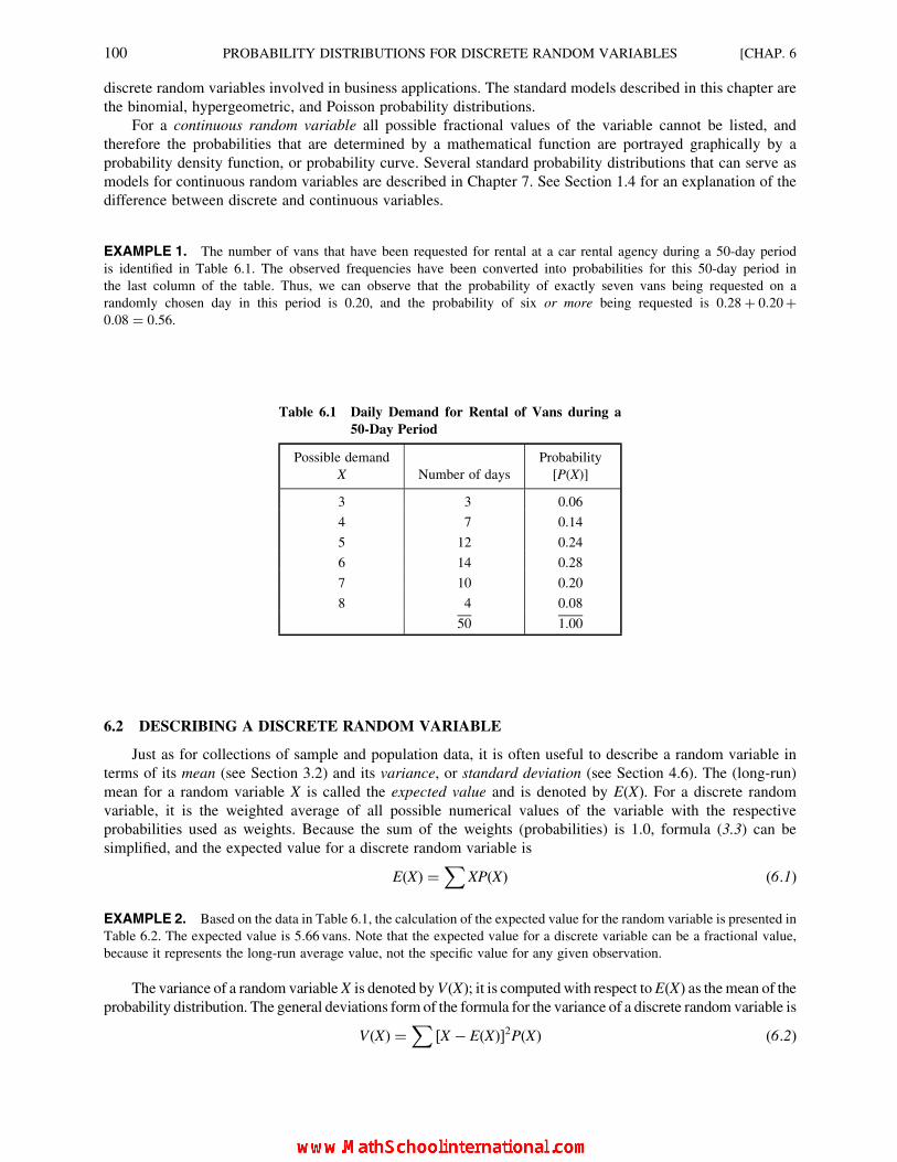
discrete random variables involved in business applications. The standard models described in this chapter are
the binomial, hypergeometric, and Poisson probability distributions.
For a continuous random variable all possible fractional values of the variable cannot be listed, and
therefore the probabilities that are determined by a mathematical function are portrayed graphically by a
probability density function, or probability curve. Several standard probability distributions that can serve as
models for continuous random variables are described in Chapter 7. See Section 1.4 for an explanation of the
difference between discrete and continuous variables.
EXAMPLE 1. The number of vans that have been requested for rental at a car rental agency during a 50-day period
is identified in Table 6.1. The observed frequencies have been converted into probabilities for this 50-day period in
the last column of the table. Thus, we can observe that the probability of exactly seven vans being requested on a
randomly chosen day in this period is 0.20, and the probability of six or more being requested is 0:28þ 0:20þ0:08 ¼ 0:56.
6.2 DESCRIBING A DISCRETE RANDOM VARIABLE
Just as for collections of sample and population data, it is often useful to describe a random variable in
terms of its mean (see Section 3.2) and its variance, or standard deviation (see Section 4.6). The (long-run)
mean for a random variable X is called the expected value and is denoted by E(X). For a discrete random
variable, it is the weighted average of all possible numerical values of the variable with the respective
probabilities used as weights. Because the sum of the weights (probabilities) is 1.0, formula (3.3) can be
simplified, and the expected value for a discrete random variable is
E(X) ¼X
XP(X) (6:1)
EXAMPLE 2. Based on the data in Table 6.1, the calculation of the expected value for the random variable is presented in
Table 6.2. The expected value is 5:66 vans. Note that the expected value for a discrete variable can be a fractional value,
because it represents the long-run average value, not the specific value for any given observation.
The variance of a random variable X is denoted byV(X); it is computedwith respect toE(X) as themean of the
probability distribution. The general deviations form of the formula for the variance of a discrete random variable is
V(X) ¼X
[X � E(X)]2P(X) (6:2)
Table 6.1 Daily Demand for Rental of Vans during a
50-Day Period
Possible demand
X Number of days
Probability
[P(X)]
3 3 0.06
4 7 0.14
5 12 0.24
6 14 0.28
7 10 0.20
8 4 0.08
50 1.00
100 PROBABILITY DISTRIBUTIONS FOR DISCRETE RANDOM VARIABLES [CHAP. 6

The computational form of the formula for the variance of a discrete random variable, which does not require
the determination of deviations from the mean, is
V(X) ¼X
X2P(X)�X
XP(X)h i2
¼ E(X2)� [E(X)]2 (6:3)
EXAMPLE 3. The worksheet for the calculation of the variance for the demand for van rentals is presented in Table 6.3,
using the computational version of the formula. As indicated below, the variance has a value of 1.74.
V(X) ¼ E(X2)� [E(X)]2 ¼ 33:78� (5:66)2 ¼ 33:78� 32:04 ¼ 1:74
As is true in Section 4.6 for populations and samples, the standard deviation for a random variable is simply
the square root of the variance:
s ¼ffiffiffiffiffiffiffiffiffiffiV(X)
p(6:4)
An advantage of the standard deviation is that it is expressed in the same units as the random variable,
rather than being in squared units.
EXAMPLE 4. The standard deviation with respect to the demand for van rentals is
s ¼ffiffiffiffiffiffiffiffiffiffiV(X)
p¼
ffiffiffiffiffiffiffiffiffi1:74
p¼ 1:32 vans
Table 6.2 Expected Value Calculation for the Demand
for Vans
Possible demand
X
Probability
[P(X)]
Weighted value
[XP(X)]
3 0.06 0.18
4 0.14 0.56
5 0.24 1.20
6 0.28 1.68
7 0.20 1.40
8 0.08 0.64
1.00 E(X) ¼ 5.66
Table 6.3 Worksheet for the Calculation of the Variance for the Demand for Vans
Possible
demand
X
Probability
[P(X)]
Weighted value
[XP(X)]
Squared
demand
(X 2)
Weighted square
[X 2P(X)]
3 0.06 0.18 9 0.54
4 0.14 0.56 16 2.24
5 0.24 1.20 25 6.00
6 0.28 1.68 36 10.08
7 0.20 1.40 49 9.80
8 0.08 0.64 64 5.12
E(X) ¼ 5.66 E(X 2) ¼ 33.78
CHAP. 6] PROBABILITY DISTRIBUTIONS FOR DISCRETE RANDOM VARIABLES 101

6.3 THE BINOMIAL DISTRIBUTION
The binomial distribution is a discrete probability distribution that is applicable as a model for decision-
making situations in which a sampling process can be assumed to conform to a Bernoulli process. A Bernoulli
process is a sampling process in which
(1) Only two mutually exclusive possible outcomes are possible in each trial, or observation. For
convenience these are called success and failure.
(2) The outcomes in the series of trials, or observations, constitute independent events.
(3) The probability of success in each trial, denoted by p, remains constant from trial to trial. That is,
the process is stationary.
The binomial distribution can be used to determine the probability of obtaining a designated number of
successes in a Bernoulli process. Three values are required: the designated number of successes (X); the number
of trials, or observations (n); and the probability of success in each trial (p). Where q ¼ (1� p), the formula for
determining the probability of a specific number of successes X for a binomial distribution is
P(Xjn, p) ¼ nCX p Xq n�X
¼ n!
X!(n � X)!p Xq n�X (6:5)
EXAMPLE 5. The probability that a randomly chosen sales prospect will make a purchase is 0.20. If a sales representative
calls on six propects, the probability that exactly four sales will be made is determined as follows:
P(X ¼ 4jn ¼ 6, p ¼ 0:20) ¼ 6C4(0:20)4(0:80)2 ¼ 6!
4!2!(0:20)4(0:80)2
¼ 6� 5� 4� 3� 2
(4� 3� 2)(2)(0:0016)(0:64) ¼ 0:01536 ffi 0:015
Often there is an interest in the cumulative probability of “X or more” successes or “X or fewer” successes
occurring in n trials. In such a case, the probability of each outcome included within the designated interval
must be determined, and then these probabilities are summed.
EXAMPLE 6. For Example 5, the probability that the salesperson will make four or more sales is determined as follows:
P(X � 4jn ¼ 6, p ¼ 0:20) ¼ P(X ¼ 4)þ P(X ¼ 5)þ P(X ¼ 6)
¼ 0:01536þ 0:001536þ 0:000064 ¼ 0:016960 ffi 0:017
where P(X ¼ 4) ¼ 0:01536 (from Example 5)
P(X ¼ 5) ¼ 6C5(0:20)5(0:80)1 ¼ 6!
5!1!(0:20)5(0:80) ¼ 6(0:00032)(0:80) ¼ 0:001536
P(X ¼ 6) ¼ 6C6(0:20)6(0:80)0 ¼ 6!
6!0!(0:000064)(1) ¼ (1)(0:000064) ¼ 0:000064
(Note: Recall that any value raised to the zero power is equal to 1.)
Because use of the binomial formula involves considerable arithmetic when the sample is relatively large,
tables of binomial probabilities are often used. (See Appendix 2.)
EXAMPLE 7. If the probability that a randomly chosen sales prospect will make a purchase is 0.20, the probability that a
salesperson who calls on 15 prospects will make fewer than three sales is
P(X , 3jn ¼ 15, p ¼ 0:20) ¼ P(X 2) ¼ P(X ¼ 0)þ P(X ¼ 1)þ P(X ¼ 2)
¼ 0:0352þ 0:1319þ 0:2309 (from Appendix 2)
¼ 0:3980 ffi 0:40
102 PROBABILITY DISTRIBUTIONS FOR DISCRETE RANDOM VARIABLES [CHAP. 6

The values of p referenced in Appendix 2 do not exceed p ¼ 0:50. If the value of p in a particular application exceeds
0.50, the problem is restated so that the event is defined in terms of the number of failures rather than the number of
successes (see Problem 6.9).
The expected value (long-run mean) and variance for a given binomial distribution could be determined
by listing the probability distribution in a table and applying the formulas presented in Section 6.2. However,
the expected number of successes can be computed directly:
E(X) ¼ np (6:6)
Where q ¼ (1� p), the variance of the number of successes can also be computed directly:
V(X) ¼ npq (6:7)
EXAMPLE 8. For Example 7, the expected number of sales (as a long-run average), the variance, and the standard
deviation associated with making calls on 15 prospects are
E(X) ¼ np ¼ 15(0:20) ¼ 3:00 sales
V(X) ¼ np(q) ¼ 15(0:20)(0:80) ¼ 2:40
s ¼ffiffiffiffiffiffiffiffiffiffiV(X)
p¼
ffiffiffiffiffiffiffi2:4
p¼ 1:55 sales
6.4 THE BINOMIAL VARIABLE EXPRESSED BY PROPORTIONS
Instead of expressing the random binomial variable as the number of successes X, we can designate it in
terms of the proportion of successes pp, which is the ratio of the number of successes to the number of trials:
pp ¼ X
n(6:8)
In such cases, formula (6.5) is modified only with respect to defining the proportion. Thus, the probability
of observing exactly pp proportion of successes in n Bernoulli trials is
P pp ¼ X
njn, p
� �¼ nC
XpXqn�X (6:9)
or
P pp ¼ X
njn, p
� �¼ nC
XpX(1� p)n�X (6:10)
In formula (6.10), p (Greek “pı”) is the equivalent of p except that it specifically indicates that the
probability of success in an individual trial is a population or process parameter.
EXAMPLE 9. The probability that a randomly selected salaried employee is a participant in an optional retirement
program is 0.40. If five salaried employees are chosen randomly, the probability that the proportion of participants is exactly
0.60, or 3/5 of the five sampled employees, is
P( pp ¼ 0:60) ¼ P pp ¼ 3
5jn ¼ 5, p ¼ 0:40
� �¼ 5C3(0:40)
3(0:60)2 ¼ 5!
3!2!(0:064)(0:36) ¼ 0:2304 ffi 0:23
When the binomial variable is expressed as a proportion, the distribution is still discrete and not
continuous. Only the particular proportions for which the number of successes X is a whole number can
occur. For instance, in Example 9 it is not possible for there to be a proportion of 0.50 participant out of a
sample of five. The use of the binomial table with respect to proportions simply requires converting the
designated proportion pp to the number of successes X for the given sample size n.
EXAMPLE 10. The probability that a randomly selected employee is a participant in an optional retirement program is
0.40. If 10 employees are chosen randomly, the probability that the proportion of participants is at least 0.70 is
P( pp � 0:70) ¼ P(X � 7jn ¼ 10, p ¼ 0:10) ¼ P(X ¼ 7)þ P(X ¼ 8)þ P(X ¼ 9)þ P(X ¼ 10)
¼ 0:0425þ 0:0106þ 0:0016þ 0:0001 ¼ 0:0548
CHAP. 6] PROBABILITY DISTRIBUTIONS FOR DISCRETE RANDOM VARIABLES 103

The expected value for a binomial probability distribution expressed by proportions is equal to the
population proportion, which may be designated by either p or p:
E( pp) ¼ p (6:11)
or E( pp) ¼ p (6:12)
The variance of the proportion of successes for a binomial probability distribution, when q ¼ (1� p), is
V( pp) ¼ pq
n(6:13)
or V( pp) ¼ p(1� p)
n(6:14)
6.5 THE HYPERGEOMETRIC DISTRIBUTION
When sampling is done without replacement of each sampled item taken from a finite population of items, the
Bernoulli process does not apply because there is a systematic change in the probability of success as items are
removed from the population. When sampling without replacement is used in a situation that would otherwise
qualify as a Bernoulli process, the hypergeometric distribution is the appropriate discrete probability distribution.
Given that X is the designated number of successes, N is the total number of items in the population, T is
the total number of successes included in the population, and n is the number of items in the sample, the formula
for determining hypergeometric probabilities is
P(XjN, T , n) ¼N � T
n � X
� �T
X
� �N
n
� � (6:15)
EXAMPLE 11. Of six employees, three have been with the company five or more years. If four employees are chosen
randomly from the group of six, the probability that exactly two will have five or more years seniority is
P(X ¼ 2jN ¼ 6, T ¼ 3, n ¼ 4) ¼6� 3
4� 2
� �3
2
� �6
4
� � ¼3
2
� �3
2
� �6
4
� � ¼3!
2!1!
3!
2!1!6!
4!2!
¼ (3)(3)15
¼ 0:60
Note that in Example 11, the required probability value is computed by determining the number of different
combinations that would include two high-seniority and two low-seniority employees as a ratio of the total
number of combinations of four employees taken from the six. Thus, the hypergeometric formula is a direct
application of the rules of combinatorial analysis described in Section 5.10.
When the population is large and the sample is relatively small, the fact that sampling is done without
replacement has little effect on the probability of success in each trial. A convenient rule of thumb is that a
binomial probability can be used as an approximation of a hypergeometric probability value when n , 0:05N.
That is, the sample size should be less than 5 percent of the population size. Different texts use somewhat
different rules for determining when such approximation is appropriate.
6.6 THE POISSON DISTRIBUTION
The Poisson distribution can be used to determine the probability of a designated number of events
occurring when the events occur in a continuum of time or space. Such a process is called a Poisson process;
104 PROBABILITY DISTRIBUTIONS FOR DISCRETE RANDOM VARIABLES [CHAP. 6

it is similar to the Bernoulli process (see Section 6.3) except that the events occur over a continuum (e.g., during
a time interval) and there are no trials as such. An example of such a process is the arrival of incoming calls
at a telephone switchboard. As was the case for the Bernoulli process, it is assumed that the events are
independent and that the process is stationary.
Only one value is required to determine the probability of a designated number of events occurring in a
Poisson process: the long-run mean number of events for the specific time or space dimension of interest. This
mean generally is represented by l (Greek lambda), or possibly by m. The formula for determining the
probability of a designated number of successes X in a Poisson distribution is
P(Xjl) ¼ lXe�l
X!(6:16)
Here e is the constant 2.7183 that is the base of natural logarithms, and the values of e�l may be obtained
from Appendix 3.
EXAMPLE 12. An average of five calls for service per hour are received by a machine repair department. The probability
that exactly three calls for service will be received in a randomly selected hour is
P(X ¼ 3jl ¼ 5:0) ¼ (5)3e�5
3!¼ (125)(0:00674)
6¼ 0:1404
Alternatively, a table of Poisson probabilities may be used. Appendix 4 identifies the probability of each
designated number of successes for various values of l.
EXAMPLE 13. We can determine the answer to Example 12 by use of Appendix 4 for Poisson probabilities as follows:
P(X ¼ 3jl ¼ 5:0) ¼ 0:1404
When there is an interest in the probability of “X or more” or “X or fewer” successes, the rule of addition
for mutually exclusive events is applied.
EXAMPLE 14. If an average of five service calls per hour are received at a machine repair department, the probability
that fewer than three calls will be received during a randomly chosen hour is determined as follows:
P(X , 3jl ¼ 5:0) ¼ P(X 2) ¼ P(X ¼ 0)þ P(X ¼ 1)þ P(X ¼ 2)
¼ 0:0067þ 0:0337þ 0:0842 ¼ 0:1246
where P(X ¼ 0jl ¼ 5:0) ¼ 0:0067 (from Appendix 4)
P(X ¼ 1jl ¼ 5:0) ¼ 0:0337P(X ¼ 2jl ¼ 5:0) ¼ 0:0842
Because a Poisson process is assumed to be stationary, it follows that the mean of the process is always
proportional to the length of the time or space continuum. Therefore, if the mean is available for one length of
time, the mean for any other required time period can be determined.
This is important, because the value of k which is used must apply to the time period of interest.
CHAP. 6] PROBABILITY DISTRIBUTIONS FOR DISCRETE RANDOM VARIABLES 105

EXAMPLE 15. On the average, 12 people per hour ask questions of a decorating consultant in a fabric store. The
probability that three or more people will approach the consultant with questions during a 10-min period (1/6 of an hour) isdetermined as follows:
Average per hour ¼ 0:12
l ¼ average per 10 min ¼ 12
6¼ 2:0
P(X � 3jl ¼ 2:0) ¼ P(X ¼ 3jl ¼ 2:0)þ P(X ¼ 4jl ¼ 2:0)þ P(X ¼ 5jl ¼ 2:0)þ � � �¼ 0:1804þ 0:0902þ 0:0361þ 0:0120þ 0:0034þ 0:0009þ 0:0002 ¼ 0:3232
where P(X ¼ 3jl ¼ 2:0) ¼ 0:1804) (from Appendix 4)
P(X ¼ 4jl ¼ 2:0) ¼ 0:0902P(X ¼ 5jl ¼ 2:0) ¼ 0:0361P(X ¼ 6jl ¼ 2:0) ¼ 0:0120P(X ¼ 7jl ¼ 2:0) ¼ 0:0034P(X ¼ 8jl ¼ 2:0) ¼ 0:0009P(X ¼ 9jl ¼ 2:0) ¼ 0:0002
By definition, the expected value (long-run mean) for a Poisson probability distribution is equal to the mean
of the distribution:
E(X) ¼ l (6:17)
As it happens, the variance of the number of events for a Poisson probability distribution is also equal to the
mean of the distribution, l. The standard deviation then is the square root of l:
V(X) ¼ l (6:18)
s ¼ffiffiffil
p(6:19)
6.7 POISSON APPROXIMATION OF BINOMIAL PROBABILITIES
When the number of observations or trials n in a Bernoulli process is large, computations are quite tedious.
Further, tabled probabilities for very small values of p are not generally available. Fortunately, the Poisson
distribution is suitable as an approximation of binomial probabilities when n is large and p or q is small. A
convenient rule is that such approximation can be made when n � 30, and either np , 5 or nq , 5. Different
texts use somewhat different rules for determining when such approximation is appropriate.
The mean for the Poisson probability distribution that is used to approximate binomial probabilities is
l ¼ np (6:20)
EXAMPLE 16. For a large shipment of transistors from a supplier, 1 percent of the items is known to be defective.
If a sample of 30 transistors is randomly selected, the probability that two or more transistors will be defective can be
determined by use of the binomial probabilities in Appendix 2:
P(X � 2jn ¼ 30, p ¼ 0:01) ¼ P(X ¼ 2)þ P(X ¼ 3)þ � � � ¼ 0:0328þ 0:0031þ 0:0002 ¼ 0:0361
Where l ¼ np ¼ 30(0:01) ¼ 0:3, Poisson approximation of the above probability value is
P(X � 2jl ¼ 0:3) ¼ P(X ¼ 2)þ P(X ¼ 3)þ � � � ¼ 0:0333þ 0:0033þ 0:0002 ¼ 0:0368
Thus, the difference between the Poisson approximation and the actual binomial probability value is just 0.0007.
When n is large but neither np nor nq is less than 5.0, binomial probabilities can be approximated by use of
the normal probability distribution (see Section 7.4).
Overall, the availability of computers has made the approximation of probabilities for one model based on
another probability model less important.
106 PROBABILITY DISTRIBUTIONS FOR DISCRETE RANDOM VARIABLES [CHAP. 6

6.8 USING EXCEL AND MINITAB
Computer software for statistical analysis typically includes the capability of providing probability values
for the standard discrete probability distributions that are used as models for decision-making situations. Such
availability is particularly useful when the particular probabilities are not available in standard tables.
Solved Problems 6.21 and 6.22 illustrate the use of Excel and Minitab, respectively, for the determination of
binomial probabilities. Problems 6.23 and 6.24 illustrate the use of Excel and Minitab, respectively, for the
determination of Poisson probabilities.
Solved Problems
DISCRETE RANDOM VARIABLES
6.1. The number of trucks arriving hourly at a warehouse facility has been found to follow the probability
distribution in Table 6.4. Calculate (a) the expected number of arrivals X per hour, (b) the variance, and
(c) the standard deviation for the discrete random variable.
From Table 6.5,
(a) E(X) ¼ 3:15 trucks
(b) V(X) ¼ E(X2)� [E(X)]2 ¼ 12:05� (3:15)2 ¼ 12:05� 9:9225 ¼ 2:1275 ffi 2:13
(c) s ¼ ffiffiffiffiffiffiffiffiffiffiV(X)
p ¼ ffiffiffiffiffiffiffiffiffiffiffiffiffiffi2:1275
p ¼ 1:46 trucks
Table 6.4 Hourly Arrival of Trucks at a Warehouse
Number of trucks (X) 0 1 2 3 4 5 6
Probability [P(X)] 0.05 0.10 0.15 0.25 0.30 0.10 0.05
Table 6.5 Worksheet for the Truck Arrival Calculations
Number of
trucks
(X)
Probability
[P(X)]
Weighted value
[XP(X)]
Squared number
(X 2)
Weighted square
[X 2P(X)]
0 0.05 0 0 0
1 0.10 0.10 1 0.10
2 0.15 0.30 4 0.60
3 0.25 0.75 9 2.25
4 0.30 1.20 16 4.80
5 0.10 0.50 25 2.50
6 0.05 0.30 36 1.80
E(X) ¼ 3.15 E(X 2) ¼ 12.05
CHAP. 6] PROBABILITY DISTRIBUTIONS FOR DISCRETE RANDOM VARIABLES 107

6.2. Table 6.6 identifies the probability that a computer network will be inoperative the indicated number of
periods per week during the initial installation phase for the network. Calculate (a) the expected number
of times per week that the network is inoperative and (b) the standard deviation for this variable.
Using Table 6.7,
(a) E(X) ¼ 6:78 periods
(b) V(X) ¼ E(X2)� [E(X)]2 ¼ 47:00� (6:78)2 ¼ 47:00� 45:9684 ¼ 1:0316
(c) s ¼ ffiffiffiffiffiffiffiffiffiffiV(X)
p ¼ ffiffiffiffiffiffiffiffiffiffiffiffiffiffi1:0316
p ¼ 1:0157 ffi 1:02 periods
6.3. Table 6.8 lists the possible outcomes associated with the toss of two 6-sided dice and the probability
associated with each outcome. The probabilities were determined by use of the rules of addition and
multiplication discussed in Sections 5.4 and 5.6. For example, a 3 can be obtained by a combination of a
1 and 2, or a combination of a 2 and 1. Each sequence has a probability of occurrence of
(1=6)� (1=6) ¼ 1=36, and since the two sequences are mutually exclusive, P(X ¼ 3) ¼ 1=36þ1=36 ¼ 2:36. Determine (a) the expected number on the throw of two dice and (b) the standard
deviation of this distribution.
From Table 6.9,
(a) E(X) ¼ 7
(b) V(X) ¼ E(X2)� [E(X)]2 ¼ 54:83� (7)2 ¼ 54:83� 49 ¼ 5:83
(c) s ¼ ffiffiffiffiffiffiffiffiffiffiV(X)
p ¼ ffiffiffiffiffiffiffiffiffi5:83
p ffi 2:41
Table 6.6 Number of Inoperative Periods per Week for a New Computer
Network
Number of periods (X) 4 5 6 7 8 9
Probability [P(X)] 0.01 0.08 0.29 0.42 0.14 0.06
Table 6.7 Worksheet for the Computer Malfunction Calculations
Number of
periods
(X)
Probability
[P(X)]
Weighted value
[XP(X)]
Squared number
(X 2)
Weighted square
[X 2P(X)]
4 0.01 0.04 16 0.16
5 0.08 0.40 25 2.00
6 0.29 1.74 36 10.44
7 0.42 2.94 49 20.58
8 0.14 1.12 64 8.96
9 0.06 0.54 81 4.86
1.00 E(X) ¼ 6.78 E(X 2) ¼ 47.00
Table 6.8 Possible Outcomes on the Toss of Two Dice
Number on two dice (X) 2 3 4 5 6 7 8 9 10 11 12
Probability [P(X)] 136
236
336
436
536
636
536
436
336
236
136
108 PROBABILITY DISTRIBUTIONS FOR DISCRETE RANDOM VARIABLES [CHAP. 6

THE BINOMIAL DISTRIBUTION
6.4. Because of economic conditions, a firm reports that 30 percent of its accounts receivable from other
business firms are overdue. If an accountant takes a random sample of five such accounts, determine the
probability of each of the following events by use of the formula for binomial probabilities: (a) none of
the accounts is overdue, (b) exactly two accounts are overdue, (c) most of the accounts are overdue, (d)
exactly 20 percent of the accounts are overdue.
(a) P(X ¼ 0jn ¼ 5, p ¼ 0:30) ¼ 5C0(0:30)0(0:70)5 ¼ 5!
0!5!(0:30)0(0:70)5 ¼ (1)(1)(0:16807) ¼ 0:16807
(b) P(X ¼ 2jn ¼ 5, p ¼ 0:30) ¼ 5C2(0:30)2(0:70)3 ¼ 5!
2!3!(0:30)2(0:70)3 ¼ (10)(0:09)(0:343) ¼ 0:3087
(c) P(X � 3jn ¼ 5, p ¼ 0:30) ¼ P(X ¼ 3)þ P(X ¼ 4)þ P(X ¼ 5) ¼ 0:1323þ 0:02835þ 0:00243 ¼ 0:16308
where P(X ¼ 3) ¼ 5!
3!2!(0:30)3(0:70)2 ¼ (10)(0:027)(0:49) ¼ 0:1323
P(X ¼ 4) ¼ 5!
4!1!(0:30)4(0:70)1 ¼ (5)(0:0081)(0:70) ¼ 0:02835
P(X ¼ 5 ¼ 5!
5!0!(0:30)5(0:70)0 ¼ (1)(0:00243)(1) ¼ 0:00243
(d) PX
n¼ 0:20jn ¼ 5, p ¼ 0:30
� �¼ P(X ¼ 1jn ¼ 5, p ¼ 0:30) ¼ 5C1(0:30)
1(0:70)4 ¼ 5!
1!4!(0:30)1(0:70)4
¼ (5)(0:30)(0:2401) ¼ 0:36015
6.5. A mail-order firm has a circular that elicits a 10 percent response rate. Suppose 20 of the circulars are
mailed as a market test in a new geographic area. Assuming that the 10 percent response rate is
applicable in the new area, determine the probabilities of the following events by use of Appendix 2:
(a) no one responds, (b) exactly two people respond, (c) a majority of the people respond, (d) less than
20 percent of the people respond.
(a) P(X ¼ 0jn ¼ 20, p ¼ 0:10) ¼ 0:1216
(b) P(X ¼ 2jn ¼ 20, p ¼ 0:10) ¼ 0:2852
Table 6.9 Worksheet for the Calculations Concerning the Toss of Two Dice
Number
(X)
Probability
[P(X)]
Weighted value
[XP(X)]
Squared
number
(X 2)
Weighted square
[X 2P(X)]
2 1/36 2/36 4 4/36
3 2/36 6/36 9 18/36
4 3/36 12/36 16 48/36
5 4/36 20/36 25 100/36
6 5/36 30/36 36 180/36
7 6/36 42/36 49 294/36
8 5/36 40/36 64 320/36
9 4/36 36/36 81 324/36
10 3/36 30/36 100 300/36
11 2/36 22/36 121 242/36
12 1/36 12/36 144 144/36
36/36 E(X) ¼ 252/36 ¼ 7.0 E(X 2) ¼ 1,974/36 ffi 54.83
CHAP. 6] PROBABILITY DISTRIBUTIONS FOR DISCRETE RANDOM VARIABLES 109

(c) P(X ¼ 11jn ¼ 20, p ¼ 0:10) ¼ P(X ¼ 11)þ P(X ¼ 12)þ � � � ¼ 0:0000 ffi 0
(d) PX
n, 0:20jn ¼ 20, p ¼ 0:10
� �¼ P(X 3jn ¼ 20, p ¼ 0:10)
¼ P(X ¼ 0)þ P(X ¼ 1)þ P(X ¼ 2)þ P(X ¼ 3)
¼ 0:1216þ 0:2702þ 0:2852þ 0:1901 ¼ 0:8671
6.6. The binomial formula can be viewed as being composed of two parts: a combinations formula to
determine the number of different ways in which the designated event can occur and the rule of
multiplication to determine the probability of each sequence. Suppose that three items are selected
randomly from a process known to produce 10 percent defectives. Construct a three-step tree diagram
portraying the selection of the three items and using D for a defective item being selected and D0 for anondefective item being selected. Also, enter the appropriate probability values in the diagram and use
the multiplication rule for independent events to determine the probability of each possible sequence of
three events occurring.
See Fig. 6-1.
Fig. 6-1
6.7. From Problem 6.6, determine the probability that exactly one of the three sampled items is defective,
referring to Fig. 6-1 and using the addition rule for mutually exclusive events.
Beginning from the top of the tree diagram, the fourth, sixth, and seventh sequences include exactly one
defective item. Thus,
P(X ¼ 1) ¼ (D and D0 and D0)þ (D0 and D and D0)þ (D0 and D0 and D)
¼ 0:081þ 0:081þ 0:081 ¼ 0:243
110 PROBABILITY DISTRIBUTIONS FOR DISCRETE RANDOM VARIABLES [CHAP. 6

6.8. From Problems 6.6 and 6.7, determine the probability of obtaining exactly one defective item by use of
the binomial formula, and note the correspondence between the values in the formula and the values
obtained from the tree diagram.
Using formula (6.4),
P(X ¼ 1jn ¼ 3, p ¼ 0:10) ¼ 3C1(0:10)1(0:90)2 ¼ 3!
1!2!(0:10)(0:81)
¼ 3(0:081) ¼ 0:243
Thus, the first part of the binomial formula indicates the number of different sequences in the tree diagram that
include the designated number of successes (in this case there are three ways in which one defective item can be
included in the group of three items). The second part of the formula represents the rule of multiplication for the
specified independent events.
6.9. During a particular year, 70 percent of the common stocks listed on the New York Stock Exchange
increased in market value, while 30 percent were unchanged or declined in market value. At the
beginning of the year a stock advisory service chose 10 stock issues as being “specially recommended.”
If the 10 issues represent a random selection, what is the probability that (a) all 10 issues and (b) at least
eight issues increased in market value?
(a) P(X ¼ 10jn ¼ 10, p ¼ 0:70) ¼ P(X0 ¼ 0jn ¼ 10, q ¼ 0:30) ¼ 0:0282(Note: When p is greater than 0.50, the problem has to be restated in terms of X0 (read “not X”) and it follows
that X0 ¼ n � X. Thus, “all 10 increased” is the same event as “none decreased.”)
(b) P(X � 8jn ¼ 10, p ¼ 0:70) ¼ P(X0 2jn ¼ 10, q ¼ 0:30)¼ P(X0 ¼ 0)þ P(X0 ¼ 1)þ P(X0 ¼ 2)
¼ 0:0282þ 0:1211þ 0:2335 ¼ 0:3828(Note: When a probability statement is restated in terms of X0 instead of X and an inequality is involved, the
inequality symbol in the original statement simply is reversed.)
6.10. Using Appendix 2, determine:
(a) P(X ¼ 5jn ¼ 9, p ¼ 0:50)
(b) P(X ¼ 7jn ¼ 15, p ¼ 0:60)
(c) P(X 3jn ¼ 20, p ¼ 0:05)
(d) P(X � 18jn ¼ 20, p ¼ 0:90)
(e) P(X . 8jn ¼ 10, p ¼ 0:70)
(a) P(X ¼ 5jn ¼ 9, p ¼ 0:50) ¼ 0:2461
(b) P(X ¼ 7jn ¼ 15, p ¼ 0:60) ¼ P(X0 ¼ 8jn ¼ 15, q ¼ 0:40) ¼ 0:1181
(c) P(X 3jn ¼ 20, p ¼ 0:05) ¼ P(X ¼ 0)þ P(X ¼ 1)þ P(X ¼ 2)þ P(X ¼ 3)
¼ 0:3585þ 0:3774þ 0:1887þ 0:0596 ¼ 0:9842
(d) P(X � 18jn ¼ 20, p ¼ 0:90) ¼ P(X0 2jn ¼ 20, q ¼ 0:10)¼ P(X0 ¼ 0)þ P(X0 ¼ 1)þ P(X0 ¼ 2)
¼ 0:1216þ 0:2702þ 0:2852 ¼ 0:6770
(e) P(X . 8jn ¼ 10, p ¼ 0:70) ¼ P(X0 , 2jn ¼ 10, q ¼ 0:30)¼ P(X0 ¼ 0)þ P(X0 ¼ 1) ¼ 0:0282þ 0:1211 ¼ 0:1493
6.11 If a fair coin is tossed five times, the probability distribution with respect to the number of heads
observed is based on the binomial distribution, with n ¼ 5 and p ¼ 0:50 (see. Table 6.10). Determine
(a) the expected number of heads and (b) the standard deviation for the number of heads by use
of the general formulas for discrete random variables.
CHAP. 6] PROBABILITY DISTRIBUTIONS FOR DISCRETE RANDOM VARIABLES 111

Using Table 6.11.
(a) E(X) ¼ 2:4995 ffi 2:50 heads
(b) V(X) ¼ E(X2)� [E(X)]2 ¼ 7:4979� (2:4995)2 ¼ 7:4979� 6:2475 ¼ 1:2504
(c) s ¼ ffiffiffiffiffiffiffiffiffiffiV(X)
p ¼ ffiffiffiffiffiffiffiffiffiffiffiffiffiffi1:2504
p ¼ 1:1182 ffi 1:12 heads
6.12. Referring to Problem 6.11, determine (a) the expected number of heads and (b) the standard deviation
for the number of heads by use of the special formulas applicable for binomial probability distributions.
(c) Compare your answers to those in Problem 6.11.
(a) E(X) ¼ np ¼ 5(0:50) ¼ 2:50 heads
(b) V(X) ¼ npq ¼ (5)(0:50)(0:50) ¼ 1:2500
s ¼ ffiffiffiffiffiffiffiffiffiffiV(X)
p ¼ ffiffiffiffiffiffiffiffiffiffiffiffiffiffi1:2500
p ¼ 1:1180 ffi 1:12 heads
(c) Except for a slight difference due to rounding of values, the answers obtained with the special formulas that are
applicable for binomial distributions correspond with the answers obtained by the lengthier general formulas
applicable for any discrete random variable.
THE HYPERGEOMETRIC DISTRIBUTION
6.13. A manager randomly selects n ¼ 3 individuals from a group of 10 employees in a department for
assignment to a project team. Assuming that four of the employees were assigned to a similar project
previously, construct a three-step tree diagram portraying the selection of the three individuals in terms
of whether each individual chosen has had experience E or has no previous experience E0 in such a
project. Further, enter the appropriate probability values in the diagram and use the multiplication rule
for dependent events to determine the probability of each possible sequence of three events occurring.
See Fig. 6-2.
Table 6.10 Binomial Probability Distribution of the Number of Heads Occurring in
Five Tosses of a Fair Coin
Number of heads (X) 0 1 2 3 4 5
Probability [P(X)] 0.0312 0.1562 0.3125 0.3125 0.1562 0.0312
Table 6.11 Worksheet for the Calculations for Problem 6.11
Number of
heads (X)
Probability
[P(X)]
Weighted value
[XP(X)]
Squared number
(X 2)
Weighted square
[X 2P(X)]
0 0.0312 0 0 0
1 0.1562 0.1562 1 0.1562
2 0.3125 0.6250 4 1.2500
3 0.3125 0.9375 9 2.8125
4 0.1562 0.6248 16 2.4992
5 0.0312 0.1560 25 0.7800
E(X) ¼ 2.4995 E(X 2) ¼ 7.4979
112 PROBABILITY DISTRIBUTIONS FOR DISCRETE RANDOM VARIABLES [CHAP. 6

6.14. Referring to Problem 6.13, determine the probability that exactly two of the three employees selected
have had previous experience in such a project by reference to Fig. 6-2 and use of the addition rule for
mutually exclusive events.
Beginning from the top of the tree diagram, the second, third, and fifth sequences include exactly two
employees with experience. Thus, by the rule of addition for these mutually exclusive sequences:
P(X ¼ 2) ¼ (E and E and E0)þ (E and E0 and E)þ (E0 and E and E)
¼ 0:100þ 0:100þ 0:100 ¼ 0:30
6.15. Referring to Problem 6.13, determine the probability that exactly two of the three employees have had
the previous experience, using the formula for determining hypergeometric probabilities.
From formula (6.14),
P(XjN, T , n) ¼N � T
n � X
� �T
X
� �N
n
� �
P(X ¼ 2jN ¼ 10, T ¼ 4, n ¼ 3) ¼10� 4
3� 2
� �4
2
� �10
3
� � ¼6
1
� �4
2
� �10
3
� � ¼6!
1!5!
� �4!
2!2!
� �10!
3!7!
� � ¼ (6)(6)120
¼ 0:30
Fig. 6-2
CHAP. 6] PROBABILITY DISTRIBUTIONS FOR DISCRETE RANDOM VARIABLES 113

6.16. Section 6.5 states that the hypergeometric formula is a direct application of the rules of combinatorial
analysis described in Section 5.9. To demonstrate this, apply the hypergeometric formula to
Problem 5.26(a).
P(X ¼ 4jN ¼ 10, T ¼ 6, n ¼ 6) ¼10� 6
6� 4
� �6
6
� �10
6
� � ¼4!
2!2!
� �6!
4!2!
� �10!
6!4!
� �
¼ (6)(15)210
¼ 90
210¼ 3
7ffi 0:43
[Note: This result is equivalent to the use of the combinatorial analysis formula in the solution to
Problem 5.26(a).]
THE POISSON PROBABILITY DISTRIBUTION
6.17. On average, five people per hour conduct transactions at a special services desk in a commercial bank.
Assuming that the arrival of such people is independently distributed and equally likely throughout the
period of concern, what is the probability that more than 10 people will wish to conduct transactions at
the special services desk during a particular hour?
Using Appendix 4,
P(X . 10jl ¼ 5:0) ¼ P(X � 11jl ¼ 5:0) ¼ P(X ¼ 11)þ P(X ¼ 12)þ � � �¼ 0:0082þ 0:0034þ 0:0013þ 0:0005þ 0:0002 ¼ 0:0136
6.18. On average, a ship arrives at a certain dock every second day. What is the probability that two or more
ships will arrive on a randomly selected day?
Since the average per two days ¼ 1.0, then l ¼ average per day ¼ 1:0� ð12Þ ¼ 0:5. Substituting from
Appendix 4,
P(X � 2jl ¼ 0:5) ¼ P(X ¼ 2)þ P(X ¼ 3)þ � � �¼ 0:0758þ 0:0126þ 0:0016þ 0:0002 ¼ 0:0902
6.19. Each 500-ft roll of sheet steel includes two flaws, on average. A flaw is a scratch or mar that would affect
the use of that segment of sheet steel in the finished product. What is the probability that a particular
100-ft segment will include no flaws?
If the average per 500-ft roll ¼ 2:0, then l ¼ average per 100-ft roll ¼ 2:0� (100=500) ¼ 0:40. Thus, fromAppendix 4,
P(X ¼ 0jl ¼ 0:40) ¼ 0:6703
6.20. An insurance company is considering the addition of major-medical coverage for a relatively rare
ailment. The probability that a randomly selected individual will have the ailment is 0.001, and 3,000
individuals are included in the group that is insured.
(a) What is the expected number of people who will have the ailment in the group?
(b) What is the probability that no one in this group of 3,000 people will have this ailment?
(a) The distribution of the number of people who will have the ailment would follow the binomial probability
distribution with n ¼ 3,000 and p ¼ 0:001.
E(X) ¼ np ¼ (3,000)(0:001) ¼ 3:0 people
114 PROBABILITY DISTRIBUTIONS FOR DISCRETE RANDOM VARIABLES [CHAP. 6
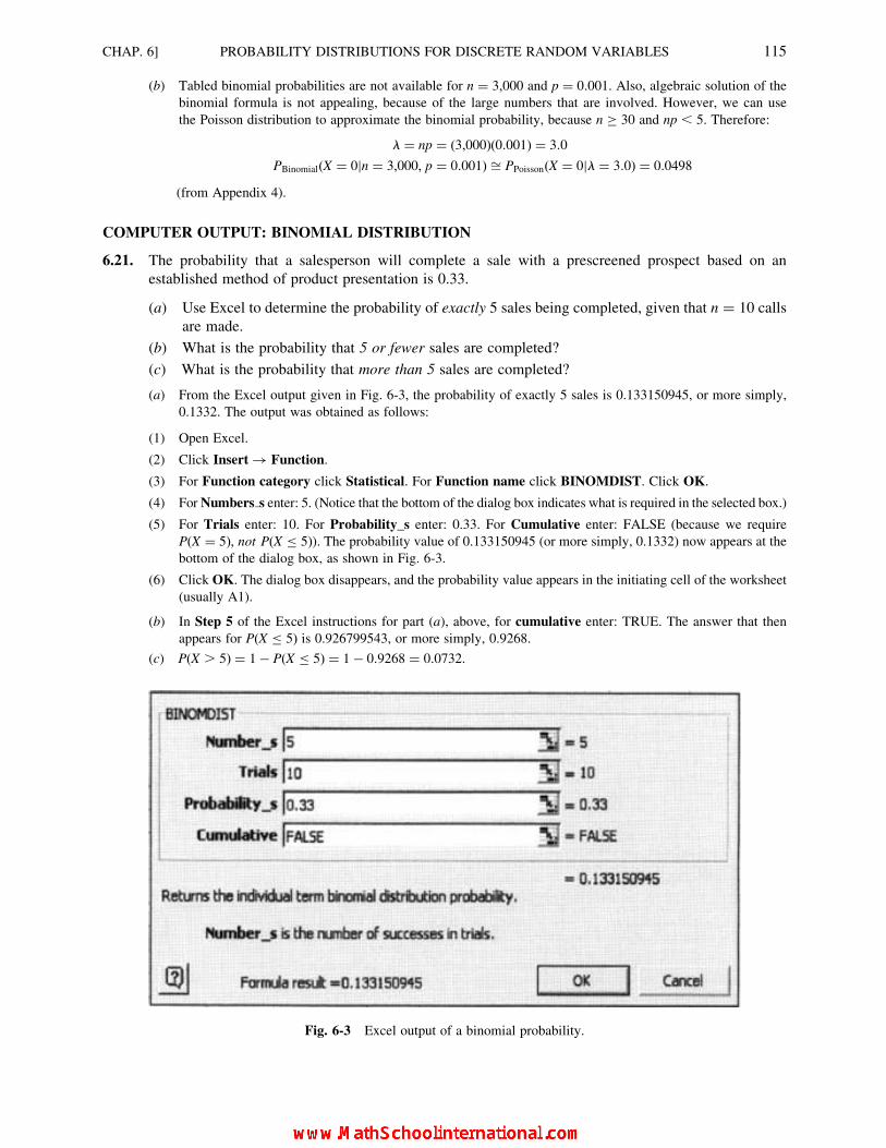
(b) Tabled binomial probabilities are not available for n ¼ 3,000 and p ¼ 0:001. Also, algebraic solution of the
binomial formula is not appealing, because of the large numbers that are involved. However, we can use
the Poisson distribution to approximate the binomial probability, because n � 30 and np , 5. Therefore:
l ¼ np ¼ (3,000)(0:001) ¼ 3:0
PBinomial(X ¼ 0jn ¼ 3,000, p ¼ 0:001) ffi PPoisson(X ¼ 0jl ¼ 3:0) ¼ 0:0498
(from Appendix 4).
COMPUTER OUTPUT: BINOMIAL DISTRIBUTION
6.21. The probability that a salesperson will complete a sale with a prescreened prospect based on an
established method of product presentation is 0.33.
(a) Use Excel to determine the probability of exactly 5 sales being completed, given that n ¼ 10 calls
are made.
(b) What is the probability that 5 or fewer sales are completed?
(c) What is the probability that more than 5 sales are completed?
(a) From the Excel output given in Fig. 6-3, the probability of exactly 5 sales is 0.133150945, or more simply,
0.1332. The output was obtained as follows:
(1) Open Excel.
(2) Click Insert ! Function.
(3) For Function category click Statistical. For Function name click BINOMDIST. Click OK.
(4) For Numbers s enter: 5. (Notice that the bottom of the dialog box indicates what is required in the selected box.)
(5) For Trials enter: 10. For Probability_s enter: 0.33. For Cumulative enter: FALSE (because we require
P(X ¼ 5), not P(X 5)). The probability value of 0.133150945 (or more simply, 0.1332) now appears at the
bottom of the dialog box, as shown in Fig. 6-3.
(6) Click OK. The dialog box disappears, and the probability value appears in the initiating cell of the worksheet
(usually A1).
(b) In Step 5 of the Excel instructions for part (a), above, for cumulative enter: TRUE. The answer that then
appears for P(X 5) is 0.926799543, or more simply, 0.9268.
(c) P(X . 5) ¼ 1� P(X 5) ¼ 1� 0:9268 ¼ 0:0732.
Fig. 6-3 Excel output of a binomial probability.
CHAP. 6] PROBABILITY DISTRIBUTIONS FOR DISCRETE RANDOM VARIABLES 115

6.22. The probability that a salesperson will complete a sale with a prescreened prospect based on an
established method of product presentation is 0.33.
(a) Use Minitab to determine the probability of exactly 5 sales being completed, given that n ¼ 10
calls are made.
(b) What is the probability that 5 or fewer sales are completed?
(c) What is the probability that more than 5 sales are completed?
(a) Figure 6-4 presents the probability of each possible number of sales. From the printout, we see that the
probability of exactly 5 sales being completed is 0.1332. The Minitab instructions that result in the output are
(1) Open Minitab.
(2) Name column C1 “Sales.” Enter the numbers 0, 1, 2, . . . , 10 in this column.
(3) Click Calc ! Probability Distributions ! Binomial.
(4) In the dialog box, select Probability.
(5) For Number of trials enter: 10. For Probability of success enter: 0.33. For Input column enter: Sales.
(6) Click OK.
(b) Figure 6-5 presents the cumulative distribution function from Minitab. In Step 4, above, select Cumulative
probability to obtain the output. From the table, we see that P(X 5) ¼ 0:9268.
(c) P(X . 5) ¼ 1� P(X 5) ¼ 1� 0:9268 ¼ 0:0732.
Fig. 6-5 Minitab output of cumulative binomial probabilities.
Fig. 6-4 Minitab output of binomial probabilities.
116 PROBABILITY DISTRIBUTIONS FOR DISCRETE RANDOM VARIABLES [CHAP. 6

COMPUTER OUTPUT: POISSON DISTRIBUTION
6.23. Arrivals at a self-service gasoline station average 15 vehicles per hour. Suppose the attendant leaves the
service booth for 5 minutes.
(a) Using Excel, what is the probability that no one arrives for service during the 5-minute period?
(b) What is the probability that at least one vehicle arrives?
(a) The Excel output given in Fig. 6-6 was obtained as follows:
(1) Open Excel.
(2) Click Insert ! Function.
(3) For Function category click Statistical. For Function name click POISSON. Click OK.
(4) For X enter: 0. For Mean enter: 1.25.
(Note: Since there are 15 arrivals per hour, the arrival rate per minute ¼ 0:25, and the arrival rate per
5-minute periods ¼ 5� 0:25 ¼ 1:25.)
(5) For Cumulative enter: FALSE (because we require the probability of one specific outcome, that there are 0
arrivals). The probability value of 0.286504797 (or more simply, 0.2865) now appears at the bottom of the
dialog box, as shown in Figure 6-6.
(6) Click OK. The dialog box disappears, and the probability value appears in the initiating cell of the worksheet
(usually A1).
(b) The probability that at least one vehicle arrives is 1 minus the probability that no vehicle arrives, obtained
from part (a): P(X � 1) ¼ 1� P(X ¼ 0) ¼ 1� 0:2865 ¼ 0:7135.
6.24. Arrivals at a self-service gasoline station average 15 vehicles per hour. Suppose the attendant leaves the
service booth for 5 minutes.
(a) Using Minitab, what is the probability that no one arrives for service during the 5-minute period?
(b) What is the probability that at least one vehicle arrives?
Fig. 6-6 Excel output of a Poisson probability.
CHAP. 6] PROBABILITY DISTRIBUTIONS FOR DISCRETE RANDOM VARIABLES 117

(a) Figure 6-7 presents the probability of each possible number of arrivals. From the printout, we see that the
probability of 0 vehicles arriving is 0.2865. The Minitab instruction that result in the output are
(1) Open Minitab.
(2) Name column C1 “Arrivals.” Enter the numbers 0, 1, 2, . . . , 10 in this column.
(3) Click Calc ! Probability Distributions ! Poisson.
(4) In the dialog box, select Probability.
(5) For Mean enter: 1.25.
(Note: Since there are 15 arrivals per hour, the arrival rate per minute ¼ 0:25, and the arrival rate per 5-
minute periods ¼ 5� 0:25 ¼ 1:25:)
(6) For Input column enter: Arrivals.
(7) Click OK.
(b) The probability that at least one vehicle arrives is 1 minus the probability that no vehicle arrives, obtained
from part (a): P(X � 1) ¼ 1� P(X ¼ 0) ¼ 1� 0:2865 ¼ 0:7135.
Supplementary Problems
DISCRETE RANDOM VARIABLES
6.25. The arrival of customers during randomly chosen 10-min intervals at a drive-in facility specializing in photo
development and film sales has been found to follow the probability distribution in Table 6.12. Calculate the
expected number of arrivals for 10-min intervals and the standard deviation of the arrivals.
Ans. E(X) ¼ 2:00, s ¼ 1:38 arrivals
Fig. 6-7 Minitab output of Poisson probabilities.
Table 6.12 Arrivals of Customers at a Photo-processing Facility during
10-min Intervals
Number of arrivals (X) 0 1 2 3 4 5
Probability [P(X)] 0.15 0.25 0.25 0.20 0.10 0.05
118 PROBABILITY DISTRIBUTIONS FOR DISCRETE RANDOM VARIABLES [CHAP. 6

6.26. The newsstand sales of a monthly magazine have been found to follow the probability distribution in Table 6.13.
Calculate the expected value and the standard deviation for the magazine sales, in thousands.
Ans. E(X) ¼ 17:80, s ¼ 1:29
6.27. A salesperson has found that the probability of making various numbers of sales per day, given that calls on 10 sales
prospects can be made, is presented in Table 6.14. Calculate the expected number of sales per day and the standard
deviation of the number of sales.
Ans. E(X) ¼ 4:00, s ¼ 1:59 sales
6.28. Referring to Problem 6.27, suppose the sales representative earns a commission of $25 per sale. Determine the
expected daily commission earnings by (a) substituting the commission amount for each of the sales numbers in
Table 6.14 and calculating the expected commission amount, and (b) multiplying the expected sales number
calculated in Problem 6.27 by the commission rate.
Ans. (a) $100.00, (b) $100.00
THE BINOMIAL DISTRIBUTION
6.29. There is a 90 percent chance that a particular type of component will perform adequately under high temperature
conditions. If the device involved has four such components, determine the probability of each of the following
events by use of the formula for binomial probabilities.
(a) All of the components perform adequately and therefore the device is operative.
(b) The device is inoperative because exactly one of the four components fails.
(c) The device is inoperative because one or more of the components fail.
Ans. (a) 0.6561, (b) 0.2916, (c) 0.3439
6.30. Verify the answers to Problem 6.29 by constructing a tree diagram and determining the probabilities by the use of
the appropriate rules of multiplication and of addition.
6.31. Verify the answers to Problem 6.29 by use of Appendix 2.
6.32. Using the table of binomial probabilities, determine:.
(a) P(X ¼ 8jn ¼ 20, p ¼ 0:30) (d) P(X ¼ 5jn ¼ 10, p ¼ 0:40)
(b) P(X � 10jn ¼ 20, p ¼ 0:30) (e) P(X . 5jn ¼ 10, p ¼ 0:40)
(c) P(X 5jn ¼ 20, p ¼ 0:30) ( f ) P(X , 5jn ¼ 10, p ¼ 0:40)
Ans. (a) 0.1144, (b) 0.0479, (c) 0.4165, (d) 0.2007, (e) 0.1663, ( f ) 0.6330
Table 6.13 Newsstand Sales of a Monthly Magazine
Number of magazines (X), thousands 15 16 17 18 19 20
Probability [P(X)] 0.05 0.10 0.25 0.30 0.20 0.10
Table 6.14 Sales per Day when 10 Prospects Are Contacted
Number of sales (X) 1 2 3 4 5 6 7 8
Probability [P(X)] 0.04 0.15 0.20 0.25 0.19 0.10 0.05 0.02
CHAP. 6] PROBABILITY DISTRIBUTIONS FOR DISCRETE RANDOM VARIABLES 119
6.33. Using the table of binomial probabilities, determine:.
(a) P(X ¼ 4jn ¼ 12, p ¼ 0:70) (d) P(X , 3jn ¼ 8, p ¼ 0:60)
(b) P(X � 9jn ¼ 12, p ¼ 0:70) (e) P(X ¼ 5jn ¼ 10, p ¼ 0:90)
(c) P(X 3jn ¼ 8, p ¼ 0:60) ( f ) P(X . 7jn ¼ 10, p ¼ 0:90)
Ans. (a) 0.0078, (b) 0.4925, (c) 0.1738, (d) 0.0499, (e) 0.0015, ( f ) 0.9298
6.34. Suppose that 40 percent of the employees in a large firm are in favor of union representation, and a random sample
of 10 employees are contacted and asked for an anonymous response. What is the probability that (a) a majority of
the respondents and (b) fewer than half of the respondents will be in favor of union representation?
Ans. (a) 0.1663, (b) 0.6330
6.35. Determine the probabilities in Problem 6.34, if 60 percent of the employees are in favor of union representation.
Ans. (a) 0.6330, (b) 0.1663
6.36. Refer to the probability distribution in Problem 6.27. Does this probability distribution appear to follow a binomial
probability distribution in its form? [Hint: Convert the E(X) found in Problem 6.27 into a proportion and use this
value as the value of p for comparison with the binomial distribution with n ¼ 10.]
Ans. The two probability distributions correspond quite closely.
THE HYPERGEOMETRIC DISTRIBUTION
6.37. In a class containing 20 students, 15 are dissatisfied with the text used. If a random sample of four students are asked
about the text, determine the probability that (a) exactly three, and (b) at least three are dissatisfied with the text.
Ans. (a) P ffi 0:47, (b) P ffi 0:75
6.38. Verify the answers to Problem 6.37 by constructing a tree diagram and determining the probabilities by use of the
appropriate rules of multiplication and of addition.
6.39. In Section 6.5 it is suggested that the binomial distribution can generally be used to approximate hypergeometric
probabilities when n , 0:05 N. Demonstrate that the binomial approximation of the probability values requested in
Problem 6.35 is quite poor. (Hint: Use T=N as the p value for the binomial table, which does not conform to the
sample size requirement, with n ¼ 4 being much more than 0:05(20) ¼ 1.)
6.40 A department group includes five engineers and nine technicians. If five individuals are randomly chosen and
assigned to a project, what is the probability that the project group will include exactly two engineers?
(Note: This is a restatement of Problem 5.57(a), for which the answer was determined by combinational analysis.)
Ans. P ffi 0:42
THE POISSON PROBABILITY DISTRIBUTION
6.41. On average, six people per hour use an electronic teller machine during the prime shopping hours in a department
store. What is the probability that
(a) exactly six people will use the machine during a randomly selected hour?
(b) fewer than five people will use the machine during a randomly selected hour?
(c) no one will use the facility during a 10-min interval?
(d) no one will use the facility during a 5-min interval?
Ans. (a) 0.1606, (b) 0.2851, (c) 0.3679, (d) 0.6065
6.42. Suppose that the manuscript for a textbook has a total of 50 errors, or typos, included in the 500 pages of material,
and that the errors are distributed randomly throughout the text. What is the probability that
(a) a 30-page chapter has two or more errors?
(b) a 50-page chapter has two or more errors?
120 PROBABILITY DISTRIBUTIONS FOR DISCRETE RANDOM VARIABLES [CHAP. 6

(c) a randomly selected page has no error?
Ans. (a) 0.8008, (b) 0.9596, (c) 0.9048
6.43. Only one personal computer per thousand is found to be defective after assembly in a manufacturing plant, and the
defective PCs are distributed randomly throughout the production run.
(a) What is the probability that a shipment of 500 PCs includes no defective computer?
(b) What is the probability that a shipment of 100 PCs includes at least one defective computer?
Ans. By the Poisson approximation of binomial probabilities, (a) 0.6065, (b) 0.0952
6.44. Refer to the probability distribution in Problem 6.24. Does this probability distribution of arrivals appear to follow a
Poisson probability distribution in its form? [Hint: Use the E(X) calculated in Problem 6.25 as the mean (l) fordetermining the Poisson distribution with which the probabilities are to be compared.]
Ans. The two probability distributions correspond quite closely.
COMPUTER APPLICATIONS
6.45. The probability that a particular electronic component will be defective is 0.005.
(a) Using available computer software, determine the probability that exactly one component is defective.
(b) Using available computer software, determine the probability that one or more components are defective.
Ans. (a) 0.0386, (b) 0.0393
6.46. The number of paint blisters that occur in an automated painting process is known to be Poisson-distributed with a
mean of 0.005 blisters per square foot. The process is to be used to paint storage-shed panels measuring 10� 15 ft.
(a) Using available software, determine the probability that no blister occurs on a particular panel.
(b) What is the probability that at least one blister occurs on the panel?
Ans. (a) P ¼ 0:4724 (based on l ¼ 0:75 per 10� 15 ft panel), (b) P ¼ 0:5276
CHAP. 6] PROBABILITY DISTRIBUTIONS FOR DISCRETE RANDOM VARIABLES 121

CHAPTER 7
ProbabilityDistributions forContinuous RandomVariables: Normal andExponential
7.1 CONTINUOUS RANDOM VARIABLES
As contrasted to a discrete random variable, a continuous random variable is one that can assume any
fractional value within a defined range of values. (See Section 1.4.) Because there is an infinite number of
possible fractional measurements, one cannot list every possible value with a corresponding probability.
Instead, a probability density function is defined. This mathematical expression gives the function of X,
represented by the symbol f(X), for any designated value of the random variable X. The plot for such a function
is called a probability curve, and the area between any two points under the curve indicates the probability of a
value between these two points occurring by chance.
EXAMPLE 1. For the continuous probability distribution in Fig. 7-1, the probability that a randomly selected shipment
will have a net weight between 6,000 and 8,000 lb is equal to the proportion of the total area under the curve that is included
within the shaded area. That is, the total area under the probability density function is defined as being equal to 1, and the
proportion of this area that is included between the two designated points can be determined by applying the method of
integration (from calculus) in conjunction with the mathematical probability density function for this probability curve.
Several standard continuous probability distributions are applicable as models to a wide variety of
continuous variables under designated circumstances. Probability tables have been prepared for these standard
122
Copyright 2004, 1996, 1988, 1976 by The McGraw-Hill Companies, Inc. Click Here for Terms of Use.
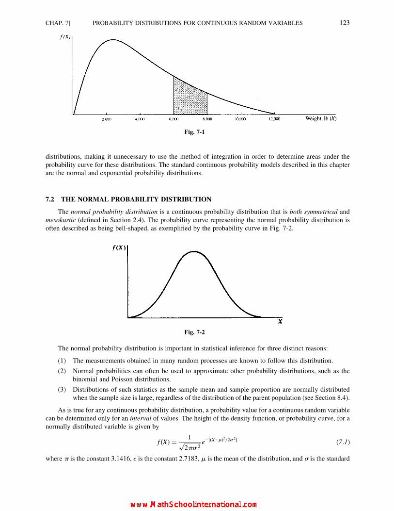
distributions, making it unnecessary to use the method of integration in order to determine areas under the
probability curve for these distributions. The standard continuous probability models described in this chapter
are the normal and exponential probability distributions.
7.2 THE NORMAL PROBABILITY DISTRIBUTION
The normal probability distribution is a continuous probability distribution that is both symmetrical and
mesokurtic (defined in Section 2.4). The probability curve representing the normal probability distribution is
often described as being bell-shaped, as exemplified by the probability curve in Fig. 7-2.
Fig. 7-2
The normal probability distribution is important in statistical inference for three distinct reasons:
(1) The measurements obtained in many random processes are known to follow this distribution.
(2) Normal probabilities can often be used to approximate other probability distributions, such as the
binomial and Poisson distributions.
(3) Distributions of such statistics as the sample mean and sample proportion are normally distributed
when the sample size is large, regardless of the distribution of the parent population (see Section 8.4).
As is true for any continuous probability distribution, a probability value for a continuous random variable
can be determined only for an interval of values. The height of the density function, or probability curve, for a
normally distributed variable is given by
f (X) ¼ 1ffiffiffiffiffiffiffiffiffiffiffiffi2ps 2
p e�[(X�m)2=2s 2] (7:1)
where p is the constant 3.1416, e is the constant 2.7183, m is the mean of the distribution, and s is the standard
Fig. 7-1
CHAP. 7] PROBABILITY DISTRIBUTIONS FOR CONTINUOUS RANDOM VARIABLES 123
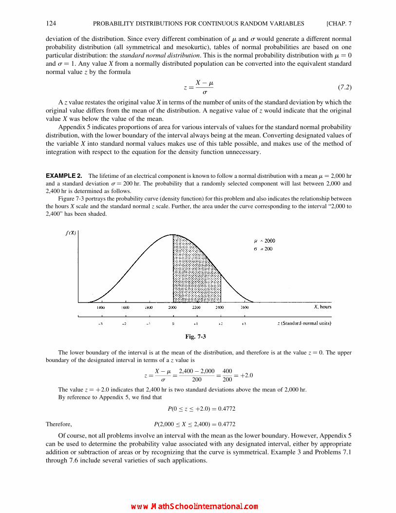
deviation of the distribution. Since every different combination of m and s would generate a different normal
probability distribution (all symmetrical and mesokurtic), tables of normal probabilities are based on one
particular distribution: the standard normal distribution. This is the normal probability distribution with m ¼ 0
and s ¼ 1. Any value X from a normally distributed population can be converted into the equivalent standard
normal value z by the formula
z ¼ X � m
s(7:2)
A z value restates the original value X in terms of the number of units of the standard deviation by which the
original value differs from the mean of the distribution. A negative value of z would indicate that the original
value X was below the value of the mean.
Appendix 5 indicates proportions of area for various intervals of values for the standard normal probability
distribution, with the lower boundary of the interval always being at the mean. Converting designated values of
the variable X into standard normal values makes use of this table possible, and makes use of the method of
integration with respect to the equation for the density function unnecessary.
EXAMPLE 2. The lifetime of an electrical component is known to follow a normal distribution with a mean m ¼ 2,000 hr
and a standard deviation s ¼ 200 hr. The probability that a randomly selected component will last between 2,000 and
2,400 hr is determined as follows.
Figure 7-3 portrays the probability curve (density function) for this problem and also indicates the relationship between
the hours X scale and the standard normal z scale. Further, the area under the curve corresponding to the interval “2,000 to
2,400” has been shaded.
Fig. 7-3
The lower boundary of the interval is at the mean of the distribution, and therefore is at the value z ¼ 0. The upper
boundary of the designated interval in terms of a z value is
z ¼ X � m
s¼ 2,400� 2,000
200¼ 400
200¼ þ2:0
The value z ¼ þ2.0 indicates that 2,400 hr is two standard deviations above the mean of 2,000 hr.
By reference to Appendix 5, we find that
P(0 z þ2:0) ¼ 0:4772
Therefore, P(2,000 X 2,400) ¼ 0:4772
Of course, not all problems involve an interval with the mean as the lower boundary. However, Appendix 5
can be used to determine the probability value associated with any designated interval, either by appropriate
addition or subtraction of areas or by recognizing that the curve is symmetrical. Example 3 and Problems 7.1
through 7.6 include several varieties of such applications.
124 PROBABILITY DISTRIBUTIONS FOR CONTINUOUS RANDOM VARIABLES [CHAP. 7
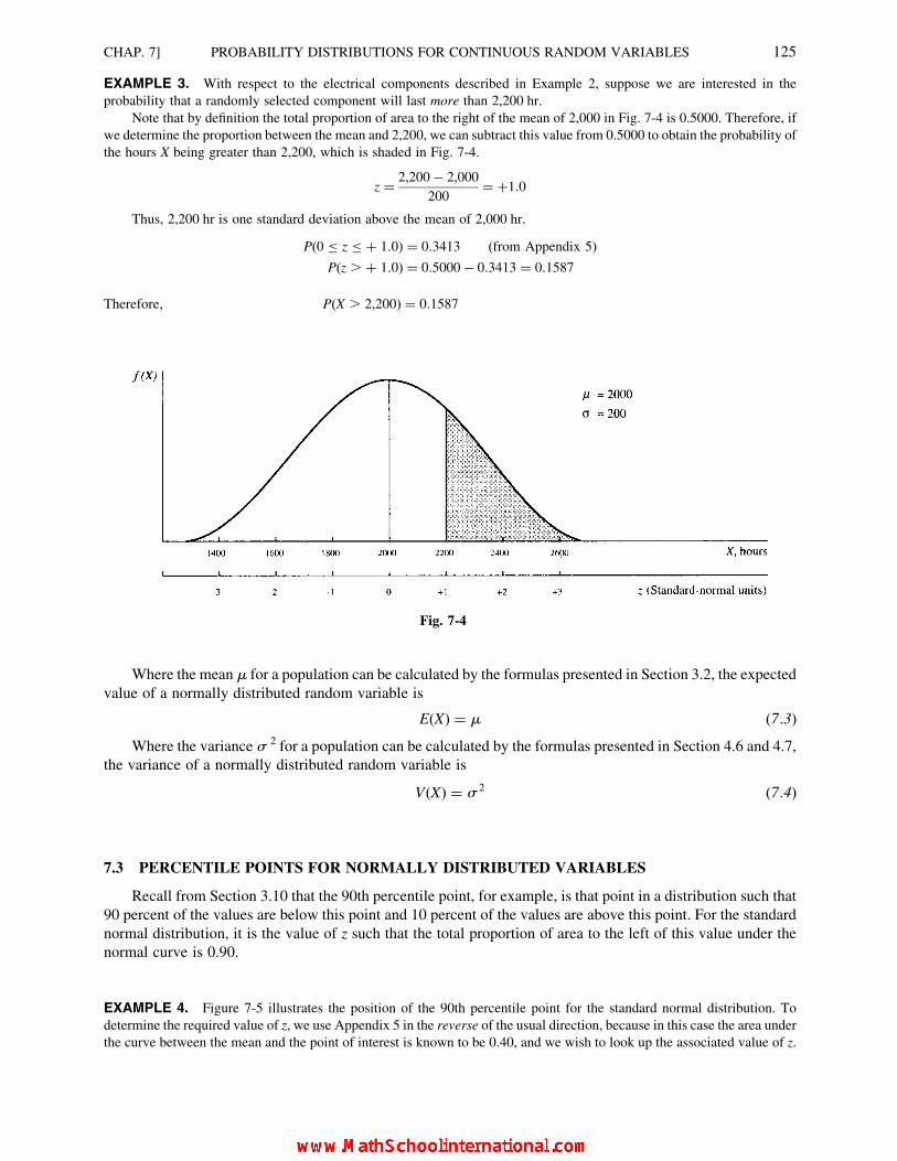
EXAMPLE 3. With respect to the electrical components described in Example 2, suppose we are interested in the
probability that a randomly selected component will last more than 2,200 hr.
Note that by definition the total proportion of area to the right of the mean of 2,000 in Fig. 7-4 is 0.5000. Therefore, if
we determine the proportion between the mean and 2,200, we can subtract this value from 0.5000 to obtain the probability of
the hours X being greater than 2,200, which is shaded in Fig. 7-4.
z ¼ 2,200� 2,000
200¼ þ1:0
Thus, 2,200 hr is one standard deviation above the mean of 2,000 hr.
P(0 z þ 1:0) ¼ 0:3413 (from Appendix 5)
P(z . þ 1:0) ¼ 0:5000� 0:3413 ¼ 0:1587
Therefore, P(X . 2,200) ¼ 0:1587
Fig. 7-4
Where the mean m for a population can be calculated by the formulas presented in Section 3.2, the expected
value of a normally distributed random variable is
E(X) ¼ m (7:3)
Where the variance s 2 for a population can be calculated by the formulas presented in Section 4.6 and 4.7,
the variance of a normally distributed random variable is
V(X) ¼ s 2 (7:4)
7.3 PERCENTILE POINTS FOR NORMALLY DISTRIBUTED VARIABLES
Recall from Section 3.10 that the 90th percentile point, for example, is that point in a distribution such that
90 percent of the values are below this point and 10 percent of the values are above this point. For the standard
normal distribution, it is the value of z such that the total proportion of area to the left of this value under the
normal curve is 0.90.
EXAMPLE 4. Figure 7-5 illustrates the position of the 90th percentile point for the standard normal distribution. To
determine the required value of z, we use Appendix 5 in the reverse of the usual direction, because in this case the area under
the curve between the mean and the point of interest is known to be 0.40, and we wish to look up the associated value of z.
CHAP. 7] PROBABILITY DISTRIBUTIONS FOR CONTINUOUS RANDOM VARIABLES 125

In Appendix 5 we look in the body of the table for the value closest to 0.4000. It is 0.3997. From the row and column
headings, the value of z associated with this area is 1.28, and therefore z 0.90 ¼ þ1.28. The sign is positive because the 90th
percentile point is greater than the mean, and thus the value of z is above its mean of 0.
Fig. 7-5
Given the procedure in Example 4 for determining a percentile point for the standard normal distribution,
a percentile point for a normally distributed random variable can be determined by solving Formula (7.2)
for X (rather than z), resulting in:
X ¼ mþ zs (7:5)
EXAMPLE 5. For the lifetime of the electrical component described in Examples 2 and 3, and utilizing the solution in
Example 4, the 90th percentile point for the life of the component is
X ¼ mþ zs ¼ 2,000þ (1:28)(200) ¼ 2,256 hr
For percentile points below the 50th percentile, the associated z value will always be negative, since the
value is below the mean of 0 for the standard normal distribution.
EXAMPLE 6. Continuing from Example 5, suppose we wish to determine the lifetime of the component such that only 10
percent of the components will fail before that time (10th percentile point). See Fig. 7-6 for the associated area for the
standard normal probability distribution. Just as we did in Example 4, we look in the body of the table in Appendix 5 for the
area closest to 0.4000, but in this case the value of z is taken to be negative. The solution is
X ¼ mþ zs ¼ 2,000þ (�1:28)(200) ¼ 1,744 hr
Fig. 7-6
7.4 NORMAL APPROXIMATION OF BINOMIAL PROBABILITIES
When the number of observations or trials n is relatively large, the normal probability distribution can be
used to approximate binomial probabilities. A convenient rule is that such approximation is acceptable when
n � 30, and both np � 5 and nq � 5. This rule, combined with the one given in Section 6.7 for the Poisson
approximation of binomial probabilities, means that whenever n � 30, binomial probabilities can be
approximated by either the normal or the Poisson distribution, depending on the values of np and nq. Different
texts use somewhat different rules for determining when such approximations are appropriate.
126 PROBABILITY DISTRIBUTIONS FOR CONTINUOUS RANDOM VARIABLES [CHAP. 7

When the normal probability distribution is used as the basis for approximating a binomial probability
value, the mean and standard deviation are based on the expected value and variance of the number of successes
for the binomial distribution, as given in Section 6.3. The mean number of successes is
m ¼ np (7:6)
The standard deviation of the number of successes is
s ¼ ffiffiffiffiffiffiffiffinpq
p(7:7)
EXAMPLE 7. For a large group of sales prospects, it has been observed that 20 percent of those contacted personally by a
sales representative will make a purchase. If a sales representative contacts 30 prospects, we can determine the probability
that 10 or more will make a purchase by reference to the binomial probabilities in Appendix 2:
P(X � 10jn ¼ 30, p ¼ 0:20) ¼ P(X ¼ 10)þ P(X ¼ 11)þ � � �¼ 0:0355þ 0:0161þ 0:0064þ 0:0022þ 0:0007þ 0:0002
¼ 0:0611 (the exact binomial probability value)
Now we check to determine if the criteria for normal approximation are satisfied:
Is n � 30? Yes, n ¼ 30
Is np � 5? Yes, np ¼ 30(0.20) ¼ 6
Is nq � 5? Yes, nq ¼ 30(0.80) ¼ 24
The normal approximation of the binomial probability value is
m ¼ np ¼ (30)(0:20) ¼ 60
s ¼ ffiffiffiffiffiffiffiffinpq
p ¼ffiffiffiffiffiffiffiffiffiffiffiffiffiffiffiffiffiffiffiffiffiffiffiffiffiffiffiffiffiffiffiffi(30)(0:20)(0:80)
p¼
ffiffiffiffiffiffiffi4:8
pffi 2:19
PBinomial(X � 10jn ¼ 30, p ¼ 0:20) ffi PNormal(X � 9:5jm ¼ 6:0, s ¼ 2:19)
(Note: This includes the correction for continuity discussed below.)
z ¼ X � m
s¼ 9:5� 6:0
2:19¼ 3:5
2:19ffi þ 1:60
P(X � 9:5jm ¼ 6:0, s ¼ 2:19) ¼ P(z � þ 1:60)
¼ 0:5000� P(0 z þ 1:60) ¼ 0:5000� 0:4452
¼ 0:0548 (the normal approximation)
In Example 7, the class of events “10 or more” is assumed to begin at 9.5 when the normal approximation is
used. This adjustment by one-half unit is called the correction for continuity. It is required because all the area
under the continuous normal distribution has to be assigned to some numeric event, even though no fractional
number of successes is possible, for example, between “9 purchasers” and “10 purchasers.” Put another way, in the
process of normal approximation, a discrete event such as “10 purchasers” has to be considered as a continuous
interval of values ranging from an exact lower limit of 9.5 to an exact upper limit of 10.5. Therefore, if Example 7
had asked for the probability of “more than 10 purchasers,” the appropriate correction for continuity would involve
adding 0.5 to the 10 and determining the area for the interval beginning at 10.5. By the above rationale, the 0.5 is
either added or subtracted as a continuity correction according to the form of the probability statement:
(1) Subtract 0.5 from X when P(X � Xi) is required.
(2) Subtract 0.5 from X when P(X , Xi) is required.
(3) Add 0.5 to X when P(X Xi) is required.
(4) Add 0.5 to X when P(X . Xi) is required.
CHAP. 7] PROBABILITY DISTRIBUTIONS FOR CONTINUOUS RANDOM VARIABLES 127

7.5 NORMAL APPROXIMATION OF POISSON PROBABILITIES
When the mean l of a Poisson distribution is relatively large, the normal probability distribution can be used
to approximate Poisson probabilities. A convenient rule is that such approximation is acceptable when l � 10.0.
The mean and standard deviation of the normal probability distribution are based on the expected value and
the variance of the number of events in a Poisson process, as given in Section 6.6. This mean is
m ¼ l (7:8)
The standard deviation is
s ¼ffiffiffil
p(7:9)
EXAMPLE 8. The average number of calls for service received by a machine repair department per 8-hr shift is 10.0.
We can determine the probability that more than 15 calls will be received during a randomly selected 8-hr shift using
Appendix 4:
P(X . 15jl ¼ 10:0) ¼ P(X ¼ 16)þ P(X ¼ 17)þ � � �¼ 0:0217þ 0:0128þ 0:0071þ 0:0037þ 0:0019þ 0:0009þ 0:0004þ 0:0002þ 0:0001
¼ 0:0488 (the exact Poisson probability)
Because the value of l is (at least) 10, the normal approximation of the Poisson probability value is acceptable. The
normal approximation of the Poisson probability value is
m ¼ l ¼ 10:0
s ¼ffiffiffil
p¼
ffiffiffiffiffiffiffiffiffi10:0
pffi 3:16
PPoisson(X . 15jl ¼ 10:0) ffi PNormal(X � 15:5jm ¼ 10:0, s ¼ 3:16)
(Note: This includes the correction for continuity, discussed below.)
z ¼ X � m
s¼ 15:5� 10:0
3:16¼ 5:5
3:16ffi þ 1:74
P(z � þ 1:74) ¼ 0:5000� P(0 z þ 1:74) ¼ 0:5000� 0:4591 ¼ 0:0409 (the normal approximation)
The correction for continuity applied in Example 8 is the same type of correction described for the normal
approximation of binomial probabilities. The rules provided in Section 7.4 as to when 0.5 is added to and
subtracted from X apply equally to the situation in which the normal probability distribution is used to
approximate Poisson probabilities.
7.6 THE EXPONENTIAL PROBABILITY DISTRIBUTION
If events occur in the context of a Poisson process, as described in Section 6.6, then the length of time or
space between successive events follows an exponential probability distribution. Because the time or space is a
continuum, such a measurement is a continuous random variable. As is the case of any continuous random
variable, it is not meaningful to ask, “What is the probability that the first request for service will arrive in
exactly one minute?” Rather, we must designate an interval within which the event is to occur, such as by
asking, “What is the probability that the first request for service will arrive within a minute?”
Since the Poisson process is stationary, with equal likelihood of the event occurring throughout the relevant
period of time, the exponential distribution applies whether we are concerned with the time (or space) until the
very first event, the time between two successive events, or the time until the first event occurs after any selected
point in time.
Where l is the mean number of occurrences for the interval of interest (see Section 6.6), the exponential
probability that the first event will occur within the designated interval of time or space is
P(T t) ¼ 1� e�l (7:10)
128 PROBABILITY DISTRIBUTIONS FOR CONTINUOUS RANDOM VARIABLES [CHAP. 7

Similarly, the exponential probability that the first event will not occur within the designated interval of
time or space is
P(T . t) ¼ e�l (7:11)
For both of the above formulas the value of e 2l may be obtained from Appendix 3.
EXAMPLE 9. An average of five calls per hour are received by a machine repair department. Beginning the observation at
any point in time, the probability that the first call for service will arrive within a half hour is
Average per hour ¼ 5:0
l ¼ Average per half hour ¼ 2:5
P ¼ 1� e�l ¼ 1� e�2:5 ¼ 1� 0:08208 ¼ 0:91792 (from Appendix 3)
The expected value and the variance of an exponential probability distribution, where the variable is
designated as time T and l is for one unit of time or space (such as one hour), are
E(T) ¼ 1
l(7:12)
V(T) ¼ 1
l2(7:13)
7.7 USING EXCEL AND MINITAB
Computer software for statistical analysis frequently includes the capability of providing probabilities for
intervals of values for normally distributed variables. Solved Problems 7.23 through 7.26 are concerned with
determining normal probabilities and with determining percentile points for normally distributed variables,
using both Excel and Minitab.
Solved Problems
THE NORMAL PROBABILITY DISTRIBUTION
7.1. The packaging process in a breakfast cereal company has been adjusted so that an average of
m ¼ 13.0 oz of cereal is placed in each package. Of course, not all packages have precisely 13.0 oz
because of random sources of variability. The standard deviation of the actual net weight is s ¼ 0.1 oz,
and the distribution of weights is known to follow the normal probability distribution. Determine the
probability that a randomly chosen package will contain between 13.0 and 13.2 oz of cereal and illustrate
the proportion of area under the normal curve which is associated with this probability value.
From Fig 7-7,
z ¼ X � m
s¼ 13:2� 13:0
0:1¼ þ 2:0
P(13:0 X 13:2) ¼ P(0 z þ2:0) ¼ 0:4772 (from Appendix 5)
7.2. For the situation described in Problem 7.1, what is the probability that the weight of the cereal will
exceed 13.25 oz? Illustrate the proportion of area under the normal curve which is relevant in this case.
CHAP. 7] PROBABILITY DISTRIBUTIONS FOR CONTINUOUS RANDOM VARIABLES 129
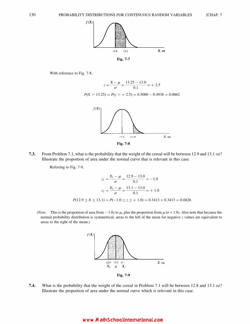
With reference to Fig. 7-8,
z ¼ X � m
s¼ 13:25� 13:0
0:1¼ þ 2:5
P(X . 13:25) ¼ P(z . þ 2:5) ¼ 0:5000� 0:4938 ¼ 0:0062
Fig. 7-8
7.3. From Problem 7.1, what is the probability that the weight of the cereal will be between 12.9 and 13.1 oz?
Illustrate the proportion of area under the normal curve that is relevant in this case.
Referring to Fig. 7-9,
z1 ¼ X1 � m
s¼ 12:9� 13:0
0:1¼ �1:0
z2 ¼ X2 � m
s¼ 13:1� 13:0
0:1¼ þ 1:0
P(12:9 X 13:1) ¼ P(�1:0 z þ 1:0) ¼ 0:3413þ 0:3413 ¼ 0:6826
(Note: This is the proportion of area from21.0z to m, plus the proportion from m toþ1.0z. Also note that because the
normal probability distribution is symmetrical, areas to the left of the mean for negative z values are equivalent to
areas to the right of the mean.)
Fig. 7-9
7.4. What is the probability that the weight of the cereal in Problem 7.1 will be between 12.8 and 13.1 oz?
Illustrate the proportion of area under the normal curve which is relevant in this case.
Fig. 7-7
130 PROBABILITY DISTRIBUTIONS FOR CONTINUOUS RANDOM VARIABLES [CHAP. 7

With reference to Fig. 7-10,
z1 ¼ X1 � m
s¼ 12:8� 13:0
0:1¼ �0:2
0:1¼ � 2:0
z2 ¼ X2 � m
s¼ 13:1� 13:0
0:1¼ 0:1
0:1¼ þ 1:0
P(12:8 X 13:1) ¼ P(� 2:0 z 1:0) ¼ 0:4772þ 0:3413 ¼ 0:8185
7.5. From Problem 7.1, what is the probability that the weight of the cereal will be between 13.1 and 13.2 oz?
Illustrate the proportion of area under the normal curve which is relevant in this case.
Referring to Fig. 7-11,
z1 ¼ X1 � m
s¼ 13:1� 13:0
0:1¼ þ 1:0
z2 ¼ X2 � m
s¼ 13:2� 13:0
0:1¼ þ 2:0
P(13:1 X 13:2) ¼ P(þ 1:0 z þ 2:0) ¼ 0:4772� 0:3413 ¼ 0:1359
(Note: The probability is equal to the proportion of area from 13.0 to 13.2, minus the proportion of area from 13.0
to 13.1.)
Fig. 7-11
7.6. The amount of time required for routine automobile transmission service is normally distributed with
the mean m ¼ 45 min and the standard deviation s ¼ 8.0 min. The service manager plans to have work
begin on the transmission of a customer’s car 10 min after the car is dropped off, and the customer is told
that the car will be ready within 1 hr total time. What is the probability that the service manager will be
wrong? Illustrate the proportion of area under the normal curve which is relevant in this case.
Fig. 7-10
CHAP. 7] PROBABILITY DISTRIBUTIONS FOR CONTINUOUS RANDOM VARIABLES 131

From Fig. 7-12,
P(Wrong) ¼ P(X . 50), since actual work is to begin in 10 min
z ¼ X � m
s¼ 50� 45
8:0¼ 5:0
8:0¼ þ 0:62
P(X . 50) ¼ P(z . þ 0:62) ¼ 0:5000� 0:2324 ¼ 0:2676
Fig. 7-12
PERCENTILE POINTS FOR NORMALLY DISTRIBUTED VARIABLES
7.7. Referring to Problem 7.6, what is. the required working time allotment such that there is a 75 percent
chance that the transmission service will be completed within that time? Illustrate the proportion of area
that is relevant.
As illustrated in Fig. 7-13, a proportion of area of 0.2500 is included between the mean and the 75th percentile
point. Therefore, as the first step in the solution we determine the required z value by finding the area in the body of
the table in Appendix 5 that is closest to 0.2500. The closest area is 0.2486, with z 0.75 ¼ þ 0.67. We then convert
this value of z into the required value of X by:
X ¼ mþ zs ¼ 45þ (0:67)(8:0) ¼ 50:36 min
Fig. 7-13
7.8. With reference to Problem 7.6, what is the working time allotment such that there is a probability of just
30 percent that the transmission service can be completed within that time? Illustrate the proportion of
area which is relevant.
Since a proportion of area of 0.30 is to the left of the unknown value of X in Fig. 7-14, it follows that a
proportion of 0.20 is between that percentile point and the mean. By reference to Appendix 5, the proportion of area
132 PROBABILITY DISTRIBUTIONS FOR CONTINUOUS RANDOM VARIABLES [CHAP. 7

closest to this 0.1985, with z 0.30 ¼ 20.52. The z value is negative because the percentile point is to the left of the
mean. Finally, the z value is converted to the required value of X:
X ¼ mþ zs
X ¼ 45þ (�0:52)(8:0) ¼ 45� 4:16 ¼ 40:84 min
Fig. 7-14
NORMAL APPROXIMATION OF BINOMIAL AND POISSON PROBABILITIES
7.9. Of the people who enter a large shopping mall, it has been found that 70 percent will make at least one
purchase. For a sample of n ¼ 50 individuals, what is the probability that at least 40 people make one or
more purchases each?
The normal approximation of the required binomial probability value can be used, because n � 30, np � 5, and
n(q) � 5.
m ¼ np ¼ (50)(0:70) ¼ 35:0
s ¼ ffiffiffiffiffiffiffiffinpq
p ¼ffiffiffiffiffiffiffiffiffiffiffiffiffiffiffiffiffiffiffiffiffiffiffiffiffiffiffiffiffiffiffiffi(50)(0:70)(0:30)
p¼
ffiffiffiffiffiffiffiffiffi10:5
p¼ 3:24
PBinomial(X � 40jn ¼ 50, p ¼ 0:70) ffi PNormal(X � 39:5jm ¼ 35:0, s ¼ 3:24)
(Note: The correction for continuity is included, as described in Section 7.4.)
z ¼ X � m
s¼ 39:5� 35:0
3:24¼ 4:5
3:24¼ þ 1:39
P(X � 39:5) ¼ P(z � þ 1:39) ¼ 0:5000� 0:4177 ¼ 0:0823
7.10. For the situation described in Problem 7.9, what is the probability that fewer than 30 of the 50 sampled
individuals make at least one purchase?
Since, from Problem 7.9, m ¼ 35.0 and s ¼ 3.24,
PBinomial(X , 30jn ¼ 50, p ¼ 0:70) ffi PNormal(X 29:5jm ¼ 35:0, s ¼ 3:24)
(Note: The correction for continuity is included.)
z ¼ X � m
s¼ 29:5� 35:0
3:24¼ �5:5
3:24¼ �1:70
P(X 29:5) ¼ P(z �1:70) ¼ 0:5000� 0:4554 ¼ 0:0446
7.11. Calls for service are known to arrive randomly and as a stationary process at an average of five calls per
hour. What is the probability that more than 50 calls for service will be received during an 8-hr shift?
Because the mean for the 8-hr period for this Poisson process exceeds l ¼ 10 (l ¼ 8 � 5 ¼ 40), the
normal probability distribution can be used to approximate the Poisson probability value. With m ¼ l ¼ 40.0 and
s ¼ ffiffiffil
p ¼ ffiffiffiffiffiffiffiffiffi40:0
p ¼ 6:32,
PPoisson(X . 50jl ¼ 40:0) ffi PNormal(X � 50:5jm ¼ 40:0, s ¼ 6:32)
CHAP. 7] PROBABILITY DISTRIBUTIONS FOR CONTINUOUS RANDOM VARIABLES 133

(Note: The correction for continuity is included.)
z ¼ X � m
s¼ 50:5� 40:0
6:32¼ 10:5
6:32¼ þ 1:66
P(X � 50:5) ¼ P(z � þ 1:66) ¼ 0:5000� 0:4515 ¼ 0:0485
7.12. Referring to Problem 7.11, what is the probability that 35 or fewer calls for service will be received
during an 8-hr shift?
Since m ¼ 40.0 and s ¼ 6.32,
PPoisson(X 35jl ¼ 40:0) ffi PNormal(X 35:5jm ¼ 40:0, s ¼ 6:32)
(Note: The correction for continuity is included.)
z ¼ X � m
s¼ 35:5� 40:0
6:32¼ �4:5
6:32¼ �0:71
P(X 35:5) ¼ P(z �0:71) ¼ 0:5000� 0:2612 ¼ 0:2388
THE EXPONENTIAL PROBABILITY DISTRIBUTION
7.13. On the average, a ship arrives at a certain dock every second day. What is the probability that after the
departure of a ship four days will pass before the arrival of the next ship?
Average per 2 days ¼ 1:0
Average per day ¼ 0:5
l ¼ average per 4-day period ¼ 4� 0:5 ¼ 2:0
P(T . 4) ¼ e�l ¼ e�2:0 ¼ 0:13534 (from Appendix 3)
7.14. Each 500-ft roll of sheet steel includes two flaws on average. What is the probability that as the sheet
steel is unrolled the first flaw occurs within the first 50-ft segment?
Average per 500-ft roll ¼ 2:0
l ¼ average per 50-ft segment ¼ 2:0
10¼ 0:20
P(T 50) ¼ 1� e�l ¼ 1� e�0:20 ¼ 1� 0:81873 ¼ 0:18127 (from Appendix 3)
7.15. An application that is concerned with use of the exponential distribution can be transformed into
Poisson distribution form, and vice versa. To illustrate such transformation, suppose that an average of
four aircraft per 8-hr day arrive for repairs at a repair facility. (a) What is the probability that the first
arrival does not occur during the first hour of work? (b) Demonstrate that the equivalent Poisson-
oriented problem is the probability that there will be no arrivals in the 1-hr period. (c) What is the
probability that the first arrival occurs within the first hour? (d) Demonstrate that the equivalent Poisson-
oriented problem is the probability that there will be one or more arrivals during the 1-hr period.
(a) l ¼ 0.5 (per hour)
P(T . 1) ¼ e2l ¼ e20.5 ¼ 0.60653 (from Appendix 3)
(b) P(X ¼ 0jl ¼ 0.5) ¼ 0.6065 (from Appendix 4)
(c) l ¼ 0.5 (per hour)
P(T 1) ¼ 1 2 e2l ¼ 1 2 e20.5 ¼ 1 2 0.60653 ¼ 0.39347 (from Appendix 3)
(d) P(X � 1jl ¼ 0.5) ¼ 1 2 P(X ¼ 0) ¼ 1.0000 2 0.6065 ¼ 0.3935 (from Appendix 4)
Thus, in the case of both transformations the answers are identical, except for the number of digits which
happen to be carried in the two tables.
134 PROBABILITY DISTRIBUTIONS FOR CONTINUOUS RANDOM VARIABLES [CHAP. 7

MISCELLANEOUS PROBLEMS CONCERNING PROBABILITY DISTRIBUTIONS
(Note: Problems 7.16 through 7.22 involve the use of all of the probability distributions covered in Chapters 6 and 7.)
7.16. A shipment of 10 engines includes one that is defective. If seven engines arc chosen randomly from this
shipment, what is the probability that none of the seven is defective?
Using the hypergeometric distribution (see Section 6.5),
P(XjN, T , n) ¼N � T
n � X
� �T
X
� �Nn
� �
P(X ¼ 0jN ¼ 10, T ¼ 1, n ¼ 7) ¼10� 1
7� 0
� �1
0
� �107
� � ¼9!
7!2!
� �1!
0!1!
� �10!
7!3!
� � ¼ (36)(1)120
¼ 0:30
7.17. Suppose that in Problem 7.16 the overall proportion of engines with some defect is 0.10, but that a very
large number are being assembled in an engine-assembly plant. What is the probability that a random
sample of seven engines will include no defective engines?
Using the binomial distribution (see Section 6.3),
P(X ¼ 0jn ¼ 7, p ¼ 0:10) ¼ 0:4783 (from Appendix 2)
7.18. Suppose that the proportion of engines that contain a defect in an assembly operation is 0.10, and a
sample of 200 engines is included in a particular shipment. What is the probability that at least 30 of the
200 engines contain a defect?
Use of the normal approximation of the binomial probability distribution as described in Section 7.4 is
acceptable, because n � 30, np � 5, and n(q) � 5.
m ¼ np ¼ (200)(0:10) ¼ 20:0
s ¼ffiffiffiffiffiffiffiffiffiffiffinp(q)
p¼
ffiffiffiffiffiffiffiffiffiffiffiffiffiffiffiffiffiffiffiffiffiffiffiffiffiffiffiffiffiffiffiffiffiffi(200)(0:10)(0:90)
p¼
ffiffiffiffiffiffiffiffiffiffiffi18:00
pffi 4:24
PBinomial(X � 30jn ¼ 200, p ¼ 0:10) ffi PNormal(X � 29:5jm ¼ 20:0, s ¼ 4:24)
(Note: The correction for continuity is included.)
z ¼ X � m
s¼ 29:5� 20:0
4:24¼ 9:5
4:24¼ þ 2:24
P(X � 29:5) ¼ P(z � þ 2:24) ¼ 0:5000� 0:4875 ¼ 0:0125 (from Appendix 5)
7.19. Suppose that the proportion of engines that contain a defect in an assembly operation is 0.01, and a
sample of 200 engines are included in a particular shipment. What is the probability that three or fewer
engines contain a defect?
Use of the Poisson approximation of the binomial probability distribution (see Section 6.7) is acceptable in this
case because n � 30 and np , 5.
l ¼ np ¼ (200)(0:01) ¼ 2:0
PBinomial(X 3jn ¼ 200, p ¼ 0:01) ffi PPoisson(X 3jl ¼ 2:0)
¼ 0:1353þ 0:2707þ 0:2707þ 0:1804 ¼ 0:8571
(from Appendix 4)
7.20. An average of 0.5 customer per minute arrives at a checkout stand. After an attendant opens the stand,
what is the probability that there will be a wait of at least 3 min before the first customer arrives?
CHAP. 7] PROBABILITY DISTRIBUTIONS FOR CONTINUOUS RANDOM VARIABLES 135

Using the exponential probability distribution described in Section 7.6,
Average per minute ¼ 0:5
l ¼ average for 3 min ¼ 0:5� 3 ¼ 1:5
P(T . 3) ¼ e�l ¼ e�1:5 ¼ 0:22313 (from Appendix 3)
7.21. An average of 0.5 customer per minute arrives at a checkout stand. What is the probability that five or
more customers will arrive in a given 5-min interval?
From Section 6.6 on the Poisson probability distribution,
Average per minute ¼ 0:5
l ¼ average for 5 min ¼ 0:5� 5 ¼ 2:5
P(X � 5jl ¼ 2:5) ¼ 0:0668þ 0:0278þ 0:0099þ 0:0031þ 0:0009þ 0:0002 ¼ 0:1087
(from Appendix 4)
7.22. An average of 0.5 curomer per minute arrives at a checkout stand. What is the probability that more than
20 customers arrive at the stand during a particular interval of 0.5 hr?
Use of the normal approximation of the Poisson probability distribution described in Section 7.5 is acceptable
because l � 10.0.
Average per minute ¼ 0:5
l ¼ average for 30 min ¼ 0:5� 30 ¼ 15:0
m ¼ l ¼ 15:0
s ¼ffiffiffil
p¼
ffiffiffiffiffiffiffiffiffi15:0
pffi 3:87
PPoisson(X . 20jl ¼ 15:0) ffi PNormal(X � 20:5jm ¼ 15:0, s ¼ 3:87)
(Note: The correction for continuity is included.)
z ¼ X � m
s¼ 20:5� 15:0
3:87¼ 5:50
3:87¼ þ 1:42
P(X � 20:5) ¼ P(z � þ 1:42) ¼ 0:5000� 0:4222 ¼ 0:0778 (from Appendix 5)
COMPUTER APPLICATIONS: DETERMINING NORMAL PROBABILITIES
7.23. From Problem 7.1, the mean weight of cereal per package is m ¼ 13.0 oz with a s ¼ 0.1 oz. The
weights are normally distributed. Using Excel, determine probability that the weight of a randomly
selected package exceeds 13.25 oz.
Refer to Fig. 7-15. The (rounded) probability reported at the bottom of the dialog box of 0.9938 is the
cumulative probability of the weight being less than or equal to 13.25 oz. Therefore, the probability that the weight
will exceed 13.25 oz is obtained by subtracting the reported value from 1.0:
P(X . 13:25) ¼ 1:0� P(X 13:25)
¼ 1:0� 0:9938 ¼ 0:0062
The above result corresponds to the manually derived answer obtained in Problem 7.2. The Excel output given
in Fig. 7-15 was obtained as follows:
(1) Open Excel.
(2) Click Insert ! Function.
(3) For Function category choose Statistical. For Function name choose NORMDIST. Click OK.
136 PROBABILITY DISTRIBUTIONS FOR CONTINUOUS RANDOM VARIABLES [CHAP. 7

(4) In the dialog box, for X insert: 13.25. For Mean insert: 13.0. For Standard dev insert 0.1. For Cumulative insert:
TRUE. The probability value of 0.99379032 (or more simply, 0.9938) now appears at the bottom of the dialog
box, as shown in Fig. 7-l5.
(5) Click OK. The dialog box disappears and the probability value appears in the initiating cell of the worksheet
(usually A1).
Fig. 7-15 Excel output of a normal probability.
7.24. From Problem 7.1, the mean weight of cereal per package is m ¼ 13.0 oz with s ¼ 0.1 oz. The weights
are normally distributed. Using Minitab, determine the probability that the weight of one randomly
selected package exceeds 13.25 oz.
Refer to Fig. 7-16. The probability reported value of 0.9938 that is reported is the cumulative probability
of the weight being less than or equal to 13.25 oz. Therefore, the probability that the weight will exceed
13.25 oz is obtained by subtracting the reported value from 1.0:
P(X . 13:25) ¼ 1:0� P(X 13:25)
¼ 1:0� 0:9938 ¼ 0:0062
The above result corresponds to the manually derived answer in Problem 7.2. The Minitab output given in
Fig. 7-16 was obtained as follows:
(1) Open Minitab.
(2) Click Calc ! Probability distributions ! Normal.
(3) In the dialog box, select Cumulative probability. For Mean enter: 13.0. For Standard deviation enter: 0.1.
For Input constant enter 13.25.
(4) Click OK.
Fig. 7-16 Minitab output of a normal probability.
CHAP. 7] PROBABILITY DISTRIBUTIONS FOR CONTINUOUS RANDOM VARIABLES 137

COMPUTER APPLICATIONS: DETERMINING PERCENTILES
7.25. From Problem 7.6, the amount of time required for transmission service is normally distributed, with
m ¼ 45 min and s ¼ 8.0 min. Using Excel, determine the time amount at the 75th percentile.
From Fig. 7-17 the answer given at the bottom of the dialog box is 50.4 min (rounded). This answer
corresponds to the manually derived solution in Problem 7.7. The Excel output given in Fig. 7-17 was obtained as
follows:
(1) Open Excel.
(2) Click Insert ! Function.
(3) For Function category choose Statistical. For Function name choose NORMINV. Click OK.
(4) In the dialog box, for Probability insert: 0.75. For Mean insert: 45.0. For Standard dev insert 8.0.
The value 50.39592293 (or more simply, 50.4) now appears at the bottom of the dialog box, as shown in Fig. 7-15.
(5) Click OK. The dialog box disappears and the 75th percentile value appears in the initiating cell of the worksheet
(usually Al).
Fig. 7-17 Excel output of a percentile.
7.26. From Problem 7.6, the amount of time required for transmission service is normally distributed, with
m ¼ 45 min and s ¼ 8.0 min. Using Minitab, determine the time amount at the 75th percentile.
From Fig. 7-18 the answer given is 50.3959, or 50.4 min rounded. This answer corresponds to the manually
derived solution in Problem 7.7. The Minitab output given in Fig. 7-18 was obtained as follows:
(1) Open Minitab.
(2) Click Calc ! Probability distributions ! Normal.
(3) In the dialog box, select Inverse cumulative probability. For Mean enter: 45.0. For Standard deviation enter:
8.0. For Input constant enter: 0.75.
(4) Click OK.
Fig. 7-18 Minitab output of a percentile.
138 PROBABILITY DISTRIBUTIONS FOR CONTINUOUS RANDOM VARIABLES [CHAP. 7

Supplementary Problems
THE NORMAL PROBABILITY DISTRIBUTION
7.27. The reported scores on a nationally standardized achievement test for high school graduates have a mean ofm ¼ 500
with the standard deviation s ¼ 100. The scores are approximately normally distributed. What is the probability that
the score of a randomly chosen individual will be (a) between 500 and 650? (b) Between 450 and 600?
Ans. (a) 0.4332, (b) 0.5328
7.28. For a nationally standardized achievement test themean ism ¼ 500 withs ¼ 100. The scores are normally distributed.
What is the probability that a randomly chosen individual will have a score (a) below 300? (b) Above 650?
Ans. (a) 0.0228, (b) 0.0668
7.29. The useful life of a certain brand of performance tires has been found to follow a normal distribution with
m ¼ 38,000 miles and s ¼ 3,000 miles. (a) What is the probability that a randomly selected tire will have a useful
life of at least 35,000 miles? (b) What is the probability that it will last more than 45,000 miles?
Ans. (a) 0.8413, (b) 0.0099
7.30. A dealer orders 500 of the tires specified in Problem 7.29 for resale. Approximately what number of tires will last
(a) between 40,000 and 45,000 miles? (b) 40,000 miles or more?
Ans. (a) 121, (b) 126
7.31. An individual buys four of the tires described in Problem 7.29. What is the probability that all four tires will last
(a) at least 38,000 miles? (b) At least 35,000 miles? (Hint: After obtaining the probability for one tire, use
the multiplication rule for independent events from Section 5.6 to determine the probability for all four tires.)
Ans. (a) 0.0625, (b) 0.5010
7.32. The amount of time required per individual at a bank teller’s window has been found to be approximately
normally distributed with m ¼ 130 sec and s ¼ 45 sec. What is the probability that a randomly selected
individual will (a) require less than 100 sec to complete a transaction? (b) Spend between 2.0 and 3.0 min at the
teller’s window?
Ans. (a) 0.2514, (b) 0.4536
PERCENTILE POINTS FOR NORMALLY DISTRIBUTED VARIABLES
7.33. For a nationally standardized achievement test the mean is m ¼ 500 with s ¼ 100. The scores are normally
distributed. What score is at the (a) 50th percentile point, (b) 30th percentile point, and (c) 90th percentile point?
Ans. (a) 500, (b) 448, (c) 628
7.34. Under the conditions specified in Problem 7.32, (a) within what length of time do the 20 percent of individuals with
the simplest transactions complete their business at the window? (b) At least what length of time is required for the
individuals in the top 5 percent of required time?
Ans. (a) 92 sec, (b) 204 sec
NORMAL APPROXIMATION OF BINOMIAL AND POISSON PROBABILITIES
7.35. For the several thousand items stocked by a mail-order firm, there is an overall probability of 0.08 that a particular
item (including specific size and color, etc.) is out of stock. If a shipment covers orders for 120 different items, what
is the probability that 15 or more items are out of stock?
Ans. 0.0495
7.36. For the shipment described in Problem 7.35, what is the probability that there are between 10 and 15 items out
of stock?
Ans. 0.4887
CHAP. 7] PROBABILITY DISTRIBUTIONS FOR CONTINUOUS RANDOM VARIABLES 139

7.37. During the 4 P.M. to 6 P.M. peak period in an automobile service station, one car enters the station every 3 min, on
average. What is the probability that at least 25 cars enter the station for service between 4 P.M. and 5 P.M.?
Ans. 0.1562
7.38. For the service station arrivals in Problem 7.37, what is the probability that fewer than 30 cars enter the station
between 4 P.M. and 6 P.M. on a randomly selected day?
Ans. 0.0485
THE EXPONENTIAL PROBABILITY DISTRIBUTION
7.39. On average, six people per hour use an electronic teller machine during the prime shopping hours in a department
store.
(a) What is the probability that at least 10 min will pass between the arrival of two customers?
(b) What is the probability that after a customer leaves, another customer does not arrive for at least 20 min?
(c) What is the probability that a second customer arrives within 1 min after a first customer begins a banking
transaction?
Ans. (a) 0.36788, (b) 0.13534, (c) 0.09516
7.40. Suppose that the manuscript for a textbook has a total of 50 errors, or typos, included in the 500 pages of material,
and that the errors are distributed randomly throughout the text. As the technical proofreader begins reading a
particular chapter, what is the probability that the first error in that chapter (a) is included within the first five pages?
(b) Occurs beyond the first 15 pages?
Ans. (a) 0.39347, (b) 0.22313
MISCELLANEOUS PROBLEMS CONCERNING PROBABILITY DISTRIBUTIONS
(Note: Problems 7.41 through 7.48 involve the use of all of the probability distributions covered in Chapters 6 and 7.)
7.41. The frequency distribution of the length of stay of Medicare patients in a community hospital has been found to be
approximately symmetrical and mesokurtic, with m ¼ 8.4 days and s ¼ 2.6 days (with fractions of days measured).
What is the probability that a randomly chosen individual will be in the hospital for (a) less than 5.0 days? (b) More
than 8.0 days?
Ans. (a) 0.0951, (b) 0.5596
7.42. A firm that manufactures and markets a wide variety of low-priced specialty toys (such as a ball that bounces in
unexpected directions) has found that in the long run 40 percent of the toys which it develops have at least moderate
market success. If six new toys have been developed for market introduction next summer, what is the probability
that at least three of them will have moderate market success?
Ans. 0.4557
7.43. The firm in Problem 7.42 has 60 toy ideas in the process of development for introduction during the next few years.
If all 60 of these are eventually marketed, what is the probability that at least 30 of them will have moderate market
success?
Ans. 0.0735
7.44. From Problems 7.42 and 7.43, above, suppose 5 percent of the toys that are marketed turn out to be outstanding
sales successes. If 60 new toys are introduced during the next few years, what is the probability that none of them
will turn out to be an outstanding sales success?
Ans. 0.0498
7.45. Customers arrive at a refreshment stand located in a sports arena at an average rate of two per minute. What is the
probability that five or more people will approach the stand for refreshments during a randomly chosen minute?
Ans. 0.0526
140 PROBABILITY DISTRIBUTIONS FOR CONTINUOUS RANDOM VARIABLES [CHAP. 7

7.46. From Problem 7.45, what is the probability that after the refreshment stand opens, two full minutes pass before the
first customer arrives?
Ans. 0.01832
7.47. For the situation described in Problem 7.45, what is the probability that more than 50 people will come to the stand
during a half-hour period?
Ans. 0.8907
7.48. Of the eight hotels located in a resort area, three can be described as being mediocre in terms of customer services. A
travel agent chooses two of the hotels randomly for each of two clients planning vacations in the resort area. What is
the probabilty that at least one of the clients will end up in one of the mediocre hotels?
Ans. 0.6429
COMPUTER APPLICATIONS
7.49. From Problem 7.28, the scores on a nationally standardized achievement test are normally distributed, with m ¼ 500
and s ¼ 100. Using an available computer program, determine the probability that a randomly chosen individual
will have a score (a) below 300 and (b) above 650.
Ans. (a) 0.0228, (b) 0.0668 (which correspond to the manual solutions in Problem 7.28)
7.50. From Problem 7.33, the scores on a nationally standardized achievement test are normally distributed, with m ¼ 500
and s ¼ 100. Using an available computer program, determine the value at the (a) 30th percentile point and
(b) 90th percentile point.
Ans. (a) 448, (b) 628 (which correspond to the manual solutions in Problem 7.33)
CHAP. 7] PROBABILITY DISTRIBUTIONS FOR CONTINUOUS RANDOM VARIABLES 141

CHAPTER 8
SamplingDistributions andConfidence Intervalsfor the Mean
8.1 POINT ESTIMATION OF A POPULATION OR PROCESS PARAMETER
Because of factors such as time and cost, the parameters of a population or process frequently are estimated
on the basis of sample statistics. As defined in Section 1.2, a parameter is a summary value for a population or
process, whereas a sample statistic is a summary value for a sample. In order to use a sample statistic as an
estimator of a parameter, the sample must be a random sample from a population (see Section 1.6) or a rational
subgroup from a process (see Section 1.7).
EXAMPLE 1. The mean m and standard deviation s of a population of measurements are population parameters. The
mean �XX and standard deviation s of a sample of measurements are sample statistics.
A point estimator is the numeric value of a sample statistic that is used to estimate the value of a population or
process parameter. One of the most important characteristics of an estimator is that it be unbiased. An unbiased
estimator is a sample statistic whose expected value is equal to the parameter being estimated. As explained in
Section 6.2, an expected value is the long-run mean average of the sample statistic. The elimination of any
systematic bias is assured when the sample statistic is for a random sample taken from a population (see Section
1.6) or a rational subgroup taken from a process (see Section 1.7). Either sampling method assures that the sample
is unbiased but does not eliminate sampling variability, or sampling error, as explained in the following section.
Table 8.1 presents some frequently used point estimators of population parameters. In every case, the
appropriate estimator of a population parameter simply is the corresponding sample statistic. However, note
that in Section 4.6, Formula (4.6) for the sample variance includes a correction factor. Without this correction,
the sample variance would be a biased estimator of the population variance.
142
Copyright 2004, 1996, 1988, 1976 by The McGraw-Hill Companies, Inc. Click Here for Terms of Use.
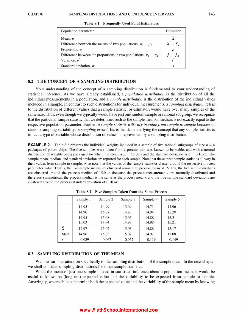
Table 8.1 Frequently Used Point Estimators
Population parameter Estimator
Mean, m �XX
Difference between the means of two populations, m1 � m2�XX1 � �XX2
Proportion, p pp
Difference between the proportions in two populations, p1 � p2 pp1 � pp2
Variance, s2 s2
Standard deviation, s s
8.2 THE CONCEPT OF A SAMPLING DISTRIBUTION
Your understanding of the concept of a sampling distribution is fundamental to your understanding of
statistical inference. As we have already established, a population distribution is the distribution of all the
individual measurements in a population, and a sample distribution is the distribution of the individual values
included in a sample. In contrast to such distributions for individual measurements, a sampling distribution refers
to the distribution of different values that a sample statistic, or estimator, would have over many samples of the
same size. Thus, even though we typically would have just one random sample or rational subgroup, we recognize
that the particular sample statistic that we determine, such as the samplemean ormedian, is not exactly equal to the
respective population parameter. Further, a sample statistic will vary in value from sample to sample because of
random sampling variability, or sampling error. This is the idea underlying the concept that any sample statistic is
in fact a type of variable whose distribution of values is represented by a sampling distribution.
EXAMPLE 2. Table 8.2 presents the individual weights included in a sample of five rational subgroups of size n ¼ 4
packages of potato chips. The five samples were taken from a process that was known to be stable, and with a normal
distribution of weights being packaged for which the mean is m ¼ 15:0 oz and the standard deviation is s ¼ 0:10 oz. Thesample mean, median, and standard deviation are reported for each sample. Note that these three sample statistics all vary in
their values from sample to sample. Also note that the values of the sample statistics cluster around the respective process
parameter value. That is, the five sample means are clustered around the process mean of 15.0 oz, the five sample medians
are clustered around the process median of 15.0 oz (because the process measurements are normally distributed and
therefore symmetrical, the process median is the same as the process mean), and the five sample standard deviations are
clustered around the process standard deviation of 0.10 oz.
Table 8.2 Five Samples Taken from the Same Process
Sample 1 Sample 2 Sample 3 Sample 4 Sample 5
14.95 14.99 15.09 14.71 14.96
14.96 15.07 14.98 14.94 15.20
14.95 15.08 15.05 14.88 15.31
15.03 14.94 14.99 14.98 15.21
�XX 14.97 15.02 15.03 14.88 15.17
Med 14.96 15.03 15.02 14.91 15.08
s 0.039 0.067 0.052 0.119 0.149
8.3 SAMPLING DISTRIBUTION OF THE MEAN
We now turn our attention specifically to the sampling distribution of the sample mean. In the next chapter
we shall consider sampling distributions for other sample statistics.
When the mean of just one sample is used in statistical inference about a population mean, it would be
useful to know the (long-run) expected value and the variability to be expected from sample to sample.
Amazingly, we are able to determine both the expected value and the variability of the sample mean by knowing
CHAP. 8] SAMPLING DISTRIBUTIONS AND CONFIDENCE INTERVALS 143

the mean and standard deviation of the population (or process). But what if the parameter values are not known,
and we have data from only one sample? Even then, the variability of the sample statistic, such as the sample
mean, from sample to sample can still be determined and used in statistical inference.
The sampling distribution of the mean is described by determining the mean of such a distribution, which is
the expected value E( �XX), and the standard deviation of the distribution of sample means, designated s �xx.
Because this standard deviation is indicative of the accuracy of the sample statistic as an estimator of a
population mean, s �xx usually is called the standard error of the mean. When the population or process
parameters are known, the expected value and standard error for the sampling distribution of the mean are
E( �XX) ¼ m (8:1)
s �xx ¼ sffiffiffin
p (8:2)
EXAMPLE 3. Suppose the mean of a very large population is m ¼ 50:0 and the standard deviation of the measurements is
s ¼ 12:0. We determine the sampling distribution of the sample means for a sample size of n ¼ 36, in terms of the expected
value and the standard error of the distribution, as follows:
E( �XX) ¼ m ¼ 50:0
s �xx ¼ sffiffiffin
p ¼ 12:0ffiffiffiffiffi36
p ¼ 12:0
6¼ 2:0
When sampling from a population that is finite and of limited size, a finite correction factor is available for
the correct determination of the standard error. The effect of this correction factor is always to reduce the value
that otherwise would be calculated. As a general rule, the correction is negligible and can be omitted when
n , 0:05N, that is, when the sample size is less than 5 percent of the population size. Because populations from
which samples are taken are usually large, many texts and virtually all computer programs do not include this
correction option. The formula for the standard error of the mean with the finite correction factor included is
s �xx ¼ sffiffiffin
pffiffiffiffiffiffiffiffiffiffiffiffiN � n
N � 1
r(8:3)
The correction factor in the above formula is the factor under the square root that has been appended to the
basic formula for the standard error of the mean. This same correction factor can be appended to the formulas
for any of the standard error formulas for the mean, difference between means, proportion, and difference
between proportions that are described and used in this and the following chapters. However, we omit any
consideration of the finite correction factor after this chapter.
EXAMPLE 4. To illustrate that the finite correction factor reduces the size of the standard error of the mean when its use is
appropriate, suppose that in Example 3 the sample of n ¼ 36 values was taken from a population of just 100 values. The
sample thus constitutes 36 percent of the population. The expected value and standard error of the sampling distribution of
the mean are
E( �XX) ¼ m ¼ 50:0
s �xx ¼ sffiffiffin
pffiffiffiffiffiffiffiffiffiffiffiffiN � n
N � 1
r¼ 12:0ffiffiffiffiffi
36p
ffiffiffiffiffiffiffiffiffiffiffiffiffiffiffiffiffiffi100� 36
100� 1
r¼ 2:00(0:80) ¼ 1:60
If the standard deviation of the population or process is not known, the standard error of the mean can be
estimated by using the sample standard deviation as an estimator of the population standard deviation. To
differentiate this estimated standard error from the precise one based on a known s, it is designated by the
symbol s�xx (or by ss �xx in some texts). A few textbooks do not differentiate the exact standard error from
the estimated standard error, and instead use the simplified SE( �XX) to represent the standard error of the mean.
The formula for the estimated standard error of the mean is
s�xx ¼ sffiffiffin
p (8:4)
144 SAMPLING DISTRIBUTIONS AND CONFIDENCE INTERVALS [CHAP. 8

EXAMPLE 5. An auditor takes a random sample of size n ¼ 16 from a set of N ¼ 1,500 accounts receivable. The
standard deviation of the amounts of the receivables for the entire group of 1,500 accounts is not known. However,
the sample standard deviation is s ¼ $57:00. We determine the value of the standard error for the sampling distribution of
the mean as follows:
s�xx ¼ sffiffiffin
p ¼ 57:00ffiffiffiffiffi16
p ¼ $14:25
8.4 THE CENTRAL LIMIT THEOREM
If the population or process from which a sample is taken is normally distributed, then the sampling
distribution of the mean also will be normally distributed, regardless of sample size. However, what if a
population is not normally distributed? Remarkably, a theorem from mathematical statistics still permits
application of the normal distribution with respect to such sampling distributions. The central limit theorem
states that as sample size is increased, the sampling distribution of the mean (and for other sample statistics as
well) approaches the normal distribution in form, regardless of the form of the population distribution from
which the sample was taken. For practical purposes, the sampling distribution of the mean can be assumed to be
approximately normally distributed, even for the most nonnormal populations or processes, whenever the
sample size is n � 30. For populations that are only somewhat nonnormal, even a smaller sample size will
suffice. But a sample size of at least 30 will take care of the most adverse population situation.
8.5 DETERMINING PROBABILITY VALUES FOR THE SAMPLE MEAN
If the sampling distribution of the mean is normally distributed, either because the population is normally
distributed or because the central limit theorem is invoked, then we can determine probabilities regarding the
possible values of the samplemean, given that the populationmean and standard deviation are known. The process
is analogous to determining probabilities for individual observations using the normal distribution, as described in
Section 7.2. In the present application, however, it is the designated value of the sample mean that is converted into a
value of z in order to use the table of normal probabilities. This conversion formula uses the standard error of the
mean because this is the standard deviation for the �XX variable. Thus, the conversion formula is
z ¼�XX � m
s �xx(8:5)
EXAMPLE 6. An auditor takes a random sample of size n ¼ 36 from a population of 1,000 accounts receivable. The
mean value of the accounts receivable for the population is m ¼ $260:00, with the population standard deviation
s ¼ $45:00. What is the probability that the sample mean will be less than $250.00?
Fig. 8-1
CHAP. 8] SAMPLING DISTRIBUTIONS AND CONFIDENCE INTERVALS 145

Figure 8-1 portrays the probability curve. The sampling distribution is described by the mean and standard error:
E( �XX) ¼ m ¼ 260:00 (as given)
s �xx ¼ sffiffiffin
p ¼ 45:00ffiffiffiffiffi36
p ¼ 45:00
6¼ 7:50
z ¼�XX � m
s �xx¼ 250:00� 260:00
7:50¼ �10:00
7:50¼ �1:33
Therefore,
P( �XX , 250:00jm ¼ 260:00, s �xx ¼ 7:50) ¼ P(z , �1:33)
P(z , �1:33) ¼ 0:5000� P(� 1:33 z 0)
¼ 0:5000� 0:4082 ¼ 0:0918
EXAMPLE 7. With reference to Example 6, what is the probability that the sample mean will be within $15.00 of the
population mean?
Figure 8-2 portrays the probability curve for the sampling distribution.
P(245:00 �XX 275:00jm ¼ 260:00, s �xx ¼ 7:50)
z1 ¼ 245:00� 260:00
7:50¼ � 2:00
z2 ¼ 275:00� 260:00
7:50¼ þ 2:00
where
P(�2:00 z þ 2:00) ¼ 0:4772þ 0:4772 ¼ 0:9544 ffi 95%
Fig. 8-2
8.6 CONFIDENCE INTERVALS FOR THE MEAN USING THE NORMAL DISTRIBUTION
Examples 6 and 7, above, are concerned with determining the probability that the sample mean will have
various values given that the population mean and standard deviation are known. What is involved is deductive
reasoning with respect to the sample result based on known population parameters. We now concern ourselves
with inductive reasoning by using sample data to make statements about the value of the population mean.
The methods of interval estimation in this section are based on the assumption that the normal probability
distribution can be used. Such use is warranted (1) whenever n � 30, because of the central limit theorem, or (2)
when n , 30 but the population is normally distributed and s is known. (The case of n , 30 with s not known
is considered in Section 8.8.)
146 SAMPLING DISTRIBUTIONS AND CONFIDENCE INTERVALS [CHAP. 8

Although the sample mean is useful as an unbiased estimator of the population mean, there is no way of
expressing the degree of accuracy of a point estimator. In fact, mathematically speaking, the probability that the
sample mean is exactly correct as an estimator of the population mean is P ¼ 0. A confidence interval for the
mean is an estimate interval constructed with respect to the sample mean bywhich the likelihood that the interval
includes the value of the population mean can be specified. The level of confidence associated with a confidence
interval indicates the long-run percentage of such intervals which would include the parameter being estimated.
Confidence intervals for the mean typically are constructed with the unbiased estimator �XX at the midpoint
of the interval. However, Problems 8.14 and 8.15 demonstrate the construction of a so-called one-sided
confidence interval, for which the sample mean is not at the midpoint of the interval. When use of the normal
probability distribution is warranted, the confidence interval for the mean is determined by
�XX + zs �xx (8:6)
or when the population s is not known, by
�XX + zs�xx (8:7)
The +zs �xx or +zs�xx frequently is called the margin of error for the confidence interval.
The most frequently used confidence intervals are the 90 percent, 95 percent, and 99 percent confidence
intervals. The values of z required in conjuction with such intervals are given in Table 8.3.
Table 8.3 Selected Proportions of Area under the Normal Curve
z (the number of standard deviation
units from the mean)
Proportion of area in the
interval m+ zs
1.645 0.90
1.96 0.95
2.58 0.99
EXAMPLE 8. For a given week, a random sample of 30 hourly employees selected from a very large number of
employees in a manufacturing firm has a sample mean wage of �XX ¼ $180:00, with a sample standard deviation of
s ¼ $14:00. We estimate the mean wage for all hourly employees in the firm with an interval estimate such that we can be 95
percent confident that the interval includes the value of the population mean, as follows:
�XX + 1:96s�xx ¼ 180:000+ 1:96(2:56) ¼ $174:98 to $185:02
where �XX ¼ $180:00 (as given)
s�xx ¼ sffiffiffin
p ¼ 14:00ffiffiffiffiffi30
p ¼ 2:56
(Note: s is used as an estimator of s.)Thus, we can state that the mean wage level for all employees is between $174.98 and $185.02, with a 95 percent level
of confidence in this estimate.
In addition to estimating the value of the population mean as such, there is sometimes an interest in
estimating the total quantity, or total amount, of something in the population. See Problem 8.11(b).
8.7 DETERMINING THE REQUIRED SAMPLE SIZE FOR ESTIMATING THE MEAN
Suppose the desired size of a confidence interval and the level of confidence to be associated with it are
specified. If s is known or can be estimated, such as from the results of similar studies, the required sample size
based on use of the normal distribution is
n ¼ zs
E
� 2(8:8)
CHAP. 8] SAMPLING DISTRIBUTIONS AND CONFIDENCE INTERVALS 147

In Formula (8.8), z is the value used for the specified level of confidence, s is the standard deviation of the
population (or estimate thereof), and E is the plus and minus sampling error allowed in the interval (always one-
half the total confidence interval).
(Note: When solving for sample size, any fractional result is always rounded up. Further, unless s is known
and the population is normally distributed, any computed sample size below 30 should be increased to 30
because formula (8.8) is based on use of the normal distribution.)
EXAMPLE 9. A personnel department analyst wishes to estimate the mean number of training hours annually for
supervisors in a division of the company within 3.0 hr (plus or minus) and with 90 percent confidence. Based on data from
other divisions, the analyst estimates the standard deviation of training hours to be s ¼ 20:0 hr. The minimum required
sample size is
n ¼�
zs
E
�2
¼ (1:645)(20:0)
3:0
� �2¼ 32:9
3:0
� �2
¼ 120:27 ffi 121
8.8 THE t DISTRIBUTION AND CONFIDENCE INTERVALS FOR THE MEAN
In Section 8.4 we indicated that use of the normal distribution in estimating a population mean is warranted
for any large sample (n � 30), and for a small sample (n , 30) only if the population is normally distributed
and s is known. In this section we handle the situation in which the sample is small and the population is
normally distributed, but s is not known.
If a population is normally distributed, the sampling distribution of the mean for any sample size will also
be normally distributed; this is true whether s is known or not. However, in the process of inference each value
of the mean is converted to a standard normal value, and herein lies the problem. If s is unknown,
the conversion formula ( �XX � m)=s�xx includes a variable in the denominator, because s, and therefore s�xx, will be
somewhat different from sample to sample. The result is that use of the variable s�xx rather than the constant s �xx in
the denominator results in converted values that are not distributed as z values. Instead, the values are
distributed according to the t distribution, which is platykurtic (flat) as compared with the distribution of z.
Appendix 6 indicates proportions of area for the t distribution. The distribution is a family of distributions, with
a somewhat different distribution associated with the degrees of freedom (df ). For a confidence interval for the
population mean based on a sample of size n, df ¼ n � 1.
The degrees of freedom indicate the number of values that are in fact “free to vary” in the sample that
serves as the basis for the confidence interval. Offhand, it would seem that all of the values in the sample are
always free to vary in their measured values. However, what is different for the t distribution as compared to the
z is that both the sample mean and the sample standard deviation are required as parameter estimators in order to
define a confidence interval for the population mean. The need for the additional parameter estimate is a
limitation on the sample. Without considering the mathematical abstractions, the bottom line is that, in general,
one degree of freedom is lost with each additional parameter estimate that is required beyond the one parameter
toward which the statistical inference is directed.
Use of the t distribution for inference concerning the population mean is appropriate whenever s is not
known and the sampling distribution of the mean is normal (either because the population is normally
distributed or the central limit theorem is invoked). Just as is true for the z distribution, the t distribution has a
mean of 0. However, it is flatter and wider than the z (and thus has a standard deviation. 1:0). With increasing
sample size and df, the t distribution approaches the form of the standard normal z distribution. For hand
calculations, a general rule is that required t values can be approximated by z values when n . 30 (or df . 29).
For computer applications there is no need to use approximations, and therefore the t distribution is used for
large as well as small samples whenever the standard error is estimated on the basis of the sample standard
deviation.
148 SAMPLING DISTRIBUTIONS AND CONFIDENCE INTERVALS [CHAP. 8
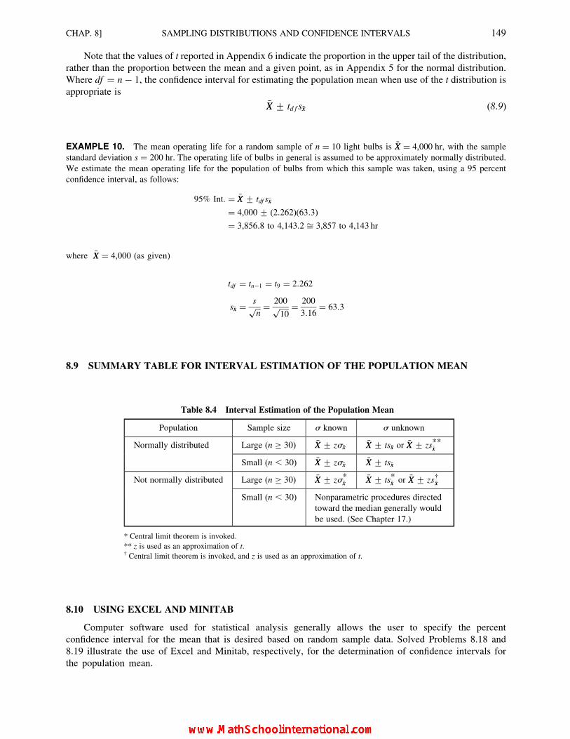
Note that the values of t reported in Appendix 6 indicate the proportion in the upper tail of the distribution,
rather than the proportion between the mean and a given point, as in Appendix 5 for the normal distribution.
Where df ¼ n � 1, the confidence interval for estimating the population mean when use of the t distribution is
appropriate is
�XX + td f s�xx (8:9)
EXAMPLE 10. The mean operating life for a random sample of n ¼ 10 light bulbs is �XX ¼ 4,000 hr, with the sample
standard deviation s ¼ 200 hr. The operating life of bulbs in general is assumed to be approximately normally distributed.
We estimate the mean operating life for the population of bulbs from which this sample was taken, using a 95 percent
confidence interval, as follows:
95% Int. ¼ �XX + tdf s�xx
¼ 4,000+ (2:262)(63:3)
¼ 3,856:8 to 4,143:2 ffi 3,857 to 4,143 hr
where �XX ¼ 4,000 (as given)
tdf ¼ tn�1 ¼ t9 ¼ 2:262
s�xx ¼ sffiffiffin
p ¼ 200ffiffiffiffiffi10
p ¼ 200
3:16¼ 63:3
8.9 SUMMARY TABLE FOR INTERVAL ESTIMATION OF THE POPULATION MEAN
8.10 USING EXCEL AND MINITAB
Computer software used for statistical analysis generally allows the user to specify the percent
confidence interval for the mean that is desired based on random sample data. Solved Problems 8.18 and
8.19 illustrate the use of Excel and Minitab, respectively, for the determination of confidence intervals for
the population mean.
Table 8.4 Interval Estimation of the Population Mean
Population Sample size s known s unknown
Normally distributed Large (n � 30) �XX + zs�xx�XX + ts�xx or �XX + zs**�xx
Small (n , 30) �XX + zs�xx�XX + ts�xx
Not normally distributed Large (n � 30) �XX + zs*�xx �XX + ts*�xx or �XX + zsy�xx
Small (n , 30) Nonparametric procedures directed
toward the median generally would
be used. (See Chapter 17.)
* Central limit theorem is invoked.
** z is used as an approximation of t.† Central limit theorem is invoked, and z is used as an approximation of t.
CHAP. 8] SAMPLING DISTRIBUTIONS AND CONFIDENCE INTERVALS 149

Solved Problems
SAMPLING DISTRIBUTION OF THE MEAN
8.1. For a particular brand of TV picture tube, it is known that the mean operating life of the tubes is
m ¼ 9,000 hr with a standard deviation of s ¼ 500 hr. (a) Determine the expected value and standard
error of the sampling distribution of the mean given a sample size of n ¼ 25. (b) Interpret the meaning of
the computed values.
ðaÞ E( �XX) ¼ m ¼ 9,000
s �xx ¼ sffiffiffin
p ¼ 500ffiffiffiffiffi25
p ¼ 500
5¼ 100
(b) These calculations indicate that in the long run the mean of a large group of sample means, each based on a
sample size of n ¼ 25, will be equal to 9,000 hr. Further, the variability of these sample means with respect to
the expected value of 9,000 hr is expressed by a standard deviation of 100 hr.
8.2. For a large population of normally distributed account balances, the mean balance is m ¼ $150:00 withstandard deviation s ¼ $35:00. What is the probability that one randomly sampled account has a
balance that exceeds $160.00?
Fig. 8-3
Figure 8-3 portrays the probability curve for the variable.
z ¼ X � m
s¼ 160:00� 150:00
35:00¼ þ 0:29
P(X . 160:00jm ¼ 150:00, s ¼ 35:00) ¼ P(z . þ 0:29)
¼ 0:5000� P(0 z þ 0:29) ¼ 0:5000� 0:1141 ¼ 0:3859
8.3. With reference to Problem 8.2 above, what is the probability that the mean for a random sample of
n ¼ 40 accounts will exceed $160.00?
Figure 8-4 portrays the probability curve for the sampling distribution E( �XX) ¼ m ¼ $150:00.
s �xx ¼ sffiffiffin
p ¼ 35:00
40¼ $5:53
z ¼�XX � m
s �xx¼ 160:00� 150:00
5:53¼ 10:00
5:53¼ þ1:81
150 SAMPLING DISTRIBUTIONS AND CONFIDENCE INTERVALS [CHAP. 8

Therefore,
P( �XX . 160:00jm ¼ 150:00, s �xx ¼ 5:53) ¼ P(z . þ 1:81)
¼ 0:5000� P(0 z þ 1:81)
¼ 0:5000� 0:4649 ¼ 0:0351
8.4. This problem and the following two problems serve to illustrate the meaning of the sampling
distribution of the mean by reference to a highly simplified population. Suppose a population consists of
just the four values 3, 5, 7, and 8. Compute (a) the population mean m and (b) the population standard
deviation s.
With reference to Table 8.5,
(a) m ¼ SX
N¼ 23
4¼ 5:75
(b) s ¼ffiffiffiffiffiffiffiffiffiffiffiffiffiffiffiffiffiffiffiffiffiffiffiffiffiffiffiffiffiSX2
N� SX
N
� �2s
¼ffiffiffiffiffiffiffiffiffiffiffiffiffiffiffiffiffiffiffiffiffiffiffiffiffiffiffi147
4� 23
4
� �2s
¼ffiffiffiffiffiffiffiffiffiffiffiffiffiffiffiffiffiffiffiffiffiffiffiffiffiffiffiffiffiffiffi36:75� (5:75)2
q¼
ffiffiffiffiffiffiffiffiffiffiffiffiffiffiffiffiffiffiffiffiffiffiffiffiffiffiffiffiffiffiffiffiffi36:75� 33:0625
p¼ 1:92
Table 8.5 Worksheet for Problem 8.4
X X 2
3 9
5 25
7 49
8 64
SX ¼23 SX2 ¼ 147
8.5. For the population described in Problem 8.4, suppose that simple random samples of size n ¼ 2 each are
taken from this population. For each sample the first sampled item is not replaced in the population
before the second item is sampled.
(a) List all possible pairs of values which can constitute a sample.
(b) For each of the pairs identified in (a), compute the samplemean �XX and demonstrate that themean of all
possible samplemeansm�xx is equal to themeanof the population fromwhich the sampleswere selected.
(a) and (b) From Table 8.6,
m�xx ¼S �XX
Nsamples
¼ 34:5
6¼ 5:75
[which equals m as computed in Problem 8.4(a)].
Fig. 8-4
CHAP. 8] SAMPLING DISTRIBUTIONS AND CONFIDENCE INTERVALS 151

8.6. For the sampling situation described in Problems 8.4 and 8.5, (a) compute the standard error of the mean
by determining the standard deviation of the six possible sample means identified in Problem 8.5 with
respect to the population mean m. (b) Then compute the standard error of the mean based on s being
known and sampling from a finite population, using the appropriate formula from this chapter. Verify
that the two standard error values are the same.
With reference to Table 8.6, we get Table 8.7
(a) First method:
s �xx ¼ffiffiffiffiffiffiffiffiffiffiffiffiffiffiffiffiffiffiffiffiffiffiffiffiffiffiffiffiffiS �XX
2
Ns
� S �XX
Ns
� �2s
¼ffiffiffiffiffiffiffiffiffiffiffiffiffiffiffiffiffiffiffiffiffiffiffiffiffiffiffiffiffiffiffiffiffiffiffiffi205:75
6� 34:5
6
� �2s
¼ffiffiffiffiffiffiffiffiffiffiffiffiffiffiffiffiffiffiffiffiffiffiffiffiffiffiffiffiffiffiffiffiffiffiffiffi34:2917� (5:75)2
q¼
ffiffiffiffiffiffiffiffiffiffiffiffiffiffiffiffiffiffiffiffiffiffiffiffiffiffiffiffiffiffiffiffiffiffiffiffiffiffi34:2917� 33:0625
p¼ 1:11
(b) Second method:
s �xx ¼ sffiffiffin
pffiffiffiffiffiffiffiffiffiffiffiffiN � n
N � 1
r¼ 1:92ffiffiffi
2p
ffiffiffiffiffiffiffiffi4–2
4–1
r
¼ 1:92
1:414
ffiffiffiffiffiffiffiffiffiffiffiffiffiffi0:6666
p¼ 1:358ð0:816Þ ¼ 1:11
Of course, the second method is the one always used for determining the standard error of the mean in actual data
situations. But conceptually, the first method illustrates more directly the meaning of the standard error of the mean.
Table 8.7 Worksheet for Problem 8.6
�XX �XX2
4.0 16.00
5.0 25.00
5.5 30.25
6.0 36.00
6.5 42.25
7.5 56.25
S �XX ¼ 34.5 S �XX2 ¼ 205.75
Table 8.6 Possible Samples and Sample
Means for Problem 8.5
Possible samples �XX
3, 5 4.0
3, 7 5.0
3, 8 5.5
5, 7 6.0
5, 8 6.5
7, 8 7.5
S �XX ¼ 34.5
152 SAMPLING DISTRIBUTIONS AND CONFIDENCE INTERVALS [CHAP. 8
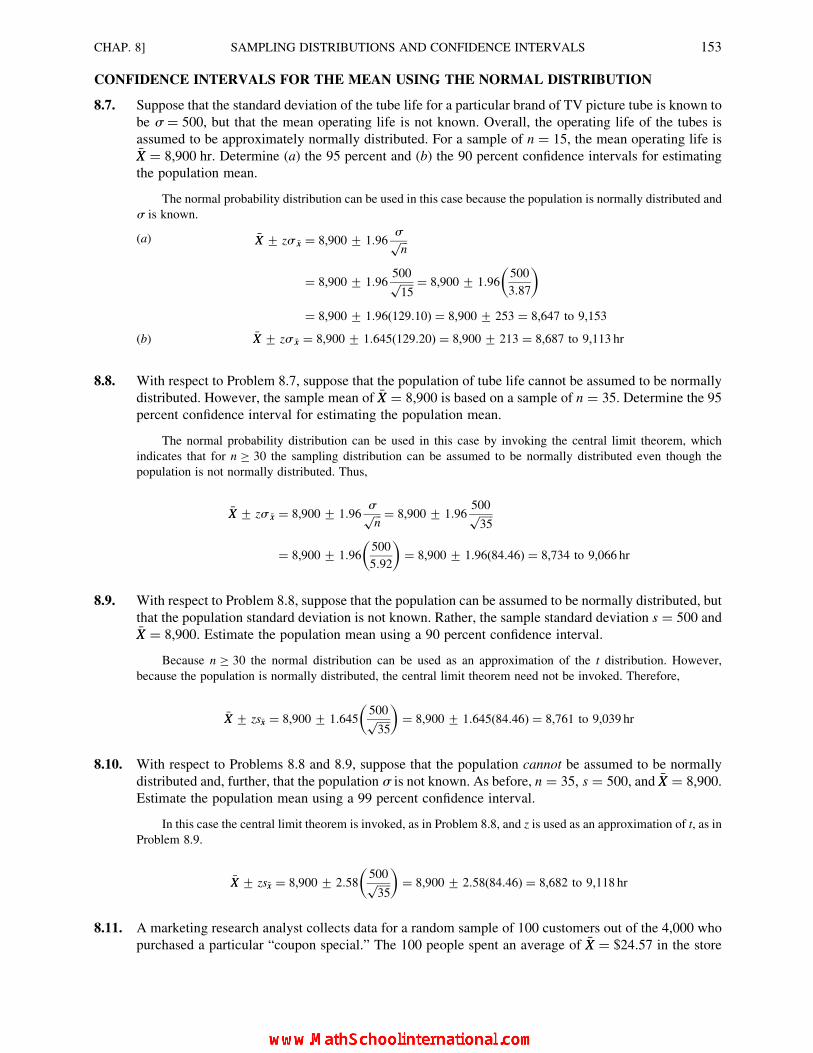
CONFIDENCE INTERVALS FOR THE MEAN USING THE NORMAL DISTRIBUTION
8.7. Suppose that the standard deviation of the tube life for a particular brand of TV picture tube is known to
be s ¼ 500, but that the mean operating life is not known. Overall, the operating life of the tubes is
assumed to be approximately normally distributed. For a sample of n ¼ 15, the mean operating life is�XX ¼ 8,900 hr. Determine (a) the 95 percent and (b) the 90 percent confidence intervals for estimating
the population mean.
The normal probability distribution can be used in this case because the population is normally distributed and
s is known.
(a) �XX + zs �xx ¼ 8,900+ 1:96sffiffiffin
p
¼ 8,900+ 1:96500ffiffiffiffiffi15
p ¼ 8,900+ 1:96500
3:87
� �
¼ 8,900+ 1:96(129:10) ¼ 8,900+ 253 ¼ 8,647 to 9,153
(b) �XX + zs �xx ¼ 8,900+ 1:645(129:20) ¼ 8,900+ 213 ¼ 8,687 to 9,113 hr
8.8. With respect to Problem 8.7, suppose that the population of tube life cannot be assumed to be normally
distributed. However, the sample mean of �XX ¼ 8,900 is based on a sample of n ¼ 35. Determine the 95
percent confidence interval for estimating the population mean.
The normal probability distribution can be used in this case by invoking the central limit theorem, which
indicates that for n � 30 the sampling distribution can be assumed to be normally distributed even though the
population is not normally distributed. Thus,
�XX + zs �xx ¼ 8,900+ 1:96sffiffiffin
p ¼ 8,900+ 1:96500ffiffiffiffiffi35
p
¼ 8,900+ 1:96500
5:92
� �¼ 8,900+ 1:96(84:46) ¼ 8,734 to 9,066 hr
8.9. With respect to Problem 8.8, suppose that the population can be assumed to be normally distributed, but
that the population standard deviation is not known. Rather, the sample standard deviation s ¼ 500 and�XX ¼ 8,900. Estimate the population mean using a 90 percent confidence interval.
Because n � 30 the normal distribution can be used as an approximation of the t distribution. However,
because the population is normally distributed, the central limit theorem need not be invoked. Therefore,
�XX + zs�xx ¼ 8,900+ 1:645500ffiffiffiffiffi35
p� �
¼ 8,900+ 1:645(84:46) ¼ 8,761 to 9,039 hr
8.10. With respect to Problems 8.8 and 8.9, suppose that the population cannot be assumed to be normally
distributed and, further, that the population s is not known. As before, n ¼ 35, s ¼ 500, and �XX ¼ 8,900.
Estimate the population mean using a 99 percent confidence interval.
In this case the central limit theorem is invoked, as in Problem 8.8, and z is used as an approximation of t, as in
Problem 8.9.
�XX + zs�xx ¼ 8,900+ 2:58500ffiffiffiffiffi35
p� �
¼ 8,900+ 2:58(84:46) ¼ 8,682 to 9,118 hr
8.11. A marketing research analyst collects data for a random sample of 100 customers out of the 4,000 who
purchased a particular “coupon special.” The 100 people spent an average of �XX ¼ $24:57 in the store
CHAP. 8] SAMPLING DISTRIBUTIONS AND CONFIDENCE INTERVALS 153

with a standard deviation of s ¼ $6:60. Using a 95 percent confidence interval, estimate (a) the mean
purchase amount for all 4,000 customers and (b) the total dollar amount of purchases by the 4,000
customers.
(a) s�xx ¼ sffiffiffin
p ¼ 6:60ffiffiffiffiffiffiffiffi100
p ¼ 0:66
�XX + zs�xx ¼ 24:57+ 1:96(0:66) ¼ $24:57+ $1:29 ¼ $23:28 to $25:86
(b) N( �XX + zs�xx) ¼ 4,000($23:28 to $25:86) ¼ $93,120 to $103,440
or
N �XX + N(zs�xx) ¼ 4,000(24:57)+ 4,000(1:29)¼ 98,280+ 5,160 ¼ $93,120 to $103,440
(Note: The confidence interval for the dollar amount of purchases is simply the total number of customers in the
population multiplied by the confidence limits for the mean purchase amount per customer. Such a population
value is referred to as the total quantity in some textbooks.)
DETERMINING THE REQUIRED SAMPLE SIZE FOR ESTIMATING THE MEAN
8.12. A prospective purchaser wishes to estimate the mean dollar amount of sales per customer at a toy store
located at an airlines terminal. Based on data from other similar airports, the standard deviation of such
sales amounts is estimated to be about s ¼ $3:20. What size of random sample should be collected, as a
minimum, if the purchaser wants to estimate the mean sales amount within $1:00 and with 99 percent
confidence?
n ¼ zs
E
� 2¼ (2:58)(3:20)
1:00
� �2¼ (8:256)2 ¼ 68:16 ffi 69
8.13. Referring to Problem 8.12, what is the minimum required sample size if the distribution of sales
amounts is not assumed to be normal and the purchaser wishes to estimate the mean sales amount within
$2:00 with 99 percent confidence?
n ¼ zs
E
� 2¼ (2:58)(3:20)
2:00
� �2¼ (4:128)2 ¼ 17:04 ffi 18
However, because the population is not assumed to be normally distributed, the minimum sample size is
n ¼ 30, so that the central limit theorem can be invoked as the basis for using the normal probability distribution for
constructing the confidence interval.
ONE-SIDED CONFIDENCE INTERVALS FOR THE POPULATION MEAN
8.14. Occasionally, a one-sided confidence interval may be of greater interest than the usual two-sided
interval. Such would be the case if we are interested only in the highest (or only in the lowest) value of
the mean at the indicated level of confidence. An “upper 95 percent interval” extends from a computed
lower limit to positive infinity, with a proportion of 0.05 of the area under the normal curve being to the
left of the lower limit. Similarly, a “lower 95 percent confidence interval” extends from negative infinity
to a computed upper limit, with a proportion of 0.05 of the area under the normal curve being to the right
of the upper limit.
Suppose a prospective purchaser of a toy store at an airlines terminal observes a random sample of
n ¼ 64 sales and finds that the sample mean is �XX ¼ $14:63, with the sample standard deviation
154 SAMPLING DISTRIBUTIONS AND CONFIDENCE INTERVALS [CHAP. 8

s ¼ $2:40. Determine the upper 95 percent confidence interval so that the minimum value of the
population mean is identified with a 95 percent degree of confidence.
s�xx ¼ sffiffiffin
p ¼ 2:40ffiffiffiffiffi64
p ¼ 2:40
8¼ 0:30
Upper 95% int: ¼ �XX � zs�xx ¼ 14:63� 1:645(0:30) ¼ $14:14 or higher
Thus, with a 95 percent degree of confidence we can state that the mean sales amount for the population of all
customers is equal to or greater than $14:14.
8.15. With 99 percent confidence, what is the estimate of the maximum value of the mean sales amount in
Problem 8.14?
Since �XX ¼ $14:63 and s�xx ¼ 0:30,
Lower 99% int: ¼ �XX þ zs�xx ¼ 14:63þ 2:33(0:30) ¼ $15:33 or less
Thus, with a 99 percent degree of confidence, we can state that the mean sales amount is no larger than $15:33.
USE OF THE t DISTRIBUTION
8.16. In Problem 8.7 we constructed confidence intervals for estimating the mean operating life of a particular
brand of TV picture tube based on the assumption that the operating life of all tubes is approximately
normally distributed and s ¼ 500, and given a sample of n ¼ 15 with �XX ¼ 8,900 hr. Suppose that s is
not known, but rather, that the sample standard deviation is s ¼ 500.
(a) Determine the 95 percent confidence interval for estimating the population mean and compare this
interval with the answer to Problem 8.7(a).
(b) Determine the 90 percent confidence interval for estimating the population mean and compare this
interval with the answer to Problem 8.7(b).
(Note: Use of a t distribution is required in this case because the population is assumed to be normally
distributed, s is not known, and the sample is small (n , 30).)
(a) �XX + tdf s�xx ¼ 8,900+ 2:145sffiffiffin
p ¼ 8,900+ 2:145500ffiffiffiffiffi15
p
¼ 8,900+ 2:145500
3:87
� �¼ 8,900+ 2:145(129:199) ¼ 8,900+ 277 ¼ 8; 623 to 9,177 hr
The confidence interval is wider than the one in Problem 8.7(a), reflecting the difference between the t
distribution with df ¼ 15� 1 ¼ 14, and the normal probability distribution.
(b) �XX + td f s�xx ¼ 8,900+ 1:761(129:199) ¼ 8,900+ 228 ¼ 8,672 to 9,128 hr
Again, the confidence interval is wider than the one in Problem 8.7(b).
8.17. As a commercial buyer for a private supermarket brand, suppose you take a random sample of 12 No. 303
cans of green beans at a canning plant. The net weight of the drained beans in each can is reported in Table
8.8. Determine (a) the mean net weight of string beans being packed in each can for this sample and (b) the
sample standard deviation. (c) Assuming that the net weights per can are normally distributed, estimate the
mean weight per can of beans being packed using a 95 percent confidence interval.
Table 8.8 Net Weight of Beans Packed in 12 No. 303 Cans
Ounces per can 15.7 15.8 15.9 16.0 16.1 16.2
Number of cans 1 2 2 3 3 1
CHAP. 8] SAMPLING DISTRIBUTIONS AND CONFIDENCE INTERVALS 155
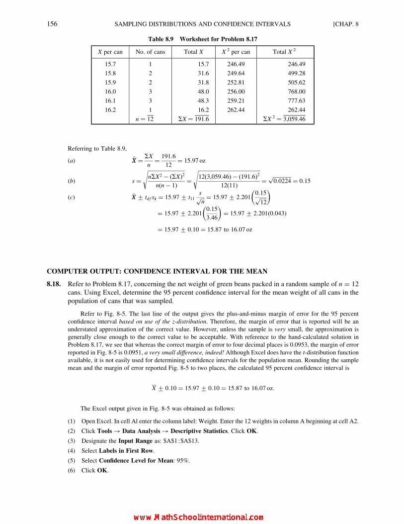
Referring to Table 8.9,
(a) �XX ¼ SX
n¼ 191:6
12¼ 15:97 oz
(b) s ¼ffiffiffiffiffiffiffiffiffiffiffiffiffiffiffiffiffiffiffiffiffiffiffiffiffiffiffiffinSX2 � (SX)2
n(n � 1)
s¼
ffiffiffiffiffiffiffiffiffiffiffiffiffiffiffiffiffiffiffiffiffiffiffiffiffiffiffiffiffiffiffiffiffiffiffiffiffiffiffiffiffiffiffiffiffiffiffi12(3,059:46)� (191:6)2
12(11)
s¼
ffiffiffiffiffiffiffiffiffiffiffiffiffiffi0:0224
p¼ 0:15
(c) �XX + td f s�xx ¼ 15:97+ t11sffiffiffin
p ¼ 15:97+ 2:2010:15ffiffiffiffiffi12
p� �
¼ 15:97+ 2:2010:15
3:46
� �¼ 15:97+ 2:201(0:043)
¼ 15:97+ 0:10 ¼ 15:87 to 16:07 oz
COMPUTER OUTPUT: CONFIDENCE INTERVAL FOR THE MEAN
8.18. Refer to Problem 8.17, concerning the net weight of green beans packed in a random sample of n ¼ 12
cans. Using Excel, determine the 95 percent confidence interval for the mean weight of all cans in the
population of cans that was sampled.
Refer to Fig. 8-5. The last line of the output gives the plus-and-minus margin of error for the 95 percent
confidence interval based on use of the z-distribution. Therefore, the margin of error that is reported will be an
understated approximation of the correct value. However, unless the sample is very small, the approximation is
generally close enough to the correct value to be acceptable. With reference to the hand-calculated solution in
Problem 8.17, we see that whereas the correct margin of error to four decimal places is 0.0953, the margin of error
reported in Fig. 8-5 is 0.0951, a very small difference, indeed! Although Excel does have the t-distribution function
available, it is not easily used for determining confidence intervals for the population mean. Rounding the sample
mean and the margin of error reported Fig. 8-5 to two places, the calculated 95 percent confidence interval is
X + 0:10 ¼ 15:97+ 0:10 ¼ 15:87 to 16:07 oz:
The Excel output given in Fig. 8-5 was obtained as follows:
(1) Open Excel. In cell Al enter the column label: Weight. Enter the 12 weights in column A beginning at cell A2.
(2) Click Tools ! Data Analysis ! Descriptive Statistics. Click OK.
(3) Designate the Input Range as: $A$1 :$A$13.
(4) Select Labels in First Row.
(5) Select Confidence Level for Mean: 95%.
(6) Click OK.
Table 8.9 Worksheet for Problem 8.17
X per can No. of cans Total X X 2 per can Total X 2
15.7 1 15.7 246.49 246.49
15.8 2 31.6 249.64 499.28
15.9 2 31.8 252.81 505.62
16.0 3 48.0 256.00 768.00
16.1 3 48.3 259.21 777.63
16.2 1 16.2 262.44 262.44
n ¼ 12 SX ¼ 191.6 SX 2 ¼ 3,059.46
156 SAMPLING DISTRIBUTIONS AND CONFIDENCE INTERVALS [CHAP. 8
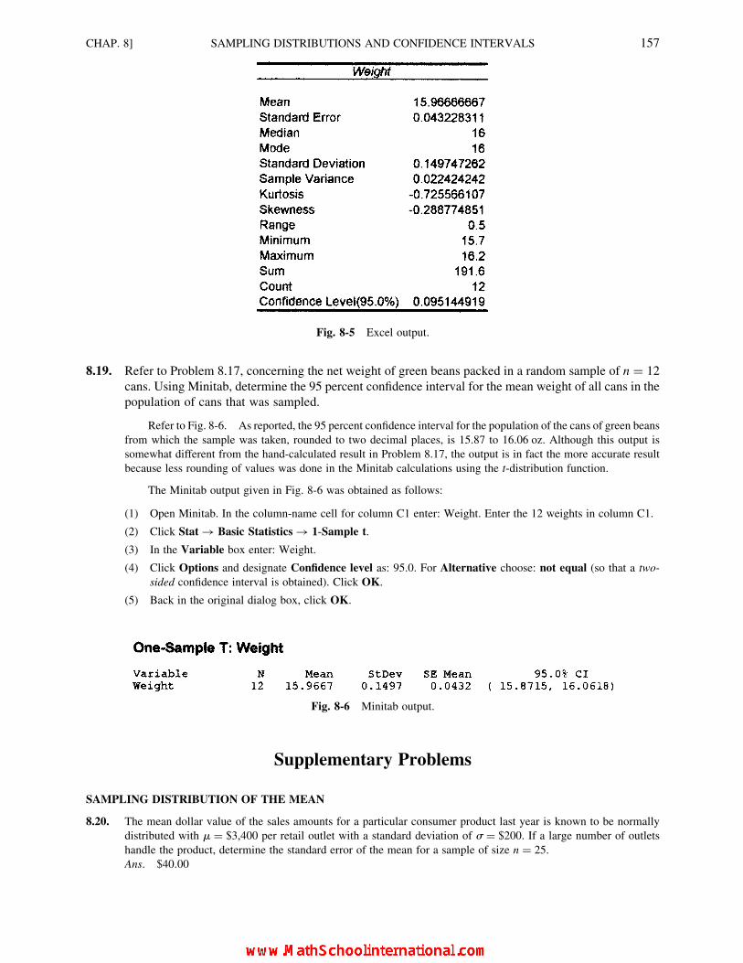
8.19. Refer to Problem 8.17, concerning the net weight of green beans packed in a random sample of n ¼ 12
cans. Using Minitab, determine the 95 percent confidence interval for the mean weight of all cans in the
population of cans that was sampled.
Refer to Fig. 8-6. As reported, the 95 percent confidence interval for the population of the cans of green beans
from which the sample was taken, rounded to two decimal places, is 15.87 to 16.06 oz. Although this output is
somewhat different from the hand-calculated result in Problem 8.17, the output is in fact the more accurate result
because less rounding of values was done in the Minitab calculations using the t-distribution function.
The Minitab output given in Fig. 8-6 was obtained as follows:
(1) Open Minitab. In the column-name cell for column C1 enter: Weight. Enter the 12 weights in column C1.
(2) Click Stat ! Basic Statistics ! 1-Sample t.
(3) In the Variable box enter: Weight.
(4) Click Options and designate Confidence level as: 95.0. For Alternative choose: not equal (so that a two-
sided confidence interval is obtained). Click OK.
(5) Back in the original dialog box, click OK.
Supplementary Problems
SAMPLING DISTRIBUTION OF THE MEAN
8.20. The mean dollar value of the sales amounts for a particular consumer product last year is known to be normally
distributed with m ¼ $3,400 per retail outlet with a standard deviation of s ¼ $200. If a large number of outlets
handle the product, determine the standard error of the mean for a sample of size n ¼ 25.
Ans. $40:00
Fig. 8-5 Excel output.
Fig. 8-6 Minitab output.
CHAP. 8] SAMPLING DISTRIBUTIONS AND CONFIDENCE INTERVALS 157

8.21. Refer to Problem 8.20. What is the probability that the sales amount for one randomly sampled retail outlet will be
(a) greater than $3;500? (b) Between $3;350 and $3;450?Ans. (a) 0.3085, (b) 0.1974
8.22. Refer to Problem 8.20. What is the probability that the sample mean for the sample of n ¼ 25 will be (a) greater than
$3;500? (b) Between $3;350 and $3;450? Compare your answers with the answers to Problem 8.21.
Ans. (a) 0.0062, (b) 0.7888
CONFIDENCE INTERVALS FOR THE MEAN
8.23. Suppose that you wish to estimate the mean sales amount per retail outlet for a particular consumer product during
the past year. The number of retail outlets is large. Determine the 95 percent confidence interval given that the sales
amounts are assumed to be normally distributed, �XX ¼ $3,425, s ¼ $200, and n ¼ 25.
Ans. $3;346:60 to $3;503:40
8.24. Referring to Problem 8.23, determine the 95 percent confidence interval given that the population is assumed to be
normally distributed, �XX ¼ $3,425, s ¼ $200, and n ¼ 25.
Ans. $3;342:44 to $3;507:56
8.25. For Problem 8.23, determine the 95 percent confidence interval given that the population is not assumed to be
normally distributed, �XX ¼ $3,425, s ¼ $200, and n ¼ 50.
Ans. $3;369:55 to $3;480:45
8.26. For a sample of 50 firms taken from a particular industry the mean number of employees per firm is 420.4 with a
sample standard deviation of 55.7. There is a total of just 380 firms in this industry. Determine the standard error of
the mean to be used in conjunction with estimating the population mean by a confidence interval.
Ans. 7.33
8.27. For Problem 8.26, determine the 90 percent confidence interval for estimating the average number of workers per
firm in the industry.
Ans. 408.3 to 432.5
8.28. For the situations described in Problems 8.26 and 8.27, determine the 90 percent confidence interval for estimating
the total number of workers employed in the industry.
Ans. 155,154 to 164,350
8.29. An analyst in a personnel department randomly selects the records of 16 hourly employees and finds that the mean
wage rate per hour is $9:50. The wage rates in the firm are assumed to be normally distributed. If the standard
deviation of the wage rates is known to be $1:00, estimate the mean wage rate in the firm using an 80 percent
confidence interval.
Ans. $9:18 to $9:82
8.30. Referring to Problem 8.29, suppose that the standard deviation of the population is not known, but that the standard
deviation of the sample is $1:00. Estimate the mean wage rate in the firm using an 80 percent confidence interval.
Ans. $9:16 to $9:84
8.31. The mean diameter of a sample of n ¼ 12 cylindrical rods included in a shipment is 2:350mm with a sample
standard deviation of 0:050mm. The distribution of the diameters of all of the rods included in the shipment is
assumed to be approximately normal. Determine the 99 percent confidence interval for estimating the mean
diameter of all of the rods included in the shipment.
Ans. 2.307 to 2:393mm
158 SAMPLING DISTRIBUTIONS AND CONFIDENCE INTERVALS [CHAP. 8

8.32. The mean diameter of a sample of n ¼ 100 rods included in a shipment is 2:350mm with a standard deviation of
0:050mm. Estimate the mean diameter of all rods included in the shipment if the shipment contains 500 rods, using
a 99 percent confidence interval.
Ans. 2.338 to 2:362mm
8.33. The mean weight per rod for the sample of 100 rods in Problem 8.32 is 8:45 g with a standard deviation of 0:25 g.
Estimate the total weight of the entire shipment (exclusive of packing materials), using a 99 percent confidence
interval.
Ans. 4,195 to 4,255 g
DETERMINING THE REQUIRED SAMPLE SIZE FOR ESTIMATING THE MEAN
8.34. From historical records, the standard deviation of the sales level per retail outlet for a consumer product is known to
be s ¼ $200, and the population of sales amounts per outlet is assumed to be normally distributed. What is the
minimum sample size required to estimate the mean sales per outlet within $100 and with 95 percent confidence?
Ans. 15:37 ffi 16
8.35. An analyst wishes to estimate the mean hourly wage of workers in a particular company within 25c/ and 90 percent
confidence. The standard deviation of the wage rates is estimated as being no larger than $1:00. What is the number
of personnel records that should be sampled, as a minimum, to satisfy this research objective?
Ans. 43:56 ffi 44
ONE-SIDED CONFIDENCE INTERVALS FOR THE POPULATION MEAN
8.36. Instead of the two-sided confidence interval constructed in Problem 8.23, suppose we wish to estimate the minimum
value of the mean level of sales per retail outlet for a particular product during the past year. As before, the
distribution of sales amounts per store is assumed to be approximately normal. Determine the minimum value of the
mean using a 95 percent confidence interval given that �XX ¼ $3,425, s ¼ $200, and n ¼ 25. Compare your
confidence interval with the one constructed in Problem 8.23.
Ans. Est. m � $3,359
8.37. Using the data in Problem 8.31, determine the 99 percent lower confidence interval for estimating the mean
diameter of all the rods included in the shipment. Compare the interval with the one constructed in Problem 8.31.
Ans. Est. m 2:388mm
COMPUTER OUTPUT
8.38. Refer to Table 2.19 (page 41) for the amounts of 40 personal loans. Assuming that these are random sample data,
use available computer software to determine the 99 percent confidence interval for the mean loan amount in the
population.
Ans. $822 to $1;372
CHAP. 8] SAMPLING DISTRIBUTIONS AND CONFIDENCE INTERVALS 159

CHAPTER 9
Other ConfidenceIntervals
9.1 CONFIDENCE INTERVALS FOR THE DIFFERENCE BETWEEN
TWO MEANS USING THE NORMAL DISTRIBUTION
There is often a need to estimate the difference between two population means, such as the difference
between the wage levels in two firms. As indicated in Section 8.1, the unbiased point estimate of (m1 � m2) is
( �XX1 � �XX2). The confidence interval is constructed in a manner similar to that used for estimating the mean,
except that the relevant standard error for the sampling distribution is the standard error of the difference
between means. Use of the normal distribution is based on the same conditions as for the sampling distribution
of the mean (see Section 8.4), except that two samples are involved. The formula used for estimating the
difference between two population means with confidence intervals is
( �XX1 � �XX2)+ zs �xx1��xx2 (9:1)
or ( �XX1 � �XX2)+ zs�xx1��xx2 (9:2)
When the standard deviations of the two populations are known, the standard error of the difference
between means is
s �xx1��xx2 ¼ffiffiffiffiffiffiffiffiffiffiffiffiffiffiffiffiffiffiffiffis 2
�xx1þ s 2
�xx2
q(9:3)
When the standard deviations of the populations are not known, the estimated standard error of the
difference between means given that use of the normal distribution is appropriate is
s�xx1��xx2 ¼ffiffiffiffiffiffiffiffiffiffiffiffiffiffiffiffiffis2�xx1 þ s2�xx2
q(9:4)
The values of the standard errors of the respective means included in these formulas are calculated by the
formulas given in Section 8.3, including the possibility of using finite correction factors when appropriate.
EXAMPLE 1. The mean weekly wage for a sample of n ¼ 30 employees in a large manufacturing firm is �XX ¼ $280.00
with a sample standard deviation of s ¼ $14:00. In another large firm a random sample of n ¼ 40 hourly employees has
160
Copyright 2004, 1996, 1988, 1976 by The McGraw-Hill Companies, Inc. Click Here for Terms of Use.

a mean weekly wage of $270.00 with a sample standard deviation of s ¼ $10:00. The 99 percent confidence interval for
estimating the difference between the mean weekly wage levels in the two firms is
99% Int: ¼ ( �XX1 � �XX2)+ zs�xx1��xx2
¼ $10:00+ 2:58(3:01)
¼ $10:00+ 7:77
¼ $2:23 to $17:77
where �XX1 � �XX2 ¼ $280:00� $270:00 ¼ $10:00
z ¼ 2:58
s�xx1 ¼s1ffiffiffiffiffin1
p ¼ 14:00ffiffiffiffiffi30
p ¼ 14:00
5:477¼ 2:56
s�xx2 ¼s2ffiffiffiffiffin2
p ¼ 10:00ffiffiffiffiffi40
p ¼ 10:00
6:325¼ 1:58
s�xx1��xx2 ¼ffiffiffiffiffiffiffiffiffiffiffiffiffiffiffiffiffis2�xx1 þ s2�xx2
q¼
ffiffiffiffiffiffiffiffiffiffiffiffiffiffiffiffiffiffiffiffiffiffiffiffiffiffiffiffiffiffiffiffiffi(2:56)2 þ (1:58)2
q¼ ffiffiffiffiffiffiffiffiffiffiffiffiffiffiffiffiffiffiffiffiffiffiffiffiffiffiffiffiffiffiffiffiffi
6:5536þ 2:4964p ffi 3:01
Thus, we can state that the average weekly wage in the first firm is greater than the average in the second firm by an
amount somewhere between $2:23 and $17:77, with 99 percent confidence in this interval estimate. Note that the sample
sizes are large enough to permit the use of Z to approximate the t value (see Sec. 9.2, which follows).
In addition to the two-sided confidence interval, a one-sided confidence interval for the difference between
means can also be constructed. (See Problems 9.4 and 9.5.)
9.2 THE t DISTRIBUTION AND CONFIDENCE INTERVALS FOR
THE DIFFERENCE BETWEEN TWO MEANS
As explained in Section 8.8, use of the t distribution in conjunction with one sample is necessary when
(1) Population standard deviations s are not known.
(2) Samples are small (n , 30). If samples are large, then t values can be approximated by the standard
normal z.
(3) Populations are assumed to be approximately normally distributed (note that the central limit theorem
cannot be invoked for small samples).
In addition to the above, when the t distribution is used to define confidence intervals for the difference
between two means, rather than for inference concerning only one population mean, an additional assumption
usually required is
(4) The two (unknown) population variances are equal, s 21 ¼ s 2
2.
Because of the above equality assumption, the first step in determining the standard error of the difference
between means when the t distribution is to be used typically is to pool the two sample variances:
ss 2 ¼ (n1 � 1)s21 þ (n2 � 1)s22n1 þ n2 � 2
(9:5)
The standard error of the difference between means based on using the pooled variance estimate ss 2 is
ss �xx1��xx2 ¼ffiffiffiffiffiffiffiffiffiffiffiffiffiffiffiffiffiffiss 2
n1
þ ss 2
n2
s(9:6)
CHAP. 9] OTHER CONFIDENCE INTERVALS 161

Where d f ¼ n1 þ n2 � 2, the confidence interval is
( �XX1 � �XX2)+ tdf ss �xx1��xx2 (9:7)
Note: Some computer software does not require that the two population variances be assumed to be
equal. Instead, a corrected value for the degrees of freedom is determined that results in reduced df, and
thus in a somewhat larger value of t and somewhat wider confidence interval.
EXAMPLE 2. For a random sample of n1 ¼ 10 bulbs, the mean bulb life is �XX1 ¼ 4:600 hr with s1 ¼ 250 hr. For another
brand of bulbs the mean bulb life and standard deviation for a sample of n2 ¼ 8 bulbs are �XX2 ¼ 4,000 hr and s2 ¼ 200 hr. The
bulb life for both brands is assumed to be normally distributed. The 90 percent confidence interval for estimating the
difference between the mean operating life of the two brands of bulbs is
90% Int: ¼ ( �XX1 � �XX2)+ t16ss �xx1��xx2
¼ 600+ 1:746(108:847) ¼ 600+ 190 ¼ 410 to 790 hr
where �XX1 � �XX2 ¼ 4,600� 4,000 ¼ 600
td f ¼ tn1þn2�2 ¼ t16 ¼ 1:746
ss 2 ¼ (n1 � 1)s21 þ (n2 � 1)s22n1 þ n2 � 2
¼ 9(250)2 þ 7(200)2
10þ 8� 2¼ 52,656:25
ss �xx1��xx2 ¼ffiffiffiffiffiffiffiffiffiffiffiffiffiffiffiffiffiffiss 2
n1þ ss 2
n2
s¼
ffiffiffiffiffiffiffiffiffiffiffiffiffiffiffiffiffiffiffiffiffiffiffiffiffiffiffiffiffiffiffiffiffiffiffiffiffiffiffiffiffiffiffiffiffi52,656:25
10þ 52,656:25
8
r¼ 108:847
Thus, we can state with 90 percent confidence that the first brand of bulbs has a mean life that is greater than that of the
second brand by an amount between 410 and 790 hr.
Note that in the two-sample case it is possible for each sample to be small (n , 30), and yet the normal
distribution could be used to approximate the t because df � 29. However, in such use the two populations
must be assumed to be approximately normally distributed, because the central limit theorem cannot be invoked
with respect to a small sample.
9.3 CONFIDENCE INTERVALS FOR THE POPULATION PROPORTION
As explained in Section 6.4, the probability distribution that is applicable to proportions is the binomial
probability distribution. However, the mathematics associated with determining a confidence interval for an
unknown population proportion on the basis of the Bernoulli process described in Section 6.3 are complex.
Therefore, all applications-oriented textbooks utilize the normal distribution as an approximation of the exact
solution for confidence intervals for proportions. As explained in Section 7.4, such approximation is appropriate
when n � 30 and both np � 5 and nq � 5 (where q ¼ 1� p). However, when the population proportion p (or
p) is not known, most statisticians suggest that a sample of n � 100 should be taken. Note that in the context of
statistical estimation p is not known, but is estimated by pp.
The variance of the distribution of proportions (see Section 6.4) serves as the basis for the standard error.
Given an observed sample proportion, pp, the estimated standard error of the proportion is
spp ¼ffiffiffiffiffiffiffiffiffiffiffiffiffiffiffiffiffipp(1� pp)
n
r(9:8)
In the context of statistical estimation, the population p (or p) would not be known because that is the valuebeing estimated. If the population is finite, then use of the finite correction factor is appropriate (see Section
8.3). As was the case for the standard error of the mean, use of this correction is generally not considered
necessary if n , 0:05N, that is, when the sample size is less than 5 percent of the population size.
The approximate confidence interval for a population proportion is
pp + zspp (9:9)
162 OTHER CONFIDENCE INTERVALS [CHAP. 9

In addition to the two-sided confidence interval, a one-sided confidence interval for the population
proportion can also be determined. (See Problem 9.11.)
EXAMPLE 3. Amarketing research firm contacts a random sample of 100men in a large community and finds that a sample
proportion of 0.40 prefer the razor blades manufactured by the client firm to all other brands. The 95 percent confidence interval
for the proportion of all men in the community who prefer the client firm’s razor blades is determined as follows:
spp ¼ffiffiffiffiffiffiffiffiffiffiffiffiffiffiffiffiffipp(1� pp)
n
r¼
ffiffiffiffiffiffiffiffiffiffiffiffiffiffiffiffiffiffiffiffiffiffiffiffi(0:40)(0:60)
100
r¼
ffiffiffiffiffiffiffiffiffi0:24
100
r¼
ffiffiffiffiffiffiffiffiffiffiffiffiffiffi0:0024
pffi 0:05
pp + zspp ¼ 0:40+ 1:96(0:05)
¼ 0:40+ 0:098 ffi 0:40+ 0:10 ¼ 0:30 to 0:50
Therefore, with 95 percent confidence we estimate the proportion of all men in the community who prefer the client firm’s
blades to be somewhere between 0.30 and 0.50.
9.4 DETERMINING THE REQUIRED SAMPLE SIZE FORESTIMATING THE PROPORTION
Before a sample is actually collected, the minimum required sample size can be determined by specifying
the level of confidence required, the sampling error that is acceptable, and by making an initial (subjective)
estimate of p, the unknown population proportion:
n ¼ z2p (1� p)
E 2(9:10)
In (9.10), z is the value used for the specified confidence interval, p is the initial estimate of the population
proportion, and E is the “plus and minus” sampling error allowed in the interval (always one-half the total
confidence interval).
If an initial estimate of p is not possible, then it should be estimated as being 0.50. Such an estimate is
conservative in that it is the value for which the largest sample size would be required. Under such an
assumption, the general formula for sample size is simplified as follows:
n ¼ z
2E
� �2
(9:11)
(Note: When solving for sample size, any fractional result is always rounded up. Further, any computed
sample size below 100 should be increased to 100 because Formulas (9.10) and (9.11) are based on use
of the normal distribution.)
EXAMPLE 4. For the study in Example 3, suppose that before data were collected it was specified that the 95 percent
interval estimate should be within+0:05 and no prior judgment was made about the likely value of p. The minimum sample
size which should be collected is
n ¼ z
2E
� �2
¼ 1:96
2(0:05)
� �2¼ 1:96
0:10
� �2
¼ (19:6)2 ¼ 384:16 ¼ 385
In addition to estimating the population proportion, the total number in a category of the population can also be
estimated. [See Problem 9.7(b).]
9.5 CONFIDENCE INTERVALS FOR THE DIFFERENCE BETWEEN
TWO PROPORTIONS
In order to estimate the difference between the proportions in two populations, the unbiased point estimate
of (p1 � p2) is (pp1 � pp2). See Section 8.1. The confidence interval involves use of the standard error of
CHAP. 9] OTHER CONFIDENCE INTERVALS 163
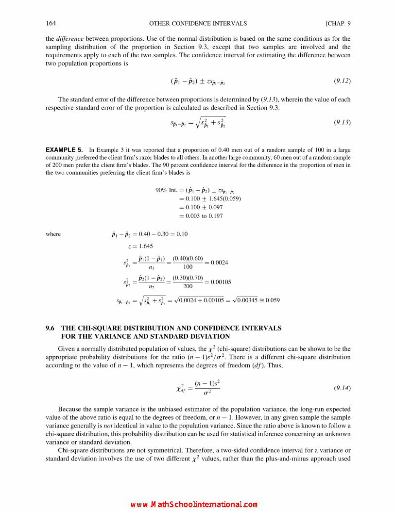
the difference between proportions. Use of the normal distribution is based on the same conditions as for the
sampling distribution of the proportion in Section 9.3, except that two samples are involved and the
requirements apply to each of the two samples. The confidence interval for estimating the difference between
two population proportions is
( pp1 � pp2)+ zspp1�pp2 (9:12)
The standard error of the difference between proportions is determined by (9.13), wherein the value of each
respective standard error of the proportion is calculated as described in Section 9.3:
spp1�pp2 ¼ffiffiffiffiffiffiffiffiffiffiffiffiffiffiffiffiffiffis2
pp1þ s2
pp2
q(9:13)
EXAMPLE 5. In Example 3 it was reported that a proportion of 0.40 men out of a random sample of 100 in a large
community preferred the client firm’s razor blades to all others. In another large community, 60 men out of a random sample
of 200 men prefer the client firm’s blades. The 90 percent confidence interval for the difference in the proportion of men in
the two communities preferring the client firm’s blades is
90% Int: ¼ ( pp1 � pp2)+ zspp1�pp2
¼ 0:100+ 1:645(0:059)
¼ 0:100+ 0:097
¼ 0:003 to 0:197
where �pp1 � �pp2 ¼ 0:40� 0:30 ¼ 0:10
z ¼ 1:645
s2pp1 ¼pp1(1� pp1)
n1¼ (0:40)(0:60)
100¼ 0:0024
s2pp2 ¼pp2(1� pp2)
n2¼ (0:30)(0:70)
200¼ 0:00105
spp1�pp2 ¼ffiffiffiffiffiffiffiffiffiffiffiffiffiffiffiffiffis2
pp1þ s2
pp2
q¼ ffiffiffiffiffiffiffiffiffiffiffiffiffiffiffiffiffiffiffiffiffiffiffiffiffiffiffiffiffiffiffiffiffiffiffi
0:0024þ 0:00105p ¼
ffiffiffiffiffiffiffiffiffiffiffiffiffiffiffiffi0:00345
pffi 0:059
9.6 THE CHI-SQUARE DISTRIBUTION AND CONFIDENCE INTERVALS
FOR THE VARIANCE AND STANDARD DEVIATION
Given a normally distributed population of values, the x 2 (chi-square) distributions can be shown to be the
appropriate probability distributions for the ratio (n � 1)s2=s 2. There is a different chi-square distribution
according to the value of n � 1, which represents the degrees of freedom (df ). Thus,
x 2df ¼
(n � 1)s2
s2(9:14)
Because the sample variance is the unbiased estimator of the population variance, the long-run expected
value of the above ratio is equal to the degrees of freedom, or n � 1. However, in any given sample the sample
variance generally is not identical in value to the population variance. Since the ratio above is known to follow a
chi-square distribution, this probability distribution can be used for statistical inference concerning an unknown
variance or standard deviation.
Chi-square distributions are not symmetrical. Therefore, a two-sided confidence interval for a variance or
standard deviation involves the use of two different x 2 values, rather than the plus-and-minus approach used
164 OTHER CONFIDENCE INTERVALS [CHAP. 9

with the confidence intervals based on the normal and t distributions. The formula for constructing a confidence
interval for the population variance is
(n � 1)s2
x2df ,upper
s 2 (n � 1)s2
x2df , lower
(9:15)
The confidence interval for the population standard deviation is
ffiffiffiffiffiffiffiffiffiffiffiffiffiffiffiffiffiffi(n � 1)s2
x2df ,upper
s s
ffiffiffiffiffiffiffiffiffiffiffiffiffiffiffiffiffiffi(n � 1)s2
x2df , lower
s(9:16)
Appendix 7 indicates the proportions of area under the chi-square distributions according to various
degrees of freedom, or df . In the general formula above, the subscripts upper and lower identify the percentile
points on the particular x 2 distribution to be used for constructing the confidence interval. For example, for a
90 percent confidence interval the upper point is x 20:95 and the lower point is x 2
0:05. By excluding the highest
5 percent and lowest 5 percent of the chi-square distribution, what remains is the “middle” 90 percent.
EXAMPLE 6. The mean weekly wage for a sample of 30 hourly employees in a large firm is �XX ¼ $280:00 with a
sample standard deviation of s ¼ $14:00. The weekly wage amounts in the firm are assumed to be approximately
normally distributed. The 95 percent confidence interval for estimating the standard deviation of weekly wages in the
population is
ffiffiffiffiffiffiffiffiffiffiffiffiffiffiffiffiffiffi(n � 1)s2
xdf , upper
s s
ffiffiffiffiffiffiffiffiffiffiffiffiffiffiffiffiffiffi(n � 1)s2
x 2df , lower
s
ffiffiffiffiffiffiffiffiffiffiffiffiffiffiffiffiffiffiffiffiffiffiffiffiffi(29)(196:00)
x 229,0:975
s s
ffiffiffiffiffiffiffiffiffiffiffiffiffiffiffiffiffiffiffiffiffiffiffiffiffi(29)(196:00)
x 229,0:025
s
ffiffiffiffiffiffiffiffiffiffiffiffiffiffiffiffiffi5,684:00
45:72
r s
ffiffiffiffiffiffiffiffiffiffiffiffiffiffiffiffiffi5,684:00
16:05
r
ffiffiffiffiffiffiffiffiffiffiffiffiffiffiffiffiffiffiffi124:3220
p s
ffiffiffiffiffiffiffiffiffiffiffiffiffiffiffiffiffiffiffi354:1433
p
11:15 s 18:82
In the above example, note that because the column headings in Appendix 7 are right-tail probabilities,
rather than percentile values, the column headings that are used in the table are the complementary values of the
required upper and lower percentile values.
As an alternative to a two-sided confidence interval, a one-sided confidence interval for the variance or
standard deviation can also be determined. (See Problem 9.14.)
9.7 USING EXCEL AND MINITAB
Computer software for statistical analysis generally includes the capability to determine a number of types
of confidence intervals, in addition to confidence intervals for the population mean. Solved Problems 9.15 and
9.16 illustrate the use of Excel and Minitab, respectively, to obtain confidence intervals for the difference
between two population means.
CHAP. 9] OTHER CONFIDENCE INTERVALS 165

Solved Problems
CONFIDENCE INTERVALS FOR THE DIFFERENCE BETWEEN
TWO MEANS USING THE NORMAL DISTRIBUTION
9.1. For the study reported in Problem 8.11, suppose that there were 9,000 customers who did not purchase
the “coupon special” but who did make other purchases in the store during the period of the study. For a
sample of 200 of these customers, the mean purchase amount was �XX ¼ $19:60 with a sample standard
deviation of s ¼ $8:40.
(a) Estimate the mean purchase amount for the noncoupon customers, using a 95 percent confidence
interval.
(b) Estimate the difference between the mean purchase amount of coupon and noncoupon customers,
using a 90 percent confidence interval.
(a) s�xx ¼ sffiffiffin
p ¼ 8:40ffiffiffiffiffiffiffiffi200
p ¼ 8:40
14:142
ffiffiffiffiffiffiffiffiffiffiffiffiffiffi0:7786
p¼ 0:59
�XX + zs�xx ¼ 19:60+ 1:96(0:59) ¼ $19:60+ 1:16 ¼ $18:44 to $20:76
(b) s�xx1��xx2 ¼ffiffiffiffiffiffiffiffiffiffiffiffiffiffiffiffiffiffis 2�xx1 þ s 2�xx2
q¼
ffiffiffiffiffiffiffiffiffiffiffiffiffiffiffiffiffiffiffiffiffiffiffiffiffiffiffiffiffiffiffiffiffiffi(0:66)2 þ (0:59)2
q¼ ffiffiffiffiffiffiffiffiffiffiffiffiffiffiffiffiffiffiffiffiffiffiffiffiffiffiffiffiffiffiffiffiffi
0:4356þ 0:3481p ¼ 0:885
( �XX1 � �XX2)+ zs�xx1��xx2 ¼ (24:57� 19:60)+ 1:645(0:885) ¼ $4:97+ 1:46 ¼ $3:51 to $6:43
Thus, we can state with 90 percent confidence that the mean level of sales for coupon customers exceeds that
for noncoupon customers by an amount somewhere between $3:51 and $6:43.
9.2. A random sample of 50 households in community A has a mean household income of �XX ¼ $44,600 witha standard deviation s ¼ $2,200. A random sample of 50 households in community B has a mean of�XX ¼ $43,800 with a standard deviation of s ¼ $2,800. Estimate the difference in the average household
income in the two communities using a 95 percent confidence interval.
s�xx1 ¼s1ffiffiffiffiffin1
p ¼ 2,200ffiffiffiffiffi50
p ¼ 2,200
7:07¼ $311:17
s�xx2 ¼s2ffiffiffiffiffin2
p ¼ 2,800ffiffiffiffiffi50
p ¼ 2,800
7:07¼ $396:04
s�xx1��xx2 ¼ffiffiffiffiffiffiffiffiffiffiffiffiffiffiffiffiffis2�xx1 þ s2�xx2
q¼
ffiffiffiffiffiffiffiffiffiffiffiffiffiffiffiffiffiffiffiffiffiffiffiffiffiffiffiffiffiffiffiffiffiffiffiffiffiffiffiffiffiffiffi(311:17)2 þ (396:04)2
q¼
ffiffiffiffiffiffiffiffiffiffiffiffiffiffiffiffiffiffiffiffiffiffiffiffiffiffiffiffiffiffiffiffiffiffiffiffiffiffiffiffiffiffiffiffiffiffiffi96,826:77þ 156,847:68
q¼ $503:66
( �XX1 � �XX2)+ zs�xx1��xx2 ¼ (44,600� 43,800)+ 1:96(503:66)
¼ 800+ 987:17 ¼ �$187:17 to $1,787:17
With a 95 percent level of confidence, the limits of the confidence interval indicate that the mean in the first
community might be less than the mean in the second community by $187:17, while at the other limit the mean of
the first community might exceed that in the second by as much as $1,787:17. Note that the possibility that there is
no actual difference between the two population means is included within this 95 percent confidence interval.
USE OF THE t DISTRIBUTION
9.3. In one canning plant the average net weight of string beans being packed in No. 303 cans for a sample of
n ¼ 12 cans is �XX1 ¼ 15:97 oz, with s1 ¼ 0:15 oz. At another canning plant the average net weight of
string beans being packed in No. 303 cans for a sample of n2 ¼ 15 cans is �XX2 ¼ 16:14 oz with a standarddeviation of s2 ¼ 0:09 oz. The distributions of the amounts packed are assumed to be approximately
166 OTHER CONFIDENCE INTERVALS [CHAP. 9

normal. Estimate the difference between the average net weight of beans being packed in No. 303 cans
at the two plants, using a 90 percent confidence interval.
ss 2 ¼ (n1 � 1)s21 þ (n2 � 1)s22n1 þ n2 � 2
¼ 11(0:15)2 þ 14(0:09)2
12þ 15� 2¼ 0:014436
ss �xx1��xx2 ¼ffiffiffiffiffiffiffiffiffiffiffiffiffiffiffiffiffiss 2
n1þ ss 2
n2
s¼
ffiffiffiffiffiffiffiffiffiffiffiffiffiffiffiffiffiffiffiffiffiffiffiffiffiffiffiffiffiffiffiffiffiffiffiffiffiffiffiffiffiffiffi0:014436
12þ 0:014436
15
s¼ 0:047
(�xx1 � �xx2)+ tdf ss �xx1��xx2 ¼ (15:97� 16:14)+ t25(0:047)
¼ (�0:17)+ 1:708(0:047) ¼ (�0:17)+ 0:08 ¼ �0:25 to �0:09
In other words, with 90 percent confidence we can state the average net weight being packed at the second
plant is somewhere between 0.09 and 0:25 oz more than at the first plant.
ONE-SIDED CONFIDENCE INTERVALS FOR THE DIFFERENCE
BETWEEN TWO MEANS
9.4. Just as for the mean, as explained in Problem 8.14, a difference between means can be estimated by the
use of a one-sided confidence interval. Referring to the data in Problem 9.1(b), estimate the minimum
difference between the mean purchase amounts of “coupon” and “noncoupon” customers by
constructing a 90 percent upper confidence interval.
Since, from Problem 9.1(b), �XX1 � �XX2 ¼ $4:97 and s�xx1��xx2 ¼ 0:772,
Est: (m1 � m2) � ( �XX1 � �XX2)� zs �xx1��xx2
� $4:97� (1:28)(0:772)� $3:98
9.5. For the income data reported in Problem 9.2, estimate the maximum difference between the mean
income levels in the first and second community by constructing a 95 percent lower confidence interval.
Since, from Problem 9.2, �XX1 � �XX2 ¼ $800 and s�xx1��xx2 ¼ $503:66,
Est: (m1 � m2) ( �XX1 � �XX2)þ zs �xx1��xx2
$800þ 1:645(503:66)
$1,628:52
CONFIDENCE INTERVALS FOR ESTIMATING THE POPULATION PROPORTION
9.6. A college administrator collects data on a nationwide random sample of 230 students enrolled in M.B.A.
programs and finds that 54 of these students have undergraduate degrees in business. Estimate the
proportion of such students in the nationwide population who have undergraduate degrees in business,
using a 90 percent confidence interval.
pp ¼ 54
230¼ 0:235
spp ¼ffiffiffiffiffiffiffiffiffiffiffiffiffiffiffiffiffipp(1� pp)
n
r¼
ffiffiffiffiffiffiffiffiffiffiffiffiffiffiffiffiffiffiffiffiffiffiffiffiffiffiffiffiffi(0:235)(0:765)
230
r¼
ffiffiffiffiffiffiffiffiffiffiffiffiffiffiffiffiffiffiffi0:179775
230
r¼
ffiffiffiffiffiffiffiffiffiffiffiffiffiffiffiffiffiffiffiffiffi0:0007816
p¼ 0:028
pp + zspp ¼ 0:235+ 1:645(0:028)
¼ 0:235+ 0:046 ffi 0:19 to 0:28
9.7. In a large metropolitan area in which a total of 800 gasoline service stations are located, for a random
sample of n ¼ 36 stations, 20 of them carry a particular nationally advertised brand of oil. Using a
CHAP. 9] OTHER CONFIDENCE INTERVALS 167

95 percent confidence interval estimate (a) the proportion of all stations in the area that carry the oil and
(b) the total number of service stations in the area that carry the oil.
(a) pp ¼ 20
36¼ 0:5555 ffi 0:56
spp ¼ffiffiffiffiffiffiffiffiffiffiffiffiffiffiffiffiffipp(1� pp)
n
r¼
ffiffiffiffiffiffiffiffiffiffiffiffiffiffiffiffiffiffiffiffiffiffiffiffi(0:56)(0:44)
36
r¼
ffiffiffiffiffiffiffiffiffiffiffiffiffiffi0:2464
36
r¼
ffiffiffiffiffiffiffiffiffiffiffiffiffiffiffiffiffiffiffi0:006844
p¼ 0:083
pp + zspp ¼ 0:56+ 1:96(0:083) ¼ 0:40 to 0:72
(b) [Note: As was the case in the solution to Problem 8.11(b) for the mean and the total quantity, the
total number in a category of the population is determined by multiplying the confidence limits
for the proportion by the total number of all elements in the population.]
N( pp + zspp) ¼ 800(0:40 to 0:72) ¼ 320 to 576 stations
N( pp)+ N(zspp) ¼ 800(0:56)+ 800(0:16) ¼ 320 to 576 stations(or)
DETERMINING THE REQUIRED SAMPLE SIZE FOR ESTIMATING THE PROPORTION
9.8. A university administrator wishes to estimate within +0:05 and with 90 percent confidence the
proportion of students enrolled in M.B.A. programs who also have undergraduate degrees in business.
What sample size should be collected, as a minimum, if there is no basis for estimating the approximate
value of the proportion before the sample is taken?
Using formula (9.11),
n ¼ z
2E
� �2
¼ 1:645
2(0:05)
� �2
¼ (16:45)2 ¼ 270:60 ffi 271
9.9. With respect to Problem 9.8, what is the minimum sample size required if prior data and information
indicate that the proportion will be no larger than 0.30?
From formula (9.10),
n ¼ z2p (1� p)
E 2¼ (1:645)
2(0:30)(0:70)
(0:05)2¼ 227:31 ffi 228
CONFIDENCE INTERVALS FOR THE DIFFERENCE BETWEEN TWO PROPORTIONS
9.10. In attempting to gauge voter sentiment regarding a school-bond proposal, a superintendent of schools
collects random samples of n ¼ 100 in each of the two major residential areas included within the
school district. In the first area 70 of the 100 sampled voters indicate that they intend to vote for
the proposal, while in the second area 50 of 100 sampled voters indicate this intention. Estimate the
difference between the actual proportions of voters in the two areas who intend to vote for the proposal,
using 95 percent confidence limits.
s 2pp1 ¼pp1(1� pp1)
n1
¼ (0:70)(0:30)100
¼ 0:21
100¼ 0:0021
s 2pp2 ¼pp2(1� pp2)
n2¼ (0:50)(0:50)
100¼ 0:25
100¼ 0:0025
Therefore,
spp1�pp2 ¼ffiffiffiffiffiffiffiffiffiffiffiffiffiffiffiffiffiffis 2
pp1þ s 2
pp2
q¼
ffiffiffiffiffiffiffiffiffiffiffiffiffiffiffiffiffiffiffiffiffiffiffiffiffiffiffiffiffiffiffiffiffi0:0021þ 0:0025
q¼
ffiffiffiffiffiffiffiffiffiffiffiffiffiffi0:0046
q¼ 0:068
( pp1 � pp2)+ zspp1�pp2 ¼ (0:70� 0:50)+ 1:96(0:068) ¼ 0:20+ 0:13 ¼ 0:07 to 0:33
Thus, the difference in the population proportions is somewhere between 0.07 and 0.33 (or 7 to 33 percent).
168 OTHER CONFIDENCE INTERVALS [CHAP. 9
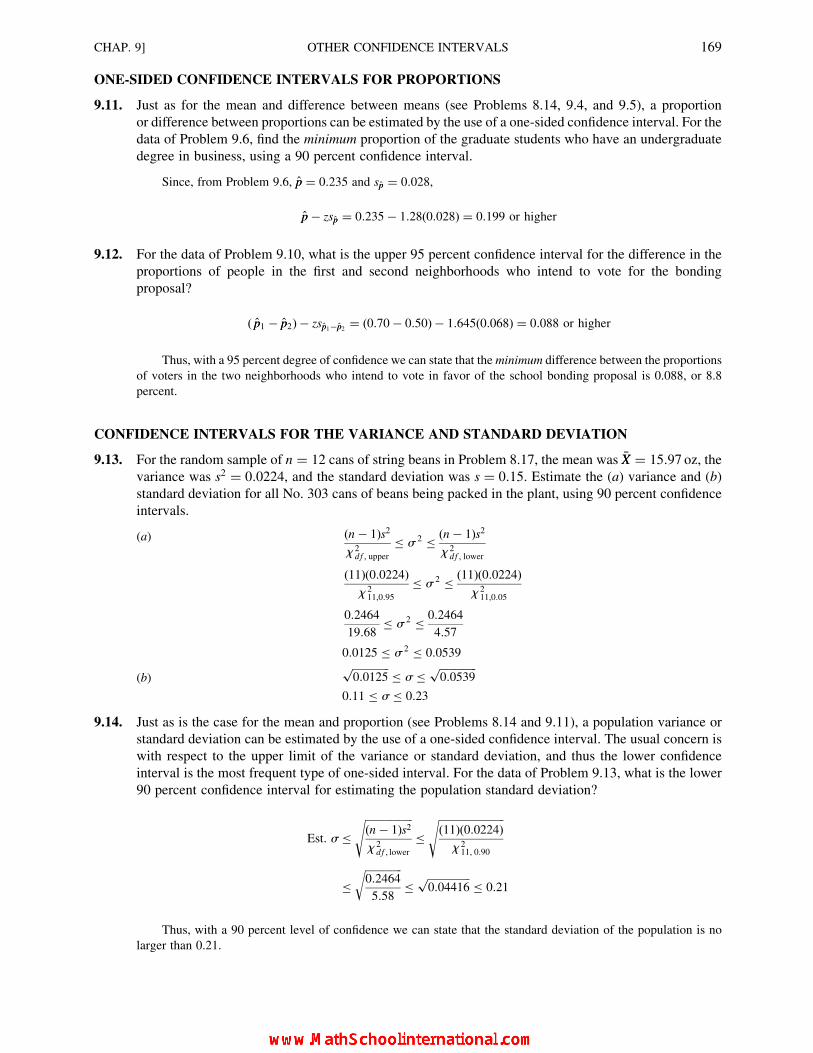
ONE-SIDED CONFIDENCE INTERVALS FOR PROPORTIONS
9.11. Just as for the mean and difference between means (see Problems 8.14, 9.4, and 9.5), a proportion
or difference between proportions can be estimated by the use of a one-sided confidence interval. For the
data of Problem 9.6, find the minimum proportion of the graduate students who have an undergraduate
degree in business, using a 90 percent confidence interval.
Since, from Problem 9.6, pp ¼ 0:235 and spp ¼ 0:028,
pp � zspp ¼ 0:235� 1:28(0:028) ¼ 0:199 or higher
9.12. For the data of Problem 9.10, what is the upper 95 percent confidence interval for the difference in the
proportions of people in the first and second neighborhoods who intend to vote for the bonding
proposal?
( pp1 � pp2)� zspp1�pp2 ¼ (0:70� 0:50)� 1:645(0:068) ¼ 0:088 or higher
Thus, with a 95 percent degree of confidence we can state that the minimum difference between the proportions
of voters in the two neighborhoods who intend to vote in favor of the school bonding proposal is 0.088, or 8.8
percent.
CONFIDENCE INTERVALS FOR THE VARIANCE AND STANDARD DEVIATION
9.13. For the random sample of n ¼ 12 cans of string beans in Problem 8.17, the mean was �XX ¼ 15:97 oz, thevariance was s2 ¼ 0:0224, and the standard deviation was s ¼ 0:15. Estimate the (a) variance and (b)
standard deviation for all No. 303 cans of beans being packed in the plant, using 90 percent confidence
intervals.
(a) (n � 1)s2
x 2df , upper
s 2 (n � 1)s2
x 2df , lower
(11)(0:0224)
x 211,0:95
s 2 (11)(0:0224)x 2
11,0:05
0:2464
19:68 s 2 0:2464
4:57
0:0125 s 2 0:0539
(b)ffiffiffiffiffiffiffiffiffiffiffiffiffiffi0:0125
p s
ffiffiffiffiffiffiffiffiffiffiffiffiffiffi0:0539
p
0:11 s 0:23
9.14. Just as is the case for the mean and proportion (see Problems 8.14 and 9.11), a population variance or
standard deviation can be estimated by the use of a one-sided confidence interval. The usual concern is
with respect to the upper limit of the variance or standard deviation, and thus the lower confidence
interval is the most frequent type of one-sided interval. For the data of Problem 9.13, what is the lower
90 percent confidence interval for estimating the population standard deviation?
Est: s ffiffiffiffiffiffiffiffiffiffiffiffiffiffiffiffiffiffi(n � 1)s2
x 2df , lower
s
ffiffiffiffiffiffiffiffiffiffiffiffiffiffiffiffiffiffiffiffiffiffiffiffiffi(11)(0:0224)
x 211, 0:90
s
ffiffiffiffiffiffiffiffiffiffiffiffiffiffi0:2464
5:58
r
ffiffiffiffiffiffiffiffiffiffiffiffiffiffiffiffi0:04416
p 0:21
Thus, with a 90 percent level of confidence we can state that the standard deviation of the population is no
larger than 0.21.
CHAP. 9] OTHER CONFIDENCE INTERVALS 169
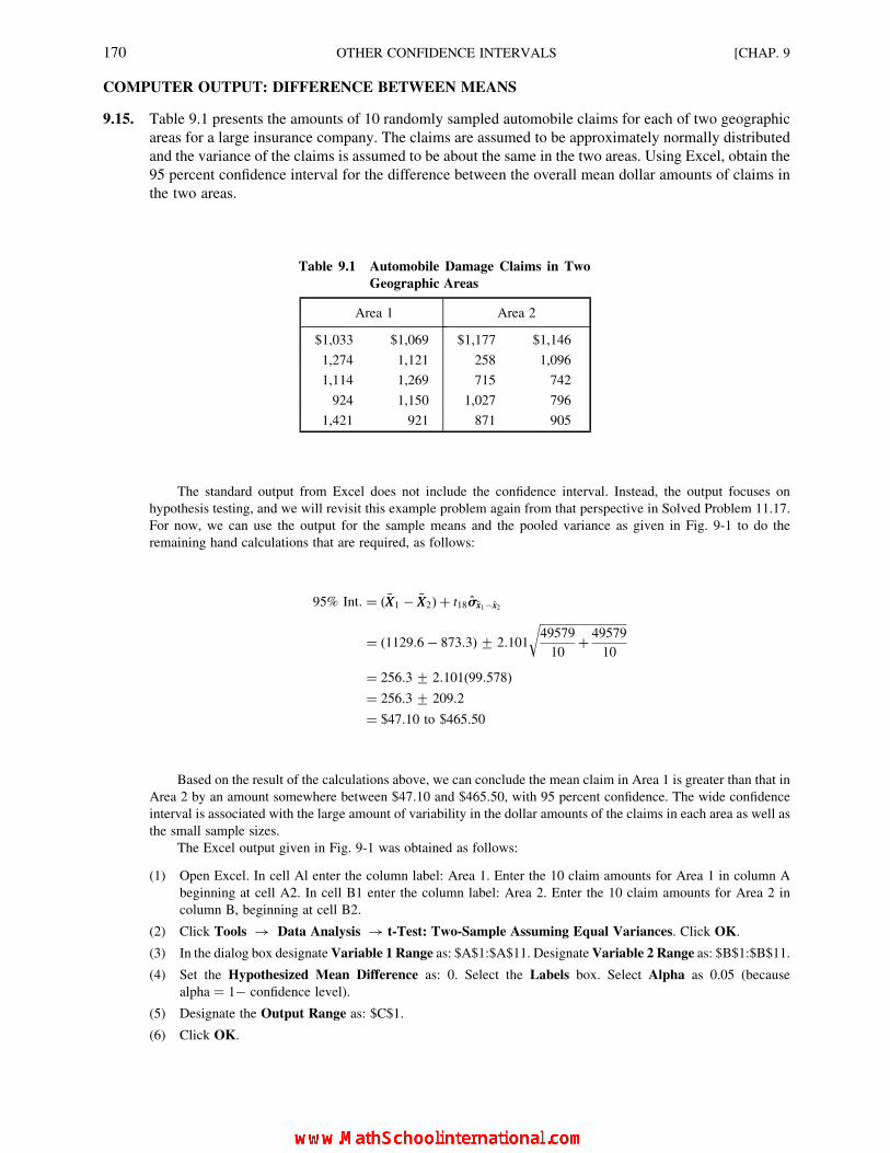
COMPUTER OUTPUT: DIFFERENCE BETWEEN MEANS
9.15. Table 9.1 presents the amounts of 10 randomly sampled automobile claims for each of two geographic
areas for a large insurance company. The claims are assumed to be approximately normally distributed
and the variance of the claims is assumed to be about the same in the two areas. Using Excel, obtain the
95 percent confidence interval for the difference between the overall mean dollar amounts of claims in
the two areas.
The standard output from Excel does not include the confidence interval. Instead, the output focuses on
hypothesis testing, and we will revisit this example problem again from that perspective in Solved Problem 11.17.
For now, we can use the output for the sample means and the pooled variance as given in Fig. 9-1 to do the
remaining hand calculations that are required, as follows:
95% Int: ¼ ( �XX1 � �XX2)þ t18ss�xx1��xx2
¼ (1129:6� 873:3)+ 2:101
ffiffiffiffiffiffiffiffiffiffiffiffiffiffiffiffiffiffiffiffiffiffiffiffiffiffiffiffiffiffi49579
10þ 49579
10
r
¼ 256:3+ 2:101(99:578)
¼ 256:3+ 209:2
¼ $47:10 to $465:50
Based on the result of the calculations above, we can conclude the mean claim in Area 1 is greater than that in
Area 2 by an amount somewhere between $47:10 and $465:50, with 95 percent confidence. The wide confidence
interval is associated with the large amount of variability in the dollar amounts of the claims in each area as well as
the small sample sizes.
The Excel output given in Fig. 9-1 was obtained as follows:
(1) Open Excel. In cell Al enter the column label: Area 1. Enter the 10 claim amounts for Area 1 in column A
beginning at cell A2. In cell B1 enter the column label: Area 2. Enter the 10 claim amounts for Area 2 in
column B, beginning at cell B2.
(2) Click Tools ! Data Analysis ! t-Test: Two-Sample Assuming Equal Variances. Click OK.
(3) In the dialog box designate Variable 1 Range as: $A$1:$A$11. Designate Variable 2 Range as: $B$1:$B$11.
(4) Set the Hypothesized Mean Difference as: 0. Select the Labels box. Select Alpha as 0.05 (because
alpha ¼ 1� confidence level).
(5) Designate the Output Range as: $C$1.
(6) Click OK.
Table 9.1 Automobile Damage Claims in Two
Geographic Areas
Area 1 Area 2
$1,033 $1,069 $1,177 $1,146
1,274 1,121 258 1,096
1,114 1,269 715 742
924 1,150 1,027 796
1,421 921 871 905
170 OTHER CONFIDENCE INTERVALS [CHAP. 9
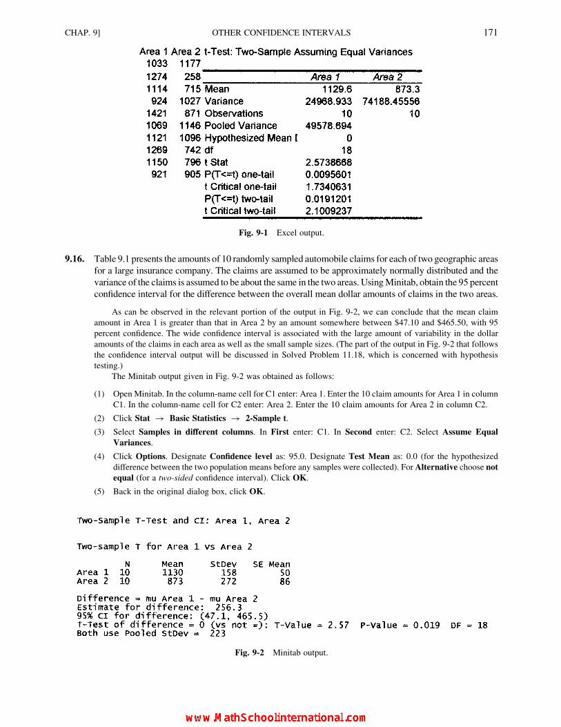
9.16. Table 9.1 presents the amounts of 10 randomly sampled automobile claims for each of two geographic areas
for a large insurance company. The claims are assumed to be approximately normally distributed and the
variance of the claims is assumed to be about the same in the two areas. UsingMinitab, obtain the 95 percent
confidence interval for the difference between the overall mean dollar amounts of claims in the two areas.
As can be observed in the relevant portion of the output in Fig. 9-2, we can conclude that the mean claim
amount in Area 1 is greater than that in Area 2 by an amount somewhere between $47.10 and $465.50, with 95
percent confidence. The wide confidence interval is associated with the large amount of variability in the dollar
amounts of the claims in each area as well as the small sample sizes. (The part of the output in Fig. 9-2 that follows
the confidence interval output will be discussed in Solved Problem 11.18, which is concerned with hypothesis
testing.)
The Minitab output given in Fig. 9-2 was obtained as follows:
(1) Open Minitab. In the column-name cell for C1 enter: Area 1. Enter the 10 claim amounts for Area 1 in column
C1. In the column-name cell for C2 enter: Area 2. Enter the 10 claim amounts for Area 2 in column C2.
(2) Click Stat ! Basic Statistics ! 2-Sample t.
(3) Select Samples in different columns. In First enter: C1. In Second enter: C2. Select Assume Equal
Variances.
(4) Click Options. Designate Confidence level as: 95.0. Designate Test Mean as: 0.0 (for the hypothesized
difference between the two population means before any samples were collected). For Alternative choose not
equal (for a two-sided confidence interval). Click OK.
(5) Back in the original dialog box, click OK.
Fig. 9-1 Excel output.
Fig. 9-2 Minitab output.
CHAP. 9] OTHER CONFIDENCE INTERVALS 171
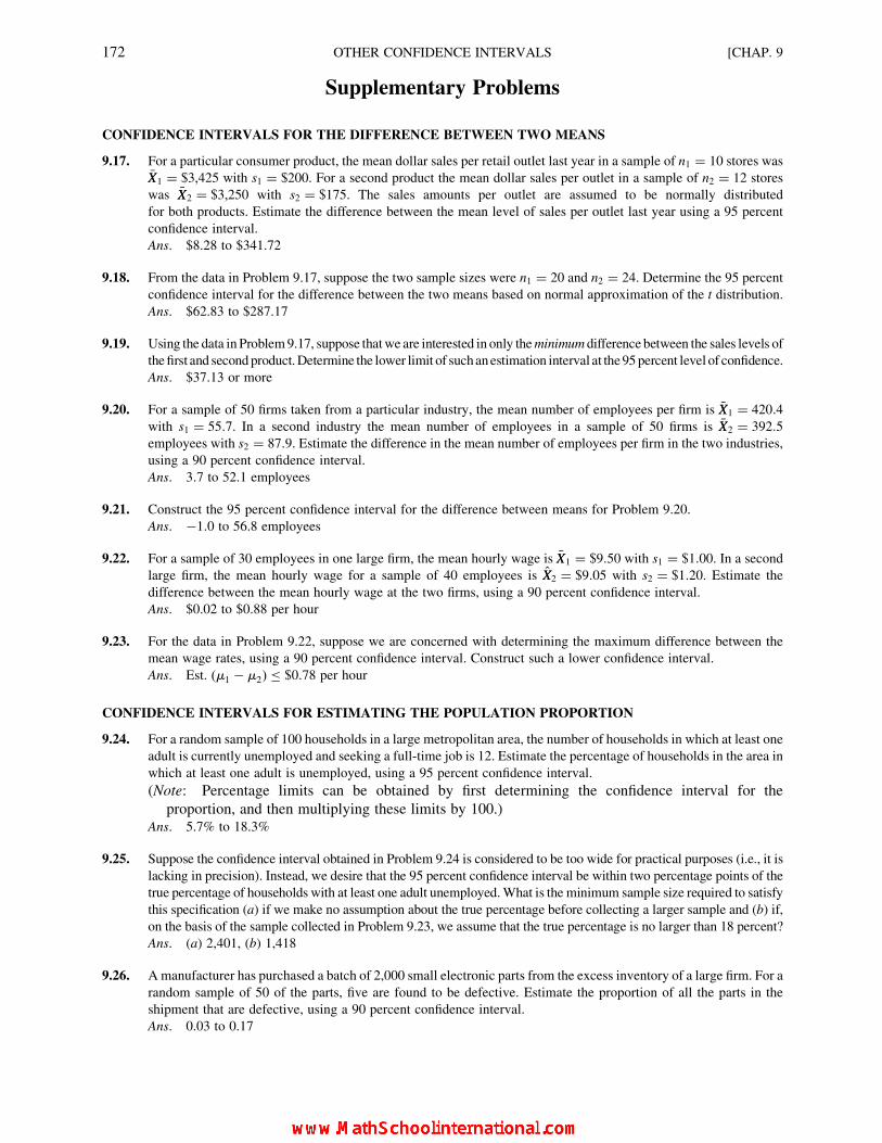
Supplementary Problems
CONFIDENCE INTERVALS FOR THE DIFFERENCE BETWEEN TWO MEANS
9.17. For a particular consumer product, the mean dollar sales per retail outlet last year in a sample of n1 ¼ 10 stores was�XX1 ¼ $3,425 with s1 ¼ $200. For a second product the mean dollar sales per outlet in a sample of n2 ¼ 12 stores
was �XX2 ¼ $3,250 with s2 ¼ $175. The sales amounts per outlet are assumed to be normally distributed
for both products. Estimate the difference between the mean level of sales per outlet last year using a 95 percent
confidence interval.
Ans. $8.28 to $341.72
9.18. From the data in Problem 9.17, suppose the two sample sizes were n1 ¼ 20 and n2 ¼ 24. Determine the 95 percent
confidence interval for the difference between the two means based on normal approximation of the t distribution.
Ans. $62.83 to $287.17
9.19. Using the data in Problem9.17, suppose thatwe are interested in only theminimum difference between the sales levels of
thefirst and secondproduct.Determine the lower limit of suchanestimation interval at the95percent level of confidence.
Ans. $37.13 or more
9.20. For a sample of 50 firms taken from a particular industry, the mean number of employees per firm is �XX1 ¼ 420:4with s1 ¼ 55:7. In a second industry the mean number of employees in a sample of 50 firms is �XX2 ¼ 392:5employees with s2 ¼ 87:9. Estimate the difference in the mean number of employees per firm in the two industries,
using a 90 percent confidence interval.
Ans. 3:7 to 52.1 employees
9.21. Construct the 95 percent confidence interval for the difference between means for Problem 9.20.
Ans. �1:0 to 56.8 employees
9.22. For a sample of 30 employees in one large firm, the mean hourly wage is �XX1 ¼ $9:50 with s1 ¼ $1:00. In a second
large firm, the mean hourly wage for a sample of 40 employees is XX2 ¼ $9:05 with s2 ¼ $1:20. Estimate the
difference between the mean hourly wage at the two firms, using a 90 percent confidence interval.
Ans. $0.02 to $0.88 per hour
9.23. For the data in Problem 9.22, suppose we are concerned with determining the maximum difference between the
mean wage rates, using a 90 percent confidence interval. Construct such a lower confidence interval.
Ans. Est. (m1 � m2) $0:78 per hour
CONFIDENCE INTERVALS FOR ESTIMATING THE POPULATION PROPORTION
9.24. For a random sample of 100 households in a large metropolitan area, the number of households in which at least one
adult is currently unemployed and seeking a full-time job is 12. Estimate the percentage of households in the area in
which at least one adult is unemployed, using a 95 percent confidence interval.
(Note: Percentage limits can be obtained by first determining the confidence interval for the
proportion, and then multiplying these limits by 100.)Ans. 5.7% to 18.3%
9.25. Suppose the confidence interval obtained in Problem 9.24 is considered to be too wide for practical purposes (i.e., it is
lacking in precision). Instead, we desire that the 95 percent confidence interval be within two percentage points of the
true percentage of households with at least one adult unemployed.What is the minimum sample size required to satisfy
this specification (a) if we make no assumption about the true percentage before collecting a larger sample and (b) if,
on the basis of the sample collected in Problem 9.23, we assume that the true percentage is no larger than 18 percent?
Ans. (a) 2,401, (b) 1,418
9.26. Amanufacturer has purchased a batch of 2,000 small electronic parts from the excess inventory of a large firm. For a
random sample of 50 of the parts, five are found to be defective. Estimate the proportion of all the parts in the
shipment that are defective, using a 90 percent confidence interval.
Ans. 0.03 to 0.17
172 OTHER CONFIDENCE INTERVALS [CHAP. 9

9.27. For Problem 9.26, estimate the total number of the 2,000 parts in the shipment that are defective, using a 90 percent
confidence interval.
Ans. 60 to 340
9.28. For the situation in Problem 9.26, suppose the price of the electronics parts was such that the purchaser would be
satisfied with the purchase as long as the true proportion of defective parts does not exceed 0.20. Construct a one-
sided 95 percent confidence interval and observe whether the upper limit of this interval exceeds the proportion 0.20.
Ans. Est. p 0:17
CONFIDENCE INTERVALS FOR THE DIFFERENCE BETWEEN TWO PROPORTIONS
9.29. In contrast to the data in Problem 9.24, in a second metropolitan area a random sample of 100 households yields only
six households in which at least one adult is unemployed and seeking a full-time job. Estimate the difference in the
percentage of households in the two areas that include an unemployed adult, using a 90 percent confidence interval.
Ans. �0:6% to þ12:6%
9.30. Referring to Problem 9.29, what is the maximum percentage by which the household unemployment in the first
metropolitan area exceeds the percentage unemployment in the second area, using a 90 percent one-sided
confidence interval?
Ans. Est. Dif. 11:1%
CONFIDENCE INTERVALS FOR THE VARIANCE AND STANDARD DEVIATION
9.31. For a particular consumer product, the mean dollar sales per retail outlet last year in a sample of n ¼ 10 stores was�XX ¼ $3,425 with s ¼ $200. The sales amounts per outlet are assumed to be normally distributed. Estimate the (a)
variance and (b) standard deviation of dollar sales of this product in all stores last year, using a 90 percent
confidence interval.
Ans. (a) 21:278 s 2 108,271, (b) 145.9 s 329:0
9.32. With reference to Problem 9.31, there is particular concern about how large the standard deviation of dollar sales
might be. Construct the 90 percent one-sided confidence interval that identifies this value.
Ans. s 293:9
COMPUTER OUTPUT
9.33. A business firm that processes many of its orders by telephone has two types of customers: general and commercial.
Table 9.2 reports the required per item telephone order times for a random sample of 12 general-customer calls and
10 commercial-customer calls. The amounts of time required for each type of call are assumed to be approximately
normally distributed. Using available computer software, obtain the 95 percent confidence interval for the
difference in the mean amount of per item time required for each type of call.
Ans. �23 to 52 sec
Table 9.2 Time (in Seconds) Required per Item Order
General customers Commercial customers
48 81
66 137
106 107
84 110
146 107
139 40
154 154
150 142
177 34
156 165
122
121
CHAP. 9] OTHER CONFIDENCE INTERVALS 173

CHAPTER 10
Testing HypothesesConcerning theValue of thePopulation Mean
10.1 INTRODUCTON
The purpose of hypothesis testing is to determine whether a claimed (hypothesized) value for a population
parameter, such as a population mean, should be accepted as being plausible based on sample evidence. Recall
from Section 8.2 on sampling distributions that a sample mean generally will differ in value from the population
mean. If the observed value of a sample statistic, such as the sample mean, is close to the claimed parameter
value and differs only by an amount that would be expected because of random sampling, then the hypothesized
value is not rejected. If the sample statistic differs from the claim by an amount that cannot be ascribed to
chance, then the hypothesis is rejected as not being plausible.
Three different procedures have been developed for testing hypotheses, with all of them leading to the same
decision when the same probability (and risk) standards are used. In this chapter we first describe the critical
value approach to hypothesis testing. By this approach, the so-called critical values of the test statistic that
would dictate rejection of a hypothesis are determined, and then the observed test statistic is compared to the
critical values. This is the first approach that was developed, and thus much of the language of hypothesis
testing stems from it. More recently, the P-value approach has become popular because it is the one most easily
applied with computer software. This approach is based on determining the conditional probability that
the observed value of a sample statistic could occur by chance, given that a particular claim for the value of the
associated population parameter is in fact true. The P-value approach is described in Section 10.7. Finally, the
confidence interval approach is based on observing whether the claimed value of a population parameter is
included within the range of values that define a confidence interval for that parameter. This approach to
hypothesis testing is described in Section 10.8.
174
Copyright 2004, 1996, 1988, 1976 by The McGraw-Hill Companies, Inc. Click Here for Terms of Use.

No matter which approach to hypothesis testing is used, note that if a hypothesized value is not rejected,
and therefore is accepted, this does not constitute a “proof ” that the hypothesized value is correct. Acceptance
of a claimed value for the parameter simply indicates that it is a plausible value, based on the observed value of
the sample statistic.
10.2 BASIC STEPS IN HYPOTHESIS TESTING BY THE CRITICAL VALUE APPROACH
Step 1. Formulate the null hypothesis and the alternative hypothesis. The null hypothesis (H0) is the
hypothesized parameter value which is compared with the sample result. It is rejected only if the sample result
is unlikely to have occurred given the correctness of the hypothesis. Thealternative hypothesis (H1) is accepted
only if the null hypothesis is rejected. The alternative hypothesis is also designated by Ha in many texts.
EXAMPLE 1. An auditor wishes to test the assumption that the mean value of all accounts receivable in a given firm is
$260.00 by taking a sample of n ¼ 36 and computing the sample mean. The auditor wishes to reject the assumed value of
$260.00 only if it is clearly contradicted by the sample mean, and thus the hypothesized value should be given the benefit of
the doubt in the testing procedure. The null and alternative hypotheses for this test are H0: m ¼ $260:00 and
H1: m = $260:00.
Step 2. Specify the level of significance to be used. The level of significance is the statistical standard
which is specified for rejecting the null hypothesis. If a 5 percent level of significance is specified, then the
null hypothesis is rejected only if the sample result is so different from the hypothesized value that a
difference of that amount or larger would occur by chance with a probability of 0.05 or less.
Note that if the 5 percent level of significance is used, there is a probability of 0.05 of rejecting the null
hypothesis when it is in fact true. This is called Type I error. The probability of Type I error is always equal to
the level of significance that is used as the standard for rejecting the null hypothesis; it is designated by the
lowercase Greek a (alpha), and thus a also designates the level of significance. The most frequently used levels
of significance in hypothesis testing are the 5 percent and 1 percent levels.
A Type II error occurs if the null hypothesis is not rejected, and therefore accepted, when it is in fact false.
Determining the probability of Type II error is explained in Section 10.4. Table 10.1 summarizes the types of
decisions and the possible consequences of the decisions which are made in hypothesis testing.
Step 3. Select the test statistic. The test statistic will either be the sample statistic (the unbiased estimator
of the parameter being tested), or a standardized version of the sample statistic. For example, in order to test
a hypothesized value of the population mean, the mean of a random sample taken from that population could
serve as the test statistic. However, if the sampling distribution of the mean is normally distributed, then the
value of the sample mean typically is converted into a z value, which then serves as the test statistic.
Step 4. Establish the critical value or values of the test statistic. Having specified the null hypothesis, the
level of significance, and the test statistic to be used, we now establish the critical value(s) of the test
Table 10.1 Consequences of Decisions in Hypothesis Testing
Possible decision
Possible states
Null
hypothesis
true
Null
hypothesis
false
Accept null hypothesis Correctly
accepted
Type II
error
Reject null hypothesis Type I
error
Correctly
rejected
CHAP. 10] TESTING HYPOTHESES 175
statistic. There may be one or two such values, depending on whether a so-called one-sided or two-sided
test is involved (see Section 10.3). In either case, a critical value identifies the value of the test statistic that
is required to reject the null hypothesis.
Step 5. Determine the actual value of the test statistic. For example, in testing a hypothesized value of the
population mean, a random sample is collected and the value of sample mean is determined. If the critical
value was established as a z value, then the sample mean is converted into a z value.
Step 6. Make the decision. The observed value of the sample statistic is compared with the critical value
(or values) of the test statistic. The null hypothesis is then either rejected or not rejected. If the null
hypothesis is rejected, the alternative hypothesis is accepted. In turn, this decision will have relevance to
other decisions to be made by operating managers, such as whether a standard of performance is being
maintained or which of two marketing strategies should be used.
10.3 TESTING A HYPOTHESIS CONCERNING THE MEAN BY USE OF THE
NORMAL DISTRIBUTION
The normal probability distribution can be used for testing a hypothesized value of the population mean (1)
whenever n � 30, because of the central limit theorem, or (2) when n , 30 but the population is normally
distributed and s is known. (See Sections 8.3 and 8.4.)
A two-sided test is used when we are concerned about a possible deviation in either direction from the
hypothesized value of the mean. The formula used to establish the critical values of the sample mean is
similar to the formula for determining confidence limits for estimating the population mean (see Section
8.6), except that the hypothesized value of the population mean m0 is the reference point rather than the
sample mean. The critical values of the sample mean for a two-sided test, according to whether or not s is
known, are
�XXCR ¼ m 0 + zs �xx (10:1)
or �XXCR ¼ m 0 + zs �xx (10:2)
EXAMPLE 2. For the null hypothesis formulated in Example 1, determine the critical values of the sample mean for
testing the hypothesis at the 5 percent level of significance. Given that the standard deviation of the accounts receivable
amounts is known to be s ¼ $43:00, the critical values are
Hypotheses: H0: m ¼ $260:00; H1: m = $260:00
Level of significance: a ¼ 0:05
Test statistic: �XX based on a sample of n ¼ 36 and with s ¼ 43:00
�XXCR ¼ critical values of the sample mean
�XXCR ¼ m0 + zs �xx ¼ 260:00+ 1:96sffiffiffin
p ¼ 260+ 1:9643:00ffiffiffiffiffi
36p
¼ 260:00+ 1:96(7:17) ¼ 260:00+ 14:05 ¼ $245:95 and $274:05
Therefore, in order to reject the null hypothesis the sample mean must have a value that is less than $245.95 or
greater than $274.05. Thus, there are two regions of rejection in the case of a two-sided test (see Fig. 10-1). The z
values of +1:96 are used to establish the critical limits, because for the standard normal distribution a proportion of
0.05 of the area remains in the two tails, which corresponds to the specified a ¼ 0:05.
Instead of establishing critical values in terms of the sample mean, the critical values in hypothesis testing
typically are specified in terms of z values. For the 5 percent level of significance the critical values z for a two-
sided test are �1:96 and þ1:96, for example. When the value of the sample mean is determined, it is converted
176 TESTING HYPOTHESES [CHAP. 10

to a z value so that it can be compared with the critical values of z. The conversion formula, according to
whether or not s is known, is
z ¼�XX � m0
s �xx(10:3)
or z ¼�XX � m0
s�xx(10:4)
EXAMPLE 3. For the hypothesis testing problem in Examples 1 and 2, suppose the sample mean is �XX ¼ $240:00. We
determine whether the null hypothesis should be rejected by converting this mean to a z value and comparing it to the critical
values of +1:96 as follows:
s �xx ¼ 7:17 (from Example 2)
z ¼�XX � m 0
s �xx¼ 240:00� 260:00
7:17¼ �20:00
7:17¼ �2:79
This value of z is in the left-tail region of rejection of the hypothesis testing model portrayed in Fig. 10-2. Thus, the null
hypothesis is rejected and the alternative, that m = $260:00, is accepted. Note that the same conclusion would be reached in
Example 2 by comparing the sample mean of �XX ¼ $240:00 with the critical limits for the mean identified in Fig. 10-1.
A one-sided test is appropriatewhenwe are concerned about possible deviations in only one direction from the
hypothesized value of the mean. The auditor in Example 1 may not be concerned that the true average of
all accounts receivable exceeds $260.00, but only that it might be less than $260.00. Thus, if the auditor gives the
benefit of the doubt to the stated claim that the truemean is at least $260.00, the null and alternative hypotheses are
H0: m ¼ $260:00 and H1: m , $260:00
Note: In some texts the above null hypothesis would be stated as H0: m � $260:00. We include only the equal
sign because, even for a one-sided test, the procedure is carried out with respect to this particular value. Put
another way, it is the alternative hypothesis that is one-sided.
There is only one region of rejection for a one-sided test, and for the above example the test is thus a lower-
tail test. The region of rejection for a one-sided test is always in the tail that represents support of the alternative
hypothesis. As is the case for a two-sided test, the critical value can be determined for the mean, as such, or in
terms of a z value. However, critical values for one-sided tests differ from those for two-sided tests because the
Fig. 10-1
Fig. 10-2
CHAP. 10] TESTING HYPOTHESES 177

given proportion of area is all in one tail of the distribution. Table 10.2 presents the values of z needed for one-
sided and two-sided tests. The general formula to establish the critical value of the sample mean for a one-sided
test, according to whether or not s is known, is
�XXCR ¼ m0 þ zs �xx (10:5)
or �XXCR ¼ m0 þ zs �xx (10:6)
In formulas (10.5) and (10.6) above, note that z can be negative, resulting in a subtraction of the second
term in each formula.
EXAMPLE 4. Assume that the auditor in Examples 1 through 3 began with the alternative hypothesis that the mean value
of all accounts receivable is less than $260.00. Given that the sample mean is $240.00, we test this hypothesis at the 5
percent level of significance by the following two separate procedures.
(1) Determining the critical value of the sample mean, where H0: m ¼ $260:00 and H1:m , $260:00.
�XXCR ¼ m 0 þ zs �xx ¼ 260þ (�1:645)(7:17) ¼ $248:21
Since �XX ¼ $240:00, it is in the region of rejection. The null hypothesis is therefore rejected and the alternative
hypothesis, that m , $260:00, is accepted.
(2) Specifying the critical value in terms of z, where critical z (a ¼ 0:05) ¼ �1:645:
z ¼�XX � m0
s �xx¼ 240:00� 260:00
7:17¼ �2:79
Since z ¼ �2:79 is in the region of rejection (to the left of the critical value of �1:645), the null hypothesis is
rejected. Figure 10-3 portrays the critical value for this one-sided test in terms of �XX and z.
Table 10.2 Critical Values of z in Hypothesis Testing
Type of test
Level of significance One-sided Two-sided
5% þ1.645
(or 21.645)
+1.96
1% þ2.33
(or 22.33)
+2.58
Fig. 10-3
178 TESTING HYPOTHESES [CHAP. 10

10.4 TYPE I AND TYPE II ERRORS IN HYPOTHESIS TESTING
In this section Type I and Type II errors (defined in Section 10.2) are considered entirely with respect to
one-sided tests of a hypothesized mean. However, the basic concepts illustrated here apply to other hypothesis
testing models as well.
The maximum probability of Type I error is designated by the Greek a (alpha). It is always equal to the
level of significance used in testing the null hypothesis. This is so because by definition the proportion of area in
the region of rejection is equal to the proportion of sample results that would occur in that region given that the
null hypothesis is true.
The probability of Type II error is generally designated by the Greek b (beta). The only way it can be
determined is with respect to a specific value included within the range of the alternative hypothesis.
EXAMPLE 5. As in Example 4, the null hypothesis is that the mean of all accounts receivable is $260.00 with the
alternative hypothesis being that it is less than this amount, and this test is to be carried out at the 5 percent level of
significance. Further, the auditor indicates that an actual mean of $240.00 (or less) would be considered to be an important
and material difference from the hypothesized value of $260.00. As before, s ¼ $43:00 and the sample size is n ¼ 36
accounts. The determination of the probability of Type II error requires that we
(1) formulate the null and alternative hypotheses for this testing situation,
(2) determine the critical value of the sample mean to be used in testing the null hypothesis at the 5 percent level of
significance,
(3) identify the probability of Type I error associated with using the critical value computed above as the basis for the
decision rule,
(4) determine the probability of Type II error associated with the decision rule given the specific alternative mean value of
$240.00.
The complete solution is
(1) H0: m ¼ $260:00 H1: m , $260:00
(2) �XXCR ¼ m 0 þ zs �xx ¼ 260:00þ (�1:645)(7:17) ¼ $248:21
where s �xx ¼ sffiffiffin
p ¼ 43:00ffiffiffiffiffi36
p ¼ 43:00
6¼ 7:17
(3) The maximum probability of Type I error equals 0.05 (the level of significance used in testing the null hypothesis).
(4) The probability of Type II error is the probability that the mean of the random sample will equal or exceed $248.21,
given that the mean of all accounts is actually at $240.00.
z ¼�XXCR � m1
s �xx¼ 248:21� 240:00
7:17¼ 8:21
7:17¼ þ 1:15
P(Type II error) ¼ P(z � þ 1:15) ¼ 0:5000� 0:3749 ¼ 0:1251 ffi 0:13
Figure 10-4 illustrates the approach followed in Example 5. In general, the critical value of the mean
determined with respect to the null hypothesis is “brought down” and used as the critical value with respect to
the specific alternative hypothesis. Problem 10.13 illustrates the determination of the probability of Type II
error for a two-sided test.
With the level of significance and sample size held constant, the probability of Type II error decreases as the
specific alternative value of the mean is set farther from the value in the null hypothesis. It increases as the
alternative value is set closer to the value in the null hypothesis. An operating characteristic (OC) curve portrays
the probability of accepting the null hypothesis given various alternative values of the population mean.
Figure 10-5 is the OC curve applicable to any lower-tail test for a hypothesized mean carried out at the 5 percent
level of significance and based on the use of the normal probability distribution. Note that it is applicable to any
such test, because the values on the horizontal axis are stated in units of the standard error of the mean. For any
values to the left ofm0, the probability of acceptance indicates the probability of Type II error. To the right ofm0,
CHAP. 10] TESTING HYPOTHESES 179

the probabilities indicate correct acceptance of the null hypothesis. As indicated by the dashed lines, when
m ¼ m0, the probability of accepting the null hypothesis is 1� a, or in this case, 1� 0:05 ¼ 0:95.
EXAMPLE 6. We can verify the probability of Type II error determined in Example 5 by reference to Fig. 10-5, as
follows:
As identified in Example 5, m 0 ¼ $260:00, m1 ¼ $240:00, and s �xx ¼ 7:17. Therefore, the difference between the two
designated values of the mean in units of the standard error is
z ¼ m1 � m0
s �xx¼ 240� 260
7:17¼ �2:8
By reference to Fig. 10-5, the height of the curve at a horizontal axis value of m0 � 2:8s �xx can be seen to be just above
0.10, as indicated by the dotted lines. The actual computed value in Example 5 is 0.13.
In hypothesis testing, the concept of power refers to the probability of rejecting a null hypothesis that is
false, given a specific alternative value of the parameter (in our examples, the population mean). Where the
probability of Type II error is designated b, it follows that the power of the test is always 1� b. Referring to
Fig. 10-5
Fig. 10-4
180 TESTING HYPOTHESES [CHAP. 10

Fig. 10-5, note that the power for alternative values of the mean is the difference between the value indicated by
the OC curve and 1.0, and thus a power curve can be obtained by subtraction, with reference to the OC curve.
EXAMPLE 7. Referring to Example 5, we determine the power of the test, given the specific alternative value of the mean
of $240.00, as follows:
Since b ¼ P(Type II error) ¼ 0:13 (from Example 5),
Power ¼ 1� b ¼ 1:00� 0:13 ¼ 0:87
(Note: This is the probability of correctly rejecting the null hypothesis when m ¼ $240:00.)
10.5 DETERMINING THE REQUIRED SAMPLE SIZE FOR TESTING THE MEAN
Before a sample is actually collected, the required sample size can be determined by specifying (1)
the hypothesized value of the mean, (2) a specific alternative value of the mean such that the difference from the
null hypothesized value is considered important, (3) the level of significance to be used in the test, (4) the
probability of Type II error which is to be permitted, and (5) the value of the population standard deviation s.The formula for determining the minimum sample size required in conjunction with testing a hypothesized
value of the mean, based on use of the normal distribution, is
n ¼ (z0 � z1)2s 2
(m1 � m 0)2
(10:7)
In (10.7), z0 is the critical value of z used in conjunction with the specified level of significance (a level),
while z1 is the value of z with respect to the designated probability of Type II error (b level). The value of seither must be known or be estimated. Formula (10.7) can be used for either one-sided or two-sided tests. The
only value that differs for the two types of tests is the value of z 0 which is used (see Examples 8 and 9).
[Note: When solving for minimum sample size, any fractional result is always rounded up. Further, unless s is
known and the population is normally distributed, any computed sample size below 30 should be increased to
30 because (10.7) is based on the use of the normal distribution.]
EXAMPLE 8. An auditor wishes to test the null hypothesis that the mean value of all accounts receivable is $260.00
against the alternative that it is less than this amount. The auditor considers that the difference would be material and
important if the true mean is at the specific alternative of $240.00 (or less). The acceptable levels of Type I error (a) andType II error (b) are set at 0.05 and 0.10, respectively. The standard deviation of the accounts receivable amounts is known
to be s ¼ $43:00. The size of the sample which should be collected, as a minimum, to carry out this test is
n ¼ (z 0 � z1)2s 2
(m1 � m 0)2¼ (�1:645� 1:28)2(43:00)2
(240:00� 260:00)2¼ (8:5556)(1,849)
400¼ 39:55 ffi 40
(Note: Because z 0 and z1 would always have opposite algebraic signs, the result is that the two z values are always
accumulated in the numerator above. If the accumulated value is a negative value, the process of squaring results in a
positive value.)
EXAMPLE 9. Suppose the auditor in Example 8 is concerned about a discrepancy in either direction from the null
hypothesized value of $260.00, and that a discrepancy of $20 in either direction would be considered important. Given the
other information and specifications in Example 8, the minimum size of the sample that should be collected is
n ¼ (z 0 � z1)2s 2
(m1 � m 0)2¼ (�1:96� 1:28)2s 2
(240:00� 260:00)2or
[1:96� (�1:28)]2s 2
(280:00� 260:00)2
¼ (�3:24)2(43:00)2
(�20)2or
(3:24)2(43:00)2
(20)2
¼ (10:4976)(1,849)400
¼ 48:53 ffi 49
CHAP. 10] TESTING HYPOTHESES 181

(Note: Because any deviation from the hypothesized value can be only in one direction or the other, we use eitherþ1:96 or�1:96 as the value of z0 in conjunction with the then relevant value of z1. As in Example 8, the two z values will, in effect,
always be accumulated before being squared.)
10.6 TESTING A HYPOTHESIS CONCERNING THE MEAN BY USE OF THE
t DISTRIBUTION
The t distribution (see Section 8.8) is the appropriate basis for determining the standardized test statistic
when the sampling distribution of the mean is normally distributed but s is not known. The sampling
distribution can be assumed to be normal either because the population is normal or because the sample is large
enough to invoke the central limit theorem. (See Section 8.4.) As in Section 8.8, the t distribution is required
when the sample is small (n , 30). For larger samples, normal approximation can be used. For the critical value
approach, the procedure is identical to that described in Section 10.3 for the normal distribution, except for the
use of t instead of z as the test statistic. The test statistic is
t ¼�XX � m 0
s�xx(10:8)
EXAMPLE 10. The null hypothesis that the mean operating life of light bulbs of a particular brand is 4,200 hr has been
formulated against the alternative that it is less. The mean operating life for a random sample of n ¼ 10 light bulbs is�XX ¼ 4,000 hr with a sample standard deviation of s ¼ 200 hr. The operating life of bulbs in general is assumed to be
normally distributed. We test the null hypothesis at the 5 percent level of significance as follows:
H0: m ¼ 4,200 H1: m , 4,200
Critical t(df ¼ 9, a ¼ 0:05) ¼ �1:833
s�xx ¼ sffiffiffin
p ¼ 200ffiffiffiffiffi10
p ¼ 200
3:16¼ 63:3 hr
t ¼�XX � m0
s�xx¼ 4,000� 4,200
63:3¼ �200
63:3¼ �3:16
Because �3:16 is in the left-tail region of rejection (to the left of the critical value �1:833), the null hypothesis is
rejected and the alternative hypothesis; that the true mean operating life is less than 4,200 hours, is accepted.
10.7 THE P-VALUE APPROACH TO TESTING HYPOTHESES CONCERNING THE
POPULATION MEAN
The probability of the observed sample result occurring, given that the null hypothesis is true, is determined
by the P-value approach, and this probability is then compared to the designated level of significance a.Consistent with the critical value approach we described in the preceding sections, the idea is that a low P value
indicates that the sample would be unlikely to occur when the null hypothesis is true; therefore, obtaining a low
P value leads to rejection of the null hypothesis. Note that the P value is not the probability that the null
hypothesis is true given the sample result. Rather, it is the probability of the sample result given that the null
hypothesis is true.
EXAMPLE 11. Refer to Example 4, in which H0: m ¼ $260:00, H1: m , $260:00, a ¼ 0:05, and �XX ¼ $240:00. Becausethe sample mean is in the direction of the alternative hypothesis for this one-sided test, we determine the probability of a
sample mean having a value this small or smaller:
P( �XX 240:00) where z ¼�XX � m 0
s �xx¼ 240:00� 260:00
7:17¼ �2:79
¼ P(z �2:79) ¼ 0:5000� 0:4974 ¼ 0:0026
Figure 10-6 portrays the left-tail area for which the probability has been determined. Because the P value of
0.0026 is less than the designated level of significance of a ¼ 0:05, the null hypothesis is rejected.
182 TESTING HYPOTHESES [CHAP. 10

For two-sided tests, the P value for the smaller tail of the distribution is determined, and then doubled. The
resulting value indicates the probability of the observed amount of difference in either direction between the
values of the sample mean and the hypothesized population mean.
The P-value approach has become popular because the standard format of computer output for hypothesis
testing includes P values. The reader of the output determines whether a null hypothesis is rejected by
comparing the reported P value with the desired level of significance. (See Problems 10.25 and 10.26.)
When hand calculation of probabilities based on the use of the t distribution is required, an exact P value
cannot be determined because of the limitations of the standard table. (See Problem 10.21.) However, no such
limitation exists when using computer software.
10.8 THE CONFIDENCE INTERVAL APPROACH TO TESTING HYPOTHESESCONCERNING THE MEAN
By this approach, a confidence interval for the population mean is constructed based on the sample results,
and then we observe whether the hypothesized value of the population mean is included within the confidence
interval. If the hypothesized value is included within the interval, then the null hypothesis cannot be rejected. If
the hypothesized value is not included in the interval, then the null hypothesis is rejected. Where a is the level
of significance to be used for the test, the 1� a confidence interval is constructed.
EXAMPLE 12. Refer to Example 3, in whichH0: m ¼ $260:00,H1: m = $260:00,a ¼ 0:05, �XX ¼ $240:00, ands�xx ¼ 7:17.We can test the null hypothesis at the 5 percent level of significance by constructing the 95 percent confidence interval:
�XX + zs�xx ¼ 240:00+ 1:96(7:17) ¼ 240+ 14:05
¼ $225:95 to $254:05
Because the hypothesized value of $260.00 is not included within the 95 percent confidence interval, the null hypothesis is
rejected at the 5 percent level of significance.
For a one-tail test, a one-sided confidence interval is appropriate. (See Problem 10.23.) However, a simpler
approach is to determine a two-sided interval, but at the level of confidence that would include the desired
area in the one tail of interest. Specifically, for a one-sided test at a ¼ 0:05, the 90 percent, two-sided
confidence interval is appropriate because this interval includes the area of 0.05 in the one tail of interest.
(See Problem 10.24.)
The confidence interval approach is favored in texts that emphasize the so-called data-analysis approach to
business statistics. In the area of statistical description, the data-analysis approach gives special attention to
Fig. 10-6
CHAP. 10] TESTING HYPOTHESES 183

exploratory data analysis (see Section 2.8). In the area of statistical inference, the philosophy of the data-analysis
approach is that managers are more concerned with estimation and confidence intervals concerning unknown
parameters, such as the uncertain level of sales for a new product, rather than in the concepts of hypothesis testing.
10.9 TESTING WITH RESPECT TO THE PROCESS MEAN IN STATISTICAL
PROCESS CONTROL
The use and interpretation of control charts in statistical process control is a direct application of the
methods and concepts of hypothesis testing. The null hypothesis is that the process is stable and only common
causes of variation exist. The alternative hypothesis is that the process is unstable and includes assignable-cause
variation. The critical value approach to hypothesis testing is used, with the norm being that the lower and upper
control limits (which are the same as “critical values” in the present chapter) are defined at +3 standard error
units from the hypothesized mean for the process.
The methodology for preparing and interpreting control charts is described in Chapter 19, Statistical
Process Control. Sections 19.5 and 19.6 are concerned particulary with the process mean.
EXAMPLE 13. Example 16 in Chapter 2 (page 19) presents a sequence of mean weights for samples of n ¼ 4 packages of
potato chips taken in a packaging process. The run chart for the sequence of weights is portrayed in Fig. 2-11. Suppose that the
process specifications call for a mean weight ofm ¼ 15:0 oz. An overview of Fig. 2-11 might lead one to question whether this
standard is being maintained throughout the process, and particularly at samples #8 and #9. In Problems 19.12 and 19.15 we
shall observe that these two sample means are beyond the lower control limit and not likely to have occurred simply because of
common-cause variation. Therefore, we shall reject the null hypothesis that the process mean throughout the time period has
been 15.0, and conclude that there is strong evidence of assignable-cause variation with respect to the process mean.
10.10 SUMMARY TABLE FOR TESTING A HYPOTHESIZED VALUE OF THE MEAN
Table 10.3 Testing a Hypothesized Value of the Mean
Population Sample size s known s unknown
Normally distributed Large (n � 30) z ¼�XX � m 0
s �xxt ¼
�XX � m 0
s�xx
or
z ¼�XX � m 0
s�xx
��
Small (n , 30) z ¼�XX � m 0
s �xxt ¼
�XX � m 0
s �xx
Not normally distributed Large (n � 30) z ¼�XX � m 0
s�xx
�t ¼
�XX � m 0
s�xx
�
or
z ¼�XX � m 0
s �xx
y
Small (n , 30) Nonparametric tests directed toward the
median generally would be used.
(See Chapter 17).
* Central limit theorem is invoked.
** z is used as an approximation of t.† Central limit theorem is invoked and z is used as an approximation of t.
184 TESTING HYPOTHESES [CHAP. 10

10.11 USING EXCEL AND MINITAB
Computer software for statistical analysis generally includes the capability of testing hypotheses
concerning the value of the population mean. Solved Problems 10.25 and 10.26 illustrate the use of Excel and
Minitab, respectively, for such a purpose.
Solved Problems
TESTING A HYPOTHESIS CONCERNING THE MEAN BY USE OF THE
NORMAL DISTRIBUTION
10.1. A representative of a community group informs the prospective developer of a shopping center that the
average income per household in the area is $45,000. Suppose that for the type of area involved
household income can be assumed to be approximately normally distributed, and that the standard
deviation can be accepted as being equal to s ¼ $2,000, based on an earlier study. For a random sample
of n ¼ 15 households, the mean household income is found to be �XX ¼ $44,000. Test the null hypothesisthat m ¼ $45,000 by establishing critical limits of the sample mean in terms of dollars, using the 5
percent level of significance.
(Note: The normal probability distribution can be used even though the sample is small, because the population is
assumed to be normally distributed and s is known.)
Since H0: m ¼ $45,000 and H1: m = $45,000, the critical limits of �XX(a ¼ 0:05) are
�XXCR ¼ m 0 + zs �xx ¼ m 0zsffiffiffin
p� �
¼ 45,000+ 1:962,000ffiffiffiffiffi
15p
� �
¼ 45,000+ 1:962,000
3:87
� �¼ 45,000+ 1:96(516:80) ¼ $43,987 and $46,013
Since the sample mean of �XX ¼ $44,000 is between the two critical limits and in the region of acceptance of
the null hypothesis, the community representative’s claim cannot be rejected at the 5 percent level of
significance.
10.2. Test the hypothesis in Problem 10.1, by using the standard normal variable z as the test statistic.
H0: m ¼ $45,000 H1: m = $45,000
Critical z (a ¼ 0:05) ¼ +1:96
Thus, s �xx ¼ sffiffiffin
p ¼ 2,000ffiffiffiffiffi15
p ¼ 2,000
3:87¼ $516:80
z ¼ �xx � m0
s �xx¼ 44,000� 45,000
516:80¼ �1,000
516:80¼ �1:93
Since the computed z of �1:93 is in the region of acceptance of the null hypothesis, the community
representative’s claim cannot be rejected at the 5 percent level of significance.
10.3. With reference to Problems 10.1 and 10.2, the prospective developer is not really concerned about
the possibility that the average household income is higher than the claimed $45,000, but only that it
CHAP. 10] TESTING HYPOTHESES 185

might be lower. Accordingly, reformulate the null and alternate hypotheses and carry out the
appropriate statistical test, still giving the benefit of the doubt to the community representative’s
claim.
H0: m ¼ $45,000 H1: m , $45,000
Critical z (a ¼ 0:05) ¼ �1:645
z ¼ �1:93 (from Problem 10:2)
The computed z of�1:93 is less than the critical z of�1:645 for this lower-tail test. Therefore, null hypothesisis rejected at the 5 percent level of significance, and the alternative hypothesis, that the mean household income is
less than $45,000, is accepted. The reason for the change in the decision from Problem 10.2 is that the 5 percent
region of rejection is located entirely in one tail of the distribution.
10.4. For Problem 10.3, suppose that the population standard deviation is not known, which typically would
be the case, and the population of income figures is not assumed to be normally distributed. For a sample
of n ¼ 30 households, the sample standard deviation is s ¼ $2,000 and the sample mean remains�XX ¼ $44,000. Test the null hypothesis that the mean household income in the population is at least
$45,000, using the 5 percent level of significance.
(Note: The normal probability distribution can be used both because of the central limit theorem and because z can
be used as an approximation of t when n � 30.)
H0: m ¼ $45,000 H1: m , $45,000
Critical z (a ¼ 0:05) ¼ �1:645
s�xx ¼ sffiffiffin
p ¼ 2,000ffiffiffiffiffi30
p ¼ 2,000
5:48¼ $364:96
z ¼�XX � m0
s�xx¼ 44,000� 45,000
364:96¼ �1,000
364:96¼ �2:74
The computed value of z of�2:74 is less than the critical z of�1:645 for this lower-tail test. Therefore, the nullhypothesis is rejected at the 5 percent level of significance. Notice that the computed value of z in this case is
arithmetically smaller in value and more clearly in the region of rejection as compared with Problem 10.3. This is
due entirely to the increase in sample size from n ¼ 15 to n ¼ 30, which results in a smaller value for the standard
error of the mean.
10.5. A manufacturer contemplating the purchase of new toolmaking equipment has specified that, on
average, the equipment should not require more than 10min of setup time per hour of operation. The
purchasing agent visits a company where the equipment being considered is installed; from records
there the agent notes that 40 randomly selected hours of operation included a total of 7hr and 30min of
setup time, and the standard deviation of setup time per hour was 3.0 min. Based on this sample result,
can the assumption that the equipment meets setup time specifications be rejected at the 1 percent level
of significance?
H0: m ¼ 10:0 min (per hour) H1: m . 10:0 min (per hour)
Critical z (a ¼ 0:01) ¼ þ2:33
�XX ¼ SX
n¼ 450 min
40¼ 11:25 min
s�xx ¼ sffiffiffin
p ¼ 3:0ffiffiffiffiffi40
p ¼ 3:0
6:32¼ 0:47 min
z ¼�XX � m 0
s�xx¼ 11:25� 10:0
0:47¼ 1:25
0:47¼ þ2:66
The calculated z ofþ 2:66 is greater than the critical value ofþ 2:33 for this upper-tail test. Therefore, the nullhypothesis is rejected at the 1 percent level of significance, and the alternative hypothesis, that the average setup
time for this equipment is greater than 10min per hour of operation, is accepted.
186 TESTING HYPOTHESES [CHAP. 10

10.6. The standard deviation of the life for a particular brand of ultraviolet tube is known to be s ¼ 500 hr,
and the operating life of the tubes is normally distributed. The manufacturer claims that average tube life
is at least 9,000hr. Test this claim at the 5 percent level of significance against the alternative hypothesis
that the mean life is less than 9,000 hr, and given that for a sample of n ¼ 15 tubes the mean operating
life was �XX ¼ 8,800 hr.
H0: m ¼ 9,000 H1: m , 9,000
Critical z (a ¼ 0:05) ¼ �1:645
s�xx ¼ sffiffiffin
p ¼ 500ffiffiffiffiffi15
p ¼ 500
3:87¼ 129:20
z ¼�XX � m 0
s �xx¼ 8,000� 9,000
129:20¼ �200
129:20¼ �1:55
The calculated z of �1:55 is not less than the critical z of �1:645 for this lower-tail test. Therefore, the null
hypothesis cannot be rejected at the 5 percent level of significance.
10.7. With respect to Problem 10.6, suppose the sample data were obtained for a sample of n ¼ 35 sets. Test
the claim at the 5 percent level of significance.
H0: m ¼ 9,000 H1: m , 9,000
Critical z (a ¼ 0:05) ¼ �1:645
s �xx ¼ sffiffiffin
p ¼ 500ffiffiffiffiffi35
p ¼ 500
5:92¼ 84:46
z ¼�XX � m 0
s �xx¼ 8,800� 9,000
84:46¼ �200
84:46¼ �2:37
The calculated z of �2:37 is less than the critical z of �1:645 for this lower-tail test. Therefore, the null
hypothesis is rejected at the 5 percent level of significance.
10.8. A marketing research analyst collects data for a random sample of 100 customers out of the 4,000 who
purchased a particular “coupon special.” The 100 people spent an average of �XX ¼ $24:57 in the store
with a standard deviation of s ¼ $6:60. Before seeing these sample results, the marketing manager had
claimed that the average purchase by those responding to the coupon offer would be at least $25.00. Can
this claim be rejected, using the 5 percent level of significance?
H0: m ¼ $25:00 H1: m , $25:00
Critical z (a ¼ 0:05) ¼ �1:645
s�xx ¼ sffiffiffin
p ¼ 6:60ffiffiffiffiffiffiffiffi100
p ¼ 6:60
10¼ 0:66
z ¼�XX � m 0
s�xx¼ 24:57� 25:00
0:66¼ �0:43
0:66¼ �0:65
The calculated z of �0:65 is not less than the critical z of �1:645 for this lower-tail test. Therefore, the claim
cannot be rejected at the 5 percent level of significance. Note that z is used as an approximation of t in this solution.
TYPE I AND TYPE II ERRORS IN HYPOTHESIS TESTING
10.9. For Problem 10.3, suppose the prospective developer would consider it an important discrepancy if the
average household income were at or below $43,500, as contrasted to the $45,000 claimed income level.
CHAP. 10] TESTING HYPOTHESES 187

Identify (a) the probability of Type I error, (b) the probability of Type II error, (c) the power associated
with this lower-tail test.
(a) P(Type I error) = 0.05 (the a-level, or level of significance)
(b) P(Type II error) ¼ P(critical limit of �XX will be exceeded given m ¼ $43,500)
Lower critical limit of �XX ¼ m 0 þ zs �xx ¼ 45,000þ (�1:645)(516:80) ¼ $44,149:86where m 0 ¼ $45,000
z ¼ �1:645
s�xx ¼ sffiffiffin
p ¼ 2,000ffiffiffiffiffi15
p ¼ 2,000
3:87¼ $516:80
P(Type II error) ¼ P( �XX � 44,149:86 j m1 ¼ 43,500, s �xx ¼ 516:80)
z1 ¼�XXCR � m 1
s �xx¼ 44,149:86� 43,500
516:80¼ 649:86
516:80¼ 1:26
P(Type II error) ¼ P(z1 � þ 1:26) ¼ 0:5000� 0:3962 ¼ 0:1038 ffi 0:10
(c) Power ¼ 1� P(Type II error) ¼ 1:00� 0:10 ¼ 0:90
10.10. With respect to Problems 10.3 and 10.9, the specific null hypothesized value of the mean is m0 ¼$45,000 and the specific alternative value is m1 ¼ $43,500. Based on the sample of n ¼ 15, s�xx ¼ 516:80and the critical value of the sample mean is �XXCR ¼ $44,149:86. (a) Explain what is meant by calling the
last value above a “critical” value. (b) If the true value of the population mean is m ¼ $43,000, what isthe power of the statistical test?
(a) The $44,149.86 value is the “critical” value of the sample mean in that if the sample mean equals or exceeds
this value, the null hypothesis (H0: m ¼ $45,000)will be accepted, whereas if the sample mean is less than this
value, the null hypothesis will be rejected and the alternative hypothesis (H1: m , $45,000) will be accepted.
(b) Power ¼ P(rejecting a false null hypothesis given a specific value of m). In this case, Power ¼ P( �XX ,
44,149:86 j m1 ¼ 43,000, s �xx ¼ 516:80)
z ¼�XXCR � m1
s �xx¼ 44,149:86� 43,000
516:80¼ 1,149:86
516:80¼ þ2:22
Power ¼ P(z , þ 2:22) ¼ 0:5000þ 0:4868 ¼ 0:9868 ffi 0:99
In other words, given a population mean of m ¼ $43,000, there is about a 99 percent chance that the null
hypothesiswill be (correctly) rejected, and about a 1 percent chance that it will be (incorrectly) accepted (Type II error).
10.11. Referring to Problem 10.10,
(a) What is the power of the statistical test if the population mean is m ¼ 44,000? Compare this
answer with the value obtained for m ¼ $43,000 in the answer to Problem 10.10(b).
(b) What is the power of the statistical test if the population mean is m ¼ $44,500? Compare this answer
with the values obtained for m ¼ $43,000 in Problem 10.10(b) and for m ¼ $44,000 in (a) above.
ðaÞ Power ¼ P( �XX , 44,149:86 j m ¼ 44,000, s �xx ¼ 516:80) ¼ P(z , 0:29)
¼ 0:5000þ 0:1141 ¼ 0:6141 ffi 0:61
where z ¼�XXCR � m1
s �xx¼ 44,149:86� 44,000
516:80¼ 149:86
516:80¼ þ0:29
The power of the test in this case is substantially lower than the power of 0.99 in Problem 10.10(b). This
would be expected, since the present mean of m ¼ $44,000 is closer in value to the null-hypothesized
m ¼ $45,000.
188 TESTING HYPOTHESES [CHAP. 10

ðbÞ Power ¼ P( �XX , 44,149:86 j m ¼ 44,500, s �xx ¼ 516:80) ¼ P(z , �0:68)
¼ 0:5000� 0:2518 ¼ 0:2482 ffi 0:25
where z ¼�XXCR � m1
s �xx¼ 44,149:86� 44,500
516:80¼ �350:14
516:80¼ �0:68
The power of the test is substantially lower than the previous values of 0.99 and 0.61.
10.12. In Problems 10.9, 10.10, and 10.11, the power of the one-sided statistical test associated with alternative
values of the population mean of $44,500, $44,000, $43,500, and $43,000 was determined to be 0.25,
0.61, 0.89, and 0.99, respectively. Determine the OC values associated with these alternative values of
the population mean, and also for the case where m ¼ $45,000 (with H0: m ¼ $45,000).
Since OC value ¼ P (accepting the null hypothesis given a specific value of m), OC value ¼ 1� power (for
each specific value of m), as reported in Table 10.4.
In Table 10.4, since $45,000 is the null-hypothesized value, the power is in fact the probability of incorrect
rejection of the null hypothesis and is also therefore equal to the level of significance and the probability of Type I
error. When m is less than $45,000 in the table, the OC value is the probability of incorrectly accepting the null
hypothesis and is thus the probability of Type II error.
10.13. For Problems 10.1 and 10.2, suppose that the prospective developer would consider it important if the
average household income per year differed from the claimed $45,000 by $1,500 or more in either
direction. Given that the null hypothesis is being tested at the 5 percent level of significance, identify the
probability of Type I and Type II error.
(Note: This solution is an extension of the explanation given in Section 10.3 except that a two-tail test rather than a
one-tail test is involved.)
P(Type I error) ¼ 0:05 (the a-level, or level of significance)
P(Type II error) ¼ P(lower critical limit of �XX will be exceeded given m ¼ $43,500) or
¼ P( �XX will be below the upper critical limit given m ¼ $46,500)
(Note: Either calculation will yield the solution for the probability of Type II error. These two values are not
accumulated, because the specific alternative value can be at only one point in a given situation. The calculation
below is by the first of the two alternative approaches.)
Since, from Problem 10.1, the lower critical limit of �XX ¼ $43,987 and s �xx ¼ $516:80,
P(Type II error) ¼ P( �XX � 43,987 j m1 ¼ 43,500, s �xx ¼ 516:80) ¼ P(z � þ0:94)
¼ 0:5000� 0:3264 ¼ 0:1736 ffi 0:17
where z1 ¼�XXCR � m1
s �xx¼ 43,987� 43,500
516:80¼ 487
516:80¼ þ 0:94
Table 10.4 Power and OC Values
Value of m Power OC Value
$45,000 0.05 0.95
44,500 0.25 0.75
44,000 0.61 0.39
43,500 0.90 0.10
43,000 0.99 0.01
CHAP. 10] TESTING HYPOTHESES 189

DETERMINING THE REQUIRED SAMPLE SIZE FOR TESTING THE MEAN
10.14. Suppose the prospective developer of the shopping center in Problem 10.3 wishes to test the null
hypothesis at the 5 percent level of significance and considers it an important difference if the average
household income level is at (or below) $43,500. Because the developer is particularly concerned about
the error of developing a shopping center in an area where it cannot be supported, the desired level of
Type II error is set at b ¼ 0:01. If the standard deviation for such income data is assumed to be
s ¼ $2,000, determine the size of the sample required to achieve the developer’s objectives in regard to
Type I and Type II error if no assumption is made about the normality of the population.
n ¼ (z0 � z1)2s 2
(m1 � m 0)2¼ [�1:645� (þ2:33)]2(2,000)2
(43,500� 45,000)2¼ (�3:975)2(4,000,000)
(�1,500)2
¼ 63,202,500
2,250,000¼ 28:09 ¼ 29 households
However, because the population is not assumed to be normally distributed, the required sample size is
increased to n ¼ 30, so that the central limit theorem can be invoked as the basis for using the normal probability
distribution.
10.15. Refer to Problem 10.5. Suppose the manufacturer would be particularly concerned if the average set-up
time per hour were 12.0min or more. The standard deviation is estimated at about s ¼ 3:0min, and a
variable such as setup time is assumed to be normally distributed. Because of the long-run cost
implications of this decision, the manufacturer designates that the probability of both Type I error and
Type II error should be held to 0.01. How many randomly selected hours of equipment operation should
be sampled, as a minimum, to satisfy the testing objectives?
n ¼ (z0 � z1)2s 2
(m1 � m 0)2¼ [2:33� (�2:33)]2(3:0)2
(12:0� 10:0)2
¼ (4:66)2(9)
(2:0)2¼ 21:7156(9)
4:0¼ 195:4404
4:0¼ 48:86 ¼ 49 hr
USE OF THE t DISTRIBUTION
10.16. As a modification of Problem 10.3, a representative of a community group informs the prospective
developer of a shopping center that the average household income in the community is at least
m ¼ $45,000, and this claim is given the benefit of doubt in the hypothesis testing procedure. As before,
the population of income figures in the community is assumed to be normally distributed. For a random
sample of n ¼ 15 households taken in the community, the sample mean is �XX ¼ $44,000 and the sample
standard deviation is s ¼ $2,000. Test the null hypothesis at the 5 percent level of significance.
(Note: The t distribution is appropriate because the sample is small (n , 30), s is not known, and the population is
assumed to be normally distributed.)
H0: m ¼ $45,000 H1: m , $45,000
Critical t (d f ¼ 14, a ¼ 0:05) ¼ �1:761
s�xx ¼ sffiffiffin
p ¼ 2,000ffiffiffiffiffi15
p ¼ 2,000
3:87¼ 516:80
t ¼�XX � m 0
s�xx¼ 44,000� 45,000
516:80¼ �1,000
516:80¼ �1:935
190 TESTING HYPOTHESES [CHAP. 10
The calculated t of �1:935 is less than the critical t of �1:761 for this lower-tail test. Therefore the null
hypothesis is rejected at the 5 percent level of significance. The decision is the same as in Problem 10.3 in which swas known, except that in the former case z was the test statistic, and the critical value was z ¼ �1:645.
10.17. For a large group of juniors and seniors majoring in accounting, a random sample of n ¼ 12 students has
a mean grade-point average of 2.70 (where A ¼ 4:00) with a sample standard deviation of s ¼ 0:40.Grade-point averages for juniors and seniors are assumed to be normally distributed. Test the hypothesis
that the overall grade-point average for all students majoring in accounting is at least 3.00, using the 1
percent level of significance.
H0: m ¼ 3:00 H1: m , 3:00
Critical t (d f ¼ 11, a ¼ 0:01) ¼ �2:718
s�xx ¼ sffiffiffin
p ¼ 0:40ffiffiffiffiffi12
p ¼ 0:40
3:46¼ 0:116
t ¼�XX � m 0
s�xx¼ 2:70� 3:00
0:116¼ �0:30
0:116¼ �2:586
The calculated t of �2:586 is not less than the critical value of �2:718 for this lower-tail test. Therefore, the
null hypothesis cannot be rejected and is accepted as being plausible.
10.18. As a commercial buyer for a private supermarket brand, suppose you take a random sample of 12 No.
303 cans of string beans at a canning plant. The average weight of the drained beans in each can is found
to be �XX ¼ 15:97 oz, with s ¼ 0:15. The claimed minimum average net weight of the drained beans per
can is 16.0 oz. Can this claim be rejected at the 10 percent level of significance?
H0: m ¼ 16:0 H1: m , 16:0
Critical t (d_ff ¼ 11, a ¼ 0:10) ¼ �1:363
s�xx ¼ sffiffiffin
p ¼ 0:15ffiffiffiffiffi12
p ¼ 0:15
3:46¼ 0:043 oz
t ¼�XX � m 0
s�xx¼ 15:97� 16:00
0:043¼ �0:03
0:043¼ �0:698
The calculated t of �0:698 is not less than the critical value of �1:363 for this lower-tail test. Therefore the
claim cannot be rejected at the 10 percent level of significance.
THE P-VALUE APPROACH TO TESTING HYPOTHESES CONCERNING THE
POPULATION MEAN
10.19. Using the P-value approach, test the null hypothesis in Problem 10.2 at the 5 percent level of
significance.
H0: m ¼ $45,000 H1: m = $45,000
z ¼ �1:93 (from Problem 10:2)
P(z �1:93) ¼ 0:5000� 0:4732 ¼ 0:0268
Finally, because this is a two-tail test:
P ¼ 2(0:0268) ¼ 0:0536
Because the P value of 0.0536 is larger than the level of significance of 0.05, the null hypothesis cannot be
rejected at this level. Therefore, we cannot reject the claim that the mean household income in the population is
$45,000 and we accept this value as being plausible.
CHAP. 10] TESTING HYPOTHESES 191

10.20. Using the P-value approach, test the null hypothesis in Problem 10.3 at the 5 percent level of
significance.
H0: m ¼ $45,000 H1: m , $45,000
z ¼ �1:93 (from Problem 10:3)
(Note that the z statistic is in the direction of the region of rejection for this left-tail test.)
P(z �1:93) ¼ 0:5000� 0:4732 ¼ 0:0268
Because the P value of 0.0268 is smaller than the level of significance of 0.05, we reject the null hypothesis.
Therefore the alternative hypothesis, that themean household income in the population is less than $45,000, is accepted.
10.21. Using the P-value approach, test the null hypothesis in Problem 10.16 at the 5 percent level of
significance.
H0: m ¼ $45,000 H1: m , $45,000
t ¼ �19:3 (from Problem 10:16)
For this left-tail test, and with d f ¼ 14:
P(t �1:93) ¼ (0:025 , P , 0:05)
The probability of the t statistic of �1:93 occurring by chance when the null hypothesis is true is
somewhere between 0.025 and 0.05, because a t value of �2:145 is required for a left-tail probability of 0.025
while a t value of �1:761 is required for a left-tail probability of 0.05. Therefore, the null hypothesis is rejected
at the 5 percent level of significance, and we conclude that the mean household income in the population is less
than $45,000. With the use of computer software an exact probability could be determined (see Problems 10.25
and 10.26).
THE CONFIDENCE INTERVAL APPROACH TO TESTING HYPOTHESES
CONCERNING THE MEAN
10.22. Apply the confidence interval approach to testing the null hypothesis in Problem 10.2, using the 5
percent level of significance.
H0: m ¼ $45,000 H1: m = $45,000
�XX ¼ $44,000
s �xx ¼ $516:80 (from Problem 10:2)
95% Conf. Int. ¼ �XX + zs �xx ¼ 44,000+ 1:96(516:80)
¼ 44,000+ 1,012:93 ¼ $42,987:07 to $45,012:93
Because the 95 percent confidence interval includes the hypothesized value of $45,000, the null hypothesis
cannot be rejected at the 5 percent level of significance.
10.23. Apply the confidence interval approach to test the null hypothesis in Problem 10.3, by defining a one-
sided confidence interval and using the 5 percent level of significance.
H0: m ¼ 45,000 H1: m , $45,000
�XX ¼ $44,000
s �xx ¼ $516:80 (from Problem 10:3)
Upper Conf. Limit ¼ �XX þ zs �xx ¼ 44,000þ 1:645(516:80)
¼ 44,000þ 850:14 ¼ $44; 850:14
192 TESTING HYPOTHESES [CHAP. 10
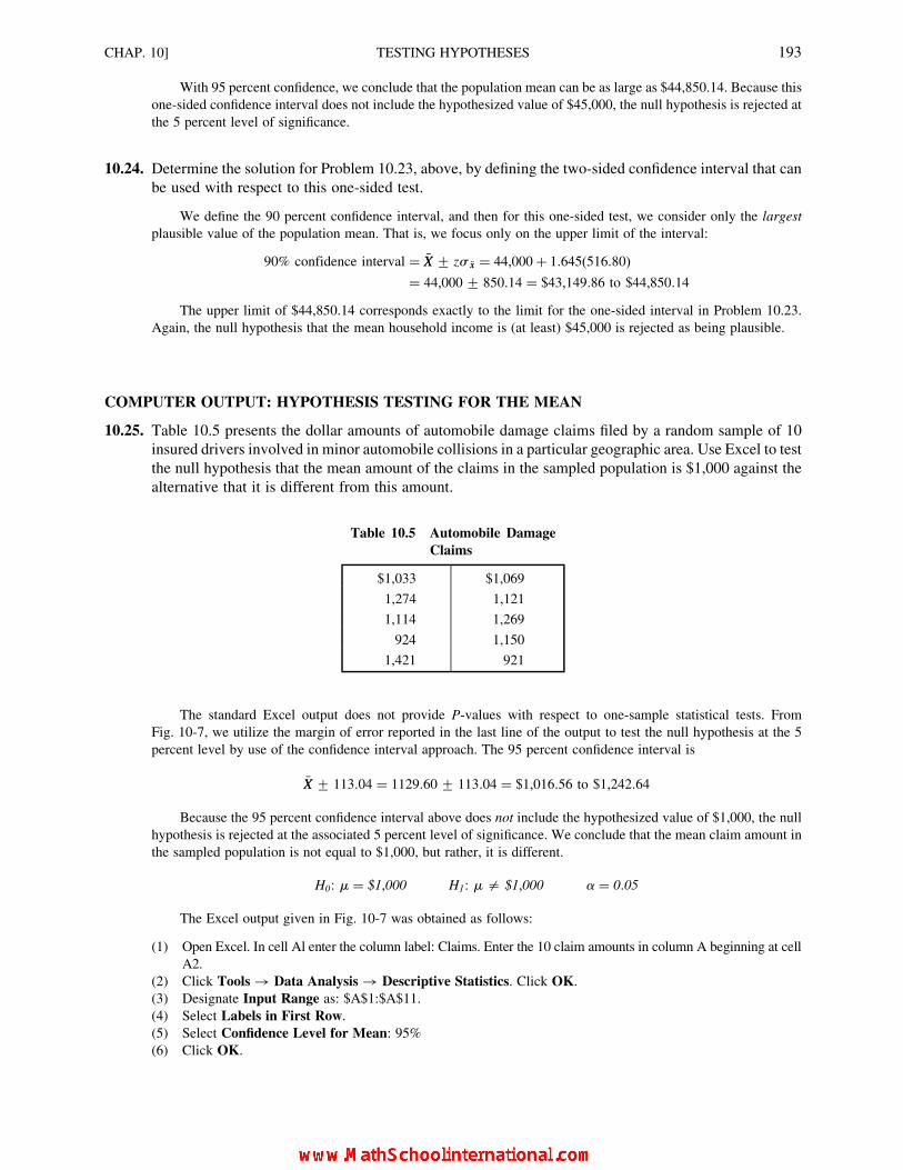
With 95 percent confidence, we conclude that the population mean can be as large as $44,850.14. Because this
one-sided confidence interval does not include the hypothesized value of $45,000, the null hypothesis is rejected at
the 5 percent level of significance.
10.24. Determine the solution for Problem 10.23, above, by defining the two-sided confidence interval that can
be used with respect to this one-sided test.
We define the 90 percent confidence interval, and then for this one-sided test, we consider only the largest
plausible value of the population mean. That is, we focus only on the upper limit of the interval:
90% confidence interval ¼ �XX + zs �xx ¼ 44,000þ 1:645(516:80)
¼ 44,000+ 850:14 ¼ $43,149:86 to $44,850:14
The upper limit of $44,850.14 corresponds exactly to the limit for the one-sided interval in Problem 10.23.
Again, the null hypothesis that the mean household income is (at least) $45,000 is rejected as being plausible.
COMPUTER OUTPUT: HYPOTHESIS TESTING FOR THE MEAN
10.25. Table 10.5 presents the dollar amounts of automobile damage claims filed by a random sample of 10
insured drivers involved in minor automobile collisions in a particular geographic area. Use Excel to test
the null hypothesis that the mean amount of the claims in the sampled population is $1,000 against the
alternative that it is different from this amount.
The standard Excel output does not provide P-values with respect to one-sample statistical tests. From
Fig. 10-7, we utilize the margin of error reported in the last line of the output to test the null hypothesis at the 5
percent level by use of the confidence interval approach. The 95 percent confidence interval is
�XX + 113:04 ¼ 1129:60+ 113:04 ¼ $1,016:56 to $1,242:64
Because the 95 percent confidence interval above does not include the hypothesized value of $1,000, the null
hypothesis is rejected at the associated 5 percent level of significance. We conclude that the mean claim amount in
the sampled population is not equal to $1,000, but rather, it is different.
H0: m ¼ $1,000 H1: m = $1,000 a ¼ 0:05
The Excel output given in Fig. 10-7 was obtained as follows:
(1) Open Excel. In cell Al enter the column label: Claims. Enter the 10 claim amounts in column A beginning at cell
A2.
(2) Click Tools ! Data Analysis ! Descriptive Statistics. Click OK.
(3) Designate Input Range as: $A$1:$A$11.
(4) Select Labels in First Row.
(5) Select Confidence Level for Mean: 95%
(6) Click OK.
Table 10.5 Automobile Damage
Claims
$1,033 $1,069
1,274 1,121
1,114 1,269
924 1,150
1,421 921
CHAP. 10] TESTING HYPOTHESES 193

10.26. Table 10.5 presents the dollar amounts of automobile damage claims filed by a random sample of 10
insured drivers involved in minor automobile collisions in a particular geographic area. Use Minitab to
test the null hypothesis that the mean amount of the claims in the sampled population is $1,000 against
the alternative that it is different from this amount.
Refer to Fig. 10-8. Note that in the first line of output the test is correctly identified as being a two-tail test
(“. . . vs mu not ¼ 1000”). In the last line of output the P value is reported as being 0.029. Because this probability is
less than the designated level of significance of 0.05, the null hypothesis is rejected. We conclude that the mean
claim amount in the population is not equal to $1,000, but is different.
H0: m ¼ $1,000 H1: m = $1,000 a ¼ 0:05
The Minitab output given in Fig. 10-8 was obtained as follows:
(1) Open Minitab. In the column-name cell for column C1 enter: Claims. Enter the 10 claim amounts in C1.
(2) Click Stat ! Basic Statistics ! 1-Sample t.
(3) In the Variable box enter: Claims.
(4) For Test mean enter: 1000.
(5) Click Options and designate Confidence level as: 95.0 (because this is the confidence level that is equivalent
to a test at the 5 percent level). Designate Alternative as: not equal (because a two-sided test is required—a
test for a difference in either direction from the null-hypothesized value).
(6) Click OK.
(7) Back in the original dialog box, click OK.
Fig. 10-8 Minitab output.
Fig. 10-7 Excel output.
194 TESTING HYPOTHESES [CHAP. 10

Supplementary Problems
TESTING A HYPOTHESIZED VALUE OF THE MEAN
10.27. A fast-food chain will build a new outlet in a proposed location only if more than 200 cars per hour pass the location
during certain hours. For 20 randomly sampled hours during the designated hours, the average number of cars
passing the location is �XX ¼ 208:5 with s ¼ 30:0. The statistical population is assumed to be approximately normal.
The management of the chain conservatively adopted the alternative hypothesis H1: m . 200:0. Can the null
hypothesis be rejected at the 5 percent level of significance?
Ans. No.
10.28. Suppose the sample results in Problem 10.27 are based on a sample of n ¼ 50 hr. Can the null hypothesis be rejected
at the 5 percent level of significance?
Ans. Yes.
10.29. The mean sales amount per retail outlet for a particular consumer product during the past year is found to be�XX ¼ $3,425 in a sample of n ¼ 25 outlets. Based on sales data for other similar products, the distribution of sales is
assumed to be normal and the standard deviation of the population is assumed to be s ¼ $200. Suppose it was
claimed that the true sales amount per outlet is at least $3,500. Test this claim at the (a) 5 percent and (b) 1 percent
level of significance.
Ans. (a) Reject H0, (b) accept H0.
10.30. In Problem 10.29, suppose that no assumption was made about the population standard deviation, but that s ¼ $200.
Test the claim at the (a) 5 percent and (b) 1 percent level of significance.
Ans. (a) Reject H0, (b) accept H0.
10.31. The manufacturer of a new compact car claims that the car will average at least 35 miles per gallon in general
highway driving. For 40 test runs, the car averaged 34.5 miles per gallon, with a standard deviation of 2.3 miles per
gallon. Can the manufacturer’s claim be rejected at the 5 percent level of significance?
Ans. No.
10.32. Referring to Problem 10.31, before the highway tests were carried out, a consumer advocate claimed that the
compact car would not exceed 35 miles per gallon in general highway driving. Can this claim be rejected at the 5
percent level of significance? Consider the implications of your answer to this question and in Problem 10.31
regarding the importance of which hypothesis is designated as the alternative hypothesis.
Ans. No.
10.33. An analyst in a personnel department randomly selects the records of 16 hourly employees and finds that the mean
wage rate is �XX ¼ $9:50 with a standard deviation of s ¼ $1:00. The wage rates in the firm are assumed to be
normally distributed. Test the null hypothesis H0:m ¼ $10:00, using the 10 percent level of significance.
Ans. Reject H0.
10.34. A random sample of 30 employees at the Secretary II level in a large organization take a standardized word
processing test. The sample results are �XX ¼ 63:0wpm (words per minute) with s ¼ 5:0wpm. Test the null
hypothesis that the word-processing operators in general do not exceed a keyboarding speed of 60wpm, using the 1
percent level of significance.
Ans. Reject H0.
10.35. An automatic soft ice cream dispenser has been set to dispense 4:00 oz per serving. For a sample of n ¼ 10 servings,
the average amount of ice cream is �XX ¼ 4:05 oz with s ¼ 0:10 oz. The amounts being dispensed are assumed to be
normally distributed. Basing the null hypothesis on the assumption that the process is “in control,” should the
dispenser be reset as a result of applying a test at the 5 percent level of significance?
Ans. No.
TYPE I AND TYPE II ERRORS IN HYPOTHESIS TESTING
10.36. With reference to Problem 10.34, suppose it is considered an important difference from the hypothesized value of the
mean if the average typing speed is at least 64:0wpm.Determine the probability of (a) Type I error and (b) Type II error.
Ans. (a) a ¼ 0:01, (b) b ¼ 0:0192 ffi 0:02.
CHAP. 10] TESTING HYPOTHESES 195

10.37. For Problem 10.36, determine the probability of Type II error (a) if the level of significance is changed to
the 5 percent level and (b) if the level of significance is kept at the 1 percent level, but the sample size is n ¼ 60
instead of n ¼ 30.
Ans. (a) b ¼ 0:003, (b) b , 0:001.
10.38. For the testing procedure described in Problem 10.31, suppose it is considered an important discrepancy from the
claim if the average mileage is 34.0 miles per gallon or less. Given this additional information, determine (a) the
minimum OC value if the null hypothesis is true, and (b) the minimum power associated with the, statistical test if
the discrepancy from the claim is an important one.
Ans. (a) OC ¼ 0:95, (b) power ¼ 0:8729 ffi 0:87.
10.39. Determine the minimum power of the test in Problem 10.38, given that it is considered an important discrepancy if
the true mileage is (a) 0.5 mile per gallon and (b) 0.1 mile per gallon less than the claim. Comparing the several
power values, consider the implication of the standard used to define an “important discrepancy.”
Ans. (a) Power ¼ 0:4013 ffi 0:40, (b) power ¼ 0:0869 ffi 0:09.
DETERMINING THE REQUIRED SAMPLE SIZE FOR TESTING THE MEAN
10.40. Before collecting any sample data, the fast-food chain in Problem 10.27 stipulates that the level of Type I error
should be no larger than a ¼ 0:01, and that if the number of cars passing the site is at or above m ¼ 210 per hour,
then the level of Type II error also should not exceed b ¼ 0:01. The population standard deviation is estimated as
being no larger than s ¼ 40. What sample size is required to achieve these objectives?
Ans. n ¼ 347:45 ¼ 348.
10.41. For the testing situation described in Problem 10.29, it is considered an important discrepancy if the mean sales
amount per outlet is $100 less than the claimed amount. What sample size is required if the test is to be carried out at
the 1 percent level of significance, allowing a maximum probability of Type II error of b ¼ 0:05?Ans. n ¼ 63:20 ¼ 64.
THE P-VALUE APPROACH TO TESTING HYPOTHESES CONCERNING THE
POPULATION MEAN
10.42. Using the P-value approach, test the null hypothesis in Problem 10.28 at the 5 percent level of significance.
Ans. Reject H0 (P ¼ 0:0228).
10.43. Using the P-value approach, test the null hypothesis in Problem 10.29 at the 5 percent level of significance.
Ans. Reject H0 (P ¼ 0:0307).
THE CONFIDENCE INTERVAL APPROACH TO TESTING HYPOTHESES CONCERNING
THE MEAN
10.44. Apply the confidence interval approach to testing the null hypothesis in Problem 10.28 using the 5 percent level of
significance.
Ans. Reject H0.
10.45. Apply the confidence interval approach to testing the null hypothesis in Problem 10.33, using the 10 percent level of
significance.
Ans. Reject H0.
COMPUTER OUTPUT
10.46. Refer to Table 2.19 (page 41) for the amounts of 40 personal loans. Assuming that these are random sample data,
use available computer software to test the null hypothesis that the mean loan amount in the population is $1,000.00
against the alternative that it is different, using the 1 percent level of significance.
Ans. Accept H0 (P ¼ 0:34).
196 TESTING HYPOTHESES [CHAP. 10

CHAPTER 11
Testing OtherHypotheses
11.1 TESTING THE DIFFERENCE BETWEEN TWO MEANS USING THE
NORMAL DISTRIBUTION
The procedure associated with testing a hypothesis concerning the difference between two population
means is similar to that for testing a hypothesis concerning the value of one population mean (see Sections 10.2
and 10.3). The procedure differs only in that the standard error of the difference between the means is used to
determine the z (or t) value associated with the sample result. Use of the normal distribution is based on the
same conditions as in the one-sample case, except that two independent random samples are involved. The
general formula for determining the z value for testing a hypothesis concerning the difference between two
means, according to whether the s values for the two populations are known, is
z ¼ (�XX1 � �XX2)� (m1 � m2)0
s �xx1��xx2
(11:1)
or z ¼ (�XX1 � �XX2)� (m1 � m2)0
s�xx1��xx2
(11:2)
As implied by (11.1) and (11.2), we may begin with any particular hypothesized difference, (m1 � m2)0, that
is to be tested. However, the usual null hypothesis is that the two samples have been obtained from populations
with means that are equal. In this case (m1 � m2)0 ¼ 0, and the above formulas are simplified as follows:
z ¼�XX1 � �XX2
s �xx1��xx2
(11:3)
or z ¼�XX1 � �XX2
s�xx1��xx2
(11:4)
In general, the standard error of the difference between means is computed as described in Section 9.1 [see
Formulas (9.3) and (9.4)]. However, in testing the difference between two means, the null hypothesis of interest
is generally not only that the sample means were obtained from populations with equal means, but that the two
samples were in fact obtained from the same population of values. This means that s1 ¼ s2, which we can
197
Copyright 2004, 1996, 1988, 1976 by The McGraw-Hill Companies, Inc. Click Here for Terms of Use.

simply designate s. The assumed common variance is often estimated by pooling the two sample variances, and
the estimated value of s 2 is then used as the basis for the standard error of the difference. The pooled estimate of
the population variance is
ss 2 ¼ (n1 � 1)s21 þ (n2 � 1)s22n1 þ n2 � 2
(11:5)
The estimated standard error of the difference based on the assumption that the population standard
deviations (and variances) are equal is
ss�xx1��xx2 ¼ffiffiffiffiffiffiffiffiffiffiffiffiffiffiffiffiffiss2
n1
þ ss2
n2
s(11:6)
The assumption that the two sample variances were obtained from populations with equal variances can
itself be tested as the null hypothesis (see Section 11.10).
Tests concerned with the difference between means can be either two-sided or one-sided, as illustrated in
the following examples.
EXAMPLE 1. The mean weekly wage for a sample of n1 ¼ 30 employees in a large manufacturing firm is �XX1 ¼ $280:00with a sample standard deviation of s1 ¼ $14:00. In another large firm a random sample of n2 ¼ 40 employees has a mean
wage of �XX2 ¼ $270:00 with a standard deviation of s2 ¼ $10:00. The standard deviations of the two populations of wage
amounts are not assumed to be equal. We test the hypothesis that there is no difference between the mean weekly wage
amounts in the two firms, using the 5 percent level of significance, as follows:
H0: (m1 � m2) ¼ 0 or, equivalently, m1 ¼ m2�XX1 ¼ $280:00 �XX2 ¼ $270:00
H1: (m1 � m2)= 0 or, equivalently, m1 = m2 s1 ¼ $14:00 s2 ¼ $10:00
n1 ¼ 30 n2 ¼ 40
Critical z (a ¼ 0:05) ¼ +1:96
z ¼�XX1 � �XX1
s�xx1��xx2
¼ 280� 270
3:01¼ 10:0
3:01¼ þ 3:32
where s�xx1 ¼s1ffiffiffiffiffin1
p ¼ 14:00ffiffiffiffiffi30
p ¼ 14:00
5:477¼ 2:56
s�xx2 ¼s2ffiffiffiffiffin2
p ¼ 10:00ffiffiffiffiffi40
p ¼ 10:00
6:325¼ 1:58
s�xx1��xx2 ¼ffiffiffiffiffiffiffiffiffiffiffiffiffiffiffiffiffis2�xx1 þ s2�xx2
q¼
ffiffiffiffiffiffiffiffiffiffiffiffiffiffiffiffiffiffiffiffiffiffiffiffiffiffiffiffiffiffiffiffiffi(2:56)2 þ (1:58)2
q¼
ffiffiffiffiffiffiffiffiffiffiffiffiffiffiffiffiffiffiffiffiffiffiffiffiffiffiffiffiffiffiffiffiffiffi6:5536 þ 2:4964
q¼ 3:01
The computed z ofþ 3:32 is in the region of rejection of the hypothesis testing model portrayed in Fig. 11-1. Therefore,
the null hypothesis is rejected, and the alternative hypothesis, that the average weekly wage in the two firms is different, is
accepted.
Fig. 11-1
198 TESTING OTHER HYPOTHESES [CHAP. 11

EXAMPLE 2. Before seeing the sample results in Example 1, a wage analyst believed that the average wage in the first
firm was greater than the wage in the second firm. In order to subject this belief to a critical test, the analyst gives the benefit
of the doubt to the opposite possibility, and formulates the null hypothesis that the average wage in the first firm is equal to or
less than the average in the second firm.We test this hypothesis at the 1 percent level of significance, again without assuming
that the standard deviations of the two populations are equal, as follows:
H0: (m1 � m2) 0 or, equivalently, m1 m2
H1: (m1 � m2) . 0 or, equivalently, m1 . m2
Critical z (a ¼ 0:01) ¼ þ 2:33
Computed z ¼ þ 3:32 (from Example 1)
The computed z of þ 3:32 is greater than the critical value of þ2:33 for this upper-tail test, as portrayed in Fig. 11-2.
Therefore, the null hypothesis is rejected and the alternative hypothesis, that the average wage in the first firm is greater than
the average wage in the second firm, is accepted.
11.2 TESTING THE DIFFERENCE BETWEEN MEANS USING THE t DISTRIBUTION
When the difference between two means is tested by the use of the t distribution, a necessary assumption in
the standard procedure used in most texts is that the variances of the two populations are equal. Therefore, in
such a test the estimated standard error of the mean is calculated from (11.5) and (11.6). The several
requirements associated with the appropriate use of the t distribution are described in Sections 8.8 and 10.6.
EXAMPLE 3. For a random sample of n1 ¼ 10 light bulbs, the mean bulb life is �XX1 ¼ 4,000 hr with s1 ¼ 200. For another
brand of bulbs whose useful life is also assumed to be normally distributed, a random sample of n2 ¼ 8 has a sample mean of�XX2 ¼ 4,300 hr and a sample standard deviation of s ¼ 250. We test the hypothesis that there is no difference between the
mean operating life of the two brands of bulbs, using the 1 percent level of significance, as follows:
H0: (m1 � m2) ¼ 0 �XX1 ¼ 4,000 hr �XX2 ¼ 4,300 hr
H1: (m1 � m2)= 0 s1 ¼ 200 hr s2 ¼ 250 hr
n1 ¼ 10 n2 ¼ 8
df ¼ n1 þ n2 � 2 ¼ 10þ 8� 2 ¼ 16
Critical t (df ¼ 16, a ¼ 0:01) ¼ + 2:921
ss2 ¼ (n1 � 1)s21 þ (n2 � 1)s22n1 þ n2 � 2
¼ (9)(200)2 þ (7)(250)2
10þ 8� 2¼ 360,000þ 437,500
16¼ 49,843:75
ss �xx1��xx2 ¼ffiffiffiffiffiffiffiffiffiffiffiffiffiffiffiffiffiss2
n1
þ ss2
n2
s¼
ffiffiffiffiffiffiffiffiffiffiffiffiffiffiffiffiffiffiffiffiffiffiffiffiffiffiffiffiffiffiffiffiffiffiffiffiffiffiffiffiffiffiffiffiffi49,843:75
10þ 49,843:75
8
r¼
ffiffiffiffiffiffiffiffiffiffiffiffiffiffiffiffiffiffiffiffiffiffi11,214:843
p¼ 105:9
t ¼�XX1 � �XX2
ss �xx1��xx2
¼ 4,000� 4,300
105:9¼ �300
105:9¼ �2:833
The computed t of�2:833 is in the region of acceptance of the null hypothesis. Therefore, the null hypothesis cannot berejected at the 1 percent level of significance.
Fig. 11-2
CHAP. 11] TESTING OTHER HYPOTHESES 199

11.3 TESTING THE DIFFERENCE BETWEEN MEANS BASED ON
PAIRED OBSERVATIONS
The procedures in Sections 11.1 and 11.2 are based on the assumption that the two samples were collected
as two independent random samples. However, in many situations the samples are collected as pairs of values,
such as when determining the productivity level of each worker before and after a training program. These are
referred to as paired observations, or matched pairs. Also, as contrasted to independent samples, two samples
that contain paired observations often are called dependent samples.
For paired observations the appropriate approach for testing the difference between the means of the two
samples is to first determine the difference d between each pair of values, and then test the null hypothesis that
the mean population difference is zero. Thus, from the computational standpoint the test is applied to the one
sample of d values, with H0: md ¼ 0.
The mean and standard deviation of the sample d values are obtained by use of the basic formulas in
Chapters 3 and 4, except that d is substituted for X. The mean difference for a set of differences between paired
observations is
�d ¼ Sd
n(11:7)
The deviations formula and the computational formula for the standard deviation of the differences
between paired observations are, respectively,
sd ¼ffiffiffiffiffiffiffiffiffiffiffiffiffiffiffiffiffiffiffiffiS(d � �d )2
n � 1
s(11:8)
sd ¼ffiffiffiffiffiffiffiffiffiffiffiffiffiffiffiffiffiffiffiffiffiffiSd2 � n �d 2
n � 1
r(11:9)
The standard error of the mean difference between paired observations is obtained by Formula (8.4) for the
standard error of the mean, except that d is again substituted for X:
s �d ¼ sdffiffiffin
p (11:0)
Because the standard error of the mean difference is computed on the basis of the standard deviation of the
sample of differences (that is, the population value sd is unknown) and because values of d generally can be
assumed to be normally distributed, the t distribution is appropriate for testing the null hypothesis that md ¼ 0.
The degrees of freedom is the number of differences minus one, or n � 1. As discussed in Section 8.8, the
standard normal z distribution can be used as an approximation of the t distributions when n � 30. Example 4
illustrates a two-sided test, whereas Problem 11.5 illustrates a one-sided test. The test statistic used to test the
hypothesis that there is no difference between the means of a set of paired observations is
t ¼ �d
s �d
(11:11)
EXAMPLE 4. An automobile manufacturer collects mileage data for a sample of n ¼ 10 cars in various weight categories
using a standard grade of gasoline with and without a particular additive. Of course, the engines were tuned to the same
specifications before each run, and the same drivers were used for the two gasoline conditions (with the driver in fact being
unaware of which gasoline was being used on a particular run). Given the mileage data in Table 11.1, we test the hypothesis
that there is no difference between the mean mileage obtained with and without the additive, using the 5 percent level of
significance, as follows:
Average with additive ¼ 276:8
10¼ 27:68mpg
Average without additive ¼ 275:1
10¼ 27:51mpg
200 TESTING OTHER HYPOTHESES [CHAP. 11

H0: md ¼ 0
H1: md = 0
Critical t (d f ¼ 9, a ¼ 0:05) ¼ + 2:262
�dd ¼ Sd
n¼ 1:7
10¼ 0:17
sd ¼ffiffiffiffiffiffiffiffiffiffiffiffiffiffiffiffiffiffiffiffiffiSd2 � n �d 2
n � 1
s¼
ffiffiffiffiffiffiffiffiffiffiffiffiffiffiffiffiffiffiffiffiffiffiffiffiffiffiffiffiffiffiffiffiffi1:31� 10(0:17)2
10� 1
s¼
ffiffiffiffiffiffiffiffiffiffiffiffiffiffiffiffiffiffiffiffiffiffiffiffiffiffiffiffiffiffiffiffiffiffiffiffi1:31� 10(0:0289)
9
s¼
ffiffiffiffiffiffiffiffiffiffiffiffiffiffi0:1134
p¼ 0:337
s �dd ¼ sdffiffiffin
p ¼ 0:337ffiffiffiffiffi10
p ¼ 0:337
3:16¼ 0:107
t ¼�dd
s �dd¼ 0:17
0:107¼ þ 1:59
The computed t ofþ 1:59 is not in the region of rejection of the null hypothesis. Therefore, the null hypothesis that thereis no difference in the miles per gallon obtained with as compared to without the additive is accepted as being plausible.
11.4 TESTING A HYPOTHESIS CONCERNING THE VALUE OF THE
POPULATION PROPORTION
As explained in Section 7.4, the normal distribution can be used as an approximation of a binomial
distribution when n � 30 and both np � 5 and n(q) � 5, where q ¼ 1� p. This is the basis upon which
confidence intervals for the proportion are determined in Section 9.3, where the standard error of the proportion
is also discussed. However, in the case of confidence intervals, a sample size of at least n ¼ 100 is generally
required, as explained in Section 9.3.
In determining confidence intervals in Section 9.3 the sample proportion pp serves as the basis for the
standard error. In hypothesis testing, the value of the standard error of the proportion generally is based on using
the hypothesized value p0:
spp ¼ffiffiffiffiffiffiffiffiffiffiffiffiffiffiffiffiffiffiffiffiffiffip0(1� p0)
n
r(11:12)
The procedure associated with testing a hypothesized value of the population proportion is identical to that
described in Section 10.3, except that the null hypothesis is concerned with a value of the population proportion
Table 11.1 Automobile Mileage Data and Worksheet for Computing the
Mean Difference and the Standard Deviation of the Difference
Automobile
Mileage
with additive
Mileage
without additive d d 2
1 36.7 36.2 0.5 0.25
2 35.8 35.7 0.1 0.01
3 31.9 32.3 20.4 0.16
4 29.3 29.6 20.3 0.09
5 28.4 28.1 0.3 0.09
6 25.7 25.8 20.1 0.01
7 24.2 23.9 0.3 0.09
8 22.6 22.0 0.6 0.36
9 21.9 21.5 0.4 0.16
10 20.3 20.0 0.3 0.09
Total 276.8 275.1 þ1.7 1.31
CHAP. 11] TESTING OTHER HYPOTHESES 201

rather than the population mean. Thus, the formula for the z statistic for testing a hypothesis concerning the
value of the population proportion is
z ¼ pp � p0
spp
(11:13)
EXAMPLE 5. The director of a university placement office claimed that at least 50 percent of the graduating seniors had
finalized job arrangements by March 1. Suppose a random sample of n ¼ 30 seniors was polled, and only 10 of the students
indicated that they had concluded their job arrangements by March 1. Can the placement director’s claim be rejected at the
5 percent level of significance? We utilize z as the test statistic, as follows:
H0: p ¼ 0:50 H1: p , 0:50
Critical z (a ¼ 0:05) ¼ �1:645
[Use of the normal distribution is warranted because n � 30, np0 � 5, and n(1� p0) � 5.]
spp ¼ffiffiffiffiffiffiffiffiffiffiffiffiffiffiffiffiffiffiffiffiffiffip0(1� p0)
n
r¼
ffiffiffiffiffiffiffiffiffiffiffiffiffiffiffiffiffiffiffiffiffiffiffiffi(0:50)(0:50)
30
r¼
ffiffiffiffiffiffiffiffiffi0:25
30
r¼
ffiffiffiffiffiffiffiffiffiffiffiffiffiffi0:0083
p¼ 0:09
z ¼ pp � p0
spp
¼ 0:33� 0:50
0:09¼ �0:17
0:09¼ �1:88
The computed z of�1:88 is less than the critical value of�1:645 for this lower-tail test. Therefore, the director’s claimis rejected at the 5 percent level of significance.
11.5 DETERMINING REQUIRED SAMPLE SIZE FOR TESTING THE PROPORTION
Before a sample is actually collected, the required sample size for testing a hypothesis concerning the
population proportion can be determined by specifying (1) the hypothesized value of the proportion, (2) a
specific alternative value of the proportion such that the difference from the null-hypothesized value is
considered important, (3) the level of significance to be used in the test, and (4) the probability of Type II error
that is to be permitted. The formula for determining the minimum sample size required for testing a
hypothesized value of the proportion is
n ¼ z0ffiffiffiffiffiffiffiffiffiffiffiffiffiffiffiffiffiffiffiffiffiffip0(1� p0)
p� z1
ffiffiffiffiffiffiffiffiffiffiffiffiffiffiffiffiffiffiffiffiffiffip1(1� p1)
pp1 � p0
" #2
(11:14)
In (11.14), z0 is the critical value of z used in conjunction with the specified level of significance (a level),
while z1 is the value of z with respect to the designated probability of Type II error (b level). As was true in
Section 10.5 on determining sample size for testing the mean, z0 and z1 always have opposite algebraic signs.
The result is that the two products in the numerator will always be accumulated. Also, Formula (11.14) can be
used in conjunction with either one-tail or two-tail tests and any fractional sample size is rounded up. Finally,
the sample size should be large enough to warrant use of the normal ability probability distribution in
conjunction with p0 and p1, as reviewed in Section 11.4.
EXAMPLE 6. A member of Congress wishes to test the hypothesis that at least 60 percent of constituents are in favor of
labor legislation being introduced in Congress, using the 5 percent level of significance. The discrepancy from this
hypothesis is considered to be important if only 50 percent (or fewer) favor the legislation, and the risk of a Type II error of
b ¼ 0:05 is acceptable. The sample size which should be collected, as a minimum, to satisfy these decision-making
specifications is
n ¼ z0ffiffiffiffiffiffiffiffiffiffiffiffiffiffiffiffiffiffiffiffiffip0(1� p0)
p� z1
ffiffiffiffiffiffiffiffiffiffiffiffiffiffiffiffiffiffiffiffiffip1(1� p1)
pp1 � p0
" #2
¼ �1:645ffiffiffiffiffiffiffiffiffiffiffiffiffiffiffiffiffiffiffiffiffiffiffiffi(0:60)(0:40)
p� (þ 1:645)
ffiffiffiffiffiffiffiffiffiffiffiffiffiffiffiffiffiffiffiffiffiffiffiffi(0:50)(0:50)
p0:50� 0:60
" #2
¼ �1:645(0:49)� 1:645(0:50)
�0:10
� �2¼ �0:806� 0:822
�0:10
� �2
¼ (16:28)2 ¼ 265:04 ¼ 266
202 TESTING OTHER HYPOTHESES [CHAP. 11

11.6 TESTING WITH RESPECT TO THE PROCESS PROPORTION IN
STATISTICAL PROCESS CONTROL
As described in Section 10.9, the use and interpretation of control charts in statistical process control is a
direct application of the methods and concepts of hypothesis testing. Just as is true for the process mean in
Section 10.9, the control limits for a process proportion are defined at +3 standard error units for the
hypothesized (acceptable) value. The methodology for preparing and interpreting control charts is described in
Chapter 19, Statistical Process Control. Section 19.9 is concerned particularly with the process proportion.
EXAMPLE 7. When a coupon redemption process is in control, a maximum of 3 percent of the rebates are done
incorrectly, for a maximum acceptable proportion of errors of 0.03. For 20 sequential samples of 100 coupon redemptions
each, an audit reveals that the number of errors found in the rational subgroup samples is: 2, 2, 3, 6, 1, 3, 6, 4, 7, 2, 5, 0, 3, 2,
4, 5, 3, 8, 1, and 4. The run chart for the sequence of the sample proportions of error for the 20 samples is portrayed in
Fig. 2-31 (page 35). An overview of this figure might lead one to question whether the standard of allowing a maximum
proportion of errors of 0.03 in the process is being maintained, particularly at samples #9 and #18. In Problems 19.22
through 19.25 we shall observe that these two sample proportions are not beyond the upper control limits, and thus could
have occurred simply because of common-cause variation. Therefore, we will not reject the null hypothesis that the process
proportion of defectives is being maintained at 0.03.and that the process is stable.
11.7 TESTING THE DIFFERENCE BETWEEN TWO POPULATION PROPORTIONS
When we wish to test the hypothesis that the proportions in two populations are not different, the two
sample proportions are pooled as a basis for determining the standard error of the difference between
proportions. Note that this differs from the procedure used in Section 9.5 on statistical estimation, in which the
assumption of no difference was not made. Further, the present procedure is conceptually similar to that
presented in Section 11.1, in which the two sample variances are pooled as the basis for computing the standard
error of the difference between means. The pooled estimate of the population proportion, based on the
proportions obtained in two independent samples, is
pp ¼ n1pp1 þ n2pp2
n1 � n2
(11:15)
The standard error of the difference between proportions used in conjunction with testing the assumption of
no difference is
sspp1�pp2 ¼ffiffiffiffiffiffiffiffiffiffiffiffiffiffiffiffiffiffiffiffiffiffiffiffiffiffiffiffiffiffiffiffiffiffiffiffiffiffiffiffiffiffiffipp (1� pp)
n1
þ pp (1� pp)
n2
s(11:16)
The formula for the z statistic for testing the null hypothesis that there is no difference between two
population proportions is
z ¼ pp1 � pp2
sspp1�pp2
(11:17)
A test of the difference between proportions can be carried out as either a one-sided test (see Problem 11.8)
or a two-sided test (see Example 8).
EXAMPLE 8. A sample of 50 households in one community shows that 10 of them are watching a TV special on the
national economy. In a second community, 15 of a random sample of 50 households are watching the TV special. We test the
hypothesis that the overall proportion of viewers in the two communities does not differ, using the 1 percent level of
significance, as follows:
H0: (p2 � p2)¼0 or, equivalently, p1 ¼ p2
H1: (p1 � p2)=0 or, equivalently, p1 = p2
CHAP. 11] TESTING OTHER HYPOTHESES 203

Critical z (a ¼ 0:01) ¼ +2:58
pp ¼ n1pp1 þ n2pp2
n1 þ n2¼ 50(0:20)þ 50(0:30)
50þ 50¼ 10þ 15
100¼ 0:25
ss pp1�pp2 ¼ffiffiffiffiffiffiffiffiffiffiffiffiffiffiffiffiffiffiffiffiffiffiffiffiffiffiffiffiffiffiffiffiffiffiffiffiffiffiffiffiffiffiffipp (1� pp)
n1þ pp (1� pp)
n2
s¼
ffiffiffiffiffiffiffiffiffiffiffiffiffiffiffiffiffiffiffiffiffiffiffiffiffiffiffiffiffiffiffiffiffiffiffiffiffiffiffiffiffiffiffiffiffiffiffiffiffiffiffiffiffi(0:25)(0:75)
50þ (0:25)(0:75)
50
s¼ ffiffiffiffiffiffiffiffiffiffiffiffiffiffiffiffiffiffiffiffiffiffiffiffiffiffiffiffiffiffiffiffiffiffiffiffiffiffi
0:00375þ 0:00375p ¼ 0:087
z ¼ pp1 � pp2
sspp1�pp2
¼ 0:20� 0:30
0:087¼ �0:10
0:087¼ �1:15
The computed z of�1:15 is in the region of acceptance of the null hypothesis. Therefore, the hypothesis that there is nodifference in the proportion of viewers in the two areas cannot be rejected.
11.8 TESTING A HYPOTHESIZED VALUE OF THE VARIANCE USING THE
CHI-SQUARE DISTRIBUTION
As explained in Section 9.6, for a normally distributed population the ratio (n � 1)s2=s 2 follows a x2
probability distribution, with there being a different chi-square distribution according to degrees of freedom
(n � 1). Therefore, the statistic which is used to test a hypothesis concerning the value of the population
variance is
x2 ¼ (n � 1)s2
s 20
(11:18)
The test based on (11.18) can be either a one-sided test or a two-sided test, although most often hypotheses
about a population variance relate to one-sided tests. Appendix 7 can be used to determine the critical value(s)
of the chi-square statistic for various levels of significance.
EXAMPLE 9. The mean operating life for a random sample of n ¼ 10 light bulbs is �XX ¼ 4,000 hr with a standard
deviation of s ¼ 200 hr. The operating life of bulbs in general is assumed to be normally distributed. Suppose that before the
sample was collected, it was hypothesized that the population standard deviation is no larger than s ¼ 150. Based on the
sample results, this hypothesis is tested at the 1 percent level of significance as follows:
H0: s2 ¼ 22,500 [because s 2
0 ¼ (150)2 ¼ 22,500] H1: s2 . 22,500
Critical x 2 (df ¼ 0, a ¼ 0:01) ¼ 21:67
x2 ¼ (n � 1)s2
s 20
¼ (9)(40,000)22,500
¼ 360,000
22,500¼ 16:0
Because the calculated test statistic of 16.0 does not exceed the critical value of 21.67 for this upper-tail test, the null
hypothesis that s 150 cannot be rejected at the 1 percent level of significance.
11.9 TESTING WITH RESPECT TO PROCESS VARIABILITY IN STATISTICAL
PROCESS CONTROL
As described in Section 10.9 on testing the process mean and in Section 11.6 on testing the process
proportion, the use and interpretation of control charts in statistical process control is a direct application of the
methods and concepts of hypothesis testing. Process variability is monitored and controlled either with respect
to the process standard deviation or the process range. As is the case with control charts for the process mean
and process proportion, the control limits are defined at +3 standard error units with respect to the expected
centerline value on the chart when the null hypothesis that there is no assignable-cause variation is true. The
methodology for preparing and interpreting control charts is described in Chapter 19, Statistical Process
204 TESTING OTHER HYPOTHESES [CHAP. 11

Control. Section 19.7 is concerned with the process standard deviation and Section 19.8 is concerned with the
process range.
EXAMPLE 10. Rational-subgroup samples of n ¼ 4 packages of potato chips are taken in a packaging process. In
Example 13 of Chapter 10 (page 184) we considered whether the process appears to be stable with respect to the process
mean. For the sequence of 15 samples, the sample standard deviations are (in oz): 0.148, 0.045, 0.088, 0.057, 0.042, 0.071,
0.083, 0.116, 0.127, 0.066, 0.141, 0.056, 0.047, 0.068, and 0.125. Figure 11-3 is the run chart for this sequence of standard
deviations. Viewing the run chart, it is unclear whether there are any unusual sample standard deviations, since the apparent
large amount of variability throughout the chart could just be a matter of how the vertical axis was scaled. In Solved
Problems 19.16 through 19.19 we shall in fact observe that all the sample standard deviations are within the lower and upper
control limits. Thus, the null hypothesis that there is no assignable-cause variation will not be rejected, and we will conclude
that the process is stable with respect to the standard deviation of package contents. Incidentally, just because there is no
assignable-cause variation does not in itself make the variability in the process acceptable. If there is too much continuing
variability due to common causes, then the process needs to be redesigned and improved.
11.10 THE F DISTRIBUTION AND TESTING THE EQUALITY OF TWO
POPULATION VARIANCES
The F distribution can be shown to be the appropriate probability model for the ratio of the variances of two
samples taken independently from the same normally distributed population, with there being a different F
distribution for every combination of the degrees of freedom df associated with each sample. For each sample,
df ¼ n � 1. The statistic that is used to test the null hypothesis that two population variances are equal is
Fd f1,d f2 ¼s21s22
(11:19)
Since each sample variance is an unbiased estimator of the same population variance, the long-run
expected value of the above ratio is about 1.0. (Note: The expected value is not exactly 1.0, but rather is
d f2=(d f2 � 2), for mathematical reasons that are outside of the scope of this outline.) However, for any
given pair of samples the sample variances are not likely to be identical in value, even though the null
hypothesis is true. Since this ratio is known to follow an F distribution, this probability distribution can be
used in conjunction with testing the difference between two variances. Although a necessary mathematical
Fig. 11-3 Run chart.
CHAP. 11] TESTING OTHER HYPOTHESES 205
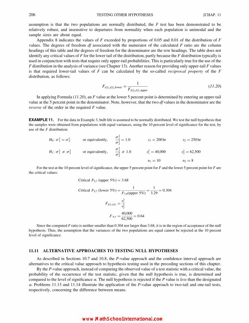
assumption is that the two populations are normally distributed, the F test has been demonstrated to be
relatively robust, and insensitive to departures from normality when each population is unimodal and the
sample sizes are about equal.
Appendix 8 indicates the values of F exceeded by proportions of 0.05 and 0.01 of the distribution of F
values. The degrees of freedom df associated with the numerator of the calculated F ratio are the column
headings of this table and the degrees of freedom for the denominator are the row headings. The table does not
identify any critical values of F for the lower tail of the distribution, partly because the F distribution typically is
used in conjunction with tests that require only upper-tail probabilities. This is particularly true for the use of the
F distribution in the analysis of variance (see Chapter 13). Another reason for providing only upper-tail F values
is that required lower-tail values of F can be calculated by the so-called reciprocal property of the F
distribution, as follows:
Fd f1,d f2,lower ¼1
Fd f2,d f1,upper
(11:20)
In applying Formula (11.20), an F value at the lower 5 percent point is determined by entering an upper-tail
value at the 5 percent point in the denominator. Note, however, that the two df values in the denominator are the
reverse of the order in the required F value.
EXAMPLE 11. For the data in Example 3, bulb life is assumed to be normally distributed. We test the null hypothesis that
the samples were obtained from populations with equal variances, using the 10 percent level of significance for the test, by
use of the F distribution:
H0: s21 ¼ s 2
2 or equivalently,s 2
1
s 22
¼ 1:0 s1 ¼ 200 hr s2 ¼ 250 hr
H1: s21 = s 2
2 or equivalently,s 2
1
s 22
= 1:0 s21 ¼ 40,000 s22 ¼ 62,500
n1 ¼ 10 n2 ¼ 8
For the test at the 10 percent level of significance, the upper 5 percent point for F and the lower 5 percent point for F are
the critical values:
Critical F9,7 (upper 5%) ¼ 3:68
Critical F9,7 (lower 5%) ¼ 1
F7,9(upper 5%)¼ 1
3:29¼ 0:304
Fd f1 ,d f2 ¼s21s22
F 9,7 ¼ 40,000
62,500¼ 0:64
Since the computed F ratio is neither smaller than 0.304 nor larger than 3.68, it is in the region of acceptance of the null
hypothesis. Thus, the assumption that the variances of the two populations are equal cannot be rejected at the 10 percent
level of significance.
11.11 ALTERNATIVE APPROACHES TO TESTING NULL HYPOTHESES
As described in Sections 10.7 and 10.8, the P-value approach and the confidence interval approach are
alternatives to the critical value approach to hypothesis testing used in the preceding sections of this chapter.
By the P-value approach, instead of comparing the observed value of a test statistic with a critical value, the
probability of the occurrence of the test statistic, given that the null hypothesis is true, is determined and
compared to the level of significance a. The null hypothesis is rejected if the P value is less than the designated
a. Problems 11.13 and 11.14 illustrate the application of the P-value approach to two-tail and one-tail tests,
respectively, concerning the difference between means.
206 TESTING OTHER HYPOTHESES [CHAP. 11

By the confidence interval approach, the 1� a confidence interval is constructed for the parameter value of
concern. If the hypothesized value of the parameter is not included in the interval, then the null hypothesis is
rejected. Problems 11.15 and 11.16 illustrate the application of the confidence interval approach to two-tail and
one-tail tests, respectively, concerning the difference between means.
11.12 USING EXCEL AND MINITAB
Computer software is available for most of the hypothesis-testing applications described in this chapter.
The P-value approach to hypothesis testing generally is used, as described in Section 11.11. The use of Excel
and Minitab for testing the difference between the means of two independent samples is illustrated in Solved
Problems 11.17 and 11.18, respectively, while the use of Excel and Minitab with the paired-observations design
for testing the difference between means is illustrated in Problems 11.19 and 11.20.
Solved Problems
TESTING THE DIFFERENCE BETWEEN TWO MEANS USING THE
NORMAL DISTRIBUTION
11.1. A developer is considering two alternative sites for a regional shopping center. Since household income
in the community is one important consideration in such site selection, the developer wishes to test the
null hypothesis that there is no difference between the mean household income amounts in the two
communities. Consistent with this hypothesis, it is assumed that the standard deviation of household
income is also the same in the two communities. For a sample of n1 ¼ 30 households in the first
community, the average annual income is �XX1 ¼ $45,500 with the sample standard deviation
s1 ¼ $1,800. For a sample of n2 ¼ 40 households in the second community, �XX2 ¼ $44,600 and
s2 ¼ $2,400. Test the null hypothesis at the 5 percent level of significance.
H0: (m1 ¼ m2) ¼ 0
�XX1 ¼ $45,500
s1 ¼ $1,800
n1 ¼ 30
H1: (m1 � m 2)= 0
�XX2 ¼ $44,600
s2 ¼ $2,400
n2 ¼ $40
Critical z (a ¼ 0:05) ¼ +1:96
ss2 ¼ (n1 � 1)s21 þ (n2 � 1)s22n1 þ n2 � 2
¼ 29(1,800)2 þ 39(2,400)2
30þ 40� 2¼ 318,600,000
68¼ $4,685,294
(The variances are pooled because of the assumption that the standard deviation values in the two populations are
equal.)
ss�xx1��xx2 ¼ffiffiffiffiffiffiffiffiffiffiffiffiffiffiffiffiss2
n1þ ss2
n2
s¼
ffiffiffiffiffiffiffiffiffiffiffiffiffiffiffiffiffiffiffiffiffiffiffiffiffiffiffiffiffiffiffiffiffiffiffiffiffiffiffiffiffiffiffiffiffi4,685,294
30þ 4,685,294
40
s¼
ffiffiffiffiffiffiffiffiffiffiffiffiffiffiffiffiffiffiffiffiffiffiffiffiffiffiffiffiffiffiffiffiffiffiffiffiffiffiffiffiffiffiffiffiffiffiffiffiffiffi156,176:46þ 117,132:35
p¼ $522:79
z ¼�XX1 � �XX2
ss�xx1��xx2
¼ 35,500� 34,600
522:79¼ 900
522:79¼ þ 1:72
The computed z value of þ1:72 is in the region of acceptance of the null hypothesis. Therefore the null
hypothesis cannot be rejected at the 5 percent level of significance, and the hypothesis that the average income per
household in the two communities does not differ is accepted as being plausible.
11.2. With reference to Problem 11.1, before any data were collected it was the developer’s judgment that
income in the first community might be higher. In order to subject this judgment to a critical test, the
developer gave the benefit of doubt to the other possibility and formulated the null hypothesis
CHAP. 11] TESTING OTHER HYPOTHESES 207
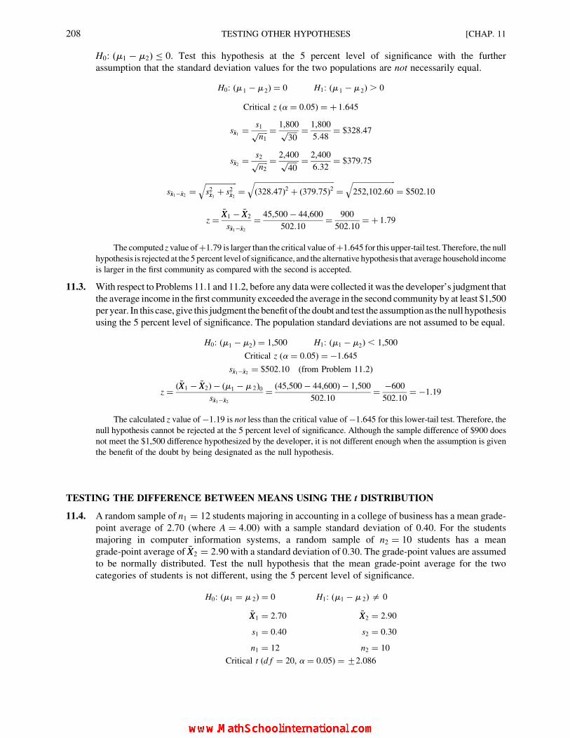
H0: (m1 � m2) 0. Test this hypothesis at the 5 percent level of significance with the further
assumption that the standard deviation values for the two populations are not necessarily equal.
H0: (m 1 � m 2) ¼ 0 H1: (m 1 � m 2) . 0
Critical z (a ¼ 0:05) ¼ þ 1:645
s�xx1 ¼s1ffiffiffiffiffin1
p ¼ 1,800ffiffiffiffiffi30
p ¼ 1,800
5:48¼ $328:47
s�xx2 ¼s2ffiffiffiffiffin2
p ¼ 2,400ffiffiffiffiffi40
p ¼ 2,400
6:32¼ $379:75
s�xx1��xx2 ¼ffiffiffiffiffiffiffiffiffiffiffiffiffiffiffiffiffis2�xx1 þ s2�xx2
q¼
ffiffiffiffiffiffiffiffiffiffiffiffiffiffiffiffiffiffiffiffiffiffiffiffiffiffiffiffiffiffiffiffiffiffiffiffiffiffiffiffiffiffiffi(328:47)2 þ (379:75)2
q¼
ffiffiffiffiffiffiffiffiffiffiffiffiffiffiffiffiffiffiffiffiffiffiffi252,102:60
q¼ $502:10
z ¼�XX1 � �XX2
s�xx1��xx2
¼ 45,500� 44,600
502:10¼ 900
502:10¼ þ 1:79
The computed z value ofþ1:79 is larger than the critical value ofþ1:645 for this upper-tail test. Therefore, the nullhypothesis is rejected at the 5 percent level of significance, and the alternative hypothesis that average household income
is larger in the first community as compared with the second is accepted.
11.3. With respect to Problems 11.1 and 11.2, before any datawere collected it was the developer’s judgment that
the average income in the first community exceeded the average in the second community by at least $1,500
per year. In this case, give this judgment thebenefit of thedoubt and test the assumptionas thenull hypothesis
using the 5 percent level of significance. The population standard deviations are not assumed to be equal.
H0: (m1 � m2) ¼ 1,500 H1: (m1 � m2) , 1,500
Critical z (a ¼ 0:05) ¼ �1:645
s�xx1��xx2 ¼ $502:10 (from Problem 11:2)
z ¼ (�XX1 � �XX2)� (m1 � m 2)0
s�xx1��xx2
¼ (45,500� 44,600)� 1,500
502:10¼ �600
502:10¼ �1:19
The calculated z value of�1:19 is not less than the critical value of�1:645 for this lower-tail test. Therefore, thenull hypothesis cannot be rejected at the 5 percent level of significance. Although the sample difference of $900 does
not meet the $1,500 difference hypothesized by the developer, it is not different enough when the assumption is given
the benefit of the doubt by being designated as the null hypothesis.
TESTING THE DIFFERENCE BETWEEN MEANS USING THE t DISTRIBUTION
11.4. A random sample of n1 ¼ 12 students majoring in accounting in a college of business has a mean grade-
point average of 2.70 (where A ¼ 4:00) with a sample standard deviation of 0.40. For the students
majoring in computer information systems, a random sample of n2 ¼ 10 students has a mean
grade-point average of �XX2 ¼ 2:90 with a standard deviation of 0.30. The grade-point values are assumed
to be normally distributed. Test the null hypothesis that the mean grade-point average for the two
categories of students is not different, using the 5 percent level of significance.
H0: (m1 ¼ m 2) ¼ 0
�XX1 ¼ 2:70
s1 ¼ 0:40
n1 ¼ 12
H1: (m1 � m 2)= 0
�XX2 ¼ 2:90
s2 ¼ 0:30
n2 ¼ 10
Critical t (d f ¼ 20, a ¼ 0:05) ¼ +2:086
208 TESTING OTHER HYPOTHESES [CHAP. 11
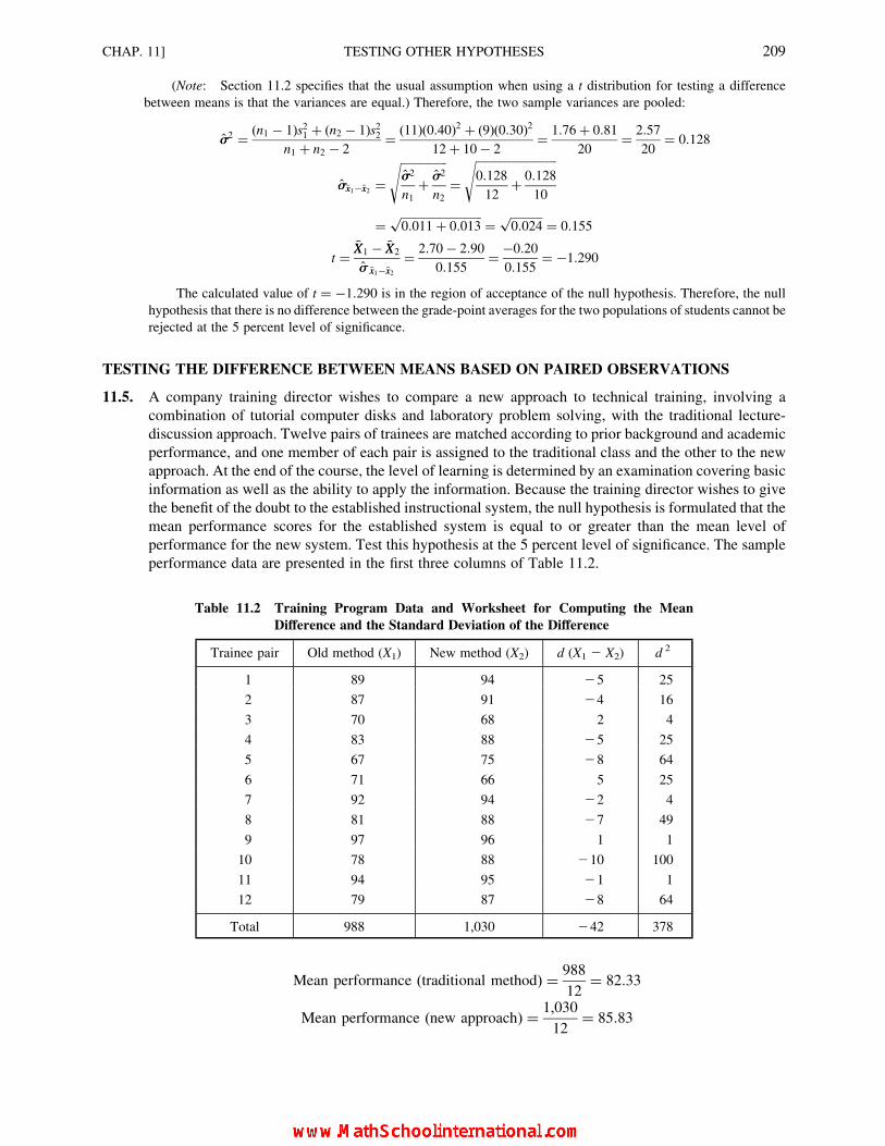
(Note: Section 11.2 specifies that the usual assumption when using a t distribution for testing a difference
between means is that the variances are equal.) Therefore, the two sample variances are pooled:
ss2 ¼ (n1 � 1)s21 þ (n2 � 1)s22n1 þ n2 � 2
¼ (11)(0:40)2 þ (9)(0:30)2
12þ 10� 2¼ 1:76þ 0:81
20¼ 2:57
20¼ 0:128
ss�xx1��xx2 ¼ffiffiffiffiffiffiffiffiffiffiffiffiffiffiffiffiss2
n1þ ss2
n2
s¼
ffiffiffiffiffiffiffiffiffiffiffiffiffiffiffiffiffiffiffiffiffiffiffiffiffiffiffiffi0:128
12þ 0:128
10
s
¼ ffiffiffiffiffiffiffiffiffiffiffiffiffiffiffiffiffiffiffiffiffiffiffiffiffiffiffiffi0:011þ 0:013
p ¼ffiffiffiffiffiffiffiffiffiffiffi0:024
p¼ 0:155
t ¼�XX1 � �XX2
ss �xx1��xx2
¼ 2:70� 2:90
0:155¼ �0:20
0:155¼ �1:290
The calculated value of t ¼ �1:290 is in the region of acceptance of the null hypothesis. Therefore, the null
hypothesis that there is no difference between the grade-point averages for the two populations of students cannot be
rejected at the 5 percent level of significance.
TESTING THE DIFFERENCE BETWEEN MEANS BASED ON PAIRED OBSERVATIONS
11.5. A company training director wishes to compare a new approach to technical training, involving a
combination of tutorial computer disks and laboratory problem solving, with the traditional lecture-
discussion approach. Twelve pairs of trainees are matched according to prior background and academic
performance, and one member of each pair is assigned to the traditional class and the other to the new
approach. At the end of the course, the level of learning is determined by an examination covering basic
information as well as the ability to apply the information. Because the training director wishes to give
the benefit of the doubt to the established instructional system, the null hypothesis is formulated that the
mean performance scores for the established system is equal to or greater than the mean level of
performance for the new system. Test this hypothesis at the 5 percent level of significance. The sample
performance data are presented in the first three columns of Table 11.2.
Mean performance (traditional method) ¼ 988
12¼ 82:33
Mean performance (new approach) ¼ 1,030
12¼ 85:83
Table 11.2 Training Program Data and Worksheet for Computing the Mean
Difference and the Standard Deviation of the Difference
Trainee pair Old method (X1) New method (X2) d (X1 2 X2) d 2
1 89 94 25 25
2 87 91 24 16
3 70 68 2 4
4 83 88 25 25
5 67 75 28 64
6 71 66 5 25
7 92 94 22 4
8 81 88 27 49
9 97 96 1 1
10 78 88 210 100
11 94 95 21 1
12 79 87 28 64
Total 988 1,030 242 378
CHAP. 11] TESTING OTHER HYPOTHESES 209
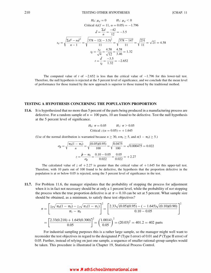
H0: md ¼ 0 H1: md , 0
Critical t(d f ¼ 11, a ¼ 0:05) ¼ �1:796
�d ¼ Sd
n¼ �42
12¼ �3:5
sd ¼ffiffiffiffiffiffiffiffiffiffiffiffiffiffiffiffiffiffiffiffiffiffiSd2 � n �d
2
n � 1
s¼
ffiffiffiffiffiffiffiffiffiffiffiffiffiffiffiffiffiffiffiffiffiffiffiffiffiffiffiffiffiffiffiffiffiffiffi378� 12(� 3:5)2
11
s¼
ffiffiffiffiffiffiffiffiffiffiffiffiffiffiffiffiffiffiffiffiffi378� 147
11
r¼
ffiffiffiffiffiffiffiffi231
11
r¼
ffiffiffiffiffi21
p¼ 4:58
s �d ¼ sdffiffiffin
p ¼ 4:58ffiffiffiffiffi12
p ¼ 4:58
3:46¼ 1:32
t ¼ �d
s �d¼ �3:5
1:32¼ �2:652
The computed value of t of �2:652 is less than the critical value of �1:796 for this lower-tail test.
Therefore, the null hypothesis is rejected at the 5 percent level of significance, and we conclude that the mean level
of performance for those trained by the new approach is superior to those trained by the traditional method.
TESTING A HYPOTHESIS CONCERNING THE POPULATION PROPORTION
11.6. It is hypothesized that no more than 5 percent of the parts being produced in a manufacturing process are
defective. For a random sample of n ¼ 100 parts, 10 are found to be defective. Test the null hypothesis
at the 5 percent level of significance.
H0: p ¼ 0:05 H1: p . 0:05
Critical z (a ¼ 0:05) ¼ þ 1:645
(Use of the normal distribution is warranted because n � 30, np0 � 5, and n(1� p0) � 5:)
spp ¼ffiffiffiffiffiffiffiffiffiffiffiffiffiffiffiffiffiffiffiffiffiffip0(1� p0)
n
r¼
ffiffiffiffiffiffiffiffiffiffiffiffiffiffiffiffiffiffiffiffiffiffiffiffi(0:05)(0:95)
100
r¼
ffiffiffiffiffiffiffiffiffiffiffiffiffiffi0:0475
100
r¼
ffiffiffiffiffiffiffiffiffiffiffiffiffiffiffiffiffiffiffi0:000475
p¼ 0:022
z ¼ pp � p0
spp
¼ 0:10� 0:05
0:022¼ 0:05
0:022¼ þ 2:27
The calculated value of z of þ 2:27 is greater than the critical value of þ 1:645 for this upper-tail test.
Therefore, with 10 parts out of 100 found to be defective, the hypothesis that the proportion defective in the
population is at or below 0.05 is rejected, using the 5 percent level of significance in the test.
11.7. For Problem 11.6, the manager stipulates that the probability of stopping the process for adjustment
when it is in fact not necessary should be at only a 1 percent level, while the probability of not stopping
the process when the true proportion defective is at p ¼ 0:10 can be set at 5 percent. What sample size
should be obtained, as a minimum, to satisfy these test objectives?
n ¼ z0ffiffiffiffiffiffiffiffiffiffiffiffiffiffiffiffiffiffiffiffiffiffip0(1� p0)
p� z1
ffiffiffiffiffiffiffiffiffiffiffiffiffiffiffiffiffiffiffiffiffiffip1(1� p1)
pp1 � p0
" #2
¼ 2:33ffiffiffiffiffiffiffiffiffiffiffiffiffiffiffiffiffiffiffiffiffiffiffiffi(0:05)(0:95)
p� (� 1:645)
ffiffiffiffiffiffiffiffiffiffiffiffiffiffiffiffiffiffiffiffiffiffiffiffi(0:10)(0:90)
p0:10� 0:05
" #2
¼ 2:33(0:218)þ 1:645(0:300)
0:05
� �2¼ 1:0014
0:05
� �2
¼ (20:03)2 ¼ 401:2 ¼ 402 parts
For industrial sampling purposes this is a rather large sample, so the manager might well want to
reconsider the test objectives in regard to the designated P (Type I error) of 0.01 and P (Type II error) of
0.05. Further, instead of relying on just one sample, a sequence of smaller rational-group samples would
be taken. This procedure is illustrated in Chapter 19, Statistical Process Control.
210 TESTING OTHER HYPOTHESES [CHAP. 11

TESTING THE DIFFERENCE BETWEEN TWO POPULATION PROPORTIONS
11.8. A manufacturer is evaluating two types of equipment for the fabrication of a component. A random
sample of n1 ¼ 50 is collected for the first brand of equipment, and five items are found to be defective.
A random sample of n2 ¼ 80 is collected for the second brand and six items are found to be defective.
The fabrication rate is the same for the two brands. However, because the first brand costs substantially
less, the manufacturer gives this brand the benefit of the doubt and formulates the hypothesis
H0: p1 p2. Test this hypothesis at the 5 percent level of significance.
H0: (p1 � p2) ¼ 0 H1: (p1 � p2) . 0
Critical z (a ¼ 0:05) ¼ þ 1:645
pp ¼ n1pp1 þ n2pp2
n1 þ n2¼ 50(0:10)þ 80(0:075)
50þ 80¼ 5þ 6
130¼ 0:085
sspp1�pp2 ¼ffiffiffiffiffiffiffiffiffiffiffiffiffiffiffiffiffiffiffiffiffiffiffiffiffiffiffiffiffiffiffiffiffiffiffiffiffiffiffiffiffiffipp(1� pp)
n1þ pp(1� pp)
n2
s¼
ffiffiffiffiffiffiffiffiffiffiffiffiffiffiffiffiffiffiffiffiffiffiffiffiffiffiffiffiffiffiffiffiffiffiffiffiffiffiffiffiffiffiffiffiffiffiffiffiffiffiffiffiffiffiffiffiffiffiffiffiffiffi(0:085)(0:915)
50þ (0:085)(0:915)
80
r
¼ffiffiffiffiffiffiffiffiffiffiffiffiffiffiffiffiffiffiffiffiffiffiffiffiffiffiffiffiffiffiffiffiffi0:0778
50þ 0:0778
80
r¼ ffiffiffiffiffiffiffiffiffiffiffiffiffiffiffiffiffiffiffiffiffiffiffiffiffiffiffiffiffiffiffiffiffi
0:0016þ 0:0010p ¼ 0:051
z ¼ pp1 � pp2
sspp1�pp2
¼ 0:10� 0:075
0:051¼ 0:025
0:051¼ þ 0:49
The calculated value of z of þ 0:49 is not greater than þ1:645 for this upper-tail test. Therefore, the null
hypothesis cannot be rejected at the 5 percent level of significance.
TESTING A HYPOTHESIZED VALUE OF THE VARIANCE USING THECHI-SQUARE DISTRIBUTION
11.9. Suppose it is hypothesized that the standard deviation of household income per year in a particular
community is $3,000. For a sample of n ¼ 15 randomly selected households, the standard deviation is
s ¼ $2,000. The household income figures for the population are assumed to be normally distributed. On
the basis of this sample result, can the null hypothesis be rejected using the 5 percent level of significance?
H0: s2 ¼ (3,000)2 ¼ 9,000,000 H1: s
2 = 9,000,000
Critical x 2(d f ¼ 14, a ¼ 0:05) ¼ 5:63 and 26:12 (respectively, for the two-tail test)
x 2 ¼ (n � 1)s2
s 20
¼ (14)(2,000)2
(3,000)2¼ 14(4,000,000)
9,000,000¼ 56,000,000
9,000,000¼ 6:22
The computed value of 6.22 is neither less than the lower critical value of 5.63 nor larger than the upper critical
value of 26.12 for this two-tail test. Therefore the hypothesis that s ¼ $3,000 is not rejected at the 5 percent level of
significance. It is plausible that the population standard deviation is $3,000.
11.10. For Problem 11.9, suppose the null hypothesis was that the population standard deviation is at least
$3,000. Test this hypothesis at the 5 percent level of significance.
H0: s2 ¼ 9,000,000 H1: s
2 , 9,000,000
Critical x 2(d f ¼ 14, a ¼ 0:05) ¼ 6:57 (lower-tail critical value)
x 2 ¼ 6:22 (from Problem 11.9)
The calculated test statistic of 6.22 is just less than the critical value of 6.57 for this lower-tail test. Therefore
the null hypothesis is rejected at the 5 percent level of significance, and the alternative hypothesis, that s 2 ,9,000,000 (that s , $3,000), is accepted.
CHAP. 11] TESTING OTHER HYPOTHESES 211

TESTING THE EQUALITY OF TWO POPULATION VARIANCES
11.11. In Problem 11.4, concerned with testing the difference between two means using a t distribution, a
necessary assumption was that the two population variances are equal. The two sample variances were
s21 ¼ 0:402 ¼ 0:16, and s22 ¼ 0:302 ¼ 0:09, with n1 ¼ 12 and n2 ¼ 10, respectively. Test the null
hypothesis that the two population variances are indeed equal, using a 10 percent level of significance.
H0: s21 ¼ s 2
2 s 21 ¼ 0:16 s 2
2 ¼ 0:09H1: s
21 = s 2
2 n1 ¼ 12 n2 ¼ 10
Critical F11,9(upper 5%) ¼ 3:10 (from Appendix 8)
Critical F11,9 (lower 5%) ¼ 1
F9,11(upper 5%)¼ 1
2:90¼ 0:345
Fd f1 ,d f2 ¼s 21
s 22
¼ 0:16
0:09¼ 1:78
The calculated F statistic of 1.78 is neither less than the lower critical value of 0.345 nor greater than the upper
critical value of 3.10. Therefore, the hypothesis of no difference between the variances cannot be rejected, and the
assumption of equal variances is warranted.
11.12. In Problem 11.1, the assumption was made that the variance of household income was not different in
the two communities. Test the null hypothesis that the two variances are equal, using the 10 percent
level of significance.
H0: s21 ¼ s 2
2 s 21 ¼ (1,800)2 ¼ 3,240,000 s 2
2 ¼ (2,400)2 ¼ 5,760,000
H1: s21 = s 2
2 n1 ¼ 30 n2 ¼ 40
(Note: Because of limitations in Appendix 8, the specific F values for 29 and 39 degrees of freedom cannot be
determined exactly. Therefore, the approximate F values are determined by using the nearest degrees of
freedom of 30 and 40, respectively.)
Critical F30, 40 (upper 5%) ¼ 1:74
Critical F30, 40 (lower 5%) ¼ 1
F40, 30(upper 5%)¼ 1
1:79¼ 0:599
Fd f1 ,d f2 ¼s 21
s 22
¼ 3,240,000
5,760,000¼ 0:562
The computed F statistic is neither less than the lower critical value of 0.559 nor greater than the upper critical
value of 1.74. Therefore, the F statistic is just within the region of acceptance of the null hypothesis at the 10
percent level of significance, and the assumption of equal variances is warranted.
ALTERNATIVE APPROACHES TO TESTING NULL HYPOTHESES
11.13. Using the P-value approach, test the null hypothesis in Problem 11.1 at the 5 percent level of
significance.
H0: (m1 � m2) ¼ 0 H1: (m1 � m2)= 0
z ¼ þ 1:72 (from Problem 11.1)
P(z � þ 1:72) ¼ 0:5000� 0:4573 ¼ 0:0427
Finally, because this is a two-tail test,
P ¼ 2(0:0427) ¼ 0:0854
212 TESTING OTHER HYPOTHESES [CHAP. 11

Because the P value of 0.0854 is larger than the level of significance of 0.05, the null hypothesis cannot be
rejected at this level. Therefore, we conclude that there is no difference between the mean household income
amounts in the two communities.
11.14. Using the P-value approach, test the null hypothesis in Problem 11.2 at the 5 percent level of significance.
H0: (m1 � m2) ¼ 0 H1: (m1 � m2) . 0
z ¼ þ 1:79 (from Problem 11.2)
(Note that the z statistic is in the direction of the region of rejection for this upper-tail test.)
P(z � þ1:79) ¼ 0:5000� 0:4633 ¼ 0:0367
Because the P value of 0.0367 is smaller than the level of significance of 0.05, we reject the null hypothesis and
conclude that the mean level of income in the first community is greater than the mean income in the second
community.
11.15. Apply the confidence interval approach to testing the null hypothesis in Problem 11.1, using the 5
percent level, of significance.
H0: (m1 � m2) ¼ 0 H1: (m1 � m2)= 0
�XX1 ¼ $45,500 �XX2 ¼ $44,600
ss �xx1��xx2 ¼ $522:79 (from Problem 11.1)
95% Confidence interval ¼ ( �XX1 � �XX2)+ zss �xx1��xx2
¼ (45,500� 44,600)+ 1:96(522:79)
¼ 900+ 1,024:67 ¼ �$124:67 to $1,924:67
Because the 95 percent confidence interval includes the hypothesized difference of $0, the null hypothesis
cannot be rejected at the 5 percent level of significance.
11.16. Apply the confidence interval approach to testing the null hypothesis in Problem 11.2.
H0: (m1 � m2) ¼ 0 H1: (m1 � m2) . 0
�XX1 ¼ $45,500 �XX2 ¼ $44,600
s�xx1��xx2 ¼ $502:10 (from Problem 11.2)
Lower confidence limit ¼ ( �XX1 � �XX2)� z s�xx1��xx2
¼ (45,500� 44,600)� 1:645(502:10)
¼ 900� 825:95 ¼ $74:05
With 95 percent confidence, we conclude that the difference between the population means can be as small as
$74.05. Because this one-sided confidence interval does not include the hypothesized value of $0 (or less), the null
hypothesis is rejected at the 5 percent level of significance, and we conclude that the average household income in
the first community is greater than the average household income in the second community.
COMPUTER OUTPUT: DIFFERENCE BETWEEN MEANS (INDEPENDENT SAMPLES)
11.17. Refer to the Excel output for Problem 9.15 (Fig. 9-1, page 171). The data are for two random samples of
automobile damage claims, each sample taken from a different geographic area. In Problem 9.15 the
output was used for determining the 95 percent confidence interval for the difference between the two
population means. For our purpose now, test the null hypothesis that there is no difference between the
means of the two populations, using the 5 percent level of significance for the test.
H0: (m1 � m2) ¼ 0 H1: (m1 � m2)= 0 a ¼ 0:05
CHAP. 11] TESTING OTHER HYPOTHESES 213
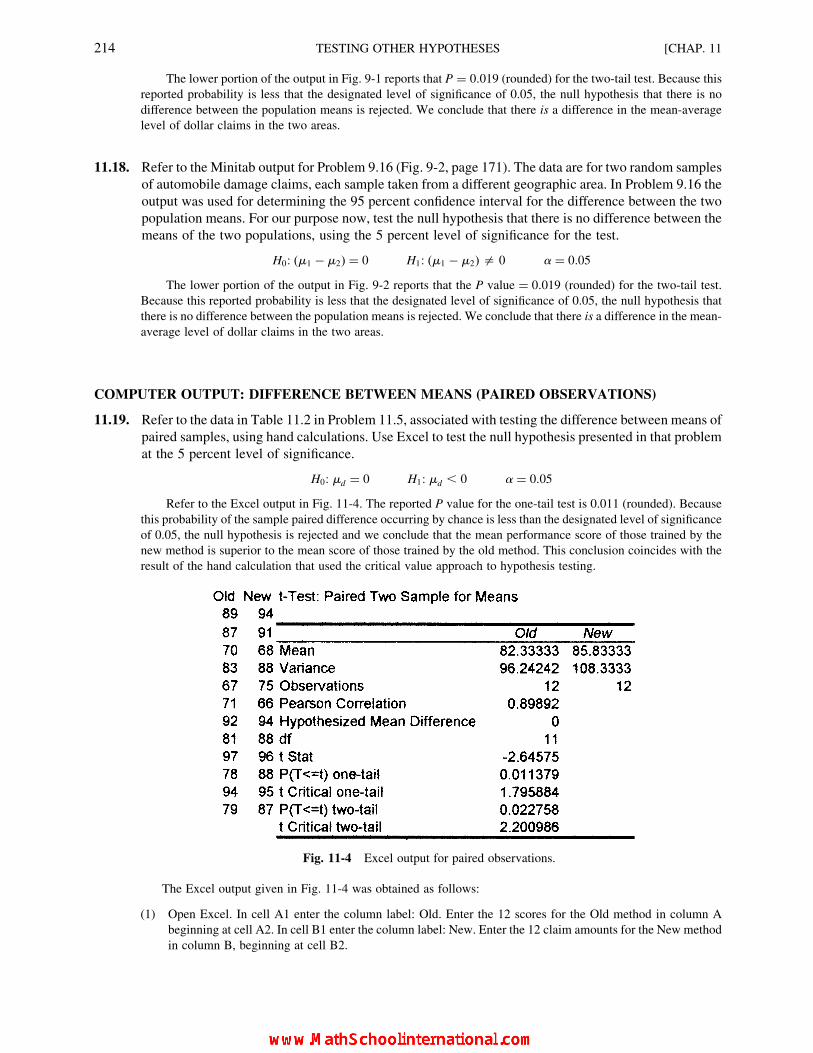
The lower portion of the output in Fig. 9-1 reports that P ¼ 0:019 (rounded) for the two-tail test. Because thisreported probability is less that the designated level of significance of 0.05, the null hypothesis that there is no
difference between the population means is rejected. We conclude that there is a difference in the mean-average
level of dollar claims in the two areas.
11.18. Refer to the Minitab output for Problem 9.16 (Fig. 9-2, page 171). The data are for two random samples
of automobile damage claims, each sample taken from a different geographic area. In Problem 9.16 the
output was used for determining the 95 percent confidence interval for the difference between the two
population means. For our purpose now, test the null hypothesis that there is no difference between the
means of the two populations, using the 5 percent level of significance for the test.
H0: (m1 � m2) ¼ 0 H1: (m1 � m2)= 0 a ¼ 0:05
The lower portion of the output in Fig. 9-2 reports that the P value ¼ 0:019 (rounded) for the two-tail test.
Because this reported probability is less that the designated level of significance of 0.05, the null hypothesis that
there is no difference between the population means is rejected. We conclude that there is a difference in the mean-
average level of dollar claims in the two areas.
COMPUTER OUTPUT: DIFFERENCE BETWEEN MEANS (PAIRED OBSERVATIONS)
11.19. Refer to the data in Table 11.2 in Problem 11.5, associated with testing the difference between means of
paired samples, using hand calculations. Use Excel to test the null hypothesis presented in that problem
at the 5 percent level of significance.
H0: md ¼ 0 H1: md , 0 a ¼ 0:05
Refer to the Excel output in Fig. 11-4. The reported P value for the one-tail test is 0.011 (rounded). Because
this probability of the sample paired difference occurring by chance is less than the designated level of significance
of 0.05, the null hypothesis is rejected and we conclude that the mean performance score of those trained by the
new method is superior to the mean score of those trained by the old method. This conclusion coincides with the
result of the hand calculation that used the critical value approach to hypothesis testing.
The Excel output given in Fig. 11-4 was obtained as follows:
(1) Open Excel. In cell A1 enter the column label: Old. Enter the 12 scores for the Old method in column A
beginning at cell A2. In cell B1 enter the column label: New. Enter the 12 claim amounts for the New method
in column B, beginning at cell B2.
Fig. 11-4 Excel output for paired observations.
214 TESTING OTHER HYPOTHESES [CHAP. 11

(2) Click Tools ! Data Analysis ! t-Test: Paired Two-Sample for Means. Click OK.
(3) In the dialog box designate Variable 1 Range as: $A$1:$A$13. Designate Variable 2 Range as:
$B$1:$B$13.
(4) Set the Hypothesized Mean Difference as: 0. Select the Labels box. Select Alpha as 0.05.
(5) Designate the Output Range as: $C$1.
(6) Click OK.
11.20. Refer to the data in Table 11.2 in Problem 11.5, associated with testing the difference between means of
paired samples, using hand calculations. Use Minitab to test the null hypothesis presented in that
problem at the 5 percent level of significance.
H0: md ¼ 0 H1: md , 0 a ¼ 0:05
Refer to the Minitab output in Fig. 11-5. The reported P value for the one-tail test is 0.011. Because this
probability of the sample paired difference occurring by chance is less than the designated level of significance of
0.05, the null hypothesis is rejected and we conclude that the mean performance score of those trained by the new
method is superior to the mean score of those trained by the old method. This conclusion coincides with the result of
the hand calculation that used the critical value approach to hypothesis testing.
The Minitab output given in Fig. 11-5 was obtained as follows:
(1) Open Minitab. In the column name cell for C1 enter: Old. Enter the 12 scores for the Old method in column
C1. In the column name cell for C2 enter: New. Enter the 12 claim amounts for the New method in column
C2.
(2) Click Stat ! Basic Statistics ! Paired t.
(3) For First sample enter: Old. For Second sample enter: New.
(4) Click Options. Designate Confidence level as: 95.0. Designate Test Mean as: 0.0. For Alternative choose
less than (for a one-tail test). Click OK.
(5) Back in the original dialog box, click OK.
Supplementary Problems
TESTING THE DIFFERENCE BETWEEN TWO MEANS
11.21. As reported in Problem 9.17, for one consumer product the mean dollar sales per retail outlet last year in a sample of
n1 ¼ 10 stores was �XX1 ¼ $3,425 with s1 ¼ $200. For a second product the mean dollar sales per outlet in a sample
of n2 ¼ 12 stores was �XX2 ¼ $3,250 with s2 ¼ $175. The sales amounts per outlet are assumed to be normally
distributed for both products. Test the null hypothesis that there is no difference between the mean dollar sales for
the two products using the 1 percent level of significance.
Ans. Accept H0.
Fig. 11-5 Minitab output for paired observations.
CHAP. 11] TESTING OTHER HYPOTHESES 215
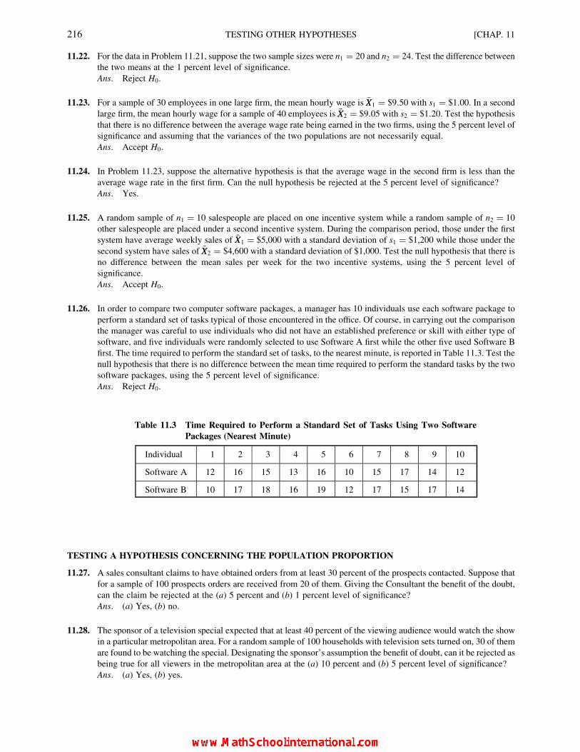
11.22. For the data in Problem 11.21, suppose the two sample sizes were n1 ¼ 20 and n2 ¼ 24. Test the difference between
the two means at the 1 percent level of significance.
Ans. Reject H0.
11.23. For a sample of 30 employees in one large firm, the mean hourly wage is �XX1 ¼ $9:50 with s1 ¼ $1:00. In a second
large firm, the mean hourly wage for a sample of 40 employees is �XX2 ¼ $9:05 with s2 ¼ $1:20. Test the hypothesisthat there is no difference between the average wage rate being earned in the two firms, using the 5 percent level of
significance and assuming that the variances of the two populations are not necessarily equal.
Ans. Accept H0.
11.24. In Problem 11.23, suppose the alternative hypothesis is that the average wage in the second firm is less than the
average wage rate in the first firm. Can the null hypothesis be rejected at the 5 percent level of significance?
Ans. Yes.
11.25. A random sample of n1 ¼ 10 salespeople are placed on one incentive system while a random sample of n2 ¼ 10
other salespeople are placed under a second incentive system. During the comparison period, those under the first
system have average weekly sales of �XX1 ¼ $5,000 with a standard deviation of s1 ¼ $1,200 while those under the
second system have sales of �XX2 ¼ $4,600 with a standard deviation of $1,000. Test the null hypothesis that there is
no difference between the mean sales per week for the two incentive systems, using the 5 percent level of
significance.
Ans. Accept H0.
11.26. In order to compare two computer software packages, a manager has 10 individuals use each software package to
perform a standard set of tasks typical of those encountered in the office. Of course, in carrying out the comparison
the manager was careful to use individuals who did not have an established preference or skill with either type of
software, and five individuals were randomly selected to use Software A first while the other five used Software B
first. The time required to perform the standard set of tasks, to the nearest minute, is reported in Table 11.3. Test the
null hypothesis that there is no difference between the mean time required to perform the standard tasks by the two
software packages, using the 5 percent level of significance.
Ans. Reject H0.
TESTING A HYPOTHESIS CONCERNING THE POPULATION PROPORTION
11.27. A sales consultant claims to have obtained orders from at least 30 percent of the prospects contacted. Suppose that
for a sample of 100 prospects orders are received from 20 of them. Giving the Consultant the benefit of the doubt,
can the claim be rejected at the (a) 5 percent and (b) 1 percent level of significance?
Ans. (a) Yes, (b) no.
11.28. The sponsor of a television special expected that at least 40 percent of the viewing audience would watch the show
in a particular metropolitan area. For a random sample of 100 households with television sets turned on, 30 of them
are found to be watching the special. Designating the sponsor’s assumption the benefit of doubt, can it be rejected as
being true for all viewers in the metropolitan area at the (a) 10 percent and (b) 5 percent level of significance?
Ans. (a) Yes, (b) yes.
Table 11.3 Time Required to Perform a Standard Set of Tasks Using Two Software
Packages (Nearest Minute)
Individual 1 2 3 4 5 6 7 8 9 10
Software A 12 16 15 13 16 10 15 17 14 12
Software B 10 17 18 16 19 12 17 15 17 14
216 TESTING OTHER HYPOTHESES [CHAP. 11

11.29. For Problem 11.28, suppose the sponsor specifies that as the result of the study the probability of rejecting a true
claim should be no larger than P ¼ 0:02, and the probability of accepting the claim given that the percentage
viewing the program is actually 30 percent or less should be no larger than P ¼ 0:05. What sample size is required
in the study, as a minimum, to satisfy this requirement?
Ans. 311 households.
11.30. For Problem 11.28, it was suggested that the program might appeal differently to urban versus suburban residents,
but there was a difference of opinion among the production staff regarding the direction of the difference. For a
random sample of 50 urban households, 20 reported watching the program. For a random sample of 50 suburban
households, 30 reported watching the program. Can the difference be considered significant at the (a) 10 percent
and (b) 5 percent level?
Ans. (a) Yes, (b) yes.
TESTING A HYPOTHESIZED VALUE OF THE VARIANCE AND THE EQUALITY OF
TWO VARIANCES
11.31. Based on the specifications provided by the process designer, the standard deviation of casting diameters
is hypothesized to be no larger than 3.0mm. For a sample of n ¼ 12 castings, the sample standard deviation is
s ¼ 4:2mm. The distribution of the diameters is assumed to be approximately normal. Can the null hypothesis that
the true standard deviation is no larger than 3.0mm be rejected at the (a) 5 percent and (b) 1 percent level of
significance?
Ans. (a) Yes, (b) no.
11.32. In Problem 11.21, under the necessary assumption that the variances of the two populations are equal, the null
hypothesis that the means are equal could not be rejected using the t test at the 1 percent level of significance. At the
10 percent level of significance, is the assumption that the two variances are not different warranted?
Ans. Yes.
11.33. A new molding process is designed to reduce the variability of casting diameters. To test the new process, we
conservatively formulate the alternative hypothesis that the variance of casting diameters under the new process is
less than the variance for the old process. Rejection of the null hypothesis would then permit us to accept the
alternative hypothesis that the variance associated with the new process is smaller than that associated with the old
process. For a sample of n1 ¼ 8 castings produced by the new process s1 ¼ 4:2mm. For a sample of n2 ¼ 10
castings produced by the old process s2 ¼ 5:8mm. Can the null hypothesis be rejected at the 5 percent level of
significance?
Ans. No.
ALTERNATIVE APPROACHES TO TESTING NULL HYPOTHESES
11.34. Using the P-value approach, test the null hypothesis in Problem 11.23 at the 5 percent level of significance.
Ans. Accept H0 (P ¼ 0:0836).
11.35. Using the P-value approach, test the null hypothesis in Problem 11.24 at the 5 percent level of significance.
Ans. Reject H0 (P ¼ 0:0418).
11.36. Apply the confidence interval approach to testing the null hypothesis in Problem 11.23, using the 5 percent level of
significance.
Ans. Accept H0.
11.37. Apply the confidence interval approach to testing the null hypothesis in Problem 11.24, using the 5 percent level of
significance.
Ans. Reject H0.
CHAP. 11] TESTING OTHER HYPOTHESES 217

COMPUTER OUTPUT
11.38. Refer to the data in Table 9.2, which was used to obtain the 95 percent confidence interval for the difference between
means in Problem 9.33. Using available computer software, test the null hypothesis that the mean amount of per-
item time does not differ for the two types of calls, using the 5 percent level of significance.
Ans. Accept H0 (P ¼ 0:42).
11.39. Refer to the data in Table 11.3, concerned with the time required to perform a standard set of tasks using two
different software packages. The null hypothesis that there is no difference between the average time required for
the two packages was tested in Problem 11.26. Using available computer software, again test this hypothesis at the 5
percent level of significance.
Ans. Reject H0 (P ¼ 0:038).
218 TESTING OTHER HYPOTHESES [CHAP. 11

CHAPTER 12
The Chi-Square Testfor the Analysis of
Qualitative Data
12.1 GENERAL PURPOSE OF THE CHI-SQUARE TEST
The procedures that are described in this chapter all involve the comparison of the observed pattern of the
frequencies of observations for sample data have been entered into defined data catagories, with the expected
pattern of frequencies based on a particular null hypothesis.
Use of the x 2 (chi-square) probability distribution with respect to statistical inference concerning the
population variance is described in Sections 9.6 and 11.8. The test statistic presented in the following sections
also is distributed as the chi-square probability model, and since hypothesis testing is involved, the basic steps
in hypothesis testing described in Section 10.2 apply in this chapter as well.
This chapter covers the use of the chi-square test for testing the goodness of fit, testing the independence of
two variables, and testing hypotheses concerning proportions. One of the tests of proportions is that of testing
the differences among several population proportions, which is an extension of testing the difference between
two population proportions, as described in Section 11.7.
12.2 GOODNESS OF FIT TESTS
The null hypothesis in a goodness of fit test is a stipulation concerning the expected pattern of frequencies
in a set of categories. The expected pattern may conform to the assumption of equal likelihood and may
therefore be uniform, or the expected pattern may conform to such patterns as the binomial, Poisson, or normal.
EXAMPLE 1. A regional distributor of air-conditioning systems has subdivided the region into four territories. A
prospective purchaser of the distributionship is told that installations of the equipment are about equally distributed among
the four territories. The prospective purchaser takes a random sample of 40 installations performed during the past year from
219
Copyright 2004, 1996, 1988, 1976 by The McGraw-Hill Companies, Inc. Click Here for Terms of Use.

the company’s files, and finds that the number installed in each of the four territories is as listed in the first row of Table 12.1
(where fo means “observed frequency”). On the basis of the hypothesis that installations are equally distributed, the expected
uniform distribution of the installations is given in the second row of Table 12.1 (where fe means “expected frequency”).
For the null hypothesis to be accepted, the differences between observed and expected frequencies must be
attributable to sampling variability at the designated level of significance. Thus, the chi-square test statistic is
based on the magnitude of this difference for each category in the frequency distribution.
The chi-square value for testing the difference between an obtained and expected pattern of frequencies is
x 2 ¼X ( fo � fe)
2
fe(12:1)
By Formula (12.1) above, note that if the observed frequencies are very close to the expected frequencies,
then the calculated value of the chi-square statistic will be close to zero. As the observed frequencies become
increasingly different from the expected frequencies, the value of chi-square becomes larger. Therefore it
follows that the chi-square test involves the use of just the upper tail of the chi-square distribution to determine
whether an observed pattern of frequencies is different from an expected pattern.
EXAMPLE 2. The calculation of the chi-square test statistic for the pattern of observed and expected frequencies in Table
12.1 is as follows:
x 2 ¼X ( fo � fe)
2
fe
¼ (6� 10)2
10þ (12� 10)2
10þ (14� 10)2
10þ (8� 10)2
10¼ 40
10¼ 4:00
The required value of the chi-square test statistic to reject the null hypothesis depends on the level of
significance that is specified and the degrees of freedom. In goodness of fit tests, the degrees of freedom df are
equal to the number of categories minus the number of parameter estimators based on the sample and minus
1. Where k ¼ number of categories of data and m ¼ number of parameter values estimated on the basis of the
sample, the degrees of freedom in a chi-square goodness of fit test are
d f ¼ k � m � 1 (12:2)
When the null hypothesis is that the frequencies are equally distributed, no parameter estimation is ever
involved and m ¼ 0. (Examples in which m is greater than zero are provided in Problems 12.6 and 12.8.) The
subtraction of 1 is always included, because given a total number of observations, once observed frequencies
have been entered in k 2 1 categories of a table of frequencies, the last cell is in fact not free to vary.
For instance, given that the first three categories in Table 12.1 have observed frequencies of 6, 12, and 14,
respectively, it follows that the fourth category must have a frequency of 8 in order to cumulate to the
designated sample size of n ¼ 40.
Table 12.1 Number of Installations of Air-Conditioning Systems According
to Territory
Territory
A B C D Total
Number installed in sample, fo 6 12 14 8 40
Expected number of installations, fe 10 10 10 10 40
220 THE CHI-SQUARE TEST [CHAP. 12

EXAMPLE 3. Following is a complete presentation of the hypothesis testing procedure associated with the data in Table
12.1, with the null hypothesis being tested at the 5 percent level of significance.
H0: The number of installations is uniformly distributed among the four territories.
H1: The number of installations is not uniformly distributed among the four territories.
d f ¼ k � m � 1 ¼ 4� 0� 1 ¼ 3
Critical x 2(d f ¼ 3, a ¼ 0:05) ¼ 7:81 (from Appendix 7)
Computed x 2 ¼ 4:00 (from Example 2)
Because the calculated value of chi-square of 4.00 is not greater than the critical value of 7.81, the null hypothesis that
the installations are equally distributed among the four territories cannot be rejected at the 5 percent level of significance.
Computed values of the chi-square test statistic are based on discrete counts, whereas the chi-square
distribution is a continuous distribution. When the expected frequencies fe for the cells are not small, this factor
is not important in terms of the extent to which the distribution of the test statistic is approximated by the chi-
square distribution. A frequently used rule is that the expected frequency fe for each cell, or category, should be
at least 5. Cells that do not meet this criterion should be combined with adjacent categories, when possible, so
that this requirement is satisfied. The reduced number of categories then becomes the basis for determining the
degrees of freedom df applicable in the test situation. See Problems 12.6 and 12.8. The expected frequencies for
all cells of a data table also can be increased by increasing the overall sample size. Compare the expected
frequencies in Problems 12.1 and 12.3.
The expected frequencies may be based on any hypothesis regarding the form of the population
frequency distribution. If the hypothesis is based on the observed historical pattern of frequencies, then, as
in the case of the equally likely hypothesis, no parameter estimation is involved, and df ¼ k � m � 1 ¼k � 0� 1 ¼ k � 1.
EXAMPLE 4. Historically, a manufacturer of TV sets has had 40 percent of sales in small-screen sets (under 20in), 40
percent in the mid-range sizes (20in to 27in), and 20 percent in the large-screen category (above 27in). In order to ascertain
appropriate production schedules for the next month, a random sample of 100 purchases during the current period is taken
and it is found that 55 of the sets purchased were small, 35 were middle-sized, and 10 were large. Below we test the null
hypothesis that the historical pattern of sales still prevails, using the 1 percent level of significance.
H0: The percentages of all purchases in the small-, medium-, and large-screen categories of TV sets
are 40 percent, 40 percent, and 20 percent, respectively.
H1: The present pattern of TV set purchases is different from the historical pattern in H0:
d f ¼ k � m � 1 ¼ 3� 0� 1 ¼ 2
Critical x 2(d f ¼ 2, a ¼ 0:01) ¼ 9:21
Computed x 2 (see Table 12.2 for observed and expected frequencies):
x 2 ¼X ( fo � fe)
2
fe
¼ (55� 40)2
40þ (35� 40)2
40þ (10� 20)2
20¼ 11:25
The calculated chi-square statistic of 11.25 is greater than the critical value of 9.21. Therefore, the null hypothesis is
rejected at the 1 percent level of significance. Comparing the obtained and expected frequencies in Table 12.2, we find that
the principal change involves more small sets and fewer large sets being sold, with some reduction in middle-sized sets also
possibly occurring.
Table 12.2 Observed and Expected Purchases of TV Sets by Screen Size
Screen size
Small Medium Large Total
Observed frequency, fo 55 35 10 100
Historical pattern, fe 40 40 20 100
CHAP. 12] THE CHI-SQUARE TEST 221

12.3 TESTS FOR THE INDEPENDENCE OF TWO CATEGORICAL VARIABLES
(CONTINGENCY TABLE TESTS)
In the case of goodness of fit tests, there is only one categorical variable, such as the screen size of TV sets
that have been sold, and what is tested is a hypothesis concerning the pattern of frequencies, or the distribution,
of the variable. The observed frequencies can be listed as a single row, or as a single column, of categories.
Tests for independence involve (at least) two categorical variables, and what is tested is the assumption that the
variables are statistically independent. Independence implies that knowledge of the category in which an
observation is classified with respect to one variable has no affect on the probability of the other variable being
in one of the several categories. When two variables are involved, the observed frequencies are entered in a two-
way classification table, or contingency table (see Section 5.8). The dimensions of such tables are defined by
r � k, in which r indicates the number of rows and k indicates the number of columns.
EXAMPLE 5. Table 12.3 is repeated from Section 5.8 and is an example of the simplest possible format for a contingency
table, in that each of the two variables (sex and age) has only two classification levels, or categories. Thus, this is a 2� 2
contingency table.
If the null hypothesis of independence is rejected for classified data such as in Table 12.3, this indicates that
the two variables are dependent and that there is a relationship between them. For Table 12.3, for instance, this
would indicate that there is a relationship between age and the sex of stereo shop customers.
Given the hypothesis of independence of the two variables, the expected frequency associated with each
cell of a contingency table should be proportionate to the total observed frequencies included in the column and
in the row in which the cell is located as related to the total sample size. Where fr is the total frequency in a
given row and fk is the total frequency in a given column, a convenient formula for determining the expected
frequency for the cell of the contingency table that is located in that row and column is
fe ¼ frfk
n(12:3)
The general formula for the degrees of freedom associated with a test for independence is
d f ¼ (r � 1)(k � 1) (12:4)
EXAMPLE 6. The expected frequencies for the data of Table 12.3 are reported in Table 12.4. For row 1, column 1, for
instance, the calculation of the expected frequency is
fe ¼ fr fk
n¼ (110)(140)
200¼ 15,400
200¼ 77
Note that in this case the three remaining expected frequencies can be obtained by subtraction from row and column
totals, as an alternative to using (12.3). This is a direct indication that there is one degree of freedom for a 2� 2 contingency
table, and that only one cell frequency is free to vary.
Table 12.3 Contingency Table for Stereo Shop
Customers
Sex
Age Male Female Total
Under 30 60 50 110
30 and over 80 10 90
Total 140 60 200
222 THE CHI-SQUARE TEST [CHAP. 12

The chi-square test statistic for contingency tables is computed exactly as for the goodness of fit tests
(see Section 12.2).
EXAMPLE 7. Following is the test of the null hypothesis of independence for the data of Table 12.3, using the 1 percent
level of significance.
H0: Sex and age of stereo shop customers are independent.
H1: Sex and age are dependent variables (there is a relationship between the variables).
df ¼ (r � 1)(k � 1) ¼ (2� 1)(2� 1) ¼ 1
Critical x 2(d f ¼ 1, a ¼ 0:01) ¼ 6:63
x2 ¼P ( fo � fe)2
fe¼ (60� 77)2
77þ (50� 33)2
33þ (80� 63)2
63þ (10� 27)2
27¼ 27:80
The calculated test statistic of 27.80 exceeds the required critical value of 6.63. Therefore, the null hypothesis of
independence is rejected at the 1 percent level of significance. Referring to Table 12.3, we see that male customers are more
likely to be over 30 years of age while female customers are more likely to be under 30. The result of the chi-square test
indicates that this observed relationship in the sample cannot be ascribed to chance at the 1 percent level of significance.
12.4 TESTING HYPOTHESES CONCERNING PROPORTIONS
Testing a Hypothesized Value of the Proportion. Given a hypothesized population proportion and an
observed proportion for a random sample taken from the population, in Section 11.4 we used the normal
probability distribution as an approximation for the binomial process in order to test the null hypothesis.
Mathematically it can be shown that such a two-sided test is equivalent to a chi-square goodness of fit test
involving one row of frequencies and two categories (a 1 � 2 table). Since the chi-square test involves an
analysis of differences between obtained and expected frequencies regardless of the direction of the differences,
there is no chi-square test procedure that is the equivalent of a one-sided test concerning the value of a
population proportion.
EXAMPLE 8. A personnel department manager estimates that a proportion of p ¼ 0:40 of the employees in a large firm
will participate in a new stock investment program. A random sample of n ¼ 50 employees is contacted, and 10 indicate
their intention to participate. The hypothesized value of the population proportion could be tested using the normal
probability distribution, as described in Section 11.4. Following is the use of the chi-square test to accomplish the same
objective, using the 5 percent level of significance.
H0: p ¼ 0:40 H1: p = 0:40
d f ¼ k � m � 1 ¼ 2� 0� 1 ¼ 1
(There are two categories of observed frequencies, as indicated in Table 12.5.)
Table 12.4 Table of Expected Frequencies for
the Observed Frequencies Reported
in Table 12.3
Sex
Age Male Female Total
Under 30 77 33 110
30 and over 63 27 90
Total 140 60 200
CHAP. 12] THE CHI-SQUARE TEST 223

Critical x 2(d f ¼ 1, v ¼ 0:05) ¼ 3:84
Computed x 2 (Table 12.5 indicates the observed and expected frequencies):
x 2 ¼X ( fo � fe)
2
fe
¼ (10� 20)2
20þ (40� 30)2
30¼ 8:33
The calculated test statistic of 8.33 exceeds the critical value of 3.84. Therefore, the null hypothesis is rejected at the 5
percent level of significance, and we conclude that the proportion of program participants in the entire firm is not 0.40.
Testing the Difference between Two Population Proportions. A procedure for testing the null hypothesis
that there is no difference between two proportions based on use of the normal probability distribution is
presented in Section 11.7. Mathematically, it can be shown that such a two-tail test is equivalent to a chi-square
contingency table test in which the observed frequencies are entered in a 2 � 2 table. Again, there is no chi-
square test equivalent to a one-sided test based on use of the normal probability distribution.
The sampling procedure used in conjunction with testing the difference between two proportions is that two
random samples are collected, one for each of the two (k) categories. This contrasts with use of a 2 � 2 table for
testing the independence of two variables in Section 12.3, in which one random sample is collected for the
overall analysis.
EXAMPLE 9. Example 8 in Section 11.7 reports that 10 out of 50 households in one community watched a TV special on
the national economy and 15 out of 50 households in a second community watched the TV special. In that example the null
hypothesis H0: (p1 � p2) ¼ 0 or, equivalently, H0: p1 ¼ p 2 is tested at the 1 percent level of significance. Below is the
equivalent test using the chi-square test statistic.
H0: p1 ¼ p 2 H1: p1 = p1
d f ¼ (r � 1)(k � 1) ¼ (2� 1)(2� 1) ¼ 1
(The observed frequencies are entered in a 2 � 2 table, as indicated in Table 12.6.)
Critical x 2(d f ¼ 1, a ¼ 0:01) ¼ 6:63
Computed x 2 (The observed frequencies are presented in Table 12.6 while the expected frequencies, calculated by formula
(12.3), are presented in Table 12.7):
x 2 ¼X ( fo � fe)
2
fe¼ (10� 12:5)2
12:5þ (15� 12:5)2
12:5þ (40� 37:5)2
37:5þ (35� 37:5)2
37:5¼ 1:34
Table 12.5 Observed and Expected Frequencies for Example 8
Participation in program
Yes No Total
Number observed in sample, fo 10 40 50
Number expected in sample, fe 20 30 50
Table 12.6 Extent of TV Program Viewing in Two Communities
Communities
Community 1 Community 2 Total
Number watching 10 15 25
Number not watching 40 35 75
Total 50 50 100
224 THE CHI-SQUARE TEST [CHAP. 12

The calculated test statistic of 1.34 is not greater than the critical value of 6.63. Therefore, the null hypothesis cannot be
rejected at the 1 percent level of significance, and we conclude that the proportion of viewers in the two communities may
not differ. This is the same conclusion as in Section 11.7, using the z statistic.
Testing the Differences among Several Population Proportions. Given the basic approach in Example 9,
the chi-square test can be used to test the differences among several (k) population proportions by using a 2� k
tabular design for the analysis of the frequencies. In this case, there is no mathematically equivalent procedure
based on use of the z statistic. The null hypothesis is that the several population proportions are all mutually
equal (or, that the several different sample proportions could have been obtained by chance from the same
population). The sampling procedure is that several independent random samples are collected, one for each of
the k data categories.
EXAMPLE 10. From Example 9, suppose households in four communities are sampled in regard to the number viewing a
TV special on the national economy. Table 12.8 presents the observed sample data while Table 12.9 presents the expected
frequencies, based on Formula (12.3). The test of the null hypothesis that there are no differences among the population
proportions, using the 1 percent level of significance, follows.
H0: p1 ¼ p 2 ¼ p3 ¼ p4 H1: Not all p1 ¼ p 2 ¼ p3 ¼ p4:
(Note: Rejection of the null hypothesis does not indicate that all of the equalities are untrue, but only that at least one
equality is untrue.)
d f ¼ (r � 1)(k � 1) ¼ (2� 1)(4� 1) ¼ 3
Critical x 2(d f ¼ 3, a ¼ 0:01) ¼ 11:35
x 2 ¼X ( fo � fe)
2
fe
¼ (10� 12)2
12þ (15� 12)2
12þ (5� 12)2
12þ (18� 12)2
12
þ (40� 38)2
38þ (35� 38)2
38þ (45� 38)2
38þ (32� 38)2
38
¼ 0:33þ 0:75þ 4:08þ 3:0þ 0:11þ 0:24þ 1:29þ 0:95 ¼ 10:75
Table 12.7 Expected Frequencies for the Data of Table 12.6
Communities
Community 1 Community 2 Total
Number watching 12.5 12.5 25
Number not watching 37.5 37.5 75
Total 50 50 100
Table 12.8 Extent of TV Program Viewing in Four Communities
Communities
1 2 3 4 Total
Number watching 10 15 5 18 48
Number not watching 40 35 45 32 152
Total 50 50 50 50 200
CHAP. 12] THE CHI-SQUARE TEST 225

The calculated chi-square statistic of 10.75 is not greater than the critical value of 11.35. Therefore the differences in
the proportion of viewers among the four sampled communities are not large enough to reject the null hypothesis at the 1
percent level of significance. It is plausible that the proportions of the viewers in the several communities are the same, and
do not differ.
12.5 USING COMPUTER SOFTWARE
Computer software for statistical analysis generally includes the capability of carrying out both goodness
of fit tests and contingency table tests. For goodness of fit tests, both the observed frequencies and the expected
frequencies usually have to be input for the analysis. The expected frequencies have to be input because they are
based on the particular null hypothesis to be tested. For contingency table tests the expected frequencies are
determined directly from the sample data. Therefore, such tests require input only of the observed frequencies
in order to carry out the test. As explained in Sections 12.3 and 12.4, contingency table tests can be used for
testing the independence of two categorical variables or for testing hypotheses concerning the equality of two or
more population proportions. Excel requires a rather complex combination of procedures to carry out chi-
square tests. Therefore, Solved Problem 12.15 illustrates only the use of Minitab.
Solved Problems
GOODNESS OF FIT TESTS
12.1. It is claimed that an equal number of men and women patronize a retail outlet specializing in the sale of
jeans. A random sample of 40 customers is observed, with 25 being men and 15 being women. Test the
null hypothesis that the overall number of men and women customers is equal by applying the chi-
square test and using the 5 percent level of significance.
From Table 12.10,
H0: The number of men and women customers is equal (the pattern of frequencies is uniform).
H1: The number of men and women customers is not equal.
d f ¼ k � m � 1 ¼ 2� 0� 1 ¼ 1
Critical x 2(d f ¼ 1, a ¼ 0:05) ¼ 3:84
x 2 ¼X ( fo � fe)
2
fe¼ (25� 20)2
20þ (15� 20)2
20
¼ (5)2
20þ (�5)2
20¼ 2:50
The calculated test statistic of 2.50 is not greater than the critical value of 3.84. Therefore, the null hypothesis
cannot be rejected at the 5 percent level of significance.
Table 12.9 Expected Frequencies for the Data of Table 12.8
Communities
1 2 3 4 Total
Number watching 12.0 12.0 12.0 12.0 48
Number not watching 38.0 38.0 38.0 38.0 152
Total 50 50 50 50 200
226 THE CHI-SQUARE TEST [CHAP. 12

12.2. With reference to Problem 12.1, suppose it had instead been claimed that twice as many men as
compared with women were store customers. Using the observed data in Table 12.11, test this
hypothesis using the 5 percent level of significance.
From Table 12.11
H0: There are twice as many men as there are women customers.
H1: There are not twice as many men as women customers.
d f ¼ k � m � 1 ¼ 2� 0� 1 ¼ 1
Critical x 2(d f ¼ 1, a ¼ 0:05) ¼ 3:84
x 2 ¼X ( fo � fe)
2
fe¼ (25� 26:67)2
26:67þ (15� 13:33)2
13:33
¼ (�1:67)2
26:67þ (1:67)
2
13:33¼ 0:10þ 0:21 ¼ 0:31
The calculated chi-square statistic of 0.31 clearly does not exceed the critical value of 3.84. Therefore, the null
hypothesis cannot be rejected at the 5 percent level of significance. The fact that neither of the null hypotheses in
Problems 12.1 and 12.2 could be rejected demonstrates the benefit of the doubt given to the null hypothesis in each
case. However, the size of the sample also affects the probability of sample results (see Problem 12.3).
12.3. For the situation described in Problem 12.1, suppose the same null hypothesis is tested, but that the
sample frequencies in each category are exactly doubled. That is, of 80 randomly selected customers 50
are men and 30 are women. Test the null hypothesis at the 5 percent level of significance and compare
your decision with the one in Problem 12.1.
From Table 12.12,
H0: The number of men and women customers is equal.
H1: The number of men and women customers is not equal.
d f ¼ k � m � 1 ¼ 2� 0� 1 ¼ 1
Critical x 2(d f ¼ 1, a ¼ 0:05) ¼ 3:84
x 2 ¼X ( fo � fe)
2
fe¼ (50� 40)2
40þ (30� 40)2
40¼ 5:00
The calculated chi-square value of 5.00 is greater than the critical value of 3.84. Therefore, the null hypothesis
is rejected at the 5 percent level of significance. Even though the sample data are proportionally the same as in
Problem 12.1, the decision now is reject H0 instead of accept H0. This demonstrates the greater sensitivity of a
statistical test associated with a larger sample size.
Table 12.10 Obtained and Expected Frequencies for Problem 12.1
Customers
Men Women Total
Number in sample ( fo) 25 15 40
Number expected ( fe) 20 20 40
Table 12.11 Obtained and Expected Frequencies for Problem 12.2
Customers
Men Women Total
Number in sample ( fo) 25 15 40
Number expected ( fe) 26.67 13.33 40
CHAP. 12] THE CHI-SQUARE TEST 227

12.4. A manufacturer of refrigerators offers three basic product lines, which can be described as being low,
intermediate, and high in terms of comparative price. Before a sales promotion aimed at highlighting the
virtues of the high-priced refrigerators, the percentage of sales in the three categories was 45, 30, and 25,
respectively. Of a random sample of 50 refrigerators sold after the promotion, the number sold in the
low-, intermediate-, and high-priced categories is 15, 15, and 20, respectively. Test the null hypothesis
that the current pattern of sales does not differ from the historical pattern, using the 5 percent level of
significance.
With reference to Table 12.13,
H0: The present pattern of sales frequencies follows the historical pattern.
H1: The present pattern of sales frequencies is different from the historical pattern.
d f ¼ k � m � 1 ¼ 3� 0� 1 ¼ 2
Critical x 2(d f ¼ 2, a ¼ 0:05) ¼ 5:99
x 2 ¼X ( fo � fe)
2
fe
¼ (15� 22:5)2
22:5þ (15� 15)2
15þ (20� 12:5)2
12:5
¼ (�7:5)2
22:5þ (0)
2
15þ (7:5)
2
12:5¼ 7:00
The calculated value of the test statistic of 7.00 is greater than the critical value of 5.99. Therefore, the null
hypothesis is rejected at the 5 percent level of significance. Although such rejection does not itself indicate in what
respect the present pattern of sales differs from the historical pattern, a review of Table 12.13 indicates that more
high-priced and fewer low-priced refrigerators were sold than would be expected in terms of the historical pattern
of sales.
12.5. Any probability model can serve as the basis for determining the expected frequencies associated with a
goodness of fit test (see Section 12.2). Suppose it is hypothesized that the distribution of machine
breakdowns per hour in any assembly plant conforms to a Poisson probability distribution, as described
in Section 6.6. However, the particular Poisson distribution as determined by the mean of the
distribution, l, is not specified. Table 12.14 presents the observed number of breakdowns during 40
sampled hours.
Table 12.12 Obtained and Expected Frequencies for Problem 12.3
Customers
Men Women Total
Number in sample ( fo) 50 30 80
Number expected ( fe) 40 40 80
Table 12.13 Obtained and Expected Frequencies for Problem 12.4
Price category of refrigerator
Low Intermediate High Total
Number sold ( fo) 15 15 20 50
Number expected to
be sold ( fe)
22.5 15 12.5 50
228 THE CHI-SQUARE TEST [CHAP. 12
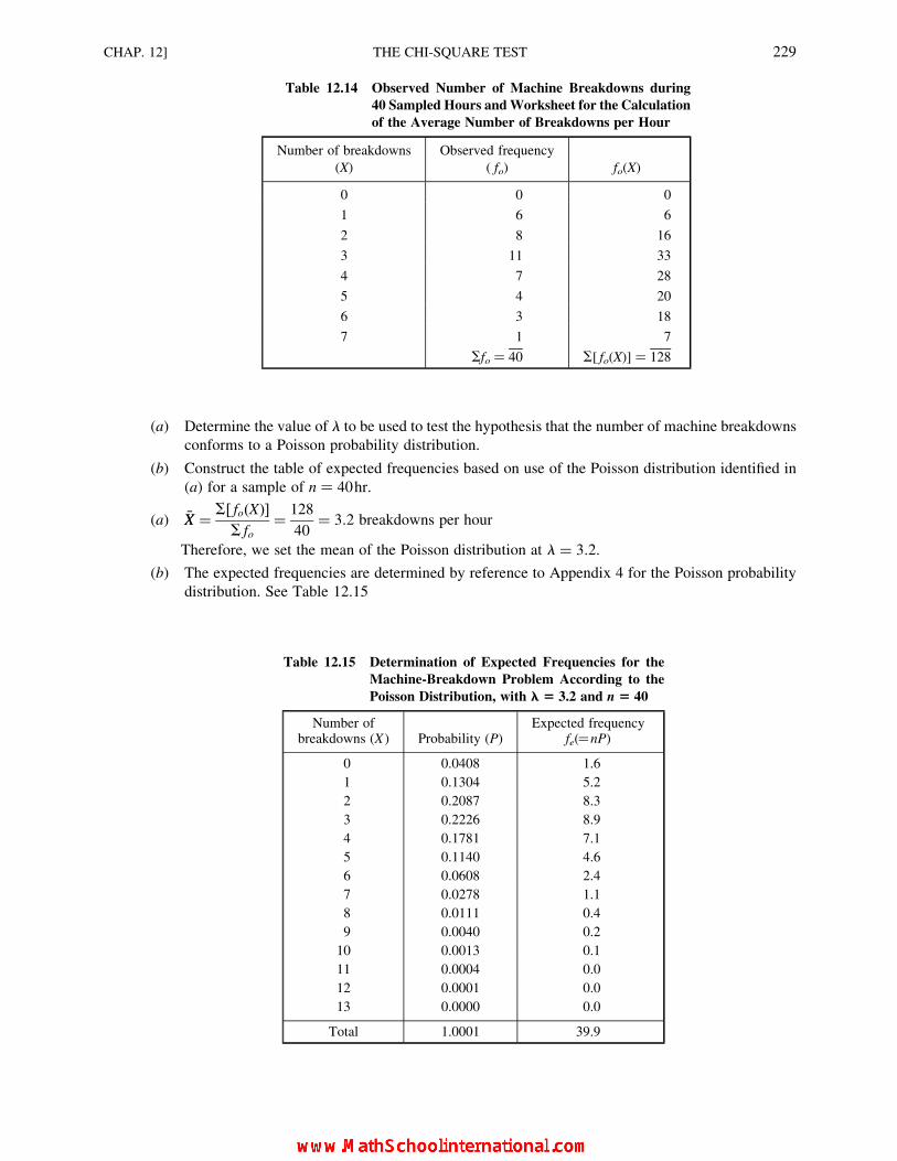
(a) Determine the value of l to be used to test the hypothesis that the number of machine breakdowns
conforms to a Poisson probability distribution.
(b) Construct the table of expected frequencies based on use of the Poisson distribution identified in
(a) for a sample of n ¼ 40hr.
(a) �XX ¼ S[ fo(X)]
S fo
¼ 128
40¼ 3:2 breakdowns per hour
Therefore, we set the mean of the Poisson distribution at l ¼ 3:2.
(b) The expected frequencies are determined by reference to Appendix 4 for the Poisson probability
distribution. See Table 12.15
Table 12.14 Observed Number of Machine Breakdowns during
40 Sampled Hours and Worksheet for the Calculation
of the Average Number of Breakdowns per Hour
Number of breakdowns
(X)
Observed frequency
( fo) fo(X)
0 0 0
1 6 6
2 8 16
3 11 33
4 7 28
5 4 20
6 3 18
7 1 7
Sfo ¼ 40 S[ fo(X)] ¼ 128
Table 12.15 Determination of Expected Frequencies for the
Machine-Breakdown Problem According to the
Poisson Distribution, with l 5 3.2 and n 5 40
Number ofbreakdowns (X ) Probability (P)
Expected frequencyfe(¼nP)
0 0.0408 1.6
1 0.1304 5.2
2 0.2087 8.3
3 0.2226 8.9
4 0.1781 7.1
5 0.1140 4.6
6 0.0608 2.4
7 0.0278 1.1
8 0.0111 0.4
9 0.0040 0.2
10 0.0013 0.1
11 0.0004 0.0
12 0.0001 0.0
13 0.0000 0.0
Total 1.0001 39.9
CHAP. 12] THE CHI-SQUARE TEST 229
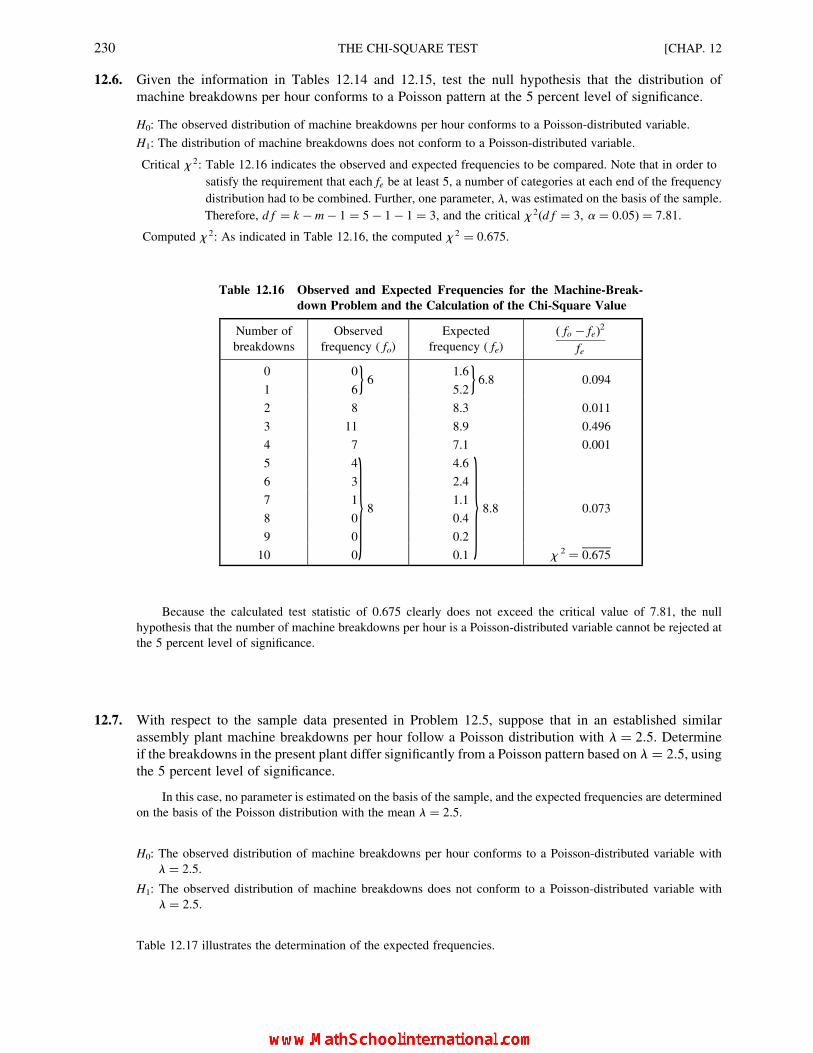
12.6. Given the information in Tables 12.14 and 12.15, test the null hypothesis that the distribution of
machine breakdowns per hour conforms to a Poisson pattern at the 5 percent level of significance.
H0: The observed distribution of machine breakdowns per hour conforms to a Poisson-distributed variable.
H1: The distribution of machine breakdowns does not conform to a Poisson-distributed variable.
Critical x 2: Table 12.16 indicates the observed and expected frequencies to be compared. Note that in order to
satisfy the requirement that each fe be at least 5, a number of categories at each end of the frequency
distribution had to be combined. Further, one parameter, l, was estimated on the basis of the sample.
Therefore, d f ¼ k � m � 1 ¼ 5� 1� 1 ¼ 3, and the critical x 2(d f ¼ 3, a ¼ 0:05) ¼ 7:81.
Computed x 2: As indicated in Table 12.16, the computed x 2 ¼ 0:675.
Because the calculated test statistic of 0.675 clearly does not exceed the critical value of 7.81, the null
hypothesis that the number of machine breakdowns per hour is a Poisson-distributed variable cannot be rejected at
the 5 percent level of significance.
12.7. With respect to the sample data presented in Problem 12.5, suppose that in an established similar
assembly plant machine breakdowns per hour follow a Poisson distribution with l ¼ 2:5. Determine
if the breakdowns in the present plant differ significantly from a Poisson pattern based on l ¼ 2:5, usingthe 5 percent level of significance.
In this case, no parameter is estimated on the basis of the sample, and the expected frequencies are determined
on the basis of the Poisson distribution with the mean l ¼ 2:5.
H0: The observed distribution of machine breakdowns per hour conforms to a Poisson-distributed variable with
l ¼ 2:5.
H1: The observed distribution of machine breakdowns does not conform to a Poisson-distributed variable with
l ¼ 2:5.
Table 12.17 illustrates the determination of the expected frequencies.
Table 12.16 Observed and Expected Frequencies for the Machine-Break-
down Problem and the Calculation of the Chi-Square Value
Number of
breakdowns
Observed
frequency ( fo)
Expected
frequency ( fe)
( fo � fe)2
fe
0 06g 1.6
6.8g 0.0941 6 5.2
2 8 8.3 0.011
3 11 8.9 0.496
4 7 7.1 0.001
5 4 4.6
6 3 2.4
7 18
1.18.8g 0.073
8 0g 0.4
9 0 0.2
10 0 0.1 x 2 ¼ 0.675
230 THE CHI-SQUARE TEST [CHAP. 12
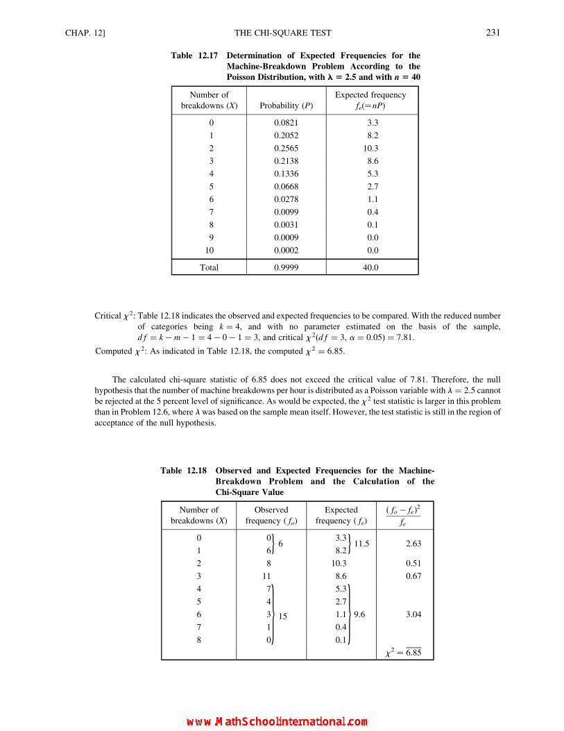
Critical x 2: Table 12.18 indicates the observed and expected frequencies to be compared. With the reduced number
of categories being k ¼ 4, and with no parameter estimated on the basis of the sample,
d f ¼ k � m � 1 ¼ 4� 0� 1 ¼ 3, and critical x 2(d f ¼ 3, a ¼ 0:05) ¼ 7:81.
Computed x 2: As indicated in Table 12.18, the computed x 2 ¼ 6:85.
The calculated chi-square statistic of 6.85 does not exceed the critical value of 7.81. Therefore, the null
hypothesis that the number of machine breakdowns per hour is distributed as a Poisson variable with l ¼ 2:5 cannotbe rejected at the 5 percent level of significance. As would be expected, the x 2 test statistic is larger in this problem
than in Problem 12.6, where lwas based on the sample mean itself. However, the test statistic is still in the region of
acceptance of the null hypothesis.
Table 12.17 Determination of Expected Frequencies for the
Machine-Breakdown Problem According to the
Poisson Distribution, with l 5 2.5 and with n 5 40
Number of
breakdowns (X) Probability (P)
Expected frequency
fe(¼nP)
0 0.0821 3.3
1 0.2052 8.2
2 0.2565 10.3
3 0.2138 8.6
4 0.1336 5.3
5 0.0668 2.7
6 0.0278 1.1
7 0.0099 0.4
8 0.0031 0.1
9 0.0009 0.0
10 0.0002 0.0
Total 0.9999 40.0
Table 12.18 Observed and Expected Frequencies for the Machine-
Breakdown Problem and the Calculation of the
Chi-Square Value
Number of
breakdowns (X)
Observed
frequency ( fo)
Expected
frequency ( fe)
( fo � fe)2
fe
0 06g 3.3
11.5g 2.631 6 8.2
2 8 10.3 0.51
3 11 8.6 0.67
4 7 5.3
5 4 2.7
6 3 15g 1.1 9.6g 3.04
7 1 0.4
8 0 0.1
x2 ¼ 6.85
CHAP. 12] THE CHI-SQUARE TEST 231

12.8. Table 12.19, taken from Problem 2.16, indicates the average number of injuries per thousand worker-
hours in a sample of 50 firms taken from a particular industry. The mean for this variable is �XX ¼ 2:32and the sample standard deviation is s ¼ 0:42. Test the null hypothesis that the population pattern of
frequencies is distributed as a normal distribution, using the 5 percent level of significance.
H0: The frequency distribution follows a normal distribution.
H1: The frequency distribution does not follow a normal distribution.
The expected frequencies are determined in Table 12.20, based on use of Appendix 5 for the standard normal
distribution and using the sample mean and sample standard deviation as estimators for the respective population
parameters. Table 12.21 indicates the observed and expected frequencies to be compared.
d f ¼ k � m � 1 ¼ 4� 2� 1 ¼ 1
Critical x 2(d f ¼ 1, a ¼ 0:05) ¼ 3:84
Computed x 2 ¼ 1:65 (as indicated in Table 12.21)
The calculated chi-square statistic of 1.65 is not greater than the critical value of 3.84. Therefore, the null
hypothesis that the frequency distribution of accident rates is normally distributed cannot be rejected at the 5 percent
level of significance, and the hypothesis is therefore accepted as being plausible.
Table 12.19 Industrial Injuries in 50 Firms
Average number of injuries per
thousand worker-hours
Number of
firms
1.5–1.7 3
1.8–2.0 12
2.1–2.3 14
2.4–2.6 9
2.7–2.9 7
3.0–3.2 5
50
Table 12.20 Determination of Expected Frequencies for the Industrial Injuries in 50 Firms
Average number of injuries
per thousand worker-hours
(class boundaries)
Class boundaries
in standard-normal
units (z)*
Probability of
being in each
category (P)†
Expected
frequency
(¼50 � P)
1.45–1.75 22.07 to 21.36 0.09 4.5
1.75–2.05 21.36 to 20.64 0.17 8.5
2.05–2.35 20.64 to 0.07 0.27 13.5
2.35–2.65 0.07 to 0.79 0.26 13.0
2.65–2.95 0.79 to 1.50 0.15 7.5
2.95–3.25 1.50 to 2.21 0.07 3.5
1.01 50.5
* Based on m ¼ X ¼ 2.32 and s ¼ s ¼ 0.42; for example, for X ¼ 1.45, z ¼ (X 2 m)/s ¼ (1.45 2 2.32)/
0.42 ¼ 22.07.† The first probability value of 0.09 is the proportion of area in the entire tail to the left of z ¼ 21.36 and the last
probability value of 0.07 is the proportion of area in the entire tail to the right of z ¼ 1.50. This procedure is necessary
for the end classes so that the entire area under the normal curve is allocated in the frequency distribution.
232 THE CHI-SQUARE TEST [CHAP. 12

TESTS FOR THE INDEPENDENCE OF TWO CATEGORICAL VARIABLES
(CONTINGENCY TABLE TESTS)
12.9. Table 12.22 (a contingency table taken from Problem 5.21) presents voter reactions to a new property tax
plan according to party affiliation. From these data, construct a table of the expected frequencies based on
the assumption that there is no relationship between party affiliation and reaction to the tax plan.
The expected cell frequencies presented in Table 12.23 are determined by the formula fe ¼ ( fr fk)=n (see
Section 12.3).
Table 12.22 Contingency Table for Voter Reactions to a New
Property Tax Plan
Reaction
Party affiliation In favor Neutral Opposed Total
Democratic 120 20 20 160
Republican 50 30 60 140
Independent 50 10 40 100
Total 220 60 120 400
Table 12.21 Observed and Expected Frequencies for the Industrial Injuries
Data and the Determinations of the x2 Value
Average number of injuries per
thousand worker-hours
Observed
frequency ( fo)
Expected
frequency ( fe)
( fo � fe)2
fe
1.5–1.7 315g 4.5
13.0g 0.311.8–2.0 12 8.5
2.1–2.3 14 13.5 0.02
2.4–2.6 9 13.0 1.23
2.7–2.9 712g 7.5
11.0g 0.093.0–3.2 5 3.5
x 2 ¼ 1.65
Table 12.23 Table of Expected Frequencies for the Observed
Frequencies Reported in Table 12.22
Reaction
Party affiliation In favor Neutral Opposed Total
Democratic 88 24 48 160
Republican 77 21 42 140
Independent 55 15 30 100
Total 220 60 120 400
CHAP. 12] THE CHI-SQUARE TEST 233

12.10. Referring to Table 12.22 and 12.23, test the null hypothesis that there is no relationship between party
affiliation and voter reaction, using the 1 percent level of significance.
H0: Party affiliation and voter reaction are independent (there is no relationship).
H1: Party affiliation and voter reaction are not independent.
d f ¼ (r � 1)(k � 1) ¼ (3� 1)(3� 1) ¼ 4
Critical x 2(d f ¼ 4, a ¼ 0:01) ¼ 13:28
x 2 ¼X ( fo � fe)
2
fe
¼ (120� 88)2
88þ (20� 24)2
24þ (20� 48)2
48þ (50� 77)2
77
þ (30� 21)2
21þ (60� 42)2
42þ (50� 55)2
55þ (10� 15)2
15þ (40� 30)2
30
¼ 11:64þ 0:67þ 16:33þ 9:47þ 3:86þ 7:71þ 0:45þ 1:67þ 3:33 ¼ 55:13
The calculated test statistic of 55.13 clearly exceeds the critical value of 13.28. Therefore, the null hypothesis is
rejected at the 1 percent level of significance, and we conclude that there is a relationship between party affiliation
and reaction to the new tax plan.
12.11. Table 12.24 indicates student reaction to expansion of a college athletic program according to class
standing where “lower division” indicates freshman or sophomore class standing and “upper division”
indicates junior or senior class standing. Test the null hypothesis that class standing and reaction to
expanding the athletic program are independent variables, using the 5 percent level of significance.
H0: Class standing and reaction to expanding the athletic program are independent.
H1: Class standing and reaction to expanding the athletic program are not independent.
d f ¼ (r � 1)(k � 1) ¼ (2� 1)(2� 1) ¼ 1
Critical x 2(d f ¼ 1, a ¼ 0:05) ¼ 3:84
Computed x 2 (The expected cell frequencies are presented in Table 12.25):
x 2 ¼X ( fo � fe)
2
fe¼ (20� 18)2
18þ (19� 21)2
21þ (10� 12)2
12þ (16� 14)2
14¼ 1:03
The calculated test statistic of 1.03 is not greater than the critical value of 3.84. Therefore, the null hypothesis
cannot be rejected at the 5 percent level of significance, and the hypothesis that the two variables are independent is
accepted as being plausible.
TESTING HYPOTHESES CONCERNING PROPORTIONS
12.12. Since Problem 12.1 involves a 1� 2 table of observed frequencies, the procedure is equivalent to testing
a hypothesis concerning the value of the population proportion, as explained in Section 12.4.
Table 12.24 Student Reaction to Expanding the Athletic
Program According to Class Standing
Class standing
Reaction Lower division Upper division Total
In favor 20 19 39
Against 10 16 26
Total 30 35 65
234 THE CHI-SQUARE TEST [CHAP. 12

(a) Formulate the null hypothesis as a hypothesized proportion and interpret the result of the test
carried out in Problem 12.1 from this standpoint.
(b) Test the hypothesized proportion by using the normal probability distribution as the basis of the
test and demonstrate that the result is equivalent to using the chi-square test.
(a) H0: The proportion of mean customers p ¼ 0:50; H1: p = 0:50
Critical x 1(d f ¼ 1, a ¼ 0:05) ¼ 3:84
x 2 ¼ 2:50 (from Problem 12:1)
The calculated chi-square value of 2.50 is not greater than the critical value of 3.84. Therefore, we cannot reject
the hypothesis that p ¼ 0:50 at the 5 percent level of significance.
(b) H0: p ¼ 0:50 H1: p = 0:50
Critical z (a ¼ 0:05) ¼ + 1:96
Using formula (11.12),
s pp ¼ffiffiffiffiffiffiffiffiffiffiffiffiffiffiffiffiffiffiffiffiffiffip0(1� p0)
n
r¼
ffiffiffiffiffiffiffiffiffiffiffiffiffiffiffiffiffiffiffiffiffiffiffiffi(0:50)(0:50)
40
r¼
ffiffiffiffiffiffiffiffiffi0:25
40
r¼
ffiffiffiffiffiffiffiffiffiffiffiffiffiffiffiffi0:00625
p¼ 0:079
From formula (11.14),
z ¼ pp � p0
spp
¼ 0:375� 0:50
0:079¼ �0:125
0:079¼ �1:58
The calculated z value of 21.58 is not in a region of rejection of the null hypothesis. Therefore, the null
hypothesis cannot be rejected at the 5 percent level of significance, and we conclude that p ¼ 0:50.
12.13. Because Problem 12.11 involves a 2 � 2 table of observed frequencies, the procedure is equivalent to
testing the null hypothesis that there is no difference between two population proportions. State the null
and alternative hypothesis from this point of view and interpret the test carried out in Problem 12.11. In
this case we assume that two independent random samples, one for each student class standing, were
collected.
H0: p1 ¼ p 2 H1: p1 = p 2
where p1 ¼ proportion of lower-division students in favor of expanding the athletic program
p 2 ¼ proportion of upper-division students in favor of expanding the athletic program
Critical x 2(d f ¼ 1, a ¼ 0:05) ¼ 3:84
x 2 ¼ 1:03 (from Problem 12:11)
The calculated test statistic of 1.03 is not greater than the critical value of 3.84. Therefore, the null hypothesis
cannot be rejected at the 5 percent level of significance, and the hypothesis that the proportion of lower-division
students in favor of expanding the athletic program is equal to the proportion of upper-division students with this
view is accepted as being plausible.
Table 12.25 Table of Expected Frequencies for the Observed
Frequencies Reported in Table 12.24
Class standing
Reaction Lower division Upper division Total
In favor 18 21 39
Against 12 14 26
Total 30 35 65
CHAP. 12] THE CHI-SQUARE TEST 235
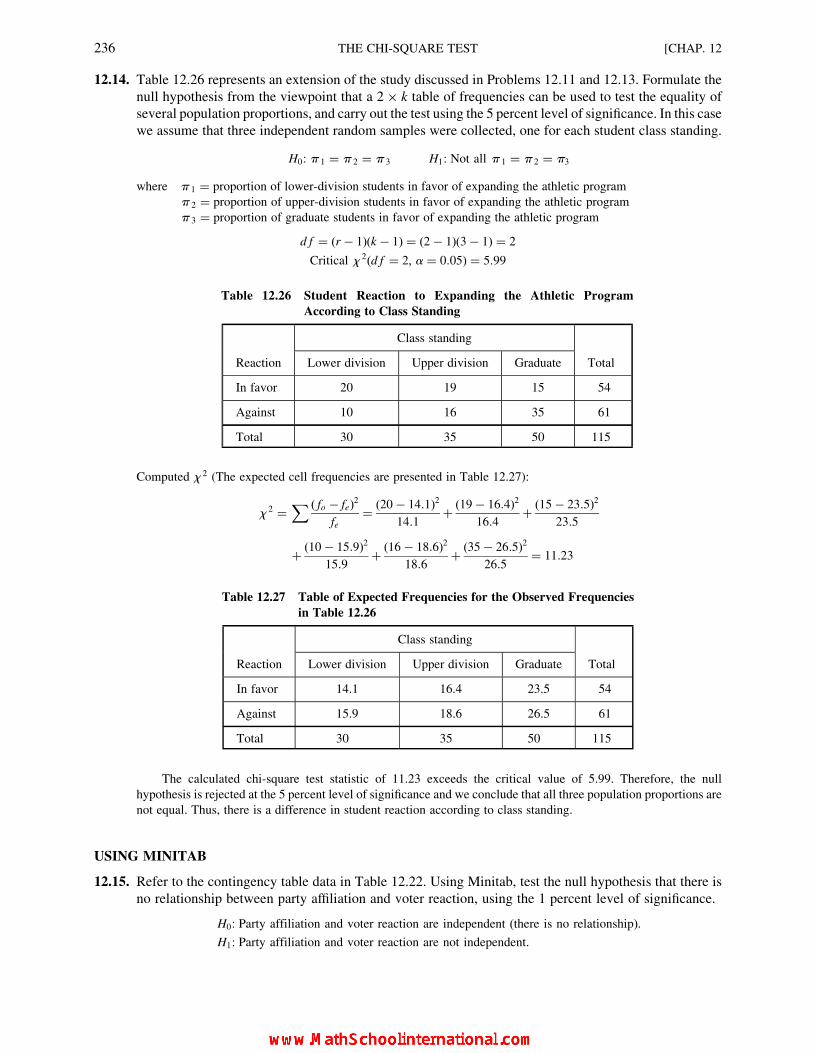
12.14. Table 12.26 represents an extension of the study discussed in Problems 12.11 and 12.13. Formulate the
null hypothesis from the viewpoint that a 2� k table of frequencies can be used to test the equality of
several population proportions, and carry out the test using the 5 percent level of significance. In this case
we assume that three independent random samples were collected, one for each student class standing.
H0: p 1 ¼ p 2 ¼ p 3 H1: Not all p 1 ¼ p 2 ¼ p3
where p 1 ¼ proportion of lower-division students in favor of expanding the athletic program
p 2 ¼ proportion of upper-division students in favor of expanding the athletic program
p 3 ¼ proportion of graduate students in favor of expanding the athletic program
d f ¼ (r � 1)(k � 1) ¼ (2� 1)(3� 1) ¼ 2
Critical x 2(d f ¼ 2, a ¼ 0:05) ¼ 5:99
Computed x 2 (The expected cell frequencies are presented in Table 12.27):
x 2 ¼X ( fo � fe)
2
fe¼ (20� 14:1)2
14:1þ (19� 16:4)2
16:4þ (15� 23:5)2
23:5
þ (10� 15:9)2
15:9þ (16� 18:6)2
18:6þ (35� 26:5)2
26:5¼ 11:23
The calculated chi-square test statistic of 11.23 exceeds the critical value of 5.99. Therefore, the null
hypothesis is rejected at the 5 percent level of significance and we conclude that all three population proportions are
not equal. Thus, there is a difference in student reaction according to class standing.
USING MINITAB
12.15. Refer to the contingency table data in Table 12.22. Using Minitab, test the null hypothesis that there is
no relationship between party affiliation and voter reaction, using the 1 percent level of significance.
H0: Party affiliation and voter reaction are independent (there is no relationship).
H1: Party affiliation and voter reaction are not independent.
Table 12.26 Student Reaction to Expanding the Athletic Program
According to Class Standing
Class standing
Reaction Lower division Upper division Graduate Total
In favor 20 19 15 54
Against 10 16 35 61
Total 30 35 50 115
Table 12.27 Table of Expected Frequencies for the Observed Frequencies
in Table 12.26
Class standing
Reaction Lower division Upper division Graduate Total
In favor 14.1 16.4 23.5 54
Against 15.9 18.6 26.5 61
Total 30 35 50 115
236 THE CHI-SQUARE TEST [CHAP. 12

From the computer output in Fig. 12-1:
d f ¼ 4
Computed x 2 ¼ 55:130
Critical x 2(d f ¼ 4, a ¼ 0:01) ¼ 13:28 (from Appendix 7)
Refer to Fig. 12-1. The Minitab output includes the expected frequencies, as well as the observed frequencies,
the calculated chi-square test statistic, the degrees of freedom for the test, and the calculated P value. The reported
chi-square value corresponds to the hand-calculated value in Problem 12.10. The P value is 0.000 (to the third
decimal place). Therefore, the null hypothesis is rejected, and we conclude that there is a relationship between party
affiliation and reaction to the new tax plan in the sampled population.
The Minitab output given in Fig. 12-1 was obtained as follows:
(1) Open Minitab. In the column name cell for C1, enter: In Favor. Enter the three observed frequencies for this
category in column C1. In the column name cell for C2 enter: Neutral. Enter the three associated frequencies in
column C2. In the column name cell for C3 enter: Opposed. Enter the three associated frequencies in column C3.
(2) Click Stat ! Tables ! Chi-Square Test.
(3) In the resulting dialog box, for Columns containing the table enter: C1-C3. Click OK.
Supplementary Problems
GOODNESS OF FIT TESTS
12.16. Refer to Table 12.28 and test the null hypothesis that the consumer preferences for the four brands of wine are equal,
using the 1 percent level of significance.
Ans. Reject H0.
12.17. Using Table 12.28, test the hypothesis that Brand C is preferred by as many as the other three brands combined at
the 1 percent level of significance.
Ans. Accept H0.
Fig. 12-1 Minitab output.
CHAP. 12] THE CHI-SQUARE TEST 237

12.18. Table 12.29 reports the single most important safety feature desired by a random sample of car purchasers. Test the
null hypothesis that the general population of car buyers is equally distributed in terms of primary preference for
these safety features, using the (a) 5 percent and (b) 1 percent level of significance.
Ans. (a) Reject H0, (b) accept H0.
12.19. In a college course in business statistics, the historical distribution of the A, B, C, D, and E grades has been 10, 30,
40, 10, and 10 percent, respectively. A particular class taught by a new instructor completes the semester with 8
students earning a grade of A, 17 with B, 20 with C, 3 with D, and 2 with E. Test the null hypothesis that this sample
does not differ significantly from the historical pattern, using the 5 percent level of significance.
Ans. Accept H0.
12.20. Table 12.30 reports the number of computer chips that do not meet a stringent quality requirement in 20 samples of
n ¼ 10 each. Test the null hypothesis that this distribution is not significantly different from the binomial
distribution with n ¼ 10 and p ¼ 0:30, using the 5 percent level of significance.
Ans. Reject H0.
12.21. Refer to Table 2.18 (page 40). For these data, �XX ¼ 28:95 and s ¼ 2:52. Test the null hypothesis that this distributionof frequencies conforms to a normal distribution pattern at the 5 percent level of significance.
Ans. Cannot be tested, because d f ¼ 0.
12.22. Refer to Table 2.21 (page 42). For this sample data, �XX ¼ 23:3 years and s ¼ 3.4 years. Test the null hypothesis that
this distribution of frequencies follows a normal distribution pattern, using the 1 percent level of significance.
Ans. Reject H0.
Table 12.28 Consumer Panel Preferences for Four Brands
of Rhine Wine
Brand
A B C D Total
30 20 40 10 100
Table 12.29 Identification of Most Important Safety Feature Desired by Car
Buyers
Safety feature
ABS
brakes
Modified
suspension Air bags
Automatic
door locks
Cruise
control Total
20 10 30 25 15 100
Table 12.30 Number of Defective Computer Chips in 20 Samples of Size n 5 10 Each
Number defective
per sample 0 1 2 3 4 5 6 7 8 9 10
Number of samples 0 1 2 4 5 5 2 1 0 0 0
238 THE CHI-SQUARE TEST [CHAP. 12

TESTS FOR THE INDEPENDENCE OF TWO CATEGORICAL VARIABLES (CONTINGENCY
TABLE TESTS)
12.23. As an extension of Problem 12.18, the opinions of men and women were tallied separately (see Table 12.31). Test
the hypothesis that there is no relationship between sex and which safety feature is preferred, using the 1 percent
level of significance.
Ans. Reject H0.
12.24. In order to investigate the relationship between employment status at the time a loan was arranged and whether or
not the loan is now in default, a loan company manager randomly chooses 100 accounts, with the results indicated in
Table 12.32. Test the null hypothesis that employment status and status of the loan are independent variables, using
the 5 percent level of significance for the test.
Ans. Accept H0.
12.25. An elementary school principal categorizes parents into three income categories according to residential area, and
into three levels of participation in school programs. From Table 12.33, test the hypothesis that there is no
relationship between income level and school program participation, using the 5 percent level of significance.
Consider the meaning of the test results.
Ans. Reject H0.
TESTING HYPOTHESES CONCERNING PROPORTIONS
12.26. Refer to Problems 12.16 to 12.25 and identify those applications of the chi-square test that are equivalent to testing a
hypothesis concerning the value of the population proportion. For each problem you identify, formulate such a null
hypothesis.
Ans. Problem 12.17
H0: p (for Brand C) ¼ 0:50; H1: p = 0:50
Table 12.31 Identification of Most Important Safety Feature Desired by Car Buyers,
According to Sex
Respondents
ABS
brakes
Modified
suspension Air bags
Automatic
door locks
Cruise
control Total
Men 15 5 20 5 5 50
Women 5 5 10 20 10 50
Total 20 10 30 25 15 100
Table 12.32 Employment Status and Loan Status for a Sample of 100 Accounts
Employment status at time of loanPresent status
of loan Employed Unemployed Total
In default 10 8 18
Not in default 60 22 82
Total 70 30 100
CHAP. 12] THE CHI-SQUARE TEST 239

12.27. Refer to Problems 12.16 to 12.25 and identify those applications which are equivalent to testing the null hypothesis
that there is no difference between two population proportions, recognizing that two separate random samples are
required. For each problem you identify, formulate such a null hypothesis.
Ans. Problem 12.24.
H0: p1 ¼ p 2;
H1: p1 = p 2 (where p1 ¼ proportion of employed in default and
p 2 ¼ proportion of unemployed in default)
COMPUTER OUTPUT
12.28. Refer to the contingency table data in Table 12.33. Use available computer software to test the null hypothesis that
there is no relationship between income level and program participation, using the 5 percent level of significance.
Ans. Reject H0.
Table 12.33 Income Level and Participation in School
Programs by Parents of Elementary School
Students
Income levelProgram
participation Low Middle High Total
Never 28 48 16 92
Occasional 22 65 14 101
Regular 17 74 3 94
Total 67 187 33 287
240 THE CHI-SQUARE TEST [CHAP. 12

CHAPTER 13
Analysis of Variance
13.1 BASIC RATIONALE ASSOCIATED WITH TESTING THE DIFFERENCES AMONG
SEVERAL POPULATION MEANS
Whereas the chi-square test can be used to test the differences among several population proportions (see
Section 12.4), the analysis of variance can be used to test the differences among several population means. The
null hypothesis is that the several population means are mutually equal. The sampling procedure used is that
several independent random samples are collected, one for each of the data categories (treatment levels).
The assumption underlying the use of the analysis of variance is that the several sample means were
obtained from normally distributed populations having the same variance s2. However, the test procedure has
been found to be relatively unaffected by violations of the normality assumption when the populations are
unimodal and the sample sizes are approximately equal. Because the null hypothesis is that the population
means are equal, the assumption of equal variance (homogeneity of variance) also implies that for practical
purposes the test is concerned with the hypothesis that the means came from the same population. This is so
because any normally distributed population is defined by the mean and variance (or standard deviation) as the
two parameters. (See Section 7.2 for a general description of the normal probability distribution.) All of the
computational procedures presented in this chapter are for fixed-effects models as contrasted to random-effects
models. This distinction is explained in Section 13.6.
The basic rationale underlying the analysis of variance was first developed by the British statistician
Ronald A. Fisher for the purpose of designing experiments and interpreting experimental data. The
F distribution described below was named in his honor. The conceptual rationale is as follows:
(1) Compute the mean for each sample group and then determine the standard error of the mean s�xx based
only on the several sample means. Computationally, this is the standard deviation of these several
mean values.
(2) Now, given the formula s�xx ¼ s=ffiffiffin
p, it follows that s ¼ ffiffiffi
np
s�xx and that s 2 ¼ ns2�xx . Therefore, the
standard error of the mean computed in (1) can be used to estimate the variance of the (common)
population from which the several samples were obtained. This estimate of the population variance is
called the mean square among treatment groups (MSTR). Fisher called any variance estimate a mean
square because computationally a variance is the mean of the squared deviations from the group mean
(see Section 4.6).
(3) Compute the variance separately for each sample group and with respect to each group mean. Then
pool these variance values by weighting them according to n � 1 for each sample. This weighting
procedure for the variance is an extension of the procedure for combining and weighting two sample
241
Copyright 2004, 1996, 1988, 1976 by The McGraw-Hill Companies, Inc. Click Here for Terms of Use.

variances (see Section 11.1). The resulting estimate of the population variance is called the mean
square error (MSE) and is based on within group differences only. Again, it is called a mean square
because it is a variance estimate. It is due to “error” because the deviations within each of the sample
groups can be due only to random sampling error, and they cannot be due to any differences among
the means of the population groups.
(4) If the null hypothesis that m1 ¼ m2 ¼ m3 ¼ � � � ¼ mk is true, then it follows that each of the two mean
squares obtained in (2) and (3) is an unbiased and independent estimator of the same population
variance s 2. However, if the null hypothesis is false, then the expected value of MSTR is larger than
MSE. Essentially, any differences among the population means will inflate MSTR while having no
effect on MSE, which is based on within group differences only.
(5) Based on the observation in (4), the F distribution can be used to test the difference between the two
variances, as described in Section 11.9. A one-sided test is involved, and the general form of the F test
in the analysis of variance is
Fd f1; d f2 ¼MSTR
MSE(13:1)
If the F ratio is in the region of rejection for the specified level of significance, then the null hypothesis
that the several population means are mutually equal is rejected.
Problem 13.1 illustrates the application of these five steps to a hypothesis testing problem involving three
data categories, or treatments.
Although the above steps are useful for describing the conceptual approach underlying the analysis of
variance (ANOVA), extension of this procedure for designs that are more complex than the simple comparison
of k sample means is cumbersome. Therefore, in the following sections of this chapter each design is described
in terms of the linear model that identifies the components influencing the random variable. Also, a standard
analysis of variance table that includes the formulas that are needed for the calculation of the required mean
square values is presented for each type of experimental design.
13.2 ONE-FACTOR COMPLETELY RANDOMIZED DESIGN (ONE-WAY ANOVA)
The one-way analysis of variance procedure is concerned with testing the difference among k sample
means when the subjects are assigned randomly to each of the several treatment groups. Therefore, the general
explanation in Section 13.1 concerns this one-way classification model.
The linear equation, or model, that represents the one-factor completely randomized design is
Xik ¼ mþ ak þ 1ik (13:2)
where m ¼ the overall mean of all k treatment populations
ak ¼ effect of the treatment in the particular group k from which the value was sampled
1ik ¼ the random error associated with the process of sampling (1 is the Greek epsilon)
Table 13.1 is the summary table for the one-factor completely randomized design of the analysis of
variance, including all computational formulas. The application of these formulas to sample data is illustrated in
Problems 13.2 to 13.4. The symbol system used in this table is somewhat different from that used in Section 13.1
because of the need to use a system which can be extended logically to two-way analysis of variance. Thus,
MSTR becomes the mean square among the A treatment groups (MSA). Further, note that the definition of
symbols in the context of analysis of variance is not necessarily consistent with the use of these symbols in
general statistical analysis. For example, ak in (13.2) is concerned with the effect on a randomly sampled value
originating from the treatment group in which the value is located; it has nothing to do with the concept of a in
general hypothesis testing procedures as described in Section 10.2. Similarly, N in Table 13.1 designates the
total size of the sample for all treatment groups combined, rather than a population size. New symbols included
in Table 13.1 are Tk, which represents the sum (total) of the values in a particular treatment group, and T , which
represents the sum of the sampled values in all groups combined.
242 ANALYSIS OF VARIANCE [CHAP. 13

Instead of the form of the null hypothesis described in paragraph (4) of Section 13.1, the general form of the
null hypothesis in the analysis of variance makes reference to the relevant component of the linear model. Thus,
for the one-way analysis of variance the null and alternative hypotheses can be stated as
H0: m1 ¼ m2 ¼ � � � ¼ mk or, equivalently, H0: ak ¼ 0 for all treatments (factor levels)
H1: not all m1 ¼ m2 ¼ � � � ¼ mk H1: ak = 0 for some treatments
13.3 TWO-WAY ANALYSIS OF VARIANCE (TWO-WAY ANOVA)
Two-way analysis of variance is based on two dimensions of classifications, or treatments. For example, in
analyzing the level of achievement in a training program we could consider both the effect of the method of
instruction and the effect of prior school achievement. Similarly, we could investigate gasoline mileage
according to the weight category of the car and according to the grade of gasoline. In data tables, the treatments
identified in the column headings are typically called the A treatments; those in the row headings are called the B
treatments.
Interaction in a two-factor experiment means that the two treatments are not independent, and that the
effect of a particular treatment in one factor differs according to levels of the other factor. For example, in
studying automobile mileage a higher-octane gasoline may improve mileage for certain types of cars but not for
others. Similarly, the effectiveness of various methods of instruction may differ according to the ability levels of
the students. In order to test for interaction, more than one observation or sampled measurement (i.e.,
replication) has to be included in each cell of the two-way data table. Section 13.4 presents the analytical
procedure that is appropriate when there is only one observation per cell, and in which interaction between the
two factors cannot be tested. The analytical procedure is extended to include replication and the analysis of
interaction effects in Section 13.5.
13.4 THE RANDOMIZED BLOCK DESIGN
(TWO-WAY ANOVA, ONE OBSERVATION PER CELL)
The two-way analysis of variance model in which there is only one observation per cell is generally
referred to as the randomized block design, because of the principal use for this model. What if we extend the
idea of using paired observations to compare two sample means (see Section 11.3) to the basic one-way analysis
of variance model, and have groups of k matched individuals assigned randomly to each treatment level? In
analysis of variance, such matched groups are called blocks, and because the individuals (or items) are
randomly assigned based on the identified block membership, the design is referred to as the randomized block
design. In such a design the blocks dimension is not a treatment dimension as such. The objective of using this
design is not for the specific purpose of testing for a blocks effect. Rather, by being able to assign some of the
variability among subjects to prior achievement, for example, the MSE can be reduced and the resulting test of
the A treatments effect is more sensitive.
Table 13.1 Summary Table for One-Way Analysis of Variance (Treatment Groups Need Not Be Equal)
Source of variation
Degrees of freedom
(df )
Sum of squares
(SS)
Mean square
(MS) F ratio
Among treatment
groups (A) K 2 1 SSA ¼XK
k¼1
T 2k
nk
� T 2
NMSA ¼ SSA
K � 1F ¼ MSA
MSE
Sampling error (E) N 2 K SSE ¼ SST � SSA MSE ¼ SSE
N � K
Total (T) N 2 1 SST ¼Xn
i¼ 1
XK
k¼ 1
X 2 � T 2
N
CHAP. 13] ANALYSIS OF VARIANCE 243
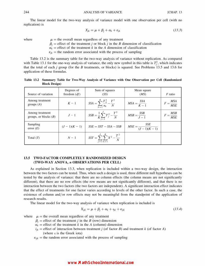
The linear model for the two-way analysis of variance model with one observation per cell (with no
replication) is
Xjk ¼ mþ bj þ ak þ 1jk (13:3)
where m ¼ the overall mean regardless of any treatment
bj ¼ effect of the treatment j or block j in the B dimension of classificationak ¼ effect of the treatment k in the A dimension of classification
1jk ¼ the random error associated with the process of sampling
Table 13.2 is the summary table for the two-way analysis of variance without replication. As compared
with Table 13.1 for the one-way analysis of variance, the only new symbol in this table is T2j , which indicates
that the total of each j group (for the B treatments, or blocks) is squared. See Problems 13.5 and 13.6 for
application of these formulas.
13.5 TWO-FACTOR COMPLETELY RANDOMIZED DESIGN
(TWO-WAY ANOVA, n OBSERVATIONS PER CELL)
As explained in Section 13.3, when replication is included within a two-way design, the interaction
between the two factors can be tested. Thus, when such a design is used, three different null hypotheses can be
tested by the analysis of variance: that there are no column effects (the column means are not significantly
different), that there are no row effects (the row means are not significantly different), and that there is no
interaction between the two factors (the two factors are independent). A significant interaction effect indicates
that the effect of treatments for one factor varies according to levels of the other factor. In such a case, the
existence of column and/or row effects may not be meaningful from the standpoint of the application of
research results.
The linear model for the two-way analysis of variance when replication is included is
Xijk ¼ mþ bj þ ak þ ijk þ 1ijk (13:4)
where m ¼ the overall mean regardless of any treatment
bj ¼ effect of the treatment j in the B (row) dimensionak ¼ effect of the treatment k in the A (column) dimension
ijk ¼ effect of interaction between treatment j (of factor B) and treatment k (of factor A)
(where i is the Greek iota)
1ijk ¼ the random error associated with the process of sampling
Table 13.2 Summary Table for Two-Way Analysis of Variance with One Observation per Cell (Randomized
Block Design)
Source of variation
Degrees of
freedom (df )
Sum of squares
(SS)
Mean square
(MS) F ratio
Among treatment
groups (A) K 2 1 SSA ¼XK
k¼ 1
T 2k
nk
� T 2
NMSA ¼ SSA
K � 1F ¼ MSA
MSE
Among treatment
groups, or blocks (B) J 2 1 SSB ¼ 1
K
XJ
j¼ 1
T 2j �
T 2
NMSB ¼ SSB
J � 1F ¼ MSB
MSE
Sampling
error (E)(J 2 1)(K 2 1) SSE ¼ SST � SSA � SSB MSE ¼ SSE
(J � 1)(K � 1)
Total (T) N 2 1 SST ¼XJ
j¼ 1
XK
k ¼ 1
X 2 � T 2
N
244 ANALYSIS OF VARIANCE [CHAP. 13

Table 13.3 is the summary table for the two-way analysis of variance with replication. The formulas
included in this table are based on the assumption that there are an equal number of observations in all of the
cells. See Problem 13.7 for application of these formulas.
13.6 ADDITIONAL CONSIDERATIONS
All of the computational procedures presented in this chapter are for fixed-effects models of the analysis of
variance. In a fixed-effects model, all of the treatments of concern for a given factor are included in the
experiment. For instance, in Problem 13.1 it is assumed that the only instructional methods of concern are the
three methods included in the design. A random-effects model, however, includes only a random sample from
all the possible treatments for the factor in the experiment. For instance, out of ten different instructional
methods, three might have been randomly chosen. A different computational method is required in the latter
case because the null hypothesis is that there are no differences among the various instructional methods in
general, and not just among the particular instructional methods that were included in the experiment. In most
experiments the fixed-effects model is appropriate, and therefore the presentation in this chapter has been
limited to such models.
The concepts presented in this chapter can be extended to more than two factors, or dimensions. Designs
involving three or more factors are called factorial designs, and in fact most statisticians include the two-way
analysis of variance with replication in this category. Although a number of different null hypotheses can be
tested with the same body of data by the use of factorial designs, the extension of such designs can lead to an
extremely large number of categories (cells) in the data table, with related sampling problems. Because of such
difficulties, designs have been developed that do not require every possible combination of the treatment levels
of every factor being included in the analysis. Such designs as the Latin Square design and incomplete block
designs are examples of such developments and are described in specialized textbooks in the analysis of
variance.
Whatever experimental design is used, rejection of a null hypothesis in the analysis of variance typically
does not present the analyst with the basis for final decisions, because such rejection does not serve to pinpoint
the exact differences among the treatments, or factor levels. For example, given that there is a significant
difference in student achievement among three instructional methods, we would next want to determine which
Table 13.3 Summary Table for Two-Way Analysis of Variance with More than One Observation per Cell
Source of variation
Degrees of
freedom (df ) Sum of squares (SS) Mean square (MS) F ratio
Among treatment
groups (A) K 2 1 SSA ¼XK
k¼ 1
T 2k
nJ� T 2
NMSA ¼ SSA
K � 1F ¼ MSA
MSE
Among treatment
groups (B) J 2 1 SSB ¼XJ
j¼ 1
T 2j
nK� T 2
NMSB ¼ SSB
J � 1F ¼ MSB
MSE
Interaction (between)
factors (A and B) (I) (J � 1)(K � 1) SSI ¼ 1
n
XJ
j¼ 1
XK
k¼ 1
Xn
i¼ 1
X
!2
� SSA � SSB � T 2
N
MSI ¼ SSI
(J � 1)(K � 1)F ¼ MSI
MSE
Sampling
error (E) JK(n � 1) SSE ¼ SST � SSA
� SSB � SSIMSE ¼ SSE
JK(n � 1)
Total (T) N 2 1 SST ¼Xn
i¼ 1
XJ
j¼ 1
XK
k¼ 1
X2 � T2
N
CHAP. 13] ANALYSIS OF VARIANCE 245
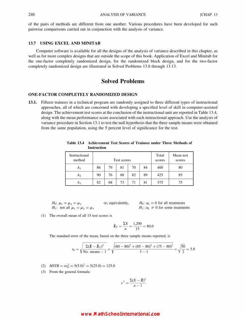
of the pairs of methods are different from one another. Various procedures have been developed for such
pairwise comparisons carried out in conjunction with the analysis of variance.
13.7 USING EXCEL AND MINITAB
Computer software is available for all the designs of the analysis of variance described in this chapter, as
well as for more complex designs that are outside the scope of this book. Application of Excel and Minitab for
the one-factor completely randomized design, for the randomized block design, and for the two-factor
completely randomized design are illustrated in Solved Problems 13.8 through 13.13.
Solved Problems
ONE-FACTOR COMPLETELY RANDOMIZED DESIGN
13.1. Fifteen trainees in a technical program are randomly assigned to three different types of instructional
approaches, all of which are concerned with developing a specified level of skill in computer-assisted
design. The achievement test scores at the conclusion of the instructional unit are reported in Table 13.4,
along with the mean performance score associated with each instructional approach. Use the analysis of
variance procedure in Section 13.1 to test the null hypothesis that the three sample means were obtained
from the same population, using the 5 percent level of significance for the test.
H0: m1 ¼ m2 ¼ m3 or, equivalently, H0: ak ¼ 0 for all treatments
H1: not all m1 ¼ m2 ¼ m3 H1: ak = 0 for some treatments
(1) The overall mean of all 15 test scores is
�XXT ¼ SX
n¼ 1,200
15¼ 80:0
The standard error of the mean, based on the three sample means reported, is
s�xx ¼ffiffiffiffiffiffiffiffiffiffiffiffiffiffiffiffiffiffiffiffiffiffiffiffiffiffiffiffiffiffiS( �XX � �XXT )
2
No. means� 1
s¼
ffiffiffiffiffiffiffiffiffiffiffiffiffiffiffiffiffiffiffiffiffiffiffiffiffiffiffiffiffiffiffiffiffiffiffiffiffiffiffiffiffiffiffiffiffiffiffiffiffiffiffiffiffiffiffiffiffiffiffiffiffiffiffiffiffiffiffiffiffiffiffiffiffiffi(80� 80)2 þ (85� 80)2 þ (75� 80)2
3� 1
s¼
ffiffiffiffiffi50
2
r¼ 5:0
(2) MSTR ¼ ns2�xx ¼ 5(5:0)2 ¼ 5(25:0) ¼ 125:0
(3) From the general formula:
s 2 ¼ S(X � �XX)2
n � 1
Table 13.4 Achievement Test Scores of Trainees under Three Methods of
Instruction
Instructional
method Test scores
Total
scores
Mean test
scores
A1 86 79 81 70 84 400 80
A2 90 76 88 82 89 425 85
A3 82 68 73 71 81 375 75
246 ANALYSIS OF VARIANCE [CHAP. 13
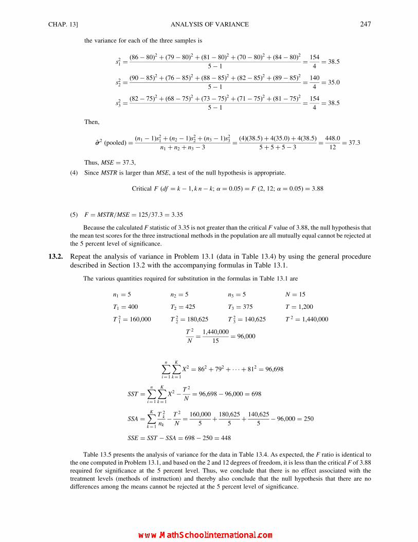
the variance for each of the three samples is
s21 ¼(86� 80)2 þ (79� 80)2 þ (81� 80)2 þ (70� 80)2 þ (84� 80)2
5� 1¼ 154
4¼ 38:5
s22 ¼(90� 85)2 þ (76� 85)2 þ (88� 85)2 þ (82� 85)2 þ (89� 85)2
5� 1¼ 140
4¼ 35:0
s23 ¼(82� 75)2 þ (68� 75)2 þ (73� 75)2 þ (71� 75)2 þ (81� 75)2
5� 1¼ 154
4¼ 38:5
Then,
ss2 (pooled) ¼ (n1 � 1)s21 þ (n2 � 1)s22 þ (n3 � 1)s23n1 þ n2 þ n3 � 3
¼ (4)(38:5)þ 4(35:0)þ 4(38:5)
5þ 5þ 5� 3¼ 448:0
12¼ 37:3
Thus, MSE ¼ 37:3,
(4) Since MSTR is larger than MSE, a test of the null hypothesis is appropriate.
Critical F (df ¼ k � 1, k n � k; a ¼ 0:05) ¼ F (2, 12; a ¼ 0:05) ¼ 3:88
(5) F ¼ MSTR=MSE ¼ 125=37:3 ¼ 3:35
Because the calculated F statistic of 3.35 is not greater than the critical F value of 3.88, the null hypothesis that
the mean test scores for the three instructional methods in the population are all mutually equal cannot be rejected at
the 5 percent level of significance.
13.2. Repeat the analysis of variance in Problem 13.1 (data in Table 13.4) by using the general procedure
described in Section 13.2 with the accompanying formulas in Table 13.1.
The various quantities required for substitution in the formulas in Table 13.1 are
n1 ¼ 5 n2 ¼ 5 n3 ¼ 5 N ¼ 15
T1 ¼ 400 T2 ¼ 425 T3 ¼ 375 T ¼ 1,200
T 21 ¼ 160,000 T 2
2 ¼ 180,625 T 23 ¼ 140,625 T 2 ¼ 1,440,000
T 2
N¼ 1,440,000
15¼ 96,000
Xn
i¼ 1
XK
k¼ 1
X2 ¼ 862 þ 792 þ � � � þ 812 ¼ 96,698
SST ¼Xn
i¼ 1
XK
k¼ 1
X2 � T 2
N¼ 96,698� 96,000 ¼ 698
SSA ¼XK
k¼ 1
T 2k
nk
� T 2
N¼ 160,000
5þ 180,625
5þ 140,625
5� 96,000 ¼ 250
SSE ¼ SST � SSA ¼ 698� 250 ¼ 448
Table 13.5 presents the analysis of variance for the data in Table 13.4. As expected, the F ratio is identical to
the one computed in Problem 13.1, and based on the 2 and 12 degrees of freedom, it is less than the critical F of 3.88
required for significance at the 5 percent level. Thus, we conclude that there is no effect associated with the
treatment levels (methods of instruction) and thereby also conclude that the null hypothesis that there are no
differences among the means cannot be rejected at the 5 percent level of significance.
CHAP. 13] ANALYSIS OF VARIANCE 247
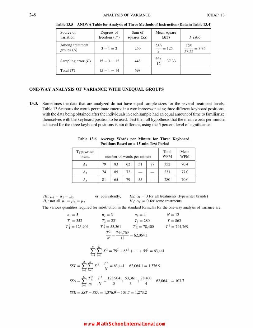
ONE-WAY ANALYSIS OF VARIANCE WITH UNEQUAL GROUPS
13.3. Sometimes the data that are analyzed do not have equal sample sizes for the several treatment levels.
Table 13.6 reports thewordsperminute entered in awordprocessor using three different keyboardpositions,
with the data being obtained after the individuals in each sample had an equal amount of time to familiarize
themselves with the keyboard position to be used. Test the null hypothesis that the mean words per minute
achieved for the three keyboard positions is not different, using the 5 percent level of significance.
H0: m1 ¼ m2 ¼ m3 or, equivalently, H0: ak ¼ 0 for all treatments (typewriter brands)
H1: not all m1 ¼ m2 ¼ m3 H1: ak = 0 for some treatments
The various quantities required for substitution in the standard formulas for the one-way analysis of variance are
n1 ¼ 5 n2 ¼ 3 n3 ¼ 4 N ¼ 12
T1 ¼ 352 T2 ¼ 231 T3 ¼ 280 T ¼ 863
T 21 ¼ 123,904 T 2
2 ¼ 53,361 T 23 ¼ 78,400 T 2 ¼ 744,769
T 2
N¼ 744,769
12¼ 62,064:1
Xn
i¼1
XK
k¼1
X 2 ¼ 792 þ 832 þ � � � þ 552 ¼ 63,441
SST ¼Xn
i¼1
XK
k¼1
X 2 � T 2
N¼ 63,441� 62,064:1 ¼ 1,376:9
SSA ¼XK
k¼1
T 2k
nk
� T 2
N¼ 123,904
5þ 53,361
3þ 78,400
4� 62,064:1 ¼ 103:7
SSE ¼ SST � SSA ¼ 1,376:9� 103:7 ¼ 1,273:2
Table 13.5 ANOVA Table for Analysis of Three Methods of Instruction (Data in Table 13.4)
Source of
variation
Degrees of
freedom (df )
Sum of
squares (SS)
Mean square
(MS) F ratio
Among treatment
groups (A) 3� 1 ¼ 2 250250
2¼ 125
125
37:33¼ 3:35
Sampling error (E) 15� 3 ¼ 12 448448
12¼ 37:33
Total (T) 15� 1 ¼ 14 698
Table 13.6 Average Words per Minute for Three Keyboard
Positions Based on a 15-min Test Period
Typewriter
brand number of words per minute
Total
WPM
Mean
WPM
A1 79 83 62 51 77 352 70.4
A2 74 85 72 — — 231 77.0
A3 81 65 79 55 — 280 70.0
248 ANALYSIS OF VARIANCE [CHAP. 13
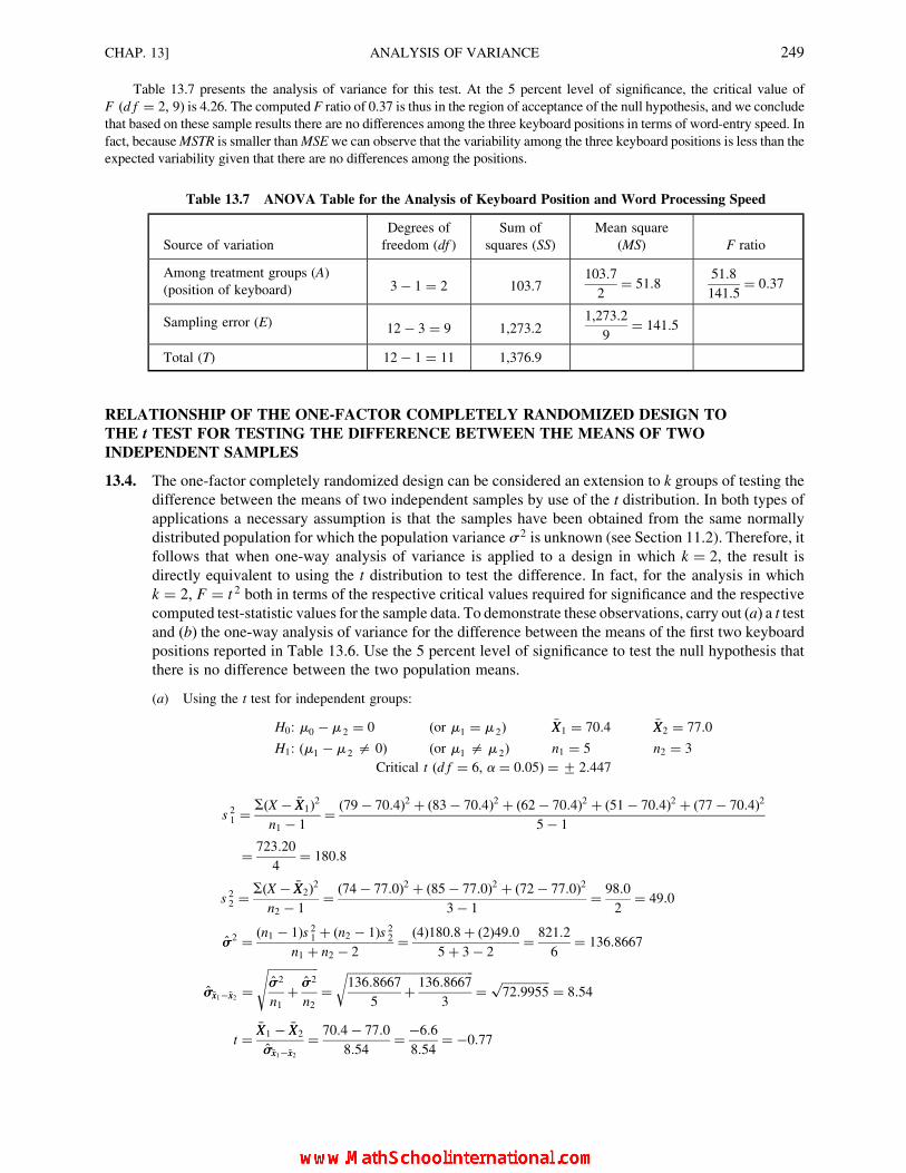
Table 13.7 presents the analysis of variance for this test. At the 5 percent level of significance, the critical value of
F (d f ¼ 2, 9) is 4.26. The computed F ratio of 0.37 is thus in the region of acceptance of the null hypothesis, and we conclude
that based on these sample results there are no differences among the three keyboard positions in terms of word-entry speed. In
fact, because MSTR is smaller than MSE we can observe that the variability among the three keyboard positions is less than the
expected variability given that there are no differences among the positions.
RELATIONSHIP OF THE ONE-FACTOR COMPLETELY RANDOMIZED DESIGN TO
THE t TEST FOR TESTING THE DIFFERENCE BETWEEN THE MEANS OF TWOINDEPENDENT SAMPLES
13.4. The one-factor completely randomized design can be considered an extension to k groups of testing the
difference between the means of two independent samples by use of the t distribution. In both types of
applications a necessary assumption is that the samples have been obtained from the same normally
distributed population for which the population variance s 2 is unknown (see Section 11.2). Therefore, it
follows that when one-way analysis of variance is applied to a design in which k ¼ 2, the result is
directly equivalent to using the t distribution to test the difference. In fact, for the analysis in which
k ¼ 2, F ¼ t 2 both in terms of the respective critical values required for significance and the respective
computed test-statistic values for the sample data. To demonstrate these observations, carry out (a) a t test
and (b) the one-way analysis of variance for the difference between the means of the first two keyboard
positions reported in Table 13.6. Use the 5 percent level of significance to test the null hypothesis that
there is no difference between the two population means.
(a) Using the t test for independent groups:
H0: m0 � m 2 ¼ 0 (or m1 ¼ m 2) �XX1 ¼ 70:4 �XX2 ¼ 77:0
H1: (m1 � m 2 = 0) (or m1 = m 2) n1 ¼ 5 n2 ¼ 3
Critical t (d f ¼ 6, a ¼ 0:05) ¼ + 2:447
s 21 ¼
S(X � �XX1)2
n1 � 1¼ (79� 70:4)2 þ (83� 70:4)2 þ (62� 70:4)2 þ (51� 70:4)2 þ (77� 70:4)2
5� 1
¼ 723:20
4¼ 180:8
s 22 ¼
S(X � �XX2)2
n2 � 1¼ (74� 77:0)2 þ (85� 77:0)2 þ (72� 77:0)2
3� 1¼ 98:0
2¼ 49:0
ss2 ¼ (n1 � 1)s 21 þ (n2 � 1)s 2
2
n1 þ n2 � 2¼ (4)180:8þ (2)49:0
5þ 3� 2¼ 821:2
6¼ 136:8667
ss�xx1��xx2 ¼ffiffiffiffiffiffiffiffiffiffiffiffiffiffiffiffiffiss2
n1þ ss2
n2
s¼
ffiffiffiffiffiffiffiffiffiffiffiffiffiffiffiffiffiffiffiffiffiffiffiffiffiffiffiffiffiffiffiffiffiffiffiffiffiffiffiffiffiffiffi136:8667
5þ 136:8667
3
r¼
ffiffiffiffiffiffiffiffiffiffiffiffiffiffiffiffi72:9955
p¼ 8:54
t ¼�XX1 � �XX2
ss�xx1��xx2
¼ 70:4� 77:0
8:54¼ �6:6
8:54¼ �0:77
Table 13.7 ANOVA Table for the Analysis of Keyboard Position and Word Processing Speed
Source of variation
Degrees of
freedom (df )
Sum of
squares (SS)
Mean square
(MS) F ratio
Among treatment groups (A)
(position of keyboard) 3� 1 ¼ 2 103.7103:7
2¼ 51:8
51:8
141:5¼ 0:37
Sampling error (E) 12� 3 ¼ 9 1,273.21,273:2
9¼ 141:5
Total (T) 12� 1 ¼ 11 1,376.9
CHAP. 13] ANALYSIS OF VARIANCE 249

The computed t statistic of �0:77 is in the region of acceptance of the null hypothesis, and therefore the null
hypothesis cannot be rejected at the 5 percent level of significance.
(b) For the two treatment levels (keyboard positions), based on the one-way analysis of variance:
H0: m1 ¼ m 2 (or ak ¼ 0) n1 ¼ 5 n2 ¼ 3 N ¼ 8
H1: m1 = m 2 (or ak = 0) T1 ¼ 352 T2 ¼ 231 T ¼ 583
T 21 ¼ 123,904 T 2
2 ¼ 53,361 T 2 ¼ 339,889
T 2
N¼ 339,889
8¼ 42,486:1
Xn
i¼ 1
XK
k¼ 1
X 2 ¼ 792 þ 832 þ � � � þ 722 ¼ 43,389
SST ¼Xn
i¼ 1
XK
k¼ 1
X2 ¼ T2
N¼ 43,389� 42,468:1 ¼ 902:9
SSA ¼XK
k¼ 1
T 2k
nk
� T2
N¼ 123,904
5þ 53,361
3� 42,486:1 ¼ 81:7
SSE ¼ SST � SSA ¼ 902:9� 81:7 ¼ 821:2
Table 13.8 presents the analysis of variance for this test. At the 5 percent level of significance, the critical value
of F (d f ¼ 1, 6) is 5.99. Since the computed F statistic of 0.60 is the region of acceptance of the null hypothesis, the
hypothesis that there is no treatment effect cannot be rejected.
Thus, the observation about the comparability of the two testing procedures is supported. In terms of the
critical values, critical F ¼ 5:99 and critical t ¼ +2:447. Thus, (+2:447)2 ¼ 5:99. As for the computed test-
statistic values of F and t, F ¼ 0:60 and t ¼ �0:77; (�0:77)2 ¼ 0:59 ffi 0:60, with the slight difference being due
solely to rounding error.
THE RANDOMIZED BLOCK DESIGN
(TWO-WAY ANALYSIS WITHOUT INTERACTION)
13.5. For the data in Table 13.4, suppose a randomized block design was in fact used and trainees were
matched before the experiment, with a trainee from each ability group (based on prior course
achievement) assigned to each method of instruction. Table 13.9 is a revision of Table 13.4 in that
the values reported are reorganized to reflect the randomized block design. Note, however, that the same
values are included in each A treatment group as in Table 13.4, except that they are reported according to
the B ability groups and therefore are arranged in a different order. Test the null hypothesis that there is
no difference in the mean performance among the three methods of instruction, using the 5 percent level
of significance.
Table 13.8 ANOVA Table for the Analysis of Keyboard Position and Word Processing Speed
Source of variation
Degrees of
freedom (df )
Sum of
squares (SS)
Mean square
(MS) F ratio
Among treatment (A)
(position of keyboard) 2� 1 ¼ 1 81.781:7
1¼ 81:7
81:7
136:9¼ 0:60
Sampling error (E) 8� 2 ¼ 6 821.2821:2
6¼ 136:96
Total (T ) 8� 1 ¼ 7 902.9
250 ANALYSIS OF VARIANCE [CHAP. 13

The various quantities required for the analysis of variance table are
For j:
T1 ¼ 258 T2 ¼ 254 T3 ¼ 242 T4 ¼ 223 T5 ¼ 223
T 21 ¼ 66,564 T 2
2 ¼ 64,516 T 23 ¼ 58,564 T 2
4 ¼ 49,729 T 25 ¼ 49,729
For k:
T1 ¼ 400 T2 ¼ 425 T3 ¼ 375
T 21 ¼ 160,000 T 2
2 ¼ 180,625 T 23 ¼ 140,625
n1 ¼ 5 n2 ¼ 5 n3 ¼ 5
Overall:
T ¼ 1,200 T 2 ¼ 1,440,000 N ¼ 15
T 2
N¼ 1,440,000
15¼ 96,000
XJ
j¼1
XK
k¼1
X 2 þ 862 þ 842 þ � � � þ 712 ¼ 96,698
SST ¼XJ
j¼ 1
XK
k¼ 1
X2 � T 2
N¼ 96,698� 96,000 ¼ 698
SSA ¼XK
k¼ 1
T 2k
nk
� T 2
N¼ 160,000
5þ 180,625
5þ 140,625
5� 96,000 ¼ 250
SSB ¼ 1
K
XJ
j¼ 1
T 2j �
T 2
N¼ 1
3(66,564þ 64,516þ 58,564þ 49,729þ 49,729)� 96,000 ¼ 367:3
SSE ¼ SST � SSA � SSB ¼ 698� 250� 367:3 ¼ 80:7
Table 13.10 presents the analysis of variance for these data. With respect to the linear equation representing
this model, the two F ratios in Table 13.10 are concerned with the tests of the following null and alternative
hypotheses:
H0: ak ¼ 0 for all columns H0: bj ¼ 0 for all rows
H1: ak = 0 for some columns H1: bj = 0 for some rows
In terms of practical implications, the first null hypothesis is concerned with testing the difference among the
column means, which is the basic purpose of the analysis. The second null hypothesis is concerned with testing the
difference among the row means, which reflect the blocking that was done according to level of ability.
Table 13.9 Achievement Test Scores of Trainees under Methods of Instruction,
According to Ability Level
Level of ability Method of instruction
(Block) A1 A2 A3 Total (Tj) Mean ( �XXj)
B1 86 90 82 258 86.0
B2 84 89 81 254 84.7
B3 81 88 73 242 80.7
B4 79 76 68 223 74.3
B5 70 82 71 223 74.3
Total (Tk) 400 425 375
Grand total
T ¼ 1,200
Mean ( �XXk) 80.0 85.0 75.0
Grand mean�XXT ¼ 80:0
CHAP. 13] ANALYSIS OF VARIANCE 251

Using the 5 percent level of significance, the required F ratio for the rejection of the first null hypothesis
(df ¼ 2, 8) ¼ 4:46 while the required F for the second null hypothesis (df ¼ 4, 8) ¼ 3:84. Thus, both of the
calculated F ratios in Table 13.10 are in the region of rejection of the null hypothesis. We conclude that there is a
significant difference in achievement test scores for the different methods of instruction, and also that there is a
significant difference in achievement test scores for the different levels of ability. Note that this is in contrast to the
result in Problem 13.2, where the data were treated as three independent samples. The MSE in the present analysis is
substantially lower than that determined in Problem 13.2 because much of that variability could be identified as
being due to differences in ability level.
RELATIONSHIP OF THE RANDOMIZED BLOCK DESIGN TO THE t TEST FOR TESTING
THE DIFFERENCE BETWEEN TWO MEANS USING PAIRED OBSERVATIONS
13.6. When k ¼ 2, the randomized block design is equivalent to the t test for the difference between the means
of paired observations and F ¼ t2. This is similar to the case in Problem 13.4 for two independent
samples. To demonstrate these points, apply the analysis of variance to the data in Table 13.11, taken
Table 13.10 ANOVA Table for Analysis of Three Methods of Instruction According to Ability Level
Source variation
Sum of squares
(SS)
Degrees of
freedom (df )
Mean square
(MS) F ratio
Among treatment
groups (A) (method) 250.0 3� 1 ¼ 2250:0
2¼ 125:0
125
10:1¼ 12:4
Among blocks (B)
(ability level) 367.3 5� 1 ¼ 4367:3
4¼ 91:8
91:8
10:1¼ 9:1
Sampling error (E) 80.7 (5� 1)(3� 1) ¼ 880:7
8¼ 10:1
Total (T ) 698.0 15� 1 ¼ 14
Table 13.11 Automobile Mileage Obtained with and without a Gasoline Additive for 10
Sampled Cars
Automobile
Mileage with
additive (per gal)
Mileage without
additive (per gal) Total (Tj) Mean ( �XXj)
1 36.7 36.2 72.9 36.45
2 35.8 35.7 71.5 35.75
3 31.9 32.3 64.2 32.10
4 29.3 29.6 58.9 29.45
5 28.4 28.1 56.5 18.25
6 25.7 25.8 51.5 25.75
7 24.2 23.9 48.1 24.05
8 22.6 22.0 44.6 22.30
9 21.9 21.5 43.4 21.70
10 20.3 20.0 40.3 20.15
Total (Tk) 276.8 275.1
Grand total
T ¼ 551.9
Mean ( �XXk) 27.68 27.51
Grand mean�XXT ¼ 27:60
252 ANALYSIS OF VARIANCE [CHAP. 13
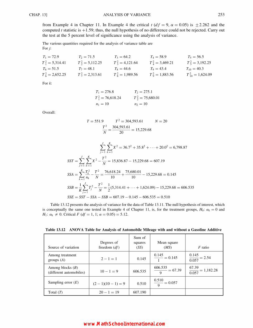
from Example 4 in Chapter 11. In Example 4 the critical t (d f ¼ 9, a ¼ 0:05) is +2:262 and the
computed t statistic is þ1:59; thus, the null hypothesis of no difference could not be rejected. Carry out
the test at the 5 percent level of significance using the analysis of variance.
The various quantities required for the analysis of variance table are
For j:
T1 ¼ 72:9 T2 ¼ 71:5 T3 ¼ 64:2 T4 ¼ 58:9 T5 ¼ 56:5
T 21 ¼ 5,314:41 T 2
2 ¼ 5,112:25 T 23 ¼ 4,121:64 T 2
4 ¼ 3,469:21 T 25 ¼ 3,192:25
T6 ¼ 51:5 T7 ¼ 48:1 T8 ¼ 44:6 T9 ¼ 43:4 T10 ¼ 40:3
T 26 ¼ 2,652:25 T 2
7 ¼ 2,313:61 T 28 ¼ 1,989:56 T 2
9 ¼ 1,883:56 T 210 ¼ 1,624:09
For k:
T1 ¼ 276:8 T2 ¼ 275:1
T 21 ¼ 76,618:24 T 2
2 ¼ 75,680:01
n1 ¼ 10 n2 ¼ 10
Overall:
T ¼ 551:9 T 2 ¼ 304,593:61 N ¼ 20
T 2
N¼ 304,593:61
20¼ 15,229:68
XJ
j¼ 1
XK
k¼ 1
X 2 ¼ 36:72 þ 35:82 þ � � � þ 20:02 ¼ 6,798:87
SST ¼XJ
j¼ 1
XK
k ¼ 1
X 2 � T 2
N¼ 15,836:87� 15,229:68 ¼ 607:19
SSA ¼XK
k ¼ 1
T 2k
nk
� T 2
N¼ 76,618:24
10þ 75,680:01
10� 15,229:68 ¼ 0:145
SSB ¼ 1
K
XJ
j¼ 1
T 2j � T 2
N¼ 1
2(5,314:41þ � � � þ 1,624:09)� 15,229:68 ¼ 606:535
SSE ¼ SST � SSA � SSB ¼ 607:19� 0:145� 606:535 ¼ 0:510
Table 13.12 presents the analysis of variance for the data of Table 13.11. The null hypothesis of interest, which
is conceptually the same one tested in Example 4 of Chapter 11, is, for the treatment groups, H0: ak ¼ 0 and
H1: ak = 0. Critical F (df ¼ 1, 1; a ¼ 0:05) ¼ 5:12.
Table 13.12 ANOVA Table for Analysis of Automobile Mileage with and without a Gasoline Additive
Source of variation
Degrees of
freedom (df )
Sum of
squares
(SS)
Mean square
(MS) F ratio
Among treatment
groups (A) 2� 1 ¼ 1 0.1450:145
1¼ 0:145
0:145
0:057¼ 2:54
Among blocks (B)
(different automobiles) 10� 1 ¼ 9 606.535606:535
9¼ 67:39
67:39
0:057¼ 1,182:28
Sampling error (E) (2� 1)(10� 1) ¼ 9 0.5100:510
9¼ 0:057
Total (T) 20� 1 ¼ 19 607.190
CHAP. 13] ANALYSIS OF VARIANCE 253

Since the computed value of F statistic of 2.54 is not greater than the critical value of 5.12, the hypothesis of no
treatment effect (of no difference between the means) cannot be rejected at the 5 percent level of significance. Thus
we conclude that the additive does not increase automobile mileage.
Note the very large value of the computed F for the blocks dimension. Referring to the data in Table 13.11, this
result is not surprising, since the 10 automobiles were apparently in different weight categories and differed
substantially in mileage achieved according to category.
As expected, the critical value of F in this problem is equal to the square of the critical value used in the t test:
5:12 ¼ (+2:262)2. Also, except for the rounding error, the computed t2 value in Example 4 of Chapter 11 is equal to
the computed F of 2.54 here, with t2 ¼ (1:59)2 ¼ 2:53.
TWO-FACTOR COMPLETELY RANDOMIZED DESIGN
13.7. Nine trainees in each of four different subject areas were randomly assigned to three different methods
of instruction. Three students were assigned to each instructional method.With reference to Table 13.13,
test the various null hypotheses that are of interest with respect to such a design at the 5 percent level of
significance.
The various quantities required for the analysis of variance table are
For J:
T1 ¼ 717 T2 ¼ 709 T3 ¼ 722 T4 ¼ 732
T 21 ¼ 514,089 T 2
2 ¼ 502,681 T 23 ¼ 521,284 T 2
4 ¼ 535,824
For k:
T1 ¼ 960 T2 ¼ 1,020 T3 ¼ 900
T 21 ¼ 921,600 T 2
2 ¼ 1,040,000 T 23 ¼ 810,000
Overall:
T ¼ 2,880 T 2 ¼ 8,294,400 N ¼ 36
T 2
N¼ 8,294,400
36¼ 230,400
XJ
j¼ 1
XK
k¼ 1
Xn
i¼ 1
X
!2
¼ (70þ 79þ 72)2 þ (77þ 81þ 79)2 þ � � � þ (68þ 71þ 69)2 ¼ 694,694
Xn
i¼ 1
XJ
j¼ 1
XK
k¼ 1
X 2 ¼ 702 þ 792 þ 722 þ 772 þ � � � þ 692 ¼ 232,000
SST ¼Xn
i¼ 1
XJ
j¼ 1
XK
k ¼ 1
X 2 � T2
N¼ 232,000� 230,400 ¼ 1,600
SSA ¼XK
k¼ 1
T 2k
nJ� T 2
N¼ 921,600
(3)(4)þ 1,040,400
(3)(4)þ 810,000
(3)(4)� 230,400 ¼ 600
SSB ¼XJ
j¼ 1
T 2j
nK� T 2
N¼ 514,089
(3)(3)þ 502,681
(3)(3)þ 521,284
(3)(3)þ 535,824
(3)(3)¼ 230,400 ¼ 30:8
SSI ¼ 1
n
XJ
j¼ 1
XK
k¼ 1
Xn
i¼ 1
X
!2
þ SSA � SSB � T 2
N¼ 1
3(694,694)� 600� 30:8� 230,400 ¼ 533:9
SSE ¼ SST � SSA � SSB � SSI ¼ 1,600:0� 600:0� 30:8� 533:9 ¼ 435:3
254 ANALYSIS OF VARIANCE [CHAP. 13

Table 13.14 presents the analysis of variance for the data of Table 13.13. With respect to the linear model for
two-way analysis of variance with replication, the three F ratios reported in Table 13.14 are concerned with the
following null and alternative hypotheses:
H0: ak ¼ 0 for all columns ; H1: ak = 0 for some columns
H0: bj ¼ 0 for all rows; H1: bj = 0 for some rows
H0: ijk ¼ 0 for all cells; H1: ijk = 0 for some cells
Using the 5 percent level of significance, the required F ratio for the rejection of the first null hypothesis
(df ¼ 2, 24) is 3.40, for the second the required F (df ¼ 3, 24) is 3.01, and for the third the required F (df ¼ 6, 24)
Table 13.14 ANOVA Table for Analysis of Three Methods of Instruction Applied in Four Subject Areas
Source of variation
Degrees of
freedom (df )
Sum of squares
(SS)
Mean square
(MS) F ratio
Between treatment
groups (A) (method) 3� 1 ¼ 2 600.0600:0
2¼ 300:0
300:0
18:1¼ 16:57
Between treatment
groups (B) (subject) 4� 1 ¼ 3 30.830:8
3¼ 10:3
10:3
18:1¼ 0:57
Interaction between
method and subject (I) (4� 1)(3� 1) ¼ 6 533.9533:9
6¼ 89:0
89:0
18:1¼ 4:92
Sampling error (E) (4)(3)(3� 1) ¼ 24 435.3435:3
24¼ 18:1
Total (T) 36� 1 ¼ 35 1,600.0
Table 13.13 Achievement Test Scores of Trainees under Three Methods
of Instruction and for Four Subject Areas
Subject Method of instruction Total Mean
area A1 A2 A3 (Tj) ( �XXj)
B1 70 83 81 717 79.7
79 89 86
72 78 79
B2 77 77 74 709 78.8
81 87 69
79 88 77
B3 82 94 72 722 80.2
78 83 79
80 79 75
B4 85 84 68 732 81.3
90 90 71
87 88 69
Total (Tk) 960 1,020 900
Grand total
T ¼ 2,880
Mean ( �XXk) 80 85 75
Grand mean�XXT ¼ 80
CHAP. 13] ANALYSIS OF VARIANCE 255

is 2.51. Thus, we conclude that there is a significant difference in test scores for the different methods of instruction,
that there is no significant difference among the different subject areas, and that there is significant interaction
between the two factors. The last conclusion indicates that the effectiveness of the three methods of instruction
varies for the different subject areas. For example, in Table 13.13 notice that for subject area B1 method A1 was the
least effective method, while for subject are a B4, method A3 was the least effective method. In reviewing this table,
however, method A2 is observed to be at least equal to the other methods for every subject area. Thus, the possibility
of using different methods of instruction as being best for different subject areas does not appear to be the
appropriate decision in this case, even though there was a significant interaction effect.
COMPUTER OUTPUT: ONE-FACTOR COMPLETELY RANDOMIZED DESIGN
13.8. Use Excel to carry out the analysis in Problem 13.2 (data is Table 13.4).
The output given in Fig. 13-1 corresponds to the results obtained by manual calculation in Table 13.5. Whereas
the critical-value approach to hypothesis testing had to be used in the hand calculation, the printout provides the
P value, which is 0.069909, or 0.070 rounded. Since this value is not less than 0.05, the null hypothesis that there are
no differences among the population means cannot be rejected at the 5 percent level of significance.
The Excel output given in Fig. 13-1 was obtained as follows:
(1) Open Excel. In cell A1 enter: A1 (the label for the first instructional method). In cell B1 enter: A2. In cell C1
enter: A3. Then enter the 5 scores for each method in the respective column. (Note that the data are entered by
column, even though they are listed by row in Table 13.4.)
(2) Click Tools ! Data Analysis ! Anova: Single Factor. Click OK.
(3) In the dialog box, for Input Range enter: $A$1:$C$6. Select Columns. Check Labels in First Row. For
Output Range enter: $D$1. Click OK.
13.9. Use Minitab to carry out the analysis in Problem 13.2 (data is Table 13.4).
The output given in Fig. 13-2 corresponds to the results obtained by manual calculation in Table 13.5. Whereas
the critical-value approach to hypothesis testing had to be used in the hand calculation, the printout provides the
P value, which is 0.070. Since this value is not less than 0.05, the null hypothesis that there are no differences among
the population means cannot be rejected at the 5 percent level of significance.
Fig. 13-1 Excel output for one-factor design.
256 ANALYSIS OF VARIANCE [CHAP. 13

The Minitab output given in Fig. 13-2 was obtained as follows:
(1) Open Minitab. In the column-name for C1 enter: Method. In the column name for C2 enter: Score. Since there
are 5 scores for each method, in C1 enter five 1s, five 2s and five 3s, which are the method labels. In C2 enter
the 15 test scores, each associated (in groups of 5) with one of the three methods of instruction in C1.
(2) Click Stat ! ANOVA ! One-way. For Response enter: Score. For Factor enter: Method. Click OK.
COMPUTER OUTPUT: RANDOMIZED BLOCK DESIGN
13.10. Use Excel to carry out the analysis in Problem 13.5 (data in Table 13.9).
The output given in Fig. 13-3 corresponds to the results obtained by manual calculation in Table 13.10. In the
printout, “Columns” designates the Method dimension. The reported P value is 0.003542, or 0.004 rounded.
Because this P value is less than 0.05, we reject the null hypothesis at the 5 percent level of significance and
Fig. 13-2 Minitab output for one-factor design.
Fig. 13-3 Excel output for randomized block design.
CHAP. 13] ANALYSIS OF VARIANCE 257

conclude that there is a difference among the means in the sampled population for the different methods of
instruction. Note that there is also a difference among the means with respect to the blocking factor of level of ability
(with P ¼ 0:004499). But this is not the focus of our interest, and indeed, we would expect that trainees at differentlevels of ability would perform differently.
The Excel output given in Fig. 13-3 was obtained as follows:
(1) Open Excel. In cell A1 enter: Level. Enter the labels for the 5 levels of ability in column A, beginning at cell
A2: B1, B2, B3, B4, and B5. In cells B1 to D1 enter the labels A1, A2, and A3, respectively. Enter the data in
each column as given in Table 13.9.
(2) Click Tools ! Data Analysis ! Anova: Two-Factor Without Replication. Click OK.
(3) In the dialog box, for Input Range enter: $A$1:$D$6. CheckLabels. ForOutput Range enter: $E$1. ClickOK.
13.11. Use Minitab to carry out the analysis in Problem 13.5 (data in Table 13.9).
The output given in Fig. 13-4 corresponds to the results obtained by manual calculation in Table 13.10. The
reported P value for the Method dimension is 0.004. Because this P value is less than 0.05, we reject the null
hypothesis at the 5 percent level of significance and conclude that there is a difference among the means in the
sampled population for the different methods of instruction. Note that there is also a difference among the means
with respect to the blocking factor of level of ability (with P ¼ 0:004). But this is not the focus of our interest, andindeed, we would expect that trainees at different levels of ability would perform differently.
The Minitab output given in Fig. 13-4 was obtained as follows:
(1) OpenMinitab. In the column name for C1 enter: Method. In the column name for C2 enter: Block. In the column
name forC3 enter: Score. Since there are five scores for eachmethod, inC1 enter five 1s, five 2s, and five 3s,which
are the method labels. In C2 the blocking is identified by entering the labels sequence 1, 2, 3, 4, and 5 three times,
once for each method of instruction. In C3 enter the 15 test scores in the column order as listed in Table 13.9.
(2) Click Stat ! ANOVA ! Two-way. For Response enter: Score. For Row factor enter: Method, and check
Display means. For Column factor enter: Block. Click OK.
COMPUTER OUTPUT: TWO-FACTOR COMPLETELY RANDOMIZED DESIGN
13.12. Use Excel to carry out the analysis in Problem 13.7 (data in Table 13.13).
The output given in Fig. 13-5 corresponds to the results obtained by manual calculation in Table 13.14. Three
P values are reported. The P ¼ 0:641678 for “Sample” is for the differences among the means for the subject areas;
the result indicates that there is no difference in mean scores according to subject area of instruction. The
P ¼ 3:05E� 05, or less than 0.000, is for the mean differences among the methods of instruction; at the designated
Fig. 13-4 Minitab output for randomized block design.
258 ANALYSIS OF VARIANCE [CHAP. 13

5 percent level of significance, the null hypothesis is rejected, and there is a difference among the mean scores
according to the method of instruction in the population. The P ¼ 0:002111 is for the interaction effect between
method of instruction and subject area; consequently, at the 5 percent level of significance, we reject the null
hypothesis that there is no interaction effect in the population. This means that in the population the effectiveness of
the three methods of instruction varies according to subject area.
The Excel output given in Fig. 13-5 was obtained as follows:
(1) Open Excel. In cell A1 enter: Subject. In cells B1-D1 enter A1, A2, and A3, respectively. Then in column A, in
cell A2 enter: B1. In cell A5 enter: B2. In cell A8 enter: B3. In cell A11 enter: B4. Enter the date in columns B
to D as given in Table 13.13.
(2) Click Tools ! Data Analysis ! Anova: Two-Factor With Replication. Click OK.
(3) In the dialog box, for Input Range enter: $A$1:$D$13. For Rows per sample enter: 3. For Output Range
enter: $E$1. Click OK.
Fig. 13-5 Excel output for two-factor design.
CHAP. 13] ANALYSIS OF VARIANCE 259
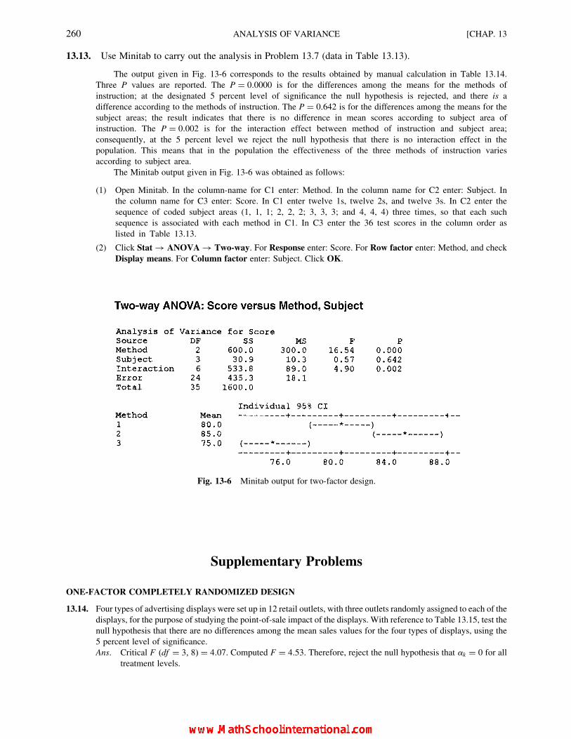
13.13. Use Minitab to carry out the analysis in Problem 13.7 (data in Table 13.13).
The output given in Fig. 13-6 corresponds to the results obtained by manual calculation in Table 13.14.
Three P values are reported. The P ¼ 0:0000 is for the differences among the means for the methods of
instruction; at the designated 5 percent level of significance the null hypothesis is rejected, and there is a
difference according to the methods of instruction. The P ¼ 0:642 is for the differences among the means for the
subject areas; the result indicates that there is no difference in mean scores according to subject area of
instruction. The P ¼ 0:002 is for the interaction effect between method of instruction and subject area;
consequently, at the 5 percent level we reject the null hypothesis that there is no interaction effect in the
population. This means that in the population the effectiveness of the three methods of instruction varies
according to subject area.
The Minitab output given in Fig. 13-6 was obtained as follows:
(1) Open Minitab. In the column-name for C1 enter: Method. In the column name for C2 enter: Subject. In
the column name for C3 enter: Score. In C1 enter twelve 1s, twelve 2s, and twelve 3s. In C2 enter the
sequence of coded subject areas (1, 1, 1; 2, 2, 2; 3, 3, 3; and 4, 4, 4) three times, so that each such
sequence is associated with each method in C1. In C3 enter the 36 test scores in the column order as
listed in Table 13.13.
(2) Click Stat ! ANOVA ! Two-way. For Response enter: Score. For Row factor enter: Method, and check
Display means. For Column factor enter: Subject. Click OK.
Supplementary Problems
ONE-FACTOR COMPLETELY RANDOMIZED DESIGN
13.14. Four types of advertising displays were set up in 12 retail outlets, with three outlets randomly assigned to each of the
displays, for the purpose of studying the point-of-sale impact of the displays. With reference to Table 13.15, test the
null hypothesis that there are no differences among the mean sales values for the four types of displays, using the
5 percent level of significance.
Ans. Critical F (df ¼ 3, 8) ¼ 4:07. Computed F ¼ 4:53. Therefore, reject the null hypothesis that ak ¼ 0 for all
treatment levels.
Fig. 13-6 Minitab output for two-factor design.
260 ANALYSIS OF VARIANCE [CHAP. 13

13.15. Use available computer software to carry out the analysis in Problem 13.14 (data in Table 13.15) for the one-factor
completely randomized design.
Ans. Same as for Problem 13.14.
THE RANDOMIZED BLOCK DESIGN (TWO-WAY ANALYSIS WITHOUT INTERACTION)
13.16. The designs produced by four automobile designers are evaluated by three product managers, as reported in
Table 13.16. Test the null hypothesis that the average ratings of the designs do not differ, using the 1 percent
level of significance.
Ans. Critical F (df ¼ 3, 6) ¼ 9:78. Computed F ¼ 12:29. Therefore, reject the null hypothesis that ak ¼ 0 for all
treatment (column) effects.
13.17. Use available computer software to carry out the analysis in Problem 13.16 (data in Table 13.16) for the randomized
block design.
Ans. Same as for Problem 13.16.
TWO-FACTOR COMPLETELY RANDOMIZED DESIGN
13.18. The smallest data table for which two-way analysis of variance with interaction can be carried out is a 2� 2 table
with two observations per cell. Table 13.17, which presents sales data for a consumer product in eight randomly
assigned regions, is such a table. Test the effect of the two factors and of the interaction between the two factors on
the weekly sales levels, using the 1 percent level of significance. Consider the meaning of your test results.
Ans. At the 1 percent level of significance the critical values of F associated with the column, row, and interaction
effects are, respectively, F (df ¼ 1, 4) ¼ 21:20; F (df ¼ 1, 4) ¼ 21:20; and F (df ¼ 1, 4) ¼ 21:20. The computed
F ratios are, respectively, F ¼ 96:00, F ¼ 49:52, and F ¼ 7:66. Therefore, there are significant column and row
effects, but no significant interaction effects. Both advertising and discounting influence the level of sales, and they
do so independently of each other.
Table 13.16 Ratings of Automobile Designs
Designer
Evaluator 1 2 3 4 Total (Tj) Mean ( �XXj)
A 87 79 83 92 341 85.25
B 83 73 85 89 330 82.50
C 91 85 90 92 358 89.50
Total (Tk) 261 237 258 273
Grand Total
T ¼ 1,029
Mean rating ( �XXk) 87.0 79.0 86.0 91.0
Grand mean�XXT ¼ 85:75
Table 13.15 Product Sales According to Advertising
Display Used
Type
display Sales
Total
sales
Mean
sales
A1 40 44 43 127 42.3
A2 53 54 59 166 55.3
A3 48 38 46 132 44.0
A4 48 61 47 156 52.0
CHAP. 13] ANALYSIS OF VARIANCE 261
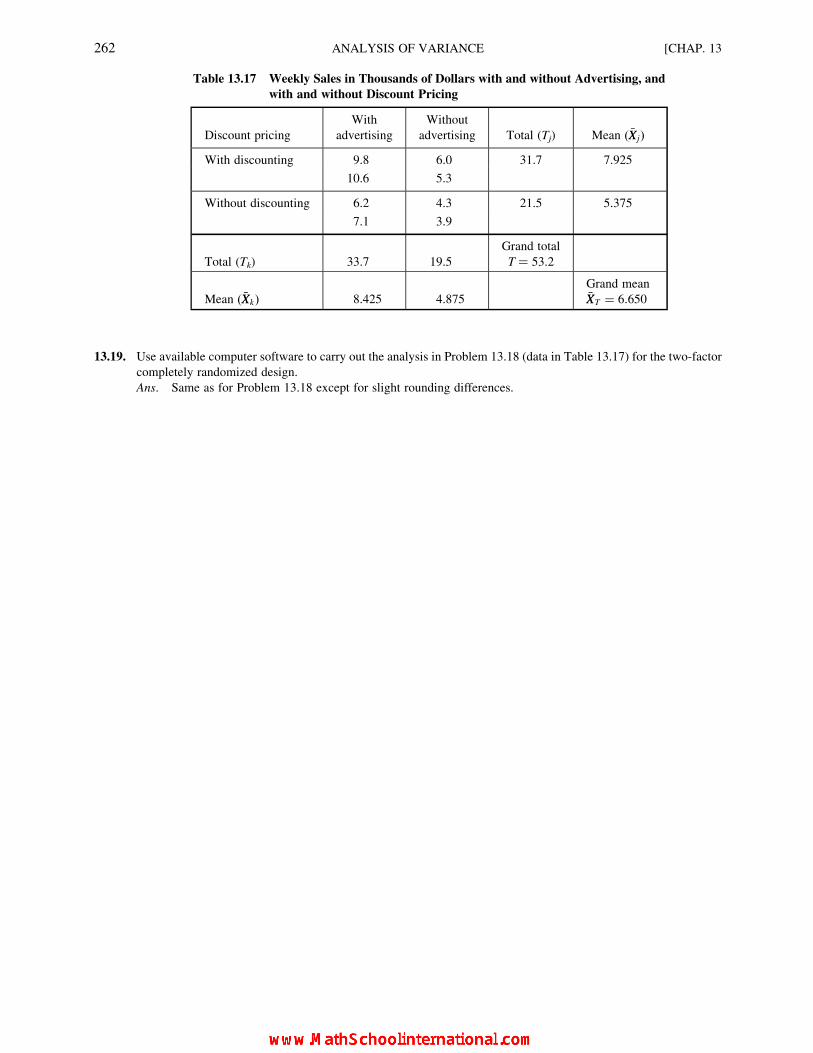
13.19. Use available computer software to carry out the analysis in Problem 13.18 (data in Table 13.17) for the two-factor
completely randomized design.
Ans. Same as for Problem 13.18 except for slight rounding differences.
Table 13.17 Weekly Sales in Thousands of Dollars with and without Advertising, and
with and without Discount Pricing
Discount pricing
With
advertising
Without
advertising Total (Tj) Mean ( �XXj)
With discounting 9.8 6.0 31.7 7.925
10.6 5.3
Without discounting 6.2 4.3 21.5 5.375
7.1 3.9
Total (Tk) 33.7 19.5
Grand total
T ¼ 53.2
Mean ( �XXk) 8.425 4.875
Grand mean�XXT ¼ 6:650
262 ANALYSIS OF VARIANCE [CHAP. 13

CHAPTER 14
Linear Regression andCorrelation Analysis
14.1 OBJECTIVES AND ASSUMPTIONS OF REGRESSION ANALYSIS
The primary objective of regression analysis is to estimate the value of a random variable (the dependent
variable) given that the value of an associated variable (the independent variable) is known. The dependent
variable is also called the response variable, while the independent variable is also called the predictor
variable. The regression equation is the algebraic formula by which the estimated value of the dependent, or
response, variable is determined (see Section 14.3).
The term simple regression analysis indicates that the value of a dependent variable is estimated on the
basis of one independent, or predictor, variable. Multiple regression analysis (covered in Chapter 15) is
concerned with estimating the value of a dependent variable on the basis of two or more independent variables.
The general assumptions underlying the regression analysis model presented in this chapter are that (1) the
dependent variable is a random variable, and (2) the independent and dependent variables are linearly
associated. Assumption (1) indicates that although the values of the independent variable may be controlled, the
values of the dependent variable must be obtained through the process of random sampling.
If interval estimation or hypothesis testing is done in the regression analysis, three additional required
assumptions are that (3) the variances of the conditional distributions of the dependent variable, given different
values for the independent variable, are all equal, (4) the conditional distributions of the dependent variable,
given different values for the independent variable, are all normally distributed in the population of values, and
(5) the observed values of the dependent variable are independent of each other.
EXAMPLE 1. An analyst wishes to estimate delivery time as the dependent variable, based on distance as the independent
variable for industrial parts shipped by truck. Suppose 10 recent shipments are chosen from the company’s records such that
the highway distances involved are about equally dispersed between 100 miles distance and 1,000 miles distance, and the
delivery times for each shipment are recorded. Since the highway distance is to be used as the independent variable, this
selection of trips of specific distances is acceptable. On the other hand, the dependent variable of delivery time is a random
variable in this study, which conforms to the assumption underlying regression analysis. Whether or not the two variables
have a linear relationship would generally be investigated by constructing a scatter plot (see Section 14.2) or a residual plot
(see Section 14.4). Such diagrams also are used to observe whether the vertical scatter (variance) is about equal along the
regression line.
263
Copyright 2004, 1996, 1988, 1976 by The McGraw-Hill Companies, Inc. Click Here for Terms of Use.

14.2 THE SCATTER PLOT
A scatter plot is a graph in which each plotted point represents an observed pair of values for the
independent and dependent variables. The value of the independent variable X is plotted with respect to the
horizontal axis, and the value of the dependent variable Y is plotted with respect to the vertical axis.
(See Problem 14.1.)
The form of the relationship represented by the scatter plot can be curvilinear rather than linear.
While regression analysis for curvilinear relationships is outside the scope of this book, there is a limited
discussion of curvilinear trend analysis in Section 16.2. For relationships that are not linear, a frequent
approach is to determine a method of transforming values of one or both variables so that the relationship
of the transformed values is linear. Then linear regression analysis can be applied to the transformed
values, and estimated values of the dependent variable can be transformed back to the original
measurement scale.
EXAMPLE 2. An example of a curvilinear relationship would be the relationship between years since incorporation
for a company and sales level, given that each year the sales level has increased by the same percentage
over the preceding year. The resulting curve with an increasing slope would be indicative of a so-called exponential
relationship.
If the scatter plot indicates a relationship that is generally linear, then a straight line is fitted to the
data. The precise location of this line is determined by the method of least squares (see Section 14.3). As
illustrated in Example 3, a regression line with a positive slope indicates a direct relationship between the
variables, a negative slope indicates an inverse relationship between the variables, and a slope of
zero indicates that the variables are unrelated. Further, the extent of vertical scatter of the
plotted points with respect to the regression line indicates the degree of relationship between the two
variables.
EXAMPLE 3. Figure 14-1 includes several scatter plots and associated regression lines demonstrating several types of
relationships between the variables.
Fig. 14-1
264 LINEAR REGRESSION AND CORRELATION ANALYSIS [CHAP. 14

14.3 THE METHOD OF LEAST SQUARES FOR FITTING A REGRESSION LINE
The linear equation that represents the simple linear regression model is
Yi ¼ b0 þ b1Xi þ 1i (14:1)
where Yi ¼ value of the dependent variable in the ith trial, or observation
b0 ¼ first parameter of the regression equation, which indicates the value of Y when X ¼ 0
b1 ¼ second parameter of the regression equation, called the regression coefficients, which indicates
the slope of the regression line
Xi ¼ the specified value of the independent variable in the ith trial, or observation
1i ¼ random-sampling error in the ith trial, or observation (1 is the Greek epsilon)
The parameters b0 and b1 in the linear regression model are estimated by the values b0 and b1 that are based
on sample data. Thus, the linear regression equation based on sample data that is used to estimate a single
(conditional) value of the dependent variable, where the “hat” over the Y indicates that it is an estimated value, is
YY ¼ b0 þ b1X (14:2)
Depending on the mathematical criterion used, a number of different linear equations can be developed for a
given scatter plot. By the least-squares criterion the best-fitting regression line (and the best equation) is that for
which the sum of the squared deviations between the estimated and actual values of the dependent variable for
the sample data is minimized. The computational formulas by which the values of b0 and b1 in the regression
equation can be determined for the equation which satisfies the least-squares criterion are
b1 ¼ SXY � n �XX �YY
SX2 � n �XX2
(14:3)
b0 ¼ �YY � b1�XX (14:4)
Once the regression equation is formulated, then this equation can be used to estimate the value of the
dependent variable given the value of the independent variable. However, such estimation should be done only
within the range of the values of the independent variable originally sampled, since there is no statistical basis to
assume that the regression line is appropriate outside these limits. Further, it should be determined whether the
relationship expressed by the regression equation is real or could have occurred in the sample data purely by
chance (see Section 14.6). Problem 14.2 illustrates the determination of a regression equation based on sample
data.
14.4 RESIDUALS AND RESIDUAL PLOTS
For a given value X of the independent variable, the regression line value YY often is called the fitted value of
the dependent variable. The difference between the observed value Y and the fitted value YY is called the residual
for that observation and is denoted by e:
e ¼ Y � YY (14:5)
Problem 14.3 reports the full set of residuals for particular sample data. A residual plot is obtained by
plotting the residuals e with respect to the independent variable X or, alternatively with respect to the fitted
regression line values YY . Such a plot can be used as an alternative to the use of the scatter plot to investigate
whether the assumptions concerning linearity and equality of conditional variances appear to be satisfied.
CHAP. 14] LINEAR REGRESSION AND CORRELATION ANALYSIS 265

Problem 14.3 includes a residual plot for the data. Residual plots are particularly important in multiple
regression analysis, as described in Chapter 15.
The set of residuals for the sample data also serve as the basis for calculating the standard error of estimate,
as described in the following section.
14.5 THE STANDARD ERROR OF ESTIMATE
The standard error of estimate is the conditional standard deviation of the dependent variable Y given a
value of the independent variable X. For population data, the standard error of estimate is represented by the
symbol sY :X . The deviations formula by which this value is estimated on the basis of sample data is
sY :X ¼ffiffiffiffiffiffiffiffiffiffiffiffiffiffiffiffiffiffiffiffiffiS(Y � YY)2
n � 2
s¼
ffiffiffiffiffiffiffiffiffiffiffiSe2
n � 2
s(14:6)
Note that the numerator in Formula (14.6) is the sum of the squares of the residuals described in the preceding
section. Although Formula (14.6) clearly reflects the idea that the standard error of estimate is the standard
deviation with respect to the regression line (that is, it is the standard deviation of the vertical “scatter” about the
line), computationally the formula requires that every fitted value YY be calculated for the sample data. The
alternative computational formula, which does not require determination of each fitted value and is therefore
generally easier to use, is
sY :X ¼ffiffiffiffiffiffiffiffiffiffiffiffiffiffiffiffiffiffiffiffiffiffiffiffiffiffiffiffiffiffiffiffiffiffiffiffiffiffiffiffiffiffiffiffiffiSY 2 � b0SY � b1SXY
n � 2
r(14:7)
As will be seen in the following sections, the standard error of estimate serves as the cornerstone for the
various standard errors used in the hypothesis testing and interval-estimation procedures in regression analysis.
Problems 14.5 and 14.6 illustrate the calculation of the standard error of estimate by the computational formula
and deviations formula, respectively.
14.6 INFERENCES CONCERNING THE SLOPE
Before a regression equation is used for the purpose of estimation or prediction, we should first determine if
a relationship appears to exist between the two variables in the population, or whether the observed relationship
in the sample could have occurred by chance. In the absence of any relationship in the population, the slope of
the population regression line would, by definition, be zero: b1 ¼ 0. Therefore the usual null hypothesis tested
is H0: b1 ¼ 0. The null hypothesis can also be formulated as a one-tail test, in which case the alternative
hypothesis is not simply that the two variables are related, but that the relationship is of a specific type (direct or
inverse).
A hypothesized value of the slope is tested by computing a t statistic and using n � 2 degrees of freedom.
Two degrees of freedom are lost in the process of inference because two parameter estimates, b0 and b1, are
included in the regression equation. The standard formula is
t ¼ b1 � (b1)0sb1
(14:8)
where
sb1 ¼sY :Xffiffiffiffiffiffiffiffiffiffiffiffiffiffiffiffiffiffiffiffiffiffiffi
SX2 � n �XX
2q (14:9)
266 LINEAR REGRESSION AND CORRELATION ANALYSIS [CHAP. 14

However, when the null hypothesis is that the slope is zero, which generally is the hypothesis, then formula
(14.8) is simplified and is stated as
t ¼ b1
sb1
(14:10)
Problems 14.7 and 14.8 illustrate a two-tail test and a one-tail test for the slope, respectively.
The confidence interval for the population slope b1, in which the degrees of freedom associated with the t
are once again n 2 2, is constructed as follows:
b1 + tsb1 (14:11)
Problem 14.9 illustrates the construction of a confidence interval for the population slope.
14.7 CONFIDENCE INTERVALS FOR THE CONDITIONAL MEAN
The point estimate for the conditional mean of the dependent variable, given a specific value of X, is the
regression line value YY . When we use the regression equation to estimate the conditional mean, the appropriate
symbol for the conditional mean of Y that is estimated is mmY :
mmY ¼ b0 þ b1X (14:12)
Based on sample data, the standard error of the conditional mean varies in value according to the
designated value of X and is
s �YY :X ¼ sY :X
ffiffiffiffiffiffiffiffiffiffiffiffiffiffiffiffiffiffiffiffiffiffiffiffiffiffiffiffiffiffiffiffiffiffiffiffiffiffiffiffiffiffi1
nþ (X � �XX)2
SX 2 � [(SX)2=n]
s(14:13)
Given the point estimate of the conditional mean and the standard error of the conditional mean, the
confidence interval for the conditional mean, using n � 2 degrees of freedom, is
mmY + ts �YY :X (14:14)
Again, it is n � 2 degrees of freedom because the two parameter estimates b0 and b1 are required in the
regression equation. Problem 14.10 illustrates the construction of a confidence interval for the conditional mean.
14.8 PREDICTION INTERVALS FOR INDIVIDUAL VALUES OF THE
DEPENDENT VARIABLE
As contrasted to a confidence interval, which is concerned with estimating a population parameter, a
prediction interval is concerned with estimating an individual value and is therefore a probability interval. It
might seem that a prediction interval could be constructed by using the standard error of estimate defined in
Formulas (14.6) and (14.7). However, such an interval would be incomplete, because the standard error of
estimate does not include the uncertainty associated with the fact that the position of the regression line based
on sample data includes sampling error and generally is not identical to the population regression line. The
complete standard error for a prediction interval is called the standard error of forecast, and it includes the
uncertainty associated with the vertical “scatter” about the regression line plus the uncertainty associated with
the position of the regression line value itself. The basic formula for the standard error of forecast is
sY(next) ¼ffiffiffiffiffiffiffiffiffiffiffiffiffiffiffiffiffiffiffiffiffiffiffiffiffiffisY :X
2 þ s �YY :X2
p(14:15)
CHAP. 14] LINEAR REGRESSION AND CORRELATION ANALYSIS 267
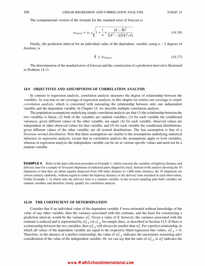
The computational version of the formula for the standard error of forecast is
sY(next) ¼ sY :X
ffiffiffiffiffiffiffiffiffiffiffiffiffiffiffiffiffiffiffiffiffiffiffiffiffiffiffiffiffiffiffiffiffiffiffiffiffiffiffiffiffiffiffiffiffiffiffiffiffiffi1þ 1
nþ (X � �XX)2
SX2 � [(SX)2=n]
s(14:16)
Finally, the prediction interval for an individual value of the dependent, variable, using n � 2 degrees of
freedom, is
YY + tsY(next) (14:17)
The determination of the standard error of forecast and the construction of a prediction interval is illustrated
in Problem 14.11.
14.9 OBJECTIVES AND ASSUMPTIONS OF CORRELATION ANALYSIS
In contrast to regression analysis, correlation analysis measures the degree of relationship between the
variables. As was true in our coverage of regression analysis, in this chapter we restrict our coverage to simple
correlation analysis, which is concerned with measuring the relationship between only one independent
variable and the dependent variable. In Chapter 15, we describe multiple correlation analysis.
The population assumptions underlying simple correlation analysis are that (1) the relationship between the
two variables is linear, (2) both of the variables are random variables, (3) for each variable the conditional
variances, given different values of the other variable, are equal, (4) for each variable, observed values are
independent of other observed values for that variable, and (5) for each variable the conditional distributions,
given different values of the other variable, are all normal distributions. The last assumption is that of a
bivariate normal distribution. Note that these assumptions are similar to the assumptions underlying statistical
inference in regression analysis, except that in correlation analysis the assumptions apply to both variables,
whereas in regression analysis the independent variable can be set at various specific values and need not be a
random variable.
EXAMPLE 4. Refer to the data collection procedure in Example 1, which concerns the variables of highway distance and
delivery time for a sample of 10 recent shipments of industrial parts shipped by truck. Instead of the analyst choosing the 10
shipments so that they are about equally dispersed from 100 miles distance to 1,000 miles distance, the 10 shipments are
chosen entirely randomly, without regard to either the highway distance or the delivery time included in each observation,
Unlike Example 1, in which only the delivery time is a random variable, in the revised sampling plan both variables are
random variables and therefore clearly qualify for correlation analysis.
14.10 THE COEFFICIENT OF DETERMINATION
Consider that if an individual value of the dependent variable Y were estimated without knowledge of the
value of any other variable, then the variance associated with this estimate, and the basis for constructing a
prediction interval, would be the variance s 2Y . Given a value of X, however, the variance associated with the
estimate is reduced and is represented by s 2Y :X (or s 2
Y :X for sample data), as described in Section 14.5. If there is
a relationship between the two variables, then s 2Y :X will always be smaller than s 2
Y . For a perfect relationship, in
which all values of the dependent variable are equal to the respective fitted regression line values, s 2Y :X ¼ 0.
Therefore, in the absence of a perfect relationship, the value of s 2Y :X indicates the uncertainty remaining after
consideration of the value of the independent variable. Or, we can say that the ratio of s 2Y :X to s 2
Y indicates the
268 LINEAR REGRESSION AND CORRELATION ANALYSIS [CHAP. 14

proportion of variance (uncertainty) in the dependent variable that remains unexplained after a specific value of
the independent variable has been given:
proportion of variance
remaining unexplained
� �¼ s 2
Y :X
sY2¼ unexplained variance remaining in Y
total variance in Y(14:18)
In (14.18) s 2Y :X is determined by the procedure described in Section 14.5 (except that population data are
assumed) and s 2Y is calculated by the general formulas presented in Sections 4.6 and 4.7.
Given the proportion of unexplained variance, a useful measure of relationship is the coefficient of
determination—the complement of the above ratio, indicating the proportion of variance in the dependent
variable that is statistically explained by the regression equation (i.e., by knowledge of the associated
independent variable X). For population data the coefficient of determination is represented by the Greek r2 (rhosquared) and is determined by
r2 ¼ 1� s 2Y :X
s 2Y
(14:19)
proportion of explained variance ¼ 1� (proportion of unexplained variance)
For sample data, the estimated value of the coefficient of determination can be obtained by the
corresponding formula:
r 2 ¼ 1� s 2Y :X
s 2Y
(14:20)
For computational purposes, the following formula for the sample coefficient of determination is
convenient:
r2 ¼ b0SY þ b1SXY � n �YY2
SY2 � n �YY
2(14:21)
Application of (14.21) is illustrated in Problem 14.12. Although this is a frequently used formula for
computing the coefficient of determination for sample data, it does not incorporate any correction for biasedness
and includes a slight positive bias. See the following section for the correction factor that can be used.
14.11 THE COEFFICIENT OF CORRELATION
Although the coefficient of determination r2 is relatively easy to interpret, it does not lend itself to statistical
testing. However, the square root of the coefficient of determination, which is called the coefficient of
correlation r, does lend itself to statistical testing because it can be used to define a test statistic that is
distributed as the t distribution when the population correlation r equals 0. The value of the correlation
coefficient can range from �1:00 to þ1:00. The arithmetic sign associated with the correlation coefficient,
which is always the same as the sign associated with b1 in the regression equation, indicates the direction of the
relationship between X and Y (positive ¼ direct; negative ¼ inverse). The coefficient of correlation for
population data, with the arithmetic sign being the same as that for the slope b1 in the regression equation, is
r ¼ffiffiffiffiffir 2
p(14:22)
The coefficient of correlation for sample data, with the arithmetic sign being the same as that for the sample
slope b1, is
r ¼ffiffiffiffir2
p(14:23)
In summary, the sign of the correlation coefficient indicates the direction of the relationship between the X
and Y variables, while the absolute value of the coefficient indicates the extent of relationship. The squared
value of the correlation coefficient is the coefficient of determination and indicates the proportion of the
variance in Y explained by knowledge of X (and vice versa).
CHAP. 14] LINEAR REGRESSION AND CORRELATION ANALYSIS 269

EXAMPLE 5. Figure 14-2 illustrates the general appearance of the scatter diagrams associated with several correlation
values.
As an alternative to (14.21), the following formula does not require prior determination of the regression
value of b0 and b1. This formula would be used when the purpose of the analysis is to determine the extent and
type of relationship between two variables, but without an accompanying interest in estimating Y given X.
When this formula is used, the sign of the correlation coefficient is determined automatically, without the
necessity of observing or calculating the slope of the regression line. The formula is
r ¼ nSXY � SXSYffiffiffiffiffiffiffiffiffiffiffiffiffiffiffiffiffiffiffiffiffiffiffiffiffiffiffiffiffinSX 2 � (SX)2
p ffiffiffiffiffiffiffiffiffiffiffiffiffiffiffiffiffiffiffiffiffiffiffiffiffiffiffiffinSY 2 � (SY)2
p (14:24)
Application of (14.24) is illustrated in Problem 14.13.
The sample coefficient of correlation r is somewhat biased as an estimator ofr,with anabsolute value that is toolarge. This factor is not mentioned in many textbooks because the amount of bias is slight, except for very small
samples. An unbiased estimator for the coefficient of determination for the population can be obtained as follows:
rr2 ¼ 1� (1� r2)n � 1
n � 2
� �(14:25)
14.12 THE COVARIANCE APPROACH TO UNDERSTANDING THE CORRELATION
COEFFICIENT
Another measure that can be used to express the relationship between two random variables is the sample
covariance. The covariance measures the extent to which two variables “vary together” and is used by financial
analysts for determining the total risk associated with interrelated investments. Just as for the correlation
coefficient, a positive sign indicates a direct relationship while a negative sign indicates an inverse relationship.
The formula for the sample covariances is
cov(X, Y) ¼ S[(X � �XX)(Y � �YY)]
n � 1(14:26)
By studying Formula (14.26) we can conclude, for example, that when the observed value of Y tends to vary in
the same direction from its mean as does the observed value of X from its mean, then the products of those
Fig. 14-2
270 LINEAR REGRESSION AND CORRELATION ANALYSIS [CHAP. 14
deviations will tend to be positive values. The sum of such products will then be positive, indicating the direct,
rather than inverse, relationship. Whereas the coefficient of correlation is a standardized measure of relationship
that can range in value between only �1:00 and þ1:00, the covariance has no such limits in value and is not a
standardized measure. The formula by which the covariance can be converted into the coefficient of correlation is
r ¼ cov(X, Y)
sXsY
(14:27)
Problem 14.14 illustrates the determination of a sample covariance and its conversion into the associated
correlation coefficient.
14.13 SIGNIFICANCE TESTING WITH RESPECT TO THE CORRELATION COEFFICIENT
Typically, the null hypothesis of interest is that the population correlation r ¼ 0, for if this hypothesis is rejected
at a specified a level, we would conclude that there is a relationship between the two variables in the population. The
hypothesis can also be formulated as a one-tail test. Given that the assumptions in Section 14.9 are satisfied, the
following sampling statistic involving r is distributed as the t distribution with d f ¼ n � 2 when r ¼ 0:
t ¼ rffiffiffiffiffiffiffiffiffiffiffiffiffi1� r 2
n � 2
r (14:28)
Testing the null hypothesis that r ¼ 0 is equivalent to testing the null hypothesis that b ¼ 0 in the regression
equation. (See Problem 14.15.)
14.14 PITFALLS AND LIMITATIONS ASSOCIATED WITH REGRESSION AND
CORRELATION ANALYSIS
(1) In regression analysis a value of Y cannot be legitimately estimated if the value of X is outside the
range of values that served as the basis for the regression equation.
(2) If the estimate of Y involves the prediction of a result that has not yet occurred, the historical data
that served as the basis for the regression equation may not be relevant for future events.
(3) The use of a prediction or a confidence interval is based on the assumption that the conditional
distributions of Y, and thus of the residuals, are normal and have equal variances.
(4) A significant correlation coefficient does not necessarily indicate causation, but rather may
indicate a common linkage to other events.
(5) A significant correlation is not necessarily an important correlation. Given a large sample, a
correlation of, say, r ¼ þ0:10 can be significantly different from 0 at a ¼ 0:05. Yet the coefficientof determination of r2 ¼ 0:01 for this example indicates that only 1 percent of the variance in Y is
statistically explained by knowing X.
(6) The interpretation of the coefficients of correlation and determination is based on the assumption of a
bivariate normal distribution for the population and, for each variable, equal conditional variances.
(7) For both regression and correlation analysis, a linear model is assumed. For a relationship that is
curvilinear, a transformation to achieve linearity may be available. Another possibility is to restrict
the analysis to the range of values within which the relationship is essentially linear.
14.15 USING EXCEL AND MINITAB
Computer software is available to carry out the various procedures of simple regression and correlation
analysis that are covered in this chapter. Solved Problem 14.17 illustrates the use of Excel and compares the
output to the results obtained by manual calculation in the preceding end-of-chapter problems. Problem 14.18
illustrates the use of Minitab and compares the output to the results obtained by manual calculation in the
preceding end-of-chapter problems.
CHAP. 14] LINEAR REGRESSION AND CORRELATION ANALYSIS 271

Solved Problems
LINEAR REGRESSION ANALYSIS
14.1. Suppose an analyst takes a random sample of 10 recent truck shipments made by a company and records
the distance in miles and delivery time to the nearest half-day from the time that the shipment was made
available for pick-up. Construct the scatter plot for the data in Table 14.1 and consider whether linear
regression analysis appears appropriate.
Table 14.1 Sample Observations of Trucking Distance and Delivery Time for 10 Randomly Selected
Shipments
Sampled
shipment 1 2 3 4 5 6 7 8 9 10
Distance (X),
miles 825 215 1,070 550 480 920 1,350 325 670 1,215
Delivery
time (Y), days 3.5 1.0 4.0 2.0 1.0 3.0 4.5 1.5 3.0 5.0
The scatter plot for these data is portrayed in Fig. 14-3. The first reported pair of values in the table is
represented by the dot entered above 825 on the X axis and aligned with 3.5 with respect to the Y axis. The other nine
points in the scatter plot were similarly entered. From the diagram, it appears that the plotted points generally follow
a linear relationship and the vertical scatter at the line is about the same for low values and high values of X. Thus
linear regression analysis appears appropriate.
14.2. Determine the least-squares regression equation for the data in Problem 14.1, and enter the regression
line on the scatter plot for these data.
Referring to Table 14.2,
b1 ¼ SXY � n �XX �YY
SX2 � n �XX
2¼ (26,370)� (10)(762)(2:85)
7,104,300� (10)(762)2 ¼ 4,653
1,297,860¼ 0:0035851 ffi 0:0036
b0 ¼ �YY � b �XX ¼ 2:85� (0:0036)(762) ¼ 0:1068 ffi 0:11
Therefore; �YY ¼ b0 þ b1X ¼ 0:11þ 0:0036X
Fig. 14-3
272 LINEAR REGRESSION AND CORRELATION ANALYSIS [CHAP. 14

This estimated regression line based on sample data is entered in the scatter plot for these data in Fig. 14-4.
Note the dashed lines indicating the amount of deviation between each sampled value of Y and the corresponding
estimated value, YY . It is the sum of these squared deviations that is minimized by the linear regression line
determined by the above procedure.
14.3. Determine the residuals and construct a residual plot with respect to the fitted values for the data in
Table 14.2, using the regression equation developed in Problem 14.2. Compare the residual plot to the
scatter plot in Fig. 14-4.
Table 14.3 presents the calculation of the residuals, while Fig. 14-5 portrays the residual plot. Note that the
general form of the scatter of the dependent-variable values Y with respect to the regression line in the scatter plot
and the scatter of the residuals e with respect to the “0” line of deviation in the residual plot are similar, except for
the “stretched” vertical scale in the residual plot.
Fig. 14-4
Table 14.2 Calculations Associated with Determining the Linear Regression Equation for
Estimating Delivery Time on the Basis of Trucking Distance
Sampled
shipment
Distance (X),
miles
Delivery time (Y),
days XY X 2 Y 2
1 825 3.5 2,887.5 680,625 12.25
2 215 1.0 215.0 46,225 1.00
3 1,070 4.0 4,280.0 1,144,900 16.00
4 550 2.0 1,100.0 302,500 4.00
5 480 1.0 480.0 230,400 1.00
6 920 3.0 2,760.0 846,400 9.00
7 1,350 4.5 6,075.0 1,822,500 20.25
8 325 1.5 487.5 105,625 2.25
9 670 3.0 2,010.0 448,900 9.00
10 1,215 5.0 6,075.0 1,476,225 25.00
Totals 7,620 2.85 26,370.0 7,104,300 99.75
Mean �XX ¼ SX
n¼ 7,620
10
¼ 762
�YY ¼ SY
n¼ 28:5
10
¼ 2:85
CHAP. 14] LINEAR REGRESSION AND CORRELATION ANALYSIS 273
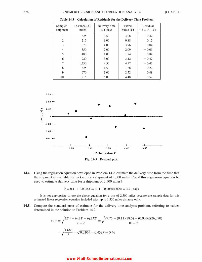
14.4. Using the regression equation developed in Problem 14.2, estimate the delivery time from the time that
the shipment is available for pick-up for a shipment of 1,000 miles. Could this regression equation be
used to estimate delivery time for a shipment of 2,500 miles?
YY ¼ 0:11þ 0:0036X ¼ 0:11þ 0:0036(1,000) ¼ 3:71 days
It is not appropriate to use the above equation for a trip of 2,500 miles because the sample data for this
estimated linear regression equation included trips up to 1,350 miles distance only.
14.5. Compute the standard error of estimate for the delivery-time analysis problem, referring to values
determined in the solution to Problem 14.2.
sY :X ¼ffiffiffiffiffiffiffiffiffiffiffiffiffiffiffiffiffiffiffiffiffiffiffiffiffiffiffiffiffiffiffiffiffiffiffiffiffiffiffiffiffiffiffiffiffiSY 2 � b0SY � b1SXY
n � 2
r¼
ffiffiffiffiffiffiffiffiffiffiffiffiffiffiffiffiffiffiffiffiffiffiffiffiffiffiffiffiffiffiffiffiffiffiffiffiffiffiffiffiffiffiffiffiffiffiffiffiffiffiffiffiffiffiffiffiffiffiffiffiffiffiffiffiffiffiffiffiffiffiffiffiffiffiffiffiffiffiffi99:75� (0:11)(28:5)� (0:0036)(26,370)
10� 2
r
¼ffiffiffiffiffiffiffiffiffiffiffi1:683
8
r¼
ffiffiffiffiffiffiffiffiffiffiffiffiffiffi0:2104
p¼ 0:4587 ffi 0:46
Table 14.3 Calculation of Residuals for the Delivery Time Problem
Sampled
shipment
Distance (X),
miles
Delivery time
(Y), days
Fitted
value (YY)
Residual
(e ¼ Y � YY)
1 825 3.50 3.08 0.42
2 215 1.00 0.88 0.12
3 1,070 4.00 3.96 0.04
4 550 2.00 2.09 20.09
5 480 1.00 1.84 20.84
6 920 3.00 3.42 20.42
7 1,350 4.50 4.97 20.47
8 325 1.50 1.28 0.22
9 670 3.00 2.52 0.48
10 1,215 5.00 4.48 0.52
Fig. 14-5 Residual plot.
274 LINEAR REGRESSION AND CORRELATION ANALYSIS [CHAP. 14

14.6. Compute the standard error of estimate by the basic formula that utilizes the residuals determined in
Problem 14.3. Compare your answer to that obtained by the computational formula in Problem 14.5
above.
sY:X ¼ffiffiffiffiffiffiffiffiffiffiffiSe2
n � 2
r¼
ffiffiffiffiffiffiffiffiffiffiffiffiffiffi1:8526
10� 2
r¼ 0:4812 ffi 0:48
Except for a slight rounding difference, this answer corresponds to the one obtained in Problem 14.5.
14.7. Using the standard error of estimate from Problem 14.5, test the null hypothesis H0: b1 ¼ 0 for the
trucking distance and delivery-time data in Table 14.2, using the 5 percent level of significance.
Given sY:X ¼ 0:46 and the values in Table 14.2,
sb1 ¼sY:Xffiffiffiffiffiffiffiffiffiffiffiffiffiffiffiffiffiffiffiffiffiffiffi
SX2 � n �XX
2q ¼ 0:46ffiffiffiffiffiffiffiffiffiffiffiffiffiffiffiffiffiffiffiffiffiffiffiffiffiffiffiffiffiffiffiffiffiffiffiffiffiffiffiffiffiffiffi
7,104,300� 10(762)2p ¼ 0:46
1,139:24¼ 0:0004
H0: b1 ¼ 0 H1: b1 = 0
Critical t(d f ¼ 8, a ¼ 0:05) ¼ + 2:306
t ¼ b1
sb1
¼ 0:0036
0:0004¼ þ 9:00
Because the calculated t of þ 9:00 is in a region of rejection for this two-sided test, we conclude that there is asignificant relationship between trucking distance and delivery time.
14.8. Referring to Problem 14.7, above, test the null hypothesis H0: b1 0 at the 5 percent level of
significance.
H0: b1 ¼ 0 H1: b1 . 0
Critical t(d f ¼ 8, a ¼ 0:05) ¼ þ 1:860
t ¼ þ 9:00 (from Problem 14:7)
Because the calculated t statistic ofþ 9:00 exceeds the critical value ofþ 1:860, the null hypothesis is rejected.For this one-tail test, we conclude that the slope of the population regression line is positive, and thus that there is a
direct (rather than inverse) relationship between shipment distance and delivery time.
14.9. Determine the 95 percent confidence interval for b1 for the trucking distance and delivery-time data
discussed in the preceding problems.
Since b1 ¼ 0:0036 (from Problem 14.2) and d f ¼ n � 2 ¼ 10� 2 ¼ 8, the 95 percent confidence interval
for b1 is
b1 + tsb1 ¼ 0:0036+ (2:306)(0:0004) ¼ 0:0036+ 0:0009 ¼ 0:0027 to 0:0045
Thus, with each additional mile of distance, the number of additional days required for delivery is somewhere
between 0.0027 and 0.0045 with 95 percent confidence. Assuming a 24-hour day at receiving docks, this is
equivalent to the additional delivery time per mile being somewhere between 3.9 and 6.5min, with 95 percent
confidence.
14.10. Using the values determined in the preceding problems, construct the 95 percent confidence interval for
the mean delivery time for a trucking distance of 1,000 miles.
Given mm �YY (for X ¼ 1,000) ¼ 3:71 days, sY:X ¼ 0:46, and the values in Table 14.2,
s �YY:X ¼ sY :X
ffiffiffiffiffiffiffiffiffiffiffiffiffiffiffiffiffiffiffiffiffiffiffiffiffiffiffiffiffiffiffiffiffiffiffiffiffiffiffi1
nþ (X � �XX)2
SX 2 � (SX)2=n
s¼ 0:46
ffiffiffiffiffiffiffiffiffiffiffiffiffiffiffiffiffiffiffiffiffiffiffiffiffiffiffiffiffiffiffiffiffiffiffiffiffiffiffiffiffiffiffiffiffiffiffiffiffiffiffiffiffiffiffiffiffiffiffi1
10þ (1000� 762)2
7,104,300� (7,620)2=10
s¼ 0:1748 ffi 0:17
CHAP. 14] LINEAR REGRESSION AND CORRELATION ANALYSIS 275
The 95 percent confidence interval for the conditional mean (where df ¼ 10� 2 ¼ 8) is
mm Y + ts �YY :X ¼ 3:71+ (2:306)(0:17) ¼ 3:71+ 0:39 ¼ 3:32 to 4:10 days
Thus, for truck shipments of 1,000 miles, we estimate that the mean delivery time from the time that the
shipment is available is between 3.32 and 4.10 days, with 95 percent confidence in this estimation interval.
14.11. Using the values determined in the preceding problems, determine the 95 percent prediction interval for
the delivery time of a single shipment given that a distance of 1,000 miles is involved. Compare this
interval with the one constructed in Problem 14.10.
Since YY (for X ¼ 1,000) ¼ 3:71 days, sY:X ¼ 0:46, and s �YY:X ¼ 0:17,
sYnext ¼ffiffiffiffiffiffiffiffiffiffiffiffiffiffiffiffiffiffiffiffiffiffis 2Y:X þ s 2�YY:X
q¼
ffiffiffiffiffiffiffiffiffiffiffiffiffiffiffiffiffiffiffiffiffiffiffiffiffiffiffiffiffiffiffiffiffi(0:46)2 þ (0:17)2
q¼
ffiffiffiffiffiffiffiffiffiffiffiffiffiffi0:2405
p¼ 0:4904 ffi 0:49
Where d f ¼ 10� 2 ¼ 8, the 95 percent prediction interval is
YY + tsYnext ¼ 3:71+ 2:306(0:49) ¼ 3:71+ 1:13 ¼ 2:58 to 4:84 days
As expected, this prediction interval is somewhat wider than the confidence interval for the conditional mean in
Problem 14.10, since in the present application the interval concerns an individual value for one particular shipment
rather than a mean.
CORRELATION ANALYSIS
14.12. For the trucking distance and delivery-time data, the sampling procedure described in Problem 14.1
indicates that both variables are in fact random variables. If we further assume a bivariate normal
distribution for the population and, for each variable, equal conditional variances, then correlation
analysis can be applied to the sample data. Using values calculated in Problem 14.2, calculate the
coefficient of determination for the sample data (ignore the slight biasedness associated with this
coefficient).
r 2 ¼ b0SY þ b1 SXY � n �YY2
SY2 � n �YY
2
¼ (0:11)(28:5)þ (0:0036)(26,370)� (10)(2:85)2
99:75� (10)(2:85)2
¼ 16:842
18:525¼ 0:9091 ffi 0:91
Thus, as a point estimate we can conclude that about 91 percent of the variance in delivery time is statistically
explained by the trucking distance involved. Further, given the trucking distance involved, we can also conclude
that only about 9 percent of the variance remains unexplained.
14.13. For the trucking distance and delivery-time data, (a) calculate the coefficient of correlation by reference
to the coefficient of determination in Problem 14.12, and (b) determine the coefficient of correlation by
using the alternative computational formula for r.
ðaÞ r ¼ffiffiffiffir2
p¼
ffiffiffiffiffiffiffiffiffiffiffiffiffiffi0:9091
p¼ þ 0:9535 ffi þ 0:95
The positive value for the correlation value is based on the observation that the slope b1 of the regression line is
positive, as determined in Problem 14.2.
276 LINEAR REGRESSION AND CORRELATION ANALYSIS [CHAP. 14
ðbÞ r ¼ nSXY � SXSYffiffiffiffiffiffiffiffiffiffiffiffiffiffiffiffiffiffiffiffiffiffiffiffiffiffiffiffiffinSX 2 � (SX)2
p ffiffiffiffiffiffiffiffiffiffiffiffiffiffiffiffiffiffiffiffiffiffiffiffiffiffiffiffiffinSY 2 � (SY)2
p ¼ (10)(26,370)� (7,620)(28:5)ffiffiffiffiffiffiffiffiffiffiffiffiffiffiffiffiffiffiffiffiffiffiffiffiffiffiffiffiffiffiffiffiffiffiffiffiffiffiffiffiffiffiffiffiffiffiffiffiffiffiffiffi(10)(7,104,300)� (7,620)2
p ffiffiffiffiffiffiffiffiffiffiffiffiffiffiffiffiffiffiffiffiffiffiffiffiffiffiffiffiffiffiffiffiffiffiffiffiffiffiffiffiffiffi(10)(99:75)� (28:5)2
p¼ 46,530
(3,602:5824)(13:6107)¼ 46,530
49,033:668¼ þ 0:9489 ffi þ 0:95
Except for a slight difference due to rounding, the two values are the same.
14.14. For the trucking distance and delivery-time data, (a) calculate the sample covariance, and (b) convert the
covariance value into the coefficient of correlation. Compare your answer in (b) to the answers for the
coefficient of correlation obtained in Problem 14.13 above.
ðaÞ cov(X, Y) ¼ S[(X � �XX)(Y � �YY)]
n � 1
¼ 4,653
9¼ 517:00 (from Table 14:4)
ðbÞ r ¼ cov(X, Y)
sX , sY
where sX ¼ffiffiffiffiffiffiffiffiffiffiffiffiffiffiffiffiffiffiffiffiffiffiffiSX
2 � n �XX2
n � 1
s[from formula (4:11)]
¼ffiffiffiffiffiffiffiffiffiffiffiffiffiffiffiffiffiffiffiffiffiffiffiffiffiffiffiffiffiffiffiffiffiffiffiffiffiffiffiffiffiffiffi7,104,300� 10(762)2
10� 1
s(from Table 14:2)
¼ffiffiffiffiffiffiffiffiffiffiffiffiffiffiffiffiffiffiffiffiffiffi144,206:66
p¼ 379:7455
sY ¼ffiffiffiffiffiffiffiffiffiffiffiffiffiffiffiffiffiffiffiffiffiffiffiSY
2 � n �YY2
n � 1
s[from formula (4:11)]
¼ffiffiffiffiffiffiffiffiffiffiffiffiffiffiffiffiffiffiffiffiffiffiffiffiffiffiffiffiffiffiffiffiffiffiffiffi99:75� 10(2:85)2
10� 1
s(from Table 14:2)
¼ffiffiffiffiffiffiffiffiffiffiffiffiffiffiffiffiffiffiffi2:058333
p¼ 1:4347
r ¼ 517:00
(379:7455)(1:4347)¼ þ 0:9489 ffi þ 0:95
The correlation coefficient matches those calculated in Problem 14.13 above.
14.15. Determine whether the correlation value computed in Problem 14.14(b) is significantly different from
zero at the 5 percent level of significance.
H0: r ¼ 0 H1: r = 0
Critical t(df ¼ 8, a ¼ 0:05) ¼ + 2:306
t ¼ rffiffiffiffiffiffiffiffiffiffiffiffiffiffiffiffi(1� r2)
(n � 2)
r ¼ 0:9489ffiffiffiffiffiffiffiffiffiffiffiffiffiffiffiffiffiffiffiffiffiffiffiffiffi(1� 0:9004)(10� 2)
r ¼ 0:9489
0:1116¼ þ8:50
Because the test statistic of t ¼ þ8:50 is in a region of rejection, the null hypothesis that there is no relationshipbetween the two variables is rejected, and we conclude that there is a significant relationship between trucking
distance and delivery time. Note that this conclusion coincides with the test of the null hypothesis that b1 ¼ 0 in
Problem 14.7. The difference in the calculated values of t in these two tests is due to rounding of values in the
calculations.
CHAP. 14] LINEAR REGRESSION AND CORRELATION ANALYSIS 277

14.16. For a sample of n ¼ 10 loan recipients at a finance company, the correlation coefficient between
household income and amount of outstanding short-term debt is found to be r ¼ þ 0:50.
(a) Test the hypothesis that there is no correlation between these two variables for the entire
population of loan recipients, using the 5 percent level of significance.
(b) Interpret the meaning of the correlation coefficient which was computed.
ðaÞ H0: r ¼ 0 H1: r = 0
Critical t (d f ¼ 10� 2 ¼ 8, a ¼ 0:05) ¼ + 2:306
t ¼ rffiffiffiffiffiffiffiffiffiffiffiffiffiffiffiffi(1� r2)
(n � 2)
r ¼ 0:50ffiffiffiffiffiffiffiffiffiffiffiffiffiffiffiffiffiffiffiffiffiffi(1� 0:50)2
8
r ¼ 0:50
0:306¼ þ 1:634
Because the computed t statistic of þ 1:634 is not in a region of rejection, the null hypothesis cannot be
rejected, and we continue to accept the assumption that there is no relationship between the two variables. The
observed sample relationship can be ascribed to chance at the 5 percent level of significance.
(b) Based on the correlation coefficient of r ¼ þ 0:50, we might be tempted to conclude that because r 2 ¼ 0:25,approximately 25 percent of the variance in short-term debt is explained statistically by the amount of
household income. This is true for the sample data. However, because the null hypothesis in part (a) above was
not rejected, a more appropriate interpretation for the population is that none of the variance in Y can be
assumed to be associated with changes in X.
COMPUTER OUTPUT
14.17. Use Excel to carry out the regression analysis for the data on distance and delivery time in Table 14.2.
Compare the output with the results of some of the manual calculations in the preceding exercises.
Fig. 14-6 gives the standard regression output from Excel. Some of the output corresponds to the manual
calculations done in the preceding Solved Problems. The numbered labels below identify such correspondence and
refer to labels that have been inserted in Fig. 14-6.
(1) The regression coefficients for the intercept and the slope correspond to the solution in Problem 14.2, except
for the rounding of values in the manual calculations.
Table 14.4 Calculation of the Covariance
Sampled
shipment
Distance
(X), miles
Delivery
time (Y), days X � �XX Y � �YY (X � �XX)(Y � �YY)
1 825 3.5 63 0.65 40.95
2 215 1.0 2547 21.85 1,011.95
3 1,070 4.0 308 1.15 354.20
4 550 2.0 2212 20.85 180.20
5 480 1.0 2282 21.85 521.70
6 920 3.0 158 0.15 23.70
7 1,350 4.5 588 1.65 970.20
8 325 1.5 2437 21.35 589.95
9 670 3.0 292 0.15 213.80
10 1,215 5.0 453 2.15 973.95
�XX ¼ 762 �YY ¼ 2:85 S ¼ 4,653:00
278 LINEAR REGRESSION AND CORRELATION ANALYSIS [CHAP. 14

(2) The t test for the null hypothesis, H0: r ¼ 0, corresponds to the solution in Problem 14.7, except that P value is
also determined. Because a very small P of 2.79E-05 is less than the designated level of significance of 0.05,
the null hypothesis is rejected, and we conclude that there is a relationship between distance and delivery time
in the sampled population.
(3) The coefficient of determination between distance and delivery time corresponds to the solution in
Problem 14.12.
The Excel output given in Fig. 14-6 was obtained as follows:
(1) Open Excel. In cell A1 enter: Distance. In cell B1 enter: Time. Enter the distance and time data in the
respective columns.
(2) Click Tools ! Data Analysis ! Regression. Click OK.
(3) For Input Y Range enter: $B$1:$B$11. For Input X Range enter: $A$1:$A$11. Check Labels. Click OK.
14.18. Use Minitab to carry out the regression analysis for the data on distance and delivery time in Table 14.2.
Compare the output with the results of some of the manual calculations in the preceding exercises.
Fig. 14-7 gives the standard regression output fromMinitab. The output corresponds to the manual calculations
done in some of the preceding Solved Problems. The numbered labels below identify such correspondence and refer
to labels that have been inserted in Fig. 14-7.
W1 The regression equation in Fig. 14-7 corresponds to the solution in Problem 14.2, except for the rounding of
values in the manual calculations.
W2 The standard error of estimate corresponds to the solution in Problem 14.6.
W3 The t test for the null hypothesis, H0: r ¼ 0, corresponds to the solution in Problem 14.7, except that the P
value is also determined. Because the reported P of 0.000 is less than the designated level of significance of
0.05, the null hypothesis is rejected and we conclude that there is a relationship between distance and delivery
time in the sampled population.
W4 The coefficient of determination between distance and delivery time corresponds to the solution in
Problem 14.12.
W5 The estimated delivery time for a shipment of 1,000 miles in Fig. 14-7 corresponds to the solution in
Problem 14.4.
Fig. 14-6 Regression output from Excel.
CHAP. 14] LINEAR REGRESSION AND CORRELATION ANALYSIS 279
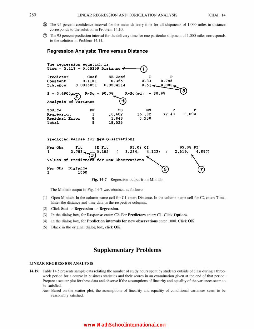
W6 The 95 percent confidence interval for the mean delivery time for all shipments of 1,000 miles in distance
corresponds to the solution in Problem 14.10.
W7 The 95 percent prediction interval for the delivery time for one particular shipment of 1,000 miles corresponds
to the solution in Problem 14.11.
The Minitab output in Fig. 14-7 was obtained as follows:
(1) Open Minitab. In the column name cell for C1 enter: Distance. In the column name cell for C2 enter: Time.
Enter the distance and time data in the respective columns.
(2) Click Stat ! Regression ! Regression.
(3) In the dialog box, for Response enter: C2. For Predictors enter: C1. Click Options.
(4) In the dialog box, for Prediction intervals for new observations enter 1000. Click OK.
(5) Black in the original dialog box, click OK.
Supplementary Problems
LINEAR REGRESSION ANALYSIS
14.19. Table 14.5 presents sample data relating the number of study hours spent by students outside of class during a three-
week period for a course in business statistics and their scores in an examination given at the end of that period.
Prepare a scatter plot for these data and observe if the assumptions of linearity and equality of the variances seem to
be satisfied.
Ans. Based on the scatter plot, the assumptions of linearity and equality of conditional variances seem to be
reasonably satisfied.
Fig. 14-7 Regression output from Minitab.
280 LINEAR REGRESSION AND CORRELATION ANALYSIS [CHAP. 14

14.20. Determine the least-squares regression line for the data in Table 14.5 and enter the line on the plot constructed in
Problem 14.19.
Ans. YY ¼ 40þ 1:5X
14.21. Determine the residuals and construct a residual plot with respect to the fitted values for the data in Table 14.5, using
the regression equation developed in Problem 14.19. Compare the residual plot to the scatter plot prepared in
Problem 14.19.
14.22. Calculate the standard error of estimate for the data in Table 14.5 by using the residuals determined in Problem
14.21.
Ans. sY:X ¼ 6:16
14.23. For the sample information presented in Problem 14.19, (a) test the null hypothesis that the slope of the regression
line is zero, using the 1 percent level of significance, and interpret the result of your test. (b) Repeat the test for the
null hypothesis that the true regression coefficient is equal to or less than zero, using the 1 percent level of
significance.
Ans. (a) Reject H0 and conclude that there is a significant relationship. (b) Reject H0 and conclude that there is a
significant positive relationship.
14.24. Use the regression equation determined in Problem 14.20 to estimate the examination grade of a student who
devoted 30hr of study to the course material.
Ans. Y ¼ 85
14.25. Refer to Problems 14.22 and 14.24. Construct the 90 percent confidence interval for estimating the mean exam
grade for students who devote 30 hr to course preparation.
Ans. 79.02 to 90.98
14.26. Referring to the preceding problems construct the 90 percent prediction interval for the examination grade of an
individual student who devoted 30 hr to course preparation.
Ans. 71.59 to 98.41
14.27. Table 14.6 presents data relating the number of weeks of experience in a job involving the wiring of miniature
electronic components and the number of components which were rejected during the past week for 12 randomly
selected workers. Plot these sample data on a scatter plot.
Table 14.5 Hours Spent on a Statistics Course and Examination Grades for a Sample
of n ¼ 8 Students
Sampled student 1 2 3 4 5 6 7 8
Study hours (X) 20 16 34 23 27 32 18 22
Examination grade (Y) 64 61 84 70 88 92 72 77
Table 14.6 Weeks of Experience and Number of Components Rejected During a Sampled Week for 12
Assembly Workers
Sampled
worker 1 2 3 4 5 6 7 8 9 10 11 12
Weeks of
experience (X) 7 9 6 14 8 12 10 4 2 11 1 8
Number of
rejects (Y) 26 20 28 16 23 18 24 26 38 22 32 25
CHAP. 14] LINEAR REGRESSION AND CORRELATION ANALYSIS 281
14.28. From Table 14.6 determine the regression equation for predicting the number of components rejected given the
number of weeks experience, and enter the regression line on the scatter plot. Comment on the nature of the
relationship as indicated by the regression equation.
Ans. YY ¼ 35:57� 1:40X
14.29. Test the null hypothesis that there is no relationship between the variables in Table 14.6, and that the slope of the
population regression line is zero, using the 5 percent level of significance for the test.
Ans. Reject H0 and conclude that there is a relationship.
14.30. For the sample information in Problems 14.27 and 14.28, construct the 95 percent confidence interval for estimating
the value of the population regression coefficient b1, and interpret the value of this coefficient.
Ans. �1:85 to �0:95
14.31. Using the regression equation developed in Problem 14.28, estimate the number of components rejected for an
employee with three weeks of experience in the job.
Ans. YY ¼ 31:37
14.32. Continuing with Problem 14.31, construct the 95 percent confidence interval for estimating the mean number of
rejects for employees with three weeks experience in the operation.
Ans. 28.74 to 34.00
14.33. Refer to Problems 14.31 and 14.32. Construct the 95 percent prediction interval for the number of components
rejected for an employee with three weeks experience in the job.
Ans. 25.09 to 37.65
CORRELATION ANALYSIS
14.34. Compute the coefficient of determination and the coefficient of correlation for the data in Table 14.5 and analyzed in
Problems 14.19 to 14.26, taking advantage of the fact that the values of b0 and b1 for the regression equation were
calculated in Problem 14.20. Interpret the computed coefficients.
Ans. r 2 ¼ 0:7449 ffi 0:74, r ¼ þ 0:863 ffi þ 0:86
14.35. For the sample correlation value determined in Problem 14.34, test the null hypotheses that (a) r ¼ 0 and (b) p 0,
using the 1 percent level of significance with respect to each test. Interpret your results.
Ans. (a) Reject H0 and conclude that there is a significant relationship. (b) Reject H0 and conclude that there is a
significant positive relationship.
14.36. For the data in Table 14.5, (a) calculate the sample covariance and (b) convert the covariance value into the
coefficient of correlation. Compare your answer in (b) to the correlation coefficient obtained in Problem 14.34.
Ans. (a) cov(X, Y) ¼ þ 62.86, (b) r ¼ þ 08622 ffi þ 0:86
14.37. For the sample data reported in Table 14.6 and analyzed in Problems 14.27 to 14.33, determine the value of the
correlation coefficient by the formula which is not based on the use of the estimated regression line values of b0 and
b1. Interpret the meaning of this value by computing the coefficient of determination.
Ans. r ¼ �0:908 ffi �0:91, r 2 ¼ 0:8245 ffi 0:82
COMPUTER OUTPUT
14.38. Use available computer software to carry out the regression and correlation analysis for the data in Table 14.6. As
part of the output, determine the regression equation and the coefficient of determination. Compare the computer
output to the results of the manual calculations in the preceding exercises.
Ans. Except for minor differences due to rounding, the results are the same as for the manual calculations.
282 LINEAR REGRESSION AND CORRELATION ANALYSIS [CHAP. 14
CHAPTER 15
Multiple Regressionand Correlation
15.1 OBJECTIVES AND ASSUMPTIONS OF MULTIPLE REGRESSION ANALYSIS
Multiple regression analysis is an extension of simple regression analysis, as described in Chapter 14, to
applications involving the use of two or more independent variables (predictors) to estimate the value of the
dependent variable (response variable). In the case of two independent variables, denoted by X1 and X2, the
linear algebraic model is
Yi ¼ b0 þ b1Xi,1 þ b2 Xi,2 þ 1i (15:1)
The definitions of the above terms are equivalent to the definitions in Section 14.3 for simple regression
analysis, except that more than one independent variable is involved in the present case. Based on sample data,
the linear regression equation for the case of two independent variables is
YY ¼ b0 þ b1X1 þ b2X2 (15:2)
(Note: In some textbooks and computer software the dependent variable is designated X1, with the several
independent variables then identified sequentially beginning with X2.)
The multiple regression equation identifies the best-fitting line based on the method of least squares, as
described in Section 14.3. In the case of multiple regression analysis, the best-fitting line is a line through
n-dimensional space (3-dimensional in the case of two independent variables). The calculations required for
determining the values of the parameter estimates in a multiple regression equation and the associated standard
error values are quite complex and generally involve matrix algebra. However, computer software is widely
available for carrying out such calculations, and the solved problems at the end of this chapter are referenced to
the use of such software. Specialized textbooks in regression and correlation analysis include complete
descriptions of the mathematical analyses involved.
The assumptions of multiple linear regression analysis are similar to those of the simple case involving
only one independent variable. For point estimation, the principal assumptions are that (1) the dependent
variable is a random variable, and (2) the relationship between the several independent variables and the one
dependent variable is linear. Additional assumptions for statistical inference (estimation or hypothesis testing)
283
Copyright 2004, 1996, 1988, 1976 by The McGraw-Hill Companies, Inc. Click Here for Terms of Use.
are that (3) the variances of the conditional distributions of the dependent variable, given various combinations
of values of the independent variables, are all equal, (4) the conditional distributions of the dependent variable
are normally distributed, and (5) the observed values of the dependent variable are independent of each other.
Violation of assumption (5), above, is called autocorrelation, as discussed in Section 15.8.
15.2 ADDITIONAL CONCEPTS IN MULTIPLE REGRESSION ANALYSIS
Constant (in the regression equation). Although the b0 and the several bi values are all estimates of
parameters in the regression equation, in most computer output the term constant refers to the value of the b0
intercept. In multiple regression analysis, this is the regression equation value of the dependent variable Y given
that all of the independent variables are equal to zero.
Partial regression coefficient (or net regression coefficient). Each of the bi regression coefficients is in
fact a partial regression coefficient. A partial regression coefficient is the conditional coefficient given that one
or more other independent variables (and their coefficients) are also included in the regression equation.
Conceptually, a partial regression coefficient represents the slope of the regression line between the independent
variable of interest and the dependent variable given that the other independent variables are included in the
model and are thereby statistically “held constant.” The symbol bY1:2 (or b12:3 when the dependent variable is
designated by X1) is the partial regression coefficient for the first independent variable given that a second
independent variable is also included in the regression equation. For simplicity, when the entire regression
equation is presented, this coefficient usually is designated by b1.
Use of the F test. As described in Section 15.5, the analysis of variance is used in regression analysis to
test for the significance of the overall model, as contrasted to considering the significance of the individual
independent variables by use of t tests, below.
Use of t tests. As illustrated in the Solved Problems at the end of the chapter, t tests are used to determine
if the partial regression coefficient for each independent variable represents a significant contribution to the
overall model.
Confidence interval for the conditional mean. The determination of such a confidence interval is
illustrated in Problem 15.9. Where the standard error of the conditional mean in the case of two independent
variables is designated by s �YY : 12, the formula for the confidence interval is
mmY + ts �YY : 12 (15:3)
Prediction intervals. The prediction interval for estimating the value of an individual observation of the
dependent variable, given the values of the several independent variables, is similar to the prediction interval in
simple regression analysis as described in Section 14.8. Determination of such an interval is illustrated in
Problem 15.10. The general formula for the prediction interval is
YY + tsY(next) (15:4)
Stepwise regression analysis. In forward stepwise regression analysis, one independent variable is added
to the model in each step of selecting such variables for inclusion in the final model. In backward stepwise
regression analysis, we begin with all the variables under consideration being included in the model, and then
(possibly) we remove one variable in each step. These are two of several available approaches to choosing the
“best” set of independent variables for the model, as discussed in specialized books in linear algebraic models
and multiple regression analysis, Computer software is available to do either forward or backward stepwise
regression analysis.
15.3 THE USE OF INDICATOR (DUMMY) VARIABLES
Although the linear regression model is based upon the independent variables being on a quantitative
measurement scale, it is possible to include a qualitative (categorical) variable in a multiple regression model.
284 MULTIPLE REGRESSION AND CORRELATION [CHAP. 15

Examples of such variables are the sex of an employee in a study of salary levels and the location codes in a real
estate appraisal model.
The indicator variable utilizes a binary 0, 1 code. Where k designates the number of categories that exist for
the qualitative variable, k � 1 indicator variables are required to code the qualitative variable. Thus, the sex of
an employee can be coded by one indicator variable, because k ¼ 2 in this case, and 2� 1 ¼ 1. The code
system then can be 0 ¼ female and 1 ¼ male (or vice versa). For a real estate appraisal model in which there are
three types of locations, labeled A, B, and C, k ¼ 3 and therefore 3� 1 ¼ 2 indicator variables are required.
These could be coded as follows, assuming that two other independent variables, X1 and X2, are already in the
model:
Location X3 X4
A 0 0
B 1 0
C 0 1
(Note: In the binary code scheme illustrated above, there can be no more than one “1” in each row, and there
must be exactly one “1” in each column.)
The difficulty associated with having a qualitative variable that has more than two categories is that more
than one indicator is required to represent the variable in the regression equation. Specifically, indicator
variables X3 and X4 above, taken together, represent the one variable of location. It then follows that such
indicator variables must be considered together rather than individually, in stepwise regression. This issue is
considered in advanced textbooks in regression analysis. The end-of-chapter Solved Problems include
consideration only of a two-category qualitative variable, which requires only one indicator variable.
15.4 RESIDUALS AND RESIDUAL PLOTS
As originally defined in Section 14.4, a residual in regression analysis is
e ¼ Y � YY (15:5)
In Section 14.4 the residual plot was defined as a plot of the residuals e with respect to the independent
variable X or with respect to the fitted value YY . In simple regression analysis, either a scatter plot or a residual
plot can be used to observe if the assumptions of linearity and equality of conditional variances appear to be
satisfied. In multiple regression analysis, however, the only type of plot that addresses these issues for the
overall model is the residual plot with respect to the fitted value YY , because this is the only two-dimensional plot
that can incorporate the use of several independent variables. If a problem with respect to linearity or equality of
conditional variances is observed to exist on such a plot, then individual scatter plots or residual plots can be
prepared with respect to each independent variable in the model in order to trace the source of the problem. The
computer output associated with the Solved Problems includes the residual plot for the overall model as well as
residual plots for the individual independent variables.
15.5 ANALYSIS OF VARIANCE IN LINEAR REGRESSION ANALYSIS
As indicated in Section 15.2, an F test is used to test for the significance of the overall model. That is, it is
used to test the null hypothesis that there is no relationship in the population between the (several) independent
variables taken as a group and the one dependent variable. Specifically, the null hypothesis states that all of the
net regression coefficients in the regression equation for the population are equal to zero. Therefore, for the case
of two independent variables, or predictors, the null hypothesis with respect to the F test is H0: b1 ¼ b2 ¼ 0.
CHAP. 15] MULTIPLE REGRESSION AND CORRELATION 285

If there is only one independent variable in the regression model, then the F test is equivalent to a two-tail t
test directed at the slope b1 (H0: b1 ¼ 0). Therefore, use of the F test is not required in simple regression
analysis. For clarity, however, we focus on the simple regression model to explain the rationale of using the
analysis of variance. The explanation applies similarly to the case of multiple regression, except that the
estimated YY values are based on several independent variables rather than only one.
Consider the scatter plot in Fig. 15-1. If there is no regression effect in the population, then the YY line
differs from the �YY line purely by chance. It follows that the variance estimate based on the differences
(YY � �YY), called mean square regression (MSR), would be different only by chance from the variance
estimate based on the residuals (Y � YY), called mean square error (MSE). On the other hand, if there is a
regression effect, then the mean square regression is inflated in value as compared with the mean square
error. Table 15.1 presents the standard format for the analysis of variance table that is used to test for the
significance of an overall regression effect. The degrees of freedom k associated with MSR in the table is
the number of independent variables in the multiple regression equation. As indicated in the table, the test
statistic is
F ¼ MSR
MSE(15:6)
Problems 15.8 and 15.14 illustrate the use of the F test in multiple regression analysis using Excel and
Minitab, respectively.
Fig. 15-1
Table 15.1 Analysis of Variance Table for Testing the Significance of the Regression Effect
Source of variation Degrees of freedom (df) Sum of squares (SS) Mean square (MS) F ratio
Regression (R) k SSR MSR ¼ SSR
kF ¼ MSR
MSE
Sampling error (E) n 2 k 2 1 SSE MSE ¼ SSE
n � k � 1
Total (T) n 2 1 SST
286 MULTIPLE REGRESSION AND CORRELATION [CHAP. 15
15.6 OBJECTIVES AND ASSUMPTIONS OF MULTIPLE CORRELATION ANALYSIS
Multiple correlation analysis is an extension of simple correlation analysis, as described in Chapter 14, to
situations involving two or more independent variables and their degree of association with the dependent
variable. As is the case for multiple regression analysis described in Section 15.1, the dependent variable is
designated by Y , while the several independent variables are designated sequentially beginning with X1. (Note:
In some textbooks and computer software the dependent variable is designated by X1, in which case the
independent variables are designated sequentially beginning with X2.)
The coefficient of multiple correlation, which is designated by the uppercase RY : 12 for the case of two
independent variables, is indicative of the extent of the relationship between two independent variables taken as
a group and the dependent variable. It is possible that one of the independent variables alone could have a
positive relationship with the dependent variable while the other independent variable could have a negative
relationship with the dependent variable. All R values are reported as absolute values, without an arithmetic
sign. Problem 15.12 includes determination of a coefficient of multiple correlation and consideration of how
this coefficient is tested for significance.
The coefficient of multiple determination is designated by R2Y : 12 for the case of two independent variables.
Similar to the interpretation of the simple coefficient of determination (see Section 14.10), this coefficient
indicates the proportion of variance in the dependent variable which is statistically accounted for by knowledge
of the two (or more) independent variables. The sample coefficient of multiple determination for the case of two
independent variables is
R 2Y :12 ¼ 1� s 2
Y :12
s 2Y
(15:7)
Formula (15.7) is equivalent to formula (14.20) in simple regression analysis and is presented for
conceptual purposes, rather than for computational application. Because it is the orientation in this chapter that
computer software should be used for multiple regression and correlation analysis, computational procedures
are not included. Problem 15.12 includes consideration of a coefficient of multiple determination included in
computer output and the interpretation of this coefficient.
The assumptions of multiple correlation analysis are similar to those of the simple case involving only one
independent variable. These are that (1) all variables involved in the analysis are random variables, (2) the
relationships are all linear, (3) the conditional variances are all equal (homoscedasticity), (4) for each variable,
observed values are independent of other observed values for that variable, and (5) the conditional distributions
are all normal. These requirements are quite stringent and are seldom completely satisfied in real data situations.
However, multiple correlation analysis is quite robust in the sense that some of these assumptions, and
particularly the assumption about all the conditional distributions being normally distributed, can be violated
without serious consequences in terms of the validity of the results.
15.7 ADDITIONAL CONCEPTS IN MULTIPLE CORRELATION ANALYSIS
In addition to the coefficient of multiple correlation and the coefficient of multiple determination
described in the preceding section, the following concepts or procedures are unique to multiple correlation
analysis.
Coefficient of partial correlation. Indicates the correlation between one of the independent variables in
the multiple correlation analysis and the dependent variable, with the other independent variable(s) held
constant statistically. The partial correlation with the first of two independent variables would be designated by
rY1:2, while the partial correlation with the second of two independent variables would be designated by rY2:1. (If
the dependent variable is designated by X1, then these two coefficients would be designated by r12:3 and r13:2,
CHAP. 15] MULTIPLE REGRESSION AND CORRELATION 287

respectively.) The partial correlation value is different from a simple correlation value because, for the latter
case, other independent variables are not statistically controlled.
Coefficient of partial determination. This is the squared value of the coefficient of partial correlation
described above. The coefficient indicates the proportion of variance statistically accounted for by one
particular independent variable, with the other independent variable(s) held constant statistically.
15.8 PITFALLS AND LIMITATIONS ASSOCIATED WITH MULTIPLE REGRESSION AND
MULTIPLE CORRELATION ANALYSIS
Two principal areas of difficulty are those associated with colinearity and autocorrelation. These are
described briefly below. Detailed discussions of these problems and what can be done about them are included
in specialized textbooks in regression and correlation analysis.
Colinearity. When the independent variables in a multiple regression analysis are highly correlated with
each other, the partial (or net) regression coefficients are unreliable in terms of meaning. Similarly, the practical
meaning of the coefficients of partial correlation may be questionable. It is possible, for example, that the
partial correlation for a given independent variable will be highly negative even though the respective simple
correlation is highly positive. In general, therefore, care should be taken in interpreting partial regression
coefficients and partial correlation coefficients when the independent variables have a high positive or negative
correlation with one another.
Autocorrelation (Serial Correlation). Refers to the absence of independence in the sequence of values
of the dependent variable Y , and thus also in the sequence of the residuals (Y � YY) with respect to the
regression line. That is, in the case of positive autocorrelation, a value of Y that is above (or below) the
regression line is likely to be followed sequentially by a Y value that is also so positioned. A negative
autocorrelation would describe the situation in which an observed value of Y is likely to be followed
sequentially by a Y value that is positioned on the opposite side (vertically) of the regression line.
Autocorrelation is often associated with the dependent variable being a sequence of time-series values, rather
than being randomly sampled observations. For time series values, such as a series of monthly dollar sales
amounts or monthly closing stock prices, there is frequently a period-to-period relationship in the sequence
of values and in the sequence of the residuals for those values. The effect of autocorrelation statistically is
that the standard error values associated with each partial regression coefficient and the standard error of
estimate are understated. The result is that null hypotheses concerning the absence of relationships are too
often rejected, and the prediction intervals and confidence intervals are narrower (more precise) than they
should be.
A statistical test for autocorrelation that is frequently reported in computer output is the Durbin-Watson
test. The value of the test statistic can range from 0 to 4.0, and is approximately 2.0 when there is no
autocorrelation (serial correlation) present with respect to the residuals. Advanced texts in statistics include
tables of significant values for the test statistic. In general, a value of the statistic below 1.4 indicates the
existence of strong positive serial correlation, while a value greater than 2.6 indicates the existence of strong
negative serial correlation.
15.9 USING EXCEL AND MINITAB
Solved Problems 15.6 to 15.11 illustrate the use of Excel for multiple regression and correlation analysis.
Problems 15.12 to 15.18 illustrate the use of Minitab for multiple regression and correlation analysis.
288 MULTIPLE REGRESSION AND CORRELATION [CHAP. 15

Solved Problems
15.1. Suppose that the regression equation has been determined for estimating home prices in a subdivision
based on the square footage of the home. If the square footage of the land is added as a second predictor,
would the regression coefficient for home size from the simple regression model be the same value in the
model with two predictors?
The value of the coefficient for the original predictor will be different after a second predictor is added to the
equation. The partial, or net, regression coefficient in multiple regression indicates the effect of that predictor on the
value of the dependent variable given that the other variables in the model are statistically held at constant values.
This is a different meaning from simple regression, in which any other potential predictors are uncontrolled, and are
random variables. Thus, multiple regression is a powerful statistical tool by which values that cannot be controlled
and held constant in the “real world” can nevertheless be statistically controlled.
15.2. What is the purpose of the analysis of variance, and the associated F test, in multiple regression analysis.
Why is the use of this test not necessary in simple regression analysis?
The analysis of variance is required in order to test for the significance of the overall model, with several
predictors. Specifically, the null hypothesis is that there is no relationship between the several predictors taken as a
group and the response variable. Although the F test also is routinely included in computer output for simple
regression analysis, it is not needed because the t test is used to test for the significance for the one predictor, and the
result associated with either test is always the same.
15.3. In simple regression analysis, the linearity of the relationship between the two variables and other issues
can be investigated by constructing a scatter plot. If there are three predictors, for example, one cannot
possibly construct such a plot, which would require “4-dimentional space.” How, then, can linearity and
other associated issues be investigated in multiple regression?
A residual plot is used in multiple regression. A residual value is the difference between the observed value of
the response variable and the estimated value based on the regression equation. There are several versions of
residual plots, but they all have the purpose of investigating the linearity of the fit and the variability of the scatter
with respect to the plot. A residual plot is described in Solved Problem 15.18.
15.4. What is “colinearity,” and how can its existence be determined in multiple regression analysis?
The term colinearity refers to the situation in which some of the predictors are highly correlated with one
another, in addition to being correlated with the response variable. This issue is not a serious one with respect to the
usefulness of the overall model, but it does affect any attempt to interpret the meaning of the partial regression
coefficients in the model. The existence of colinearity can be determined by determining the pairwise correlation
coefficients for all of the predictors in the regression model.
15.5. How does “autocorrelation” in regression analysis differ from “colinearity”?
As contrasted to colinearity, as described in Solved Problem 15.4, above, autocorrelation refers to an
association among the sequence of values of the dependent, or response, variable. Such association is typical in time
series values. A series of such values as, for example, unemployment rates, certainly are not statistically
independent from period to period. The result is understatement of standard error values, too often leading to the
conclusion that a relationship exists where it does not exist.
MULTIPLE REGRESSION ANALYSIS WITH EXCEL
15.6. Use Excel to carry out multiple regression analysis for the data presented in Table 5.2. The data are for a
random sample of electronic technicians employed in a telecommunications firm.
CHAP. 15] MULTIPLE REGRESSION AND CORRELATION 289

Fig. 15-2 presents the standard output for multiple regression analysis from Excel. We shall consider some of
the major elements of this output in the Solved Problems that follow. The regression output given in Fig. 15-2 was
obtained as follows:
(1) Open Excel. In cell A1 enter: Salary. In cell B1 enter: Experience. In cell C1 enter: Education. In D1 enter:
Sex. Enter the data in the respective columns. (Note: For Sex use the numeric codes F ¼ 0 and M ¼ 1.)
(2) Click Tools ! DataAnalysis ! Regression. Click OK.
(3) For Input Y Range enter: $A$1:$A$15. For Input X Range enter: $B$1:$D$15. Check Labels. Click OK.
15.7. Based on the Excel output in Fig. 15-2, what is the multiple regression equation for estimating Salary
based on Experience, Education, and Sex?
Table 15.2 Annual Salaries for a Sample of Technicians
Sampled
individual Annual salary (Y)
Years of
experience (X1)
Years of
postsecondary
education (X2) Sex (X3)
1 $54,900 5.5 4.0 F
2 60,500 9.0 4.0 M
3 58,900 4.0 5.0 F
4 59,000 8.0 4.0 M
5 57,500 9.5 5.0 M
6 55,500 3.0 4.0 F
7 56,000 7.0 3.0 F
8 52,700 1.5 4.5 F
9 65,000 8.5 5.0 M
10 60,000 7.5 6.0 F
11 56,000 9.5 2.0 M
12 53,600 6.0 2.0 F
13 55,000 2.5 4.0 M
14 52,500 1.5 4.5 M
Fig. 15-2 Multiple regression output from Excel.
290 MULTIPLE REGRESSION AND CORRELATION [CHAP. 15
From the lower portion of the output, the equation with values rounded to the first decimal place is
Y ¼ 45495:3þ 801:6X1 þ 1595:7X2 þ 382:6X3
where X1 ¼ Yrs: Experience; X2 ¼ Yrs: Education; X3 ¼ Sex (coded)
The above equation indicates, for example, that for each additional year of experience, and with the other
predictors held constant in value, a person is paid about $802 more per year of experience, on the average.
15.8. Based on Fig. 15-2, test the null hypothesis that there is no relationship in the population between the
three predictors taken as a group and the annual salary of the technicians, using the 1 percent level of
significance.
From the ANOVA table, we observe that the P value for the calculated F statistic is 0.008, rounded to three
decimal places. Therefore, the hypothesis of no relationship is rejected, and we conclude that there is a relationship
in the population between the three predictors as a group and annual salary.
15.9. Suppose that backward stepwise regression is to be used to remove any predictors that do not
contribute to the regression model, using the 1 percent level of significance. What predictor would be
removed from the present model? Why?
The variable Sex would clearly be removed. In the lower portion of the output in Fig. 15-2, the P value
associated with this predictor when used with the other two predictors is 0.772 (rounded). Given the use of the
other two predictors, this predictor does not contribute to the regression model for the sampled population. This
result is “good news” for the company, since it indicates that the sex of the person does not affect annual salary,
given that years of experience and education are taken into consideration.
15.10. Based on the Excel output, what is the coefficient of multiple correlation between the three predictors
taken as a group and annual salary?
The coefficient of multiple correlation is 0.82 (rounded), as reported on the first line of output.
15.11. Interpret the coefficient of multiple correlation from the standpoint of the proportion of variance in the
salary amounts that is statistically accounted for by the three predictors.
The proportion of variance in salary that is eliminated by use of the three predictors is 0.68 (rounded). This is
the coefficient of multiple determination, which is labeled “R square” in Fig. 15-2.
MULTIPLE REGRESSION ANALYSIS WITH MINITAB
15.12. Use Minitab to carry out multiple regression analysis for the data presented in Table 5.2, including a
plot of the residuals vs. the fitted values. The data are for a random sample of electronic technicians
employed in a telecommunications firm.
Fig. 15-3 presents the standard output for multiple regression analysis from Minitab, while Fig. 15-4 is the
required plot. The output given in these two figures was obtained as follows:
(1) Open Minitab. In the column name cell for C1 enter: Salary. In the column name cell for C2 enter: Experience.
In the column name cell for C3 enter: Education. In the column name cell for C4 enter: Sex. Enter the data in
the respective columns.
(Note: For Sex use the numeric codes F ¼ 0 and M ¼ 1.)
(2) Click Stat ! Regression ! Regression.
(3) In the dialog box, for Response enter: C1. For Predictors enter: C2-C4. Click Graphs.
(4) In the dialog box for Graphs, check Residuals versus fits. Click OK.
(5) Back in the original dialog box, click OK.
15.13. Based on the Minitab output in Fig. 15-3, what is the multiple regression equation for estimating Salary
based on Experience, Education, and Sex?
CHAP. 15] MULTIPLE REGRESSION AND CORRELATION 291

Fig. 15-3 Multiple regression output from Minitab.
Fig. 15-4 Residual plot from Minitab.
292 MULTIPLE REGRESSION AND CORRELATION [CHAP. 15

From the top portion of the output, the equation is
Salary ¼ 45495þ 802(Experience)þ 1596(Education)þ 383(Sex)
The above equation indicates, for example, that with each additional year of experience, and with the other
predictors held constant, a person is paid $802 more per year, on the average.
15.14. Based on Fig. 15-3, test the null hypothesis that there is no relationship in the population between the
three predictors taken as a group and the annual salary of the technicians, using the 1 percent level of
significance.
From the Analysis of Variance table included in Fig. 15-3, we observe that the P value for the calculated F
statistic is 0.008. Therefore, the hypothesis of no relationship is rejected, and we conclude that there is a relationship
in the population between the three predictors as a group and annual salary.
15.15. Suppose that backward stepwise regression is to be used to remove any predictors that do not contribute
to the regression model, using the 1 percent level of significance. What predictor would be removed
from the present model? Why?
The variable Sex would clearly be removed. In the portion of the output just below the regression equation in
Fig. 15-2, the P value associated with this predictor when used with the other two predictors is 0.772. Given the use
of the other two predictors, this predictor does not contribute to the regression model for the sampled population.
This result is “good news” for the company, since it indicates that the sex of the person does not affect annual salary,
given that years of experience and education are taken into consideration.
15.16. Based on the Minitab output, what is the coefficient of multiple correlation between the three predictors
taken as a group and annual salary?
The coefficient of multiple correlation, R, is the square-root of the reported R-Sq value, which is 67.5 percent,
or more properly, 0.675. Thus:
R ¼ffiffiffiffiffiffiffiffiffiffiffi0:675
p¼ 0:82 (rounded)
15.17. Interpret the coefficient of multiple correlation from the standpoint of the proportion of variance in the
salary amounts that is statistically accounted for by the three predictors.
The proportion of variance in salary that is eliminated by use of the three predictors is the coefficient of
multiple determination, which is R-Sq in the output in Fig. 15-3, ¼ 67:5 percent. Minitab expresses the result as a
percentage, rather than as a proportion.
15.18. Interpret the residual plot in Fig. 15-4 that was obtained from Minitab.
The pattern of the scatter of the residuals with respect to the fitted values indicates that the linearity
assumption is satisfied. However, notice that there appears to be greater variability in the residuals as the fitted
values of the estimated annual salary amounts become larger for this limited sample. That people at the higher
end of salaries tend to have greater differences among themselves comes as no surprise. However, the absence
of uniform scatter in the residual plot means that any confidence and prediction intervals for salary will be
unreliable.
CHAP. 15] MULTIPLE REGRESSION AND CORRELATION 293

Supplementary Problems
Table 15.3 reports single-family house prices, with a random sample of 10 houses taken from each of three
housing subdivisions. As indicated, in addition to the subdivision and the price, the square footage of each
house and each lot have been collected. With price being the dependent variable, carry out multiple regression
analysis using computer software to serve as the basis for the solutions to the supplementary problems that
follow. Use the binary coding scheme described in Section 15.3 for the two indicator variables that are required
for coding the housing subdivision.
Table 15.3 Single-Family House Prices in Three Subdivisions
Sampled
house Price
Living
area, sq. ft
Lot size,
sq. ft Subdivision
1 102,200 1,500 12,000 A
2 103,950 1,200 10,000 A
3 87,900 1,200 10,000 A
4 110,000 1,600 15,000 A
5 97,000 1,400 12,000 A
6 95,700 1,200 10,000 A
7 113,600 1,600 15,000 A
8 109,600 1,500 12,000 A
9 110,800 1,500 12,000 A
10 90,600 1,300 12,000 A
11 109,000 1,600 13,000 B
12 133,000 1,900 15,000 B
13 134,000 1,800 15,000 B
14 120,300 2,000 17,000 B
15 137,000 2,000 17,000 B
16 122,400 1,700 15,000 B
17 121,700 1,800 15,000 B
18 126,000 1,900 16,000 B
19 128,000 2,000 16,000 B
20 117,500 1,600 13,000 B
21 158,700 2,400 18,000 C
22 186,800 2,600 18,000 C
23 172,400 2,300 16,000 C
24 151,200 2,200 16,000 C
25 179,100 2,800 20,000 C
26 182,300 2,700 20,000 C
27 195,850 3,000 22,000 C
28 168,000 2,400 18,000 C
29 199,400 2,500 20,000 C
30 163,000 2,400 18,000 C
294 MULTIPLE REGRESSION AND CORRELATION [CHAP. 15

15.19. Obtain the multiple regression equation for estimating house price based on all three variables of house size, lot size,
and location. Test the multiple regression model for significance at the 5 percent level.
Ans. YY ¼ 40,462þ 36:0X1 þ 0:94X2 þ 4,267X3 þ 26,648X4. The regression model is significant at the 5 percent
level (F ¼ 109:08; P ¼ 0:000).
15.20. Observe which variable has the partial regression coefficient with the lowest reported t statistic (and highest P
value), and determine whether the contribution of that variable is significant at the 5 percent level. (Note: For our
solution we take the view that given that the two indicator variables represent the one qualitative variable of
location, either both should be removed or neither should be removed from the model. Therefore, we will consider
only the higher of the two t ratios associated with the indicator variables.)
Ans. Lot size has the smallest test-statistic value (t ¼ 0:44) and the highest P value (P ¼ 0:666), and should be
removed from the model.
15.21. Continuing from Problem 15.20, obtain the multiple regression equation for the reduced model and test the model
for significance at the 5 percent level.
Ans. YY ¼ 41,153þ 43:6X1 þ 4,025X3 þ 24,319X4. The regression model is significant at the 5 percent level
(F ¼ 150:04; P ¼ 0:000).
15.22. As in Problem 15.14, observe which variable has the partial regression coefficient with the lowest reported t statistic
(and highest P value), and determine whether the contribution of that variable to the multiple regression model is
significant at the 5 percent level.
Ans. The lowest test statistic is for the first indicator variable (t ¼ 0:79 with P ¼ 0:436), which we ignore based onthe approach to the indicator variables described in Problem 15.20. The next-lowest test statistic is for the
second indicator variable (t ¼ 2:44 with P ¼ 0:022), and it is significant at the 5 percent level. Therefore, novariable should be removed from the model.
15.23. Use the regression model in Problem 15.21 and estimate the price of a house with (a) 1,200sq. ft. and in subdivision
A, (b) 1,800 sq. ft. and in subdivision B, (c) 2,400 sq. ft. and in subdivision C.
Ans. (a) $93,423, (b) $123,583, (c) $170,012
15.24. Use the regression model in Problem 15.21 to determine the 95 percent confidence interval for the conditional mean
price of all houses with (a) 1,200 sq. ft. in subdivision A, (b) 1,800 sq. ft. in subdivision B, (c) 2,400 sq. ft. and in
subdivision C (given that your software can provide such output).
Ans. (a) $87,118 to $99,728, (b) $118,229 to $128,937, (c) $164,250 to $175,774
15.25. Continuing with Problem 15.24, determine the 95 percent prediction interval for the price of an individual house in
each of the three categories identified above (given that your software can provide such output).
Ans. (a) $75,428 to $111,419, (b) $105,898 to $141,268, (c) $152,200 to $187,825
15.26. Determine (a) the coefficient of multiple determination (uncorrected for degrees of freedom) and (b) the coefficient
of multiple correlation for the final multiple regression model, from Problem 15.21.
Ans. (a) R 2 ¼ 0:945, (b) R ¼ ffiffiffiffiffiffiffiffiffiffiffi0:945
p ¼ 0:972
CHAP. 15] MULTIPLE REGRESSION AND CORRELATION 295

CHAPTER 16
Time Series Analysisand BusinessForecasting
16.1 THE CLASSICAL TIME SERIES MODEL
A time series is a set of observed values, such as production or sales data, for a sequentially ordered series
of time periods. Examples of such data are sales of a particular product for a series of months and the number of
workers employed in a particular industry for a series of years. A time series is portrayed graphically by a line
graph (see Section 2.11), with the time periods represented on the horizontal axis and time series values
represented on the vertical axis.
EXAMPLE 1. Figure 16-1 is a line graph that portrays the annual dollar sales for a graphics software company (fictional)
that was incorporated in 1990. As can be observed, a peak in annual sales was achieved in 1995, followed by two years of
declining sales that culminated in the trough (trof) in 1997, which was then followed by increasing levels of sales during the
final three years of the reported time series values.
Fig. 16-1
296
Copyright 2004, 1996, 1988, 1976 by The McGraw-Hill Companies, Inc. Click Here for Terms of Use.

Time series analysis is the procedure by which the time-related factors that influence the values observed in
the time series are identified and segregated. Once identified, they can be used to aid in the interpretation of
historical time series values and to forecast future time series values. The classical approach to time series
analysis identifies four such influences, or, components:
(1) Trend (T): The general long-term movement in the time series values (Y) over an extended period of years.
(2) Cyclical fluctuations (C): Recurring up and down movements with respect to trend that have a duration of
several years.
(3) Seasonal variations (S): Up and down movements with respect to trend that are completed within a year and
recur annually. Such variations typically are identified on the basis of monthly or quarterly data.
(4) Irregular variations (I): The erratic variations from trend that cannot be ascribed to the cyclical or seasonal
influences.
The model underlying classical time series analysis is based on the assumption that for any designated
period in the time series the value of the variable is determined by the four components defined above, and,
furthermore, that the components have amultiplicative relationship. Thus, where Y represents the observed time
series value,
Y ¼ T � C � S � I (16:1)
The model represented by (16.1) is used as the basis for separating the influences of the various components
that affect time series values, as described in the following sections of this chapter.
16.2 TREND ANALYSIS
Because trend analysis is concerned with the long-term direction of movement in the time series, such
analysis generally is performed using annual data. Typically, at least 15 or 20 years of data should be used, so
that cyclical movements, involving several years duration are not taken to be indicative of the overall trend of
the time series values.
The method of least squares (see Section 14.3) is the most frequent basis used for identifying the trend
component of the time series by determining the equation for the best-fitting trend line. Note that statistically
speaking, a trend line is not a regression line, since the dependent variable Y is not a random variable, but,
rather, a series of historical values. Further, there can be only one historical value for any given time period (not
a distribution of values) and the values associated with adjoining time periods are likely to be dependent, rather
than independent. Nevertheless, the least-squares method is a convenient basis for determining the trend
component of a time series. When the long-term increase or decrease appears to follow a linear trend, the
equation for the trend line values, with X representing the year, is
YT ¼ b0 þ b1X (16:2)
As explained in Section 14.3, the b0 in (16.2) represents the point of intersection of the trend line with the Y
axis, whereas the b1 represents the slope of the trend line. Where X is the year and Y is the observed time series
value, the formulas for determining the values of b0 and b1 for the linear trend equation are
b1 ¼ SXY � n �XX �YY
SX2 � n �XX
2(16:3)
b0 ¼ �YY � b1�XX (16:4)
See Problem 16.1 for the determination of a linear trend equation.
In the case of nonlinear trend, a type of trend curve often found to be useful is the exponential trend curve.
A typical exponential trend curve is one that reflects a constant rate of growth during a period of years, as might
CHAP. 16] TIME SERIES ANALYSIS AND BUSINESS FORECASTING 297

apply to the sales of personal computers during the 1980s. See Fig. 16-2(a). An exponential curve is so named
because the independent variable X is the exponent of b1 in the general equation:
YT ¼ b0 b X1 (16:5)
where b0 ¼ value of YT in Year 0
b1 ¼ rate of growth (e.g., 1:10 ¼ 10% rate of growth)
Taking the logarithm of both sides of (16.5) results in a linear logarithmic trend equation,
logYT ¼ log b0 þ X log b1 (16:6)
The advantage of the transformation into logarithms is that the linear equation for trend analysis can be
applied to the logs of the values when the time series follows an exponential curve. The forecasted log values
for YT can then be reconverted to the original measurement units by taking the antilog of the values. We do not
demonstrate such analysis in this book.
Many time series for the sales of a particular product can be observed to include three stages: an
introductory stage of slow growth in sales, a middle stage of rapid sales increases, and a final stage of slow
growth as market saturation is reached. For some products, such as structural steel, the complete set of three
stages may encompass many years. For other products, such as citizen band radios, the stage of saturation may
be reached relatively quickly. One particular trend curve that includes the three stages just described is the
S-shaped Gompertz curve, as portrayed in Fig. 16-2(b). An equation that can be used to fit the Gompertz trend
curve is
YT ¼ b0 b(b2)X1 (16:7)
The values of b0, b1, and b2 are determined by first taking the logarithm of both sides of the equation, as
follows:
log YT ¼ log b0 þ ( log b1)bX2 (16:8)
Finally, the values to form the trend curve are calculated by taking the antilog of the values calculated
by Formula (16.8). The details of such calculations are included in specialized books on time series
analysis.
16.3 ANALYSIS OF CYCLICAL VARIATIONS
Annual time series values represent the effects of only the trend and cyclical components, because the
seasonal and irregular components are defined as short-run influences. Therefore, for annual data the
cyclical component can be identified as being the component that would remain in the data after the influence of
Fig. 16-2
298 TIME SERIES ANALYSIS AND BUSINESS FORECASTING [CHAP. 16

the trend component is removed. This removal is accomplished by dividing each of the observed values by the
associated trend value, as follows:
Y
YT
¼ T � C
T¼ C (16:9)
The ratio in (16.9) is multiplied by 100 so that the mean cyclical relative will be 100.0. A cyclical relative
of 100 would indicate the absence of any cyclical influence on the annual time series value. See Problem 16.2.
In order to aid in the interpretation of cyclical relatives, a cycle chart which portrays the cyclical relatives
according to year is often prepared. The peaks and troughs associated with the cyclical component of the time
series can be made more apparent by the construction of such a chart. See Problem 16.3.
16.4 MEASUREMENT OF SEASONAL VARIATIONS
The influence of the seasonal component on time series values is identified by determining the seasonal
index number associated with each month (or quarter) of the year. The arithmetic mean of all 12 monthly index
numbers (or four quarterly index numbers) is 100. The identification of positive and negative seasonal
influences is important for production and inventory planning.
EXAMPLE 2. An index number of 110 associated with a given month indicates that the time series values for that month
have averaged 10 percent higher than for other months because of some positive seasonal factor. For instance, the unit sales
of men’s shavers might be 10 percent higher in June as compared with other months because of Father’s Day.
The procedure most frequently used to determine seasonal index numbers is the ratio-to-moving-average
method. By this method, the ratio of each monthly value to the moving average centered at that month is first
determined. Because a moving average based on monthly (or quarterly) data for an entire year would average
out the seasonal and irregular fluctuations, but not the longer-term trend and cyclical influences, the ratio of a
monthly (or quarterly) value to a moving average can be represented symbolically by
Y
Moving average¼ T � C � S � I
T � C¼ S � I (16:10)
The second step in the ratio-to-moving-average method is to average out the irregular component. This is
typically done by listing the several ratios applicable to the same month (or quarter) for the several years,
eliminating the highest and lowest values, and computing the mean of the remaining ratios. The resulting mean
is called a modified mean, because of the elimination of the two extreme values.
The final step in the ratio-to-moving-average method is to adjust the modified mean ratios by a
correction factor so that the sum of the 12 monthly ratios is 1,200 (or 400 for four quarterly ratios). See
Problem 16.4.
16.5 APPLYING SEASONAL ADJUSTMENTS
One frequent application of seasonal indexes is that of adjusting observed time series data by removing the
influence of the seasonal component from the data. Such adjusted data are called seasonally adjusted data, or
deseasonalized data. Seasonal adjustments are particularly relevant if we wish to compare data for different
months to determine if an increase (or decrease) relative to seasonal expectations has taken place.
EXAMPLE 3. An increase in lawn fertilizer sales of 10 percent from April to May of a given year represents a relative
decrease if the seasonal index number for May is 20 percent above the index number for April. In other words, if an increase
occurs but is not as large as expected based on historical data, then relative to these expectations a relative decline in demand
has occurred.
CHAP. 16] TIME SERIES ANALYSIS AND BUSINESS FORECASTING 299
The observed monthly (or quarterly) time series values are adjusted for seasonal influence by dividing each
value by the monthly (or quarterly) index for that month. The result is then multiplied by 100 to maintain the
decimal position of the original data. The process of adjusting data for the influence of seasonal variations can
be represented by
Y
S¼ T � C � S � I
S¼ T � C � I (16:11)
Although the resulting values after the application of (16.11) are in the same measurement units as the
original data, they do not represent actual data. Rather, they are relative values and are meaningful for
comparative purposes only. See Problem 16.5.
16.6 FORECASTING BASED ON TREND AND SEASONAL FACTORS
A beginning point for long-term forecasting of annual values is provided by use of the trend line (16.2)
equation. However, a particularly important consideration in long-term forecasting is the cyclical component of
the time series. There is no standard method by which the cyclical component can be forecast based on
historical time series values alone, but certain economic indicators (see Section 16.7) are useful for anticipating
cyclical turning points.
For short-term forecasting, one possible approach is to deseasonalize the most-recent observed value and
then to multiply this deseasonalized value by the seasonal index for the forecast period. This approach assumes
that the only difference between the two periods will be the difference that is attributable to the seasonal
influence. An alternative approach is to use the projected trend value as the basis for the forecast and then adjust
it for the seasonal component. When the equation for the trend line is based on annual values, one must first
“step down” the equation so that is expressed in terms of months (or quarters). A trend equation based on annual
data is modified to obtain projected monthly values as follows:
YT ¼ b0
12þ b1
12
� �X
12
� �¼ b0
12þ b1
144X (16:12)
A trend equation based on annual data is modified to obtain projected quarterly values as follows:
YT ¼ b0
4þ b1
4
� �X
4
� �¼ b0
4þ b1
16X (16:13)
The basis for the above modifications is not obvious if one overlooks the fact that trend values are not
associated with points in time, but rather, with periods of time. Because of this consideration, all three elements
in the equation for annual trend (b0, b1, and X) have to be stepped down.
By the transformation for monthly data in (16.12), the base point in the year that was formerly coded X ¼ 0
would be at the middle of the year, or July 1. Because it is necessary that the base point be at the middle of the
first month of the base year, or January 15, the intercept b0/12 in the modified equation is then reduced by 5.5
times the modified slope. A similar adjustment is made for quarterly data. Thus, a trend equation which is
modified to obtain projected monthly values and with X ¼ 0 placed at January 15 of the base year is
YT ¼ b0
12� (5:5) b1
144
� �þ b1
144X (16:14)
Similarly, a trend equation that is modified to obtain projected quarterly values and with X ¼ 0 placed at the
middle of the first quarter of the base year is
YT ¼ b0
4� (1:5) bi
16
� �þ b1
16X (16:15)
Problem 16.6 illustrates the process of stepping down a trend equation. After monthly (or quarterly) trend
values have been determined, each value can be multiplied by the appropriate seasonal index (and divided by
100 to preserve the decimal location in the values) to establish a beginning point for short-term forecasting.
See Problem 16.7.
300 TIME SERIES ANALYSIS AND BUSINESS FORECASTING [CHAP. 16

16.7 CYCLICAL FORECASTING AND BUSINESS INDICATORS
As indicated in Section 16.6, forecasting based on the trend and seasonal components of a time series is
considered only a beginning point in economic forecasting. One reason is the necessity to consider the likely
effect of the cyclical component during the forecast period, while the second is the importance of identifying the
specific causative factors that have influenced the time series variables.
For short-term forecasting, the effect of the cyclical component is often assumed to be the same as included
in recent time series values. However, for longer periods, or even for short periods during economic instability,
the identification of the cyclical turning points for the national economy is important. Of course, the cyclical
variations associated with a particular product may or may not coincide with the general business cycle.
EXAMPLE 4. Historically, factory sales of passenger cars have coincided closely with the general business cycle for the
national economy. On the other hand, sales of automobile repair parts have often been countercyclic with respect to the
general business cycle.
The National Bureau of Economic Research (NBER) has identified a number of published time series that
historically have been indicators of cyclic revivals and recessions with respect to the general business cycle.
One group, called leading indicators, has usually reached cyclical turning points prior to the corresponding
change in general economic activity. The leading indicators include such measures as average weekly hours
worked in manufacturing, value of new orders for consumer goods and materials, and a common stock price
index. A second group, called coincident indicators, are time series which have generally had turning points
coinciding with the general business cycle. Coincident indicators include such measures as the employment rate
and the index of industrial production. The third group, called lagging indicators, are those time series for
which the peaks and troughs usually lag behind those of the general business cycle. Lagging indicators include
such measures as manufacturing and trade inventories and the average prime rate charged by banks.
In addition to considering the effect of cyclical fluctuations and forecasting such fluctuations, specific
causative variables that have influenced the time series values historically should also be studied. Regression
and correlation analysis (see Chapters 14 and 15) are particularly applicable for such studies as the relationship
between pricing strategy and sales volume. Beyond the historical analyses, the possible implications of new
products and of changes in the marketing environment are also areas of required attention.
16.8 FORECASTING BASED ON MOVING AVERAGES
A moving average is the average of the most recent n data values in a time series. This procedure can be
represented by
MA ¼ S (most recent n values)
n(16:16)
As each new data value becomes available in a time series, the newest observation replaces the oldest
observation in the set of n values as the basis for determining the new average, and this is why it is called a
moving average.
The moving average can be used to forecast the data value for the next (forthcoming) period in the time
series, but not for periods that are farther in the future. It is an appropriate method of forecasting when there is
no trend, cyclical or seasonal influence on the data, which of course is an unlikely situation. The procedure
serves simply to average out the irregular component in the recent time series data. See Problem 16.8.
16.9 EXPONENTIAL SMOOTHING AS A FORECASTING METHOD
Exponential smoothing is a method of forecasting that is also based on using a moving average, but it is a
weighted moving average rather than one in which the preceding data values are equally weighted. The basis for
the weights is exponential because the greatest weight is given to the data value for the period immediately
CHAP. 16] TIME SERIES ANALYSIS AND BUSINESS FORECASTING 301

preceding the forecast period and the weights decrease exponentially for the data values of earlier periods.
There are, in fact, several types of exponential smoothing models, as described in specialized books in business
forecasting. The method presented here is called simple exponential smoothing.
The following algebraic model serves to represent how the exponentially decreasing weights are
determined. Specifically, where a is a smoothing constant discussed below, the most recent value of the time
series is weighted by a, the next most recent value is weighted by a (1 2 a), the next value by a(1 2 a)2, andso forth, and all the weighted values are then summed to determine the forecast:
YYt�1 ¼ aYt þ a (1� a)Yt�1 þ a (1� a)2Yt�2 þ � � � þ a (1� a)kYt�k (16:17)
where YYtþ1 ¼ forecast for the next period
a ¼ smoothing constant (0 a 1)
Yt ¼ actual value for the most recent period
Yt�1 ¼ actual value for the period preceding the most recent period
Yt�k ¼ actual value for k periods preceding the most recent period
Although the above formula serves to present the rationale of exponential smoothing, its use is quite
cumbersome. A simplified procedure that requires an initial “seed” forecast but does not require the
determination of weights is generally used instead. The formula for determining the forecast by the simplified
method of exponential smoothing is
YYtþ1 ¼ YYt þ a (Yt � YYt) (16:18)
where YYtþ1 ¼ forecast for the next period
YYt ¼ forecast for the most recent period
a ¼ smoothing constant (0 a 1)
Yt ¼ actual value for the most recent period
Because the most recent time series value must be available to determine a forecast for the following
period, simple exponential smoothing can be used only to forecast the value for the next period in the time
series, not for several periods into the future. The closer the value of the smoothing constant is set to 1.0, the
more heavily is the forecast weighted by the most recent results. See Problem 16.9
16.10 OTHER FORECASTING METHODS THAT INCORPORATE SMOOTHING
Whereas the moving average is appropriate as the basis for forecasting only when the irregular influence
causes the time series values to vary, simple exponential smoothing is most appropriate only when the cyclical
and irregular influences comprise the main effects on the observed values. In both methods, a forecast can be
obtained only for the next period in the time series, and not for periods farther into the future. Other
more complex methods of smoothing incorporate more influences and permit forecasting for several periods
into the future. These methods are briefly described below. Full explanations and descriptions of these methods
are included in specialized textbooks on forecasting.
Linear exponential smoothing utilizes a linear trend equation based on the time series data. However,
unlike the simple trend equation presented in Section 16.2, the values in the series are exponentially weighted
based on the use of a smoothing constant. As in simple exponential smoothing, the constant can vary from
0 to 1.0.
Holt’s exponential smoothing utilizes a linear trend equation based on using two smoothing constants: one
to estimate the current level of the time series values and the other to estimate the slope.
Winter’s exponential smoothing incorporates seasonal influences in the forecast. Three smoothing
constants are used: one to estimate the current level of the time series values, the second to estimate the slope of
the trend line, and the third to estimate the seasonal factor to be used as a multiplier.
302 TIME SERIES ANALYSIS AND BUSINESS FORECASTING [CHAP. 16

Autoregressive integrated moving average (ARIMA) models are a category of forecasting methods in which
previously observed values in the time series are used as independent variables in regression models. The most
widely used method in this category was developed by Box and Jenkins, and is generally called the Box-Jenkins
method. These methods make explicit use of the existence of autocorrelation in the time series, which is the
correlation between a variable, lagged one or more periods, with itself. As described in Section 15.8, the
Durbin-Watson test serves to detect the existence of autocorrelated residuals (serial correlation) in time series
values. A value of the test statistic close to 2.0 supports the null hypothesis that no autocorrelation exists in the
time series. A value below 1.4 generally is indicative of strong positive serial correlation, while a value greater
than 2.6 indicates the existence of strong negative serial correlation.
16.11 USING COMPUTER SOFTWARE
Specialized software is available in time series analysis and business forecasting, with much of it
incorporating the more sophisticated techniques that are described in the preceding section of this chapter.
Problems 16.10 through 16.13 illustrate the use of Execustat for determining a linear trend equation, doing
seasonal analysis, using the method of moving averages for the purpose of forecasting, and using simple
exponential smoothing for the purpose of forecasting.
Solved Problems
TREND ANALYSIS
16.1 Table 16.1 presents sales data for an 11-year period for a graphics software company (fictional)
incorporated in 1990, as described in Example 1, and for which the time series data are portrayed by the
line graph in Fig. 16-1. Included also are worktable calculations needed to determine the equation for
the trend line. (a) Determine the linear trend equation for these data by the least-square method, coding
1990 as 0 and carrying all values to two places beyond the decimal point. Using this equation determine
the forecast of sales for the year 2001. (b) Enter the trend line on the line graph in Fig. 16.1.
ðaÞ YT ¼ b0 þ b1X
where �XX ¼ SX
n¼ 55
11¼ 5:00
�YY ¼ SY
n¼ 12:9
11¼ 1:17
b1 ¼ SXY � n �XX �YY
SX 2 � n �XX2¼ 85:2� 11(5:00)(1:17)
385� 11(5:00)2
¼ 20:85
110¼ 0:19
b0 ¼ �YY � b1 �XX ¼ 1:17� 0:19(5:00) ¼ 0:22
YT ¼ 0:22þ 0:19X(with X ¼ 0 at 1990)
YT (2001) ¼ 0:22þ 0:19(11) ¼ 2:31 (in millions)
CHAP. 16] TIME SERIES ANALYSIS AND BUSINESS FORECASTING 303
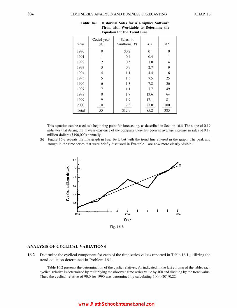
This equation can be used as a beginning point for forecasting, as described in Section 16.6. The slope of 0.19
indicates that during the 11-year existence of the company there has been an average increase in sales of 0.19
million dollars ($190,000) annually.
(b) Figure 16-3 repeats the line graph in Fig. 16-1, but with the trend line entered in the graph. The peak and
trough in the time series that were briefly discussed in Example 1 are now more clearly visible.
ANALYSIS OF CYCLICAL VARIATIONS
16.2 Determine the cyclical component for each of the time series values reported in Table 16.1, utilizing the
trend equation determined in Problem 16.1.
Table 16.2 presents the determination of the cyclic relatives. As indicated in the last column of the table, each
cyclical relative is determined by multiplying the observed time series value by 100 and dividing by the trend value.
Thus, the cyclical relative of 90.0 for 1990 was determined by calculating 100(0.20)/0.22.
Table 16.1 Historical Sales for a Graphics Software
Firm, with Worktable to Determine the
Equation for the Trend Line
Year
Coded year
(X)
Sales, in
$millions (Y) X Y X 2
1990 0 $0.2 0 0
1991 1 0.4 0.4 1
1992 2 0.5 1.0 4
1993 3 0.9 2.7 9
1994 4 1.1 4.4 16
1995 5 1.5 7.5 25
1996 6 1.3 7.8 36
1997 7 1.1 7.7 49
1998 8 1.7 13.6 64
1999 9 1.9 17.1 81
2000 10 2.3 23.0 100
Total 55 $12.9 85.2 385
Fig. 16-3
304 TIME SERIES ANALYSIS AND BUSINESS FORECASTING [CHAP. 16
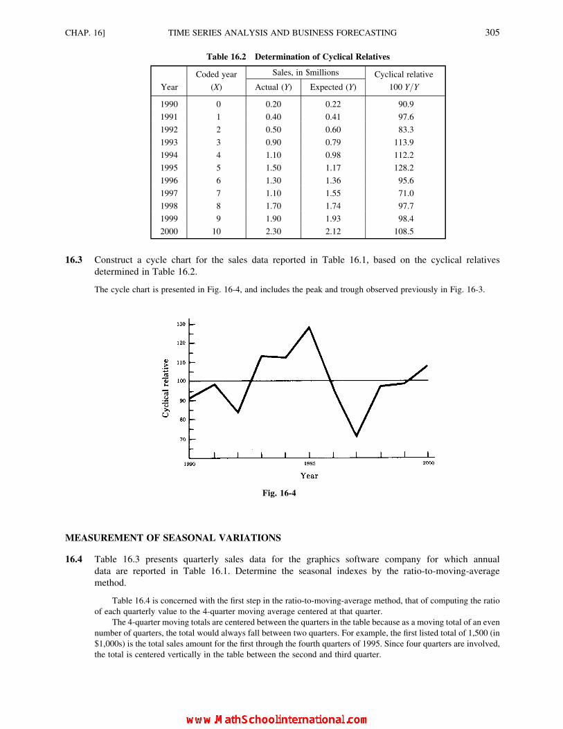
16.3 Construct a cycle chart for the sales data reported in Table 16.1, based on the cyclical relatives
determined in Table 16.2.
The cycle chart is presented in Fig. 16-4, and includes the peak and trough observed previously in Fig. 16-3.
MEASUREMENT OF SEASONAL VARIATIONS
16.4 Table 16.3 presents quarterly sales data for the graphics software company for which annual
data are reported in Table 16.1. Determine the seasonal indexes by the ratio-to-moving-average
method.
Table 16.4 is concerned with the first step in the ratio-to-moving-average method, that of computing the ratio
of each quarterly value to the 4-quarter moving average centered at that quarter.
The 4-quarter moving totals are centered between the quarters in the table because as a moving total of an even
number of quarters, the total would always fall between two quarters. For example, the first listed total of 1,500 (in
$1,000s) is the total sales amount for the first through the fourth quarters of 1995. Since four quarters are involved,
the total is centered vertically in the table between the second and third quarter.
Table 16.2 Determination of Cyclical Relatives
Coded year Sales, in $millions Cyclical relative
Year (X) Actual (Y) Expected (Y) 100 Y/Y
1990 0 0.20 0.22 90.9
1991 1 0.40 0.41 97.6
1992 2 0.50 0.60 83.3
1993 3 0.90 0.79 113.9
1994 4 1.10 0.98 112.2
1995 5 1.50 1.17 128.2
1996 6 1.30 1.36 95.6
1997 7 1.10 1.55 71.0
1998 8 1.70 1.74 97.7
1999 9 1.90 1.93 98.4
2000 10 2.30 2.12 108.5
Fig. 16-4
CHAP. 16] TIME SERIES ANALYSIS AND BUSINESS FORECASTING 305

Table 16.3 Quarterly Sales for the Graphics Software Firm
Quarterly sales, in $1,000s
Quarter 1995 1996 1997 1998 1999 2000
1 500 450 350 550 550 750
2 350 350 200 350 400 500
3 250 200 150 250 350 400
4 400 300 400 550 600 650
Table 16.4 Worktable for Determining the Ratio-to-Moving-Average for the Quarterly
Sales Data (sales in $1,000s)
Year Quarter Sales
4-quarter
moving
total
2-year centered
moving
total
4-quarter
centered
moving
average
Ratio-to-
moving-average
(percent)
1995 I 500
II 3501,500
III 2501,450
2,950 368.75 67.8
IV 400 2,900 362.50 110.3
1996 I 4501,450
2,850 356.25 126.3
II 3501,400
2,700 337.50 103.7
III 2001,300
2,500 312.50 64.0
IV 3001,200
2,250 281.25 106.7
1997 I 3501,050
2,050 256.25 136.6
II 2001,000
2,100 262.50 76.2
III 1501,100
2,400 300.00 50.0
IV 4001,300
2,750 343.75 116.4
1998 I 5501,450
3,000 375.00 146.7
II 3501,550
3,250 406.25 86.2
III 2501,700
3,400 425.00 58.8
IV 5501,700
3,450 431.25 127.5
1999 I 5501,750
3,600 450.00 122.2
II 4001,850
3,750 468.75 85.3
III 3501,900
4,000 500.00 70.0
IV 6002,100
4,300 537.50 111.6
2000 I 7502,200
4,450 556.25 134.8
II 5002,250
4,550 568.75 87.9
III 4002,300
IV 650
306 TIME SERIES ANALYSIS AND BUSINESS FORECASTING [CHAP. 16

Because it is desired that the moving average be centered at each quarter, instead of between quarters,
adjoining 4-quarter moving totals are combined to form the 2-year centered moving totals. Note that this type of
total does not include two years of data as such. Rather, two overlapping 4-quarter periods are included in the total.
For example, the first centered moving total of 2,950 (in $1,000s) includes the 4-quarter total of 1,500 for the four
quarters of 1995, plus the 4-quarter total of 1,450 for the second quarter of 1995 through the first quarter of 1996.
The 4-quarter centered moving average simply is the 2-year centered moving total divided by 8.
Finally, the ratio-to-moving-average in the last column of Table 16.4 is the ratio of each quarterly sales value to
the centered moving average for that quarter. This ratio is multiplied by 100 and in effect is reported as a percentage.
Table 16.5 incorporates the second and third steps in determining the seasonal indexes. The modified mean for
each quarter is the mean of the three remaining ratios for each quarter after elimination of the highest and lowest
ratios. For example, for Quarter 1 the two extreme ratios 122.2 and 146.7, are eliminated from consideration, with
the mean of the remaining three ratios being 132.6.
Finally, the modified means are multiplied by an adjustment factor so that the sum of the index is approximately 400
(1,200 for monthly indexes). The adjustment factor used withmodifiedmean quarterly indexes to obtain the quarterly indexes is
Quarterly adjustment factor ¼ 400
sum of quarterly means(16:19)
The adjustment factor used with modified mean monthly indexes to obtain the monthly indexes is
Monthly adjustment factor ¼ 1,200
sum of monthly means(16:20)
For the ratios in Table 16.5, the adjustment factor is 400/395.4, or 1.0116. Each modified mean is multiplied by this
adjustment factor to obtain the quarterly indexes. Overall, we can observe that the quarter with the greatest positive seasonal
effect is Quarter 1, with sales generally being about 34.1 percent higher than the typical quarter. On the other hand, sales in
Quarter 3 generally are just 64.2 percent of the sales in the typical quarter. By being aware of such seasonal variations, a firm
can take them into consideration when planning work schedules and in making forecasts of sales.
APPLYING SEASONAL ADJUSTMENTS
16.5 Refer to the seasonal indexes determined in Table 16.5.
(a) Compute the seasonally adjusted value for each quarter, rounding the values to whole thousand
dollar amounts.(b) Compare the results for the third and fourth quarters of 2000 based on (1) the reported level of
actual sales, and (2) the seasonally adjusted values.
Table 16.5 Calculation of the Seasonal Indexes for the Quarterly Data
Quarter 1995 1996 1997 1998 1999 2000
Modified
mean
Seasonal
index:
mean �1.0116*
1 126.3 136.6 146.7 122.2 134.8 132.6 134.1
2 103.7 76.2 86.2 85.3 87.9 86.5 87.5
3 67.8 64.0 50.0 58.8 70.0 63.5 64.2
4 110.3 106.7 116.4 127.5 111.6 112.8 114.1
395.4 399.9
*Adjustment factor ¼ 400/395.4 ¼ 1.0116.
CHAP. 16] TIME SERIES ANALYSIS AND BUSINESS FORECASTING 307

(a) The seasonally adjusted values are reported in Table 16.6. Each deseasonalized value was determined by
dividing the quarterly value in Table 16.3 by the seasonal index for that quarter (from Table 16.5), and
multiplying by 100 to preserve the location of the decimal point. For example, the seasonally adjusted value of
373 (in $1,000s) for Quarter 1 of 1995 was obtained by dividing 500 (from Table 16.3) by 134.1 (from
Table 16.5) and multiplying by 100.
(b) The reported levels of sales for the third and fourth quarters indicate a substantial increase in sales between
the two quarters—from $400,000 to $650,000. However, on a seasonally adjusted basis there is a decline
of 8.5 percent, from $623,000 to $570,000. Thus, although sales increased in the fourth quarter, the
increase was not as large as it should have been, based on the different historical seasonal influences for
these two quarters
FORECASTING BASED ON TREND AND SEASONAL FACTORS
16.6 Step down the trend equation developed in Problem 16.1 so that it is expressed in terms of quarters
rather than years. Also, adjust the equation so that the trend values are in thousands of dollars instead of
millions of dollars. Carry the final values to the first place beyond the decimal point.
YT (quarterly) ¼ b0
4� 1:5
b1
16
� �þ b1
16
� �X
¼ 0:22
4� 15
0:19
16
� �þ 0:19
16
� �X
¼ 0:0550� 0:0178þ 0:0119X
¼ 0:0372þ 0:0119X
The quarterly trend equation in units of thousands of dollars is:
YT (quarterly) ¼ 1,000 (0:0372þ 0:0119X) ¼ 37:2þ 11:9X
For the above equation, X ¼ 0 at the first quarter of 1990.
16.7 Forecast the level of quarterly sales for each quarter of 2001 based on the quarterly trend equation
determined in Problem 16.6 and the seasonal indexes determined in Table 16.5.
Table 16.6 Seasonally Adjusted Values for the Quarterly Data
Quarter 1995 1996 1997 1998 1999 2000
1 $373 $336 $261 $410 $410 $559
2 400 400 229 400 457 571
3 389 312 234 389 545 623
4 351 263 351 482 526 570
308 TIME SERIES ANALYSIS AND BUSINESS FORECASTING [CHAP. 16

The forecasted values based on the quarterly trend equation, and then adjusted for the quarterly seasonal
indexes, are
First quarter, 2001 ¼ [37:2þ 11:9(44)]� 134:1
100¼ 752:0
Second quarter, 2001 ¼ [37:2þ 11:9(45)]� 87:5
100¼ 501:1
Third quarter, 2001 ¼ [37:2þ 11:9(46)]� 64:2
100¼ 375:3
Fourth quarter, 2001 ¼ [37:2þ 11:9(47)]� 114:1
100¼ 680:6
FORECASTING BASED ON MOVING AVERAGES
16.8 Refer to the annual time series data in Table 16.1. Begin with 1994 and determine the 3-year moving
averages that would have been used to forecast the sales (in $millions) for the years subsequent to each
group of three years. Determine the forecast error associated with each forecast.
Table 16.7 is the worktable that reports the forecasts and the forecast errors. For example, the forecast for the
year 2000 is based on the 3-year average sales for 1997–99. The amounts of forecast error will be compared with
those for the method of exponential smoothing in the next Solved Problem, 16.9.
EXPONENTIAL SMOOTHING AS A FORECASTING METHOD
16.9 Refer to the annual time series data in Table 16.1. Using the actual level of sales for 1994 of 1.1 million
dollars as the “seed” forecast for 1995, determine the forecast for each annual sales amount by the
method of simple exponential smoothing. First use a smoothing constant of a ¼ 0.80, then use a
smoothing constant of a ¼ 0.20, and compare the two sets of forecasts.
Table 16.8 is the worktable that reports the two sets of forecasts. For example, the forecast amount for 1996
based on a ¼ 0.20 was determined as follows:
YYtþ1 ¼ YYt þ a(Yt � YYt)
YY1996 ¼ YY1995 þ a(Y1995 � YY1995)
¼ $1:1þ 0:20(0:4) ¼ 1:1þ 0:08 ¼ 1:18 ffi $1:2
Table 16.7 Year-by-Year Forecasts by the
Method of Moving Averages
Year
(t)
Sales in
millions
(Yt)
Forecast
(YYt)
Forecast
error
(Yt � YYt)
1994 $1.1
1995 1.5
1996 1.3
1997 1.1 $1.3 $20.2
1998 1.7 1.3 0.4
1999 1.9 1.4 0.5
2000 2.3 1.6 0.7
2001 2.0
CHAP. 16] TIME SERIES ANALYSIS AND BUSINESS FORECASTING 309
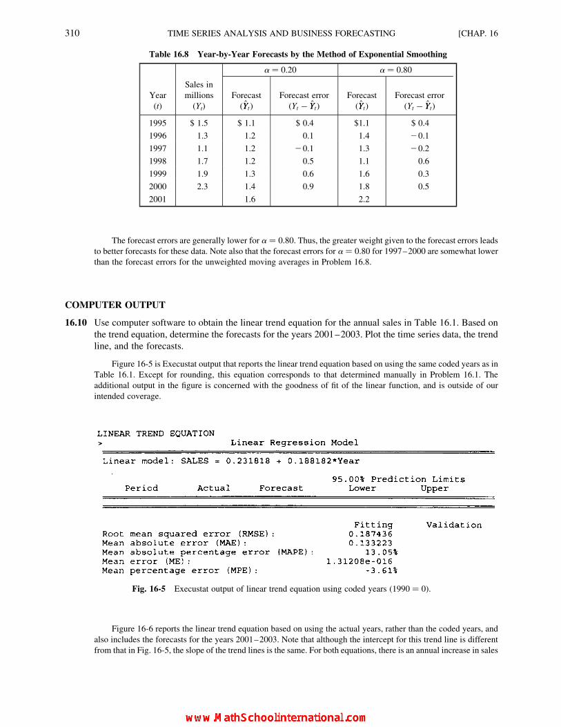
The forecast errors are generally lower for a ¼ 0.80. Thus, the greater weight given to the forecast errors leads
to better forecasts for these data. Note also that the forecast errors for a ¼ 0.80 for 1997–2000 are somewhat lower
than the forecast errors for the unweighted moving averages in Problem 16.8.
COMPUTER OUTPUT
16.10 Use computer software to obtain the linear trend equation for the annual sales in Table 16.1. Based on
the trend equation, determine the forecasts for the years 2001–2003. Plot the time series data, the trend
line, and the forecasts.
Figure 16-5 is Execustat output that reports the linear trend equation based on using the same coded years as in
Table 16.1. Except for rounding, this equation corresponds to that determined manually in Problem 16.1. The
additional output in the figure is concerned with the goodness of fit of the linear function, and is outside of our
intended coverage.
Figure 16-6 reports the linear trend equation based on using the actual years, rather than the coded years, and
also includes the forecasts for the years 2001–2003. Note that although the intercept for this trend line is different
from that in Fig. 16-5, the slope of the trend lines is the same. For both equations, there is an annual increase in sales
Table 16.8 Year-by-Year Forecasts by the Method of Exponential Smoothing
a ¼ 0.20 a ¼ 0.80
Year
(t)
Sales in
millions
(Yt)
Forecast
(YYt)
Forecast error
(Yt � YYt)
Forecast
(YYt)
Forecast error
(Yt � YYt)
1995 $ 1.5 $ 1.1 $ 0.4 $1.1 $ 0.4
1996 1.3 1.2 0.1 1.4 20.1
1997 1.1 1.2 20.1 1.3 20.2
1998 1.7 1.2 0.5 1.1 0.6
1999 1.9 1.3 0.6 1.6 0.3
2000 2.3 1.4 0.9 1.8 0.5
2001 1.6 2.2
Fig. 16-5 Execustat output of linear trend equation using coded years (1990 ¼ 0).
310 TIME SERIES ANALYSIS AND BUSINESS FORECASTING [CHAP. 16

of about $0:188 million (or $188,000). Figure 16-6 also reports the forecasts for the years 2001–2003 based on the
trend equation, including 95 percent prediction limits. Note that the forecast for the year 2001 corresponds to the
one we determined manually in Problem 16.1.
Figure 16-7 is the plot that includes the time series values, the trend line, and the forecasts for the years
2001–2003.
Fig. 16-6 Execustat output of linear trend equation and forecasts using uncoded years.
Fig. 16-7 Execustat plot for Problem 16.10.
CHAP. 16] TIME SERIES ANALYSIS AND BUSINESS FORECASTING 311
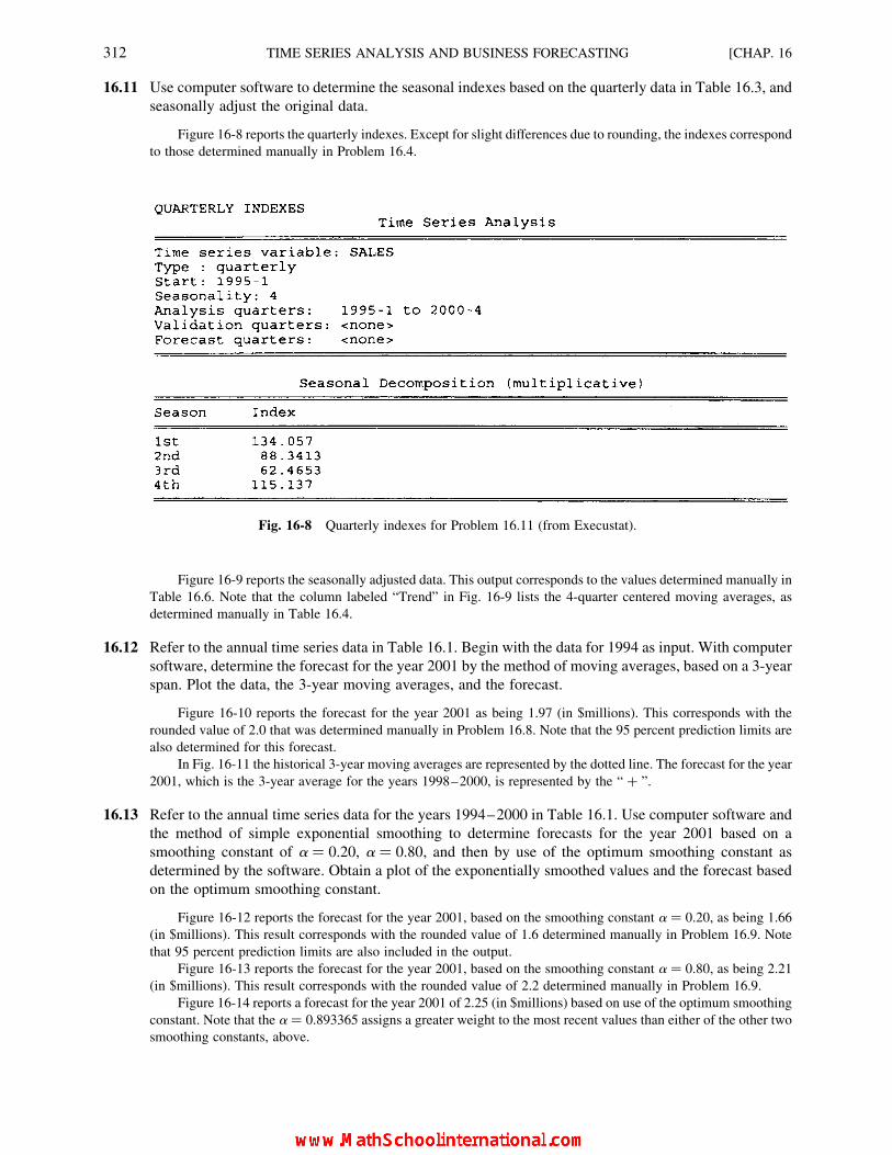
16.11 Use computer software to determine the seasonal indexes based on the quarterly data in Table 16.3, and
seasonally adjust the original data.
Figure 16-8 reports the quarterly indexes. Except for slight differences due to rounding, the indexes correspond
to those determined manually in Problem 16.4.
Figure 16-9 reports the seasonally adjusted data. This output corresponds to the values determined manually in
Table 16.6. Note that the column labeled “Trend” in Fig. 16-9 lists the 4-quarter centered moving averages, as
determined manually in Table 16.4.
16.12 Refer to the annual time series data in Table 16.1. Begin with the data for 1994 as input. With computer
software, determine the forecast for the year 2001 by the method of moving averages, based on a 3-year
span. Plot the data, the 3-year moving averages, and the forecast.
Figure 16-10 reports the forecast for the year 2001 as being 1.97 (in $millions). This corresponds with the
rounded value of 2.0 that was determined manually in Problem 16.8. Note that the 95 percent prediction limits are
also determined for this forecast.
In Fig. 16-11 the historical 3-year moving averages are represented by the dotted line. The forecast for the year
2001, which is the 3-year average for the years 1998–2000, is represented by the “ þ ”.
16.13 Refer to the annual time series data for the years 1994–2000 in Table 16.1. Use computer software and
the method of simple exponential smoothing to determine forecasts for the year 2001 based on a
smoothing constant of a ¼ 0.20, a ¼ 0.80, and then by use of the optimum smoothing constant as
determined by the software. Obtain a plot of the exponentially smoothed values and the forecast based
on the optimum smoothing constant.
Figure 16-12 reports the forecast for the year 2001, based on the smoothing constant a ¼ 0.20, as being 1.66
(in $millions). This result corresponds with the rounded value of 1.6 determined manually in Problem 16.9. Note
that 95 percent prediction limits are also included in the output.
Figure 16-13 reports the forecast for the year 2001, based on the smoothing constant a ¼ 0.80, as being 2.21
(in $millions). This result corresponds with the rounded value of 2.2 determined manually in Problem 16.9.
Figure 16-14 reports a forecast for the year 2001 of 2.25 (in $millions) based on use of the optimum smoothing
constant. Note that the a ¼ 0.893365 assigns a greater weight to the most recent values than either of the other two
smoothing constants, above.
Fig. 16-8 Quarterly indexes for Problem 16.11 (from Execustat).
312 TIME SERIES ANALYSIS AND BUSINESS FORECASTING [CHAP. 16

Fig. 16-9 Seasonally adjusted data for Problem 16.11 (from Execustat).
Fig. 16-10 Execustat output for Problem 16.12.
CHAP. 16] TIME SERIES ANALYSIS AND BUSINESS FORECASTING 313

Figure 16-15 is the plot that includes the time series data the exponentially smoothed values based on the
optimum smoothing constant, and the forecast for the year 2001. Because the most recent value is heavily weighted,
note that the forecast for the year 2001 is close to the sales figure for the year 2000.
Fig. 16-11 Execustat plot of moving averages.
Fig. 16-12 Execustat output for Problem 16.13 (a ¼ 0.20).
314 TIME SERIES ANALYSIS AND BUSINESS FORECASTING [CHAP. 16

Supplementary Problems
TREND ANALYSIS
16.14 Given the data in Table 16.9, determine the linear trend equation for construction contracts for commercial and
industrial buildings for a geographic area (data fictional), designating 1995 as the base year for the purpose of
coding the years.
Ans. YT ¼ 269:401þ 4:274X (in thous. sq. ft)
6.15 Construct the line graph for the data in Table 16.9 and enter the trend line on this graph.
ANALYSIS OF CYCLICAL VARIATIONS
16.16 Determine the cyclical relatives for the annual time series data reported in Table 16.9.
16.17 Prepare a cycle chart to portray the cyclical relatives determined in Problem 16.16 above.
Ans. The cyclical relatives would reflect peaks (e.g., 1999) and troughs (e.g., 2002) in the regional economy.
MEASUREMENT OF SEASONAL VARIATIONS
16.18 Table 16.10 presents quarterly data for the number of customer orders received in a mail-order firm (fictional).
Determine the seasonal indexes based on these data, carrying three places beyond the decimal point during
calculations and rounding the indexes to two places.
Ans. I ¼ 68.19, II ¼ 93.76, III ¼ 113.42, IV ¼ 124.64
Fig. 16-13 Execustat output for Problem 16.13 (a ¼ 0.80).
Fig. 16-14 Execustat output for Problem 16.13 (optimum a).
CHAP. 16] TIME SERIES ANALYSIS AND BUSINESS FORECASTING 315

Fig. 16-15 Execustat plot for Problem 16.13.
Table 16.9 Construction Contracts for
Commercial and Industrial
Buildings, thous. sq. ft.
Year Construction contracts
1995 291.60
1996 205.72
1997 251.84
1998 322.92
1999 361.36
2000 311.24
2001 310.88
2002 229.52
2003 255.44
2004 312.28
2005 345.68
316 TIME SERIES ANALYSIS AND BUSINESS FORECASTING [CHAP. 16

APPLYING SEASONAL ADJUSTMENTS
16.19 Continuing with Problem 16.18, seasonally adjust the data and comment on the comparison of the resulting values
for the third and fourth quarters of 2000.
Ans. Although there was an increase in orders from the third to the fourth quarters in the original data, on a
seasonally adjusted basis there was a decline in orders.
FORECASTING BASED ON TREND AND SEASONAL FACTORS
16.20 Suppose that the trend equation for quarterly sales orders (in thousands) is YT ¼ 13.91 þ 0.43X, with X ¼ 0 at the
first quarter of 1996. Forecast the number of orders for each of the four quarters of 2001 based on the trend and
seasonal components of the time series.
Ans. I ¼ 15.34, II ¼ 21.51, III ¼ 26.51, IV ¼ 29.66
EXPONENTIAL SMOOTHING AS A FORECASTING METHOD
16.21 Refer to the construction data in Table 16.9. Using the year 2002 construction amount of 229.52 (thous. sq. ft.) as the
“seed” forecast for 2003, use the method of simple exponential smoothing with a smoothing constant of a ¼ 0.70 to
determine year-by-year forecasts for 2003 through 2006.
Ans. 229.52, 273.58, 339.37, 350.10
COMPUTER OUTPUT
16.22 Use available computer software to determine the linear trend equation for the construction data in Table 16.9,
designating 1995 as the coded year X ¼ 0, Determine the forecast for 2006 based on the linear trend equations.
16.23 Use available computer software to (a) determine the quarterly seasonal indexes and (b) deseasonalize the data on
the number of customer orders in Table 16.10.
16.24 Use available computer software to determine the forecast for the year 2006 for the construction data in Table 16.9
by use of simple exponential smoothing. Compare the output using smoothing constants of a ¼ 0.30 and a ¼ 0.60,
and then using the optimum smoothing constant as determined by the software.
Table 16.10 Number of Customer Orders in a
Mail-Order Firm (in 1,000s)
Year
Quarter 1996 1997 1998 1999 2000
I 9 10 13 11 14
II 16 15 22 17 18
III 18 18 17 25 25
IV 21 20 24 21 26
CHAP. 16] TIME SERIES ANALYSIS AND BUSINESS FORECASTING 317
CHAPTER 17
NonparametricStatistics
17.1 SCALES OF MEASUREMENT
Before considering how nonparametric methods of statistics differ from the parametric procedures that
constitute most of this book, it is useful to define four types of measurement scales in terms of the precision
represented by reported values.
In the nominal scale, numbers are used only to identify categories. They do not represent any amount or
quantity as such.
EXAMPLE 1. If four sales regions are numbered 1 through 4 as general identification numbers only, then the nominal
scale is involved, since the numbers simply serve as category names.
In the ordinal scale, the numbers represent ranks. The numbers indicate relative magnitude, but the
differences between the ranks are not assumed to be equal.
EXAMPLE 2. An investment analyst ranks five stocks from 1 to 5 in terms of appreciation potential. The difference in the
appreciation potential between the stocks ranked 1 and 2 generally would not be the same as, say, the difference between the
stocks ranked 3 and 4.
In the interval scale, measured differences between values are represented. However, the zero point is
arbitrary, and is not an “absolute” zero. Therefore, the numbers cannot be compared by ratios.
EXAMPLE 3. In either the Fahrenheit or the Celsius temperature scales, a 58 difference, from, say, 708F, to 758F is the
same amount of difference in temperature as from 808F to 858F. However, we cannot say that 608F is twice as warm as 308F,because the 08F point is not an absolute zero point (the complete absence of all heat).
In the ratio scale, there is a true zero point, and therefore measurements can be compared in the form of
ratios.
318
Copyright 2004, 1996, 1988, 1976 by The McGraw-Hill Companies, Inc. Click Here for Terms of Use.
EXAMPLE 4. Not only is it true that a difference in inventory value of $5,000 is the same amount of difference whether
between, say, $50,000 and $55,000 or between $60,000 and $65,000, it is also true that an inventory value of $100,000 is
twice as great as an inventory value of $50,000.
17.2 PARAMETRIC VS. NONPARAMETRIC STATISTICAL METHODS
Most of the statistical methods described in this book are called parametric methods. The focal point of
parametric analysis is some population parameter for which the sampling statistic follows a known distribution,
with measurements being made at the interval or ratio scale. When one or more of these requirements or
assumptions are not satisfied, then the so-called nonparametric methods can be used. An alternative term is
distribution-free methods, which focuses particularly on the fact that the distribution of the sampling statistic is
not known.
If use of a parametric test, such as the t test, is warranted, then we would always prefer its use to the
nonparametric equivalent. This is so because if we use the same level of significance for both tests, then the
power associated with the nonparametric test is always less than the parametric equivalent. (Recall from
Section 10.4 that the power of a statistical test is the probability of rejecting a false null hypothesis.)
Nonparametric tests often are used in conjunction with small samples, because for such samples the central
limit theorem cannot be invoked (see Section 8.4).
Nonparametric tests can be directed toward hypotheses concerning the form, dispersion, or location
(median) of the population. In the majority of the applications, the hypotheses are concerned with the value of a
median, the difference between medians, or the differences among several medians. This contrasts with the
parametric procedures that are focused principally on population means.
Of the statistical tests already described in this book, the chi-square test covered in Chapter 12 is a
nonparametric test. Recall, for example, that the data that are analyzed are at the nominal scale (categorical
data). A separate chapter was devoted to the chi-square test because of the extent of its use and the variety of its
applications.
17.3 THE RUNS TEST FOR RANDOMNESS
Where a run is a series of like observations, the runs test is used to test the randomness of a series of
observations when each observation can be assigned to one of two categories.
EXAMPLE 5. For a random sample of n ¼ 10 individuals, suppose that when they are categorized by sex, the sequence of
observations is: M, M, M, M, F, F, F, F, M, M. For these data there are three runs, or series of like items.
For numeric data, one way by which the required two-category scheme can be achieved is to classify each
observation as being either above or below the median of the group. In general, either too few runs or too many
runs than would be expected by chance would result in rejecting the null hypothesis that the sequence of
observations is a random sequence.
The number of runs of like items is determined for the sample data, with the symbol R used to designate the
number of observed runs. Where n1 equals the number of sampled items of one type and n2 equals the number of
sampled items of the second type, the mean and the standard error associated with the sampling distribution of
the R test statistic when the sequence is random are
mR ¼ 2n1n2
n1 þ n2
þ 1 (17:1)
sR ¼ffiffiffiffiffiffiffiffiffiffiffiffiffiffiffiffiffiffiffiffiffiffiffiffiffiffiffiffiffiffiffiffiffiffiffiffiffiffiffiffiffiffiffiffiffiffi2n1n2(2n1n2 � n1 � n2)
(n1 þ n2)2(n1 þ n2 � 1)
s(17:2)
CHAP. 17] NONPARAMETRIC STATISTICS 319
If either n1 . 20 or n2 . 20, the sampling distribution of r approximates the normal distribution. Therefore
under such circumstances the R statistic can be converted to the z test statistic as follows:
z ¼ R � mR
sR
(17:3)
Where both n1 20 and n2 20, tables of critical values for the R test statistic are available in specialized
textbooks in nonparametric statistics.
See Problem 17.1 for an application of the runs test for randomness.
17.4 ONE SAMPLE: THE SIGN TEST
The sign test can be used to test a null hypothesis concerning the value of the population median. Therefore,
it is the nonparametric equivalent to testing a hypothesis concerning the value of the population mean. The
values in the random sample are required to be at least at the ordinal scale, with no assumptions required about
the form of the population distribution.
The null and alternative hypotheses can designate either a two-sided or a one-sided test. Where Med
denotes the population median and Med0 designates the hypothesized value, the null and alternative hypotheses
for a two-sided test are
H0: Med ¼ Med0
H1: Med = Med0
A plus sign is assigned for each observed sample value that is larger than the hypothesized value of the
median, and a minus sign is assigned for each value that is smaller than the hypothesized value of the median. If
a sample value is exactly equal to the hypothesized median, no sign is recorded and the effective sample size is
thereby reduced. If the null hypothesis regarding the value of the median is true, the number of plus signs should
approximately equal the number of minus signs. Or put another way, the proportion of plus signs (or minus
signs) should be about 0.50. Therefore, the null hypothesis tested for a two-sided test is H0:p ¼ 0:50, where p is
the population proportion of the plus (or the minus) signs. Thus, a hypothesis concerning the value of the
median in fact is tested as a hypothesis concerning p. If the sample is large, the normal distribution can be used,
as described in Section 11.4.
See Problem 17.2 for the use of the sign test to test a null hypothesis concerning the population median.
17.5 ONE SAMPLE: THE WILCOXON TEST
Just as is the case for the sign test, the Wilcoxon test can be used to test a null hypothesis concerning the
value of the population median. Because the Wilcoxon test considers the magnitude of the difference between
each sample value and the hypothesized value of the median, it is a more sensitive test than the sign test. On the
other hand, because differences are determined, the values must be at least at the interval scale. No assumptions
are required about the form of the population distribution.
The null and alternative hypotheses are formulated with respect to the population median as either a one-
sided or two-sided test. The difference between each observed value and the hypothesized value of the median
is determined, and this difference, with arithmetic sign, is designated d:d ¼ (X �Med0). If any difference is
equal to zero, the associated observation is dropped from the analysis and the effective sample size is thereby
reduced. The absolute values of the differences are then ranked from lowest to highest, with the rank of 1
assigned to the smallest absolute difference. When absolute differences are equal, the mean rank is assigned to
the tied values. Finally, the sum of the ranks is obtained separately for the positive and negative differences. The
smaller of these two sums is the Wilcoxon T statistic for a two-sided test. In the case of a one-sided test, the
smaller sum must be associated with the directionality of the null hypothesis. Appendix 10 identifies the critical
values of T according to sample size and level of significance. For rejection of the null hypothesis, the obtained
value of T must be smaller than the critical value given in the table.
320 NONPARAMETRIC STATISTICS [CHAP. 17

When n � 25 and the null hypothesis is true, the T statistic is approximately normally distributed. The
mean and standard error associated with this sampling distribution are, respectively,
m T ¼ n(n þ 1)
4(17:4)
sT ¼ffiffiffiffiffiffiffiffiffiffiffiffiffiffiffiffiffiffiffiffiffiffiffiffiffiffiffiffiffiffiffiffiffin(n þ 1)(2n þ 1)
24
r(17:5)
Therefore, for a relatively large sample the test can be carried out by using the normal probability
distribution and computing the z test statistic as follows:
z ¼ T � mT
sT
(17:6)
See Problem 17.3 for an application of the Wilcoxon test to test a null hypothesis concerning the population
median.
17.6 TWO INDEPENDENT SAMPLES: THE MANN–WHITNEY TEST
The Mann–Whitney test can be used to test the null hypothesis that the medians of two populations are
equal. It is assumed that the two populations have the same form and dispersion, because such differences also
would lead to rejection of the null hypothesis. It is required that the values in the two independent random
samples be at least at the ordinal scale.
Two samples are combined into one ordered array, with each sample value identified according to the
original sample group. The values are then ranked from lowest to highest, with the rank of 1 assigned to the
lowest observed sample value. For equal values the mean rank is assigned to the tied, or equal, values. If the null
hypothesis is true, the average of the ranks for each sample group should be approximately equal. The statistic
calculated to carry out this test is designated U, and it can be based on the sum of the ranks in either of the two
random samples, as follows:
U1 ¼ n1n2 þ n1(n1 þ 1)
2� R1 (17:7)
or U2 þ n1n2 þ n2(n2 þ 1)
2� R2 (17:8)
where n1 ¼ size of the first sample
n2 ¼ size of the second sample
R1 ¼ sum of the ranks in the first sample
R2 ¼ sum of the ranks in the second sample
Given that n1 . 10, n2 . 10, and the null hypothesis is true, the sampling distribution of U is
approximately normal, with the following parameters:
mU ¼ n1n2
2(17:9)
sU ¼ffiffiffiffiffiffiffiffiffiffiffiffiffiffiffiffiffiffiffiffiffiffiffiffiffiffiffiffiffiffiffiffiffiffiffin1n2(n1 þ n2 þ 1)
12
r(17:10)
Therefore, the test statistic for testing the null hypothesis that the medians of two populations are equal is
z ¼ U � mU
sU
(17:11)
where U equals U1 or U2.
CHAP. 17] NONPARAMETRIC STATISTICS 321

For data situations in which n1 , 10, n2 , 10, or both n1 and n2 , 10, the normal probability distribution
cannot be used for this test. However, special tables for the U statistic are available for such small samples in
specialized textbooks on nonparametric statistics.
Problem 17.4 illustrates the use of the Mann–Whitney test.
17.7 PAIRED OBSERVATIONS: THE SIGN TEST
For two samples collected as paired observations (see Section 11.3), the sign test described in Section 17.4
can be used to test the null hypothesis that the two population medians are equal. The sample values must be at
least at the ordinal scale, and no assumptions are required about the forms of the two population distributions.
A plus sign is assigned for each pair of values for which the measurement in the first sample is greater than
the measurement in the second sample, and a minus sign is assigned when the opposite condition is true. If a
pair of measurements have the same value, these tied values are dropped from the analysis, with the effective
sample size thereby being reduced. If the hypothesis that the two populations are at the same level of magnitude
is true, the number of plus signs should approximately equal the number of minus signs. Therefore, the null
hypothesis tested is H0: p ¼ 0.50, where p is the population proportion of the plus (or the minus) signs. If the
sample is large (n . 30), the normal distribution can be used, as described in Section 11.5. Note that although
two samples have been collected, the test is applied to the one set of plus and minus signs that results from the
comparison of the pairs of measurements.
Problem 17.5 illustrates use of the sign test for testing the difference between two medians for data that
have been collected as paired observations.
17.8 PAIRED OBSERVATIONS: THE WILCOXON TEST
For two samples collected as paired observations, the Wilcoxon test described in Section 17.5 can be used
to test the null hypothesis that the two population medians are equal. Because the Wilcoxon test considers the
magnitude of the difference between the values in each matched pair, and not just the direction or sign of the
difference, it is a more sensitive test than the sign test. However, the sample values must be at the interval scale.
No assumptions are required about the forms of the two distributions.
The difference between each pair of values is determined, and this difference, with the associated
arithmetic sign, is designated by d. If any difference is equal to zero, this pair of observations is dropped from
the analysis, thus reducing the effective sample size. Then the absolute values of the differences are ranked from
lowest to highest, with the rank of 1 assigned to the smallest absolute difference. When absolute differences are
equal, the mean rank is assigned to the tied values. Finally, the sum of the ranks is obtained separately for the
positive and negative differences. The smaller of these two sums is the Wilcoxon T statistic for a two-sided test.
For a one-sided test the smaller sum must be associated with the directionality of the null hypothesis, as
illustrated in the one-sample application of the Wilcoxon test in Problem 17.3. Appendix 10 identifies the
critical value of T according to sample size and level of significance. For rejection of the null hypothesis, the T
statistic must be smaller than the critical value given in the table.
When n � 25 and the null hypothesis is true, the T statistic is approximately normally distributed. The
formulas for the mean and standard error of the sampling distribution of T and the formula for the z test statistic
are given in Section 17.5, on the one-sample application of the Wilcoxon test.
Problem 17.6 illustrates the use of the Wilcoxon test for testing the difference between two medians data
that have been collected as paired observations.
17.9 SEVERAL INDEPENDENT SAMPLES: THE KRUSKAL–WALLIS TEST
The Kruskal–Wallis test is used to test the null hypothesis that several populations have the same
medians. As such, it is the nonparametric equivalent of the one-factor completely randomized design of the
322 NONPARAMETRIC STATISTICS [CHAP. 17
analysis of variance. It is assumed that the several populations have the same form and dispersion for the
above hypothesis to be applicable, because differences in form or dispersion would also lead to rejection of
the null hypothesis. The values for the several independent random samples are required to be at least at the
ordinal scale.
The several samples are first viewed as one array of values, and each value in this combined group is
ranked from lowest to highest. For equal values the mean rank is assigned to the tied values. If the null
hypothesis is true, the average of the ranks for each sample group should be about equal. The test statistic
calculated is designated H and is based on the sum of the ranks in each of the several random samples, as
follows:
H ¼ 12
N(N þ 1)
� � XR2j
nj
" #( )� 3(N þ 1) (17:12)
where N ¼ combined sample size of the several samples
(note that N does not designate population size in this case)
Rj ¼ sum of the ranks for the jth sample or treatment group
nj ¼ number of observations in the jth sample
Given that the size of each sample group is at least nj � 5 and the null hypothesis is true, the sampling
distribution of H is approximately distributed as the x 2 distribution with df ¼ K � 1, where K is the number
of treatment or sample groups. The x 2 value that approximates the critical value of the test statistic is
always the upper-tail value. This test procedure is analogous to the upper tail of the F distribution being
used in the analysis of variance.
For tied ranks the test statistic H should be corrected. The corrected value of the test statistic is designated
Hc and is computed as follows:
Hc ¼ H
1� [P (t 3j � tj)=(N3 � N)](17:13)
where tj represents the number of tied scores in the j th sample.
The effect of this correction is to increase the value of the calculated H statistic. Therefore, if the
uncorrected value of H leads to the rejection of the null hypothesis, there is no need to correct this value for the
effect of tied ranks.
Problem 17.7 illustrates use of the Kruskal–Wallis test for testing the null hypothesis that several
populations have the same median.
17.10 USING MINITAB
Whereas Excel has no direct method for nonparametric procedures, Minitab includes a variety of such
techniques. Solved Problems 17.8 through 17.10 illustrate the use of Minitab for the one-sample Wilcoxon test,
the two-sample Mann–Whitney test for independence, and the Kruskal–Wallis test for several independent
samples.
CHAP. 17] NONPARAMETRIC STATISTICS 323

Solved Problems
THE RUNS TEST FOR RANDOMNESS
17.1. A sample of 36 individuals were interviewed in a market-research survey, with 22 women (W) and 14
men (M) included in the sample. The sampled individuals were obtained in the following order: M, W,
W, W, W, M, M, M, W, M, W, W,W, M, M, W, W,W, W, M, W, W,W, M, M, W, W,W, M, W, M, M,
W, W, W, M. Use the runs test to test the randomness of this set of observations, using the 5 percent
level of significance.
The number of runs in this sample is R ¼ 17, as indicated by the underscores above. Where n1 ¼ the number of
women and n2 ¼ the number of men, we can use the normal distribution to test the null hypothesis that the sampling
process was random, because n1 . 20. We compute the mean and the standard error of the sampling distribution of
R as follows:
mR ¼ 2n1n2
n1 þ n2þ 1 ¼ 2(22)(14)
22þ 14þ 1 ¼ 616
36þ 1 ¼ 18:1
sR ¼ffiffiffiffiffiffiffiffiffiffiffiffiffiffiffiffiffiffiffiffiffiffiffiffiffiffiffiffiffiffiffiffiffiffiffiffiffiffiffiffiffiffiffiffiffiffi2n1n2(2n1n2 � n1 � n2)
(n1 þ n2)2(n1 þ n2 � 1)
s¼
ffiffiffiffiffiffiffiffiffiffiffiffiffiffiffiffiffiffiffiffiffiffiffiffiffiffiffiffiffiffiffiffiffiffiffiffiffiffiffiffiffiffiffiffiffiffiffiffiffiffiffiffiffiffiffiffiffiffiffiffiffi2(22)(14)[2(22)(14)� 22� 14]
(22þ 14)2(22þ 14� 1)
s
¼ffiffiffiffiffiffiffiffiffiffiffiffiffiffiffiffiffiffiffiffiffiffiffiffiffiffiffiffiffi616(616� 36)
362(35)
s¼
ffiffiffiffiffiffiffiffiffiffiffiffiffiffiffiffi357,280
45,360
s¼
ffiffiffiffiffiffiffiffiffiffiffiffiffiffi7:8765
p¼ 2:81
When the 5 percent level of significance is used, the critical values of the z statistic are z ¼ +1.96. The value
of the z test statistic for these data is
z ¼ R � mR
sR
¼ 17� 18:1
2:81¼ �1:1
2:81¼ �0:39
Therefore, using the 5 percent level of significance, we cannot reject the null hypothesis that the sequence of
women and men occurred randomly.
ONE SAMPLE: THE SIGN TEST
17.2. It is claimed that the units assembled with a redesigned product assembly system will be greater than
with the old system, for which the population median is 80 units per workshift. Not giving the benefit of
the doubt to the redesigned system, formulate the null hypothesis and test it at the 5 percent level of
significance. The sample data are reported in the first part of Table 17.1.
The null and alternative hypotheses are
H0: Med ¼ 80
H1: Med . 80
Because no assumption is made about the form of the population distribution, a nonparametric test is
appropriate. Using the sign test, the null and alternative hypotheses in terms of the proportion of plus signs of the
differences, where d ¼ (X � 80), are
H0: p ¼ 0:50
H1: p . 0:50
324 NONPARAMETRIC STATISTICS [CHAP. 17
Referring to Table 17.1, we see that for the fourth sampled workshift the number of units assembled happened
to be exactly equal to the hypothesized value of the population median. Therefore, this observation is omitted from
the following analysis, resulting in an effective sample size of n ¼ 11. Of the 11 signs of the differences reported in
Table 17.1, 9 are plus signs. The test is to be carried out using the 5 percent level of significance.
Because the sample size is n , 30, the binomial distribution is the appropriate basis for this test. Using the P-
value approach to hypothesis testing, as described in Section 10.7, we determine the probability of observing 9 or
more plus signs in 11 observations, given that the population of plus signs is 0.50, by reference to Appendix 2 for
binomial probabilities:
P(X � 9 j n ¼ 11, p ¼ 0:50) ¼ 0:0269þ 0:0054þ 0:0005 ¼ 0:0328
Since the P value associated with the sample result is less than 0.05, the null hypothesis is rejected at the 5
percent level of significance for this one-sided test. That is, the probability of observing such a large number (or
more) of plus signs when the null hypothesis is true is less than 0.05; specifically, the probability is 0.0328.
Therefore, we accept the alternative hypothesis and conclude that the median output per workshift for the new
assembly system is greater than 80 units.
A two-sided sign test is illustrated in Problem 17.5, where the sign test is used in conjunction with paired
observations.
ONE SAMPLE: THE WILCOXON TEST
17.3. Use the Wilcoxon test with respect to the null hypothesis and the data in Problem 17.2, above, and
compare your solution to the one obtained in Problem 17.2.
H0: Med ¼ 80
H1: Med . 80
The sample data are repeated in Table 17.2, which is the worktable for the Wilcoxon test. In this
table note that for the fourth sampled workshift the number of units assembled happened to be
exactly equal to the hypothesized value of the population median. Therefore, this observation was
dropped from the analysis, resulting in an effective sample size of n ¼ 11. Also note that the absolute
value of d for the first and second sampled workshifts is the same, and therefore the mean rank of 4.5
was assigned to each of these sampled workshifts (in lieu of ranks 4 and 5). The next rank assigned is
then rank 6.
Table 17.1 Number of Units Assembled with the Redesigned Sampled
Sampled workshift Units assembled (X) Sign of difference (X 2 80)
1 75 2
2 85 þ3 92 þ4 80 0
5 94 þ6 90 þ7 91 þ8 76 2
9 88 þ10 82 þ11 96 þ12 83 þ
CHAP. 17] NONPARAMETRIC STATISTICS 325

In order to reject the null hypothesis H0: Med ¼ 80 for this upper-tail test, it follows that the differences
d ¼ (X �Med0) must be predominantly positive, for negative differences would represent positive support for
the null hypothesis. Therefore, for this upper-tail test the sum of the ranks for the negative differences must be
the smaller sum. Referring to Table 17.2, we see that such is in fact the case, and the value of the Wilcoxon test
statistic is T ¼ 7:5.The null hypothesis is to be tested at the 5 percent level of significance. Appendix 10 indicates that for
n ¼ 11 (the effective sample size) the critical value of T for a one-tail test at the 5 percent level of
significance is T ¼ 14. Because the obtained, value of T is smaller than the critical value, the null hypothesis
is rejected at the 5 percent level of significance, and we conclude that the median units assembled with the
new system is greater than 80 units. This is the same conclusion as with the use of the sign test in the
preceding section, in which the P value for the test was P ¼ 0:0328. However, reference to Appendix 10 for
the Wilcoxon test indicates that for n ¼ 11 and a ¼ 0:025 the critical value is T ¼ 11. Therefore, the null
hypothesis could be rejected at the 2.5 percent level of significance with the Wilcoxon test, but not with the
sign test. This observation is consistent with our earlier observations that the Wilcoxon test is the more
sensitive of the two tests.
TWO INDEPENDENT SAMPLES: THE MANN–WHITNEY TEST
17.4. To evaluate and compare two methods of instruction for industrial apprentices, a training director
assigns 15 randomly selected trainees to each of the two methods. Because of normal attrition, 14
apprentices complete the course taught by method 1 and 12 apprentices complete the course taught by
method 2. The same achievement test is then given to both trainee groups, as reported in Table 17.3.
Test the null hypothesis that the median level of test performance does not differ for the two methods of
instruction, using the 5 percent level of significance.
H0: Med1 ¼ Med2 H1: Med1 = Med2
Table 17.2 Number of Units Assembled with the Redesigned System and the
Determination of Signed Ranks
Sampled Units Difference Rank
Signed rank
workshift assembled (X) [d ¼ (X � 80)] of jdj (þ) (2 )
1 75 25 4.5 4.5
2 85 5 4.5 4.5
3 92 12 9 9
4 80 0
5 94 14 10 10
6 90 10 7 7
7 91 11 8 8
8 76 24 3 3
9 88 8 6 6
10 82 2 1 1
11 96 16 11 11
12 83 3 2 2
Total 58.5 T ¼ 7.5
326 NONPARAMETRIC STATISTICS [CHAP. 17

Table 17.4 lists the achievement test scores in one array, ranked from lowest to highest score. The ranks are
presented in the second column of Table 17.4. Notice the way the rankings are assigned to the tied scores: For the
three test scores of 82, for example, the scores are at the rank positions 12, 13, and 14 in the second column of the
table. Therefore, the mean of these three ranks, 13, is assigned to these three test scores. Then note that the next rank
assigned is 15, and 14, because the assignment of the mean rank of 13 to the three scores of 82 has brought the score
of 83 to the 15th position in the array. Similarly, there are two scores of 86; the ranks for these two positions are 18
and 19, and therefore the mean rank of 18.5 is assigned to each of these scores. The next score in the array, 87, is
assigned the rank 20. The last two columns in Table 17.4 list the ranks according to the sample, which represents the
teaching method used, and the sums of these two columns of ranks are the two values R1 and R2, respectively.
Applying Formula (17.7), we determine the value of U1 as follows:
U1 ¼ n1n2 þ n1(n1 þ 1)
2� R1 ¼ 14(12)þ 14(14þ 1)
2� 161
¼ 168þ 210
2� 161 ¼ 112
Because n1 . 10 and n2 . 10, the normal probability distribution can be used to test the null hypothesis that
the value of mU is the same for both samples. The test is to be carried out at the 5 percent level of significance. Based
on Formula (17.9), the value of mU is
mU ¼ n1n2
2¼ 14(12)
2¼ 84
Thus the hypotheses are
H0: mU ¼ 84
H1: mU = 84
Table 17.3 Achievement Test Scores of
Apprentice Trainees Taught
by Two Methods of
Instruction
Method 1 Method 2
70 86
90 78
82 90
64 82
86 65
77 87
84 80
79 88
82 95
89 85
73 76
81 94
83
66
CHAP. 17] NONPARAMETRIC STATISTICS 327
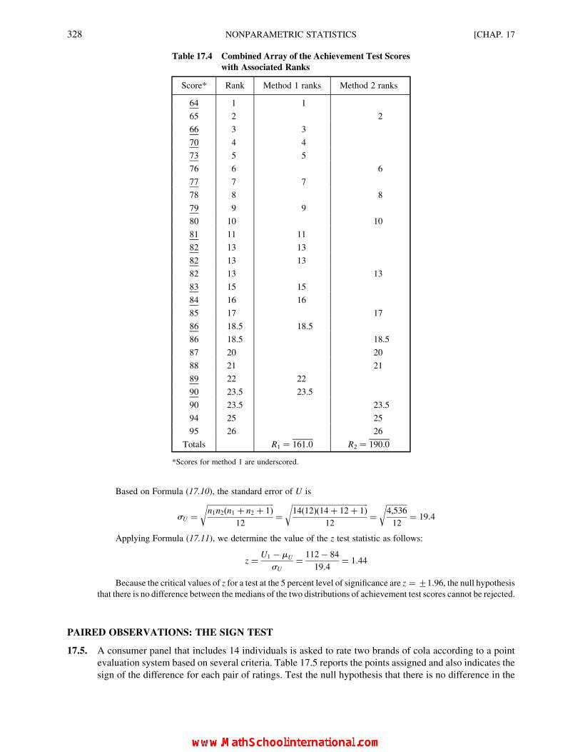
Based on Formula (17.10), the standard error of U is
sU ¼ffiffiffiffiffiffiffiffiffiffiffiffiffiffiffiffiffiffiffiffiffiffiffiffiffiffiffiffiffiffiffiffiffiffiffin1n2(n1 þ n2 þ 1)
12
r¼
ffiffiffiffiffiffiffiffiffiffiffiffiffiffiffiffiffiffiffiffiffiffiffiffiffiffiffiffiffiffiffiffiffiffiffiffiffiffiffiffi14(12)(14þ 12þ 1)
12
r¼
ffiffiffiffiffiffiffiffiffiffiffi4,536
12
r¼ 19:4
Applying Formula (17.11), we determine the value of the z test statistic as follows:
z ¼ U1 � mU
sU
¼ 112� 84
19:4¼ 1:44
Because the critical values of z for a test at the 5 percent level of significance are z ¼ +1:96, the null hypothesisthat there is no difference between the medians of the two distributions of achievement test scores cannot be rejected.
PAIRED OBSERVATIONS: THE SIGN TEST
17.5. A consumer panel that includes 14 individuals is asked to rate two brands of cola according to a point
evaluation system based on several criteria. Table 17.5 reports the points assigned and also indicates the
sign of the difference for each pair of ratings. Test the null hypothesis that there is no difference in the
Table 17.4 Combined Array of the Achievement Test Scores
with Associated Ranks
Score* Rank Method 1 ranks Method 2 ranks
64 1 1
65 2 2
66 3 3
70 4 4
73 5 5
76 6 6
77 7 7
78 8 8
79 9 9
80 10 10
81 11 11
82 13 13
82 13 13
82 13 13
83 15 15
84 16 16
85 17 17
86 18.5 18.5
86 18.5 18.5
87 20 20
88 21 21
89 22 22
90 23.5 23.5
90 23.5 23.5
94 25 25
95 26 26
Totals R1 ¼ 161.0 R2 ¼ 190.0
*Scores for method 1 are underscored.
328 NONPARAMETRIC STATISTICS [CHAP. 17

level of ratings for the two brands of cola at the 5 percent level of significance by use of the sign test,
formulating the null and alternative hypotheses in terms of the proportion of plus signs.
H0: p ¼ 0:50
H1: p = 0:50
Referring to Table 17.5, we see that two of the consumers rated the two brands of cola as equal, and therefore
these two panel members are omitted from the following analysis, resulting in an effective sample size of n ¼ 12. Of
the 12 signs, 8 are plus signs.
Because the number of pairs of values is n , 30, the binomial distribution is the appropriate basis for this test.
As in Problem 17.2, on the one-sample sign test, we use the P-value approach to hypothesis testing. The probability
of observing 8 or more plus signs in 12 observations given that the population proportion of plus signs is 0.50 is
determined by reference to Appendix 2 for binomial probabilities:
P(X � 8 j n ¼ 12, p ¼ 0:50) ¼ 0:1208þ 0:0537þ 0:0161þ 0:0029þ 0:0002
¼ 0:1937
The probability calculated above is for the one-tail P(X � 8). Because a two-sided test is involved in the
present application, this probability must be doubled to obtain the P value: P ¼ 2� 0:1937 ¼ 0:3874. That is, theprobability is 0.3874 that the observed deviation in either direction from the expected number of plus signs of
np0 ¼ 12(0:50) ¼ 6. This P value is well above the 0.05 probability level, and therefore the null hypothesis that the
two brands of cola have equal consumer preference clearly cannot be rejected.
PAIRED OBSERVATIONS: THE WILCOXON TEST
17.6. Apply the Wilcoxon test to the data in Problem 17.5, above, using the 5 percent level of significance.
We repeat the ratings in Table 17.6, determine the values of d, rank the absolute values of d, and finally, we
determine the sum of the plus and minus rankings.
Referring to Table 17.6, note that the two panel members who rated the two brands of cola equally are dropped
from the analysis, because the difference d ¼ 0 is not assigned a rank. Therefore, the effective sample size is
Table 17.5 Ratings Assigned to Two Brands of Cola by a
Consumer Panel
Point rating assigned to
each brand
Panel member Brand 1 Brand 2 Sign of difference
1 20 16 þ2 24 26 2
3 28 18 þ4 24 17 þ5 20 20 0
6 29 21 þ7 19 23 2
8 27 22 þ9 20 23 2
10 30 20 þ11 18 18 0
12 28 21 þ13 26 17 þ14 24 26 2
CHAP. 17] NONPARAMETRIC STATISTICS 329

n ¼ 12. Of the 12 absolute values of d, several tied pairs result in the assignment of the mean ranks. For instance,
there are two absolute differences tied for the positions of rank 1 and rank 2; therefore, each of these absolute
differences is assigned the mean rank 1.5. The next rank assigned is then rank 3. Because the sum of the ranks for the
negative differences is smaller than the sum for the positive differences, this smaller sum is labelled T in Table 17.6.
Appendix 10 indicates that for n ¼ 12 (the effective sample size) the critical value of the Wilcoxon T statistic
for a two-sided test at the 5 percent level of significance is T ¼ 14. Since T is the smaller sum of the signed ranks for
a two-sided test, the obtained value of the test statistic as calculated in Table 17.6 is T ¼ 10:5. Because this value isless than the critical value, the null hypothesis that there is no difference in the ratings for the two brands of cola is
rejected.
Note that the null hypothesis of no difference could not be rejected at the 5 percent level when the sign test was
applied to these same data in Problem 17.5. Because the Wilcoxon test considers the magnitude of the difference
between each matched pair and not just the sign of the difference, the Wilcoxon test for paired observations is a
more sensitive test than the sign test.
SEVERAL INDEPENDENT SAMPLES: THE KRUSKAL–WALLIS TEST
17.7. In Problem 13.1 on the one-factor completely randomized design of the analysis of variance, we
presented achievement test scores for a random sample of n ¼ 5 trainees randomly assigned to each of
three instructional methods. In those sections the null hypothesis was that the mean levels of
achievement for the three different levels of instruction did not differ, and because of the small samples
it was necessary to assume that the three populations were normally distributed. Suppose we cannot
make this assumption. Apply the Kruskal–Wallis test to test the null hypothesis that the several
populations have the same median, using the 5 percent level of significance.
Table 17.6 Ratings Assigned to Two Brands of Cola by a Consumer Panel and the Determination of
Signed Ranks
Signed rank
Panel
member Brand 1 (X1) Brand 2 (X2)
Difference
(d ¼ X1 � X2) Rank of jdj (þ) (2)
1 20 16 4 4.5 4.5
2 24 26 22 1.5 1.5
3 28 18 10 11.5 11.5
4 24 17 7 7.5 7.5
5 20 20 0
6 29 21 8 9 9
7 19 23 24 4.5 4.5
8 27 22 5 6 6
9 20 23 23 3 3
10 30 20 10 11.5 11.5
11 18 18 0
12 28 21 7 7.5 7.5
13 26 17 9 10 10
14 24 26 22 1.5 1.5
Total 67.5 T ¼ 10.5
330 NONPARAMETRIC STATISTICS [CHAP. 17
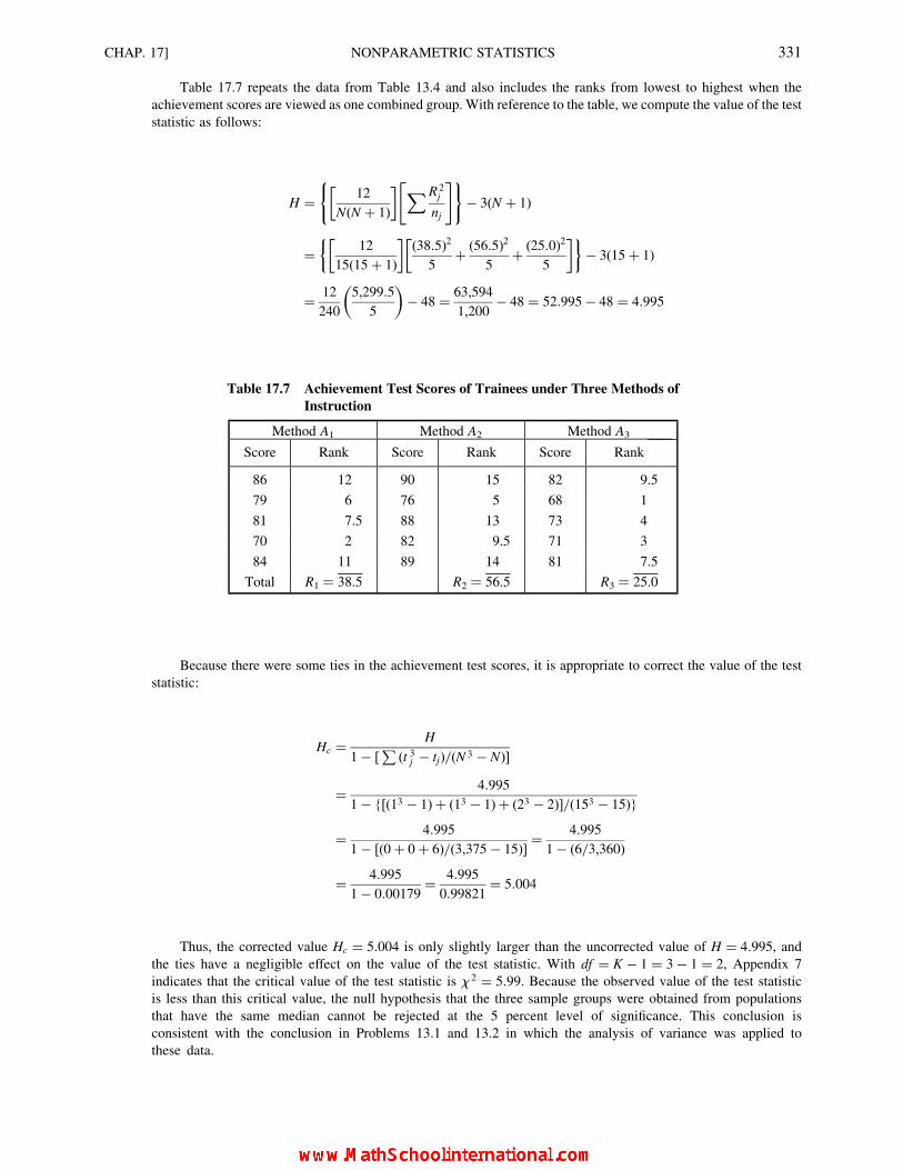
Table 17.7 repeats the data from Table 13.4 and also includes the ranks from lowest to highest when the
achievement scores are viewed as one combined group. With reference to the table, we compute the value of the test
statistic as follows:
H ¼ 12
N(N þ 1)
� � XR 2j
nj
" #( )� 3(N þ 1)
¼ 12
15(15þ 1)
� �(38:5)2
5þ (56:5)
2
5þ (25:0)
2
5
� �� �� 3(15þ 1)
¼ 12
240
5,299:5
5
� �� 48 ¼ 63,594
1,200� 48 ¼ 52:995� 48 ¼ 4:995
Because there were some ties in the achievement test scores, it is appropriate to correct the value of the test
statistic:
Hc ¼ H
1� [P (t 3j � tj)=(N 3 � N)]
¼ 4:995
1� {[(13 � 1)þ (13 � 1)þ (23 � 2)]=(153 � 15)}
¼ 4:995
1� [(0þ 0þ 6)=(3,375� 15)]¼ 4:995
1� (6=3,360)
¼ 4:995
1� 0:00179¼ 4:995
0:99821¼ 5:004
Thus, the corrected value Hc ¼ 5:004 is only slightly larger than the uncorrected value of H ¼ 4:995, andthe ties have a negligible effect on the value of the test statistic. With df ¼ K � 1 ¼ 3� 1 ¼ 2, Appendix 7
indicates that the critical value of the test statistic is x 2 ¼ 5:99. Because the observed value of the test statistic
is less than this critical value, the null hypothesis that the three sample groups were obtained from populations
that have the same median cannot be rejected at the 5 percent level of significance. This conclusion is
consistent with the conclusion in Problems 13.1 and 13.2 in which the analysis of variance was applied to
these data.
Table 17.7 Achievement Test Scores of Trainees under Three Methods of
Instruction
Method A1 Method A2 Method A3
Score Rank Score Rank Score Rank
86 12 90 15 82 9.5
79 6 76 5 68 1
81 7.5 88 13 73 4
70 2 82 9.5 71 3
84 11 89 14 81 7.5
Total R1 ¼ 38.5 R2 ¼ 56.5 R3 ¼ 25.0
CHAP. 17] NONPARAMETRIC STATISTICS 331
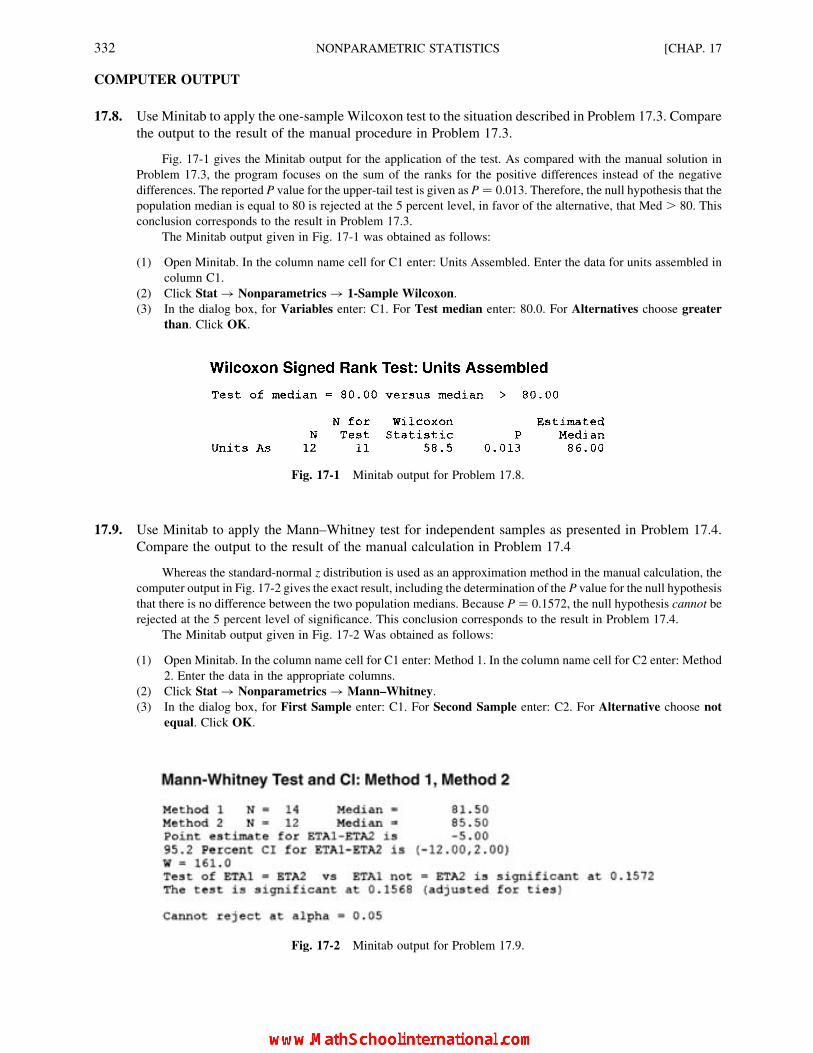
COMPUTER OUTPUT
17.8. Use Minitab to apply the one-sample Wilcoxon test to the situation described in Problem 17.3. Compare
the output to the result of the manual procedure in Problem 17.3.
Fig. 17-1 gives the Minitab output for the application of the test. As compared with the manual solution in
Problem 17.3, the program focuses on the sum of the ranks for the positive differences instead of the negative
differences. The reported P value for the upper-tail test is given as P ¼ 0.013. Therefore, the null hypothesis that the
population median is equal to 80 is rejected at the 5 percent level, in favor of the alternative, that Med . 80. This
conclusion corresponds to the result in Problem 17.3.
The Minitab output given in Fig. 17-1 was obtained as follows:
(1) Open Minitab. In the column name cell for C1 enter: Units Assembled. Enter the data for units assembled in
column C1.
(2) Click Stat ! Nonparametrics ! 1-Sample Wilcoxon.
(3) In the dialog box, for Variables enter: C1. For Test median enter: 80.0. For Alternatives choose greater
than. Click OK.
17.9. Use Minitab to apply the Mann–Whitney test for independent samples as presented in Problem 17.4.
Compare the output to the result of the manual calculation in Problem 17.4
Whereas the standard-normal z distribution is used as an approximation method in the manual calculation, the
computer output in Fig. 17-2 gives the exact result, including the determination of the P value for the null hypothesis
that there is no difference between the two population medians. Because P ¼ 0.1572, the null hypothesis cannot be
rejected at the 5 percent level of significance. This conclusion corresponds to the result in Problem 17.4.
The Minitab output given in Fig. 17-2 Was obtained as follows:
(1) Open Minitab. In the column name cell for C1 enter: Method 1. In the column name cell for C2 enter: Method
2. Enter the data in the appropriate columns.
(2) Click Stat ! Nonparametrics ! Mann–Whitney.
(3) In the dialog box, for First Sample enter: C1. For Second Sample enter: C2. For Alternative choose not
equal. Click OK.
Fig. 17-1 Minitab output for Problem 17.8.
Fig. 17-2 Minitab output for Problem 17.9.
332 NONPARAMETRIC STATISTICS [CHAP. 17

17.10. Use Minitab to apply the Kruskal–Wallis test to the situation described in Problem 17.7. Compare the
computer output to the result of the manual calculation in that problem.
Figure 17-3 is the Minitab output with respect to the null hypothesis that the three population medians are not
different against the alternative that there is a difference. In Problem 17.7 we could not reject the null hypothesis
based on use of the critical value approach to hypothesis testing. The output in Fig. 17-3 gives the same values for H
and Hc as calculated in Problem 17.7 and also provides the P value for the test, which is P ¼ 0.082. Since P . 0.05,
the null hypothesis cannot be rejected at the 5 percent level of significance.
The Minitab output in Fig. 17-3 was obtained as follows:
1. Open Minitab. In the column name cell for C1 enter: Method. In the column name cell for C2 enter: Score.
Since there are 5 scores for each method, in C1 enter five 1s, five 2s, and five 3s, which are the method labels. In
C2 enter the 15 test scores, each associated (in groups of 5) with one of the three methods of instruction in C1.
2. Click Stat ! Nonparametrics ! Kruskal–Wallis.
3. In the dialog box, for Response enter: C2. For Factor enter: C1. Click OK.
Supplementary Problems
THE RUNS TEST FOR RANDOMNESS
17.11. Refer to Table 2.19 on page 41 in which 40 randomly sampled personal loan amounts are reported. The sequence of
data collection was according to row in the table (that is, the sequence of observed amounts was $932, $1,000, $356,
etc.). The median loan amount for the data in the table is $944.50. Test the randomness of this sequence of loan
amounts by classifying each amount as being above or below the median, using the 5 percent level of significance.
Ans. Critical z ¼ +1:96, R ¼ 28, and z ¼ 2:56. The null hypothesis that the sequence is random is rejected. There
is an unusually large number of runs.
ONE SAMPLE: THE SIGN TEST
17.12. The following table reports the unit sales of a new tool in a sample of 12 outlets in a given month. The form of the
distribution is unknown, and thus a parametric statistical test is not appropriate given the small sample size. Use the
sign test with respect to the null hypothesis that the median sales amount in the population is no greater than 10.0
units per outlet, using the 5 percent level of significance.
Ans. P ¼ 0.1719; the null hypothesis cannot be rejected.
Fig. 17-3 Minitab output for Problem 17.10.
Tools/outlet 8 18 9 12 10 14 16 7 14 11 10 20
CHAP. 17] NONPARAMETRIC STATISTICS 333

ONE SAMPLE: THE WILCOXON TEST
17.13. Apply theWilcoxon test with respect to the null hypothesis and the data in Problem 17.9, using the 5 percent level of
significance.
Ans. Critical T ¼ 11, T ¼ 10; the null hypothesis is rejected.
TWO INDEPENDENT SAMPLES: THE MANN–WHITNEY TEST
17.14. A process control department wishes to compare the time required for two alternative systems to diagnose
equipment failure. A sample of 30 equipment failures are randomly assigned for diagnosis to the two systems with
14 failures assigned for diagnosis to the first system and 16 assigned for diagnosis to the second system. Table 17.8
reports total time, in minutes, required to diagnose each failure. No assumption can be made concerning the
distribution of the total time required to diagnose such failures. Using the 10 percent level of significance, test the
null hypothesis that the two samples have been obtained from populations that have the same median.
Ans. R1 ¼ 173:5, R2 ¼ 291:5, critical z ¼ +1:645, z ¼ 1:87; the null hypothesis is rejected at a ¼ 0:10.
PAIRED OBSERVATIONS: THE SIGN TEST
17.15. Instead of the experimental design used in Problem 17.14, the same random sample of 10 equipment failures is
diagnosed by the two systems. Thus, each of the 10 pieces of equipment is subjected to diagnosis twice, and the time
required in minutes to diagnose the failure by each system is noted. Table 17.9 indicates the number of minutes
required for each diagnosis. Using the 10 percent level of significance, test the null hypothesis that the two samples
came from populations that are not different in level. That is, the null hypothesis is that there is no difference in the
median amount of time required to diagnose equipment failure by the twomethods. Use the sign test for this analysis.
Ans. P ¼ 0.3438; the null hypothesis cannot be rejected.
Table 17.8 Time Required to
Diagnose Equip-
ment Failures (in
Minutes)
System 1 System 2
25 18
29 37
42 40
16 56
31 49
14 28
33 20
45 34
26 39
34 47
30 31
43 65
28 38
19 32
24
49
334 NONPARAMETRIC STATISTICS [CHAP. 17
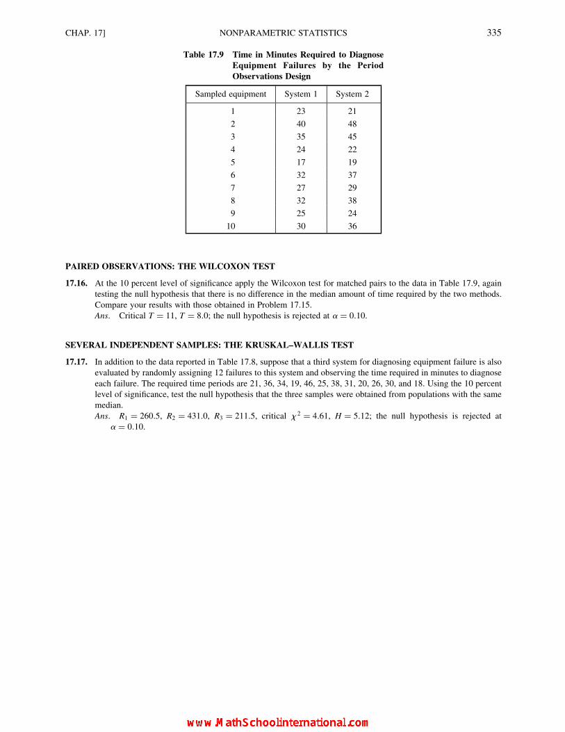
PAIRED OBSERVATIONS: THE WILCOXON TEST
17.16. At the 10 percent level of significance apply the Wilcoxon test for matched pairs to the data in Table 17.9, again
testing the null hypothesis that there is no difference in the median amount of time required by the two methods.
Compare your results with those obtained in Problem 17.15.
Ans. Critical T ¼ 11, T ¼ 8:0; the null hypothesis is rejected at a ¼ 0:10.
SEVERAL INDEPENDENT SAMPLES: THE KRUSKAL–WALLIS TEST
17.17. In addition to the data reported in Table 17.8, suppose that a third system for diagnosing equipment failure is also
evaluated by randomly assigning 12 failures to this system and observing the time required in minutes to diagnose
each failure. The required time periods are 21, 36, 34, 19, 46, 25, 38, 31, 20, 26, 30, and 18. Using the 10 percent
level of significance, test the null hypothesis that the three samples were obtained from populations with the same
median.
Ans. R1 ¼ 260:5, R2 ¼ 431:0, R3 ¼ 211:5, critical x 2 ¼ 4:61, H ¼ 5:12; the null hypothesis is rejected at
a ¼ 0:10.
Table 17.9 Time in Minutes Required to Diagnose
Equipment Failures by the Period
Observations Design
Sampled equipment System 1 System 2
1 23 21
2 40 48
3 35 45
4 24 22
5 17 19
6 32 37
7 27 29
8 32 38
9 25 24
10 30 36
CHAP. 17] NONPARAMETRIC STATISTICS 335

CHAPTER 18
Decision Analysis:Payoff Tables and
Decision Trees
18.1 THE STRUCTURE OF PAYOFF TABLES
From the standpoint of statistical decision theory, a decision situation under conditions of uncertainty can
be represented by certain common ingredients that are included in the structure of the payoff table for the
situation. Essentially, a payoff table identifies the conditional gain (or loss) associated with every possible
combination of decision acts and events; it also typically indicates the probability of occurrence for each of the
mutually exclusive events.
In Table 18.1, the acts are the alternative courses of action, or strategies, that are available to the decision
maker. As the result of the analysis, one of these acts is chosen as being the best act. The basis for this choice is
the subject matter of this chapter. As a minimum, there must be at least two possible acts available, so that the
opportunity for choice in fact exists. An example of an act is the number of units of a particular item to be
ordered for stock.
Table 18.1 General Structure of a Payoff Table
Acts
Events Probability A1 A2 A3 . . . An
E1 P1 X11 X12 X13 . . . X1n
E2 P2 X21 X22 X23 . . . X2n
E3 P3 X31 X32 X33 . . . X3n
. . . . . . . . . . . . . . . . . . . . .
Em Pm Xm1 Xm2 Xm3 . . . Xmn
336
Copyright 2004, 1996, 1988, 1976 by The McGraw-Hill Companies, Inc. Click Here for Terms of Use.

The events identify the occurrences that are outside of the decision maker’s control and that determine the
level of success for a given act. These events are often called “states of nature,” “states,” or “outcomes.” We are
concerned only with discrete events in this chapter. An example of an event is the level of marked demand for a
particular item during a stipulated time period.
The probability of each event is included as part of the general format of a decision table when such
probability values are in fact available. However, one characteristic of decision analysis is that such
probabilities should always be available since they can be based on either objective data or be determined
subjectively on the basis of judgment. Because the events in the payoff table are mutually exclusive and
exhaustive, the sum of the probability values should be 1.0.
Finally, the cell entries are the conditional values, or conditional economic consequences. These values are
usually called payoffs in the literature, and they are conditional in the sense that the economic result which is
experienced depends on the decision act that is chosen and the event that occurs.
EXAMPLE 1. A heating and air-conditioning contractor must commit to the purchase of central air-conditioning units as
of April 1 for resale and installation during the following summer season. Based on demand during the previous summer,
current economic conditions, and competitive factors in the market, the contractor estimates that there is a 0.10 probability
of selling only 5 units, a 0.30 probability of selling 10 units, a 0.40 probability of selling 15 units, and a 0.20 probability of
selling 20 units. The air-conditioning units can be ordered only in groups of five, with the cost per unit being $1,000 and the
retail price being $1,300 (plus installation charges). Any unsold units at the end of the season are returned to the
manufacturer for a net credit of $800, after deduction of shipping charges.
Table 18.2 is the payoff table for this situation. Note that because we estimate there will be a market
demand for at least 5 units but not more than 20 units, these are logically also the limits for our possible acts
(units ordered). Our stipulation that units can be ordered only in groups of five serves to simplify the problem
and reduce the size of the payoff table. The payoffs in Table 18.2 are based on a markup of $300 per unit sold
and a loss of $200 for each unsold unit. Thus, for example, if 15 units are ordered for stock and only 10 are sold,
the economic result is a gain of $3,000 on the 10 units sold less a loss of $1,000 on the 5 units returned to the
manufacturer, for a resulting payoff of $2,000 at A3, E2 in the table.
In the following sections we refer to Example 1 in order to demonstrate the application of different decision
criteria, or standards, that can be used to identify the decision act which is considered to be the best act. Themethods
in this chapter, which involve the use of the probability values associated with each event, are concerned only with
the probabilities formulated during the initial structuring of the payoff table. Because these values are formulated
before the collection of any additional information, they are called prior probabilities in decision analysis.
18.2 DECISION MAKING BASED UPON PROBABILITIES ALONE
A complete application of Bayesian decision analysis involves use of all of the information included in a
payoff table. However, in this section we briefly consider the criteria that could be used if the economic
Table 18.2 Payoff Table for the Number of Air-Conditioning Units to Be Ordered
Order quantity
Market demand Probability A1 : 5 A2 : 10 A3 : 15 A4 : 20
E1 : 5 0.10 $1,500 $ 500 2$ 500 2$1,500
E2 : 10 0.30 1,500 3,000 2,000 1,000
E3 : 15 0.40 1,500 3,000 4,500 3,500
E4 : 20 0.20 1,500 3,000 4,500 6,000
1.00
CHAP. 18] DECISION ANALYSIS: PAYOFF TABLES AND DECISION TREES 337
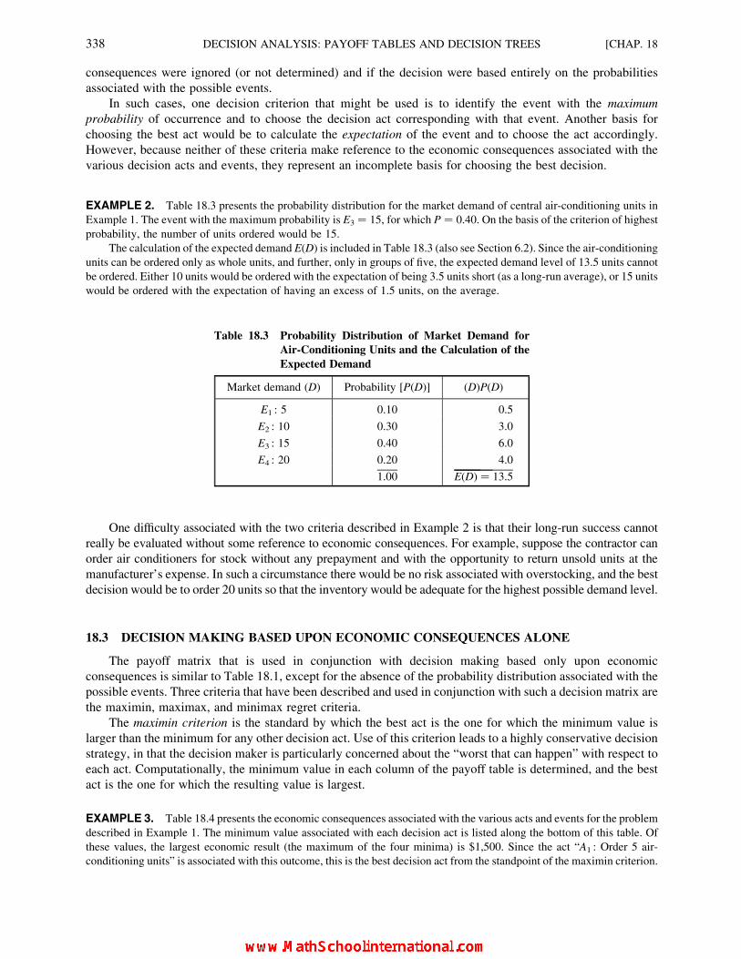
consequences were ignored (or not determined) and if the decision were based entirely on the probabilities
associated with the possible events.
In such cases, one decision criterion that might be used is to identify the event with the maximum
probability of occurrence and to choose the decision act corresponding with that event. Another basis for
choosing the best act would be to calculate the expectation of the event and to choose the act accordingly.
However, because neither of these criteria make reference to the economic consequences associated with the
various decision acts and events, they represent an incomplete basis for choosing the best decision.
EXAMPLE 2. Table 18.3 presents the probability distribution for the market demand of central air-conditioning units in
Example 1. The event with the maximum probability is E3 ¼ 15, for which P ¼ 0.40. On the basis of the criterion of highest
probability, the number of units ordered would be 15.
The calculation of the expected demand E(D) is included in Table 18.3 (also see Section 6.2). Since the air-conditioning
units can be ordered only as whole units, and further, only in groups of five, the expected demand level of 13.5 units cannot
be ordered. Either 10 units would be ordered with the expectation of being 3.5 units short (as a long-run average), or 15 units
would be ordered with the expectation of having an excess of 1.5 units, on the average.
One difficulty associated with the two criteria described in Example 2 is that their long-run success cannot
really be evaluated without some reference to economic consequences. For example, suppose the contractor can
order air conditioners for stock without any prepayment and with the opportunity to return unsold units at the
manufacturer’s expense. In such a circumstance there would be no risk associated with overstocking, and the best
decision would be to order 20 units so that the inventory would be adequate for the highest possible demand level.
18.3 DECISION MAKING BASED UPON ECONOMIC CONSEQUENCES ALONE
The payoff matrix that is used in conjunction with decision making based only upon economic
consequences is similar to Table 18.1, except for the absence of the probability distribution associated with the
possible events. Three criteria that have been described and used in conjunction with such a decision matrix are
the maximin, maximax, and minimax regret criteria.
The maximin criterion is the standard by which the best act is the one for which the minimum value is
larger than the minimum for any other decision act. Use of this criterion leads to a highly conservative decision
strategy, in that the decision maker is particularly concerned about the “worst that can happen” with respect to
each act. Computationally, the minimum value in each column of the payoff table is determined, and the best
act is the one for which the resulting value is largest.
EXAMPLE 3. Table 18.4 presents the economic consequences associated with the various acts and events for the problem
described in Example 1. The minimum value associated with each decision act is listed along the bottom of this table. Of
these values, the largest economic result (the maximum of the four minima) is $1,500. Since the act “A1 : Order 5 air-
conditioning units” is associated with this outcome, this is the best decision act from the standpoint of the maximin criterion.
Table 18.3 Probability Distribution of Market Demand for
Air-Conditioning Units and the Calculation of the
Expected Demand
Market demand (D) Probability [P(D)] (D)P(D)
E1 : 5 0.10 0.5
E2 : 10 0.30 3.0
E3 : 15 0.40 6.0
E4 : 20 0.20 4.0
1.00 E(D) ¼ 13.5
338 DECISION ANALYSIS: PAYOFF TABLES AND DECISION TREES [CHAP. 18
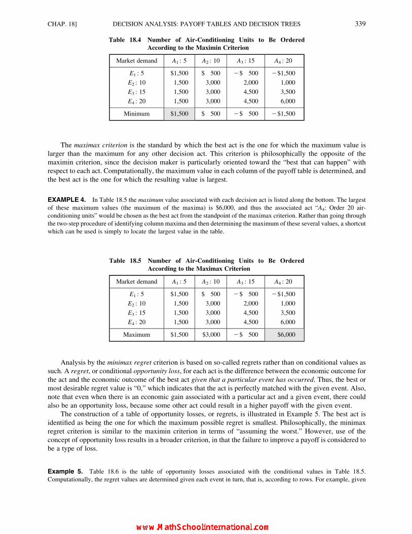
The maximax criterion is the standard by which the best act is the one for which the maximum value is
larger than the maximum for any other decision act. This criterion is philosophically the opposite of the
maximin criterion, since the decision maker is particularly oriented toward the “best that can happen” with
respect to each act. Computationally, the maximum value in each column of the payoff table is determined, and
the best act is the one for which the resulting value is largest.
EXAMPLE 4. In Table 18.5 the maximum value associated with each decision act is listed along the bottom. The largest
of these maximum values (the maximum of the maxima) is $6,000, and thus the associated act “A4: Order 20 air-
conditioning units” would be chosen as the best act from the standpoint of the maximax criterion. Rather than going through
the two-step procedure of identifying column maxima and then determining the maximum of these several values, a shortcut
which can be used is simply to locate the largest value in the table.
Analysis by the minimax regret criterion is based on so-called regrets rather than on conditional values as
such. A regret, or conditional opportunity loss, for each act is the difference between the economic outcome for
the act and the economic outcome of the best act given that a particular event has occurred. Thus, the best or
most desirable regret value is “0,” which indicates that the act is perfectly matched with the given event. Also,
note that even when there is an economic gain associated with a particular act and a given event, there could
also be an opportunity loss, because some other act could result in a higher payoff with the given event.
The construction of a table of opportunity losses, or regrets, is illustrated in Example 5. The best act is
identified as being the one for which the maximum possible regret is smallest. Philosophically, the minimax
regret criterion is similar to the maximin criterion in terms of “assuming the worst.” However, use of the
concept of opportunity loss results in a broader criterion, in that the failure to improve a payoff is considered to
be a type of loss.
Example 5. Table 18.6 is the table of opportunity losses associated with the conditional values in Table 18.5.
Computationally, the regret values are determined given each event in turn, that is, according to rows. For example, given
Table 18.4 Number of Air-Conditioning Units to Be Ordered
According to the Maximin Criterion
Market demand A1 : 5 A2 : 10 A3 : 15 A4 : 20
E1 : 5 $1,500 $ 500 2$ 500 2$1,500
E2 : 10 1,500 3,000 2,000 1,000
E3 : 15 1,500 3,000 4,500 3,500
E4 : 20 1,500 3,000 4,500 6,000
Minimum $1,500 $ 500 2$ 500 2$1,500
Table 18.5 Number of Air-Conditioning Units to Be Ordered
According to the Maximax Criterion
Market demand A1 : 5 A2 : 10 A3 : 15 A4 : 20
E1 : 5 $1,500 $ 500 2$ 500 2$1,500
E2 : 10 1,500 3,000 2,000 1,000
E3 : 15 1,500 3,000 4,500 3,500
E4 : 20 1,500 3,000 4,500 6,000
Maximum $1,500 $3,000 2$ 500 $6,000
CHAP. 18] DECISION ANALYSIS: PAYOFF TABLES AND DECISION TREES 339

that E1 occurs, the best act (by reference to the payoff matrix in Table 18.2) is A1, with a value of $1,500. If A2 is chosen, the
result is $500, which differs from the best act by $1,000, and which is then the regret value for A2. If A3 is chosen,
regret ¼ $1,500 2 (2500) ¼ $2,000. If A4 is chosen, regret ¼ $1,500 2 (21,500) ¼ $3,000. The remaining
opportunity loss values are similarly determined, with the best conditional value in each row serving as the basis for
determining regret values in that row. For instance, in row 2, for E2: 10, the best act is A2: 10 with a payoff value of $3,000 in
Table 18.5.
The maximum regret which can occur in conjunction with each decision act is listed along the bottom of Table 18.6.
The smallest of these maxima (the minimum of the maximum regrets) is $2,000; “A3: Order 15 units” would thus be chosen
as the best act from the standpoint of the minimax regret criterion.
18.4 DECISION MAKING BASED UPON BOTH PROBABILITIES AND ECONOMICCONSEQUENCES: THE EXPECTED PAYOFF CRITERION
The methods presented in this section utilize all the information contained in the basic payoff table (see
Section 18.1). Thus, we consider both the probabilities associated with the possible events and the economic
consequences for all combinations of the several acts and several events.
The expected payoff (EP) criterion is the standard by which the best act is the one for which the expected
economic outcome is the highest, as a long-run average. Note that in the present case we are concerned about
the long-run average economic result, and not simply the-long-run average event value (demand level)
discussed in Section 18.2. Computationally, the expected payoff for each act is determined by multiplying the
conditional payoff for each event/act combination by the probability of the event and summing these products
for each act.
EXAMPLE 6. Table 18.7 repeats the information from Table 18.2, except that the expected payoffs have been identified
along the bottom. Table 18.8 illustrates the procedure by which such expected payoffs are calculated. In Table 18.7, the
largest expected payoff is $3,250, and thus the associated act “A3: Order 15 units” is the best act from the standpoint of the
expected payoff criterion.
The expected payoff criterion often is referred to as the Bayesian criterion. Use of the adjective Bayesian
here is distinct from the use of Bayes’ theorem for revising a prior probability value, determined before the
selection of a sample, by considering the sample outcome (see Section 5.7). Thus, a reference to Bayesian
procedures in decision analysis can involve use of the expected payoff criterion, revision of prior probability
values, or both.
Table 18.6 Opportunity Loss Table for the Number of Air-Conditioning Units to Be Ordered and Application of the
Minimax Regret Criterion
Market
demand A1 : 5 A2 : 10 A3 : 15 A4 : 20
E1 : 5 $ 0 $1,000
(¼$1,500 2 500)
$2,000
[¼$1,500 2 (2500)]
$3,000
[¼$1,500 2 (21,500)]
E2 : 10 1,500
(¼3,000 2 1,500)
0 1,000
(¼3,000 2 2,000)
2,000
(¼3,000 2 1,000)
E3 : 15 3,000
(¼4,500 2 1,500)
1,500
(¼4,500 2 3,000)
0 1,000
(¼4,500 2 3,500)
E4 : 20 4,500
(¼6,000 2 1,500)
3,000
(¼6,000 2 3,000)
1,500
(¼6,000 2 3,000)
0
Maximum
regret $4,500 $3,000 $2,000 $3,000
340 DECISION ANALYSIS: PAYOFF TABLES AND DECISION TREES [CHAP. 18
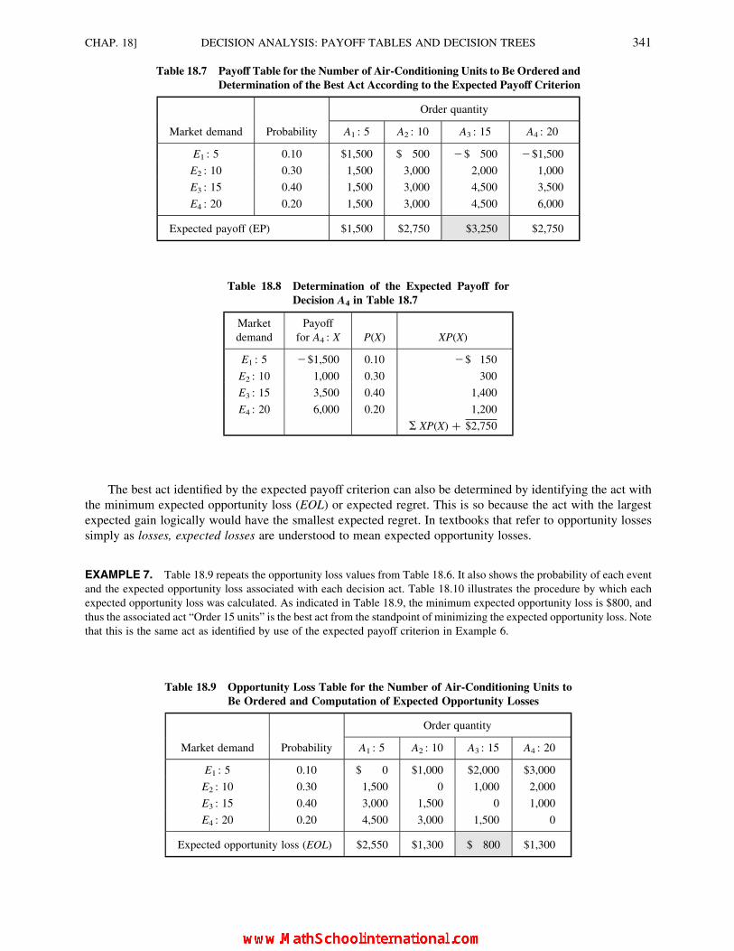
The best act identified by the expected payoff criterion can also be determined by identifying the act with
the minimum expected opportunity loss (EOL) or expected regret. This is so because the act with the largest
expected gain logically would have the smallest expected regret. In textbooks that refer to opportunity losses
simply as losses, expected losses are understood to mean expected opportunity losses.
EXAMPLE 7. Table 18.9 repeats the opportunity loss values from Table 18.6. It also shows the probability of each event
and the expected opportunity loss associated with each decision act. Table 18.10 illustrates the procedure by which each
expected opportunity loss was calculated. As indicated in Table 18.9, the minimum expected opportunity loss is $800, and
thus the associated act “Order 15 units” is the best act from the standpoint of minimizing the expected opportunity loss. Note
that this is the same act as identified by use of the expected payoff criterion in Example 6.
Table 18.7 Payoff Table for the Number of Air-Conditioning Units to Be Ordered and
Determination of the Best Act According to the Expected Payoff Criterion
Order quantity
Market demand Probability A1 : 5 A2 : 10 A3 : 15 A4 : 20
E1 : 5 0.10 $1,500 $ 500 2$ 500 2$1,500
E2 : 10 0.30 1,500 3,000 2,000 1,000
E3 : 15 0.40 1,500 3,000 4,500 3,500
E4 : 20 0.20 1,500 3,000 4,500 6,000
Expected payoff (EP) $1,500 $2,750 $3,250 $2,750
Table 18.8 Determination of the Expected Payoff for
Decision A4 in Table 18.7
Market
demand
Payoff
for A4 : X P(X) XP(X)
E1 : 5 2$1,500 0.10 2$ 150
E2 : 10 1,000 0.30 300
E3 : 15 3,500 0.40 1,400
E4 : 20 6,000 0.20 1,200
S XP(X) þ $2,750
Table 18.9 Opportunity Loss Table for the Number of Air-Conditioning Units to
Be Ordered and Computation of Expected Opportunity Losses
Order quantity
Market demand Probability A1 : 5 A2 : 10 A3 : 15 A4 : 20
E1 : 5 0.10 $ 0 $1,000 $2,000 $3,000
E2 : 10 0.30 1,500 0 1,000 2,000
E3 : 15 0.40 3,000 1,500 0 1,000
E4 : 20 0.20 4,500 3,000 1,500 0
Expected opportunity loss (EOL) $2,550 $1,300 $ 800 $1,300
CHAP. 18] DECISION ANALYSIS: PAYOFF TABLES AND DECISION TREES 341
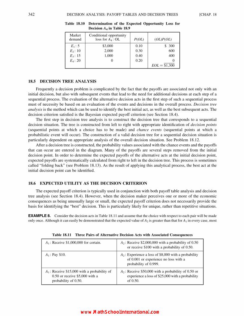
18.5 DECISION TREE ANALYSIS
Frequently a decision problem is complicated by the fact that the payoffs are associated not only with an
initial decision, but also with subsequent events that lead to the need for additional decisions at each step of a
sequential process. The evaluation of the alternative decision acts in the first step of such a sequential process
must of necessity be based on an evaluation of the events and decisions in the overall process. Decision tree
analysis is the method which can be used to identify the best initial act, as well as the best subsequent acts. The
decision criterion satisfied is the Bayesian expected payoff criterion (see Section 18.4).
The first step in decision tree analysis is to construct the decision tree that corresponds to a sequential
decision situation. The tree is constructed from left to right with appropriate identification of decision points
(sequential points at which a choice has to be made) and chance events (sequential points at which a
probabilistic event will occur). The construction of a valid decision tree for a sequential decision situation is
particularly dependent on appropriate analysis of the overall decision situation. See Problem 18.12.
After a decision tree is constructed, the probability values associated with the chance events and the payoffs
that can occur are entered in the diagram. Many of the payoffs are several steps removed from the initial
decision point. In order to determine the expected payoffs of the alternative acts at the initial decision point,
expected payoffs are systematically calculated from right to left in the decision tree. This process is sometimes
called “folding back” (see Problem 18.13). As the result of applying this analytical process, the best act at the
initial decision point can be identified.
18.6 EXPECTED UTILITY AS THE DECISION CRITERION
The expected payoff criterion is typically used in conjunction with both payoff table analysis and decision
tree analysis (see Section 18.4). However, when the decision maker perceives one or more of the economic
consequences as being unusually large or small, the expected payoff criterion does not necessarily provide the
basis for identifying the “best” decision. This is particularly likely for unique, rather than repetitive situations.
EXAMPLE 8. Consider the decision acts in Table 18.11 and assume that the choice with respect to each pair will be made
only once. Although it can easily be demonstrated that the expected value of A2 is greater than that for A1 in every case, most
Table 18.10 Determination of the Expected Opportunity Loss for
Decision A4 in Table 18.9
Marketdemand
Conditional opportunityloss for A4 : OL P(OL) (OL)P(OL)
E1 : 5 $3,000 0.10 $ 300
E2 : 10 2,000 0.30 600
E3 : 15 1,000 0.40 400
E4 : 20 0 0.20 0
EOL ¼ $1,300
Table 18.11 Three Pairs of Alternative Decision Acts with Associated Consequences
A1 : Receive $1,000,000 for certain. A2 : Receive $2,000,000 with a probability of 0.50
or receive $100 with a probability of 0.50.
A1 : Pay $10. A2 : Experience a loss of $8,000 with a probability
of 0.001 or experience no loss with a
probability of 0.999.
A1 : Receive $15,000 with a probability of
0.50 or receive $5,000 with a
probability of 0.50.
A2 : Receive $50,000 with a probability of 0.50 or
experience a loss of $25,000 with a probability
of 0.50.
342 DECISION ANALYSIS: PAYOFF TABLES AND DECISION TREES [CHAP. 18

people would choose A1 in preference to A2 for each of these pairs. In the context of each choice being a one-time act, the
choice of A1 is rational even though the expected payoff is not maximized. The implication of such a conclusion is that
monetary values may not adequately represent true values to the decision maker in decision situations that include the
possibility of exceptional losses and/or exceptional gains.
Utility is a measure of value that expresses the true relative value of various outcomes, including economic
consequences, for a decision maker. This book deals only with the utility of economic consequences. Any given
utility scale can begin at an arbitrary minimum value and have an arbitrarily assigned maximum value.
However, it is convenient to have utility values begin at a minimum of 0 and extend to a maximum of 1.00, and
this is the scale most frequently used. With such a scale, an outcome with a utility of 0.60 is understood to be
twice, as desirable as one with a utility of 0.30. On the other hand, note that an economic outcome of $60,000 is
not necessarily twice as desirable as an outcome of $30,000 for a decision maker with limited resources.
Using a reference contract, you can determine an individual’s utility values for different monetary values.
By this approach, the individual is asked to designate an amount certain that would be accepted, or paid, as
being equivalent to each of a series of uncertain situations involving risk. The first risk situation portrayed
always includes the two extreme limits of the range of monetary values of interest, i.e., lower and upper limits
having utilities of 0 and 1.0, respectively. See Problem 18.14.
Once a reference-contract procedure has been established, it can be continued by changing either the
designated probabilities or one or more of the economic consequences in the risk situation. In this way, the set
of utility values corresponding to a range of monetary values can be determined. See Problem 18.15.
After the utility values have been determined, the paired values may be plotted on a graph. A best-fitting
smooth line can be drawn through the plotted points as an approximation of the decision maker’s utility function
for various payoffs. The standard convention is to plot the monetary values with respect to the horizontal axis
and the utility values with respect to the vertical axis. This graph can be used as the basis for estimating the
utility value of any monetary outcome between the designated limits of the function. In turn, this makes it
possible to substitute utility values for monetary values in a payoff table, and to determine the best act by
identifying that act for which the expected utility (EU) is maximized. See Problems 18.16 and 18.17.
The form of the utility function indicates whether a decision maker is a risk averter or a risk seeker (see
Fig. 18-1). For the risk averter [Fig. 18-1(a)], each additional dollar along the horizontal axis is associated with
a declining slope of the utility function. That is, one might say that each additional increment has positive
value to the decision maker, but not as much as the preceding increments (the curve is concave). Conversely,
Fig. 18-1(c) indicates that for the risk seeker each additional monetary increment has increasing value to the
decision maker (the curve is convex). It can also be shown that the risk averter designates an amount certain that
is consistently less than the expected payoff for the risk situation, while the risk seeker designates an amount
certain that is consistently greater than the expected payoff for the risk situation. See Problem 18.16.
Overall, the form of the utility curve reflects a decision maker’s attitude toward risk, and therefore is an
important factor in determining which act is best for the decision maker at a particular time. For a firm in
financial jeopardy, a particular contract opportunity that includes the possibility of a high loss and subsequent
business failure may not represent a good opportunity even though the expected payoff associated with the
contract is positive and represents a substantial return. The concept of utility provides the basis for
Fig. 18-1
CHAP. 18] DECISION ANALYSIS: PAYOFF TABLES AND DECISION TREES 343

demonstrating why both parties to a contract (such as insurer and insured) can experience a positive utility and
why a risk situation which is “right” for one firm may not be right for another. However, if the utility function is
linear or approximately so, as in Fig. 18-1(b), then the expected payoff criterion is equivalent to the expected
utility criterion for that decision maker.
Solved Problems
PAYOFF TABLES
18.1 Based on a new technological approach, a manufacturer has developed a color TV set with a 45-in
picture tube. The owner of a small retail store estimates that at the selling price of $2,800 the probability
values associated with selling 2, 3, 4, or 5 sets during the three months of concern are 0.30, 0.40, 0.20,
and 0.10, respectively. Based only on these probability values, how many sets should the retailer order
for stock, assuming no reorders are possible during the period?
Based on the criterion of maximum probability, three sets would be ordered, since the probability 0.40
associated with three sets being sold is higher than the probability of any other event.
On the other hand, the expectation of the demand level is
2(0:30)þ 3(0:40)þ 4(0:20)þ 5(0:10) ¼ 3:1
Based on this expectation of the event, the act that comes closest to corresponding with it is also that of
ordering three sets.
18.2 For the inventory decision situation in Problem 18.1, the profit margin for each set sold is $200. If any
sets are not sold during the three months, the total loss per set to the retailer will be $300. Based on these
economic consequences alone, and ignoring the probability values identified in Problem 18.1, determine
the best decision act from the standpoint of the maximin and of the maximax criteria.
With reference to Table 18.12, for the maximin criterion the best act is A1: Order two sets. For the maximax
criterion, the best act is A4: Order five sets.
18.3 Determine the best decision act from the standpoint of the minimax regret criterion for the decision
situation described in Problems 18.1 and 18.2.
Table 18.12 Number of TV Sets to Be Ordered According to
the Maximin and Maximax Criteria
Order quantity
Market demand A1 : 2 A2 : 3 A3 : 4 A4 : 5
E1 : 2 $400 $100 2$200 2$ 500
E2 : 3 400 600 300 0
E3 : 4 400 600 800 500
E4 : 5 400 600 800 1,000
Minimum $400 $100 2$200 2$ 500
Maximum $400 $600 $800 $1,000
344 DECISION ANALYSIS: PAYOFF TABLES AND DECISION TREES [CHAP. 18

Table 18.13 indicates the opportunity losses (regrets) for this decision situation. From the standpoint of the
minimax regret criterion, the best act is A2: Order three sets.
18.4 With reference to Problems 18.1 and 18.2, determine the best act from the standpoint of the expected
payoff criterion.
Table 18.14 is the complete decision table for this problem and reports the expected payoffs associated with the
possible decision acts. As indicated in the table, the best act from the standpoint of the expected payoff criterion is
A2: Order three sets.
18.5 Using Table 18.14, determine the best act for the Bayesian criterion by identifying the act with the
lowest expected opportunity loss.
Table 18.15 repeats the opportunity loss values from Table 18.13 and identifies the expected opportunity
loss associated with each act. As indicated in the table, the best act from the standpoint of minimizing the
expected opportunity loss is A2 : Order three sets. This result was expected, since the act which satisfies the
Bayesian criterion of maximizing the expected payoff will also be the act which has the minimum expected
opportunity loss.
Table 18.14 Payoff Table for the Number of TV Sets to Be Ordered and
Application of the Expected Payoff Criterion
Order quantityMarket
demand Probability A1 : 2 A2 : 3 A3 : 4 A4 : 5
E1 : 2 0.30 $400 $100 2$200 $ 500
E2 : 3 0.40 400 600 300 0
E3 : 4 0.20 400 200 800 500
E4 : 5 0.10 400 600 800 1,000
Expected payoff (EP) $400 $450 $300 2$ 50
Table 18.13 Opportunity Loss Table for the Number of TV
Sets to Be Ordered and Application of the
Minimax Regret Criterion
Order quantity
Market demand A1 : 2 A2 : 3 A3 : 4 A4 : 5
E1 : 2 $ 0 $300 $600 $900
E2 : 3 200 0 300 600
E3 : 4 400 200 0 300
E4 : 5 600 400 200 0
Maximum regret $600 $400 $600 $900
CHAP. 18] DECISION ANALYSIS: PAYOFF TABLES AND DECISION TREES 345

18.6 Table 18.16 presents the payoffs (returns) associated with five alternative types of investment decisions
for a 1-year period. Given that the probabilities associated with the possible states are not available,
determine the best act from the standpoint of the maximin and of the maximax criteria.
Table 18.17 identifies the minimum and maximum values for each act in Table 18.16. As would be expected,
the maximin criterion leads to the selection of the very conservative decision A1 : Invest in a savings account. The
maximax criterion, on the other hand, leads to the selection of the decision act at the other extreme, A5 : Invest in
stock options.
18.7 Determine the best decision act from the standpoint of the minimax regret criterion for the situation
described in Problem 18.6.
Table 18.18 indicates that the best act in this case is A4 : Invest in speculative stocks. Note the extent to which
the maximum regret values for the first four acts are influenced by the possibility of the large gain with A5, and that
there is no consideration of probability values using the minimax regret criterion.
Table 18.17 Investment Decision to Be Made According to the Maximin and Maximax Criteria
Investment decision
Economic
consequence
A1
Savings
account
A2
Corporate
bonds
A3
Blue chip
stocks
A4
Speculative
stocks
A5
Stock
options
Minimum $600 $500 2$2,500 2$5,000 2$10,000
Maximum $600 $900 $4,000 $10,000 $20,000
Table 18.15 Opportunity Loss Table for the Number of TV Sets to Be Ordered
and Computation of Expected Opportunity Losses
Order quantityMarket
demand Probability A1 : 2 A2 : 3 A3 : 4 A4 : 5
E1 : 2 0.30 $ 0 $300 $600 $900
E2 : 3 0.40 200 0 300 600
E3 : 4 0.20 400 200 0 300
E4 : 5 0.10 600 400 200 0
Expected opportunity loss (EOL) $220 $170 $320 $570
Table 18.16 Monetary Returns Associated with Several Investment Alternatives for a $10,000 Fund
Investment decision
State of
economy
A1
Savings
account
A2
Corporate
bonds
A3
Blue chip
stocks
A4
Speculative
stocks
A5
Stock
options
E1 : Recession $600 $500 2$2,500 2$ 5,000 2$10,000
E2 : Stable 600 900 800 400 25,000
E3 : Expansion 600 900 4,000 10,000 20,000
346 DECISION ANALYSIS: PAYOFF TABLES AND DECISION TREES [CHAP. 18
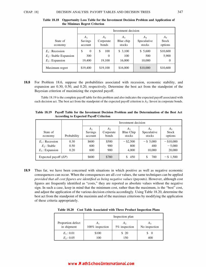
18.8 For Problem 18.6, suppose the probabilities associated with recession, economic stability, and
expansion are 0.30, 0.50, and 0.20, respectively. Determine the best act from the standpoint of the
Bayesian criterion of maximizing the expected payoff.
Table 18.19 is the complete payoff table for this problem and also indicates the expected payoff associated with
each decision act. The best act from the standpoint of the expected payoff criterion is A2: Invest in corporate bonds.
18.9 Thus far, we have been concerned with situations in which positive as well as negative economic
consequences can occur. When the consequences are all cost values, the same techniques can be applied
provided that all cost figures are identified as being negative values (payouts). However, although cost
figures are frequently identified as “costs,” they are reported as absolute values without the negative
sign. In such a case, keep in mind that the minimum cost, rather than the maximum, is the “best” cost,
and adjust the application of the various decision criteria accordingly. Using Table 18.20, determine the
best act from the standpoint of the maximin and of the maximax criterions by modifying the application
of these criteria appropriately.
Table 18.18 Opportunity Loss Table for the Investment Decision Problem and Application of
the Minimax Regret Criterion
Investment decision
State of
economy
A1
Savings
account
A2
Corporate
bonds
A3
Blue chip
stocks
A4
Speculative
stocks
A5
Stock
options
E1 : Recession $ 0 $ 100 $ 3,100 $ 5,600 $10,600
E2 : Stable Expansion 300 0 100 500 5,900
E3 : Expansion 19,400 19,100 16,000 10,000 0
Maximum regret $19,400 $19,100 $16,000 $10,000 $10,600
Table 18.20 Cost Table Associated with Three Product Inspection Plans
Inspection plan
Proportion defect
in shipment
A1
100% inspection
A2
5% inspection
A3
No inspection
E1 : 0.01 $100 $ 20 $ 0
E2 : 0.05 100 150 400
Table 18.19 Payoff Table for the Investment Decision Problem and the Determination of the Best Act
According to Expected Payoff Criterion
Investment decision
State ofeconomy Probability
A1
Savingsaccount
A2
Corporatebonds
A3
Blue Chipstocks
A4
Speculativestocks
A5
Stockoptions
E1 : Recession 0.30 $600 $500 2$2,500 2$ 5,000 2$10,000
E2 : Stable 0.50 600 900 800 400 25,000
E3 : Expansion 0.20 600 900 4,000 10,000 20,000
Expected payoff (EP) $600 $780 $ 450 $ 700 2$ 1,500
CHAP. 18] DECISION ANALYSIS: PAYOFF TABLES AND DECISION TREES 347
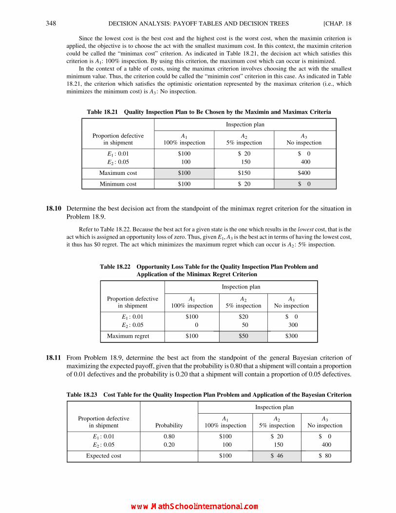
Since the lowest cost is the best cost and the highest cost is the worst cost, when the maximin criterion is
applied, the objective is to choose the act with the smallest maximum cost. In this context, the maximin criterion
could be called the “minimax cost” criterion. As indicated in Table 18.21, the decision act which satisfies this
criterion is A1: 100% inspection. By using this criterion, the maximum cost which can occur is minimized.
In the context of a table of costs, using the maximax criterion involves choosing the act with the smallest
minimum value. Thus, the criterion could be called the “minimin cost” criterion in this case. As indicated in Table
18.21, the criterion which satisfies the optimistic orientation represented by the maximax criterion (i.e., which
minimizes the minimum cost) is A3 : No inspection.
18.10 Determine the best decision act from the standpoint of the minimax regret criterion for the situation in
Problem 18.9.
Refer to Table 18.22. Because the best act for a given state is the one which results in the lowest cost, that is the
act which is assigned an opportunity loss of zero. Thus, given E1, A3 is the best act in terms of having the lowest cost,
it thus has $0 regret. The act which minimizes the maximum regret which can occur is A2 : 5% inspection.
18.11 From Problem 18.9, determine the best act from the standpoint of the general Bayesian criterion of
maximizing the expected payoff, given that the probability is 0.80 that a shipment will contain a proportion
of 0.01 defectives and the probability is 0.20 that a shipment will contain a proportion of 0.05 defectives.
Table 18.22 Opportunity Loss Table for the Quality Inspection Plan Problem and
Application of the Minimax Regret Criterion
Inspection plan
Proportion defectivein shipment
A1
100% inspectionA2
5% inspectionA3
No inspection
E1 : 0.01 $100 $20 $ 0
E2 : 0.05 0 50 300
Maximum regret $100 $50 $300
Table 18.21 Quality Inspection Plan to Be Chosen by the Maximin and Maximax Criteria
Inspection plan
Proportion defectivein shipment
A1
100% inspectionA2
5% inspectionA3
No inspection
E1 : 0.01 $100 $ 20 $ 0
E2 : 0.05 100 150 400
Maximum cost $100 $150 $400
Minimum cost $100 $ 20 $ 0
Table 18.23 Cost Table for the Quality Inspection Plan Problem and Application of the Bayesian Criterion
Inspection plan
Proportion defectivein shipment Probability
A1
100% inspectionA2
5% inspectionA3
No inspection
E1 : 0.01 0.80 $100 $ 20 $ 0
E2 : 0.05 0.20 100 150 400
Expected cost $100 $ 46 $ 80
348 DECISION ANALYSIS: PAYOFF TABLES AND DECISION TREES [CHAP. 18
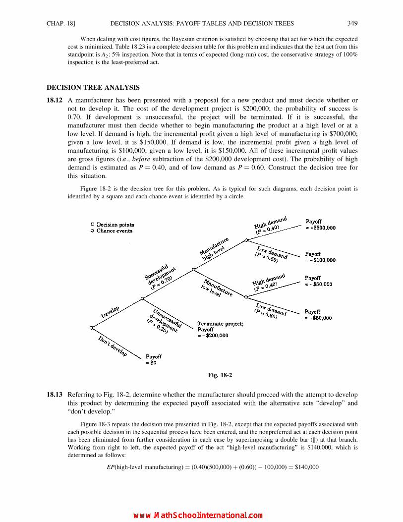
When dealing with cost figures, the Bayesian criterion is satisfied by choosing that act for which the expected
cost is minimized. Table 18.23 is a complete decision table for this problem and indicates that the best act from this
standpoint is A2 : 5% inspection. Note that in terms of expected (long-run) cost, the conservative strategy of 100%
inspection is the least-preferred act.
DECISION TREE ANALYSIS
18.12 A manufacturer has been presented with a proposal for a new product and must decide whether or
not to develop it. The cost of the development project is $200,000; the probability of success is
0.70. If development is unsuccessful, the project will be terminated. If it is successful, the
manufacturer must then decide whether to begin manufacturing the product at a high level or at a
low level. If demand is high, the incremental profit given a high level of manufacturing is $700,000;
given a low level, it is $150,000. If demand is low, the incremental profit given a high level of
manufacturing is $100,000; given a low level, it is $150,000. All of these incremental profit values
are gross figures (i.e., before subtraction of the $200,000 development cost). The probability of high
demand is estimated as P ¼ 0.40, and of low demand as P ¼ 0.60. Construct the decision tree for
this situation.
Figure 18-2 is the decision tree for this problem. As is typical for such diagrams, each decision point is
identified by a square and each chance event is identified by a circle.
18.13 Referring to Fig. 18-2, determine whether the manufacturer should proceed with the attempt to develop
this product by determining the expected payoff associated with the alternative acts “develop” and
“don’t develop.”
Figure 18-3 repeats the decision tree presented in Fig. 18-2, except that the expected payoffs associated with
each possible decision in the sequential process have been entered, and the nonpreferred act at each decision point
has been eliminated from further consideration in each case by superimposing a double bar (k) at that branch.Working from right to left, the expected payoff of the act “high-level manufacturing” is $140,000, which is
determined as follows:
EP(high-level manufacturing) ¼ (0:40)(500,000)þ (0:60)(� 100,000) ¼ $140,000
Fig. 18-2
CHAP. 18] DECISION ANALYSIS: PAYOFF TABLES AND DECISION TREES 349

Similarly,
EP(low-level manufacturing) ¼ (0:40)(� 50,000)þ (0:60)(� 50,000) ¼ �$50,000
Comparing the two expected payoffs, the best act is “high-level manufacturing”; the other act possibility is eliminated.
Moving leftward to the next decision point (which is also the initial decision point in this case), the expected payoffs for the
two possible decision acts are
EP(develop) ¼ (0:70)(40,000)þ (0:30)(� 200,000) ¼ $38,000
EP(don’t develop) ¼ 0
Comparing the two expected payoffs, the best act at the initial decision point is “develop.” In the calculation of the
expected payoff for “develop,” note that the probability of 0.70 (for “successful development”) is multiplied by $140,000,
with the 2$50,000 in the adjoining branch being ignored because it is associated with a decision act eliminated in the
previous step of analysis.
UTILITY FUNCTIONS AND EXPECTED UTILITY
18.14 Referring to Table 18.2, we see that the two extreme monetary outcomes are 2$1,500 and þ$6,000.
Suppose that a decision maker indicates indifference to receiving an amount certain of $1,200 in lieu of
a risk situation in which there is a 50 percent chance of gaining $6,000 and a 50 percent chance of a
$1,500 loss. Following the convention of assigning the extreme lower and upper monetary values with
utility values of “0” and “1.0,” respectively, determine the utility values associated with 2$1,500,
$1,200, and $6,000.
We begin by assigning utility values to the two extreme monetary consequences:
U(� $1,500) ¼ 0 U(6,000) ¼ 1:0
The utility associated with the amount certain of $1,200 is determined as follows:
U(amount certain) ¼ P(U of high outcome)þ (1� P)(U of low outcome)
U($1,200) ¼ 0:50(1:0)þ 0:50(0)
U($1,200) ¼ 0:50
Fig. 18-3
350 DECISION ANALYSIS: PAYOFF TABLES AND DECISION TREES [CHAP. 18
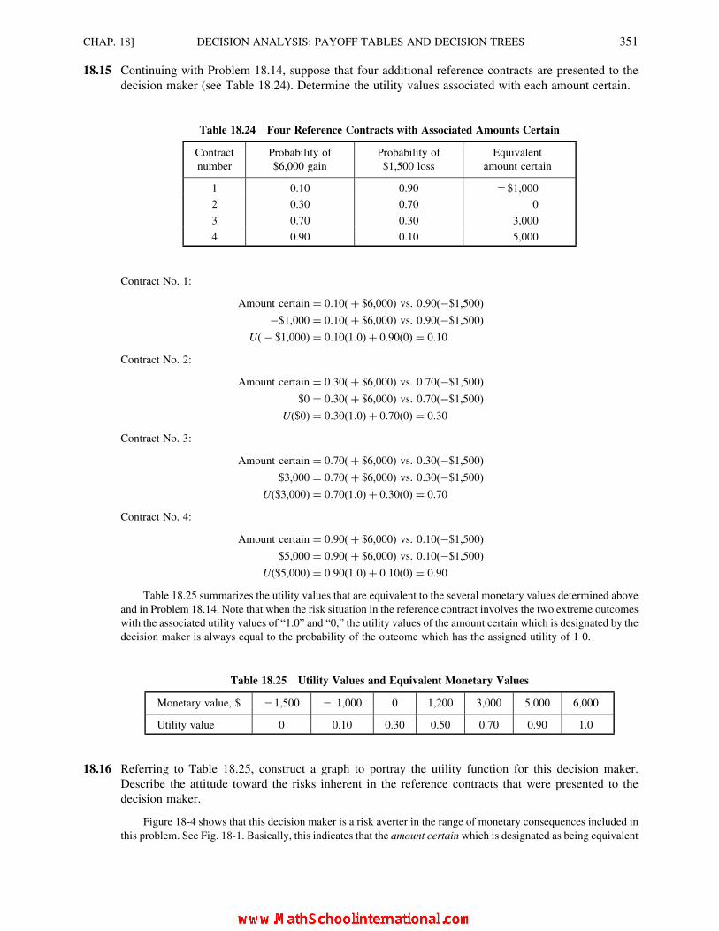
18.15 Continuing with Problem 18.14, suppose that four additional reference contracts are presented to the
decision maker (see Table 18.24). Determine the utility values associated with each amount certain.
Contract No. 1:
Amount certain ¼ 0:10(þ $6,000) vs. 0:90(�$1,500)
�$1,000 ¼ 0:10(þ $6,000) vs. 0:90(�$1,500)
U(� $1,000) ¼ 0:10(1:0)þ 0:90(0) ¼ 0:10
Contract No. 2:
Amount certain ¼ 0:30(þ $6,000) vs. 0:70(�$1,500)
$0 ¼ 0:30(þ $6,000) vs. 0:70(�$1,500)
U($0) ¼ 0:30(1:0)þ 0:70(0) ¼ 0:30
Contract No. 3:
Amount certain ¼ 0:70(þ $6,000) vs. 0:30(�$1,500)
$3,000 ¼ 0:70(þ $6,000) vs. 0:30(�$1,500)
U($3,000) ¼ 0:70(1:0)þ 0:30(0) ¼ 0:70
Contract No. 4:
Amount certain ¼ 0:90(þ $6,000) vs. 0:10(�$1,500)
$5,000 ¼ 0:90(þ $6,000) vs. 0:10(�$1,500)
U($5,000) ¼ 0:90(1:0)þ 0:10(0) ¼ 0:90
Table 18.25 summarizes the utility values that are equivalent to the several monetary values determined above
and in Problem 18.14. Note that when the risk situation in the reference contract involves the two extreme outcomes
with the associated utility values of “1.0” and “0,” the utility values of the amount certain which is designated by the
decision maker is always equal to the probability of the outcome which has the assigned utility of 1 0.
18.16 Referring to Table 18.25, construct a graph to portray the utility function for this decision maker.
Describe the attitude toward the risks inherent in the reference contracts that were presented to the
decision maker.
Figure 18-4 shows that this decision maker is a risk averter in the range of monetary consequences included in
this problem. See Fig. 18-1. Basically, this indicates that the amount certain which is designated as being equivalent
Table 18.25 Utility Values and Equivalent Monetary Values
Monetary value, $ 21,500 2 1,000 0 1,200 3,000 5,000 6,000
Utility value 0 0.10 0.30 0.50 0.70 0.90 1.0
Table 18.24 Four Reference Contracts with Associated Amounts Certain
Contract
number
Probability of
$6,000 gain
Probability of
$1,500 loss
Equivalent
amount certain
1 0.10 0.90 2$1,000
2 0.30 0.70 0
3 0.70 0.30 3,000
4 0.90 0.10 5,000
CHAP. 18] DECISION ANALYSIS: PAYOFF TABLES AND DECISION TREES 351

to the designated risk situation in the reference contract is always less than the associated expected payoff, except for
the two extreme end points of the utility curve. For instance, in Problem 18.14 the decision maker stated that a
certain $1,200 was equivalent to a probability of 0.50 of gaining $6,000 and a probability of 0.50 of losing $1,500.
However, the payoff of this risk situation is 0.50($6,000) þ 0.50(2$1,500) ¼ $3,000 þ (2$750) ¼ $2,250.
18.17 Referring to the utility function in Fig. 18-4, determine the approximate utility values corresponding to
each payoff in Table 18.2, and determine the best act from the standpoint of maximizing the expected
utility.
Table 18.26 identifies the utility values that are equivalent to the payoffs in Table 18.2. Using the criterion of
maximizing the expected utility, the best act is A3, as it was for the expected payoff criterion (see Example 6).
However, note that whereas the expected payoffs for acts A2 and A4 are equal in Table 18.7, the expected utility
value of these two acts are not equal.
Fig. 18-4
Table 18.26 Utility Table for the Number for Air-Conditioning Units to
Be Ordered and Determination of the Best Act According
to the Expected Utility Criterion
Order quantityMarket
demand Probability A1 : 5 A2 : 10 A3 : 15 A4 : 20
E1 : 5 0.10 0.55 0.38 0.21 0
E2 : 10 0.30 0.55 0.70 0.61 0.47
E3 : 15 0.40 0.55 0.70 0.86 0.78
E4 : 20 0.20 0.55 0.70 0.86 1.00
Expected utility (EU) 0.550 0.668 0.720 0.653
352 DECISION ANALYSIS: PAYOFF TABLES AND DECISION TREES [CHAP. 18

Supplementary Problems
PAYOFF TABLES
18.18 An investment analyst estimates that there is about a 50 percent chance of an upturn in the chemical industry during
the first quarter of the year, with the probabilities of no change and a downturn being about equal. A client is
considering either the investment of $10,000 in a mutual fund specializing in chemical industry common stocks or
investing in corporate AAA-rated bonds yielding 8.0 percent per year. If the chemical industry experiences an
upturn during the first quarter, the value of the mutual fund shares (including dividends) will increase by 15.0
percent during the next 12 months. If there is no change, the value will increase by 3.0 percent. If there is a
downturn, the value will decrease by 10.0 percent. Ignoring any commission costs, construct a payoff table for this
investment problem.
18.19 For the investment decision described in Problem 18.18, determine the best decision act from the standpoint of the
(a) maximin criterion and (b) maximax criterion.
Ans. (a) A2 : Invest in AAA bonds, (b) A1: Invest in mutual fund
18.20 Determine the best act from the standpoint of the minimax regret criterion for Problem 18.18.
Ans. A2 : Invest in AAA bonds
18.21 For Problem 18.18, determine the best act from the standpoint of the expected payoff criterion.
Ans. A2 : Invest in AAA bonds
18.22 A retailer buys a certain product for $3 per case and sells it for $5 per case. The high markup is reflective of the
perishability of the product, since it has no value after five days. Based on experience with similar products, the
retailer is confident that the demand for the item will be somewhere between 9 and 12 cases, inclusive.
Construct an appropriate payoff table. Determine the best act from the standpoint of (a) the maximin criterion
and (b) the maximax criterion.
Ans. (a) A1 : Order 9 cases, (b) A4 : Order 12 cases
18.23 Construct the table of opportunity losses (regrets) for Problem 18.22, and determine the best act from the standpoint
of the minimax regret criterion.
Ans. A2 : Order 10 cases
18.24 Continuing with Problem 18.22, the retailer further estimates that the probability values associated with selling 9 to
12 cases of the item are 0.30, 0.40, 0.20, and 0.10, respectively. Determine the best decision acts from the standpoint
of the (a) maximum probability criterion and (b) expectation of the event.
Ans. (a) A2 : Order 10 cases, (b) A2 : Order 10 cases
18.25 Referring to Problems 18.22 and 18.23, determine the best order quantity from the standpoint of the (a) expected
payoff criterion and (b) the criterion of minimizing the expected opportunity loss. Demonstrate that these are
equivalent criteria by also identifying the “second best” and “worst” acts with respect to each criterion.
Ans. (a) A2 : Order 10 cases, (b) A2 : Order 10 cases
18.26 In conjunction with the installation of a new marine engine, a charter vessel owner has the opportunity to buy spare
propellers at $200 each for use during the coming cruise season. The propellers are custom fit for the vessel, and
because the owner had already contracted to sell the boat after the cruise season, there is no value associated with
having spare propellers left over after the season. If a spare propeller is not immediately available when needed, the
cost of buying a needed spare propeller, including lost cruise time, is $400. Based on previous experience, the vessel
owner estimates that the probability values associated with needing 0 to 3 propellers during the coming cruise
season are 0.30, 0.30, 0.30, and 0.10, respectively. Construct a cost table for this problem and determine the number
of propellers that should be ordered from the standpoint of (a) the maximin criterion and (b) the maximax criterion.
Ans. (a) A4 : Order three spare propellers, (b) A1 : Order no spare propellers
CHAP. 18] DECISION ANALYSIS: PAYOFF TABLES AND DECISION TREES 353

18.27 For the situation in Problem 18.26, determine the best act from the standpoint of the (a) maximum probability
criterion and (b) the expectation of the event.
Ans. (a) Indifferent between 0, 1, and 2 propellers; (b) A2 : Order 1 propeller
18.28 For Problem 18.26, determine the best act from the standpoint of the expected payoff criterion (in this case,
expected cost).
Ans. A2 : Order 1 propeller
18.29 Several weeks before an annual Water Carnival, a college social group must decide to order either blankets, beach
umbrellas, or neither for resale at the event. The monetary success of the decision to sell one of the two items is
dependent on the weather conditions, as indicated in Table 18.27. Determine the best act from the standpoint of the
(a) maximin criterion and (b) maximax criterion.
Ans. (a) A3 : Neither, (b) A2 : Beach umbrellas
18.30 Determine the best act from the standpoint of the minimax regret criterion for Problem 18.29.
Ans. A3 : Neither
18.31 Continuing with Problem 18.29, one of the club members calls the weather bureau and learns that during the past 10
years the weather has been hot on 6 of the 10 days on the date when the Water Carnival is to be held. Use this
information to estimate the probabilities associated with the two weather conditions. Then determine the best act
from the standpoint of the (a) maximum probability and (b) expected payoff criterion.
Ans. (a) A2 : Beach umbrellas, (b) A2 : Beach umbrellas
DECISION TREE ANALYSIS
18.32 An investor is considering placing a $10,000 deposit to reserve a franchise opportunity in a new residential area
for one year. There are two areas of uncertainty associated with this sequential decision situation: whether or
not a prime franchise competitor will decide to locate an outlet in the same area and whether or not the
residential area will develop to be a moderate or large market. The investor estimates that there is a 50–50
chance that the competing franchise system will develop an outlet. Thus, the investor must first decide whether
to make the initial $10,000 down payment. After the decision of the competing system is known, the investor
must then decide whether to proceed with constructing the franchise outlet. If there is competition and the
market is large, the net gain during the relevant period is estimated as being $15,000; if the market is moderate,
there will be a net loss of $10,000. If there is no competition and the market is large, the net gain will be
$30,000; if the market is moderate, there will be a net gain of $10,000. The investor estimates that there is
about a 40 percent chance that the market will be large. Using decision tree analysis, determine whether or not
the initial deposit of $10,000 should be made.
Ans. Make the deposit (EP ¼ $9,000)
UTILITY FUNCTIONS AND EXPECTED UTILITY
18.33 For Problems 18.6 to 18.8, the extreme points of the possible monetary consequences are 2$10,000 and $20,000.
Describe how you would go about developing a utility function for the individual who is involved in this investment
decision.
Table 18.27 Payoffs for the “Water Carnival” Decision Problem
Weather A2: Blankets A2: Beach umbrellas A3: Neither
Cool $100 2$ 80 $0
Hot 250 150 0
354 DECISION ANALYSIS: PAYOFF TABLES AND DECISION TREES [CHAP. 18

18.34 Based on your answer to Problem 18.33, suppose the set of utility values reported in Table 18.28 has been
developed. Construct the appropriate utility curve and use it to determine whether the investor can be described as a
risk averter, a risk seeker, or neutral with respect to risk. Illustrate the meaning of your conclusion in the context of
this decision problem.
Ans. The decisions is a risk seeker.
18.35 Determine the best act for the investment decision described in Problems 18.6 to 18.8, based on the expected utility
criterion and using the utility function developed in Problem 18.34.
Ans. A5: Invest in stock options (EU ffi 0.230)
Table 18.28 Utility Values Equivalent to Monetary Values for the Investment Decision Problem
Monetary value, $ 210,000 22,500 2,000 10,000 14,000 18,000 20,000
Utility value 0 0.1 0.2 0.4 0.6 0.8 1.0
CHAP. 18] DECISION ANALYSIS: PAYOFF TABLES AND DECISION TREES 355

CHAPTER 19
Statistical ProcessControl
19.1 TOTAL QUALITY MANAGEMENT
Total Quality Management (TQM) is an approach to management in which the quality of the organization’s
output is given first and foremost attention. The output can be in the form either of a product or a service.
Further, the output may be one that is delivered to external customers, or it may be internal output to other units
of the organization. How is quality determined? It is based on the judgment of the customer. Thus, customer
satisfaction is the ultimate objective of TQM.
EXAMPLE 1. An example of an external product output is the production of video recorders. An example of an external
service output is the services provided to patients and clients by a health maintenance organization (HMO). An example of
an internal product output is the production of the gear department being sent to the transmission assembly department of a
vehicle plant, while an example of an internal service output is the personnel training function carried out by a human
resources department for other departments in the organization.
The TQM approach not only sets out to achieve high quality, but incorporates the philosophy by which this
objective can be achieved. Traditional methods of quality assurance focused on finding and correcting product
(and sometimes service) defects. The result was the use of a hierarchical command structure and an ever-
increasing number of inspection steps. In an inspection-orientated manufacturing plant, half of the workers can
be involved in finding and reworking rejects. The TQM philosophy is that quality should be designed into the
product or service, and that sampling-based statistical quality control should be used, rather than attempting to
inspect every unit of output. Further, quality should be monitored by those who are responsible for the output,
rather than by staff personnel who represent higher management echelons. This approach results in elimination
of traditional inspectors. Instead, employee teams have both the authority and responsibility for the quality of
their output and its improvement. Thus, employee participation in setting unit goals and devising the strategies
by which they are to be achieved is critical to the success of TQM.
EXAMPLE 2. In the traditional automobile manufacturing plant the inspectors in the various departments were
employees of the industrial engineering department and not of the departments in which the inspection functions were
performed. The theory was that inspection should be done by an outside objective party, thus setting the stage for so-called
356
Copyright 2004, 1996, 1988, 1976 by The McGraw-Hill Companies, Inc. Click Here for Terms of Use.

line versus staff conflicts. In the TQM approach the employees of each group, with their supervisors, are responsible for and
monitor product quality and are rewarded for their success as a team. For internal products, such as car parts, the ultimate
judgment of the quality is made by the departments that use the parts for further processing.
19.2 STATISTICAL QUALITY CONTROL
Although there are several different ingredients that constitute Total Quality Management, the statistical
contribution has its roots in statistical quality control. Sampling techniques for quality inspection date back to
the 1930s. These include the development of statistically based sampling plans as an alternative to 100 percent
inspection and the associated use of control charts. However, it was not until the 1970s, when U.S. industry
began to react seriously to the high quality of products imported from Japan, that the application of statistical
quality control became widespread. The continuing trade imbalance with Japan became a national issue during
the 1980s and 1990s, and thus spurred further interest in quality improvement.
Ironically, the high quality of Japanese products was achieved largely because they adopted suggestions of
U.S. consultants in the restructuring of their manufacturing processes after World War II. Preeminent among
these consultants was the statistician W. Edwards Deming, after whom the Deming Award for Quality was
named in Japan. Deming developed a philosophy of quality management that was the precursor of what is now
called Total Quality Management, and which he summarized in his “14 Points.”
EXAMPLE 3. Table 19-1 lists Deming’s 14 points. Notice how closely many of the suggestions correspond to our
description of TQM in the preceding section. For instance, there is a clear focus on quality in point #1, rejection of
command-oriented mass inspection in point #3, the need for continual improvement in #5, and the call for action to establish
the new participative environment in #14.
Table 19.1 Deming’s 14 Points
1. Create consistency of purpose for improvement of products and services. That purpose
should be quality, not short-term profits.
2. Adopt the new philosophy. Reject the focus on the inspection-rejection-rework viewpoint
in favor of a preventive approach.
3. Cease dependence on mass inspection to achieve quality. Improve product design and institute
sampling-based process control.
4. End the practice of awarding business on the basis of price tag alone. Consider quality
and the development of supplier loyalty.
5. Improve constantly and forever the system of production and service.
6. Institute training.
7. Institute leadership. Autocratic management is not true leadership.
8. Drive out fear. People do their best work if they feel secure.
9. Break down barriers between departments. Different areas should not have conflicting goals.
10. Eliminate slogans, exhortations, and numerical targets for the work force. Simply telling
people to improve does not work.
11. Eliminate numerical quotas. Such quotas do not take quality into consideration, and in
centralized economies such quotas have often been achieved at the expense of other
products or services.
12. Remove barriers to pride of workmanship. These include poor supervision, poor product design,
defective materials, and defective machines.
13. Institute a vigorous program of education and self-improvement for everyone in the organization.
This includes the need to know modern methods of statistical process control.
14. Take action to accomplish the transformation. This requires the leadership of top management to
establish the new environment.
CHAP. 19] STATISTICAL PROCESS CONTROL 357

19.3 TYPES OF VARIATION IN PROCESSES
A process is a sequence of operations by which such inputs as labor, materials, and methods are
transformed into outputs, in the form of products or services. In the first section of this chapter we differentiated
internal and external outputs as well as product and service outputs. In any process, some variation in the
quality measure from product to product or from service to service is unavoidable.
EXAMPLE 4. One measure of output quality in an HMO is the waiting time before a patient with an appointment sees the
medical practitioner. Even when all of the waiting times on a particular day are within a “reasonable” time limit, there will
nevertheless be variation from patient to patient.
Statistical process control refers to the application of the methods of statistical quality control to the
monitoring of processes (and not just, as in the earlier practice, to the inspection of the final outputs of the
processes). The purpose is to control the quality of product or service outputs from a process by maintaining
control of the process. When a process is described as being “in control,” it means that the amount of variation
in the output is relatively constant and within established limits that are deemed acceptable. There are two kinds
of causes of variation in a process. Common causes, or chance causes, of variation are due to factors that are
inherent in the design of the system, and reflect the usual amount of variation to be expected. Assignable causes,
or special causes, of variation are due to unusual factors that are not part of the process design and not ordinarily
part of the process.
A stable process is one in which only common causes of variation affect the output quality. Such a process
can also be described as being in a state of statistical control. An unstable process is one in which both
assignable causes and common causes affect the output quality. (Note that, by definition, the common causes
are always present.) Such a process can also be described as being out of control, particularly when the
assignable cause is controllable.
EXAMPLE 5. If the waiting time for patients in an HMO on a particular day is deemed “reasonable,” this would indicate
that only common causes of variation in waiting time occurred on that day. Such common causes would include the
variability in the amount of time spent with the patients who had appointments earlier in the day. If an “unreasonable” length
of waiting time was experienced by some patients, this would indicate that one or more assignable causes of variation
occurred. This could include such causes as a practitioner arriving late at the facility because of a medical emergency, an
earlier patient who required more time than planned, or a delay in accessing medical records for patients because of a
computer network problem.
The way we set out to improve the quality of output for a process depends on the source of process
variation. For a process that is stable, improvement can take place only by improving the design of the process.
A pervasive error in process management is tampering, which is to take actions (such as making machine
adjustments) that presume that a process is not in control, when in fact it is stable. Such actions only increase
variability, and are analogous to the over-correcting that new drivers do in learning to steer a car. For a process
that is unstable, improvement can be achieved by identifying and correcting assignable causes.
EXAMPLE 6. In our HMO example, if the process is stable we nevertheless have the opportunity to reduce the waiting
time by improving the process. Suppose all patients are scheduled for 20-minute contact times with the physician. An
alternative design would be to have variable contact times planned, based on the reason for the appointment. As indicated in
Example 5, an unstable process could be due to a computer network problem on that day. For an unstable process such as
this, correcting the computer network problem so that it does not recur would improve the process.
19.4 CONTROL CHARTS
As introduced in Section 2.12, a run chart is a time series plot that plots levels of output quality on the
vertical axis, with respect to a sequence of time periods on the horizontal axis. In the context of statistical
process control the measurements that are graphed are typically sample data that have been obtained by the
358 STATISTICAL PROCESS CONTROL [CHAP. 19

method of rational subgroups, as described in Section 1.7. A control chart is a run chart that includes the lower
and upper control limits that identify the range of variation that can be ascribed to common causes. Any outputs
that are outside of the control limits suggest the existence of assignable-cause variation. The control limits are
determined either by process parameters having been specified, or by observing sample outcomes during a
period of time in which the process is deemed to be in a stable condition.
The statistical methods of process control are based on the concepts of hypothesis testing, as presented in
Chapter 10. The rationale is presented in Table 19-2. The null hypothesis is that the process is stable and only
common causes of variation exist. The alternative hypothesis is that the process is unstable and includes
assignable-cause variation. Thus, the lower and upper control limits on a control chart are the critical values
with respect to rejecting or not rejecting the null hypothesis that the process is stable and in control.
The standard practice is to place the control limits at three standard error units above and below the
hypothesized value. This 3-sigma rule is applied for all of the control chart examples in the Solved Problems
included with this chapter. If a process is stable, not only should all sample statistics be within the control limits,
but there also should be no discernable pattern in the sequence of the sample statistics.
In the following sections of this chapter we present the methods for determining control limits and we
describe the interpretation of control charts for the process mean, process standard deviation, process range,
and process proportion. Of these four, control charts for the mean, standard deviation, and range are designated
as control charts for variables, because measurements are involved. Control charts for the proportion are
designated as control charts for attributes, because counts (which are discrete rather than continuous variables)
are involved.
19.5 CONTROL CHARTS FOR THE PROCESS MEAN: XX CHARTS
Process Mean and Standard Deviation Known. The process mean and standard deviation would be
known either because they are process specifications or are based on historical observations of the process when
it was deemed to be stable. The centerline for the �XX chart is set at the process mean. Using the 3-sigma rule, the
control limits are defined by the same method as that used for determining critical values for hypothesis testing
in Section 10.2:
Control limits ¼ m+ 3sffiffiffin
p (19:1)
Solved Problem 19.12 illustrates the determination of lower and upper control limits for an �XX chart when
the process mean and standard deviation are known. Problem 19.13 presents the �XX chart that incorporates these
control limits and that has the centerline at the designated process mean.
Table 19.2 Outcomes in Statistical Process Control
Condition of Process
H0 True: Stable H0 False: Unstable
Continue Process Correct decision Type II error:
Allowing an unstable
process to continue
Decision Adjust Process Type I error:
Adjusting a stable
process
Correct decision
CHAP. 19] STATISTICAL PROCESS CONTROL 359
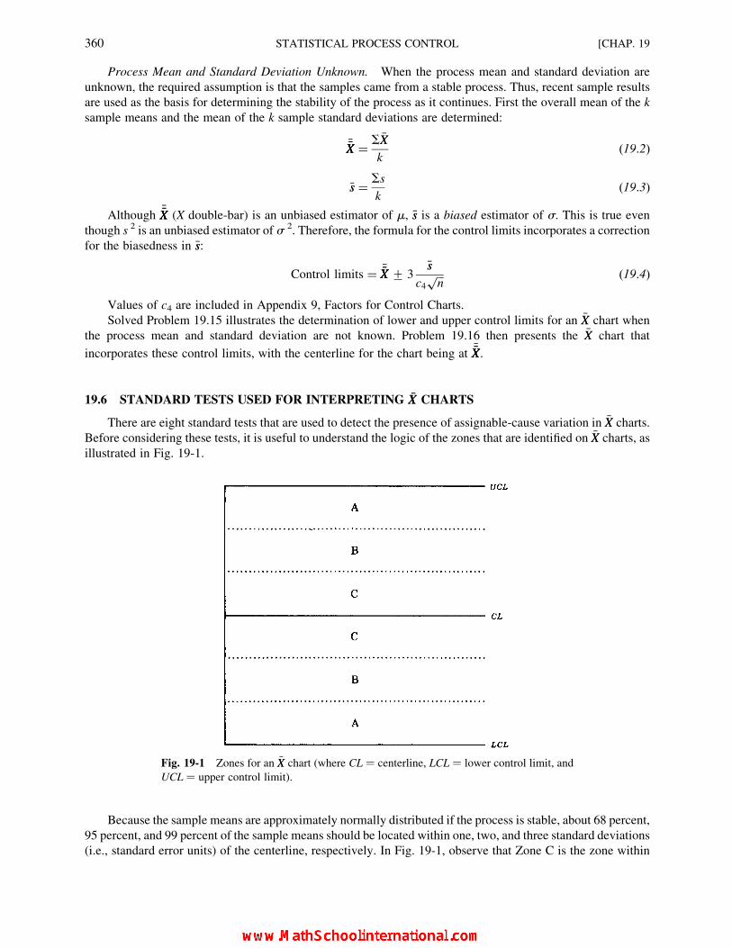
Process Mean and Standard Deviation Unknown. When the process mean and standard deviation are
unknown, the required assumption is that the samples came from a stable process. Thus, recent sample results
are used as the basis for determining the stability of the process as it continues. First the overall mean of the k
sample means and the mean of the k sample standard deviations are determined:
��XX�XX ¼ S �XX
k(19:2)
�ss ¼ Ss
k(19:3)
Although ��XX�XX (X double-bar) is an unbiased estimator of m, �ss is a biased estimator of s. This is true even
though s 2 is an unbiased estimator of s 2. Therefore, the formula for the control limits incorporates a correction
for the biasedness in �ss:
Control limits ¼ ��XX�XX + 3�ss
c4ffiffiffin
p (19:4)
Values of c4 are included in Appendix 9, Factors for Control Charts.
Solved Problem 19.15 illustrates the determination of lower and upper control limits for an �XX chart when
the process mean and standard deviation are not known. Problem 19.16 then presents the �XX chart that
incorporates these control limits, with the centerline for the chart being at ��XX�XX.
19.6 STANDARD TESTS USED FOR INTERPRETING XX CHARTS
There are eight standard tests that are used to detect the presence of assignable-cause variation in �XX charts.
Before considering these tests, it is useful to understand the logic of the zones that are identified on �XX charts, as
illustrated in Fig. 19-1.
Because the sample means are approximately normally distributed if the process is stable, about 68 percent,
95 percent, and 99 percent of the sample means should be located within one, two, and three standard deviations
(i.e., standard error units) of the centerline, respectively. In Fig. 19-1, observe that Zone C is the zone within
Fig. 19-1 Zones for an �XX chart (where CL ¼ centerline, LCL ¼ lower control limit, and
UCL ¼ upper control limit).
360 STATISTICAL PROCESS CONTROL [CHAP. 19

one standard deviation of the centerline, Zone B is the zone between one and two standard deviations from the
centerline, and Zone A, the outermost labeled zone, is between two and three standard deviations from the
centerline.
The eight tests we now consider were developed by Lloyd S. Nelson, a process control expert. They are
based on his determination that the identified patterns are very unlikely to occur in stable processes. Thus
the existence of any of these patterns in an �XX chart indicates that the process may be unstable, and that one or
more assignable causes may exist. Fig. 19-2 includes graphic examples of test failure for each of the eight tests,
with a description for each graph as to what is required for the illustrated test failure.
The most obvious test in terms of its rationale is Test 1, which simply requires that at least one value of�XX be beyond Zone A. For a sample mean to be beyond three standard errors from the centerline is of course
very unlikely in a stable process. The other seven patterns also are very unlikely. The one test whose
rationale is not obvious is Test 7, which requires that 15 consecutive values of �XX be in Zone C, which is
within one standard error of the centerline. Although this kind of pattern would seem to be very desirable, it
Fig. 19-2 Eight tests for assignable (special) cause variation. (Reprinted by permission from Exhibit 12.1, User’s Guide 2:
Analysis and Quality Tools, Release 13, q 2000 by Minitab Inc.)
CHAP. 19] STATISTICAL PROCESS CONTROL 361

is also very unlikely. It may, for example, indicate that the process standard deviation was overstated in the
process specifications or that the sample measurements are in error. Whatever the cause, the results are too
good to be true and therefore require investigation. Solved Problems 19.14 and 19.16 include interpretations
of test results for �XX charts.
Although the eight tests were developed specifically for �XX charts, the first four tests also are applicable to
p charts for sample proportions, as considered further in Section 19.9. The tests are not applicable to either
s charts or R charts, both of which are concerned with the amount of sample-to-sample variation that exists in
the variability of a process.
19.7 CONTROL CHARTS FOR THE PROCESS STANDARD DEVIATION: s CHARTS
Process Standard Deviation Known. The centerline for the control chart is not set at the designated
process standard deviation, as one might expect. The reason is that even though s 2 is an unbiased estimator of
s 2, the sample standard deviation s is a biased estimator of s. Because it is required that the centerline be
applicable for sample standard deviations, the value of the process s must be adjusted so that the expected
biasedness in the sample standard deviations is included :
E(s) ¼ c4s (19:5)
The standard error of s has not been considered previously, and a full explanation is beyond the scope of
this book. The constant c5, included in Appendix 9, is used to determine the standard error of s:
ss ¼ c5s (19:6)
The 3-sigma control limits for the s chart are
Control limits ¼ c4s+ 3c5s (19:7)
Solved Problem 19.17 illustrates the determination of the control limits for the standard deviation when the
process standard deviation is known, while Problem 19.18 presents the s chart that incorporates these control
limits.
Process Standard Deviation Unknown. As explained for �XX charts, the required assumption is that the
samples came from a stable process. Consistent with our discussion of biasedness in the paragraphs above,
when s is known, no correction in the biasedness of s is required in determining the centerline when s is known.
This is so because the individual sample standard deviations have this same biasedness expectation. However
the c4 correction for biasedness does need to be included in the formula for the estimated standard error of s.
With the values for c4 and c5 taken from Appendix 9, the formula for the control limits then is
Control limits ¼ �ss + 3c5 �ss
c4(19:8)
Solved Problem 19.19 illustrates the determination of the control limits for an s chart when the process
standard deviation is unknown, while Problem 19.20 presents the s chart that incorporates these control limits.
If the s chart indicates that the process is unstable in terms of process variability, then this issue should be
addressed before there is any attempt to assess process stability with respect to the process mean.
19.8 CONTROL CHARTS FOR THE PROCESS RANGE: R CHARTS
The R chart is an alternative to the s chart for assessing the stability of a process with respect to
variability. The s chart is preferred because this measure of variation considers the value of every sampled
item, and thus leads to a more precise measure of variability. R charts were predominant for many years
because of ease of computation, but this advantage is no longer relevant given the use of programmable
devices in process control.
362 STATISTICAL PROCESS CONTROL [CHAP. 19

The centerline for the R chart is set at the unbiased estimator of the population range, R, which is the mean
of the several sample ranges:
�RR ¼ SR
k(19:9)
The standard error of R has not been considered previously, and a full explanation is outside the scope of
this book. The constants d2 and d3, included in Appendix 9, are required. The formula for the control limits
then is
Control limits ¼ �RR + 3 �RRd3
d2
¼ �RR 1+ 3d3
d2
� �(19:10)
To achieve a simplified formula for practitioners, we first define the two factors:
D3 ¼ 1� 3d3
d2
(19:11)
D4 ¼ 1þ 3d3
d2
(19:12)
Then using the values of D3 and D4 from Appendix 9, the simplified formulas for the control limits for R
charts are
Lower control limit ¼ �RRD3 (19:13)
Upper control limit ¼ �RRD4 (19:14)
Solved Problem 19.21 illustrates the determination of lower and upper control limits for an R chart, while
Problem 19.22 presents the R chart for the example.
If the R chart indicates that the process is unstable in terms of process variability, then this issue should be
addressed before there is any attempt to assess process stability with respect to the process mean.
19.9 CONTROL CHARTS FOR THE PROCESS PROPORTION: p CHARTS
Process Proportion Known. The process proportion would be known either because it is a process
specification, such as the proportion defective that are acceptable, or it is based on historical observations of the
process when it was deemed to be stable. The centerline for the p chart is set at the process proportion, p. Usingthe 3-sigma rule, the control limits are set by the same method used to determine critical values for hypothesis
testing in Section 11.4:
Control limits ¼ p+ 3
ffiffiffiffiffiffiffiffiffiffiffiffiffiffiffiffiffiffiffip (1� p)
n
r(19:15)
Solved Problem 19.23 illustrates the determination of lower and upper control limits for a p chart when the
process proportion is known, while Problem 19.24 presents the p chart that incorporates these control limits.
As indicated in Section 19.6, the first four of the eight standard tests that are used to detect assignable-cause
variation in �XX charts also are used with respect to p charts. Solved Problem 19.24 includes interpretation of the
test results for a p chart.
Process Proportion Unknown. When the process proportion is unknown, the required assumption is that
the recent samples come from a stable process. Thus the recent sample results are used as the basis for
determining the stability of the process as it continues. Therefore, first the overall mean proportion for the k
sample proportions is determined:
�pp ¼ Sp
k(19:16)
CHAP. 19] STATISTICAL PROCESS CONTROL 363

Note: The p in the numerator of the above formula refers to the sample proportion for each individual sample, and thus is
the same as p, as used in estimation and hypothesis testing in Sections 9.3 and 11.4. We use the symbol p in the
present coverage to be consistent with the common practice in process control.
An alternative formula for �pp is to sum the number of items in each sample that have the identified
characteristic, such as the number of defectives in each sample, and then divide by the total number of items in
all k samples. Assuming equal sample sizes, the formula is
�pp ¼ SX
k n(19:17)
Because �pp is an unbiased estimator of p, the standard error of �pp is estimated by
s�pp ¼ffiffiffiffiffiffiffiffiffiffiffiffiffiffiffiffiffiffi�pp(1� �pp)
n
r(19:18)
Therefore the formula for the control limits for the sample proportion is
Control limits ¼ �pp + 3
ffiffiffiffiffiffiffiffiffiffiffiffiffiffiffiffiffiffi�pp(1� �pp)
n
r(19:19)
Solved Problem 19.25 illustrates the determination of lower and upper control limits for a p chart when the
process proportion is unknown. Problem 19.26 then presents the p chart that incorporates these control limits
and includes interpretation of the four standard tests for assignable-cause variation as applied to the chart.
19.10 USING MINITAB
Whereas Excel has no direct method for obtaining control charts, Minitab provides a variety of such
commands. Solved Problems 19.13, 19.15, 19.17, 19.19, 19.21, 19.23, and 19.25 illustrate the use of Minitab
and include comparisons with hand-calculated solutions.
Solved Problems
TOTAL QUALITY MANAGEMENT
19.1 From the perspective of Total Quality Management (TQM), who ultimately determines the quality of a
product or service?
The customer of that product or service.
19.2 What is the difference between an internal versus an external product?
An internal product is output in one unit of an organization that becomes the input for another unit in the same
organization. An example is furniture casters produced in one department that are input into the furniture assembly
process in another department. An external product is output intended for the final consumer; in our example, it
would be the assembled furniture.
19.3 Who has responsibility for quality control in a traditional manufacturing plant, as contrasted to a plant
that follows the TQM philosophy?
By the traditional approach, inspectors are employees of a quality control staff that, in effect, represents upper
management control of operations. In contrast, TQM places full authority and responsibility for quality on the
employee groups and their supervisors who produce the output.
364 STATISTICAL PROCESS CONTROL [CHAP. 19

STATISTICAL QUALITY CONTROL
19.4 How does statistical quality control differ from the earlier approach to product inspection?
Statistical quality control is based on sampling, rather than 100 percent inspection, and the use of control charts
for assessing the sample results. In contrast to correcting defective products, the focus of statistical quality control is
on controlling the process itself, and thereby also controlling the quality of the output.
19.5 What was the contribution of W. Edwards Deming in the area of statistical quality control?
As described in Section 19.2, his work in post-World War II Japan had a dramatic impact on the quality of
manufactured goods in that country. Further, he developed a philosophy in his “14 Points” for a quality orientation
that was the forerunner of TQM.
TYPES OF VARIATION IN PROCSSES
19.6 Differentiate common (or chance) causes of variation in the quality of process output from assignable
(or special) causes.
Common causes are inherent in the design of the system and reflect the typical variation to be expected.
Assignable causes are special causes of variation that are ordinarily not part of the process, and should be corrected
as warranted.
19.7 Differentiate a stable process from an unstable process.
A stable process is one that exhibits only common-cause variation. An unstable process exhibits variation due
to both assignable and common causes.
19.8 Describe how the output of a stable process can be improved. What actions do not improve a stable
process, but rather, make the output more variable?
A stable process can be improved only by changing the design of the process. Attempts to make adjustments to
a stable process, which is called tampering, results in more variation in the quality of the output.
CONTROL CHARTS
19.9 What is the purpose of maintaining control charts?
Control charts are used to detect the occurrence of assignable causes affecting the quality of process output.
19.10 From what methodology of statistical inference are the techniques of statistical process control derived?
Hypothesis testing.
19.11 As contrasted to critical values being set according to levels of significance in hypothesis testing, what is
the standard used for setting the control limits in process control?
The standard practice is to set the control limits at three standard errors from the centerline. Thus, they are
called 3-sigma limits.
CHAP. 19] STATISTICAL PROCESS CONTROL 365

CONTROL CHARTS FOR THE PROCESS MEAN: XX CHARTS
19.12 Table 19.3 presents the weights, in ounces, for a sequence of 15 rational subgroup samples of potato
chips, with n ¼ 4 for each sample., The sample means, standard deviations, and ranges also are reported.
Suppose that the packaging specifications call for a mean weight per package of m ¼ 15.0 oz and a
standard deviation of s ¼ 0.1 oz. Using these parameter values, determine the centerline and the lower
and upper control limits for the �XX chart.
Centerline ¼ m ¼ 15.0 oz
Control limits ¼ m+ 3sffiffiffin
p
¼ 15:0+ 30:1ffiffiffi4
p
¼ 14:85 and 15:15 oz
19.13 Using Minitab, obtain the �XX chart for the data in Table 19.3 by use of the parameter values for the
specified mean and standard deviation given in Problem 19.12, above. Compare the centerline and
control limits with those calculated in Problem 19.12. Identity the test failures that occurred with respect
to the eight standard tests for special causes, as described in Section 19.6.
Figure 19-3 presents the required chart. The centerline and control limits correspond to those calculated in
Problem 19.12. As indicated in the output message given just below the chart, there were two sample means (for
samples #8 and #9) that were beyond 3 sigmas from the centerline. From Table 19.3 we can observe that the two
values were 14.84 oz and 14.80 oz, respectively. Thus, there is strong evidence of assignable-cause variation
associated with these sample data.
The Minitab output given in Fig. 19-3 was obtained as follows:
(1) Open Minitab. In the column name cell for C1 enter: Weight. Enter the data row by row from Table 19.3 into
column C1.
Table 19.3 Weights of Packages of Potato Chips
Sample
No. Package weights (oz) X s R
1 15.01 14.98 15.16 14.80 14.99 0.148 0.36
2 15.09 15.14 15.08 15.03 15.08 0.045 0.11
3 15.04 15.10 14.93 15.13 15.05 0.088 0.20
4 14.90 15.03 14.94 14.92 14.95 0.057 0.13
5 15.04 15.05 15.08 14.98 15.04 0.042 0.10
6 14.96 14.81 14.96 14.91 14.91 0.071 0.15
7 15.01 15.10 14.90 15.03 15.01 0.083 0.20
8 14.71 14.92 14.77 14.95 14.84 0.116 0.24
9 14.81 14.80 14.64 14.95 14.80 0.127 0.31
10 15.03 14.89 14.99 15.03 14.98 0.066 0.14
11 15.16 14.91 14.95 14.83 14.96 0.141 0.33
12 14.92 15.05 15.01 15.02 15.00 0.056 0.13
13 15.06 15.03 14.95 15.02 15.02 0.047 0.11
14 14.99 15.14 15.04 15.11 15.07 0.068 0.15
15 14.94 15.08 14.90 15.17 15.02 0.125 0.27
366 STATISTICAL PROCESS CONTROL [CHAP. 19
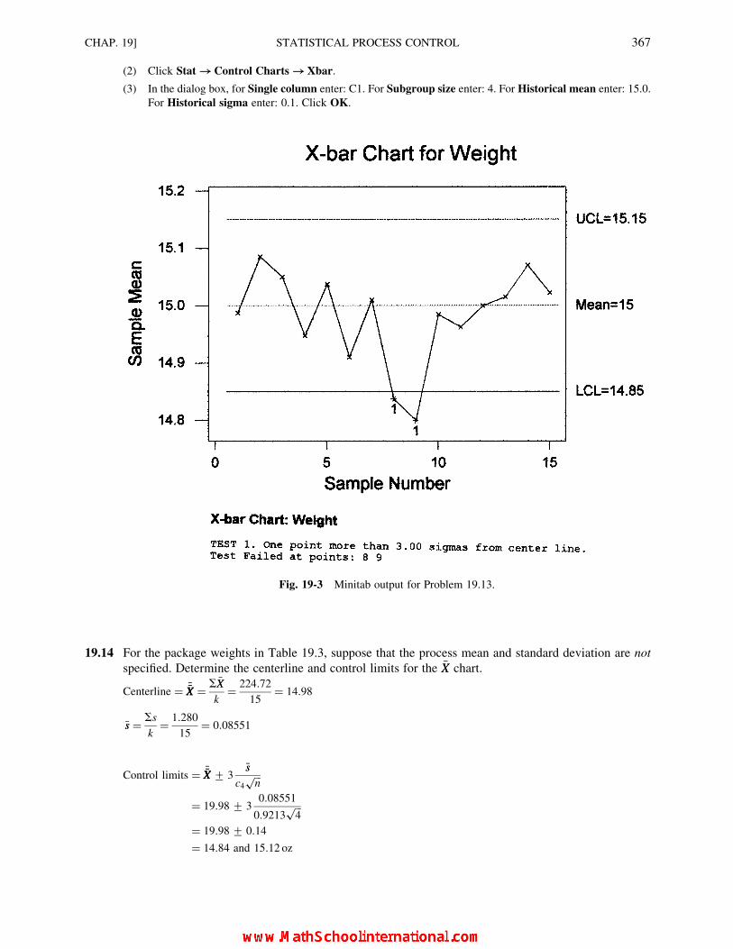
(2) Click Stat !!Control Charts !!Xbar.
(3) In the dialog box, for Single column enter: C1. For Subgroup size enter: 4. For Historical mean enter: 15.0.
For Historical sigma enter: 0.1. Click OK.
19.14 For the package weights in Table 19.3, suppose that the process mean and standard deviation are not
specified. Determine the centerline and control limits for the �XX chart.
Centerline ¼ ��XX�XX ¼ S �XX
k¼ 224:72
15¼ 14:98
�ss ¼ Ss
k¼ 1:280
15¼ 0:08551
Control limits ¼ ��XX�XX + 3�ss
c4ffiffiffin
p
¼ 19:98+ 30:08551
0:9213ffiffiffi4
p
¼ 19:98+ 0:14
¼ 14:84 and 15:12 oz
Fig. 19-3 Minitab output for Problem 19.13.
CHAP. 19] STATISTICAL PROCESS CONTROL 367
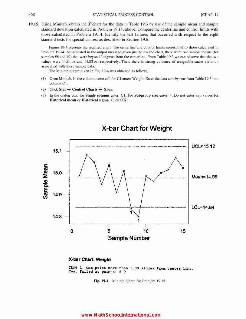
19.15 Using Minitab, obtain the �XX chart for the data in Table 19.3 by use of the sample mean and sample
standard deviation calculated in Problem 19.14, above. Compare the centerline and control limits with
those calculated in Problem 19.14. Identify the test failures that occurred with respect to the eight
standard tests for special causes, as described in Section 19.6.
Figure 19-4 presents the required chart. The centerline and control limits correspond to those calculated in
Problem 19.14. As indicated in the output message given just below the chart, there were two sample means (for
samples #8 and #9) that were beyond 3 sigmas from the centerline. From Table 19.3 we can observe that the two
values were 14.84 oz and 14.80 oz, respectively. Thus, there is strong evidence of assignable-cause variation
associated with these sample data.
The Minitab output given in Fig. 19-4 was obtained as follows:
(1) Open Minitab. In the column name cell for C1 enter: Weight. Enter the data row by row from Table 19.3 into
column C1.
(2) Click Stat !! Control Charts !! Xbar.
(3) In the dialog box, for Single column enter: C1. For Subgroup size enter: 4. Do not enter any values for
Historical mean or Historical sigma. Click OK.
Fig. 19-4 Minitab output for Problem 19.15.
368 STATISTICAL PROCESS CONTROL [CHAP. 19

CONTROL CHARTS FOR THE PROCESS STANDARD DEVIATION: s CHARTS
19.16 For the package weights in. Table 19.3, suppose that the process specifications require that s ¼ 0.10 oz.
Determine the centerline and the lower and upper control limits for the s chart.
Centerline ¼ E(s) ¼ c4s ¼ 0.9213(0.10) ¼ 0.09213
Control limits ¼ c4s+ 3c5s
¼ 0:09213+ 3(0:3889)(0:10)
¼ 0:09213+ 0:11667
¼ � 0:02454 and 0:2088
¼ 0 and 0:2088 (The lower control limit is set at zero because a negative
standard deviation is not possible.)
19.17 Using Minitab, obtain the s chart for the data in Table 19.3 using the specified process standard
deviation of 0.1. Compare the centerline and control limits with those calculated in Problem 19.16,
above. Identify any test failures that occurred with respect to the first four standard tests for special
causes, as described in Section 19.6, which are the only tests that are applied to s charts.
Figure 19-5 is the s chart given that the process standard deviation is specified. The centerline and control
limits correspond to those calculated in Problem 19.16. As can be observed in the figure, only common-cause
variation appears to exist. Therefore the associated �XX chart in Fig. 19-3 can be interpreted without concern that the
observed variability in the sample means could be associated with a lack of control of process variability.
The Minitab output given in Fig. 19-5 was obtained as follows:
(1) Open Minitab. In the column name cell for C1 enter: Weight. Enter the data row by row from Table 19.3 into
column C1.
(2) Click Stat !! Control Charts !! s.
(3) In the dialog box, for Single column enter: C1. For Subgroup size enter: 4. For Historical sigma enter: 0.1.
Click OK.
Fig. 19-5 Minitab output for Problem 19.17.
CHAP. 19] STATISTICAL PROCESS CONTROL 369

19.18 Suppose the process standard deviation was not specified for the package weights in Table 19.3.
Determine the centerline and control limits for the s chart.
Centerline ¼ �ss ¼ Ss
k¼ 1:280
15¼ 0:08551
Control limits ¼ �ss + 3c5�ss
c4
¼ 0:08551+ 30:3889(0:08551)
0:9213
¼ 0:08551+ 0:1083
¼ � 0:0228 and 0:1938
¼ 0 and 0:1938 (The lower control limit is set at zero because a negative
standard deviation is not possible.)
19.19 Using Minitab, obtain the s chart for the data in Table 19.3 using the standard deviation based on the
sample data. Compare the centerline and control limits with those calculated in Problem 19.18, above.
Identify any test failures that occurred with respect to the first four standard tests for special causes, as
described in Section 19.6, which are the only tests that are applied to s charts.
Figure 19-6 is the s chart given that the process standard deviation is not specified, but rather, is based on
sample data. The centerline and control limits correspond to those calculated in Problem 19.18. As can be observed
in the figure, only common-cause variation appears to exist. Therefore, the associated �XX chart in Fig. 19-4 can be
interpreted without concern that the observed variability in the sample means could be associated with a lack of
control of process variability.
The Minitab output given in Fig. 19-6 was obtained as follows:
(1) Open Minitab. In the column name cell for C1 enter: Weight. Enter the data row by row from Table 19.3 into
column C1.
(2) Click Stat !! Control Charts !! s.
(3) In the dialog box, for Single column enter: C1. For Subgroup size enter: 4.
(4) In the Estimate dialog box choose Pooled standard deviation. Click OK.
(5) Back in the original dialog box, click OK.
Fig. 19-6 Minitab output for Problem 19.19.
370 STATISTICAL PROCESS CONTROL [CHAP. 19

CONTROL CHARTS FOR THE PROCESS RANGE: R CHARTS
19.20 Determine the centerline and control limits with respect to the R chart for the package weights in
Table 19.3.
Centerline ¼ �RR ¼ SR
k¼ 2:93
15¼ 0:19533
Lower control limit ¼ �RRD3 ¼ 0:19533(0) ¼ 0
Upper control limit ¼ �RRD4 ¼ 0:19533(2:282) ¼ 0:4458
19.21 Using Minitab, obtain the R chart for the weight data in Table 19.3 using the mean range that was
determined in Problem 19.20, above. Compare the centerline and control limits in the chart with those
calculated in Problem 19.20. Identify any test failures that occurred with respect to the first four standard
tests for special causes, as described in Section 19.6, which are the only tests that are applied to R charts.
Figure 19-7 is the R chart obtained with Minitab. The centerline and control limits correspond to those
calculated in Problem 19.20. As can be observed in the figure, only common-cause variation appears to exist.
Therefore, the associated �XX chart in Fig. 19-4 can be interpreted without concern that the observed variability in the
sample means could be associated with a lack of control of process variability.
The Minitab output given in Fig. 19-7 was obtained as follows:
(1) Open Minitab. In the column name cell for C1 enter: Weight. Enter the data row by row from Table 19.3 into
column C1.
(2) Click Stat !! Control Charts !! R.
(3) In the dialog box, for Single column enter: C1. For Subgroup size enter: 4. Do not enter any value for
Historical sigma. Click OK.
Fig. 19-7 Minitab output for Problem 19.21.
CHAP. 19] STATISTICAL PROCESS CONTROL 371

CONTROL CHARTS FOR THE PROCESS PROPORTION: p CHARTS
19.22 When a coupon redemption process is in control, then a maximum of 3 percent of the rebates are done
incorrectly, for a maximum acceptable proportion of errors of 0.03. For 20 sequential samples of 100
coupon redemptions each, an audit reveals that the number of errors found in the rational subgroup
samples is: 2, 2, 3, 6, 1, 3, 6, 4, 7, 2, 5, 0, 3, 2, 4, 5, 3, 8, 1, and 4. Determine the control limits for the
proportion of errors per sample, given that the process proportion is specified as being p ¼ 0.03.
Control limits ¼ p+ 3
ffiffiffiffiffiffiffiffiffiffiffiffiffiffiffiffiffiffiffip (1� p)
n
r
¼ 0:03+ 3
ffiffiffiffiffiffiffiffiffiffiffiffiffiffiffiffiffiffiffiffiffiffi0:0:3(0:97)
100
r
¼ 0:03+ 3(0:0170587)
¼ 0:03+ 0:05118
¼ � 0:02118 and 0:08118
¼ 0 and 0:08118 (The lower control limit is set at zero because a negative
sample proportion is neither possible nor relevant for this one-sided test.)
19.23 Using Minitab, obtain the p chart for the data in Problem 19.22, above, given that the process proportion
of errors is specified as 0.03. Compare the centerline and control limits in the chart with those calculated
in Problem 19.22. Identify any test failures that occurred with respect to the first four standard tests for
special causes, as described in Section 19.6, which are the only tests that are applied to p charts.
Figure 19-8 is the p chart obtained with Minitab. The centerline and control limits correspond to those
calculated in Problem 19.22. As can be observed in the figure, only common-cause variation is included in the chart,
and the process appears to be stable.
The Minitab output given in Fig. 19-8 was obtained as follows:
(1) Open Minitab. In the column name cell for C1 enter: Errors. Enter the error data into C1.
(2) Click Stat !! Control Charts !! P.
(3) In the dialog box, for Variable enter: C1. For Subgroup size enter: 100. For Historical p enter: 0.03. Click OK.
Fig. 19-8 Minitab output for Problem 19.23.
372 STATISTICAL PROCESS CONTROL [CHAP. 19
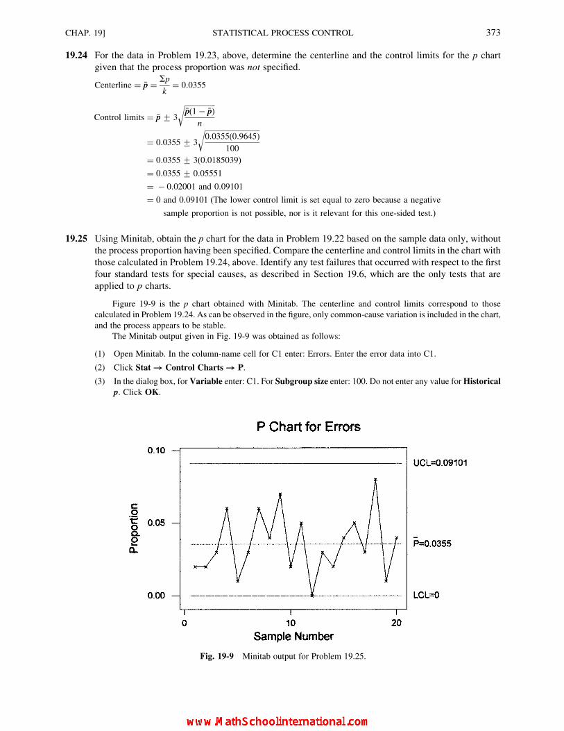
19.24 For the data in Problem 19.23, above, determine the centerline and the control limits for the p chart
given that the process proportion was not specified.
Centerline ¼ �pp ¼ Sp
k¼ 0:0355
Control limits ¼ �pp + 3
ffiffiffiffiffiffiffiffiffiffiffiffiffiffiffiffiffi�pp(1� �pp)
n
r
¼ 0:0355+ 3
ffiffiffiffiffiffiffiffiffiffiffiffiffiffiffiffiffiffiffiffiffiffiffiffiffiffiffiffiffiffi0:0355(0:9645)
100
r¼ 0:0355+ 3(0:0185039)
¼ 0:0355+ 0:05551
¼ � 0:02001 and 0:09101
¼ 0 and 0:09101 (The lower control limit is set equal to zero because a negative
sample proportion is not possible, nor is it relevant for this one-sided test.)
19.25 Using Minitab, obtain the p chart for the data in Problem 19.22 based on the sample data only, without
the process proportion having been specified. Compare the centerline and control limits in the chart with
those calculated in Problem 19.24, above. Identify any test failures that occurred with respect to the first
four standard tests for special causes, as described in Section 19.6, which are the only tests that are
applied to p charts.
Figure 19-9 is the p chart obtained with Minitab. The centerline and control limits correspond to those
calculated in Problem 19.24. As can be observed in the figure, only common-cause variation is included in the chart,
and the process appears to be stable.
The Minitab output given in Fig. 19-9 was obtained as follows:
(1) Open Minitab. In the column-name cell for C1 enter: Errors. Enter the error data into C1.
(2) Click Stat !! Control Charts !! P.
(3) In the dialog box, for Variable enter: C1. For Subgroup size enter: 100. Do not enter any value for Historical
p. Click OK.
Fig. 19-9 Minitab output for Problem 19.25.
CHAP. 19] STATISTICAL PROCESS CONTROL 373
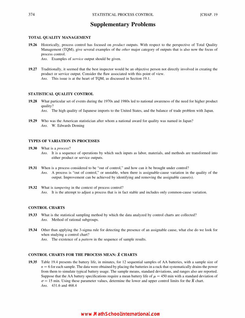
Supplementary Problems
TOTAL QUALITY MANAGEMENT
19.26 Historically, process control has focused on product outputs. With respect to the perspective of Total Quality
Management (TQM), give several examples of the other major category of outputs that is also now the focus of
process control.
Ans. Examples of service output should be given.
19.27 Traditionally, it seemed that the best inspector would be an objective person not directly involved in creating the
product or service output. Consider the flaw associated with this point of view.
Ans. This issue is at the heart of TQM, as discussed in Section 19.1.
STATISTICAL QUALITY CONTROL
19.28 What particular set of events during the 1970s and 1980s led to national awareness of the need for higher product
quality?
Ans. The high quality of Japanese imports to the United States, and the balance of trade problem with Japan.
19.29 Who was the American statistician after whom a national award for quality was named in Japan?
Ans. W. Edwards Deming
TYPES OF VARIATION IN PROCESSES
19.30 What is a process?
Ans. It is a sequence of operations by which such inputs as labor, materials, and methods are transformed into
either product or service outputs.
19.31 When is a process considered to be “out of control,” and how can it be brought under control?
Ans. A process is “out of control,” or unstable, when there is assignable-cause variation in the quality of the
output. Improvement can be achieved by identifying and removing the assignable cause(s).
19.32 What is tampering in the context of process control?
Ans. It is the attempt to adjust a process that is in fact stable and includes only common-cause variation.
CONTROL CHARTS
19.33 What is the statistical sampling method by which the data analyzed by control charts are collected?
Ans. Method of rational subgroups.
19.34 Other than applying the 3-sigma rule for detecting the presence of an assignable cause, what else do we look for
when studying a control chart?
Ans. The existence of a pattern in the sequence of sample results.
CONTROL CHARTS FOR THE PROCESS MEAN: XX CHARTS
19.35 Table 19.4 presents the battery life, in minutes, for 12 sequential samples of AA batteries, with a sample size of
n ¼ 6 for each sample. The data were obtained by placing the batteries in a rack that systematically drains the power
from them to simulate typical battery usage. The sample means, standard deviations, and ranges also are reported.
Suppose that the AA battery specifications require a mean battery life of m ¼ 450 min with a standard deviation of
s ¼ 15 min. Using these parameter values, determine the lower and upper control limits for the �XX chart.
Ans. 431.6 and 468.4
374 STATISTICAL PROCESS CONTROL [CHAP. 19

19.36 Prepare the �XX chart for the data in Table 19.4 using the parameter values and control limits from the preceding
problem. Interpret any test failures that occurred with respect to the eight standard tests that are used with �XX charts.
Ans. Test 3 failed at point 10.
19.37 Suppose that the process mean and standard deviation are not specified for the battery-life data in Table 19.4.
Determine the centerline and control limits for the �XX chart.
Ans. Centerline ¼ ��XX�XX ¼ 447:3; control limits ¼ 427.3 and 467.3.
19.38 Prepare the �XX chart for the data in Table 19.4 using the sample statistics and control limits determined in the
preceding problem. Interpret the results associated with the eight standard tests for �XX charts.
Ans. Test 3 failed at point 10.
CONTROL CHARTS FOR THE PROCESS STANDARD DEVIATION: s CHARTS
19.39 For the battery-life data in Table 19.4, suppose that the process specifications require that s ¼ 15 mm. Determine
the centerline and the lower and upper control limits for the s chart.
Ans. Centerline ¼ 14.27; control limits ¼ 0.4334 and 28.11
19.40 Prepare the s chart for the battery-life data in Table 19.4 using the centerline and control limits determined in the
preceding problem. Interpret the chart.
Ans. There appears to be no assignable cause associated with the variation in the sample standard deviations.
19.41 Suppose that the process standard deviation was not specified for the battery-life data in Table 19.4. Determine the
centerline and control limits for the s chart.
Ans. Centerline ¼ �ss15.55; control limits ¼ 0.4723 and 30.64
19.42 Prepare the s chart for the data in Table 19.4 using the centerline and control limits determined in the preceding
problem. Interpret the chart.
Ans. There appears to be no assignable cause associated with the variation in the sample standard deviations.
CONTROL CHARTS FOR THE PROCESS RANGE: R CHARTS
19.43 Prepare the R chart for the battery-life data in Table 19.4 using computer software. Interpret the chart.
Ans. From Minitab: Centerline ¼ 41.42; control limits ¼ 0 and 83.00. There appears to be no assignable cause
associated with the variation in the sample ranges.
Table 19.4 Battey Life
Sample
No. Battery life (min) X s R
1 445.4 470.3 466.5 432.3 445.5 425.4 447.6 17.94 44.9
2 479.7 466.1 439.2 442.0 432.1 429.4 448.1 20.22 50.3
3 449.7 450.1 432.2 468.1 446.3 452.6 449.8 11.53 35.9
4 467.6 427.9 453.9 445.4 467.9 449.3 452.0 15.04 40.0
5 484.5 436.8 458.6 465.2 437.1 445.1 454.6 18.63 47.7
6 470.5 469.3 435.9 438.1 461.0 431.4 451.0 17.85 39.1
7 411.6 459.7 450.9 449.6 444.9 467.5 447.4 19.29 55.9
8 458.8 442.5 462.2 417.2 424.6 463.9 444.9 20.19 46.7
9 435.4 435.6 451.2 434.7 465.9 425.2 441.3 14.65 40.7
10 448.2 449.7 435.7 438.4 432.7 426.5 438.5 9.00 23.2
11 458.5 436.7 455.5 449.2 440.6 424.0 444.1 12.92 34.5
12 444.6 430.8 463.6 458.2 436.2 458.8 448.7 13.47 32.8
CHAP. 19] STATISTICAL PROCESS CONTROL 375

CONTROL CHARTS FOR THE PROCESS PROPORTION: p CHARTS
19.44 A health maintenance organization (HMO) has established the standard that no more than 8 percent of the patients
should have to wait more than 20 minutes beyond the appointed time to see the medical provider. For 20 sequential
samples of 80 patients, the number of patients who had to wait more than 20 minutes was: 3, 4, 10, 10, 9, 7, 9, 7, 8, 9,
7, 10, 8, 4, 8, 5, 2, 8, 8, and 6. Determine the centerline and the upper control limit for the p chart that would be used
to monitor this process.
Ans. Centerline ¼ p ¼ 0.08; upper control limit ¼ 0.1710
19.45 Prepare the p chart by using the centerline and upper control limit determined in the preceding problem. Apply and
interpret the result associated with the four standard tests for proportions.
Ans. Test 2 failed at samples 11, 12, and 13.
19.46 With respect to the patient waiting times in Problem 19.44, suppose no standard had been set regarding the
proportion of patients who are required to wait more than 20 minutes to see the medical provider. Determine the
centerline and the upper control limit for the p chart.
Ans. Centerline ¼ �pp ¼ 0.08875; upper control limit ¼ 0.1841
19.47 Prepare the p chart for the waiting times in Problem 19.44, but using the centerline and control limits determined in
Problem 19.46, above. Apply and interpret the result associated with the four standard tests for proportions.
Ans. No test failures occurred. Using the mean of the sample proportions as the basis for the centerline, there is no
assignable-cause variation in the series of proportions.
376 STATISTICAL PROCESS CONTROL [CHAP. 19

APPENDIX 1
Table of RandomNumbers
10097 85017 84532 13618 23157 86952 02438 76520 91499 38631 79430 62421 97959 67422 69992 68479
37542 16719 82789 69041 05545 44109 05403 64894 80336 49172 16332 44670 35089 17691 89246 26940
08422 65842 27672 82186 14871 22115 86529 19645 44104 89232 57327 34679 62235 79655 81336 85157
99019 76875 20684 39187 38976 94324 43204 09376 12550 02844 15026 32439 58537 48274 81330 11100
12807 93640 39160 41453 97312 41548 93137 80157 63606 40387 65406 37920 08709 60623 2237 16505
66065 99478 70086 71265 11742 18226 29004 34072 61196 80240 44177 51171 08723 39323 05798 26457
31060 65119 26486 47353 43361 99436 42753 45571 15474 44910 99321 72173 56239 04595 10836 95270
85269 70322 21592 48233 93806 32584 21828 02051 94557 33663 86347 00926 44915 34823 51770 67897
63573 58133 41278 11697 49540 61777 67954 05325 42481 86430 19102 37420 41976 76559 24358 97344
73796 44655 81255 31133 36768 60452 38537 03529 23523 31379 68588 81675 15694 43438 36879 73208
98520 02295 13487 98662 07092 44673 61303 14905 04493 98086 32533 17767 14523 52494 24826 75246
11805 85035 54881 35587 43310 48897 48493 39808 00549 33185 04805 05431 94598 97654 16232 64051
83452 01197 86935 28021 61570 23350 65710 06288 35963 80951 68953 99634 81949 15307 00406 26898
88685 97907 19078 40646 31352 48625 44369 86507 59808 79752 02529 40200 73742 08391 49140 45427
99594 63268 96905 28797 57048 46359 74294 87517 46058 18633 99970 67348 49329 95236 32537 01390
65481 52841 59684 67411 09243 56092 84369 17468 32179 74029 74717 17674 90446 00597 45240 87379
80124 53722 71399 10916 07959 21225 13018 17727 69234 54178 10805 35635 45266 61406 41941 20117
74350 11434 51908 62171 93732 26958 02400 77402 19565 11664 77602 99817 28573 41430 96382 01758
69916 62375 99292 21177 72721 66995 07289 66252 45155 48324 32135 26803 16213 14938 71961 19476
09893 28337 20923 87929 61020 62841 31374 14225 94864 69074 45753 20505 78317 31994 98145 36168
377
Copyright 2004, 1996, 1988, 1976 by The McGraw-Hill Companies, Inc. Click Here for Terms of Use.
APPENDIX 2
BinomialProbabilities
378
Copyright 2004, 1996, 1988, 1976 by The McGraw-Hill Companies, Inc. Click Here for Terms of Use.

pp
nx
.01
.05
.10
.15
.20
.25
.30
.35
.40
.45
.50
nx
.01
.05
.10
.15
.20
.25
.30
.35
.40
.45
.50
10
.9900
.9500
.9000
.8500
.8000
.7500
.7000
.6500
.6000
.5500
.5000
93
.0001
.0077
.0446
.1069
.1762
.2336
.2668
.2716
.2508
.2119
.1641
1.0100
.0500
.1000
.1500
.2000
.2500
.3000
.3500
.4000
.4500
.5000
4.0000
.0006
.0074
.0283
.0661
.1168
.1715
.2194
.2508
.2600
.2461
20
.9801
.9025
.8100
.7225
.6400
.5625
.4900
.4225
.3600
.3025
.2500
5.0000
.0000
.0008
.0050
.0165
.0389
.0735
.1181
.1672
.2128
.2461
1.0198
.0950
.1800
.2550
.3200
.3750
.4200
.4550
.4800
.4950
.5000
6.0000
.0000
.0001
.0006
.0028
.0087
.0210
.0424
.0743
.1160
.1641
2.0001
.0025
.0100
.0225
.0400
.0625
.0900
.1225
.1600
.2025
.2500
7.0000
.0000
.0000
.0000
.0003
.0012
.0039
.0098
.0212
.0407
.0703
8.0000
.0000
.0000
.0000
.0000
.0001
.0004
.0013
.0035
.0083
.0176
30
.9703
.8574
.7290
.6141
.5120
.4219
.3430
.2746
.2160
.1664
.1250
9.0000
.0000
.0000
.0000
.0000
.0000
.0000
.0001
.0003
.0008
.0020
1.0294
.1354
.2430
.3251
.3840
.4219
.4410
.4436
.4320
.4084
.3750
2.0003
.0071
.0270
.0574
.0960
.1406
.1890
.2389
.2880
.3341
.3750
10
0.9044
.5987
.3487
.1969
.1074
.0563
.0282
.0135
.0060
.0025
.0010
3.0000
.0001
.0010
.0034
.0080
.0156
.0270
.0429
.0640
.0911
.1250
1.0914
.3151
.3874
.3474
.2684
.1877
.1211
.0725
.0403
.0207
.0098
2.0042
.0746
.1937
.2759
.3020
.2816
.2335
.1757
.1209
.0763
.0439
40
.9606
.8145
.6561
.5220
.4096
.3164
.2401
.1785
.1296
.0915
.0625
3.0001
.0105
.0574
.1298
.2013
.2503
.2668
.2522
.2150
.1665
.1172
1.0388
.1715
.2916
.3685
.4096
.4219
.4116
.3845
.3456
.2995
.2500
4.0000
.0010
.0112
.0401
.0881
.1460
.2001
.2377
.2508
.2384
.2051
2.0006
.0135
.0486
.0975
.1536
.2109
.2646
.3105
.3456
.3675
.3750
3.0000
.0005
.0036
.0115
.0256
.0469
.0756
.1115
.1536
.2005
.2500
5.0000
.0001
.0015
.0085
.0264
.0584
.1029
.1536
.2007
.2340
.2461
4.0000
.0000
.0001
.0005
.0016
.0039
.0081
.0150
.0256
.0410
.0625
6.0000
.0000
.0001
.0012
.0055
.0162
.6368
.0689
.1115
.1596
.2051
7.0000
.0000
.0000
.0001
.0008
.0031
.0090
.0212
.0425
.0746
.1172
50
.9510
.7738
.5905
.4437
.3277
.2373
.1681
.1160
.0778
.0503
.0312
8.0000
.0000
.0000
.0000
.0001
.0004
.0014
.0043
.0106
.0229
.0439
1.0480
.2036
.3280
.3915
.4096
.3955
.3602
.3124
.2592
.2059
.1562
9.0000
.0000
.0000
.0000
.0000
.0000
.0001
.0005
.0016
.0042
.0098
2.0010
.0214
.0729
.1382
.2048
.2637
.3087
.3364
.3456
.3369
.3125
10
.0000
.0000
.0000
.0000
.0000
.0000
.0000
.0000
.0001
.0003
.0010
3.0000
.0011
.0081
.0244
.0512
.0879
.1323
.1811
.2304
.2757
.3125
4.0000
.0000
.0004
.0022
.0064
.0146
.0284
.0488
.0768
.1128
.1562
11
0.8953
.5688
.3138
.1673
.0859
.0422
.0198
.0088
.0036
.0014
.0005
1.0995
.3293
.3835
.3248
.2362
.1549
.0932
.0518
.0266
.0125
.0054
5.0000
.0000
.0000
.0001
.0003
.0010
.0024
.0053
.0102
.0185
.0312
2.0050
.0867
.2131
.2866
.2953
.2581
.1998
.1395
.0887
.0513
.0269
3.0002
.0137
.0710
.1517
.2215
.2581
.2568
.2254
.1774
.1259
.0806
60
.9415
.7351
.5314
.3771
.2621
.1780
.1176
.0754
.0467
.0277
.0156
4.0000
.0014
.0158
.0536
.1107
.1721
.2201
.2428
.2365
.2060
.1611
1.0571
.2321
.3543
.3993
.3932
.3560
.3025
.2437
.1866
.1359
.0938
2.0014
.0305
.0984
.1762
.2458
.2966
.3241
.3280
.3110
.2780
.2344
5.0000
.0001
.0025
.0132
.0388
.0803
.1321
.1830
.2207
.2360
.2256
3.0000
.0021
.0146
.0415
.0819
.1318
.1852
.2355
.2765
.3032
.3125
6.0000
.0000
.0003
.0023
.0097
.0268
.0566
.0985
.1471
.1931
.2256
4.0000
.0001
.0012
.0055
.0154
.0330
.0595
.0951
.1382
.1861
.2344
7.0000
.0000
.0000
.0003
.0017
.0064
.0173
.0379
.0701
.1128
.1611
8.0000
.0000
.0000
.0000
.0002
.0011
.0037
.0102
.0234
.0462
.0806
5.0000
.0000
.0001
.0004
.0015
.0044
.0102
.0205
.0369
.0609
.0938
9.0000
.0000
.0000
.0000
.0000
.0001
.0005
.0018
.0052
.0126
.0269
6.0000
.0000
.0000
.0000
.0001
.0002
.0007
.0018
.0041
.0083
.0156
10
.0000
.0000
.0000
.0000
.0000
.0000
.0000
.0002
.0007.
.0021
.0054
70
.9321
.6983
.4783
.3206
.2097
.1335
.0824
.0490
.0280
.0152
.0078
11
.0000
.0000
.0000
.0000
.0000
.0000
.0000
.0000
.0000
.0002
.0005
1.0659
.2573
.3720
.3960
.3670
.3115
.2471
.1848
.1306
.0872
.0547
2.0020
.0406
.1240
.2097
.2753
.3115
.3177
.2985
.2613
.2140
.1641
12
0.8864
.5404
.2824
.1422
.0687
.0317
.0138
.0057
.0022
.0008
.0002
3.0000
.0036
.0230
.0617
.1147
.1730
.2269
.2679
.2903
.2918
.2734
1.1074
.3413
.3766
.3012
.2062
.1267
.0712
.0368
.0174
.0075
.0029
4.0000
.0002
.0026
.0109
.0287
.0577
.0972
.1442
.1935
.2388
.2734
2.0060
.0988
.2301
.2924
.2835
.2323
.1678
.1088
.0639
.0339
.0161
3.0002
.0173
.0852
.1720
.2362
.2581
.2397
.1954
.1419
.0923
.0537
5.0000
.0000
.0002
.0012
.0043
.0115
.0250
.0466
.0774
.1172
.1641
4.0000
.0021
.0213
.0683
.1329
.1936
.2311
.2367
.2128
.1700
.1208
6.0000
.0000
.0000
.0001
.0004
.0013
.0036
.0084
.0172
.0320
.0547
7.0000
.0000
.0000
.0000
.0000
.0001
.0002
.0006
.0016
.0037
.0078
5.0000
.0002
.0038
.0193
.0532
.1032
.1585
.2039
.2270
.2225
.1934
6.0000
.0000
.0005
.0040
.0155
.0401
.0792
.1281
.1766
.2124
.2256
80
.9227
.6634
.4305
.2725
.1678
.1002
.0576
.0319
.0168
.0084
.0039
7.0000
.0000
.0000
.0006
.0033
.0115
.0291
.0591
.1009
.1489
.1934
1.0746
.2793
.3826
.3847
.3355
.2670
.1977
.1373
.0896
.0548
.0312
8.0000
.0000
.0000
.0001
.0005
.0024
.0078
.0199
.0420
.0762
.1208
2.0026
.0515
.1488
.2376
.2936
.3115
.2065
.2587
.2090
.1569
.1094
9.0000
.0000
.0000
.0000
.0001
.0004
.0015
.0048
.0125
.0277
.0537
3.0001
.0054
.0331
.0839
.1468
.2076
.2541
.2786
.2787
.2568
.2188
4.0000
.0004
.0046
.0185
.0459
.0865
.1361
.1875
.2322
.2627
.2734
10
.0000
.0000
.0000
.0000
.0000
.0000
.0002
.0008
.0025
.0068
.0161
11
.0000
.0000
.0000
.0000
.0000
.0000
.0000
.0001
.0003
.0010
.0029
5.0000
.0000
.0004
.0026
.0092
.0231
.0467
.0808
.1239
.1719
.2188
12
.0000
.0000
.0000
.0000
.0000
.0000
.0000
.0000
.0000
.0001
.0002
6.0000
.0000
.0000
.0002
.0011
.0038
.0100
.0217
.0413
.0403
.1094
7.0000
.0000
.0000
.0000
.0001
.0004
.0012
.0033
.0079
.0164
.0312
13
0.8775
.5133
.2542
.1209
.0550
.0238
.0097
.0037
.0013
.0004
.0001
8.0000
.0000
.0000
.0000
.0000
.0000
.0001
.0002
.0007
.0017
.0039
1.1152
.3512
.3672
.2774
.1787
.1029
.0540
.0259
.0113
.0045
.0016
2.0070
.1109
.2448
.2937
.2680
.2059
.1388
.0836
.0453
.0220
.0095
90
.9135
.6302
.3874
.2316
.1342
.0751
.0404
.0207
.0101
.0046
.0020
3.0003
.0214
.0997
.1900
.2457
.2517
.2181
.1651
.1107
.0660
.0349
1.0830
.2985
.3874
.3679
.3020
.2253
.1556
.1004
.0605
.0339
.0176
4.0000
.0028
.0277
.0838
.1535
.2097
.2337
.2222
.1845
.1350
.0873
2.0034
.0629
.1722
.2597
.3020
.3003
.2668
.2162
.1612
.1110
.0793
Exam
ple:
p(x
¼3jn
¼6,
p¼
0.50)¼
0.3125
APPENDIX 2] BINOMIAL PROBABILITIES 379

pp
nx
.01
.05
.10
.15
.20
.25
.30
.35
.40
.45
.50
nx
.01
.05
.10
.15
.20
.25
.30
.35
.40
.45
.50
13
5.0000
.0003
.0055
.0266
.0691
.1258
.1803
.2154
.2214
.1989
.1571
16
7.0000
.0000
.0004
.0045
.0197
.0524
.1010
.1524
.1889
.1969
.1746
6.0000
.0000
.0008
.0063
.0230
.0559
.1030
.1546
.1968
.2169
.2095
8.0000
.0000
.0001
.0009
.0055
.0197
.0487
.0923
.1417
.1812
.1964
7.0000
.0000
.0001
.0011
.0058
.0186
.0442
.0833
.1312
.1775
.2095
9.0000
.0000
.0000
.0001
.0012
.0058
.0185
.0442
.0840
.1318
.1746
8.0000
.0000
.0001
.0001
.0011
.0047
.0142
.0336
.0656
.1089
.1571
9.0000
.0000
.0000
.0000
.0001
.0009
.0034
.0101
.0243
.0495
.0873
10
.0000
.0000
.0000
.0000
.0002
.0014
.0056
.0167
.0392
.0755
.1222
11
.0000
.0000
.0000
.0000
.0000
.0002
.0013
.0049
.0142
.0337
.0667
10
.0000
.0000
.0000
.0000
.0000
.0001
.0006
.0022
.0065
.0162
.0349
12
.0000
.0000
.0000
.0000
.0000
.0000
.0002
.0011
.0040
.0115
.0278
11
.0000
.0000
.0000
.0000
.0000
.0000
.0001
.0003
.0012
.0036
.0095
13
.0000
.0000
.0000
.0000
.0000
.0000
.0000
.0002
.0008
.0029
.0085
12
.0000
.0000
.0000
.0000
.0000
.0000
.0000
.0000
.0001
.0005
.0016
14
.0000
.0000
.0000
.0000
.0000
.0000
.0000
.0000
.0001
.0005
.0018
13
.0000
.0000
.0000
.0000
.0000
.0000
.0000
.0000
.0000
.0000
.0001
15
.0000
.0000
.0000
.0000
.0000
.0000
.0000
.0000
.0000
.0001
.0002
14
0.8687
.4877
.2288
.1028
.0440
.0178
.0068
.0024
.0008
.0002
.0001
16
.0000
.0000
.0000
.0000
.0000
.0000
.0000
.0000
.0000
.0000
.0000
1.1229
.3593
.3559
.2539
.1539
.0832
.0407
.0181
.0073
.0027
.0009
2.0081
.1229
.2570
.2912
.2501
.1802
.1134
.0634
.0317
.0141
.0056
17
0.8429
.4181
.1668
.0631
.0225
.0075
.0023
.0007
.0002
.0000
.0000
3.0003
.0259
.1142
.2056
.2501
.2402
.1943
.1366
.0845
.0462
.0222
1.1447
.3741
.3150
.1893
.0957
.0426
.0169
.0060
.0019
.0005
.0001
4.0000
.0037
.0349
.0998
.1720
.2202
.2290
.2022
.1549
.1040
.0611
2.0117
.1575
.2800
.2673
.1914
.1136
.0581
.0260
.0102
.0035
.0010
3.0006
.0415
.1556
.2359
.2393
.1893
.1245
.0701
.0341
.0144
.0052
5.0000
.0004
.0078
.0352
.0860
.1468
.1963
.2178
.2066
.1701
.1222
4.0000
.0076
.0605
.1457
.2093
.2209
.1868
.1320
.0796
.0411
.0182
6.0000
.0000
.0013
.0093
.0322
.0734
.1262
.1759
.2066
.2088
.1833
7.0000
.0000
.0002
.0019
.0092
.0280
.0618
.1082
.1574
.1952
.2095
5.0000
.0010
.0175
.0668
.1361
.1914
.2081
.1849
.1379
.0875
.0472
8.0000
.0000
.0000
.0003
.0020
.0082
.0232
.0510
.0918
.1398
.1833
6.0000
.0001
.0039
.0236
.0680
.1276
.1784
.1991
.1839
.1432
.0944
9.0000
.0000
.0000
.0000
.0003
.0018
.0066
.0183
.0408
.0762
.1222
7.0000
.0000
.0007
.0065
.0267
.0668
.1201
.1685
.1927
.1841
.1484
8.0000
.0000
.0001
.0014
.0084
.0279
.0644
.1134
.1606
.1883
.1855
10
.0000
.0000
.0000
.0000
.0000
.0003
.0014
.0049
.0136
.0312
.0611
9.0000
.0000
.0000
.0003
.0021
.0093
.0276
.0611
.1070
.1540
.1855
11
.0000
.0000
.0000
.0000
.0000
.0000
.0002
.0010
.0033
.0093
.0222
12
.0000
.0000
.0000
.0000
.0000
.0000
.0000
.0001
.0005
.0019
.0056
10
.0000
.0000
.0000
.0000
.0004
.0025
.0095
.0263
.0571
.1008
.1484
13
.0000
.0000
.0000
.0000
.0000
.0000
.0000
.0000
.0001
.0002
.0009
11
.0000
.0000
.0000
.0000
.0001
.0005
.0026
.0090
.0242
.0525
.0944
14
.0000
.0000
.0000
.0000
.0000
.0000
.0000
.0000
.0000
.0000
.0001
12
.0000
.0000
.0000
.0000
.0000
.0001
.0006
.0024
.0081
.0215
.0472
13
.0000
.0000
.0000
.0000
.0000
.0000
.0001
.0005
.0021
.0068
.0182
15
0.8601
.4633
.2059
.0874
.0352
.0134
.0047
.0016
.0005
.0001
.0000
14
.0000
.0000
.0000
.0000
.0000
.0000
.0000
.0001
.0004
.0016
.0052
1.1303
.3658
.3432
.2312
.1319
.0668
.0305
.0126
.0047
.0016
.0005
2.0092
.1348
.2669
.2856
.2309
.1559
.0916
.0476
.0219
.0090
.0032
15
.0000
.0000
.0000
.0000
.0000
.0000
.0000
.0000
.0001
.0003
.0010
3.0004
.0307
.1285
.2184
.2501
.2252
.1700
.1110
.0634
.0318
.0139
16
.0000
.0000
.0000
.0000
.0000
.0000
.0000
.0000
.0000
.0000
.0001
4.0000
.0049
.0428
.1156
.1876
.2252
.2186
.1792
.1268
.0780
.0417
17
.0000
.0000
.0000
.0000
.0000
.0000
.0000
.0000
.0000
.0000
.0000
5.0000
.0006
.0105
.0449
.1032
.1651
.2061
.2123
.1859
.1404
.0916
18
0.8345
.3972
.1501
.0536
.0180
.0056
.0016
.0004
.0001
.0000
.0000
6.0000
.0000
.0019
.0132
.0430
.0917
.1472
.1906
.2066
.1914
.1527
1.1517
.3763
.3002
.1704
.0811
.0338
.0126
.0042
.0012
.0003
.0001
7.0000
.0000
.0003
.0030
.0138
.0393
.0811
.1319
.1771
.2013
.1964
2.0130
.1683
.2835
.2556
.1723
.0958
.0458
.0190
.0069
.0022
.0006
8.0000
.0000
.0000
.0005
.0035
.0131
.0348
.0710
.1181
.1647
.1964
3.0007
.0473
.1680
.2406
.2297
.1704
.1046
.0547
.0246
.0095
.0031
9.0000
.0000
.0000
.0001
.0007
.0034
.0116
.0298
.0612
.1048
.1527
4.0000
.0093
.0700
.1592
.2153
.2130
.1681
.1104
.0614
.0291
.0117
10
.0000
.0000
.0000
.0000
.0001
.0007
.0030
.0096
.0245
.0515
.0916
5.0000
.0014
.0218
.0787
.1507
.1988
.2017
.1664
.1146
.0666
.0327
11
.0000
.0000
.0000
.0000
.0000
.0001
.0006
.0024
.0074
.0191
.0417
6.0000
.0002
.0052
.0301
.0816
.1436
.1873
.1941
.1655
.1181
.0708
12
.0000
.0000
.0000
.0000
.0000
.0000
.0001
.0004
.0016
.0052
.0139
7.0000
.0000
.0010
.0091
.0350
.0820
.1376
.1792
.1892
.1657
.1214
13
.0000
.0000
.0000
.0000
.0000
.0000
.0000
.0001
.0003
.0010
.0032
8.0000
.0000
.0002
.0022
.0120
.0376
.0811
.1327
.1734
.1864
.1669
14
.0000
.0000
.0000
.0000
.0000
.0000
.0000
.0000
.0000
.0001
.0005
9.0000
.0000
.0000
.0004
.0033
.0139
.0386
.0794
.1284
.1694
.1855
15
.0000
.0000
.0000
.0000
.0000
.0000
.0000
.0000
.0000
.0000
.0000
10
.0000
.0000
.0000
.0001
.0008
.0042
.0149
.0385
.0771
.1248
.1669
11
.0000
.0000
.0000
.0000
.0001
.0010
.0046
.0151
.0374
.0742
.1214
16
0.8515
.4401
.1853
.0743
.0281
.0100
.0033
.0010
.0003
.0001
.0000
12
.0000
.0000
.0000
.0000
.0000
.0002
.0012
.0047
.0145
.0354
.0708
1.1376
.3706
.3294
.2097
.1126
.0535
.0228
.0087
.0030
.0009
.0002
13
.0000
.0000
.0000
.0000
.0000
.0000
.0002
.0012
.0045
.0134
.0327
2.0104
.1463
.2745
.2775
.2111
.1336
.0732
.0353
.0150
.0056
.0018
14
.0000
.0000
.0000
.0000
.0000
.0000
.0000
.0002
.0011
.0039
.0117
3.0005
.0359
.1423
.2285
.2463
.2079
.1465
.0888
.0468
.0215
.0085
4.0000
.0061
.0514
.1311
.2001
.2252
.2040
.1553
.1014
.0572
.0278
15
.0000
.0000
.0000
.0000
.0000
.0000
.0000
.0000
.0002
.0009
.0031
16
.0000
.0000
.0000
.0000
.0000
.0000
.0000
.0000
.0000
.0001
.0006
5.0000
.0008
.0137
.0555
.1201
.1802
.2099
.2008
.1623
.1123
.0667
17
.0000
.0000
.0000
.0000
.0000
.0000
.0000
.0000
.0000
.0000
.0001
6.0000
.0001
.0028
.0180
.0550
.1101
.1649
.1982
.1983
.1684
.1222
18
.0000
.0000
.0000
.0000
.0000
.0000
.0000
.0000
.0000
.0000
.0000
380 BINOMIAL PROBABILITIES [APPENDIX 2
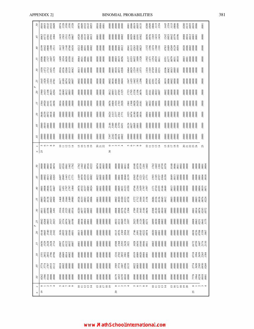
pp
nx
.01
.05
.10
.15
.20
.25
.30
.35
.40
.45
.50
nx
.01
.05
.10
.15
.20
.25
.30
.35
.40
.45
.50
19
0.8262
.3774
.1351
.0456
.0144
.0042
.0011
.0003
.0001
.0000
.0000
25
5.0000
.0060
.0646
.1564
.1960
.1645
.1030
.0506
.0199
.0063
.0016
1.1586
.3774
.2852
.1529
.0685
.0268
.0093
.0029
.0008
.0002
.0000
6.0000
.0010
.0239
.0920
.1633
.1828
.1472
.0908
.0442
.0172
.0053
2.0144
.1787
.2852
.2428
.1540
.0803
.0358
.0138
.0046
.0013
.0003
7.0000
.0001
.0072
.0441
.1108
.1654
.1712
.1327
.0800
.0381
.0143
3.0008
.0533
.1796
.2428
.2182
.1517
.0869
.0422
.0175
.0062
.0018
8.0000
.0000
.0018
.0175
.0623
.1241
.1651
.1607
.1200
.0701
.0322
4.0000
.0112
.0798
.1714
.2182
.2023
.1491
.0909
.0467
.0203
.0074
9.0000
.0000
.0004
.0058
.0294
.0781
.1336
.1635
.1511
.1084
.0609
5.0000
.0018
.0266
.0907
.1636
.2023
.1916
.1468
.0933
.0497
.0222
10
.0000
.0000
.0000
.0016
.0118
.0417
.0916
.1409
.1612
.1419
.0974
6.0000
.0002
.0069
.0374
.0955
.1574
.1916
.1844
.1451
.0949
.0518
11
.0000
.0000
.0000
.0004
.0040
.0189
.0536
.1034
.1465
.1583
.1328
7.0000
.0000
.0014
.0122
.0443
.0974
.1525
.1844
.1797
.1443
.0961
12
.0000
.0000
.0000
.0000
.0012
.0074
.0268
.0650
.1140
.1511
.1550
8.0000
.0000
.0002
.0032
.0166
.0487
.0981
.1489
.1797
.1771
.1442
13
.0000
.0000
.0000
.0000
.0003
.0025
.0115
.0350
.0760
.1236
.1550
9.0000
.0000
.0000
.0007
.0051
.0198
.0514
.0980
.1464
.1771
.1762
14
.0000
.0000
.0000
.0000
.0000
.0007
.0042
.0161
.0434
.0867
.1328
10
.0000
.0000
.0000
.0001
.0013
.0066
.0220
.0528
.0976
.1449
.1762
15
.0000
.0000
.0000
.0000
.0000
.0002
.0013
.0064
.0212
.0520
.0974
11
.0000
.0000
.0000
.0000
.0003
.0018
.0077
.0233
.0532
.0970
.1442
16
.0000
.0000
.0000
.0000
.0000
.0000
.0004
.0021
.0088
.0266
.0609
12
.0000
.0000
.0000
.0000
.0000
.0004
.0022
.0083
.0237
.0529
.0961
17
.0000
.0000
.0000
.0000
.0000
.0000
.0001
.0006
.0031
.0115
.0322
13
.0000
.0000
.0000
.0000
.0000
.0001
.0005
.0024
.0085
.0233
.0518
18
.0000
.0000
.0000
.0000
.0000
.0000
.0000
.0001
.0009
.0042
.0143
14
.0000
.0000
.0000
.0000
.0000
.0000
.0001
.0006
.0024
.0082
.0222
19
.0000
.0000
.0000
.0000
.0000
.0000
.0000
.0000
.0002
.0013
.0053
15
.0000
.0000
.0000
.0000
.0000
.0000
.0000
.0001
.0005
.0022
.0074
20
.0000
.0000
.0000
.0000
.0000
.0000
.0000
.0000
.0000
.0001
.0016
16
.0000
.0000
.0000
.0000
.0000
.0000
.0000
.0000
.0001
.0005
.0018
21
.0000
.0000
.0000
.0000
.0000
.0000
.0000
.0000
.0000
.0000
.0004
17
.0000
.0000
.0000
.0000
.0000
.0000
.0000
.0000
.0000
.0001
.0003
22
.0000
.0000
.0000
.0000
.0000
.0000
.0000
.0000
.0000
.0000
.0001
18
.0000
.0000
.0000
.0000
.0000
.0000
.0000
.0000
.0000
.0000
.0000
19
.0000
.0000
.0000
.0000
.0000
.0000
.0000
.0000
.0000
.0000
.0000
30
0.7397
.2146
.0424
.0076
.0012
.0002
.0000
.0000
.0000
.0000
.0000
1.2242
.3389
.1413
.0404
.0093
.0018
.0003
.0000
.0000
.0000
.0000
20
0.8179
.3585
.1216
.0388
.0115
.0032
.0008
.0002
.0000
.0000
.0000
2.0328
.2586
.2277
.1034
.0337
.0086
.0018
.0003
.0000
.0000
.0000
1.1652
.3774
.2702
.1368
.0576
.0211
.0068
.0020
.0005
.0001
.0000
3.0031
.1270
.2361
.1703
.0785
.0269
.0072
.0015
.0003
.0000
.0000
2.0159
.1887
.2852
.2293
.1369
.0669
.0278
.0100
.0031
.0008
.0002
4.0002
.0451
.1771
.2028
.1325
.0604
.0208
.0056
.0012
.0002
.0000
3.0010
.0596
.1901
.2428
.2054
.1339
.0716
.0323
.0123
.0040
.0011
4.0000
.0133
.0898
.1821
.2182
.1897
.1304
.0738
.0350
.0139
.0046
5.0000
.0124
.1023
.1861
.1723
.1047
.0464
.0157
.0041
.0008
.0001
6.0000
.0027
.0474
.1368
.1795
.1455
.0829
.0353
.0115
.0029
.0006
5.0000
.0022
.0319
.1028
.1746
.2023
.1789
.1272
.0746
.0365
.0148
7.0000
.0005
.0180
.0828
.1538
.1662
.1219
.0652
.0263
.0081
.0019
6.0000
.0003
.0089
.0454
.1091
.1686
.1916
.1712
.1244
.0746
.0370
8.0000
.0001
.0058
.0420
.1106
.1593
.1501
.1009
.0505
.0191
.0055
7.0000
.0000
.0020
.0160
.0545
.1124
.1643
.1844
.1659
.1221
.0739
9.0000
.0000
.0016
.0181
.0676
.1298
.1573
.1328
.0823
.0382
.0133
8.0000
.0000
.0004
.0046
.0222
.0609
.1144
.1614
.1797
.1623
.1201
9.0000
.0000
.0001
.0011
.0074
.0271
.0654
.1158
.1597
.1771
.1602
10
.0000
.0000
.0004
.0067
.0355
.0909
.1416
.1502
.1152
.0656
.0280
11
.0000
.0000
.0001
.0022
.0161
.0551
.1103
.1471
.1396
.0976
.0509
10
.0000
.0000
.0000
.0002
.0020
.0099
.0308
.0686
.1171
.1593
.1762
12
.0000
.0000
.0000
.0006
.0064
.0291
.0749
.1254
.1474
.1265
.0806
11
.0000
.0000
.0000
.0000
.0005
.0030
.0120
.0336
.0710
.1185
.1602
13
.0000
.0000
.0000
.0001
.0022
.0134
.0444
.0935
.1360
.1433
.1115
12
.0000
.0000
.0000
.0000
.0001
.0008
.0039
.0136
.0355
.0727
.1201
14
.0000
.0000
.0000
.0000
.0007
.0054
.0231
.0611
.1101
.1424
.1354
13
.0000
.0000
.0000
.0000
.0000
.0002
.0010
.0045
.0146
.0366
.0739
14
.0000
.0000
.0000
.0000
.0000
.0000
.0002
.0012
.0049
.0150
.0370
15
.0000
.0000
.0000
.0000
.0002
.0019
.0106
.0351
.0783
.1242
.1445
16
.0000
.0000
.0000
.0000
.0000
.0006
.0042
.0177
.0489
.0953
.1354
15
.0000
.0000
.0000
.0000
.0000
.0000
.0000
.0003
.0013
.0049
.0148
17
.0000
.0000
.0000
.0000
.0000
.0002
.0015
.0079
.0269
.0642
.1115
16
.0000
.0000
.0000
.0000
.0000
.0000
.0000
.0000
.0003
.0013
.0046
18
.0000
.0000
.0000
.0000
.0000
.0000
.0005
.0031
.0129
.0379
.0806
17
.0000
.0000
.0000
.0000
.0000
.0000
.0000
.0000
.0000
.0002
.0011
19
.0000
.0000
.0000
.0000
.0000
.0000
.0001
.0010
.0054
.0196
.0509
18
.0000
.0000
.0000
.0000
.0000
.0000
.0000
.0000
.0000
.0000
.0002
19
.0000
.0000
.0000
.0000
.0000
.0000
.0000
.0000
.0000
.0000
.0000
20
.0000
.0000
.0000
.0000
.0000
.0000
.0000
.0003
.0020
.0088
.0280
20
.0000
.0000
.0000
.0000
.0000
.0000
.0000
.0000
.0000
.0000
.0000
21
.0000
.0000
.0000
.0000
.0000
.0000
.0000
.0001
.0006
.0034
.0133
22
.0000
.0000
.0000
.0000
.0000
.0000
.0000
.0000
.0002
.0012
.0055
25
0.7778
.2774
.0718
.0172
.0038
.0008
.0001
.0000
.0000
.0000
.0000
23
.0000
.0000
.0000
.0000
.0000
.0000
.0000
.0000
.0000
.0003
.0019
1.1964
.3650
.1994
.0759
.0236
.0063
.0014
.0003
.0000
.0000
.0000
24
.0000
.0000
.0000
.0000
.0000
.0000
.0000
.0000
.0000
.0001
.0006
2.0238
.2305
.2659
.1607
.0708
.0251
.0074
.0018
.0004
.0001
.0000
3.0018
.0930
.2265
.2174
.1358
.0641
.0243
.0076
.0019
.0004
.0001
25
.0000
.0000
.0000
.0000
.0000
.0000
.0000
.0000
.0000
.0000
.0001
4.0001
.0269
.1384
.2110
.1867
.1175
.0572
.0224
.0071
.0018
.0004
APPENDIX 2] BINOMIAL PROBABILITIES 381

APPENDIX 3
Values of e2l
l e 2l l e 2l
0.0 1.00000 2.5 .08208
0.1 .90484 2.6 .07427
0.2 .81873 2.7 .06721
0.3 .74082 2.8 .06081
0.4 .67032 2.9 .05502
0.5 .60653 3.0 .04979
0.6 .54881 3.2 .04076
0.7 .49659 3.4 .03337
0.8 .44933 3.6 .02732
0.9 .40657 3.8 .02237
1.0 .36788 4.0 .01832
1.1 .33287 4.2 .01500
1.2 .30119 4.4 .01228
1.3 .27253 4.6 .01005
1.4 .24660 4.8 .00823
1.5 .22313 5.0 .00674
1.6 .20190 5.5 .00409
1.7 .18268 6.0 .00248
1.8 .16530 6.5 .00150
1.9 .14957 7.0 .00091
2.0 .13534 7.5 .00055
2.1 .12246 8.0 .00034
2.2 .00180 8.5 .00020
2.3 .10026 9.0 .00012
2.4 .09072 10.0 .00005
382
Copyright 2004, 1996, 1988, 1976 by The McGraw-Hill Companies, Inc. Click Here for Terms of Use.

APPENDIX 4
PoissonProbabilities
l
X 0.1 0.2 0.3 0.4 0.5 0.6 0.7 0.8 0.9 1.0
0 .9048 .8187 .7408 .6703 .6065 .5488 .4966 .4493 .4066 .3679
1 .0905 .1637 .2222 .2681 .3033 .3293 .3476 .3595 .3659 .3679
2 .0045 .0164 .0333 .0536 .0758 .0988 .1217 .1438 .1647 .1839
3 .0002 .0011 .0033 .0072 .0126 .0198 .0284 .0383 .0494 .0613
4 .0000 .0001 .0002 .0007 .0016 .0030 .0050 .0077 .0111 .0153
5 .0000 .0000 .0000 .0001 .0002 .0004 .0007 .0012 .0020 .0031
6 .0000 .0000 .0000 .0000 .0000 .0000 .0001 .0002 .0003 .0005
7 .0000 .0000 .0000 .0000 .0000 .0000 .0000 .0000 .0000 .0001
l
X 1.1 1.2 1.3 1.4 1.5 1.6 1.7 1.8 1.9 2.0
0 .3329 .3012 .2725 .2466 .2231 .2019 .1827 .1653 .1496 .1353
1 .3662 .3614 .3543 .3452 .3347 .3230 .3106 .2975 .2842 .2707
2 .2014 .2169 .2303 .2417 .2510 .2584 .2640 .2678 .2700 .2707
3 .0738 .0867 .0998 .1128 .1255 .1378 .1496 .1607 .1710 .1804
4 .0203 .0260 .0324 .0395 .0471 .0551 .0636 .0723 .0812 .0902
5 .0045 .0062 .0084 .0111 .0141 .0176 .0216 .0260 .0309 .0361
6 .0008 .0012 .0018 .0026 .0035 .0047 .0061 .0078 .0098 .0120
7 .0001 .0002 .0003 .0005 .0008 .0011 .0015 .0020 .0027 .0034
8 .0000 .0000 .0001 .0001 .0001 .0002 .0003 .0005 .0006 .0009
9 .0000 .0000 .0000 .0000 .0000 .0000 .0001 .0001 .0001 .0002
l
X 2.1 2.2 2.3 2.4 2.5 2.6 2.7 2.8 2.9 3.0
0 .1225 .1108 .1003 .0907 .0821 .0743 .0672 .0608 .0550 .0498
1 .2572 .2438 .2306 .2177 .2052 .1931 .1815 .1703 .1396 .1494
2 .2700 .2681 .2652 .2613 .2565 .2510 .2450 .2384 .2314 .2240
Example: P(X ¼ 2jl ¼ 2.5) ¼ 0.2565
383
Copyright 2004, 1996, 1988, 1976 by The McGraw-Hill Companies, Inc. Click Here for Terms of Use.

l
X 2.1 2.2 2.3 2.4 2.5 2.6 2.7 2.8 2.9 3.0
3 .1890 .1966 .2033 .2090 .2138 .2176 .2205 .2225 .2237 .2240
4 .0992 .1082 .1169 .1254 .1336 .1414 .1488 .1557 .1622 .1680
5 .0417 .0476 .0538 .0602 .0668 .0735 .0804 .0872 .0940 .1008
6 .0146 .0174 .0206 .0241 .0278 .0319 .0362 .0407 .0455 .0504
7 .0044 .0055 .0068 .0083 .0099 .0118 .0139 .0163 .0188 .0216
8 .0011 .0015 .0019 .0025 .0031 .0038 .0047 .0057 .0068 .0081
9 .0003 .0004 .0005 .0007 .0009 .0011 .0014 .0018 .0022 .0027
10 .0001 .0001 .0001 .0002 .0002 .0003 .0004 .0005 .0006 .0008
11 .0000 .0000 .0000 .0000 .0000 .0001 .0001 .0001 .0002 .0002
12 .0000 .0000 .0000 .0000 .0000 .0000 .0000 .0000 .0000 .0001
l
X 3.1 3.2 3.3 3.4 3.5 3.6 3.7 3.8 3.9 4.0
0 .0450 .0408 .0369 .0334 .0302 .0273 .0247 .0224 .0202 .0183
1 .1397 .1304 .1217 .1135 .1057 .0984 .0915 .0850 .0789 .0733
2 .2165 .2087 .2008 .1929 .1850 .1771 .1692 .1615 .1539 .1465
3 .2237 .2226 .2209 .2186 .2158 .2125 .2087 .2046 .2001 .1954
4 .1734 .1781 .1823 .1858 .1888 .1912 .1931 .1944 .1951 .1954
5 .1075 .1140 .1203 .1264 .1322 .1377 .1429 .1477 .1522 .1563
6 .0555 .0608 .0662 .0716 .0771 .0826 .0881 .0936 .0989 .1042
7 .0246 .0278 .0312 .0348 .0385 .0425 .0466 .0508 .0551 .0595
8 .0095 .0111 .0129 .0148 .0169 .0191 .0215 .0241 .0269 .0298
9 .0033 .0040 .0047 .0056 .0066 .0076 .0089 .0102 .0116 .0132
10 .0010 .0013 .0016 .0019 .0023 .0028 .0033 .0039 .0045 .0053
11 .0003 .0004 .0005 .0006 .0007 .0009 .0011 .0013 .0016 .0019
12 .0001 .0001 .0001 .0002 .0002 .0003 .0003 .0004 .0005 .0006
13 .0000 .0000 .0000 .0000 .0001 .0001 .0001 .0001 .0002 .0002
14 .0000 .0000 .0000 .0000 .0000 .0000 .0000 .0000 .0000 .0001
l
X 4.1 4.2 4.3 4.4 4.5 4.6 4.7 4.8 4.9 5.0
0 .0166 .0150 .0136 .0123 .0111 .0101 .0091 .0082 .0074 .0067
1 .0679 .0630 .0583 .0540 .0500 .0462 .0427 .0395 .0365 .0337
2 .1393 .1323 .1254 .1188 .1125 .1063 .1005 .0948 .0894 .0842
3 .1904 .1852 .1798 .1743 .1687 .1631 .1574 .1517 .1460 .1404
4 .1951 .1944 .1933 .1917 .1898 .1875 .1849 .1820 .1789 .1755
5 .1600 .1633 .1662 .1687 .1708 .1725 .1738 .1747 .1753 .1755
6 .1093 .1143 .1191 .1237 .1281 .1323 .1362 .1398 .1432 .1462
7 .0640 .0686 .0732 .0778 .0824 .0869 .0914 .0959 .1002 .1044
8 .0328 .0360 .0393 .0428 .0463 .0500 .0537 .0575 .0614 .0653
9 .0150 .0168 .0188 .0209 .0232 .0255 .0280 .0307 .0334 .0363
10 .0061 .0071 .0081 .0092 .0104 .0118 .0132 .0147 .0164 .0181
11 .0023 .0027 .0032 .0037 .0043 .0049 .0056 .0064 .0073 .0082
12 .0008 .0009 .0011 .0014 .0016 .0019 .0022 .0026 .0030 .0034
384 POISSON PROBABILITIES [APPENDIX 4

l
X 4.1 4.2 4.3 4.4 4.5 4.6 4.7 4.8 4.9 5.0
13 .0002 .0003 .0004 .0005 .0006 .0007 .0008 .0009 .0011 .0013
14 .0001 .0001 .0001 .0001 .0002 .0002 .0003 .0003 .0004 .0005
15 .0000 .0000 .0000 .0000 .0001 .0001 .0001 .0001 .0001 .0002
l
X 5.1 5.2 5.3 5.4 5.5 5.6 5.7 5.8 5.9 6.0
0 .0061 .0055 .0050 .0045 .0041 .0037 .0033 .0030 .0027 .0025
1 .0311 .0287 .0265 .0244 0255 .0207 .0191 .0176 .0162 .0149
2 .0793 .0746 .0701 .0659 .0618 .0580 .0544 .0509 .0477 .0446
3 .1348 .1293 .1239 .1185 .1133 .1082 .1033 .0985 .0938 .0892
4 .1719 .1681 .1641 .1600 .1558 .1515 .1472 .1428 .1383 .1339
5 .1753 .1748 .1740 .1728 .1714 .1697 .1678 .1656 .1632 .1606
6 .1490 .1515 .1537 .1555 .1571 .1584 .1594 .1601 .1605 .1606
7 .1086 .1125 .1163 .1200 .1234 .1267 .1298 .1326 .1353 .1377
8 .0692 .0731 .0771 .0810 .0849 .0887 .0925 .0962 .0998 .1033
9 .0392 .0423 .0454 .0486 .0519 .0552 .0586 .0620 .0654 .0688
10 .0200 .0220 .0241 .0262 .0285 .0309 .0334 .0359 .0386 .0413
11 .0093 .0104 .0116 .0129 .0143 .0157 .0173 .0190 .0207 .0225
12 .0039 .0045 .0051 .0058 .0065 .0073 .0082 .0092 .0102 .0113
13 .0015 .0018 .0021 .0024 .0028 .0032 .0036 .0041 .0046 .0052
14 .0006 .0007 .0008 .0009 .0011 .0013 .0015 .0017 .0019 .0022
15 .0002 .0002 .0003 .0003 .0004 .0005 .0006 .0007 .0008 .0009
16 .0001 .0001 .0001 .0001 .0001 .0002 .0002 .0002 .0003 .0003
17 .0000 .0000 .0000 .0000 .0000 .0001 .0001 .0001 .0001 .0001
l
X 6.1 6.2 6.3 6.4 6.5 6.6 6.7 6.8 6.9 7.0
0 .0022 .0020 .0018 .0017 .0015 .0014 .0012 .0011 .0010 .0009
1 .0137 .0126 .0116 .0106 .0098 .0090 .0082 .0076 .0070 .0064
2 .0417 .0390 .0364 .0340 .0318 .0296 .0276 .0258 .0240 .0223
3 .0848 .0806 .0765 .0726 .0688 .0652 .0617 .0584 .0552 .0521
4 .1294 .1249 .1205 .1162 .1118 .1076 .1034 .0992 .0952 .0912
5 .1579 .1549 .1519 .1487 .1454 .1420 .1385 .1349 .1314 .1277
6 .1605 .1601 .1595 .1586 .1575 .1562 .1546 .1529 .1511 .1490
7 .1399 .1418 .1435 .1450 .1462 .1472 .1480 .1486 .1489 .1490
8 .1066 .1099 .1130 .1160 .1188 .1215 .1240 .1263 .1284 .1304
9 .0723 .0757 .0791 .0825 .0858 .0891 .0923 .0954 .0985 .1014
10 .0441 .0469 .0498 .0528 .0558 .0558 .0618 .0649 .0679 .0710
11 .0245 .0265 .0285 .0307 .0330 .0353 .0377 .0401 .0426 .0452
12 .0124 .0137 .0150 .0164 .0179 .0194 .0210 .0227 .0245 .0262
13 .0058 .0065 .0073 .0081 .0089 .0098 .0108 .0119 .0130 .0142
14 .0025 .0029 .0033 .0037 .0041 .0046 .0052 .0058 .0064 .0071
15 .0010 .0012 .0014 .0016 .0018 .0020 .0023 .0026 .0029 .0033
16 .0004 .0005 .0005 .0006 .0007 .0008 .0010 .0011 .0013 .0014
17 .0001 .0002 .0002 .0002 .0003 .0003 .0004 .0004 .0005 .0006
18 .0000 .0001 .0001 .0001 .0001 .0001 .0001 .0002 .0002 .0002
19 .0000 .0000 .0000 .0000 .0000 .0000 .0000 .0001 .0001 .0001
APPENDIX 4] POISSON PROBABILITIES 385

l
X 7.1 7.2 7.3 7.4 7.5 7.6 7.7 7.8 7.9 8.0
0 .0008 .0007 .0007 .0006 .0006 .0005 .0005 .0004 .0004 .0003
1 .0059 .0054 .0049 .0045 .0041 .0038 .0035 .0032 .0029 .0027
2 .0208 .0194 .0180 .0167 .0156 .0145 .0134 .0125 .0116 .0107
3 .0492 .0464 .0438 .0413 .0389 .0366 .0345 .0324 .0305 .0286
4 .0874 .0836 .0799 .0764 .0729 .0696 .0663 .0632 .0602 .0573
5 .1241 .1204 .1167 .1130 .1094 .1057 .1021 .0986 .0951 .0916
6 .1468 .1445 .1420 .1394 .1367 .1339 .1311 .1282 .1252 .1221
7 .1489 .1486 .1481 .1474 .1465 .1454 .1442 .1428 .1413 .1396
8 .1321 .1337 .1351 .1363 .1373 .1382 .1388 .1392 .1395 .1396
9 .1042 .1070 .1096 .1121 .1144 .1167 .1187 .1207 .1224 .1241
10 .0740 .0770 .0800 .0829 .0858 .0887 .0914 .0941 .0967 .0993
11 .0478 .0504 .0531 .0558 .0585 .0613 .0640 .0667 .0695 .0722
12 .0283 .0303 .0323 .0344 .0366 .0388 .0411 .0434 .0457 .0481
13 .0154 .0168 .0181 .0196 .0211 .0227 .0243 .0260 .0278 .0296
14 .0078 .0086 .0095 .0104 .0113 .0123 .0134 .0145 .0157 .0169
15 .0037 .0041 .0046 .0051 .0057 .0062 .0069 .0075 .0083 .0090
16 .0016 .0019 .0021 .0024 .0026 .0030 .0033 .0037 .0041 .0045
17 .0007 .0008 .0009 .0010 .0012 .0013 .0015 .0017 .0019 .0021
18 .0003 .0003 .0004 .0004 .0005 .0006 .0006 .0007 .0008 .0009
19 .0001 .0001 .0001 .0002 .0002 .0002 .0003 .0003 .0003 .0004
20 .0000 .0000 .0001 .0001 .0001 .0001 .0001 .0001 .0001 .0002
21 .0000 .0000 .0000 .0000 .0000 .0000 .0000 .0000 .0001 .0001
l
X 8.1 8.2 8.3 8.4 8.5 8.6 8.7 8.8 8.9 9.0
0 .0003 .0003 .0002 .0002 .0002 .0002 .0002 .0002 .0001 .0001
1 .0025 .0023 .0021 .0019 .0017 .0016 .0014 .0013 .0012 .0011
2 .0100 .0092 .0086 .0079 .0074 .0068 .0063 .0058 .0054 .0050
3 .0269 .0252 .0237 .0222 .0208 .0195 .0183 .0171 .0160 .0150
4 .0544 .0517 .0491 .0466 .0443 .0420 .0398 .0377 .0357 .0337
5 .0882 .0849 .0816 .0784 .0752 .0722 .0692 .0663 .0635 .0607
6 .1191 .1160 .1128 .1097 .1066 .1034 .1003 .0972 .0941 .0911
7 .1378 .1358 .1338 .1317 .1294 .1271 .1247 .1222 .1197 .1171
8 .1395 .1392 .1388 .1382 .1375 .1366 .1356 .1344 .1332 .1318
9 1256 .1269 .1280 .1290 .1299 .1306 .1311 .1315 .1317 .1318
10 .1017 .1040 .1063 .1084 .1104 .1123 .1140 .1157 .1172 .1186
11 .0749 .0776 .0802 .0828 .0853 .0878 .0902 .0925 .0948 .0970
12 .0505 .0530 .0555 .0579 .0604 .0629 .0654 .0679 .0703 .0728
13 .0315 .0334 .0354 .0374 .0395 .0416 .0438 .0459 .0481 .0504
14 .0182 .0196 .0210 .0225 .0240 .0256 .0272 .0289 .0306 .0324
15 .0098 .0107 .0116 .0126 .0136 .0147 .0158 .0169 .0182 .0194
16 .0050 .0055 .0060 .0066 .0072 .0079 .0086 .0093 .0101 .0109
17 .0024 .0026 .0029 .0033 .0036 .0040 .0044 .0048 .0053 .0058
18 .0011 .0012 .0014 .0015 .0017 .0019 .0021 .0024 .0026 .0029
19 .0005 .0005 .0006 .0007 .0008 .0009 .0010 .0011 .0012 .0014
386 POISSON PROBABILITIES [APPENDIX 4
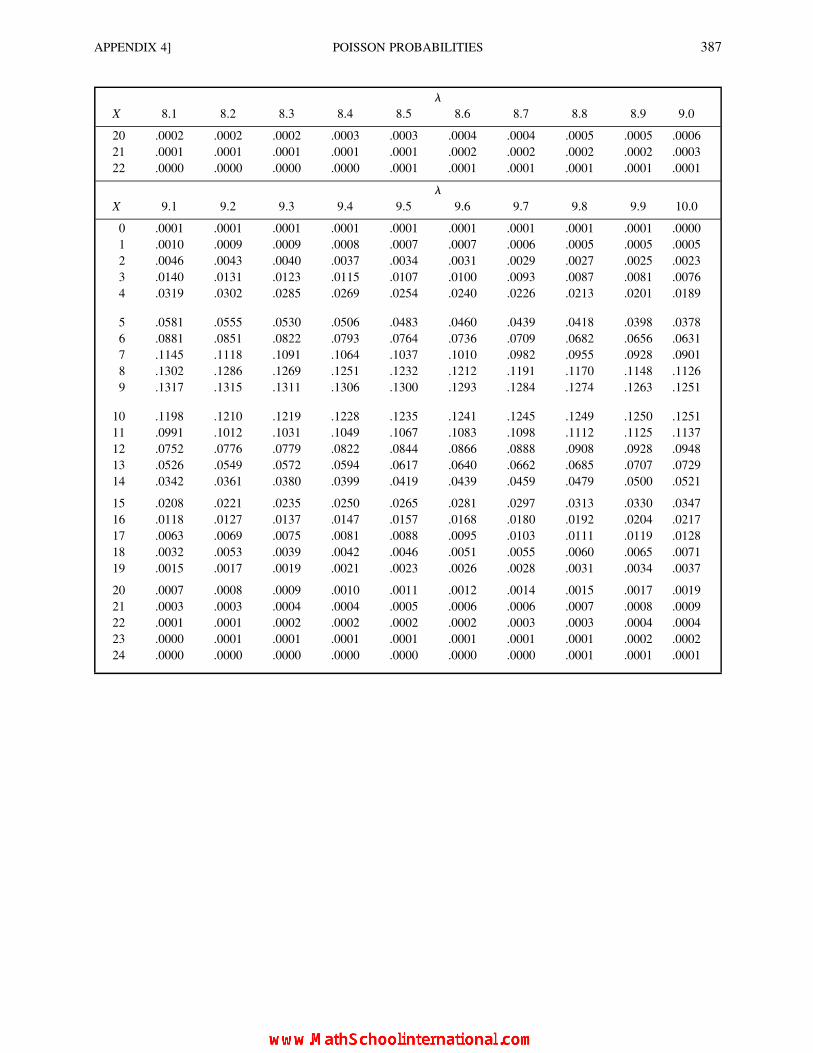
l
X 8.1 8.2 8.3 8.4 8.5 8.6 8.7 8.8 8.9 9.0
20 .0002 .0002 .0002 .0003 .0003 .0004 .0004 .0005 .0005 .0006
21 .0001 .0001 .0001 .0001 .0001 .0002 .0002 .0002 .0002 .0003
22 .0000 .0000 .0000 .0000 .0001 .0001 .0001 .0001 .0001 .0001
l
X 9.1 9.2 9.3 9.4 9.5 9.6 9.7 9.8 9.9 10.0
0 .0001 .0001 .0001 .0001 .0001 .0001 .0001 .0001 .0001 .0000
1 .0010 .0009 .0009 .0008 .0007 .0007 .0006 .0005 .0005 .0005
2 .0046 .0043 .0040 .0037 .0034 .0031 .0029 .0027 .0025 .0023
3 .0140 .0131 .0123 .0115 .0107 .0100 .0093 .0087 .0081 .0076
4 .0319 .0302 .0285 .0269 .0254 .0240 .0226 .0213 .0201 .0189
5 .0581 .0555 .0530 .0506 .0483 .0460 .0439 .0418 .0398 .0378
6 .0881 .0851 .0822 .0793 .0764 .0736 .0709 .0682 .0656 .0631
7 .1145 .1118 .1091 .1064 .1037 .1010 .0982 .0955 .0928 .0901
8 .1302 .1286 .1269 .1251 .1232 .1212 .1191 .1170 .1148 .1126
9 .1317 .1315 .1311 .1306 .1300 .1293 .1284 .1274 .1263 .1251
10 .1198 .1210 .1219 .1228 .1235 .1241 .1245 .1249 .1250 .1251
11 .0991 .1012 .1031 .1049 .1067 .1083 .1098 .1112 .1125 .1137
12 .0752 .0776 .0779 .0822 .0844 .0866 .0888 .0908 .0928 .0948
13 .0526 .0549 .0572 .0594 .0617 .0640 .0662 .0685 .0707 .0729
14 .0342 .0361 .0380 .0399 .0419 .0439 .0459 .0479 .0500 .0521
15 .0208 .0221 .0235 .0250 .0265 .0281 .0297 .0313 .0330 .0347
16 .0118 .0127 .0137 .0147 .0157 .0168 .0180 .0192 .0204 .0217
17 .0063 .0069 .0075 .0081 .0088 .0095 .0103 .0111 .0119 .0128
18 .0032 .0053 .0039 .0042 .0046 .0051 .0055 .0060 .0065 .0071
19 .0015 .0017 .0019 .0021 .0023 .0026 .0028 .0031 .0034 .0037
20 .0007 .0008 .0009 .0010 .0011 .0012 .0014 .0015 .0017 .0019
21 .0003 .0003 .0004 .0004 .0005 .0006 .0006 .0007 .0008 .0009
22 .0001 .0001 .0002 .0002 .0002 .0002 .0003 .0003 .0004 .0004
23 .0000 .0001 .0001 .0001 .0001 .0001 .0001 .0001 .0002 .0002
24 .0000 .0000 .0000 .0000 .0000 .0000 .0000 .0001 .0001 .0001
APPENDIX 4] POISSON PROBABILITIES 387

APPENDIX 5
Proportions of Areafor the StandardNormal Distribution
388
Copyright 2004, 1996, 1988, 1976 by The McGraw-Hill Companies, Inc. Click Here for Terms of Use.

z .00 .01 .02 .03 .04 .05 .06 .07 .08 .09
0.0 .0000 .0040 .0080 .0120 .0160 .0199 .0239 .0279 .0319 .0359
0.1 .0398 .0438 .0478 .0517 .0557 .0596 .0636 .0675 .0714 .0753
0.2 .0793 .0832 .0871 .0910 .0948 .0987 .1026 .1064 .1103 .1141
0.3 .1179 .1217 .1255 .1293 .1331 .1368 .1406 .1443 .1480 .1517
0.4 .1554 .1591 .1628 .1664 .1700 .1736 .1772 .1808 .1844 .1879
0.5 .1915 .1950 .1985 .2019 .2054 .2088 .2123 .2157 .2190 .2224
0.6 .2257 .2291 .2324 .2357 .2389 .2422 .2454 .2486 .2518 .2549
0.7 .2580 .2612 .2642 .2673 .2704 .2734 .2764 .2794 .2823 .2852
0.8 .2881 .2910 .2939 .2967 .2995 .3023 .3051 .3078 .3106 .3133
0.9 .3159 .3186 .3212 .3238 .3264 .3289 .3315 .3340 .3365 .3389
1.0 .3413 .3438 .3461 .3485 .3508 .3531 .3554 .3577 .3599 .3621
1.1 .3643 .3665 .3686 .3708 .3729 .3749 .3770 .3790 .3810 .3830
1.2 .3849 .3869 .3888 .3907 .3925 .3944 .3962 .3980 .3997 .4014
1.3 .4032 .4049 .4066 .4082 .4099 .4115 .4131 .4147 .4162 .4177
1.4 .4192 .4207 .4222 .4236 .4251 .4265 .4279 .4292 .4306 .4319
1.5 .4332 .4345 .4357 .4370 .4382 .4394 .4406 .4418 .4429 .4441
1.6 .4452 .4463 .4474 .4484 .4495 .4505 .4515 .4525 .4535 .4545
1.7 .4554 .4564 .4573 .4582 .4591 .4599 .4608 .4616 .4625 .4633
1.8 .4641 .4649 .4656 .4664 .4671 .4678 .4686 .4693 .4699 .4706
1.9 .4713 .4719 .4725 .4732 .4738 .4744 .4750 .4756 .4761 .4767
2.0 .4772 .4778 .4783 .4788 .4793 .4798 .4803 .4808 .4812 .4817
2.1 .4821 .4826 .4830 .4834 .4838 .4842 .4846 .4850 .4854 .4857
2.2 .4861 .4864 .4868 .4871 .4875 .4878 .4881 .4884 .4887 .4890
2.3 .4893 .4896 .4898 .4901 .4904 .4906 .4909 .4911 .4913 .4916
2.4 .4918 .4920 .4922 .4925 .4927 .4929 .4931 .4932 .4934 .4936
2.5 .4938 .4940 .4941 .4943 .4945 .4946 .4948 .4949 .4951 .4952
2.6 .4953 .4955 .4956 .4957 .4959 .4960 .4961 .4962 .4963 .4964
2.7 .4965 .4966 .4967 .4968 .4969 .4970 .4971 .4972 .4973 .4974
2.8 .4974 .4975 .4976 .4977 .4977 .4978 .4979 .4979 .4980 .4981
2.9 .4981 .4982 .4983 .4983 .4984 .4984 .4985 .4985 .4986 .4986
3.0 .4987
3.5 .4997
4.0 .4999
*Example: for z ¼ 1.96, shaded area is 0.4750 out of the total area of 1.0000
APPENDIX 5] PROPORTIONS OF AREA FOR THE STANDARD NORMAL DISTRIBUTION 389
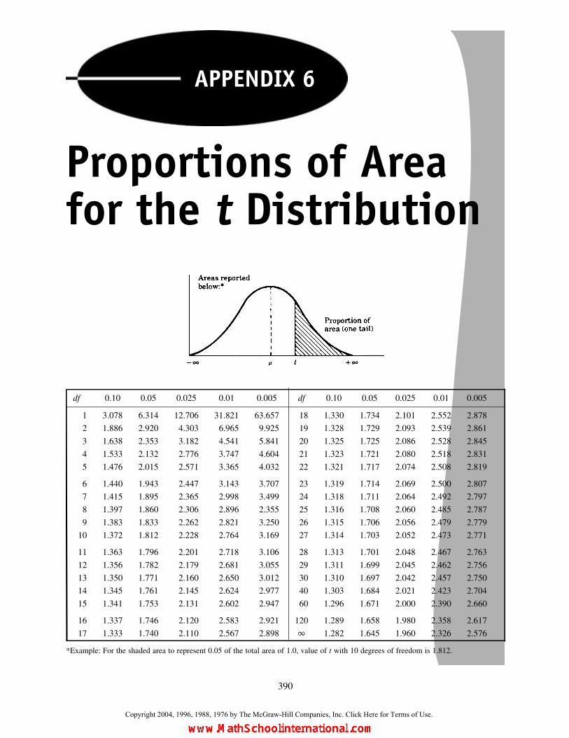
APPENDIX 6
Proportions of Areafor the t Distribution
df 0.10 0.05 0.025 0.01 0.005 df 0.10 0.05 0.025 0.01 0.005
1 3.078 6.314 12.706 31.821 63.657 18 1.330 1.734 2.101 2.552 2.878
2 1.886 2.920 4.303 6.965 9.925 19 1.328 1.729 2.093 2.539 2.861
3 1.638 2.353 3.182 4.541 5.841 20 1.325 1.725 2.086 2.528 2.845
4 1.533 2.132 2.776 3.747 4.604 21 1.323 1.721 2.080 2.518 2.831
5 1.476 2.015 2.571 3.365 4.032 22 1.321 1.717 2.074 2.508 2.819
6 1.440 1.943 2.447 3.143 3.707 23 1.319 1.714 2.069 2.500 2.807
7 1.415 1.895 2.365 2.998 3.499 24 1.318 1.711 2.064 2.492 2.797
8 1.397 1.860 2.306 2.896 2.355 25 1.316 1.708 2.060 2.485 2.787
9 1.383 1.833 2.262 2.821 3.250 26 1.315 1.706 2.056 2.479 2.779
10 1.372 1.812 2.228 2.764 3.169 27 1.314 1.703 2.052 2.473 2.771
11 1.363 1.796 2.201 2.718 3.106 28 1.313 1.701 2.048 2.467 2.763
12 1.356 1.782 2.179 2.681 3.055 29 1.311 1.699 2.045 2.462 2.756
13 1.350 1.771 2.160 2.650 3.012 30 1.310 1.697 2.042 2.457 2.750
14 1.345 1.761 2.145 2.624 2.977 40 1.303 1.684 2.021 2.423 2.704
15 1.341 1.753 2.131 2.602 2.947 60 1.296 1.671 2.000 2.390 2.660
16 1.337 1.746 2.120 2.583 2.921 120 1.289 1.658 1.980 2.358 2.617
17 1.333 1.740 2.110 2.567 2.898 1 1.282 1.645 1.960 2.326 2.576
*Example: For the shaded area to represent 0.05 of the total area of 1.0, value of t with 10 degrees of freedom is 1.812.
390
Copyright 2004, 1996, 1988, 1976 by The McGraw-Hill Companies, Inc. Click Here for Terms of Use.

APPENDIX 7
Proportions ofArea for the
x2 Distribution
391
Copyright 2004, 1996, 1988, 1976 by The McGraw-Hill Companies, Inc. Click Here for Terms of Use.

Proportion of area
df 0.995 0.990 0.975 0.950 0.900 0.500 0.100 0.050 0.025 0.010 0.005
1 0.00004 0.00016 0.00098 0.00393 0.0158 0.455 2.71 3.84 5.02 6.63 7.88
2 0.0100 0.0201 0.0506 0.103 0.211 1.386 4.61 5.99 7.38 9.21 10.60
3 0.072 0.115 0.216 0.352 0.584 2.366 6.25 7.81 9.35 11.34 12.84
4 0.207 0.297 0.484 0.711 1.064 3.357 7.78 9.49 11.14 13.28 14.86
5 0.412 0.554 0.831 1.145 1.61 4.251 9.24 11.07 12.83 15.09 16.75
6 0.676 0.872 1.24 1.64 2.20 5.35 10.64 12.59 14.45 16.81 18.55
7 0.989 1.24 1.69 2.17 2.83 6.35 12.02 14.07 16.01 18.48 20.28
8 1.34 1.65 2.18 2.73 3.49 7.34 13.36 15.51 17.53 20.09 21.96
9 1.73 2.09 2.70 3.33 4.17 8.34 14.68 16.92 19.02 21.67 23.59
10 2.16 2.56 3.25 3.94 4.87 9.34 15.99 18.31 20.48 23.21 25.19
11 2.60 3.05 3.82 4.57 5.58 10.34 17.28 19.68 21.92 24.73 26.76
12 3.07 3.57 4.40 5.23 6.30 11.34 18.55 21.03 23.34 26.22 28.30
13 3.57 4.11 5.01 5.89 7.04 12.34 19.81 22.36 24.74 27.69 29.82
14 4.07 4.66 5.63 6.57 7.79 13.34 21.06 23.68 26.12 29.14 31.32
15 4.60 5.23 6.26 7.26 8.55 14.34 22.31 25.00 27.49 30.58 32.80
16 5.14 5.81 6.91 7.96 9.31 15.34 23.54 26.30 28.85 32.00 34.27
17 5.70 6.41 7.56 8.67 10.09 16.34 24.77 27.59 30.19 33.41 35.72
18 6.26 7.01 8.23 9.39 10.86 17.34 25.99 28.87 31.53 34.81 37.16
19 6.84 7.63 8.91 10.12 11.65 18.34 27.20 30.14 32.85 36.19 38.58
20 7.43 8.26 9.59 10.85 12.44 19.34 28.41 31.41 34.17 37.57 40.00
21 8.03 8.90 10.28 11.59 13.24 20.34 29.62 32.67 35.48 38.93 41.40
22 8.64 9.54 10.98 12.34 14.04 21.34 30.81 33.92 36.78 40.29 42.80
23 9.26 10.20 11.69 13.09 14.85 22.34 32.01 35.17 38.08 41.64 44.18
24 9.89 10.86 12.40 13.85 15.66 23.34 33.20 36.42 39.36 42.98 45.56
25 10.52 11.52 13.12 14.61 16.47 24.34 34.38 37.65 40.65 44.31 46.93
26 11.16 12.20 13.84 15.38 17.29 25.34 35.56 38.89 41.92 45.64 48.29
27 11.81 12.83 14.57 16.15 18.11 26.34 36.74 40.11 43.19 46.96 49.64
28 12.46 13.56 15.31 16.93 18.94 27.34 37.92 41.34 44.46 48.28 50.99
29 13.12 14.26 16.05 17.71 19.77 28.34 39.09 42.56 45.72 49.59 52.34
30 13.79 14.95 16.79 18.49 20.60 29.34 40.26 43.77 46.98 50.89 53.67
40 20.71 22.16 24.43 26.51 29.05 39.34 51.81 55.76 59.34 63.69 66.77
50 27.99 29.71 32.36 34.76 37.69 49.33 63.17 67.50 71.42 76.15 79.49
60 35.53 37.43 40.48 43.19 46.46 59.33 74.40 79.08 83.30 88.38 91.95
70 43.28 45.44 48.76 51.74 55.33 69.33 85.53 90.53 95.02 100.4 104.2
80 51.17 53.54 51.17 60.39 64.28 79.33 98.58 101.9 106.6 112.3 116.3
90 59.20 61.75 65.65 69.13 73.29 89.33 107.6 113.1 118.1 124.1 128.3
100 67.33 70.06 74.22 77.93 82.36 99.33 118.5 124.3 129.6 135.8 140.2
*Example: For the shaded area to represent 0.05 of the total area of 1.0 under the density function, the value of x 2 is 18.31 when df ¼ 10.
392 PROPORTIONS OF AREA FOR THE x2 DISTRIBUTION [APPENDIX 7
APPENDIX 8
Values of FExceeded withProbabilities
of 5% and 1%
393
Copyright 2004, 1996, 1988, 1976 by The McGraw-Hill Companies, Inc. Click Here for Terms of Use.

df(numerator)
12
34
56
78
910
11
12
14
16
20
24
30
40
50
75
100
200
500
11
161
200
216
225
230
234
237
239
241
242
243
244
245
246
248
249
250
251
252
253
253
254
254
254
4,0
52
4,9
99
5,4
03
5,6
25
5,7
64
5,8
59
5,9
28
5,9
81
6,0
22
6,0
56
6,0
82
6,1
06
6,1
42
6,1
69
6,2
08
6,2
34
6,2
61
6,2
86
6,3
02
6,3
23
6,3
34
6,3
52
6,3
61
6,3
66
218.51
19.00
19.16
19.25
19.30
19.33
19.36
19.37
19.38
19.39
19.40
19.41
19.42
19.43
19.44
19.45
19.46
19.47
19.47
19.48
19.49
19.49
19.50
19.50
98.4
999.0
099.1
799.2
599.3
099.3
399.3
699.3
799.3
999.4
099.4
199.4
299.4
399.4
499.4
599.4
699.4
799.4
899.4
899.4
999.4
999.4
999.5
099.5
0
310.13
9.55
9.28
9.12
9.01
8.94
8.88
8.84
8.81
8.78
8.76
8.74
8.71
8.69
8.66
8.64
8.62
8.60
8.58
8.57
8.56
8.54
8.54
8.53
34.1
230.8
229.4
628.7
128.2
427.9
127.6
727.4
927.3
427.2
327.1
327.0
526.9
226.8
326.6
926.6
026.5
026.4
126.3
526.2
726.2
326.1
826.1
426.1
2
47.71
6.94
6.59
6.39
6.26
6.16
6.09
6.04
6.00
5.96
5.93
5.91
5.87
5.84
5.80
5.77
5.74
5.71
5.70
5.68
5.66
5.65
5.64
5.63
21.2
018.0
016.6
915.9
815.5
215.2
114.9
814.8
014.6
614.5
414.4
514.3
714.2
414.1
514.0
213.9
313.8
313.7
413.6
913.6
113.5
713.5
213.4
813.4
6
56.61
5.79
5.41
5.19
5.05
4.95
4.88
4.82
4.78
4.74
4.70
4.68
4.64
4.60
4.56
4.53
4.50
4.46
4.44
4.42
4.40
4.38
4.37
4.36
16.2
613.2
712.0
611.3
910.9
710.6
710.4
510.2
910.1
510.0
59.9
69.8
99.7
79.6
89.5
59.4
79.3
89.2
99.2
49.1
79.1
39.0
79.0
49.0
2
65.99
5.14
4.76
4.53
4.39
4.28
4.21
4.15
4.10
4.06
4.03
4.00
3.96
3.92
3.87
3.84
3.81
3.77
3.75
3.72
3.71
3.69
3.68
3.67
13.7
410.9
29.7
89.1
58.7
58.4
78.2
68.1
07.9
87.8
77.7
97.7
27.6
07.5
27.3
97.3
17.2
37.1
47.0
97.0
26.9
96.9
46.9
06.8
8
75.59
4.74
4.34
4.12
3.97
3.87
3.79
3.73
3.68
3.63
3.60
3.57
3.52
3.49
3.44
3.41
3.38
3.34
3.32
3.29
3.28
3.25
3.24
3.23
12.2
59.5
58.4
57.8
57.4
67.1
97.0
06.8
46.7
16.6
26.5
46.4
76.3
56.2
76.1
56.0
75.9
85.9
05.8
55.7
85.7
55.7
05.6
75.6
5
85.32
4.46
4.07
3.84
3.69
3.58
3.50
3.44
3.39
3.34
3.31
3.28
3.23
3.20
3.15
3.12
3.08
3.05
3.03
3.00
2.98
2.96
2.94
2.93
11.2
68.6
57.5
97.0
16.6
36.3
76.1
96.0
35.9
15.8
25.7
45.6
75.5
65.4
85.3
65.2
85.2
05.1
15.0
65.0
04.9
64.9
14.8
84.8
6
95.12
4.26
3.86
3.63
3.48
3.37
3.29
3.23
3.18
3.13
3.10
3.07
3.02
2.98
2.93
2.90
2.86
2.82
2.80
2.77
2.76
2.73
2.72
2.71
10.5
68.0
26.9
96.4
26.0
65.8
05.6
25.4
75.3
55.2
65.1
85.1
15.0
04.9
24.8
04.7
34.6
44.5
64.5
14.4
54.4
14.3
64.3
34.3
1
10
4.96
4.10
3.71
3.48
3.33
3.22
3.14
3.07
3.02
2.97
2.94
2.91
2.86
2.82
2.77
2.74
2.70
2.67
2.64
2.61
2.59
2.56
2.55
2.54
10.0
47.5
66.5
55.9
95.6
45.3
95.2
15.0
64.9
54.8
54.7
84.7
14.6
04.5
24.4
14.3
34.2
54.1
74.1
24.0
54.0
13.9
63.9
33.9
1
11
4.84
3.98
3.59
3.36
3.20
3.09
3.01
2.95
2.90
2.86
2.82
2.79
2.74
2.70
2.65
2.61
2.57
2.53
2.50
2.47
2.45
2.42
2.41
2.40
9.6
57.2
06.2
25.6
75.3
25.0
74.8
84.7
44.6
34.5
44.4
64.4
04.2
94.2
14.1
04.0
23.9
43.8
63.8
03.7
43.7
03.6
63.6
23.6
0
12
4.75
3.88
3.49
3.26
3.11
3.00
2.92
2.85
2.80
2.76
2.72
2.69
2.64
2.60
2.54
2.50
2.46
2.42
2.40
2.36
2.35
2.32
2.31
2.30
9.3
36.9
35.9
55.4
15.0
64.8
24.6
54.5
04.3
94.3
04.2
24.1
64.0
53.9
83.8
63.7
83.7
03.6
13.5
63.4
93.4
63.4
13.3
83.3
6
13
4.67
3.80
3.41
3.18
3.02
2.92
2.84
2.77
2.72
2.67
2.63
2.60
2.55
2.51
2.46
2.42
2.38
2.34
2.32
2.28
2.26
2.24
2.22
2.21
9.0
76.7
05.7
45.2
04.8
64.6
24.4
44.3
04.1
94.1
04.0
23.9
63.8
53.7
83.6
73.5
93.5
13.4
23.3
73.3
03.2
73.2
13.1
83.1
6
14
4.60
3.74
3.34
3.11
2.96
2.85
2.77
2.70
2.65
2.60
2.56
2.53
2.48
2.44
2.39
2.35
2.31
2.27
2.24
2.21
2.19
2.16
2.14
2.13
8.8
66.5
15.5
65.0
34.6
94.4
64.2
84.1
44.0
33.9
43.8
63.8
03.7
03.6
23.5
13.4
33.3
43.2
63.2
13.1
43.1
13.0
63.0
23.0
0
15
4.54
3.68
3.29
3.06
2.90
2.79
2.70
2.64
2.59
2.55
2.51
2.48
2.43
2.39
2.33
2.29
2.25
2.21
2.18
2.15
2.12
2.10
2.08
2.07
8.6
86.3
65.4
24.8
94.5
64.3
24.1
44.0
03.8
93.8
03.7
33.6
73.5
63.4
83.3
63.2
93.2
03.1
23.0
73.0
02.9
72.9
22.8
92.8
7
16
4.49
3.63
3.24
3.01
2.85
2.74
2.66
2.59
2.54
2.49
2.45
2.42
2.37
2.33
2.28
2.24
2.20
2.16
2.13
2.09
2.07
2.04
2.02
2.01
8.5
36.2
35.2
94.7
74.4
44.2
04.0
33.8
93.7
83.6
93.6
13.5
53.4
53.3
73.2
53.1
83.1
03.0
12.9
62.8
82.8
62.8
02.7
72.7
5
17
4.45
3.59
3.20
2.96
2.81
2.70
2.62
2.55
2.50
2.45
2.41
2.38
2.33
2.29
2.23
2.19
2.15
2.11
2.08
2.04
2.02
1.99
1.97
1.96
8.4
06.1
15.1
84.6
74.3
44.1
03.9
33.7
93.6
83.5
93.5
23.4
53.3
53.2
73.1
63.0
83.0
02.9
22.8
62.7
92.7
62.7
02.6
72.6
5
18
4.41
3.55
3.16
2.93
2.77
3.66
2.58
2.51
2.46
2.41
2.37
2.34
2.29
2.25
2.19
2.15
2.11
2.07
2.04
2.00
1.98
1.95
1.93
1.92
8.2
86.0
15.0
94.5
84.2
54.0
13.8
53.7
13.6
03.5
13.4
43.3
73.2
73.1
93.0
73.0
02.9
12.8
32.7
82.7
12.6
82.6
22.5
92.5
7
(conti
nued
)
df(denominator)
394 VALUES OF F EXCEEDED WITH PROBABILITIES OF 5% AND 1% [APPENDIX 8

df(numerator)
12
34
56
78
910
11
12
14
16
20
24
30
40
50
75
100
200
500
119
4.38
3.52
3.13
2.90
2.74
2.63
2.55
2.48
2.43
2.38
2.34
2.31
2.26
2.21
2.15
2.11
2.07
2.02
2.00
1.96
1.94
1.91
1.90
1.88
8.1
85.9
35.0
14.5
04.1
73.9
43.7
73.6
33.5
23.4
33.3
63.3
03.1
93.1
23.0
02.9
22.8
42.7
62.7
02.6
32.6
02.5
42.5
12.4
9
20
4.35
3.49
3.10
2.87
2.71
2.60
2.52
2.45
2.40
2.35
2.31
2.28
2.23
2.18
2.12
2.08
2.04
1.99
1.96
1.92
1.90
1.87
1.85
1.84
8.1
05.8
54.9
44.4
34.1
03.8
73.7
13.5
63.4
53.3
73.3
03.2
33.1
33.0
52.9
42.8
62.7
72.6
92.6
32.5
62.5
32.4
72.4
42.4
2
21
4.32
3.47
3.07
2.84
2.68
2.57
2.49
2.42
2.37
2.32
2.28
2.25
2.20
2.15
2.09
2.05
2.00
1.96
1.93
1.89
1.87
1.84
1.82
1.81
8.0
25.7
84.8
74.3
74.0
43.8
13.6
53.5
13.4
03.3
13.2
43.1
73.0
72.9
92.8
82.8
02.7
22.6
32.5
82.5
12.4
72.4
22.3
82.3
6
22
4.30
3.44
3.05
2.82
2.66
2.55
2.47
2.40
2.35
2.30
2.26
2.23
2.18
2.13
2.07
2.03
1.98
1.93
1.91
1.87
1.84
1.81
1.80
1.78
7.9
45.7
24.8
24.3
13.9
93.7
63.5
93.4
53.3
53.2
63.1
83.1
23.0
22.9
42.8
32.7
52.6
72.5
82.5
32.4
62.4
22.3
72.3
32.3
1
23
4.28
3.42
3.03
2.80
2.64
2.53
2.45
2.38
2.32
2.28
2.24
2.20
2.14
2.10
2.04
2.00
1.96
1.91
1.88
1.84
1.82
1.79
1.77
1.76
7.8
85.6
64.7
64.2
63.9
43.7
13.5
43.4
13.3
03.2
13.1
43.0
72.9
72.8
92.7
82.7
02.6
22.5
32.4
82.4
12.3
72.3
22.2
82.2
6
24
4.26
3.40
3.01
2.78
2.62
2.51
2.43
2.36
2.30
2.26
2.22
2.18
2.13
2.09
2.02
1.98
1.94
1.89
1.86
1.82
1.80
1.76
1.74
1.73
7.8
25.6
14.7
24.2
23.9
03.6
73.5
03.3
63.2
53.1
73.0
93.0
32.9
32.8
52.7
42.6
62.5
82.4
92.4
42.3
62.3
32.2
72.2
32.2
1
25
4.24
3.38
2.99
2.76
2.60
2.49
2.41
2.34
2.28
2.24
2.20
2.16
2.11
2.06
2.00
1.96
1.92
1.87
1.84
1.80
1.77
1.74
1.72
1.71
7.7
75.5
74.6
84.1
83.8
63.6
33.4
63.3
23.2
13.1
33.0
52.9
92.8
92.8
12.7
02.6
22.5
42.4
52.4
02.3
22.2
92.2
32.1
92.1
7
26
4.22
3.37
2.98
2.74
2.59
2.47
2.39
2.32
2.27
2.22
2.18
2.15
2.10
2.05
1.99
1.95
1.90
1.85
1.82
1.78
1.76
1.72
1.70
1.69
7.7
25.5
34.6
44.1
43.8
23.5
93.4
23.2
93.1
73.0
93.0
22.9
62.8
62.7
72.6
62.5
82.5
02.4
12.3
62.2
82.2
52.1
92.1
52.1
3
27
4.21
3.35
2.96
2.73
2.57
2.46
2.37
2.30
2.25
2.20
2.16
2.13
2.08
2.03
1.97
1.93
1.88
1.84
1.80
1.76
1.74
1.71
1.68
1.67
7.6
85.4
94.6
04.1
13.7
93.5
63.3
93.2
63.1
43.0
62.9
82.9
32.8
32.7
42.6
32.5
52.4
72.3
82.3
32.2
52.2
12.1
62.1
22.1
0
28
4.20
3.34
2.95
2.71
2.56
2.44
2.36
2.29
2.24
2.19
2.15
2.12
2.06
2.02
1.96
1.91
1.87
1.81
1.78
1.75
1.72
1.69
1.67
1.65
7.6
45.4
54.5
74.0
73.7
63.5
33.3
63.2
33.1
13.0
32.9
52.9
02.8
02.7
12.6
02.5
22.4
42.3
52.3
02.2
22.1
82.1
32.0
92.0
6
29
4.18
3.33
2.93
2.70
2.54
2.43
2.35
2.28
2.22
2.18
2.14
2.10
2.05
2.00
1.94
1.90
1.85
1.80
1.77
1.73
1.71
1.68
1.65
1.64
7.6
05.4
24.5
44.0
43.7
33.5
03.3
33.2
03.0
83.0
02.9
22.8
72.7
72.6
82.5
72.4
92.4
12.3
22.2
72.1
92.1
52.1
02.0
62.0
3
30
4.17
3.32
2.92
2.69
2.53
2.42
2.34
2.27
2.21
2.16
2.12
2.09
2.04
1.99
1.93
1.89
1.84
1.79
1.76
1.72
1.69
1.66
1.64
1.62
7.5
65.3
94.5
14.0
23.7
03.4
73.3
03.1
73.0
62.9
82.9
02.8
42.7
42.6
62.5
52.4
72.3
82.2
92.2
42.1
62.1
32.0
72.0
32.0
1
32
4.15
3.30
2.90
2.67
2.51
2.40
2.32
2.25
2.19
2.14
2.10
2.07
2.02
1.97
1.91
1.86
1.82
1.76
1.74
1.69
1.67
1.64
1.61
1.59
7.5
05.3
44.4
63.9
73.6
63.4
23.2
53.1
23.0
12.9
42.8
62.8
02.7
02.6
22.5
12.4
22.3
42.2
52.2
02.1
22.0
82.0
21.9
81.9
6
34
4.13
3.28
2.88
2.65
2.49
2.38
2.30
2.23
2.17
2.12
2.08
2.05
2.00
1.95
1.89
1.84
1.80
1.74
1.71
1.67
1.64
1.61
1.59
1.57
7.4
45.2
94.4
23.9
33.6
13.3
83.2
13.0
82.9
72.8
92.8
22.7
62.6
62.5
82.4
72.3
82.3
02.2
12.1
52.0
82.0
41.9
81.9
41.9
1
36
4.11
3.26
2.86
2.63
2.48
2.36
2.28
2.21
2.15
2.10
2.06
2.03
1.98
1.93
1.87
1.82
1.78
1.72
1.69
1.65
1.62
1.59
1.56
1.55
7.3
95.2
54.3
83.8
93.5
83.3
53.1
83.0
42.9
42.8
62.7
82.7
22.6
22.5
42.4
32.3
52.2
62.1
72.1
22.0
42.0
01.9
41.9
01.8
7
38
4.10
3.25
2.85
2.62
2.46
2.35
2.26
2.19
2.14
2.09
2.05
2.02
1.96
1.92
1.85
1.80
1.76
1.71
1.67
1.63
1.60
1.57
1.54
1.53
7.3
55.2
14.3
43.8
63.5
43.3
23.1
53.0
22.9
12.8
22.7
52.6
92.5
92.5
12.4
02.3
22.2
22.1
42.0
82.0
01.9
71.9
01.8
61.8
4
40
4.07
3.23
2.84
2.61
2.45
2.34
2.25
2.18
2.12
2.07
2.04
2.00
1.95
1.90
1.84
1.79
1.74
1.69
1.66
1.61
1.59
1.55
1.53
1.51
7.3
15.1
84.3
13.8
33.5
13.2
93.1
22.9
92.8
82.8
02.7
32.6
62.5
62.4
92.3
72.2
92.2
02.1
12.0
51.9
71.9
41.8
81.8
41.8
1
(conti
nued
)
df(denominator)
APPENDIX 8] VALUES OF F EXCEEDED WITH PROBABILITIES OF 5% AND 1% 395

df(numerator)
12
34
56
78
910
11
12
14
16
20
24
30
40
50
75
100
200
500
142
4.07
3.22
2.83
2.59
2.44
2.32
2.24
2.17
2.11
2.06
2.02
1.99
1.94
1.89
1.82
1.78
1.73
1.68
1.64
1.60
1.57
1.54
1.51
1.49
7.2
75.1
54.2
93.8
03.4
93.2
63.1
02.9
62.8
62.7
72.7
02.6
42.5
42.4
62.3
52.2
62.1
72.0
82.0
21.9
41.9
11.8
51.8
01.7
8
44
4.06
3.21
2.82
2.58
2.43
2.31
2.23
2.16
2.10
2.05
2.01
1.98
1.92
1.88
1.81
1.76
1.72
1.66
1.63
1.58
1.56
1.52
1.50
1.48
7.2
45.1
24.2
63.7
83.4
63.2
43.0
72.9
42.8
42.7
52.6
82.6
22.5
22.4
42.3
22.2
42.1
52.0
62.0
01.9
21.8
81.8
21.7
81.7
5
46
4.05
3.20
2.81
2.57
2.42
2.30
2.22
2.14
2.09
2.04
2.00
1.97
1.91
1.87
1.80
1.75
1.71
1.65
1.62
1.57
1.54
1.51
1.48
1.46
7.2
15.1
04.2
43.7
63.4
43.2
23.0
52.9
22.8
22.7
32.6
62.6
02.5
02.4
22.3
02.2
22.1
32.0
41.9
81.9
01.8
61.8
01.7
61.7
2
48
4.04
3.19
2.80
2.56
2.41
2.30
2.21
2.14
2.08
2.03
1.99
1.96
1.90
1.86
1.79
1.74
1.70
1.64
1.61
1.56
1.53
1.50
1.47
1.45
7.1
95.0
84.2
23.7
43.4
23.2
03.0
42.9
02.8
02.7
12.6
42.5
82.4
82.4
02.2
82.2
02.1
12.0
21.9
61.8
81.8
41.7
81.7
31.7
0
50
4.03
3.18
2.79
2.56
2.40
2.29
2.20
2.13
2.07
2.02
1.98
1.95
1.90
1.85
1.78
1.74
1.69
1.63
1.60
1.55
1.52
1.48
1.46
1.44
7.1
75.0
64.2
03.7
23.4
13.1
83.0
22.8
82.7
82.7
02.6
22.5
62.4
62.3
92.2
62.1
82.1
02.0
01.9
41.8
61.8
21.7
61.7
11.6
8
55
4.02
3.17
2.78
2.54
2.38
2.27
2.18
2.11
2.05
2.00
1.97
1.93
1.88
1.83
1.76
1.72
1.67
1.61
1.58
1.52
1.50
1.46
1.43
1.41
7.1
25.0
14.1
63.6
83.3
73.1
52.9
82.8
52.7
52.6
62.5
92.5
32.4
32.3
52.2
32.1
52.0
61.9
61.9
01.8
21.7
81.7
11.6
61.6
4
60
4.00
3.15
2.76
2.52
2.37
2.25
2.17
2.10
2.04
1.99
1.95
1.92
1.86
1.81
1.75
1.70
1.65
1.59
1.56
1.50
1.48
1.44
1.41
1.39
7.0
84.9
84.1
33.6
53.3
43.1
22.9
52.8
22.7
22.6
32.5
62.5
02.4
02.3
22.2
02.1
22.0
31.9
31.8
71.7
91.7
41.6
81.6
31.6
0
65
3.99
3.14
2.75
2.51
2.36
2.24
2.15
2.08
2.02
1.98
1.94
1.90
1.85
1.80
1.73
1.68
1.63
1.57
1.54
1.49
1.46
1.42
1.39
1.37
7.0
44.9
54.1
03.6
23.3
13.0
92.9
32.7
92.7
02.6
12.5
42.4
72.3
72.3
02.1
82.0
92.0
01.9
01.8
41.7
61.7
11.6
41.6
01.5
6
70
3.98
3.13
2.74
2.50
2.35
2.23
2.14
2.07
2.01
1.97
1.93
1.89
1.84
1.79
1.72
1.67
1.62
1.56
1.53
1.47
1.45
1.40
1.37
1.35
7.0
14.9
24.0
83.6
03.2
93.0
72.9
12.7
72.6
72.5
92.5
12.4
52.3
52.2
82.1
52.07
1.9
81.8
81.8
21.7
41.6
91.6
21.5
61.5
3
80
3.96
3.11
2.72
2.48
2.33
2.21
2.12
2.05
1.99
1.95
1.91
1.88
1.82
1.77
1.70
1.65
1.60
1.54
1.51
1.45
1.42
1.38
1.35
1.32
6.9
64.8
84.0
43.5
63.2
53.0
42.8
72.7
42.6
42.5
52.4
82.4
12.3
22.2
42.1
12.0
31.9
41.8
41.7
81.7
01.6
51.5
71.5
21.4
9
100
3.94
3.09
2.70
2.46
2.30
2.19
2.10
2.03
1.97
1.92
1.88
1.85
1.79
1.75
1.68
1.63
1.57
1.51
1.48
1.42
1.39
1.34
1.30
1.28
6.9
04.8
23.9
83.5
13.2
02.9
92.8
22.6
92.5
92.5
12.4
32.3
62.2
62.1
92.0
61.9
81.8
91.7
91.7
31.6
41.5
91.5
11.4
61.4
3
125
3.92
3.07
2.68
2.44
2.29
2.17
2.08
2.01
1.95
1.90
1.86
1.83
1.77
1.72
1.65
1.60
1.55
1.49
1.45
1.39
1.36
1.31
1.27
1.25
6.8
44.7
83.9
43.4
73.1
72.9
52.7
92.6
52.5
62.4
72.4
02.3
32.2
32.1
52.0
31.9
41.8
51.7
51.6
81.5
91.5
41.4
61.4
01.3
7
150
3.91
3.06
2.67
2.43
2.27
2.16
2.07
2.00
1.94
1.89
1.85
1.82
1.76
1.71
1.64
1.59
1.54
1.47
1.44
1.37
1.34
1.29
1.25
1.22
6.8
14.7
53.9
13.4
43.1
42.9
22.7
62.6
22.5
32.4
42.3
72.3
02.2
02.1
22.0
01.9
11.8
31.7
21.6
61.5
61.5
11.4
31.3
71.3
3
200
3.89
3.04
2.65
2.41
2.26
2.14
2.05
1.98
1.92
1.87
1.83
1.80
1.74
1.69
1.62
1.57
1.52
1.45
1.42
1.35
1.32
1.26
1.22
1.19
6.7
64.7
13.8
83.4
13.1
12.9
02.7
32.6
02.5
02.4
12.3
42.2
82.1
72.0
91.9
71.8
81.7
91.6
91.6
21.5
31.4
81.3
91.3
31.2
8
400
3.86
3.02
2.62
2.39
2.23
2.12
2.03
1.96
1.90
1.85
1.91
1.78
1.72
1.67
1.60
1.54
1.49
1.42
1.38
1.32
1.28
1.22
1.16
1.13
6.7
04.6
63.8
33.3
63.0
62.8
52.6
92.5
52.4
62.3
72.2
92.2
32.1
22.0
41.9
21.8
41.7
41.6
41.5
71.4
71.4
21.3
21.2
41.1
9
1000
3.85
3.00
2.61
2.38
2.22
2.10
2.02
1.95
1.89
1.84
1.80
1.76
1.70
1.65
1.58
1.53
1.47
1.41
1.36
1.30
1.26
1.19
1.13
1.08
6.6
64.6
23.8
03.3
43.0
42.8
22.6
62.5
32.4
32.3
42.2
62.2
02.0
92.0
11.8
91.8
11.7
11.6
11.5
41.4
41.3
81.2
81.1
91.1
1
13.84
2.99
2.60
2.37
2.21
2.09
2.01
1.94
1.88
1.83
1.79
1.75
1.69
1.64
1.57
1.52
1.46
1.40
1.35
1.28
1.24
1.17
1.11
1.00
6.6
44.6
03.7
83.3
23.0
22.8
02.6
42.5
12.4
12.3
22.2
42.1
82.0
71.9
91.8
71.7
91.6
91.5
91.5
21.4
11.3
61.2
51.1
51.0
0
df(denominator)
396 VALUES OF F EXCEEDED WITH PROBABILITIES OF 5% AND 1% [APPENDIX 8

APPENDIX 9
Factors for ControlCharts
Sample
size
n c4 c5 d2 d3 D3 D4
2 0.7979 0.6028 1.128 0.853 0 3.267
3 0.8862 0.4633 1.693 0.888 0 2.574
4 0.9213 0.3889 2.059 0.880 0 2.282
5 0.9400 0.3412 2.326 0.864 0 2.114
6 0.9515 0.3076 2.534 0.848 0 2.004
7 0.9594 0.2820 2.704 0.833 0.076 1.924
8 0.9650 0.2622 2.847 0.820 0.136 1.864
9 0.9693 0.2459 2.970 0.808 0.184 1.816
10 0.9727 0.2321 3.078 0.797 0.223 1.777
11 0.9754 0.2204 3.173 0.787 0.256 1.744
12 0.9776 0.2105 3.258 0.778 0.283 1.717
13 0.9794 0.2019 3.336 0.770 0.307 1.693
14 0.9810 0.1940 3.407 0.763 0.328 1.672
15 0.9823 0.1873 3.472 0.756 0.347 1.653
16 0.9835 0.1809 3.532 0.750 0.363 1.637
17 0.9845 0.1754 3.588 0.744 0.378 1.622
18 0.9854 0.1703 3.640 0.739 0.391 1.608
19 0.9862 0.1656 3.689 0.734 0.403 1.597
20 0.9869 0.1613 3.735 0.729 0.415 1.585
21 0.9876 0.1570 3.778 0.724 0.425 1.575
22 0.9882 0.1532 3.819 0.720 0.434 1.566
23 0.9887 0.1499 3.858 0.716 0.443 1.557
24 0.9892 0.1466 3.895 0.712 0.451 1.548
25 0.9896 0.1438 3.931 0.708 0.459 1.541
397
Copyright 2004, 1996, 1988, 1976 by The McGraw-Hill Companies, Inc. Click Here for Terms of Use.

APPENDIX 10
Critical Values of T inthe Wilcoxon Test
1-sided 2-sided n ¼ 5 n ¼ 6 n ¼ 7 n ¼ 8 n ¼ 9 n ¼ 10
P ¼ 0.05 P ¼ 0.10 1 2 4 6 8 11
P ¼ 0.025 P ¼ 0.05 1 2 4 6 8
P ¼ 0.01 P ¼ 0.02 0 2 3 5
P ¼ 0.005 P ¼ 0.01 0 2 3
1-sided 2-sided n ¼ 11 n ¼ 12 n ¼ 13 n ¼ 14 n ¼ 15 n ¼ 16
P ¼ 0.05 P ¼ 0.10 14 17 21 26 30 36
P ¼ 0.025 P ¼ 0.05 11 14 17 21 25 30
P ¼ 0.01 P ¼ 0.02 7 10 13 16 20 24
P ¼ 0.005 P ¼ 0.01 5 7 10 13 16 19
1-sided 2-sided n ¼ 17 n ¼ 18 n ¼ 19 n ¼ 20 n ¼ 21 n ¼ 22
P ¼ 0.05 P ¼ 0.10 41 47 54 60 68 75
P ¼ 0.025 P ¼ 0.05 35 40 46 52 59 66
P ¼ 0.01 P ¼ 0.02 28 33 38 43 49 56
P ¼ 0.005 P ¼ 0.01 23 28 32 37 43 49
1-sided 2-sided n ¼ 23 n ¼ 24 n ¼ 25 n ¼ 26 n ¼ 27 n ¼ 28
P ¼ 0.05 P ¼ 0.10 83 92 101 110 120 130
P ¼ 0.025 P ¼ 0.05 73 81 90 98 107 117
P ¼ 0.01 P ¼ 0.02 62 69 77 85 93 102
P ¼ 0.005 P ¼ 0.01 55 68 68 75 84 92
1-sided 2-sided n ¼ 29 n ¼ 30 n ¼ 31 n ¼ 32 n ¼ 33 n ¼ 34
P ¼ 0.05 P ¼ 0.10 141 152 163 175 188 201
P ¼ 0.025 P ¼ 0.05 127 137 148 159 171 183
P ¼ 0.01 P ¼ 0.02 111 120 130 141 151 162
P ¼ 0.005 P ¼ 0.01 100 109 118 128 138 149
398
Copyright 2004, 1996, 1988, 1976 by The McGraw-Hill Companies, Inc. Click Here for Terms of Use.

1-sided 2-sided n ¼ 35 n ¼ 36 n ¼ 37 n ¼ 38 n ¼ 39 n ¼ 40
P ¼ 0.05 P ¼ 0.10 214 228 242 256 271 287
P ¼ 0.025 P ¼ 0.05 195 208 222 235 250 264
P ¼ 0.01 P ¼ 0.02 174 186 198 211 224 238
P ¼ 0.005 P ¼ 0.01 160 171 183 195 208 221
1-sided 2-sided n ¼ 41 n ¼ 42 n ¼ 43 n ¼ 44 n ¼ 45
P ¼ 0.05 P ¼ 0.10 303 319 336 353 371
P ¼ 0.025 P ¼ 0.05 279 295 311 327 344
P ¼ 0.01 P ¼ 0.02 252 267 281 297 313
P ¼ 0.005 P ¼ 0.01 234 248 262 277 292
1-sided 2-sided n ¼ 46 n ¼ 47 n ¼ 48 n ¼ 49 n ¼ 50
P ¼ 0.05 P ¼ 0.10 389 408 427 446 466
P ¼ 0.025 P ¼ 0.05 361 379 397 415 434
P ¼ 0.01 P ¼ 0.02 329 345 362 380 398
P ¼ 0.005 P ¼ 0.01 307 323 339 356 373
APPENDIX 10] CRITICAL VALUES OF T IN THE WILCOXON TEST 399

INDEX
Absolute deviations, 46, 59
Addition, rules of, 76–77
Alternative hypothesis, 175
Amount certain, 343
Analysis of variance, 241–246
basic rationale, 241–242
one-factor completely randomized
design, 242–243
randomized-block design, 243–244
in regression analysis, 285–286
two-factor completely randomized
design, 244–245
two-way, 243–244
‘‘And under’’ type of frequency
distribution, 15
ANOVA (see Analysis of variance)
A priori probability, 74
ARIMA (autoregressive integrated moving
average), 303
Arithmetic average, 44
Arithmetic mean, 44
Assignable cause, 358
Autocorrelation, 288
test for, 288, 303
Autoregressive integrated moving average
(ARIMA), 303
Average, 44
Backward conditional probability, 80
Backward stepwise regression analysis,
284
Bar chart, 16–17
Bayes’ theorem, 80
Bayesian criterion, 340
Bell-shaped curve, 62, 123
Bernoulli process, 102
Bimodal distribution, 46
Binomial probabilities, 102–104
normal approximation of, 126–128
Poisson approximation of, 106
table of, 378–381
Bivariate normal distribution, 268, 271
Blocks, in analysis of variance, 243–244
Box-Jenkins method, 288, 303
Box plot, 58–59
Business indicators, 301
Business statistics, definition of, 1
Census, 1
Central limit theorem, 145
Central tendency, measure of, 44
Chance cause in process control, 358
Chance events in decision tree analysis,
342
Chi-square distribution:
for categorical variables, 219
for contingency table tests, 222–223
for estimating:
population standard deviation,
164–165
population variance, 164–165
for goodness of fit tests, 219–221
table of areas for, 391–392
for testing difference:
among several proportions, 225–226
between two proportions, 224–225
independence for categorical
variables, 222–223
for testing value:
of population proportion,
223–224
of the population variance, 204
Chi-square test, 219–226
Class boundaries, 11
Class interval, 11
Class limits:
exact, 11
stated, 11
Class midpoint, 11
Classical approach to probability, 74
Classical statistics, 2
Cluster sample, 3
Coefficient:
of correlation, 269–271, 287
of determination, 268–269, 287
of multiple correlation, 287
of multiple determination, 287
of partial correlation, 287–288
of partial determination, 288
of skewness, 64
of variation, 63–64
Coincident indicators, 301
Colinearity, 288
Combinations, 83
Common causes, 358
Component bar chart, 17
Computer applications:
for analysis of variance, 246, 256–260
for binomial probabilities, 107,
115–116
for chi-square test, 226, 236–237
for contingency table test, 226, 236–237
for correlation analysis, 271, 278–280
Computer applications (Cont.):
for descriptive measures for data sets,
19, 32–40, 48, 53–54, 64, 70–71
for discrete probability distributions,
107, 115–118
for estimating:
difference between means, 165,
170–171
the mean, 149, 156–157
for forecasting:
based on moving averages, 303,
313–314
based on simple exponential
smoothing, 303, 314–316
for generating random numbers, 4, 6–7
for hypotheses:
concerning differences between
means, 207, 213–215
concerning the mean, 185, 193–194
for multiple correlation analysis,
288–293
for multiple regression analysis,
288–293
for nonparametric procedures, 323,
332–335
for normally distributed variables, 129,
136–138
for Poisson probabilities, 107, 117–118
for process control, 364, 366–373
for regression analysis, 271, 278–280
for seasonal analysis, 303, 312–313
for trend analysis, 303, 310–311
Conditional mean, in regression analysis,
267, 284
Conditional probability, 77–78
Confidence interval approach to
hypothesis testing, 174, 183–184,
206–207
Confidence intervals:
for conditional mean in regression
analysis, 267, 284
for difference:
between means, 160–162
between proportions, 163–164
for mean, 146–149
for proportion, 162–163
for slope in regression analysis, 266
for standard deviation, 164–165
summary table for the mean, 149
for variance, 164–165
Confirmatory data analysis, 15
Contingency table, 81
401Copyright 2004, 1996, 1988, 1976 by The McGraw-Hill Companies, Inc. Click Here for Terms of Use.

Contingency table test, 222–223
Continuity correction factor, 127
Continuous random variable, 100,
122–123
Continuous variable, 2
Control chart, 18, 358–359
for process mean, 359–362
for process proportion, 363–364
for process range, 362–363
for process standard deviation, 362
relationship to hypothesis testing, 359
standard tests for, 359
table of factors for, 397
zones in, 360–361
Control limits, 359
Convenience sample, 4
Correction for continuity, 127
Correlation analysis, 268–271
multiple, 287–288
Correlation coefficient, 269–271, 287
Covariance, 270–271
Critical value, 175
Cumulative frequency distribution, 13–14
Curvilinear relationship, 264
Cycle chart, 299
Cyclical fluctuations, 297
Cyclical forecasting, 301
Cyclical turning points, 301
Cyclical variations, analysis of, 298–299
Deciles, 48
Decision analysis, 1, 75, 336–344
Decision points, 342
Decision tree analysis, 342
Deductive reasoning, 146
Degree of belief, 75
Degree of confidence, 147
Degrees of freedom (df ), 148
for contingency table tests, 222
for F distribution, 205
for goodness of fit tests, 220
Deming, W. Edwards, 357
Density function, 122
for normal distribution, 123–124
Dependent events, 77–78
Dependent variable, 263
Descriptive statistics, 1
Deseasonalized data, 299
Determination, coefficient of, 268–269,
287
Difference:
between means:
confidence intervals for, 160–162
between proportions:
confidence intervals for, 163–164
testing for:
among several means, 241–242
among several proportions, 225–226
by use of chi-square distribution,
224–225
by use of normal distribution,
203–204
testing hypotheses for, 197–201
Discrete random variable, 99
Discrete variable, 2
Dispersion, measures of, 57
Distribution-free methods, 319
Dotplot, 16
Dummy variable, 284–285
Durbin–Watson test, 303
e�l values, table of, 382
Empirical approach to probability, 74
EOL (expected opportunity loss), 341–342
EP (expected payoff ), 340
Estimation (see Confidence intervals)
Events:
conditional, 77–78
dependent, 77–78
independent, 77–78
mutually exclusive, 76
nonexclusive, 76
in payoff table, 337
Exact class limits, 11
Expected frequency ( fe), 220
Expected loss, 341–342
Expected opportunity loss (EOL),
341–342
Expected payoff (EP) criterion, 340–341
Expected utility criterion, 342–344
Expected value, 100, 142
for discrete random variable, 100
Experiment, 2
Exploratory data analysis, 15, 58
Exponential probability distribution,
128–129
Exponential smoothing, 301–302
Exponential trend curve, 297–298
F distribution, 205–206
table of areas for, 393–396
F ratio, 242–243
Factorial design, 245
Finite correction factor, 144
Fisher, Ronald A., 241
Fitted value, 265
Fixed-effect model, 245
Folding back, in decision tree analysis, 342
Forecasting, 300–303
Forward stepwise regression analysis, 284
Frequency curve, 12–13
Frequency distribution, 10
Frequency polygon, 12
Gompertz curve, 298
Goodness of fit tests, 219–221
Greek letters, use of, as symbols, 44
Grouped data, 10
Histogram, 12
Holt’s exponential smoothing, 302
Homogeneity of variance, 241
Hypergeometric distribution, 104
Hypothesis testing:
as applied in control charts, 358–359
confidence interval approach, 174,
183–184, 206–207
for correlation analysis, 271
critical value approach, 174–176
for difference:
among several means, 241–242
among several medians, 322–323
among several proportions, 225–226
between means, 197–201
between medians, 321–322
between proportions, 203–204,
224–225
between variances, 205–206
for mean, 174–184
for median, 320–321
for multiple regression analysis, 284
P-value approach, 174, 182–183
for paired observations, 200–201
for proportion, 201–202
for regression analysis, 266–267
for standard deviation, 204
summary table for the mean, 184
for variance, 204
Incomplete block design, 245
Independence, test for categorical data,
222–223
Independent events, 77–78
Independent variable, 263
Indicator variables, 284–285
Inductive reasoning, 146
Inferential statistics, 1
Interaction, in analysis of variance,
243–245
Intersection of two events, 76–77
Interval of class, 11
Interval scale, 318
Irregular variations in time series data, 297
Joint probability table, 81
Judgment sample, 4
Kruskal–Wallis test, 322–323
Kurtosis, 13
Lagging indicators, 301
Latin square design, 245
Leading indicators, 301
Least squares criterion, 47, 62, 264
use of, in regression analysis, 265
Leptokurtic frequency curve, 13
Level of confidence, 147
Level of significance, 175
Line graph, 17–18
Linear exponential smoothing, 302
Linear relationship, 264
Linear regression analysis, 263–268
402 INDEX

Linearity in regression and correlation,
263, 268, 271
Location, measures of, 44
Mann–Whitney test, 321–322
Margin of error, 147
Marginal probability, 81
Matched pairs, 200
Maximax criterion, 339
Maximin criterion, 338–339
Mean, 44
MAD (mean absolute deviation), 59
Mean absolute deviation (MAD), 59
Mean square error (MSE):
in analysis of variance, 242
in regression analysis, 286
Mean square regression (MSR), 286
Mean square among treatment groups
(MSTR), 241
Median, 45–46, 320
Mesokurtic frequency curve, 13
Midpoint of class, 11
Minimax regret criterion, 339–340
Mode, 46
Modified ranges, 58
Moving average, 301
MSE (mean square error), 242, 286
MSR (mean square regression), 286
MSTR (mean square among treatment
groups), 241
Multimodal distribution, 46
Multiple correlation analysis, 287–288
Multiple regression analysis, 263,
283–286, 288
Multiplication, rules of, 78–80
Mutually exclusive events, 76
Negative skewness, 12–13, 46
Nelson, Lloyd S., 361
Net regression coefficient, 284
Nominal scale, 318
Nonexclusive events, 76
Nonparametric statistical methods, 319
Nonparametric statistical tests, 319–323
Normal approximation:
of binomial probabilities, 126–128
of Poisson probabilities, 128
Normal probability distribution, 123–125
table of areas for, 388–389
Normally distributed variable, 62
Null hypothesis, 175
Objective approach to probability, 75
Observed frequency ( fo), 220
OC (operating characteristic) curve,
179–180
Odds ratio, 75–76
Ogive, 14
One-factor analysis of variance, 242–243
One-sided test, 177–178
Operating characteristic (OC) curve,
179–180
Opportunity loss, 339, 341
Ordinal scale, 318
p chart, 363–364
P-value approach to hypothesis testing,
174, 182–183, 206–207
Paired observations, 200–201, 322
Parameter, 1, 44, 142
Parametric statistical methods, 319
Pareto chart, 16–17
Partial correlation coefficient, 287–288
Partial regression coefficient, 284
Payoff table, 336–337
Payoffs, 337
Pearson’s coefficient of skewness, 64
Percentage pie chart, 19
Percentiles, 14, 48
for normally distributed variables,
125–126
Permutations, 82
Personalistic approach to probability, 75
Pie chart, 19
Platykurtic frequency curve, 13
Point estimator, 142
Poisson approximation of binomial
probabilities, 106
Poisson probability distribution, 104–106
normal approximation of, 128
table of values for, 383–387
Poisson process, 104–105
Population distribution, 143
Population parameter, 1, 44
Positive skewness, 12–13, 46
Power, in hypothesis testing, 180–181
Prediction interval, 267–268
in multiple regression analysis, 284
Predictor variable, 263
Probability, 74–76
a priori, 74
classical, 74
conditional, 77–78
empirical, 74
marginal, 81
objective, 75
personalistic, 75
prior, 337
relative frequency, 74
subjective, 75
Probability curve, 122
Probability density function, 122
for normal distribution, 123
Probability distribution, 99
Probability sample, 3
Process control (see Statistical process
control)
Qualitative variable, 16
Quartiles, 48
R chart, 362–363
Random-effects model, 245
Random number generator, 3
Random numbers, 3
table of, 377
Random sample, 3
Random variable:
continuous, 100, 122–123
discrete, 99
Randomized block design, 243–244
Range, 57–58
Ratio scale, 318–319
Rational subgroup, 4
Ratio-to-moving-average method, 299
Reference contract, 343
Regression analysis, 263–268
multiple, 283–286, 288
stepwise, 284
Regression equation, 263–268, 271
multiple, 283–284
Regret, in decision analysis, 339
Relative frequency approach to
probability, 74
Relative frequency distribution, 14
Residual, 265, 285
Residual plot, 265–266, 285
Response variable, 263
Risk averter, 343
Risk neutral, 343
Risk seeker, 343
Roman letters, use of, as symbols, 44
Run chart, 18, 358
Runs test for randomness, 319–320
s chart, 362
Sample:
cluster, 3
convenience, 4
judgment, 4
probability, 3
random, 3
rational subgroup, 4
scientific, 3
simple random, 3
stratified, 3
systematic, 3
Sample distribution, 143
Sample size:
for estimating:
mean, 147–148
proportion, 163
for testing:
mean, 181–182
proportion, 202
Sample statistic, 1, 44, 142
Sampling distribution, 143
of the mean, 143–145
Sampling error, 142–143
Sampling without replacement, 104
Scales of measurement, 318–319
Scatter plot, 264
Scientific sample, 3
Seasonal adjustments, 299–300
Seasonal variations, 297
measurement of, 299
INDEX 403

Seasonally adjusted data, 299
Serial correlation, 288
Sign test:
for one sample, 320
for paired observations, 322
Simple correlation analysis, 268
Simple exponential smoothing, 302
Simple random sample, 3
Simple regression analysis, 263
Skewness:
coefficient of, 64
negative and positive, 12–13, 46
Slope of regression line, 265
inferences concerning, 266–267
Special cause in process control, 358
Squared deviations, 47
Stable process, 358
Standard deviation, 60–64
Standard error:
of conditional mean, 267, 284
of difference:
between means, 160–162, 197–199
between proportions, 163–164
of estimate, 266
of forecast, 267–268
of mean, 144–145
of mean difference, 200–201
of proportion, 162–163, 201–202
Standard normal distribution, 124
Stated class limits, 11
Statistical process control, 2, 48, 62–63,
356–364
for process mean, 184, 359–362
for process proportion, 203, 363–364
for process range, 204, 362–363
for process standard deviation,
204–205, 362
standard tests for, 360–362
Statistical quality control, 357
Statistics:
descriptive, 1
inferential, 1
Stem-and-leaf diagram, 15–16
Stepwise regression analysis, 284
Stratified sample, 3
Student’s t distribution (see t distribution)
Subjective approach to probability, 75
Survey, 2
Symmetrical distribution, 12–13, 46
Systematic sample, 3
t distribution, 148–149
table of areas for, 390
T statistic in Wilcoxon test, 320–322
table of critical values for, 398–399
Test statistic, 175
Testing a hypothesis (see Hypothesis
testing)
Tests for control charts, 359
Three-sigma rule, 359
Time series, 16, 296
Time series analysis, 296–303
Time series model, 296–297
Total Quality Management (TQM),
356–357
TQM (Total Quality Management),
356–357
Trend, 287
Trend analysis, 297–298
Trend line, 297–298
Two-factor analysis of variance, 244–245
Two-sided test, 176-178
Two-way analysis of variance, 243–245
Type I error, 175, 179–181
Type II error, 175, 179–181
Unbiased estimator, 142
Ungrouped data, 10
Unimodal distribution, 46
Union of two events, 76
Unstable process, 358
Utility, 343
Utility curve, 343–344
Utility function, 343
Variability, measures of, 57
Variables:
continuous, 2
discrete, 2
qualitative, 16
random, 99–100, 122–123
Variance, 60–62
homogeneity of, 241
Variation, coefficient of, 63–64
Venn diagram, 77
Weighted average, 45
Weighted mean, 45
Wilcoxon test:
for one sample, 320–321
for paired observations, 322
table of critical values for, 398–399
Winter’s exponential smoothing, 302
X chart, 359–362
z distribution, table of areas for, 388–389
z value, 124
Zones in control charts, 360–361
404 INDEX