matching contributions and the voluntary provision of a...
TRANSCRIPT

CAEPR Working Paper
2006-007
Matching Contributions and the Voluntary
Provision of a Pure Public Good Experimental Evidence
Ronald J Baker II
Millersville University of Pennsylvania
James M Walker Indiana University - Bloomington
Arlington W Williams
Indiana University - Bloomington
September 1 2006
UPDATED December 14 2007
This paper can be downloaded without charge from the Social Science Research Network electronic library at httpssrncomabstract=932687 The Center for Applied Economics and Policy Research resides in the Department of Economics at Indiana University Bloomington CAEPR can be found on the Internet at httpwwwindianaedu~caepr CAEPR can be reached via email at caeprindianaedu or via phone at 812-855-4050
copy2007 by Ronald J Baker II James M Walker and Arlington W Williams All rights reserved Short sections of text not to exceed two paragraphs may be quoted without explicit permission provided that full credit including copy notice is given to the source
Matching Contributions and the Voluntary Provision of a Pure Public Good Experimental Evidence
Ronald J Baker II dagger
Department of Economics Millersville University of Pennsylvania
PO Box 1002 Millersville PA 17551 Phone 1-717-872-3560
Fax 1-717-871-2326 (ronaldbakermillersvilleedu)
James M Walker
Department of Economics Indiana University ndash Bloomington
105 Wylie Hall Bloomington IN 47405 (walkerjindianaedu)
Arlington W Williams
Department of Economics Indiana University ndash Bloomington
105 Wylie Hall Bloomington IN 47408 (williamaindianaedu)
Revised December 2007
Abstract
Laboratory experiments are used to study the voluntary provision of a pure public good in the presence of an anonymous external donor The external funds are used in two different settings lump-sum matching and one-to-one matching to examine how allocations to the public good are affected The experimental results reveal that allocations to the public good under lump-sum matching are significantly higher and have significantly lower within-group dispersion relative to one-to-one matching and two baseline settings without external matching funds In addition a comparison of the two baseline conditions reveals a positive framing effect on public goods allocations when it is explicitly revealed to subjects that an outside source has made an unconditional allocation to the public good JEL Classification C91 H41 dagger Corresponding Author
Research support from the Indiana University Center on Philanthropy is gratefully acknowledged as are constructive comments from David Jacho-Chavez and two anonymous referees for this journal
2
Matching Contributions and the Voluntary Provision of a Pure Public Good
Experimental Evidence 1 Introduction
Laboratory experimental research on the provision of public goods has focused primarily
on decision making in what is referred to as the voluntary contributions mechanism (VCM) In
the most standard VCM decision setting a group is comprised of a fixed number of individuals
Each individual is endowed with resources that can be allocated to either a private good that
benefits only the individual (the private account) or to a pure public good that benefits all
members of the group (the group account) The benefits are structured so that group earnings are
maximized if all endowed resources are allocated to the group account Each individual however
has an incentive to free ride on the group-account allocations of other group members by
allocating their resource endowment to the private account
One topic addressed in the experimental public goods literature is institutional
arrangements that reduce collective action problems by creating incentives that facilitate
cooperation The research reported here examines voluntary contributions to a public good in the
presence of an external source of resources that are used for matching the contributions of group
members Two matching settings are examined In the first referred to as lump-sum matching a
publicly announced fixed level of resources from the external source flow to the group account
only if the internal contributions of group members reach or exceed a pre-announced threshold
level In the second referred to as one-to-one matching each resource unit contributed to the
group account is matched by the external source up to a publicly announced maximum level
Undertaking a controlled laboratory comparison of these alternative matching-fund settings is
motivated by the observation that both arrangements are commonplace in fund drives for the
provision of public goods in field settings (eg public radio fund drives)1 The two settings with
1 See Shang and Croson (2006) for a discussion of field experiments specifically linked to on-air public radio fund drives as well as a review of other related studies
3
matching are contrasted with two control settings without matching where external funds are
allocated to the group account regardless of internal contributions One control setting explicitly
frames the unconditional contribution as a specific amount coming from an external source and
the alternative control setting simply adds without explanation the earnings generated by the
external tokens to the payoff table for the group account when internal token allocations are zero
These changes in experimental settings can be thought of in the following way Assume a
public good is to be partially funded through voluntary contributions Further assume that the
fund drive organizers have prior funding commitments that can be used for matching other
potential donorsrsquo contributions From the perspective of agencies receiving contributions the
strategic question is what type of institution makes best use of the matching funds As discussed
below in the standard VCM environment matching funds create incentives where equilibrium
strategies exist that imply non-zero provision of the public good
The free-rider problem is particularly relevant for charitable giving volunteerism and
other forms of philanthropy While some of these activities can no doubt be rationalized as
privately optimal and in this respect no different from other economic activities a significant
amount of these activities entails personal sacrifices in order to improve social outcomes This
research is informative about the origin of such behaviors and their maintenance within social
groups since experiment participants experience similar incentives albeit in a more abstract
setting By focusing on such a setting the effect of economic incentives per se is investigated and
comparisons are made that control for other factors that may affect behavior In this context the
research reported here studies the role of alternative philanthropic institutions for promoting
charitable contributions and explores how such institutions affect individual incentives behavior
and resulting group outcomes relative to a known socially optimal outcome that maximizes the
grouprsquos monetary earnings
4
The paper is organized as follows Section 2 summarizes related literature Section 3
provides details of the experimental design and procedures Section 4 presents experimental
results and conclusions are offered in Section 5
2 Related Literature
There is a substantial literature in experimental economics studying the linear VCM
decision setting The stylized facts emerging from this type of experiment are that contributions
to the group account exceed the standard economic prediction of zero tokens but are below the
socially optimal level of 100 percent contributions There is however considerable
heterogeneity across individuals in their choice of contributions and across decision making
settings where group size and the relative payoffs of the public good to the private good are
varied (See for example Ledyard [1995] and Isaac et al [1994])
Because outcomes in public goods settings have tended to be sub-optimal researchers
have investigated ways to foster cooperation through for example face-to-face communication
sanctions and rewards In addition several scholars have investigated institutional changes that
relate more directly to the research reported here Eckel and Grossman (2003) examine charitable
contributions in the context of a one shot individual choice environment referred to as a
ldquomodifiedrdquo dictator game Given endowments subjects choose a contribution level to actual
charities under alternative subsidies Rebate and matching mechanisms are investigated that
under suitable parameterizations are functionally equivalent Holding monetary incentives
constant gross contributions are greater in the case of matching One explanation for this
phenomenon is purely framing subjects may view the act of contributing with matching in a
more favorable context than a rebate leading to greater overall contributions2 More recently
Karlan and List (2006) report the results of a field experiment examining the impact of one-to-
one matching funds on contributions to a non-profit organization Their design utilizes 1-to-1 2-
2 See Davis (2006) for further research related to the impact on charitable contributions of subsidies versus matching funds
5
to-1 and 3-to-1 matching ratios They conclude that matching increases both the probability of
contributing and the magnitude of contributions but variation in the matching ratio does not have
a significant impact on contributions
List (2006) provides a review of additional field experiments devoted to charitable
giving One such study relevant to the research reported here is Landry et al (2006) The authors
conducted a door-to-door fundraising experiment with contributions to a public good solicited in
four treatment conditions a standard VCM setting a VCM setting with seed money and two
lottery conditions where subjects purchased raffle tickets one with a single fixed cash prize the
other with multiple fixed cash prizes Overall contributions to the public good ranked (from
highest to lowest) multiple prize lottery single prize lottery VCM with seed money VCM In
addition the investigation into potential framing effects of the control setting in this study is
closely related to a strand of existing VCM literature relating to ldquoleadershiprdquo contributions This
literature examines the extent to which leadership contributions to the public good that occur
early in the experiment can have a positive impact on the level of contributions see for example
Rose-Ackerman (1986) List and Lucking-Reiley (2002) List and Rondeau (2003) Gachter and
Renner (2004) Andreoni (2006) and Potters et al (2007)
Finally from the perspective of strategic behavior the literature on provision-point
public goods relates closely to the lump-sum matching setting investigated here See Marks and
Croson (1998) for a review of this literature The addition of a provision point to the VCM
decision setting designates a publicly announced minimum level of resources that must be
allocated to the public good in order for the public good to yield a positive return If the provision
point is not met a refund condition is specified Under a no-refund condition if the provision
point is not met any contributions to the public good are lost and yield no return to the
contributors In contrast under a full-refund condition contributions are returned when the
provision point is not met If the provision point is exceeded a rebate policy must be specified for
how such contributions will be used The provision-point setting leads to multiple Nash
6
equilibria While all individuals allocating zero resources to the group account remains a Nash
equilibrium the group income-maximizing Nash equilibrium is to meet the provision point
exactly Nevertheless exactly reaching the provision point can be achieved by multiple
combinations of individual allocations This implies a distributional conflict across subjects
where some subjects may attempt to free ride on the allocations of others
3 Experimental Design and Procedures
3A The Decision Settings
This study incorporated four decision settings lump-sum matching one-to-one
matching and two no-matching baselines All decision settings utilized variations of the VCM
framework of Isaac et al (1994) henceforth referred to as the standard VCM setting Individuals
made decisions in fixed groups of size N At the start of each round individual i was endowed
with Zi tokens which were divided between a private account earning a constant return of pi per
token and a group account earning a return based upon the total number of tokens allocated by
the group Tokens could not be carried across rounds For a given round let mi represent
individual irsquos allocation of tokens to the group account and summj represent the sum of tokens
placed in the group account by all other individuals (j ne i) Each individual earned [G(mi
+summj)]N cents from the group account Because each individual received a 1N share of the total
earnings from the group account the group account was a pure public good At the end of each
decision round subjects were informed of their grouprsquos allocation to the group account as well as
their earnings for that round Subjects were not informed of the individual decisions of group
members
The experiments were parameterized with subjects in groups of size N = 4 and individual
endowments of 25 tokens per round The return from each individualrsquos private account was one
cent per token and the grouprsquos return from a token placed in the group account was G() = 24
cents Defining the marginal per-capita return from the group account (MPCR) as the ratio of
7
private monetary benefits to private monetary costs for moving one token from the private
account to the group account yields MPCR = G()N = 060
Under the assumption that it is common knowledge that subjects maximize own-earnings
and play a finitely repeated game with a commonly known end point the sub-game perfect non-
cooperative Nash equilibrium in this standard VCM setting is for each subject to allocate zero
tokens to the group account As discussed below however the settings that incorporate matching
funds have important consequences for equilibrium predictions Finally note that the payoff
dominant Pareto optimum in the standard VCM setting and for all decision settings investigated
in this study is for subjects to allocate all tokens to the group account
Lump-Sum Matching
In addition to the instructions for the standard VCM setting subjects were informed that
if total allocations to the group account met or exceeded 60 tokens the group account would
automatically have an additional 60 tokens added to it from an ldquoexternal sourcerdquo of tokens with
the earnings from these additional tokens being identical to those allocated by group members3
Lump-sum matching creates a discontinuity in the payoffs associated with the group
account at the point where the subjects meet the minimum threshold of 60 tokens This property
of the payoff function implies strategic elements to the game that lead to alternative Nash
equilibria In particular similar to experiments with provision points there are now multiple Nash
equilibria While all individuals allocating zero tokens to the group account remains a Nash
equilibrium the group income-maximizing Nash equilibrium is to meet the lump-sum matching
threshold exactly Thus the symmetric Nash equilibrium is 15 tokens from each group member
but any other (asymmetric) combination of group-account allocations that exactly meet the lump-
sum match threshold is also a Nash equilibrium From a non-cooperative perspective subjects
have an incentive to free ride on the allocations of others if they expect others to allocate
3 Subjects were explicitly informed that the external source was a computerized robot player and loaded words such as ldquodonorrdquo or ldquocontributorrdquo were not used to describe the external source Similarly tokens were ldquoallocatedrdquo to the group account rather than ldquodonatedrdquo or ldquocontributedrdquo
8
sufficient funds to the group account to meet the lump-sum matching threshold On the other
hand from a game theoretic perspective the symmetric Nash equilibrium of 15 tokens per group
member may serve as a focal point for subjects (see Marks and Croson [1998])
It is important to note a key difference between this setting and the provision point setting
discussed above In the lump-sum setting if allocations to the group account do not meet the
minimum requirement of 60 tokens those tokens are still utilized as group-account allocations
and generate earnings for the group In the provision-point environments studied to date if group
account allocations do not meet the provision point those tokens are either refunded to the private
account or lost depending upon the particular setting under investigation
One-to-One Matching
Subjects were informed that each token allocated to the group account up to a group
maximum of 60 automatically led to an additional token being added to the group account from
an external source The group account earnings generated by each additional external token was
identical to those internally allocated by the four group members
The experiments with one-to-one matching create an increase in the marginal gain from
allocations to the group account up to the maximum level of matching Since the experiment is
parameterized with an MPCR = 06 one-to-one matching implies an MPCR of 12 for group-
account allocations up to 60 tokens This property of the payoff function implies the existence of
multiple Nash equilibria In particular an allocation to the group account that is matched yields a
marginal return to the group member above the $001 per-token opportunity cost In this setting
all group members allocating zero tokens to the group account is no longer a Nash equilibrium
As with lump-sum matching there are multiple Nash equilibria where group membersrsquo total
allocations to the group account exactly meet the maximum level of matching and the symmetric
equilibrium may serve as a focal point From a non-cooperative perspective subjects have an
incentive to free ride if they expect othersrsquo group-account allocations to be sufficient to extract
the maximum level of matching funds
9
Note that the earnings consequences of some allocations in the one-to-one setting differ
substantially from those in the lump-sum setting In particular in both settings subjects face the
problem of coordinating over whom will provide the group-account allocations to be matched
The penalty however for not meeting the full-match threshold in the lump-sum setting is larger
than in the one-to-one setting In the lump-sum setting the penalty is $036 per individual
regardless of how close the total group allocation is to the threshold In the one-to-one setting the
penalty per individual is $0006 for each token the group falls short of the maximum level of
matching Thus falling a few tokens short of the threshold in the lump-sum setting has a
relatively large negative effect on earnings while an identical group-account allocation in the
one-to-one setting has a much smaller effect Focusing on this difference in the group-account
earnings functions leads to the conjecture that lump-sum matching will generate greater group-
account allocations than one-to-one matching On the other hand if group members in the one-
to-one setting realize that matching results in the marginal private benefit of a token allocated to
the group account exceeding the marginal private cost (MPCR = 12) an alternative conjecture is
that the one-to-one setting will lead to a higher level of group-account allocations Thus standard
theoretical considerations do not yield a clear prediction as to differences across the two settings
in regard to the level of allocations to the group account
Because of payoff differences that can occur within groups the analysis of experimental
outcomes will also focus on within-group dispersion of allocations to the group account Both the
lump-sum setting and the one-to-one setting lead to multiple equilibria that can support within-
group dispersion in allocations to the group account and subsequent subject payoffs Given the
severe penalty for not meeting the match in the lump-sum setting however the group allocation
of 15 tokens per subjects may serve as a stronger focal point in this condition than in the one-to-
one setting Based on this consideration one might expect to observe smaller within-group
dispersion of allocations to the group account in the lump-sum setting than the one-to-one setting
10
No-Matching Baselines
In addition to the two settings with external matching funds allocation decisions from
control groups without matching funds were also obtained The earnings opportunities in these
no-matching baseline settings paralleled those in the matching-fund settings but without the
strategic elements related to matching The first baseline setting can be interpreted as framing the
external tokens in a manner similar to a ldquoleadershiprdquo contribution All group members received a
message that in each decision round an external source would allocate 60 tokens to the group
account regardless of the group membersrsquo internal allocations Thus the minimum possible
group earnings from the group account was 60 x $0024 = $144
A potential consequence of presenting the baseline setting in this frame is that subjects
could be influenced by the external-source allocation to increase their own allocations to the
group account To investigate whether framing the additional 60 tokens as coming from an
external source may have affected group membersrsquo allocation decisions an alternative baseline
setting was also implemented In the alternative baseline group members were not given a
message regarding the source of the external tokens they simply observed an earnings table that
associated $144 with zero tokens allocated to the group account instead of $000 when zero
tokens were allocated
The theoretical predictions for both baseline settings are identical to the standard VCM
setting Based purely on pecuniary gains the sub-game perfect Nash equilibrium is zero tokens
allocated to the group account Thus standard theoretical considerations suggest that both the
lump-sum setting and the one-to-one setting are expected to yield higher allocations to the group
account than the baseline settings Further due to the existence of multiple equilibria both the
lump-sum setting and the one-to-one setting are expected to yield greater dispersion of within-
group allocations to the group account than the baseline settings However a large number of
experiments examining the VCM setting report behavior that varies significantly from that
predicted by standard theoretical considerations Based on this evidence it is an open question
11
whether the baseline settings will yield smaller allocations to the group account and smaller
within-group dispersion relative to the two settings that incorporate matching funds
3B Procedures
[Table 1 here]
[Figure 1 here]
Table 1 and Figure 1 summarize the key elements of each decision setting Each
experimental session utilized twelve subjects who were randomly assigned to three four-person
groups in each of three phases within a session Subjects participated in a sequence of ten (phase-
one) decision rounds in a particular setting were then randomly reassigned to a new four-person
group for ten (phase-two) decision rounds using a different setting and were then randomly
reassigned to another four-person group for the final ten (phase-three) decision rounds using a
different setting Each phase corresponded to a specific decision setting (baseline lump-sum
matching or one-to-one matching) and the order of experimental settings was systematically
varied across sessions Thus data on nine four-person groups were collected in each 12-person
experimental session three groups in each of the three phases yielding three replications of a
particular ordering of decision settings
The experiments were conducted using NovaNET software at the Interdisciplinary
Experimental Laboratory at Indiana University-Bloomington during the 2004-2005 academic
year Subjects were recruited from a database of volunteers4 After being seated at
microcomputer workstations subjects were given preliminary instructions that were projected on
a large screen at the front of the room and read aloud by the experimenter5 Before beginning the
first ten-round decision-making phase in the session subjects were informed publicly that 1) the
experiment would consist of thirty decision rounds that were broken down into three ten-round
4 A representative from the lab visited various large introductory classes (psychology geography and economics) to ask students to enlist in the database if they were interested in participating in experiments A wide variety of majors are represented in these large introductory classes 5 Instructions are available upon request
12
sequences 2) for each ten-round sequence they would be randomly reassigned to a four-person
group 3) earnings at the beginning of each ten-round sequence would be displayed on their
computer screen as zero but 4) their final earnings would be the sum of earnings across all three
ten-round sequences plus a $5 payment for showing up Subjects then privately read through a
set of computerized instructions describing the decision setting and familiarizing them with
specific screen displays While subjects were privately reading the set of computerized
instructions an overhead was also presented with summary information related to the private and
group accounts Finally in the transition from one phase to the next summary information
regarding the subsequent decision setting was publicly projected on a large screen at the front of
the lab and then read aloud by the experimenter
The experimental design called for two replications of each of the six unique permutation
orders of the three decision settings excluding the alternative baseline This led to twelve
experimental sessions with 144 unique subjects To investigate the potential framing effect
associated with an unconditional external allocation to the group account the remaining subject-
motivation funds in our grant budget allowed two additional sessions utilizing the following
ordering of decision settings 1) alternate baseline lump-sum matching one-to-one matching and
2) alternate baseline one-to-one matching lump-sum matching Thus the results reported below
are drawn from a total of fourteen experimental sessions using 168 subjects to form 126 decision-
making groups Each group interacts over ten decision rounds resulting in a total of 1260
observations at the group level and 5040 observations at the individual level
4 Experimental Results
Subject decisions are analyzed both graphically and econometrically at the group and
individual level to examine the effects on allocations to the group account of changing the
experimental setting The analysis focuses on three performance measures The first measure
reported is the per-round token allocations to the group account by each four-person group
excluding any external matching allocations The second performance measure is the per-round
13
efficiency where efficiency is defined as the percentage of maximum possible earnings extracted
by the group6 The third performance measure is the per-round within-group dispersion of
allocations to the group account Specifically the standard deviation about the mean group-
member allocation is calculated
4A Graphical Overview
[Figure 2 here]
[Figure 3 here]
[Figure 4 here]
Figures 2-4 display the mean value of each performance measure for each round pooled
across experimental phases Several very general observations can be made from these figures
Observation 1 Mean allocations to the group account are highest in the lump-sum setting in all
ten decision rounds and lowest in the alternate baseline in eight of ten rounds
Observation 2 Mean efficiency averaged over all ten decision rounds is lowest in the lump-sum
setting but the rank ordering across treatments varies from round to round
Observation 3 Mean dispersion of group-account allocations within groups is lowest in the lump-
sum setting in all ten decision rounds
The lump-sum setting appears to be the most effective at generating allocations to the
group account as mean allocations in this setting are higher than all other settings for every
round In most rounds however average efficiency is lower in the lump-sum setting because of
the severe penalty (loss of 60 tokens) if the threshold for the match is not reached7 This penalty
6 The formula for calculating per-round efficiency is
1600240tokens)-(100001 tokens)external tokens(0240 ++ where ldquotokensrdquo is defined as the aggregate internal
token allocation to the group account and ldquoexternal tokensrdquo is defined as the tokens allocated to the group account by the external source Because the external tokens are not provided by a subject within the experiment the efficiency measure used in the analysis does not account for the value to the ldquoexternal sourcerdquo of unused tokens This measure of efficiency is highly positively correlated with the total tokens (group + external) allocated to the group account in a round (r = 09829) 7 Groups in the lump-sum setting failed to reach the threshold necessary for matching funds in 183 of all rounds
14
is not as severe in the one-to-one setting and the full match was always present in both baseline
settings The lump-sum setting also appears to diminish the end-game effect (ie decreasing
allocations to the group account in Rounds 9 and 10) that is present in the other experimental
settings However dispersion of group-account allocations within groups increases in Rounds 9
and 10 for all experimental settings
4B Nonparametric Tests
This subsection presents two-tailed nonparametric tests to evaluate the validity of the
above observations Potential treatment-sequencing effects are also examined The data to test
Observation 1 are the mean per-round allocation of tokens to the group account for each group
(one observation per four-person group) Group means from all phases are included in each of
the four samples (lump-sum one-to-one baseline alternate-baseline) and these tests assume
independence of group means within and across phases A Kruskal-Wallis test rejects the joint
null hypothesis that the data from all four settings are drawn from identical populations (p =
0018) To further examine differences between experimental settings a Wilcoxon rank-sum test
is used for each setting pair The null hypothesis of identical populations is rejected for the
following pairs lump-sum vs baseline (p = 0032 N=42 36) lump-sum vs one-to-one (p =
0024 N=42 42) and lump-sum vs alternate-baseline (p = 0013 N=42 6) The other three
pairs are not significantly different at the 10 significance level Thus the nonparametric tests
support the observation that group-account allocations are highest under lump-sum matching
The above analysis is repeated to test Observation 2 The data are the mean per-round
efficiency for each group (one observation per group) A Kruskal-Wallis test fails to reject the
joint null hypothesis that the data from all four samples are drawn from identical populations (p =
05098) Further Wilcoxon rank-sum tests are not significant at the 10 level for any of the pair-
wise comparisons These nonparametric tests are thus not supportive of the Observation 2
implication that efficiency is significantly lower on average under lump-sum matching relative
15
to the other treatments The insignificance of the rank-sum tests is not surprising however given
the variation in efficiency rankings across rounds
The data to test Observation 3 are the mean per-round within-group standard deviation of
group-account allocations (one observation per group) A Kruskal-Wallis test rejects the null
hypothesis of the samples being drawn from identical populations at a 10 significance level (p =
00973) Wilcoxon rank-sum tests are also significant at the 10 level for both lump-sum vs
baseline (p = 0052 N = 42 36) and lump-sum vs one-to-one (p = 0034 N = 42 42) All other
setting pairs are not significant at the 10 level These nonparametric tests offer marginal
support for the observation that within-group allocation decisions tend to have lower dispersion
under lump-sum matching
The three-phase sequenced structure of the experiment may lead to differences in group-
account allocations due to the particular phase in which the setting occurred Therefore in order
to assess differences in group-account allocations between experimental settings it is imperative
to examine whether differences in allocations are related to the placement of a setting within a
three-phase sequence To examine the significance of sequence effects Kruskal-Wallis tests are
used A test was completed for the baseline lump-sum match and one-to-one match setting8
The samples are constructed by calculating the mean group-aggregate per-round allocations of
tokens to the group account for each sequencing history For example the seven samples used in
the lump-sum matching test are phase 1 (N = 12) phase 2 preceded by baseline (N = 6) phase 2
preceded by one-to-one matching (N = 6) phase 2 preceded by the alternate baseline (N = 3)
phase 3 preceded by phase 1 lump-sum matching and phase 2 one-to-one matching (N = 6) phase
3 preceded by phase 1 one-to-one matching and phase 2 lump-sum matching (N = 6) and phase 3
preceded by phase 1 alternate baseline and phase 2 one-to-one matching (N = 3) The Kruskal-
Wallis tests for each setting were not significant at the 10 level Based on these nonparametric
8 The alternate baseline setting occurred only in phase 1 of the two experimental sessions in which it was used
16
tests it appears that the sequence of the experimental settings does not contribute to differences in
group -account allocations
4C Regression Analysis
To further investigate the effect of decision settings phases and rounds on group-account
allocations an individual-specific fixed-effects regression model is estimated using all 5040
individual-level allocations to the group account The individual-specific error components are
estimated using the 30 decisions across all three phases for each of the 168 individual subjects
To account for lack of independence within a ten-round four-person group clustered robust
standard errors are utilized where the data are clustered by these 40 within-group decisions9 The
regression equation is
102132116821x ===+prime+= rpiuβy rpirpiirpi α (1)
The ipr subscripts index individuals phases and rounds respectively The dependent variable
yipr is the allocation to the group account αi is the individual-specific fixed-effect vector and x
is the data matrix of independent variables a lump-sum matching dummy variable (LUMP) a
one-to-one matching dummy variable (1TO1) an alternative-baseline dummy variable
(ALTBASE) two treatment-phase dummy variables (PHASE2 and PHASE3) and nine decision-
round dummy variables (RNDr r=2 3 hellip 10) The usual idiosyncratic residual error vector is
uipr
[Table 2 here]
Table 2 displays the coefficient point estimates clustered robust standard errors and two-
tailed significance tests of the coefficients In support of Observation 1 the table reveals that
lump-sum matching generates a significant increase in tokens allocated to the group account
relative to the original no-matching baseline however the smaller increase generated by one-to-
9 For a detailed discussion of the heteroskedasticity-robust HuberWhite sandwich estimator of variance in panel-data models see for example Cameron and Trivedi (2005 Chapter 21 Section 2123) The specific implementation utilized here is documented in Rogers (1993)
17
one matching is not significantly different from the original baseline As expected the
ALTBASE coefficient is negative removing the ldquoexternal sourcerdquo frame from the baseline
group-account earnings function tends to reduce group-account allocations This difference is
significant Wald tests result in rejection of the following pair-wise null hypotheses LUMP =
1TO1 (p = 0000) LUMP = ALTBASE (p = 0000) and 1TO1 = ALTBASE (p = 0000)10 Thus
allocations to the group account are significantly higher in the lump-sum setting than either the
alternate baseline or the one-to-one setting Further allocations in the one-to-one setting are
significantly higher than the alternate baseline setting While the primary focus here is on the
effects of altering the experimental decision setting note that the treatment-phase dummies are
not significant but there are significant differences across decision rounds In particular relative
to round 1 group-account allocations tend to be slightly higher on average in rounds 2-4 and
there is a significant drop in group-account allocations in the final two rounds Referring back to
Figure 2 this end-game drop in allocations is evident in all except the lump-sum setting
[Table 3 here]
The conclusions from the individual fixed-effects model are also supported when the
group-account allocations are analyzed at the group level Table 3 reports estimates from a
random-effects regression model using all 1260 group-level observations where tokens allocated
10 Two additional models were also estimated The results reported in Table 2 are robust to these alternative model specifications The first model is an individual-specific random-effects model using only phase-1 data As in Table 2 cluster-robust standard errors are utilized with allocation decisions clustered by the forty within-group observations The random-effects estimator is necessary since all three experimental setting dummy variables are round invariant removing the possibility of using the fixed-effects estimator Estimation of the phase-1 random-effects model results in only one minor deviation from the results reported in Table 2 a Wald test for the null hypothesis 1TO1 = ALTBASE is significant at the 10 level (p = 00803) The second model is a two-limit censored-normal (Tobit) regression model with group-level clustered standard errors This model makes strict distributional assumptions to account for the observations that occur at the fixed boundaries of group account allocations Approximately 313 of the observations on the dependent variable (1579 of 5040) occur at the fixed upper boundary of 25 tokens to the group account and 103 of the observations (518 of 5040) occur at the lower boundary of zero The estimates of the Tobit regression are similar in sign and magnitude to the estimates reported in Table 2 The significance of the setting dummy variables and pair-wise Wald tests from the Tobit model result in two deviations from the fixed-effects model ALTBASE is not significant at the 10 level and the Wald test for 1TO1 = ALTBASE is significant at the 10 level (p = 0056)
18
to the group account by a four-person group (the aggregate allocation excluding external tokens)
is the dependent variable 11 The regression equation is
10213214221x rpg ===++prime+= rpguβy grpgrpg εα (2)
The gpr subscripts index four-person groups phases and rounds respectively The independent
variables are identical to those described for equation 1 and reported in Table 2 The usual
idiosyncratic residual error vector is ugpr and εg is a group-specific error component Cluster-
robust standard errors are utilized with observations clustered by experimental sessions (nine
groups across the three phases) to account for possible lack of independence across groups within
a session The results reported in Table 3 are very similar to those using the group-account
allocations at the individual level that were reported in the fixed-effect model Specifically
lump-sum matching significantly increases group-account allocations relative to the baseline
setting however allocations in the one-to-one setting are not significantly different from the
baseline The alternate baseline significantly reduces allocations relative to the baseline Further
the following null hypotheses are rejected using Wald tests LUMP = 1TO1 (p = 0000) LUMP =
ALTBASE (p = 0000) 1TO1 = ALTBASE (p = 0013) Therefore allocations at the group level
are greatest in the lump-sum setting The one-to-one setting does not significantly increase
allocations relative to the baseline while allocations are lowest in the alternate baseline12
[Table 4 here]
The efficiency and allocation-dispersion performance measures also require analysis at
the group level First efficiency is considered The regression model described in equation (2) is
repeated using a grouprsquos per-round efficiency as the dependent variable Table 4 displays the
regression coefficients robust standard errors and two-tailed significance tests for the
coefficients In support of Observation 2 the table reveals that lump-sum matching results in a
11 Random effects are needed because the experimental settings variables are round invariant for groups 12 The significance of all Wald tests reported for the random-effects model in Table 3 is upheld when the model is estimated using only phase-1 data which avoids the possible lack-of-independence complication for phase-2 and phase-3 groups within a three-phase experimental session
19
small but significant (p = 0007) decrease in efficiency compared to the baseline Average
efficiencies in the other settings are also significantly decreased from the baseline Despite the
differences in penalties from failing to reach the full match a Wald test comparing the pair-wise
null hypothesis of LUMP = 1TO1 is not rejected (p = 0278) One reason for the lack of
significance between efficiencies in the lump-sum setting and the one-to-one setting is that there
were substantially more full matches in the lump-sum setting compared to the one-to-one setting
(817 of all rounds compared to 614 of all rounds respectively) Again an end-game effect
is present efficiency decreases by an average of 3 in round 9 and 4 in round 10 when
compared to round 1 This result is consistent with Figure 3 which displays a decrease in
efficiency for the final two rounds in all environments but lump-sum matching13
[Table 5 here]
The third performance measure to analyze is the dispersion of within-group allocations to
the group account where dispersion is calculated by the standard deviation about the mean
individual allocation to the group account The regression model described in equation (2) is
estimated using per-round standard deviation of group-member allocations as the dependent
variable Table 5 displays the regression coefficients robust standard errors and 2-tailed
significance tests for the coefficients In support of Observation 3 the table reveals that the
lump-sum setting results in a significant (p = 0019) decrease in dispersion compared to the
baseline setting Wald tests reject the pair-wise null hypotheses of LUMP = 1TO1 (p = 0000)
and LUMP = ALTBASE (p = 0078) A Wald test comparing the remaining pair-wise null
hypothesis (1TO1 = ALTBASE) is not significant at the 10 level Thus dispersion in group
13 Two robustness checks for the random-effects model of efficiency were completed First the random-effects model was estimated using only phase-1 data Tests of the significance of the coefficient estimates were qualitatively similar to the results presented in Table 4 with one exception The null hypothesis of LUMP = BASELINE was not rejected at the 10 significance level Second a two-limit censored-normal (Tobit) model employing clustered standard errors at the group level was also estimated to account for the observations at the boundaries of the decision space Thirty-one of 1260 observations are at the upper efficiency limit (1) and one observation is at the variable lower efficiency limit (The lower efficiency limits in the baseline and alternate baseline are larger than the lower limit in the matching environments) All tests of significance were qualitatively similar to those shown in Table 4
20
account allocations is significantly less in the lump-sum setting than either the one-to-one setting
or the alternate baseline As can be seen in Figure 4 dispersion increases during the final three
rounds in each setting This observation is supported by the regression results as RND8 (p =
0055) RND9 (p = 0000) and RND10 (p = 0000) are all positive and significant14
4D Individual Allocations to the Group Account Benchmark Frequencies
[Figure 5 here]
This subsection analyzes group-account allocations at the individual level organized
around the frequency of occurrence of three benchmark allocations the individual maximum (25
tokens) the symmetric Nash equilibrium (15 tokens) and complete free riding (0 tokens)15 To
avoid any possible impact on token allocations from an individualrsquos participation in multiple
decision settings only the phase-one data are examined Figure 5 displays relative frequencies of
these benchmark allocations for each experimental decision setting pooling across all ten
decision rounds16 The percentage of occurrences of the maximum allocation is somewhat higher
in the matching settings relative to the baseline settings Further the lump-sum setting results in
more allocations that are consistent with the symmetric Nash equilibrium compared to the one-to-
one setting and complete free riding occurs less frequently under lump-sum matching relative to
the other three settings
To formally examine the significance of these informal observations negative binomial
count-data regressions are performed where the dependent variable is the number of rounds that
an individual submitted a specific benchmark allocation (an integer between 0 and 10) The
independent variables are the LUMP 1TO1 and ALTBASE dummy variables described at the
14 Using only phase-1 data in the random-effects allocation-dispersion model results in the null hypothesis of 1TO1 = BASELINE being rejected at the 5 level (p = 0019) The other tests are qualitatively similar to the results reported above and in Table 5 15 Allocations near the symmetric Nash equilibrium (14 le tokens le 16) were also examined The results were very similar to those of the symmetric Nash equilibrium 16 Note that the symmetric Nash equilibrium only applies to lump-sum matching and one-to-one matching The unique Nash equilibrium allocation to the group account is zero tokens for each baseline environment
21
beginning of section 4C17 Because each individual is part of a four-person group an
individualrsquos token allocations are likely to be influenced by the previous allocations of other
group members To account for this within-group dependence robust clustered standard errors
are reported where observations are clustered by decision groups
[Table 6 here]
[Table 7 here]
[Table 8 here]
The regression results for each benchmark allocation appear in Tables 6 7 and 8 A
convenient way to interpret the regression coefficients in the negative binomial model is to
examine incidence-rate ratios (IRR) where ie β=IRR IRRs reveal the percentage change in the
expected count of a benchmark allocation due to a change in the treatment condition holding all
other independent variables constant For example in Table 6 the lump-sum setting increases
the expected frequency for the maximum allocation by a multiple of 118 compared to the
baseline setting an 18 increase [ie 100(IRR ndash 1)] Overall however Table 6 shows the
regression model is not significant when the maximum allocation count is used as the dependent
variable (p = 0251) Table 7 shows that the coefficient for the LUMP dummy is positive and
significant (p = 0009) the IRR indicates a 79 increase over one-to-one matching in the
expected number of rounds where the symmetric Nash equilibrium allocation is submitted
Finally Table 8 shows that the coefficient for the LUMP dummy is negative and marginally
significant (p = 0064) the IRR indicates a 62 decrease in the number of complete free-riding
rounds relative to the baseline level Wald tests of null hypotheses LUMP = 1TO1 (p = 00112)
and LUMP = ALTBASE (p = 00634) are significant The remaining pair-wise null hypothesis
1TO1 = ALTBASE is not rejected at the 10 level Thus significantly less free riding occurs in
17 A Poisson regression model was estimated first but the results indicated that the assumption of equidispersion (equality of the mean and variance inherent in a Poisson process) must be rejected Following Long (Chapter 8 1997) and Cameron amp Trivedi (Chapter 20 2005) the negative binomial model was utilized to capture overdispersion in the dependent variable
22
the lump-sum setting than either the one-to-one or the alternate baseline setting In summary
lump-sum matching appears to 1) significantly increase the frequency of individual allocations
consistent with the symmetric Nash equilibrium relative to one-to-one matching and 2)
significantly decrease the frequency of complete free-riding allocations relative to the other
decision settings examined here
5 Summary and Conclusions
In the experimental literature on the voluntary provision of public goods a wide range of
studies examine alternative institutional arrangements intended to reduce collective action
problems by creating incentives that facilitate cooperation The research reported in this study
adds to this literature by examining behavior in two fund-raising institutions found commonly in
the field lump-sum matching and one-to-one matching where matching funds are provided by an
ldquoexternalrdquo donor
The experimental results reveal higher ldquointernalrdquo (within-group) resource allocations to
the public good under lump-sum matching An explanation supporting this result is that missing
the threshold required to provide the full match results in a larger earnings loss in the lump-sum
setting when compared to the one-to-one setting Internal allocations in the lump-sum setting are
also less dispersed with more individual allocations at or near the symmetric Nash equilibrium
prediction and fewer individual allocations consistent with complete free riding Neither the
lump-sum nor the one-to-one setting provides strong support for play of the symmetric Nash
equilibrium Finally although lump-sum matching leads to greater internal allocations to the
public good there is not a significant difference in efficiency between the two matching-funds
settings due to decision rounds where groups under lump-sum matching do not reach the
threshold and thus receive no matching funds In the experimental settings investigated here
external matching funds that are not extracted by a four-person group are wasted rather than
being carried over to future decision rounds In naturally-occurring field settings the validity of
this rather harsh component of the experimental environment is doubtful To the extent that
23
unused matching funds are transferred to future endeavors that augment the provision of the
public good the efficiency comparisons reported here are of less relevance than the comparison
of internal resource allocations to the public good
As a methodological issue it is interesting to note the behavioral response to the framing
change made between the baseline and alternate baseline settings The alternate baseline removed
any wording that alluded to allocations to the group account from an external source Instead the
additional tokens were simply added to payoffs from the group account by adjusting the intercept
term of the group account return function With this framing change lower allocations to the
group account were observed in the alternate baseline Although based on a small sample size
this result is supportive of similar results that examine leadership contributions to a public good
Fund-raising drives suggest several other interesting extensions to the experiments
reported here In particular in field applications organizations often provide information on the
current status of the fund drive with respect to donations Future research will examine this issue
using both lump-sum and one-to-one matching by giving subjects intra-round information on the
current aggregate allocation to the public good in conjunction with intra-round updating of
individual allocation decisions An ldquoincrease-onlyrdquo allocation rule can be applied to intra-round
updates of individual decisions Larger group sizes other group-account earnings structures and
the use of nonmonetary rewards will also be investigated
24
References
Andreoni J 2006 Leadership Giving In Charitable Fund Raising Journal of Public Economic Theory 8(1) 1-22 Cameron AC Trivedi PK 2005 Microeconometrics Methods and Applications New York Cambridge University Press Davis D 2006 Rebate Subsides Matching Subsidies and Isolation Effects Judgment and Decision-Making 1 13-22 Eckel C Grossman P 2003 Rebate versus Matching Does How We Subsidize Charitable Contributions Matter Journal of Public Economics 87 681-701 Gachter S Renner E 2004 Leading By Example in the Presence of Free-Rider Incentives Working paper Isaac M Walker J Williams A 1994 Group Size and the Voluntary Provision of Public Goods Experimental Evidence Utilizing Large Groups Journal of Public Economics 54(1) 1-36 Karlan D List J 2006 Does Price Matter in Charitable Giving Evidence from a Large-Scale Natural Field Experiment Yale Working Papers on Economic Applications and Policy 13 Landry C Lange A List J Price M Rupp N 2006 Toward an Understanding of the Economics of Charity Evidence From a Field Experiment Quarterly Journal of Economics 121 747-782 Ledyard J 1995 Public Goods A Survey of Experimental Research In Kagel J Roth A (Eds) Handbook of Experimental Economics New Jersey Princeton University Press 111-195 List J Lucking-Reiley D 2002 The Effects of Seed Money and Refunds on Charitable Giving Experimental Evidence from a University Capital Campaign Journal of Political Economy 110(1) 215-233 List J Rondeau D 2003 The Impact of Challenge Gifts on Charitable Giving An Experimental Investigation Economics Letters 79 153-159 List J 2006 Field Experiments Advances in Economic Analysis and Policy 6 1-45 Long JS 1997 Regression Models for Categorical and Limited Dependent Variables California SAGE Publications Marks M Croson R 1998 Alternative Rebate Rules in the Provision of a Threshold Public Good An Experimental Investigation Journal of Public Economics 67 195-220 Potters J Sefton M Vesterlund L 2007 Leading-by-example and Signaling in Voluntary Contribution Games Economic Theory 33 169-182 Rogers WH 1993 Regression standard errors in clustered samples Stata Technical Bulletin Reprints 3 88-94
25
Rose-Ackerman S 1986 Do government grants to charity reduce private donations In Rose-Ackerman S (Ed) The Economics of Nonprofit Institutions Oxford University Press New York Shang J Croson R 2006 Field Experiments in Charitable Contribution The Impact of Social Influence on the Voluntary Provision of Public Goods Working paper University of Pennsylvania
26
Table 1 Characteristics of Decision Settings
Baseline
Lump-Sum Matching
One-to-One Matching
Individual Token Endowment Per-Round 25 25 25
Decision Rounds 10 10 10 Per-Token Return to
Private Account $001 $001 $001
Individual Per-Token Return from Group Account $0006
$0006 for tokens other than the
60th token
$0012 for tokens 1-60 $0006 for
tokens 61 and above Total Individual Earnings
All Tokens to the Private Account
$610 $250 $250
Total Individual Earnings Symmetric Nash Equilibrium of
15 tokens NA $820 $820
Total Individual Earnings All Tokens to the Group Account
$960 $960 $960
27
Table 2 Fixed-Effects Model Individual Allocations to Group Account
Independent Variable
Coefficient Estimate
Robust Clustered Standard Error
Ho Coefficient = 0 t p-value
CONSTANT 155658 05166 3013 0 LUMP 22728 04582 496 0 1TO1 06258 04815 13 0196
ALTBASE -21035 08251 -255 0012 PHASE2 -06439 04529 -142 0158 PHASE3 -06575 04203 -156 012
RND2 10119 02945 344 0001 RND3 06706 03523 19 0059 RND4 08512 03648 233 0021 RND5 03234 03870 084 0405 RND6 -00337 03882 -009 0931 RND7 00218 03846 006 0955 RND8 -01310 03747 -035 0727 RND9 -07044 03908 -18 0074
RND10 -12480 04464 -28 0006 Total Number of Observations = 5040 = 126 clusters of 40 observations
Model F(14125) = 904 p = 0000 Fraction of variance due to fixed effect 0442
Table 3 Random-Effects Model Group Allocations to Group Account
Independent Variable
Coefficient Estimate
Robust Clustered Standard Error
Ho Coefficient = 0 Z p-value
CONSTANT 621570 19186 3240 0000 LUMP 91312 13950 655 0000 1TO1 25431 16925 150 0133
ALTBASE -78864 41244 -191 0056 PHASE2 -24819 13498 -184 0066 PHASE3 -25605 16786 -153 0127
RND2 40476 10352 391 0000 RND3 26825 13671 196 005 RND4 34048 14013 243 0015 RND5 12937 21349 061 0545 RND6 -01349 16227 -008 0934 RND7 00873 15262 006 0954 RND8 -05238 14321 -037 0715 RND9 -27381 15577 -176 0079
RND10 -49921 11084 -450 0000 Total Number of Observations = 1260 = 14 clusters of 90 observations
Fraction of variance due to session-specific random effect 0565
28
Table 4 Random-Effects Model Group Efficiency
Independent Variable
Coefficient Estimate
Robust Clustered Standard Error
Ho Coefficient = 0 Z p-value
CONSTANT 08771 00127 6913 0000 LUMP -00351 00129 -272 0007 1TO1 -00224 00104 -215 0032
ALTBASE -00340 00160 -212 0034 PHASE2 -00170 00087 -196 0050 PHASE3 -00171 00157 -109 0276
RND2 00204 00077 266 0008 RND3 00074 00119 062 0534 RND4 00055 00096 057 0567 RND5 -00091 00177 -051 0608 RND6 -00134 00130 -103 0303 RND7 -00149 00119 -125 0212 RND8 -00141 00120 -117 0242 RND9 -00286 00148 -194 0052
RND10 -00396 00124 -320 0001 Total Number of Observations = 1260 = 14 clusters of 90 observations
Fraction of variance due to session-specific random effect 0342
Table 5 Random-Effects Model Within-Group Standard Deviation of Individual Allocations to Group Account
Independent
Variable Coefficient
Estimate Robust Clustered
Standard Error Ho Coefficient = 0
Z p-value CONSTANT 75268 04048 1859 0000
LUMP -10568 04517 -234 0019 1TO1 00677 04557 015 0882
ALTBASE 04012 08684 046 0644 PHASE2 -01001 03629 -028 0783 PHASE3 -01227 03140 -039 0696
RND2 -02424 01835 -132 0187 RND3 01594 02473 064 0519 RND4 00351 02892 012 0903 RND5 03553 02554 139 0164 RND6 04774 02734 175 0081 RND7 04384 02840 154 0123 RND8 05451 02846 192 0055 RND9 13791 02933 470 0000
RND10 16131 03266 494 0000 Total Number of Observations = 1260 = 14 clusters of 90 observations
Fraction of variance due to session-specific random effect 0496
29
Table 6 Count-Data Model Maximum Allocation
Independent Variable
IRR
Coefficient Estimate
Robust Clustered Standard Error
Ho Coefficient = 0 Z p-value
CONSTANT 10488 00908 1156 0000 LUMP 11825 01676 01515 111 0269 1TO1 12482 02217 01487 149 0136
ALTBASE 09051 -00997 01790 -056 0578 Total Number of Observations = 168 = 42 clusters of 4 observations
Model χ2(3) = 410 p = 0251
Table 7 Count-Data Model Symmetric Nash Equilibrium Allocation
Independent Variable
IRR
Coefficient Estimate
Robust Clustered Standard Error
Ho Coefficient = 0 Z p-value
CONSTANT -02336 01693 -138 0168 LUMP 17895 05819 02227 261 0009
Total Number of Observations = 96 = 24 clusters of 4 observations Model χ2(1) = 683 p = 0009
Table 8 Count-Data Model Complete Free-Riding Allocation
Independent Variable
IRR Coefficient Estimate
Robust Clustered Standard Error
Ho Coefficient = 0 Z p-value
CONSTANT -01335 02902 -046 0645 LUMP 03810 -09651 05205 -185 0064 1TO1 13333 02877 03758 077 0444
ALTBASE 11429 01335 04978 027 0789 Total Number of Observations = 168 = 42 clusters of 4 observations
Model χ2(3) = 654 p = 0088
30
Figure 1 Group-Account Earnings for the Decision Settings
31
Figure 2 Mean Internal Token Allocation to the Group Account
0
10
20
30
40
50
60
70
80
90
100
1 2 3 4 5 6 7 8 9 10
round
mea
n to
kens
to g
roup
acc
ount
(max
= 1
00)
baseline
lump
1to1
altbase
60 tokens
Figure 3 Mean Efficiency
07
075
08
085
09
095
1
1 2 3 4 5 6 7 8 9 10
round
effic
ienc
y
baseline
lump
1to1
altbase
60 tokens
32
Figure 4 Mean Standard Deviation of Tokens to the Group Account
0
1
2
3
4
5
6
7
8
9
10
1 2 3 4 5 6 7 8 9 10
round
mea
n st
dev
of to
kens
to g
roup
acc
ount
baseline
lump
1to1
altbase
Figure 5 Individual Token Allocations to the Group Account All Rounds Phase 1
0
005
01
015
02
025
03
035
04
0 15 25
tokens
rela
tive
freq
uenc
y
baseline lump 1to1 altbase

2
Matching Contributions and the Voluntary Provision of a Pure Public Good
Experimental Evidence 1 Introduction
Laboratory experimental research on the provision of public goods has focused primarily
on decision making in what is referred to as the voluntary contributions mechanism (VCM) In
the most standard VCM decision setting a group is comprised of a fixed number of individuals
Each individual is endowed with resources that can be allocated to either a private good that
benefits only the individual (the private account) or to a pure public good that benefits all
members of the group (the group account) The benefits are structured so that group earnings are
maximized if all endowed resources are allocated to the group account Each individual however
has an incentive to free ride on the group-account allocations of other group members by
allocating their resource endowment to the private account
One topic addressed in the experimental public goods literature is institutional
arrangements that reduce collective action problems by creating incentives that facilitate
cooperation The research reported here examines voluntary contributions to a public good in the
presence of an external source of resources that are used for matching the contributions of group
members Two matching settings are examined In the first referred to as lump-sum matching a
publicly announced fixed level of resources from the external source flow to the group account
only if the internal contributions of group members reach or exceed a pre-announced threshold
level In the second referred to as one-to-one matching each resource unit contributed to the
group account is matched by the external source up to a publicly announced maximum level
Undertaking a controlled laboratory comparison of these alternative matching-fund settings is
motivated by the observation that both arrangements are commonplace in fund drives for the
provision of public goods in field settings (eg public radio fund drives)1 The two settings with
1 See Shang and Croson (2006) for a discussion of field experiments specifically linked to on-air public radio fund drives as well as a review of other related studies
3
matching are contrasted with two control settings without matching where external funds are
allocated to the group account regardless of internal contributions One control setting explicitly
frames the unconditional contribution as a specific amount coming from an external source and
the alternative control setting simply adds without explanation the earnings generated by the
external tokens to the payoff table for the group account when internal token allocations are zero
These changes in experimental settings can be thought of in the following way Assume a
public good is to be partially funded through voluntary contributions Further assume that the
fund drive organizers have prior funding commitments that can be used for matching other
potential donorsrsquo contributions From the perspective of agencies receiving contributions the
strategic question is what type of institution makes best use of the matching funds As discussed
below in the standard VCM environment matching funds create incentives where equilibrium
strategies exist that imply non-zero provision of the public good
The free-rider problem is particularly relevant for charitable giving volunteerism and
other forms of philanthropy While some of these activities can no doubt be rationalized as
privately optimal and in this respect no different from other economic activities a significant
amount of these activities entails personal sacrifices in order to improve social outcomes This
research is informative about the origin of such behaviors and their maintenance within social
groups since experiment participants experience similar incentives albeit in a more abstract
setting By focusing on such a setting the effect of economic incentives per se is investigated and
comparisons are made that control for other factors that may affect behavior In this context the
research reported here studies the role of alternative philanthropic institutions for promoting
charitable contributions and explores how such institutions affect individual incentives behavior
and resulting group outcomes relative to a known socially optimal outcome that maximizes the
grouprsquos monetary earnings
4
The paper is organized as follows Section 2 summarizes related literature Section 3
provides details of the experimental design and procedures Section 4 presents experimental
results and conclusions are offered in Section 5
2 Related Literature
There is a substantial literature in experimental economics studying the linear VCM
decision setting The stylized facts emerging from this type of experiment are that contributions
to the group account exceed the standard economic prediction of zero tokens but are below the
socially optimal level of 100 percent contributions There is however considerable
heterogeneity across individuals in their choice of contributions and across decision making
settings where group size and the relative payoffs of the public good to the private good are
varied (See for example Ledyard [1995] and Isaac et al [1994])
Because outcomes in public goods settings have tended to be sub-optimal researchers
have investigated ways to foster cooperation through for example face-to-face communication
sanctions and rewards In addition several scholars have investigated institutional changes that
relate more directly to the research reported here Eckel and Grossman (2003) examine charitable
contributions in the context of a one shot individual choice environment referred to as a
ldquomodifiedrdquo dictator game Given endowments subjects choose a contribution level to actual
charities under alternative subsidies Rebate and matching mechanisms are investigated that
under suitable parameterizations are functionally equivalent Holding monetary incentives
constant gross contributions are greater in the case of matching One explanation for this
phenomenon is purely framing subjects may view the act of contributing with matching in a
more favorable context than a rebate leading to greater overall contributions2 More recently
Karlan and List (2006) report the results of a field experiment examining the impact of one-to-
one matching funds on contributions to a non-profit organization Their design utilizes 1-to-1 2-
2 See Davis (2006) for further research related to the impact on charitable contributions of subsidies versus matching funds
5
to-1 and 3-to-1 matching ratios They conclude that matching increases both the probability of
contributing and the magnitude of contributions but variation in the matching ratio does not have
a significant impact on contributions
List (2006) provides a review of additional field experiments devoted to charitable
giving One such study relevant to the research reported here is Landry et al (2006) The authors
conducted a door-to-door fundraising experiment with contributions to a public good solicited in
four treatment conditions a standard VCM setting a VCM setting with seed money and two
lottery conditions where subjects purchased raffle tickets one with a single fixed cash prize the
other with multiple fixed cash prizes Overall contributions to the public good ranked (from
highest to lowest) multiple prize lottery single prize lottery VCM with seed money VCM In
addition the investigation into potential framing effects of the control setting in this study is
closely related to a strand of existing VCM literature relating to ldquoleadershiprdquo contributions This
literature examines the extent to which leadership contributions to the public good that occur
early in the experiment can have a positive impact on the level of contributions see for example
Rose-Ackerman (1986) List and Lucking-Reiley (2002) List and Rondeau (2003) Gachter and
Renner (2004) Andreoni (2006) and Potters et al (2007)
Finally from the perspective of strategic behavior the literature on provision-point
public goods relates closely to the lump-sum matching setting investigated here See Marks and
Croson (1998) for a review of this literature The addition of a provision point to the VCM
decision setting designates a publicly announced minimum level of resources that must be
allocated to the public good in order for the public good to yield a positive return If the provision
point is not met a refund condition is specified Under a no-refund condition if the provision
point is not met any contributions to the public good are lost and yield no return to the
contributors In contrast under a full-refund condition contributions are returned when the
provision point is not met If the provision point is exceeded a rebate policy must be specified for
how such contributions will be used The provision-point setting leads to multiple Nash
6
equilibria While all individuals allocating zero resources to the group account remains a Nash
equilibrium the group income-maximizing Nash equilibrium is to meet the provision point
exactly Nevertheless exactly reaching the provision point can be achieved by multiple
combinations of individual allocations This implies a distributional conflict across subjects
where some subjects may attempt to free ride on the allocations of others
3 Experimental Design and Procedures
3A The Decision Settings
This study incorporated four decision settings lump-sum matching one-to-one
matching and two no-matching baselines All decision settings utilized variations of the VCM
framework of Isaac et al (1994) henceforth referred to as the standard VCM setting Individuals
made decisions in fixed groups of size N At the start of each round individual i was endowed
with Zi tokens which were divided between a private account earning a constant return of pi per
token and a group account earning a return based upon the total number of tokens allocated by
the group Tokens could not be carried across rounds For a given round let mi represent
individual irsquos allocation of tokens to the group account and summj represent the sum of tokens
placed in the group account by all other individuals (j ne i) Each individual earned [G(mi
+summj)]N cents from the group account Because each individual received a 1N share of the total
earnings from the group account the group account was a pure public good At the end of each
decision round subjects were informed of their grouprsquos allocation to the group account as well as
their earnings for that round Subjects were not informed of the individual decisions of group
members
The experiments were parameterized with subjects in groups of size N = 4 and individual
endowments of 25 tokens per round The return from each individualrsquos private account was one
cent per token and the grouprsquos return from a token placed in the group account was G() = 24
cents Defining the marginal per-capita return from the group account (MPCR) as the ratio of
7
private monetary benefits to private monetary costs for moving one token from the private
account to the group account yields MPCR = G()N = 060
Under the assumption that it is common knowledge that subjects maximize own-earnings
and play a finitely repeated game with a commonly known end point the sub-game perfect non-
cooperative Nash equilibrium in this standard VCM setting is for each subject to allocate zero
tokens to the group account As discussed below however the settings that incorporate matching
funds have important consequences for equilibrium predictions Finally note that the payoff
dominant Pareto optimum in the standard VCM setting and for all decision settings investigated
in this study is for subjects to allocate all tokens to the group account
Lump-Sum Matching
In addition to the instructions for the standard VCM setting subjects were informed that
if total allocations to the group account met or exceeded 60 tokens the group account would
automatically have an additional 60 tokens added to it from an ldquoexternal sourcerdquo of tokens with
the earnings from these additional tokens being identical to those allocated by group members3
Lump-sum matching creates a discontinuity in the payoffs associated with the group
account at the point where the subjects meet the minimum threshold of 60 tokens This property
of the payoff function implies strategic elements to the game that lead to alternative Nash
equilibria In particular similar to experiments with provision points there are now multiple Nash
equilibria While all individuals allocating zero tokens to the group account remains a Nash
equilibrium the group income-maximizing Nash equilibrium is to meet the lump-sum matching
threshold exactly Thus the symmetric Nash equilibrium is 15 tokens from each group member
but any other (asymmetric) combination of group-account allocations that exactly meet the lump-
sum match threshold is also a Nash equilibrium From a non-cooperative perspective subjects
have an incentive to free ride on the allocations of others if they expect others to allocate
3 Subjects were explicitly informed that the external source was a computerized robot player and loaded words such as ldquodonorrdquo or ldquocontributorrdquo were not used to describe the external source Similarly tokens were ldquoallocatedrdquo to the group account rather than ldquodonatedrdquo or ldquocontributedrdquo
8
sufficient funds to the group account to meet the lump-sum matching threshold On the other
hand from a game theoretic perspective the symmetric Nash equilibrium of 15 tokens per group
member may serve as a focal point for subjects (see Marks and Croson [1998])
It is important to note a key difference between this setting and the provision point setting
discussed above In the lump-sum setting if allocations to the group account do not meet the
minimum requirement of 60 tokens those tokens are still utilized as group-account allocations
and generate earnings for the group In the provision-point environments studied to date if group
account allocations do not meet the provision point those tokens are either refunded to the private
account or lost depending upon the particular setting under investigation
One-to-One Matching
Subjects were informed that each token allocated to the group account up to a group
maximum of 60 automatically led to an additional token being added to the group account from
an external source The group account earnings generated by each additional external token was
identical to those internally allocated by the four group members
The experiments with one-to-one matching create an increase in the marginal gain from
allocations to the group account up to the maximum level of matching Since the experiment is
parameterized with an MPCR = 06 one-to-one matching implies an MPCR of 12 for group-
account allocations up to 60 tokens This property of the payoff function implies the existence of
multiple Nash equilibria In particular an allocation to the group account that is matched yields a
marginal return to the group member above the $001 per-token opportunity cost In this setting
all group members allocating zero tokens to the group account is no longer a Nash equilibrium
As with lump-sum matching there are multiple Nash equilibria where group membersrsquo total
allocations to the group account exactly meet the maximum level of matching and the symmetric
equilibrium may serve as a focal point From a non-cooperative perspective subjects have an
incentive to free ride if they expect othersrsquo group-account allocations to be sufficient to extract
the maximum level of matching funds
9
Note that the earnings consequences of some allocations in the one-to-one setting differ
substantially from those in the lump-sum setting In particular in both settings subjects face the
problem of coordinating over whom will provide the group-account allocations to be matched
The penalty however for not meeting the full-match threshold in the lump-sum setting is larger
than in the one-to-one setting In the lump-sum setting the penalty is $036 per individual
regardless of how close the total group allocation is to the threshold In the one-to-one setting the
penalty per individual is $0006 for each token the group falls short of the maximum level of
matching Thus falling a few tokens short of the threshold in the lump-sum setting has a
relatively large negative effect on earnings while an identical group-account allocation in the
one-to-one setting has a much smaller effect Focusing on this difference in the group-account
earnings functions leads to the conjecture that lump-sum matching will generate greater group-
account allocations than one-to-one matching On the other hand if group members in the one-
to-one setting realize that matching results in the marginal private benefit of a token allocated to
the group account exceeding the marginal private cost (MPCR = 12) an alternative conjecture is
that the one-to-one setting will lead to a higher level of group-account allocations Thus standard
theoretical considerations do not yield a clear prediction as to differences across the two settings
in regard to the level of allocations to the group account
Because of payoff differences that can occur within groups the analysis of experimental
outcomes will also focus on within-group dispersion of allocations to the group account Both the
lump-sum setting and the one-to-one setting lead to multiple equilibria that can support within-
group dispersion in allocations to the group account and subsequent subject payoffs Given the
severe penalty for not meeting the match in the lump-sum setting however the group allocation
of 15 tokens per subjects may serve as a stronger focal point in this condition than in the one-to-
one setting Based on this consideration one might expect to observe smaller within-group
dispersion of allocations to the group account in the lump-sum setting than the one-to-one setting
10
No-Matching Baselines
In addition to the two settings with external matching funds allocation decisions from
control groups without matching funds were also obtained The earnings opportunities in these
no-matching baseline settings paralleled those in the matching-fund settings but without the
strategic elements related to matching The first baseline setting can be interpreted as framing the
external tokens in a manner similar to a ldquoleadershiprdquo contribution All group members received a
message that in each decision round an external source would allocate 60 tokens to the group
account regardless of the group membersrsquo internal allocations Thus the minimum possible
group earnings from the group account was 60 x $0024 = $144
A potential consequence of presenting the baseline setting in this frame is that subjects
could be influenced by the external-source allocation to increase their own allocations to the
group account To investigate whether framing the additional 60 tokens as coming from an
external source may have affected group membersrsquo allocation decisions an alternative baseline
setting was also implemented In the alternative baseline group members were not given a
message regarding the source of the external tokens they simply observed an earnings table that
associated $144 with zero tokens allocated to the group account instead of $000 when zero
tokens were allocated
The theoretical predictions for both baseline settings are identical to the standard VCM
setting Based purely on pecuniary gains the sub-game perfect Nash equilibrium is zero tokens
allocated to the group account Thus standard theoretical considerations suggest that both the
lump-sum setting and the one-to-one setting are expected to yield higher allocations to the group
account than the baseline settings Further due to the existence of multiple equilibria both the
lump-sum setting and the one-to-one setting are expected to yield greater dispersion of within-
group allocations to the group account than the baseline settings However a large number of
experiments examining the VCM setting report behavior that varies significantly from that
predicted by standard theoretical considerations Based on this evidence it is an open question
11
whether the baseline settings will yield smaller allocations to the group account and smaller
within-group dispersion relative to the two settings that incorporate matching funds
3B Procedures
[Table 1 here]
[Figure 1 here]
Table 1 and Figure 1 summarize the key elements of each decision setting Each
experimental session utilized twelve subjects who were randomly assigned to three four-person
groups in each of three phases within a session Subjects participated in a sequence of ten (phase-
one) decision rounds in a particular setting were then randomly reassigned to a new four-person
group for ten (phase-two) decision rounds using a different setting and were then randomly
reassigned to another four-person group for the final ten (phase-three) decision rounds using a
different setting Each phase corresponded to a specific decision setting (baseline lump-sum
matching or one-to-one matching) and the order of experimental settings was systematically
varied across sessions Thus data on nine four-person groups were collected in each 12-person
experimental session three groups in each of the three phases yielding three replications of a
particular ordering of decision settings
The experiments were conducted using NovaNET software at the Interdisciplinary
Experimental Laboratory at Indiana University-Bloomington during the 2004-2005 academic
year Subjects were recruited from a database of volunteers4 After being seated at
microcomputer workstations subjects were given preliminary instructions that were projected on
a large screen at the front of the room and read aloud by the experimenter5 Before beginning the
first ten-round decision-making phase in the session subjects were informed publicly that 1) the
experiment would consist of thirty decision rounds that were broken down into three ten-round
4 A representative from the lab visited various large introductory classes (psychology geography and economics) to ask students to enlist in the database if they were interested in participating in experiments A wide variety of majors are represented in these large introductory classes 5 Instructions are available upon request
12
sequences 2) for each ten-round sequence they would be randomly reassigned to a four-person
group 3) earnings at the beginning of each ten-round sequence would be displayed on their
computer screen as zero but 4) their final earnings would be the sum of earnings across all three
ten-round sequences plus a $5 payment for showing up Subjects then privately read through a
set of computerized instructions describing the decision setting and familiarizing them with
specific screen displays While subjects were privately reading the set of computerized
instructions an overhead was also presented with summary information related to the private and
group accounts Finally in the transition from one phase to the next summary information
regarding the subsequent decision setting was publicly projected on a large screen at the front of
the lab and then read aloud by the experimenter
The experimental design called for two replications of each of the six unique permutation
orders of the three decision settings excluding the alternative baseline This led to twelve
experimental sessions with 144 unique subjects To investigate the potential framing effect
associated with an unconditional external allocation to the group account the remaining subject-
motivation funds in our grant budget allowed two additional sessions utilizing the following
ordering of decision settings 1) alternate baseline lump-sum matching one-to-one matching and
2) alternate baseline one-to-one matching lump-sum matching Thus the results reported below
are drawn from a total of fourteen experimental sessions using 168 subjects to form 126 decision-
making groups Each group interacts over ten decision rounds resulting in a total of 1260
observations at the group level and 5040 observations at the individual level
4 Experimental Results
Subject decisions are analyzed both graphically and econometrically at the group and
individual level to examine the effects on allocations to the group account of changing the
experimental setting The analysis focuses on three performance measures The first measure
reported is the per-round token allocations to the group account by each four-person group
excluding any external matching allocations The second performance measure is the per-round
13
efficiency where efficiency is defined as the percentage of maximum possible earnings extracted
by the group6 The third performance measure is the per-round within-group dispersion of
allocations to the group account Specifically the standard deviation about the mean group-
member allocation is calculated
4A Graphical Overview
[Figure 2 here]
[Figure 3 here]
[Figure 4 here]
Figures 2-4 display the mean value of each performance measure for each round pooled
across experimental phases Several very general observations can be made from these figures
Observation 1 Mean allocations to the group account are highest in the lump-sum setting in all
ten decision rounds and lowest in the alternate baseline in eight of ten rounds
Observation 2 Mean efficiency averaged over all ten decision rounds is lowest in the lump-sum
setting but the rank ordering across treatments varies from round to round
Observation 3 Mean dispersion of group-account allocations within groups is lowest in the lump-
sum setting in all ten decision rounds
The lump-sum setting appears to be the most effective at generating allocations to the
group account as mean allocations in this setting are higher than all other settings for every
round In most rounds however average efficiency is lower in the lump-sum setting because of
the severe penalty (loss of 60 tokens) if the threshold for the match is not reached7 This penalty
6 The formula for calculating per-round efficiency is
1600240tokens)-(100001 tokens)external tokens(0240 ++ where ldquotokensrdquo is defined as the aggregate internal
token allocation to the group account and ldquoexternal tokensrdquo is defined as the tokens allocated to the group account by the external source Because the external tokens are not provided by a subject within the experiment the efficiency measure used in the analysis does not account for the value to the ldquoexternal sourcerdquo of unused tokens This measure of efficiency is highly positively correlated with the total tokens (group + external) allocated to the group account in a round (r = 09829) 7 Groups in the lump-sum setting failed to reach the threshold necessary for matching funds in 183 of all rounds
14
is not as severe in the one-to-one setting and the full match was always present in both baseline
settings The lump-sum setting also appears to diminish the end-game effect (ie decreasing
allocations to the group account in Rounds 9 and 10) that is present in the other experimental
settings However dispersion of group-account allocations within groups increases in Rounds 9
and 10 for all experimental settings
4B Nonparametric Tests
This subsection presents two-tailed nonparametric tests to evaluate the validity of the
above observations Potential treatment-sequencing effects are also examined The data to test
Observation 1 are the mean per-round allocation of tokens to the group account for each group
(one observation per four-person group) Group means from all phases are included in each of
the four samples (lump-sum one-to-one baseline alternate-baseline) and these tests assume
independence of group means within and across phases A Kruskal-Wallis test rejects the joint
null hypothesis that the data from all four settings are drawn from identical populations (p =
0018) To further examine differences between experimental settings a Wilcoxon rank-sum test
is used for each setting pair The null hypothesis of identical populations is rejected for the
following pairs lump-sum vs baseline (p = 0032 N=42 36) lump-sum vs one-to-one (p =
0024 N=42 42) and lump-sum vs alternate-baseline (p = 0013 N=42 6) The other three
pairs are not significantly different at the 10 significance level Thus the nonparametric tests
support the observation that group-account allocations are highest under lump-sum matching
The above analysis is repeated to test Observation 2 The data are the mean per-round
efficiency for each group (one observation per group) A Kruskal-Wallis test fails to reject the
joint null hypothesis that the data from all four samples are drawn from identical populations (p =
05098) Further Wilcoxon rank-sum tests are not significant at the 10 level for any of the pair-
wise comparisons These nonparametric tests are thus not supportive of the Observation 2
implication that efficiency is significantly lower on average under lump-sum matching relative
15
to the other treatments The insignificance of the rank-sum tests is not surprising however given
the variation in efficiency rankings across rounds
The data to test Observation 3 are the mean per-round within-group standard deviation of
group-account allocations (one observation per group) A Kruskal-Wallis test rejects the null
hypothesis of the samples being drawn from identical populations at a 10 significance level (p =
00973) Wilcoxon rank-sum tests are also significant at the 10 level for both lump-sum vs
baseline (p = 0052 N = 42 36) and lump-sum vs one-to-one (p = 0034 N = 42 42) All other
setting pairs are not significant at the 10 level These nonparametric tests offer marginal
support for the observation that within-group allocation decisions tend to have lower dispersion
under lump-sum matching
The three-phase sequenced structure of the experiment may lead to differences in group-
account allocations due to the particular phase in which the setting occurred Therefore in order
to assess differences in group-account allocations between experimental settings it is imperative
to examine whether differences in allocations are related to the placement of a setting within a
three-phase sequence To examine the significance of sequence effects Kruskal-Wallis tests are
used A test was completed for the baseline lump-sum match and one-to-one match setting8
The samples are constructed by calculating the mean group-aggregate per-round allocations of
tokens to the group account for each sequencing history For example the seven samples used in
the lump-sum matching test are phase 1 (N = 12) phase 2 preceded by baseline (N = 6) phase 2
preceded by one-to-one matching (N = 6) phase 2 preceded by the alternate baseline (N = 3)
phase 3 preceded by phase 1 lump-sum matching and phase 2 one-to-one matching (N = 6) phase
3 preceded by phase 1 one-to-one matching and phase 2 lump-sum matching (N = 6) and phase 3
preceded by phase 1 alternate baseline and phase 2 one-to-one matching (N = 3) The Kruskal-
Wallis tests for each setting were not significant at the 10 level Based on these nonparametric
8 The alternate baseline setting occurred only in phase 1 of the two experimental sessions in which it was used
16
tests it appears that the sequence of the experimental settings does not contribute to differences in
group -account allocations
4C Regression Analysis
To further investigate the effect of decision settings phases and rounds on group-account
allocations an individual-specific fixed-effects regression model is estimated using all 5040
individual-level allocations to the group account The individual-specific error components are
estimated using the 30 decisions across all three phases for each of the 168 individual subjects
To account for lack of independence within a ten-round four-person group clustered robust
standard errors are utilized where the data are clustered by these 40 within-group decisions9 The
regression equation is
102132116821x ===+prime+= rpiuβy rpirpiirpi α (1)
The ipr subscripts index individuals phases and rounds respectively The dependent variable
yipr is the allocation to the group account αi is the individual-specific fixed-effect vector and x
is the data matrix of independent variables a lump-sum matching dummy variable (LUMP) a
one-to-one matching dummy variable (1TO1) an alternative-baseline dummy variable
(ALTBASE) two treatment-phase dummy variables (PHASE2 and PHASE3) and nine decision-
round dummy variables (RNDr r=2 3 hellip 10) The usual idiosyncratic residual error vector is
uipr
[Table 2 here]
Table 2 displays the coefficient point estimates clustered robust standard errors and two-
tailed significance tests of the coefficients In support of Observation 1 the table reveals that
lump-sum matching generates a significant increase in tokens allocated to the group account
relative to the original no-matching baseline however the smaller increase generated by one-to-
9 For a detailed discussion of the heteroskedasticity-robust HuberWhite sandwich estimator of variance in panel-data models see for example Cameron and Trivedi (2005 Chapter 21 Section 2123) The specific implementation utilized here is documented in Rogers (1993)
17
one matching is not significantly different from the original baseline As expected the
ALTBASE coefficient is negative removing the ldquoexternal sourcerdquo frame from the baseline
group-account earnings function tends to reduce group-account allocations This difference is
significant Wald tests result in rejection of the following pair-wise null hypotheses LUMP =
1TO1 (p = 0000) LUMP = ALTBASE (p = 0000) and 1TO1 = ALTBASE (p = 0000)10 Thus
allocations to the group account are significantly higher in the lump-sum setting than either the
alternate baseline or the one-to-one setting Further allocations in the one-to-one setting are
significantly higher than the alternate baseline setting While the primary focus here is on the
effects of altering the experimental decision setting note that the treatment-phase dummies are
not significant but there are significant differences across decision rounds In particular relative
to round 1 group-account allocations tend to be slightly higher on average in rounds 2-4 and
there is a significant drop in group-account allocations in the final two rounds Referring back to
Figure 2 this end-game drop in allocations is evident in all except the lump-sum setting
[Table 3 here]
The conclusions from the individual fixed-effects model are also supported when the
group-account allocations are analyzed at the group level Table 3 reports estimates from a
random-effects regression model using all 1260 group-level observations where tokens allocated
10 Two additional models were also estimated The results reported in Table 2 are robust to these alternative model specifications The first model is an individual-specific random-effects model using only phase-1 data As in Table 2 cluster-robust standard errors are utilized with allocation decisions clustered by the forty within-group observations The random-effects estimator is necessary since all three experimental setting dummy variables are round invariant removing the possibility of using the fixed-effects estimator Estimation of the phase-1 random-effects model results in only one minor deviation from the results reported in Table 2 a Wald test for the null hypothesis 1TO1 = ALTBASE is significant at the 10 level (p = 00803) The second model is a two-limit censored-normal (Tobit) regression model with group-level clustered standard errors This model makes strict distributional assumptions to account for the observations that occur at the fixed boundaries of group account allocations Approximately 313 of the observations on the dependent variable (1579 of 5040) occur at the fixed upper boundary of 25 tokens to the group account and 103 of the observations (518 of 5040) occur at the lower boundary of zero The estimates of the Tobit regression are similar in sign and magnitude to the estimates reported in Table 2 The significance of the setting dummy variables and pair-wise Wald tests from the Tobit model result in two deviations from the fixed-effects model ALTBASE is not significant at the 10 level and the Wald test for 1TO1 = ALTBASE is significant at the 10 level (p = 0056)
18
to the group account by a four-person group (the aggregate allocation excluding external tokens)
is the dependent variable 11 The regression equation is
10213214221x rpg ===++prime+= rpguβy grpgrpg εα (2)
The gpr subscripts index four-person groups phases and rounds respectively The independent
variables are identical to those described for equation 1 and reported in Table 2 The usual
idiosyncratic residual error vector is ugpr and εg is a group-specific error component Cluster-
robust standard errors are utilized with observations clustered by experimental sessions (nine
groups across the three phases) to account for possible lack of independence across groups within
a session The results reported in Table 3 are very similar to those using the group-account
allocations at the individual level that were reported in the fixed-effect model Specifically
lump-sum matching significantly increases group-account allocations relative to the baseline
setting however allocations in the one-to-one setting are not significantly different from the
baseline The alternate baseline significantly reduces allocations relative to the baseline Further
the following null hypotheses are rejected using Wald tests LUMP = 1TO1 (p = 0000) LUMP =
ALTBASE (p = 0000) 1TO1 = ALTBASE (p = 0013) Therefore allocations at the group level
are greatest in the lump-sum setting The one-to-one setting does not significantly increase
allocations relative to the baseline while allocations are lowest in the alternate baseline12
[Table 4 here]
The efficiency and allocation-dispersion performance measures also require analysis at
the group level First efficiency is considered The regression model described in equation (2) is
repeated using a grouprsquos per-round efficiency as the dependent variable Table 4 displays the
regression coefficients robust standard errors and two-tailed significance tests for the
coefficients In support of Observation 2 the table reveals that lump-sum matching results in a
11 Random effects are needed because the experimental settings variables are round invariant for groups 12 The significance of all Wald tests reported for the random-effects model in Table 3 is upheld when the model is estimated using only phase-1 data which avoids the possible lack-of-independence complication for phase-2 and phase-3 groups within a three-phase experimental session
19
small but significant (p = 0007) decrease in efficiency compared to the baseline Average
efficiencies in the other settings are also significantly decreased from the baseline Despite the
differences in penalties from failing to reach the full match a Wald test comparing the pair-wise
null hypothesis of LUMP = 1TO1 is not rejected (p = 0278) One reason for the lack of
significance between efficiencies in the lump-sum setting and the one-to-one setting is that there
were substantially more full matches in the lump-sum setting compared to the one-to-one setting
(817 of all rounds compared to 614 of all rounds respectively) Again an end-game effect
is present efficiency decreases by an average of 3 in round 9 and 4 in round 10 when
compared to round 1 This result is consistent with Figure 3 which displays a decrease in
efficiency for the final two rounds in all environments but lump-sum matching13
[Table 5 here]
The third performance measure to analyze is the dispersion of within-group allocations to
the group account where dispersion is calculated by the standard deviation about the mean
individual allocation to the group account The regression model described in equation (2) is
estimated using per-round standard deviation of group-member allocations as the dependent
variable Table 5 displays the regression coefficients robust standard errors and 2-tailed
significance tests for the coefficients In support of Observation 3 the table reveals that the
lump-sum setting results in a significant (p = 0019) decrease in dispersion compared to the
baseline setting Wald tests reject the pair-wise null hypotheses of LUMP = 1TO1 (p = 0000)
and LUMP = ALTBASE (p = 0078) A Wald test comparing the remaining pair-wise null
hypothesis (1TO1 = ALTBASE) is not significant at the 10 level Thus dispersion in group
13 Two robustness checks for the random-effects model of efficiency were completed First the random-effects model was estimated using only phase-1 data Tests of the significance of the coefficient estimates were qualitatively similar to the results presented in Table 4 with one exception The null hypothesis of LUMP = BASELINE was not rejected at the 10 significance level Second a two-limit censored-normal (Tobit) model employing clustered standard errors at the group level was also estimated to account for the observations at the boundaries of the decision space Thirty-one of 1260 observations are at the upper efficiency limit (1) and one observation is at the variable lower efficiency limit (The lower efficiency limits in the baseline and alternate baseline are larger than the lower limit in the matching environments) All tests of significance were qualitatively similar to those shown in Table 4
20
account allocations is significantly less in the lump-sum setting than either the one-to-one setting
or the alternate baseline As can be seen in Figure 4 dispersion increases during the final three
rounds in each setting This observation is supported by the regression results as RND8 (p =
0055) RND9 (p = 0000) and RND10 (p = 0000) are all positive and significant14
4D Individual Allocations to the Group Account Benchmark Frequencies
[Figure 5 here]
This subsection analyzes group-account allocations at the individual level organized
around the frequency of occurrence of three benchmark allocations the individual maximum (25
tokens) the symmetric Nash equilibrium (15 tokens) and complete free riding (0 tokens)15 To
avoid any possible impact on token allocations from an individualrsquos participation in multiple
decision settings only the phase-one data are examined Figure 5 displays relative frequencies of
these benchmark allocations for each experimental decision setting pooling across all ten
decision rounds16 The percentage of occurrences of the maximum allocation is somewhat higher
in the matching settings relative to the baseline settings Further the lump-sum setting results in
more allocations that are consistent with the symmetric Nash equilibrium compared to the one-to-
one setting and complete free riding occurs less frequently under lump-sum matching relative to
the other three settings
To formally examine the significance of these informal observations negative binomial
count-data regressions are performed where the dependent variable is the number of rounds that
an individual submitted a specific benchmark allocation (an integer between 0 and 10) The
independent variables are the LUMP 1TO1 and ALTBASE dummy variables described at the
14 Using only phase-1 data in the random-effects allocation-dispersion model results in the null hypothesis of 1TO1 = BASELINE being rejected at the 5 level (p = 0019) The other tests are qualitatively similar to the results reported above and in Table 5 15 Allocations near the symmetric Nash equilibrium (14 le tokens le 16) were also examined The results were very similar to those of the symmetric Nash equilibrium 16 Note that the symmetric Nash equilibrium only applies to lump-sum matching and one-to-one matching The unique Nash equilibrium allocation to the group account is zero tokens for each baseline environment
21
beginning of section 4C17 Because each individual is part of a four-person group an
individualrsquos token allocations are likely to be influenced by the previous allocations of other
group members To account for this within-group dependence robust clustered standard errors
are reported where observations are clustered by decision groups
[Table 6 here]
[Table 7 here]
[Table 8 here]
The regression results for each benchmark allocation appear in Tables 6 7 and 8 A
convenient way to interpret the regression coefficients in the negative binomial model is to
examine incidence-rate ratios (IRR) where ie β=IRR IRRs reveal the percentage change in the
expected count of a benchmark allocation due to a change in the treatment condition holding all
other independent variables constant For example in Table 6 the lump-sum setting increases
the expected frequency for the maximum allocation by a multiple of 118 compared to the
baseline setting an 18 increase [ie 100(IRR ndash 1)] Overall however Table 6 shows the
regression model is not significant when the maximum allocation count is used as the dependent
variable (p = 0251) Table 7 shows that the coefficient for the LUMP dummy is positive and
significant (p = 0009) the IRR indicates a 79 increase over one-to-one matching in the
expected number of rounds where the symmetric Nash equilibrium allocation is submitted
Finally Table 8 shows that the coefficient for the LUMP dummy is negative and marginally
significant (p = 0064) the IRR indicates a 62 decrease in the number of complete free-riding
rounds relative to the baseline level Wald tests of null hypotheses LUMP = 1TO1 (p = 00112)
and LUMP = ALTBASE (p = 00634) are significant The remaining pair-wise null hypothesis
1TO1 = ALTBASE is not rejected at the 10 level Thus significantly less free riding occurs in
17 A Poisson regression model was estimated first but the results indicated that the assumption of equidispersion (equality of the mean and variance inherent in a Poisson process) must be rejected Following Long (Chapter 8 1997) and Cameron amp Trivedi (Chapter 20 2005) the negative binomial model was utilized to capture overdispersion in the dependent variable
22
the lump-sum setting than either the one-to-one or the alternate baseline setting In summary
lump-sum matching appears to 1) significantly increase the frequency of individual allocations
consistent with the symmetric Nash equilibrium relative to one-to-one matching and 2)
significantly decrease the frequency of complete free-riding allocations relative to the other
decision settings examined here
5 Summary and Conclusions
In the experimental literature on the voluntary provision of public goods a wide range of
studies examine alternative institutional arrangements intended to reduce collective action
problems by creating incentives that facilitate cooperation The research reported in this study
adds to this literature by examining behavior in two fund-raising institutions found commonly in
the field lump-sum matching and one-to-one matching where matching funds are provided by an
ldquoexternalrdquo donor
The experimental results reveal higher ldquointernalrdquo (within-group) resource allocations to
the public good under lump-sum matching An explanation supporting this result is that missing
the threshold required to provide the full match results in a larger earnings loss in the lump-sum
setting when compared to the one-to-one setting Internal allocations in the lump-sum setting are
also less dispersed with more individual allocations at or near the symmetric Nash equilibrium
prediction and fewer individual allocations consistent with complete free riding Neither the
lump-sum nor the one-to-one setting provides strong support for play of the symmetric Nash
equilibrium Finally although lump-sum matching leads to greater internal allocations to the
public good there is not a significant difference in efficiency between the two matching-funds
settings due to decision rounds where groups under lump-sum matching do not reach the
threshold and thus receive no matching funds In the experimental settings investigated here
external matching funds that are not extracted by a four-person group are wasted rather than
being carried over to future decision rounds In naturally-occurring field settings the validity of
this rather harsh component of the experimental environment is doubtful To the extent that
23
unused matching funds are transferred to future endeavors that augment the provision of the
public good the efficiency comparisons reported here are of less relevance than the comparison
of internal resource allocations to the public good
As a methodological issue it is interesting to note the behavioral response to the framing
change made between the baseline and alternate baseline settings The alternate baseline removed
any wording that alluded to allocations to the group account from an external source Instead the
additional tokens were simply added to payoffs from the group account by adjusting the intercept
term of the group account return function With this framing change lower allocations to the
group account were observed in the alternate baseline Although based on a small sample size
this result is supportive of similar results that examine leadership contributions to a public good
Fund-raising drives suggest several other interesting extensions to the experiments
reported here In particular in field applications organizations often provide information on the
current status of the fund drive with respect to donations Future research will examine this issue
using both lump-sum and one-to-one matching by giving subjects intra-round information on the
current aggregate allocation to the public good in conjunction with intra-round updating of
individual allocation decisions An ldquoincrease-onlyrdquo allocation rule can be applied to intra-round
updates of individual decisions Larger group sizes other group-account earnings structures and
the use of nonmonetary rewards will also be investigated
24
References
Andreoni J 2006 Leadership Giving In Charitable Fund Raising Journal of Public Economic Theory 8(1) 1-22 Cameron AC Trivedi PK 2005 Microeconometrics Methods and Applications New York Cambridge University Press Davis D 2006 Rebate Subsides Matching Subsidies and Isolation Effects Judgment and Decision-Making 1 13-22 Eckel C Grossman P 2003 Rebate versus Matching Does How We Subsidize Charitable Contributions Matter Journal of Public Economics 87 681-701 Gachter S Renner E 2004 Leading By Example in the Presence of Free-Rider Incentives Working paper Isaac M Walker J Williams A 1994 Group Size and the Voluntary Provision of Public Goods Experimental Evidence Utilizing Large Groups Journal of Public Economics 54(1) 1-36 Karlan D List J 2006 Does Price Matter in Charitable Giving Evidence from a Large-Scale Natural Field Experiment Yale Working Papers on Economic Applications and Policy 13 Landry C Lange A List J Price M Rupp N 2006 Toward an Understanding of the Economics of Charity Evidence From a Field Experiment Quarterly Journal of Economics 121 747-782 Ledyard J 1995 Public Goods A Survey of Experimental Research In Kagel J Roth A (Eds) Handbook of Experimental Economics New Jersey Princeton University Press 111-195 List J Lucking-Reiley D 2002 The Effects of Seed Money and Refunds on Charitable Giving Experimental Evidence from a University Capital Campaign Journal of Political Economy 110(1) 215-233 List J Rondeau D 2003 The Impact of Challenge Gifts on Charitable Giving An Experimental Investigation Economics Letters 79 153-159 List J 2006 Field Experiments Advances in Economic Analysis and Policy 6 1-45 Long JS 1997 Regression Models for Categorical and Limited Dependent Variables California SAGE Publications Marks M Croson R 1998 Alternative Rebate Rules in the Provision of a Threshold Public Good An Experimental Investigation Journal of Public Economics 67 195-220 Potters J Sefton M Vesterlund L 2007 Leading-by-example and Signaling in Voluntary Contribution Games Economic Theory 33 169-182 Rogers WH 1993 Regression standard errors in clustered samples Stata Technical Bulletin Reprints 3 88-94
25
Rose-Ackerman S 1986 Do government grants to charity reduce private donations In Rose-Ackerman S (Ed) The Economics of Nonprofit Institutions Oxford University Press New York Shang J Croson R 2006 Field Experiments in Charitable Contribution The Impact of Social Influence on the Voluntary Provision of Public Goods Working paper University of Pennsylvania
26
Table 1 Characteristics of Decision Settings
Baseline
Lump-Sum Matching
One-to-One Matching
Individual Token Endowment Per-Round 25 25 25
Decision Rounds 10 10 10 Per-Token Return to
Private Account $001 $001 $001
Individual Per-Token Return from Group Account $0006
$0006 for tokens other than the
60th token
$0012 for tokens 1-60 $0006 for
tokens 61 and above Total Individual Earnings
All Tokens to the Private Account
$610 $250 $250
Total Individual Earnings Symmetric Nash Equilibrium of
15 tokens NA $820 $820
Total Individual Earnings All Tokens to the Group Account
$960 $960 $960
27
Table 2 Fixed-Effects Model Individual Allocations to Group Account
Independent Variable
Coefficient Estimate
Robust Clustered Standard Error
Ho Coefficient = 0 t p-value
CONSTANT 155658 05166 3013 0 LUMP 22728 04582 496 0 1TO1 06258 04815 13 0196
ALTBASE -21035 08251 -255 0012 PHASE2 -06439 04529 -142 0158 PHASE3 -06575 04203 -156 012
RND2 10119 02945 344 0001 RND3 06706 03523 19 0059 RND4 08512 03648 233 0021 RND5 03234 03870 084 0405 RND6 -00337 03882 -009 0931 RND7 00218 03846 006 0955 RND8 -01310 03747 -035 0727 RND9 -07044 03908 -18 0074
RND10 -12480 04464 -28 0006 Total Number of Observations = 5040 = 126 clusters of 40 observations
Model F(14125) = 904 p = 0000 Fraction of variance due to fixed effect 0442
Table 3 Random-Effects Model Group Allocations to Group Account
Independent Variable
Coefficient Estimate
Robust Clustered Standard Error
Ho Coefficient = 0 Z p-value
CONSTANT 621570 19186 3240 0000 LUMP 91312 13950 655 0000 1TO1 25431 16925 150 0133
ALTBASE -78864 41244 -191 0056 PHASE2 -24819 13498 -184 0066 PHASE3 -25605 16786 -153 0127
RND2 40476 10352 391 0000 RND3 26825 13671 196 005 RND4 34048 14013 243 0015 RND5 12937 21349 061 0545 RND6 -01349 16227 -008 0934 RND7 00873 15262 006 0954 RND8 -05238 14321 -037 0715 RND9 -27381 15577 -176 0079
RND10 -49921 11084 -450 0000 Total Number of Observations = 1260 = 14 clusters of 90 observations
Fraction of variance due to session-specific random effect 0565
28
Table 4 Random-Effects Model Group Efficiency
Independent Variable
Coefficient Estimate
Robust Clustered Standard Error
Ho Coefficient = 0 Z p-value
CONSTANT 08771 00127 6913 0000 LUMP -00351 00129 -272 0007 1TO1 -00224 00104 -215 0032
ALTBASE -00340 00160 -212 0034 PHASE2 -00170 00087 -196 0050 PHASE3 -00171 00157 -109 0276
RND2 00204 00077 266 0008 RND3 00074 00119 062 0534 RND4 00055 00096 057 0567 RND5 -00091 00177 -051 0608 RND6 -00134 00130 -103 0303 RND7 -00149 00119 -125 0212 RND8 -00141 00120 -117 0242 RND9 -00286 00148 -194 0052
RND10 -00396 00124 -320 0001 Total Number of Observations = 1260 = 14 clusters of 90 observations
Fraction of variance due to session-specific random effect 0342
Table 5 Random-Effects Model Within-Group Standard Deviation of Individual Allocations to Group Account
Independent
Variable Coefficient
Estimate Robust Clustered
Standard Error Ho Coefficient = 0
Z p-value CONSTANT 75268 04048 1859 0000
LUMP -10568 04517 -234 0019 1TO1 00677 04557 015 0882
ALTBASE 04012 08684 046 0644 PHASE2 -01001 03629 -028 0783 PHASE3 -01227 03140 -039 0696
RND2 -02424 01835 -132 0187 RND3 01594 02473 064 0519 RND4 00351 02892 012 0903 RND5 03553 02554 139 0164 RND6 04774 02734 175 0081 RND7 04384 02840 154 0123 RND8 05451 02846 192 0055 RND9 13791 02933 470 0000
RND10 16131 03266 494 0000 Total Number of Observations = 1260 = 14 clusters of 90 observations
Fraction of variance due to session-specific random effect 0496
29
Table 6 Count-Data Model Maximum Allocation
Independent Variable
IRR
Coefficient Estimate
Robust Clustered Standard Error
Ho Coefficient = 0 Z p-value
CONSTANT 10488 00908 1156 0000 LUMP 11825 01676 01515 111 0269 1TO1 12482 02217 01487 149 0136
ALTBASE 09051 -00997 01790 -056 0578 Total Number of Observations = 168 = 42 clusters of 4 observations
Model χ2(3) = 410 p = 0251
Table 7 Count-Data Model Symmetric Nash Equilibrium Allocation
Independent Variable
IRR
Coefficient Estimate
Robust Clustered Standard Error
Ho Coefficient = 0 Z p-value
CONSTANT -02336 01693 -138 0168 LUMP 17895 05819 02227 261 0009
Total Number of Observations = 96 = 24 clusters of 4 observations Model χ2(1) = 683 p = 0009
Table 8 Count-Data Model Complete Free-Riding Allocation
Independent Variable
IRR Coefficient Estimate
Robust Clustered Standard Error
Ho Coefficient = 0 Z p-value
CONSTANT -01335 02902 -046 0645 LUMP 03810 -09651 05205 -185 0064 1TO1 13333 02877 03758 077 0444
ALTBASE 11429 01335 04978 027 0789 Total Number of Observations = 168 = 42 clusters of 4 observations
Model χ2(3) = 654 p = 0088
30
Figure 1 Group-Account Earnings for the Decision Settings
31
Figure 2 Mean Internal Token Allocation to the Group Account
0
10
20
30
40
50
60
70
80
90
100
1 2 3 4 5 6 7 8 9 10
round
mea
n to
kens
to g
roup
acc
ount
(max
= 1
00)
baseline
lump
1to1
altbase
60 tokens
Figure 3 Mean Efficiency
07
075
08
085
09
095
1
1 2 3 4 5 6 7 8 9 10
round
effic
ienc
y
baseline
lump
1to1
altbase
60 tokens
32
Figure 4 Mean Standard Deviation of Tokens to the Group Account
0
1
2
3
4
5
6
7
8
9
10
1 2 3 4 5 6 7 8 9 10
round
mea
n st
dev
of to
kens
to g
roup
acc
ount
baseline
lump
1to1
altbase
Figure 5 Individual Token Allocations to the Group Account All Rounds Phase 1
0
005
01
015
02
025
03
035
04
0 15 25
tokens
rela
tive
freq
uenc
y
baseline lump 1to1 altbase

3
matching are contrasted with two control settings without matching where external funds are
allocated to the group account regardless of internal contributions One control setting explicitly
frames the unconditional contribution as a specific amount coming from an external source and
the alternative control setting simply adds without explanation the earnings generated by the
external tokens to the payoff table for the group account when internal token allocations are zero
These changes in experimental settings can be thought of in the following way Assume a
public good is to be partially funded through voluntary contributions Further assume that the
fund drive organizers have prior funding commitments that can be used for matching other
potential donorsrsquo contributions From the perspective of agencies receiving contributions the
strategic question is what type of institution makes best use of the matching funds As discussed
below in the standard VCM environment matching funds create incentives where equilibrium
strategies exist that imply non-zero provision of the public good
The free-rider problem is particularly relevant for charitable giving volunteerism and
other forms of philanthropy While some of these activities can no doubt be rationalized as
privately optimal and in this respect no different from other economic activities a significant
amount of these activities entails personal sacrifices in order to improve social outcomes This
research is informative about the origin of such behaviors and their maintenance within social
groups since experiment participants experience similar incentives albeit in a more abstract
setting By focusing on such a setting the effect of economic incentives per se is investigated and
comparisons are made that control for other factors that may affect behavior In this context the
research reported here studies the role of alternative philanthropic institutions for promoting
charitable contributions and explores how such institutions affect individual incentives behavior
and resulting group outcomes relative to a known socially optimal outcome that maximizes the
grouprsquos monetary earnings
4
The paper is organized as follows Section 2 summarizes related literature Section 3
provides details of the experimental design and procedures Section 4 presents experimental
results and conclusions are offered in Section 5
2 Related Literature
There is a substantial literature in experimental economics studying the linear VCM
decision setting The stylized facts emerging from this type of experiment are that contributions
to the group account exceed the standard economic prediction of zero tokens but are below the
socially optimal level of 100 percent contributions There is however considerable
heterogeneity across individuals in their choice of contributions and across decision making
settings where group size and the relative payoffs of the public good to the private good are
varied (See for example Ledyard [1995] and Isaac et al [1994])
Because outcomes in public goods settings have tended to be sub-optimal researchers
have investigated ways to foster cooperation through for example face-to-face communication
sanctions and rewards In addition several scholars have investigated institutional changes that
relate more directly to the research reported here Eckel and Grossman (2003) examine charitable
contributions in the context of a one shot individual choice environment referred to as a
ldquomodifiedrdquo dictator game Given endowments subjects choose a contribution level to actual
charities under alternative subsidies Rebate and matching mechanisms are investigated that
under suitable parameterizations are functionally equivalent Holding monetary incentives
constant gross contributions are greater in the case of matching One explanation for this
phenomenon is purely framing subjects may view the act of contributing with matching in a
more favorable context than a rebate leading to greater overall contributions2 More recently
Karlan and List (2006) report the results of a field experiment examining the impact of one-to-
one matching funds on contributions to a non-profit organization Their design utilizes 1-to-1 2-
2 See Davis (2006) for further research related to the impact on charitable contributions of subsidies versus matching funds
5
to-1 and 3-to-1 matching ratios They conclude that matching increases both the probability of
contributing and the magnitude of contributions but variation in the matching ratio does not have
a significant impact on contributions
List (2006) provides a review of additional field experiments devoted to charitable
giving One such study relevant to the research reported here is Landry et al (2006) The authors
conducted a door-to-door fundraising experiment with contributions to a public good solicited in
four treatment conditions a standard VCM setting a VCM setting with seed money and two
lottery conditions where subjects purchased raffle tickets one with a single fixed cash prize the
other with multiple fixed cash prizes Overall contributions to the public good ranked (from
highest to lowest) multiple prize lottery single prize lottery VCM with seed money VCM In
addition the investigation into potential framing effects of the control setting in this study is
closely related to a strand of existing VCM literature relating to ldquoleadershiprdquo contributions This
literature examines the extent to which leadership contributions to the public good that occur
early in the experiment can have a positive impact on the level of contributions see for example
Rose-Ackerman (1986) List and Lucking-Reiley (2002) List and Rondeau (2003) Gachter and
Renner (2004) Andreoni (2006) and Potters et al (2007)
Finally from the perspective of strategic behavior the literature on provision-point
public goods relates closely to the lump-sum matching setting investigated here See Marks and
Croson (1998) for a review of this literature The addition of a provision point to the VCM
decision setting designates a publicly announced minimum level of resources that must be
allocated to the public good in order for the public good to yield a positive return If the provision
point is not met a refund condition is specified Under a no-refund condition if the provision
point is not met any contributions to the public good are lost and yield no return to the
contributors In contrast under a full-refund condition contributions are returned when the
provision point is not met If the provision point is exceeded a rebate policy must be specified for
how such contributions will be used The provision-point setting leads to multiple Nash
6
equilibria While all individuals allocating zero resources to the group account remains a Nash
equilibrium the group income-maximizing Nash equilibrium is to meet the provision point
exactly Nevertheless exactly reaching the provision point can be achieved by multiple
combinations of individual allocations This implies a distributional conflict across subjects
where some subjects may attempt to free ride on the allocations of others
3 Experimental Design and Procedures
3A The Decision Settings
This study incorporated four decision settings lump-sum matching one-to-one
matching and two no-matching baselines All decision settings utilized variations of the VCM
framework of Isaac et al (1994) henceforth referred to as the standard VCM setting Individuals
made decisions in fixed groups of size N At the start of each round individual i was endowed
with Zi tokens which were divided between a private account earning a constant return of pi per
token and a group account earning a return based upon the total number of tokens allocated by
the group Tokens could not be carried across rounds For a given round let mi represent
individual irsquos allocation of tokens to the group account and summj represent the sum of tokens
placed in the group account by all other individuals (j ne i) Each individual earned [G(mi
+summj)]N cents from the group account Because each individual received a 1N share of the total
earnings from the group account the group account was a pure public good At the end of each
decision round subjects were informed of their grouprsquos allocation to the group account as well as
their earnings for that round Subjects were not informed of the individual decisions of group
members
The experiments were parameterized with subjects in groups of size N = 4 and individual
endowments of 25 tokens per round The return from each individualrsquos private account was one
cent per token and the grouprsquos return from a token placed in the group account was G() = 24
cents Defining the marginal per-capita return from the group account (MPCR) as the ratio of
7
private monetary benefits to private monetary costs for moving one token from the private
account to the group account yields MPCR = G()N = 060
Under the assumption that it is common knowledge that subjects maximize own-earnings
and play a finitely repeated game with a commonly known end point the sub-game perfect non-
cooperative Nash equilibrium in this standard VCM setting is for each subject to allocate zero
tokens to the group account As discussed below however the settings that incorporate matching
funds have important consequences for equilibrium predictions Finally note that the payoff
dominant Pareto optimum in the standard VCM setting and for all decision settings investigated
in this study is for subjects to allocate all tokens to the group account
Lump-Sum Matching
In addition to the instructions for the standard VCM setting subjects were informed that
if total allocations to the group account met or exceeded 60 tokens the group account would
automatically have an additional 60 tokens added to it from an ldquoexternal sourcerdquo of tokens with
the earnings from these additional tokens being identical to those allocated by group members3
Lump-sum matching creates a discontinuity in the payoffs associated with the group
account at the point where the subjects meet the minimum threshold of 60 tokens This property
of the payoff function implies strategic elements to the game that lead to alternative Nash
equilibria In particular similar to experiments with provision points there are now multiple Nash
equilibria While all individuals allocating zero tokens to the group account remains a Nash
equilibrium the group income-maximizing Nash equilibrium is to meet the lump-sum matching
threshold exactly Thus the symmetric Nash equilibrium is 15 tokens from each group member
but any other (asymmetric) combination of group-account allocations that exactly meet the lump-
sum match threshold is also a Nash equilibrium From a non-cooperative perspective subjects
have an incentive to free ride on the allocations of others if they expect others to allocate
3 Subjects were explicitly informed that the external source was a computerized robot player and loaded words such as ldquodonorrdquo or ldquocontributorrdquo were not used to describe the external source Similarly tokens were ldquoallocatedrdquo to the group account rather than ldquodonatedrdquo or ldquocontributedrdquo
8
sufficient funds to the group account to meet the lump-sum matching threshold On the other
hand from a game theoretic perspective the symmetric Nash equilibrium of 15 tokens per group
member may serve as a focal point for subjects (see Marks and Croson [1998])
It is important to note a key difference between this setting and the provision point setting
discussed above In the lump-sum setting if allocations to the group account do not meet the
minimum requirement of 60 tokens those tokens are still utilized as group-account allocations
and generate earnings for the group In the provision-point environments studied to date if group
account allocations do not meet the provision point those tokens are either refunded to the private
account or lost depending upon the particular setting under investigation
One-to-One Matching
Subjects were informed that each token allocated to the group account up to a group
maximum of 60 automatically led to an additional token being added to the group account from
an external source The group account earnings generated by each additional external token was
identical to those internally allocated by the four group members
The experiments with one-to-one matching create an increase in the marginal gain from
allocations to the group account up to the maximum level of matching Since the experiment is
parameterized with an MPCR = 06 one-to-one matching implies an MPCR of 12 for group-
account allocations up to 60 tokens This property of the payoff function implies the existence of
multiple Nash equilibria In particular an allocation to the group account that is matched yields a
marginal return to the group member above the $001 per-token opportunity cost In this setting
all group members allocating zero tokens to the group account is no longer a Nash equilibrium
As with lump-sum matching there are multiple Nash equilibria where group membersrsquo total
allocations to the group account exactly meet the maximum level of matching and the symmetric
equilibrium may serve as a focal point From a non-cooperative perspective subjects have an
incentive to free ride if they expect othersrsquo group-account allocations to be sufficient to extract
the maximum level of matching funds
9
Note that the earnings consequences of some allocations in the one-to-one setting differ
substantially from those in the lump-sum setting In particular in both settings subjects face the
problem of coordinating over whom will provide the group-account allocations to be matched
The penalty however for not meeting the full-match threshold in the lump-sum setting is larger
than in the one-to-one setting In the lump-sum setting the penalty is $036 per individual
regardless of how close the total group allocation is to the threshold In the one-to-one setting the
penalty per individual is $0006 for each token the group falls short of the maximum level of
matching Thus falling a few tokens short of the threshold in the lump-sum setting has a
relatively large negative effect on earnings while an identical group-account allocation in the
one-to-one setting has a much smaller effect Focusing on this difference in the group-account
earnings functions leads to the conjecture that lump-sum matching will generate greater group-
account allocations than one-to-one matching On the other hand if group members in the one-
to-one setting realize that matching results in the marginal private benefit of a token allocated to
the group account exceeding the marginal private cost (MPCR = 12) an alternative conjecture is
that the one-to-one setting will lead to a higher level of group-account allocations Thus standard
theoretical considerations do not yield a clear prediction as to differences across the two settings
in regard to the level of allocations to the group account
Because of payoff differences that can occur within groups the analysis of experimental
outcomes will also focus on within-group dispersion of allocations to the group account Both the
lump-sum setting and the one-to-one setting lead to multiple equilibria that can support within-
group dispersion in allocations to the group account and subsequent subject payoffs Given the
severe penalty for not meeting the match in the lump-sum setting however the group allocation
of 15 tokens per subjects may serve as a stronger focal point in this condition than in the one-to-
one setting Based on this consideration one might expect to observe smaller within-group
dispersion of allocations to the group account in the lump-sum setting than the one-to-one setting
10
No-Matching Baselines
In addition to the two settings with external matching funds allocation decisions from
control groups without matching funds were also obtained The earnings opportunities in these
no-matching baseline settings paralleled those in the matching-fund settings but without the
strategic elements related to matching The first baseline setting can be interpreted as framing the
external tokens in a manner similar to a ldquoleadershiprdquo contribution All group members received a
message that in each decision round an external source would allocate 60 tokens to the group
account regardless of the group membersrsquo internal allocations Thus the minimum possible
group earnings from the group account was 60 x $0024 = $144
A potential consequence of presenting the baseline setting in this frame is that subjects
could be influenced by the external-source allocation to increase their own allocations to the
group account To investigate whether framing the additional 60 tokens as coming from an
external source may have affected group membersrsquo allocation decisions an alternative baseline
setting was also implemented In the alternative baseline group members were not given a
message regarding the source of the external tokens they simply observed an earnings table that
associated $144 with zero tokens allocated to the group account instead of $000 when zero
tokens were allocated
The theoretical predictions for both baseline settings are identical to the standard VCM
setting Based purely on pecuniary gains the sub-game perfect Nash equilibrium is zero tokens
allocated to the group account Thus standard theoretical considerations suggest that both the
lump-sum setting and the one-to-one setting are expected to yield higher allocations to the group
account than the baseline settings Further due to the existence of multiple equilibria both the
lump-sum setting and the one-to-one setting are expected to yield greater dispersion of within-
group allocations to the group account than the baseline settings However a large number of
experiments examining the VCM setting report behavior that varies significantly from that
predicted by standard theoretical considerations Based on this evidence it is an open question
11
whether the baseline settings will yield smaller allocations to the group account and smaller
within-group dispersion relative to the two settings that incorporate matching funds
3B Procedures
[Table 1 here]
[Figure 1 here]
Table 1 and Figure 1 summarize the key elements of each decision setting Each
experimental session utilized twelve subjects who were randomly assigned to three four-person
groups in each of three phases within a session Subjects participated in a sequence of ten (phase-
one) decision rounds in a particular setting were then randomly reassigned to a new four-person
group for ten (phase-two) decision rounds using a different setting and were then randomly
reassigned to another four-person group for the final ten (phase-three) decision rounds using a
different setting Each phase corresponded to a specific decision setting (baseline lump-sum
matching or one-to-one matching) and the order of experimental settings was systematically
varied across sessions Thus data on nine four-person groups were collected in each 12-person
experimental session three groups in each of the three phases yielding three replications of a
particular ordering of decision settings
The experiments were conducted using NovaNET software at the Interdisciplinary
Experimental Laboratory at Indiana University-Bloomington during the 2004-2005 academic
year Subjects were recruited from a database of volunteers4 After being seated at
microcomputer workstations subjects were given preliminary instructions that were projected on
a large screen at the front of the room and read aloud by the experimenter5 Before beginning the
first ten-round decision-making phase in the session subjects were informed publicly that 1) the
experiment would consist of thirty decision rounds that were broken down into three ten-round
4 A representative from the lab visited various large introductory classes (psychology geography and economics) to ask students to enlist in the database if they were interested in participating in experiments A wide variety of majors are represented in these large introductory classes 5 Instructions are available upon request
12
sequences 2) for each ten-round sequence they would be randomly reassigned to a four-person
group 3) earnings at the beginning of each ten-round sequence would be displayed on their
computer screen as zero but 4) their final earnings would be the sum of earnings across all three
ten-round sequences plus a $5 payment for showing up Subjects then privately read through a
set of computerized instructions describing the decision setting and familiarizing them with
specific screen displays While subjects were privately reading the set of computerized
instructions an overhead was also presented with summary information related to the private and
group accounts Finally in the transition from one phase to the next summary information
regarding the subsequent decision setting was publicly projected on a large screen at the front of
the lab and then read aloud by the experimenter
The experimental design called for two replications of each of the six unique permutation
orders of the three decision settings excluding the alternative baseline This led to twelve
experimental sessions with 144 unique subjects To investigate the potential framing effect
associated with an unconditional external allocation to the group account the remaining subject-
motivation funds in our grant budget allowed two additional sessions utilizing the following
ordering of decision settings 1) alternate baseline lump-sum matching one-to-one matching and
2) alternate baseline one-to-one matching lump-sum matching Thus the results reported below
are drawn from a total of fourteen experimental sessions using 168 subjects to form 126 decision-
making groups Each group interacts over ten decision rounds resulting in a total of 1260
observations at the group level and 5040 observations at the individual level
4 Experimental Results
Subject decisions are analyzed both graphically and econometrically at the group and
individual level to examine the effects on allocations to the group account of changing the
experimental setting The analysis focuses on three performance measures The first measure
reported is the per-round token allocations to the group account by each four-person group
excluding any external matching allocations The second performance measure is the per-round
13
efficiency where efficiency is defined as the percentage of maximum possible earnings extracted
by the group6 The third performance measure is the per-round within-group dispersion of
allocations to the group account Specifically the standard deviation about the mean group-
member allocation is calculated
4A Graphical Overview
[Figure 2 here]
[Figure 3 here]
[Figure 4 here]
Figures 2-4 display the mean value of each performance measure for each round pooled
across experimental phases Several very general observations can be made from these figures
Observation 1 Mean allocations to the group account are highest in the lump-sum setting in all
ten decision rounds and lowest in the alternate baseline in eight of ten rounds
Observation 2 Mean efficiency averaged over all ten decision rounds is lowest in the lump-sum
setting but the rank ordering across treatments varies from round to round
Observation 3 Mean dispersion of group-account allocations within groups is lowest in the lump-
sum setting in all ten decision rounds
The lump-sum setting appears to be the most effective at generating allocations to the
group account as mean allocations in this setting are higher than all other settings for every
round In most rounds however average efficiency is lower in the lump-sum setting because of
the severe penalty (loss of 60 tokens) if the threshold for the match is not reached7 This penalty
6 The formula for calculating per-round efficiency is
1600240tokens)-(100001 tokens)external tokens(0240 ++ where ldquotokensrdquo is defined as the aggregate internal
token allocation to the group account and ldquoexternal tokensrdquo is defined as the tokens allocated to the group account by the external source Because the external tokens are not provided by a subject within the experiment the efficiency measure used in the analysis does not account for the value to the ldquoexternal sourcerdquo of unused tokens This measure of efficiency is highly positively correlated with the total tokens (group + external) allocated to the group account in a round (r = 09829) 7 Groups in the lump-sum setting failed to reach the threshold necessary for matching funds in 183 of all rounds
14
is not as severe in the one-to-one setting and the full match was always present in both baseline
settings The lump-sum setting also appears to diminish the end-game effect (ie decreasing
allocations to the group account in Rounds 9 and 10) that is present in the other experimental
settings However dispersion of group-account allocations within groups increases in Rounds 9
and 10 for all experimental settings
4B Nonparametric Tests
This subsection presents two-tailed nonparametric tests to evaluate the validity of the
above observations Potential treatment-sequencing effects are also examined The data to test
Observation 1 are the mean per-round allocation of tokens to the group account for each group
(one observation per four-person group) Group means from all phases are included in each of
the four samples (lump-sum one-to-one baseline alternate-baseline) and these tests assume
independence of group means within and across phases A Kruskal-Wallis test rejects the joint
null hypothesis that the data from all four settings are drawn from identical populations (p =
0018) To further examine differences between experimental settings a Wilcoxon rank-sum test
is used for each setting pair The null hypothesis of identical populations is rejected for the
following pairs lump-sum vs baseline (p = 0032 N=42 36) lump-sum vs one-to-one (p =
0024 N=42 42) and lump-sum vs alternate-baseline (p = 0013 N=42 6) The other three
pairs are not significantly different at the 10 significance level Thus the nonparametric tests
support the observation that group-account allocations are highest under lump-sum matching
The above analysis is repeated to test Observation 2 The data are the mean per-round
efficiency for each group (one observation per group) A Kruskal-Wallis test fails to reject the
joint null hypothesis that the data from all four samples are drawn from identical populations (p =
05098) Further Wilcoxon rank-sum tests are not significant at the 10 level for any of the pair-
wise comparisons These nonparametric tests are thus not supportive of the Observation 2
implication that efficiency is significantly lower on average under lump-sum matching relative
15
to the other treatments The insignificance of the rank-sum tests is not surprising however given
the variation in efficiency rankings across rounds
The data to test Observation 3 are the mean per-round within-group standard deviation of
group-account allocations (one observation per group) A Kruskal-Wallis test rejects the null
hypothesis of the samples being drawn from identical populations at a 10 significance level (p =
00973) Wilcoxon rank-sum tests are also significant at the 10 level for both lump-sum vs
baseline (p = 0052 N = 42 36) and lump-sum vs one-to-one (p = 0034 N = 42 42) All other
setting pairs are not significant at the 10 level These nonparametric tests offer marginal
support for the observation that within-group allocation decisions tend to have lower dispersion
under lump-sum matching
The three-phase sequenced structure of the experiment may lead to differences in group-
account allocations due to the particular phase in which the setting occurred Therefore in order
to assess differences in group-account allocations between experimental settings it is imperative
to examine whether differences in allocations are related to the placement of a setting within a
three-phase sequence To examine the significance of sequence effects Kruskal-Wallis tests are
used A test was completed for the baseline lump-sum match and one-to-one match setting8
The samples are constructed by calculating the mean group-aggregate per-round allocations of
tokens to the group account for each sequencing history For example the seven samples used in
the lump-sum matching test are phase 1 (N = 12) phase 2 preceded by baseline (N = 6) phase 2
preceded by one-to-one matching (N = 6) phase 2 preceded by the alternate baseline (N = 3)
phase 3 preceded by phase 1 lump-sum matching and phase 2 one-to-one matching (N = 6) phase
3 preceded by phase 1 one-to-one matching and phase 2 lump-sum matching (N = 6) and phase 3
preceded by phase 1 alternate baseline and phase 2 one-to-one matching (N = 3) The Kruskal-
Wallis tests for each setting were not significant at the 10 level Based on these nonparametric
8 The alternate baseline setting occurred only in phase 1 of the two experimental sessions in which it was used
16
tests it appears that the sequence of the experimental settings does not contribute to differences in
group -account allocations
4C Regression Analysis
To further investigate the effect of decision settings phases and rounds on group-account
allocations an individual-specific fixed-effects regression model is estimated using all 5040
individual-level allocations to the group account The individual-specific error components are
estimated using the 30 decisions across all three phases for each of the 168 individual subjects
To account for lack of independence within a ten-round four-person group clustered robust
standard errors are utilized where the data are clustered by these 40 within-group decisions9 The
regression equation is
102132116821x ===+prime+= rpiuβy rpirpiirpi α (1)
The ipr subscripts index individuals phases and rounds respectively The dependent variable
yipr is the allocation to the group account αi is the individual-specific fixed-effect vector and x
is the data matrix of independent variables a lump-sum matching dummy variable (LUMP) a
one-to-one matching dummy variable (1TO1) an alternative-baseline dummy variable
(ALTBASE) two treatment-phase dummy variables (PHASE2 and PHASE3) and nine decision-
round dummy variables (RNDr r=2 3 hellip 10) The usual idiosyncratic residual error vector is
uipr
[Table 2 here]
Table 2 displays the coefficient point estimates clustered robust standard errors and two-
tailed significance tests of the coefficients In support of Observation 1 the table reveals that
lump-sum matching generates a significant increase in tokens allocated to the group account
relative to the original no-matching baseline however the smaller increase generated by one-to-
9 For a detailed discussion of the heteroskedasticity-robust HuberWhite sandwich estimator of variance in panel-data models see for example Cameron and Trivedi (2005 Chapter 21 Section 2123) The specific implementation utilized here is documented in Rogers (1993)
17
one matching is not significantly different from the original baseline As expected the
ALTBASE coefficient is negative removing the ldquoexternal sourcerdquo frame from the baseline
group-account earnings function tends to reduce group-account allocations This difference is
significant Wald tests result in rejection of the following pair-wise null hypotheses LUMP =
1TO1 (p = 0000) LUMP = ALTBASE (p = 0000) and 1TO1 = ALTBASE (p = 0000)10 Thus
allocations to the group account are significantly higher in the lump-sum setting than either the
alternate baseline or the one-to-one setting Further allocations in the one-to-one setting are
significantly higher than the alternate baseline setting While the primary focus here is on the
effects of altering the experimental decision setting note that the treatment-phase dummies are
not significant but there are significant differences across decision rounds In particular relative
to round 1 group-account allocations tend to be slightly higher on average in rounds 2-4 and
there is a significant drop in group-account allocations in the final two rounds Referring back to
Figure 2 this end-game drop in allocations is evident in all except the lump-sum setting
[Table 3 here]
The conclusions from the individual fixed-effects model are also supported when the
group-account allocations are analyzed at the group level Table 3 reports estimates from a
random-effects regression model using all 1260 group-level observations where tokens allocated
10 Two additional models were also estimated The results reported in Table 2 are robust to these alternative model specifications The first model is an individual-specific random-effects model using only phase-1 data As in Table 2 cluster-robust standard errors are utilized with allocation decisions clustered by the forty within-group observations The random-effects estimator is necessary since all three experimental setting dummy variables are round invariant removing the possibility of using the fixed-effects estimator Estimation of the phase-1 random-effects model results in only one minor deviation from the results reported in Table 2 a Wald test for the null hypothesis 1TO1 = ALTBASE is significant at the 10 level (p = 00803) The second model is a two-limit censored-normal (Tobit) regression model with group-level clustered standard errors This model makes strict distributional assumptions to account for the observations that occur at the fixed boundaries of group account allocations Approximately 313 of the observations on the dependent variable (1579 of 5040) occur at the fixed upper boundary of 25 tokens to the group account and 103 of the observations (518 of 5040) occur at the lower boundary of zero The estimates of the Tobit regression are similar in sign and magnitude to the estimates reported in Table 2 The significance of the setting dummy variables and pair-wise Wald tests from the Tobit model result in two deviations from the fixed-effects model ALTBASE is not significant at the 10 level and the Wald test for 1TO1 = ALTBASE is significant at the 10 level (p = 0056)
18
to the group account by a four-person group (the aggregate allocation excluding external tokens)
is the dependent variable 11 The regression equation is
10213214221x rpg ===++prime+= rpguβy grpgrpg εα (2)
The gpr subscripts index four-person groups phases and rounds respectively The independent
variables are identical to those described for equation 1 and reported in Table 2 The usual
idiosyncratic residual error vector is ugpr and εg is a group-specific error component Cluster-
robust standard errors are utilized with observations clustered by experimental sessions (nine
groups across the three phases) to account for possible lack of independence across groups within
a session The results reported in Table 3 are very similar to those using the group-account
allocations at the individual level that were reported in the fixed-effect model Specifically
lump-sum matching significantly increases group-account allocations relative to the baseline
setting however allocations in the one-to-one setting are not significantly different from the
baseline The alternate baseline significantly reduces allocations relative to the baseline Further
the following null hypotheses are rejected using Wald tests LUMP = 1TO1 (p = 0000) LUMP =
ALTBASE (p = 0000) 1TO1 = ALTBASE (p = 0013) Therefore allocations at the group level
are greatest in the lump-sum setting The one-to-one setting does not significantly increase
allocations relative to the baseline while allocations are lowest in the alternate baseline12
[Table 4 here]
The efficiency and allocation-dispersion performance measures also require analysis at
the group level First efficiency is considered The regression model described in equation (2) is
repeated using a grouprsquos per-round efficiency as the dependent variable Table 4 displays the
regression coefficients robust standard errors and two-tailed significance tests for the
coefficients In support of Observation 2 the table reveals that lump-sum matching results in a
11 Random effects are needed because the experimental settings variables are round invariant for groups 12 The significance of all Wald tests reported for the random-effects model in Table 3 is upheld when the model is estimated using only phase-1 data which avoids the possible lack-of-independence complication for phase-2 and phase-3 groups within a three-phase experimental session
19
small but significant (p = 0007) decrease in efficiency compared to the baseline Average
efficiencies in the other settings are also significantly decreased from the baseline Despite the
differences in penalties from failing to reach the full match a Wald test comparing the pair-wise
null hypothesis of LUMP = 1TO1 is not rejected (p = 0278) One reason for the lack of
significance between efficiencies in the lump-sum setting and the one-to-one setting is that there
were substantially more full matches in the lump-sum setting compared to the one-to-one setting
(817 of all rounds compared to 614 of all rounds respectively) Again an end-game effect
is present efficiency decreases by an average of 3 in round 9 and 4 in round 10 when
compared to round 1 This result is consistent with Figure 3 which displays a decrease in
efficiency for the final two rounds in all environments but lump-sum matching13
[Table 5 here]
The third performance measure to analyze is the dispersion of within-group allocations to
the group account where dispersion is calculated by the standard deviation about the mean
individual allocation to the group account The regression model described in equation (2) is
estimated using per-round standard deviation of group-member allocations as the dependent
variable Table 5 displays the regression coefficients robust standard errors and 2-tailed
significance tests for the coefficients In support of Observation 3 the table reveals that the
lump-sum setting results in a significant (p = 0019) decrease in dispersion compared to the
baseline setting Wald tests reject the pair-wise null hypotheses of LUMP = 1TO1 (p = 0000)
and LUMP = ALTBASE (p = 0078) A Wald test comparing the remaining pair-wise null
hypothesis (1TO1 = ALTBASE) is not significant at the 10 level Thus dispersion in group
13 Two robustness checks for the random-effects model of efficiency were completed First the random-effects model was estimated using only phase-1 data Tests of the significance of the coefficient estimates were qualitatively similar to the results presented in Table 4 with one exception The null hypothesis of LUMP = BASELINE was not rejected at the 10 significance level Second a two-limit censored-normal (Tobit) model employing clustered standard errors at the group level was also estimated to account for the observations at the boundaries of the decision space Thirty-one of 1260 observations are at the upper efficiency limit (1) and one observation is at the variable lower efficiency limit (The lower efficiency limits in the baseline and alternate baseline are larger than the lower limit in the matching environments) All tests of significance were qualitatively similar to those shown in Table 4
20
account allocations is significantly less in the lump-sum setting than either the one-to-one setting
or the alternate baseline As can be seen in Figure 4 dispersion increases during the final three
rounds in each setting This observation is supported by the regression results as RND8 (p =
0055) RND9 (p = 0000) and RND10 (p = 0000) are all positive and significant14
4D Individual Allocations to the Group Account Benchmark Frequencies
[Figure 5 here]
This subsection analyzes group-account allocations at the individual level organized
around the frequency of occurrence of three benchmark allocations the individual maximum (25
tokens) the symmetric Nash equilibrium (15 tokens) and complete free riding (0 tokens)15 To
avoid any possible impact on token allocations from an individualrsquos participation in multiple
decision settings only the phase-one data are examined Figure 5 displays relative frequencies of
these benchmark allocations for each experimental decision setting pooling across all ten
decision rounds16 The percentage of occurrences of the maximum allocation is somewhat higher
in the matching settings relative to the baseline settings Further the lump-sum setting results in
more allocations that are consistent with the symmetric Nash equilibrium compared to the one-to-
one setting and complete free riding occurs less frequently under lump-sum matching relative to
the other three settings
To formally examine the significance of these informal observations negative binomial
count-data regressions are performed where the dependent variable is the number of rounds that
an individual submitted a specific benchmark allocation (an integer between 0 and 10) The
independent variables are the LUMP 1TO1 and ALTBASE dummy variables described at the
14 Using only phase-1 data in the random-effects allocation-dispersion model results in the null hypothesis of 1TO1 = BASELINE being rejected at the 5 level (p = 0019) The other tests are qualitatively similar to the results reported above and in Table 5 15 Allocations near the symmetric Nash equilibrium (14 le tokens le 16) were also examined The results were very similar to those of the symmetric Nash equilibrium 16 Note that the symmetric Nash equilibrium only applies to lump-sum matching and one-to-one matching The unique Nash equilibrium allocation to the group account is zero tokens for each baseline environment
21
beginning of section 4C17 Because each individual is part of a four-person group an
individualrsquos token allocations are likely to be influenced by the previous allocations of other
group members To account for this within-group dependence robust clustered standard errors
are reported where observations are clustered by decision groups
[Table 6 here]
[Table 7 here]
[Table 8 here]
The regression results for each benchmark allocation appear in Tables 6 7 and 8 A
convenient way to interpret the regression coefficients in the negative binomial model is to
examine incidence-rate ratios (IRR) where ie β=IRR IRRs reveal the percentage change in the
expected count of a benchmark allocation due to a change in the treatment condition holding all
other independent variables constant For example in Table 6 the lump-sum setting increases
the expected frequency for the maximum allocation by a multiple of 118 compared to the
baseline setting an 18 increase [ie 100(IRR ndash 1)] Overall however Table 6 shows the
regression model is not significant when the maximum allocation count is used as the dependent
variable (p = 0251) Table 7 shows that the coefficient for the LUMP dummy is positive and
significant (p = 0009) the IRR indicates a 79 increase over one-to-one matching in the
expected number of rounds where the symmetric Nash equilibrium allocation is submitted
Finally Table 8 shows that the coefficient for the LUMP dummy is negative and marginally
significant (p = 0064) the IRR indicates a 62 decrease in the number of complete free-riding
rounds relative to the baseline level Wald tests of null hypotheses LUMP = 1TO1 (p = 00112)
and LUMP = ALTBASE (p = 00634) are significant The remaining pair-wise null hypothesis
1TO1 = ALTBASE is not rejected at the 10 level Thus significantly less free riding occurs in
17 A Poisson regression model was estimated first but the results indicated that the assumption of equidispersion (equality of the mean and variance inherent in a Poisson process) must be rejected Following Long (Chapter 8 1997) and Cameron amp Trivedi (Chapter 20 2005) the negative binomial model was utilized to capture overdispersion in the dependent variable
22
the lump-sum setting than either the one-to-one or the alternate baseline setting In summary
lump-sum matching appears to 1) significantly increase the frequency of individual allocations
consistent with the symmetric Nash equilibrium relative to one-to-one matching and 2)
significantly decrease the frequency of complete free-riding allocations relative to the other
decision settings examined here
5 Summary and Conclusions
In the experimental literature on the voluntary provision of public goods a wide range of
studies examine alternative institutional arrangements intended to reduce collective action
problems by creating incentives that facilitate cooperation The research reported in this study
adds to this literature by examining behavior in two fund-raising institutions found commonly in
the field lump-sum matching and one-to-one matching where matching funds are provided by an
ldquoexternalrdquo donor
The experimental results reveal higher ldquointernalrdquo (within-group) resource allocations to
the public good under lump-sum matching An explanation supporting this result is that missing
the threshold required to provide the full match results in a larger earnings loss in the lump-sum
setting when compared to the one-to-one setting Internal allocations in the lump-sum setting are
also less dispersed with more individual allocations at or near the symmetric Nash equilibrium
prediction and fewer individual allocations consistent with complete free riding Neither the
lump-sum nor the one-to-one setting provides strong support for play of the symmetric Nash
equilibrium Finally although lump-sum matching leads to greater internal allocations to the
public good there is not a significant difference in efficiency between the two matching-funds
settings due to decision rounds where groups under lump-sum matching do not reach the
threshold and thus receive no matching funds In the experimental settings investigated here
external matching funds that are not extracted by a four-person group are wasted rather than
being carried over to future decision rounds In naturally-occurring field settings the validity of
this rather harsh component of the experimental environment is doubtful To the extent that
23
unused matching funds are transferred to future endeavors that augment the provision of the
public good the efficiency comparisons reported here are of less relevance than the comparison
of internal resource allocations to the public good
As a methodological issue it is interesting to note the behavioral response to the framing
change made between the baseline and alternate baseline settings The alternate baseline removed
any wording that alluded to allocations to the group account from an external source Instead the
additional tokens were simply added to payoffs from the group account by adjusting the intercept
term of the group account return function With this framing change lower allocations to the
group account were observed in the alternate baseline Although based on a small sample size
this result is supportive of similar results that examine leadership contributions to a public good
Fund-raising drives suggest several other interesting extensions to the experiments
reported here In particular in field applications organizations often provide information on the
current status of the fund drive with respect to donations Future research will examine this issue
using both lump-sum and one-to-one matching by giving subjects intra-round information on the
current aggregate allocation to the public good in conjunction with intra-round updating of
individual allocation decisions An ldquoincrease-onlyrdquo allocation rule can be applied to intra-round
updates of individual decisions Larger group sizes other group-account earnings structures and
the use of nonmonetary rewards will also be investigated
24
References
Andreoni J 2006 Leadership Giving In Charitable Fund Raising Journal of Public Economic Theory 8(1) 1-22 Cameron AC Trivedi PK 2005 Microeconometrics Methods and Applications New York Cambridge University Press Davis D 2006 Rebate Subsides Matching Subsidies and Isolation Effects Judgment and Decision-Making 1 13-22 Eckel C Grossman P 2003 Rebate versus Matching Does How We Subsidize Charitable Contributions Matter Journal of Public Economics 87 681-701 Gachter S Renner E 2004 Leading By Example in the Presence of Free-Rider Incentives Working paper Isaac M Walker J Williams A 1994 Group Size and the Voluntary Provision of Public Goods Experimental Evidence Utilizing Large Groups Journal of Public Economics 54(1) 1-36 Karlan D List J 2006 Does Price Matter in Charitable Giving Evidence from a Large-Scale Natural Field Experiment Yale Working Papers on Economic Applications and Policy 13 Landry C Lange A List J Price M Rupp N 2006 Toward an Understanding of the Economics of Charity Evidence From a Field Experiment Quarterly Journal of Economics 121 747-782 Ledyard J 1995 Public Goods A Survey of Experimental Research In Kagel J Roth A (Eds) Handbook of Experimental Economics New Jersey Princeton University Press 111-195 List J Lucking-Reiley D 2002 The Effects of Seed Money and Refunds on Charitable Giving Experimental Evidence from a University Capital Campaign Journal of Political Economy 110(1) 215-233 List J Rondeau D 2003 The Impact of Challenge Gifts on Charitable Giving An Experimental Investigation Economics Letters 79 153-159 List J 2006 Field Experiments Advances in Economic Analysis and Policy 6 1-45 Long JS 1997 Regression Models for Categorical and Limited Dependent Variables California SAGE Publications Marks M Croson R 1998 Alternative Rebate Rules in the Provision of a Threshold Public Good An Experimental Investigation Journal of Public Economics 67 195-220 Potters J Sefton M Vesterlund L 2007 Leading-by-example and Signaling in Voluntary Contribution Games Economic Theory 33 169-182 Rogers WH 1993 Regression standard errors in clustered samples Stata Technical Bulletin Reprints 3 88-94
25
Rose-Ackerman S 1986 Do government grants to charity reduce private donations In Rose-Ackerman S (Ed) The Economics of Nonprofit Institutions Oxford University Press New York Shang J Croson R 2006 Field Experiments in Charitable Contribution The Impact of Social Influence on the Voluntary Provision of Public Goods Working paper University of Pennsylvania
26
Table 1 Characteristics of Decision Settings
Baseline
Lump-Sum Matching
One-to-One Matching
Individual Token Endowment Per-Round 25 25 25
Decision Rounds 10 10 10 Per-Token Return to
Private Account $001 $001 $001
Individual Per-Token Return from Group Account $0006
$0006 for tokens other than the
60th token
$0012 for tokens 1-60 $0006 for
tokens 61 and above Total Individual Earnings
All Tokens to the Private Account
$610 $250 $250
Total Individual Earnings Symmetric Nash Equilibrium of
15 tokens NA $820 $820
Total Individual Earnings All Tokens to the Group Account
$960 $960 $960
27
Table 2 Fixed-Effects Model Individual Allocations to Group Account
Independent Variable
Coefficient Estimate
Robust Clustered Standard Error
Ho Coefficient = 0 t p-value
CONSTANT 155658 05166 3013 0 LUMP 22728 04582 496 0 1TO1 06258 04815 13 0196
ALTBASE -21035 08251 -255 0012 PHASE2 -06439 04529 -142 0158 PHASE3 -06575 04203 -156 012
RND2 10119 02945 344 0001 RND3 06706 03523 19 0059 RND4 08512 03648 233 0021 RND5 03234 03870 084 0405 RND6 -00337 03882 -009 0931 RND7 00218 03846 006 0955 RND8 -01310 03747 -035 0727 RND9 -07044 03908 -18 0074
RND10 -12480 04464 -28 0006 Total Number of Observations = 5040 = 126 clusters of 40 observations
Model F(14125) = 904 p = 0000 Fraction of variance due to fixed effect 0442
Table 3 Random-Effects Model Group Allocations to Group Account
Independent Variable
Coefficient Estimate
Robust Clustered Standard Error
Ho Coefficient = 0 Z p-value
CONSTANT 621570 19186 3240 0000 LUMP 91312 13950 655 0000 1TO1 25431 16925 150 0133
ALTBASE -78864 41244 -191 0056 PHASE2 -24819 13498 -184 0066 PHASE3 -25605 16786 -153 0127
RND2 40476 10352 391 0000 RND3 26825 13671 196 005 RND4 34048 14013 243 0015 RND5 12937 21349 061 0545 RND6 -01349 16227 -008 0934 RND7 00873 15262 006 0954 RND8 -05238 14321 -037 0715 RND9 -27381 15577 -176 0079
RND10 -49921 11084 -450 0000 Total Number of Observations = 1260 = 14 clusters of 90 observations
Fraction of variance due to session-specific random effect 0565
28
Table 4 Random-Effects Model Group Efficiency
Independent Variable
Coefficient Estimate
Robust Clustered Standard Error
Ho Coefficient = 0 Z p-value
CONSTANT 08771 00127 6913 0000 LUMP -00351 00129 -272 0007 1TO1 -00224 00104 -215 0032
ALTBASE -00340 00160 -212 0034 PHASE2 -00170 00087 -196 0050 PHASE3 -00171 00157 -109 0276
RND2 00204 00077 266 0008 RND3 00074 00119 062 0534 RND4 00055 00096 057 0567 RND5 -00091 00177 -051 0608 RND6 -00134 00130 -103 0303 RND7 -00149 00119 -125 0212 RND8 -00141 00120 -117 0242 RND9 -00286 00148 -194 0052
RND10 -00396 00124 -320 0001 Total Number of Observations = 1260 = 14 clusters of 90 observations
Fraction of variance due to session-specific random effect 0342
Table 5 Random-Effects Model Within-Group Standard Deviation of Individual Allocations to Group Account
Independent
Variable Coefficient
Estimate Robust Clustered
Standard Error Ho Coefficient = 0
Z p-value CONSTANT 75268 04048 1859 0000
LUMP -10568 04517 -234 0019 1TO1 00677 04557 015 0882
ALTBASE 04012 08684 046 0644 PHASE2 -01001 03629 -028 0783 PHASE3 -01227 03140 -039 0696
RND2 -02424 01835 -132 0187 RND3 01594 02473 064 0519 RND4 00351 02892 012 0903 RND5 03553 02554 139 0164 RND6 04774 02734 175 0081 RND7 04384 02840 154 0123 RND8 05451 02846 192 0055 RND9 13791 02933 470 0000
RND10 16131 03266 494 0000 Total Number of Observations = 1260 = 14 clusters of 90 observations
Fraction of variance due to session-specific random effect 0496
29
Table 6 Count-Data Model Maximum Allocation
Independent Variable
IRR
Coefficient Estimate
Robust Clustered Standard Error
Ho Coefficient = 0 Z p-value
CONSTANT 10488 00908 1156 0000 LUMP 11825 01676 01515 111 0269 1TO1 12482 02217 01487 149 0136
ALTBASE 09051 -00997 01790 -056 0578 Total Number of Observations = 168 = 42 clusters of 4 observations
Model χ2(3) = 410 p = 0251
Table 7 Count-Data Model Symmetric Nash Equilibrium Allocation
Independent Variable
IRR
Coefficient Estimate
Robust Clustered Standard Error
Ho Coefficient = 0 Z p-value
CONSTANT -02336 01693 -138 0168 LUMP 17895 05819 02227 261 0009
Total Number of Observations = 96 = 24 clusters of 4 observations Model χ2(1) = 683 p = 0009
Table 8 Count-Data Model Complete Free-Riding Allocation
Independent Variable
IRR Coefficient Estimate
Robust Clustered Standard Error
Ho Coefficient = 0 Z p-value
CONSTANT -01335 02902 -046 0645 LUMP 03810 -09651 05205 -185 0064 1TO1 13333 02877 03758 077 0444
ALTBASE 11429 01335 04978 027 0789 Total Number of Observations = 168 = 42 clusters of 4 observations
Model χ2(3) = 654 p = 0088
30
Figure 1 Group-Account Earnings for the Decision Settings
31
Figure 2 Mean Internal Token Allocation to the Group Account
0
10
20
30
40
50
60
70
80
90
100
1 2 3 4 5 6 7 8 9 10
round
mea
n to
kens
to g
roup
acc
ount
(max
= 1
00)
baseline
lump
1to1
altbase
60 tokens
Figure 3 Mean Efficiency
07
075
08
085
09
095
1
1 2 3 4 5 6 7 8 9 10
round
effic
ienc
y
baseline
lump
1to1
altbase
60 tokens
32
Figure 4 Mean Standard Deviation of Tokens to the Group Account
0
1
2
3
4
5
6
7
8
9
10
1 2 3 4 5 6 7 8 9 10
round
mea
n st
dev
of to
kens
to g
roup
acc
ount
baseline
lump
1to1
altbase
Figure 5 Individual Token Allocations to the Group Account All Rounds Phase 1
0
005
01
015
02
025
03
035
04
0 15 25
tokens
rela
tive
freq
uenc
y
baseline lump 1to1 altbase

4
The paper is organized as follows Section 2 summarizes related literature Section 3
provides details of the experimental design and procedures Section 4 presents experimental
results and conclusions are offered in Section 5
2 Related Literature
There is a substantial literature in experimental economics studying the linear VCM
decision setting The stylized facts emerging from this type of experiment are that contributions
to the group account exceed the standard economic prediction of zero tokens but are below the
socially optimal level of 100 percent contributions There is however considerable
heterogeneity across individuals in their choice of contributions and across decision making
settings where group size and the relative payoffs of the public good to the private good are
varied (See for example Ledyard [1995] and Isaac et al [1994])
Because outcomes in public goods settings have tended to be sub-optimal researchers
have investigated ways to foster cooperation through for example face-to-face communication
sanctions and rewards In addition several scholars have investigated institutional changes that
relate more directly to the research reported here Eckel and Grossman (2003) examine charitable
contributions in the context of a one shot individual choice environment referred to as a
ldquomodifiedrdquo dictator game Given endowments subjects choose a contribution level to actual
charities under alternative subsidies Rebate and matching mechanisms are investigated that
under suitable parameterizations are functionally equivalent Holding monetary incentives
constant gross contributions are greater in the case of matching One explanation for this
phenomenon is purely framing subjects may view the act of contributing with matching in a
more favorable context than a rebate leading to greater overall contributions2 More recently
Karlan and List (2006) report the results of a field experiment examining the impact of one-to-
one matching funds on contributions to a non-profit organization Their design utilizes 1-to-1 2-
2 See Davis (2006) for further research related to the impact on charitable contributions of subsidies versus matching funds
5
to-1 and 3-to-1 matching ratios They conclude that matching increases both the probability of
contributing and the magnitude of contributions but variation in the matching ratio does not have
a significant impact on contributions
List (2006) provides a review of additional field experiments devoted to charitable
giving One such study relevant to the research reported here is Landry et al (2006) The authors
conducted a door-to-door fundraising experiment with contributions to a public good solicited in
four treatment conditions a standard VCM setting a VCM setting with seed money and two
lottery conditions where subjects purchased raffle tickets one with a single fixed cash prize the
other with multiple fixed cash prizes Overall contributions to the public good ranked (from
highest to lowest) multiple prize lottery single prize lottery VCM with seed money VCM In
addition the investigation into potential framing effects of the control setting in this study is
closely related to a strand of existing VCM literature relating to ldquoleadershiprdquo contributions This
literature examines the extent to which leadership contributions to the public good that occur
early in the experiment can have a positive impact on the level of contributions see for example
Rose-Ackerman (1986) List and Lucking-Reiley (2002) List and Rondeau (2003) Gachter and
Renner (2004) Andreoni (2006) and Potters et al (2007)
Finally from the perspective of strategic behavior the literature on provision-point
public goods relates closely to the lump-sum matching setting investigated here See Marks and
Croson (1998) for a review of this literature The addition of a provision point to the VCM
decision setting designates a publicly announced minimum level of resources that must be
allocated to the public good in order for the public good to yield a positive return If the provision
point is not met a refund condition is specified Under a no-refund condition if the provision
point is not met any contributions to the public good are lost and yield no return to the
contributors In contrast under a full-refund condition contributions are returned when the
provision point is not met If the provision point is exceeded a rebate policy must be specified for
how such contributions will be used The provision-point setting leads to multiple Nash
6
equilibria While all individuals allocating zero resources to the group account remains a Nash
equilibrium the group income-maximizing Nash equilibrium is to meet the provision point
exactly Nevertheless exactly reaching the provision point can be achieved by multiple
combinations of individual allocations This implies a distributional conflict across subjects
where some subjects may attempt to free ride on the allocations of others
3 Experimental Design and Procedures
3A The Decision Settings
This study incorporated four decision settings lump-sum matching one-to-one
matching and two no-matching baselines All decision settings utilized variations of the VCM
framework of Isaac et al (1994) henceforth referred to as the standard VCM setting Individuals
made decisions in fixed groups of size N At the start of each round individual i was endowed
with Zi tokens which were divided between a private account earning a constant return of pi per
token and a group account earning a return based upon the total number of tokens allocated by
the group Tokens could not be carried across rounds For a given round let mi represent
individual irsquos allocation of tokens to the group account and summj represent the sum of tokens
placed in the group account by all other individuals (j ne i) Each individual earned [G(mi
+summj)]N cents from the group account Because each individual received a 1N share of the total
earnings from the group account the group account was a pure public good At the end of each
decision round subjects were informed of their grouprsquos allocation to the group account as well as
their earnings for that round Subjects were not informed of the individual decisions of group
members
The experiments were parameterized with subjects in groups of size N = 4 and individual
endowments of 25 tokens per round The return from each individualrsquos private account was one
cent per token and the grouprsquos return from a token placed in the group account was G() = 24
cents Defining the marginal per-capita return from the group account (MPCR) as the ratio of
7
private monetary benefits to private monetary costs for moving one token from the private
account to the group account yields MPCR = G()N = 060
Under the assumption that it is common knowledge that subjects maximize own-earnings
and play a finitely repeated game with a commonly known end point the sub-game perfect non-
cooperative Nash equilibrium in this standard VCM setting is for each subject to allocate zero
tokens to the group account As discussed below however the settings that incorporate matching
funds have important consequences for equilibrium predictions Finally note that the payoff
dominant Pareto optimum in the standard VCM setting and for all decision settings investigated
in this study is for subjects to allocate all tokens to the group account
Lump-Sum Matching
In addition to the instructions for the standard VCM setting subjects were informed that
if total allocations to the group account met or exceeded 60 tokens the group account would
automatically have an additional 60 tokens added to it from an ldquoexternal sourcerdquo of tokens with
the earnings from these additional tokens being identical to those allocated by group members3
Lump-sum matching creates a discontinuity in the payoffs associated with the group
account at the point where the subjects meet the minimum threshold of 60 tokens This property
of the payoff function implies strategic elements to the game that lead to alternative Nash
equilibria In particular similar to experiments with provision points there are now multiple Nash
equilibria While all individuals allocating zero tokens to the group account remains a Nash
equilibrium the group income-maximizing Nash equilibrium is to meet the lump-sum matching
threshold exactly Thus the symmetric Nash equilibrium is 15 tokens from each group member
but any other (asymmetric) combination of group-account allocations that exactly meet the lump-
sum match threshold is also a Nash equilibrium From a non-cooperative perspective subjects
have an incentive to free ride on the allocations of others if they expect others to allocate
3 Subjects were explicitly informed that the external source was a computerized robot player and loaded words such as ldquodonorrdquo or ldquocontributorrdquo were not used to describe the external source Similarly tokens were ldquoallocatedrdquo to the group account rather than ldquodonatedrdquo or ldquocontributedrdquo
8
sufficient funds to the group account to meet the lump-sum matching threshold On the other
hand from a game theoretic perspective the symmetric Nash equilibrium of 15 tokens per group
member may serve as a focal point for subjects (see Marks and Croson [1998])
It is important to note a key difference between this setting and the provision point setting
discussed above In the lump-sum setting if allocations to the group account do not meet the
minimum requirement of 60 tokens those tokens are still utilized as group-account allocations
and generate earnings for the group In the provision-point environments studied to date if group
account allocations do not meet the provision point those tokens are either refunded to the private
account or lost depending upon the particular setting under investigation
One-to-One Matching
Subjects were informed that each token allocated to the group account up to a group
maximum of 60 automatically led to an additional token being added to the group account from
an external source The group account earnings generated by each additional external token was
identical to those internally allocated by the four group members
The experiments with one-to-one matching create an increase in the marginal gain from
allocations to the group account up to the maximum level of matching Since the experiment is
parameterized with an MPCR = 06 one-to-one matching implies an MPCR of 12 for group-
account allocations up to 60 tokens This property of the payoff function implies the existence of
multiple Nash equilibria In particular an allocation to the group account that is matched yields a
marginal return to the group member above the $001 per-token opportunity cost In this setting
all group members allocating zero tokens to the group account is no longer a Nash equilibrium
As with lump-sum matching there are multiple Nash equilibria where group membersrsquo total
allocations to the group account exactly meet the maximum level of matching and the symmetric
equilibrium may serve as a focal point From a non-cooperative perspective subjects have an
incentive to free ride if they expect othersrsquo group-account allocations to be sufficient to extract
the maximum level of matching funds
9
Note that the earnings consequences of some allocations in the one-to-one setting differ
substantially from those in the lump-sum setting In particular in both settings subjects face the
problem of coordinating over whom will provide the group-account allocations to be matched
The penalty however for not meeting the full-match threshold in the lump-sum setting is larger
than in the one-to-one setting In the lump-sum setting the penalty is $036 per individual
regardless of how close the total group allocation is to the threshold In the one-to-one setting the
penalty per individual is $0006 for each token the group falls short of the maximum level of
matching Thus falling a few tokens short of the threshold in the lump-sum setting has a
relatively large negative effect on earnings while an identical group-account allocation in the
one-to-one setting has a much smaller effect Focusing on this difference in the group-account
earnings functions leads to the conjecture that lump-sum matching will generate greater group-
account allocations than one-to-one matching On the other hand if group members in the one-
to-one setting realize that matching results in the marginal private benefit of a token allocated to
the group account exceeding the marginal private cost (MPCR = 12) an alternative conjecture is
that the one-to-one setting will lead to a higher level of group-account allocations Thus standard
theoretical considerations do not yield a clear prediction as to differences across the two settings
in regard to the level of allocations to the group account
Because of payoff differences that can occur within groups the analysis of experimental
outcomes will also focus on within-group dispersion of allocations to the group account Both the
lump-sum setting and the one-to-one setting lead to multiple equilibria that can support within-
group dispersion in allocations to the group account and subsequent subject payoffs Given the
severe penalty for not meeting the match in the lump-sum setting however the group allocation
of 15 tokens per subjects may serve as a stronger focal point in this condition than in the one-to-
one setting Based on this consideration one might expect to observe smaller within-group
dispersion of allocations to the group account in the lump-sum setting than the one-to-one setting
10
No-Matching Baselines
In addition to the two settings with external matching funds allocation decisions from
control groups without matching funds were also obtained The earnings opportunities in these
no-matching baseline settings paralleled those in the matching-fund settings but without the
strategic elements related to matching The first baseline setting can be interpreted as framing the
external tokens in a manner similar to a ldquoleadershiprdquo contribution All group members received a
message that in each decision round an external source would allocate 60 tokens to the group
account regardless of the group membersrsquo internal allocations Thus the minimum possible
group earnings from the group account was 60 x $0024 = $144
A potential consequence of presenting the baseline setting in this frame is that subjects
could be influenced by the external-source allocation to increase their own allocations to the
group account To investigate whether framing the additional 60 tokens as coming from an
external source may have affected group membersrsquo allocation decisions an alternative baseline
setting was also implemented In the alternative baseline group members were not given a
message regarding the source of the external tokens they simply observed an earnings table that
associated $144 with zero tokens allocated to the group account instead of $000 when zero
tokens were allocated
The theoretical predictions for both baseline settings are identical to the standard VCM
setting Based purely on pecuniary gains the sub-game perfect Nash equilibrium is zero tokens
allocated to the group account Thus standard theoretical considerations suggest that both the
lump-sum setting and the one-to-one setting are expected to yield higher allocations to the group
account than the baseline settings Further due to the existence of multiple equilibria both the
lump-sum setting and the one-to-one setting are expected to yield greater dispersion of within-
group allocations to the group account than the baseline settings However a large number of
experiments examining the VCM setting report behavior that varies significantly from that
predicted by standard theoretical considerations Based on this evidence it is an open question
11
whether the baseline settings will yield smaller allocations to the group account and smaller
within-group dispersion relative to the two settings that incorporate matching funds
3B Procedures
[Table 1 here]
[Figure 1 here]
Table 1 and Figure 1 summarize the key elements of each decision setting Each
experimental session utilized twelve subjects who were randomly assigned to three four-person
groups in each of three phases within a session Subjects participated in a sequence of ten (phase-
one) decision rounds in a particular setting were then randomly reassigned to a new four-person
group for ten (phase-two) decision rounds using a different setting and were then randomly
reassigned to another four-person group for the final ten (phase-three) decision rounds using a
different setting Each phase corresponded to a specific decision setting (baseline lump-sum
matching or one-to-one matching) and the order of experimental settings was systematically
varied across sessions Thus data on nine four-person groups were collected in each 12-person
experimental session three groups in each of the three phases yielding three replications of a
particular ordering of decision settings
The experiments were conducted using NovaNET software at the Interdisciplinary
Experimental Laboratory at Indiana University-Bloomington during the 2004-2005 academic
year Subjects were recruited from a database of volunteers4 After being seated at
microcomputer workstations subjects were given preliminary instructions that were projected on
a large screen at the front of the room and read aloud by the experimenter5 Before beginning the
first ten-round decision-making phase in the session subjects were informed publicly that 1) the
experiment would consist of thirty decision rounds that were broken down into three ten-round
4 A representative from the lab visited various large introductory classes (psychology geography and economics) to ask students to enlist in the database if they were interested in participating in experiments A wide variety of majors are represented in these large introductory classes 5 Instructions are available upon request
12
sequences 2) for each ten-round sequence they would be randomly reassigned to a four-person
group 3) earnings at the beginning of each ten-round sequence would be displayed on their
computer screen as zero but 4) their final earnings would be the sum of earnings across all three
ten-round sequences plus a $5 payment for showing up Subjects then privately read through a
set of computerized instructions describing the decision setting and familiarizing them with
specific screen displays While subjects were privately reading the set of computerized
instructions an overhead was also presented with summary information related to the private and
group accounts Finally in the transition from one phase to the next summary information
regarding the subsequent decision setting was publicly projected on a large screen at the front of
the lab and then read aloud by the experimenter
The experimental design called for two replications of each of the six unique permutation
orders of the three decision settings excluding the alternative baseline This led to twelve
experimental sessions with 144 unique subjects To investigate the potential framing effect
associated with an unconditional external allocation to the group account the remaining subject-
motivation funds in our grant budget allowed two additional sessions utilizing the following
ordering of decision settings 1) alternate baseline lump-sum matching one-to-one matching and
2) alternate baseline one-to-one matching lump-sum matching Thus the results reported below
are drawn from a total of fourteen experimental sessions using 168 subjects to form 126 decision-
making groups Each group interacts over ten decision rounds resulting in a total of 1260
observations at the group level and 5040 observations at the individual level
4 Experimental Results
Subject decisions are analyzed both graphically and econometrically at the group and
individual level to examine the effects on allocations to the group account of changing the
experimental setting The analysis focuses on three performance measures The first measure
reported is the per-round token allocations to the group account by each four-person group
excluding any external matching allocations The second performance measure is the per-round
13
efficiency where efficiency is defined as the percentage of maximum possible earnings extracted
by the group6 The third performance measure is the per-round within-group dispersion of
allocations to the group account Specifically the standard deviation about the mean group-
member allocation is calculated
4A Graphical Overview
[Figure 2 here]
[Figure 3 here]
[Figure 4 here]
Figures 2-4 display the mean value of each performance measure for each round pooled
across experimental phases Several very general observations can be made from these figures
Observation 1 Mean allocations to the group account are highest in the lump-sum setting in all
ten decision rounds and lowest in the alternate baseline in eight of ten rounds
Observation 2 Mean efficiency averaged over all ten decision rounds is lowest in the lump-sum
setting but the rank ordering across treatments varies from round to round
Observation 3 Mean dispersion of group-account allocations within groups is lowest in the lump-
sum setting in all ten decision rounds
The lump-sum setting appears to be the most effective at generating allocations to the
group account as mean allocations in this setting are higher than all other settings for every
round In most rounds however average efficiency is lower in the lump-sum setting because of
the severe penalty (loss of 60 tokens) if the threshold for the match is not reached7 This penalty
6 The formula for calculating per-round efficiency is
1600240tokens)-(100001 tokens)external tokens(0240 ++ where ldquotokensrdquo is defined as the aggregate internal
token allocation to the group account and ldquoexternal tokensrdquo is defined as the tokens allocated to the group account by the external source Because the external tokens are not provided by a subject within the experiment the efficiency measure used in the analysis does not account for the value to the ldquoexternal sourcerdquo of unused tokens This measure of efficiency is highly positively correlated with the total tokens (group + external) allocated to the group account in a round (r = 09829) 7 Groups in the lump-sum setting failed to reach the threshold necessary for matching funds in 183 of all rounds
14
is not as severe in the one-to-one setting and the full match was always present in both baseline
settings The lump-sum setting also appears to diminish the end-game effect (ie decreasing
allocations to the group account in Rounds 9 and 10) that is present in the other experimental
settings However dispersion of group-account allocations within groups increases in Rounds 9
and 10 for all experimental settings
4B Nonparametric Tests
This subsection presents two-tailed nonparametric tests to evaluate the validity of the
above observations Potential treatment-sequencing effects are also examined The data to test
Observation 1 are the mean per-round allocation of tokens to the group account for each group
(one observation per four-person group) Group means from all phases are included in each of
the four samples (lump-sum one-to-one baseline alternate-baseline) and these tests assume
independence of group means within and across phases A Kruskal-Wallis test rejects the joint
null hypothesis that the data from all four settings are drawn from identical populations (p =
0018) To further examine differences between experimental settings a Wilcoxon rank-sum test
is used for each setting pair The null hypothesis of identical populations is rejected for the
following pairs lump-sum vs baseline (p = 0032 N=42 36) lump-sum vs one-to-one (p =
0024 N=42 42) and lump-sum vs alternate-baseline (p = 0013 N=42 6) The other three
pairs are not significantly different at the 10 significance level Thus the nonparametric tests
support the observation that group-account allocations are highest under lump-sum matching
The above analysis is repeated to test Observation 2 The data are the mean per-round
efficiency for each group (one observation per group) A Kruskal-Wallis test fails to reject the
joint null hypothesis that the data from all four samples are drawn from identical populations (p =
05098) Further Wilcoxon rank-sum tests are not significant at the 10 level for any of the pair-
wise comparisons These nonparametric tests are thus not supportive of the Observation 2
implication that efficiency is significantly lower on average under lump-sum matching relative
15
to the other treatments The insignificance of the rank-sum tests is not surprising however given
the variation in efficiency rankings across rounds
The data to test Observation 3 are the mean per-round within-group standard deviation of
group-account allocations (one observation per group) A Kruskal-Wallis test rejects the null
hypothesis of the samples being drawn from identical populations at a 10 significance level (p =
00973) Wilcoxon rank-sum tests are also significant at the 10 level for both lump-sum vs
baseline (p = 0052 N = 42 36) and lump-sum vs one-to-one (p = 0034 N = 42 42) All other
setting pairs are not significant at the 10 level These nonparametric tests offer marginal
support for the observation that within-group allocation decisions tend to have lower dispersion
under lump-sum matching
The three-phase sequenced structure of the experiment may lead to differences in group-
account allocations due to the particular phase in which the setting occurred Therefore in order
to assess differences in group-account allocations between experimental settings it is imperative
to examine whether differences in allocations are related to the placement of a setting within a
three-phase sequence To examine the significance of sequence effects Kruskal-Wallis tests are
used A test was completed for the baseline lump-sum match and one-to-one match setting8
The samples are constructed by calculating the mean group-aggregate per-round allocations of
tokens to the group account for each sequencing history For example the seven samples used in
the lump-sum matching test are phase 1 (N = 12) phase 2 preceded by baseline (N = 6) phase 2
preceded by one-to-one matching (N = 6) phase 2 preceded by the alternate baseline (N = 3)
phase 3 preceded by phase 1 lump-sum matching and phase 2 one-to-one matching (N = 6) phase
3 preceded by phase 1 one-to-one matching and phase 2 lump-sum matching (N = 6) and phase 3
preceded by phase 1 alternate baseline and phase 2 one-to-one matching (N = 3) The Kruskal-
Wallis tests for each setting were not significant at the 10 level Based on these nonparametric
8 The alternate baseline setting occurred only in phase 1 of the two experimental sessions in which it was used
16
tests it appears that the sequence of the experimental settings does not contribute to differences in
group -account allocations
4C Regression Analysis
To further investigate the effect of decision settings phases and rounds on group-account
allocations an individual-specific fixed-effects regression model is estimated using all 5040
individual-level allocations to the group account The individual-specific error components are
estimated using the 30 decisions across all three phases for each of the 168 individual subjects
To account for lack of independence within a ten-round four-person group clustered robust
standard errors are utilized where the data are clustered by these 40 within-group decisions9 The
regression equation is
102132116821x ===+prime+= rpiuβy rpirpiirpi α (1)
The ipr subscripts index individuals phases and rounds respectively The dependent variable
yipr is the allocation to the group account αi is the individual-specific fixed-effect vector and x
is the data matrix of independent variables a lump-sum matching dummy variable (LUMP) a
one-to-one matching dummy variable (1TO1) an alternative-baseline dummy variable
(ALTBASE) two treatment-phase dummy variables (PHASE2 and PHASE3) and nine decision-
round dummy variables (RNDr r=2 3 hellip 10) The usual idiosyncratic residual error vector is
uipr
[Table 2 here]
Table 2 displays the coefficient point estimates clustered robust standard errors and two-
tailed significance tests of the coefficients In support of Observation 1 the table reveals that
lump-sum matching generates a significant increase in tokens allocated to the group account
relative to the original no-matching baseline however the smaller increase generated by one-to-
9 For a detailed discussion of the heteroskedasticity-robust HuberWhite sandwich estimator of variance in panel-data models see for example Cameron and Trivedi (2005 Chapter 21 Section 2123) The specific implementation utilized here is documented in Rogers (1993)
17
one matching is not significantly different from the original baseline As expected the
ALTBASE coefficient is negative removing the ldquoexternal sourcerdquo frame from the baseline
group-account earnings function tends to reduce group-account allocations This difference is
significant Wald tests result in rejection of the following pair-wise null hypotheses LUMP =
1TO1 (p = 0000) LUMP = ALTBASE (p = 0000) and 1TO1 = ALTBASE (p = 0000)10 Thus
allocations to the group account are significantly higher in the lump-sum setting than either the
alternate baseline or the one-to-one setting Further allocations in the one-to-one setting are
significantly higher than the alternate baseline setting While the primary focus here is on the
effects of altering the experimental decision setting note that the treatment-phase dummies are
not significant but there are significant differences across decision rounds In particular relative
to round 1 group-account allocations tend to be slightly higher on average in rounds 2-4 and
there is a significant drop in group-account allocations in the final two rounds Referring back to
Figure 2 this end-game drop in allocations is evident in all except the lump-sum setting
[Table 3 here]
The conclusions from the individual fixed-effects model are also supported when the
group-account allocations are analyzed at the group level Table 3 reports estimates from a
random-effects regression model using all 1260 group-level observations where tokens allocated
10 Two additional models were also estimated The results reported in Table 2 are robust to these alternative model specifications The first model is an individual-specific random-effects model using only phase-1 data As in Table 2 cluster-robust standard errors are utilized with allocation decisions clustered by the forty within-group observations The random-effects estimator is necessary since all three experimental setting dummy variables are round invariant removing the possibility of using the fixed-effects estimator Estimation of the phase-1 random-effects model results in only one minor deviation from the results reported in Table 2 a Wald test for the null hypothesis 1TO1 = ALTBASE is significant at the 10 level (p = 00803) The second model is a two-limit censored-normal (Tobit) regression model with group-level clustered standard errors This model makes strict distributional assumptions to account for the observations that occur at the fixed boundaries of group account allocations Approximately 313 of the observations on the dependent variable (1579 of 5040) occur at the fixed upper boundary of 25 tokens to the group account and 103 of the observations (518 of 5040) occur at the lower boundary of zero The estimates of the Tobit regression are similar in sign and magnitude to the estimates reported in Table 2 The significance of the setting dummy variables and pair-wise Wald tests from the Tobit model result in two deviations from the fixed-effects model ALTBASE is not significant at the 10 level and the Wald test for 1TO1 = ALTBASE is significant at the 10 level (p = 0056)
18
to the group account by a four-person group (the aggregate allocation excluding external tokens)
is the dependent variable 11 The regression equation is
10213214221x rpg ===++prime+= rpguβy grpgrpg εα (2)
The gpr subscripts index four-person groups phases and rounds respectively The independent
variables are identical to those described for equation 1 and reported in Table 2 The usual
idiosyncratic residual error vector is ugpr and εg is a group-specific error component Cluster-
robust standard errors are utilized with observations clustered by experimental sessions (nine
groups across the three phases) to account for possible lack of independence across groups within
a session The results reported in Table 3 are very similar to those using the group-account
allocations at the individual level that were reported in the fixed-effect model Specifically
lump-sum matching significantly increases group-account allocations relative to the baseline
setting however allocations in the one-to-one setting are not significantly different from the
baseline The alternate baseline significantly reduces allocations relative to the baseline Further
the following null hypotheses are rejected using Wald tests LUMP = 1TO1 (p = 0000) LUMP =
ALTBASE (p = 0000) 1TO1 = ALTBASE (p = 0013) Therefore allocations at the group level
are greatest in the lump-sum setting The one-to-one setting does not significantly increase
allocations relative to the baseline while allocations are lowest in the alternate baseline12
[Table 4 here]
The efficiency and allocation-dispersion performance measures also require analysis at
the group level First efficiency is considered The regression model described in equation (2) is
repeated using a grouprsquos per-round efficiency as the dependent variable Table 4 displays the
regression coefficients robust standard errors and two-tailed significance tests for the
coefficients In support of Observation 2 the table reveals that lump-sum matching results in a
11 Random effects are needed because the experimental settings variables are round invariant for groups 12 The significance of all Wald tests reported for the random-effects model in Table 3 is upheld when the model is estimated using only phase-1 data which avoids the possible lack-of-independence complication for phase-2 and phase-3 groups within a three-phase experimental session
19
small but significant (p = 0007) decrease in efficiency compared to the baseline Average
efficiencies in the other settings are also significantly decreased from the baseline Despite the
differences in penalties from failing to reach the full match a Wald test comparing the pair-wise
null hypothesis of LUMP = 1TO1 is not rejected (p = 0278) One reason for the lack of
significance between efficiencies in the lump-sum setting and the one-to-one setting is that there
were substantially more full matches in the lump-sum setting compared to the one-to-one setting
(817 of all rounds compared to 614 of all rounds respectively) Again an end-game effect
is present efficiency decreases by an average of 3 in round 9 and 4 in round 10 when
compared to round 1 This result is consistent with Figure 3 which displays a decrease in
efficiency for the final two rounds in all environments but lump-sum matching13
[Table 5 here]
The third performance measure to analyze is the dispersion of within-group allocations to
the group account where dispersion is calculated by the standard deviation about the mean
individual allocation to the group account The regression model described in equation (2) is
estimated using per-round standard deviation of group-member allocations as the dependent
variable Table 5 displays the regression coefficients robust standard errors and 2-tailed
significance tests for the coefficients In support of Observation 3 the table reveals that the
lump-sum setting results in a significant (p = 0019) decrease in dispersion compared to the
baseline setting Wald tests reject the pair-wise null hypotheses of LUMP = 1TO1 (p = 0000)
and LUMP = ALTBASE (p = 0078) A Wald test comparing the remaining pair-wise null
hypothesis (1TO1 = ALTBASE) is not significant at the 10 level Thus dispersion in group
13 Two robustness checks for the random-effects model of efficiency were completed First the random-effects model was estimated using only phase-1 data Tests of the significance of the coefficient estimates were qualitatively similar to the results presented in Table 4 with one exception The null hypothesis of LUMP = BASELINE was not rejected at the 10 significance level Second a two-limit censored-normal (Tobit) model employing clustered standard errors at the group level was also estimated to account for the observations at the boundaries of the decision space Thirty-one of 1260 observations are at the upper efficiency limit (1) and one observation is at the variable lower efficiency limit (The lower efficiency limits in the baseline and alternate baseline are larger than the lower limit in the matching environments) All tests of significance were qualitatively similar to those shown in Table 4
20
account allocations is significantly less in the lump-sum setting than either the one-to-one setting
or the alternate baseline As can be seen in Figure 4 dispersion increases during the final three
rounds in each setting This observation is supported by the regression results as RND8 (p =
0055) RND9 (p = 0000) and RND10 (p = 0000) are all positive and significant14
4D Individual Allocations to the Group Account Benchmark Frequencies
[Figure 5 here]
This subsection analyzes group-account allocations at the individual level organized
around the frequency of occurrence of three benchmark allocations the individual maximum (25
tokens) the symmetric Nash equilibrium (15 tokens) and complete free riding (0 tokens)15 To
avoid any possible impact on token allocations from an individualrsquos participation in multiple
decision settings only the phase-one data are examined Figure 5 displays relative frequencies of
these benchmark allocations for each experimental decision setting pooling across all ten
decision rounds16 The percentage of occurrences of the maximum allocation is somewhat higher
in the matching settings relative to the baseline settings Further the lump-sum setting results in
more allocations that are consistent with the symmetric Nash equilibrium compared to the one-to-
one setting and complete free riding occurs less frequently under lump-sum matching relative to
the other three settings
To formally examine the significance of these informal observations negative binomial
count-data regressions are performed where the dependent variable is the number of rounds that
an individual submitted a specific benchmark allocation (an integer between 0 and 10) The
independent variables are the LUMP 1TO1 and ALTBASE dummy variables described at the
14 Using only phase-1 data in the random-effects allocation-dispersion model results in the null hypothesis of 1TO1 = BASELINE being rejected at the 5 level (p = 0019) The other tests are qualitatively similar to the results reported above and in Table 5 15 Allocations near the symmetric Nash equilibrium (14 le tokens le 16) were also examined The results were very similar to those of the symmetric Nash equilibrium 16 Note that the symmetric Nash equilibrium only applies to lump-sum matching and one-to-one matching The unique Nash equilibrium allocation to the group account is zero tokens for each baseline environment
21
beginning of section 4C17 Because each individual is part of a four-person group an
individualrsquos token allocations are likely to be influenced by the previous allocations of other
group members To account for this within-group dependence robust clustered standard errors
are reported where observations are clustered by decision groups
[Table 6 here]
[Table 7 here]
[Table 8 here]
The regression results for each benchmark allocation appear in Tables 6 7 and 8 A
convenient way to interpret the regression coefficients in the negative binomial model is to
examine incidence-rate ratios (IRR) where ie β=IRR IRRs reveal the percentage change in the
expected count of a benchmark allocation due to a change in the treatment condition holding all
other independent variables constant For example in Table 6 the lump-sum setting increases
the expected frequency for the maximum allocation by a multiple of 118 compared to the
baseline setting an 18 increase [ie 100(IRR ndash 1)] Overall however Table 6 shows the
regression model is not significant when the maximum allocation count is used as the dependent
variable (p = 0251) Table 7 shows that the coefficient for the LUMP dummy is positive and
significant (p = 0009) the IRR indicates a 79 increase over one-to-one matching in the
expected number of rounds where the symmetric Nash equilibrium allocation is submitted
Finally Table 8 shows that the coefficient for the LUMP dummy is negative and marginally
significant (p = 0064) the IRR indicates a 62 decrease in the number of complete free-riding
rounds relative to the baseline level Wald tests of null hypotheses LUMP = 1TO1 (p = 00112)
and LUMP = ALTBASE (p = 00634) are significant The remaining pair-wise null hypothesis
1TO1 = ALTBASE is not rejected at the 10 level Thus significantly less free riding occurs in
17 A Poisson regression model was estimated first but the results indicated that the assumption of equidispersion (equality of the mean and variance inherent in a Poisson process) must be rejected Following Long (Chapter 8 1997) and Cameron amp Trivedi (Chapter 20 2005) the negative binomial model was utilized to capture overdispersion in the dependent variable
22
the lump-sum setting than either the one-to-one or the alternate baseline setting In summary
lump-sum matching appears to 1) significantly increase the frequency of individual allocations
consistent with the symmetric Nash equilibrium relative to one-to-one matching and 2)
significantly decrease the frequency of complete free-riding allocations relative to the other
decision settings examined here
5 Summary and Conclusions
In the experimental literature on the voluntary provision of public goods a wide range of
studies examine alternative institutional arrangements intended to reduce collective action
problems by creating incentives that facilitate cooperation The research reported in this study
adds to this literature by examining behavior in two fund-raising institutions found commonly in
the field lump-sum matching and one-to-one matching where matching funds are provided by an
ldquoexternalrdquo donor
The experimental results reveal higher ldquointernalrdquo (within-group) resource allocations to
the public good under lump-sum matching An explanation supporting this result is that missing
the threshold required to provide the full match results in a larger earnings loss in the lump-sum
setting when compared to the one-to-one setting Internal allocations in the lump-sum setting are
also less dispersed with more individual allocations at or near the symmetric Nash equilibrium
prediction and fewer individual allocations consistent with complete free riding Neither the
lump-sum nor the one-to-one setting provides strong support for play of the symmetric Nash
equilibrium Finally although lump-sum matching leads to greater internal allocations to the
public good there is not a significant difference in efficiency between the two matching-funds
settings due to decision rounds where groups under lump-sum matching do not reach the
threshold and thus receive no matching funds In the experimental settings investigated here
external matching funds that are not extracted by a four-person group are wasted rather than
being carried over to future decision rounds In naturally-occurring field settings the validity of
this rather harsh component of the experimental environment is doubtful To the extent that
23
unused matching funds are transferred to future endeavors that augment the provision of the
public good the efficiency comparisons reported here are of less relevance than the comparison
of internal resource allocations to the public good
As a methodological issue it is interesting to note the behavioral response to the framing
change made between the baseline and alternate baseline settings The alternate baseline removed
any wording that alluded to allocations to the group account from an external source Instead the
additional tokens were simply added to payoffs from the group account by adjusting the intercept
term of the group account return function With this framing change lower allocations to the
group account were observed in the alternate baseline Although based on a small sample size
this result is supportive of similar results that examine leadership contributions to a public good
Fund-raising drives suggest several other interesting extensions to the experiments
reported here In particular in field applications organizations often provide information on the
current status of the fund drive with respect to donations Future research will examine this issue
using both lump-sum and one-to-one matching by giving subjects intra-round information on the
current aggregate allocation to the public good in conjunction with intra-round updating of
individual allocation decisions An ldquoincrease-onlyrdquo allocation rule can be applied to intra-round
updates of individual decisions Larger group sizes other group-account earnings structures and
the use of nonmonetary rewards will also be investigated
24
References
Andreoni J 2006 Leadership Giving In Charitable Fund Raising Journal of Public Economic Theory 8(1) 1-22 Cameron AC Trivedi PK 2005 Microeconometrics Methods and Applications New York Cambridge University Press Davis D 2006 Rebate Subsides Matching Subsidies and Isolation Effects Judgment and Decision-Making 1 13-22 Eckel C Grossman P 2003 Rebate versus Matching Does How We Subsidize Charitable Contributions Matter Journal of Public Economics 87 681-701 Gachter S Renner E 2004 Leading By Example in the Presence of Free-Rider Incentives Working paper Isaac M Walker J Williams A 1994 Group Size and the Voluntary Provision of Public Goods Experimental Evidence Utilizing Large Groups Journal of Public Economics 54(1) 1-36 Karlan D List J 2006 Does Price Matter in Charitable Giving Evidence from a Large-Scale Natural Field Experiment Yale Working Papers on Economic Applications and Policy 13 Landry C Lange A List J Price M Rupp N 2006 Toward an Understanding of the Economics of Charity Evidence From a Field Experiment Quarterly Journal of Economics 121 747-782 Ledyard J 1995 Public Goods A Survey of Experimental Research In Kagel J Roth A (Eds) Handbook of Experimental Economics New Jersey Princeton University Press 111-195 List J Lucking-Reiley D 2002 The Effects of Seed Money and Refunds on Charitable Giving Experimental Evidence from a University Capital Campaign Journal of Political Economy 110(1) 215-233 List J Rondeau D 2003 The Impact of Challenge Gifts on Charitable Giving An Experimental Investigation Economics Letters 79 153-159 List J 2006 Field Experiments Advances in Economic Analysis and Policy 6 1-45 Long JS 1997 Regression Models for Categorical and Limited Dependent Variables California SAGE Publications Marks M Croson R 1998 Alternative Rebate Rules in the Provision of a Threshold Public Good An Experimental Investigation Journal of Public Economics 67 195-220 Potters J Sefton M Vesterlund L 2007 Leading-by-example and Signaling in Voluntary Contribution Games Economic Theory 33 169-182 Rogers WH 1993 Regression standard errors in clustered samples Stata Technical Bulletin Reprints 3 88-94
25
Rose-Ackerman S 1986 Do government grants to charity reduce private donations In Rose-Ackerman S (Ed) The Economics of Nonprofit Institutions Oxford University Press New York Shang J Croson R 2006 Field Experiments in Charitable Contribution The Impact of Social Influence on the Voluntary Provision of Public Goods Working paper University of Pennsylvania
26
Table 1 Characteristics of Decision Settings
Baseline
Lump-Sum Matching
One-to-One Matching
Individual Token Endowment Per-Round 25 25 25
Decision Rounds 10 10 10 Per-Token Return to
Private Account $001 $001 $001
Individual Per-Token Return from Group Account $0006
$0006 for tokens other than the
60th token
$0012 for tokens 1-60 $0006 for
tokens 61 and above Total Individual Earnings
All Tokens to the Private Account
$610 $250 $250
Total Individual Earnings Symmetric Nash Equilibrium of
15 tokens NA $820 $820
Total Individual Earnings All Tokens to the Group Account
$960 $960 $960
27
Table 2 Fixed-Effects Model Individual Allocations to Group Account
Independent Variable
Coefficient Estimate
Robust Clustered Standard Error
Ho Coefficient = 0 t p-value
CONSTANT 155658 05166 3013 0 LUMP 22728 04582 496 0 1TO1 06258 04815 13 0196
ALTBASE -21035 08251 -255 0012 PHASE2 -06439 04529 -142 0158 PHASE3 -06575 04203 -156 012
RND2 10119 02945 344 0001 RND3 06706 03523 19 0059 RND4 08512 03648 233 0021 RND5 03234 03870 084 0405 RND6 -00337 03882 -009 0931 RND7 00218 03846 006 0955 RND8 -01310 03747 -035 0727 RND9 -07044 03908 -18 0074
RND10 -12480 04464 -28 0006 Total Number of Observations = 5040 = 126 clusters of 40 observations
Model F(14125) = 904 p = 0000 Fraction of variance due to fixed effect 0442
Table 3 Random-Effects Model Group Allocations to Group Account
Independent Variable
Coefficient Estimate
Robust Clustered Standard Error
Ho Coefficient = 0 Z p-value
CONSTANT 621570 19186 3240 0000 LUMP 91312 13950 655 0000 1TO1 25431 16925 150 0133
ALTBASE -78864 41244 -191 0056 PHASE2 -24819 13498 -184 0066 PHASE3 -25605 16786 -153 0127
RND2 40476 10352 391 0000 RND3 26825 13671 196 005 RND4 34048 14013 243 0015 RND5 12937 21349 061 0545 RND6 -01349 16227 -008 0934 RND7 00873 15262 006 0954 RND8 -05238 14321 -037 0715 RND9 -27381 15577 -176 0079
RND10 -49921 11084 -450 0000 Total Number of Observations = 1260 = 14 clusters of 90 observations
Fraction of variance due to session-specific random effect 0565
28
Table 4 Random-Effects Model Group Efficiency
Independent Variable
Coefficient Estimate
Robust Clustered Standard Error
Ho Coefficient = 0 Z p-value
CONSTANT 08771 00127 6913 0000 LUMP -00351 00129 -272 0007 1TO1 -00224 00104 -215 0032
ALTBASE -00340 00160 -212 0034 PHASE2 -00170 00087 -196 0050 PHASE3 -00171 00157 -109 0276
RND2 00204 00077 266 0008 RND3 00074 00119 062 0534 RND4 00055 00096 057 0567 RND5 -00091 00177 -051 0608 RND6 -00134 00130 -103 0303 RND7 -00149 00119 -125 0212 RND8 -00141 00120 -117 0242 RND9 -00286 00148 -194 0052
RND10 -00396 00124 -320 0001 Total Number of Observations = 1260 = 14 clusters of 90 observations
Fraction of variance due to session-specific random effect 0342
Table 5 Random-Effects Model Within-Group Standard Deviation of Individual Allocations to Group Account
Independent
Variable Coefficient
Estimate Robust Clustered
Standard Error Ho Coefficient = 0
Z p-value CONSTANT 75268 04048 1859 0000
LUMP -10568 04517 -234 0019 1TO1 00677 04557 015 0882
ALTBASE 04012 08684 046 0644 PHASE2 -01001 03629 -028 0783 PHASE3 -01227 03140 -039 0696
RND2 -02424 01835 -132 0187 RND3 01594 02473 064 0519 RND4 00351 02892 012 0903 RND5 03553 02554 139 0164 RND6 04774 02734 175 0081 RND7 04384 02840 154 0123 RND8 05451 02846 192 0055 RND9 13791 02933 470 0000
RND10 16131 03266 494 0000 Total Number of Observations = 1260 = 14 clusters of 90 observations
Fraction of variance due to session-specific random effect 0496
29
Table 6 Count-Data Model Maximum Allocation
Independent Variable
IRR
Coefficient Estimate
Robust Clustered Standard Error
Ho Coefficient = 0 Z p-value
CONSTANT 10488 00908 1156 0000 LUMP 11825 01676 01515 111 0269 1TO1 12482 02217 01487 149 0136
ALTBASE 09051 -00997 01790 -056 0578 Total Number of Observations = 168 = 42 clusters of 4 observations
Model χ2(3) = 410 p = 0251
Table 7 Count-Data Model Symmetric Nash Equilibrium Allocation
Independent Variable
IRR
Coefficient Estimate
Robust Clustered Standard Error
Ho Coefficient = 0 Z p-value
CONSTANT -02336 01693 -138 0168 LUMP 17895 05819 02227 261 0009
Total Number of Observations = 96 = 24 clusters of 4 observations Model χ2(1) = 683 p = 0009
Table 8 Count-Data Model Complete Free-Riding Allocation
Independent Variable
IRR Coefficient Estimate
Robust Clustered Standard Error
Ho Coefficient = 0 Z p-value
CONSTANT -01335 02902 -046 0645 LUMP 03810 -09651 05205 -185 0064 1TO1 13333 02877 03758 077 0444
ALTBASE 11429 01335 04978 027 0789 Total Number of Observations = 168 = 42 clusters of 4 observations
Model χ2(3) = 654 p = 0088
30
Figure 1 Group-Account Earnings for the Decision Settings
31
Figure 2 Mean Internal Token Allocation to the Group Account
0
10
20
30
40
50
60
70
80
90
100
1 2 3 4 5 6 7 8 9 10
round
mea
n to
kens
to g
roup
acc
ount
(max
= 1
00)
baseline
lump
1to1
altbase
60 tokens
Figure 3 Mean Efficiency
07
075
08
085
09
095
1
1 2 3 4 5 6 7 8 9 10
round
effic
ienc
y
baseline
lump
1to1
altbase
60 tokens
32
Figure 4 Mean Standard Deviation of Tokens to the Group Account
0
1
2
3
4
5
6
7
8
9
10
1 2 3 4 5 6 7 8 9 10
round
mea
n st
dev
of to
kens
to g
roup
acc
ount
baseline
lump
1to1
altbase
Figure 5 Individual Token Allocations to the Group Account All Rounds Phase 1
0
005
01
015
02
025
03
035
04
0 15 25
tokens
rela
tive
freq
uenc
y
baseline lump 1to1 altbase

5
to-1 and 3-to-1 matching ratios They conclude that matching increases both the probability of
contributing and the magnitude of contributions but variation in the matching ratio does not have
a significant impact on contributions
List (2006) provides a review of additional field experiments devoted to charitable
giving One such study relevant to the research reported here is Landry et al (2006) The authors
conducted a door-to-door fundraising experiment with contributions to a public good solicited in
four treatment conditions a standard VCM setting a VCM setting with seed money and two
lottery conditions where subjects purchased raffle tickets one with a single fixed cash prize the
other with multiple fixed cash prizes Overall contributions to the public good ranked (from
highest to lowest) multiple prize lottery single prize lottery VCM with seed money VCM In
addition the investigation into potential framing effects of the control setting in this study is
closely related to a strand of existing VCM literature relating to ldquoleadershiprdquo contributions This
literature examines the extent to which leadership contributions to the public good that occur
early in the experiment can have a positive impact on the level of contributions see for example
Rose-Ackerman (1986) List and Lucking-Reiley (2002) List and Rondeau (2003) Gachter and
Renner (2004) Andreoni (2006) and Potters et al (2007)
Finally from the perspective of strategic behavior the literature on provision-point
public goods relates closely to the lump-sum matching setting investigated here See Marks and
Croson (1998) for a review of this literature The addition of a provision point to the VCM
decision setting designates a publicly announced minimum level of resources that must be
allocated to the public good in order for the public good to yield a positive return If the provision
point is not met a refund condition is specified Under a no-refund condition if the provision
point is not met any contributions to the public good are lost and yield no return to the
contributors In contrast under a full-refund condition contributions are returned when the
provision point is not met If the provision point is exceeded a rebate policy must be specified for
how such contributions will be used The provision-point setting leads to multiple Nash
6
equilibria While all individuals allocating zero resources to the group account remains a Nash
equilibrium the group income-maximizing Nash equilibrium is to meet the provision point
exactly Nevertheless exactly reaching the provision point can be achieved by multiple
combinations of individual allocations This implies a distributional conflict across subjects
where some subjects may attempt to free ride on the allocations of others
3 Experimental Design and Procedures
3A The Decision Settings
This study incorporated four decision settings lump-sum matching one-to-one
matching and two no-matching baselines All decision settings utilized variations of the VCM
framework of Isaac et al (1994) henceforth referred to as the standard VCM setting Individuals
made decisions in fixed groups of size N At the start of each round individual i was endowed
with Zi tokens which were divided between a private account earning a constant return of pi per
token and a group account earning a return based upon the total number of tokens allocated by
the group Tokens could not be carried across rounds For a given round let mi represent
individual irsquos allocation of tokens to the group account and summj represent the sum of tokens
placed in the group account by all other individuals (j ne i) Each individual earned [G(mi
+summj)]N cents from the group account Because each individual received a 1N share of the total
earnings from the group account the group account was a pure public good At the end of each
decision round subjects were informed of their grouprsquos allocation to the group account as well as
their earnings for that round Subjects were not informed of the individual decisions of group
members
The experiments were parameterized with subjects in groups of size N = 4 and individual
endowments of 25 tokens per round The return from each individualrsquos private account was one
cent per token and the grouprsquos return from a token placed in the group account was G() = 24
cents Defining the marginal per-capita return from the group account (MPCR) as the ratio of
7
private monetary benefits to private monetary costs for moving one token from the private
account to the group account yields MPCR = G()N = 060
Under the assumption that it is common knowledge that subjects maximize own-earnings
and play a finitely repeated game with a commonly known end point the sub-game perfect non-
cooperative Nash equilibrium in this standard VCM setting is for each subject to allocate zero
tokens to the group account As discussed below however the settings that incorporate matching
funds have important consequences for equilibrium predictions Finally note that the payoff
dominant Pareto optimum in the standard VCM setting and for all decision settings investigated
in this study is for subjects to allocate all tokens to the group account
Lump-Sum Matching
In addition to the instructions for the standard VCM setting subjects were informed that
if total allocations to the group account met or exceeded 60 tokens the group account would
automatically have an additional 60 tokens added to it from an ldquoexternal sourcerdquo of tokens with
the earnings from these additional tokens being identical to those allocated by group members3
Lump-sum matching creates a discontinuity in the payoffs associated with the group
account at the point where the subjects meet the minimum threshold of 60 tokens This property
of the payoff function implies strategic elements to the game that lead to alternative Nash
equilibria In particular similar to experiments with provision points there are now multiple Nash
equilibria While all individuals allocating zero tokens to the group account remains a Nash
equilibrium the group income-maximizing Nash equilibrium is to meet the lump-sum matching
threshold exactly Thus the symmetric Nash equilibrium is 15 tokens from each group member
but any other (asymmetric) combination of group-account allocations that exactly meet the lump-
sum match threshold is also a Nash equilibrium From a non-cooperative perspective subjects
have an incentive to free ride on the allocations of others if they expect others to allocate
3 Subjects were explicitly informed that the external source was a computerized robot player and loaded words such as ldquodonorrdquo or ldquocontributorrdquo were not used to describe the external source Similarly tokens were ldquoallocatedrdquo to the group account rather than ldquodonatedrdquo or ldquocontributedrdquo
8
sufficient funds to the group account to meet the lump-sum matching threshold On the other
hand from a game theoretic perspective the symmetric Nash equilibrium of 15 tokens per group
member may serve as a focal point for subjects (see Marks and Croson [1998])
It is important to note a key difference between this setting and the provision point setting
discussed above In the lump-sum setting if allocations to the group account do not meet the
minimum requirement of 60 tokens those tokens are still utilized as group-account allocations
and generate earnings for the group In the provision-point environments studied to date if group
account allocations do not meet the provision point those tokens are either refunded to the private
account or lost depending upon the particular setting under investigation
One-to-One Matching
Subjects were informed that each token allocated to the group account up to a group
maximum of 60 automatically led to an additional token being added to the group account from
an external source The group account earnings generated by each additional external token was
identical to those internally allocated by the four group members
The experiments with one-to-one matching create an increase in the marginal gain from
allocations to the group account up to the maximum level of matching Since the experiment is
parameterized with an MPCR = 06 one-to-one matching implies an MPCR of 12 for group-
account allocations up to 60 tokens This property of the payoff function implies the existence of
multiple Nash equilibria In particular an allocation to the group account that is matched yields a
marginal return to the group member above the $001 per-token opportunity cost In this setting
all group members allocating zero tokens to the group account is no longer a Nash equilibrium
As with lump-sum matching there are multiple Nash equilibria where group membersrsquo total
allocations to the group account exactly meet the maximum level of matching and the symmetric
equilibrium may serve as a focal point From a non-cooperative perspective subjects have an
incentive to free ride if they expect othersrsquo group-account allocations to be sufficient to extract
the maximum level of matching funds
9
Note that the earnings consequences of some allocations in the one-to-one setting differ
substantially from those in the lump-sum setting In particular in both settings subjects face the
problem of coordinating over whom will provide the group-account allocations to be matched
The penalty however for not meeting the full-match threshold in the lump-sum setting is larger
than in the one-to-one setting In the lump-sum setting the penalty is $036 per individual
regardless of how close the total group allocation is to the threshold In the one-to-one setting the
penalty per individual is $0006 for each token the group falls short of the maximum level of
matching Thus falling a few tokens short of the threshold in the lump-sum setting has a
relatively large negative effect on earnings while an identical group-account allocation in the
one-to-one setting has a much smaller effect Focusing on this difference in the group-account
earnings functions leads to the conjecture that lump-sum matching will generate greater group-
account allocations than one-to-one matching On the other hand if group members in the one-
to-one setting realize that matching results in the marginal private benefit of a token allocated to
the group account exceeding the marginal private cost (MPCR = 12) an alternative conjecture is
that the one-to-one setting will lead to a higher level of group-account allocations Thus standard
theoretical considerations do not yield a clear prediction as to differences across the two settings
in regard to the level of allocations to the group account
Because of payoff differences that can occur within groups the analysis of experimental
outcomes will also focus on within-group dispersion of allocations to the group account Both the
lump-sum setting and the one-to-one setting lead to multiple equilibria that can support within-
group dispersion in allocations to the group account and subsequent subject payoffs Given the
severe penalty for not meeting the match in the lump-sum setting however the group allocation
of 15 tokens per subjects may serve as a stronger focal point in this condition than in the one-to-
one setting Based on this consideration one might expect to observe smaller within-group
dispersion of allocations to the group account in the lump-sum setting than the one-to-one setting
10
No-Matching Baselines
In addition to the two settings with external matching funds allocation decisions from
control groups without matching funds were also obtained The earnings opportunities in these
no-matching baseline settings paralleled those in the matching-fund settings but without the
strategic elements related to matching The first baseline setting can be interpreted as framing the
external tokens in a manner similar to a ldquoleadershiprdquo contribution All group members received a
message that in each decision round an external source would allocate 60 tokens to the group
account regardless of the group membersrsquo internal allocations Thus the minimum possible
group earnings from the group account was 60 x $0024 = $144
A potential consequence of presenting the baseline setting in this frame is that subjects
could be influenced by the external-source allocation to increase their own allocations to the
group account To investigate whether framing the additional 60 tokens as coming from an
external source may have affected group membersrsquo allocation decisions an alternative baseline
setting was also implemented In the alternative baseline group members were not given a
message regarding the source of the external tokens they simply observed an earnings table that
associated $144 with zero tokens allocated to the group account instead of $000 when zero
tokens were allocated
The theoretical predictions for both baseline settings are identical to the standard VCM
setting Based purely on pecuniary gains the sub-game perfect Nash equilibrium is zero tokens
allocated to the group account Thus standard theoretical considerations suggest that both the
lump-sum setting and the one-to-one setting are expected to yield higher allocations to the group
account than the baseline settings Further due to the existence of multiple equilibria both the
lump-sum setting and the one-to-one setting are expected to yield greater dispersion of within-
group allocations to the group account than the baseline settings However a large number of
experiments examining the VCM setting report behavior that varies significantly from that
predicted by standard theoretical considerations Based on this evidence it is an open question
11
whether the baseline settings will yield smaller allocations to the group account and smaller
within-group dispersion relative to the two settings that incorporate matching funds
3B Procedures
[Table 1 here]
[Figure 1 here]
Table 1 and Figure 1 summarize the key elements of each decision setting Each
experimental session utilized twelve subjects who were randomly assigned to three four-person
groups in each of three phases within a session Subjects participated in a sequence of ten (phase-
one) decision rounds in a particular setting were then randomly reassigned to a new four-person
group for ten (phase-two) decision rounds using a different setting and were then randomly
reassigned to another four-person group for the final ten (phase-three) decision rounds using a
different setting Each phase corresponded to a specific decision setting (baseline lump-sum
matching or one-to-one matching) and the order of experimental settings was systematically
varied across sessions Thus data on nine four-person groups were collected in each 12-person
experimental session three groups in each of the three phases yielding three replications of a
particular ordering of decision settings
The experiments were conducted using NovaNET software at the Interdisciplinary
Experimental Laboratory at Indiana University-Bloomington during the 2004-2005 academic
year Subjects were recruited from a database of volunteers4 After being seated at
microcomputer workstations subjects were given preliminary instructions that were projected on
a large screen at the front of the room and read aloud by the experimenter5 Before beginning the
first ten-round decision-making phase in the session subjects were informed publicly that 1) the
experiment would consist of thirty decision rounds that were broken down into three ten-round
4 A representative from the lab visited various large introductory classes (psychology geography and economics) to ask students to enlist in the database if they were interested in participating in experiments A wide variety of majors are represented in these large introductory classes 5 Instructions are available upon request
12
sequences 2) for each ten-round sequence they would be randomly reassigned to a four-person
group 3) earnings at the beginning of each ten-round sequence would be displayed on their
computer screen as zero but 4) their final earnings would be the sum of earnings across all three
ten-round sequences plus a $5 payment for showing up Subjects then privately read through a
set of computerized instructions describing the decision setting and familiarizing them with
specific screen displays While subjects were privately reading the set of computerized
instructions an overhead was also presented with summary information related to the private and
group accounts Finally in the transition from one phase to the next summary information
regarding the subsequent decision setting was publicly projected on a large screen at the front of
the lab and then read aloud by the experimenter
The experimental design called for two replications of each of the six unique permutation
orders of the three decision settings excluding the alternative baseline This led to twelve
experimental sessions with 144 unique subjects To investigate the potential framing effect
associated with an unconditional external allocation to the group account the remaining subject-
motivation funds in our grant budget allowed two additional sessions utilizing the following
ordering of decision settings 1) alternate baseline lump-sum matching one-to-one matching and
2) alternate baseline one-to-one matching lump-sum matching Thus the results reported below
are drawn from a total of fourteen experimental sessions using 168 subjects to form 126 decision-
making groups Each group interacts over ten decision rounds resulting in a total of 1260
observations at the group level and 5040 observations at the individual level
4 Experimental Results
Subject decisions are analyzed both graphically and econometrically at the group and
individual level to examine the effects on allocations to the group account of changing the
experimental setting The analysis focuses on three performance measures The first measure
reported is the per-round token allocations to the group account by each four-person group
excluding any external matching allocations The second performance measure is the per-round
13
efficiency where efficiency is defined as the percentage of maximum possible earnings extracted
by the group6 The third performance measure is the per-round within-group dispersion of
allocations to the group account Specifically the standard deviation about the mean group-
member allocation is calculated
4A Graphical Overview
[Figure 2 here]
[Figure 3 here]
[Figure 4 here]
Figures 2-4 display the mean value of each performance measure for each round pooled
across experimental phases Several very general observations can be made from these figures
Observation 1 Mean allocations to the group account are highest in the lump-sum setting in all
ten decision rounds and lowest in the alternate baseline in eight of ten rounds
Observation 2 Mean efficiency averaged over all ten decision rounds is lowest in the lump-sum
setting but the rank ordering across treatments varies from round to round
Observation 3 Mean dispersion of group-account allocations within groups is lowest in the lump-
sum setting in all ten decision rounds
The lump-sum setting appears to be the most effective at generating allocations to the
group account as mean allocations in this setting are higher than all other settings for every
round In most rounds however average efficiency is lower in the lump-sum setting because of
the severe penalty (loss of 60 tokens) if the threshold for the match is not reached7 This penalty
6 The formula for calculating per-round efficiency is
1600240tokens)-(100001 tokens)external tokens(0240 ++ where ldquotokensrdquo is defined as the aggregate internal
token allocation to the group account and ldquoexternal tokensrdquo is defined as the tokens allocated to the group account by the external source Because the external tokens are not provided by a subject within the experiment the efficiency measure used in the analysis does not account for the value to the ldquoexternal sourcerdquo of unused tokens This measure of efficiency is highly positively correlated with the total tokens (group + external) allocated to the group account in a round (r = 09829) 7 Groups in the lump-sum setting failed to reach the threshold necessary for matching funds in 183 of all rounds
14
is not as severe in the one-to-one setting and the full match was always present in both baseline
settings The lump-sum setting also appears to diminish the end-game effect (ie decreasing
allocations to the group account in Rounds 9 and 10) that is present in the other experimental
settings However dispersion of group-account allocations within groups increases in Rounds 9
and 10 for all experimental settings
4B Nonparametric Tests
This subsection presents two-tailed nonparametric tests to evaluate the validity of the
above observations Potential treatment-sequencing effects are also examined The data to test
Observation 1 are the mean per-round allocation of tokens to the group account for each group
(one observation per four-person group) Group means from all phases are included in each of
the four samples (lump-sum one-to-one baseline alternate-baseline) and these tests assume
independence of group means within and across phases A Kruskal-Wallis test rejects the joint
null hypothesis that the data from all four settings are drawn from identical populations (p =
0018) To further examine differences between experimental settings a Wilcoxon rank-sum test
is used for each setting pair The null hypothesis of identical populations is rejected for the
following pairs lump-sum vs baseline (p = 0032 N=42 36) lump-sum vs one-to-one (p =
0024 N=42 42) and lump-sum vs alternate-baseline (p = 0013 N=42 6) The other three
pairs are not significantly different at the 10 significance level Thus the nonparametric tests
support the observation that group-account allocations are highest under lump-sum matching
The above analysis is repeated to test Observation 2 The data are the mean per-round
efficiency for each group (one observation per group) A Kruskal-Wallis test fails to reject the
joint null hypothesis that the data from all four samples are drawn from identical populations (p =
05098) Further Wilcoxon rank-sum tests are not significant at the 10 level for any of the pair-
wise comparisons These nonparametric tests are thus not supportive of the Observation 2
implication that efficiency is significantly lower on average under lump-sum matching relative
15
to the other treatments The insignificance of the rank-sum tests is not surprising however given
the variation in efficiency rankings across rounds
The data to test Observation 3 are the mean per-round within-group standard deviation of
group-account allocations (one observation per group) A Kruskal-Wallis test rejects the null
hypothesis of the samples being drawn from identical populations at a 10 significance level (p =
00973) Wilcoxon rank-sum tests are also significant at the 10 level for both lump-sum vs
baseline (p = 0052 N = 42 36) and lump-sum vs one-to-one (p = 0034 N = 42 42) All other
setting pairs are not significant at the 10 level These nonparametric tests offer marginal
support for the observation that within-group allocation decisions tend to have lower dispersion
under lump-sum matching
The three-phase sequenced structure of the experiment may lead to differences in group-
account allocations due to the particular phase in which the setting occurred Therefore in order
to assess differences in group-account allocations between experimental settings it is imperative
to examine whether differences in allocations are related to the placement of a setting within a
three-phase sequence To examine the significance of sequence effects Kruskal-Wallis tests are
used A test was completed for the baseline lump-sum match and one-to-one match setting8
The samples are constructed by calculating the mean group-aggregate per-round allocations of
tokens to the group account for each sequencing history For example the seven samples used in
the lump-sum matching test are phase 1 (N = 12) phase 2 preceded by baseline (N = 6) phase 2
preceded by one-to-one matching (N = 6) phase 2 preceded by the alternate baseline (N = 3)
phase 3 preceded by phase 1 lump-sum matching and phase 2 one-to-one matching (N = 6) phase
3 preceded by phase 1 one-to-one matching and phase 2 lump-sum matching (N = 6) and phase 3
preceded by phase 1 alternate baseline and phase 2 one-to-one matching (N = 3) The Kruskal-
Wallis tests for each setting were not significant at the 10 level Based on these nonparametric
8 The alternate baseline setting occurred only in phase 1 of the two experimental sessions in which it was used
16
tests it appears that the sequence of the experimental settings does not contribute to differences in
group -account allocations
4C Regression Analysis
To further investigate the effect of decision settings phases and rounds on group-account
allocations an individual-specific fixed-effects regression model is estimated using all 5040
individual-level allocations to the group account The individual-specific error components are
estimated using the 30 decisions across all three phases for each of the 168 individual subjects
To account for lack of independence within a ten-round four-person group clustered robust
standard errors are utilized where the data are clustered by these 40 within-group decisions9 The
regression equation is
102132116821x ===+prime+= rpiuβy rpirpiirpi α (1)
The ipr subscripts index individuals phases and rounds respectively The dependent variable
yipr is the allocation to the group account αi is the individual-specific fixed-effect vector and x
is the data matrix of independent variables a lump-sum matching dummy variable (LUMP) a
one-to-one matching dummy variable (1TO1) an alternative-baseline dummy variable
(ALTBASE) two treatment-phase dummy variables (PHASE2 and PHASE3) and nine decision-
round dummy variables (RNDr r=2 3 hellip 10) The usual idiosyncratic residual error vector is
uipr
[Table 2 here]
Table 2 displays the coefficient point estimates clustered robust standard errors and two-
tailed significance tests of the coefficients In support of Observation 1 the table reveals that
lump-sum matching generates a significant increase in tokens allocated to the group account
relative to the original no-matching baseline however the smaller increase generated by one-to-
9 For a detailed discussion of the heteroskedasticity-robust HuberWhite sandwich estimator of variance in panel-data models see for example Cameron and Trivedi (2005 Chapter 21 Section 2123) The specific implementation utilized here is documented in Rogers (1993)
17
one matching is not significantly different from the original baseline As expected the
ALTBASE coefficient is negative removing the ldquoexternal sourcerdquo frame from the baseline
group-account earnings function tends to reduce group-account allocations This difference is
significant Wald tests result in rejection of the following pair-wise null hypotheses LUMP =
1TO1 (p = 0000) LUMP = ALTBASE (p = 0000) and 1TO1 = ALTBASE (p = 0000)10 Thus
allocations to the group account are significantly higher in the lump-sum setting than either the
alternate baseline or the one-to-one setting Further allocations in the one-to-one setting are
significantly higher than the alternate baseline setting While the primary focus here is on the
effects of altering the experimental decision setting note that the treatment-phase dummies are
not significant but there are significant differences across decision rounds In particular relative
to round 1 group-account allocations tend to be slightly higher on average in rounds 2-4 and
there is a significant drop in group-account allocations in the final two rounds Referring back to
Figure 2 this end-game drop in allocations is evident in all except the lump-sum setting
[Table 3 here]
The conclusions from the individual fixed-effects model are also supported when the
group-account allocations are analyzed at the group level Table 3 reports estimates from a
random-effects regression model using all 1260 group-level observations where tokens allocated
10 Two additional models were also estimated The results reported in Table 2 are robust to these alternative model specifications The first model is an individual-specific random-effects model using only phase-1 data As in Table 2 cluster-robust standard errors are utilized with allocation decisions clustered by the forty within-group observations The random-effects estimator is necessary since all three experimental setting dummy variables are round invariant removing the possibility of using the fixed-effects estimator Estimation of the phase-1 random-effects model results in only one minor deviation from the results reported in Table 2 a Wald test for the null hypothesis 1TO1 = ALTBASE is significant at the 10 level (p = 00803) The second model is a two-limit censored-normal (Tobit) regression model with group-level clustered standard errors This model makes strict distributional assumptions to account for the observations that occur at the fixed boundaries of group account allocations Approximately 313 of the observations on the dependent variable (1579 of 5040) occur at the fixed upper boundary of 25 tokens to the group account and 103 of the observations (518 of 5040) occur at the lower boundary of zero The estimates of the Tobit regression are similar in sign and magnitude to the estimates reported in Table 2 The significance of the setting dummy variables and pair-wise Wald tests from the Tobit model result in two deviations from the fixed-effects model ALTBASE is not significant at the 10 level and the Wald test for 1TO1 = ALTBASE is significant at the 10 level (p = 0056)
18
to the group account by a four-person group (the aggregate allocation excluding external tokens)
is the dependent variable 11 The regression equation is
10213214221x rpg ===++prime+= rpguβy grpgrpg εα (2)
The gpr subscripts index four-person groups phases and rounds respectively The independent
variables are identical to those described for equation 1 and reported in Table 2 The usual
idiosyncratic residual error vector is ugpr and εg is a group-specific error component Cluster-
robust standard errors are utilized with observations clustered by experimental sessions (nine
groups across the three phases) to account for possible lack of independence across groups within
a session The results reported in Table 3 are very similar to those using the group-account
allocations at the individual level that were reported in the fixed-effect model Specifically
lump-sum matching significantly increases group-account allocations relative to the baseline
setting however allocations in the one-to-one setting are not significantly different from the
baseline The alternate baseline significantly reduces allocations relative to the baseline Further
the following null hypotheses are rejected using Wald tests LUMP = 1TO1 (p = 0000) LUMP =
ALTBASE (p = 0000) 1TO1 = ALTBASE (p = 0013) Therefore allocations at the group level
are greatest in the lump-sum setting The one-to-one setting does not significantly increase
allocations relative to the baseline while allocations are lowest in the alternate baseline12
[Table 4 here]
The efficiency and allocation-dispersion performance measures also require analysis at
the group level First efficiency is considered The regression model described in equation (2) is
repeated using a grouprsquos per-round efficiency as the dependent variable Table 4 displays the
regression coefficients robust standard errors and two-tailed significance tests for the
coefficients In support of Observation 2 the table reveals that lump-sum matching results in a
11 Random effects are needed because the experimental settings variables are round invariant for groups 12 The significance of all Wald tests reported for the random-effects model in Table 3 is upheld when the model is estimated using only phase-1 data which avoids the possible lack-of-independence complication for phase-2 and phase-3 groups within a three-phase experimental session
19
small but significant (p = 0007) decrease in efficiency compared to the baseline Average
efficiencies in the other settings are also significantly decreased from the baseline Despite the
differences in penalties from failing to reach the full match a Wald test comparing the pair-wise
null hypothesis of LUMP = 1TO1 is not rejected (p = 0278) One reason for the lack of
significance between efficiencies in the lump-sum setting and the one-to-one setting is that there
were substantially more full matches in the lump-sum setting compared to the one-to-one setting
(817 of all rounds compared to 614 of all rounds respectively) Again an end-game effect
is present efficiency decreases by an average of 3 in round 9 and 4 in round 10 when
compared to round 1 This result is consistent with Figure 3 which displays a decrease in
efficiency for the final two rounds in all environments but lump-sum matching13
[Table 5 here]
The third performance measure to analyze is the dispersion of within-group allocations to
the group account where dispersion is calculated by the standard deviation about the mean
individual allocation to the group account The regression model described in equation (2) is
estimated using per-round standard deviation of group-member allocations as the dependent
variable Table 5 displays the regression coefficients robust standard errors and 2-tailed
significance tests for the coefficients In support of Observation 3 the table reveals that the
lump-sum setting results in a significant (p = 0019) decrease in dispersion compared to the
baseline setting Wald tests reject the pair-wise null hypotheses of LUMP = 1TO1 (p = 0000)
and LUMP = ALTBASE (p = 0078) A Wald test comparing the remaining pair-wise null
hypothesis (1TO1 = ALTBASE) is not significant at the 10 level Thus dispersion in group
13 Two robustness checks for the random-effects model of efficiency were completed First the random-effects model was estimated using only phase-1 data Tests of the significance of the coefficient estimates were qualitatively similar to the results presented in Table 4 with one exception The null hypothesis of LUMP = BASELINE was not rejected at the 10 significance level Second a two-limit censored-normal (Tobit) model employing clustered standard errors at the group level was also estimated to account for the observations at the boundaries of the decision space Thirty-one of 1260 observations are at the upper efficiency limit (1) and one observation is at the variable lower efficiency limit (The lower efficiency limits in the baseline and alternate baseline are larger than the lower limit in the matching environments) All tests of significance were qualitatively similar to those shown in Table 4
20
account allocations is significantly less in the lump-sum setting than either the one-to-one setting
or the alternate baseline As can be seen in Figure 4 dispersion increases during the final three
rounds in each setting This observation is supported by the regression results as RND8 (p =
0055) RND9 (p = 0000) and RND10 (p = 0000) are all positive and significant14
4D Individual Allocations to the Group Account Benchmark Frequencies
[Figure 5 here]
This subsection analyzes group-account allocations at the individual level organized
around the frequency of occurrence of three benchmark allocations the individual maximum (25
tokens) the symmetric Nash equilibrium (15 tokens) and complete free riding (0 tokens)15 To
avoid any possible impact on token allocations from an individualrsquos participation in multiple
decision settings only the phase-one data are examined Figure 5 displays relative frequencies of
these benchmark allocations for each experimental decision setting pooling across all ten
decision rounds16 The percentage of occurrences of the maximum allocation is somewhat higher
in the matching settings relative to the baseline settings Further the lump-sum setting results in
more allocations that are consistent with the symmetric Nash equilibrium compared to the one-to-
one setting and complete free riding occurs less frequently under lump-sum matching relative to
the other three settings
To formally examine the significance of these informal observations negative binomial
count-data regressions are performed where the dependent variable is the number of rounds that
an individual submitted a specific benchmark allocation (an integer between 0 and 10) The
independent variables are the LUMP 1TO1 and ALTBASE dummy variables described at the
14 Using only phase-1 data in the random-effects allocation-dispersion model results in the null hypothesis of 1TO1 = BASELINE being rejected at the 5 level (p = 0019) The other tests are qualitatively similar to the results reported above and in Table 5 15 Allocations near the symmetric Nash equilibrium (14 le tokens le 16) were also examined The results were very similar to those of the symmetric Nash equilibrium 16 Note that the symmetric Nash equilibrium only applies to lump-sum matching and one-to-one matching The unique Nash equilibrium allocation to the group account is zero tokens for each baseline environment
21
beginning of section 4C17 Because each individual is part of a four-person group an
individualrsquos token allocations are likely to be influenced by the previous allocations of other
group members To account for this within-group dependence robust clustered standard errors
are reported where observations are clustered by decision groups
[Table 6 here]
[Table 7 here]
[Table 8 here]
The regression results for each benchmark allocation appear in Tables 6 7 and 8 A
convenient way to interpret the regression coefficients in the negative binomial model is to
examine incidence-rate ratios (IRR) where ie β=IRR IRRs reveal the percentage change in the
expected count of a benchmark allocation due to a change in the treatment condition holding all
other independent variables constant For example in Table 6 the lump-sum setting increases
the expected frequency for the maximum allocation by a multiple of 118 compared to the
baseline setting an 18 increase [ie 100(IRR ndash 1)] Overall however Table 6 shows the
regression model is not significant when the maximum allocation count is used as the dependent
variable (p = 0251) Table 7 shows that the coefficient for the LUMP dummy is positive and
significant (p = 0009) the IRR indicates a 79 increase over one-to-one matching in the
expected number of rounds where the symmetric Nash equilibrium allocation is submitted
Finally Table 8 shows that the coefficient for the LUMP dummy is negative and marginally
significant (p = 0064) the IRR indicates a 62 decrease in the number of complete free-riding
rounds relative to the baseline level Wald tests of null hypotheses LUMP = 1TO1 (p = 00112)
and LUMP = ALTBASE (p = 00634) are significant The remaining pair-wise null hypothesis
1TO1 = ALTBASE is not rejected at the 10 level Thus significantly less free riding occurs in
17 A Poisson regression model was estimated first but the results indicated that the assumption of equidispersion (equality of the mean and variance inherent in a Poisson process) must be rejected Following Long (Chapter 8 1997) and Cameron amp Trivedi (Chapter 20 2005) the negative binomial model was utilized to capture overdispersion in the dependent variable
22
the lump-sum setting than either the one-to-one or the alternate baseline setting In summary
lump-sum matching appears to 1) significantly increase the frequency of individual allocations
consistent with the symmetric Nash equilibrium relative to one-to-one matching and 2)
significantly decrease the frequency of complete free-riding allocations relative to the other
decision settings examined here
5 Summary and Conclusions
In the experimental literature on the voluntary provision of public goods a wide range of
studies examine alternative institutional arrangements intended to reduce collective action
problems by creating incentives that facilitate cooperation The research reported in this study
adds to this literature by examining behavior in two fund-raising institutions found commonly in
the field lump-sum matching and one-to-one matching where matching funds are provided by an
ldquoexternalrdquo donor
The experimental results reveal higher ldquointernalrdquo (within-group) resource allocations to
the public good under lump-sum matching An explanation supporting this result is that missing
the threshold required to provide the full match results in a larger earnings loss in the lump-sum
setting when compared to the one-to-one setting Internal allocations in the lump-sum setting are
also less dispersed with more individual allocations at or near the symmetric Nash equilibrium
prediction and fewer individual allocations consistent with complete free riding Neither the
lump-sum nor the one-to-one setting provides strong support for play of the symmetric Nash
equilibrium Finally although lump-sum matching leads to greater internal allocations to the
public good there is not a significant difference in efficiency between the two matching-funds
settings due to decision rounds where groups under lump-sum matching do not reach the
threshold and thus receive no matching funds In the experimental settings investigated here
external matching funds that are not extracted by a four-person group are wasted rather than
being carried over to future decision rounds In naturally-occurring field settings the validity of
this rather harsh component of the experimental environment is doubtful To the extent that
23
unused matching funds are transferred to future endeavors that augment the provision of the
public good the efficiency comparisons reported here are of less relevance than the comparison
of internal resource allocations to the public good
As a methodological issue it is interesting to note the behavioral response to the framing
change made between the baseline and alternate baseline settings The alternate baseline removed
any wording that alluded to allocations to the group account from an external source Instead the
additional tokens were simply added to payoffs from the group account by adjusting the intercept
term of the group account return function With this framing change lower allocations to the
group account were observed in the alternate baseline Although based on a small sample size
this result is supportive of similar results that examine leadership contributions to a public good
Fund-raising drives suggest several other interesting extensions to the experiments
reported here In particular in field applications organizations often provide information on the
current status of the fund drive with respect to donations Future research will examine this issue
using both lump-sum and one-to-one matching by giving subjects intra-round information on the
current aggregate allocation to the public good in conjunction with intra-round updating of
individual allocation decisions An ldquoincrease-onlyrdquo allocation rule can be applied to intra-round
updates of individual decisions Larger group sizes other group-account earnings structures and
the use of nonmonetary rewards will also be investigated
24
References
Andreoni J 2006 Leadership Giving In Charitable Fund Raising Journal of Public Economic Theory 8(1) 1-22 Cameron AC Trivedi PK 2005 Microeconometrics Methods and Applications New York Cambridge University Press Davis D 2006 Rebate Subsides Matching Subsidies and Isolation Effects Judgment and Decision-Making 1 13-22 Eckel C Grossman P 2003 Rebate versus Matching Does How We Subsidize Charitable Contributions Matter Journal of Public Economics 87 681-701 Gachter S Renner E 2004 Leading By Example in the Presence of Free-Rider Incentives Working paper Isaac M Walker J Williams A 1994 Group Size and the Voluntary Provision of Public Goods Experimental Evidence Utilizing Large Groups Journal of Public Economics 54(1) 1-36 Karlan D List J 2006 Does Price Matter in Charitable Giving Evidence from a Large-Scale Natural Field Experiment Yale Working Papers on Economic Applications and Policy 13 Landry C Lange A List J Price M Rupp N 2006 Toward an Understanding of the Economics of Charity Evidence From a Field Experiment Quarterly Journal of Economics 121 747-782 Ledyard J 1995 Public Goods A Survey of Experimental Research In Kagel J Roth A (Eds) Handbook of Experimental Economics New Jersey Princeton University Press 111-195 List J Lucking-Reiley D 2002 The Effects of Seed Money and Refunds on Charitable Giving Experimental Evidence from a University Capital Campaign Journal of Political Economy 110(1) 215-233 List J Rondeau D 2003 The Impact of Challenge Gifts on Charitable Giving An Experimental Investigation Economics Letters 79 153-159 List J 2006 Field Experiments Advances in Economic Analysis and Policy 6 1-45 Long JS 1997 Regression Models for Categorical and Limited Dependent Variables California SAGE Publications Marks M Croson R 1998 Alternative Rebate Rules in the Provision of a Threshold Public Good An Experimental Investigation Journal of Public Economics 67 195-220 Potters J Sefton M Vesterlund L 2007 Leading-by-example and Signaling in Voluntary Contribution Games Economic Theory 33 169-182 Rogers WH 1993 Regression standard errors in clustered samples Stata Technical Bulletin Reprints 3 88-94
25
Rose-Ackerman S 1986 Do government grants to charity reduce private donations In Rose-Ackerman S (Ed) The Economics of Nonprofit Institutions Oxford University Press New York Shang J Croson R 2006 Field Experiments in Charitable Contribution The Impact of Social Influence on the Voluntary Provision of Public Goods Working paper University of Pennsylvania
26
Table 1 Characteristics of Decision Settings
Baseline
Lump-Sum Matching
One-to-One Matching
Individual Token Endowment Per-Round 25 25 25
Decision Rounds 10 10 10 Per-Token Return to
Private Account $001 $001 $001
Individual Per-Token Return from Group Account $0006
$0006 for tokens other than the
60th token
$0012 for tokens 1-60 $0006 for
tokens 61 and above Total Individual Earnings
All Tokens to the Private Account
$610 $250 $250
Total Individual Earnings Symmetric Nash Equilibrium of
15 tokens NA $820 $820
Total Individual Earnings All Tokens to the Group Account
$960 $960 $960
27
Table 2 Fixed-Effects Model Individual Allocations to Group Account
Independent Variable
Coefficient Estimate
Robust Clustered Standard Error
Ho Coefficient = 0 t p-value
CONSTANT 155658 05166 3013 0 LUMP 22728 04582 496 0 1TO1 06258 04815 13 0196
ALTBASE -21035 08251 -255 0012 PHASE2 -06439 04529 -142 0158 PHASE3 -06575 04203 -156 012
RND2 10119 02945 344 0001 RND3 06706 03523 19 0059 RND4 08512 03648 233 0021 RND5 03234 03870 084 0405 RND6 -00337 03882 -009 0931 RND7 00218 03846 006 0955 RND8 -01310 03747 -035 0727 RND9 -07044 03908 -18 0074
RND10 -12480 04464 -28 0006 Total Number of Observations = 5040 = 126 clusters of 40 observations
Model F(14125) = 904 p = 0000 Fraction of variance due to fixed effect 0442
Table 3 Random-Effects Model Group Allocations to Group Account
Independent Variable
Coefficient Estimate
Robust Clustered Standard Error
Ho Coefficient = 0 Z p-value
CONSTANT 621570 19186 3240 0000 LUMP 91312 13950 655 0000 1TO1 25431 16925 150 0133
ALTBASE -78864 41244 -191 0056 PHASE2 -24819 13498 -184 0066 PHASE3 -25605 16786 -153 0127
RND2 40476 10352 391 0000 RND3 26825 13671 196 005 RND4 34048 14013 243 0015 RND5 12937 21349 061 0545 RND6 -01349 16227 -008 0934 RND7 00873 15262 006 0954 RND8 -05238 14321 -037 0715 RND9 -27381 15577 -176 0079
RND10 -49921 11084 -450 0000 Total Number of Observations = 1260 = 14 clusters of 90 observations
Fraction of variance due to session-specific random effect 0565
28
Table 4 Random-Effects Model Group Efficiency
Independent Variable
Coefficient Estimate
Robust Clustered Standard Error
Ho Coefficient = 0 Z p-value
CONSTANT 08771 00127 6913 0000 LUMP -00351 00129 -272 0007 1TO1 -00224 00104 -215 0032
ALTBASE -00340 00160 -212 0034 PHASE2 -00170 00087 -196 0050 PHASE3 -00171 00157 -109 0276
RND2 00204 00077 266 0008 RND3 00074 00119 062 0534 RND4 00055 00096 057 0567 RND5 -00091 00177 -051 0608 RND6 -00134 00130 -103 0303 RND7 -00149 00119 -125 0212 RND8 -00141 00120 -117 0242 RND9 -00286 00148 -194 0052
RND10 -00396 00124 -320 0001 Total Number of Observations = 1260 = 14 clusters of 90 observations
Fraction of variance due to session-specific random effect 0342
Table 5 Random-Effects Model Within-Group Standard Deviation of Individual Allocations to Group Account
Independent
Variable Coefficient
Estimate Robust Clustered
Standard Error Ho Coefficient = 0
Z p-value CONSTANT 75268 04048 1859 0000
LUMP -10568 04517 -234 0019 1TO1 00677 04557 015 0882
ALTBASE 04012 08684 046 0644 PHASE2 -01001 03629 -028 0783 PHASE3 -01227 03140 -039 0696
RND2 -02424 01835 -132 0187 RND3 01594 02473 064 0519 RND4 00351 02892 012 0903 RND5 03553 02554 139 0164 RND6 04774 02734 175 0081 RND7 04384 02840 154 0123 RND8 05451 02846 192 0055 RND9 13791 02933 470 0000
RND10 16131 03266 494 0000 Total Number of Observations = 1260 = 14 clusters of 90 observations
Fraction of variance due to session-specific random effect 0496
29
Table 6 Count-Data Model Maximum Allocation
Independent Variable
IRR
Coefficient Estimate
Robust Clustered Standard Error
Ho Coefficient = 0 Z p-value
CONSTANT 10488 00908 1156 0000 LUMP 11825 01676 01515 111 0269 1TO1 12482 02217 01487 149 0136
ALTBASE 09051 -00997 01790 -056 0578 Total Number of Observations = 168 = 42 clusters of 4 observations
Model χ2(3) = 410 p = 0251
Table 7 Count-Data Model Symmetric Nash Equilibrium Allocation
Independent Variable
IRR
Coefficient Estimate
Robust Clustered Standard Error
Ho Coefficient = 0 Z p-value
CONSTANT -02336 01693 -138 0168 LUMP 17895 05819 02227 261 0009
Total Number of Observations = 96 = 24 clusters of 4 observations Model χ2(1) = 683 p = 0009
Table 8 Count-Data Model Complete Free-Riding Allocation
Independent Variable
IRR Coefficient Estimate
Robust Clustered Standard Error
Ho Coefficient = 0 Z p-value
CONSTANT -01335 02902 -046 0645 LUMP 03810 -09651 05205 -185 0064 1TO1 13333 02877 03758 077 0444
ALTBASE 11429 01335 04978 027 0789 Total Number of Observations = 168 = 42 clusters of 4 observations
Model χ2(3) = 654 p = 0088
30
Figure 1 Group-Account Earnings for the Decision Settings
31
Figure 2 Mean Internal Token Allocation to the Group Account
0
10
20
30
40
50
60
70
80
90
100
1 2 3 4 5 6 7 8 9 10
round
mea
n to
kens
to g
roup
acc
ount
(max
= 1
00)
baseline
lump
1to1
altbase
60 tokens
Figure 3 Mean Efficiency
07
075
08
085
09
095
1
1 2 3 4 5 6 7 8 9 10
round
effic
ienc
y
baseline
lump
1to1
altbase
60 tokens
32
Figure 4 Mean Standard Deviation of Tokens to the Group Account
0
1
2
3
4
5
6
7
8
9
10
1 2 3 4 5 6 7 8 9 10
round
mea
n st
dev
of to
kens
to g
roup
acc
ount
baseline
lump
1to1
altbase
Figure 5 Individual Token Allocations to the Group Account All Rounds Phase 1
0
005
01
015
02
025
03
035
04
0 15 25
tokens
rela
tive
freq
uenc
y
baseline lump 1to1 altbase

6
equilibria While all individuals allocating zero resources to the group account remains a Nash
equilibrium the group income-maximizing Nash equilibrium is to meet the provision point
exactly Nevertheless exactly reaching the provision point can be achieved by multiple
combinations of individual allocations This implies a distributional conflict across subjects
where some subjects may attempt to free ride on the allocations of others
3 Experimental Design and Procedures
3A The Decision Settings
This study incorporated four decision settings lump-sum matching one-to-one
matching and two no-matching baselines All decision settings utilized variations of the VCM
framework of Isaac et al (1994) henceforth referred to as the standard VCM setting Individuals
made decisions in fixed groups of size N At the start of each round individual i was endowed
with Zi tokens which were divided between a private account earning a constant return of pi per
token and a group account earning a return based upon the total number of tokens allocated by
the group Tokens could not be carried across rounds For a given round let mi represent
individual irsquos allocation of tokens to the group account and summj represent the sum of tokens
placed in the group account by all other individuals (j ne i) Each individual earned [G(mi
+summj)]N cents from the group account Because each individual received a 1N share of the total
earnings from the group account the group account was a pure public good At the end of each
decision round subjects were informed of their grouprsquos allocation to the group account as well as
their earnings for that round Subjects were not informed of the individual decisions of group
members
The experiments were parameterized with subjects in groups of size N = 4 and individual
endowments of 25 tokens per round The return from each individualrsquos private account was one
cent per token and the grouprsquos return from a token placed in the group account was G() = 24
cents Defining the marginal per-capita return from the group account (MPCR) as the ratio of
7
private monetary benefits to private monetary costs for moving one token from the private
account to the group account yields MPCR = G()N = 060
Under the assumption that it is common knowledge that subjects maximize own-earnings
and play a finitely repeated game with a commonly known end point the sub-game perfect non-
cooperative Nash equilibrium in this standard VCM setting is for each subject to allocate zero
tokens to the group account As discussed below however the settings that incorporate matching
funds have important consequences for equilibrium predictions Finally note that the payoff
dominant Pareto optimum in the standard VCM setting and for all decision settings investigated
in this study is for subjects to allocate all tokens to the group account
Lump-Sum Matching
In addition to the instructions for the standard VCM setting subjects were informed that
if total allocations to the group account met or exceeded 60 tokens the group account would
automatically have an additional 60 tokens added to it from an ldquoexternal sourcerdquo of tokens with
the earnings from these additional tokens being identical to those allocated by group members3
Lump-sum matching creates a discontinuity in the payoffs associated with the group
account at the point where the subjects meet the minimum threshold of 60 tokens This property
of the payoff function implies strategic elements to the game that lead to alternative Nash
equilibria In particular similar to experiments with provision points there are now multiple Nash
equilibria While all individuals allocating zero tokens to the group account remains a Nash
equilibrium the group income-maximizing Nash equilibrium is to meet the lump-sum matching
threshold exactly Thus the symmetric Nash equilibrium is 15 tokens from each group member
but any other (asymmetric) combination of group-account allocations that exactly meet the lump-
sum match threshold is also a Nash equilibrium From a non-cooperative perspective subjects
have an incentive to free ride on the allocations of others if they expect others to allocate
3 Subjects were explicitly informed that the external source was a computerized robot player and loaded words such as ldquodonorrdquo or ldquocontributorrdquo were not used to describe the external source Similarly tokens were ldquoallocatedrdquo to the group account rather than ldquodonatedrdquo or ldquocontributedrdquo
8
sufficient funds to the group account to meet the lump-sum matching threshold On the other
hand from a game theoretic perspective the symmetric Nash equilibrium of 15 tokens per group
member may serve as a focal point for subjects (see Marks and Croson [1998])
It is important to note a key difference between this setting and the provision point setting
discussed above In the lump-sum setting if allocations to the group account do not meet the
minimum requirement of 60 tokens those tokens are still utilized as group-account allocations
and generate earnings for the group In the provision-point environments studied to date if group
account allocations do not meet the provision point those tokens are either refunded to the private
account or lost depending upon the particular setting under investigation
One-to-One Matching
Subjects were informed that each token allocated to the group account up to a group
maximum of 60 automatically led to an additional token being added to the group account from
an external source The group account earnings generated by each additional external token was
identical to those internally allocated by the four group members
The experiments with one-to-one matching create an increase in the marginal gain from
allocations to the group account up to the maximum level of matching Since the experiment is
parameterized with an MPCR = 06 one-to-one matching implies an MPCR of 12 for group-
account allocations up to 60 tokens This property of the payoff function implies the existence of
multiple Nash equilibria In particular an allocation to the group account that is matched yields a
marginal return to the group member above the $001 per-token opportunity cost In this setting
all group members allocating zero tokens to the group account is no longer a Nash equilibrium
As with lump-sum matching there are multiple Nash equilibria where group membersrsquo total
allocations to the group account exactly meet the maximum level of matching and the symmetric
equilibrium may serve as a focal point From a non-cooperative perspective subjects have an
incentive to free ride if they expect othersrsquo group-account allocations to be sufficient to extract
the maximum level of matching funds
9
Note that the earnings consequences of some allocations in the one-to-one setting differ
substantially from those in the lump-sum setting In particular in both settings subjects face the
problem of coordinating over whom will provide the group-account allocations to be matched
The penalty however for not meeting the full-match threshold in the lump-sum setting is larger
than in the one-to-one setting In the lump-sum setting the penalty is $036 per individual
regardless of how close the total group allocation is to the threshold In the one-to-one setting the
penalty per individual is $0006 for each token the group falls short of the maximum level of
matching Thus falling a few tokens short of the threshold in the lump-sum setting has a
relatively large negative effect on earnings while an identical group-account allocation in the
one-to-one setting has a much smaller effect Focusing on this difference in the group-account
earnings functions leads to the conjecture that lump-sum matching will generate greater group-
account allocations than one-to-one matching On the other hand if group members in the one-
to-one setting realize that matching results in the marginal private benefit of a token allocated to
the group account exceeding the marginal private cost (MPCR = 12) an alternative conjecture is
that the one-to-one setting will lead to a higher level of group-account allocations Thus standard
theoretical considerations do not yield a clear prediction as to differences across the two settings
in regard to the level of allocations to the group account
Because of payoff differences that can occur within groups the analysis of experimental
outcomes will also focus on within-group dispersion of allocations to the group account Both the
lump-sum setting and the one-to-one setting lead to multiple equilibria that can support within-
group dispersion in allocations to the group account and subsequent subject payoffs Given the
severe penalty for not meeting the match in the lump-sum setting however the group allocation
of 15 tokens per subjects may serve as a stronger focal point in this condition than in the one-to-
one setting Based on this consideration one might expect to observe smaller within-group
dispersion of allocations to the group account in the lump-sum setting than the one-to-one setting
10
No-Matching Baselines
In addition to the two settings with external matching funds allocation decisions from
control groups without matching funds were also obtained The earnings opportunities in these
no-matching baseline settings paralleled those in the matching-fund settings but without the
strategic elements related to matching The first baseline setting can be interpreted as framing the
external tokens in a manner similar to a ldquoleadershiprdquo contribution All group members received a
message that in each decision round an external source would allocate 60 tokens to the group
account regardless of the group membersrsquo internal allocations Thus the minimum possible
group earnings from the group account was 60 x $0024 = $144
A potential consequence of presenting the baseline setting in this frame is that subjects
could be influenced by the external-source allocation to increase their own allocations to the
group account To investigate whether framing the additional 60 tokens as coming from an
external source may have affected group membersrsquo allocation decisions an alternative baseline
setting was also implemented In the alternative baseline group members were not given a
message regarding the source of the external tokens they simply observed an earnings table that
associated $144 with zero tokens allocated to the group account instead of $000 when zero
tokens were allocated
The theoretical predictions for both baseline settings are identical to the standard VCM
setting Based purely on pecuniary gains the sub-game perfect Nash equilibrium is zero tokens
allocated to the group account Thus standard theoretical considerations suggest that both the
lump-sum setting and the one-to-one setting are expected to yield higher allocations to the group
account than the baseline settings Further due to the existence of multiple equilibria both the
lump-sum setting and the one-to-one setting are expected to yield greater dispersion of within-
group allocations to the group account than the baseline settings However a large number of
experiments examining the VCM setting report behavior that varies significantly from that
predicted by standard theoretical considerations Based on this evidence it is an open question
11
whether the baseline settings will yield smaller allocations to the group account and smaller
within-group dispersion relative to the two settings that incorporate matching funds
3B Procedures
[Table 1 here]
[Figure 1 here]
Table 1 and Figure 1 summarize the key elements of each decision setting Each
experimental session utilized twelve subjects who were randomly assigned to three four-person
groups in each of three phases within a session Subjects participated in a sequence of ten (phase-
one) decision rounds in a particular setting were then randomly reassigned to a new four-person
group for ten (phase-two) decision rounds using a different setting and were then randomly
reassigned to another four-person group for the final ten (phase-three) decision rounds using a
different setting Each phase corresponded to a specific decision setting (baseline lump-sum
matching or one-to-one matching) and the order of experimental settings was systematically
varied across sessions Thus data on nine four-person groups were collected in each 12-person
experimental session three groups in each of the three phases yielding three replications of a
particular ordering of decision settings
The experiments were conducted using NovaNET software at the Interdisciplinary
Experimental Laboratory at Indiana University-Bloomington during the 2004-2005 academic
year Subjects were recruited from a database of volunteers4 After being seated at
microcomputer workstations subjects were given preliminary instructions that were projected on
a large screen at the front of the room and read aloud by the experimenter5 Before beginning the
first ten-round decision-making phase in the session subjects were informed publicly that 1) the
experiment would consist of thirty decision rounds that were broken down into three ten-round
4 A representative from the lab visited various large introductory classes (psychology geography and economics) to ask students to enlist in the database if they were interested in participating in experiments A wide variety of majors are represented in these large introductory classes 5 Instructions are available upon request
12
sequences 2) for each ten-round sequence they would be randomly reassigned to a four-person
group 3) earnings at the beginning of each ten-round sequence would be displayed on their
computer screen as zero but 4) their final earnings would be the sum of earnings across all three
ten-round sequences plus a $5 payment for showing up Subjects then privately read through a
set of computerized instructions describing the decision setting and familiarizing them with
specific screen displays While subjects were privately reading the set of computerized
instructions an overhead was also presented with summary information related to the private and
group accounts Finally in the transition from one phase to the next summary information
regarding the subsequent decision setting was publicly projected on a large screen at the front of
the lab and then read aloud by the experimenter
The experimental design called for two replications of each of the six unique permutation
orders of the three decision settings excluding the alternative baseline This led to twelve
experimental sessions with 144 unique subjects To investigate the potential framing effect
associated with an unconditional external allocation to the group account the remaining subject-
motivation funds in our grant budget allowed two additional sessions utilizing the following
ordering of decision settings 1) alternate baseline lump-sum matching one-to-one matching and
2) alternate baseline one-to-one matching lump-sum matching Thus the results reported below
are drawn from a total of fourteen experimental sessions using 168 subjects to form 126 decision-
making groups Each group interacts over ten decision rounds resulting in a total of 1260
observations at the group level and 5040 observations at the individual level
4 Experimental Results
Subject decisions are analyzed both graphically and econometrically at the group and
individual level to examine the effects on allocations to the group account of changing the
experimental setting The analysis focuses on three performance measures The first measure
reported is the per-round token allocations to the group account by each four-person group
excluding any external matching allocations The second performance measure is the per-round
13
efficiency where efficiency is defined as the percentage of maximum possible earnings extracted
by the group6 The third performance measure is the per-round within-group dispersion of
allocations to the group account Specifically the standard deviation about the mean group-
member allocation is calculated
4A Graphical Overview
[Figure 2 here]
[Figure 3 here]
[Figure 4 here]
Figures 2-4 display the mean value of each performance measure for each round pooled
across experimental phases Several very general observations can be made from these figures
Observation 1 Mean allocations to the group account are highest in the lump-sum setting in all
ten decision rounds and lowest in the alternate baseline in eight of ten rounds
Observation 2 Mean efficiency averaged over all ten decision rounds is lowest in the lump-sum
setting but the rank ordering across treatments varies from round to round
Observation 3 Mean dispersion of group-account allocations within groups is lowest in the lump-
sum setting in all ten decision rounds
The lump-sum setting appears to be the most effective at generating allocations to the
group account as mean allocations in this setting are higher than all other settings for every
round In most rounds however average efficiency is lower in the lump-sum setting because of
the severe penalty (loss of 60 tokens) if the threshold for the match is not reached7 This penalty
6 The formula for calculating per-round efficiency is
1600240tokens)-(100001 tokens)external tokens(0240 ++ where ldquotokensrdquo is defined as the aggregate internal
token allocation to the group account and ldquoexternal tokensrdquo is defined as the tokens allocated to the group account by the external source Because the external tokens are not provided by a subject within the experiment the efficiency measure used in the analysis does not account for the value to the ldquoexternal sourcerdquo of unused tokens This measure of efficiency is highly positively correlated with the total tokens (group + external) allocated to the group account in a round (r = 09829) 7 Groups in the lump-sum setting failed to reach the threshold necessary for matching funds in 183 of all rounds
14
is not as severe in the one-to-one setting and the full match was always present in both baseline
settings The lump-sum setting also appears to diminish the end-game effect (ie decreasing
allocations to the group account in Rounds 9 and 10) that is present in the other experimental
settings However dispersion of group-account allocations within groups increases in Rounds 9
and 10 for all experimental settings
4B Nonparametric Tests
This subsection presents two-tailed nonparametric tests to evaluate the validity of the
above observations Potential treatment-sequencing effects are also examined The data to test
Observation 1 are the mean per-round allocation of tokens to the group account for each group
(one observation per four-person group) Group means from all phases are included in each of
the four samples (lump-sum one-to-one baseline alternate-baseline) and these tests assume
independence of group means within and across phases A Kruskal-Wallis test rejects the joint
null hypothesis that the data from all four settings are drawn from identical populations (p =
0018) To further examine differences between experimental settings a Wilcoxon rank-sum test
is used for each setting pair The null hypothesis of identical populations is rejected for the
following pairs lump-sum vs baseline (p = 0032 N=42 36) lump-sum vs one-to-one (p =
0024 N=42 42) and lump-sum vs alternate-baseline (p = 0013 N=42 6) The other three
pairs are not significantly different at the 10 significance level Thus the nonparametric tests
support the observation that group-account allocations are highest under lump-sum matching
The above analysis is repeated to test Observation 2 The data are the mean per-round
efficiency for each group (one observation per group) A Kruskal-Wallis test fails to reject the
joint null hypothesis that the data from all four samples are drawn from identical populations (p =
05098) Further Wilcoxon rank-sum tests are not significant at the 10 level for any of the pair-
wise comparisons These nonparametric tests are thus not supportive of the Observation 2
implication that efficiency is significantly lower on average under lump-sum matching relative
15
to the other treatments The insignificance of the rank-sum tests is not surprising however given
the variation in efficiency rankings across rounds
The data to test Observation 3 are the mean per-round within-group standard deviation of
group-account allocations (one observation per group) A Kruskal-Wallis test rejects the null
hypothesis of the samples being drawn from identical populations at a 10 significance level (p =
00973) Wilcoxon rank-sum tests are also significant at the 10 level for both lump-sum vs
baseline (p = 0052 N = 42 36) and lump-sum vs one-to-one (p = 0034 N = 42 42) All other
setting pairs are not significant at the 10 level These nonparametric tests offer marginal
support for the observation that within-group allocation decisions tend to have lower dispersion
under lump-sum matching
The three-phase sequenced structure of the experiment may lead to differences in group-
account allocations due to the particular phase in which the setting occurred Therefore in order
to assess differences in group-account allocations between experimental settings it is imperative
to examine whether differences in allocations are related to the placement of a setting within a
three-phase sequence To examine the significance of sequence effects Kruskal-Wallis tests are
used A test was completed for the baseline lump-sum match and one-to-one match setting8
The samples are constructed by calculating the mean group-aggregate per-round allocations of
tokens to the group account for each sequencing history For example the seven samples used in
the lump-sum matching test are phase 1 (N = 12) phase 2 preceded by baseline (N = 6) phase 2
preceded by one-to-one matching (N = 6) phase 2 preceded by the alternate baseline (N = 3)
phase 3 preceded by phase 1 lump-sum matching and phase 2 one-to-one matching (N = 6) phase
3 preceded by phase 1 one-to-one matching and phase 2 lump-sum matching (N = 6) and phase 3
preceded by phase 1 alternate baseline and phase 2 one-to-one matching (N = 3) The Kruskal-
Wallis tests for each setting were not significant at the 10 level Based on these nonparametric
8 The alternate baseline setting occurred only in phase 1 of the two experimental sessions in which it was used
16
tests it appears that the sequence of the experimental settings does not contribute to differences in
group -account allocations
4C Regression Analysis
To further investigate the effect of decision settings phases and rounds on group-account
allocations an individual-specific fixed-effects regression model is estimated using all 5040
individual-level allocations to the group account The individual-specific error components are
estimated using the 30 decisions across all three phases for each of the 168 individual subjects
To account for lack of independence within a ten-round four-person group clustered robust
standard errors are utilized where the data are clustered by these 40 within-group decisions9 The
regression equation is
102132116821x ===+prime+= rpiuβy rpirpiirpi α (1)
The ipr subscripts index individuals phases and rounds respectively The dependent variable
yipr is the allocation to the group account αi is the individual-specific fixed-effect vector and x
is the data matrix of independent variables a lump-sum matching dummy variable (LUMP) a
one-to-one matching dummy variable (1TO1) an alternative-baseline dummy variable
(ALTBASE) two treatment-phase dummy variables (PHASE2 and PHASE3) and nine decision-
round dummy variables (RNDr r=2 3 hellip 10) The usual idiosyncratic residual error vector is
uipr
[Table 2 here]
Table 2 displays the coefficient point estimates clustered robust standard errors and two-
tailed significance tests of the coefficients In support of Observation 1 the table reveals that
lump-sum matching generates a significant increase in tokens allocated to the group account
relative to the original no-matching baseline however the smaller increase generated by one-to-
9 For a detailed discussion of the heteroskedasticity-robust HuberWhite sandwich estimator of variance in panel-data models see for example Cameron and Trivedi (2005 Chapter 21 Section 2123) The specific implementation utilized here is documented in Rogers (1993)
17
one matching is not significantly different from the original baseline As expected the
ALTBASE coefficient is negative removing the ldquoexternal sourcerdquo frame from the baseline
group-account earnings function tends to reduce group-account allocations This difference is
significant Wald tests result in rejection of the following pair-wise null hypotheses LUMP =
1TO1 (p = 0000) LUMP = ALTBASE (p = 0000) and 1TO1 = ALTBASE (p = 0000)10 Thus
allocations to the group account are significantly higher in the lump-sum setting than either the
alternate baseline or the one-to-one setting Further allocations in the one-to-one setting are
significantly higher than the alternate baseline setting While the primary focus here is on the
effects of altering the experimental decision setting note that the treatment-phase dummies are
not significant but there are significant differences across decision rounds In particular relative
to round 1 group-account allocations tend to be slightly higher on average in rounds 2-4 and
there is a significant drop in group-account allocations in the final two rounds Referring back to
Figure 2 this end-game drop in allocations is evident in all except the lump-sum setting
[Table 3 here]
The conclusions from the individual fixed-effects model are also supported when the
group-account allocations are analyzed at the group level Table 3 reports estimates from a
random-effects regression model using all 1260 group-level observations where tokens allocated
10 Two additional models were also estimated The results reported in Table 2 are robust to these alternative model specifications The first model is an individual-specific random-effects model using only phase-1 data As in Table 2 cluster-robust standard errors are utilized with allocation decisions clustered by the forty within-group observations The random-effects estimator is necessary since all three experimental setting dummy variables are round invariant removing the possibility of using the fixed-effects estimator Estimation of the phase-1 random-effects model results in only one minor deviation from the results reported in Table 2 a Wald test for the null hypothesis 1TO1 = ALTBASE is significant at the 10 level (p = 00803) The second model is a two-limit censored-normal (Tobit) regression model with group-level clustered standard errors This model makes strict distributional assumptions to account for the observations that occur at the fixed boundaries of group account allocations Approximately 313 of the observations on the dependent variable (1579 of 5040) occur at the fixed upper boundary of 25 tokens to the group account and 103 of the observations (518 of 5040) occur at the lower boundary of zero The estimates of the Tobit regression are similar in sign and magnitude to the estimates reported in Table 2 The significance of the setting dummy variables and pair-wise Wald tests from the Tobit model result in two deviations from the fixed-effects model ALTBASE is not significant at the 10 level and the Wald test for 1TO1 = ALTBASE is significant at the 10 level (p = 0056)
18
to the group account by a four-person group (the aggregate allocation excluding external tokens)
is the dependent variable 11 The regression equation is
10213214221x rpg ===++prime+= rpguβy grpgrpg εα (2)
The gpr subscripts index four-person groups phases and rounds respectively The independent
variables are identical to those described for equation 1 and reported in Table 2 The usual
idiosyncratic residual error vector is ugpr and εg is a group-specific error component Cluster-
robust standard errors are utilized with observations clustered by experimental sessions (nine
groups across the three phases) to account for possible lack of independence across groups within
a session The results reported in Table 3 are very similar to those using the group-account
allocations at the individual level that were reported in the fixed-effect model Specifically
lump-sum matching significantly increases group-account allocations relative to the baseline
setting however allocations in the one-to-one setting are not significantly different from the
baseline The alternate baseline significantly reduces allocations relative to the baseline Further
the following null hypotheses are rejected using Wald tests LUMP = 1TO1 (p = 0000) LUMP =
ALTBASE (p = 0000) 1TO1 = ALTBASE (p = 0013) Therefore allocations at the group level
are greatest in the lump-sum setting The one-to-one setting does not significantly increase
allocations relative to the baseline while allocations are lowest in the alternate baseline12
[Table 4 here]
The efficiency and allocation-dispersion performance measures also require analysis at
the group level First efficiency is considered The regression model described in equation (2) is
repeated using a grouprsquos per-round efficiency as the dependent variable Table 4 displays the
regression coefficients robust standard errors and two-tailed significance tests for the
coefficients In support of Observation 2 the table reveals that lump-sum matching results in a
11 Random effects are needed because the experimental settings variables are round invariant for groups 12 The significance of all Wald tests reported for the random-effects model in Table 3 is upheld when the model is estimated using only phase-1 data which avoids the possible lack-of-independence complication for phase-2 and phase-3 groups within a three-phase experimental session
19
small but significant (p = 0007) decrease in efficiency compared to the baseline Average
efficiencies in the other settings are also significantly decreased from the baseline Despite the
differences in penalties from failing to reach the full match a Wald test comparing the pair-wise
null hypothesis of LUMP = 1TO1 is not rejected (p = 0278) One reason for the lack of
significance between efficiencies in the lump-sum setting and the one-to-one setting is that there
were substantially more full matches in the lump-sum setting compared to the one-to-one setting
(817 of all rounds compared to 614 of all rounds respectively) Again an end-game effect
is present efficiency decreases by an average of 3 in round 9 and 4 in round 10 when
compared to round 1 This result is consistent with Figure 3 which displays a decrease in
efficiency for the final two rounds in all environments but lump-sum matching13
[Table 5 here]
The third performance measure to analyze is the dispersion of within-group allocations to
the group account where dispersion is calculated by the standard deviation about the mean
individual allocation to the group account The regression model described in equation (2) is
estimated using per-round standard deviation of group-member allocations as the dependent
variable Table 5 displays the regression coefficients robust standard errors and 2-tailed
significance tests for the coefficients In support of Observation 3 the table reveals that the
lump-sum setting results in a significant (p = 0019) decrease in dispersion compared to the
baseline setting Wald tests reject the pair-wise null hypotheses of LUMP = 1TO1 (p = 0000)
and LUMP = ALTBASE (p = 0078) A Wald test comparing the remaining pair-wise null
hypothesis (1TO1 = ALTBASE) is not significant at the 10 level Thus dispersion in group
13 Two robustness checks for the random-effects model of efficiency were completed First the random-effects model was estimated using only phase-1 data Tests of the significance of the coefficient estimates were qualitatively similar to the results presented in Table 4 with one exception The null hypothesis of LUMP = BASELINE was not rejected at the 10 significance level Second a two-limit censored-normal (Tobit) model employing clustered standard errors at the group level was also estimated to account for the observations at the boundaries of the decision space Thirty-one of 1260 observations are at the upper efficiency limit (1) and one observation is at the variable lower efficiency limit (The lower efficiency limits in the baseline and alternate baseline are larger than the lower limit in the matching environments) All tests of significance were qualitatively similar to those shown in Table 4
20
account allocations is significantly less in the lump-sum setting than either the one-to-one setting
or the alternate baseline As can be seen in Figure 4 dispersion increases during the final three
rounds in each setting This observation is supported by the regression results as RND8 (p =
0055) RND9 (p = 0000) and RND10 (p = 0000) are all positive and significant14
4D Individual Allocations to the Group Account Benchmark Frequencies
[Figure 5 here]
This subsection analyzes group-account allocations at the individual level organized
around the frequency of occurrence of three benchmark allocations the individual maximum (25
tokens) the symmetric Nash equilibrium (15 tokens) and complete free riding (0 tokens)15 To
avoid any possible impact on token allocations from an individualrsquos participation in multiple
decision settings only the phase-one data are examined Figure 5 displays relative frequencies of
these benchmark allocations for each experimental decision setting pooling across all ten
decision rounds16 The percentage of occurrences of the maximum allocation is somewhat higher
in the matching settings relative to the baseline settings Further the lump-sum setting results in
more allocations that are consistent with the symmetric Nash equilibrium compared to the one-to-
one setting and complete free riding occurs less frequently under lump-sum matching relative to
the other three settings
To formally examine the significance of these informal observations negative binomial
count-data regressions are performed where the dependent variable is the number of rounds that
an individual submitted a specific benchmark allocation (an integer between 0 and 10) The
independent variables are the LUMP 1TO1 and ALTBASE dummy variables described at the
14 Using only phase-1 data in the random-effects allocation-dispersion model results in the null hypothesis of 1TO1 = BASELINE being rejected at the 5 level (p = 0019) The other tests are qualitatively similar to the results reported above and in Table 5 15 Allocations near the symmetric Nash equilibrium (14 le tokens le 16) were also examined The results were very similar to those of the symmetric Nash equilibrium 16 Note that the symmetric Nash equilibrium only applies to lump-sum matching and one-to-one matching The unique Nash equilibrium allocation to the group account is zero tokens for each baseline environment
21
beginning of section 4C17 Because each individual is part of a four-person group an
individualrsquos token allocations are likely to be influenced by the previous allocations of other
group members To account for this within-group dependence robust clustered standard errors
are reported where observations are clustered by decision groups
[Table 6 here]
[Table 7 here]
[Table 8 here]
The regression results for each benchmark allocation appear in Tables 6 7 and 8 A
convenient way to interpret the regression coefficients in the negative binomial model is to
examine incidence-rate ratios (IRR) where ie β=IRR IRRs reveal the percentage change in the
expected count of a benchmark allocation due to a change in the treatment condition holding all
other independent variables constant For example in Table 6 the lump-sum setting increases
the expected frequency for the maximum allocation by a multiple of 118 compared to the
baseline setting an 18 increase [ie 100(IRR ndash 1)] Overall however Table 6 shows the
regression model is not significant when the maximum allocation count is used as the dependent
variable (p = 0251) Table 7 shows that the coefficient for the LUMP dummy is positive and
significant (p = 0009) the IRR indicates a 79 increase over one-to-one matching in the
expected number of rounds where the symmetric Nash equilibrium allocation is submitted
Finally Table 8 shows that the coefficient for the LUMP dummy is negative and marginally
significant (p = 0064) the IRR indicates a 62 decrease in the number of complete free-riding
rounds relative to the baseline level Wald tests of null hypotheses LUMP = 1TO1 (p = 00112)
and LUMP = ALTBASE (p = 00634) are significant The remaining pair-wise null hypothesis
1TO1 = ALTBASE is not rejected at the 10 level Thus significantly less free riding occurs in
17 A Poisson regression model was estimated first but the results indicated that the assumption of equidispersion (equality of the mean and variance inherent in a Poisson process) must be rejected Following Long (Chapter 8 1997) and Cameron amp Trivedi (Chapter 20 2005) the negative binomial model was utilized to capture overdispersion in the dependent variable
22
the lump-sum setting than either the one-to-one or the alternate baseline setting In summary
lump-sum matching appears to 1) significantly increase the frequency of individual allocations
consistent with the symmetric Nash equilibrium relative to one-to-one matching and 2)
significantly decrease the frequency of complete free-riding allocations relative to the other
decision settings examined here
5 Summary and Conclusions
In the experimental literature on the voluntary provision of public goods a wide range of
studies examine alternative institutional arrangements intended to reduce collective action
problems by creating incentives that facilitate cooperation The research reported in this study
adds to this literature by examining behavior in two fund-raising institutions found commonly in
the field lump-sum matching and one-to-one matching where matching funds are provided by an
ldquoexternalrdquo donor
The experimental results reveal higher ldquointernalrdquo (within-group) resource allocations to
the public good under lump-sum matching An explanation supporting this result is that missing
the threshold required to provide the full match results in a larger earnings loss in the lump-sum
setting when compared to the one-to-one setting Internal allocations in the lump-sum setting are
also less dispersed with more individual allocations at or near the symmetric Nash equilibrium
prediction and fewer individual allocations consistent with complete free riding Neither the
lump-sum nor the one-to-one setting provides strong support for play of the symmetric Nash
equilibrium Finally although lump-sum matching leads to greater internal allocations to the
public good there is not a significant difference in efficiency between the two matching-funds
settings due to decision rounds where groups under lump-sum matching do not reach the
threshold and thus receive no matching funds In the experimental settings investigated here
external matching funds that are not extracted by a four-person group are wasted rather than
being carried over to future decision rounds In naturally-occurring field settings the validity of
this rather harsh component of the experimental environment is doubtful To the extent that
23
unused matching funds are transferred to future endeavors that augment the provision of the
public good the efficiency comparisons reported here are of less relevance than the comparison
of internal resource allocations to the public good
As a methodological issue it is interesting to note the behavioral response to the framing
change made between the baseline and alternate baseline settings The alternate baseline removed
any wording that alluded to allocations to the group account from an external source Instead the
additional tokens were simply added to payoffs from the group account by adjusting the intercept
term of the group account return function With this framing change lower allocations to the
group account were observed in the alternate baseline Although based on a small sample size
this result is supportive of similar results that examine leadership contributions to a public good
Fund-raising drives suggest several other interesting extensions to the experiments
reported here In particular in field applications organizations often provide information on the
current status of the fund drive with respect to donations Future research will examine this issue
using both lump-sum and one-to-one matching by giving subjects intra-round information on the
current aggregate allocation to the public good in conjunction with intra-round updating of
individual allocation decisions An ldquoincrease-onlyrdquo allocation rule can be applied to intra-round
updates of individual decisions Larger group sizes other group-account earnings structures and
the use of nonmonetary rewards will also be investigated
24
References
Andreoni J 2006 Leadership Giving In Charitable Fund Raising Journal of Public Economic Theory 8(1) 1-22 Cameron AC Trivedi PK 2005 Microeconometrics Methods and Applications New York Cambridge University Press Davis D 2006 Rebate Subsides Matching Subsidies and Isolation Effects Judgment and Decision-Making 1 13-22 Eckel C Grossman P 2003 Rebate versus Matching Does How We Subsidize Charitable Contributions Matter Journal of Public Economics 87 681-701 Gachter S Renner E 2004 Leading By Example in the Presence of Free-Rider Incentives Working paper Isaac M Walker J Williams A 1994 Group Size and the Voluntary Provision of Public Goods Experimental Evidence Utilizing Large Groups Journal of Public Economics 54(1) 1-36 Karlan D List J 2006 Does Price Matter in Charitable Giving Evidence from a Large-Scale Natural Field Experiment Yale Working Papers on Economic Applications and Policy 13 Landry C Lange A List J Price M Rupp N 2006 Toward an Understanding of the Economics of Charity Evidence From a Field Experiment Quarterly Journal of Economics 121 747-782 Ledyard J 1995 Public Goods A Survey of Experimental Research In Kagel J Roth A (Eds) Handbook of Experimental Economics New Jersey Princeton University Press 111-195 List J Lucking-Reiley D 2002 The Effects of Seed Money and Refunds on Charitable Giving Experimental Evidence from a University Capital Campaign Journal of Political Economy 110(1) 215-233 List J Rondeau D 2003 The Impact of Challenge Gifts on Charitable Giving An Experimental Investigation Economics Letters 79 153-159 List J 2006 Field Experiments Advances in Economic Analysis and Policy 6 1-45 Long JS 1997 Regression Models for Categorical and Limited Dependent Variables California SAGE Publications Marks M Croson R 1998 Alternative Rebate Rules in the Provision of a Threshold Public Good An Experimental Investigation Journal of Public Economics 67 195-220 Potters J Sefton M Vesterlund L 2007 Leading-by-example and Signaling in Voluntary Contribution Games Economic Theory 33 169-182 Rogers WH 1993 Regression standard errors in clustered samples Stata Technical Bulletin Reprints 3 88-94
25
Rose-Ackerman S 1986 Do government grants to charity reduce private donations In Rose-Ackerman S (Ed) The Economics of Nonprofit Institutions Oxford University Press New York Shang J Croson R 2006 Field Experiments in Charitable Contribution The Impact of Social Influence on the Voluntary Provision of Public Goods Working paper University of Pennsylvania
26
Table 1 Characteristics of Decision Settings
Baseline
Lump-Sum Matching
One-to-One Matching
Individual Token Endowment Per-Round 25 25 25
Decision Rounds 10 10 10 Per-Token Return to
Private Account $001 $001 $001
Individual Per-Token Return from Group Account $0006
$0006 for tokens other than the
60th token
$0012 for tokens 1-60 $0006 for
tokens 61 and above Total Individual Earnings
All Tokens to the Private Account
$610 $250 $250
Total Individual Earnings Symmetric Nash Equilibrium of
15 tokens NA $820 $820
Total Individual Earnings All Tokens to the Group Account
$960 $960 $960
27
Table 2 Fixed-Effects Model Individual Allocations to Group Account
Independent Variable
Coefficient Estimate
Robust Clustered Standard Error
Ho Coefficient = 0 t p-value
CONSTANT 155658 05166 3013 0 LUMP 22728 04582 496 0 1TO1 06258 04815 13 0196
ALTBASE -21035 08251 -255 0012 PHASE2 -06439 04529 -142 0158 PHASE3 -06575 04203 -156 012
RND2 10119 02945 344 0001 RND3 06706 03523 19 0059 RND4 08512 03648 233 0021 RND5 03234 03870 084 0405 RND6 -00337 03882 -009 0931 RND7 00218 03846 006 0955 RND8 -01310 03747 -035 0727 RND9 -07044 03908 -18 0074
RND10 -12480 04464 -28 0006 Total Number of Observations = 5040 = 126 clusters of 40 observations
Model F(14125) = 904 p = 0000 Fraction of variance due to fixed effect 0442
Table 3 Random-Effects Model Group Allocations to Group Account
Independent Variable
Coefficient Estimate
Robust Clustered Standard Error
Ho Coefficient = 0 Z p-value
CONSTANT 621570 19186 3240 0000 LUMP 91312 13950 655 0000 1TO1 25431 16925 150 0133
ALTBASE -78864 41244 -191 0056 PHASE2 -24819 13498 -184 0066 PHASE3 -25605 16786 -153 0127
RND2 40476 10352 391 0000 RND3 26825 13671 196 005 RND4 34048 14013 243 0015 RND5 12937 21349 061 0545 RND6 -01349 16227 -008 0934 RND7 00873 15262 006 0954 RND8 -05238 14321 -037 0715 RND9 -27381 15577 -176 0079
RND10 -49921 11084 -450 0000 Total Number of Observations = 1260 = 14 clusters of 90 observations
Fraction of variance due to session-specific random effect 0565
28
Table 4 Random-Effects Model Group Efficiency
Independent Variable
Coefficient Estimate
Robust Clustered Standard Error
Ho Coefficient = 0 Z p-value
CONSTANT 08771 00127 6913 0000 LUMP -00351 00129 -272 0007 1TO1 -00224 00104 -215 0032
ALTBASE -00340 00160 -212 0034 PHASE2 -00170 00087 -196 0050 PHASE3 -00171 00157 -109 0276
RND2 00204 00077 266 0008 RND3 00074 00119 062 0534 RND4 00055 00096 057 0567 RND5 -00091 00177 -051 0608 RND6 -00134 00130 -103 0303 RND7 -00149 00119 -125 0212 RND8 -00141 00120 -117 0242 RND9 -00286 00148 -194 0052
RND10 -00396 00124 -320 0001 Total Number of Observations = 1260 = 14 clusters of 90 observations
Fraction of variance due to session-specific random effect 0342
Table 5 Random-Effects Model Within-Group Standard Deviation of Individual Allocations to Group Account
Independent
Variable Coefficient
Estimate Robust Clustered
Standard Error Ho Coefficient = 0
Z p-value CONSTANT 75268 04048 1859 0000
LUMP -10568 04517 -234 0019 1TO1 00677 04557 015 0882
ALTBASE 04012 08684 046 0644 PHASE2 -01001 03629 -028 0783 PHASE3 -01227 03140 -039 0696
RND2 -02424 01835 -132 0187 RND3 01594 02473 064 0519 RND4 00351 02892 012 0903 RND5 03553 02554 139 0164 RND6 04774 02734 175 0081 RND7 04384 02840 154 0123 RND8 05451 02846 192 0055 RND9 13791 02933 470 0000
RND10 16131 03266 494 0000 Total Number of Observations = 1260 = 14 clusters of 90 observations
Fraction of variance due to session-specific random effect 0496
29
Table 6 Count-Data Model Maximum Allocation
Independent Variable
IRR
Coefficient Estimate
Robust Clustered Standard Error
Ho Coefficient = 0 Z p-value
CONSTANT 10488 00908 1156 0000 LUMP 11825 01676 01515 111 0269 1TO1 12482 02217 01487 149 0136
ALTBASE 09051 -00997 01790 -056 0578 Total Number of Observations = 168 = 42 clusters of 4 observations
Model χ2(3) = 410 p = 0251
Table 7 Count-Data Model Symmetric Nash Equilibrium Allocation
Independent Variable
IRR
Coefficient Estimate
Robust Clustered Standard Error
Ho Coefficient = 0 Z p-value
CONSTANT -02336 01693 -138 0168 LUMP 17895 05819 02227 261 0009
Total Number of Observations = 96 = 24 clusters of 4 observations Model χ2(1) = 683 p = 0009
Table 8 Count-Data Model Complete Free-Riding Allocation
Independent Variable
IRR Coefficient Estimate
Robust Clustered Standard Error
Ho Coefficient = 0 Z p-value
CONSTANT -01335 02902 -046 0645 LUMP 03810 -09651 05205 -185 0064 1TO1 13333 02877 03758 077 0444
ALTBASE 11429 01335 04978 027 0789 Total Number of Observations = 168 = 42 clusters of 4 observations
Model χ2(3) = 654 p = 0088
30
Figure 1 Group-Account Earnings for the Decision Settings
31
Figure 2 Mean Internal Token Allocation to the Group Account
0
10
20
30
40
50
60
70
80
90
100
1 2 3 4 5 6 7 8 9 10
round
mea
n to
kens
to g
roup
acc
ount
(max
= 1
00)
baseline
lump
1to1
altbase
60 tokens
Figure 3 Mean Efficiency
07
075
08
085
09
095
1
1 2 3 4 5 6 7 8 9 10
round
effic
ienc
y
baseline
lump
1to1
altbase
60 tokens
32
Figure 4 Mean Standard Deviation of Tokens to the Group Account
0
1
2
3
4
5
6
7
8
9
10
1 2 3 4 5 6 7 8 9 10
round
mea
n st
dev
of to
kens
to g
roup
acc
ount
baseline
lump
1to1
altbase
Figure 5 Individual Token Allocations to the Group Account All Rounds Phase 1
0
005
01
015
02
025
03
035
04
0 15 25
tokens
rela
tive
freq
uenc
y
baseline lump 1to1 altbase

7
private monetary benefits to private monetary costs for moving one token from the private
account to the group account yields MPCR = G()N = 060
Under the assumption that it is common knowledge that subjects maximize own-earnings
and play a finitely repeated game with a commonly known end point the sub-game perfect non-
cooperative Nash equilibrium in this standard VCM setting is for each subject to allocate zero
tokens to the group account As discussed below however the settings that incorporate matching
funds have important consequences for equilibrium predictions Finally note that the payoff
dominant Pareto optimum in the standard VCM setting and for all decision settings investigated
in this study is for subjects to allocate all tokens to the group account
Lump-Sum Matching
In addition to the instructions for the standard VCM setting subjects were informed that
if total allocations to the group account met or exceeded 60 tokens the group account would
automatically have an additional 60 tokens added to it from an ldquoexternal sourcerdquo of tokens with
the earnings from these additional tokens being identical to those allocated by group members3
Lump-sum matching creates a discontinuity in the payoffs associated with the group
account at the point where the subjects meet the minimum threshold of 60 tokens This property
of the payoff function implies strategic elements to the game that lead to alternative Nash
equilibria In particular similar to experiments with provision points there are now multiple Nash
equilibria While all individuals allocating zero tokens to the group account remains a Nash
equilibrium the group income-maximizing Nash equilibrium is to meet the lump-sum matching
threshold exactly Thus the symmetric Nash equilibrium is 15 tokens from each group member
but any other (asymmetric) combination of group-account allocations that exactly meet the lump-
sum match threshold is also a Nash equilibrium From a non-cooperative perspective subjects
have an incentive to free ride on the allocations of others if they expect others to allocate
3 Subjects were explicitly informed that the external source was a computerized robot player and loaded words such as ldquodonorrdquo or ldquocontributorrdquo were not used to describe the external source Similarly tokens were ldquoallocatedrdquo to the group account rather than ldquodonatedrdquo or ldquocontributedrdquo
8
sufficient funds to the group account to meet the lump-sum matching threshold On the other
hand from a game theoretic perspective the symmetric Nash equilibrium of 15 tokens per group
member may serve as a focal point for subjects (see Marks and Croson [1998])
It is important to note a key difference between this setting and the provision point setting
discussed above In the lump-sum setting if allocations to the group account do not meet the
minimum requirement of 60 tokens those tokens are still utilized as group-account allocations
and generate earnings for the group In the provision-point environments studied to date if group
account allocations do not meet the provision point those tokens are either refunded to the private
account or lost depending upon the particular setting under investigation
One-to-One Matching
Subjects were informed that each token allocated to the group account up to a group
maximum of 60 automatically led to an additional token being added to the group account from
an external source The group account earnings generated by each additional external token was
identical to those internally allocated by the four group members
The experiments with one-to-one matching create an increase in the marginal gain from
allocations to the group account up to the maximum level of matching Since the experiment is
parameterized with an MPCR = 06 one-to-one matching implies an MPCR of 12 for group-
account allocations up to 60 tokens This property of the payoff function implies the existence of
multiple Nash equilibria In particular an allocation to the group account that is matched yields a
marginal return to the group member above the $001 per-token opportunity cost In this setting
all group members allocating zero tokens to the group account is no longer a Nash equilibrium
As with lump-sum matching there are multiple Nash equilibria where group membersrsquo total
allocations to the group account exactly meet the maximum level of matching and the symmetric
equilibrium may serve as a focal point From a non-cooperative perspective subjects have an
incentive to free ride if they expect othersrsquo group-account allocations to be sufficient to extract
the maximum level of matching funds
9
Note that the earnings consequences of some allocations in the one-to-one setting differ
substantially from those in the lump-sum setting In particular in both settings subjects face the
problem of coordinating over whom will provide the group-account allocations to be matched
The penalty however for not meeting the full-match threshold in the lump-sum setting is larger
than in the one-to-one setting In the lump-sum setting the penalty is $036 per individual
regardless of how close the total group allocation is to the threshold In the one-to-one setting the
penalty per individual is $0006 for each token the group falls short of the maximum level of
matching Thus falling a few tokens short of the threshold in the lump-sum setting has a
relatively large negative effect on earnings while an identical group-account allocation in the
one-to-one setting has a much smaller effect Focusing on this difference in the group-account
earnings functions leads to the conjecture that lump-sum matching will generate greater group-
account allocations than one-to-one matching On the other hand if group members in the one-
to-one setting realize that matching results in the marginal private benefit of a token allocated to
the group account exceeding the marginal private cost (MPCR = 12) an alternative conjecture is
that the one-to-one setting will lead to a higher level of group-account allocations Thus standard
theoretical considerations do not yield a clear prediction as to differences across the two settings
in regard to the level of allocations to the group account
Because of payoff differences that can occur within groups the analysis of experimental
outcomes will also focus on within-group dispersion of allocations to the group account Both the
lump-sum setting and the one-to-one setting lead to multiple equilibria that can support within-
group dispersion in allocations to the group account and subsequent subject payoffs Given the
severe penalty for not meeting the match in the lump-sum setting however the group allocation
of 15 tokens per subjects may serve as a stronger focal point in this condition than in the one-to-
one setting Based on this consideration one might expect to observe smaller within-group
dispersion of allocations to the group account in the lump-sum setting than the one-to-one setting
10
No-Matching Baselines
In addition to the two settings with external matching funds allocation decisions from
control groups without matching funds were also obtained The earnings opportunities in these
no-matching baseline settings paralleled those in the matching-fund settings but without the
strategic elements related to matching The first baseline setting can be interpreted as framing the
external tokens in a manner similar to a ldquoleadershiprdquo contribution All group members received a
message that in each decision round an external source would allocate 60 tokens to the group
account regardless of the group membersrsquo internal allocations Thus the minimum possible
group earnings from the group account was 60 x $0024 = $144
A potential consequence of presenting the baseline setting in this frame is that subjects
could be influenced by the external-source allocation to increase their own allocations to the
group account To investigate whether framing the additional 60 tokens as coming from an
external source may have affected group membersrsquo allocation decisions an alternative baseline
setting was also implemented In the alternative baseline group members were not given a
message regarding the source of the external tokens they simply observed an earnings table that
associated $144 with zero tokens allocated to the group account instead of $000 when zero
tokens were allocated
The theoretical predictions for both baseline settings are identical to the standard VCM
setting Based purely on pecuniary gains the sub-game perfect Nash equilibrium is zero tokens
allocated to the group account Thus standard theoretical considerations suggest that both the
lump-sum setting and the one-to-one setting are expected to yield higher allocations to the group
account than the baseline settings Further due to the existence of multiple equilibria both the
lump-sum setting and the one-to-one setting are expected to yield greater dispersion of within-
group allocations to the group account than the baseline settings However a large number of
experiments examining the VCM setting report behavior that varies significantly from that
predicted by standard theoretical considerations Based on this evidence it is an open question
11
whether the baseline settings will yield smaller allocations to the group account and smaller
within-group dispersion relative to the two settings that incorporate matching funds
3B Procedures
[Table 1 here]
[Figure 1 here]
Table 1 and Figure 1 summarize the key elements of each decision setting Each
experimental session utilized twelve subjects who were randomly assigned to three four-person
groups in each of three phases within a session Subjects participated in a sequence of ten (phase-
one) decision rounds in a particular setting were then randomly reassigned to a new four-person
group for ten (phase-two) decision rounds using a different setting and were then randomly
reassigned to another four-person group for the final ten (phase-three) decision rounds using a
different setting Each phase corresponded to a specific decision setting (baseline lump-sum
matching or one-to-one matching) and the order of experimental settings was systematically
varied across sessions Thus data on nine four-person groups were collected in each 12-person
experimental session three groups in each of the three phases yielding three replications of a
particular ordering of decision settings
The experiments were conducted using NovaNET software at the Interdisciplinary
Experimental Laboratory at Indiana University-Bloomington during the 2004-2005 academic
year Subjects were recruited from a database of volunteers4 After being seated at
microcomputer workstations subjects were given preliminary instructions that were projected on
a large screen at the front of the room and read aloud by the experimenter5 Before beginning the
first ten-round decision-making phase in the session subjects were informed publicly that 1) the
experiment would consist of thirty decision rounds that were broken down into three ten-round
4 A representative from the lab visited various large introductory classes (psychology geography and economics) to ask students to enlist in the database if they were interested in participating in experiments A wide variety of majors are represented in these large introductory classes 5 Instructions are available upon request
12
sequences 2) for each ten-round sequence they would be randomly reassigned to a four-person
group 3) earnings at the beginning of each ten-round sequence would be displayed on their
computer screen as zero but 4) their final earnings would be the sum of earnings across all three
ten-round sequences plus a $5 payment for showing up Subjects then privately read through a
set of computerized instructions describing the decision setting and familiarizing them with
specific screen displays While subjects were privately reading the set of computerized
instructions an overhead was also presented with summary information related to the private and
group accounts Finally in the transition from one phase to the next summary information
regarding the subsequent decision setting was publicly projected on a large screen at the front of
the lab and then read aloud by the experimenter
The experimental design called for two replications of each of the six unique permutation
orders of the three decision settings excluding the alternative baseline This led to twelve
experimental sessions with 144 unique subjects To investigate the potential framing effect
associated with an unconditional external allocation to the group account the remaining subject-
motivation funds in our grant budget allowed two additional sessions utilizing the following
ordering of decision settings 1) alternate baseline lump-sum matching one-to-one matching and
2) alternate baseline one-to-one matching lump-sum matching Thus the results reported below
are drawn from a total of fourteen experimental sessions using 168 subjects to form 126 decision-
making groups Each group interacts over ten decision rounds resulting in a total of 1260
observations at the group level and 5040 observations at the individual level
4 Experimental Results
Subject decisions are analyzed both graphically and econometrically at the group and
individual level to examine the effects on allocations to the group account of changing the
experimental setting The analysis focuses on three performance measures The first measure
reported is the per-round token allocations to the group account by each four-person group
excluding any external matching allocations The second performance measure is the per-round
13
efficiency where efficiency is defined as the percentage of maximum possible earnings extracted
by the group6 The third performance measure is the per-round within-group dispersion of
allocations to the group account Specifically the standard deviation about the mean group-
member allocation is calculated
4A Graphical Overview
[Figure 2 here]
[Figure 3 here]
[Figure 4 here]
Figures 2-4 display the mean value of each performance measure for each round pooled
across experimental phases Several very general observations can be made from these figures
Observation 1 Mean allocations to the group account are highest in the lump-sum setting in all
ten decision rounds and lowest in the alternate baseline in eight of ten rounds
Observation 2 Mean efficiency averaged over all ten decision rounds is lowest in the lump-sum
setting but the rank ordering across treatments varies from round to round
Observation 3 Mean dispersion of group-account allocations within groups is lowest in the lump-
sum setting in all ten decision rounds
The lump-sum setting appears to be the most effective at generating allocations to the
group account as mean allocations in this setting are higher than all other settings for every
round In most rounds however average efficiency is lower in the lump-sum setting because of
the severe penalty (loss of 60 tokens) if the threshold for the match is not reached7 This penalty
6 The formula for calculating per-round efficiency is
1600240tokens)-(100001 tokens)external tokens(0240 ++ where ldquotokensrdquo is defined as the aggregate internal
token allocation to the group account and ldquoexternal tokensrdquo is defined as the tokens allocated to the group account by the external source Because the external tokens are not provided by a subject within the experiment the efficiency measure used in the analysis does not account for the value to the ldquoexternal sourcerdquo of unused tokens This measure of efficiency is highly positively correlated with the total tokens (group + external) allocated to the group account in a round (r = 09829) 7 Groups in the lump-sum setting failed to reach the threshold necessary for matching funds in 183 of all rounds
14
is not as severe in the one-to-one setting and the full match was always present in both baseline
settings The lump-sum setting also appears to diminish the end-game effect (ie decreasing
allocations to the group account in Rounds 9 and 10) that is present in the other experimental
settings However dispersion of group-account allocations within groups increases in Rounds 9
and 10 for all experimental settings
4B Nonparametric Tests
This subsection presents two-tailed nonparametric tests to evaluate the validity of the
above observations Potential treatment-sequencing effects are also examined The data to test
Observation 1 are the mean per-round allocation of tokens to the group account for each group
(one observation per four-person group) Group means from all phases are included in each of
the four samples (lump-sum one-to-one baseline alternate-baseline) and these tests assume
independence of group means within and across phases A Kruskal-Wallis test rejects the joint
null hypothesis that the data from all four settings are drawn from identical populations (p =
0018) To further examine differences between experimental settings a Wilcoxon rank-sum test
is used for each setting pair The null hypothesis of identical populations is rejected for the
following pairs lump-sum vs baseline (p = 0032 N=42 36) lump-sum vs one-to-one (p =
0024 N=42 42) and lump-sum vs alternate-baseline (p = 0013 N=42 6) The other three
pairs are not significantly different at the 10 significance level Thus the nonparametric tests
support the observation that group-account allocations are highest under lump-sum matching
The above analysis is repeated to test Observation 2 The data are the mean per-round
efficiency for each group (one observation per group) A Kruskal-Wallis test fails to reject the
joint null hypothesis that the data from all four samples are drawn from identical populations (p =
05098) Further Wilcoxon rank-sum tests are not significant at the 10 level for any of the pair-
wise comparisons These nonparametric tests are thus not supportive of the Observation 2
implication that efficiency is significantly lower on average under lump-sum matching relative
15
to the other treatments The insignificance of the rank-sum tests is not surprising however given
the variation in efficiency rankings across rounds
The data to test Observation 3 are the mean per-round within-group standard deviation of
group-account allocations (one observation per group) A Kruskal-Wallis test rejects the null
hypothesis of the samples being drawn from identical populations at a 10 significance level (p =
00973) Wilcoxon rank-sum tests are also significant at the 10 level for both lump-sum vs
baseline (p = 0052 N = 42 36) and lump-sum vs one-to-one (p = 0034 N = 42 42) All other
setting pairs are not significant at the 10 level These nonparametric tests offer marginal
support for the observation that within-group allocation decisions tend to have lower dispersion
under lump-sum matching
The three-phase sequenced structure of the experiment may lead to differences in group-
account allocations due to the particular phase in which the setting occurred Therefore in order
to assess differences in group-account allocations between experimental settings it is imperative
to examine whether differences in allocations are related to the placement of a setting within a
three-phase sequence To examine the significance of sequence effects Kruskal-Wallis tests are
used A test was completed for the baseline lump-sum match and one-to-one match setting8
The samples are constructed by calculating the mean group-aggregate per-round allocations of
tokens to the group account for each sequencing history For example the seven samples used in
the lump-sum matching test are phase 1 (N = 12) phase 2 preceded by baseline (N = 6) phase 2
preceded by one-to-one matching (N = 6) phase 2 preceded by the alternate baseline (N = 3)
phase 3 preceded by phase 1 lump-sum matching and phase 2 one-to-one matching (N = 6) phase
3 preceded by phase 1 one-to-one matching and phase 2 lump-sum matching (N = 6) and phase 3
preceded by phase 1 alternate baseline and phase 2 one-to-one matching (N = 3) The Kruskal-
Wallis tests for each setting were not significant at the 10 level Based on these nonparametric
8 The alternate baseline setting occurred only in phase 1 of the two experimental sessions in which it was used
16
tests it appears that the sequence of the experimental settings does not contribute to differences in
group -account allocations
4C Regression Analysis
To further investigate the effect of decision settings phases and rounds on group-account
allocations an individual-specific fixed-effects regression model is estimated using all 5040
individual-level allocations to the group account The individual-specific error components are
estimated using the 30 decisions across all three phases for each of the 168 individual subjects
To account for lack of independence within a ten-round four-person group clustered robust
standard errors are utilized where the data are clustered by these 40 within-group decisions9 The
regression equation is
102132116821x ===+prime+= rpiuβy rpirpiirpi α (1)
The ipr subscripts index individuals phases and rounds respectively The dependent variable
yipr is the allocation to the group account αi is the individual-specific fixed-effect vector and x
is the data matrix of independent variables a lump-sum matching dummy variable (LUMP) a
one-to-one matching dummy variable (1TO1) an alternative-baseline dummy variable
(ALTBASE) two treatment-phase dummy variables (PHASE2 and PHASE3) and nine decision-
round dummy variables (RNDr r=2 3 hellip 10) The usual idiosyncratic residual error vector is
uipr
[Table 2 here]
Table 2 displays the coefficient point estimates clustered robust standard errors and two-
tailed significance tests of the coefficients In support of Observation 1 the table reveals that
lump-sum matching generates a significant increase in tokens allocated to the group account
relative to the original no-matching baseline however the smaller increase generated by one-to-
9 For a detailed discussion of the heteroskedasticity-robust HuberWhite sandwich estimator of variance in panel-data models see for example Cameron and Trivedi (2005 Chapter 21 Section 2123) The specific implementation utilized here is documented in Rogers (1993)
17
one matching is not significantly different from the original baseline As expected the
ALTBASE coefficient is negative removing the ldquoexternal sourcerdquo frame from the baseline
group-account earnings function tends to reduce group-account allocations This difference is
significant Wald tests result in rejection of the following pair-wise null hypotheses LUMP =
1TO1 (p = 0000) LUMP = ALTBASE (p = 0000) and 1TO1 = ALTBASE (p = 0000)10 Thus
allocations to the group account are significantly higher in the lump-sum setting than either the
alternate baseline or the one-to-one setting Further allocations in the one-to-one setting are
significantly higher than the alternate baseline setting While the primary focus here is on the
effects of altering the experimental decision setting note that the treatment-phase dummies are
not significant but there are significant differences across decision rounds In particular relative
to round 1 group-account allocations tend to be slightly higher on average in rounds 2-4 and
there is a significant drop in group-account allocations in the final two rounds Referring back to
Figure 2 this end-game drop in allocations is evident in all except the lump-sum setting
[Table 3 here]
The conclusions from the individual fixed-effects model are also supported when the
group-account allocations are analyzed at the group level Table 3 reports estimates from a
random-effects regression model using all 1260 group-level observations where tokens allocated
10 Two additional models were also estimated The results reported in Table 2 are robust to these alternative model specifications The first model is an individual-specific random-effects model using only phase-1 data As in Table 2 cluster-robust standard errors are utilized with allocation decisions clustered by the forty within-group observations The random-effects estimator is necessary since all three experimental setting dummy variables are round invariant removing the possibility of using the fixed-effects estimator Estimation of the phase-1 random-effects model results in only one minor deviation from the results reported in Table 2 a Wald test for the null hypothesis 1TO1 = ALTBASE is significant at the 10 level (p = 00803) The second model is a two-limit censored-normal (Tobit) regression model with group-level clustered standard errors This model makes strict distributional assumptions to account for the observations that occur at the fixed boundaries of group account allocations Approximately 313 of the observations on the dependent variable (1579 of 5040) occur at the fixed upper boundary of 25 tokens to the group account and 103 of the observations (518 of 5040) occur at the lower boundary of zero The estimates of the Tobit regression are similar in sign and magnitude to the estimates reported in Table 2 The significance of the setting dummy variables and pair-wise Wald tests from the Tobit model result in two deviations from the fixed-effects model ALTBASE is not significant at the 10 level and the Wald test for 1TO1 = ALTBASE is significant at the 10 level (p = 0056)
18
to the group account by a four-person group (the aggregate allocation excluding external tokens)
is the dependent variable 11 The regression equation is
10213214221x rpg ===++prime+= rpguβy grpgrpg εα (2)
The gpr subscripts index four-person groups phases and rounds respectively The independent
variables are identical to those described for equation 1 and reported in Table 2 The usual
idiosyncratic residual error vector is ugpr and εg is a group-specific error component Cluster-
robust standard errors are utilized with observations clustered by experimental sessions (nine
groups across the three phases) to account for possible lack of independence across groups within
a session The results reported in Table 3 are very similar to those using the group-account
allocations at the individual level that were reported in the fixed-effect model Specifically
lump-sum matching significantly increases group-account allocations relative to the baseline
setting however allocations in the one-to-one setting are not significantly different from the
baseline The alternate baseline significantly reduces allocations relative to the baseline Further
the following null hypotheses are rejected using Wald tests LUMP = 1TO1 (p = 0000) LUMP =
ALTBASE (p = 0000) 1TO1 = ALTBASE (p = 0013) Therefore allocations at the group level
are greatest in the lump-sum setting The one-to-one setting does not significantly increase
allocations relative to the baseline while allocations are lowest in the alternate baseline12
[Table 4 here]
The efficiency and allocation-dispersion performance measures also require analysis at
the group level First efficiency is considered The regression model described in equation (2) is
repeated using a grouprsquos per-round efficiency as the dependent variable Table 4 displays the
regression coefficients robust standard errors and two-tailed significance tests for the
coefficients In support of Observation 2 the table reveals that lump-sum matching results in a
11 Random effects are needed because the experimental settings variables are round invariant for groups 12 The significance of all Wald tests reported for the random-effects model in Table 3 is upheld when the model is estimated using only phase-1 data which avoids the possible lack-of-independence complication for phase-2 and phase-3 groups within a three-phase experimental session
19
small but significant (p = 0007) decrease in efficiency compared to the baseline Average
efficiencies in the other settings are also significantly decreased from the baseline Despite the
differences in penalties from failing to reach the full match a Wald test comparing the pair-wise
null hypothesis of LUMP = 1TO1 is not rejected (p = 0278) One reason for the lack of
significance between efficiencies in the lump-sum setting and the one-to-one setting is that there
were substantially more full matches in the lump-sum setting compared to the one-to-one setting
(817 of all rounds compared to 614 of all rounds respectively) Again an end-game effect
is present efficiency decreases by an average of 3 in round 9 and 4 in round 10 when
compared to round 1 This result is consistent with Figure 3 which displays a decrease in
efficiency for the final two rounds in all environments but lump-sum matching13
[Table 5 here]
The third performance measure to analyze is the dispersion of within-group allocations to
the group account where dispersion is calculated by the standard deviation about the mean
individual allocation to the group account The regression model described in equation (2) is
estimated using per-round standard deviation of group-member allocations as the dependent
variable Table 5 displays the regression coefficients robust standard errors and 2-tailed
significance tests for the coefficients In support of Observation 3 the table reveals that the
lump-sum setting results in a significant (p = 0019) decrease in dispersion compared to the
baseline setting Wald tests reject the pair-wise null hypotheses of LUMP = 1TO1 (p = 0000)
and LUMP = ALTBASE (p = 0078) A Wald test comparing the remaining pair-wise null
hypothesis (1TO1 = ALTBASE) is not significant at the 10 level Thus dispersion in group
13 Two robustness checks for the random-effects model of efficiency were completed First the random-effects model was estimated using only phase-1 data Tests of the significance of the coefficient estimates were qualitatively similar to the results presented in Table 4 with one exception The null hypothesis of LUMP = BASELINE was not rejected at the 10 significance level Second a two-limit censored-normal (Tobit) model employing clustered standard errors at the group level was also estimated to account for the observations at the boundaries of the decision space Thirty-one of 1260 observations are at the upper efficiency limit (1) and one observation is at the variable lower efficiency limit (The lower efficiency limits in the baseline and alternate baseline are larger than the lower limit in the matching environments) All tests of significance were qualitatively similar to those shown in Table 4
20
account allocations is significantly less in the lump-sum setting than either the one-to-one setting
or the alternate baseline As can be seen in Figure 4 dispersion increases during the final three
rounds in each setting This observation is supported by the regression results as RND8 (p =
0055) RND9 (p = 0000) and RND10 (p = 0000) are all positive and significant14
4D Individual Allocations to the Group Account Benchmark Frequencies
[Figure 5 here]
This subsection analyzes group-account allocations at the individual level organized
around the frequency of occurrence of three benchmark allocations the individual maximum (25
tokens) the symmetric Nash equilibrium (15 tokens) and complete free riding (0 tokens)15 To
avoid any possible impact on token allocations from an individualrsquos participation in multiple
decision settings only the phase-one data are examined Figure 5 displays relative frequencies of
these benchmark allocations for each experimental decision setting pooling across all ten
decision rounds16 The percentage of occurrences of the maximum allocation is somewhat higher
in the matching settings relative to the baseline settings Further the lump-sum setting results in
more allocations that are consistent with the symmetric Nash equilibrium compared to the one-to-
one setting and complete free riding occurs less frequently under lump-sum matching relative to
the other three settings
To formally examine the significance of these informal observations negative binomial
count-data regressions are performed where the dependent variable is the number of rounds that
an individual submitted a specific benchmark allocation (an integer between 0 and 10) The
independent variables are the LUMP 1TO1 and ALTBASE dummy variables described at the
14 Using only phase-1 data in the random-effects allocation-dispersion model results in the null hypothesis of 1TO1 = BASELINE being rejected at the 5 level (p = 0019) The other tests are qualitatively similar to the results reported above and in Table 5 15 Allocations near the symmetric Nash equilibrium (14 le tokens le 16) were also examined The results were very similar to those of the symmetric Nash equilibrium 16 Note that the symmetric Nash equilibrium only applies to lump-sum matching and one-to-one matching The unique Nash equilibrium allocation to the group account is zero tokens for each baseline environment
21
beginning of section 4C17 Because each individual is part of a four-person group an
individualrsquos token allocations are likely to be influenced by the previous allocations of other
group members To account for this within-group dependence robust clustered standard errors
are reported where observations are clustered by decision groups
[Table 6 here]
[Table 7 here]
[Table 8 here]
The regression results for each benchmark allocation appear in Tables 6 7 and 8 A
convenient way to interpret the regression coefficients in the negative binomial model is to
examine incidence-rate ratios (IRR) where ie β=IRR IRRs reveal the percentage change in the
expected count of a benchmark allocation due to a change in the treatment condition holding all
other independent variables constant For example in Table 6 the lump-sum setting increases
the expected frequency for the maximum allocation by a multiple of 118 compared to the
baseline setting an 18 increase [ie 100(IRR ndash 1)] Overall however Table 6 shows the
regression model is not significant when the maximum allocation count is used as the dependent
variable (p = 0251) Table 7 shows that the coefficient for the LUMP dummy is positive and
significant (p = 0009) the IRR indicates a 79 increase over one-to-one matching in the
expected number of rounds where the symmetric Nash equilibrium allocation is submitted
Finally Table 8 shows that the coefficient for the LUMP dummy is negative and marginally
significant (p = 0064) the IRR indicates a 62 decrease in the number of complete free-riding
rounds relative to the baseline level Wald tests of null hypotheses LUMP = 1TO1 (p = 00112)
and LUMP = ALTBASE (p = 00634) are significant The remaining pair-wise null hypothesis
1TO1 = ALTBASE is not rejected at the 10 level Thus significantly less free riding occurs in
17 A Poisson regression model was estimated first but the results indicated that the assumption of equidispersion (equality of the mean and variance inherent in a Poisson process) must be rejected Following Long (Chapter 8 1997) and Cameron amp Trivedi (Chapter 20 2005) the negative binomial model was utilized to capture overdispersion in the dependent variable
22
the lump-sum setting than either the one-to-one or the alternate baseline setting In summary
lump-sum matching appears to 1) significantly increase the frequency of individual allocations
consistent with the symmetric Nash equilibrium relative to one-to-one matching and 2)
significantly decrease the frequency of complete free-riding allocations relative to the other
decision settings examined here
5 Summary and Conclusions
In the experimental literature on the voluntary provision of public goods a wide range of
studies examine alternative institutional arrangements intended to reduce collective action
problems by creating incentives that facilitate cooperation The research reported in this study
adds to this literature by examining behavior in two fund-raising institutions found commonly in
the field lump-sum matching and one-to-one matching where matching funds are provided by an
ldquoexternalrdquo donor
The experimental results reveal higher ldquointernalrdquo (within-group) resource allocations to
the public good under lump-sum matching An explanation supporting this result is that missing
the threshold required to provide the full match results in a larger earnings loss in the lump-sum
setting when compared to the one-to-one setting Internal allocations in the lump-sum setting are
also less dispersed with more individual allocations at or near the symmetric Nash equilibrium
prediction and fewer individual allocations consistent with complete free riding Neither the
lump-sum nor the one-to-one setting provides strong support for play of the symmetric Nash
equilibrium Finally although lump-sum matching leads to greater internal allocations to the
public good there is not a significant difference in efficiency between the two matching-funds
settings due to decision rounds where groups under lump-sum matching do not reach the
threshold and thus receive no matching funds In the experimental settings investigated here
external matching funds that are not extracted by a four-person group are wasted rather than
being carried over to future decision rounds In naturally-occurring field settings the validity of
this rather harsh component of the experimental environment is doubtful To the extent that
23
unused matching funds are transferred to future endeavors that augment the provision of the
public good the efficiency comparisons reported here are of less relevance than the comparison
of internal resource allocations to the public good
As a methodological issue it is interesting to note the behavioral response to the framing
change made between the baseline and alternate baseline settings The alternate baseline removed
any wording that alluded to allocations to the group account from an external source Instead the
additional tokens were simply added to payoffs from the group account by adjusting the intercept
term of the group account return function With this framing change lower allocations to the
group account were observed in the alternate baseline Although based on a small sample size
this result is supportive of similar results that examine leadership contributions to a public good
Fund-raising drives suggest several other interesting extensions to the experiments
reported here In particular in field applications organizations often provide information on the
current status of the fund drive with respect to donations Future research will examine this issue
using both lump-sum and one-to-one matching by giving subjects intra-round information on the
current aggregate allocation to the public good in conjunction with intra-round updating of
individual allocation decisions An ldquoincrease-onlyrdquo allocation rule can be applied to intra-round
updates of individual decisions Larger group sizes other group-account earnings structures and
the use of nonmonetary rewards will also be investigated
24
References
Andreoni J 2006 Leadership Giving In Charitable Fund Raising Journal of Public Economic Theory 8(1) 1-22 Cameron AC Trivedi PK 2005 Microeconometrics Methods and Applications New York Cambridge University Press Davis D 2006 Rebate Subsides Matching Subsidies and Isolation Effects Judgment and Decision-Making 1 13-22 Eckel C Grossman P 2003 Rebate versus Matching Does How We Subsidize Charitable Contributions Matter Journal of Public Economics 87 681-701 Gachter S Renner E 2004 Leading By Example in the Presence of Free-Rider Incentives Working paper Isaac M Walker J Williams A 1994 Group Size and the Voluntary Provision of Public Goods Experimental Evidence Utilizing Large Groups Journal of Public Economics 54(1) 1-36 Karlan D List J 2006 Does Price Matter in Charitable Giving Evidence from a Large-Scale Natural Field Experiment Yale Working Papers on Economic Applications and Policy 13 Landry C Lange A List J Price M Rupp N 2006 Toward an Understanding of the Economics of Charity Evidence From a Field Experiment Quarterly Journal of Economics 121 747-782 Ledyard J 1995 Public Goods A Survey of Experimental Research In Kagel J Roth A (Eds) Handbook of Experimental Economics New Jersey Princeton University Press 111-195 List J Lucking-Reiley D 2002 The Effects of Seed Money and Refunds on Charitable Giving Experimental Evidence from a University Capital Campaign Journal of Political Economy 110(1) 215-233 List J Rondeau D 2003 The Impact of Challenge Gifts on Charitable Giving An Experimental Investigation Economics Letters 79 153-159 List J 2006 Field Experiments Advances in Economic Analysis and Policy 6 1-45 Long JS 1997 Regression Models for Categorical and Limited Dependent Variables California SAGE Publications Marks M Croson R 1998 Alternative Rebate Rules in the Provision of a Threshold Public Good An Experimental Investigation Journal of Public Economics 67 195-220 Potters J Sefton M Vesterlund L 2007 Leading-by-example and Signaling in Voluntary Contribution Games Economic Theory 33 169-182 Rogers WH 1993 Regression standard errors in clustered samples Stata Technical Bulletin Reprints 3 88-94
25
Rose-Ackerman S 1986 Do government grants to charity reduce private donations In Rose-Ackerman S (Ed) The Economics of Nonprofit Institutions Oxford University Press New York Shang J Croson R 2006 Field Experiments in Charitable Contribution The Impact of Social Influence on the Voluntary Provision of Public Goods Working paper University of Pennsylvania
26
Table 1 Characteristics of Decision Settings
Baseline
Lump-Sum Matching
One-to-One Matching
Individual Token Endowment Per-Round 25 25 25
Decision Rounds 10 10 10 Per-Token Return to
Private Account $001 $001 $001
Individual Per-Token Return from Group Account $0006
$0006 for tokens other than the
60th token
$0012 for tokens 1-60 $0006 for
tokens 61 and above Total Individual Earnings
All Tokens to the Private Account
$610 $250 $250
Total Individual Earnings Symmetric Nash Equilibrium of
15 tokens NA $820 $820
Total Individual Earnings All Tokens to the Group Account
$960 $960 $960
27
Table 2 Fixed-Effects Model Individual Allocations to Group Account
Independent Variable
Coefficient Estimate
Robust Clustered Standard Error
Ho Coefficient = 0 t p-value
CONSTANT 155658 05166 3013 0 LUMP 22728 04582 496 0 1TO1 06258 04815 13 0196
ALTBASE -21035 08251 -255 0012 PHASE2 -06439 04529 -142 0158 PHASE3 -06575 04203 -156 012
RND2 10119 02945 344 0001 RND3 06706 03523 19 0059 RND4 08512 03648 233 0021 RND5 03234 03870 084 0405 RND6 -00337 03882 -009 0931 RND7 00218 03846 006 0955 RND8 -01310 03747 -035 0727 RND9 -07044 03908 -18 0074
RND10 -12480 04464 -28 0006 Total Number of Observations = 5040 = 126 clusters of 40 observations
Model F(14125) = 904 p = 0000 Fraction of variance due to fixed effect 0442
Table 3 Random-Effects Model Group Allocations to Group Account
Independent Variable
Coefficient Estimate
Robust Clustered Standard Error
Ho Coefficient = 0 Z p-value
CONSTANT 621570 19186 3240 0000 LUMP 91312 13950 655 0000 1TO1 25431 16925 150 0133
ALTBASE -78864 41244 -191 0056 PHASE2 -24819 13498 -184 0066 PHASE3 -25605 16786 -153 0127
RND2 40476 10352 391 0000 RND3 26825 13671 196 005 RND4 34048 14013 243 0015 RND5 12937 21349 061 0545 RND6 -01349 16227 -008 0934 RND7 00873 15262 006 0954 RND8 -05238 14321 -037 0715 RND9 -27381 15577 -176 0079
RND10 -49921 11084 -450 0000 Total Number of Observations = 1260 = 14 clusters of 90 observations
Fraction of variance due to session-specific random effect 0565
28
Table 4 Random-Effects Model Group Efficiency
Independent Variable
Coefficient Estimate
Robust Clustered Standard Error
Ho Coefficient = 0 Z p-value
CONSTANT 08771 00127 6913 0000 LUMP -00351 00129 -272 0007 1TO1 -00224 00104 -215 0032
ALTBASE -00340 00160 -212 0034 PHASE2 -00170 00087 -196 0050 PHASE3 -00171 00157 -109 0276
RND2 00204 00077 266 0008 RND3 00074 00119 062 0534 RND4 00055 00096 057 0567 RND5 -00091 00177 -051 0608 RND6 -00134 00130 -103 0303 RND7 -00149 00119 -125 0212 RND8 -00141 00120 -117 0242 RND9 -00286 00148 -194 0052
RND10 -00396 00124 -320 0001 Total Number of Observations = 1260 = 14 clusters of 90 observations
Fraction of variance due to session-specific random effect 0342
Table 5 Random-Effects Model Within-Group Standard Deviation of Individual Allocations to Group Account
Independent
Variable Coefficient
Estimate Robust Clustered
Standard Error Ho Coefficient = 0
Z p-value CONSTANT 75268 04048 1859 0000
LUMP -10568 04517 -234 0019 1TO1 00677 04557 015 0882
ALTBASE 04012 08684 046 0644 PHASE2 -01001 03629 -028 0783 PHASE3 -01227 03140 -039 0696
RND2 -02424 01835 -132 0187 RND3 01594 02473 064 0519 RND4 00351 02892 012 0903 RND5 03553 02554 139 0164 RND6 04774 02734 175 0081 RND7 04384 02840 154 0123 RND8 05451 02846 192 0055 RND9 13791 02933 470 0000
RND10 16131 03266 494 0000 Total Number of Observations = 1260 = 14 clusters of 90 observations
Fraction of variance due to session-specific random effect 0496
29
Table 6 Count-Data Model Maximum Allocation
Independent Variable
IRR
Coefficient Estimate
Robust Clustered Standard Error
Ho Coefficient = 0 Z p-value
CONSTANT 10488 00908 1156 0000 LUMP 11825 01676 01515 111 0269 1TO1 12482 02217 01487 149 0136
ALTBASE 09051 -00997 01790 -056 0578 Total Number of Observations = 168 = 42 clusters of 4 observations
Model χ2(3) = 410 p = 0251
Table 7 Count-Data Model Symmetric Nash Equilibrium Allocation
Independent Variable
IRR
Coefficient Estimate
Robust Clustered Standard Error
Ho Coefficient = 0 Z p-value
CONSTANT -02336 01693 -138 0168 LUMP 17895 05819 02227 261 0009
Total Number of Observations = 96 = 24 clusters of 4 observations Model χ2(1) = 683 p = 0009
Table 8 Count-Data Model Complete Free-Riding Allocation
Independent Variable
IRR Coefficient Estimate
Robust Clustered Standard Error
Ho Coefficient = 0 Z p-value
CONSTANT -01335 02902 -046 0645 LUMP 03810 -09651 05205 -185 0064 1TO1 13333 02877 03758 077 0444
ALTBASE 11429 01335 04978 027 0789 Total Number of Observations = 168 = 42 clusters of 4 observations
Model χ2(3) = 654 p = 0088
30
Figure 1 Group-Account Earnings for the Decision Settings
31
Figure 2 Mean Internal Token Allocation to the Group Account
0
10
20
30
40
50
60
70
80
90
100
1 2 3 4 5 6 7 8 9 10
round
mea
n to
kens
to g
roup
acc
ount
(max
= 1
00)
baseline
lump
1to1
altbase
60 tokens
Figure 3 Mean Efficiency
07
075
08
085
09
095
1
1 2 3 4 5 6 7 8 9 10
round
effic
ienc
y
baseline
lump
1to1
altbase
60 tokens
32
Figure 4 Mean Standard Deviation of Tokens to the Group Account
0
1
2
3
4
5
6
7
8
9
10
1 2 3 4 5 6 7 8 9 10
round
mea
n st
dev
of to
kens
to g
roup
acc
ount
baseline
lump
1to1
altbase
Figure 5 Individual Token Allocations to the Group Account All Rounds Phase 1
0
005
01
015
02
025
03
035
04
0 15 25
tokens
rela
tive
freq
uenc
y
baseline lump 1to1 altbase

8
sufficient funds to the group account to meet the lump-sum matching threshold On the other
hand from a game theoretic perspective the symmetric Nash equilibrium of 15 tokens per group
member may serve as a focal point for subjects (see Marks and Croson [1998])
It is important to note a key difference between this setting and the provision point setting
discussed above In the lump-sum setting if allocations to the group account do not meet the
minimum requirement of 60 tokens those tokens are still utilized as group-account allocations
and generate earnings for the group In the provision-point environments studied to date if group
account allocations do not meet the provision point those tokens are either refunded to the private
account or lost depending upon the particular setting under investigation
One-to-One Matching
Subjects were informed that each token allocated to the group account up to a group
maximum of 60 automatically led to an additional token being added to the group account from
an external source The group account earnings generated by each additional external token was
identical to those internally allocated by the four group members
The experiments with one-to-one matching create an increase in the marginal gain from
allocations to the group account up to the maximum level of matching Since the experiment is
parameterized with an MPCR = 06 one-to-one matching implies an MPCR of 12 for group-
account allocations up to 60 tokens This property of the payoff function implies the existence of
multiple Nash equilibria In particular an allocation to the group account that is matched yields a
marginal return to the group member above the $001 per-token opportunity cost In this setting
all group members allocating zero tokens to the group account is no longer a Nash equilibrium
As with lump-sum matching there are multiple Nash equilibria where group membersrsquo total
allocations to the group account exactly meet the maximum level of matching and the symmetric
equilibrium may serve as a focal point From a non-cooperative perspective subjects have an
incentive to free ride if they expect othersrsquo group-account allocations to be sufficient to extract
the maximum level of matching funds
9
Note that the earnings consequences of some allocations in the one-to-one setting differ
substantially from those in the lump-sum setting In particular in both settings subjects face the
problem of coordinating over whom will provide the group-account allocations to be matched
The penalty however for not meeting the full-match threshold in the lump-sum setting is larger
than in the one-to-one setting In the lump-sum setting the penalty is $036 per individual
regardless of how close the total group allocation is to the threshold In the one-to-one setting the
penalty per individual is $0006 for each token the group falls short of the maximum level of
matching Thus falling a few tokens short of the threshold in the lump-sum setting has a
relatively large negative effect on earnings while an identical group-account allocation in the
one-to-one setting has a much smaller effect Focusing on this difference in the group-account
earnings functions leads to the conjecture that lump-sum matching will generate greater group-
account allocations than one-to-one matching On the other hand if group members in the one-
to-one setting realize that matching results in the marginal private benefit of a token allocated to
the group account exceeding the marginal private cost (MPCR = 12) an alternative conjecture is
that the one-to-one setting will lead to a higher level of group-account allocations Thus standard
theoretical considerations do not yield a clear prediction as to differences across the two settings
in regard to the level of allocations to the group account
Because of payoff differences that can occur within groups the analysis of experimental
outcomes will also focus on within-group dispersion of allocations to the group account Both the
lump-sum setting and the one-to-one setting lead to multiple equilibria that can support within-
group dispersion in allocations to the group account and subsequent subject payoffs Given the
severe penalty for not meeting the match in the lump-sum setting however the group allocation
of 15 tokens per subjects may serve as a stronger focal point in this condition than in the one-to-
one setting Based on this consideration one might expect to observe smaller within-group
dispersion of allocations to the group account in the lump-sum setting than the one-to-one setting
10
No-Matching Baselines
In addition to the two settings with external matching funds allocation decisions from
control groups without matching funds were also obtained The earnings opportunities in these
no-matching baseline settings paralleled those in the matching-fund settings but without the
strategic elements related to matching The first baseline setting can be interpreted as framing the
external tokens in a manner similar to a ldquoleadershiprdquo contribution All group members received a
message that in each decision round an external source would allocate 60 tokens to the group
account regardless of the group membersrsquo internal allocations Thus the minimum possible
group earnings from the group account was 60 x $0024 = $144
A potential consequence of presenting the baseline setting in this frame is that subjects
could be influenced by the external-source allocation to increase their own allocations to the
group account To investigate whether framing the additional 60 tokens as coming from an
external source may have affected group membersrsquo allocation decisions an alternative baseline
setting was also implemented In the alternative baseline group members were not given a
message regarding the source of the external tokens they simply observed an earnings table that
associated $144 with zero tokens allocated to the group account instead of $000 when zero
tokens were allocated
The theoretical predictions for both baseline settings are identical to the standard VCM
setting Based purely on pecuniary gains the sub-game perfect Nash equilibrium is zero tokens
allocated to the group account Thus standard theoretical considerations suggest that both the
lump-sum setting and the one-to-one setting are expected to yield higher allocations to the group
account than the baseline settings Further due to the existence of multiple equilibria both the
lump-sum setting and the one-to-one setting are expected to yield greater dispersion of within-
group allocations to the group account than the baseline settings However a large number of
experiments examining the VCM setting report behavior that varies significantly from that
predicted by standard theoretical considerations Based on this evidence it is an open question
11
whether the baseline settings will yield smaller allocations to the group account and smaller
within-group dispersion relative to the two settings that incorporate matching funds
3B Procedures
[Table 1 here]
[Figure 1 here]
Table 1 and Figure 1 summarize the key elements of each decision setting Each
experimental session utilized twelve subjects who were randomly assigned to three four-person
groups in each of three phases within a session Subjects participated in a sequence of ten (phase-
one) decision rounds in a particular setting were then randomly reassigned to a new four-person
group for ten (phase-two) decision rounds using a different setting and were then randomly
reassigned to another four-person group for the final ten (phase-three) decision rounds using a
different setting Each phase corresponded to a specific decision setting (baseline lump-sum
matching or one-to-one matching) and the order of experimental settings was systematically
varied across sessions Thus data on nine four-person groups were collected in each 12-person
experimental session three groups in each of the three phases yielding three replications of a
particular ordering of decision settings
The experiments were conducted using NovaNET software at the Interdisciplinary
Experimental Laboratory at Indiana University-Bloomington during the 2004-2005 academic
year Subjects were recruited from a database of volunteers4 After being seated at
microcomputer workstations subjects were given preliminary instructions that were projected on
a large screen at the front of the room and read aloud by the experimenter5 Before beginning the
first ten-round decision-making phase in the session subjects were informed publicly that 1) the
experiment would consist of thirty decision rounds that were broken down into three ten-round
4 A representative from the lab visited various large introductory classes (psychology geography and economics) to ask students to enlist in the database if they were interested in participating in experiments A wide variety of majors are represented in these large introductory classes 5 Instructions are available upon request
12
sequences 2) for each ten-round sequence they would be randomly reassigned to a four-person
group 3) earnings at the beginning of each ten-round sequence would be displayed on their
computer screen as zero but 4) their final earnings would be the sum of earnings across all three
ten-round sequences plus a $5 payment for showing up Subjects then privately read through a
set of computerized instructions describing the decision setting and familiarizing them with
specific screen displays While subjects were privately reading the set of computerized
instructions an overhead was also presented with summary information related to the private and
group accounts Finally in the transition from one phase to the next summary information
regarding the subsequent decision setting was publicly projected on a large screen at the front of
the lab and then read aloud by the experimenter
The experimental design called for two replications of each of the six unique permutation
orders of the three decision settings excluding the alternative baseline This led to twelve
experimental sessions with 144 unique subjects To investigate the potential framing effect
associated with an unconditional external allocation to the group account the remaining subject-
motivation funds in our grant budget allowed two additional sessions utilizing the following
ordering of decision settings 1) alternate baseline lump-sum matching one-to-one matching and
2) alternate baseline one-to-one matching lump-sum matching Thus the results reported below
are drawn from a total of fourteen experimental sessions using 168 subjects to form 126 decision-
making groups Each group interacts over ten decision rounds resulting in a total of 1260
observations at the group level and 5040 observations at the individual level
4 Experimental Results
Subject decisions are analyzed both graphically and econometrically at the group and
individual level to examine the effects on allocations to the group account of changing the
experimental setting The analysis focuses on three performance measures The first measure
reported is the per-round token allocations to the group account by each four-person group
excluding any external matching allocations The second performance measure is the per-round
13
efficiency where efficiency is defined as the percentage of maximum possible earnings extracted
by the group6 The third performance measure is the per-round within-group dispersion of
allocations to the group account Specifically the standard deviation about the mean group-
member allocation is calculated
4A Graphical Overview
[Figure 2 here]
[Figure 3 here]
[Figure 4 here]
Figures 2-4 display the mean value of each performance measure for each round pooled
across experimental phases Several very general observations can be made from these figures
Observation 1 Mean allocations to the group account are highest in the lump-sum setting in all
ten decision rounds and lowest in the alternate baseline in eight of ten rounds
Observation 2 Mean efficiency averaged over all ten decision rounds is lowest in the lump-sum
setting but the rank ordering across treatments varies from round to round
Observation 3 Mean dispersion of group-account allocations within groups is lowest in the lump-
sum setting in all ten decision rounds
The lump-sum setting appears to be the most effective at generating allocations to the
group account as mean allocations in this setting are higher than all other settings for every
round In most rounds however average efficiency is lower in the lump-sum setting because of
the severe penalty (loss of 60 tokens) if the threshold for the match is not reached7 This penalty
6 The formula for calculating per-round efficiency is
1600240tokens)-(100001 tokens)external tokens(0240 ++ where ldquotokensrdquo is defined as the aggregate internal
token allocation to the group account and ldquoexternal tokensrdquo is defined as the tokens allocated to the group account by the external source Because the external tokens are not provided by a subject within the experiment the efficiency measure used in the analysis does not account for the value to the ldquoexternal sourcerdquo of unused tokens This measure of efficiency is highly positively correlated with the total tokens (group + external) allocated to the group account in a round (r = 09829) 7 Groups in the lump-sum setting failed to reach the threshold necessary for matching funds in 183 of all rounds
14
is not as severe in the one-to-one setting and the full match was always present in both baseline
settings The lump-sum setting also appears to diminish the end-game effect (ie decreasing
allocations to the group account in Rounds 9 and 10) that is present in the other experimental
settings However dispersion of group-account allocations within groups increases in Rounds 9
and 10 for all experimental settings
4B Nonparametric Tests
This subsection presents two-tailed nonparametric tests to evaluate the validity of the
above observations Potential treatment-sequencing effects are also examined The data to test
Observation 1 are the mean per-round allocation of tokens to the group account for each group
(one observation per four-person group) Group means from all phases are included in each of
the four samples (lump-sum one-to-one baseline alternate-baseline) and these tests assume
independence of group means within and across phases A Kruskal-Wallis test rejects the joint
null hypothesis that the data from all four settings are drawn from identical populations (p =
0018) To further examine differences between experimental settings a Wilcoxon rank-sum test
is used for each setting pair The null hypothesis of identical populations is rejected for the
following pairs lump-sum vs baseline (p = 0032 N=42 36) lump-sum vs one-to-one (p =
0024 N=42 42) and lump-sum vs alternate-baseline (p = 0013 N=42 6) The other three
pairs are not significantly different at the 10 significance level Thus the nonparametric tests
support the observation that group-account allocations are highest under lump-sum matching
The above analysis is repeated to test Observation 2 The data are the mean per-round
efficiency for each group (one observation per group) A Kruskal-Wallis test fails to reject the
joint null hypothesis that the data from all four samples are drawn from identical populations (p =
05098) Further Wilcoxon rank-sum tests are not significant at the 10 level for any of the pair-
wise comparisons These nonparametric tests are thus not supportive of the Observation 2
implication that efficiency is significantly lower on average under lump-sum matching relative
15
to the other treatments The insignificance of the rank-sum tests is not surprising however given
the variation in efficiency rankings across rounds
The data to test Observation 3 are the mean per-round within-group standard deviation of
group-account allocations (one observation per group) A Kruskal-Wallis test rejects the null
hypothesis of the samples being drawn from identical populations at a 10 significance level (p =
00973) Wilcoxon rank-sum tests are also significant at the 10 level for both lump-sum vs
baseline (p = 0052 N = 42 36) and lump-sum vs one-to-one (p = 0034 N = 42 42) All other
setting pairs are not significant at the 10 level These nonparametric tests offer marginal
support for the observation that within-group allocation decisions tend to have lower dispersion
under lump-sum matching
The three-phase sequenced structure of the experiment may lead to differences in group-
account allocations due to the particular phase in which the setting occurred Therefore in order
to assess differences in group-account allocations between experimental settings it is imperative
to examine whether differences in allocations are related to the placement of a setting within a
three-phase sequence To examine the significance of sequence effects Kruskal-Wallis tests are
used A test was completed for the baseline lump-sum match and one-to-one match setting8
The samples are constructed by calculating the mean group-aggregate per-round allocations of
tokens to the group account for each sequencing history For example the seven samples used in
the lump-sum matching test are phase 1 (N = 12) phase 2 preceded by baseline (N = 6) phase 2
preceded by one-to-one matching (N = 6) phase 2 preceded by the alternate baseline (N = 3)
phase 3 preceded by phase 1 lump-sum matching and phase 2 one-to-one matching (N = 6) phase
3 preceded by phase 1 one-to-one matching and phase 2 lump-sum matching (N = 6) and phase 3
preceded by phase 1 alternate baseline and phase 2 one-to-one matching (N = 3) The Kruskal-
Wallis tests for each setting were not significant at the 10 level Based on these nonparametric
8 The alternate baseline setting occurred only in phase 1 of the two experimental sessions in which it was used
16
tests it appears that the sequence of the experimental settings does not contribute to differences in
group -account allocations
4C Regression Analysis
To further investigate the effect of decision settings phases and rounds on group-account
allocations an individual-specific fixed-effects regression model is estimated using all 5040
individual-level allocations to the group account The individual-specific error components are
estimated using the 30 decisions across all three phases for each of the 168 individual subjects
To account for lack of independence within a ten-round four-person group clustered robust
standard errors are utilized where the data are clustered by these 40 within-group decisions9 The
regression equation is
102132116821x ===+prime+= rpiuβy rpirpiirpi α (1)
The ipr subscripts index individuals phases and rounds respectively The dependent variable
yipr is the allocation to the group account αi is the individual-specific fixed-effect vector and x
is the data matrix of independent variables a lump-sum matching dummy variable (LUMP) a
one-to-one matching dummy variable (1TO1) an alternative-baseline dummy variable
(ALTBASE) two treatment-phase dummy variables (PHASE2 and PHASE3) and nine decision-
round dummy variables (RNDr r=2 3 hellip 10) The usual idiosyncratic residual error vector is
uipr
[Table 2 here]
Table 2 displays the coefficient point estimates clustered robust standard errors and two-
tailed significance tests of the coefficients In support of Observation 1 the table reveals that
lump-sum matching generates a significant increase in tokens allocated to the group account
relative to the original no-matching baseline however the smaller increase generated by one-to-
9 For a detailed discussion of the heteroskedasticity-robust HuberWhite sandwich estimator of variance in panel-data models see for example Cameron and Trivedi (2005 Chapter 21 Section 2123) The specific implementation utilized here is documented in Rogers (1993)
17
one matching is not significantly different from the original baseline As expected the
ALTBASE coefficient is negative removing the ldquoexternal sourcerdquo frame from the baseline
group-account earnings function tends to reduce group-account allocations This difference is
significant Wald tests result in rejection of the following pair-wise null hypotheses LUMP =
1TO1 (p = 0000) LUMP = ALTBASE (p = 0000) and 1TO1 = ALTBASE (p = 0000)10 Thus
allocations to the group account are significantly higher in the lump-sum setting than either the
alternate baseline or the one-to-one setting Further allocations in the one-to-one setting are
significantly higher than the alternate baseline setting While the primary focus here is on the
effects of altering the experimental decision setting note that the treatment-phase dummies are
not significant but there are significant differences across decision rounds In particular relative
to round 1 group-account allocations tend to be slightly higher on average in rounds 2-4 and
there is a significant drop in group-account allocations in the final two rounds Referring back to
Figure 2 this end-game drop in allocations is evident in all except the lump-sum setting
[Table 3 here]
The conclusions from the individual fixed-effects model are also supported when the
group-account allocations are analyzed at the group level Table 3 reports estimates from a
random-effects regression model using all 1260 group-level observations where tokens allocated
10 Two additional models were also estimated The results reported in Table 2 are robust to these alternative model specifications The first model is an individual-specific random-effects model using only phase-1 data As in Table 2 cluster-robust standard errors are utilized with allocation decisions clustered by the forty within-group observations The random-effects estimator is necessary since all three experimental setting dummy variables are round invariant removing the possibility of using the fixed-effects estimator Estimation of the phase-1 random-effects model results in only one minor deviation from the results reported in Table 2 a Wald test for the null hypothesis 1TO1 = ALTBASE is significant at the 10 level (p = 00803) The second model is a two-limit censored-normal (Tobit) regression model with group-level clustered standard errors This model makes strict distributional assumptions to account for the observations that occur at the fixed boundaries of group account allocations Approximately 313 of the observations on the dependent variable (1579 of 5040) occur at the fixed upper boundary of 25 tokens to the group account and 103 of the observations (518 of 5040) occur at the lower boundary of zero The estimates of the Tobit regression are similar in sign and magnitude to the estimates reported in Table 2 The significance of the setting dummy variables and pair-wise Wald tests from the Tobit model result in two deviations from the fixed-effects model ALTBASE is not significant at the 10 level and the Wald test for 1TO1 = ALTBASE is significant at the 10 level (p = 0056)
18
to the group account by a four-person group (the aggregate allocation excluding external tokens)
is the dependent variable 11 The regression equation is
10213214221x rpg ===++prime+= rpguβy grpgrpg εα (2)
The gpr subscripts index four-person groups phases and rounds respectively The independent
variables are identical to those described for equation 1 and reported in Table 2 The usual
idiosyncratic residual error vector is ugpr and εg is a group-specific error component Cluster-
robust standard errors are utilized with observations clustered by experimental sessions (nine
groups across the three phases) to account for possible lack of independence across groups within
a session The results reported in Table 3 are very similar to those using the group-account
allocations at the individual level that were reported in the fixed-effect model Specifically
lump-sum matching significantly increases group-account allocations relative to the baseline
setting however allocations in the one-to-one setting are not significantly different from the
baseline The alternate baseline significantly reduces allocations relative to the baseline Further
the following null hypotheses are rejected using Wald tests LUMP = 1TO1 (p = 0000) LUMP =
ALTBASE (p = 0000) 1TO1 = ALTBASE (p = 0013) Therefore allocations at the group level
are greatest in the lump-sum setting The one-to-one setting does not significantly increase
allocations relative to the baseline while allocations are lowest in the alternate baseline12
[Table 4 here]
The efficiency and allocation-dispersion performance measures also require analysis at
the group level First efficiency is considered The regression model described in equation (2) is
repeated using a grouprsquos per-round efficiency as the dependent variable Table 4 displays the
regression coefficients robust standard errors and two-tailed significance tests for the
coefficients In support of Observation 2 the table reveals that lump-sum matching results in a
11 Random effects are needed because the experimental settings variables are round invariant for groups 12 The significance of all Wald tests reported for the random-effects model in Table 3 is upheld when the model is estimated using only phase-1 data which avoids the possible lack-of-independence complication for phase-2 and phase-3 groups within a three-phase experimental session
19
small but significant (p = 0007) decrease in efficiency compared to the baseline Average
efficiencies in the other settings are also significantly decreased from the baseline Despite the
differences in penalties from failing to reach the full match a Wald test comparing the pair-wise
null hypothesis of LUMP = 1TO1 is not rejected (p = 0278) One reason for the lack of
significance between efficiencies in the lump-sum setting and the one-to-one setting is that there
were substantially more full matches in the lump-sum setting compared to the one-to-one setting
(817 of all rounds compared to 614 of all rounds respectively) Again an end-game effect
is present efficiency decreases by an average of 3 in round 9 and 4 in round 10 when
compared to round 1 This result is consistent with Figure 3 which displays a decrease in
efficiency for the final two rounds in all environments but lump-sum matching13
[Table 5 here]
The third performance measure to analyze is the dispersion of within-group allocations to
the group account where dispersion is calculated by the standard deviation about the mean
individual allocation to the group account The regression model described in equation (2) is
estimated using per-round standard deviation of group-member allocations as the dependent
variable Table 5 displays the regression coefficients robust standard errors and 2-tailed
significance tests for the coefficients In support of Observation 3 the table reveals that the
lump-sum setting results in a significant (p = 0019) decrease in dispersion compared to the
baseline setting Wald tests reject the pair-wise null hypotheses of LUMP = 1TO1 (p = 0000)
and LUMP = ALTBASE (p = 0078) A Wald test comparing the remaining pair-wise null
hypothesis (1TO1 = ALTBASE) is not significant at the 10 level Thus dispersion in group
13 Two robustness checks for the random-effects model of efficiency were completed First the random-effects model was estimated using only phase-1 data Tests of the significance of the coefficient estimates were qualitatively similar to the results presented in Table 4 with one exception The null hypothesis of LUMP = BASELINE was not rejected at the 10 significance level Second a two-limit censored-normal (Tobit) model employing clustered standard errors at the group level was also estimated to account for the observations at the boundaries of the decision space Thirty-one of 1260 observations are at the upper efficiency limit (1) and one observation is at the variable lower efficiency limit (The lower efficiency limits in the baseline and alternate baseline are larger than the lower limit in the matching environments) All tests of significance were qualitatively similar to those shown in Table 4
20
account allocations is significantly less in the lump-sum setting than either the one-to-one setting
or the alternate baseline As can be seen in Figure 4 dispersion increases during the final three
rounds in each setting This observation is supported by the regression results as RND8 (p =
0055) RND9 (p = 0000) and RND10 (p = 0000) are all positive and significant14
4D Individual Allocations to the Group Account Benchmark Frequencies
[Figure 5 here]
This subsection analyzes group-account allocations at the individual level organized
around the frequency of occurrence of three benchmark allocations the individual maximum (25
tokens) the symmetric Nash equilibrium (15 tokens) and complete free riding (0 tokens)15 To
avoid any possible impact on token allocations from an individualrsquos participation in multiple
decision settings only the phase-one data are examined Figure 5 displays relative frequencies of
these benchmark allocations for each experimental decision setting pooling across all ten
decision rounds16 The percentage of occurrences of the maximum allocation is somewhat higher
in the matching settings relative to the baseline settings Further the lump-sum setting results in
more allocations that are consistent with the symmetric Nash equilibrium compared to the one-to-
one setting and complete free riding occurs less frequently under lump-sum matching relative to
the other three settings
To formally examine the significance of these informal observations negative binomial
count-data regressions are performed where the dependent variable is the number of rounds that
an individual submitted a specific benchmark allocation (an integer between 0 and 10) The
independent variables are the LUMP 1TO1 and ALTBASE dummy variables described at the
14 Using only phase-1 data in the random-effects allocation-dispersion model results in the null hypothesis of 1TO1 = BASELINE being rejected at the 5 level (p = 0019) The other tests are qualitatively similar to the results reported above and in Table 5 15 Allocations near the symmetric Nash equilibrium (14 le tokens le 16) were also examined The results were very similar to those of the symmetric Nash equilibrium 16 Note that the symmetric Nash equilibrium only applies to lump-sum matching and one-to-one matching The unique Nash equilibrium allocation to the group account is zero tokens for each baseline environment
21
beginning of section 4C17 Because each individual is part of a four-person group an
individualrsquos token allocations are likely to be influenced by the previous allocations of other
group members To account for this within-group dependence robust clustered standard errors
are reported where observations are clustered by decision groups
[Table 6 here]
[Table 7 here]
[Table 8 here]
The regression results for each benchmark allocation appear in Tables 6 7 and 8 A
convenient way to interpret the regression coefficients in the negative binomial model is to
examine incidence-rate ratios (IRR) where ie β=IRR IRRs reveal the percentage change in the
expected count of a benchmark allocation due to a change in the treatment condition holding all
other independent variables constant For example in Table 6 the lump-sum setting increases
the expected frequency for the maximum allocation by a multiple of 118 compared to the
baseline setting an 18 increase [ie 100(IRR ndash 1)] Overall however Table 6 shows the
regression model is not significant when the maximum allocation count is used as the dependent
variable (p = 0251) Table 7 shows that the coefficient for the LUMP dummy is positive and
significant (p = 0009) the IRR indicates a 79 increase over one-to-one matching in the
expected number of rounds where the symmetric Nash equilibrium allocation is submitted
Finally Table 8 shows that the coefficient for the LUMP dummy is negative and marginally
significant (p = 0064) the IRR indicates a 62 decrease in the number of complete free-riding
rounds relative to the baseline level Wald tests of null hypotheses LUMP = 1TO1 (p = 00112)
and LUMP = ALTBASE (p = 00634) are significant The remaining pair-wise null hypothesis
1TO1 = ALTBASE is not rejected at the 10 level Thus significantly less free riding occurs in
17 A Poisson regression model was estimated first but the results indicated that the assumption of equidispersion (equality of the mean and variance inherent in a Poisson process) must be rejected Following Long (Chapter 8 1997) and Cameron amp Trivedi (Chapter 20 2005) the negative binomial model was utilized to capture overdispersion in the dependent variable
22
the lump-sum setting than either the one-to-one or the alternate baseline setting In summary
lump-sum matching appears to 1) significantly increase the frequency of individual allocations
consistent with the symmetric Nash equilibrium relative to one-to-one matching and 2)
significantly decrease the frequency of complete free-riding allocations relative to the other
decision settings examined here
5 Summary and Conclusions
In the experimental literature on the voluntary provision of public goods a wide range of
studies examine alternative institutional arrangements intended to reduce collective action
problems by creating incentives that facilitate cooperation The research reported in this study
adds to this literature by examining behavior in two fund-raising institutions found commonly in
the field lump-sum matching and one-to-one matching where matching funds are provided by an
ldquoexternalrdquo donor
The experimental results reveal higher ldquointernalrdquo (within-group) resource allocations to
the public good under lump-sum matching An explanation supporting this result is that missing
the threshold required to provide the full match results in a larger earnings loss in the lump-sum
setting when compared to the one-to-one setting Internal allocations in the lump-sum setting are
also less dispersed with more individual allocations at or near the symmetric Nash equilibrium
prediction and fewer individual allocations consistent with complete free riding Neither the
lump-sum nor the one-to-one setting provides strong support for play of the symmetric Nash
equilibrium Finally although lump-sum matching leads to greater internal allocations to the
public good there is not a significant difference in efficiency between the two matching-funds
settings due to decision rounds where groups under lump-sum matching do not reach the
threshold and thus receive no matching funds In the experimental settings investigated here
external matching funds that are not extracted by a four-person group are wasted rather than
being carried over to future decision rounds In naturally-occurring field settings the validity of
this rather harsh component of the experimental environment is doubtful To the extent that
23
unused matching funds are transferred to future endeavors that augment the provision of the
public good the efficiency comparisons reported here are of less relevance than the comparison
of internal resource allocations to the public good
As a methodological issue it is interesting to note the behavioral response to the framing
change made between the baseline and alternate baseline settings The alternate baseline removed
any wording that alluded to allocations to the group account from an external source Instead the
additional tokens were simply added to payoffs from the group account by adjusting the intercept
term of the group account return function With this framing change lower allocations to the
group account were observed in the alternate baseline Although based on a small sample size
this result is supportive of similar results that examine leadership contributions to a public good
Fund-raising drives suggest several other interesting extensions to the experiments
reported here In particular in field applications organizations often provide information on the
current status of the fund drive with respect to donations Future research will examine this issue
using both lump-sum and one-to-one matching by giving subjects intra-round information on the
current aggregate allocation to the public good in conjunction with intra-round updating of
individual allocation decisions An ldquoincrease-onlyrdquo allocation rule can be applied to intra-round
updates of individual decisions Larger group sizes other group-account earnings structures and
the use of nonmonetary rewards will also be investigated
24
References
Andreoni J 2006 Leadership Giving In Charitable Fund Raising Journal of Public Economic Theory 8(1) 1-22 Cameron AC Trivedi PK 2005 Microeconometrics Methods and Applications New York Cambridge University Press Davis D 2006 Rebate Subsides Matching Subsidies and Isolation Effects Judgment and Decision-Making 1 13-22 Eckel C Grossman P 2003 Rebate versus Matching Does How We Subsidize Charitable Contributions Matter Journal of Public Economics 87 681-701 Gachter S Renner E 2004 Leading By Example in the Presence of Free-Rider Incentives Working paper Isaac M Walker J Williams A 1994 Group Size and the Voluntary Provision of Public Goods Experimental Evidence Utilizing Large Groups Journal of Public Economics 54(1) 1-36 Karlan D List J 2006 Does Price Matter in Charitable Giving Evidence from a Large-Scale Natural Field Experiment Yale Working Papers on Economic Applications and Policy 13 Landry C Lange A List J Price M Rupp N 2006 Toward an Understanding of the Economics of Charity Evidence From a Field Experiment Quarterly Journal of Economics 121 747-782 Ledyard J 1995 Public Goods A Survey of Experimental Research In Kagel J Roth A (Eds) Handbook of Experimental Economics New Jersey Princeton University Press 111-195 List J Lucking-Reiley D 2002 The Effects of Seed Money and Refunds on Charitable Giving Experimental Evidence from a University Capital Campaign Journal of Political Economy 110(1) 215-233 List J Rondeau D 2003 The Impact of Challenge Gifts on Charitable Giving An Experimental Investigation Economics Letters 79 153-159 List J 2006 Field Experiments Advances in Economic Analysis and Policy 6 1-45 Long JS 1997 Regression Models for Categorical and Limited Dependent Variables California SAGE Publications Marks M Croson R 1998 Alternative Rebate Rules in the Provision of a Threshold Public Good An Experimental Investigation Journal of Public Economics 67 195-220 Potters J Sefton M Vesterlund L 2007 Leading-by-example and Signaling in Voluntary Contribution Games Economic Theory 33 169-182 Rogers WH 1993 Regression standard errors in clustered samples Stata Technical Bulletin Reprints 3 88-94
25
Rose-Ackerman S 1986 Do government grants to charity reduce private donations In Rose-Ackerman S (Ed) The Economics of Nonprofit Institutions Oxford University Press New York Shang J Croson R 2006 Field Experiments in Charitable Contribution The Impact of Social Influence on the Voluntary Provision of Public Goods Working paper University of Pennsylvania
26
Table 1 Characteristics of Decision Settings
Baseline
Lump-Sum Matching
One-to-One Matching
Individual Token Endowment Per-Round 25 25 25
Decision Rounds 10 10 10 Per-Token Return to
Private Account $001 $001 $001
Individual Per-Token Return from Group Account $0006
$0006 for tokens other than the
60th token
$0012 for tokens 1-60 $0006 for
tokens 61 and above Total Individual Earnings
All Tokens to the Private Account
$610 $250 $250
Total Individual Earnings Symmetric Nash Equilibrium of
15 tokens NA $820 $820
Total Individual Earnings All Tokens to the Group Account
$960 $960 $960
27
Table 2 Fixed-Effects Model Individual Allocations to Group Account
Independent Variable
Coefficient Estimate
Robust Clustered Standard Error
Ho Coefficient = 0 t p-value
CONSTANT 155658 05166 3013 0 LUMP 22728 04582 496 0 1TO1 06258 04815 13 0196
ALTBASE -21035 08251 -255 0012 PHASE2 -06439 04529 -142 0158 PHASE3 -06575 04203 -156 012
RND2 10119 02945 344 0001 RND3 06706 03523 19 0059 RND4 08512 03648 233 0021 RND5 03234 03870 084 0405 RND6 -00337 03882 -009 0931 RND7 00218 03846 006 0955 RND8 -01310 03747 -035 0727 RND9 -07044 03908 -18 0074
RND10 -12480 04464 -28 0006 Total Number of Observations = 5040 = 126 clusters of 40 observations
Model F(14125) = 904 p = 0000 Fraction of variance due to fixed effect 0442
Table 3 Random-Effects Model Group Allocations to Group Account
Independent Variable
Coefficient Estimate
Robust Clustered Standard Error
Ho Coefficient = 0 Z p-value
CONSTANT 621570 19186 3240 0000 LUMP 91312 13950 655 0000 1TO1 25431 16925 150 0133
ALTBASE -78864 41244 -191 0056 PHASE2 -24819 13498 -184 0066 PHASE3 -25605 16786 -153 0127
RND2 40476 10352 391 0000 RND3 26825 13671 196 005 RND4 34048 14013 243 0015 RND5 12937 21349 061 0545 RND6 -01349 16227 -008 0934 RND7 00873 15262 006 0954 RND8 -05238 14321 -037 0715 RND9 -27381 15577 -176 0079
RND10 -49921 11084 -450 0000 Total Number of Observations = 1260 = 14 clusters of 90 observations
Fraction of variance due to session-specific random effect 0565
28
Table 4 Random-Effects Model Group Efficiency
Independent Variable
Coefficient Estimate
Robust Clustered Standard Error
Ho Coefficient = 0 Z p-value
CONSTANT 08771 00127 6913 0000 LUMP -00351 00129 -272 0007 1TO1 -00224 00104 -215 0032
ALTBASE -00340 00160 -212 0034 PHASE2 -00170 00087 -196 0050 PHASE3 -00171 00157 -109 0276
RND2 00204 00077 266 0008 RND3 00074 00119 062 0534 RND4 00055 00096 057 0567 RND5 -00091 00177 -051 0608 RND6 -00134 00130 -103 0303 RND7 -00149 00119 -125 0212 RND8 -00141 00120 -117 0242 RND9 -00286 00148 -194 0052
RND10 -00396 00124 -320 0001 Total Number of Observations = 1260 = 14 clusters of 90 observations
Fraction of variance due to session-specific random effect 0342
Table 5 Random-Effects Model Within-Group Standard Deviation of Individual Allocations to Group Account
Independent
Variable Coefficient
Estimate Robust Clustered
Standard Error Ho Coefficient = 0
Z p-value CONSTANT 75268 04048 1859 0000
LUMP -10568 04517 -234 0019 1TO1 00677 04557 015 0882
ALTBASE 04012 08684 046 0644 PHASE2 -01001 03629 -028 0783 PHASE3 -01227 03140 -039 0696
RND2 -02424 01835 -132 0187 RND3 01594 02473 064 0519 RND4 00351 02892 012 0903 RND5 03553 02554 139 0164 RND6 04774 02734 175 0081 RND7 04384 02840 154 0123 RND8 05451 02846 192 0055 RND9 13791 02933 470 0000
RND10 16131 03266 494 0000 Total Number of Observations = 1260 = 14 clusters of 90 observations
Fraction of variance due to session-specific random effect 0496
29
Table 6 Count-Data Model Maximum Allocation
Independent Variable
IRR
Coefficient Estimate
Robust Clustered Standard Error
Ho Coefficient = 0 Z p-value
CONSTANT 10488 00908 1156 0000 LUMP 11825 01676 01515 111 0269 1TO1 12482 02217 01487 149 0136
ALTBASE 09051 -00997 01790 -056 0578 Total Number of Observations = 168 = 42 clusters of 4 observations
Model χ2(3) = 410 p = 0251
Table 7 Count-Data Model Symmetric Nash Equilibrium Allocation
Independent Variable
IRR
Coefficient Estimate
Robust Clustered Standard Error
Ho Coefficient = 0 Z p-value
CONSTANT -02336 01693 -138 0168 LUMP 17895 05819 02227 261 0009
Total Number of Observations = 96 = 24 clusters of 4 observations Model χ2(1) = 683 p = 0009
Table 8 Count-Data Model Complete Free-Riding Allocation
Independent Variable
IRR Coefficient Estimate
Robust Clustered Standard Error
Ho Coefficient = 0 Z p-value
CONSTANT -01335 02902 -046 0645 LUMP 03810 -09651 05205 -185 0064 1TO1 13333 02877 03758 077 0444
ALTBASE 11429 01335 04978 027 0789 Total Number of Observations = 168 = 42 clusters of 4 observations
Model χ2(3) = 654 p = 0088
30
Figure 1 Group-Account Earnings for the Decision Settings
31
Figure 2 Mean Internal Token Allocation to the Group Account
0
10
20
30
40
50
60
70
80
90
100
1 2 3 4 5 6 7 8 9 10
round
mea
n to
kens
to g
roup
acc
ount
(max
= 1
00)
baseline
lump
1to1
altbase
60 tokens
Figure 3 Mean Efficiency
07
075
08
085
09
095
1
1 2 3 4 5 6 7 8 9 10
round
effic
ienc
y
baseline
lump
1to1
altbase
60 tokens
32
Figure 4 Mean Standard Deviation of Tokens to the Group Account
0
1
2
3
4
5
6
7
8
9
10
1 2 3 4 5 6 7 8 9 10
round
mea
n st
dev
of to
kens
to g
roup
acc
ount
baseline
lump
1to1
altbase
Figure 5 Individual Token Allocations to the Group Account All Rounds Phase 1
0
005
01
015
02
025
03
035
04
0 15 25
tokens
rela
tive
freq
uenc
y
baseline lump 1to1 altbase

9
Note that the earnings consequences of some allocations in the one-to-one setting differ
substantially from those in the lump-sum setting In particular in both settings subjects face the
problem of coordinating over whom will provide the group-account allocations to be matched
The penalty however for not meeting the full-match threshold in the lump-sum setting is larger
than in the one-to-one setting In the lump-sum setting the penalty is $036 per individual
regardless of how close the total group allocation is to the threshold In the one-to-one setting the
penalty per individual is $0006 for each token the group falls short of the maximum level of
matching Thus falling a few tokens short of the threshold in the lump-sum setting has a
relatively large negative effect on earnings while an identical group-account allocation in the
one-to-one setting has a much smaller effect Focusing on this difference in the group-account
earnings functions leads to the conjecture that lump-sum matching will generate greater group-
account allocations than one-to-one matching On the other hand if group members in the one-
to-one setting realize that matching results in the marginal private benefit of a token allocated to
the group account exceeding the marginal private cost (MPCR = 12) an alternative conjecture is
that the one-to-one setting will lead to a higher level of group-account allocations Thus standard
theoretical considerations do not yield a clear prediction as to differences across the two settings
in regard to the level of allocations to the group account
Because of payoff differences that can occur within groups the analysis of experimental
outcomes will also focus on within-group dispersion of allocations to the group account Both the
lump-sum setting and the one-to-one setting lead to multiple equilibria that can support within-
group dispersion in allocations to the group account and subsequent subject payoffs Given the
severe penalty for not meeting the match in the lump-sum setting however the group allocation
of 15 tokens per subjects may serve as a stronger focal point in this condition than in the one-to-
one setting Based on this consideration one might expect to observe smaller within-group
dispersion of allocations to the group account in the lump-sum setting than the one-to-one setting
10
No-Matching Baselines
In addition to the two settings with external matching funds allocation decisions from
control groups without matching funds were also obtained The earnings opportunities in these
no-matching baseline settings paralleled those in the matching-fund settings but without the
strategic elements related to matching The first baseline setting can be interpreted as framing the
external tokens in a manner similar to a ldquoleadershiprdquo contribution All group members received a
message that in each decision round an external source would allocate 60 tokens to the group
account regardless of the group membersrsquo internal allocations Thus the minimum possible
group earnings from the group account was 60 x $0024 = $144
A potential consequence of presenting the baseline setting in this frame is that subjects
could be influenced by the external-source allocation to increase their own allocations to the
group account To investigate whether framing the additional 60 tokens as coming from an
external source may have affected group membersrsquo allocation decisions an alternative baseline
setting was also implemented In the alternative baseline group members were not given a
message regarding the source of the external tokens they simply observed an earnings table that
associated $144 with zero tokens allocated to the group account instead of $000 when zero
tokens were allocated
The theoretical predictions for both baseline settings are identical to the standard VCM
setting Based purely on pecuniary gains the sub-game perfect Nash equilibrium is zero tokens
allocated to the group account Thus standard theoretical considerations suggest that both the
lump-sum setting and the one-to-one setting are expected to yield higher allocations to the group
account than the baseline settings Further due to the existence of multiple equilibria both the
lump-sum setting and the one-to-one setting are expected to yield greater dispersion of within-
group allocations to the group account than the baseline settings However a large number of
experiments examining the VCM setting report behavior that varies significantly from that
predicted by standard theoretical considerations Based on this evidence it is an open question
11
whether the baseline settings will yield smaller allocations to the group account and smaller
within-group dispersion relative to the two settings that incorporate matching funds
3B Procedures
[Table 1 here]
[Figure 1 here]
Table 1 and Figure 1 summarize the key elements of each decision setting Each
experimental session utilized twelve subjects who were randomly assigned to three four-person
groups in each of three phases within a session Subjects participated in a sequence of ten (phase-
one) decision rounds in a particular setting were then randomly reassigned to a new four-person
group for ten (phase-two) decision rounds using a different setting and were then randomly
reassigned to another four-person group for the final ten (phase-three) decision rounds using a
different setting Each phase corresponded to a specific decision setting (baseline lump-sum
matching or one-to-one matching) and the order of experimental settings was systematically
varied across sessions Thus data on nine four-person groups were collected in each 12-person
experimental session three groups in each of the three phases yielding three replications of a
particular ordering of decision settings
The experiments were conducted using NovaNET software at the Interdisciplinary
Experimental Laboratory at Indiana University-Bloomington during the 2004-2005 academic
year Subjects were recruited from a database of volunteers4 After being seated at
microcomputer workstations subjects were given preliminary instructions that were projected on
a large screen at the front of the room and read aloud by the experimenter5 Before beginning the
first ten-round decision-making phase in the session subjects were informed publicly that 1) the
experiment would consist of thirty decision rounds that were broken down into three ten-round
4 A representative from the lab visited various large introductory classes (psychology geography and economics) to ask students to enlist in the database if they were interested in participating in experiments A wide variety of majors are represented in these large introductory classes 5 Instructions are available upon request
12
sequences 2) for each ten-round sequence they would be randomly reassigned to a four-person
group 3) earnings at the beginning of each ten-round sequence would be displayed on their
computer screen as zero but 4) their final earnings would be the sum of earnings across all three
ten-round sequences plus a $5 payment for showing up Subjects then privately read through a
set of computerized instructions describing the decision setting and familiarizing them with
specific screen displays While subjects were privately reading the set of computerized
instructions an overhead was also presented with summary information related to the private and
group accounts Finally in the transition from one phase to the next summary information
regarding the subsequent decision setting was publicly projected on a large screen at the front of
the lab and then read aloud by the experimenter
The experimental design called for two replications of each of the six unique permutation
orders of the three decision settings excluding the alternative baseline This led to twelve
experimental sessions with 144 unique subjects To investigate the potential framing effect
associated with an unconditional external allocation to the group account the remaining subject-
motivation funds in our grant budget allowed two additional sessions utilizing the following
ordering of decision settings 1) alternate baseline lump-sum matching one-to-one matching and
2) alternate baseline one-to-one matching lump-sum matching Thus the results reported below
are drawn from a total of fourteen experimental sessions using 168 subjects to form 126 decision-
making groups Each group interacts over ten decision rounds resulting in a total of 1260
observations at the group level and 5040 observations at the individual level
4 Experimental Results
Subject decisions are analyzed both graphically and econometrically at the group and
individual level to examine the effects on allocations to the group account of changing the
experimental setting The analysis focuses on three performance measures The first measure
reported is the per-round token allocations to the group account by each four-person group
excluding any external matching allocations The second performance measure is the per-round
13
efficiency where efficiency is defined as the percentage of maximum possible earnings extracted
by the group6 The third performance measure is the per-round within-group dispersion of
allocations to the group account Specifically the standard deviation about the mean group-
member allocation is calculated
4A Graphical Overview
[Figure 2 here]
[Figure 3 here]
[Figure 4 here]
Figures 2-4 display the mean value of each performance measure for each round pooled
across experimental phases Several very general observations can be made from these figures
Observation 1 Mean allocations to the group account are highest in the lump-sum setting in all
ten decision rounds and lowest in the alternate baseline in eight of ten rounds
Observation 2 Mean efficiency averaged over all ten decision rounds is lowest in the lump-sum
setting but the rank ordering across treatments varies from round to round
Observation 3 Mean dispersion of group-account allocations within groups is lowest in the lump-
sum setting in all ten decision rounds
The lump-sum setting appears to be the most effective at generating allocations to the
group account as mean allocations in this setting are higher than all other settings for every
round In most rounds however average efficiency is lower in the lump-sum setting because of
the severe penalty (loss of 60 tokens) if the threshold for the match is not reached7 This penalty
6 The formula for calculating per-round efficiency is
1600240tokens)-(100001 tokens)external tokens(0240 ++ where ldquotokensrdquo is defined as the aggregate internal
token allocation to the group account and ldquoexternal tokensrdquo is defined as the tokens allocated to the group account by the external source Because the external tokens are not provided by a subject within the experiment the efficiency measure used in the analysis does not account for the value to the ldquoexternal sourcerdquo of unused tokens This measure of efficiency is highly positively correlated with the total tokens (group + external) allocated to the group account in a round (r = 09829) 7 Groups in the lump-sum setting failed to reach the threshold necessary for matching funds in 183 of all rounds
14
is not as severe in the one-to-one setting and the full match was always present in both baseline
settings The lump-sum setting also appears to diminish the end-game effect (ie decreasing
allocations to the group account in Rounds 9 and 10) that is present in the other experimental
settings However dispersion of group-account allocations within groups increases in Rounds 9
and 10 for all experimental settings
4B Nonparametric Tests
This subsection presents two-tailed nonparametric tests to evaluate the validity of the
above observations Potential treatment-sequencing effects are also examined The data to test
Observation 1 are the mean per-round allocation of tokens to the group account for each group
(one observation per four-person group) Group means from all phases are included in each of
the four samples (lump-sum one-to-one baseline alternate-baseline) and these tests assume
independence of group means within and across phases A Kruskal-Wallis test rejects the joint
null hypothesis that the data from all four settings are drawn from identical populations (p =
0018) To further examine differences between experimental settings a Wilcoxon rank-sum test
is used for each setting pair The null hypothesis of identical populations is rejected for the
following pairs lump-sum vs baseline (p = 0032 N=42 36) lump-sum vs one-to-one (p =
0024 N=42 42) and lump-sum vs alternate-baseline (p = 0013 N=42 6) The other three
pairs are not significantly different at the 10 significance level Thus the nonparametric tests
support the observation that group-account allocations are highest under lump-sum matching
The above analysis is repeated to test Observation 2 The data are the mean per-round
efficiency for each group (one observation per group) A Kruskal-Wallis test fails to reject the
joint null hypothesis that the data from all four samples are drawn from identical populations (p =
05098) Further Wilcoxon rank-sum tests are not significant at the 10 level for any of the pair-
wise comparisons These nonparametric tests are thus not supportive of the Observation 2
implication that efficiency is significantly lower on average under lump-sum matching relative
15
to the other treatments The insignificance of the rank-sum tests is not surprising however given
the variation in efficiency rankings across rounds
The data to test Observation 3 are the mean per-round within-group standard deviation of
group-account allocations (one observation per group) A Kruskal-Wallis test rejects the null
hypothesis of the samples being drawn from identical populations at a 10 significance level (p =
00973) Wilcoxon rank-sum tests are also significant at the 10 level for both lump-sum vs
baseline (p = 0052 N = 42 36) and lump-sum vs one-to-one (p = 0034 N = 42 42) All other
setting pairs are not significant at the 10 level These nonparametric tests offer marginal
support for the observation that within-group allocation decisions tend to have lower dispersion
under lump-sum matching
The three-phase sequenced structure of the experiment may lead to differences in group-
account allocations due to the particular phase in which the setting occurred Therefore in order
to assess differences in group-account allocations between experimental settings it is imperative
to examine whether differences in allocations are related to the placement of a setting within a
three-phase sequence To examine the significance of sequence effects Kruskal-Wallis tests are
used A test was completed for the baseline lump-sum match and one-to-one match setting8
The samples are constructed by calculating the mean group-aggregate per-round allocations of
tokens to the group account for each sequencing history For example the seven samples used in
the lump-sum matching test are phase 1 (N = 12) phase 2 preceded by baseline (N = 6) phase 2
preceded by one-to-one matching (N = 6) phase 2 preceded by the alternate baseline (N = 3)
phase 3 preceded by phase 1 lump-sum matching and phase 2 one-to-one matching (N = 6) phase
3 preceded by phase 1 one-to-one matching and phase 2 lump-sum matching (N = 6) and phase 3
preceded by phase 1 alternate baseline and phase 2 one-to-one matching (N = 3) The Kruskal-
Wallis tests for each setting were not significant at the 10 level Based on these nonparametric
8 The alternate baseline setting occurred only in phase 1 of the two experimental sessions in which it was used
16
tests it appears that the sequence of the experimental settings does not contribute to differences in
group -account allocations
4C Regression Analysis
To further investigate the effect of decision settings phases and rounds on group-account
allocations an individual-specific fixed-effects regression model is estimated using all 5040
individual-level allocations to the group account The individual-specific error components are
estimated using the 30 decisions across all three phases for each of the 168 individual subjects
To account for lack of independence within a ten-round four-person group clustered robust
standard errors are utilized where the data are clustered by these 40 within-group decisions9 The
regression equation is
102132116821x ===+prime+= rpiuβy rpirpiirpi α (1)
The ipr subscripts index individuals phases and rounds respectively The dependent variable
yipr is the allocation to the group account αi is the individual-specific fixed-effect vector and x
is the data matrix of independent variables a lump-sum matching dummy variable (LUMP) a
one-to-one matching dummy variable (1TO1) an alternative-baseline dummy variable
(ALTBASE) two treatment-phase dummy variables (PHASE2 and PHASE3) and nine decision-
round dummy variables (RNDr r=2 3 hellip 10) The usual idiosyncratic residual error vector is
uipr
[Table 2 here]
Table 2 displays the coefficient point estimates clustered robust standard errors and two-
tailed significance tests of the coefficients In support of Observation 1 the table reveals that
lump-sum matching generates a significant increase in tokens allocated to the group account
relative to the original no-matching baseline however the smaller increase generated by one-to-
9 For a detailed discussion of the heteroskedasticity-robust HuberWhite sandwich estimator of variance in panel-data models see for example Cameron and Trivedi (2005 Chapter 21 Section 2123) The specific implementation utilized here is documented in Rogers (1993)
17
one matching is not significantly different from the original baseline As expected the
ALTBASE coefficient is negative removing the ldquoexternal sourcerdquo frame from the baseline
group-account earnings function tends to reduce group-account allocations This difference is
significant Wald tests result in rejection of the following pair-wise null hypotheses LUMP =
1TO1 (p = 0000) LUMP = ALTBASE (p = 0000) and 1TO1 = ALTBASE (p = 0000)10 Thus
allocations to the group account are significantly higher in the lump-sum setting than either the
alternate baseline or the one-to-one setting Further allocations in the one-to-one setting are
significantly higher than the alternate baseline setting While the primary focus here is on the
effects of altering the experimental decision setting note that the treatment-phase dummies are
not significant but there are significant differences across decision rounds In particular relative
to round 1 group-account allocations tend to be slightly higher on average in rounds 2-4 and
there is a significant drop in group-account allocations in the final two rounds Referring back to
Figure 2 this end-game drop in allocations is evident in all except the lump-sum setting
[Table 3 here]
The conclusions from the individual fixed-effects model are also supported when the
group-account allocations are analyzed at the group level Table 3 reports estimates from a
random-effects regression model using all 1260 group-level observations where tokens allocated
10 Two additional models were also estimated The results reported in Table 2 are robust to these alternative model specifications The first model is an individual-specific random-effects model using only phase-1 data As in Table 2 cluster-robust standard errors are utilized with allocation decisions clustered by the forty within-group observations The random-effects estimator is necessary since all three experimental setting dummy variables are round invariant removing the possibility of using the fixed-effects estimator Estimation of the phase-1 random-effects model results in only one minor deviation from the results reported in Table 2 a Wald test for the null hypothesis 1TO1 = ALTBASE is significant at the 10 level (p = 00803) The second model is a two-limit censored-normal (Tobit) regression model with group-level clustered standard errors This model makes strict distributional assumptions to account for the observations that occur at the fixed boundaries of group account allocations Approximately 313 of the observations on the dependent variable (1579 of 5040) occur at the fixed upper boundary of 25 tokens to the group account and 103 of the observations (518 of 5040) occur at the lower boundary of zero The estimates of the Tobit regression are similar in sign and magnitude to the estimates reported in Table 2 The significance of the setting dummy variables and pair-wise Wald tests from the Tobit model result in two deviations from the fixed-effects model ALTBASE is not significant at the 10 level and the Wald test for 1TO1 = ALTBASE is significant at the 10 level (p = 0056)
18
to the group account by a four-person group (the aggregate allocation excluding external tokens)
is the dependent variable 11 The regression equation is
10213214221x rpg ===++prime+= rpguβy grpgrpg εα (2)
The gpr subscripts index four-person groups phases and rounds respectively The independent
variables are identical to those described for equation 1 and reported in Table 2 The usual
idiosyncratic residual error vector is ugpr and εg is a group-specific error component Cluster-
robust standard errors are utilized with observations clustered by experimental sessions (nine
groups across the three phases) to account for possible lack of independence across groups within
a session The results reported in Table 3 are very similar to those using the group-account
allocations at the individual level that were reported in the fixed-effect model Specifically
lump-sum matching significantly increases group-account allocations relative to the baseline
setting however allocations in the one-to-one setting are not significantly different from the
baseline The alternate baseline significantly reduces allocations relative to the baseline Further
the following null hypotheses are rejected using Wald tests LUMP = 1TO1 (p = 0000) LUMP =
ALTBASE (p = 0000) 1TO1 = ALTBASE (p = 0013) Therefore allocations at the group level
are greatest in the lump-sum setting The one-to-one setting does not significantly increase
allocations relative to the baseline while allocations are lowest in the alternate baseline12
[Table 4 here]
The efficiency and allocation-dispersion performance measures also require analysis at
the group level First efficiency is considered The regression model described in equation (2) is
repeated using a grouprsquos per-round efficiency as the dependent variable Table 4 displays the
regression coefficients robust standard errors and two-tailed significance tests for the
coefficients In support of Observation 2 the table reveals that lump-sum matching results in a
11 Random effects are needed because the experimental settings variables are round invariant for groups 12 The significance of all Wald tests reported for the random-effects model in Table 3 is upheld when the model is estimated using only phase-1 data which avoids the possible lack-of-independence complication for phase-2 and phase-3 groups within a three-phase experimental session
19
small but significant (p = 0007) decrease in efficiency compared to the baseline Average
efficiencies in the other settings are also significantly decreased from the baseline Despite the
differences in penalties from failing to reach the full match a Wald test comparing the pair-wise
null hypothesis of LUMP = 1TO1 is not rejected (p = 0278) One reason for the lack of
significance between efficiencies in the lump-sum setting and the one-to-one setting is that there
were substantially more full matches in the lump-sum setting compared to the one-to-one setting
(817 of all rounds compared to 614 of all rounds respectively) Again an end-game effect
is present efficiency decreases by an average of 3 in round 9 and 4 in round 10 when
compared to round 1 This result is consistent with Figure 3 which displays a decrease in
efficiency for the final two rounds in all environments but lump-sum matching13
[Table 5 here]
The third performance measure to analyze is the dispersion of within-group allocations to
the group account where dispersion is calculated by the standard deviation about the mean
individual allocation to the group account The regression model described in equation (2) is
estimated using per-round standard deviation of group-member allocations as the dependent
variable Table 5 displays the regression coefficients robust standard errors and 2-tailed
significance tests for the coefficients In support of Observation 3 the table reveals that the
lump-sum setting results in a significant (p = 0019) decrease in dispersion compared to the
baseline setting Wald tests reject the pair-wise null hypotheses of LUMP = 1TO1 (p = 0000)
and LUMP = ALTBASE (p = 0078) A Wald test comparing the remaining pair-wise null
hypothesis (1TO1 = ALTBASE) is not significant at the 10 level Thus dispersion in group
13 Two robustness checks for the random-effects model of efficiency were completed First the random-effects model was estimated using only phase-1 data Tests of the significance of the coefficient estimates were qualitatively similar to the results presented in Table 4 with one exception The null hypothesis of LUMP = BASELINE was not rejected at the 10 significance level Second a two-limit censored-normal (Tobit) model employing clustered standard errors at the group level was also estimated to account for the observations at the boundaries of the decision space Thirty-one of 1260 observations are at the upper efficiency limit (1) and one observation is at the variable lower efficiency limit (The lower efficiency limits in the baseline and alternate baseline are larger than the lower limit in the matching environments) All tests of significance were qualitatively similar to those shown in Table 4
20
account allocations is significantly less in the lump-sum setting than either the one-to-one setting
or the alternate baseline As can be seen in Figure 4 dispersion increases during the final three
rounds in each setting This observation is supported by the regression results as RND8 (p =
0055) RND9 (p = 0000) and RND10 (p = 0000) are all positive and significant14
4D Individual Allocations to the Group Account Benchmark Frequencies
[Figure 5 here]
This subsection analyzes group-account allocations at the individual level organized
around the frequency of occurrence of three benchmark allocations the individual maximum (25
tokens) the symmetric Nash equilibrium (15 tokens) and complete free riding (0 tokens)15 To
avoid any possible impact on token allocations from an individualrsquos participation in multiple
decision settings only the phase-one data are examined Figure 5 displays relative frequencies of
these benchmark allocations for each experimental decision setting pooling across all ten
decision rounds16 The percentage of occurrences of the maximum allocation is somewhat higher
in the matching settings relative to the baseline settings Further the lump-sum setting results in
more allocations that are consistent with the symmetric Nash equilibrium compared to the one-to-
one setting and complete free riding occurs less frequently under lump-sum matching relative to
the other three settings
To formally examine the significance of these informal observations negative binomial
count-data regressions are performed where the dependent variable is the number of rounds that
an individual submitted a specific benchmark allocation (an integer between 0 and 10) The
independent variables are the LUMP 1TO1 and ALTBASE dummy variables described at the
14 Using only phase-1 data in the random-effects allocation-dispersion model results in the null hypothesis of 1TO1 = BASELINE being rejected at the 5 level (p = 0019) The other tests are qualitatively similar to the results reported above and in Table 5 15 Allocations near the symmetric Nash equilibrium (14 le tokens le 16) were also examined The results were very similar to those of the symmetric Nash equilibrium 16 Note that the symmetric Nash equilibrium only applies to lump-sum matching and one-to-one matching The unique Nash equilibrium allocation to the group account is zero tokens for each baseline environment
21
beginning of section 4C17 Because each individual is part of a four-person group an
individualrsquos token allocations are likely to be influenced by the previous allocations of other
group members To account for this within-group dependence robust clustered standard errors
are reported where observations are clustered by decision groups
[Table 6 here]
[Table 7 here]
[Table 8 here]
The regression results for each benchmark allocation appear in Tables 6 7 and 8 A
convenient way to interpret the regression coefficients in the negative binomial model is to
examine incidence-rate ratios (IRR) where ie β=IRR IRRs reveal the percentage change in the
expected count of a benchmark allocation due to a change in the treatment condition holding all
other independent variables constant For example in Table 6 the lump-sum setting increases
the expected frequency for the maximum allocation by a multiple of 118 compared to the
baseline setting an 18 increase [ie 100(IRR ndash 1)] Overall however Table 6 shows the
regression model is not significant when the maximum allocation count is used as the dependent
variable (p = 0251) Table 7 shows that the coefficient for the LUMP dummy is positive and
significant (p = 0009) the IRR indicates a 79 increase over one-to-one matching in the
expected number of rounds where the symmetric Nash equilibrium allocation is submitted
Finally Table 8 shows that the coefficient for the LUMP dummy is negative and marginally
significant (p = 0064) the IRR indicates a 62 decrease in the number of complete free-riding
rounds relative to the baseline level Wald tests of null hypotheses LUMP = 1TO1 (p = 00112)
and LUMP = ALTBASE (p = 00634) are significant The remaining pair-wise null hypothesis
1TO1 = ALTBASE is not rejected at the 10 level Thus significantly less free riding occurs in
17 A Poisson regression model was estimated first but the results indicated that the assumption of equidispersion (equality of the mean and variance inherent in a Poisson process) must be rejected Following Long (Chapter 8 1997) and Cameron amp Trivedi (Chapter 20 2005) the negative binomial model was utilized to capture overdispersion in the dependent variable
22
the lump-sum setting than either the one-to-one or the alternate baseline setting In summary
lump-sum matching appears to 1) significantly increase the frequency of individual allocations
consistent with the symmetric Nash equilibrium relative to one-to-one matching and 2)
significantly decrease the frequency of complete free-riding allocations relative to the other
decision settings examined here
5 Summary and Conclusions
In the experimental literature on the voluntary provision of public goods a wide range of
studies examine alternative institutional arrangements intended to reduce collective action
problems by creating incentives that facilitate cooperation The research reported in this study
adds to this literature by examining behavior in two fund-raising institutions found commonly in
the field lump-sum matching and one-to-one matching where matching funds are provided by an
ldquoexternalrdquo donor
The experimental results reveal higher ldquointernalrdquo (within-group) resource allocations to
the public good under lump-sum matching An explanation supporting this result is that missing
the threshold required to provide the full match results in a larger earnings loss in the lump-sum
setting when compared to the one-to-one setting Internal allocations in the lump-sum setting are
also less dispersed with more individual allocations at or near the symmetric Nash equilibrium
prediction and fewer individual allocations consistent with complete free riding Neither the
lump-sum nor the one-to-one setting provides strong support for play of the symmetric Nash
equilibrium Finally although lump-sum matching leads to greater internal allocations to the
public good there is not a significant difference in efficiency between the two matching-funds
settings due to decision rounds where groups under lump-sum matching do not reach the
threshold and thus receive no matching funds In the experimental settings investigated here
external matching funds that are not extracted by a four-person group are wasted rather than
being carried over to future decision rounds In naturally-occurring field settings the validity of
this rather harsh component of the experimental environment is doubtful To the extent that
23
unused matching funds are transferred to future endeavors that augment the provision of the
public good the efficiency comparisons reported here are of less relevance than the comparison
of internal resource allocations to the public good
As a methodological issue it is interesting to note the behavioral response to the framing
change made between the baseline and alternate baseline settings The alternate baseline removed
any wording that alluded to allocations to the group account from an external source Instead the
additional tokens were simply added to payoffs from the group account by adjusting the intercept
term of the group account return function With this framing change lower allocations to the
group account were observed in the alternate baseline Although based on a small sample size
this result is supportive of similar results that examine leadership contributions to a public good
Fund-raising drives suggest several other interesting extensions to the experiments
reported here In particular in field applications organizations often provide information on the
current status of the fund drive with respect to donations Future research will examine this issue
using both lump-sum and one-to-one matching by giving subjects intra-round information on the
current aggregate allocation to the public good in conjunction with intra-round updating of
individual allocation decisions An ldquoincrease-onlyrdquo allocation rule can be applied to intra-round
updates of individual decisions Larger group sizes other group-account earnings structures and
the use of nonmonetary rewards will also be investigated
24
References
Andreoni J 2006 Leadership Giving In Charitable Fund Raising Journal of Public Economic Theory 8(1) 1-22 Cameron AC Trivedi PK 2005 Microeconometrics Methods and Applications New York Cambridge University Press Davis D 2006 Rebate Subsides Matching Subsidies and Isolation Effects Judgment and Decision-Making 1 13-22 Eckel C Grossman P 2003 Rebate versus Matching Does How We Subsidize Charitable Contributions Matter Journal of Public Economics 87 681-701 Gachter S Renner E 2004 Leading By Example in the Presence of Free-Rider Incentives Working paper Isaac M Walker J Williams A 1994 Group Size and the Voluntary Provision of Public Goods Experimental Evidence Utilizing Large Groups Journal of Public Economics 54(1) 1-36 Karlan D List J 2006 Does Price Matter in Charitable Giving Evidence from a Large-Scale Natural Field Experiment Yale Working Papers on Economic Applications and Policy 13 Landry C Lange A List J Price M Rupp N 2006 Toward an Understanding of the Economics of Charity Evidence From a Field Experiment Quarterly Journal of Economics 121 747-782 Ledyard J 1995 Public Goods A Survey of Experimental Research In Kagel J Roth A (Eds) Handbook of Experimental Economics New Jersey Princeton University Press 111-195 List J Lucking-Reiley D 2002 The Effects of Seed Money and Refunds on Charitable Giving Experimental Evidence from a University Capital Campaign Journal of Political Economy 110(1) 215-233 List J Rondeau D 2003 The Impact of Challenge Gifts on Charitable Giving An Experimental Investigation Economics Letters 79 153-159 List J 2006 Field Experiments Advances in Economic Analysis and Policy 6 1-45 Long JS 1997 Regression Models for Categorical and Limited Dependent Variables California SAGE Publications Marks M Croson R 1998 Alternative Rebate Rules in the Provision of a Threshold Public Good An Experimental Investigation Journal of Public Economics 67 195-220 Potters J Sefton M Vesterlund L 2007 Leading-by-example and Signaling in Voluntary Contribution Games Economic Theory 33 169-182 Rogers WH 1993 Regression standard errors in clustered samples Stata Technical Bulletin Reprints 3 88-94
25
Rose-Ackerman S 1986 Do government grants to charity reduce private donations In Rose-Ackerman S (Ed) The Economics of Nonprofit Institutions Oxford University Press New York Shang J Croson R 2006 Field Experiments in Charitable Contribution The Impact of Social Influence on the Voluntary Provision of Public Goods Working paper University of Pennsylvania
26
Table 1 Characteristics of Decision Settings
Baseline
Lump-Sum Matching
One-to-One Matching
Individual Token Endowment Per-Round 25 25 25
Decision Rounds 10 10 10 Per-Token Return to
Private Account $001 $001 $001
Individual Per-Token Return from Group Account $0006
$0006 for tokens other than the
60th token
$0012 for tokens 1-60 $0006 for
tokens 61 and above Total Individual Earnings
All Tokens to the Private Account
$610 $250 $250
Total Individual Earnings Symmetric Nash Equilibrium of
15 tokens NA $820 $820
Total Individual Earnings All Tokens to the Group Account
$960 $960 $960
27
Table 2 Fixed-Effects Model Individual Allocations to Group Account
Independent Variable
Coefficient Estimate
Robust Clustered Standard Error
Ho Coefficient = 0 t p-value
CONSTANT 155658 05166 3013 0 LUMP 22728 04582 496 0 1TO1 06258 04815 13 0196
ALTBASE -21035 08251 -255 0012 PHASE2 -06439 04529 -142 0158 PHASE3 -06575 04203 -156 012
RND2 10119 02945 344 0001 RND3 06706 03523 19 0059 RND4 08512 03648 233 0021 RND5 03234 03870 084 0405 RND6 -00337 03882 -009 0931 RND7 00218 03846 006 0955 RND8 -01310 03747 -035 0727 RND9 -07044 03908 -18 0074
RND10 -12480 04464 -28 0006 Total Number of Observations = 5040 = 126 clusters of 40 observations
Model F(14125) = 904 p = 0000 Fraction of variance due to fixed effect 0442
Table 3 Random-Effects Model Group Allocations to Group Account
Independent Variable
Coefficient Estimate
Robust Clustered Standard Error
Ho Coefficient = 0 Z p-value
CONSTANT 621570 19186 3240 0000 LUMP 91312 13950 655 0000 1TO1 25431 16925 150 0133
ALTBASE -78864 41244 -191 0056 PHASE2 -24819 13498 -184 0066 PHASE3 -25605 16786 -153 0127
RND2 40476 10352 391 0000 RND3 26825 13671 196 005 RND4 34048 14013 243 0015 RND5 12937 21349 061 0545 RND6 -01349 16227 -008 0934 RND7 00873 15262 006 0954 RND8 -05238 14321 -037 0715 RND9 -27381 15577 -176 0079
RND10 -49921 11084 -450 0000 Total Number of Observations = 1260 = 14 clusters of 90 observations
Fraction of variance due to session-specific random effect 0565
28
Table 4 Random-Effects Model Group Efficiency
Independent Variable
Coefficient Estimate
Robust Clustered Standard Error
Ho Coefficient = 0 Z p-value
CONSTANT 08771 00127 6913 0000 LUMP -00351 00129 -272 0007 1TO1 -00224 00104 -215 0032
ALTBASE -00340 00160 -212 0034 PHASE2 -00170 00087 -196 0050 PHASE3 -00171 00157 -109 0276
RND2 00204 00077 266 0008 RND3 00074 00119 062 0534 RND4 00055 00096 057 0567 RND5 -00091 00177 -051 0608 RND6 -00134 00130 -103 0303 RND7 -00149 00119 -125 0212 RND8 -00141 00120 -117 0242 RND9 -00286 00148 -194 0052
RND10 -00396 00124 -320 0001 Total Number of Observations = 1260 = 14 clusters of 90 observations
Fraction of variance due to session-specific random effect 0342
Table 5 Random-Effects Model Within-Group Standard Deviation of Individual Allocations to Group Account
Independent
Variable Coefficient
Estimate Robust Clustered
Standard Error Ho Coefficient = 0
Z p-value CONSTANT 75268 04048 1859 0000
LUMP -10568 04517 -234 0019 1TO1 00677 04557 015 0882
ALTBASE 04012 08684 046 0644 PHASE2 -01001 03629 -028 0783 PHASE3 -01227 03140 -039 0696
RND2 -02424 01835 -132 0187 RND3 01594 02473 064 0519 RND4 00351 02892 012 0903 RND5 03553 02554 139 0164 RND6 04774 02734 175 0081 RND7 04384 02840 154 0123 RND8 05451 02846 192 0055 RND9 13791 02933 470 0000
RND10 16131 03266 494 0000 Total Number of Observations = 1260 = 14 clusters of 90 observations
Fraction of variance due to session-specific random effect 0496
29
Table 6 Count-Data Model Maximum Allocation
Independent Variable
IRR
Coefficient Estimate
Robust Clustered Standard Error
Ho Coefficient = 0 Z p-value
CONSTANT 10488 00908 1156 0000 LUMP 11825 01676 01515 111 0269 1TO1 12482 02217 01487 149 0136
ALTBASE 09051 -00997 01790 -056 0578 Total Number of Observations = 168 = 42 clusters of 4 observations
Model χ2(3) = 410 p = 0251
Table 7 Count-Data Model Symmetric Nash Equilibrium Allocation
Independent Variable
IRR
Coefficient Estimate
Robust Clustered Standard Error
Ho Coefficient = 0 Z p-value
CONSTANT -02336 01693 -138 0168 LUMP 17895 05819 02227 261 0009
Total Number of Observations = 96 = 24 clusters of 4 observations Model χ2(1) = 683 p = 0009
Table 8 Count-Data Model Complete Free-Riding Allocation
Independent Variable
IRR Coefficient Estimate
Robust Clustered Standard Error
Ho Coefficient = 0 Z p-value
CONSTANT -01335 02902 -046 0645 LUMP 03810 -09651 05205 -185 0064 1TO1 13333 02877 03758 077 0444
ALTBASE 11429 01335 04978 027 0789 Total Number of Observations = 168 = 42 clusters of 4 observations
Model χ2(3) = 654 p = 0088
30
Figure 1 Group-Account Earnings for the Decision Settings
31
Figure 2 Mean Internal Token Allocation to the Group Account
0
10
20
30
40
50
60
70
80
90
100
1 2 3 4 5 6 7 8 9 10
round
mea
n to
kens
to g
roup
acc
ount
(max
= 1
00)
baseline
lump
1to1
altbase
60 tokens
Figure 3 Mean Efficiency
07
075
08
085
09
095
1
1 2 3 4 5 6 7 8 9 10
round
effic
ienc
y
baseline
lump
1to1
altbase
60 tokens
32
Figure 4 Mean Standard Deviation of Tokens to the Group Account
0
1
2
3
4
5
6
7
8
9
10
1 2 3 4 5 6 7 8 9 10
round
mea
n st
dev
of to
kens
to g
roup
acc
ount
baseline
lump
1to1
altbase
Figure 5 Individual Token Allocations to the Group Account All Rounds Phase 1
0
005
01
015
02
025
03
035
04
0 15 25
tokens
rela
tive
freq
uenc
y
baseline lump 1to1 altbase
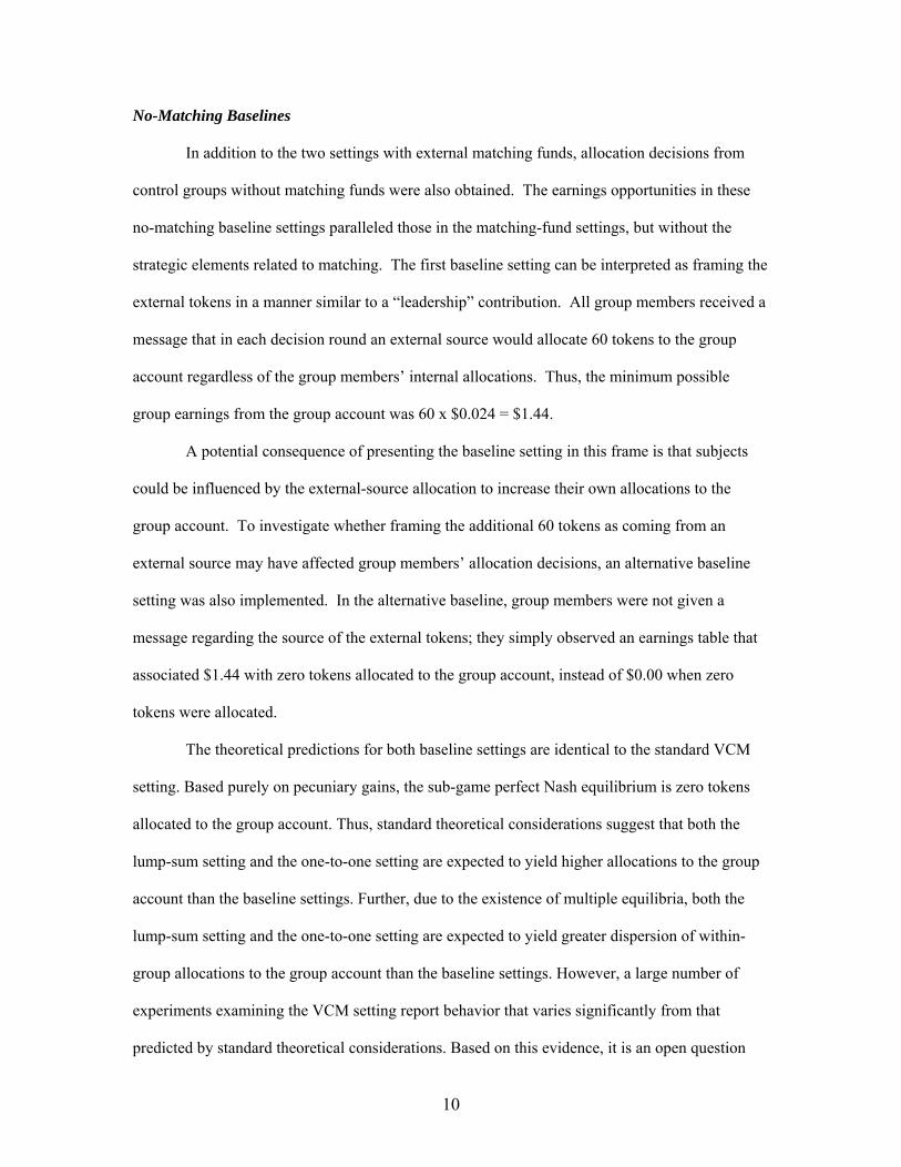
10
No-Matching Baselines
In addition to the two settings with external matching funds allocation decisions from
control groups without matching funds were also obtained The earnings opportunities in these
no-matching baseline settings paralleled those in the matching-fund settings but without the
strategic elements related to matching The first baseline setting can be interpreted as framing the
external tokens in a manner similar to a ldquoleadershiprdquo contribution All group members received a
message that in each decision round an external source would allocate 60 tokens to the group
account regardless of the group membersrsquo internal allocations Thus the minimum possible
group earnings from the group account was 60 x $0024 = $144
A potential consequence of presenting the baseline setting in this frame is that subjects
could be influenced by the external-source allocation to increase their own allocations to the
group account To investigate whether framing the additional 60 tokens as coming from an
external source may have affected group membersrsquo allocation decisions an alternative baseline
setting was also implemented In the alternative baseline group members were not given a
message regarding the source of the external tokens they simply observed an earnings table that
associated $144 with zero tokens allocated to the group account instead of $000 when zero
tokens were allocated
The theoretical predictions for both baseline settings are identical to the standard VCM
setting Based purely on pecuniary gains the sub-game perfect Nash equilibrium is zero tokens
allocated to the group account Thus standard theoretical considerations suggest that both the
lump-sum setting and the one-to-one setting are expected to yield higher allocations to the group
account than the baseline settings Further due to the existence of multiple equilibria both the
lump-sum setting and the one-to-one setting are expected to yield greater dispersion of within-
group allocations to the group account than the baseline settings However a large number of
experiments examining the VCM setting report behavior that varies significantly from that
predicted by standard theoretical considerations Based on this evidence it is an open question
11
whether the baseline settings will yield smaller allocations to the group account and smaller
within-group dispersion relative to the two settings that incorporate matching funds
3B Procedures
[Table 1 here]
[Figure 1 here]
Table 1 and Figure 1 summarize the key elements of each decision setting Each
experimental session utilized twelve subjects who were randomly assigned to three four-person
groups in each of three phases within a session Subjects participated in a sequence of ten (phase-
one) decision rounds in a particular setting were then randomly reassigned to a new four-person
group for ten (phase-two) decision rounds using a different setting and were then randomly
reassigned to another four-person group for the final ten (phase-three) decision rounds using a
different setting Each phase corresponded to a specific decision setting (baseline lump-sum
matching or one-to-one matching) and the order of experimental settings was systematically
varied across sessions Thus data on nine four-person groups were collected in each 12-person
experimental session three groups in each of the three phases yielding three replications of a
particular ordering of decision settings
The experiments were conducted using NovaNET software at the Interdisciplinary
Experimental Laboratory at Indiana University-Bloomington during the 2004-2005 academic
year Subjects were recruited from a database of volunteers4 After being seated at
microcomputer workstations subjects were given preliminary instructions that were projected on
a large screen at the front of the room and read aloud by the experimenter5 Before beginning the
first ten-round decision-making phase in the session subjects were informed publicly that 1) the
experiment would consist of thirty decision rounds that were broken down into three ten-round
4 A representative from the lab visited various large introductory classes (psychology geography and economics) to ask students to enlist in the database if they were interested in participating in experiments A wide variety of majors are represented in these large introductory classes 5 Instructions are available upon request
12
sequences 2) for each ten-round sequence they would be randomly reassigned to a four-person
group 3) earnings at the beginning of each ten-round sequence would be displayed on their
computer screen as zero but 4) their final earnings would be the sum of earnings across all three
ten-round sequences plus a $5 payment for showing up Subjects then privately read through a
set of computerized instructions describing the decision setting and familiarizing them with
specific screen displays While subjects were privately reading the set of computerized
instructions an overhead was also presented with summary information related to the private and
group accounts Finally in the transition from one phase to the next summary information
regarding the subsequent decision setting was publicly projected on a large screen at the front of
the lab and then read aloud by the experimenter
The experimental design called for two replications of each of the six unique permutation
orders of the three decision settings excluding the alternative baseline This led to twelve
experimental sessions with 144 unique subjects To investigate the potential framing effect
associated with an unconditional external allocation to the group account the remaining subject-
motivation funds in our grant budget allowed two additional sessions utilizing the following
ordering of decision settings 1) alternate baseline lump-sum matching one-to-one matching and
2) alternate baseline one-to-one matching lump-sum matching Thus the results reported below
are drawn from a total of fourteen experimental sessions using 168 subjects to form 126 decision-
making groups Each group interacts over ten decision rounds resulting in a total of 1260
observations at the group level and 5040 observations at the individual level
4 Experimental Results
Subject decisions are analyzed both graphically and econometrically at the group and
individual level to examine the effects on allocations to the group account of changing the
experimental setting The analysis focuses on three performance measures The first measure
reported is the per-round token allocations to the group account by each four-person group
excluding any external matching allocations The second performance measure is the per-round
13
efficiency where efficiency is defined as the percentage of maximum possible earnings extracted
by the group6 The third performance measure is the per-round within-group dispersion of
allocations to the group account Specifically the standard deviation about the mean group-
member allocation is calculated
4A Graphical Overview
[Figure 2 here]
[Figure 3 here]
[Figure 4 here]
Figures 2-4 display the mean value of each performance measure for each round pooled
across experimental phases Several very general observations can be made from these figures
Observation 1 Mean allocations to the group account are highest in the lump-sum setting in all
ten decision rounds and lowest in the alternate baseline in eight of ten rounds
Observation 2 Mean efficiency averaged over all ten decision rounds is lowest in the lump-sum
setting but the rank ordering across treatments varies from round to round
Observation 3 Mean dispersion of group-account allocations within groups is lowest in the lump-
sum setting in all ten decision rounds
The lump-sum setting appears to be the most effective at generating allocations to the
group account as mean allocations in this setting are higher than all other settings for every
round In most rounds however average efficiency is lower in the lump-sum setting because of
the severe penalty (loss of 60 tokens) if the threshold for the match is not reached7 This penalty
6 The formula for calculating per-round efficiency is
1600240tokens)-(100001 tokens)external tokens(0240 ++ where ldquotokensrdquo is defined as the aggregate internal
token allocation to the group account and ldquoexternal tokensrdquo is defined as the tokens allocated to the group account by the external source Because the external tokens are not provided by a subject within the experiment the efficiency measure used in the analysis does not account for the value to the ldquoexternal sourcerdquo of unused tokens This measure of efficiency is highly positively correlated with the total tokens (group + external) allocated to the group account in a round (r = 09829) 7 Groups in the lump-sum setting failed to reach the threshold necessary for matching funds in 183 of all rounds
14
is not as severe in the one-to-one setting and the full match was always present in both baseline
settings The lump-sum setting also appears to diminish the end-game effect (ie decreasing
allocations to the group account in Rounds 9 and 10) that is present in the other experimental
settings However dispersion of group-account allocations within groups increases in Rounds 9
and 10 for all experimental settings
4B Nonparametric Tests
This subsection presents two-tailed nonparametric tests to evaluate the validity of the
above observations Potential treatment-sequencing effects are also examined The data to test
Observation 1 are the mean per-round allocation of tokens to the group account for each group
(one observation per four-person group) Group means from all phases are included in each of
the four samples (lump-sum one-to-one baseline alternate-baseline) and these tests assume
independence of group means within and across phases A Kruskal-Wallis test rejects the joint
null hypothesis that the data from all four settings are drawn from identical populations (p =
0018) To further examine differences between experimental settings a Wilcoxon rank-sum test
is used for each setting pair The null hypothesis of identical populations is rejected for the
following pairs lump-sum vs baseline (p = 0032 N=42 36) lump-sum vs one-to-one (p =
0024 N=42 42) and lump-sum vs alternate-baseline (p = 0013 N=42 6) The other three
pairs are not significantly different at the 10 significance level Thus the nonparametric tests
support the observation that group-account allocations are highest under lump-sum matching
The above analysis is repeated to test Observation 2 The data are the mean per-round
efficiency for each group (one observation per group) A Kruskal-Wallis test fails to reject the
joint null hypothesis that the data from all four samples are drawn from identical populations (p =
05098) Further Wilcoxon rank-sum tests are not significant at the 10 level for any of the pair-
wise comparisons These nonparametric tests are thus not supportive of the Observation 2
implication that efficiency is significantly lower on average under lump-sum matching relative
15
to the other treatments The insignificance of the rank-sum tests is not surprising however given
the variation in efficiency rankings across rounds
The data to test Observation 3 are the mean per-round within-group standard deviation of
group-account allocations (one observation per group) A Kruskal-Wallis test rejects the null
hypothesis of the samples being drawn from identical populations at a 10 significance level (p =
00973) Wilcoxon rank-sum tests are also significant at the 10 level for both lump-sum vs
baseline (p = 0052 N = 42 36) and lump-sum vs one-to-one (p = 0034 N = 42 42) All other
setting pairs are not significant at the 10 level These nonparametric tests offer marginal
support for the observation that within-group allocation decisions tend to have lower dispersion
under lump-sum matching
The three-phase sequenced structure of the experiment may lead to differences in group-
account allocations due to the particular phase in which the setting occurred Therefore in order
to assess differences in group-account allocations between experimental settings it is imperative
to examine whether differences in allocations are related to the placement of a setting within a
three-phase sequence To examine the significance of sequence effects Kruskal-Wallis tests are
used A test was completed for the baseline lump-sum match and one-to-one match setting8
The samples are constructed by calculating the mean group-aggregate per-round allocations of
tokens to the group account for each sequencing history For example the seven samples used in
the lump-sum matching test are phase 1 (N = 12) phase 2 preceded by baseline (N = 6) phase 2
preceded by one-to-one matching (N = 6) phase 2 preceded by the alternate baseline (N = 3)
phase 3 preceded by phase 1 lump-sum matching and phase 2 one-to-one matching (N = 6) phase
3 preceded by phase 1 one-to-one matching and phase 2 lump-sum matching (N = 6) and phase 3
preceded by phase 1 alternate baseline and phase 2 one-to-one matching (N = 3) The Kruskal-
Wallis tests for each setting were not significant at the 10 level Based on these nonparametric
8 The alternate baseline setting occurred only in phase 1 of the two experimental sessions in which it was used
16
tests it appears that the sequence of the experimental settings does not contribute to differences in
group -account allocations
4C Regression Analysis
To further investigate the effect of decision settings phases and rounds on group-account
allocations an individual-specific fixed-effects regression model is estimated using all 5040
individual-level allocations to the group account The individual-specific error components are
estimated using the 30 decisions across all three phases for each of the 168 individual subjects
To account for lack of independence within a ten-round four-person group clustered robust
standard errors are utilized where the data are clustered by these 40 within-group decisions9 The
regression equation is
102132116821x ===+prime+= rpiuβy rpirpiirpi α (1)
The ipr subscripts index individuals phases and rounds respectively The dependent variable
yipr is the allocation to the group account αi is the individual-specific fixed-effect vector and x
is the data matrix of independent variables a lump-sum matching dummy variable (LUMP) a
one-to-one matching dummy variable (1TO1) an alternative-baseline dummy variable
(ALTBASE) two treatment-phase dummy variables (PHASE2 and PHASE3) and nine decision-
round dummy variables (RNDr r=2 3 hellip 10) The usual idiosyncratic residual error vector is
uipr
[Table 2 here]
Table 2 displays the coefficient point estimates clustered robust standard errors and two-
tailed significance tests of the coefficients In support of Observation 1 the table reveals that
lump-sum matching generates a significant increase in tokens allocated to the group account
relative to the original no-matching baseline however the smaller increase generated by one-to-
9 For a detailed discussion of the heteroskedasticity-robust HuberWhite sandwich estimator of variance in panel-data models see for example Cameron and Trivedi (2005 Chapter 21 Section 2123) The specific implementation utilized here is documented in Rogers (1993)
17
one matching is not significantly different from the original baseline As expected the
ALTBASE coefficient is negative removing the ldquoexternal sourcerdquo frame from the baseline
group-account earnings function tends to reduce group-account allocations This difference is
significant Wald tests result in rejection of the following pair-wise null hypotheses LUMP =
1TO1 (p = 0000) LUMP = ALTBASE (p = 0000) and 1TO1 = ALTBASE (p = 0000)10 Thus
allocations to the group account are significantly higher in the lump-sum setting than either the
alternate baseline or the one-to-one setting Further allocations in the one-to-one setting are
significantly higher than the alternate baseline setting While the primary focus here is on the
effects of altering the experimental decision setting note that the treatment-phase dummies are
not significant but there are significant differences across decision rounds In particular relative
to round 1 group-account allocations tend to be slightly higher on average in rounds 2-4 and
there is a significant drop in group-account allocations in the final two rounds Referring back to
Figure 2 this end-game drop in allocations is evident in all except the lump-sum setting
[Table 3 here]
The conclusions from the individual fixed-effects model are also supported when the
group-account allocations are analyzed at the group level Table 3 reports estimates from a
random-effects regression model using all 1260 group-level observations where tokens allocated
10 Two additional models were also estimated The results reported in Table 2 are robust to these alternative model specifications The first model is an individual-specific random-effects model using only phase-1 data As in Table 2 cluster-robust standard errors are utilized with allocation decisions clustered by the forty within-group observations The random-effects estimator is necessary since all three experimental setting dummy variables are round invariant removing the possibility of using the fixed-effects estimator Estimation of the phase-1 random-effects model results in only one minor deviation from the results reported in Table 2 a Wald test for the null hypothesis 1TO1 = ALTBASE is significant at the 10 level (p = 00803) The second model is a two-limit censored-normal (Tobit) regression model with group-level clustered standard errors This model makes strict distributional assumptions to account for the observations that occur at the fixed boundaries of group account allocations Approximately 313 of the observations on the dependent variable (1579 of 5040) occur at the fixed upper boundary of 25 tokens to the group account and 103 of the observations (518 of 5040) occur at the lower boundary of zero The estimates of the Tobit regression are similar in sign and magnitude to the estimates reported in Table 2 The significance of the setting dummy variables and pair-wise Wald tests from the Tobit model result in two deviations from the fixed-effects model ALTBASE is not significant at the 10 level and the Wald test for 1TO1 = ALTBASE is significant at the 10 level (p = 0056)
18
to the group account by a four-person group (the aggregate allocation excluding external tokens)
is the dependent variable 11 The regression equation is
10213214221x rpg ===++prime+= rpguβy grpgrpg εα (2)
The gpr subscripts index four-person groups phases and rounds respectively The independent
variables are identical to those described for equation 1 and reported in Table 2 The usual
idiosyncratic residual error vector is ugpr and εg is a group-specific error component Cluster-
robust standard errors are utilized with observations clustered by experimental sessions (nine
groups across the three phases) to account for possible lack of independence across groups within
a session The results reported in Table 3 are very similar to those using the group-account
allocations at the individual level that were reported in the fixed-effect model Specifically
lump-sum matching significantly increases group-account allocations relative to the baseline
setting however allocations in the one-to-one setting are not significantly different from the
baseline The alternate baseline significantly reduces allocations relative to the baseline Further
the following null hypotheses are rejected using Wald tests LUMP = 1TO1 (p = 0000) LUMP =
ALTBASE (p = 0000) 1TO1 = ALTBASE (p = 0013) Therefore allocations at the group level
are greatest in the lump-sum setting The one-to-one setting does not significantly increase
allocations relative to the baseline while allocations are lowest in the alternate baseline12
[Table 4 here]
The efficiency and allocation-dispersion performance measures also require analysis at
the group level First efficiency is considered The regression model described in equation (2) is
repeated using a grouprsquos per-round efficiency as the dependent variable Table 4 displays the
regression coefficients robust standard errors and two-tailed significance tests for the
coefficients In support of Observation 2 the table reveals that lump-sum matching results in a
11 Random effects are needed because the experimental settings variables are round invariant for groups 12 The significance of all Wald tests reported for the random-effects model in Table 3 is upheld when the model is estimated using only phase-1 data which avoids the possible lack-of-independence complication for phase-2 and phase-3 groups within a three-phase experimental session
19
small but significant (p = 0007) decrease in efficiency compared to the baseline Average
efficiencies in the other settings are also significantly decreased from the baseline Despite the
differences in penalties from failing to reach the full match a Wald test comparing the pair-wise
null hypothesis of LUMP = 1TO1 is not rejected (p = 0278) One reason for the lack of
significance between efficiencies in the lump-sum setting and the one-to-one setting is that there
were substantially more full matches in the lump-sum setting compared to the one-to-one setting
(817 of all rounds compared to 614 of all rounds respectively) Again an end-game effect
is present efficiency decreases by an average of 3 in round 9 and 4 in round 10 when
compared to round 1 This result is consistent with Figure 3 which displays a decrease in
efficiency for the final two rounds in all environments but lump-sum matching13
[Table 5 here]
The third performance measure to analyze is the dispersion of within-group allocations to
the group account where dispersion is calculated by the standard deviation about the mean
individual allocation to the group account The regression model described in equation (2) is
estimated using per-round standard deviation of group-member allocations as the dependent
variable Table 5 displays the regression coefficients robust standard errors and 2-tailed
significance tests for the coefficients In support of Observation 3 the table reveals that the
lump-sum setting results in a significant (p = 0019) decrease in dispersion compared to the
baseline setting Wald tests reject the pair-wise null hypotheses of LUMP = 1TO1 (p = 0000)
and LUMP = ALTBASE (p = 0078) A Wald test comparing the remaining pair-wise null
hypothesis (1TO1 = ALTBASE) is not significant at the 10 level Thus dispersion in group
13 Two robustness checks for the random-effects model of efficiency were completed First the random-effects model was estimated using only phase-1 data Tests of the significance of the coefficient estimates were qualitatively similar to the results presented in Table 4 with one exception The null hypothesis of LUMP = BASELINE was not rejected at the 10 significance level Second a two-limit censored-normal (Tobit) model employing clustered standard errors at the group level was also estimated to account for the observations at the boundaries of the decision space Thirty-one of 1260 observations are at the upper efficiency limit (1) and one observation is at the variable lower efficiency limit (The lower efficiency limits in the baseline and alternate baseline are larger than the lower limit in the matching environments) All tests of significance were qualitatively similar to those shown in Table 4
20
account allocations is significantly less in the lump-sum setting than either the one-to-one setting
or the alternate baseline As can be seen in Figure 4 dispersion increases during the final three
rounds in each setting This observation is supported by the regression results as RND8 (p =
0055) RND9 (p = 0000) and RND10 (p = 0000) are all positive and significant14
4D Individual Allocations to the Group Account Benchmark Frequencies
[Figure 5 here]
This subsection analyzes group-account allocations at the individual level organized
around the frequency of occurrence of three benchmark allocations the individual maximum (25
tokens) the symmetric Nash equilibrium (15 tokens) and complete free riding (0 tokens)15 To
avoid any possible impact on token allocations from an individualrsquos participation in multiple
decision settings only the phase-one data are examined Figure 5 displays relative frequencies of
these benchmark allocations for each experimental decision setting pooling across all ten
decision rounds16 The percentage of occurrences of the maximum allocation is somewhat higher
in the matching settings relative to the baseline settings Further the lump-sum setting results in
more allocations that are consistent with the symmetric Nash equilibrium compared to the one-to-
one setting and complete free riding occurs less frequently under lump-sum matching relative to
the other three settings
To formally examine the significance of these informal observations negative binomial
count-data regressions are performed where the dependent variable is the number of rounds that
an individual submitted a specific benchmark allocation (an integer between 0 and 10) The
independent variables are the LUMP 1TO1 and ALTBASE dummy variables described at the
14 Using only phase-1 data in the random-effects allocation-dispersion model results in the null hypothesis of 1TO1 = BASELINE being rejected at the 5 level (p = 0019) The other tests are qualitatively similar to the results reported above and in Table 5 15 Allocations near the symmetric Nash equilibrium (14 le tokens le 16) were also examined The results were very similar to those of the symmetric Nash equilibrium 16 Note that the symmetric Nash equilibrium only applies to lump-sum matching and one-to-one matching The unique Nash equilibrium allocation to the group account is zero tokens for each baseline environment
21
beginning of section 4C17 Because each individual is part of a four-person group an
individualrsquos token allocations are likely to be influenced by the previous allocations of other
group members To account for this within-group dependence robust clustered standard errors
are reported where observations are clustered by decision groups
[Table 6 here]
[Table 7 here]
[Table 8 here]
The regression results for each benchmark allocation appear in Tables 6 7 and 8 A
convenient way to interpret the regression coefficients in the negative binomial model is to
examine incidence-rate ratios (IRR) where ie β=IRR IRRs reveal the percentage change in the
expected count of a benchmark allocation due to a change in the treatment condition holding all
other independent variables constant For example in Table 6 the lump-sum setting increases
the expected frequency for the maximum allocation by a multiple of 118 compared to the
baseline setting an 18 increase [ie 100(IRR ndash 1)] Overall however Table 6 shows the
regression model is not significant when the maximum allocation count is used as the dependent
variable (p = 0251) Table 7 shows that the coefficient for the LUMP dummy is positive and
significant (p = 0009) the IRR indicates a 79 increase over one-to-one matching in the
expected number of rounds where the symmetric Nash equilibrium allocation is submitted
Finally Table 8 shows that the coefficient for the LUMP dummy is negative and marginally
significant (p = 0064) the IRR indicates a 62 decrease in the number of complete free-riding
rounds relative to the baseline level Wald tests of null hypotheses LUMP = 1TO1 (p = 00112)
and LUMP = ALTBASE (p = 00634) are significant The remaining pair-wise null hypothesis
1TO1 = ALTBASE is not rejected at the 10 level Thus significantly less free riding occurs in
17 A Poisson regression model was estimated first but the results indicated that the assumption of equidispersion (equality of the mean and variance inherent in a Poisson process) must be rejected Following Long (Chapter 8 1997) and Cameron amp Trivedi (Chapter 20 2005) the negative binomial model was utilized to capture overdispersion in the dependent variable
22
the lump-sum setting than either the one-to-one or the alternate baseline setting In summary
lump-sum matching appears to 1) significantly increase the frequency of individual allocations
consistent with the symmetric Nash equilibrium relative to one-to-one matching and 2)
significantly decrease the frequency of complete free-riding allocations relative to the other
decision settings examined here
5 Summary and Conclusions
In the experimental literature on the voluntary provision of public goods a wide range of
studies examine alternative institutional arrangements intended to reduce collective action
problems by creating incentives that facilitate cooperation The research reported in this study
adds to this literature by examining behavior in two fund-raising institutions found commonly in
the field lump-sum matching and one-to-one matching where matching funds are provided by an
ldquoexternalrdquo donor
The experimental results reveal higher ldquointernalrdquo (within-group) resource allocations to
the public good under lump-sum matching An explanation supporting this result is that missing
the threshold required to provide the full match results in a larger earnings loss in the lump-sum
setting when compared to the one-to-one setting Internal allocations in the lump-sum setting are
also less dispersed with more individual allocations at or near the symmetric Nash equilibrium
prediction and fewer individual allocations consistent with complete free riding Neither the
lump-sum nor the one-to-one setting provides strong support for play of the symmetric Nash
equilibrium Finally although lump-sum matching leads to greater internal allocations to the
public good there is not a significant difference in efficiency between the two matching-funds
settings due to decision rounds where groups under lump-sum matching do not reach the
threshold and thus receive no matching funds In the experimental settings investigated here
external matching funds that are not extracted by a four-person group are wasted rather than
being carried over to future decision rounds In naturally-occurring field settings the validity of
this rather harsh component of the experimental environment is doubtful To the extent that
23
unused matching funds are transferred to future endeavors that augment the provision of the
public good the efficiency comparisons reported here are of less relevance than the comparison
of internal resource allocations to the public good
As a methodological issue it is interesting to note the behavioral response to the framing
change made between the baseline and alternate baseline settings The alternate baseline removed
any wording that alluded to allocations to the group account from an external source Instead the
additional tokens were simply added to payoffs from the group account by adjusting the intercept
term of the group account return function With this framing change lower allocations to the
group account were observed in the alternate baseline Although based on a small sample size
this result is supportive of similar results that examine leadership contributions to a public good
Fund-raising drives suggest several other interesting extensions to the experiments
reported here In particular in field applications organizations often provide information on the
current status of the fund drive with respect to donations Future research will examine this issue
using both lump-sum and one-to-one matching by giving subjects intra-round information on the
current aggregate allocation to the public good in conjunction with intra-round updating of
individual allocation decisions An ldquoincrease-onlyrdquo allocation rule can be applied to intra-round
updates of individual decisions Larger group sizes other group-account earnings structures and
the use of nonmonetary rewards will also be investigated
24
References
Andreoni J 2006 Leadership Giving In Charitable Fund Raising Journal of Public Economic Theory 8(1) 1-22 Cameron AC Trivedi PK 2005 Microeconometrics Methods and Applications New York Cambridge University Press Davis D 2006 Rebate Subsides Matching Subsidies and Isolation Effects Judgment and Decision-Making 1 13-22 Eckel C Grossman P 2003 Rebate versus Matching Does How We Subsidize Charitable Contributions Matter Journal of Public Economics 87 681-701 Gachter S Renner E 2004 Leading By Example in the Presence of Free-Rider Incentives Working paper Isaac M Walker J Williams A 1994 Group Size and the Voluntary Provision of Public Goods Experimental Evidence Utilizing Large Groups Journal of Public Economics 54(1) 1-36 Karlan D List J 2006 Does Price Matter in Charitable Giving Evidence from a Large-Scale Natural Field Experiment Yale Working Papers on Economic Applications and Policy 13 Landry C Lange A List J Price M Rupp N 2006 Toward an Understanding of the Economics of Charity Evidence From a Field Experiment Quarterly Journal of Economics 121 747-782 Ledyard J 1995 Public Goods A Survey of Experimental Research In Kagel J Roth A (Eds) Handbook of Experimental Economics New Jersey Princeton University Press 111-195 List J Lucking-Reiley D 2002 The Effects of Seed Money and Refunds on Charitable Giving Experimental Evidence from a University Capital Campaign Journal of Political Economy 110(1) 215-233 List J Rondeau D 2003 The Impact of Challenge Gifts on Charitable Giving An Experimental Investigation Economics Letters 79 153-159 List J 2006 Field Experiments Advances in Economic Analysis and Policy 6 1-45 Long JS 1997 Regression Models for Categorical and Limited Dependent Variables California SAGE Publications Marks M Croson R 1998 Alternative Rebate Rules in the Provision of a Threshold Public Good An Experimental Investigation Journal of Public Economics 67 195-220 Potters J Sefton M Vesterlund L 2007 Leading-by-example and Signaling in Voluntary Contribution Games Economic Theory 33 169-182 Rogers WH 1993 Regression standard errors in clustered samples Stata Technical Bulletin Reprints 3 88-94
25
Rose-Ackerman S 1986 Do government grants to charity reduce private donations In Rose-Ackerman S (Ed) The Economics of Nonprofit Institutions Oxford University Press New York Shang J Croson R 2006 Field Experiments in Charitable Contribution The Impact of Social Influence on the Voluntary Provision of Public Goods Working paper University of Pennsylvania
26
Table 1 Characteristics of Decision Settings
Baseline
Lump-Sum Matching
One-to-One Matching
Individual Token Endowment Per-Round 25 25 25
Decision Rounds 10 10 10 Per-Token Return to
Private Account $001 $001 $001
Individual Per-Token Return from Group Account $0006
$0006 for tokens other than the
60th token
$0012 for tokens 1-60 $0006 for
tokens 61 and above Total Individual Earnings
All Tokens to the Private Account
$610 $250 $250
Total Individual Earnings Symmetric Nash Equilibrium of
15 tokens NA $820 $820
Total Individual Earnings All Tokens to the Group Account
$960 $960 $960
27
Table 2 Fixed-Effects Model Individual Allocations to Group Account
Independent Variable
Coefficient Estimate
Robust Clustered Standard Error
Ho Coefficient = 0 t p-value
CONSTANT 155658 05166 3013 0 LUMP 22728 04582 496 0 1TO1 06258 04815 13 0196
ALTBASE -21035 08251 -255 0012 PHASE2 -06439 04529 -142 0158 PHASE3 -06575 04203 -156 012
RND2 10119 02945 344 0001 RND3 06706 03523 19 0059 RND4 08512 03648 233 0021 RND5 03234 03870 084 0405 RND6 -00337 03882 -009 0931 RND7 00218 03846 006 0955 RND8 -01310 03747 -035 0727 RND9 -07044 03908 -18 0074
RND10 -12480 04464 -28 0006 Total Number of Observations = 5040 = 126 clusters of 40 observations
Model F(14125) = 904 p = 0000 Fraction of variance due to fixed effect 0442
Table 3 Random-Effects Model Group Allocations to Group Account
Independent Variable
Coefficient Estimate
Robust Clustered Standard Error
Ho Coefficient = 0 Z p-value
CONSTANT 621570 19186 3240 0000 LUMP 91312 13950 655 0000 1TO1 25431 16925 150 0133
ALTBASE -78864 41244 -191 0056 PHASE2 -24819 13498 -184 0066 PHASE3 -25605 16786 -153 0127
RND2 40476 10352 391 0000 RND3 26825 13671 196 005 RND4 34048 14013 243 0015 RND5 12937 21349 061 0545 RND6 -01349 16227 -008 0934 RND7 00873 15262 006 0954 RND8 -05238 14321 -037 0715 RND9 -27381 15577 -176 0079
RND10 -49921 11084 -450 0000 Total Number of Observations = 1260 = 14 clusters of 90 observations
Fraction of variance due to session-specific random effect 0565
28
Table 4 Random-Effects Model Group Efficiency
Independent Variable
Coefficient Estimate
Robust Clustered Standard Error
Ho Coefficient = 0 Z p-value
CONSTANT 08771 00127 6913 0000 LUMP -00351 00129 -272 0007 1TO1 -00224 00104 -215 0032
ALTBASE -00340 00160 -212 0034 PHASE2 -00170 00087 -196 0050 PHASE3 -00171 00157 -109 0276
RND2 00204 00077 266 0008 RND3 00074 00119 062 0534 RND4 00055 00096 057 0567 RND5 -00091 00177 -051 0608 RND6 -00134 00130 -103 0303 RND7 -00149 00119 -125 0212 RND8 -00141 00120 -117 0242 RND9 -00286 00148 -194 0052
RND10 -00396 00124 -320 0001 Total Number of Observations = 1260 = 14 clusters of 90 observations
Fraction of variance due to session-specific random effect 0342
Table 5 Random-Effects Model Within-Group Standard Deviation of Individual Allocations to Group Account
Independent
Variable Coefficient
Estimate Robust Clustered
Standard Error Ho Coefficient = 0
Z p-value CONSTANT 75268 04048 1859 0000
LUMP -10568 04517 -234 0019 1TO1 00677 04557 015 0882
ALTBASE 04012 08684 046 0644 PHASE2 -01001 03629 -028 0783 PHASE3 -01227 03140 -039 0696
RND2 -02424 01835 -132 0187 RND3 01594 02473 064 0519 RND4 00351 02892 012 0903 RND5 03553 02554 139 0164 RND6 04774 02734 175 0081 RND7 04384 02840 154 0123 RND8 05451 02846 192 0055 RND9 13791 02933 470 0000
RND10 16131 03266 494 0000 Total Number of Observations = 1260 = 14 clusters of 90 observations
Fraction of variance due to session-specific random effect 0496
29
Table 6 Count-Data Model Maximum Allocation
Independent Variable
IRR
Coefficient Estimate
Robust Clustered Standard Error
Ho Coefficient = 0 Z p-value
CONSTANT 10488 00908 1156 0000 LUMP 11825 01676 01515 111 0269 1TO1 12482 02217 01487 149 0136
ALTBASE 09051 -00997 01790 -056 0578 Total Number of Observations = 168 = 42 clusters of 4 observations
Model χ2(3) = 410 p = 0251
Table 7 Count-Data Model Symmetric Nash Equilibrium Allocation
Independent Variable
IRR
Coefficient Estimate
Robust Clustered Standard Error
Ho Coefficient = 0 Z p-value
CONSTANT -02336 01693 -138 0168 LUMP 17895 05819 02227 261 0009
Total Number of Observations = 96 = 24 clusters of 4 observations Model χ2(1) = 683 p = 0009
Table 8 Count-Data Model Complete Free-Riding Allocation
Independent Variable
IRR Coefficient Estimate
Robust Clustered Standard Error
Ho Coefficient = 0 Z p-value
CONSTANT -01335 02902 -046 0645 LUMP 03810 -09651 05205 -185 0064 1TO1 13333 02877 03758 077 0444
ALTBASE 11429 01335 04978 027 0789 Total Number of Observations = 168 = 42 clusters of 4 observations
Model χ2(3) = 654 p = 0088
30
Figure 1 Group-Account Earnings for the Decision Settings
31
Figure 2 Mean Internal Token Allocation to the Group Account
0
10
20
30
40
50
60
70
80
90
100
1 2 3 4 5 6 7 8 9 10
round
mea
n to
kens
to g
roup
acc
ount
(max
= 1
00)
baseline
lump
1to1
altbase
60 tokens
Figure 3 Mean Efficiency
07
075
08
085
09
095
1
1 2 3 4 5 6 7 8 9 10
round
effic
ienc
y
baseline
lump
1to1
altbase
60 tokens
32
Figure 4 Mean Standard Deviation of Tokens to the Group Account
0
1
2
3
4
5
6
7
8
9
10
1 2 3 4 5 6 7 8 9 10
round
mea
n st
dev
of to
kens
to g
roup
acc
ount
baseline
lump
1to1
altbase
Figure 5 Individual Token Allocations to the Group Account All Rounds Phase 1
0
005
01
015
02
025
03
035
04
0 15 25
tokens
rela
tive
freq
uenc
y
baseline lump 1to1 altbase

20
account allocations is significantly less in the lump-sum setting than either the one-to-one setting
or the alternate baseline As can be seen in Figure 4 dispersion increases during the final three
rounds in each setting This observation is supported by the regression results as RND8 (p =
0055) RND9 (p = 0000) and RND10 (p = 0000) are all positive and significant14
4D Individual Allocations to the Group Account Benchmark Frequencies
[Figure 5 here]
This subsection analyzes group-account allocations at the individual level organized
around the frequency of occurrence of three benchmark allocations the individual maximum (25
tokens) the symmetric Nash equilibrium (15 tokens) and complete free riding (0 tokens)15 To
avoid any possible impact on token allocations from an individualrsquos participation in multiple
decision settings only the phase-one data are examined Figure 5 displays relative frequencies of
these benchmark allocations for each experimental decision setting pooling across all ten
decision rounds16 The percentage of occurrences of the maximum allocation is somewhat higher
in the matching settings relative to the baseline settings Further the lump-sum setting results in
more allocations that are consistent with the symmetric Nash equilibrium compared to the one-to-
one setting and complete free riding occurs less frequently under lump-sum matching relative to
the other three settings
To formally examine the significance of these informal observations negative binomial
count-data regressions are performed where the dependent variable is the number of rounds that
an individual submitted a specific benchmark allocation (an integer between 0 and 10) The
independent variables are the LUMP 1TO1 and ALTBASE dummy variables described at the
14 Using only phase-1 data in the random-effects allocation-dispersion model results in the null hypothesis of 1TO1 = BASELINE being rejected at the 5 level (p = 0019) The other tests are qualitatively similar to the results reported above and in Table 5 15 Allocations near the symmetric Nash equilibrium (14 le tokens le 16) were also examined The results were very similar to those of the symmetric Nash equilibrium 16 Note that the symmetric Nash equilibrium only applies to lump-sum matching and one-to-one matching The unique Nash equilibrium allocation to the group account is zero tokens for each baseline environment
21
beginning of section 4C17 Because each individual is part of a four-person group an
individualrsquos token allocations are likely to be influenced by the previous allocations of other
group members To account for this within-group dependence robust clustered standard errors
are reported where observations are clustered by decision groups
[Table 6 here]
[Table 7 here]
[Table 8 here]
The regression results for each benchmark allocation appear in Tables 6 7 and 8 A
convenient way to interpret the regression coefficients in the negative binomial model is to
examine incidence-rate ratios (IRR) where ie β=IRR IRRs reveal the percentage change in the
expected count of a benchmark allocation due to a change in the treatment condition holding all
other independent variables constant For example in Table 6 the lump-sum setting increases
the expected frequency for the maximum allocation by a multiple of 118 compared to the
baseline setting an 18 increase [ie 100(IRR ndash 1)] Overall however Table 6 shows the
regression model is not significant when the maximum allocation count is used as the dependent
variable (p = 0251) Table 7 shows that the coefficient for the LUMP dummy is positive and
significant (p = 0009) the IRR indicates a 79 increase over one-to-one matching in the
expected number of rounds where the symmetric Nash equilibrium allocation is submitted
Finally Table 8 shows that the coefficient for the LUMP dummy is negative and marginally
significant (p = 0064) the IRR indicates a 62 decrease in the number of complete free-riding
rounds relative to the baseline level Wald tests of null hypotheses LUMP = 1TO1 (p = 00112)
and LUMP = ALTBASE (p = 00634) are significant The remaining pair-wise null hypothesis
1TO1 = ALTBASE is not rejected at the 10 level Thus significantly less free riding occurs in
17 A Poisson regression model was estimated first but the results indicated that the assumption of equidispersion (equality of the mean and variance inherent in a Poisson process) must be rejected Following Long (Chapter 8 1997) and Cameron amp Trivedi (Chapter 20 2005) the negative binomial model was utilized to capture overdispersion in the dependent variable
22
the lump-sum setting than either the one-to-one or the alternate baseline setting In summary
lump-sum matching appears to 1) significantly increase the frequency of individual allocations
consistent with the symmetric Nash equilibrium relative to one-to-one matching and 2)
significantly decrease the frequency of complete free-riding allocations relative to the other
decision settings examined here
5 Summary and Conclusions
In the experimental literature on the voluntary provision of public goods a wide range of
studies examine alternative institutional arrangements intended to reduce collective action
problems by creating incentives that facilitate cooperation The research reported in this study
adds to this literature by examining behavior in two fund-raising institutions found commonly in
the field lump-sum matching and one-to-one matching where matching funds are provided by an
ldquoexternalrdquo donor
The experimental results reveal higher ldquointernalrdquo (within-group) resource allocations to
the public good under lump-sum matching An explanation supporting this result is that missing
the threshold required to provide the full match results in a larger earnings loss in the lump-sum
setting when compared to the one-to-one setting Internal allocations in the lump-sum setting are
also less dispersed with more individual allocations at or near the symmetric Nash equilibrium
prediction and fewer individual allocations consistent with complete free riding Neither the
lump-sum nor the one-to-one setting provides strong support for play of the symmetric Nash
equilibrium Finally although lump-sum matching leads to greater internal allocations to the
public good there is not a significant difference in efficiency between the two matching-funds
settings due to decision rounds where groups under lump-sum matching do not reach the
threshold and thus receive no matching funds In the experimental settings investigated here
external matching funds that are not extracted by a four-person group are wasted rather than
being carried over to future decision rounds In naturally-occurring field settings the validity of
this rather harsh component of the experimental environment is doubtful To the extent that
23
unused matching funds are transferred to future endeavors that augment the provision of the
public good the efficiency comparisons reported here are of less relevance than the comparison
of internal resource allocations to the public good
As a methodological issue it is interesting to note the behavioral response to the framing
change made between the baseline and alternate baseline settings The alternate baseline removed
any wording that alluded to allocations to the group account from an external source Instead the
additional tokens were simply added to payoffs from the group account by adjusting the intercept
term of the group account return function With this framing change lower allocations to the
group account were observed in the alternate baseline Although based on a small sample size
this result is supportive of similar results that examine leadership contributions to a public good
Fund-raising drives suggest several other interesting extensions to the experiments
reported here In particular in field applications organizations often provide information on the
current status of the fund drive with respect to donations Future research will examine this issue
using both lump-sum and one-to-one matching by giving subjects intra-round information on the
current aggregate allocation to the public good in conjunction with intra-round updating of
individual allocation decisions An ldquoincrease-onlyrdquo allocation rule can be applied to intra-round
updates of individual decisions Larger group sizes other group-account earnings structures and
the use of nonmonetary rewards will also be investigated
24
References
Andreoni J 2006 Leadership Giving In Charitable Fund Raising Journal of Public Economic Theory 8(1) 1-22 Cameron AC Trivedi PK 2005 Microeconometrics Methods and Applications New York Cambridge University Press Davis D 2006 Rebate Subsides Matching Subsidies and Isolation Effects Judgment and Decision-Making 1 13-22 Eckel C Grossman P 2003 Rebate versus Matching Does How We Subsidize Charitable Contributions Matter Journal of Public Economics 87 681-701 Gachter S Renner E 2004 Leading By Example in the Presence of Free-Rider Incentives Working paper Isaac M Walker J Williams A 1994 Group Size and the Voluntary Provision of Public Goods Experimental Evidence Utilizing Large Groups Journal of Public Economics 54(1) 1-36 Karlan D List J 2006 Does Price Matter in Charitable Giving Evidence from a Large-Scale Natural Field Experiment Yale Working Papers on Economic Applications and Policy 13 Landry C Lange A List J Price M Rupp N 2006 Toward an Understanding of the Economics of Charity Evidence From a Field Experiment Quarterly Journal of Economics 121 747-782 Ledyard J 1995 Public Goods A Survey of Experimental Research In Kagel J Roth A (Eds) Handbook of Experimental Economics New Jersey Princeton University Press 111-195 List J Lucking-Reiley D 2002 The Effects of Seed Money and Refunds on Charitable Giving Experimental Evidence from a University Capital Campaign Journal of Political Economy 110(1) 215-233 List J Rondeau D 2003 The Impact of Challenge Gifts on Charitable Giving An Experimental Investigation Economics Letters 79 153-159 List J 2006 Field Experiments Advances in Economic Analysis and Policy 6 1-45 Long JS 1997 Regression Models for Categorical and Limited Dependent Variables California SAGE Publications Marks M Croson R 1998 Alternative Rebate Rules in the Provision of a Threshold Public Good An Experimental Investigation Journal of Public Economics 67 195-220 Potters J Sefton M Vesterlund L 2007 Leading-by-example and Signaling in Voluntary Contribution Games Economic Theory 33 169-182 Rogers WH 1993 Regression standard errors in clustered samples Stata Technical Bulletin Reprints 3 88-94
25
Rose-Ackerman S 1986 Do government grants to charity reduce private donations In Rose-Ackerman S (Ed) The Economics of Nonprofit Institutions Oxford University Press New York Shang J Croson R 2006 Field Experiments in Charitable Contribution The Impact of Social Influence on the Voluntary Provision of Public Goods Working paper University of Pennsylvania
26
Table 1 Characteristics of Decision Settings
Baseline
Lump-Sum Matching
One-to-One Matching
Individual Token Endowment Per-Round 25 25 25
Decision Rounds 10 10 10 Per-Token Return to
Private Account $001 $001 $001
Individual Per-Token Return from Group Account $0006
$0006 for tokens other than the
60th token
$0012 for tokens 1-60 $0006 for
tokens 61 and above Total Individual Earnings
All Tokens to the Private Account
$610 $250 $250
Total Individual Earnings Symmetric Nash Equilibrium of
15 tokens NA $820 $820
Total Individual Earnings All Tokens to the Group Account
$960 $960 $960
27
Table 2 Fixed-Effects Model Individual Allocations to Group Account
Independent Variable
Coefficient Estimate
Robust Clustered Standard Error
Ho Coefficient = 0 t p-value
CONSTANT 155658 05166 3013 0 LUMP 22728 04582 496 0 1TO1 06258 04815 13 0196
ALTBASE -21035 08251 -255 0012 PHASE2 -06439 04529 -142 0158 PHASE3 -06575 04203 -156 012
RND2 10119 02945 344 0001 RND3 06706 03523 19 0059 RND4 08512 03648 233 0021 RND5 03234 03870 084 0405 RND6 -00337 03882 -009 0931 RND7 00218 03846 006 0955 RND8 -01310 03747 -035 0727 RND9 -07044 03908 -18 0074
RND10 -12480 04464 -28 0006 Total Number of Observations = 5040 = 126 clusters of 40 observations
Model F(14125) = 904 p = 0000 Fraction of variance due to fixed effect 0442
Table 3 Random-Effects Model Group Allocations to Group Account
Independent Variable
Coefficient Estimate
Robust Clustered Standard Error
Ho Coefficient = 0 Z p-value
CONSTANT 621570 19186 3240 0000 LUMP 91312 13950 655 0000 1TO1 25431 16925 150 0133
ALTBASE -78864 41244 -191 0056 PHASE2 -24819 13498 -184 0066 PHASE3 -25605 16786 -153 0127
RND2 40476 10352 391 0000 RND3 26825 13671 196 005 RND4 34048 14013 243 0015 RND5 12937 21349 061 0545 RND6 -01349 16227 -008 0934 RND7 00873 15262 006 0954 RND8 -05238 14321 -037 0715 RND9 -27381 15577 -176 0079
RND10 -49921 11084 -450 0000 Total Number of Observations = 1260 = 14 clusters of 90 observations
Fraction of variance due to session-specific random effect 0565
28
Table 4 Random-Effects Model Group Efficiency
Independent Variable
Coefficient Estimate
Robust Clustered Standard Error
Ho Coefficient = 0 Z p-value
CONSTANT 08771 00127 6913 0000 LUMP -00351 00129 -272 0007 1TO1 -00224 00104 -215 0032
ALTBASE -00340 00160 -212 0034 PHASE2 -00170 00087 -196 0050 PHASE3 -00171 00157 -109 0276
RND2 00204 00077 266 0008 RND3 00074 00119 062 0534 RND4 00055 00096 057 0567 RND5 -00091 00177 -051 0608 RND6 -00134 00130 -103 0303 RND7 -00149 00119 -125 0212 RND8 -00141 00120 -117 0242 RND9 -00286 00148 -194 0052
RND10 -00396 00124 -320 0001 Total Number of Observations = 1260 = 14 clusters of 90 observations
Fraction of variance due to session-specific random effect 0342
Table 5 Random-Effects Model Within-Group Standard Deviation of Individual Allocations to Group Account
Independent
Variable Coefficient
Estimate Robust Clustered
Standard Error Ho Coefficient = 0
Z p-value CONSTANT 75268 04048 1859 0000
LUMP -10568 04517 -234 0019 1TO1 00677 04557 015 0882
ALTBASE 04012 08684 046 0644 PHASE2 -01001 03629 -028 0783 PHASE3 -01227 03140 -039 0696
RND2 -02424 01835 -132 0187 RND3 01594 02473 064 0519 RND4 00351 02892 012 0903 RND5 03553 02554 139 0164 RND6 04774 02734 175 0081 RND7 04384 02840 154 0123 RND8 05451 02846 192 0055 RND9 13791 02933 470 0000
RND10 16131 03266 494 0000 Total Number of Observations = 1260 = 14 clusters of 90 observations
Fraction of variance due to session-specific random effect 0496
29
Table 6 Count-Data Model Maximum Allocation
Independent Variable
IRR
Coefficient Estimate
Robust Clustered Standard Error
Ho Coefficient = 0 Z p-value
CONSTANT 10488 00908 1156 0000 LUMP 11825 01676 01515 111 0269 1TO1 12482 02217 01487 149 0136
ALTBASE 09051 -00997 01790 -056 0578 Total Number of Observations = 168 = 42 clusters of 4 observations
Model χ2(3) = 410 p = 0251
Table 7 Count-Data Model Symmetric Nash Equilibrium Allocation
Independent Variable
IRR
Coefficient Estimate
Robust Clustered Standard Error
Ho Coefficient = 0 Z p-value
CONSTANT -02336 01693 -138 0168 LUMP 17895 05819 02227 261 0009
Total Number of Observations = 96 = 24 clusters of 4 observations Model χ2(1) = 683 p = 0009
Table 8 Count-Data Model Complete Free-Riding Allocation
Independent Variable
IRR Coefficient Estimate
Robust Clustered Standard Error
Ho Coefficient = 0 Z p-value
CONSTANT -01335 02902 -046 0645 LUMP 03810 -09651 05205 -185 0064 1TO1 13333 02877 03758 077 0444
ALTBASE 11429 01335 04978 027 0789 Total Number of Observations = 168 = 42 clusters of 4 observations
Model χ2(3) = 654 p = 0088
30
Figure 1 Group-Account Earnings for the Decision Settings
31
Figure 2 Mean Internal Token Allocation to the Group Account
0
10
20
30
40
50
60
70
80
90
100
1 2 3 4 5 6 7 8 9 10
round
mea
n to
kens
to g
roup
acc
ount
(max
= 1
00)
baseline
lump
1to1
altbase
60 tokens
Figure 3 Mean Efficiency
07
075
08
085
09
095
1
1 2 3 4 5 6 7 8 9 10
round
effic
ienc
y
baseline
lump
1to1
altbase
60 tokens
32
Figure 4 Mean Standard Deviation of Tokens to the Group Account
0
1
2
3
4
5
6
7
8
9
10
1 2 3 4 5 6 7 8 9 10
round
mea
n st
dev
of to
kens
to g
roup
acc
ount
baseline
lump
1to1
altbase
Figure 5 Individual Token Allocations to the Group Account All Rounds Phase 1
0
005
01
015
02
025
03
035
04
0 15 25
tokens
rela
tive
freq
uenc
y
baseline lump 1to1 altbase
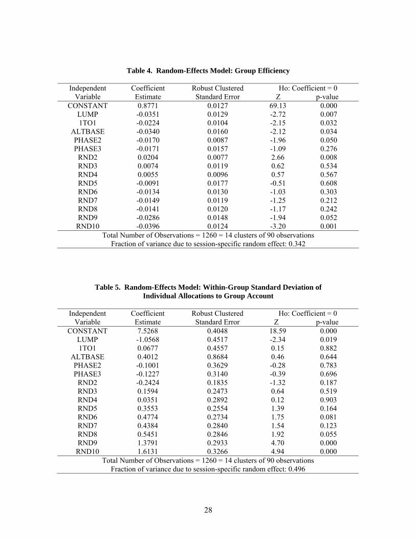

30
Figure 1 Group-Account Earnings for the Decision Settings
31
Figure 2 Mean Internal Token Allocation to the Group Account
0
10
20
30
40
50
60
70
80
90
100
1 2 3 4 5 6 7 8 9 10
round
mea
n to
kens
to g
roup
acc
ount
(max
= 1
00)
baseline
lump
1to1
altbase
60 tokens
Figure 3 Mean Efficiency
07
075
08
085
09
095
1
1 2 3 4 5 6 7 8 9 10
round
effic
ienc
y
baseline
lump
1to1
altbase
60 tokens
32
Figure 4 Mean Standard Deviation of Tokens to the Group Account
0
1
2
3
4
5
6
7
8
9
10
1 2 3 4 5 6 7 8 9 10
round
mea
n st
dev
of to
kens
to g
roup
acc
ount
baseline
lump
1to1
altbase
Figure 5 Individual Token Allocations to the Group Account All Rounds Phase 1
0
005
01
015
02
025
03
035
04
0 15 25
tokens
rela
tive
freq
uenc
y
baseline lump 1to1 altbase