OTC-28015-MS

Integration of Ensemble Data Assimilation and Deep Learning for HistoryMatching Facies Models

Smith Arauco Canchumuni, PUC-RIO; Alexandre A. Emerick, PETROBRAS; Marco Aurelio Pacheco, PUC-RIO

Copyright 2017, Offshore Technology Conference

This paper was prepared for presentation at the Offshore Technology Conference Brasil held in Rio de Janeiro, Brazil, 24–26 October 2017.

This paper was selected for presentation by an OTC program committee following review of information contained in an abstract submitted by the author(s). Contents ofthe paper have not been reviewed by the Offshore Technology Conference and are subject to correction by the author(s). The material does not necessarily reflect anyposition of the Offshore Technology Conference, its officers, or members. Electronic reproduction, distribution, or storage of any part of this paper without the writtenconsent of the Offshore Technology Conference is prohibited. Permission to reproduce in print is restricted to an abstract of not more than 300 words; illustrations maynot be copied. The abstract must contain conspicuous acknowledgment of OTC copyright.

AbstractEnsemble data assimilation methods have been applied with remarkable success in several real-life history-matching problems. However, because these methods rely on Gaussian assumptions, their performanceis severely degraded when the prior geology is described in terms of complex facies distributions.This fact motivated an intense investigation reported in the literature to develop efficient and robustparameterizations. Despite the large number of publications, preserving plausible geological features whenupdating facies models is still one of the main challenges with ensemble-based history matching.

This work reports our initial results towards the development of a robust parameterization based onDeep Learning (DL) for proper history matching of facies models with ensemble methods. The processbegins with a set of prior facies realizations, which are used for training a DL network. DL identifies themain features of the facies images, allowing the construction of a reduced parameterization of the models.This parameterization is transformed to follow a Gaussian distribution, which is updated to account forthe dynamic observed data using the method known as ensemble smoother with multiple data assimilation(ES-MDA). After each data assimilation, DL is used to reconstruct the facies models based on the initiallearning. The proposed method is tested in a synthetic history-matching problem based on the well-knownPUNQ-S3 case. We compare the results of the proposed method against the standard ES-MDA (with noparameterization) and another parameterization based on principal component analysis.

IntroductionThe number of successful applications of ensemble-based history matching reported in the literature isbecoming quite large; see, e.g., (Evensen et al., 2007; Haugen et al., 2008; Cominelli et al., 2009; Zhangand Oliver, 2011; Emerick and Reynolds, 2011, 2013b; Chen and Oliver, 2014; Emerick, 2016). The mainadvantages attributed to these methods include the computational efficiency, the ability to work with largedimensions and the ease of implementation. Examples of these methods include the ensemble smootherwith multiple data assimilation (ES-MDA) has been calling attention because its efficiency and simplicity.However, previous results [see e.g., (Emerick, 2017) and reference therein] show that the direct applicationof ES-MDA to complex geological reservoir models tends to distort the prior geological description,especially when discrete facies appears in the reservoir model. There are several works proposing different

2 OTC-28015-MS

parameterization algorithms to deal with the loss of geological realism after history matching. Among theproposed methods, perhaps the ones based on truncated pluri-gaussian simulation (TPG) (Armstrong et al.,2011) are the most successful; see, e.g., (Liu and Oliver, 2005; Agbalaka and Oliver, 2008; Sebacher et al.,2013; Zhao et al., 2008). Another set of parameterizations are based on level-set functions (Chang et al.,2010; Ping and Zhang, 2014). However, TPG and level-set functions do not seem adequate to parameterizechannelized models and geometries that are more complex (particularly when the models are generatedby object-based or multiple-point statistics algorithms). Another group of methods used to parameterizechannelized facies models are based on principal component analysis (PCA). Among these methods, wehave the kernel principal component analysis (Sarma et al., 2008), the hybrid method of the cumulativedensity function with a principal component analysis (CDF-PCA) (Chen et al., 2016) and the optimization-based PCA (Vo and Durlofsky, 2014).

This work reports our initial results towards the development of a robust parameterization based onDeep Learning (DL) for proper history matching of facies models with ensemble methods. DL representa class of algorithms in the Machine Learning area specialized in learning data representation. DL allowscomputational models that are composed of multiple processing layers to automatically learn representationsof data with multiple levels of abstraction. This is one of the main foundations, for which these architectureare able to learn complex functions, building a representation of the input data simply based on the trainingset, without depending completely on human-crafted features. Many times, obtain higher-level abstractionsis of vital importance. Due, which humans often do not know how represent information in terms of rawsensory input(LeCun et al., 2015). DL has been applied in diverse research fields, dramatically improvingthe state-of-the-art of all applications. The literature on DL is vast; see, e.g., (Bengio, 2009) and referencestherein. To the best of our knowledge, this is the first work attempting to use DL for history matching. Therationality is to use ability of DL to learn representations from data, here given in terms of geological imagesgenerated by means of geostatistics, to re-parameterizes these images in terms of coefficients followingGaussian distributions, which are easier to update in an ensemble-based data assimilation process.

The remaining of this paper is organized as follows: first, we present a brief description of ES-MDA andDL. After that, we introduce a workflow to integrate ES-MDA with the parameterization based on DL. Wealso present an alternative parameterization based on PCA. Then, we present a test case based on the well-known PUNQ-S3 problem (Floris et al., 2001). The last section of the paper summarizes the conclusions.

Ensemble Smoother with Multiple Data AssimilationES-MDA is an ensemble-based method introduced by (Emerick and Reynolds, 2013a). In its simplest form,the method employs the standard ensemble smoother analysis equation a pre-defined number of times withthe covariance matrix of the measured data error multiplied by a coefficient α. The coefficients must beselect such that the following condition is satisfied

(1)

where Na is the number of times the analysis step is repeated. The ES-MDA analysis applied to a vectorof model parameters, m, can be written as

(2)

where Cmd is the cross-covariance between the vector of model parameters and predicted data, g(m). Cdd

is the covariance of predicted data. Both covariances are estimated using an ensemble of size Ne. dobs is thevector of observed data and £ is a random vector sampled from N(0, αCε), with Cε denoting the covariance

OTC-28015-MS 3

matrix of the measurement errors. More details about the method can be found in (Emerick and Reynolds,2013a; Emerick, 2016).

Deep LearningFor geological facies parameterization, it is difficult to know what features should be extracted, since faciesmodels have strong nonlinearities and present non-gaussian distributions. To ease the mentioned problems,DL seems to be a good candidate methods because its ability of extracting relevant, non-redundant andnonlinear features from images (Muthukumar and Black, 2014). In fact, DL can be seen as a nonlineargeneralization of principal component analysis (Deng et al., 2017).

DL comprises as series of algorithms and architectures that are able to model complex structured datatypes such as images, sounds and text. However, deep architectures have been focused on supervisedlearning algorithms, which try to learn a statistical model for estimating a the posterior probability p(y|x)from an input vector x to an output vector y, commonly used for classification problems. However, thereare deep unsupervised feature learning algorithms that learn a feature representation by extracting randompatches from unlabeled training data, applying a pre-processing stage to the patches and learning a feature-mapping by the use of an unsupervised learning algorithm (Coates et al., 2011). This group of techniquesare known as deep generative models, which can be trained to build models using autoencoder algorithms.These models can be represent a probability distribution function (PDF), where some PDF allow to beevaluated explicitly, while other, despite not allowing the evaluation of the PDF, admit operations thatimplicitly require knowledge of it (e.g., drawing samples from the PDF). (Goodfellow et al., 2016).

Autoencoders are neural networks which are trained aiming to copy its input to its output. See section4.6 of (Bengio, 2009) for an overview of autoencoders. Internally, autoencoders has a hidden layer, heredenoted by a vector h, that represents a code used to mapped the input, that in the majority of the applicationsthese parameters are used like parameterization. The simplest autoencoder network consists of two parts:

• Encoder h = fe(x): a nonlinear model that maps the input to another space, often referred to as ahidden layer, represented by h.

(3)• Decoder : a nonlinear model that learns the inverse mapping from the latent to input space.

(4)

where We, be, Wd and bd are the weight matrix and bias vector for the encoder and decoder, respectively.The basic training process of an autoencoder is considered as optimization problem, where the objectiveis minimizing of a cost function. It is function measures the error between the input vector x and itsreconstruction at the output . The general cost function is an adjusted mean squared error function withthe form

(5)

In the above equation, Fr(W) is a regularization function, Q is the number of parameters in the trainingset and N represents the number of observations. Generally an autoencoder use deterministic functions forencoder and decoder. However modern autoencoder are using stochastic functions in the encoder e decoder,where these functions are PDF (Goodfellow et al., 2016),ρencoder(h|x) and ρdecoder (x|h).

4 OTC-28015-MS

Figure 1—The general architecture of deep autoencoders. Where the input x are mappingin the internal representation h (hidden layer) and reconstructed to an output . The

two components of the autoencoder: the encoder (blue) and the decoder (yellow).

Standard autoencoders are trained with a single layer encoder and decoder. However, these twocomponents can be connected together in deep architectures to create an end-to-end trainable model to learnhigh-level feature representations from a large supply of data inputs. The deep architecture used in thiswork is presented in Fig. 1, where the left side shows the encoder network and the right side shows thedecoder. If during the training process an autoencoder used a function lineal at the decoder and the meansquared error as a cost function, the performance of a standard autoencoder is similar to the PCA learning.In contrast, when the encoder and decoder are nonlinear functions, autoencoders have the ability to learn amore powerful non-linear generalization of PCA (Goodfellow et al., 2016).

The DL parameterization for facies models proposed in this work is implemented in the hidden layer ofthe deep architectures, as discussed in the following section.

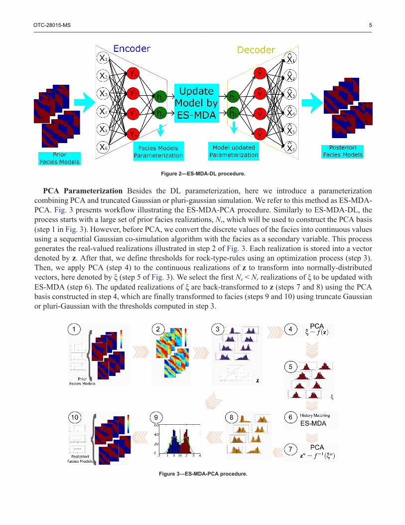
Proposed ParameterizationsDeep Learning Parameterization Here, we use a deep autoencoder with architecture presented in Fig.1. The basic idea is to use a set of prior facies realizations for training the DL network. Then, we use thecoefficients of the hidden layer (outputs of the encoder) as history-matching parameters which are adjustedusing the ES-MDA analysis equation. After that, the updated coefficients are used to reconstruct faciesmodels based on the initial training (decoder). Here, we refer to the resulting method as ES-MDA-DL. Theoverall procedure consists of three main steps and it is summarized in Fig. 2.

1. Training of the DL using the autoencoders architecture based on a large set of facies realizations, Nr,to identify the main features of the model.

2. Update the coefficients of the hidden layer corresponding to Ne < Nr prior realizations with ES-MDAanalysis equation.

3. Reconstruct the Ne facies realizations using the decoder from the initial learning with the updatedcoefficients from ES-MDA analysis.

OTC-28015-MS 5

Figure 2—ES-MDA-DL procedure.

PCA Parameterization Besides the DL parameterization, here we introduce a parameterizationcombining PCA and truncated Gaussian or pluri-gaussian simulation. We refer to this method as ES-MDA-PCA. Fig. 3 presents workflow illustrating the ES-MDA-PCA procedure. Similarly to ES-MDA-DL, theprocess starts with a large set of prior facies realizations, Nr, which will be used to construct the PCA basis(step 1 in Fig. 3). However, before PCA, we convert the discrete values of the facies into continuous valuesusing a sequential Gaussian co-simulation algorithm with the facies as a secondary variable. This processgenerates the real-valued realizations illustrated in step 2 of Fig. 3. Each realization is stored into a vectordenoted by z. After that, we define thresholds for rock-type-rules using an optimization process (step 3).Then, we apply PCA (step 4) to the continuous realizations of z to transform into normally-distributedvectors, here denoted by ξ (step 5 of Fig. 3). We select the first Ne < Nr realizations of ξ to be updated withES-MDA (step 6). The updated realizations of ξ are back-transformed to z (steps 7 and 8) using the PCAbasis constructed in step 4, which are finally transformed to facies (steps 9 and 10) using truncate Gaussianor pluri-Gaussian with the thresholds computed in step 3.

Figure 3—ES-MDA-PCA procedure.

6 OTC-28015-MS

Figure 4—Reference model. From left to right layers 1 to 5. Facies (top row),logarithm of horizontal permeability (middle row) and histogram (bottom row)

Test CaseThe test case corresponds to modified version of the well-known PUNQ-S3 model (Floris et al., 2001).Unlike the original case, we introduced facies to the problem, but respecting the original descriptionpresented in the Appendix section of (Floris et al., 2001). These facies were generated using the multiple-point statistics algorithm SNESIM (Strebelle, 2002) implemented in the SGeMS package (Remy et al.,2009). Layers 1, 3 and 5 of the model have similar reservoir characteristics (facies Mudstone and Channel).The precise values of the parameters differ for each layer. Layer 2 has a much lower reservoir quality (faciesMarine and Mudstone) and layer 4 has intermediate reservoir quality (facies Mouthbar and Mudstone).Fig. 4 presents the reference model which is used to generate the synthetic production history. Thepetrophysical properties (porosity, horizontal and vertical permeability) of each facies type were generatedusing sequential Gaussian simulation with the data summarized in Table 1.

Using the same geostatistical parameters used to construct the reference model, we generated a priorensemble with 6000 realizations. The first Nr = 5000 realizations were taken as part of the training set andthe remaining 1000 were used as part of the validation set to construct the DL parameterization. The same5000 realizations were also used to construct the PCA basis according to the procedure described in theprevious section. Moreover, we selected the first 200 realizations to form the prior ensemble for historymatching. The first three prior realizations of facies are illustrated in Fig. 5, the corresponding horizontalpermeability and histograms (in log-10 scale).

OTC-28015-MS 7

Table 1—Mean and standard deviation of the petrophysical properties per facies type

Layer 1 Layer 2 Layer 3 Layer 4 Layer 5

Porosity Mean Std. dev. Mean Std. dev. Mean Std. dev. Mean Std. dev. Mean Std. dev.

Mudstone 0.1 0.031 0.035 0.031 0.1 0.031 0.06 0.071 0.1 0.031

Channel 0.23 0.031 − − 0.23 0.031 − − 0.23 0.031

Marine − − 0.1 0.045 − − − − − −

Mouthbar − − − − − − 0.15 0.031 − −

Horiz. log-permeability Mean Std. dev. Mean Std. dev. Mean Std. dev. Mean Std. dev. Mean Std. dev.

Mudstone 1.8 0.224 0.8 0.283 1.8 0.224 1.4 0.224 1.8 0.224

Channel 2.5 0.224 − − 2.5 0.224 − − 2.5 0.224

Marine − − 1.7 0.224 − − − − − −

Mouthbar − − − − − − 2.2 0.224 − −

Vert. log-permeability Mean Std. dev. Mean Std. dev. Mean Std. dev. Mean Std. dev. Mean Std. dev.

Mudstone 1.5 0.224 0.4 0.173 1.5 0.224 1.1 0.173 1.5 0.224

Channel 2.2 0.224 − − 2.2 0.224 − − 2.2 0.224

Marine − − 1.1 0,173 − − − − − −

Mouthbar − − − − − − 1.6 0.173 − −

Table 2—History matching parameters

Method Parameters

ES-MDA ϕ, log10(ĸh) and log10ĸv)

ES-MDA-PCA ξ, ϕF1,ϕF2, log10(ĸh,F1), log10(ĸh,F2), log10(ĸV,F1) and log10(ĸh,F2)

ES-MDA-DL h, ϕF1,ϕF2, log10(ĸh,F1), log10(ĸh,F2), log10(ĸV,F1) and log10(ĸh,F2)

The data assimilations were conducted with ES-MDA with Na = 4 and αk= 4 (constant). Besides theES-MDA-DL and ES-MDA-PCA, we also applied the standard ES-MDA (with no parameterization) forcomparisons. Table 2 summarizes the content of the vectors of model parameters, m, which are updatedwith the ES-MDA analysis (Eq. 2). In this table, ϕ, log10 (ĸh) and log10 (ĸv) stand for porosity, horizontal andvertical log-permeabilities, respectively. Note that for standard ES- MDA we only update the petrophysicalproperties. For ES-MDA-PCA and ES-MDA-DL, we update the facies type using the correspondingparameterizations (vectors ξ and h in Table 2). Moreover, for both cases we update the petrophysicalproperties for each facies type.

8 OTC-28015-MS

Figure 5—First three prior realizations (layer 1). Facies (top row), logarithmof horizontal permeability (middle row) and histogram (bottom row).

DL Training process The first step of ES-MDA-DL method is the training of the DL network. Recallthat here we use autoencoders with architecture illustrated in Fig. 1. The training consisted in a unsupervisedlearning based on 5000 realizations of facies. After training, the DL network was tested with the validationset of 1000 realizations of facies. The trained DL network resulted in a reproduction of facies models with anaverage error of 0.16% in the validation set. Fig. 6 illustrates the result of the facies reconstruction with thetrained DL network. This figure shows in the left an initial facies realization, which was transformed into aset of coefficients of the hidden layer, i.e., entries of the vector h after the encoder. Note that this coefficientsfollows a Gaussian distribution (as shown in the histogram of Fig. 6), which makes the parameterizationsuitable for ES-MDA. Finally, in the right is presented the reconstructed used the trained decoder showingan nearly perfect agreement with the initial facies realization.

Figure 6—Example of facies parameterization with DL showing the initial facies, thecorresponding parameters with a Gaussian distribution and the re-constructed facies.

OTC-28015-MS 9

The training process in very computationally demanding. Here, we handled this problem using a graphicscard "GeForce GTX 1080," with a MatLab library for GPU. In our limited set of tests, the use of GPUcorresponded to a decreasing on the order of eight times on the computational time required by a CPU(Intel(R) Core(TM) i7-4770 with a clock of 3.4GHz, 32GB RAM). the training process of the DL networktook around 6.1 hours in CPU and around 45 minutes in GPU.

Results

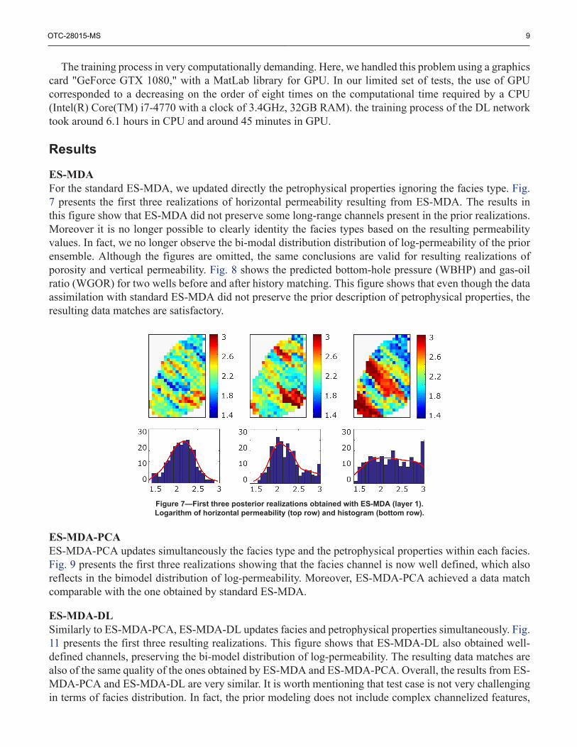
ES-MDAFor the standard ES-MDA, we updated directly the petrophysical properties ignoring the facies type. Fig.7 presents the first three realizations of horizontal permeability resulting from ES-MDA. The results inthis figure show that ES-MDA did not preserve some long-range channels present in the prior realizations.Moreover it is no longer possible to clearly identity the facies types based on the resulting permeabilityvalues. In fact, we no longer observe the bi-modal distribution distribution of log-permeability of the priorensemble. Although the figures are omitted, the same conclusions are valid for resulting realizations ofporosity and vertical permeability. Fig. 8 shows the predicted bottom-hole pressure (WBHP) and gas-oilratio (WGOR) for two wells before and after history matching. This figure shows that even though the dataassimilation with standard ES-MDA did not preserve the prior description of petrophysical properties, theresulting data matches are satisfactory.

Figure 7—First three posterior realizations obtained with ES-MDA (layer 1).Logarithm of horizontal permeability (top row) and histogram (bottom row).

ES-MDA-PCAES-MDA-PCA updates simultaneously the facies type and the petrophysical properties within each facies.Fig. 9 presents the first three realizations showing that the facies channel is now well defined, which alsoreflects in the bimodel distribution of log-permeability. Moreover, ES-MDA-PCA achieved a data matchcomparable with the one obtained by standard ES-MDA.

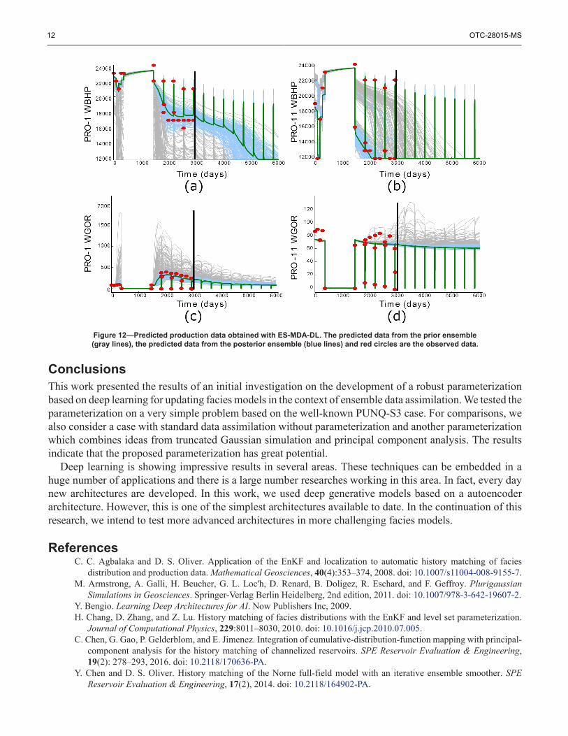
ES-MDA-DLSimilarly to ES-MDA-PCA, ES-MDA-DL updates facies and petrophysical properties simultaneously. Fig.11 presents the first three resulting realizations. This figure shows that ES-MDA-DL also obtained well-defined channels, preserving the bi-model distribution of log-permeability. The resulting data matches arealso of the same quality of the ones obtained by ES-MDA and ES-MDA-PCA. Overall, the results from ES-MDA-PCA and ES-MDA-DL are very similar. It is worth mentioning that test case is not very challengingin terms of facies distribution. In fact, the prior modeling does not include complex channelized features,

10 OTC-28015-MS

such as curved fluvial channels. Therefore the linear parameterization introduced in the ES-MDA-PCAseems to be enough to obtain plausible reservoir models in this case.

Figure 8—Predicted production data obtained with ES-MDA. The predicted data from the prior ensemble(gray lines), the predicted data from the posterior ensemble (blue lines) and red circles are the observed data.

Figure 9—First three realizations obtained with ES-MDA-PCA (layer 1). Facies (toprow), logarithm of horizontal permeability (middle row) and histogram (bottom row).

OTC-28015-MS 11

Figure 10—Predicted production data obtained with ES-MDA-PCA. The predicted data from the prior ensemble(gray lines), the predicted data from the posterior ensemble (blue lines) and red circles are the observed data.

Figure 11—First three realizations obtained with ES-MDA-DL (layer 1). Facies (toprow), logarithm of horizontal permeability (middle row) and histogram (bottom row).

12 OTC-28015-MS

Figure 12—Predicted production data obtained with ES-MDA-DL. The predicted data from the prior ensemble(gray lines), the predicted data from the posterior ensemble (blue lines) and red circles are the observed data.

ConclusionsThis work presented the results of an initial investigation on the development of a robust parameterizationbased on deep learning for updating facies models in the context of ensemble data assimilation. We tested theparameterization on a very simple problem based on the well-known PUNQ-S3 case. For comparisons, wealso consider a case with standard data assimilation without parameterization and another parameterizationwhich combines ideas from truncated Gaussian simulation and principal component analysis. The resultsindicate that the proposed parameterization has great potential.

Deep learning is showing impressive results in several areas. These techniques can be embedded in ahuge number of applications and there is a large number researches working in this area. In fact, every daynew architectures are developed. In this work, we used deep generative models based on a autoencoderarchitecture. However, this is one of the simplest architectures available to date. In the continuation of thisresearch, we intend to test more advanced architectures in more challenging facies models.

ReferencesC. C. Agbalaka and D. S. Oliver. Application of the EnKF and localization to automatic history matching of facies

distribution and production data. Mathematical Geosciences, 40(4):353–374, 2008. doi: 10.1007/s11004-008-9155-7.M. Armstrong, A. Galli, H. Beucher, G. L. Loc'h, D. Renard, B. Doligez, R. Eschard, and F. Geffroy. Plurigaussian

Simulations in Geosciences. Springer-Verlag Berlin Heidelberg, 2nd edition, 2011. doi: 10.1007/978-3-642-19607-2.Y. Bengio. Learning Deep Architectures for AI. Now Publishers Inc, 2009.H. Chang, D. Zhang, and Z. Lu. History matching of facies distributions with the EnKF and level set parameterization.

Journal of Computational Physics, 229:8011–8030, 2010. doi: 10.1016/j.jcp.2010.07.005.C. Chen, G. Gao, P. Gelderblom, and E. Jimenez. Integration of cumulative-distribution-function mapping with principal-

component analysis for the history matching of channelized reservoirs. SPE Reservoir Evaluation & Engineering,19(2): 278–293, 2016. doi: 10.2118/170636-PA.

Y. Chen and D. S. Oliver. History matching of the Norne full-field model with an iterative ensemble smoother. SPEReservoir Evaluation & Engineering, 17(2), 2014. doi: 10.2118/164902-PA.

OTC-28015-MS 13

A. Coates, A. Ng, and H. Lee. An analysis of single-layer networks in unsupervised feature learning. In Proceedings ofthe 14th International Conference on Artificial Intelligence and Statistics, Fort Lauderdale, FL, USA, 2011.

A. Cominelli, L. Dovera, S. Vimercati, and G. Nsvdal. Benchmark study of ensemble Kalman filter methodology: Historymatching and uncertainty quantification for a deep-water oil reservoir. In Proceedings of the International PetroleumTechnology Conference, Doha, Qatar, 7-9 December, number IPTC 13748, 2009. doi: 10.2523/13748-MS.

X. Deng, X. Tian, S. Chen, and C. J. Harris. Deep learning based nonlinear principal component analysis for industrialprocess fault detection. In Proceedings of the 2017 International Joint Conference on Neural Networks (IJCNN), 2017.doi: 10.1109/IJCNN.2017.7965994.

A. A. Emerick. Analysis of the performance of ensemble-based assimilation of production and seismic data. Journal ofPetroleum Science and Engineering, 139:219–239, 2016. doi: 10.1016/j.petrol.2016.01.029.

A. A. Emerick. Investigation on principal component analysis parameterizations for history matching channelizedfacies models with ensemble-based data assimilation. Mathematical Geosciences, 49(1):85–120, 2017. doi: 10.1007/s11004-016-9659-5.

A. A. Emerick and A. C. Reynolds. History matching a field case using the ensemble Kalman filter with covariancelocalization. SPE Reservoir Evaluation & Engineering, 14(4):423–432, 2011. doi: 10.2118/141216-PA.

A. A. Emerick and A. C. Reynolds. Ensemble smoother with multiple data assimilation. Computers & Geosciences, 55:3–15, 2013a. doi: 10.1016/j.cageo.2012.03.011.

A. A. Emerick and A. C. Reynolds. History matching of production and seismic data for a real field case using theensemble smoother with multiple data assimilation. In Proceedings of the SPE Reservoir Simulation Symposium, TheWoodlands, Texas, USA, 18-20 February, number SPE 163675, 2013b. doi: 10.2118/163675-MS.

F. Evensen, J. Hove, H. C. Meisingset, E. Reiso, K. S. Seim, and Ø. Espelid. Using the EnKF for assisted history matchingof a North Sea reservoir model. In Proceedings of the SPE Reservoir Simulation Symposium, Houston, Texas, 26-28February, number SPE 106184, 2007. doi: 10.2118/106184-MS.

F. J. T. Floris, M. D. Bush, M. Cuypers, F. Roggero, and A. R. Syversveen. Methods for quantifying the uncertainty ofproduction forecasts: A comparative study. Petroleum Geoscience, 7(SUPP):87–96, 2001.

I. Goodfellow, Y. Bengio, and A. Courville. Deep Learning. MIT Press, 2016.V. Haugen, G. Nsvdal, L.-J. Natvik, G. Evensen, A. M. Berg, and K. M. Flornes. History matching using the ensemble

Kalman filter on a North Sea field case. SPE Journal, 13(4):382–391, 2008. doi: 10.2118/102430-PA.Y. LeCun, Y. Bengio, and G. Hinton. Deep learning. Nature, 521:436–444, 2015. doi: 10.1038/nature14539.N. Liu and D. S. Oliver. Ensemble Kalman filter for automatic history matching of geologic facies. Journal of Petroleum

Science and Engineering, 47(3-4):147–161, 2005. doi: 10.1016/j.petrol.2005.03.006.P. K. Muthukumar and A. W. Black. A deep learning approach to data-driven parameterizations for statistical parametric

speech synthesis. arXiv:1409.8558 [cs.CL], 2014. URL http://arxiv.org/abs/1409.8558.J. Ping and D. Zhang. History matching of channelized reservoirs with vector-based level-set parameterization. SPE

Journal, 19(3):514–529, 2014. doi: 10.2118/169898-PA.N. Remy, A. Boucher, and J. Wu. Applied Geostatistics with SGeMS-A User's Guide. 2009.P. Sarma, L. J. Durlofsky, and K. Aziz. Kernel principal component analysis for efficient differentiable parameterization

of multipoint geostatistics. Mathematical Geosciences, 40(1):3–32, 2008. doi: 10.1007/s11004-007-9131-7.B. M. Sebacher, R. Hanea, and A. Heemink. A probabilistic parametrization for geological uncertainty estimation using the

ensemble Kalman filter (EnKF). Computational Geosciences, 17(5):813–832, 2013. doi: 10.1007/s10596-013-9357-z.S. Strebelle. Conditional simulation of complex geological structures using multiple-point statistics. Mathematical

Geology, 34(1):1–21, 2002. doi: 10.1023/A:1014009426274.G. X. Vo and L. J. Durlofsky. A new differentiable parameterization based on principal component analysis for the

lowdimensional representation of complex geological models. Mathematical Geosciences, 46(7):775–813, 2014. doi:10.1007/s11004-014-9541-2.

Y. Zhang and D. S. Oliver. History matching using the ensemble Kalman filter with multiscale parameterization: A fieldcase study. SPE Journal, 16(2):307–317, 2011. doi: 10.2118/118879-PA.

Y. Zhao, A. C. Reynolds, and G. Li. Generating facies maps by assimilating production data and seismic data with theensemble Kalman filter. In Proceedings of the SPE Improved Oil Recovery Symposium, Tulsa, Oklahoma, 20-23April, number SPE 113990, 2008. doi: 10.2118/113990-MS.