matcont and cl matcont: continuation toolboxes in...
TRANSCRIPT
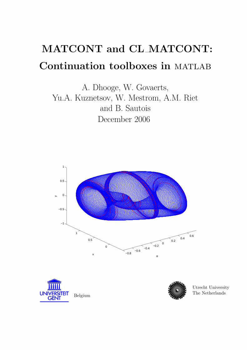
MATCONT and CL MATCONT:
Continuation toolboxes in matlab
A. Dhooge, W. Govaerts,
Yu.A. Kuznetsov, W. Mestrom, A.M. Riet
and B. Sautois
December 2006
−0.8−0.6
−0.4−0.2
00.2
0.40.6
0
0.5
1
−1
−0.5
0
0.5
1
αx
y
Belgium
Utrecht UniversityThe Netherlands
Contents
1 Introduction 5
1.1 Features . . . . . . . . . . . . . . . . . . . . . . . . . . . . . . . . . . . . . . . 51.2 Software requirements . . . . . . . . . . . . . . . . . . . . . . . . . . . . . . . 81.3 Availability . . . . . . . . . . . . . . . . . . . . . . . . . . . . . . . . . . . . . 91.4 Disclaimer . . . . . . . . . . . . . . . . . . . . . . . . . . . . . . . . . . . . . . 9
2 Numerical continuation algorithm 10
2.1 Prediction . . . . . . . . . . . . . . . . . . . . . . . . . . . . . . . . . . . . . . 102.2 Correction . . . . . . . . . . . . . . . . . . . . . . . . . . . . . . . . . . . . . . 10
2.2.1 Pseudo-arclength continuation . . . . . . . . . . . . . . . . . . . . . . 102.2.2 Moore-Penrose continuation . . . . . . . . . . . . . . . . . . . . . . . . 11
2.3 Stepsize control . . . . . . . . . . . . . . . . . . . . . . . . . . . . . . . . . . . 12
3 Singularity handling 13
3.1 Test functions . . . . . . . . . . . . . . . . . . . . . . . . . . . . . . . . . . . . 133.2 Multiple test functions . . . . . . . . . . . . . . . . . . . . . . . . . . . . . . . 133.3 Singularity matrix . . . . . . . . . . . . . . . . . . . . . . . . . . . . . . . . . 143.4 User location . . . . . . . . . . . . . . . . . . . . . . . . . . . . . . . . . . . . 14
4 Software 15
4.1 System definition . . . . . . . . . . . . . . . . . . . . . . . . . . . . . . . . . . 154.2 Continuation and output . . . . . . . . . . . . . . . . . . . . . . . . . . . . . . 154.3 Curve file . . . . . . . . . . . . . . . . . . . . . . . . . . . . . . . . . . . . . . 184.4 Options . . . . . . . . . . . . . . . . . . . . . . . . . . . . . . . . . . . . . . . 18
4.4.1 The options-structure . . . . . . . . . . . . . . . . . . . . . . . . . . . 184.4.2 Derivatives of the ODE-file . . . . . . . . . . . . . . . . . . . . . . . . 204.4.3 Singularities and test functions . . . . . . . . . . . . . . . . . . . . . . 214.4.4 Locators . . . . . . . . . . . . . . . . . . . . . . . . . . . . . . . . . . . 214.4.5 User functions . . . . . . . . . . . . . . . . . . . . . . . . . . . . . . . 214.4.6 Defaultprocessor . . . . . . . . . . . . . . . . . . . . . . . . . . . . . . 224.4.7 Special processors . . . . . . . . . . . . . . . . . . . . . . . . . . . . . 224.4.8 Workspace . . . . . . . . . . . . . . . . . . . . . . . . . . . . . . . . . 224.4.9 Adaptation . . . . . . . . . . . . . . . . . . . . . . . . . . . . . . . . . 224.4.10 Summary . . . . . . . . . . . . . . . . . . . . . . . . . . . . . . . . . . 23
4.5 Error handling . . . . . . . . . . . . . . . . . . . . . . . . . . . . . . . . . . . 234.6 Structure . . . . . . . . . . . . . . . . . . . . . . . . . . . . . . . . . . . . . . 234.7 Directories . . . . . . . . . . . . . . . . . . . . . . . . . . . . . . . . . . . . . . 25
5 Continuer example: a circle object 27
6 Time integration and Poincare maps 29
6.1 Time integration . . . . . . . . . . . . . . . . . . . . . . . . . . . . . . . . . . 296.1.1 Solver output properties . . . . . . . . . . . . . . . . . . . . . . . . . . 296.1.2 Jacobian matrices . . . . . . . . . . . . . . . . . . . . . . . . . . . . . 30
6.2 Poincare section and Poincare map . . . . . . . . . . . . . . . . . . . . . . . . 306.2.1 Poincare maps in MatCont . . . . . . . . . . . . . . . . . . . . . . . 30
2
6.2.2 The Steinmetz-Larter example . . . . . . . . . . . . . . . . . . . . . . 31
7 Equilibrium continuation 34
7.1 Mathematical definition . . . . . . . . . . . . . . . . . . . . . . . . . . . . . . 347.2 Bifurcations . . . . . . . . . . . . . . . . . . . . . . . . . . . . . . . . . . . . . 34
7.2.1 Branch point locator . . . . . . . . . . . . . . . . . . . . . . . . . . . . 357.3 Equilibrium initialization . . . . . . . . . . . . . . . . . . . . . . . . . . . . . 357.4 Bratu example . . . . . . . . . . . . . . . . . . . . . . . . . . . . . . . . . . . 36
8 The Brusselator example: Continuation of a solution to a boundary value
problem in a free parameter 41
9 Continuation of limit cycles 46
9.1 Mathematical definition . . . . . . . . . . . . . . . . . . . . . . . . . . . . . . 469.2 Bifurcations . . . . . . . . . . . . . . . . . . . . . . . . . . . . . . . . . . . . . 46
9.2.1 Branch Point Locator . . . . . . . . . . . . . . . . . . . . . . . . . . . 489.2.2 Processing . . . . . . . . . . . . . . . . . . . . . . . . . . . . . . . . . . 48
9.3 Limitcycle initialization . . . . . . . . . . . . . . . . . . . . . . . . . . . . . . 499.4 Example . . . . . . . . . . . . . . . . . . . . . . . . . . . . . . . . . . . . . . . 509.5 The phase response curve . . . . . . . . . . . . . . . . . . . . . . . . . . . . . 53
10 Continuation of codim 1 bifurcations 57
10.1 Fold Continuation . . . . . . . . . . . . . . . . . . . . . . . . . . . . . . . . . 5710.1.1 Mathematical definition . . . . . . . . . . . . . . . . . . . . . . . . . . 5710.1.2 Bifurcations . . . . . . . . . . . . . . . . . . . . . . . . . . . . . . . . . 5710.1.3 Fold initialization . . . . . . . . . . . . . . . . . . . . . . . . . . . . . . 5810.1.4 Adaptation . . . . . . . . . . . . . . . . . . . . . . . . . . . . . . . . . 5910.1.5 Example . . . . . . . . . . . . . . . . . . . . . . . . . . . . . . . . . . . 59
10.2 Hopf Continuation . . . . . . . . . . . . . . . . . . . . . . . . . . . . . . . . . 6110.2.1 Mathematical definition . . . . . . . . . . . . . . . . . . . . . . . . . . 6110.2.2 Bifurcations . . . . . . . . . . . . . . . . . . . . . . . . . . . . . . . . . 6110.2.3 Hopf initialization . . . . . . . . . . . . . . . . . . . . . . . . . . . . . 6210.2.4 Adaptation . . . . . . . . . . . . . . . . . . . . . . . . . . . . . . . . . 6210.2.5 Example . . . . . . . . . . . . . . . . . . . . . . . . . . . . . . . . . . . 62
10.3 Period Doubling . . . . . . . . . . . . . . . . . . . . . . . . . . . . . . . . . . 6410.3.1 Mathematical definition . . . . . . . . . . . . . . . . . . . . . . . . . . 6410.3.2 Bifurcations . . . . . . . . . . . . . . . . . . . . . . . . . . . . . . . . . 6410.3.3 Period doubling initialization . . . . . . . . . . . . . . . . . . . . . . . 6610.3.4 Example . . . . . . . . . . . . . . . . . . . . . . . . . . . . . . . . . . . 66
10.4 Continuation of fold bifurcation of limit cycles . . . . . . . . . . . . . . . . . 6810.4.1 Mathematical definition . . . . . . . . . . . . . . . . . . . . . . . . . . 6810.4.2 Bifurcations . . . . . . . . . . . . . . . . . . . . . . . . . . . . . . . . . 6910.4.3 Fold initialization . . . . . . . . . . . . . . . . . . . . . . . . . . . . . . 7010.4.4 Example . . . . . . . . . . . . . . . . . . . . . . . . . . . . . . . . . . . 71
10.5 Continuation of torus bifurcation of limit cycles . . . . . . . . . . . . . . . . . 7310.5.1 Mathematical definition . . . . . . . . . . . . . . . . . . . . . . . . . . 7310.5.2 Bifurcations . . . . . . . . . . . . . . . . . . . . . . . . . . . . . . . . . 75
3
10.5.3 Torus bifurcation initialization . . . . . . . . . . . . . . . . . . . . . . 7610.5.4 Example . . . . . . . . . . . . . . . . . . . . . . . . . . . . . . . . . . . 76
11 Continuation of codim 2 bifurcations 80
11.1 Branch Point Continuation . . . . . . . . . . . . . . . . . . . . . . . . . . . . 8011.1.1 Mathematical definition . . . . . . . . . . . . . . . . . . . . . . . . . . 8011.1.2 Bifurcations . . . . . . . . . . . . . . . . . . . . . . . . . . . . . . . . . 8011.1.3 Branch Point initialization . . . . . . . . . . . . . . . . . . . . . . . . . 8011.1.4 Example . . . . . . . . . . . . . . . . . . . . . . . . . . . . . . . . . . . 80
11.2 Branch Point of Cycles Continuation . . . . . . . . . . . . . . . . . . . . . . . 8311.2.1 Mathematical Definition . . . . . . . . . . . . . . . . . . . . . . . . . . 8311.2.2 Bifurcations . . . . . . . . . . . . . . . . . . . . . . . . . . . . . . . . . 8411.2.3 Branch Point of Cycles initialization . . . . . . . . . . . . . . . . . . . 8411.2.4 Example . . . . . . . . . . . . . . . . . . . . . . . . . . . . . . . . . . . 84
12 Continuation of homoclinic orbits 89
12.1 Mathematical definition . . . . . . . . . . . . . . . . . . . . . . . . . . . . . . 8912.1.1 Homoclinic-to-Hyperbolic-Saddle Orbits . . . . . . . . . . . . . . . . . 8912.1.2 Homoclinic-to-Saddle-Node Orbits . . . . . . . . . . . . . . . . . . . . 91
12.2 Bifurcations . . . . . . . . . . . . . . . . . . . . . . . . . . . . . . . . . . . . . 9112.3 Homoclinic initialization . . . . . . . . . . . . . . . . . . . . . . . . . . . . . . 9312.4 Examples . . . . . . . . . . . . . . . . . . . . . . . . . . . . . . . . . . . . . . 94
12.4.1 CL MatCont: the MLFast example . . . . . . . . . . . . . . . . . . 9412.4.2 MatCont: the Koper example . . . . . . . . . . . . . . . . . . . . . . 95
4
1 Introduction
The study of differential equations requires good and powerful mathematical software. Also, aflexible and extendible package is important. However, most of the existing software all havetheir own manner of specifying the system or are written in a relatively low-level programminglanguage, so it is hard to extend it.
A powerful and widely used environment for scientific computing is matlab[25]. The aimof MatCont and CL MatCont is to provide a continuation toolbox which is compatiblewith the standard matlab ODE representation of differential equations. The user can easilyuse his/her models without rewriting them to a specific package. The matlab programminglanguage makes the use and extensions of the toolbox very easy.
This document is structured as follows. In section 2 the underlying mathematics of con-tinuation will be treated. Section 3 introduces how singularities will be represented. Thetoolbox specification is explained in section 4 with a simple example in section 5. A morecomplex application of the toolbox, continuation of equilibria, is described in section 7. Thecontinuation of a solution to a boundary value problem in a free parameter with the 1-DBrusselator as example is described in Section 8. Section 9 describes the continuation of limitcycles and the computation of the phase response curve. Section 10 describes the continua-tion of codim 1 bifurcations, at present limit points of equilibria, Hopf bifurcation points ofequilibria, period doubling bifurcation points of limit cycles, fold bifurcation points of limitcycles and Neimark-Sacker bifurcation points of limit cycles. Section 11 describes the con-tinuation of codim 2 bifurcations, at present branch points of equilibria and branch points oflimit cycles. Section 12 deals with the continuation of homoclinic orbits.
1.1 Features
Upon the development of MatCont and CL MatCont, there were multiple objectives:
• Cover as many bifurcations in ODEs as possible (e.g. now all bifurcations with twocontrol parameters are covered).
• Allow easier data exchange between programs and with matlab’s standard ODE solvers.
• Implement robust and efficient numerical methods for all computations, using minimallyextended systems where possible.
• Represent results in a form suitable for standard control, identification, and visualiza-tion.
• Allow for easy extendibility.
A general comparison of the available features during computations for ODEs currentlysupported by the most widely used software packages auto97/2000 [9], content 1.5 [24]and MatCont/CL MatCont are indicated in Table 1.
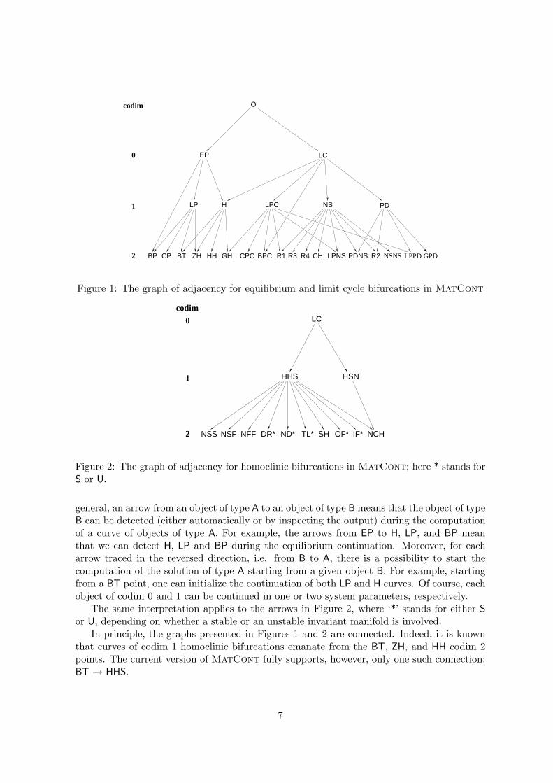
Relationships between objects of codimension 0, 1 and 2 computed by MatCont andCL MatCont are presented in Figures 1 and 2, while the symbols and their meaning aresummarized in Tables 2 and 3, where the standard terminology is used, see [23].
An arrow in Figure 1 from O to EP or LC means that by starting time integration froma given point we can converge to a stable equilibrium or a stable limit cycle, respectively. In
5
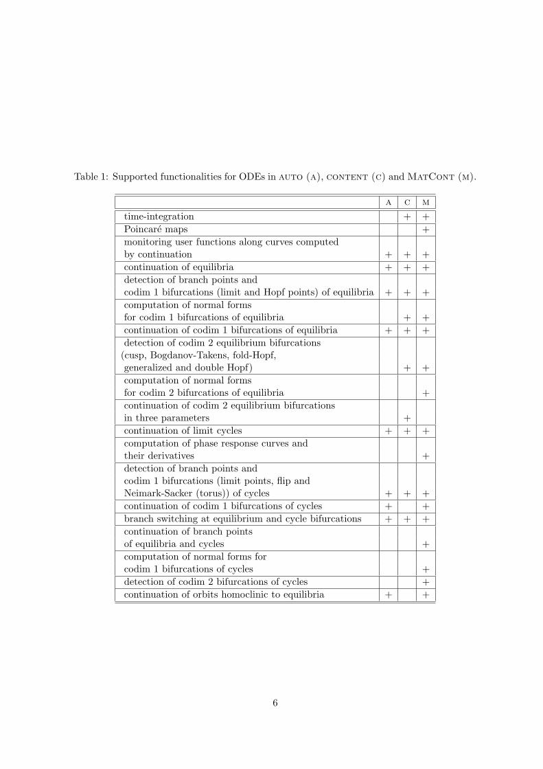
Table 1: Supported functionalities for ODEs in auto (a), content (c) and MatCont (m).
a c m
time-integration + +
Poincare maps +
monitoring user functions along curves computedby continuation + + +
continuation of equilibria + + +
detection of branch points andcodim 1 bifurcations (limit and Hopf points) of equilibria + + +
computation of normal formsfor codim 1 bifurcations of equilibria + +
continuation of codim 1 bifurcations of equilibria + + +
detection of codim 2 equilibrium bifurcations(cusp, Bogdanov-Takens, fold-Hopf,generalized and double Hopf) + +
computation of normal formsfor codim 2 bifurcations of equilibria +
continuation of codim 2 equilibrium bifurcationsin three parameters +
continuation of limit cycles + + +
computation of phase response curves andtheir derivatives +
detection of branch points andcodim 1 bifurcations (limit points, flip andNeimark-Sacker (torus)) of cycles + + +
continuation of codim 1 bifurcations of cycles + +
branch switching at equilibrium and cycle bifurcations + + +
continuation of branch pointsof equilibria and cycles +
computation of normal forms forcodim 1 bifurcations of cycles +
detection of codim 2 bifurcations of cycles +
continuation of orbits homoclinic to equilibria + +
6
GPDCPCZH HHBP CP BT GH BPC R3R1 R4 CH LPNS PDNS
PD
EP
O
LP NS
LC
H LPC1
0
codim
2 R2 NSNS LPPD
Figure 1: The graph of adjacency for equilibrium and limit cycle bifurcations in MatCont
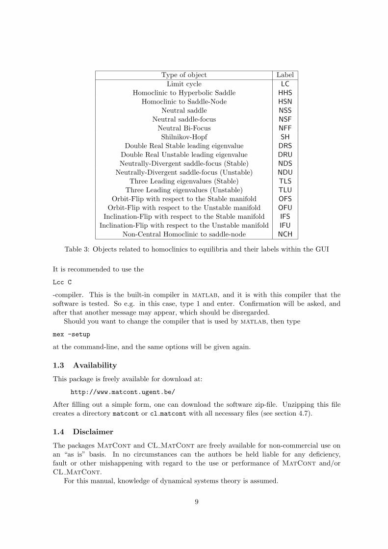
NSFNSS NFF ND* TL* SH OF* IF* NCH
HSN
codimLC
HHS
DR*2
1
0
Figure 2: The graph of adjacency for homoclinic bifurcations in MatCont; here * stands forS or U.
general, an arrow from an object of type A to an object of type B means that the object of typeB can be detected (either automatically or by inspecting the output) during the computationof a curve of objects of type A. For example, the arrows from EP to H, LP, and BP meanthat we can detect H, LP and BP during the equilibrium continuation. Moreover, for eacharrow traced in the reversed direction, i.e. from B to A, there is a possibility to start thecomputation of the solution of type A starting from a given object B. For example, startingfrom a BT point, one can initialize the continuation of both LP and H curves. Of course, eachobject of codim 0 and 1 can be continued in one or two system parameters, respectively.
The same interpretation applies to the arrows in Figure 2, where ‘*’ stands for either S
or U, depending on whether a stable or an unstable invariant manifold is involved.In principle, the graphs presented in Figures 1 and 2 are connected. Indeed, it is known
that curves of codim 1 homoclinic bifurcations emanate from the BT, ZH, and HH codim 2points. The current version of MatCont fully supports, however, only one such connection:BT → HHS.
7
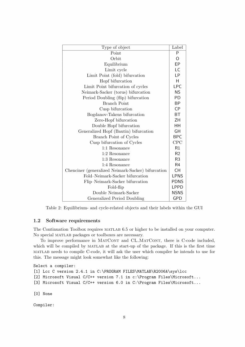
Type of object Label
Point P
Orbit O
Equilibrium EP
Limit cycle LC
Limit Point (fold) bifurcation LP
Hopf bifurcation H
Limit Point bifurcation of cycles LPC
Neimark-Sacker (torus) bifurcation NS
Period Doubling (flip) bifurcation PD
Branch Point BP
Cusp bifurcation CP
Bogdanov-Takens bifurcation BT
Zero-Hopf bifurcation ZH
Double Hopf bifurcation HH
Generalized Hopf (Bautin) bifurcation GH
Branch Point of Cycles BPC
Cusp bifurcation of Cycles CPC1:1 Resonance R1
1:2 Resonance R2
1:3 Resonance R3
1:4 Resonance R4
Chenciner (generalized Neimark-Sacker) bifurcation CH
Fold–Neimark-Sacker bifurcation LPNS
Flip–Neimark-Sacker bifurcation PDNS
Fold-flip LPPD
Double Neimark-Sacker NSNS
Generalized Period Doubling GPD
Table 2: Equilibrium- and cycle-related objects and their labels within the GUI
1.2 Software requirements
The Continuation Toolbox requires matlab 6.5 or higher to be installed on your computer.No special matlab packages or toolboxes are necessary.
To improve performance in MatCont and CL MatCont, there is C-code included,which will be compiled by matlab at the start-up of the package. If this is the first timematlab needs to compile C-code, it will ask the user which compiler he intends to use forthis. The message might look somewhat like the following:
Select a compiler:
[1] Lcc C version 2.4.1 in C:\PROGRAM FILES\MATLAB\R2006A\sys\lcc
[2] Microsoft Visual C/C++ version 7.1 in c:\Program Files\Microsoft...
[3] Microsoft Visual C/C++ version 6.0 in C:\Program Files\Microsoft...
[0] None
Compiler:
8
Type of object Label
Limit cycle LC
Homoclinic to Hyperbolic Saddle HHS
Homoclinic to Saddle-Node HSN
Neutral saddle NSS
Neutral saddle-focus NSF
Neutral Bi-Focus NFF
Shilnikov-Hopf SH
Double Real Stable leading eigenvalue DRS
Double Real Unstable leading eigenvalue DRU
Neutrally-Divergent saddle-focus (Stable) NDS
Neutrally-Divergent saddle-focus (Unstable) NDU
Three Leading eigenvalues (Stable) TLS
Three Leading eigenvalues (Unstable) TLU
Orbit-Flip with respect to the Stable manifold OFS
Orbit-Flip with respect to the Unstable manifold OFU
Inclination-Flip with respect to the Stable manifold IFS
Inclination-Flip with respect to the Unstable manifold IFU
Non-Central Homoclinic to saddle-node NCH
Table 3: Objects related to homoclinics to equilibria and their labels within the GUI
It is recommended to use the
Lcc C
-compiler. This is the built-in compiler in matlab, and it is with this compiler that thesoftware is tested. So e.g. in this case, type 1 and enter. Confirmation will be asked, andafter that another message may appear, which should be disregarded.
Should you want to change the compiler that is used by matlab, then type
mex -setup
at the command-line, and the same options will be given again.
1.3 Availability
This package is freely available for download at:
http://www.matcont.ugent.be/
After filling out a simple form, one can download the software zip-file. Unzipping this filecreates a directory matcont or cl matcont with all necessary files (see section 4.7).
1.4 Disclaimer
The packages MatCont and CL MatCont are freely available for non-commercial use onan “as is” basis. In no circumstances can the authors be held liable for any deficiency,fault or other mishappening with regard to the use or performance of MatCont and/orCL MatCont.
For this manual, knowledge of dynamical systems theory is assumed.
9
2 Numerical continuation algorithm
Consider a smooth function F : Rn+1 → Rn. We want to compute a solution curve of theequation F (x) = 0. Numerical continuation is a technique to compute a consecutive sequenceof points which approximate the desired branch. Most continuation algorithms implement apredictor-corrector method. The idea behind this method is to generate a sequence of pointsxi, i = 1, 2, . . . along the curve, satisfying a chosen tolerance criterion: ||F (xi)|| ≤ ǫ for someǫ > 0 and an additional accuracy condition ||δxi|| ≤ ǫ′ where ǫ′ > 0 and δxi is the last Newtoncorrection.
To show how the points are generated, suppose we have found a point xi on the curve.Also suppose we have a normalized tangent vector vi at xi, i.e. Fx(xi)vi = 0, 〈vi, vi〉 = 1.
The computation of the next point xi+1 consists of 2 steps:
• prediction of a new point
• correction of the predicted point
2.1 Prediction
Suppose h > 0 which will represent a stepsize. A commonly used predictor is tangent predic-tion:
X0 = xi + hvi. (1)
The choice of the stepsize is discussed in section 2.3.
2.2 Correction
We assume that X0 is close to the curve. To find the point xi+1 on the curve we use aNewton-like procedure. Since the standard Newton iterations can only be applied to systemswith the same number of equations as unknowns, we have to append an extra scalar condition:
{F (x) = 0,g(x) = 0.
(2)
The question is how to choose the function g(x).
2.2.1 Pseudo-arclength continuation
One option for choosing g(x) is to select a hyperplane passing through X0 that is orthogonalto the vector vi:
g(x) = 〈x−X0, vi〉 . (3)
So, the Newton iteration becomes:
Xk+1 = Xk −H−1x (Xk)H(Xk) (4)
H(X) =
(F (X)
0
), Hx(X) =
(Fx(X)vTi
). (5)
Then one can prove that the Newton iteration for (2) will converge to a point xi+1 on thecurve from X0 provided that the stepsize h is sufficiently small and that the curve is regular
10
V0
V1
X0
X2
V2
X1
xi
xi+1
vi+1
vi
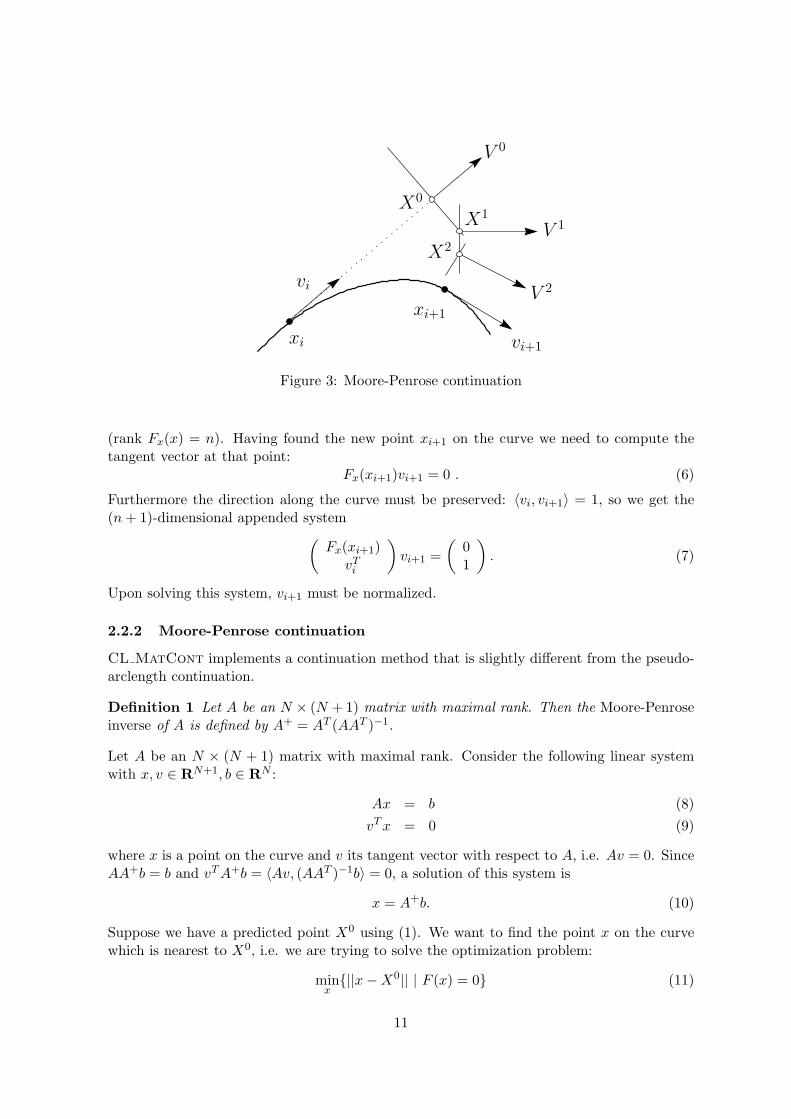
Figure 3: Moore-Penrose continuation
(rank Fx(x) = n). Having found the new point xi+1 on the curve we need to compute thetangent vector at that point:
Fx(xi+1)vi+1 = 0 . (6)
Furthermore the direction along the curve must be preserved: 〈vi, vi+1〉 = 1, so we get the(n+ 1)-dimensional appended system
(Fx(xi+1)
vTi
)vi+1 =
(01
). (7)
Upon solving this system, vi+1 must be normalized.
2.2.2 Moore-Penrose continuation
CL MatCont implements a continuation method that is slightly different from the pseudo-arclength continuation.
Definition 1 Let A be an N × (N + 1) matrix with maximal rank. Then the Moore-Penroseinverse of A is defined by A+ = AT (AAT )−1.
Let A be an N × (N + 1) matrix with maximal rank. Consider the following linear systemwith x, v ∈ RN+1, b ∈ RN :
Ax = b (8)
vTx = 0 (9)
where x is a point on the curve and v its tangent vector with respect to A, i.e. Av = 0. SinceAA+b = b and vTA+b = 〈Av, (AAT )−1b〉 = 0, a solution of this system is
x = A+b. (10)
Suppose we have a predicted point X0 using (1). We want to find the point x on the curvewhich is nearest to X0, i.e. we are trying to solve the optimization problem:
minx
{||x−X0|| | F (x) = 0} (11)
11
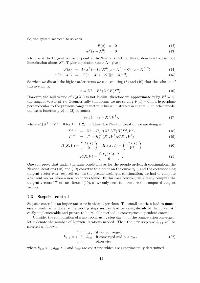
So, the system we need to solve is:
F (x) = 0 (12)
wT (x−X0) = 0 (13)
where w is the tangent vector at point x. In Newton’s method this system is solved using alinearization about X0. Taylor expansion about X0 gives:
F (x) = F (X0) + Fx(X0)(x−X0) + O(||x−X0||2) (14)
wT (x−X0) = vT (x−X0) + O(||x−X0||2) . (15)
So when we discard the higher order terms we can see using (8) and (10) that the solution ofthis system is:
x = X0 − F+x (X0)F (X0) . (16)
However, the null vector of Fx(X0) is not known, therefore we approximate it by V 0 = vi,the tangent vector at xi. Geometrically this means we are solving F (x) = 0 in a hyperplaneperpendicular to the previous tangent vector. This is illustrated in Figure 3. In other words,the extra function g(x) in (2) becomes:
gk(x) = 〈x−Xk, V k〉, (17)
where Fx(Xk−1)V k = 0 for k = 1, 2, . . .. Thus, the Newton iteration we are doing is:
Xk+1 = Xk −H−1x (Xk, V k)H(Xk, V k) (18)
V k+1 = V k −H−1x (Xk, V k)R(Xk, V k) (19)
H(X,V ) =
(F (X)
0
), Hx(X,V ) =
(Fx(X)V T
)(20)
R(X,V ) =
(Fx(X)V
0
). (21)
One can prove that under the same conditions as for the pseudo-arclength continuation, theNewton iterations (18) and (19) converge to a point on the curve xi+1 and the correspondingtangent vector vi+1, respectively. In the pseudo-arclength continuation, we had to computea tangent vector when a new point was found. In this case however, we already compute thetangent vectors V k at each iterate (19), so we only need to normalize the computed tangentvectors.
2.3 Stepsize control
Stepsize control is an important issue in these algorithms. Too small stepsizes lead to unnec-essary work being done, while too big stepsizes can lead to losing details of the curve. Aneasily implementable and proven to be reliable method is convergence-dependent control.
Consider the computation of a next point using step size hi. If the computation converged,let n denote the number of Newton iterations needed. Then the new step size hi+1 will beselected as follows:
hi+1 =
hi · hdec if not convergedhi · hinc if converged and n < nthr
hi otherwise(22)
where hdec < 1, hinc > 1 and nthr are constants which are experimentally determined.
12
3 Singularity handling
This section explains the idea of singularities which can occur on a solution branch.
3.1 Test functions
The idea to detect singularities is to define smooth scalar functions which have regular zerosat the singularity points. These functions are called test functions. Suppose we have asingularity S which is detectable by a test function φ : Rn+1 → R. Also assume we havefound two consecutive points xi and xi+1 on the curve
F (x) = 0, F : Rn+1 → Rn . (23)
The singularity S will then be detected if
φ(xi)φ(xi+1) < 0 . (24)
Having found two points xi and xi+1 one may want to locate the point x∗ where φ(x)vanishes. A logical solution is to solve the following system
F (x) = 0 (25)
φ(x) = 0 (26)
using Newton iterations starting at xi. However, to use this method, one should be able tocompute the derivatives of φ(x) with respect to x, which is not always easy. To avoid thisdifficulty we implemented by default a one-dimensional secant method to locate φ(x) = 0along the curve. Notice that this involves Newton corrections at each intermediate point.
3.2 Multiple test functions
The above is a general way to detect and locate singularities depending on one test function.However, it may happen that it is not possible to represent a singularity with only one testfunction.
Suppose we have a singularity S which depends on nt test functions. Also assume we havefound two consecutive points xi and xi+1 and all nt test functions change sign:
∀j ∈ [1, nt] : φj(xi)φj(xi+1) < 0 (27)
Also assume we have found, using a one-dimensional secant method, all zeros x∗j of the testfunctions. In the ideal (exact) case all these zeros will coincide:
∀j ∈ [1, nt] : x∗ = x∗j and φj(x∗
j ) = 0 (28)
Since the continuation is not exact but numerical, we cannot assume this. However, thelocations of x∗j probably will be clustered around some center point xc. In this case we willglue the points x∗j to x∗ = xc.
A cluster will be detected if ∀i, j ∈ [1, nt] : ||x∗i − x∗j || ≤ ǫ for some small value ǫ. In thiscase we define x∗ as the mean of all located zeroes:
x∗ =1
nt
nt∑
j=1
x∗j (29)
13
3.3 Singularity matrix
Until now we have discussed singularities depending only on test functions which vanish.Suppose we have two singularities S1 and S2, depending respectively on test functions φ1
and φ2. Namely, assume that φ1 vanishes at both S1 and S2, while φ2 vanishes at only S2.Therefore we need a possibility to represent singularities using non-vanishing test functions.
To represent all singularities we will introduce a singularity matrix (as in [24]). This matrixis a compact way to describe the relation between the singularities and all test functions.
Suppose we are interested in ns singularities and nt test functions which are needed todetect and locate the singularities. Then let S be the ns × nt matrix, such that:
Sij =
0 singularity i: test function j must vanish,1 singularity i: test function j must not vanish,
otherwise singularity i: ignore test function j.(30)
3.4 User location
In some cases the default location algorithm can have problems to locate a bifurcation point.Therefore we provide the possibility to define a specific location algorithm for a particularbifurcation. E.g. for the localization of branch points a special algorithm is used.
14
4 Software
4.1 System definition
The user defines his dynamical system in a systemfile, using the framework as in the filestandard.m in the Systems subdirectory.
In the function fun eval, the dynamical system is to be given, where the parametersshould be listed individually. Under init, the user can define some initialization parameters,as the phase variable values, the timespan, etc. All phase variables and parameters areexpected to be scalar variables, not vectors or matrices. In the further functions, it is possibleto supply the symbolic derivatives of the system to various orders to increase the speed and/orimprove accuracy of the algorithm. Note that for the hessians or higher order derivatives, nomixed derivatives are supplied through the system definition file, since they are never usedin (CL )MatCont. The option SymDerivative indicates to which order the derivatives areprovided.
Finally, it can contain the description of any number of user functions, i.e. functions thatcan be monitored along computed curves and whose zeros can be detected and located.
The system m-file can either be written by the user or generated automatically by the GUIof MatCont. The latter is strongly encouraged if the matlab symbolic toolbox is availableand symbolic derivatives are desirable. But when using the GUI input window, users shouldavoid using loops, conditional statements, or other specific programming constructions inthe system definition. If needed, they can be added manually to the system m-file, afterMatCont has generated it.
4.2 Continuation and output
The syntax of the continuer is:
[x,v,s,h,f] = cont(@curve, x0, v0, options);
curve is a matlab m-file where the problem is specified (cf. section 4.3). Evaluating a func-tion by means of a function handle replaces the earlier matlab mechanism of evaluating afunction through a string containing the function name.x0 and v0 are respectively the initial point and the tangent vector at the initial point wherethe continuation starts.options is a structure as described in section 4.4.The arguments v0 and options can be omitted. In this case the tangent vector at x0 iscomputed internally and default options are used.
The function returns a series of matrices:
x and v are the points and their tangent vectors along the curve. Each column in x andv corresponds to a point on the curve.
s is an array with structures containing information about the found singularities. Itsfirst and last elements always refer to the first and last points of the curve, respectively, sincefor convenience these are also considered ”special”.
15
Each element of this structure array s has the following fields:s.index index of the singularity point in x, so s(1).index is always equal to 1 and
s(end).index is the number of computed points.s.label label of the singularity; by convention s(1).label is ”00” and s(end).label is
”99”.s.msg a string that may contain any information which is useful for the user,
for example the full name of the detected special point.s.data For each special point it contains fields with additional
information, depending on the type of point, and accumulating with increasingcodimension:
• Equilibrium: s.data.v = tangent vector at the bifurcation
– Hopf point: s.data.lyapunov = first Lyapunov coefficient
– Limit point: s.data.a = normal form coefficient
∗ Bogdanov-Takens / Zero Hopf / Double Hopf / Generalized Hopf / Cusp :s.data.c = normal form coefficient
• Limit cycle:
s.data.multipliers = multipliers at the bifurcation
s.data.timemesh = time mesh of the orbit at the bifurcation
s.data.ntst = number of test intervals
s.data.ncol = number of collocation points
s.data.parametervalues = parameter values at the bifurcation
s.data.T = period of the orbit at the bifurcation
s.data.phi = bordering vector for locating PD bifurcations
– Period-doubling point: s.data.pdcoefficient = normal form coefficient
– Limit point of cycles: s.data.lpccoefficient = normal form coefficient
– Neimark-Sacker point: s.data.nscoefficient = normal form coefficient
• Homoclinic to hyperbolic saddle / Homoclinic to saddle-node:
s.data.timemesh = time mesh of the orbit at the bifurcation
s.data.ntst = number of test intervals
s.data.ncol = number of collocation points
s.data.parametervalues = parameter values at the bifurcation
s.data.T = period of the orbit at the bifurcation
h contains some information on the continuation process. Its columns are related to thecomputed points, and have the following components:Stepsize Stepsize used to calculate this point (zero for initial
point and singular points)Half the number of correction itera- For singular points this is the number of locatortions, rounded up to the next integer iterationsUser function values The values of all active user functionsTest function values The values of all active test functions
16
f contains different information, depending on the continuation run. For noncycle-relatedcontinuations, the f-vector just contains the eigenvalues, if asked for. For limit cycle contin-uations, it begins with the mesh points of the time- discretization, followed by, if they wereasked for, the PRC- and dPRC-values in all points of the periodic orbit (cf. section 9.5).Then, if required, follow the multipliers.
It is also possible to extend the most recently computed curve with the same options (alsosame number of points) as it was first computed. The syntax to extend this curve is:
[x, v, s, h, f] = cont( x, v, s, h, f, cds);
x, v, s, h and f are the results of the previous call to the continuer and cds is the globalvariable that contains the curve description of the most recently computed curve (note thatthis variable has to be defined as global cds in the calling command). The function returnsthe same output as before, extended with the new results.
In MatCont, all curves that have been computed using a specific system are storedin separate .mat-files, in a directory called diagram, under a subdirectory named after thesystem. For example, curves of the Connor system will be kept in .mat-files under thesubdirectory Systems/Connor/diagram/. For continuation runs, each such mat-file containsthe computed x,v,s,h,f arrays, plus the cds structure and a structure related to the curvetype. Also, it contains the variables point, ctype and num. To understand their meaning,suppose that we are computing curves of limit cycles that we start from Hopf points. Thefirst such computed curve then gets the name ”H LC(1)”, point stores the string ”H” andctype stores the string ”LC”. Furthermore, num stores the index in s of the last selectedpoint of the curve (the default is 1). The second curve of the same type is called ”H LC(2)”and so on. In fact, to save storage space, only a limited number of curves of a certain type isstored. This number can be set by the user and the default is 2. To save a computed curvepermanently, the user must change its name.
For time integration runs, cf. §6.1 (Curve Type O) and §6.2.1 (Curve type DO), themat-file contains ctype, option, param, point, s, t, x. Here t is the vector of time pointsand x is the corresponding array of computed points. s contains data on the first and lastcomputed points. The meaning of point,ctype is similar to the case of continuation curves.Finally, param is the vector of parameters of the ODE (constant during time integration) andoption is a structure that contains optional settings for time integration.
To export the computed results of a system to a different installation of MatCont onehas to copy the corresponding m-file, the mat-file and the directory of the system.
These files also contain all information needed to export the computed results to the gen-eral matlab environment, so MatCont is really an open system.
MatCont also produces graphical output. 2D and 3D graphs are plotted in matlab fig-ure windows. Such a graph can be handled as any other graph that is produced in matlab.It can be selected using the arrow-function of the matlab figure, and the line width, linestyle and colour can be altered. Markers can be set on the curve. It can be copy-pasted intoanother matlab figure. In a figure, textboxes can be inserted and axes labels can be added.Thus the user has a plethora of possibilities to combine different MatCont output graphs
17

into one figure.
Finally, we note that users often want to introduce new systems that are modifications ofexisting systems, but with slightly different sets of state variables and/or parameters. Thebest strategy to do this in MatCont is first to edit the existing system, change its name to anew one and click ”OK” to build an m-file with a different name and no associated directoryof computed curves. Afterwards, one can edit the newly created system, make all desiredchanges and click ”OK” again.
4.3 Curve file
The continuer uses a special m-file where the type of solution branch is defined. This file,further referred to as curve.m, contains the following sections:
• curve func: contains the evaluation of the right-hand side of that type of solutionbranch.
• defaultprocessor: is called and executed after each point computed during a contin-uation experiment.
• options: sets the default setting for the options-structure for this type of solutionbranch (more details are given in section 4.4).
• jacobian: contains the evaluation of the jacobian of that type of solution branch.
• hessians: contains the evaluation of the hessians of that type of solution branch.
• testf: contains the test functions for detecting bifurcations along the branch.
• userf: calls the user-defined functions if there are any.
• process: is called when a bifurcation point is detected, to handle any necessary outputmessages and storage.
• singmat: defines the singularity matrix of the solution branch (cf. section 3.3).
• locate: here specific localisation functions can be defined for bifurcations (cf. section3.4)
• init: handles any special initialisations needed in the parameters or workspace.
• done: handles any special actions needed at the end of continuing the solution branch.
• adapt: this is called after every n steps, where n is user-defined. It handles any adap-tation of parameters, subspaces, etc.
4.4 Options
4.4.1 The options-structure
It is possible to specify various options for the continuation run. In the continuation we usethe options structure which is initially created with contset:
18
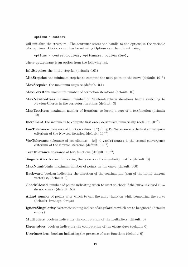
options = contset;
will initialize the structure. The continuer stores the handle to the options in the variablecds.options. Options can then be set using Options can then be set using
options = contset(options, optionname, optionvalue);
where optionname is an option from the following list.
InitStepsize the initial stepsize (default: 0.01)
MinStepsize the minimum stepsize to compute the next point on the curve (default: 10−5)
MaxStepsize the maximum stepsize (default: 0.1)
MaxCorrIters maximum number of correction iterations (default: 10)
MaxNewtonIters maximum number of Newton-Raphson iterations before switching toNewton-Chords in the corrector iterations (default: 3)
MaxTestIters maximum number of iterations to locate a zero of a testfunction (default:10)
Increment the increment to compute first order derivatives numerically (default: 10−5)
FunTolerance tolerance of function values: ||F (x)|| ≤ FunTolerance is the first convergencecriterium of the Newton iteration (default: 10−6)
VarTolerance tolerance of coordinates: ||δx|| ≤ VarTolerance is the second convergencecriterium of the Newton iteration (default: 10−6)
TestTolerance tolerance of test functions (default: 10−5)
Singularities boolean indicating the presence of a singularity matrix (default: 0)
MaxNumPoints maximum number of points on the curve (default: 300)
Backward boolean indicating the direction of the continuation (sign of the initial tangentvector) v0 (default: 0)
CheckClosed number of points indicating when to start to check if the curve is closed (0 =do not check) (default: 50)
Adapt number of points after which to call the adapt-function while computing the curve(default: 1=adapt always)
IgnoreSingularity vector containing indices of singularities which are to be ignored (default:empty)
Multipliers boolean indicating the computation of the multipliers (default: 0)
Eigenvalues boolean indicating the computation of the eigenvalues (default: 0)
Userfunctions boolean indicating the presence of user functions (default: 0)
19
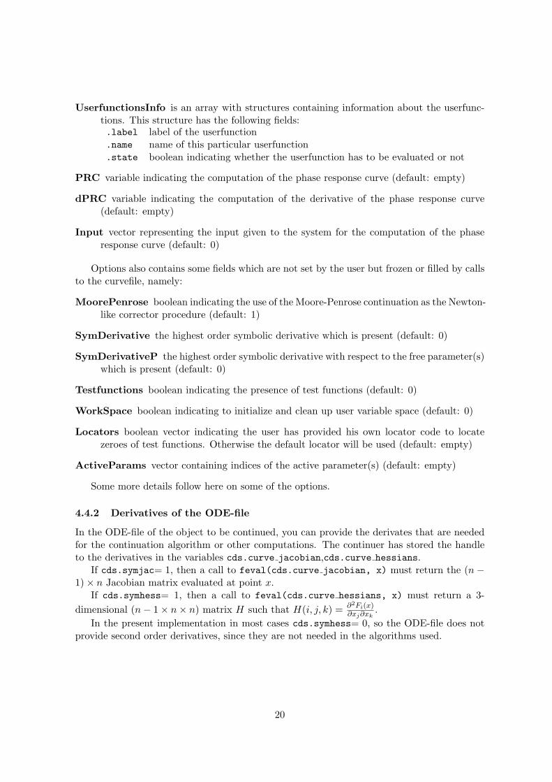
UserfunctionsInfo is an array with structures containing information about the userfunc-tions. This structure has the following fields:.label label of the userfunction.name name of this particular userfunction.state boolean indicating whether the userfunction has to be evaluated or not
PRC variable indicating the computation of the phase response curve (default: empty)
dPRC variable indicating the computation of the derivative of the phase response curve(default: empty)
Input vector representing the input given to the system for the computation of the phaseresponse curve (default: 0)
Options also contains some fields which are not set by the user but frozen or filled by callsto the curvefile, namely:
MoorePenrose boolean indicating the use of the Moore-Penrose continuation as the Newton-like corrector procedure (default: 1)
SymDerivative the highest order symbolic derivative which is present (default: 0)
SymDerivativeP the highest order symbolic derivative with respect to the free parameter(s)which is present (default: 0)
Testfunctions boolean indicating the presence of test functions (default: 0)
WorkSpace boolean indicating to initialize and clean up user variable space (default: 0)
Locators boolean vector indicating the user has provided his own locator code to locatezeroes of test functions. Otherwise the default locator will be used (default: empty)
ActiveParams vector containing indices of the active parameter(s) (default: empty)
Some more details follow here on some of the options.
4.4.2 Derivatives of the ODE-file
In the ODE-file of the object to be continued, you can provide the derivates that are neededfor the continuation algorithm or other computations. The continuer has stored the handleto the derivatives in the variables cds.curve jacobian,cds.curve hessians.
If cds.symjac= 1, then a call to feval(cds.curve jacobian, x) must return the (n−1) × n Jacobian matrix evaluated at point x.
If cds.symhess= 1, then a call to feval(cds.curve hessians, x) must return a 3-
dimensional (n− 1 × n× n) matrix H such that H(i, j, k) = ∂2Fi(x)∂xj∂xk
.
In the present implementation in most cases cds.symhess= 0, so the ODE-file does notprovide second order derivatives, since they are not needed in the algorithms used.
20
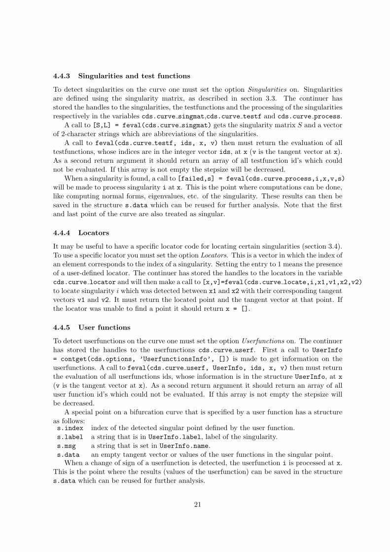
4.4.3 Singularities and test functions
To detect singularities on the curve one must set the option Singularities on. Singularitiesare defined using the singularity matrix, as described in section 3.3. The continuer hasstored the handles to the singularities, the testfunctions and the processing of the singularitiesrespectively in the variables cds.curve singmat,cds.curve testf and cds.curve process.
A call to [S,L] = feval(cds.curve singmat) gets the singularity matrix S and a vectorof 2-character strings which are abbreviations of the singularities.
A call to feval(cds.curve testf, ids, x, v) then must return the evaluation of alltestfunctions, whose indices are in the integer vector ids, at x (v is the tangent vector at x).As a second return argument it should return an array of all testfunction id’s which couldnot be evaluated. If this array is not empty the stepsize will be decreased.
When a singularity is found, a call to [failed,s] = feval(cds.curve process,i,x,v,s)
will be made to process singularity i at x. This is the point where computations can be done,like computing normal forms, eigenvalues, etc. of the singularity. These results can then besaved in the structure s.data which can be reused for further analysis. Note that the firstand last point of the curve are also treated as singular.
4.4.4 Locators
It may be useful to have a specific locator code for locating certain singularities (section 3.4).To use a specific locator you must set the option Locators. This is a vector in which the index ofan element corresponds to the index of a singularity. Setting the entry to 1 means the presenceof a user-defined locator. The continuer has stored the handles to the locators in the variablecds.curve locator and will then make a call to [x,v]=feval(cds.curve locate,i,x1,v1,x2,v2)
to locate singularity i which was detected between x1 and x2 with their corresponding tangentvectors v1 and v2. It must return the located point and the tangent vector at that point. Ifthe locator was unable to find a point it should return x = [].
4.4.5 User functions
To detect userfunctions on the curve one must set the option Userfunctions on. The continuerhas stored the handles to the userfunctions cds.curve userf. First a call to UserInfo
= contget(cds.options, ’UserfunctionsInfo’, []) is made to get information on theuserfunctions. A call to feval(cds.curve userf, UserInfo, ids, x, v) then must returnthe evaluation of all userfunctions ids, whose information is in the structure UserInfo, at x
(v is the tangent vector at x). As a second return argument it should return an array of alluser function id’s which could not be evaluated. If this array is not empty the stepsize willbe decreased.
A special point on a bifurcation curve that is specified by a user function has a structureas follows:s.index index of the detected singular point defined by the user function.s.label a string that is in UserInfo.label, label of the singularity.s.msg a string that is set in UserInfo.name.s.data an empty tangent vector or values of the user functions in the singular point.
When a change of sign of a userfunction is detected, the userfunction i is processed at x.This is the point where the results (values of the userfunction) can be saved in the structures.data which can be reused for further analysis.
21

4.4.6 Defaultprocessor
In many cases it is useful to do some general computations for every calculated point onthe curve. The results of these computations can then be used by for example the test-functions. The continuer has stored the handle to the defaultprocessor in the variablecds.curve defaultprocessor.
The defaultprocessor is called as [failed,f,s] = feval(cds.curve defaultprocressor,x,v,s).x and v are the point on the curve and it’s tangent vector. The argument s is only suppliedif the point is a singular point, in that case the defaultprocessor may also add some data tothe s.data field. If for some reason the default processor fails it should set failed to 1. Thiswill result in a reduction of the stepsize and a retry which should solve the problem. Anyinformation that is to be preserved, should be put in f. f must be a column vector and mustbe of equal size for every call to the default processor.
4.4.7 Special processors
After a singular point has been detected and located a singular point data structure willbe created and initialized as described in section 4.2. If there are some special data (likeeigenvalues) which may be of interest for a particular singular point then a call to [failed,s]
= feval(cds.curve process,i,x,v,s) should store this data in the s.data field. Here i
indicates which singularity was detected and x and v are the point and tangent vector wherethis singularity was detected.
4.4.8 Workspace
During the computation of a curve it is sometimes necessary to introduce variables and doadditional computations that are common to all points of the curve. The continuer has storedthe handle to the initialization and cleaning of the workspace in the variables cds.curve init
and cds.curve done. These can be relegated to a call of the type
feval(cds.curve_init,x,v).
This option has to be provided only if the variable WorkSpace in cds.options is switchedon. In this case a call
feval(cds.curve_done,x,v)
must clear the workspace. Variables in the workspace must be set global.
4.4.9 Adaptation
It is possible to adapt the problem while generating the curve. If Adapt has a value, say 5,then after 5 computed points a call to [reeval,x,v]=feval(cds.curve adapt,x,v) will bemade where the user can program to change the system.
For some applications it is useful to change or modify the used test functions while com-puting the curve (like in bordering techniques). In order to preserve the correct signs of thetest functions it is sometimes necessary to reevaluate the test functions after adaptation. Todo this reeval should be one otherwise zero. The return variables x and v should be theupdated x and v which may have changed because of the changes made to the system.
22
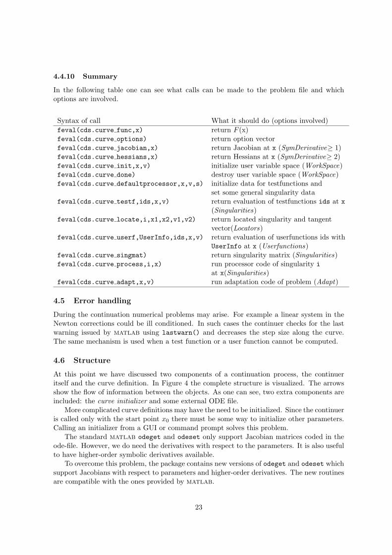
4.4.10 Summary
In the following table one can see what calls can be made to the problem file and whichoptions are involved.
Syntax of call What it should do (options involved)
feval(cds.curve func,x) return F (x)feval(cds.curve options) return option vectorfeval(cds.curve jacobian,x) return Jacobian at x (SymDerivative≥ 1)feval(cds.curve hessians,x) return Hessians at x (SymDerivative≥ 2)feval(cds.curve init,x,v) initialize user variable space (WorkSpace)feval(cds.curve done) destroy user variable space (WorkSpace)feval(cds.curve defaultprocessor,x,v,s) initialize data for testfunctions and
set some general singularity datafeval(cds.curve testf,ids,x,v) return evaluation of testfunctions ids at x
(Singularities)feval(cds.curve locate,i,x1,x2,v1,v2) return located singularity and tangent
vector(Locators)feval(cds.curve userf,UserInfo,ids,x,v) return evaluation of userfunctions ids with
UserInfo at x (Userfunctions)feval(cds.curve singmat) return singularity matrix (Singularities)feval(cds.curve process,i,x) run processor code of singularity i
at x(Singularities)feval(cds.curve adapt,x,v) run adaptation code of problem (Adapt)
4.5 Error handling
During the continuation numerical problems may arise. For example a linear system in theNewton corrections could be ill conditioned. In such cases the continuer checks for the lastwarning issued by matlab using lastwarn() and decreases the step size along the curve.The same mechanism is used when a test function or a user function cannot be computed.
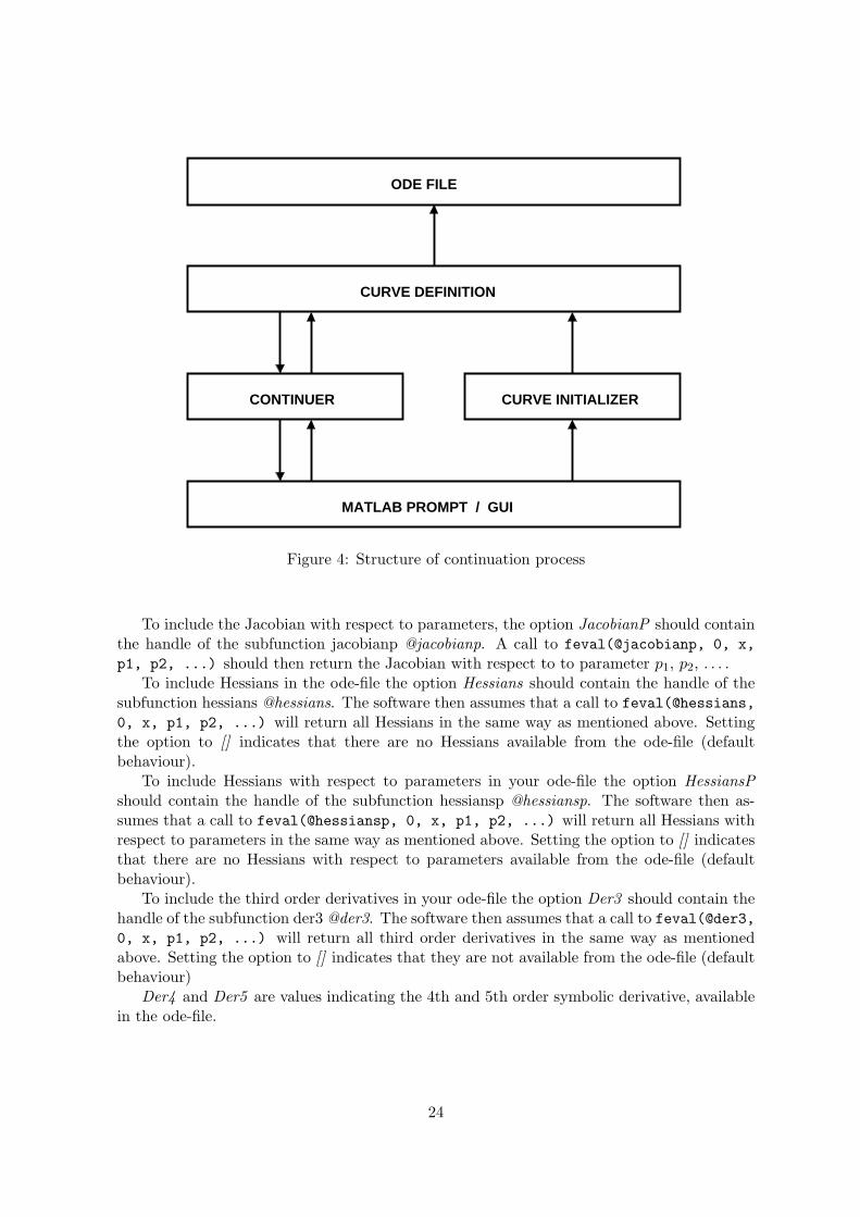
4.6 Structure
At this point we have discussed two components of a continuation process, the continueritself and the curve definition. In Figure 4 the complete structure is visualized. The arrowsshow the flow of information between the objects. As one can see, two extra components areincluded: the curve initializer and some external ODE file.
More complicated curve definitions may have the need to be initialized. Since the continueris called only with the start point x0 there must be some way to initialize other parameters.Calling an initializer from a GUI or command prompt solves this problem.
The standard matlab odeget and odeset only support Jacobian matrices coded in theode-file. However, we do need the derivatives with respect to the parameters. It is also usefulto have higher-order symbolic derivatives available.
To overcome this problem, the package contains new versions of odeget and odeset whichsupport Jacobians with respect to parameters and higher-order derivatives. The new routinesare compatible with the ones provided by matlab.
23
CONTINUER CURVE INITIALIZER
ODE FILE
CURVE DEFINITION
MATLAB PROMPT / GUI
Figure 4: Structure of continuation process
To include the Jacobian with respect to parameters, the option JacobianP should containthe handle of the subfunction jacobianp @jacobianp. A call to feval(@jacobianp, 0, x,
p1, p2, ...) should then return the Jacobian with respect to to parameter p1, p2, . . . .To include Hessians in the ode-file the option Hessians should contain the handle of the
subfunction hessians @hessians. The software then assumes that a call to feval(@hessians,
0, x, p1, p2, ...) will return all Hessians in the same way as mentioned above. Settingthe option to [] indicates that there are no Hessians available from the ode-file (defaultbehaviour).
To include Hessians with respect to parameters in your ode-file the option HessiansPshould contain the handle of the subfunction hessiansp @hessiansp. The software then as-sumes that a call to feval(@hessiansp, 0, x, p1, p2, ...) will return all Hessians withrespect to parameters in the same way as mentioned above. Setting the option to [] indicatesthat there are no Hessians with respect to parameters available from the ode-file (defaultbehaviour).
To include the third order derivatives in your ode-file the option Der3 should contain thehandle of the subfunction der3 @der3. The software then assumes that a call to feval(@der3,
0, x, p1, p2, ...) will return all third order derivatives in the same way as mentionedabove. Setting the option to [] indicates that they are not available from the ode-file (defaultbehaviour)
Der4 and Der5 are values indicating the 4th and 5th order symbolic derivative, availablein the ode-file.
24
4.7 Directories
The files of the toolbox are organized in the following directories
• ContinuerHere are all the main files stored for the continuer, which are needed to calculate andplot any curve.
• EquilibriumHere are all files stored needed to do an equilibrium continuation. This includes theinitializers and the equilibrium curve definition file.
• LimitCycleHere are all files stored needed to do a limit cycle continuation. This includes theinitializers and the limitcycle curve definition file.
• LimitpointHere are all files stored needed to do a limitpoint continuation. This includes theinitializers and the limitpoint curve definition file.
• HopfHere are all files stored needed to do a Hopf point continuation. This includes theinitializers and the Hopf point curve definition file.
• PeriodDoublingHere are all files stored needed to do a period doubling bifurcation continuation. Thisincludes the initializers and perioddoubling curve definition files.
• LimitPointCycleHere are all files stored needed to do a fold bifurcation of limit cycles continuation. Thisincludes the initializers and limitpoint of cycles curve definition files.
• NeimarkSackerHere are all files stored needed to do a torus bifurcation of limit cycles continuation.This includes the initializers and torus curve definition files.
• BranchPointHere are all files stored needed to do a branch point continuation. This includes theinitializers and a branch point curve definition file.
• BranchPointCycleHere are all files stored needed to do a branch point of cycles continuation. This inludedthe initializers and branch point of cycles definition files.
• HomoclinicHere are all files stored needed to do a homoclinic-to-hyperbolic-saddle continuation.This includes the initializers and the curve definition file.
• HomoclinicSaddleNodeHere are all files stored needed to do a homoclinic-to-saddle-node continuation. Thisincludes the initializers and the curve definition file.
25
• MultiLinearFormsHere are files stored needed to compute high-order derivatives of systems and normal-form coefficients of bifurcations.
• SystemsHere all system definition files and files related to computed curves are stored.
• GUIIn MatCont, this directory contains all GUI-related files.
• TestrunsOnly in CL MatCont.Here are some example testruns stored. It can be used to runthe examples described in this manual and to test if everything is working correctly.
• HelpContains the help-files.
The only files which are not in any of these directories are in CL MatCont init.m andcpl.m and in MatCont matcont.fig and matcont.m. The function init must be calledbefore doing anything with the command-line toolbox so matlab can find all the neededfunctions. cpl is used to plot the results of the continuation in CL MatCont. matcont.m
is the start-up file of the GUI version MatCont, and matcont.fig is the related figure-file.
26
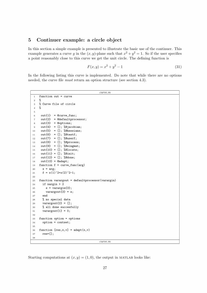
5 Continuer example: a circle object
In this section a simple example is presented to illustrate the basic use of the continuer. Thisexample generates a curve g in the (x, y)-plane such that x2 + y2 = 1. So if the user specifiesa point reasonably close to this curve we get the unit circle. The defining function is
F (x, y) = x2 + y2 − 1 (31)
In the following listing this curve is implemented. Do note that while there are no optionsneeded, the curve file must return an option structure (see section 4.3).
curve.m
1 function out = curve
2 %
3 % Curve file of circle
4 %
5
6 out{1} = @curve_func;
7 out{2} = @defaultprocessor;
8 out{3} = @options;
9 out{4} = []; %@jacobian;
10 out{5} = []; %@hessians;
11 out{6} = []; %@testf;
12 out{7} = []; %@userf;
13 out{8} = []; %@process;
14 out{9} = []; %@singmat;
15 out{10} = []; %@locate;
16 out{11} = []; %@init;
17 out{12} = []; %@done;
18 out{13} = @adapt;
19 function f = curve_func(arg)
20 x = arg;
21 f = x(1)^2+x(2)^2-1;
22
23 function varargout = defaultprocessor(varargin)
24 if nargin > 2
25 s = varargin{3};
26 varargout{3} = s;
27 end
28 % no special data
29 varargout{2} = [];
30 % all done succesfully
31 varargout{1} = 0;
32
33 function option = options
34 option = contset;
35
36 function [res,x,v] = adapt(x,v)
37 res=[];
38
curve.m
Starting computations at (x, y) = (1, 0), the output in matlab looks like:
27
−0.8 −0.6 −0.4 −0.2 0 0.2 0.4 0.6 0.8 1
−0.8
−0.6
−0.4
−0.2
0
0.2
0.4
0.6
0.8
x(1)
x(2)
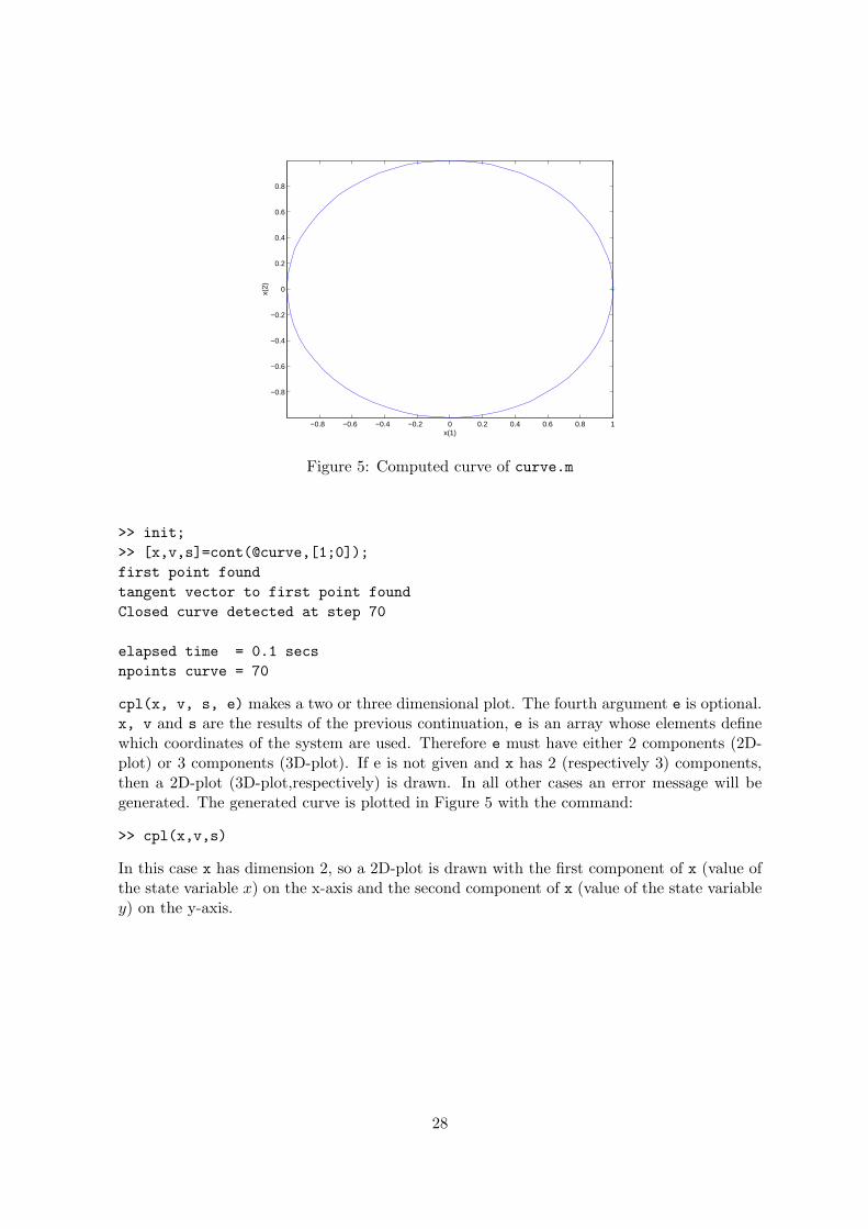
Figure 5: Computed curve of curve.m
>> init;
>> [x,v,s]=cont(@curve,[1;0]);
first point found
tangent vector to first point found
Closed curve detected at step 70
elapsed time = 0.1 secs
npoints curve = 70
cpl(x, v, s, e) makes a two or three dimensional plot. The fourth argument e is optional.x, v and s are the results of the previous continuation, e is an array whose elements definewhich coordinates of the system are used. Therefore e must have either 2 components (2D-plot) or 3 components (3D-plot). If e is not given and x has 2 (respectively 3) components,then a 2D-plot (3D-plot,respectively) is drawn. In all other cases an error message will begenerated. The generated curve is plotted in Figure 5 with the command:
>> cpl(x,v,s)
In this case x has dimension 2, so a 2D-plot is drawn with the first component of x (value ofthe state variable x) on the x-axis and the second component of x (value of the state variabley) on the y-axis.
28
6 Time integration and Poincare maps
matlab provides a suite of ODE-solvers. To create a combined integration-continuationenvironment, we have made them all accessible in MatCont and added two new ones, ode78and ode87. ode78 is an explicit Runge-Kutta method that uses 7th order Fehlberg formulas[Fehlberg 1969]. This is a 7-8th-order accurate integrator, therefore the local error normallyexpected is O(h9). ode87 is a Runge-Kutta method that uses 8-7th order Dorman and Princeformulas. See [Prince and Dorman 1981]. This is a 8th-order accurate integrator thereforethe local error normally expected is O(h9). In MatCont the choice of the solver is madevia the Integrator window that is opened automatically when the curve type O (Orbit) ischosen. We note that the Starter window has a SelectCycle button that allows to start thecontinuation of periodic orbits from curves computed by time integration.
6.1 Time integration
MatCont uses the matlab representation of ODEs, which can also be used by the matlabODE solvers. The user of Cl MatCont is therefore also able to use his/her model withinthe standard ODE solver without rewriting the code. In MatCont, also backward time inte-gration is possible using the standard ODE solvers. To make them accessible in MatCont,some output functions and properties were created.
6.1.1 Solver output properties
The solver output properties allow one to control the output that the solvers generate. Mat-Cont detects whether extra output is needed by looking at the number of open outputwindows (2D, 3D or numeric). If extra output is required, MatCont sets the OutputFcnproperty to the output function, integplot which is passed to an ODE solver by options
= odeset(’OutputFcn’, @integplot), otherwise it is set to the function integ prs. Theoutput function must be of the form status = integplot(t, y, flag, p1, p2,...). Thesolver calls this function after every successful integration step with the following flags. Notethat the syntax of the call differs with the flag. The function must respond appropriately:
• init: The solver calls integplot(tspan,y0,’init’) before beginning the integration,to allow the output function to initialize. This part initializes the output windowsand does some initializations to speed up the further processing of the output. It alsolaunches the window that makes it possible to interactively ”stop/pause/resume” thecomputations.
• {none}: within MatCont it is possible to define the number of points (npoints) afterwhich output is needed. Because the solver calls status = integplot (t,y) after eachintegration step, the number of calls to integplot and npoints does not correspond.Therefore this part is divided into two parts. t contains points where output wasgenerated during the step, and y is the numerical solution at the points in t. If tis a vector, the i-th column of y corresponds to the i-th element of t. The outputis produced according to the Refine option. integplot must return a status outputvalue of 0 or 1. If status = 1, the solver halts integration. This part also handles the”stop/pause/resume” interactions.
29
• done: The solver calls integplot([],[],’done’) when integration is completed toallow the output function to perform any cleanup chores. The stop-window is alsodeleted.
Setting the OutputFcn property to the output function, integ prs, reduces the output time.It only allows to interactively pause, resume and stop the integration.
6.1.2 Jacobian matrices
Stiff ODE solvers often execute faster if the Jacobian matrix, i.e. the matrix of partial deriva-tives of the RHS that defines the differential equations, is provided. The Jacobian matrixpertains only to those solvers for stiff problems (ode15s, ode23s, ode23t, ode23tb), forwhich it can be critical for reliability and efficiency. If the user does not provide a code tocalculate the Jacobian matrix, these solvers approximate it numerically using finite differ-ences. Supplying an analytical Jacobian matrix often increases the speed and reliability ofthe solution for stiff problems. If the Jacobian matrix is provided (symbolically) in the odefile,MatCont stores as property the function handle of the Jacobian, otherwise this handle isset empty.
The standard matlab odeget and odeset only support Jacobian matrices of the RHSw.r.t. the state variables. However, we do need derivatives with respect to the parametersfor the continuation. To compute normal form coefficients, it also useful to have higher-order symbolic derivatives. To overcome this problem, MatCont contains new versions ofodeget and odeset, which support Jacobian matrices with respect to parameters and higher-order partial derivatives w.r.t state variables. The new routines are compatible with the onesprovided by matlab.
6.2 Poincare section and Poincare map
A Poincare section is a surface in phase space that cuts across the flow of a dynamicalsystem. It is a carefully chosen (in general, curved) surface in the phase space that is crossedby almost all orbits. It is a tool developed by Poincare for visualization of the flow in morethan two dimensions. The Poincare section has one dimension less than the phase spaceand the Poincare map transforms the Poincare section onto itself by relating two consecutiveintersection points, say uk and uk+1. We note that only those intersection points count,which come from the same side of the section. The Poincare map is invertible because onegets un from un+1 by following the orbit backwards. A Poincare map turns a continuous-timedynamical system into a discrete-time one. If the Poincare section is carefully chosen noinformation is lost concerning the qualitative behaviour of the dynamics. For example, if thesystem is being attracted to a limit cycle, one observes dots converging to a fixed point in thePoincare section.
6.2.1 Poincare maps in MatCont
In some ODE problems the timing of specific events is important, such as the time and place atwhich a Poincare section is crossed. For this purpose, MatCont provides the special curvetype DO (Discrete Orbit) which is similar to O (Orbit) but provides a Starter window inwhich one can specify several event functions of the form G(u) =
∑nj=1 ajuj −a0, so G(u) = 0
corresponds to a Poincare section (to avoid nonlinear interpolation problems, only this form of
30
function G is allowed). While integrating, the ODE solvers can detect such events by locatingtransitions to, from or through zeros of G(u(t))). One does this by setting the Events propertyto a function handle, e.g. @events, and creating a function [value,isterminal,direction]
= events(t,y) and calling[t,Y,TE,YE,IE] = solver(odefun,tspan,y0,options).
For the i-th event function:
• value(i) is the value of the function.
• isterminal(i) = 1 if the integration is to terminate at a zero of this event functionand 0 otherwise.
• direction(i) = 0 if all zeros are to be computed (the default), +1 if only the zerosare needed where the event function increases, and -1 if only the zeros where the eventfunction decreases.
Corresponding entries in TE, YE, and IE return, respectively, the time at which an eventoccurs, the solution at the time of the event, and the index i of the event function thatvanishes.
Unfortunately this method can only be used in Cl MatCont. MatCont needs someinteraction between (t,Y) and (TE,YE). This is not possible by using the Events property.The part that handles the Poincare map is the OutputFcn property of the integrators whichis now set to integplotDO. The user is able to enter the equation G(u) in the Starter window.This output function is divided into three parts:
• The solver calls integplotDO(tspan,y0,’init’) before starting the integration, to ini-tialize the output function. Here G(u(t0)) is initialized. The same output initializationsare done as in the function integplot(see §6.1.1).
• The solver calls integplotDO(tspan,y0). We are looking for a value t∗ for whichG(u(t∗)) = 0. The function integDOzero calculates the value of G(u(ti)) and looksfor a sign change. If there is one, the function tries to locate it. Afterwards, someprocessing is done.
• The solver calls integplotDO(tspan,y0,’done’) when the integration is completed,to allow the output function to perform any cleanup chores.
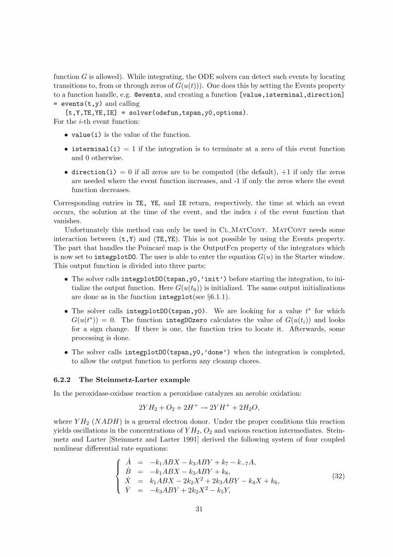
6.2.2 The Steinmetz-Larter example
In the peroxidase-oxidase reaction a peroxidase catalyzes an aerobic oxidation:
2Y H2 +O2 + 2H+ → 2Y H+ + 2H2O,
where Y H2 (NADH) is a general electron donor. Under the proper conditions this reactionyields oscillations in the concentrations of Y H2, O2 and various reaction intermediates. Stein-metz and Larter [Steinmetz and Larter 1991] derived the following system of four couplednonlinear differential rate equations:
A = −k1ABX − k3ABY + k7 − k−7A,
B = −k1ABX − k3ABY + k8,
X = k1ABX − 2k2X2 + 2k3ABY − k4X + k6,
Y = −k3ABY + 2k2X2 − k5Y,
(32)
31
Variable Value Parameter Value Parameter Value
A 1.8609653 k1 0.1631021 k5 1.104
B 25.678306 k2 1250 k6 0.001
X 0.010838258 k3 0.046875 k7 0.71643356
Y 0.094707061 k4 20 k8 0.5
k−7 0.1175
Table 5: Values of a point on the first NS- cycle in the Steinmetz-Larter model.
Variable Value Parameter Value
A 6.1231735 k7 1.5163129
B 9.1855407 k8 0.83200664
X 0.0054271408
Y 0.024602951
Table 6: Values of the second NS point in the Steinmetz-Larter model.
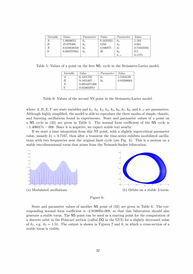
where A,B,X, Y are state variables and k1, k2, k3, k4, k5, k6, k7, k8, and k−7 are parameters.Although highly simplified, the model is able to reproduce the three modes of simple, chaotic,and bursting oscillations found in experiments. State and parameter values of a point ona NS cycle in (32) are given in Table 5. The normal form coefficient of the NS cycle is−1.406017e− 006. Since it is negative, we expect stable tori nearby.
If we start a time integration from this NS point, with a slightly supercritical parametervalue, namely k7 = 0.7167, then after a transient the time-series exhibits modulated oscilla-tions with two frequencies near the original limit cycle (see Fig. 6). This is a motion on astable two-dimensional torus that arises from the Neimark-Sacker bifurcation.
0 200 400 600 800 1000 1200 1400 1600 180026
26.05
26.1
26.15
26.2
26.25
26.3
26.35
26.4
26.45
26.5
t
B
25.2 25.4 25.6 25.8 26 26.2 26.40.01
0.012
0.014
0.016
0.018
0.02
0.022
B
X
(a) Modulated oscillations. (b) Orbits on a stable 2-torus.
Figure 6:
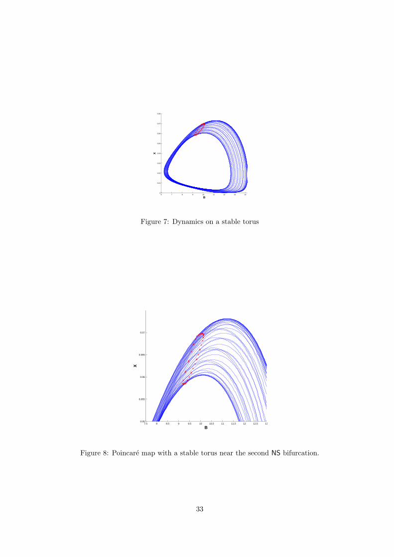
State and parameter values of another NS point of (32) are given in Table 6. The cor-responding normal form coefficient is -2.919895e-008, so that this bifurcation should alsogenerate a stable torus. The NS point can be used as a starting point for the computation ofa discrete orbit in the Poincare section (called DO in the GUI) for a slightly decreased valueof k7, e.g. k7 = 1.51. The output is shown in Figures 7 and 8, in which a cross-section of astable torus is visible.
32
6 7 8 9 10 11 12 13 140
0.01
0.02
0.03
0.04
0.05
0.06
0.07
0.08
B
X
Figure 7: Dynamics on a stable torus
7.5 8 8.5 9 9.5 10 10.5 11 11.5 12 12.5 130.05
0.055
0.06
0.065
0.07
B
X
Figure 8: Poincare map with a stable torus near the second NS bifurcation.
33
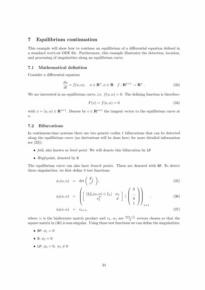
7 Equilibrium continuation
This example will show how to continue an equilibrium of a differential equation defined ina standard matlab ODE file. Furthermore, this example illustrates the detection, location,and processing of singularities along an equilibrium curve.
7.1 Mathematical definition
Consider a differential equation
du
dt= f(u, α), u ∈ Rn, α ∈ R f : Rn+1 → Rn . (33)
We are interested in an equilibrium curve, i.e. f(u, α) = 0. The defining function is therefore:
F (x) = f(u, α) = 0 (34)
with x = (u, α) ∈ Rn+1. Denote by v ∈ Rn+1 the tangent vector to the equilibrium curve atx.
7.2 Bifurcations
In continuous-time systems there are two generic codim 1 bifurcations that can be detectedalong the equilibrium curve (no derivations will be done here; for more detailed informationsee [23]):
• fold, also known as limit point. We will denote this bifurcation by LP
• Hopf-point, denoted by H
The equilibrium curve can also have branch points. These are denoted with BP. To detectthese singularities, we first define 3 test functions:
φ1(u, α) = det
(Fx
vT
), (35)
φ2(u, α) =
[(2fu(u, α) ⊙ In) w1
vT1 d
]\
0...01
n+1
, (36)
φ3(u, α) = vn+1, (37)
where ⊙ is the bialternate matrix product and v1, w1 are n(n−1)2 vectors chosen so that the
square matrix in (36) is non-singular. Using these test functions we can define the singularities:
• BP: φ1 = 0
• H: φ2 = 0
• LP: φ3 = 0, φ1 6= 0
34
A proof that these test functions correctly detect the mentioned singularities can be found in[23]. Here we only notice that φ2 = 0 not only at Hopf points but also at neutral saddles, i.e.points where fx has two real eigenvalues with sum zero. So, the singularity matrix is:
S =
0 − −− 0 −1 − 0
(38)
For each detected limit point, the corresponding quadratic normal form coefficient is com-puted:
a =1
2pT fuu[q, q], (39)
where fuq = fTu p = 0, qT q = 1, pT q = 1. At a Hopf bifurcation point, the first Lyapunov
coefficient is computed by the formula
l1 =1
2Re
{pT
(fuuu[q, q, q] − 2fuu[q, F−1
u fuu[q, q]] + fuu[q, (2iωIn − fu)−1fuu[q, q]])}, (40)
where fuq = iωq, qT q = 1, fTu p = −iωp, pT q = 1.
7.2.1 Branch point locator
The location of Hopf and limit points usually does not cause problems. However, the locationof branch points can give problems. The region of attraction of the Newton type continuationmethod which is used, has the shape of a cone (see [1]). In the localisation process we cannotassume to stay in this cone. This difficulty can be avoided by introducing p ∈ Rn and β ∈ R
and considering the extended system:
f(u, α) + βp = 0fT
u (u, α)p = 0pT fα(u, α) = 0pT p− 1 = 0
(41)
We solve this system by Newton’s method with initial data β = 0 and p : fTu p = µp where
µ is the real eigenvalue with smallest norm. A branch point (u, α) corresponds to a regularsolution (u, α, 0, p) of system (41) (see [3],p. 165). We note that the second order partialderivatives (Hessian) of f with respect to u and α are required.
The tangent vector at the singularity is also computed here. This is related to the pro-cessing of the branch point (computing the direction of the secondary branch).
7.3 Equilibrium initialization
Naively, one would start the continuation immediately with:
[x,v,s,h,f]=cont(@equilibrium, x0, v0, opt)
However, the equilibrium curve file has to know :
• which ode file to use,
• the values of all state variables,
35
• the values of all parameters,
• which parameter is active.
All this information can be supplied by one of the following two starting functions. Bothfunctions return an initial point x0 as well as its tangent vector v0.
• [x0,v0]=init EP EP(@odefile, x, p, ap)
This routine stores its information in a global structure eds (see also Figure 4). Theresult of init EP EP is a vector x0 with the state variables and the active parameterand a vector v0 that is empty. Here odefile is the ode-file (system-definition file) to beused, x is a vector containing the values of the state variables. p is the vector containingthe current values of the parameters and ap is the active parameter. The full listingof the equilibrium initializer can be found in the file ’Equilibrium/init EP EP.m’ of thetoolbox.
• [x0,v0]=init BP EP(@odefile, x, p, s, h)
Calculates an initial point for starting a new branch from a branch point detected onan equilibrium curve. This routine stores its information in a global structure eds (seealso Figure 4). Here odefile is the ode-file (system-definition file) to be used, x is avector containing the values of the state variables returned by a previous equilibriumcurve continuation. p is the vector containing the current values of the parametersand h contains the value of the initial amplitude. The full listing of the equilibriuminitializer and the curve definition can be found in the files ’Equilibrium/init BP EP.m’and ’equilibrium.m’ of the toolbox, respectively.
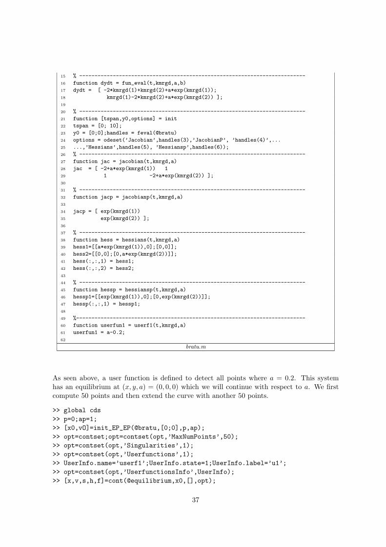
7.4 Bratu example
The first example we will look at is a 4-point discretization of the Bratu-Gelfand BVP [19].This model is defined as follows:
x′ = y − 2x+ aex (42)
y′ = x− 2y + aey (43)
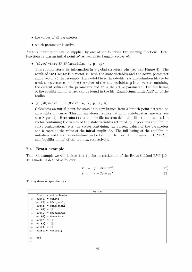
The system is specified as
bratu.m
1 function out = bratu
2 out{1} = @init;
3 out{2} = @fun_eval;
4 out{3} = @jacobian;
5 out{4} = [];
6 out{5} = @hessians;
7 out{6} = @hessiansp;
8 out{7} = [];
9 out{8} = [];
10 out{9} = [];
11 out{10}= @userf1;
12
13 end
14
36
15 % --------------------------------------------------------------------------
16 function dydt = fun_eval(t,kmrgd,a,b)
17 dydt = [ -2*kmrgd(1)+kmrgd(2)+a*exp(kmrgd(1));
18 kmrgd(1)-2*kmrgd(2)+a*exp(kmrgd(2)) ];
19
20 % --------------------------------------------------------------------------
21 function [tspan,y0,options] = init
22 tspan = [0; 10];
23 y0 = [0;0];handles = feval(@bratu)
24 options = odeset(’Jacobian’,handles(3),’JacobianP’, ’handles(4)’,...
25 ...,’Hessians’,handles(5), ’Hessiansp’,handles(6));
26 % --------------------------------------------------------------------------
27 function jac = jacobian(t,kmrgd,a)
28 jac = [ -2+a*exp(kmrgd(1)) 1
29 1 -2+a*exp(kmrgd(2)) ];
30
31 % --------------------------------------------------------------------------
32 function jacp = jacobianp(t,kmrgd,a)
33
34 jacp = [ exp(kmrgd(1))
35 exp(kmrgd(2)) ];
36
37 % --------------------------------------------------------------------------
38 function hess = hessians(t,kmrgd,a)
39 hess1=[[a*exp(kmrgd(1)),0];[0,0]];
40 hess2=[[0,0];[0,a*exp(kmrgd(2))]];
41 hess(:,:,1) = hess1;
42 hess(:,:,2) = hess2;
43
44 % --------------------------------------------------------------------------
45 function hessp = hessiansp(t,kmrgd,a)
46 hessp1=[[exp(kmrgd(1)),0];[0,exp(kmrgd(2))]];
47 hessp(:,:,1) = hessp1;
48
49 %---------------------------------------------------------------------------
60 function userfun1 = userf1(t,kmrgd,a)
61 userfun1 = a-0.2;
62
bratu.m
As seen above, a user function is defined to detect all points where a = 0.2. This systemhas an equilibrium at (x, y, a) = (0, 0, 0) which we will continue with respect to a. We firstcompute 50 points and then extend the curve with another 50 points.
>> global cds
>> p=0;ap=1;
>> [x0,vO]=init_EP_EP(@bratu,[0;0],p,ap);
>> opt=contset;opt=contset(opt,’MaxNumPoints’,50);
>> opt=contset(opt,’Singularities’,1);
>> opt=contset(opt,’Userfunctions’,1);
>> UserInfo.name=’userf1’;UserInfo.state=1;UserInfo.label=’u1’;
>> opt=contset(opt,’UserfunctionsInfo’,UserInfo);
>> [x,v,s,h,f]=cont(@equilibrium,x0,[],opt);
37
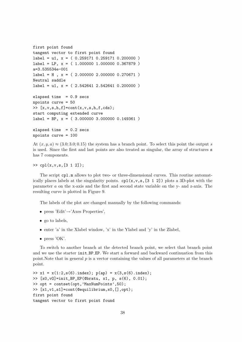
first point found
tangent vector to first point found
label = u1, x = ( 0.259171 0.259171 0.200000 )
label = LP, x = ( 1.000000 1.000000 0.367879 )
a=3.535534e-001
label = H , x = ( 2.000000 2.000000 0.270671 )
Neutral saddle
label = u1, x = ( 2.542641 2.542641 0.200000 )
elapsed time = 0.9 secs
npoints curve = 50
>> [x,v,s,h,f]=cont(x,v,s,h,f,cds);
start computing extended curve
label = BP, x = ( 3.000000 3.000000 0.149361 )
elapsed time = 0.2 secs
npoints curve = 100
At (x, y, a) ≈ (3.0; 3.0; 0.15) the system has a branch point. To select this point the output sis used. Since the first and last points are also treated as singular, the array of structures s
has 7 components.
>> cpl(x,v,s,[3 1 2]);
The script cpl.m allows to plot two- or three-dimensional curves. This routine automat-ically places labels at the singularity points. cpl(x,v,s,[3 1 2]) plots a 3D-plot with theparameter a on the x-axis and the first and second state variable on the y- and z-axis. Theresulting curve is plotted in Figure 9.
The labels of the plot are changed manually by the following commands:
• press ’Edit’→’Axes Properties’,
• go to labels,
• enter ’a’ in the Xlabel window, ’x’ in the Ylabel and ’y’ in the Zlabel,
• press ’OK’.
To switch to another branch at the detected branch point, we select that branch pointand we use the starter init BP EP. We start a forward and backward continuation from thispoint.Note that in general p is a vector containing the values of all parameters at the branchpoint.
>> x1 = x(1:2,s(6).index); p(ap) = x(3,s(6).index);
>> [x0,vO]=init_BP_EP(@bratu, x1, p, s(6), 0.01);
>> opt = contset(opt,’MaxNumPoints’,50);
>> [x1,v1,s1]=cont(@equilibrium,x0,[],opt);
first point found
tangent vector to first point found
38
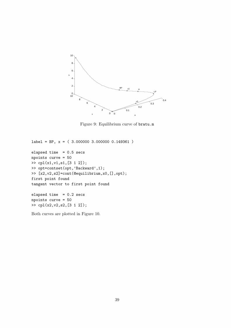
00.1
0.20.3
0.4
0
2
4
6
8
100
2
4
6
8
10
LPH
u1
a
u1BP
x
y
Figure 9: Equilibrium curve of bratu.m
label = BP, x = ( 3.000000 3.000000 0.149361 )
elapsed time = 0.5 secs
npoints curve = 50
>> cpl(x1,v1,s1,[3 1 2]);
>> opt=contset(opt,’Backward’,1);
>> [x2,v2,s2]=cont(@equilibrium,x0,[],opt);
first point found
tangent vector to first point found
elapsed time = 0.2 secs
npoints curve = 50
>> cpl(x2,v2,s2,[3 1 2]);
Both curves are plotted in Figure 10.
39
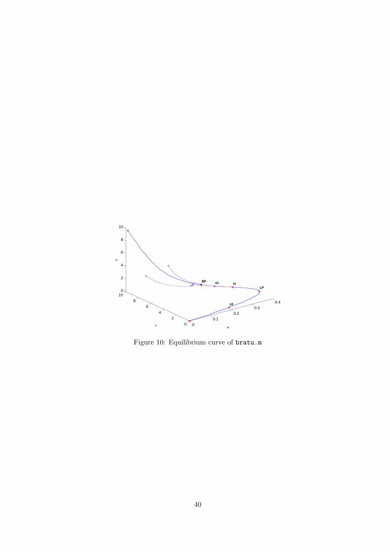
00.1
0.20.3
0.4
0
2
4
6
8
100
2
4
6
8
10
LPLPH H
u1u1
a
u1u1BPBPLP
x
y
Figure 10: Equilibrium curve of bratu.m
40
8 The Brusselator example: Continuation of a solution to a
boundary value problem in a free parameter
Discretized solutions of PDEs can also be continued in CL MatCont. We illustrate thisby continuing the equilibrium solution to a one-dimensional PDE. The curve type is called’pde 1’.
The Brusselator is a system of equations intended to model the Belusov-Zhabotinskyreaction. This is a system of reaction-diffusion equations that is known to exhibit oscillatorybehavior. The unknowns are the concentrations X(x, t), Y (x, t), A(x, t) and B(x, t) of fourreactants. Here t denotes time and x is a one-dimensional space variable normalized so thatx ∈ [0, 1]. The length L of the reactor is a parameter of the problem. In our simplified settingA and B are constants.
The system is described by two partial differential equations:
∂X∂t = Dx
L2
∂2X∂x2 +A− (B − 1)X +X2Y
∂Y∂t =
Dy
L2
∂2Y∂x2 +BX −X2Y
(44)
with x ∈ [0, 1], t ≥ 0. HereDx, Dy are the diffusion coefficients ofX and Y . At the boundariesx = 0 and x = 1 Dirichlet conditions are imposed:
{X(0, t) = X(1, t) = A
Y (0, t) = Y (1, t) = BA
(45)
We are interested in equilibrium solutions X(x) and Y (x) to the system and their dependenceon the parameter L.
The approximate equilibrium solution is:
{X(x) = A+ 2 sin(πx)
Y (x) = BA − 1
2 sin(πx)(46)
The initial values of the parameters are: A = 2, B = 4.6, Dx = 0.0016, Dy = 0.08 andL = 0.06. The initial solution (46) is not an equilibrium, but the continuer will try to convergeto an equilibrium close to the initial solution. We use equidistant meshes. To avoid spurioussolutions (solutions that are induced by the discretization but do not actually correspond tosolutions of the undiscretized problem) one can vary the number of mesh points by settingthe parameter N . If the same solution is found for several discretizations, then we can assumethat they correspond to solutions of the continuous problem.
The second order space derivative is approximated using the well-known three-points
difference formula: ∂2f∂x2 = 1
h2 (fi−1 − 2fi + fi+1), where h = 1N+1 , where N is the number of
grid points on which we discretize X and Y . So N is a parameter of the problem and 2N isthe number of state variables (which is not fixed in this case).
The Jacobian is a sparse 5-band matrix. In the ode-file describing the problem the Ja-cobian is introduced as a sparse matrix. The Hessian is never computed as such but secondorder derivatives are computed by finite differences whenever needed. We note that matlab6.5 or 7 does not provide sparse structures for 3-dimensional arrays.
bruss.m
41
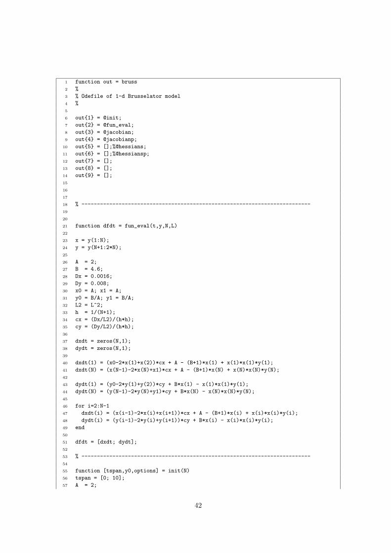
1 function out = bruss
2 %
3 % Odefile of 1-d Brusselator model
4 %
5
6 out{1} = @init;
7 out{2} = @fun_eval;
8 out{3} = @jacobian;
9 out{4} = @jacobianp;
10 out{5} = [];%@hessians;
11 out{6} = [];%@hessiansp;
12 out{7} = [];
13 out{8} = [];
14 out{9} = [];
15
16
17
18 % --------------------------------------------------------------------------
19
20
21 function dfdt = fun_eval(t,y,N,L)
22
23 x = y(1:N);
24 y = y(N+1:2*N);
25
26 A = 2;
27 B = 4.6;
28 Dx = 0.0016;
29 Dy = 0.008;
30 x0 = A; x1 = A;
31 y0 = B/A; y1 = B/A;
32 L2 = L^2;
33 h = 1/(N+1);
34 cx = (Dx/L2)/(h*h);
35 cy = (Dy/L2)/(h*h);
36
37 dxdt = zeros(N,1);
38 dydt = zeros(N,1);
39
40 dxdt(1) = (x0-2*x(1)+x(2))*cx + A - (B+1)*x(1) + x(1)*x(1)*y(1);
41 dxdt(N) = (x(N-1)-2*x(N)+x1)*cx + A - (B+1)*x(N) + x(N)*x(N)*y(N);
42
43 dydt(1) = (y0-2*y(1)+y(2))*cy + B*x(1) - x(1)*x(1)*y(1);
44 dydt(N) = (y(N-1)-2*y(N)+y1)*cy + B*x(N) - x(N)*x(N)*y(N);
45
46 for i=2:N-1
47 dxdt(i) = (x(i-1)-2*x(i)+x(i+1))*cx + A - (B+1)*x(i) + x(i)*x(i)*y(i);
48 dydt(i) = (y(i-1)-2*y(i)+y(i+1))*cy + B*x(i) - x(i)*x(i)*y(i);
49 end
50
51 dfdt = [dxdt; dydt];
52
53 % --------------------------------------------------------------------------
54
55 function [tspan,y0,options] = init(N)
56 tspan = [0; 10];
57 A = 2;
42
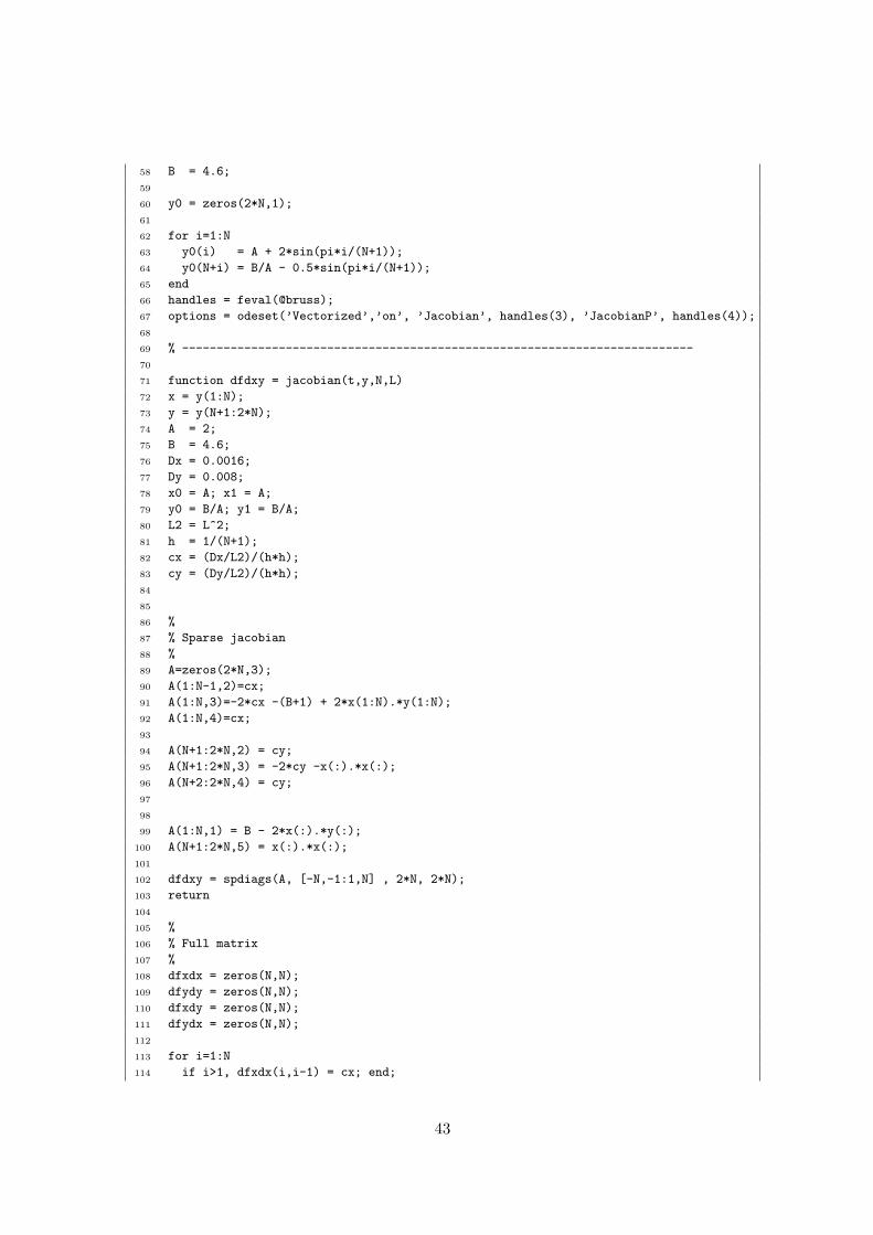
58 B = 4.6;
59
60 y0 = zeros(2*N,1);
61
62 for i=1:N
63 y0(i) = A + 2*sin(pi*i/(N+1));
64 y0(N+i) = B/A - 0.5*sin(pi*i/(N+1));
65 end
66 handles = feval(@bruss);
67 options = odeset(’Vectorized’,’on’, ’Jacobian’, handles(3), ’JacobianP’, handles(4));
68
69 % --------------------------------------------------------------------------
70
71 function dfdxy = jacobian(t,y,N,L)
72 x = y(1:N);
73 y = y(N+1:2*N);
74 A = 2;
75 B = 4.6;
76 Dx = 0.0016;
77 Dy = 0.008;
78 x0 = A; x1 = A;
79 y0 = B/A; y1 = B/A;
80 L2 = L^2;
81 h = 1/(N+1);
82 cx = (Dx/L2)/(h*h);
83 cy = (Dy/L2)/(h*h);
84
85
86 %
87 % Sparse jacobian
88 %
89 A=zeros(2*N,3);
90 A(1:N-1,2)=cx;
91 A(1:N,3)=-2*cx -(B+1) + 2*x(1:N).*y(1:N);
92 A(1:N,4)=cx;
93
94 A(N+1:2*N,2) = cy;
95 A(N+1:2*N,3) = -2*cy -x(:).*x(:);
96 A(N+2:2*N,4) = cy;
97
98
99 A(1:N,1) = B - 2*x(:).*y(:);
100 A(N+1:2*N,5) = x(:).*x(:);
101
102 dfdxy = spdiags(A, [-N,-1:1,N] , 2*N, 2*N);
103 return
104
105 %
106 % Full matrix
107 %
108 dfxdx = zeros(N,N);
109 dfydy = zeros(N,N);
110 dfxdy = zeros(N,N);
111 dfydx = zeros(N,N);
112
113 for i=1:N
114 if i>1, dfxdx(i,i-1) = cx; end;
43
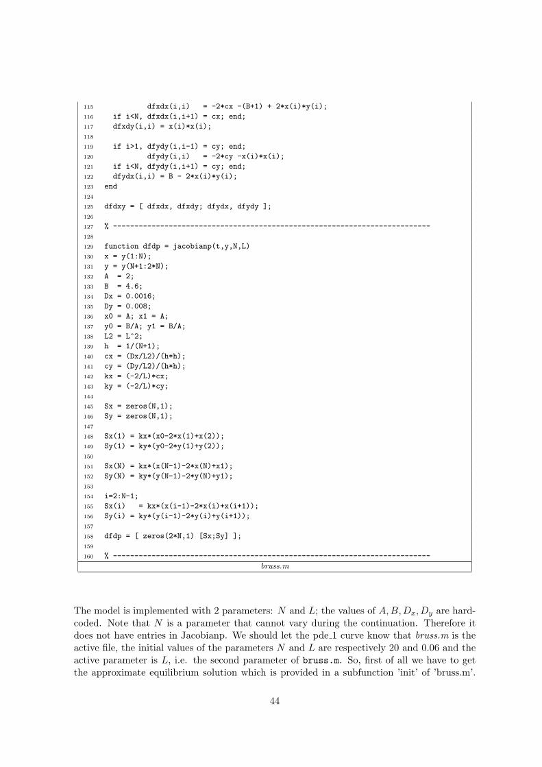
115 dfxdx(i,i) = -2*cx -(B+1) + 2*x(i)*y(i);
116 if i<N, dfxdx(i,i+1) = cx; end;
117 dfxdy(i,i) = x(i)*x(i);
118
119 if i>1, dfydy(i,i-1) = cy; end;
120 dfydy(i,i) = -2*cy -x(i)*x(i);
121 if i<N, dfydy(i,i+1) = cy; end;
122 dfydx(i,i) = B - 2*x(i)*y(i);
123 end
124
125 dfdxy = [ dfxdx, dfxdy; dfydx, dfydy ];
126
127 % --------------------------------------------------------------------------
128
129 function dfdp = jacobianp(t,y,N,L)
130 x = y(1:N);
131 y = y(N+1:2*N);
132 A = 2;
133 B = 4.6;
134 Dx = 0.0016;
135 Dy = 0.008;
136 x0 = A; x1 = A;
137 y0 = B/A; y1 = B/A;
138 L2 = L^2;
139 h = 1/(N+1);
140 cx = (Dx/L2)/(h*h);
141 cy = (Dy/L2)/(h*h);
142 kx = (-2/L)*cx;
143 ky = (-2/L)*cy;
144
145 Sx = zeros(N,1);
146 Sy = zeros(N,1);
147
148 Sx(1) = kx*(x0-2*x(1)+x(2));
149 Sy(1) = ky*(y0-2*y(1)+y(2));
150
151 Sx(N) = kx*(x(N-1)-2*x(N)+x1);
152 Sy(N) = ky*(y(N-1)-2*y(N)+y1);
153
154 i=2:N-1;
155 Sx(i) = kx*(x(i-1)-2*x(i)+x(i+1));
156 Sy(i) = ky*(y(i-1)-2*y(i)+y(i+1));
157
158 dfdp = [ zeros(2*N,1) [Sx;Sy] ];
159
160 % --------------------------------------------------------------------------
bruss.m
The model is implemented with 2 parameters: N and L; the values of A,B,Dx, Dy are hard-coded. Note that N is a parameter that cannot vary during the continuation. Therefore itdoes not have entries in Jacobianp. We should let the pde 1 curve know that bruss.m is theactive file, the initial values of the parameters N and L are respectively 20 and 0.06 and theactive parameter is L, i.e. the second parameter of bruss.m. So, first of all we have to getthe approximate equilibrium solution which is provided in a subfunction ’init’ of ’bruss.m’.
44
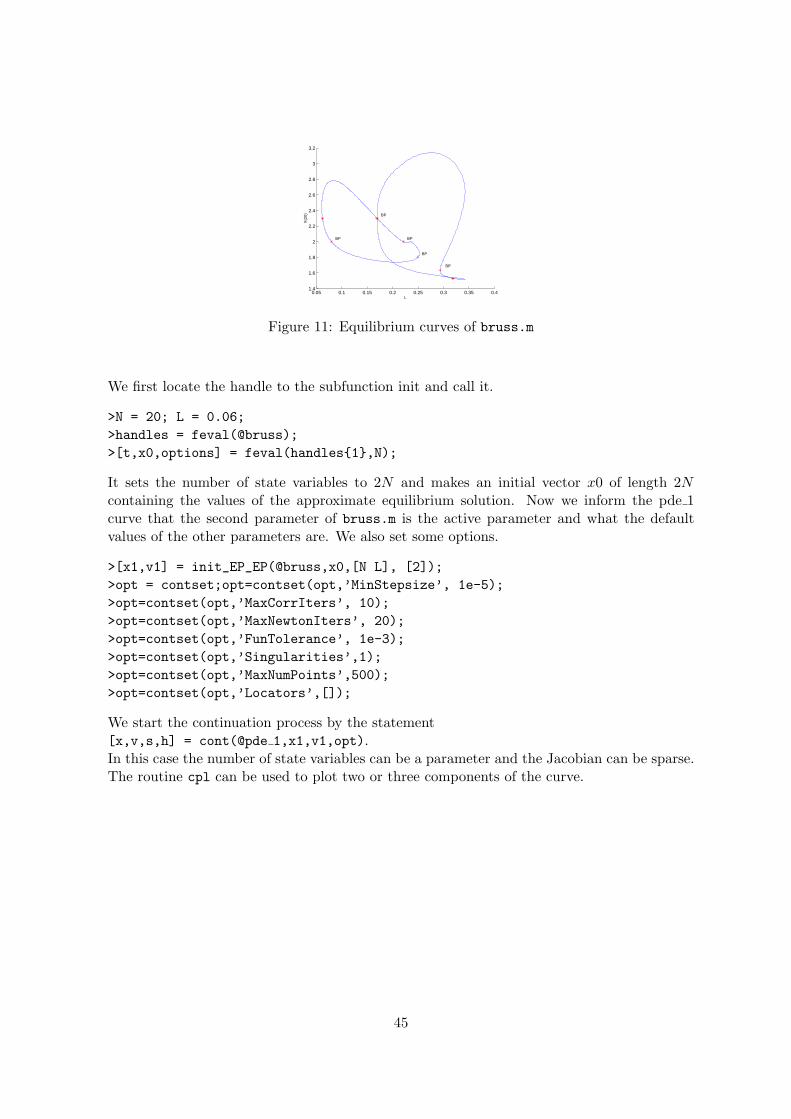
0.05 0.1 0.15 0.2 0.25 0.3 0.35 0.41.4
1.6
1.8
2
2.2
2.4
2.6
2.8
3
3.2
BP
BP
BP
BP
BP
L
X(2
0)
Figure 11: Equilibrium curves of bruss.m
We first locate the handle to the subfunction init and call it.
>N = 20; L = 0.06;
>handles = feval(@bruss);
>[t,x0,options] = feval(handles{1},N);
It sets the number of state variables to 2N and makes an initial vector x0 of length 2Ncontaining the values of the approximate equilibrium solution. Now we inform the pde 1curve that the second parameter of bruss.m is the active parameter and what the defaultvalues of the other parameters are. We also set some options.
>[x1,v1] = init_EP_EP(@bruss,x0,[N L], [2]);
>opt = contset;opt=contset(opt,’MinStepsize’, 1e-5);
>opt=contset(opt,’MaxCorrIters’, 10);
>opt=contset(opt,’MaxNewtonIters’, 20);
>opt=contset(opt,’FunTolerance’, 1e-3);
>opt=contset(opt,’Singularities’,1);
>opt=contset(opt,’MaxNumPoints’,500);
>opt=contset(opt,’Locators’,[]);
We start the continuation process by the statement[x,v,s,h] = cont(@pde 1,x1,v1,opt).In this case the number of state variables can be a parameter and the Jacobian can be sparse.The routine cpl can be used to plot two or three components of the curve.
45
9 Continuation of limit cycles
9.1 Mathematical definition
Consider the following differential equation
du
dt= f(u, α) (47)
with u ∈ Rn and α ∈ R. A periodic solution with period T satisfies the following system
{dudt = f(u, α)u(0) = u(T )
. (48)
For simplicity the period T is treated as a parameter resulting in the system
{dudτ = T f(u, α)u(0) = u(1)
. (49)
If u(τ) is its solution then the shifted solution u(τ + s) is also a solution to (49) for any valueof s. To select one solution, a phase condition is added to the system. The complete BVP(boundary value problem) is
dudτ − Tf(u, α) = 0u(0) − u(1) = 0∫ 1
0 〈u(t), uold(t)〉dt = 0
(50)
where uold is the derivative of a previous solution. A limit cycle is a closed phase orbitcorresponding to this periodic solution. This system is discretized using orthogonal collocation[6], the same way as it was done in AUTO [9]. The left hand side of the resulting system isthe defining function F (u, T, α) for limit cycles.
9.2 Bifurcations
On a limit cycle curve the following bifurcations can occur
• Branch Point of Cycles, this will be denoted as BPC
• Period Doubling, denoted as PD
• Fold, also known as Limit Point of Cycles, this will be denoted as LPC
• Neimark-Sacker, this will be denoted as NS
The test function for the Period Doubling bifurcation is defined by the following system
v(τ) − Tfu(u, α)v(τ) +Gϕ(τ) = 0v(0) + v(1) = 0∫ 1
0 〈ψ(τ), v(τ)〉dτ = 1
(51)
here ϕ and ψ are so-called bordering vector-functions [23], see [12] for details on the im-plementation. The system is discretized using orthogonal collocation and solved using the
46
standard matlab sparse system solver. The solution component G ∈ R of this system is thetest function and equals zero when there is a Period Doubling bifurcation.
The Fold bifurcation is detected in the same way as the Fold bifurcation of equilibria, thelast component of the tangent vector (the α component) is used as the test function.
The Neimark-Sacker bifurcation is detected by monitoring the eigenvalues of the mon-odromy matrix for the cycle. The monodromy matrix is computed like in auto by a blockelimination in the discretized form of the Jacobian of (50).
BPC cycles are not generic in families of limit cycles, but they are common in the case ofsymmetries, if the branch parameter is also the continuation parameter. CL MatCont usesa strategy that requires only the solution of linear systems; it is based on the fact that in asymmetry-breaking BPC cycle MD has rank defect two, where MD is the square matrix MD,obtained from the discretized form of the Jacobian of (50). To be precise, if h ∈ C1([0, 1], IRn),then
Mh =
[h− Tfx(x(t), α)h
h(0) − h(1)
],
and
MD(h)dm =
[(h− Tfx(x(t), α)h)dc
h(0) − h(1)
],
where ()dm and ()dc denote discretization in mesh points and in collocation points, respectively.Therefore we border MD with two additional rows and columns to obtain
MDbb =
MD w1 w2
v∗1 0 0v∗2 0 0
,
so that MDbb is nonsingular in the BPC cycle. Then we solve the systems
MDbb
ψ11 ψ12
gBPC11 gBPC12
gBPC21 gBPC22
=
0(Nm+1)n 0(Nm+1)n
1 00 1
,
where ψ11, ψ12 have (Nm + 1)n components, and gBPC11, gBPC12, gBPC21, and gBPC22, arescalar test functions for the BPC. In the BPC cycle they all vanish.
The singularity matrix is
S =
0 0 0 0 − − − −− − − − − 0 − −− − − − − − 0 −− − − − 1 − 1 0
(52)
The first row corresponds to the BPC. It contains 4 zeros which indicates that gBPC11, gBPC12,gBPC21, and gBPC22 should vanish. The last row corresponds to the NS. Because we have toexclude that all four testfunctions of the BPC are zeros, we introduce an extra testfunctionwhich corresponds to the norm of these four testfunctions. A NS is detected if this norm isnonzero,the testfunction for the fold is nonzero and the testfunction for the NS is equal tozero.
47
9.2.1 Branch Point Locator
The location of BPC points in the non-generic situation (i.e. where some symmetry is present)as zeros of the test functions is numerically suspect because no local quadratic convergencecan be guaranteed. This difficulty can be avoided by introducing an additional unknownβ ∈ R and considering the minimally extended system:
dxdt − Tf(x, α) + βp1 = 0x(0) − x(1) + βp2 = 0∫ 10 〈x(t), xold(t)〉dt+ βp3 = 0G[x, T, α] = 0
(53)
where G is defined as in (87) and [pT1 p
T2 p3]
T is the bordering vector [w01;w02;w03]T in (89).
We solve this system with respect to x, T, α and β by Newton’s method with initial β = 0. Abranch point (x, T, α) corresponds to a regular solution (x, T, α, 0) of system (53) (see [3],p.165). We note, however that the second order partial derivatives (Hessian) of f with respectto x and α are required. The tangent vector v1st at the BPC singularity is approximated asv1st = v1+v2
2 where v1 is the tangent vector in the continuation point previous to the BPCand v2 is the one in the next point.
9.2.2 Processing
It is know that the periodic normal form at the Limit Point of Cycles (LPC) bifurcation is{
dτdt = 1 − ξ + aξ2 + · · · ,
dξdt = bξ2 + · · · ,
(54)
where τ ∈ [0, T ], ξ is a real coordinate on the center manifold that is transverse to the limit-cycle, a, b ∈ R, and dots denote nonautonomous T -periodic O(ξ3)-terms. For each detectedLPC point the normal form coefficient b is computed. A Cusp Point of Cycles (CPC) isdetected for b = 0.
The periodic normal form at the Period Doubling (PD) bifurcation is{
dτdt = 1 + aξ2 + · · · ,
dξdt = cξ3 + · · · ,
(55)
where τ ∈ [0, 2T ], ξ is a real coordinate on the center manifold that is transverse to the limitcycle, a, c ∈ R, and dots denote nonautonomous 2T -periodic O(ξ4)-terms. The coefficient cdetermines the stability of the period doubled cycle in the center manifold and is computedduring the processing of each PD point.
The periodic normal form at the Neimark-Sacker (NS) bifurcation is{
dτdt = 1 + a|ξ|2 + · · · ,
dξdt = iθ
T ξ + dξ|ξ|2 + · · · ,(56)
where τ ∈ [0, T ], ξ is a complex coordinate on the center manifold that is complementaryto τ , a ∈ R, d ∈ C, and dots denote nonautonomous T -periodic O(|ξ|4)-terms. The criticalcoefficient d in the periodic normal form for the NS bifurcation is computed during theprocessing of a NS point. The critical cycle is stable within the center manifold if Re d < 0and is unstable if Re d > 0. In the former case, the Neimark-Sacker bifurcation is supercritical,while in the latter case it is subcritical.
48
9.3 Limitcycle initialization
For limit cycles the same problems occur as with equilibria, a limit cycle continuation can’tbe done by just calling the continuer as
[x,v,s,h,f]=cont(@limitcycle, x0, v0, opt)
The limit cycle curve file has to know
• which ode file to use,
• which parameter is active,
• the values of all parameters,
• the number of mesh and collocation points to use for the discretization.
Also an initial cycle x0 has to be known. All this information can be supplied using any of thefollowing three starting functions. All three return an initial cycle x0 as well as its tangentvector v0.
• [x0,v0]=init H LC(@odefile, x, p, ap, h, ntst, ncol)
Calculates an initial cycle from a Hopf point detected on an equilibrium curve. Hereodefile is the ode-file to be used. x is a vector containing the values of the state vari-ables returned by a previous equilibrium curve continuation. p is the vector containingthe current values of the parameters. ap is the active parameter, h contains the value ofthe initial amplitude and ntst and ncol are the number of mesh and collocation pointsto be used for the discretization.
• [x0,v0]=init BPC LC(@odefile, x, v, s, ap, ntst, ncol,h)
Calculates an initial cycle for starting a secondary cycle from a BPC detected on a pre-vious calculated limit cycle. odefile, ap, ntst and ncol are the same as for init H LC.x, v and s are here the x, v and s as returned by a previous limit cycle continuationand h contains the value of the initial amplitude.
• [x0,v0]=init LC LC(@odefile, x, v, s, ap, ntst, ncol)
This starter can be used to start a limit cycle continuation from a previous limit cyclecontinuation. odefile, ap, ntst and ncol are the same as for init H LC. x, v and s
are here the x, v and s as returned by a previous limit cycle continuation.
• [x0,v0]=init PD LC(@odefile, x, s, ap, ntst, ncol)
This starter calculates an initial double period cycle from a period doubling bifurcation.All arguments are the same as for init LC LC except for v, which is not needed, and s,which should only be the special point structure for the period doubling bifurcation fromwhich to start a double period cycle, not the complete list of special point structures asreturned by the continuer.
49
9.4 Example
For this example the following system from adaptive control was used in a feedback controlsystem, as described in [17], [18] and further used in [23] (Example 5.4, p. 178):
x = yy = zz = −αz − βy − x+ x2
(57)
This system has a Hopf point at the origin for α = 1 and β = 1. From this Hopf pointan initial cycle is calculated using the starter init H LC. The results of the continuation areplotted using the plot function plotcycle(x,v,s,e) (see Figure 12). This function plotsthe cycles x. e is an array whith either 2 or 3 elements for 2-dimensional and 3-dimensionalplotting respectively. Its entries must be indices of state variables or active parameters in x.The index of the active parameter is size(x,1)
>> init;
>> [x0,v0]=init_EP_EP(@adapt,[0;0;0],[-10;1],[1]);
>> opt=contset;opt=contset(opt,’Singularities’,1);
>> [x,v,s,h,f]=cont(@equilibrium,x0,[],opt);
first point found
tangent vector to first point found
label = H , x = ( 0.000000 0.000000 0.000000 1.000000 )
First Lyapunov coefficient = -6.000000e-001
elapsed time = 0.5 secs
npoints curve = 300
>> x1=x(1:3,s(2).index);p=[x(end,s(2).index);1];
>> [x0,v0]=init_H_LC(@adapt,x1,p,[1],1e-6,20,4);
>> opt = contset(opt,’MaxNumPoints’,200);
>> opt = contset(opt,’Multipliers’,1);
>> opt = contset(opt,’Adapt’,1);
>> [xlc,vlc,slc,hlc,flc]=cont(@limitcycle,x0,v0,opt);
first point found
tangent vector to first point found
Limit point cycle (period = 6.283185e+000, parameter = 1.000000e+000)
Normal form coefficient = -1.306146e+000
Period Doubling (period = 6.364071e+000, parameter = 6.303020e-001)
Normal form coefficient = -4.267737e-002
Neimark-Sacker (period = 6.433818e+000, parameter = -7.056304e-010)
Normal form coefficient = 1.047430e+004
Period Doubling (period = 6.364071e+000, parameter = -6.303020e-001)
Normal form coefficient = 4.268605e-002
elapsed time = 73.6 secs
npoints curve = 200
>> plotcycle(xlc,vlc,slc,[size(xlc,1) 1 2]);
50
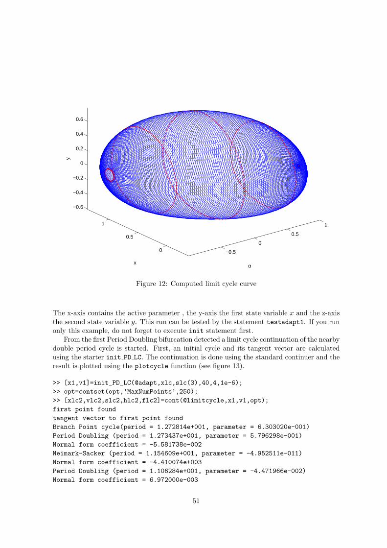
−0.5
0
0.5
1
0
0.5
1
−0.6
−0.4
−0.2
0
0.2
0.4
0.6
αx
y
Figure 12: Computed limit cycle curve
The x-axis contains the active parameter , the y-axis the first state variable x and the z-axisthe second state variable y. This run can be tested by the statement testadapt1. If you runonly this example, do not forget to execute init statement first.
From the first Period Doubling bifurcation detected a limit cycle continuation of the nearbydouble period cycle is started. First, an initial cycle and its tangent vector are calculatedusing the starter init PD LC. The continuation is done using the standard continuer and theresult is plotted using the plotcycle function (see figure 13).
>> [x1,v1]=init_PD_LC(@adapt,xlc,slc(3),40,4,1e-6);
>> opt=contset(opt,’MaxNumPoints’,250);
>> [xlc2,vlc2,slc2,hlc2,flc2]=cont(@limitcycle,x1,v1,opt);
first point found
tangent vector to first point found
Branch Point cycle(period = 1.272814e+001, parameter = 6.303020e-001)
Period Doubling (period = 1.273437e+001, parameter = 5.796298e-001)
Normal form coefficient = -5.581738e-002
Neimark-Sacker (period = 1.154609e+001, parameter = -4.952511e-011)
Normal form coefficient = -4.410074e+003
Period Doubling (period = 1.106284e+001, parameter = -4.471966e-002)
Normal form coefficient = 6.972000e-003
51
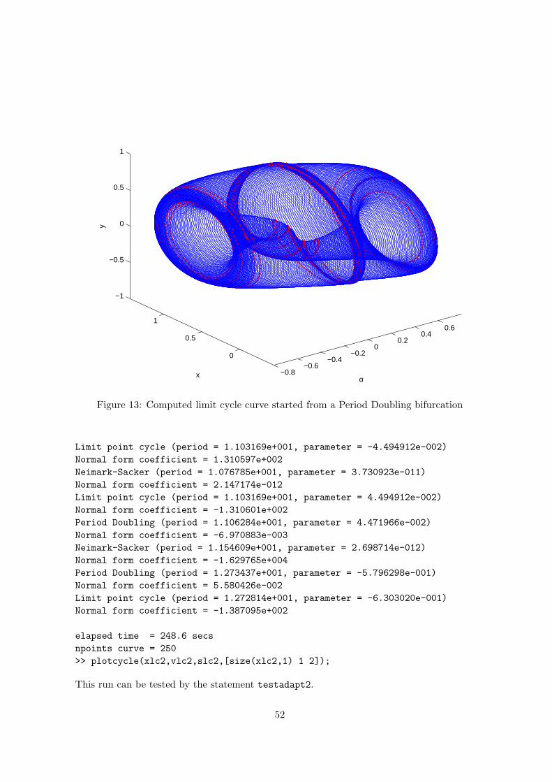
−0.8−0.6
−0.4−0.2
00.2
0.40.6
0
0.5
1
−1
−0.5
0
0.5
1
αx
y
Figure 13: Computed limit cycle curve started from a Period Doubling bifurcation
Limit point cycle (period = 1.103169e+001, parameter = -4.494912e-002)
Normal form coefficient = 1.310597e+002
Neimark-Sacker (period = 1.076785e+001, parameter = 3.730923e-011)
Normal form coefficient = 2.147174e-012
Limit point cycle (period = 1.103169e+001, parameter = 4.494912e-002)
Normal form coefficient = -1.310601e+002
Period Doubling (period = 1.106284e+001, parameter = 4.471966e-002)
Normal form coefficient = -6.970883e-003
Neimark-Sacker (period = 1.154609e+001, parameter = 2.698714e-012)
Normal form coefficient = -1.629765e+004
Period Doubling (period = 1.273437e+001, parameter = -5.796298e-001)
Normal form coefficient = 5.580426e-002
Limit point cycle (period = 1.272814e+001, parameter = -6.303020e-001)
Normal form coefficient = -1.387095e+002
elapsed time = 248.6 secs
npoints curve = 250
>> plotcycle(xlc2,vlc2,slc2,[size(xlc2,1) 1 2]);
This run can be tested by the statement testadapt2.
52
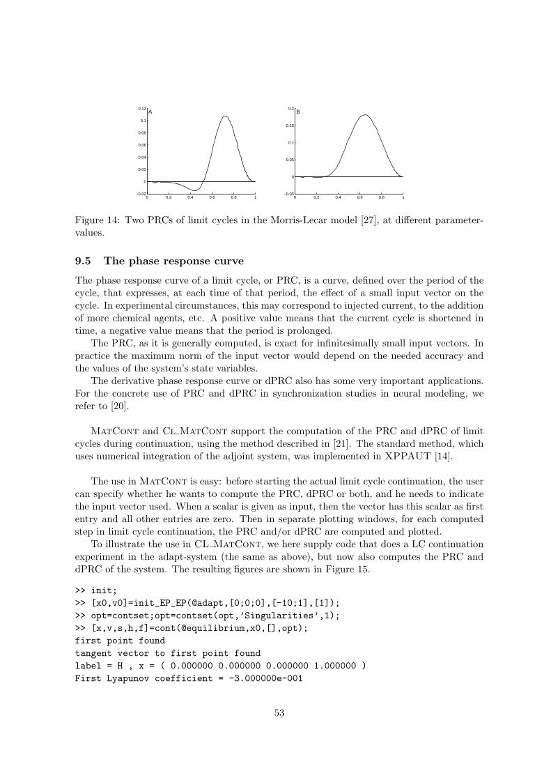
0 0.2 0.4 0.6 0.8 1−0.02
0
0.02
0.04
0.06
0.08
0.1
0.12A
0 0.2 0.4 0.6 0.8 1−0.05
0
0.05
0.1
0.15
0.2B
Figure 14: Two PRCs of limit cycles in the Morris-Lecar model [27], at different parameter-values.
9.5 The phase response curve
The phase response curve of a limit cycle, or PRC, is a curve, defined over the period of thecycle, that expresses, at each time of that period, the effect of a small input vector on thecycle. In experimental circumstances, this may correspond to injected current, to the additionof more chemical agents, etc. A positive value means that the current cycle is shortened intime, a negative value means that the period is prolonged.
The PRC, as it is generally computed, is exact for infinitesimally small input vectors. Inpractice the maximum norm of the input vector would depend on the needed accuracy andthe values of the system’s state variables.
The derivative phase response curve or dPRC also has some very important applications.For the concrete use of PRC and dPRC in synchronization studies in neural modeling, werefer to [20].
MatCont and Cl MatCont support the computation of the PRC and dPRC of limitcycles during continuation, using the method described in [21]. The standard method, whichuses numerical integration of the adjoint system, was implemented in XPPAUT [14].
The use in MatCont is easy: before starting the actual limit cycle continuation, the usercan specify whether he wants to compute the PRC, dPRC or both, and he needs to indicatethe input vector used. When a scalar is given as input, then the vector has this scalar as firstentry and all other entries are zero. Then in separate plotting windows, for each computedstep in limit cycle continuation, the PRC and/or dPRC are computed and plotted.
To illustrate the use in CL MatCont, we here supply code that does a LC continuationexperiment in the adapt-system (the same as above), but now also computes the PRC anddPRC of the system. The resulting figures are shown in Figure 15.
>> init;
>> [x0,v0]=init_EP_EP(@adapt,[0;0;0],[-10;1],[1]);
>> opt=contset;opt=contset(opt,’Singularities’,1);
>> [x,v,s,h,f]=cont(@equilibrium,x0,[],opt);
first point found
tangent vector to first point found
label = H , x = ( 0.000000 0.000000 0.000000 1.000000 )
First Lyapunov coefficient = -3.000000e-001
53
elapsed time = 1.8 secs
npoints curve = 300
>> x1=x(1:3,s(2).index);p=[x(end,s(2).index);1];
>> [x0,v0]=init_H_LC(@adapt,x1,p,[1],1e-6,20,4);
>> opt = contset(opt,’MaxNumPoints’,10);
>> opt = contset(opt,’Multipliers’,1);
>> opt = contset(opt,’Adapt’,1);
>> [xlc,vlc,slc,hlc,flc]=cont(@limitcycle,x0,v0,opt);
first point found
tangent vector to first point found
Limit point cycle (period = 6.283185e+000, parameter = 1.000000e+000)
Normal form coefficient = -1.240467e+000
elapsed time = 3.0 secs
npoints curve = 10
>> [x1,v1] = init_LC_LC(@adapt, xlc, vlc, slc(end), 1, 20, 4);
>> opt = contset(opt,’PRC’,1);
>> opt = contset(opt,’dPRC’,1);
>> opt = contset(opt,’Input’,1);
>> opt = contset(opt,’MaxNumPoints’,20);
>> [xlc1,vlc1,slc1,hlc1,flc1]=cont(@limitcycle,x1,v1,opt);
As an example application for the specific computation during continuation, one can studythe evolution of the PRCs of limit cycles, when these approach certain bifurcations. E.g. thecloser a limit cycle is to a homoclinic orbit, the smaller the negative part of the PRC becomes(relatively): it is harder to increase the period of the cycle. In Figure 14 two PRCs areshown for the same dynamical system, but at different distances from a homoclinic orbit. InFigure 16 a sequence of PRCs is shown, computed during the continuation of a limit cycleapproaching a homoclinic orbit.
54
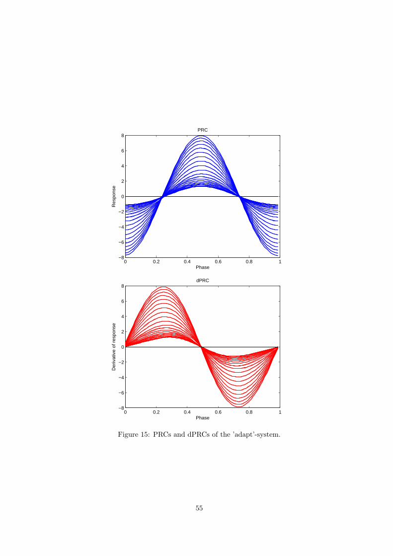
0 0.2 0.4 0.6 0.8 1−8
−6
−4
−2
0
2
4
6
8
Phase
Res
pons
e
PRC
0 0.2 0.4 0.6 0.8 1−8
−6
−4
−2
0
2
4
6
8
Phase
Der
ivat
ive
of r
espo
nse
dPRC
Figure 15: PRCs and dPRCs of the ’adapt’-system.
55
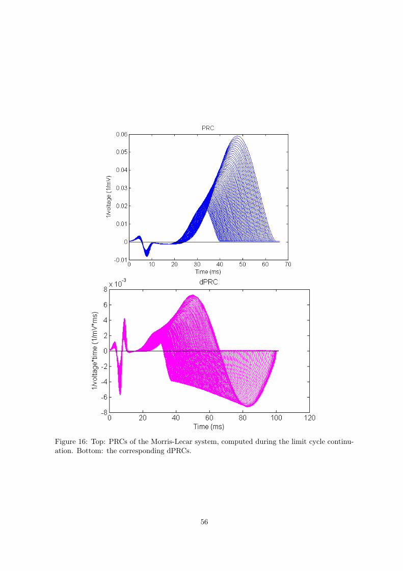
Figure 16: Top: PRCs of the Morris-Lecar system, computed during the limit cycle continu-ation. Bottom: the corresponding dPRCs.
56
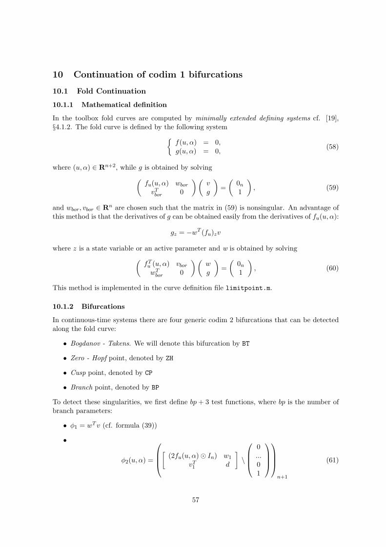
10 Continuation of codim 1 bifurcations
10.1 Fold Continuation
10.1.1 Mathematical definition
In the toolbox fold curves are computed by minimally extended defining systems cf. [19],§4.1.2. The fold curve is defined by the following system
{f(u, α) = 0,g(u, α) = 0,
(58)
where (u, α) ∈ Rn+2, while g is obtained by solving
(fu(u, α) wbor
vTbor 0
) (vg
)=
(0n
1
), (59)
and wbor, vbor ∈ Rn are chosen such that the matrix in (59) is nonsingular. An advantage ofthis method is that the derivatives of g can be obtained easily from the derivatives of fu(u, α):
gz = −wT (fu)zv
where z is a state variable or an active parameter and w is obtained by solving
(fT
u (u, α) vbor
wTbor 0
)(wg
)=
(0n
1
), (60)
This method is implemented in the curve definition file limitpoint.m.
10.1.2 Bifurcations
In continuous-time systems there are four generic codim 2 bifurcations that can be detectedalong the fold curve:
• Bogdanov - Takens. We will denote this bifurcation by BT
• Zero - Hopf point, denoted by ZH
• Cusp point, denoted by CP
• Branch point, denoted by BP
To detect these singularities, we first define bp+ 3 test functions, where bp is the number ofbranch parameters:
• φ1 = wT v (cf. formula (39))
•
φ2(u, α) =
[(2fu(u, α) ⊙ In) w1
vT1 d
]\
0...01
n+1
(61)
57
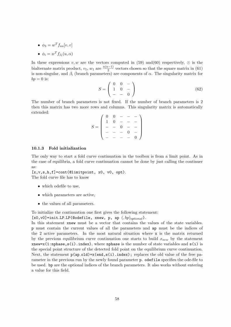
• φ3 = wT fuu[v, v]
• φi = wT fβi(u, α)
In these expressions v, w are the vectors computed in (59) and(60) respectively, ⊙ is the
bialternate matrix product, v1, w1 are n(n−1)2 vectors chosen so that the square matrix in (61)
is non-singular, and βi (branch parameters) are components of α. The singularity matrix forbp = 0 is:
S =
0 0 −1 0 −− − 0
(62)
The number of branch parameters is not fixed. If the number of branch parameters is 2then this matrix has two more rows and columns. This singularity matrix is automaticallyextended:
S =
0 0 − − −1 0 − − −− − 0 − −− − − 0 −− − − − 0
10.1.3 Fold initialization
The only way to start a fold curve continuation in the toolbox is from a limit point. As inthe case of equilibria, a fold curve continuation cannot be done by just calling the continueras:[x,v,s,h,f]=cont(@limitpoint, x0, v0, opt).The fold curve file has to know
• which odefile to use,
• which parameters are active,
• the values of all parameters.
To initialize the continuation one first gives the following statement:[x0,v0]=init LP LP(@odefile, xnew, p, ap (, bp)optional).In this statement xnew must be a vector that contains the values of the state variables.p must contain the current values of all the parameters and ap must be the indices ofthe 2 active parameters. In the most natural situation where x is the matrix returnedby the previous equilibrium curve continuation one starts to build xnew by the statementxnew=x(1:nphase,s(i).index), where nphase is the number of state variables and s(i) isthe special point structure of the detected fold point on the equilibrium curve continuation.Next, the statement p(ap old)=x(end,s(i).index); replaces the old value of the free pa-rameter in the previous run by the newly found parameter p. odefile specifies the ode-file tobe used. bp are the optional indices of the branch parameters. It also works without enteringa value for this field.
58
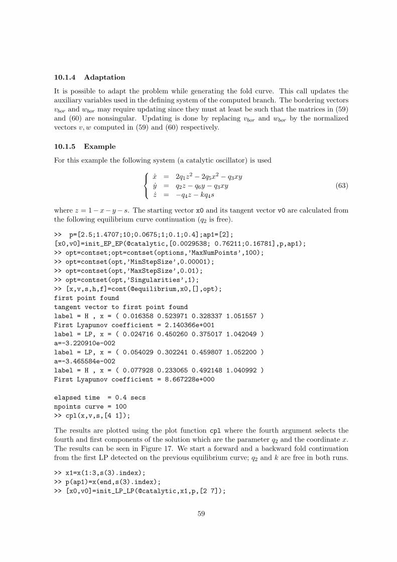
10.1.4 Adaptation
It is possible to adapt the problem while generating the fold curve. This call updates theauxiliary variables used in the defining system of the computed branch. The bordering vectorsvbor and wbor may require updating since they must at least be such that the matrices in (59)and (60) are nonsingular. Updating is done by replacing vbor and wbor by the normalizedvectors v, w computed in (59) and (60) respectively.
10.1.5 Example
For this example the following system (a catalytic oscillator) is used
x = 2q1z2 − 2q5x
2 − q3xyy = q2z − q6y − q3xyz = −q4z − kq4s
(63)
where z = 1−x− y− s. The starting vector x0 and its tangent vector v0 are calculated fromthe following equilibrium curve continuation (q2 is free).
>> p=[2.5;1.4707;10;0.0675;1;0.1;0.4];ap1=[2];
[x0,v0]=init_EP_EP(@catalytic,[0.0029538; 0.76211;0.16781],p,ap1);
>> opt=contset;opt=contset(options,’MaxNumPoints’,100);
>> opt=contset(opt,’MinStepSize’,0.00001);
>> opt=contset(opt,’MaxStepSize’,0.01);
>> opt=contset(opt,’Singularities’,1);
>> [x,v,s,h,f]=cont(@equilibrium,x0,[],opt);
first point found
tangent vector to first point found
label = H , x = ( 0.016358 0.523971 0.328337 1.051557 )
First Lyapunov coefficient = 2.140366e+001
label = LP, x = ( 0.024716 0.450260 0.375017 1.042049 )
a=-3.220910e-002
label = LP, x = ( 0.054029 0.302241 0.459807 1.052200 )
a=-3.465584e-002
label = H , x = ( 0.077928 0.233065 0.492148 1.040992 )
First Lyapunov coefficient = 8.667228e+000
elapsed time = 0.4 secs
npoints curve = 100
>> cpl(x,v,s,[4 1]);
The results are plotted using the plot function cpl where the fourth argument selects thefourth and first components of the solution which are the parameter q2 and the coordinate x.The results can be seen in Figure 17. We start a forward and a backward fold continuationfrom the first LP detected on the previous equilibrium curve; q2 and k are free in both runs.
>> x1=x(1:3,s(3).index);
>> p(ap1)=x(end,s(3).index);
>> [x0,v0]=init_LP_LP(@catalytic,x1,p,[2 7]);
59
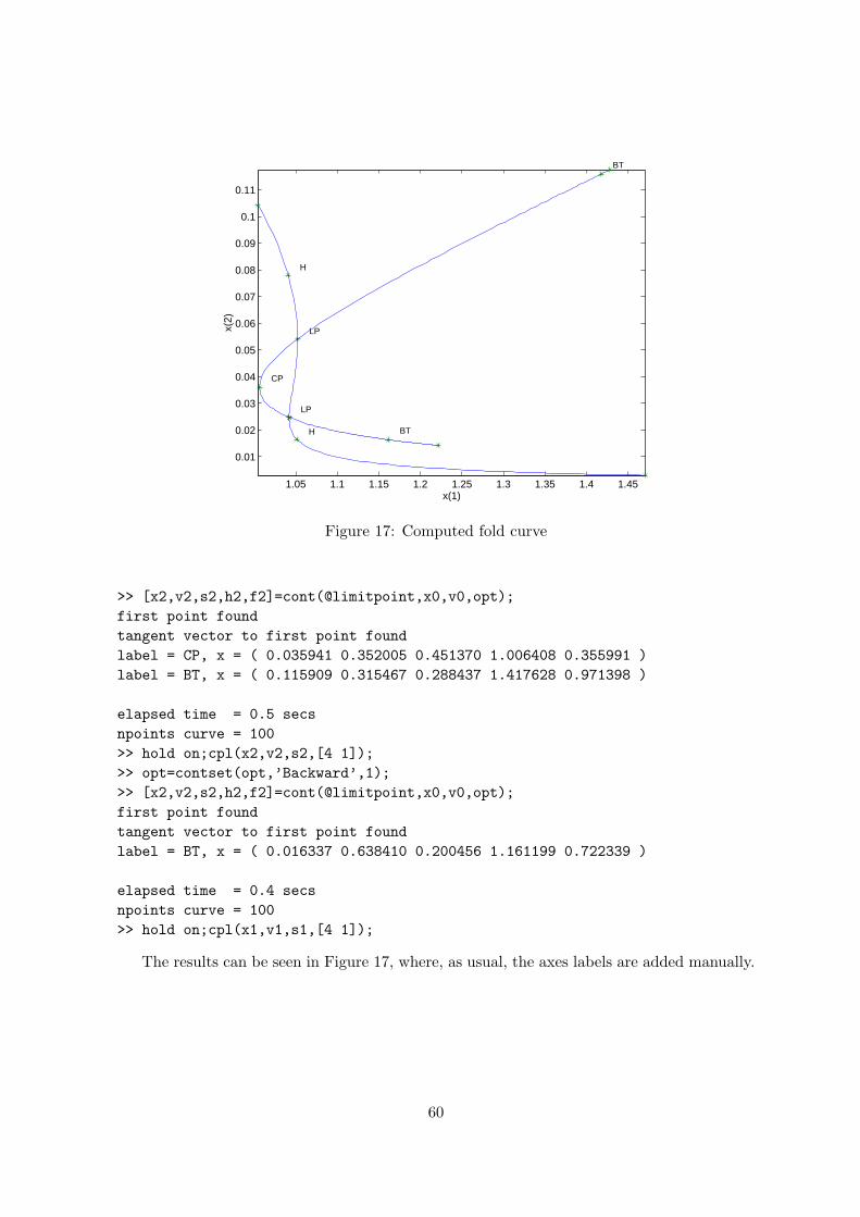
1.05 1.1 1.15 1.2 1.25 1.3 1.35 1.4 1.45
0.01
0.02
0.03
0.04
0.05
0.06
0.07
0.08
0.09
0.1
0.11
x(1)
x(2)
H
LP
LP
H
CP
BT
BT
Figure 17: Computed fold curve
>> [x2,v2,s2,h2,f2]=cont(@limitpoint,x0,v0,opt);
first point found
tangent vector to first point found
label = CP, x = ( 0.035941 0.352005 0.451370 1.006408 0.355991 )
label = BT, x = ( 0.115909 0.315467 0.288437 1.417628 0.971398 )
elapsed time = 0.5 secs
npoints curve = 100
>> hold on;cpl(x2,v2,s2,[4 1]);
>> opt=contset(opt,’Backward’,1);
>> [x2,v2,s2,h2,f2]=cont(@limitpoint,x0,v0,opt);
first point found
tangent vector to first point found
label = BT, x = ( 0.016337 0.638410 0.200456 1.161199 0.722339 )
elapsed time = 0.4 secs
npoints curve = 100
>> hold on;cpl(x1,v1,s1,[4 1]);
The results can be seen in Figure 17, where, as usual, the axes labels are added manually.
60
10.2 Hopf Continuation
10.2.1 Mathematical definition
In the MatCont / CL MatCont toolbox Hopf curves are computed by minimally extendeddefining systems, cf. [19] §4.3.4. The Hopf curve is defined by the following system
f(u, α) = 0,gi1j1(u, α, k) = 0gi2j2(u, α, k) = 0
(64)
with the unknowns u, α, k, (i1, j1, i2, j2) ∈ {1, 2} and where g =
(g11 g12g21 g22
)is obtained by
solving (f2
u + kIn Wbor
V Tbor O
)(VG
)=
(0n,2
I2
), (65)
where fu has eigenvalues ±iω, ω > 0, k = ω2 and Vbor,Wbor ∈ Rn×2 are chosen such that thematrix in (65) is nonsingular. i1, j1, i2, j2, Vbor and Wbor are auxiliary variables that can beadapted. This method is implemented in the curve definition file hopf.m.
10.2.2 Bifurcations
In continuous-time systems there are four generic codim 2 bifurcations that can be detectedalong the Hopf curve:
• Bogdanov - Takens. We will denote this bifurcation by BT
• Zero - Hopf point, denoted by ZH
• Double - Hopf point, denoted by HH
• Generalized Hopf point, denoted by GH
To detect these singularities, we first define 4 test functions:
• φ1 = k
• φ2 = det(fu)
• φ3 =
[(2fu(u, α) ⊙ In) w1
vT1 d
]\
0...01
n+1
• φ4 = l1 (first Lyapunov coefficient, see (40)),
where v1, w1 are carefully constructed and updated n(n−1)2 × 2 matrices.
In this case the singularity matrix is:
S =
0 0 − −1 0 − −− − 0 −− − − 0
(66)
61
10.2.3 Hopf initialization
The only way to start the continuation of a Hopf bifurcation curve is to start it from a Hopfpoint, typically found on an equilibrium curve. The continuation of Hopf points cannot simplybe started by using the following statement:[x,v,s,h,f]=cont(@hopf, x0, v0, opt)
The Hopf curve file has to know
• the values of all state variables,
• which ode file to use,
• which parameters are active,
• the values of all parameters.
Also an initial point x0 has to be known. All this information can be supplied using thefollowing statement:[x0,v0]=init H H(@odefile, xnew, p, ap).
The input arguments odefile, xnew, p, ap are built exactly as in init LP LP. The outputvector x0 consists of xnew extended with the free parameters and paramter k from (65).
10.2.4 Adaptation
It is possible to adapt the problem while generating the Hopf curve. This call updatesthe auxiliary variables used in the defining system of the computed branch. The borderingmatrices Vbor and Wbor may require updating since they must at least be such that the matrixin (65) is nonsingular. Updating of Vbor and Wbor is done exactly as in the LP case. Updatingof i1, j1, i2, j2 is done in such a way that the linearized system of (64) is as well-conditionedas possible.
10.2.5 Example
For this example we again use the system (63). The starting vector is calculated from thefirst Hopf bifurcation point detected in the equilibrium continuation example (see 10.1.5). q2and k are free.
>> x1=x(1:3,s(2).index);
>> p(ap1)=x(end,s(2).index);
>> [x0,v0]=init_H_H(@catalytic,x1,p,[2 7]);
>> opt=contset;opt=contset(options,’Singularities’,1);
>> [x2,v2,s2,h2,f2]=cont(@hopf,x0,[],opt);
first point found
tangent vector to first point found
label = GH, x = ( 0.018022 0.368277 0.497926 0.891362 0.232514 0.003324 )
label = GH, x = ( 0.064312 0.211095 0.554869 0.924257 0.305881 0.003512 )
label = BT, x = ( 0.115909 0.315467 0.288437 1.417628 0.971398 -0.000000 )
label = BT, x = ( 0.016337 0.638410 0.200456 1.161199 0.722339 0.000000 )
Closed curve detected at step 159
62
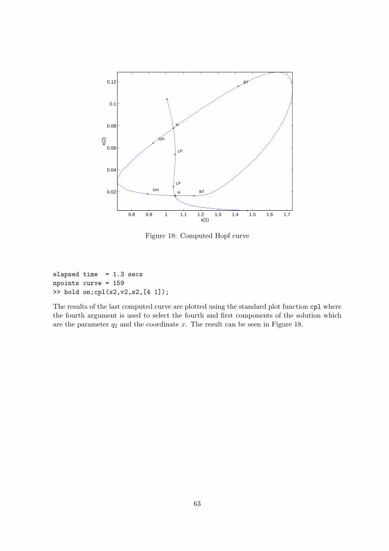
0.8 0.9 1 1.1 1.2 1.3 1.4 1.5 1.6 1.7
0.02
0.04
0.06
0.08
0.1
0.12
x(1)
x(2)
H
LP
LP
H
GH
GH
BT
BT
Figure 18: Computed Hopf curve
elapsed time = 1.3 secs
npoints curve = 159
>> hold on;cpl(x2,v2,s2,[4 1]);
The results of the last computed curve are plotted using the standard plot function cpl wherethe fourth argument is used to select the fourth and first components of the solution whichare the parameter q2 and the coordinate x. The result can be seen in Figure 18.
63
10.3 Period Doubling
10.3.1 Mathematical definition
The Period Doubling bifurcation curve is defined by the following system
dudτ − Tf(u, α) = 0u(0) − u(1) = 0∫ 10 〈u(t), uold(t)〉dt = 0G(u, T, α) = 0
(67)
this is exactly the system defining limit cycles but with one extra constraint G(u, T, α) = 0where G(u, T, α) is defined as the solution component G of the system
v(τ) − Tfu(u, α)v(τ) +Gϕ(τ) = 0v(0) + v(1) = 0∫ 1
0 〈ψ(τ), v(τ)〉dτ = 1
(68)
which is exactly the same system as was used to detect the Period Doubling bifurcation.Instead of using this functional G both systems can be combined in one larger system
dudτ − Tf(u, α) = 0u(0) − u(1) = 0∫ 10 〈u(t), uold(t)〉dt = 0v(τ) − Tfu(u, α)v(τ) = 0v(0) + v(1) = 0∫ 10 〈vold(τ), v(τ)〉dτ − 1 = 0
(69)
The first method (using system (67) and (68)) is implemented in the curve definition fileperioddoubling and the second (using system (69)) in perioddoubling2. For both methodsthe discretization is done using orthogonal collocation in the same way it was done for limitcycles.
10.3.2 Bifurcations
In MatCont / CL MatCont there are four generic codim 2 bifurcations that can bedetected along the flip curve:
• Strong 1:2 resonance. We will denote this bifurcation with R2
• Fold - flip, Limit Point - Period Doublingor We will denote this bifurcation with LPPD
• Flip - Neimark-Sacker, denoted as PDNS
• Generalized period doubling point, denoted as GPD
To detect these singularities, we define 4 test functions:
• φ1 = (v∗1)TW1LC×Mv1M
• φ2 = (ψ∗1)
TW1
(F (u0,1(t)))C
64
• φ3 = det ((M ⊙M) − In)
• φ4 = c
where c is the coefficient defined in (55), M is the monodromy matrix and ⊙ is the bialternateproduct.
The v1’s and ψ1’s are obtained as follows. For a given ζ ∈ C1([0, 1],Rn) we consider threedifferent discretizations:
• ζM ∈ R(Nm+1)n the vector of values in the mesh points,
• ζC ∈ RNmn the vector of values in the collocation points,
• ζW =
[ζW1
ζW2
]∈ R
Nmn ×Rn where ζW1
is the vector of values in the collocation points
multiplied with the Gauss - Legendre weights and the lengths of the mesh intervals, andζW2
= ζ(0).
Formally we further introduce LC×M which is a structured sparse matrix that converts avector ζM of values in the mesh points into a vector ζC of values in the collocation points byζC = LC×MζM . We compute v1M by solving
[D − TA(t)δ0 + δ1
]
disc
v1M = 0. (70)
The normalization of v1M is done by requiring∑N
i=1
∑mj=0 σj〈(v1M )(i−1)m+j , (v1M )(i−1)m+j〉∆i =
1 where σj is the Gauss-Lagrange quadrature coefficient and ∆i is the length of the i-th in-terval. By discretization we obtain
(v∗1W )T
[D − TA(t)δ0 + δ1
]
disc
= 0.
To normalize (v∗1)W1we require
∑Ni=1
∑mj=1 |((v
∗1)W1
)ij |1 = 1. Then∫ 10 〈v∗1(t), v1(t)〉dt is
approximated by (v∗1)TW1LC×Mv1M and if this quantity is nonzero, v∗1W is rescaled so that∫ 1
0 〈v∗1(t), v1(t)〉dt = 12 . We compute ψ∗
1W by solving
(ψ∗
1W )T
[D − TA(t)δ0 − δ1
]
disc
= 0
and normalize ψ∗
1W1by requiring
∑Ni=1
∑mj=1 |((ψ
∗1)W1
)ij |1 = 1. Then∫ 10 〈ψ∗
1(t), F (u0,1(t))〉dt
is approximated by (ψ∗1)
TW1
(F (u0,1(t)))C and if this quantity is nonzero, ψ∗
1W is rescaled so
that∫ 10 〈ψ∗
1(t), F (u0,1(t))〉dt = 1. a1 can be computed as (ψ∗
W1)T (B(t, v1M , v1M ))C . The
computation of (h2,1)M is done by solving
(D − TA(t))C×M (h2,1)M = (B(t; v1M , v1M ))C + 2a1(F (u0,1(t)))C , t ∈ [0, 1](δ(0) − δ(1))(h2,1)M = 0,
(ψ∗
W1)TLC×M (h2,1)M = 0.
The expression for the normal form coefficient c becomes
c = 13((v∗1W1
)T (C(t; v1M ,1T v1M , v1M )C + 3(B(t; v1M , (h2,1)M )C
−6a1
T (v∗1W1)T (A(t)v1(t))C).
65
The singularity matrix is:
S =
0 − −− 0 −1 1 0
. (71)
10.3.3 Period doubling initialization
The only way to start a Period Doubling bifurcation curve continuation supported in thecurrent version is to start it from a Period Doubling bifurcation point on a limit cycle curve.This can be done using the following statement: [x0,v0]=init PD PD(@odefile, x, s, ap,
ntst, ncol). x should be the x as returned by the previous limit cycle continuation. s isthe special point structure of the detected Period Doubling point on the limit cycle curve.odefile specifies the ode-file to be used. ap is the active parameter and ntst and ncol areagain the number of mesh and collocation points for the discretization.
To use the perioddoubling2 curve definition file use the init PD PD2 starter instead. Ittakes the same arguments as init PD PD.
10.3.4 Example
For this example the following system is used
x = yy = zz = −αz − βy − x+ x2
(72)
that is the same system as in the limit cycle continuation example. The starting vectorx0 is calculated from the Period Doubling bifurcation detected in the limit cycle example(section 9.4) using init PD PD. Continuation is done using a call to the standard continuerwith perioddoubling as curve definition file. The results are plotted using the standard plotfunction cpl where the fourth argument is used to select the 245th and 246th component ofthe solution which are the parameters α and β. The results can be seen in Figure 19. Thelabels of the plot are added manually and the direction of the x-axis is reversed. It can betested by the statement testadapt3.
>> [x0,v0]=init_PD_PD(@adapt,xlc,slc(3),[1 2],20,4);
>> opt = contset; opt = contset(opt,’Singularities’,1);
>> [xpd,vpd,spd,hpd,fpd]=cont(@perioddoubling,x0,v0,opt);
first point found
tangent vector to first point found
1:2 resonance (period = 4.841835e+000, parameters = -3.400993e-010, 1.698711e+000)
1:2 resonance (period = 9.058318e+000, parameters = 4.486764e-009, 6.782783e-001)
elapsed time = 154.4 secs
npoints curve = 300
>> cpl(xpd,vpd,spd,[245 246]);
In the next example the second Period Doubling bifurcation is used that was detected inthe second limit cycle continuation in section 9.4. Here init PD PD2 and perioddoubling2
are used instead of init PD PD and perioddoubling. The results are plotted similarly as forthe previous example (see Figure 20).
66
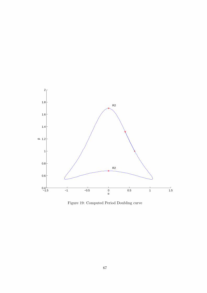
−1.5 −1 −0.5 0 0.5 1 1.50.4
0.6
0.8
1
1.2
1.4
1.6
1.8
2
R2
R2
α
β
Figure 19: Computed Period Doubling curve
67
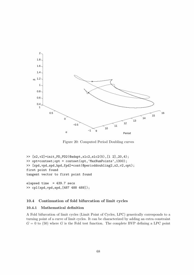
910
1112
1314
1516
−1
−0.5
0
0.5
10.4
0.6
0.8
1
1.2
1.4
1.6
1.8
2
Periodα
β
Figure 20: Computed Period Doubling curves
>> [x2,v2]=init_PD_PD2(@adapt,xlc2,slc2(5),[1 2],20,4);
>> opt=contset;opt = contset(opt,’MaxNumPoints’,1300);
>> [xpd,vpd,spd,hpd,fpd]=cont(@perioddoubling2,x2,v2,opt);
first point found
tangent vector to first point found
elapsed time = 439.7 secs
>> cpl(xpd,vpd,spd,[487 488 489]);
10.4 Continuation of fold bifurcation of limit cycles
10.4.1 Mathematical definition
A Fold bifurcation of limit cycles (Limit Point of Cycles, LPC) generically corresponds to aturning point of a curve of limit cycles. It can be characterized by adding an extra constraintG = 0 to (50) where G is the Fold test function. The complete BVP defining a LPC point
68
using the minimal extended system is
dudt − Tf(u, α) = 0u(0) − u(1) = 0∫ 10 〈u(t), uold(t)〉dt = 0G[u, T, α] = 0
(73)
where G is defined by requiring
N1
vSG
=
0001
. (74)
Here v is a function, S and G are scalars and
N1 =
D − Tfu(u(t), α) − f(u(t), α) w01
δ1 − δ0 0 w02
Intf(u(·),α) 0 w03
Intv01v02 0
(75)
where the bordering functions v01, w01, vector w02 and scalars v02 and w03 are chosen so thatN1 is nonsingular [12]. This method (using system (74) and (75)) is implemented in the curvedefinition file limitpointcycle. The discretization is done using orthogonal collocation inthe same way as it was done for limit cycles.
10.4.2 Bifurcations
In CL MatCont there are five generic codim 2 bifurcations that can be detected along thefold curve:
• Branch point. We will denote this bifurcation with BPC
• Strong 1:1 resonance. We will denote this bifurcation with R1
• Cusp point, denoted by CPC
• Fold - flip, Limit Point - Period Doublingor We will denote this bifurcation by LPPD
• Fold - Neimark-Sacker, denoted by LPNS
A Generalized Hopf (GH) marks the end (or start) of an LPC curve.To detect the generic singularities, we first define bp+5 test functions, where bp is the numberof branch parameters:
• ψi = wT fβi(u, α), i ∈ (1, ..., bp)
• ψbp+1 = (ϕ∗1)
TW1LC×Mv1M
• ψbp+2 = b (normal form coefficient)
• φbp+3 = det (M + In)
69
• ψbp+4 = det ((M2 ⊙M2) − In)
In the ψi expressions w is the vector computed in (60) and βi (branch parameter) is acomponent of α.
In the second expression ψbp+1, we compute v1M by solving
D − TA(t)δ0 − δ1∫ 1
0 F (u0,1(t))LC×M
disc
v1M =
TF (u0,1(t))
00
disc
. (76)
By discretization we obtain
(ϕ∗
1W )T
[D − TA(t)δ0 − δ1
]
disc
= 0.
To normalize (ϕ∗1)W1
we require∑N
i=1
∑mj=1
∣∣((v∗1)W1)(i−1)m+j
∣∣1
= 1. Then∫ 10 〈ϕ∗
1(t), v1(t)〉dt
is approximated by (ϕ∗1)
TW1LC×Mv1M and if this quantity is nonzero, ϕ∗
1W is rescaled so that∫ 10 〈ϕ∗
1(t), v1(t)〉dt = 1.So the third expression for the normal form coefficient b becomes
b =1
2((ϕ∗
1W1)T ((B(t; v1M , v1M )C + 2(A(t)v1(t))C)).
In the fourth expression, M is the monodromy matrix.In the fifth expression, M2 = (M−In)2, restricted to the subspace without the two eigen-
values with smallest norm.
The number of branch parameters is not fixed. If the number of branch parameters is 3then this matrix has three more rows and columns. This singularity matrix is automaticallyextended:
S =
0 − − − −− 0 − − −− − 0 − −− − − 0 −− − − 1 0
.
10.4.3 Fold initialization
One way to start a Fold bifurcation of cycles continuation supported in the current ver-sion is to start it from a fold bifurcation point (LPC) on a limit cycle curve. This can bedone using the following statement: [x0,v0]=init LPC LPC(@odefile, x, s, ap, ntst,
ncol(, bp)optional). x should be the x as returned by the previous limit cycle continuation. s
is the special point structure of the detected Fold bifurcation point on the limit cycle curve.odefile specifies the ode-file to be used. ap is the active parameter and ntst and ncol
are again the number of mesh and collocation points for the discretization. bp are the op-tional indices of the branch parameters. It also works without entering a value for this field:[x0,v0]=init LPC LPC(@odefile, x, s, ap, ntst, ncol).
70
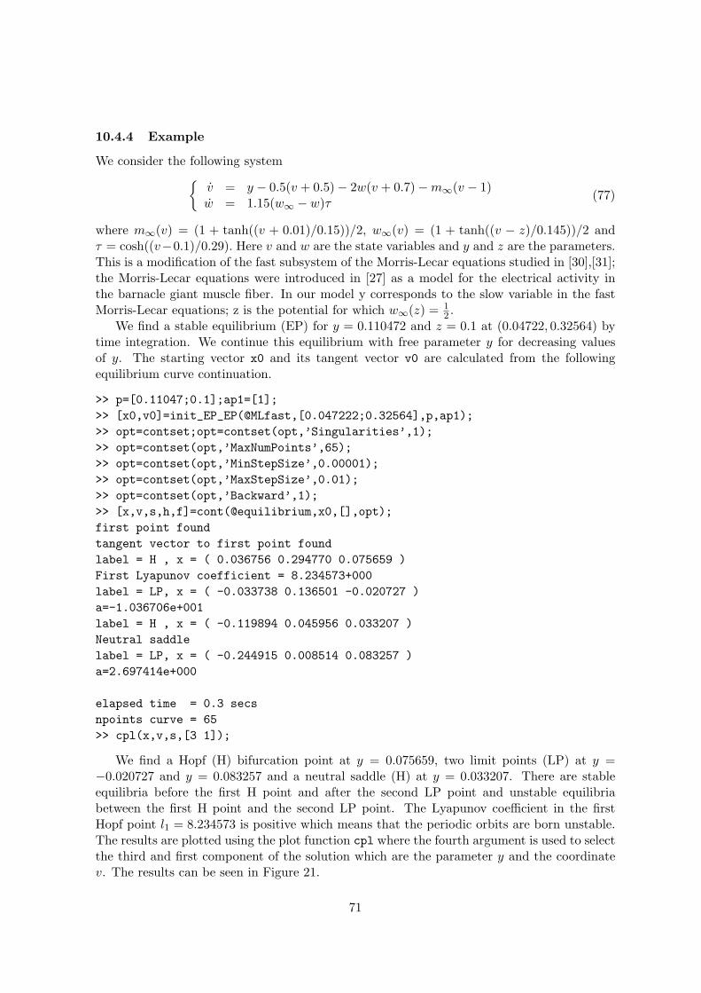
10.4.4 Example
We consider the following system{
v = y − 0.5(v + 0.5) − 2w(v + 0.7) −m∞(v − 1)w = 1.15(w∞ − w)τ
(77)
where m∞(v) = (1 + tanh((v + 0.01)/0.15))/2, w∞(v) = (1 + tanh((v − z)/0.145))/2 andτ = cosh((v−0.1)/0.29). Here v and w are the state variables and y and z are the parameters.This is a modification of the fast subsystem of the Morris-Lecar equations studied in [30],[31];the Morris-Lecar equations were introduced in [27] as a model for the electrical activity inthe barnacle giant muscle fiber. In our model y corresponds to the slow variable in the fastMorris-Lecar equations; z is the potential for which w∞(z) = 1
2 .We find a stable equilibrium (EP) for y = 0.110472 and z = 0.1 at (0.04722, 0.32564) by
time integration. We continue this equilibrium with free parameter y for decreasing valuesof y. The starting vector x0 and its tangent vector v0 are calculated from the followingequilibrium curve continuation.
>> p=[0.11047;0.1];ap1=[1];
>> [x0,v0]=init_EP_EP(@MLfast,[0.047222;0.32564],p,ap1);
>> opt=contset;opt=contset(opt,’Singularities’,1);
>> opt=contset(opt,’MaxNumPoints’,65);
>> opt=contset(opt,’MinStepSize’,0.00001);
>> opt=contset(opt,’MaxStepSize’,0.01);
>> opt=contset(opt,’Backward’,1);
>> [x,v,s,h,f]=cont(@equilibrium,x0,[],opt);
first point found
tangent vector to first point found
label = H , x = ( 0.036756 0.294770 0.075659 )
First Lyapunov coefficient = 8.234573+000
label = LP, x = ( -0.033738 0.136501 -0.020727 )
a=-1.036706e+001
label = H , x = ( -0.119894 0.045956 0.033207 )
Neutral saddle
label = LP, x = ( -0.244915 0.008514 0.083257 )
a=2.697414e+000
elapsed time = 0.3 secs
npoints curve = 65
>> cpl(x,v,s,[3 1]);
We find a Hopf (H) bifurcation point at y = 0.075659, two limit points (LP) at y =−0.020727 and y = 0.083257 and a neutral saddle (H) at y = 0.033207. There are stableequilibria before the first H point and after the second LP point and unstable equilibriabetween the first H point and the second LP point. The Lyapunov coefficient in the firstHopf point l1 = 8.234573 is positive which means that the periodic orbits are born unstable.The results are plotted using the plot function cpl where the fourth argument is used to selectthe third and first component of the solution which are the parameter y and the coordinatev. The results can be seen in Figure 21.
71
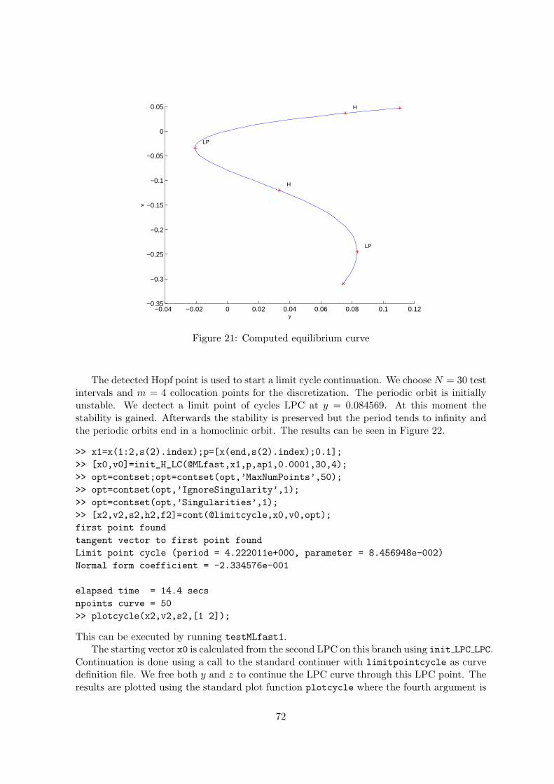
−0.04 −0.02 0 0.02 0.04 0.06 0.08 0.1 0.12−0.35
−0.3
−0.25
−0.2
−0.15
−0.1
−0.05
0
0.05 H
LP
H
LP
y
v
Figure 21: Computed equilibrium curve
The detected Hopf point is used to start a limit cycle continuation. We choose N = 30 testintervals and m = 4 collocation points for the discretization. The periodic orbit is initiallyunstable. We dectect a limit point of cycles LPC at y = 0.084569. At this moment thestability is gained. Afterwards the stability is preserved but the period tends to infinity andthe periodic orbits end in a homoclinic orbit. The results can be seen in Figure 22.
>> x1=x(1:2,s(2).index);p=[x(end,s(2).index);0.1];
>> [x0,v0]=init_H_LC(@MLfast,x1,p,ap1,0.0001,30,4);
>> opt=contset;opt=contset(opt,’MaxNumPoints’,50);
>> opt=contset(opt,’IgnoreSingularity’,1);
>> opt=contset(opt,’Singularities’,1);
>> [x2,v2,s2,h2,f2]=cont(@limitcycle,x0,v0,opt);
first point found
tangent vector to first point found
Limit point cycle (period = 4.222011e+000, parameter = 8.456948e-002)
Normal form coefficient = -2.334576e-001
elapsed time = 14.4 secs
npoints curve = 50
>> plotcycle(x2,v2,s2,[1 2]);
This can be executed by running testMLfast1.The starting vector x0 is calculated from the second LPC on this branch using init LPC LPC.
Continuation is done using a call to the standard continuer with limitpointcycle as curvedefinition file. We free both y and z to continue the LPC curve through this LPC point. Theresults are plotted using the standard plot function plotcycle where the fourth argument is
72
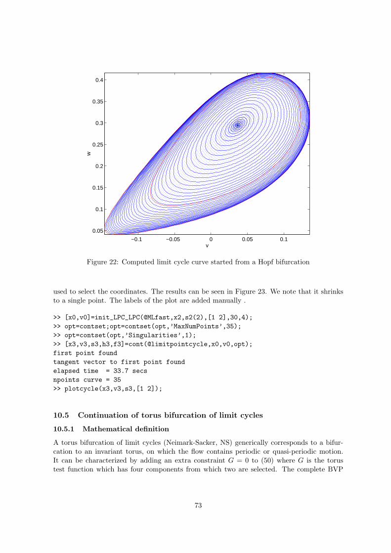
−0.1 −0.05 0 0.05 0.1
0.05
0.1
0.15
0.2
0.25
0.3
0.35
0.4
v
w
Figure 22: Computed limit cycle curve started from a Hopf bifurcation
used to select the coordinates. The results can be seen in Figure 23. We note that it shrinksto a single point. The labels of the plot are added manually .
>> [x0,v0]=init_LPC_LPC(@MLfast,x2,s2(2),[1 2],30,4);
>> opt=contset;opt=contset(opt,’MaxNumPoints’,35);
>> opt=contset(opt,’Singularities’,1);
>> [x3,v3,s3,h3,f3]=cont(@limitpointcycle,x0,v0,opt);
first point found
tangent vector to first point found
elapsed time = 33.7 secs
npoints curve = 35
>> plotcycle(x3,v3,s3,[1 2]);
10.5 Continuation of torus bifurcation of limit cycles
10.5.1 Mathematical definition
A torus bifurcation of limit cycles (Neimark-Sacker, NS) generically corresponds to a bifur-cation to an invariant torus, on which the flow contains periodic or quasi-periodic motion.It can be characterized by adding an extra constraint G = 0 to (50) where G is the torustest function which has four components from which two are selected. The complete BVP
73
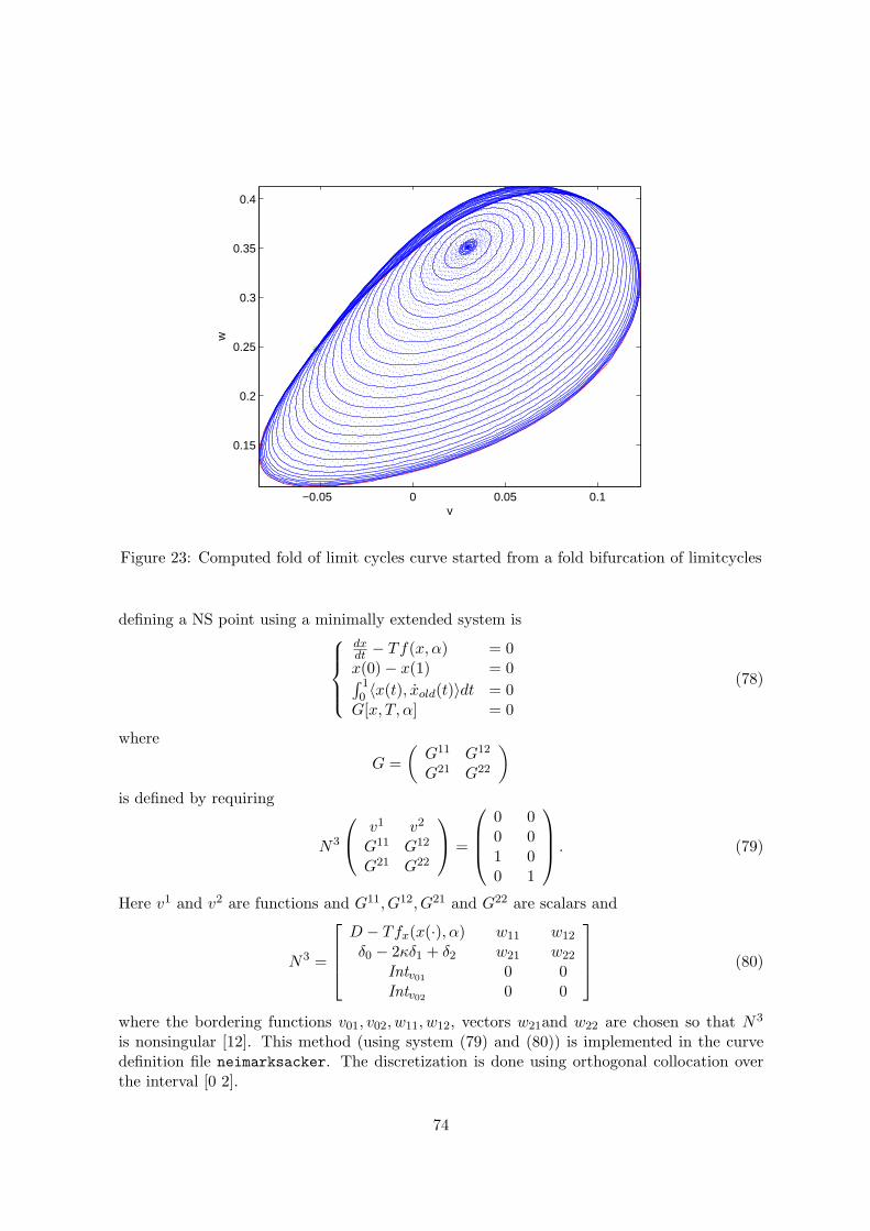
−0.05 0 0.05 0.1
0.15
0.2
0.25
0.3
0.35
0.4
v
w
Figure 23: Computed fold of limit cycles curve started from a fold bifurcation of limitcycles
defining a NS point using a minimally extended system is
dxdt − Tf(x, α) = 0x(0) − x(1) = 0∫ 10 〈x(t), xold(t)〉dt = 0G[x, T, α] = 0
(78)
where
G =
(G11 G12
G21 G22
)
is defined by requiring
N3
v1 v2
G11 G12
G21 G22
=
0 00 01 00 1
. (79)
Here v1 and v2 are functions and G11, G12, G21 and G22 are scalars and
N3 =
D − Tfx(x(·), α) w11 w12
δ0 − 2κδ1 + δ2 w21 w22
Intv010 0
Intv020 0
(80)
where the bordering functions v01, v02, w11, w12, vectors w21and w22 are chosen so that N3
is nonsingular [12]. This method (using system (79) and (80)) is implemented in the curvedefinition file neimarksacker. The discretization is done using orthogonal collocation overthe interval [0 2].
74
10.5.2 Bifurcations
In continuous-time systems there are eight generic codim 2 bifurcations that can be detectedalong the torus curve:
• 1:1 resonance. We will denote this bifurcation by R1
• 2:1 resonance point, denoted by R2
• 3:1 resonance point, denoted by R3
• 4:1 resonance point, denoted by R4
• Fold-Neimarksacker point, denoted by LPNS
• Chenciner point, denoted by CH.
• Flip-Neimarksacker point, denoted by PDNS
• Double Neimarksacker bifurcation point, denoted by NSNS
To detect these singularities, we first define 6 test functions:
• ψ1 = κ− 1 (cf. formula (39))
• ψ2 = κ+ 1
• ψ3 = κ− 1/2
• ψ4 = κ
• ψ5 = (v∗1)TW1LC×Mv1M
• ψ6 = Re(d)
• ψ7 = det (M + In)
• ψ8 = det ((M2 ⊙M2) − In)
where v1M is computed by solving[D − TA(t) + iθI
δ0 − δ1
]
D
v1M = 0. (81)
The normalization of v1M is done by requiring∑N
i=1
∑mj=0 σj〈(v1M )ij , (v1M )ij〉ti = 1 where
σj is the Gauss-Lagrange quadrature coefficient. By discretization we obtain
(v∗1W )H
[D − TA(t) + iθ
δ0 + δ1
]
disc
= 0.
To normalize (v∗1)W1we require
∑Ni=1
∑mj=1 |((v
∗1)W1
)ij |1 = 1. Then∫ 10 〈v∗1(t), v1(t)〉dt is
approximated by (v∗1)TW1LC×Mv1M and if this quantity is nonzero, v∗1W is rescaled so that∫ 1
0 〈v∗1(t), v1(t)〉dt = 1. We compute ϕ∗
1W by solving
(ϕ∗
1W )T
[D − TA(t)δ0 − δ1
]
disc
= 0
75
and normalize ϕ∗
1W1by requiring
∑Ni=1
∑mj=1 |((ϕ
∗1)W1
)ij |1 = 1. Then∫ 10 〈ϕ∗
1(t), F (u0,1(t))〉dt
is approximated by (ϕ∗1)
TW1
(F (u0,1(t)))C and if this quantity is nonzero, ϕ∗
1W is rescaled so
that∫ 10 〈ϕ∗
1(t), F (u0,1(t))〉dt = 1. We compute h20,1M by solving[D − TA(t) + 2iθI
δ0 − δ1
]
disc
h20,1M =
[B(t, v1M (t), v1M (t))
0
].
a1 can be computed as (ϕ∗
W1)T (B(t, v1M , v1M ))C .
The computation of (h11,1)M is done by solving
(D − TA(t))C×M
δ(0) − δ(1)(ϕ∗
W1)TLC×M
(h11,1)M =
B(t; v1M , v1M ))C − a1(F (u0,1(t)))C
00
The expression for the normal form coefficient d becomes
d = 12((v∗1W1
)T , (B(t;h11,1M , v1M ))C + (B(t;h20,1M , v1M ))C + 1T (C(t; v1M , v1M , v1M ))C)
−a1
T (v∗1W1)T (A(t)v1(t))C + ia1θ
T 2 .
In the 7th test function, M is the monodromy matrix.In the 8th test function, M2 = (M − In)2, restricted to the subspace without the two
eigenvalues with smallest norm.
The singularity matrix is:
S =
0 − − − − −− 0 − − − −− − 0 − − −− − − 0 − −− − − − 0 −− − − − 1 0
. (82)
10.5.3 Torus bifurcation initialization
One way to start a continuation of torus bifurcations of cycles supported in the current versionis to start it from a torus bifurcation point or neimarksacker point (NS) on a limit cycle curve.This can be done using the following statement: [x0,v0]=init NS NS(@odefile, x, s, ap,
ntst, ncol). x should be the x as returned by the previous limit cycle continuation. s isthe special point structure of the detected torus bifurcation point on the limit cycle curve.odefile specifies the ode-file to be used. ap is the array containing the two active parametersand ntst and ncol are again the number of mesh and collocation points for the discretization.
10.5.4 Example
We consider the following model of an autonomous electronic circuit [15] where x, y and z arestate variables and β, γ, ν, r, a3, b3 are parameters :
x = (−(β + ν) ∗ x+ β ∗ y − a3 ∗ x3 + b3 ∗ (y − x)3)/r
y = β ∗ x− (β + γ) ∗ y − z − b3 ∗ (y − x)3
z = y(83)
76
A torus bifurcation in this system is described in the manual of [11]. It is found by startingan equilibrium curve from the trival equilibrium point (x = y = z = 0) at β = 0.5, γ = −0.6,r = 0.6, a3 = 0.32858 b3 = 0.93358, ν = −0.9. The free parameter is ν and the branch is thetrivial one (x = y = z = 0). On this branch a Hopf bifurcation is detected at ν = −0.58934.On the emerging branch of limit cycles a branch point of limit cycles is found; by continuingthe newly found branch one detects a torus bifurcation of periodic orbits.
We proceed in a somewhat different way; to avoid the branch point of periodic orbits westart with a slightly perturbed system where the last equation of (83) is replaced by
z = y + ǫ
with initially ǫ = 0.001. The trivial solution is replaced by x = 0.00125, y = −0.001,z = 0.00052502 and we again compute a branch of equilibria with free parameter ν. Thestarting vector x0 and its tangent vector v0 are calculated from the following equilibriumcurve continuation.
>> p=[0.5;-0.6;0.6;0.32858;0.93358;-0.9;0.001];
>> [x0,v0]=init_EP_EP(@tor,[0.00125;-0.001;0.0052502],p,[6]);
>> opt=contset; opt= contset(opt,’Singularities’,1);
>> opt=contset(opt,’MaxNumPoints’,10);
>> [x,v,s,h,f]=cont(@equilibrium,x0,[],opt);
first point found
tangent vector to first point found
label = H , x = ( 0.005604 -0.001000 0.002702 -0.589286 )
First Lyapunov coefficient = -4.548985e-001
elapsed time = 0.1 secs
npoints curve = 10
A Hopf point is found for ν = −0.58928 for the state values x = 0.0056037, y = −0.001,z = 0.0027021. We start a curve of periodic orbits from this Hopf point, using N = 25 testintervals and m = 4 collocation points and choosing ν as the free parameter. The results canbe seen in Figure 24.
>> x1=x(1:3,s(2).index);p(6)= x(end,s(2).index);
>> [x0,v0]=init_H_LC(@tor,x1,p,[6],0.0001,25,4);
>> opt=contset; opt= contset(opt,’Singularities’,1);
>> opt=contset(opt,’MaxNumPoints’,50);
>> opt=contset(opt,’Multipliers’,1);
>> [x,v,s,h,f]=cont(@limitcycle,x0,v0,opt);
first point found
tangent vector to first point found
Limit point cycle (period = 8.411855e+000, parameter = -5.844928e-001)
Normal form coefficient = 1.788080e-001
Neimark-Sacker (period = 8.861103e+000, parameter = -5.957506e-001)
Normal form coefficient = -9.605627e-003
Period Doubling (period = 9.256846e+000, parameter = -6.146817e-001)
Normal form coefficient = -6.068973e-003
77
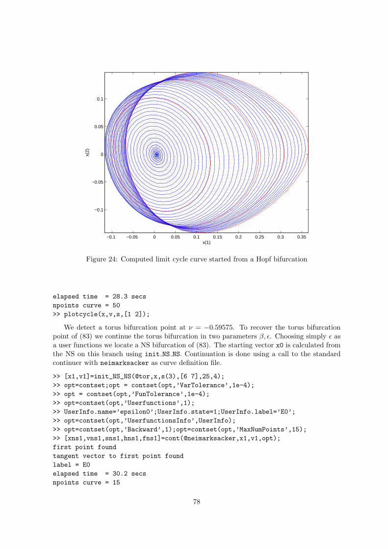
−0.1 −0.05 0 0.05 0.1 0.15 0.2 0.25 0.3 0.35
−0.1
−0.05
0
0.05
0.1
x(1)
x(2)
Figure 24: Computed limit cycle curve started from a Hopf bifurcation
elapsed time = 28.3 secs
npoints curve = 50
>> plotcycle(x,v,s,[1 2]);
We detect a torus bifurcation point at ν = −0.59575. To recover the torus bifurcationpoint of (83) we continue the torus bifurcation in two parameters β, ǫ. Choosing simply ǫ asa user functions we locate a NS bifurcation of (83). The starting vector x0 is calculated fromthe NS on this branch using init NS NS. Continuation is done using a call to the standardcontinuer with neimarksacker as curve definition file.
>> [x1,v1]=init_NS_NS(@tor,x,s(3),[6 7],25,4);
>> opt=contset;opt = contset(opt,’VarTolerance’,1e-4);
>> opt = contset(opt,’FunTolerance’,1e-4);
>> opt=contset(opt,’Userfunctions’,1);
>> UserInfo.name=’epsilon0’;UserInfo.state=1;UserInfo.label=’E0’;
>> opt=contset(opt,’UserfunctionsInfo’,UserInfo);
>> opt=contset(opt,’Backward’,1);opt=contset(opt,’MaxNumPoints’,15);
>> [xns1,vns1,sns1,hns1,fns1]=cont(@neimarksacker,x1,v1,opt);
first point found
tangent vector to first point found
label = E0
elapsed time = 30.2 secs
npoints curve = 15
78
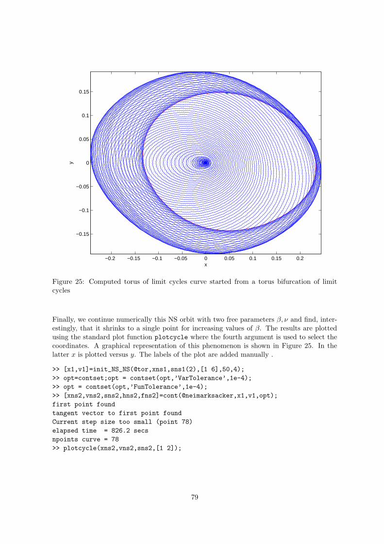
−0.2 −0.15 −0.1 −0.05 0 0.05 0.1 0.15 0.2
−0.15
−0.1
−0.05
0
0.05
0.1
0.15
x
y
Figure 25: Computed torus of limit cycles curve started from a torus bifurcation of limitcycles
Finally, we continue numerically this NS orbit with two free parameters β, ν and find, inter-estingly, that it shrinks to a single point for increasing values of β. The results are plottedusing the standard plot function plotcycle where the fourth argument is used to select thecoordinates. A graphical representation of this phenomenon is shown in Figure 25. In thelatter x is plotted versus y. The labels of the plot are added manually .
>> [x1,v1]=init_NS_NS(@tor,xns1,sns1(2),[1 6],50,4);
>> opt=contset;opt = contset(opt,’VarTolerance’,1e-4);
>> opt = contset(opt,’FunTolerance’,1e-4);
>> [xns2,vns2,sns2,hns2,fns2]=cont(@neimarksacker,x1,v1,opt);
first point found
tangent vector to first point found
Current step size too small (point 78)
elapsed time = 826.2 secs
npoints curve = 78
>> plotcycle(xns2,vns2,sns2,[1 2]);
79
11 Continuation of codim 2 bifurcations
11.1 Branch Point Continuation
11.1.1 Mathematical definition
In the toolbox branch point curves are computed by minimally extended defining systems, cf.[19], §4.1.2. The branch point curve is defined by the following system
f(u, α) = 0,g1(u, α) = 0,g2(u, α) = 0,
(84)
where (u, α) ∈ Rn+2, while g1 and g2 are obtained by solving
N4
v11 v21v12 v22g1 g2
=
0n 0n
1 00 1
. (85)
Here v11 and v21 are functions and v12, v22, g1 and g2 are scalars and
N4 =
fu(u, α) fβ(u, α) w01
v11T0 v12T
0 0v21T0 v22T
0 0
where the bordering functions v110 , v
210 , w01 and scalars v12
0 , v220 are chosen so that N4 is non-
singular. This method is implemented in the curve definition file branchpoint.m.
11.1.2 Bifurcations
In the current version no bifurcations are detected.
11.1.3 Branch Point initialization
The only way to start a continuation of branch points supported in the current version is tostart it from a Branch point detected on an equilibrium curve or on a fold curve. This canbe done using the following statement: [x0,v0]=init BP BP(@odefile, x, p, ap, bp).This routine stores its information in a global stucture bpds. The result of init BP BP
contains a vector x0 with the state variables and the three active parameters and a vectorv0 that is empty. Here odefile is the ode-file to be used, x is a vector of state variablescontaining the values of the state variables returned by a previous equilibrium curve or foldcurve continuation, p is the vector containing the current values of the parameters, ap is thevector containing the indices of the 3 active parameters and bp is the index of the branchparameter.
11.1.4 Example
For this example the following system is used
{x = α3 − (1 + λ)x+ λα1/(1 + λα2 ∗ e
−α4x/(1+x)) (86)
80
where α1 = 10 − 9 ∗ β + γ, α2 = 10 − 9 ∗ β and α3 = −0.9 + 0.4 ∗ β. The starting vector x0
and its tangent vector v0 are calculated from the following equilibrium curve continuation (λis free).
>> p=[-0.22746164;0;0;3];ap1=[1];
>> [x0,v0]=init_EP_EP(@cstr,[0.9],p,ap1);
>> opt=contset(opt,’VarTolerance’,1e-3);
>> opt=contset(opt,’FunTolerance’,1e-3);
>> opt=contset(opt,’Backward’,1e-3);
>> opt=contset(opt,’Singularities’,1);
>> [x,v,s,h,f]=cont(@equilibrium,x0,[],opt);
first point found
tangent vector to first point found
label = LP, x = ( 0.393331 0.377651 )
a=-7.369928e-001
label = LP, x = ( -0.143564 1.250669 )
a=1.550145e+000
Current step size too small (point 55)
elapsed time = 0.4 secs
npoints curve = 55
>> cpl(x,v,s,[2 1]);
The results are plotted using the plot function cpl where the fourth argument is used to selectthe second and first components of the solution which are the parameter λ and the coordinatex. The resulting curve is a part of Figure 26. We start a backward fold continuation fromthe first LP detected on the previous equilibrium curve; λ and β are free in this run.
>> x1=x(1,s(2).index);
>> p(ap1)=x(end,s(2).index);
>> [x0,v0]=init_LP_LP(@cstr,x1,p,[1 2],[1 2 3 4]);
>> [x2,v2,s2,h2,f2]=cont(@limitpoint,x0,v0,opt);
first point found
tangent vector to first point found
label = BP4, x = ( 0.000005 0.421692 0.528991 )
label = CP , x = ( -0.173872 0.405524 0.608093 )
c=-2.263123e+000
label = BP4, x = ( 0.000001 1.707425 -0.124966 )
label = BP1, x = ( 0.030645 1.772458 -0.127542 )
label = CP , x = ( 0.259554 1.968966 -0.090655 )
c=-8.847089e-001
label = BP1, x = ( 2.018621 0.581081 -4.709219 )
Closed curve detected at step 157
elapsed time = 0.9 secs
npoints curve = 157
>> hold on;cpl(x2,v2,s2,[2 1]);
The results are plotted using the standard plot function cpl where the fourth argumentis used to select the second and first components of the solution which are the parameter λ
81
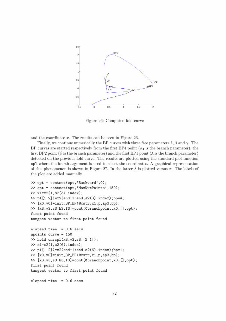
−0.5 0 0.5 1 1.5 2−1
−0.5
0
0.5
1
1.5
2
2.5
LP
LP
LP
LPBP4CP
BP4BP1
CP
BP1
Figure 26: Computed fold curve
and the coordinate x. The results can be seen in Figure 26.Finally, we continue numerically the BP curves with three free parameters λ, β and γ. The
BP curves are started respectively from the first BP4 point (α4 is the branch parameter), thefirst BP2 point (β is the branch parameter) and the first BP1 point (λ is the branch parameter)detected on the previous fold curve. The results are plotted using the standard plot functioncpl where the fourth argument is used to select the coordinates. A graphical representationof this phenomenon is shown in Figure 27. In the latter λ is plotted versus x. The labels ofthe plot are added manually .
>> opt = contset(opt,’Backward’,0);
>> opt = contset(opt,’MaxNumPoints’,150);
>> x1=x2(1,s2(3).index);
>> p([1 2])=x2(end-1:end,s2(3).index);bp=4;
>> [x0,v0]=init_BP_BP(@cstr,x1,p,ap3,bp);
>> [x3,v3,s3,h3,f3]=cont(@branchpoint,x0,[],opt);
first point found
tangent vector to first point found
elapsed time = 0.6 secs
npoints curve = 150
>> hold on;cpl(x3,v3,s3,[2 1]);
>> x1=x2(1,s2(6).index);
>> p([1 2])=x2(end-1:end,s2(6).index);bp=1;
>> [x0,v0]=init_BP_BP(@cstr,x1,p,ap3,bp);
>> [x3,v3,s3,h3,f3]=cont(@branchpoint,x0,[],opt);
first point found
tangent vector to first point found
elapsed time = 0.6 secs
82
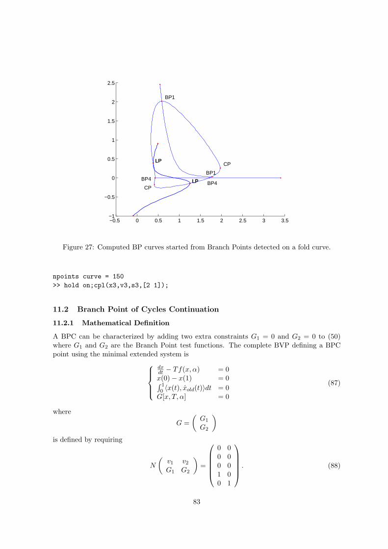
−0.5 0 0.5 1 1.5 2 2.5 3 3.5−1
−0.5
0
0.5
1
1.5
2
2.5
LP
LP
LP
LPBP4
CP BP4
BP1
CP
BP1
Figure 27: Computed BP curves started from Branch Points detected on a fold curve.
npoints curve = 150
>> hold on;cpl(x3,v3,s3,[2 1]);
11.2 Branch Point of Cycles Continuation
11.2.1 Mathematical Definition
A BPC can be characterized by adding two extra constraints G1 = 0 and G2 = 0 to (50)where G1 and G2 are the Branch Point test functions. The complete BVP defining a BPCpoint using the minimal extended system is
dxdt − Tf(x, α) = 0x(0) − x(1) = 0∫ 10 〈x(t), xold(t)〉dt = 0G[x, T, α] = 0
(87)
where
G =
(G1
G2
)
is defined by requiring
N
(v1 v2G1 G2
)=
0 00 00 01 00 1
. (88)
83
Here v1 and v2 are functions, G1 and G2 are scalars and
N =
D − Tfx(x(·), α) − f(x(·), α) − Tfβ(x(·), α) w01
δ1 − δ0 0 0 w02
Intxold(·) 0 0 w03
v11 v12 v13 0v21 v22 v23 0
(89)
where the bordering operators v11, v21, function w01, vector w02 and scalars v12, v22, v13, v23and w03 are chosen so that N is nonsingular [12][13].
11.2.2 Bifurcations
In the current version no bifurcations are detected.
11.2.3 Branch Point of Cycles initialization
The only way to start a continuation of branch points supported in the current version is tostart it from a BPC detected on an limitcycle curve or on an LPC curve. This can be doneusing the following statement: [x0,v0]=init BPC BPC(@odefile, x, s, ap, ntst, ncol,
bp). This routine stores its information in a global stucture lds. The result of init BP BP
contains a vector x0 with the state variables and the three active parameters and a vectorv0 that is empty. Here odefile is the ode-file to be used, x is a vector of state variablescontaining the values of the state variables returned by a previous limit cycle curve or foldof cycles curve continuation, s is a structure containing the BPC point values returned by aprevious limit cycle curve or fold of cycles curve continuation, ap is the vector containing theindices of the 3 active parameters and bp is the index of the branch parameter. ntst andncol are again the number of mesh and collocation points for the discretization.
11.2.4 Example
In this section we discuss a non-generic situation, i.e. a case with a symmetry and a contin-uation of BPC points that involves two effective parameters and one artificial parameter.
For this example the following model is used:
x = (−(β + ν)x+ βy − a3x3 + b3(y − x)3)/r
y = βx− (β + γ)y − z − b3(y − x)3
z = y(90)
which is the same system as in the torus of cycles continuation. It has a trivial solution branchx = y = z = 0 for all parameter values. Moreover, it has the Z2 - symmetry x→ −x,y → −y.To compute the branch of BPC points with respect to ν through the BPC point that we willdetect on a limitcycle continued with free parameters ν, β, we need to introduce an additionalfree parameter that breaks the symmetry. There are many choices for this; we choose tointroduce a parameter ǫ and extend the system (90) by simply adding a term +ǫ to the firstright-hand-side. For ǫ = 0 this reduces to (90) while for ǫ 6= 0 the symmetry is broken.
We start by computing the trivial branch with fixed parameters γ = −0.6, r = 0.6,a3 = 0.328578, b3 = 0.933578, β = 0.5,ǫ = 0 and free parameter ν with initially ν = −0.9.On this branch a Hopf point is detected for ν = −0.58933644 and a branch point of equilibriafor ν = −0.5.
84
>> p=[0.5;-0.6;0.6;0.32858;0.93358;-0.9;0];
>> [x0,v0]=init_EP_EP(@torBPC,[0;0;0],p,[6]);
>> opt=contset; opt= contset(opt,’Singularities’,1);
>> opt=contset(opt,’MaxNumPoints’,50);
>> [x,v,s,h,f]=cont(@equilibrium,x0,[],opt);
first point found
tangent vector to first point found
label = H , x = ( 0.000000 0.000000 0.000000 -0.589336 )
First Lyapunov coefficient = -4.563631e-001
label = BP, x = ( 0.000000 0.000000 0.000000 -0.500000 )
elapsed time = 0.3 secs
npoints curve = 50
From the Hopf point we start the computation of a curve of limit cycles, using 25 testintervals and 4 collocation points. This is clearly a branch of symmetric solutions of (90); wedetect one LPC and two BPC, see Fig. 28.
>> x1=x(1:3,s(2).index);p(6)= x(end,s(2).index);ap = 6;
>> [x0,v0]=init_H_LC(@torBPC,x1,p,ap,0.0001,25,4);
>> opt=contset; opt= contset(opt,’Singularities’,1);
>> opt=contset(opt,’Multipliers’,1);
>> opt=contset(opt,’MaxNumPoints’,150);
>> opt=contset(opt,’Adapt’,5);
>> [xlc,vlc,slc,hlc,flc]=cont(@limitcycle,x0,v0,opt);
first point found
tangent vector to first point found
Limit point cycle (period = 8.426472e+000, parameter = -5.843348e-001)
Normal form coefficient = 1.553595e-001
Branch Point cycle(period = 8.689669e+000, parameter = -5.870290e-001)
Neimark-Sacker (period = 8.743033e+000, parameter = -5.881194e-001)
Neutral saddle
elapsed time = 30.2 secs
npoints curve = 150
>> plotcycle(xlc,vlc,slc,[1 2]);
We continue the secondary cycle branch passing through the BPC point. From Fig. 29 it isclear that in the secondary cycle the symmetry is broken.
>> [x1,v1]=init_BPC_LC(@torBPC,xlc,vlc,slc(3),25,4,1e-6);
>> opt=contset(opt,’MaxNumPoints’,50);
>> [xlc1,vlc1,slc1,hlc1,flc1]=cont(@limitcycle,x1,v1,opt);
first point found
tangent vector to first point found
Neimark-Sacker (period = 8.794152e+000, parameter = -5.916502e-001)
Normal form coefficient = -8.661266e-003
Period Doubling (period = 9.266303e+000, parameter = -6.149552e-001)
85
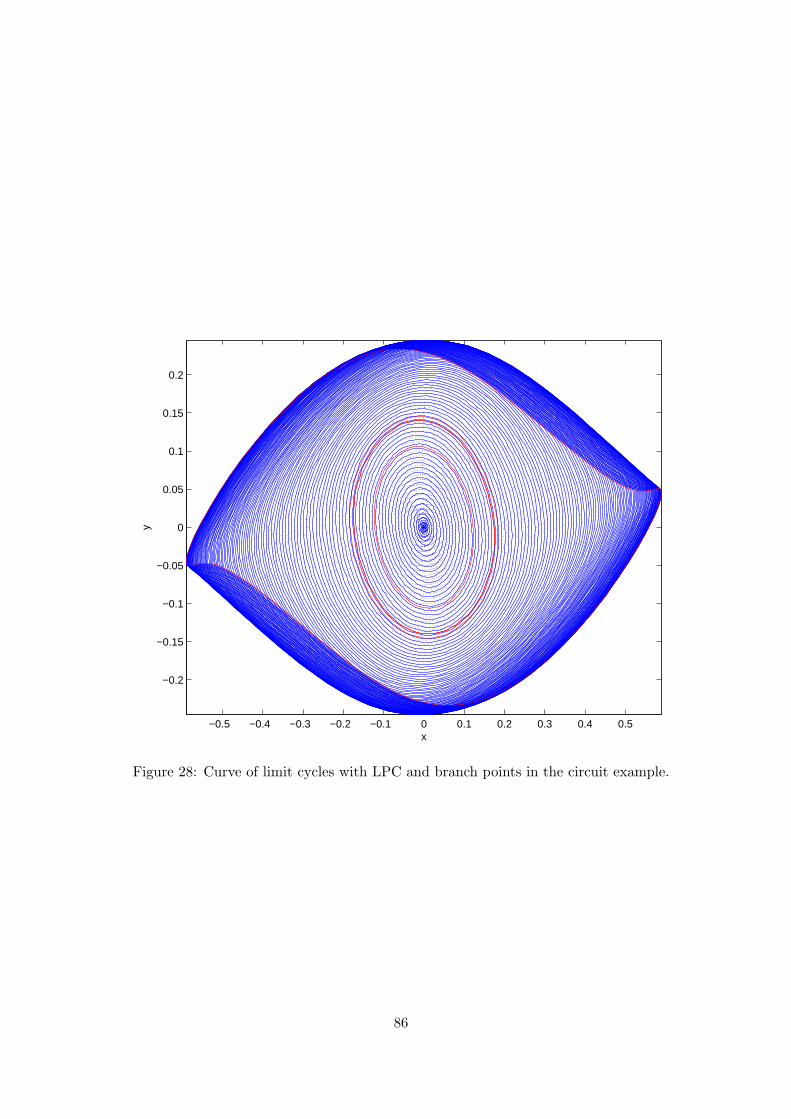
−0.5 −0.4 −0.3 −0.2 −0.1 0 0.1 0.2 0.3 0.4 0.5
−0.2
−0.15
−0.1
−0.05
0
0.05
0.1
0.15
0.2
x
y
Figure 28: Curve of limit cycles with LPC and branch points in the circuit example.
86

−0.1 0 0.1 0.2 0.3 0.4
−0.15
−0.1
−0.05
0
0.05
0.1
0.15
x
y
Figure 29: Asymetric curve of limit cycles in the circuit example.
Normal form coefficient = -6.374237e-003
elapsed time = 13.6 secs
npoints curve = 50
>> plotcycle(xlc1,vlc1,slc1,[1 2]);
Using the code for the continuation of generic BPC points with three free parametersν, β, ǫ we continue the curve of non-generic BPC points, where ǫ remains close to zero. Thepicture in Fig. 30 clearly shows that the symmetry is preserved.
>> [x1,v1]=init_BPC_BPC(@torBPC,xlc,slc(3,[1 6 7],25,4,ap);
>> opt=contset(opt,’MaxNumPoints’,200);
>> [xbpc,vbpc,sbpc,hbpc,fbpc]=cont(@branchpointcycle,x1,v1,opt);
first point found
tangent vector to first point found
elapsed time = 158.1 secs
npoints curve = 200
>> plotcycle(xbpc,vbpc,sbpc,[1 2]);
87
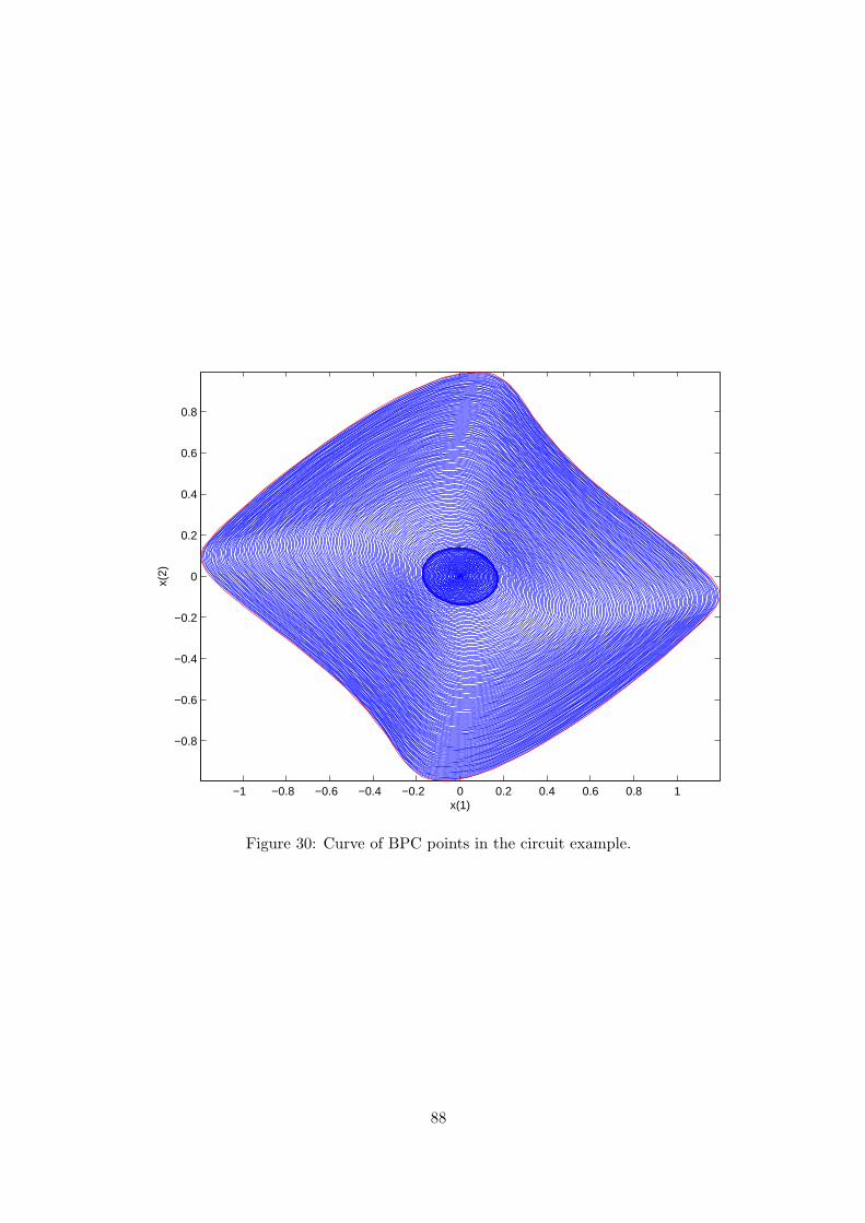
−1 −0.8 −0.6 −0.4 −0.2 0 0.2 0.4 0.6 0.8 1
−0.8
−0.6
−0.4
−0.2
0
0.2
0.4
0.6
0.8
x(1)
x(2)
Figure 30: Curve of BPC points in the circuit example.
88
12 Continuation of homoclinic orbits
12.1 Mathematical definition
In dynamical systems theory, an orbit corresponding to a solution u(t) is called homoclinicto the equilibrium point u0 of the dynamical system if u(t) → u0 as t → ±∞. There aretwo types of homoclinic orbits with codimension 1, namely homoclinic-to-hyperbolic-saddle(HHS), if u0 is a saddle (saddle-focus or bi-focus), and homoclinic-to-saddle-node (HSN), if u0
is a saddle-node (i.e., exhibits a limit point bifurcation). We recall that auto has a toolboxfor homoclinic continuation, named HomCont [4], [5].
During the continuation, it is necessary to keep track of several eigenspaces of the equi-librium in each step. To do this in an efficient way, MatCont incorporates the continuationof invariant subspaces [7] into the defining system. For some details on the implementationof the homoclinic continuation we refer to [16].
12.1.1 Homoclinic-to-Hyperbolic-Saddle Orbits
To continue HHS orbits in two free parameters, we use an extended defining system thatconsists of several parts.
First, the infinite time interval is truncated, so that instead of [−∞,+∞] we use [−T,+T ],which is scaled to [0, 1] and divided into mesh-intervals. The mesh is nonuniform and adap-tive. Each mesh interval is further subdivided by equidistant fine mesh points. Also, eachmesh interval contains a number of collocation points. (This discretization is the same asthat in auto for boundary value problems.) The equation
x(t) − 2Tf(x(t), α) = 0, (91)
must be satisfied in each collocation point.
The second part is the equilibrium condition
f(x0, α) = 0. (92)
Third, there is a so-called phase condition needed for the homoclinic solution, similar toperiodic solutions ∫ 1
0
˙x∗
(t)[x(t) − x(t)]dt = 0. (93)
Here x(t) is some initial guess for the solution, typically obtained from the previous continua-tion step. We note that in the literature another phase condition is also used, see, for example[10]. However, in the present implementation we employ the condition (93).
Fourth, there are the homoclinic-specific constraints to the solution. For these we needaccess to the stable and unstable eigenspaces of the system in the equilibrium point aftereach step. It is not efficient to recompute the spaces from scratch in each continuation-step.Instead, we use the algorithm for continuing invariant subspaces, as described in [7]. Thismethod adds two small-sized vectors (YS and YU ) to the system variables, from which thenecessary eigenspaces (stable and unstable, respectively) can easily be computed in each step.
89
If Q(0) is an orthogonal matrix whose first m columns form a basis for the invariant sub-space under consideration in the previous step, and A = fx(x0, α) is the Jacobian at the newequilibrium point, then we first compute the so-called Ricatti-blocks, Tij , by the formula
[T11 T12
T21 T22
]= Q(0)T AQ(0). (94)
If n is the number of state variables, then T11 is of size m×m and T22 is (n−m)× (n−m).This is done for the stable and unstable eigenspaces separately. Now YS and YU are obtainedfrom the Ricatti equations
T22UYU − YUT11U + T21U − YUT12UYU = 0,T22S YS − YS T11S + T21S − YS T12S YS = 0.
(95)
Now we can formulate constraints on the behavior of the solution close to the equilibriumx0. The initial vector of the orbit, (x(0) − x0), is placed in the unstable eigenspace of thesystem in the equilibrium. We express that by the requirement that it is orthogonal to theorthogonal complement of the unstable eigenspace. Using YU , we can compute the orthogonalcomplement of the unstable eigenspace. If QU (0) is the orthogonal matrix from the previousstep, related to the unstable invariant subspace, then a basis for the orthogonal complementin the new step Q⊥
U (s) is
Q⊥
U (s) = QU (0)
[−Y T
U
I
].
Note that Q⊥
U (s) is not orthogonal. The full orthogonal matrix Q1U needed for the next step,is computed separately after each step. The equations to be added to the system are (afteranalogous preparatory computations for the stable eigenspace)
Q⊥
U (s)T (x(0) − x0) = 0,Q⊥
S (s)T (x(1) − x0) = 0.(96)
Finally, the distances between x(0) (resp., x(1)) and x0 must be small enough, so that
‖x(0) − x0‖ − ǫ0 = 0,‖x(1) − x0‖ − ǫ1 = 0.
(97)
A system consisting of all equations (91), (92), (93), (95), (96) and (97), is overdetermined.The basic defining system for the continuation of a HHS orbit in two free parameters consistsof (91), (92), (95), (96), and (97) with fixed ǫ0,1, so that the phase condition (93) is not used.The variables in this system are stored in one vector. It contains the values of x(t) in thefine mesh points including x(0) and x(1), the truncation time T , two free system parameters,the coordinates of the saddle x0, and the elements of the matrices YS and YU . Alternatively,the phase condition (93) can be added if T is kept fixed but ǫ0 and ǫ1 are allowed to vary.It is also possible to fix T and ǫ0, say, and allow ǫ1 to vary, again with no phase condition.Other combinations are also possible, in particular, when the homotopy method [7] is usedto compute a starting homoclinic solution.
90
12.1.2 Homoclinic-to-Saddle-Node Orbits
For a homoclinic orbit to a saddle-node equilibrium, the extended defining system undergoessome small changes. Now (x(0) − x0) has to be placed in the center-unstable subspace.Analogously, (x(1) − x0) must be in the center-stable subspace. This again is implementedby requiring that the vector is orthogonal to the orthogonal complement of the correspondingspace. So the equations (96) themselves do not really change; the changes happen in thecomputation of the matrices Q. The defining system now has one equation less than inthe HHS case (ns + nu < n, with ns the dimension of the stable, and nu of the unstableeigenspace); the number of equations is restored however, by adding the constraint that theequilibrium must be a saddle-node. For this we use the bordering technique, as described insection 4.2.1 of [19].
12.2 Bifurcations
During HSN continuation, only one bifurcation is tested for, namely the non-central homoclinic-to-saddle-node orbit or NCH. This orbit forms the transition between HHS and HSN curves.The strategy used for detection is taken from HomCont [5].
During HHS continuation, all bifurcations detected in HomCont are also detected in ourimplementation. For this, mostly test functions from [5] are used.
Suppose that the eigenvalues of fx(x0, α0) can be ordered according to
ℜ(µns) ≤ ... ≤ ℜ(µ1) < 0 < ℜ(λ1) ≤ ... ≤ ℜ(λnu), (98)
where ℜ() stands for ’real part of’, ns is the number of stable, and nu the number of unstableeigenvalues. The test functions for the bifurcations are
• Neutral saddle, saddle-focus or bi-focus
ψ = ℜ(µ1) + ℜ(λ1)
If both µ1 and λ1 are real, then it is a neutral saddle, if one is real and one consists of apair of complex conjugates, the bifurcation is a saddle-focus, and it is a bi-focus whenboth eigenvalues consist of a pair of complex conjugates.
• Double real stable leading eigenvalue
ψ =
{(ℜ(µ1) −ℜ(µ2))
2, ℑ(µ1) = 0−(ℑ(µ1) −ℑ(µ2))
2, ℑ(µ1) 6= 0
• Double real unstable leading eigenvalue
ψ =
{(ℜ(λ1) −ℜ(λ2))
2, ℑ(λ1) = 0−(ℑ(λ1) −ℑ(λ2))
2, ℑ(λ1) 6= 0
• Neutrally-divergent saddle-focus (stable)
ψ = ℜ(µ1) + ℜ(µ2) + ℜ(λ1)
91
• Neutrally-divergent saddle-focus (unstable)
ψ = ℜ(µ1) + ℜ(λ2) + ℜ(λ1)
• Three leading eigenvalues (stable)
ψ = ℜ(µ1) −ℜ(µ3)
• Three leading eigenvalues (unstable)
ψ = ℜ(λ1) + ℜ(λ3)
• Non-central homoclinic-to-saddle-node
ψ = ℜ(µ1)
• Shil’nikov-Hopfψ = ℜ(λ1)
• Bogdanov-Takens point
ψ =
{ℜ(µ1)ℜ(λ1)
For orbit- and inclination-flip bifurcations, we assume the same ordering of the eigenvaluesof fx(x0, α0) = A(x0, α0) as shown in (98), but also that the leading eigenvalues µ1 and λ1
are unique and real:
ℜ(µns) ≤ ... ≤ ℜ(µ2) < µ1 < 0 < λ1 < ℜ(λ2) ≤ ... ≤ ℜ(λnu) .
Then it is possible to choose normalised eigenvectors ps1 and pu
1 of AT (x0, α0) and qs1 and qu
1
of A(x0, α0) depending smoothly on (x0, α0), which satisfy
AT (x0, α0) ps1 = µ1 p
s1 AT (x0, α0) p
u1 = λ1 p
u1
A(x0, α0) qs1 = µ1 q
s1 A(x0, α0) q
u1 = λ1 q
u1 .
The test functions for the orbit-flip bifurcations are then:
• Orbit-flip with respect to the stable manifold
ψ = e−µ1T < ps1, x(1) − x0 >
• Orbit-flip with respect to the unstable manifold
ψ = eλ1T < pu1 , x(0) − x0 >
For the inclination-flip bifurcations, in [5] the following test functions are introduced:
• Inclination-flip with respect to the stable manifold
ψ = e−µ1T < qs1, φ(0) >
92
• Inclination-flip with respect to the unstable manifold
ψ = eλ1T < qu1 , φ(1) >
where φ (φ ∈ C1([0, 1],Rn)) is the solution to the adjoint system, which can be written as
φ(t) + 2 T AT (x(t), α0) φ(t) = 0(Ls)
Tφ(1) = 0(Lu)Tφ(0) = 0∫ 10 φ
T (t)[φ(t) − φ(t)]dt = 0
(99)
where Ls and Lu are matrices whose columns form bases for the stable and unstable eigenspacesof A(x0, α0), respectively, and the last condition selects one solution out of the family cφ(t)for c ∈ R. Lu is equivalent to QU from the mathematical definition of the system, and Ls toQS . In the homoclinic defining system the orthogonal complements of QS and QU are used;in the adjoint system for the inclination-flip bifurcation, we use the matrices themselves (orat least, their transposed versions).
12.3 Homoclinic initialization
For homoclinics the same problems occur as with limt cycles, a homoclinic continuation can’tbe done by just calling the continuer as
[x,v,s,h,f]=cont(@homoclinic, x0, v0, opt)
The homoclinic curve file has to know
• which ode file to use,
• which parameter is active,
• the values of all parameters,
• the number of mesh and collocation points to use for the discretization.
Also an initial cycle x0 has to be known. All this information can be supplied using aninitializer. All initializers return an initial cycle x0 as well as its tangent vector v0.
• [x0,v0]=init LC Hom(@odefile, x, s, p, ap, ntst, ncol, extravec, T, eps0,
eps1)
Calculates an initial homoclinic orbit from a limit cycle with large period. Here odefileis the ode-file to be used. x and s are here the x and s belonging to the limit cyclewith large period, obtained in a previous continuation. p is the vector containing thecurrent values of the parameters. ap is the active parameter and ntst and ncol are thenumber of mesh and collocation points to be used for the discretization. extravec isa vector of 3 integers, which are either 0 or 1, and which indicate which of T, eps0,
eps1 are to be variable during the continuation. The vector is 1 for those that shouldbe variable. This can either be 1 or 2 or the three parameters. T, eps0 and eps1 arevalues for these parameters.
In the GUI-version MatCont, you call do this by selecting the cycle with large periodas initial point, and then defining it (Type → Initial Point) as a Homoclinic-to-Saddle.
93
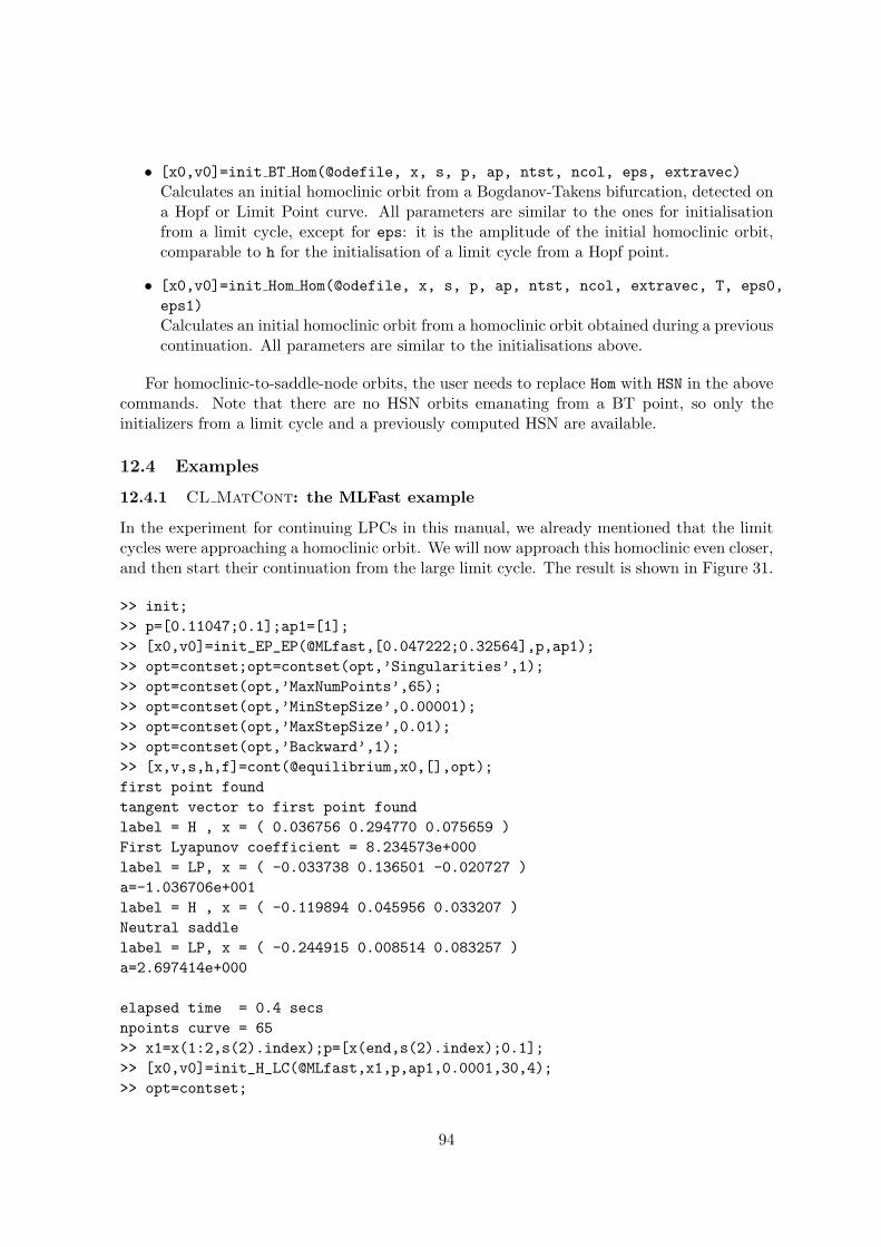
• [x0,v0]=init BT Hom(@odefile, x, s, p, ap, ntst, ncol, eps, extravec)
Calculates an initial homoclinic orbit from a Bogdanov-Takens bifurcation, detected ona Hopf or Limit Point curve. All parameters are similar to the ones for initialisationfrom a limit cycle, except for eps: it is the amplitude of the initial homoclinic orbit,comparable to h for the initialisation of a limit cycle from a Hopf point.
• [x0,v0]=init Hom Hom(@odefile, x, s, p, ap, ntst, ncol, extravec, T, eps0,
eps1)
Calculates an initial homoclinic orbit from a homoclinic orbit obtained during a previouscontinuation. All parameters are similar to the initialisations above.
For homoclinic-to-saddle-node orbits, the user needs to replace Hom with HSN in the abovecommands. Note that there are no HSN orbits emanating from a BT point, so only theinitializers from a limit cycle and a previously computed HSN are available.
12.4 Examples
12.4.1 CL MatCont: the MLFast example
In the experiment for continuing LPCs in this manual, we already mentioned that the limitcycles were approaching a homoclinic orbit. We will now approach this homoclinic even closer,and then start their continuation from the large limit cycle. The result is shown in Figure 31.
>> init;
>> p=[0.11047;0.1];ap1=[1];
>> [x0,v0]=init_EP_EP(@MLfast,[0.047222;0.32564],p,ap1);
>> opt=contset;opt=contset(opt,’Singularities’,1);
>> opt=contset(opt,’MaxNumPoints’,65);
>> opt=contset(opt,’MinStepSize’,0.00001);
>> opt=contset(opt,’MaxStepSize’,0.01);
>> opt=contset(opt,’Backward’,1);
>> [x,v,s,h,f]=cont(@equilibrium,x0,[],opt);
first point found
tangent vector to first point found
label = H , x = ( 0.036756 0.294770 0.075659 )
First Lyapunov coefficient = 8.234573e+000
label = LP, x = ( -0.033738 0.136501 -0.020727 )
a=-1.036706e+001
label = H , x = ( -0.119894 0.045956 0.033207 )
Neutral saddle
label = LP, x = ( -0.244915 0.008514 0.083257 )
a=2.697414e+000
elapsed time = 0.4 secs
npoints curve = 65
>> x1=x(1:2,s(2).index);p=[x(end,s(2).index);0.1];
>> [x0,v0]=init_H_LC(@MLfast,x1,p,ap1,0.0001,30,4);
>> opt=contset;
94
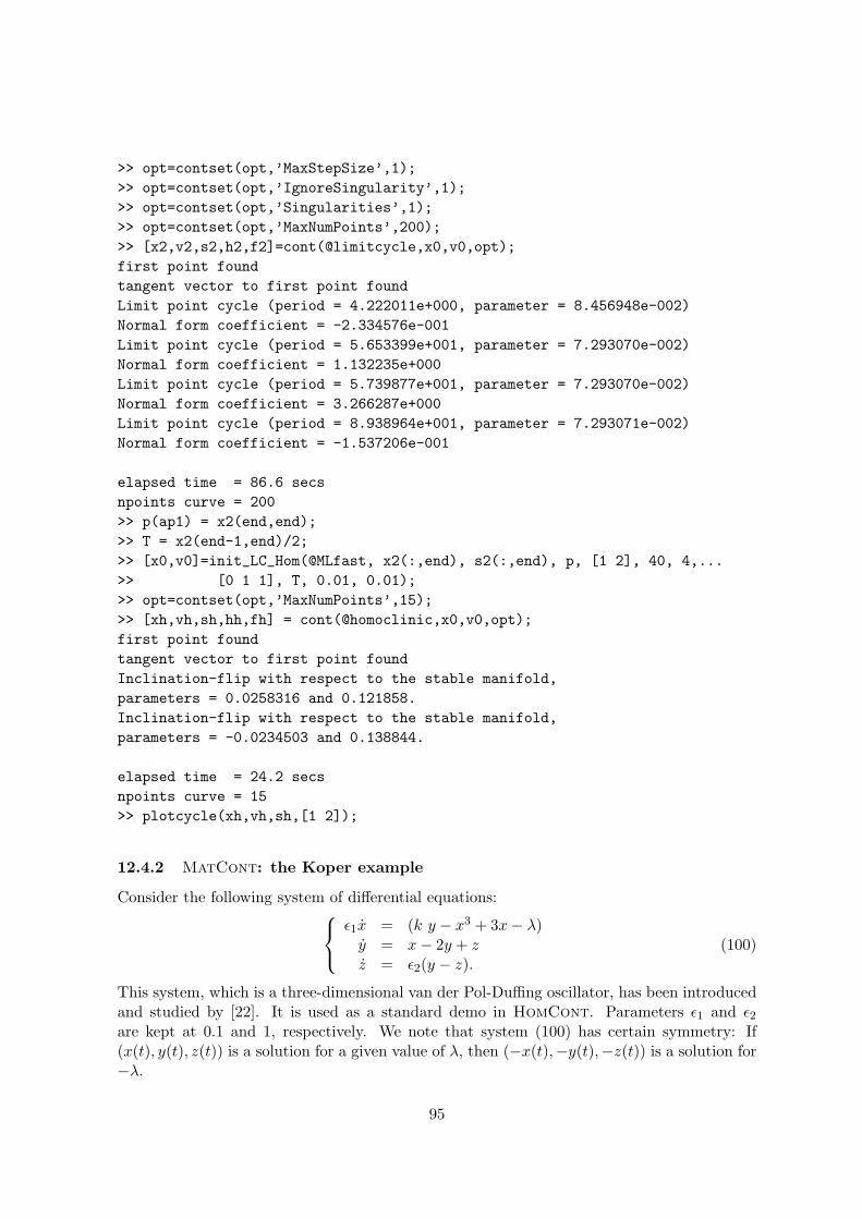
>> opt=contset(opt,’MaxStepSize’,1);
>> opt=contset(opt,’IgnoreSingularity’,1);
>> opt=contset(opt,’Singularities’,1);
>> opt=contset(opt,’MaxNumPoints’,200);
>> [x2,v2,s2,h2,f2]=cont(@limitcycle,x0,v0,opt);
first point found
tangent vector to first point found
Limit point cycle (period = 4.222011e+000, parameter = 8.456948e-002)
Normal form coefficient = -2.334576e-001
Limit point cycle (period = 5.653399e+001, parameter = 7.293070e-002)
Normal form coefficient = 1.132235e+000
Limit point cycle (period = 5.739877e+001, parameter = 7.293070e-002)
Normal form coefficient = 3.266287e+000
Limit point cycle (period = 8.938964e+001, parameter = 7.293071e-002)
Normal form coefficient = -1.537206e-001
elapsed time = 86.6 secs
npoints curve = 200
>> p(ap1) = x2(end,end);
>> T = x2(end-1,end)/2;
>> [x0,v0]=init_LC_Hom(@MLfast, x2(:,end), s2(:,end), p, [1 2], 40, 4,...
>> [0 1 1], T, 0.01, 0.01);
>> opt=contset(opt,’MaxNumPoints’,15);
>> [xh,vh,sh,hh,fh] = cont(@homoclinic,x0,v0,opt);
first point found
tangent vector to first point found
Inclination-flip with respect to the stable manifold,
parameters = 0.0258316 and 0.121858.
Inclination-flip with respect to the stable manifold,
parameters = -0.0234503 and 0.138844.
elapsed time = 24.2 secs
npoints curve = 15
>> plotcycle(xh,vh,sh,[1 2]);
12.4.2 MatCont: the Koper example
Consider the following system of differential equations:
ǫ1x = (k y − x3 + 3x− λ)y = x− 2y + zz = ǫ2(y − z).
(100)
This system, which is a three-dimensional van der Pol-Duffing oscillator, has been introducedand studied by [22]. It is used as a standard demo in HomCont. Parameters ǫ1 and ǫ2are kept at 0.1 and 1, respectively. We note that system (100) has certain symmetry: If(x(t), y(t), z(t)) is a solution for a given value of λ, then (−x(t),−y(t),−z(t)) is a solution for−λ.
95
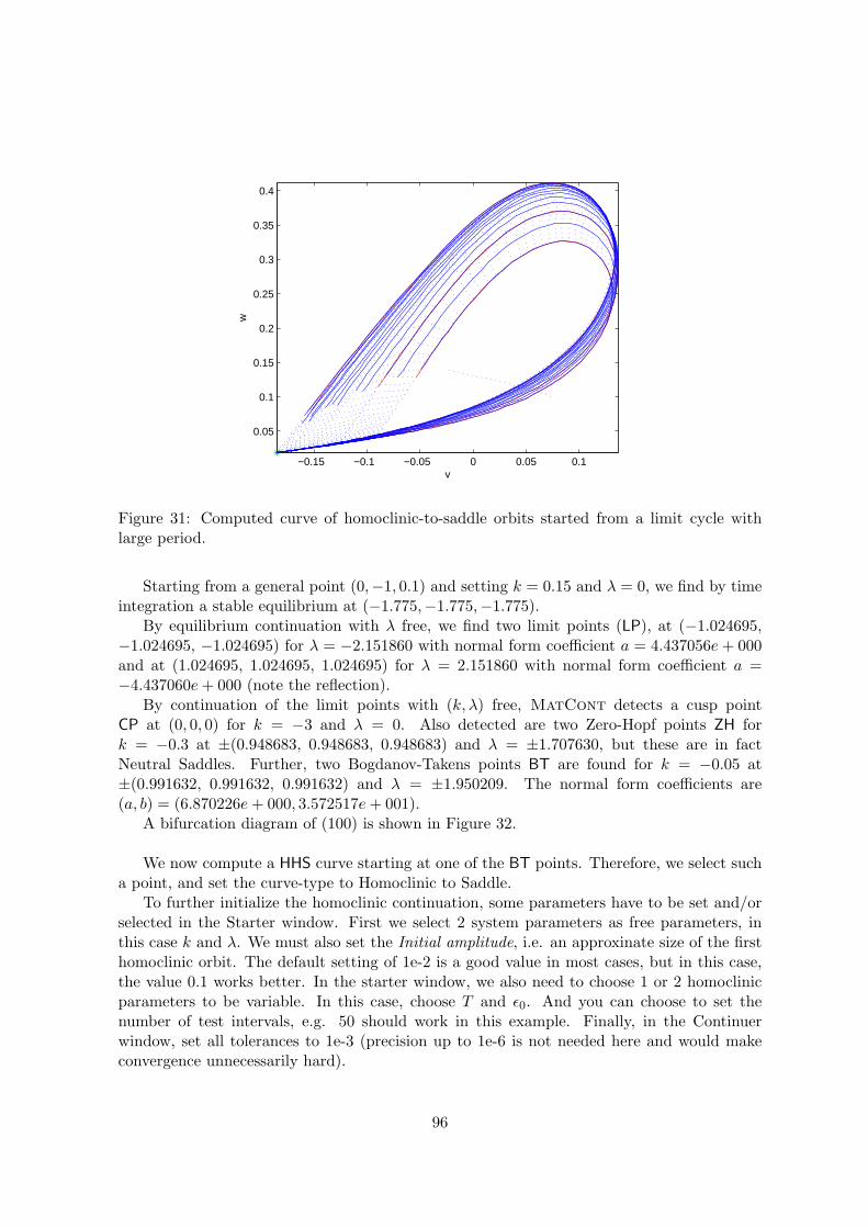
−0.15 −0.1 −0.05 0 0.05 0.1
0.05
0.1
0.15
0.2
0.25
0.3
0.35
0.4
w
v
Figure 31: Computed curve of homoclinic-to-saddle orbits started from a limit cycle withlarge period.
Starting from a general point (0,−1, 0.1) and setting k = 0.15 and λ = 0, we find by timeintegration a stable equilibrium at (−1.775,−1.775,−1.775).
By equilibrium continuation with λ free, we find two limit points (LP), at (−1.024695,−1.024695, −1.024695) for λ = −2.151860 with normal form coefficient a = 4.437056e+ 000and at (1.024695, 1.024695, 1.024695) for λ = 2.151860 with normal form coefficient a =−4.437060e+ 000 (note the reflection).
By continuation of the limit points with (k, λ) free, MatCont detects a cusp pointCP at (0, 0, 0) for k = −3 and λ = 0. Also detected are two Zero-Hopf points ZH fork = −0.3 at ±(0.948683, 0.948683, 0.948683) and λ = ±1.707630, but these are in factNeutral Saddles. Further, two Bogdanov-Takens points BT are found for k = −0.05 at±(0.991632, 0.991632, 0.991632) and λ = ±1.950209. The normal form coefficients are(a, b) = (6.870226e+ 000, 3.572517e+ 001).
A bifurcation diagram of (100) is shown in Figure 32.
We now compute a HHS curve starting at one of the BT points. Therefore, we select sucha point, and set the curve-type to Homoclinic to Saddle.
To further initialize the homoclinic continuation, some parameters have to be set and/orselected in the Starter window. First we select 2 system parameters as free parameters, inthis case k and λ. We must also set the Initial amplitude, i.e. an approxinate size of the firsthomoclinic orbit. The default setting of 1e-2 is a good value in most cases, but in this case,the value 0.1 works better. In the starter window, we also need to choose 1 or 2 homoclinicparameters to be variable. In this case, choose T and ǫ0. And you can choose to set thenumber of test intervals, e.g. 50 should work in this example. Finally, in the Continuerwindow, set all tolerances to 1e-3 (precision up to 1e-6 is not needed here and would makeconvergence unnecessarily hard).
96
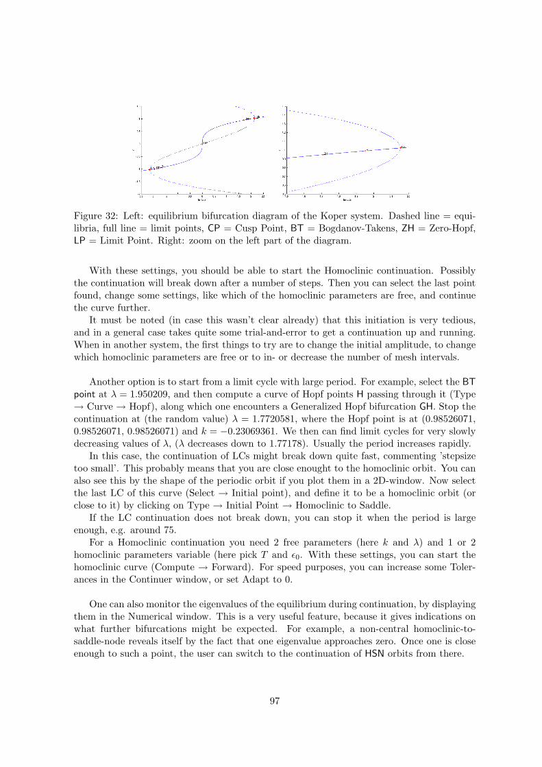
Figure 32: Left: equilibrium bifurcation diagram of the Koper system. Dashed line = equi-libria, full line = limit points, CP = Cusp Point, BT = Bogdanov-Takens, ZH = Zero-Hopf,LP = Limit Point. Right: zoom on the left part of the diagram.
With these settings, you should be able to start the Homoclinic continuation. Possiblythe continuation will break down after a number of steps. Then you can select the last pointfound, change some settings, like which of the homoclinic parameters are free, and continuethe curve further.
It must be noted (in case this wasn’t clear already) that this initiation is very tedious,and in a general case takes quite some trial-and-error to get a continuation up and running.When in another system, the first things to try are to change the initial amplitude, to changewhich homoclinic parameters are free or to in- or decrease the number of mesh intervals.
Another option is to start from a limit cycle with large period. For example, select the BT
point at λ = 1.950209, and then compute a curve of Hopf points H passing through it (Type→ Curve → Hopf), along which one encounters a Generalized Hopf bifurcation GH. Stop thecontinuation at (the random value) λ = 1.7720581, where the Hopf point is at (0.98526071,0.98526071, 0.98526071) and k = −0.23069361. We then can find limit cycles for very slowlydecreasing values of λ, (λ decreases down to 1.77178). Usually the period increases rapidly.
In this case, the continuation of LCs might break down quite fast, commenting ’stepsizetoo small’. This probably means that you are close enought to the homoclinic orbit. You canalso see this by the shape of the periodic orbit if you plot them in a 2D-window. Now selectthe last LC of this curve (Select → Initial point), and define it to be a homoclinic orbit (orclose to it) by clicking on Type → Initial Point → Homoclinic to Saddle.
If the LC continuation does not break down, you can stop it when the period is largeenough, e.g. around 75.
For a Homoclinic continuation you need 2 free parameters (here k and λ) and 1 or 2homoclinic parameters variable (here pick T and ǫ0. With these settings, you can start thehomoclinic curve (Compute → Forward). For speed purposes, you can increase some Toler-ances in the Continuer window, or set Adapt to 0.
One can also monitor the eigenvalues of the equilibrium during continuation, by displayingthem in the Numerical window. This is a very useful feature, because it gives indications onwhat further bifurcations might be expected. For example, a non-central homoclinic-to-saddle-node reveals itself by the fact that one eigenvalue approaches zero. Once one is closeenough to such a point, the user can switch to the continuation of HSN orbits from there.
97
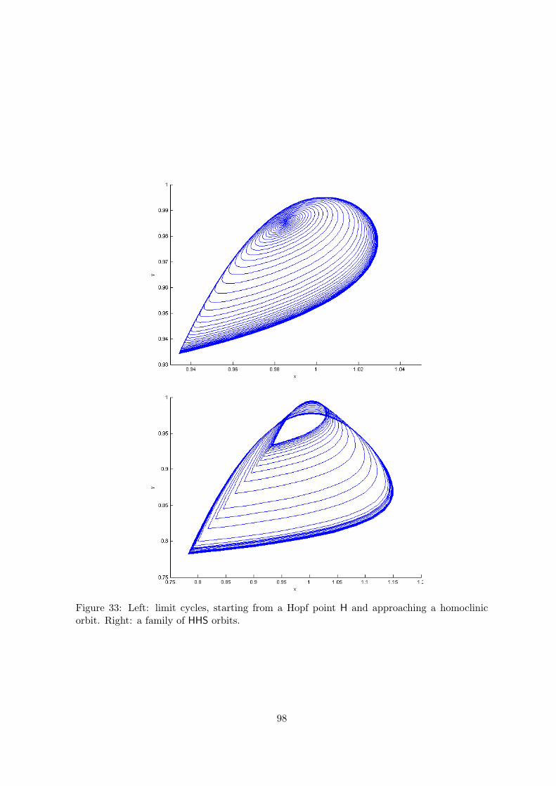
Figure 33: Left: limit cycles, starting from a Hopf point H and approaching a homoclinicorbit. Right: a family of HHS orbits.
98
References
[1] E.L. Allgower and K. Georg, Numerical Continuation Methods: An introduction,Springer-Verlag, 1990 .
[2] Beyn, W.-J. 1994. Numerical analysis of homoclinic orbits emanating from aTakens-Bogdanov point. IMA J. Numerical Analysis, 14, 381-410.
[3] W.J. Beyn, A. Champneys, E. Doedel, W. Govaerts, Yu.A. Kuznetsov, and B. Sand-stede, Numerical continuation and computation of normal forms. In: B. Fiedler, G.Iooss, and N. Kopell (eds.) “Handbook of Dynamical Systems : Vol 2”, Elsevier2002, pp 149 - 219.
[4] Champneys, A.R. and Kuznetsov Yu.A. 1994. Numerical detection and con-tinuation of codimension-two homoclinic orbits. Int. J. Bifurcation Chaos, 4(4),785-822.
[5] Champneys, A.R., Kuznetsov Yu.A. and Sandstede B. 1996. A numericaltoolbox for homoclinic bifurcation analysis. Int. J. Bifurcation Chaos, 6(5), 867-887.
[6] C. De Boor and B. Swartz, Collocation at Gaussian points, SIAM Journal on Nu-merical Analysis 10 (1973), pp. 582-606.
[7] Demmel, J.W., Dieci, L. and Friedman, M.J. 2001. Computing connectingorbits via an improved algorithm for continuing invariant subspaces. SIAM J. Sci.Comput., 22(1), 81-94.
[8] A. Dhooge, W. Govaerts and Yu. A. Kuznetsov, MATCONT : A matlab packagefor numerical bifurcation analysis of ODEs, ACM Transactions on MathematicalSoftware 29(2) (2003), pp. 141-164.
[9] E. Doedel and J Kernevez, AUTO: Software for continuation problems in ordinarydifferential equations with applications, California Institute of Technology, AppliedMathematics, 1986.
[10] Doedel, E.J. and Friedman, M.J.: Numerical computation of heteroclinic orbits, J.Comp. Appl. Math. 26 (1989) 155-170.
[11] E.J. Doedel, A.R. Champneys, T.F. Fairgrieve, Yu.A. Kuznetsov, B. Sandstede andX.J. Wang, auto97-00 : Continuation and Bifurcation Software for Ordinary Dif-ferential Equations (with HomCont), User’s Guide, Concordia University, Montreal,Canada (1997-2000). (http://indy.cs.concordia.ca).
[12] Doedel, E.J., Govaerts W., Kuznetsov, Yu.A.: Computation of Periodic SolutionBifurcations in ODEs using Bordered Systems, SIAM Journal on Numerical Anal-ysis 41,2(2003) 401-435.
[13] Doedel, E.J., Govaerts, W., Kuznetsov, Yu.A., Dhooge, A.: Numerical continuationof branch points of equilibria and periodic orbits, (preprint 2003) .
[14] Ermentrout, B.: Simulating, Analyzing, and Animating Dynamical Systems. SiamPublications, Philadelphia, 2002.
99
[15] Freire, E., Rodriguez-Luis, A., Gamero E. and Ponce, E., A case study for homo-clinic chaos in an autonomous electronic circuit: A trip form Takens-Bogdanov toHopf- Shilnikov, Physica D 62 (1993) 230–253.
[16] Friedman, M., Govaerts, W., Kuznetsov, Yu.A. and Sautois, B. 2005. Continuationof homoclinic orbits in matlab. LNCS, 3514, 263-270.
[17] Genesio, R. and Tesi, A. Harmonic balance methods for the analysis of chaoticdynamics in nonlinear systems. Automatica 28 (1992), 531-548.
[18] Genesio, R., Tesi, A., and Villoresi, F. Models of complex dynamics in nonlinearsystems. Systems Control Lett. 25 (1995), 185-192.
[19] W.J.F. Govaerts, Numerical Methods for Bifurcations of Dynamical Equilibria,SIAM, 2000.
[20] Govaerts, W. and Sautois, B.: Phase response curves, delays and synchronizationin matlab. LNCS, 3992 (2006), 391-398.
[21] Govaerts, W. and Sautois, B.: Computation of the phase response curve: a directnumerical approach. Neural Comput. 18(4) (2006), 817-847.
[22] Koper, M. 1995. Bifurcations of mixed-mode oscillations in a three-variable au-tonomous Van der Pol-Duffing model with a cross-shaped phase diagram. Phys. D,80, 72-94.
[23] Yu.A. Kuznetsov, Elements of Applied Bifurcation Theory, Springer-Verlag, 1998.
[24] Yu.A. Kuznetsov and V.V. Levitin, CONTENT: Integrated Envi-ronment for analysis of dynamical systems. CWI, Amsterdam 1997:ftp://ftp.cwi.nl/pub/CONTENT
[25] matlab, The Mathworks Inc., http://www.mathworks.com.
[26] W. Mestrom, Continuation of limit cycles in matlab, Master Thesis, MathematicalInstitute, Utrecht University, The Netherlands, 2002.
[27] Morris, C., Lecar,H., Voltage oscillations in the barnacle giant muscle fiber,BiophysJ. 35 (1981) 193–213.
[28] A. Riet, A Continuation Toolbox in matlab, Master Thesis, Mathematical Insti-tute, Utrecht University, The Netherlands, 2000.
[29] D. Roose et al., Aspects of continuation software, in : Continuation and Bifurca-tions: Numerical Techniques and Applications, (eds. D. Roose, B. De Dier and A.Spence), NATO ASI series, Series C, Vol. 313, Kluwer 1990, pp. 261-268.
[30] Terman, D., Chaotic spikes arising from a model of bursting in excitable membranes,Siam J. Appl. Math. 51 (1991) 1418–1450.
[31] Terman, D., The transition from bursting to continuous spiking in excitable mem-brane models, J. Nonlinear Sci. 2, (1992) 135–182.
100