mateus sousa - impa.br · resumo nesta tese de doutorado discutimos desigualdades ótimas...
TRANSCRIPT
Instituto Nacional de Matemática Pura e Aplicada
Some sharp inequalities in harmonic analysis
Mateus Sousa
supervised by
Prof. Emanuel Carneiro
Rio de Janeiro, 2017


Abstract
In this Ph.D. thesis we discuss sharp inequalities related to two different subjects in
harmonic analysis: (a) smoothness properties of maximal functions of convolution type as-
sociated to a variety of kernels; (b) extremal problems related to Fourier restriction estimates
on spheres and hyperboloids.
i


Resumo
Nesta tese de Doutorado discutimos desigualdades ótimas associadas a dois assuntos
diferentes em análise harmônica: (a) propriedades de suavidade de funções maximais de tipo
convolução associadas a uma variedade de núcleos; (b) problemas extremais relacionados a
estimativas de restrição da transformada de Fourier a esferas e hiperbolóides.
iii


Acknowledgments
This thesis is a crucial milestone of my journey as a mathematician. This journey was
not a lonely one, and so far I shared it with many people, with whom I learned not only
about mathematics, but life itself. Trying to write down some sort of thanks to all these
people is very hard, and I hope this attempt transmits at least a piece of my feelings.
First of all, I have to give special thanks to my advisor, Emanuel Carneiro, for being the
amazing person he is. He was a sensational teacher, a incredible collaborator and a great
friend.
Besides my advisor, I had many great masters, which I feel indebted to. Among those,
I have to highlight a few for different reasons. I cannot forget Cristina Vaz, José Miguel
Veloso, Giovany Figueiredo, Marcos Diniz and Mauro Lima from UFPA, as they introduced
me to research and pointed me to IMPA, guiding me in my path there, while being good
friends on the way. Cristoph Thiele, for receiving me many times at Bonn and making me
feel at home there. Dr. Dimitrov, for the many advices. And finally, Felipe Linares, for the
helpful hand in many different occasions. Thanks to you all.
Also, I have to mention my debt to those who collaborated with the mathematics that
was developed in this thesis. To Carlos Pérez, Olli Saari, and Tiago Picon, and specially
Diogo Oliveira e Silva, who served as my second advisor many times, thank you very much.
I am very thankful to all my friends, as I was blessed with many. The ones from my
childhood, Babi, Teo, Débora, Gih, Guga, Shamir, and from high school, Caio, Bel, Geraldo,
Natalia and Thamy, and many others from Belém, as they were my safe space from math-
v

vi ACKNOWLEDGMENTS
ematics whenever I needed it. To my many classmates at UFPA, who made my undergrad
life a lot funnier. To the friends I made during my math life at IMPA and around the world,
specially Adriana Sánchez, Alan Anderson, Alessandro Gaio, Catalina Freijo, Cayo Dória,
Clara Macedo, Daniel Ungaretti, David Beltran, Diogo Santos, Eduardo Garcez, Gennady
Uraltsev, Gianmarco Brocchi, Gregory Cosac, Hugo Araújo, Jamerson Douglas, João Pe-
dro Ramos, Leandro Cruz, Lucas Ambrozio, Lucrezia Cossetti, Luiz Paulo Freire, Marco
Fraccaroli, Mauricio Poletti, Michal Warchalski, Ricardo Misturini, Ricardo Paleari, Suzana
Frometa, Vanderson Lima, and many others. And lastly, to my friend, José Leandro, who
left us much earlier than we all wanted, but his impression will stay forever engraved in the
hearts of everyone who had the opportunity and pleasure met him.
Finally, I thank my loving family, specially my parents, Manoel and Terezinha, my
siblings, Matias and Marina, and my grandmother, Maria de Nazaré. Without their constant
support this endeavor would have been many times harder.

To my family, for their unwavering support. To José Leandro, for the inspiration.

Contents
Abstract i
Resumo iii
Acknowledgments v
1 Introduction 11.1 Sharp Fourier restriction theory . . . . . . . . . . . . . . . . . . . . . . . . . . 21.2 Smoothness of maximal functions . . . . . . . . . . . . . . . . . . . . . . . . . 41.3 A word on notation . . . . . . . . . . . . . . . . . . . . . . . . . . . . . . . . . 6
2 Sharp restriction on hyperboloids 92.1 Preliminaries . . . . . . . . . . . . . . . . . . . . . . . . . . . . . . . . . . . . 9
2.1.1 Klein–Gordon propagator . . . . . . . . . . . . . . . . . . . . . . . . . 122.1.2 Lorentz invariance . . . . . . . . . . . . . . . . . . . . . . . . . . . . . 132.1.3 Convolutions . . . . . . . . . . . . . . . . . . . . . . . . . . . . . . . . 17
2.2 Endpoint results . . . . . . . . . . . . . . . . . . . . . . . . . . . . . . . . . . 222.3 Nonendpoint results . . . . . . . . . . . . . . . . . . . . . . . . . . . . . . . . 25
2.3.1 The quest for a special cap . . . . . . . . . . . . . . . . . . . . . . . . 252.3.2 Concentration compactness . . . . . . . . . . . . . . . . . . . . . . . . 36
3 Sharp mixed norm restriction on spheres 433.1 Preliminaries . . . . . . . . . . . . . . . . . . . . . . . . . . . . . . . . . . . . 433.2 Extremizers for Vega’s inequality . . . . . . . . . . . . . . . . . . . . . . . . . 47
3.2.1 Revisiting the proof of Vega’s inequality . . . . . . . . . . . . . . . . . 473.2.2 The case q even . . . . . . . . . . . . . . . . . . . . . . . . . . . . . . . 503.2.3 Open set property: a qualitative approach . . . . . . . . . . . . . . . . 54
3.3 Effective bounds for Bessel functions . . . . . . . . . . . . . . . . . . . . . . . 553.3.1 The upper bound for Λd,q(k) . . . . . . . . . . . . . . . . . . . . . . . 55
3.4 The neighboorhood at infinity . . . . . . . . . . . . . . . . . . . . . . . . . . . 583.4.1 Preliminaries . . . . . . . . . . . . . . . . . . . . . . . . . . . . . . . . 583.4.2 Estimating q0(d) for d ≥ 3 . . . . . . . . . . . . . . . . . . . . . . . . . 593.4.3 The case d = 2 . . . . . . . . . . . . . . . . . . . . . . . . . . . . . . . 61
3.5 The Tomas–Stein case . . . . . . . . . . . . . . . . . . . . . . . . . . . . . . . 623.5.1 Preliminaries . . . . . . . . . . . . . . . . . . . . . . . . . . . . . . . . 62
viii

CONTENTS ix
3.5.2 Numerics . . . . . . . . . . . . . . . . . . . . . . . . . . . . . . . . . . 62
4 Variation-diminishing maximal functions 674.1 Preliminaries . . . . . . . . . . . . . . . . . . . . . . . . . . . . . . . . . . . . 67
4.1.1 Periodic analogues . . . . . . . . . . . . . . . . . . . . . . . . . . . . . 704.1.2 Maximal operators on the sphere . . . . . . . . . . . . . . . . . . . . . 724.1.3 Nontangential maximal operators . . . . . . . . . . . . . . . . . . . . . 754.1.4 A brief strategy outline . . . . . . . . . . . . . . . . . . . . . . . . . . 76
4.2 Results on the Euclidean space . . . . . . . . . . . . . . . . . . . . . . . . . . 764.2.1 Preliminaries on the kernel . . . . . . . . . . . . . . . . . . . . . . . . 764.2.2 Auxiliary lemmas . . . . . . . . . . . . . . . . . . . . . . . . . . . . . . 784.2.3 Proof of Theorem 4.1 . . . . . . . . . . . . . . . . . . . . . . . . . . . 84
4.3 Results on the torus . . . . . . . . . . . . . . . . . . . . . . . . . . . . . . . . 864.3.1 Auxiliary lemmas . . . . . . . . . . . . . . . . . . . . . . . . . . . . . . 864.3.2 Proof of Theorem 4.2 . . . . . . . . . . . . . . . . . . . . . . . . . . . 87
4.4 Results on the sphere . . . . . . . . . . . . . . . . . . . . . . . . . . . . . . . . 874.4.1 Auxiliary lemmas . . . . . . . . . . . . . . . . . . . . . . . . . . . . . . 874.4.2 Proof of Theorem 4.3 . . . . . . . . . . . . . . . . . . . . . . . . . . . 93
4.5 Nontangential maximal operators . . . . . . . . . . . . . . . . . . . . . . . . . 934.5.1 Auxiliary lemmas . . . . . . . . . . . . . . . . . . . . . . . . . . . . . . 934.5.2 Proof of Theorem 4.4 . . . . . . . . . . . . . . . . . . . . . . . . . . . 954.5.3 A counterexample in higher dimensions . . . . . . . . . . . . . . . . . 95
5 Maximal functions on Hardy-Sobolev spaces 975.1 Preliminaries . . . . . . . . . . . . . . . . . . . . . . . . . . . . . . . . . . . . 975.2 Auxiliary lemmas . . . . . . . . . . . . . . . . . . . . . . . . . . . . . . . . . . 1005.3 Main result . . . . . . . . . . . . . . . . . . . . . . . . . . . . . . . . . . . . . 101
5.3.1 The case of compact support . . . . . . . . . . . . . . . . . . . . . . . 1015.3.2 The case of a general support . . . . . . . . . . . . . . . . . . . . . . . 103
5.4 Remarks . . . . . . . . . . . . . . . . . . . . . . . . . . . . . . . . . . . . . . . 1045.4.1 The hypothesis on the kernels . . . . . . . . . . . . . . . . . . . . . . . 1045.4.2 Sharpness of the results in terms of the range of exponents . . . . . . 1045.4.3 Local Hardy spaces . . . . . . . . . . . . . . . . . . . . . . . . . . . . . 105
Bibliography 107


Chapter 1
Introduction
This thesis is composed of the following four papers:
[P1] Extremizers for Fourier restriction on hyperboloids, (with E. Carneiro, and D. Oliveirae Silva), Preprint, arXiv:1708.03826 (2017).
[P2] Sharp mixed norm spherical restriction, (with E. Carneiro, and D. Oliveira e Silva),Preprint, arXiv:1710.10365 (2017).
[P3] On the variation of maximal operators of convolution type, II (with E. Carneiro, andR. Finder), to appear in Revista Matemática Iberoamericana.
[P4] Regularity of maximal functions on Hardy-Sobolev spaces (with C. Pérez, T. Picon,and O. Saari), Preprint, arXiv:1711.01484 (2017).
These works all deal with functional inequalities and extremal problems related to them,such as classifying the sharp constants involved, determining existence and characterizationof extremizers, optimal range etc. [P1] and [P2] deal with sharp Fourier restriction theory,and I describe their content in Chapter 2 and 3 respectively. [P3] and [P4] are concernedwith questions involving smoothness properties of maximal functions, and I explain theirresults in Chapters 4 and 5.
This introduction is a prelude of the content of the chapters to come, and an attempt topresent the basic background involved and fix the notation that will be present throughoutthe exposition.
1

2 CHAPTER 1. INTRODUCTION
1.1 Sharp Fourier restriction theory
Arguably the most basic object in harmonic analysis is the Fourier transform. It is welldefined on a very large class of objects, such as tempered distributions S ′(Rd), and its mostbasic presentation is that of an operator from Lp(Rd) to its dual space Lp′(Rd), provided1 ≤ p ≤ 2. It has very different natures in this interval of exponents. In the lower endpointit is very regular, i.e, given any f ∈ L1(Rd) its Fourier transform f is bounded, continuousand decays to zero at infinity. On the other side of the interval, when p = 2, the situation iswilder and, up to normalization, the Fourier transform defines a unitary operator.
This means when p = 1 one can make sense of values of f on sets of zero Lebesguemeasure of Rd, such as submanifolds. Meanwhile, when p = 2, a Fourier transform f can beany function in L2(Rd), and therefore the behavior of f in sets of zero measure can not bedefined in any reasonable way. This raises the natural question of what happens betweenthese endpoint situations. This is the starting point of the so-called Fourier restriction theory
Given a surface S ⊂ Rd+1, and a measure σ supported in S, we define formally theFourier extension operator T , associated to the pair (S, σ), as
Tf(ξ) =
ˆSf(x)eix·ξ dσ(x). (1.1.1)
The celebrated Tomas-Stein theorem states that when S is the unit sphere Sd ⊂ Rd+1, andσ its surface measure, then the estimate
‖Tf‖Lp(Rd+1) ≤ C‖f‖L2(Sd,σ), (1.1.2)
holds for every f ∈ S(Rd+1), with constant C = C(d) independent of f , if and only if2(d+2)d ≤ p ≤ ∞. This means one can extend T as a bounded operator from L2(Sd, σ) to
Lp(Rd+1) and, up to normalization, its adjoint T ? : Lp′(Rd+1)→ L2(Sd, σ) acts on f ∈ S(Rd)
in a very simple fashion: T ?(f) is simply the restriction of f to Sd, i.e, T ?(f) = f|Sd . Thesame is true whenever one has a Lq → Lp estimate instead of L2 → Lp in (1.1.2), i.e, if
‖Tf‖Lp(Rd+1) ≤ C‖f‖Lq(Sd,σ), (1.1.3)
then the adjoint T ? : Lp′(Rd+1)→ Lq
′(Sd, σ) acts as the restriction of f to S if f ∈ S(Rd+1).
By duality, this means one can make sense of T ?(f) as the restriction of the Fourier transformof f ∈ Lp′(Rd+1) to the sphere Sd, provided T extends to a bounded operator from Lq(Sd, σ)
to Lp(Rd+1), for some 1 ≤ q ≤ ∞.
Understanding boundedness properties of the operator T is a very active area in cur-rent research in harmonic analysis, referred to as Fourier restriction theory. People have

1.1. SHARP FOURIER RESTRICTION THEORY 3
considered this problem for a wide class of submanifolds and measures, and norms differentthan the Lp(Rd). These questions have deep and important connections with other fieldsof mathematics, such as the analysis of partial differential equations and number theory.Determining when (1.1.3) holds for some pair (p, q) is a widely open question, and even inthe very basic case of the sphere Sd with surface measure a complete answers for q 6= 2 isonly known for the circle S1.
In this thesis we investigate extremal question related to these estimates: (i) given an apriori known restriction/extension estimate what is the value of the sharp constant in (1.1.2),i.e,
C = sup{‖Tf‖Lp(Rd+1) : ‖f‖L2(S,σ) = 1}?
(ii) Are there functions 0 6= f ∈ L2(S, σ) such that
‖Tf‖Lp(Rd+1) = C‖f‖L2(S,σ)? (1.1.4)
(iii) In case there are functions satisfying (1.1.4), which we refer to as extremizers, can wecharacterize them?
Chapters 2 and 3 of this thesis cover the study of two of those extremal question. Chapter2 is concerned with certain hyperboloids, equipped with Lorentz invariant measures, whileChapter 3 deals with the unit sphere equipped with its surface measures.
The work of Strichartz [80] establishes a family of estimates for the extension operatoron the hyperboloid Hd =
{(y, y′) ∈ Rd × R : y′ =
√1 + |y|2
}equipped with the Lorentz
invariant measuredσ(y, y′) = δ
(y′ −
√1 + |y|2
) dy dy′√1 + |y|2
. (1.1.5)
Estimate (1.1.2) for the correspondent extension operator holds in this case provided6 ≤ p <∞, if d = 1,
2(d+2)d ≤ p ≤ 2(d+1)
d−1 , if d ≥ 2.
Quilodrán [68], who studied the cases (d, p) ∈ {(2, 4), (2, 6), (3, 4)}, computed the value ofthe sharp constants in these situation and showed that extremizers do not exist. Continuinghis work, in Chapter 2 we present the study of the endpoint case (d, p) = (1, 6) and obtain theexplicit value of the sharp constant and the analogue nonexistence of extremizers. We alsostudy the nonendpoint cases when d ∈ {1, 2}, and show that in these dimensions extremizersexist. These problems are connected with space-time decay estimates for the Klein–Gordonpropagator, a feature we explore.
In Chapter 3 we study the following mixed norm inequality proved by L. Vega [84, 85]

4 CHAPTER 1. INTRODUCTION
for the spherical extension operator.
∥∥Tf∥∥LqradL
2ang(Rd+1)
:=
(ˆ ∞0
(ˆSd
∣∣Tf(rω)∣∣2 dσω
)q/2rd dr
)1/q
≤ Cd,q ‖f‖L2(Sd,σ),
which holds when q > 2(d + 1)/d. This inequality is a consequence of the aforementionedTomas-Stein theorem when q ≥ 2(d + 2)/d by a simple application of Hölder’s inequality,but outside of this range it offers a new and interesting inequality. We prove that constantsare the unique extremizers for this estimate whenever q is an even integer or q = ∞. Wealso establish that, for each dimension d, the set Ad of exponents where constants are theunique extremizers is open, including a neighborhood at infinity (q0(d),∞], and we obtainexplicit bounds for this neighborhood such that q0(d) ≤ (1
2 + o(1))d log d.Our results complement the recent, vast and very interesting body of work concerning
sharp Fourier restriction and Strichartz estimates. Sharp Fourier restriction theory hasa relatively short history, with the first works on the subject going back to Kunze [52],Foschi [32] and Hundertmark–Zharnitsky [43]. These works concern extremizers and optimalconstants for the Strichartz inequality for the homogeneous Schrödinger equation in the lowerdimensional cases. These are the cases for which the Strichartz exponent is an even integer,and one can rewrite the left-hand side of the Strichartz inequality as an L2-norm, and invokePlancherel’s theorem in order to reduce the problem to a multilinear convolution estimate.
This subject is becoming increasingly more popular, as shown by the large body of workthat appeared in the last decade, and in particular in the last few years. We mention a fewinteresting works that deal with sharp Fourier restriction theory on spheres [14, 19, 24, 25,33, 35, 73], paraboloids [5, 12, 23, 40, 72], and cones [6, 8, 67, 69]. Perturbations of thesemanifolds have been considered in [30, 44, 62, 63, 64]. Finally, we mention a recent survey [34]on sharp Fourier restriction theory which may be consulted for information complementaryto that on this introduction, including further references.
1.2 Smoothness of maximal functions
Roughly speaking, maximal operators are objects designed to bound averages. Theyappear throughout analysis in different situations, and perhaps the most basic one is theHardy-Littlewood maximal operator, which we will denote by M from this point on. Givena function f ∈ L1
loc(Rd), Mf(x) is simply the supremum of all averages of |f | on ballscentered at x. The celebrated theorem of Hardy-Littewood-Wiener establishes this operatoris bounded from Lp(Rd) to Lp(Rd), when p > 1, and it satisfies a L1(Rd) to L1,∞(Rd)bound when p = 1. The uses of boundedness properties of maximal operators are many.In the case of M , it implies the Lebesgue Differentiation theorem, and a variety of other

1.2. SMOOTHNESS OF MAXIMAL FUNCTIONS 5
maximal operators have been employed to obtain pointwise convergence results. Theseinclude Carleson’s theorem on convergence of Fourier series, Birkhoff’s ergodic theorem andmany others.
Let ϕ : Rd × (0,∞)→ R be a nonnegative function such thatˆRdϕ(x, t) dx = 1. (1.2.1)
The maximal operator associated to ϕ is defined as
Mϕf(x) = supt>0
ϕ(·, t) ∗ |f |(x),
for f ∈ L1loc(Rd). These operators are a generalization of M , as can be seen by choosing
ϕ(x, t) = 1tdm(B1)
χB1(x/t), where B1 is the unit ball centered at the origin and m(B1) isits d-dimensional Lebesgue measure. For each fixed time t > 0, the convolution ϕ(·, t) ∗ |f |can be understood as a smoothing agent, as it improves regularity of f . On the otherhand, the supremum involved is a less regular object, and can break smoothness very easily.We are interested in how these competing phenomena interact with regards to preservingsmoothness. Given a maximal operatorMϕ and a space of smooth functions, e.g. Sobolevfunctions or BV functions, we are interested in which casesMϕ preserves this smoothness.
The first work in this direction is due to Kinnunen [46]. He proved that the maximaloperator M is bounded from W 1,p(Rd) to W 1,p(Rd), providedp > 1. His proof exploits weakcompactness of these spaces and the aforementioned Lp-boundedness to obtain
‖∇Mf‖Lp(Rd) ≤ Cp‖∇f‖Lp(Rd), (1.2.2)
which readily impliesW 1,p(Rd) boundedness. This Lp-bound impliesW 1,p-bounds paradigmhas been extended to several other maximal functions in different contexts. When p = 1
things become subtler.
In general,Mϕf /∈ L1(Rd) for f 6= 0, and therefore W 1,1(Rd) to W 1,1(Rd) boundednessis false. Even though, |∇Mϕf | may be in fact a L1(Rd) function and one might have abound like (1.2.2) for p = 1, i.e,
‖∇Mϕf‖L1(Rd) ≤ C‖∇f‖L1(Rd). (1.2.3)
In this thesis we investigate this possibility and related problems for several maximal oper-ators.
The first half of our investigation, which is the content of Chapter 4, is concerned with thequestion of boundedness as well of the sharp constants involved in the inequalities for a family

6 CHAPTER 1. INTRODUCTION
of maximal operators that are connected to partial differential equations of elliptic/paraboliccharacter. Our techniques can be utilized to study similar question when the ambient spaceis not Rd, and we present some results for maximal operators on the torus and on the sphere.
The second part of our investigation, which comprises Chapter 5, deals with smoothnessproperties related to Hardy-Sobolev spaces. These spaces are a natural substitute for theSobolev spaces W 1,p(Rd) in the range of exponents 0 < p ≤ 1, and we obtain results ofboundedness on the derivative level for a large class of maximal functions of convolutiontype associated to smooth kernels, provided 1/p > 1 + 1/d. We also show this range ofexponents is sharp.
Questions about boundedness of maximal operators outside the range of Lp boundednessof these operators have garnished a lot of attention over the last few years, as well as theproblem of determining the optimal constant in (1.2.3). The first work in this direction isdue to Tanaka [82], who studied the case of ϕ(x, t) = (1/t)1[0,1](x/t), the one-sided Hardy–Littlewood maximal operator, and obtained (1.2.3) with C = 1. Later, Kurka proved thesame result for the one-dimensional Hardy–Littlewood maximal operator, with C = 240.004.Still in the one-dimensional setting, the same results for the Heat and the Poisson kernelswere obtained by Carneiro and Svaiter [22] with C = 1. Other interesting results related tothe regularity of maximal operators are [2, 7, 15, 16, 18, 41, 42, 48, 56, 57, 71, 83].
1.3 A word on notation
We denote by f the Fourier transform of a function f : Rd → C, which we normalize as
f(ξ) :=
ˆRdf(x)eix·y dx.
With this normalization, the convolution and the L2(Rd+1) norm satisfy
g ∗ h = g · h, and ‖g‖L2(Rd+1) = (2π)d+12 ‖g‖L2(Rd+1).
In particular, Tf as in (1.1.1) is simply the distributional Fourier transform of the measurefσ seen as a tempered distribution in S(Rd) and we will write fσ when it is more convenient.We represent the characteristic function of E by 1E , and averages of f ∈ L1(E) are denotedas
1
m(E)
ˆEf(y) dy =
Ef(y) dy = fE
whenever E is a measurable set with finite Lebesgue measure, and reserve the letter B forEuclidean balls. If not otherwise stated, all spaces of functions are defined over the wholeRd, e.g. L1 = L1(Rd). We denote by ‖f‖r,∞ the Lr,∞(Rd) norm of f , i.e, the weak Lr(Rd)-

1.3. A WORD ON NOTATION 7
norm of f . The positive part of a function f is denoted by (f)+ := 1{f>0}f . The usualinner product between vectors x, y ∈ Rd will continue to be denoted by x · y, and we define〈x〉 :=
√1 + |x|2.
Although we are careful with constants in a large part of the exposition, sometimes theyplay no relevant role in the results. In this case, given functions f and g, we will writef = O(g) or f . g if there exists a finite constant C such that |f(x)| ≤ C|g(x)|, and f ' g
if C−1|f(x)| ≤ |g(x)| ≤ C|f(x)| for some finite constant C 6= 0. By f = o(g) we mean|f(x)/g(x)| → 0 whenever x→∞, where the notion convergence to infinity will be clear bythe domain of definition of the functions involved, e.g, the integers or real numbers. If wewant to make explicit the dependence of the constant C on some parameter α, we will writef = Oα(g), f .α g or f = oα(g).


Chapter 2
Sharp restriction on hyperboloids
This chapter is dedicated to the contents of [P1], which deals with sharp Fourier restric-tion inequalities on the hyperboloid. These were first studied by Quilodrán [68], who furtherdeveloped methods from earlier seminal work of Foschi [32] in the context of paraboloidsand cones. We divide this chapter in 3 sections. The first section serves to introduce theobjects we will be dealing with and a few key results. Second and third sections will dealwith endpoint and nonendpoint issues respectively.
2.1 Preliminaries
Consider the hyperboloid Hd ⊂ Rd+1 defined by
Hd ={
(y, y′) ∈ Rd × R : y′ =√
1 + |y|2}, (2.1.1)
equipped with the Lorentz invariant measure
dσ(y, y′) = δ(y′ −
√1 + |y|2
) dy dy′√1 + |y|2
, (2.1.2)
which is defined by duality via the relationˆHdϕ(y, y′) dσ(y, y′) =
ˆRdϕ(y,
√1 + |y|2)
dy√1 + |y|2
.
Following (1.1.1), the Fourier extension operator on Hd is given by
Tf(x, t) =
ˆRdeix·yeit
√1+|y|2f(y)
dy√1 + |y|2
,
9

10 CHAPTER 2. SHARP RESTRICTION ON HYPERBOLOIDS
where (x, t) ∈ Rd × R and f belongs to the Schwartz class in Rd. Here we are identifying afunction f : Hd → C with a complex-valued function on Rd. Its norm in Lp(Hd, σ) is
‖f‖Lp(Hd) =(ˆ
Rd|f(y)|p dy√
1 + |y|2) 1p.
As already mentioned, the classical work of Strichartz [80] establishes a family of es-timates for the operator T . Given a dimension d ≥ 1 and an exponent p ∈ [1,∞], theestimate
‖Tf‖Lp(Rd+1) ≤ Cd,p‖f‖L2(Hd) (2.1.3)
holds uniformly for every f ∈ L2(Hd), with a finite constant Cd,p <∞, provided6 ≤ p <∞, if d = 1,
2d+2d ≤ p ≤ 2d+1
d−1 , if d ≥ 2.(2.1.4)
For a fixed dimension d ≥ 1, the lower and upper bounds in the admissible range of exponentsp given by (2.1.4) correspond to the unique exponents for which the extension operatoris bounded on the paraboloid and the cone, respectively, both equipped with projectionmeasure. Given a pair (d, p) in the admissible range (2.1.4), we wish to understand theextremizers and extremizing sequences for inequality (2.1.3), and we are interested in thevalue of the sharp constant
Hd,p := sup0 6=f∈L2(Hd)
‖Tf‖Lp(Rd+1)
‖f‖L2(Hd)
.
As already noted, Quilodrán [68] studied the endpoint cases (d, p) ∈ {(2, 4), (2, 6), (3, 4)}.More precisely, he computed the values
H2,4 = 234π, H2,6 = (2π)
56 , and H3,4 = (2π)
54 ,
and established the nonexistence of extremizers for the inequality (2.1.3) associated to thesethree cases, which are the only ones for which d > 1 and p is an even integer. The argumentsin [68] rely on explicit computations of the n-fold convolution of the measure σ with itself,and these are computationally challenging if n ≥ 3 and d 6= 2.
Here we answer two questions raised by Quilodrán [68, p. 39], regarding: (i) the valueof the sharp constant and existence of extremizers in the endpoint case (d, p) = (1, 6); (ii)the existence of extremizers in the nonendpoint cases in dimensions d ∈ {1, 2}. Our resultsbelow, together with the previous results of Quilodrán [68], provide a complete qualitativedescription of this problem in low dimensions.
2.1. PRELIMINARIES 11
Theorem 2.1. The value of the optimal constant in the case (d, p) = (1, 6) is
H1,6 = 3−112 (2π)
12 .
Moreover, extremizers for inequality (2.1.3) do not exist in this case.
From Plancherel’s theorem it follows that
‖Tf‖3L6(R2) = ‖(fσ)3‖L2(R2) = ‖(fσ ∗ fσ ∗ fσ) ‖L2(R2) = 2π‖fσ ∗ fσ ∗ fσ‖L2(R2),
which in particular implies that
H31,6 = 2π sup
06=f∈L2(H1)
‖fσ ∗ fσ ∗ fσ‖L2(R2)
‖f‖3L2(H1)
. (2.1.5)
We are thus led to studying convolution measure σ ∗ σ ∗ σ, a task which we will undertakein greater generality below. The rigidity of the endpoint lies at the heart of the mechanismresponsible for the lack of compactness in these situations (with p even). It would be in-teresting to investigate if, in all the other endpoint cases (d, p) (now with p not an eveninteger), one still has lack of extremizers for (2.1.3).
On the other hand, recent works of Fanelli, Vega and Visciglia [30, 31] indicate thatconcentration-compactness arguments may ensure the existence of extremizers in nonend-point cases for certain families of restriction/extension estimates. It is important to remarkthat the problem considered here does not fall under the scope of the methods of [30, 31],since the hyperboloid is a non-compact surface which lacks dilation homogeneity (althoughmany ideas from [30, 31] shall be useful). Our next result establishes that extremizers doexist in every nonendpoint case of the one- and two-dimensional settings.
Theorem 2.2. Extremizers for inequality (2.1.3) do exist in the following cases:
(a) d = 1 and 6 < p <∞.
(b) d = 2 and 4 < p < 6.
As suggested, our proof of Theorem 2.2 relies on concentration-compactness arguments.The heart of the matter lies in the construction of a special cap, i.e. a cap that containsa positive universal proportion of the total mass in an extremizing sequence, possibly afterapplying the symmetries of the problem. This rules out the possibility of “mass concentrationat infinity" and is the missing part in [68, Proposition 2.1], which originally outlined the proofof a dichotomy statement for extremizing sequences. The successful quest for a special caprelies partly on the fact that the lower endpoint p is an even integer in these dimensions, and

12 CHAPTER 2. SHARP RESTRICTION ON HYPERBOLOIDS
that the corresponding (p/2)-fold convolution of the measure σ with itself, when properlyparametrized, decays to zero at infinity. In this regard, our argument does not generalize todimensions d ≥ 3. Other tools (e.g. coming from bilinear restriction theory, as in [10, 35, 69])may be required to address the existence of extremizers in this general nonendpoint setting.
2.1.1 Klein–Gordon propagator
Estimates for Fourier extension operators are deeply connected to estimates for dispersivepartial differential equations. In our case, the operator T is related to the following Klein–Gordon equation
∂2t u = ∆xu− u, (x, t) ∈ Rd × R;
u(x, 0) = u0(x), ∂tu(x, 0) = u1(x).(2.1.6)
The connection comes from the following operator, the Klein–Gordon propagator,
eit√
1−∆g(x) :=1
(2π)d
ˆRdg(ξ) eix·ξ eit
√1+|ξ|2 dξ.
Indeed, one can see that solutions to (2.1.6) can be written as
u(·, t) =1
2
(eit√
1−∆u0(·)− ieit√
1−∆(√
1−∆)−1u1(·))
+
1
2
(e−it
√1−∆u0(·) + ie−it
√1−∆(
√1−∆)−1u1(·)
),
and thatTf(x, t) = (2π)d eit
√1−∆g(x), (2.1.7)
whereg(y) :=
f(y)√1 + |y|2
. (2.1.8)
This relation implies that the estimate (2.1.3) is equivalent to
‖eit√
1−∆g‖Lpx,t(Rd×R) ≤ (2π)−dHd,p ‖g‖W 2, 12 (Rd)
,
where W 2,s(Rd), for s ≥ 0, is the nonhomogeneous Sobolev space defined by
Hs(Rd) = {g ∈ L2(Rd) : ‖g‖2W 2,s(Rd) :=
ˆRd|g(ξ)|2(1 + |ξ|2)s dξ <∞}.
This equivalent formulation will be very useful. In our concentration-compactness argu-ments, we explore the fact that convergence of an extremizing sequence {fn} in L2(Hd) is

2.1. PRELIMINARIES 13
equivalent to convergence in W 2, 12 (Rd) of the sequence {gn} determined by (2.1.8), and,
once on the Sobolev side, we may use local compact embeddings. Observe also that, for eacht ∈ R, the operator eit
√1−∆ is unitary in W 2, 1
2 (Rd).
2.1.2 Lorentz invariance
The measure σ defined in (2.1.2) has been referred to as the Lorentz invariant measureon the hyperboloid. The Lorentz group, denoted by L, is defined as the group of invertiblelinear transformations in Rd+1 that preserve the bilinear form
B(x, y) = xd+1yd+1 − xdyd − . . .− x1y1.
In particular, if L ∈ L, we have |detL| = 1. We denote the subgroup of L that preservesthe hyperboloid Hd by L+. The measure σ is likewise preserved under the action of L+, inthe sense that ˆ
Hdf ◦ L dσ =
ˆHdf dσ,
for every f ∈ L1(Hd) and L ∈ L+. This can be readily seen by writing
dσ(y, y′) = 2 δ(y′2 − |y|2 − 1
)1{y′>0}(y, y
′) dy dy′.
Now, given t ∈ (−1, 1), define the linear map Lt : Rd+1 → Rd+1 via
Lt(ξ1, . . . , ξd, τ) =( ξ1 + tτ√
1− t2, ξ2, . . . , ξd,
τ + tξ1√1− t2
).
The family {Lt}t∈(−1,1) defines a one-parameter subgroup of L+. In particular, the inverseof Lt is L−t. Further notice that, given an orthogonal matrix A ∈ O(d), the transformation(ξ, τ) 7→ ρA(ξ, τ) = (Aξ, τ) belongs to L+.
As already observed in [68, Section 3], given (ξ, τ) ∈ Rd+1 satisfying τ > |ξ|, a suitablecomposition of transformations of the form Lt and ρA as defined above produces a mapL ∈ L+, such that
L(ξ, τ) = (0,√τ2 − |ξ|2).
This observation will simplify several computations involving convolutions of the measure σwith itself, which we explore in the next section. Given p ∈ [1,∞], L ∈ L+ and f ∈ Lp(Hd),define the composition L∗f = f ◦ L. The considerations made so far imply that
‖L∗f‖Lp(Hd) = ‖f‖Lp(Hd), and ‖T (L∗f)‖Lp(Rd+1) = ‖Tf‖Lp(Rd+1). (2.1.9)
In particular, if {fn}n∈N is an extremizing sequence for inequality (2.1.3) and {Ln}n∈N ⊂ L+,
14 CHAPTER 2. SHARP RESTRICTION ON HYPERBOLOIDS
then {L∗nfn}n∈N is still an extremizing sequence for inequality (2.1.3).The Lorentz invariance just discussed will be crucial in several of our arguments, as it
allows to localize the action to a fixed bounded region. We now detail this principle in thelower dimensional setting d ∈ {1, 2}.
One-dimensional tessellations
Let us define a one-dimensional cap to be a set of the form
Ck := {(ξ, τ) ∈ H1 : sinh(k − 1/2) ≤ ξ < sinh(k + 1/2)}
= {(sinh(u), cosh(u)) ∈ R2 : k − 1/2 ≤ u < k + 1/2} ,(2.1.10)
for some k ∈ Z. The following simple result already illustrates the main point.
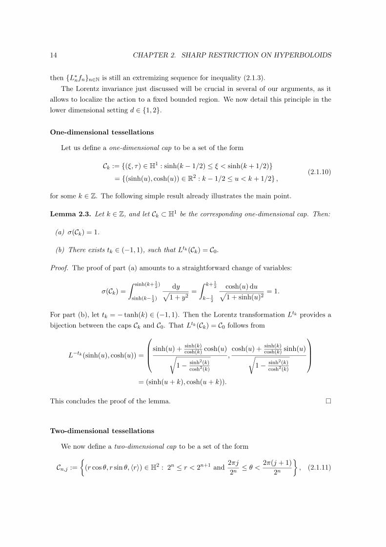
Lemma 2.3. Let k ∈ Z, and let Ck ⊂ H1 be the corresponding one-dimensional cap. Then:
(a) σ(Ck) = 1.
(b) There exists tk ∈ (−1, 1), such that Ltk(Ck) = C0.
Proof. The proof of part (a) amounts to a straightforward change of variables:
σ(Ck) =
ˆ sinh(k+ 12
)
sinh(k− 12
)
dy√1 + y2
=
ˆ k+ 12
k− 12
cosh(u) du√1 + sinh(u)2
= 1.
For part (b), let tk = − tanh(k) ∈ (−1, 1). Then the Lorentz transformation Ltk provides abijection between the caps Ck and C0. That Ltk(Ck) = C0 follows from
L−tk(sinh(u), cosh(u)) =
sinh(u) + sinh(k)cosh(k) cosh(u)√
1− sinh2(k)
cosh2(k)
,cosh(u) + sinh(k)
cosh(k) sinh(u)√1− sinh2(k)
cosh2(k)
= (sinh(u+ k), cosh(u+ k)).
This concludes the proof of the lemma.
Two-dimensional tessellations
We now define a two-dimensional cap to be a set of the form
Cn,j :=
{(r cos θ, r sin θ, 〈r〉) ∈ H2 : 2n ≤ r < 2n+1 and
2πj
2n≤ θ < 2π(j + 1)
2n
}, (2.1.11)

2.1. PRELIMINARIES 15
Figure 2.1: The one-dimensional cap movement: a carefully chosen Lorentz transformationinterchanges the caps. Here, Lt(C−2) = C0 for t = tanh(2).
for some n ∈ N and 0 ≤ j < 2n, and additionally we consider
C0,0 := {(ξ, τ) ∈ H2 : |ξ| < 2}. (2.1.12)
Grouping together the caps of the n-th generation, we notice that the hyperboloid H2 ispartitioned into a disjoint union of annuli,
H2 =∞⋃n=0
An, where An :=2n−1⋃j=0
Cn,j . (2.1.13)
See Figure 2.2 for an illustration of these decompositions.
Given ϕ ∈ [0, 2π), denote by Rϕ the rotation in R3 by angle ϕ around the vertical τ−axis:
Rϕ(ξ1, ξ2, τ) = (ξ1 cosϕ+ ξ2 sinϕ,−ξ1 sinϕ+ ξ2 cosϕ, τ).
The next result is the two-dimensional equivalent of Lemma 2.3, and in particular showsthat any cap can be mapped into the ball of radius 2
√2π centered at the origin by an
appropriate composition of Lorentz transformations. See Figure 2.3 for an illustration ofthese movements.
Lemma 2.4. Let n ∈ N0 and 0 ≤ j < 2n, and let Cn,j ⊂ H2 be the corresponding two-dimensional cap. Then:
(a) σ(Cn,j) ' 1.

16 CHAPTER 2. SHARP RESTRICTION ON HYPERBOLOIDS
Figure 2.2: Projection of the tessellation of H2 into caps {Cn,j} onto the horizontal planeτ = 0.
(b) There exists t ∈ [0, 1) and ϕ ∈ [0, 2π), such that
(L−t ◦Rϕ)(Cn,j) ⊆ {(ξ, τ) ∈ H2 : |ξ| ≤ 2√
2π}.
Proof. Let n ∈ N and 0 ≤ j < 2n. A computation in polar coordinates shows that
σ(Cn,j) =
ˆ 2n+1
2n
(ˆ 2π(j+1)2n
2πj2n
dθ
)r dr√1 + r2
=2π
2n
(√1 + 4n+1 −
√1 + 4n
),
from which one easily checks that
9
10≤ σ(Cn,j)
2π≤ 1.
Moreover, σ(C0,0) = 2π(√
5− 1), and so one sees that the σ-measure of any two-dimensionalcap is comparable to 1. This establishes part (a).
For part (b), we lose no generality in assuming n ≥ 3, for otherwise we can simply taket = ϕ = 0. Given such n, and 0 ≤ j < 2n, choose ϕ ∈ [0, 2π) so that
Rϕ(Cn,j) ⊆{
(r cos θ, r sin θ, 〈r〉) ∈ H2 : 2n ≤ r < 2n+1 and |θ| ≤ π
2n
}.
Let t := 1− ( π2n )2, which is nonnegative since n ≥ 3. Noting that
(L−t◦Rϕ)(Cn,j) ⊆{(
r cos θ − t〈r〉√1− t2
, r sin θ,〈r〉 − tr cos θ√
1− t2
)∈ H2 : 2n ≤ r < 2n+1 and |θ| ≤ π
2n
},

2.1. PRELIMINARIES 17
Figure 2.3: Projection of the two-dimensional cap movement: a rotation followed by aLorentz transformation moves the cap inside the set {(ξ, τ) ∈ H2 : |ξ| ≤ 2
√2π}.
it suffices to check that ∣∣∣∣r cos θ − t〈r〉√1− t2
∣∣∣∣ ≤ 2π, and |r sin θ| ≤ 2π.
Observe that r ≤ 〈r〉 and cos θ ≥ cos( π2n ) ≥ 1− 12( π2n )2 > t. We first claim that r cos θ−t〈r〉 ≥
0. In fact, using the fact that 1 + x2 ≥√
1 + x, we have
cos θ
t≥
1− 12( π2n )2
1− ( π2n )2≥ 1 +
1
22n+1≥√
1 +1
22n≥√
1 +1
r2=〈r〉r.
Therefore it follows that∣∣∣∣r cos θ − t〈r〉√1− t2
∣∣∣∣ ≤ r(cos θ − t)√1− t2
≤ r(1− t)√1− t2
= r
√1− t1 + t
≤ r√
1− t < 2n+1 π
2n= 2π.
Noting that sin(x)x ≤ 1, we similarly have that
|r sin θ| < 2n+1 sin( π
2n
)= 2π
sin( π2n )π2n
≤ 2π.
This concludes the proof of the lemma.
2.1.3 Convolutions
We collect some facts about n-fold convolutions of the measure σ that will be relevantin the sequel. We start with some general considerations which hold in arbitrary dimensionsd ≥ 1. Let σ(∗n) = σ ∗ . . . ∗σ denote the n-fold convolution of the Lorentz invariant measureσ defined in (2.1.2) with itself. If n ≥ 2, then the convolution measure σ(∗n) is absolutely

18 CHAPTER 2. SHARP RESTRICTION ON HYPERBOLOIDS
continuous with respect to Lebesgue measure on Rd+1, and it is supported in the closure ofthe region
Pd,n := {(ξ, τ) ∈ Rd × R : τ >√n2 + |ξ|2}. (2.1.14)
The Lorentz invariance discussed in the previous section implies that σ(∗n) is constant alongcertain hyperboloids. More precisely, if (ξ, τ) ∈ Pd,n, then
σ(∗n)(ξ, τ) = σ(∗n)(0,√τ2 − |ξ|2). (2.1.15)
The next result establishes some basic convolution properties on the one-dimensional hyper-bola (H1, σ).
Lemma 2.5. Let σ denote the Lorentz invariant measure on the hyperbola H1. Then, forevery (ξ, τ) ∈ R× R,
(a) The convolution measure σ ∗ σ is given by
(σ ∗ σ)(ξ, τ) =4√
τ2 − ξ2√τ2 − ξ2 − 4
1{τ≥√
22+ξ2}(ξ, τ).
(b) The following recursive formula holds for n ≥ 2:
σ(∗(n+1))(ξ, τ) = 4
ˆ √τ2−ξ2−1
n
x σ(∗n)(0, x)
(√τ2 − ξ2 + 1)2 − x2)
12 (√τ2 − ξ2 − 1)2 − x2)
12
dx.
Proof. We start with part (a). By the Lorentz invariance (2.1.15), it suffices to prove that
(σ ∗ σ)(0, τ) =4
τ√τ2 − 4
1{τ≥2}(τ). (2.1.16)
This can be obtained as follows: first of all,
(σ ∗ σ)(0, τ) =
ˆRδ(τ − 2〈y〉
) dy
〈y〉2= 2
ˆ ∞0
δ(τ − 2〈y〉
) dy
〈y〉2.
Changing variables u = 〈y〉, and then v = 2u, we have that
(σ ∗ σ)(0, τ) = 2
ˆ ∞1
δ(τ − 2u
) 1
u2
u√u2 − 1
du = 4
ˆ ∞2
δ(τ − v
)v√v2 − 4
dv.
This implies (2.1.16) at once, and finishes the proof of part (a).

2.1. PRELIMINARIES 19
We now turn to the proof of part (b). Again by Lorentz invariance, it suffices to establish
σ(∗(n+1))(0, τ) = 4
ˆ τ−1
n
x σ(∗n)(0, x)√(τ + 1)2 − x2
√(τ − 1)2 − x2
dx. (2.1.17)
We proceed by induction on n. Since σ(∗n) is a function by hypothesis, the (n + 1)-foldconvolution can be obtained by convolving that function with the measure σ, as follows:
σ(∗(n+1))(0, τ) =
ˆH1
σ(∗n)((0, τ)− (y, y′)) dσ(y, y′)
=
ˆRσ(∗n)(−y, τ − 〈y〉) dy
〈y〉
= 2
ˆ ∞0
σ(∗n)(0,√τ2 − 2τ〈y〉+ 1)
dy
〈y〉,
where the Lorentz invariance (2.1.15) was again used in the last identity. Changing variablesu = 〈y〉 as before, we have that:
σ(∗(n+1))(0, τ) = 2
ˆ τ2+1−n22τ
1
σ(∗n)(0,√τ2 − 2τu+ 1)√u2 − 1
du,
where the upper limit in the region of integration is due to support considerations involving(2.1.14). Changing variables v = τ2 − 2τu+ 1, we continue to compute:
σ(∗(n+1))(0, τ) = 2
ˆ (τ−1)2
n2
σ(∗n)(0,√v)√
(τ2 − v + 1)2 − (2τ)2dv.
A final change of variables x =√v yields the desired formula (2.1.17). This finishes the
proof.
Identities (2.1.16) and (2.1.17) for n = 2 imply the following integral formula for the3-fold convolution measure which should be compared to [14, Lemma 8]: If τ > 3, then
σ(∗3)(0, τ) = 16
ˆ τ−1
2
1√(τ + 1)2 − x2
√(τ − 1)2 − x2
dx√x2 − 4
. (2.1.18)
This integral representation is amenable to a robust numerical treatment with Mathematica,see Figure 2.4 below. It is also the starting point for the study of the basic properties of theconvolution measure σ(∗3), which are summarized in the following result.
Lemma 2.6. Let σ denote the Lorentz invariant measure on the hyperbola H1. Then thefunction τ 7→ σ(∗3)(0, τ) is continuous on the half-line τ > 3. It extends continuously to the

20 CHAPTER 2. SHARP RESTRICTION ON HYPERBOLOIDS
boundary of its support, in such a way that
supτ>3
σ(∗3)(0, τ) = σ(∗3)(0, 3) =2π√
3, (2.1.19)
and this global maximum is strict, i.e.
σ(∗3)(0, τ) <2π√
3, for every τ > 3. (2.1.20)
In particular, this implies that
H1,6 ≤ 3−112 (2π)
12 . (2.1.21)
Proof. An application of Lebesgue’s dominated convergence theorem to the integral (2.1.18)establishes that the function τ 7→ σ(∗3)(0, τ) is continuous for τ > 3. We can appeal to thesame formula to crudely estimate:
σ(∗3)(0, τ) ≥ L(τ), for every τ > 3, (2.1.22)
where L denotes the lower bound
L(τ) :=16 I(τ)√
(τ + 1)2 − 22√
(τ − 1) + (τ − 1)√
(τ − 1) + 2,
and I(τ) denotes the integral
I(τ) :=
ˆ τ−1
2
1√(τ − 1)− x
dx√x− 2
.
Via the affine change of variables x 7→ (τ − 3)x + 2, we see that I(τ) = π, for every τ > 3.Substituting in (2.1.22), we have that
lim infτ→3+
σ(∗3)(0, τ) ≥ 2π√3. (2.1.23)
Crude upper bounds of similar flavor yield
σ(∗3)(0, τ) ≤ U(τ), for every τ > 3, (2.1.24)
where the upper bound U is given by
U(τ) :=16π√
(τ + 1)2 − (τ − 1)2√
(τ − 1) + 2√
2 + 2.
2.1. PRELIMINARIES 21
4 5 6 7 8 9 10
1
2
3
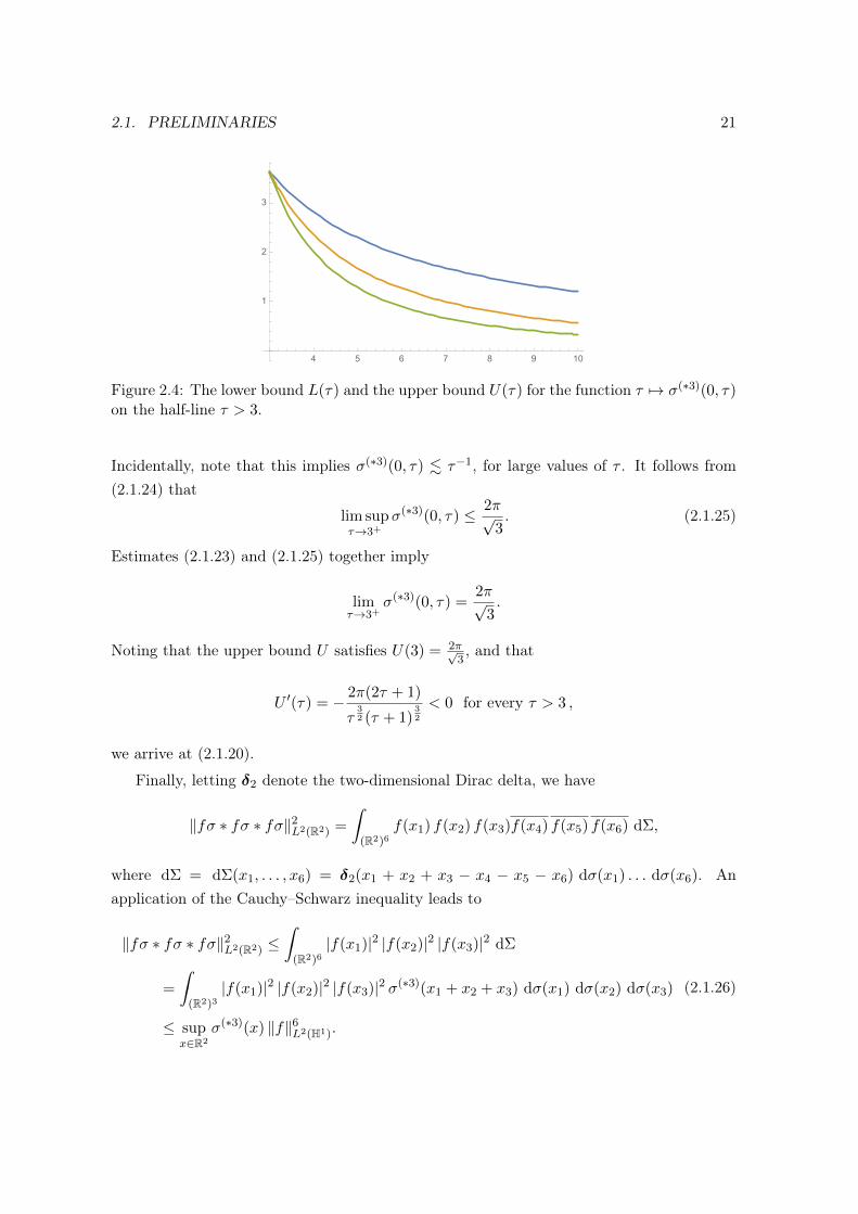
Figure 2.4: The lower bound L(τ) and the upper bound U(τ) for the function τ 7→ σ(∗3)(0, τ)on the half-line τ > 3.
Incidentally, note that this implies σ(∗3)(0, τ) . τ−1, for large values of τ . It follows from(2.1.24) that
lim supτ→3+
σ(∗3)(0, τ) ≤ 2π√3. (2.1.25)
Estimates (2.1.23) and (2.1.25) together imply
limτ→3+
σ(∗3)(0, τ) =2π√
3.
Noting that the upper bound U satisfies U(3) = 2π√3, and that
U ′(τ) = − 2π(2τ + 1)
τ32 (τ + 1)
32
< 0 for every τ > 3 ,
we arrive at (2.1.20).
Finally, letting δ2 denote the two-dimensional Dirac delta, we have
‖fσ ∗ fσ ∗ fσ‖2L2(R2) =
ˆ(R2)6
f(x1) f(x2) f(x3)f(x4) f(x5) f(x6) dΣ,
where dΣ = dΣ(x1, . . . , x6) = δ2(x1 + x2 + x3 − x4 − x5 − x6) dσ(x1) . . . dσ(x6). Anapplication of the Cauchy–Schwarz inequality leads to
‖fσ ∗ fσ ∗ fσ‖2L2(R2) ≤ˆ
(R2)6|f(x1)|2 |f(x2)|2 |f(x3)|2 dΣ
=
ˆ(R2)3
|f(x1)|2 |f(x2)|2 |f(x3)|2 σ(∗3)(x1 + x2 + x3) dσ(x1) dσ(x2) dσ(x3)
≤ supx∈R2
σ(∗3)(x) ‖f‖6L2(H1).
(2.1.26)

22 CHAPTER 2. SHARP RESTRICTION ON HYPERBOLOIDS
Estimate (2.1.21) now follows from (2.1.5), (2.1.19) and (2.1.26). This completes the proofof the lemma.
Two-dimensional counterparts of the results from this section were obtained in [68,Lemma 5.1]. We record them here.
Lemma 2.7 (cf. [68]). Let σ denote the Lorentz invariant measure on the hyperboloid H2.Then, for every (ξ, τ) ∈ R2 × R,
(a) (σ ∗ σ)(ξ, τ) = 2π√τ2−|ξ|2
1{τ≥√
22+|ξ|2}(ξ, τ),
(b) (σ ∗ σ ∗ σ)(ξ, τ) = (2π)2(
1− 3√τ2−|ξ|2
)1{τ≥
√32+|ξ|2}(ξ, τ).
2.2 Endpoint results
This section is dedicated to the proof of Theorem 2.1. The heart of the matter lies in theconstruction of an explicit extremizing sequence for inequality (2.1.3), which is the contentof the next result.
Proposition 2.8. Let σ denote the Lorentz invariant measure on the hyperbola H1. Givena > 0, let fa(y) = e−a〈y〉, y ∈ R. Then:
(a) For every n ∈ N we have
(faσ)(∗n)(ξ, τ) = e−aτσ(∗n)(ξ, τ).
(b) The function a 7→√a e2a‖fa‖2L2(H1) is bounded on the half-line a > 0, and satisfies
lima→∞
√a e2a‖fa‖2L2(H1) =
√π. (2.2.1)
(c) The sequence {fa}a∈N satisfies
lima→∞
‖faσ ∗ faσ ∗ faσ‖2L2(R2)
‖fa‖6L2(H1)
=2π√
3, (2.2.2)
and is extremizing for inequality (2.1.3) when (d, p) = (1, 6), as a→∞. In particular,
H1,6 = 3−112 (2π)
12 .
Proof. The proof of (a) is analogous to part of the proof of [68, Lemma B.1]. We present thedetails for the convenience of the reader. Letting ga(ξ, τ) = e−aτ , we have that (faσ)(∗n) =

2.2. ENDPOINT RESULTS 23
(gaσ)(∗n). Therefore,
(faσ)(∗n)(ξ, τ) = (gaσ)(∗n)(ξ, τ) = ga(ξ, τ)σ(∗n)(ξ, τ) = e−aτσ(∗n)(ξ, τ),
where the second identity follows from the fact that ga is the exponential of a linear function.
For part (b), change variables 〈y〉 = cosh t to compute
‖fa‖2L2(H1) =
ˆRe−2a〈y〉 dy
〈y〉= 2
ˆ ∞0
e−2a cosh t dt = 2K0(2a). (2.2.3)
Here, the modified Bessel function of the second kind Kν is given for <(z) > 0 by
Kν(z) =
ˆ ∞0
exp(−z cosh t) cosh(νt) dt.
Claim (2.2.1) boils down to the well-known fact
lima→∞
√a e2aK0(2a) =
√π
2, (2.2.4)
see e.g. [86, Section 7.34 (1)]. We finish the proof of part (b) by invoking the facts thatK0(x) . | log(x)| as x→ 0+ (see e.g. [1, formula (9.6.8) on p. 375]), and that K0 monoton-ically decreases on the positive half-axis, which follows directly from the definition of K0.Figure 2.5 illustrates these facts.
We next turn to part (c). Part (a) implies
‖faσ ∗ faσ ∗ faσ‖2L2(R2) =
ˆP1,3
e−2aτ (σ(∗3)(ξ, τ))2 dξ dτ,
where the support region P1,3 was defined in (2.1.14). We perform the change of variablesφ(ξ, τ) = (ξ,
√τ2 + ξ2), which has Jacobian determinant
J(φ)(ξ, τ) = det
1 ξ√τ2+ξ2
0 τ√τ2+ξ2
=τ√
τ2 + ξ2.
As a consequence,
‖faσ ∗ faσ ∗ faσ‖2L2(R2) =
ˆφ−1(P1,3)
e−2a√τ2+ξ2
(σ(∗3)
(ξ,√τ2 + ξ2
))2 τ√τ2 + ξ2
dξ dτ
=
ˆ ∞3
τ(σ(∗3)(0, τ)
)2(ˆR
e−2a√τ2+ξ2√
τ2 + ξ2dξ)
dτ, (2.2.5)
where in the last identity we used the Lorentz invariance (2.1.15) of the convolution σ(∗3),

24 CHAPTER 2. SHARP RESTRICTION ON HYPERBOLOIDS
together with the fact that φ−1(P1,3) = R× (3,∞). Define G(a) := ‖fa‖2L2(H1). Recognizingthe inner integral in (2.2.5) as the quantity G(aτ), we have that
‖faσ ∗ faσ ∗ faσ‖2L2(R2)
‖fa‖6L2(H1)
=
ˆ ∞3
τ(σ(∗3)(0, τ))2G(aτ)
G(a)3dτ. (2.2.6)
We will be interested in the regime where a→∞, for which the approximation
lima→∞
(G(aτ)
G(a)3
)/(a
π
e−2a(τ−3)
√τ
)= 1 (2.2.7)
follows from (2.2.3) and (2.2.4). On the other hand, we have noted in the course of the proofof Lemma 2.6 that
σ(∗3)(0, τ) .1
τ, for τ > 3.
From this and support considerations, it follows that the function τ 7→√τ(σ(∗3)(0, τ))2 is
bounded on the positive half-axis. It is also continuous there, except for a jump discontinuityat τ = 3. Given an even function ϕ : R→ [0,∞) satisfying
´R ϕ = 1, we have
lima→∞
ˆR
√|τ |(σ(∗3)(0, τ))2 aϕ(a(τ − 3)) dτ =
√3
(σ(∗3)(0, 3−))2 + (σ(∗3)(0, 3+))2
2
=√
302 + ( 2π√
3)2
2=
2π2
√3.
This follows from the fact that {aϕ(a ·)}a∈N constitutes an approximate identity sequence,as a→∞. Specializing to ϕ(t) = e−2|t|, and using (2.2.6) and (2.2.7), we check that (2.2.2)holds. From (2.1.5) and (2.1.21) it follows that the sequence {fa}a∈N is extremizing forinequality (2.1.3), and
H1,6 = 3−112 (2π)
12 .
This completes the proof of the proposition (and of part of Theorem 2.1).
To prove that extremizers do not exist, we invoke the useful observation from [68, Corol-lary 4.3], which we record here.
Lemma 2.9 (cf. [68]). Let (d, p) satisfy (1.1), and suppose that p = 2n is an even integer.Suppose that
Hd,p = (2π)d+1p ‖σ(∗n)‖
1p
L∞(Rd+1),
and that σ(∗n)(ξ, τ) < ‖σ(∗n)‖L∞(Rd+1) for a.e. (ξ, τ) in the support of σ(∗n). Then extrem-izers for inequality (2.1.3) do not exist for the pair (d, p).

2.3. NONENDPOINT RESULTS 25
0 1 2 3 4 5 6
0.2
0.4
0.6
0.8
1.0
0 1 2 3 4 5 6
0.2
0.4
0.6
0.8
1.0
Figure 2.5: The function x 7→ K0(x), and the function x 7→√xe2xK0(2x) together with its
horizontal asymptote y =√π
2 .
Armed with Lemma 2.6, Proposition 2.8 (c) and Lemma 2.9, it is now an easy matter tofinish the proof of Theorem 2.1.
2.3 Nonendpoint results
This section is dedicated to the proof of Theorem 2.2. First we prove the existence ofa special cap, and for that task different geometrical considerations will be used in eachdimension. Once the existence of a special cap is obtained, we proceed to run the necessaryconcentration-compactness machinery.
2.3.1 The quest for a special cap
In this section, we seek to locate a distinguished cap which carries a non-trivial amountof L2 mass. This is essential to start gaining some control on compactness properties ofextremizing sequences. In the one-dimensional situation, we establish a refinement of theFourier extension inequality. In the two-dimensional setting, we reduce matters to the studyof bilinear interactions in the lower endpoint case.
One-dimensional setting
This subsection in partially inspired by [67, Section 3] (see also [45, Section 4]). To studythe interaction between the distinct caps from the family {Ck}k∈Z, defined in (2.1.10), wemake use of the following standard result on fractional integration.
Lemma 2.10 (Hardy–Littlewood–Sobolev). Given r, s ∈ (1,∞) with 1r + 1
s > 1, let α =
2− 1r −
1s . For any f ∈ Lr(R) and g ∈ Ls(R),
ˆ ∞−∞
ˆ ∞−∞|f(x)||x− y|−α|g(y)| dx dy .r,s ‖f‖Lr(R)‖g‖Ls(R).

26 CHAPTER 2. SHARP RESTRICTION ON HYPERBOLOIDS
The following result shows that distant caps interact weakly.
Lemma 2.11. Let 2 < q <∞. For any k, ` ∈ Z, if supp(f) ⊂ Ck and supp(g) ⊂ C`, then
‖Tf · Tg‖Lq(R2) .q e− |k−`|
2q ‖f‖L
2q2q−3 (H1)
‖g‖L
2q2q−3 (H1)
.
Proof. Define the auxiliary function
h(ξ1, ξ2) := (f(ξ1)g(ξ2) + f(ξ2)g(ξ1))1{ξ1≥ξ2}(ξ1, ξ2),
for which(Tf · Tg)(x, t) =
ˆR2
eix(ξ1+ξ2)eit(〈ξ1〉+〈ξ2〉)h(ξ1, ξ2)dξ1
〈ξ1〉dξ2
〈ξ2〉.
Following an argument that goes back to early work of Carleson–Sjölin [11], we changevariables
(ξ1, ξ2) 7→ (u, v) = (ξ1 + ξ2, 〈ξ1〉+ 〈ξ2〉)
in the region of integration {(ξ1, ξ2) ∈ R2 : ξ1 ≥ ξ2}. Note that this is a bijective map ontothe region {(u, v) ∈ R× R+ : v2 − u2 ≥ 4}. It follows that
(Tf · Tg)(x, t) =
ˆR2
ei(x,t)·(u,v) h(ξ1, ξ2)
J(ξ1, ξ2)
du
〈ξ1〉dv
〈ξ2〉,
where J denotes the Jacobian of this transformation, given by
J(ξ1, ξ2) =
∣∣∣∣ ∂(u, v)
∂(ξ1, ξ2)
∣∣∣∣ =
∣∣∣∣ ξ1
〈ξ1〉− ξ2
〈ξ2〉
∣∣∣∣ .The Hausdorff–Young inequality on R2 implies that, for every q ≥ 2,
‖Tf · Tg‖Lq(R2) ≤
(ˆR2
∣∣∣∣h(ξ1, ξ2)
J(ξ1, ξ2)
1
〈ξ1〉〈ξ2〉
∣∣∣∣ qq−1
du dv
) q−1q
.
Changing back to the original variables (ξ1, ξ2), we obtain
‖Tf · Tg‖Lq(R2) ≤
(ˆR2
|h(ξ1, ξ2)|qq−1
(J(ξ1, ξ2)〈ξ1〉〈ξ2〉)1q−1
dξ1
〈ξ1〉dξ2
〈ξ2〉
) q−1q
.
In order to invoke Lemma 2.10, it is convenient to perform another change of variables(ξ1, ξ2) = (sinh(θ1), sinh(θ2)). Noting that
J(ξ1, ξ2)〈ξ1〉〈ξ2〉 = | sinh(θ1 − θ2)|,

2.3. NONENDPOINT RESULTS 27
Minkowski’s inequality yields
‖Tf · Tg‖Lq(R2) ≤
(ˆR2
|h(sinh(θ1), sinh(θ2))|qq−1
| sinh(θ1 − θ2)|1q−1
dθ1 dθ2
) q−1q
.
(ˆR2
|f(sinh(θ1))g(sinh(θ2))|qq−1
| sinh(θ1 − θ2)|1q−1
dθ1 dθ2
) q−1q
.
(2.3.1)
We now use the lower bound
| sinh(θ)| ≥ |θ|2
exp
(|θ|2
),
which is valid for any θ ∈ R, together with Lemma 2.10 with the choices α = 1q−1 and
r = s = 2q−22q−3 (which are admissible since 2 < q <∞). From (2.3.1) we get
‖Tf · Tg‖Lq(R2) .
ˆR2
|f(sinh(θ1))g(sinh(θ2))|qq−1
|θ1 − θ2|1q−1 e
|θ1−θ2|2(q−1)
dθ1 dθ2
q−1q
.q e− |k−`|
2q ‖f‖L
2q2q−3 (H1)
‖g‖L
2q2q−3 (H1)
,
where we have used that |(θ1 − θ2)− (k − `)| ≤ 1, since |θ1 − k| ≤ 12 and |θ2 − `| ≤ 1
2 . Thiscompletes the proof of the lemma.
Lemma 2.11 is the key ingredient in order to establish the following refinement of theinequality (2.1.3) in the case d = 1. In what follows, given f ∈ L2(H1), we shall decomposef =
∑k∈Z fk with fk := f1Ck .
Proposition 2.12. Let 3 ≤ q <∞. For any f ∈ L2(H1) we have
‖Tf‖L2q(R2) .q
(∑k∈Z‖fk‖3
L2q
2q−3 (H1)
) 13
. (2.3.2)
When 3 ≤ q ≤ ∞, note that 1 ≤ 2q2q−3 ≤ 2. In this case, the estimates
‖Tf‖L6(R2) . ‖f‖L2(H1), and ‖Tf‖L∞(R2) ≤ ‖f‖L1(H1)
can be interpolated to yield
‖Tf‖L2q(R2) .q ‖f‖L
2q2q−3 (H1)
. (2.3.3)

28 CHAPTER 2. SHARP RESTRICTION ON HYPERBOLOIDS
Proof of Proposition 2.12. Writing
(Tf)3 =∑
k,`,m∈ZTfk · Tf` · Tfm,
Minkowski’s triangle inequality plainly implies that
‖Tf‖3L2q(R2) =∥∥(Tf)3
∥∥L
2q3 (R2)
≤∑
k,`,m∈Z‖Tfk · Tf` · Tfm‖
L2q3 (R2)
. (2.3.4)
Given a triplet (k, `,m) ∈ Z3, we lose no generality in assuming that
|k − `| = max{|k − `|, |`−m|, |m− k|}.
Hölder’s inequality, Lemma 2.11 (recall that q <∞) and estimate (2.3.3), together with themaximality of |k − `|, imply
‖Tfk · Tf` · Tfm‖L
2q3 (R2)
≤ ‖Tfk · Tf`‖Lq(R2)‖Tfm‖L2q(R2)
.q e− |k−`|
2q ‖fk‖L
2q2q−3 (H1)
‖f`‖L
2q2q−3 (H1)
‖fm‖L
2q2q−3 (H1)
≤ e−|k−`|6q e
− |`−m|6q e
− |m−k|6q ‖fk‖
L2q
2q−3 (H1)‖f`‖
L2q
2q−3 (H1)‖fm‖
L2q
2q−3 (H1).
(2.3.5)
Putting together (2.3.4) and (2.3.5), we conclude that
‖Tf‖3L2q(R2) .q
∑k,`,m∈Z
e− |k−`|
6q e− |`−m|
6q e− |m−k|
6q ‖fk‖L
2q2q−3 (H1)
‖f`‖L
2q2q−3 (H1)
‖fm‖L
2q2q−3 (H1)
.
≤∑
k,`,m∈Ze− |k−`|
6q e− |`−m|
6q e− |m−k|
6q ‖fk‖3L
2q2q−3 (H1)
,
where the last line follows from the inequality between the arithmetic and the geometricmeans. Summing two geometric series, we finally have that
‖Tf‖3L2q(R2) .q
∑k∈Z‖fk‖3
L2q
2q−3 (H1),
as desired. This completes the proof of the proposition.
We have the following immediate but useful consequence.
Corollary 2.13. Let 6 ≤ p <∞. Then there exists Cp <∞ such that, for any f ∈ L2(H1),
‖Tf‖Lp(R2) ≤ Cp supk∈Z‖fk‖
13
L2(H1)‖f‖
23
L2(H1). (2.3.6)
2.3. NONENDPOINT RESULTS 29
Proof. Using estimate (2.3.2) with p = 2q we get
‖Tf‖Lp(R2) ≤ Cp supk∈Z‖fk‖
13
Lpp−3 (H1)
(∑k∈Z‖fk‖2
Lpp−3 (H1)
) 13
, (2.3.7)
for some constant Cp <∞. Applying Hölder’s inequality, and recalling that σ(Ck) = 1,
‖fk‖L
pp−3 (H1)
≤ ‖1Ck‖L
2pp−6 (H1)
‖fk‖L2(H1) = ‖fk‖L2(H1).
Plugging this into the right-hand side of (2.3.7), and appealing to the disjointness of thesupports of the {fk}, yields the desired conclusion.
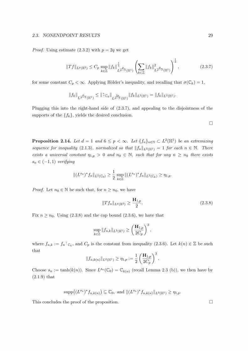
Proposition 2.14. Let d = 1 and 6 ≤ p < ∞. Let {fn}n∈N ⊂ L2(H1) be an extremizingsequence for inequality (2.1.3), normalized so that ‖fn‖L2(H1) = 1 for each n ∈ N. Thereexists a universal constant η1,p > 0 and n0 ∈ N, such that for any n ≥ n0 there existssn ∈ (−1, 1) verifying
‖(Lsn)∗fn‖L2(C0) ≥1
2supk∈Z‖(Lsn)∗fn‖L2(Ck) ≥ η1,p.
Proof. Let n0 ∈ N be such that, for n ≥ n0, we have
‖Tfn‖Lp(R2) ≥H1,p
2. (2.3.8)
Fix n ≥ n0. Using (2.3.8) and the cap bound (2.3.6), we have that
supk∈Z‖fn,k‖L2(H1) ≥
(H1,p
2Cp
)3
,
where fn,k := fn1Ck , and Cp is the constant from inequality (2.3.6). Let k(n) ∈ Z be suchthat
‖fn,k(n)‖L2(H1) ≥ η1,p :=1
2
(H1,p
2Cp
)3
.
Choose sn := tanh(k(n)). Since Lsn(C0) = Ck(n) (recall Lemma 2.3 (b)), we then have by(2.1.9) that
supp((Lsn)∗fn,k(n)
)⊆ C0, and ‖(Lsn)∗fn,k(n)‖L2(H1) ≥ η1,p.
This concludes the proof of the proposition.

30 CHAPTER 2. SHARP RESTRICTION ON HYPERBOLOIDS
Two-dimensional setting
In order to study the interaction between the distinct caps from the family {Cn,j} definedin (2.1.11) and (2.1.12), we try to relate the nonendpoint problem to the lower endpointproblem. Log-convexity of Lebesgue norms readily implies the following: given p ∈ (4, 6),there exists θ ∈ (0, 1) such that
‖Tf‖Lp(R3) ≤ ‖Tf‖θL4(R3)‖Tf‖1−θL6(R3)
. (2.3.9)
In particular, if {fn}n∈N is an extremizing sequence for inequality (2.1.3) when d = 2 andp ∈ (4, 6), normalized so that ‖fn‖L2(H2) = 1 for each n ∈ N, then both quantities on theright-hand side of inequality (2.3.9) cannot be too small, in the sense that there exists auniversal constant γp > 0, depending on p but not on n, and n0 ∈ N such that
min{‖Tfn‖L4(R3), ‖Tfn‖L6(R3)} ≥ γp, for any n ≥ n0.
The idea will be to exploit the convolution structure of the lower endpoint problem(d, p) = (2, 4) to derive some nontrivial information about the nonendpoint case. The cruxof the matter lies in the following result.
Proposition 2.15. Let f ∈ L2(H2), normalized so that ‖f‖L2(H2) = 1. Let ε > 0 andassume that
supn,j‖f‖L2(Cn,j) ≤ ε,
where the supremum is taken over all n ∈ N ∪ {0} and 0 ≤ j < 2n. Then
‖Tf‖4L4(R3) . ε log2(ε−1). (2.3.10)
Remark: The relevant feature of the function Φ(ε) = ε log2(ε−1) is that Φ(ε)→ 0, as ε→ 0+.Any other Φ with the same property would serve our purpose equally well.
Proof. Recalling Tf is a Fourier transform, the usual application of Plancherel’s theoremand the Cauchy–Schwarz inequality (the latter as in (2.1.26)) yields
‖Tf‖4L4(R3) ' ‖fσ ∗ fσ‖2L2(R3) ≤
ˆR2×R2
|f(ξ)|2|f(η)|2(σ ∗ σ)(ξ + η, 〈ξ〉+ 〈η〉) dξ
〈ξ〉dη
〈η〉.
Abusing notation slightly, and still denoting by {Cn,j} the projection of the caps defined in(2.1.11) and (2.1.12) onto the ξ-plane, we have that
‖Tf‖4L4(R3) .∑
(m,`),(n,j)
ˆCm,`
ˆCn,j|f(ξ)|2|f(η)|2(σ ∗ σ)(ξ + η, 〈ξ〉+ 〈η〉) dξ
〈ξ〉dη
〈η〉. (2.3.11)

2.3. NONENDPOINT RESULTS 31
Here, the sum is taken over all pairs (m, `), (n, j) with 0 ≤ n ≤ m, and 0 ≤ ` < 2m,0 ≤ j < 2n. We seek to obtain some control over the height s, defined via the equation
s2 := (〈ξ〉+ 〈η〉)2 − |ξ + η|2 = 2(1 + 〈ξ〉〈η〉 − ξ · η). (2.3.12)
With this purpose in mind, we split the sum in (2.3.11) into two pieces, depending on whetheror not the direction of the caps is approximately the same. In the former case, the boundwill be in terms of the distance between the centers of the caps, whereas in the latter caseone obtains an improved bound in terms of the angular separation between the caps. SeeFigure 2.6 for an illustration of two extreme cases of this separation.
Let S ⊂ R. In what follows, we say that x ∈ Smod 1 if x + k ∈ S for some k ∈ Z.Analogously, for m ∈ N∪{0}, we say that x ∈ Smod 2m if x+ k2m ∈ S for some k ∈ Z. Wealso define
‖x‖ := min{|x− k| : k ∈ Z} (2.3.13)
for the distance of x to the nearest integer.
Case 1. `2m −
j2n ∈
[− 2
2n ,2
2n
)mod 1. In this case, we are considering indices ` belonging to
A(j)m,n :=
{0 ≤ ` < 2m : ` ∈
[2m−n(j − 2), 2m−n(j + 2)
)mod 2m
},
a set of cardinality∣∣A(j)
m,n
∣∣ = 2m−n+2. We seek to estimate the sum
S1 :=∑n≥0
∑m≥n
∑0≤j<2n
∑`∈A(j)
m,n
ˆCm,`
ˆCn,j|f(ξ)|2|f(η)|2(σ ∗ σ)(ξ + η, 〈ξ〉+ 〈η〉) dξ
〈ξ〉dη
〈η〉.
Note that x 7→ 〈x〉|x|−1 is a decreasing function of |x|. For ξ ∈ Cn,j and η ∈ Cm,`, we canestimate the height s defined in (2.3.12) from below, as follows:
s2 & 〈ξ〉〈η〉 − ξ · η ≥ |ξ||η|(〈ξ〉〈η〉|ξ||η|
− 1
)≥ 1
42n+1 2m+1
(〈2n+1〉〈2m+1〉
2n+12m+1− 1
).
Writing 2n+1 = sinh(sinh−1(2n+1)) and 〈2n+1〉 = cosh(sinh−1(2n+1)), and similarly for m,we have that
s2 & cosh(
sinh−1(2m+1)− sinh−1(2n+1)).
Since sinh−1(x) = log(x+√x2 + 1) and cosh(x) & exp(x), we can further estimate
s2 & cosh(log(2m+1 +√
22m+2 + 1)− log(2n+1 +√
22n+2 + 1))
& exp(log(2m+1 +√
22m+2 + 1)− log(2n+1 +√
22n+2 + 1))

32 CHAPTER 2. SHARP RESTRICTION ON HYPERBOLOIDS
=2m+1 +
√22m+2 + 1
2n+1 +√
22n+2 + 1& 2m−n.
Under the same assumptions on ξ, η, it follows from the Lorentz invariance (2.1.15) andLemma 2.7 (a) that
(σ ∗ σ)(ξ + η, 〈ξ〉+ 〈η〉) = (σ ∗ σ)(0, s) . s−1 . 2−m−n
2 .
The sum S1 can then be estimated by
S1 .∑n≥0
∑m≥n
∑0≤j<2n
‖f‖2L2(Cn,j)
2m−n
2
( ∑`∈A(j)
m,n
‖f‖2L2(Cm,`)
),
where the inner sum is trivially bounded by∑`∈A(j)
m,n
‖f‖2L2(Cm,`) ≤ min{
1, ε2 2m−n+2}.
It follows that
S1 .∑n≥0
‖f‖2L2(An)
∑m≥n
min{1, ε2 2m−n+2}2m−n
2
, (2.3.14)
where An denotes the annulus defined in (2.1.13). We estimate the inner sum on the right-hand side of (2.3.14) by breaking it up in two pieces, according to whether or not the integerκ := m− n+ 2 satisfies ε22κ < 1, or equivalently κ < 2 log2(ε−1). We obtain
∑m≥n
min{1, ε2 2m−n+2}2m−n
2
=∑
κ<2 log2(ε−1)
ε2 2κ2
+1 +∑
κ≥2 log2(ε−1)
2−κ2
+1 . ε,
where both geometric sums were estimated by their largest terms. Plugging this back into(2.3.14), and recalling that ‖f‖L2(H2) = 1 and that the annuli in the family {An}n∈N aredisjoint, we finally obtain S1 . ε.
Case 2. `2m −
j2n ∈
[−1
2 ,12
)\[− 2
2n ,2
2n
)mod 1. Note that this case is non-empty only if
n ≥ 3. Let ξ ∈ Cn,j and η ∈ Cm,`. Setting θn,j := arg(ξ) and θm,` := arg(η), we note that,since n ≤ m, ∣∣∣∣θn,j − θm,`2π
−( j
2n− `
2m
)∣∣∣∣ < 1
2n. (2.3.15)
Before we move on, let us make a useful observation. Let
Γk =
{ξ ∈ R2 :
kπ
2≤ arg(ξ) <
(k + 1)π
2
}, for 0 ≤ k ≤ 3,

2.3. NONENDPOINT RESULTS 33
be the four quadrants of the ξ-plane. We may split the function f into four pieces writingf =
∑3k=0 f
(k), where f (k) = f1Γk . Since ‖Tf‖4L4(R3) .∑3
k=0 ‖Tf (k)‖4L4(R3) it suffices toprove (2.3.10) for each function f (k) separately. In particular, throughout the rest of thisproof we may assume that our f is supported in one of the quadrants, say Γ0. Note that thisyields |θn,j − θm,`| ≤ π
2 in the support of f and hence
1− cos(θn,j − θm,`) & |θn,j − θm,`|2.
As a consequence,
s2 & 〈ξ〉〈η〉 − ξ · η ≥ |ξ||η|(1− cos(θn,j − θm,`)) & 2m+n|θn,j − θm,`|2
in the support of f . Invoking Lemma 2.7 (a) as before, we have that
(σ ∗ σ)(ξ + η, 〈ξ〉+ 〈η〉) . 2−m+n
2 |θn,j − θm,`|−1. (2.3.16)
We seek to estimate the sum
S2 :=∑n≥0
∑m≥n
∑0≤j<2n
∑`/∈A(j)
m,n
ˆCm,`
ˆCn,j|f(ξ)|2|f(η)|2(σ ∗σ)(ξ+η, 〈ξ〉+ 〈η〉) dξ
〈ξ〉dη
〈η〉. (2.3.17)
For fixed indices 0 ≤ n ≤ m and 0 ≤ j < 2n, we consider the block
B(j,k)m,n :=
{0 ≤ ` < 2m : ` ∈
[2m−n(j + k), 2m−n(j + k + 1)
)mod 2m
}, (2.3.18)
for −2 ≤ k ≤ 2n − 3. Note that∣∣B(j,k)
m,n
∣∣ = 2m−n. Moreover, since A(j)m,n can be partitioned
as a disjoint union,A(j)m,n = B(j,−2)
m,n ∪B(j,−1)m,n ∪B(j,0)
m,n ∪B(j,1)m,n ,
the fact that ` /∈ A(j)m,n is equivalent to ` ∈ B(j,k)
m,n , for some 2 ≤ k ≤ 2n−3. If ` ∈ B(j,k)m,n \A(j)
m,n,then condition (2.3.18) can be rewritten as
`
2m− j
2n∈[k
2n,k + 1
2n
)mod 1 ,
and it follows from (2.3.15) that
|θn,j − θm,`| &∥∥∥∥ k2n
∥∥∥∥ , (2.3.19)

34 CHAPTER 2. SHARP RESTRICTION ON HYPERBOLOIDS
where ‖x‖ was defined in (2.3.13). Associated to these index blocks, we define the set
B(j,k)m,n :=
⋃`∈B(j,k)
m,n
Cm,`.
From (2.3.16), (2.3.17) and (2.3.19) we get
S2 .∑n≥0
∑m≥n
∑0≤j<2n
2n−3∑k=2
∑`∈B(j,k)
m,n
‖f‖2L2(Cm,`)‖f‖2L2(Cn,j)2
−m+n2 |θn,j − θm,`|−1
.∑n≥0
∑m≥n
∑0≤j<2n
2n−3∑k=2
‖f‖2L2(B(j,k)m,n
)‖f‖2L2(Cn,j)2−m+n
2
∥∥∥∥ k2n∥∥∥∥−1
≤∑n≥0
∑m≥n
∑0≤j<2n
2n−1−1∑k=2
(‖f‖2
L2(B(j,k)m,n
) + ‖f‖2L2(B(j,2
n−k−1)m,n
)) ‖f‖2L2(Cn,j)2−m+n
2
(k
2n
)−1
.
In order to make use of the trivial bound
‖f‖2L2(B(j,k)m,n
) ≤ min{1, ε22m−n}, (2.3.20)
we invoke the Cauchy–Schwarz inequality on the innermost sum of
S2 .∑n≥0
∑m≥n
2−m−n
2
∑0≤j<2n
‖f‖2L2(Cn,j)
2n−1−1∑k=2
‖f‖2L2(B(j,k)m,n
) + ‖f‖2L2(B(j,2
n−k−1)m,n
)k
.∑n≥0
∑m≥n
2−m−n
2
∑0≤j<2n
‖f‖2L2(Cn,j)
(2n−3∑k=2
‖f‖4L2(B(j,k)m,n
)) 12(
2n−1−1∑k=2
1
k2
) 12
.
Recalling (2.3.20), and noting that the unions
2n−1⋃j=0
Cn,j = An, and2n−3⋃k=2
B(j,k)m,n ⊆ Am
are disjoint, we have that
S2 .∑n≥0
∑m≥n
2−m−n
2 min{1, ε 2m−n
2 }‖f‖L2(Am)‖f‖2L2(An).

2.3. NONENDPOINT RESULTS 35
Figure 2.6: For a fixed j, the regions of Case 1 (on the left) and Case 2 (on the right) of theproof of Proposition 2.15.
We use ‖f‖L2(Am) ≤ 1 and estimate the inner sum on the right-hand side of
S2 .∑n≥0
‖f‖2L2(An)
(∑m≥n
2−m−n
2 min{1, ε 2m−n
2 }
)(2.3.21)
as before. In more detail, set κ := m− n and break up the sum in two pieces, depending onwhether or not the condition ε 2
κ2 < 1 is satisfied. This yields:∑
m≥n2−
m−n2 min
{1, ε 2
m−n2}≤
∑κ<2 log2(ε−1)
2−κ2 ε 2
κ2 +
∑κ≥2 log2(ε−1)
2−κ2 . ε log2(ε−1).
Plugging this back into (2.3.21), we finally obtain that S2 . ε log2(ε−1). This completes theproof.
Proposition 2.16. Let d = 2 and 4 ≤ p < 6. Let {fn}n∈N ⊂ L2(H2) be an extremizingsequence for inequality (2.1.3), normalized so that ‖fn‖L2(H2) = 1 for each n ∈ N. Thereexists a universal constant η2,p > 0 and n0 ∈ N, such that for any n ≥ n0 there existsn ∈ (−1, 1) and ϕn ∈ [0, 2π) verifying
‖(Lsn ◦Rϕn)∗fn‖L2(D) ≥ η2,p ,
where D := {(ξ, τ) ∈ H2 : |ξ| ≤ 2√
2π}.
Proof. Let n0 ∈ N be such that, for n ≥ n0, we have
‖Tfn‖Lp(R3) ≥H2,p
2.

36 CHAPTER 2. SHARP RESTRICTION ON HYPERBOLOIDS
Fix n ≥ n0. We claim that there exists γp > 0, depending only on p, such that
supm,`‖fn‖L2(Cm,`) ≥ γp > 0, (2.3.22)
where the supremum is taken over integers m ≥ 0 and 0 ≤ ` < 2m. For otherwise we couldappeal to Proposition 2.15 to ensure
H2,p
2≤ ‖Tfn‖Lp(R3) ≤ ‖Tfn‖θL4(R3)‖Tfn‖
1−θL6(R3)
. (ε log2(ε−1))θ4 ,
which is a contradiction provided θ > 0 and ε > 0 is sufficiently small. Knowing (2.3.22), it isnow a simple matter to invoke Lemma 2.4 (b) and conclude the proof of the proposition.
2.3.2 Concentration compactness
We rely on the following key result from [30, Proposition 1.1].
Lemma 2.17 (cf. [30]). Let H be a Hilbert space and S : H → Lp(Rd) be a bounded linearoperator with p ∈ (2,∞). Consider {hn}n∈N ⊂ H such that
(i) limn→∞ ‖hn‖H = 1;
(ii) limn→∞ ‖S(hn)‖Lp(Rd) = ‖S‖H→Lp(Rd);
(iii) hn ⇀ h 6= 0;
(iv) S(hn)→ S(h) almost everywhere in Rd.
Then hn → h in H. In particular, ‖h‖H = 1 and ‖S(h)‖Lp(Rd) = ‖S‖H→Lp(Rd).
The argument which we will present next works as long as one can produce a specialcap, as was done in Section 2.3 in the lower dimensional cases d ∈ {1, 2}. We state thenext two results in general dimensions d, thereby guaranteeing the existence of extremizers,conditionally on the existence of a special cap.
Proposition 2.18. Let d ≥ 1 and let p be such that6 < p <∞, if d = 1;
2(d+2)d < p ≤ 2(d+1)
d−1 , if d ≥ 2.
Assume the existence of two universal constants η = ηd,p > 0 and r = rd,p > 0 verifying thefollowing property: for any extremizing sequence {fn}n∈N ⊂ L2(Hd) for inequality (2.1.3),
2.3. NONENDPOINT RESULTS 37
normalized so that ‖fn‖L2(Hd) = 1 for each n ∈ N, there exists n0 ∈ N such that
‖fn‖L2(D) ≥ η
for any n ≥ n0, where D := {(ξ, τ) ∈ Hd : |ξ| ≤ r}. Then there exists (xn, tn) ∈ Rd×R suchthat the sequence {gn}n∈N defined by
gn(y) := eixn·yeitn〈y〉fn(y)
admits a subsequence that converges weakly to a nonzero limit in L2(Hd).
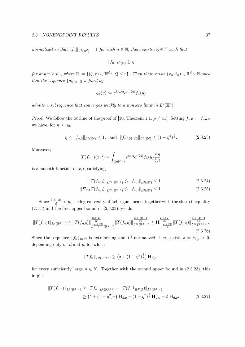
Proof. We follow the outline of the proof of [30, Theorem 1.1, p 6=∞]. Setting fn,0 := fn1D
we have, for n ≥ n0,
η ≤ ‖fn,0‖L2(Hd) ≤ 1, and ‖fn1Hd\D‖L2(Hd) ≤ (1− η2)12 . (2.3.23)
Moreover,
T (fn,0)(x, t) =
ˆ{|y|≤r}
eix·yeit〈y〉fn(y)dy
〈y〉
is a smooth function of x, t, satisfying
‖T (fn,0)‖L∞(Rd+1) . ‖fn,0‖L2(Hd) ≤ 1, (2.3.24)
‖∇x,tT (fn,0)‖L∞(Rd+1) . ‖fn,0‖L2(Hd) ≤ 1. (2.3.25)
Since 2(d+2)d < p, the log-convexity of Lebesgue norms, together with the sharp inequality
(2.1.3) and the first upper bound in (2.3.23), yields
‖T (fn,0)‖Lp(Rd+1) ≤ ‖T (fn,0)‖2(d+2)dp
L2(d+2)d (Rd+1)
‖T (fn,0)‖d(p−2)−4
dp
L∞(Rd+1)≤ H
2(d+2)dp
d,2(d+2)d
‖T (fn,0)‖d(p−2)−4
dp
L∞(Rd+1).
(2.3.26)Since the sequence {fn}n∈N is extremizing and L2-normalized, there exists δ = δd,p > 0,depending only on d and p, for which
‖Tfn‖Lp(Rd+1) ≥(δ + (1− η2)
12)Hd,p ,
for every sufficiently large n ∈ N. Together with the second upper bound in (2.3.23), thisimplies
‖T (fn,0)‖Lp(Rd+1) ≥ ‖Tfn‖Lp(Rd+1) − ‖T (fn1Hd\D)‖Lp(Rd+1)
≥(δ + (1− η2)
12)Hd,p − (1− η2)
12 Hd,p = δHd,p. (2.3.27)

38 CHAPTER 2. SHARP RESTRICTION ON HYPERBOLOIDS
From (2.3.26) and (2.3.27) we get
‖T (fn,0)‖L∞(Rd+1) ≥ γ := δdp
d(p−2)−4 Hdp
d(p−2)−4
d,p H− 2(d+2)d(p−2)−4
d,2(d+2)d
.
This readily implies the existence of (xn, tn) ∈ Rd × R, for which
|T (fn,0)(xn, tn)| ≥ γ
2. (2.3.28)
Settinggn(y) := eixn·yeitn〈y〉fn,0(y), (2.3.29)
we have that ‖gn‖L2(Hd) = ‖fn,0‖L2(Hd). Moreover, T (gn) amounts to a space-time transla-tion of the function T (fn,0). From (2.3.24), (2.3.25) and (2.3.28), it then follows that
‖T (gn)‖L∞(Rd+1) . 1, ‖∇x,tT (gn)‖L∞(Rd+1) . 1, and |T (gn)(0, 0)| ≥ γ
2. (2.3.30)
The implicit constants in the first and second estimates in (2.3.30) are independent of n,and so the sequence {T (gn)}n∈N is uniformly bounded and equicontinuous on the unit cube[−1
2 ,12 ]d+1. The Arzelà–Ascoli theorem on Rd+1 then implies that the sequence {T (gn)}n∈N
has a subsequence which converges uniformly to a limit. That this limit is nonzero followsat once from the third estimate in (2.3.30).
Now, since the sequence {gn}n∈N is bounded on L2(Hd), it has a weakly convergentsubsequence. In other words, we may thus assume, possibly after extraction, that thereexists a function g ∈ L2(Hd), such that gn ⇀ g weakly in L2(Hd), as n → ∞. Since theoperator T is bounded from L2(Hd) to Lp(Rd+1), it follows that T (gn) ⇀ T (g) weakly inLp(Rd+1), as n → ∞. From the previous paragraph we conclude that T (g) is nonzero, andso the function g is itself nonzero.
This implies that the sequence {gn}n∈N defined by
gn(y) := eixn·yeitn〈y〉fn(y),
where the parameters (xn, tn) are those from (2.3.29), has a subsequence which convergesweakly to a nonzero limit. Indeed, if g ∈ L2(Hd) is such that gn ⇀ g weakly in L2(Hd), asn→∞, then gn1D ⇀ g1D weakly in L2(Hd), as n→∞. Therefore, in order to prove that gis nonzero, it suffices to show that it has nonzero mass inside D. This follows from the factthat g is nonzero, which we checked in the last paragraph. The proof of the proposition isnow complete.

2.3. NONENDPOINT RESULTS 39
Proposition 2.19. Let d ∈ N, and let p be such that6 < p <∞, if d = 1;
2(d+2)d < p ≤ 2(d+1)
d−1 , if d ≥ 2.
Let {fn}n∈N ⊂ L2(Hd) be an extremizing sequence for inequality (2.1.3), normalized so that‖fn‖L2(Hd) = 1 for each n ∈ N, which converges weakly to a nonzero limit f ∈ L2(Hd). Then,possibly after passing to a subsequence,
Tfn(x, t)→ Tf(x, t), as n→∞,
for almost every (x, t) ∈ Rd × R.
Proof. We follow the outline of the proof of [31, Theorem 1.1]. For each n ∈ N, define theauxiliary functions
gn(y) :=fn(y)
〈y〉, and also g(y) :=
f(y)
〈y〉.
As it has been pointed out in (2.1.7), the extension operator on the hyperboloid and theKlein–Gordon propagator are related by
Tfn(x, t) = (2π)d eit√
1−∆gn(x),
and it suffices to show that, pointwise for almost every (x, t) ∈ Rd × R,
eit√
1−∆gn(x)→ eit√
1−∆g(x), as n→∞,
possibly after extraction of a subsequence. For t ∈ R and R > 0, we define
Fn(t, R) :=
ˆ{|x|≤R}
∣∣eit√1−∆(gn − g)(x)∣∣2 dx,
and we claim thatlimn→∞
Fn(t, R) = 0 (2.3.31)
In order to prove this claim, first recall that {gn}n∈N is bounded on the Sobolev spaceW 2, 1
2 (Rd), with‖gn‖
W 2, 12 (Rd)= ‖fn‖L2(Hd) = 1. (2.3.32)
Let BR ⊂ Rd denote the ball centered at the origin of radius R. The hypothesis fn ⇀ f
weakly in L2(Hd) can be equivalently restated as gn ⇀ g weakly in W 2, 12 (Rd). Since, for
fixed t ∈ R, the operator eit√
1−∆ is unitary on W 2, 12 (Rd), it follows that eit
√1−∆gn ⇀

40 CHAPTER 2. SHARP RESTRICTION ON HYPERBOLOIDS
eit√
1−∆g weakly in W 2, 12 (Rd), which in turn implies that eit
√1−∆gn ⇀ eit
√1−∆g weakly in
W 2, 12 (BR). As a consequence of (2.3.32) and of Rellich’s theorem, see e.g. [28, Theorem 7.1
and Proposition 3.4], we find
eit√
1−∆gn → eit√
1−∆g strongly in L2(BR), as n→∞.
In other words, (2.3.31) holds as claimed. We further note, since the operator eit√
1−∆ isunitary on L2(Rd), that
Fn(t, R) ≤∥∥eit√1−∆(gn − g)
∥∥2
L2(Rd)= ‖gn − g‖2L2(Rd) . ‖gn − g‖2
W 2, 12 (Rd). 1.
This justifies the applicability of Lebesgue’s dominated convergence theorem which, to-gether with (2.3.31), implies
limn→∞
ˆ R
−RFn(t, R) dt = lim
n→∞
ˆ R
−R
ˆ{|x|≤R}
∣∣eit√1−∆(gn − g)(x)∣∣2 dx dt = 0.
As a consequence, up to a subsequence,
eit√
1−∆(gn − g)(x)→ 0, as n→∞, for a.e. (x, t) ∈ BR × (−R,R).
The extraction of the subsequence depends on the radius R. To remedy this, repeat theargument on a discrete sequence of radii {Rj}j∈N satisfying Rj →∞, as j →∞, to conclude,via a standard diagonal argument, that there exists a subsequence {gnk}k∈N ⊂ {gn}n∈N suchthat
eit√
1−∆(gnk − g)(x)→ 0, as k →∞, for a.e. (x, t) ∈ Rd × R.
This concludes the proof of the proposition.
It is now an easy matter to finish the proof of Theorem 2.2.
Proof of Theorem 2.2. Let us start by considering the case d = 1 and p ∈ (6,∞). Thestrategy is to invoke Lemma 2.17 with S = T and H = L2(H1). With that purpose in mind,let {fn}n∈N be an extremizing sequence for the inequality
‖Tf‖Lp(R2) ≤ H1,p‖f‖L2(H1), (2.3.33)
normalized so that ‖fn‖L2(H1) = 1 for each n ∈ N. In particular, conditions (i) and (ii)from Lemma 2.17 are automatically met. We will be done once we check that conditions(iii) and (iv) hold as well. By Proposition 2.14, the sequence {(Lsn)∗fn}n∈N, which is still

2.3. NONENDPOINT RESULTS 41
extremizing for (2.3.33), verifies
‖(Lsn)∗fn‖L2(C0) ≥ η1,p > 0,
for every n ∈ N. By Proposition 2.18, the sequence {gn}n∈N defined by
gn(y) = eixnyeitn〈y〉((Lsn)∗fn)(y),
which is still extremizing for (2.3.33), is such that
gn ⇀ g 6= 0 weakly in L2(H1), as n→∞,
possibly after passing to a subsequence. By Proposition 2.19, we then know that
T (gn)→ T (g) pointwise a.e. on R2, as n→∞,
again possibly after passing to a subsequence. By Lemma 2.17, we finally conclude thatgn → g in L2(H1), as n → ∞. In other words, g is an extremizer for inequality (2.3.33).This concludes the proof of the one-dimensional case. The two-dimensional case d = 2 andp ∈ (4, 6) can be handled in an analogous way. One just invokes Proposition 2.16 instead ofProposition 2.14, the rest of the argument being identical. This concludes the proof.

Chapter 3
Sharp mixed norm restriction onspheres
This chapter is dedicated to the contents of [P2], which deals with LqradL2ang spherical
restriction estimates proved by L. Vega [84, 85]. Sharp versions of these inequalities werefirst considered considered in [34], when q = 6 on S1. We divide this chapter in five sections.The first section is meant as an introduction. The other sections are each dedicated to theproof of one Theorem.
3.1 Preliminaries
In this chapter we seek to determine the sharp constant of the following inequality 1
∥∥fσ∥∥LqradL
2ang(Rd)
:=
(ˆ ∞0
(ˆSd−1
∣∣fσ(rω)∣∣2 dσω
)q/2rd−1 dr
)1/q
≤ Cd,q ‖f‖L2(Sd−1,σ),
(3.1.1)
and characterize its (complex-valued) extremizers, i.e. we wish to calculate the value
Cd,q := supf 6=0
∥∥fσ∥∥LqradL
2ang(Rd)
‖f‖L2(Sd−1)
,
and describe the functions 0 6= f ∈ L2(Sd−1) that verify
∥∥fσ∥∥LqradL
2ang(Rd)
= Cd,q ‖f‖L2(Sd−1).
1We do a harmless change of notation from Sd to Sd−1 as was featured in the Introduction to not divergefrom the one used in [84, 85].
43

44 CHAPTER 3. SHARP MIXED NORM RESTRICTION ON SPHERES
Throughout this chapter, we let Hdk denote the space of spherical harmonics of degree k inthe sphere Sd−1, and let Jν denote the classical Bessel function of the first kind, which forν ∈ 1
2Z is given by
Jν(x) :=1
π
ˆ π
0cos(ντ − x sin τ) dτ.
We shall always be dealing with ν ≥ 0. For d ≥ 2 and 2d/(d − 1) < q < ∞ we define, foreach k ∈ {0, 1, 2, . . .}, the Bessel integral
Λd,q(k) :=
(ˆ ∞0
∣∣r− d2+1 J d2−1+k(r)
∣∣q rd−1 dr
)1/q
. (3.1.2)
For q =∞ we defineΛd,∞(k) = sup
r≥0
∣∣r− d2+1 J d2−1+k(r)
∣∣.Theorem 3.1. Let d ≥ 2 and 2d/(d− 1) < q ≤ ∞. The following propositions hold.
(i) The sequence {Λd,q(k)}k≥0 verifies limk→∞ Λd,q(k) = 0 and we have
Cd,q = (2π)d/2 maxk≥0
Λd,q(k).
Moreover, f is an extremizer of (3.1.1) if and only if f ∈ Hd` , where ` is such that
Λd,q(`) = maxk≥0
Λd,q(k).
(ii) If q is an even integer or q =∞, then
Cd,q = (2π)d/2Λd,q(0),
and the constant functions are the unique extremizers of (3.1.1).
(iii) For a fixed dimension d, the set Ad = {q ∈ (2d/(d−1),∞] : Λd,q(0) > Λd,q(k) for all k ≥1}, for which the constant functions are the unique extremizers of (3.1.1), is an openset in the extended topology2. From (ii), Ad contains the even integers and the pointat infinity and, in particular, we may define
q0(d) := inf{r : 2d/(d− 1) < r <∞ and (r,∞] ⊂ Ad}. (3.1.3)
2That is, the topology generated by the open sets of the form (a, b) and (a,∞].
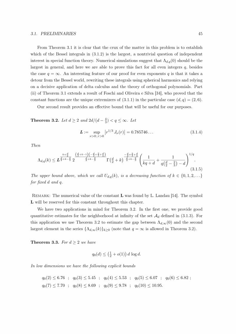
3.1. PRELIMINARIES 45
From Theorem 3.1 it is clear that the crux of the matter in this problem is to establishwhich of the Bessel integrals in (3.1.2) is the largest, a nontrivial question of independentinterest in special function theory. Numerical simulations suggest that Λd,q(0) should be thelargest in general, and here we are able to prove this fact for all even integers q, besidesthe case q = ∞. An interesting feature of our proof for even exponents q is that it takes adetour from the Bessel world, rewriting these integrals using spherical harmonics and relyingon a decisive application of delta calculus and the theory of orthogonal polynomials. Part(ii) of Theorem 3.1 extends a result of Foschi and Oliveira e Silva [34], who proved that theconstant functions are the unique extremizers of (3.1.1) in the particular case (d, q) = (2, 6).
Our second result provides an effective bound that will be useful for our purposes.
Theorem 3.2. Let d ≥ 2 and 2d/(d− 43) < q ≤ ∞. Let
L := supν>0 ; r>0
∣∣r1/3 Jν(r)∣∣ = 0.785746 . . . (3.1.4)
Then
Λd,q(k) ≤ Lk+ dqd2+k− 2
3 2
( d2+k−1)(− d2+23+ dq )
d2+k− 2
3 Γ(d2 + k
)− d2+23+ dq
d2+k− 2
3
(1
kq + d+
1
q(d2 −
23
)− d
)1/q
.
(3.1.5)The upper bound above, which we call Ud,q(k), is a decreasing function of k ∈ {0, 1, 2, . . .}for fixed d and q.
Remark: The numerical value of the constant L was found by L. Landau [54]. The symbolL will be reserved for this constant throughout this chapter.
We have two applications in mind for Theorem 3.2. In the first one, we provide goodquantitative estimates for the neighborhood at infinity of the set Ad defined in (3.1.3). Forthis application we use Theorem 3.2 to estimate the gap between Λd,∞(0) and the secondlargest element in the series {Λd,∞(k)}k≥0 (note that q =∞ is allowed in Theorem 3.2).
Theorem 3.3. For d ≥ 2 we have
q0(d) ≤(
12 + o(1)
)d log d.
In low dimensions we have the following explicit bounds
q0(2) ≤ 6.76 ; q0(3) ≤ 5.45 ; q0(4) ≤ 5.53 ; q0(5) ≤ 6.07 ; q0(6) ≤ 6.82 ;
q0(7) ≤ 7.70 ; q0(8) ≤ 8.69 ; q0(9) ≤ 9.78 ; q0(10) ≤ 10.95.
46 CHAPTER 3. SHARP MIXED NORM RESTRICTION ON SPHERES
Remark: Inequality (3.4.12) in the proof of Theorem 3.3 allows one to find an upper boundfor q0(d) for any fixed dimension d.
A few features of Theorem 3.3 are worthy of highlights. Firstly, it is an interestingquestion whether one can bring down the order of magnitude of the asymptotic upper boundfor q0(d) or, even with the order d log d, whether one can bring down the value of theleading constant 1/2. Of course, it may just be possible that q0(d) equals the lower endpoint2d/(d − 1), but our techniques are still far from yielding bounds of order O(1). A secondpoint of interest is that in low dimensions the upper bounds seem quite good, leaving onlya relatively small part of the range as uncharted territory.
Theorem 3.2 is also useful in the following sense: in the range q > 2d/(d− 43) it simply
reduces the problem of finding the largest element in the sequence {Λd,q(k)}k≥0 to a numer-ical verification. We illustrate this point in our second application, establishing the sharpform of the inequality (3.1.1) in the Tomas–Stein endpoint q = 2(d+1)/(d−1) in dimensionsd = 4 and d = 5 (note that the Tomas–Stein endpoints in dimensions d = 2 and d = 3 arealready covered by Theorem 3.1). Recall that the Tomas-Stein endpoint is the smallest q forwhich the extension inequality holds in the case of the sphere Sd−1.
Theorem 3.4. In the cases (d, q) = (4, 103 ) and (d, q) = (5, 3) we have
Cd,q = (2π)d/2Λd,q(0),
and the constant functions are the unique extremizers of (3.1.1).
Breaking the barrier of even exponents in the study of the sharp form of (3.1.1) isconsiderably harder and seems to require genuinely new ideas. A historically similar situationsurrounded the epic breakthrough of Beckner [4] for the Hausdorff–Young inequality. In thiscontext, our results bring interesting new perspectives to this theory. As already noted, in therestricted Tomas–Stein range q ≥ 2(d+ 1)/(d− 1), Vega’s inequality (3.1.1) is qualitativelyweaker than the Fourier extension (1.1.2) in the case S = Sd−1. In fact, a simple applicationof Hölder’s inequality yields
∥∥fσ∥∥LqradL
2ang(Rd)
≤ ω1/2−1/qd−1
∥∥fσ∥∥Lq(Rd)
≤ C ‖f‖L2(Sd−1, dσ), (3.1.6)
where ωd−1 := σ(Sd−1) = 2πd/2Γ(d/2)−1 denotes the total surface area of Sd−1. Therefore,if constants are the unique extremizers of the inequality on the right-hand side of (3.1.6),then it follows that they are also the unique extremizers of (3.1.1) (in particular, part (ii) ofTheorem 3.1 in the cases (d, q) = (3, 4), (4, 4), (5, 4), (6, 4), (7, 4) follows from [33] and [19]).The opposite implication is not necessarily true, but the fact that the constants extremize

3.2. EXTREMIZERS FOR VEGA’S INEQUALITY 47
(3.1.1) in the cases where q is even is in alignment with the possibility that they may beextremizers for the spherical Fourier extension in these cases as well.
3.2 Extremizers for Vega’s inequality
3.2.1 Revisiting the proof of Vega’s inequality
We start by providing a brief direct proof of (3.1.1), from which the conclusion of part (i)of Theorem 3.1 will follow. The first ingredient we need is the following precise asymptoticdescription for weighted Lq-norms of Bessel functions, obtained by Stempak in [78, Eq. (6)].
Lemma 3.5 (cf. [78]). Let 1 ≤ p ≤ ∞ and α < 12 −
1p . Then, as ν →∞ we have
(ˆ ∞0
∣∣Jν(r) rα∣∣p dr
)1/p
∼
να− 1
2+ 1p , 1 ≤ p < 4;
να−14 (log ν)
14 , p = 4;
να− 1
3+ 1
3p , 4 < p ≤ ∞.(3.2.1)
For p =∞ one takes supr>0
∣∣Jν(r) rα∣∣ as the L∞-norm. Here f(ν) ∼ g(ν) as ν →∞ stands
for f(ν) = O(g(ν)) and g(ν) = O(f(ν)) as ν → ∞. The implicit constants in (3.2.1) maydepend on the parameters p and α.
We specialize (3.2.1) to our situation by setting p = q, α = d−1q −
d2 +1 and ν = d
2−1+k.Note that, when 4 < p ≤ ∞, we have α − 1
3 + 13p < 0 in our case. It plainly follows from
(3.2.1) thatlimk→∞
Λd,q(k) = 0. (3.2.2)
The second ingredient we need is a formula for the Fourier transform of a spherical har-monic. Let Yk ∈ Hdk (we shall usually not display the dependence of the spherical harmonicon the dimension d, believing this is clear from the context). With our normalization for theFourier transform we have
Ykσ(x) = (2π)d2 i−k |x|−
d2
+1 J d2−1+k(|x|)Yk
(x
|x|
). (3.2.3)
For a proof of this formula we refer the reader to [77, Chapter IV, Eq. (2.19) and Theorem3.10].
With these two ingredients in hand we may prove (3.1.1). Let 0 6= f ∈ L2(Sd−1) benormalized so that ‖f‖L2(Sd−1) = 1. We may expand it as f =
∑k≥0 akYk, where ak ∈ C,
Yk ∈ Hdk and ‖Yk‖L2(Sd−1) = 1. From the orthogonality of the subspaces {Hdk}k≥0 we findthat
∑k≥0 |ak|2 = 1. In the following computation let us assume that q 6=∞. We use (3.2.3)
and the orthogonality relations on the second line, Jensen’s inequality on the third line, and

48 CHAPTER 3. SHARP MIXED NORM RESTRICTION ON SPHERES
(3.2.2) on the fifth line to obtain
∥∥fσ∥∥qLqradL
2ang(Rd)
=
ˆ ∞0
(ˆSd−1
∣∣fσ(rω)∣∣2 dσω
)q/2rd−1 dr
= (2π)qd/2ˆ ∞
0
∑k≥0
r−d+2∣∣J d
2−1+k(r)
∣∣2 |ak|2q/2
rd−1 dr
≤ (2π)qd/2ˆ ∞
0
∑k≥0
∣∣r− d2+1 J d2−1+k(r)
∣∣q |ak|2 rd−1 dr (3.2.4)
= (2π)qd/2∑k≥0
Λqd,q(k) |ak|2
≤ (2π)qd/2(
maxk≥0
Λd,q(k)
)q.
This establishes inequality (3.1.1) with constant
Cd,q = (2π)d/2 maxk≥0
Λd,q(k).
To see that this is indeed the sharp constant, let ` ≥ 0 be such that Λd,q(`) = maxk≥0 Λd,q(k).It is easy to see that f = Y` verifies the equality in the two inequalities of (3.2.4). Finally,let us characterize all the extremizers in the case q 6= ∞. The case of equality in the lastinequality of (3.2.4) is achieved if and only if
f =
J∑j=1
a`jY`j ,
where {`j}Jj=1 are such that Λd,q(`j) = maxk≥0 Λd,q(k) for all j = 1, 2, . . . , J (note that thisis a finite set of indices by (3.2.2)). In the event that J ≥ 2 and two or more of the {a`j}Jj=1
are nonzero, for almost every r ∈ (0,∞) (in fact we just need a set of positive measure) wehave strict inequality in the third step of (3.2.4) (this follows from the fact that the set ofpoints r > 0 where
∣∣J d2−1+k(r)
∣∣ =∣∣J d
2−1+`(r)
∣∣, for k 6= `, consists of isolated points). Thisimplies that the extremizers need to be a single spherical harmonic, which concludes theproof of part (i) of Theorem 3.1 (modulo the case q =∞ that we treat next).

3.2. EXTREMIZERS FOR VEGA’S INEQUALITY 49
The case q =∞
If f ∈ L1(Sd−1) then fσ is a continuous function in Rd which goes to zero at infinity.Using the triangle inequality and Hölder’s inequality we have
∥∥fσ∥∥L∞radL
2ang(Rd)
= supr≥0
(ˆSd−1
∣∣fσ(rω)∣∣2 dσω
)1/2
≤ ω1/2d−1
∥∥fσ∥∥L∞(Rd)
(3.2.5)
≤ ω1/2d−1 ‖f‖L1(Sd−1)
≤ ωd−1 ‖f‖L2(Sd−1).
This establishes inequality (3.1.1) with constant
Cd,∞ = ωd−1 =2πd/2
Γ(d2
) = (2π)d/2|r−d2
+1 J d2−1(r)
∣∣∣∣∣r=0
= (2π)d/2Λd,∞(0).
The latter two identities are classical in Bessel function theory, see Lemma 3.6 below. Theexample f ≡ 1 shows that (3.2.5) is indeed sharp.
Now let us characterize all the extremizers. The equality in the the third inequality of(3.2.5) (Hölder’s inequality) occurs if and only if |f | is constant a.e. in Sd−1. Suppose that∥∥fσ∥∥
L∞(Rd)is attained at a point x0 ∈ Rd (we know it is attained somewhere since fσ is
continuous and goes to zero at infinity). In order to have equality in the second inequalityof (3.2.5),
∥∥fσ∥∥L∞(Rd)
=∣∣fσ(x0)
∣∣ =
∣∣∣∣ˆSd−1
e−ix0·ξ f(ξ) dσξ
∣∣∣∣ ≤ ˆSd−1
|f(ξ)| dσξ ,
we need to have f(ξ) = c eix0·ξ g(ξ) where c ∈ C and g is a nonnegative function. From thefact that |f | is constant, we find that g is constant (say g ≡ 1) and hence f(ξ) = c eix0·ξ. Inthis case fσ(x) = c σ(x − x0). Using the explicit form of σ given by (3.2.3), and observingthat it attains its maximum modulus only at the origin, one arrives at the conclusion thatequality in the first inequality on (3.2.5) can only occur if x0 = 0, which forces f to be aconstant.
In particular, taking f = Yk with ‖Yk‖L2(Sd−1) = 1 and using (3.2.3), we get
∥∥fσ∥∥L∞radL
2ang(Rd)
= supr≥0
(ˆSd−1
∣∣fσ(rω)∣∣2 dσω
)1/2
= (2π)d/2Λd,∞(k) < (2π)d/2Λd,∞(0)
for all k ≥ 1, since the constants are the only extremizers in this case.

50 CHAPTER 3. SHARP MIXED NORM RESTRICTION ON SPHERES
3.2.2 The case q even
We now move to the proof of part (ii) of Theorem 3.1, in the case of even exponents q.Throughout this proof let us write q = 2m, with m ∈ Z and m ≥ 2 (in the case d = 2 wehave m ≥ 3). From part (i) it suffices to show that
Λd,2m(k) < Λd,2m(0)
for all k ≥ 1. An interesting feature of this proof is that we accomplish this without divinginto the classical Bessel machinery, as we shall see.
Delta calculus tools
Let us start by fixing an orthonormal basis {Yk,`}hd,k`=1 ofHdk. Here hd,k =
(d+k−1k
)−(d+k−3k−2
)denotes the dimension of this vector space (with the convention hd,0 = 1 and hd,1 = d). IfYk ∈ Hdk is a generic spherical harmonic of degree k (recall that the dependence of thespherical harmonics on the dimension d is implicit here), from (3.2.3) we have, for r > 0 andω ∈ Sd−1, ∣∣Ykσ(rω)
∣∣2 = (2π)d∣∣r− d2+1 J d
2−1+k(r)
∣∣2 |Yk(ω)|2. (3.2.6)
Therefore, for any m-uple (j1, j2, . . . , jm) with 1 ≤ ji ≤ hd,k for i = 1, 2, . . . ,m, we use(3.2.6) and the definition of the Fourier transform to obtain
(2π)mdΛ2md,2m(k)
m∏i=1
∣∣Yk,ji(ω)∣∣2 =
ˆ ∞0
m∏i=1
∣∣Yk,jiσ(rω)∣∣2 rd−1 dr
=
ˆ ∞0
m∏i=1
(ˆSd−1
ˆSd−1
e−irω·(ξi−ηi) Yk,ji(ξi)Yk,ji(ηi) dσξi dσηi
)rd−1 dr (3.2.7)
=
ˆ ∞0
ˆ(Sd−1)2m
e−irω·(∑mi=1 ξi−
∑mi=1 ηi)
(m∏i=1
Yk,ji(ξi)Yk,ji(ηi)
)dΣ rd−1 dr,
where dΣ = dσξ1 . . . dσξm dση1 . . . σηm .
From [77, Chapter IV, Lemma 2.8 and Corollary 2.9] we know that the function
Zk(ξ, η) :=
hd,k∑`=1
Yk,`(ξ)Yk,`(η) (3.2.8)
is real-valued, does not depend on the choice of the orthonormal basis {Yk,`}hd,k`=1 and verifies,

3.2. EXTREMIZERS FOR VEGA’S INEQUALITY 51
for any ξ, η ∈ Sd−1,
|Zk(ξ, η)| ≤ Zk(ξ, ξ) =
hd,k∑`=1
∣∣Yk,`(ξ)∣∣2 = hd,k ω−1d−1. (3.2.9)
The function Zk(ξ, η) is simply the reproducing kernel of the finite dimensional space Hdk.We now sum (3.2.7) over all possible m-uples (j1, j2, . . . , jm), and use (3.2.8) and (3.2.9) toget
(2π)md Λ2md,2m(k)hmd,k ω
−md−1 = (2π)md Λ2m
d,2m(k)
hd,k∑`=1
∣∣Yk,`(ω)∣∣2m
=
ˆ ∞0
ˆ(Sd−1)2m
e−irω·(∑mi=1 ξi−
∑mi=1 ηi)
(m∏i=1
Zk(ξi, ηi)
)dΣ rd−1 dr.
(3.2.10)
At this point we would like to have an inequality for the integral on the right-handside of (3.2.10) by replacing Zk(ξi, ηi) by the larger quantity Zk(ξi, ξi), while still keepingthe oscillatory exponential factor intact. Although this is generally a flawed idea, in thisparticular case it turns out that we actually can do that, and this is exactly where thedelta calculus tools come into play. Start by observing that the left-hand side of (3.2.10)is independent of the point ω ∈ Sd−1. We may then integrate (3.2.10) over Sd−1, and useFubini’s theorem and (3.2.9) to get
(2π)mdΛ2md,2m(k)hmd,k ω
−m+1d−1 =
ˆ(Sd−1)2m
(m∏i=1
Zk(ξi, ηi)
)δ
(m∑i=1
ξi −m∑i=1
ηi
)dΣ
≤ˆ
(Sd−1)2m
(m∏i=1
|Zk(ξi, ηi)|
)δ
(m∑i=1
ξi −m∑i=1
ηi
)dΣ
≤ˆ
(Sd−1)2m
(m∏i=1
Zk(ξi, ξi)
)δ
(m∑i=1
ξi −m∑i=1
ηi
)dΣ (3.2.11)
= hmd,k
ˆ(Sd−1)2m
(m∏i=1
Z0(ξi, ξi)
)δ
(m∑i=1
ξi −m∑i=1
ηi
)dΣ
= (2π)mdΛ2md,2m(0)hmd,k ω
−m+1d−1 ,
where δ denotes the d-dimensional Dirac delta. Above we have also used the fact thatZ0(ξ, ξ) = ω−1
d−1, and in the last line of (3.2.11) we have simply used back the identity of the

52 CHAPTER 3. SHARP MIXED NORM RESTRICTION ON SPHERES
first line in the case k = 0. This plainly establishes that
Λd,2m(k) ≤ Λd,2m(0). (3.2.12)
The strict inequality: orthogonal polynomials tools
To argue that inequality (3.2.12) is indeed strict for k ≥ 1 we proceed as follows. Thefunction Zk(ξ, η) has a particularly simple expression in terms of the Gegenbauer (or ul-traspherical) polynomials Cλk . For λ > 0, these are orthogonal polynomials in the interval[−1, 1] with respect to the measure (1− t2)λ−
12 dt (in particular, Cλk has degree k), and are
defined by the generating function
(1− 2rt+ r2)−λ =
∞∑k=0
Cλk (t) rk. (3.2.13)
From [77, Chapter IV, Theorem 2.14], if d > 2 we have
Zk(ξ, η) = cd,k C(d−2)/2k (ξ · η), (3.2.14)
where cd,k is a constant. From (3.2.9) it follows that
cd,k C(d−2)/2k (1) = hd,k ω
−1d−1. (3.2.15)
The case d = 2 is also important to us, and we can deal with this case directly by choosingthe orthonormal basis Yk,1(cos θ, sin θ) = 1√
πcos kθ and Yk,2(cos θ, sin θ) = 1√
πsin kθ, for
k ≥ 1. We then findZk(ξ, η) =
1
πTk(ξ · η), (3.2.16)
where {Tk}k≥0 is the classical family of Chebyshev polynomials that verify cos(kθ) =
Tk(cos θ). These are orthogonal polynomials in the interval [−1, 1] with respect to themeasure (1− t2)−
12 dt, and are defined by the generating function
1− rt1− 2rt+ r2
=
∞∑k=0
Tk(t) rk. (3.2.17)
Note that by differentiating (3.2.13), adding 1 on both sides, and sending λ→ 0+ we obtain,from (3.2.17), the relation Tk(t) = k
2 limλ→0+Cλk (t)λ , for k ≥ 1.
It is known that the Gegenbauer polynomial Cλk , for λ > 0 and k ≥ 1, attains itsmaximum modulus in the interval [−1, 1] only at the endpoints ±1, see [81, Theorems 7.32.1and 7.33.1]. The Chebyshev polynomial Tk, for k ≥ 1, attains its maximum modulus inthe interval [−1, 1] at the k + 1 points {cos(πj/k)}kj=0 since Tk(cos(πj/k)) = cos(πj) = ±1.

3.2. EXTREMIZERS FOR VEGA’S INEQUALITY 53
From (3.2.14) and (3.2.16) we also record the fact that
|Zk(ξ, η)| = |Zk(±ξ,±η)| (3.2.18)
for any ξ, η ∈ Sd−1. In order to explore these facts, we revisit (3.2.11) and introduce a usefulintermediate step by applying Hölder’s inequality. In what follows we let σ∗(n) denote then-fold convolution of the surface measure σ with itself. For n ≥ 2, we recall that the measureσ∗(n) is absolutely continuous with respect to the Lebesgue measure, and we identify it withits Radon-Nykodim derivative, which is a positive radial function supported in the open ballBn of radius n (see for instance [19, Lemma 5]). In the case d > 2, proceeding as in (3.2.11)with the convention that σ∗(n)(x) = σ∗(n)(|x|), we have (note the use of (3.2.18) in the thirdline below)
(2π)mdΛ2md,2m(k)hmd,k ω
−m+1d−1 =
ˆ(Sd−1)2m
(m∏i=1
Zk(ξi, ηi)
)δ
(m∑i=1
ξi −m∑i=1
ηi
)dΣ
≤ˆ
(Sd−1)2m
(m∏i=1
|Zk(ξi, ηi)|
)δ
(m∑i=1
ξi −m∑i=1
ηi
)dΣ
=
ˆ(Sd−1)2m
(m∏i=1
|Zk(ξi, ηi)|
)δ
(m∑i=1
ξi +
m∑i=1
ηi
)dΣ
≤m∏i=1
(ˆ(Sd−1)2m
|Zk(ξi, ηi)|m δ
(m∑i=1
ξi +
m∑i=1
ηi
)dΣ
)1/m
=
ˆ(Sd−1)2
|Zk(ξ, η)|m σ∗(2m−2)(ξ + η) dσξ dση
= cmd,k
ˆ(Sd−1)2
∣∣C(d−2)/2k (ξ · η)
∣∣m σ∗(2m−2)(√
2 + 2 ξ · η)
dσξ dση
= cmd,k ωd−1 ωd−2
ˆ 1
−1
∣∣C(d−2)/2k (t)
∣∣m σ∗(2m−2)(√
2 + 2 t)
(1− t2)(d−3)/2 dt
≤ cmd,k ωd−1 ωd−2
ˆ 1
−1C
(d−2)/2k (1)m σ∗(2m−2)
(√2 + 2 t
)(1− t2)(d−3)/2 dt
= (2π)mdΛ2md,2m(0)hmd,k ω
−m+1d−1 .
(3.2.19)
In the last identity we have used (3.2.15) and reversed the steps above. Now it is clearthat the last inequality in (3.2.19) is strict for k ≥ 1. The argument in dimension d = 2 isanalogous, using the orthogonal polynomials {Tk}k≥0. This concludes the proof of part (ii)of Theorem 3.1.

54 CHAPTER 3. SHARP MIXED NORM RESTRICTION ON SPHERES
3.2.3 Open set property: a qualitative approach
We now move to the proof of part (iii) of Theorem 3.1. Recall that we have defined theset
Ad = {q ∈ (2d/(d− 1),∞] : Λd,q(0) > Λd,q(k) for all k ≥ 1},
consisting of exponents for which the constant functions are the unique extremizers of (3.1.1).We want to show that this is an open set in the extended topology. We present here a briefqualitative bootstrapping argument.
Let us fix s ∈ Ad, with 2d/(d− 1) < s <∞. Fix p and r such that 2d/(d− 1) < p < s <
r <∞. For any q with p < q < r, a basic interpolation yields
∥∥fσ∥∥LqradL
2ang(Rd)
≤∥∥fσ∥∥θ
LpradL2ang(Rd)
∥∥fσ∥∥1−θLrradL
2ang(Rd)
for some 0 < θ = θ(q) < 1. Applying this to f = Yk ∈ Hdk, with ‖Yk‖L2(Sd−1) = 1, yields
Λd,q(k) ≤ Λθd,p(k) Λ1−θd,r (k). (3.2.20)
From (3.2.2) we may choose k0 sufficiently large so that
Λd,p(k) ≤Λd,s(0)
4and Λd,r(k) ≤
Λd,s(0)
4
for k > k0. Since the function q 7→ Λd,q(0) is continuous, for any q in a small neighborhoodU around s we have
Λd,p(k) ≤Λd,q(0)
2and Λd,r(k) ≤
Λd,q(0)
2(3.2.21)
for k > k0. From (3.2.20) and (3.2.21) we obtain
Λd,q(k) ≤Λd,q(0)
2
for k > k0 and q ∈ U . Hence, when testing for the condition Λd,q(0) > Λd,q(k) for all k ≥ 1,we may restrict ourselves to the range k ≤ k0 for any q ∈ U . Since these k0 conditions areverified when q = s, we can certainly find a neighborhood V with s ∈ V ⊂ U , where theywill still be verified.
The case s = ∞ follows similar ideas. Let us fix here p = 6. As in (3.2.20), for any6 < q <∞ we have, for k ≥ 1,
Λd,q(k) ≤ Λθd,6(k) Λ1−θd,∞(k) < ρΛθd,6(0) Λ1−θ
d,∞(0) (3.2.22)
for some 0 < θ = θ(q) < 1 and for some fixed 0 < ρ < 1. Note the use of part (ii) of Theorem

3.3. EFFECTIVE BOUNDS FOR BESSEL FUNCTIONS 55
3.1 above, and the insertion of the factor ρ < 1, which is possible since we know from (3.2.2)that there exists a gap between Λd,6(0) (resp. Λd,∞(0)) and the second largest Λd,6(k) (resp.Λd,∞(k)). Using the fact that Λd,q(0) → Λd,∞(0) as q → ∞, and that θ(q) → 0 as q → ∞,from (3.2.22) we conclude that there exists q1 such that
Λd,q(k) <(ρ+ 1−ρ
2
)Λd,q(0) < Λd,q(0)
for any q > q1 and any k ≥ 1 (the term 1−ρ2 above bears no particular significance, it could
be any 0 < δ with ρ+ δ < 1). This yields the desired neighborhood of infinity and concludesthe proof of Theorem 3.1.
3.3 Effective bounds for Bessel functions
Our analysis ultimately relies on some classical facts from Bessel function theory. It isworth mentioning that the bounds in this section can potentially be sharpened by using morerefined estimates for Bessel functions (for instance using Lemma 3.8 below or [50, Theorem2]). In what follows we choose a sample of estimates that already convey the main ideasand suffice for our upcoming applications. They also have the advantage of keeping thetechnicalities within a reasonable limit.
Lemma 3.6 (Bessel facts I). For all ν ≥ 0 and r > 0 we have
∣∣Jν(r)∣∣ ≤ rν
2ν Γ(ν + 1). (3.3.1)
Moreover,
supr>0
∣∣r−ν Jν(r)∣∣ = lim
r→0+
∣∣r−ν Jν(r)∣∣ =
1
2ν Γ(ν + 1). (3.3.2)
Proof. We refer the reader to Watson’s classical treatise [86, p. 48–49].
3.3.1 The upper bound for Λd,q(k)
Let q <∞. We start by breaking the integral defining Λqd,q(k) into two parts
Λqd,q(k) :=
ˆ ∞0
∣∣r− d2+1 J d2−1+k(r)
∣∣q rd−1 dr =
ˆ a
0+
ˆ ∞a
=: I(a) + II(a), (3.3.3)
with a free parameter a to be properly chosen later. We now estimate I(a) and II(a) sepa-rately.

56 CHAPTER 3. SHARP MIXED NORM RESTRICTION ON SPHERES
Estimating I(a)
Using (3.3.1) we have
I(a) ≤ 1
2q(d2
+k−1) Γ(d2 + k
)q ˆ a
0rkq+d−1 dr =
akq+d
(kq + d) 2q(d2
+k−1) Γ(d2 + k
)q . (3.3.4)
Estimating II(a)
Using (3.1.4) we have
II(a) ≤ Lqˆ ∞a
r−q(d2− 2
3)+d−1 dr = Lq
a−q(d2− 2
3)+d
q(d2 −23)− d
. (3.3.5)
In order to have integrability in (3.3.5) we constrain ourselves to the range
q >2d
d− 43
. (3.3.6)
Optimizing the parameter a
From (3.3.3), (3.3.4) and (3.3.5) we find, for any a > 0, that
Λqd,q(k) ≤ akq+d
(kq + d) 2q(d2
+k−1) Γ(d2 + k
)q + Lqa−q(
d2− 2
3)+d
q(d2 −
23
)− d
.
By calculus, the optimal choice of the parameter a verifies
ad2
+k− 23 = L 2
d2
+k−1 Γ(d2 + k
),
which leads us to
Λqd,q(k) ≤ Lqk+dd2+k− 2
3 2
( d2+k−1)(−q(d2−
23
)+d
)d2+k− 2
3 Γ(d2 + k
)−q( d2− 23
)+d
d2+k− 2
3
(1
kq + d+
1
q(d2 −
23
)− d
).
(3.3.7)It is easy to see that the first, second and fourth factors on the right-hand side of (3.3.7)are decreasing functions of the parameter k ∈ {0, 1, 2, . . .} (recall that we work in the range(3.3.6)). Let us show that the same is true for the third factor as well. For this we need toshow that
Γ(x)x+ 13 < Γ(x+ 1)x−
23

3.3. EFFECTIVE BOUNDS FOR BESSEL FUNCTIONS 57
for x ∈ 12Z with x ≥ 1. Since Γ(x+ 1) = xΓ(x), this is equivalent to the claim
Γ(x) < xx−23 .
If x is an integer, then
Γ(x) = (x− 1)! ≤ (x− 1)x−1 < xx−1 < xx−23 .
If x is a half-integer, then
Γ(x) = (x− 1)(x− 2) . . . (3/2)(1/2)Γ(1/2) ≤ (x− 1)x−32 (1/2)
√π < xx−
23 .
This shows that the right-hand side of (3.3.7) is a decreasing function of k ∈ {0, 1, 2, . . .}.
Taking q-roots on both sides of (3.3.7) yields
Λd,q(k) ≤ Lk+ dqd2+k− 2
3 2
( d2+k−1)(− d2+23+ dq )
d2+k− 2
3 Γ(d2 + k
)− d2+23+ dq
d2+k− 2
3
(1
kq + d+
1
q(d2 −
23
)− d
)1/q
.
(3.3.8)
Note that we may send q →∞ in (3.3.8) to obtain
Λd,∞(k) ≤ Lk
d2+k− 2
3 2
( d2+k−1)(− d2+23)
d2+k− 2
3 Γ(d2 + k
) − d2+23
d2+k− 2
3 . (3.3.9)
This completes the proof of Theorem 3.2.
Remark: Using Lemma 3.8 in the set r > 32(d2 − 1 + k) and repeating the procedure above
in the set r ≤ 32(d2 − 1 + k) yields an upper bound for Λqd,q(k) in the whole range 2d
d−1 < q.However, in the range 2d
d−1 < q < 2dd− 4
3
, such upper bound tends to ∞ as k →∞, and in the
point q = 2dd− 4
3
such upper bound tends to a stationary value when k →∞. Finding explicit
bounds in the range 2dd−1 < q ≤ 2d
d− 43
, that are decreasing and tend to zero as k →∞, seemsto be a slightly more complicated task from the technical point of view, and is related to theproblem of finding explicit constants for the corresponding asymptotic estimates in Lemma3.5 (due to Stempak [78]). The tricky point is that Lemma 3.5 relies on estimates fromthe classical work of Barceló and Córdoba [3], some of which derive from stationary phasemethods. We do not pursue such matters here since, for the applications we have in mind(the Tomas–Stein endpoints and the neighborhood at infinity), the restricted range given by(3.3.6) is sufficient.

58 CHAPTER 3. SHARP MIXED NORM RESTRICTION ON SPHERES
3.4 The neighboorhood at infinity
3.4.1 Preliminaries
We start again by collecting some facts from the theory of special functions that shall berelevant in this section.
Lemma 3.7 (Bessel facts II and Stirling’s formula).
(i) For ν > 0 the following explicit formula holds
ˆ ∞0
∣∣Jν(r)∣∣4 r1−2ν dr =
Γ(ν) Γ(2ν)
2π Γ(ν + 1
2
)2Γ(3ν)
. (3.4.1)
(ii) For ν ≥ 0 we have
Γ(ν + 1)(r
2
)−νJν(r) ≥ 1− r2
4(ν + 1)(3.4.2)
in the range 0 ≤ r ≤ 2(ν + 1)1/2.
(iii) (Stirling’s formula) For x > 0 we have
Γ(x) =√
2π xx−12 e−x eµ(x) , (3.4.3)
where the function µ(x) verifies 112x+1 < µ(x) < 1
12x .
Proof. Part (i) can be found in [36, §6.579, Eq. 3]3 and part (iii) is proved in [70]. Forpart (ii) observe that r 7→ Γ(ν + 1)
(r2
)−νJν(r) is an entire function of order 1 with series
expansion
Γ(ν + 1)(r
2
)−νJν(r) =
∞∑n=0
(−1)n(
12r)2n
n!(ν + 1)(ν + 2)...(ν + n).
Note that the approximation proposed in (3.4.2) is just the quadratic truncation of thisTaylor series. To verify the inequality in (3.4.2) it suffices to establish that consecutiveterms n = 2k and n = 2k + 1 (for k ≥ 1) in this Taylor expansion add up to a nonnegativequantity (in the range 0 ≤ r ≤ 2(ν + 1)1/2). That is equivalent to showing that(
12r)4k
(2k)!(ν + 1)(ν + 2)...(ν + 2k)≥
(12r)4k+2
(2k + 1)!(ν + 1)(ν + 2)...(ν + 2k + 1),
3We note that there is a typo in identity [36, §6.579, Eq. 3]. There is a parameter a on the left-handside that is not appearing on the right-hand side, and it should appear as a2ν−2. This is in alignment withthe following identity [36, §6.579, Eq. 4]. In our case we have a = 1.

3.4. THE NEIGHBOORHOOD AT INFINITY 59
which simplifies to
1 ≥(
12r)2
(2k + 1)(ν + 2k + 1).
The latter is obviously true in the range 0 ≤ r ≤ 2(ν + 1)1/2.
3.4.2 Estimating q0(d) for d ≥ 3
Recall that Ud,q(k) and Ud,∞(k) denote the upper bounds on the right-hand sides of(3.3.8) and (3.3.9), respectively. In light of (3.3.2), we start by observing that
Λd,∞(0) = Ud,∞(0) =1
2d2−1 Γ
(d2
) . (3.4.4)
The gap
We already know from Theorem 3.1 that there exists a gap between Λd,∞(0) and therest of the Λd,∞(k) for k ≥ 1. The first main ingredient we need is an explicit estimate forsuch gap. Since k 7→ Ud,∞(k) is a decreasing function of k, we may use (3.4.4) to obtain, fork ≥ 1, the following estimate
Λd,∞(k)
Λd,∞(0)≤Ud,∞(k)
Ud,∞(0)≤Ud,∞(1)
Ud,∞(0)=
(L6
(23d−6 Γ
(d2
)6d3d−4
)) 13d+2
=: β(d). (3.4.5)
For the rest of this subsection we work in dimension d ≥ 3 and consider q ≥ 4. From Hölder’sinequality, part (ii) of Theorem 3.1 and inequality (3.4.5) we have, for k ≥ 1,
Λd,q(k) ≤ Λd,4(k)4/q Λd,∞(k)1−4/q < Λd,4(0)4/q β(d)1−4/q Λd,∞(0)1−4/q. (3.4.6)
Therefore, in order to show that q ∈ Ad for some q ≥ 4, it suffices to verify that
Λd,4(0)4/q β(d)1−4/q Λd,∞(0)1−4/q < Λd,q(0). (3.4.7)
Note that this is the case for large enough q since β(d) < 1 and Λd,q(0)→ Λd,∞(0) as q →∞.
Replacing Λd,q(0) by an explicit lower bound
We shall use (3.4.2) with ν = d2 − 1. In the following computation let us write α =
2(ν + 1)1/2 = 2(d/2)1/2. From (3.4.2) we obtain
Λd,q(0) >
(ˆ α
0
∣∣r− d2+1 J d2−1(r)
∣∣q rd−1 dr
)1/q

60 CHAPTER 3. SHARP MIXED NORM RESTRICTION ON SPHERES
≥ 1
2d2−1 Γ
(d2
) (ˆ α
0
(1− r2
α2
)qrd−1 dr
)1/q
=
(αd
2
)1/q2d2−1 Γ
(d2
) (ˆ 1
0(1− t)q t
d2−1 dt
)1/q
(3.4.8)
=
(2(d−1)
(d2
)d/2)1/q
2d2−1 Γ
(d2
) (Γ(q + 1)Γ
(d2
))
Γ(q + d
2 + 1) )1/q
,
where we have used the relationˆ 1
0(1− t)x−1 ty−1 dt =: B(x, y) =
Γ(x)Γ(y)
Γ(x+ y).
Conclusion
From (3.4.7) and (3.4.8) it suffices to estimate q such that
Λd,4(0)4/q β(d)1−4/q Λd,∞(0)1−4/q ≤
(2(d−1)
(d2
)d/2)1/q
2d2−1 Γ
(d2
) (Γ(q + 1)Γ
(d2
))
Γ(q + d
2 + 1) )1/q
.
From (3.4.4) this simplifies to
(Λd,4(0)
β(d) Λd,∞(0)
)4/q
≤
(2(d−1)
(d2
)d/2)1/q
β(d)
(Γ(q + 1)Γ
(d2
))
Γ(q + d
2 + 1) )1/q
. (3.4.9)
Raising both sides of (3.4.9) to the q-th power and rearranging terms, this is equivalent to(Λd,4(0)
β(d) Λd,∞(0)
)4 1
2(d−1)(d2
)d/2Γ(d2
) ≤ Γ(q + 1)
β(d)q Γ(q + d
2 + 1) . (3.4.10)
Observe now from (3.4.1) that
Λ4d,4(0) =
ˆ ∞0
∣∣J d2−1(r)
∣∣4 r−d+3 dr =Γ(d2 − 1
)Γ(d− 2)
2π Γ(d2 −
12
)2Γ(
3d2 − 3
) . (3.4.11)
Using (3.4.4) and (3.4.11) we rewrite (3.4.10) as
Γ(d2 − 1
)Γ(d− 2)
2π Γ(d2 −
12
)2Γ(
3d2 − 3
) (2d2−1 Γ
(d2
))4 1
2(d−1)(d2
)d/2Γ(d2
) ≤ Γ(q + 1)
β(d)q−4 Γ(q + d
2 + 1) .
(3.4.12)

3.4. THE NEIGHBOORHOOD AT INFINITY 61
At this point it should be clear that, for each fixed dimension d, there is a threshold ex-ponent q for which (3.4.12) starts to hold, since the exponential factor on the right-handside eventually dominates. By taking the logarithm on both sides, and carefully applyingStirling’s formula (3.4.3) in the form
log Γ(x) = x log x− x− 12 log x+O(1),
one realizes that the main term in (3.4.12) is of order d log d and we arrive at
q0(d) ≤(
12 + o(1)
)d log d.
Note that β(d)→ e−1 as d→∞.
Relation (3.4.12) can also be used directly to estimate the threshold exponent q for anyfixed dimension d. A routine numerical evaluation yields the values
q0(3) ≤ 5.45 ; q0(4) ≤ 5.53 ; q0(5) ≤ 6.07 ; q0(6) ≤ 6.82 ;
q0(7) ≤ 7.70 ; q0(8) ≤ 8.69 ; q0(9) ≤ 9.78 ; q0(10) ≤ 10.95.
3.4.3 The case d = 2
This case needs to be treated slightly differently since the exponent 4 is not in theadmissible range. We start as in (3.4.6), but now considering q ≥ 6,
Λ2,q(k) ≤ Λ2,6(k)6/q Λ2,∞(k)1−6/q < Λ2,6(0)6/q β(2)1−6/q Λ2,∞(0)1−6/q.
Again, in order to show that q ∈ A2 for some q ≥ 6, it suffices to verify that
Λ2,6(0)6/q β(2)1−6/q Λ2,∞(0)1−6/q < Λ2,q(0).
The rest of the analysis is exactly the same. Instead of (3.4.10) we arrive at(Λ2,6(0)
β(2) Λ2,∞(0)
)6 1
2≤ Γ(q + 1)
β(2)q Γ(q + 2).
From (3.4.4) we have Λ2,∞(0) = 1 and the inequality above simplifies to
Λ62,6(0)
2≤ 1
β(2)q−6(q + 1).

62 CHAPTER 3. SHARP MIXED NORM RESTRICTION ON SPHERES
The approximation Λ62,6(0) = 0.3368280 was computed in [14, Table 1], accurate to 5×10⁻⁷.
With this in hand, a routine numerical evaluation yields
q0(2) ≤ 6.76.
This concludes the proof of Theorem 3.3.
3.5 The Tomas–Stein case
In this section we prove Theorem 3.4.
3.5.1 Preliminaries
We need one last fact from the theory of Bessel functions which consists of a uniformpointwise bound.
Lemma 3.8 (Bessel facts III). For all ν ≥ 12 and r > 3
2ν we have
|Jν(r)| ≤ r−1/2. (3.5.1)
Proof. This follows from [51, Theorem 3].
3.5.2 Numerics
Let (d, q) ∈ {(4, 103 ), (5, 3)}. In light of part (i) of Theorem 3.1, it suffices to show
Λd,q(k) < Λd,q(0), for all k ≥ 1. (3.5.2)
We shall accomplish this in three steps:
(a) Determine a good numerical lower bound for the quantity Λqd,q(0);
(b) Invoke the upper bound from Theorem 3.2 in order to discard all but finitely manycases 1 ≤ k ≤ K, for some K = K(d, q) <∞;
(c) Determine a good numerical upper bound for Λqd,q(k), when 1 ≤ k ≤ K.
Remark: Step (b) above relies on the critical exponent for Theorem 3.2 being less thanthe Tomas–Stein exponent, 2d/(d− 4
3) < 2(d+ 1)/(d− 1).

3.5. THE TOMAS–STEIN CASE 63
The case (d, q) = (4, 103 )
In order to find a good lower bound for the integral
Λ103
4, 103
(0) =
ˆ ∞0
∣∣r−1J1(r)∣∣ 103 r3 dr,
we split the region of integration into two pieces, 0 ≤ r ≤ 200 and r > 200. A routinenumerical evaluation (e.g. on M athematica) of the integral
ˆ 200
0
∣∣r−1J1(r)∣∣ 103 r3 dr (3.5.3)
returns the value 0.257 (3 d.p.).4 To estimate the tail integral, we use Lemma 3.8. Thisyields the exact upper bound
ˆ ∞200
∣∣r−1J1(r)∣∣ 103 r3 dr ≤
ˆ ∞200
∣∣r−1r−12
∣∣ 103 r3 dr = 0.005.
The estimate (3.3.7) then reduces the proof of the case (d, q) = (4, 103 ) of Theorem 3.4
to a numerical verification of all those k for which
U103
4, 103
(k) =
(L
32
(5k+6)
2k+1Γ(k + 2)
) 49k+12
(9
4+
1
4 + 10k3
)> 0.257− 0.005. (3.5.4)
One easily checks that inequality (3.5.4) holds if and only if k ≤ 28.
In the range 1 ≤ k ≤ 28, the integrals
Λ103
4, 103
(k) =
ˆ ∞0
∣∣r−1Jk+1(r)∣∣ 103 r3 dr
are treated numerically on the interval 0 ≤ r ≤ 200, and estimated crudely when r > 200.Numerical evaluation of the integrals
ˆ 200
0
∣∣r−1Jk+1(r)∣∣ 103 r3 dr
returns the following values (3 d.p.), for each 1 ≤ k ≤ 28:
0.146, 0.103, 0.080, 0.066, 0.056, 0.048, 0.043, 0.038, 0.035, 0.032, 0.029, 0.027, 0.025, 0.024,0.022, 0.021, 0.020, 0.019, 0.018, 0.017, 0.016, 0.016, 0.015, 0.014, 0.014, 0.013, 0.013, 0.012.
4This means that the exact value of the integral (3.5.3) lies in the interval [0.257, 0.258).
64 CHAPTER 3. SHARP MIXED NORM RESTRICTION ON SPHERES
The tails are again estimated with (3.5.1). For every 1 ≤ k ≤ 28, note that 32(k + 1) <
32(29 + 1) < 200, so that the assumptions of Lemma 3.8 are verified, and therefore
ˆ ∞200
∣∣r−1Jk+1(r)∣∣ 103 r3 dr ≤
ˆ ∞200
∣∣r−1r−12
∣∣ 103 r3 dr = 0.005.
In particular, (3.5.2) holds when (d, q) = (4, 103 ).
The case (d, q) = (5, 3)
In order to find a good lower bound for the integral
Λ35,3(0) =
ˆ ∞0
∣∣r− 32J 3
2(r)∣∣3 r4 dr,
we split the region of integration into the same two pieces. Numerical evaluation of theintegral ˆ 200
0
∣∣r− 32J 3
2(r)∣∣3 r4 dr
returns the value 0.210 (3 d.p.). To estimate the tail integral, we use Lemma 3.8. This yieldsthe exact upper bound
ˆ ∞200
∣∣r− 32J 3
2(r)∣∣3 r4 dr ≤
ˆ ∞200
∣∣r− 32 r−
12
∣∣3 r4 dr = 0.005.
The estimate (3.3.7) then reduces the proof of the case (d, q) = (5, 3) of Theorem 3.4 toa numerical verification of all those k for which
U35,3(k) =
(L6k+10
2k+ 32 Γ(k + 5
2)
) 1
2k+113(
2 +1
5 + 3k
)> 0.210− 0.005. (3.5.5)
One easily checks that inequality (3.5.5) holds if and only if k ≤ 28.
In the range 1 ≤ k ≤ 28, the integrals
Λ35,3(k) =
ˆ ∞0
∣∣r− 32Jk+ 3
2(r)∣∣3 r4 dr
are treated numerically on the interval 0 ≤ r ≤ 200, and estimated crudely when r > 200.Numerical evaluation of the integrals
ˆ 200
0
∣∣r− 32Jk+ 3
2(r)∣∣3 r4 dr
returns the following values (3 d.p.), for each 1 ≤ k ≤ 28:

3.5. THE TOMAS–STEIN CASE 65
0.134, 0.099, 0.079, 0.066, 0.056, 0.049, 0.044, 0.039, 0.036, 0.033, 0.030, 0.028, 0.026, 0.024,0.023, 0.022, 0.020, 0.019, 0.018, 0.017, 0.017, 0.016, 0.015, 0.015, 0.014, 0.014, 0.013, 0.013.
The tails are again estimated with Lemma 3.8. For every 1 ≤ k ≤ 28, recall that 32(k+ 1) <
200, and finally concludeˆ ∞
200
∣∣r− 32Jk+1(r)
∣∣3 r4 dr ≤ˆ ∞
200
∣∣r− 32 r−
12
∣∣3 r4 dr = 0.005.
In particular, (3.5.2) holds when (d, q) = (5, 3). This concludes the proof of Theorem 3.4.


Chapter 4
Variation-diminishing maximalfunctions
This chapter is dedicated to the results in [P3]. We prove that several maximal opera-tors of convolution type are variation-diminishing. These operator are connected to partialdifferential equations of elliptic and parabolic type, and include those studied in [22], theprecursor of [P3]. We present the results in 5 sections. First section introduces the prelimi-naries on the several kernels. Second through fourth sections deal with essentially the samevariation-diminishing issues, but in different manifolds. The last section 5 is dedicated to anontangential case.
4.1 Preliminaries
Let ϕ : Rd × (0,∞)→ R be again a nonnegative function such thatˆRdϕ(x, t) dx = 1 (4.1.1)
for each t > 0. Assume also that, when t→ 0, the family ϕ(·, t) is an approximation of theidentity, in the sense that limt→0 ϕ(·, t)∗f(x) = f(x) for a.e. x ∈ Rd, if f ∈ Lp(Rd) for some1 ≤ p ≤ ∞. For an initial datum u0 : Rd → R we consider the evolution u : Rd× (0,∞)→ Rgiven by
u(x, t) = ϕ(·, t) ∗ |u0|(x),
and the associated maximal function 1
u∗(x) = supt>0
u(x, t).
1Instead of Mϕ(f) and f we use u∗ and u0 to illustrate the connection with the equations to come.
67

68 CHAPTER 4. VARIATION-DIMINISHING MAXIMAL FUNCTIONS
For a fixed time t > 0, due to (4.1.1), the convolution ϕ(·, t) ∗ |u0| is simply a weightedaverage of |u0|, and hence it does not increase its variation (understood as the classical totalvariation or, more generally, as an Lp-norm of the gradient for some 1 ≤ p ≤ ∞). One ofthe questions that interest us here is to know whether this smoothing behavior is preservedwhen we pass to the maximal function u∗. For instance, if u0 : R → R is a function ofbounded variation, do we have
V (u∗) ≤ C V (u0) (4.1.2)
for some C > 0? Furthermore, is it possible (4.1.2) holds with C = 1? Here V (f) denotesthe total variation of the function f .
In [22, Theorems 1 and 2], the precursor of [P3], Carneiro and Svaiter proved thevariation-diminishing property, i.e. inequality (4.1.2) with C = 1, for the maximal oper-ators associated to the Poisson kernel
P (x, t) =Γ(d+1
2
)π(d+1)/2
t
(|x|2 + t2)(d+1)/2(4.1.3)
and the Gauss kernelK(x, t) =
1
(4πt)d/2e−|x|
2/4t. (4.1.4)
Their proof is based on an interplay between the analysis of the maximal functions andthe structure of the underlying partial differential equations (Laplace’s equation and heatequation).
A question that derives from our precursor [22] is whether the variation-diminishingproperty is a peculiarity of the smooth kernels (4.1.3) and (4.1.4) or if these can be seen asparticular cases of a general family. One could, for example, look at the semigroup structurevia the Fourier transforms (in space) of these kernels:
P (ξ, t) = e−t|ξ| and K(ξ, t) = e−t|ξ|2.
A reasonable way to connect these kernels would be to consider the one-parameter family
ϕα(ξ, t) = e−t|ξ|α,
for 1 ≤ α ≤ 2. However, in this case, the function u(x, t) = ϕα(·, t)∗u0(x) solves an evolutionequation related to the fractional Laplacian
ut + (−∆)α/2 u = 0 ,
for which we do not have a local maximum principle, essential to run the argument of

4.1. PRELIMINARIES 69
Carneiro and Svaiter in [22]. The problem of proving that the corresponding maximaloperator is variation-diminishing seems more delicate and it is currently open.
A more suitable way to address this question is to consider the Gauss kernel as anappropriate limiting case. For a > 0 and b ≥ 0 we define (motivated by the partial differentialequation (4.1.9) below)
ϕa,b(ξ, t) := e−t(−b+√b2+4a|ξ|22a
). (4.1.5)
Note that when a = 1 and b = 0 we have the Fourier transform of the Poisson kernel, andwhen b = 1 and a→ 0+ the function (4.1.5) tends pointwise to the Fourier transform of theGauss kernel by a Taylor expansion. For completeness, let us then define
ϕ0,b(ξ, t) := e−tb|ξ|2 , (4.1.6)
for b > 0. We will show that the inverse Fourier transform
ϕa,b(x, t) =1
(2π)d
ˆRdϕa,b(ξ, t) e
ix·ξ dξ (4.1.7)
is a nonnegative radial function that has the desired properties of an approximation of theidentity. Let us consider the corresponding maximal operator
u∗(x) = supt>0
ϕa,b(·, t) ∗ |u0|(x). (4.1.8)
The fact that u∗(x) ≤Mu0(x) pointwise, where M denotes the Hardy-Littlewood maximaloperator, follows as in [76, Chapter III, Theorem 2]. Hence, for 1 < p ≤ ∞, we have‖u∗‖Lp(Rd) ≤ C ‖u0‖Lp(Rd) for some C > 1. We also notice, from the work of Kinnunen [46,proof of Theorem 1.4], that the maximal operator of convolution type (4.1.8) is bounded onW 1,p(Rd) for 1 < p ≤ ∞, with ‖∇u∗‖Lp(Rd) ≤ C ‖∇u0‖Lp(Rd) for some C > 1.
Our first result establishes that the corresponding maximal operator (4.1.8) is indeedvariation-diminishing in multiple contexts. This extends [22, Theorems 1 and 2].
Theorem 4.1. Let a, b ≥ 0 with (a, b) 6= (0, 0), and let u∗ be the maximal function definedin (4.1.8). The following propositions hold.
(i) Let 1 < p ≤ ∞ and u0 ∈W 1,p(R). Then u∗ ∈W 1,p(R) and
‖(u∗)′‖Lp(R) ≤ ‖u′0‖Lp(R).

70 CHAPTER 4. VARIATION-DIMINISHING MAXIMAL FUNCTIONS
(ii) Let u0 ∈W 1,1(R). Then u∗ ∈ L∞(R) and has a weak derivative (u∗)′ that satisfies
‖(u∗)′‖L1(R) ≤ ‖u′0‖L1(R).
(iii) Let u0 be of bounded variation on R. Then u∗ is of bounded variation on R and
V (u∗) ≤ V (u0).
(iv) Let d > 1 and u0 ∈W 1,p(Rd), for p = 2 or p =∞. Then u∗ ∈W 1,p(Rd) and
‖∇u∗‖Lp(Rd) ≤ ‖∇u0‖Lp(Rd).
We shall see that the kernel (4.1.7) has an elliptic character (when a > 0) in the sensethat u(x, t) = ϕa,b(·, t) ∗ |u0|(x) solves the equation
autt − but + ∆u = 0 in Rd × (0,∞) (4.1.9)
withlimt→0+
u(x, t) = |u0(x)| a.e. in Rd.
In particular, the corresponding maximum principle plays a relevant role in our analysis. Byappropriate dilations in the space variable x and the time variable t, Theorem 4.1 essentiallysplits into three regimes: (i) the case a = 1 and b = 0 (which models all cases a > 0 andb = 0, corresponding to Laplace’s equation) in which the level surfaces |ξ| = τ in (4.1.5) arecones; (ii) the case a = 0 and b = 1 (which models all cases a = 0 and b > 0, correspondingto the heat equation), in which the level surfaces |ξ|2 = τ in (4.1.6) are paraboloids; (iii) thecase a = 1 and b = 1 (which models all the remaining cases a > 0 and b > 0), in whichthe level surfaces −1 +
√1 + 4π|ξ|2 = τ in (4.1.5) are hyperboloids. The first two cases
were proved in [22, Theorems 1 and 2] (although here we provide a somewhat different andsimpler proof than that of [22]) and the third regime is our novel contribution.
4.1.1 Periodic analogues
We now address similar problems in the torus Td ' Rd/Zd. For a > 0, b ≥ 0, t > 0 andn ∈ Zd let us now define
Ψa,b(n, t) := e−t(−b+√b2+4aπ|n|22a
),

4.1. PRELIMINARIES 71
and when a = 0 and b > 0 we define
Ψ0,b(n, t) := e−tb|n|2 .
We then consider the periodic kernel, for x ∈ Rd,
Ψa,b(x, t) =∑n∈Zd
Ψa,b(n, t) eix·n.
It is clear that Ψa,b ∈ C∞(Rd × (0,∞)). By Poisson summation formula, Ψa,b is simply theperiodization of ϕa,b defined in (4.1.7), i.e.
Ψa,b(x, t) =∑n∈Zd
ϕa,b(x+ n, t).
Since ϕa,b is nonnegative, and Ψa,b(n, t) is also nonnegative, it follows that
0 ≤ Ψa,b(x, t) ≤ Ψa,b(0, t)
for all x ∈ Rd and t > 0. The approximate identity properties of the family ϕa,b(·, t),reviewed in Section 4.2.1, transfer to Ψa,b(·, t) in the periodic setting. For an initial datumu0 : Td → R (which we identify with its periodic extension to Rd) we keep denoting theevolution u(x, t) : Td × (0,∞)→ R+ by
u(x, t) = Ψa,b(·, t) ∗ |u0|(x) =
ˆTd
Ψa,b(x− y, t) |u0(y)| dy =
ˆRdϕa,b(x− y, t) |u0(y)| dy.
(4.1.10)Also, we keep denoting the maximal function u∗ : Td → R+ by
u∗(x) = supt>0
u(x, t). (4.1.11)
From (4.1.10) it follows that u∗(x) ≤ Mu0(x), where M denotes the Hardy-Littlewoodmaximal operator on Rd, and hence the operator u0 7→ u∗ is bounded on Lp(Td) for 1 < p ≤∞ and maps L1(Td) into L1
weak(Td) (the case p = ∞ is trivial; the case p = 1 follows bythe usual Vitali covering argument; the general case 1 < p < ∞ follows by Marcinkiewiczinterpolation). Then, it follows as in [46, proof of Theorem 1.4] that u0 7→ u∗ is bounded onW 1,p(Td) for 1 < p ≤ ∞, with ‖∇u∗‖Lp(Td) ≤ C ‖∇u0‖Lp(Td) for some C > 1.
Our second result establishes the variation-diminishing property for the operator (4.1.11)in several cases.

72 CHAPTER 4. VARIATION-DIMINISHING MAXIMAL FUNCTIONS
Theorem 4.2. Let a, b ≥ 0 with (a, b) 6= (0, 0), and let u∗ be the maximal function definedin (4.1.11). The following propositions hold.
(i) Let 1 < p ≤ ∞ and u0 ∈W 1,p(T). Then u∗ ∈W 1,p(T) and
‖(u∗)′‖Lp(T) ≤ ‖u′0‖Lp(T).
(ii) Let u0 ∈W 1,1(T). Then u∗ ∈ L∞(T) and has a weak derivative (u∗)′ that satisfies
‖(u∗)′‖L1(T) ≤ ‖u′0‖L1(T).
(iii) Let u0 be of bounded variation on T. Then u∗ is of bounded variation on T and
V (u∗) ≤ V (u0).
(iv) Let d > 1 and u0 ∈W 1,p(Td), for p = 2 or p =∞. Then u∗ ∈W 1,p(Td) and
‖∇u∗‖Lp(Td) ≤ ‖∇u0‖Lp(Td).
As in the case of Rd, a relevant feature for proving Theorem 4.2 is the fact that u(x, t) =
Ψa,b(·, t) ∗ |u0|(x) solves the partial differential equation
autt − but + ∆u = 0 in Td × (0,∞)
withlimt→0+
u(x, t) = |u0(x)| a.e. in Td.
4.1.2 Maximal operators on the sphere
The set of techniques presented here allows us to address similar problems on othermanifolds. We exemplify this by considering here the Poisson maximal operator and theheat flow maximal operator on the sphere Sd.
Poisson maximal operator
Let u0 ∈ Lp(Sd) with 1 ≤ p ≤ ∞. For ω ∈ Sd and 0 ≤ ρ < 1, let u(ω, ρ) = u(ρω) be thefunction defined on the unit (d+ 1)-dimensional open ball B1 ⊂ Rd+1 as
u(ω, ρ) =
ˆSdP(ω, η, ρ) |u0(η)| dσ(η) , (4.1.12)

4.1. PRELIMINARIES 73
where P(ω, η, ρ) is the Poisson kernel defined for ω, η ∈ Sd by
P(ω, η, ρ) =1− ρ2
σd |ρω − η|d=
1− ρ2
σd (ρ2 − 2ρω · η + 1)d/2,
with σd being the surface area of Sd. In this case, we know that u ∈ C∞(B1) and it solvesthe Dirichlet problem ∆u = 0 in B1 ;
limρ→1
u(ω, ρ) = |u0(ω)| for a.e. ω ∈ Sd. (4.1.13)
From [27, Chapter II, Theorem 2.3.6] we know that for each 0 ≤ ρ < 1 we have u(ω, ρ) ≤Mu0(ω), whereM denotes de Hardy-Littlewood maximal operator on the sphere Sd (takenwith respect to geodesic balls). Hence, we can define
u∗(ω) = sup0≤ρ<1
u(ω, ρ) (4.1.14)
and we know that u0 7→ u∗ is bounded on Lp(Sd) for 1 < p ≤ ∞ (see [27, Chapter II,Corollary 2.3.4]). Moreover, with an argument similar to [46, proof of Theorem 1.4], using(4.4.8) and (4.4.9) below to explore the convolution structure of the sphere at the gradientlevel, one can show that u0 7→ u∗ is a bounded operator on W 1,p(Sd) for 1 < p ≤ ∞, with‖∇u∗‖Lp(Sd) ≤ C ‖∇u0‖Lp(Sd) for some C > 1.
Heat flow maximal operator
Let u0 ∈ Lp(Sd) with 1 ≤ p ≤ ∞. For ω ∈ Sd and t ∈ (0,∞) let u(ω, t) be the functiongiven by
u(ω, t) =
ˆSdK(ω, η, t) |u0(η)| dσ(η) , (4.1.15)
where K(ω, η, t) is the heat kernel on Sd. Letting{Y `n
}, ` = 1, 2, . . . ,dimHd+1
n , be anorthonormal basis of the space Hd+1
n of spherical harmonics of degree n in the sphere Sd
(these are eigenvectors of the spherical Laplacian), we can write an explicit expression forthis kernel as follows (see [27, Lemma 1.2.3, Theorem 1.2.6 and Eq. 7.5.5])
K(ω, η, t) =∞∑n=0
e−tn(n+d−1)dimHd+1
n∑`=1
Y `n(ω)Y `
n(η) =∞∑n=0
e−tn(n+d−1) (n+ λ)
λCλn(ω · η),
where λ = d−12 and t 7→ Cβn (t), for β > 0, are the already defined Gegenbauer polynomials.
As discussed in [74, Chapter III, Section 2], the kernel K verifies the following properties:

74 CHAPTER 4. VARIATION-DIMINISHING MAXIMAL FUNCTIONS
(A1) K : Sd×Sd×(0,∞)→ R is a nonnegative smooth function that verifies ∂tK−∆ωK = 0,where ∆ω denotes the Laplace-Beltrami operator with respect to the variable ω.
(A2) K(ω, η, t) = K(ν, t), where ν = d(ω, η) = arccos(η ·ω) is the geodesic distance betweenω and η. Moreover, we also have ∂K
∂ν < 0, which means that K is radially decreasingin the spherical sense.
(A3) (Approximate identity) For each t > 0 and ω ∈ Sd we haveˆSdK(ω, η, t) dσ(η) = 1,
and the function u(ω, t) defined in (4.1.15) converges pointwise a.e. to |u0| as t → 0
(if u0 ∈ C(Sd) the convergence is uniform).
It then follows from (A1) and (A3) that u(ω, t) defined in (4.1.15) solves the heat equation ∂tu−∆u = 0 in Sd × (0,∞) ;
limt→0+
u(ω, t) = |u0(ω)| for a.e. ω ∈ Sd.
From (A2) and (A3) it follows from [27, Chapter II, Theorem 2.3.6] that u(ω, t) ≤Mu0(ω),for each t > 0. This allows us to define
u∗(ω) = supt>0
u(ω, t) , (4.1.16)
and we see that u0 7→ u∗ is bounded on Lp(Sd) for 1 < p ≤ ∞. As in the case of the Poissonmaximal operator on Sd (or any maximal operator on the sphere associated to a smoothconvolution kernel depending only on the inner product ω · η), using (4.4.8) below and [46,proof of Theorem 1.4], one can show that u0 7→ u∗ is bounded on W 1,p(Sd) for 1 < p ≤ ∞,with ‖∇u∗‖Lp(Sd) ≤ C ‖∇u0‖Lp(Sd) for some C > 1.
Variation-diminishing property
Our next result establishes the variation-diminishing property for these maximal opera-tors on the sphere Sd.
Theorem 4.3. Let u∗ be the maximal function defined in (4.1.14) or (4.1.16). The followingpropositions hold.
(i) Let 1 < p ≤ ∞ and u0 ∈W 1,p(S1). Then u∗ ∈W 1,p(S1) and
‖(u∗)′‖Lp(S1) ≤ ‖u′0‖Lp(S1).

4.1. PRELIMINARIES 75
(ii) Let u0 ∈W 1,1(S1). Then u∗ ∈ L∞(S1) and has a weak derivative (u∗)′ that satisfies
‖(u∗)′‖L1(S1) ≤ ‖u′0‖L1(S1).
(iii) Let u0 be of bounded variation on S1. Then u∗ is of bounded variation on S1 and
V (u∗) ≤ V (u0).
(iv) Let d > 1 and u0 ∈W 1,p(Sd), for p = 2 or p =∞. Then u∗ ∈W 1,p(Sd) and
‖∇u∗‖L2(Sd) ≤ ‖∇u0‖L2(Sd).
Remark: Since S1 ∼ T, in the case of the heat flow maximal operator, parts (i), (ii) and(iii) of Theorem 4.3 have already been considered in Theorem 4.2, and the novel part hereis actually (iv).
4.1.3 Nontangential maximal operators
The last operator considered here is the classical nontangential maximal operator asso-ciated to the Poisson kernel (4.1.3). For α ≥ 0 we consider
u∗(x) = supt>0
|y−x|≤αt
P (·, t) ∗ |u0|(y). (4.1.17)
This operator is bounded on Lp(Rd) for 1 < p ≤ ∞ (see [77, Chapter II, Equation (3.18)]).A modification of [46, proof of Theorem 1.4] (here one must discretize in time and in theset of possible directions) yields that this maximal operator is bounded on W 1,p(R) for1 < p ≤ ∞, with ‖∇u∗‖Lp(Rd) ≤ C ‖∇u0‖Lp(Rd) for some C > 1. Here we establish thevariation-diminishing property of this operator in dimension d = 1.
Theorem 4.4. Let α ≥ 0 and let u∗ be the maximal function defined in (4.1.17). Thefollowing propositions hold.
(i) Let 1 < p ≤ ∞ and u0 ∈W 1,p(R). Then u∗ ∈W 1,p(R) and
‖(u∗)′‖Lp(R) ≤ ‖u′0‖Lp(R).
76 CHAPTER 4. VARIATION-DIMINISHING MAXIMAL FUNCTIONS
(ii) Let u0 ∈W 1,1(R). Then u∗ ∈ L∞(R) and has a weak derivative (u∗)′ that satisfies
‖(u∗)′‖L1(R) ≤ ‖u′0‖L1(R).
(iii) Let u0 be of bounded variation on R. Then u∗ is of bounded variation on R and
V (u∗) ≤ V (u0).
4.1.4 A brief strategy outline
The proofs of Theorems 4.1 - 4.4 follow the same broad outline, each with their owntechnicalities. One component of the proof is to establish that it is sufficient to considera Lipschitz continuous initial datum u0. The second and crucial component of the proofis to establish that, for a Lipschitz continuous initial datum u0, the maximal function issubharmonic in the detachment set. The steps leading to these results are divided in severalauxiliary lemmas in the proofs of each theorem.
We remark that the subharmonicity property for the nontangential maximal function(4.1.17) in dimension d > 1 is not true. We present a counterexample after the proof ofTheorem 4.4.
4.2 Results on the Euclidean space
4.2.1 Preliminaries on the kernel
Let a > 0 and b > 0. We first observe that the function ϕa,b(·, t) : Rd → R defined in(4.1.5) belongs to the Schwartz class for each t > 0. Moreover, the function g : [0,∞)→ R+
defined byϕa,b(ξ, t) =: g(|ξ|2)
is completely monotone, in the sense that it verifies (−1)ng(n)(s) ≥ 0 for s > 0 and n =
0, 1, 2, . . . and g(0+) = g(0). We may hence invoke a classical result of Schoenberg [75,Theorems 2 and 3] to conclude that there exists a finite nonnegative measure µa,b,t on [0,∞)
such thatϕa,b(ξ, t) =
ˆ ∞0
e−πλ|ξ|2
dµa,b,t(λ).
An application of Fubini’s theorem gives us
ϕa,b(x, t) =
ˆRdϕa,b(ξ, t) e
2πix·ξ dξ =
ˆ ∞0
λ−d2 e−
π|x|2λ dµa,b,t(λ). (4.2.1)

4.2. RESULTS ON THE EUCLIDEAN SPACE 77
In particular, (4.2.1) implies that ϕa,b(·, t) : Rd → R is nonnegative and radial decreasing.It is convenient to record the explicit form of µa,b,t. Starting from the identity [77, page 6],for β > 0,
e−β =1√π
ˆ ∞0
e−u√ue−
β2
4u dr =1
2π
ˆ ∞0
e−πσβ2e−
14πσ σ−
32 dσ,
we make β = t2a
(b2 + 16aπ2|ξ|2
)1/2 to obtain
dµa,b,t(λ) =
(etb2a
t√ae−
λb2
16πa e−πt2
aλ λ−32
)dλ. (4.2.2)
From (4.2.1), (4.2.2) and dominated convergence we see that, for a fixed x 6= 0,
limt→0+
ϕa,b(x, t) = 0 ,
and, for a fixed δ > 0,
limt→0+
ˆ|x|≥δ
ϕa,b(x, t) dx = 0. (4.2.3)
For f ∈ Lp(Rd) with 1 ≤ p <∞, it follows from (4.1.1) and (4.2.3) that
limt→0+
‖ϕa,b(·, t) ∗ f − f‖Lp(Rd) = 0. (4.2.4)
The additional fact that ϕa,b(·, t) is radial decreasing for each t > 0 implies the pointwiseconvergence
limt→0+
ϕa,b(·, t) ∗ f(x) = f(x) for a.e. x ∈ Rd. (4.2.5)
In (4.2.5) we may allow f ∈ Lp(Rd) with 1 ≤ p ≤ ∞ and the convergence happens at everypoint in the Lebesgue set of f . The proofs of (4.2.4) and (4.2.5) follow along the same linesof the proofs of [77, Chapter I, Theorems 1.18 and 1.25] and we omit the details.
From (4.2.1) and (4.2.2) we see that ϕa,b ∈ C∞(Rd × (0,∞)). Moreover its decay isstrong enough to assure that, if the initial datum u0 ∈ Lp(Rd) for some 1 ≤ p ≤ ∞, thenu(x, t) = ϕa,b(·, t)∗u0(x) ∈ C∞(Rd× (0,∞)), with Dαu(x, t) = (Dαϕa,b(·, t))∗u0(x) for anymulti-index α ∈ (Z+)d+1. Finally, observe that u(x, t) solves the partial differential equation
autt − but + ∆u = 0 in Rd × (0,∞). (4.2.6)
This follows since the kernel ϕ(x, t) solves the same equation, a fact that can be verified bydifferentiating under the integral sign the leftmost identity in (4.2.1). We also remark thatif u0 ∈ C(Rd) ∩ Lp(Rd) for some 1 ≤ p < ∞, or if u0 is bounded and Lipschitz continuous,then the function u(x, t) is continuous up to the boundary Rd × {t = 0} (this follows from(4.2.5) and (4.2.7) below).

78 CHAPTER 4. VARIATION-DIMINISHING MAXIMAL FUNCTIONS
4.2.2 Auxiliary lemmas
In order to prove Theorem 4.1, we may assume without loss of generality that u0 ≥ 0.In fact, if u0 ∈ W 1,p(Rd) we have |u0| ∈ W 1,p(Rd) and |∇|u0|| = |∇u0| a.e. if u0 is real-valued (in the general case of u0 complex-valued we have |∇|u0|| ≤ |∇u0| a.e), and if u0 is ofbounded variation on R we have V (|u0|) ≤ V (u0). We adopt such assumption throughoutthe rest of this section.
The cases when a = 0 (heat kernel) or b = 0 (Poisson kernel) were already consideredin [22, Theorems 1 and 2], so we focus in the remaining case a > 0, b > 0 2. We start withsome auxiliary lemmas, following the strategy outlined in [22]. Throughout this section wewrite
Lip(u) = supx,y∈Rdx 6=y
|u(x)− u(y)||x− y|
for the Lipschitz constant of a function u : Rd → R. Let Br(x) ⊂ Rd denote the open ballof radius r and center x, and let Br(x) denote the corresponding closed ball. When x = 0
we shall simply write Br.
Lemma 4.5 (Continuity). Let a, b > 0 and u∗ be the maximal function defined in (4.1.8).
(i) If u0 ∈ C(Rd) ∩ Lp(Rd), for some 1 ≤ p <∞, then u∗ ∈ C(Rd).
(ii) If u0 is bounded and Lipschitz continuous then u∗ is bounded and Lipschitz continuouswith Lip(u∗) ≤ Lip(u0).
Proof. Let us denote τhu0 := u0(x− h). Given x ∈ Rd, we can choose δ > 0 such that
|τhu0 − u0| ∗ ϕa,b(·, t)(x)
=
ˆ|y|<1
|τhu0 − u0|(x− y)ϕa,b(y, t) dy +
ˆ|y|≥1
|τhu0 − u0|(x− y)ϕa,b(y, t) dy
≤ supw∈B1(x)
|τhu0 − u0|(w) + ‖τhu0 − u0‖p ‖χ{|·|≥1} ϕa,b(·, t)‖p′
< ε
(4.2.7)
whenever |h| < δ, for all t > 0. Above we have used the fact that ‖χ{|·|≥1} ϕa,b(·, t)‖p′ isuniformly bounded. Using the sublinearity, we then arrive at
∣∣τhu∗(x)− u∗(x)∣∣ ≤ (τhu0 − u0)∗(x) ≤ ε
for |h| < δ, which shows that u∗ is continuous at the point x.2By appropriate dilations in the space variable x and the time variable t, we could assume that a = b = 1.
However, this reduction is mostly aesthetical and offers no major technical simplification.

4.2. RESULTS ON THE EUCLIDEAN SPACE 79
(ii) Observe that for each t > 0 the function u(x, t) = ϕa,b(·, t) ∗ u0(x) is bounded by ‖u0‖∞and Lipschitz continuous with Lip(u(·, t)) ≤ Lip(u0). The result then follows since we aretaking a pointwise supremum of uniformly bounded and Lipschitz functions.
Lemma 4.6 (Behaviour at large times). Let a, b > 0 and u(x, t) = ϕa,b(·, t) ∗ u0(x).
(i) If u0 ∈ Lp(Rd) for some 1 ≤ p <∞, then for a given ε > 0 there exists a time tε <∞such that ‖u(·, t)‖∞ < ε for all t > tε.
(ii) If u0 is bounded and if r > 0 and ε > 0 are given, then there exists a time tr,ε < ∞such that |u(x, t)− u(y, t)| < ε for all x, y ∈ Br and t > tr,ε.
Proof. (i) The first statement follows from Hölder’s inequality
‖u(·, t)‖∞ ≤ ‖u0‖p ‖ϕa,b(·, t)‖p′
and the fact that ‖ϕa,b(·, t)‖p′ → 0 as t→∞. The latter follows from the estimate
‖ϕa,b(·, t)‖p′ ≤ ‖ϕa,b(·, t)‖p′−1p′∞ ‖ϕa,b(·, t)‖
1p′1 ,
observing that ‖ϕa,b(·, t)‖1 = 1 and ‖ϕa,b(·, t)‖∞ → 0 as t → ∞ by the leftmost identity in(4.2.1) and dominated convergence.
(ii) Since ϕa,b(·, t) is in the Schwartz class, for every index k ∈ {1, . . . , d} we have
∂u
∂xk(x, t) =
∂ϕa,b∂xk
(·, t) ∗ u0(x).
This implies that u(·, t) is a Lipschitz function with constant bounded by ‖u0‖∞∑d
k=1
∥∥∂ϕa,b∂xk
(·, t)∥∥
1.
By (4.2.1), (4.2.2) and Fubini’s theorem,∥∥∥∥∂ϕa,b∂xk(·, t)
∥∥∥∥1
=
(ˆRd
2π|xk|e−π|x|2
dx
)(ˆ ∞0
λ−1/2 dµa,b,t(λ)
)=
(ˆRd
2π|xk|e−π|x|2
dx
)(ˆ ∞0
t√aλ2
e−λ
16πa(b− 4πtλ )
2
dλ
).
Setting λ = tν and applying dominated convergence, one concludes that the second factorconverges to 0 as t→∞. The result plainly follows from this.
We now start to explore the qualitative properties of the underlying elliptic equation(4.2.6). We say that a continuous function f is subharmonic in an open set A ⊂ Rd if, for

80 CHAPTER 4. VARIATION-DIMINISHING MAXIMAL FUNCTIONS
every x ∈ A, and every ball Br(x) ⊂ A we have
f(x) ≤ 1
σd−1
ˆSd−1
f(x+ rξ) dσ(ξ),
where σd−1 denotes the surface area of the unit sphere Sd−1, and dσ denotes its surfacemeasure.
Lemma 4.7 (Subharmonicity). Let a, b > 0 and u∗ be the maximal function defined in(4.1.8). Let u0 ∈ C(Rd) ∩ Lp(Rd) for some 1 ≤ p < ∞ or u0 be bounded and Lipschitzcontinuous. Then u∗ is subharmonic in the open set A = {x ∈ Rd; u∗(x) > u0(x)}.
Proof. From (4.2.5) we have u∗(x) ≥ u0(x) for all x ∈ Rd. From Lemma 4.5 we observe thatu∗ is a continuous function and hence the set A is indeed open. Let x0 ∈ A and Br(x0) ⊂ A.Let h : Br(x0)→ R be the solution of the Dirichlet boundary value problem{
∆h = 0 in Br(x0);
h = u∗ in ∂Br(x0).
Note that the auxiliary function v(x, t) = u(x, t)− h(x) solves the equation
avtt − bvt + ∆v = 0 in Br(x0)× (0,∞)
and it is continuous in Br(x0) × [0,∞), with v(x, 0) = u0(x) − h(x). Let y0 ∈ Br(x0) besuch that M = max
x∈Br(x0)v(x, 0) = v(y0, 0). We claim that M ≤ 0.
Assume that M > 0. Note that v(x, t) ≤ 0 for every x ∈ ∂Br(x0) and every t > 0. Thisimplies that y0 ∈ Br(x0). By the maximum principle, observe that h ≥ 0 in Br(x0) andlet x1 ∈ ∂Br(x0) be such that min
x∈Br(x0)h(x) = h(x1). Given ε > 0, from Lemma 4.6 we
may find a time t0 such that |u(x, t1) − u(y, t1)| ≤ ε for all x, y ∈ Br(x0) and t1 > t0. Inparticular, for any x ∈ Br(x0), we have
v(x, t1) ≤ v(x, t1)−v(x1, t1) = u(x, t1)−u(x1, t1)− (h(x)−h(x1)) ≤ u(x, t1)−u(x1, t1) ≤ ε ,
for t1 > t0. If we take ε < M , the maximum principle applied to the cylinder Γ = Br(x0)×[0, t1] with t1 > t0 gives us
v(y0, t) ≤ v(y0, 0) = M
for all 0 ≤ t ≤ t1. This plainly implies that u(y0, t) ≤ u0(y0) for all 0 ≤ t ≤ t1. Since t1 isarbitrarily large, we obtain u∗(y0) = u0(y0), contradicting the fact that y0 ∈ A. This provesour claim.

4.2. RESULTS ON THE EUCLIDEAN SPACE 81
Once established that M ≤ 0, given ε > 0 we apply again the maximum principle to thecylinder Γ = Br(x0) × [0, t1] with t1 > t0 as above to obtain v(x0, t) ≤ ε for all 0 ≤ t ≤ t1.This implies that u(x0, t) ≤ h(x0) + ε for all 0 ≤ t ≤ t1, and since t1 is arbitrarily large, wefind that u∗(x0) ≤ h(x0) + ε. Since ε > 0 is arbitrarily small, we conclude that
u∗(x0) ≤ h(x0) =1
σd−1
ˆSd−1
h(x0 + rξ) dσ(ξ) =1
σd−1
ˆSd−1
u∗(x0 + rξ) dσ(ξ) ,
by the mean value property of the harmonic function h. This concludes the proof.
The next lemma is a general result of independent interest. We shall use it in the proofof Theorem 4.1 for the case p = 2.
Lemma 4.8. Let f, g ∈ C(Rd)∩W 1,2(Rd) be real-valued functions with g Lipschitz. Supposethat g ≥ 0 and that f is subharmonic in the open set J = {x ∈ Rd; g(x) > 0}. Then
ˆRd∇f(x) .∇g(x) dx ≤ 0.
t
Proof. This is [22, Lemma 9]. To say a few words about this proof, an integration by partsat a formal level ˆ
Rd∇f .∇g dx =
ˆRd
(−∆f) g dx
would imply the result. However, in principle, ∆f is not a well-defined function, and onemust be a bit careful and argue via approximation by smooth functions.
Lemma 4.9 (Reduction to the Lipschitz case). In order to prove parts (i), (iii) and (iv)of Theorem 4.1 it suffices to assume that the initial datum u0 : Rd → R+ is bounded andLipschitz.
Proof. Parts (i) and (iv). For the case p =∞, recall that any function u0 ∈ W 1,∞(Rd) canbe modified in a set of measure zero to become bounded and Lipschitz continuous.
If 1 < p < ∞, for ε > 0 we write uε = ϕa,b(·, ε) ∗ u0. It is clear that uε is bounded,Lipschitz continuous and belongs to W 1,p(Rd). Assuming that the result holds for such uε,we would have u∗ε ∈W 1,p(Rd) with
‖∇u∗ε‖p ≤ ‖∇uε‖p. (4.2.8)
Note thatu∗ε(x) = sup
t>0ϕa,b(·, t) ∗ uε(x) = sup
t>εϕa,b(·, t) ∗ u0(x), (4.2.9)

82 CHAPTER 4. VARIATION-DIMINISHING MAXIMAL FUNCTIONS
due to the semigroup property (4.1.5). Recall that there exists a universal C > 1 such that
‖u∗ε‖p ≤ C ‖uε‖p. (4.2.10)
From Young’s inequality (and also Minkowski’s inequality in the case of the gradients) wehave
‖uε‖p ≤ ‖u0‖p and ‖∇uε‖p ≤ ‖∇u0‖p. (4.2.11)
From (4.2.8), (4.2.10) and (4.2.11) we see that u∗ε is uniformly bounded in W 1,p(Rd). From(4.2.9) we have u∗ε → u∗ pointwise as ε → 0. Hence, by the weak compactness of the spaceW 1,p(Rd), we must have u∗ ∈ W 1,p(Rd) and u∗ε ⇀ u∗ as ε → 0. It then follows from thelower semicontinuity of the norm under weak limits, (4.2.8) and (4.2.11) that
‖∇u∗‖p ≤ lim infε→0
‖∇u∗ε‖p ≤ lim infε→0
‖∇uε‖p ≤ ‖∇u0‖p.
Part (iii). Let u0 : R→ R+ be of bounded variation. For ε > 0 write uε = ϕa,b(·, ε)∗u0. Thenuε ∈ C∞(R) is bounded and Lipschitz continuous, and it is easy to see that V (uε) ≤ V (u0).Assume that the result holds for such uε, i.e. that V (u∗ε) ≤ V (uε). For any partitionP = {x0 < x1 < . . . < xN} we then have
VP(u∗ε) :=
N∑n=1
|u∗ε(xn)− u∗ε(xn−1)| ≤ V (uε) ≤ V (u0). (4.2.12)
By (4.2.9), we recall that u∗ε → u∗ pointwise as ε→ 0. Passing this limit in (4.2.12) yields
VP(u∗) :=N∑n=1
|u∗(xn)− u∗(xn−1)| ≤ V (u0).
Since this holds for any partition P, we conclude that V (u∗) ≤ V (u0). This completes theproof.
The next lemma will be used in the proof of part (i) of Theorem 4.1.
Lemma 4.10. Let [α, β] be a compact interval. Let f, g : [α, β]→ R be absolutely continuousfunctions with g convex. If f(α) = g(α), f(β) = g(β) and f(x) < g(x) for all x ∈ (α, β),then
‖g′‖Lp([α,β]) ≤ ‖f ′‖Lp([α,β]) (4.2.13)
for any 1 ≤ p ≤ ∞.
Proof. Let us consider the case 1 ≤ p < ∞. The case p = ∞ follows by a passage to thelimit in (4.2.13). Assume that the right-hand side of (4.2.13) is finite, otherwise there is

4.2. RESULTS ON THE EUCLIDEAN SPACE 83
nothing to prove. Let X ⊂ (α, β) be the set of points where g is differentiable and choose asequence {xn}∞n=1 of elements of X that is dense in (α, β). For each xn consider the affinefunction Ln(x) := g(xn) + g′(xn)(x− xn). Note that Ln(x) ≤ g(x) for all x ∈ [α, β]. We setf0 = f and define inductively fn+1 = max{fn, Ln+1}. It is clear that each fn is absolutelycontinuous. Let Un = {x ∈ (α, β); Ln+1(x) > fn(x)}. Then
ˆ[α,β]|f ′n+1(x)|p dx =
ˆ[α,β]\Un
|f ′n(x)|p dx+m(Un) |g′(xn+1)|p. (4.2.14)
By Jensen’s inequality, in each connected component I = (r, s) of Un we have
ˆI|f ′n(x)|p dx ≥ (s− r)
(1
s− r
ˆI|f ′n(x)| dx
)p≥ (s− r)
∣∣∣∣fn(s)− fn(r)
s− r
∣∣∣∣p = (s− r) |g′(xn+1)|p.
(4.2.15)
By (4.2.14) and (4.2.15) we conclude that
‖f ′n+1‖Lp([α,β]) ≤ ‖f ′n‖Lp([α,β]). (4.2.16)
Let x ∈ X. For sufficiently large N , there are indices j, k ∈ {1, 2, . . . , N} such thatxj ≤ x < xk. Take these indices such that xj is as large as possible and xk is as small aspossible. Since f(x) < g(x), for large values of N we have f(x) < Lj(x) and f(x) < Lk(x).Therefore fN (x) = max{f(x), L1(x), . . . , LN (x)} is either equal to Lj(x) or Lk(x). In fact,the function fN is differentiable in x with f ′N (x) = g′(xj) or f ′N (x) = g′(xk), except in thecase where g′(xj) 6= g′(xk) and Lj(x) = Lk(x), which only happens in a countable set ofpoints Y . Assuming that x /∈ Y and that g′ : X → R is continuous at x (this is a set of fullmeasure in (α, β)) we have f ′N (x)→ g′(x) as N →∞. From (4.2.16) and Fatou’s lemma weobtain
‖g′‖Lp([α,β]) ≤ lim infN→∞
‖f ′N‖Lp([α,β]) ≤ ‖f ′‖Lp([α,β]).
Remark: If f, g : [α,∞) → R are absolutely continuous functions with g convex, andf(α) = g(α) ≥ 0, limx→∞ f(x) = limx→∞ g(x) = 0 and f(x) < g(x) for all x ∈ (α,∞), thesame proof of Lemma 4.10 gives
‖g′‖Lp([α,∞)) ≤ ‖f ′‖Lp([α,∞))
for any 1 ≤ p < ∞. Observe in (4.2.14) that either g′(xn+1) = 0 or Un is bounded. Thesame remark applies to the analogous situation on the interval (−∞, β].

84 CHAPTER 4. VARIATION-DIMINISHING MAXIMAL FUNCTIONS
4.2.3 Proof of Theorem 4.1
We are now in position to prove the main result of this section.
Proof of part (i)
We defer the case p = ∞ to part (iv). Let us consider here the case 1 < p < ∞.From Lemma 4.9 we may assume that u0 ∈ Lp(R) is bounded and Lipschitz continuous.Then, from Lemma 4.5, we find that u∗ is Lipschitz continuous and the detachment setA = {x ∈ R; u∗(x) > u0(x)} is open. Let us write A as a countable union of open intervals
A =⋃j
Ij =⋃j
(αj , βj). (4.2.17)
We allow the possibility of having αj = −∞ or βj = ∞, but note that, if u0 6≡ 0, we musthave u∗(x0) = u0(x0) at a global maximum x0 of u0, hence A 6= (−∞,∞). From Lemma4.7, u∗ is subharmonic (hence convex) in each subinterval Ij = (αj , βj). Part (i) now followsfrom Lemma 4.10 (and the remark thereafter, since u0, u
∗ ∈ Lp(R)).
Proof of part (ii)
Recall that a function u0 ∈W 1,1(R) can be modified in a set of measure zero to becomeabsolutely continuous. Then, from Lemma 4.5 we find that u∗ is continuous and the detach-ment set A = {x ∈ R; u∗(x) > u0(x)} is open. Let us decompose A as in (4.2.17). FromLemma 4.7, u∗ is subharmonic (hence convex) in each subinterval Ij = (αj , βj). Hence u∗
is differentiable a.e. in A, with derivative denoted by v. It then follows from Lemma 4.10(and the remark thereafter, since u∗ ∈ L1
weak(R)) that for each interval Ij we have
ˆIj
|v(x)| dx ≤ˆIj
|u′0(x)| dx , (4.2.18)
and since u′0 ∈ L1(R) we find that v ∈ L1(A).We now claim that u∗ is weakly differentiable with (u∗)′ = χA.v + χAc .u
′0. In fact, if
ψ ∈ C∞c (R) we haveˆRu∗(x)ψ′(x) dx =
ˆAcu0(x)ψ′(x) dx+
∑j
ˆIj
u∗(x)ψ′(x) dx
=
ˆAcu0(x)ψ′(x) dx+
∑j
(u0(βj)ψ(βj)− u0(αj)ψ(αj)−
ˆIj
v(x)ψ(x) dx
)
=
ˆAcu0(x)ψ′(x) dx+
∑j
(ˆIj
u0(x)ψ′(x) dx+
ˆIj
u′0(x)ψ(x) dx−ˆIj
v(x)ψ(x) dx
)

4.2. RESULTS ON THE EUCLIDEAN SPACE 85
= −ˆAcu′0(x)ψ(x) dx−
ˆAv(x)ψ(x) dx,
as claimed. Finally, using (4.2.18) we arrive atˆR|(u∗)′(x)| dx =
ˆA|v(x)| dx+
ˆAc|u′0(x)| dx ≤
ˆR|u′0(x)| dx,
which concludes the proof of this part.
Proof of part (iii)
By Lemma 4.9 we may assume that u0 : R→ R+ of bounded variation is also Lipschitzcontinuous. By Lemma 4.7 the function u∗ is subharmonic (hence convex) in the detachmentset A = {x ∈ R; u∗(x) > u0(x)}. This plainly leads to V (u∗) ≤ V (u0), since the variationdoes not increase in each connected component of A.
Proof of part (iv)
We include here the case d = 1 as well. If p =∞, a function u0 ∈W 1,∞(Rd) can be mod-ified on a set of measure zero to become Lipschitz continuous with Lip(u0) ≤ ‖∇u0‖∞. FromLemma 4.5, the function u∗ is also be bounded and Lipschitz continuous, with Lip(u∗) ≤Lip(u0), and the result follows, since in this case u∗ ∈W 1,∞(Rd) with ‖∇u∗‖∞ ≤ Lip(u∗).
If p = 2, from Lemma 4.9 it suffices to consider the case where u0 ∈W 1,2(Rd) is Lipschitzcontinuous. In this case, we have seen from the discussion in the Introduction and fromLemma 4.5 that the maximal function u∗ ∈ W 1,2(Rd) is also Lipschitz continuous. FromLemma 4.7, u∗ is subharmonic in the detachment set A = {x ∈ Rd; u∗(x) > u0(x)} and wemay apply Lemma 4.8 with f = u∗ and g = (u∗ − u0) to obtain
‖∇u0‖22 =
ˆRd|∇u0|2 dx =
ˆRd|∇u∗ −∇(u∗ − u0)|2 dx
=
ˆRd|∇(u∗ − u0)|2 dx− 2
ˆRd∇u∗ .∇(u∗ − u0) dx+
ˆRd|∇u∗|2 dx
≥ˆRd|∇u∗|2 dx = ‖∇u∗‖22.
This concludes the proof.

86 CHAPTER 4. VARIATION-DIMINISHING MAXIMAL FUNCTIONS
4.3 Results on the torus
4.3.1 Auxiliary lemmas
We follow here the same strategy used in the proof of Theorem 4.1. We may assume inwhat follows that the initial datum u0 is nonnegative. We now have to consider the wholerange a, b ≥ 0 with (a, b) 6= (0, 0).
Lemma 4.11 (Continuity - periodic version). Let a, b ≥ 0 with (a, b) 6= (0, 0) and u∗ be themaximal function defined in (4.1.11).
(i) If u0 ∈ C(Td) then u∗ ∈ C(Td).
(ii) If u0 is Lipschitz continuous then u∗ is Lipschitz continuous with Lip(u∗) ≤ Lip(u0).
Proof. Part (i). If u0 ∈ C(Td) then u0 is uniformly continuous in Td. Therefore, given ε > 0,there exists δ such that |u0(x−h)−u0(x)| ≤ ε whenever |h| ≤ δ. It follows that (recall thatτhu0 := u0(x− h))
|τhu0 − u0| ∗Ψa,b(·, t)(x) =
ˆTd|τhu0 − u0|(x− y) Ψa,b(y, t) dy < ε
if |h| ≤ δ, for every t > 0. Using the sublinearity, we then arrive at
∣∣τhu∗(x)− u∗(x)∣∣ ≤ (τhu0 − u0)∗(x) ≤ ε
for |h| < δ, which shows that u∗ is continuous at the point x.Part (ii). It follows since Lip(u(·, t)) ≤ Lip(u0) for each t > 0.
Lemma 4.12 (Behaviour at large times - periodic version). Let a, b ≥ 0 with (a, b) 6= (0, 0)
and u(x, t) = Ψa,b(·, t) ∗ u0(x). If u0 : Td → R+ is bounded and if r > 0 and ε > 0 aregiven, then there exists a time tr,ε <∞ such that |u(x, t)− u(y, t)| < ε for all x, y ∈ Br andt > tr,ε.
Proof. It follows from (4.1.10) and Lemma 4.6 (ii).
Lemma 4.13 (Subharmonicity). Let a, b ≥ 0 with (a, b) 6= (0, 0) and u∗ be the maximalfunction defined in (4.1.11). If u0 ∈ C(Td) then u∗ is subharmonic in the open set A = {x ∈Td; u∗(x) > u0(x)}.
Proof. Note initially that, by Lemma 4.11, the function u∗ is continuous and the set A ⊂ Td
is indeed open. Moreover we have A 6= Td, since u∗(x) = u0(x) at a global maximum x ofu0. The rest of the proof is similar to the proof of Lemma 4.7, using the maximum principlefor the heat equation in the case a = 0.

4.4. RESULTS ON THE SPHERE 87
Lemma 4.14. Let f, g ∈ C(Td) ∩W 1,2(Td) with g Lipschitz. Suppose that g ≥ 0 and thatf is subharmonic in the open set J = {x ∈ Td; g(x) > 0}. Then
ˆTd∇f(x) .∇g(x) dx ≤ 0.
Proof. This follows as in [22, Lemma 9]. We omit the details.
Lemma 4.15 (Reduction to the Lipschitz case - periodic version). In order to prove parts(i), (iii) and (iv) of Theorem 4.2 it suffices to assume that the initial datum u0 : Td → R+
is Lipschitz.
Proof. This follows as in the proof of Lemma 4.9.
4.3.2 Proof of Theorem 4.2
Once we have established the lemmas of the previous subsection, together with Lemma4.10, the proof of Theorem 4.2 follows essentially as in the proof of Theorem 4.1. We omitthe details.
4.4 Results on the sphere
4.4.1 Auxiliary lemmas
As before, we may assume that the initial datum u0 is nonnegative.In this section we denote by Br(ω) ⊂ Sd the geodesic ball of center ω and radius r, i.e.
Br(ω) = {η ∈ Sd; d(η, ω) = arccos(η · ω) < r}.
We say that a continuous function f : Sd → R is subharmonic in a relatively open set A ⊂ Sd
if, for every ω ∈ A, and every geodesic ball Br(ω) ⊂ A we have
f(ω) ≤ 1
σ(∂Br(ω))
ˆ∂Br(ω)
f(η) dσ(η),
where σ(∂Br(ω)) denotes the surface area of ∂Br(ω), and dσ denotes its surface measure.Throughout this section we write
Lip(u) = supω,η∈Sdω 6=η
|u(ω)− u(η)|d(ω, η)
for the Lipschitz constant of a function u : Sd → R.

88 CHAPTER 4. VARIATION-DIMINISHING MAXIMAL FUNCTIONS
Lemma 4.16 (Continuity - spherical version). Let u∗ be the maximal function defined in(4.1.14) or (4.1.16).
(i) If u0 ∈ C(Sd) then u∗ ∈ C(Sd).
(ii) If u0 is Lipschitz continuous then u∗ is Lipschitz continuous with Lip(u∗) ≤ Lip(u0).
Proof. (i) For the Poisson kernel this follows easily from the uniform continuity of u definedin (4.1.12) in the unit ball B1 ⊂ Rd+1. For the heat kernel we use the fact that the functionu(ω, t) defined in (4.1.15) converges uniformly to the average value M = 1
σd
´Sd u0(η) dσ(η)
as t→∞, which implies that u is uniformly continuous in Sd × [0,∞).(ii) Let us consider the case of the Poisson kernel. The case of the heat kernel is analogous.Fix 0 < ρ < 1 and consider two vectors ω1 and ω2 in Sd. Let E = span{ω1, ω2} and F bethe orthogonal complement of E in Rd+1. Let T be an orthogonal transformation in Rd+1
such T |E is a rotation with Tω1 = ω2 and T |F = I. It follows that for any η ∈ Sd we haved(η, Tη) ≤ d(ω1, ω2). Using the fact that the Poisson kernel P(ω, η, ρ) depends only on theinner product ω · η (the same holds for the heat kernel) we have
|u(ω1, ρ)− u(ω2, ρ)| =∣∣∣∣ˆ
SdP(ω1, η, ρ)u0(η) dσ(η)−
ˆSdP(ω2, η, ρ)u0(η) dσ(η)
∣∣∣∣=
∣∣∣∣ˆSdP(ω1, η, ρ)u0(η) dσ(η)−
ˆSdP(T−1ω2, η, ρ)u0(Tη) dσ(η)
∣∣∣∣≤ˆSdP(ω1, η, ρ)
∣∣u0(η)− u0(Tη)∣∣ dσ(η)
≤ˆSdP(ω1, η, ρ) Lip(u0) d(η, Tη) dσ(η)
≤ Lip(u0) d(ω1, ω2).
Hence Lip(u(·, ρ)) ≤ Lip(u0) and the pointwise supremum of Lipschitz functions with con-stants at most Lip(u0) is also a Lipschitz function with constant at most Lip(u0).
Lemma 4.17 (Subharmonicity - spherical version). Let u∗ be the maximal function definedin (4.1.14) or (4.1.16). If u0 ∈ C(Sd) then u∗ is subharmonic in the open set A = {x ∈Sd; u∗(ω) > u0(ω)}.
Proof. First we deal with the maximal function associated to the Poisson kernel in (4.1.14).By Lemma 4.16 we know that u∗ is continuous and the set A is indeed open. Take ω0 ∈ Aand consider a radius r > 0 such that the closed geodesic ball Br(ω0) is contained in A. Leth : Br(ω0)→ R be the solution of the Dirichlet problem{
∆h = 0 in Br(ω0);
h = u∗ in ∂Br(ω0),

4.4. RESULTS ON THE SPHERE 89
where ∆ = ∆Sd is the Laplace-Beltrami operator with respect to the usual metric in Sd.Since u∗ is continuous, the unique solution h belongs to C2(Br(ω0)) ∩ C(Br(ω0)). We nowdefine the function
v(ω, ρ) = u(ω, ρ)− h(ω),
which is harmonic (now with respect to the Euclidean Laplacian) in the open set U = {ρω ∈Rd; ω ∈ Br(ω0), 0 < ρ < 1}. We claim that v ≤ 0 in U . Assume that this is not the caseand let
M = supUv(ω, ρ) > 0. (4.4.1)
Let ω1 ∈ ∂Br(ω0) (by the maximum principle) be such that
minω∈Br(ω0)
h(ω) = h(ω1). (4.4.2)
Since u is continuous in the unit Euclidean ball, let ε > 0 be such that (recall that we identifyu(ω, ρ) = u(ρω))
|u(ω, ρ)− u(0)| ≤ M
2(4.4.3)
for 0 ≤ ρ ≤ ε. Therefore, for 0 < ρ ≤ ε, by (4.4.2) and (4.4.3) we have
v(ω, ρ) = u(ω, ρ)− h(ω) ≤(u(0) +
M
2
)− h(ω1) ≤
(u∗(ω1) +
M
2
)− h(ω1) =
M
2.
(4.4.4)
Let Uε = {ρω ∈ Rd; ω ∈ Br(ω0), ε < ρ < 1}. Note that v is continuous up to the boundaryof Uε and by (4.4.1) and (4.4.4) we have
M = maxUε
v(ω, ρ).
By the maximum principle, this maximum is attained at the boundary of Uε. From (4.4.4)we may rule out the set where ρ = ε. Since h = u∗ in ∂Br(ω0), we have v ≤ 0 in the set{ρω ∈ Rd; ω ∈ ∂Br(ω0), ε ≤ ρ ≤ 1}. Hence the maximum M must be attained at a pointη ∈ Br(ω0) (and ρ = 1). It follows that
u(η, ρ)− h(η) ≤ u0(η)− h(η)
for every 0 < ρ < 1, which implies that u∗(η) = u0(η), a contradiction. This establishes ourclaim.
It then follows that u(ω, ρ) ≤ h(ω) for any ω ∈ Br(ω0) and 0 < ρ < 1, and this yieldsu∗ ≤ h in Br(ω0). Since this is true for any ω0 ∈ A and any r > 0 such that Br(ω0) ⊂ A,

90 CHAPTER 4. VARIATION-DIMINISHING MAXIMAL FUNCTIONS
we conclude that u∗ is subharmonic in A.
The proof for the maximal operator associated to the heat kernel (4.1.16) follows alongthe same lines (see the proof of [22, Lemma 8]), using the maximum principle for the heatequation.
Lemma 4.18. Let f, g ∈ C(Sd)∩W 1,2(Sd) be real-valued functions. Suppose that g ≥ 0 andthat f is subharmonic in the open set J = {ω ∈ Sd; g(ω) > 0}. Then
ˆSd∇f(ω) · ∇g(ω) dσ(ω) ≤ 0.
Proof. If both functions were smooth, the result would follow from integration by parts onthe sphere (see [27, Chapter I, Proposition 1.8.7]), since
ˆSd∇f · ∇g dσ(ω) =
ˆSd
(−∆f) g dσ(ω) ≤ 0
and −∆f ≤ 0 in the set where g > 0. To prove the result we approximate f and g by smoothfunctions in a suitable way.
Let O(d + 1) be the group of rotations of Rd+1 and let µ be its Haar probability mea-sure. We consider a family ψε of nonnegative C∞-functions in O(d + 1) supported in anε-neighborhood of the identity transformation with
ˆO(d+1)
ψε(R) dµ(R) = 1 ,
and we ask for each ε that ψε(StRS) = ψε(R) for every S ∈ O(d+1), i.e., that ψε is invariantunder conjugation. To construct such ψε, it is enough to consider a smooth function of thetrace in O(d + 1) which is concentrated in the set where the trace is in a neighborhood ofd+ 1. We now define fε by
fε(ω) =
ˆO(d+1)
f(Rω)ψε(R) dµ(R). (4.4.5)
We now observe the following facts:
1. The function fε ∈ C∞(Sd). To see this we argue as follows. Let e1 be the first canonicalvector of Rd+1 and define Fε : O(d+ 1)→ R by
Fε(T ) =
ˆO(d+1)
f(RTe1)ψε(R) dµ(R)
=
ˆO(d+1)
f(Re1)ψε(RT−1) dµ(R).

4.4. RESULTS ON THE SPHERE 91
Since ψε(RT−1) is smooth as a function of R and T , the function Fε is also smooth. Thenthe equality Fε = fε(Te1) and the fact that T 7→ Te1 is a smooth submersion from O(d+ 1)
to Sd imply that fε is also smooth.
2. The family fε approximates f in W 1,2(Sd) as ε → 0. This can be verified directly from(4.4.5).
3. The function fε is subharmonic in the set Jε := {ω ∈ J ; d(ω, ∂J) > ε}. In fact, using theinvariance of geodesic spheres under rotations and Fubini’s theorem we find, for ω ∈ Jε,
fε(ω) =
ˆO(d+1)
f(Rω)ψε(R) dµ(R)
≤ˆO(d+1)
(1
σ(∂Br(Rω))
ˆ∂Br(Rω)
f(η) dσ(η)
)ψε(R) dµ(R)
=
ˆO(d+1)
(1
σ(∂Br(ω))
ˆ∂Br(ω)
f(Rζ) dσ(ζ)
)ψε(R) dµ(R)
=1
σ(∂Br(ω))
ˆ∂Br(ω)
fε(ζ) dσ(ζ).
Since fε is smooth, this implies that (−∆fε) ≤ 0 in Jε.
4. This is more a remark and will not be strictly necessary for our proof. The function fεcan be given as a convolution with a kernel that depends on the inner product of the entries.In fact, by the co-area formula one gets
fε(ω) =
ˆO(d+1)
f(Rω)ψε(R) dµ(R)
=
ˆSdf(η)
ˆ{Rω=η}
ψε(R) JFω(R)K−1 dHd(d−1)/2(R) dσ(η)
=
ˆSdf(η) Ψε(ω, η) dσ(η),
We now conclude the proof. Since g is continuous, for each ε > 0 there is a δ = δ(ε),which goes to 0 as ε goes to 0, such that g(ω) ≤ δ for each ω ∈ J \ Jε. We then consider thefunction gδ = (g − δ)+, i.e. the function that is g − δ when g ≥ δ and 0 otherwise. Thengδ → g in W 1,2(Sd) as δ → 0 and it follows that
ˆSd∇fε · ∇gδ dσ(ω)→
ˆSd∇f · ∇g dσ(ω). (4.4.6)
92 CHAPTER 4. VARIATION-DIMINISHING MAXIMAL FUNCTIONS
By integration by parts we haveˆSd∇fε · ∇gδ dσ(ω) =
ˆSd
(−∆fε) gδ dσ(ω)
=
ˆJε
(−∆fε) gδ dσ(ω) +
ˆJ\Jε
(−∆fε) gδ dσ(ω)
≤ 0.
(4.4.7)
The result follows from (4.4.6) and (4.4.7).
Lemma 4.19 (Reduction to the continuous case - spherical version). In order to prove parts(i), (iii) and (iv) of Theorem 4.3 it suffices to assume that the initial datum u0 : Sd → R+
is continuous.
Proof. We consider here the Poisson case and the heat flow case is analogous. For 0 < r < 1
and ω ∈ Sd let ur(ω) = u(rω). It is clear that ur is a continuous function (in fact it issmooth) and that the solution of the Dirichlet problem (4.1.13), with ur replacing u0 as theboundary condition, is a suitable dilation of u defined in (4.1.12). Hence
u∗r(ω) = sup0≤ρ<r
u(ρω),
which implies that u∗r → u∗ pointwise as r → 1.
For any ω, v ∈ Sd such that ω · v = 0, let T be the linear transformation such thatT (ω) = v, T (v) = −ω and T (ζ) = 0 whenever ζ is orthogonal to ω and v. For λ ∈ R observethat eλT is a rotation on Rd+1 and hence
ur(eλTω) =
ˆSdP(eλTω, ζ, r)u0(ζ) dσ(ζ)
=
ˆSdP(ω, η, r)u0(eλT η) dσ(η).
Differentiating both sides with respect to λ and evaluating at λ = 0 yields
∇ur(ω) · v =
ˆSdP(ω, η, r) (∇u0(η) · T (η)) dσ(η).
We then observe that
|∇ur(ω)| ≤ˆSdP(ω, η, r) |∇u0(η)| dσ(η). (4.4.8)
It follows that|∇ur(ω)| ≤ |∇u0|∗(ω) (4.4.9)

4.5. NONTANGENTIAL MAXIMAL OPERATORS 93
and, by (4.4.8) and Jensen’s inequality, we obtain
‖∇ur‖Lp(Sd) ≤ ‖∇u0‖Lp(Sd)
for 1 ≤ p ≤ ∞. The rest of the proof follows as in Lemma 4.9.
4.4.2 Proof of Theorem 4.3
Combining the lemmas of the previous subsection with Lemma 4.10, the proof of Theorem4.3 follows as in the proof of Theorem 4.1. We omit the details.
4.5 Nontangential maximal operators
4.5.1 Auxiliary lemmas
We keep the same strategy. The first step is still to note that the initial condition u0
may be assumed to be nonnegative. In this section u(x, t) = P (·, t) ∗ u0(x) for t > 0 andu(x, 0) = u0(x). The function u defined this way is harmonic in the open upper half-plane.We may restrict ourselves to the novel case α > 0.
Lemma 4.20 (Continuity - nontangential version). Let α > 0 and u∗ be the maximal func-tion defined in (4.1.17).
(i) If u0 ∈ C(R) ∩ Lp(R), for some 1 ≤ p <∞, then u∗ ∈ C(R).
(ii) If u0 is bounded and Lipschitz continuous then u∗ is bounded and Lipschitz continuouswith Lip(u∗) ≤ Lip(u0).
Proof. (i) From the hypothesis u0 ∈ C(R) ∩ Lp(R), we know that u is continuous up tothe boundary. By Hölder’s inequality, |u(x, t)| ≤ ‖P (·, t)‖p′‖u0‖p and so u(x, t) convergesuniformly to zero as t→∞. These facts imply that u∗ ∈ C(R).(ii) For any t > 0 and y ∈ R, the function x 7→ u(x + y, t) is bounded by ‖u0‖∞ and isLipschitz continuous with constant less than or equal to Lip(u0). The claim follows sinceu∗(x) is the supremum of these functions over all pairs (t, y) such that |y| ≤ αt.
Lemma 4.21 (Subharmonicity - nontangential version). Let α > 0 and u∗ be the maximalfunction defined in (4.1.17). Let u0 ∈ C(R)∩Lp(R) for some 1 ≤ p <∞ or u0 be bounded andLipschitz continuous. Then u∗ is subharmonic in the open set A = {x ∈ R; u∗(x) > u0(x)}.
Proof. The set A is in fact open due to Lemma 4.20.

94 CHAPTER 4. VARIATION-DIMINISHING MAXIMAL FUNCTIONS
Step 1. We first prove the following claim: for any x0 ∈ A there exist arbitrarily smallpositive values of ε such that
u∗(x0 + ε) + u∗(x0 − ε) ≥ 2u∗(x0). (4.5.1)
Case 1. Assume that u0 is bounded and Lipschitz continuous and that
d = u∗(x0)− supt>0
|y−x0|=αt
u(y, t) > 0. (4.5.2)
Since Lip(u(·, t)) ≤ Lip(u0) for any positive t, we have
u∗(x0) = supt>0
|y−x0|≤αt− d2Lip(u0)
u(y, t). (4.5.3)
For 0 < ε < d2Lip(u0) the region over which we take the supremum in (4.5.3) is contained in
the region |y − (x0 + ε)| ≤ αt and so u∗(x0 + ε) ≥ u∗(x0). Similarly u∗(x0 − ε) ≥ u∗(x0),and this establishes (4.5.1).
Case 2. Let us define two operators: u∗R(x) = supt>0 u(x+ αt, t) and u∗L(x) = supt>0 u(x−αt, t). If (4.5.2) does not happen then
u∗(x0) = max{u∗R(x0), u∗L(x0)}. (4.5.4)
This is certainly the case when u0 ∈ C(R) ∩ Lp(R), since the function u(x, t) converges tozero uniformly as t → ∞ and (4.5.4) follows by the maximum principle. Let us assumewithout loss of generality that u∗(x0) = u∗R(x0).
Let θ = arctanα and let T : R2 → R2 be the counterclockwise rotation of angle θ,given explicitly by T (x, t) = (x cos θ − t sin θ, x sin θ + t cos θ). Letting v = u ◦ T−1, weobtainthat v is continuous on {(x, t) ∈ R2; αx ≤ t}, v(x cos θ, x sin θ) = u0(x) and u∗R(x) =
supt>x sin θ v(x cos θ, t) for any x ∈ R. Since rotations preserve harmonicity, if t > x0 sin θ
and r < (t− x0 sin θ) cos θ we have
v(x0 cos θ, t) =1
πr2
ˆBr(x0 cos θ,t)
v(y, s) dy ds ≤ 1
πr2
ˆ r
−r2√r2 − y2 u∗R
(x0 cos θ + y
cos θ
)dy.
(4.5.5)
Since we are assuming that x0 ∈ A and u∗(x0) = u∗R(x0) > u0(x0), by the continuity of vthere exists a δ = δ(x0) such that
v(x0 cos θ, t) < u∗(x0)− 12(u∗(x0)− u0(x0))

4.5. NONTANGENTIAL MAXIMAL OPERATORS 95
for x0 sin θ < t < x0 sin θ+δ. Hence the supremum in u∗(x0) = u∗R(x0) = supt>x0 sin θ v(x0 cos θ, t)
can be restricted to times t ≥ x0 sin θ+ δ, and we can choose any r < δ cos θ in (4.5.5) to get
u∗(x0) ≤ 1
πr2
ˆ r
−r2√r2 − y2 u∗
(x0 +
y
cos θ
)dy
and this implies the existence of ε < rcos θ verifying (4.5.1).
Step 2. If u∗ were not subharmonic (i.e. convex in each connected component), we would beable to find an interval [a, b] ⊂ A such that u∗(a)+u∗(b) < 2u∗(a+b
2 ). Let h(x) = x−ab−au
∗(b)+b−xb−au
∗(a). Then u∗ − h vanishes at the endpoints a and b but is positive at their arithmeticmean. Choose x0 ∈ [a, b] as small as possible such that (u∗ − h)(x0) = supx∈[a,b](u
∗ − h)(x).Then for all ε sufficiently small,
(u∗ − h)(x0 + ε) + (u∗ − h)(x0 − ε) < 2(u∗ − h)(x0),
which contradicts (4.5.1). This completes the proof.
Lemma 4.22 (Reduction to the Lipschitz case - nontangential version). In order to proveparts (i) and (iii) of Theorem 4.4 it suffices to assume that the initial datum u0 : R→ R+
is Lipschitz.
Proof. It is the same as the proof of Lemma 4.9, replacing identity (4.2.9) with
u∗ε(x) = supt>0
|y−x|≤αt
P (·, t) ∗ uε(y) = supt>0
|y−x|≤αt
u(y, t+ ε).
Note that u∗ε → u∗ pointwise as ε→ 0.
4.5.2 Proof of Theorem 4.4
Once we have established the lemmas of the previous subsection, together with Lemma4.10, the proof of Theorem 4.4 follows essentially as in the proof of Theorem 4.1. We omitthe details.
4.5.3 A counterexample in higher dimensions
If α > 0 and d > 1, the nontangential maximal function (4.1.17) in Rd is not necessarilysubharmonic in the detachment set. We now present a counterexample.
Recall the explicit form of the Poisson kernel P (x, t) as defined in (4.1.3). Let u0 : Rd → Rbe given by
u0(x) = (1 + |x|2)−d+1
2 = (d− 1)
ˆ ∞1
s
(s2 + |x|2)d+12
dr.

96 CHAPTER 4. VARIATION-DIMINISHING MAXIMAL FUNCTIONS
Writing Cd = Γ(d+1
2
)π−(d+1)/2 we get
u(x, t) =
ˆRdP (x− y, t)u0(y) dy
=(d− 1)
Cd
ˆRd
ˆ ∞1
P (x− y, t)P (y, s) dr dy
=(d− 1)
Cd
ˆ ∞1
ˆRdP (x− y, t)P (y, s) dy dr
=(d− 1)
Cd
ˆ ∞1
P (x, t+ s) dr
=((t+ 1)2 + |x|2
)−d+12 .
This is a translation of the fundamental solution of Laplace’s equation on Rd+1. A directcomputation yields
u∗(x) =
u0(x) if |x| ≤ 1α ;(
(α+|x|)2α2+1
)−d+12
if |x| > 1α .
From this we obtain
−∆u∗(x) = (d− 1)(α2 + 1)
d−12
(α+ |x|)d+1
(α
|x|(d− 1)− 1
)for |x| > 1
α . This is strictly positive (hence u∗ is superharmonic) for 1α < |x| < (d − 1)α
(assuming that this interval is nonempty, i.e. that (d− 1)α2 > 1).
Chapter 5
Maximal functions on Hardy-Sobolevspaces
This chapter is comprised of [P4]. We prove that maximal operators of convolution typeassociated to smooth kernels are bounded in certain Hardy-Sobolev spaces. We divide thischapter in 4 sections. The first section is an introduction, while the second presents the mainlemmas. The third section is the proof of the main result, while the fourth section containsa few remarks on the hypothesis assumed and sharpness of the range studied.
5.1 Preliminaries
In this chapter we will be concerned with maximal operators Mϕ where ϕ(x, t) =
(1/t)−dϕ(x/t) for some ϕ : Rd → [0,∞) such thatˆRdϕ(x) dx = 1.
In [46], Kinnunen obtained the bound (1.2.2) by proving that a function f ∈ W 1,p(Rd)satisfies
|∂jMf(x)| ≤M(∂j(f))(x), (5.1.1)
for almost every x ∈ Rd, and this last inequality readily implies∑j
‖∂jMf‖Lp(Rd) ≤ Cp,d∑j
‖∂jf‖Lp(Rd), (5.1.2)
97

98 CHAPTER 5. MAXIMAL FUNCTIONS ON HARDY-SOBOLEV SPACES
which, combined with the well known Lp-boundedness, implies the W 1,p-boundedness. Hisproof extends to allMϕ of convolution type that are Lp-bounded, i.e,
|∂jMϕf(x)| ≤ Mϕ(∂j(f))(x),
and henceforth one has the analogue of (1.2.2) forMϕ, and as a consequence the W 1,p(Rd)-boundedness.
As pointed out, when p = 1, Kinnunen’s result can not hold because of the fact thatMϕf /∈ L1(Rd), and this completely rules out the possibility ofMϕf belonging toW 1,1(Rd).This means his result is sharp in the sense of range of exponents for W 1,p(Rd). Despite that,one could still ask what happens when examining only the derivative level of the inequality,i.e, couldMϕ satisfy an inequality like (1.2.2) for 0 < p ≤ 1? A natural way to address whathappens in this regime is switching from the Lebesgue Lp(Rd) spaces to the Hardy spacesHp(Rd).
For 0 < p < ∞, a (bounded) distribution f ∈ S ′(Rd) lies in the Hardy space Hp(Rd) ifits nontangential Poisson maximal function lies in Lp(Rd). Given ϕ : Rd → C as before, thenontangential maximal function1 associated to ψ of a function f is defined as
Mψf(x) = sup|x−y|≤t
|ψt ∗ f(y)|,
and f ∈ Hp(Rd) if MP f ∈ Lp(Rd), where P is the already defined Poisson kernel, and weset
‖f‖Hp(Rd) := ‖MP f‖Lp(Rd).
For p > 1, as a consequence of the Lp-boundedness of the nontangential maximal functionsand the approximation identity theorem, one has Hp(Rd) = Lp(Rd) with equivalent norms(see [38, Theorem 2.1.2]). When 0 < p ≤ 1 the scenario is different and Hp(Rd) differs fromLp(Rd), what makes them natural substitutes for the Lp spaces in this range of exponents.
A distribution f ∈ §′(Rd) belongs to the homogeneous Hardy–Sobolev spaces H1,p(Rd)if for j = 1, . . . , d, it has a weak derivative ∂jf in the space Hp(Rd), and in this case we set
‖f‖H1,p(Rd) :=∑j
‖∂jf‖Hp(Rd).
These spaces were first studied by Strichartz [79] and, when 1/p < 1+1/d, every distributionf ∈ H1,p(Rd) is known to coincide with a locally integrable function. In particular, one canalways make sense ofMϕf , as well as its distributional derivatives, whenever ϕ is sufficientlyregular, which raises the natural question of boundedness ofMϕ in these spaces on this range
1This nontangential maximal function differs from the one in Chapter 4 as it captures more cancellation.

5.1. PRELIMINARIES 99
of exponents. As the main result of this chapter, we answer this question for ϕ ∈ S(Rd).
Theorem 5.1. Let ϕ ∈ S(Rd) be non-negative,´ϕ = 1 and 1/p < 1+1/d. If f ∈ H1,p(Rd),
thenMϕf ∈ H1,p(Rd) and there is C = C(ϕ, p, d) > 0 such that
‖Mϕf‖H1,p(Rd) ≤ C‖f‖H1,p(Rd). (5.1.3)
In particular,Mϕ is a bounded operator from H1,p(Rd) to H1,p(Rd).
Theorem 5.1 offers a new way to obtain a derivative level boundedness result as (1.2.2)which avoids (5.1.1) and introduces Hardy space regularity of maximal functions into thefold for the first time. There are three main steps in the proof of Theorem 5.1. Let ψ ∈C∞c (B(0, 1)), such that ‖∇ψ‖L∞ , ‖ψ‖L∞ ≤ 1 and ψ ≥ 0. Given x, y ∈ Rd satisfying|x− y| ≤ t, one has
|(∂jMϕf) ∗ ψt(y)| = |Mϕf ∗ (∂kψt)(y)|
≤ 2t−d−1
ˆB(x,2t)
(Mϕf(z)− c)+ dz(5.1.4)
for any c ∈ R. It is a well known result [38, Theorem 2.1.4] that there is a constantC = C(ψ) > 0 such that
1
C‖Mψf‖Lp(Rd) ≤ ‖f‖Hp(Rd) ≤ C‖Mψf‖Lp(Rd), (5.1.5)
and in order to obtain Theorem 5.1, the first step is the choice of an appropriate c ∈ R foreach t in (5.1.4). We then split B2t into two sets, a local and a non-local piece. The secondstep is the analysis of the local piece and has two main ingredients: a characterization ofHardy–Sobolev spaces by Miyachi [61], which is given in terms of the following maximaloperator
Npf(x) = supB3x
infc∈R|B|−1/d
( B|f(y)− c|p dy
)1/p
, (5.1.6)
and a self-improvement lemma from [55]. The third step is the study of the non-local piece,in which we will obtaina bound in terms of the nontangential maximal function associatedto ϕ. At this point the aforementioned quasi-norm equivalence (5.1.5) will come into play.Lastly, Theorem 5.1 is sharp in term of the range of exponents, and we show it in the lastsection.
It is worth noting that the results presented here are valid in arbitrary dimension d ≥1. This is still almost uncharted territory for the W 1,1(Rd) case when d > 1, althoughsome progress has been made. Recently, Luiro [59] proved that inequality (1.2.3) is truein any dimension for the uncentered Hardy–Littlewood maximal function, provided one

100 CHAPTER 5. MAXIMAL FUNCTIONS ON HARDY-SOBOLEV SPACES
considers only radial functions. Later Luiro and Madrid [60] extended the radial paradigmto the uncentered fractional Hardy–Littlewood maximal function. As a straightforwardconsequence of Theorem 5.1, we obtain partial progress towards the understanding of theW 1,1 scenario.
Corollary 5.2. Let ϕ ∈ S(Rd) and´ϕ = 1. If f ∈ W 1,1(Rd) and ∂1f, . . . , ∂df ∈ H1(Rd),
then there is a C = C(ϕ, d) > 0 such that
‖∇Mϕf‖L1(Rd) ≤ C‖f‖H1,1(Rd). (5.1.7)
In the same spirit of [59, 60], Corollary 5.2 implies that |∇Mϕf | ∈ L1(Rd) under strongerconditions than just f ∈W 1,1(Rd), which sheds new light on the question if one might have(1.2.3) for general f ∈W 1,1(Rd).
5.2 Auxiliary lemmas
Given a function f ∈ L1loc, let Np(f) be the maximal function defined in (5.1.6). This
operator was first considered by Calderón [9], when p > 1, to characterize functions withweak derivatives in Lp spaces, and later studied by Miyachi [61], for 0 < p ≤ 1, in orderto obtain similar characterizations for Hardy spaces. As our first ingredient, we use hischaracterization in the form of the next result.
Lemma 5.3 (Calderón [9], Miyachi [61]). Let 1/p < 1 + 1/d and f ∈ L1loc. Then
‖Npf‖Lp h ‖f‖H1,p (5.2.1)
Proof. This follows from Theorem 3 (ii) and Theorem 4 (ii) in [61].
Our second ingredient is a self-improvement lemma from [55]. Let r ∈ (0,∞). Let B bethe family of all Euclidean balls in Rd. A functional a : B → [0,∞] satisfies the conditionDr if there is a finite constant c such that∑
i
a(Bi)r|Bi| ≤ cra(B)|B|
whenever the sum is over a family of pairwise disjoint sub-balls of B.For any locally finite Borel measure µ, the functional
a(B) = |B|1/d(µ(B)
|B|
)1/q
satisfies Ddq/(d−q). In particular, r = dq/(d− q) > 1 if and only if 1/q < 1 + 1/d.

5.3. MAIN RESULT 101
Let 0 < q < p. For every f ∈ Lqloc it always holds
infc∈R
( B|f − c|q
)1/q
≤ C|B|1/d(
B|Npf |q dy
)1/q
.
Applying Corollary 1.4 in [55] together with Lemma 5.3, we obtain the following lemma:
Lemma 5.4 (Lerner–Pérez [55]). Let p, q > 0 be such that 1/p < 1/q < 1 + 1/d and letf ∈ L1
loc(Rd) have first distributional derivatives in Hp(Rd). Then
|B|−1/r‖1B(f − fB)‖r,∞ ≤ C|B|1/d(
2B|Npf |q dy
)1/q
for all balls B and r = dqd−q .
5.3 Main result
5.3.1 The case of compact support
Let f ∈ H1,p(Rd) and ϕ be smooth and compactly supported. By a simple dilationargument, we can assume that supp (ϕ) ⊂ B(0, 1). Fix k ∈ {1, . . . , d} and ψ ∈ C∞0 (B(0, 1))
with ‖∇ψ‖L∞ , ‖ψ‖L∞ ≤ 1 and ψ ≥ 0. As pointed out in (5.1.4), if |x− y| ≤ t then
|(∂kMϕf) ∗ ψt(y)| = |(∂k(Mϕf − c)) ∗ ψt(y)|
= |(Mϕf − c) ∗ (∂kψt)(y)|
≤ t−d−1
ˆB(x,2t)
(Mϕf(z)− c)+ dz
for any c ∈ R. Since ‖∂j |f |‖Hp . ‖∂jf‖Hp as a consequence of [49, Theorem 1], it sufficesto prove the claim for |f |. Hence, without loss of generality, we may assume that f ≥ 0. Wechoose c = (Mϕf)B(x,4t). We set
E1 = {y ∈ B(x, 2t) :Mϕf(y) = supr<t
ϕt ∗ f(y)},
E2 = {y ∈ B(x, 2t) :Mϕf(y) = supr≥t
ϕt ∗ f(y)},
and we proceed to analyze each set separately.
First, we note that (Mϕf)B(x,4t) ≥ fB(x,4t). SinceMϕf .Mf , we have
ˆE1
(Mϕf(y)− (Mϕf)B(x,4t))+ dy ≤
ˆE1
(Mϕf(y)− fB(x,4t))+ dy

102 CHAPTER 5. MAXIMAL FUNCTIONS ON HARDY-SOBOLEV SPACES
≤ˆE1
Mϕ(|f − fB(x,4t)|1B(x,4t))(y) dy
.ˆE1
M(|f − fB(x,4t)|1B(x,4t))(y) dy.
In the second inequality above we have used that supp (ϕ) ⊂ B(0, 1) and the definition ofE1. Since for any h ∈ L1
loc and r > 1 one has
‖h‖L1(E) ≤ r′|E|1−1/r‖h‖r,∞,
for any choice of q ∈ (d/(d+ 1), p), we have for r = dq/(d− q) thatˆE1
(Mϕf(y)− (Mϕf)B(x,4t))+ dy . |E1|1−1/r‖M(|f − fB(x,4t)|1B(x,4t))‖Lr,∞
. |B4t|1−1/r‖(f − fB(x,4t))1B(x,4t)‖Lr,∞ ,
the last inequality being due to boundedness of M on Lr,∞(Rd) when r > 1. Now we appealto Lemma 5.4 in order to obtain
ˆE1
(Mϕf(y)− (Mϕf)B(x,4t))+ dy . td+1
( B(x,8t)
|Npf(y)|q dy
)1/q
≤ td+1Mq(Npf)(x).
(5.3.1)
We move on to estimate the integral over E2. Let y ∈ E2, z ∈ B(x, 4t) and r > t. Let~e = y−z
|y−z| . Then
ϕr ∗ f(y)− ϕr ∗ f(z) =
ˆRdf(w)[ϕr(y − w)− ϕr(z − w)] dr
=
ˆRd
ˆ |y−z|0
(f(w)~e ) · ∇ϕr (z − w + τ~e) dτ dr
≤ |y − z|d∑j=1
sup|η|≤|y−z|
|f ∗ ∂jϕr (z + η) |
since |(z + η)− z| = |η| ≤ |y − z| ≤ 8t < 8r, and |f ∗ ∂jϕ| = |∂jf ∗ ϕ|, we have
ϕr ∗ f(y)− ϕr ∗ f(z) ≤ 8t
d∑j=1
sup|w−z|≤8r
|∂jf ∗ ϕr (w) | ≤ 8t
d∑j=1
M8ϕ(∂jf)(z).

5.3. MAIN RESULT 103
Consequently, for y ∈ E2
Mϕf(y)− (Mϕf)B(x,4t) ≤Mϕf(y)− infz∈B(x,4t)
Mϕf(z)
= supr>t
infz∈B(x,4t)
supρ>0
(ϕr ∗ f(y)− ϕρ ∗ f(z))
≤ supr>t
infz∈B(x,4t)
(ϕr ∗ f(y)− ϕr ∗ f(z))
≤ 8t infz∈B(x,4t)
M8ϕ(∂jf)(z)
≤ 8tM8ϕ(∂jf)(x),
and we concludeˆE2
(Mϕf − c)+ dy ≤ 8t|E2|M8ϕ(∂jf)(x) . td+1M8
ϕ(∂jf)(x). (5.3.2)
Combining (5.1.4), (5.3.1) and (5.3.2) we have
sup|x−y|≤t
|(∂kMϕf) ∗ ψt(y)| .MqNpf(x) +
d∑j=1
M8ϕ(∂jf)(x),
and since p/q > 1, it from follows boundedness of Mq on Lp, the already mentioned quasi-norm equivalence (5.1.5) in Hp applied to both ψ and ϕ1/8, and Lemma 5.3 that
‖(Mϕf)‖H1,p . ‖Npf‖Lp +d∑j=1
‖M8ϕ(∂jf)‖Lp . ‖f‖H1,p ,
which is the desired result.
5.3.2 The case of a general support
Given ϕ ∈ S(Rd), for some constant C = C(ϕ) one has
ϕ(x) ≤ C∞∑k=0
2−k 1|B(0,2k)|1B(0,2k).
We can proceed now as in the case of compact support and divide B(x, 2t) into E1 and E2.In E2 the support does not play a role in the proof. In E1 one just has to observe that
(Mϕf − fB(x,4t))+ .
∑k
2−kM(|f − fB(x,4t)|1B(x,2k(4t)))

104 CHAPTER 5. MAXIMAL FUNCTIONS ON HARDY-SOBOLEV SPACES
≤∑k
2−k[M(|f − fB(x,2k(4t))|1B(x,2k(4t))) + |fB(x,4t) − fB(x,2k(4t))|]
=∑k
2−k[M(|f − fB(x,2k(4t))|1B(x,2k(4t))) + |(f − fB(x,2k(4t)))B(x,4t)|]
.∑k
2−kM(|f − fB(x,2k(4t))|1B(x,2k(4t))).
Now integrating over E1 and applying Lemma 5.4 in each B(x, 2k(4t)) as done before willimply the desired result for Schwartz kernels.
5.4 Remarks
5.4.1 The hypothesis on the kernels
One might wonder if the hypothesis ϕ ∈ S(Rd) can be weakened, to obtain, for instance,the same result for the Hardy-Littlewood maximal function. In the analysis of the localpiece, smoothness is not used at all, so this part of the analysis holds as long as the kernelhas sufficiently fast decay. On the other hand, the analysis of the non-local piece depends onnorm equivalence considerations in Hp(Rd). To keep technicalities to a minimum we state itonly in terms of Schwartz functions, but as long asMϕ satisfies (5.1.5) and decays faster than(1 + |x|)−d−1, the same techniques apply. Unfortunately, this means the Hardy-Littlewoodcase falls out of the scope of the techniques employed.
5.4.2 Sharpness of the results in terms of the range of exponents
One might wonder if its possible to extend the results in Theorem 5.1 to the case 1/p ≤1 + 1/d. The answer is negative. If one considers any smooth compactly supported functionf with vanishing moments up to order 1, then f ∈ H1, d
d+1 (Rd). On the other, for any kernelϕ ∈ C∞c (R), one has for j = 1, . . . , d that (∂jMϕ(f))′(x) h |x|−(d+1) when |x| → ∞, whichimplies it does not belong to L
dd+1 (Rd), and therefore does not belong to H
dd+1 (Rd) as well.
To see this is true, we use the following observation due to Luiro [56]: if for some t > 0 onehasMϕ(f)(x) = |f | ∗ ϕt(x) then
∂jMϕ(f)(x) = ∂j |f | ∗ ϕt(x) = 1t |f | ∗ (∂jϕ)t(x)
Now, when |x| → ∞, any admissible t will be roughly the size of |x|, and now by standardconsiderations this will imply ∂jMϕ(f)(x) h |x|−(d+1).
5.4. REMARKS 105
5.4.3 Local Hardy spaces
One can consider similar questions on the local Hardy spaces hp(Rd) introduced byGoldberg [39]. They are defined similarly as the spaces Hp(Rd), but with a truncatednontangential maximal operator, i.e, f ∈ hp(Rd) when M1
P f ∈ Lp(Rd), where
mP f(x) = sup|x−y|≤t0<t≤1
|Pt ∗ f(y)|.
For p > 1 we have hp(Rd) = Lp(Rd) with equivalent norms and h1(Rd) is a normed spacedensely contained in L1(Rd). Moreover Hp(Rd) ⊂ hp(Rd) strictly.
A tempered distribution belongs to h1,p(Rd) if ∂1f, . . . , ∂df ∈ hp(Rd) and we set
‖f‖h1,p(Rd) :=∑j
‖∂jf‖hp(Rd).
If one considers the operator
mϕf(x) := sup0<t≤1
ϕt ∗ |f |(x),
we have the following result
Theorem 5.5. Let ϕ ∈ S(Rd) be non-negative,´ϕ > 0 and 1/p < 1 + 1/d. Then mϕ is a
bounded operator from h1,p(Rd) to h1,p(Rd).
The proof of this result follows the same lines as Theorem 5.1 since one has the analogueof Lemma 5.3 (see [61]) for the h1,p spaces, as well as the norm equivalence with any truncatednontangential maximal operator associated to a Schwartz kernel, so we omit the details.


Bibliography
[1] M. Abramowitz and I. A. Stegun, Handbook of mathematical functions with for-mulas, graphs, and mathematical tables, Dover Publications, 1970.
[2] J. M. Aldaz and J. Pérez Lázaro, Functions of bounded variation, the derivativeof the one dimensional maximal function, and applications to inequalities, Trans. Amer.Math. Soc. 359 (2007), no. 5, 2443–2461.
[3] J. A. Barceló and A. Córdoba, Band-limited functions: Lp-convergence, Trans.Amer. Math. Soc. 313 (1989), no. 2, 655–669.
[4] W. Beckner, Inequalities in Fourier analysis, Ann. of Math. (2) 102 (1975), no. 1,159–182.
[5] J. Bennett, N. Bez, A. Carbery and D. Hundertmark, Heat-flow monotonicityof Strichartz norms, Anal. PDE 2 (2009), no. 2, 147–158.
[6] N. Bez and K. Rogers, A sharp Strichartz estimate for the wave equation with datain the energy space, J. Eur. Math. Soc. (JEMS) 15 (2013), no. 3, 805–823.
[7] J. Bober, E. Carneiro, K. Hughes and L. B. Pierce, On a discrete version ofTanaka’s theorem for maximal functions, Proc. Amer. Math. Soc. 140 (2012), 1669–1680.
[8] A. Bulut, Maximizers for the Strichartz inequalities for the wave equation, DifferentialIntegral Equations 23 (2010), no. 11–12, 1035–1072.
[9] A. Calderón, Estimates for singular integral operators in terms of maximal functions,Studia Math. 44 (1972), 563–582.
[10] T. Candy, Multi-scale bilinear restriction estimates for general phases, Preprint, 2017,arXiv:1707.08944.
[11] L. Carleson and P. Sjölin, Oscillatory integrals and a multiplier problem for thedisc, Studia Math. 44 (1972), 287–299.
107

108 BIBLIOGRAPHY
[12] E. Carneiro, A sharp inequality for the Strichartz norm, Int. Math. Res. Not. IMRN(2009), no. 16, 3127–3145.
[13] E. Carneiro, R. Finder and M. Sousa, On the variation of maximal operators ofconvolution type, II, Preprint, 2015, arXiv:1512.02715. To apper in Rev. Mat. Iberoam.
[14] E. Carneiro, D. Foschi, D. Oliveira e Silva and C. Thiele, A sharp trilinearinequality related to Fourier restriction on the circle, Preprint, 2015, arXiv:1509.06674.To appear in Rev. Mat. Iberoam.
[15] E. Carneiro and K. Hughes, On the endpoint regularity of discrete maximal oper-ators, Math. Res. Lett. 19, no. 6 (2012), 1245–1262.
[16] E. Carneiro and J. Madrid, Derivative bounds for fractional maximal functions,Trans. Amer. Math. Soc. 369 (2017), no. 6, 4063–4092.
[17] E. Carneiro, L. Pierce and J. Madrid, Endpoint Sobolev and BV continuity formaximal operators, J. Funct. Anal. 273 (2017), 3262-3294.
[18] E. Carneiro and D. Moreira, On the regularity of maximal operators, Proc. Amer.Math. Soc. 136 (2008), no. 12, 4395–4404.
[19] E. Carneiro and D. Oliveira e Silva, Some sharp restriction inequalities on thesphere, Int. Math. Res. Not. IMRN (2015), no. 17, 8233–8267.
[20] E. Carneiro, D. Oliveira e Silva and M. Sousa, Extremizers for Fourier restric-tion on hyperboloids, Preprint, 2017, arXiv:1708.03826.
[21] E. Carneiro, D. Oliveira e Silva and M. Sousa, Sharp mixed norm sphericalrestriction, Preprint, 2017, arXiv:1710:03826.
[22] E. Carneiro and B. F. Svaiter, On the variation of maximal operators of convolu-tion type, J. Funct. Anal. 265 (2013), 837–865.
[23] M. Christ and R. Quilodrán, Gaussians rarely extremize adjoint Fourier restrictioninequalities for paraboloids, Proc. Amer. Math. Soc. 142 (2014), no. 3, 887–896.
[24] M. Christ and S. Shao, Existence of extremals for a Fourier restriction inequality,Anal. PDE. 5 (2012), no. 2, 261–312.
[25] M. Christ and S. Shao, On the extremizers of an adjoint Fourier restriction inequal-ity, Adv. Math. 230 (2012), no. 3, 957–977.

BIBLIOGRAPHY 109
[26] Y. Cho and J. Kim, Atomic decomposition on Hardy-Sobolev spaces, Studia Math.177 (2006), no. 1, 25-42.
[27] F. Dai and Y. Xu, Approximation theory and harmonic analysis on spheres and balls,Springer, 2013.
[28] E. Di Nezza, G. Palatucci and E. Valdinoci, Hitchhiker’s guide to the fractionalSobolev spaces, Bull. Sci. Math. 136 (2012), no. 5, 521–573.
[29] J. Duoandikoetxea, Fourier analysis, Graduate Studies in Mathematics, 29. Amer-ican Mathematical Society, Providence, RI, 2001.
[30] L. Fanelli, L. Vega and N. Visciglia, On the existence of maximizers for a familyof restriction theorems, Bull. Lond. Math. Soc. 43 (2011), no. 4, 811–817.
[31] L. Fanelli, L. Vega and N. Visciglia, Existence of maximizers for Sobolev–Strichartz inequalities, Adv. Math. 229 (2012), no. 3, 1912–1923.
[32] D. Foschi, Maximizers for the Strichartz inequality, J. Eur. Math. Soc. (JEMS) 9(2007), no. 4, 739–774.
[33] D. Foschi, Global maximizers for the sphere adjoint Fourier restriction inequality, J.Funct. Anal. 268 (2015), 690–702.
[34] D. Foschi and D. Oliveira e Silva, Some recent progress in sharp Fourier restrictiontheory, Preprint, 2017, arXiv:1701.06895. To appear in Analysis Math.
[35] R. Frank, E. H. Lieb and J. Sabin, Maximizers for the Stein–Tomas inequality,Geom. Funct. Anal. 26 (2016), no. 4, 1095–1134.
[36] I. S. Gradshteyn and I. M. Ryzhik, Table of integrals, series, and products, (trans-lated from Russian), seventh edition, Elsevier/Academic Press, Amsterdam (2007).
[37] L. Grafakos, Classical Fourier Analysis, Third Edition, Graduate Texts in Mathe-matics, Springer, 2014.
[38] L. Grafakos, Classical Fourier Analysis, Third Edition, Graduate Texts in Mathe-matics, Springer, 2014.
[39] D. Goldberg, A local version of real Hardy spaces, Duke Math. J. 46 (1979), 27–42.
[40] F. Gonçalves, Orthogonal polynomials and sharp estimates for the Schrödinger equa-tion, Preprint, 2017, arXiv:1702.08510.

110 BIBLIOGRAPHY
[41] P. Hajłasz and J. Maly, On approximate differentiability of the maximal function,Proc. Amer. Math. Soc. 138 (2010), 165–174.
[42] P. Hajłasz and J. Onninen, On boundedness of maximal functions in Sobolevspaces, Ann. Acad. Sci. Fenn. Math. 29 (2004), no. 1, 167–176.
[43] D. Hundertmark and V. Zharnitsky, On sharp Strichartz inequalities in lowdimensions, Int. Math. Res. Not. IMRN (2006), Art. ID 34080, 1–18.
[44] J.-C. Jiang, S. Shao and B. Stovall, Linear profile decompositions for a family offourth order Schrödinger equations, Preprint, 2014, arXiv:1410.7520.
[45] R. Killip, B. Stovall and M. Visan, Scattering for the cubic Klein–Gordon equa-tion in two space dimensions, Trans. Amer. Math. Soc. 364 (2012), no. 3, 1571–1631.
[46] J. Kinnunen, The Hardy-Littlewood maximal function of a Sobolev function, IsraelJ. Math. 100 (1997), 117–124.
[47] J. Kinnunen and P. Lindqvist, The derivative of the maximal function, J. ReineAngew. Math. 503 (1998), 161–167.
[48] J. Kinnunen and E. Saksman, Regularity of the fractional maximal function, Bull.London Math. Soc. 35 (2003), no. 4, 529–535.
[49] P. Koskela and E. Saksman, Pointwise characterizations of Hardy-Sobolev func-tions, Math. Res. Lett. 15 (2008), no. 4, 727–744.
[50] I. Krasikov, Uniform bounds for Bessel functions, J. Appl. Anal. 12 (2006), no. 1,83–91.
[51] I. Krasikov, Approximations for the Bessel and Airy functions with an explicit errorterm, LMS J. Comput. Math. 17 (2014), no. 1, 209–225.
[52] M. Kunze, On the existence of a maximizer for the Strichartz inequality, Comm.Math. Phys. 243 (2003), no. 1, 137–162.
[53] O. Kurka, On the variation of the Hardy-Littlewood maximal function, Ann. Acad.Sci. Fenn. Math. 40 (2015), 109–133.
[54] L. J. Landau, Bessel functions: monotonicity and bounds, J. London Math. Soc. 261 (2000), no. 1, 197–215.
[55] A. Lerner and C. Pérez, Self-improving properties of generalized Poincaré typeinequalities through rearrangements, Math. Scand. 97 (2005), no. 2, 217–234.

BIBLIOGRAPHY 111
[56] H. Luiro, Continuity of the maximal operator in Sobolev spaces, Proc. Amer. Math.Soc. 135 (2007), no. 1, 243–251.
[57] H. Luiro, On the regularity of the Hardy-Littlewood maximal operator on subdomainsof Rd, Proc. Edinburgh Math. Soc. 53 (2010), no 1, 211–237.
[58] H. Luiro, The variation of the maximal function of a radial function, Preprint, 2017,arXiv:1702.00669.
[59] H. Luiro, The variation of the maximal function of a radial function, Preprint, 2017,arXiv:1702.00669.
[60] H. Luiro and J. Madrid, The Variation of the Fractional Maximal Function of aRadial Function, Preprint, 2017, arXiv:1710.07233.
[61] A. Miyachi, Hardy-Sobolev spaces and maximal functions, J. Math. Soc. Japan 42(1990), no. 1, 73–90.
[62] D. Oliveira e Silva, Extremals for Fourier restriction inequalities: convex arcs, J.Anal. Math. 124 (2014), 337–385.
[63] D. Oliveira e Silva, Nonexistence of extremizers for certain convex curves, Preprint,2012, arXiv:1210.0585. To appear in Math. Res. Lett.
[64] D. Oliveira e Silva and R. Quilodrán, On extremizers for Strichartz estimatesfor higher order Schrödinger equations, Preprint, 2016, arXiv:1606.02623. To appear inTrans. Amer. Math. Soc.
[65] D. Oliveira e Silva and C. Thiele, Estimates for certain integrals of products of sixBessel functions, Preprint, 2015, arXiv:1509.06309. To appear in Rev. Mat. Iberoam.
[66] C. Perez, T. Picon, O. Saari and M. Sousa, Regularity of maximal operators onHardy-Sobolev spaces, Preprint, 2017, arXiv:1711.01484.
[67] R. Quilodrán, On extremizing sequences for the adjoint restriction inequality on thecone, J. Lond. Math. Soc. (2) 87 (2013), no. 1, 223–246.
[68] R. Quilodrán, Nonexistence of extremals for the adjoint restriction inequality on thehyperboloid, J. Anal. Math. 125 (2015), 37–70.
[69] J. Ramos, A refinement of the Strichartz inequality for the wave equation with appli-cations, Adv. Math. 230 (2012), no. 2, 649–698.
[70] H. Robbins, A remark on Stirling’s formula, Amer. Math. Monthly 62 (1955), 26–29.

112 BIBLIOGRAPHY
[71] O. Saari, Poincaré inequalities for the maximal function, Preprint, 2016,arXiv:1605.05176.
[72] S. Shao, Maximizers for the Strichartz and the Sobolev–Strichartz inequalities for theSchrödinger equation, Electron. J. Differential Equations (2009), No. 3, 13 pp.
[73] S. Shao, On existence of extremizers for the Tomas–Stein inequality for S1, J. Funct.Anal. 270 (2016), 3996–4038.
[74] R. Schoen and S-T. Yau, Lectures in differential geometry, International Press,2010.
[75] I. J. Schoenberg, Metric spaces and completely monotone functions, Ann. of Math.(2) 39 (1938), 811–841.
[76] E. M. Stein, Singular integrals and differentiability properties of functions, PrincetonUniv. Press, 1970.
[77] E. Stein and G. Weiss, Introduction to Fourier Analysis on Euclidean Spaces, Prince-ton University Press, 1971.
[78] K. Stempak, A weighted uniform Lp-estimate of Bessel functions: a note on a paperof K. Guo, Proc. Amer. Math. Soc. 128 (2000), no. 10, 2943–2945.
[79] R. Strichartz, Hp Sobolev spaces, Colloq. Math. 60/61 (1990), no. 1, 129–139.
[80] R. S. Strichartz, Restrictions of Fourier transforms to quadratic surfaces and decayof solutions of wave equations, Duke Math. J. 44 (1977), no. 3, 705–714.
[81] G. Szegö, Orthogonal Polynomials, American Mathematical Society, Fourth Edition,1975.
[82] H. Tanaka, A remark on the derivative of the one-dimensional Hardy-Littlewoodmaximal function, Bull. Austral. Math. Soc. 65 (2002), no. 2, 253–258.
[83] F. Temur, On regularity of the discrete Hardy-Littlewood maximal function, Preprint,2013, arXiv:1303.3993.
[84] L. Vega, El multiplicador de Schrödinger, la funcion maximal y los operadores derestricción, Ph.D. thesis, Universidad Autónoma de Madrid, 1988.
[85] L. Vega, Restriction theorems and the Schrödinger multiplier on the torus, Partialdifferential equations with minimal smoothness and applications (Chicago, IL, 1990),199–211, IMA Vol. Math. Appl., 42, Springer, New York, 1992.

BIBLIOGRAPHY 113
[86] G. N. Watson, A Treatise on the Theory of Bessel Functions, Second Edition. Cam-bridge University Press, Cambridge, 1966.