math 115 - calculus i - university of michigan

Math 115 - Calculus I

Lectures by Sameer KailasaNotes by Sameer Kailasa

University of Michigan-Ann Arbor, Winter 2019

Lecture 1 (2019-01-09) 1

Lecture 2 (2019-01-11) 4

Lecture 3 (2019-01-15) 6

Lecture 4 (2019-01-16) 8

Lecture 5 (2019-01-18) 10

Lecture 6 (2019-01-23) 13

Lecture 7 (2019-01-24) 16

Lecture 8 (2019-01-29) 20

Lecture 9 (2019-02-01) 21

Lecture 10 (2019-02-05) 23

Lecture 11 (2019-02-06) 24

Lecture 12 (2019-02-13) 26

Lecture 13 (2019-02-15) 28

Lecture 14 (2019-02-19) 31

Lecture 15 (2019-02-20) 34

Lecture 16 (2019-02-22) 37

Lecture 17 (2019-02-26) 39

Lecture 18 (2019-02-27) 41

Lecture 19 (2019-03-11) 43

Lecture 20 (2019-03-12) 45

Lecture 21 (2019-03-12) 48

Lecture 22 (2019-03-29) 51

Lecture 23 (2019-04-02) 53

Lecture 24 (2019-04-03) 55

Lecture 25 (2019-04-03) 57

Introduction

The LaTeX coursenote template used is by Zev Chonoles (http://math.uchicago.edu/ chonoles/).

Please email any corrections or suggestions to [email protected].

http://math.uchicago.edu/~chonoles/

mailto:[email protected]

Lecture 1 (2019-01-09)

Calculus is a mathematical framework for working with and extracting useful informationfrom functions. Thus, in order to understand and appreciate the meat of calculus, we firstneed to make sure we know a) what functions are, b) why we care about functions/whatfunctions are useful for, and c) many examples of common functions and their properties.These topics are roughly the content of ‘‘precalculus’’ courses, such as Math 105 here atUMich. Over the next few weeks, we are going to very rapidly review this material. Evenif you feel comfortable with these concepts, don’t check out! Use this as an opportunity toensure facility and confidence with the basics. Try to notice new things you hadn’t noticedbefore. Let the ideas marinate.

What is a function? Often in life and the world, we know, or at least have a strong intuition,that one quantity A depends on another quantity B in some fashion. In such a situation, wemight say in a colloquial sense that A is a function of B. The formal definition of function isintended to capture this notion of ‘‘two quantities have some dependence relation’’ abstractly:

Definition. A function is a rule that takes certain numbers as inputs and assigns to eacha definite output number.

Notation. We denote a function by the letter f (although other letters work just as well)and we denote a specific input to the function by the letter x (although other letters workjust as well). We write f(x) to denote the output obtained when you input the quantity xinto the function f .

Examples. • The functions you have seen already (and which we will often be workingwith) are those described by mathematical formulas. For example, f(x) = 3x + 2 isthe function that takes as input a number x, then outputs the result of multiplying xby three and then adding two. Another example is g(y) = y2, which takes as input anumber y, then outputs the result of multiplying y with itself.

• Consider the function B which takes as input the number of drinks d that Homer haswith dinner, and outputs the quantity B(d) which is Homer’s blood alcohol content 30minutes later. This function illustrates some general features. We posit that there is arelationship between d and B(d), but we don’t necessarily know the precise nature ofthis relationship; in particular, the function B is not defined by an explicit formula.Furthermore, B only takes certain numbers as inputs (Homer can’t have -7 drinks) andhas a designated range of output values (Homer’s blood alcohol content can’t be 12,since BAC values are always between 0 and 1).

Definition. Suppose f is a function. The domain of f is defined to be the set of allowedinput values; we often denote the domain of f by Dom(f). The range of f is defined to bethe set of possible output values; we often denote the range of f by Ran(f).

Example. Consider the function

q(t) =3t+ 1

t− 2

You can input any number t into this function except for t = 2 (since you can’t divide by

Last edited2019-04-09

Math 115 - Calculus I Page 1Lecture 1

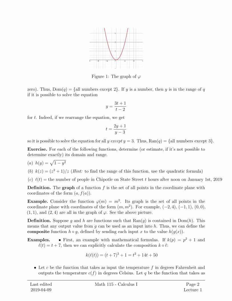
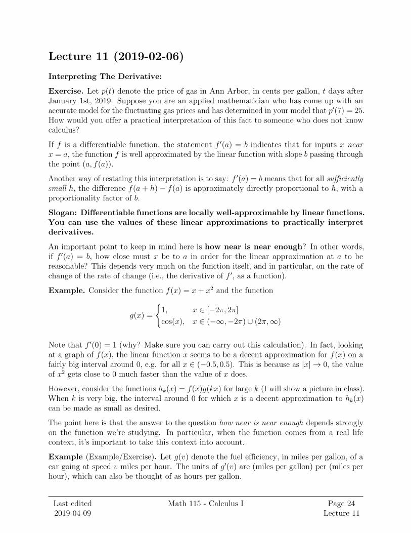
Figure 1: The graph of ϕ

zero). Thus, Dom(q) = all numbers except 2. If y is a number, then y is in the range of qif it is possible to solve the equation

y =3t+ 1

t− 2

for t. Indeed, if we rearrange the equation, we get

t =2y + 1

y − 3

so it is possible to solve the equation for all y except y = 3. Thus, Ran(q) = all numbers except 3.

Exercise. For each of the following functions, determine (or estimate, if it’s not possible todetermine exactly) its domain and range.

(a) h(y) =√

1− y2

(b) k(z) = (z2 + 1)/z (Hint: to find the range of this function, use the quadratic formula)

(c) `(t) = the number of people in Chipotle on State Street t hours after noon on January 1st, 2019

Definition. The graph of a function f is the set of all points in the coordinate plane withcoordinates of the form (a, f(a)).

Example. Consider the function ϕ(m) = m2. Its graph is the set of all points in thecoordinate plane with coordinates of the form (m,m2). For example, (−2, 4), (−1, 1), (0, 0),(1, 1), and (2, 4) are all in the graph of ϕ. See the above picture.

Definition. Suppose g and h are functions such that Ran(g) is contained in Dom(h). Thismeans that any output value from g can be used as an input into h. Thus, we can define thecomposite function h g, defined by sending each input x to the value h(g(x)).

Examples. • First, an example with mathematical formulas. If k(p) = p2 + 1 and`(t) = t+ 7, then we can explicitly calculate the composition k `:

k(`(t)) = (t+ 7)2 + 1 = t2 + 14t+ 50

• Let c be the function that takes as input the temperature f in degrees Fahrenheit andoutputs the temperature c(f) in degrees Celsius. Let q be the function that takes as



input the temperature t in degrees Celsius and outputs the likelihood q(t) that thetemperature will dip below t degrees today. Then, the composition q c also outputsthe likelihood that the temperature will dip below the input temperature, but acceptsthe input in degrees Fahrenheit rather than degrees Celsius.

Exercise. Express the function f(t) = t2 + 2t+ 1 as a composite in at least two differentways, i.e. find at least two different pairs of functions (g, h) such that f(t) = g(h(t)).

Definition. A function f is called invertible if there exists another function g such that

(f g)(x) = (g f)(x) = x

for all input values x. In this situation, the function g is called the inverse of f , and denotedf−1. Intuitively, f−1 ‘‘undoes’’ the effect of f .

A function f is invertible precisely when, for every number y in Ran(f), there is exactly oneinput a such that f(a) = y. This input a is the value f−1(y). We can think of f−1(y) as‘‘the number which, when plugged into f , yields a result of y.’’

If you have available the graph of a function f , a quick way to check if f is invertible is thehorizontal line test.

Exercise. Suppose f is an invertible function. Explain why Dom(f−1) = Ran(f) andRan(f−1) = Dom(f).

Important Remark: Even if a function is not invertible, it might become invertible whenwe restrict its domain. For example, consider the function ϕ(m) = m2. We know thatDom(ϕ) = all numbers and Ran(ϕ) = all nonnegative numbers.

The function ϕ is not invertible when thought of as a function on its entire domain: for anynumber z, there are two numbers m such that ϕ(m) = z (the positive and negative squareroot of z). Thus, ϕ is not invertible.

However, suppose we think of ϕ as a function that is only allowed to eat positive numbers.In other words, we restrict the domain of ϕ to the interval (0,∞). Now, for every z, there isexactly one number m in the domain of ϕ such that ϕ(m) = z (the positive square root of z).Thought of as a function with domain (0,∞), ϕ becomes invertible.

This trick is very important/useful to define inverses of functions that aren’t invertibleon their entire domains. We will use it especially when defining inverses of trigonometricfunctions.

Exercise. The function q(t) = sin(t) is not invertible on its entire domain. Give threedifferent examples of domains on which it is invertible.

Tidbits I might mention in class: interval notation, set membership notation.



Lecture 2 (2019-01-11)

We now have a general sense of what a function is. Today, we’re going to talk about thegrowth of functions, and review the properties of some common functions of interest (namely,linear and exponential functions).

Suppose f is a function. We are often interested in the problem of determining how theoutput f(x) changes/grows/varies as the input x changes/grows/varies. A rough way tocategorize growth behavior is via the notions of increasing and decreasing functions:

Definition. Suppose f is a function and S is a subset of the domain Dom(f). We say f isincreasing on S if whenever x, y ∈ S satisfy y > x, then f(y) > f(x). In words, biggerinputs from S yield bigger outputs.

Analogously, we say f is decreasing on S if whenever x, y ∈ S satisfy y > x, thenf(y) < f(x). In words, bigger inputs from S yield smaller outputs.

If f is increasing on Dom(f), we just call it increasing.

If f is decreasing on Dom(f), we just call it decreasing.

Examples. • Consider the function $(q), which is the rule that takes input a numberof quarters q and outputs the value $(q) of q quarters, in cents. We all know that aformula for $(q) is given by $(q) = 25q. Here, $ is increasing on its entire domain, sincebigger inputs numbers of quarters always correspond to larger monetary values.

• You’re growing amoebas in a culture. At noon, you start with 1 amoeba in the culture.Suppose it takes any amoeba an hour to split into two amoebas, and they just keepsplitting, because that’s what amoebas do. At 1PM, you’ll have 2 amoebas, at 2PMyou’ll have 4 amoebas, etc.

Let A(t) be the rule that outputs the number A(t) of amoebas in the culture t hoursafter noon. We know A(0) = 1, A(1) = 2, A(2) = 4. In general, A(t) = 2t. Note that Ais also increasing on its entire domain, since later times always mean you’ll have moreamoebas in the culture.

Exercise. Think of another example of an increasing function and three examples of de-creasing functions (either a mathematical formula, or describing some real-world relationshipbetween quantities).

Important Observation: Both $ and A as defined above are increasing functions. Butintuitively, one of them is increasing much faster than the other. Even though the valuesof A are initially much smaller than the values of $, the function A initially ‘‘overtakes’’ $.Let’s make careful sense of this notion of ‘‘increasing faster’’.

Definition. Suppose f is a function with the closed interval [a, b] in its domain. The averagerate of change of f on the interval [a, b] is defined by the formula

f(b)− f(a)

b− a=

change in output

change in input



The average rate of change of f on [a, b] roughly answers the question ‘‘how much does theoutput of f change when going from a to b, relative to the length of the interval [a, b]?’’ Wesay ‘‘roughly’’ because the average rate of change ignores everything that’s happening insidethe interval [a, b].

Let’s apply this concept to our functions $ and A. Suppose we restrict both functions to thedomain 1, 2, 3, 4, 5. We can calculate the following tables:

q 1 2 3 4 5$(q) 25 50 75 100 125Average rate of change of $ on the interval [t, t+ 1] 25 25 25 25 25

t 1 2 3 4 5A(t) 2 4 8 16 32Average rate of change of A on the interval [q, q + 1] 2 4 8 16 32

The average rate of change of $ is constant over every interval. Although $ is alwaysincreasing, the rate at which it’s increasing never changes.

The average rate of A is itself increasing as t gets bigger; in fact, it looks like you always getback A(t) as the rate of change of A on the interval [t, t+ 1]. This is ‘‘compounded growth’’.

This is why we say A is ‘‘increasing faster’’ than $: because the rate of change of $ staysconstant, but the rate of change of A itself increases as the input gets larger.

Definition. A function f is called linear if its average rate of change is constant on everyinterval. This constant average rate of change is called the slope of f .

Definition (can’t quite make sense of this precisely yet). A function f is called exponentialif its ‘‘rate of change’’ is directly proportional to f .

Theorem. (a) Every linear function is of the form g(y) = ay + b for some numbers a, b.

(b) Every exponential function is of the form h(z) = abz for some numbers a, b (here, b > 0).

Exercise. For which pairs of numbers a and b is g(y) = ay + b an increasing function? Forwhich pairs is g decreasing?

For which pairs of numbers a and b is h(z) = abz an increasing function (exponential growth)?For which pairs is h decreasing (exponential decay)?

Note: Exponential growth always eventually dominates linear growth.

Exercise. The table below depicts values sampled from two functions f and g. One of thefunctions is exponential and one is linear. Which one is which? Find explicit formulas foreach one.

t 0 1 3 4f(t) 64 96 216 324g(t) 64 129 259 324



Lecture 3 (2019-01-15)

Quiz Today! -- Student Website + Grading Guidelines + Team HW. If youhaven’t already, please remember to fill out the Student Data Sheet by midnighttonight.

Before we start new material, some review problems:

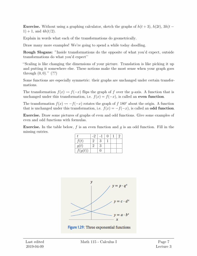
• A certain region has a population of 10 million and an annual growth rate of 2%.Estimate the doubling time by guessing and checking. Then, calculate the doublingtime exactly.

• Figure 1.29 (on the back of this page) is the graph of three exponential functions. Whatcan you say about the values of the six constants a, b, c, d, p, q?

Our goal for today is to study some common transformations of functions. A transformationis an operation that you do to a function which yields a new function.

Some common transformations are the following:

• Translation Of Input: replace the function x 7→ f(x) with the function x 7→ f(x+a)for some number a

• Scaling Of Input: replace the function x 7→ f(x) with the function x 7→ f(cx) forsome number c

• Translation Of Output: replace the function x 7→ f(x) with the function x 7→f(x) + a for some number a

• Scaling Of Output: replace the function x 7→ f(x) wih the function x 7→ cf(x) forsome number c

• Any Combinations Of the Above

One way to think about these transformations is pre-processing the input to the function orpost-processing the output of the function.

To get a better handle on these transformations, we study carefully how they geometricallychange the graph of a function. For example:

Example. Suppose g(t) = t2 is the function that we start with. The graph of g is a standardparabola in the coordinate plane. What does the graph of h(t) = g(t− 2) look like?

Let’s plot some points: on the graph of g we have (0, 0), (1, 1), (2, 4), (3, 9), etc. On thegraph of h we have (2, 0), (3, 1), (4, 4), (5, 9). In general, the points on the graph of g all havethe form (t, t2), and the points on the graph of h all have the form (t+ 2, t2) = (t, t2) + (2, 0).

We get the graph of h by adding (2, 0) to the points of (t, t2). This shifts the whole graphtwo units to the right.



Exercise. Without using a graphing calculator, sketch the graphs of h(t+ 3), h(2t), 3h(t−1) + 1, and 4h(t/2).

Explain in words what each of the transformations do geometrically.

Draw many more examples! We’re going to spend a while today doodling.

Rough Slogans: ”Inside transformations do the opposite of what you’d expect, outsidetransformations do what you’d expect’’

‘‘Scaling is like changing the dimensions of your picture. Translation is like picking it upand putting it somewhere else. These notions make the most sense when your graph goesthrough (0, 0).’’ (??)

Some functions are especially symmetric: their graphs are unchanged under certain transfor-mations.

The transformation f(x) f(−x) flips the graph of f over the y-axis. A function that isunchanged under this transformation, i.e. f(x) = f(−x), is called an even function.

The transformation f(x) −f(−x) rotates the graph of f 180 about the origin. A functionthat is unchanged under this transformation, i.e. f(x) = −f(−x), is called an odd function.

Exercise. Draw some pictures of graphs of even and odd functions. Give some examples ofeven and odd functions with formulas.

Exercise. In the table below, f is an even function and g is an odd function. Fill in themissing entries.

t -2 -1 0 1 2f(t) 2 3 1g(t) 2 3f(g(t)) 0



Lecture 4 (2019-01-16)

Exercise. Given the graph of some function f , how do you obtain the graph of f−1? Describesome geometric transformation that turns the graph of f into the graph of f−1 and explainwhy this works.

To describe the growth of a function, we discussed the notions of increasing and decreasing.However, we also saw that these notions are insufficient to some extent: the linear functionf(s) = s and the exponential function g(s) = 2s are both increasing on their domains, butthe exponential function g is ‘‘eventually increasing faster.’’

More precisely, we saw that the average rate of change of f is constant on every interval(what is this constant?) whereas the average rate of change of g is increasing as we look at‘‘increasingly rightward’’ intervals.

There is an important definition that encapsulates the notion of ‘‘increasing rate of change’’:

Definition. Let f be a function and suppose S is a subset of Dom(f). We say f is concaveup on S if whenever a, b, c ∈ S with a < b < c, the average rate of change of f on theinterval [b, c] is bigger than the average rate of change of f on the interval [a, b]. In words,the rate of change of f is increasing on S.

Similarly, we say f is concave down on S if whenever a, b, c ∈ S with a < b < c, theaverage rate of change of f on the interval [b, c] is smaller than the average rate of change onthe interval [a, b]. In words, the rate of change of f is decreasing on S.

Important note: a function can be both concave up and decreasing, or concave down andincreasing! Concavity says something about the rate of change of the rate of change of thefunction; it doesn’t directly say something about the rate of change.

Exercise. Sketch some graphs of functions that are

• concave up and increasing

• concave up and decreasing

• concave down and increasing

• concave down and decreasing

Exercise. Suppose f is a function that is concave up on the open interval (0, 6). If f(1) = 2,f(3) = 5, and f(4) = 11. What are the possible values of f(2)?

If g is a function satisfying g(2) = 7, g(3) = 5, and g(4) = 6, could g be concave down on theinterval (0, 6)?

Let’s remind ourselves of the algebraic properties of exponential and logarithmic functions.First of all, recall that loga(x) is what we write to denote the inverse of the function ax.



(Note that ax always passes the horizontal line test, so it has an inverse defined on all of(0,∞)).

We write ln(x) to denote loge(x), where e ≈ 2.718.. is that magic number that keeps showingup. We also often denote log10(x) simply by log(x).

Recall that ax+y = ax · ay for any numbers x and y. In particular, if we set x = loga(m) andy = loga(n), then

aloga(m)+loga(n) = m · n =⇒ loga(m) + loga(n) = m · n

for any positive numbers m and n.

We also have the ‘‘change of base formula’’:

loga(b) =logc(b)

logc(a)

for any c. In particular, this formula implies that

loga(bc) =

logb(bc)

logb(a)=

c

logb(a)=

c

log(b)/ log(a)=c log(a)

log(b)= c loga(b)

so logarithms ‘‘turn powers into multiplications.’’

Exercise. A circle has a radius of log10(a2) and a circumference of log10(b

4). What is loga(b)?

Exercise. • Find all solutions x for the equation 7ex+3 + 5 = 13.

• Find all solutions x for the equation 4x = 2x+1 + 1. (Hint: Use the quadratic formula)

A neat thing: Consider the powers of two, i.e. 1, 2, 4, 8, 16, 32, etc. How often is the leftmostdigit equal to 1? Explain/support your answer.



Lecture 5 (2019-01-18)

Today, our goal is to do a rapid review of trigonometric functions.

The convention is that angles input into trigonometric functions are always in radians. Recallthat you can convert from degrees to radians by setting up a direct proportion using the factthat

2π rad = 360

Constructing Sine and Cosine From Scratch

I’m going to construct the functions ‘‘sine’’ and ‘‘cosine’’ from scratch. Our goal in doing thisis primarily to remind ourselves of some of the most important properties of these functions.

Suppose θ is an acute angle. Let 4ABC be a right triangle with ∠B = π/2 and ∠A = θ.We define

sin(θ) =BC

AC

cos(θ) =AB

AC

Note that if 4A′B′C ′ is another right triangle with ∠B′ = π/2 and ∠A′ = θ, then 4ABCand 4A′B′C ′ are similar. Thus, we have the equalities

BC

AC=B′C ′

A′C ′(= sin(θ))

AB

AC=A′B′

A′C ′(= cos(θ))

Thus, the numbers sin(θ) and cos(θ) are independent of the right triangle you use to calculatethem; they only depend on the angle θ.

This gives us a definition of sin and cos for acute angles θ. Note that by this definition, whenθ is an acute angle, the numbers sin(θ) and cos(θ) are both positive. How do we extend makesense of sin(θ) and cos(θ) when θ is not an acute angle?

First, recall the unit circle is the set of points (x, y) in the coordinate plane with x2 + y2 = 1.If P is a point on the unit circle, let ∠(P ) be the (smallest nonnegative) angle at whichP is located, measured counterclockwise from the positive x-axis. In particular, we insist∠((1, 0)) = 0, and we have now a function

∠ : points on the unit circle → [0, 2π)

(A function that eats points and spits out angles!) This ∠ is an invertible function, and wecan write ∠−1(θ) to denote the unique point P on the unit circle with ∠(P ) = θ.

Now, note that by our definition of sin and cos, if 0 ≤ θ < π/2, then the coordinatesof the point ∠−1(θ) are exactly (cos(θ), sin(θ)). Turning this observation around on its



head, we define sin(θ) and cos(θ) to be the y- and x-coordinates, respectively, of ∠−1(θ) forπ/2 < θ < 2π as well! Note that this means sin and cos now attain negative values too: forexample sin(3π/2) = −1 and cos(π) = −1.

So, we have a definition of sin and cos for angles 0 ≤ θ < 2π. Finally, we insist that sin andcos satisfy the rules

sin(θ + 2π) = sin(θ)

cos(θ + 2π) = cos(θ)

for all angles θ. In other words, sin and cos should be ‘‘2π-periodic’’. This gives a definitionof sin and cos that works when you plug in any angle θ (it can be bigger than 2π, or evennegative).

In particular, based on how we defined sin and cos via the coordinates of points on the unitcircle, these functions satisfy the fundamental equation

sin2(θ) + cos2(θ) = 1

for all angles θ.

Finally, we define a few additional trigonometric functions in terms of sin and cos:

tan(θ) =sin(θ)

cos(θ)

sec(θ) =1

cos(θ)

csc(θ) =1

sin(θ)

cot(θ) =1

cot(θ)

Exercise. We defined the functions sin and cos each to have domain (−∞,∞). What isthe range of sin? What is the range of cos? What are the domain and the range of tan?

Exercise. Some values of sin and cos can be explicitly calculated, and it’s important toknow what they are. Use geometry to calculate the coordinates of ∠−1(π/6), ∠−1(π/4), and∠−1(π/3).

Inverse Trig Functions

Since sin and cos are 2π-periodic, they fail the horizontal line test pretty badly. In fact, theyalready failed the horizontal line test even when we only had definitions for angles θ between0 and 2π (why?).

However, the function sin(θ) is invertible when restricted to the domain [−π/2, π/2]. Similarly,the function cos(θ) is invertible when restricted to the domain [0, π]. We also see that the



function tan(θ) is invertible when restricted to the domain (−π/2, π/2). Moreover, on all ofthese subdomains, every value in the range of each of the functions is in fact attained.

Accordingly, we define the basic inverse trig functions as follows:

arcsin(x) = the unique angle θ in [−π/2, π/2] such that sin(θ) = x

arccos(x) = the unique angle θ in [0, π] such that cos(θ) = x

arctan(x) = the unique angle θ in (−π/2, π/2) such that cos(θ) = x

Keep in mind, however, that trigonometric equations have (many) more solutions than just the‘‘canonical’’ solutions identified by the inverse trig functions. For example, arcsin(

√2/2) =

π/4, but the equation sin(θ) =√

2/2 has the (infinite!) solution set

θ =

· · · ,−7π

4,−5π

4,π

4,3π

4,9π

4,11π

4, · · ·

General Sinusoidal Functions

We now describe a notion of ‘‘general sinusoidal function’’. These functions are just the sinand cos functions scaled and translated via the transformations we discussed two classes ago.These functions are often used to (crudely) model periodic phenomena (real-world processesthat repeat/recur).

Definition. A general sinusoidal function is any function of the form

f(t) = A sin(Bt+ C) +D

for numbers A, B, C, and D.

Example. Note that cos is indeed a general periodic function, since we always have theidentity

cos(t) = sin(π

2− t)

Definition. For a general sinusoidal function f of the form in the above definition, thequantity |A| is called the amplitude of f . It is the amount by which the original sin curvehas been vertically scaled. Note that the range of f is [−|A|+D, |A|+D].

The quantity 2π/|B| is called the period of f . It is the smallest amount of time neededfor the function to execute one complete cycle. This makes sense, since B measures thehorizontal scaling of the original sin curve: large B (i.e. |B| > 1) means super squished curvemeans short period; small B (i.e. |B| < 1) means super stretched curve means long period.

Remark. For a general sinusoidal function f , the quantity C/B describes the amount ofhorizontal shift. More precisely, f is obtained from the function g : t 7→ A sin(Bt) +D byshifting g by C/B units to the left. Indeed, the shifted function is then given by

g

(t+

C

B

)= A sin

(B

(t+

C

B

))+D = A sin(Bt+ C) +D = f(t)



Lecture 6 (2019-01-23)

Today, we’ll talk about polynomials and rational functions. These are an exceptionallyimportant class of functions for a few reasons:

• They are easy to calculate, since they are built entirely out of the arithmetic operationsof addition, subtraction, multiplication, and division.

• They are very rigid, in that they are (almost) entirely determined by their set of rootsand poles.

Definition. A polynomial is a function that is entirely built out of the operations ofrepeated addition, subtraction, and multiplication of the input. More precisely, a polynomialis a function of the form

p(x) = anxn + an−1x

n−1 + · · ·+ a2x2 + a1x+ a0

where all the ai’s are constants. For example, f(t) = t2 + t + 1, g(s) = −s + 7, andh(q) = −2q3 + q + 1 are all polynomials.

Definition. The degree of a polynomial p(x) is the largest power of x that appears in theexpression of p(x). For example, the degree of f(t) = t2+t+1 is 2, the degree of g(s) = −s+7is 1, and the degree of h(q) = −2q3 + q + 1 is 3.

Remark. Here is a geometric interpretation of the degree of a polynomial. The graph ofa polynomial of degree n always has at most n − 1 bends. More precisely, if you imaginethat the polynomial function p(t) describes the location at time t of a particle moving on thenumber line, then if p has degree n, the particle changes its direction of movement at mostn− 1 times.

Definition. If f is a function, a root or zero of f is any number r ∈ (−∞,∞) such thatf(r) = 0.

Example. The polynomial g(s) = −s + 7 has a root at 7, since g(7) = −7 + 7 = 0. Thepolynomial f(t) = t2 + t+ 1 has no roots. This can be seen in (at least) two ways:

• Using the quadratic formula, the roots of f , if they exist, are of the form

t =−1±

√−3

2

But there is no square root of −3 in (−∞,∞), so there are no real solutions.

• Completing the square, we see that

f(t) =

(t+

1

2

)2

+3

4

which is the parabola with equation m(t) = t2 shifted 1/2 units to the left and 3/4units upwards. In particular, the graph of f(t) does not intersect the x-axis, so f hasno real roots.



Theorem. Suppose p(x) is a polynomial and r is a root of p(x). Then p(x) = (x− r)q(x)for some polynomial q(x). In other words, roots can be ‘‘factored out’’ of polynomials.

Example. Suppose p(x) is a cubic polynomial with roots at 1, 2, and 3, such that p(0) = 7.Using the above theorem, p(x) must be of the form

p(x) = c(x− 1)(x− 2)(x− 3)

Using the fact that p(0) = 7, we see that

7 = p(0) = −6c =⇒ c = −7

6

so that

p(x) =−7

6(x− 1)(x− 2)(x− 3)

Knowing the roots of p and one additional value allowed us to deduce the general form ofthe function p(x).

Definition. A rational function is a function of the form p(x)/q(x), where p and q areboth polynomials. For example,

h(s) =3s+ 2

s− 1

and

k(t) =−7t2

t3 + t+ 1

are both rational functions.

Behavior of polynomials and rational functions as x → ∞, −∞: We are ofteninterested in the ‘‘long run’’ behavior of a function, i.e. how it behaves when x gets verypositive, or when x gets very negative. We say that a function f has a horizontal asymptoteat y = c if the graph of f approaches the line y = c as x→∞ or as x→ −∞.

Example. Consider the rational function

g(m) =3m2 + 2

m2 + 7m

Note that we can rewrite this as

g(m) =3 + (2/m2)

1 + (7/m)

When |m| is very large, the terms 2/m2 and 7/m are essentially zero, so g(m) is essentially 3.In other words, g has a horizontal asymptote at y = 3, which it approaches as m→∞ andas m→ −∞.

Definition. If f(x) = p(x)/q(x) is a rational function, we say r is a pole of f if r is a rootof q(x). Basically, a pole is a place where f is undefined. If f has a pole at r, we say that fhas a vertical asymptote at x = r. We can ask what the behavior of f is as x approachesa pole from the left or the right.



Domination: Given two functions f(x) and g(x), we say f dominates g as x→∞ if

f(x)

g(x)→∞

as x→∞. This is a way to compare the growth of f and g as x gets very large.

Example. If f(x) = x and g(x) = 2x+ 7, then neither function dominates the other, sincef/g → 1/2 as x→∞. On the other hand, if q(x) = x2 and r(x) = x, then q/r = x, whichgoes to ∞ as x→∞. Thus, q dominates r.

In general, polynomial growth of higher degree dominates polynomial growth of lower degree.Moreover, exponential growth always dominates any polynomial growth.



Lecture 7 (2019-01-24)

Today, we’re going to discuss the concept of limits. This concept is the technical heart ofcalculus, and it can take some doing to wrap your head around.

Limits Of Functions As We Approach A Number

Suppose f is a function, and the following table of values is sampled from f :

t 0.9 0.99 0.999 0.9999 0.99999f(t) 2.11 2.04 2.005 2.00001 2.0000001

Based on this information, what would you guess the value of f(1) is? The table stronglysuggests that a prediction of f(1) = 2 is reasonable.

This is a very reasonable prediction, but it’s not necessarily true. The value of a function ata point does not have to bear any resemblance to the values nearby. For all we know, itcould be that f(1) = 9 billion. Moreover, even supposing that f(1) is 9 billion, the functioncould actually reach this value in pretty different ways:

• One possibility is that, if we were to continue making the table above, with t valueseven closer to 1, we see something like this:

t 0.99999 0.999999 0.9999999 0.99999999 0.9999999999f(t) 2.0000001 2.5 10 106 8.7 ·109

Upon zooming in to a sufficiently fine time-scale, the function actually stops decreasingto 2 and blows up towards 9 billion. The pattern of getting closer to 2, which wenoticed in the earlier table, fails to continue.

• Another possibility is that, if we were to continue making the table above, with t valueseven closer to 1, we see something like this:

t 0.99999 0.999999 0.9999999 0.99999999f(t) 2.0000001 2.000000001 2.0000000000001 2.0000000000000000001

In this case, the values of the function continue to approach 2 as the inputs continueto approach 1. Keep in mind, this is still no guarantee that upon making inputs evencloser to 1, the outputs don’t start veering upwards towards 9 billion.

Very roughly speaking, we are suggesting two kinds of behaviors (these are not the onlytwo things the function could do, it could also do even more complicated things!): eithereventually as t → 1, the function’s outputs shoot up towards 9 billion, or they always getcloser to 2 (and there is a discontinuous ‘‘jump’’ to 9 billion at t = 1 exactly).

In the latter case, we say that f(t) has a left limit of 2 as t approaches 1 from below.This is written with the notation limt→1− f(t) = 2. More precisely, we have the followingdefinition:



Definition. Suppose f(t) is a function. We say f has a left limit at t = a if, as t approachesa from below (i.e., through numbers slightly smaller than a), the values of f(t) always getcloser and closer to some number L. This number L is called the left limit of f at a, andwe denote

limt→a−

f(t) = L

We similarly have a notion of right limit at t = a, denoted

limt→a+

f(t)

if it exists.

Remark. Note that these limits don’t necessarily have anything to do with the value f(a).In our above example with tables, we had a case where limt→1− f(t) = 2 but f(1) = 9 billion.

I’ll say it again: limits of f as the input approaches a are defined without referenceto the value f(a)!

Definition. Suppose f(t) is a function and a is some number such that

limt→a−

f(t)

andlimt→a+

f(t)

both exist and are equal, say to some number L. Then, we say that the (nondirectional)limit of f exists as t→ a (without a plus or minus sign!) and write

L = limt→a

f(t)

In other words, when the left and right limits at a are the same, we just call it the limit.

Remark. One very useful way to conceptualize the concept of a limit as t → a is to askyourself: if I knew nothing about the value of f(a) but knew everything about the valuesf(t) for t close to a, what would I predict f(a) to be?

(Again, the prediction here is not necessarily correct, but if the function permits such aprediction, we call this prediction the limit of f as t→ a.)

Example. We have looked at examples where the values of f(t) really do approach somenumber as t approaches a. This is not necessarily always going to happen! For example,consider the function g(s) = 1/s. As s → 0+, the values of g(s) blow up to ∞ and don’tapproach any fixed number! In this case, we say the limit does not exist.

Limits can fail to exist even more extravagantly. In the case of g above, as s → 0+, thevalues g(s) don’t approach any fixed number but are always strictly increasing. A wilderexample is the function

h(y) = sin

(1

y

)As y → 0+, note that h(y) oscillates wildly between 1 and −1, and never settles on movingtowards some fixed number. This is another case of the limit failing to exist.



Definition. Suppose f(t) is a function defined in an open interval containing t = a andlimt→a f(t) exists and equals f(a). Then, we say f is continuous at t = a. In other words,we say f is continuous at t = a if the prediction for f(a) obtained by studying values f(t)for t close to (but not equal to) a is correct.

Slogan: Continuity = correct prediction from nearby values.

Limits Of Functions As We Approach +∞ Or −∞

There is an analogous notion of limits as input values approach +∞ or −∞. Since ∞ is notactually a number, we do not have a corresponding notion of continuity at ∞!

Definition. Suppose f(t) is a function. We say f has a limit at infinity if, as the inputvalues t approach infinity (more precisely, get arbitrarily large), then the values of f(t) alwaysget closer and closer to some number L. This number L is called the limit of f at infinityand we denote

limt→∞

f(t) = L

Similarly, we have a notion of limit at −∞, which is denoted

limt→−∞

f(t)

if it exists.

Remark. We can reconceptualize vertical and horizontal asymptotes in terms of limits.Horizontal asymptotes correspond to limits at ∞ and −∞. Vertical asymptotes are a bitmore complicated: they correspond to input values where the left/right limits do not exist,but only fail to exist in the ‘‘blow up to infinity or minus infinity’’ sense and not in the‘‘oscillate wildly and never settle on any direction to go’’ sense.



Exercise: A Classic And Important Example

Always keep in mind that limt→a f(t) does not depend on f(a). In fact, f need not even bedefined at a for a limit to exist. A classic example is the following:

Consider the function

h(θ) =sin(θ)

θ

Note that h is not even defined at θ = 0. However, the limit limθ→0 h(θ) still exists.

Can you guess what the limit is? Make sure to justify your guess somehow.

Can you explain/prove why this is the limit? (The proof is tricky, and counts for extracredit.)

Exercise: Limit Of A Composition

Consider the function

j(p) =

−p− 3 p < 0

0 p = 0

3− p p > 0

What is limp→0− j(p) What is limp→0+ j(p)? Does limp→0 j(p) exist?

Now, consider the composition j(j(p)). Does limp→0 j(j(p)) exist? Is j(j(p)) continuous atp = 0?



Lecture 8 (2019-01-29)

Imagine there is a magician, who performs the following two (incredibly breathtaking) tricks:

• She takes a grapefruit and tosses it into the air. The position of the grapefruit is givenby a function g(t), where t is measured in seconds since the grapefruit has been tossed,and g(t) is measured in meters above the ground.

• She takes a dove in her hands and simply lets go of the dove. The dove falls momentarily,then catches itself and begins to fly upwards. The position of the dove is given by afunction d(t) where t is measured in seconds since the dove has been let go of, and d(t)is measured in meters above the ground.

Suppose that g(0) = h(0) = .5 and g(1) = h(1) = 2. If this is the case, then both g and h willhave the same average rate of change on the interval [0, 1], namely (2− .5)/(1− 0) = 1.5.

However, the functions g and d are surely doing something different near or at t = 0: thefunction g is initially increasing, but the function d is initially decreasing. Moreover, this isactually reflected by calculating average rates of change on short enough time intervals near0, perhaps like [0, .2] or [0, .02], etc.

This is an extremely important observation! If we calculate average rates of changeon shorter time intervals [0, ε], we get numbers that are more reflective the behavior of thefunction at or near time t = 0.



Lecture 9 (2019-02-01)

Last time, we introduced the concept of instantaneous rate of change. There are threeimportant perspectives to keep in mind on this concept:

The ‘‘kinematic’’ perspective: We have a function f(x) and are interested in studyingits behavior near some point x = a. The average rate of change of f on the interval [a, a+ h]is given by the formula

AvgRate(a, h) :=f(a+ h)− f(a)

hAs h gets very small (equivalently, as the interval [a, a+ h] becomes very small in length),the average rates of change AvgRate(a, h) become more and more reflective of the behaviorof f near or at a. Accordingly, we define the instantaneous rate of change of f at a tobe

f ′(a) := limh→0

AvgRate(a, h) = limh→0

f(a+ h)− f(a)

h(if this limit exists!).

The ‘‘geometric’’ perspective: The point (a, f(a)) is on the graph of f(x). If we chooseh to be a small number, the slope of the line joining (a, f(a)) and (a+ h, f(a+ h)) is givenby the formula

f(a+ h)− f(a)

hAs h gets very small, the line joining (a, f(a)) and (a+ h, f(a+ h)) approaches the tangentline to the graph of f at a. Accordingly, if the limit

f ′(a) = limh→0

f(a+ h)− f(a)

h

exists, it describes the slope of the tangent line to f at a.

The ‘‘approximation’’ perspective: We might be interested in calculating the value off(x) for some input x that is close to a. But f might be a complicated function for whichit is not so clear how to calculate its values (for example, how would you calculate cos(1)without just plugging into a calculator? How is your calculator doing the computation?). Acrucial observation is that for ‘‘nice’’ functions, when you zoom far enough into the pictureof the function’s graph, the picture looks very much like a line. In other words, we might beable to approximate f near a by a linear function. Here are the details:

First, translate f so that the point (a, f(a)) becomes the point (0, 0). More precisely, replacef with g(x) = f(x + a) − f(a). Now, using our knowledge of functional transformations,recall that ‘‘zooming in’’ to the graph of g near (0, 0) with a ‘‘magnification factor’’ of camounts to replacing g with

cg(xc

)The ‘‘infinitely zoomed in’’ function is h(x) = limc→∞ cg

(xc

). If h(x) is linear, then we can

recover its slope by looking at h(x)/x. Indeed, we have

h(x)

x= lim

c→∞

c

xg(xc

)= lim

c→∞

c

x

(f(xc

+ a)− f(a)

)= lim

ε→0

f(ε+ a)− f(a)

ε



which is exactly the definition from above. To summarize, at each input value a where thelimit defining f ′(a) exists, we have a linear approximation at a, i.e. a linear function(whose equation coincides with the equation of the tangent line) that is a decent approximationfor the values of f(x) when the input x is near a. Another way of stating this is that for xclose to a, we have

f(x) ≈ f(a) + f ′(a)(x− a)

The Derivative As a Function

We introduce some terminology/definitions. Suppose f is a function and the limit definingf ′(a) exists; then, we say f is differentiable at a. (Conversely, if the limit does not exist,we say f is not differentiable at a.)

Suppose f is a function that is differentiable everywhere. For each a ∈ Dom(f), we have anassignment a 7→ f ′(a). The rule that takes in an input a and outputs the instantaneous rateof change of f at a is itself a function. We call this function the derivative of f and oftendenote it by f ′(x).

Example. Consider s(t) = t2. Rather than calculating the instantaneous rate of change atsome fixed number a (like a = 2 as we did last time), we can carry out the same algebra forarbitrary a:

s′(a) = limh→0

s(a+ h)− s(a)

h= lim

h→0

(a+ h)2 − a2

h= lim

h→0

2ah+ h2

h= lim

h→0(2a+ h) = 2a

Thus, as a function, the derivative of s(t) = t2 is given by the function s′(t) = 2t.

Exercise. Some important special cases of the derivative as a function: if f is a constantfunction, what is f ′ (as a function)? If f is a linear function, what is f ′ (as a function)?

Exercise. Here’s an example of a function that is not differentiable everywhere. Let q(r) = |r|.Graph the function q(r) and explain why it is not differentiable at r = 0.

Exercise. See the image below.



Lecture 10 (2019-02-05)

Some Important General Comments:

• In general, both on exams and often in life, getting the right answer counts for muchless than being able to clearly communicate your ideas/efforts to other people. This iswhy it is so important to organize your work, make clear and precise statements, andto understand the types of various mathematical objects. (Examples: work throughtrig problem again from last quiz; ‘‘the function is symmetric’’; ‘‘some men are doctors’’and ‘‘some doctors are tall’’ does not imply ‘‘some men are tall’’; if f(t) = t2, thestatement ‘‘at t = 3, the function is 9’’)

• Always ask yourself at the end: does this make sense? Be sure to check that youranswer/solution is consistent with the information given in the problem. This is a greatway to determine if you’ve worked out the problem correctly. If you discover that youranswer is inconsistent with the information, go back to your work and see if you canfigure out what went wrong. Make sure your work is clearly organized so that it’s easyto review it if necessary.

• When you’re stuck, you have to try to actively problem solve. Some potential strategies:draw a picture, make a table, remind yourself what the concepts mean, solve an easierproblem, think wishfully and imaginatively, take a break and return. When faced with anovel mathematical problem/situation, we often find ourselves thinking ‘‘I Don’t KnowWhat To Do Here /’’ and giving up. But if we push through this and experiment, wewill find that we often are able to prevail.

A Digression: Sums Of Powers

(a) Find a nice, simple formula for1 + 2 + · · ·+ n

where n is any positive whole number. Prove your answer.

(b) Can you find and prove a nice, simple formula for

13 + 23 + · · ·+ n3

where n is any positive whole number?



Lecture 11 (2019-02-06)

Interpreting The Derivative:

Exercise. Let p(t) denote the price of gas in Ann Arbor, in cents per gallon, t days afterJanuary 1st, 2019. Suppose you are an applied mathematician who has come up with anaccurate model for the fluctuating gas prices and has determined in your model that p′(7) = 25.How would you offer a practical interpretation of this fact to someone who does not knowcalculus?

If f is a differentiable function, the statement f ′(a) = b indicates that for inputs x nearx = a, the function f is well approximated by the linear function with slope b passing throughthe point (a, f(a)).

Another way of restating this interpretation is to say: f ′(a) = b means that for all sufficientlysmall h, the difference f(a+ h)− f(a) is approximately directly proportional to h, with aproportionality factor of b.

Slogan: Differentiable functions are locally well-approximable by linear functions.You can use the values of these linear approximations to practically interpretderivatives.

An important point to keep in mind here is how near is near enough? In other words,if f ′(a) = b, how close must x be to a in order for the linear approximation at a to bereasonable? This depends very much on the function itself, and in particular, on the rate ofchange of the rate of change (i.e., the derivative of f ′, as a function).

Example. Consider the function f(x) = x+ x2 and the function

g(x) =

1, x ∈ [−2π, 2π]

cos(x), x ∈ (−∞,−2π) ∪ (2π,∞)

Note that f ′(0) = 1 (why? Make sure you can carry out this calculation). In fact, lookingat a graph of f(x), the linear function x seems to be a decent approximation for f(x) on afairly big interval around 0, e.g. for all x ∈ (−0.5, 0.5). This is because as |x| → 0, the valueof x2 gets close to 0 much faster than the value of x does.

However, consider the functions hk(x) = f(x)g(kx) for large k (I will show a picture in class).When k is very big, the interval around 0 for which x is a decent approximation to hk(x)can be made as small as desired.

The point here is that the answer to the question how near is near enough depends stronglyon the function we’re studying. In particular, when the function comes from a real lifecontext, it’s important to take this context into account.

Example (Example/Exercise). Let g(v) denote the fuel efficiency, in miles per gallon, of acar going at speed v miles per hour. The units of g′(v) are (miles per gallon) per (miles perhour), which can also be thought of as hours per gallon.



What is the practical meaning of g′(55) = −0.54? This example is from a multiple choicetextbook problem, which indicates that more than one of the choices may be reasonable.Before we even look at the choices, let’s think about what the equation means. It tells usthat when the car is going 55 mph, the instantaneous rate of change of the fuel efficiency is-0.54 mpg/mph. This can be interpreted as suggesting that, if we were to wiggle the input 55into 55 + ε for some sufficently small number ε, then

g(55 + ε)− g(5)) ≈ −0.54ε

So, for instance, assuming ε = .5 is small enough for this approximation to be valid, then wemay say

g(55.5)− g(55) ≈ −0.27

In words, increasing speed from 55 mph to 55.5 mph reduces fuel efficiency by approximately0.27 mpg. Similarly, if ε = 1 is small enough for the approximation to be valid, then we mayasay

g(56)− g(55) ≈ −0.54

In words, increasing speed from 55 mph to 56 mph reduces fuel efficiency by approximately0.54 mph.

Now, let’s go through all the choices carefully:

(a) When the car is going 55 mph, the rate of change of the fuel efficiency decreases toapproximately 0.54 miles/gal.

(b) When the car is going 55 mph, the rate of change of the fuel efficiency decreases byapproximately 0.54 miles/gal.

(c) If the car speeds up from 55 to 56 mph, then the fuel efficiency is approximately −0.54miles/gal.

(d) If the car speeds up from 55 to 56 mph, then the car becomes less fuel efficient byapproximately 0.54 miles/gal.

Here, (d) is exactly the fact that we discovered above, so statement (d) is a reason-able/correct interpretation of the knowledge that g′(55) = −.54. How about statements(a), (b), and (c)? In fact, they are all incorrect. Why?

What Does f ′ > 0 Mean? f ′ < 0?

Theorem. Suppose f is a differentiable function and f ′(x) > 0 for all x ∈ (a, b) (where (a, b)is some open interval). Then f is increasing on the interval (a, b). Similarly, if f ′(x) < 0 forall x ∈ (a, b), then f is decreasing on (a, b).



Lecture 12 (2019-02-13)

The Second Derivative

Given a function f , the function f ′ gives information about the rate of change of f . Oftentimes(if f ′ is again differentiable), we can carry out this process once more and study the derivativeof f ′, denoted f ′′. This f ′′ called the second derivative of f . It gives information aboutthe rate of change of f ′, or equivalently, the rate of change of the rate of change of f .

This is a concept we have already thought a bit about. Recall that a function f is concaveup on an interval (a, b) if its rate of change is increasing on (a, b). In other words, thefunction f ′ should be increasing on (a, b), and this is the same as asking for f ′′ > 0 on (a, b).This is very useful: we have a criterion for checking the geometric property of concavity bystudying derivatives.

Proposition. Suppose f is defined on (a, b) and twice-differentiable (i.e., both f and f ′ aredifferentiable). Then if f ′′ > 0 on (a, b), the graph of f is concave up on (a, b). If f ′′ < 0 on(a, b), the graph of f is concave down on (a, b).

Conversely, if f is concave up on (a, b), then f ′′ ≥ 0 on (a, b). If f is concave down on (a, b),then f ′′ ≤ 0 on (a, b).

Remark. Note that f ′′ > 0 implies concave up, but concave up only implies f ′′ ≥ 0. Anexample of a concave up function for which f ′′ ≥ 0 is f(x) = x4. The key point is that f ′′

does not change sign at x = 0, so the concavity of f does not change from up to down as wemove past 0.

Example. Suppose s(t) is a function that describes the position of a moving particle at timet. Then s′(t) outputs the velocity of the particle at time t, and s′′(t) outputs the accelerationof the particle at time t.

Exercise. A headline in the New York Times on December 14, 2014 read

‘‘A Steep Slide In Law School Enrollment Accelerates’’

What function is the author talking about? Draw a possible graph for the function. In termsof derivatives, what is the headline saying?

Exercise. Give an example of a function f for which f ′(0) = 0 but f ′′(0) 6= 0.

Application of Calculus: Newton’s Method

The quadratic formula lets us calculate the solution to a quadratic equation explicitly. Thereis a similar cubic formula (which is very complicated) and quartic formula (which I think isless complicated than the cubic formula?). But a famous theorem of Abel proves that theredoes not exist a quintic formula, or a sextic formula, or a n-tic formula for any n ≥ 5.

If that’s the case, how do we solve a degree 5 polynomial equation? For concreteness, considerthe polynomial function f(x) = x5 − x+ 1. The polynomial f(x) has a root in the interval



(−2,−1). (Why? Hint: the intermediate value theorem.) In fact, this is the only root of f(Why? this is a little trickier and requires calculating a derivative). Call this unique root r.

How can we figure out what r is? (If your instinct is to say ‘‘use the equation solver on mycalculator,’’ ask yourself: how does a calculator figure out what r is? After all, there isn’t aquintic formula to plug f into)

Newton’s amazing idea for solving equations like this was via iterated linear approximation.Here’s the idea: start with a guess for r. We know it’s between −2 and −1, so let’s justguess r0 = −1.5. There is a linear approximation to f at r0, call it `0. This `0 has a root,which we call r1. Then, we find the linear approximation at r1 and call it `1. Then, we findthe root of `1 and call it r2, and so on. We get a sequence r0, r1, r2, r3 · · · which converges tor! (In class, I will demonstrate this procedure with numbers and pictures.)



Lecture 13 (2019-02-15)

At this point, we are hopefully convinced that derivatives of functions are interesting/usefulthings to study. However, beyond very basic examples, we have not actually calculated manyderivatives. Currently, the only method we really have for computing the derivative of afunction is to plug the function into the limit definition and try to figure out the limit. Thiscan get unwieldy very fast, as the functions we’re interested in computing with increase incomplexity. This lack of computational toolkit is a pretty glaring problem; after all, in orderto obtain any useful information from the derivative of a function, you need to know whatthe derivative of the function is!

Our goal for the next few weeks (i.e., chapter 3) is to construct a basic toolkit that we canuse to explicitly calculate derivatives of lots of functions. The toolkit has two main parts:

1. We will calculate the derivatives of some basic functions using the limit definition. Bybasic functions, I mean things like power functions, sin, cos, ex, etc, which are used tobuild more complicated functions like rational functions, general sinusoidal functions,etc.

2. We will have theorems that allow us to combine derivatives of basic functions to obtainthe derivative of a combination of basic functions. By combination of basic functions, Imean operations like compositions of functions, product/quotients of functions, etc.

To be especially clear and pedantic, I’ll indicate when we’re working on part 1 or part 2 ofour project by writing the number and circling/bolding it. That said, let’s get started.

Some Rules For Derivatives Of Combinations (2)

Notation. I want to introduce something called Leibniz notation, which is a very usefulnotation when working with derivatives of functions. Assume that, as is often the case,we are referring to the input variable of a function as x. We introduce an operator called‘‘d/dx’’, which should be thought of as a machine that eats functions and spits out newfunctions (a function-valued function!). In particular, d/dx eats a function f(x) and spitsout its derivative f ′(x). This is written

d

dx[f(x)] = f ′(x)

This is often further consolidated: the output of the operator d/dx after inputting anyfunction f is written df/dx, so we have

df

dx= f ′

In particular, df/dx is just another notation for the function f ′.

Important remark: The Leibniz notation conceptually emphasizes the fact that the derivativemeasures the change in output ‘‘df ’’ relative to an infinitesimal change in input ‘‘dx’’ nearsome particular input into the original function.



Proposition. Throughout, assume f and g are differentiable functions.

• (Sum Rule)d(f + g)

dx=df

dx+dg

dxIn words, the derivative of the sum of two functions equals the sum of the derivatives.

• (Scaling Rule) Suppose c is any constant. Then

d(cf)

dx= c

df

dx

In words, the derivative of a scaled function is just the derivative of the original function,scaled.

• (Product Rule)d(fg)

dx=df

dx· g + f · dg

dxAnother way to write this, using the usual notation f ′ for the derivative of f , is

d(fg)

dx(a) = f ′(a)g(a) + f(a)g′(a)

for any input a.

Next time, I’ll try to explain a bit why the product rule is true. For now, let’s just apply itto (1) of our grand project.

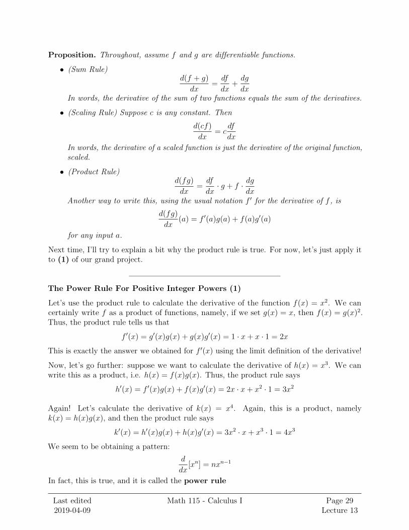
The Power Rule For Positive Integer Powers (1)

Let’s use the product rule to calculate the derivative of the function f(x) = x2. We cancertainly write f as a product of functions, namely, if we set g(x) = x, then f(x) = g(x)2.Thus, the product rule tells us that

f ′(x) = g′(x)g(x) + g(x)g′(x) = 1 · x+ x · 1 = 2x

This is exactly the answer we obtained for f ′(x) using the limit definition of the derivative!

Now, let’s go further: suppose we want to calculate the derivative of h(x) = x3. We canwrite this as a product, i.e. h(x) = f(x)g(x). Thus, the product rule says

h′(x) = f ′(x)g(x) + f(x)g′(x) = 2x · x+ x2 · 1 = 3x2

Again! Let’s calculate the derivative of k(x) = x4. Again, this is a product, namelyk(x) = h(x)g(x), and then the product rule says

k′(x) = h′(x)g(x) + h(x)g′(x) = 3x2 · x+ x3 · 1 = 4x3

We seem to be obtaining a pattern:

d

dx[xn] = nxn−1

In fact, this is true, and it is called the power rule



Proposition (Power Rule). Let n > 0 be an integer. Then

d

dx[xn] = nxn−1

Proof. We can actually prove this by extending the same calculation we did above; we usedthe derivative of x to calculate the derivative of x2, we used the derivative of x2 to calculatethe derivative of x3, we used the derivative of x3 to calculate the derivative of x4. In fact,you can keep going. Here are the details:

Suppose we already know that the derivative of xn is nxn−1. Then xn+1 = xn · x, so usingthe product rule, we have

d(xn+1)

dx=d(xn)

dx· x+ xn · dx

dx= nxn−1 · x+ xn · 1 = (n+ 1)xn

Thus, if the derivative of xn is what the power rule predicts, then so is the derivative of xn+1.Since we know the power rule is correct for the derivative of x1, this argument shows thatit’s correct for x2, x3, x4, x5, and so on forever!

(This ‘‘knocking over all the dominoes argument’’ is an extremely important technique calledmathematical induction.)

Example. We now have enough technology to calculate the derivative of any polynomialfunction. This is because polynomials are just sums of scaled copies of the power functions xn

for n ≥ 0, so we can use the Sum Rule, Scaling Rule, and Power Rule in tandem to calculatethe derivative. For example,

d

dx[2x3 − 7x+ 2] = 2

d

dx[x3]− 7

d

dx[x] +

d

dx[2] = 2 · 3x2 − 7 · 1 + 0 = 6x2 − 7

For the rest of class, let’s use this technology to study the graphs of polynomial functions.

Exercise. Consider the polynomial function p(x) = x3 − 3x+ 1.

(a) At what points on the graph of p is the slope of the tangent line equal to 45?

(b) On what intervals is p increasing? On what intervals is it decreasing?

(c) On what intervals is p concave up? On what intervals is it concave down?

Exercise. Consider the polynomial function q(x) = x2 − 2x+ 4. Find the equations of thelines through the origin that are tangent to the graph of q.

Exercise. Consider the polynomial function r(x) = (x− 1)(x+ 0.5)(x+ 1.5)(. There is aunique line that is tangent to the graph of r at two distinct points. Find the equation of thisline.

(You may have to use a calculator/computer!)



Lecture 14 (2019-02-19)

Today, we start off by working on (2) of our differentiation toolkit project.

Why Is The Product Rule True?

Recall that if f and g are differentiable functions, then the product rule says that

d(fg)

dx=df

dx· g + f · dg

dx

Why is this true? Recall that for any number a, we have linear approximations to f and gnear a. These linear approximations say that for sufficiently small h, we have

f(a+ h) ≈ f(a) + f ′(a)h

g(a+ h) ≈ g(a) + g′(a)h

Let k(x) = f(x)g(x). Multiplying these, we get an approximation for k near x = a, namely

f(a+ h)g(a+ h) ≈ f(a)g(a) + (f(a)g′(a) + f ′(a)g(a))h+ f ′(a)g′(a)h2

=⇒ k(a+ h) ≈ k(a) + (f(a)g′(a) + f ′(a)g(a))h+ f ′(a)g′(a)h2

for small h. (Look at that coefficient of h!) We can use this approximation to calculate k′(a)using the limit definition of the derivative:

k′(a) = limh→0

k(a+ h)− k(a)

h≈ lim

h→0

(f(a)g′(a) + f ′(a)g(a))h+ f ′(a)g′(a)h2

h= f(a)g′(a)+f ′(a)g(a)

The Quotient Rule

The product rule tells us how to calculate the derivative of a product of functions (in termsof the original functions and their derivatives). There is a similar rule that tells us how todifferentiate quotients of functions, which is aptly named the quotient rule:

Proposition (Quotient Rule). Suppose f and g are differentiable. Away from points wheref/g is undefined, we have

d(f/g)

dx=

df

dx· g − f · dg

dxg2

Proof. We can deduce the quotient rule from the product rule. Let h(x) = f(x)/g(x). Wewant to calculate h′(x) in terms of f , g, f ′, and g′. Writing f(x) = h(x)g(x), we can nowapply the product rule to obtain

f ′(x) = h′(x)g(x) + h(x)g′(x)

=⇒ h′(x) =f ′(x)− h(x)g′(x)

g(x)=f ′(x)− f(x)

g(x)g′(x)

g(x)=f ′(x)g(x)− g′(x)f(x)

g(x)2

as desired.



Example (Power Rule Holds For All Integer Exponents). Last class, we showed that

d

dx[xn] = nxn−1

when n is a positive integer. In fact, this is true even when n is a negative integer. This is animmediate consequence of the quotient rule. We are interested in calculating the derivativeof x−n when n > 0. Rewriting x−n = 1/xn, note that we can represent x−n as the quotientof two functions whose derivatives we already know, namely 1 and xn. It follows that

d

dx[x−n] =

d(1)

dx· xn − 1 · d(xn)

dxx2n

=−nxn−1

x2n= −nx−n−1

which is exactly what the power rule would predict!

Example. Now that we know the quotient rule, it is possible to calculate the derivative ofany rational function, since rational functions are just quotients of polynomials. Here’s aquick example:

d

dx

[x+ 1

2x− 1

]=

1 · (2x− 1)− 2(x+ 1)

(2x− 1)2=

1

(2x− 1)2

The Chain Rule

The chain rule tells you how to calculate the derivative of the composite of two functionsin terms of the original functions and their derivatives. Let’s try to figure out what thisrule should be, using linear approximation. Suppose f and g are differentiable functions,and we are interested in differentiating k(x) = f(g(x)) at x = a. Near a, we have the linearapproximation

g(a+ h) ≈ g(a) + g′(a)h

Similarly, near g(a), we have the linear approximation

f(g(a) + h) ≈ f(g(a)) + f ′(g(a))h

for sufficiently small h. It follows that

k′(a) = limh→0

k(a+ h)− k(a)

h= lim

h→0

f(g(a+ h))− f(g(a))

h

≈ limh→0

f(g(a) + g′(a)h)− f(g(a))

h≈ lim

h→0

f(g(a)) + f ′(g(a))g′(a)h− f(g(a))

h= f ′(g(a))g′(a)

We have therefore ‘‘proven’’ the:

Proposition (Chain Rule). If f and g are differentiable functions, then

d(f g)

dx(a) =

df

dx(g(a)) · dg

dx(a)

Another (less unwieldy) way of expressing this rule is to say that the derivative of (f g)(x)is f ′(g(x))g′(x).



Example (Power Rule Holds For All Rational Exponents). At this point, we know thepower rule

d

dx[xn] = nxn−1

is true whenever n is an integer. In fact, this is true when n is any rational number, andwe can deduce this quickly using the chain rule. Given a rational number n, write n = p/qwhere p and q are integers. We want to differentiate f(x) = xn = xp/q. Taking the qthpowers of both sides, we see that f(x)q = xp. Now, the left hand side can be expressed ash(f(x)) where h(x) = xq, so the chain rule implies that its derivative is

d

dx[left hand side] = h′(f(x))f ′(x) = q(f(x))q−1f ′(x)

Furthermore,d

dx[right hand side] = pxp−1

It follows that

f ′(x) =pxp−1

q(f(x))q−1=

pxp−1

qxp(q−1)/q=p

qxp−1−p+(p/q) =

p

qx(p/q)−1 = nxn−1

Example. We now know the power rule holds for any rational exponents. Using this fact intandem with the chain rule, we can differentiate any function that involves only radicals andpower functions. For example, consider the function f(x) = 3

√x2 + 1. We can write this as a

composition f(x) = k(`(x)) where k(x) = 3√x and `(x) = x2+1. We know k′(x) = (1/3)x−2/3

using the power rule for rational exponents. Thus, the chain rule implies

f ′(x) = k′(`(x))`′(x) =1

3(x2 + 1)−2/3 · 2x

Let’s finish off today with a bit of work on (1).

Derivatives of Exponential Functions

We want to differentiate the exponential function ax. Recall that we can change bases andwrite ax = eln(a)x. Write f(x) = ex, so that ax = f(ln(a)x). Now, by the chain rule, it followsthat

d

dx[ax] = f ′(ln(a)x) · ln(a)

so to calculate the derivative of ax for any exponential base a, it will suffice to know thederivative of ex.

Let’s try to calculate this derivative using the limit definition:

f ′(x) = limh→0

ex+h − ex

h= ex lim

h→0

eh − 1

h=: Lex

Exercise: Estimate L and make a conjecture as to its exact value.



Lecture 15 (2019-02-20)

Expectations for Individual Meetings

I would like the individual meetings to be a way to discuss your performance on the firstexam and your comfort with the material thus far, making a plan for moving forward ifnecessary. To prepare for the meeting, please review your first exam and be ready to explainwhat mistakes you made. Grading for these meetings will be solely participation-based (asin, show up and be ready to discuss the midterm).

I’ll start by writing down some of the material we covered last class but that wasn’t in thenotes.

Derivatives of Logarithmic Functions

The key fact from which you can calculate the derivative of any exponential function is that

d

dx[ex] = ex

i.e. the function ex is its own derivative. Similarly, recall that for any a, we have the changeof base formula loga(x) = ln(x)/ ln(a). This implies that

d

dx[loga(x)] =

1

ln(a)

d

dx[ln(x)]

so to calculate the derivative of any logarithmic function, it will suffice to figure out what thederivative of ln(x) is. To do this, recall that ln(x) is defined as the inverse of the exponentialfunction ex, so in particular satisfies the equation

eln(x) = x

Differentiating both sides of this equation (and applying chain rule to do so) yields theequation

x · ddx

[ln(x)] = eln(x) · ddx

[ln(x)] =d

dx[eln(x)] =

d

dx[x] = 1

It follows thatd

dx[ln(x)] =

1

x

(Note that the derivative of ln(x), which is related to exponential/logarithmic functions, is apower function! This is a surprising and extremely important fact in math, and people havebuilt careers off of exploiting this relationship.) Therefore, we have

d

dx[loga(x)] =

1

x ln(a)



Derivatives of Inverse Functions

To calculate the derivative of ln(x), we used the equation that defines it as the inverse ofex, namely eln(x) = x. More generally, if f is any invertible function, we have the definingequation f(f−1(x)) = x. Just as above, we can differentiate this equation and obtain ageneral formula for the derivative of the inverse of a function:

f ′(f−1(x))(f−1)′(x) =d

dx[f(f−1(x))] =

d

dx[x] = 1

=⇒ (f−1)′(x) =1

f ′(f−1(x))

I would highly recommend that you do not memorize this formula, as it is easy to mix upthe ′ and −1. Instead, understand that it comes from differentiating the defining relation ofan inverse function.

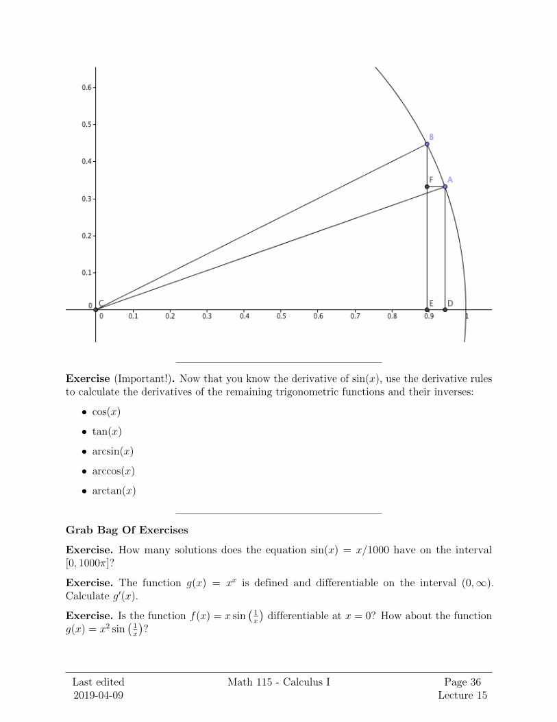
Derivatives of Trigonometric Functions

Today, we will continue (1) by figuring out the derivatives of trigonometric functions. Sincethese are all built out of sin and cos, we need to calculate the derivatives of sin and cos andthen use our rules to compute the derivatives of functions ‘‘built out of’’ sin and cos (e.g.tan, arcsin, etc). In fact, since cos is just a transformed copy of sin, it will suffice to calculatethe derivative of sin by hand.

To do this, we use the geometry of the unit circle. Suppose θ is an angle and θ + h is a smallperturbation of this angle. Let A be the point on the unit circle at an angle of θ (measured,as usual, counterclockwise from the positive x-axis) and let B be the point at an angle ofθ + h. Recall that sin(θ) is the y-coordinate of A and sin(θ + h) is the y-coordinate of B.Thus, sin(θ + h)− sin(θ) is the length FB in the image below. Note that the length of thecircular arc BA is exactly h, and as h gets smaller, this arc more and more closely resemblesa straight line segment. Thus, when h is very small, we have

sin(θ + h)− sin(θ)

h≈ sin(∠BAF )

Moreover, when h is very small, the angle ∠BAC gets very close to 90, so

∠BAF = ∠BAC − ∠FAC = ∠BAC − ∠ACD = ∠FAC − θ

gets very close to π2− θ (when measured in radians). Thus, we see that

limh→0

sin(θ + h)− sin(θ)

h= sin

(π2− θ)

= cos(θ)

We conclude thatd

dx[sin(x)] = cos(x)



Exercise (Important!). Now that you know the derivative of sin(x), use the derivative rulesto calculate the derivatives of the remaining trigonometric functions and their inverses:

• cos(x)

• tan(x)

• arcsin(x)

• arccos(x)

• arctan(x)

Grab Bag Of Exercises

Exercise. How many solutions does the equation sin(x) = x/1000 have on the interval[0, 1000π]?

Exercise. The function g(x) = xx is defined and differentiable on the interval (0,∞).Calculate g′(x).

Exercise. Is the function f(x) = x sin(1x

)differentiable at x = 0? How about the function

g(x) = x2 sin(1x

)?



Lecture 16 (2019-02-22)

A plane curve is the set of points in the coordinate plane determined by an equation of theform f(x, y) = 0. For example, if f(x, y) = x2 + y2 − 1, then the corresponding plane curveis the set of points whose coordinates satisfy x2 + y2 = 1, i.e. the unit circle.

We are interested in studying plane curves for two reasons:

• They are a vast class of examples with lots of interesting geometry.

• Oftentimes in real life, quantities of interest are constrained to satisfy particularequations. To visualize these quantities, one would then study the corresponding planecurves. For example, if a bug was moving on the unit circle, its coordinates (x, y) atany point in time would have to satisfy x2 + y2 = 1.

The key point is that by suitably restricting their domains (I won’t get into this, but askme if you’re curious), the quantities x and y that are constrained to lie on the plane curvef(x, y) = 0 may be thought of as functions of one another, i.e. y = y(x) or x = x(y). Moreprecisely, when the domain of x is suitably restricted, for each x in the restricted domain thereis a unique y = y(x) such that f(x, y(x)) = 0; we can then study this function x 7→ y(x).

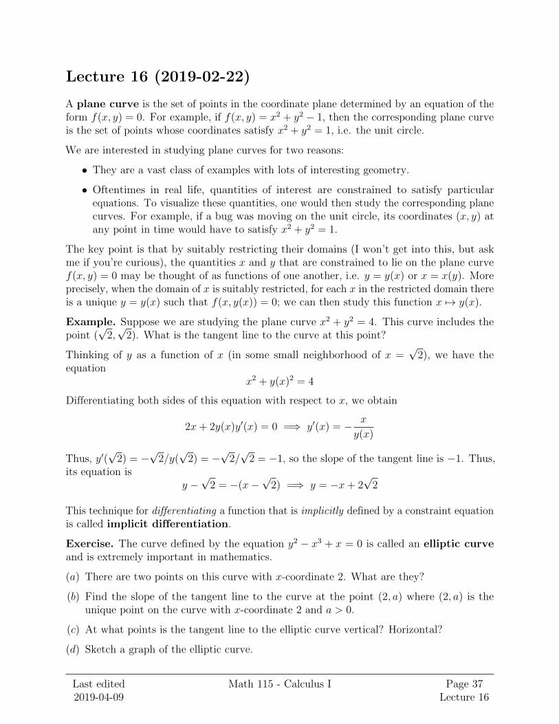
Example. Suppose we are studying the plane curve x2 + y2 = 4. This curve includes thepoint (

√2,√

2). What is the tangent line to the curve at this point?

Thinking of y as a function of x (in some small neighborhood of x =√

2), we have theequation

x2 + y(x)2 = 4

Differentiating both sides of this equation with respect to x, we obtain

2x+ 2y(x)y′(x) = 0 =⇒ y′(x) = − x

y(x)

Thus, y′(√

2) = −√

2/y(√

2) = −√

2/√

2 = −1, so the slope of the tangent line is −1. Thus,its equation is

y −√

2 = −(x−√

2) =⇒ y = −x+ 2√

2

This technique for differentiating a function that is implicitly defined by a constraint equationis called implicit differentiation.

Exercise. The curve defined by the equation y2 − x3 + x = 0 is called an elliptic curveand is extremely important in mathematics.

(a) There are two points on this curve with x-coordinate 2. What are they?

(b) Find the slope of the tangent line to the curve at the point (2, a) where (2, a) is theunique point on the curve with x-coordinate 2 and a > 0.

(c) At what points is the tangent line to the elliptic curve vertical? Horizontal?

(d) Sketch a graph of the elliptic curve.



Exercise. The curve defined by the equation x2/3 + y2/3 = 2 is called an astroid.

There is a unique point P on the astroid which is in the second quadrant and has anx-coordinate of −1/8. What is the slope of the tangent line to the astroid at P?

Exercise. Investigate the plane curve given by equation x3 + y3 = 3xy − 1. Calculate theslopes of the tangent lines at various points on this curve (use a calculator if necessary). Doyou notice anything interesting? Can you explain your observations?



Lecture 17 (2019-02-26)

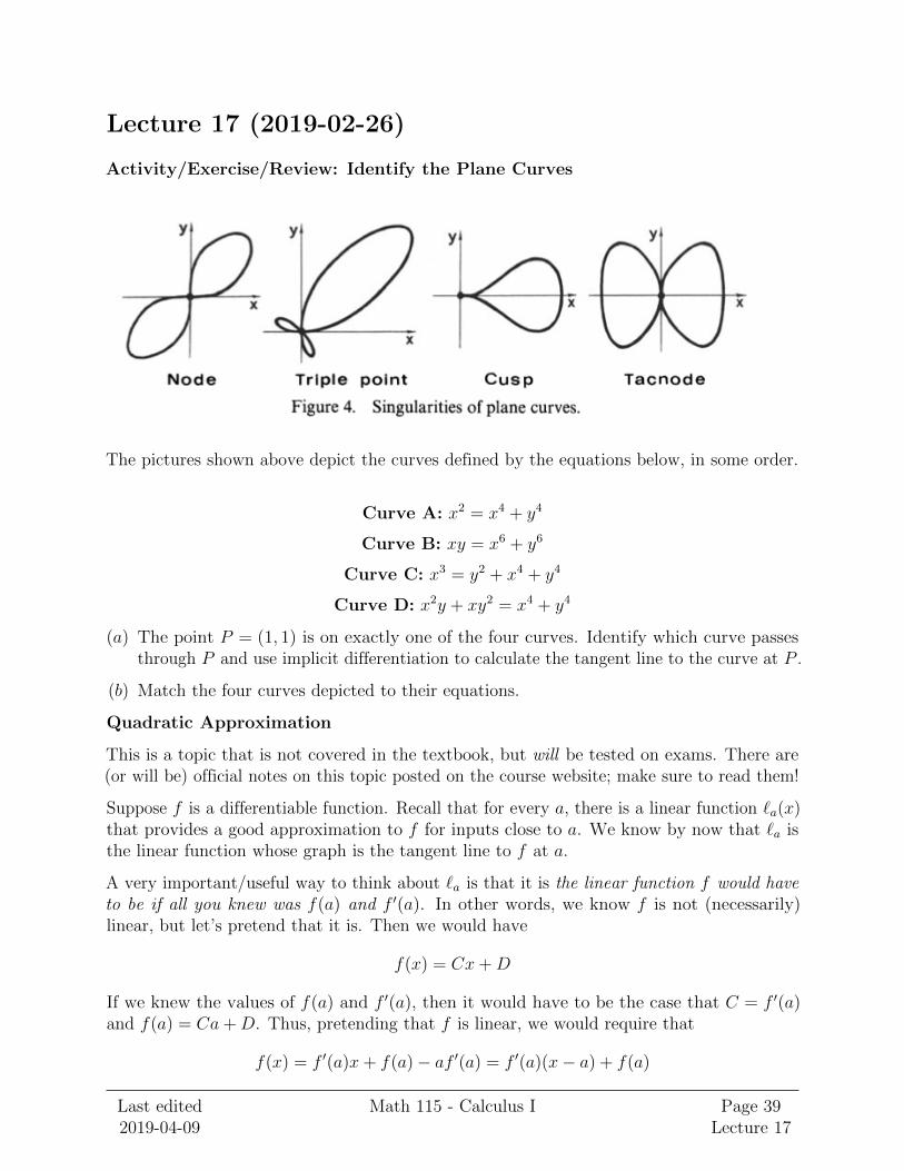
Activity/Exercise/Review: Identify the Plane Curves

The pictures shown above depict the curves defined by the equations below, in some order.

Curve A: x2 = x4 + y4

Curve B: xy = x6 + y6

Curve C: x3 = y2 + x4 + y4

Curve D: x2y + xy2 = x4 + y4

(a) The point P = (1, 1) is on exactly one of the four curves. Identify which curve passesthrough P and use implicit differentiation to calculate the tangent line to the curve at P .

(b) Match the four curves depicted to their equations.

Quadratic Approximation

This is a topic that is not covered in the textbook, but will be tested on exams. There are(or will be) official notes on this topic posted on the course website; make sure to read them!

Suppose f is a differentiable function. Recall that for every a, there is a linear function à(x)that provides a good approximation to f for inputs close to a. We know by now that à isthe linear function whose graph is the tangent line to f at a.

A very important/useful way to think about à is that it is the linear function f would haveto be if all you knew was f(a) and f ′(a). In other words, we know f is not (necessarily)linear, but let’s pretend that it is. Then we would have

f(x) = Cx+D

If we knew the values of f(a) and f ′(a), then it would have to be the case that C = f ′(a)and f(a) = Ca+D. Thus, pretending that f is linear, we would require that

f(x) = f ′(a)x+ f(a)− af ′(a) = f ′(a)(x− a) + f(a)



which is exactly the linear approximation à to f at a!

Recap: if we pretend f is linear, then the ‘‘local’’ information f(a) and f ′(a) would implythat f = à.

We can carry out an entirely analogous procedure where we pretend that f is quadratic andask, based on information coming from x = a, what quadratic does f have to be?

Let’s carry out this procedure in the case where a = 0. Pretend f is a quadratic function, i.e.

f(x) = Cx2 +Dx+ E

and suppose we know the values f(0), f ′(0), and f ′′(0). It follows that E = f(0), D = f ′(0),and C = f ′′(0)/2.

Thus, if f was a quadratic function compatible with the given values of f(0), f ′(0), and f ′′(0),it would have to equal (f ′′(0)/2)x2 + f ′(0)x+ f(0). This is the ‘‘best quadratic function’’ thatfits the ‘‘second order information’’ coming from f .

More generally, let a be any number. Near 0, the function g(x) = f(x+ a) looks exactly likef does near a; in particular, g(0) = f(a), g′(0) = f ′(a), and g′′(0) = f ′′(a). As we saw above,the quadratic best approximating g near 0 is given by

(g′′(0)/2)x2 + g′(0)x+ g(0) = (f ′′(a)/2)x2 + f ′(a)x+ f(a)

Thus, the quadratic best approximating f near a should be the above function, but translateda units to the right.

Putting all this together, we have:

Fact. The quadratic approximation to f(x) near x = a is given by the formula

qa(x) = f(a) + f ′(a)(x− a) +f ′′(a)

2(x− a)2

In particular, note that

qa(x) = à(x) +f ′′(a)

2(x− a)2

i.e. it is the linear approximation to f at a, plus a ‘‘quadratic correction’’ term.

Exercise. Consider the function f(x) = ln(x).

(a) Is the linear approximation to f(x) near (1, 0) an overestimate or an underestimate (orneither) for the actual values of f(x)?

(b) Use the linear approximation for f(x) near (1, 0) to estimate ln(1.1). Then, use thequadratic approximation for f(x) near (1, 0) to estimate ln(1.1). Is the quadratic estimatebetter than the linear estimate?



Lecture 18 (2019-02-27)

Some Review on Linear and Quadratic Approximation

Exercise. 1. Let g(s) = cos(s). Calculate the linear and quadratic approximations to gat s = π/2. Use these approximations to estimate cos(1.6).

2. Suppose z is a twice-differentiable function with z(1) = 5, z′(1) = −2, and z′′(1) = 3.Estimate z(0.9) using the linear approximation to z at 1. Do you expect this value willbe an over-estimate or under-estimate? Explain your reasoning.

3. Suppose f is a differentiable function, and let q be the quadratic approximation to f atx = 1. Given that q(1) = 1, q(2) = −2, and q(3) = 4, find f(1), f ′(1), and f ′′(1).

The Mean Value Theorem

The mean value theorem is intuitively ‘‘obvious’’, but important on account of encapsulatingthe obvious intuition in a piece of rigorous mathematics.

Theorem (Mean value Theorem). Suppose f is continuous on the closed interval [a, b] anddifferentiable on the open interval (a, b). Then, the average rate of change of f on [a, b]is attained by the derivative f ′ at some point in (a, b). More precisely, there exists somec ∈ (a, b) such that

f ′(c) =f(b)− f(a)

b− aExample. Consider the function f(x) = x2 − 2x+ 3. On the interval [0, 3], the average rateof change of f is

f(3)− f(0)

3− 0=

6− 3

3− 0= 1

so the mean value theorem predicts that there must exist some c ∈ [0, 3] such that f ′(c) = 1.Indeed, we can calculate f ′(x) = 2x − 2; this equals 1 precisely when x = 1.5, which iscertainly in the interval [0, 3]. Thus, the average rate of change of f on [0, 3] is attained asan instantaneous rate of change at a ‘‘moment’’ in [0, 3].

Example (A Fable). The following story is definitely not true, but calculus teachers oftenlike to claim that it is, because it makes them feel powerful.

A couple of years ago, I drove up to the Bay Area, which is 400 miles, and I drove fast, so ittook me five hours. At the end of the trip, I slowed down, because I didn’t want to get aticket, and when I got off the freeway, I was traveling at the speed limit. Then a policeofficer pulled me over, and he said, ”You were going a little fast there.” I said I was goingthe speed limit, but he responded, ”Maybe you were a little while ago, but earlier, you werespeeding.” I asked how he knew that, and he said, ”Son, by the mean value theo rem ofcalculus, at some moment in the last five hours, you were going at exactly 80 m.p.h.”

I took the ticket to court, and when push came to shove, the officer was unable to prove themean value theorem beyond a reasonable doubt.



Exercise (based on the fable above). (a) Assuming the officer could prove the mean valuetheorem beyond a reasonable doubt, would his statement have been correct? Explainyour reasoning.

(b) Suppose we change the ending of the story so that the officer said, ”I can’t prove the meanvalue theorem, your Honor, but I can prove the intermediate value theorem, and usingthis I can show that there was a time interval of exactly one minute during which thedefendant drove at an average speed of 80 miles per hours.” Explain the cop’s reasoning.

Exercise. (a) Let k(i) = i2 + 7i + 5. Find all values c ∈ (−1, 2) at which h satisfies theconclusion of the mean value theorem for the interval [−1, 2].

(b) Let h(y) = sin(y). Find all values c ∈ (0, 5π/2) at which h satisfies the conclusion of themean value theorem for the interval [0, 5π/2].

Grab Bag Of Chapter 3 Review Exercises

Exercise. The function g : R → R is differentiable and has a differentiable inverse. If(g−1)′(3) = 2 and g(2) = 3, what is g′(2)?

Exercise. The nth Chebyshev polynomial is the unique polynomial Tn such that Tn(cos(θ)) =cos(nθ) for all θ ∈ [0, 2π]. What is T10

′(1/2)?

Exercise. Suppose a is the unique solution in (−∞,∞) to the equation x = cos(x). Withoutusing a calculator, estimate the value of a.

Exercise. The picture below depicts three surfaces in three-dimensional space, and theequations that cut them out. Match the equations to the pictures.

Exercise (Extra Credit -- tricky, but doable). Calculate f ′′′(0), where f is given by

f(x) = sin(sin(· · · sin(x) · · · ))︸︷︷︸2019 iterations of sine



Lecture 19 (2019-03-11)

Using Calculus For Optimization

In Chapter 4, our focus will be on optimization problems. From the perspective ofmany applications, optimization is essentially the raison d’etre of calculus. The problem ofoptimization is, in a nutshell, to find the maximum/minimum values attained by a functionof interest. For instance, a company interested in maximizing profits might develop amathematical model for its activities then use the tools of calculus to find the parameters atwhich the company makes the most money (e.g., the optimal amount of labor to enlist, theoptimal amount of initial capital to invest, etc.).

Definition. Let f be any function.

• We say f has a local minimum at p ∈ Dom(f) if f(p) ≤ f(p+ h) for all sufficientlysmall h. In other words, the value of f at p is lower than all the nearby values.

• We say f has a local maximum at p ∈ Dom(f) if f(p) ≥ f(p+ h) for all sufficientlysmall h. In other words, the value of f at p is higher than all the nearby values.

• We say f has a local extremum at p ∈ Dom(f) if f has either a local maximum orlocal minimum at p.

Definition. Let f be any function.

• We say f has a global minimum at p ∈ Dom(f) if f(p) ≤ f(x) for all x ∈ Dom(f).In other words, the value of f at p is lowest possible value attained by f .

• We say f has a global maximum at p ∈ Dom(f) if f(p) ≥ f(x) for all x ∈ Dom(f).In other words, the value of f at p is highest possible value attained by f .

• We say f has a global extremum at p ∈ Dom(f) if f has either a global maximumor global minimum at p.

Remark. Note that if f has a global minimum/maximum at p, then it certainly has a localminimum/maximum at p as well. However, a local minimum/maximum is not necessarily aglobal minimum/maximum.

Examples. (a) The function s(t) = t3 − t has a local maximum at t = −1/√

3 but s doesnot have a global maximum, since as t→∞, we have s(t)→∞. Similarly, s has a localminimum at t = 1/

√3 but has no global minimum. Note that the inputs ±1/

√3 are

precisely the zeroes of the derivative function s′(t); studying the zeroes of the derivativeis an important way to detect mins/maxes, as we’ll see presently.

(b) The function q(s) = 3− |s− 1| has a global maximum at s = 1. Note that this globalmaximum is attained at a point where q is not differentiable.

(c) Consider the function `(q) = bqc, where bqc denotes the greatest integer less than orequal to q; in other words, ` is the ‘‘round down’’ function, with `(3.4) = 3, `(5) = 5,and `(−2.3) = −3. (We saw this function on a quiz a while ago!) Note that ` has noglobal extrema. However, by our definition of local min/max, the function ` has a local



maximum at every input q ∈ (−∞,∞)! The local minima are precisely at the inputsthat are not whole numbers.

Today, we will focus on how to use calculus to detect local maxima and minima. Here is themain theorem:

Theorem (Key Theorem On Local Extrema/First Derivative Test). Suppose f is differen-tiable on some open interval I, and p ∈ Dom(f).

• The function f has a local minimum at p if there is some h > 0 such that f ′ < 0 onthe interval (p− h, p) and f ′ > 0 on the interval (p, p+ h). In words, the sign of thederivative changes from negative to positive at p.

• The function f has a local maximum at p if there is some h > 0 such that f ′ > 0 onthe interval (p− h, p) and f ′ < 0 on the interval (p, p+ h). In words, the sign of thederivative changes from positive to negative at p.

In particular, if f has a local extremum at p, then f ′(p) = 0.

Remark (Warning). Even if f ′(p) = 0, this does not imply that f must have a localextremum at p. For example, the function g(s) = s3 has g′(0) = 0, but has neither a localmaximum nor local minimum at 0. Indeed, the derivative does not change sign at 0.

Slogan: Local extrema occur where the derivative of a function changes sign.

Note that the key theorem tells us about the case where the function f is differentiable onthe interval of interest. In this case, local extrema can only occur at points p with f ′(p) = 0(but again, every such point need not be a local extremum). On the other hand, we may beworking with a function that is not differentiable at certain points; it is important to checkthese points as well to determine if they are local extrema.

Definition. Suppose f is a continuous function. A point p ∈ Dom(f) is called a criticalpoint if either:

• f is not differentiable at p

• f is differentiable at p and f ′(p) = 0

Corollary (Corollary of Key Theorem). If a function f has a local extremum at p, then p isa critical point of f .

Exercise. Find all critical points of the following functions. Use this information to determineand classify their local extrema. Can you say anything about global extrema?

(a) z(q) = q3(q − 1)2

(b) Θ(β) = ln(β/ ln(β))

(c) t(x) =√x+ 1√

x

(d) x(h) = |h− 1| − |h− 2|+ |h− 3|



Lecture 20 (2019-03-12)

Second Derivative Things

Yesterday, we talked about how to detect local extrema of functions using the first derivativetest. If a function is in fact twice-differentiable, we can alternatively use the ”second derivativetest” to detect when a local extremum occurs and whether or not it is a local maximum orlocal minimum.

Theorem (Second Derivative Test). Suppose f is twice-differentiable on some interval I,and p ∈ I.

• If f ′(p) = 0 and f ′′(p) > 0, then f has a local minimum at p.

• If f ′(p) = 0 and f ′′(p) < 0, then f has a local maximum at p.

• If f ′(p) = 0 and f ′′(p) = 0, then the test is inconclusive.

Remark (Warning). The second derivative test can be inconclusive, as in the examplef(x) = x4 at x = 0. Indeed, we then have f ′(0) = f ′′(0) = 0. When the second derivativetest is inconclusive, you should fall back on the first derivative test. In this case, f ′(x) = 4x3

so f ′ has a sign change at 0 from negative to positive. So the critical point at x = 0 is a localminimum.

Our interest in points where f ′ changes sign led us to study critical points. There is a similarnotion of where f ′′ changes sign, called inflection points. Geometrically, this is a placewhere the graph of the function changes concavity (i.e. goes from concave up to concavedown or concave down to concave up).

Definition. Let f be any function. A point p is an inflection point of f if the concavityof f changes at p.

If f is actually twice-differentiable, we can interpret this in terms of the second derivative:

• p is an inflection point if f ′′ changes sign at p.

In this situation, another useful rephrasing is to say that:

• p is an inflection point if f ′ has a local extremum at p.

Fact. If p is an inflection point of f , then f ′′(p) = 0. The converse is not necessarily true,e.g. f(x) = x4 at x = 0.

Exercise. Study the function f(x) = xe−x. Find its critical points and inflection points,determine where it is increasing/decreasing/concave up/concave down, and use all of thisinformation to sketch an accurate graph of the function. (Don’t use a graphing calculator!)



Global Optimization

The techniques we’ve discussed so far allow us to find the local extrema of a function. Tofind global extrema, we only need to work a little bit harder. The key point is that everyglobal extremum of a function is a local extremum. Thus, to find the global extrema, wehave the following heuristic procedure:

Heuristic Algorithm For Finding Global Extrema:

1. Find the critical points of your function. Use the first derivative/second derivative testto classify these critical points and determine the local extrema.

2. Compute the value of the function at the local extrema and pick out candidates forglobal maximum and global minimum (which, if they exist, must be among these localextrema).

3. Determine if the candidates for global max/min are actually global max/min by studyingthe end behavior of the function (i.e., the behavior as input values approach ±∞ or anendpoint of the domain).

Examples. (a) The global extrema of a function depend heavily on the domain of consider-ation. For example, consider the function f(x) = x2. On the domain [1,∞) it attains aglobal minimum at x = 1 and has no global maximum. On the domain [−0.5, 1] it attainsa global maximum at x = 1 and global minimum at x = 0. On the domain (−∞,∞) itattains a global minimum at x = 0 and has no global maximum.

(b) Let’s work out an example in its entirety. We want to find the global extrema of thefunction

g(t) =e−t/2

1 + t2

Every global extremum has to be a local extremum, so let’s start by finding the localextrema. We calculate

g′(t) = −e−t/2(t2 + 4t+ 1)

(1 + t2)2

The zeroes of this function are at

t = −2±√

3

and these are the only critical points, since the function is everywhere differentiable. Callthese zeroes α = −2−

√3 and β = −2 +

√3. Then we have

g′(t) = h(t)(t− α)(t− β)

where h(t) is some function that’s always negative. Thus, we have that g′ is

− · − · − = −

on (−∞, β), it’s− · − ·+ = +



on (β, α), and it’s− ·+ ·+ = −

on (α,∞). So the critical point at β is a local minimum and the critical point at α is alocal maximum (note that this is definitely a situation where we want to sue the firstderivative test and not the second derivative test; calculating the derivative of g′ lookslike pain).

We now have to determine if the local extrema at α and β are global extrema. Since gwas increasing on (β, α), we at least know g(β) < g(α). What’s left is to figure out if thefunction ever takes on values lower than g(β) or higher than g(α). Indeed, as t→∞,we have g(t)→ 0 (from above), so in particular it must eventually attain values lowerthan g(β) (which is positive). Similarly, as t→ −∞, we have g(t)→∞, so in particularit must attain values greater than g(α). So neither α nor β is a global extremum!

(c) Let’s do another example. We want to find the global extrema of the function

h(x) =

−xex x ≤ 0

−x 0 ≤ x ≤ 4

−√x− 1− 4 +

√3 4 ≤ x ≤ 7

Assume the domain of h is precisely (−∞, 7]. First, we determine the critical points.On the intervals (−∞, 0), (0, 4), and (4, 7), the function is differentiable, so on thoseintervals we should just find where the derivative equals 0. On (−∞, 0) we find a criticalpoint at x = −1, and this is a local max. On (0, 4) and (4, 7), the calculation reveals nocritical points.

Now we should examine the points x = 0 and x = 4. At x = 0, the function is continuousand differentiable, so there is no critical point. At x = 4, the function is not differentiable,so there is a critical point, but a sign chart reveals that it is neither a local max ormin; in fact, h is decreasing to the left and right of x = 4. Accordingly, on [−1, 7] thefunction is decreasing, and on (−∞,−1) it is positive, so the global minimum occurs atthe endpoint x = 7. The global maximum occurs at the critical point x = −1.



Lecture 21 (2019-03-12)

A Review Problem

Exercise. For this exercise, consider the function

g(x) =

ex x ≤ 0

−ex ln(x) 0 < x ≤ 1

C(cos(πx) + 1) x > 1

where C > 0 is some positive constant.

(a) Where is g continuous? Where is g differentiable?

(b) Find the critical points of g, and use this information to find and classify the localextrema of g.

(c) Find the global maximum and minimum of g, if they exist. Your answer will depend onthe value of C.

Optimization Problems Galore

Now that we have developed the techniques necessary to determine extrema of functions,the next step is to apply this technology to actual optimization problems. In this class,optimization problems are typically of the following form:

• You are given a function you wish to optimize. This function often depends on morethan one variable/quantity.

• The input variables of the function of interest are required to satisfy certain constraintequations. This allows you to eliminate all but one of the variables in the function andtreat the problem as a single-variable optimization problem.

• Once you have a single-variable function and a domain on which you are required tooptimize it, you can go ahead and use single-variable calculus (i.e., the calculus we’vebeen studying) to solve the problem.

In practice, this process can be very challenging! In particular, the tricky part isoften figuring out to use your constraints to reduce to a single-variable optimization problem.Keep your wits about you.

Example. Alastair is trying to build a rectangular fence in his backyard in order to keepthe neighbors’ dogs from relieving themselves on his property. He has 500 meters of fencingmaterial to use. What is the maximum area he can enclose with his fence?

Suppose x is the length of the fence and y is the width. We wish to maximize the quantity

Area(x, y) = x · y



Since Alastair has 500 total meters of fencing material, assuming he uses all of the material,we have the constraint equation 2x+ 2y = 500 =⇒ x+ y = 250. Thus, the area functioncan actually be thought of as a single-variable function

Area(x) = x · (250− x)

where x is allowed to vary in the domain 0 ≤ x ≤ 250. We wish to maximize the function onthis domain.

Note that the derivative of Area(x) is Area′(x) = 250 − 2x, so there is a critical point atx = 125 (and the derivative is defined everywhere in (0, 250), so there are no other criticalpoints in the interior). Furthermore, Area′ is negative for all x > 125 and positive for allx < 125, so the local maximum at x = 125 is actually a global maximum. We conclude thatArea(125) = 1252 meters2 is the maximum area enclosed by a fence.

Example. Let’s do a harder one. Suppose that the unit circle encloses a lake, in whichAndy’s friend is drowning. Andy’s friend is located at the point (−0.5, 0.5), and Andy isinitially located at the point (1, 0). Suppose that Andy swims half as fast as he is able to runon land. Where should he jump into the lake?

We assume that Andy runs along the circumference of the lake for some time, then jumpsinto the lake and swims in a straight line towards his friend. The question is, where shouldAndy jump in to the lake?

Let v be Andy’s speed on land, so that v/2 is his swimming speed. Suppose he decides tojump into the lake at the point on the unit circle located at an angle θ counterclockwisefrom (1, 0) (i.e., Andy’s initial position). The coordinates of this point are (cos(θ), sin(θ)).The amount of time it takes Andy to run from (1, 0) to (cos(θ), sin(θ)) is θ/v, and then theamount of time it takes Andy to swim to his friend is√

(cos(θ) + .5)2 + (sin(θ)− .5)2/(v/2)

so the function we want to minimize is

t(θ) = θ/v +√

(cos(θ) + .5)2 + (sin(θ)− .5)2/(v/2)

We wish to minimize this function on the domain 0 ≤ θ ≤ 2π, on which the function iscontinuous and differentiable on the interior.

We calculate

t′(θ) =1

v

(− sin(θ)− cos(θ)√

(sin(θ)− .5)2 + (cos(θ) + .5)2+ 1

)The critical points of t therefore occur at solutions to

−√

(sin(θ)− .5)2 + (cos(θ) + .5)2 = − sin(θ)− cos(θ)

Squaring this equation yields

((sin(θ)− .5)2 + (cos(θ) + .5)2) = (sin(θ) + cos(θ))2



Expanding gives(1.5− sin(θ) + cos(θ)) = 1 + 2 sin(θ) cos(θ)

At this point, we have the equation in a simple enough form that we may want to justput it in a calculator. The calculator will actually find that there are solutions in [0, 2π] atθ = π/6, 2π/3, 5π/6, 4π/3. Substituting these solutions back into the formula for t′(θ), wefind that critical points only occur at π/6 and 2π/3 (since we squared a lot to get the trigequation we ultimately solved, some vestigial solutions were introduced).

Finally, making a sign chart and classifying the critical points, we find a local max at π/6and a local min at 2π/3. Comparing the values t(0) = t(2π) and t(2π/3), we find that thelocal min is actually a global min on [0, 2π]. Thus, Andy’s optimal strategy is to run aroundthe lake for 2π/3 radians, a.k.a. 120, and then begin swimming towards his friend!

Exercise. Suppose Andy is a faster swimmer than in the above scenario. For example,suppose he is only 1.75 times slower at swimming than running. Should he still run aroundthe lake for a while or should he start swimming from the get-go? What if he’s 1.5 timesslower at swimming? For what threshold value of vland/vwater does his optimal rescue planchange from ”run for a bit, then start swimming” to ”start swimming immediately”?

Here is a collection of more optimization problems, of varying difficulty. For the exam, youshould understand how to set up and solve problems like this. In particular, you’ll need torefresh some geometry formulas/write them on your notecard; a list of fair game formulas ison the course website.

In general, these problems are hard because they involve a three-step process of thinking abouta situation, converting it into math, and then doing calculus. For these word problems, andfor optimization in general, do not blindly apply formulas/algorithms. For basicallyevery formula/algorithm, there is some situation where it doesn’t apply, so makesure to understand what’s going on and what the words mean!

Exercise. You are building a cylindrical silo that holds 20 cubic meters of grain. Thematerial with which the top and bottom are built costs $10 per square meter, and thematerial with which the side is built costs $8 per square meter. Find the radius and heightof the most economical silo.

Exercise. A Norman window is a window constructed by adjoining a semicircle to the topof an ordinary rectangular window. What are the dimensions of the Norman window withperimeter 18 meters and maximum possible area?

Exercise. Let P = (5, 2). What is the point on the parabola y = x2 that is closest to P?

Exercise. Suppose three points are chosen on the unit circle. What is the maximum possiblearea of the triangle whose vertices are at these three points?



Lecture 22 (2019-03-29)

Families of Functions

In applications and in pure math, one is often interested in analyzing the behavior of familiesof functions as certain parameters that these families depend upon vary. For example, instatistics, one might be interested in how the shape of a statistical distribution changes asone varies parameters such as mean and standard deviation. Many questions of this type canbe analyzed using tools from calculus, and we’ll spend today working through some examples.A key tool to aid in visualizing/understanding here is Desmos, which has nice little slidersyou can use to vary parameters of interest.

Example. Consider the family of functions of the form

fa,b(x) = eax+bx2

In other words, for every pair of numbers (a, b), we can plug them into the expression aboveto obtain a specific function. We are now interested in answering specific questions aboutthis family of functions. For instance:

1. For which pairs (a, b) does fa,b have a global maximum? For which pairs does it havea global minimum? Neither?

2. For which pairs (a, b) does fa,b have no inflection point? For which pairs does it havetwo inflection points? Can fa,b have other numbers of inflection points?

Let’s work through these questions. You’ll see that the ideas/methods we’re using are exactlythe same as those we’ve been using to study extrema of functions for this whole chapter; theadded difficulty comes from working with the ‘‘varying constants’’ a and b.

The First Part: We first calculate f ′a,b(x) and find

f ′a,b(x) = eax+bx2

(a+ 2bx)

Thus, the function always has exactly one critical point, at x = −a/2b. Let’s now split intothree cases: when b > 0, b = 0, and b < 0.

Case 1, b > 0: By making a sign chart, we see that f ′a,b is negative for x < −a/2b and positivefor x > −a/2b. Since this is the only critical point of the function, it is a global minimum.

Case 2, b = 0: In this case, the function is just fa,b(x) = eax, which is a normal exponentialfunction; it has no global min/max.

Case 3, b < 0: By making a sign chart, we see that f ′a,b is negative for x > −a/2b and positivefor x < −a/2b. Since this is the only critical point of the function, it is a global maximum.

The Second Part: We now calculate

f ′′a,b(x) = eax+bx2

(a+ 2bx)2 + eax+bx2 · 2b = eax+bx

2

((a+ 2bx)2 + 2b)

The function fa,b will have no inflection points if f ′′a,b has no roots, which happens preciselywhen b > 0. Let’s now look at the remaining two cases.



Case 2, b = 0: In this case, the function is a standard exponential, which has no inflectionpoints.

Case 3, b < 0: In this case, we know from above that fa,b has a unique global maximum. Wecalculate that the critical points of f ′a,b occur at x = (±

√−2b− a)/(2b); denote these values

by r and s, where r < s. Then we can write

f ′′a,b(x) = eax+bx2 1

4b2(x− r)(x− s)

and now you can check that f ′′a,b does change sign at r and s, so they are both inflectionpoints.

Exercise. Consider the family of functions fa(x) = ln(x2 + a), where a ranges over allpositive numbers. For what value of a does the function fa(x) have inflection points atx = ±2019?

Exercise. Consider the family of functions

fa,b(x) = eax + ebx

where a, b range over all nonzero numbers. Explain why every function in this family isconcave up. For which pairs (a, b) does fa,b have a global minimum?

Exercise. Consider the family of functions fm,n(x) = xm(1 − x)n where m, n range overpositive integers. For which pairs (m,n) does the function fm,n have a global maximum?Where does it occur and what is its value?

Exercise. Consider the family of plane curves

Pa = (x, y) : y2 = x3 + ax+ 1

There is a number c such that for all a > c, the graph of Pa consists of one connected piece,and for all a < c, the graph of Pa consists of two distinct connected pieces. What is c?

Exercise (Extra Credit). Consider the family of functions

fn(x) = 2x + 3x − nx

For all n > 3, the function fn(x) has a global maximum; call this global maximum Mn. Whatis limn→∞Mn? Justify your answer.



Lecture 23 (2019-04-02)

Review Problem: Families of Functions

Consider the family of functions

fb(x) =x3

b+ ex

where b ranges over all real numbers.

For which values of b does fb have a global maximum? Global minimum? Local maximum?Local minimum? Justify your answers clearly using calculus.

(This problem, like many families of functions problems, is not so easy. Don’t forget to keepsight of what you’re trying to figure out, and make sure to draw/graph lots of pictures.)

Applications to Marginality a.k.a. the Econ Section

In this section, we will be doing exactly the same kinds of problems we’ve been doing sofar, but in the context of some new economics vocabulary. Businesses (typically) want tomaximize profit, which can be modeled as a function of the quantity q of goods produced. Inother words, we have a profit function π(q) which eats ‘‘quantity q of goods produced’’ andoutputs ‘‘profit π(q) made by the business at a production level of q.’’

We know thatprofit = revenue− cost

so, after inventing the revenue function R(q) (which eats quantity q of goods produced andoutputs the revenue obtained at this production level) and the cost function C(q) (whicheats quantity of goods produced and outputs the cost to produce this many goods), we havethe equation

π(q) = R(q)− C(q)

Here’s a bit of vocabulary: the fixed cost of an enterprise is the amount of money it costs toproduce no quantity of goods, i.e. C(0). This is typically a positive number, and it representsthe ‘‘startup’’ cost of the business, e.g., labor, rent, etc.

Here’s some more vocabulary: marginal cost is a fancy way to say ‘‘derivative of the costfunction.’’ Marginal revenue is, similarly, a fancy way to say ‘‘derivative of the revenuefunction’’.

We know that the maxima of a function occur at its critical points, so the maxima of the profitfunction should occur at values of q such that 0 = π′(q) = R′(q)− C ′(q) =⇒ R′(q) = C ′(q).In words, the maxima of the profit function can occur at values of q where marginal costequals marginal revenue. First off, keep in mind that this does not mean a maximum mustoccur when marginal cost equals marginal revenue (more generally, keep in mind that notevery critical point has to be an extremum). Second, do NOT memorize this piece ofvocabulary; instead, treat any of these ‘‘profit’’ problems exactly the way you would treat astandard optimization problem.



Exercise: Danny runs a company that used to make salt and vinegar chips. After realizingsalt and vinegar chips are terrible, he changed the direction of the company, and it nowproduces microchips. Suppose that the revenue function is given by

R(q) = 5q − 0.003q2

where q is the number of microchips produced and R(q) is the corresponding revenue, indollars. Similarly, suppose the cost function is given by

C(q) = 300 + 1.1q

where q is the number of microchips produced and C(q) is the cost of production, in dollars.If the company cannot afford to produce more than 800 microchips in total, what number ofmicrochips should it produce to maximize profit?



Lecture 24 (2019-04-03)

Related Rates

Today, we’re going to discuss a new problem type called related rates. These problems aresimilar to optimization word problems, in the sense that the set-up is often the hardest part.Just as for optimization word problems, we reduced to a calculus ‘‘find the global optima’’problem, here we will reduce related rates word problems to implicit differentiation problems.The premise of related rates problems is essentially the following:

• There are several quantities we are interested in, which are varying with respect tosome variable, typically time. These quantities will satisfy constraint equations, whichyou must find.

• Once you find the constraint equations, implicitly differentiate the equations withrespect to the (time) variable and use the resulting relations to calculate the desiredvalues.

Let’s see this premise in practice:

Example. Suppose 4ABC is a right triangle, with ∠ABC = 90. The legs AB and BC of4ABC are getting longer, at a rate of 3 m/s and 4 m/s, respectively. At what rate is thehypotenuse of 4ABC growing when the legs are of length AB = 5 and BC = 12?

For simplicity, let’s write AB = a, BC = b, and AC = c. These quantities depend on time,so we actually have functions a(t), b(t), and c(t). We are given that a and b are linearfunctions, with a′(t) = 3 and b′(t) = 4. We are asked to compute c′(s), where s is the timesuch that a(s) = 5 and b(s) = 12. Note that the Pythagorean theorem implies c(s) = 13.

We know that the functions a, b, and c satisfy the Pythagorean theorem:

a(t)2 + b(t)2 = c(t)2

By differentiating both sides of this equation with respect to t, we find

a′(t)a(t) + b′(t)b(t) = c′(t)c(t)

We want to calculate c′(s), so setting t = s in the equation, we have

c′(s) =a′(s)a(s) + b′(s)b(s)

c(s)=

3 · 5 + 4 · 12

13=

63

13

(The units of c′(s) are meters per second.)

Example. A spherical snowball is melting. Its radius is decreasing at a rate of 0.2 centimetersper hour, at the moment when its radius equals 15 centimeters. How fast is the volumedecreasing at this moment?

We have two quantities of interest, the radius r of the snowball and its volume V . These areboth functions r(t) and V (t) of time, which are related via the formula

V (t) =4π

3r(t)3



We wish to find V ′(s), where s is the moment in time when r(s) = 15; we are given thatr′(s) = −0.2. Differentiating the equation with respect to t, we find

V ′(t) = 4πr(t)2r′(t) =⇒ V ′(s) = 4πr(s)2r′(s) = 900π(−0.2) = −180π

(The units of V ′(s) are cubic centimeters per hour.)

Exercise. A ladder that is leaning against a wall starts slipping down. If the point wherethe ladder touches the ground is moving away from the wall at a constant rate, is the pointwhere the ladder touches the wall falling at a constant rate? Explain your answer clearly.

Exercise. Suppose a street lamp is located 10 meters above the ground. You are walkingaway from the street lamp at a rate of 1 meter per second. When you are 5 meters awayfrom the street lamp, what is the rate of change of the area of your shadow? For simplicity’ssake, model yourself as a rectangle for this problem, say of height 1.5 meters and width 0.5meters.

Exercise. When the growth of a spherical cell depends on the flow of nutrients throughits surface, it is reasonable to assume that the volume growth rate dV/dt is proportional tothe surface area S. Assume that for a particular cell, the volume growth rate satisfies theequation dV/dt = S/3 (as functions, not at a particular moment in time). At what rate isthe radius of the cell increasing?

Exercise. Suppose the minutes hand of a clock is 15 millimeters long and the hours hand is12 millimeters long. How fast is the distance between the hours and minutes hand changingat 2 P.M.?

(Hint: Use the Law of Cosines)

Exercise. Doppler radar measures the rate of change of the distance from an object to theobserver. Suppose a police officer a meters from a straight road points a Doppler radar gunat a car travelling along the road, c meters away (this is the distance from the officer directlyto the car), and measures a speed of v. What is the car’s actual speed?



Lecture 25 (2019-04-03)

Two Questions

Consider the following two questions:

(a) Given the derivative f ′(x) of some function f(x), how do we recover the original functionf(x)?

(b) Given a function f(x), how do we find the area of the region bounded by the graph of fand the x-axis?

Amazingly, it turns out that these questions are roughly ‘‘the same,’’ in the sense that bothare answered by the operation of integration. We will very soon make this more precise.

Areas Under Curves

We will begin by answering question (b): how to find the area under a curve. Suppose f(x) isa function and we wish to find the area of the region bounded by the graph of f , the x-axis,and the two vertical delimiters x = a and x = b; suppose a < b. The idea is to approximatethe region by rectangles (whose areas are easy to calculate) and then take a limit as thenumber of rectangles goes to infinity.

Slogan: An infinitely accurate approximation ceases to be an approximation!

Definition. Imagine dividing the interval [a, b] into n equal subintervals, each of whichhas length (b− a)/n: setting x0 = a and xn = b, we suppose these subintervals are [x0, x1],[x1, x2], · · · , [xn−1, xn]. Now, on top of each interval [xi, xi+1], we place a rectangle whoseheight is either f(xi) or f(xi+1). In the former case, we are taking a left-hand Riemannsum and in the latter case, we are taking a right-hand Riemann sum.

We define the left-hand Riemann sum to be the sum of the areas of all the left-endpoint-heighted rectangles:

L(f, [a, b], n) :=b− an

n−1∑k=0

f(xk)

and similarly we define the right-hand Riemann sum to be the sum of the areas of allthe right-endpoint-heighted rectangles:

R(f, [a, b], n) =b− an

n∑k=1

f(xk)

(Note the different indexing on the two sums!)

Theorem. If f is a piecewise continuous function, then

limn→∞

L(f, [a, b], n)

andlimn→∞

R(f, [a, b], n)



both exist and are finite. Moreover, in this situation we have

limn→∞

L(f, [a, b], n) = limn→∞

R(f, [a, b], n)

and the common value is called the definite integral of f on [a, b]. This number isdenoted via the symbol ∫ b

a

f(x) dx

The definite integral of f on [a, b] represents the area under the graph of f and over theinterval [a, b] on the x-axis. We have to be a little bit careful when we say ‘‘area’’; for

example, what if f is negative on the interval [a, b]? In fact,∫ baf(x) dx gives the signed

area under the curve: area sitting above the x-axis is counted positively and area sittingbelow the x-axis is counted negatively.

Example. Let

f(x) =

1 x ≥ 0

−1 x < 0

Then∫ 5

−7 f(x) dx = −2, because over the interval [−7, 5], we get a positively-counted rectanglesitting over [0, 5] with height 1, and a negatively-counted rectangle sitting over [−7, 0] withheight 1, so the signed area is 5− 7 = −2.

Proposition. So far, we have defined the definite integral∫ baf(x) dx for when a < b; we

can also make sense of this notation when b < a by defining∫ a

b

f(x) dx := −∫ b

a

f(x) dx

With this definition, we have transitive bounds property of the definite integralwhich says that for any numbers a, b, c, the equation∫ b

a

f(x) dx+

∫ c

b

f(x) dx =

∫ c

a

f(x) dx

holds. At least in the setting where a < b < c and f is positive, this should be somewhatgeometrically intuitive: it just says that areas add.

Another important property is linearity of integration; just like differentiation, we havethat if f and g are functions, then∫ b

a

f(x) + g(x) dx =

∫ b

a

f(x) dx+

∫ b

a

g(x) dx

and if c is a constant, then ∫ b

a

cf(x) dx = c

∫ b

a

f(x) dx



Exercise. Suppose f is increasing, f(2) = 7 and f(6) = 11. Find a value of n such that the

error between R(f, [2, 6], n) and∫ 6

2f(x) dx is less than 10−9.

Exercise. If a function f is increasing or decreasing, then the definite integral∫ baf(x) dx is

sandwiched between R(f, [a, b], n) and L(f, [a, b], n) for all n. This need not be the case if f isnot monotonic: give an example of a function f and an interval [a, b] such that R(f, [a, b], 2)

and L(f, [a, b], 2) are both bigger than∫ baf(x) dx.

Recovering a Function From Its Derivative

Now, we turn to question (a): how do we recover a function f(x) from its derivative f ′(x)?The idea here is to use ‘‘iterated linear approximation.’’ Suppose we know the value of f(a),and we wish to find the value of f(b), where a < b.

Divide the interval [a, b] into n equal subintervals (just as before); again, each of these haslength (b − a)/n and setting x0 = a and xn = b, we may suppose these subintervals are[x0, x1], [x1, x2], · · · , [xn−1, xn]. On each of these intervals, we will use linear approximationto approximate the value of f(xi+1) from the value of f(xi).

Start with the value f(a) = f(x0). Using the linear approximation at a, we have

f(x1) ≈ f(x0) + f ′(x0) ·b− an

and similarly, using the linear approximation at xi, we have

f(xi+1) =≈ f(xi) + f ′(xi) ·b− an

⇐⇒ f(xi+1)− f(xi) ≈ f ′(xi) · b− an

Adding these all up and ‘‘telescoping,’’ we get

f(b)− f(a) ≈ b− an·n−1∑k=0

f ′(xk)

Note that this is exactly a left-hand Riemann sum for f ′ over the interval [a, b]! (If we hadchosen to use the linear approximation at x1 first, then we’d have gotten the right-handRiemann sum.)

As we take n→∞, our approximation becomes exact, so we obtain the following (extremelyimportant) theorem:

Theorem (Fundamental Theorem of Calculus (FTC)). If f is differentiable, then for anyinterval [a, b], we have ∫ b

a

f ′(x) dx = f(b)− f(a)

The Area Under a Parabola and Antiderivatives

We can use the FTC to calculate the area under the parabola y = x2 over the interval [0, 1].The idea is that x2 is the derivative of a function we can explicitly write down, namely



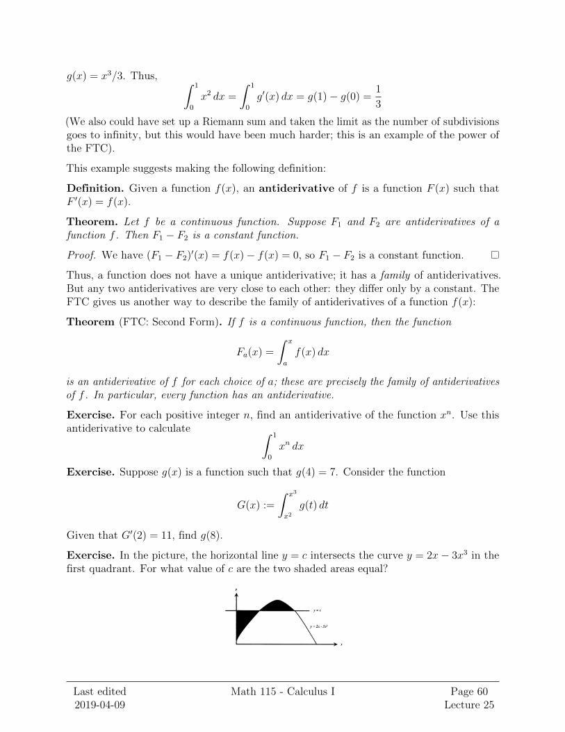
g(x) = x3/3. Thus, ∫ 1

0

x2 dx =

∫ 1

0

g′(x) dx = g(1)− g(0) =1

3

(We also could have set up a Riemann sum and taken the limit as the number of subdivisionsgoes to infinity, but this would have been much harder; this is an example of the power ofthe FTC).

This example suggests making the following definition:

Definition. Given a function f(x), an antiderivative of f is a function F (x) such thatF ′(x) = f(x).

Theorem. Let f be a continuous function. Suppose F1 and F2 are antiderivatives of afunction f . Then F1 − F2 is a constant function.

Proof. We have (F1 − F2)′(x) = f(x)− f(x) = 0, so F1 − F2 is a constant function.

Thus, a function does not have a unique antiderivative; it has a family of antiderivatives.But any two antiderivatives are very close to each other: they differ only by a constant. TheFTC gives us another way to describe the family of antiderivatives of a function f(x):

Theorem (FTC: Second Form). If f is a continuous function, then the function

Fa(x) =

∫ x

a

f(x) dx

is an antiderivative of f for each choice of a; these are precisely the family of antiderivativesof f . In particular, every function has an antiderivative.

Exercise. For each positive integer n, find an antiderivative of the function xn. Use thisantiderivative to calculate ∫ 1

0

xn dx

Exercise. Suppose g(x) is a function such that g(4) = 7. Consider the function

G(x) :=

∫ x3

x2g(t) dt

Given that G′(2) = 11, find g(8).

Exercise. In the picture, the horizontal line y = c intersects the curve y = 2x− 3x3 in thefirst quadrant. For what value of c are the two shaded areas equal?



math 115 - calculus i - university of michigan

Documents