math 115a: linear algebramjandr/math115a/115a.pdf3 lecture on august 6th: sets and functions 3.1...

Math 115A: Linear Algebra

Michael AndrewsUCLA Mathematics Department

September 13, 2018

Contents

1 Boring things 41.1 Quizzes . . . . . . . . . . . . . . . . . . . . . . . . . . . . . . . . . . . . . . . . . . . 41.2 Final . . . . . . . . . . . . . . . . . . . . . . . . . . . . . . . . . . . . . . . . . . . . . 41.3 Make-up exams? . . . . . . . . . . . . . . . . . . . . . . . . . . . . . . . . . . . . . . 41.4 Questions for turning in . . . . . . . . . . . . . . . . . . . . . . . . . . . . . . . . . . 41.5 Grading . . . . . . . . . . . . . . . . . . . . . . . . . . . . . . . . . . . . . . . . . . . 41.6 Discussion . . . . . . . . . . . . . . . . . . . . . . . . . . . . . . . . . . . . . . . . . . 51.7 Office hours . . . . . . . . . . . . . . . . . . . . . . . . . . . . . . . . . . . . . . . . . 5

2 Please talk to me, Kevin, and your peers 5

3 Lecture on August 6th: Sets and functions 63.1 Sets . . . . . . . . . . . . . . . . . . . . . . . . . . . . . . . . . . . . . . . . . . . . . 63.2 Some more on sets (covered in discussion) . . . . . . . . . . . . . . . . . . . . . . . . 93.3 Functions . . . . . . . . . . . . . . . . . . . . . . . . . . . . . . . . . . . . . . . . . . 10

4 Questions due on August 8th 13

5 Lecture on August 8th: Vector spaces over R 15


7 Lecture on August 9th: Subspaces and linear transformations 217.1 Subspaces . . . . . . . . . . . . . . . . . . . . . . . . . . . . . . . . . . . . . . . . . . 217.2 Linear transformations . . . . . . . . . . . . . . . . . . . . . . . . . . . . . . . . . . . 24


9 Lecture on August 13th:Kernels, images, linear transformations from Rn, matrices 349.1 Kernels and images . . . . . . . . . . . . . . . . . . . . . . . . . . . . . . . . . . . . . 349.2 Linear transformations from Rn . . . . . . . . . . . . . . . . . . . . . . . . . . . . . . 359.3 Basic matrix operations (in case you have forgotten) . . . . . . . . . . . . . . . . . . 36

1

9.4 How to think about matrices the “right” way . . . . . . . . . . . . . . . . . . . . . . 36


11 Lecture on August 15th: Spans and linear (in)dependence 4111.1 Linear combinations and spans of tuples . . . . . . . . . . . . . . . . . . . . . . . . . 4111.2 Linear combinations and spans of arbitrary sets (omitted) . . . . . . . . . . . . . . . 4211.3 Linear dependence and linear independence . . . . . . . . . . . . . . . . . . . . . . . 42


13 Lecture on August 16th: Towards bases and dimension 4513.1 Spans and linear (in)dependence . . . . . . . . . . . . . . . . . . . . . . . . . . . . . 4513.2 Towards bases and dimension . . . . . . . . . . . . . . . . . . . . . . . . . . . . . . . 46


15 Solutions to the previous questions 53

16 Quiz 1 60

17 Comments on quiz 1 64

18 Lecture on August 20th: Dimension 66


20 Lecture on August 22th: The Rank-Nullity Theorem 6920.1 Leftover from last time . . . . . . . . . . . . . . . . . . . . . . . . . . . . . . . . . . . 6920.2 Rank-Nullity . . . . . . . . . . . . . . . . . . . . . . . . . . . . . . . . . . . . . . . . 6920.3 Isomorphisms . . . . . . . . . . . . . . . . . . . . . . . . . . . . . . . . . . . . . . . . 71


22 Lecture on August 23th: The classification theorem andthe matrix of a linear transformation 7422.1 The classification of finite-dimensional vector spaces over R . . . . . . . . . . . . . . 7422.2 The matrix of a linear transformation . . . . . . . . . . . . . . . . . . . . . . . . . . 76


24 Lecture on August 27th 8124.1 The matrix of a linear transformation . . . . . . . . . . . . . . . . . . . . . . . . . . 8124.2 The purpose of matrices and vectors . . . . . . . . . . . . . . . . . . . . . . . . . . . 8324.3 Isomorphisms and invertible matrices . . . . . . . . . . . . . . . . . . . . . . . . . . . 8324.4 Sean’s proof of theorem 24.1.4 . . . . . . . . . . . . . . . . . . . . . . . . . . . . . . . 85


2

26 Solutions to the previous questions 89

27 Lecture on August 29th 9327.1 The change of coordinate matrix . . . . . . . . . . . . . . . . . . . . . . . . . . . . . 9327.2 Determinants of matrices (not lectured) . . . . . . . . . . . . . . . . . . . . . . . . . 9327.3 Eigenvectors . . . . . . . . . . . . . . . . . . . . . . . . . . . . . . . . . . . . . . . . . 96


29 Quiz 2 98

30 Comments on quiz 2 102

31 Lecture on August 30th: Diagonalizable Transformations 103

32 Questions due on September 5th 105

33 Sketch solutions for the previous questions 108

34 Proving theorem 31.10 (I’ll lecture a strict subset of this) 112

35 Lecture on September 5th 11635.1 Vector spaces over a field . . . . . . . . . . . . . . . . . . . . . . . . . . . . . . . . . 11635.2 Inner products . . . . . . . . . . . . . . . . . . . . . . . . . . . . . . . . . . . . . . . 117


37 Lecture on September 6th 12137.1 Gram-Schmidt and orthonormal bases . . . . . . . . . . . . . . . . . . . . . . . . . . 12137.2 Orthogonal complements and the Riesz representation lemma . . . . . . . . . . . . . 123


39 Lecture (final one) on September 10th: The spectral theorem 12839.1 Adjoints and self-adjoint operators . . . . . . . . . . . . . . . . . . . . . . . . . . . . 12839.2 The spectral theorem . . . . . . . . . . . . . . . . . . . . . . . . . . . . . . . . . . . . 130

40 Exam Expectations 131

41 The final 136

3

1 Boring things

1.1 Quizzes

There will be quizzes on Monday 20th August and Thursday 30th August.They will take place in the first 50 minutes of class.

1.2 Final

The final exam will take place on Thursday 13th September.The exam will be 2 hours long and will take place in the usual classroom.To give adequate preparation time, the final Tuesday and Wednesday will consist of office hours inthe usual classroom.

1.3 Make-up exams?

There will not be any make-up exams. Note that university policy requires that a student who hasan undocumented absence from the final exam be given a failing grade in the class.

1.4 Questions for turning in

Each lecture I will assign problems for you to turn in during the next lecture. In total, you’ll turnin work 15 times. Not everything will be graded because the grader has a limited number of hours,but we’ll try to choose good questions for them to grade in order to keep you updated on how wellyou are doing. Sometimes I might let you know if a question is going to be graded in advance. Iwill sum up your scores in five groups of 3. Your lowest scoring group of questions will not counttowards your grade.

I’ll be reasonable about how many questions I assign: on Wednesdays, I will not give you muchto turn in on Thursday. There will be more questions assigned on a Thursday. Thursday’s questionsare likely to ask about the whole week’s material and to develop ideas that we do not have timefor in class. I’ll post them as soon as we have covered the relevant material in class.

If you have to miss a lecture, please have a friend turn in your questions.You should expect to receive your work back within two lectures.Please staple your work. I have given the grader permission to take off points for not stapling.Kevin is not the grader of the homeworks.

1.5 Grading

Using your turned in questions, quizzes, and final, two scores will be calculated for you using thefollowing schemes:

Scheme 1 Scheme 2

Turned in questions (lowest group of 3 dropped) 15% 15%

Better Quiz 25% 25%

Other Quiz 20% 0%

Final 40% 60%

4

Your final score will be the higher of those two scores.You will be assigned a letter grade using your class rank.

Any issues about grading must be addressed within two weeks. After that time no score changeswill be allowed. Scores will be available online through my.ucla.edu.

1.6 Discussion

Ask Kevin to solve a Rubrix cube blindfolded.

1.7 Office hours

Office hours are posted on the website: math.ucla.edu/~mjandr/Math115A.

2 Please talk to me, Kevin, and your peers

What do I like least in a (math) classroom? When my students don’t talk!When my students don’t talk to me, I don’t know whether they are confused or bored. If I can

tell that they are confused, I still don’t know when they became confused or what confused them.Was the previous two weeks worth of material overwhelming, or was it the last five minutes? HaveI made a mistake on the board? Is it that which is causing confusion? Oh wait, finally someonepointed it out - silly old me! (I officially become old this birthday.) I wish someone had spoken up20 minutes ago when they were first confused!

There are many reasons that I can think of for students to be hesitant to speak out. In myMath 95 class, I’m going to make a note of the reasons that they think of, so take a look at mynotes for that course if you’re interested: http://math.ucla.edu/~mjandr/Math95. I hope thatthis list of the most important things that I learned in grad school might help you to be less quiet.

• I am in control of my learning. How much I participate usually corresponds with how muchI enjoy a class and how much I learn in the class.

• Asking a question earlier rather than later usually results in less confusion on my part.

• If I am confused, it is likely that half the room is confused too, and my question will probablyhelp others. It can help in two ways.

– Directly, by clearing up a mistake or something that the lecturer said unclearly.

– Indirectly, by calling the lecturer’s attention to the fact that people are confused, forcinga flexible lecturer to try to change something.

• My “stupid” questions are usually my most important questions and it makes me feel betterif I do not think of them as “stupid.”

• Math is really difficult, and on some days it feels worse than others. It’s better to be kind tomyself on such days, and to ask the people who are explaining ideas to me to slow down orexplain things more thoroughly if necessary.

• The lecturer probably likes questions.

5

my.ucla.edu

math.ucla.edu/~mjandr/Math115A

http://math.ucla.edu/~mjandr/Math95

3 Lecture on August 6th: Sets and functions

3.1 Sets

Definition 3.1.1. A set is a collection of mathematical things. The members of a set are calledits elements. We write x ∈ X to mean that “x is an element of a set X.”

Definition 3.1.2. We often use curly brackets (braces) for sets whose elements can be written downeasily. For example, the set whose elements are a1, a2, a3, . . . , an is written as {a1, a2, a3, . . . , an},and the set whose elements are those of an infinite sequence a1, a2, a3, . . . is written as {a1, a2, a3, . . .}.

Remark 3.1.3. Some infinite sets can not be written out in an infinite sequence, so not all sets canbe described using the notation just defined. An example is the set of real numbers. If this interestsyou, come to the first week or so of my math 95 class: http://math.ucla.edu/~mjandr/Math95.

Definition 3.1.4. We often describe a set as “elements with some property.” For example, the setof elements with a property P is written as {x : x has property P}, and the elements of a previouslydefined set X with a property P is written as {x ∈ X : x has property P}.

Remark 3.1.5. • In the previous definition the colons should be read as “such that.”

• The second way of describing a set {x ∈ X : x has property P} is much better than the firstbecause the first allows for Russell’s paradox: the “set” {A : A is a set and A /∈ A} makesno sense! http://en.wikipedia.org/wiki/Barber_paradox#Paradox

Notation 3.1.6. Here is some notation for familiar sets. “:=” means “is defined to be equal to.”

1. the empty set ∅ := { } is the set with no elements,

2. the natural numbers N := {1, 2, 3, . . .},

3. the integers Z := {0,−1, 1,−2, 2,−3, 3, . . .},

4. the rationals Q := {mn : m ∈ Z, n ∈ N},

5. the reals R,

6. the complex numbers C := {x+ iy : x, y ∈ R}.

Definition 3.1.7. Suppose X and Y are sets. We say that X is a subset of Y iff whenever z ∈ X,we have z ∈ Y . We write X ⊆ Y to mean “X is a subset of Y .”

Remark 3.1.8. In this definition “iff” stands for “if and only if.” This means that saying “X isa subset of Y ” is exactly the same as saying “whenever z ∈ X, we have z ∈ Y .”

Often, in definitions, mathematicians say “if” even though the meaning is “iff.” I normally dothis, and I feel a little silly for writing “iff,” but I decided that it’s the least confusing thing I cando. To make this “iff” feel different from a non-definitional “iff” I have used bold.

Remark 3.1.9. Suppose X and Y are sets, that X is a subset of Y , and that you want to write aproof for this. What do you write?

Well, another way of expressing the “whenever” sentence in the previous definition is “if z ∈ X,then z ∈ Y .” To verify a sentence like “if P , then Q” directly you assume that P is true, and checkthat Q is true. Thus, the definition forces our proof to look as follows.

6


http://en.wikipedia.org/wiki/Barber_paradox#Paradox

• We wish to show X ⊆ Y .

• By definition, we must show that if z ∈ X, then z ∈ Y .

• So suppose that z ∈ X.

• We want to show that z ∈ Y .

• [Insert mathematical arguments to show that z ∈ Y .]

• We conclude that z ∈ Y , and so we have shown that X ⊆ Y .

Theorem 3.1.10. Let A = {n ∈ N : n ≥ 8 and n is prime} and B = {n ∈ Z : n is odd}.We have A ⊆ B.

Proof. Let A and B be as in the theorem statement.We wish to show A ⊆ B. By definition, we must show that if n ∈ A, then n ∈ B. So suppose

that n ∈ A. We want to show that n ∈ B.Because n ∈ A, the definition of A tells us that n is a natural number which is greater than or

equal 8 and prime. In order to show n ∈ B, we must demonstrate that n is an odd integer. Naturalnumbers are integers and n is a natural number, and so n is an integer. We are just left to show nis odd.

Suppose for contradiction that n is not odd. Then n is even, and n2 ∈ N. Since n ≥ 8, n

2 ≥ 4.Thus, writing n = 2 · n2 shows that n is not prime. This contradicts the fact that n is prime, andso n must be odd.

We conclude that n ∈ B, and so we have shown that A ⊆ B.

Here is a complete list of the things we do during the previous proof. You might want to rewritethis list in your notes and add to it whenever we learn new things to do in a proof.

• We introduce the mathematical objects that are we are going to be using during the proof.

• We state what we wish to demonstrate before doing so.

• We unpack and use definitions where necessary (which is a lot of the time). We try to highlightwhen we are doing this unless we think that the reader can figure it out without such help.We should assume that the reader is another student in the class.

• We state assumptions.

• We prove an if-then statement directly.

• We use modus ponens.

The first paragraph of http://en.wikipedia.org/wiki/Modus_ponens and the first para-graph of the section “explanation” are useful. You might find the rest overly confusing.

An example of using modus ponens we might see later is: “we know that bases are linearlyindependent, and (v1, . . . , vn) is a basis, so (v1, . . . , vn) is linearly independent.”

You could abbreviate this using the words “in particular” by saying: “(v1, . . . , vn) is a basis.In particular, (v1, . . . , vn) is linearly independent.”

We could also abbreviate to “since (v1, . . . , vn) is a basis, (v1, . . . , vn) is linearly independent.”

7

http://en.wikipedia.org/wiki/Modus_ponens

• We make a deduction from an assumption declared in the previous sentence.

For example, “Suppose that (v1, . . . , vn) is a basis. Then (v1, . . . , vn) is linearly independent.”

• We use a proof by contradiction:

– We make an assumption that is going to cause a contradiction, the negation of what wewant to verify. We use the words “suppose for contradiction. . .”

– We highlight what causes the contradiction, and conclude what we wanted to verify.

• We use a mathematical equation.

• We summarize what we have done.

For each sentence of the previous proof, find the appropriate bullet point(s) describing what we aredoing.

There is one case when the previous proof format for showing that X ⊆ Y breaks down.

Theorem 3.1.11. Suppose X is a set. Then ∅ ⊆ X.

Proof. Suppose X is a set. We wish to show that ∅ ⊆ X. By definition, we must show that if z ∈ ∅,then z ∈ X. Since the empty set has no elements, z ∈ ∅ is never true, and so there is nothing tocheck. We conclude that ∅ ⊆ X.

Remark 3.1.12. Maybe the “whenever” wording makes this proof seems less strange.Let X be a set. We must check that whenever z ∈ ∅, we have z ∈ X. However, since ∅ has no

elements, there is nothing to check. We conclude that ∅ ⊆ X.

Definition 3.1.13. Suppose X and Y are sets. We say that X is equal to Y iff X is a subset ofY and Y is a subset of X. We write X = Y to mean “X is equal Y .”

Remark 3.1.14. Suppose X and Y are sets, that X is equal to Y , and that you want to write aproof for this. What do you write?

• We wish to show X = Y .

• By definition, we must show that X ⊆ Y , and Y ⊆ X.

• [Insert proof that X ⊆ Y .]

• [Insert proof that Y ⊆ X.]

• We have shown that X ⊆ Y and Y ⊆ X, so we have shown that X = Y .

Example 3.1.15.

1. {0, 1} = {0, 0, 0, 1, 1} = {1, 0}.

2. ∅ 6= {∅}. This is because ∅ /∈ ∅ and so {∅} 6⊆ ∅.

3. {n ∈ N : n divides 12} = {1, 2, 3, 4, 6, 12}.

8

3.2 Some more on sets (covered in discussion)

Definition 3.2.1. Suppose X and Y are sets.We write X ∪ Y for the set

{z : z ∈ X or z ∈ Y }.

X ∪ Y is read as “X union Y ” or “the union of X and Y .”We write X ∩ Y for the set

{z : z ∈ X and z ∈ Y }.

X ∩ Y is read as “X intersect Y ” or “the intersection of X and Y .”We write X \ Y for the set

{z : z ∈ X and z /∈ Y }.

X \ Y is read as “X takeaway Y .” x /∈ Y means, and is read as “x is not an element of Y .”

Example 3.2.2. I hope Kevin will give examples in discussion.

Theorem 3.2.3 (De Morgan’s Laws). Suppose X, A, and B are sets. Then

X \ (A ∪B) = (X \A) ∩ (X \B),

X \ (A ∩B) = (X \A) ∪ (X \B).

Proof. Let X, A, and B be sets.

1. Due on Wednesday.

2. Suppose X, A, and B are sets. We wish to show that

X \ (A ∩B) = (X \A) ∪ (X \B).

By definition of set equality, we must show that

X \ (A ∩B) ⊆ (X \A) ∪ (X \B) and X \ (A ∩B) ⊇ (X \A) ∪ (X \B).

(a) First, we demonstrate that X \ (A∩B) ⊆ (X \A)∪ (X \B), that is, if z ∈ X \ (A∩B),then z ∈ (X \A) ∪ (X \B).

Suppose z ∈ X \ (A ∩B). By definition of \, this means z ∈ X and z /∈ A ∩B.

We cannot have both x ∈ A and x ∈ B since, by definition of ∩, this would tell us thatz ∈ A ∩B.

i. Case 1: z /∈ A. Since z ∈ X, the definition of \ tells us that z ∈ X \A.Thus, by definition of ∪, z ∈ (X \A) ∪ (X \B).

ii. Case 2: z /∈ B. Since z ∈ X, the definition of \ tells us that z ∈ X \B.Thus, by definition of ∪, z ∈ (X \A) ∪ (X \B).

In either case we have shown that z ∈ (X \A) ∪ (X \B).

9

(b) Next, we show that if z ∈ (X \A) ∪ (X \B), then z ∈ X \ (A ∩B).

Suppose z ∈ (X \A) ∪ (X \B). By definition of ∪, this means z ∈ X \A or z ∈ X \B.

i. Case 1: z ∈ X \A. By definition of \, this means that z ∈ X and z /∈ A.We cannot have z ∈ A∩B, since otherwise, by the definition of ∩, we’d have z ∈ A.So z ∈ X and z /∈ A ∩B, and the definition of \ gives z ∈ X \ (A ∩B).

ii. Case 2: z ∈ X \B. By definition of \, this means that z ∈ X and z /∈ B.We cannot have z ∈ A∩B, since otherwise, by the definition of ∩, we’d have z ∈ B.So z ∈ X and z /∈ A ∩B, and the definition of \ gives z ∈ X \ (A ∩B).

In either case we have shown that z ∈ X \ (A ∩B).

Remark 3.2.4. In the proof of the second result above, both directions broke into cases. In bothinstances, the cases were almost identical with A and B swapping roles. Because of the symmetry ofthe situation it might be reasonable to expect the reader to see that both cases are proved similarly.Often in such cases the proof-writer might say, “case 2 is similar” or they might say “without lossof generality we only need to consider the first case.” I’d hesistate to do such things unless you havewritten out the proof and seen that it really is identical. Sometimes things can appear symmetric,but after careful consideration, you might realize it’s not that easy!

3.3 Functions

Definition 3.3.1. A function f : X −→ Y consists of:

• a set X called the domain of f ;

• a set Y called the codomain of f ;

• a way of assigning to each x ∈ X, exactly one y ∈ Y .

We write f(x) for the unique y ∈ Y assigned to x.

Notation 3.3.2. We often use the notation f : X −→ Y , x 7−→ f(x).“7−→” is read as “maps to.”

Definition 3.3.3. Suppose X and Y are sets and that f : X −→ Y is a function.

1. We say f is injective iff whenever x1, x2 ∈ X, f(x1) = f(x2) implies x1 = x2.

2. We say f is surjective iff whenever y ∈ Y , we can find an x ∈ X such that f(x) = y.

3. We say f is bijective iff f is injective and surjective.

Remark 3.3.4. We may also use “one-to-one” for injective, and “onto” for surjective.There are noun forms of the words in the previous definition too. We speak of an injection, a

surjection, and a bijection.

Remark 3.3.5. Suppose X and Y are sets, f : X −→ Y is a function, and that f is injective.How do you write a proof that f is injective?Well, another way of expressing the “whenever” sentence in part 1 of the previous definition is

“if x1, x2 ∈ X and f(x1) = f(x1), then x1 = x2.”Thus, the definition forces our proof to look as follows.

10

• We wish to show that f is injective.

• By definition, we must show that if x1, x2 ∈ X and f(x1) = f(x1), then x1 = x2.

• So suppose that x1, x2 ∈ X and f(x1) = f(x2).

• (We want to show that x1 = x2.)

• [Insert mathematical arguments to show that x1 = x2.]

• We conclude that x1 = x2, and so we have shown that f is injective.

Theorem 3.3.6. The function f : {x ∈ R : x ≥ 0} −→ R, x 7−→ x2 is injective.

Proof. Let X = {x ∈ R : x ≥ 0} and f : X −→ R be as in the theorem statement. We wish to showthat f is injective. By definition of injectivity, we must show that if x1, x2 ∈ X and f(x1) = f(x1),then x1 = x2. So suppose x1, x2 ∈ X and f(x1) = f(x2). By definition of f , f(x1) = f(x2) tells usthat x2

1 = x22. Taking the square roots of both sides gives |x1| = |x2|. Since x1, x2 ∈ X, x1, x2 ≥ 0,

and the previous equations says that x1 = x2. We have now shown that f is injective.

Remark 3.3.7. Suppose X and Y are sets, f : X −→ Y is a function, and that f is surjective.How do you write a proof that f is surjective?Well, another way of expressing the “whenever” sentence in part 2 of the previous definition is

“if y ∈ Y , then we can find an x ∈ X such that f(x) = y.”Thus, the definition forces our proof to look as follows.

• We wish to show that f is surjective.

• By definition, we must show that if y ∈ Y , then we can find an x ∈ X such that f(x) = y.

• So suppose that y ∈ Y .

• (We want to show that we can find an x ∈ X such that f(x) = y.)

• [Insert mathematical arguments.]

These arguments must do two things:

– Specify an element x ∈ X.

– Check that the specified x satisfies the equation f(x) = y.

• We have completed the demonstration that f is surjective.

Theorem 3.3.8. The function f : R −→ {y ∈ R : y ≥ 0}, x 7−→ x2 is surjective.

Proof. Let Y = {y ∈ R : y ≥ 0} and f : R −→ Y be defined as in the theorem statement. We wishto show that f is surjective. By definition of surjectivity, we must show that if y ∈ Y , then we canfind an x ∈ R such that f(x) = y. So suppose that y ∈ Y . Since y ≥ 0, we can let x =

√y. Then

f(x) = x2 = (√y)2 = y, and we have completed the demonstration that f is surjective.

11

Remark 3.3.9. Suppose X and Y are sets, f : X −→ Y is a function, and that f is a bijection.How do you write a proof that f is a bijection?The definition forces our proof to look as follows.

• We wish to show that f is bijection.

• By definition, we must show that f is injective and surjective.

• [Insert proof that f is injective.]

• [Insert proof that f is surjective.]

• We have demonstrated that f is bijection.

Theorem 3.3.10. The function f : {x ∈ R : x ≥ 0} −→ {y ∈ R : y ≥ 0}, x 7−→ x2 is a bijection.

Proof. Omitted.

Definition 3.3.11. Suppose X, Y , and Z are sets, and that f : X −→ Y and g : Y −→ Z arefunctions. The composition of f and g is the function g◦f : X → Z defined by (g◦f)(x) = g(f(x)).

Theorem 3.3.12. Suppose X, Y , and Z are sets, and f : X −→ Y and g : Y −→ Z are functions.

1. If g ◦ f is injective, then f is injective.

2. If g ◦ f is surjective, then g is surjective.

3. If f and g are injective, then g ◦ f is injective.

4. If f and g are surjective, then g ◦ f is surjective.

Proof. Left to you.

12

4 Questions due on August 8th

1. (a) How many functions are there with domain {1, 2, 3} and codomain {1, 2, 3, 4, 5}?(b) How many injective functions are there with domain {1, 2, 3} and codomain {1, 2, 3, 4, 5}?(c) How many surjective functions are there with domain {1, 2, 3} and codomain {1, 2, 3, 4, 5}?(d) How many functions are there with domain {1, 2, 3, 4, 5} and codomain {1, 2, 3}?(e) How many injective functions are there with domain {1, 2, 3, 4, 5} and codomain {1, 2, 3}?(f) How many surjective functions are there with domain {1, 2, 3, 4, 5} and codomain {1, 2, 3}?

Hint: how many functions are there with domain {1, 2, 3, 4, 5} and codomain {1, 2}?(g) Let n ∈ N. How many bijections are there with domain and codomain {1, 2, . . . , n}?

Solution:

(a) 53. (1 pt.)

(b) 5 · 4 · 3. (1 pt.)

(c) 0. (1 pt.)

(d) 35.

(e) 0.

(f) Let try to count how many functions f : {1, 2, 3, 4, 5} −→ {1, 2, 3} are NOT surjective.There are three cases: Let X = {1, 2, 3, 4, 5}

i. 1 /∈ f(A): then f is basically a function X −→ {2, 3}. There are 25 such functions.

ii. 2 /∈ f(A): then f is basically a function X −→ {1, 3}. There are 25 such functions.

iii. 3 /∈ f(A): then f is basically a function X −→ {1, 2}. There are 25 such functions.

It looks like we have counted that there are 3 · 25 functions which are NOT surjective.But we have double counted: there are three constant functions which have been countedtwice. So there are 3 · 25 − 3 functions which are NOT sujective.

The answer is 35 − 3 · 25 + 3. (2 pts.)

(g) n! (1 pt.)

2. Prove part 1 of theorem 3.3.12. Here’s a general outline for how your proof should look.

(a) Introduce relevant mathematical objects.

(b) State what you want to prove.

(c) It is an if-then sentence, so suppose the premise and say that you would like to verifythe conclusion.

(d) Unpack the definition of the what you have just said you want to verify.

(e) It is an if-then sentence, so suppose the premise and say that you would like to verifythe conclusion.

(f) Figure out how to do this verification. You’ll need to use your assumptions. This is thecrux of proof, but without the context for this argument (the previous 5 steps) it doesnot really make any sense.

(g) Conclude your proof.

13

Solution: (2 pts. for format, 2 pts. for (f).)

(a) Suppose X, Y , and Z are sets, and that f : X −→ Y and g : Y −→ Z are functions.

(b) We want to prove that if g ◦ f is injective, then f is injective.

(c) So suppose g ◦ f is injective. We would like to verify that f is injective.

(d) By definition, we must show that if x1, x2 ∈ X and f(x1) = f(x1), then x1 = x2.

(e) So let x1, x2 ∈ X and suppose that f(x1) = f(x2). We need to show that x1 = x2.

(f) Since f(x1) = f(x2), we can apply g to see g(f(x1)) = g(f(x2)). By definition of g ◦ f ,this says that (g ◦ f)(x1) = (g ◦ f)(x2). Since g ◦ f is injective, this gives x1 = x2.

(g) Thus, we have shown f is injective, and this finishes the proof that if g ◦ f is injective,then f is injective.

3. Prove part 1 of theorem 3.2.3.

[You should be trying to write the proof similarly to how I proved part 2 in the notes, or howKevin proved it in discussion. My proof of the current result does not need case work; in thissense, the current proof is easier than the one in the notes.]

Solution: (1 pt. for completion.)

Suppose X, A, and B are sets. We wish to show that

X \ (A ∪B) = (X \A) ∩ (X \B).

By definition of set equality, we must show that

X \ (A ∪B) ⊆ (X \A) ∩ (X \B) and X \ (A ∪B) ⊇ (X \A) ∩ (X \B).

(a) First, we demonstrate that X \ (A ∪B) ⊆ (X \A) ∩ (X \B).

By definition of ⊆, we have to show that whenever z ∈ X \ (A ∪ B), it is the case thatz ∈ (X \A) ∩ (X \B).

So suppose z ∈ X \ (A ∪ B). By definition of \, this means z ∈ X and z /∈ A ∪ B. Wecannot have z ∈ A or z ∈ B since, by the definition of ∪, both these conditions implyz ∈ A ∪B.

Thus, z ∈ X and z /∈ A, and the definition of \ gives z ∈ X \A.

Similarly, z ∈ X and z /∈ B, and the definition of \ gives z ∈ X \B.

By the definition of ∩, the last two facts say z ∈ (X \A) ∩ (X \B).

(b) Next, we show that X \ (A ∪B) ⊇ (X \A) ∩ (X \B), i.e if z ∈ (X \A) ∩ (X \B), thenz ∈ X \ (A ∪B).

Suppose that z ∈ (X \A) ∩ (X \B). By definition of ∩, this means that z ∈ X \A andz ∈ X \B.

The first statement together with the definition of \ says z ∈ X and z /∈ A.

The second statement together with the definition of \ says z ∈ X and z /∈ B.

If we had z ∈ A∪B, by definition of ∪, we’d have either z ∈ A or z ∈ B, and this is notthe case. Thus, z /∈ A ∪B.

In conclusion, z ∈ X and z /∈ A ∪B, so the definition of \ gives z ∈ X \ (A ∪B).

14

5 Lecture on August 8th: Vector spaces over R

Definition 5.1. Suppose X and Y are sets. We write X × Y for the set

{(x, y) : x ∈ X, y ∈ Y },

that is the set of ordered pairs where one coordinate has its value in X and the other has its valuein Y . X × Y is called the Cartesian product of X and Y .

Example 5.2.

1. {0, 1} × {5, 6, 7} = {(0, 5), (0, 6), (0, 7), (1, 5), (1, 6), (1, 7)}.

2. R× R is the Cartesian plane R2.

3. R× R× R is the home of 3D calculus R3.

Definition 5.3. A vector space over R is a set V together with operations

• + : V × V −→ V, (v, w) 7−→ v + w (addition)

• · : R× V −→ V, (λ, v) 7−→ λv (scalar multiplication)

which satisfy the following axioms (“∀” = “for all”, “∃” = “there exists”, “:” = “such that”):

1. ∀u ∈ V, ∀v ∈ V, u+ v = v + u

(vector space addition is commutative).

2. ∀u ∈ V, ∀v ∈ V, ∀w ∈ V, (u+ v) + w = u+ (v + w)

(vector space addition is associative).

3. There exists an element of V , which we call 0, with the property that ∀v ∈ V, v + 0 = v

(there is an identity element for vector space addition).

4. ∀u ∈ V, ∃v ∈ V : u+ v = 0

(additive inverses exist for vector space addition).

5. ∀v ∈ V, 1v = v

(the multiplicative identity element of R acts sensibly under scalar multiplication).

6. ∀λ ∈ R, ∀µ ∈ R, ∀v ∈ V, (λµ)v = λ(µv)

(the interaction of R’s multiplication and scalar multiplication is sensible).

7. ∀λ ∈ R, ∀u ∈ V, ∀v ∈ V, λ(u+ v) = λu+ λv

(the interaction of scalar multiplication and vector space addition is sensible).

8. ∀λ ∈ R, ∀µ ∈ R, ∀v ∈ V, (λ+ µ)v = λv + µv

(the interaction of R’s addition and scalar multiplication is sensible).

15

Example 5.4.

1. Supppose n ∈ N. Then the set of n-tuples Rn is a vector space over R under coordinatewiseaddition and scalar multiplication.

In class, for the case of n = 2, I’ll check axioms 1, 3, and 4.

2. Suppose m,n ∈ N. Then the set of real m × n matrices, Mm×n(R) is a vector space over Runder matrix addition and scalar multiplication.

3. Suppose X is a non-empty set. The set of real-valued functions from X, {f : X −→ R} is avector space over R under pointwise addition and scalar multiplication.

In class, I’ll check axioms 2, 3, and 6.

I’d certainly copy down what I write, and check with me and friends that you copied correctly.

4. Suppose n ∈ N. The set of degree n real-valued polynomials Pn(R) is a vector space over Runder coefficientwise addition and scalar multiplication.

5. The set of real-valued polynomials P(R) =⋃n∈N Pn(R) is a vector space over R under coef-

ficientwise addition and scalar multiplication.

Example 5.5.

1. Define an unusual addition and scalar multiplication on R2 by

(x1, x2) + (y1, y2) = (x1 + y1, x2 − y2), λ(x1, x2) = (λx1, λx2).

Axioms 3, 4, 5, 6, 7 all hold; checking 3 and 4 is a good exercise.

Axioms 1, 2, and 8 fail.

Let’s consider axiom 1: ∀(x1, x2) ∈ R2, ∀(y1, y2) ∈ R2, (x1, x2) + (y1, y2) = (y1, y2) + (x1, x2).This says ∀(x1, x2) ∈ R2, ∀(y1, y2) ∈ R2, (x1 + y1, x2 − y2) = (y1 + x1, y2 − x2).

You might say that this is false because x2−y2 6= y2−x2, but this is sometimes true. The bestway to demonstrate the falseness of a “for all” statement is to give a very explicit example ofits failure. In this case, I would say axiom 1 fails because

(0, 1) + (0, 0) = (0, 1) 6= (0,−1) = (0, 0) + (0, 1).

Similarly, axiom 2 fails because

((0, 0) + (0, 0)) + (0, 1) = (0, 0) + (0, 1) = (0,−1),

(0, 0) + ((0, 0) + (0, 1)) = (0, 0) + (0,−1) = (0, 1),

and (0,−1) 6= (0, 1).

Axiom 8 fails because

(0 + 1)(0, 1) = 1(0, 1) = (0, 1) 6= (0,−1) = (0, 0) + (0, 1) = 0(0, 1) + 1(0, 1).

16

2. Define an unusual addition and scalar multiplication on R2 by

(x1, x2) + (y1, y2) = (x1 + y1, 0), λ(x1, x2) = (λx1, 0).

Axioms 1, 2, 6, 7, 8 all hold.

However, axiom 3 fails. To see this, suppose for contradiction that there exists an element 0with the property that

∀(x1, x2) ∈ R2, (x1, x2) + 0 = (x1, x2).

In particular, by taking (x1, x2) = (0, 1), we see that (0, 1)+0 = (0, 1). However, by definitionof addition, the second coordinate of (0, 1) + 0 is 0, not 1, and this contradicts the previousequation. Thus, there cannot be such an element 0.

Remark 5.6. Maybe a reminder of how a proof by contradiction works is still useful. Youwant to prove a statement P . “Suppose for contradiction, that P is false.” You then make aload of arguments based on this assumption. As soon as you get a contradiction, you shouldexplain what the contradiction is. After that, you can conclude that P is true. In the previousargument, the statement P was “there is not an element 0 with the property that. . .”

Because axiom 3 fails, axiom 4 does not even make sense.

Axiom 5 also fails. Its negation

∃(x1, x2) ∈ R2 : 1(x1, x2) 6= (x1, x2)

is true because 1(0, 1) = (0, 0) 6= (0, 1).

There are facts which we would like to take for granted whenever dealing with vector spaces.Proving these facts gives us permission to take them for granted forever afterwards (unless I askyou to prove them on an exam). I’m not a big fan of axiomatic proofs, but in the following proofsthere are some things which we do which you can add to your “good proofs” list.

• We explain our ideas to the reader.

• We reference and use axioms clearly.

• We see what it means to be the unique element with a property, and how to use uniqueness.

• We reduce a proof to a more easily obtained goal using a previously proven fact.

• We reference previously obtained facts.

• We leave some things to the reader. Maybe that is frustrating for you? So you can see whywe deduct points when not everything is properly explained.

17

Theorem 5.7. Suppose V is a vector space over R.

1. Let u, v, w ∈ V . If u+ w = v + w, then u = v.

2. The vector 0 ∈ V is the unique vector with the property that ∀v ∈ V, v + 0 = v.

3. Suppose u ∈ V . There is a unique vector v ∈ V with the property that u+ v = 0.

We give it a more useful name: (−u).

4. Let λ ∈ R and 0 be the identity additive element of V . Then λ0 = 0.

5. Let v ∈ V . Then 0v = 0.

6. Let v ∈ V . Then (−1)v = −v.

7. Let λ ∈ R and v ∈ V . Then −(λv) = (−λ)v = λ(−v).

Proof. Suppose V is a vector space over R.

1. Let u, v, w ∈ V . Suppose that u + w = v + w. We need to show that u = v. The idea is toadd an element to both sides to cancel w.

By axiom 4, we know there exists an element w′ such that w + w′ = 0. We add w′ to bothsides, and then we can summarize our calculation in one line. By using axiom 3, 0 = w+w′,axiom 2, u+ w = v + w, axiom 2, w + w′ = 0, axiom 3, in exactly that order, we find that

u = u+ 0 = u+ (w + w′) = (u+ w) + w′ = (v + w) + w′ = v + (w + w′) = v + 0 = v.

2. To show 0 ∈ V is unique, we suppose that there exists another such element 0′ ∈ V with theproperty that ∀v ∈ V, v + 0′ = v. We need to show that 0 = 0′. This is true because

0 = 0 + 0′ = 0′ + 0 = 0′,

where the first equality uses the property of 0′, the second equality uses commutativity ofaddition, and the last equality uses the property of 0.

3. Suppose u ∈ V . Axiom 4 tells us that there is a v ∈ V such that u + v = 0. We must nowaddress uniqueness. Suppose that there is another v′ ∈ V such that u+v′ = 0. Then we haveu+v = u+v′. Because vector space addition is commutative, this tells us that v+u = v′+u.Using part 1 to cancel the u’s, we obtain v = v′.

4. Let λ ∈ R and 0 be the identity additive element of V . We wish to show λ0 = 0. By part 1,it is enough to show λ0 + λ0 = 0 + λ0. Well,

λ0 + λ07.= λ(0 + 0)

3.= λ0

3.= λ0 + 0

1.= 0 + λ0.

5. Let v ∈ V . We wish to show 0v = 0. By part 1, it is enough to show that 0v + 0v = 0 + 0v.In R, we have 0 + 0 = 0, and so

0v + 0v8.= (0 + 0)v = 0v

3.= 0v + 0

1.= 0 + 0v.

18

6. Let v ∈ V . Thenv + (−1)v

5.= 1v + (−1)v

8.= (1 + (−1))v = 0v.

By part 5, this is 0, and so v + (−1)v = 0. By part 3, −v is the unique element such thatv + (−v) = 0, so (−1)v = −v.

7. Let λ ∈ R and v ∈ V . Then we have

−(λv) = (−1)(λv)6.= ((−1)λ)v = (−λ)v = (λ(−1))v

6.= λ((−1)v) = λ(−v),

where the unmarked inequalities come from part 6 or properties of R (I’ll leave it to you tofigure out which is which).

19


1. In class, I said that R2 is a vector space over R when equipped with coordinatewise additionand scalar multiplication. I checked axioms 1, 3, and 4, but I omitted checking axiom 2, andaxioms 5-8.

Carefully verify axioms 2, 5, 6, 7. Each of your equalities should be justified. Are you usingthe definition of addition for R2, the definition of scalar multiplication for R2, properties ofreal number addition and/or multiplication?

I suppose you can do 8 as well if you want more practice.


I’ll post a little bit of axiom checking in the solutions to the weekend problems.

2. Let V be a vector space over R, λ, µ ∈ R, and u, v ∈ V . (Since axiom 2 is true, it does notmatter how you parenthesize expressions involving the addition of three or more vectors.)Prove that

(λ+ µ)(u+ v) = λu+ λv + µu+ µv,

carefully referencing which axioms of a vector space you use for every equality.

(I can think of two proofs and one is shorter than the other.)


Let V be a vector space over R, λ, µ ∈ R, and u, v ∈ V . Then

(λ+ µ)(u+ v) = λ(u+ v) + µ(u+ v) = λu+ λv + µu+ µv.

The first equality is axiom 8; the second is axiom 7 twice.

20

7 Lecture on August 9th: Subspaces and linear transformations

7.1 Subspaces

Definition 7.1.1. Suppose V is a vector space over R with operations

+ : V × V −→ V and · : R× V −→ V,

and that W is a set.We call W a subspace of V iff

• W ⊆ V ;

• The operations + and · restrict to operations

+ : W ×W −→W, · : R×W −→W ;

• With these operations W is a vector space over R.

Example 7.1.2. {(x, 0) : x ∈ R} is a subspace of R2.

Example 7.1.3. Suppose that V is a vector space over R with zero element 0. Then {0} and Vare subspaces of V .

With the definition above it seems laborious to check that something is a subspace: we have tocheck it is a vector space in its own right, and we’ve seen that checking the axioms is tedious. Thisis why the following theorem, often called the subspace test, is useful.

Theorem 7.1.4. Suppose V is a vector space over R with operations + : V ×V → V , · : R×V → V ,zero element 0, and that W is a subset of V . W is a subspace of V if and only if the following threeconditions hold:

1. 0 ∈W .

2. If w ∈W and w′ ∈W , then w + w′ ∈W .

3. If λ ∈ R and w ∈W , then λw ∈W .

Proof. Suppose V is a vector space over R with operations + : V × V −→ V and · : R× V −→ V ,and that W is a subset of V .

First, we show the “only if” direction of the theorem statement. So suppose W is a subspace ofV . By definition of what it means to be a subspace, the operations + and · restrict to operations

+ : W ×W −→W, · : R×W −→W.

This is exactly the same as saying 2 and 3. So we just have to think about why 1 is true. BecauseW is a vector space, it has a unique zero element. Right now, for all we know, this zero elementcould be different to the unique zero element in V , so, for clarity, call the zero element of V , 0V ,and the zero element of W , 0W . We show that they’re not different by showing 0V = 0W . For this,we note that following equalities in V :

0V + 0W = 0W + 0V = 0W = 0W + 0W .

21

The first equality is by commutativity of addition in V . The second equality is because 0V is thezero element of V . The third equality is because 0W ∈ W , the addition in W coincides with thatin V , and 0W is the zero element of W . By cancellation, we conclude that 0V = 0W , as required.

Next, we show the “if” direction. So suppose that statements 1, 2, and 3 hold. The first partof the definition of a subspace holds because W ⊆ V . Assumptions 2 and 3 tell us the operationsin V restrict to operations in W . We just have to show W is a vector space over R, i.e. that theaxioms hold. Axioms 1, 2, 5, 6, 7, 8 all hold because they hold in V . We just have to think aboutaxioms 3 and 4. By assumption 1, 0 ∈ W , and so axiom 3 holds. For axiom 4, suppose w ∈ W .Because V is a vector space, we have the multiplicative inverse −w ∈ V . By theorem 5.7 part 6,we know that −w = (−1)w and by assumption 3, this shows −w ∈W .

Remark 7.1.5. Having proved this theorem, we should never worry EVER AGAIN about the 0of a subspace being different to the 0 in the containing vector space.

Example 7.1.6.

{(x1, x2, x3, x4) ∈ R4 : 8x1 + 18x2 + 88x3 = 0 and 7x2 + 14x3 + 94x4 = 0}

is a subspace of R4 (with the usual addition and scalar multiplication).I’ll check this carefully in class using the subspace test.

Example 7.1.7.

1. The set of even functions

{f : R −→ R : for all t ∈ R, f(−t) = f(t)}

is a subspace of {f : R −→ R}.

2. The set of odd functions

{f : R −→ R : for all t ∈ R, f(−t) = −f(t)}

is a subspace of {f : R −→ R}.

3. Suppose n,m ∈ N and n ≤ m. Pn(R) is a subspace of Pm(R).

4. Suppose n ∈ N. Pn(R) is a subspace of P(R).

5. You might want to try and say that P(R) is a subspace of {f : R −→ R}.However, there is an issue here that needs to be considered carefully. A polynomial is NOT,by definition, a function; it is a formal sum of terms like anx

n. By allowing yourself to plugin real numbers for the variable, you obtain a function. But what if two different polynomialsend up defining the same function? This cannot happen over R, but since it can happen ifyou consider polynomials over a finite field, this magic fact requires a proof.

Can you prove that the function

i : P(R) −→ {f : R −→ R}

defined by i(p(x))(t) = p(t), is injective? Your best strategy is to show that i is linear andthat its kernel is {0}, but you’ll have to wait a little to be told the definitions of these terms.

22

Theorem 7.1.8. Suppose W is a subspace of R3. Then W is either:

1. a line through the origin.

This means that there is a vector (a1, a2, a3) ∈ R3 \ {0} such that

W = {λ(a1, a2, a3) : λ ∈ R}.

2. a plane through the origin.

This means that there is a vector (n1, n2, n3) ∈ R3 \ {0} such that

W = {λ(x1, x2, x3) ∈ R3 : x1n1 + x2n2 + x3n3 = 0.}

3. a trivial subspace, either {0} or R3.

Remark 7.1.9. We will not prove this theorem until later. Until we do prove it, you should notuse it in your proofs. On the other hand, you should use it to help you think sensibly about whethercertain statements concerning subspaces are likely to be true or not.

Theorem 7.1.10. Suppose V is a vector space over a R. Suppose that {Wi : i ∈ I} is somecollection of subspaces of V . Then the intersection⋂

i∈IWi := {w ∈ V : ∀i ∈ I, w ∈Wi}

is a subspace of V .

Remark 7.1.11. In the above, I is an indexing set. For example, if I = {1, 2, 3}, then⋂i∈I

Wi = W1 ∩W2 ∩W3.

However, I is allowed to be infinite in this notation.

Proof. Suppose V is a vector space over a R. Suppose that {Wi : i ∈ I} is some collection ofsubspaces of V and let W =

⋂i∈IWi. We wish to show W is a subspace of V .

First, we have to show 0 ∈ W . Since each Wi is a subspace, we have 0 ∈ Wi for all i ∈ I, andso, by definition of the intersection, 0 ∈W .

Next suppose w ∈W , w′ ∈W , and λ ∈ R. We have to show that w+w′ ∈W and λw ∈W . Bydefinition of intersection, we have w ∈ Wi and w′ ∈ Wi for all i ∈ I. Since each Wi is a subspace,we have w+w′ ∈Wi and λw ∈Wi for all i ∈ I, and so, by definition of the intersection, w+w′ ∈Wand λw ∈W .

23

7.2 Linear transformations

Definition 7.2.1. Let V and W be vector spaces over R. A function T : V −→W is said to be alinear transformation iff

1. ∀v1 ∈ V , ∀v2 ∈ V , T (v1 + v2) = T (v1) + T (v2).

2. ∀λ ∈ R, ∀v ∈ V , T (λv) = λT (v).

Often, we say just “T is linear.”

Lemma 7.2.2. Let V and W be vector spaces over R and T : V −→W be a function.

1. If T is linear, then T (0) = 0.

2. T is linear if and only if

∀λ ∈ R, ∀v1 ∈ V, ∀v2 ∈ V, T (λv1 + v2) = λT (v1) + T (v2).

Concise proof. Let V and W be vector spaces over R and T : V −→W be a function. We’ll provepart 1 as we prove part 2. Suppose T is linear, λ ∈ R, v1 ∈ V , v2 ∈ V . Then

T (λv1 + v2) = T (λv1) + T (v2) = λT (v1) + T (v2).

Conversely, suppose that

∀λ ∈ R, ∀v1 ∈ V, ∀v2 ∈ V, T (λv1 + v2) = λT (v1) + T (v2).

Taking λ = 1 proves that the first part of linearity, and we now have T (0)+T (0) = T (0+0) = T (0),so that T (0) = 0. Taking v2 = 0 proves the second part of linearity.

Example 7.2.3. Suppose m,n ∈ N and A ∈ Mm×n(R). Then TA : Rn → Rm defined by TA(x) =Ax is a linear transformation. This follows from facts about matrix-vector multiplication. We’lluse the notation TA throughout the rest of the class, so don’t ignore this.

Remark 7.2.4. Notice that for the previous example to make sense, we have to think of elementsof Rn and Rm as column vectors, rather than row vectors / n-tuples. We’ll often blur the distinctionbetween row and column vectors. If you are ever confused about this, please ask.

Example 7.2.5. Suppose that X is a nonempty set. Recall that F = {f : X −→ R} is a vectorspace over R. Given x0 ∈ X, evx0 : F −→ R, f 7−→ f(x0) is linear.

Example 7.2.6. Suppose V and W are vector spaces over R.

• The identity function 1V : V −→ V, v 7−→ v is a linear transformation.

• The zero function 0V,W : V −→W, v 7−→ 0 is a linear transformation.

Notation 7.2.7. Suppose U , V , and W are vector spaces over R, that T : U → V and S : V →Ware linear transformations. Then we write ST : U −→W for the composite S ◦ T .

Lemma 7.2.8. Suppose U , V , and W are vector spaces over R, that T : U → V and S : V → Ware linear transformations. Then ST : U −→W is a linear transformation.

24

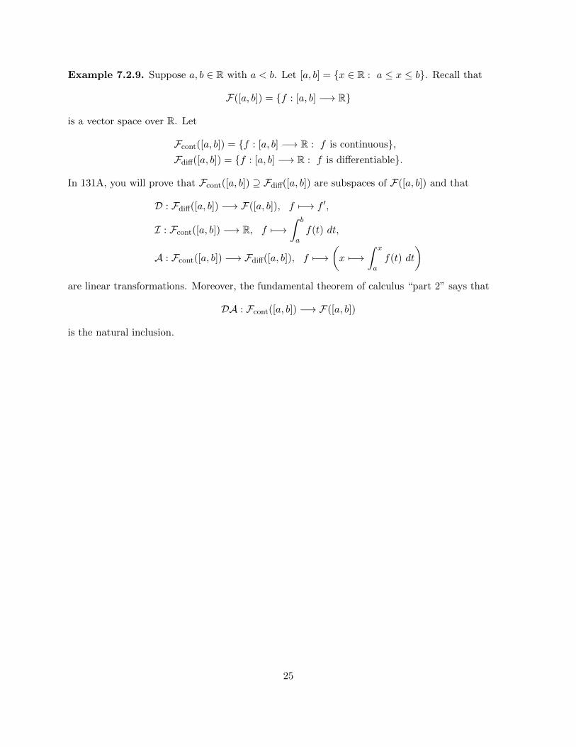
Example 7.2.9. Suppose a, b ∈ R with a < b. Let [a, b] = {x ∈ R : a ≤ x ≤ b}. Recall that

F([a, b]) = {f : [a, b] −→ R}

is a vector space over R. Let

Fcont([a, b]) = {f : [a, b] −→ R : f is continuous},Fdiff([a, b]) = {f : [a, b] −→ R : f is differentiable}.

In 131A, you will prove that Fcont([a, b]) ⊇ Fdiff([a, b]) are subspaces of F([a, b]) and that

D : Fdiff([a, b]) −→ F([a, b]), f 7−→ f ′,

I : Fcont([a, b]) −→ R, f 7−→∫ b

af(t) dt,

A : Fcont([a, b]) −→ Fdiff([a, b]), f 7−→(x 7−→

∫ x

af(t) dt

)are linear transformations. Moreover, the fundamental theorem of calculus “part 2” says that

DA : Fcont([a, b]) −→ F([a, b])

is the natural inclusion.

25


1. Prove part 2 of theorem 3.3.12.

The format of your proof should be similar to that of part 1. You should note that part (f)requires specifying a y ∈ Y with a given property. To write down such a y, you probably needto have found another element first. I’ll leave for you to think about which set this elementis contained in. You will get this auxilary element using an assumed surjectivity.

Solution: [1 pt. for completion]

(a) Suppose X, Y , and Z are sets, and that f : X −→ Y and g : Y −→ Z are functions.

(b) We want to prove that if g ◦ f is surjective, then g is surjective.

(c) So suppose g ◦ f is surjective. We would like to verify that g is surjective.

(d) By definition, we must show that if z ∈ Z, then we can find an y ∈ Y such that g(y) = z.

(e) So let z ∈ Z. We need to specify a y ∈ Y with g(y) = z.

(f) Since g ◦ f is surjective, we can find an x ∈ X with (g ◦ f)(x) = z.

Let y = f(x). Then g(y) = g(f(x)) = (g ◦ f)(x) = z.

(g) Thus, we have shown g is surjective, and this finishes the proof that if g ◦ f is surjective,then g is surjective.

2. [Optional]

Suppose X, Y , A, and B are sets and that A ⊆ X and B ⊆ Y . Prove that

(X × Y ) \ (A×B) = ((X \A)× Y ) ∪ (X × (Y \B)).

Cases made my proof clearer.

If you’re attempting to be careful, then you should make explicit reference to the definition ofthe Cartesian product. For example, you might say the following. “Let z ∈ (X×Y )\(A×B).Then z ∈ X × Y . By the definition of the Cartesian product, z = (x, y) for some x ∈ X andsome y ∈ Y .”

Solution:

Suppose X, Y , A, and B are sets and that A ⊆ X and B ⊆ Y . We wish to show that

(X × Y ) \ (A×B) = ((X \A)× Y ) ∪ (X × (Y \B)).

By definition of set equality, we must show “⊆” and “⊇.”

(a) First, we show ‘⊆.”

Suppose z ∈ (X × Y ) \ (A×B).

By definition of \, this says z ∈ X × Y and z /∈ A × B. By definition of the Cartesianproduct X × Y , we can write z = (x, y) where x ∈ X and y ∈ Y .

We cannot have x ∈ A and y ∈ B, for otherwise the definition of the Cartesian productA×B would give z = (x, y) ∈ A×B. Thus, either x /∈ A, or y /∈ B.

26

i. Case 1: x /∈ A.Since we have x ∈ X, the definition of \ gives x ∈ X \A.Since y ∈ Y , the definition of Cartesian product gives z = (x, y) ∈ (X \A)× Y .By definition of ∪, this gives z ∈ ((X \A)× Y ) ∪ (X × (Y \B)).

ii. Case 2: y /∈ B.Since we have y ∈ Y , the definition of \ gives y ∈ Y \B.Since x ∈ X, the definition of Cartesian product gives z = (x, y) ∈ X × (Y \B).By definition of ∪, this gives z ∈ ((X \A)× Y ) ∪ (X × (Y \B)).

In either case, we have z ∈ ((X \A)× Y ) ∪ (X × (Y \B)).

(b) First, we show ‘⊇.”

Suppose z ∈ ((X \A)× Y ) ∪ (X × (Y \B)). By definition of ∪, there are two cases.

i. Case 1: z ∈ (X \A)× Y .By definition of Cartesian product, z = (x, y) where x ∈ X \A and y ∈ Y .By definition of \, we have x ∈ X and x /∈ A.Because x ∈ X and y ∈ Y , the definition of the Cartesian product X × Y tells usthat we have z = (x, y) ∈ X × Y .Because x /∈ A, the definition of the Cartesian product A × B tells us that we donot have (x, y) ∈ A×B.So, by definition of \, we have z ∈ (X × Y ) \ (A×B).

ii. Case 2: z ∈ X × (Y \B).By definition of Cartesian product, z = (x, y) where x ∈ X and y ∈ Y \B.By definition of \, we have y ∈ Y and y /∈ B.Because x ∈ X and y ∈ Y , the definition of the Cartesian product X × Y tells usthat we have z = (x, y) ∈ X × Y .Because y /∈ B, the definition of the Cartesian product A × B tells us that we donot have (x, y) ∈ A×B.So, by definition of \, we have z ∈ (X × Y ) \ (A×B).

In either case, we have z ∈ (X × Y ) \ (A×B).

3. The first time I taught this class, someone suggested that

{(x1, x2) ∈ R2 : x1x2 ≥ 0}

with addition defined by

(x1, x2) + (y1, y2) = (x1 + y1, x2 + y2)

and scalar multiplication defined by λ(x1, x2) = (λx1, λx2) is a vector space over R.

Although this is incorrect, I was very grateful for their suggestion. Please do not stop makingsuch suggestions! This is a great example for improving your intuition of what a vector spaceis, and making sure that you understand all the ingredients to be one.

(a) Which axioms are true for this wannabe-vector-space? You don’t need to write down allof your proofs. If you think for a while, you’ll see that most of them are the same proofsthat you or I did for R2. Perhaps you could expand on axiom 4 a little.

27

(b) Does addition always make sense?

If yes, give a quick explanation as to why it is always okay.

If not, give an explicit example to show it screws up.

(c) Does scalar multiplication always make sense?

If yes, give a quick explanation as to why it is always okay.

If not, give an explicit example to show it screws up.

(d) Why is this wannabe-vector-space just a wannabe?

(e) This wannabe-vector-space is actually a subset of the vector space R2.

Show that it fails the subspace test.

Solution:

(a) In (b), you find out that addition it not well-defined. Because of this axioms 1,2,3,4,7,8are just weird from the get-go. However, if you don’t see the problem with addition, andnaıvely check the axioms, you’ll succeed! Even axiom 4 works since (−x1)(−x2) = x1x2.

(b) [2 pts.] Addition is not well-defined since it would say

(1, 0) + (0,−1) = (1,−1);

(1, 0), (0,−1) are in the wannabe-vector-space, but (1,−1) is not in there.

(c) Scalar multiplication is okay: because (λx1)(λx2) = λ2(x1x2) and λ2 ≥ 0, we find that(λx1, λx2) is an element of the wannabe-vector-space whenever (x1, x2) is.

(d) Addition is not well-defined.

(e) Our example in (b) shows that it fails the subspace test.

4. (a) [Optional (just part (a))]

Let V = {0} consist of a single vector 0. Define addition and scalar multiplication by

0 + 0 = 0, λ0 = 0 (λ ∈ R),

respectively. Prove that, with these operations, V is a vector space over R.

Your proof should not be long! I won’t have this one graded, so you should be tryingfor the most concise proof that says everything that is necessary.

(b) Suppose V is a vector space over R. Is the following statement true or false?

If λ, µ ∈ R, v ∈ V, and λv = µv, then λ = µ.

If not, you should be giving the most concise (but explicit) counter-example.

(c) Suppose V is a vector space over R. Is the following statement true or false?

If λ ∈ R, u, v ∈ V, and λu = λv, then u = v.

Help: your answer will depend on what V is.

This is reasonable since V was given to you before the statement. A similar thing happensin the following English excerpts because “it” means something different.

Have you tried Poke? It’s delicious and healthy.

Have you tried Fat Sal’s? It’s delicious and healthy.

28

Solution:

(a) Here’s the long proof. . .

Define addition and scalar multiplication on {0} by 0 + 0 = 0, λ0 = 0 (λ ∈ R), respec-tively. We verify the axioms of a vector space as follows:

i. Let u, v ∈ {0}. Then u = v = 0, so u+ v = 0 + 0 = v + u.

ii. Let u, v, w ∈ {0}. Then u = v = w = 0, so that

(u+ v) + w = (0 + 0) + 0 = 0 + 0 = 0 + (0 + 0) = u+ (v + w),

where the second and third equalities are by definition of addition.

iii. We already have an element called 0. We must check that it has the correct property.Let v ∈ {0}. Then v = 0, so v + 0 = 0 + 0 = 0 = v, where the second equality is bydefinition of addition.

iv. Let u ∈ {0} and v = 0. Then v ∈ {0}. Also, u = 0, so u+ v = 0 + 0 = 0, where thesecond equality is by definition of addition.

v. Let v ∈ {0}. Then v = 0, so 1v = 1 · 0 = 0 = v, where the second equality is bydefinition of scalar multiplication.

vi. Let λ, µ ∈ R, v ∈ {0}. Then v = 0, so

(λµ)v = (λµ)0 = 0 = λ0 = λ(µ0) = λ(µv),

where the second, third, and fourth equalities are by definition of scalar multiplica-tion.

vii. Let λ ∈ R, u, v ∈ {0}. Then u = v = 0, so

λ(u+ v) = λ(0 + 0) = λ0 = 0 = 0 + 0 = λ0 + λ0 = λu+ λv,

where the second and fourth equalities are by definition of addition, and the thirdand fifth equalities are by definition of scalar multiplication.

viii. Let λ, µ ∈ R, v ∈ {0}. Then v = 0, so

(λ+ µ)v = (λ+ µ)0 = 0 = 0 + 0 = λ0 + µ0 = λv + µv,

where the second and fourth equalities are by definition of scalar multiplication, andthe third is by definition of addition.

Here’s the short proof. . .

Every element we think of, and every expression we can think of writing down is equalto 0. So the axioms all hold trivially.

(b) Suppose V is a vector space over R. The statement is false because here is a counter-example: let λ = 0, µ = 1, and v = 0; then λv = 0 = µv, but λ 6= µ.

(c) [2pts.] Suppose V is a vector space over R, and V 6= {0}. Then the statement is falsebecause here is a counter-example: let λ = 0, u = 0, v ∈ V \ {0}; then λu = 0 = λv, butu 6= v.

If V = {0}, then the statement is true since whenever u, v ∈ V , we have u = 0 = v.

29

5. Suppose X is a nonempty set. In class, I said that the set of real-valued functions from X,{f : X −→ R} is a vector space over R when equipped with pointwise addition and scalarmultiplication. I checked axioms 2, 3, and 6.

(a) Carefully check axioms 5, 7, and 8.

I suppose you can check the others as well if you want more practice.

(b) Taking X = {0, 1} we see that {f : {0, 1} −→ R} is a vector space over R under pointwiseaddition and scalar multiplication. Let

f, g, h : {0, 1} −→ R

be defined by f(t) = 2t+ 1, g(t) = 1 + 4t− 2t2, and h(t) = 5t + 1.

Prove that f = g and f + g = h.

For the first, you need to remember (or sensibly decide) what it means for two functionsto be equal. For the second, you need to use this definition again, as well as the definitionof f + g in terms of f and g.

Solution:

Suppose X is a nonempty set.

(a) [3 pts.] For axiom 5, suppose that f : X −→ R and x ∈ X. Then

(1f)(x) = 1(f(x)) = f(x)

where the first equality is by definition of scalar multiplication, and the second is becauseof how 1 multiplies with real numbers. Since x ∈ X is arbitrary, we conclude that 1f = f .

For axiom 7, suppose λ ∈ R, f : X −→ R, g : X −→ R, and x ∈ X. Then

(λ(f + g))(x) = λ((f + g)(x)) = λ(f(x) + g(x))

= λ(f(x)) + λ(g(x)) = (λf)(x) + (λg)(x) = (λf + λg)(x),

where the first and fourth equalities are by definition of scalar multiplication, the secondand fifth equalities are by definition of addition, and the third is by the distributivity ofthe real numbers’ addition and multiplication. Since x ∈ X was arbitrary, we concludethat λ(f + g) = λf + λg.

For axiom 8, suppose λ, µ ∈ R, f : X −→ R, and x ∈ X. Then

((λ+µ)f)(x) = (λ+µ)(f(x)) = λ(f(x)) +µ(f(x)) = (λf)(x) + (µf)(x) = (λf +µf)(x),

where the first and third equalities are by definition of scalar multiplication, and thesecond is by the distributivity of the real numbers’ addition and multiplication, and thefourth is by definition of addition. Because x ∈ X was arbitrary, we can conclude that(λ+ µ)f = λf + µf .

(b) Let X, f , g, and h, be as in the question.

Then f(0) = 1 = g(0) and f(1) = 3 = g(1), so f = g.

Moreover, (f + g)(0) = f(0) + g(0) = 1 + 1 = 2 = h(0) and (f + g)(1) = f(1) + g(1) =3 + 3 = 6 = h(1), so that f + g = h.

30

6. (a) Recall theorem 7.1.4. It says that in order to check a subset W of a vector space V overR is a subspace, we just have to check that the following three conditions hold.

i. 0 ∈W .

ii. If w ∈W and w′ ∈W , then w + w′ ∈W .

iii. If λ ∈ R and w ∈W , then λw ∈W .

Why is the first condition necessary; doesn’t it follow iii. and the fact that 0w = 0?

(b) Suppose V is a vector space over R with operations + : V ×V → V , · : R×V → V , zeroelement 0, and that W is a subset of V . Prove that W is a subspace of V if and only ifthe following two conditions hold:

i. 0 ∈W .

ii. If λ ∈ R, w ∈W , and w′ ∈W , then λw + w′ ∈W .

I would call the conditions in (a), ai, aii, aiii, and the conditions in (b), bi, bii. Then Iwould go about proving that (ai, aii, and aiii hold) if and only if (bi and bii hold). Soyour proof should have two parts. One should begin with “suppose ai, aii, and aiii hold”and the other with “suppose bi and bii hold.”

Solution:

(a) [1pt.] The empty set satisfies the second and third condition, but it is not a subspacebecause the empty set is not a vector space. This is because the empty set does not havea zero element (because it has no elements).

(b) [4 pts.] Suppose V is a vector space over R with operations + : V ×V → V , · : R×V → V ,zero element 0, and that W is a subset of V . Consider the following conditions.

i. 0 ∈W .

ii. If w ∈W and w′ ∈W , then w + w′ ∈W .

iii. If λ ∈ R and w ∈W , then λw ∈W .

iv. If λ ∈ R, w ∈W , and w′ ∈W , then λw + w′ ∈W .

Using the subspace test (theorem 7.3), it is enough to show that

i, ii, iii ⇐⇒ i, iv.

Suppose i, ii, iii. We need to show i, iv. i is trivial because we assumed it! To show iv,let λ ∈ F, w,w′ ∈ W . Because condition iii holds λw ∈ W . Because condition ii holds,λw + w′ ∈W .

Suppose i, iv. We need to show i, ii, iii. i is trivial because we assumed it!

To show ii, let w,w′ ∈W . Since 1 ∈ R, and condition iv holds, w +w′ = 1w +w′ ∈W .

To show iii, let λ ∈ R and w ∈ W . Because i holds, we have 0 ∈ W . Because iv holds,we have λw = λw + 0 ∈W .

31

7. (a) Let X be a nonempty subset of R. Recall that the set of real-valued functions from X,F = {f : X −→ R} is a vector space over R when equipped with pointwise addition andscalar multiplication.

Fix an x0 ∈ X.

i. Prove that evx0 : F −→ R, f 7−→ f(x0) is linear.

ii. Prove that Kevx0 = {f ∈ F : f(x0) = 0} is a subspace of F .(“Kev” does not stand for Kevin. Can you figure out what it stands for?)

(b) Taking X = R we see that the real-valued functions on the real line V = {f : R −→ R}form a vector space over R under pointwise addition and scalar multiplication. Considerthe subset of even functions

E = {f : R −→ R : for all t ∈ R, f(−t) = f(t)}.

Prove that E is a subspace of V .

Solution:

(a) [1pt. for completion]

i. Let f, g ∈ F . Then

evx0(f + g) = (f + g)(x0) = f(x0) + g(x0) = evx0(f) + evx0(g),

where the first and last equality are by definition of evx0 , and the middle equalityis by definition of addition in F .Let λ ∈ R, f ∈ F . Then

evx0(λf) = (λf)(x0) = λ(f(x0)) = λ · evx0(f),

where the first and last equality are by definition of evx0 , and the middle equalityis by definition of scalar multiplication in F .We have shown that evx0 is linear.

ii. Here is the slow way. . .Let X be a nonempty subset of R, F = {f : X −→ R}.Fix an x0 ∈ X.We wish to show that Kevx0 = {f : X −→ R : f(x0) = 0} is a subspace of F .We use the subspace test.Notice 0 ∈ Kevx0 since 0(x0) = 0.Let f, g ∈ Kevx0 . Then (f + g)(x0) = f(x0) + g(x0) = 0 + 0 = 0, where the firstequality is by definition of addition in F , and the second is because f, g ∈ Kevx0 .We conclude that f + g ∈ Kevx0 .Let λ ∈ R, f ∈ Kevx0 . Then (λf)(x0) = λ(f(x0)) = λ0 = 0, where the first equalityis by definition of scalar multiplication in F , and the second is because f ∈ Kevx0 .We conclude that λf ∈ Kevx0 .

Here is the fast way: Kevx0 = ker (evx0), and every kernel is a subspace.

32

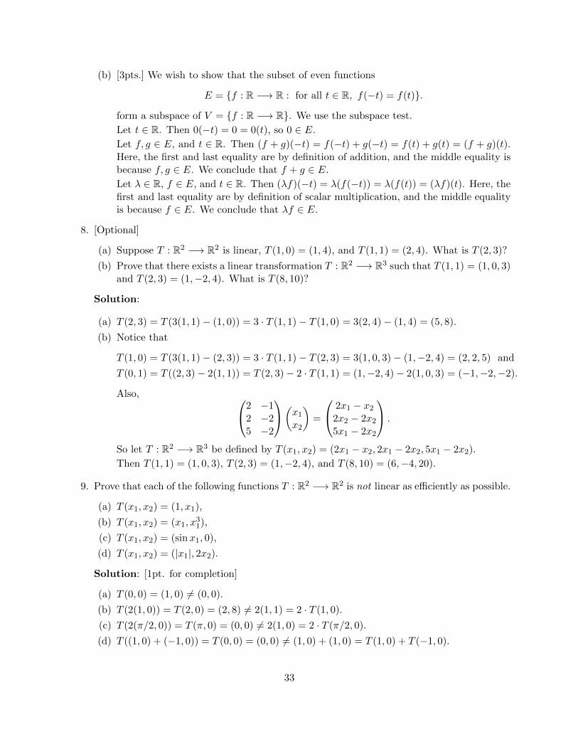
(b) [3pts.] We wish to show that the subset of even functions

E = {f : R −→ R : for all t ∈ R, f(−t) = f(t)}.

form a subspace of V = {f : R −→ R}. We use the subspace test.

Let t ∈ R. Then 0(−t) = 0 = 0(t), so 0 ∈ E.

Let f, g ∈ E, and t ∈ R. Then (f + g)(−t) = f(−t) + g(−t) = f(t) + g(t) = (f + g)(t).Here, the first and last equality are by definition of addition, and the middle equality isbecause f, g ∈ E. We conclude that f + g ∈ E.

Let λ ∈ R, f ∈ E, and t ∈ R. Then (λf)(−t) = λ(f(−t)) = λ(f(t)) = (λf)(t). Here, thefirst and last equality are by definition of scalar multiplication, and the middle equalityis because f ∈ E. We conclude that λf ∈ E.

8. [Optional]

(a) Suppose T : R2 −→ R2 is linear, T (1, 0) = (1, 4), and T (1, 1) = (2, 4). What is T (2, 3)?

(b) Prove that there exists a linear transformation T : R2 −→ R3 such that T (1, 1) = (1, 0, 3)and T (2, 3) = (1,−2, 4). What is T (8, 10)?

Solution:

(a) T (2, 3) = T (3(1, 1)− (1, 0)) = 3 · T (1, 1)− T (1, 0) = 3(2, 4)− (1, 4) = (5, 8).

(b) Notice that

T (1, 0) = T (3(1, 1)− (2, 3)) = 3 · T (1, 1)− T (2, 3) = 3(1, 0, 3)− (1,−2, 4) = (2, 2, 5) and

T (0, 1) = T ((2, 3)− 2(1, 1)) = T (2, 3)− 2 · T (1, 1) = (1,−2, 4)− 2(1, 0, 3) = (−1,−2,−2).

Also, 2 −12 −25 −2

(x1

x2

)=

2x1 − x2

2x2 − 2x2

5x1 − 2x2

.

So let T : R2 −→ R3 be defined by T (x1, x2) = (2x1 − x2, 2x1 − 2x2, 5x1 − 2x2).

Then T (1, 1) = (1, 0, 3), T (2, 3) = (1,−2, 4), and T (8, 10) = (6,−4, 20).

9. Prove that each of the following functions T : R2 −→ R2 is not linear as efficiently as possible.

(a) T (x1, x2) = (1, x1),

(b) T (x1, x2) = (x1, x31),

(c) T (x1, x2) = (sinx1, 0),

(d) T (x1, x2) = (|x1|, 2x2).

Solution: [1pt. for completion]

(a) T (0, 0) = (1, 0) 6= (0, 0).

(b) T (2(1, 0)) = T (2, 0) = (2, 8) 6= 2(1, 1) = 2 · T (1, 0).

(c) T (2(π/2, 0)) = T (π, 0) = (0, 0) 6= 2(1, 0) = 2 · T (π/2, 0).

(d) T ((1, 0) + (−1, 0)) = T (0, 0) = (0, 0) 6= (1, 0) + (1, 0) = T (1, 0) + T (−1, 0).

33

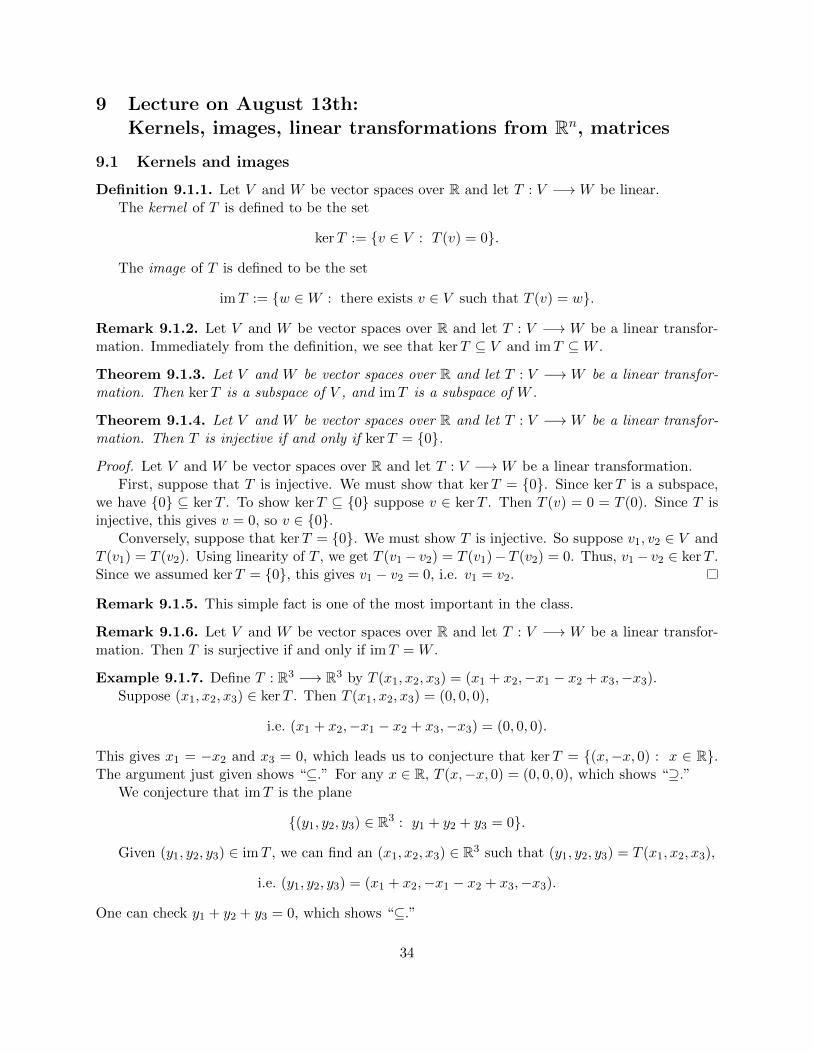
9 Lecture on August 13th:Kernels, images, linear transformations from Rn, matrices

9.1 Kernels and images

Definition 9.1.1. Let V and W be vector spaces over R and let T : V −→W be linear.The kernel of T is defined to be the set

kerT := {v ∈ V : T (v) = 0}.

The image of T is defined to be the set

imT := {w ∈W : there exists v ∈ V such that T (v) = w}.

Remark 9.1.2. Let V and W be vector spaces over R and let T : V −→ W be a linear transfor-mation. Immediately from the definition, we see that kerT ⊆ V and imT ⊆W .

Theorem 9.1.3. Let V and W be vector spaces over R and let T : V −→ W be a linear transfor-mation. Then kerT is a subspace of V , and imT is a subspace of W .

Theorem 9.1.4. Let V and W be vector spaces over R and let T : V −→ W be a linear transfor-mation. Then T is injective if and only if kerT = {0}.

Proof. Let V and W be vector spaces over R and let T : V −→W be a linear transformation.First, suppose that T is injective. We must show that kerT = {0}. Since kerT is a subspace,

we have {0} ⊆ kerT . To show kerT ⊆ {0} suppose v ∈ kerT . Then T (v) = 0 = T (0). Since T isinjective, this gives v = 0, so v ∈ {0}.

Conversely, suppose that kerT = {0}. We must show T is injective. So suppose v1, v2 ∈ V andT (v1) = T (v2). Using linearity of T , we get T (v1− v2) = T (v1)−T (v2) = 0. Thus, v1− v2 ∈ kerT .Since we assumed kerT = {0}, this gives v1 − v2 = 0, i.e. v1 = v2.

Remark 9.1.5. This simple fact is one of the most important in the class.

Remark 9.1.6. Let V and W be vector spaces over R and let T : V −→ W be a linear transfor-mation. Then T is surjective if and only if imT = W .

Example 9.1.7. Define T : R3 −→ R3 by T (x1, x2, x3) = (x1 + x2,−x1 − x2 + x3,−x3).Suppose (x1, x2, x3) ∈ kerT . Then T (x1, x2, x3) = (0, 0, 0),

i.e. (x1 + x2,−x1 − x2 + x3,−x3) = (0, 0, 0).

This gives x1 = −x2 and x3 = 0, which leads us to conjecture that kerT = {(x,−x, 0) : x ∈ R}.The argument just given shows “⊆.” For any x ∈ R, T (x,−x, 0) = (0, 0, 0), which shows “⊇.”

We conjecture that imT is the plane

{(y1, y2, y3) ∈ R3 : y1 + y2 + y3 = 0}.

Given (y1, y2, y3) ∈ imT , we can find an (x1, x2, x3) ∈ R3 such that (y1, y2, y3) = T (x1, x2, x3),

i.e. (y1, y2, y3) = (x1 + x2,−x1 − x2 + x3,−x3).

One can check y1 + y2 + y3 = 0, which shows “⊆.”

34

Conversely, given (y1, y2, y3) ∈ R3, with y1 + y2 + y3 = 0, let (x1, x2, x3) = (y1, 0,−y3). ThenT (x1, x2, x3) = (x1 + x2,−x1− x2 + x3,−x3) = (y1 + 0,−y1− 0− y3, y3) = (y1,−y1− y3, y3). Sincey1 + y2 + y3 = 0, we have y2 = −y1− y3, and (y1, y2, y3) = (y1,−y1− y3, y3) = T (x1, x2, x3) ∈ imT .Thus, we have “⊇.”

Remark 9.1.8. Such calculations will be far quicker once we have the rank-nullity theorem at ourdisposal.

9.2 Linear transformations from Rn

Definition 9.2.1. Suppose V is a vector space over R and n ∈ N. By an n-tuple of vectors in V ,we mean an element of the Cartesian product V n, (v1, v2, . . . , vn).

We take as convention that there is one 0-tuple, the empty tuple ( ).

We’ll use the following notation throughout the rest of the class, so don’t ignore this.

Notation 9.2.2. Suppose V is a vector space over R and n ∈ N, and α = (v1, . . . , vn) is an n-tupleof vectors in V . We write Γα : Rn −→ V for the function

(λ1, λ2, . . . , λn) 7−→ λ1v1 + λ2v2 + . . .+ λnvn.

Remark 9.2.3. In case you ever worry about whether n = 0 is allowed, it is a sensible conventionto take R0 = {0}. Moreover, if α is the empty tuple ( ), Γα : R0 −→ V is the inclusion of 0 into V .

Theorem 9.2.4. Suppose V is a vector space over R, and α = (v1, . . . , vn) is an n-tuple of vectorsin V . The function Γα : Rn −→ V is linear.

Remark 9.2.5. Linear transformations Γα : Rn −→ V where α is an n-tuple of vectors in V will bevery important for us. This is because these type of transformations clarify almost every conceptthat we study in the remainder of the class. Moreover, every linear transformation out of Rn is ofthis form.

Theorem 9.2.6. Suppose V is a vector space over R and T : Rn → V is a linear transformation.For j ∈ {1, . . . , n}, let vj = T (ej) where ej = (0, . . . , 0, 1, 0, . . . , 0) with the 1 in the j-th position.Let α = (v1, . . . , vn). Then T = Γα.

Proof. Let everything be as in the theorem statement. Then for all (λ1, λ2, . . . , λn) ∈ Rn, we have

T (λ1, λ2, . . . , λn) = T (λ1e1 + λ2e2 + . . .+ λnen)

= λ1T (e1) + λ2T (e2) + . . .+ λnT (en)

= λ1v1 + λ2v2 + . . .+ λnvn

= Γα(λ1, λ2, . . . , λn).

Remark 9.2.7. Recall remark 7.2.4. Suppose v1, v2, . . . , vn ∈ Rm and A is the m×n matrix with j-th column given by vj . Recall example 7.2.3 which tells us that TA : Rn −→ Rm, x 7−→ Ax is a lineartransformation. We also have Γ(v1,v2,...,vn) : Rn −→ Rm, (λ1, λ2, . . . , λn) 7−→ λ1v1+λ2v2+. . .+λnvn.The definition of matrix-vector multiplication ensures that TA = Γ(v1,v2,...,vn).

35

Corollary 9.2.8. Suppose m,n ∈ N and T : Rn → Rm is a linear transformation. Then there is aunique matrix A ∈Mm×n(R) such that T = TA.

Proof. We use the previous theorem and remark.For j ∈ {1, . . . , n}, let vj = T (ej) where ej = (0, . . . , 0, 1, 0, . . . , 0) with the 1 in the j-th position,

let α = (v1, . . . , vn), and let A be the m × n matrix with j-th column given by vj . The theoremsays that T = Γα. The remark gives TA = Γα. So T = TA. This completes the existence proof.

For uniqueness, suppose A,B ∈Mm×n(R) and TA = TB. For each j ∈ {1, . . . , n}, we have

j-th column of A = Aej = TA(ej) = TB(ej) = Bej = j-th column of B.

Thus, A = B.

9.3 Basic matrix operations (in case you have forgotten)

Recall that an m× n matrix is a grid of numbers with m rows and n colums:

A =

A11 A12 A13 · · · A1n

A21 A22 A23 · · · A2n

A31 A32 A33 · · · A3n...

......

. . ....

Am1 Am2 Am3 · · · Amn

We can add two m× n matrices entrywise, so that [A+B]ij = Aij +Bij . We can also multiply bya scalar, so that [λA]ij = λAij .

Given an m×n matrix A, and an n× p matrix B, we can multiply A and B to obtain an m× pmatrix AB. There is a concise formula for the (i, j)-entry of AB, in terms of the entries of A andB:

[AB]ij =n∑k=1

AikBkj = Ai1B1j +Ai2B2j + . . .+AinBnj .

One way to think of this is as the dot product between the i-th row of A, and the j-th column ofB. Thinking about things this way will allow you to multiply two matrices correctly. It gives noinsight into what on earth is going on. The language we have developed can be used to fix this.

9.4 How to think about matrices the “right” way

The previous corollary says that linear transformations Rn → Rm are the “same” as m×n matrices.In 33A, you spend all quarter thinking about and using matrices. Matrices are arrays of num-

bers which can often be overwhelming. Although they are computationally useful, for conceptualpurposes it is often better to think about the linear transformations that they define: instead ofthinking about the matrix A, think about the linear transformation TA. For example, do you preferthinking about a special orthogonal matrix or a rotation? A rotation seems far more reasonable tome! The difference between thinking about a matrix versus a linear transformation is somewhatphilosophical since one determines the other, but while matrices just sit there being all ugly, lineartransformations do something: they move vectors to new vectors.

As before, let ej = (0, . . . , 0, 1, 0, . . . , 0) ∈ Rn with the 1 in the j-th position. While proving theprevious corollary, we used the following important fact.

Aej = the j-th column of the matrix A.

36

Remark 9.4.1. We can now summarize the two most important properties of m× n matrices.

• An m× n matrix A does something: via the linear transformation TA, it takes vectors in Rnto vectors in Rm.

• The j-th column of A tells you where ej goes under TA.

Remark 9.4.2. The importance of these two bullet points cannot be overstated. If you ever hada moment in 33A where your TA could see something about a matrix was true and it appeared tobe black magic on their part, it was probably just that your TA knew these two facts.

Because of the last bullet point, when thinking about matrix-vector multiplication, the columnsof the matrix are the most important. Write an m×n matrix A as its column vectors next to eachother:

A =

(v1

∣∣∣∣∣v2

∣∣∣∣∣ · · ·∣∣∣∣∣vn), v1, v2, . . . , vn ∈ Rm.

Then matrix-vector multiplication can be described as follows:

A

λ1

λ2...λn

= λ1v1 + λ2v2 + . . .+ λnvn.

Notice that this is precisely Γ(v1,v2,...,vn)(λ1, λ2, . . . , λn). This is the right way to think about matrix-vector multiplication. Given an m× n matrix A, and a vector x ∈ Rn, Ax is a linear combinationof the columns of the matrix. The components of the vector tell you what scalar multiple of eachcolumn of the matrix to take.

As long as we’re thinking about m × n matrices in terms of their linear transformations, thenthere is a right way to think about matrix multiplication too. Given an m × n matrix A, and ann× p matrix B, write B as its column vectors next to each other

B =

(w1

∣∣∣∣∣w2

∣∣∣∣∣ · · ·∣∣∣∣∣wp), w1, w2, . . . , wp ∈ Rn.

Then

AB =

(Aw1

∣∣∣∣∣Aw2

∣∣∣∣∣ · · ·∣∣∣∣∣Awp

),

and each of Aw1, Aw2, . . . , Awp ∈ Rm can be calculated as just described in the previous paragraph.

Example 9.4.3. I gave examples of “reflect across the x-axis” and “project onto the xy-plane” inclass.

37


1. Suppose V is a vector space over R, and that W1 and W2 are subspaces of V .

Prove that W1 ∪W2 is a subspace of V if and only if W1 ⊆W2 or W2 ⊆W1.

Hint: For the forwards implication =⇒ , I would prove the contrapositive which is

If W1 6⊆W2 and W2 6⊆W1, then W1 ∪W2 is not a subspace of V.

Solution:

Suppose V is a vector space over R, and that W1 and W2 are subspaces of V .

First, suppose W1 ⊆W2. Then W1 ∪W2 = W2, and so W1 ∪W2 is a subspace.

Second, suppose W2 ⊆W1. Then W1 ∪W2 = W1, and so W1 ∪W2 is a subspace.

Now suppose that W1 6⊆ W2 and W2 6⊆ W1. This means we can choose elements w1 and w2

such that w1 ∈W1 \W2 and w2 ∈W2 \W1. We have w1, w2 ∈W1∪W2, and we will show thatW1 ∪W2 is not a subspace by showing that w1 + w2 6∈ W1 ∪W2. Suppose for contradictionthat w1 + w2 ∈W1 ∪W2.

(a) Case 1: w1 + w2 ∈W1. Since w1 ∈W1 and W1 is a subspace, −w1 ∈W1, and so

w2 = (w1 + w2) + (−w1) ∈W1.

This is a contradiction to how we chose w2.

(b) Case 2: w1 + w2 ∈W2. Since w2 ∈W2 and W2 is a subspace, −w2 ∈W2, and so

w1 = (w1 + w2) + (−w2) ∈W2.

This is a contradiction to how we chose w1.

2. Prove lemma 7.2.8.

On the one hand, I think this is very easy, and should feel very boring if you understand whatis going on.

On the other hand, if you don’t say the phrases “suppose T : U → V and S : V → W arelinear”, “by definition of ST” a few times, “since T is linear,” and “since S is linear,” thenyou don’t know what you’re doing, and you need to talk to me, Kevin, or a friend who doesknow what is happening.

Solution:

Suppose U , V , and W are vector spaces over R, that T : U → V and S : V → W are lineartransformations. We wish to show ST : U −→W is a linear transformation.

Let u1, u2 ∈ U . Then

(ST )(u1 + u2) = S(T (u1 + u2)) = S(T (u1) + T (u2))

= S(T (u1)) + S(T (u2)) = (ST )(u1) + (ST )(u2).

Here the first and last equalities are by definition of ST , the second is by linearity of T , andthe third is by linearity of S.

Similarly, you can check that for λ ∈ R and u ∈ U , (ST )(λu) = λ(ST )(u). Thus, ST is linear.

38

3. [More difficult, but not optional]

Let V be the vector space {f : R −→ R} of real-valued functions on the real line.

Let f1, f2, f3 ∈ V be defined by f1(t) = 1, f2(t) = cos2 t, f3(t) = sin2(t).

Let α be the 2-tuple (f1, f2) and β be the 3-tuple (f1, f2, f3). Look back on 9.2.2.

We have the linear transformations Γα : R2 −→ V , Γβ : R3 −→ V .

(a) Prove that ker Γα = {0}. (So Γα is injective!)

Showing “⊆” is the harder direction.

“Suppose (λ1, λ2) ∈ ker Γα. We want to show (λ1, λ2) = (0, 0) . . .”

You might find the linear transformations ev0 : V −→ R, evπ2

: V −→ R useful.

(b) Find an element of (λ1, λ2, λ3) ∈ (ker Γβ) \ {0}.(c) Prove that ker Γβ = {µ(λ1, λ2, λ3) : µ ∈ R}.

Solution:

(a) ker Γα is a subspace of R2 so {0} ⊆ ker Γα.

We must show ker Γα ⊆ {0}. So suppose (λ1, λ2) ∈ ker Γα. Then

λ1f1 + λ2f2 = Γα(λ1, λ2) = 0.

This equation expresses an equality of functions. In particular, 0 means the 0-function.We apply ev0 and evπ

2to obtain useful equations:

λ1 + λ2 = 0 and λ1 = 0.

These imply (λ1, λ2) = (0, 0), as required.

(b) Γβ(−1, 1, 1) = −f1 + f2 + f3. Evaluating this function at t ∈ R gives

−1 + cos2 t+ sin2 t = 0.

Thus, Γβ(−1, 1, 1) is the zero function and (−1, 1, 1) ∈ ker Γβ \ {0}.(c) We wish to show ker Γβ = {µ(−1, 1, 1) : µ ∈ R}.

“⊇” is clear since (−1, 1, 1) ∈ ker Γβ and ker Γβ is a subspace of R3.

For “⊆,” suppose (λ1, λ2, λ3) ∈ ker Γβ.

Thenλ1f1 + λ2f2 + λ3f3 = Γβ(λ1, λ2, λ3) = 0.

This equation expresses an equality of functions. In particular, 0 means the 0-function.We apply ev0 and evπ

2to obtain useful equations:

λ1 + λ2 = 0 and λ1 + λ3 = 0.

Thus, (λ1, λ2, λ3) = (λ1,−λ1,−λ1) = −λ1(−1, 1, 1) ∈ {µ(−1, 1, 1) : µ ∈ R}.

39

4. [Optional]

Corollary 9.2.8 together with remark 9.4.1 makes question 8.(b) in the last lot of questionsmuch easier. Revisit that question.

Solution:

A solution to last week’s 8.(b) has been posted.

Remark. Kevin was concerned that he may have confused some people in discussion.There are a few things he wanted me to emphasize.

1. A linear transformation T : W −→ V can only be of the form Γα if W = Rn for some n.

2. A linear transformation T : W −→ V can only be of the form TA (for some matrix A) whenW = Rn for some n and V = Rm for some m.

3. Eventually, we will address how matrices show up from linear transformations T : W −→ Vbetween abstract vector spaces. This will require picking bases for W and V . So far, we havenot spoken about bases and none of the definitions I have made have used this concept.

Be patient! Make sure that you understand the definitions given so far.

40

11 Lecture on August 15th: Spans and linear (in)dependence

11.1 Linear combinations and spans of tuples

Recall that whenever we have a vector space V over R and an n-tuple α = (v1, . . . , vn) of vectorsin V , we have a linear transformation Γα : Rn −→ V defined by

(λ1, λ2, . . . , λn) 7−→ λ1v1 + λ2v2 + . . .+ λnvn.

In this section, we consider the image of such transformations and the condition for such a trans-formation to be surjective.

Definition 11.1.1. Suppose V is a vector space over R and (v1, v2, . . . , vn) is an n-tuple of vectorsin V . An element v ∈ V is said to be a linear combination of (v1, v2, . . . , vn) iff there exist scalarsλ1, λ2, . . . , λn ∈ R such that

v = λ1v1 + λ2v2 + . . .+ λnvn.

In this case, we call λ1, λ2, . . . , λn the coefficients of the linear combination.

Remark 11.1.2. It is a sensible convention to regard 0 as the only linear combination of the emptytuple.

Example 11.1.3. 1. In R3, (1, 8, 1) is a linear combination of ((1, 2, 1), (0, π, 0)).

2. In R3, (0, 0, 1) is not a linear combination of ((1, 1, 0), (0, 1, 1)).

Definition 11.1.4. Suppose V is a vector space over R and (v1, v2, . . . , vn) is an n-tuple of vectorsin V . The span of (v1, v2, . . . , vn) is the set

span(v1, v2, . . . , vn) := {λ1v1 + λ2v2 + . . .+ λnvn : λ1, λ2, . . . , λn ∈ R}.

Remark 11.1.5. It is a sensible convention to take the span of the empty tuple to be {0}.

Remark 11.1.6. Suppose V is a vector space over R and (v1, v2, . . . , vn) is an n-tuple of vectors inV . It is immediate from the previous two definitions that an element v ∈ V is a linear combinationof (v1, v2, . . . , vn) if and only if v ∈ span(v1, v2, . . . , vn).

Definition 11.1.7. Suppose V is a vector space over R and (v1, v2, . . . , vn) is an n-tuple of vectorsin V . We say that (v1, v2, . . . , vn) spans V iff every v ∈ V is a linear combination of (v1, v2, . . . , vn).

Remark 11.1.8. Suppose V is a vector space over R and (v1, v2, . . . , vn) is an n-tuple of vectorsin V . It is immediate from the previous two definitions that (v1, v2, . . . , vn) spans V if and only ifspan(v1, v2, . . . , vn) = V .

Example 11.1.9. 1. Let n ∈ N. The tuple (e1, e2, . . . , en) spans Rn.

2. The tuple (e1, e1 + e2, e2) spans R2.

3. Let n ∈ N. The tuple (1, x, x2, . . . , xn) spans Pn(R).

Remark 11.1.10. Suppose V is a vector space over R and (v1, v2, . . . , vn) is an n-tuple of vectorsin V . First, notice that span(v1, v2, . . . , vn) is precisely the image of Γ(v1,v2,...,vn). This tells us thatspan(v1, v2, . . . , vn) is a subspace of V . Moreover, notice that (v1, v2, . . . , vn) spans V if and only ifΓ(v1,v2,...,vn) is surjective.

41

11.2 Linear combinations and spans of arbitrary sets (omitted)

This section is not necessary for the main results of the class. This is because we focus on finite-dimensional vector spaces.

Definition 11.2.1. Suppose V is a vector space over R and that ∅ 6= S ⊆ V .An element v ∈ V is said to be a linear combination of vectors in S iff there exists an n-tuple

of vectors (v1, v2, . . . , vn) in S such that v is a linear combination of (v1, v2, . . . , vn).

Definition 11.2.2. Suppose V is a vector space over R and that ∅ 6= S ⊆ V .The span of S is the set

span(S) := {v ∈ V : v is a linear combination of vectors in S}.

Our conventions regarding the empty tuple mean that span(∅) = {0}.

Definition 11.2.3. Suppose V is a vector space over R, and that S ⊆ V .We say that S spans V iff span(S) = V .

Theorem 11.2.4. Suppose V is a vector space over R and S ⊆ V .Then span(S) is the smallest subspace of V which contains S.

11.3 Linear dependence and linear independence


(λ1, λ2, . . . , λn) 7−→ λ1v1 + λ2v2 + . . .+ λnvn.

In this section, we consider the kernel of such transformations and the condition for such a trans-formation to be injective.

Definition 11.3.1. Suppose V is a vector space over R and (v1, v2, . . . , vn) is an n-tuple of vectorsin V . An equation

λ1v1 + λ2v2 + . . .+ λnvn = 0

with λ1, λ2, . . . , λn ∈ R is called a dependency relation for (v1, v2, . . . , vn).The equation 0v1+0v2+. . .+0vn = 0 is called the trivial dependency relation for (v1, v2, . . . , vn).

Other dependency relations are called non-trivial.

Definition 11.3.2. Suppose V is a vector space over R and (v1, v2, . . . , vn) is an n-tuple of vectors inV . (v1, v2, . . . , vn) is said to be linearly dependent iff there exists a non-trivial dependency relationfor (v1, v2, . . . , vn). (v1, v2, . . . , vn) is said to be linearly independent iff the only dependency relationfor (v1, v2, . . . , vn) is the trivial one.

Remark 11.3.3. It is a sensible convention to regard the empty tuple as linearly independent.

Example 11.3.4.

1. Let f1, f2, f3 : R −→ R be defined by f1(t) = 1, f2(t) = cos2 t, f3(t) = sin2 t.

These are elements of the vector space F = {f : R −→ R}.(f1, f2, f3) is linearly dependent. (f1, f2) is linearly independent.

2. The tuple ((1,−1, 2), (2, 0, 1), (−1, 2,−1)) of vectors in R3 is linearly independent.

42

Remark 11.3.5. Suppose V is a vector space over R and (v1, v2, . . . , vn) is an n-tuple of vectorsin V . Notice that we have a dependency relation

λ1v1 + λ2v2 + . . .+ λnvn = 0

if and only if (λ1, λ2, . . . , λn) in the kernel of Γ(v1,v2,...,vn).The fact that a tuple (v1, v2, . . . , vn) always has the trivial dependency relation is related to the

fact that 0 is always an element of the kernel of a linear transformation.Moreover, (v1, v2, . . . , vn) is linearly independent if and only if ker Γ(v1,v2,...,vn) = {0}, and this

latter condition is equivalent to the statement that Γ(v1,v2,...,vn) is injective.

Lemma 11.3.6. Suppose V is a vector space over R and v ∈ V .The 1-tuple (v) is linearly dependent if and only if v = 0.

Proof. Suppose V is a vector space over R and that v ∈ V . First, assume that v = 0. Then 1v = 0is a nontrivial dependency relation, so the 1-tuple (v) is linearly dependent. Conversely, assumethat the 1-tuple (v) is linearly dependent. Then there exists a nonzero scalar λ ∈ R such thatλv = 0. Thus, v = λ−1(λv) = λ−10 = 0.

Corollary 11.3.7. Suppose V is a vector space over R and v ∈ V .The 1-tuple (v) is linearly independent if and only if v 6= 0.

Example 11.3.8. Suppose V is a vector space over R and that v ∈ V . The 2-tuple (v, v) is linearlydependent. This is because 1v + (−1)v = 0 is a non-trivial dependency relation.

Remark 11.3.9. My definition differs from that of the textbook. The authors of the textbooktalk about a set of vectors being linearly (in)dependent, whereas I talk about an n-tuple of vectorsbeing linearly (in)dependent. Later on in the book, they will want to say that an n× n matrix isinvertible if and only if its column vectors are linearly independent. At this moment, they shouldrealize, but they don’t :(, that their definition sucks! The issue is that their definition says the set{

(1, 0), (1, 0)}

={

(1, 0)}

is linearly independent, but my definition says that the 2-tuple((1, 0), (1, 0)

)is linearly dependent. In the end, the concept of a multiset is the best-suited to talking about lineardependence. Even though they are not particularly difficult, I don’t expect you to know what theyare, so we’ll stick with n-tuples (which are elements of a Cartesian product).

Notice that my proofs of theorem 13.1.1 and theorem 13.2.5 are easier than the correspondingproofs in the textbook, those of theorems 1.7 and 1.9, largely because of these choices of definitions.

As a final piece of propaganda: “there are at least two exercises in the textbook that are wrongbecause the authors chose their definition incorrectly.”

Theorem 11.3.10. Suppose V is a vector space over R, that n,m ∈ N ∪ {0}, and that

v1, . . . , vn, vn+1, . . . , vn+m ∈ V.

If (v1, . . . , vn) is linearly dependent, then (v1, . . . , vn+m) is linearly dependent; if (v1, . . . , vn+m) islinearly independent, then (v1, . . . , vn) is linearly independent.

43


1. (a) [Optional]

Question 5 of page 34 from the textbook (but replace the word “set” by “tuple” andbraces {} with parentheses ()).

(b) Give an example a linearly dependent 3-tuple in R3 such that none of the 3 vectors is amultiple of another.

Solution: ((1, 0, 0), (0, 1, 0), (1, 1, 0)).

(c) [Optional]

Question 2(a)-(f) of page 40 of the textbook (but replace the word “set” by “tuple” andbraces {} with parentheses ()).

(d) Prove that (1 10 00 0

,

0 01 10 0

,

0 00 01 1

,

1 01 01 0

,

0 10 10 1

)

is linearly dependent in M3×2(R).

Solution: The following is a nontrivial dependecy relation:

1 ·

1 10 00 0

+ 1 ·

0 01 10 0

+ 1 ·

0 00 01 1

+ (−1) ·

1 01 01 0

+ (−1) ·

0 10 10 1

= 0

(e) Prove that(

(1, 1, 0), (0, 1, 1), (1, 0, 1))

is linearly independent in R3.

Solution: Suppose we have a dependency relation

λ1(1, 1, 0) + λ2(0, 1, 1) + λ3(1, 0, 1) = 0.

We wish to show that this must be the trivial dependency relation, i.e. that λ1 = λ2 =λ3 = 0. The above equation says (λ1 + λ3, λ1 + λ2, λ2 + λ3) = 0.

So λ1 + λ3 = 0, λ1 + λ2 = 0, and λ2 + λ3 = 0. Thus,

λ1 =+ (λ1 + λ3) + (λ1 + λ2)− (λ2 + λ3)

2=

0 + 0 + 0

2= 0,

λ2 =− (λ1 + λ3) + (λ1 + λ2) + (λ2 + λ3)

2=

0 + 0 + 0

2= 0,

λ3 =+ (λ1 + λ3)− (λ1 + λ2) + (λ2 + λ3)

2=

0 + 0 + 0

2= 0.

44

13 Lecture on August 16th: Towards bases and dimension

13.1 Spans and linear (in)dependence

Theorem 13.1.1. Suppose V is a vector space over R, that n ∈ N∪{0}, that (v1, . . . , vn) is linearlyindependent in V , and that vn+1 ∈ V .

Then (v1, . . . , vn, vn+1) is linearly dependent if and only if vn+1 ∈ span(v1, . . . , vn).

Proof. Suppose V is a vector space over R, that n ∈ N∪{0}, that (v1, . . . , vn) is linearly independentin V , and that vn+1 ∈ V .

First, suppose that vn+1 ∈ span(v1, . . . , vn). By definition of “span,” there exist λ1, . . . , λn ∈ Rsuch that

vn+1 = λ1v1 + . . . λnvn.

(v1, . . . , vn, vn+1) is linearly dependent because the following dependency relation is nontrivial:

(−λ1)v1 + . . . (−λn)vn + 1 · vn+1 = 0.

Now suppose that (v1, . . . , vn, vn+1) is linearly dependent. By definition of linear dependence,there is a nontrivial dependency relation:

λ1v1 + . . .+ λnvn + λn+1vn+1 = 0.

We cannot have λn+1 = 0, since otherwise we’d have a nontrivial dependency relation

λ1v1 + . . .+ λnvn = 0,

contradicting the fact that (v1, . . . , vn) is linearly independent. Thus, we have

vn+1 = λ−1n+1(λn+1vn+1) = (−λ1λ

−1n+1)v1 + . . .+ (−λnλ−1

n+1)vn ∈ span(v1, . . . , vn).

This proof reads well when n ∈ N. When n = 0, you have to be a bit more careful about whatsome expressions mean. With the correct interpretation it is just lemma 11.3.6 all over again, butyou might prefer to divide the proof into two cases. (The textbook fails to point this out.)

45

13.2 Towards bases and dimension


(λ1, λ2, . . . , λn) 7−→ λ1v1 + λ2v2 + . . .+ λnvn.

In this section, we consider the condition under which such a transformation is a bjiection.One can think of Γα as an attempt to coordinate-ify V using the tuple of vectors (v1, v2, . . . , vn):

a collection of coordinates (λ1, λ2, . . . , λn) determines a vector λ1v1 + λ2v2 + . . .+ λnvn.First, we can ask that every vector have a coordinate. This is the same as demanding that

Γα be surjective. We have seen that this, in turn, is the same as demanding that (v1, v2, . . . , vn)spans V . Second, we can ask that every vector have at most one coordinate. This is the same asdemanding that Γα be injective. We have seen, in turn, that this is the same as demanding that(v1, v2, . . . , vn) be linearly independent. We find that every vector has exactly one coordinate whenΓα is a bijection, and that this is the case when (v1, v2, . . . , vn) spans V and is linearly independent.

Definition 13.2.1. Suppose V is a vector space over R. An n-tuple (v1, v2, . . . , vn) of vectors inV is said to be a basis for V iff :

1. (v1, v2, . . . , vn) spans V and

2. (v1, v2, . . . , vn) is linearly independent.

Example 13.2.2. The empty tuple is a basis for {0}.By our conventions, we have span( ) = {0} and ( ) is linearly independent.

Theorem 13.2.3. Suppose V is a vector space over R. An n-tuple (v1, v2, . . . , vn) of vectors in Vis a basis for V if and only if for all v ∈ V , there are unique λ1, . . . , λn ∈ R such that

v = λ1v1 + λ2v2 + . . .+ λnvn.

Proof. Suppose V is a vector space over R. We have seen that an n-tuple α = (v1, v2, . . . , vn) ofvectors in V is a basis for V if and only if Γα is a bijection. This latter statement is the same assaying that for all v ∈ V , there are unique λ1, . . . , λn ∈ R such that

v = λ1v1 + λ2v2 + . . .+ λnvn.

You should try writing the proof out in more elementary terms using the definition of span andlinear independence.

We would like to make the following definition.

Definition 13.2.4. Suppose V is a vector space over R. We say V is finite-dimensional iff V is thespan of a finite tuple; otherwise, we say V is infinite-dimensional. When V is finite-dimensional,the dimension of V , written dimV , is the number of elements in a basis for V .

At the present moment, there are two problems with this definition. First, if V is spanned byfinitely many elements, does V even have a basis? Second, what if V is finite-dimensional and thereare two bases for V with different sizes; then doesn’t dimension become ambiguous?

The answer to the first question is “yes,” and the answer to the second question is “this cannothappen.” We need to prove these answers!

46

Theorem 13.2.5. Suppose V is a vector space over R and (v1, v2, . . . , vn) is an n-tuple of vectorsin V which spans V . Then some sub-tuple (vm1 , vm2 , . . . , vmr) is a basis for V .

In particular, V has a basis.

Proof. Suppose V and (v1, v2, . . . , vn) are as in the theorem statment.First, we note the two extreme cases. If (v1, v2, . . . , vn) is linearly independent, then (v1, . . . , vn)

is a basis for V and there is nothing to do: we can simply take mk = k for k = 1, . . . , n. Also, ifevery vi = 0, then V = {0}, and the empty tuple is a basis for V : we never even have to pick anm1. Notice that when n = 0, these extreme cases coincide.

Suppose that not every vi = 0. First, we shall construct a sub-tuple (vm1 , . . . , vmr) of (v1, . . . , vn)which is linearly independent and maximal with this property, i.e. adding any vector of (v1, . . . , vn)results in it becoming linearly dependent. Choose m1 to be the smallest number such that vm1 6= 0.By example 11.3.7, this is the same as choosing m1 to be the smallest number such that the 1-tuple (vm1) is linearly independent. While possible, repeat this process, choosing m2 to be thesmallest number such that (vm1 , vm2) is linearly independent, and m3 to be the smallest numbersuch that (vm1 , vm2 , vm3) is linearly independent. . . This process cannot continue forever. Thisis because we’d find ourselves adding a vector of (v1, . . . , vn) to the tuple twice, and this resultsin a tuple which is linearly dependent (example 11.3.8). Thus, we obtain m1,m2, . . . ,mr suchthat (vm1 , vm2 , . . . , vmr) is linearly independent and adding any vector of (v1, . . . , vn) results in itbecoming linearly dependent.

We claim that (vm1 , vm2 , . . . , vmr) is a basis for V . By construction, we have that (vm1 , . . . , vmr)is linearly independent. So we are just left to show that (vm1 , . . . , vmr) spans V .

As a first step towards this, we show {v1, v2, . . . , vn} ⊆ span(vm1 , . . . , vmr). With this goal, leti ∈ {1, . . . , n}. We need vi ∈ span(vm1 , . . . , vmr). By theorem 13.1.1, it is enough for us to knowthat (vm1 , . . . , vmr , vi) is linearly dependent, and this is true by construction of (vm1 , . . . , vmr).

Since span(vm1 , . . . , vmr) is a subspace of V , from {v1, . . . , vn} ⊆ span(vm1 , . . . , vmr), we obtain

span(v1, v2, . . . , vn) = {λ1v1 + λ2v2 + . . .+ λnvn : λ1, λ2, . . . , λn ∈ R} ⊆ span(vm1 , . . . , vmr).

We supposed that span(v1, v2, . . . , vn) = V , so this shows V ⊆ span(vm1 , . . . , vmr).Thus, V = span(vm1 , . . . , vmr), i.e. (vm1 , . . . , vmr) spans V , which completes the proof.

47

Theorem 13.2.6 (Replacement theorem). Let V be a vector space over R, and m,n ∈ N ∪ {0}.Suppose that (v1, v2, . . . , vm) and (w1, w2, . . . , wn) are tuples of vectors in V .Moreover, suppose that (v1, v2, . . . , vm) is linearly independent and (w1, w2, . . . , wn) spans V .Then m ≤ n, and we can pick n−m vectors from w1, w2, . . . , wn, say wk1 , wk2 , . . . , wkn−m such

that (v1, v2, . . . , vm, wk1 , wk2 , . . . , wkn−m) spans V .

Proof. Let V be a vector space over R.First, we note that if m = 0 and n ∈ N ∪ {0}, the statement of the theorem is true: 0 ≤ n and

we just pick all the vectors w1, w2, . . . , wn.Now, suppose that statement of the theorem is true for m,n ∈ N∪ {0}. We would like to show

that the result is true for m + 1, n. So suppose that v1, v2, . . . , vm, vm+1 ∈ V , w1, w2, . . . , wn ∈ V ,(v1, v2, . . . , vm, vm+1) is linearly independent, and (w1, w2, . . . , wn) spans V .

Since (v1, v2, . . . , vm) is linearly independent (theorem 11.3.10), we have, by the m,n result,that m ≤ n, and we can pick n−m vectors from w1, w2, . . . , wn, say wk1 , wk2 , . . . , wkn−m such that

α = (v1, v2, . . . , vm, wk1 , wk2 , . . . , wkn−m−1 , wkn−m)

spans V . Therefore, there exists scalars λ1, λ2, . . . , λm, µ1, µ2, . . . , µn−m ∈ R such that

vm+1 = λ1v1 + λ2v2 + . . .+ λmvm + µ1wk1 + µ2wk2 + . . .+ µn−m−1wkn−m−1 + µn−mwkn−m .

Since (v1, v2, . . . , vm, vm+1) is linearly independent, theorem 13.1.1 tells us that

vm+1 /∈ span(v1, v2, . . . , vm).

Thus, we must have n−m > 0, and at least one µi must be nonzero. This gives n ≥ m+ 1. Also,by reordering the wi’s and µi’s we may as well assume that µn−m 6= 0. We claim that

α′ = (v1, v2, . . . , vm, vm+1, wk1 , wk2 , . . . , wkn−m−1)

spans V . This claim would complete our goal of showing that the m + 1, n result is true. Noticethat we’re replacing wkn−m with vm+1 to go from α to α′ which is why the theorem has its name.

First, we’ll show that every element of α is in span(α′). We immediately have

v1, v2, . . . , vm, wk1 , wk2 , . . . , wkn−m−1 ∈ span(v1, v2, . . . , vm, vm+1, wk1 , wk2 , . . . , wkn−m−1)

= span(α′).

Also, because

wkn−m = (−λ1µ−1n−m)v1 + (−λ2µ

−1n−m)v2 + . . .+ (−λmµ−1

n−m)vm + µ−1n−mvm+1 +

(−µ1µ−1n−m)wk1 + (−µ2µ

−1n−m)wk2 + . . .+ (−µn−m−1µ

−1n−m)wkn−m−1 ,

we have wkn−m ∈ span(v1, v2, . . . , vm, vm+1, wk1 , wk2 , . . . , wkn−m−1) = span(α′).Since span(α′) is a subspace of V , any linear combination of α is also in span(α′). Thus, we

obtain span(α) ⊆ span(α′). Because V = span(α), this tells us that span(α′) = V , as we claimed.Thus, we have demonstrated that the m+ 1, n result follows from the m,n result.

The theorem is true by mathematical induction on m.

48


The first 4 questions are designed to encourage you to start thinking about matrices, matrix-vectormultiplication, and matrix multiplication more in line with how I think about them, and how Idiscussed them in lecture. The key things to remember and internalize are:

• An m× n matrix A does something: multiplying on the left takes vectors in Rn to vectors inRm. This is the linear transformation TA.

• The j-th column of A tells you where ej (the vector with 1 in the j-th place and 0’s elsewhere)goes.

• Matrix multiplication is just the same as lots of matrix-vector multiplications:

A

(w1

∣∣∣∣∣w2

∣∣∣∣∣ · · ·∣∣∣∣∣wp)

=

(Aw1

∣∣∣∣∣Aw2

∣∣∣∣∣ · · ·∣∣∣∣∣Awp

).

If you do these questions by trial-and-error, or by doing a bunch of matrix multiplications in therow-dot-column way of thinking, you’ll be missing the point. I can promise you that the perspectiveI am trying to provide you with here is one of the most fundamental in linear algebra and, in termsof your success in this class, it will be completely invaluable once we come to the matrix of a lineartransformation.

(These questions (1-4) should not take a long time.On the other hand, question 7 and 8 might take longer, but they’re important.)

1. This question will be concerned with 3× 3 matrices and linear functions R3 −→ R3. Let

e1 =

100

, e2 =

010

, and e3 =

001

.

(a) Find the 3× 3 matrix which defines the functionxyz

7−→xy

0

,

by thinking about what this function does to the vectors e1, e2, and e3.

(b) Similarly, find the 3× 3 matrix which defines the functionxyz

7−→yxz

.

(c) Find the 3× 3 matrix which defines the functionxyz

7−→ x

x+ yx+ y + z

.

49

2. Let e1, e2 and e3 be as in the previous problem and let

A =

0 0 11 0 00 1 0

=

(e2

∣∣∣∣∣e3

∣∣∣∣∣e1

).

(Matrix A is a special type of matrix called a permutation matrix.)

(a) What does the matrix A do to the vectors e1, e2, and e3?

(b) Without multiplying matrices, what does A2 do to e1, e2, and e3?

(c) Without multiplying matrices, what is A2?

(d) Check your answer to (c) by doing the matrix multiplication.

Be sure to think of the matrix multiplication as three matrix-vector multiplications.Wait. . . hopefully this forced you to redo some of the thinking in (b) again - hmmm.

(e) Without multiplying matrices, what does A3 = A ·A2 do to e1, e2, and e3?

(f) Without multiplying matrices, what is A3?

(g) Check your answer to (f) by doing the matrix multiplication A ·A2.

Be sure to think of the matrix multiplication as three matrix-vector multiplications.Wait. . . hopefully this forced you to redo some of the thinking in (e) again - hmmm.

3. Let e1, e2, e3, e4, e5 ∈ R5 be as in lecture, and let

B =

0 1 0 0 01 0 0 0 00 0 0 0 10 0 1 0 00 0 0 1 0

=

(e2

∣∣∣∣∣e1

∣∣∣∣∣e4

∣∣∣∣∣e5

∣∣∣∣∣e3

).

(Matrix B is also a permutation matrix.)

(a) What does the matrix B do to the vectors e1, e2, e3, e4, and e5?

(b) What is the smallest n ∈ N = {1, 2, 3, . . .} such that

Bn =

1 0 0 0 00 1 0 0 00 0 1 0 00 0 0 1 00 0 0 0 1

= I5?

Explain your answer fully without ever multiplying matrices.

(c) Do you want to check your answer with matrix multiplication?

(d) (Only if you answered “yes” to (c).)

Are you okay? Do you want me to set a bigger example to convince you otherwise?

50

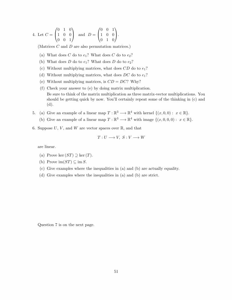
4. Let C =

0 1 01 0 00 0 1

and D =

0 0 11 0 00 1 0

.

(Matrices C and D are also permutation matrices.)

(a) What does C do to e1? What does C do to e2?

(b) What does D do to e1? What does D do to e2?

(c) Without multiplying matrices, what does CD do to e1?

(d) Without multiplying matrices, what does DC do to e1?

(e) Without multiplying matrices, is CD = DC? Why?

(f) Check your answer to (e) by doing matrix multiplication.

Be sure to think of the matrix multiplication as three matrix-vector multiplications. Youshould be getting quick by now. You’ll certainly repeat some of the thinking in (c) and(d).

5. (a) Give an example of a linear map T : R3 −→ R4 with kernel {(x, 0, 0) : x ∈ R}.(b) Give an example of a linear map T : R3 −→ R4 with image {(x, 0, 0, 0) : x ∈ R}.

6. Suppose U , V , and W are vector spaces over R, and that

T : U −→ V, S : V −→W

are linear.

(a) Prove ker (ST ) ⊇ ker (T ).

(b) Prove im(ST ) ⊆ imS.

(c) Give examples where the inequalities in (a) and (b) are actually equality.

(d) Give examples where the inequalities in (a) and (b) are strict.

Question 7 is on the next page.

51

7. Suppose that V is a vector space over R and that (v1, v2, . . . , vn) is a tuple of vectors in V .

(a) Suppose that n ≥ 2. Prove that (v1, v2, . . . , vn) is linearly dependent if and only if oneof the vectors can be written as a linear combination of the others.

(b) Prove that (v1, v2, . . . , vn) is linearly dependent if and only if there is a k ∈ {1, 2, . . . , n}such that

vk ∈ span(v1, v2, . . . , vk−1).

(When k = 1, the formula above should be read as saying v1 = 0.)

8. This is probably the best / most important question.

Suppose V and W are vector spaces over R, that T : V →W is a linear transformation, andthat (v1, v2, . . . , vn) is a tuple of vectors in V .

(a) Prove that if (v1, v2, . . . , vn) is linearly dependent,

then (T (v1), T (v2), . . . , T (vn)) is linearly dependent.

(b) Prove that if (T (v1), T (v2), . . . , T (vn)) is linearly independent,

then (v1, v2, . . . , vn) is linearly independent.

(c) Suppose kerT = {0}.Prove that if (T (v1), T (v2), . . . , T (vn)) is linearly dependent,

then (v1, v2, . . . , vn) is linearly dependent.

(d) Suppose kerT = {0}.Prove that if (v1, v2, . . . , vn) is linearly independent,

then (T (v1), T (v2), . . . , T (vn)) is linearly independent.

(e) Prove that if (v1, . . . , vn) spans V ,

then (T (v1), . . . , T (vn)) spans imT .

(f) Prove that if (v1, v2, . . . , vn) spans V

and (T (v1), T (v2), . . . , T (vn)) is linearly independent,

then kerT = {0}.

9. Let V be a vector space over R, and let u, v, w ∈ V .

(a) Prove that (u, v) is linearly independent if and only if (u+v, u−v) is linearly independent.

If you thought I was weird for giving the textbook such a hard time about its definitionof linearly (in)dependent, take a look at their version of this question: page 42, 13(a).

As long as V 6= {0}, their statement is false because you can take u 6= 0 and v = 0. Then{u, v} is linearly dependent, and {u+ v, u− v} = {u} is linearly independent (accordingto THEIR definition which involves sets instead of tuples).

I rest my case.

(b) Prove that (u, v, w) is linearly independent if and only if (u+ v, v+w,w+ u) is linearlyindependent.

52

15 Solutions to the previous questions

1. (a) e1 7−→ e1, e2 7−→ e2, e3 7−→ 0, so (e1|e2|0).

(b) e1 7−→ e2, e2 7−→ e1, e3 7−→ e3, so (e2|e1|e3).

(c) e1 7−→ e1 + e2 + e3, e2 7−→ e2 + e3, e3 7−→ e3, so (e1 + e2 + e3|e2 + e3|e3).

2. (a) A : e1 7−→ e2 7−→ e3 7−→ e1.

(b) A2 : e1 7−→ e3 7−→ e2 7−→ e1.

(c) A2 = (e3|e1|e2).

(d) A2 = (Ae2|Ae3|Ae1) = (e3|e1|e2).

(e) A3 : e1 7−→ e1, e2 7−→ e2, e3 7−→ e3.

(f) A3 = (e1|e2|e3) = I3.

(g) A3 = A ·A2 = (Ae3|Ae1|Ae2) = (e1|e2|e3) = I3.

3. (a) B : e1 7−→ e2 7−→ e1, e3 7−→ e4 7−→ e5 7−→ e3.

(b) We find that Bne1 = e1 and Bne2 = e2 if and only if n is even.

We find that Bne3 = e3, Bne4 = e4, and Bne5 = e5 if and only if n is divisible by 3.

Thus, Bn = I5 if and only if n is even and divisible by 3. The smallest such n ∈ N is 6.

(c) No.

(d) If I did, I wouldn’t be okay. I’d be extremely upset and bored.

4. (a) C : e1 7−→ e2 7−→ e1.

(b) D : e1 7−→ e2 7−→ e3.

(c) CD : e1 7−→ e1.

(d) DC : e1 7−→ e3.

(e) The previous two observations tell us the first column of CD is different from the firstcolumn of DC.

(f) CD = C(e2|e3|e1) = (Ce2|Ce3|Ce1) = (e1|e3|e2).

DC = D(e2|e1|e3) = (De2|De1|De3) = (e3|e2|e1).

53

5. (a) T (x1, x2, x3) = (0, x2, x3, 0).

(b) T (x1, x2, x3) = (x1, 0, 0, 0).

6. Suppose U , V , and W are vector spaces over R, and that

T : U −→ V, S : V −→W

are linear.

(a) We’ll prove that ker (ST ) ⊇ ker (T ). Let u ∈ ker (T ). Then

(ST )(u) = S(T (u)) = S(0) = 0.

The first equality holds by the definition of ST . The second hold because u ∈ kerT . Thelast equality is a consequence of S being linear. This calculation shows that u ∈ ker (ST ).

(b) We’ll prove that im(ST ) ⊆ imS. Let w ∈ im(ST ). By the definition of im(ST ), we canfind a u ∈ U such that w = (ST )(u). Letting v = T (u), we have

S(v) = S(T (u)) = (ST )(u) = w.

The first equality is because v = T (u). The second is by definition of ST . The third isbecause of how we chose u. This calculation shows that w ∈ imS.

(c) Take U = V = W = {0}.(d) Take T : R −→ R2, T (x) = (x, 0), and S : R2 −→ R, S(x1, x2) = x2. Then, for all x ∈ R,

(ST )(x) = S(T (x)) = S(x, 0) = 0.

Thus, ker (ST ) = R and im(ST ) = {0}.On the other hand, we have ker (T ) = {0} and imS = R.

54

7. Suppose that V is a vector space over R and that (v1, v2, . . . , vn) is a tuple of vectors in V .

(a) First, suppose that (v1, v2, . . . , vn) is linearly dependent. This means that we can find anon-trivial dependency relation

λ1v1 + λ2v2 + . . .+ λnvn = 0.

Since the dependency relation is non-trivial, we can choose a k ∈ {1, 2, . . . , n} such thatλk 6= 0. We have

vk =

(− λ1

λk

)v1 + . . .+

(− λk−1

λk

)vk−1 +

(− λk+1

λk

)vk+1 + . . .+

(− λnλk

)vn,

so vk is a linear combination of (v1, . . . , vk−1, vk+1, . . . , vn).

Conversely, suppose that vk is a linear combination of (v1, . . . , vk−1, vk+1, . . . , vn). Thenthere are λ1, . . . , λk−1, λk+1, . . . λn ∈ R such that

vk = λ1v1 + . . .+ λk−1vk−1 + λk+1vk+1 + . . .+ λnvn.

This gives

(−λ1)v1 + . . .+ (−λk−1)vk−1 + 1 · vk + (−λk+1)vk+1 + . . .+ (−λn)vn = 0.

Since 1 6= 0, this is a non-trivial dependency relation, and so this shows (v1, v2, . . . , vn)is linearly dependent.

We don’t need n ≥ 2, as long as you have the correct convention regarding “others.”

(b) Suppose there is a k ∈ {1, 2, . . . , n} such that

vk ∈ span(v1, v2, . . . , vk−1).

If k = 1, this means that v1 = 0, so (v1) is linearly dependent. In any case, the argumentgiven in part (a) shows that (v1, . . . , vk) is linearly dependent, and theorem 11.3.10 saysthat (v1, . . . , vn) is linearly dependent.

Conversely, suppose (v1, v2, . . . , vn) is linearly dependent. Let k ∈ {1, 2, . . . , n} be theminimum value such that (v1, v2, . . . , vk) is linearly dependent. If k = 1, this means (v1)is linearly dependent, so v1 = 0, which is what we mean by

vk ∈ span(v1, v2, . . . , vk−1).

In any case, we have that (v1, . . . , vk−1) is linearly independent, and (v1, . . . , vk−1, vk) islinearly dependent, so theorem 13.1.1 tells us that vk ∈ span(v1, v2, . . . , vk−1).

(c) Another proof of the harder direction of (b) which refines the argument of (a) says. . .

Suppose that (v1, v2, . . . , vn) is linearly dependent. Then there exist λ1, λ2, . . . , λn ∈ R,not all zero, such that λ1v1 + λ2v2 + . . . + λnvn = 0. Let λk be the largest nonzero λ.Then vk = −1

λk(λ1v1 + . . .+ λk−1vk−1) ∈ span(v1, . . . , vk−1).

55

8. Suppose V and W are vector spaces over R, that T : V →W is a linear transformation, andthat (v1, v2, . . . , vn) is a tuple of vectors in V .

(a) Suppose (v1, v2, . . . , vn) is linearly dependent. This means that we can find a non-trivialdependency relation

λ1v1 + λ2v2 + . . .+ λnvn = 0. (15.1)

We obtain

λ1T (v1) + λ2T (v2) + . . .+ λnT (vn) = T (λ1v1 + λ2v2 + . . .+ λnvn) = T (0) = 0.

The first and last equalities use the linearity of T . The middle equality is obtained byapplying T to (15.1).

λ1T (v1) + λ2T (v2) + . . .+ λnT (vn) = 0

is a non-trivial dependency relation for (T (v1), T (v2), . . . , T (vn)), so (T (v1), . . . , T (vn))is linearly dependent.

(b) This is the contrapositive of (a).

(c) Suppose kerT = {0}. Also, suppose that (T (v1), T (v2), . . . , T (vn)) is linearly dependent.This means that we can find a non-trivial dependency relation

λ1T (v1) + λ2T (v2) + . . .+ λnT (vn) = 0.

Using linearity of T , we obtain

T (λ1v1 + λ2v2 + . . .+ λnvn) = λ1T (v1) + λ2T (v2) + . . .+ λnT (vn) = 0.

This shows λ1v1 + λ2v2 + . . .+ λnvn ∈ kerT . Since kerT = {0},

λ1v1 + λ2v2 + . . .+ λnvn = 0

and this is a non-trivial dependency relation for (v1, v2, . . . , vn), so (v1, . . . , vn) is linearlydependent.

(d) This is the contrapositive of (c).

(e) Suppose (v1, . . . , vn) spans V . It is clear that imT ⊇ span(T (v1), T (v2), . . . , T (vn)). Wewish to show that imT ⊆ span(T (v1), T (v2), . . . , T (vn)).

Let w ∈ imT . By definition of imT , we can find a v ∈ V such that T (v) = w.

Since (v1, v2, . . . , vn) spans V , we can find λ1, λ2, . . . , λn ∈ R such that

v = λ1v1 + λ2v2 + . . .+ λnvn.

Applying T and using the fact that T is linear gives

T (v) = λ1T (v1) + λ2T (v2) + . . .+ λnT (vn).

Since this quantity is equal to w, we see that w ∈ span(T (v1), T (v2), . . . , T (vn)).

Thus, imT = span(T (v1), T (v2), . . . , T (vn)), i.e. (T (v1), . . . , T (vn)) spans imT .

56

(f) Suppose that (v1, v2, . . . , vn) spans V and that (T (v1), T (v2), . . . , T (vn)) is linearly inde-pendent. We wish show kerT = {0}.Let v ∈ kerT . Since (v1, v2, . . . , vn) spans V , we can find λ1, λ2, . . . , λn ∈ R such that

λ1v1 + λ2v2 + . . .+ λnvn = v. (15.2)

We obtain

λ1T (v1) + λ2T (v2) + . . .+ λnT (vn) = T (λ1v1 + λ2v2 + . . .+ λnvn) = T (v) = 0.

The first equality uses the linearity of T . The middle equality is obtained by applyingT to (15.2). The last equality is because v ∈ kerT .

λ1T (v1) + λ2T (v2) + . . .+ λnT (vn) = 0

is a dependency relation for (T (v1), T (v2), . . . , T (vn)). Since (T (v1), T (v2), . . . , T (vn)) islinearly independent, it must be the trivial dependency relation, i.e. λ1 = . . . = λn = 0.Thus, v = λ1v1 + λ2v2 + . . .+ λnvn = 0, and v ∈ {0}.We have shown that kerT ⊆ {0}. kerT ⊇ {0} is always true. Thus, kerT = {0}.

57

9. This question turned out to be longer than I thought it would be. I’m sorry.

(a) Let V be a vector space over R, and let u, v ∈ V .

Suppose (u, v) is linearly independent, λ1, λ2 ∈ R, and that

λ1(u+ v) + λ2(u− v) = 0.

Rewriting this gives(λ1 + λ2)u+ (λ1 − λ2)v = 0.

Since (u, v) is linearly independent, we obtain

λ1 + λ2 = λ1 − λ2 = 0.

Thus,

λ1 =(λ1 + λ2) + (λ1 − λ2)

2=

0 + 0

2= 0,

λ2 =(λ1 + λ2)− (λ1 − λ2)

2=

0 + 0

2= 0.

We conclude (u+ v, u− v) is linearly independent.

Suppose (u+ v, u− v) is linearly independent, λ1, λ2 ∈ R, and that

λ1u+ λ2v = 0.

Rewriting this gives (λ1 + λ2

2

)(u+ v) +

(λ1 − λ2

2

)(u− v) = 0.

Since (u+ v, u− v) is linearly independent, we obtain

λ1 + λ2

2=λ1 − λ2

2= 0.

Thus,

λ1 =λ1 + λ2

2+λ1 − λ2

2= 0 + 0 = 0,

λ2 =λ1 + λ2

2− λ1 − λ2

2= 0− 0 = 0.

58

(b) Let V be a vector space over R, and let u, v, w ∈ V .

Suppose (u, v, w) is linearly independent, λ1, λ2, λ3 ∈ R, and that

λ1(u+ v) + λ2(v + w) + λ3(w + u) = 0.

Rewriting this gives

(λ3 + λ1)u+ (λ1 + λ2)v + (λ2 + λ3)w = 0.

Since (u, v, w) is linearly independent, we obtain

λ3 + λ1 = λ1 + λ2 = λ2 + λ3 = 0.

Thus,

λ1 =+ (λ3 + λ1) + (λ1 + λ2)− (λ2 + λ3)

2=

0 + 0 + 0

2= 0,

λ2 =− (λ3 + λ1) + (λ1 + λ2) + (λ2 + λ3)

2=

0 + 0 + 0

2= 0,

λ3 =+ (λ3 + λ1)− (λ1 + λ2) + (λ2 + λ3)

2=

0 + 0 + 0

2= 0.

We conclude that (u+ v, v + w,w + u) is linearly independent.

Suppose (u+ v, v + w,w + u) is linearly independent, λ1, λ2, λ3 ∈ R, and that

λ1u+ λ2v + λ3w = 0.

Rewriting this gives(+ λ1 + λ2 − λ3

2

)(u+ v) +

(− λ1 + λ2 + λ3

2

)(v + w)

+

(+ λ1 − λ2 + λ3

2

)(w + u) = 0.

Since (u+ v, v + w,w + u) is linearly independent, we obtain

+ λ1 + λ2 − λ3

2=− λ1 + λ2 + λ3

2=

+ λ1 − λ2 + λ3

2= 0.

Then

λ1 =+ λ1 + λ2 − λ3

2+

+ λ1 − λ2 + λ3

2= 0 + 0 = 0,

λ2 =+ λ1 + λ2 − λ3

2+− λ1 + λ2 + λ3

2= 0 + 0 = 0,

λ3 =− λ1 + λ2 + λ3

2+

+ λ1 − λ2 + λ3

2= 0 + 0 = 0.

We conclude that (u, v, w) is linearly independent.

59

16 Quiz 1

1. Recall that R1 = { (x) : x ∈ R} is a vector space over R with coordinatewise addition andscalar multiplication.

(a) List every subspace of R1. You don’t need to prove your claim in this part.

Solution: {0} and R1.

(b) Suppose V is a subspace of R1.

Prove that V has to be equal to one of the subspaces you wrote down in part (a).

Solution: There are two cases.

i. V = {0}. Then, trivially, V is one of the subspaces we wrote down in part (a).

ii. V 6= {0}. We wish to show that V = R1.Since V is a subspace, we have {0} ⊆ V . Thus, V 6= {0} tells us that V 6⊆ {0}. Thismeans we can find an element (x) ∈ V with x 6= 0. Since x 6= 0, x−1 is a well-definedreal number. Because (x) ∈ V and V is closed under scalar multiplication, we findthat x−1(x) ∈ V , i.e. (1) ∈ V .We trivially have V ⊆ R1 because V is a subspace. Conversely, given (y) ∈ R1, wehave (y) = y(1) ∈ V because V is closed under scalar multiplication. Thus, V = R1.

2. Suppose X is a nonempty set.

In class and on the homework, we proved that the set of real-valued functions from X,

F = {f : X −→ R}

is a vector space over R when equipped with pointwise addition and scalar multiplication.

(a) Give the definition of addition and scalar multiplication in F .

Solution: For f, g ∈ F , λ ∈ R, x ∈ X, we have

(f + g)(x) := f(x) + g(x) and (λf)(x) := λ(f(x)).

(b) Verify the eighth axiom of a vector space for F , that is, that for all λ, µ ∈ R, and for allf ∈ F , (λ+ µ)f = λf + µf .

Solution: see homework.

(c) Fix x0, x1 ∈ X. Prove that T : F −→ R, f 7−→ f(x0) + f(x1) is linear.

Solution: Let f, g ∈ F , λ ∈ R. Then

T (f + g) = (f + g)(x0) + (f + g)(x1) = f(x0) + g(x0) + f(x1) + g(x1)

= f(x0) + f(x1) + g(x0) + g(x1) = T (f) + T (g).

The first and last equality follow from the definition of T . The second follows from thedefinition of addition given in part (a). The third uses commutativity of addition in R.

Also,

T (λf) = (λf)(x0) + (λf)(x1) = λ(f(x0)) + λ(f(x1)) = λ(f(x0) + f(x1)) = λT (f).

The first and last equality follow from the definition of T . The second follows from thedefinition of scalar multiplication given in part (a). The third follows from distributivityof addition and multiplication in R.

60

Now take X = R so that F = {f : R −→ R}.(d) Is the subset {f ∈ F : f(0) = 1} a subspace of F?

Solution: No, because the zero function is not contained in this subset.

(e) Is the subset {f ∈ F : f(−1) · f(1) = 0} a subspace of F?

Solution: No. Here’s why. . .

Call the set in question G. Let f+, f− : R −→ R be defined by f+(x) = 1+x and f−(x) =1− x. Then f+(−1) = 0 and f−(1) = 0, so f+, f− ∈ G. However, (f+ + f−)(x) = 2, so

(f+ + f−)(−1) · (f+ + f−)(1) = 2 · 2 = 4 6= 0,

which means f+ + f− /∈ G.

3. Let (e1, e2, . . . , e6) be the standard basis of R6. Consider the 6× 6 matrix

A =

(2e5

∣∣∣∣e3

∣∣∣∣3e6

∣∣∣∣5e4

∣∣∣∣e1

∣∣∣∣e2

).

Calculate A30 and A31 efficiently.

Solution:

• A : e4 7−→ 5e4,

• A : e5 7−→ e1 7−→ 2e5,

• A : e6 7−→ e2 7−→ e3 7−→ 3e6.

Thus,

• An : e4 7−→ 5ne4,

• A2n : e1 7−→ 2ne1, e5 7−→ 2ne5,

• A3n : e2 7−→ 3ne2, e3 7−→ 3ne3, e6 7−→ 3ne6.

In particular,

• A30 : e4 7−→ 530e4,

• A30 : e1 7−→ 215e1, e5 7−→ 215e5,

• A30 : e2 7−→ 310e2, e3 7−→ 310e3, e6 7−→ 310e6.

So A30 =

(215e1

∣∣∣∣310e2

∣∣∣∣310e3

∣∣∣∣530e4

∣∣∣∣215e5

∣∣∣∣310e6

)and

A31 =

(215Ae1

∣∣∣∣310Ae2

∣∣∣∣310Ae3

∣∣∣∣530Ae4

∣∣∣∣215Ae5

∣∣∣∣310Ae6

)=

(216e5

∣∣∣∣310e3

∣∣∣∣311e6

∣∣∣∣531e4

∣∣∣∣215e1

∣∣∣∣310e2

).

61

4. (a) Prove that the following tuple spans R3.((1, 0, 0), (1, 1, 0), (1, 1, 1)

)Solution: For any (λ1, λ2, λ3) ∈ R3, we have

(λ1, λ2, λ3) = (λ1 − λ2)(1, 0, 0) + (λ2 − λ3)(1, 1, 0) + λ3(1, 1, 1).

This shows R3 ⊆ span

((1, 0, 0), (1, 1, 0), (1, 1, 1)

). The other inclusion is trivial.

(b) Define T : R3 −→ R3 by

T

x1

x2

x3

=

1 0 −11 −1 00 1 −1

x1

x2

x3

.

For this particular example, describe kerT , and prove your claim.

Solution: We claim that

kerT =

λ1

11

: λ ∈ R

.

“⊇” is easy since you can just check that for any λ ∈ R, T

λ1

11

= 0.

For “⊆”, suppose that

x1

x2

x3

∈ kerT , i.e. T

x1

x2

x3

= 0. The definition of T gives

x1 − x3

x1 − x2

x2 − x3

= 0.

Looking at the second coordinate gives x1 = x2, while looking at the third coordinategives x2 = x3. Letting λ = x1, we obtainx1

x2

x3

= λ

111

.

Thus,

x1

x2

x3

∈λ

111

: λ ∈ R

.

62

5. Suppose V and W are vector spaces over R, that S : V →W is a linear transformation, andthat (v1, v2, . . . , vn) is a tuple of vectors in V .

Always true or sometimes false (i.e. depends on V , W , S, etc.)?

(a) If (v1, v2, . . . , vn) spans V ,

then (S(v1), S(v2), . . . , S(vn)) is linearly independent and kerS = {0}.(b) If kerS = {0} and (S(v1), S(v2), . . . , S(vn)) is linearly independent,

then (v1, v2, . . . , vn) is linearly independent.

(c) If im S = W , then (S(v1), S(v2), . . . , S(vn)) spans W .

(d) If (v1, v2, . . . , vn) is linearly independent,

then (S(v1), S(v2), . . . , S(vn)) is linearly independent.

Solution:

(a) Sometimes false. Consider the case when S : R −→ {0}, and v1 = 1.

(v1) spans R, but (S(v1)) = (0) is linearly dependent and kerS = R.

(b) Always true. You proved this on the homework.

In fact, the kerS = {0} hypothesis is not even needed.

(c) Sometimes false. Consider the case when S : R −→ R is the identity, and v1 = 0. ThenimS = R, but (S(v1)) = (0) does not span R.

(d) Sometimes false. Consider the case when S : R −→ {0}, and v1 = 1.

(v1) is linearly independent, but (S(v1)) = (0) is linearly dependent.

63

17 Comments on quiz 1

1. (a) {1, 2, . . . , n}?!

{(x) : x ∈ N \ {0}}?!

{0, 1, 2, . . . , n}?!

N, Z?!

You really should know from 33A that the only subspaces of R1 are {0} and R1. 33A isa prerequisite for this class.

(b) Most common error. . .

You proved that {0} is a subspace and that R1 is a subspace. Yes, this is true. It’s thesimplest fact I can think of about subspaces. However, it is not at all what the questionasks you to do, and is completely irrelevant for answering the question. In proving theseresults you’re addressing the claim:

if V = {0} or V = R1, then V is a subspace of R1 .

The question asks you to prove:

if V is a subspace of R1, then V = {0} or V = R1.

2. Main complaints. . .

• Why do you not know definitions which I have given in class and have used excessivelyin my homework solutions?

• Every time I have checked an axiom, I have done one of two things:

– labelled each equality with a justification;

– addressed, in a paragraph after the relevant equations, why each equality is true.

What are you not doing the same?

• To show that {f ∈ F : f(−1) · f(1) = 0} is not closed under addition, you must providean explicit counter-example. This means defining functions.

I do something similar in 3.(b) of the 8/13 questions where I use explicit vectors.

Also, in class I showed

A =

{(x, 0) : x ∈ R

}∪{

(0, y) : y ∈ R}

is not a subspace of R2 by saying that (1, 0), (0, 1) ∈ A, but (1, 0) + (0, 1) /∈ A.

3. Not much to say about this.

64

4. Main complaints. . .

• I never use the symbol =⇒ in my notes or in lecture. I would encourage you to avoidit too. For one thing, most mathematicians, even experienced ones, misuse this symbolterribly. For another, in lots of your arguments, you needed ⇐= instead. Using wordsmight cause you to realize this.

• In (b), realizing that

kerT =

λ1

11

: λ ∈ R

is 33A-level stuff. But this is 115A, so we require more. . .

At the time of this quiz, we did not have the rank-nullity theorem or the consequencesof the replacement theorem. There was exactly one way to address this equality of sets:prove “⊆” and “⊇” directly.

I have done this literally every time in lecture, pointed out that I am doing this, and Ihave done it in my homework solutions: see example 9.1.7, 8/8: 3, 8/13: 2, 8/15: 3.

5. If you said something is true when it is false, then you are missing the point of proving results.The purpose of proving results is to have a complete understanding of why they are true. Ifyou do not have a solid reason for knowing why something is true, then don’t claim it is true.

If you said something is false when it is true, then you are missing the point of counter-examples. The purpose of a counter-example is to have an indisputable and explicit exampleof something being false. If you cannot give one, then maybe the result is true. Don’t dismissit necessarily.

65

18 Lecture on August 20th: Dimension

Recall theorem 13.2.5.

Theorem. Suppose V is a vector space over R and that (v1, v2, . . . , vn) is an n-tuple of vectors inV which spans V . Then some sub-tuple (vm1 , vm2 , . . . , vmr) is a basis for V .

In particular, V has a basis.

Recall the replacement theorem.

Theorem (Replacement theorem). Let V be a vector space over R, and m,n ∈ N ∪ {0}.Suppose that (v1, v2, . . . , vm) and (w1, w2, . . . , wn) are tuples of vectors in V .Moreover, suppose that (v1, v2, . . . , vm) is linearly independent and (w1, w2, . . . , wn) spans V .Then m ≤ n, and we can pick n−m vectors from w1, w2, . . . , wn, say wk1 , wk2 , . . . , wkn−m such

that (v1, v2, . . . , vm, wk1 , wk2 , . . . , wkn−m) spans V .

Corollary 18.1. Let V be a vector space over R, and m,n ∈ N ∪ {0}.Suppose that (v1, v2, . . . , vm) and (w1, w2, . . . , wn) are bases for V . Then m = n.

Proof. Let V be a vector space over R, and m,n ∈ N ∪ {0}.Suppose that (v1, v2, . . . , vm) and (w1, w2, . . . , wn) are bases for V . We use the previous theorem

twice: since (v1, v2, . . . , vm) is linearly independent and (w1, w2, . . . , wn) spans V , we have m ≤ n;since (w1, w2, . . . , wn) is linearly independent and (v1, v2, . . . , vm) spans V , we have n ≤ m. Thus,m = n.

Recall definition 13.2.4.

Definition. Suppose V is a vector space over R. We say V is finite-dimensional iff V is the spanof a finite tuple; otherwise, we say V is infinite-dimensional. When V is finite-dimensional, thedimension of V , written dimV , is the number of elements in a basis for V .

Theorem 18.2. Definition 13.2.4 makes sense.

Proof. There was no doubt that the definition of “finite-dimensional” and “infinite-dimensional”made sense. Suppose that V is a finite-dimensional vector space over R. By definition, we can finda tuple (v1, v2, . . . , vn) spanning V . Theorem 13.2.5 shows that V has a basis. Moreover, the lastcorollary shows that any bases have the same number of elements. Thus, dimV is well-defined.

Example 18.3.

1. The vector space {0} has dimension 0, since its basis is the empty tuple.

2. Let n ∈ N. The vector space Rn has dimension n, since (e1, . . . , en) is a basis.

3. Let m,n ∈ N. The vector space Mm×n(R) has dimension mn, since

(E11, E21, E31, . . . , Em1, E12, E22, E32, . . . , Em2, . . . . . . , E1n, E2n, E3n, . . . , Emn)

is a basis; here [Epq]ij = δp,iδq,j where δk,l = 1 if k = l, and 0 otherwise.

4. Let n ∈ N. The vector space Pn(R) has dimension n+ 1, since (1, x, . . . , xn) is a basis.

66

Theorem 18.4. Let V be a finite-dimensional vector space over R and suppose that dimV = n.

1. Suppose (v1, v2, . . . , vm) spans V . Then m ≥ n.

2. Suppose (v1, v2, . . . , vn) spans V . Then (v1, v2, . . . , vn) is a basis for V .

3. Suppose (v1, . . . , vm) is linearly independent in V . Then m ≤ n. Moreover, there are vectorsvm+1, . . . , vn ∈ V such that (v1, . . . , vm, vm+1, . . . vn) is a basis for V .

4. Suppose (v1, v2, . . . , vn) is linearly independent in V . Then (v1, v2, . . . , vn) is a basis for V .

Proof. Let V be a finite-dimensional vector space over R and suppose that dimV = n.

1. Suppose (v1, . . . , vm) spans V . By theorem 13.2.5, we know that some sub-tuple of (v1, . . . , vm)is a basis of V . Because dimV = n, this sub-tuple has n elements, and so m ≥ n.

2. Suppose (v1, . . . , vn) span V . By theorem 13.2.5, we know that some sub-tuple of (v1, . . . , vn)is a basis of V . On the other hand, a basis of V must have n elements, so the sub-tuple mustbe the whole tuple, and (v1, . . . , vn) is a basis.

3. Suppose (v1, v2, . . . , vm) is linearly independent in V , and let (b1, b2, . . . , bn) be a basis for V .The replacement theorem tells us that m ≤ n, and that it is possible for us to pick n −mvectors from b1, b2, . . . , bn, say bk1 , bk2 , . . . , bkn−m such that (v1, v2, . . . , vm, bk1 , bk2 , . . . , bkn−m)spans V . Let vm+i = bki for i ∈ {1, . . . , n−m}. We know (v1, . . . , vm, vm+1, . . . vn) spans V .By part 2, (v1, . . . , vm, vm+1, . . . vn) is a basis for V .

4. This is the m = n version of part 3.

67


1. [Optional]

page 53, question 1, but replace “subset” by “tuple” where appropriate, and “generates” with“spans.” page 54, question 2, but replace “sets” by “tuple.”

2. This question should be quick! Use theorem 18.4.

(a) Is

((1, 4,−6), (1, 5, 8), (2, 1, 1), (0, 1, 0)

)linearly independent in R3?

Solution: No. There are 4 vectors and 4 > 3 = dimR3.

(b) Does (x3 − 2x2 + 1, 4x2 − x+ 3, 3x− 2) span P3(R)?

Solution: No. There are 3 polynomials and 3 < 4 = dimP3(R).

3. You should know the following definition. We’ll need it later, for sure!

Definition. Suppose V is a vector space over R, and that S1 and S2 are subsets of V . Thenthe sum of S1 and S2 is the set

S1 + S2 := {s1 + s2 : s1 ∈ S1, s2 ∈ S2}.

Remark. This means that in proofs you write things like. . .

Let x ∈ S1 + S2. By definition, we can find s1 ∈ S1 and s2 ∈ S2 such that x = s1 + s2.

Or. . . We have s1 ∈ S1 and s2 ∈ S2, and so, by definition, s1 + s2 ∈ S1 + S2.

Suppose V is a vector space over R.

(a) Suppose that W1 and W2 are subspaces of V .

Prove that W1 +W2 is a subspace of V that contains both W1 and W2.

(b) Suppose that W1 and W2 are subspaces of V .

Prove that any subspace of V that contains both W1 and W2 must also contain W1 +W2.

(c) Suppose that v1, v2, . . . , vn, vn+1, . . . , vn+m ∈ V .

Prove that span(v1, . . . , vn+m) = span(v1, . . . , vn) + span(vn+1, . . . , vn+m).

68

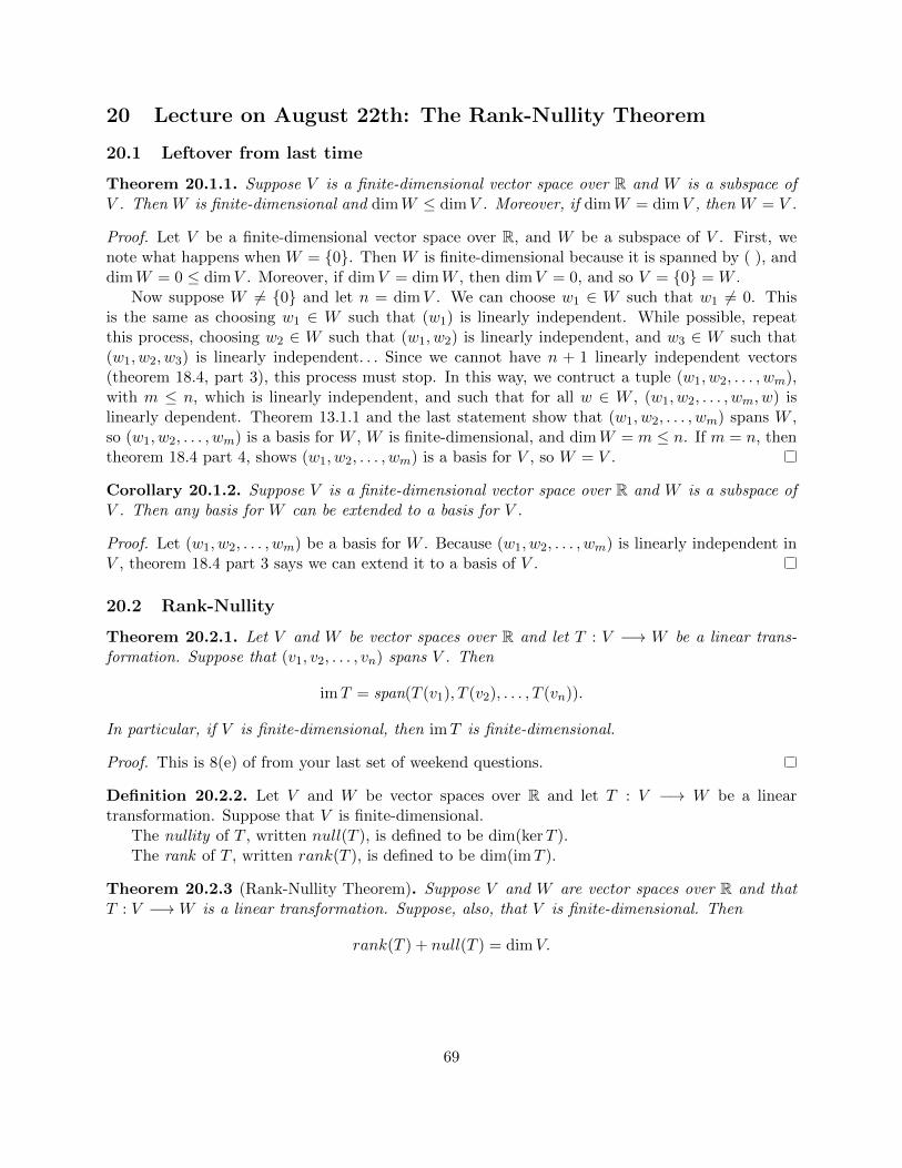
20 Lecture on August 22th: The Rank-Nullity Theorem

20.1 Leftover from last time

Theorem 20.1.1. Suppose V is a finite-dimensional vector space over R and W is a subspace ofV . Then W is finite-dimensional and dimW ≤ dimV . Moreover, if dimW = dimV , then W = V .

Proof. Let V be a finite-dimensional vector space over R, and W be a subspace of V . First, wenote what happens when W = {0}. Then W is finite-dimensional because it is spanned by ( ), anddimW = 0 ≤ dimV . Moreover, if dimV = dimW , then dimV = 0, and so V = {0} = W .

Now suppose W 6= {0} and let n = dimV . We can choose w1 ∈ W such that w1 6= 0. Thisis the same as choosing w1 ∈ W such that (w1) is linearly independent. While possible, repeatthis process, choosing w2 ∈ W such that (w1, w2) is linearly independent, and w3 ∈ W such that(w1, w2, w3) is linearly independent. . . Since we cannot have n + 1 linearly independent vectors(theorem 18.4, part 3), this process must stop. In this way, we contruct a tuple (w1, w2, . . . , wm),with m ≤ n, which is linearly independent, and such that for all w ∈ W , (w1, w2, . . . , wm, w) islinearly dependent. Theorem 13.1.1 and the last statement show that (w1, w2, . . . , wm) spans W ,so (w1, w2, . . . , wm) is a basis for W , W is finite-dimensional, and dimW = m ≤ n. If m = n, thentheorem 18.4 part 4, shows (w1, w2, . . . , wm) is a basis for V , so W = V .

Corollary 20.1.2. Suppose V is a finite-dimensional vector space over R and W is a subspace ofV . Then any basis for W can be extended to a basis for V .

Proof. Let (w1, w2, . . . , wm) be a basis for W . Because (w1, w2, . . . , wm) is linearly independent inV , theorem 18.4 part 3 says we can extend it to a basis of V .

20.2 Rank-Nullity

Theorem 20.2.1. Let V and W be vector spaces over R and let T : V −→ W be a linear trans-formation. Suppose that (v1, v2, . . . , vn) spans V . Then

imT = span(T (v1), T (v2), . . . , T (vn)).

In particular, if V is finite-dimensional, then imT is finite-dimensional.

Proof. This is 8(e) of from your last set of weekend questions.

Definition 20.2.2. Let V and W be vector spaces over R and let T : V −→ W be a lineartransformation. Suppose that V is finite-dimensional.

The nullity of T , written null(T ), is defined to be dim(kerT ).The rank of T , written rank(T ), is defined to be dim(imT ).

Theorem 20.2.3 (Rank-Nullity Theorem). Suppose V and W are vector spaces over R and thatT : V −→W is a linear transformation. Suppose, also, that V is finite-dimensional. Then

rank(T ) + null(T ) = dimV.

69

Proof. Let V and W be vector spaces over R and let T : V −→ W be a linear transformation.Suppose that V is finite-dimensional, let m = dimV , and n = null(T ). Recall that n = dim(kerT )by definition of nullity.

Choose a basis (v1, . . . , vn) for kerT . Extend it to a basis (v1, . . . , vn, vn+1, . . . , vm) of V . Weclaim that (T (vn+1), . . . , T (vm)) is a basis for im(T ). As long as we prove the claim, we will haverank(T ) = dim(imT ) = m− n = dimV − null(T ), and the theorem will follow.

First, we show (T (vn+1), . . . , T (vm)) spans imT . Since (v1, . . . , vn, vn+1, . . . , vm) spans V , theo-rem 20.2.1 tells us that (T (v1), . . . , T (vn), T (vn+1), . . . , T (vm)) spans imT . Since v1, . . . , vn ∈ kerT ,we have T (v1) = . . . = T (vn) = 0. So

span(T (vn+1), . . . , T (vm)) = span(T (v1), . . . , T (vn), T (vn+1), . . . , T (vm)) = imT.

Now we show that (T (vn+1), . . . , T (vm)) is linearly independent. Suppose that λn+1, . . . , λm ∈ Rand

λn+1T (vn+1) + . . .+ λmT (vm) = 0.

By linearity of T , this gives T (λn+1vn+1 + . . .+λmvm) = 0, so that λn+1vn+1 + . . .+λmvm ∈ kerT .Thus, λn+1vn+1 + . . .+λmvm is a linear combination of (v1, . . . , vn), i.e. there exists λ1, . . . , λn ∈ Rsuch that

λ1v1 + . . .+ λnvn = λn+1vn+1 + . . .+ λmvm.

Equivalently, (−λ1)v1+. . . (−λn)vn+λn+1vn+1+. . .+λmvm = 0. Because (v1, . . . , vn, vn+1, . . . , vm)is linearly independent, we see that λn+1 = . . . = λm = 0.

Theorem 20.2.4. Let n ∈ N ∪ {0}, let V and W be finite-dimensional vector spaces over R eachwith dimension n, and let T : V −→W be a linear transformation.

The following conditions are equivalent:

1. T is injective;

2. kerT = {0};

3. null(T ) = 0;

4. T is surjective;

5. imT = W ;

6. rank(T ) = n.

Proof. Let n ∈ N∪{0}, let V and W be finite-dimensional vector spaces over R each with dimensionn, and let T : V −→W be a linear transformation.

Theorem 9.1.4 says that conditions 1 and 2 are equivalent.Condition 2 implies condition 3 since dim{0} = 0.Condition 3 implies condition 2 since {0} is the only vector space over R with dimension 0.

Remark 9.1.6 says that conditions 4 and 5 are equivalent.Condition 5 implies condition 6 since dimW = n.Condition 6 implies condition 5 by theorem 20.1.1 applied to imT ⊆W .

Rank-Nullity says rank(T ) + null(T ) = n and so conditions 3 and 6 are equivalent.

70

The rank-nullity theorem allows one to calculate bases for kernels and images of linear trans-formations very quickly. The next example illustrates this. I’ll be disappointed if you don’t usethis type of argument on quiz 2 or the final.

Example 20.2.5. Let

A =

1 6 1 15 10 3 0 6 10 5 1 11 10 3 0 6 1

Then TA : R5 −→ R4. Here is the best way to find a basis for kerTA and imTA.

• βK =

1−1203

,

405−16

is tuple of vectors in kerTA.

• βI =

1000

,

1010

,

1111

is tuple of vectors in imTA.

• The tuples that we just wrote down are both linearly independent and this is easy to check.Theorem 18.4 (part 3) tells us that null(TA) ≥ 2 and rank(TA) ≥ 3. The rank-nullity theoremtells us that rank(TA) + null(TA) = 5. These two pieces of information imply null(TA) = 2and rank(TA) = 3.

• Theorem 18.4 (part 4) tells us that βK is a basis for kerTA and that βI is a basis for imTA.

• We see that from this calculation that TA is neither injective or surjective.

20.3 Isomorphisms

Lemma 20.3.1. Suppose that V and W are vector spaces over R, that T : V −→W is an injectivelinear transformation, and that S : W −→ V is a function with TS = 1W . Then S is linear.

Proof. Suppose that V and W are vector spaces over R, that T : V −→ W is an injective lineartransformation, and that S : W −→ V is a function with TS = 1W . We will show that S is linear.

Let w1, w2 ∈W . We wish to show

S(w1 + w2) = S(w1) + S(w2).

Since T is injective, it is enough to show T (S(w1 +w2)) = T (S(w1) + S(w2)). Since TS = 1W , theLHS is w1 + w2. Since T is linear, the RHS is T (S(w1)) + T (S(w2)). Moreover, since TS = 1W ,this is w1 + w2. Thus, S(w1 + w2) = S(w1) + S(w2).

Similarly, we can show that if λ ∈ R and w ∈W , then S(λw) = λS(w).

71

Theorem 20.3.2. Suppose that V and W are vector spaces over R, and T : V −→ W is a lineartransformation. The following statements are equivalent.

1. kerT = {0} and imT = W .

2. T is injective and surjective, that is, T is a bijection.

3. There exists a linear transformation S : W −→ V such that ST = 1V and TS = 1W .

Proof. Suppose that V and W are vector spaces over R, and T : V −→W is a linear transformation.

• 1. =⇒ 2.

We said this back in section 9.1.

• 2. =⇒ 3.

Suppose T is a bijection. It is a theorem in set theory that there is a function S : W −→ Vsuch that ST = 1V and TS = 1W . You can see http://math.ucla.edu/~mjandr/Math95

(theorem 11.2.4) for a proof. The lemma tells us that S is linear.

• 3. =⇒ 1.

Suppose we have S : W −→ V with the property that ST = 1V and TS = 1W .

Given v ∈ kerT , we have v = 1V (v) = (ST )(v) = S(T (v)) = S(0) = 0, so kerT = {0}.Given w ∈W , we have w = 1W (w) = (TS)(w) = T (S(w)) ∈ imT , so imT = W .

Definition 20.3.3. Suppose that V and W are vector spaces over R, and T : V −→W is a lineartransformation. We say that T is an isomorphism iff any of the three statements in the theoremhold.

Theorem 20.3.4. Let V and W be vector spaces over R.Suppose T : V −→W is a linear transformation, and that (v1, v2, . . . , vn) is a basis for V . Then

T is an isomorphism if and only if (T (v1), T (v2), . . . , T (vn)) is a basis for W .

Proof. Let V and W be vector spaces over R. Also, suppose T : V −→W is a linear transformation,and that (v1, v2, . . . , vn) is a basis for V .

First, suppose T is an isomorphism.We have kerT = {0} and (v1, v2, . . . , vn) is linearly independent, so 8.(d) of the last weekend

questions shows that (T (v1), T (v2), . . . , T (vn)) is linearly independent.We have imT = W and (v1, v2, . . . , vn) spans V , so 8.(e) of the last weekend questions shows

that (T (v1), T (v2), . . . , T (vn)) spans W .Thus, (T (v1), T (v2), . . . , T (vn)) is a basis for W .

Conversely, suppose that (T (v1), T (v2), . . . , T (vn)) is a basis for W . This immediately gives imT =W . Moreover, since (v1, v2, . . . , vn) spans V and (T (v1), T (v2), . . . , T (vn)) is linearly independent,8.(f) of the last weekend questions shows that kerT = {0}. Thus, T is an isomorphism.

72



0. Have the night off, or start the weekend’s questions, or read over the lecture notes.

73

22 Lecture on August 23th: The classification theorem andthe matrix of a linear transformation

22.1 The classification of finite-dimensional vector spaces over R

Theorem 22.1.1. Suppose that V and W are vector spaces over R, and T : V −→ W is a lineartransformation.

1. If T is injective, dimV ≤ dimW .

2. If T is surjective, dimV ≥ dimW .

3. If T is an isomorphism, then dimV = dimW .

Proof. The first two statements are question 2 of your weekend questions.The last statement follows from the first two statements, or the previous theorem.

Theorem 22.1.2 (Classification theorem). Let V be a finite-dimensional vector space over R. Letn = dimV . Then there exists an isomorphism Rn −→ V .

Proof. Let V be a finite-dimensional vector space over R. Let n = dimV . Pick a basis

β = (v1, v2, . . . , vn)

for V . We have a linear map Γβ : Rn −→ V , (λ1, λ2, . . . , λn) 7−→ λ1v1 + λ2v2 + . . .+ λnvn.We have already seen that β spanning V gives surjectivity and β being linearly independent gives

injectivity. Thus, Γβ is an isomorphism. (Perhaps you’d prefer to argue surjectivity directly anduse theorem 20.2.4 to get injectivity, or maybe you’d prefer to say that Γβ takes the standard basis(e1, e2, . . . , en) to the basis (v1, v2, . . . , vn), and use theorem 20.3.4 to conclude it’s an isomorphism.)

Theorem 22.1.3. Suppose that V and W are finite-dimensional vector spaces over R and thatdimV = dimW . Then there exists an isomorphism V −→W .

Proof. Suppose that V and W are finite-dimensional vector spaces over R and that dimV = dimW .Let n be the dimension of V and W . We have isomorphisms ϕV : Rn −→ V and ϕW : Rn −→ W .ϕWϕ

−1V : V →W and ϕV ϕ

−1W : W → V are inverse linear transformations. Thus, ϕWϕ

−1V : V →W

is an isomorphism.

Theorem 22.1.4. Let V and W be vector spaces over R. Suppose (v1, v2, . . . , vn) is a basis for Vand that (w1, w2, . . . , wn) is a tuple of vectors in W . Then there is exactly one linear transformationT : V −→W with the property that for all j ∈ {1, 2, . . . , n},

T (vj) = wj .

Proof. Let V and W be vector spaces over R. Suppose β = (v1, v2, . . . , vn) is a basis for V and thatγ = (w1, w2, . . . , wn) is a tuple of vectors in W . These choice of tuples determine the isomorphismΓβ : Rn −→ V , and the linear map Γγ : Rn −→ W . We claim that T = ΓγΓ−1

β : V −→ W has the

desired property. Let j ∈ {1, 2, . . . , n}. Since Γβ(ej) = vj , we have Γ−1β (vj) = ej . Thus,

T (vj) = ΓγΓ−1β (vj) = Γγ(ej) = wj .

74

We now address the uniqueness of T . Suppose that S is linear and satisfies S(vj) = wj for allj ∈ {1, 2, . . . , n} too. Let v ∈ V ; we’ll show that S(v) = T (v). Because (v1, v2, . . . , vn) spans V , wecan find λ1, λ2, . . . , λn ∈ R such that v = λ1v1 + λ2v2 + . . .+ λnvn. Then

S(v) = S(λ1v1 + λ2v2 + . . .+ λnvn)

= λ1S(v1) + λ2S(v2) + . . .+ λnS(vn)

= λ1w1 + λ2w2 + . . .+ λnwn.

= λ1T (v1) + λ2T (v2) + . . .+ λnT (vn)

= T (λ1v1 + λ2v2 + . . .+ λnvn)

= T (v).

(I’ll leave it to you to justify the equalities.) Since v ∈ V was arbitrary, this shows S = T .

75

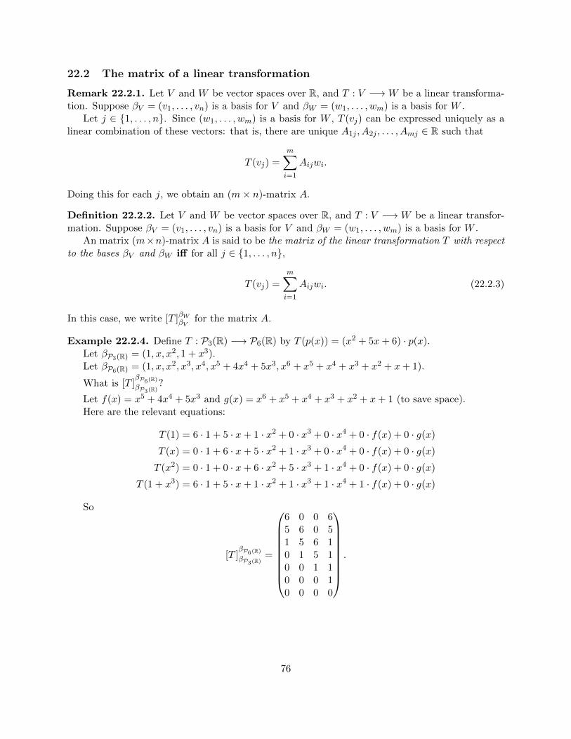
22.2 The matrix of a linear transformation

Remark 22.2.1. Let V and W be vector spaces over R, and T : V −→W be a linear transforma-tion. Suppose βV = (v1, . . . , vn) is a basis for V and βW = (w1, . . . , wm) is a basis for W .

Let j ∈ {1, . . . , n}. Since (w1, . . . , wm) is a basis for W , T (vj) can be expressed uniquely as alinear combination of these vectors: that is, there are unique A1j , A2j , . . . , Amj ∈ R such that

T (vj) =m∑i=1

Aijwi.

Doing this for each j, we obtain an (m× n)-matrix A.

Definition 22.2.2. Let V and W be vector spaces over R, and T : V −→W be a linear transfor-mation. Suppose βV = (v1, . . . , vn) is a basis for V and βW = (w1, . . . , wm) is a basis for W .

An matrix (m×n)-matrix A is said to be the matrix of the linear transformation T with respectto the bases βV and βW iff for all j ∈ {1, . . . , n},

T (vj) =

m∑i=1

Aijwi. (22.2.3)

In this case, we write [T ]βWβV for the matrix A.

Example 22.2.4. Define T : P3(R) −→ P6(R) by T (p(x)) = (x2 + 5x+ 6) · p(x).Let βP3(R) = (1, x, x2, 1 + x3).Let βP6(R) = (1, x, x2, x3, x4, x5 + 4x4 + 5x3, x6 + x5 + x4 + x3 + x2 + x+ 1).

What is [T ]βP6(R)βP3(R)

?

Let f(x) = x5 + 4x4 + 5x3 and g(x) = x6 + x5 + x4 + x3 + x2 + x+ 1 (to save space).Here are the relevant equations:

T (1) = 6 · 1 + 5 · x+ 1 · x2 + 0 · x3 + 0 · x4 + 0 · f(x) + 0 · g(x)

T (x) = 0 · 1 + 6 · x+ 5 · x2 + 1 · x3 + 0 · x4 + 0 · f(x) + 0 · g(x)

T (x2) = 0 · 1 + 0 · x+ 6 · x2 + 5 · x3 + 1 · x4 + 0 · f(x) + 0 · g(x)

T (1 + x3) = 6 · 1 + 5 · x+ 1 · x2 + 1 · x3 + 1 · x4 + 1 · f(x) + 0 · g(x)

So

[T ]βP6(R)βP3(R)

=

6 0 0 65 6 0 51 5 6 10 1 5 10 0 1 10 0 0 10 0 0 0

.

76


1. Find bases for the following subspaces of R5 and tell me their dimension:

W1 =

{(x1, x2, x3, x4, x5) ∈ R5 : x1 − x3 − x4 = 0

},

W2 =

{(x1, x2, x3, x4, x5) ∈ R5 : x2 = x3 = x4 and x1 + x5 = 0

}.

Solution: The tuple

β1 = ((0, 1, 0, 0, 0), (1, 0, 1, 0, 0), (1, 0, 0, 1, 0), (0, 0, 0, 0, 1))

is a linearly independent tuple of vectors in W1. Part 3 of theorem 18.4 tells us that dimW1 ≥4. Since (1, 0, 0, 0, 0) /∈ W1, theorem 20.1.1 gives dimW1 < 5. Thus, dimW1 = 4, and part 4of theorem 18.4 tells us β1 is a basis of W1.

Let T : R5 → R3 defined by T (x1, x2, x3, x4, x5) = (x2−x3, x4−x3, x1 +x5). Then T is linearand one can show that W2 = kerT .

T (0, 1, 0, 0, 0) = (1, 0, 0), T (0, 0, 0, 1, 0) = (0, 1, 0), T (0, 0, 0, 0, 1) = (0, 0, 1), and so imT = R3.Thus, rank(T ) = 3. The rank-nullity theorem tells us null(T ) = 2. So dimW2 = 2. Moreover,

β2 = ((1, 0, 0, 0,−1), (0, 1, 1, 1, 0))

is a linearly independent tuple of vectors in W1. Part 4 of theorem 18.4 tells us β2 is a basisof W2.

2. Suppose V and W are finite-dimensional vector spaces over R, and T : V −→ W is a lineartransformation. Use the rank-nullity to theorem to prove:

(a) if T is injective, then dim(V ) ≤ dim(W ).

(b) if T is surjective, then dim(V ) ≥ dim(W );

Solution: Suppose V and W are finite-dimensional vector spaces over R, and T : V −→ Wis a linear transformation.

(a) Suppose T is injective. Then null(T ) = 0, so we have

dimV = rank(T ) + null(T ) = rank(T ) ≤ dimW.

The first equality is the rank-nullity theorem.

The second equality uses null(T ) = 0. The fourth equality is because imT ⊆W .

(b) Suppose T is surjective. Then imT = W , so we have

dimV = rank(T ) + null(T ) ≥ rank(T ) = dimW.

The first equality is the rank-nullity theorem.

The second equality uses null(T ) ≥ 0. The fourth equality is because imT = W .

77

3. For each of the following, check T is linear, give a basis for kerT and imT , and say whetherT is injective or surjective.

The following is almost always the most efficient way to proceed with such questions:

• prove that T is a linear transformation;

• write down a linearly independent tuple in kerT which seems as big as possible;

• write down a linearly independent tuple in imT which seems as big as possible;

• use theorem 18.4 (part 3) and rank-nullity to deduce what null(T ) and rank(T ) are;

• use theorem 18.4 (part 4) to conclude that you have a basis for kerT and imT ;

• say whether T is injective or surjective.

(a) T : R3 −→ R2 defined by T (x1, x2, x3) = (x1 − x2, 2x3).

(b) T : R2 −→ R3 defined by T (x1, x2) = (x1 + x2, 0, 2x1 − x2).

(c) T : M2×3(R) −→M2×2(R) defined by

T

((x11 x12 x13

x21 x22 x23

))=

(2x11 − x12 x13 + 2x12

0 0

).

Solution:

(a) • T is a linear. Y’eard me.

• βK = ((1, 1, 0)) is a linearly independent tuple in kerT .

• βI = ((1, 0), (0, 2)) = (T (1, 0, 0), T (0, 0, 1)) is a linearly independent tuple in imT .

• Theorem 18.4 (part 3) gives null(T ) ≥ 1 and rank(T ) ≥ 2. The rank-nullity theoremgives rank(T ) + null(T ) = 3. Thus, null(T ) = 1 and rank(T ) = 2.

• Theorem 18.4 (part 4) tells us that βK and βI are bases for kerT and imT , respec-tively.

• T is surjective, but not injective.

(b) • T is a linear. Have it.

• βI = ((3, 0, 0), (0, 0, 3)) = (T (1, 2), T (1,−1)) is linearly independent in imT .

• null(T ) ≥ 0. Theorem 18.4 (part 3) gives rank(T ) ≥ 2. The rank-nullity theoremgives rank(T ) + null(T ) = 2. Thus, null(T ) = 0 and rank(T ) = 2.

• ( ) is a basis for kerT . Theorem 18.4 (part 4) tells us that βI is a basis for imT .

• T is injective, but not surjective.

78

(c) • T is linear. Big mood.

• βK =

((1 2 −40 0 0

),

(0 0 01 0 0

),

(0 0 00 1 0

),

(0 0 00 0 1

))is a linearly indepen-

dent tuple in kerT .

• βI =

((2 00 0

),

(0 10 0

))=

(T

((1 0 00 0 0

)), T

((0 0 10 0 0

)))is a linearly

independent tuple in imT .

• Theorem 18.4 (part 3) gives null(T ) ≥ 4 and rank(T ) ≥ 2. The rank-nullity theoremgives rank(T ) + null(T ) = 2 · 3 = 6. Thus, null(T ) = 4 and rank(T ) = 2.

• Theorem 18.4 (part 4) tells us that βK and βI are bases for kerT and imT , respec-tively.

• T is neither injective nor surjective.

4. Suppose U , V , and W are finite-dimensional vector spaces over R, and that

T : U −→ V, S : V −→W

are linear.

(a) Prove null(ST ) ≥ null(T ).

(b) Prove rank(ST ) ≤ min{rank(S), rank(T )}.

Solution:

(a) We know from a previous homework that ker (ST ) ⊇ ker (T ).

Applying dim(−) gives null(ST ) ≥ null(T ).

(b) We know from a previous homework that im(ST ) ⊆ im(S).

Applying dim(−) gives rank(ST ) ≤ rank(S).

Part (a) together with the rank-nullity theorem gives

dim(U)− rank(ST ) ≥ dim(U)− rank(T ).

So rank(ST ) ≤ rank(T ).

Together, the two inequalities concerning rank(ST ) show that

rank(ST ) ≤ min{rank(S), rank(T )}.

79

Definition. Suppose V and W are vector spaces over R, that S : V −→W and T : V −→Ware linear transformations. Then S + T : V −→W is defined by (S + T )(v) := S(v) + T (v).

5. Suppose V and W are finite-dimensional vector spaces over R, and that

S : V −→W, T : V −→W

are linear.

(a) Prove im(S + T ) ⊆ im(S) + im(T ).

(b) Suppose U1 and U2 are subspaces of W . Prove that

dim(U1 + U2) ≤ dimU1 + dimU2.

(c) Prove rank(S + T ) ≤ rank(S) + rank(T ).

(d) Give examples where the inequality in (c) is equality, and when it is strict.

Solution: Suppose V and W are finite-dimensional vector spaces over R, and that

S : V −→W, T : V −→W

are linear.

(a) Let w ∈ im(S+T ). Then there is a v ∈ V such that w = (S+T )(v), i.e. w = S(v)+T (v).Since S(v) ∈ imS and T (v) ∈ imT , this shows that w ∈ imS + imT .

(b) Suppose U1 and U2 are subspaces of W . Let m1 = dimU1 and m2 = dimU2, and choosebases for U1 and U2, respectively: (u1,1, u1,2, . . . , u1,m1) and (u2,1, u2,2, . . . , u2,m2).

By a previous homework, span(u1,1, u1,2, . . . , u1,m1 , u2,1, u2,2, . . . , u2,m2) is equal to

span(u1,1, u1,2, . . . , u1,m1) + span(u2,1, u2,2, . . . , u2,m2) = U1 + U2.

Thus, U1 + U2 has a spanning tuple of size m1 + m2, and so the dimension of U1 + U2

is less than or equal to m1 +m2 (theorem 18.4 part 1), i.e.

dim(U1 + U2) ≤ dimU1 + dimU2.

(c) We have

rank(S + T ) = dim(im(S + T )) ≤ dim(im(S) + im(T ))

≤ dim(im(S)) + dim(im(T )) = rank(S) + rank(T ).

The equalities are definitional.

The first inequality follows form part (a). The second follows from part (b).

(d) Let V = W = R and S = 1R.

When T = 0, we have

rank(S + T ) = rank(1R) = 1 = 1 + 0 = rank(S) + rank(T ).

When T = −1R, we have

rank(S + T ) = rank(0) = 0 < 2 = rank(S) + rank(T ).

80

24 Lecture on August 27th

24.1 The matrix of a linear transformation

Remark 24.1.1. Recall that (e1, . . . , en) is a basis for Rn and (e1, . . . , em) is a basis for Rm. Notice,here, that there is some potential for confusion since e1 could be referring to a vector in Rn or Rm.The equations should make it clear where an element lives.

Example 24.1.2. Suppose m,n ∈ N and A is an (m×n)-matrix. We have the linear transformationTA : Rn −→ Rm. Because

TA(ej) = Aej = j-th column of A =m∑i=1

Aijei,

the matrix of TA with respect to the bases (e1, . . . , en) and (e1, . . . , em) is the original matrix A.

Notation 24.1.3. Suppose V is a vector space over R, and that β = (v1, v2, . . . , vn) is a basis forV . We have the isomorphism Γβ : Rn −→ V .

For the rest of the class, for v ∈ V , we will use the notation [v]β for Γ−1β (v), so that

[λ1v1 + λ2v2 + . . .+ λnvn]β = (λ1, λ2, . . . , λn) and Γβ([v]β) = v.

The first equation shows that [v]β returns the coordinates of an abstract vector v ∈ V with respectto the basis β. The second equation will be useful in the proof of the next theorem.

Theorem 24.1.4. Let V and W be vector spaces over R, and T : V −→W be a linear transforma-tion. Suppose βV = (v1, . . . , vn) is a basis for V and βW = (w1, . . . , wm) is a basis for W . Then,for all v ∈ V ,

[T ]βWβV [v]βV = [T (v)]βW .

Proof. Let V , W , T , βV , βW be as in the theorem statement, and let A = [T ]βWβV be the matrix ofthe linear transformation T with respect to the bases βV and βW .

Consider the following diagram of linear maps.

Rn TA //

ΓβV

��

Rm

ΓβW

��V

T //W

First, we will show that ΓβW ◦ TA = T ◦ ΓβV . By theorem 22.1.4, it is enough to check this on thebasis elements e1, e2, . . . , en ∈ Rn.

81

ej� //

_

��

∑mi=1Aijei_

��

Rn TA //

ΓβV

��

Rm

ΓβW

��V

T //W

vj� //

∑mi=1Aijwi

So let j ∈ {1, 2, . . . , n}. Then

(ΓβW ◦ TA)(ej) = ΓβW (TA(ej)) = ΓβW (A(ej)) = ΓβW

(m∑i=1

Aijei

)

=m∑i=1

Aij · ΓβW (ei)

=m∑i=1

Aijwi = T (vj) = T (ΓβV (ej)) = (T ◦ ΓβV )(ej).

Remark 24.1.5. The previous diagram is actually the entire point of the matrix A. Given T , βV ,βW , the function Γ−1

βW◦T ◦ΓβV is a linear transformation Rn → Rm. Thus, by corollary 9.2.8, there

is a unique matrix A such that TA = Γ−1βW◦T ◦ΓβV . It is then immediate that ΓβW ◦TA = T ◦ΓβV . We

could have used these observations to define [T ]βWβV , but I thought the more calculational definitionwould be more comfortable you.

We are now ready to prove the result. Let v ∈ V . We wish to show that [T ]βWβV [v]βV = [T (v)]βW ,

i.e. TA([v]βV ) = [T (v)]βW

Since ΓβW is injective, it is enough to show that

ΓβW (TA([v]βV )) = ΓβW ([T (v)]βW ). (24.1.6)

By the previous calculation, the LHS is equal to T (ΓβV ([v]βV )).Now recall that for all v ∈ V , ΓβV ([v]βV ) = v, and for all w ∈W , ΓβW ([w]βW ) = w. Thus, both

sides of (24.1.6) are equal to T (v). This finishes the proof.

82

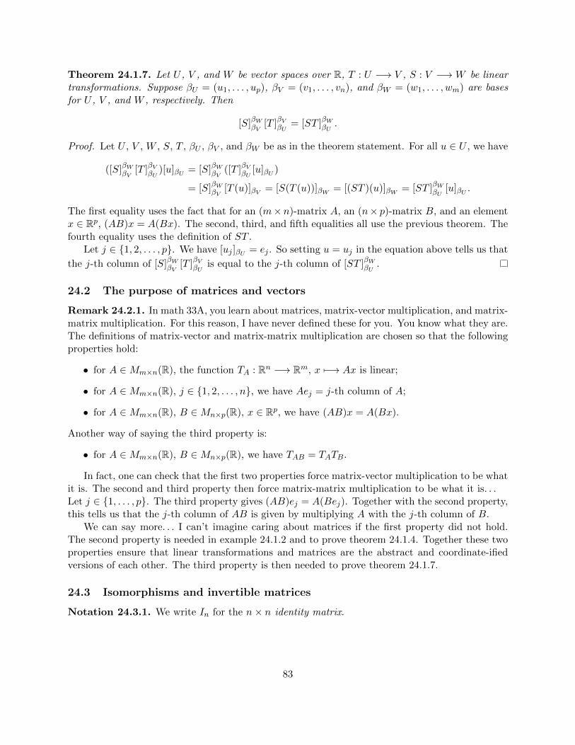
Theorem 24.1.7. Let U , V , and W be vector spaces over R, T : U −→ V , S : V −→W be lineartransformations. Suppose βU = (u1, . . . , up), βV = (v1, . . . , vn), and βW = (w1, . . . , wm) are basesfor U , V , and W , respectively. Then

[S]βWβV [T ]βVβU = [ST ]βWβU .

Proof. Let U , V , W , S, T , βU , βV , and βW be as in the theorem statement. For all u ∈ U , we have

([S]βWβV [T ]βVβU )[u]βU = [S]βWβV ([T ]βVβU [u]βU )

= [S]βWβV [T (u)]βV = [S(T (u))]βW = [(ST )(u)]βW = [ST ]βWβU [u]βU .

The first equality uses the fact that for an (m×n)-matrix A, an (n× p)-matrix B, and an elementx ∈ Rp, (AB)x = A(Bx). The second, third, and fifth equalities all use the previous theorem. Thefourth equality uses the definition of ST .

Let j ∈ {1, 2, . . . , p}. We have [uj ]βU = ej . So setting u = uj in the equation above tells us that

the j-th column of [S]βWβV [T ]βVβU is equal to the j-th column of [ST ]βWβU .

24.2 The purpose of matrices and vectors

Remark 24.2.1. In math 33A, you learn about matrices, matrix-vector multiplication, and matrix-matrix multiplication. For this reason, I have never defined these for you. You know what they are.The definitions of matrix-vector and matrix-matrix multiplication are chosen so that the followingproperties hold:

• for A ∈Mm×n(R), the function TA : Rn −→ Rm, x 7−→ Ax is linear;

• for A ∈Mm×n(R), j ∈ {1, 2, . . . , n}, we have Aej = j-th column of A;

• for A ∈Mm×n(R), B ∈Mn×p(R), x ∈ Rp, we have (AB)x = A(Bx).

Another way of saying the third property is:

• for A ∈Mm×n(R), B ∈Mn×p(R), we have TAB = TATB.

In fact, one can check that the first two properties force matrix-vector multiplication to be whatit is. The second and third property then force matrix-matrix multiplication to be what it is. . .Let j ∈ {1, . . . , p}. The third property gives (AB)ej = A(Bej). Together with the second property,this tells us that the j-th column of AB is given by multiplying A with the j-th column of B.

We can say more. . . I can’t imagine caring about matrices if the first property did not hold.The second property is needed in example 24.1.2 and to prove theorem 24.1.4. Together these twoproperties ensure that linear transformations and matrices are the abstract and coordinate-ifiedversions of each other. The third property is then needed to prove theorem 24.1.7.

24.3 Isomorphisms and invertible matrices

Notation 24.3.1. We write In for the n× n identity matrix.

83

Definition 24.3.2. We say a matrix A ∈Mn×n(R) is invertible iff there is a matrix B ∈Mn×n(R)such that

AB = BA = In.

The matrix B is often written as A−1 and is called the inverse of A.Non-square matrices are never called invertible.

Theorem 24.3.3. Let V and W be vector spaces over R, and T : V −→ W be a linear transfor-mation. Suppose that βV = (v1, . . . , vn) is a basis for V and βW = (w1, . . . , wm) is a basis for W .

If T is an isomorphism, then [T ]βWβV is invertible.

Proof. Let V , W , T , βV , βW be as in the theorem statement. Suppose that T is an isomorphism.From theorem 22.1.1, we know dimV = dimW , so [T ]βWβV is a square matrix.Also, T has an inverse linear transformation S : W −→ V with ST = 1V and TS = 1W . Using

theorem 24.1.7, we obtain

[S]βVβW [T ]βWβV = [1V ]βVβV = In and [T ]βWβV [S]βVβW = [1W ]βWβW = In,

so [T ]βWβV is invertible.

Theorem 24.3.4. Suppose A is an (m×n)-matrix. TA : Rn → Rm is an isomorphism if and onlyif A is invertible.

Proof. Suppose A is an (m× n)-matrix.First, suppose TA is an isomorphism. From theorem 22.1.1, we know n = m. Let β = (e1, . . . , en)

be the standard basis of Rn. The previous theorem tells us that [TA]ββ is invertible. Example 24.1.2

shows [TA]ββ = A, and so we conclude A is invertible.Conversely, suppose that A is invertible. Then n = m and there exists another matrix B such

that AB = BA = In. We have TATB = TAB = TIn = 1Rn and TBTA = TBA = TIn = 1Rn . Thus,TA is an isomorphism.

Theorem 24.3.5. Suppose A,B ∈Mn×n(R). If AB = In, then BA = In.

Proof. Suppose A,B ∈Mn×n(R) and that AB = In. Then TATB = TAB = TIn = 1Rn . Thus, givenv ∈ Rn, we have v = 1Rn(v) = TA(TB(v)), and so TA is surjective. By theorem 20.2.4, TA is alsoinjective. So TA is an isomorphism, and the previous theorem tells us that A is invertible.

Let C be an inverse for A, so that CA = In. Then

B = InB = (CA)B = C(AB) = CIn = C.

Here, the second equality uses CA = In and the fourth uses AB = In. The equations B = C andCA = In show that BA = In.

Theorem 24.3.6. Let V and W be vector spaces over R, and T : V −→ W be a linear transfor-mation. Suppose that βV = (v1, . . . , vn) is a basis for V and βW = (w1, . . . , wm) is a basis for W .

If [T ]βWβV is invertible, then T is an isomorphism

Proof. Let V , W , T , βV , βW be as in the theorem statement and suppose that [T ]βWβV is invertible.

Let A = [T ]βWβV , so that A is invertible. Theorem 24.3.4 says that TA is an isomorphism.

We saw in a previous proof that T = ΓβW ◦ TA ◦ Γ−1βV

.

T is an isomorphism because it has an inverse ΓβV ◦ (TA)−1 ◦ Γ−1βW

.

84

24.4 Sean’s proof of theorem 24.1.4

The proof of theorem 24.1.4 may seem weird to you. . .Category theory is an area of mathematics that has infiltrated my life since I was 21, and it

leads me to think a certain way. This way of thinking means that if V is a vector space over R, Iprefer linear transformations Rn −→ V over linear transformations V −→ Rn. That’s one reasonfor the proof I gave.

I also took the proof of theorem 24.1.4 as an excuse to introduce a diagram I find particularlyuseful. The extent to which you find it useful will vary, but if you do lots more math, I expect it’llcome back to get you! I used this diagram in a later proof.

Having said all that (in some defence of the proof I gave) a student presented to me a delightfulproof of theorem 24.1.4 in office hours, and you will probably prefer his proof to mine. Here it is. . .

Sean’s proof of theorem 24.1.4. Let V , W , T , βV , βW be as in the theorem statement, and letA = [T ]βWβV be the matrix of the linear transformation T with respect to the bases βV and βW .

Define S1 : V −→ Rm and S2 : V −→ Rm by

S1(v) = A[v]βV and S2(v) = [T (v)]βW .

We just have to show that S1 = S2. Since S1 and S2 are linear, by theorem 22.1.4, it is enough tocheck this on the basis elements v1, v2, . . . , vn ∈ V .

Let j ∈ {1, 2, . . . , n}. Then

S1(vj) = A[vj ]βV = Aej =m∑i=1

Aijei.

The first equality uses the definition of S1. The second uses [vj ]βV = ej . The third expresses thefact that Aej = the j-th column of A.

Also,

S2(vj) = [T (vj)]βW =

[m∑i=1

Aijwi

]βW

=

m∑i=1

Aij [wi]βW =

m∑i=1

Aijei.

The first equality is the definition of S2. The second uses the definition of A = [T ]βWβV . The thirduses linearity of [−]βW . The fourth uses [wi]βW = ei.

Well done, Sean!

85


1. On the next page, in each part, I define a linear map T : V −→ W , give bases βV , βW , andan element v ∈ V . You should:

• calculate [v]βV ,

• calculate T (v),

• calculate [T (v)]βW ,

• calculate [T ]βWβV ,

• confirm that [T ]βWβV [v]βV = [T (v)]βW .

86

(a) T : P5(R) −→ P4(R) is defined by p(x) 7−→ p′(x).

βP5(R) = (1, x, x2, x3, x4, x5), βP4(R) = (1, x, x2, x3, x4).

v = 4 + 3x− 2x2 + x3 + 5x4 − 8x5.

Remark. A polynomial is not a function by definition, but you can do something whichlooks a lot like differentiation to polynomials by enforcing the “power rule.” This is aformal operation which coincides with differentiation once we allow polynomials to definea function.

(b) T : P5(R) −→ P4(R) is defined by p(x) 7−→ p′(x).

βP5(R) = (1, x, x2, x3, x4, x5), βP4(R) = (x4, x3, x2, x, 1),

v = 4 + 3x− 2x2 + x3 + 5x4 − 8x5.

(c) T : P5(R) −→ P4(R) is defined by p(x) 7−→ p′(x).

βP5(R) = (x5, x4, x3, x2, x, 1), βP4(R) = (x4, x3, x2, x, 1),

v = 4 + 3x− 2x2 + x3 + 5x4 − 8x5.

(d) T : P5(R) −→ P4(R) is defined by p(x) 7−→ p′(x).

βP5(R) = (1, 1+x, 1+x+x2, 1+x+x2 +x3, 1+x+x2 +x3 +x4, 1+x+x2 +x3 +x4 +x5),

βP4(R) = (1, x, x2, x3, x4),

v = 4 + 3x− 2x2 + x3 + 5x4 − 8x5.

(e) T : P5(R) −→ P4(R) is defined by p(x) 7−→ p′(x).

βP5(R) = (1, x, x2, x3, x4, x5),

βP4(R) = (1, 1 + x, 1 + x+ x2, 1 + x+ x2 + x3, 1 + x+ x2 + x3 + x4),

v = 4 + 3x− 2x2 + x3 + 5x4 − 8x5.

(f) T : P4(R) −→ P5(R) is defined by p(x) 7−→∫ x

0 p(t) dt.

βP5(R) = (1, x, x2, x3, x4, x5), βP4(R) = (1, x, x2, x3, x4),

v = 8 + 4x− 3x2 − 4x3 + 120x4.

Remark. A polynomial is not a function by definition. However, you can do somethingwhich looks a lot like integration to polynomials by enforcing the “power rule.” This isa formal operation which coincides with integration once we allow polynomials to definea function.

(g) T : P4(R) −→ P5(R) is defined by p(x) 7−→∫ x

1 p(t) dt.

βP5(R) = (1, x, x2, x3, x4, x5), βP4(R) = (1, x, x2, x3, x4),

v = 8 + 4x− 3x2 − 4x3 + 120x4.

(h) In this part, V = W and βV = βW .

Let A =

1 −1 0−1 0 10 1 1

and T = TA : R3 −→ R3.

βR3 =

−1−21

,

101

,

−111

, v =

012

.

87

2. Below, in each part, I define linear maps T : U −→ V , S : V −→ W , and give bases βU , βV ,βW . You should:

• calculate [T ]βVβU ,

• calculate [S]βWβV ,

• calculate ST ,

• calculate [ST ]βWβU ,

• confirm that [S]βWβV [T ]βVβU = [ST ]βWβU .

(a) In this part, U = W and βU = βW .

T : P4(R) −→ P5(R) is defined by p(x) 7−→∫ x

0 p(t) dt.

S : P5(R) −→ P4(R) is defined by p(x) 7−→ p′(x).

βP4(R) = (1, x, x2, x3, x4), βP5(R) = (1, x, x2, x3, x4, x5).

(b) In this part, U = W and βU = βW .

T : P5(R) −→ P4(R) is defined by p(x) 7−→ p′(x).

S : P4(R) −→ P5(R) is defined by p(x) 7−→∫ x

0 p(t) dt.


(c) In this part, U = W and βU = βW .

T : P4(R) −→ P5(R) is defined by p(x) 7−→∫ x

1 p(t) dt.

S : P5(R) −→ P4(R) is defined by p(x) 7−→ p′(x).

βP4(R) = (1, x, x2, x3, x4), βP5(R) = (1, x, x2, x3, x4, x5).

(d) In this part, U = W and βU = βW .

T : P5(R) −→ P4(R) is defined by p(x) 7−→ p′(x).

S : P4(R) −→ P5(R) is defined by p(x) 7−→∫ x

1 p(t) dt.


(e) [Optional]

I suppose I never thought up one where U 6= W . . .

T : P2(R) −→ P3(R) is defined by T (p(x)) = (3 + x)p′(x) + 2p(x).

S : P3(R) −→ R3 is defined by S(a+ bx+ cx2 + dx3) = (a+ b, c, a− b).βP2(R) = (1, x, x2), βP3(R) = (1, x, x2, x3), βR3 = (e1, e2, e3).

88

26 Solutions to the previous questions

1. (a) • [4 + 3x− 2x2 + x3 + 5x4 − 8x5]βP5(R) = (4, 3,−2, 1, 5,−8),

• T (4 + 3x− 2x2 + x3 + 5x4 − 8x5) = 3− 4x+ 3x2 + 20x3 − 40x4,

• [T (4 + 3x− 2x2 + x3 + 5x4 − 8x5)]βP4(R) = (3,−4, 3, 20,−40),

• [T ]βP4(R)βP5(R)

=

0 1 0 0 0 00 0 2 0 0 00 0 0 3 0 00 0 0 0 4 00 0 0 0 0 5

.

(b) • [4 + 3x− 2x2 + x3 + 5x4 − 8x5]βP5(R) = (4, 3,−2, 1, 5,−8),

• T (4 + 3x− 2x2 + x3 + 5x4 − 8x5) = 3− 4x+ 3x2 + 20x3 − 40x4,

• [T (4 + 3x− 2x2 + x3 + 5x4 − 8x5)]βP4(R) = (−40, 20, 3,−4, 3),

• [T ]βP4(R)βP5(R)

=

0 0 0 0 0 50 0 0 0 4 00 0 0 3 0 00 0 2 0 0 00 1 0 0 0 0

.

(c) • [4 + 3x− 2x2 + x3 + 5x4 − 8x5]βP5(R) = (−8, 5, 1,−2, 3, 4),

• T (4 + 3x− 2x2 + x3 + 5x4 − 8x5) = 3− 4x+ 3x2 + 20x3 − 40x4,

• [T (4 + 3x− 2x2 + x3 + 5x4 − 8x5)]βP4(R) = (−40, 20, 3,−4, 3),

• [T ]βP4(R)βP5(R)

=

5 0 0 0 0 00 4 0 0 0 00 0 3 0 0 00 0 0 2 0 00 0 0 0 1 0

.

(d) • [4 + 3x− 2x2 + x3 + 5x4 − 8x5]βP5(R) = (1, 5,−3,−4, 13,−8),

• T (4 + 3x− 2x2 + x3 + 5x4 − 8x5) = 3− 4x+ 3x2 + 20x3 − 40x4,

• [T (4 + 3x− 2x2 + x3 + 5x4 − 8x5)]βP4(R) = (3,−4, 3, 20,−40),

• [T ]βP4(R)βP5(R)

=

0 1 1 1 1 10 0 2 2 2 20 0 0 3 3 30 0 0 0 4 40 0 0 0 0 5

.

(e) • [4 + 3x− 2x2 + x3 + 5x4 − 8x5]βP5(R) = (4, 3,−2, 1, 5,−8),

• T (4 + 3x− 2x2 + x3 + 5x4 − 8x5) = 3− 4x+ 3x2 + 20x3 − 40x4,

• [T (4 + 3x− 2x2 + x3 + 5x4 − 8x5)]βP4(R) = (7,−7,−17, 60,−40),

• [T ]βP4(R)βP5(R)

=

0 1 −2 0 0 00 0 2 −3 0 00 0 0 3 −4 00 0 0 0 4 −50 0 0 0 0 5

.

89

(f) • [8 + 4x− 3x2 − 4x3 + 120x4]βP4(R) = (8, 4,−3,−4, 120),

• T (8 + 4x− 3x2 − 4x3 + 120x4) = 8x+ 2x2 − x3 − x4 + 24x5,

• [T (v)]βP5(R) = (0, 8, 2,−1,−1, 24),

• [T ]βP5(R)βP4(R)

=

0 0 0 0 01 0 0 0 00 1

2 0 0 00 0 1

3 0 00 0 0 1

4 00 0 0 0 1

5

.

(g) • [8 + 4x− 3x2 − 4x3 + 120x4]βP4(R) = (8, 4,−3,−4, 120),

• T (8 + 4x− 3x2 − 4x3 + 120x4) = −32 + 8x+ 2x2 − x3 − x4 + 24x5,

• [T (v)]βP5(R) = (−32, 8, 2,−1,−1, 24),

• [T ]βP5(R)βP4(R)

=

−1 −12 −1

3 −14 −1

51 0 0 0 00 1

2 0 0 00 0 1

3 0 00 0 0 1

4 00 0 0 0 1

5

.

(h) • [(0, 1, 2)]βR3 = (0, 1, 1),

• T (0, 1, 2) = (−1, 2, 3),

• [T (0, 1, 2)]βR3 = (0, 1, 2),

• [T ]βR3βR3

=

−1 0 00 1 00 0 2

.

90

(i) This was not a question but it provides more examples of coordinate change matrices.

In (a), we calculated the matrix of T : P5(R) → P4(R) defined by p(x) 7−→ p′(x) withrespect to the standard basis for P4(R) and P5(R). It’s

A =

0 1 0 0 0 00 0 2 0 0 00 0 0 3 0 00 0 0 0 4 00 0 0 0 0 5

.

Then in questions (b-e), we calculated the matrix with respect to different bases. Hereare the relevant versions of the formula A′ = P−1AQ:

0 0 0 0 0 50 0 0 0 4 00 0 0 3 0 00 0 2 0 0 00 1 0 0 0 0

=

0 0 0 0 10 0 0 1 00 0 1 0 00 1 0 0 01 0 0 0 0

−1

A

1 0 0 0 0 00 1 0 0 0 00 0 1 0 0 00 0 0 1 0 00 0 0 0 1 00 0 0 0 0 1

5 0 0 0 0 00 4 0 0 0 00 0 3 0 0 00 0 0 2 0 00 0 0 0 1 0

=

0 0 0 0 10 0 0 1 00 0 1 0 00 1 0 0 01 0 0 0 0

−1

A

0 0 0 0 0 10 0 0 0 1 00 0 0 1 0 00 0 1 0 0 00 1 0 0 0 01 0 0 0 0 0

0 1 1 1 1 10 0 2 2 2 20 0 0 3 3 30 0 0 0 4 40 0 0 0 0 5

=

1 0 0 0 00 1 0 0 00 0 1 0 00 0 0 1 00 0 0 0 1

−1

A

1 1 1 1 1 10 1 1 1 1 10 0 1 1 1 10 0 0 1 1 10 0 0 0 1 10 0 0 0 0 1

0 1 −2 0 0 00 0 2 −3 0 00 0 0 3 −4 00 0 0 0 4 −50 0 0 0 0 5

=

1 1 1 1 10 1 1 1 10 0 1 1 10 0 0 1 10 0 0 0 1

−1

A

1 0 0 0 0 00 1 0 0 0 00 0 1 0 0 00 0 0 1 0 00 0 0 0 1 00 0 0 0 0 1

In (h), we learned that−1 0 0

0 1 00 0 2

=

−1 1 −1−2 0 11 1 1

−1 1 −1 0−1 0 10 1 1

−1 1 −1−2 0 11 1 1

.

91

2. (a) ST = 1P4(R). 0 1 0 0 0 00 0 2 0 0 00 0 0 3 0 00 0 0 0 4 00 0 0 0 0 5

0 0 0 0 01 0 0 0 00 1

2 0 0 00 0 1

3 0 00 0 0 1

4 00 0 0 0 1

5

= I5.

(b) (ST )(p(x)) = p(x)− p(0).

0 0 0 0 01 0 0 0 00 1

2 0 0 00 0 1

3 0 00 0 0 1

4 00 0 0 0 1

5

0 1 0 0 0 00 0 2 0 0 00 0 0 3 0 00 0 0 0 4 00 0 0 0 0 5

=

0 0 0 0 0 00 1 0 0 0 00 0 1 0 0 00 0 0 1 0 00 0 0 0 1 00 0 0 0 0 1

.

(c) ST = 1P4(R).

0 1 0 0 0 00 0 2 0 0 00 0 0 3 0 00 0 0 0 4 00 0 0 0 0 5

−1 −12 −1

3 −14 −1

51 0 0 0 00 1

2 0 0 00 0 1

3 0 00 0 0 1

4 00 0 0 0 1

5

= I5.

(d) (ST )(p(x)) = p(x)− p(1).

−1 −12 −1

3 −14 −1

51 0 0 0 00 1

2 0 0 00 0 1

3 0 00 0 0 1

4 00 0 0 0 1

5

0 1 0 0 0 00 0 2 0 0 00 0 0 3 0 00 0 0 0 4 00 0 0 0 0 5

=

0 −1 −1 −1 −1 −10 1 0 0 0 00 0 1 0 0 00 0 0 1 0 00 0 0 0 1 00 0 0 0 0 1

.

92

27 Lecture on August 29th

27.1 The change of coordinate matrix

Definition 27.1.1. Suppose V is a vector space over R, that β = (v1, . . . , vn) and β′ = (v′1, . . . , v′n)

are bases for V . Then [1V ]ββ′ is called the change of coordinate matrix from β′ to β.

Remark 27.1.2. Suppose V is a vector space over R, that β = (v1, . . . , vn) and β′ = (v′1, . . . , v′n)

are bases for V . Let Q = [1V ]ββ′ . Then, for j ∈ {1, 2, . . . , n}, we have

v′j = 1V (v′j) =n∑i=1

Qijvi.

Also, for v ∈ V , we have [v]β = [1V (v)]β = [1V ]ββ′ [v]β′ = Q[v]β′ .Finally, both of these equations allow one to see that the j-th column of Q is [v′j ]β.

Theorem 27.1.3. Let V and W be vector spaces over R, and T : V −→ W be a linear transfor-mation. Suppose βV = (v1, . . . , vn) and β′ = (v′1, . . . , v

′n) are bases for V , and βW = (w1, . . . , wm)

and β′ = (w′1, . . . , w′m) are bases for W .

Suppose A is the matrix of T with respect to the bases βV and βW , and that A′ is the matrix ofT with respect to the bases β′V and β′W .

Suppose that Q is the change of coordinate matrix from β′V to βV , and that P is the change ofcoordinate matrix from β′W to βW . Then

A′ = P−1AQ.

Proof. A′ = [T ]β′Wβ′V

= [1WT1V ]β′Wβ′V

= [1W ]β′WβW

[T ]βWβV [1V ]βVβ′V

= ([1W ]βWβ′W

)−1[T ]βWβV [1V ]βVβ′V

= P−1AQ.

Corollary 27.1.4. Suppose m,n ∈ N, A ∈Mm×n(R), that βRn = (v1, . . . , vn) is a basis of Rn, andβRm = (w1, . . . , wm) is a basis of Rm. Then the matrix of the linear transformation TA : Rn → Rmwith respect to the bases βRn and βRm is given by(

w1

∣∣∣∣ · · · ∣∣∣∣wm)−1

A

(v1

∣∣∣∣ · · · ∣∣∣∣vn).Example 27.1.5. See the previous questions’ solutions for examples: 1i.

27.2 Determinants of matrices (not lectured)

Notation 27.2.1. Suppose A ∈ Mn×n(R). Denote the (n− 1)× (n− 1) matrix obtained from A

by deleting the i-th row and j-th column by Aij .

Theorem 27.2.2. For each n ∈ N, there is a function called the determinant, det : Mn×n(R) −→R. The functions have the following properties.

93

1. (a) If A ∈M1×1(R) so that A = (A11), then detA = A11.

(b) If A ∈Mn×n(R) where n ≥ 2, and j ∈ {1, . . . , n}, then

det(A) =n∑i=1

(−1)i+jAij · det(Aij).

2. (a) det(In) = 1.

(b) Suppose j ∈ {1, . . . , n}, v1, . . . , vj−1, vj+1, . . . , vn ∈ Rn, u,w ∈ Rn, and λ ∈ R. Then

det

(v1

∣∣∣∣∣ · · ·∣∣∣∣∣vj−1

∣∣∣∣∣u+ λw

∣∣∣∣∣vj+1

∣∣∣∣∣ · · ·∣∣∣∣∣vn)

= det

(v1

∣∣∣∣∣ · · ·∣∣∣∣∣vj−1

∣∣∣∣∣u∣∣∣∣∣vj+1

∣∣∣∣∣ · · ·∣∣∣∣∣vn)

+ λ det

(v1

∣∣∣∣∣ · · ·∣∣∣∣∣vj−1

∣∣∣∣∣w∣∣∣∣∣vj+1

∣∣∣∣∣ · · ·∣∣∣∣∣vn).

This says det is linear in each column.

(c) Suppose j, k ∈ {1, . . . , n}, j < k, v1, . . . , vj−1, vj+1, . . . , vk−1, vk+1, . . . , vn ∈ Rn, v ∈ Rn.Then

det

(v1

∣∣∣∣∣ · · ·∣∣∣∣∣vj−1

∣∣∣∣∣v∣∣∣∣∣vj+1

∣∣∣∣∣ · · ·∣∣∣∣∣vk−1

∣∣∣∣∣v∣∣∣∣∣vk+1

∣∣∣∣∣ · · ·∣∣∣∣∣vn)

= 0.

This says that if two columns are the same, then det is zero.

3. (a) Suppose j ∈ {1, . . . , n} and v1, . . . , vj−1, vj+1, . . . , vn ∈ Rn. Then

det

(v1

∣∣∣∣∣ · · ·∣∣∣∣∣vj−1

∣∣∣∣∣0∣∣∣∣∣vj+1

∣∣∣∣∣ · · ·∣∣∣∣∣vn)

= 0.

This says that if a column is zero, then det is zero.

(b) Suppose j, k ∈ {1, . . . , n}, j < k, and v1, . . . , vn ∈ Rn. Then

det

(v1

∣∣∣∣∣ · · ·∣∣∣∣∣vj−1

∣∣∣∣∣vk∣∣∣∣∣vj+1

∣∣∣∣∣ · · ·∣∣∣∣∣vk−1

∣∣∣∣∣vj∣∣∣∣∣vk+1

∣∣∣∣∣ · · ·∣∣∣∣∣vn)

= −det

(v1

∣∣∣∣∣ · · ·∣∣∣∣∣vn).

This says that swapping two columns introduces a minus sign to the determinant.

(c) Suppose j, k ∈ {1, . . . , n}, j 6= k, v1, . . . , vn ∈ Rn, and λ ∈ R. Then

det

(v1

∣∣∣∣∣ · · ·∣∣∣∣∣vj−1

∣∣∣∣∣vj + λvk

∣∣∣∣∣vj+1

∣∣∣∣∣ · · ·∣∣∣∣∣vn)

= det

(v1

∣∣∣∣∣ · · ·∣∣∣∣∣vn).

This says that adding a scalar multiple of one column to another column does not changethe determinant.

4. If A ∈Mn×n(R), then det(AT ) = det(A).

5. If A,B ∈Mn×n(R), then det(AB) = det(A) det(B).

6. If A ∈Mn×n(R), A is invertible if and only if det(A) 6= 0.

94

Remark 27.2.3. If we always take j = 1, then 1 provides a definition of the determinant.The determinant is the only function with the properties of 2.Property 3a follows from 2b. Property 3b follows from 2b and 2c, and the same is true for 3c.Property 4 implies that for every property involving columns, there is a corresponding property

for rows.Properties 5 and 6 are useful.

It is good practice to prove the following theorem.

Theorem 27.2.4. Suppose properties 3a and 3c. Then we can prove half of property 6 quickly: ifA ∈Mn×n(R) is not invertible, then detA = 0.

Proof. Suppose properties 3a and 3c and that A ∈Mn×n(R) is not invertible. Write

A =

(v1

∣∣∣∣∣ · · ·∣∣∣∣∣vn)

where v1, . . . , vn ∈ Rn and let α = (v1, . . . , vn).Since A is not invertible, TA is not an isomorphism (theorem 24.3.4). Thus, TA is not injective

(theorem 20.2.4). TA = Γα, so this shows that α is linearly dependent (remark 11.3.5).By a homework problem, we can rewrite some vj as a linear combination of the other vectors

vj = λ1v1 + . . .+ λj−1vj−1 + λj+1vj+1 + . . .+ λnvn.

So

detA = det

(v1

∣∣∣∣∣ · · ·∣∣∣∣∣vj−1

∣∣∣∣∣λ1v1 + . . .+ λj−1vj−1 + λj+1vj+1 + . . .+ λnvn

∣∣∣∣∣vj+1

∣∣∣∣∣ · · ·∣∣∣∣∣vn).

Property 3c allows us to see that

detA = det

(v1

∣∣∣∣∣ · · ·∣∣∣∣∣vj−1

∣∣∣∣∣0∣∣∣∣∣vj+1

∣∣∣∣∣ · · ·∣∣∣∣∣vn)

and property 3a gives detA = 0.

Lemma 27.2.5. Suppose properties 2a and 5. Then we can prove half of property 6 quickly: ifA ∈Mn×n(R) is invertible, then detA 6= 0.

Remark 27.2.6. Without property 5, the proof that “if A ∈Mn×n(R) is invertible, then detA 6= 0”is more annoying. A good reason to believe that this result is true is that the det is connected withvolume. The argument in the previous proof (24.3.4, 20.2.4, 11.3.5) can be enhanced to say that amatrix

A =

(v1

∣∣∣∣∣ · · ·∣∣∣∣∣vn)

is invertible if and only if (v1, . . . , vn) is a basis for Rn. Drawing a higher dimensional parallelogramusing these vectors, we see that it has non-zero volume exactly when (v1, . . . , vn) is a basis for Rn.

95

27.3 Eigenvectors

Definition 27.3.1. Suppose V is a vector space over R and T : V −→ V is a linear transformation.A vector v ∈ V is said to be an eigenvector of T iff the following conditions hold:

• v 6= 0;

• Tv = λv for some λ ∈ R (often we write Tv instead of T (v)).

If v ∈ V is an eigenvector of T and Tv = λv, then λ is called the eigenvalue corresponding to v.A scalar λ ∈ R is said to be an eigenvalue of T iff there is an eigenvector v of T such that λ is

the eigenvalue corresponding to v.

Definition 27.3.2. Suppose V andW are vector spaces over R, that S : V −→W and T : V −→Ware linear transformations and λ ∈ R. Then S + T : V −→W and λT : V −→W are defined by

(S + T )(v) := S(v) + T (v) and (λT )(v) := λ(T (v)).

Theorem 27.3.3. Suppose V and W are vector spaces over R, that S : V −→W and T : V −→Ware linear transformations and that λ ∈ R. Then S + T : V −→ W and λT : V −→ W are lineartransformations.

If βV and βW are bases for V and W , respectively, then

[S + T ]βWβV = [S]βWβV + [T ]βWβV and [λT ]βWβV = λ[T ]βWβV .

Theorem 27.3.4. Suppose that V is a vector space over R, T : V −→ V is a linear transformation,v ∈ V , and λ ∈ R. v is an eigenvector of T with corresponding eigenvalue λ if and only if

v ∈ ker (T − λ1V ) \ {0}.

Proof. Suppose that V is a vector space over R, T : V −→ V is a linear transformation, v ∈ V ,and λ ∈ R. Notice that

(T − λ1V )(v) = T (v)− λ1V (v) = Tv − λv.

Thus, the condition (T − λ1V )(v) = 0 is equivalent to Tv = λv.Now suppose v is an eigenvector of T with corresponding eigenvalue λ. This means v 6= 0, and

Tv = λv. The second equation gives (T − λ1V )(v) = 0, so v ∈ ker (T − λ1V ) \ {0}.Conversely, suppose v ∈ ker (T − λ1V ) \ {0}. Then v 6= 0 and (T − λ1V )(v) = 0. The second

equation gives Tv = λv, so v is an eigenvector of T with corresponding eigenvalue λ.

Corollary 27.3.5. Suppose V is a vector space over R, T : V −→ V is a linear transformation,and λ ∈ R. λ is an eigenvalue of T if and only if ker (T − λ1V ) 6= {0}.

Definition 27.3.6. Suppose V is a vector space over R, T : V −→ V is a linear transformation,and λ ∈ R. Eλ := ker (T − λ1V ) is called the eigenspace of T corresponding to λ.

Remark 27.3.7. We normally only talk about eigenspaces Eλ when λ is an eigenvalue of T .

96


0. Get ready for the quiz.

97

29 Quiz 2

1. Suppose X is a nonempty set.

In class and on the homework, we proved that the set of real-valued functions from X,

F = {f : X −→ R}

is a vector space over R when equipped with pointwise addition and scalar multiplication.

(a) Give the definition of addition and scalar multiplication in F .

Solution: see quiz 1.

(b) Verify the seventh axiom of a vector space for F , that is, that for all λ ∈ R, and for allf, g ∈ F , λ(f + g) = λf + λg.


(c) Fix x0 ∈ X. Prove that T : F −→ R, f 7−→ f(x0) is linear.


Now take X = R so that F = {f : R −→ R}.(d) Is the subset {f ∈ F : f(−8) · f(18) = 0} a subspace of F?

Prove your claim.

Solution: No, it’s not. Let f(x) = x + 8 and g(x) = x − 18. Then f(−8) · f(18) = 0and g(−8) · g(18) = 0, but (f + g)(−8) · (f + g)(18) = −262 6= 0.

2. Suppose U , V , and W are finite-dimensional vector spaces over R, and that

T : U −→ V, S : V −→W

are linear transformations.

For each of the following two statements, either prove that it is always true, or give an exampleof U , V , W , S, T demonstrating that it is sometimes false.

(a) null(ST ) ≤ null(S).

Solution: Let U = R, V = {0}, W = {0}, S = 0, and T = 0.

Then null(ST ) = 1 > 0 = null(S). Thus, the statement is sometimes false.

(b) null(ST ) ≥ null(S).

Solution: Let U = {0}, V = R, W = {0}, S = 0, and T = 0.

Then null(ST ) = 0 < 1 = null(S). Thus, the statement is sometimes false.

98

3. Define T : R4 −→ R3 by

T

x1

x2

x3

x4

=

1 0 0 −11 −1 0 00 1 0 −1

x1

x2

x3

x4

.

Find bases for kerT and imT .

Justify your claim that they are bases as efficiently as possible while stating any results thatyou use clearly, e.g. consequences of the replacement theorem.

Solution: Consider the following two tuples.

βK =

1101

,

0010

, βI =

110

,

0−11

= (T (e1), T (e2))

The vectors in βK are easily checked to be in kerT . They are linearly independent.

The vectors in βI are seen to be in imT . They are linearly independent.

It is a consequence of the replacement theorem that linearly independent tuples are smallerthan or equal to bases in size. Thus, we obtain null(T ) ≥ 2 and rank(T ) ≥ 2.

The rank-nullity theorem tells us rank(T ) + null(T ) = 4.

Thus, rank(T ) = null(T ) = 2.

It is a consequence of the replacement theorem that linearly independent tuples of the correctsize are bases. Thus, βK and βI are bases for kerT and imT , respectively.

99

4. Suppose V is a finite-dimensional vector space over R, and that U and W are subspaces ofV . Recall that the sum of U and W is defined by

U +W := {u+ w : u ∈ U, w ∈W},

and that it is a subspace of V that contains both U and W .

Prove that dim(U +W ) ≤ dimU + dimW stating any results that you use clearly.

This combines two homework problems. You do not get 8 points for noticing this!

You can assume that bases exist, the concept of dimension makes sense, subspaces of finite-dimensional vector spaces are finite-dimensional, any direct consequences of the replacementtheorem, and what I told you above. Everything else should be proved.

Solution:

Let m = dimU and n = dimW , and choose bases for U and W , respectively:

(u1, u2, . . . , um) and (w1, w2, . . . , wn).

We claim (u1, u2, . . . , um, w1, w2, . . . , wn) spans U +W .

Provided that we prove the claim, U + W has a spanning tuple of size m + n, and so thedimension of U +W is less than or equal to m+ n (this is a consequence of the replacementtheorem), i.e.

dim(U +W ) ≤ dimU + dimW.

To prove the claim let v ∈ U +W .

By definition of U +W , we can find u ∈ U and w ∈W such that v = u+ w.

Since (u1, u2, . . . , um) is a basis for U , u = λ1u1 + . . . + λmum for some λ1, . . . , λm ∈ R.Similarly, w = µ1w1 + . . .+ µnwn for some µ1, . . . , µn ∈ R. Thus,

v = u+ w = (λ1u1 + + . . . λmum) + (µ1w1 + . . .+ µnwn).

This shows v is in the span of (u1, u2, . . . , um, w1, w2, . . . , wn), so (u1, . . . , um, w1, . . . , wn)spans U +W .

100

5. (a) Let A =

0 1 23 4 56 7 8

.

Consider the linear transformation TA : R3 −→ R3.

Let βD = (e2, e3, e1) and βC = (e1, e3, e2).

Here D stands for domain and C stands for codomain.

Write down [TA]βCβD .

Solution:

1 2 07 8 64 5 3

.

(b) Suppose T : V −→ P2(R) is linear, βV is a basis for V , and

βP2(R) = (1, 1 + x, x+ x2).

Suppose, also, that v ∈ V , [v]βV = (1,−1), and

[T ]βP2(R)βV

=

3 28 64 1

.

What’s T (v)? Solution: 1 · 1 + 2 · (1 + x) + 3 · (x+ x2) = 3 + 5x+ 3x2.

(c) Is there a linear transformation T : P3(R) −→ R2 with the following properties?

• T (x2 + x+ 1) = (3, 0)

• T (x+ 1) = (1, 0)

• T (x2 + 1) = (1, 0)

• T (x2 + x) = (1, 0)

Solution: No. If there was, we’d have

(6, 0) = 2 · T (x2 + x+ 1)

= T ((x2 + x) + (x2 + 1) + (x+ 1)) = (1, 0) + (1, 0) + (1, 0) = (3, 0).

(d) Is there a linear transformation T : P3(R) −→ R2 with the following properties?

• T (x3 + x2 + x+ 1) = (1,−1)

• T (x+ 3) = (0, 1)

• T (x− 3) = (1, 0)

• T (6) = (−1, 1)

Solution: Yes. (6, 2x, x2, x3 + x2 + x+ 1) is a basis for P3(R) and we can define T by

T (6) = (−1, 1), T (2x) = (1, 1), T (x2) = (0, 0), T (x3 + x2 + x+ 1) = (1,−1).

101

30 Comments on quiz 2

1. This was a clone of a quiz 1 question.

2. This problem was more difficult than intended.

What did you know going in?

• ker (ST ) ⊇ ker (T ), so null(ST ) ≥ null(T ).

• im(ST ) ⊆ im(S), so rank(ST ) ≤ rank(S).

• im(T ) ⊆ V and im(ST ) ⊆W , so these subspaces cannot be subsets of one another unlessV and W are related. However, rank(ST ) and rank(T ) can always be compared:

– null(ST ) ≥ null(T ) and the rank-nullity theorem allow us to see that rank(ST ) ≤rank(T ). When applying the rank-nullity theorem, it is important that the domainof ST and T are the same. In both cases, their domain is U .

– Alternatively, you can note that we have a surjective linear transformation

S : imT −→ im(ST ), v 7−→ S(v).

Thus, dim(imT ) ≥ dim(im(ST )).

This prepares one to become pessimistic about comparing null(ST ) and null(S) . . .

• ker (ST ) ⊆ U and ker (S) ⊆ V , so these subspaces cannot be subsets of each other unlessU and V are related.

• Although we know that rank(ST ) ≤ rank(S), applying the rank-nullity gives

dim(U)− null(ST ) ≤ dim(V )− null(S).

dimU and dimV could be very different, so this does not help us.

• Although we have a linear transformation

T : ker (ST ) −→ ker (S), u 7−→ T (u),

it is impossible to say anything about its injectivity or surjectivity.

All of this should lead one to doubt that either inequality holds in general and to look forcounter-examples. What if S = 0? Then null(ST ) = dimU and null(S) = dimV . You cansurely arrange for either dimU > dimV or dimU < dimV . . .

3. This was exactly the same in spirit as example 20.2.5 and 8/27 question 3.

4. This was the concatenation of two homework problems: 8/22 3c and 8/27 5b.

5. (a) A simple calculation.

(b) A simple calculation.

(c) You spot a dependency relation and show it creates a problem with defining a T .

(d) You spot a dependency relation but show it does not prevent defining a T .

102

31 Lecture on August 30th: Diagonalizable Transformations

Definition 31.1. Suppose V is a finite-dimensional vector space over R and T : V → V is a lineartransformation. T is said to be diagonalizable iff V has a basis consisting of eigenvectors of T , i.e.there exist eigenvectors v1, . . . , vn ∈ V such that (v1, . . . , vn) is a basis.

This is because, if β = (v1, . . . , vn) is such a basis, then [T ]ββ is a diagonal matrix.

I want to state the conditions for a linear transformation T : V −→ V from a finite-dimensionalvector space to itself to be diagonalizable as soon as possible. We’ll worry about proving it after.

Definition 31.2. Suppose V is a finite-dimensional vector space over R and T : V −→ V is alinear transformation. The determinant of T is defined by the following equation

det(T ) = det([T ]βVβV ).

Here, βV is any basis of V .

Remark 31.3. Suppose V is a finite-dimensional vector space over R, T : V −→ V is a lineartransformation, βV and β′V are bases for V , and P is the change of coordinate matrix from β′V toβV . Then

det([T ]β′Vβ′V

) = det(P−1[T ]βVβV P ) = det(P−1P [T ]βVβV ) = det([T ]βVβV ).

Thus, the previous definition does not depend on the choice of basis.

Definition 31.4. Suppose V is a finite-dimensional vector space over R and T : V → V is a lineartransformation. The characteristic polynomial of T is defined by the following equation

cT (x) = det(T − x1V ).

Theorem 31.5. Suppose V is a finite-dimensional vector space over R, T : V → V is a lineartransformation, and that λ ∈ R. λ is an eigenvalue of T if and only if λ is a root of the characteristicpolynomial of T .

Proof. Suppose V is a finite-dimensional vector space over R, that T : V −→ V is a linear trans-formation, and that λ ∈ R. Suppose βV is a basis for V . Then

λ is an eigenvalue of T

⇐⇒ ker (T − λ1V ) 6= {0} (corollary 27.3.5)

⇐⇒ T − λ1V is not an isomorphism (since the domain and codomain have the same dimension)

⇐⇒ [T − λ1V ]βVβV is not invertible (section 24.3)

⇐⇒ det([T − λ1V ]βVβV ) = 0 (section 27.2)

⇐⇒ det(T − λ1V ) = 0 (definition 31.2)

⇐⇒ cT (λ) = 0 (definition 31.4).

cT (λ) = 0 is exactly what we mean when we say λ is a root of cT (x), so this finishes the proof.

103

Example 31.6. Let A =

(1 10 1

), so that TA : R2 −→ R2. We have

cTA(x) = det(TA − x1R2) = det([TA − x1R2 ](e1,e2)(e1,e2)) = det

((1− x 1

0 1− x

))= (x− 1)2.

So the only eigenvalue of TA is 1. Moreover, a direct calculation gives

E1 = ker (TA − 1R2) =

{(x1

0

): x1 ∈ R

}.

We’ll show that TA is not diagonalizable.Suppose for contradiction that TA is diagonalizable. Then there is a basis (v1, v2) of R2 consisting

of eigenvectors of TA. Since 1 is the only eigenvalue of TA, we have v1, v2 ∈ E1 = ker (TA − 1R2).This gives E1 = R2 which contradicts the calculation above.

The reason this result occurs is that 1 6= 2: here, 1 is the dimension of E1, and 2 is the powerof (x− 1) in cT (x). This is an attempt to motivate the next definition.

Definition 31.7. Suppose V is a finite-dimensional vector space over R, T : V −→ V is a lineartransformation, and λ is an eigenvalue of T .

The geometric multiplicity of λ is

dimEλ = null(T − λ1V ).

The algebraic multiplicity of λ is

max{k ∈ N : (x− λ)k is a factor of cT (x)}.

Theorem 31.8. Suppose V is a finite-dimensional vector space over R, T : V −→ V is a lineartransformation, and λ is an eigenvalue of T . Let G be the geometric multiplicity of λ and A be thealgebraic multiplicity of λ. Then 1 ≤ G ≤ A.

Definition 31.9. A polynomial p(x) ∈ P(R) splits over R iff there are scalars c, σ1, σ2, . . . , σn ∈ Rsuch that

p(x) = c(x− σ1)(x− σ2) · · · (x− σn).

Theorem 31.10. Suppose V is a finite-dimensional vector space over R and T : V −→ V is alinear transformation. T is diagonalizable if and only if

• the characteristic polynomial of T splits over R; and

• for each eigenvalue λ of T , its geometric multiplicity is equal to its algebraic multiplicity.


(0 −11 0

), so that TA : R2 −→ R2.

TA is not diagonalizable since cTA(x) = det

(−x −11 −x

)= x2 + 1 does not split over R.


(1 10 1

), so that TA : R2 −→ R2.

TA is not diagonalizable since the geometric multiplicity of 1 is 1, but the algebraic multiplicityof 1 is 2.

104

32 Questions due on September 5th

You should know the following definition. We’ll need it next week, for sure!

Definition. Suppose V is a vector space over R, and that W1 and W2 are subspaces of V . We saythat V is the direct sum of W1 and W2 iff V = W1 + W2 and that W1 ∩W2 = {0}. In this case,we write V = W1 ⊕W2.

1. (a) Consider the following subspaces of R2.

W1 = {(x, 0) : x ∈ R}, W2 = {(t, t) : t ∈ R}.

Prove that W1 ⊕W2 = R2.

(b) Recall that the set of functions V = {f : R −→ R} form a vector space over R underpointwise addition and scalar multiplication. The subsets of odd functions

W1 = {f : R −→ R : for all t ∈ R, f(−t) = −f(t)}

and even functions

W2 = {f : R −→ R : for all t ∈ R, f(−t) = f(t)}

are subspaces of V . Prove that V = W1⊕W2.

2. (a) Suppose V is a vector space over R, and that W1 and W2 are subspaces of V . Prove thatV is the direct sum of W1 and W2 if and only if each v ∈ V can be written uniquely asw1 + w2 for w1 ∈W1 and w2 ∈W2.

(b) Suppose W1 and W2 are vector spaces over R. Let

V := W1 ×W2 = {(w1, w2) : w1 ∈W1, w2 ∈W2}.

V is a vector space over R with the operations

(w1, w2) + (w′1, w′2) := (w1 + w′1, w2 + w′2) and λ(w1, w2) := (λw1, λw2).

(If you want more practice, you could try and prove this.)

Write 0W1 and 0W2 for the zeros of W1 and W2, respectively. The zero of V is given by0V = (0W1 , 0W2). Let W 1 = {(w1, 0W2) : w1 ∈ W1} and W 2 = {(0W1 , w2) : w2 ∈ W2}.W 1 and W 2 are subspaces of V . Prove that V = W 1 ⊕W 2.

3. Suppose V and W are finite-dimensional vector spaces over R, and that T : V →W is a lineartransformation. Show that there is a subspace U ⊆ V with the following two properties:

(a) V = kerT ⊕ U ;

(b) The linear transformation S : U → imT defined by S(u) := T (u) is an isomorphism.

Read the proof of rank-nullity and define U as the span of some tuple; use theorem 20.3.4.

4. Suppose V is a vector space over R and that T : V −→ V is a linear transformation with theproperty that T 2 = T . Prove that V = kerT ⊕ imT .

T 2 means TT , i.e. T composed with itself.

105

5. Suppose V is a vector space over R and that T : V −→ V is a linear transformation with twodistinct eigenvectors λ, µ ∈ R.

Recall the eigenspaces Eλ = ker (T − λ1V ) and Eµ = ker (T − µ1V ).

(a) Prove that Eλ ∩ Eµ = {0}.(b) Suppose, in addition, that λ and µ are the only eigenvalues of T , and that T is diago-

nalizable. Prove that V = Eλ ⊕ Eµ.

6. (a) Consider P(R), the vector space of real polynomials.

Define T : P(R) −→ P(R) by T (p(x)) = x · p′(x).

Tell me infinitely many eigenvalues of T , and give a corresponding eigenvector for each.

(b) Let n ∈ N.

Consider Pn(R), the vector space of real polynomials of degree less than or equal to n.

Define T : Pn(R) −→ Pn(R) by T (p(x)) = x · p′(x).

Prove that T is diagonalizable.

(c) [Optional but instructive]

Recall that the set of real-valued functions on R

F = {f : R −→ R}

is a vector space over R.

Given a ∈ R, define fa : R −→ R by fa(x) = eax.

Let V = span{fa : a ∈ R}. You’ll need section 11.2 to make sense of this.

Define T : V −→ V by f 7−→ f ′ (this is well-defined).

Tell me infinitely many eigenvalues of T , and give a corresponding eigenvector for each.

7. Read the rest of section 31.

For each of the linear transformations T : V −→ V on the next page,

• calculate cT (x);

• list the (real) eigenvalues λ1, . . . , λn of T ;

• give their algebraic multiplicity;

• write down a basis for their eigenspaces;

• give their geometric multiplicity;

• say whether T is diagonalizable (over R);

• if T is diagonalizable (over R), give a basis of eigenvectors;

106

(a) T : R6 −→ R6 defined by

x1

x2

x3

x4

x5

x6

7−→

2 0 0 0 0 00 2 0 0 0 00 0 2 0 0 00 0 0 2 0 00 0 0 0 3 00 0 0 0 0 3

x1

x2

x3

x4

x5

x6

.

(b) T : R6 −→ R6 defined by

x1

x2

x3

x4

x5

x6

7−→

2 0 0 0 0 00 2 1 0 0 00 0 2 1 0 00 0 0 2 0 00 0 0 0 3 10 0 0 0 0 3

x1

x2

x3

x4

x5

x6

.

(c) T : R6 −→ R6 defined by

x1

x2

x3

x4

x5

x6

7−→

2 1 0 0 0 00 2 0 0 0 00 0 2 1 0 00 0 0 2 0 00 0 0 0 3 10 0 0 0 0 3

x1

x2

x3

x4

x5

x6

.

(d) T : R2 −→ R2 defined by

(x1

x2

)7−→

(1 −11 1

)(x1

x2

).

(e) T : R8 −→ R8 defined by

x1

x2

x3

x4

x5

x6

x7

x8

7−→

1 −1 0 0 0 0 0 01 1 0 0 0 0 0 00 0 2 1 0 0 0 00 0 0 2 0 0 0 00 0 0 0 2 1 0 00 0 0 0 0 2 0 00 0 0 0 0 0 3 10 0 0 0 0 0 0 3

x1

x2

x3

x4

x5

x6

x7

x8

.

(f) T : P2(R) −→ P2(R) defined by p(x) 7−→ p′(x).

(g) T : P2(R) −→ P2(R) defined by p(x) 7−→ p′(x) + p(x).

(h) T : P2(R) −→ P2(R) defined by p(x) 7−→ p′(x) + p(x) + p(0).

107

33 Sketch solutions for the previous questions

The following are definitely sketch solutions. Your solutions should contain more details.

1. (a) Suppose (x1, x2) ∈W1 ∩W2. Since (x1, x2) ∈W1, x2 = 0. Since (x1, x2) ∈W2, x1 = x2.Thus, (x1, x2) = (0, 0) = 0 ∈ {0}.To see that R2 = W1 +W2, we note that for any (x1, x2) ∈ R2,

(x1, x2) = (x1 − x2, 0) + (x2, x2) ∈W1 +W2.

(b) Suppose f ∈W1 ∩W2 and t ∈ R. Since f ∈W1, we have f(t) = −f(−t). Since f ∈W2,we have f(−t) = f(t). These two equations show f(t) = −f(t), so f(t) = 0. Since t ∈ Rwas arbitrary, this shows f is the zero function, i.e. f ∈ {0}.To see that V = W1 +W2, we note that for any f ∈ V , and t ∈ R,

f(t) =

(f(t)− f(−t)

2

)+

(f(t) + f(−t)

2

),

that(t 7−→ f(t)−f(−t)

2

)∈W1, and

(t 7−→ f(t)+f(−t)

2

)∈W2.

2. (a) Suppose V = W1⊕W2 and v ∈ V . We can definitely write v = w1+w2 for some w1 ∈W1

and w2 ∈ W2. That much is definitional. Suppose we can also express v as w′1 + w′2 forw′1 ∈W1 and w′2 ∈W2. We find that w1 − w′1 = w′2 − w2 ∈W1 ∩W2 = {0}, so w1 = w′1and w2 = w′2.

Conversely, suppose that each v ∈ V can be written uniquely as w1 +w2 for w1 ∈W1 andw2 ∈ W2. The existence assumption gives V = W1 +W2. Suppose v ∈ W1 ∩W2. Thenv = v + 0 = 0 + v and the uniqueness assumption forces v = 0. Thus, W1 ∩W2 = {0}.

(b) Easy.

3. Suppose V and W are finite-dimensional vector spaces over R, and T : V −→ W is a lineartransformation. Choose a basis (v1, . . . , vn) for kerT , and extend it to a basis

(v1, . . . , vn, vn+1, . . . , vm)

of V . Let U = span(vn+1, . . . , vm) and define

S : U −→ imT, u 7−→ T (u).

First, we show that S is an isomorphism. . . Because (v1, . . . , vn, vn+1, . . . , vm) is linearly in-dependent, theorem 11.3.10 tells us that (vn+1, . . . , vm) is linearly independent. By definitionof U , (vn+1, . . . , vm) spans U . So (vn+1, . . . , vm) is a basis for U . We know from the proofof the rank-nullity theorem that (S(vn+1), . . . , S(vm)) = (T (vn+1), . . . , T (vm)) is a basis forim(T ). Theorem 20.3.4 says that S is an isomorphism.

Now we show that V = kerT ⊕ U . By a previous homework, we have

kerT + U = span(v1, . . . , vn) + span(vn+1, . . . , vm)

= span(v1, . . . , vn, vn+1, . . . , vm) = V.

Now let u ∈ kerT ∩ U . Then S(u) = T (u) = 0. Since S is injective, this gives u = 0. Thus,kerT ∩ U = {0}.

108

4. Suppose V is a vector space over R and that T : V −→ V is a linear transformation with theproperty that T 2 = T .

To show kerT ∩ imT = {0}, let v ∈ kerT ∩ imT .

Since v ∈ imT , we can find a v′ ∈ V such that v = T (v′). Since v ∈ kerT , T (v) = 0. Thus,

v = T (v′) = T 2(v′) = T (T (v′)) = T (v) = 0

and we conclude that kerT ∩ imT = {0}.To show V = kerT + imT , let v ∈ V . We have v − T (v) ∈ kerT because

T (v − T (v)) = T (v)− T (T (v)) = T (v)− T 2(v) = T (v)− T (v) = 0.

We also have T (v) ∈ imT .

Thus, v = (v − T (v)) + T (v) ∈ kerT + imT and so V = kerT + imT .

We conclude that V = kerT ⊕ imT .

5. Suppose V is a vector space over R and that T : V −→ V is a linear transformation with twodistinct eigenvectors λ, µ ∈ R.

(a) Let v ∈ Eλ ∩ Eµ. Then λv = Tv = µv. So (λ− µ)v = 0.

Since λ− µ 6= 0, this gives v = 0. So Eλ ∩ Eµ = {0}.(b) Suppose that λ and µ are the only eigenvalues of T , and that T is diagonalizable.

Let (v1, . . . , vm, vm+1, . . . , vn) be a basis of V consisting of eigenvectors of T where λis the eigenvalue corresponding to v1, . . . , vm and µ is the eigenvalue corresponding tovm+1, . . . , vn. Given v ∈ V , we can find σ1, . . . , σn ∈ R such that v = σ1v1 + . . .+ σnvn;then

v = (σ1v1 + . . .+ σmvm) + (σm+1vm+1 + . . .+ σnvn) ∈ Eλ + Eµ.

Thus, V = Eλ + Eµ. We have shown in part (a) that Eλ ∩ Eµ = {0}.

6. (a) For each n ∈ N, xn is an eigenvector of T with corresponding eigenvalue n.

(b) (1, x, x2, . . . , xn) is a basis consisting of eigenvectors.

(c) For each a ∈ R, fa is an eigenvector with eigenvalue a.

109

7. (a) • (x− 2)4(x− 3)2

• 2, 3

• 4, 2

• (e1, e2, e3, e4), (e5, e6)

• 4, 2

• Yes

• (e1, e2, e3, e4, e5, e6)

(b) • (x− 2)4(x− 3)2

• 2, 3

• 4, 2

• (e1, e2), (e5)

• 2, 1

• No

• N/A

(c) • (x− 2)4(x− 3)2

• 2, 3

• 4, 2

• (e1, e3), (e5)

• 2, 1

• No

• N/A

(d) • (x− 1)2 + 1

• ∅• N/A

• N/A

• N/A

• No

• N/A

110

(e) • ((x− 1)2 + 1)(x− 2)4(x− 3)2

• 2, 3

• 4, 2

• (e3, e5), (e7)

• 2, 1

• No

• N/A

(f) • −x3

• 0

• 3

• (1)

• 1

• No

• N/A

(g) • −(x− 1)3

• 1

• 3

• (1)

• 1

• No

• N/A

(h) • −(x− 1)2(x− 2)

• 1, 2

• 2, 1

• (x− 1), (1)

• 1, 1

• No

• N/A

111

34 Proving theorem 31.10 (I’ll lecture a strict subset of this)

The results of this section are ordered from the easiest to the most difficult rather than what I thinkis the most natural order. The first theorem highlights a connection between a linear transformationbeing diagonalizable and its characteristic polynomial splitting over R.

Theorem 34.1. Suppose V is a finite-dimensional vector space over R, T : V −→ V is a lineartransformation, and T is diagonalizable. Then cT (x) splits over R.

Proof. Suppose V is a vector space over R, T : V −→ V is a linear transformation, and T isdiagonalizable. Let βV = (v1, . . . , vn) be a basis of eigenvectors of T . Let λ1, . . . , λn ∈ R be theeigenvalues corresponding to v1, . . . , vn, respectively. Then

cT (x) = det(T − x1V ) = det([T − x1V ]βVβV )

= det([T ]βVβV − x[1V ]βVβV )

= det(diag(λ1, . . . , λn)− xIn)

= det(diag(λ1 − x, . . . , λn − x) = (−1)n(x− λ1) · · · (x− λn).

The next theorem relates the concept eigenvectors and linear independence.

Theorem 34.2. Suppose V is a vector space over R, T : V −→ V is a linear transformation,λ1, . . . , λn ∈ R are distinct eigenvalues of T , and v1, . . . , vn ∈ V are eigenvectors of T such that foreach j ∈ {1, . . . , n}, λj is the eigenvalue corresponding to vj.

Then (v1, . . . , vn) is linearly independent.

Proof. We prove the result by mathematical induction on n.When n = 1, the result is true since eigenvectors are non-zero, and (v) is linearly independent

as long as v 6= 0.Suppose that n ∈ N, and that the result is true for this n. Now suppose V is a vector space

over R, T : V −→ V is a linear transformation, λ1, . . . , λn, λn+1 ∈ R are distinct eigenvalues of T ,and v1, . . . , vn, vn+1 ∈ V are eigenvectors of T such that for each j ∈ {1, . . . , n, n + 1}, λj is theeigenvalue corresponding to vj . We wish to show that (v1, . . . , vn, vn+1) is linearly independent. Sosuppose µ1, . . . , µn, µn+1 ∈ R and that

µ1v1 + . . .+ µnvn + µn+1vn+1 = 0.

Applying (T − λn+11V ) to this equation gives

µ1(λ1 − λn+1)v1 + . . .+ µn(λn − λn+1)vn = 0.

By the inductive hypothesis, (v1, v2, . . . , vn) is linearly independent, so we obtain

µ1(λ1 − λn+1) = . . . = µn(λn − λn+1) = 0.

Since, the λj ’s are distinct, this gives

µ1 = . . . = µn = 0.

Going back to the first equation, we find that µn+1vn+1 = 0. Since vn+1 is an eigenvector, it isnon-zero, so µn+1 = 0. We have shown that all the µj ’s are zero. Thus, (v1, . . . , vn, vn+1) is linearlyindependent and we have completed the proof of the inductive step.

112

Here is the simplest condition which ensures a linear transformation is diagonalizable.

Theorem 34.3. Suppose V is a finite-dimensional vector space over R and T : V −→ V is a lineartransformation. If T has dimV distinct eigenvalues, then T is diagonalizable.

Proof. Suppose V is a finite-dimensional vector space over R and that T : V −→ V is a lineartransformation. Let n = dimV and suppose that λ1, . . . , λn ∈ R are the distinct eigenvalues of T .We can choose v1, . . . , vn ∈ V such that for j ∈ {1, . . . , n}, λj is the eigenvalue corresponding to vj .Because the λj ’s are distinct, the previous theorem tells us that (v1, . . . , vn) is linearly independent.Thus, by theorem 18.4 (part 4), (v1, . . . , vn) is a basis of V consisting of eigenvectors of T .

The next lemma and theorem build on theorem 34.2.

Lemma 34.4. Suppose that V is a vector space over R, T : V −→ V is a linear transformation,λ1, . . . , λn ∈ R are distinct scalars, and v1, . . . , vn ∈ V have the property that for all j ∈ {1, . . . , n},vj ∈ Eλj . If

v1 + . . .+ vn = 0,

then for all j ∈ {1, . . . , n}, vj = 0.

Proof. Suppose V is a vector space over R, T : V → V is a linear transformation, λ1, . . . , λn ∈ Rare distinct scalars, v1, . . . , vn ∈ V have the property that for all j ∈ {1, . . . , n}, vj ∈ Eλj , and

v1 + . . .+ vn = 0.

Say that there are m non-zero vj ’s. Suppose for contradiction that m 6= 0. Then m ∈ {1, . . . , n},and by reordering the vj ’s, we can assume that for j ∈ {1, . . . ,m}, vj 6= 0, and for j ∈ {m+1, . . . , n},vj = 0. Now, v1, . . . , vm are eigenvectors of T corresponding to distinct eigenvalues, so the previoustheorem tells us (v1, . . . , vm) is linearly independent. However, 1 · v1 + . . .+ 1 · vm = 0. This is therequired contradiction.

Theorem 34.5. Suppose V is a vector space over R, T : V −→ V is a linear transformation,and that λ1, . . . , λn ∈ R are distinct eigenvalues of T . Suppose, also, that for each j ∈ {1, . . . , n},(vj,1, . . . , vj,rj ) is a linearly independent tuple in the eigenspace Eλj . Then

(v1,1, . . . , v1,r1 , v2,1, . . . , v2,r2 , . . . . . . , vn,1, . . . , vn,rn)

is linearly independent.

Proof. Suppose we have scalars µ1,1, . . . , µ1,r1 , µ2,1, . . . , µ2,r2 , . . . . . . , µn,1, . . . , µn,rn ∈ R such that

n∑j=1

rj∑k=1

µj,kvj,k = 0.

The previous lemma tells us that for each j ∈ {1, . . . , n},rj∑k=1

µj,kvj,k = 0.

Since (vj,1, . . . , vj,rj ) is a linearly independent tuple for each j ∈ {1, . . . , n}, this tells us all the µ’sare zero.

113

We now turn to the proofs of theorem 31.8 and theorem 31.10.

Theorem. Suppose V is a finite-dimensional vector space over R, T : V −→ V is a linear trans-formation, and λ is an eigenvalue of T . Let G be the geometric multiplicity of λ and A be thealgebraic multiplicity of λ. Then 1 ≤ G ≤ A.

Proof. Suppose V , T , λ, G, and A are as in the theorem statement. Let (v1, . . . , vG) be a basis for

Eλ. Extend it to a basis βV = (v1, . . . , vn) for V . Then [T ]βVβV is equal to(λIG B

0 C

)for some B ∈MG×(n−G)(R) and C ∈M(n−G)×(n−G)(R). Thus,

cT (x) = det([T ]βVβV − xIn) = det

((λ− x)IG B

0 C − xI(n−G)

)= det((λ− x)IG) · det(C − xI(n−G)) = (x− λ)G · p(x)

where p(x) = (−1)G det(C−xI(n−G)). Here, we have used a fact about calculating determinants inblock form; the fact that the bottom left block is full of zeros is essential. The last equation shows(x− λ)G is a factor of cT (x) and so, by the definition of algebraic multiplicity, we have A ≥ G.

Since λ is an eigenvalue of T , Eλ 6= {0}, so G = dimEλ ≥ 1.

The next theorem is over the page.

114

Theorem. Suppose V is a finite-dimensional vector space over R and T : V −→ V is a lineartransformation. T is diagonalizable if and only if

• the characteristic polynomial of T splits over R; and

• for each eigenvalue λ of T , its geometric multiplicity is equal to its algebraic multiplicity.

Proof. Suppose V is a finite-dimensional vector space over R and T : V −→ V is linear.Before proving the theorem, we make some observations. Let λ1, . . . , λn ∈ R be the distinct

eigenvalues of T . For j ∈ {1, . . . , n}, let Gj be the geometric multiplicity of λj , and let Aj be thealgebraic multiplicity of λj . The previous theorem tells us that for each j ∈ {1, . . . , n}, 1 ≤ Gj ≤ Aj .

By theorem 31.5 and definition 31.7, we have

cT (x) = (x− λ1)A1(x− λ2)A2 · · · (x− λn)An · p(x)

for some polynomial p(x) ∈ P(R) which has no real roots. So

n∑j=1

Aj ≤ deg cT (x) = dimV.

We have equality in this equation if and only if p(x) is a degree zero polynomial, that is, if andonly if cT (x) splits over R.

In summary,n∑j=1

Gj ≤n∑j=1

Aj ≤ dimV.

The second inequality is an equality if and only if cT (x) splits over R. The first inequality is anequality if and only for each eigenvalue λ of T , its geometric multiplicity is equal to its algebraicmultiplicity. We are now ready to prove the theorem.

First, suppose that T is diagonalizable. Let

(v1,1, . . . , v1,r1 , v2,1, . . . , v2,r2 , . . . . . . , vn,1, . . . , vn,rn)

be a basis of T consisting of eigenvectors such that λj is the eigenvalue corresponding to vj,1, . . . , vj,rj .We know (theorem 34.1) that cT (x) splits as ±(x − λ1)r1(x − λ2)r2 · · · (x − λn)rn , and so Aj = rjfor all j ∈ {1, . . . , n}. Let j ∈ {1, . . . , n}. We know from the previous theorem that Gj ≤ Aj . Since(vj,1, . . . , vj,rj ) is linearly independent and consists of vectors in Eλj , we also know

Gj = dimEλj ≥ rj = Aj .

Thus, Gj = Aj for all j ∈ {1, . . . , n}.Conversely, suppose that cT (x) splits over R and that Gj = Aj for all j ∈ {1, . . . , n}. By the

observations made before starting the proof, we obtain

n∑j=1

Gj =n∑j=1

Aj = dimV.

For each j ∈ {1, . . . , n}, choose a basis of Eλj : (vj,1, . . . , vj,Gj ). By theorem 34.5,

(v1,1, . . . , v1,G1 , v2,1, . . . , v2,G2 , . . . . . . , vn,1, . . . , vn,Gn)

is linearly independent. Because it is a (dimV )-tuple, theorem 18.4 tells us that it is a basis for V .Since it consists of eigenvectors of T , this shows that T is diagonalizable.

115

35 Lecture on September 5th

35.1 Vector spaces over a field

Definition 35.1.1. A field is a set F together with operations

• + : F× F −→ F, (λ, µ) 7−→ λ+ µ (addition)

• · : F× F −→ F, (λ, µ) 7−→ λµ (multiplication)

which satisfy various axioms. We will not concern ourselves with the details of the axioms. Amongother things they say that we can subtract, and that we can divide by non-zero numbers.

Example 35.1.2.

1. Q, R, and C are fields with the notion of addition and multiplication that you know.

2. F2 = {0, 1} is a field with addition and multiplication defined as follows:

0 + 0 = 0, 0 · 0 = 0

0 + 1 = 1, 0 · 1 = 0

1 + 0 = 1, 1 · 0 = 0

1 + 1 = 0, 1 · 1 = 1.

A good way to think about these operations is 0 = “even” and 1 = “odd”.

Definition 35.1.3. A vector space over a field F is a set V together with operations

• + : V × V −→ V, (v, w) 7−→ v + w (addition)

• · : F× V −→ V, (λ, v) 7−→ λv (scalar multiplication)

which satisfy axioms. The axioms are identical to those of definition 5.3 except all occurrences ofR are replaced with F.

Theorem 35.1.4. Every major definition that we have given and every major theorem that wehave proved works for vector spaces over any field.

Proof. Read the definitions and the proofs of the theorems. We never used anything special aboutR. Everything we used about R is true for any field.

In the next section, we will use vector spaces over C as well as vector spaces over R.

Example 35.1.5. C is a vector space over R and a vector space over C.

• As a vector space over R, (1, i) is a basis for C, and so dimRC = 2.

• As a vector space over C, (1) is a basis for C, and so dimCC = 1.

Example 35.1.6. Let A =

(0 −11 0

), and consider T : C2 −→ C2, x 7−→ Ax.

cT (x) = det

(−x −11 −x

)= x2 + 1 = (x− i)(x+ i) splits over C, and T is diagonalizable.

116

35.2 Inner products

Definition 35.2.1. Suppose V is a vector space over R. An inner product on V is a function

〈 , 〉 : V × V −→ R

with the following properties.

1. ∀λ ∈ R, ∀u1 ∈ V , ∀u2 ∈ V , ∀v ∈ V ,

〈λu1 + u2, v〉 = λ〈u1, v〉+ 〈u2, v〉.

2. ∀u ∈ V , ∀v ∈ V , 〈u, v〉 = 〈v, u〉.

3. ∀v ∈ V , v 6= 0 =⇒ 〈v, v〉 > 0.

Definition 35.2.2. A real inner product space is a vector space V over R, together with an innerproduct 〈 , 〉 on V .

Example 35.2.3. Let n ∈ N. Rn has an inner product, the standard inner product defined by⟨(x1, x2, . . . , xn), (y1, y2, . . . , yn)

⟩=

n∑i=1

xiyi.

Example 35.2.4. Let C be{f : f is a function {x ∈ R : 0 ≤ x ≤ 1} −→ R and f is continuous

}.

In 131A, you prove that C is a vector space over R, and we have an inner product defined by

〈f, g〉 =

∫ 1

0f(x)g(x) dx.

Definition 35.2.5. Suppose V is a vector space over C. An inner product on V is a function

〈 , 〉 : V × V −→ C

with the following properties.

1. ∀λ ∈ C, ∀u1 ∈ V , ∀u2 ∈ V , ∀v ∈ V ,

〈λu1 + u2, v〉 = λ〈u1, v〉+ 〈u2, v〉.

2. ∀u ∈ V , ∀v ∈ V , 〈u, v〉 = 〈v, u〉.

3. ∀v ∈ V , v 6= 0 =⇒ 〈v, v〉 > 0.

Definition 35.2.6. A complex inner product space is a vector space V over C, together with aninner product 〈 , 〉 on V .

117

Example 35.2.7. Let n ∈ N. Cn has an inner product, the standard inner product defined by⟨(x1, x2, . . . , xn), (y1, y2, . . . , yn)

⟩=

n∑i=1

xiyi.

Theorem 35.2.8. Suppose V is an inner product space over R (or C). Then

1. 〈 , 〉 is (conjugate) linear in the second variable.

2. For all v ∈ V , 〈0, v〉 = 〈v, 0〉 = 0.

3. For all v ∈ V , v = 0 if and only if 〈v, v〉 = 0.

4. Suppose v1, v2 ∈ V . If 〈u, v1〉 = 〈u, v2〉 for all u ∈ V , then v1 = v2.

Definition 35.2.9. Let V be an inner product space over R or C. For v ∈ V , we define the normof v by ‖v‖ =

√〈v, v〉. You should think of this as the length of v.

Theorem 35.2.10. Let V be an inner product space over R or C. Let λ be a scalar and u, v ∈ V .Then

1. ‖v‖ ≥ 0 with equality if and only if v = 0.

2. ‖λv‖ = |λ|‖v‖.

3. ‖u+ v‖ ≤ ‖u‖+ ‖v‖ (triangle inequality).

4. |〈u, v〉| ≤ ‖u‖ · ‖v‖ (Cauchy-Schwartz).

Proof. We’ll just do 3 and 4 in the case that v 6= 0.Let V be an inner product space over R or C, λ be a scalar, and u, v ∈ V with v 6= 0. Note that

0 ≤ ‖u+ λv‖2 = 〈u+ λv, u+ λv〉 = 〈u, u〉+ λ〈u, v〉+ λ〈v, u〉+ λλ〈v, v〉= ‖u‖2 + λ〈u, v〉+ λ〈u, v〉+ |λ|2‖v‖2.

Since λ was arbitrary, we can take λ = − 〈u,v〉‖v‖2 to see that 0 ≤ ‖u‖2 − |〈u,v〉|2

‖v‖2 , from which we obtain

Cauchy-Schwarz.Moreover, we have

‖u+ v‖2 = 〈u+ v, u+ v〉 = 〈u, u〉+ 〈u, v〉+ 〈v, u〉+ 〈v, v〉= ‖u‖2 + 〈u, v〉+ 〈u, v〉+ ‖v‖2

≤ ‖u‖2 + 2|〈u, v〉|+ ‖v‖2

≤ ‖u‖2 + 2‖u‖‖v‖+ ‖v‖2 = (‖u‖+ ‖v‖)2,

so ‖u+ v‖ ≤ ‖u‖+ ‖v‖.

118

Remark 35.2.11. If one draws the correct picture, then the triangle inequality expresses the factthat the length of one side of a triangle is less than or equal to the sum of the lengths of the othertwo sides of that triangle.

If one draws the correct picture, then Cauchy-Schwartz expresses the fact that the hypothenuseof a right-angled triangle is the longest side.

Cauchy-Schwartz also allows us to define the angle between two non-zero vectors u and v as

arccos

(|〈u, v〉|‖u‖‖v‖

).

Definition 35.2.12. Let V be an inner product space over R or C, and let u, v ∈ V . We say thatu, v are orthogonal iff 〈u, v〉 = 0. v is said to be a unit vector iff ‖v‖ = 1.

Definition 35.2.13. Let V be an inner product space over R or C and let v1, . . . , vn ∈ V . Thetuple (v1, . . . , vn) is said to be orthogonal iff for every i, j ∈ {1, . . . , n} with i 6= j, vi and vj areorthogonal. We say that (v1, . . . , vn) is othonormal iff it is orthogonal, and each vi is a unit vector.

Remark 35.2.14. Suppose V is an inner product space over R or C. Notice that (v1, . . . , vn) isorthonormal if and only if for all i, j ∈ {1, . . . , n},

〈vi, vj〉 = δi,j .

Example 35.2.15. Let n ∈ N, and let Rn have the standard inner product. The standard basis isan orthonormal tuple.

Theorem 35.2.16 (The Fourier basis). Let n ∈ N, and let Cn have the standard inner product.

Let ζ = e2πin , and for k ∈ Z, let

fk =(ζk, ζ2k, . . . , ζ(n−1)k, ζnk)√

n∈ Cn.

Then (f1, f2, . . . , fn) is an orthonormal tuple.

Proof. Let k, l ∈ Z. Then

〈fk, fl〉 =1

n

n∑j=1

ζjkζjl =1

n

n∑j=1

(ζk−l)j .

If k − l is divisible by n, ζk−l = 1, and so 〈fk, fl〉 = 1.If k − l = 1, then 〈fk, fl〉 is 1

n times the sum of the roots of zn − 1 = 0, which is 0.It’s an exercise to show that the other cases give 0 too.Your proof will break into cases depending on what highest common factor of k− l and n is.

119


Definition. Let V and W be inner product spaces over R and suppose that T : V −→ W is alinear transformation. T is said to be an isometry iff for all v1, v2 ∈ V , 〈Tv1, T v2〉 = 〈v1, v2〉.

Note that on the left side of the last equation 〈 , 〉 is the inner product on W ; on the right sideof the equation, it is the inner product on V .

1. Let V andW be inner product spaces over R. Suppose T : V −→W is a linear transformation.

(a) Show that for all v1, v2 ∈ V ,

〈v1, v2〉 =‖v1 + v2‖2 − ‖v1 − v2‖2

4.

(b) Show that T is an isometry if and only if for all v ∈ V , ‖Tv‖ = ‖v‖.(c) Suppose that T is an isometry. Prove that T is injective.

2. Read and understand the section that goes through the proof of theorem 31.10.

Solution. . .

1. (a) Let v1, v2 ∈ V . Then

‖v1 + v2‖2 − ‖v1 − v2‖2 = 〈v1 + v2, v1 + v2〉 − 〈v1 − v2, v1 − v2〉= + 〈v1, v1〉+ 〈v1, v2〉+ 〈v2, v1〉+ 〈v2, v2〉− 〈v1, v1〉+ 〈v1, v2〉+ 〈v2, v1〉 − 〈v2, v2〉

= 4〈v1, v2〉.

Thus,

〈v1, v2〉 =‖v1 + v2‖2 − ‖v1 − v2‖2

4.

(b) Suppose T is an isometry and v ∈ V . Then

‖Tv‖2 = 〈Tv, Tv〉 = 〈v, v〉 = ‖v‖2

and so ‖Tv‖ = ‖v‖.Conversely, suppose that for all v ∈ V , ‖Tv‖ = ‖v‖, and let v1, v2 ∈ V . Then

〈Tv1, T v2〉 =‖Tv1 + Tv2‖2 − ‖Tv1 − Tv2‖2

4

=‖T (v1 + v2)‖2 − ‖T (v1 − v2)‖2

4=‖v1 + v2‖2 − ‖v1 − v2‖2

4= 〈v1, v2〉,

so T is an isometry.

(c) Suppose that T is an isometry and that v ∈ kerT .

Then ‖v‖ = ‖Tv‖ = ‖0‖ = 0. Thus, v = 0, so kerT = {0} and T is injective.

120

37 Lecture on September 6th

37.1 Gram-Schmidt and orthonormal bases

Theorem 37.1.1. Let V be an inner product space and w1, . . . , wn ∈ V . Suppose that (w1, . . . , wn)is orthogonal and consists of non-zero vectors, λ1, . . . , λn are scalars, and that

v =

n∑j=1

λjwj .

Then for each i ∈ {1, . . . , n}, λi = 〈v,wi〉‖wi‖2 .

Proof. Let V be an inner product space and w1, . . . , wn ∈ V . Suppose that (w1, . . . , wn) is orthog-onal and consists of non-zero vectors, λ1, . . . , λn are scalars, and that

v =

n∑j=1

λjwj .

Let i ∈ {1, . . . , n}. Then

〈v, wi〉 =

⟨n∑j=1

λjwj , wi

⟩=

n∑j=1

λj〈wj , wi〉 = λi〈wi, wi〉 = λi‖wi‖2.

Since wi 6= 0, this gives λi = 〈v,wi〉‖wi‖2 .

Corollary 37.1.2. Suppose V is an inner product space and that w1, . . . , wn ∈ V . If (w1, . . . , wn)is orthogonal and consists of non-zero vectors, then (w1, . . . , wn) is linearly independent.

Corollary 37.1.3. Let V be an inner product space and w1, . . . , wn ∈ V . Suppose that (w1, . . . , wn)is orthonormal, λ1, . . . , λn are scalars, and that

v =

n∑j=1

λjwj .

Then for each i ∈ {1, . . . , n}, λi = 〈v, wi〉.

Corollary 37.1.4. Suppose V is an inner product space, β = (w1, . . . , wn) is an orthonormal basisof V , and v ∈ V . Then

[v]β =

(〈v, w1〉, . . . , 〈v, wn〉

).

Theorem 37.1.5 (Gram-Schmidt). Let V be an inner product space, v1, . . . , vn ∈ V , and suppose(v1, . . . , vn) is linearly independent. Define new vectors w1, . . . , wn ∈ V by:

• w1 = v1;

• for k ∈ {2, . . . , n}, wk = vk −∑k−1

j=1〈vk,wj〉‖wj‖2 wj.

These formulae make sense, and the vectors w1, . . . , wn have the following two properties:

• (w1, . . . , wn) is orthogonal and consists of non-zero vectors;

• for all k ∈ {1, . . . , n}, span(w1, . . . , wk) = span(v1, . . . , vk).

121

Proof. Let V be an inner product space, v1, . . . , vn ∈ V , and suppose (v1, . . . , vn) is linearly inde-pendent. We prove, by induction on k, that:

• the formula defining wk makes sense;

• (w1, . . . , wk) is orthogonal and consists of non-zero vectors;

• span(w1, . . . , wk) = span(v1, . . . , vk).

First, we address the base case, that’s when k = 1. The formula defining w1 makes sense and(w1) is orthogonal. Since (v1, . . . , vn) is linearly independent, v1 is non-zero. Thus, since w1 = v1,(w1) consists of non-zero vectors. Moreover, span(w1) = span(v1).

Suppose the properties above hold for some k ∈ {1, . . . , n − 1}. We show the properties holdfor k + 1. Since (w1, . . . , wk) consists of non-zero vectors the formula

wk+1 = vk+1 −k∑j=1

〈vk+1, wj〉‖wj‖2

wj

makes sense.We know (w1, . . . , wk) are orthogonal. To show (w1, . . . , wk, wk+1) is orthogonal, we just have

to show that for all i ∈ {1, . . . , k}, 〈wk+1, wi〉 = 0. Let i ∈ {1, . . . , k}. Then

〈wk+1, wi〉 =

⟨vk+1 −

k∑j=1


wj , wi

⟩

= 〈vk+1, wi〉 −k∑j=1


〈wj , wi〉

= 〈vk+1, wi〉 −〈vk+1, wi〉‖wi‖2

〈wi, wi〉

= 〈vk+1, wi〉 − 〈vk+1, wi〉= 0.

We know (w1, . . . , wk) consists of non-zero vectors. To show (w1, . . . , wk, wk+1) consists of non-zerovectors, we just have to show that wk+1 6= 0. Suppose for contradiction that wk+1 = 0. This is thesame as saying

vk+1 =k∑j=1


wj .

Thus, vk+1 ∈ span(w1, . . . , wk) = span(v1, . . . , vk) which contradicts the fact (v1, . . . , vn) is linearlyindependent.

The definition of wk+1 gives

wk+1 ∈ span(w1, . . . , wk, vk+1) = span(v1, . . . , vk, vk+1),

and so span(w1, . . . , wk, wk+1) ⊆ span(v1, . . . , vk, vk+1). Because (w1, . . . , wk, wk+1) is orthogonaland consists of non-zero vectors, it is linearly independent. (v1, . . . , vk, vk+1) is linearly independenttoo, and so

dim(span(w1, . . . , wk, wk+1)) = k + 1 = dim(span(v1, . . . , vk, vk+1)).

We conclude span(w1, . . . , wk, wk+1) = span(v1, . . . , vk, vk+1).

122

Theorem 37.1.6. Suppose V is a finite-dimensional inner product space and that (w1, . . . , wm) isorthonormal. Then we can extend (w1, . . . , wm) to an orthonormal basis (w1, . . . , wn) of V .

Proof. Suppose V is a finite-dimensional inner product space and that (w1, . . . , wm) is orthonormal.Extend (w1, . . . , wm) to a basis of V : (w1, . . . , wm, vm+1, . . . , vn). The Gram-Schmidt process leavesw1, . . . , wm alone, so run Gram-Schmidt to obtain orthogonal (w1, . . . , wm, wm+1, . . . , wn). Consider(

w1, . . . , wm,wm+1

‖wm+1‖, . . . ,

wn‖wn‖

).

It is orthonormal and so it’s linearly independent. Theorem 18.4 tells us it is a basis. Thus, it’s anorthonormal basis for V .

Corollary 37.1.7. Suppose V is a finite-dimensional inner product space.Then V has an orthonormal basis.

37.2 Orthogonal complements and the Riesz representation lemma

Definition 37.2.1. Suppose V is an inner product space, and that S is a nonempty subset of V .Then the orthogonal complement of S is the set

S⊥ = {v ∈ V : ∀s ∈ S, 〈v, s〉 = 0}.

S⊥ is read as “S perp.”

Remark 37.2.2. You can check that S⊥ is a subspace.

Theorem 37.2.3. Suppose V is a finite-dimensional vector space, that U , W are subspaces of V ,and that V = U ⊕W . Then dim(V ) = dim(U) + dim(W ).

Proof. Let (u1, . . . , um) be a basis for U , and (w1, . . . , wn) be a basis for W . We claim that

(u1, . . . , um, w1, . . . , wn)

is a basis for V .Suppose λ1u1 + . . .+ λmum + µ1w1 + . . .+ µnwn = 0. Then

λ1u1 + . . .+ λmum = (−µ1)w1 + . . .+ (−µn)wn ∈ U ∩W = {0}.

Linear independence of (u1, . . . , um) and (w1, . . . , wn) show that all the coefficients are 0. Thus,(u1, . . . , um, w1, . . . , wn) is linearly independent. So dim(V ) ≥ m+ n = dim(U) + dim(W ).

We proved that (u1, . . . , um, w1, . . . , wn) spans V and that the opposite inequality holds on thehomework.

123

Theorem 37.2.4. Suppose V is a finite-dimensional inner product space, and that W is a subspaceof V . Then V = W ⊕W⊥. Thus, dim(V ) = dim(W ) + dim(W⊥).

Proof. First, note that if w ∈W ∩W⊥, then ‖w‖2 = 〈w,w〉 = 0, so w = 0.Let n = dimV , and m = dimW . Let (w1, . . . , wm) be an orthonormal basis for W . Extend it

to an orthonormal basis of V : (w1, . . . , wm, wm+1, . . . , wn). (wm+1, . . . , wn) consists of vectors inW⊥. Thus, given v ∈ V , we have

v =n∑i=1

〈v, wi〉wi =m∑i=1

〈v, wi〉wi +n∑

i=m+1

〈v, wi〉wi ∈W +W⊥,

which completes the proof that V = W ⊕W⊥.Aside: notice that (wm+1, . . . , wn) is a basis of W⊥.

Once one progresses to the infinite-dimensional context, the next theorem is often called theRiesz representation lemma. In its statement, F can be taken to be R or C.

Theorem 37.2.5. Suppose V is a finite-dimensional inner product space over F and that f : V → Fis a linear transformation. Then there exists a unique r ∈ V such that f(v) = 〈v, r〉 for all v ∈ V .

Proof. Suppose V is a finite-dimensional inner product space over F and that f : V → F is a lineartransformation.

When f = 0, we can take r = 0, so suppose f 6= 0. The rank-nullity theorem gives null(f) =dim(V )− 1. Thus, dim(ker (f)⊥) = 1. Pick any s ∈ ker (f)⊥ with ‖s‖ = 1, and let r = f(s)s. Wenote:

• for v ∈ ker (f), f(v) = 0 = 〈v, r〉 (the second equality comes from r ∈ ker (f)⊥);

• when v = r, we have v = f(s)s, so that

f(v) = f(f(s)s) = f(s)f(s) = |f(s)|2 = |f(s)|2‖s‖2 = ‖f(s)s‖2 = ‖v‖2 = 〈v, v〉 = 〈v, r〉.

From these two observations, we conclude that f(v) = 〈v, r〉 for all v ∈ ker (f) + span(r).Since s ∈ ker (f)⊥ and ‖s‖ = 1, we have s /∈ ker (f). Thus, f(s) 6= 0 and span(r) = span(s) =

ker (f)⊥. This means ker (f) + span(r) = V , and so we have shown f(v) = 〈v, r〉 for all v ∈ V .Suppose r′ ∈ V and f(v) = 〈v, r′〉 for all v ∈ V . Then 〈v, r〉 = 〈v, r′〉 for all v ∈ V , which gives

r = r′ by theorem 35.2.8 (part 4).

124


1. Consider R4 with its standard inner product. Apply Gram-Schmidt to the 4-tuple:((1, 1, 1, 1), (0, 4, 0, 0), (0, 0, 12, 0), (0, 0, 0, 24)

).

Solution: 1111

=

1111

0400

−

1111

=

−13−1−1

00120

− 3

1111

+

−13−1−1

=

−408−4

00024

− 6

1111

+ 2

−13−1−1

+

−408−4

=

−12

0012

2. Define 〈 , 〉 : R2 × R2 −→ R by⟨

(x1, x2), (y1, y2)

⟩= 2x1y1 + x1y2 + x2y1 + x2y2.

(a) Check that 〈 , 〉 is an inner product on R2.

(b) Find an orthonormal basis for R2 with respect to this inner product.

Solution:

(a) I checked (privately!) that 〈 , 〉 is linear in the first variable, and that it has the requisitesymmetry. For the last property, note that⟨

(x1, x2), (x1, x2)

⟩= 2x2

1 + 2x1x2 + x22 = x2

1 + (x1 + x2)2.

If (x1, x2) 6= 0, then either x1 6= 0, or x1 = 0 and we must have x1 + x2 6= 0. In bothcases, we see that ⟨

(x1, x2), (x1, x2)

⟩> 0.

(b)((1,−1), (0, 1)

).

125

3. Suppose that V is an inner product space.

(a) Suppose that S is a nonempty subset of V . Prove that S⊥ is a subspace of V .

(b) Suppose that ∅ 6= S′ ⊆ S. Prove that (S′)⊥ ⊇ S⊥.

(c) Suppose that v1, . . . , vn ∈ V . Prove that {v1, . . . , vn}⊥ = (span(v1, . . . , vn))⊥.

(d) Suppose that W is a subspace of V . Prove that W ⊆ (W⊥)⊥.

(e) Suppose, in addition, that V is finite-dimensional.

Use theorem 37.2.4 to prove that W = (W⊥)⊥.

(f) [Optional and only accessible if you’ve done 131A]

Let

l2 =

{(an)∞n=1 :

∞∑n=1

a2n converges

}.

It is a theorem that l2 is a vector space over R when given the following operations.

(an)∞n=1 + (bn)∞n=1 := (an + bn)∞n=1, λ(an)∞n=1 := (λan)∞n=1.

Moreover, it is also a theorem that l2 has a well-defined inner product:⟨(an)∞n=1, (bn)∞n=1

⟩=∞∑n=1

anbn.

Let W = {(an)∞n=1 : there exists an N ∈ N such that an = 0 whenever n ≥ N}.It is easy to show that W is a subspace of l2. Prove that W 6= (W⊥)⊥.

Solution:

(a) Routine.

(b) Suppose v ∈ S⊥ and s ∈ S′. Since S′ ⊆ S, s ∈ S, so 〈v, s〉 = 0.

Since v ∈ S⊥ and s ∈ S′ were arbitrary, this shows S⊥ ⊆ (S′)⊥.

(c) {v1, . . . , vn} ⊆ span(v1, . . . , vn), so the previous part gives

{v1, . . . , vn}⊥ ⊇ span(v1, . . . , vn)⊥.

For the other inclusion, suppose w ∈ {v1, . . . , vn}⊥ and v ∈ span(v1, . . . , vn).

We can find scalars λ1, . . . , λn such that v = λ1v1 + . . .+ λnvn. Then

〈w, v〉 =

⟨w, λ1v1 + . . .+ λnvn

⟩= λ1〈w, v1〉+ . . .+ λn〈w, vn〉 = λ10 + . . .+ λn0 = 0.

Since w ∈ {v1, . . . , vn}⊥ and v ∈ span(v1, . . . , vn) were arbitrary, this shows

{v1, . . . , vn}⊥ ⊆ span(v1, . . . , vn)⊥.

(d) “Obvious.”

126

(e) We have W ⊆ (W⊥)⊥.

Also, dim((W⊥)⊥) = dimV − dimW⊥ = dimV − (dimV − dimW ) = dimW .

Thus, W = (W⊥)⊥.

(f) Let ej be the sequence (δj,n)∞n=1, the sequence whose j-th term is 1, and all other termsare 0. Notice that for all j ∈ N, ej ∈W .

Now suppose (an)∞n=1 ∈W⊥. Then for all j ∈ N, we have

aj =

⟨(an)∞n=1, ej

⟩= 0.

Thus, (an)∞n=1 = 0. We have shown W⊥ = {0}, so (W⊥)⊥ = l2. W 6= (W⊥)⊥ because(1

2n

)∞n=1

∈ (W⊥)⊥ \W.

4. [Optional] Suppose that V is a finite-dimensional inner product space and that T : V −→ Vis a linear transformation. Let T ∗ : V −→ V be the adjoint of T (this is defined in definition39.1.2).

(a) Prove kerT ⊆ (imT ∗)⊥.

(b) Prove kerT ⊇ (imT ∗)⊥. Hint: Let v ∈ (imT ∗)⊥.

You want to show Tv = 0. For this, it is enough to show ‖Tv‖2 = 0.

(c) You’ve shown kerT = (imT ∗)⊥.

(d) Use (c), a result from question 3, and theorem 39.1.3 to prove imT = (kerT ∗)⊥.

Solution:

(a) Let v ∈ kerT and w ∈ imT ∗. We can find a v′ ∈ V such that w = T ∗(v′). Thus,

〈v, w〉 = 〈v, T ∗(v′)〉 = 〈T (v), v′〉 = 〈0, v′〉 = 0.

Since v and w were arbitrary, this shows kerT ⊆ (imT ∗)⊥.

(b) Let v ∈ (imT ∗)⊥. Then T ∗(Tv) ∈ imT ∗, so

‖Tv‖2 = 〈Tv, Tv〉 = 〈v, T ∗(Tv)〉 = 0.

Thus, Tv = 0 and so v ∈ kerT .

(c) We have kerT = (imT ∗)⊥.

(d) Using (c) and 3(e), we get imT ∗ = ((imT ∗)⊥)⊥ = (kerT )⊥.

Replacing T by T ∗ and using theorem 39.1.3 shows imT = im((T ∗)∗) = (kerT ∗)⊥.

5. Prepare for the final. See the final section of these notes for what to expect.

127

39 Lecture (final one) on September 10th: The spectral theorem

Throughout all of this lecture, F will refer to R or C.

39.1 Adjoints and self-adjoint operators

Theorem 39.1.1. Suppose V is a finite-dimensional inner product space and that T : V −→ V isa linear transformation. Then there exists a unique function T ∗ : V −→ V such that

〈T (v), v′〉 = 〈v, T ∗(v′)〉

for all v, v′ ∈ V . Moreover, T ∗ is linear.

Proof. First, fix v′ ∈ V . Define fv′ : V −→ F by fv′(v) = 〈T (v), v′〉. fv′ is linear and so the Rieszrepresentation lemma provides an rv′ such that for all v ∈ V ,

fv′(v) = 〈v, rv′〉, i.e. 〈T (v), v′〉 = 〈v, rv′〉.

We can now vary v′, and define T ∗ : V −→ V by T ∗(v′) = rv′ .The uniqueness of rv′ implies T ∗ is unique.I’ll prove in lecture that T ∗ is linear.

Definition 39.1.2. Suppose V is a finite-dimensional inner product space and that T : V −→ Vis a linear transformation. The unique linear transformation T ∗ : V −→ V such that

〈T (v), v′〉 = 〈v, T ∗(v′)〉

for all v, v′ ∈ V is called the adjoint of T .

Theorem 39.1.3. Suppose V is a finite-dimensional inner product space, that S, T : V −→ V arelinear transformations, and λ ∈ F. Then

1. (S + T )∗ = S∗ + T ∗;

2. (λT )∗ = λT ∗;

3. (ST )∗ = T ∗S∗;

4. (T ∗)∗ = T ;

5. 1∗V = 1V .

128

Theorem 39.1.4. Suppose V is an inner product space, β = (w1, . . . , wn) is an orthonormal basis

of V , T : V −→ V is a linear transformation, and A = [T ]ββ. Then for i, j ∈ {1, . . . , n},

Aij = 〈T (wj), wi〉.

Proof. Suppose V is an inner product space, β = (w1, . . . , wn) is an orthonormal basis of V , that

T : V −→ V is a linear transformation, and A = [T ]ββ. Then for j ∈ {1, . . . , n},

T (wj) =

n∑k=1

Akjwk.

Thus, for i, j ∈ {1, . . . , n},

〈T (wj), wi〉 =

⟨n∑k=1

Akjwk, wi

⟩=

n∑k=1

Akj〈wk, wi〉 = Aij〈wi, wi〉 = Aij .

Theorem 39.1.5. Suppose V is an inner product space, β = (w1, . . . , wn) is an orthonormal basis

of V , T : V −→ V is a linear transformation, A = [T ]ββ, and B = [T ∗]ββ. Then for i, j ∈ {1, . . . , n},Aij = Bji.

Proof. The previous theorem says that Aij = 〈T (wj), wi〉 and Bij = 〈T ∗(wj), wi〉. Thus,

Aij = 〈T (wj), wi〉 = 〈wj , T ∗(wi)〉 = 〈T ∗(wi), wj〉 = Bji.

Definition 39.1.6. Suppose V is a finite-dimensional inner product space and that T : V −→ Vis a linear transformation. We say T is self-adjoint iff T ∗ = T .

Theorem 39.1.7. Suppose V is a finite-dimensional complex inner product space, that T : V → Vis self-adjoint, and that λ is an eigenvalue of T . Then λ ∈ R.

Proof. Let v ∈ V be a unit eigenvector of T with eigenvalue λ. Then

λ = λ〈v, v〉 = 〈λv, v〉 = 〈T (v), v〉 = 〈v, T ∗(v)〉 = 〈v, T (v)〉 = 〈v, λv〉 = λ〈v, v〉 = λ.

Remark 39.1.8. The word “complex” is not necessary in the previous theorem. However, whenV is a real inner product space, the result is not very interesting!

129

39.2 The spectral theorem

Theorem 39.2.1. Suppose V is a finite-dimensional inner product space, and that T : V −→ V isself-adjoint. Then T has an eigenvector.

Proof. Suppose V is a finite-dimensional inner product space, and that T : V −→ V is self-adjoint.

1. If V is a vector space over C, then cT (x) has a root (the fundamental theorem of algebra);this means that T has an eigenvalue, and there’s a corresponding eigenvector.

We do not need to use self-adjointness anywhere.

2. We are left with the case when V is a vector space over R.

Choose an orthonormal basis of V , β = (w1, . . . , wn), and let A = [T ]ββ. A is a matrix withreal entries. Because T is self-adjoint, theorem 39.1.5 tells us that A is an n × n symmetricmatrix. Now define a linear transformation between complex vector spaces by

S : Cn −→ Cn, x 7−→ Ax.

Because [T ]ββ = A = [S](e1,...,en)(e1,...,en), we have

cT (x) = det(T − x1V ) = det(A− xIn) = det(S − x1Cn) = cS(x).

To show that T has an eigenvector, it is enough to show that cT (x) has a real root. By theobservation just made, it is enough to show that cS(x) has a real root, and to do this, it isenough to show that S has a real eigenvalue.

Since S is a linear transformation between vector spaces over C, S has an eigenvalue λ ∈ C.We claim that λ ∈ R. By theorem 39.1.7, it is enough to show that S is self-adjoint. This istrue: for x1, x2 ∈ Cn, we have

〈Sx1, x2〉 = 〈Ax1, x2〉 = (Ax1)Tx2 = xT1 ATx2 = xT1 Ax2 = 〈x1, Ax2〉 = 〈x1, Sx2〉.

Theorem 39.2.2 (Spectral Theorem). Suppose V is a finite-dimensional inner product space, andthat T : V −→ V is self-adjoint. Then there exists an orthonormal basis (v1, . . . , vn) of V consistingof eigenvectors of T .

Proof. Suppose V is a finite-dimensional inner product space, and that T : V −→ V is self-adjoint.Let n = dimV and let vn be an eigenvector of T . By normalizing, we can assume that ‖vn‖ = 1.

Let W = span(vn)⊥ and attempt to define S : W −→ W by S(w) = T (w). In order to see thismakes sense, we must show that whenever w ∈W , we have T (w) ∈W . So let w ∈W . Writing λnfor the eigenvalue corresponding to vn, we have

〈T (w), vn〉 = 〈w, T ∗(vn)〉 = 〈w, T (vn)〉 = 〈w, λnvn〉 = λn〈w, vn〉 = 0.

This shows T (w) ∈W . Thus, S : W −→W is well-defined.S is self-adjoint because T is: given w1, w2 ∈W , we have

〈w1, S∗(w2)〉 = 〈S(w1), w2〉 = 〈T (w1), w2〉 = 〈w1, T

∗(w2)〉 = 〈w1, T (w2)〉 = 〈w1, S(w2)〉.

Moreover, dimW = dimV − 1 = n− 1. Thus, an inductive hypothesis tells us that there exists anorthonormal basis (v1, . . . , vn−1) of W consisting of eigenvectors of S. (v1, . . . , vn) is an orthonormalbasis of V consisting of eigenvectors of T .

130

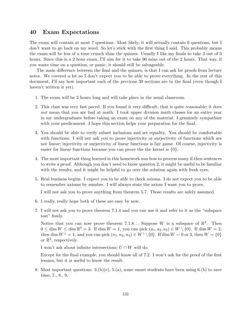
40 Exam Expectations

The exam will contain at most 7 questions. Most likely, it will actually contain 6 questions, but Idon’t want to go back on my word. So let’s stick with the first thing I said. This probably meansthe exam will be less of a time crunch than the quizzes. Usually I like my finals to take 2 out of 3hours. Since this is a 2 hour exam, I’ll aim for it to take 90 mins out of the 2 hours. That way, ifyou waste time on a question, or panic, it should still be salvageable.

The main difference between the final and the quizzes, is that I can ask for proofs from lecturenotes. We covered a lot so I don’t expect you to be able to prove everything. In the rest of thisdocument, I’ll say how important each of the previous 39 sections are to the final (even though Ihaven’t written it yet).

1. The exam will be 2 hours long and will take place in the usual classroom.

2. This class was very fast paced. If you found it very difficult, that is quite reasonable; it doesnot mean that you are bad at math. I took upper division math classes for an entire yearin my undergraduate before taking an exam on any of the material. I genuinely sympathizewith your predicament. I hope this section helps your preparation for the final.

3. You should be able to verify subset inclusions and set equality. You should be comfortablewith functions. I will not ask you to prove injectivity or surjectivity of functions which arenot linear; injectivity or surjectivity of linear functions is fair game. Of course, injectivity iseasier for linear functions because you can prove the the kernel is {0}.

4. The most important thing learned in this homework was how to process many if-then sentencesto write a proof. Although you don’t need to know question 2, it might be useful to be familiarwith the results, and it might be helpful to go over the solution again with fresh eyes.

5. Real business begins. I expect you to be able to check axioms. I do not expect you to be ableto remember axioms by number. I will always state the axiom I want you to prove.

I will not ask you to prove anything from theorem 5.7. Those results are safely assumed.

6. I really, really hope both of these are easy by now.

7. I will not ask you to prove theorem 7.1.4 and you can use it and refer to it as the “subspacetest” freely.

Notice that you can now prove theorem 7.1.8. . . Suppose W is a subspace of R3. Then0 ≤ dimW ≤ dimR3 = 3. If dimW = 1, you can pick (a1, a2, a3) ∈ W \ {0}. If dimW = 2,then dimW⊥ = 1, and you can pick (n1, n2, n3) ∈W⊥\{0}. If dimW = 0 or 3, then W = {0}or R3, respectively.

I won’t ask about infinite intersections; U ∩W will do.

Except for the final example, you should know all of 7.2. I won’t ask for the proof of the firstlemma, but it is useful to know the result.

8. Most important questions: 3.(b)(e), 5.(a), some smart students have been using 6.(b) to savetime, 7., 8., 9.

131

9. Everything in 9.1 is fair game, proofs included.

From 9.2, you should definitely know what Γα means. As for the rest of the 9.2, you shouldknow by now whether you find it useful to think about or not. Certainly, I have encounteredsome students who are finding this way of thinking useful. But you may also find it confusing.I think you should at least know that the final corollary is true. That corollary is the entirereason matrices are even a thing. I won’t ask for the proof.

9.4 will not be examined explicitly. However, if you still think about matrix-vector multiplica-tion as some terrible thing you do with a load of numbers for no reason, then you have missedthe point of the matrix of a linear transformation, and the linear transformation associatedwith a matrix.

10. I hope question 1 feels easy compared to the other things we have been doing.

11. Probably the most essential section of the entire class.

Again, if you like thinking about Γα, that is great - me too! If not, I wrote things in such away that you can ignore my remarks concerning it. However, eventually it becomes essentialfor defining various isomorphisms.

11.2 will not be examined.

12. This was all routine or tedious.

13. The proof of theorem 13.1.1 is examinable.

Notice that wherever there is an “if and only if” statement, I could ask a shorter question byasking for the proof of only one direction.

I think it is a good exercise to prove theorem 13.2.3 using the definition of span and linearindependence (with no reference to Γα).

You should know theorem 13.2.5, but its proof is too long for me to examine.

You know by now that the consequences of the replacement theorem are more important thanthe theorem itself.

You should know the first conclusion of the replacement theorem: that linearly independenttuples are smaller than or equal to spanning tuples. You do not need to know the other part,or the proof.

14. Question 6, 7, and 8 are the most important.

15. . . . as are the solutions!

16. Question 1 would now be slightly silly because you can make a dimension argument.

I already said above that I wouldn’t bother with a question 3 type question again.

Question 3 on quiz 2 shows that asking something like question 4(b) again would also be abit silly. This is because you can calculate a basis for the kernel and the image of a lineartransformation using the rank-nullity theorem and the replacement theorem in the same timeas calculating a kernel directly.

17. The comments about question 2 might still be relevant.

132

18. This section contains some of the most important results of the class.

The corollary is a very quick proof which you should know.

I will not ask for the proof of theorem 18.4, but I think that understanding it should be easierthan when we first covered it, and could be useful for you. These type of size arguments haveshown up a few times now.

19. Question 1 was probably tedious. Question 2 was easy, but important.

The main point of question 3 was to have you write proofs correctly by addressing the remarkI made before the question.

20. You should know the results of 20.1. I won’t ask for proofs.

The proof of the rank-nullity theorem is reasonably long. But I could ask for you to proverank(T ) +null(T ) ≤ dimV or rank(T ) +null(T ) ≥ dimV . Then that cuts the proof in half.It is too nice of a proof, and too important of a result for me to say this one is non-examinable.Learn it!

Theorem 20.2.4 is incredibly important. It might be a weird one for me to ask for the proof,but I still think you should know the proof.

You should understand example 20.2.5 flawlessly.

You can ignore the first lemma of 20.3. You should know the other results from 20.3. Onlythe proof of the last theorem is examinable. Since this builds on a homework question, Iwould arrange a question on it so that only a subset of the homework is required, and all ofit is provable in one go (similar to quiz 2, question 4).

21. http://soundcloud.com/mjandr/sets/best-of

22. You should be able to prove the first two theorems.

You should know the third theorem. Proving it is unnecessary.

You should definitely know theorem 22.1.4, and be able to use it. You do not need to be ableto prove it.

You should know all of 22.2.

23. All of this homework is important.

24. You should know the results of 24.1. The proofs can be ignored.

24.2 can be ignored.

Theorem 24.3.5 is one of my favorite results. I won’t ask for the proofs of this section, but youshould understand what the important ideas are in these proofs. Mostly, there’s applicationsof theorem 20.2.4 and theorem 22.1.1.

Why can’t a non-square matrix A define an isomorphism TA?

24.4 stunned me. I won’t ask for his proof, but note how he makes use of theorem 22.1.4.

25. All of this homework was important to check that you can do the calculations.

Revisit 1.(h) to help put diagonalization into persepctive.

133

http://soundcloud.com/mjandr/sets/best-of

26. So many matrices. Notice the examples that I gave of coordinate change matrices.

27. I won’t ask for proofs of the results in 27.1.

All I’ll expect from 27.2 is that you can calculate very easy determinants.

In 27.3, you can believe the unproved theorem. You should know everything else.

28. http://vimeo.com/mjandr

29. All of these types of questions are reasonable for the final.

30. I said some things, I guess, hopefully useful.

31. You should know all of this section as written (i.e. only one proof).

I’ll address the big theorem’s proofs shortly.

32. Direct sums are fair game on the final.

I think questions 1, 4, 5, 6, and 7 are the most important questions

33. . . . as are the solutions!

34. You should be able to prove theorem 34.1.

Other than that, you should read the proofs to help your understanding. Ideas in them couldbe useful, but I won’t examine them explicitly.

35. In the exam, I will not use complex numbers. The reason I introduced them is so that I canprove the spectral theorem, and so that I could tell you the full story about inner productspaces. (Both of these topics are part of UCLA’s 115A syllabus.)

So you can ignore 35.1.

In 35.2, you can ignore anything to do with the word “conjugate.” You can ignore the 131Aexample I gave. You should know the poof of theorem 35.2.8 (it’s in the book).

You do not need to know the proofs of the triangle inequality and Cauchy-Schwartz.

You do not need to know about “angles” other than the concept of orthogonal.

The Fourier basis is off-syllabus even though it is my favorite bit of math ever.

36. This question was a piece of cake.

37. The proof of Gram-Schmidt is too long. You do not need to know this proof.

The Riesz representation lemma is probably a little confusing. You do not need to know thisresult.

Everything else is fair game.

38. Questions 2 and 3 are important.

I changed my mind from earlier, and decided that question 4 is non-examinable.

39. Non-examinable, but it really is one of the coolest things we have done.

Please try and appreciate this after the exam has passed.

134

http://vimeo.com/mjandr

40. By commenting on this section within this section, does it create a glitch in the MATRIX?

135

41 The final

1. Suppose V and W are vector spaces over R, that S : V −→ W is a linear transformation,and that v1, v2, . . . , vn ∈ V . Always true or sometimes false (i.e. depends on V , W , S, etc.)?

(a) If kerS = {0} and (v1, v2, . . . , vn) is linearly independent,

then (S(v1), S(v2), . . . , S(vn)) is linearly independent.

(b) If (v1, v2, . . . , vn) spans V and (S(v1), S(v2), . . . , S(vn)) is a basis for W ,

then S is an isomorphism.

(c) If S is an isomorphism and (v1, v2, . . . , vn) spans V ,

then (S(v1), S(v2), . . . , S(vn)) is a basis for W .

(d) If (S(v1), S(v2), . . . , S(vn)) is a basis for W and S is an isomorphism,

then (v1, v2, . . . , vn) spans V .

Solution. T,T,F,T.

2. Let V and W be vector spaces over R and let T : V −→W be a linear transformation.

(a) Suppose that (v1, v2, . . . , vn) is a tuple of vectors in V which spans V ,

and that (T (v1), T (v2), . . . , T (vn)) is linearly independent.

Prove that kerT = {0}.Solution. 8/20 homework, question 8.(f).

(b) Suppose that kerT = {0}. Prove that T is injective, i.e. that

if v1, v2 ∈ V and T (v1) = T (v2), then v1 = v2.

Solution. Second half of theorem 9.1.4.

3. (a) Suppose V and W are finite-dimensional vector spaces over Rand that T : V −→W is a linear transformation.

Prove that rank(T ) + null(T ) ≤ dimV .

Solution. Write out the first half of the proof of the rank-nullity theorem, and then useconsequences of the replacement theorem to conclude the inequality.

(b) Suppose U , V , and W are finite-dimensional vector spaces over R, and that

T : U −→ V, S : V −→W

are linear transformations. Prove that rank(ST ) ≤ rank(T ).

Solution. 8/20 homework, question 6.(a) and 8/27 homework, question 4.

(c) Suppose m,n ∈ N, m < n, A is an n×m matrix, and B is an m× n matrix.

Prove that AB 6= In, but BA = Im is possible.

Solution. If AB = In, we’d have n = rank(TAB) = rank(TATB) ≤ rank(TB) ≤ m < n.

On the other hand, if A =

(Im

0(n−m)×m

)and B =

(Im 0m×(n−m)

), then BA = Im.

136

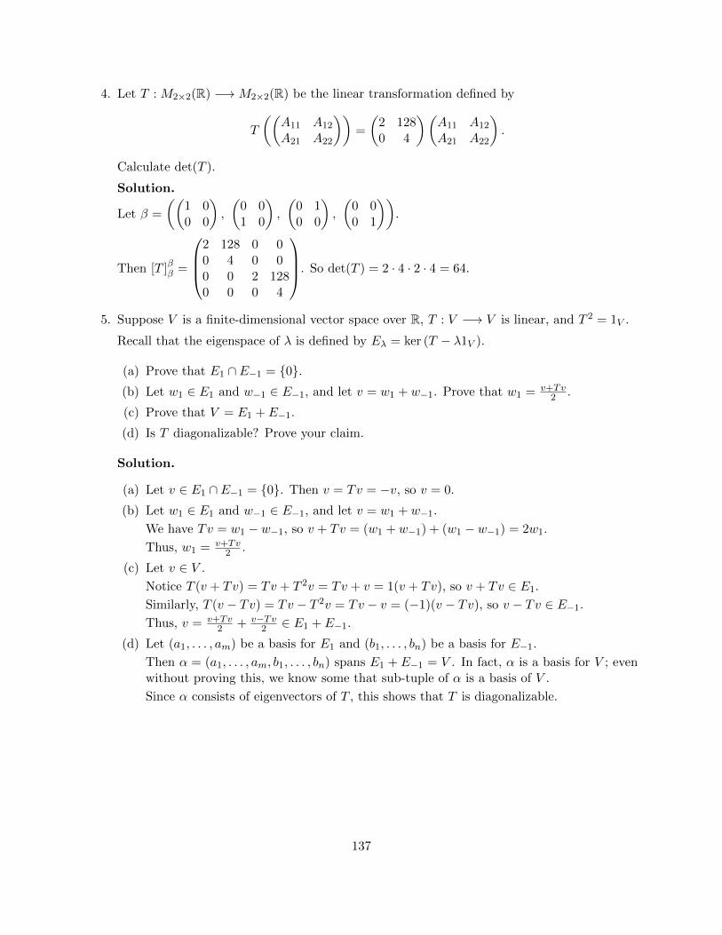
4. Let T : M2×2(R) −→M2×2(R) be the linear transformation defined by

T

((A11 A12

A21 A22

))=

(2 1280 4

)(A11 A12

A21 A22

).

Calculate det(T ).

Solution.

Let β =

((1 00 0

),

(0 01 0

),

(0 10 0

),

(0 00 1

)).

Then [T ]ββ =

2 128 0 00 4 0 00 0 2 1280 0 0 4

. So det(T ) = 2 · 4 · 2 · 4 = 64.

5. Suppose V is a finite-dimensional vector space over R, T : V −→ V is linear, and T 2 = 1V .

Recall that the eigenspace of λ is defined by Eλ = ker (T − λ1V ).

(a) Prove that E1 ∩ E−1 = {0}.(b) Let w1 ∈ E1 and w−1 ∈ E−1, and let v = w1 + w−1. Prove that w1 = v+Tv

2 .

(c) Prove that V = E1 + E−1.

(d) Is T diagonalizable? Prove your claim.

Solution.

(a) Let v ∈ E1 ∩ E−1 = {0}. Then v = Tv = −v, so v = 0.

(b) Let w1 ∈ E1 and w−1 ∈ E−1, and let v = w1 + w−1.

We have Tv = w1 − w−1, so v + Tv = (w1 + w−1) + (w1 − w−1) = 2w1.

Thus, w1 = v+Tv2 .

(c) Let v ∈ V .

Notice T (v + Tv) = Tv + T 2v = Tv + v = 1(v + Tv), so v + Tv ∈ E1.

Similarly, T (v − Tv) = Tv − T 2v = Tv − v = (−1)(v − Tv), so v − Tv ∈ E−1.

Thus, v = v+Tv2 + v−Tv

2 ∈ E1 + E−1.

(d) Let (a1, . . . , am) be a basis for E1 and (b1, . . . , bn) be a basis for E−1.

Then α = (a1, . . . , am, b1, . . . , bn) spans E1 + E−1 = V . In fact, α is a basis for V ; evenwithout proving this, we know some that sub-tuple of α is a basis of V .

Since α consists of eigenvectors of T , this shows that T is diagonalizable.

137

6. (a) Let V be an inner product space over R.

Suppose that (v1, . . . , vn) is orthonormal tuple of vectors in V .

Prove that (v1, . . . , vn) is linearly independent.

Solution. Suppose λ1, . . . , λn ∈ R, λ1v1 + . . .+λnvn = 0, and let j ∈ {1, 2 . . . , n}. Then

λj = λj〈vj , vj〉 =n∑i=1

λi〈vi, vj〉 =

⟨n∑i=1

λivi, vj

⟩= 〈0, vj〉 = 0.

(b) Define an unusual inner product on R2 by 〈 , 〉 : R2 × R2 −→ R⟨(x1, x2), (y1, y2)

⟩= x1y1 + 2x1y2 + 2x2y1 + 5x2y2.

Find an orthonormal basis for R2.

Solution. (1, 0), (2,−1).

(c) Let V be an inner product space over R.

Suppose that U and W are subspaces of V .

Prove that U⊥ +W⊥ ⊆ (U ∩W )⊥.

Solution. Let v′ ∈ U⊥+W⊥. By definition of addition of sets, we can write v′ = u′+w′

for some u′ ∈ U⊥ and some w′ ∈W⊥.

Now let v ∈ U ∩W .

Because u′ ∈ U⊥ and v ∈ U , we have 〈u′, v〉 = 0.

Because w′ ∈W⊥ and v ∈W , we have 〈w′, v〉 = 0.

Thus, 〈v′, v〉 = 〈u′, v〉+ 〈w′, v〉 = 0.

Since v was an arbitrary element in U ∩W , this shows that v′ ∈ (U ∩W )⊥.

138

math 115a: linear algebramjandr/math115a/115a.pdf3 lecture on august 6th: sets and functions 3.1...

Documents