math 144: 5: hypothesis testing - iuma - ulpgcnunez/mastertecnologiastelecomunicacion... · math...

$: Math 144: 5: Hypothesis Testing - IUMA - ULPGCnunez/mastertecnologiastelecomunicacion... · Math 144: \ 5: Hypothesis Testing ... the scientist or engineer may not be so much the$
Math 144: \ 5: Hypothesis Testing

Introduction

Previously, we introduced the point and interval estimation of an unknownparameter(s), say µ and σ2. However, in practice, the problem confrontingthe scientist or engineer may not be so much the parameter estimation, butrather the formation of a data-based decision procedure that can produce aconclusion about some scientific system.

For example:

• a medical researcher may decide on the basis of experimental evidencewhether coffee drinking increases the risk of cancer in humans;

• a sociologist may wish to collect appropriate data to enable him or herto decide whether a person’s blood type and eye color are independentvariables.

• an engineer may decide on the basis of sample data whether the trueaverage lifetime of a certain kind of tire is at least 22,000 miles;

• an agronomist may want to decide on the basis of experiments whetherone kind of fertilizer produces a higher yield of soybeans than another;

• a manufacturer of pharmaceutical products may decide on the basis ofsamples whether 90% of all patients given a new medication will recoverfrom a certain disease.

In each of these cases, the scientist or engineer conjectures something abouta system. In addition, each must involve the use of experimental data anddecision making that is based on the data. Formally, in each case, the con-jecture can be put in the form of a statistical test of hypothesis.

In particular, in the third case, we might say that the engineer has totest the hypothesis that θ, the parameter of an exponential population, isat least 22,000; in the fourth case we might say that the agronomist has

1

to decide whether µ1 > µ2, where µ1 and µ2 are the means of two normalpopulations; and in the last case we might say that the manufacturer has todecide whether θ, the parameter of a binomial population, equals 0.90. Forthese three cases, it must be assumed that the chosen distribution correctlydescribes the experimental conditions, namely, that the distribution providesthe correct statistical model.

Procedures that lead to the acceptance or rejection of statistical hypothesessuch as these comprise a major area of statistical inference. First, let us defineprecisely what we mean by a statistical hypothesis.

Definition 1. A statistical hypothesis is an assertion or conjecture or state-ment about the population, usually formulated in terms of population parame-ters. The two complementary statements concerning the population are callednull hypothesis H0 and alternative hypothesis H1.

Example 1:

H0 : µ = 0 (null)

H1 : µ 6= 0 (alternative)or

H0 : µ = µ0 (null)

H1 : µ > µ0 (alternative)

or

H0 : σ = 1 (null)

H1 : σ 6= 1 (alternative)

Definition 2. A test of statistical hypothesis H0 is a procedure, based uponthe observed values of the random sample obtained, that leads to the rejectionor non-rejection of the hypothesis H0.

2

Example 2:

For testing H0 : µ = 1, the procedure ”reject H0 if X > 2 or X < 0” is a test.

In testing statistical hypothesis, we are testing H0 against H1, i.e. weobserve the data to see if there is enough evidence to reject H0. Ifwe have enough evidence to reject H0, we can have great confidence that H0

is false and H1 is true. However, if we observe the data and find that H0 isnot rejected, it does not mean that we have great confidence in the truth ofH0. It only means that we do not have enough evidence to reject H0. So, weshould say ”do not reject H0”, instead of ”accept H0”.

Indeed, the test procedure mentioned before can lead to two kinds or errors.For instance, if the true value of the parameter θ is θ0 and we incorrectlyconcludes that θ = θ1, then we will commit an error of the false rejection ofH0. On the other hand, if the true value of the parameter θ is θ1 and weincorrectly concludes that θ = θ0, then we will commit an error of the falseacceptance of H0. More formally, these two types of error are called:

Type I error, which is the error of rejecting H0 when it is in fact true,

Type II error, which is the error of not rejecting H0 when it is in fact false.

Not reject H0 Reject H0

If H0 is true no error type I errorIf H0 is false type II error no error

Define

α = P (Type I error) = P (reject H0 |H0 is true)and β = P (Type II error) = P (not reject H0 |H0 is false).

Often, α is called the significance level of a test.

Naturally, we cannot control them simultaneously, unless we canvary the sample size. More precisely, there is a trade-off between the twotypes of error. Making α smaller will lead to a larger β, and vice versa.

3

Therefore in designing a test we can only control one of them, say, guaranteeα in a desired low level, say 0.1, 0.05 or 0.01, and then try to reduce β asmuch as we could (i.e. type I error is considered as more serious than typeII error). That is why the roles of H0 and H1 are not interchangeable.

Example 3: Suppose we knew that the light bulbs produced from astandard manufacturing process have life times distributed as normal with astandard deviation σ = 300 hours. However, we did not know the meanlifetime µ. For simplicity, assume that we were sure that the mean lifetimeshould be either 1200 or 1240. Then we may set up the followinghypotheses:

H0 : µ = 1200

H1 : µ = 1240

Suppose that we draw a sample of 100 light bulbs and measure theirlifetimes. The sample mean X can be used to estimate the true populationmean µ. Intuitively, a large value of X will lead to the rejection of H0. So ifwe construct a test as

”Reject H0 if X > 1249”,

then

α = P (Reject H0 |H0 is true) = P (X > 1249 |µ = 1200),

and

β = P (Not reject H0 |H0 is false) = P (X ≤ 1249 |µ = 1240).

Now let’s see a picture why we cannot control the Type I error and Type IIerror simultaneously.

4

Picture:

Choice of H0 and H1:

Criterion 1: Since we will keep P (reject H0 |H0 is true) in a low level, wechoose a statement as H0 when falsely rejecting it is considered as a seriouserror.

Example 4: Suppose that we want to know if a man is guilty or not,

A :

H0 : He is guilty.

H1 : He is not guilty.

or B :

H0 : He is not guilty.

H1 : He is guilty.

Since the false judgment of the guilty of a man is considered as a moreserious error than the false judgment of the non-guilty of a man, we chooseB.

5

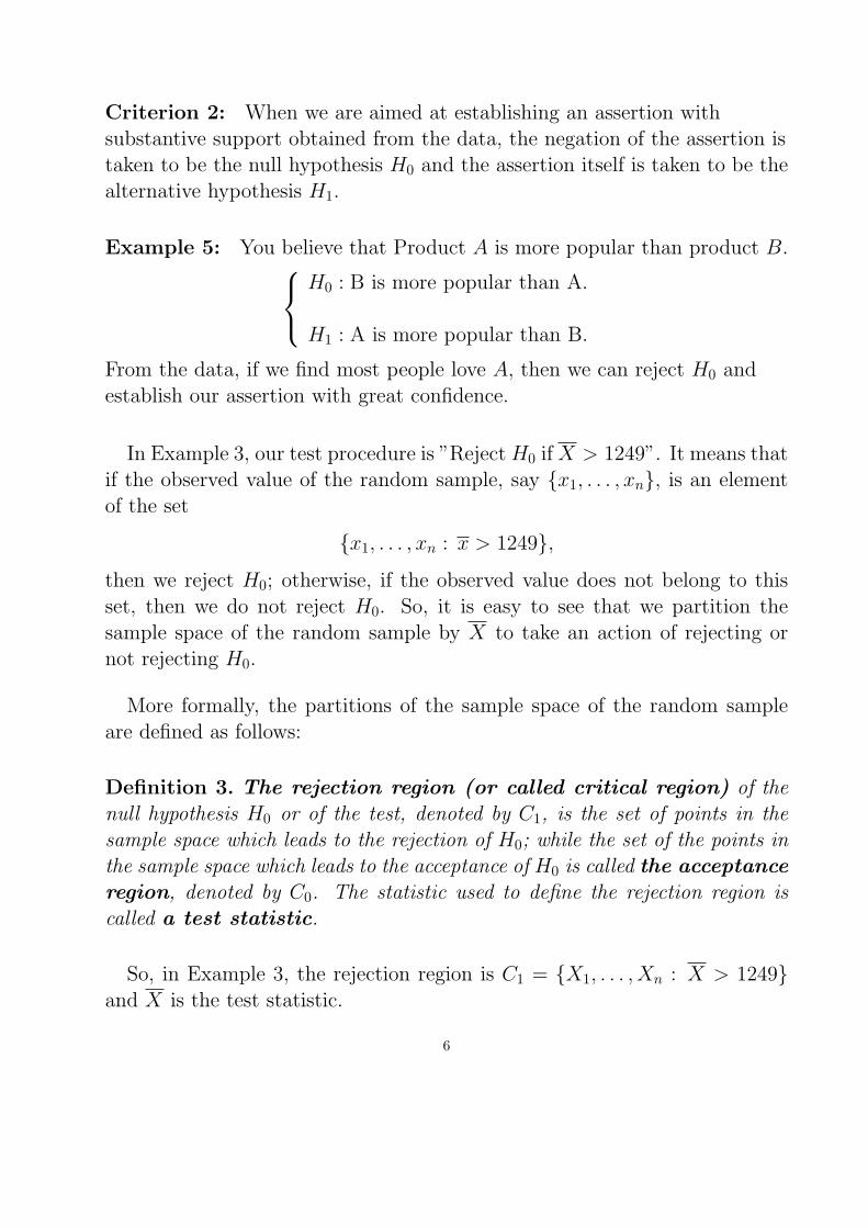
Criterion 2: When we are aimed at establishing an assertion withsubstantive support obtained from the data, the negation of the assertion istaken to be the null hypothesis H0 and the assertion itself is taken to be thealternative hypothesis H1.

Example 5: You believe that Product A is more popular than product B.

H0 : B is more popular than A.

H1 : A is more popular than B.

From the data, if we find most people love A, then we can reject H0 andestablish our assertion with great confidence.

In Example 3, our test procedure is ”Reject H0 if X > 1249”. It means thatif the observed value of the random sample, say {x1, . . . , xn}, is an elementof the set

{x1, . . . , xn : x > 1249},then we reject H0; otherwise, if the observed value does not belong to thisset, then we do not reject H0. So, it is easy to see that we partition thesample space of the random sample by X to take an action of rejecting ornot rejecting H0.

More formally, the partitions of the sample space of the random sampleare defined as follows:

Definition 3. The rejection region (or called critical region) of thenull hypothesis H0 or of the test, denoted by C1, is the set of points in thesample space which leads to the rejection of H0; while the set of the points inthe sample space which leads to the acceptance of H0 is called the acceptanceregion, denoted by C0. The statistic used to define the rejection region iscalled a test statistic.

So, in Example 3, the rejection region is C1 = {X1, . . . , Xn : X > 1249}and X is the test statistic.

6

Remark that the rejection region is decided BEFORE we actually observeour data.

Recall that in hypothesis testing, we cannot control two error probabilitiessimultaneously. Therefore, in designing a test, we often control the Type Ierror probability or the significance level, α, in a desired low level, say 0.01,0.05 or 0.1, and then try to reduce the Type II error probability β as muchas we could.

Referring to Example 3 again, we have a random sample of size n = 100,{X1, . . . , Xn} from N(µ, 3002), where µ is unknown. Now we want to test

H0 : µ = 1200 (simple null hypothesis)

H1 : µ = 1240 (simple alternative hypothesis)

at α = 0.05.

Since the previous test procedure ”Reject H0 if X > 1249” does not satisfythe requirement of the Type I error probability, we have to use another testprocedure. That is, we have to define another rejection region C1.

Suppose that we still use the intuitive test statistic: X ∼ N(µ, 3002

100 ). Thenit is reasonable for us to reject H0 if X is too large. That is, a reasonabletest would be

”Reject H0 if X > c”,

where c, often called a critical value , is constant to be determined by thecondition that α = 0.05.

In the following, we will see how to find a value of c. First, we must keep

0.05 = α = P (reject H0 |H0 is true)

= P (X > c |µ = 1200)

= P( X − 1200

300/√

100>

c− 1200

300/√

100|µ = 1200

)

= 1− Φ(c− 1200

30

)

7

=⇒ c− 1200

30= 1.645. So, the critical value c is 1249.35. Hence, the

rejection region is

{X1, . . . , Xn : X > 1249.35},

i.e. we have a test that

Rejects H0 at the significance level α = 0.05 if X > 1249.35.

Suppose that we observe the random sample and find that x = 1237, whichis less than 1249.35. So, we conclude that we do not have enough evidenceto reject H0 at the significance level α = 0.05.

Now let’s see the Type II error probability, β, of this test.

β = P (do not reject H0 |H0 is false)

= P (X ≤ 1249.35 |H1 is true)

= P (X ≤ 1249.35 |µ = 1240)

= P( X − 1240

300/√

100≤ 1249.35− 1240

300/√

100|µ = 1240

)

= Φ(0.312) = 0.6225.

In statistics, the value 1− β is called the power of a test. Thus, in theabove case, the test has a power 1 − 0.6225 = 0.3775, so we would say thatit is not very powerful. For the comparison of two tests with common α, thebigger the power of the test is, the better the test is.

As can be seen in the picture on page 5 before, using a smaller value of c

can reduce β (i.e. increase the power). However, this will also increase thevalue of α. If we want to keep α fixed and reduce β in the same time, wehave to increase the sample size such that we can get more information fortesting the hypothesis.

For a sample with size n = 400, the critical value c of the rejection region

8

for a test with α = 0.05 is given by

c− 1200

300/√

400= 1.645 =⇒ c = 1224.675 .

Therefore, the rejection region becomes X > 1224.675, i.e. we will reject H0

at α = 0.05 if X > 1224.675. For this test,

β = P( X − 1240

300/√

400≤ 1224.675− 1240

300/√

400|µ = 1240

)

= Φ(−1.022) = 0.1534.

Hence, the power is 1− β = 0.8466, which is much improved!!

Question: If {X1, . . . , Xn} is a random sample from N(µ, 3002), where µand n are unknown. Now we want to test

H0 : µ = 1200 (simple null hypothesis)

H1 : µ = 1240 (simple alternative hypothesis)

Use a rejection region X > c. Then determine a critical value c and asample size n such that α = 0.05 and power at µ = 1240 is 0.9.

9

Other Types of a test:

Definition 4. A test of any statistical hypothesis is called a one-tailed testor one-sided test if the alternative hypothesis is one-sided. That is,

H0 : µ = µ0

H1 : µ > µ0.or

H0 : µ = µ0.

H1 : µ < µ0.

Definition 5. A test of any statistical hypothesis is called a two-tailed testor two-sided test if the alternative hypothesis is two-sided. That is,

H0 : µ = µ0

H1 : µ 6= µ0.

Summary for the approach to hypothesis testing with fixed α:

1. State the null and alternative hypotheses, i.e. H0 and H1.

2. Choose a fixed significance level α. (It will be given in this course, so youdo not need to choose it by yourselves)

3. Use an appropriate test statistic and establish the rejection region C1

based on α. (We will discuss what test statistic we should use later.)

4. From the observed value of the test statistic, reject H0 at the significancelevel α if it is inside C1; otherwise, do NOT reject H0 at the significancelevel α.

10

Testing for the population mean µ and population variance σ2:

Recall that throughout this course, we are only interested in making an in-ference about the population mean µ and the population variance σ2. In thefollowing, we will consider different cases for testing µ and σ2.

(I) One-sample tests for the mean µ:

Consider a random sample of size n, {X1, . . . , Xn}, from a distribution (notnecessary normal) with mean µ and variance σ2. An intuitive and reasonabletest statistic for testing µ is the sample mean X of a random sample.

1. One-tailed test (right):

Consider

H0 : µ = µ0

H1 : µ > µ0.

We reject H0 if x > a, where a can be determined by a given significancelevel α. Indeed, under H0,

P (X > a) = α,

which implies thata− µ0

σ/√

n= zα, i.e. a = µ0 + zα

σ√n. Thus, we

Reject H0 at the significance level α if x > µ0 + zασ√n, when σ2 is known.

When σ2 is unknown, we have that under H0,

α = P (X > a) = P(T >

a− µ0

S/√

n

),

where T =X − µ0

S/√

nhas a (approximate) t-distribution with n−1 degrees

of freedom. So,

a = µ0 + tn−1,αs√n

.

11

Thus, we

Reject H0 at a significance level α if x > µ0 + tn−1,αs√n

, when σ2 is unknown.

2. One-tailed test (left)

Similarly, for the testing of

H0 : µ = µ0

H1 : µ < µ0.

We reject H0 if x < a, where a can be determined by a given significancelevel α. Thus, if σ2 is known, then

We reject H0 at the significance level α if x < µ0 − zασ√n.

Also, when σ2 is unknown, then we

Reject H0 at the significance level α if x < µ0 − tn−1,αs√n

.

3. Two-tailed test

Consider

H0 : µ = µ0

H1 : µ 6= µ0.

We reject H0 if x < a or x > b, where a and b can be determined by agiven significance level α. Under H0, consider

α = P (X < a OR X > b) = 1− P (a ≤ X ≤ b).

So,

1− α = P (a− µ0

σ/√

n≤ Z ≤ b + µ0

σ/√

n),

12

where Z =X − µ0

σ/√

nhas a (approximate) standard normal distribution.

Thus, we have

a− µ0

σ/√

n= −zα/2 and

b− µ0

σ/√

n= zα/2.

That is,

a = µ0 − zα/2σ√n

and b = µ0 + zα/2σ√n

.

So, we

Reject H0 at the significance level α if∣∣∣x− µ0

σ/√

n

∣∣∣ > zα/2, when σ2 is known.

When σ2 is unknown, we

Reject H0 at the significance level α if∣∣∣x− µ0

s/√

n

∣∣∣ > tn−1,α/2.

Question : A random sample of 100 recorded deaths in the United Statesduring the past year showed an average life span of 71.8 years. Assuming apopulation standard deviation of 8.9 years, does this seem to indicate thatthe mean life span today is greater than 70 years? Use a significance level of0.05.

13

Question : The average length of time for students to register for classesat a certain college has been 46 minutes. A new registration procedureusing modern computing machines is being tried. If a random sample of 12students had an average registration time of 42 minutes with a standarddeviation of 11.9 minutes under the new system. Test the hypothesis thatthe population mean is now less than 46. Use a 0.05 level of significance.

Question: A manufacturer of sports equipment has developed a newsynthetic fishing line that he claims has a mean breaking strength of 8kilograms with a standard deviation of 0.5 kilogram. Test the hypothesisthat µ = 8 kilograms against the alternative that µ 6= 8 kilograms if arandom sample of 50 lines is tested and found to have a mean breakingstrength of 7.8 kilograms. Use a 0.01 level of significance.

14

(II) One-sample tests for the variance σ2:

Consider a random sample of size n, {X1, . . . , Xn}, from a distribution (notnecessary normal) with mean µ and variance σ2. An intuitive and reasonabletest statistic for testing σ2 is the sample variance S2 of a random sample.Remark that the notation χ2

α below is with respect to the chi-squared distri-bution with n−1 degrees of freedom, i.e. P (X2 > χ2

α) = α, where X2 ∼ χ2n−1.


Consider

H0 : σ2 = σ20

H1 : σ2 > σ20.

We reject H0 if s2 > a, where a can be determined by a given signifi-cance level α. Indeed, under H0,

P (S2 > a) = α,

which implies that(n− 1)a

σ20

= χ2α, i.e. a =

σ20χ

2α

n− 1. Thus, we

Reject H0 at the significance level α if s2 >σ2

0χ2α

n− 1.

2. One-tailed test (left):

Consider

H0 : σ2 = σ20

H1 : σ2 < σ20.

We reject H0 if s2 < a, where a can be determined by a given signifi-cance level α. Thus, we

Reject H0 at the significance level α if s2 <σ2

0χ21−α

n− 1.

15

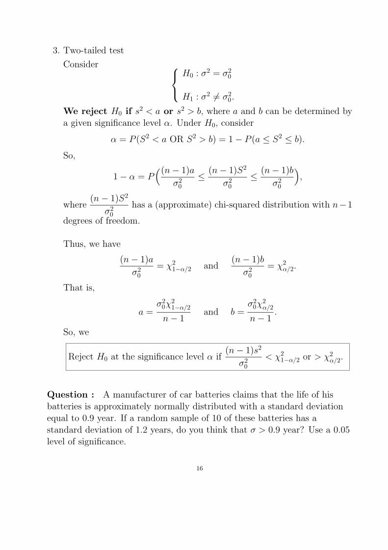
3. Two-tailed test

Consider

H0 : σ2 = σ20

H1 : σ2 6= σ20.

We reject H0 if s2 < a or s2 > b, where a and b can be determined bya given significance level α. Under H0, consider

α = P (S2 < a OR S2 > b) = 1− P (a ≤ S2 ≤ b).

So,

1− α = P((n− 1)a

σ20

≤ (n− 1)S2

σ20

≤ (n− 1)b

σ20

),

where(n− 1)S2

σ20

has a (approximate) chi-squared distribution with n−1

degrees of freedom.

Thus, we have

(n− 1)a

σ20

= χ21−α/2 and

(n− 1)b

σ20

= χ2α/2.

That is,

a =σ2

0χ21−α/2

n− 1and b =

σ20χ

2α/2

n− 1.

So, we

Reject H0 at the significance level α if(n− 1)s2

σ20

< χ21−α/2 or > χ2

α/2.

Question : A manufacturer of car batteries claims that the life of hisbatteries is approximately normally distributed with a standard deviationequal to 0.9 year. If a random sample of 10 of these batteries has astandard deviation of 1.2 years, do you think that σ > 0.9 year? Use a 0.05level of significance.

16

(III) Two-sample tests for the mean difference:

Suppose that we have two independent random samples {X1, . . . , Xn} froma population with mean µX and variance σ2

X , and {Y1, . . . , Ym} from anotherpopulation with mean µY and variance σ2

Y .


Consider

H0 : µX − µY = d0

H1 : µX − µY > d0.

We reject H0 if x − y > a, where a can be determined by a givensignificance level α. Indeed, under H0,

P (X − Y > a) = α.

which implies thata− (µX − µY )√σ2

X/n + σ2Y /m

= zα, i.e. a = d0 + zα

√σ2

X

n+

σ2Y

m.

Thus, we

Reject H0 at α if x− y > d0 + zα

√σ2

X

n+

σ2Y

m, when σ2

X and σ2Y are known.


Consider

H0 : µX − µY = d0

H1 : µX − µY < d0.

We reject H0 if x − y < a, where a can be determined by a givensignificance level α. Thus, we

Reject H0 at α if x− y < d0 − zα

√σ2

X

n+

σ2Y

m, when σ2

X and σ2Y are known.

17

3. Two-tailed test:

Consider

H0 : µX − µY = d0

H1 : µX − µY 6= d0.

We reject H0 if x−y < a or x−y > b, where a and b can be determinedby a given significance level α. Similar to what we did in a one-sampletwo tailed case, we

Reject H0 at α if

∣∣∣∣∣(x− y)− d0√

σ2X

n +σ2

Y

m

∣∣∣∣∣ > zα/2, when σ2X and σ2

Y are known.

When population variances σ2X and σ2

Y are unknown, we consider the fol-lowing four situations:

1. Not equal, small sample sizes:

Recalling the result on pages 18 - 19 of the note on estimation, we havethat the sampling distribution of

(X − Y )− (µX − µY )√(

S2X

n +S2

Y

m )

is an approximate t distribution with v degrees of freedom, where

v =(

S2X

n +S2

Y

m )2

1n−1(

S2X

n )2 + 1m−1(

S2Y

m )2.

Thus, for

(a) One-tailed test (right)

Reject H0 at a level α if x− y > d0 + tv,α

√s2X

n+

s2Y

m.

18

(b) One-tailed test (left)

Reject H0 at a level α if x− y < d0 − tv,α

√s2X

n+

s2Y

m.

(c) Two-tailed test

Reject H0 at a level α if

∣∣∣∣∣(x− y)− d0√

s2X

n +s2

Y

m

∣∣∣∣∣ > tv,α/2.

Again, based on the observed values of s2X and s2

Y , the degree offreedom v is not always an integer. So, in practice, we must rounddown to the nearest integer to draw the conclusion of the test. Forinstance, if v = 1.4, then take 1; if v = 2.9, then take 2.

2. Not equal, large sample sizes:

If the sample sizes n and m are large enough that the degree of freedomv ≥ 30, then we know that tv,α ≈ zα. Hence, for


Reject H0 at a level α if x− y > d0 + zα

√s2X

n+

s2Y

m.


Reject H0 at a level α if x− y < d0 − zα

√s2X

n+

s2Y

m.

(c) Two-tailed test


∣∣∣∣∣(x− y)− d0√

s2X

n +s2

Y

m

∣∣∣∣∣ > zα/2.

19

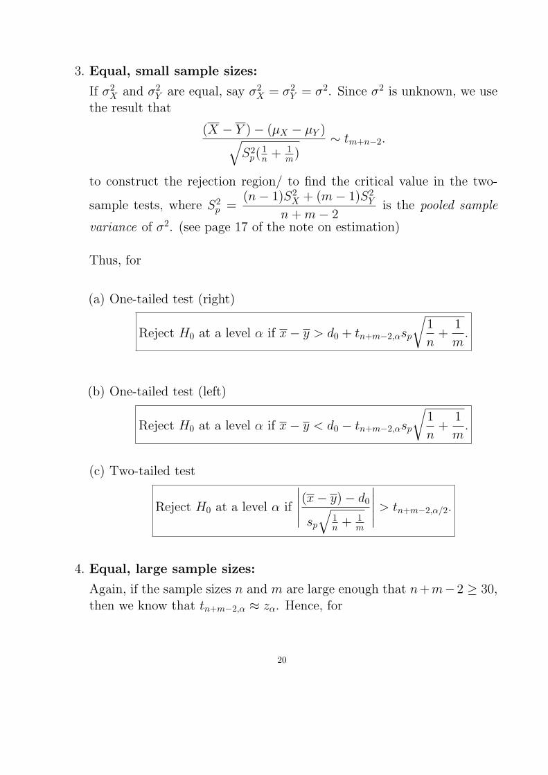
3. Equal, small sample sizes:

If σ2X and σ2

Y are equal, say σ2X = σ2

Y = σ2. Since σ2 is unknown, we usethe result that

(X − Y )− (µX − µY )√S2

p(1n + 1

m)∼ tm+n−2.

to construct the rejection region/ to find the critical value in the two-

sample tests, where S2p =

(n− 1)S2X + (m− 1)S2

Y

n + m− 2is the pooled sample

variance of σ2. (see page 17 of the note on estimation)

Thus, for


Reject H0 at a level α if x− y > d0 + tn+m−2,αsp

√1

n+

1

m.


Reject H0 at a level α if x− y < d0 − tn+m−2,αsp

√1

n+

1

m.

(c) Two-tailed test


∣∣∣∣∣(x− y)− d0

sp

√1n + 1

m

∣∣∣∣∣ > tn+m−2,α/2.

4. Equal, large sample sizes:

Again, if the sample sizes n and m are large enough that n+m−2 ≥ 30,then we know that tn+m−2,α ≈ zα. Hence, for

20


Reject H0 at a level α if x− y > d0 + zαsp

√1

n+

1

m.


Reject H0 at a level α if x− y < d0 − zαsp

√1

n+

1

m.

(c) Two-tailed test


∣∣∣∣∣(x− y)− d0

sp

√1n + 1

m

∣∣∣∣∣ > zα/2.

Question : An experiment was performed to compare the abrasive wearof two different laminated materials. 12 pieces of material 1 were tested byexposing each piece to a machines measuring wear. 10 pieces of material 2were similarly tested. In each case, the depth of wear was observed. Thesamples of material 1 gave an average (coded) wear of 85 units with asample standard deviation of 4, while the samples of material 2 gave anaverage of 81 and a samples standard deviation of 5. Can we conclude atthe 0.05 level of significance that the abrasive wear of material 1 exceedsthat of material 2 by more than 2 units? Assume that both populations areapproximately normally distributed with equal variances.

21

Question : From a class X, a sample of 4 scores were drawn: 64, 66, 89and 77. An independent sample of 3 scores were drawn from another classY: 56, 71 and 53. Assume that both populations are normal with equalvariances. Then test

H0 : µX = µY

H1 : µX 6= µY ,

at the significance level α = 0.05.

22

p-value

Alternatively, instead of finding the critical value to determine whether H0

is or is not rejected, we can consider the p-value, which is defined below.

Definition 6. The p-value of an observed value of the test statistic is thesmallest probability for which this observation leads to the rejection of H0 ifH0 is true.

Remark that the smaller the magnitude of p-value, the stronger the evi-dence against H0.

Example 6: Consider Example 3 with a test statistic X and n = 482again. Suppose that we observed x = 1237. Then the smallest probabilityfor which this observation leads to the rejection of H0 is the probability ofrejecting H0 with the critical value c = 1237. Hence,

p-value = P (X > 1237 |µ = 1200)

= P( X − 1200

300/√

482>

1237− 1200

300/√

482|µ = 1200

)

= 1− Φ(2.708) = 0.00342.

The interpretation of this p-value is that if H0 is true, then there would beonly 0.00342 probability of observing X as large as 1237, the observed valueof X. Therefore, there is a very strong disagreement between the data andH0.

So now, given a user-specified significance level of α, there are two ways tomake a decision of rejecting or NOT rejecting H0 at this level by

• either comparing the observed value of the test statistic with the criticalvalue,

• or comparing the p-value from the observed value of the test statisticwith α.

23

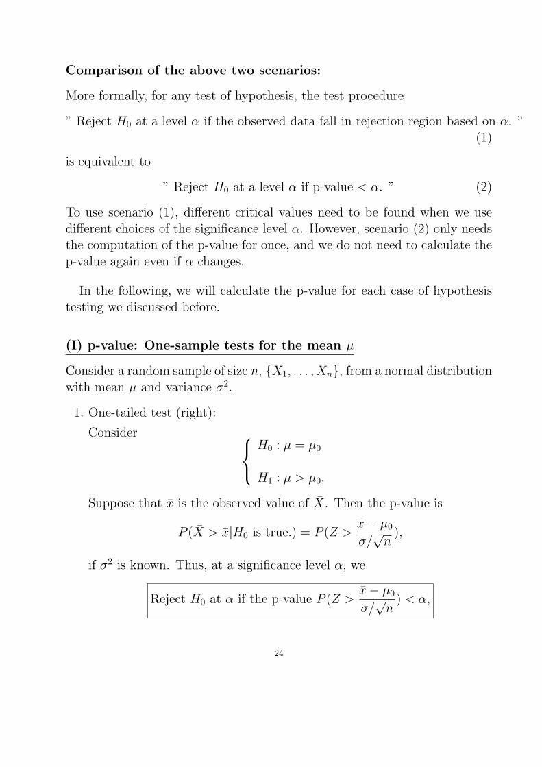
Comparison of the above two scenarios:

More formally, for any test of hypothesis, the test procedure

” Reject H0 at a level α if the observed data fall in rejection region based on α. ”(1)

is equivalent to

” Reject H0 at a level α if p-value < α. ” (2)

To use scenario (1), different critical values need to be found when we usedifferent choices of the significance level α. However, scenario (2) only needsthe computation of the p-value for once, and we do not need to calculate thep-value again even if α changes.

In the following, we will calculate the p-value for each case of hypothesistesting we discussed before.

(I) p-value: One-sample tests for the mean µ

Consider a random sample of size n, {X1, . . . , Xn}, from a normal distributionwith mean µ and variance σ2.


Consider

H0 : µ = µ0

H1 : µ > µ0.

Suppose that x is the observed value of X. Then the p-value is

P (X > x|H0 is true.) = P (Z >x− µ0

σ/√

n),

if σ2 is known. Thus, at a significance level α, we

Reject H0 at α if the p-value P (Z >x− µ0

σ/√

n) < α,

24

where Z has a standard normal distribution.

If σ2 is unknown, then

Reject H0 at α if the p-value P (T >x− µ0

s/√

n) < α,

where T has a t-distribution with n− 1 degrees of freedom.


Similarly, consider

H0 : µ = µ0

H1 : µ < µ0.


P (X < x|H0 is true.) = P (Z <x− µ0

σ/√

n),


Reject H0 at α if the p-value P (Z <x− µ0

σ/√

n) < α,



Reject H0 at α if the p-value P (T <x− µ0

s/√

n) < α,


3. Two-tailed test:

Consider

H0 : µ = µ0

H1 : µ 6= µ0.

25


P(|Z| >

∣∣∣x− µ0

σ/√

n

∣∣∣)

= 2P(Z >

∣∣∣ x− µ0

σ/√

n

∣∣∣).


Reject H0 at α if the p-value 2P(Z >

∣∣∣ x− µ0

σ/√

n

∣∣∣)

< α,



Reject H0 at α if the p-value 2P(T >

∣∣∣ x− µ0

s/√

n

∣∣∣)

< α,


(II) p-value: One-sample tests for the variance σ2

Consider a random sample of size n, {X1, . . . , Xn}, from a normal distributionwith mean µ and variance σ2.


Consider

H0 : σ2 = σ20

H1 : σ2 > σ20.

Suppose that s2 is the observed value of S2. Then, we

Reject H0 at the significance level α if P(X2 >

(n− 1)s2

σ20

)< α,

where X2 =(n− 1)S2

σ20

has a chi-squared distribution with n− 1 degrees

of freedom.

26


Consider

H0 : σ2 = σ20

H1 : σ2 < σ20.


Reject H0 at the significance level α if P(X2 <

(n− 1)s2

σ20

)< α,


σ20


of freedom.

3. Two-tailed test

Consider

H0 : σ2 = σ20

H1 : σ2 6= σ20.


Reject H0 at α if P(X2 <

(n− 1)s2

σ20

)< α/2 OR P

(X2 >

(n− 1)s2

σ20

)< α/2,


σ20


of freedom.

Question : (p-value) A manufacturer of car batteries claims that the lifeof his batteries is approximately normally distributed with a standarddeviation equal to 0.9 year. If a random sample of 10 of these batteries hasa standard deviation of 1.2 years, do you think that σ > 0.9 year? Use a0.05 level of significance.

27

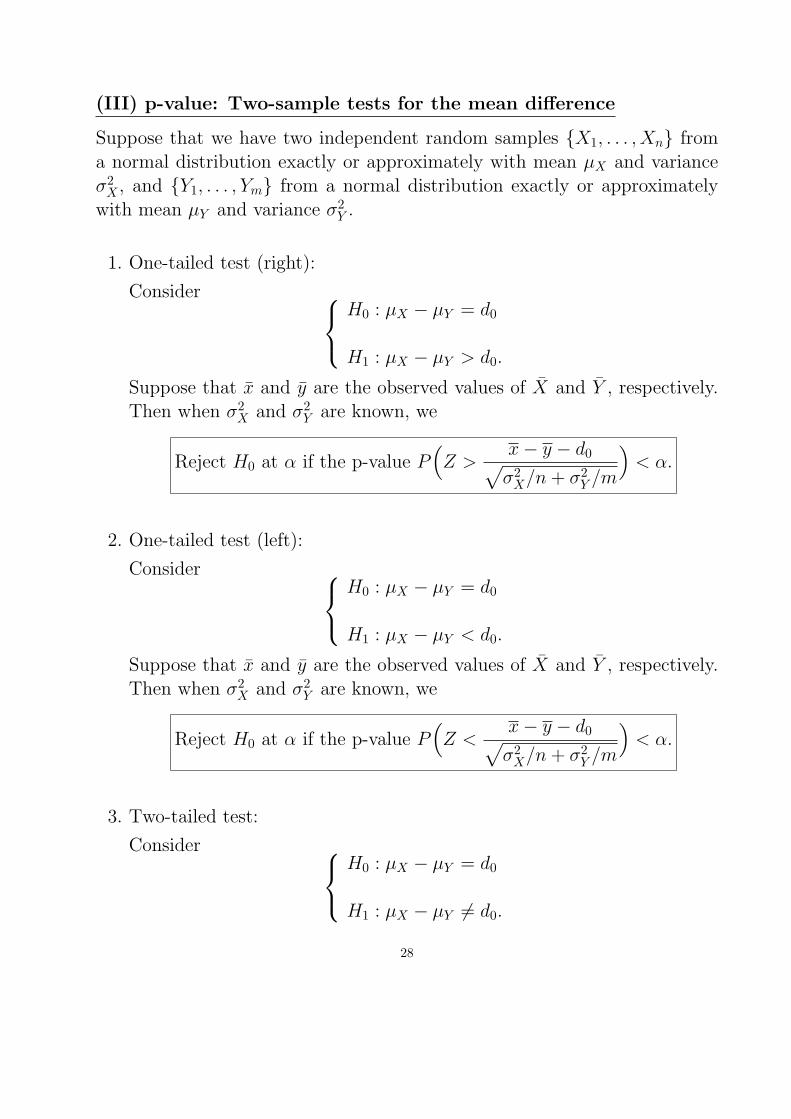
(III) p-value: Two-sample tests for the mean difference

Suppose that we have two independent random samples {X1, . . . , Xn} froma normal distribution exactly or approximately with mean µX and varianceσ2

X , and {Y1, . . . , Ym} from a normal distribution exactly or approximatelywith mean µY and variance σ2

Y .


Consider

H0 : µX − µY = d0

H1 : µX − µY > d0.

Suppose that x and y are the observed values of X and Y , respectively.Then when σ2

X and σ2Y are known, we

Reject H0 at α if the p-value P(Z >

x− y − d0√σ2

X/n + σ2Y /m

)< α.


Consider

H0 : µX − µY = d0

H1 : µX − µY < d0.



Reject H0 at α if the p-value P(Z <

x− y − d0√σ2

X/n + σ2Y /m

)< α.

3. Two-tailed test:

Consider

H0 : µX − µY = d0

H1 : µX − µY 6= d0.

28



Reject H0 at α if the p-value 2P(Z >

∣∣∣ x− y − d0√σ2

X/n + σ2Y /m

∣∣∣)

< α.

By the p-value approach, when population variances σ2X and σ2

Y are un-known in two-sample tests, we have the following four situations:

1. Not equal, small sample sizes:

Recall that the sampling distribution of

Tv =(X − Y )− (µX − µY )√

(S2

X

n +S2

Y

m )

is an approximate t distribution with v degrees of freedom, where

v =(

S2X

n +S2

Y

m )2

1n−1(

S2X

n )2 + 1m−1(

S2Y

m )2.

Thus, for


Reject H0 at a level α if the p-value P(Tv >

x− y − d0√s2X/n + s2

Y /m

)< α.


Reject H0 at a level α if the p-value P(Tv <

x− y − d0√s2X/n + s2

Y /m

)< α.

29

(c) Two-tailed test

Reject H0 at a level α if the p-value 2P(Tv >

∣∣∣ x− y − d0√s2X/n + s2

Y /m

∣∣∣)

< α.

Again, based on the observed values of s2X and s2

Y , the degree offreedom v is not always an integer. So, in practice, we must rounddown to the nearest integer to draw the conclusion of the test. Forinstance, if v = 1.4, then take 1; if v = 2.9, then take 2.

2. Not equal, large sample sizes:

If the sample sizes n and m are large enough that the degree of freedomv ≥ 30, then we know that the t-distribution with v degrees of freedomis close to the standard normal distribution. Hence, for


Reject H0 at a level α if the p-value P(Z >

x− y − d0√s2X/n + s2

Y /m

)< α.


Reject H0 at a level α if the p-value P(Z <

x− y − d0√s2X/n + s2

Y /m

)< α.

(c) Two-tailed test

Reject H0 at a level α if the p-value 2P(Z >

∣∣∣ x− y − d0√s2X/n + s2

Y /m

∣∣∣)

< α.

30

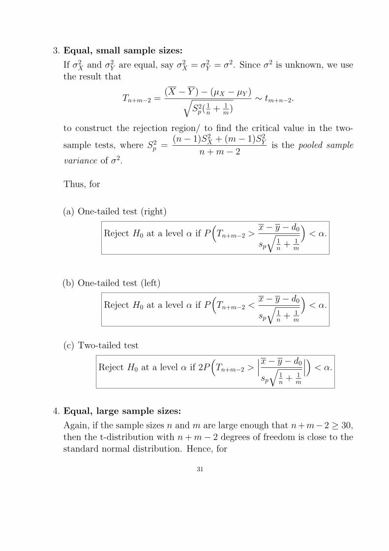
3. Equal, small sample sizes:

If σ2X and σ2

Y are equal, say σ2X = σ2

Y = σ2. Since σ2 is unknown, we usethe result that

Tn+m−2 =(X − Y )− (µX − µY )√

S2p(

1n + 1

m)∼ tm+n−2.

to construct the rejection region/ to find the critical value in the two-

sample tests, where S2p =

(n− 1)S2X + (m− 1)S2

Y

n + m− 2is the pooled sample

variance of σ2.

Thus, for


Reject H0 at a level α if P(Tn+m−2 >

x− y − d0

sp

√1n + 1

m

)< α.


Reject H0 at a level α if P(Tn+m−2 <

x− y − d0

sp

√1n + 1

m

)< α.

(c) Two-tailed test

Reject H0 at a level α if 2P(Tn+m−2 >

∣∣∣x− y − d0

sp

√1n + 1

m

∣∣∣)

< α.

4. Equal, large sample sizes:

Again, if the sample sizes n and m are large enough that n+m−2 ≥ 30,then the t-distribution with n + m− 2 degrees of freedom is close to thestandard normal distribution. Hence, for

31


Reject H0 at a level α if P(Z >

x− y − d0

sp

√1n + 1

m

)< α.


Reject H0 at a level α if P(Z <

x− y − d0

sp

√1n + 1

m

)< α.

(c) Two-tailed test

Reject H0 at a level α if 2P(Z >

∣∣∣x− y − d0

sp

√1n + 1

m

∣∣∣)

< α.

Question : (p-value) From a class X, a sample of 4 scores were drawn:64, 66, 89 and 77. An independent sample of 3 scores were drawn fromanother class Y: 56, 71 and 53. Assume that both populations are normalwith equal variances. Then test

H0 : µX = µY

H1 : µX 6= µY ,

at the significance level α = 0.05.

32

Question : (p-value) An experiment was performed to compare theabrasive wear of two different laminated materials. 12 pieces of material 1were tested by exposing each piece to a machines measuring wear. 10 piecesof material 2 were similarly tested. In each case, the depth of wear wasobserved. The samples of material 1 gave an average (coded) wear of 85units with a sample standard deviation of 4, while the samples of material 2gave an average of 81 and a samples standard deviation of 5. Can weconclude at the 0.05 level of significance that the abrasive wear of material1 exceeds that of material 2 by more than 2 units? Assume that bothpopulations are normally distributed with equal variances.

33

math 144: 5: hypothesis testing - iuma - ulpgcnunez/mastertecnologiastelecomunicacion... · math...

Documents