math 222 - lie groups and lie algebras - github pages€¦ · math 222 - lie groups and lie...

Math 222 - Lie Groups and Lie Algebras

Taught by Fabian HaidenNotes by Dongryul Kim

Spring 2017

This course was taught by Fabian Haiden, at MWF 10-11am in ScienceCenter 310. The textbook was An Introduction to Lie Groups and Lie Algebrasby A. Kirillov. There were 6 undergraduates and 10 graduate students enrolled.There were weekly problem sets and a final presentation. The course assistantwas Yusheng Luo.

Contents

1 January 23, 2017 51.1 Logistics . . . . . . . . . . . . . . . . . . . . . . . . . . . . . . . . 51.2 Lie groups . . . . . . . . . . . . . . . . . . . . . . . . . . . . . . . 51.3 Lie algebras . . . . . . . . . . . . . . . . . . . . . . . . . . . . . . 6

2 January 25, 2017 72.1 Smooth manifolds . . . . . . . . . . . . . . . . . . . . . . . . . . 72.2 Fiber bundles . . . . . . . . . . . . . . . . . . . . . . . . . . . . . 82.3 Tangent vectors . . . . . . . . . . . . . . . . . . . . . . . . . . . . 9

3 January 27, 2017 103.1 Submanifolds . . . . . . . . . . . . . . . . . . . . . . . . . . . . . 103.2 Fundamental groups and covering spaces . . . . . . . . . . . . . . 10

4 January 30, 2017 124.1 Universal covers and connected components of Lie groups . . . . 124.2 Fiber bundle from a map of Lie groups . . . . . . . . . . . . . . . 13

5 February 1, 2017 145.1 Group actions . . . . . . . . . . . . . . . . . . . . . . . . . . . . . 14

6 February 3, 2017 166.1 Classical groups . . . . . . . . . . . . . . . . . . . . . . . . . . . . 166.2 The exponential map . . . . . . . . . . . . . . . . . . . . . . . . . 17

1 Last Update: August 27, 2018

7 February 6, 2017 197.1 The exponential map . . . . . . . . . . . . . . . . . . . . . . . . . 197.2 Defining the Lie bracket . . . . . . . . . . . . . . . . . . . . . . . 20

8 February 8, 2017 218.1 The Jacobi identity . . . . . . . . . . . . . . . . . . . . . . . . . . 218.2 Sub-Lie algebras . . . . . . . . . . . . . . . . . . . . . . . . . . . 228.3 Lie algebra of vector fields . . . . . . . . . . . . . . . . . . . . . . 22

9 February 10, 2017 239.1 Stabilizer of a Lie group action . . . . . . . . . . . . . . . . . . . 23

10 February 13, 2017 2510.1 Baker–Campbell–Hausdorff formula . . . . . . . . . . . . . . . . . 2510.2 Recovering the Lie group from its algebra . . . . . . . . . . . . . 26

11 February 15, 2017 2711.1 Real and complex forms . . . . . . . . . . . . . . . . . . . . . . . 28

12 February 17, 2017 2912.1 Representations . . . . . . . . . . . . . . . . . . . . . . . . . . . . 2912.2 Irreducibility . . . . . . . . . . . . . . . . . . . . . . . . . . . . . 30

13 February 22, 2017 3113.1 Schur’s lemma . . . . . . . . . . . . . . . . . . . . . . . . . . . . 3113.2 Unitary representations . . . . . . . . . . . . . . . . . . . . . . . 32

14 February 24, 2017 3314.1 Integration on compact Lie groups . . . . . . . . . . . . . . . . . 3314.2 Characters . . . . . . . . . . . . . . . . . . . . . . . . . . . . . . . 34

15 February 27, 2017 3515.1 Peter–Weyl theorem . . . . . . . . . . . . . . . . . . . . . . . . . 3515.2 Representation theory of sl(2,C) . . . . . . . . . . . . . . . . . . 36

16 March 1, 2017 3716.1 Spherical Laplacian . . . . . . . . . . . . . . . . . . . . . . . . . . 37

17 March 3, 2017 3917.1 Solvable and nilpotent Lie algebras . . . . . . . . . . . . . . . . . 39

18 March 6, 2017 4118.1 Representations of solvable algebras . . . . . . . . . . . . . . . . 41

19 March 8, 2017 4319.1 Radical of a Lie algebra . . . . . . . . . . . . . . . . . . . . . . . 4319.2 Classical groups are reductive . . . . . . . . . . . . . . . . . . . . 44

2

20 March 10, 2017 4520.1 Cartan’s criterion . . . . . . . . . . . . . . . . . . . . . . . . . . . 45

21 March 20, 2017 4721.1 Compact real form . . . . . . . . . . . . . . . . . . . . . . . . . . 47

22 March 22, 2017 4922.1 Jordan decomposition in semisimple algebras . . . . . . . . . . . 4922.2 Cartan subalgebra . . . . . . . . . . . . . . . . . . . . . . . . . . 50

23 March 24, 2017 5123.1 Root decomposition . . . . . . . . . . . . . . . . . . . . . . . . . 51

24 March 27, 2017 5324.1 Symmetries of the roots . . . . . . . . . . . . . . . . . . . . . . . 53

25 March 29, 2017 5525.1 Abstract root system . . . . . . . . . . . . . . . . . . . . . . . . . 5525.2 Classification of rank 2 reduced root systems . . . . . . . . . . . 56

26 March 31, 2017 5726.1 Positive and simple roots . . . . . . . . . . . . . . . . . . . . . . 5726.2 Lattices from root system . . . . . . . . . . . . . . . . . . . . . . 58

27 April 3, 2017 6027.1 Weyl chamber . . . . . . . . . . . . . . . . . . . . . . . . . . . . . 60

28 April 5, 2017 6228.1 Cayley graph of the Weyl group . . . . . . . . . . . . . . . . . . . 6228.2 Dynkin diagram . . . . . . . . . . . . . . . . . . . . . . . . . . . 63

29 April 7, 2017 6429.1 Classification of simply laced Dynkin diagrams . . . . . . . . . . 6429.2 Recovering the Lie algebra . . . . . . . . . . . . . . . . . . . . . . 65

30 April 10, 2017 6630.1 Representations of semisimple Lie algebras . . . . . . . . . . . . . 66

31 April 12, 2017 6831.1 Highest weight representations . . . . . . . . . . . . . . . . . . . 68

32 April 14, 2017 7032.1 Classification of irreducible representations . . . . . . . . . . . . 7032.2 Weyl character formula . . . . . . . . . . . . . . . . . . . . . . . 71

33 April 17, 2017 7233.1 Representations of sl(n,C) . . . . . . . . . . . . . . . . . . . . . . 7233.2 The McKay correspondence . . . . . . . . . . . . . . . . . . . . . 73

3

34 April 19, 2017 7634.1 Spin groups and spin representations . . . . . . . . . . . . . . . . 7634.2 Symmetric spaces . . . . . . . . . . . . . . . . . . . . . . . . . . . 78

35 April 21, 2017 7935.1 Formal group laws . . . . . . . . . . . . . . . . . . . . . . . . . . 7935.2 Groups of Lie type . . . . . . . . . . . . . . . . . . . . . . . . . . 80

36 April 24, 2017 8136.1 Virosoro algebra . . . . . . . . . . . . . . . . . . . . . . . . . . . 8136.2 Universal enveloping algebras . . . . . . . . . . . . . . . . . . . . 81

37 April 26, 2017 8437.1 Affine Lie algebras . . . . . . . . . . . . . . . . . . . . . . . . . . 8437.2 Peter–Weyl theorem . . . . . . . . . . . . . . . . . . . . . . . . . 84

4

Math 222 Notes 5

1 January 23, 2017

1.1 Logistics

A famous mathematician said that you can do nothing without Lie groups andLie algebras. The goal of this course is to learn and use this language. Officehours are Tuesdays 5–6 pm and Fridays 2–3 pm. Prerequisites include:

• (multi-)linear algebra

• abstract algebra: language of group theory

• calculus on manifolds

• topology: fundamental groups and covering spaces

The textbook for this course is An introduction to Lie groups and Lie algebras byKirillov. Another good reference is Notes on Lie groups by Richard Borcherds.For those who are taking this course for a grade, there will be weekly homeworksdue Mondays. There will be a take-home midterm and a final paper (which willbe due the end of reading period).

1.2 Lie groups

Definition 1.1. A Lie group is a C∞ manifold G with a group structure:

• a composition G×G→ G; (g, h) 7→ gh that is smooth and associative,

• an identity element 1 ∈ G,

• for every g ∈ G an inverse g−1 ∈ G so that the inverse map G → G; g 7→g−1 is smooth.

Example 1.2. The space GL(n,R) of invertible n × n real matrices is a Liegroup. There is also GL(n,C), the invertible complex manifolds.

For finite or finitely generated groups, there are ways to write it down. Forexample,

π1(genus 2 surface) = 〈a1, a2, b1, b2 | a1b1a−11 b−1

1 a2b2a−12 b−1

2 = 1〉.

But Lie groups are uncountable, unless it is 0-dimensional. So we use “infinites-imal generators” instead. For example, the vector field

−y ∂∂x

+ x∂

∂y

generates the 1-parameter group of diffeomorphisms. This gives a morphism

R→ GL(2,R); t 7→(

cos t − sin tsin t cos t

).

Math 222 Notes 6

1.3 Lie algebras

For a fixed g ∈ G, denote by Lg : G → G the map h 7→ gh. The infinitesimalgenerators of a Lie group G is its Lie algebra.

Definition 1.3. The Lie algebra of G is defined as

g = Lie(G) = T1G.

For example, the Lie algebra of G = GL(n,R) is Lie(G) = gl(n,R) =Mat(n,R). The 1-parameter family that is generated by A ∈ Mat(n,R) is

t 7→ exp(tA) =

∞∑n=0

tnAn

n!.

If we look at the composition, something interesting happens. Heuristically,

(1 + εA)(1 + εB) = 1 + ε(A+B) +O(ε2)

and so composition is commutative to first order. At the second order, thecommutator is

(1 + εA)(1 + εB)(1 + εA)−1(1 + εB)−1)

= (1 + εA)(1 + εB)(1− εA+ ε2A2)(1− εB + ε2B2)

= · · · = 1 + ε2(AB −BA) +O(ε3).

We write [A,B] = AB −BA. This is only for GL(n,R), but in general, the Liealgebra g carries a product map g× g→ g.

Definition 1.4. A Lie algebra is a vector space g with a map g × g → gwritten as (a, b) 7→ [a, b] such that

(1) [a, b] = −[b, a] (antisymmetry),

(2) [a, [b, c]] + [b, [c, a]] + [c, [a, b]] = 0 (Jacobi identity).

The Jacobi identity is Leibniz’s rule in disguise, if you write it this way:

[a, [b, c]] = [[a, b], c] + [b, [a, c]]

Just to make the analogy, note that

∂

∂t(fg) =

( ∂∂tf)g + f

( ∂∂tg).

There are two things that Lie(G) does not see. The first is other connectedcomponents, and the second is passing the covering spaces/quotients by discretegroups. For example, there is a covering map (R,+)→ S1 ⊆ C∗ and so the Liealgebra of S1 is (R,+). This might not be surprising, but the surprising thingis that this is all. There is an equivalence of categories:

{connected, simply connected Lie groups}l

{finite dimensional Lie algebras}That is, every Lie algebra comes from a Lie group, and group homomorphismsG→ H comes from algebra homomorphisms g→ h.

Math 222 Notes 7

2 January 25, 2017

Today I want to talk about some motivations and a review of smooth manifolds.Consider the Laplacian ∆S2 : C∞(S2) → C∞(S2) on the 2-sphere. This is

defined as

∆S2f = (∆R3 f)|S2 ,

where f is the extension such that it is constant on the rays from the origin.A physically and mathematically interesting problem is to determine the eigen-values and eigenfunctions of this differential operator. This is a second-orderdifferential equation ∆S2f = λf but it has non-constant coefficients; it doesnot have translational symmetry. So we can’t just apply Fourier theory to solveit. But it has a SO(3) symmetry. Compare this with the same problem on S1,which can be solved via Fourier theory.

What is Fourier theory? This is basically saying that locally compact abeliangroups G correspond to its characters χ : G→ S1 = O(1). If G is non-abelian,then any character χ is trivial on the commutator, i.e., it only sees G/[G,G].So we instead consider linear representations G→ GL(n,C). This gives rise tothe problem of understanding the representations of a given Lie group.

One line of attack is to look at representations of the Lie algebra g. Theseare the maps g→ Mat(n,C) that preserves bracket. This problem is solvable ifg is “semisimple”, which we will talk about later.

It turns out that the eigenfunctions of ∆S2 are the restrictions of polynomialson R3.

2.1 Smooth manifolds

Intuitively manifolds are pieces of Rn glued together.

Definition 2.1. A smooth manifold is a Hausdorff, second countable topo-logical space M with an atlas (collection of charts) ϕα : Uα → Vα ⊆ Rn sothat ϕα ◦ ϕ−1

β is C∞ where it is defined.

Example 2.2. GL(n,R) ⊆ Mat(n,R)2 is a manifold because it is open. Thiscan be covered by a single chart. The circle S1 is a smooth manifold that canbe covered by two charts.

The Lie group

SU(2) = {M ∈ GL(2,C) : MMT = 1,detM = 1}

=

{(α β−β α

): α, β ∈ C, |α|2 + |β|2 = 1

}= {x ∈ R4 : x2

1 + · · ·+ x24 = 1} = S3

is a smooth manifold. This raises the question, what spheres can be given a Liegroup structure? It turns out S1 and S3 are the only ones.

Math 222 Notes 8

Definition 2.3. A map f : M → N is C∞ or smooth if for any charts

Vα Uα ⊆M N ⊇ Uβ Vβϕα f ψβ

the composition ψβ◦f◦ϕ−1α is a smooth map where defined. A diffeomorphism

is a smooth map with smooth inverse.

The multiplication map GL(n,R)×GL(n,R)→ GL(n,R) is a smooth mapbecause the entries are polynomials. The inverse GL(n,R) → GL(n,R) is alsosmooth because there is a formula for the inverse. Alternatively you can usethe inverse function theorem.

Definition 2.4. A map between Lie groups is a C∞ group homomorphisms.

2.2 Fiber bundles

Definition 2.5. A fiber bundle with fiber F is a map p : E →M such that,locally in M , looks like F ×M → M . More formally, for any x ∈ M there isa open neighborhood U 3 x such that there is a diffeomorphism ϕ : p−1(U) →F × U so that the following diagram commutes:

p−1(U) F × U

U U

p

ϕ

It is customary to write this as a sequence

F E M,p

even though there is no literal map F → E.

Example 2.6 (The Hopf fibration). The group SU(2) acts on C2 and so itacts on CP 1 ∼= S2. This action is transitive. Now fix a point p ∈ CP 1. Thenwe get a map

SU(2)→ CP 2; A 7→ Ap.

The stabilizer of this action are the rotations {( eiφ 00 e−iφ

)} ∼= U(1). So this gives

a fibration S1 → S3 → S2.

A special case of a fiber bundle is vector bundle.

Definition 2.7. A vector bundle is a fiber bundle with fiber F = Rn. Thenfibers have vector space structures and trivializations are fiber-wise linear.

Math 222 Notes 9

2.3 Tangent vectors

There is a mathematician’s way of defining a tangent vector and a physicist’sway.

Definition 2.8. A tangent vector at p ∈M is a derivation X : C∞(M)→ Rthat satisfies the following conditions:

• if f = g in a neighborhood of p then X(f) = X(g)

• X(µf + λg) = µX(f) + λX(g)

• X(fg) = X(f)g(p) + f(p)X(g)

Definition 2.9. In coordinates x1, . . . , xn, a tangent vector is something ofthe form

a1∂

∂x1+ · · ·+ an

∂

∂xn

that in different coordinates transforms via the chain rule.

The space of tangent vectors at p is called the tangent space and is denotedby TpM . There can be given a vector bundle structure on

⋃p∈M TpM and this

is called the tangent bundle and is denoted TM .

Math 222 Notes 10

3 January 27, 2017

Today is going to be mostly about topology, fundamental groups and coveringspaces.

3.1 Submanifolds

There are two notions: immersed manifolds and embedded manifolds.

Definition 3.1. An immersion is a smooth map i : M → N such that Di isinjective at every point.

For example, the map R→ (R/Z)2 given by x 7→ (x, ax) is an immersion. Ifa is irrational, then the image is dense.

Definition 3.2. An embedding is an immersion that is an homeomorphismonto its image. In this case, the image is called a submanifold.

Definition 3.3. A closed Lie subgroup is a subgroup which is an embeddedsubmanifold.

A subgroup which is also an embedded manifold is always closed. This isan exercise. Note that embedded manifolds are not necessarily closed: a openinterval in the plane is not closed.

Theorem 3.4. If G is a Lie group and H ⊆ G is a closed subgroup, then it isa closed Lie subgroup.

3.2 Fundamental groups and covering spaces

Definition 3.5. For a topological space with basepoint (X,x0), its fundamen-tal group is defined as

π1(X,x0) = {paths x0 → x0}/homotopy,

with multiplication being concatenation.

The fundamental group of any contractible space is trivial. π1(S1) = Z).For n ≥ 2, π1(Sn) = 1 and π1(RPn) = Z/2.

A good way to compute π1 is to use the cell complex structure on X. Thegenerators will be all the 1-cells and relations will come from the 2-cells.

The interesting thing about Lie groups is that they have abelian fundamentalgroups. How do I show that π1(G, 1) is abelian? For α, β ∈ π1(G, 1) we wantto show that α ◦ β is homotopic to β ◦ α. Consider a map

I2 → G; (s, t) 7→ α(s)β(t).

Then this square gives a homotopy between αβ and βα. This is not very specificto Lie groups. If we have some kind of multiplication, i.e., for H-spaces, thisargument works.

Math 222 Notes 11

Definition 3.6. A topological space is simply connected if it is path con-nected and has trivial fundamental group.

Definition 3.7. A covering of X is a fiber bundle F → E → X such that Fis discrete (0-dimensional).

Example 3.8. Let

Sp(1) = {a+ bi+ cj + dk ∈ H : a2 + b2 + c2 + d2 = 1} ∼= S3 = SU(2).

This acts on the subspace R3 = {bi + cj + dk} = Lie(sp(1)) by conjugation.Sp(1) acts by isometries, and so we get a map Sp(1)→ SO(3). It is an exerciseto show that this map is onto and has kernel {±1} ∼= Z/2Z. So

SO(3) = Sp(1)/{±1} = SU(2)/{±1} ∼= RP 3.

This gives another description SU(2) = Spin(3). Also we see that π1(SO(3)) =Z/2Z. There is a Dirac belt trick that demonstrates this fact.

Let X be a “nice” topological space (for example cell complexes or mani-folds). Also assume that it is path connected. Any covering map p : Y → Xgives an injective group homomorphism

p∗ : π1(Y )→ π1(X).

This gives a correspondence{connected

coverings of X

}←→

{conjugacy classes ofsubgroups of π1(X)

}.

The universal covering X of X is the one corresponding to the trivial sub-group {1} ⊆ π1(X). Explicitly it is constructed as

X = {(x, α) : x ∈ X,α a homotopy class of paths x0 → x}.

Note that π1(X,x0) acts on X. So for a subgroup N ⊆ π1(X) we get a coveringX/N → X.

There is a lifting property. Let f : (X,x0) → (Y, y0) be a map of pointedspaces. The it uniquely lifts to the universal covers:

(X, x0) (Y , y0)

(X,x0) (Y, y0)

f

f

Math 222 Notes 12

4 January 30, 2017

The first problem set is problems 2.1, 2.2, 2.3, 2.5, 2.11 from the textbook.

4.1 Universal covers and connected components of Liegroups

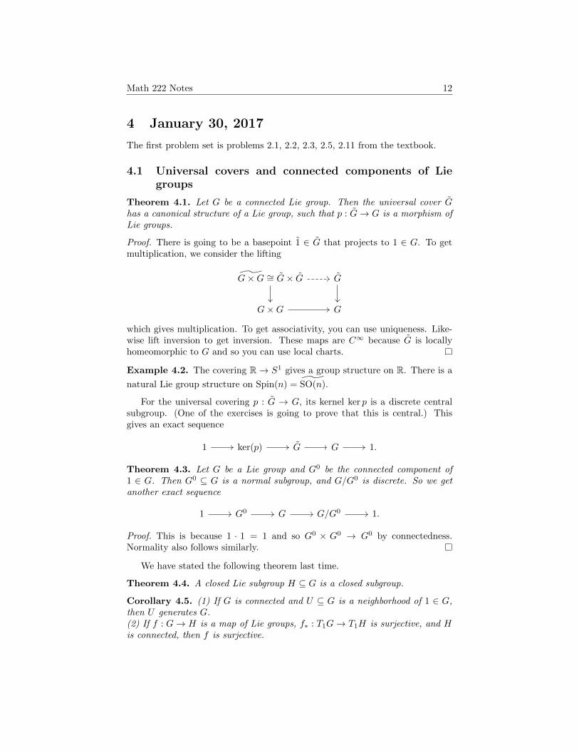
Theorem 4.1. Let G be a connected Lie group. Then the universal cover Ghas a canonical structure of a Lie group, such that p : G→ G is a morphism ofLie groups.

Proof. There is going to be a basepoint 1 ∈ G that projects to 1 ∈ G. To getmultiplication, we consider the lifting

G×G ∼= G× G G

G×G G

which gives multiplication. To get associativity, you can use uniqueness. Like-wise lift inversion to get inversion. These maps are C∞ because G is locallyhomeomorphic to G and so you can use local charts.

Example 4.2. The covering R→ S1 gives a group structure on R. There is a

natural Lie group structure on Spin(n) = SO(n).

For the universal covering p : G → G, its kernel ker p is a discrete centralsubgroup. (One of the exercises is going to prove that this is central.) Thisgives an exact sequence

1 ker(p) G G 1.

Theorem 4.3. Let G be a Lie group and G0 be the connected component of1 ∈ G. Then G0 ⊆ G is a normal subgroup, and G/G0 is discrete. So we getanother exact sequence

1 G0 G G/G0 1.

Proof. This is because 1 · 1 = 1 and so G0 × G0 → G0 by connectedness.Normality also follows similarly.

We have stated the following theorem last time.

Theorem 4.4. A closed Lie subgroup H ⊆ G is a closed subgroup.

Corollary 4.5. (1) If G is connected and U ⊆ G is a neighborhood of 1 ∈ G,then U generates G.(2) If f : G→ H is a map of Lie groups, f∗ : T1G→ T1H is surjective, and His connected, then f is surjective.

Math 222 Notes 13

Proof. (1) Let H ⊆ G be the subgroup generated by U . Then H ⊆ G is openbecause gU ⊆ H for all g ∈ H. Then it is automatically a closed Lie subgroup(i.e., embedded submanifold) and hence closed. Then H is closed and open andG is connected, so H = G.

(2) Because f∗ : T1G→ T1H is surjective, implicit function theorem tells usthat im(f) contains a neighborhood of 1 ∈ H. So by (1), im(f) = H.

4.2 Fiber bundle from a map of Lie groups

Theorem 4.6. If G is a Lie group and H ⊆ G is a closed Lie subgroup, thenG/H has a canonical structure of a smooth manifold, such that we get a fiberbundle

H G G/H.p

Moreover TH(G/H) = T1G/T1H. If H is a normal subgroup, then G/H isgoing to be a Lie group.

Proof. It suffices to choose a local section, because we can then construct a localtrivialization by multiplying H. Choose a submanifold M ⊆ G with transverseintersection to g ·H at g: TgG = Tg(gH)⊕TgM . Then we get a map M×H → Gwhich is a diffeomorphism in a neighborhood of {g} × H. Set U to be theneighborhood of g ∈ M such that U × H → G is a embedding. We can thenuse U = p(U) = p(UH) as charts. These are also local trivializations.

UH U ×H

U

p

You can check that the charts are compatible and thus the smooth structureon G/H is independent of the choice of g and M . It is also clear that ker(p∗ :TgG→ Tg(G/H)) = TgH.

Corollary 4.7. (1) If H ⊆ G is a connected subgroup then π0(G/H) = π0(G).(2) If H → G → G/H is a fiber bundle, and G and H are connected, then weget an exact sequence of group

π2(G/H) π1(H) π1(G) π1(G/H) 1.

Math 222 Notes 14

5 February 1, 2017

Lie groups appear as symmetries of spaces.

5.1 Group actions

Definition 5.1. An action of a Lie group G on a manifold M is a grouphomomorphism φ : G → Diff(M) such that the induced map G ×M → M issmooth.

Example 5.2. The group GL(n,R) acts on Rn. This is even a linear represen-tation. The group SO(n,R) acts on Sn−1 ⊆ Rn, and the complex version SU(n)acts on S2n−1.

Definition 5.3. A representation of a Lie group G on a vector space V (overR or C) is a group homomorphism ρ : G→ GL(V ). In the case of dimV <∞,we also require G× V → V be smooth.

Definition 5.4. A morphism between representations (V, ρV ) → (W,ρW ) isa linear map f : V →W such that

V V

W W

ρV (g)

f f

ρW (g)

commutes for all g ∈ G.

Definition 5.5. If G acts on M , then the orbit of m is the set G ·m = {gm :g ∈ G}. The stabilizer of m is defined as

Gm = StabG(m) = {g ∈ G : gm = m}.

Note that if m and m′ are in the same orbit, then Stab(m) and Stab(m′) areconjugates.

Theorem 5.6. (1) StabG(m) ⊆ G is a closed Lie subgroup.(2) We get an injective immersion G/StabG(m) ↪→M .

We will prove this later using the technology of Lie algebras.

Definition 5.7. A G-homogeneous space is a manifold M with a transitiveaction of G.

If we fix a point m ∈ M then we can identify M = G/StabG(m). This willbe a diffeomorphism. We can also say that G→M is a fiber bundle with fiberStabG(m).

Math 222 Notes 15

Example 5.8. We have SO(n,R) acting on Sn−1. So we have a fiber bundle

SO(n− 1,R)→ SO(n,R)→ Sn−1.

Likewise there is an action SU(n,R) on S2n−1 and so

SU(n− 1)→ SU(n)→ S2n−1.

Example 5.9. A flag in Rn is a sequence of subspaces

{0} = V0 ⊆ V1 ⊆ V2 ⊆ · · · ⊆ Vn = Rn

with dimVk = k. Let Fn(R) be the set of all flags in Rn. Then GL(n,R)acts transitively, and the stabilizer of the standard flag is B(n,R), the space ofinvertible upper triangular matrices.

The quotient space M/G can be very pathological, even non-Hausdorff. Forexample, let G = GL(n,C) act on Mat(n,C) by conjugation. Then M/G is theset of Jordan normal forms. There are some fields devoted to these pathologicalquotients like geometric invariance theory or non-commutative geometry.

Any Lie group G acts on itself in 3 canonical way:

Left action Lg : G→ G, h 7→ gh,

Right action Rg : G→ G, h 7→ hg−1,

Adjoint action Adg : G→ G, h 7→ ghg−1.

The adjoint action always fixed 1 ∈ G. So we get an induced action (Adg)∗ :T1G → T1G. This already gives a representation of G on T1G. But it doesn’tneed to be faithful. In fact, there are Lie groups that cannot be embedded into

GL(n,R). For example, ˜GL+(2,R) does not have a faithful finite-dimensionalrepresentation.

Math 222 Notes 16

6 February 3, 2017

6.1 Classical groups

We will look at some examples of groups.

• The general linear group GL(n,K), the group of invertible linear trans-formations, where K = C or R.

• The special linear group SL(n,K), the transformations that preservethe volume form.

• The orthogonal group O(n,K), the transformations preserving the usualbilinear inner product.

• The special orthogonal group SO(n,K) = O(n,K) ∩ SL(n,K), trans-formations preserving the volume and the inner product.

• More generally the groups O(p, q) and SO(p, q) that preserve the non-degenerate quadratic form of signature (p, q) (over R).

• The symplectic group Sp(n,K) = {A ∈ GL(2n,K) : ω(X,Y ) = ω(A(X), A(Y ))},transformations preserving the symplectic form, a non-degenerate skew-symmetric form.

• The unitary group U(n), transformations preserving the hermitian innerproduct (over C).

• The special unitary group SU(n) = U(n) ∩ SL(n,C), transformationspreserving the hermitian inner product and have determinant 1.

• The compact symplectic group Sp(n) = Sp(n,C) ∩U(2n,C).

One surprising coincidence is that SO+(1, 3) = PSL(2,C). This is useful inphysics.

G GL(n,C) SL(n,C) O(n,C) SO(n,C) Sp(n,C)g gl(n,C) tr = 0 X +Xt = 0 X +Xt = 0 JX +XtJ = 0

dimC n2 n2 − 1 n(n− 1)/2 n(n− 1)/2 n(2n+ 1)π0 1 1 Z/2 1 1π1 Z 1 Z/2 (n ≥ 3) Z/2 (n ≥ 3) 1

G U(n) SU(n) O(n,R) SO(n,R) Sp(n)

g X +X∗ = 0X +X∗ = 0

trX = 0X = X

Xt +X = 0X = X

Xt +X = 0X +X∗ = 0JX +XtJ = 0

G Sp(n,R) GL(n,R) SL(n,R)

Table 1: Complex groups and their maximal compact subgroups

Math 222 Notes 17

6.2 The exponential map

For a complex matrix A ∈ Mat(n,C), we define the exponential map exp :gl(n,K)→ GL(n,K) as

exp(A) = eA =

∞∑n=0

An

n!.

This converges absolutely and is defined holomorphically. The map has a partialinverse near the identity given by

log(1 +A) =

∞∑n=1

(−1)n+1An

n.

This converges only for A close to 0.

Theorem 6.1. (1) exp(logA) = A and log(expA) = A when they are defined.(2) exp(0) = 1 and exp∗(0) = idgl(n,K).(3) XY = Y X implies eXeY = eX+Y and log(XY ) = logX + log Y .(4) For X ∈ gl(n,K) the map K → GL(n,K) given by t 7→ etX is a homomor-phism of Lie groups.(5) eAXA

−1

= AeXA−1 and eAt

= (eA)t.

Proof. (1) You can check this at the level of power series. This follows from the1-variable case.

(2) Clear.(3) Again check this for the power series in 2 variables.(4) This follows from (3).(5) Plug in the definition of as the power series. Same for the transpose.

These maps give local charts for the classical groups we have defined above.

Theorem 6.2. If G ⊆ GL(n,K) is a classical group, then there is a subspace g ⊆gl(n,K), a neighborhood U of 0 ∈ gl(n,K), a neighborhood V of 1 ∈ GL(n,K)such that exp and log give diffeomorphisms on G ∩ V and g ∩ U .

Proof. We have to go through that list and identify what the Lie algebra is.For GL(n,K) we have g = gl(n,K) and the theorem follows from the inverse

function theorem.For SL(n,K), we have A = eX ∈ SL(n,K) near 1 and want to figure out

what X is. We have 1 = detA = det eX = exp(trX). So trX = 0. This showsthat g is the space of traceless matrices.

For O(n,K), we want AtA = 1 so eX+Xt = 1. This shows that g is theskew-symmetric matrices.

The group SO(n,K) is a connected component so it has the same g.The group U(n) has the algebra u(n) = {X+X∗ = 0} and su(n) has another

traceless condition.The group Sp(n,K) has algebra sp(n,K) = {JX + XtJ = 0} and for the

compact symplectic group you put the two conditions together.

Math 222 Notes 18

Corollary 6.3. Each classical group G is a Lie group with T1G = g. SodimG = dim g.

Proof. We get a chart on G near 1. Then using left multiplication by g weget a chart on G near g. The reason T1G = g is because exp(0) = 1 andexp∗(0) = id.

Math 222 Notes 19

7 February 6, 2017

The second problem set due next Monday is: 2.7, 2.13, 2.14, 2.15, 3.1.

7.1 The exponential map

We want to define exp : g → G for general Lie groups, not only for matrixgroups.

Proposition 7.1. Let G be a Lie group and x ∈ g = T1G. Then there is aunique map of Lie groups γx : K → G such that γx(0) = x. This is called theone-parameter subgroup corresponding to x.

Proof. We want γ(s + t) = γ(s)γ(t). That is, we want γ(t) = γ(t)γ(0) =γ(0)γ(t). Then γx solves the initial value problem γ = γx and γ(0) = 1.(In other words, γ is the trajectory of left-invariant vector fields.) By generaltheory of uniqueness and existence of solutions to ODEs, we see that γx isunique on some small t. Then extend the solution to the whole space via thehomomorphism property.

Definition 7.2. Define the exponential map exp : g→ G by exp(x) = γx(1).

From uniqueness, we have γx(t) = γtx(1) = exp(tx). For G = GL(n,K), expcoincides with the matrix exponential.

Theorem 7.3. (1) exp(0) = 1, exp∗(0) = idg.(2) exp is C∞ (analytic in the case of complex groups), is a diffeomorphismfrom a neighborhood of 0 ∈ g to a neighborhood of 1 ∈ G.(3) exp((s+ t)x) = exp(tx) exp(sx) for s, t ∈ R.(4) exp is natural: if φ : G→ H induces φ∗ : g→ h, then

g h

G H

exp

φ∗

exp

φ

commutes.(5) If g ∈ G and x ∈ g then g exp(x)g−1 = exp(Ad(g)x), a special case of (4).

Proof. (1) Clear from the definition.(2) C∞ follows from the smooth dependence of solutions to ODEs.(3) This also follows from the definition.(4) Uniqueness of the exp map shows that the two things are the same.

φ(exp(tx)) is a one-parameter subgroup with derivative at 0 being φ∗x.

The map exp : g → G has image contained in G0 ⊆ G. A natural questionis whether im exp = G0. In general it is not. (One of the homework gives youan explicit counterexample.) We have im(exp) = G0 if

Math 222 Notes 20

(1) G = GL(n,C),

(2) G is compact, (in this case, you can give a Riemannian metric and thetheory of exp in Riemannian manifolds show that exp is surjective.)

(3) G is nilpotent.

Proposition 7.4. If G,H are Lie groups with G connected, then φ : G→ H isuniquely determined by φ∗ : g→ h.

Proof. The image of exp contains a neighborhood of G and this neighborhoodgenerates G.

7.2 Defining the Lie bracket

Our next goal is to define [−,−] on g in general. For matrix groups, this isgoing to be the usual matrix commutator.

Definition 7.5. Define a map µ : g×g→ g locally near 0 given by exp(x) exp(y) =exp(µ(x, y)) for x, y in some small neighborhood of 0.

Lemma 7.6. The Taylor series for µ is given by

µ(x, y) = x+ y + λ(x, y) + terms of order ≥ 3,

with λ a bilinear skew-symmetric map.

Proof. Let us write

µ(x, y) = α1(x) + α2(y) +Q1(x) +Q2(y) + λ(x, y) + · · · ,

where α are linear and Q are quadratic. Computing µ(x, 0) yields α1(x) =x and Q1 = 0. Computing µ(0, y) yields α2(y) = y and Q2 = 0. Becauseexp(x) exp(x) = exp(2x), we have λ(x, x) = 0. This means that λ is skew-symmetric.

Definition 7.7. Define the Lie bracket as [x, y] = 2λ(x, y).

Math 222 Notes 21

8 February 8, 2017

There was a function µ(x, y) defined by

exp(x) exp(y) = exp(µ(x, y))

for x, y small, and found out that

µ(x, y) = x+ y +1

2[x, y] + higher order.

where [x, y] is bilinear and skew-symmetric.

Proposition 8.1. (1) If φ : G → H induces φ∗ : g → h, then φ∗[x, y] =[φ∗x, φ∗y].(2) In particular, Ad(g)[x, y] = [Ad(g)x,Ad(g)y].(3) exp(x) exp(y) exp(x)−1 exp(y)−1 = exp([x, y] + · · · ).

Because of (3), we can think the Lie bracket as the commutator.

Proof. (1) [−,−] is defined in terms of exp, and exp is natural.(3) This follows from direct computation.

Corollary 8.2. If G is commutative, then [x, y] = 0 for all x, y ∈ g.

8.1 The Jacobi identity

We have an adjoint action Ad : G → GL(g). So taking the derivative we getad : g→ gl(g).

Lemma 8.3. (1) ad(x)y = [x, y].(2) Ad(expx) = exp(adx).

Proof. (1) By definition, Ad(g)y = (d/dt)|t=0g exp(ty)g−1. So

ad(x)y =d

ds

d

dt

∣∣∣t=s=0

exp(sx) exp(ty) exp(−sx)

=d

dx

d

dt

∣∣∣t=s=0

exp(t) exp(st[x, y] + · · · ) = [x, y].

(2) is clear.

Theorem 8.4. If G is a Lie group and g = Lie(G), then the bracket [−,−]satisfies the Jacobi identity:

[x, [y, z]] = [[x, y], z] + [y, [x, z]],

i.e., g is a Lie algebra.

Proof. Note that ad : g→ gl(g) preserves [−,−]. So

ad[x, y] = [adx, ad y] = ad(x) ad(y)− ad(y) ad(x) ∈ gl(g).

Acting on z, we get [[x, y], z] = [x, [y, z]]− [y, [x, z]].

So we get a functor from the category of Lie groups to the category of Liealgebras.

Math 222 Notes 22

8.2 Sub-Lie algebras

Definition 8.5. A subspace h ⊆ g is a sub-Lie algebra if [h, h] ⊆ h. Asubspace h ⊆ g is an ideal if [h, g] ⊆ h.

If h ⊆ g is an ideal, then g/h is a Lie algebra with induced bracket.

Theorem 8.6. (1) Let H ⊆ G is a Lie subgroup. Then h ⊆ g is a Lie subalgebra.(2) If H ⊆ G is a closed normal Lie subgroup, then h ⊆ g is an ideal, withLie(G/H) = g/h. Conversely, if H ⊆ G is a closed Lie subgroup, and G and Hare connected, then h ⊆ g being an ideal implies H ⊆ G normal.

Proof. (1) This just follows from the naturality of the Lie bracket.(2) A subgroup H ⊆ G is a closed normal subgroup if and only if Ad(g)

preserves H for any g ∈ G. This is equivalent to Ad(g) preserving h for any g,because H is connected. This is equivalent to ad(x) preserving h for any x ∈ g.This just means h is and ideal.

8.3 Lie algebra of vector fields

This doesn’t really fit into what we have done, but it is interesting. For amanifold M , take

G = Diff(M) = {group of diffeomorphisms}.

Then we can think its Lie algebra as

g = {vector fields on M} = Γ(M,TM).

Then a 1-parameter subgroup corresponding to X ∈ g is the vector flow gener-ated by the field. This is the exponential map. If M is non-compact, the flowis only defined in a neighborhood of M × {0}.

We can also define the Lie bracket as

[X,Y ](f) = Y (X(f))−X(Y (f))

like we do in differential geometry. (There is this sign issue, but Kirillov con-vinces you why the sign should be changed.)

Math 222 Notes 23

9 February 10, 2017

For vector fields X,Y on M , we have the Lie bracket

[X,Y ]f = Y (X(f))−X(Y (f)).

In coordinates, this can be written as[∑i

fi∂

∂xi,∑i

gi∂

∂xi

]=∑i,j

(gi∂fj∂xi− fi

∂gj∂xi

) ∂

∂xj.

Equivalently, ΦtX ◦ ΦsY ◦ Φ−tX ◦ Φ−sY = Φst[X,Y ] + higher order terms.

Theorem 9.1. For an action ρ : G→ Diff(M) of an Lie group on a manifold,there is a map ρ∗ : g→ Vect(M) of Lie algebras.

Proof. This map can be defined using the diagram:

g Vect(M)

G Diff(M)

exp

ρ∗

exp

ρ

This is compatible with the Lie bracket because ρ preserves the commutator ingroups, and the Lie bracket is determined using the commutator.

Example 9.2. GL(n,R) acts on Rn. So any A ∈ gl(n,R) gives a vector fieldρ∗(A) given by A : Rn → TpRn = Rn.

Example 9.3. Let G act on G by left multiplication. Then we get a mapρ∗ : g → Vect(G) given by sending a vector to the associated right-invariantvector field. So we get an isomorphism

g −→ {right-invariant vector fields}

of Lie algebras.

9.1 Stabilizer of a Lie group action

Theorem 9.4. Let a Lie group G act on M , and let m ∈M be a point.(1) StabG(m) ⊆ G is a closed Lie subgroup.(2) The map G/StabG(m) ↪→M is an immersion.

Proof. (1) Define

h = {x ∈ g : ρx(x)(m) = 0} = ker(g→ Vect(M)→ TmM).

The formula for [−,−] shows that h is a Lie algebra.

Math 222 Notes 24

To show that StabG(m) is a closed Lie subgroup it suffices to find a neigh-borhood U ⊆ G of 1 such that StabG(m) ∩ U is a smooth manifold. This isbecause you can use multiplication to move charts around.

Take a vector space u such that h⊕ u = g. By definition, ρ∗ : u → TmM isnow an isomorphism of vector spaces. Then the map

u→M ; x 7→ (ρ exp(x))(m)

is injective locally at the origin by the implicit function theorem, becauseρ exp(x) ∈ StabG(m) is equivalent to x ∈ h locally.

Any g ∈ G near 1 can be written uniquely as g = exp(y) exp(x) for x ∈ hand y ∈ u by the decomposition g = h ⊕ u. Then gm = exp(y)m and sog ∈ StabG(m) if and only if y = 0 locally. This shows that exp : h→ StabG(m)is a bijection near 0 ∈ h.

(2) We already know T1(G/StabG(m)) = u and this injects into TmM . Sowe get an immersion.

Corollary 9.5. If f : G→ H is a map of Lie groups,(1) ker(f) ⊆ G is a closed Lie subgroup.(2) im(f) ⊆ H is an immersed subgroup.

Proof. We let G act on H by g(h) = f(g)h.

Example 9.6. Let V be a finite dimensional vector space and B : V ×V → K bea nondegenerate bilinear form. We have an action GL(V ) on Hom(V ⊗ V,K).Then the stabilizer of B, O(V,B), is a closed subgroup of GL(V ). The Liealgebra is

o(V,B) = {A ∈ gl(V ) : B(Av,w) +B(v,Aw) = 0}.

Math 222 Notes 25

10 February 13, 2017

Example 10.1. Let A be a finite dimensional (possibly nonassociative) algebraover K. So there is a multiplication µ ∈ Hom(A ⊗ A,A). The group GL(A)acts on A, so it acts on the space Hom(A ⊗ A,A). So M/GL(A) classifies thealgebra structures on A up to isomorphism. The stabilizer of µ will be

StabGL(A)(µ) = {φ ∈ GL(A) : φ(ab) = φ(a)φ(b)} = Aut(A).

Its Lie algebra is

{D ∈ gl(A) : D(ab) = D(a)b+ aD(b)} = Der(A).

We can do this for A = g a Lie algebra.

Definition 10.2. The center of a Lie algebra g is defined as

Z(g) = {x ∈ g : [x, y] = 0 for all y ∈ g}.

Theorem 10.3. If a Lie group G is connected, then Z(G) ⊆ G is a closedsubgroup and Z(g) = Lie(Z(G)).

The proof is similar.

10.1 Baker–Campbell–Hausdorff formula

We know that eX+Y = eXeY for matrices X,Y if [X,Y ] = 0.

Theorem 10.4. Let G be a Lie group and X,Y ∈ g with [X,Y ] = 0. Thenexp(X) exp(Y ) = exp(X + Y ).

Theorem 10.5 (Baker–Campbell–Hausdorff formula). Let G be a Lie groupwith g = Lie(G). For sufficiently small x, y ∈ g,

log(exp(x) exp(y)) = x+ y +1

2[x, y] +

1

12([x, [x, y]] + [y, [y, x]]) + · · ·

=

∞∑n=1

µn(x, y),

where µn is a Lie polynomial over Q, homogeneous of degree n in x, y.

The useful part of this theorem is that there exists a formula. Then the Liebracket locally determines multiplication near the identity. Or in special cases,all except for finite terms disappear and so it becomes a useful formula.

We are not going to prove this. There are several proofs. The first one usesan analytic approach. You first prove

log(exey) = x+

∫ 1

0

ψ(ead(x)et ad(y))dt, where ψ(z) =z log z

z − 1.

Math 222 Notes 26

Alternatively, you can look at the completion of the free nonassociative algebraK〈〈x, y〉〉 with the coproduct map ∆ : A → A⊗ A given by ∆(ab) = ∆(a)∆(b)and ∆(x) = 1⊗ x+ x⊗ 1. You can define the formal exp and log,

{ax+ by + · · · } {1 + zx+ by + · · · },exp

log

which is actually a bijection. The free Lie algebra generated by x and y turnsout to be the set of primitive elements, {∆(a) = 1⊗a+a⊗1}, and the image ofthis set under exp is the set of group-like elements, {∆(a) = a⊗ a}. So for x, yprimitive, exp(x) and exp(y) are group-like. Then exp(x) exp(y) is group-like,so log(exp(x) exp(y)) is primitive.

Corollary 10.6. Suppose G is connected. Then the product on G is uniquelydetermined by Lie(G).

10.2 Recovering the Lie group from its algebra

So far, we have:

(1) We have a functor {Lie groups/K} → {Lie algebras/K}. If G is connected,then Hom(G,H)→ Hom(g, h) is injective.

(2) We can recover multiplication on a connected G from g.

Theorem 10.7. (1) If G is a Lie group, then there is a one-to-one correspon-dence {

connectedsubgroups H ⊆ G

}←→

{subalgebras

h ⊆ g

}.

(2) If G is simply connected, then

Hom(G,H)→ Hom(g, h), φ 7→ φ∗

is a bijection.(3) If g is a finite-dimensional Lie algebra over K, then there is a correspondingLie group G with Lie(G) = g.

Math 222 Notes 27


The third problem set is 3.5, 3.6, 3.7, 3.9, 3.13 due Wednesday, February 22.

Theorem 11.1. (1) If G is any Lie group over K, there is a correspondence{H ⊆ G

connected

}←→

{h ⊆ g

subalgebras

}.

(2) If G,H are Lie groups, and G is simply connected, then

Hom(G,H)→ Hom(g, h); φ 7→ φ∗

is a bijection.(3) If g is a finite dimensional Lie algebra, then there is a Lie group G withLie(G) = g.

Proof. (3) By Ado’s theorem, which we haven’t proved, we have g ⊆ gl(n,K)for some n. Then (1) shows that g corresponds to some G ⊆ GL(n,K) withLie(G) = g.

(2) Injectivity is clear, because we can use the fact that exp and φ commute,and G is generated by a neighborhood of 1.

Now suppose G1, G2 be Lie groups and f : g1 → g2 be a morphism of Liealgebras. We want to construct a map φ : G1 → G2. Take the Lie groupG = G1 ×G2 and let

h = (graph of f) = {(x, f(x)) : x ∈ g1} ⊆ g1 × g2 = g.

Then (1) tells us that there is a corresponding connected subgroup H ⊆ G1×G2.The composite of H ↪→ G1 ×G2 → G1 induces an isomorphism of Lie algebras,and so it must be a covering map. But G1 is simply connected, and thus this isan isomorphism. Now let us look at

G1 → H ↪→ G1 ×G2 → G2.

This gives the map, inducing φ∗ = f .(1) In the case dim h = 1, we can produce H = exp(h) ⊆ G easily. But if

dim h > 1, then exp(h) is not a subgroup in general. Consider the subbundle E ⊆TG with Eg = hg ⊆ TgG. (A subbundle of TM is also called a distribution.)Then because h ⊆ g is a subalgebra, for any vector fields X,Y ∈ Vect(G) withX(p), Y (p) ∈ Ep for all p, we have [X,Y ](p) ∈ Ep. You can check this byLeibniz’s rule. (This condition is called integrability.) Frobenius’ theoremthen says that there is a maximal connected submanifold H ⊆ G such thatTpH = Ep for all p ∈ H.

By maximality, we see that for any x ∈ h, the curve etx is always in H. Thenexp(h) ⊆ H. Since 1 ∈ H−1, maximality tells us that H−1 = H. Then for anyh ∈ H, 1 ∈ Hh so we get Hh = H. Hence H is a subgroup.

Corollary 11.2. If g is a finite dimensional Lie algebra over K, then there isa unique simply connected Lie group G with Lie(G) = g. If G′ is any connectedLie group with Lie(G′) = g, then G′ = G/Z for some discrete central subgroupZ ⊆ G.

Math 222 Notes 28

11.1 Real and complex forms

If g is a Lie algebra over R, then there is a complexification gC = g ⊗R C withthe bracket extended in the obvious way.

Example 11.3. If you complexify sl(2,R), you get sl(2,C). If you complexifysu(2), you also get sl(2,C), because su(2) is the traceless anti-hermitian matri-ces. But we see that sl(2,R) and su(2) are not isomorphic as Lie algebras. Youcan see that by looking at the corresponding Lie groups. Alternatively, you canlook at the Killing form (x, y) 7→ tr(xy), which has different signature for thetwo algebras.

Definition 11.4. We see that g is a real form of gC. If G is a Lie group overC, a (connected) real subgroup H ⊆ G is called a real form of G if h ⊆ g is areal form.

Example 11.5. SL(2,R)→ SL(2,C) is a real form. But SL(2,R) has a Z-to-1

universal cover ˜SL(2,R). But SL(2,C) is already simply connected. So ˜SL(2,R)is not a real form of anything.

In general, you can define the complexification GC using the universal prop-erty

G GC

H,

f

where H is a Lie group over C. Note that G→ GC may not be injective.

Math 222 Notes 29


12.1 Representations

Definition 12.1. A representation is a morphism ρ : G → GL(V ) or Liegroups. A representation of a Lie algebra is a morphism ρ : g→ gl(V ) of Liealgebras.

We are mostly going to work with V finite dimensional over C. This isbecause the case V over R is generally more complicated.

Theorem 12.2. (1) A representation ρ : G→ GL(V ) induces a representationρ∗ : g → gl(V ). This is a functor Rep(G) → Rep(g) because G-equivariant Liegroup morphisms induce G-equivariant Lie algebra morphisms.(2) If G is simply connected, the functor Rep(G)→ Rep(g) is an equivalence ofcategories.

If G is only connected, we have G = G/Z where Z is a discrete centralsubgroup. Then a representation of G gives a representation of G by

G

G GL(V ).

πρG

ρG

Then representations of G are representations of G that is trivial on Z.

Theorem 12.3. If g is a Lie algebra over R, then there is a equivalence ofcategories Rep(g) ∼= Rep(gC).

This is just the universal property of complexification. So for instance

Rep(SU(2)) ∼= Rep(su(2)) ∼= Rep(sl(2,C)) ∼= Rep(SL(2,C)).

Example 12.4. There is the trivial representation ρ : G → GL(C) given byg 7→ 1, and for the Lie algebra, ρ : g→ gl(C) given by x 7→ 0. This is sometimesdenoted by just C.

Example 12.5. There is the adjoint representation given by ρ : G → GL(g)with g 7→ Ad(g) and the corresponding g→ gl(g) given by x 7→ ad(x) = [x,−].

Definition 12.6. A subrepresentation of a representation ρ : G → GL(V )is a subspace W such that ρ(G)W ⊆W . Likewise for the Lie algebra.

Likewise one can define quotient representations. If G is connected, subrep-resentations of G on V correspond to subrepresentations of g on V .

You can define V ⊕W , V ⊗W , V ∗, Hom(V,W ) = V ∗⊗W of representationsV and W . When taking the dual, you have to be careful and define

(g · v)(w) = v(g−1w), (x · v)(w) = −v(x · w)

Math 222 Notes 30

for g ∈ G, x ∈ g, v ∈ V ∗, and w ∈ V . So the representation for Hom(V,W ) willbe

gA = ρW (g)A(ρV (g))−1.

Now for a representation, we define the invariant vectors as

V G = {v ∈ V : gv = v for all g ∈ G} ⊆ V,V g = {v ∈ V : xv = 0 for all x ∈ g} ⊆ V.

Then we see that

Hom(V,W )G = HomG(V,W ), V G = HomG(C, V ).

12.2 Irreducibility

Definition 12.7. A representation V is irreducible or simple if V 6= 0 and0, V are the only subrepresentations of V .

Example 12.8. We have SL(n,C) acting on Cn, and this is irreducible becausethe action is almost transitive. If dimV = 1, then it is automatically irreducible.

These are the elementary building blocks in some sense. If V which is notirreducible, there is a non-trivial representation W ⊆ V and so we get a exactsequence

0→W → V → V/W → 0

in the category of representations. So every representation is an extension ofirreducible ones.

Definition 12.9. A representation V is completely reducible or semisim-ple if V =

⊕i niVi with ni ≥ 1 multiplicities and Vi pairwise non-isomorphic

irreducible representations.

Example 12.10. Take G = R so that g = R. A representation on V isdetermined by ρ(1) = A, where A ∈ gl(V ) is an arbitrary linear map. Then therepresentation of G will be given by t 7→ etA ∈ GL(V ).

If v ∈ V is an eigenvector of V , then Cv ⊆ V is a subrepresentation. Soonly the 1-dimensional representations are irreducible. This means that therepresentation is completely reducible if and only if A is diagonalizable. So notevery representation of R is semisimple. This is because R is not compact.

Lemma 12.11. If V is a representation of G and A ∈ EndG(V ), then everyeigenspace Vλ ⊆ V of A is a subrepresentation. If A is diagonalizable, thenV =

⊕λ∈C Vλ as a representation of G.

Proof. If v ∈ Vλ, then A(g · v) = g ·Av = g · λv = λ(g · v) = g · v ∈ Vλ.

Math 222 Notes 31


The fourth problem set is 3.16, 3.17, 3.18, 4.2, 4.6 due February 27.

Lemma 13.1. Let V be a representation and A ∈ EndG(V ). Any eigenspaceVλ of A is a subrepresentation and if A is diagonalizable then V =

⊕λ Vλ.

Corollary 13.2. If Z ⊆ G is a central subgroup and ρ(Z) is diagonal, thenV =

⊕λ Vλ where Vλ are the eigenspaces of ρ(Z).

Example 13.3. Consider the action of GL(n,C) on Cn ⊗ Cn. Then the mapv⊗w 7→ w⊗ v is map of G-representations. The eigenspaces are V1 = Sym2 Cnand V−1 =

∧2Cn. In this case, it turns out that they are both irreducible

representations.

13.1 Schur’s lemma

Lemma 13.4 (Schur’s lemma). Let V and W be irreducible representations ofG. Then

HomG(V,W ) ∼=

{C if V ∼= W

0 if V 6∼= W.

Proof. If f ∈ HomG(V,W ), then ker(f) ⊆ V and im(f) ⊆ W are subrepresen-tations. Since V and W are irreducible, either f = 0 or f is an isomorphism.

Now assume that V and W are indeed isomorphic. For any f ∈ EndG(V ), fhas an eigenvalue λ ∈ C. This means that f−λ idV ∈ EndG(V ). Then f−λ idVis not invertible, and hence has to be 0. So f = λ idV .

Example 13.5. The action of GL(n,C) on Cn is irreducible. So by Schur,Z(GL(n,C)) = C∗ and Z(gl(n,C)) = C. This is because g ∈ Z(GL(n,C))implies that ρ(g) : Cn → Cn is in EndG(Cn). You can do the same for SL(n,C),U(n), and SU(n).

Corollary 13.6. If V =⊕

i niVi and W =⊕

imiVi then

HomG(V,W ) =⊕i

Hom(Cni ,Cmi).

Theorem 13.7. If G is abelian, then any irreducible representation is 1-dimensional.

Proof. If ρ : G → V then ρ(g) ∈ EndG(V ) for any g. By Schur’s lemma, weget ρ(g) ∈ λ(g) · 1V for some λ(g) ∈ C. Then every subspace W ⊆ V is asubrepresentation. So dimV = 1.

Example 13.8. The group S1 = U(1) has irreducible representations z 7→ zk

for some k ∈ Z.

Math 222 Notes 32

13.2 Unitary representations

Definition 13.9. A representation ρ : G→ GL(V ) is unitary if there is a innerproduct on V such that ρ : G→ U(V ). Likewise a representation ρ : g→ gl(V )is unitary if there is a inner product such that ρ : g→ u(V ).

Example 13.10. For G = R, the map t 7→ etA for A : V → V is unitary if andonly if A is diagonalizable with eigenvalues in iR.

Theorem 13.11. Unitary representations are completely reducible (semisim-ple).

Proof. Let V be a unitary representation and we have an invariant inner prod-uct. We want to prove that if W ⊆ V is a subrepresentation then

0→W → V → V/W → 0

splits. Take W⊥ ⊆ V , which is a subrepresentation. Then W⊥ ∼= V/W . Nowby induction we can decompose V into irreducible representations.

Theorem 13.12. Any representation of a finite group is unitary.

Proof. We start with any hermitian inner productB(v, w). Produce an invariantinner product by averaging:

〈v, w〉 =1

|G|∑g∈G

B(gv, gw).

Corollary 13.13. Any representation of of a finite group is completely re-ducible.

This extends to compact groups. Take any compact Lie group G over R. Avolume element dV (of positive density) on G if left (resp. right) invariant∫

G

f(hg)dV (g) =

∫G

f(g)dV (g), resp.

∫G

f(gh)dV (g) =

∫G

f(g)dV (g).

Example 13.14. On R>0 the invariant measure is dx/x. On GL(n,R) themeasure |detX|−1dX is invariant.

Math 222 Notes 33


We’re getting into the theory of compact Lie groups. First we are going to showthat any representation of a compact Lie group over R is completely reducible.There is then the question of computing the irreducible representations. We arealso going to talk about harmonic analysis on G, which is the analogue of doingFourier analysis. This is decomposing L2(G), which is naturally a representationof G into irreducible representations.

14.1 Integration on compact Lie groups

We started talking about integration with a volume element dV on G. This canbe left-invariant or right-invariant. As in the case of left-invariant vector fields,we have one-to-one correspondences{

left-invariantdensities

}←→ |

∧dimGg∗| ←→

{right-invariant

densities

}.

Fix a right-invariant volume form dV . Then g · dV is still right-invariant.By uniqueness of the volume-element, we have

g · dV = φ(g)dV

for some φ(g) ∈ R>0. So this gives a map of Lie groups φ : G→ R>0.

Definition 14.1. The Lie group G is called unimodular if φ ≡ 1. Thisis equivalent to saying that the left-invariant densities are the right-invariantdensities.

Any compact group is going to be unimodular, because the image of φ mustbe a compact subgroup of R>0.

Example 14.2. The group GL(n,R) is unimodular, because the volume el-ement dV = |detX|−ndX is a both right-invariant and left-invariant volumeelement.

Example 14.3. The group of affine transformations x 7→ ax + b of R is notunimodular.

Theorem 14.4. Any representation of a compact group is unitary and thereforecompletely reducible.

Proof. Take any inner product B(v, w) on V . For a representation ρ : G →GL(V ), we define

〈v, w〉 =

∫G

B(gv, gw)dV.

This is again an inner product.

Math 222 Notes 34

14.2 Characters

Definition 14.5. Given a representation ρ : G → GL(V ), we define its char-acter as the function

χV : G→ C; g 7→ tr ρ(g).

Theorem 14.6. (1) If V = C is the trivial representation, then χV = 1.(2) χV⊕W = χV + χW .(3) χV⊗W = χV χW .(4) χV (ghg−1) = χV (h).(5) If V is unitary, χV ∗ = χV .

So if V =⊕

i niVi then χV =∑i niχVi .

Theorem 14.7. If G is compact, and V and W are irreducible representations,then

〈χV , χW 〉 =

{1 if V ∼= W,

0 if V 6∼= W.

Here the inner product is defined as

〈f1, f2〉 =

∫G

f1f2dV.

We are going to prove a stronger statement later.

Corollary 14.8. (1) V is irreducible if and only if 〈χV , χV 〉 = 1.(2) If V =

⊕i niVi then ni = 〈χVi , χV 〉.

Given a representation ρ : G → GL(V ) with V having a basis, its entriesconsidered as matrices are functions ρi,j : G→ C.

Theorem 14.9. (1) If V 6∼= W are irreducible representations, then

〈ρVi,j , ρWk,l〉 = 0.

(2) If V is an irreducible representation and the basis on V is orthonormal, then

〈ρVi,j , ρVk,l〉 =1

dimVδikδjl.

Lemma 14.10. (1) If V 6∼= W are irreducible and T : V → W is any linearmap, then ∫

G

gTg−1dg = 0.

(2) If V is irreducible and T : V → V , then∫G

gTg−1dg =tr(T )

dimVidV .

Proof. (1) The integrating can be thought of as a projection Hom(V,W ) →HomG(V,W ). But we have HomG(V,W ) = 0 by Schur’s lemma.

(2) This is because the projection preserves trace.

Math 222 Notes 35


There is another problem set 5 due next week: 4.4, 4.7, 4.11, 4.13. Today Iwant to at least state the Peter–Weyl theorem and prove one part.

15.1 Peter–Weyl theorem

Theorem 15.1. (1) If V ∼= W are non-isomorphic unitary irreducibles withbasis, then 〈ρVij , ρWkl 〉 = 0.(2) For a unitary irreducible V with basis,

〈ρVij , ρVkl〉 =1

dimVδikδjl.

Proof. Let Ejk be the matrix V → W with 1 in the jth row kth column and 0everywhere else. Using the projection lemma, we get

0 =

∫G

ρW (g)EjkρV (g)−1dg =

∑i,l

Eil

∫G

ρWij ρVlkdg.

So 〈ρWij , ρVlk〉 = 0, for any i, j, k, l.The second part is analogous. We have

δjldimV

=tr(Ejl)

dimV=

∫G

ρV (g)EjlρV (g)dg =

∑i,k

Eik

∫G

ρVijρVkldg.

Compare the entries.

There is a basis-invariant formulation. Let V be an inner product space.Then we can put an inner product on End(V ) given by

〈A,B〉 =1

dimVtr(AB∗).

For a unitary representation ρ : G→ GL(V ) we can define a map

End(V )→ C∞(G,C); A 7→ tr(ρ(g)A)

that preserves the inner product.Define, in the case when G is compact,

G = set of isomorphism classes of irreducible representaions.

Then we can put what we did together to get an isometric embedding⊕V ∈G

End(V )→ C∞(G).

Math 222 Notes 36

Theorem 15.2 (Peter–Weyl theorem). This map induces an isomorphism ofHilbert spaces ⊕

V ∈G

End(V )→ L2(G,C).

In other words, we have L2(G,C) ∼=⊕

V ∈G(dimV )V .

Corollary 15.3. We have⊕

V ∈GC1V ∼= L2(G,C)G, with χV being the basis of

L2(G,C)G.

15.2 Representation theory of sl(2,C)Theorem 15.4. Any representation of sl(2,C) is completely reducible.

Proof. Because SU(2,C) is simply connected,

Rep(sl(2,C)) ∼= Rep(su(2,C)) ∼= Rep(SU(2)).

Since SU(2) is compact, all representations are unitary. So everything is com-pletely reducible.

Let us explicitly write down the basis for sl(2,C):

e =

(0 10 0

), f =

(0 01 0

), h =

(1 00 −1

).

Then there are the Lie bracket relations

[e, f ] = h, [h, e] = 2e, [h, f ] = −2f.

Consider the eigenspaces of h:

Vλ = {v ∈ V : hv = λv}.

Lemma 15.5. eVλ ⊆ Vλ+2, fVλ ⊆ Vλ−2.

Proof. This is a direct computation:

h(ev) = [h, e]v + ehv = 2ev + eλv = (2 + λ)ev.

The same computation works for f .

Theorem 15.6. ρ(h) is diagonalizable, and so V =⊕

λ∈C Vλ.

Proof. We can assume that V is irreducible. We have V ′ =⊕

λ Vλ ⊆ V , andthis is a subrepresentation by the previous lemma. But ρ(h) has eigenvaluesand so V ′ 6= 0. Then V ′ = V .

Theorem 15.7. Any irreducible representation is of the following form: thereis a basis v0, . . . , vn and

hvi = (n− 2i)vi, evi = (n+ 1− i)vi−1, fvi = (i+ 1)vi+1.

Math 222 Notes 37

16 March 1, 2017

We were classifying representations of sl(2,C). The interesting thing was thatthere is an eigenvalue decomposition V =

⊕λ∈C Vλ.

For the irreducible representation V , take the nonzero 0 6= v ∈ Vλ such that<(λ) is maximal. We then define

vk =fk

k!v ∈ Vλ−2k.

These are linearly independent as long as they are nonzero. This shows thatvn+1 = 0 but vn 6= 0.

Lemma 16.1. fvk = (k + 1)vk+1, hvk = (λ− 2k)vk, ev0 = 0, evk = (λ− k +1)vk−1.

Proof. We have ev0 = 0 since ev0 ∈ V λ+2 and <(λ) is maximal. You can checkevk = (λ− k + 1)vk−1 for k > 0 by induction.

Corollary 16.2. The vectors v = v0, . . . , vn is a basis of V .

Proof. V is irreducible.

We further have evn+1 = 0 = (λ − n)vn and so λ = n. An alternative wayof seeing this is tr ρ(h) = tr[ρ(e), ρ(f)] = 0. So we completely understand thestructure of the representation of sl(2,C).

Theorem 16.3. Irreducible representations of sl(2,C) are classified by the high-est weight λ = 0, 1, 2, . . ..

Theorem 16.4. Let V be a representation of sl(2,C).(1) There is a weight decomposition V =

⊕n∈Z Vn by eigenspaces of ρ(h).

(2) en : V−n → Vn and fn : Vn → V−n are isomorphisms.

16.1 Spherical Laplacian

The spherical Laplacian is given by

∆R3 =1

r2∆S2 + ∆radial =

1

r2∆s2 + ∂2

r +2

r∂r,

and more explicitly,

∆S2 = J2x + J2

y + J2z , Jx = y∂z − z∂y, . . . .

Now there are two actions by ∆S2 and SO(3,R) on C∞(S2).

Lemma 16.5. ∆S2 commutes with the action of SO(3,R).

Proof. We know that both ∆R3 and ∆radial are rotation invariant.

Math 222 Notes 38

Algebraically, this can be interpreted as ∆S2 ∈ Uso(3,R) being a centralelement. This is called a “Casimir” element.

Consider

Pn =

{functions S2 → C which can be written as

polynomials in x, y, z of degree ≤ n

}.

Now it is clear that ∇S2 maps Pn to Pn. Because⋃Pn ⊆ C∞(S2) is dense, it

suffices to diagonalize ∆S2 on Pn. Here, we note that the complexification ofso(3,R) is sl(2,C) with the identification being

− i2

(e+ f)↔ Jx,1

2(f − e)↔ Jy, − ih

2↔ Jz.

We are now going to decompose Pn =⊕

i niVi into irreducible representa-tions. Let us write

u = x+ iy = ρeiϕ, v = x− iy = ρe−iϕ.

Then uv = x2 + y2 = 1− z2 = ρ2. We see that zp, zpuk, zpvk for p+ k ≤ n spanPn, because any polynomial in x, y, z can be written as a polynomial in u, v, z.Let us write

fp,k = zp√

1− z2|k|eiϕk.

These form a basis, by the uniqueness of the Fourier series.Now we note that Jz = ∂/∂ϕ and so Jzfp,k = ikfp,k. This means that the

vectors of weight 2k in Pn have basis

f0,k, f1,k, . . . , fn−|k|,k.

Math 222 Notes 39

17 March 3, 2017

We are going to be looking at finite dimensional Lie algebras over C now.One major class is the semisimple ones, meaning [g, g] = g, and nonabeliansimple ones are contained here. The other class is the solvable ones, exten-sion of abelians, and an important subclass is nilpotent algebras, satisfying[x1, [. . . , [xn−1, xn]]] = 0 for large enough n. A special case is abelian, [g, g] = 0.You can classify semisimple Lie algebras, but solvable Lie algebras are hard toclassify.

17.1 Solvable and nilpotent Lie algebras

Definition 17.1. A h ⊆ g is called a subalgebra if [h, h] ⊆ h and is called anideal if [h, g] ⊆ h.

If I, J ⊆ g are ideals, then I ∩J and [I, J ] and I +J are ideals. There is theideal of commutators, [g, g] ⊆ g. Also, if h ⊆ g is an ideal, then g/h is an Liealgebra. Then g/[g, g] is the largest abelian quotient.

Example 17.2. We have [gl(n), gl(n)] = [sl(n), sl(n)] = sl(n). One direction isobvious. For the other direction, you can use elementary matrices.

You can take the commutator ideal repeatedly:

D0g = g, D1g = [g, g], D2g = [[g, g], [g, g]], . . . , Dn+1g = [Dng, Dng].

This is called the derived series. ThenDn+1g ⊆ Dng are ideals andDng/Dn+1gare abelian. So g being solvable just means Dng = 0 for some n.

Proposition 17.3. A Lie algebra g is solvable if and only if there is a filtrationof subalgebras

0 = a0 ⊆ a1 ⊆ · · · ⊆ an = g

such that ai+1 ⊆ ai is an ideal and ai/ai+1 is abelian.

Proof. We have an−1 ⊇ [g, g] and by induction, an−k ⊇ Dkg. So having such afiltration implies solvable. The other direction is obvious.

There is also another filtration

D0g = g, D1g = [g, g], D2g = [g, [g, g]], . . . , Dng = [g, Dn−1g],

called the lower central series. We say that g is nilpotent if Dng = 0 forsome n. This just means that (n+ 1)-fold products in g vanish.

Example 17.4. Let b ⊆ gl(n,C) be the Lie algebra of upper triangular matricesand n ⊆ b be the algebra of strictly upper triangular matrices. Then b is solvablebut not nilpotent and n is nilpotent.

Math 222 Notes 40

Here is why. Geometrically we can look at b and n in terms of

0 = V0 ⊆ V1 ⊆ · · · ⊆ Vn = V

with dimVi = i as b = a0 and n = a1, where

ak = {x ∈ gl(n) : xVi ⊆ Vi−k}.

Because [ak, al] ⊆ ak+l, we see that n = a1 is nilpotent. We also have D1b =[a0, a0] ⊆ a1 since the diagonal cancel out and so b = a0 is solvable. You cancheck that the lower central series for b stabilizes at n again using elementarymatrices.

Theorem 17.5. (1) If g is solvable (resp. nilpotent), then its complexificationgC is again solvable (resp. nilpotent).(2) If g is solvable (resp. nilpotent), then so is any subalgebra or quotient.(3) If g is nilpotent, then g is solvable.(4) If 0 → h → g → g/h → 0 is an extension and h and g/h are solvable, theng is solvable.

Proof. Clear.

Theorem 17.6 (Lie). If g is solvable and ρ : g→ gl(V ) then there is a basis ofV such that all ρ(x) are upper triangular.

Proposition 17.7. If g is solvable and ρ : g → gl(V ) then there is a v ∈ Vwhich is a common eigenvector of all ρ(x).

We will discuss the proof next time.

Math 222 Notes 41

18 March 6, 2017

The sixth problem set is 4.5, 4.14, 5.3, 5.4 due March 20. We started talkingabout the general structure theory of Lie algebras.

18.1 Representations of solvable algebras

Theorem 18.1 (Lie). If g is solvable and ρ : g → gl(V ) is a representation,then there is a basis of V such that all ρ(x) are upper triangular. (This worksfor any algebraic closed field with characteristic zero.)

Proposition 18.2. If g is solvable and ρ : g→ gl(V ) is a representation, thenthere is a v ∈ V , v 6= 0 which is a common eigenvector of all ρ(x).

Proof. We induct on dim g. The case dim g = 0 is trivial. Assume dim g > 0.Then [g, g] ( g must be a proper ideal. Choose a 1-codimensional subspace[g, g] ⊆ g1 ⊆ g, which is automatically going to be an ideal.

Now write g = g1⊕Cx as a vector space. Induction tells us that there existsa v ∈ V such that hv = λ(h)v for all h ∈ g1. Consider the space

W = span{v, xv, x2v, . . .} ⊆ V.

Then g1 acts on W as

hxkv = λ(h)xkv +∑ρ<k

aklxkv,

because the commutators are in g1.Choose the smallest n such that xn+1 ∈ span{v, . . . , xnv}. Then v, . . . , xnv

form a basis of W . We know that

trW (ρ(h)) = (n+ 1)λ(h).

Then

0 = trW [ρ(x), ρ(h)] = trW ρ([x, h]) = (n+ 1)λ([x, h]).

That is, λ([x, h]) = 0.This in particular shows that hxkv = λ(h)xkv. That is, any vector in W is

a common eigenvector of all ρ(h) for h ∈ g1. Since ρ(x) acts on W , it has aneigenvector in W that is the common eigenvector of g.

Proof of Theorem 18.1. We induct on dimV . Pick a common eigenvector v,and pick a basis of V/Cv and lift it to V and add constant multiples of v.

Corollary 18.3. (1) If g is solvable and ρ : g → gl(V ) is irreducible, thendimV = 1.(2) If g is solvable, then is a series

0 ⊆ I0 ⊆ I1 ⊆ · · · ⊆ In = g

of ideals in g such that dim(Ik/Ik−1) = 1.(3) If g is solvable then [g, g] is nilpotent.

Math 222 Notes 42

Proof. (1) is clear. For (2) just apply the theorem to the adjoint representation.For (3), the reverse direction is clear. The forward direction follows from theadjoint representation. There is a basis such that every matrix is upper triangu-lar, and then ad([g, g]) are strictly upper triangular. Then for sufficiently largen,

ad([x1, . . . , [xn−1, xn]]) = 0

for every x1, . . . , xn ∈ [g, g]. By definition of the adjoint operator,

[y, [x1, . . . , [xn−1, xn]]] = 0

for every y, x1, . . . , xn ∈ [g, g].

Theorem 18.4. Let g ⊆ gl(V ) be a subalgebra consisting of nilpotent operators.Then there is a basis of V in which all g are strictly upper triangular.

Proof. The idea is the same. It is in the textbook.

Theorem 18.5 (Engel). A Lie algebra g is nilpotent if and only if ad(x) ∈End(g) is nilpotent for all x ∈ g.

Proof. The forward direction is clear. For the other direction, by the theoremthere exists a series of ideals

0 ⊂ g1 ⊂ · · · ⊂ gn = g

such that [x, gi] ⊆ gi−1. This just implies that the lower central series convergesto zero.

Definition 18.6. A Lie algebra g is simple if it is not abelian and has nonontrivial ideals. A Lie algebra g is semisimple if it contains no solvable ideals(except 0 ⊆ g).

Lemma 18.7. If g is simple then it is semisimple.

Proof. If suffices to show that if g is simple, then it is not solvable. This isbecause if it is solvable then [g, g] ( g and so [g, g] = 0.

Example 18.8. Consider the Lie algebra g = sl(2,C). Then the adjoint repre-sentation is irreducible, and so sl(2,C) is simple.

Math 222 Notes 43

19 March 8, 2017

19.1 Radical of a Lie algebra

Proposition 19.1. The set

rad(g) =⋃I⊆g

solvable

I

is a solvable ideal.

Proof. If I and J are solvable, then we have an exact sequence

0→ I → I + J → J/(I ∩ J)→ 0.

Then I + J is solvable.

Theorem 19.2. (1) g/ rad(g) is semisimple.(2) If b ⊆ g is solvable and g/b is semisimple, then b = rad(g).

Proof. For any I ⊆ g/ rad(g) solvable, we have an exact sequence

0→ rad(g)→ I = ρ−1(I)→ I → 0.

Then I is solvable and so I = rad(g). Hence I = 0.

So every Lie algebra can be uniquely split into a solvable one and a semisim-ple one.

Theorem 19.3 (Levi). The exact sequence

0→ rad(g)→ g→ g/ rad(g)→ 0

always splits. In other words, there is a subalgebra gss so that g = rad(g)⊕ gssand gss ∼= g/ rad(g).

Here is an exact sequence that does not split:0 0 ∗0 0 00 0 0

↪→

0 ∗ ∗0 0 ∗0 0 0

� C2.

So this is really a deep statement.

Definition 19.4. A Lie algebra is reductive if rad(g) = Z(g) (or equivalently,if g/Z(g) is semisimple).

Theorem 19.5. Let V be an irreducible representation of g. Then any x ∈rad(g) acts by scalar, i.e., xv = λ(x)v for some λ : rad(g) → C. In particular,x ∈ [rad(g), g] acts trivially.

Proof. Since rad(g) is solvable, there is some 0 6= v ∈ V that is a commoneigenvector of all x ∈ rad(g) with xv = λ(x)v. Define

Vλ = {x ∈ V : xw = λ(x)w for all x ∈ rad(g)}.

Then you can check that gVλ ⊆ Vλ, and because v ∈ Vλ, we get V = Vλ.

Math 222 Notes 44

19.2 Classical groups are reductive

Definition 19.6. A bilinear form B on g is called invariant if

B([x, y], z) +B(y, [x, z]) = 0

for all x, y, z ∈ g.

Lemma 19.7. If B is an invariant form on g, and I ⊆ g is an ideal, then

I⊥ = {x ∈ g : B(x, I) = 0}

is an ideal. (B can be degenerate.) In particular, g⊥ = ker(B) ⊆ g is an ideal.

Example 19.8. On g = gl(n,K), the bilinear form B(x, y) = tr(xy) is asymmetric invariant bilinear forms. On the space of symmetric matrices, Bis positive-definite, and on the space of anti-symmetric matrices, B is negative-definite.

More generally, if ρ : g→ gl(V ) is any representation, then

BV (x, y) = tr(ρ(x)ρ(y))

is a symmetric invariant bilinear form.

Theorem 19.9. If there exists a representation ρ : g→ gl(V ) such that BV isnon-degenerate, then g is reductive.

Proof. We need to show that [g, rad(g)] = 0. There exists an irreducible subrep-resentation W ⊆ V . For any x ∈ [g, rad(g)], we have xW = 0. Then x ∈ kerBW ,and we have BV = BW + BV/W . Inductively we obtain x ∈ kerBV . BecauseBV is non-degenerate, x = 0.

Theorem 19.10. All classical Lie algebras are reductive, and the semisimpleones are

sl(n,K) (n ≥ 2), so(n,K) (n ≥ 3), su(n) (n ≥ 2), sp(n) (n ≥ 1).

Proof. We find a representation with BV nondegenerate. In all this cases, let Vbe the defining representation Kn (or K2n). Then BV = tr(x, y), and you cancheck that this is nondegenerate.

Math 222 Notes 45

20 March 10, 2017

20.1 Cartan’s criterion

To every Lie algebra is associated a Killing form given by

K(x, y) = tr(ad(x) ad(y)).

Example 20.1. Consider g = sl(2,C) with basis e, h, f . Then

ad(e) =

0 −2 00 0 10 0 0

, ad(h) =

2 0 00 0 00 0 −2

, ad(f) =

0 0 0−1 0 00 2 0

.

Then the Killing form can be computed as

K(e, f) = K(f, e) = 4, K(h, h) = 8, K(h, e) = K(h, f) = 0.

So you can check that K(x, y) = 4 tr(xy). Generally, in sl(n,K), the Killing formis K(x, y) = 2n tr(xy). In gl(n,K), the Killing form is K(x, y) = 2n tr(xy) −2 tr(x) tr(y).

Theorem 20.2 (Cartan’s criterion).(1) g is solvable if and only if K([g, g], g) = 0.(2) g is semisimple if and only if K is non-degenerate.

Theorem 20.3. Suppose V/C is a finite dimensional vector space and A : V →V be a linear map.(1) A can be uniquely written as A = As + An, where [As, An] = 0 and As issemisimple and An is nilpotent.(2) For ad(A) ∈ End(End(V )), we have (adA)s = ad(As) and adAs = P (adA)for some P ∈ tC[t].(3) For As the semisimple operator with the same eigenspaces as As and complexconjugate eigenvalues, ad(As) = Q(adA) for Q ∈ tC[t].

Proof. This is just Jordan normal form.

Theorem 20.4. If g ∈ gl(V ) is a Lie subalgebra such that x ∈ g and y ∈ [g, g]implies tr(xy) = 0, then g is solvable.

Proof. Consider any x ∈ [g, g] and look at its Jordan decomposition x = xs+xn.We want to show that xs = 0. We have

tr(xxs) =∑

λiλi =∑|λi|2,

where λi are the eigenvalues. But x ∈ [g, g] and so x =∑i[yi, zi]. Then

tr(xxs) = tr(∑

[yi, zi]xs

)= −

∑tr(yi[xs, zi]).

But [xs, zi] = ad(xs)zi) = Q(ad(x))zi ∈ [g, g]. Then the right hand side is zeroand so tr(xxs) = 0. This shows that all λi are zero and so x is nilpotent for allx ∈ [g, g]. Then g is solvable.

Math 222 Notes 46

Proof of Theorem 20.2. (1) Suppose that g is solvable. Because g is solvable,using Lie’s theorem we can find a basis of g such that all ad(x) is upper triangularfor all x ∈ g. Then for any x ∈ g and y ∈ [g, g], ad(x) is upper triangular andad(y) is strictly upper triangular. This implies that tr(ad(x) ad(y)) = 0.

For the other direction, ad(g) is a subalgebra of gl(g) and so by the lemma,ad(g) is solvable. Since there is an exact sequence

0→ Z(g)→ g→ ad(g)→ 0,

the Lie algebra g is also solvable.(2) Suppose that g is semisimple. Consider the ideal I = ker(K) ⊆ g. The

Killing form on I is 0 and so (1) shows that I is solvable. The g being semisimpleimplies that K is non-degenerate.

Suppose that K is non-degenerate. Then g is reductive by what we havedone last time. Since Z(g) ⊆ ker(K) = 0, the radical is rad(g) = 0. That is, gis semisimple.

Corollary 20.5. For any Lie algebra, g/R is semisimple if and only if gC issemisimple.

Theorem 20.6. For semisimple g and an ideal I ⊆ g, there is an ideal I ′ ⊆ gsuch that g = I ⊕ I ′.

Proof. Look at the orthogonal complement with respect to the Killing form.

Corollary 20.7. Any semisimple g is a direct sum of simple Lie algebras:g =

⊕i gi.

Corollary 20.8. If g is semisimple then g = [g, g].

Proposition 20.9. If g =⊕

i gi is semisimple, any ideal I ⊆ g takes the formof I =

⊕i∈J gj for some J ⊆ {1, . . . , n}.

Proof. Assume I ⊆⊕n

i=1 gi is some ideal. Look at the projection pn : g→ gn.Because gn is simple, either pn(I) = 0 or pn(I) = gn. In the case pn(I) = 0, wehave I ⊆ g1 ⊕ · · · ⊕ gn−1 and can use the induction hypothesis. If pn(I) = gn,then [gn, I] = [gn, pn(I)] = gn. Because I is an ideal, gn ⊆ I. Then I = I ′ ⊕ gnfor some ideal I ′ ⊆ g1 ⊕ · · · ⊕ gn−1.

Corollary 20.10. If g is semisimple, and I ⊆ g is an ideal, then I and g/I aresemisimple.

Math 222 Notes 47

21 March 20, 2017

The automorphism group Aut(g) has a natural Lie group structure, and its Liealgebra is

Lie(Aut(g)) = Der(g) = {(D : g→ g) : D([x, y]) = [Dx, y] + [x,Dy]}.

Proposition 21.1. If G is a connected Lie group, and g = Lie(G) is semisimple,then Der(g) = g and Aut(g)/Ad(G) is discrete.

Proof. We note that there is a map ad : g → Der(g), and ker ad = Z(g) = 0because g is semisimple.

We can extend the Killing form to Der(g) by simply setting K(δ1, δ2) =tr(δ1δ2). We can check that [δ, ad(x)] = ad(δ(x)) for any δ ∈ Der(g) and x ∈ g.Now K is nondegenerate and so there is a splitting Der(g) = g ⊕ g⊥ as Lie why?why?algebras.

For any δ ∈ g⊥ and x ∈ g,

ad(δ(x)) = [δ, ad(x)] = 0.

This means that δ(x) = 0 and so δ = 0. Hence g⊥ = 0 and g = Der(g).

Theorem 21.2. (1) Let G be a compact Lie group over R. Then g = Lie(G)is reductive and its Killing form is negative semidefinite.(2) Let g be semisimple over R and suppose that the Killing form is negativedefinite. Then g = Lie(G) for some compact connected G.

Proof. (1) Because G is compact, any representation ρ : G → U(V ) is unitaryfor some suitable metric on V . On u(n), the form tr(xy) = − tr(xy∗) is negativedefinite. Applying this to the adjoint representation ad : g → u(g) shows thatK is negative semidefinite. Also kerK = Z(g).

(2) Let G be a connected Lie group with Lie(G) = g. The bilinear formB(x, y) = −K(x, y) is positive definite, symmetric, and Ad(G)-invariant. Thisshows that Ad : G → SO(g). Note that Ad(G) ⊆ Aut(g) is a connected com-ponent, and Aut(g) ⊆ GL(g) is a closed Lie subgroup. Thus Ad(G) ⊆ SO(g) isa closed Lie subgroup, and hence compact. Also Lie(Ad(G)) = Lie(G/Z(G)) =g/Z(g) = g.

Note that if g is semisimple over R and K is negative definite, then anyconnected G with Lie(G) = g is compact. The same argument does not workover C.

21.1 Compact real form

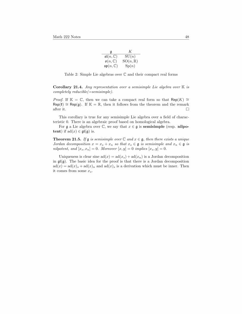
Theorem 21.3. Leg g be semisimple over C. Then there is a compact Lie groupK over R with kC ∼= g.

This k is called the compact real form of g, and it is unique up to con-jugation. If g = Lie(G), then we can choose K ⊆ G. Here are some examples:

Math 222 Notes 48

g Ksl(n,C) SU(n)o(n,C) SO(n,R)sp(n,C) Sp(n)

Table 2: Simple Lie algebras over C and their compact real forms

Corollary 21.4. Any representation over a semisimple Lie algebra over K iscompletely reducible(=semisimple).

Proof. If K = C, then we can take a compact real form so that Rep(K) ∼=Rep(k) ∼= Rep(g). If K = R, then it follows from the theorem and the remarkafter it.

This corollary is true for any semisimple Lie algebra over a field of charac-teristic 0. There is an algebraic proof based on homological algebra.

For g a Lie algebra over C, we say that x ∈ g is semisimple (resp. nilpo-tent) if ad(x) ∈ gl(g) is.

Theorem 21.5. If g is semisimple over C and x ∈ g, then there exists a uniqueJordan decomposition x = xs + xn so that xs ∈ g is semisimple and xn ∈ g isnilpotent, and [xs, xn] = 0. Moreover [x, y] = 0 implies [xs, y] = 0.

Uniqueness is clear sine ad(x) = ad(xs) + ad(xn) is a Jordan decompositionin gl(g). The basic idea for the proof is that there is a Jordan decompositionad(x) = ad(x)s + ad(x)n and ad(x)s is a derivation which must be inner. Thenit comes from some xs.

Math 222 Notes 49

22 March 22, 2017

When we studied representations of sl(2,C), we looked at eigenspaces of theelement h = ( 1 0

0 −1 ). This is called a Cartan subalgebra, and we will see that italways exists for a semisimple Lie algebra. In terms of groups, this correspondsto a maximal torus.

22.1 Jordan decomposition in semisimple algebras

The main tool is the Jordan decomposition for semisimple algebras.

Theorem 22.1. Let g be semisimple over C. For each x ∈ g, there exists aunique Jordan decomposition into x = xs + xn, where ad(xs) is semisimple andad(xn) is nilpotent, and [xs, xn] = 0.

Proof. Let us first decompose ad(x) = (adx)s + (adx)n in gl(g). Consider thedecomposition

g =⊕λ∈C

gλ

into generalized eigenspaces of adx. This is a graded structure, i.e., [gλ, gµ] ⊆gλ+µ, because

(ad(x)− (λ+ µ))n[y, z] =

n∑k=0

(n

k

)[(adx− λ)ky, (adx− µ)n−kz]

by induction. The consequence is that (adx)s is a derivation, because if y ∈ gλand z ∈ gµ then

(adx)s[y, z] = (λ+ µ)[y, z] = [(adx)sy, z] + [y, (adx)sz].

Since g is semisimple, there exists a xs ∈ g such that adxs = (adx)s. Also(adx)y = 0 implies (adxs)y = (adx)sy = 0.

Definition 22.2. h ⊆ g is a toral subalgebra if h is commutative and consistsof semisimple elements.

Theorem 22.3. If g is semisimple over C, h ⊆ g is toral, and (−,−) is anon-degenerate symmetric invariant bilinear form on g, then(1) g =

⊕α∈h∗ gα, where gα = {x ∈ g : [h, x] = α(h)x},

(2) [gα, gβ ] ⊆ gα+β,(3) if α 6= −β, then (gα, gβ) = 0,(4) (−,−) restricts to a nondegenerate pairing gα ⊗ g−α → C.

Proof. (1) Note that ad(h) is diagonalizable for every h ∈ h and also for anyh1, h2 ∈ h, we have [ad(h1), ad(h2)] = 0. So they can be simultaneously diago-nalized.

(2) If x ∈ gα and y ∈ gβ , we have

ad(h)[x, y] = [ad(h)x, y] + [x, ad(h)y] = (α+ β)(h)[x, y].

Math 222 Notes 50

(3) By invariance, for x ∈ gα and y ∈ gβ ,

0 = ([h, x], y) + (x, [h, y]) = (α+ β)(h)(x, y)

for all h. So (x, y) = 0 unless α+ β = 0.(4) This follows from (3) since the pairing is non-degenerate.

Lemma 22.4. Let g, h and (−,−) be as above. Then(1) (−,−) is non-degenerate on g0,(2) x ∈ g0 implies xs, xn ∈ g0,(3) g0 is reductive.

Proof. (1) is clear. For (2), if x ∈ g0 then [x, h] = 0. Then [xs, h] = 0 an soxs ∈ g0. For (3), note g is a representation of g0. Because K is non-degenerateon g, by (1) it is also non-degenerate on g0. Then by Theorem 19.9 g0 isreductive.

22.2 Cartan subalgebra

Definition 22.5. Let g be semisimple over C. We say that h ⊆ g is a Cartansubalgebra if it is toral with

C(h) = {x ∈ g : [x, h] = 0} = h.

Example 22.6. In sl(n,C), the subalgebra

h = {traceless diagonal matrices}

is a Cartan subalgebra.

Theorem 22.7. If h ⊆ g is a maximal toral algebra, then it is Cartan.

Proof. We have a decomposition g =⊕

α∈h∗ gα. We claim that g0 is a toralsubalgebra. Since h ⊆ g0, maximality will imply h = g0 and then h = C(h) = g0.

Consider any x ∈ g0. If (adx)|g0is not nilpotent, then 0 6= adxs|g0

and soxs /∈ h. On the other hand, [h, xs] = 0 so h⊕ Cxs is a bigger toral subalgebra.This shows that (adx)|g0 is nilpotent for every x ∈ g0. By Engel’s theorem, g0

is nilpotent, and it is also reductive. Therefore g0 is abelian.Now we want to show that any x ∈ g0 is semisimple. Using the Jordan de-

composition, we may show that xn = 0. For any y ∈ g0, we see that ad(xn) ad(y)is nilpotent because g0 is commutative. So tr(ad(xn) ad(y)) = 0, and becausethe Killing form restricted to g0 is non-degenerate, we get xn = 0. Thereforex = xs is semisimple.

Math 222 Notes 51

23 March 24, 2017

Last time we defined Cartan subalgebras. If g is semisimple over C, a subalgabrah ⊆ g is a Cartan subalgebra if h = C(h) and every x ∈ h is semisimple.

23.1 Root decomposition

This is what we proved last time.

Theorem 23.1. Let g be semisimple over C and h a Cartan subalgebra. Let(−,−) be a nondegenerate symmetric invariant bilinear form on g.

(1) There is a root decomposition

g = h⊕⊕α∈R

gα,

where gα = {x ∈ g : [h, x] = α(h)x} is the root space and R = {α ∈ h∗ :α 6= 0} is the set of roots.

(2) [gα, gβ ] ⊆ gα+β.

(3) (gα, gβ) if α+ β 6= 0.

(4) (−,−) restricts to a nondegenerate pairing gα ⊗ g−α → C.

Theorem 23.2. Let g = g1 ⊕ · · · ⊕ gn with each gi simple.

(1) If hi ⊆ gi are Cartan subalgebras, then⊕

hi = h ⊆ g is a Cartan subalge-bra with root system R = qRi.

(2) Conversely, if h ⊆ g is a Cartan subalgebra then there exist Cartan subal-gebras hi ⊆ gi such that h =

⊕hi.

Proof. (1) is clear.(2) Define hi = pi(h) ⊆ gi, where pi : g → gi is the projection. For x ∈ gi,

we have [h, x] = [pi(h), x] and so hi ⊆ gi is a Cartan subalgebra. Then h ⊆⊕

hiwhere

⊕hi is a toral algebra. By maximality of h, we get h =

⊕hi.

Example 23.3. Consider g = sl(n,C) with the Cartan subalgebra h = {X :X diagaonal, trX = 0}. We can compute

[h,Ei,j ] = (hi − hj)Ei,j

for any h ∈ h. Consider the maps ei : h→ C;h 7→ hi. The formula tells us thatthe root decomposition is

R = {ei − ej : i 6= j}, gei−ej = CEi,j .

Using this decomposition, we can compute the Killing from as

K(h, h′) = tr(ad(h) ad(h′)) =∑i6=j

(hi − hj)(h′i − h′j) = 2n∑

hih′i = 2n tr(hh′)

at least on h ⊆ g.

Math 222 Notes 52

Generally, let (−,−) be a invariant, symmetric, nondegenerate bilinear formon g. For a root α ∈ R, we can find an element Hα ∈ h such that

(α, β) = α(Hβ) = (Hα, Hβ).

Lemma 23.4. For e ∈ gα and f ∈ g−α,

[e, f ] = (e, f)Hα.

Proof. For any h ∈ h,

([e, f ], h) = (e, [f, h]) = −(e, [h, f ]) = α(h)(e, f) = (Hα, h)(e, f).

Then [e, f ] = (e, f)Hα by non-degeneracy of (−,−) on h.

Lemma 23.5. Let g be semisimple over C with h a Cartan subalgebra.

(1) If α ∈ R then (α, α) = (Hα, Hα) 6= 0.

(2) Suppose e ∈ gα and f ∈ g−α satisfy (e, f) = 2/(α, α). Define hα =2Hα/(α, α). Then α(hα) = 2 and e, f, hα span a subalgebra isomorphic tosl(2,C).

(3) The element hα is independent of (−,−).

Proof. (1) Suppose (α, α) = 0. Then α(Hα) = 0. There exist e ∈ gα, f ∈ g−αsuch that (e, f) 6= 0. Define

h = [e, f ] = (e, f)Hα,

and let a be the subalgebra generated by e, f, h. Then [h, e] = α(h)e = 0 and[h, f ] = α(h)f = 0. Hence a is solvable with [a, a] containing h. This shows thatad(h) is nilpotent, and by definition of a toral algebra, ad(h) is also semisimple.Then ad(h) = 0 and so h = 0 and so Hα = 0 and so α = 0.

(2) and (3) are exercises.

Lemma 23.6. Let α be a root and sl(2,C)α be the subalgebra spanned by e ∈ gα,f ∈ g−α, hα. Then

V = Chα ⊕⊕

06=k∈Zgkα

is an irreducible representation.

Math 222 Notes 53

24 March 27, 2017

Tomorrow I will post the midterm, consisting of eight problems.Last time we had for each α ∈ R, a copy sl(2,C)α ⊆ g spanned by e ∈ gα,

f ∈ g−α and hα ∈ h.

Lemma 24.1. Let g be a semisimple algebra over C. Then

V = Chα ⊕⊕

06=k∈Zgkα

is an irreducible representation of sl(2,C)α.

Proof. We have [e, gkα] ⊆ g(k+1)α and [e, g−α] ⊆ Chα. Similar statements holdfor f ∈ g−α.

We have (α, hα) = 2 and so there is a weight decomposition, with V [2k] =g2k, V [2k + 1] = 0 and dimV [0] = 1. This shows that V is irreducible.

24.1 Symmetries of the roots

Theorem 24.2. Suppose g is semisimple over C, and h ⊆ g is a Cartan sub-algebra. Let g = h ⊕

⊕α∈R gα be the root decomposition and let (−,−) be a

symmetric invariant form on g.

(1) R spans h∗ over C and {hα : α ∈ R} spans h.

(2) For any α ∈ R, dim gα = 1.

(3) For α, β ∈ R,

β(hα) =2(α, β)

(α, α)∈ Z.

(4) For any α, β ∈ R the reflection

sα(β) = β − β(hα)α.

is in R. In particular, sα(α) = −α ∈ R.

(5) For α ∈ R, its scalar multiple λα for λ ∈ C is in R if and only if λ = ±1.

(6) If α and β 6= ±α are roots, then

V =⊕k∈Z

gβ+kα

is an irreducible representation of sl(2,C)α.

(7) If α, β, α+ β ∈ R, then [gα, gβ ] = gα+β.

Proof. (1) Suppose there exists a h ∈ h such that α(h) = 0 for all α ∈ R. Thismeans that ad(h) = 0 by the root decomposition. This means that h ∈ Z(g) = 0and hence h = 0.

Math 222 Notes 54

(2) This follows from the previous lemma. If V is reducible, all eigenspaceshave dimension at most 1.

(3) Consider g as a representation of sl(2,Cα. The weight of gβ is β(hα) ∈ Z.(4) Assume n = β(hα) ≥ 0 is the weight. If v ∈ gβ has n then fnαv 6= 0 ∈

gβ−nα. Then 0 6= gβ−nα = gsα(β). That is, sα(β) ∈ R.

(5) Suppose α, λα ∈ R. By (3), 2c ∈ Z and so c ∈ 12Z. Also we have

1/c ∈ 12Z. This shows that c ∈ {±1/2,±1,±2}. Then we only need to exclude

the case c = 2.Consider the irreducible representation

V = Chα ⊕⊕

06=k∈Zgkα ⊆ g.

Note that V [2] = gα = Ceα and ad(eα) : V [2] → V [4] is 0. This shows thatV [4] = V [6] = · · · = 0. In particular g2α = 0 and so 2α /∈ R.

(6) Because dim gβ+kα = 1 for β + kα ∈ R, it is irreducible.(7) This follows from the representation theory of sl(2,C). The map ad(eα) :

gβ → gα+β has to be nonzero.

Theorem 24.3. Let g be semisimple over C and h ⊆ g be a Cartan subalgebra.

(1) Let hR ⊆ h be the vector space over R generated by hα for α ∈ R. Thenh∗ = hR ⊕ ihR, and K is real-valued and positive definite on hR.

(2) Let h∗R ⊆ h∗ be generated over R by R. Then h∗ = h∗R ⊕ ih∗R.

Proof. We know that

K(hα, hβ) = tr(ad(hα) ad(hβ)) =∑γ∈R

γ(hα)γ(hβ) ∈ Z.

So the restriction of K to hR is real-valued and also positive definite. Then ihRis negative definite. So they have trivial intersection but h is generated by hRand ihR. Thus h = hR ⊕ ihR.

If k ⊆ g is a compact real form, then k∩h = ihR. For example, if g = sl(n,C)and k = su(n), then they are both imaginary diagonal traceless matrices.

Let g = sl(n,C) and let x ∈ sl(2,C) have distinct eigenvalues λ1, . . . , λn ∈ C.Then the eigenvalues of ad(x) are λi − λj , and [x, y] = 0 implies that y is alsodiagonal with respect to the eigenbasis of x. Then the centralizer h ⊆ g is aCartan subalgebra. This is true for general semisimple Lie algebras over C.

Math 222 Notes 55

25 March 29, 2017

Definition 25.1. Define the nullity of x ∈ g as

n(x) = dim(ker(ad(x)n)), n� 0.

Define the rank of g asrank(g) = min

x∈gn(x).

Definition 25.2. The regular elements are

greg = {x ∈ g : n(x) = rank(g)} ⊆ g.

This set is open and dense. If we are over C, it further follows that it isconnected, because the complement will have complex codimension at least 1.

Proposition 25.3. Let g be semisimple over C.

(1) For x ∈ greg, ad(x) is semisimple and C(x) = {y ∈ g : [x, y] = 0} is aCartan subalgebra.

(2) For h ⊆ g a Cartan subalgebra and

x ∈ h ∩ greg = {x ∈ h : α(x) 6= 0 for all α ∈ R}

then C(x) = h.

(3) Any two Cartan subalgebras h1, h2 ⊆ g are conjugate under an action ofG by the adjoint action.

25.1 Abstract root system

Definition 25.4. An abstract root system is a pair (E,R) with E andEuclidean vector space and R ⊆ E \ {0} such that

(R1) R spans E,

(R2) for α, β ∈ R,

nαβ =2(α, β)

(β, β)∈ Z,

(R3) if α is a root, then

sα(β) = β − 2(α, β)

(α, α)α

sends R to R. In particular, sα(α) = −α ∈ R.

Definition 25.5. A root system is reduced if α, cα ∈ R implies c = ±1.

Example 25.6. Consider the (n− 1)-dimensional root system

E = {(λ1, . . . , λn) ∈ Rn :∑λi = 0}, R = {ei − ej : i 6= j}.

One can check that this satisfies all the axioms. This also follows from the factthat it is the root system of SL(n,C). This root system is called type An−1.

Math 222 Notes 56

An isomorphism of root system is given by a linear isomorphism φ : E1 →E2 such that

• φ(R1) = R2,

• nφ(α)φ(β) = nαβ for all α, β ∈ R.

Any α ∈ R gives an automorphism sα ∈ Aut(E,R). So this generates somegroup.

Definition 25.7. The Weyl group is the subgroup W ⊆ O(E) is the subgroupgenerated by sα for α ∈ R.

In the case of An−1, that the Weyl group is Sn.

Lemma 25.8. The Weyl group W is a finite group.

Proof. W injects in to the permutation group SR.

There can be automorphisms that are not in W . For instance, in A2 thereis the automorphism α 7→ −α that is not in W .

25.2 Classification of rank 2 reduced root systems

Theorem 25.9. Let α, β ∈ R be linearly independent with |α| ≥ |β|. Thenthere are the following possibilities:

∠(α, β) = φ |α|/|β| nαβ nβαπ/2 ? 0 0π/3 1 1 12π/3 1 −1 −1

π/4√

2 2 1

3π/4√

2 −2 −1

π/6√

3 3 1

5π/6√

3 −3 −1

Table 3: Possible configurations of two roots

Proof. We have (α, β) = |α||β| cosφ and so nαβ = 2|α|/|β| cosφ. Then nαβnβα =4 cos2 φ is an integer. So nαβnβα ∈ (0, 1, 2, 3). Now do a case-by-case analy-sis.

For rank 1, there is the unique reduced root system A1.For rank 2, there the root systems A1 q A1 = D2 coming from so(4,C) or

sl(2,C) × sl(2,C), A2 coming from so(3,C), B2 = C2 coming from so(5,C) orsp(2,C), and G2.

Math 222 Notes 57

26 March 31, 2017

Last time I drew the four root systems and claimed that they are all the rank2 reduced root systems.

Theorem 26.1. Any rank 2 reduced root system is isomorphic to A1qA1, A2,B2, or G2.

D2 A2

B2 = C2 G2

Figure 1: Root systems of rank 2

Proof. Pick α, β ∈ R such that φ = ∠(α, β) < π is maximal and |α| ≥ |β|. Thenφ ≥ π/2 since otherwise ∠(−α, β) > α(α, β). There are cases φ = π/2, 2π/3,3π/4, 5π/6.

In the case φ = 2π/3 we have |α| = |β| and reflect them around to get all ofA2. There cannot be more roots because of maximality of φ and reducedness.

In the case φ = 3π/4 we have |α| =√

2|β|. Doing the same thing gives B2,and likewise for φ = 5π/6 which gives G2 and φ = π/2 which gives D2.

Lemma 26.2. If R is a reduced root system, then (α, β) < 0 implies α+β ∈ R.

Proof. It suffices to check in the rank 2 case, because the intersection of a rootsystem with a subspace is root system. Just look at all the possible cases.

26.1 Positive and simple roots

Choose a v ∈ E such that (v, α) 6= 0 for all α ∈ R. We define

R± = {α ∈ R : ±(α, v) > 0}

so that R = R+∪R−. The roots R+ and R− are called positive and negativeroots, and this is called the polarization of R.

Math 222 Notes 58

Definition 26.3. A root α ∈ R+ is simple if it is not a sum of positive roots.

Lemma 26.4. Every α ∈ R+ is a sum of simple roots.

Proof. Break the roots into smaller positive roots if it is not simple. This processis going to end because the inner product is decreasing and there is only a finitenumber of roots.

Lemma 26.5. If α 6= β are simple roots, then (α, β) ≤ 0.

Proof. If (α, β) > 0 then (−α, β) < 0 and so β − α ∈ R. Either β − α ∈ R+ orα− β ∈ R+. In any case, this contradicts that both α and β are simple.

Theorem 26.6. Simple roots form a basis of E.

Proof. We only need to further show linear independence, which follows from(α, β) ≤ 0.

Corollary 26.7. Every α ∈ R can be written uniquely as

α =

rank∑i=1

niαi

with ni ∈ Z. Also α ∈ R± if and only if ±ni ≥ 0 for all i.

We define the height to be

h+(α) =∑

ni.

Example 26.8. Take An−1. We have R = {ei − ej : i 6= j} and chooseR+ = {ei − ej : i < j}. Then the simple roots are αi = ei − ei+1. The height isht(ei − ej) = j − i.

26.2 Lattices from root system

We define the root lattice as

Q = abelian group generated by R

= abelian group generated by simple roots

=⊕i

Zei ∼= Zrank.

Also there are the coroots given by

α ∈ R α∨ ∈ E∗ : α∨(β) =2(α, β)

(α, α).

Math 222 Notes 59

Similarly we can define the coroot lattice as

Q∨ = abelian group generated by coroots =⊕Zα∨i

The coroot lattice, is not the dual lattice of the root lattice. In fact, we definethe weight lattice as

P = dual to Q∨ = {λ ∈ E : α∨(λ) ∈ Z for all α∨ ∈ Q∨}.

There are the fundamental weights wi ∈ P such that

α∨j (wi) = δij ,

where αj are simple roots. Then P =⊕

i Zwi. Since β∨(α) = nαβ ∈ Z forα, β ∈ R, we have Q ⊆ P . Then P/Q is a finite abelian group.

Example 26.9. Let us look at the case of A1. We have Q = Zα and P =Z(α/2).

Math 222 Notes 60

27 April 3, 2017

Given an abstract root system (E,R) a reduced root system, we can break thesymmetry and define positive and negative roots R = R+ q R−. Then we candefine simple roots S = {α1, . . . , αr} that form a basis.

27.1 Weyl chamber

Recall that we can polarize with respect to a vector

v ∈ E \⋃α∈R

Lα, where Lα = {λ ∈ E : (λ, α) = 0}.

A Weyl chamber is a connected component of E \⋃α Lα.

Example 27.1. The root system A2 has 6 Weyl chambers, each of the form ofa cone with angle π/3.

Lemma 27.2. Let C be a Weyl chamber.

(1) Its closure C is an unbounded convex cone.

(2) ∂C is a union of codimension 1 faces, which are called the walls of C.

Lemma 27.3. There is a one-to-one correspondence between polarizations andWeyl chambers.

Theorem 27.4. The Weyl group W acts transitively on the set of Weyl cham-bers.

Proof. Two Weyl chambers C and C ′ are adjacent if C and C′

intersect in acodimension 1 face. Let them intersect in Lα. Then it can be checked thatC ′ = sα(C).

In a general situation, given any two chambers C and C ′, we can alwaysfind a sequence C = C0, C1, . . . , Cn = C ′ so that Ci and Ci+1 are adjacent bychoosing a generic enough path.

Each Weyl chamber has r = dimE faces, because it is given by r inequalitiescoming form the simple roots.

Corollary 27.5. Any two polarization R = R+ q R− = R′+ q R′− are relatedby an element of the Weyl group. In other words, there exists a w ∈ W suchthat w(R+) = R′+.

We would want to recover R by recording only the simple roots S.

Theorem 27.6. Let R be a reduced root system with polarization R = R+qR−.Let S = {α1, . . . , αr} be the simple roots, and let si = sαi be the reflections.

(1) s1, . . . , sr generate W .

(2) W · S = R.

Math 222 Notes 61

Proof. (1) It suffices to show that if G is the subgroup generated by s1, . . . , sr,then G acts transitively on the set of Weyl chambers. Let C+ be the positiveWeyl chamber corresponding to the polarization R = R+ qR−.

If C ′ is adjacent to C+, then C = siC+ for some 1 ≤ i ≤ r. If C = wC+

for some G and C ′ is adjacent to G, then w−1C ′ is adjacent to w−1C = C+.Then w−1C ′ = siC

+ for some si and so C ′ = wsiC+. This shows that G acts

transitively on the set of Weyl chambers and so G = W .(2) For α ∈ R choose a chamber C with Lα as a wall. We know that

C = wC+ for some w ∈ W . So Lα = wLαi for some αi ∈ S and so α = ±wαi.The sign does not matter because sα(α) = −α.

Example 27.7. Consider the An−1 with roots R = {ei − ej : i 6= j}. Thesimple roots are {e1 − e2, . . . , en−1 − en} and W = Sn are generated by thesetransposition. The positive Weyl chamber corresponding to this polarization is

C+ = {(λ1, . . . , λn) ∈ E : λ1 > λ2 > · · · > λn}.

Math 222 Notes 62

28 April 5, 2017

The eighth problem set due April 10 is 6.3, 6.4, 6.5, 6.7.So far, given a semisimple Lie algebra g over C, we looked at the Weyl group

and saw that this is generated by the simple reflections.

28.1 Cayley graph of the Weyl group

Given a generator of the group, we can construct the Cayley graph. For anyw ∈W , let us define its length as

ρ(w) = min{n : w = si1 · · · sin}.

Theorem 28.1. ρ(w) is the number of root hyperplanes Lα between C+ andw(C+).

Proof. If w = si1 · · · sin then there is a path from C+ to w(C+), which crossesn hyperplanes. So there are at most n hyperplanes between C+ and w(C+).For the other side of the inequality, if there are n hyperplanes, then take a paththat crosses exactly n hyperplanes and follow it.

Let us draw the Cayley graph of A2. The Weyl group is S3 and the elementscan be identified with the Weyl chambers.

e

(23)

(123)

(13)

(132)

(12)

Figure 2: Cayley graph of the Weyl group for A2

Let R be a reduced root system with polarization, and give an order on theset of simple roots.

Definition 28.2. The Cartan matrix is a r × r matrix A with entries

aij = nij =2(αi, αj)

(αi, αi).

We know that aii = 2 and aij ∈ {0,−1,−2,−3} if i 6= j. This matrix Adoes not depend on polarization, up to permutation of rows and columns. Alsofrom this matrix we can recover the whole root system up to isomorphism.

Math 222 Notes 63

28.2 Dynkin diagram

Let us construct a graph with

• simple roots as vertices,

• for edges, connect αi with αj if

(a) if ∠(αi, αj) = 2π3 then ,

(b) if ∠(αi, αj) = 3π4 then with the arrow pointing to the

shorter root,

(c) if ∠(αi, αj) = 5π6 then with the arrow pointing to the

shorter root.

Given two root systems (E1, R1) and (E2, R2), we can form the direct sum(E1 ⊕ E2, R1 q R2). We say that a root system (E,R) is irreducible if thereis no non-trivial partition R = R1 q R2 such that R1 ⊥ R2. This is equivalentto the Dynkin diagram being connected.

Theorem 28.3. This is the full list of Dynkin diagrams of irreducible reducedroot systems.

• An (n ≥ 0): . . . representing sl(n+ 1,C).

• Bn (n ≥ 2): . . . representing so(2n+ 1,C).

• Cn (n ≥ 3): . . . representing sp(n,C).

• Dn (n ≥ 4):

. . .

representing so(2n,C).

• E6: E7:

E8:

• F4:

• G2:

There are some coincidences,

A1 = B1 = C1

coming from sl(2,C) = so(3,C) = sp(1,C). Also we have

A3 = D3

coming from sl(4,C) = so(6,C).The classification is not hard; you will eventually figure out if you are

stranded on an island and want to prove this. For now let us consider thesimply laced algebras, i.e., those with no multiple edges. In this case, all rootshave the same length.

Math 222 Notes 64

29 April 7, 2017

Last time I put this famous list of Dynkin diagrams on the board. I will sketcha proof of this classification.

29.1 Classification of simply laced Dynkin diagrams

Let D be a connected, simply laced (no multiple edges) Dynkin diagram of aroots system. This implies that all roots have the same length. So we cannormalize everything so that (αi, αi) = 2. Note that the Cartan matrix

aij =2(αi, αj)

(αj , αj)= (αi, αj)

is a positive definite matrix. This is the essential property.If we take any (full) subgraph of the Dynkin diagram, it also has to be

positive definite. The sum of the roots on the cycle is a kernel, and so it isa contradiction. Next every vertex is connected to at most 3 edges. This isbecause if one vertex is connected to four, the sum of the four vertices minus 2times the center vertex will be in the kernel. Similarly we can exclude

. . .

by again finding something in the kernel.Now this shows that there is either no branching points, which is An, or

there is a single trivalent branching point. Let the branching point be α, andthe three branches be

β1 − β2 − · · · − βp−1 − α, γ1 − γ2 − · · · − γq−1 − α, δ1 − δ2 − · · · − δr−1 − α,

where p, q, r ≥ 2. Take the weighted sum

β =

p−1∑n=1

nβn, γ =

q−1∑n=1

nβn, δ =

r−1∑n=1

nγn.

Then β, γ, δ are pairwise orthogonal and α, β, γ, δ are linearly independent. Bythe Pythagorean theorem,(

α,β

|β|

)2

+(α,

γ

|γ|

)2

+(α,

δ

|δ|

)2

< |α|2 = 2.

We can compute (β, β) = p(p− 1) and (α, β) = −(p− 1). Therefore

p− 1

p+q − 1

q+r − 1

r< 2.

This is equivalent to 1/p + 1/q + 1/r > 1. So either p = q = 2 or p = 2, q = 3and 3 ≤ r ≤ 5. The first case is Dn+2 and the second case is E6, E7, E8.

Math 222 Notes 65

29.2 Recovering the Lie algebra

Theorem 29.1. Suppose g is semisimple over C, and h ⊆ g be a Cartan sub-algebra with root system R ⊆ h∗. Let R = R+ q R− be a polarization, withS = (α1, . . . , αr) the set of simple roots.

(1) Subspaces

n± =⊕α∈R±

gα

are subalgebras of g and g = n− ⊕ h⊕ n+ as vector spaces.

(2) Choose ei ∈ gαi , fi ∈ g−αi such that (ei, fi) = 2/(αi, αi). Let hi =2Hαi/(αi, αi) where Hα is dual to α. Then e1, . . . , er generate n+ andf1, . . . , fr generate n− as a Lie algebra. Also h1, . . . , hr is a basis of h.Thus all of these generate g as a Lie algebra.

(3) The Serre relations hold:

[hi, hj ] = 0, [hi, ej ] = aijej , [hi, fj ] = −aijfj ,[ei, fj ] = δijhi, (ad ei)

1−aijej = 0, (ad fi)1−aijfj = 0.

The Serre relations turn out to be all the relations among ei, fi, hi. That is,if you have an arbitrary Dynkin diagram, take the free Lie algebra and quotientby these relations, then you get a finite dimensional semisimple Lie algebra.

Proof. (1) We have [gα, gβ ] ⊆ gα+β , and also the sum of positive roots is posi-tive.

(2) This is quite clear. Every positive root is a sum of some simple roots.[gα, gβ ] = gα+β if α and β are positive roots.

(3) Maybe [ei, fj ] = δijhi requires some explanation. If i = j then this issome lemma we proved before. If i 6= j then [ei, fj ] ∈ gαi−αj , but αi−αj is nota root since it is neither positive nor negative.

The other two relations follow form the representation theory of sl(2,C).Consider ⊕

k≥0

gαj+kαi ,

which is a representation of sl(2,C)αi . Then ad(fi)ej = 0. This means that thelowest weight is aij . But the highest weight is the minus the lowest weight andhence −aij . So (ad ei)

1−aijej = 0.

Math 222 Notes 66

30 April 10, 2017

This is going to be the last week of lectures. The ninth problem set is Kirillov 7.1,7.3, 7.11, 7.13 due April 17.

We had these Serre relations on the simple roots.

Theorem 30.1. Let R be a reduced system with polarization R = R+ q R−and let S = {α1, . . . , αr} be the simple roots. Let g(R) be the Lie algebra overC with generators ef , fi, hi for i = 1, . . . , r and Serre relations. Then g(R) isfinite dimensional and semisimple with root system R.

This gives a correspondence{semisimple Lie algebras/C

up to isomorphism

}←→

{reduced root systemsup to isomorphism

}.

We are now going to study representations.

30.1 Representations of semisimple Lie algebras

If g is semisimple over C, any representation V of g is completely reducible:

V =⊕i

niVi,

where Vi are irreducible and ni > 0. So we want to classify irreducible repre-sentations of g and compute ni for a given V .

Fix a Cartan subalgebra h ⊆ g.

Definition 30.2. The weight space of weight λ ∈ h∗ is

V [λ] = {v ∈ V : hv = λ(h)v, h ∈ h}.

An element λ ∈ h∗ is a weight of V if V [λ] 6= 0. We also write

P (V ) = set of weights of V.

Since V [λ] ∩ V [µ] = 0 if λ 6= µ, the representation V being finite impliesP (V ) is finite.

Theorem 30.3. If V is a finite dimensional representation of g, then

(1) V =⊕

λ∈P (V ) V [λ],

(2) weights are integral, i.e., P (V ) ⊆ P .

Proof. (1) V restricts to a representation of sl(2,C)αi , which is spanned byei, fi, hi. Then hi acts diagonally on V (by representation theory of sl(2,C)).Also by definition of Cartan subalgebras, [hi, hj ] = 0. So they can be simulta-neously diagonalized and so V splits into weight spaces.

(2) It suffices to show that hα has eigenvalues in Z. This follows from thestatement for sl(2,C)α acting on V .

Math 222 Notes 67

Note that if x ∈ gα then xV [λ] ⊆ V [λ + α]. So V is some kind of gradedmodule over a graded algebra.

We now want to record the numbers dimV [λ] for λ ∈ P (V ). We define thecharacter

ch(V ) =∑λ∈P

(dimV [λ])eλ ∈ C[P ],

where eλ is just a formal symbol. The algebra C[P ] has an interpretation as afunctions on an algebraic torus

T = h/2πiQ∨ ∼= (C∗)r

by the correspondence

eλ ∈ C[P ] ↔ eλ(t) ∈ C.

If G is a simply connected group corresponding to g, and V is both a repre-sentation of g and G, then we can interpret

ch(V )(t) = trV (exp(t)).

We only had a function defined on the torus, but it can naturally be extendedto the entire group.

Example 30.4. Take g = sl(2,C). Then P = Zα2 where α is a root. Then

C[P ] = C[x±1] is the Laurent polynomials in a single variable. The character isgiven by

ch(Vn) = x−n + x−n+2 + · · ·+ xn−2 + xn =xn+1 − x−n−1

x− x−1.

In terms of groups, we had a way to compute the multiplicity of an irre-ducible representation by taking the inner product with respect to the invariantmeasure. There is going to be an analogue of this fact.

Lemma 30.5. We have ch(C) = 1, ch(V1⊕V2) = ch(V1)+ch(V2), ch(V1⊗V2) =

ch(V1) ch(V2), and ch(V ∗) = ch(V ) where we interpret eλ = e−λ.

Theorem 30.6. Let V be a finite dimensional representation of g. Then ch(V )is invariant under the Weyl group W . In other words, dimV [λ] = dimV [wλ].

Math 222 Notes 68

31 April 12, 2017

We were studying representations of a semisimple Lie algebra g over C. If h ⊆ gis a Cartan subalgebra, there is a splitting

V =⊕

λ∈P (V )

V [λ]

into eigenspaces of h. Then we can define the character

ch(V ) =∑

λ∈P (V )

(dimV [λ])eλ.

Theorem 31.1. Let V be finite dimensional. Then ch(V ) is invariant underthe Weyl group W .

Proof. It suffices to show that ch(V ) is invariant under reflections sα(λ) =λ− α∨(λ)α. Here since λ ∈ P (V ) we have n = α∨(λ) ∈ Z.

V restricts to a representation of sl(2,C)α. Then

fni : V [λ]→ V [λ− nα], eni : V [λ− nα]→ V [λ]

are isomorphisms. That is, dimV [λ] = dimV [λ− nα].

In fact, ch(V ) for V irreducible generate C[P ]W . Recall that once we choosea polarization, we get a splitting

g = n− ⊕ h⊕ n+, n± =⊕α∈R±

gα.

31.1 Highest weight representations

Definition 31.2. A vector 0 6= v ∈ V [λ] is called a highest weight vector ifn+v = 0. A representation V is called a highest weight representation if itis generated by a highest weight vector v ∈ V [λ].

Theorem 31.3. If V is an irreducible finite dimensional representation of gthen V is a highest weight representation.

Proof. Choose λ ∈ P (V ) such that λ + α /∈ P (V ) for any α ∈ R+. (Take anh ∈ h so that α(h) > 0 for all α ∈ R+, and then take λ ∈ P (V ) with λ(h)maximal.) If we choose 0 6= v ∈ V [λ], then n+v = 0. Then v generates anonzero subrepresentation of V , and this has to be V by irreducibility.

In any height weight representation V with highest weight v ∈ V [λ], wewould have some relations:

hv = λ(h)v for h ∈ h, ev = 0 if e ∈ n+.

Math 222 Notes 69

The Verma module Mλ is the universal module with these relations. Itsconstruction uses the universal enveloping algebra of g.

If ρ : g→ End(V ) is a representation, it image {ρ(g)} ⊆ End(V ) is going tobe a sub Lie algebra, but not in general an algebra. It generates some algebra,and we want this to be a quotient of some universal enveloping algebra. Sowe define

Ug =⊕n≥0

g⊗n/

([x, y]− (xy − yx)).

It is the free unital algebra generated by g with relations [x, y] = xy − yx.

Theorem 31.4 (Poincare–Birkhoff–Witt theorem). As vector spaces, Ug ∼= Sgwhere Sg is the symmetric algebra.

Using this, we can construct the Verma module as

Mλ = Ug/(Iλ = (n+, h− λ(h) : h ∈ h)).

Example 31.5. For example, when g = sl(2,C), the Verma module has a Cat each weight λ, λ − 2, λ − 4, . . .. This is going to irreducible unless λ is anonnegative integer.

Lemma 31.6. If V is a highest weight representation with highest weight λ,V ∼= Mλ/W for some subrepresentation W ⊆Mλ.

Theorem 31.7. If λ ∈ h∗ and Mλ is the corresponding Verma module withhighest weight vector vλ, then

(1) every v ∈ Mλ can be uniquely written as v = uvλ with u ∈ Un−. SoMλ = Un− as vector spaces.

(2) there is a weight decomposition Mλ =⊕

µMλ[µ] with

P (Mλ) = λ−Q+, Q+ =⊕i

Z≥0αi.

Math 222 Notes 70

32 April 14, 2017

There was this Verma module Mλ, the universal highest weight representation.Every highest weight representation is a quotient of Mλ, and every irreduciblerepresentation is a highest weight representation.

32.1 Classification of irreducible representations

Lemma 32.1. There exists a unique maximal proper submodule of Mλ.

Proof. Take the sum of all proper submodules W ⊆Mλ with W [λ] = 0.

Define Lλ = Mλ/maximal proper submodule. By construction, Lλ is irre-ducible, and any irreducible heights weight representation is isomorphic to someLλ, in particular, finite dimensional irreducible representations.

For which λ ∈ h∗ is Lλ finite dimensional? It has to be integral, and it alsohas to be on the positive Weyl chamber because it is a highest weight. We definethe dominant integral weights as

P+ = {λ ∈ P : α∨(λ) ≥ 0 for α ∈ R+} = P ∩ C+ = P/W.

Theorem 32.2. dimLλ <∞ if and only if λ ∈ P+.

Proof. If dimLλ <∞ then by the sl(2,C) case, λ ∈ P . It is clear that λ ∈ R+.For the other direction, recall that in the case of sl(2,C) we had an exact

sequence0→M−n−2 →Mn � Ln → 0.

In the general case, we define the action

ρ =1

2

∑α∈R+

α, w•λ = w(λ+ ρ)− ρ for w ∈W.

Then we can show that

Lλ = Mλ

/ r⊕i=1

Msi•λ.

It follows that Lλ is finite dimensional.

Corollary 32.3. Finite dimensional irreducible representations g are classifiedby P+.

There is the Bernstein–Gelfand–Gelfand resolution, which says that ifλ ∈ P+ then there is a long exact sequence

0← Lλ ←Mλ ←r⊕i=1

Msi•λ ←⊕

w∈W,`(w)=2

Mw•λ ← · · · ←Mw0•λ ← 0,

where w0 is the unique element of W with largest length, which sends thepositive Weyl chamber to the negative Weyl chamber.

This is secretly some topological invariant.

Math 222 Notes 71

32.2 Weyl character formula

The problem now is to find the characters ch(Lλ) for λ ∈ P+. The strategy is tocompute the characters of Verma modules ch(Mλ), and then use the Bernstein–Gelfand–Gelfand resolution. One problem is that ch(Mλ) is not in C[P ], butyou can use its some kind of completion:

C[P ] =

{f =

∑λ∈P

cλeλ : supp(f) ⊆

⋃finite

(λi − P+)

}.

Then we havech(Mλ) = eλ ch(Un−).

Here, the Poincare–Birkhoff–Witt theorem says that∏α∈R+

fnαα form a basisof Un−. So

ch(Un−) =∑µ∈Q+

e−µP (µ) =∏α∈R+

(1− e−α + e−2α + · · · ) =∏α∈R+

1

1− e−α.

Thus

ch(Mλ) = eλ∏α∈R+

1

1− e−α.

Now we use the Bernstein–Gelfand–Gelfand resolution to compute

ch(Lλ) =∑w∈W

(−1)`(w) ch(Mw•λ) =

∑w∈W (−1)`(w)ew•λ∏α∈R+

(1− e−α).

This is called the first form of the Weyl character formula. Both the numer-ator and the denominator are roughly alternating under a reflection.

Math 222 Notes 72

33 April 17, 2017

33.1 Representations of sl(n,C)Consider the Lie algebra g = sl(n,C) with the root system

R = {ei − ej : i 6= j} ⊆ h∗ = Cn/C(1, . . . , 1).

We choose the polarization

R+ = {ei − ej : i < j}.

Then the integral weights are

P = {(λ1, . . . , λn) ∈ h∗ : λi − λj ∈ Z},P+ = {(λ1, . . . , λn) ∈ h∗ : λ1 ≥ λ2 ≥ . . . ≥ λn = 0 are integers}.

If you thing about this, these are partitions. So you can represent themusing Young diagrams, with λi boxes on the ith row.

λ = (5, 3, 1, 1, 0) ↔

There is a tautological action of sl(n,C) on Cn. This representation hashighest weight e1, which is (1, 0, . . . , 0). This has the diagram:

If you take its symmetric power V = Symk(Cn), its highest weight is going tobe (k, 0, . . . , 0). Its exterior power V =

∧k(Cn) is going to have highest weight

(1, . . . , 1, 0, . . . 0). So their diagrams are

Symk(Cn) ↔ ,∧k(Cn) ↔ .

The ring C[P ] can be described as

C[P ] = C[x±11 , . . . , x±1

n ]/(x1 · · ·xn = 1).

For λ ∈ P+, the Weyl character formula tells us that

ch(Lλ) =

∑w∈W (−1)`(w)ew(λ+ρ)∏α∈R+

(eα/2 − eα/2).

Math 222 Notes 73

In the case of g = sl(n,C), we have ρ = (n− 1, n− 2, . . . , 1, 0) and so

ch(Lλ) =

∑σ∈Sn(−1)|σ|xλ1+n−1

σ(1) · · ·xλnσ(n)∏i<j(xi − xj)

For V = C, we have ch(V ) = 1, and indeed we have the Vandermondeformula ∏

i<j

(xi − xj) =∑σ∈Sn

(−1)|σ|xn−1σ(1) · · ·x

0σ(n).

33.2 The McKay correspondence

This was a presentation by Wyatt Mackey. There is a special collection of groupscalled spin groups. There is a double cover

1→ Z/2→ Spin(n)→ SO(n,R)→ 1.

Finite subgroups of SU(2) = Spin(3) correspond to lifts from SO(3,R).Let G be a finite group and fix a representation ρ. Let {ρi} = Ir(G) be the

irreducible representations of G. Form a (weighted directed) graph with vertices{ρi} labeled with dim ρi, and edges ρi → ρj with multiplicity mij if ρj appearsmij times in ρ⊗ ρi. This looks like a contrived thing to consider.

Theorem 33.1 (McKay). For a finite G ⊆ SU(2), the McKay graph withrespect to ρ the canonical representation given by G ↪→ SU(2) ↪→ GL(2,C), isof the following form, where the black dot represents the trivial representation:

• G is cyclic:. . .

• G is the spin cover of a dihedral group:

. . .

• G is the spin cover of the tetrahedral group:

• G is the spin cover of the octahedral group:

Math 222 Notes 74

• G is the spin cover of the icosahedral group:

If you remove the trivial representations in each case, you get the Dynkindiagrams. It is really surprising because we are only looking at finite subgroupsof SU(2).

Theorem 33.2. These are the graphs of the minimal resolutions of C2/G.

Here is a way to construct this graph. We have G-Hilb(A2) the resolutionand take E to be the exceptional locus. This Hilbert scheme is constructed inthe following way. Consider the functor

HX,n : Schemes→ Sets; S 7→{

subschemes of S ×Xflat finite of degree n

}.

This is represented by X [n]. Now given an action of G on X, we have Xreg thepoints on which G acts freely. Then G-Hilb(X) is the irreducible component ofX [n] which contains an orbit of a point x ∈ Xreg.

Anyways, let us define

E(i) = {J ∈ E : [MJ : Si] 6= 0}.

The socles decompose into simple modules, over Π(Q). Then we connect i andj if E(i) ∩ E(j) is nonempty.

Let us look at the example of the cyclic group G ∼= Z/nZ. The irreduciblerepresentations are ρi(1) = e2πik/n. Then the graph Γ(G, ρ1) is going to be

. . .

since SU(2) = ρ1 ⊕ ρ−1.

Definition 33.3. A quiver is a 1-dimensional set Q = (Q0, Q1). A represen-tation of a quiver is a map F : Q→ C to a category C , viewed as a simplicialset.

Definition 33.4. The path algebra KQ of a quiver is its completion to acategory.

Set Q0 = {0, . . . ,m}, and fix a dimension vector d = (d0, . . . , dm). We define

GL(d) =∏

GL(di), Rep(Q, d) =∏a∈Q1

Maps(dh(a), dt(a)).

Math 222 Notes 75

This can be thought of as an affine scheme. For an action of G on X = SpecA,we can set

AG(χ) =⊕

AG(χn) =⊕{φ ∈ A : g∗(φ) = χ(g)nφ}.

This gives the construction of McKay quivers, which makes the correspon-dence less mysterious.

Math 222 Notes 76

34 April 19, 2017

34.1 Spin groups and spin representations

This was a talk by Gregory Parker. Recall we have a short exact sequence

1→ Z/2 i−→ SU(2)π−→ SO(3)→ 1,

where the projection π is

z + wj ∈ SU(2) ⊆ H 7→ (R3 = {bj + ck + dk} ⊆ H→ R3; v 7→ qvq−1).

Given an irreducible representation SU(2) → V with weight k, this factorsthrough SO(3) if and only if k is even.

A lot of motivation comes from physics. For a spin-1/2 particle, there is theoperator Jz, and these look like they generate rotation in 3-space. But in fact,etJz is in SU(2) not in SO(3). So for instance, you have to rotate an electrontwice to make it look the same. There are also Weyl fermions,with an SO(3, 1)action on C2.

Definition 34.1. For (V, q) a vector space with inner product over R or C, wedefine the tensor algebra as

T (V ) =⊕k≥0

V ⊗k.

We can also define∧•(V ) = T (V )/(v ⊗ w + w ⊗ v).

Definition 34.2. The Clifford algebra Cl(V, q) is defined as

T (V )/(v ⊗ w + w ⊗ v + 2q(v, w)1).

Notice that there is no well-defined grading here.

Proposition 34.3. As a vector space,∧•(V ) ∼= Cl(V, q). Thus dim Cl(V, q) =

2dimV and ei1 · · · ein are a basis.

Example 34.4. Take R with the normal inner product ·. The Clifford relationssays 2e1 · e1 = −2 and so there is an isomorphism Cl(R, ·) ∼= C.

Example 34.5. Take C2 with the Hermitian inner product. This Cliffordalgebra turns out to be Mat2(C) with the isomorphism

1 7→ id, e1 7→(

0 −11 0

), e2 7→

(0 ii 0

), e1e2 7→

(1 00 −1

).

Theorem 34.6 (Periodicity of Cl(Cn)). There is an isomorphism Cl(Cn+2) ∼=Cl(Cn)⊗ Cl(C2).

Math 222 Notes 77

In particular,

Cl(C2) = Mat2(C), Cl(C3) = Mat2(C)⊕Mat2(C), Cl(C4) = Mat4(C), . . . .

Take the Lie group Cl×(V, q) ⊆ Cl(V, q) of units. Let us call this Lie algebracl×(V, q). There is an adjoint action

Ad : Cl×(V, q)→ GL(Cl(V, q)); v 7→ v(−)v−1.

Proposition 34.7. The action of Adv is (for q(v, v) 6= 0)

−Adv(w) = w − 2q(v, w)

q(v, v)v.

Proof. We can use v−1 = −v/q(v, v) and the Clifford relations.

To get rid of the minus sign, define the twisted adjoint as

Adv = α(v)wv−1, α(v) =

{−1 if v = v1 · · · vk with k odd,

1 if v = v1 · · · vk with k even.

Define the Clifford group as

Γ(V, q) = {v ∈ Cl×(V, q) : Adv(V ) ⊆ V }

Proposition 34.8. There is a natural map Ad : Γ(V )→ GL(V ).

(i) The image falls in O(V, q).

(ii) It is surjective with kernel K×.

1→ K× → Γ(V, q)→ O(V, q)→ 1

Proof. (ii) Calculate the center.(i) We check

q(Advx, Advy) = · · · = q(x, y)

using the Clifford relations. To show that it is surjective, show that all reflectionsare in the image.

Define a norm map Cl(V, q)→ K× as

‖v1 · · · vk‖ = ‖v1‖ · · · ‖vk‖.

Now defineSpin(n) = {v1 · · · vk ∈ Γ(V ) : ‖v‖ = ±1, k even}

so that1→ Z/2→ Spin(V, q)→ SO(V, q)→ 1.

We can likewise define

Pin(n) = {v1 · · · vk ∈ Γ(V ) : ‖v‖ = ±1}

so that1→ Z/2→ Pin(V, q)→ O(V, q)→ 1.

Math 222 Notes 78

34.2 Symmetric spaces

This was a presentation by Elizabeth Himwich. The goal is to classify symmetricspaces, and the idea is that we can think of them as Lie groups, and classify theassociated algebras.

On a Riemannian manifold there is an affine connection ∇X that satisfies∇fX+gY = f∇X + g∇Y and ∇X(fY ) = f∇XY + (Xf)Y . There is a torsionfree metric compatible connection, and we can also define curvature.

For any two close points p, q ∈ M , there is a geodesic t 7→ γ(t) such thatγ(0) = p and γ(1) = q, and let γ(−1) = q′. This map sp : q 7→ q′ is called theinvolutive isometry.

The isometries ofM form a group under composition, and it has the compact-open topology.

Theorem 34.9. Let I(M) be the isometry group of M .

(1) I(M) is a locally compact Lie group.

(2) For p ∈M , the subgroup K fixing p is compact.

Theorem 34.10. Consider M a symmetric space. Let p0 ∈M and G = I0(M)with K ⊆ G the subgroup fixing p0.

(1) G/K is diffeomorphic to M .

(2) φ : g 7→ s•gs• is an involution isometry.

(3) If we define g = Lie(G), t = Lie(K) with

t = {x ∈ g : (dσ)ex = x}, p = {x ∈ g : (dσ)ex = −x},

then g = t + p.

For a pair (l, s) of an Lie algebra l and s and involution, The set t of fixedpoints is a compact subalgebra of g.

There are three types:

• compact type: l is compact and semisimple

• noncompact type: l is semisimple

• Euclidean

There is a duality between the compact and noncompact types.It turns out this reduces to finding all simple Lie algebras over C, and finding

all the involutions, and finding the centers.

Math 222 Notes 79

35 April 21, 2017

35.1 Formal group laws

This was a talk by James Hotchkiss. Over R or C, a Lie group gives a Lie algebra,and the Baker–Campbell–Hausdorff formula gives access to “higher order data”.Our goal is to elaborate this over more general fields or geometries.

Definition 35.1. A formal group law of dimension n over any ring R is ann-tuple

F (X,Y ) ∈ (R[[X1, . . . , Xn, Y1, . . . , Yn]])n

such that F (X, 0) = F (0, X) = X and F (F (X,Y ), Z) = F (X,F (Y, Z)).

This is actually a group object in the category of formal schemes.

Example 35.2. Given a Lie groupG, choose local coordinates such that 0 = 1G,and choose x, y near 1G, and expand the coordinates in x and y.

We can also consider analytic groups. Let k be complete with respect to anabsolute value |·|. This is further called an ultrametric if |x− y| ≤ sup{|x|, |y|}.Over such a field, you can do pretty much the same thing.

Given a formal group law, you can construct a group in certain cases. Sup-pose k is complete with valuation ring A ⊆ k, with a maximal ideal m ⊆ A.Suppose we have a formal group law F of dimension n. Then you can actuallygive a group structure on (mA)n.

If R is a ring and F is a formal group law over R, then there is a well-definedgroup structure on the nilpotents N(R). This gives a functor Algr → Grp.

Let us see how to classify formal group laws. A 1-dimensional homomor-phism is an element α ∈ R[[x]] such that

α(F (X,Y )) = G(α(X), α(Y )).

It is further called a strict isomorphism if α = x+ · · · .

Example 35.3. Let k be a field, and define Ga(X,Y ) = X+Y , and Gm(X,Y ) =X + Y +XY . If α is an homomorphism, then

α(X)3 = α(Gm(X, Gm(X,X))) = Ga(α(X), Ga(α(X), α(X))) = 3α(X).

So if the field have positive characteristic, these two are not isomorphic.

Example 35.4. Consider R = Fp[c]/(c2). Then F (X,Y ) = X + Y +XY p is a1-dimensional formal group law but is not commutative.

Theorem 35.5. If N(R) = 0, then every 1-dimensional formal group law overR is commutative.

Math 222 Notes 80

35.2 Groups of Lie type

This was a talk by Andrew Gordon. If you were like me two weeks ago, all thesimple groups you have encountered are Z/pZ and alternative groups. Thereis an important theorem proved not too long ago, which is the classification offinite simple groups. There are Z/pZ, An, 26 sporadic groups, and groups ofLie type.

If g is a simple Lie algebra, we have proved that there is an isomorphismDer(g) ∼= g. This gives a group

Gad∼= 〈exp(thα), exp(gβ)〉α∈Π,β∈R,

which has Lie algebra g.We now want to do this over an arbitrary field, which is going to be hard

because we don’t have exp: what is 1/k! if the characteristic is positive? Notethat Ad(hα)gβ = 〈α, β〉gβ , and so we can define the analogue of exp(thα) as

hα(z)gβ = z〈α,β〉gβ .

If we have [gα, gβ ] = ±(r + 1)gα+β , then we also have

exp(tAd gα)gβ = gβ + (r + 1)gα+β +(r + 1)(r + 2)

2gα+2β + · · · .

Here all (r + 1) · · · (r + n)/n! are integers if r is an integer.There is an abstraction called a B-N pair. These are subgroups B,N ⊆ G

such that:

(1) B,N span G,

(2) B ∩N = H is a normal subgroup of N ,

(3) N/H = W is a group that is generated by elements of order 2,

(4) W does not normalize B,

(5) for s, w ∈ W with s one of the order 2 generator of W , sBw ⊆ BswB ∪BwB.

In the case of the above construction, we would want H to be generated by theCartan algebra.

Theorem 35.6. If G has a B-N pair, G = [G,G], and B contains no normalgroup of G, then G is simple.

Math 222 Notes 81

36 April 24, 2017

36.1 Virosoro algebra

This was a presentation by Adam Ball. Our plan is to define Virosoro algebras,Verma modules, and the Kac determinant. The Viroroso algebra is definedas

Vir = CC ⊕⊕n∈Z

Ln,

with the commutation relations [C,Ln] = 0 and

[Lm, Ln] = (m− n)Lm+n +C

12(m3 −m)δm+n,0.

There is further a conjugation ∗ on Vir as L∗n = L−n and C∗ = C. Then it canbe checked that [L∗m, L

∗n] = [Ln, Lm]∗.

This shares many properties with semisimple Lie algebras. This algebracomes in looking at projective representations of the Witt algebra. We canlook at the universal enveloping algebra U = U(Vir) and also define Vir± =⊕

n∈Z+ L±n. Then we write U± = U(Vir±).For physics applications, we are only interested in irreducible lowest weight

representations. A representation (ρ, V ) is going to be unitary if V has a positivedefinite hermitian form and ρ(A∗) = ρ(A)∗. Let V (c, h) be the Verma modulegenerated by v0 with L0v0 = hv0, Cv0 = cv0, and U+V (c, h) = 0. Because wewant our representation to be unitary, c, h are real.

The weight spaces of the Verma module V also has to be orthogonal. For ageneraic A,B ∈ U−, we would have

(Av0, Bv0) = (B∗Av0, v0) = (coefficient of 1 in D)

if we assume (v0, v0) = 1. So the inner product is unique. This is furtherwell-defined, because if Av0 = Bv0 then (A−B)v0 = 0 and so A−B ∈ U+, and

(Dv0, Av0)− (Dv0, Bv0) = ((A∗ −B∗)Dv0, v0) = (0, v0) = 0.

Now we have a unique well-defined hermitian form on V (c, h). Let K bethe kernel of the inner product. If k ∈ K, then (V, k) = 0 and this meansthat (A∗V, k) = 0. Let us write T (c, h) = V (c, h)/K. You can show that T isactually irreducible, and so K is the maximal subalgebra.

For the representation to be unitary, it also has to be positive definite. Thisgives more restriction on c and h. In fact, if 0 < c < 1 there is only a discretefamily irreducible unitary representations.

36.2 Universal enveloping algebras

This was a presentation by Shang Liu. We have briefly talked about universalenveloping algebras in class.

Math 222 Notes 82

Definition 36.1. For g a Lie algebra over K, we define

Ug =⊕n≥0

g⊗n/(x⊗ y − y ⊗ x− [x, y]).

Theorem 36.2. For A an algebra and ρ : g→ A a representation in the sensethat

ρ(x)ρ(y)− ρ(y)ρ(x) = ρ([x, y]),

there exists a unique algebra homomorphism ρ′ : Ug → A such that ρ factorsthrough Ug.

So if A = End(V ), then representations of g by V is the same as Ug-modulestructures on V . There is no natural grading, but there is a filtration

Upg = Span{σ(x1) · · ·σ(xk)}k≤p.

ThenK = U0g ⊆ U1g ⊆ · · · , Ug =

⋃p≥0

Upg.

Proposition 36.3. (a) This is a filtered algebra, i.e., a ∈ Upg and b ∈ Uqgimplies ab ∈ Up+qg. Moreover, ab− ba ∈ Up+q−1g.(b) If v1, . . . , vn is a basis of g then

{σ(v1)k1 · · ·σ(vn)kn :∑ki ≤ p}

generate Upg.

Proof. This is basically because if x1, . . . , xp ∈ g and π is a permutation of{1, . . . , p} then

σ(x1) · · ·σ(xp)− σ(xπ(1)) · · ·σ(xπ(p)) ∈ Up−1g.

(a) immediately follows from this and (b) also can be proved.

Theorem 36.4 (Poincare–Birkhoff–Witt). If v1, . . . , vn is a basis of g, then theset σ(v1)k1 · · ·σ(vn)kn with

∑ki ≤ p is a basis of Upg (assuming characteristic

zero).

The linear independence is hard to show. The idea is that if we havea representation/module Ug → End(V ), it suffices to show that the lineartransformations are linearly independent. Consider the polynomial algebraP = K[z1, . . . , zn] with n = dim g. Let Pi be the space of polynomials ofdegree at most i. Denote ZI = zi1 · · · zip for I = (i1, . . . , ip). By i ≤ I we willmean i ≤ ik for all k.

Lemma 36.5. Let v1, . . . , vn be a basis of g. For any p ≥ 0 there is a uniquemap fp : g⊗ Pp → P such that

(A) fp(vi ⊗ ZI) = zizI if i ≤ I and zI ∈ Pp,

Math 222 Notes 83

(B) fp(vi ⊗ ZI)− ziZI ∈ Pq, for zI ∈ Pq and q ≤ p,

(C) fp(vi⊗fp(vj⊗ZJ)) = fp(vj⊗fp(vi⊗ZJ))+fp([vi, vj ]⊗ZJ) for ZJ ∈ Pp−1.

Moreover, fp|g⊗Pp−1fp−1.

We can show that φ(σ(xi1) · · ·σ(xip))1 = xi1 · · ·xip . Since these are linearlyindependent in the polynomial algebra, the elements σ(xi1) · · ·σ(xip) are linearlyindependent in Ug.

Corollary 36.6. (1) The map σ : g→ Ug is injective.(2) If g = g1 ⊕ g2 then Ug1 ⊗ Ug2 → Ug is an isomorphism of vector spaces.

Math 222 Notes 84

37 April 26, 2017

37.1 Affine Lie algebras

This was a talk by Or Eisenberg. A generalized Cartan matrix satisfies

(1) aii = 2,

(2) aij = 0 implies aji = 0,

(3) aij ∈ Z≤0 for all i 6= j.

There are the Chevalley generators {hi, e+i , e−i }1≤i≤n with the Serre relations

[hi, hj ] = 0, [hi, e±j ] = ±ajie±j , [e±j , e

∓i ] = ±δijhi, (ad

γ−aije±i

)e±j = 0.

For a general matrix, it might be that the roots are not linearly independentand has nonzero kernel. There is a trick of making them linearly independentby extending the rows. todotodo

Given a Lie algebra g, you can define its loop algebra as

L (g) = C[t, t−1]⊗ g, [tn ⊗ g, tm ⊗ h] = tn+m ⊗ [g, h].

37.2 Peter–Weyl theorem

This was a talk by Aaron Slipper. The whole theory was started by the studyof the regular representation of a finite group. For a finite group G, the regularrepresentation is defined as

φ : G→ End(C|G|); φ(g)(eg′) = egg′ .

It turns out that this decomposes as⊕V dimVii over irreducible representations.

For a Lie group G, the regular representation is

G→ End(L2(G)); g 7→ (f(x) 7→ f(g−1x)).

Lemma 37.1. For f ∈ L2(G), the map G → L2(G); g 7→ f(g−1x) is continu-ous.

Proof. Find a continuous function c such that ‖c − f‖2 < ε. The function cis defined on a compact set, and so it is uniformly continuous. Then you canapproximate this.

The convolution is defined as

f ∗ g(x) =

∫G

f(y)g(y−1x)dy.

Lemma 37.2. Let G be a compact group and f ∈ L2(G). For all ε > 0, thereexists a finite collection of Borel sets Ei ⊆ G that Ei disjointly cover G andyi ∈ Ei such that ‖f(y−1x)− f(y−1

i x)‖2 < ε for all y ∈ Ei.

Math 222 Notes 85

Proof. By the previous lemma, there exists an neighborhood of 1 ∈ G such that‖f(gx)− f(x)‖2 < ε for all g ∈ U . Then translates of U has a finite cover.

Lemma 37.3. Let f ∈ L1(G), h ∈ L2(G), and

F (x) =

∫G

f(y)h(y−1x)dy.

Then F is the limit of a sequence of functions, each of which is a finite linearcombination of left translates of h.

Theorem 37.4 (Peter–Weyl). The (Hilbert) linear span of the matrix coeffi-cients of G is all of L2(G).

Proof. If h(x) = (φ(x)u, v) is a matrix coefficient, then h(x−1) = (φ(x)v, u)and h(gx) = (φ(x)u, φ(g−1)v) and h(xg) = (φ(x)φ(g)u, v) are also matrix coef-ficients.

Now let U be the span of matrix coefficients of G. Suppose that U⊥ 6= 0,and let F1(x) be a continuous function in U⊥ with 0 6= F1(1) ∈ R. Define

F2(x) =

∫G

F1(yxy−1)dy.

Because U is closed under the operations, U⊥ is also closed. So F2 ∈ U⊥. ThenF (x) = F2(x) + F2(x−1) is a conjugation-invariant, unitary function. Considerthe function K(x, y) = F (x−1y). Then the Hilbert operator

Tf =

∫G

K(x, y)f(y)dy

is going to be compact. Now because of the spectral theory, there exists anonzero eigenvalue λ such that Vλ is finite dimensional.

We claim that Vλ is invariant under action of G. Then this decomposesinto irreducible representations Wλ. You can show that then the inner productof F with some linear combination of matrix coefficients is positive, but F isorthogonal to U . This is a contradiction.

Index

abstract root system, 55irreducible, 63reduced, 55type An−1, 55

action, 14

B-N pair, 80Baker–Campbell–Hausdorff

formula, 25Bernstein–Gelfand–Gelfand

resolution, 70

Cartan matrix, 62Cartan subalgebra, 50Cartan’s criterion, 45character, 67Clifford algebra, 76compact real form, 47coroot, 58covering, 11

derived series, 39diffeomorphism, 8dominant integral weight, 70

embedding, 10exponential map, 17, 19

fiber bundle, 8flag, 15formal group law, 79fundamental group, 10fundamental weights, 59

height of root, 58highest weight, 68homogeneous space, 14Hopf fibration, 8

ideal, 22immersion, 10invariant volume element, 32

Killing form, 45

length, 62Lie algebra, 6

center, 25nilpotent, 39of a Lie group, 6reductive, 43semisimple, 42simple, 42solvable, 39sub-Lie algebra, 22

Lie bracket, 20Lie group, 5

closed Lie subgroup, 10loop algebra, 84lower central series, 39

McKay correspondence, 73morphism

of representations, 14

nullity, 55

one-parameter subgroup, 19orbit, 14

path algebra, 74Peter–Weyl theorem, 85Poincare–Birkhoff–Witt theorem,

69Poincare–Birkoff–Witt theorem, 82polarization, 57positive root, 57

quiver, 74

rank, 55real form, 28regular element, 55representation, 14, 29

completely reducible, 30irreducible, 30semisimple, 30simple, 30unitary, 32

86

Math 222 Notes 87

root decomposition, 51root lattice, 58

Schur’s lemma, 31Serre relations, 65simple root, 58simply connected, 11smooth manifold, 7smooth map, 8stabilizer, 14submanifold, 10

tangent bundle, 9tangent space, 9toral subalgebra, 49

unimodular group, 33universal covering, 11universal enveloping algebra, 69, 82

vector, 9vector bundle, 8Verma module, 69Virisoro algebra, 81

weight lattice, 59weight space, 66Weyl chamber, 60Weyl character formula, 71Weyl group, 56

Young diagram, 72

math 222 - lie groups and lie algebras - github pages€¦ · math 222 - lie groups and lie...

Documents