MATH 237Joe Pharaon

jpharaon@uwaterloo.ca

MC 6417

Tutorial CentreMC 3022

Mondays 3:30 - 4:30Wednesdays 1:20 - 2:20

MATH 2372019年5月6日 14:32

分区MATH 237 的第 1 页

Chapter 1 Graphs of Scalar Functions2019年1月13日 17:46

分区MATH 237 的第 2 页

A function is a RULE that assigns an element of some sets a unique element in some sets .

A set is a collection of elements.

Recall that a function associates with each element a unique element called the image of under . The set is called the domain of and is denoted by . The set is called the codomain of .

Ex: Domain: Codomain: Range:

Domain: Codomain: Range:

A singular variable scalar valued function is a rule that assigns to an element of a unique element in

A bi-variate scalar valued function is a rule that assigns to an element of . A unique element in .

Definition: Scalar Function

A scalar function of -variables in a function whose domain is a subset of and whose range is a

subset of .

Domain

Range

Quadratic FunctionLinear Function

Domain

Range singleton

Quadratic FunctionParaboloid

Domain

Range

1.1 Scalar Functions2019年1月13日 20:47

分区MATH 237 的第 3 页

Domain:

Range :

HyperboloidDomain

Range

Domain:

Range:

HemispherePart of an ellipsoid

Exercise:

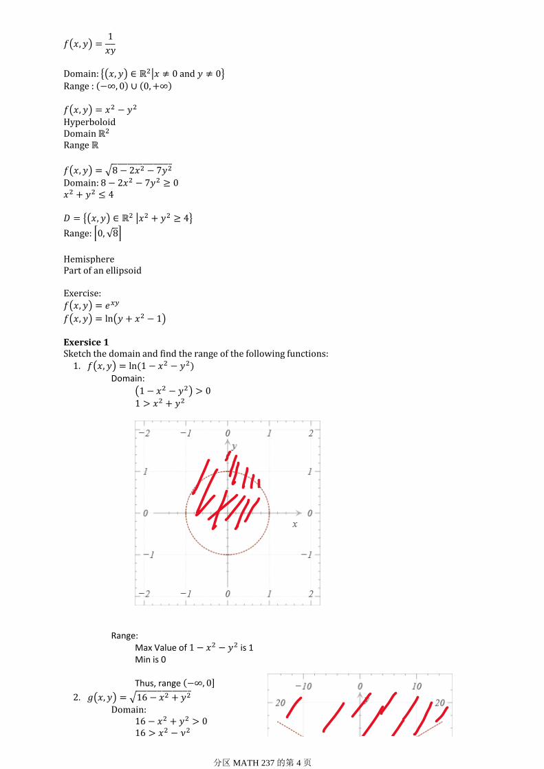
Exersice 1

Domain:

Max Value of is 1Min is 0

Thus, range

Range:

1.

Domain:

2.

Sketch the domain and find the range of the following functions:

分区MATH 237 的第 4 页

Domain:

Range:

分区MATH 237 的第 5 页

We define the graph of a function as the set of all points in such that

. We think of as representing the height of the graph above the

-plane at the point

Definition: Level Curves

The level curves of a function are the curves

Where is a constant in the range of .

The family of level curves is often called a contour map or a topographic map.

The single point is called an exceptional level curve.

Paraboloid

1.2 Geometric Interpretation of 2019年1月14日 10:00

分区MATH 237 的第 6 页

Saddle surface

Parabolic cylinder

Some other examples include use in weather maps to show curves of constant temperature called isotherms, in marine charts to indicate water depths, and in barometric pressure charts to show curves of constant pressure called isobars.

Definition: Cross SectionsA cross section of a surface is the intersection of with a plane.

For the purpose of sketching the graph of a surface , it is useful to consider the cross

sections formed by intersecting with the vertical planes and .

Generalization:Definition: Level Surfaces

A level surface of a scalar function is defined by

Definition: Level Sets

A level set a scalar function is defined by

分区MATH 237 的第 7 页

分区MATH 237 的第 8 页

Chapter 2 Limits2019年1月14日 22:58

分区MATH 237 的第 9 页

Definition: Neighborhood

A -neighbourhood of a point is a set

Remark

Recall that is the Euclidean distance in . That is,

Definition: Limit

Assume is defined in a neighborhood of , except possibly at . If for every

there exists a such that

Then

2.1 Definition of a Limit2019年1月14日 22:58

分区MATH 237 的第 10 页

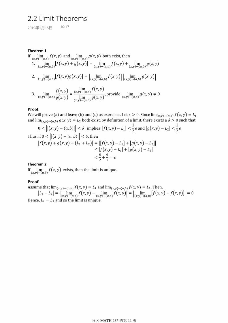
Theorem 1

1.

2.

3.

Proof:

We will prove (a) and leave (b) and (c) as exercises. Let Since

and both exist, by definition of a limit, there exists a such that

Thus, if , then

Theorem 2

Proof:

Assume that and . Then,

Hence, and so the limit is unique.

2.2 Limit Theorems2019年1月15日 10:17

分区MATH 237 的第 11 页

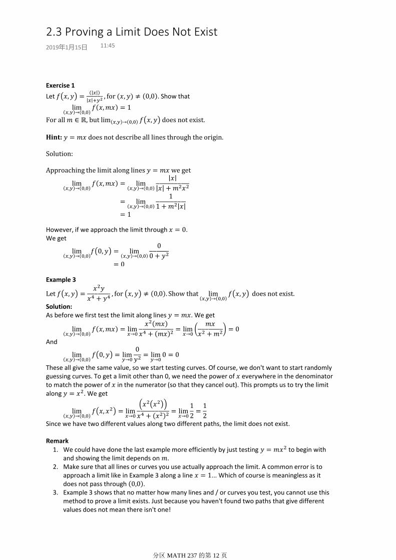
Exercise 1

Let

. Show that

For all , but does not exist.

Hint: does not describe all lines through the origin.

Solution:

Approaching the limit along lines we get

However, if we approach the limit through .

We get

Example 3

Solution:

As before we first test the limit along lines . We get

And

These all give the same value, so we start testing curves. Of course, we don't want to start randomly guessing curves. To get a limit other than 0, we need the power of everywhere in the denominator to match the power of in the numerator (so that they cancel out). This prompts us to try the limit along . We get

Since we have two different values along two different paths, the limit does not exist.

We could have done the last example more efficiently by just testing to begin with and showing the limit depends on .

1.

Make sure that all lines or curves you use actually approach the limit. A common error is to approach a limit like in Example 3 along a line ... Which of course is meaningless as it does not pass through .

2.

Example 3 shows that no matter how many lines and / or curves you test, you cannot use this method to prove a limit exists. Just because you haven't found two paths that give different values does not mean there isn't one!

3.

Remark

2.3 Proving a Limit Does Not Exist2019年1月15日 11:45

分区MATH 237 的第 12 页

Theorem 1 (Squeeze Theorem)

If there exists a function such that

In some neighborhood of and , then

Proof:

Let . Since we have that there exists a such that

Hence, if , then we have

As our hypothesis requires that for all in the neighborhood of .

Therefore, by definition of a limit, we have

Exercise 1Our statement of the Squeeze Theorem above is not a direct generalization of the Squeeze Theorem we used in single variable calculus. What would the direct generalization of the Squeeze Theorem be? Show how your generalization and the theorem above are related.

Remark

Be careful when working with inequalities! For example, the statement

Is false if . The appendix at the end of this chapter gives a brief review of inequalities.

Exercise 2.

Prove that

Does equality ever hold?

Solution:

Thus,

2.4 Proving a Limit Exists2019年1月15日 19:35

分区MATH 237 的第 13 页

Example 3

Determine whether

exists, and if so find its value.

Solution:

Trying lines we get

Since the value along each line is , we try to prove the limit is with the Squeeze Theorem. Thus, we consider

Since

Since we get

by the Squeeze Theorem.

Exercise 3

Consider defined by

Determine whether exists, and if so find its value.

Solution:

Tying lines we get

Clearly, the limit does not exist.

Remark

The concept of a neighbourhood, the definition of a limit, the Squeeze Theorem and the limit theorems are all valid for scalar functions . In fact, to generalize these concepts, one only needs to recall that if and are in , then the Euclidean

distance from to is

分区MATH 237 的第 14 页

Trichotomy Property: For any real numbers and , one and only one of the following holds:

Transitivity Property: If and , then .Addition Property: If , then for all , .Multiplication Property: If and , then .

Using these properties one can deduce other results.

The absolute value of a real number is defined by

1. if and only if 2.The Triangle Inequality: for all .3.

Three frequently used results, which follow from the axioms, are listed below.

Remark.

The Triangle Inequality1.If , then 2.The cosine inequality 3.

When using the Squeeze Theorem, the most commonly used inequalities are:

2.5 Appendix: Inequalities2019年1月17日 13:06

分区MATH 237 的第 15 页

Chapter 3 Continuous Functions2019年1月17日 13:21

分区MATH 237 的第 16 页

In many situations, we shall require that a function is continuous. Intuitively, this means that

the graph of (the surface ) has no "breaks" or "holes" in it. As with functions of one

variable, continuity is defined by using limits.

Exercise 1Review the definition of a continuous function of one variable in your first year calculus text. Give an example (formula and graph) of a function which is defined for all , but is not continuous at .

Definition: Continuous

A function is continuous at if and only if

Additionally, if is continuous at every point in a set , then we say that is continuous on .

Remark

1.

is defined at ,2.The stated equality.3.

There are really three requirements in this definition:

Exercise 2

Let be defined by

Determine whether is continuous at .

Solution:

Since , we get

Thus, is continuous at .

3.1 Definition of a Continuous Function2019年1月17日 13:21

分区MATH 237 的第 17 页

Definition: Operations on Functions

The sum is defined by 1.

The product is defined by 2.

The quotient

is defined by 3.

If and are scalar functions and , then:

Definition: Composite Function

For scalar functions and the composite function is defined by

For all for which .

We shall refer to the following theorems collectively as the Continuity Theorems.

Theorem 1If and are both continuous at , then and are continuous at .

Proof:

We prove the result for and leave the proof for as an exercise. By the hypothesis and the definition of continuous function we have that

Hence, by definition of the sum and limit properties, we get

Exercise 1Complete the proof of the theorem by proving that is continuous at .

Theorem 2

If and are both continuous at and , then the quotient

is continous at .

Exercise 2Use the Limit Theorems to prove Theorem 2. Where is the hypothesis used explicitly?

Theorem 3If is continuous at and is continuous at , then the composition is continuous at .

Proof:

Let . By definition of continuity we have that

3.2 The Continuity Theorems2019年1月18日 1:45

分区MATH 237 的第 18 页

So, by definition of a limit there exists a such that

Similarly, we have

Hence, given the above , there exists a such that

Notice that the conclusion of (3.2) is the hypothesis of (3.1) where . Hence, combining (3.1) and (3.2), we get

Consequently, by definition of a limit,

The constant function •

The power functions •

The logarithm function •

The exponential function •The trigonometric functions, , etc.•The inverse trigonometric functions, , etc.•The absolute value function •

Before we can apply these theorems, we need a list of basic functions which are known to be continuous on their domains:

Exercise 3

Prove that the constant function and the coordinate functions ,

are continuous on their domains.

Exercise 4

Prove that

is continous for all which satisfy . Which of the

theorems and basic functions do you have to use?

Solution:Basic functions:

Theorems: Multiply

Exercise 5Which of the basic functions and theorems do you have to use in order to prove that

is continuous for all

Example 2

Discuss the continuity of the function defined by

Solution:For the Continuity Theorems immediately imply that is continuous at these points.

Observe the point is singled out in the definition of the function. Thus, the Continuity Theorems cannot be appled at and so we have to use the definition. That is, we have to determine whether

分区MATH 237 的第 19 页

determine whether

On the line we get

By L'Hospital's Rule. It follows that does not equal , and hence by

definition, is not continuous at .

Exercise 6

Would the function in Example 2 be continuous at if we defined

?

Example 3

Discuss the continuity of the function defined by

Solution:For points with the Continuity Theorems immediately imply that is continuous at

these points.

We can not apply the continuity theorems at the points with . Consider any one of

these points and denote it by .

If approaches with , then , and approaches (and in

fact equals) 1. On the other hand, if approaches with , then

approaches -1. Thus,

Does not exist. So, by definition of continuity, is not continuous at .The geometric interpretation is simple. The graph of consists of two parallel half-planes which form a "step" along the line .

分区MATH 237 的第 20 页

So far in this chapter, we have shown how to prove that a function is continuous at a point essentially "by inspection" by using the Continuity Theorems. This makes it easy to evaluate if is continuous at . In particular, if is continuous at , then

can be evaluated simply by evaluating .

RemarkIn applying the Squeeze Theorem one has to prove that One hopes to

be able to evaluate this limit by inspection, and so one tries to set up the inequality in the Squeeze Theorem so that is continuous at .

3.3 Limits Revisited2019年1月19日 13:21

分区MATH 237 的第 21 页

Chapter 4 The Linear Approximation2019年1月19日 13:27

分区MATH 237 的第 22 页

Treat as a constant and differentiate with respect to to obtain

1.

Treat as a constant and differentiate with respect to to obtain

.2.

A scalar function can be differentiated in two natural ways:

The derivatives

and

are called the (first) partial derivatives of .

Here is the formal definition.

Definition: Partial Derivatives

The partial derivatives of are defined by

Provided that these limits exist.

It is sometimes convenient to use operator notation and for the partial derivatives of

. The nontation means: differentiate with respect to the variable in the first position,

holding the other fixed. If the independent variables are and , then

Example 1

Consider the function defined by where is a constant. Determine

and

.

Solution:

By using the Product Rule and Chain Rule for differentiation,

Exercise 1A function is defined by . Determine and .

Solution:

Example 2

A function is defined by

. Determine whether

exists.

Solution:

By single-variable differentiation rules,

For all such that . One cannot substitute in equation (4.1) since the

denominator would be zero. Thus, we must use the definition of the partial derivatives at . We get

4.1 Partial Derivatives2019年1月19日 13:27

分区MATH 237 的第 23 页

Example 3

Let

. Calculate and

Solution: Since changes definition at , we must use the definition of the partial derivaties. We get

Remark

In Example 2, we showed that

is not continuous at , but

we have just shown that its partial derivatives exist! This demonstrates that the concept of partial derivatives do not match our concept of differentiability for functions of one variable from Calculus 1. We will look at this more in the next chapter.

Exercise 2

Refer to the function in Example 2. Show that

does not exist for .

Exercise 3

A function is defined by . Determine whether

and

exist.

Generalization

We can extend what we have done for scalar functions of two variables to scalar functions of variables . To take the partial derivative of with respect to its -th variable, we hold all the other variables constant and differentiate with respect to the -th variable.

Example 4Let . Find , , and .

Solution:

We have

Exercise 4

For , write the precise definition of

,

,

.

分区MATH 237 的第 24 页

Second Partial Derivatives

Observe that the partial derivatives of a scalar function of two variables are both scalar functions of two variables. Therefore, we can take the partial derivatives of the partial derivatives of any scalar function.

In how many ways can one calculate a second partial derivative of ? Since both of the partial derivatives of have two partial derivatives, there are four possible second partial derivatives of . They are:

Similarly

It is often convenient to use the subscript notation or the operator notation:

The subscript notation suggests that one could write the second partial derivatives in a matrix.

Definition: Hessian Matrix

The Hessian matrix of , denoted by , is defined as

Example 1Let be a constant. Find all the second partial derivatives of .

Solution:

We first calculate the first partial derivatives. We have

Thus, we get

4.2 Higher-Order Partial Derivatives2019年1月19日 18:32

分区MATH 237 的第 25 页

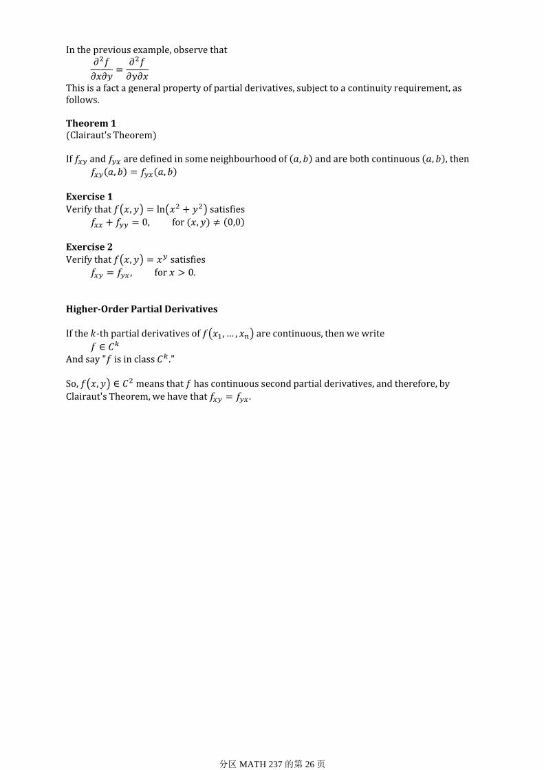
In the previous example, observe that

This is a fact a general property of partial derivatives, subject to a continuity requirement, as follows.

Theorem 1(Clairaut's Theorem)

If and are defined in some neighbourhood of and are both continuous , then

Exercise 1

Verify that satisfies

Exercise 2

Verify that satisfies

Higher-Order Partial Derivatives

If the -th partial derivatives of are continuous, then we write

And say " is in class ."

So, means that has continuous second partial derivatives, and therefore, by

Clairaut's Theorem, we have that

分区MATH 237 的第 26 页

Definition: Tangent Plane

The tangent plane to at the point is

Exercise 1

The graph of the function

Is the cone . Find the equation of the tangent plane at the point

Exercise 2Show that the tangent plane at any point on the cone in Exercise 1 passes through the origin.

RemarkIn Exercise 2, you should note that a tangent plane does not exist at the vertex of the cone, since the cone is not "smooth" there. We shall discuss the question of the existence of a tangent plane in Chapter 5.

4.3 The Tangent Plane2019年1月19日 20:32

分区MATH 237 的第 27 页

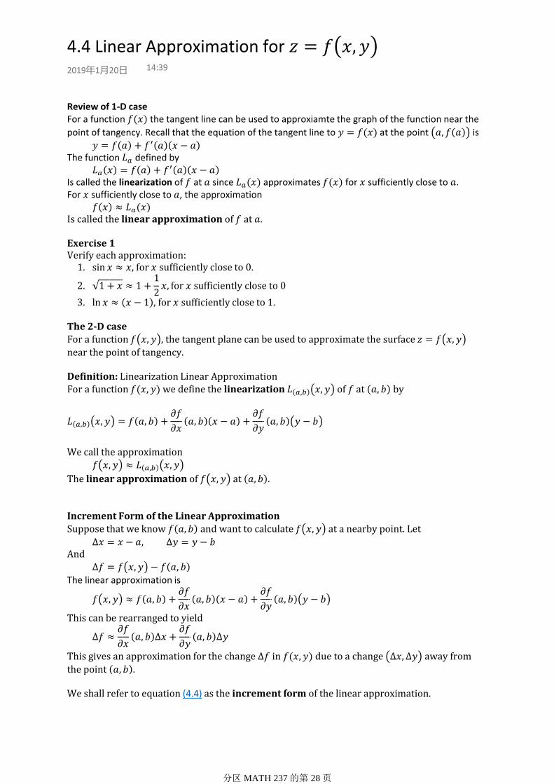
Review of 1-D case

For a function the tangent line can be used to approxiamte the graph of the function near the

point of tangency. Recall that the equation of the tangent line to at the point is

The function defined by

Is called the linearization of at since approximates for sufficiently close to .

For sufficiently close to , the approximation

Is called the linear approximation of at .

Exercise 1

, for sufficiently close to .1.

2.

, for sufficiently close to 1.3.

Verify each approximation:

The 2-D caseFor a function , the tangent plane can be used to approximate the surface

near the point of tangency.

Definition: Linearization Linear ApproximationFor a function we define the linearization of at by

We call the approximation

The linear approximation of at .

Increment Form of the Linear Approximation

Suppose that we know and want to calculate at a nearby point. Let

And

The linear approximation is

This can be rearranged to yield

This gives an approximation for the change in due to a change away from

the point .

We shall refer to equation (4.4) as the increment form of the linear approximation.

4.4 Linear Approximation for 2019年1月20日 14:39

分区MATH 237 的第 28 页

Linear Approximation in

Consider a function . By analogy with the case of a function of two variables, we define

the linearization of at by

The notation is becoming cumbersome, but one can improve matters by noting that the final three terms can be represented by the dot product of the vectors

The second vector is called the gradient of at .Here are the formal definitions.

Definition: Gradient

Suppose that has partial derivatives at . The gradient of at is defined by

Definition: Linearization Linear Approximation

Suppose that , has partial derivatives at . The linearization of at is defined by

The linear approximation of at is

Linear Approximation in

The advantage of using vector notation is that equations (4.5) and (4.6) hold for a function of variables . For arbitrary , we have

And we define the gradient of at to be

Then, the increment form of the linear approximation for is

Observe that this formula even works when . That is, for a function of one variable this gives and the increment form of the linear approximation is

Which is our familiar formula from Calculus 1.

For we have and the increment form of the linear

approximation is

Which matches our work above. Hence, we see that this is a true generalization.

4.5 Linear Approximation in Higher Dimensions2019年1月20日 15:10

分区MATH 237 的第 29 页

Chapter 5 Differentiable Functions2019年1月21日 18:25

分区MATH 237 的第 30 页

Theorem 1

If exists, then

where

Proof:

We have

The result follows from taking the limit as (details left as an exercise).

Definition: Differentiable

A function is differentiable at if

Where

Theorem 2

If a function satisfies

Then .

Proof:

Since

The limit is 0 along any path. Therefore, along the path along , we get

Similarly, approaching along we get that .

This implies that the tangent plane gives the best linear approximation to the graph near . Moreover,

it tells us that the linear approximation is a "good approximation" if and only if is differentiable at .

RemarkObserve that for the linear approximation to exist at both partial derivatives of must exist at . However, both partial derivatives existing does not guarentee that will be differentiable. We say that the partial derivatives of existing at is necessary, but not sufficient.

Exercise 1

Prove that

5.1 Definition of Differentiability2019年1月21日 18:25

分区MATH 237 的第 31 页

Is not differentiable at

Solution:

We have

and

,

Wrong Procedure

Although the procedure is not correct, it can be imaged as plug in for and let the

Same with .

So the error in the linear approximation is

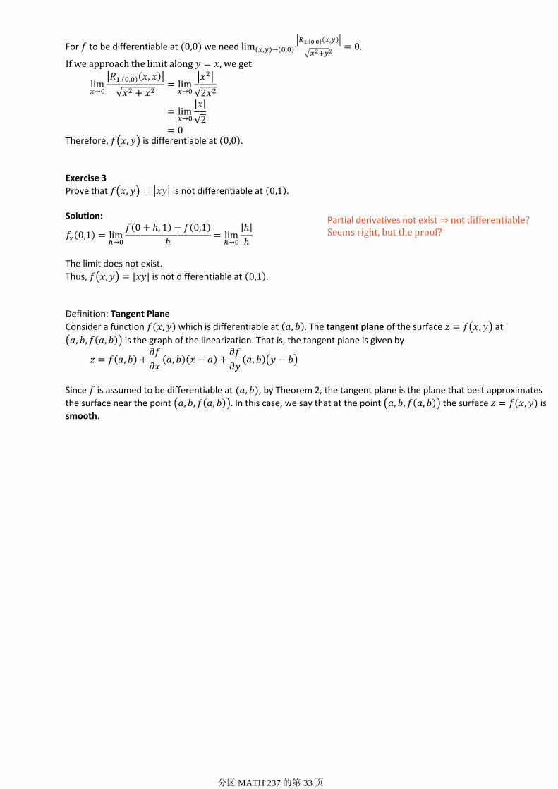
For to be differentiable at we need

.

If we approach the limit along , we get

Therefore, the limit cannot equal 0 and hence is not differentiable at

Exercise 2

Prove that is differentiable at

Solution:

So the error in the linear approximation is

For to be differentiable at we need

分区MATH 237 的第 32 页

For to be differentiable at we need

If we approach the limit along , we get

Therefore, is differentiable at .

Exercise 3

Prove that is not differentiable at

Solution:

The limit does not exist.

Thus, is not differentiable at

Definition: Tangent Plane

Consider a function which is differentiable at The tangent plane of the surface at

is the graph of the linearization. That is, the tangent plane is given by

Since is assumed to be differentiable at , by Theorem 2, the tangent plane is the plane that best approximates

the surface near the point In this case, we say that at the point the surface is

smooth.

Partial derivatives not exist not differentiable?Seems right, but the proof?

分区MATH 237 的第 33 页

Theorem 1If is differentiable at then is continuous at

Proof:

The error is defined by

Using the definition of , this equation can be rearranged to read

We can write

Since is differentiable and by the limit theorems, we get

And so by definition, is continuous at

Exercise 1

Suppose that is not continuous at Can you draw a conclusion about whether is

differentiable at ?

Solution:Take the contrapositive of Theorem 1, we get

If is not continuous at , is not differentiable at

5.2 Differentiability and Continuity2019年1月31日 21:21

分区MATH 237 的第 34 页

Theorem 1 (Mean Value Theorem)

If is continuous on the closed interval and is differentiable on the open interval

, then there exists such that

Theorem 2

If

and

are continuous at , then is differentiable at

Proof:

We derive an expression for the error , given by

Since and are continuous then and exist in some neighborhood For

, we write

By adding and subtracting . The Mean Value Theorem can be applied to each bracket,

since one variable is held fixed, and the partial derivatives are assumed to exist. For the first bracket:

Where lies between and . By adding and substracting we obtain

Where

Similarly for the second bracket:

Where

And lies between and .

Substitute equations (5.5) and (5.7) into (5.4) and then substitute equation (5.4) into (5.3) to obtain

Where and are given by equations (5.6) and (5.8). It follows by the triangle inequality that

We can now apply the Squeeze Theorem with and

As , it follows that

Since and are continuous at , it follows from equations (5.6) and (5.8) that

Equation (5.9) and the Squeeze Theorem now imply

So that is differentiable at , by definition.

5.3 Continuous Partial Derivatives and Differentiability2019年1月31日 21:37

分区MATH 237 的第 35 页

So that is differentiable at , by definition.

RemarkThe converse of Theorem 2 is not true. That is, being differentiable at does not imply that and are both continuous at

Exercise 1

Prove that

is differentiable at

Solution:

By differentiation

Thus, is differentiable at .

Exercise 2

Prove that if at , then is continuous at .

Solution:Since are continuous at .

and are differentiable at

Then and are continuous at

Then is differentiable at .Then is continuous at .

SummaryTheorem 2 makes it easy to prove that a function is differentiable at a typical point. One simply differentiates to obtain the partial derivatives , , and then checks that the partials are

continuous functions by inspection, referring to the Continuity Theorems, as in Section 3.2. It is only necessary to use the definition of a differentiable function at an exceptional point.

Generalization

The definition of a differentiable function and theorems 1 and 2 are valid for functions of variables. The only change is that there are partial derivatives,

分区MATH 237 的第 36 页

The error in the linear approximation for is defined by

Where

It is convenient to rearrange the definition of to read

The linear approximation

For sufficiently close to , arises if one neglects the error term. In general, one has no information about , and so it is not clear whether the approximation is reasonable.

However, Theorem 2 provides an important piece of information about , namely

that if the partial derivatives of are continuous at , then is differentiable and hence

In this case, the approximation (5.11) is reasonable for sufficiently close to , and we

say that is a good approximation of near .

5.4 Linear Approximation Revisited2019年2月8日 22:16

分区MATH 237 的第 37 页

Chapter 6 The Chain Rule2019年2月9日 14:08

分区MATH 237 的第 38 页

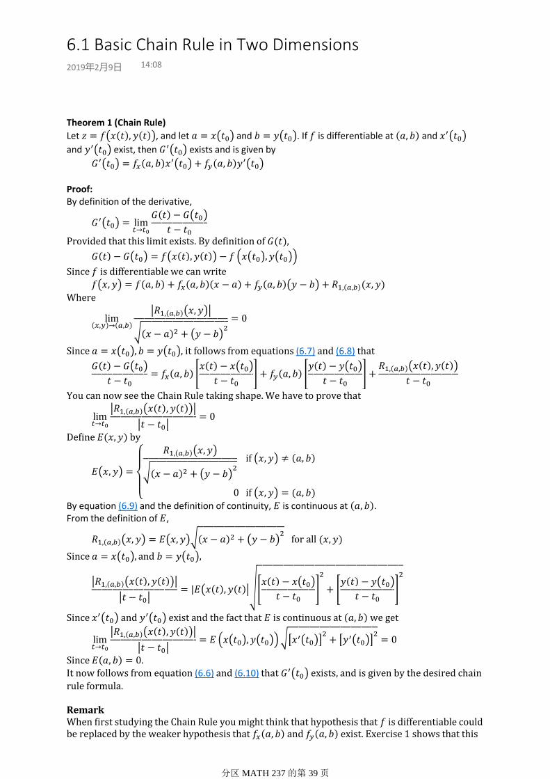
Theorem 1 (Chain Rule)

Let , and let and . If is differentiable at and

and exist, then exists and is given by

Proof:

By definition of the derivative,

Provided that this limit exists. By definition of ,

Since is differentiable we can write

Where

Since , it follows from equations (6.7) and (6.8) that

You can now see the Chain Rule taking shape. We have to prove that

Define by

By equation (6.9) and the definition of continuity, is continuous at .

From the definition of ,

Since

Since and exist and the fact that is continuous at we get

Since .It now follows from equation (6.6) and (6.10) that exists, and is given by the desired chain

rule formula.

RemarkWhen first studying the Chain Rule you might think that hypothesis that is differentiable could be replaced by the weaker hypothesis that and exist. Exercise 1 shows that this

is not the case.

6.1 Basic Chain Rule in Two Dimensions2019年2月9日 14:08

分区MATH 237 的第 39 页

is not the case.

Exercise 1

With reference to the theorem, let

Define and show that . Further show that and

, so that the Chain Rule fails. Draw a conclusion about at .

Solution:

One simple way to calculate is to substitute.

By symmetry,

Thus, the Chain Rule fails.

Not sure what this means!

Sample Answer: is not differentiable at

RemarkIn practice it is convenient to use stronger hypotheses in the Chain Rule. In particular, we usually assume that has continuous partial derivatives at and and are both continuous at . This also allows one to obtain the stronger conclusion that is continuous at . These hypotheses can usually be checked quickly, either by using the Continuity Theorems, or in more theoretical situations, by using given information.

Exercise 2 Be sure to check it again!!!!Stupid mistake, should be . So that's fine.

Let

Calculate

when in two ways, firstly by substituting and in , and secondly by evaluating

and applying the Chain Rule.

Solution:

First, we substitute and in

分区MATH 237 的第 40 页

Using L'Hospital's Rule

Same, using L'Hospital's Rule

The Chain Rule indicates

But what???

Exercise 3Define . If , find . What condition on will

guarantee the validity of your work?

Solution: . Thus, we have where and .

Next, to apply the Chain Rule, we require that is differentiable.

Assuming this condition, we get

Taking gives

We need to assume that is differentiable at

Exercise 4

A differentiable function is given, and is defined by

Where and Write out the Chain Rule for . Calculate

, if

.

Solution:

分区MATH 237 的第 41 页

The Vector Form of the Basic Chain Rule

We can use the dot product to rewrite the Chain Rule into a vector form. In particular, if we have

Where and are differentiable, then

So, we have

With

In this vector form, the Chain Rule holds for any differentiable function .

分区MATH 237 的第 42 页

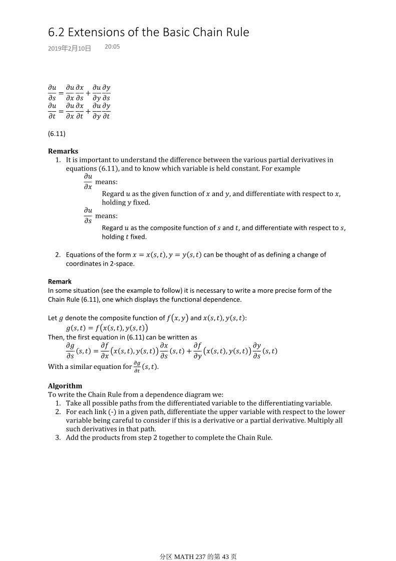
(6.11)

Regard as the given function of and , and differentiate with respect to , holding fixed.

Regard as the composite function of and , and differentiate with respect to , holding fixed.

It is important to understand the difference between the various partial derivatives in equations (6.11), and to know which variable is held constant. For example

1.

Equations of the form can be thought of as defining a change of coordinates in 2-space.

2.

Remarks

RemarkIn some situation (see the example to follow) it is necessary to write a more precise form of the Chain Rule (6.11), one which displays the functional dependence.

Let denote the composite function of and

Then, the first equation in (6.11) can be written as

With a similar equation for

Algorithm

Take all possible paths from the differentiated variable to the differentiating variable.1.For each link (-) in a given path, differentiate the upper variable with respect to the lower variable being careful to consider if this is a derivative or a partial derivative. Multiply all such derivatives in that path.

2.

Add the products from step 2 together to complete the Chain Rule.3.

To write the Chain Rule from a dependence diagram we:

6.2 Extensions of the Basic Chain Rule2019年2月10日 20:05

分区MATH 237 的第 43 页

Don't Quite Understand...

6.3 The Chain Rule for Second Partial Derivatives2019年2月12日 18:12

分区MATH 237 的第 44 页

Chapter 7 Directional Derivatives and the Gradient Vector2019年2月13日 8:44

分区MATH 237 的第 45 页

Definition: Directional Derivative

The directional derivative of at a point in the direction of a unit vector is

defined by

Provided the derivative exists.

Theorem 1

If is differentiable at and is a unit vector, then

Proof:

Since is differentiable at we can apply the Chain Rule to get

Be careful to check the condition of Theorem 1 before applying it. If is not differentiable at , then we must apply the definition of the directional derivative.

1.

If we choose or , then the directional derivative is equal to the partial derivatives or respectively.

2.

Remarks

Exercise 1

Find the directional derivative of defined by

At the point in the direction of the vector .

Solution:

The vector is not a unit vector, so we first normalize it.

Similarly,

We have

So

7.1 Directional Derivatives2019年2月13日 8:45

分区MATH 237 的第 46 页

The Greatest Rate of Change

Theorem 1

If is differentiable at and , then the largest value of is

, and occurs when is in the direction of .

Proof:

Since is differentiable at and we have

Where is the angle between and . Thus, assumes its largest value when

i.e. . Consequently, the largest value of is and occurs when

is in the direction of .

Exercise 1Find the largest rate of change of at the point , and the direction in

which it occurs.

Solution:

The direction is

Exercise 2Given a non-constant function and a point such that the directional derivative at is independent of the direction. What can you say about the tangent plane of the surface at the point ?

Solution:

According to the definition of tangent plane,

Since

Plane does not exist?Plane is horizontal.

Theorem 1 also applies in any direction. That is, if , is differentiable at and

is a unit vector, then the largest value of is , and it occurs when is in the

7.2 The Gradient Vector in Two Dimensions2019年2月21日 8:00

分区MATH 237 的第 47 页

is a unit vector, then the largest value of is , and it occurs when is in the

direction of .

The Gradient and the Level Curves of

Theorem 2If in a neighborhood of and , then is orthogonal to

the level curve through

Proof:

Since , by the Implicit Function Theorem (see Appendix 1), the level curve

can be described by parametric equations for where

and differentiable. Hence, the level curve may be written as

Suppose

Since is differentiable, we can take the derivative of this equation with respect to using the Chain Rule to get

On setting we get

Thus, is orthogonal to which is tangent to the level curve.

Exercise 3

Prove the level curves of the functions and defined by

Intersect orthogonally. Illustrate graphically.

The Gradient Vector Field

The gradient of associates a vector with each point of the domain of , and is referred to as a vector field. It is re[resented graphically by drawing as a vector emanating from the corresponding point

分区MATH 237 的第 48 页

Theorem 1

If in a neighborhood of and , then is

orthogonal to the level surface through .

The details are similar to proof of Theorem 7.2.2.

Exercise 1Find the equation of the tangent plane to the ellipsoid at the point

Solution:

Exercise 2

Find the equation of the tangent plane to the surface

Hint: Rewrite the equation as and use the above approach.

7.3 The Gradient Vector in Three Dimensions2019年2月21日 15:43

分区MATH 237 的第 49 页

Chapter 8 Taylor Polynomials and Taylor's Theorem2019年2月21日 18:57

分区MATH 237 的第 50 页

Definition: 2nd degree Taylor polynomial

The second degree Taylor polynomial of at is given by

In general, it approximates for sufficiently close to

With better accuracy than the linear approximation.

Find the Taylor polynomial for1.

At the point , by calculating the appropriate partial derivatives.

Verify your results by letting and writing2.

Expand and neglect powers higher than 2 and then convert back to and . This type of algebraic derivation can only be done for a polynomial function.

Exercise 1

1.

Thus,

Not sure what the question mean2.

Solution:

8.1 The Taylor Polynomial of Degree 22019年2月21日 18:57

分区MATH 237 的第 51 页

Review of the 1-D caseTheorem 1

If exists on , then there exists a number between and such that

Where

The 2-D CaseTheorem 2 (Taylor's Theorem)

If in some neighborhood of , then for all there exist a

point on the line segment joining and such that

Where

Proof:The idea is to reduce the given function of two variables to a function of one variable, by

considering only points on the line segment joining and .

We parameterize the line segment from to by

For simplicity write and . Then and Taylor's formula assumes the form

Where

Define by

Since has continuous second partials by hypothesis, we can apply the Chain Rule to conclude that and are continuous and are given by

For

Since is continuous on the interval , Taylor's formula may be applied to on this interval. That is, we can set and in equations (8.2) and (8.3). It follows that there exists a number , with , such that

and

Each term in this equation can be calculated using equations (8.5)-(8.7), giving

In addition, if we let , then

And equation (8.8) becomes precisely the modified version of Taylor's formula.

RemarkLike the one variable case, Taylor's Theorem for is an existence theorem. That is, it only

8.2 Taylor's Formula with Second Degree Remainder2019年2月24日 12:58

分区MATH 237 的第 52 页

Like the one variable case, Taylor's Theorem for is an existence theorem. That is, it only

tells us that the point exists, but not how to find it.

Exercise 1Let . Use Taylor's Theorem to show that the error in the linear approximation

is at most if and .

Solution:

From Taylor's Theorem, we get

As

RemarkThe most important thing about the error term is not its explicit form, but rather

its dependence on the magnitude of the displacement We state the result as a

Corollary.

Corollary 3

If in some closed neighborhood of , then there exists a positive

constant such that

分区MATH 237 的第 53 页

Exercise 1

Write out explicitly using subscript notation.

Theorem 1Taylor's Theorem of order k

If at each point on the line segment joining and , then there exists a

point on the line segment between and such that

Where

Corollary 2

If in some neighborhood of , then

Corollary 3

If in some closed neighborhood of , then there exists a constant

such that

For all

The final stage in the process of generalization is to consider functions of variables One has simply to replace the differential operator

By

Letting , we can be write this concisely in vector notation as

8.3 Generalizations2019年3月5日 15:58

分区MATH 237 的第 54 页

Chapter 9 Critical Points2019年3月5日 20:13

分区MATH 237 的第 55 页

DefinitionLocal Maximum and Minimum

A point is a local maximum point of if for all in some

neighborhood of A point is a local minimum point of if for all in some

neighborhood of

Theorem 1

If is a local maximum or minimum point of , then

Or at least one of or does not exist at

Proof:Consider the function defined by . If is a local maximum/minimum point of , then is a local maximum/minimum point of , and hence either or does not exist. Thus it follows that either or does not exist. A similar argument gives or does not exist.

DefinitionCritical Point

A point in the domain of is called a critical point of if

Or if at least one of the partial derivatives does not exist at

DefinitionSaddle Point

and

A critical point of is called a saddle point of if in every neighborhood of

there exist points and such that

Given , find all critical points of .1.

Determine whether the critical points are local maxima, minima or saddle points.2.

The problem that we are faced with has two parts.

It is essential to solve equations (9.1) and (9.2) systematically, by considering all possible cases, in order to find all critical points.

1.

You should be aware that we can only explicitly find the critical points for simple functions . The equations

2.

Are a system of equations which are generally non-linear, and there is no general algorithms for solving such systems exactly. There are, however, numerical methods for finding approximate solutions, one of which is a generalization of Newton's method. If you review the one variable case, you might see how to generalize it, using the tangent plane. It's a challenge!

Remark

9.1 Local Extrema and Critical Points2019年3月5日 20:14

分区MATH 237 的第 56 页

It's a challenge!

Exercise 1Find all critical points of

Solution:

We get two equations

Case 1:

Critical point

Case 2:

Critical point

Exercise 2Find all critical points of

Case 2??? How to deal with this situation?

Solution:

We get two equations

Case 1:

Case 2:

Exercise 3Give a function with no critical points.

分区MATH 237 的第 57 页

分区MATH 237 的第 58 页

Review of the 1-D case

For a function of one variable, the second degree Taylor polynomial approxiamtion is

For sufficiently close to . If is a critical point of , then , and the approximation can be rearranged to give

Thus, for sufficiently close to , has the same sign as If , then for sufficiently close to and is a minimum point. If , then for sufficiently close to and is a local maximum point. There is no conclusion if

The 2-D case

For , the second degree Taylor polynomial approximation is

For sufficiently close to If is a critical point of such that

Then the approximation can be rearranged to yield

For sufficiently close to . The sign of the expression on the right will determine the

sign of , and hence whether is a local maximum, local minimum or saddle

point.

The expression on the right is called a quadratic form, and at this stage it is necessary to discuss some properties of these objects.

Quadratic FormsDefinitionQuadratic Form

A function of the form

Where and are constants, is called a quadratic form on

RemarkSemidefinite quadratic forms may be split into two classes, positive semidefinite and negative semidefinite. The matrix above would be classified as positive semidefinite.

If is not a diagonal matrix, the nature of (or of ) is not immediately obvious. For example, even if all entries of are positive, it does not follow that is a positive definite matrix.

Theorem 1Second Partial Derivatives Test

If is positive definite, then is a local minimum point of .1.If is negative definite, then is a local maximum point of .2.If is indefinite, then is a saddle point of .3.

Suppose that in some neighborhood of and that

9.2 The Second Derivative Test2019年3月7日 20:57

分区MATH 237 的第 59 页

The argument preceding the theorem is not a proof, since it involves an approximation. One can use Taylor's formula and a continuity argument to give a proof. See Section 9.3.

1.

Note the analogy with the second derivative test for functions of one variable. The requirement , which implies a local minimum, is replaced by the requirement that the matrix of second partial derivatives be positive definite.

2.

Remarks

Theorem 2

is positive definite if and only if and 1. is negative definite if and only if and 2. is indefinite if and only if 3. is semidefinite if and only if 4.

If

and , then

RemarkObserve that is the determinant of the associated symmetric matrix.

Example 3Omitted

Exercise 1Fill in the details of Example 3 above.

Exercise 2Find and classify all critical points of the function

Exercise 3Find and classify all critical points of the function

RemarkAnother way of classifying the Hessian matrix is by finding its eigenvalues. In particular, a symmetric matrix is positive definite if all of its eigenvalues are positive, negative definite if all of its eigenvalues are negative, and indefinite if has both positive and negative eigenvalues.

Degenerate Critical PointsIf is semidefinite, so that the second partial derivative test gives no conclusion, we say that the crucial point is degenerate. In order to classify the critical point, one has to

investigate the sign of in a small neighborhood of .

Generalizations

The definitions of local maximum point, local minimum point and critical point can be generalized in the obvious way to functions of variables. The Hessian matrix of at is the symmetric matrix given by

Where . The Hessian matrix can be classified as positive definitem negative definite, indefinite or semidefinite by considering the associated quadratic form in

As in . The second derivative test as stated in now holds in . It can be justified heuristically by using the second degree Taylor polynomial approximation,

Which leads to

分区MATH 237 的第 60 页

Generalizing equation (9.3).

Level Curves Near a Critical Point

A point at which is called a regular point of .

Convex Functions1-D Case

for all , for any 1.

For ,

for 2.

We say that a twice differentiable function is strictly convex if for all and is convex is for all . Thus the term convex means "concave up". Convex functions have two interesting properties.

Follows from Taylor's Theorem:

where is between and

. Thus for , giving for all .

1.

Let

Then and

We must show that for By the Mean Value Theorem

for some Note that

Thus . Since then is strictly increasing. Since then on and on This implies that is strictly decreasing on and strictly increasing on . Since and we get that on and on . Therefore, on , as required.

2.

Proof:

Remark(1) says that the graph of lies above any tangent line, and (2) says that any secant line lies above the graph of .

2-D CaseSuppose has continuous second partial derivatives. We say that is strictly convex if

is positive definite for all . By Theorem 2, is strictly convex means and

for all . We get a result which is analogous to Theorem 3.

Theorem 4

for all , and 1.

for ,

2.

If has continuous second partial derivatives and is strictly convex, then

Follows from Taylor's Theorem:1.

Where is on the line segment from to . Since ,

for by Theorem 2.

Therefore, for

We parameterize the line segment from to by2.

Proof:

分区MATH 237 的第 61 页

For simplicity write and . Define by

Since has continuous second partials by hypothesis, we can apply the Chain Rule to conclude that and are continuous and are given by

For Since and

for all ,

by Theorem 2. Thus, by Theorem 3, part (2):

Therefore, for

as required.

Remark(1) says that the graph of lies above the tangent plane and (2) says that the cross-section of the graph of above the line segment from to lies below the secant line.

Theorem 5If is strictly convex and has a critical point , then for all

and has no other critical point.

Proof:Note that . Thus, for all by Theorem 4, part

(1). If has a second critical point , then by the reasoning just given

and which is a contradiction.

分区MATH 237 的第 62 页

Lemma 1

Let

be a positive definite matrix. If and are sufficiently small, then

is positive definite.

Proof:

Let and be the quadratic forms determined by the given matrices.

And similarly for We perform the change of variables

To obtain

Where

Since for and is positive definite, we must have for all ,

Let

for all Then and bu equation (9.11)

We are given that and are sufficiently small. Let

By equation (0.10) and the triangle inequality,

We now choose

Then

Which implies

This shows that for all . Therefore, is positive definite.

RemarkThe lemma is also true if "positive definite" is replaced by "negative definite" or "indefinite".

Theorem 2(The Second Partial Derivative Test)

If is positive definite, then is a local minimum point of .1.If is negative definite, then is a local maximum of .2.

Suppose that in some neighborhood of and that

9.3 Proof of the Second Partial Derivative Test2019年3月11日 8:35

分区MATH 237 的第 63 页

If is negative definite, then is a local maximum of .2.If is indefinite, then is a saddle point of .3.

Proof:We will prove (1).

We apply Taylor's formula with second order remainder. Since

Taylor's formula can be written as

Where lies on the line segment joining and . The coefficient matrix in the

quadratic expression on the right side of (9.13) is hte Hessian matrix

We are given that is positive definite. By the lemma, there exists such that if

Then is positive definite. Since the second partials of are continuous at , the definition of continuity implies that there exists a such that

Implies (9.14) and hence that is positive definite. Since

It follows that is also positive definite. It now follows from equation (9.13) and the

definition of positive definite matrix, that if , then

Thus, by definition is a local minimum point of .

Parts (2) and (3) of the second derivative test can be proved in a similar way using the modified lemma.

分区MATH 237 的第 64 页

Chapter 10 Optimization Problems2019年3月13日 8:18

分区MATH 237 的第 65 页

DefinitionAbsolute Maximum and Minimum

for all A point is an absolute maximum point of on if1.

The value is called the absolute maximum value of on .

A point is an absolute minimum point of on if2.

The value is called the absolute minimum value of on .

Given a function and a set

The Extreme Value Theorem

Theorem 1(The Extreme Value Theorem)

If is continuous on a finite closed interval , then there exists such that

Exercise 1

is closed, but does not have an absolute maximum of .1. is finite and is continuous on , but does not have an absolute maximum on .2. is finite and is continuous on , but does not have an absolute minimum.3.

Given a function and an interval such that

DefinitionBounded Set

A set is said to be bounded if and only if it is contained in some neighbourhood of the origin.

Definition Boundary Point

Given a set , a point is said to be a boundary point of if and only if every neighbourhood of contains at least one point in and one point not in .

DefinitionBoundary of

The set of all boundary points of is called the boundary of .

DefinitionClosed Set

A set is said to be closed if contains all of its boundary points.

Theorem 2

If is continuous on a closed and bounded set , then there exists points such that

10.1 The Extreme Value Theorem2019年3月13日 8:20

分区MATH 237 的第 66 页

RemarkA function may have an absolute maximum and/or an absolute minimum on a set

even if the conditions are not satisfied. We just cannot guarantee the existence with the theorem.

分区MATH 237 的第 67 页

Algorithm

Find all critical points of that are contained in . Evaluate at each such point.1.Find the maximum and minimum points of on the boundary 2.The maximum value of on is the largest value of the function found in steps (1) and (2). The minimum value of on is the smallest value of the function found in steps (1) and (2).

3.

Let be closed and bounded. To find the maximum and/or minimum value of a function

that is continuous on ,

The absolute maximum and/or minimum value may occur at more than one point in .1.It is not necessary to determine whether the critical points are local maximum or minimum points.

2.

Remarks

Exercise 1Find the maximum of on the set

Solution:Skip for now....

Exercise 2Find the maximum value of the function on the triangular region with

vertices and

10.2 Algorithm for Extreme Values2019年3月13日 8:45

分区MATH 237 的第 68 页

Method of Lagrange Multipliers

We want to find the maximum (minimum) value of a differentiable function subject to the

constraint where , or, more geometrically, find the maximum (minimum)

value of on the level set

If has a local maximum (or minimum) at relative to nearby points on the curve

and , then, by the Implicit Function Theorem (see Appendix 1),

can be described by parametric equations

With and differentiable, and for some Define

The function gives the values of on the constraint curve, and hence has a local maximum (or minimum) at . It follows that

Assuming is differentiable we can apply the Chain Rule to get

Evaluating this at and using (10.2) gives

This can be written as

Recall the geometric interpretation of the gradient vector proven in Theorem 7.2.2 that , if non-zero, is orthogonal to the level curve at Thus, since

is the tangent vector to the constraint curve (10.1) we also have

Since we are working in two dimensions, equations (10.3) and (10.4) imply that and are scalar multiples of each other. That is, there exists a constant such that

This leads to the following procedure, called the Method of Lagrange Multipliers.

Algorithm (Lagrange Multiplier Algorithm)

and 1. and 2. is an end point of the curve 3.

Assume that is a differentiable function and . To find the maximum value and

minimum value of subject to the constraint evaluate at all points

which satisfy one of the following conditions.

The maximum/minimum value of is the largest/smallest value of obtained at the

points found in

The variable , called the Lagrange multiplier, is not required for our purposes and so should be eliminated. However, in some real world applications, the value of can be extremely useful.

1.

Case (2) and (3) are both exceptional. Observe that case (2) must be included since we assume that in the derivation.

2.

In the curve is unbounded, then one must consider for

satisfying

3.

Remark

10.3 Optimization with Constraints2019年3月13日 9:05

分区MATH 237 的第 69 页

satisfying

Exercise 1Exercise 2Omitted

Functions of Three VariablesAlgorithm

and 1. and 2. is a boundary point of the surface 3.

To find the maximum/minimum value of a differentiable function subject to such that , we evaluate at all points which satisfy one of

the following:

The maximum/minimum value of is the largest/smallest value of obtained from all points found in (1) - (3).

RemarkIf condition (1) in the algorithm holds, it follows that the level surface and

the constraint surface are tangent at the point , since their normals

coincide (See Theroem 7.3.1)

RemarkKeep in mind the geometric interpretation. The level sets are spheres centered on

the point The minimum distance occurs when one of the spheres touches (i.e. Is tangent to) the constraint surface which is the sphere . At the point of tangency the

normals are parallel, i.e.

Exercise 3Omitted

Generalization

The method of Lagrange multipliers can be generalized to functions of variables

and with constraints of the form

In order to find the possible maximum and minimum points of subject to the constraints (10.18), one has to find all points such that

The scalars are the Lagrange multipliers. When , this reduces to previous algorithms.

分区MATH 237 的第 70 页

Chapter 11 Coordinate Systems2019年3月23日 18:46

分区MATH 237 的第 71 页

In a plane we choose a point called the pole (or origin). From we draw a ray called the polar axis.Let be any point in the plane. We will represent the position of by the ordered pair where is the length of the line and is the angle between the polar axis and . We call and the polar coordinates of .

We assume, as usual, that an angle is considered positive if measured in the counterclockwise direction from the polar axis and negative if measured in the clockwise direction.

1.

We represent the point by the polar coordinates for any value of .2.We are restricting to be non-negative to coincide with te interpretation of as distance. Many textbooks do not put this restriction on .

3.

Since we use the distance from the pole in our representation, polar coordinates are suited for solving problems in which there is symmetry about the pole.

4.

Remarks

Relationship to Cartesian Coordinates

Remark

The equation

does not uniquely determine since over each value of

occurs twice. One must be careful to choose the which lies in the correct quadrant.

Graphs in Polar CoordinatesThe graph of an explicitly defined polar equation or , or an implicitly defined polar equation , is a curve that consists of all points that have at least one polar representation that satisfies the equation of the curve.

Exercise 1

Sketch the polar equation

Omitted

RemarkThe polar equation gives a logarithmic spiral which often appears in nature.

Exercise 2Sketch the polar equations and

Exercise 3Convert the equation of the curve to polar coordinates.

Area in Polar Coordinates

Exercise 4

Find the area inside the lemniscate

Algorithm

11.1 Polar Coordinates2019年3月23日 18:46

分区MATH 237 的第 72 页

Algorithm

Find the points of intersections.1.Graph the curves and split the desired region into easily integrable regions.2.Integrate3.

To find the area between two curves in Polar coordinates, we use the same method we used for doing this in Cartesian coordinates.

RemarkFinding points of intersection can be tricky, especially at the pole/origin which does not have a unique representation: for any represents the origin, so simply setting expressions equal to each other may 'miss' that point. It is essential to sketch the region when finding points of intersection.

Exercise 5Find the area between the curves and .

分区MATH 237 的第 73 页

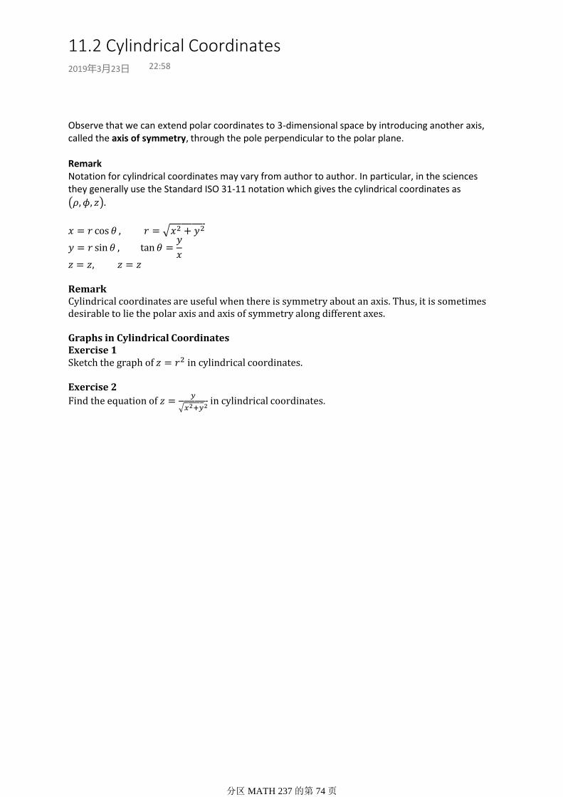
Observe that we can extend polar coordinates to 3-dimensional space by introducing another axis, called the axis of symmetry, through the pole perpendicular to the polar plane.

RemarkNotation for cylindrical coordinates may vary from author to author. In particular, in the sciences they generally use the Standard ISO 31-11 notation which gives the cylindrical coordinates as

RemarkCylindrical coordinates are useful when there is symmetry about an axis. Thus, it is sometimes desirable to lie the polar axis and axis of symmetry along different axes.

Graphs in Cylindrical CoordinatesExercise 1Sketch the graph of in cylindrical coordinates.

Exercise 2

Find the equation of

in cylindrical coordinates.

11.2 Cylindrical Coordinates2019年3月23日 22:58

分区MATH 237 的第 74 页

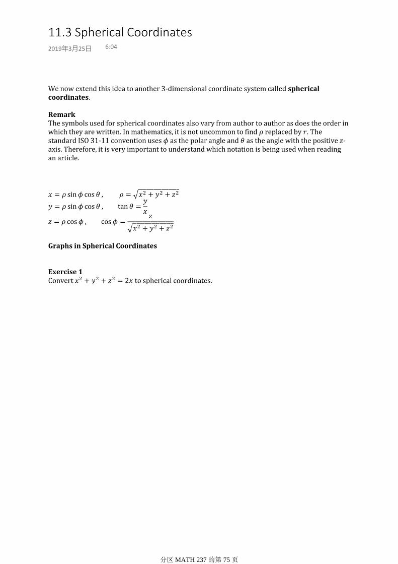
We now extend this idea to another 3-dimensional coordinate system called spherical coordinates.

RemarkThe symbols used for spherical coordinates also vary from author to author as does the order in which they are written. In mathematics, it is not uncommon to find replaced by . The standard ISO 31-11 convention uses as the polar angle and as the angle with the positive -axis. Therefore, it is very important to understand which notation is being used when reading an article.

Graphs in Spherical Coordinates

Exercise 1Convert to spherical coordinates.

11.3 Spherical Coordinates2019年3月25日 6:04

分区MATH 237 的第 75 页

DefinitionVector-Valued Function

A function whose domain is a subset of and whose codomain is is called a vector-valued function.

RemarkWhile we represent as a point in , remember that it can also be thought of as a

position vector.

DefinitionMapping

A vector-valued function whose domain is a subset of and whose codomain is a subset of

is called a mapping (or transformation).

Chapter 12 Mappings of into

2019年3月25日 6:13

分区MATH 237 的第 76 页

A pair of equations

Associates with each point a single point , and thus defines a vector-valued

function

The scalar functions and are called the component functions of the mapping.

In general, if a mapping from to acts on a curve in its domain, it will determine a curve in its range, denoted by and called the image of under .

More generally, if a mapping from to acts on any subset in its domain it will determine a set in its range, called the image of under .

Exercise 1Find the image of the circle under the mapping defined in Example 1.

Observe that each of the images are exactly what we could get if we sketched the equations as in Chapter 11.

1.

The mapping from polar coordinates to Cartesian coordinates in non-linear. The image of a straight line is not necessarily a straight line.

2.

Remarks

Exercise 2

Find the image of the square

Under the mapping defined by

12.1 The Geometry of Mappings2019年3月25日 6:22

分区MATH 237 的第 77 页

DefinitionDerivative Matrix

The derivative matrix of a mapping defined by

Is denoted and defined by

If we introduce the column vectors

Then the increment form of the linear approximation for mappings becomes

For sufficiently small. Thus, the linear approximation for mappings is

Exercise 1

Consider the mapping defined by

Approximate the image of the point under .

Generalization

A mapping from to is defined by a set of component functions:

Or, in vector notation

If we assume that has continuous partial derivatives, then the derivative matrix of is the matrix defined by

As expected, the linear approximation for at is

Where

12.2 The Linear Approximation of a Mapping2019年3月25日 13:06

分区MATH 237 的第 78 页

Theorem 1(Chain Rule in Matrix Form)

Let and be mappings from to . If has continuous partial derivatives at and has continuous partial derivatives at , then the composite mapping has continuous partial derivatives at and

Proof:

Define the component functions for and as in equations (12.1) and (12.2). Then, the chain rule for scalar functions gives

As required.

Exercise 1

Use the chain rule in matrix form to find the derivative matrix 1.Calculate 2.Use the linear approximation of mappings to approximate the image of under .

3.

Consider the mappings defined by

12.3 Composite Mappings and the Chain Rule2019年3月25日 18:05

分区MATH 237 的第 79 页

Chapter 13 Jacobians and Inverse Mappings2019年3月25日 18:29

分区MATH 237 的第 80 页

DefinitionInvertible MappingInverse Mapping

if and only if

Let be a mapping from a set onto a set . If there exists a mapping , called the inverse

of which maps onto such that

Then is said to be invertible on .

DefinitionOne-to-One

A mapping from to is said to be one-to-one on a set if and only if

implies , for all

Theorem 1Let be a mapping from a set onto a set . If is one-to-one on , then is invertible

on .

Theorem 2

Consider a mapping which maps onto . If has continuous partial derivatives at

and there exists an inverse mapping of which has continuous partial derivatives at

, then

Proof:

By the Chain Rule in Matrix Form we get

Then, by equation (13.1) we have

As required.

RemarkThe fact that we could solve and obtain a unique solution for and in the preceding example proves that has an inverse mapping on . It is only in simple examples that one can carry out this step. Hence it is useful to develop a test to determine if a mapping has an inverse mapping.

DefinitionJacobian

The Jacobian of a mapping

Is denoted

, and is defined by

13.1 The Inverse Mapping Theorem2019年3月25日 18:30

分区MATH 237 的第 81 页

Exercise 1

Calculate the Jacobian

of the mapping given by

Corollary 3

Consider a mapping defined by

Which maps a subset onto a subset . Suppose that and have continuous partials on

. If has an inverse mapping , with continuous partials on , then the Jacobian of is

non-zero:

Remark

The notation

for the Jacobian reminds one which partial derivatives have to be calculated.

Thus, if maps and is one-to-one, then the inverse mapping maps

, and the Jacobian of the inverse mapping is denoted by

Recall from linear algebra that for all matrices . Thus, we can deduce from Theorem 2 a simple relationship between the Jacobian of a mapping and the Jacobian of the inverse mapping. We state this as a corollary to Theorem 2.

Corollary 4(Inverse Property of the Jacobian)

If the hypotheses of Theorem 2 hold, then

Proof:

By Theorem 2,

Taking the determinant of this equation gives

Thus, by definition of the Jacobian,

Since is invertible, we have

. Therefore, we get

Theorem 5

分区MATH 237 的第 82 页

Theorem 5(Inverse Mapping Theorem)

If a mapping has continuous partial derivatives in some neighborhood of

and

at , then there is a neighborhood of in which has an inverse mapping

which has continuous partial derivatives.

Exercise 2

Referring to Example 3, show that the inverse mapping is given by

分区MATH 237 的第 83 页

Exercise 1

Let and let be the square pictured in the diagram. Will the image of under

have more or less area? Explain your answer.

Remark

For a linear mapping where are constants, the

derivative matrix is

And this the linear approximation is exact by Taylor's Theorem since all second partials are zero. Therefore, for a linear mapping, the approximation (13.3) becomes an exact relation.

Exercise 2Show that the linear mapping preserves area. Illustrate the

action of the mapping by finding the image of the square with vertices and .

Exercise 3

Use the Jacobian to verify the well-known result that any linear mapping which is a rotation,

Where is a constant, preserves areas.

GeneralizationAt the end of Section 12.2, we generalized the concept of a mapping from to to a mapping from to , and defined the Jacobian of the mapping, as follows.

DefinitionJacobian

For a mapping defined by

Where and , the Jacobian of is

Geometrical Interpretation of the Jacobian in 3-D

13.2 Geometrical Interpretation of the Jacobian2019年3月26日 12:38

分区MATH 237 的第 84 页

Exercise 1Find a linear mapping which will transform the ellipse into the circle .

Exercise 2Find an invertible mapping which will transform the region in the first octant bound by

into a cube in the -space.

13.3 Constructing Mappings2019年3月26日 20:16

分区MATH 237 的第 85 页

Chapter 14 Double Integrals2019年3月28日 11:49

分区MATH 237 的第 86 页

DefinitionIntegrable

Let be closed and bounded. Let be a partition of as described above, and let

denote the length of the longest side of all rectangles in the partition . A function which

is bounded on is integrable on if all Riemann sums approach the same value as .

DefinitionDouble Integral

If is integrable on a closed bounded set , then we define the double integral of on

as

Interpretation of the Double Integral

When you encounter the double integral symbol

Think of "limit of a sum". In itself, the double integral is a mathematically defined object. It has many interpretations depending on the meaning that you assign to the integrand . The

" " in the double integral symbol should remind you of the area of a rectangle in a partition of .

Double Integral as Area:

The simplest interpretation is when you specialize to be the constant function with value unity:

Then the Riemann sum (14.1) simply sums the areas of all rectangles in , and the double integral serves to define the area of the set :

Double Integral as Volume:

If for all , then the double integral

Can be interpreted as the volume of the origin defined by

Which represents the solid below the surface and above the set in the -plane.

The justification is as follows.

The partition of decomposes the solid into vertical "columns". The height of the column above the -th rectangle is approximately , and so its volume is approximately

The Riemann sum (14.1) thus approximates the volume

As the partition becomes increasingly fine, so the error in the approximation will tend to zero. Thus, the volume is

14.1 Definition of Double Integrals2019年3月28日 11:49

分区MATH 237 的第 87 页

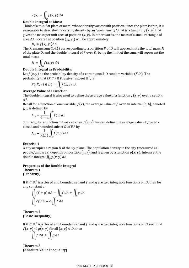
Double Integral as Mass:

Think of a thin flat plate of metal whose density varies with position. Since the plate is thin, it is reasonable to describe the varying density by an "area density", that is a function that

gives the mass per unit area at position . In other words, the mass of a small rectangle of area located at position will be approximately

The Riemann sum corresponding to a partition of will approximate the total mass of the plate , and the double integral of over , being the limit of the sum, will represent the total mass:

Double Integral as Probability:

Let be the probability density of a continuous 2-D random variable . The

probability that , a given subset , is

Average Value of a Function:The double integral is also used to define the average value of a function over a set

.

Recall for a function of one variable, , the average value of over an interval , denoted , is defined by

Similarly, for a function of two variables , we can define the average value of over a

closed and bounded subset of by

Exercise 1A city occupies a region of the -plane. The population density in the city (measured as

people/unit area) depends on position , and is given by a function . Interpret the

double integral

Properties of the Double IntegralTheorem 1(Linearity)

If is a closed and bounded set and and are two integrable functions on , then for any constant :

Theorem 2(Basic Inequality)

If is a closed and bounded set and and are two integrable functions on such that for all , then

Theorem 3(Absolute Value Inequality)

If is a closed and bounded set and is an integrable function on , then

分区MATH 237 的第 88 页

If is a closed and bounded set and is an integrable function on , then

Theorem 4(Decomposition)

Assume is a closed and bounded set and is an integrable function on . If is decomposed into two closed and bounded subsets and by a piecewise smooth curve , then

The Basic Inequality can be used to obtain an estimate for a double integral that cannot be evaluated exactly.

1.

The decomposition property is essential for dealing with complicated regions of integration and with discontinuous integrands.

2.

Remarks

分区MATH 237 的第 89 页

Theorem 1

Let be defined by

Where and are continuous for . If is continuous on , then

RemarkAlthough the parentheses around the inner integral are usually omitted, we must evaluate it first. Moreover, as in our interpretation of volume above, when evaluating the inner integral, we are integrating with respect to while holding constant. That is, we are using partial integration.

Suppose now that the set can be described by inequalities of the form

Where are constants and are continuous functions of on the interval

Then, by reversing the roles of and in Theorem 1, the double integral

can be

written as in iterated integral in the order " first, then ":

Exercise 1

Describe the set by inequalities in two ways. Evaluate the double integral

In two ways.

Exercise 2

Let be the triangular region with vertices . Evaluate

Exercise 3

Let be the triangular region with vertices . Evaluate

Exercise 4Find the volume of the solid bounded above by the paraboloid , and below by the rectangle

14.2 Iterated Integrals2019年3月28日 21:51

分区MATH 237 的第 90 页

Theorem 1(Change of Variable Theorem)

Let each of and be a closed bounded set whose boundary is a piecewise-smooth closed

curve. Let

Be a one-to-one mapping of onto , with , and

expect for possibly on a

finite collection of piecewise-smooth curves in . If is continuous on , then

Exercise 1Omitted

Double Integrals in Polar Coordinates

RemarkBecause polar coordinates have a simple geometric interpretation, one can obtain the and limits of integration directly from the diagram in the -plane, without drawing the region

in the same way as we did for finding areas in polar coordinates in Chapter 11. The method is illustrated in the diagram.

Exercise 2OmittedExercise 3OmittedExercise 4Omitted

14.3 The Change of Variable Theorem2019年3月29日 20:15

分区MATH 237 的第 91 页

Chapter 15 Triple Integrals2019年3月29日 20:42

分区MATH 237 的第 92 页

DefinitionIntegrable

A function which is bounded on a closed bounded set is said to be integrable on

if and only if all Riemann sums approach the same value as

DefinitionTriple Integral

If is integrable on a closed bounded set , then we define the triple integral of over , as

Interpretation of the Triple Integral

When you encounter the triple integral symbol

You should think of "limit of a sum". In itself, the triple integral is a mathematically defined object. It has many interpretations, depending on the interpretation that you assign to the

integrand The " " in the triple integral symbol should remind you of the volume of a

rectangular block in a partition of .

Triple Integral as Volume:

The simplest interpretation is when you specialize to be the constant function with value unity:

Then, the Riemann sum (15.1) simply sums the volumes of all rectangular blocks in , and the triple integral over serves to define the volume of the set :

Triple Integral as Mass:

Think of a planet or star whose density varies with position. Let denote the subset of

occupied by the star. Let denote the density (mass per unit volume) at position

. The mass of a small rectangular block located within the star at position will

be approximately

Thus, the Riemann sum corresponding to a partition of

Will approximate the total mass of the star, and the triple integral of over , being the limit of the Riemann sum, will represent the total mass:

Average Value of a Function:

DefinitionAverage Value

Let be closed and bounded with volume , and let be a bounded and

15.1 Definition of Triple Integrals2019年3月29日 20:43

分区MATH 237 的第 93 页

Let be closed and bounded with volume , and let be a bounded and integrable function on . The average value of over is defined by

RemarkIf you have the impression that you have read this section someplace else, you're right. Compare it with Section 14.1. The only essential change is to replace "area" with "volume".

Properties of the Triplpe IntegralTheorem 1(Linearity)

If is a closed and bounded set, is a constant, and and are two integrable functions on , then

Theorem 2(Basic Inequality)

If is a closed and bounded set and is an integrable function on . If is decomposed into two closed and bounded subsets and by a piecewise smooth curve , then

分区MATH 237 的第 94 页

Theorem 1

Let be the subset of defined by

Where and are continuous functions on , and is a closed bounded subset in ,

whose boundary is a piecewise smooth closed curve. If is continuous on , then

Remark

As with double iterated integrals, we are doing partial integration. That is, to evaluate the inner integral of

We hold and constant and integrate with respect to .

Exercise 1Exercise 2Exercise 3Exercise 4Exercise 5Omitted

15.2 Iterated Integrals2019年3月30日 1:03

分区MATH 237 的第 95 页

Theorem 1(Change of Variable Theorem)

Let

Be a one-to-one mapping of onto , with having continuous partials, and

If is continuous on , then

Exercise 1Exercise 2Omitted

Triple Integrals in Cylindrical CoordinatesExercise 3Exercise 4Omitted

Triple Integrals in Spherical CoordinatesExercise 5Exercise 6Exercise 7Omitted

15.3 The Change of Variable Theorem2019年3月30日 1:12

分区MATH 237 的第 96 页