MATH 2921 , ODE 2

Notes, Part 3, Spring, 2004 ..

Feb 16 version. Minor changes on page 30-32 from Feb. 13 version

II. Perturbation Theory.

Most problems in nonlinear applied mathematics, at least most of those thatcan be solved, involve some sort of small or large parameter. Usually this is justi�edfrom the physical application. In perturbation theory we try to approximate asolution in terms of a sum of simpler functions which are successively less and lessimportant. For example, we can consider the algebraic problem

x3 � "x� 1 = 0; (1)

to be solved for x: One approach is to use the implicit function theorem. At " = 0there is the unique real solution x = 1: Letting f (x; ") = x3 � "x� 1 = 0; we have

fx (1; 0) = 3x2 � "j(1;0) = 3:

Therefore for small " there is a unique solution x (") such that x (0) = 1: Thissolution is di¤erentiable with respect to " near " = 0: Di¤erentiating with respectto " gives �

3x2 � "� dxd"� x = 0

so dxd"j"=0 = 1

3: Further, solving for dx

d"we see that d2x

de2exists for " small, and so by

Taylor�s theorem,

x (") = 1 +1

3"+O

�"2�

as "! 0:

But this approach gets tedious when looking for higher order terms. The usualtechnique is to assume a form

x = x0 + "x1 + "2x2 + � � �

and substitute this into (1) : This gives�x0 + "x1 + "2x2 + � � �

�3 � "�x0 + "x1 + "2x2 + � � �

�� 1 = 0:

1

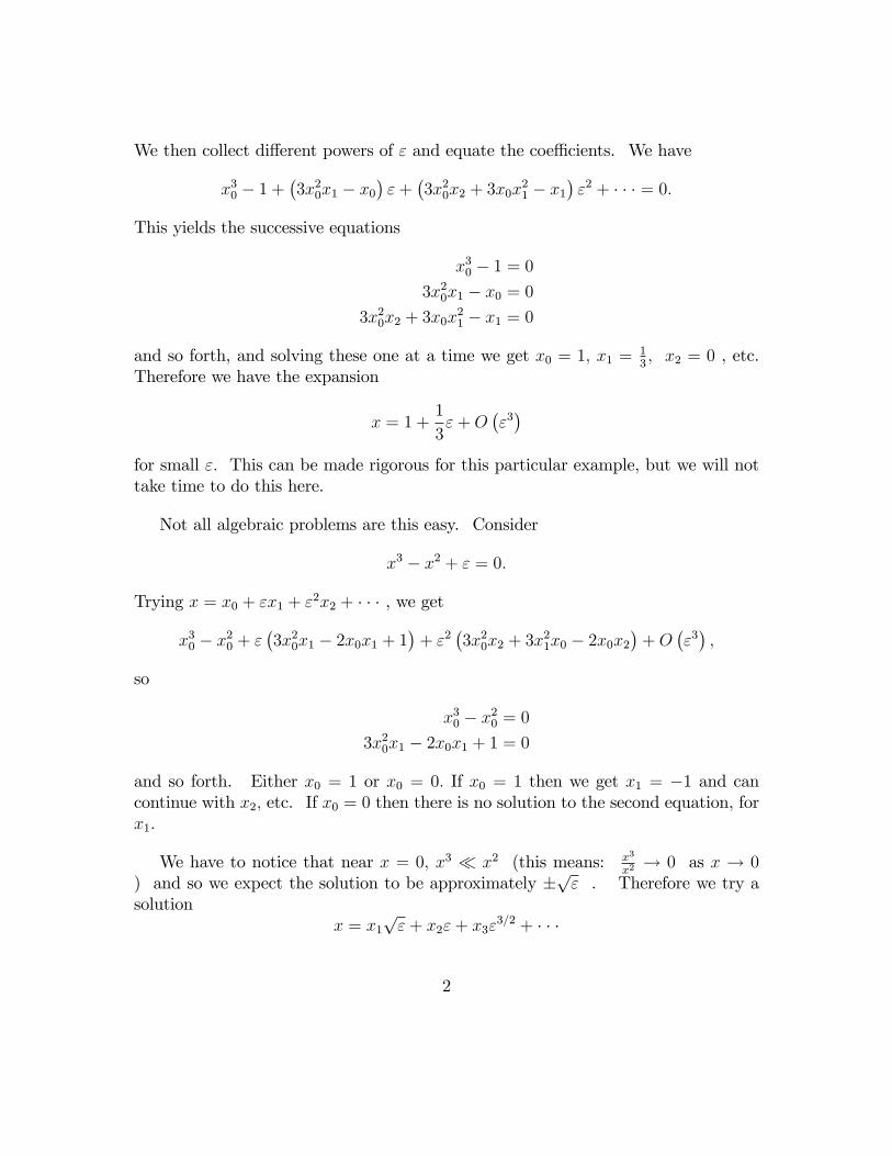
We then collect di¤erent powers of " and equate the coe¢ cients. We have

x30 � 1 +�3x20x1 � x0

�"+

�3x20x2 + 3x0x

21 � x1

�"2 + � � � = 0:

This yields the successive equations

x30 � 1 = 03x20x1 � x0 = 0

3x20x2 + 3x0x21 � x1 = 0

and so forth, and solving these one at a time we get x0 = 1; x1 = 13; x2 = 0 , etc.

Therefore we have the expansion

x = 1 +1

3"+O

�"3�

for small ": This can be made rigorous for this particular example, but we will nottake time to do this here.

Not all algebraic problems are this easy. Consider

x3 � x2 + " = 0:

Trying x = x0 + "x1 + "2x2 + � � � , we get

x30 � x20 + "�3x20x1 � 2x0x1 + 1

�+ "2

�3x20x2 + 3x

21x0 � 2x0x2

�+O

�"3�;

so

x30 � x20 = 0

3x20x1 � 2x0x1 + 1 = 0

and so forth. Either x0 = 1 or x0 = 0: If x0 = 1 then we get x1 = �1 and cancontinue with x2; etc. If x0 = 0 then there is no solution to the second equation, forx1:

We have to notice that near x = 0; x3 � x2 (this means: x3

x2! 0 as x ! 0

) and so we expect the solution to be approximately �p" . Therefore we try a

solutionx = x1

p"+ x2"+ x3"

3=2 + � � �

2

This will work out and we will be able to �nd the coe¢ cients. Again this can bemade rigorous.

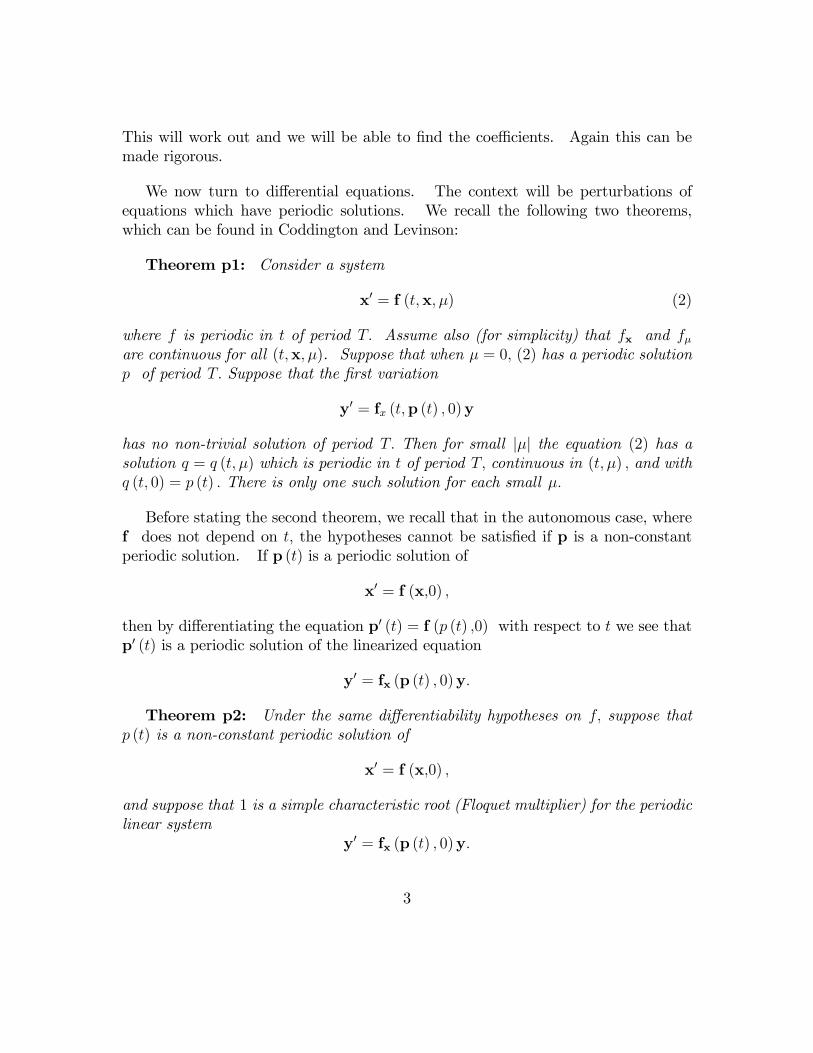
We now turn to di¤erential equations. The context will be perturbations ofequations which have periodic solutions. We recall the following two theorems,which can be found in Coddington and Levinson:

Theorem p1: Consider a system

x0 = f (t;x; �) (2)

where f is periodic in t of period T: Assume also (for simplicity) that fx and f�are continuous for all (t;x; �). Suppose that when � = 0; (2) has a periodic solutionp of period T: Suppose that the �rst variation

y0 = fx (t;p (t) ; 0)y

has no non-trivial solution of period T: Then for small j�j the equation (2) has asolution q = q (t; �) which is periodic in t of period T; continuous in (t; �) ; and withq (t; 0) = p (t) : There is only one such solution for each small �:

Before stating the second theorem, we recall that in the autonomous case, wheref does not depend on t; the hypotheses cannot be satis�ed if p is a non-constantperiodic solution. If p (t) is a periodic solution of

x0 = f (x;0) ;

then by di¤erentiating the equation p0 (t) = f (p (t) ;0) with respect to t we see thatp0 (t) is a periodic solution of the linearized equation

y0 = fx (p (t) ; 0)y:

Theorem p2: Under the same di¤erentiability hypotheses on f; suppose thatp (t) is a non-constant periodic solution of

x0 = f (x;0) ;

and suppose that 1 is a simple characteristic root (Floquet multiplier) for the periodiclinear system

y0 = fx (p (t) ; 0)y:

3

Then for small j�j the systemx0 = f (x;�)

has a solution q (t; �) of period T (�) : Both q and T are continuous in � for su¢ -ciently small j�j ; with q (t; 0) = p (t) and T (0) = T:

Our goal in this section is to study cases where these theorems do not apply.Here is a simple example (with " as the parameter instead of � :

x0 = " sin t x:

The unperturbed equation isx0 = 0;

and so any constant is a periodic solution. The linearized equation is the same, andso neither theorem applies. We can get a unique periodic solution by adding aninitial condition: say

x (0) = 1:

We can solve the complete equation exactly:

x (t; ") = e�" cos t:

Thus there is a periodic solution for every "; and lim"!0 x (t; ") = 1 uniformly on theentire line �1 < t <1:

Now consider the examplex0 = " sin2 t x:

This is still a periodic equation. The solution with x (0) = 1 is

x (t; ") = e"(t2� sin 2t

4 ): (3)

which is not periodic. In fact, it is unbounded, and so it is not true that lim"!0 x (t; ") =1 uniformly on the entire line �1 < t <1.

It is true, however, that lim"!0 x (t; ") = 1 uniformly on any compact interval[�M;M ] : But this is not saying much. We recall that solutions of the initial valueproblem x0 = " sin2 t x; x (0) = 1 are continuous with respect to ": To be moreprecise, the function x (t; ") which solves this initial value problem is continuous inthe pair (t; ") for each (t; ") where the solution exits. It is not hard to show thatthe solution exists for all (�; ") : So from advanced calculus we know that x (t; ") is

4

uniformly continuous on any compact set. In particular, it is uniformly continuouson

f(t; ") j0 � " � 1;�M � t �Mg ;and so the statement that lim"!0 x (t; ") = x (t; 0) is true uniformly on jxj � M: Noparticular information about the exact solution is required for this conclusion. Butknowing the exact solution we can say something stronger. Consider any interval�M (") � t � M (") with the property that lim"!0+ "M (") = 0: We see from (3)that

lim"!0+

sup fjx (t; ")� 1j j �M (") � t �M (")g = 0:

For example, we could have M (") = jlog "j : (Thus, M (") can be unbounded as"! 0:) In this case we would say that 1 approximates x (t; ") uniformly �on a scale ofO (jlog "j) : This is more than we get from the basic fact that solutions are continuouswith respect to ". Note, however, that we do not get uniform approximation on ascale of O

�1"

�: .

Later we will consider the problem of �nding approximate solutions on some setin more detail.

But �rst we consider another example, this time autonomous. Theorem p2 willnot apply. The equation is van der Pol�s equation, written as

x00 + "�x2 � 1

�x0 + x = 0: (4)

This is an important example which we will consider at some length.

The unperturbed equation is

x00 + x = 0:

Obviously this has many periodic solutions. You should check that the hypothesesof Theorem p2 do not apply. To within a translation in t they can all be writtenas

x = A cos t:

Any A will do. Yet, we know that for positive "; (4) has a unique periodic solution,say x (t; ") : Presumably, as "! 0; this solution tends to one of the periodic solutionwhen " = 0: The problem is, which one?

There are many approaches to this problem. Let�s start with the �naive expan-sion�approach. This means that we look for a solution

x (t; ") = x0 (t) + "x1 (t) + � � �:

5

Substituting into the di¤erential equation we have

x000 + "x001 + � � �+ "�(x0 (t) + "x1 (t) + � � �)2 � 1

�(x00 (t) + "x01 (t) + � � �)

+x0 (t) + "x1 (t) + � � � = 0:

Equating coe¢ cients of di¤erent powers of "; we get

x000 + x0 = 0

x001 +�x20 � 1

�x00 + x1 = 0;

and so forth. (This is all we need to get an interesting conclusion.) We can writethe general x0 as

x0 = A cos (t� t0) ;

but A is still to be determined. We can choose the initial condition so that t0 = 0:We then have

x001 + x1 =�1� A2 cos2 (t)

�(�A sin (t)) = A3 sin t cos2 t� A sin t:

This is a linear equation which can be solved by the variation of parameters method.Being lazy, we use Maple and get the general solution as x1 (t) = �1

8A3 sin t cos2 t�

18(cos t)A3t+ 1

2(cos t)At+ C1 cos t+ C2 sin t:

We are looking for a periodic solution. Recall that we have not speci�ed A: Twoof the terms for x1 have factors of t; which are not periodic, and which in fact areunbounded. If we are to �nd a periodic solution we must choose A so the sum ofthese terms vanishes. (This is called a �non-resonance�condition, or a condition to�eliminate secular terms�. ) This gives �A3

8+ A

2= 0; or A2 = 4: Therefore, we

conjecture that the amplitude of x0 should be A = 2: However:

This is not a rigorous proof!

Nevertheless, we may be impressed that this naive approximation method seemsto give an answer. So before turning to rigorous methods, we consider anotherexample: We will now try to apply the method to the following equation:

x00 + x+ "x3 = 0; (5)

looking for periodic solutions. Once again we try

x = x0 (t) + "x1 (t) + � � �;

6

and we �nd the equations

x000 + x0 = 0

x001 + x1 = �x30:

We set x0 (t) = A cos t and solve the x1 equation:

x001 + x1 = �A3 cos3 t (6)

The exact solution is : x1 (t) = 18A3 cos3 t� 3

8A3 cos t� 3

8A3 (sin t) t+C1 cos t+C2 sin t

Now we �nd only one resonant term, the second, and to get rid of it, the onlypossibility is that A = 0:

So we ask: Does that mean that our equation has no periodic solutions exceptpossibly some with small amplitude, order "?

We know this is not true. There is an energy function for (5) ;namely 12x02 +

12x2+ "

4x4; and all of the curves E = constant give periodic solutions. These can be

arbitrarily large in amplitude, for any " � 0: So why don�t we �nd these with ourasymptotics?

The answer is seen by looking carefully at what is implied by the equation

x (t; ") = x0 (t) + "x1 (t) +O�"2�:

Suppose that all of the xk (t) are periodic with some period T: Then we are expectingthat as " ! 0; the periodic solution tends uniformly in time (since we only haveto look at a �xed interval [0; T ] ) to a limiting nontrivial periodic solution x0 (t).This does not allow for the possibility that the period of x (t) will probably not bethe same as the period of x0 (t) ; and therefore, for any small "; the solution willeventually drift away from x0 (t) ; even if the orbits of x0 (t) and x (t; ") are veryclose. In fact, this could, and does, happen for van der Pol�s equation also. So ourderivation of the limiting value of A = 2 in van der Pol�s equation is very suspiciousindeed. We now consider an important method for resolving this di¢ culty, calledthe

Method of Averaging.

We will now give still another approach to van der Pol�s equation, and this onewe will make rigorous.

7

This material appears in GH, but here I will also use the Grimshaw referencegiven at the beginning of the course. We will start by reconsidering one of our �rstorder examples, namely

x0 = "f (x; t; ") = " sin2 t x:

x (0) = 1:

(We introduce " into the function f for greater generality later on, but in thisexample, f does not depend on ":)

First we look on an O (1) time scale. Consider a �xed interval [0; T ] : From thebasic theorem about continuity of solutions with respect to parameters, it followsthat

lim"!0

x (t; ") = 1:

uniformly on [0; T ]. However we saw before that x = 1 is a valid uniform approxi-

mation over a larger time scale, such as 0�1p"

�:For example, suppose that " = 10�4:

The approximation is valid over [0; 100] : We notice that in this interval x0 has aboutseven oscillations. The method of averaging is based on an assumption that theoscillations will somehow average out, and allow us to �nd an approximation validon even a longer time interval.

The way we average is to let

�F (x; ") =1

2�

Z 2�

0

f (x; t; ") dt:

In this case the result is simple:

�F (x; ") =1

2�

Z 2�

0

x sin2 t dt =1

2�x

�t

2� sin 2t

4

�j2�0

=x

2:

The so called �averaged�equation is

y0 = " �F (x; 0)

= "x

2;

8

with solution y (t) = e"t2 : We then have:

jx (t; ")� y (t; ")j = e"t2

�1� e�"

sin 2t4

�For a �xed "; this is unbounded as t!1; so we do not have uniform convergenceon [0;1): However, if t = K

"for some �xed K; then

jx (t; ")� y (t; ")j =����x�K" ; "

�� y

�K

"; "

����� = eK2

�1� e�"

sin K"4

�which does tend to zero as "! 0: For 0 � t � K

"we have

jx (t; ")� y (t; ")j =����x�K" ; "

�� y

�K

"; "

����� = eK2

�1� e�"

sin K"4

�� e

K2

�e"4 � 1

�:

(You need to compare 1� e�"4 and e

"4 � 1 to verify this.) Hence

lim"!0

jx (t; ")� y (t; ")j = 0

uniformly on�0; K

"

�; and so y approximates x on a time scale of O

�1"

�: This is

true not just for a periodic solution (there aren�t any for this equation) but for anysolution. We will see in higher order examples that this is a very useful method.

In the method of averaging as applied to nonlinear oscillators such as van derPol�s equation or Du¢ ng�s equation, we consider a system in polar coordinates ofthe form

r0 = "F (r; �; ")

�0 = ! (t) + "G (r; �; ")

where ! (t) is bounded away from zero and F and G are periodic with period 2�in �: In our applications we will have ! (t) = �1 for all t. This means that forsmall �; r changes slowly compared with �: Therefore we expect that on some timescale we may be able to approximate the solution by averaging the r equation withrespect to �: We let

�F (r; ") =1

2�

Z 2�

0

F (r; �; ") d� (7)

and consider the equationR0 = " �F (R; 0) : (8)

9

Since r0 ! 0 as "! 0; and also R0 ! 0; we expect that if R (0) = r (0) ; then Rand r will both be close to r (0) over an O (1) time scale. This is just the statementthat the solutions are uniformly continuous in " over a compact interval [0; T ] ,where T is constant. It turns out, however, that r is close to R over the muchlonger interval O

�1"

�. In such an interval, r can change signi�cantly and so by

studying the single equation for R; we get interesting information about just how rchanges. The complete solution (r; �) consists of the slow but signi�cant change inr on the O

�1"

�time scale and the relatively fast oscillations due to changes of � on

the O (1) time scale.

Grimshaw uses rather di¤erent notation from what I have used. GH presentssimilar material, (chapter 4) with still di¤erent notation. Because I am mainlyinterested in the two applications we have already studied, I will stick with r and R:

We consider �rst the autonomous case, with a second order equation of the form

u00 + u = "f (u; u0; ") : (9)

Note that both van der Pol�s equation and Du¢ ng�s equation in the form above canbe written like this. We then let

x = u; y = u0

and write a system

x0 = y (10)

y0 = �x+ "f (x; y; ") :

Switching to polar coordinates we write

x = r cos �; y = r sin �

so that

x0 = r0 cos � � (r sin �) �0 = r sin � (11)

y0 = r0 sin � + (r cos �) �0 = �r cos � + "f (r cos �; r sin �; ") :

10

We can easily solve these, by multiplying the equations by cos � and sin � andadding and subtracting in the right way, and we get

r0 = " sin �f (r cos �; r sin �; ") = "F (r; �; ") (12)

�0 = �1 + "

rcos �f (r cos �; r sin �; ") = �1 + "G (r; �; ") :

Notice that both F and G are periodic in � with period 2�. We let

�F (r; ") =1

2�

Z 2�

0

F (r; �; ") d�:

We then use (7) and (8) to obtain the �averaged equation�

R0 = " �F (R; 0) : (13)

Note that we have evaluated �F at " = 0; but the equation for R does have " onthe right hand side.

We will state and prove a theorem concerning the relation between R (t) andr (t) ; but �rst let us try applying this to the same Du¢ ng equation as before:

x00 + x+ "x3 = 0:

Recall that all solutions are periodic. So the problem here is not to show that thereare periodic solutions. However the period of the solution depends on its amplitude.We can ask, for example, whether the period increases or decreases with amplitude,and by how much for a given small ": The energy function

E (t) =x02

2+x

2

2

+x4

4

can be used to determine this but we can also use averaging, at least for small ":

The equations for r and � become:

r0 = �" sin �r3 cos3 ��0 = �1� "r2 cos4 �:

11

Therefore�F (r; ") = � 1

2�

Z 2�

0

sin � cos3 � d� = 0

and so the averaged R equation is

R0 = 0:

Therefore, R = A = constant.

Usually the method stops with the equation for R; but let us proceed to study �:If we let (t) = � (t) + t we get

0 = �"rcos ( � t) r3 cos3 ( � t) :

Let�G ( ; ") =

1

2�

Z 2�

0

r2 cos4 ( � t) dt:

This turns out to be �38r2; (independent of ). The averaged equation for is

0 = �38R2"

with solution = �38R2"t: Therefore the approximate angle is � = �t � 3

8R2"t

and we obtain the averaged solution

�x = A cos

��t� 3

8A2"t

�= A cos

�t+

3

8A2"t

�:

This suggests that the period is approximately 2�1+ 3

8A2"

; though of course we have

proved nothing rigorously yet.

We now state and prove our theorem concerning averaging. This is basicallyfrom Grimshaw.

Theorem 1: Suppose that there is a C0 > 0; R0; and "0 > 0 such that for0 < " < "0; the solution R (t) (= R(t; ")) of (13) with R (0) = R0 exists on theinterval

�0; C0

"

�. Suppose that there is an M > 0 such that jR (t)j � M for all

t 2�0; C0

"

�: (M is independent of ":) Then there is a C1 (independent of ") such

that if (r; �) solves (12) with r (0) = R (0) ; then (r; �) exists on�0; C0

"

�and on this

intervaljR (t)� r (t)j � C1":

12

Thus, R approximates r on a time scale of O�1"

�:

(In the case of periodic solutions of (9) ; we expect the period to be close to 2�;so an O

�1"

�time interval is more than enough to detect periodicity, as we will see

rigorously below. )

Proof: This proof is fairly technical. One source of technicality is the assumeddependence of f and g on ", which leads to an assumption that F and G dependson ". Yet, in our examples, the f and g do not not depend on ": So I will givea proof in the case where f; g and so F;G are independent of " and then outlinewhat changes are needed for the general case. So we will assume that the equationsin polar coordinates are

r0 = "F (r; �)

�0 = �1 + "G (r; �)

We then have�F (r) =

1

2�

Z 2�

0

F (r; �) d�:

Let F̂ (r; �) = F (r; �)� �F (r) : Then F̂ has period 2� in �, andZ 2�

0

F̂ (r; �) d� = 0:

Let

H (r; �) =

Z �

0

F̂ (r; s) ds:

Then H (r; 0) = H (r; 2�) = 0 and H has period 2� in �: Also, H is bounded in theregion jrj � 2M: (We need to choose a larger region than the bound assumed on R;since r could be a little bigger than R: The bound jrj � 2M is much larger thanwe actually need, but simple to work with.

Now letr̂ (t) = r (t) + "H (r (t) ; � (t)) :

13

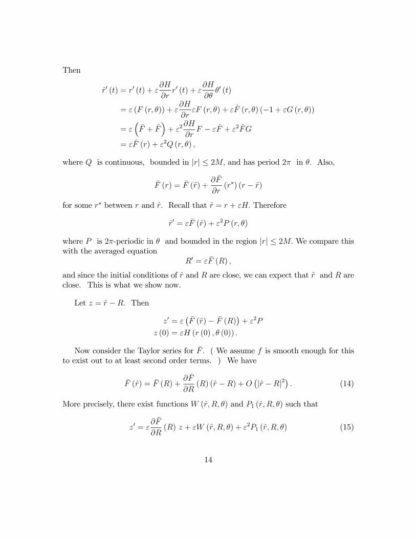
Then

r̂0 (t) = r0 (t) + "@H

@rr0 (t) + "

@H

@��0 (t)

= " (F (r; �)) + "@H

@r"F (r; �) + "F̂ (r; �) (�1 + "G (r; �))

= "��F + F̂

�+ "2

@H

@rF � "F̂ + "2F̂G

= " �F (r) + "2Q (r; �) ;

where Q is continuous, bounded in jrj � 2M; and has period 2� in �: Also,

�F (r) = �F (r̂) +@ �F

@r(r�) (r � r̂)

for some r� between r and r̂: Recall that r̂ = r + "H: Therefore

r̂0 = " �F (r̂) + "2P (r; �)

where P is 2�-periodic in � and bounded in the region jrj � 2M: We compare thiswith the averaged equation

R0 = " �F (R) ;

and since the initial conditions of r̂ and R are close, we can expect that r̂ and R areclose. This is what we show now.

Let z = r̂ �R: Then

z0 = "��F (r̂)� �F (R)

�+ "2P

z (0) = "H (r (0) ; � (0)) :

Now consider the Taylor series for �F : ( We assume f is smooth enough for thisto exist out to at least second order terms. ) We have

�F (r̂) = �F (R) +@ �F

@R(R) (r̂ �R) +O

�jr̂ �Rj2

�: (14)

More precisely, there exist functions W (r̂; R; �) and P1 (r̂; R; �) such that

z0 = "@ �F

@R(R) z + "W (r̂; R; �) + "2P1 (r̂; R; �) (15)

14

and further, there is a K > 0 such that if jr̂ �Rj and " are su¢ ciently small, then

jW (r̂; R; �)j � K jr̂ �Rj2

jP1 (r̂; R; �)j � K:

We also havez (0) = "H (r (0) ; � (0)) :

We choose K as well so that jH (r; �)j � K for jrj � 2M: Now let � =m"KC0e

KC0 where C0 was given in the statement of the Theorem and

m =8

5

C0 + 1

C0:

(We shall need that later.) Then jz (0)j = " jH (r (0) ; � (0))j < "K: SincemC0e

KC0 > 1 we see that jz (0)j < � . Hence there is some t1 = t1 (") suchthat jzj � � on [0; t1] :We must also assume that "t1 � C0: Our goal is to show that

we can choose t1 = C0":

We then integrate the absolute value of the right side of (15) ; choosing K in

addition larger than maxjrj�2Mn���@ �F@R ���o ; and get

jz (t)j � jz (0) j+K"

Z t

0

jz (s)j ds+K�2"t+K"2t:

� K"

Z t

0

jz (s)j ds+K�2"t+K"2t+K":

on the interval [0; t1] where jzj � �. This is valid because jzj2 = jr̂ �Rj2 � �2 on[0; t1] ; and also jrj � jr̂j +K" � R + jzj +K" � M + j�j +K" < 2M; if " is smallenough.

On [0; t1] we have "t � C0, and therefore K"2t � K"C0 and K�2"t � K�2C0:Then from Gronwall�s lemma we get

jz (t)j ��K�2C0 + "KC0 +K"

�eK"t �

�K�2C0 + "KC0 +K"

�eKC0 : (16)

15

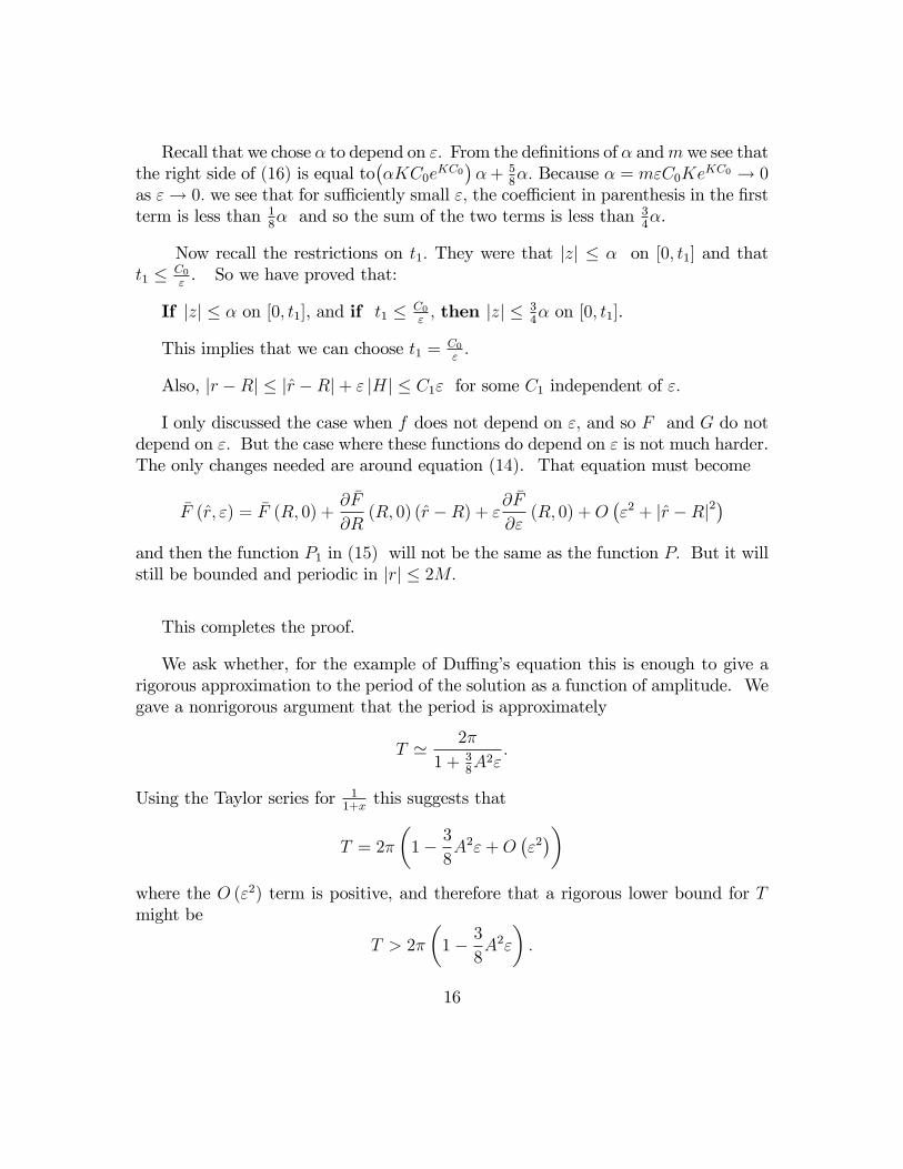
Recall that we chose � to depend on ": From the de�nitions of � andm we see thatthe right side of (16) is equal to

��KC0e

KC0��+ 5

8�: Because � = m"C0Ke

KC0 ! 0as "! 0: we see that for su¢ ciently small "; the coe¢ cient in parenthesis in the �rstterm is less than 1

8� and so the sum of the two terms is less than 3

4�.

Now recall the restrictions on t1: They were that jzj � � on [0; t1] and thatt1 � C0

". So we have proved that:

If jzj � � on [0; t1], and if t1 � C0"; then jzj � 3

4� on [0; t1].

This implies that we can choose t1 = C0":

Also, jr �Rj � jr̂ �Rj+ " jHj � C1" for some C1 independent of ":

I only discussed the case when f does not depend on "; and so F and G do notdepend on ": But the case where these functions do depend on " is not much harder.The only changes needed are around equation (14). That equation must become

�F (r̂; ") = �F (R; 0) +@ �F

@R(R; 0) (r̂ �R) + "

@ �F

@"(R; 0) +O

�"2 + jr̂ �Rj2

�and then the function P1 in (15) will not be the same as the function P: But it willstill be bounded and periodic in jrj � 2M:

This completes the proof.

We ask whether, for the example of Du¢ ng�s equation this is enough to give arigorous approximation to the period of the solution as a function of amplitude. Wegave a nonrigorous argument that the period is approximately

T ' 2�

1 + 38A2"

:

Using the Taylor series for 11+x

this suggests that

T = 2�

�1� 3

8A2"+O

�"2��

where the O ("2) term is positive, and therefore that a rigorous lower bound for Tmight be

T > 2�

�1� 3

8A2"

�:

16

By de�nition of the polar coordinates, a period is de�ned by �nding T such that� (T ) = �2�: (We know that �0 is approximately �1; hence the minus sign.)

For Du¢ ng�s equation we found that the averaged equation was

R0 = 0:

So solutions R = A exist on (�1;1) and are bounded. Hence the hypotheses ofTheorem 1 are satis�ed for any C0: Choosing C0 = 1 we can assert that there is aC1 such that jr � Aj < C1" on [0; 1

"]: Turning to the � equation we then have

�0 = �1� "r2 cos4 �:

It is less confusing to set (t) = �� (t) and get and estimate of T such that (T ) =2�: We have

0 = 1 + "2r2 cos :

From the bounds on r we get upper and lower bounds on 0: An upper bound for 0 should give us a lower bound for T: An upper bound for 0 is

0 < 1 + "B2 cos4 :

where B = A+ C1":Homework: Use the method of separation of variables to prove that

if � > 38; then for su¢ ciently small ";

T > 2�(1� �A2"):

You may want to make use one of the inequalities

1� x+ x2 >1

1 + x> 1� x: (17)

for small x > 0:

Using the same methods more precisely would give the result that

lim"!0

T � 2�"

= 2�

�3

8A2�:

Theorem 2 Suppose in addition to the hypotheses of Theorem 1 that R0 is anisolated equilibrium point of the averaged equation (13) : Suppose also that @ �F

@RjR0 6= 0:

17

Then for each su¢ ciently small " > 0 there is a periodic solution of (12), such thatlim"!0 r (t) = R0 (t) uniformly in t: If "@ �F

@RjR0 < 0 then this solution is stable,

while if "@ �F@RjR0 > 0 it is unstable.

Proof:

Once again I will only discuss the case when f; and so F;G; are independent of ":For small "; �0 < �1

2on�0; 1

"

�and so on this interval we can think of r as a function

of �: We have

dr

d�= "

F (r; �)

�1 + "G (r; �)= "K (r; �; ") : (18)

This system is non-autonomous, but the original system (12) is autonomous.Further, since � must cross some negative multiple of 2� in any time interval oflength o

�1"

�; and since F and G have period 2� in �; we can assume that � (0) = 0.

Assume that r (0) = r0: We want to �nd r0 such that r (�2�; r0; ") = r0: butsince the di¤erential equation for r is 2�-periodic in �; this is the same as sayingr (2�; r0; ") = r0: We denote the solution to (18) by r (�; r0; "). (This is an �abuseof notation�, since before we would have discussed �r (t; r0; �0; ")�.)

For " > 0 letN (r0; ") =

1

"(r (2�; r0; ")� r0)

We wish to �nd a solution to the equation

N (r0; ") = 0;

We �rst have to extend the de�nition of N to " = 0 so that N is smooth and wecan apply the implicit function theorem.

From (18) we have

r (�; r0; ") = r0 + "

Z �

0

K (r (s; r0; ") ; s; ") ds

18

and so

N (r0; ") =

Z 2�

0

K (r (s; r0; ") ; s; ") ds

=

Z 2�

0

F (r (s; r0;") ; s)

�1 + "G (r (s; r0; ") ; s)ds:

Then it is obvious that N can be extended to " = 0 with

N (r0; 0) =

Z 2�

0

�F (r0; s) ds (19)

= �2� �F (r0) ;

HenceN (R0; 0) = 0:

and@N (R; 0)

@rjr=R0 = �2�

@ �F

@R(R0) 6= 0;

and therefore the implicit function theorem says that for small " there is an r0 (")such that N (r0 (") ; ") = 0: Also, r0 (") ! R0 as " ! 0: This gives the desiredfamily of periodic solutions and proves the existence part of the theorem.

For the stability, we consider an initial condition r1 6= r0 (") : We have

r (�; r1; ") = r1 +

Z �

0

K (r (s; r1; ") ; s; ") ds;

r (�2�; r1; ") = r1 +

Z �2�

0

K (r (s; r1; ") ; s; ") ds

= �Z 0

�2�K (r (s; r1; ") ; s; ") ds:

We let

M (r1; ") = r (�2�; r1; ")� r1 = �Z 0

�2�K (r (s; r1; ") ; s; ") ds::

r (�2�; r1; ") = r1 + "M (r1; ") :

19

Also,

M (r1; ") =M (r0 (") ; ") +@M

@r(r�; ") (r1 � r0 ("))

=@M

@r(r�; ") (r1 � r0 ("))

for some r� between r1 and r0 ("). We have

M (R0; 0) = �Z 0

�2�K (R0; s; 0) ds = �

Z 2�

0

K (R0; s; 0) ds = �N (R0; 0) :

The second step is because K has period 2� in �: If @Fdr(R0; 0) = �� < 0; then from

(19) ;@M

@r(R0; 0) = �

@N

@r(R0; 0) = �

��2�@

�F

@R(R0)

�= �2�� < 0

; and for su¢ ciently small jr1 �R0j+ j"j we have @M@r(r�; ") � �2� �

2: Hence for the

case " > 0 we have

jr (�2�; r1; ")� r0 (")j =�����1 + "@M@r (r�; ")

�(r1 � r0 ("))

���� � (1� ��") j(r1 � r0 ("))j :

Iterating this map of r1 ! r (�2�; r1; ") over and over, we see that the solution tendsto r0 (") ; at an exponential rate. More speci�cally, we have jr (�2k�)� r0j �(1� ��")k jr (0)� r0j ; where r is a function of �: : Since �0 = �1 +O (") ; we can,approximately, replace � with�t:We see that with r a function of t; jr (2k�)� r0j �(1� ��")k jr (0)� r0j : Taking logs,

log jr (2k�)� r0 (")j � log jr (0)� r0j+ k log (1� ��") � �k��"

as k !1:: Hence jr (t)� r0j = O�e�

�"2t�:

Remark: That word �approximately�above means that this is not rigorous! Asan exercise you should try to �x this point.

Applications:

It is easy to apply this to the van der Pol equation. We have, from (12) ;

f (x; y) =�1� x2

�y

20

and so�F (r; ") =

1

2�

Z 2�

0

�1� r2 cos2 �

�r sin2 �d�

=1

2�

��r � 1

4r3�

�:

We see that the desired zero is R0 = 2; con�rming that there is a family of periodicsolutions for " > 0 which tends to the circle of radius 2 in the phase plane as "! 0:This is �nally is a rigorous proof of this result.

We also get information about other solutions, besides the periodic one. Theaveraged equation is

R0 = "

�R

2� 18R3�

with solution R = 2p1+4ce�"t

and so every solution of the average equation satis�es

limt!1

R (t) = 2:

This is consistent with stability of the periodic solution, but we have not provedthis, since our theorem only says that the averaged solution is an approximation ofthe periodic solution for times of order O

�1"

�: However a stronger statement of the

theorem, given in GH, pg. 168, says that solutions on the stable manifold of theperiodic solution are approximated by solutions on the stable manifold of the �xedpoint of the averaged equation uniformly on [0;1): The complete proof is not giventhere however, and reference is made to an article from 1982, which apparently wasthe �rst complete proof.

Averaging gets more interesting when we turn to non-autonomous equations,namely equations of forced oscillations. The general form to be considered now is

x00 + x = "g (x; x0; t; ") (20)

where g is periodic in t with period T:

The di¢ culty of �nding approximate solutions of (20) depends on how near to�resonance� it is. We have not de�ned resonance for a nonlinear system, but byconsidering the linear case we can see that solutions are more di¢ cult if T = 2�;since that is the natural frequency of the unforced system.

21

Another point to be kept in mind is that g may contain a linear part, say �xwhich will a¤ect the period. It is convenient to write the equation as

x00 + (1 + �")2 x = "h (x; x0; t; ") :

Consider, for example, the linear nonautonomous case where

h (x; x0; t; ") = cos t:

Thus we havex00 + (1 + �")2 x = " cos t:

We see that if � 6= 0; then for any �xed "; there is no resonance, since the forcingfrequency is di¤erent from the natural frequency. But it is not clear what happensas " ! 0; since in this limit the natural frequency is becoming closer to the forcingfrequency, but on the other hand the forcing amplitude is going to zero.

We can use the variation of parameters formula to show that this equation has aunique solution with the period, 2�, of the forcing function. This solution is mosteasily found by trying a solution A cos t+B sin t: We �nd that

x ="

(1 + �")2 � 1cos t:

Expanding the coe¢ cients in terms of "; we �nd that as " ! 0 we approach thesolution

1

2�cos t:

It is common to study the amplitude of the solution as a function of the �tuningparameter�� . This is the curve y =

�� 12�

�� :Now we want to see how this curve changes if we add two terms: a small damping

term, and a small nonlinear term.

We can start by adding a damping term to the linear equation, giving

x00 + "�x0 + (1 + �")2 x = " cos t

As "! 0 the unique periodic solution now approaches

2�

4�2 + �2cos t+

�

4�2 + �2sin t:

22

For positive � the amplitude is now bounded as �! 0; approaching 1�:

Next , we set the damping equal to zero and add a cubic term. We also followGrimshaw and put the term keeping the linearized equation away from resonance onthe right hand side. This � is not quite the same as the � above, which would haveincluded �2 if we had put the � terms on the right, but it still is �near resonance�as " ! 0: We wish to use averaging to �nd the limiting amplitude response curve.We will now allow for a variable strength forcing, though still proportional to ":

x00 + x = "�G0 cos t� �x+ x3

�; (21)

We will see the e¤ect of the nonlinear term "x3:

We �rst try the simple expansion

x = x0 + "x1 + :::

and get

x000 + x0 = 0

x001 + x1 = (G0 � A�) cos t+ A3 (cos t)3

Going through our usual procedure to eliminate resonance gives

G0 � �A+3

4A3 = 0:

This gives at least one, and perhaps three values of A; depending on �: Notice thatwe don�t have to use multiple scales here, assuming that G0 and � are non-zero.But this is only at the �rst stage. The naive method might fail when we look forx2: (I haven�t tried it!) .

Now let�s try averaging on this problem. It is of a di¤erent form from before,and the averaging must now be in t instead of the phase variable �: This requires adi¤erent approach.

The general averaging theorem for non-autonomous perturbations is given in GH,page 168. For the special case of (21) we proceed as follows.

23

We write this as a system

x0 = y (22)

y0 = �x+ "g (x; y; t; ")

and look for a solution of the form

x = a (t) cos t+ b (t) sin t (23)

y = �a (t) sin t+ b (t) cos t:

The hope is that because x02 + y02 = 2"yg (x; y; t; ") ; and so the amplitude of theoscillation changes slowly, we will �nd that a (t) and b (t) change slowly. The solutionis then an oscillation with period equal to 2� and with slowly varying amplitude.The period must be exactly 2� because g has period 2�:

To �nd equations satis�ed by a and b we di¤erentiate (23) and use (22) : Thus,

x0 = a0 cos t� a sin t+ b0 sin t+ b cos t = y = �a sin t+ b cos t

y0 = �a0 sin t� a cos t+ b0 cos t� b sin t = �x+ "g = �a cos t� b sin t+ "g (x; y; t; ")

where we substitute the expressions on the right of (23) for x and y in this lastequation. Solving for a0 and b0 gives

a0 = �" sin t g (x; y; t; ") = "F (a; b; t; ") (24)

b0 = " cos t g (x; y; t; ") : = "G (a; b; t; ") :

Thus, as expected, a0 and b0 are O (") : Note that F and G are of period 2� in t.

We now use averaging by letting

�F (a; b; ") =1

2�

Z 2�

0

F (a; b; t; ") dt

�G (a; b; ") =1

2�

Z 2�

0

G (a; b; t; ") dt:

The averaged equations are then

A0 = " �F (A;B; 0) (25)

B0 = " �G (A;B; 0) :

24

Before proceeding, note the hierarchy of averaged equations. For a singlenon-autonomous equation,

x0 = "f (x; t; ")

the averaged equation is a �rst order autonomous equation

y0 = " �F (y; 0) :

For a second order autonomous equation

x00 + x = "f (x; x0; ")

the averaged equation was a �rst order autonomous equation (for the amplitude)

R0 = " �F (R; 0) :

For a second order non-autonomous equation

x00 + x = "f (x; x0; t; ")

(equivalent to a nonautonomous system of two �rst order equations) the averagesystem is a system of two �rst order autonomous equations, (25) . The advantageof this over the original nonautonomous system is that it can be studied in the phaseplane.

We have the following theorems:

Theorem 3. Suppose that there is a C0 and a point (A0; B0) such that for eachsu¢ ciently small " > 0 the solution (A;B) of (25) with A (0) = A0; B (0) = B0exists on the interval

�0; C0

"

�: Suppose that jAj + jBj � M on this interval, where

M is a constant independent of ": Then there is a C1 > 0 such that if (a; b)solve (24) and a(0) = A (0) ; b (0) = B (0) ; then (a; b) exists on

�0; C0

"

�and

ja� Aj+ jb�Bj � C1" on�0; C0

"

�:

Theorem 4. Suppose in addition that (A0; B0) is an isolated equilibrium point

of the averaged equation (25) : Suppose also that det�

@ �F@A

@ �F@B

@ �G@A

@ �G@B

�j(A0;B0) 6= 0: Then

for each su¢ ciently small " there is a periodic solution (a; b) of (24), such thatlim"!0 (a; b) = (A0; B0) uniformly in t: This periodic solution has the same stabilityas the equilibrium point does for (25) :

25

The proofs are similar to those of Theorems 1 and 2. See Grimshaw, pg. 225.

We now consider the forced Du¢ ng equation, that is

g (x; y; t; ") = G0 cos t� �x+ x3:

Then,

F (a; b; t; ") = � sin t�G0 cos t� � (a cos t+ b sin t) + (a cos t+ b sin t)3

�G (a; b; t; ") = cos t

�G0 cos t� � (a cos t+ b sin t) + (a cos t+ b sin t)3

�

1

2�

Z 2�

0

(� sin t)�G0 cos t� � (a cos t+ b sin t) + (a cos t+ b sin t)3

�dt

=1

2

��34b3 + b�� 3

4a2b

�

1

2�

Z 2�

0

(cos t)�G0 cos t� � (a cos t+ b sin t) + (a cos t+ b sin t)3

�dt

=1

2

�G0 � �a+

3

4a3 +

3

4ab2�

Hence the averaged equations are

A0 =1

2"B

��� 3

4

�A2 +B2

��(26)

B0 =1

2"

�G0 � A

��� 3

4

�A2 +B2

���:

We �rst look for equilibrium points. From the �rst equation, either B = 0 or� = 3

4(A2 +B2) : But the second alternative gives no equilibrium with G0 6= 0; so

we have B0 = 0; and then A0 satis�es

G0 = A0��3

4A30: (27)

26

Once again we study how the amplitude depends on �; the �response diagram�foramplitude. It is found in practically every book on nonlinear oscillations. SeeGrimshaw, page 204. It gives the amplitude of the periodic solution as a functionof the tuning parameter �: One feature to notice is that for large enough � thereare two solutions A;and the maximum solution tends to in�nity as � ! 1: This isfor the equation (24) ; which has no term for damping of the oscillation.

Notice also that the amplitude is actually jAj : If A < 0 but G0 > 0 then wesolve (27) for small jAj by taking � < 0: Thus there are two branches to the curve.We can study the graph by solving for �:

� =G0 +

34A3

A

for A 6= 0: The graph will plot jAj on the positive vertical axis vs � on the horizontalaxis. There are two branches. On one, � ! �1 as jAj ! 0 and � ! 1 asjAj ! 1: On the other, �!1 both as jAj ! 0 and as jAj ! 1:

If a small damping term is added, giving

x00 + "�x0 + x = "�G0 cos t� �x+ x3

�then we put it on the right side, adding a term � (�a sin t+ b cos t) to the expression

for F (a; b; t; ") : The equation for steady states becomes A2��2 +

��� 3

4A2�2�

=

G20: One di¤erence is that A is bounded, since A2 � G20=�2. There is only one

branch, continuous but not single valued in either A or �: Thus the damping keepsthe amplitude bounded independent of �:

We then want to analyze the stability of the periodic solutions, which our theoremsays is the same as the stability of the equilibrium point, if it is hyperbolic (noeigenvalues with zero real part) . For the � = 0 case we linearize (26) around apoint where G0 = A�� 3

4A3, B = 0: We get the linearized matrix�

0 12"

��� 3

4A2�

12"

���+ 9

4A2�

0

�:

For some values of A; and the corresponding � = G0+34A3

A; the roots will be pure

imaginary and we don�t learn about stability from the linearization. However inthe region where the two terms in the matrix have the same sign we will have onereal positive eigenvalue and one real negative eigenvalue and so the equilibrium point

27

of the averaged equation, and the periodic solution of the unaveraged equation, areunstable. This is the region

3

4A2 < � <

9

4A2

between two parabolas. It can be checked that the parabola on the right intersectsthe right branch of equilibrium points in the (�; jAj) plane exactly where this branchturns around.

For � > 0 it turns out that we can show that the open region outside of theinstability region is stable.

The big advantage of averaging is that it gives information about more than justperiodic solutions. This is seen in Theorems 1 and 3. The information is only overan interval of length O

�1"

�; but that is still useful. In fact, the averaging theorem

in GH, pg. 168, gives further results that hold on [0;1);for special solutions, thoseon the �stable manifold�of a periodic solution. This is a concept we have yet todiscuss, but we will at a later point.

To get information about other solutions besides periodic ones we consider theaveraged system (26). Before we looked for equilibria, which correspond to periodicsolutions. Now we look at other orbits in the (A;B) phase plane. These willapproximate solutions of (24) on a time scale O

�1"

�:

In fact, the (A;B) phase plane is on the cover of Grimshaw�s book, as well ason page 230. It appears in GH on page 183. It will be noted that there are twoperiodic orbits, and three families of periodic solutions.

To analyze the system (26) it is useful to once again use polar coordinates. Weset

A = R cos�

B = R sin�:

Then we �nd that

R0 =1

2"G0 sin� (28)

�0 =1

2R" [G0 cos�]�R

��� 3

4R2�:

28

It is di¢ cult to deal with either (25) or (28) unless, by some chance, there isa conserved quantity, say Q (R;�) in the variables of (28) which is constant alongsolutions. We can have some hope for this because the original system,

x00 + x = "�G0 cos t� �x+ x3

�has a conserved quantity if G0 = 0; namely

E =1

2x02 +

1

2x2 (1 + �)� 1

4x4:

Since in some sense we averaged the term G0 cos t; and it has zero average, we mayhope that there is still a conserved quantity.

It is a bit of work to convert the function E into the new variables, and as far asI took it, I didn�t see that it led to anything. But somehow it was discovered that

1

2�R2 � 3

16R4 �G0R cos�

is constant. This leads to the fact that all the orbits, in either the (R;�) or (A;B)planes, are closed curves or else homoclinic orbits or pairs of heteroclinic orbits as inthe pendulum phase plane.

The number of equilibrium points is seen from (27) to be between 1 and 3;depending on � and G0. Choosing values where there are three, it is found that twoare centers and one a saddle, and that there are two homoclinic orbits tending to thesaddle. One gets a good picture using xpp on the computer.

Theorem 4 tells us that a �xed point of (25) corresponds to a family of periodicsolutions to (24) for small "; if the appropriate Jacobian determinant is nonzero. Itis important to note, however, that a periodic solution of (25) does not necessarilycorrespond to a periodic solution of (24). This is for two reasons: First, solutionsof (25) only approximate solutions of (24) . Second, the period of a solution in the(A;B) phase plane will probably not be 2�: There is no reason for it to have thisvalue, since the (A; :B) phase plane is autonomous, and the periodic solutions havemany di¤erent periods. The superimposed oscillation of period 2� due to the 2�periodicity of F and G; is likely to be incommensurate with the period in the A;Bplane, so that when the solution in the (A;B) plane returns to its starting point,

29

the values of sin t and cos t; in the formula x = a cos t + b sin t; where ja� Aj andjb�Bj are small, will probably not be back to their starting points.

� � � � � � � � � � � � � � � � � � � � � � � � � � � �Relation to Poincaré maps.

There are two notions of Poincaré map which come up frequently in oscillationtheory. The �rst applies to autonomous systems. While the terminology �Poincarémap" may not have been used, the concept was used int he proof of the Poincré-Bendixson theorem. We considered a two dimensional system,

x0 = f (x) (29)

where all vectors were two dimensional, and assumed there was a periodic solutionp (t) ; say of period T: We then considered a transversal, M, which was a linesegment intersecting the orbit of p and not tangent to this orbit at the point ofintersection. We then considered (in the main theorem about asymptotic orbitalstability of p); the ��rst return�map, following the solution through an initial point� until the next point P (�) where this solution again intersectedM. This map,� !P (�) is called a Poincaré map for the system (29) .

There is a second concept of Poincaré map, which is useful in periodic systemsof the form

x0 = f (x;t) (30)

where f (x;t+ T ) = f (x;t) for all (x;t) : This is a map de�ned on Rn where n is thedimension of x: (By contrast, the Poincare map for (29) is a one dimensional map if(29) is a two dimensional autonomous system. )

The Poincaré map for (30) is the map

x0 ! x (T;x0)

where the right side denotes the value at time T of the solution with initial valuex (0) = x0:

This can be interpreted as being of the same dimension as the previous kind ofmap if we write the non-autonomous system (30) on n equations as an autonomoussystem of n+ 1 equations, namely

y0 = f (y;s) (31)

s0 = 1

30

with s (0) = 0: In this case s (t) = t and the systems (30) and (31) are equivalent.Then the Poincare map consists of a map from the n-dimensional subspace s = 0 ofthe (n+ 1) dimensional (x;s) space phase space of (31) to the n-dimensional subspaces = T: Thus, like the map for (29) ; the Poincaré map is on a space of one lessdimension than the phase space for the autonomous system. However in this case,there is no necessary relation to a periodic solution.

If, however, (30) does have a periodic solution p (t), then p (0) will be a �xedpoint for the Poincaré map for (31).

It is useful to look at the following example.:

x0 = "��x+ cos2 t

�(32)

and

y0 = "

��y + 1

2

�: (33)

The general solutions are

x (t) ="2 cos 2t+ 2" sin 2t

2"2 + 8+1

2+ ce�"t

for (32), and

y (t) =1

2+ ce�"t

for (33). The �rst equation, (32) has a unique periodic solution p (t; ") ; obtainedby setting c = 0 in the formula for x (t) : It is a non-autonomous equation, so weconsider the Poincaré map, which is the �time 2�� map, namely x (0) ! x (2�) .We have p (0; ") = "2

"2+8+ 1

2= p0 and this is the �xed point of the Poincaré map.

Nearby points will start at p0 + c for some small c; and the Poincaré map is

x (0) = p0 + c! x (2�) = p0 + ce�2�:

In other words,

P" (x0) ="2

"2 + 8+1

2+

�x0 �

�"2

"2 + 8+1

2

��e�2�:

31

The second equation is autonomous. In this case we again consider the time 2�map. This time of 2� is not intrinsic to the equation. We choose it because of itsrelation to (32). the map is

P0 (y0) =1

2+

�y0 �

1

2

�e�2�:

We therefore see that in this case

P" (z)� P0 (z) = O�"2�

Theorem 3 concerning the method of averaging in a forced oscillation assertsthat solutions of the original equations and the averaged form which start at thesame time stay close together over an O

�1"

�time scale. This is far longer than

one period, so these theorems can be interpreted as saying that the time T Poincarémaps for the two systems are very close �within O (") : The estimate above issmaller because we are considering a �xed interval of length T; not an interval oflength O

�1"

�:

Theorem 4 discusses the relation between a hyperbolic �xed point for the averagedsystem and a periodic solution of the original forced oscillation system. Recall thesystems (24) and (25) , which were

a0 = "F (a; b; t; ")

b0: = "G (a; b; t; ") :

and

A0 = " �F (A;B; 0)

B0 = " �G (A;B; 0) :

The �rst system has a natural time T Poincaré map. The initial value of a periodicsolution is a �xed point for this map. The second system has a time T Poincarémap also, the time being chosen because it is appropriate for the �rst system. Anequilibrium point for the second, autonomous system, is a �xed point for its Poincarémap. The averaging theorem implies that these maps are very close to each other.But before we can go into further detail about this, we need to have a diversion intothe study of Poincaré maps, and indeed, n-dimensional maps in general.

32