math 323: probability...math 323: probability fall 2018 david a. stephens department of mathematics...
TRANSCRIPT
MATH 323: ProbabilityFall 2018
David A. Stephens
Department of Mathematics and Statistics, McGill University
Burnside Hall, Room 1225.

Introduction
Syllabus
1. The basics of probability.
I Review of set theory notation.I Sample spaces and events.I The probability axioms and their consequences.I Probability spaces with equally likely outcomes.I Combinatorial probability.I Conditional probability and independence.I The Theorem of Total Probability.I Bayes Theorem.
0.0 3
Syllabus (cont.)
2. Random variables and probability distributions.
I Random variables.I Discrete and continuous univariate distributions: cdfs, pmfs
and pdfs.I Moments: expectation and variance.I Moment generating functions (mgfs): derivation and uses.I Named distributions:
I discrete uniform,I hypergeometric,I binomial,I Poisson,I continuous uniform,I gamma,I exponential,I chi-squared,I beta,I Normal.
0.0 4
Syllabus (cont.)
3. Probability calculation methods.
I Transformations in one dimension.I Techniques for sums of random variables.
0.0 5

Syllabus (cont.)
4. Multivariate distributions.
I Marginal cdfs and pdfs.I Conditional cdfs and pdfs.I Conditional expectation.I Independence of random variables.I Covariance and correlation.
0.0 6
Syllabus (cont.)
5. Probability inequalities and theorems.
I Markov’s inequality.I Chebychev’s inequality.I Definition of convergence in probability.I The Weak Law of Large Numbers.I The Central Limit Theorem and applications.
0.0 7

Introduction
Introduction
This course is concerned with developing mathematical conceptsand techniques for modelling and analyzing situations involvinguncertainty.
� Uncertainty corresponds to a lack of complete or perfectknowledge.
� Assessment of uncertainty in such real-life problems is a com-plex issue which requires a rigorous mathematical treatment.
� This course will develop the probability framework in whichquestions of practical interest can be posed and resolved.
0.0 9

Introduction (cont.)
Uncertainty could be the result of
� incomplete observation of a system;
� unpredictable variation;
� simple lack of knowledge of the “state of nature”.
0.0 10

Introduction (cont.)
“State of nature”: some aspect of the real world.
� could be the current state that is imperfectly observed;
� could be the future state, that is, the result of an experimentyet to be carried out.
0.0 11
Introduction (cont.)
Example (Uncertain states of nature)
� the outcome of a coin toss;
� the millionth digit of π;
3.141592653589793238462643383279502884197169399375....
� the height of this building;
� the number of people in this room;
� the temperature at noon tomorrow.
0.0 12

Introduction (cont.)
Note
The millionth digit of π is a fixed number: however, unless weknow its value, we are still in a state of uncertainty when askedto assess it, as we have a lack of perfect knowledge.
0.0 13
Introduction (cont.)
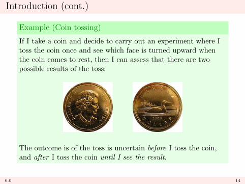
Example (Coin tossing)
If I take a coin and decide to carry out an experiment where Itoss the coin once and see which face is turned upward whenthe coin comes to rest, then I can assess that there are twopossible results of the toss:
The outcome is of the toss is uncertain before I toss the coin,and after I toss the coin until I see the result.
0.0 14

Introduction (cont.)
Example (Thumbtack tossing)
If I take a thumbtack and decide to carry out an experimentwhere I toss the thumbtack once, then I can assess that thereare two possible results of the toss:
The outcome of the toss is uncertain before I toss thethumbtack, and after I toss the thumbtack until I see the result.
0.0 15
Chapter 1: The basics of probability
What is probability ?
By probability, we generally mean the chance of a particularevent occurring, given a particular set of circumstances. Theprobability of an event is generally expressed as a quantitativemeasurement.
1.0 The basics of probability 17
What is probability ?
That is,
(i) the chance of a particular event occurring ...
(ii) ... given a particular set of circumstances.
1.0 The basics of probability 18
What is probability ?
That is,
(i) the chance of a particular event occurring ...
(ii) ... given a particular set of circumstances.
1.0 The basics of probability 19

What is probability ?
It has seemed to me that the theory of probabilities oughtto serve as the basis for the study of all the sciences.
Adolphe Quetelet
The probable is what usually happens.
Aristotle
Probability is the very guide of life.
Cicero, De Natura, 5, 12
http://probweb.berkeley.edu/quotes.html
1.0 The basics of probability 20
What is probability ? (cont.)
My thesis, paradoxically, and a little provocatively, butnonetheless genuinely, is simply this:
PROBABILITY DOES NOT EXIST
The abandonment of superstitious beliefs about the ex-istence of the Phlogiston, the Cosmic Ether, AbsoluteSpace and Time, ... or Fairies and Witches was anessential step along the road to scientific thinking.
Probability, too, if regarded as something endowed withsome kind of objective existence, is no less a mislead-ing misconception, an illusory attempt to exteriorize ormaterialize our true probabilistic beliefs.
B. de Finetti, Theory of Probability, 1970.
1.0 The basics of probability 21

What is probability ? (cont.)
That is,
� probability is not some objectively defined, universal quant-ity – it has a subjective interpretation.
� this subjective element may be commonly agreed upon incertain circumstances, but in general is always present.
� recallI coin example,I thumbtack example.
1.0 The basics of probability 22

Constructing the mathematical framework
General strategy for constructing the probability framework: fora given ‘experiment’, we
� identify the possible outcomes;
� assign numerical values to collections of possible values torepresent the chance that they will coincide with the actualoutcome;
� lay out the rules for how the numerical values can be ma-nipulated.
1.0 The basics of probability 23

Basic concepts in set theory
A set S is a collection of individual elements, such as s. We write
s ∈ S
to mean “s is one of the elements of S”.
� S = {0, 1}; 0 ∈ S, 1 ∈ S.
� S = {‘dog’, ‘cat’, ‘mouse’, ‘elephant’}; ‘elephant’ ∈ S� S = [0, 1] (that is, the closed interval from zero to one);
0.3428 ∈ S
1.1 The basics of probability | Set theory notation 24
Basic concepts in set theory (cont.)
S may be
� finite if it contains a finite number of elements;
� countable if it contains a countably infinite number of ele-ments;
� uncountable if it contains an uncountably infinite number ofelements.
1.1 The basics of probability | Set theory notation 25

Basic concepts in set theory (cont.)
A is a subset of S if it contains some, all, or none of the elementsof S
some: A ⊂ S some or all: A ⊆ S.That is, A is a subset of S if every element of A is also an elementof S
s ∈ A =⇒ s ∈ S.
� S = {0, 1}; A = {0}, or A = {1}, or A = {0, 1}.� S = {‘dog’, ‘cat’, ‘mouse’, ‘elephant’}; A = {‘cat’, ‘mouse’}� S = [0, 1]; A = (0.25, 0.3).
Special case: the empty set, ∅, is a subset that contains no ele-ments.
1.1 The basics of probability | Set theory notation 26

Basic concepts in set theory (cont.)
Note
In probability, it is necessary to think of sets of subsets of S.For example:
� S = {1, 2, 3, 4}.� Consider all the subsets of S:
One element:{1}, {2}, {3}, {4}
Two elements:{1, 2}, {1, 3}, {1, 4}, {2, 3}, {2, 4}, {3, 4}
Three elements:{1, 2, 3}, {1, 2, 4}, {1, 3, 4}, {2, 3, 4}
Four elements:{1, 2, 3, 4}.
� Add to this list the empty set (zero elements), ∅.Thus there is a collection of 16 (that is, 24) subsets of S.
1.1 The basics of probability | Set theory notation 27
Basic concepts in set theory (cont.)
Note
This is a bit trickier if S is an interval ...
1.1 The basics of probability | Set theory notation 28
Set operations
To manipulate sets, we use three basic operations: we may focuson the case where two sets A and B are subsets of a set S.
� intersection: the intersection of two sets A and B is thecollection of elements that are elements of both A and B.
s ∈ A ∩B ⇐⇒ s ∈ A and s ∈ B.
Note
We have for any A ⊆ S that
A ∩ ∅ = ∅
andA ∩ S = A.
1.1 The basics of probability | Set theory notation 29

Set operations (cont.)
Note
It is clear thatA ∩B ⊆ A
andA ∩B ⊆ B.
1.1 The basics of probability | Set theory notation 30

Set operations (cont.)
� union: the union of two sets A and B is the set of distinctelements that are either in A, or in B, or in both A and B.
s ∈ A ∪B ⇐⇒ s ∈ A or s ∈ B (or s ∈ A ∩B).
Note
We have for any A ⊆ S that
A ∪ ∅ = A
andA ∪ S = S.
1.1 The basics of probability | Set theory notation 31
Set operations (cont.)
Note
It is clear thatA ⊆ A ∪B
andB ⊆ A ∪B.
1.1 The basics of probability | Set theory notation 32
Set operations (cont.)
� complement: the complement of set A, a subset of S, is thecollection of elements of S that are not elements of A.
s ∈ A′ ⇐⇒ s ∈ S but s /∈ A.
We have that
A ∩A′ = ∅ and A ∪A′ = S.
1.1 The basics of probability | Set theory notation 33
Set operations (cont.)
Note
The notations A and Ac are also used for the complement of A.
The textbook usesA (A ∩B)
etc., but I find this leads to confusion.
Note
We have for any A ⊆ S that
(A′)′ = A.
1.1 The basics of probability | Set theory notation 34
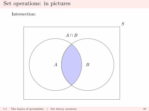
Set operations: in pictures
Intersection:
A B
A ∩B
S
1.1 The basics of probability | Set theory notation 35

Set operations: in pictures (cont.)
Union:
A B
A ∪B
S
1.1 The basics of probability | Set theory notation 36
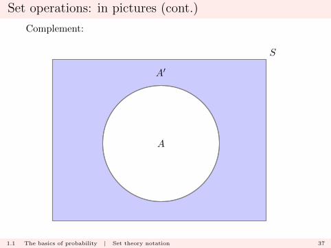
Set operations: in pictures (cont.)
Complement:
A
S
A′
1.1 The basics of probability | Set theory notation 37
Example
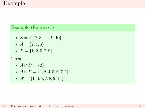
Example (Finite set)
� S = {1, 2, 3, . . . , 9, 10}� A = {2, 4, 6}� B = {1, 2, 5, 7, 9}
Then
� A ∩B = {2}� A ∪B = {1, 2, 4, 5, 6, 7, 9}� A′ = {1, 3, 5, 7, 8, 9, 10}
1.1 The basics of probability | Set theory notation 38
Set operations: extensions
� Set difference: A−B (or A\B)
s ∈ A−B ⇐⇒ s ∈ A and s ∈ B′
that is
A−B ≡ A ∩B′.
1.1 The basics of probability | Set theory notation 39
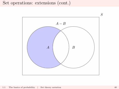
Set operations: extensions (cont.)
A B
A−B
S
1.1 The basics of probability | Set theory notation 40
Set operations: extensions (cont.)
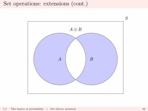
� A or B but not both: A⊕B
s ∈ A⊕B ⇐⇒ s ∈ A or s ∈ B, but s /∈ A ∩B
aka
(A ∪B)− (A ∩B)
1.1 The basics of probability | Set theory notation 41
Set operations: extensions (cont.)
A B
A⊕B
S
1.1 The basics of probability | Set theory notation 42

Combining set operations
Both intersection and union operators are binary operators, thatis, take two arguments:
A ∩B A ∪B.
We have immediately from the definitions that
A ∩B = B ∩A
and that
A ∪B = B ∪A(that is, the order does not matter).
1.1 The basics of probability | Set theory notation 43
Combining set operations (cont.)
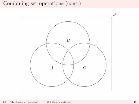
However, A and B are arbitrary, so suppose there is a third setC ⊆ S, and consider
(A ∩B) ∩ C
as A ∩B is a set in its own right. Then
s ∈ (A ∩B) ∩ C ⇐⇒ s ∈ (A ∩B) and s ∈ C⇐⇒ s ∈ A and s ∈ B and s ∈ C.
1.1 The basics of probability | Set theory notation 44

Combining set operations (cont.)
That is
(A ∩B) ∩ C = A ∩B ∩ C
and by the same logic
(A ∩B) ∩ C = A ∩ (B ∩ C)
and so on.
1.1 The basics of probability | Set theory notation 45

Combining set operations (cont.)
This extends to the case of any finite collection of sets
A1, A2, . . . , AK
and we may write
A1 ∩A2 ∩ . . . ∩AK ≡K⋂k=1
Ak
where
s ∈K⋂k=1
Ak ⇐⇒ s ∈ Ak for all k
1.1 The basics of probability | Set theory notation 46
Combining set operations (cont.)
A
B
C
S
1.1 The basics of probability | Set theory notation 47

Combining set operations (cont.)
A
B
C
S
1.1 The basics of probability | Set theory notation 48
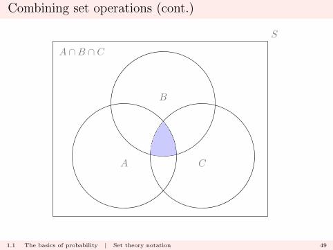
Combining set operations (cont.)
A
B
C
S
A ∩B ∩ C
1.1 The basics of probability | Set theory notation 49
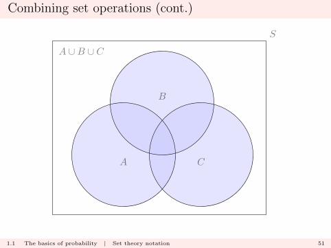
Combining set operations (cont.)
The same logic holds for the union operator:
(A ∪B) ∪ C = A ∪B ∪ C = A ∪ (B ∪ C)
and
A1 ∪A2 ∪ . . . ∪AK ≡K⋃k=1
Ak
where
s ∈K⋃k=1
Ak ⇐⇒ s ∈ Ak for at least one k
1.1 The basics of probability | Set theory notation 50
Combining set operations (cont.)
A
B
C
S
A ∪B ∪ C
1.1 The basics of probability | Set theory notation 51

Combining set operations (cont.)
Note
The intersection and union operations can be extended to workwith a countably infinite number of sets
A1, A2, . . . , Ak, . . .
and we can consider
∞⋂k=1
Ak : s ∈∞⋂k=1
Ak ⇐⇒ s ∈ Ak for all k
∞⋃k=1
Ak : s ∈∞⋃k=1
Ak ⇐⇒ s ∈ Ak for at least one k
1.1 The basics of probability | Set theory notation 52

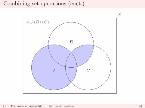
Combining set operations (cont.)
Consider now
A ∪ (B ∩ C)
To be an element in this set, you need to be an element of A oran element of B ∩ C (or both).
1.1 The basics of probability | Set theory notation 53
Combining set operations (cont.)
S
A ∪ (B ∩ C)
A
B
C
1.1 The basics of probability | Set theory notation 54
Combining set operations (cont.)
We can therefore deduce that
A ∪ (B ∩ C) ≡ (A ∪B) ∩ (A ∪ C).
Similarly
A ∩ (B ∪ C) ≡ (A ∩B) ∪ (A ∩ C).
1.1 The basics of probability | Set theory notation 55

Combining set operations (cont.)
S
A ∩ (B ∪ C)
A
B
C
1.1 The basics of probability | Set theory notation 56
Partitions
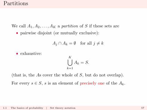
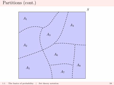
We call A1, A2, . . . , AK a partition of S if these sets are
� pairwise disjoint (or mutually exclusive):
Aj ∩Ak = ∅ for all j 6= k
� exhaustive:K⋃k=1
Ak = S.
(that is, the As cover the whole of S, but do not overlap).
For every s ∈ S, s is an element of precisely one of the Ak.
1.1 The basics of probability | Set theory notation 57
Partitions (cont.)
S
A5
A3
A6
A1
A2
A4
A7
A8
1.1 The basics of probability | Set theory notation 58

Some simple theorems
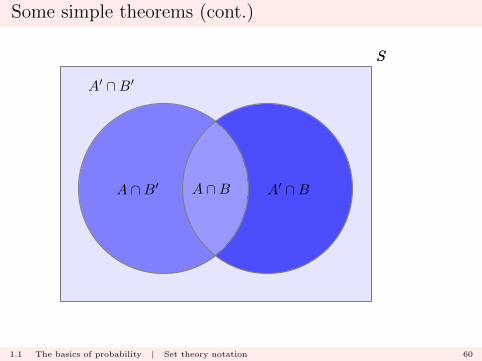
For any two subsets A and B of S, we have the partition of S viathe four sets
A ∩B A ∩B′ A′ ∩B A′ ∩B′
1.1 The basics of probability | Set theory notation 59
Some simple theorems (cont.)
SS
A ∩B
A′ ∩B′
A ∩B′ A′ ∩B
1.1 The basics of probability | Set theory notation 60

Some simple theorems (cont.)
This picture implies that
(A ∪B)′ = A′ ∩B′.
1.1 The basics of probability | Set theory notation 61
Some simple theorems (cont.)
We can prove this as follows: let
A1 = A ∪B A2 = A′ ∩B′.
We need to show that
A′1 = A2
that is,
(i) A1 ∩A2 = ∅;(ii) A1 ∪A2 = S.
1.1 The basics of probability | Set theory notation 62
Some simple theorems (cont.)
(i) Disjoint:
A1 ∩A2 = (A ∪B) ∩A2
= (A ∩A2) ∪ (B ∩A2)
= (A ∩A′ ∩B′) ∪ (B ∩A′ ∩B′)
= ∅ ∪ ∅
= ∅
1.1 The basics of probability | Set theory notation 63
Some simple theorems (cont.)
(ii) Exhaustive:
A1 ∪A2 = A1 ∪ (A′ ∩B′)
= (A1 ∪A′) ∩ (A1 ∪B′)
= (A ∪B ∪A′) ∩ (A ∪B ∪B′)
= S ∩ S
= S
1.1 The basics of probability | Set theory notation 64
Some simple theorems (cont.)
Similarly
A′ ∪B′ = (A ∩B)′
which is equivalent to saying
(A′ ∪B′)′ = A ∩B.
1.1 The basics of probability | Set theory notation 65
Some simple theorems (cont.)
The first result
(A ∪B)′ = A′ ∩B′.
holds for arbitrary sets A and B. In particular it holds for thesets
C = A′ D = B′
that is we have
(C ∪D)′ = C ′ ∩D′.
1.1 The basics of probability | Set theory notation 66
Some simple theorems (cont.)
But
C ′ = (A′)′ = A D′ = (B′)′ = B
Therefore
(A′ ∪B′)′ = A ∩B
or equivalently
A′ ∪B′ = (A ∩B)′
as required.
1.1 The basics of probability | Set theory notation 67
Some simple theorems (cont.)
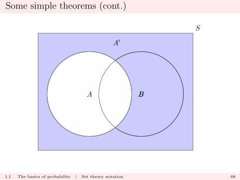
A BBA
S
A′
1.1 The basics of probability | Set theory notation 68
Some simple theorems (cont.)
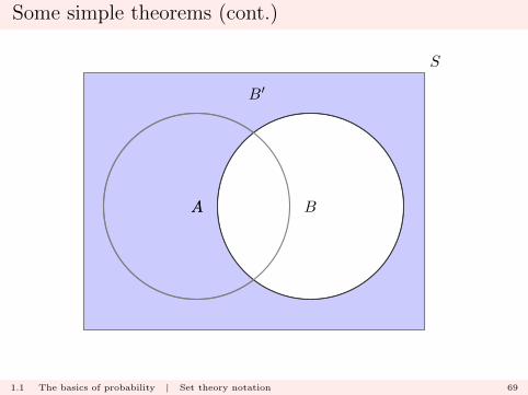
BA BA
S
B′
1.1 The basics of probability | Set theory notation 69
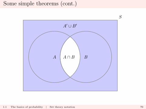
Some simple theorems (cont.)
A B
S
A′ ∪B′
A ∩B
1.1 The basics of probability | Set theory notation 70

Some simple theorems (cont.)
These two results
A′ ∩B′ = (A ∪B)′
A′ ∪B′ = (A ∩B)′
are sometimes known as de Morgan’s Laws.
1.1 The basics of probability | Set theory notation 71

Sample spaces and Events
We now utilize the set theory formulation and notation in theprobability context.
Recall the earlier informal definition:
By probability, we generally mean the chance of a par-ticular event occurring, given a particular set of cir-cumstances. The probability of an event is generallyexpressed as a quantitative measurement.
We need to carefully define what an ‘event’ is, and what consti-tutes a ‘particular set of circumstances’.
1.2 The basics of probability | Sample spaces and Events 72
Sample spaces and Events (cont.)
We will consider the general setting of an experiment :
� this can be interpreted as any setting in which an uncertainconsequence is to arise;
� could involve observing an outcome, taking a measurementetc.
1.2 The basics of probability | Sample spaces and Events 73
Constructing the framework
1. Consider the possible outcomes of the experiment:Make a ‘list’ of the outcomes that can arise, and denote thecorresponding set by S.
I S = {0, 1};I S = {‘head’, ‘tail’} ≡ {H,T};I S = {‘cured’, ‘not cured’};I S = {‘Arts’, ‘Engineering’, ‘Medicine’, ‘Science’};I S = {1, 2, 3, 4, 5, 6};I S = R+.
The set S is termed the sample space of the experiment. Theindividual elements of S are termed sample points (or sampleoutcomes).
1.2 The basics of probability | Sample spaces and Events 74

Constructing the framework (cont.)
2. Events: An event A is a collection of sample outcomes.That is, A is a subset of S,
A ⊆ S.
For example
I A = {0};I A = {‘tail’} ≡ {T};I A = {‘cured’};I A = {‘Arts’, ‘Engineering’};I A = {1, 3, 5};I A = [2, 3).
The individual sample outcomes are termed simple (orelementary) events, and may be denoted
E1, E2, . . . , EK , . . . .
1.2 The basics of probability | Sample spaces and Events 75
Constructing the framework (cont.)
3. Terminology: We say that event A occurs if the actualoutcome, s, is an element of A.
For two events A and B
I A ∩B occurs if and only if A occurs and B occurs, that is
s ∈ A ∩B.
I A ∪ B occurs if A occurs or if B occurs, or if both A and Boccur, that is
s ∈ A ∪BI if A occurs, then A′ does not occur.
1.2 The basics of probability | Sample spaces and Events 76
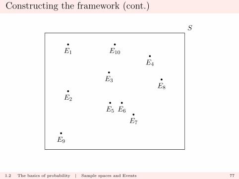
Constructing the framework (cont.)
S
E5
E3
E6
E1
E2
E4
E7
E8
E9
E10
1.2 The basics of probability | Sample spaces and Events 77
Constructing the framework (cont.)
In this case
S =
10⋃k=1
Ek.
1.2 The basics of probability | Sample spaces and Events 78
Constructing the framework (cont.)
S
E5
E3
E6
E1
E2
E4
E7
E8
E9
E10
A
1.2 The basics of probability | Sample spaces and Events 79
Constructing the framework (cont.)
S
E5
E3
E6
E1
E2
E4
E7
E8
E9
E10
B
1.2 The basics of probability | Sample spaces and Events 80
Constructing the framework (cont.)
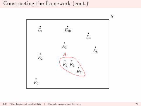
In this case
A = E5 ∪ E6 ∪ E7
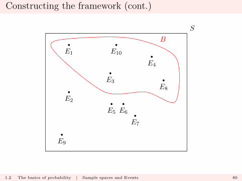
and
B = E1 ∪ E3 ∪ E4 ∪ E8 ∪ E10.
1.2 The basics of probability | Sample spaces and Events 81
Constructing the framework (cont.)
Note
� The event S is termed the certain event;
� The event ∅ is termed the impossible event.
1.2 The basics of probability | Sample spaces and Events 82
Mathematical definition of probability
Probability is a means of assigning a quantitative measure ofuncertainty to events in a sample space.
Formally, the probability function, P (.) is a function that assignsnumerical values to events.
P :A −→ R
A 7−→ p
that is
P (A) = p
that is, the probability assigned to event A (a set) is p (a numer-ical value).
1.3 The basics of probability | Mathematical definition of probability 83
Mathematical definition of probability (cont.)
Note
(i) The function P (.) is a set function (that is, it takes a setas its argument).
(ii) A is a “set of subsets of S”; we pick a subset A ∈ A andconsider its probability.
(iii) A has certain nice properties that ensure that theprobability function can operate successfully.
1.3 The basics of probability | Mathematical definition of probability 84

Mathematical definition of probability (cont.)
This definition is too general:
� what properties does P (.) have ?
� how does P (.) assign numerical values; that is, how do wecompute
P (A)
for a given event A in sample space S ?
1.3 The basics of probability | Mathematical definition of probability 85
The probability axioms
Suppose S is a sample space for an experiment, and A is an event,a subset of S. Then we assign P (A), the probability of event A,so that the following axioms hold:
(I) P (A) ≥ 0.
(II) P (S) = 1.
(III) If A1, A2, . . . form a (countable) sequence of events suchthat
Aj ∩Ak = ∅ for all j 6= k
then
P
( ∞⋃i=1
Ai
)=
∞∑i=1
P (Ai)
that is, we say that P (.) is countably additive.
1.4 The basics of probability | The probability axioms 86
The probability axioms (cont.)
Note
Axiom (III) immediately implies that P (.) is finitely additive,that is, for all n, 1 ≤ n <∞, if A1, A2, . . . , An form a sequenceof events such that Aj ∩Ak = ∅ for all j 6= k, then
P
(n⋃i=1
Ai
)=
n∑i=1
P (Ai).
To see this, fix n and define Ai = ∅ for i > n.
1.4 The basics of probability | The probability axioms 87
The probability axioms (cont.)
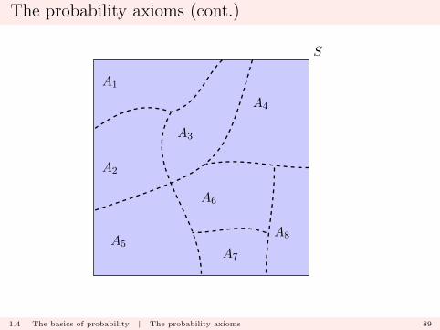
Example (Partitions)
If A1, A2, . . . , An form a partition of S, and
P (Ai) = pi i = 2, . . . , n
say, thenn∑i=1
P (Ai) =
n∑i=1
pi = 1.
1.4 The basics of probability | The probability axioms 88
The probability axioms (cont.)
S
A5
A3
A6
A1
A2
A4
A7
A8
1.4 The basics of probability | The probability axioms 89
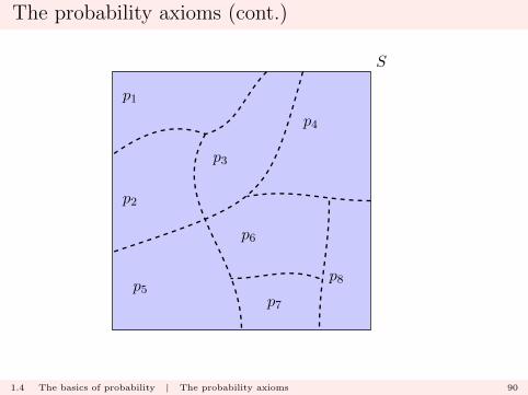
The probability axioms (cont.)
S
p5
p3
p6
p1
p2
p4
p7
p8
1.4 The basics of probability | The probability axioms 90
The probability axioms (cont.)
Some immediate corollaries of the axioms:
(i) For any A, P (A′) = 1− P (A).
I We have that S = A∪A′. By Axiom (III) we have thereforethat
P (S) = P (A) + P (A′).
I By Axiom (II), P (S) = 1, so therefore
1 = P (A) + P (A′) ∴ P (A′) = 1− P (A).
1.4 The basics of probability | The probability axioms 91
The probability axioms (cont.)
(ii) P (∅) = 0.
I Apply the result from point (i) to the set A ≡ S.I Note that by Axiom (II), P (S) = 1.
1.4 The basics of probability | The probability axioms 92
The probability axioms (cont.)
(iii) For any A, P (A) ≤ 1.
I By Axiom (III) and point (i) we have
1 = P (S) = P (A) + P (A′) ≥ P (A)
as P (A′) ≥ 0 by Axiom (I).
1.4 The basics of probability | The probability axioms 93
The probability axioms (cont.)
(iv) For any two events A and B, if A ⊆ B, then
P (A) ≤ P (B)
I We may write in this case
B = A ∪ (A′ ∩B)
and, as the two events on the right hand side are mutuallyexclusive, by Axiom (III)
P (B) = P (A) + P (A′ ∩B) ≥ P (A)
as P (A′ ∩B) ≥ 0 by Axiom (I).
1.4 The basics of probability | The probability axioms 94
The probability axioms (cont.)
Therefore, for example,
P (A ∩B) ≤ P (A) and P (A ∩B) ≤ P (B)
that is
P (A ∩B) ≤ min{P (A), P (B)}.
1.4 The basics of probability | The probability axioms 95

The probability axioms (cont.)
S
A
B
B ∩A′
1.4 The basics of probability | The probability axioms 96
The probability axioms (cont.)
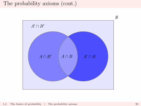
(v) General Addition Rule: For two arbitrary events Aand B,
P (A ∪B) = P (A) + P (B)− P (A ∩B).
1.4 The basics of probability | The probability axioms 97
The probability axioms (cont.)
SS
A ∩B
A′ ∩B′
A ∩B′ A′ ∩B
1.4 The basics of probability | The probability axioms 98
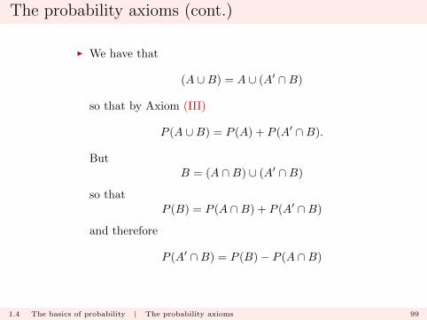
The probability axioms (cont.)
I We have that
(A ∪B) = A ∪ (A′ ∩B)
so that by Axiom (III)
P (A ∪B) = P (A) + P (A′ ∩B).
ButB = (A ∩B) ∪ (A′ ∩B)
so thatP (B) = P (A ∩B) + P (A′ ∩B)
and therefore
P (A′ ∩B) = P (B)− P (A ∩B)
1.4 The basics of probability | The probability axioms 99

The probability axioms (cont.)
Substituting back in, we have
P (A ∪B) = P (A) + P (A′ ∩B)
= P (A) + P (B)− P (A ∩B)
as required.
I We may deduce from this that
P (A ∪B) ≤ P (A) + P (B)
as P (A ∩B) ≥ 0.
1.4 The basics of probability | The probability axioms 100

The probability axioms (cont.)
In general, for events A1, A2, . . . , An, we can construct aformula for
P
(n⋃i=1
Ai
)using inductive arguments.
1.4 The basics of probability | The probability axioms 101
The probability axioms (cont.)
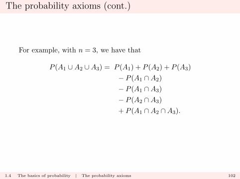
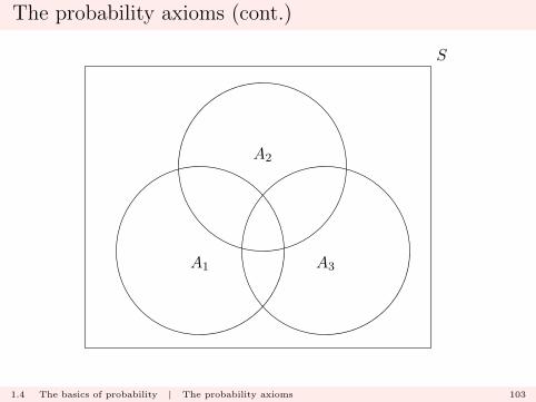
For example, with n = 3, we have that
P (A1 ∪A2 ∪A3) = P (A1) + P (A2) + P (A3)
− P (A1 ∩A2)
− P (A1 ∩A3)
− P (A2 ∩A3)
+ P (A1 ∩A2 ∩A3).
1.4 The basics of probability | The probability axioms 102
The probability axioms (cont.)
A1
A2
A3
S
1.4 The basics of probability | The probability axioms 103
The probability axioms (cont.)
A more straightforward general result is Boole’s Inequality
P
(n⋃i=1
Ai
)≤
n∑i=1
P (Ai) .
Proof of this result follows by a simple inductive argument.
1.4 The basics of probability | The probability axioms 104
Probability tables
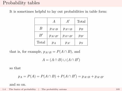
It is sometimes helpful to lay out probabilities in table form:
A A′ Total
B pA∩B pA′∩B pB
B′ pA∩B′ pA′∩B′ pB′
Total pA pA′ pS
that is, for example, pA∩B = P (A ∩B), and
A = (A ∩B) ∪ (A ∩B′)
so that
pA = P (A) = P (A ∩B) + P (A ∩B′) = pA∩B + pA∩B′
and so on.1.4 The basics of probability | The probability axioms 105
Probability tables (cont.)
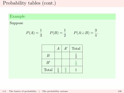
Example
Suppose
P (A) =1
3P (B) =
1
2P (A ∪B) =
3
4.
A A′ Total
B 12
B′ 12
Total 13
23 1
1.4 The basics of probability | The probability axioms 106
Probability tables (cont.)
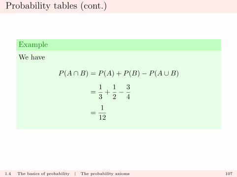
Example
We have
P (A ∩B) = P (A) + P (B)− P (A ∪B)
=1
3+
1
2− 3
4
=1
12
1.4 The basics of probability | The probability axioms 107
Probability tables (cont.)
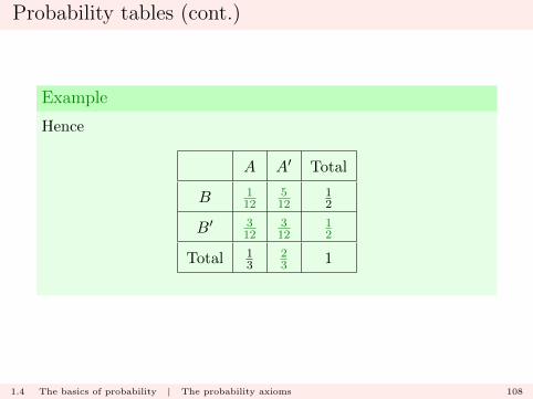
Example
Hence
A A′ Total
B 112
512
12
B′ 312
312
12
Total 13
23 1
1.4 The basics of probability | The probability axioms 108
Probability tables (cont.)
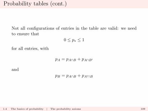
Not all configurations of entries in the table are valid: we needto ensure that
0 ≤ p∗ ≤ 1
for all entries, with
pA = pA∩B + pA∩B′
and
pB = pA∩B + pA′∩B
1.4 The basics of probability | The probability axioms 109
Specifying probabilities
The earlier discussion defines mathematically how the probabilityfunction behaves; it does not tell us how to assign numericalvalues to the probabilities of events.
It is usually thought that there are three ways via which we couldspecify the probability of an event.
1.5 The basics of probability | Specifying probabilities 110

Specifying probabilities (cont.)
1. Equally likely sample outcomes: Suppose that samplespace S is finite, with N sample outcomes in total that areconsidered to be equally likely to occur. Then for the ele-mentary events E1, E2, . . . , EN , we have
P (Ei) =1
Ni = 1, . . . , N
1.5 The basics of probability | Specifying probabilities 111
Specifying probabilities (cont.)
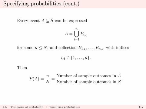
Every event A ⊆ S can be expressed
A =
n⋃i=1
EiA
for some n ≤ N , and collection E1A , . . . , EnA , with indices
iA ∈ {1, . . . , n}.
Then
P (A) =n
N=
Number of sample outcomes in A
Number of sample outcomes in S.
1.5 The basics of probability | Specifying probabilities 112

Specifying probabilities (cont.)
“Equally likely outcomes”: this is a strong (and subjective)assumption, but if it holds, then it leads to a straightforwardcalculation.
Suppose we have N = 10:
1.5 The basics of probability | Specifying probabilities 113

Specifying probabilities (cont.)
P (A) =3
10: 1A = 5, 2A = 6, 3A = 7.
S
E5
E3
E6
E1
E2
E4
E7
E8
E9
E10
A
1.5 The basics of probability | Specifying probabilities 114
Specifying probabilities (cont.)
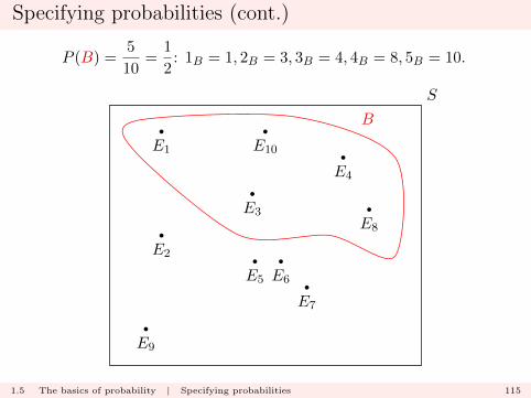
P (B) =5
10=
1
2: 1B = 1, 2B = 3, 3B = 4, 4B = 8, 5B = 10.
S
E5
E3
E6
E1
E2
E4
E7
E8
E9
E10
B
1.5 The basics of probability | Specifying probabilities 115
Specifying probabilities (cont.)
We usually apply the logic of “equally likely outcomes” incertain mechanical settings where we can appeal to some formof symmetry argument.
(a) Coins: It is common to assume the existence of a ‘fair’ coin,and an experiment involving a single flip. Here the sample spaceis
S = {Head,Tail}with elementary events E1 = {Head} and E2 = {Tail}, and itis usual to assume that
P (E1) = P (E2) =1
2.
1.5 The basics of probability | Specifying probabilities 116
Specifying probabilities (cont.)
(b) Dice: Consider a single roll of a ‘fair’ die, with the outcome be-ing the upward face after the roll is complete. Here the samplespace is
S = {1, 2, 3, 4, 5, 6}with elementary events Ei = {i} for i = 1, 2, 3, 4, 5, 6, and it isusual to assume that
P (Ei) =1
6.
Let A be the event that the outcome of the roll is an evennumber. Then
A = E2 ∪ E4 ∪ E6
and
P (A) =3
6=
1
2.
1.5 The basics of probability | Specifying probabilities 117
Specifying probabilities (cont.)
(c) Cards: A standard deck of cards contains 52 cards, compris-ing four suits (Hearts, Clubs, Diamonds, Spades) with thirteencards in each suit, with cards denominated
2, 3, 4, 5, 6, 7, 8, 9, 10, Jack,Queen,King,Ace.
Thus each card has a suit and a denomination. An experimentinvolves selecting a card from the deck after it has been wellshuffled.
There are 52 elementary outcomes, and
P (Ei) =1
52i = 1, . . . , 52.
If A is the event Ace is selected, then
P (A) =Total number of Aces
Total number of cards=
4
52=
1
13.
1.5 The basics of probability | Specifying probabilities 118
Specifying probabilities (cont.)
In a second experiment, five cards are to be selected withoutreplacement from the deck. The elementary outcomes corres-pond to all sequences of five cards that could be obtained. Allsuch sequences are equally likely.
Let A be the event that the five cards contain three cards ofone denomination, and two cards of another denomination.
What is P (A) ?
Need some rules to help in counting the elementary outcomes.
1.5 The basics of probability | Specifying probabilities 119

Specifying probabilities (cont.)
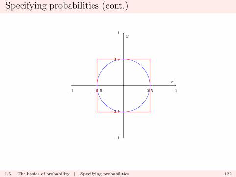
The concept of “equally likely outcomes” can be extended tothe uncountable sample space case:
I pick a point from the interval (0, 1) with each point equallylikely; if A is the event
“point picked is in the interval (0, 0.25)”
then we can set P (A) = 0.25.
I a point is picked internal to the square centered at (0, 0) withside length one, with each point equally likely. Let A be theevent that
“point lies in the circle centered at (0, 0) with radius 0.5.”
Then
P (A) =Area of circle
Area of Square=π
4= 0.7853982.
1.5 The basics of probability | Specifying probabilities 120

Specifying probabilities (cont.)
−1 −0.5 0.5 1
−1
−0.5
0.5
1
x
y
1.5 The basics of probability | Specifying probabilities 121
Specifying probabilities (cont.)
−1 −0.5 0.5 1
−1
−0.5
0.5
1
x
y
1.5 The basics of probability | Specifying probabilities 122

Specifying probabilities (cont.)
A simulation: 10000 points picked from the square.
0 2000 4000 6000 8000 10000
0.70
0.75
0.80
0.85
0.90
0.95
1.00
Number of samples
Pro
port
ion
1.5 The basics of probability | Specifying probabilities 123

Specifying probabilities (cont.)
Example (Thumbtack tossing)
I S = {Up,Down}.I A = {Up}.
What is P (A) ?
1.5 The basics of probability | Specifying probabilities 124
Specifying probabilities (cont.)
2. Relative frequencies: Suppose S is the sample space, andA is the event of interest. Consider an infinite sequence ofrepeats of the experiment under identical conditions. Thenwe may define P (A) by considering the relative frequency withwhich event A occurs in the sequence.
I Consider a finite sequence of N repeat experiments.I Let n be the number of times (out of N) that A occurs.I Define
P (A) = limN−→∞
n
N.
The frequentist definition of probability; it generalizes the“equally likely outcomes” version of probability.
1.5 The basics of probability | Specifying probabilities 125

Specifying probabilities (cont.)
The frequentist definition would cover the thumbtack example:
Can we always envisage an infinite sequence of repeats ?
1.5 The basics of probability | Specifying probabilities 126
Specifying probabilities (cont.)
3. Subjective assessment: The subjective definition of prob-ability is that for a given experiment with sample space S, theprobability of event A is
I a numerical representation of your own personal
degree of belief
that the actual outcome lies in A;I you are rational and coherent (that is, internally consistent in
your assessment).
This definition generalizes the “equally likely outcomes” and“frequentist” versions of probability.
1.5 The basics of probability | Specifying probabilities 127
Specifying probabilities (cont.)
� Especially useful for ‘one-off’ experiments.
� Assessment of ‘odds’ on an event can be helpful:
Odds :P (A)
P (A′)=
P (A)
1− P (A)
eg Odds = 10:1, then P (A) = 10/11 etc.
1.5 The basics of probability | Specifying probabilities 128
Rules for counting outcomes
Multiplication principle: A sequence of k operations, in whichoperation i can result in ni possible outcomes, can result in
n1 × n2 × · · · × nk
possible sequences of outcomes.
1.6 The basics of probability | Combinatorial probability 129
Rules for counting outcomes (cont.)
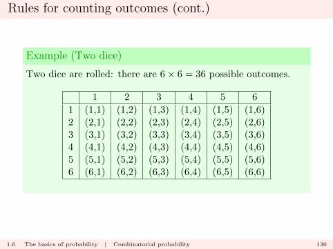
Example (Two dice)
Two dice are rolled: there are 6× 6 = 36 possible outcomes.
1 2 3 4 5 6
1 (1,1) (1,2) (1,3) (1,4) (1,5) (1,6)2 (2,1) (2,2) (2,3) (2,4) (2,5) (2,6)3 (3,1) (3,2) (3,3) (3,4) (3,5) (3,6)4 (4,1) (4,2) (4,3) (4,4) (4,5) (4,6)5 (5,1) (5,2) (5,3) (5,4) (5,5) (5,6)6 (6,1) (6,2) (6,3) (6,4) (6,5) (6,6)
1.6 The basics of probability | Combinatorial probability 130
Rules for counting outcomes (cont.)
Example
We are to pick k = 5 numbers sequentially from the set
{1, 2, 3, . . . , 100},
where every number is available on every pick. The number ofways of doing that is
100× 100× 100× 100× 100 = 1005.
1.6 The basics of probability | Combinatorial probability 131
Rules for counting outcomes (cont.)
Example
We are to pick k = 11 players sequentially from a squad of 25players. The number of ways of doing that is
25× 24× 23× · · · × 15.
as players cannot be picked twice.
1.6 The basics of probability | Combinatorial probability 132
Rules for counting outcomes (cont.)
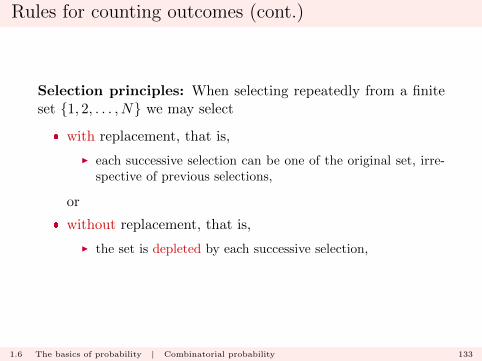
Selection principles: When selecting repeatedly from a finiteset {1, 2, . . . , N} we may select
� with replacement, that is,
I each successive selection can be one of the original set, irre-spective of previous selections,
or
� without replacement, that is,
I the set is depleted by each successive selection,
1.6 The basics of probability | Combinatorial probability 133
Rules for counting outcomes (cont.)
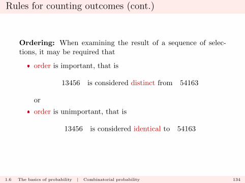
Ordering: When examining the result of a sequence of selec-tions, it may be required that
� order is important, that is
13456 is considered distinct from 54163
or
� order is unimportant, that is
13456 is considered identical to 54163
1.6 The basics of probability | Combinatorial probability 134

Rules for counting outcomes (cont.)
Example (Two dice)
Two dice are rolled: there are (7× 6)/2 = 21 possible unorderedoutcomes.
1 2 3 4 5 6
1 (1,1) (1,2) (1,3) (1,4) (1,5) (1,6)2 - (2,2) (2,3) (2,4) (2,5) (2,6)3 - - (3,3) (3,4) (3,5) (3,6)4 - - - (4,4) (4,5) (4,6)5 - - - - (5,5) (5,6)6 - - - - - (6,6)
1.6 The basics of probability | Combinatorial probability 135
Rules for counting outcomes (cont.)
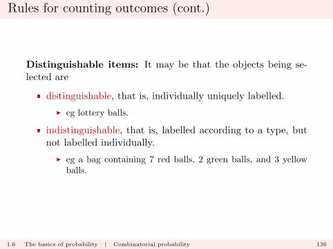
Distinguishable items: It may be that the objects being se-lected are
� distinguishable, that is, individually uniquely labelled.
I eg lottery balls.
� indistinguishable, that is, labelled according to a type, butnot labelled individually.
I eg a bag containing 7 red balls, 2 green balls, and 3 yellowballs.
1.6 The basics of probability | Combinatorial probability 136
Permutations
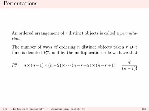
An ordered arrangement of r distinct objects is called a permuta-tion.
The number of ways of ordering n distinct objects taken r at atime is denoted Pnr , and by the multiplication rule we have that
Pnr = n× (n−1)× (n−2)×· · · (n−r+2)× (n−r+1) =n!
(n− r)!
1.6 The basics of probability | Combinatorial probability 137
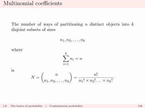
Multinomial coefficients
The number of ways of partitioning n distinct objects into kdisjoint subsets of sizes
n1, n2, . . . , nk
wherek∑i=1
ni = n
is
N =
(n
n1, n2, . . . , nk
)=
n!
n1!× n2! . . .× nk!.
1.6 The basics of probability | Combinatorial probability 138
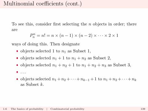
Multinomial coefficients (cont.)
To see this, consider first selecting the n objects in order; thereare
Pnn = n! = n× (n− 1)× (n− 2)× · · · × 2× 1
ways of doing this. Then designate
� objects selected 1 to n1 as Subset 1,
� objects selected n1 + 1 to n1 + n2 as Subset 2,
� objects selected n1 + n2 + 1 to n1 + n2 + n3 as Subset 3,
� . . .
� objects selected n1 +n2 + · · ·+nk−1 + 1 to n1 +n2 + · · ·+nkas Subset k.
1.6 The basics of probability | Combinatorial probability 139

Multinomial coefficients (cont.)
Then note that the specific ordered selection that achieves thepartition is only one of several that yield the same partition;there are
� n1! ways of permuting Subset 1,
� n2! ways of permuting Subset 2,
� n3! ways of permuting Subset 3,
� . . .
� nk! ways of permuting Subset k,
that yield the same partition.
1.6 The basics of probability | Combinatorial probability 140

Multinomial coefficients (cont.)
Therefore, we must have that
Pnn = n! = N × (n1!× n2! . . .× nk!)
and hence
N =n!
n1!× n2!× . . .× nk!
1.6 The basics of probability | Combinatorial probability 141
Multinomial coefficients (cont.)
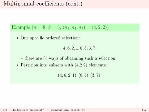
Example (n = 8, k = 3, (n1, n2, n3) = (4, 2, 2))
� One specific ordered selection:
4, 6, 2, 1, 8, 5, 3, 7
– there are 8! ways of obtaining such a selection.
� Partition into subsets with (4,2,2) elements:
(4, 6, 2, 1), (8, 5), (3, 7)
1.6 The basics of probability | Combinatorial probability 142
Multinomial coefficients (cont.)
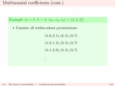
Example (n = 8, k = 3, (n1, n2, n3) = (4, 2, 2))
� Consider all within-subset permutations:
(4, 6, 2, 1), (8, 5), (3, 7)
(4, 6, 1, 2), (8, 5), (3, 7)
(4, 1, 2, 6), (8, 5), (3, 7)
...
1.6 The basics of probability | Combinatorial probability 143

Multinomial coefficients (cont.)
Example (n = 8, k = 3, (n1, n2, n3) = (4, 2, 2))
� There are
8!
4!× 2!× 2!=
40320
24× 2× 2= 420
possible distinct partitions;
(4, 6, 2, 1), (8, 5), (3, 7)
is regarded as identical to
(1, 2, 4, 6), (5, 8), (3, 7).
1.6 The basics of probability | Combinatorial probability 144

Multinomial coefficients (cont.)
Example (Department committees)
A University Department comprises 40 faculty members. Twocommittees of 12 faculty members, and two committees of 8faculty members, are needed.
The number of distinct committee configurations that can beformed is
N =
(40
12, 12, 8, 8
)=
40!
12!× 12!× 8!× 8!= 1785474512.
1.6 The basics of probability | Combinatorial probability 145

Multinomial coefficients (cont.)
Note: Binomial coefficients
Recall the binomial theorem:
(a+ b)n =
n∑j=0
(n
j
)ajbn−j
where (n
j
)=
n!
j!(n− j)! ≡(
n
j, n− j
)
1.6 The basics of probability | Combinatorial probability 146
Multinomial coefficients (cont.)
Note: Binomial coefficients
Here we are solving a partitioning problem; partition nelements into one subset of size j and one subset of size n− j.We can use this result and the multiplication principle to derivethe general multinomial coefficient result.
1.6 The basics of probability | Combinatorial probability 147
Multinomial coefficients (cont.)
Note: Binomial coefficients
For a collection of n elements:
1. Partition into two subsets of n1 and n− n1 elements;
2. Take the n− n1 elements and partition them into twosubsets of n2 and n− n1 − n2 elements;
3. Repeat until the final partition step; at this stage we have aset of n− n1 − · · · − nk−2 elements, which we partition into asubset of nk−1 elements and a subset of
nk = n− n1 − · · · − nk−2 − nk−1
elements.
1.6 The basics of probability | Combinatorial probability 148

Multinomial coefficients (cont.)
Note: Binomial coefficients
By the multiplication rule, the number of ways this sequence ofpartitioning steps can be carried out is(
n
n1
)×(n− n1n2
)× · · · ×
(n− n1 − · · · − nk−2
nk−1
)that is
n!
n1!(n− n1)!× (n− n1)!n2!(n− n1 − n2)!
× · · · × (n− n1 − · · · − nk−2)!nk−1!nk!
1.6 The basics of probability | Combinatorial probability 149
Multinomial coefficients (cont.)
Note: Binomial coefficients
Cancelling terms top and bottom in successive factors, we seethat this equals
n!
n1 × n2!× . . .× nk−1!× nk!
as required.
1.6 The basics of probability | Combinatorial probability 150
Combinations
The number combinations n objects taken r at a time is the num-ber of subsets, each of size r, that can be formed from objects.
This number is denoted
Cnr =
(n
r
)where (
n
r
)=
n!
r!(n− r)!
1.6 The basics of probability | Combinatorial probability 151
Combinations (cont.)
We first consider sequential selection of r objects: the number ofpossible selections (without replacement) is
n× (n− 1)× ...× (n− r + 1) =n!
(n− r)! = Pnr
leaving (n− r) objects unselected.
We then remember that the order of selected objects is not im-portant in identifying a combination, so therefore we must havethat
Pnr = r!× Cnr .as there are r! equivalent combinations that yield the same per-mutation. The result follows.
1.6 The basics of probability | Combinatorial probability 152
Binary sequences
Binary sequences
101000100101010
arise in many probability settings; if we take ‘1’ to indicate in-clusion and ‘0’ to indicate exclusion, then we can identify com-binations with binary sequences.
� the number of binary sequences of length n containing r 1sis (
n
r
)
1.6 The basics of probability | Combinatorial probability 153
Combinatorial probability
The above results are used to compute probabilities in the caseof equally likely outcomes.
� S: complete list of possible sequences of selections.
� A: sequences having property of interest.
� We have
P (A) =Number of elements in A
Number of elements in S=nAnS
1.6 The basics of probability | Combinatorial probability 154
Combinatorial probability (cont.)
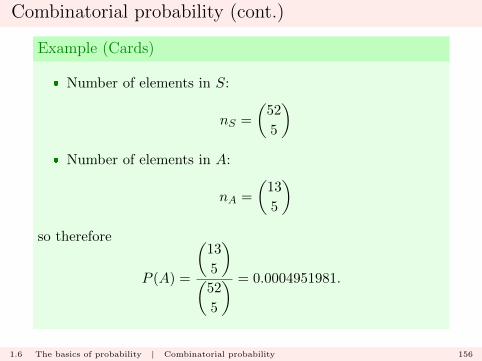
Example (Cards)
Five cards are selected without replacement from a standarddeck. What is the probability they are all Hearts ?
1.6 The basics of probability | Combinatorial probability 155
Combinatorial probability (cont.)
Example (Cards)
� Number of elements in S:
nS =
(52
5
)� Number of elements in A:
nA =
(13
5
)so therefore
P (A) =
(13
5
)(
52
5
) = 0.0004951981.
1.6 The basics of probability | Combinatorial probability 156

Other combinatorial problems
� Poker hands;
� Hypergeometric selection;
� Occupancy (or allocation) problems – allocate r objects ton boxes and identify
I the occupancy pattern;I the occupancy of a specific box.
1.6 The basics of probability | Combinatorial probability 157
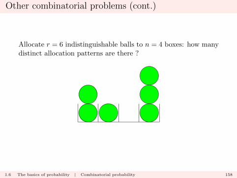
Other combinatorial problems (cont.)
Allocate r = 6 indistinguishable balls to n = 4 boxes: how manydistinct allocation patterns are there ?
1.6 The basics of probability | Combinatorial probability 158
Conditional probability
We now consider probability assessments in the presence of
partial knowledge.
In the case of ‘ordinary’ probability, we have (by assumption)that the outcome must be an element in the set S, and proceedto assess the probability that the outcome is an element of theset A ⊆ S.
That is, the only ‘certain’ knowledge we have is that the outcome,s, is in S.
1.7 The basics of probability | Conditional probability 159
Conditional probability (cont.)
Now suppose we have the ‘partial’ knowledge that, in fact,
s ∈ B ⊆ S
for some B;
� that is, we know that event B occurs.
1.7 The basics of probability | Conditional probability 160
Conditional probability (cont.)
How does this change our probability assessment concerning A ?
� in light of the information that B occurs, what do we nowthink about the probability that A occurs also ?
1.7 The basics of probability | Conditional probability 161
Conditional probability (cont.)
First, we are considering the event that both A and B occur,that is
s ∈ A ∩B
so P (A ∩B) must play a role in the calculation.
Secondly, with the knowledge that event B occurs, we restrictthe parts of the sample space that should be considered; we arecertain that the sample outcome must lie in B.
1.7 The basics of probability | Conditional probability 162
Conditional probability (cont.)
For two events A and B, the conditional probability of A givenB is denoted P (A|B), and is defined by
P (A|B) =P (A ∩B)
P (B)
Note that we consider this only in cases where P (B) > 0.
1.7 The basics of probability | Conditional probability 163
Conditional probability (cont.)
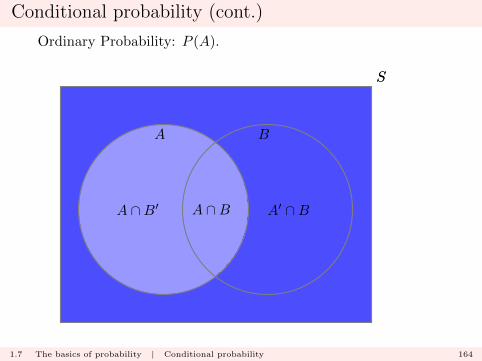
Ordinary Probability: P (A).
SS
A ∩BA ∩B′ A′ ∩B
A B
1.7 The basics of probability | Conditional probability 164
Conditional probability (cont.)
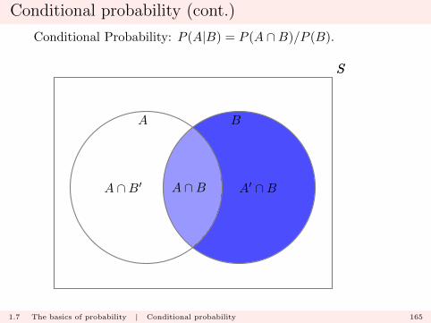
Conditional Probability: P (A|B) = P (A ∩B)/P (B).
SS
A ∩BA ∩B′ A′ ∩B
A B
1.7 The basics of probability | Conditional probability 165

Conditional probability (cont.)
Example
Experiment: roll a fair die, record the score.
� S = {1, 2, 3, 4, 5, 6}, all outcomes equally likely.
� A = {1, 3, 5} (score is odd).
� B = {4, 5, 6} (score is more than 3).
� A ∩B = {5}.
P (A) =3
6=
1
2P (B) =
3
6=
1
2P (A ∩B) =
1
6so
P (A|B) =P (A ∩B)
P (B)=
1/6
1/2=
1
3.
1.7 The basics of probability | Conditional probability 166

Conditional probability (cont.)
Example
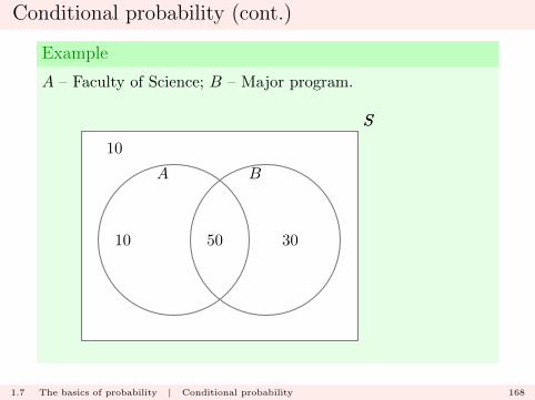
In a class of 100 students:
� 60 are from Faculty of Science, 40 are from Faculty of Arts.
� 80 are in a Major program, 20 are in another program.
� 50 of the Science students are in a Major program.
1.7 The basics of probability | Conditional probability 167
Conditional probability (cont.)
Example
A – Faculty of Science; B – Major program.
SS
50
10
10 30
A B
1.7 The basics of probability | Conditional probability 168

Conditional probability (cont.)
Example
A student is selected from the class, with all students equallylikely to be selected.
� What is the probability that the selected student is fromScience, P (A) ?:
P (A) =60
100=
3
5
1.7 The basics of probability | Conditional probability 169
Conditional probability (cont.)
Example
� What is the probability that the selected student is fromScience and in a Major program, P (A ∩B) ?:
P (A ∩B) =50
100=
1
2
1.7 The basics of probability | Conditional probability 170
Conditional probability (cont.)
Example
� If the selected student is known to be in a Major program,what is the probability that the student is from Science,P (A|B) ?:
P (A|B) =P (A ∩B)
P (B)=
50/100
80/100=
50
80=
5
8.
1.7 The basics of probability | Conditional probability 171
Conditional probability (cont.)
Note: some consequences
� If B ≡ S, then
P (A|S) =P (A ∩ S)
P (S)=P (A)
1= P (A).
� If B ≡ A, then
P (A|A) =P (A ∩A)
P (A)=P (A)
P (A)= 1.
� We have
P (A|B) =P (A ∩B)
P (B)≤ P (B)
P (B)= 1.
1.7 The basics of probability | Conditional probability 172
Conditional probability (cont.)
Direct from the definition, we have that
P (A ∩B) = P (B)P (A|B)
(recall P (B) > 0).
1.7 The basics of probability | Conditional probability 173
Conditional probability (cont.)
Note
It is important to understand the distinction between
P (A ∩B) and P (A|B).
� P (A ∩B) records the chance of A and B occurring relativeto S. A and B are treated symmetrically in the calculation.
� P (A|B) records the chance of A and B occurring relativeto B. A and B are not treated symmetrically; from thedefinition, we see that in general
P (B|A) =P (A ∩B)
P (A)6= P (A ∩B)
P (B)= P (A|B).
1.7 The basics of probability | Conditional probability 174
Conditional probability (cont.)
Note
From the above calculation, we see that we could have
P (A|B) ≤ P (A)
orP (A|B) ≥ P (A)
orP (A|B) = P (A).
That is, certain knowledge that B occurs could decrease, increaseor leave unchanged the probability that A occurs.
1.7 The basics of probability | Conditional probability 175
Conditional probability (cont.)
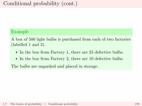
Example
A box of 500 light bulbs is purchased from each of two factories(labelled 1 and 2).
� In the box from Factory 1, there are 25 defective bulbs.
� In the box from Factory 2, there are 10 defective bulbs.
The bulbs are unpacked and placed in storage.
1.7 The basics of probability | Conditional probability 176

Conditional probability (cont.)
Example
A – Defective; B – Factory 1.
SS
25
490
10 475
A B
1.7 The basics of probability | Conditional probability 177
Conditional probability (cont.)
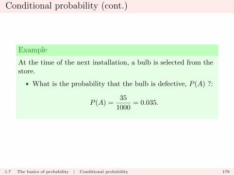
Example
At the time of the next installation, a bulb is selected from thestore.
� What is the probability that the bulb is defective, P (A) ?:
P (A) =35
1000= 0.035.
1.7 The basics of probability | Conditional probability 178
Conditional probability (cont.)
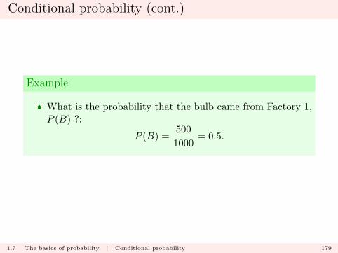
Example
� What is the probability that the bulb came from Factory 1,P (B) ?:
P (B) =500
1000= 0.5.
1.7 The basics of probability | Conditional probability 179
Conditional probability (cont.)
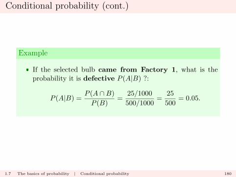
Example
� If the selected bulb came from Factory 1, what is theprobability it is defective P (A|B) ?:
P (A|B) =P (A ∩B)
P (B)=
25/1000
500/1000=
25
500= 0.05.
1.7 The basics of probability | Conditional probability 180
Conditional probability (cont.)
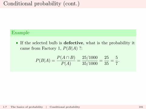
Example
� If the selected bulb is defective, what is the probability itcame from Factory 1, P (B|A) ?:
P (B|A) =P (A ∩B)
P (A)=
25/1000
35/1000=
25
35=
5
7.
1.7 The basics of probability | Conditional probability 181
Conditional probability (cont.)
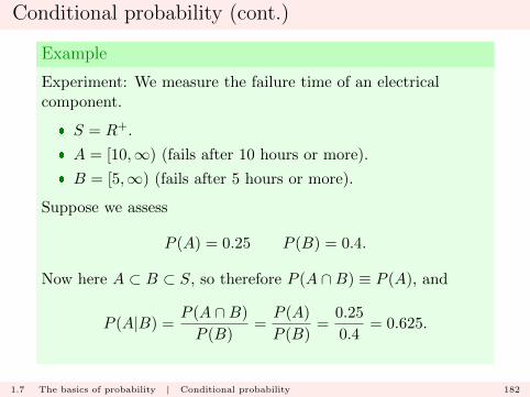
Example
Experiment: We measure the failure time of an electricalcomponent.
� S = R+.
� A = [10,∞) (fails after 10 hours or more).
� B = [5,∞) (fails after 5 hours or more).
Suppose we assess
P (A) = 0.25 P (B) = 0.4.
Now here A ⊂ B ⊂ S, so therefore P (A ∩B) ≡ P (A), and
P (A|B) =P (A ∩B)
P (B)=P (A)
P (B)=
0.25
0.4= 0.625.
1.7 The basics of probability | Conditional probability 182

Conditional probability (cont.)
The conditional probability function satisfies the Probability Ax-ioms: suppose B is an event in S such that P (B) > 0.
(I) Non-negativity:
P (A|B) =P (A ∩B)
P (B)≥ 0.
1.7 The basics of probability | Conditional probability 183

Conditional probability (cont.)
(II) For P (S|B) we have
P (S|B) =P (S ∩B)
P (B)=P (B)
P (B)= 1.
1.7 The basics of probability | Conditional probability 184

Conditional probability (cont.)
(III) Countable additivity: if A1, A2, . . . form a (countable)sequence of events such that Aj ∩Ak = ∅ for all j 6= k.
1.7 The basics of probability | Conditional probability 185
Conditional probability (cont.)
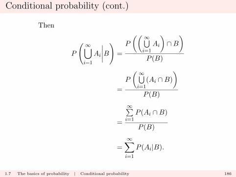
Then
P
( ∞⋃i=1
Ai
∣∣∣∣B)
=
P
(( ∞⋃i=1
Ai
)∩B
)P (B)
=
P
( ∞⋃i=1
(Ai ∩B)
)P (B)
=
∞∑i=1
P (Ai ∩B)
P (B)
=
∞∑i=1
P (Ai|B).
1.7 The basics of probability | Conditional probability 186
Conditional probability (cont.)
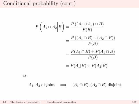
P
(A1 ∪A2
∣∣∣∣B) =P ((A1 ∪A2) ∩B)
P (B)
=P ((A1 ∩B) ∪ (A2 ∩B))
P (B)
=P (A1 ∩B) + P (A1 ∩B)
P (B)
= P (A1|B) + P (A2|B).
as
A1, A2 disjoint =⇒ (A1 ∩B), (A2 ∩B) disjoint.
1.7 The basics of probability | Conditional probability 187

Conditional probability (cont.)
Example (Three cards)
Three two sided cards:
1 2 3
One of the three cards is selected, with all cards being equallylikely to be chosen.
1.7 The basics of probability | Conditional probability 188

Conditional probability (cont.)
Example (Three cards)
One side is displayed:
What is the probability that the other side of this card is red ?
1.7 The basics of probability | Conditional probability 189
Conditional probability (cont.)
Example (Three cards)
Let
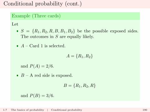
� S = {R1, R2, R,B,B1, B2} be the possible exposed sides.The outcomes in S are equally likely.
� A – Card 1 is selected.
A = {R1, R2}
and P (A) = 2/6.
� B – A red side is exposed.
B = {R1, R2, R}
and P (B) = 3/6.
1.7 The basics of probability | Conditional probability 190
Conditional probability (cont.)
Example (Three cards)
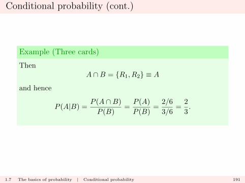
ThenA ∩B = {R1, R2} ≡ A
and hence
P (A|B) =P (A ∩B)
P (B)=P (A)
P (B)=
2/6
3/6=
2
3.
1.7 The basics of probability | Conditional probability 191
Conditional probability (cont.)
Example (Drug testing)
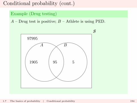
A drug testing authority tests 100000 athletes to assess whetherthey are using performance enhancing drugs (PEDs). The drugtest is not perfect as it produces
� False positives: declares an athlete to be using PEDs, whenin reality they are not.
� False negatives: declares an athlete not to be using PEDs,when in reality they are.
1.7 The basics of probability | Conditional probability 192
Conditional probability (cont.)
Example (Drug testing)
Suppose that after detailed investigation it is discovered that
� 2000 athletes gave positive test results.
� 100 athletes were using PEDs.
� 95 athletes who were using PEDs tested positive.
1.7 The basics of probability | Conditional probability 193
Conditional probability (cont.)
Example (Drug testing)
A – Drug test is positive; B – Athlete is using PED.
SS
95
97995
1905 5
A B
1.7 The basics of probability | Conditional probability 194
Conditional probability (cont.)
Example (Drug testing)
However, in the original analysis, an athlete is selected atrandom from the 100000, and is observed to test positive.
What is the probability that they actually were using PEDs ?
1.7 The basics of probability | Conditional probability 195
Conditional probability (cont.)
Example (Drug testing)
The required conditional probability is
P (B|A) =P (A ∩B)
P (A)=
95
2000= 0.0475.
Note that is very different from
P (A|B) =P (A ∩B)
P (B)=
95
100= 0.95.
1.7 The basics of probability | Conditional probability 196
Independence
Two events A and B in sample space S are independent if
P (A|B) = P (A);
equivalently, they are independent if
P (A ∩B) = P (A)P (B).
Note that if P (A|B) = P (A), then
P (B|A) =P (A ∩B)
P (A)=P (A)P (B)
P (A)= P (B).
1.8 The basics of probability | Independence 197
Independence (cont.)
Note
Independence is not a property of the events A and B themselves,it is a property of the probabilities assigned to them.
1.8 The basics of probability | Independence 198
Independence (cont.)
Note
Independence is not the same as mutual exclusivity.
Independent: P (A ∩B) = P (A)P (B)
Mutually exclusive: P (A ∩B) = 0.
1.8 The basics of probability | Independence 199
Independence (cont.)
Example
A fair coin is tossed twice, with the outcomes of the two tossesindependent. We have
S = {HH,HT, TH, TT}
with all four outcomes equally likely.
(a) If the first toss result is H, what is the probability that thesecond toss is also H ?
(b) If one result is H, what is the probability that the other isH ?
1.8 The basics of probability | Independence 200

Independence (cont.)
Example
Let
� A = {HH} (both heads).
� B = {HH,HT, TH} (at least one head).
� C = {HH,HT} (first result is head).
(a) We want P (A|C):
P (A|C) =P (A ∩ C)
P (C)=P (A)
P (C)=
1/4
2/4=
1
2.
(b) We want P (A|B):
P (A|B) =P (A ∩B)
P (B)=P (A)
P (B)=
1/4
3/4=
1
3.
1.8 The basics of probability | Independence 201
Independence for multiple events
Independence as defined above is a statement concerning twoevents.
What if we have more than two events ?
� Events A1, A2, A3 in sample space S.
� We can consider independence pairwise:
P (A1 ∩A2) = P (A1)P (A2)
P (A1 ∩A3) = P (A1)P (A3)
P (A2 ∩A3) = P (A2)P (A3)
1.8 The basics of probability | Independence 202
Independence for multiple events (cont.)
� What about
P (A1 ∩A2 ∩A3);
Can we deduce
P (A1 ∩A2 ∩A3) = P (A1)P (A2)P (A3)?
� In general, no.
1.8 The basics of probability | Independence 203
Independence for multiple events (cont.)
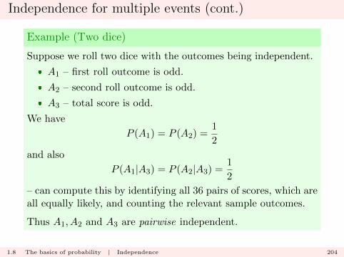
Example (Two dice)
Suppose we roll two dice with the outcomes being independent.
� A1 – first roll outcome is odd.
� A2 – second roll outcome is odd.
� A3 – total score is odd.
We have
P (A1) = P (A2) =1
2
and also
P (A1|A3) = P (A2|A3) =1
2
– can compute this by identifying all 36 pairs of scores, which areall equally likely, and counting the relevant sample outcomes.
Thus A1, A2 and A3 are pairwise independent.
1.8 The basics of probability | Independence 204
Independence for multiple events (cont.)
Example (Two dice)
However,P (A1 ∩A2 ∩A3) = 0
andP (A1|A2 ∩A3) = 0
etc.
1.8 The basics of probability | Independence 205
Independence for multiple events (cont.)
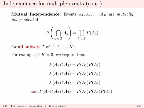
Mutual Independence: Events A1, A2, . . . , AK are mutuallyindependent if
P
( ⋂k ∈ I
Ak
)=∏k ∈ I
P (Ak)
for all subsets I of {1, 2, . . . ,K}.For example, if K = 3, we require that
P (A1 ∩A2) = P (A1)P (A2)
P (A1 ∩A3) = P (A1)P (A3)
P (A2 ∩A3) = P (A2)P (A3)
and P (A1 ∩A2 ∩A3) = P (A1)P (A2)P (A3).
1.8 The basics of probability | Independence 206
Conditional independence
Conditional independence: Consider events A1, A2 and B insample space S, with P (B) > 0. Then A1 and A2 are condition-ally independent given B if
P (A1|A2 ∩B) = P (A1|B)
or equivalently
P (A1 ∩A2|B) = P (A1|B)P (A2|B).
1.8 The basics of probability | Independence 207
General Multiplication Rule
For events A1, A2, . . . , AK , we have the general result that
P (A1 ∩A2 ∩ · · · ∩AK) = P (A1)P (A2|A1)P (A3|A1 ∩A2) . . .
. . . P (AK |A1 ∩A2 ∩ · · · ∩AK−1)
This follows by the recursive calculation
P (A1 ∩A2 ∩ · · · ∩AK) = P (A1)P (A2 ∩ · · · ∩AK |A1)
= P (A1)P (A2|A1)
P (A3 ∩ · · · ∩AK |A1 ∩A2)
= . . .
Also known as the Chain Rule for probabilities.
1.9 The basics of probability | General Multiplication Rule 208
General Multiplication Rule (cont.)
If the events are mutually independent, then we have that
P (A1 ∩A2 ∩ · · · ∩AK) =
K∏k=1
P (Ak)
1.9 The basics of probability | General Multiplication Rule 209
Probability Trees
Probability trees are simple ways to display joint probabilities ofmultiple events. They comprise
� Junctions: corresponding to the multiple events
� Branches: corresponding to paths displaying the sequence of(conditional) choices of events, given the previous choices.
We multiply along the branches to get the joint probabilities.
1.9 The basics of probability | General Multiplication Rule 210
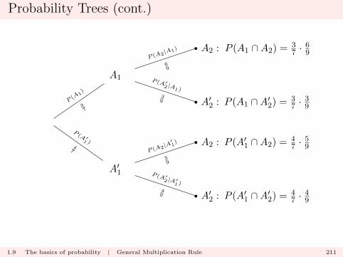
Probability Trees (cont.)
A′1
A′2 : P (A′1 ∩A′2) = 47 · 49
P (A ′2 |A ′
1 )49
A2 : P (A′1 ∩A2) = 47 · 59
P (A2|A′1)
59
P(A ′
1 )4
7
A1
A′2 : P (A1 ∩A′2) = 37 · 39
P (A ′2 |A
1 )39
A2 : P (A1 ∩A2) = 37 · 69
P (A2|A1)
69
P(A
1)
37
1.9 The basics of probability | General Multiplication Rule 211

Probability Trees (cont.)
Note that each junction has two possible branches coming fromit, corresponding to
Ak and A′k
respectively.
Such a tree extends to as many events as we need.
1.9 The basics of probability | General Multiplication Rule 212
The Theorem of Total Probability
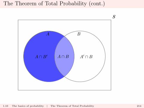
For two events A and B in sample space S, we have the partitionof A as
A = (A ∩B) ∪ (A ∩B′).
1.10 The basics of probability | The Theorem of Total Probability 213
The Theorem of Total Probability (cont.)
SS
A ∩BA ∩B′ A′ ∩B
A B
1.10 The basics of probability | The Theorem of Total Probability 214
The Theorem of Total Probability (cont.)
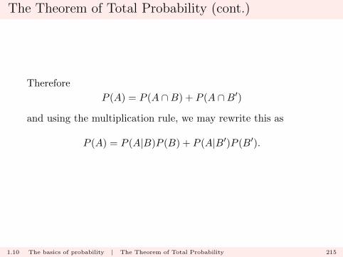
Therefore
P (A) = P (A ∩B) + P (A ∩B′)
and using the multiplication rule, we may rewrite this as
P (A) = P (A|B)P (B) + P (A|B′)P (B′).
1.10 The basics of probability | The Theorem of Total Probability 215

The Theorem of Total Probability (cont.)
B′
A′ : P (B′ ∩A′)
P (A ′|B ′)
A : P (B′ ∩A)P (A|B
′ )
P(B ′
)
B
A′ : P (B ∩A′)
P (A ′|B)
A : P (B ∩A)P (A|B
)
P(B
)
1.10 The basics of probability | The Theorem of Total Probability 216

The Theorem of Total Probability (cont.)
That is, there are two ways to get to A:
� via B;
� via B′.
To compute P (A) we add up all the probabilities on paths thatend up at A.
Note that B and B′ together form a partition of S.
1.10 The basics of probability | The Theorem of Total Probability 217
The Theorem of Total Probability (cont.)
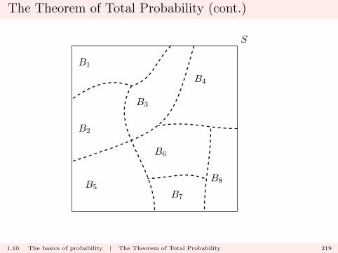
Now suppose we have a partition into n subsets
B1, B2, . . . , Bn.
Again, these events also partition A.
1.10 The basics of probability | The Theorem of Total Probability 218
The Theorem of Total Probability (cont.)
S
B5
B3
B6
B1
B2
B4
B7
B8
1.10 The basics of probability | The Theorem of Total Probability 219

The Theorem of Total Probability (cont.)
S
A
B5
B3
B6
B1
B2
B4
B7
B8
1.10 The basics of probability | The Theorem of Total Probability 220
The Theorem of Total Probability (cont.)
That is, we have that
A = (A ∩B1) ∪ (A ∩B2) ∪ · · · ∪ (A ∩Bn)
and
P (A) = P (A ∩B1) + P (A ∩B2) + · · ·+ P (A ∩Bn).
1.10 The basics of probability | The Theorem of Total Probability 221
The Theorem of Total Probability (cont.)
Using the definition of conditional probability, we therefore have
P (A) = P (A|B1)P (B1) +P (A|B2)P (B2) + · · ·+P (A|Bn)P (Bn).
that is
P (A) =
n∑i=1
P (A|Bi)P (Bi).
This result is known as the Theorem of Total Probability .
1.10 The basics of probability | The Theorem of Total Probability 222

The Theorem of Total Probability (cont.)
Notes
� The formula assumes that P (Bi) > 0 for i = 1, . . . , n.
� It might be that
P (A ∩Bi) = P (A|Bi) = 0.
for some i.
� This formula is a mathematical encapsulation of the prob-ability tree when it is used to compute P (A).
1.10 The basics of probability | The Theorem of Total Probability 223
The Theorem of Total Probability (cont.)
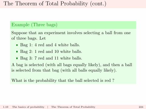
Example (Three bags)
Suppose that an experiment involves selecting a ball from oneof three bags. Let
� Bag 1: 4 red and 4 white balls.
� Bag 2: 1 red and 10 white balls.
� Bag 3: 7 red and 11 white balls.
A bag is selected (with all bags equally likely), and then a ballis selected from that bag (with all balls equally likely).
What is the probability that the ball selected is red ?
1.10 The basics of probability | The Theorem of Total Probability 224
The Theorem of Total Probability (cont.)
Example (Three bags)
Let
� S: all possible selections of balls.
� B1: bag 1 selected.
� B2: bag 2 selected.
� B2: bag 3 selected.
� A: ball selected is red.
1.10 The basics of probability | The Theorem of Total Probability 225
The Theorem of Total Probability (cont.)
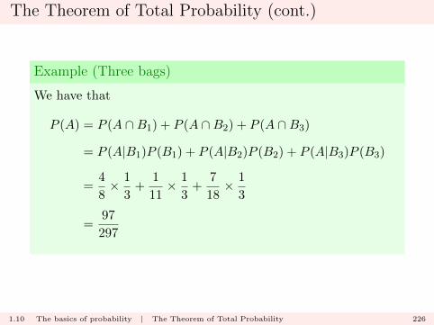
Example (Three bags)
We have that
P (A) = P (A ∩B1) + P (A ∩B2) + P (A ∩B3)
= P (A|B1)P (B1) + P (A|B2)P (B2) + P (A|B3)P (B3)
=4
8× 1
3+
1
11× 1
3+
7
18× 1
3
=97
297
1.10 The basics of probability | The Theorem of Total Probability 226
The Theorem of Total Probability (cont.)
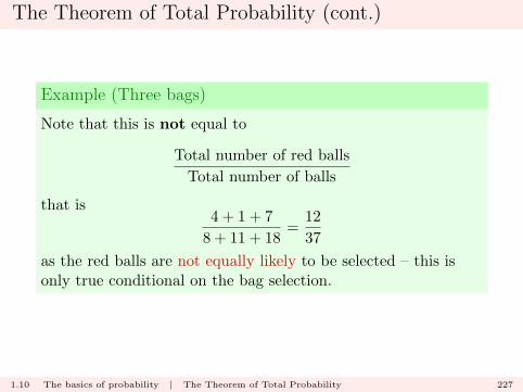
Example (Three bags)
Note that this is not equal to
Total number of red balls
Total number of balls
that is4 + 1 + 7
8 + 11 + 18=
12
37
as the red balls are not equally likely to be selected – this isonly true conditional on the bag selection.
1.10 The basics of probability | The Theorem of Total Probability 227
Bayes Theorem
The second great theorem of probability is Bayes Theorem.
� Named after Reverend Thomas Bayes (1701 – 1761)
https://en.wikipedia.org/wiki/Thomas Bayes
� Could be written Bayes’s Theorem.
� It is not really a theorem.
1.11 The basics of probability | Bayes Theorem 228
Bayes Theorem (cont.)
Bayes Theorem: For two events A and B in sample space S,with P (A) > 0 and P (B) > 0,
P (B|A) =P (A|B)P (B)
P (A).
If 0 < P (B) < 1, we may write by the Theorem of Total Prob-ability.
P (B|A) =P (A|B)P (B)
P (A|B)P (B) + P (A|B′)P (B′)
1.11 The basics of probability | Bayes Theorem 229
Bayes Theorem (cont.)
“Proof”: By the definition of conditional probability
P (A|B)P (B) = P (A ∩B) = P (B|A)P (A).
Then as P (A) > 0 and P (B) > 0 we can cross multiply and write
P (B|A) =P (A|B)P (B)
P (A).
If 0 < P (B) < 1, then we can legitimately write
P (A) = P (A|B)P (B) + P (A|B′)P (B′)
and substitute this expression in the denominator.
1.11 The basics of probability | Bayes Theorem 230

Bayes Theorem (cont.)
General version: Suppose that B1, B2, . . . , Bn form a partitionof S, with P (Bj) > 0 for j = 1, . . . , n. Suppose that A is an eventin S with P (A) > 0.
Then for i = 1, . . . , n
P (Bi|A) =P (A|Bi)P (Bi)
P (A)=
P (A|Bi)P (Bi)n∑j=1
P (A|Bj)P (Bj)
.
1.11 The basics of probability | Bayes Theorem 231

Bayes Theorem (cont.)
Probability tree interpretation: Given that we end up at A, whatis the probability that we got there via branch Bi ?
1.11 The basics of probability | Bayes Theorem 232
Bayes Theorem (cont.)
Example (Three bags)
Suppose that an experiment involves selecting a ball from oneof three bags. Let
� Bag 1: 4 red and 4 white balls.
� Bag 2: 1 red and 10 white balls.
� Bag 3: 7 red and 11 white balls.
A bag is selected (with all bags equally likely), and then a ballis selected from that bag (with all balls equally likely).
The ball selected is red. What is the probability it came fromBag 2 ?
1.11 The basics of probability | Bayes Theorem 233
Bayes Theorem (cont.)
Example (Three bags)
Let
� S: all possible selections of balls.
� B1: bag 1 selected.
� B2: bag 2 selected.
� B2: bag 3 selected.
� A: ball selected is red.
1.11 The basics of probability | Bayes Theorem 234
Bayes Theorem (cont.)
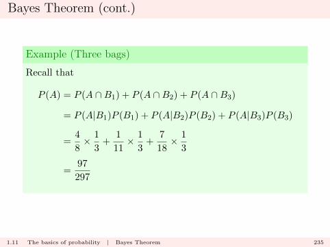
Example (Three bags)
Recall that
P (A) = P (A ∩B1) + P (A ∩B2) + P (A ∩B3)
= P (A|B1)P (B1) + P (A|B2)P (B2) + P (A|B3)P (B3)
=4
8× 1
3+
1
11× 1
3+
7
18× 1
3
=97
297
1.11 The basics of probability | Bayes Theorem 235
Bayes Theorem (cont.)
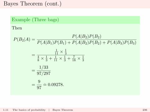
Example (Three bags)
Then
P (B2|A) =P (A|B2)P (B2)
P (A|B1)P (B1) + P (A|B2)P (B2) + P (A|B3)P (B3)
=111 × 1
348 × 1
3 + 111 × 1
3 + 718 × 1
3
=1/33
97/297
=9
97l 0.09278.
1.11 The basics of probability | Bayes Theorem 236
Bayes Theorem (cont.)
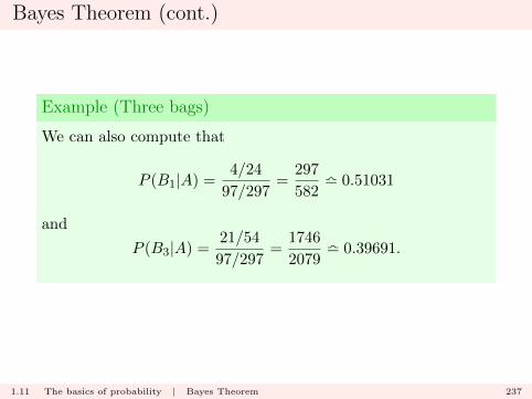
Example (Three bags)
We can also compute that
P (B1|A) =4/24
97/297=
297
582l 0.51031
and
P (B3|A) =21/54
97/297=
1746
2079l 0.39691.
1.11 The basics of probability | Bayes Theorem 237
Bayes Theorem (cont.)
Note
We have that
P (B1|A) + P (B2|A) + P (B3|A) = 1
but note that
P (A|B1) + P (A|B2) + P (A|B3) 6= 1.
In the first formula, we are conditioning on A everywhere; inthe second, we have different conditioning sets.
1.11 The basics of probability | Bayes Theorem 238
Using Bayes Theorem
Bayes theorem is often used to make probability statements con-cerning an event B that has not been observed, given an eventA that has been observed.
1.11 The basics of probability | Bayes Theorem 239
Using Bayes Theorem (cont.)
Example (Medical screening)
A health authority tests individuals from a population to assesswhether they are sufferers from some disease. The screening testis not perfect as it produces
� False positives: declares someone to be a sufferer, when inreality they are a non-sufferer.
� False negatives: declares someone to be a non-sufferer, whenin reality they are a sufferer.
1.11 The basics of probability | Bayes Theorem 240
Using Bayes Theorem (cont.)
Example (Medical screening)
Suppose that we denote by
� A – Screening test is positive;
� B – Person is actually a sufferer.
1.11 The basics of probability | Bayes Theorem 241
Using Bayes Theorem (cont.)
Example (Medical screening)
Suppose that
� P (B) = p;
� P (A|B) = 1− α (true positive rate);
� P (A|B′) = β (false positive rate).
for probabilities p, α, β.
1.11 The basics of probability | Bayes Theorem 242
Using Bayes Theorem (cont.)
Example (Medical screening)
We have for the rate of positive tests
P (A) = P (A|B)P (B) + P (A|B′)P (B′) = (1− α)p+ β(1− p)
by the Theorem of Total Probability, and by Bayes theorem
P (B|A) =P (A|B)P (B)
P (A|B)P (B) + P (A|B′)P (B′)
=(1− α)p
(1− α)p+ β(1− p) .
1.11 The basics of probability | Bayes Theorem 243
Using Bayes Theorem (cont.)
Example (Medical screening)
Similarly, for the false negative rate, we have
P (B|A′) =P (A′|B)P (B)
P (A′|B)P (B) + P (A′|B′)P (B′)
=αp
αp+ (1− β)(1− p) .
1.11 The basics of probability | Bayes Theorem 244

Using Bayes Theorem (cont.)
Example (Medical screening)
We have
P (A|B) = (1− α) P (B|A) = (1− α)p
(1− α)p+ β(1− p)
and these two values are potentially very different.
1.11 The basics of probability | Bayes Theorem 245
Using Bayes Theorem (cont.)
Example (Medical screening)
That is, in general,
P (“Spots”|“Measles”) 6= P (“Measles”|“Spots”)
1.11 The basics of probability | Bayes Theorem 246
Using Bayes Theorem (cont.)
Note
This phenomenon is sometimes known as the Prosecutor’sFallacy :
P (“Evidence”|“Guilt”) 6= P (“Guilt”|“Evidence”)
1.11 The basics of probability | Bayes Theorem 247
Bayes Theorem and Odds
Recall that the odds on event B is defined by
P (B)
P (B′)=
P (B)
1− P (B)
The conditional odds given event A (with P (A) > 0) is definedby
P (B|A)
P (B′|A)=
P (B|A)
1− P (B|A)
1.11 The basics of probability | Bayes Theorem 248
Bayes Theorem and Odds (cont.)
We have thatP (B|A)
P (B′|A)=P (A|B)
P (A|B′)P (B)
P (B′)
that is, the odds change by a factor
P (A|B)
P (A|B′) .
1.11 The basics of probability | Bayes Theorem 249

Bayes Theorem with multiple events
If A1 and A2 are two events in a sample space S so that
P (A1 ∩A2) > 0
and there is a partition of S via B1, . . . , Bn, with P (Bi) > 0,then
P (Bi|A1 ∩A2) =P (A1 ∩A2|Bi)P (Bi)n∑j=1
P (A1 ∩A2|Bj)P (Bj)
� we use the previous version of Bayes Theorem with
A ≡ A1 ∩A2.
� this extends to conditioning events A1, A2, . . . , An.
1.11 The basics of probability | Bayes Theorem 250

Bayes Theorem with multiple events (cont.)
Note that we have by earlier results
P (A1 ∩A2|Bi) = P (A1|Bi)P (A2|A1 ∩Bi)
that is, the chain rule applies to conditional probabilities also.
1.11 The basics of probability | Bayes Theorem 251

Chapter 2: Random variables and
probability distributions
Random variables
Up to this point we have dealt with probability assignments forevents defined on a general sample space S.
We now focus on the specific case where S is a subset of the realnumbers, R. We could have S
� finite or countable {0, 1, 2, . . .};� uncountable.
Events in such a sample space can be termed numerical events.
2.0 Random variables and probability distributions 253
Random variables (cont.)
For most experiments defined on an arbitrary space S, we canusually consider a simple mapping, Y , defined on S that mapsthe sample outcomes onto R, that is
Y : S −→ R
s 7−→ y
We are essentially saying that
Y (s) = y for s ∈ S.
The mapping Y is termed a random variable.
2.0 Random variables and probability distributions 254
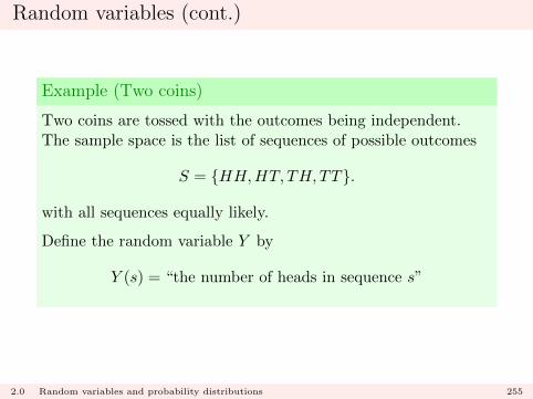
Random variables (cont.)
Example (Two coins)
Two coins are tossed with the outcomes being independent.The sample space is the list of sequences of possible outcomes
S = {HH,HT, TH, TT}.
with all sequences equally likely.
Define the random variable Y by
Y (s) = “the number of heads in sequence s”
2.0 Random variables and probability distributions 255
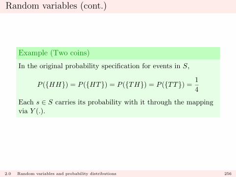
Random variables (cont.)
Example (Two coins)
In the original probability specification for events in S,
P ({HH}) = P ({HT}) = P ({TH}) = P ({TT}) =1
4
Each s ∈ S carries its probability with it through the mappingvia Y (.).
2.0 Random variables and probability distributions 256
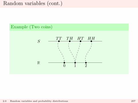
Random variables (cont.)
Example (Two coins)
TT TH HT HH
0 1 2
S
R
2.0 Random variables and probability distributions 257

Random variables (cont.)
Example (Two coins)
Then
Y (HH) = 2 Y (HT ) = Y (TH) = 1 Y (TT ) = 0
and Y (.) maps S onto the set {0, 1, 2}. We have that
P (Y = 0) ≡ P (s ∈ {TT}) =1
4
P (Y = 1) ≡ P (s ∈ {HT, TH}) =2
4
P (Y = 2) ≡ P (s ∈ {HH}) =1
4
with P (Y (s) = y) = 0 for all other real values y.
2.0 Random variables and probability distributions 258
Random variables (cont.)
Notes
� We typically consider the image of S under the mapping Y (.)first
I that is, we identify the possible values that Y can take.
� In general, Y (.) is a many-to-one mapping.
� We usually suppress the dependence of Y (.) on its argument,and merely write
P (Y = y).
2.0 Random variables and probability distributions 259

Random variables (cont.)
Notes
We typically use upper case letters
X,Y, Z
etc. to denote random variables, and lower case letters
x, y, z
etc. to denote the real values that the random variable takes.
2.0 Random variables and probability distributions 260
Discrete Random variables
A random variable Y is termed discrete if the possible values thatY can take is a countable set
y1, y2, . . . , yn, . . .
Could be a
� finite set: eg {1, 2, . . . , 100}� countably infinite set: eg Z.
I will denote the set of values that carry positive probability usingthe notation Y.
2.1 Random variables and probability distributions | Discrete random variables 261
Discrete Random variables (cont.)
In this case, the probabilities assigned to the individual points inthe set Y in must carry all the probability:∑
y ∈ YP (Y = y) = 1.
This follows by the probability axioms as all the probability fromS has been mapped into Y.
2.1 Random variables and probability distributions | Discrete random variables 262
Probability mass function
The probability mass function (pmf) for Y , p(.), is the mathem-atical function that records how probability is distributed acrosspoints in R.
That is,
p(y) = P (Y = y)
� If y ∈ Y, p(y) > 0,
� otherwise p(y) = 0.
2.1 Random variables and probability distributions | Discrete random variables 263
Probability mass function (cont.)
Note
The notation f(y) is also commonly used, and also it issometimes helpful to write
pY (y) or fY (y)
to indicate that we are dealing with the pmf for Y .
2.1 Random variables and probability distributions | Discrete random variables 264
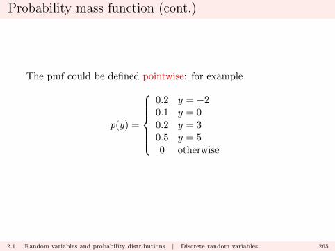
Probability mass function (cont.)
The pmf could be defined pointwise: for example
p(y) =
0.2 y = −20.1 y = 00.2 y = 30.5 y = 50 otherwise
2.1 Random variables and probability distributions | Discrete random variables 265
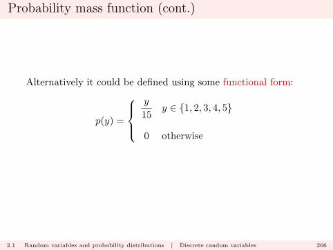
Probability mass function (cont.)
Alternatively it could be defined using some functional form:
p(y) =
y
15y ∈ {1, 2, 3, 4, 5}
0 otherwise
2.1 Random variables and probability distributions | Discrete random variables 266
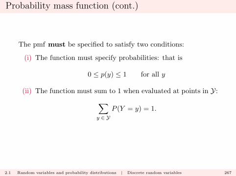
Probability mass function (cont.)
The pmf must be specified to satisfy two conditions:
(i) The function must specify probabilities: that is
0 ≤ p(y) ≤ 1 for all y
(ii) The function must sum to 1 when evaluated at points in Y:∑y ∈ Y
P (Y = y) = 1.
2.1 Random variables and probability distributions | Discrete random variables 267
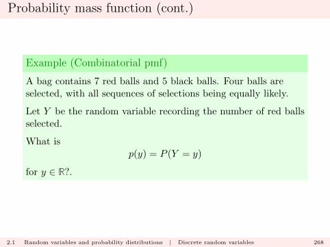
Probability mass function (cont.)
Example (Combinatorial pmf)
A bag contains 7 red balls and 5 black balls. Four balls areselected, with all sequences of selections being equally likely.
Let Y be the random variable recording the number of red ballsselected.
What isp(y) = P (Y = y)
for y ∈ R?.
2.1 Random variables and probability distributions | Discrete random variables 268
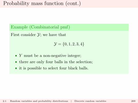
Probability mass function (cont.)
Example (Combinatorial pmf)
First consider Y; we have that
Y = {0, 1, 2, 3, 4}
� Y must be a non-negative integer;
� there are only four balls in the selection;
� it is possible to select four black balls.
2.1 Random variables and probability distributions | Discrete random variables 269

Probability mass function (cont.)
Example (Combinatorial pmf)
What is P (Y = y) for y ∈ {0, 1, 2, 3, 4} ?
(Y = y) ≡ A = {y red balls selected out of four}That is,
(Y = y) ≡ A = {y red balls, and 4− y black balls selected}
2.1 Random variables and probability distributions | Discrete random variables 270

Probability mass function (cont.)
Example (Combinatorial pmf)
We compute P (A) as follows: for y ∈ {0, 1, 2, 3, 4}
nA =
(7
y
)×(
5
4− y
)(
7
y
): number of ways of selecting the y red balls
from the 7 available.(5
4− y
): number of ways of selecting the 4− y black balls
from the 5 available.
2.1 Random variables and probability distributions | Discrete random variables 271
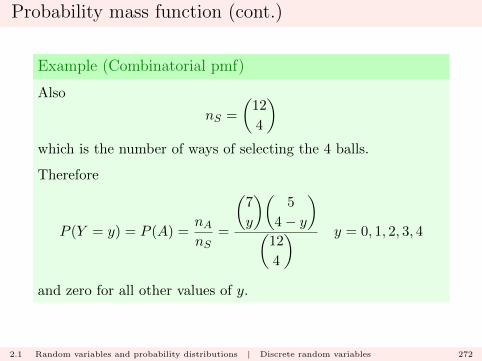
Probability mass function (cont.)
Example (Combinatorial pmf)
Also
nS =
(12
4
)which is the number of ways of selecting the 4 balls.
Therefore
P (Y = y) = P (A) =nAnS
=
(7
y
)(5
4− y
)(
12
4
) y = 0, 1, 2, 3, 4
and zero for all other values of y.
2.1 Random variables and probability distributions | Discrete random variables 272
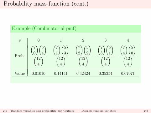
Probability mass function (cont.)
Example (Combinatorial pmf)
y 0 1 2 3 4
Prob.
(7
0
)(5
4
)(
12
4
)(
7
1
)(5
3
)(
12
4
)(
7
2
)(5
2
)(
12
4
)(
7
3
)(5
1
)(
12
4
)(
7
4
)(5
0
)(
12
4
)Value 0.01010 0.14141 0.42424 0.35354 0.07071
2.1 Random variables and probability distributions | Discrete random variables 273

Probability mass function (cont.)
Note
The collection of y values for which p(y) > 0 may be acountably infinite set, say
Y = {y1, y2, . . .}.
In this case we would require the infinite sum
∞∑i=1
p(yi)
be equal to 1.
2.1 Random variables and probability distributions | Discrete random variables 274
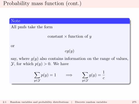
Probability mass function (cont.)
Note
All pmfs take the form
constant× function of y
orcg(y)
say, where g(y) also contains information on the range of values,Y, for which p(y) > 0. We have∑
y∈Yp(y) = 1 =⇒
∑y∈Y
g(y) =1
c
2.1 Random variables and probability distributions | Discrete random variables 275
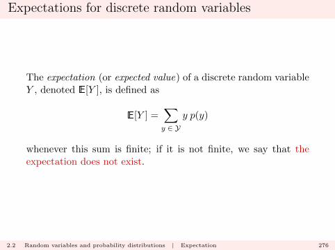
Expectations for discrete random variables
The expectation (or expected value) of a discrete random variableY , denoted E[Y ], is defined as
E[Y ] =∑y ∈ Y
y p(y)
whenever this sum is finite; if it is not finite, we say that theexpectation does not exist.
2.2 Random variables and probability distributions | Expectation 276
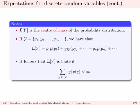
Expectations for discrete random variables (cont.)
Notes
� E[Y ] is the centre of mass of the probability distribution.
� If Y = {y1, y2, . . . , yn, . . .}, we have that
E[Y ] = y1p(y1) + y2p(y2) + · · ·+ ynp(yn) + · · ·
� It follows that E[Y ] is finite if∑y ∈ Y
|y| p(y) <∞
2.2 Random variables and probability distributions | Expectation 277
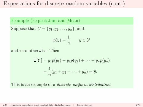
Expectations for discrete random variables (cont.)
Example (Expectation and Mean)
Suppose that Y = {y1, y2, . . . , yn}, and
p(y) =1
ny ∈ Y
and zero otherwise. Then
E[Y ] = y1p(y1) + y2p(y2) + · · ·+ ynp(yn)
=1
n(y1 + y2 + · · ·+ yn) = y.
This is an example of a discrete uniform distribution.
2.2 Random variables and probability distributions | Expectation 278
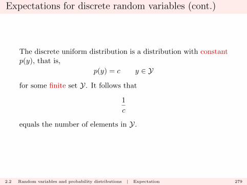
Expectations for discrete random variables (cont.)
The discrete uniform distribution is a distribution with constantp(y), that is,
p(y) = c y ∈ Y
for some finite set Y. It follows that
1
c
equals the number of elements in Y.
2.2 Random variables and probability distributions | Expectation 279
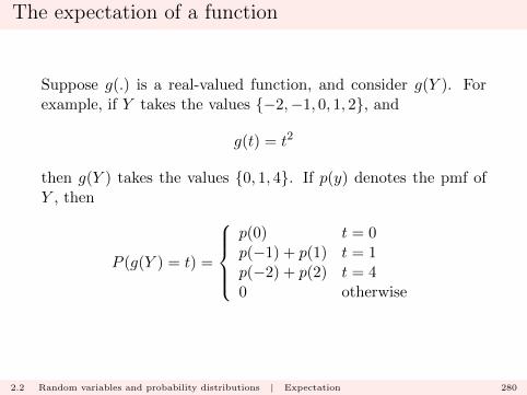
The expectation of a function
Suppose g(.) is a real-valued function, and consider g(Y ). Forexample, if Y takes the values {−2,−1, 0, 1, 2}, and
g(t) = t2
then g(Y ) takes the values {0, 1, 4}. If p(y) denotes the pmf ofY , then
P (g(Y ) = t) =
p(0) t = 0p(−1) + p(1) t = 1p(−2) + p(2) t = 40 otherwise
2.2 Random variables and probability distributions | Expectation 280
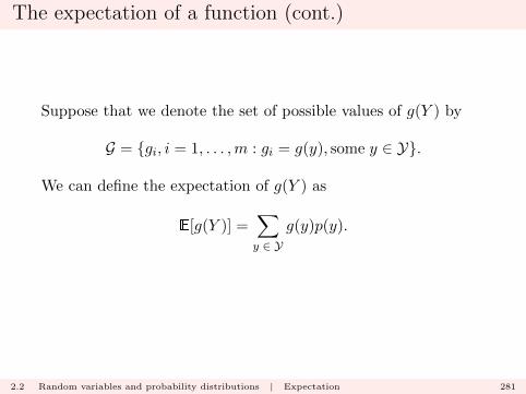
The expectation of a function (cont.)
Suppose that we denote the set of possible values of g(Y ) by
G = {gi, i = 1, . . . ,m : gi = g(y), some y ∈ Y}.
We can define the expectation of g(Y ) as
E[g(Y )] =∑y ∈ Y
g(y)p(y).
2.2 Random variables and probability distributions | Expectation 281
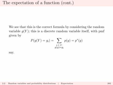
The expectation of a function (cont.)
We see that this is the correct formula by considering the randomvariable g(Y ); this is a discrete random variable itself, with pmfgiven by
P (g(Y ) = gi) =∑y ∈ Y:
g(y)=gi
p(y) = p∗(g)
say.
2.2 Random variables and probability distributions | Expectation 282

The expectation of a function (cont.)
Then
E[g(Y )] =
m∑i=1
gip∗(gi)
=
m∑i=1
gi
∑y ∈ Y:
g(y)=gi
p(y)
=∑y ∈ Y
g(y)p(y).
2.2 Random variables and probability distributions | Expectation 283
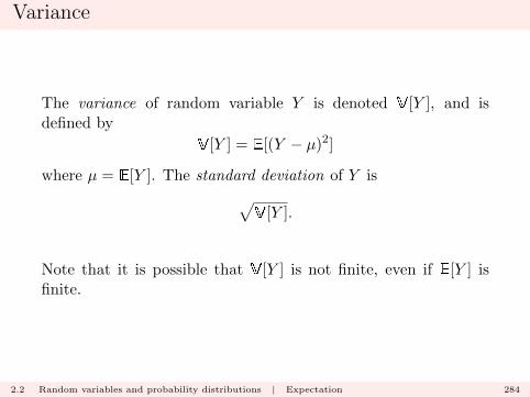
Variance
The variance of random variable Y is denoted V[Y ], and isdefined by
V[Y ] = E[(Y − µ)2]
where µ = E[Y ]. The standard deviation of Y is√V[Y ].
Note that it is possible that V[Y ] is not finite, even if E[Y ] isfinite.
2.2 Random variables and probability distributions | Expectation 284

Variance (cont.)
The variance is a measure of how “dispersed” the probabilitydistribution is.
Note that
V[Y ] = E[(Y − µ)2] =∑y
(y − µ)2p(y) ≥ 0
as p(y) ≥ 0 and (y − µ)2 ≥ 0 for all y.
2.2 Random variables and probability distributions | Expectation 285

Variance (cont.)
In fact, V[Y ] > 0 unless the distribution of Y is degenerate, thatis, for some constant c
p(c) = 1
in which case V[Y ] = 0.
2.2 Random variables and probability distributions | Expectation 286
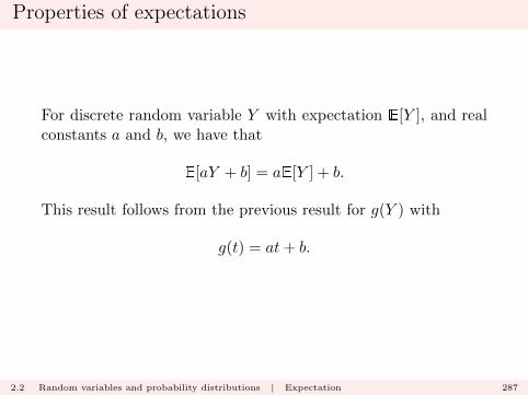
Properties of expectations
For discrete random variable Y with expectation E[Y ], and realconstants a and b, we have that
E[aY + b] = aE[Y ] + b.
This result follows from the previous result for g(Y ) with
g(t) = at+ b.
2.2 Random variables and probability distributions | Expectation 287
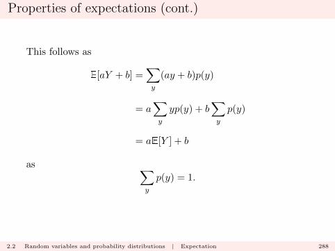
Properties of expectations (cont.)
This follows as
E[aY + b] =∑y
(ay + b)p(y)
= a∑y
yp(y) + b∑y
p(y)
= aE[Y ] + b
as ∑y
p(y) = 1.
2.2 Random variables and probability distributions | Expectation 288
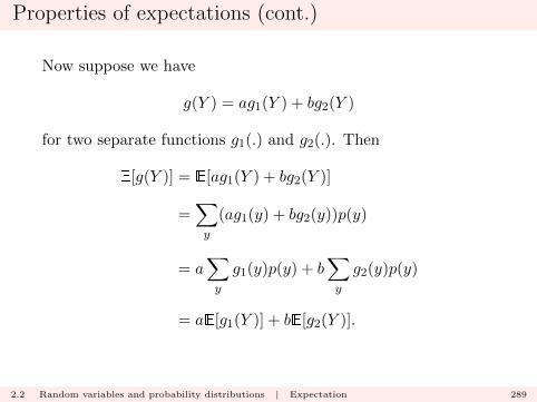
Properties of expectations (cont.)
Now suppose we have
g(Y ) = ag1(Y ) + bg2(Y )
for two separate functions g1(.) and g2(.). Then
E[g(Y )] = E[ag1(Y ) + bg2(Y )]
=∑y
(ag1(y) + bg2(y))p(y)
= a∑y
g1(y)p(y) + b∑y
g2(y)p(y)
= aE[g1(Y )] + bE[g2(Y )].
2.2 Random variables and probability distributions | Expectation 289
Properties of expectations (cont.)
Note
These results merely follow standard mathematical concepts ofthe linearity of summations:∑
i
(ai + bi) =∑i
ai +∑i
bi.
2.2 Random variables and probability distributions | Expectation 290
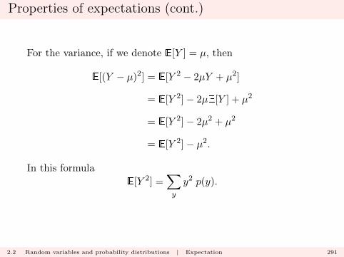
Properties of expectations (cont.)
For the variance, if we denote E[Y ] = µ, then
E[(Y − µ)2] = E[Y 2 − 2µY + µ2]
= E[Y 2]− 2µE[Y ] + µ2
= E[Y 2]− 2µ2 + µ2
= E[Y 2]− µ2.
In this formula
E[Y 2] =∑y
y2 p(y).
2.2 Random variables and probability distributions | Expectation 291

Properties of expectations (cont.)
From this we can deduce that
V[aY + b] = a2V[Y ].
We have that
E[aY + b] = aE[Y ] + b = aµ+ b
so
V[aY + b] = E[(aY + b− (aµ+ b))2]
which reduces to
E[(aY − aµ)2] = E[a2(Y − µ)2] = a2E[(Y − µ)2].
2.2 Random variables and probability distributions | Expectation 292
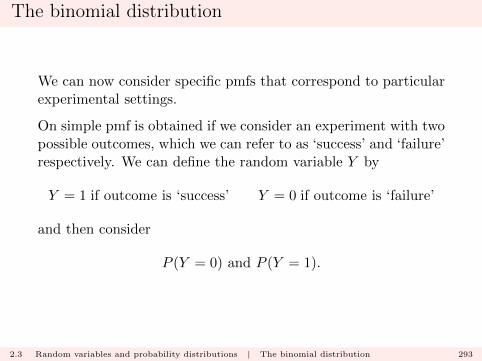
The binomial distribution
We can now consider specific pmfs that correspond to particularexperimental settings.
On simple pmf is obtained if we consider an experiment with twopossible outcomes, which we can refer to as ‘success’ and ‘failure’respectively. We can define the random variable Y by
Y = 1 if outcome is ‘success’ Y = 0 if outcome is ‘failure’
and then consider
P (Y = 0) and P (Y = 1).
2.3 Random variables and probability distributions | The binomial distribution 293
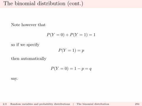
The binomial distribution (cont.)
Note however that
P (Y = 0) + P (Y = 1) = 1
so if we specify
P (Y = 1) = p
then automatically
P (Y = 0) = 1− p = q
say.
2.3 Random variables and probability distributions | The binomial distribution 294
The binomial distribution (cont.)
We may then write
p(y) = py(1− p)1−y = pyq1−y y ∈ {0, 1}
with p(y) = 0 for all other values of y.
This distribution is known as the Bernoulli distribution withparameter p.
Note
To avoid the trivial case, we typically assume that 0 < p < 1.
2.3 Random variables and probability distributions | The binomial distribution 295
The binomial distribution (cont.)
This model covers many experimental settings:
� coin tosses;
� thumbtack tosses;
� pass/fail;
� cure/not cure
etc.
2.3 Random variables and probability distributions | The binomial distribution 296
The binomial distribution (cont.)
We have for this model that
µ ≡ E[Y ] =
1∑i=0
yp(y) = (0× p(0) + 1× p(1))
= (0× q + 1× p) = p
2.3 Random variables and probability distributions | The binomial distribution 297
The binomial distribution (cont.)
Similarly
E[Y 2] =
1∑i=0
y2p(y) = (02 × p(0) + 12 × p(1))
= (0× q + 1× p) = p
so therefore
V[Y ] = E[Y 2]− µ2 = p− p2 = p(1− p).
2.3 Random variables and probability distributions | The binomial distribution 298

The binomial distribution (cont.)
We now consider an extended version of the experiment wherea sequence of n identical binary experiments (or ‘trials’) withsuccess probability p whose outcomes are independent is carriedout.
0101011101
We consider the total number of successes in the sequence.
Provided 0 < p < 1, we have that
Y = {0, 1, 2, . . . , n}
2.3 Random variables and probability distributions | The binomial distribution 299
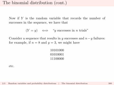
The binomial distribution (cont.)
Now if Y is the random variable that records the number ofsuccesses in the sequence, we have that
(Y = y) ⇐⇒ “y successes in n trials”
Consider a sequence that results in y successes and n−y failures:for example, if n = 8 and y = 3, we might have
101010000101000111100000
etc.
2.3 Random variables and probability distributions | The binomial distribution 300

The binomial distribution (cont.)
All such sequences are equally likely, under the ‘identical andindependent’ assumption. The probability of any such sequenceis, for y ∈ {0, 1, 2, . . . , n},
pyqn−y
that is, in the examples above
pqpqpqqqqpqpqqqppppqqqqq
etc. all yield p3q5.
2.3 Random variables and probability distributions | The binomial distribution 301
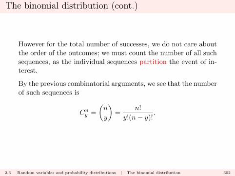
The binomial distribution (cont.)
However for the total number of successes, we do not care aboutthe order of the outcomes; we must count the number of all suchsequences, as the individual sequences partition the event of in-terest.
By the previous combinatorial arguments, we see that the numberof such sequences is
Cny =
(n
y
)=
n!
y!(n− y)!.
2.3 Random variables and probability distributions | The binomial distribution 302

The binomial distribution (cont.)
Therefore we have that
p(y) ≡ P (Y = y) =
(n
y
)pyqn−y y ∈ {0, 1, 2, . . . , n}
and p(y) = 0 for all other y.
This is the pmf for the Binomial distribution.
2.3 Random variables and probability distributions | The binomial distribution 303
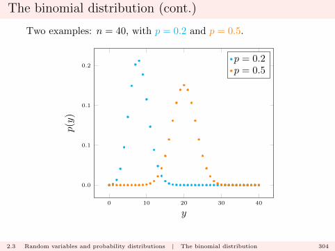
The binomial distribution (cont.)
Two examples: n = 40, with p = 0.2 and p = 0.5.
0 10 20 30 40
0.0
0.1
0.1
0.2
y
p(y
)p = 0.2p = 0.5
2.3 Random variables and probability distributions | The binomial distribution 304

The binomial distribution (cont.)
Expectation : For the expectation of a binomial distribution,we may compute directly as follows:
E[Y ] =
n∑y=0
yp(y) =
n∑y=0
y
(n
y
)pyqn−y
=
n∑y=1
yn!
y!(n− y)!pyqn−y
= n
n∑y=1
(n− 1)!
(y − 1)!(n− y)!pyqn−y
2.3 Random variables and probability distributions | The binomial distribution 305

The binomial distribution (cont.)
Now we may write
(n− y) = (n− 1)− (y − 1)
so therefore the sum can be written
n∑y=1
(n− 1)!
(y − 1)!((n− 1)− (y − 1))!pyq(n−1)−(y−1).
2.3 Random variables and probability distributions | The binomial distribution 306

The binomial distribution (cont.)
Rewriting the terms in the sum by setting j = y − 1, this equals
n−1∑j=0
(n− 1)!
j!((n− 1)− j)!pj+1q(n−1)−j .
or equivalently, by the binomial theorem, this equals
p
n−1∑j=0
(n− 1)!
j!((n− 1)− j)!pjq(n−1)−j = p(p+ q)n−1.
But p+ q = 1, so therefore
E[Y ] = np.
2.3 Random variables and probability distributions | The binomial distribution 307
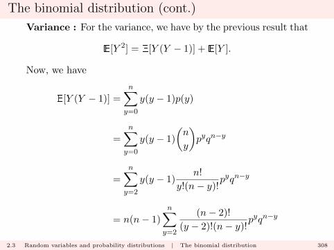
The binomial distribution (cont.)
Variance : For the variance, we have by the previous result that
E[Y 2] = E[Y (Y − 1)] + E[Y ].
Now, we have
E[Y (Y − 1)] =
n∑y=0
y(y − 1)p(y)
=
n∑y=0
y(y − 1)
(n
y
)pyqn−y
=
n∑y=2
y(y − 1)n!
y!(n− y)!pyqn−y
= n(n− 1)
n∑y=2
(n− 2)!
(y − 2)!(n− y)!pyqn−y
2.3 Random variables and probability distributions | The binomial distribution 308
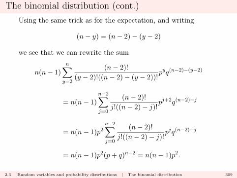
The binomial distribution (cont.)
Using the same trick as for the expectation, and writing
(n− y) = (n− 2)− (y − 2)
we see that we can rewrite the sum
n(n− 1)
n∑y=2
(n− 2)!
(y − 2)!((n− 2)− (y − 2))!pyq(n−2)−(y−2)
= n(n− 1)
n−2∑j=0
(n− 2)!
j!((n− 2)− j)!pj+2q(n−2)−j
= n(n− 1)p2n−2∑j=0
(n− 2)!
j!((n− 2)− j)!pjq(n−2)−j
= n(n− 1)p2(p+ q)n−2 = n(n− 1)p2.
2.3 Random variables and probability distributions | The binomial distribution 309

The binomial distribution (cont.)
Therefore
E[Y (Y − 1)] = n(n− 1)p2
and so
E[Y 2] = E[Y (Y −1)+Y ] = E[Y (Y −1)]+E[Y ] = n(n−1)p2+np.
Hence
V[Y ] = E[Y 2]− µ2 = n(n− 1)p2 + np− (np)2
= −np2 + np
= np(1− p)
= npq.
2.3 Random variables and probability distributions | The binomial distribution 310
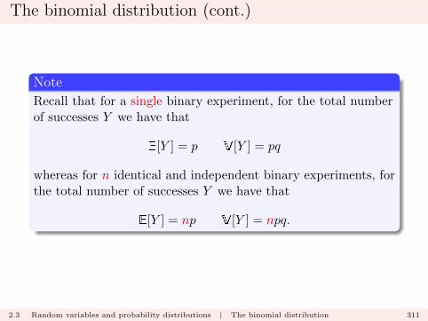
The binomial distribution (cont.)
Note
Recall that for a single binary experiment, for the total numberof successes Y we have that
E[Y ] = p V[Y ] = pq
whereas for n identical and independent binary experiments, forthe total number of successes Y we have that
E[Y ] = np V[Y ] = npq.
2.3 Random variables and probability distributions | The binomial distribution 311
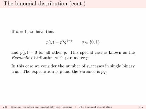
The binomial distribution (cont.)
If n = 1, we have that
p(y) = pyq1−y y ∈ {0, 1}
and p(y) = 0 for all other y. This special case is known as theBernoulli distribution with parameter p.
In this case we consider the number of successes in single binarytrial. The expectation is p and the variance is pq.
2.3 Random variables and probability distributions | The binomial distribution 312

The geometric distribution
We now consider another experimental setting based on identicaland independent binary trials. Here, rather than counting thetotal number of successes, we count the number of trials carriedout until the first success.
Using the 0/1 notation, we consider sequences such as
0001010000000011000001
etc.
2.4 Random variables and probability distributions | The geometric distribution 313
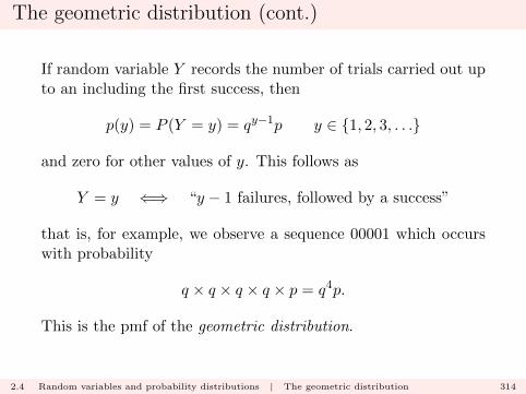
The geometric distribution (cont.)
If random variable Y records the number of trials carried out upto an including the first success, then
p(y) = P (Y = y) = qy−1p y ∈ {1, 2, 3, . . .}
and zero for other values of y. This follows as
Y = y ⇐⇒ “y − 1 failures, followed by a success”
that is, for example, we observe a sequence 00001 which occurswith probability
q × q × q × q × p = q4p.
This is the pmf of the geometric distribution.
2.4 Random variables and probability distributions | The geometric distribution 314

The geometric distribution (cont.)
Notes
� Note that
∞∑y=1
qy−1p = p
∞∑j=0
qj = p1
1− q = p1
(1− (1− p)) = 1.
� The geometric distribution is an example of a waiting-timedistribution.
2.4 Random variables and probability distributions | The geometric distribution 315

The geometric distribution (cont.)
Notes
� Sometimes the geometric distribution is written
p(y) = qyp y ∈ {0, 1, 2, . . .}
– this is the same distribution, but for the random variablethat records the number of failures observed up to the firstsuccess, that is, for the random variable
Y ∗ = Y − 1.
.
2.4 Random variables and probability distributions | The geometric distribution 316
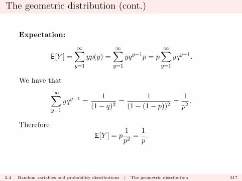
The geometric distribution (cont.)
Expectation:
E[Y ] =
∞∑y=1
yp(y) =
∞∑y=1
yqy−1p = p
∞∑y=1
yqy−1.
We have that
∞∑y=1
yqy−1 =1
(1− q)2 =1
(1− (1− p))2 =1
p2.
Therefore
E[Y ] = p1
p2=
1
p.
2.4 Random variables and probability distributions | The geometric distribution 317
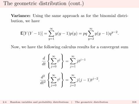
The geometric distribution (cont.)
Variance: Using the same approach as for the binomial distri-bution, we have
E[Y (Y − 1)] =
∞∑y=1
y(y − 1)p(y) = pq
∞∑y=2
y(y − 1)qy−2.
Now, we have the following calculus results for a convergent sum
d
dt
∞∑j=0
tj
=
∞∑j=1
jtj−1
d2
dt2
∞∑j=0
tj
=
∞∑j=2
j(j − 1)tj−2.
2.4 Random variables and probability distributions | The geometric distribution 318

The geometric distribution (cont.)
But∞∑j=0
tj =1
1− t
so therefore we must have that
d
dt
∞∑j=0
tj
=d
dt
{1
1− t
}=
1
(1− t)2
d2
dt2
∞∑j=0
tj
=d2
dt2
{1
1− t
}=
2
(1− t)3 .
2.4 Random variables and probability distributions | The geometric distribution 319
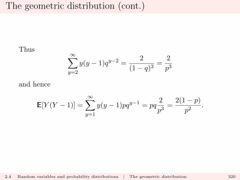
The geometric distribution (cont.)
Thus∞∑y=2
y(y − 1)qy−2 =2
(1− q)3 =2
p3
and hence
E[Y (Y − 1)] =
∞∑y=1
y(y − 1)pqy−1 = pq2
p3=
2(1− p)p2
.
2.4 Random variables and probability distributions | The geometric distribution 320
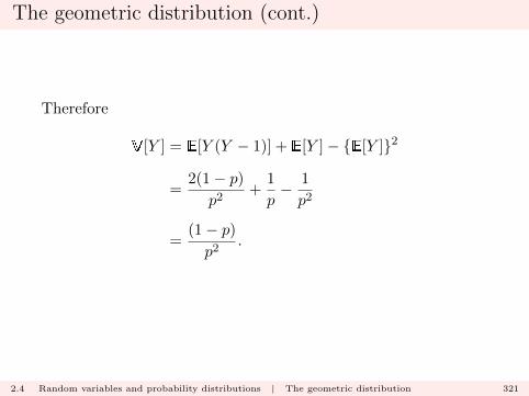
The geometric distribution (cont.)
Therefore
V[Y ] = E[Y (Y − 1)] + E[Y ]− {E[Y ]}2
=2(1− p)p2
+1
p− 1
p2
=(1− p)p2
.
2.4 Random variables and probability distributions | The geometric distribution 321

The geometric distribution (cont.)
Now consider the probability
P (Y > y)
for y ∈ {1, 2, 3, . . .}. Using a partitioning argument, we see that
P (Y > y) =
∞∑j=y+1
P (Y = j).
That is
P (Y > y) =
∞∑j=y+1
qj−1p = pqy∞∑
j=y+1
qj−y−1 = pqy1
1− q .
2.4 Random variables and probability distributions | The geometric distribution 322
The geometric distribution (cont.)
Therefore
P (Y > y) = qy y ∈ {1, 2, 3, . . .}
and consequently
P (Y ≤ y) = 1− qy = 1− (1− p)y y ∈ {1, 2, 3, . . .}.
2.4 Random variables and probability distributions | The geometric distribution 323

The geometric distribution (cont.)
We can define the function
F (y) = P (Y ≤ y) = 1− (1− p)y y ∈ {1, 2, 3, . . .}.
F (y) is known as the cumulative distribution function (cdf) ofthe distribution.
2.4 Random variables and probability distributions | The geometric distribution 324
The geometric distribution (cont.)
We can define all such ‘interval’ probabilities such as
P (Y ≤ a) P (Y ≥ b) P (c ≤ Y ≤ d)
etc. via F (y). This is because for all discrete distributions andsets X
P (Y ∈ X ) =∑y ∈ X
p(y).
2.4 Random variables and probability distributions | The geometric distribution 325
The geometric distribution (cont.)
Note
We can computeF (y) = P (Y ≤ y)
for any real value y. However, we must remember that
P (Y ≤ y) = P (Y ≤ byc)
where byc is the largest integer that is no greater than y. Forexample,
F (1.234) = F (1) F (4.789) = F (4)
etc.
2.4 Random variables and probability distributions | The geometric distribution 326

The geometric distribution (cont.)
Geometric p(y): with p = 0.8 and p = 0.1.
0 2 4 6 8 100.0
0.2
0.4
0.6
0.8
1.0
y
p(y
)
p = 0.8p = 0.1
2.4 Random variables and probability distributions | The geometric distribution 327

The geometric distribution (cont.)
Geometric F (y): with p = 0.8 and p = 0.1.
0 2 4 6 8 100.0
0.2
0.4
0.6
0.8
1.0
y
F(y
)
p = 0.8p = 0.1
2.4 Random variables and probability distributions | The geometric distribution 328
The negative binomial distribution
As an extension to the geometric distribution setting, we nowconsider a sequence of identical and independent binary trials,but we continue until we observe the rth success, where r ={1, 2, . . . , } is a fixed number. That is, if r = 3, we considersequences such as
000101010111010000011101010000010101
etc.
2.5 Random variables and probability distributions | The negative binomial distribution 329

The negative binomial distribution (cont.)
If random variable Y records the number of trials carried out upto an including the rth success, then we see that
(Y = y) ≡ A ∩B
where
A = “(r − 1) successes in the first (y − 1) trials”
B = “a success on the yth trial”
with A and B independent events.
2.5 Random variables and probability distributions | The negative binomial distribution 330

The negative binomial distribution (cont.)
We have that Y can take values on the set
r, r + 1, . . .
Now, we have from the binomial distribution that
P (A) =
(y − 1
r − 1
)pr−1q(y−1)−(r−1) y = {r, r + 1, r + 2, . . .}
and
P (B) = p
2.5 Random variables and probability distributions | The negative binomial distribution 331
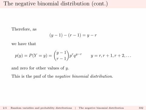
The negative binomial distribution (cont.)
Therefore, as
(y − 1)− (r − 1) = y − r
we have that
p(y) = P (Y = y) =
(y − 1
r − 1
)prqy−r y = r, r + 1, r + 2, . . .
and zero for other values of y.
This is the pmf of the negative binomial distribution.
2.5 Random variables and probability distributions | The negative binomial distribution 332

The negative binomial distribution (cont.)
Notes
� We can show (Exercise)
∞∑y=r
p(y) = 1.
� The negative binomial distribution is another example of awaiting-time distribution.
2.5 Random variables and probability distributions | The negative binomial distribution 333
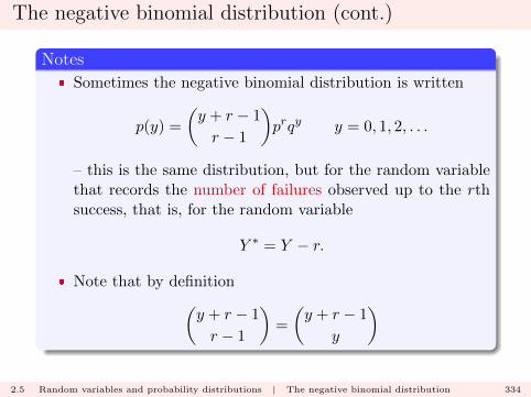
The negative binomial distribution (cont.)
Notes
� Sometimes the negative binomial distribution is written
p(y) =
(y + r − 1
r − 1
)prqy y = 0, 1, 2, . . .
– this is the same distribution, but for the random variablethat records the number of failures observed up to the rthsuccess, that is, for the random variable
Y ∗ = Y − r.
� Note that by definition(y + r − 1
r − 1
)=
(y + r − 1
y
)
2.5 Random variables and probability distributions | The negative binomial distribution 334
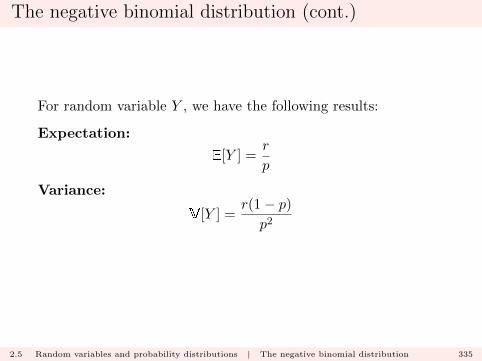
The negative binomial distribution (cont.)
For random variable Y , we have the following results:
Expectation:
E[Y ] =r
p
Variance:
V[Y ] =r(1− p)p2
2.5 Random variables and probability distributions | The negative binomial distribution 335
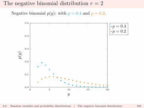
The negative binomial distribution r = 2
Negative binomial p(y): with p = 0.4 and p = 0.2.
0 5 10 15 200.0
0.1
0.2
0.3
0.4
0.5
y
p(y
)
p = 0.4p = 0.2
2.5 Random variables and probability distributions | The negative binomial distribution 336

The negative binomial distribution r = 5
Negative binomial p(y): with p = 0.4 and p = 0.2.
0 5 10 15 200.0
0.1
0.2
0.3
0.4
0.5
y
p(y
)
p = 0.4p = 0.2
2.5 Random variables and probability distributions | The negative binomial distribution 337
The hypergeometric distribution
The experimental setting for another discrete distribution knownas the hypergeometric distribution relates to the earlier combin-atorial exercises.
Suppose we have a finite ‘population’ (set) of N items whichcomprise
� r Type I items,
� N − r Type II objects.
The experiment consists of selecting n items from the population,without replacement, such that all such selections are equallylikely.
2.6 Random variables and probability distributions | The hypergeometric distribution 338
The hypergeometric distribution (cont.)
Define the random variable Y such that
(Y = y) ≡ A = “y Type I items in the selection”
First, consider the feasible values for Y ; we know that
0 ≤ y ≤ r
but also that
0 ≤ n− y ≤ N − r
2.6 Random variables and probability distributions | The hypergeometric distribution 339
The hypergeometric distribution (cont.)
Putting these two facts together, we must have that
max{0, n−N + r} ≤ y ≤ min{n, r}
so
Y = {max{0, n−N + r}, . . . ,min{n, r}}.
2.6 Random variables and probability distributions | The hypergeometric distribution 340
The hypergeometric distribution (cont.)
Secondly, we compute P (A) as follows: for y ∈ Y
nA =
(r
y
)×(N − rn− y
)(r
y
): number of ways of selecting the y Type I items
from the r available.(N − rn− y
): number of ways of selecting the n− y Type II items
from the N − r available.
2.6 Random variables and probability distributions | The hypergeometric distribution 341
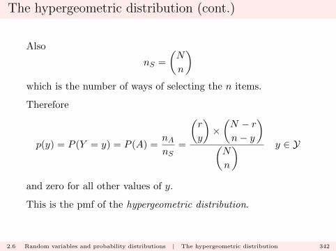
The hypergeometric distribution (cont.)
Also
nS =
(N
n
)which is the number of ways of selecting the n items.
Therefore
p(y) = P (Y = y) = P (A) =nAnS
=
(r
y
)×(N − rn− y
)(N
n
) y ∈ Y
and zero for all other values of y.
This is the pmf of the hypergeometric distribution.
2.6 Random variables and probability distributions | The hypergeometric distribution 342
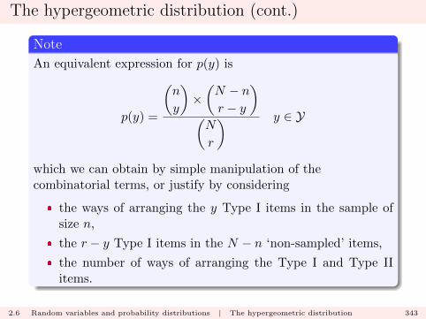
The hypergeometric distribution (cont.)
Note
An equivalent expression for p(y) is
p(y) =
(n
y
)×(N − nr − y
)(N
r
) y ∈ Y
which we can obtain by simple manipulation of thecombinatorial terms, or justify by considering
� the ways of arranging the y Type I items in the sample ofsize n,
� the r − y Type I items in the N − n ‘non-sampled’ items,
� the number of ways of arranging the Type I and Type IIitems.
2.6 Random variables and probability distributions | The hypergeometric distribution 343
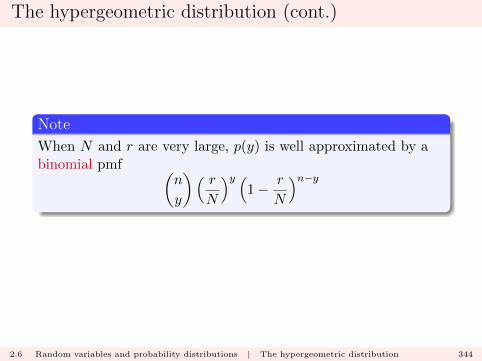
The hypergeometric distribution (cont.)
Note
When N and r are very large, p(y) is well approximated by abinomial pmf (
n
y
)( rN
)y (1− r
N
)n−y
2.6 Random variables and probability distributions | The hypergeometric distribution 344
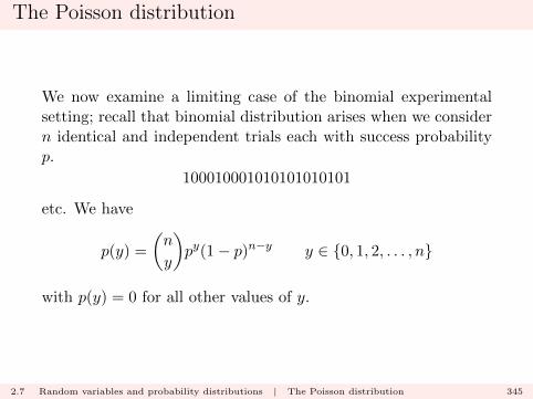
The Poisson distribution
We now examine a limiting case of the binomial experimentalsetting; recall that binomial distribution arises when we considern identical and independent trials each with success probabilityp.
100010001010101010101
etc. We have
p(y) =
(n
y
)py(1− p)n−y y ∈ {0, 1, 2, . . . , n}
with p(y) = 0 for all other values of y.
2.7 Random variables and probability distributions | The Poisson distribution 345

The Poisson distribution (cont.)
Suppose we allow n to get larger, and p to get smaller, but insuch a way that
n× p
remains constant at the value λ say. That is, we may write
p =λ
n
and consider n becoming large.
2.7 Random variables and probability distributions | The Poisson distribution 346
The Poisson distribution (cont.)
Note
The parameter λ corresponds to the ‘rate’ at which successesoccur in a continuous approximation to the experiment.
2.7 Random variables and probability distributions | The Poisson distribution 347
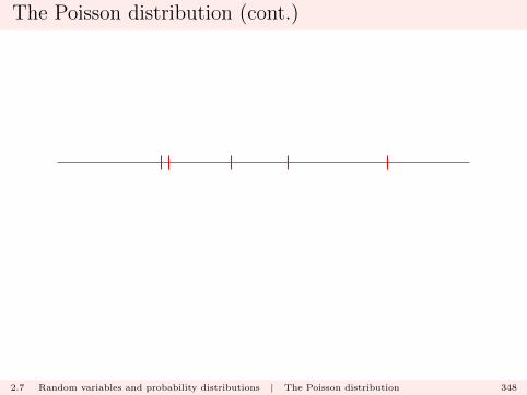
The Poisson distribution (cont.)
2.7 Random variables and probability distributions | The Poisson distribution 348
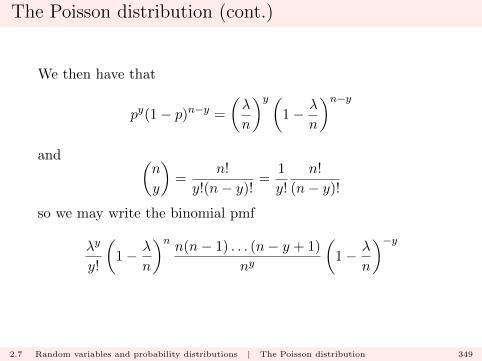
The Poisson distribution (cont.)
We then have that
py(1− p)n−y =
(λ
n
)y (1− λ
n
)n−yand (
n
y
)=
n!
y!(n− y)!=
1
y!
n!
(n− y)!
so we may write the binomial pmf
λy
y!
(1− λ
n
)n n(n− 1) . . . (n− y + 1)
ny
(1− λ
n
)−y
2.7 Random variables and probability distributions | The Poisson distribution 349
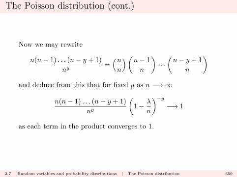
The Poisson distribution (cont.)
Now we may rewrite
n(n− 1) . . . (n− y + 1)
ny=(nn
)(n− 1
n
)· · ·(n− y + 1
n
)and deduce from this that for fixed y as n −→∞
n(n− 1) . . . (n− y + 1)
ny
(1− λ
n
)−y−→ 1
as each term in the product converges to 1.
2.7 Random variables and probability distributions | The Poisson distribution 350
The Poisson distribution (cont.)
Finally, by a standard representation
limn−→∞
(1− λ
n
)n= e−λ.
Recall that
ex = 1 + x+x2
2!+x3
3!+ · · ·
2.7 Random variables and probability distributions | The Poisson distribution 351

The Poisson distribution (cont.)
Therefore, as n −→ ∞ with p = λ/n for fixed λ, we have thatthe binomial pmf converges to
p(y) =λy
y!e−λ y ∈ {0, 1, 2, . . .}
with p(y) = 0 for other values of y.
This is the pmf for the Poisson distribution.
Note that
∞∑y=0
λy
y!e−λ = e−λ
∞∑y=0
λy
y!= e−λeλ = 1.
2.7 Random variables and probability distributions | The Poisson distribution 352
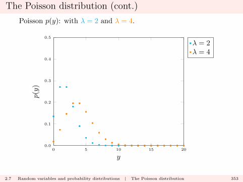
The Poisson distribution (cont.)
Poisson p(y): with λ = 2 and λ = 4.
0 5 10 15 200.0
0.1
0.2
0.3
0.4
0.5
y
p(y
)λ = 2λ = 4
2.7 Random variables and probability distributions | The Poisson distribution 353
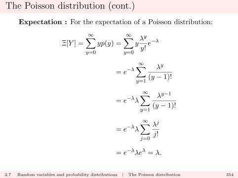
The Poisson distribution (cont.)
Expectation : For the expectation of a Poisson distribution:
E[Y ] =
∞∑y=0
yp(y) =
∞∑y=0
yλy
y!e−λ
= e−λ∞∑y=1
λy
(y − 1)!
= e−λλ
∞∑y=1
λy−1
(y − 1)!
= e−λλ
∞∑j=0
λj
j!
= e−λλeλ = λ.
2.7 Random variables and probability distributions | The Poisson distribution 354
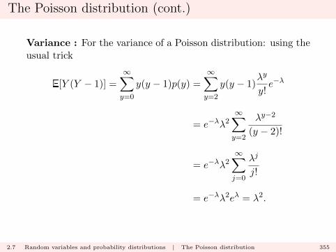
The Poisson distribution (cont.)
Variance : For the variance of a Poisson distribution: using theusual trick
E[Y (Y − 1)] =
∞∑y=0
y(y − 1)p(y) =
∞∑y=2
y(y − 1)λy
y!e−λ
= e−λλ2∞∑y=2
λy−2
(y − 2)!
= e−λλ2∞∑j=0
λj
j!
= e−λλ2eλ = λ2.
2.7 Random variables and probability distributions | The Poisson distribution 355
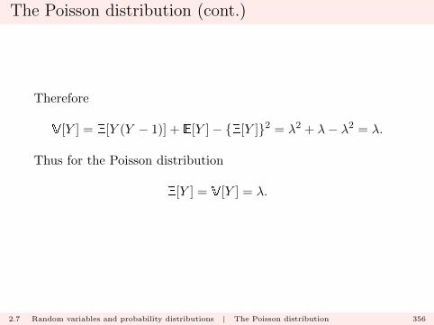
The Poisson distribution (cont.)
Therefore
V[Y ] = E[Y (Y − 1)] + E[Y ]− {E[Y ]}2 = λ2 + λ− λ2 = λ.
Thus for the Poisson distribution
E[Y ] = V[Y ] = λ.
2.7 Random variables and probability distributions | The Poisson distribution 356
The Poisson distribution (cont.)
Note
The Poisson distribution is widely used to model the distributionof count data.
It corresponds to a model where incidents (‘successes’) occur in-dependently in continuous time at a constant rate.
2.7 Random variables and probability distributions | The Poisson distribution 357
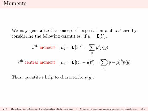
Moments
We may generalize the concept of expectation and variance byconsidering the following quantities: if µ = E[Y ],
kth moment: µ′k = E[Y k] =∑y
ykp(y)
kth central moment: µk = E[(Y − µ)k] =∑y
(y − µ)kp(y)
These quantities help to characterize p(y).
2.8 Random variables and probability distributions | Moments and moment generating functions 358
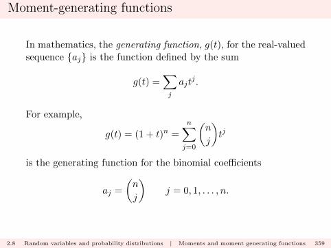
Moment-generating functions
In mathematics, the generating function, g(t), for the real-valuedsequence {aj} is the function defined by the sum
g(t) =∑j
ajtj .
For example,
g(t) = (1 + t)n =n∑j=0
(n
j
)tj
is the generating function for the binomial coefficients
aj =
(n
j
)j = 0, 1, . . . , n.
2.8 Random variables and probability distributions | Moments and moment generating functions 359

Moment-generating functions (cont.)
We can also define an (exponential) generating function as
g(t) =∑j
ajtj
j!.
2.8 Random variables and probability distributions | Moments and moment generating functions 360
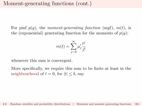
Moment-generating functions (cont.)
For pmf p(y), the moment-generating function (mgf), m(t), isthe (exponential) generating function for the moments of p(y):
m(t) =
∞∑j=0
µ′jtj
j!
whenever this sum is convergent.
More specifically, we require this sum to be finite at least in theneighbourhood of t = 0, for |t| ≤ b, say.
2.8 Random variables and probability distributions | Moments and moment generating functions 361
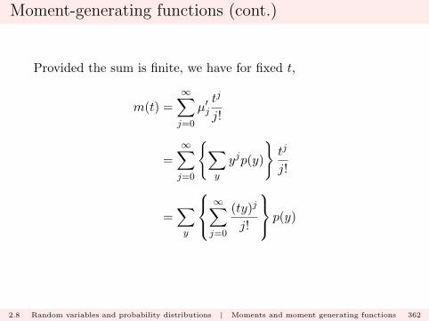
Moment-generating functions (cont.)
Provided the sum is finite, we have for fixed t,
m(t) =
∞∑j=0
µ′jtj
j!
=
∞∑j=0
{∑y
yjp(y)
}tj
j!
=∑y
∞∑j=0
(ty)j
j!
p(y)
2.8 Random variables and probability distributions | Moments and moment generating functions 362

Moment-generating functions (cont.)
But∞∑j=0
(ty)j
j!= ety
so therefore
m(t) =∑y
etyp(y) = E[etY]
2.8 Random variables and probability distributions | Moments and moment generating functions 363
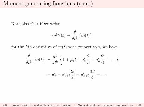
Moment-generating functions (cont.)
Note also that if we write
m(k)(t) =dk
dtk{m(t)}
for the kth derivative of m(t) with respect to t, we have
dk
dtk{m(t)} =
dk
dtk
{1 + µ′1t+ µ′2
t2
2!+ µ′3
t3
3!+ · · ·
}
= µ′k + µ′k+1
2t
2!+ µ′k+2
3t2
3!+ · · ·
2.8 Random variables and probability distributions | Moments and moment generating functions 364
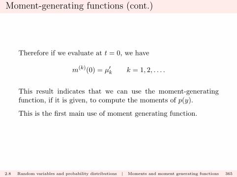
Moment-generating functions (cont.)
Therefore if we evaluate at t = 0, we have
m(k)(0) = µ′k k = 1, 2, . . . .
This result indicates that we can use the moment-generatingfunction, if it is given, to compute the moments of p(y).
This is the first main use of moment generating function.
2.8 Random variables and probability distributions | Moments and moment generating functions 365
Moment-generating functions (cont.)
The second main use is to identify distributions; suppose m1(t)and m2(t) are two moment-generating functions for pmfs p1(y)and p2(y). Then
m1(t) = m2(t) for all |t| ≤ b
for some b if and only if
p1(y) = p2(y) for all y.
2.8 Random variables and probability distributions | Moments and moment generating functions 366

Moment-generating functions (cont.)
Example (Poisson mgf)
We have for the Poisson distribution with parameter λ
m(t) =
∞∑y=0
etyp(y) =
∞∑y=0
etyλy
y!e−λ
= e−λ∞∑y=0
(λet)y
y!
= e−λ exp{λet}
= exp{λ(et − 1)}
Note that this holds for all t.
2.8 Random variables and probability distributions | Moments and moment generating functions 367

Moment-generating functions (cont.)
Example (Binomial mgf)
We have for the Binomial distribution with parameters n and p
m(t) =
n∑y=0
etyp(y) =
n∑y=0
ety(n
y
)pyqn−y
=n∑y=0
(n
y
)(pet)yqn−y
= (pet + q)n.
2.8 Random variables and probability distributions | Moments and moment generating functions 368
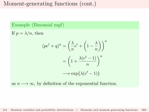
Moment-generating functions (cont.)
Example (Binomial mgf)
If p = λ/n, then
(pet + q)n =
(λ
net +
(1− λ
n
))n=
(1 +
λ(et − 1)
n
)n−→ exp{λ(et − 1)}
as n −→∞, by definition of the exponential function.
2.8 Random variables and probability distributions | Moments and moment generating functions 369
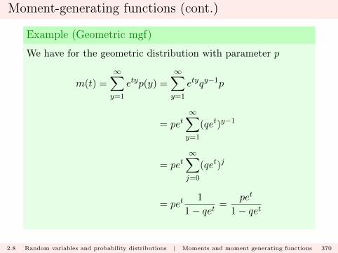
Moment-generating functions (cont.)
Example (Geometric mgf)
We have for the geometric distribution with parameter p
m(t) =
∞∑y=1
etyp(y) =
∞∑y=1
etyqy−1p
= pet∞∑y=1
(qet)y−1
= pet∞∑j=0
(qet)j
= pet1
1− qet =pet
1− qet
2.8 Random variables and probability distributions | Moments and moment generating functions 370
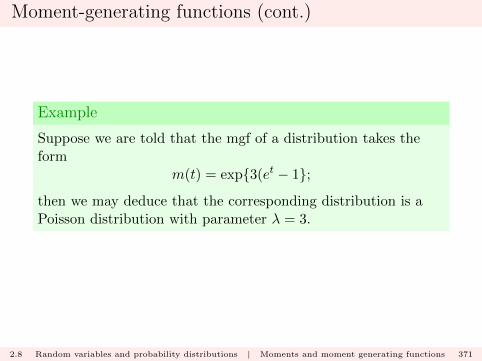
Moment-generating functions (cont.)
Example
Suppose we are told that the mgf of a distribution takes theform
m(t) = exp{3(et − 1};then we may deduce that the corresponding distribution is aPoisson distribution with parameter λ = 3.
2.8 Random variables and probability distributions | Moments and moment generating functions 371
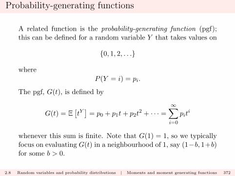
Probability-generating functions
A related function is the probability-generating function (pgf);this can be defined for a random variable Y that takes values on
{0, 1, 2, . . .}
where
P (Y = i) = pi.
The pgf, G(t), is defined by
G(t) = E[tY]
= p0 + p1t+ p2t2 + · · · =
∞∑i=0
piti
whenever this sum is finite. Note that G(1) = 1, so we typicallyfocus on evaluating G(t) in a neighbourhood of 1, say (1−b, 1+b)for some b > 0.
2.8 Random variables and probability distributions | Moments and moment generating functions 372
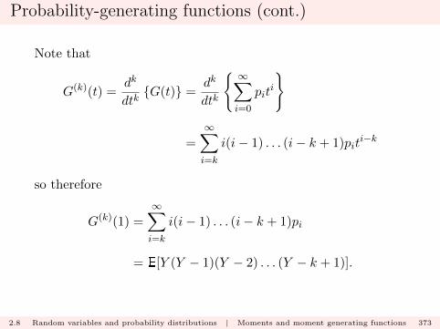
Probability-generating functions (cont.)
Note that
G(k)(t) =dk
dtk{G(t)} =
dk
dtk
{ ∞∑i=0
piti
}
=
∞∑i=k
i(i− 1) . . . (i− k + 1)piti−k
so therefore
G(k)(1) =
∞∑i=k
i(i− 1) . . . (i− k + 1)pi
= E[Y (Y − 1)(Y − 2) . . . (Y − k + 1)].
2.8 Random variables and probability distributions | Moments and moment generating functions 373

Probability-generating functions (cont.)
The quantity
µ[k] = E[Y (Y − 1)(Y − 2) . . . (Y − k + 1)]
is termed the kth factorial moment.
Recall that we previously computed
µ[2] = E[Y (Y − 1)]
to calculate the variance of a distribution.
2.8 Random variables and probability distributions | Moments and moment generating functions 374
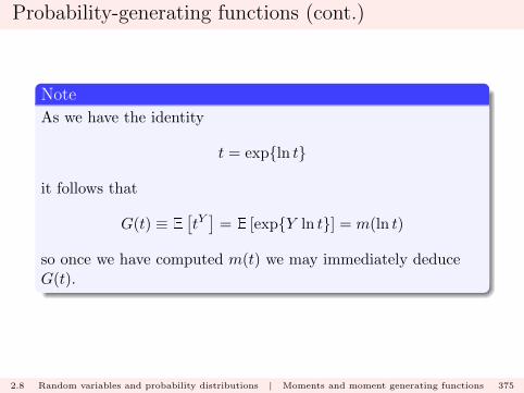
Probability-generating functions (cont.)
Note
As we have the identity
t = exp{ln t}
it follows that
G(t) ≡ E[tY]
= E [exp{Y ln t}] = m(ln t)
so once we have computed m(t) we may immediately deduceG(t).
2.8 Random variables and probability distributions | Moments and moment generating functions 375
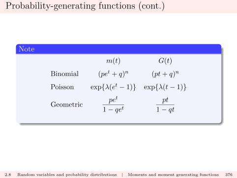
Probability-generating functions (cont.)
Note
m(t) G(t)
Binomial (pet + q)n (pt+ q)n
Poisson exp{λ(et − 1)} exp{λ(t− 1)}
Geometricpet
1− qetpt
1− qt
2.8 Random variables and probability distributions | Moments and moment generating functions 376
Continuous Random variables
Recall the previous definition of the cumulative distribution func-tion (or cdf), F (y), for a random variable:
F (y) = P (Y ≤ y)
which can be considered for any real value y. For a discreterandom variable, this function is termed a step function, withsteps at only a countable number of points.
2.9 Random variables and probability distributions | Continuous random variables 377

Continuous Random variables (cont.)
Poisson F (y): with λ = 2 and λ = 6.
0 5 10 15 200.0
0.2
0.4
0.6
0.8
1.0
y
F(y
)
2.9 Random variables and probability distributions | Continuous random variables 378

Continuous Random variables (cont.)
Directly from the probability axioms, we can deduce three prop-erties of the function F (y):
1. “Starts at zero”:
F (−∞) ≡ limy−→−∞
F (y) = 0.
2. “Ends at 1”:
F (∞) ≡ limy−→∞
F (y) = 1.
3. “Non-decreasing in between”: if y1 < y2, then
F (y1) ≤ F (y2).
2.9 Random variables and probability distributions | Continuous random variables 379
Continuous Random variables (cont.)
Now suppose that the random variable Y is most accuratelythought of as varying continuously, that is, can potentially takeany real value in an interval
� height/weight,
� temperature,
� time,
and so on.
2.9 Random variables and probability distributions | Continuous random variables 380
Continuous Random variables (cont.)
In this case it seems that the probability that Y lies in an interval(y1, y2] for y1 < y2 must be positive, but should converge to zerothe closer y1 moves to y2. That is
P (Y ∈ (y1, y2]) = P (Y ≤ y2)− P (Y ≤ y1) = F (y2)− F (y1)
should be positive, but decrease to zero as y1 −→ y2.
2.9 Random variables and probability distributions | Continuous random variables 381
Continuous Random variables (cont.)
This is not the case for a discrete random variable: suppose
p(0) =1
2p(1) =
1
4p(2) =
1
4
and p(y) = 0 for all other values of y. Then for 0 < ε < 1
F (0) = P (Y ≤ 0) =1
2
F (1− ε) =1
2
F (1) =1
2+
1
4=
3
4.
2.9 Random variables and probability distributions | Continuous random variables 382

Continuous Random variables (cont.)
A random variable Y with distribution function F (y) is calledcontinuous if F (y) is continuous for all real y. That is, for any y,
limε−→0+
F (y − ε) = limε−→0+
F (y + ε) = F (y).
2.9 Random variables and probability distributions | Continuous random variables 383
Continuous Random variables (cont.)
We often also assume that F (y) has a continuous first derivativefor all y ∈ R, except perhaps at a finite number of points.
2.9 Random variables and probability distributions | Continuous random variables 384
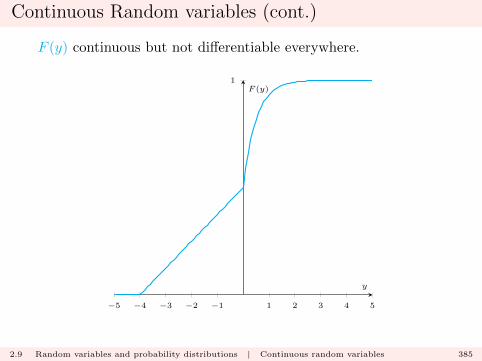
Continuous Random variables (cont.)
F (y) continuous but not differentiable everywhere.
−5 −4 −3 −2 −1 1 2 3 4 5
1
y
F (y)
2.9 Random variables and probability distributions | Continuous random variables 385
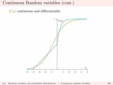
Continuous Random variables (cont.)
F (y) continuous and differentiable.
−5 −4 −3 −2 −1 1 2 3 4 5
1
y
F (y)
2.9 Random variables and probability distributions | Continuous random variables 386
Continuous Random variables (cont.)
Note
Even if Y is discrete, F (y) is right-continuous. That is, for anyy,
limε−→0+
F (y + ε) = F (y).
2.9 Random variables and probability distributions | Continuous random variables 387
Continuous Random variables (cont.)
Important Note
If F (y) is continuous, then
P (Y = y) = 0
for all y ∈ R. If there were to exist a y0 such that
P (Y = y0) = p0 > 0
then F (y) would have a step of size p0 at y0, and would be dis-continuous.
2.9 Random variables and probability distributions | Continuous random variables 388

Probability density functions
For a continuous cdf F (y), denote by f(y) the first derivative ofF (.) at y
f(y) =dF (y)
dy
wherever this derivative exists.
The function f(y) is known as the probability density function(pdf).
2.9 Random variables and probability distributions | Continuous random variables 389
Probability density functions (cont.)
It follows that
F (t) =
∫ y
−∞f(t) dt
2.9 Random variables and probability distributions | Continuous random variables 390
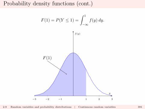
Probability density functions (cont.)
F (1) = P (Y ≤ 1) =
∫ 1
−∞f(y) dy.
−3 −2 −1 1 2 3
F (1)
y
f(y)
2.9 Random variables and probability distributions | Continuous random variables 391
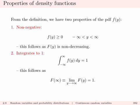
Properties of density functions
From the definition, we have two properties of the pdf f(y):
1. Non-negative:
f(y) ≥ 0 −∞ < y <∞
– this follows as F (y) is non-decreasing.
2. Integrates to 1: ∫ ∞−∞
f(y) dy = 1
– this follows as
F (∞) ≡ limy−→∞
F (y) = 1.
2.9 Random variables and probability distributions | Continuous random variables 392

Properties of density functions (cont.)
−5 −4 −3 −2 −1 1 2 3 4 5
1
12
y
F (y)
2.9 Random variables and probability distributions | Continuous random variables 393
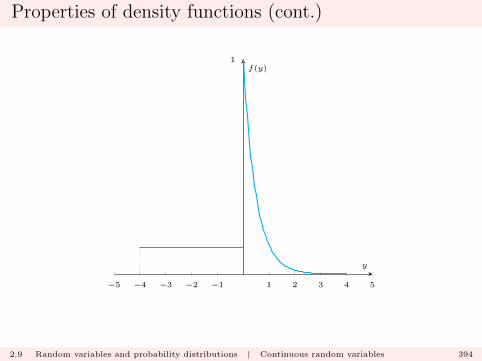
Properties of density functions (cont.)
−5 −4 −3 −2 −1 1 2 3 4 5
1
y
f(y)
2.9 Random variables and probability distributions | Continuous random variables 394
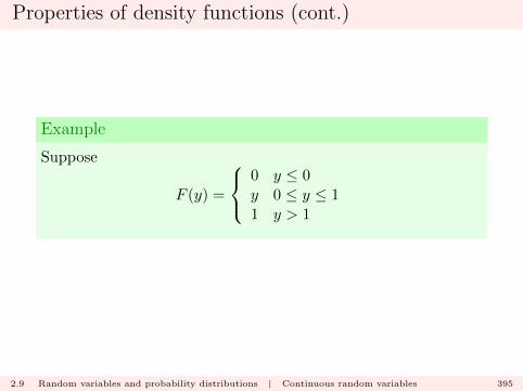
Properties of density functions (cont.)
Example
Suppose
F (y) =
0 y ≤ 0y 0 ≤ y ≤ 11 y > 1
2.9 Random variables and probability distributions | Continuous random variables 395
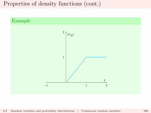
Properties of density functions (cont.)
Example
−1 1 2
1
2
y
F (y)
2.9 Random variables and probability distributions | Continuous random variables 396
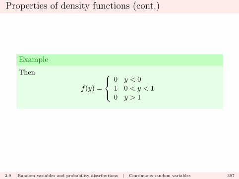
Properties of density functions (cont.)
Example
Then
f(y) =
0 y < 01 0 < y < 10 y > 1
2.9 Random variables and probability distributions | Continuous random variables 397
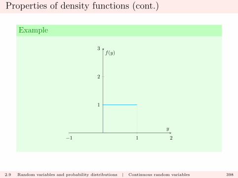
Properties of density functions (cont.)
Example
−1 1 2
1
2
3
y
f(y)
2.9 Random variables and probability distributions | Continuous random variables 398

Properties of density functions (cont.)
Example
Suppose
F (y) =
0 y ≤ 0y2 0 ≤ y ≤ 11 y > 1
2.9 Random variables and probability distributions | Continuous random variables 399
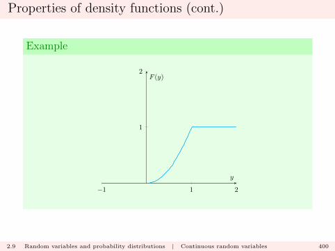
Properties of density functions (cont.)
Example
−1 1 2
1
2
y
F (y)
2.9 Random variables and probability distributions | Continuous random variables 400
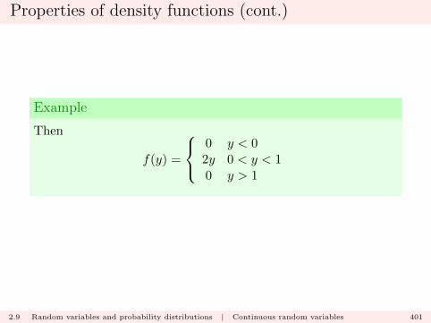
Properties of density functions (cont.)
Example
Then
f(y) =
0 y < 02y 0 < y < 10 y > 1
2.9 Random variables and probability distributions | Continuous random variables 401
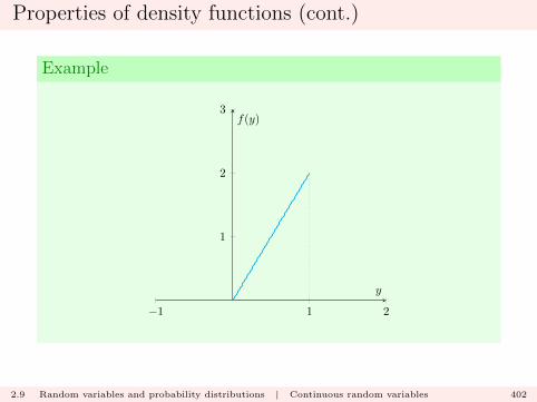
Properties of density functions (cont.)
Example
−1 1 2
1
2
3
y
f(y)
2.9 Random variables and probability distributions | Continuous random variables 402

Properties of density functions (cont.)
Example
Suppose
F (y) =
0 y ≤ 0y3 0 ≤ y ≤ 11 y > 1
2.9 Random variables and probability distributions | Continuous random variables 403
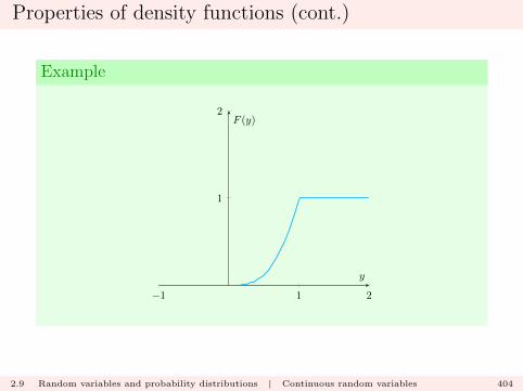
Properties of density functions (cont.)
Example
−1 1 2
1
2
y
F (y)
2.9 Random variables and probability distributions | Continuous random variables 404
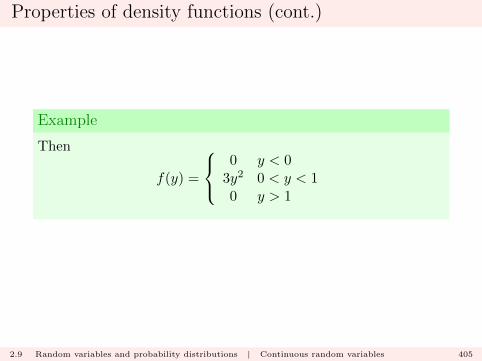
Properties of density functions (cont.)
Example
Then
f(y) =
0 y < 0
3y2 0 < y < 10 y > 1
2.9 Random variables and probability distributions | Continuous random variables 405
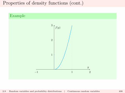
Properties of density functions (cont.)
Example
−1 1 2
1
2
3
y
f(y)
2.9 Random variables and probability distributions | Continuous random variables 406

Interval probabilities
To compute
P (a ≤ Y ≤ b)we integrate f(y) over the interval (a, b) as
P (a ≤ Y ≤ b) = P (Y ≤ b)− P (Y ≤ a)
=
∫ b
−∞f(t) dt−
∫ a
−∞f(t) dt
=
∫ b
af(t) dt.
2.9 Random variables and probability distributions | Continuous random variables 407
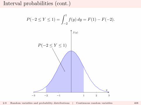
Interval probabilities (cont.)
P (−2 ≤ Y ≤ 1) =
∫ 1
−2f(y) dy = F (1)− F (−2).
−3 −2 −1 1 2 3
P (−2 ≤ Y ≤ 1)
y
f(y)
2.9 Random variables and probability distributions | Continuous random variables 408
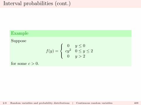
Interval probabilities (cont.)
Example
Suppose
f(y) =
0 y ≤ 0cy2 0 ≤ y ≤ 20 y > 2
for some c > 0.
2.9 Random variables and probability distributions | Continuous random variables 409
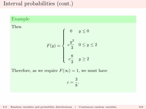
Interval probabilities (cont.)
Example
Then
F (y) =
0 y ≤ 0
cy3
30 ≤ y ≤ 2
c8
3y ≥ 2
Therefore, as we require F (∞) = 1, we must have
c =3
8.
2.9 Random variables and probability distributions | Continuous random variables 410
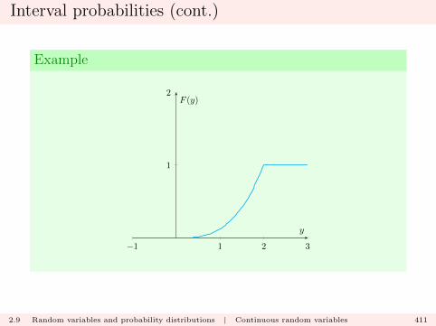
Interval probabilities (cont.)
Example
−1 1 2 3
1
2
y
F (y)
2.9 Random variables and probability distributions | Continuous random variables 411

Interval probabilities (cont.)
Example
Then
f(y) =
0 y < 0
3
8y2 0 < y < 2
0 y > 2
2.9 Random variables and probability distributions | Continuous random variables 412

Interval probabilities (cont.)
Example
−1 1 2 3
1
2
3
y
f(y)
2.9 Random variables and probability distributions | Continuous random variables 413
Interval probabilities (cont.)
To compute
P (1/2 ≤ Y ≤ 3/2)
we use the cdf to show that this is equal to
F (3/2)− F (1/2) =3
8
1
3
(3
2
)3
− 3
8
1
3
(1
2
)3
= 0.40625
2.9 Random variables and probability distributions | Continuous random variables 414
Interval probabilities (cont.)
This calculation is merely
P (1/2 ≤ Y ≤ 3/2) =
∫ 3/2
1/2
3
8y2 dy.
2.9 Random variables and probability distributions | Continuous random variables 415
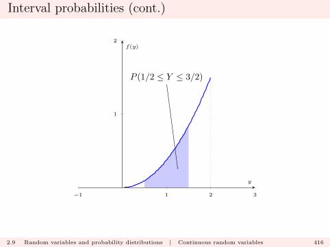
Interval probabilities (cont.)
−1 1 2 3
1
2
P (1/2 ≤ Y ≤ 3/2)
y
f(y)
2.9 Random variables and probability distributions | Continuous random variables 416

Interval probabilities (cont.)
Note
For a continuous random variable
P (a ≤ Y ≤ b) = P (a < Y ≤ b) = P (a ≤ Y < b) = P (a < Y < b)
2.9 Random variables and probability distributions | Continuous random variables 417
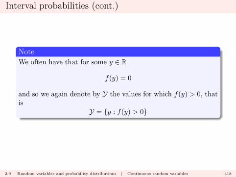
Interval probabilities (cont.)
Note
We often have that for some y ∈ R
f(y) = 0
and so we again denote by Y the values for which f(y) > 0, thatis
Y = {y : f(y) > 0}
2.9 Random variables and probability distributions | Continuous random variables 418
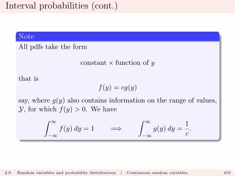
Interval probabilities (cont.)
Note
All pdfs take the form
constant× function of y
that isf(y) = cg(y)
say, where g(y) also contains information on the range of values,Y, for which f(y) > 0. We have∫ ∞
−∞f(y) dy = 1 =⇒
∫ ∞−∞
g(y) dy =1
c.
2.9 Random variables and probability distributions | Continuous random variables 419
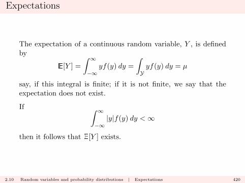
Expectations
The expectation of a continuous random variable, Y , is definedby
E[Y ] =
∫ ∞−∞
yf(y) dy =
∫Yyf(y) dy = µ
say, if this integral is finite; if it is not finite, we say that theexpectation does not exist.
If ∫ ∞−∞|y|f(y) dy <∞
then it follows that E[Y ] exists.
2.10 Random variables and probability distributions | Expectations 420

Expectations (cont.)
The expectation of a function of Y , g(Y ) say, is defined by
E[g(Y )] =
∫ ∞−∞
g(y)f(y) dy
if this integral is finite.
2.10 Random variables and probability distributions | Expectations 421
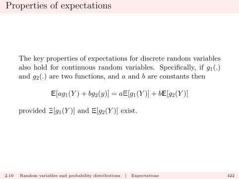
Properties of expectations
The key properties of expectations for discrete random variablesalso hold for continuous random variables. Specifically, if g1(.)and g2(.) are two functions, and a and b are constants then
E[ag1(Y ) + bg2(y)] = aE[g1(Y )] + bE[g2(Y )]
provided E[g1(Y )] and E[g2(Y )] exist.
2.10 Random variables and probability distributions | Expectations 422
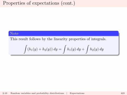
Properties of expectations (cont.)
Note
This result follows by the linearity properties of integrals.∫(h1(y) + h2(y)) dy =
∫h1(y) dy +
∫h2(y) dy
2.10 Random variables and probability distributions | Expectations 423
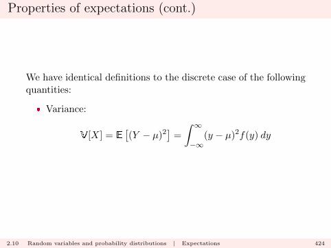
Properties of expectations (cont.)
We have identical definitions to the discrete case of the followingquantities:
� Variance:
V[X] = E[(Y − µ)2
]=
∫ ∞−∞
(y − µ)2f(y) dy
2.10 Random variables and probability distributions | Expectations 424
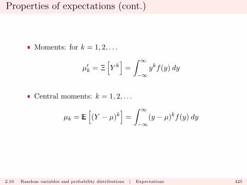
Properties of expectations (cont.)
� Moments: for k = 1, 2, . . .
µ′k = E
[Y k]
=
∫ ∞−∞
ykf(y) dy
� Central moments: k = 1, 2, . . .
µk = E
[(Y − µ)k
]=
∫ ∞−∞
(y − µ)kf(y) dy
2.10 Random variables and probability distributions | Expectations 425
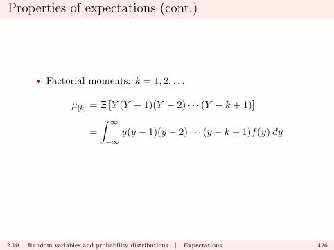
Properties of expectations (cont.)
� Factorial moments: k = 1, 2, . . .
µ[k] = E [Y (Y − 1)(Y − 2) · · · (Y − k + 1)]
=
∫ ∞−∞
y(y − 1)(y − 2) · · · (y − k + 1)f(y) dy
2.10 Random variables and probability distributions | Expectations 426
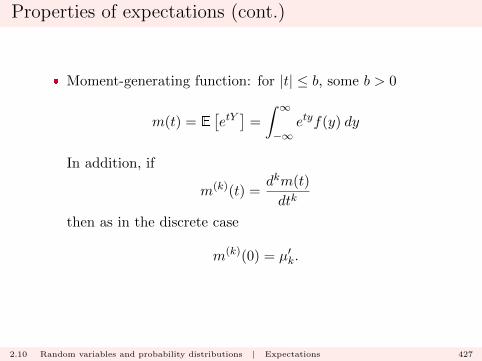
Properties of expectations (cont.)
� Moment-generating function: for |t| ≤ b, some b > 0
m(t) = E[etY]
=
∫ ∞−∞
etyf(y) dy
In addition, if
m(k)(t) =dkm(t)
dtk
then as in the discrete case
m(k)(0) = µ′k.
2.10 Random variables and probability distributions | Expectations 427

Properties of expectations (cont.)
� Factorial moment-generating function: for 1− b ≤ t ≤ 1 + b,some b > 0
G(t) = E[tY]
=
∫ ∞−∞
tyf(y) dy
In addition, if
G(k)(t) =dkG(t)
dtk
then as in the discrete case
G(k)(1) = µ[k].
Note: We do not use the terminology probability-generatingfunction in the continuous case.
2.10 Random variables and probability distributions | Expectations 428
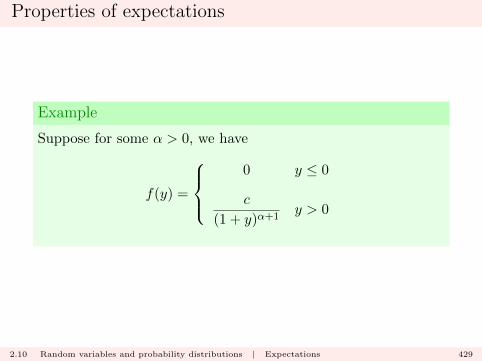
Properties of expectations
Example
Suppose for some α > 0, we have
f(y) =
0 y ≤ 0
c
(1 + y)α+1y > 0
2.10 Random variables and probability distributions | Expectations 429
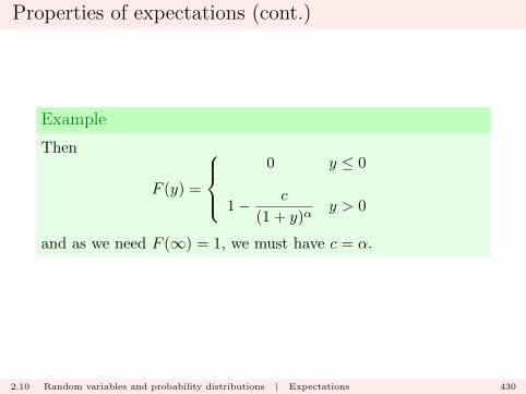
Properties of expectations (cont.)
Example
Then
F (y) =
0 y ≤ 0
1− c
(1 + y)αy > 0
and as we need F (∞) = 1, we must have c = α.
2.10 Random variables and probability distributions | Expectations 430
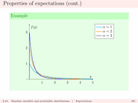
Properties of expectations (cont.)
Example
1 2 3 4 5
1
2
3
y
f(y) α = 1α = 2α = 3
2.10 Random variables and probability distributions | Expectations 431
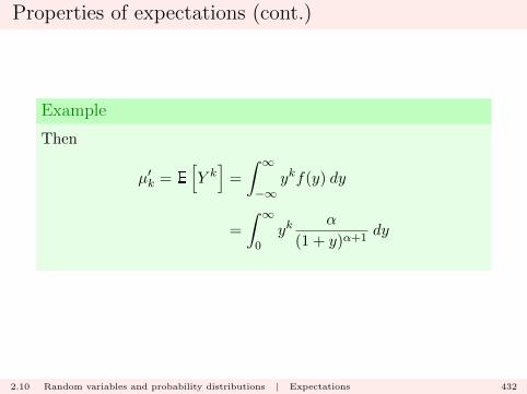
Properties of expectations (cont.)
Example
Then
µ′k = E
[Y k]
=
∫ ∞−∞
ykf(y) dy
=
∫ ∞0
ykα
(1 + y)α+1dy
2.10 Random variables and probability distributions | Expectations 432
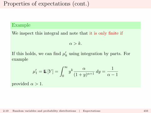
Properties of expectations (cont.)
Example
We inspect this integral and note that it is only finite if
α > k.
If this holds, we can find µ′k using integration by parts. Forexample
µ′1 = E [Y ] =
∫ ∞0
ykα
(1 + y)α+1dy =
1
α− 1
provided α > 1.
2.10 Random variables and probability distributions | Expectations 433

Properties of expectations (cont.)
The quantity α in this pdf is termed a parameter of the model.It determines the properties of the model such as
� f(y) and F (y);
� E[Y ] and other moments
2.10 Random variables and probability distributions | Expectations 434
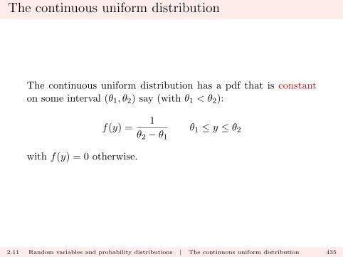
The continuous uniform distribution
The continuous uniform distribution has a pdf that is constanton some interval (θ1, θ2) say (with θ1 < θ2):
f(y) =1
θ2 − θ1θ1 ≤ y ≤ θ2
with f(y) = 0 otherwise.
2.11 Random variables and probability distributions | The continuous uniform distribution 435
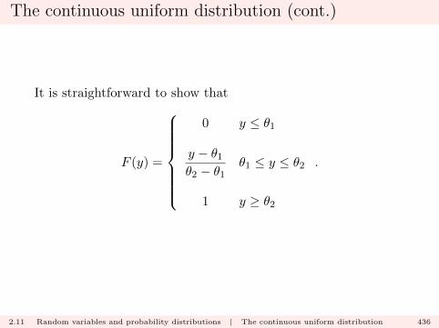
The continuous uniform distribution (cont.)
It is straightforward to show that
F (y) =
0 y ≤ θ1
y − θ1θ2 − θ1
θ1 ≤ y ≤ θ2
1 y ≥ θ2
.
2.11 Random variables and probability distributions | The continuous uniform distribution 436
The continuous uniform distribution (cont.)
By direct calculation, we can compute that
E[Y ] =θ1 + θ2
2V[Y ] =
(θ2 − θ1)212
.
2.11 Random variables and probability distributions | The continuous uniform distribution 437
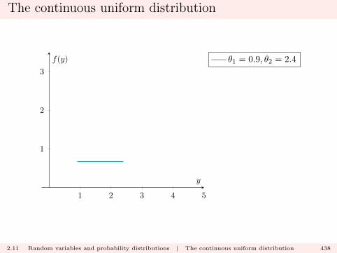
The continuous uniform distribution
1 2 3 4 5
1
2
3
y
f(y) θ1 = 0.9, θ2 = 2.4
2.11 Random variables and probability distributions | The continuous uniform distribution 438
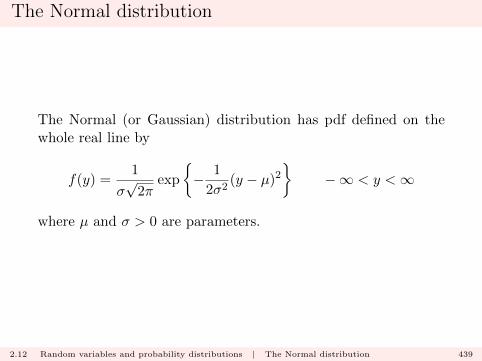
The Normal distribution
The Normal (or Gaussian) distribution has pdf defined on thewhole real line by
f(y) =1
σ√
2πexp
{− 1
2σ2(y − µ)2
}−∞ < y <∞
where µ and σ > 0 are parameters.
2.12 Random variables and probability distributions | The Normal distribution 439
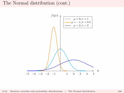
The Normal distribution (cont.)
−5 −4 −3 −2 −1 1 2 3 4 5
1
y
f(y)
µ = 0, σ = 1µ = −1, σ = 0.5µ = 2, σ = 2
2.12 Random variables and probability distributions | The Normal distribution 440
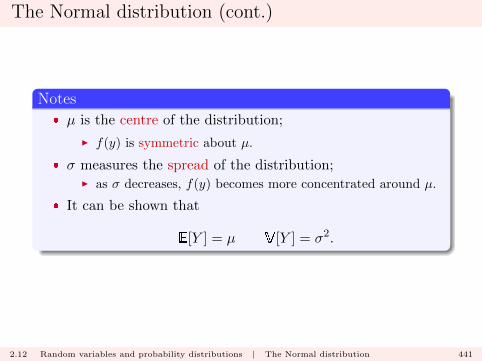
The Normal distribution (cont.)
Notes
� µ is the centre of the distribution;
I f(y) is symmetric about µ.
� σ measures the spread of the distribution;I as σ decreases, f(y) becomes more concentrated around µ.
� It can be shown that
E[Y ] = µ V[Y ] = σ2.
2.12 Random variables and probability distributions | The Normal distribution 441
The Normal distribution (cont.)
The case where µ = 0 and σ = 1 yields the standard Normal pmf
f(y) =1√2π
exp
{−y
2
2
}−∞ < y <∞
2.12 Random variables and probability distributions | The Normal distribution 442
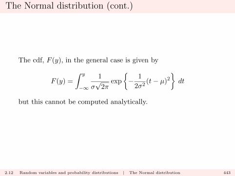
The Normal distribution (cont.)
The cdf, F (y), in the general case is given by
F (y) =
∫ y
−∞
1
σ√
2πexp
{− 1
2σ2(t− µ)2
}dt
but this cannot be computed analytically.
2.12 Random variables and probability distributions | The Normal distribution 443

The Normal distribution (cont.)
However, if Y has a Normal distribution with parameters µ andσ, and we consider the random variable Z where
Z =Y − µσ
then we see that for real value z
FZ(z) = P (Z ≤ z) = P (σZ + µ ≤ σz + µ)
= P (Y ≤ σz + µ) = FY (σz + µ)
2.12 Random variables and probability distributions | The Normal distribution 444

The Normal distribution (cont.)
The quantity on the right-hand side is∫ σz+µ
−∞
1
σ√
2πexp
{− 1
2σ2(t− µ)2
}dt
but if we make the substitution u = (t−µ)/σ in the integral, wesee that this becomes∫ z
−∞
1√2π
exp
{−u
2
2
}du
2.12 Random variables and probability distributions | The Normal distribution 445
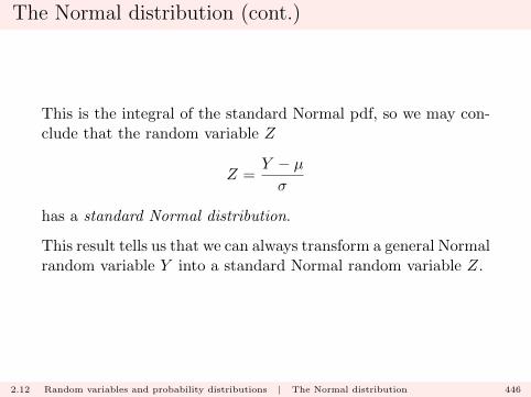
The Normal distribution (cont.)
This is the integral of the standard Normal pdf, so we may con-clude that the random variable Z
Z =Y − µσ
has a standard Normal distribution.
This result tells us that we can always transform a general Normalrandom variable Y into a standard Normal random variable Z.
2.12 Random variables and probability distributions | The Normal distribution 446

The Normal distribution (cont.)
Y : µ = 1, σ = 2 : P (−1 ≤ Y ≤ 2)
−5 −4 −3 −2 −1 1 2 3 4 5
y
fY (y)
2.12 Random variables and probability distributions | The Normal distribution 447
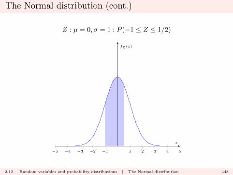
The Normal distribution (cont.)
Z : µ = 0, σ = 1 : P (−1 ≤ Z ≤ 1/2)
−5 −4 −3 −2 −1 1 2 3 4 5
z
fZ(z)
2.12 Random variables and probability distributions | The Normal distribution 448
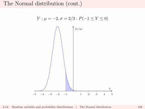
The Normal distribution (cont.)
Y : µ = −2, σ = 2/3 : P (−1 ≤ Y ≤ 0)
−5 −4 −3 −2 −1 1 2 3 4 5
y
fY (y)
2.12 Random variables and probability distributions | The Normal distribution 449

The Normal distribution (cont.)
Z : µ = 0, σ = 1 : P (3/2 ≤ Z ≤ 3)
−5 −4 −3 −2 −1 1 2 3 4 5
z
fZ(z)
2.12 Random variables and probability distributions | The Normal distribution 450
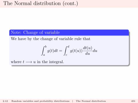
The Normal distribution (cont.)
Note: Change of variable
We have by the change of variable rule that∫ b
ag(t)dt =
∫ d
cg(t(u))
dt(u)
dudu
where t −→ u in the integral.
2.12 Random variables and probability distributions | The Normal distribution 451

Moment-generating function
For the mgf of the Normal distribution, first consider the stand-ard Normal case: we have for t ∈ R that
m(t) = E[etY]
=
∫ ∞−∞
ety1√2πe−y
2/2 dy
=
∫ ∞−∞
1√2π
exp
{ty − 1
2y2}dy
= exp
{t2
2
}∫ ∞−∞
1√2π
exp
{−(y − t)2
2
}dy
= exp
{t2
2
}as the integral is the integral of a Normal pdf where the expect-ation is µ = t.
2.12 Random variables and probability distributions | The Normal distribution 452
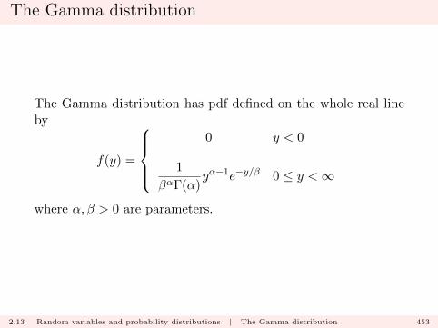
The Gamma distribution
The Gamma distribution has pdf defined on the whole real lineby
f(y) =
0 y < 0
1
βαΓ(α)yα−1e−y/β 0 ≤ y <∞
where α, β > 0 are parameters.
2.13 Random variables and probability distributions | The Gamma distribution 453
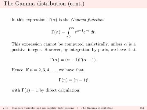
The Gamma distribution (cont.)
In this expression, Γ(α) is the Gamma function
Γ(α) =
∫ ∞0
tα−1e−t dt.
This expression cannot be computed analytically, unless α is apositive integer. However, by integration by parts, we have that
Γ(α) = (α− 1)Γ(α− 1).
Hence, if n = 2, 3, 4, . . ., we have that
Γ(n) = (n− 1)!
with Γ(1) = 1 by direct calculation.
2.13 Random variables and probability distributions | The Gamma distribution 454
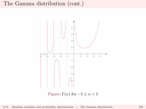
The Gamma distribution (cont.)
−4
−3
−2
−1
1
2
3
4
−5 −4 −3 −2 −1 1 2 3 4
Figure: Γ(α) for −5 ≤ α < 5
2.13 Random variables and probability distributions | The Gamma distribution 455
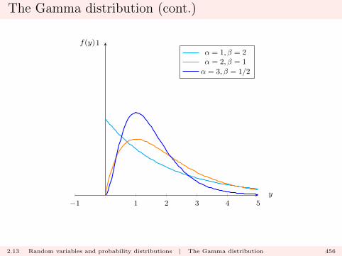
The Gamma distribution (cont.)
−1 1 2 3 4 5
1
y
f(y)
α = 1, β = 2α = 2, β = 1
α = 3, β = 1/2
2.13 Random variables and probability distributions | The Gamma distribution 456
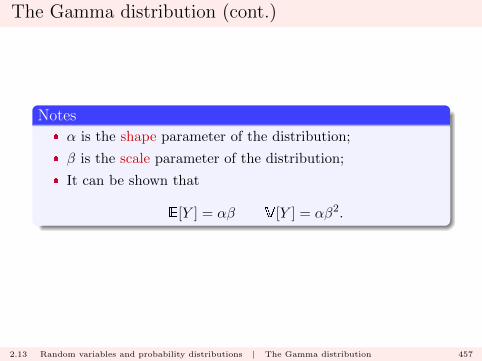
The Gamma distribution (cont.)
Notes
� α is the shape parameter of the distribution;
� β is the scale parameter of the distribution;
� It can be shown that
E[Y ] = αβ V[Y ] = αβ2.
2.13 Random variables and probability distributions | The Gamma distribution 457
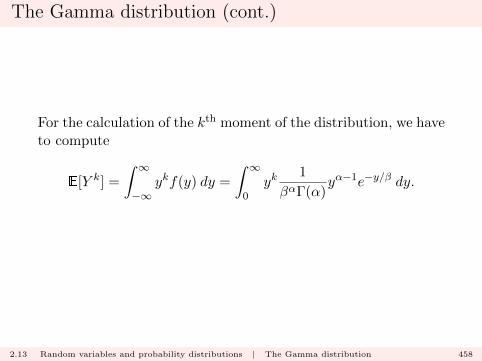
The Gamma distribution (cont.)
For the calculation of the kth moment of the distribution, we haveto compute
E[Y k] =
∫ ∞−∞
ykf(y) dy =
∫ ∞0
yk1
βαΓ(α)yα−1e−y/β dy.
2.13 Random variables and probability distributions | The Gamma distribution 458

The Gamma distribution (cont.)
Now, as we require f(y) integrate to 1, this implies that∫ ∞0
1
βαΓ(α)yα−1e−y/β dy = 1
for any α > 0, so ∫ ∞0
yα−1e−y/β dy = βαΓ(α).
2.13 Random variables and probability distributions | The Gamma distribution 459
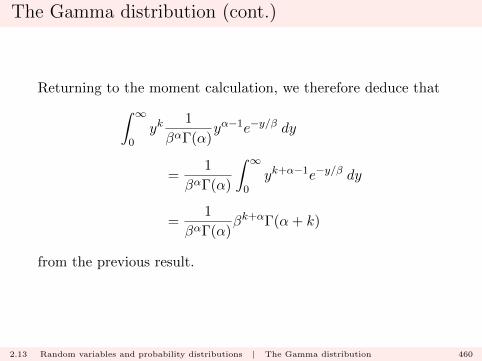
The Gamma distribution (cont.)
Returning to the moment calculation, we therefore deduce that∫ ∞0
yk1
βαΓ(α)yα−1e−y/β dy
=1
βαΓ(α)
∫ ∞0
yk+α−1e−y/β dy
=1
βαΓ(α)βk+αΓ(α+ k)
from the previous result.
2.13 Random variables and probability distributions | The Gamma distribution 460
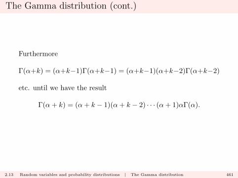
The Gamma distribution (cont.)
Furthermore
Γ(α+k) = (α+k−1)Γ(α+k−1) = (α+k−1)(α+k−2)Γ(α+k−2)
etc. until we have the result
Γ(α+ k) = (α+ k − 1)(α+ k − 2) · · · (α+ 1)αΓ(α).
2.13 Random variables and probability distributions | The Gamma distribution 461

The Gamma distribution (cont.)
Therefore
E[Y k] =1
βαΓ(α)βk+α(α+ k − 1)(α+ k − 2) · · · (α+ 1)αΓ(α)
= βk(α+ k − 1)(α+ k − 2) · · · (α+ 1)α
so that
E[Y ] = αβ E[Y 2] = α(α+ 1)β2
and so on.
2.13 Random variables and probability distributions | The Gamma distribution 462
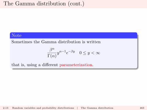
The Gamma distribution (cont.)
Note
Sometimes the Gamma distribution is written
βα
Γ(α)yα−1e−βy 0 ≤ y <∞
that is, using a different parameterization.
2.13 Random variables and probability distributions | The Gamma distribution 463
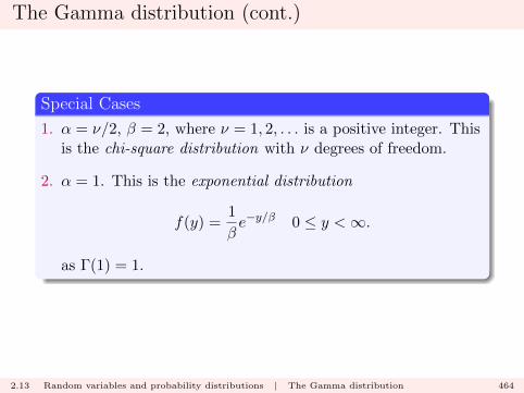
The Gamma distribution (cont.)
Special Cases
1. α = ν/2, β = 2, where ν = 1, 2, . . . is a positive integer. Thisis the chi-square distribution with ν degrees of freedom.
2. α = 1. This is the exponential distribution
f(y) =1
βe−y/β 0 ≤ y <∞.
as Γ(1) = 1.
2.13 Random variables and probability distributions | The Gamma distribution 464
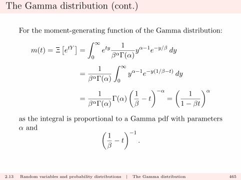
The Gamma distribution (cont.)
For the moment-generating function of the Gamma distribution:
m(t) = E[etY]
=
∫ ∞0
ety1
βαΓ(α)yα−1e−y/β dy
=1
βαΓ(α)
∫ ∞0
yα−1e−y(1/β−t) dy
=1
βαΓ(α)Γ(α)
(1
β− t)−α
=
(1
1− βt
)αas the integral is proportional to a Gamma pdf with parametersα and (
1
β− t)−1
.
2.13 Random variables and probability distributions | The Gamma distribution 465
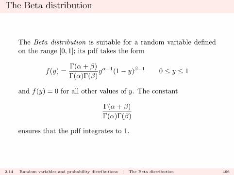
The Beta distribution
The Beta distribution is suitable for a random variable definedon the range [0, 1]; its pdf takes the form
f(y) =Γ(α+ β)
Γ(α)Γ(β)yα−1(1− y)β−1 0 ≤ y ≤ 1
and f(y) = 0 for all other values of y. The constant
Γ(α+ β)
Γ(α)Γ(β)
ensures that the pdf integrates to 1.
2.14 Random variables and probability distributions | The Beta distribution 466

The Beta distribution (cont.)
The Beta function is defined
B(α, β) =Γ(α)Γ(β)
Γ(α+ β)=
∫ 1
0yα−1(1− y)β−1 dy.
so we may write for the Beta pdf
f(y) =1
B(α, β)yα−1(1− y)β−1 0 ≤ y ≤ 1.
2.14 Random variables and probability distributions | The Beta distribution 467
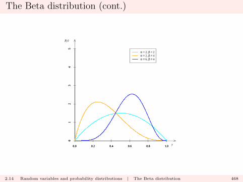
The Beta distribution (cont.)
f(y)
y0.0 0.2 0.4 0.6 0.8 1.00.0 0.2 0.4 0.6 0.8 1.0
01
23
45
01
23
45
α = 2, β = 2α = 2, β = 4α = 6, β = 4
2.14 Random variables and probability distributions | The Beta distribution 468
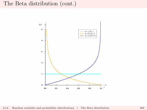
The Beta distribution (cont.)
f(y)
y0.0 0.2 0.4 0.6 0.8 1.00.0 0.2 0.4 0.6 0.8 1.0
01
23
45
01
23
45
α = 1, β = 1α = 0.5, β = 2α = 2, β = 0.75
2.14 Random variables and probability distributions | The Beta distribution 469
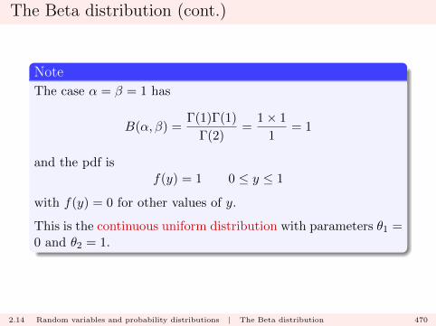
The Beta distribution (cont.)
Note
The case α = β = 1 has
B(α, β) =Γ(1)Γ(1)
Γ(2)=
1× 1
1= 1
and the pdf isf(y) = 1 0 ≤ y ≤ 1
with f(y) = 0 for other values of y.
This is the continuous uniform distribution with parameters θ1 =0 and θ2 = 1.
2.14 Random variables and probability distributions | The Beta distribution 470
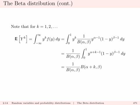
The Beta distribution (cont.)
Note that for k = 1, 2, . . .
E
[Y k]
=
∫ ∞−∞
ykf(y) dy =
∫ 1
0yk
1
B(α, β)yα−1(1− y)β−1 dy
=1
B(α, β)
∫ 1
0yα+k−1(1− y)β−1 dy
=1
B(α, β)B(α+ k, β)
2.14 Random variables and probability distributions | The Beta distribution 471
Chapter 3: Probability calculation
methods
Probability calculation methods
We now study two specific calculation methods relevant for prob-ability and distribution calculations:
� transformations;
� sums of random variables.
3.0 Probability calculation methods 473
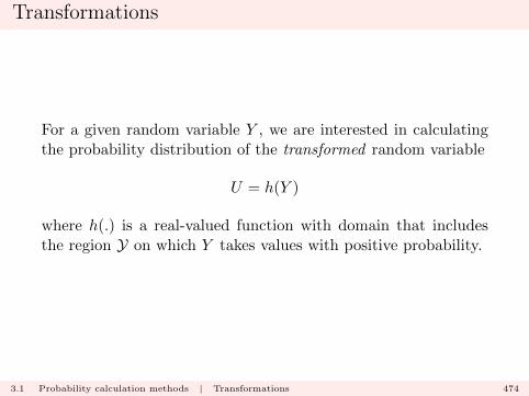
Transformations
For a given random variable Y , we are interested in calculatingthe probability distribution of the transformed random variable
U = h(Y )
where h(.) is a real-valued function with domain that includesthe region Y on which Y takes values with positive probability.
3.1 Probability calculation methods | Transformations 474
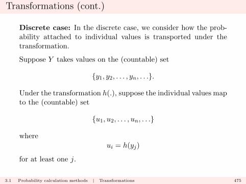
Transformations (cont.)
Discrete case: In the discrete case, we consider how the prob-ability attached to individual values is transported under thetransformation.
Suppose Y takes values on the (countable) set
{y1, y2, . . . , yn, . . .}.
Under the transformation h(.), suppose the individual values mapto the (countable) set
{u1, u2, . . . , un, . . .}
where
ui = h(yj)
for at least one j.
3.1 Probability calculation methods | Transformations 475
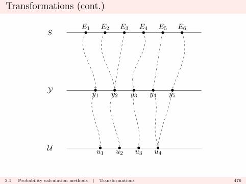
Transformations (cont.)
E1 E2 E3 E4 E5 E6
y1 y2 y3 y4 y5
u1 u2 u3 u4
S
Y
U
3.1 Probability calculation methods | Transformations 476
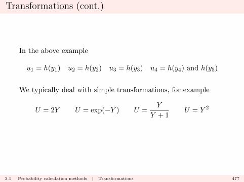
Transformations (cont.)
In the above example
u1 = h(y1) u2 = h(y2) u3 = h(y3) u4 = h(y4) and h(y5)
We typically deal with simple transformations, for example
U = 2Y U = exp(−Y ) U =Y
Y + 1U = Y 2
3.1 Probability calculation methods | Transformations 477
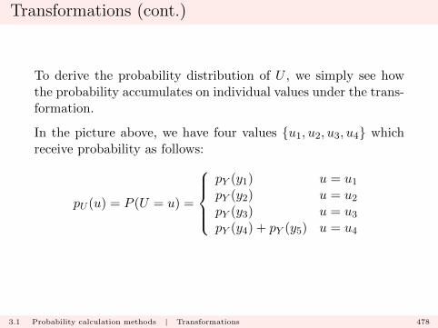
Transformations (cont.)
To derive the probability distribution of U , we simply see howthe probability accumulates on individual values under the trans-formation.
In the picture above, we have four values {u1, u2, u3, u4} whichreceive probability as follows:
pU (u) = P (U = u) =
pY (y1) u = u1pY (y2) u = u2pY (y3) u = u3pY (y4) + pY (y5) u = u4
3.1 Probability calculation methods | Transformations 478
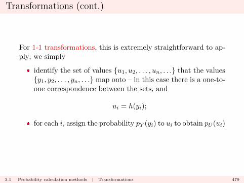
Transformations (cont.)
For 1-1 transformations, this is extremely straightforward to ap-ply; we simply
� identify the set of values {u1, u2, . . . , un, . . .} that the values{y1, y2, . . . , yn, . . .} map onto – in this case there is a one-to-one correspondence between the sets, and
ui = h(yi);
� for each i, assign the probability pY (yi) to ui to obtain pU (ui)
3.1 Probability calculation methods | Transformations 479

Transformations (cont.)
Example (Poisson case)
Suppose that Y has a Poisson distribution with parameter λ.Let U = 3Y ; then only the values in the set
U = {0, 3, 6, 9, . . . , 3n, . . .}
receive any probability, and
pU (u) =λu/3
(u/3)!e−λ u ∈ {0, 3, 6, 9, . . .}
with pU (u) equal to zero for all other values of u.
3.1 Probability calculation methods | Transformations 480
Transformations (cont.)
If the transformation is not 1-1, we essentially have to identifythe set U , and compute for each case the probability assigned tothe values in the set.
3.1 Probability calculation methods | Transformations 481
Transformations (cont.)
Continuous case: In the continuous random variable case, wetry to adopt the same strategy and follow how values in the setY carry their probability to values in a set U .
The obstacle is that for a continuous random variable Y we have
P (Y = y) = 0
for all real values y.
3.1 Probability calculation methods | Transformations 482
Transformations (cont.)
To get around this, we can instead consider
P (Y ∈ A)
for a subset (eg interval) of the real line. For example, we couldconsider A = [2, 5], and the probability
P (Y ∈ A) ≡ P (2 ≤ Y ≤ 5).
3.1 Probability calculation methods | Transformations 483
Transformations (cont.)
Suppose that B represents the set of values containing all thepoints that points in A can be mapped to under the transform-ation h(.). That is,
B = {u : u = h(y), some y ∈ A}
Then we have that probability is preserved under the mapping
P (Y ∈ A) = P (U ∈ B).
3.1 Probability calculation methods | Transformations 484
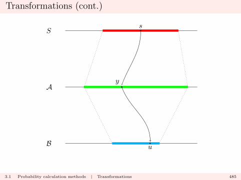
Transformations (cont.)
S
A
B
s
y
u
3.1 Probability calculation methods | Transformations 485
Transformations (cont.)
Example
Suppose Y is a continuous random variable that can take valueson [0,∞), and U = h(Y ) = 2Y . This means that we need toconsider the set
U = {u : u = 2y, some y ∈ [0,∞)} ≡ [0,∞)
that is, every point y gets mapped to u = 2y.
3.1 Probability calculation methods | Transformations 486
Transformations (cont.)
Example
Consider interval A = [a, b] for a < b; if we let c = h(a) = 2aand d = 2b, then we have that
P (a ≤ Y ≤ b) = P (c ≤ U ≤ d).
In terms of the cdfs, we have that
FY (b)− FY (a) = FU (d)− FU (c)
and letting a −→ 0, we have that
FY (b) = P (Y ≤ b) = P (U ≤ d) = FU (d).
3.1 Probability calculation methods | Transformations 487

Transformations (cont.)
Example
That is, for b ∈ R.FY (b) = FU (2b)
Now, given FY , we wish to compute FU . We can do this bynoting that, for arbitrary u
FU (u) = P (U ≤ u) = P (U/2 ≤ u/2) = P (Y ≤ u/2) = FY (u/2).
3.1 Probability calculation methods | Transformations 488
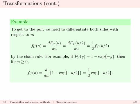
Transformations (cont.)
Example
To get to the pdf, we need to differentiate both sides withrespect to u:
fU (u) =dFU (u)
du=dFY (u/2)
du=
1
2fY (u/2)
by the chain rule. For example, if FY (y) = 1− exp{−y}, thenfor u ≥ 0,
fU (u) =d
du{1− exp{−u/2}} =
1
2exp{−u/2}.
3.1 Probability calculation methods | Transformations 489
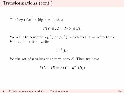
Transformations (cont.)
The key relationship here is that
P (Y ∈ A) = P (U ∈ B).
We want to compute FU (.) or fU (.), which means we want to fixB first. Therefore, write
h−1(B)
for the set of y values that map onto B. Then we have
P (U ∈ B) = P (Y ∈ h−1(B))
3.1 Probability calculation methods | Transformations 490

Transformations (cont.)
If h(.) is a 1–1 transformation, then h−1(.) is the inverse trans-formation which we can often compute explicitly.
h(y) h−1(y)
y + θ y − θλy y/λ
ey ln y
y
1 + y
y
1− y
etc.
3.1 Probability calculation methods | Transformations 491
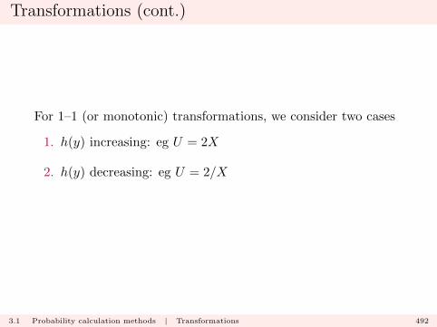
Transformations (cont.)
For 1–1 (or monotonic) transformations, we consider two cases
1. h(y) increasing: eg U = 2X
2. h(y) decreasing: eg U = 2/X
3.1 Probability calculation methods | Transformations 492
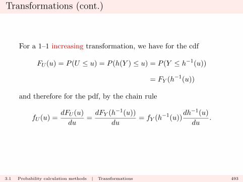
Transformations (cont.)
For a 1–1 increasing transformation, we have for the cdf
FU (u) = P (U ≤ u) = P (h(Y ) ≤ u) = P (Y ≤ h−1(u))
= FY (h−1(u))
and therefore for the pdf, by the chain rule
fU (u) =dFU (u)
du=dFY (h−1(u))
du= fY (h−1(u))
dh−1(u)
du.
3.1 Probability calculation methods | Transformations 493

Transformations (cont.)
For a 1–1 decreasing transformation, we have instead
FU (u) = P (U ≤ u) = P (h(Y ) ≤ u) = P (Y ≥ h−1(u))
= 1− FY (h−1(u))
and therefore for the pdf, by the chain rule
fU (u) =dFU (u)
du= −dFY (h−1(u))
du= −fY (h−1(u))
dh−1(u)
du.
3.1 Probability calculation methods | Transformations 494
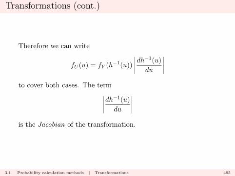
Transformations (cont.)
Therefore we can write
fU (u) = fY (h−1(u))
∣∣∣∣dh−1(u)
du
∣∣∣∣to cover both cases. The term∣∣∣∣dh−1(u)
du
∣∣∣∣is the Jacobian of the transformation.
3.1 Probability calculation methods | Transformations 495
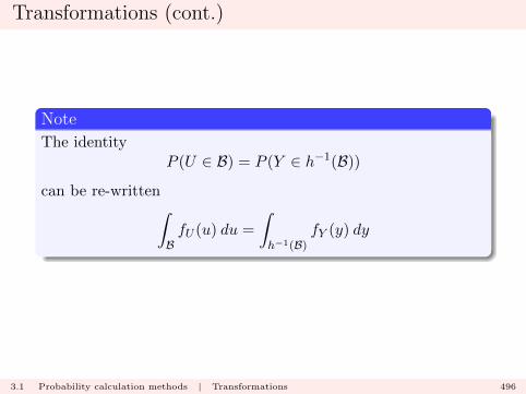
Transformations (cont.)
Note
The identityP (U ∈ B) = P (Y ∈ h−1(B))
can be re-written∫BfU (u) du =
∫h−1(B)
fY (y) dy
3.1 Probability calculation methods | Transformations 496

Transformations (cont.)
Note (cont.)
Changing variables in the right-hand integral
u = h(y) ⇐⇒ y = h−1(u)
we have by the rules of integration∫BfU (u) du =
∫BfY (h−1(u))
∣∣∣∣dh−1(u)
du
∣∣∣∣ duand the same result follows by equating the integrands.
3.1 Probability calculation methods | Transformations 497
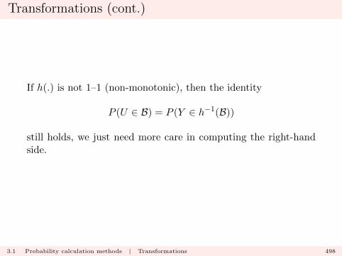
Transformations (cont.)
If h(.) is not 1–1 (non-monotonic), then the identity
P (U ∈ B) = P (Y ∈ h−1(B))
still holds, we just need more care in computing the right-handside.
3.1 Probability calculation methods | Transformations 498

Transformations (cont.)
Example
Suppose that Y has a continuous uniform distribution on therange [0, 1], and that
U = Y (1− Y )
that is U = h(Y ) with h(t) = t(1− t).
First, as Y = [0, 1], we have that
U = [0, 1/4].
3.1 Probability calculation methods | Transformations 499
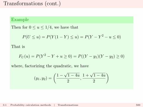
Transformations (cont.)
Example
Then for 0 ≤ u ≤ 1/4, we have that
P (U ≤ u) = P (Y (1− Y ) ≤ u) = P (Y − Y 2 − u ≤ 0)
That is
FU (u) = P (Y 2 − Y + u ≥ 0) = P ((Y − y1)(Y − y2) ≥ 0)
where, factorizing the quadratic, we have
(y1, y2) =
(1−√
1− 4u
2,1 +√
1− 4u
2
)
3.1 Probability calculation methods | Transformations 500
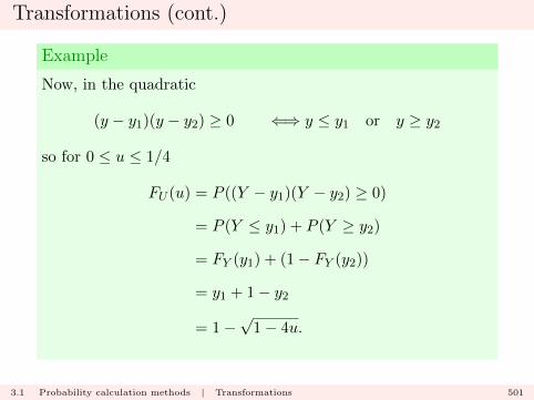
Transformations (cont.)
Example
Now, in the quadratic
(y − y1)(y − y2) ≥ 0 ⇐⇒ y ≤ y1 or y ≥ y2
so for 0 ≤ u ≤ 1/4
FU (u) = P ((Y − y1)(Y − y2) ≥ 0)
= P (Y ≤ y1) + P (Y ≥ y2)
= FY (y1) + (1− FY (y2))
= y1 + 1− y2
= 1−√
1− 4u.
3.1 Probability calculation methods | Transformations 501
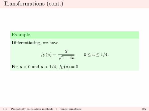
Transformations (cont.)
Example
Differentiating, we have
fU (u) =2√
1− 4u0 ≤ u ≤ 1/4.
For u < 0 and u > 1/4, fU (u) = 0.
3.1 Probability calculation methods | Transformations 502
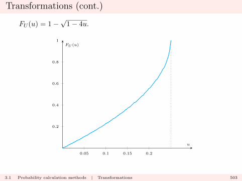
Transformations (cont.)
FU (u) = 1−√
1− 4u.
0.05 0.1 0.15 0.2
0.2
0.4
0.6
0.8
1
u
FU (u)
3.1 Probability calculation methods | Transformations 503
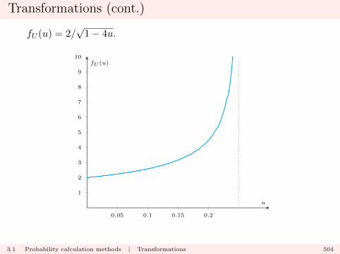
Transformations (cont.)
fU (u) = 2/√
1− 4u.
0.05 0.1 0.15 0.2
1
2
3
4
5
6
7
8
9
10
u
fU (u)
3.1 Probability calculation methods | Transformations 504
Transformations (cont.)
Note
For non 1-1 transformations, it is usually necessary to go backto ‘first principles’ and investigate
P (U ∈ B) = P (Y ∈ h−1(B))
for B = (−∞, u] and then carefully construct h−1(B) from it.
3.1 Probability calculation methods | Transformations 505
Transformations (cont.)
Expectations
We previously saw for continuous random variable Y andfunction g(.)
E[g(Y )] =
∫ ∞−∞
g(y)fY (y) dy.
However, U = g(Y ) is a random variable in its own right. Wehave
E[U ] =
∫ ∞−∞
ufY (U) du.
From the above argument, we see that
E[U ] = E[g(Y )]
that is, we can regard the computation in two equivalent ways.
3.1 Probability calculation methods | Transformations 506
Transformations (cont.)
Moment Generating Functions
Recall the definition of the moment generating function (mgf):for −b ≤ t ≤ b, b > 0,
mY (t) = E[etY ].
If U = cY + d, for constants c > 0 and d, we have that
mU (t) = E[etU]
= E
[et(cY+d)
]= E
[e(ct)Y edt
]= edtE
[e(ct)Y
]as edt is a constant. Therefore
mU (t) = edtmY (ct).
3.1 Probability calculation methods | Transformations 507
Transformations (cont.)
Moment Generating Functions: Normal case
If Y has a standard Normal distribution,
mY (t) = exp
{t2
2
}t ∈ R.
If U = σY + µ, then
mU (t) = eµtmY (σt) = exp
{µt+
(σt)2
2
}.
Thus, by the earlier result for the transformations of standardNormal random variables
m(t) = exp
{µt+
σ2t2
2
}is the mgf of the Normal(µ, σ2) distribution.
3.1 Probability calculation methods | Transformations 508
Sums of random variables
Example (Two dice)
Two fair dice are rolled, with the outcomes of the rollsindependent events.
What is the probability that the sum of the scores of the twodice exceeds 10 ?
3.2 Probability calculation methods | Sums of random variables 509
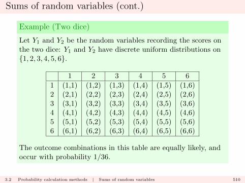
Sums of random variables (cont.)
Example (Two dice)
Let Y1 and Y2 be the random variables recording the scores onthe two dice: Y1 and Y2 have discrete uniform distributions on{1, 2, 3, 4, 5, 6}.
1 2 3 4 5 6
1 (1,1) (1,2) (1,3) (1,4) (1,5) (1,6)2 (2,1) (2,2) (2,3) (2,4) (2,5) (2,6)3 (3,1) (3,2) (3,3) (3,4) (3,5) (3,6)4 (4,1) (4,2) (4,3) (4,4) (4,5) (4,6)5 (5,1) (5,2) (5,3) (5,4) (5,5) (5,6)6 (6,1) (6,2) (6,3) (6,4) (6,5) (6,6)
The outcome combinations in this table are equally likely, andoccur with probability 1/36.
3.2 Probability calculation methods | Sums of random variables 510

Sums of random variables (cont.)
Example (Two dice)
Let Y denote the total score. The possible total scores are
Y = {2, 3, 4, 5, 6, 7, 8, 9, 10, 11, 12}
and to compute P (Y = y) we can sum down the antidiagonalsof the table to obtain
p(y) = P (Y = y) =min{6, y − 1} −max{1, y − 6}+ 1
36y ∈ Y
3.2 Probability calculation methods | Sums of random variables 511
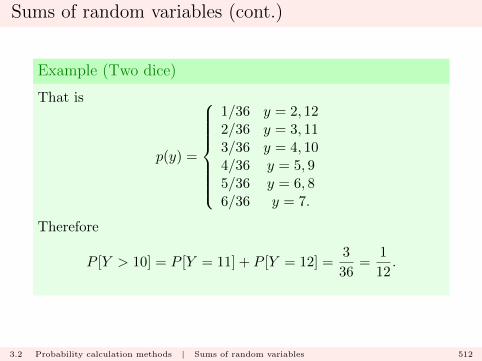
Sums of random variables (cont.)
Example (Two dice)
That is
p(y) =
1/36 y = 2, 122/36 y = 3, 113/36 y = 4, 104/36 y = 5, 95/36 y = 6, 86/36 y = 7.
Therefore
P [Y > 10] = P [Y = 11] + P [Y = 12] =3
36=
1
12.
3.2 Probability calculation methods | Sums of random variables 512
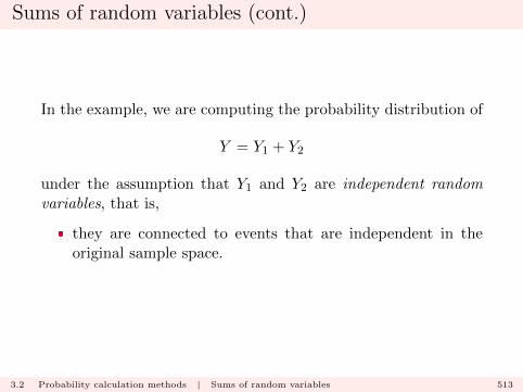
Sums of random variables (cont.)
In the example, we are computing the probability distribution of
Y = Y1 + Y2
under the assumption that Y1 and Y2 are independent randomvariables, that is,
� they are connected to events that are independent in theoriginal sample space.
3.2 Probability calculation methods | Sums of random variables 513
Sums of random variables (cont.)
The assumption of independence of the events means that wemust have
P ((Y1 = y1) ∩ (Y2 = y2)) = P (Y1 = y1)× P (Y2 = y2)
for all pairs of possible realizations (y1, y2), each value taken fromthe set {1, 2, 3, 4, 5, 6}.
3.2 Probability calculation methods | Sums of random variables 514

Sums of random variables (cont.)
Now consider the event (Y = y) for the set of possible values
y ∈ {2, 3, 4, 5, 6, 7, 8, 9, 10, 11, 12};
we have the partition given by result of the first roll
(Y = y) ≡6⋃
y1=1
(Y = y ∩ Y1 = y1).
– that is, when we observe Y = 5, say, that could arise as theunordered pairs
(1, 4), (2, 3), (3, 2), (4, 1).
3.2 Probability calculation methods | Sums of random variables 515
Sums of random variables (cont.)
However the event
(Y = y ∩ Y1 = y1)
can be re-written
(Y2 = y − y1 ∩ Y1 = y1)
as if Y = y and Y1 = y1, we must have Y2 = y − y1.
3.2 Probability calculation methods | Sums of random variables 516

Sums of random variables (cont.)
Using Axiom III, we can then write
P (Y = y) =
6∑y1=1
P ((Y = y) ∩ (Y1 = y1))
=
6∑y1=1
P ((Y2 = y − y1) ∩ (Y1 = y1))
=
6∑y1=1
P (Y1 = y1)P (Y2 = y − y1)
3.2 Probability calculation methods | Sums of random variables 517
Sums of random variables (cont.)
For the range of the summation, we require for fixed y that
1 ≤ y1 ≤ 6
so that P (Y1 = y1) > 0 and
1 ≤ y − y1 ≤ 6
in order to make
P (Y2 = y − y1) > 0.
3.2 Probability calculation methods | Sums of random variables 518
Sums of random variables (cont.)
That is we need to have
1 ≤ y1 ≤ 6
y − 6 ≤ y1 ≤ y − 1
in order for a term in the sum to be non-zero.
3.2 Probability calculation methods | Sums of random variables 519
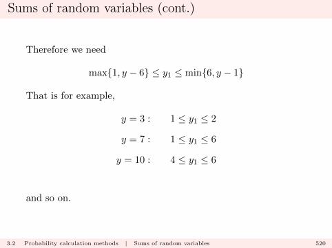
Sums of random variables (cont.)
Therefore we need
max{1, y − 6} ≤ y1 ≤ min{6, y − 1}
That is for example,
y = 3 : 1 ≤ y1 ≤ 2
y = 7 : 1 ≤ y1 ≤ 6
y = 10 : 4 ≤ y1 ≤ 6
and so on.
3.2 Probability calculation methods | Sums of random variables 520
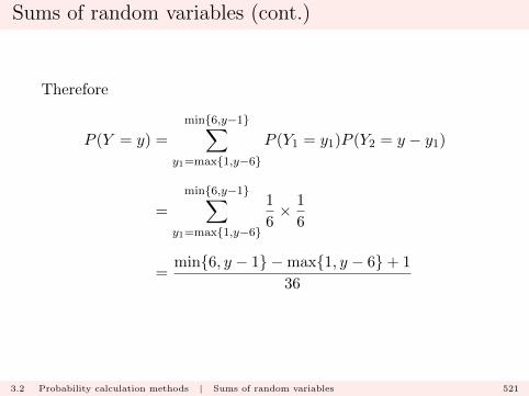
Sums of random variables (cont.)
Therefore
P (Y = y) =
min{6,y−1}∑y1=max{1,y−6}
P (Y1 = y1)P (Y2 = y − y1)
=
min{6,y−1}∑y1=max{1,y−6}
1
6× 1
6
=min{6, y − 1} −max{1, y − 6}+ 1
36
3.2 Probability calculation methods | Sums of random variables 521
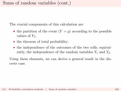
Sums of random variables (cont.)
The crucial components of this calculation are
� the partition of the event (Y = y) according to the possiblevalues of Y1;
� the theorem of total probability;
� the independence of the outcomes of the two rolls, equival-ently, the independence of the random variables Y1 and Y2.
Using these elements, we can derive a general result in the dis-crete case.
3.2 Probability calculation methods | Sums of random variables 522

Sums of random variables (cont.)
Suppose Y1 and Y2 are discrete random variables, with Y1 and Y2independent. Suppose that Y1 and Y2 take values on the sets Y1and Y2 respectively. Let Y = Y1 + Y2. Then
P (Y = y) = P
⋃y1∈Y1
(Y = y) ∩ (Y1 = y1)
=∑y1∈Y1
P ((Y = y) ∩ (Y1 = y1))
=∑y1∈Y1
P ((Y2 = y − y1) ∩ (Y1 = y1))
=∑y1∈Y1
P (Y2 = y − y1)P (Y1 = y1)
3.2 Probability calculation methods | Sums of random variables 523
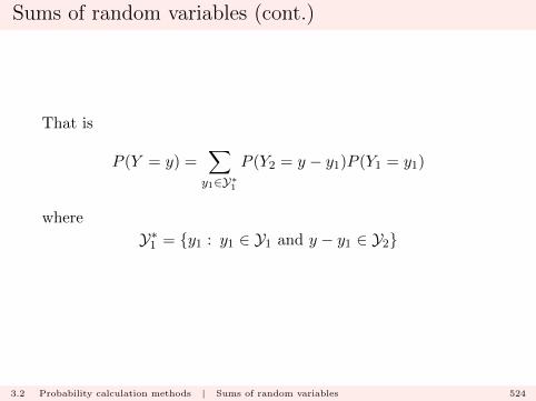
Sums of random variables (cont.)
That is
P (Y = y) =∑y1∈Y∗1
P (Y2 = y − y1)P (Y1 = y1)
where
Y∗1 = {y1 : y1 ∈ Y1 and y − y1 ∈ Y2}
3.2 Probability calculation methods | Sums of random variables 524
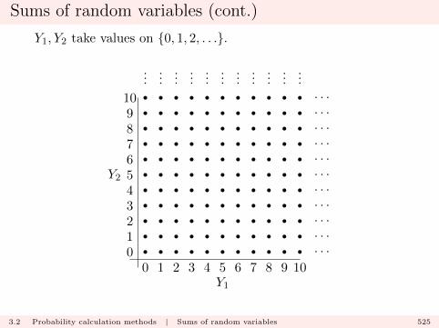
Sums of random variables (cont.)
Y1, Y2 take values on {0, 1, 2, . . .}.
0 1 2 3 4 5 6 7 8 9 10012345678910
Y1
Y2
......
......
......
......
......
...
· · ·· · ·· · ·· · ·· · ·· · ·· · ·· · ·· · ·· · ·· · ·
3.2 Probability calculation methods | Sums of random variables 525

Sums of random variables (cont.)
Y1 + Y2 = 5
0 1 2 3 4 5 6 7 8 9 10012345678910
Y1
Y2
......
......
......
......
......
...
· · ·· · ·· · ·· · ·· · ·· · ·· · ·· · ·· · ·· · ·· · ·
3.2 Probability calculation methods | Sums of random variables 526
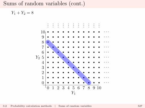
Sums of random variables (cont.)
Y1 + Y2 = 8
0 1 2 3 4 5 6 7 8 9 10012345678910
Y1
Y2
......
......
......
......
......
...
· · ·· · ·· · ·· · ·· · ·· · ·· · ·· · ·· · ·· · ·· · ·
3.2 Probability calculation methods | Sums of random variables 527
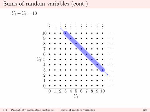
Sums of random variables (cont.)
Y1 + Y2 = 13
0 1 2 3 4 5 6 7 8 9 10012345678910
Y1
Y2
......
......
......
......
......
...
· · ·· · ·· · ·· · ·· · ·· · ·· · ·· · ·· · ·· · ·· · ·
3.2 Probability calculation methods | Sums of random variables 528
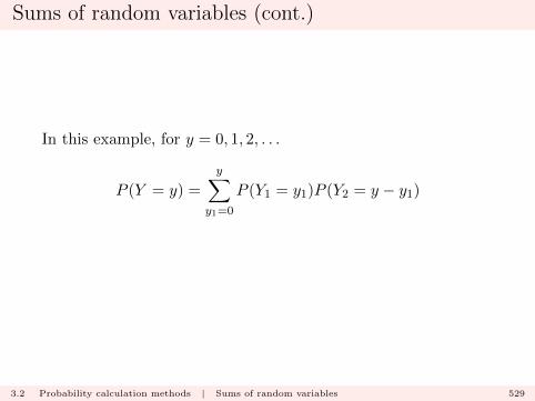
Sums of random variables (cont.)
In this example, for y = 0, 1, 2, . . .
P (Y = y) =
y∑y1=0
P (Y1 = y1)P (Y2 = y − y1)
3.2 Probability calculation methods | Sums of random variables 529
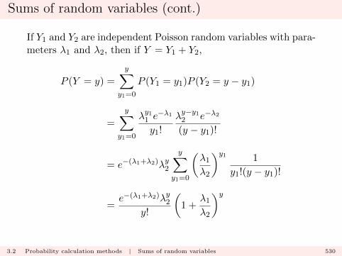
Sums of random variables (cont.)
If Y1 and Y2 are independent Poisson random variables with para-meters λ1 and λ2, then if Y = Y1 + Y2,
P (Y = y) =
y∑y1=0
P (Y1 = y1)P (Y2 = y − y1)
=
y∑y1=0
λy11 e−λ1
y1!
λy−y12 e−λ2
(y − y1)!
= e−(λ1+λ2)λy2
y∑y1=0
(λ1λ2
)y1 1
y1!(y − y1)!
=e−(λ1+λ2)λy2
y!
(1 +
λ1λ2
)y
3.2 Probability calculation methods | Sums of random variables 530
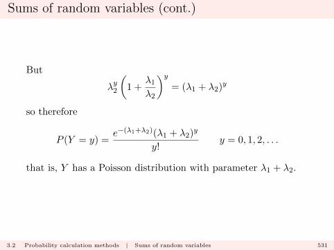
Sums of random variables (cont.)
But
λy2
(1 +
λ1λ2
)y= (λ1 + λ2)
y
so therefore
P (Y = y) =e−(λ1+λ2)(λ1 + λ2)
y
y!y = 0, 1, 2, . . .
that is, Y has a Poisson distribution with parameter λ1 + λ2.
3.2 Probability calculation methods | Sums of random variables 531
Sums of random variables (cont.)
If Y1 and Y2 are independent continuous random variables, asimilar strategy can be used. As before for continuous randomvariables, we start with the cdf and aim to compute
FY (y) = P (Y ≤ y)
If Y1 and Y2 are continuous, then it follows that Y is continuous.
3.2 Probability calculation methods | Sums of random variables 532
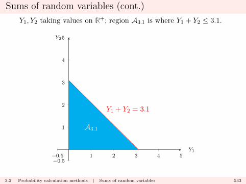
Sums of random variables (cont.)
Y1, Y2 taking values on R+; region A3.1 is where Y1 + Y2 ≤ 3.1.
−0.5 1 2 3 4 5−0.5
1
2
3
4
5
Y1 + Y2 = 3.1
A3.1
Y1
Y2
3.2 Probability calculation methods | Sums of random variables 533
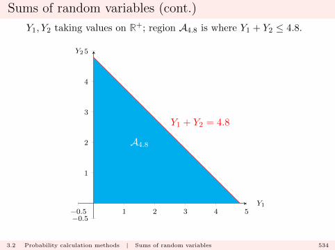
Sums of random variables (cont.)
Y1, Y2 taking values on R+; region A4.8 is where Y1 + Y2 ≤ 4.8.
−0.5 1 2 3 4 5−0.5
1
2
3
4
5
Y1 + Y2 = 4.8
A4.8
Y1
Y2
3.2 Probability calculation methods | Sums of random variables 534
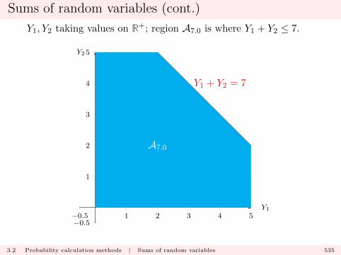
Sums of random variables (cont.)
Y1, Y2 taking values on R+; region A7.0 is where Y1 + Y2 ≤ 7.
−0.5 1 2 3 4 5−0.5
1
2
3
4
5
A7.0
Y1 + Y2 = 7
Y1
Y2
3.2 Probability calculation methods | Sums of random variables 535

Sums of random variables (cont.)
Then we have by definition that
FY (y) = P (Y ≤ y) =
∫ y
−∞fY (t) dt
where fY (y) is the pdf for Y . However,
(Y ≤ y) = (Y1 + Y2 ≤ y)
Therefore to compute FY (y) = P (Y ≤ y) we need to aggregateall the probability across the blue shaded region, denoted Ay, inthe above pictures.
3.2 Probability calculation methods | Sums of random variables 536

Sums of random variables (cont.)
In the discrete case in which
pY (y) = P (Y = y) =∑y1∈Y∗1
P (Y2 = y − y1)P (Y1 = y1)
=∑y1∈Y∗1
pY2(y − y1)pY1(y1)
where
� pY (.) is the pmf for Y ,
� pY1(.) is the pmf for Y1,
� pY2(.) is the pmf for Y2.
3.2 Probability calculation methods | Sums of random variables 537

Sums of random variables (cont.)
we may write
fY (y) =
∫ ∞−∞
fY2(y − y1)fY1(y1) dy1
where
� fY (.) is the pdf for Y ,
� fY1(.) is the pdf for Y1,
� fY2(.) is the pdf for Y2.
3.2 Probability calculation methods | Sums of random variables 538

Sums of random variables (cont.)
Note
This is termed a convolution formula.
3.2 Probability calculation methods | Sums of random variables 539

Sums of random variables (cont.)
Example (Exponential random variables)
Suppose
Y1 :fY1(y1) =1
β1e−y1/β1 y1 ≥ 0
Y2 :fY2(y2) =1
β2e−y2/β2 y2 ≥ 0
are independent random variables, and let Y = Y1 + Y2. Forconvenience, write
λ1 =1
β1λ2 =
1
β2.
3.2 Probability calculation methods | Sums of random variables 540
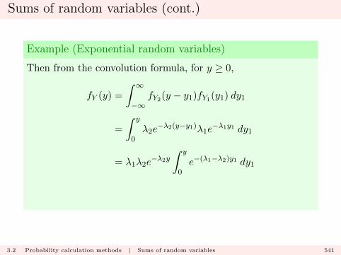
Sums of random variables (cont.)
Example (Exponential random variables)
Then from the convolution formula, for y ≥ 0,
fY (y) =
∫ ∞−∞
fY2(y − y1)fY1(y1) dy1
=
∫ y
0λ2e−λ2(y−y1)λ1e
−λ1y1 dy1
= λ1λ2e−λ2y
∫ y
0e−(λ1−λ2)y1 dy1
3.2 Probability calculation methods | Sums of random variables 541
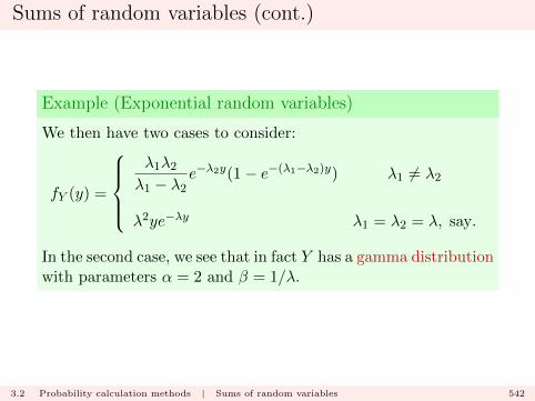
Sums of random variables (cont.)
Example (Exponential random variables)
We then have two cases to consider:
fY (y) =
λ1λ2λ1 − λ2
e−λ2y(1− e−(λ1−λ2)y) λ1 6= λ2
λ2ye−λy λ1 = λ2 = λ, say.
In the second case, we see that in fact Y has a gamma distributionwith parameters α = 2 and β = 1/λ.
3.2 Probability calculation methods | Sums of random variables 542
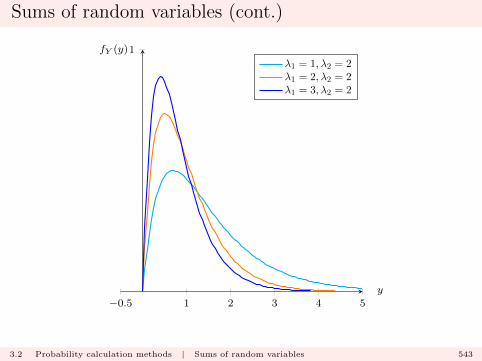
Sums of random variables (cont.)
−0.5 1 2 3 4 5
1
y
fY (y)
λ1 = 1, λ2 = 2λ1 = 2, λ2 = 2λ1 = 3, λ2 = 2
3.2 Probability calculation methods | Sums of random variables 543
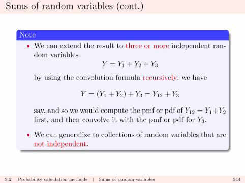
Sums of random variables (cont.)
Note
� We can extend the result to three or more independent ran-dom variables
Y = Y1 + Y2 + Y3
by using the convolution formula recursively; we have
Y = (Y1 + Y2) + Y3 = Y12 + Y3
say, and so we would compute the pmf or pdf of Y12 = Y1+Y2first, and then convolve it with the pmf or pdf for Y3.
� We can generalize to collections of random variables that arenot independent.
3.2 Probability calculation methods | Sums of random variables 544
Chapter 4: Multivariate distributions
Multivariate probability distributions
We now consider probability specifications for more than onevariable at a time.
� We have already used the straightforward concept of inde-pendent random variables, that is, variables associated withindependent events;
� for example, the random variables associated with the out-comes of two independent rolls of dice.
4.1 Multivariate distributions | Basic definitions 546
Multivariate probability distributions (cont.)
However, there are many instances where we wish to considerrandom variables where there is an absence of independence;
� for example where the outcome of one part of the experimentdepends on the outcome of the other.
In general we can consider a vector of random variables (or vectorrandom variable)
(Y1, Y2, . . . , Yn).
4.1 Multivariate distributions | Basic definitions 547
Multivariate probability distributions (cont.)
Note
The critical thing to remember is that when we distributeprobability amongst the possible values of the random variables,the total probability we assign must still equal one.
4.1 Multivariate distributions | Basic definitions 548

Discrete bivariate distributions
We consider two variables Y1 and Y2 that are both discrete. Wecan suppose that both variables take values on the integers, Z.
A discrete bivariate probability mass function is a function of twoarguments
p(y1, y2)
that distributes probability across the possible values of the vec-tor (Y1, Y2) so that
p(y1, y2) = P ((Y1 = y1) ∩ (Y2 = y2))
for −∞ < y1 <∞ and −∞ < y2 <∞.
4.2 Multivariate distributions | Discrete case: joint mass function 549
Discrete bivariate distributions (cont.)
For shorthand, we write
P ((Y1 = y1) ∩ (Y2 = y2)) ≡ P (Y1 = y1, Y2 = y2)
4.2 Multivariate distributions | Discrete case: joint mass function 550
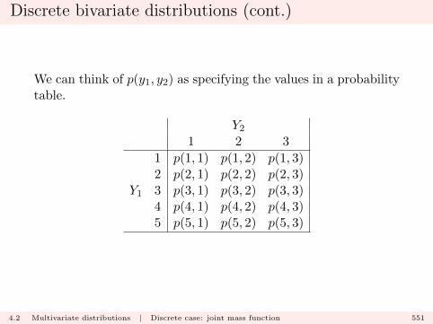
Discrete bivariate distributions (cont.)
We can think of p(y1, y2) as specifying the values in a probabilitytable.
Y21 2 3
1 p(1, 1) p(1, 2) p(1, 3)2 p(2, 1) p(2, 2) p(2, 3)
Y1 3 p(3, 1) p(3, 2) p(3, 3)4 p(4, 1) p(4, 2) p(4, 3)5 p(5, 1) p(5, 2) p(5, 3)
4.2 Multivariate distributions | Discrete case: joint mass function 551

Discrete bivariate distributions (cont.)
For 1 ≤ y1 ≤ 5, 1 ≤ y2 ≤ 3
p(y1, y2) =(y1 + y2)
75
Y21 2 3
1 2/75 3/75 4/752 3/75 4/75 5/75
Y1 3 4/75 5/75 6/754 5/75 6/75 7/755 6/75 7/75 8/75
4.2 Multivariate distributions | Discrete case: joint mass function 552
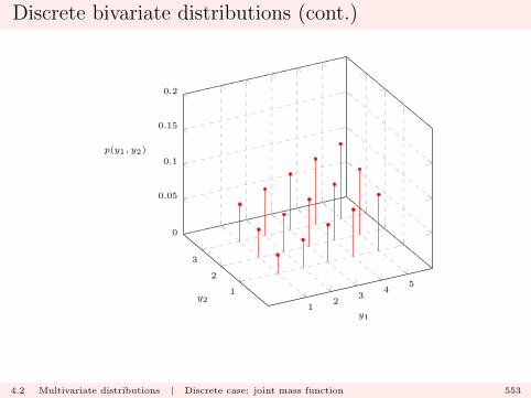
Discrete bivariate distributions (cont.)
12
34
51
2
3
0
0.05
0.1
0.15
0.2
y1
y2
p(y1, y2)
4.2 Multivariate distributions | Discrete case: joint mass function 553

Discrete bivariate distributions (cont.)
The function p(y1, y2) is the joint probability mass function: ithas two basic properties
� “specifies probabilities”
0 ≤ p(y1, y2) ≤ 1 for all y1, y2
� “sums to one”
∞∑y1=−∞
∞∑y2=−∞
p(y1, y2) = 1.
although p(y1, y2) may be zero for some arguments.
4.2 Multivariate distributions | Discrete case: joint mass function 554
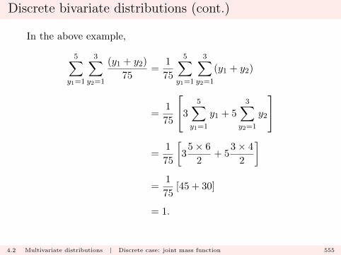
Discrete bivariate distributions (cont.)
In the above example,
5∑y1=1
3∑y2=1
(y1 + y2)
75=
1
75
5∑y1=1
3∑y2=1
(y1 + y2)
=1
75
3
5∑y1=1
y1 + 5
3∑y2=1
y2
=
1
75
[3
5× 6
2+ 5
3× 4
2
]=
1
75[45 + 30]
= 1.
4.2 Multivariate distributions | Discrete case: joint mass function 555
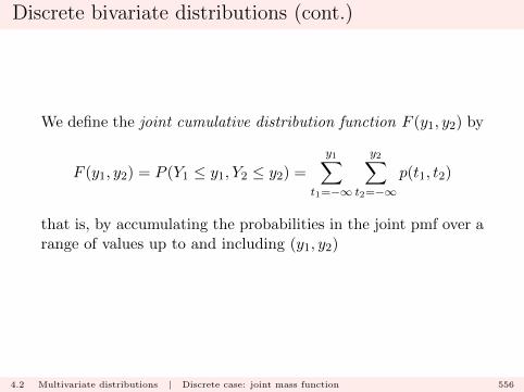
Discrete bivariate distributions (cont.)
We define the joint cumulative distribution function F (y1, y2) by
F (y1, y2) = P (Y1 ≤ y1, Y2 ≤ y2) =
y1∑t1=−∞
y2∑t2=−∞
p(t1, t2)
that is, by accumulating the probabilities in the joint pmf over arange of values up to and including (y1, y2)
4.2 Multivariate distributions | Discrete case: joint mass function 556

Discrete bivariate distributions (cont.)
F (3, 6) = P (Y1 ≤ 3, Y2 ≤ 6) =3∑
t1=0
6∑t2=0
p(t1, t2)
0 1 2 3 4 5 6 7 8 9 10012345678910
Y1
Y2
......
......
......
......
......
...
· · ·· · ·· · ·· · ·· · ·· · ·· · ·· · ·· · ·· · ·· · ·
4.2 Multivariate distributions | Discrete case: joint mass function 557
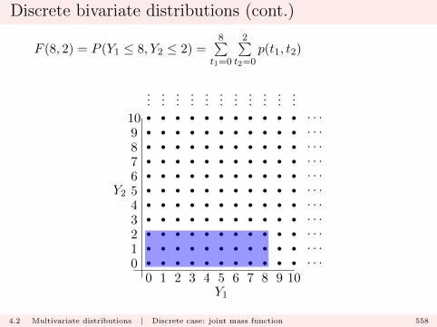
Discrete bivariate distributions (cont.)
F (8, 2) = P (Y1 ≤ 8, Y2 ≤ 2) =8∑
t1=0
2∑t2=0
p(t1, t2)
0 1 2 3 4 5 6 7 8 9 10012345678910
Y1
Y2
......
......
......
......
......
...
· · ·· · ·· · ·· · ·· · ·· · ·· · ·· · ·· · ·· · ·· · ·
4.2 Multivariate distributions | Discrete case: joint mass function 558
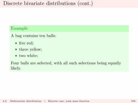
Discrete bivariate distributions (cont.)
Example
A bag contains ten balls:
� five red;
� three yellow;
� two white;
Four balls are selected, with all such selections being equallylikely.
4.2 Multivariate distributions | Discrete case: joint mass function 559
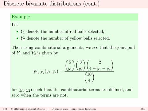
Discrete bivariate distributions (cont.)
Example
Let
� Y1 denote the number of red balls selected;
� Y2 denote the number of yellow balls selected.
Then using combinatorial arguments, we see that the joint pmfof Y1 and Y2 is given by
pY1,Y2(y1, y2) =
(5
y1
)(3
y2
)(2
4− y1 − y2
)(
10
4
)for (y1, y2) such that the combinatorial terms are defined, andzero when the terms are not.
4.2 Multivariate distributions | Discrete case: joint mass function 560

Discrete bivariate distributions (cont.)
Example
We need (y1, y2) simultaneously to satisfy
0 ≤ y1 ≤ 5 0 ≤ y2 ≤ 3 0 ≤ 4− y1 − y2 ≤ 2
in order to have a non-zero probability.
Total number of selections:
(10
4
)= 210.
4.2 Multivariate distributions | Discrete case: joint mass function 561

Discrete bivariate distributions (cont.)
Example
Y20 1 2 3
0 0 01 02 0
Y1 3 0 04 0 0 05 0 0 0 0
Red Yellow White
0 2 20 3 11 1 21 2 11 3 02 0 22 1 12 2 03 0 13 1 04 0 0
4.2 Multivariate distributions | Discrete case: joint mass function 562
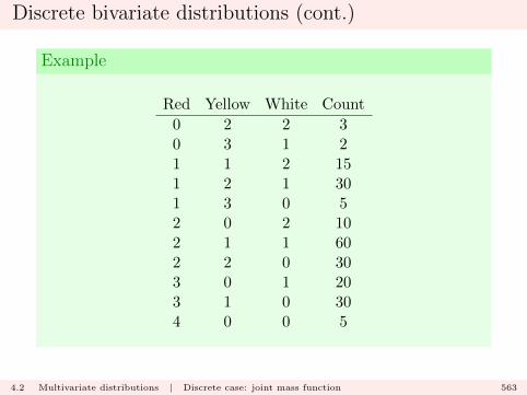
Discrete bivariate distributions (cont.)
Example
Red Yellow White Count
0 2 2 30 3 1 21 1 2 151 2 1 301 3 0 52 0 2 102 1 1 602 2 0 303 0 1 203 1 0 304 0 0 5
4.2 Multivariate distributions | Discrete case: joint mass function 563

Discrete bivariate distributions (cont.)
Example
Y20 1 2 3
0 0.0000 0.0000 0.0143 0.00951 0.0000 0.0714 0.1429 0.02382 0.0476 0.2857 0.1429 0.0000
Y1 3 0.0952 0.1429 0.0000 0.00004 0.0238 0.0000 0.0000 0.00005 0.0000 0.0000 0.0000 0.0000
4.2 Multivariate distributions | Discrete case: joint mass function 564
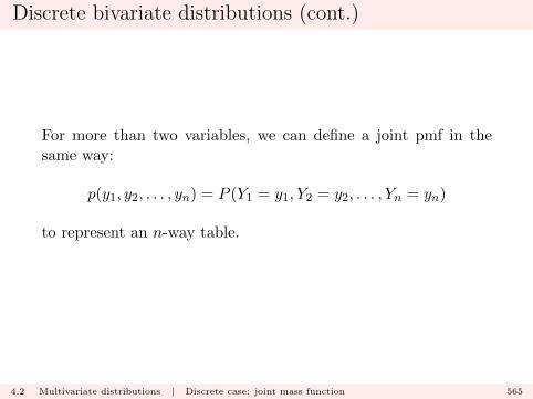
Discrete bivariate distributions (cont.)
For more than two variables, we can define a joint pmf in thesame way:
p(y1, y2, . . . , yn) = P (Y1 = y1, Y2 = y2, . . . , Yn = yn)
to represent an n-way table.
4.2 Multivariate distributions | Discrete case: joint mass function 565
The marginal mass function
Once we have specified a joint pmf, we can easily compute theprobability distribution for one of the variables alone.
The marginal probability mass function for Y1 is merely the pmfof Y1, which is computed via the Theorem of Total Probability.
4.3 Multivariate distributions | Marginal mass function 566
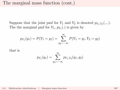
The marginal mass function (cont.)
Suppose that the joint pmf for Y1 and Y2 is denoted pY1,Y2(., .).The the marginal pmf for Y1, pY1(.) is given by
pY1(y1) = P (Y1 = y1) =
∞∑y2=−∞
P (Y1 = y1, Y2 = y2)
that is
pY1(y1) =
∞∑y2=−∞
pY1,Y2(y1, y2)
4.3 Multivariate distributions | Marginal mass function 567

The marginal mass function (cont.)
This result uses a partitioning argument:
(Y1 = y1) =
∞⋃y2=−∞
(Y1 = y1) ∩ (Y2 = y2)
4.3 Multivariate distributions | Marginal mass function 568

The marginal mass function (cont.)
For example
P (Y1 = 2) = P (Y1 = 2, Y2 = 1) + P (Y1 = 2, Y2 = 2)
+ P (Y1 = 2, Y2 = 3).
4.3 Multivariate distributions | Marginal mass function 569
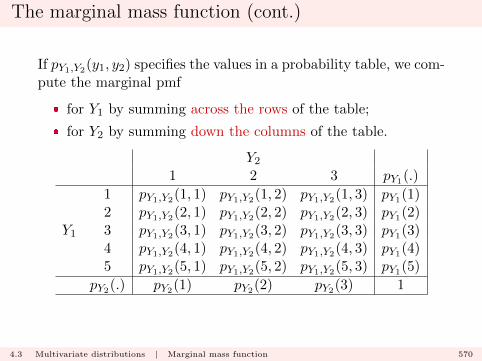
The marginal mass function (cont.)
If pY1,Y2(y1, y2) specifies the values in a probability table, we com-pute the marginal pmf
� for Y1 by summing across the rows of the table;
� for Y2 by summing down the columns of the table.
Y21 2 3 pY1(.)
1 pY1,Y2(1, 1) pY1,Y2(1, 2) pY1,Y2(1, 3) pY1(1)2 pY1,Y2(2, 1) pY1,Y2(2, 2) pY1,Y2(2, 3) pY1(2)
Y1 3 pY1,Y2(3, 1) pY1,Y2(3, 2) pY1,Y2(3, 3) pY1(3)4 pY1,Y2(4, 1) pY1,Y2(4, 2) pY1,Y2(4, 3) pY1(4)5 pY1,Y2(5, 1) pY1,Y2(5, 2) pY1,Y2(5, 3) pY1(5)
pY2(.) pY2(1) pY2(2) pY2(3) 1
4.3 Multivariate distributions | Marginal mass function 570

The marginal mass function (cont.)
Example (Previous example)
Four balls selected from 10.
� Y1 denote the number of red balls selected;
� Y2 denote the number of yellow balls selected.
The joint pmf of Y1 and Y2 is given by
pY1,Y2(y1, y2) =
(5
y1
)(3
y2
)(2
4− y1 − y2
)(
10
4
)for (y1, y2) such that the combinatorial terms are defined, andzero when the terms are not.
4.3 Multivariate distributions | Marginal mass function 571
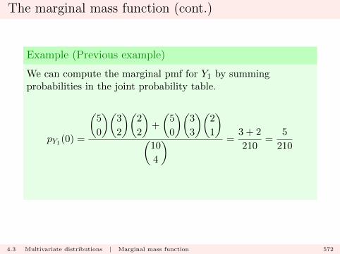
The marginal mass function (cont.)
Example (Previous example)
We can compute the marginal pmf for Y1 by summingprobabilities in the joint probability table.
pY1(0) =
(5
0
)(3
2
)(2
2
)+
(5
0
)(3
3
)(2
1
)(
10
4
) =3 + 2
210=
5
210
4.3 Multivariate distributions | Marginal mass function 572

The marginal mass function (cont.)
Example (Previous example)
pY1(1) =
(5
1
)(3
1
)(2
2
)+
(5
1
)(3
2
)(2
1
)+
(5
1
)(3
3
)(2
0
)(
10
4
)=
15 + 30 + 5
210=
50
210
4.3 Multivariate distributions | Marginal mass function 573
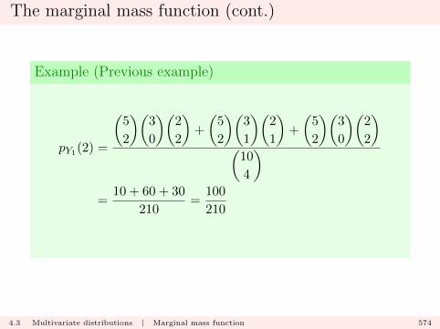
The marginal mass function (cont.)
Example (Previous example)
pY1(2) =
(5
2
)(3
0
)(2
2
)+
(5
2
)(3
1
)(2
1
)+
(5
2
)(3
0
)(2
2
)(
10
4
)=
10 + 60 + 30
210=
100
210
4.3 Multivariate distributions | Marginal mass function 574

The marginal mass function (cont.)
Example (Previous example)
pY1(3) =
(5
3
)(3
0
)(2
1
)+
(5
3
)(3
1
)(2
0
)(
10
4
)=
20 + 30
210=
50
210
4.3 Multivariate distributions | Marginal mass function 575
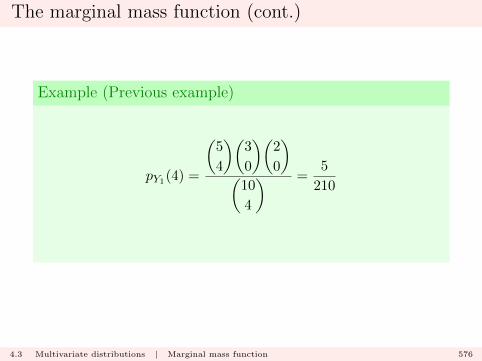
The marginal mass function (cont.)
Example (Previous example)
pY1(4) =
(5
4
)(3
0
)(2
0
)(
10
4
) =5
210
4.3 Multivariate distributions | Marginal mass function 576

The marginal mass function (cont.)
Note
In this example we can compute pY1(.) directly using the hyper-geometric formula
pY1(y1) =
(5
y1
)(5
4− y1
)(
10
4
)for 0 ≤ y1 ≤ 5 and 0 ≤ 4− y1 ≤ 5.
4.3 Multivariate distributions | Marginal mass function 577
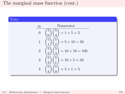
The marginal mass function (cont.)
Note
y1 Numerator
0
(5
0
)(5
4
)= 1× 5 = 5
1
(5
1
)(5
2
)= 5× 10 = 50
2
(5
2
)(5
3
)= 10× 10 = 100
3
(5
3
)(5
1
)= 10× 5 = 50
4
(5
4
)(5
0
)= 5× 1 = 5
4.3 Multivariate distributions | Marginal mass function 578
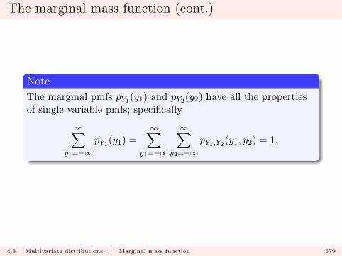
The marginal mass function (cont.)
Note
The marginal pmfs pY1(y1) and pY2(y2) have all the propertiesof single variable pmfs; specifically
∞∑y1=−∞
pY1(y1) =
∞∑y1=−∞
∞∑y2=−∞
pY1,Y2(y1, y2) = 1.
4.3 Multivariate distributions | Marginal mass function 579

The conditional mass function
Once we have the joint pmf
pY1,Y2(y1, y2) = P (Y1 = y1, Y2 = y2)
and the marginal pmf
pY1(y1) = P (Y1 = y1)
we can consider conditional pmfs.
4.4 Multivariate distributions | Conditional mass function 580
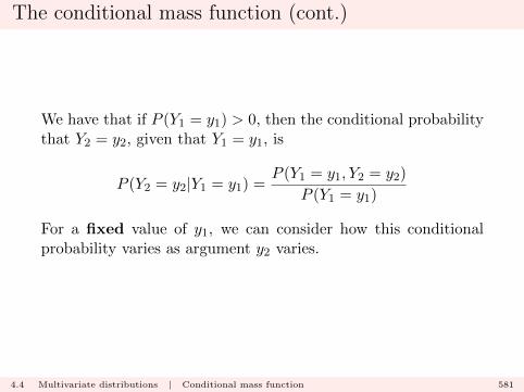
The conditional mass function (cont.)
We have that if P (Y1 = y1) > 0, then the conditional probabilitythat Y2 = y2, given that Y1 = y1, is
P (Y2 = y2|Y1 = y1) =P (Y1 = y1, Y2 = y2)
P (Y1 = y1)
For a fixed value of y1, we can consider how this conditionalprobability varies as argument y2 varies.
4.4 Multivariate distributions | Conditional mass function 581
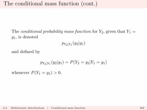
The conditional mass function (cont.)
The conditional probability mass function for Y2, given that Y1 =y1, is denoted
pY2|Y1(y2|y1)
and defined by
pY2|Y1(y2|y1) = P (Y2 = y2|Y1 = y1)
whenever P (Y1 = y1) > 0.
4.4 Multivariate distributions | Conditional mass function 582
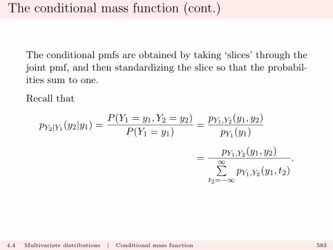
The conditional mass function (cont.)
The conditional pmfs are obtained by taking ‘slices’ through thejoint pmf, and then standardizing the slice so that the probabil-ities sum to one.
Recall that
pY2|Y1(y2|y1) =
P (Y1 = y1, Y2 = y2)
P (Y1 = y1)=pY1,Y2(y1, y2)
pY1(y1)
=pY1,Y2(y1, y2)∞∑
t2=−∞pY1,Y2(y1, t2)
.
4.4 Multivariate distributions | Conditional mass function 583
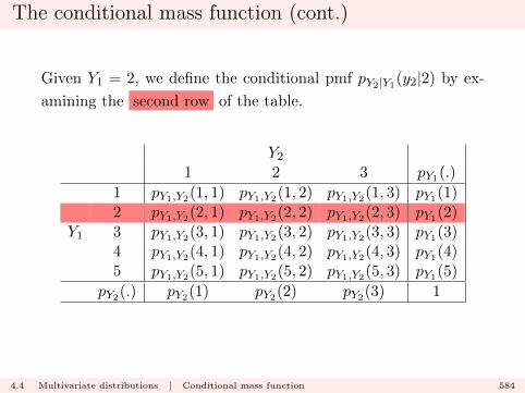
The conditional mass function (cont.)
Given Y1 = 2, we define the conditional pmf pY2|Y1(y2|2) by ex-
amining the second row of the table.
Y21 2 3 pY1(.)
1 pY1,Y2(1, 1) pY1,Y2(1, 2) pY1,Y2(1, 3) pY1(1)2 pY1,Y2(2, 1) pY1,Y2(2, 2) pY1,Y2(2, 3) pY1(2)
Y1 3 pY1,Y2(3, 1) pY1,Y2(3, 2) pY1,Y2(3, 3) pY1(3)4 pY1,Y2(4, 1) pY1,Y2(4, 2) pY1,Y2(4, 3) pY1(4)5 pY1,Y2(5, 1) pY1,Y2(5, 2) pY1,Y2(5, 3) pY1(5)
pY2(.) pY2(1) pY2(2) pY2(3) 1
4.4 Multivariate distributions | Conditional mass function 584
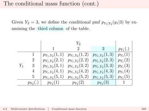
The conditional mass function (cont.)
Given Y2 = 3, we define the conditional pmf pY1|Y2(y1|3) by ex-
amining the third column of the table.
Y21 2 3 pY1(.)
1 pY1,Y2(1, 1) pY1,Y2(1, 2) pY1,Y2(1, 3) pY1(1)2 pY1,Y2(2, 1) pY1,Y2(2, 2) pY1,Y2(2, 3) pY1(2)
Y1 3 pY1,Y2(3, 1) pY1,Y2(3, 2) pY1,Y2(3, 3) pY1(3)4 pY1,Y2(4, 1) pY1,Y2(4, 2) pY1,Y2(4, 3) pY1(4)5 pY1,Y2(5, 1) pY1,Y2(5, 2) pY1,Y2(5, 3) pY1(5)
pY2(.) pY2(1) pY2(2) pY2(3) 1
4.4 Multivariate distributions | Conditional mass function 585
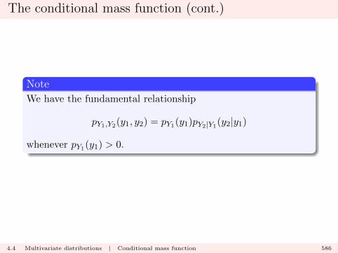
The conditional mass function (cont.)
Note
We have the fundamental relationship
pY1,Y2(y1, y2) = pY1(y1)pY2|Y1(y2|y1)
whenever pY1(y1) > 0.
4.4 Multivariate distributions | Conditional mass function 586
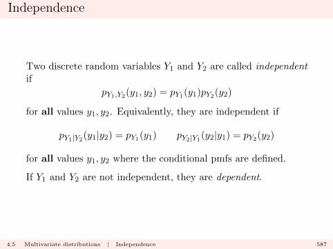
Independence
Two discrete random variables Y1 and Y2 are called independentif
pY1,Y2(y1, y2) = pY1(y1)pY2(y2)
for all values y1, y2. Equivalently, they are independent if
pY1|Y2(y1|y2) = pY1(y1) pY2|Y1
(y2|y1) = pY2(y2)
for all values y1, y2 where the conditional pmfs are defined.
If Y1 and Y2 are not independent, they are dependent.
4.5 Multivariate distributions | Independence 587

Independence (cont.)
This definition extends to multiple variables: Y1, . . . , Yn are in-dependent if
pY1,...,Yn(y1, . . . , yn) =
n∏i=1
pYi(yi)
for all vectors (y1, . . . , yn).
Note that we could make equivalent statements in terms of thejoint cdf
FY1,...,Yn(y1, . . . , yn) = P
(n⋂i=1
(Yi ≤ yi))
=
n∏i=1
FYi(yi)
4.5 Multivariate distributions | Independence 588

The joint density function
If Y1 and Y2 are two continuous random variables, then we canstill consider statements of the form
P ((Y1 ≤ y1) ∩ (Y2 ≤ y2))
and hence define the joint cumulative distribution function cdf
FY1,Y2(y1, y2) = P ((Y1 ≤ y1) ∩ (Y2 ≤ y2))
for any pair of real numbers (y1, y2).
4.6 Multivariate distributions | Continuous case: joint density function 589
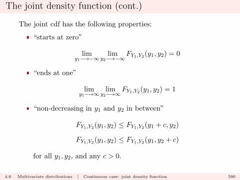
The joint density function (cont.)
The joint cdf has the following properties:
� “starts at zero”
limy1−→−∞
limy2−→−∞
FY1,Y2(y1, y2) = 0
� “ends at one”
limy1−→∞
limy2−→∞
FY1,Y2(y1, y2) = 1
� “non-decreasing in y1 and y2 in between”
FY1,Y2(y1, y2) ≤ FY1,Y2(y1 + c, y2)
FY1,Y2(y1, y2) ≤ FY1,Y2(y1, y2 + c)
for all y1, y2, and any c > 0.
4.6 Multivariate distributions | Continuous case: joint density function 590
The joint density function (cont.)
Furthermore, we have that
limy1−→∞
FY1,Y2(y1, y2) = P (Y1 <∞, Y2 ≤ y2)
= P (Y2 ≤ y2)
= FY2(y2)
and similarly
limy2−→∞
FY1,Y2(y1, y2) = FY1(y1).
4.6 Multivariate distributions | Continuous case: joint density function 591

The joint density function (cont.)
FY1,Y2(3, 5) = P (Y1 ≤ 3, Y2 ≤ 5)
−4 −2 2 4 6 8 10
−4
−2
2
4
6
8
10
y1
y2
4.6 Multivariate distributions | Continuous case: joint density function 592
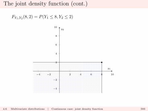
The joint density function (cont.)
FY1,Y2(8, 2) = P (Y1 ≤ 8, Y2 ≤ 2)
−4 −2 2 4 6 8 10
−4
−2
2
4
6
8
10
y1
y2
4.6 Multivariate distributions | Continuous case: joint density function 593
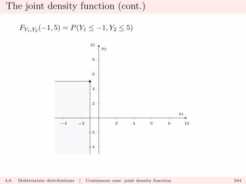
The joint density function (cont.)
FY1,Y2(−1, 5) = P (Y1 ≤ −1, Y2 ≤ 5)
−4 −2 2 4 6 8 10
−4
−2
2
4
6
8
10
y1
y2
4.6 Multivariate distributions | Continuous case: joint density function 594
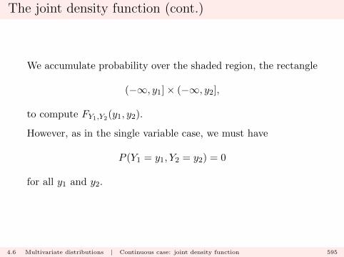
The joint density function (cont.)
We accumulate probability over the shaded region, the rectangle
(−∞, y1]× (−∞, y2],
to compute FY1,Y2(y1, y2).
However, as in the single variable case, we must have
P (Y1 = y1, Y2 = y2) = 0
for all y1 and y2.
4.6 Multivariate distributions | Continuous case: joint density function 595
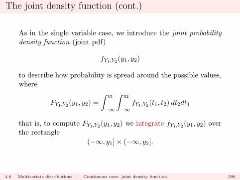
The joint density function (cont.)
As in the single variable case, we introduce the joint probabilitydensity function (joint pdf)
fY1,Y2(y1, y2)
to describe how probability is spread around the possible values,where
FY1,Y2(y1, y2) =
∫ y1
−∞
∫ y2
−∞fY1,Y2(t1, t2) dt2dt1
that is, to compute FY1,Y2(y1, y2) we integrate fY1,Y2(y1, y2) overthe rectangle
(−∞, y1]× (−∞, y2].
4.6 Multivariate distributions | Continuous case: joint density function 596

The joint density function (cont.)
We can compute the double integral as follows: writing∫ y1
−∞
{∫ y2
−∞fY1,Y2(t1, t2) dt2
}dt1
� fix t1, and perform the first (inner) integration∫ y2
−∞fY1,Y2(t1, t2) dt2
in the ‘strip’ at t1 to obtain a function g(t1, y2), say;
� perform the second (outer) integration∫ y1
−∞g(t1, y2) dt1.
to obtain the joint cdf.
4.6 Multivariate distributions | Continuous case: joint density function 597
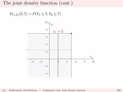
The joint density function (cont.)
FY1,Y2(5, 7) = P (Y1 ≤ 5, Y2 ≤ 7)
−4 −2 2 4 6 8 10
−4
−2
2
4
6
8
10
t1 = 2
t1
t2
4.6 Multivariate distributions | Continuous case: joint density function 598
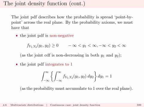
The joint density function (cont.)
The joint pdf describes how the probability is spread ‘point-by-point’ across the real plane. By the probability axioms, we musthave that
� the joint pdf is non-negative
fY1,Y2(y1, y2) ≥ 0 −∞ < y1 <∞,−∞ < y2 <∞
(as the joint cdf is non-decreasing in both y1 and y2);
� the joint pdf integrates to 1∫ ∞−∞
{∫ ∞−∞
fY1,Y2(y1, y2) dy2
}dy1 = 1
(as the probability must accumulate to 1 over the real plane).
4.6 Multivariate distributions | Continuous case: joint density function 599

The joint density function (cont.)
Example (Distribution on the unit square)
Suppose Y1 and Y2 are continuous with joint pdf
fY1,Y2(y1, y2) = c(y1 + y2) 0 ≤ y1 ≤ 1, 0 ≤ y2 ≤ 1
with fY1,Y2(y1, y2) = 0 otherwise.
4.6 Multivariate distributions | Continuous case: joint density function 600
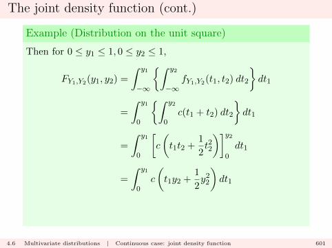
The joint density function (cont.)
Example (Distribution on the unit square)
Then for 0 ≤ y1 ≤ 1, 0 ≤ y2 ≤ 1,
FY1,Y2(y1, y2) =
∫ y1
−∞
{∫ y2
−∞fY1,Y2(t1, t2) dt2
}dt1
=
∫ y1
0
{∫ y2
0c(t1 + t2) dt2
}dt1
=
∫ y1
0
[c
(t1t2 +
1
2t22
)]y2
0
dt1
=
∫ y1
0c
(t1y2 +
1
2y22
)dt1
4.6 Multivariate distributions | Continuous case: joint density function 601

The joint density function (cont.)
Example (Distribution on the unit square)
FY1,Y2(y1, y2) =
[c
(1
2t21y2 +
1
2y22t1
)]y1
0
=c
2
(y21y2 + y1y
22
)We require that FY1,Y2(1, 1) = 1, so we must have c = 1.
4.6 Multivariate distributions | Continuous case: joint density function 602
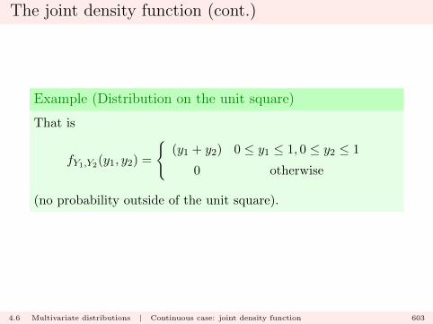
The joint density function (cont.)
Example (Distribution on the unit square)
That is
fY1,Y2(y1, y2) =
{(y1 + y2) 0 ≤ y1 ≤ 1, 0 ≤ y2 ≤ 1
0 otherwise
(no probability outside of the unit square).
4.6 Multivariate distributions | Continuous case: joint density function 603
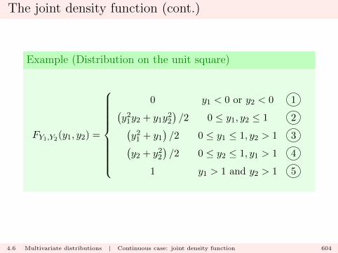
The joint density function (cont.)
Example (Distribution on the unit square)
FY1,Y2(y1, y2) =
0 y1 < 0 or y2 < 0 1(y21y2 + y1y
22
)/2 0 ≤ y1, y2 ≤ 1 2(
y21 + y1)/2 0 ≤ y1 ≤ 1, y2 > 1 3(
y2 + y22)/2 0 ≤ y2 ≤ 1, y1 > 1 4
1 y1 > 1 and y2 > 1 5
4.6 Multivariate distributions | Continuous case: joint density function 604
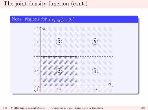
The joint density function (cont.)
Note: regions for FY1,Y2(y1, y2)
0.5 1 1.5 2
0.5
1
1.5
2
1
2
3
4
5
y1
y2
4.6 Multivariate distributions | Continuous case: joint density function 605

The joint density function (cont.)
Note
To compute FY1,Y2(y1, y2) we always integrate the joint pdf
below and to the left
of (y1, y2).
4.6 Multivariate distributions | Continuous case: joint density function 606

The joint density function (cont.)
00.2
0.40.6
0.81
0
0.2
0.4
0.6
0.8
1
0
0.5
1
1.5
2
y1
y2
fY1,Y
2(y
1,y2)
fY1,Y2(y1, y2) = (y1 + y2)
4.6 Multivariate distributions | Continuous case: joint density function 607
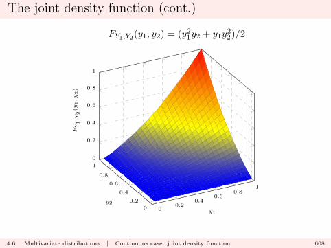
The joint density function (cont.)
00.2
0.40.6
0.81
0
0.2
0.4
0.6
0.8
1
0
0.2
0.4
0.6
0.8
1
y1
y2
FY1,Y
2(y
1,y2)
FY1,Y2(y1, y2) = (y21y2 + y1y22)/2
4.6 Multivariate distributions | Continuous case: joint density function 608
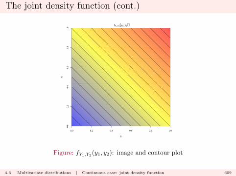
The joint density function (cont.)
0.0 0.2 0.4 0.6 0.8 1.0
0.0
0.2
0.4
0.6
0.8
1.0
y1
y 2
0.1
0.2
0.3
0.4
0.5
0.6
0.7
0.8
0.9
1
1.1
1.2
1.3 1.4
1.5
1.6 1.7
1.8
1.9
fY1,Y2(y1, y2)
Figure: fY1,Y2(y1, y2): image and contour plot
4.6 Multivariate distributions | Continuous case: joint density function 609
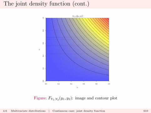
The joint density function (cont.)
0.0 0.2 0.4 0.6 0.8 1.0
0.0
0.2
0.4
0.6
0.8
1.0
y1
y 2
0.05
0.1
0.15
0.2
0.25
0.3
0.35
0.4
0.45
0.5
0.55
0.6
0.65
0.7
0.75
0.8
0.85
0.9
0.95
FY1,Y2(y1, y2)
Figure: FY1,Y2(y1, y2): image and contour plot
4.6 Multivariate distributions | Continuous case: joint density function 610

The joint density function (cont.)
0.0 0.2 0.4 0.6 0.8 1.0
0.0
0.2
0.4
0.6
0.8
1.0
y1
y 2
0.1
0.2 0.3
0.4
0.5 0.6
0.7
0.8
0.9
1
1.1
1.2
1.3
1.4
1.5
1.6
1.7
1.8
1.9
fY1,Y2(y1, y2)
Figure: fY1,Y2(y1, y2): contour plot
4.6 Multivariate distributions | Continuous case: joint density function 611
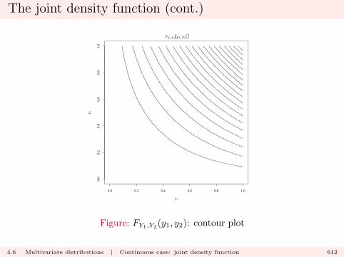
The joint density function (cont.)
0.0 0.2 0.4 0.6 0.8 1.0
0.0
0.2
0.4
0.6
0.8
1.0
y1
y 2
0.05
0.1
0.15
0.2
0.25
0.3
0.35
0.4
0.45
0.5
0.55
0.6
0.65
0.7
0.75
0.8
0.85
0.9
0.95
FY1,Y2(y1, y2)
Figure: FY1,Y2(y1, y2): contour plot
4.6 Multivariate distributions | Continuous case: joint density function 612
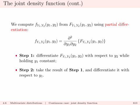
The joint density function (cont.)
We compute fY1,Y2(y1, y2) from FY1,Y2(y1, y2) using partial differ-entiation:
fY1,Y2(y1, y2) =∂2
∂y1∂y2{FY1,Y2(y1, y2)}
� Step 1: differentiate FY1,Y2(y1, y2) with respect to y2 whileholding y1 constant;
� Step 2: take the result of Step 1, and differentiate it withrespect to y1.
4.6 Multivariate distributions | Continuous case: joint density function 613

The joint density function (cont.)
We can regard the calculation as
fY1,Y2(y1, y2) =∂
∂y1
{∂FY1,Y2(y1, y2)
∂y2
}
4.6 Multivariate distributions | Continuous case: joint density function 614
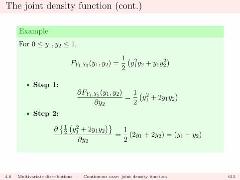
The joint density function (cont.)
Example
For 0 ≤ y1, y2 ≤ 1,
FY1,Y2(y1, y2) =1
2
(y21y2 + y1y
22
)� Step 1:
∂FY1,Y2(y1, y2)
∂y2=
1
2
(y21 + 2y1y2
)� Step 2:
∂{12
(y21 + 2y1y2
)}∂y2
=1
2(2y1 + 2y2) = (y1 + y2)
4.6 Multivariate distributions | Continuous case: joint density function 615

The joint density function (cont.)
Note
In the partial differentiation, we could choose to differentiatewith respect to y1 in Step 1, and then differentiate the resultwith respect to y2: we will get the same answer
∂2
∂y1∂y2{FY1,Y2(y1, y2)} =
∂2
∂y2∂y1{FY1,Y2(y1, y2)} .
This is a general property of partial derivatives that holdsprovided the result of each side is continuous.
4.6 Multivariate distributions | Continuous case: joint density function 616
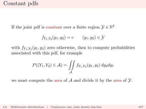
Constant pdfs
If the joint pdf is constant over a finite region Y ∈ R2
fY1,Y2(y1, y2) = c (y1, y2) ∈ Y
with fY1,Y2(y1, y2) zero otherwise, then to compute probabilitiesassociated with this pdf, for example
P ((Y1, Y2) ∈ A) =
∫∫A
fY1,Y2(y1, y2) dy2dy1
we must compute the area of A and divide it by the area of Y.
4.6 Multivariate distributions | Continuous case: joint density function 617
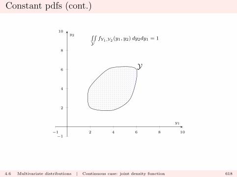
Constant pdfs (cont.)
−1 2 4 6 8 10−1
2
4
6
8
10 ∫∫YfY1,Y2
(y1, y2) dy2dy1 = 1
Y
y1
y2
4.6 Multivariate distributions | Continuous case: joint density function 618
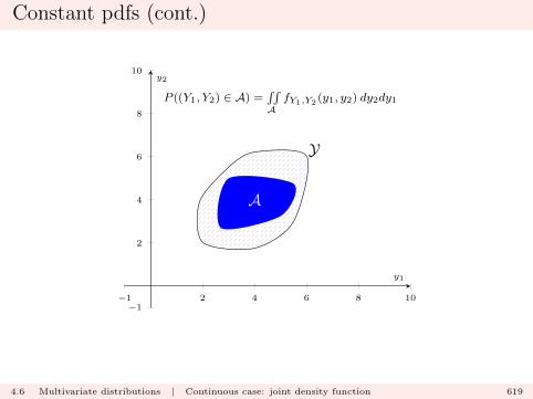
Constant pdfs (cont.)
−1 2 4 6 8 10−1
2
4
6
8
10
P ((Y1, Y2) ∈ A) =∫∫AfY1,Y2 (y1, y2) dy2dy1
Y
A
y1
y2
4.6 Multivariate distributions | Continuous case: joint density function 619
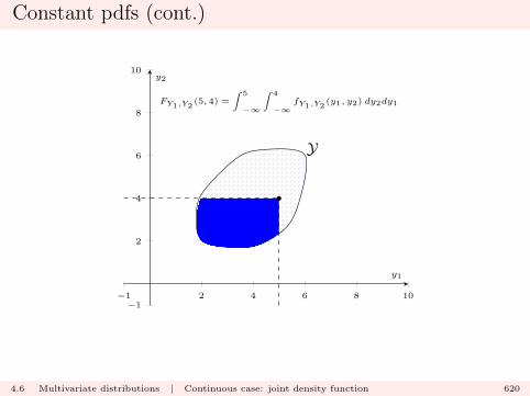
Constant pdfs (cont.)
−1 2 4 6 8 10−1
2
4
6
8
10
FY1,Y2(5, 4) =
∫ 5
−∞
∫ 4
−∞fY1,Y2
(y1, y2) dy2dy1
Y
y1
y2
4.6 Multivariate distributions | Continuous case: joint density function 620

Constant pdfs (cont.)
−1 2 4 6 8 10−1
2
4
6
8
10
FY1,Y2(3.2, 6.5) =
∫ 3.2
−∞
∫ 6.5
−∞fY1,Y2
(y1, y2) dy2dy1
Y
y1
y2
4.6 Multivariate distributions | Continuous case: joint density function 621
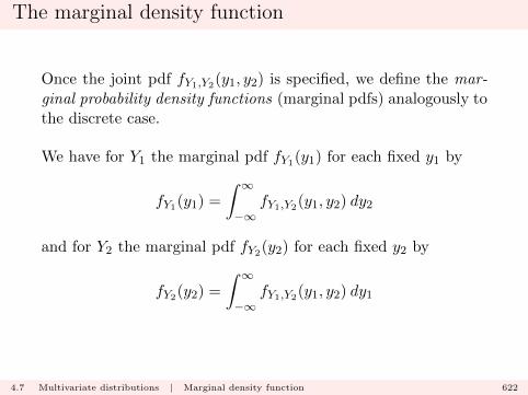
The marginal density function
Once the joint pdf fY1,Y2(y1, y2) is specified, we define the mar-ginal probability density functions (marginal pdfs) analogously tothe discrete case.
We have for Y1 the marginal pdf fY1(y1) for each fixed y1 by
fY1(y1) =
∫ ∞−∞
fY1,Y2(y1, y2) dy2
and for Y2 the marginal pdf fY2(y2) for each fixed y2 by
fY2(y2) =
∫ ∞−∞
fY1,Y2(y1, y2) dy1
4.7 Multivariate distributions | Marginal density function 622
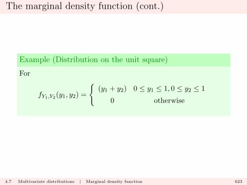
The marginal density function (cont.)
Example (Distribution on the unit square)
For
fY1,Y2(y1, y2) =
{(y1 + y2) 0 ≤ y1 ≤ 1, 0 ≤ y2 ≤ 1
0 otherwise
4.7 Multivariate distributions | Marginal density function 623

The marginal density function (cont.)
Example (Distribution on the unit square)
We have for 0 ≤ y1 ≤ 1
fY1(y1) =
∫ ∞−∞
fY1,Y2(y1, y2) dy2
=
∫ 1
0(y1 + y2) dy2
=
[y1y2 +
y222
]10
= y1 +1
2.
with fY1(y1) = 0 otherwise.
4.7 Multivariate distributions | Marginal density function 624
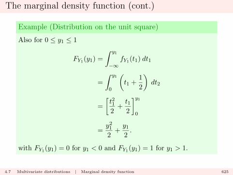
The marginal density function (cont.)
Example (Distribution on the unit square)
Also for 0 ≤ y1 ≤ 1
FY1(y1) =
∫ y1
−∞fY1(t1) dt1
=
∫ y1
0
(t1 +
1
2
)dt2
=
[t212
+t12
]y1
0
=y212
+y12.
with FY1(y1) = 0 for y1 < 0 and FY1(y1) = 1 for y1 > 1.
4.7 Multivariate distributions | Marginal density function 625
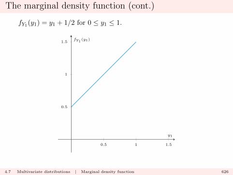
The marginal density function (cont.)
fY1(y1) = y1 + 1/2 for 0 ≤ y1 ≤ 1.
0.5 1 1.5
0.5
1
1.5
y1
fY1(y1)
4.7 Multivariate distributions | Marginal density function 626
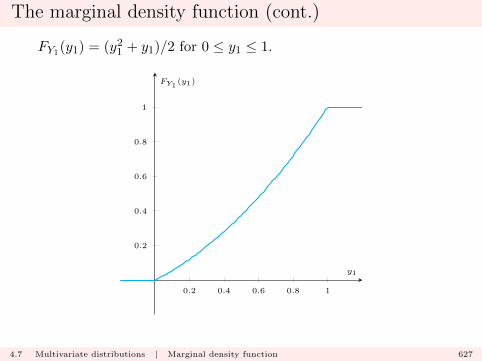
The marginal density function (cont.)
FY1(y1) = (y21 + y1)/2 for 0 ≤ y1 ≤ 1.
0.2 0.4 0.6 0.8 1
0.2
0.4
0.6
0.8
1
y1
FY1(y1)
4.7 Multivariate distributions | Marginal density function 627
The marginal density function (cont.)
Example (Distribution on the unit square)
We can perform a similar calculation and obtain
fY2(y2) = y2 +1
20 ≤ y2 ≤ 1
with fY2(y2) = 0 otherwise, and
FY2(y2) =(y22 + y2)
20 ≤ y2 ≤ 1
with FY2(y2) = 0 for y2 < 0 and FY2(y2) = 1 for y2 > 1.
4.7 Multivariate distributions | Marginal density function 628
The conditional density function
Once we have the joint pdf
fY1,Y2(y1, y2)
and the marginal pdf
fY1(y1)
we can consider conditional pdfs.
4.8 Multivariate distributions | Conditional density function 629
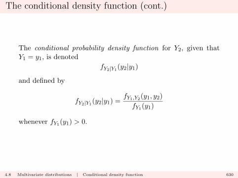
The conditional density function (cont.)
The conditional probability density function for Y2, given thatY1 = y1, is denoted
fY2|Y1(y2|y1)
and defined by
fY2|Y1(y2|y1) =
fY1,Y2(y1, y2)
fY1(y1)
whenever fY1(y1) > 0.
4.8 Multivariate distributions | Conditional density function 630
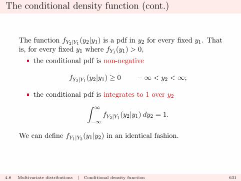
The conditional density function (cont.)
The function fY2|Y1(y2|y1) is a pdf in y2 for every fixed y1. That
is, for every fixed y1 where fY1(y1) > 0,
� the conditional pdf is non-negative
fY2|Y1(y2|y1) ≥ 0 −∞ < y2 <∞;
� the conditional pdf is integrates to 1 over y2∫ ∞−∞
fY2|Y1(y2|y1) dy2 = 1.
We can define fY1|Y2(y1|y2) in an identical fashion.
4.8 Multivariate distributions | Conditional density function 631
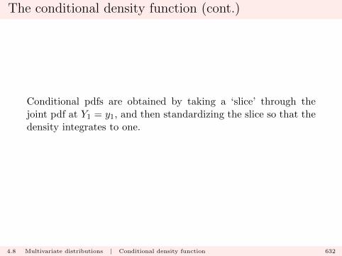
The conditional density function (cont.)
Conditional pdfs are obtained by taking a ‘slice’ through thejoint pdf at Y1 = y1, and then standardizing the slice so that thedensity integrates to one.
4.8 Multivariate distributions | Conditional density function 632

The conditional density function (cont.)
Example (Distribution on the unit square)
For
fY1,Y2(y1, y2) =
{(y1 + y2) 0 ≤ y1 ≤ 1, 0 ≤ y2 ≤ 1
0 otherwise
we can consider conditioning on values of y1 or y2 in theinterval [0, 1].
4.8 Multivariate distributions | Conditional density function 633
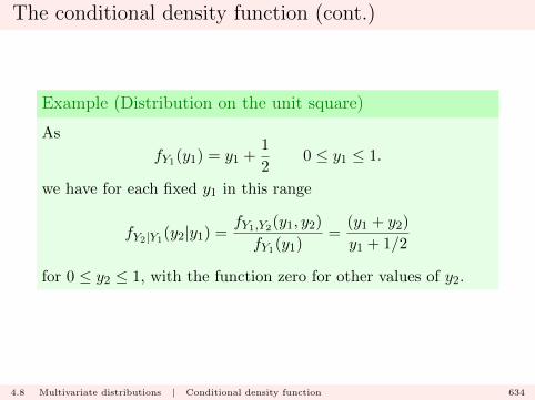
The conditional density function (cont.)
Example (Distribution on the unit square)
As
fY1(y1) = y1 +1
20 ≤ y1 ≤ 1.
we have for each fixed y1 in this range
fY2|Y1(y2|y1) =
fY1,Y2(y1, y2)
fY1(y1)=
(y1 + y2)
y1 + 1/2
for 0 ≤ y2 ≤ 1, with the function zero for other values of y2.
4.8 Multivariate distributions | Conditional density function 634

The conditional density function (cont.)
fY2|Y1(y2|y1) =
(y1 + y2)
y1 + 1/2for 0 ≤ y2 ≤ 1, with y1 = 0.2
0.5 1 1.5 2
0.5
1
1.5
2
y2
fY2|Y1(y2|0.2)
4.8 Multivariate distributions | Conditional density function 635
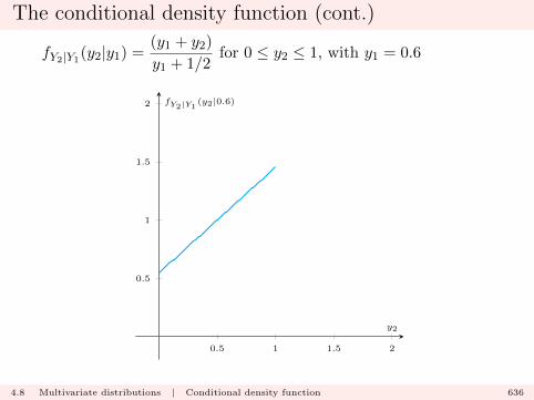
The conditional density function (cont.)
fY2|Y1(y2|y1) =
(y1 + y2)
y1 + 1/2for 0 ≤ y2 ≤ 1, with y1 = 0.6
0.5 1 1.5 2
0.5
1
1.5
2
y2
fY2|Y1(y2|0.6)
4.8 Multivariate distributions | Conditional density function 636
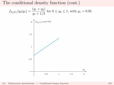
The conditional density function (cont.)
fY2|Y1(y2|y1) =
(y1 + y2)
y1 + 1/2for 0 ≤ y2 ≤ 1, with y1 = 0.95
0.5 1 1.5 2
0.5
1
1.5
2
y2
fY2|Y1(y2|0.95)
4.8 Multivariate distributions | Conditional density function 637

The conditional density function (cont.)
As in the discrete case, we have the chain rule factorization
fY1,Y2(y1, y2) = fY1(y1)fY2|Y1(y2|y1)
whenever fY1(y1) > 0.
As ever, we can exchange the roles of Y1 and Y2 to obtain that
fY1,Y2(y1, y2) = fY2(y2)fY1|Y2(y1|y2).
whenever fY1(y1) > 0.
4.8 Multivariate distributions | Conditional density function 638
Multivariate distributions
All of the above ideas extend naturally to more than two vari-ables. If (Y1, . . . , Yn) form an n-dimensional random vector, wecan consider the joint pdf
fY1,...,Yn(y1, . . . , yn)
and joint cdf
FY1,...,Yn(y1, . . . , yn).
4.9 Multivariate distributions | Multivariate distributions 639
Multivariate distributions (cont.)
We can consider marginalization by integrating out n− d < n ofthe dimensions to leave a d-dimensional probability distribution:for example if n = 4 and d = 2, we have
fY1,Y2(y1, y2) =
∫ ∞−∞
∫ ∞−∞
fY1,Y2,Y3,Y4(y1, y2, y3, y4) dy3dy4
or
fY2,Y4(y2, y4) =
∫ ∞−∞
∫ ∞−∞
fY1,Y2,Y3,Y4(y1, y2, y3, y4) dy1dy3
and so on. This construction works with any n and any d.
4.9 Multivariate distributions | Multivariate distributions 640

Independence
Continuous random variables (Y1, . . . , Yn) are independent if
fY1,...,Yn(y1, . . . , yn) =
n∏i=1
fYi(yi)
for all vectors (y1, . . . , yn) ∈ Rn. Equivalently they are independ-ent if
FY1,...,Yn(y1, . . . , yn) =
n∏i=1
FYi(yi)
for all vectors (y1, . . . , yn) ∈ Rn.
Random variables that are not independent are termed depend-ent.
4.10 Multivariate distributions | Independence 641
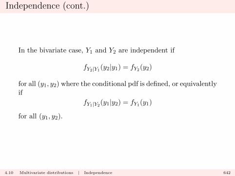
Independence (cont.)
In the bivariate case, Y1 and Y2 are independent if
fY2|Y1(y2|y1) = fY2(y2)
for all (y1, y2) where the conditional pdf is defined, or equivalentlyif
fY1|Y2(y1|y2) = fY1(y1)
for all (y1, y2).
4.10 Multivariate distributions | Independence 642
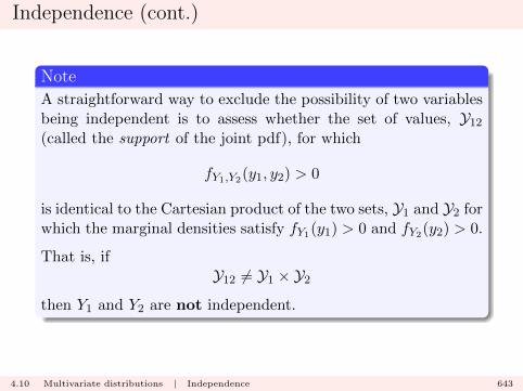
Independence (cont.)
Note
A straightforward way to exclude the possibility of two variablesbeing independent is to assess whether the set of values, Y12(called the support of the joint pdf), for which
fY1,Y2(y1, y2) > 0
is identical to the Cartesian product of the two sets, Y1 and Y2 forwhich the marginal densities satisfy fY1(y1) > 0 and fY2(y2) > 0.
That is, ifY12 6= Y1 × Y2
then Y1 and Y2 are not independent.
4.10 Multivariate distributions | Independence 643
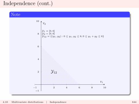
Independence (cont.)
Note
−1 2 4 6 8 10
−1
2
4
6
8
10
Y12
Y1 = [0, 6]Y2 = [0, 6]Y12 = {(y1, y2) : 0 ≤ y1, y2 ≤ 6, 0 ≤ y1 + y2 ≤ 6}
Y1
Y2
4.10 Multivariate distributions | Independence 644
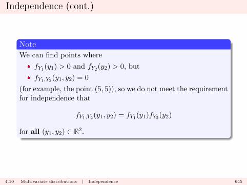
Independence (cont.)
Note
We can find points where
� fY1(y1) > 0 and fY2(y2) > 0, but
� fY1,Y2(y1, y2) = 0
(for example, the point (5, 5)), so we do not meet the requirementfor independence that
fY1,Y2(y1, y2) = fY1(y1)fY2(y2)
for all (y1, y2) ∈ R2.
4.10 Multivariate distributions | Independence 645
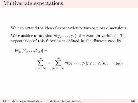
Multivariate expectations
We can extend the idea of expectation to two or more dimensions.
We consider a function g(y1, . . . , yn) of n random variables. Theexpectation of this function is defined in the discrete case by
E[g(Y1, . . ., Yn)] =
∞∑y1=−∞
· · ·∞∑
yn=−∞g(y1, . . . , yn)pY1,...,Yn(y1, . . . , yn).
4.11 Multivariate distributions | Multivariate expectations 646
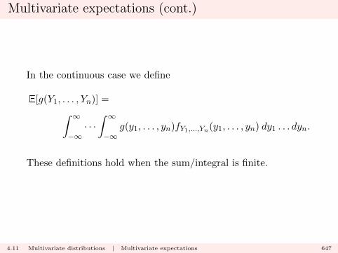
Multivariate expectations (cont.)
In the continuous case we define
E[g(Y1, . . . , Yn)] =∫ ∞−∞· · ·∫ ∞−∞
g(y1, . . . , yn)fY1,...,Yn(y1, . . . , yn) dy1 . . . dyn.
These definitions hold when the sum/integral is finite.
4.11 Multivariate distributions | Multivariate expectations 647
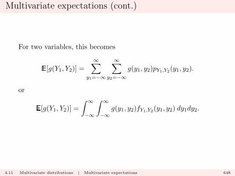
Multivariate expectations (cont.)
For two variables, this becomes
E[g(Y1, Y2)] =
∞∑y1=−∞
∞∑y2=−∞
g(y1, y2)pY1,Y2(y1, y2).
or
E[g(Y1, Y2)] =
∫ ∞−∞
∫ ∞−∞
g(y1, y2)fY1,Y2(y1, y2) dy1dy2.
4.11 Multivariate distributions | Multivariate expectations 648
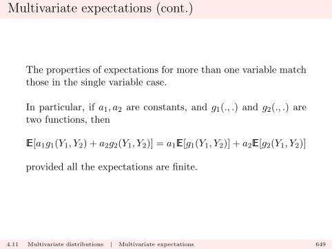
Multivariate expectations (cont.)
The properties of expectations for more than one variable matchthose in the single variable case.
In particular, if a1, a2 are constants, and g1(., .) and g2(., .) aretwo functions, then
E[a1g1(Y1, Y2) + a2g2(Y1, Y2)] = a1E[g1(Y1, Y2)] + a2E[g2(Y1, Y2)]
provided all the expectations are finite.
4.11 Multivariate distributions | Multivariate expectations 649
Covariance and correlation
For two random variables Y1 and Y2, with expectations µ1 andµ2 respectively, the covariance between Y1 and Y2, Cov[Y1, Y2],is defined by
Cov[Y1, Y2] = E[(Y1 − µ1)(Y2 − µ2)]
4.12 Multivariate distributions | Covariance and correlation 650
Covariance and correlation (cont.)
Note that
Cov[Y1, Y2] = E[(Y1 − µ1)(Y2 − µ2)]
= E[Y1Y2 − µ1Y2 − Y1µ2 + µ1µ2]
= E[Y1Y2]− µ1E[Y2]− µ2E[Y1] + µ1µ2
= E[Y1Y2]− µ1µ2 − µ2µ1 + µ1µ2
= E[Y1Y2]− µ1µ2.
4.12 Multivariate distributions | Covariance and correlation 651
Covariance and correlation (cont.)
The correlation between Y1 and Y2, Corr(Y1, Y2), is defined by
Corr[Y1, Y2] =Cov[Y1, Y2]√V[Y1]V[Y2]
4.12 Multivariate distributions | Covariance and correlation 652
Covariance and correlation (cont.)
Both covariance and correlation are measures of dependence. Wehave that for any pair of random variables,
−1 ≤ Corr[Y1, Y2] ≤ 1
4.12 Multivariate distributions | Covariance and correlation 653
Covariance and correlation (cont.)
If
Cov[Y1, Y2] = Corr[Y1, Y2] = 0
we say that Y1 and Y2 are uncorrelated.
4.12 Multivariate distributions | Covariance and correlation 654
Independent random variables
If Y1 and Y2 are independent then (in the continuous case – dis-crete case works in the same way), we have that
E[Y1Y2] =
∫ ∞−∞
∫ ∞−∞
y1y2fY1,Y2(y1, y2) dy1dy2
=
∫ ∞−∞
∫ ∞−∞
y1y2fY1(y1)fY2(y2) dy1dy2
=
∫ ∞−∞
y2fY2(y2)
{∫ ∞−∞
y1fY1(y1) dy1
}dy2
=
∫ ∞−∞
y2fY2(y2)E[Y1]dy2
= E[Y1]
∫ ∞−∞
y2fY2(y2)dy2 = E[Y1]E[Y2]
4.12 Multivariate distributions | Covariance and correlation 655
Independent random variables (cont.)
More generally, if g1(Y1) and g2(Y2) are two functions of theindependent random variables, then
E[g1(Y1)g2(Y2)] = E[g1(Y1)]E[g2(Y2)]
4.12 Multivariate distributions | Covariance and correlation 656
Independent random variables (cont.)
Therefore if two random variables Y1 and Y2 are independent,then
Cov[Y1, Y2] = E[Y1Y2]− µ1µ2= E[Y1]E[Y2]− µ1µ2= µ1µ2 − µ1µ2 = 0
and Y1 and Y2 are uncorrelated.
4.12 Multivariate distributions | Covariance and correlation 657

Linear combinations of random variables
Suppose that Y1, . . . , Yn and X1, . . . , Xm be random variableswith
E[Yi] = µi E[Xj ] = ξj .
Define
U1 =n∑i=1
aiYi U2 =
m∑j=1
bjXj
for real constants a1, . . . , an and b1, . . . , bm.
4.12 Multivariate distributions | Covariance and correlation 658
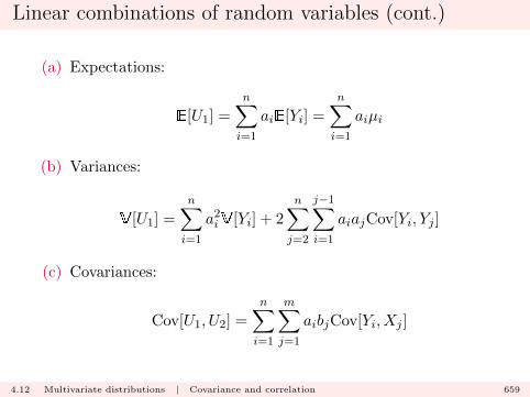
Linear combinations of random variables (cont.)
(a) Expectations:
E[U1] =
n∑i=1
aiE[Yi] =
n∑i=1
aiµi
(b) Variances:
V[U1] =
n∑i=1
a2iV[Yi] + 2
n∑j=2
j−1∑i=1
aiajCov[Yi, Yj ]
(c) Covariances:
Cov[U1, U2] =
n∑i=1
m∑j=1
aibjCov[Yi, Xj ]
4.12 Multivariate distributions | Covariance and correlation 659

Linear combinations of random variables (cont.)
For (b):
V[U1] = E[U21 ]− {E[U1]}2.
But
U21 =
(n∑i=1
aiYi
)2
=
n∑i=1
a2iY2i + 2
n∑j=2
j−1∑i=1
aiajYiYj
so therefore
E[U21 ] =
n∑i=1
a2iE[Y 2i ] + 2
n∑j=2
j−1∑i=1
aiajE[YiYj ]
4.12 Multivariate distributions | Covariance and correlation 660

Linear combinations of random variables (cont.)
Similarly
{E[U1]}2 =
{n∑i=1
aiµi
}2
=
n∑i=1
a2iµ2i + 2
n∑j=2
j−1∑i=1
aiajµiµj
Therefore
E[U21 ]− {E[U1]}2 =
n∑i=1
a2i (E[Y 2i ]− µ2i )
+ 2n∑j=2
j−1∑i=1
aiaj(E[YiYj ]− µiµj)
and the result follows.
4.12 Multivariate distributions | Covariance and correlation 661
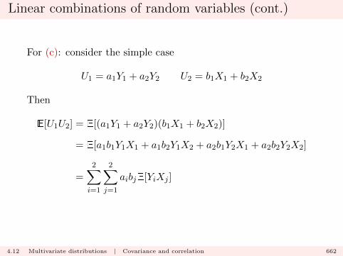
Linear combinations of random variables (cont.)
For (c): consider the simple case
U1 = a1Y1 + a2Y2 U2 = b1X1 + b2X2
Then
E[U1U2] = E[(a1Y1 + a2Y2)(b1X1 + b2X2)]
= E[a1b1Y1X1 + a1b2Y1X2 + a2b1Y2X1 + a2b2Y2X2]
=
2∑i=1
2∑j=1
aibjE[YiXj ]
4.12 Multivariate distributions | Covariance and correlation 662
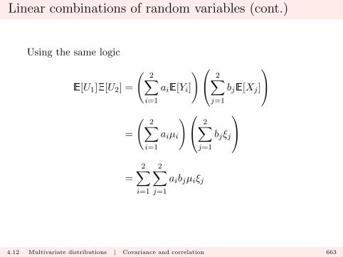
Linear combinations of random variables (cont.)
Using the same logic
E[U1]E[U2] =
(2∑i=1
aiE[Yi]
) 2∑j=1
bjE[Xj ]
=
(2∑i=1
aiµi
) 2∑j=1
bjξj
=
2∑i=1
2∑j=1
aibjµiξj
4.12 Multivariate distributions | Covariance and correlation 663

Linear combinations of random variables (cont.)
and therefore
E[U1U2]− E[U1]E[U2] =
2∑i=1
2∑j=1
aibj(E[YiXj ]− µiξj)
and the result follows.
4.12 Multivariate distributions | Covariance and correlation 664
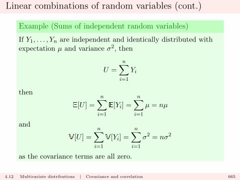
Linear combinations of random variables (cont.)
Example (Sums of independent random variables)
If Y1, . . . , Yn are independent and identically distributed withexpectation µ and variance σ2, then
U =
n∑i=1
Yi
then
E[U ] =
n∑i=1
E[Yi] =
n∑i=1
µ = nµ
and
V[U ] =
n∑i=1
V[Yi] =
n∑i=1
σ2 = nσ2
as the covariance terms are all zero.
4.12 Multivariate distributions | Covariance and correlation 665

Sums of random variables (revisited)
For two random variables Y1 and Y2 consider the distribution of
Y = Y1 + Y2
which we studied previously in the context using the convolutioncalculation in Chapter 3.
4.13 Multivariate distributions | Sums of random variables 666

Sums of random variables (revisited) (cont.)
We now see that the convolution formula can be viewed in thecontext of a joint distribution calculation:
FY (y) = P (Y ≤ y) = P (Y1+Y2 ≤ y) =
∫∫Ay
fY1,Y2(y1, y2)dy2dy1
where
Ay ={
(y1, y2) ∈ R2 : y1 + y2 ≤ y}.
4.13 Multivariate distributions | Sums of random variables 667
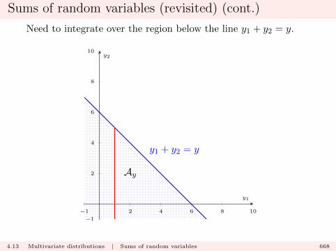
Sums of random variables (revisited) (cont.)
Need to integrate over the region below the line y1 + y2 = y.
−1 2 4 6 8 10
−1
2
4
6
8
10
Ay
y1 + y2 = y
y1
y2
4.13 Multivariate distributions | Sums of random variables 668

Sums of random variables (revisited) (cont.)
Therefore we can write
FY (y) =
∫ ∞−∞
∫ y−y1
−∞fY1,Y2(y1, y2) dy2dy1.
By differentiating with respect to y under the integral sign, usingthe Fundamental Theorem of Calculus, we see that
fY (y) =
∫ ∞−∞
fY1,Y2(y1, y − y1) dy1.
4.13 Multivariate distributions | Sums of random variables 669
Sums of random variables (revisited) (cont.)
We now consider an alternate method of calculation: recall thedefinition of the moment generating function:
mY (t) = E[etY]
for −b ≤ t ≤ b, some b > 0.
We can define a similar quantity for the random variable U whichis a transformation of Y , U = g(Y ) say, as
mU (t) = E[etU]≡ E
[etg(Y )
].
4.13 Multivariate distributions | Sums of random variables 670
Sums of random variables (revisited) (cont.)
For two random variables Y1 and Y2, with
Y = a1g1(Y1) + a2g2(Y2),
we have
mY (t) = E[etY]
= E
[et{a1g2(Y1)+a2g2(Y2)}
]This is the mgf for Y . We can write
mY (t) = E[etY]
= E
[eta1g1(Y1)eta2g2(Y2)
].
4.13 Multivariate distributions | Sums of random variables 671
Sums of random variables (revisited) (cont.)
If Y1 and Y2 are independent we can further write
mY (t) = E
[eta1g1(Y1)
]E
[eta2g2(Y2)
].
– this follows by the earlier result on expectations.
4.13 Multivariate distributions | Sums of random variables 672
Sums of random variables (revisited) (cont.)
Now consider the special case Y = Y1 + Y2:
mY (t) = E
[et{Y1+Y2}
].
It follows immediately that if Y1 and Y2 are independent,
mY (t) = E[etY1
]E[etY2
]= mY1(t)mY2(t).
This gives us a way to compute the distribution of sums of inde-pendent random variables.
4.13 Multivariate distributions | Sums of random variables 673
Sums of random variables (revisited) (cont.)
Example (Sum of Binomial random variables)
If Y1 and Y2 are independent Binomial random variables withparameters (n1, p) and (n2, p), we have
mY1(t) = (pet + q)n1 mY2(t) = (pet + q)n2
then if Y = Y1 + Y2, we have that
mY (t) = mY1(t)mY2(t) = (pet + q)n1(pet + q)n2 = (pet + q)n1+n2
and we recognize this as the mgf of the Binomial distributionwith parameters (n1 + n2, p).
4.13 Multivariate distributions | Sums of random variables 674
Sums of random variables (revisited) (cont.)
Example (Sum of Poisson random variables)
If Y1 and Y2 are independent Poisson random variables withparameters λ1 and λ2, we have
mY1(t) = exp{λ1(et − 1)} mY2(t) = exp{λ2(et − 1)}
then if Y = Y1 + Y2, we have that
mY (t) = mY1(t)mY2(t) = exp{λ1(et − 1)} exp{λ2(et − 1)}
= exp{(λ1 + λ2)(et − 1)}
and we recognize this as the mgf of the Poisson distributionwith parameter λ1 + λ2.
4.13 Multivariate distributions | Sums of random variables 675

Sums of random variables (revisited) (cont.)
Example (Sum of Normal random variables)
If Y1 and Y2 are independent Normal random variables withparameters (µ1, σ
21) and (µ2, σ
22), we have
mY1(t) = exp{µ1t+ σ21t2/2} mY2(t) = exp{µ2t+ σ22t
2/2}
then if Y = Y1 + Y2, we have that
mY (t) = mY1(t)mY2(t) = exp{µ1t+ σ21t2/2} exp{µ2t+ σ22t
2/2}
= exp{(µ1 + µ2)t+ (σ21 + σ22)t2/2}
and we recognize this as the mgf of the Normal distributionwith parameters (µ1 + µ2, σ
21 + σ22).
4.13 Multivariate distributions | Sums of random variables 676
Multivariate transformations
It is possible to consider general multivariate transformations ofvariables. For example if Y1 and Y2 are two variables with jointpdf fY1,Y2(y1, y2), we can consider
U1 = h1(Y1, Y2) U2 = h2(Y1, Y2)
and attempt to compute
fU1,U2(u1, u2).
4.14 Multivariate distributions | Multivariate transformations 677

Multivariate transformations (cont.)
For example, we might have
U1 = Y1 + Y2 U2 = Y1 − Y2
or
U1 = Y1Y2 U2 = Y1/Y2
etc.
4.14 Multivariate distributions | Multivariate transformations 678

Multivariate transformations (cont.)
We can approach this from a ‘change of variable’ perspective. Ifthe transformation
(Y1, Y2) −→ (U1, U2)
is a one-to-one transformation, then the inverse transformation
(U1, U2) −→ (Y1, Y2)
is well-defined. Suppose we write
Y1 = h−11 (U1, U2) Y2 = h−12 (U1, U2).
4.14 Multivariate distributions | Multivariate transformations 679

Multivariate transformations (cont.)
Then we may derive that for (u1, u2) ∈ R2,
fU1,U2(u1, u2) = fY1,Y2(h−11 (u1, u2), h−12 (u1, u2))|J(u1, u2)|
where J(u1, u2) is the Jacobian of the transformation, that is
J(u1, u2) = det
∂h−11 (u1, u2)
∂u1
∂h−11 (u1, u2)
∂u2
∂h−12 (u1, u2)
∂u1
∂h−12 (u1, u2)
∂u2
where det[.] denotes determinant, and |.| denotes absolute value.
4.14 Multivariate distributions | Multivariate transformations 680

Multivariate transformations (cont.)
This result holds provided that all the partial derivatives existand are continuous, and that
|J(u1, u2)| > 0.
The result extends beyond two dimensions.
4.14 Multivariate distributions | Multivariate transformations 681
Chapter 5: Probability inequalities and
theorems
Markov’s inequality
Suppose that g(Y ) is a function of continuous random variableY such that
E[|g(Y )|] <∞.
For any k > 0, let
Ak = {y ∈ R : |g(y)| ≥ k}.
5.1 Probability inequalities and theorems | Probability inequalities 683

Markov’s inequality (cont.)
Then
E[|g(Y )|] =
∫ ∞−∞|g(y)|fY (y) dy
=
∫Ak
|g(y)|fY (y) dy +
∫A′k|g(y)|fY (y) dy
≥∫Ak
|g(y)|fY (y) dy
≥∫Ak
kfY (y) dy
= k
∫Ak
fY (y) dy
= kP (|g(Y )| ≥ k)
5.1 Probability inequalities and theorems | Probability inequalities 684
Markov’s inequality (cont.)
Thus
E[|g(Y )|] ≥ kP (|g(Y )| ≥ k)
or equivalently
P (|g(Y )| ≥ k) ≤ E[|g(Y )|]k
.
5.1 Probability inequalities and theorems | Probability inequalities 685
Markov’s inequality (cont.)
Thus
1− P (|g(Y )| ≥ k) ≥ 1− E[|g(Y )|]k
or equivalently
P (|g(Y )| < k) ≥ 1− E[|g(Y )|]k
.
Note that the result is identical for a discrete random variable.
5.1 Probability inequalities and theorems | Probability inequalities 686

Chebychev’s inequality
aka
� Chebyshev’s inequality
� Bienayme-Chebyshev inequality
� Tchebysheff’s Theorem
� Chebysheff, Chebychov, Chebyshov, Tchebychev . . .
5.1 Probability inequalities and theorems | Probability inequalities 687

Chebychev’s inequality (cont.)
Suppose that Y has finite mean µ and variance σ2. In Markov’sinequality, consider the function
g(t) = (t− µ)2.
We have for any k > 0 that
P (|(Y − µ)2| < k) ≥ 1− E[|(Y − µ)2|]k
.
which can be more simply written as
P ((Y − µ)2 < k) ≥ 1− E[(Y − µ)2]
k.
5.1 Probability inequalities and theorems | Probability inequalities 688
Chebychev’s inequality (cont.)
But
E[(Y − µ)2] = σ2
and if we choose to write k = c2σ2, the inequality becomes
P ((Y − µ)2 < c2σ2) ≥ 1− E[(Y − µ)2]
c2σ2= 1− 1
c2
5.1 Probability inequalities and theorems | Probability inequalities 689

Chebychev’s inequality (cont.)
The left hand side of the inequality is equal to
P (√
(Y − µ)2 <√c2σ2) = P (|Y − µ| < cσ)
so the inequality becomes
P (|Y − µ| < cσ) ≥ 1− 1
c2.
5.1 Probability inequalities and theorems | Probability inequalities 690
Chebychev’s inequality (cont.)
An equivalent way to write this is
P (|Y − µ| ≥ cσ) ≤ 1
c2
which holds for arbitrary c > 0.
5.1 Probability inequalities and theorems | Probability inequalities 691

Chebychev’s inequality (cont.)
This states that for any distribution with finite mean µ andvariance σ2, we have that
P (µ− cσ < Y < µ+ cσ) ≥ 1− 1
c2
which bounds how much probability can be present in the tailsof the distribution.
5.1 Probability inequalities and theorems | Probability inequalities 692
The sample mean
Suppose that Y1, . . . , Yn are independent random variables thathave the same distribution, and have expectation µ and varianceσ2. Recall that if
U =
n∑i=1
Yi
then
E[U ] = nµ V[U ] = nσ2.
5.1 Probability inequalities and theorems | Probability inequalities 693

The sample mean (cont.)
Let
Y n =1
n
n∑i=1
Yi
be the sample mean random variable. Then
E[Y n] = E
[1
n
n∑i=1
Yi
]=
1
nE
[n∑i=1
Yi
]=
1
nnµ = µ
and
V[Y n] = V
[1
n
n∑i=1
Yi
]=
1
n2V
[n∑i=1
Yi
]=
1
n2nσ2 =
σ2
n.
5.1 Probability inequalities and theorems | Probability inequalities 694

The sample mean (cont.)
Now recall Chebychev’s inequality:
P (|Y − µ| ≥ cσ) ≤ 1
c2.
Applying this to Y n, we have that
P
(|Y n − µ| ≥
cσ√n
)≤ 1
c2.
5.1 Probability inequalities and theorems | Probability inequalities 695
The sample mean (cont.)
We can rewrite this for any n by setting
ε =cσ√n
so that c =
√nε
σ.
Then the inequality becomes
P (|Y n − µ| ≥ ε) ≤σ2
nε2.
5.1 Probability inequalities and theorems | Probability inequalities 696

Convergence in probability
Consider a sequence of random variables Y1, Y2, . . . , Yn, . . ., andreal constant c. We say that the sequence converges in probabilityto c as n −→∞ if, for every ε > 0,
limn−→∞
P (|Yn − c| < ε) = 1
that is, the probability
P (c− ε < Yn < c+ ε)
converges to 1 as n −→∞. We write
Ynp−→ c
as n −→∞ to indicate convergence in probability.
5.2 Probability inequalities and theorems | Definition of convergence in probability 697

Convergence in probability (cont.)
Note
� If, for a fixed ε > 0,
pn = P (|Yn − c| < ε)
the definition requires that the real sequence {pn} convergesto 1 in the usual sense.
� There is no restriction on the joint distribution of the Yis inthe sequence (that is, they can be dependent).
� We can equivalently write the condition
limn−→∞
P (|Yn − c| > ε) = 0.
5.2 Probability inequalities and theorems | Definition of convergence in probability 698
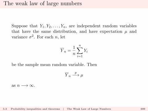
The weak law of large numbers
Suppose that Y1, Y2, . . . , Yn, are independent random variablesthat have the same distribution, and have expectation µ andvariance σ2. For each n, let
Y n =1
n
n∑i=1
Yi
be the sample mean random variable. Then
Y np−→ µ
as n −→∞.
5.3 Probability inequalities and theorems | The Weak Law of Large Numbers 699
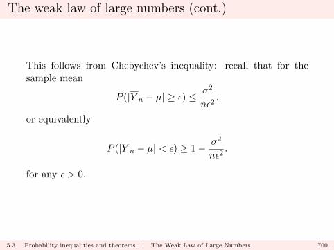
The weak law of large numbers (cont.)
This follows from Chebychev’s inequality: recall that for thesample mean
P (|Y n − µ| ≥ ε) ≤σ2
nε2.
or equivalently
P (|Y n − µ| < ε) ≥ 1− σ2
nε2.
for any ε > 0.
5.3 Probability inequalities and theorems | The Weak Law of Large Numbers 700
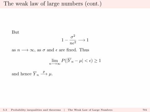
The weak law of large numbers (cont.)
But
1− σ2
nε2−→ 1
as n −→∞, as σ and ε are fixed. Thus
limn−→∞
P (|Y n − µ| < ε) ≥ 1
and hence Y np−→ µ.
5.3 Probability inequalities and theorems | The Weak Law of Large Numbers 701

The weak law of large numbers (cont.)
What this result means: under the stated conditions, thesample mean random variable converges to the expectation ofthe distribution of the Y s.
For example, if you repeatedly and independently toss a fair coin,the proportion of heads will converge to 1/2 as the number oftosses increases.
5.3 Probability inequalities and theorems | The Weak Law of Large Numbers 702
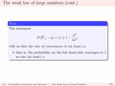
The weak law of large numbers (cont.)
Note
The statement
P (|Y n − µ| < ε) ≥ 1− σ2
nε2.
tells us that the rate of convergence is (at least) n;
� that is, the probability on the left hand side converges to 1at rate (at least) n.
5.3 Probability inequalities and theorems | The Weak Law of Large Numbers 703
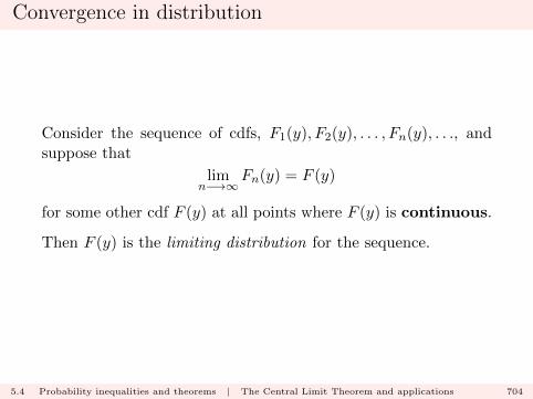
Convergence in distribution
Consider the sequence of cdfs, F1(y), F2(y), . . . , Fn(y), . . ., andsuppose that
limn−→∞
Fn(y) = F (y)
for some other cdf F (y) at all points where F (y) is continuous.
Then F (y) is the limiting distribution for the sequence.
5.4 Probability inequalities and theorems | The Central Limit Theorem and applications 704
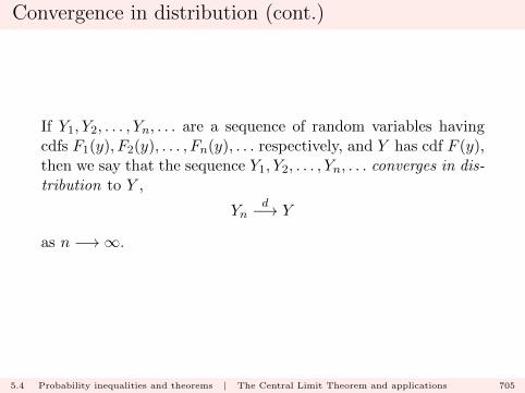
Convergence in distribution (cont.)
If Y1, Y2, . . . , Yn, . . . are a sequence of random variables havingcdfs F1(y), F2(y), . . . , Fn(y), . . . respectively, and Y has cdf F (y),then we say that the sequence Y1, Y2, . . . , Yn, . . . converges in dis-tribution to Y ,
Ynd−→ Y
as n −→∞.
5.4 Probability inequalities and theorems | The Central Limit Theorem and applications 705

The central limit theorem
Suppose that Y1, Y2, . . . , Yn, are independent random variablesthat have the same distribution, and have finite expectation µand variance σ2. For each n, let
Y n =1
n
n∑i=1
Yi
be the sample mean random variable.
5.4 Probability inequalities and theorems | The Central Limit Theorem and applications 706
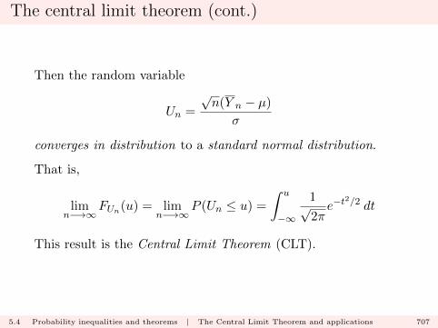
The central limit theorem (cont.)
Then the random variable
Un =
√n(Y n − µ)
σ
converges in distribution to a standard normal distribution.
That is,
limn−→∞
FUn(u) = limn−→∞
P (Un ≤ u) =
∫ u
−∞
1√2πe−t
2/2 dt
This result is the Central Limit Theorem (CLT).
5.4 Probability inequalities and theorems | The Central Limit Theorem and applications 707
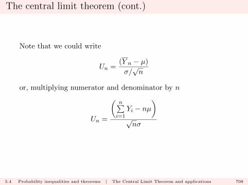
The central limit theorem (cont.)
Note that we could write
Un =(Y n − µ)
σ/√n
or, multiplying numerator and denominator by n
Un =
(n∑i=1
Yi − nµ)
√nσ
5.4 Probability inequalities and theorems | The Central Limit Theorem and applications 708
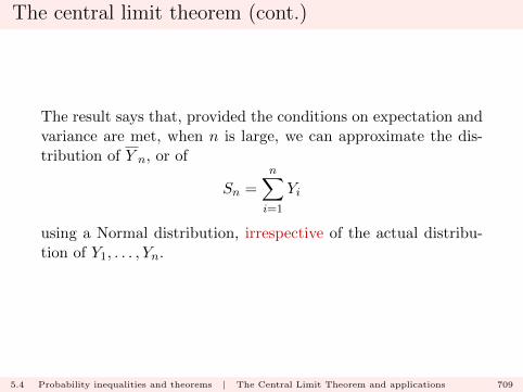
The central limit theorem (cont.)
The result says that, provided the conditions on expectation andvariance are met, when n is large, we can approximate the dis-tribution of Y n, or of
Sn =
n∑i=1
Yi
using a Normal distribution, irrespective of the actual distribu-tion of Y1, . . . , Yn.
5.4 Probability inequalities and theorems | The Central Limit Theorem and applications 709
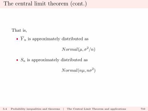
The central limit theorem (cont.)
That is,
� Y n is approximately distributed as
Normal(µ, σ2/n)
� Sn is approximately distributed as
Normal(nµ, nσ2)
5.4 Probability inequalities and theorems | The Central Limit Theorem and applications 710
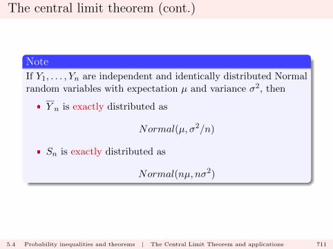
The central limit theorem (cont.)
Note
If Y1, . . . , Yn are independent and identically distributed Normalrandom variables with expectation µ and variance σ2, then
� Y n is exactly distributed as
Normal(µ, σ2/n)
� Sn is exactly distributed as
Normal(nµ, nσ2)
5.4 Probability inequalities and theorems | The Central Limit Theorem and applications 711
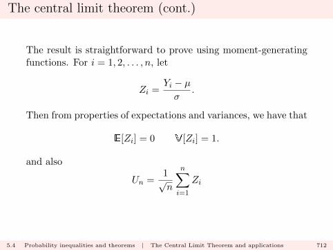
The central limit theorem (cont.)
The result is straightforward to prove using moment-generatingfunctions. For i = 1, 2, . . . , n, let
Zi =Yi − µσ
.
Then from properties of expectations and variances, we have that
E[Zi] = 0 V[Zi] = 1.
and also
Un =1√n
n∑i=1
Zi
5.4 Probability inequalities and theorems | The Central Limit Theorem and applications 712
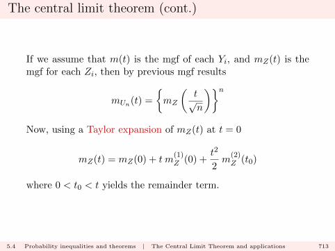
The central limit theorem (cont.)
If we assume that m(t) is the mgf of each Yi, and mZ(t) is themgf for each Zi, then by previous mgf results
mUn(t) =
{mZ
(t√n
)}nNow, using a Taylor expansion of mZ(t) at t = 0
mZ(t) = mZ(0) + t m(1)Z (0) +
t2
2m
(2)Z (t0)
where 0 < t0 < t yields the remainder term.
5.4 Probability inequalities and theorems | The Central Limit Theorem and applications 713

The central limit theorem (cont.)
Now as E[Zi] = 0, and V[Zi] = 1 we can deduce that
mZ(0) = 1 m(1)Z (0) = E[Zi] = 0
and hence
mZ(t) = 1 +t2
2m
(2)Z (t0).
5.4 Probability inequalities and theorems | The Central Limit Theorem and applications 714

The central limit theorem (cont.)
Therefore
mUn(t) =
{1 +
t2
2nm
(2)Z (t0)
}n0 < t0 <
t√n
Now, as n −→∞t√n−→ 0
so t0 −→ 0.
5.4 Probability inequalities and theorems | The Central Limit Theorem and applications 715
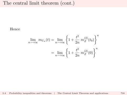
The central limit theorem (cont.)
Hence
limn−→∞
mUn(t) = limn−→∞
{1 +
t2
2nm
(2)Z (t0)
}n= lim
n−→∞
{1 +
t2
2nm
(2)Z (0)
}n
5.4 Probability inequalities and theorems | The Central Limit Theorem and applications 716

The central limit theorem (cont.)
But m(2)Z (0) = E[Z2
i ] = 1, so therefore
limn−→∞
mUn(t) = limn−→∞
{1 +
t2
2n
}n= et
2/2
by definition of the exponential function. Hence the limiting mgfis that of a standard Normal distribution, and so
Und−→ Z
where Z has a standard Normal distribution.
5.4 Probability inequalities and theorems | The Central Limit Theorem and applications 717
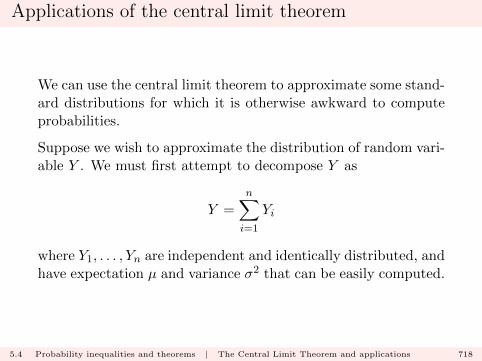
Applications of the central limit theorem
We can use the central limit theorem to approximate some stand-ard distributions for which it is otherwise awkward to computeprobabilities.
Suppose we wish to approximate the distribution of random vari-able Y . We must first attempt to decompose Y as
Y =
n∑i=1
Yi
where Y1, . . . , Yn are independent and identically distributed, andhave expectation µ and variance σ2 that can be easily computed.
5.4 Probability inequalities and theorems | The Central Limit Theorem and applications 718
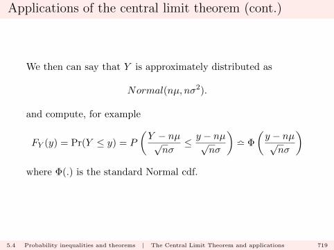
Applications of the central limit theorem (cont.)
We then can say that Y is approximately distributed as
Normal(nµ, nσ2).
and compute, for example
FY (y) = Pr(Y ≤ y) = P
(Y − nµ√
nσ≤ y − nµ√
nσ
)l Φ
(y − nµ√nσ
)where Φ(.) is the standard Normal cdf.
5.4 Probability inequalities and theorems | The Central Limit Theorem and applications 719

Applications of the central limit theorem (cont.)
Example (Binomial case)
If Y ∼ Binomial(n, p), the mgf of Y takes the form
mY (t) = (pet + q)n
By the uniqueness of mgfs, we recognize that Y has therepresentation
Y =
n∑i=1
Yi
where Yi ∼ Binomial(1, p) ≡ Bernoulli(p) are independent. Wehave
E[Yi] = p V[Yi] = pq.
5.4 Probability inequalities and theorems | The Central Limit Theorem and applications 720
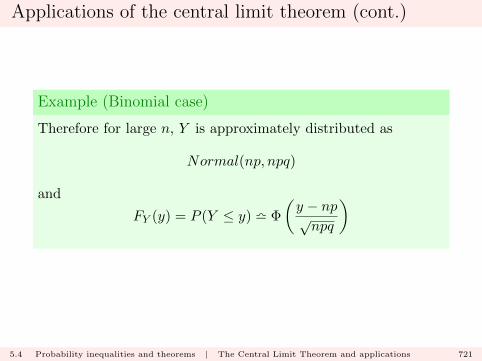
Applications of the central limit theorem (cont.)
Example (Binomial case)
Therefore for large n, Y is approximately distributed as
Normal(np, npq)
and
FY (y) = P (Y ≤ y) l Φ
(y − np√npq
)
5.4 Probability inequalities and theorems | The Central Limit Theorem and applications 721

Applications of the central limit theorem (cont.)
Binomial: n = 100, with p = 0.6.
● ● ● ● ● ● ● ● ● ● ● ● ● ● ● ● ● ● ● ● ● ● ● ● ● ● ● ● ● ● ● ● ● ● ● ● ● ● ● ● ● ● ● ● ● ●●
●
●
●
●
●
●
●
●
●
●
●
●
●
●
●
●
●
●
●
●
●
●
●
●
●
●
●●
● ● ● ● ● ● ● ● ● ● ● ● ● ● ● ● ● ● ● ● ● ● ● ● ● ●
0 20 40 60 80 100
0.00
0.02
0.04
0.06
0.08
y
f(y)
Binomial(100,0.6)Normal(60,24)
5.4 Probability inequalities and theorems | The Central Limit Theorem and applications 722
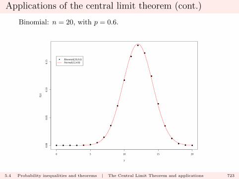
Applications of the central limit theorem (cont.)
Binomial: n = 20, with p = 0.6.
● ● ● ● ●●
●
●
●
●
●
●
●
●
●
●
●
●
●
● ●
0 5 10 15 20
0.00
0.05
0.10
0.15
y
f(y)
Binomial(20,0.6)Normal(12,4.8)
5.4 Probability inequalities and theorems | The Central Limit Theorem and applications 723
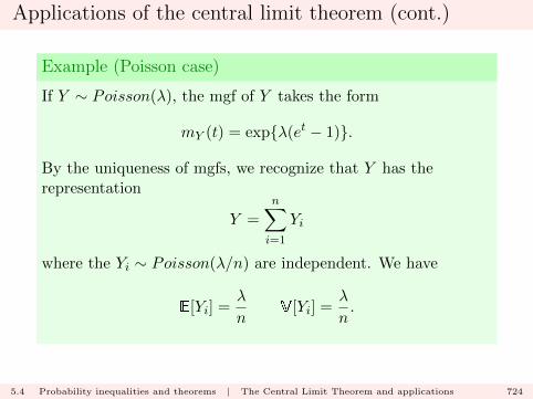
Applications of the central limit theorem (cont.)
Example (Poisson case)
If Y ∼ Poisson(λ), the mgf of Y takes the form
mY (t) = exp{λ(et − 1)}.
By the uniqueness of mgfs, we recognize that Y has therepresentation
Y =
n∑i=1
Yi
where the Yi ∼ Poisson(λ/n) are independent. We have
E[Yi] =λ
nV[Yi] =
λ
n.
5.4 Probability inequalities and theorems | The Central Limit Theorem and applications 724
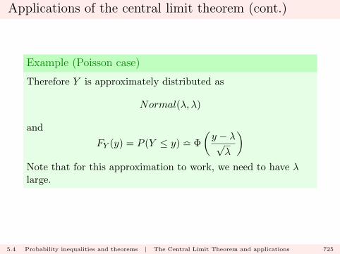
Applications of the central limit theorem (cont.)
Example (Poisson case)
Therefore Y is approximately distributed as
Normal(λ, λ)
and
FY (y) = P (Y ≤ y) l Φ
(y − λ√λ
)Note that for this approximation to work, we need to have λlarge.
5.4 Probability inequalities and theorems | The Central Limit Theorem and applications 725
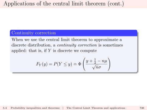
Applications of the central limit theorem (cont.)
Continuity correction
When we use the central limit theorem to approximate adiscrete distribution, a continuity correction is sometimesapplied: that is, if Y is discrete we compute
FY (y) = P (Y ≤ y) l Φ
(y + 1
2 − nµ√nσ
)
5.4 Probability inequalities and theorems | The Central Limit Theorem and applications 726

Applications of the central limit theorem (cont.)
Example (Gamma case)
If Y ∼ Gamma(α, β), the mgf of Y takes the form
mY (t) =
(1
1− βt
)αBy the uniqueness of mgfs, we recognize that Y has therepresentation
Y =
n∑i=1
Yi
where the Yi ∼ Gamma(α/n, β) are independent. We have
E[Yi] =αβ
nV[Yi] =
αβ2
n.
5.4 Probability inequalities and theorems | The Central Limit Theorem and applications 727

Applications of the central limit theorem (cont.)
Example (Gamma case)
Therefore Y is approximately distributed as
Normal(αβ, αβ2)
and
FY (y) = P (Y ≤ y) l Φ
(y − αβ√αβ2
)Note that for this approximation to work, we need to have αlarge.
5.4 Probability inequalities and theorems | The Central Limit Theorem and applications 728
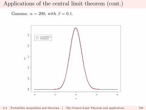
Applications of the central limit theorem (cont.)
Gamma: α = 200, with β = 0.1.
10 15 20 25 30
0.00
0.05
0.10
0.15
0.20
0.25
yv
f(y)
Gamma(200,0.1)Normal(20,2)
5.4 Probability inequalities and theorems | The Central Limit Theorem and applications 729
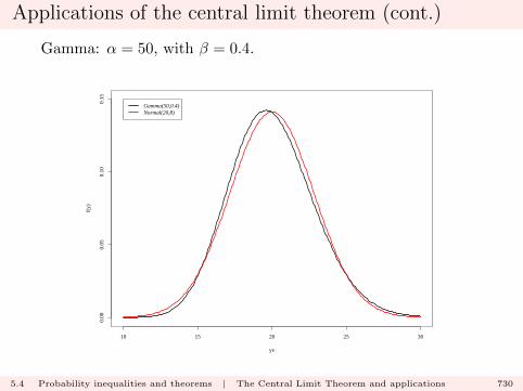
Applications of the central limit theorem (cont.)
Gamma: α = 50, with β = 0.4.
10 15 20 25 30
0.00
0.05
0.10
0.15
yv
f(y)
Gamma(50,0.4)Normal(20,8)
5.4 Probability inequalities and theorems | The Central Limit Theorem and applications 730