Math 375: Lecture notes

Professor Monika Nitsche

September 21, 2011

Contents

1 MATLAB Basics 8

1.1 Example: Plotting a function . . . . . . . . . . . . . . . . . . . . . . . . . . 8

1.2 Scripts . . . . . . . . . . . . . . . . . . . . . . . . . . . . . . . . . . . . . . . 9

1.3 Setting up vectors . . . . . . . . . . . . . . . . . . . . . . . . . . . . . . . . . 10

1.4 Vector and Matrix operations . . . . . . . . . . . . . . . . . . . . . . . . . . 11

1.5 Plotting . . . . . . . . . . . . . . . . . . . . . . . . . . . . . . . . . . . . . . 14

1.6 Printing data . . . . . . . . . . . . . . . . . . . . . . . . . . . . . . . . . . . 15

1.7 For loops . . . . . . . . . . . . . . . . . . . . . . . . . . . . . . . . . . . . . . 15

1.8 While loops . . . . . . . . . . . . . . . . . . . . . . . . . . . . . . . . . . . . 16

1.9 Timing code . . . . . . . . . . . . . . . . . . . . . . . . . . . . . . . . . . . . 17

1.10 Functions . . . . . . . . . . . . . . . . . . . . . . . . . . . . . . . . . . . . . 17

2 Computing Fundamentals 20

2.1 Vectorizing, timing, operation counts, memory allocation . . . . . . . . . . . 20

2.1.1 Vectorizing for legibility and speed . . . . . . . . . . . . . . . . . . . 20

1

2.1.2 Memory allocation . . . . . . . . . . . . . . . . . . . . . . . . . . . . 21

2.1.3 Counting operations: Horner’s algorithm . . . . . . . . . . . . . . . . 21

2.1.4 Counting operations: evaluating series . . . . . . . . . . . . . . . . . 22

2.2 Machine Representation of real numbers, Roundoff errors . . . . . . . . . . . 23

2.2.1 Decimal and binary representation of reals . . . . . . . . . . . . . . . 23

2.2.2 Floating point representation of reals . . . . . . . . . . . . . . . . . . 24

2.2.3 Machine precision, IEEE rounding, roundoff error . . . . . . . . . . . 25

2.2.4 Loss of significant digits during subtraction . . . . . . . . . . . . . . . 27

2.3 Approximating derivatives, Taylor’s Theorem, plotting y = hp . . . . . . . . 29

2.4 Big-O Notation . . . . . . . . . . . . . . . . . . . . . . . . . . . . . . . . . . 30

3 Solving nonlinear equations f(x) = 0 31

3.1 Bisection method to solve f(x) = 0 (§1.1) . . . . . . . . . . . . . . . . . . . . 32

3.2 Fixed point iteration to solve x = g(x) (FPI, §1.2) . . . . . . . . . . . . . . . 34

3.2.1 Examples . . . . . . . . . . . . . . . . . . . . . . . . . . . . . . . . . 34

3.2.2 The FPI . . . . . . . . . . . . . . . . . . . . . . . . . . . . . . . . . . 34

3.2.3 Implementing FPI in Matlab . . . . . . . . . . . . . . . . . . . . . . . 35

3.2.4 Theoretical Results . . . . . . . . . . . . . . . . . . . . . . . . . . . . 35

3.2.5 Definitions . . . . . . . . . . . . . . . . . . . . . . . . . . . . . . . . . 37

3.2.6 Stopping criterion . . . . . . . . . . . . . . . . . . . . . . . . . . . . . 37

3.3 Newton’s method to solve f(x) = 0 (§1.4) . . . . . . . . . . . . . . . . . . . 38

3.3.1 The algorithm . . . . . . . . . . . . . . . . . . . . . . . . . . . . . . . 38

3.3.2 Matlab implementation . . . . . . . . . . . . . . . . . . . . . . . . . . 38

2

3.3.3 Theoretical results . . . . . . . . . . . . . . . . . . . . . . . . . . . . 39

3.4 Secant method (§1.5) . . . . . . . . . . . . . . . . . . . . . . . . . . . . . . . 39

3.5 How things can go wrong. Conditioning. (§1.3) . . . . . . . . . . . . . . . . 39

3.5.1 Multiple roots . . . . . . . . . . . . . . . . . . . . . . . . . . . . . . . 39

3.5.2 Forward and Backward error. Error magnification. . . . . . . . . . . 40

3.5.3 Other examples of ill-conditioned problems . . . . . . . . . . . . . . . 41

3.5.4 The condition number . . . . . . . . . . . . . . . . . . . . . . . . . . 41

4 Solving linear systems 43

4.1 Gauss Elimination (§2.1) . . . . . . . . . . . . . . . . . . . . . . . . . . . . . 43

4.2 LU decomposition (§2.2) . . . . . . . . . . . . . . . . . . . . . . . . . . . . . 44

4.3 Partial Pivoting (§2.3, §2.4) . . . . . . . . . . . . . . . . . . . . . . . . . . . 45

4.4 Conditioning of linear systems (§2.3) . . . . . . . . . . . . . . . . . . . . . . 46

4.5 Iterative methods (§2.5) . . . . . . . . . . . . . . . . . . . . . . . . . . . . . 48

5 Interpolation 51

5.1 Polynomial Interpolants . . . . . . . . . . . . . . . . . . . . . . . . . . . . . 51

5.1.1 Vandermonde approach . . . . . . . . . . . . . . . . . . . . . . . . . . 52

5.1.2 Lagrange interpolants . . . . . . . . . . . . . . . . . . . . . . . . . . . 53

5.1.3 Newton’s divided differences . . . . . . . . . . . . . . . . . . . . . . . 54

5.2 Accuracy of Polynomial interpolation . . . . . . . . . . . . . . . . . . . . . . 55

5.2.1 Uniform points vs Tschebischeff points . . . . . . . . . . . . . . . . . 56

5.3 Piecewise Polynomial interpolants . . . . . . . . . . . . . . . . . . . . . . . . 58

5.3.1 Piecewise linear interpolant . . . . . . . . . . . . . . . . . . . . . . . 58

3

5.3.2 Cubic splines . . . . . . . . . . . . . . . . . . . . . . . . . . . . . . . 58

5.4 Trigonometric interpolants . . . . . . . . . . . . . . . . . . . . . . . . . . . . 62

5.4.1 Using a basis of sines and cosines . . . . . . . . . . . . . . . . . . . . 62

5.4.2 Using a basis of complex exponentials . . . . . . . . . . . . . . . . . . 62

5.4.3 Using MATLABs fft and ifft . . . . . . . . . . . . . . . . . . . . . 64

5.4.4 What if period τ 6= 2π? . . . . . . . . . . . . . . . . . . . . . . . . . . 69

5.4.5 Music and Compression . . . . . . . . . . . . . . . . . . . . . . . . . 69

6 Least Squares Solutions to Ax = b 71

6.1 Least squares solution to Ax = b . . . . . . . . . . . . . . . . . . . . . . . . 71

6.2 Approximating data by model functions . . . . . . . . . . . . . . . . . . . . 74

6.2.1 Linear least squares approximation . . . . . . . . . . . . . . . . . . . 74

6.2.2 Quadratic least squares approximation . . . . . . . . . . . . . . . . . 74

6.2.3 Approximating data by an exponential function . . . . . . . . . . . . 75

6.2.4 Approximating data by an algebraic function . . . . . . . . . . . . . . 75

6.2.5 Periodic approximations . . . . . . . . . . . . . . . . . . . . . . . . . 76

6.3 QR Factorization . . . . . . . . . . . . . . . . . . . . . . . . . . . . . . . . . 76

7 Numerical Integration (Quadrature) 77

7.1 Newton-Cotes Rules . . . . . . . . . . . . . . . . . . . . . . . . . . . . . . . 77

7.2 Composite Newton-Cotes Rules . . . . . . . . . . . . . . . . . . . . . . . . . 77

7.3 More on Trapezoid Rule . . . . . . . . . . . . . . . . . . . . . . . . . . . . . 78

7.4 Gauss Quadrature . . . . . . . . . . . . . . . . . . . . . . . . . . . . . . . . . 79

4

8 Numerical Methods for ODEs 80

8.1 Problem statement . . . . . . . . . . . . . . . . . . . . . . . . . . . . . . . . 80

8.2 Euler’s Method . . . . . . . . . . . . . . . . . . . . . . . . . . . . . . . . . . 81

8.3 Second order Method obtained by Richardson Extrapolation . . . . . . . . . 84

8.4 Second order Method obtained using Taylor Series . . . . . . . . . . . . . . . 85

8.5 4th order Runge Kutta Method . . . . . . . . . . . . . . . . . . . . . . . . . 86

5

Syllabus for Fall 2010

1. MATLAB (see Tutorial on web)Lecture 1 (Mon Aug 23) : Vectors, plotting, matrix operations.Lecture 2 (Wed Aug 25) : Scripts, label plots, printing tables/figs. If, for, while statements.Lecture 3 (Fri Aug 27) : Functions. Timing code. Vectorizing. Memory.

2. COMPUTING FUNDAMENTALSLecture 4 (Mon Aug 30) : What affects execution time? Vectorizing, initializing,

operation counts. Examples: Horners algorithm, Taylor series. Big-O notation. (§0.1)Lecture 5 (Wed Sep 1) : Binary numbers. Floating point representation. (§0.2-0.3)Lecture 6 (Fri Sep 3) : Loss of significance. (§0.4)

3. NONLINEAR EQUATIONSLecture 7 (Wed Sep 8) : Bisection method, §1.1Lecture 8 (Fri Sep 10) : Fixed point iteration, §1.2Lecture 9 (Mon Sep 13): Fixed point iteration, §1.2Lecture 10 (Wed Sep 15): Ill-conditioned problems, §1.3. Newton’s Method, §1.4Lecture 11 (Fri Sep 17) : Newton’s Method, §1.4. Secant Method. §1.5

4. SOLVING LINEAR SYSTEMSLecture 12 (Mon Sep 20): Gauss Elimination, §2.1Lecture 13 (Wed Sep 22): LU Decompo, §2.2Lecture 14 (Fri Sep 24) : EXAM 1Lecture 15 (Mon Sep 27): PLU Decomposition, §2.4Lecture 16 (Wed Sep 29): Conditioning, §2.3Lecture 17 (Fri Sep 31) : Iterative methods: Example and convergence criteria, §2.5Lecture 18 (Mon Oct 4): Iterative methods: JacobiLecture 19 (Wed Oct 6): Iterative methods: Gauss-Seidel

5. INTERPOLATIONLecture 20 (Fri Oct 8) : Polynomial interpolation. Example.Lecture 21 (Mon Oct 11): Polynomial interpolation. Lagrange approach.Lecture 22 (Wed Oct 13): Polynomial interpolation. Vandermonde approach.FALL BREAKLecture 23 (Mon Oct 18): Polynomial interpolation. Newton approach.Lecture 24 (Wed Oct 20): Polynomial interpolation. Interpolation error.Lecture 25 (Fri Oct 22) : Polynomial interpolation. Runge phenomena, Chebishev points.Lecture 26 (Mon Oct 25): Spline: linear splines, cubic splines, derivation. §3.4.Lecture 27 (Wed Oct 27): Cubic spline: derivation, MATLAB codes. §3.4.Lecture 28 (Fri Oct 29) : Cubic spline: MATLAB codes, examples. §3.4.

6

6. TRIG INTERPOLANTS AND FOURIER TRANSFORMLecture 29 (Mon Nov 1): Trig interpolation: fourier coefficients, examples.Lecture 30 (Wed Nov 3): Trig interpolation: Derive DFT, IDFT. Examples. §10.2Lecture 31 (Fri Nov 5) : Trig interpolation: Fourier coefficients and smoothness of functions.

7. LEAST SQUARESLecture 32 (Mon Nov 8): Least Squares: normal equations. §4.1Lecture 33 (Wed Nov 10): Approximating data using models. §4.2Lecture 34 (Fri Nov 12) : QR decomposition. §4.3

8. NUMERICAL INTEGRATIONLecture 35 (Mon Nov 15): Numerical Integration: Newton-Cotes. §5.2Lecture 36 (Wed Nov 17): Numerical Integration: Composite N-C. §5.3Lecture 37 (Fri Nov 19) : REVIEWLecture 38 (Mon Nov 22): EXAM 2Lecture 39 (Wed Nov 24): Numerical Integration: Mac-Laurin Formula for Trapezoid rule error. Review.THANKSGIVING BREAKLecture 40 (Mon Nov 29): Numerical Integration: Gauss Quadrature. §5.2

9. NUMERICAL DIFFERENTIATIONLecture 41 (Wed Dec 1) : Numerical Differentiation. Truncation and Roundoff. §5.1

10. ORDINARY DIFFERENTIAL EQUATIONSLecture 42 (Fri Dec 1) : Euler’s Method. MATLAB Algorithm. S 6.1Lecture 43 (Mon Dec 3) : Local and global truncation errors. §6.2Lecture 44 (Wed Dec 5) : Euler’s Method for systems. §6.3Lecture 45 (Fri Dec 7) : RK Methods. §6.4

7

1 MATLAB Basics

1.1 Example: Plotting a function

Starting MATLAB:Windows: search for MATLAB icon or link and clickLinux: % ssh linux.unm.edu

% matlab

or% matlab -nojvm

Sample MATLAB code illustrating several Matlab features; code to plot the graph of y =sin(2πx), x ∈ [0, 1]: What is really going on when you use software to graph a function?

1. The function is sampled at a set of points xk to obtain yk = f(xk).

2. The points (xk, yk) are then plotted together with some interpolant of the data (piece-wise linear or a smoother curve such as splines of Bezier curves).

In MATLAB you specify xk, then compute yk. The command plot(x,y) outputs a piecewiselinear interpolant of the data.

% Set up gridpoints x(k)

x=[0.0, 0.1,0.2,0.3,0.4...

0.5,0.6,0.7,0.8,0.9,1.0];

% Set up function values y(k)

n=length(x);

y=zeros(1,n);

for k=1:n

y(k)=sin(2*pi*x(k)); %pi is predefined

end

% plot a piecewise linear interpolant to the points (x(k),y(k))

plot(x,y)

Notes:

(1) The % sign denotes the begining of a comment. Code is well commented!

(2) The continuation symbol is ...

(3) The semicolon prevents displaying intermediate results (try it, what happens if you omitit?)

8

(4) length,zeros,sin,plot are built in MATLAB functions. Later on we will write ourown functions.

(5) In Matlab variables are defined when they are used. Reason for y=zeros(1,n): allocateamount of memory for variable y; initialize. How much memory space is allocated to y ifthat line is absent, as you step through the loop? Why is zeros not used before defining x?

(6) In Matlab all variables are matrices. Column vectors are nx1, row vectors are 1xn, scalarsare 1x1 matrices. What is output of size(x)?

(7) All vectors/matrices are indexed starting with 1. What is x(1), x(2), x(10), x(0)?

(8) Square brackets are used to define vectors. Round brackets are used to access entries invectors.

(9) Note syntax of for loop.

(10) What is the output of

plot(x,y,’*’)

plot(x,y,’*-’)

plot(x,y,’*-r’)

See Tutorial for further plotting options, or help plot. Lets create a second vector z =cos(2πx) and plot both y vs x in red dashed curve with circle markers, and z in green solidcurve with crosses as markers. Then use default. But first:

1.2 Scripts

MATLAB Script m-file: A file (appended with .m) stored in a directory containing MATLABcode. From now on I will write all code in scripts so I can easily modify it. To write abovecode in script:

make a folder with your name

if appropriate, make a folder in that folder for current howework/topic

in MATLAB, go to box next to "current directory" and find directory

click on "File/New/M-file", edit, name, save

or click on existing file to edit

execute script by typing its name in MATLAB command window

lets write a script containing above code

9

Save your work on Floppy or USBport, or ftp to other machine. No guarantees that yourfolders will be saved.

Now I’d like to modify this code and use more points to obtain a better plot by changingthe line defining x, using spacing of 1/100 instead of 1/10. But how to set up x with 101entries??

1.3 Setting up vectors

Row Vectors

• Explicit list

x=[0 1 2 3 4 5];

x=[0,1,2,3,4,5];

• Using a:increment:b. To set up a vector from x=a to x=b in increments of size h youcan use

x=a:h:b;

Here you specify beginning and endpoints, and stepsize. Most natural to me. However,if (b-a) is not an integer multiple of stepsize, endpoint will be omitted. Note, if homitted, default stepsize =1. What is?

x=0:0.1:1;

x=0:5;

We already used this notation in the for loop!

• Using linspace

x=linspace(a,b,n);

Use linspace to set up x=[0 1 2 3 4], x=[0,0.1,0.2,...,1], x=[0,0.5,1,1.5,2],

x=a:h:b

• Using for loops

Column Vectors

• Explicit list

x=[0;1;2;3;4;5];

10

• Transpose row vector

x=[0:.1:1]’;

Matrices

A=[1 1 1; 2 0 -1; 3 -1 2; 0 1 -1];

A=zeros(1,4); B=zeros(5,2); C=eye(3); D=ones(2,4); %special matrices

How to access entry in second row, first column? What is A(1,1), A(2,0)?

Now we have a better way to define x using h = 1/100! Do it.

Try x-y where x row, y column!!

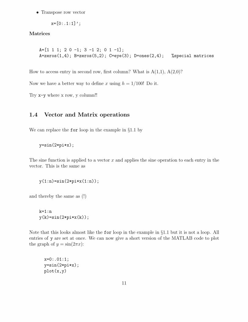
1.4 Vector and Matrix operations

We can replace the for loop in the example in §1.1 by

y=sin(2*pi*x);

The sine function is applied to a vector x and applies the sine operation to each entry in thevector. This is the same as

y(1:n)=sin(2*pi*x(1:n));

and thereby the same as (!)

k=1:n

y(k)=sin(2*pi*x(k));

Note that this looks almost like the for loop in the example in §1.1 but it is not a loop. Allentries of y are set at once. We can now give a short version of the MATLAB code to plotthe graph of y = sin(2πx):

x=0:.01:1;

y=sin(2*pi*x);

plot(x,y)

11

Since vectors are special cases of matrices, the above operation can also be applied to ma-trices. The statement B=sin(A) applies the sine function to every entry in A.

Setting up matrices. Before further addressing matrix operations, I want to mentionanother possibility to set up matrices. First note that the line A=[1 1 1; 2 0 -1; 3 -1

2; 0 1 -1]; in §1.3 can be written as

A=[1 1 1

2 0 -1

3 -1 2

0 1 -1

];

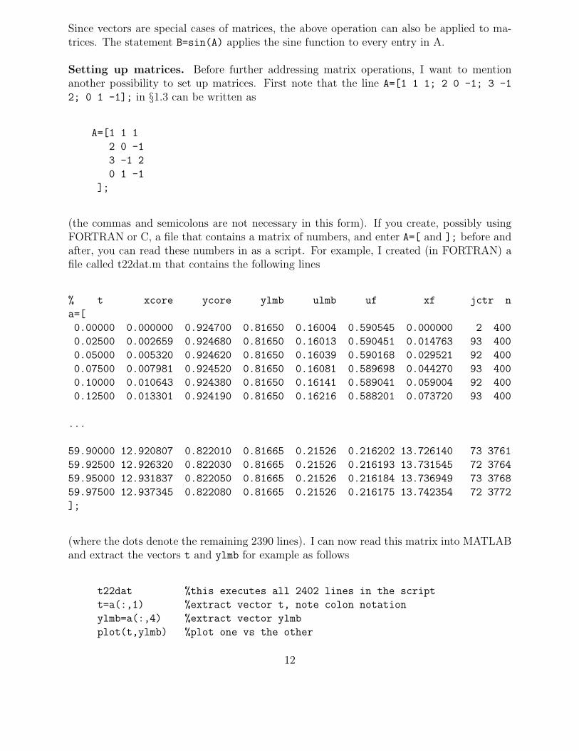
(the commas and semicolons are not necessary in this form). If you create, possibly usingFORTRAN or C, a file that contains a matrix of numbers, and enter A=[ and ]; before andafter, you can read these numbers in as a script. For example, I created (in FORTRAN) afile called t22dat.m that contains the following lines

% t xcore ycore ylmb ulmb uf xf jctr n

a=[

0.00000 0.000000 0.924700 0.81650 0.16004 0.590545 0.000000 2 400

0.02500 0.002659 0.924680 0.81650 0.16013 0.590451 0.014763 93 400

0.05000 0.005320 0.924620 0.81650 0.16039 0.590168 0.029521 92 400

0.07500 0.007981 0.924520 0.81650 0.16081 0.589698 0.044270 93 400

0.10000 0.010643 0.924380 0.81650 0.16141 0.589041 0.059004 92 400

0.12500 0.013301 0.924190 0.81650 0.16216 0.588201 0.073720 93 400

...

59.90000 12.920807 0.822010 0.81665 0.21526 0.216202 13.726140 73 3761

59.92500 12.926320 0.822030 0.81665 0.21526 0.216193 13.731545 72 3764

59.95000 12.931837 0.822050 0.81665 0.21526 0.216184 13.736949 73 3768

59.97500 12.937345 0.822080 0.81665 0.21526 0.216175 13.742354 72 3772

];

(where the dots denote the remaining 2390 lines). I can now read this matrix into MATLABand extract the vectors t and ylmb for example as follows

t22dat %this executes all 2402 lines in the script

t=a(:,1) %extract vector t, note colon notation

ylmb=a(:,4) %extract vector ylmb

plot(t,ylmb) %plot one vs the other

12

Note: entries of vectors are accessed using round brackets. Vectors are defined using squarebrackets.

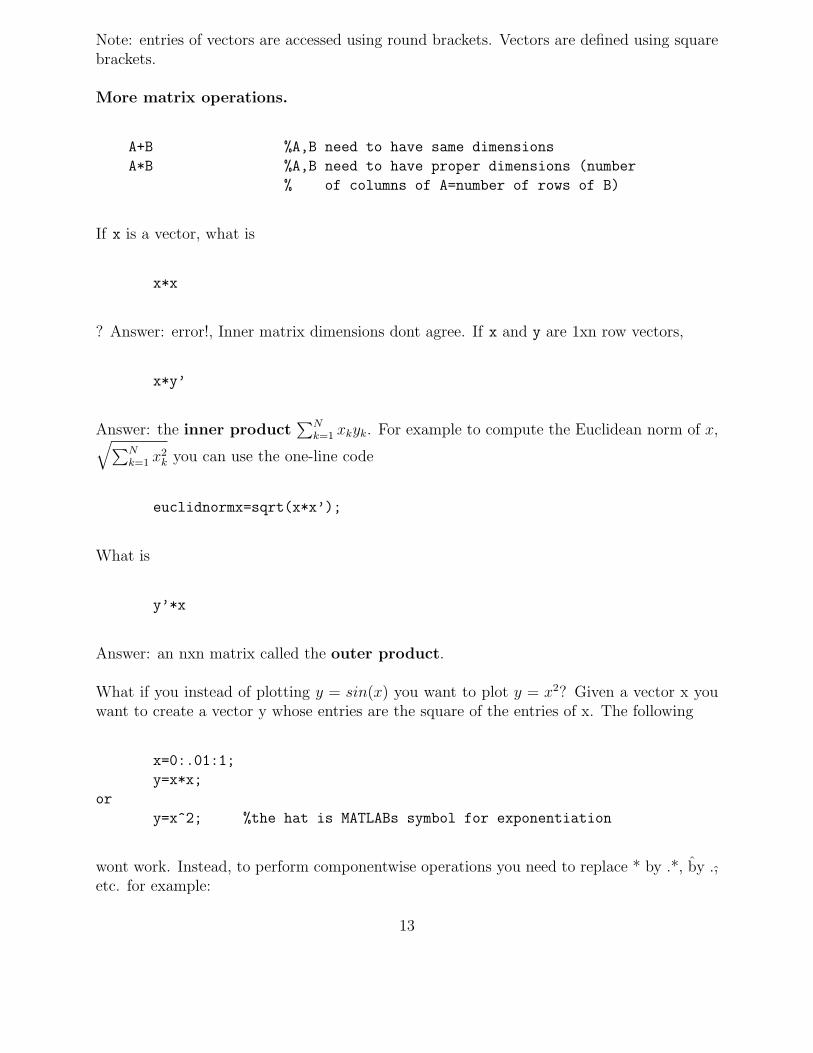
More matrix operations.

A+B %A,B need to have same dimensions

A*B %A,B need to have proper dimensions (number

% of columns of A=number of rows of B)

If x is a vector, what is

x*x

? Answer: error!, Inner matrix dimensions dont agree. If x and y are 1xn row vectors,

x*y’

Answer: the inner product∑N

k=1 xkyk. For example to compute the Euclidean norm of x,√∑Nk=1 x2

k you can use the one-line code

euclidnormx=sqrt(x*x’);

What is

y’*x

Answer: an nxn matrix called the outer product.

What if you instead of plotting y = sin(x) you want to plot y = x2? Given a vector x youwant to create a vector y whose entries are the square of the entries of x. The following

x=0:.01:1;

y=x*x;

or

y=x^2; %the hat is MATLABs symbol for exponentiation

wont work. Instead, to perform componentwise operations you need to replace * by .*, by .,etc. for example:

13

y=x.^2;

y=A.^2;

y=1./x;

y=x.*z; %where x,z are vectors/matrices of same length

Another useful built in MATLAB function is

s=sum(x);

Use the help command to figure out what it does.

1.5 Plotting

Labelling plots. In class we used:

plot(x,y,’r:x’) %options for color/line type/marker type

xlabel(’this is xlabel’)

ylabel(’this is ylabel \alpha \pi’) %using greek alphabet

title(’this is title’)

text(0.1,0.3,’some text’) %places text at given coordinates

text(0.1,0.3,’some text’,’FontSize’,20) %optional override fontsize

set(gca,’FontSize’,20) %override default fontsize

axis([0,1,-2,2]) %sets axis

axis square %square window

axis equal %units on x- and y-axis have same length

figure(2) %creates new figure or accesses existing figure(2)

Plotting several functions on one plot. Suppose we created x=0:.1:1; y1=sin(x);

y2=cos(x);. Two options. First one:

plot(x,y1,x,y2) %using default colors/lines/markers

plot(x,y1,’b--0’,x,y2,’r-’) %customizing

legend(’sin(x)’,’cos(x)’,3) %nice way to label, what does entry ’3’ do?

Second one: using hold command:

plot(x,y1)

hold on

plot(x,y2)

hold off

14

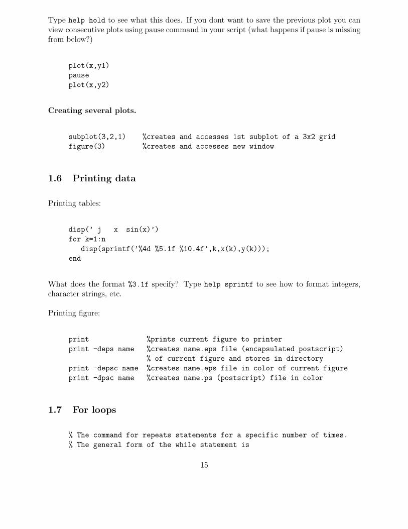
Type help hold to see what this does. If you dont want to save the previous plot you canview consecutive plots using pause command in your script (what happens if pause is missingfrom below?)

plot(x,y1)

pause

plot(x,y2)

Creating several plots.

subplot(3,2,1) %creates and accesses 1st subplot of a 3x2 grid

figure(3) %creates and accesses new window

1.6 Printing data

Printing tables:

disp(’ j x sin(x)’)

for k=1:n

disp(sprintf(’%4d %5.1f %10.4f’,k,x(k),y(k)));

end

What does the format %3.1f specify? Type help sprintf to see how to format integers,character strings, etc.

Printing figure:

print %prints current figure to printer

print -deps name %creates name.eps file (encapsulated postscript)

% of current figure and stores in directory

print -depsc name %creates name.eps file in color of current figure

print -dpsc name %creates name.ps (postscript) file in color

1.7 For loops

% The command for repeats statements for a specific number of times.

% The general form of the while statement is

15

FOR variable=expr

statements

END

% expr is often of the form i0:j0 or i0:l:j0.

% Negative steps l are allowed.

% Example : What does this code do?

n = 10;

for i=1:n

for j=1:n

a(i,j) = 1/(i+j-1);

end

end

1.8 While loops

% The command while repeats statements an indefinite number of times,

% as long as a given expression is true.

% The general form of the while statement is

WHILE expression

statement

END

% Example 1: What does this code do?

x = 4;

y = 1;

n = 1;

while n<= 10;

y = y + x^n/factorial(n);

n = n+1;

end

% Remember to initialize $n$ and update its value in the loop!

16

1.9 Timing code

tic % starts stopwatch

statements

toc % reads stopwatch

Exercise: Compare the following runtimes. What do you deduce?

tic; clear, for j=1:10000, x(j)=sin(j); end, toc

tic; clear, j=1:10000; x(j)=sin(j); toc

tic; for j=1:10000, x(j)=sin(j); end, toc

Exercise: Compare the following runtimes. What do you deduce?

clear

tic; for j=1:10000, sin(1.e8); end, toc

format long, pi2=2*pi; 1.e8/pi2

clear, alf = 1.e8-1.5915494e7;

tic; for j=1:10000, sin(alf); end, toc

clear

tic; for j=1:10000, sin(0.1); end, toc

1.10 Functions

MATLAB Functions are similar to functions in Fortran or C. They enable us to write thecode more efficiently, and in a more readable manner.

The code for a MATLAB function must be placed in a separate .m file having the same nameas the function. The general structure for the function is

function <Output parameters>=<Name of Function><Input Parameters>

% Comments that completely specify the function

<function body>

When writing a function, the following rules must be followed:

17

• Somewhere in the function body the desired value must be assigned to the outputvariable!

• Comments that completely specify the function should be given immediately after thefunction statement. The specification should describe the output and detail all inputvalue assumptions.

• The lead block of comments after the function statement is displayed when the func-tion is probed using help.

• All variables inside the function are local and are not part of the MATLAB workspace

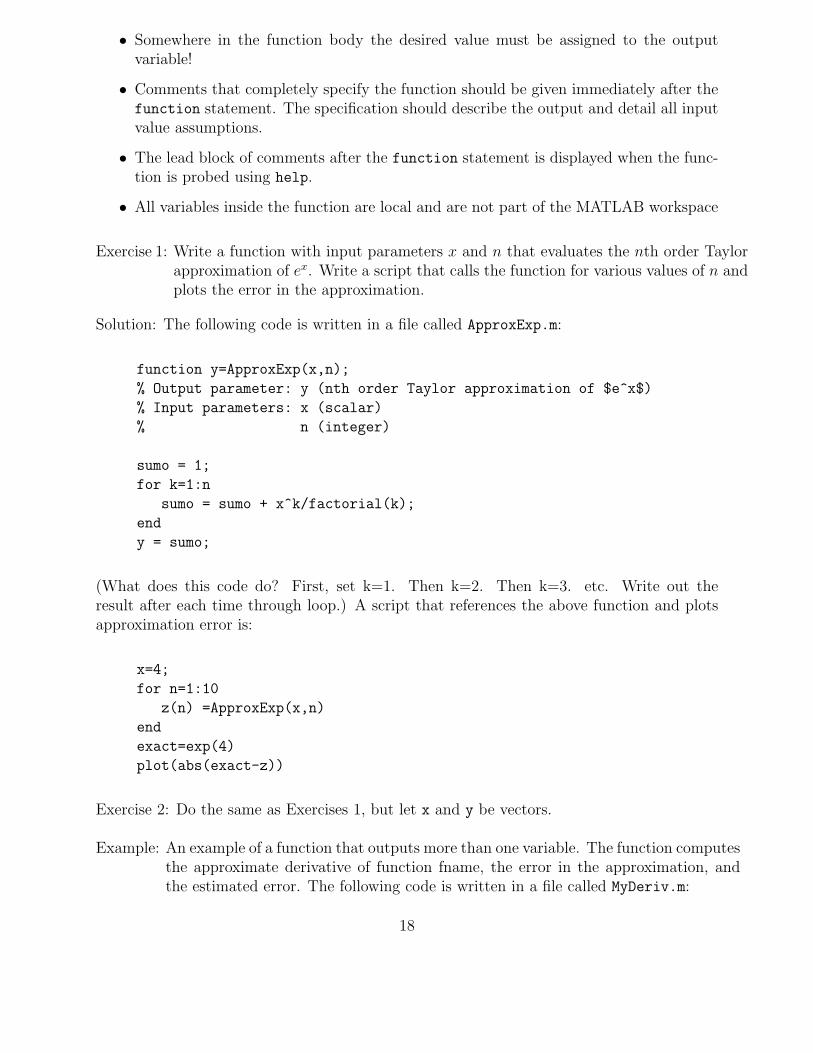
Exercise 1: Write a function with input parameters x and n that evaluates the nth order Taylorapproximation of ex. Write a script that calls the function for various values of n andplots the error in the approximation.

Solution: The following code is written in a file called ApproxExp.m:

function y=ApproxExp(x,n);

% Output parameter: y (nth order Taylor approximation of $e^x$)

% Input parameters: x (scalar)

% n (integer)

sumo = 1;

for k=1:n

sumo = sumo + x^k/factorial(k);

end

y = sumo;

(What does this code do? First, set k=1. Then k=2. Then k=3. etc. Write out theresult after each time through loop.) A script that references the above function and plotsapproximation error is:

x=4;

for n=1:10

z(n) =ApproxExp(x,n)

end

exact=exp(4)

plot(abs(exact-z))

Exercise 2: Do the same as Exercises 1, but let x and y be vectors.

Example: An example of a function that outputs more than one variable. The function computesthe approximate derivative of function fname, the error in the approximation, andthe estimated error. The following code is written in a file called MyDeriv.m:

18

function [d,err]=MyDeriv(fname,dfname,a,h);

% Output parameter: d (approximate derivative using

% finite difference (f(h+h)-f(a))/h)

% err (approximation error)

% Input parameters: fname (name of function)

% dfname (name of derivative function)

% a (point at which derivative approx)

% h (stepsize)

d = ( fname(a+h)-fname(a) )/h;

err = abs(d-dfname(a));

(Note: this works using MATLAB versions 7.0 but not 6.1. For an older MATLAB versionyou may have to use the feval command. See help, Daishu or me.)

A script that references the above function and plots the approximation error:

a=1;

h=logspace(-1,-16,16);

n=length(h);

for i=1:n

[d(i),err(i)]=MyDeriv(@sin,@cos,a,h(i));

end

loglog(h,err)

Exercise: What happens if you call

d=MyDeriv(@sin,@cos,a,h)

or simply

MyDeriv(@sin,@cos,a,h)

You can replace sin and cos by user defined functions, for example ’f1’ and ’df1’. Doit. That is, you need to write the function that evaluates f1 and df1 at x (in files f1.m anddf1.m).

19

2 Computing Fundamentals

2.1 Vectorizing, timing, operation counts, memory allocation

2.1.1 Vectorizing for legibility and speed

MATLAB allows you to write the code in vectorized form. For example you can assign thevector x using

x=0:0.01:1;

instead of the for loop

for j=1:101, x(j) = (j-1)*0.01; end

The first statement is more concise and more legible. MATLAB also evaluates it faster. Thefollowing code times the two statements

m=10^4;

tic

for i=1:m

x=0:0.01:1;

end

time1=toc;

for i=1:m

for j=1:101, x(j) = (j-1)*0.01; end

end

time2=toc;

times=[time1, time2]

ratios=[time2/time1]

On my machine the second version takes 1.9 times more time than the first.

20

2.1.2 Memory allocation

If your code requires much memory, it helps to preallocate memory before assigning largevectors or matrices. For example, if the entries of a vector are assigned in a for loop (as isoften unavoidable), we preassign memory to the vector by initializing it using the commandszeros, ones, eye. Example:

x=zeros(1,n+1);

for j=1:n+1, x(j) = (j-1)*h; end

Preallocating memory reduces coding errors, and can significantly reduce execution times.

2.1.3 Counting operations: Horner’s algorithm

The way you write a code to perform certain operations affects how fast it runs. And if itmakes a difference between 1 hour and 1 day, it matters! As we saw, the runtime dependson vectorization. But the runtime depends mainly on how many floating point opera-tions the computer has to perform. A floating point operation is a multiplication, additionor subtraction of real numbers. These are much more costly than integer operations(adding/multiplying integers), therefore they dominate the runtime.

Lets look at examples on how implementation affects the total number of operation counts.The following are three ways to evaluate the sample polynomial of degree 4, y = 2 + 4x −3x2 − x3 + x4:

y= 2 + 4*x - 3*x*x - x*x*x + x*x*x*x

y= 2 + 4*x - 3*x.^2 - x.^3 + x.^4

y= 2 + x*(4 + x.*(-3 + x.*(-1 + 1*x)))

More generally, if the polynomial is of degree N (assume a0,a1,...,amin1,an are constantsthat have already been defined in the code, and x is a vector of length m):

y= a0 + a1*x + a2*x*x + a3*x*x*x + ... + an*x*x*x*...*x

y= a0 + a1*x + a2*x.^2 + a3*x.^3 + ... + an*x.^n

y= a0 + x*(a1 + x.*(a2 + x.*(a3 + x.*(a4 ..... + x.*(amin1 + am*x)..))))

Lets count the number of operations for each entry of the vector x. The first approachcontains N additions and 1 + 2 + 3 + · · ·+ N =

∑Nk=1 k = N(N + 1)/2 multiplications for a

total ofN2/2 + 3N/2

21

floating point operations. For the second approach lets assume that one integer poweroperation takes as much as 2 multiplications (this is approximately true for some computers;others take much longer). Since the second approach contains N additions, N multiplicationsand N − 1 powers (with our assumption) it takes as much as

4N − 2

floating point operations. The third approach takes only N multiplications and N additionsfor a total of

2N

floating point operations. This is the fastest and best approach, specially if N is large, and ifthe polynomial evaluation is a significant portion of your code (performed possibly millionsof times). This approach is called Horner’s rule or nested multiplication.

I compared the timings for an example polynomial of degree 20 and found that MATLABuses about the same amount of time for the second and third approach, probably due tointernal optimization when it generates machine code.

2.1.4 Counting operations: evaluating series

Let’s implement the function ApproxExp

function y=ApproxExp(x,n);

% Output parameter: y (nth order Taylor approximation of $e^x$)

% Input parameters: x (scalar)

% n (integer)

sumo = 1;

for k=1:n

sumo = sumo + x^k/factorial(k);

end

y = sumo;

in a more efficient way using less floating point operations, as follows:

function y=ApproxExp2(x,n);

% Output parameter: y (nth order Taylor approximation of $e^x$)

% Input parameters: x (scalar)

% n (integer)

temp = 1;

22

sumo = temp;

for k=1:n

temp = temp*x/k;

sumo = sumo + temp;

end

y = sumo;

Note that the second code replaced a power and a factorial by a multiplication and a division,which should be more efficient. The script

n=100;

x=1;

tic

ApproxExp(x,n);

t1=toc

tic

ApproxExp2(x,n);

t2=toc

t1/t2

shows that the second approach is 80 times faster than the first, depending on the values ofn and on the machine.

2.2 Machine Representation of real numbers, Roundoff errors

2.2.1 Decimal and binary representation of reals

Reals can be represented in base 10 (decimal representation) using digits 0,. . . ,9, or base 2(binary representation), using digits 0,1, or any other base. Examples next.

Example: What number is (1534.4141)10?

Example: Find the base 10 representation of (1011.01101)2

Example: Find the first 10 digits of the base 2 representation of 53.710. (Use common sense,no need to learn an algorithm here.)

23

e ,e , e ,...,e10210 d ,d ,d ,...,d

52321

signbit s

exponent (11 bits) (52 bits)

mantissa

Figure 1: Machine representation of double precision real numbers in the IEEE standard.Number is stored in 64 bits: the first is the sign bit s, the following 11 ones are the exponentbits e0, . . . , e10, the last 52 bits are the mantissa d1, . . . , d52.

2.2.2 Floating point representation of reals

Machines store numbers using their binary representation (as opposed to the decimal rep-resentation). The coefficients in the binary representation are either 0 or 1 and these caneasily be stored electronically. One 0 or 1 coefficient is called a bit. Eight bits are a byte.The amount of storage in a device is measured either in kilobyte (103 bytes), megabyte(106 bytes), gigabyte (109 bytes) or terrabytes (1012 bytes).

The IEEE standard uses 64 bits (8 bytes) to store one real number in double machineprecision. See Figure 1. The first bit is the sign bit s. The following 11 ones are theexponent bits e0 . . . e10. The remaining 52 bits form the mantissa d1, . . . , d52. What numberdo these 64 digits represent? First we have to determine the exponent

F = (e10e9 . . . e1e0)2 = e10210 + e92

9 + . . . e121 + e02

0

which is an integer. Note that the largest exponent corresponds to e0 = e1 = · · · = e10 = 1and equals

∑10k=0 2k = 211 − 1 = 2047 and the smallest one corresponds to e0 = e1 = · · · =

e10 = 0 and equals 0. Thus0 ≤ F ≤ 2047

To determine which number is represented by the 64 bits one of 4 definitions is used, de-pending on the value of F :

1. Normalized numbers. If 1 ≤ F ≤ 2046 the represented real number is

V = (−1)s2E(d0.d1d2d3 . . . d52)2

where E = F −1023, d0 = 1. Thus −1022 ≤ E ≤ 1023. The smallest normalized num-ber is ±2−1022×1.000 . . . 0 = ±2−1022 The unnormalized numbers enable representationof even smaller numbers.

24

2. Unnormalized numbers. If F = 0

V = (−1)s2−1022(0.d1d2d3 . . . d52)2

3. NaN. If F = 2047 and mantissa 6= 0:

V = NaN (not-a-number)

Invalid operations such as 0/0 or ∞−∞ lead to NaNs.

4. Infinity. If F = 2047 and mantissa = 0:

V = (−1)s∞

If a valid operation leads to x too large, the result is set to ∞ with the appropriatesign.

Largest and smallest numbers. The largest number that can be representd is the largestnormalized number

Vmax = ±21023(1.1111 . . . 1)2 = ±21023

52∑

k=0

(1/2)k = ±21023(2 − 2−52) ≈ 1.7975 × 10308

The smallest number that can be representd is the smallest unnormalized number

Vmin = ±2−1022(0.000 . . . 01)2 = ±2−1074 ≈ 4.9407 × 10−324

What is result of x=1.797e308; 2*x? And of x=4.941e-324; x/2? They result in overflowor underflow exceptions respectively.

2.2.3 Machine precision, IEEE rounding, roundoff error

In double machine precision, the computer stores only the first 53 binary digits (or 52if unnormalized) of a real number x (this is equivalent to roughly 16 decimal digits). Theremaining digits that are present if x has a longer binary expansion are truncated or rounded.Thus the machine representation of x is not the same as x! We call the floating pointrepresentation of x

fl(x)

Thus: fl(x) − x 6= 0 and define

fl(x) − x as the absolute roundoff error.

f l(x) − x

xas the relative roundoff error.

25

Note: What is the result of computing 9.4-9-0.4 in MATLAB?

IEEE addition and rounding. When two numbers are added they are first placed out ofstorage into a register in which addition is performed using higher than machine precision.The result is then rounded to 52 digits after decimal (with at most 1 nonzero digit beforedecimal) and stored. IEEE rounding consists of rounding down (truncating) if the 53rd digitequals 0. Otherwise, if the 53rd digit equals 1, it rounds up UNLESS all digits to the rightof the 53rd and the 52nd digit are zero.

all 52 digits in the mantissa are zeros, the number is rounded down (truncated). Thus:

1 + 2−52 + 2−54 is rounded down to 1 + 2−52

1 + 2−52 + 2−53 is rounded up to 1 + 2−51

1 + 2−53 is rounded down to 1

1 + (2−53 + 2−54) is rounded up to 1 + 2−52

1 + 2−53 + 2−54 is rounded down to 1

1 + 2−51 + 2−53 is rounded down to 1 + 2−51

To see for example the last three, type (1+(2^ -53+2^ -54))-1, (1+2^ -53+2^ -54)-1, and(1+(2^ -51+2^ -53))-1.

Machine precision. Machine precision, or machine ǫ, measures the amount of relativeprecision you have in the floating point representation of a number. It is defined as

machine ǫ: distance between 1 and the smallest floating point number greater than 1.That is, smallest number such that

fl(1 + ǫ) 6= 1

In the IEEE standard

ǫ = 2−52 ≈ 2.2 × 10−16 (double machine precision)

ǫ = 2−23 ≈ 1.2 × 10−7 (single machine precision)

since any floating point number not equal to one has to have at least one of d1, . . . , d52

nonzero. The smallest such number bigger than 1 is the one with d52 = 1 and all otherd1 = · · · = d51 = 0. In MATLAB, it is defined as the variable eps. The relative roundofferror in representing a number is

fl(x) − x

x≤ ǫ

2.

Be sure to understand the difference between the smallest representable number 2−2074 andmachine ǫ. Many numbers below ǫ are representable, but adding them to 1 has no effect.

26

2.2.4 Loss of significant digits during subtraction

While the relative precision in the numerical representation of a number is at most ǫ/2,precision can be lost in particular during subtraction of almost equal numbers. Imagine forsimplicity that we are computing using 5 significant decimal digits.Then consider subtracting300.3 − 300. In exact arithmetic

300.3 − 300 = 1/3

In floating point arithmetic keeping 5 significant digits

fl(300.3) − fl(300) = 300.33 − 300 = 0.33

Thus the answer is represented with only 2 significant digits of accuracy. This loss of signif-icance due to subtraction of almost equal numbers can be a problem that can sometimes beremedied.

Example: Consider computing1 − cos x

sin2 xfor small x. In that case, the numerator will lead to loss of significance due to subtraction ofalmost equal numbers. The resulting error is then amplified by dividing by a small number.The alternative formulation

1

1 + cos x

(which is equal in exact arithmetic) does not lead to loss of significance. See our text-book, p 18 for a comparison of the two formulations in MATLAB. Plot both expressions vsh=logspace(-1,-16,16).

Example: The quadratic formula to solve ax2 + bx + c = 0,

x1 =−b +

√b2 − 4ac

2a, x2 =

−b −√

b2 − 4ac

2a

leads to loss of significance in x1 if 4ac ≪ b2 (much less than), and b > 0. One avoids thisloss of significance by rewriting (multiply top and bottom by conjugate and simplify) theformula for x1 as:

x1 =−c

b +√

b2 − 4ac

Example: Plot (x − 1)3 and x3 − 3x2 + 3x − 1 vs x − 1 for x = linspace(1 − h, 1 + h, 1000)for h = 10−5.

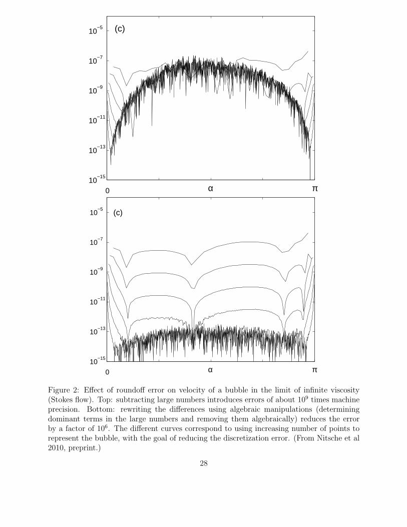
Example: This issues can be relevant in applications. Figure 2 illustrates the loss of sig-nificance when computing the velocity of a bubble in viscous fluid using a straight forwardimplementation of the governing equation (top) and after cleverly rewriting them to removesubtraction of large numbers (bottom).

27

10−15

10−13

10−11

10−9

10−7

10−5 (c)

0 πα

10−15

10−13

10−11

10−9

10−7

10−5 (c)

0 πα

Figure 2: Effect of roundoff error on velocity of a bubble in the limit of infinite viscosity(Stokes flow). Top: subtracting large numbers introduces errors of about 109 times machineprecision. Bottom: rewriting the differences using algebraic manipulations (determiningdominant terms in the large numbers and removing them algebraically) reduces the errorby a factor of 106. The different curves correspond to using increasing number of points torepresent the bubble, with the goal of reducing the discretization error. (From Nitsche et al2010, preprint.)

28

2.3 Approximating derivatives, Taylor’s Theorem, plotting y = hp

Another example of loss of significance due to subtraction comes in approximating deriva-tives, as we did earlier (MATLAB Tutorial, page 16). This example also gives us a reasonto review Taylors theorem (which is fundamental for all that we will do in this class!) andgo over plots of y = hp on a log-log scale.

Taylor’s Theorem for functions of one variable. If the n + 1st derivative of f existsand is continuous on [x, x + h] then

f(x + h) = f(x) + f ′(x)h +f ′′(x)

2h2 +

f ′′′(x)

3!h3 + · · · + f (n)(x)

n!hn +

f (n+1)(ξ)

n!hn+1

for some value ξ ∈ [x0, x]. If M is an upper bound for f (n+1) on this interval we see that thelast term is ≤ Mhn+1 and thus

f(x + h) = f(x) + f ′(x)h +f ′′(x)

2h2 +

f ′′′(x)

3!h3 + · · · + f (n)(x)

n!hn + O(hn)

using the Big-O notation defined in next section.

Approximating derivatives. Using Taylor’s theorem with n = 1 we can show that inexact arithmetic

f(x + h) − f(x)

h= f ′(x) + O(h)

Thus the approximation of the first derivative by the left hand side makes an O(h1) error,we call it a first order approximation.

Approximating derivatives in IEEE arithmetic. If h is small, then the numerator of

f(x + h) − f(x)

h

leads to loss of significance due to subtraction of almost equal numbers. In particular:

fl(f(x + h)) − fl(f(x))

fl(h)=

f(x + h) + ǫ1 − (f(x) + ǫ2)

h + ǫ3

≈ f(x + h) − f(x)

h+

ǫ4

h= O(h)+O(1/h)

where ǫ1,2,3,4 are of the order of ǫf(x). If h is large, the first term will dominate, if h is smallthe second term will dominate!. This is what we saw in the plot obtained in section 1.9.

Plotting y = hp on log-log scale. Note that if y = Chp then log y = log C + p log h.Thus plotting log y vs log h (ie, using log-log scale) we obtain a linear plot with slope p! Forexample when we plotted the error above of the form O(h) + O(1/h) we obtained a portionof the curve with slope 1 (where O(h) term dominates) and a portion with slope -1 (whereO(1/h) term dominates).

29

2.4 Big-O Notation

Let E be a function of h. We say that E(h) = O(hp) as h → 0 (Read as “E is big-O of h tothe p as h goes to 0”, or “E is of order h to the p”) if there exists constants ǫ and C suchthat

‖E(h)‖ < Chα ∀h ∈ [0, ǫ]

This is of interest since it gives an upper bound on how fast a function approaches zero inthe limit as h goes to zero. Similarly E(N) = O(N) as N → ∞ means that there existsconstants C and N0 such that

‖E(N)‖ < CN ∀N ≥ N0

and as a result, this notation gives a bound on how fast E can grow as N → ∞ (in this case,at most linearly). (Usually, we use h or ǫ to denote small numbers and N to denote largenumbers.)

30

3 Solving nonlinear equations f(x) = 0

Problem Statement: Find root of a function f(x) (linear or nonlinear). Equivalently, theproblem is to solve an equation (linear or nonlinear).

Definition:A function f(x) has a root r if f(r) = 0.

Note: Why are the two problems stated above equivalent? Because we can write the solutionto any equation as the root of a function. For example, solution to cos3 x = x+ 1 is the rootof f(x) = cos3 x − x − 1.

Intermediate Value Theorem (IVT): The IVT is a theorem that guarantees that f hasa root if it satisfies certain conditions. The theorem says:

If f(a)f(b) < 0 and f is continuous on [a, b] then f has a root in (a, b).

Note that no conclusions can be drawn if the conditions of the theorem does not apply. Forexample, if f is not continuous on [a, b], or if f(a)f(b) > 0 we CANNOT conclude anythingabout the roots of f in (a, b). But if the conditions apply, we know f has a root and wewant a numerical method to find it. Moreover, the method should be as accurate as desired(if possible), and fast.

31

3.1 Bisection method to solve f(x) = 0 (§1.1)

• Basic idea: If f is known to have a root on [a, b] by IVT, bisect interval into twosubintervals, choose the one containing the root (using IVT), repeat. The length ofthe interval decreases by half at each step, the root is known to within that precision,and can be found to specified precision by taking sufficiently many steps. In theory.

• The algorithm. Outline of algorithm for function root=bisect(f,a,b,tol)

while abs(a-b)/2>tol

c=(a+b)/2

if f(c)==0 done

if f(a)*f(c)<0

b=c

else

a=c

end

end

root = c

Problems: what if tol too small? Two function evaluations per loop. Filling in thedetails. Explain modification to book algorithm.

function [root,i]=bisect(f,a,b,tol)

fa=f(a); fb=f(b);

if (fa*fb >= 0 )

error(’f(a)f(b)<0 not satisfied’)

endif

i=0;

disp(sprintf(’ %3d %20.15f ’,i,a))

while abs(a-b)/2 > tol

c= (a+b)/2; fc=f(c);

if fc==0

break

end

if fa*fc<0

b=c; fb=fc;

else

a=c; fa=fc;

end

i=1+1;

disp(sprintf(’ %3d %20.15f ’,i,a))

end

root = (a+b)/2;

32

Example: Apply to solve 3x3 + x2 = x + 5 to within 7 decimal places.

Definition: A solution is correct within p decimal places if the error is less than0.5 × 10−p. Note, this does not mean that the pth digit is exact!

Example: Apply to approximate the cube root of 5 to within 10 decimal places.

Example: What happens if you type

[xc,niter]=bisect(@sin,3,4,10^-20)

? Fix the problem. (Replace tol by tol+eps*max(abs(a),abs(b))).

• Convergence rate. Rate of reduction of error.

The method builds a sequence of approximate solutions xk, given by the midpointsof the relevant interval. We know that, up to roundoff, the sequence of midpointsxk computed by the bisection method converges to the exact root. How fast does itconverge? That is, how fast does the error decrease in each step? We know that aftern steps, the root r lies in the n + 1st subinterval, with length (b − a)/2n+1. So

|xn − r| ≤ b − a

2n+1.

That is, the error goes down by 1/2 in each step. This is called Linear convergencewhich we will define more precisely later.

With this result we can estimate how many steps it takes to get within a prescripbedtolerance.

Example: If |b − a| = 1, tolerance tol = 5 · 10−8, the error is guaranteed to be < tol,after n = 24 steps.

33

3.2 Fixed point iteration to solve x = g(x) (FPI, §1.2)

3.2.1 Examples

• Starting with any number x0 of your choice, compute xk+1 = cos(xk) for approximately0 ≤ k ≤ 20 (by repeatedly hitting the cosine button). What do you observe?

• Method of the Babylonians (1750 BC!) to approximate√

2: Note that if x >√

2,then 2/x < 2/

√2 =

√2. The Babylonians proposed to, starting with any initial guess

x0, obtain a better approximation to√

2 by averaging x and 2/x. This leads to theiteration

xk+1 =xk + 2

xk

2Try it out with an initial guess of your choice (6= 0), and see how quickly the iteratesapproach

√2.

3.2.2 The FPI

• A fixed point iteration is of the form

xk+1 = g(xk) , with xo given

IF the iteration converges, that is, limk→∞ xk = r for some r, as in the above examples,then r satisfies

r = g(r)

and is called a fixed point of g. Geometrically, this point is the x-coordinate of theintersection of the graphs of y = g(x) and y = x. (Show that the fixed point of theBabylonian map satisfies x2 = 2.)

• The iterates of FPI can be visualized by a cobweb diagram. Starting with the point(x0, 0), get to x1 geometrically by going vertically up to the point (x0, g(x0)) on thecurve y = g(x), and then moving over horizontally to point (g(x0), g(x0)) on the liney = x. This new point has x-coordinate x1. Repeat this process. Note, to obtain anaccurate cobweb diagram, the line y = x must be drawn correctly. This is easiest if,by hand and in matlab, we use a 1-1 scale (in matlab, use axis equal).

• The cobweb diagrams for the cosine map above show that the iterates converge to theroot of r = cos r, for any x0. In this case we say the iteration is globally convergent.The cobweb diagram for the Babylonian map shows that for x0 > 0, the iteratesconverge to r =

√2, while for x0 < 0, the iterates converge to r = −

√2. It also shows

that the iterates converge very fast to r ones they are close to r, because g′(r) = 0.

• Can always rewrite f(x) = 0 as g(x) = x, but not uniquely! For example: can rewritex3 + x − 1 = 0 in three ways: as x = g1(x) = 1 − x3, x = g2(x) = (1 − x)1/3,x = g3(x) = 1+2x2

1+3x2 .

34

3.2.3 Implementing FPI in Matlab

• Pseudocode 1:

initialize vector x %to alot memory to it

initialize x(1) %to the given initial guess

for k=1:iter

x(k+1)=g(x(k))

end

where iter is the total number of iterations performed. This code saves all the iteratesof the iteration in a vector x. We are mostly interested only in the last iterate anddont want to save all the intermediate steps, in which case we simply overwrite thecurrent iterate:

Pseudocode 2:

initialize x %to the given initial guess

for k=1:iter

x=g(x)

end

• Using a function that implements either of the above, we now apply FPI to solvex3 + x − 1 = 0 in three ways. We find that (1) Diverges, (2) converges, (3) convergesmuch faster.

• The cobweb diagram show that (1) diverges because the slope of g at the root is > 1in magnitude!, |g′

1(r)| > 1. (2) converges to r (provided x0 is sufficiently close to r)since |g′

2(r)| < 1 and (3) converges faster since |g′3(r)| ≪ |g′

2(r)| < 1. Suggestion:convergence depends on local slope.

3.2.4 Theoretical Results

• Theorem: If |g′(r)| < 1 and x0 is sufficiently close to r, then the fixed point iterationconverges to r. Furthermore, the error ek = xk+1 − r satisfies

limk→∞

ek+1

ek

= g′(r)

Proof: If |g′(r)| < 1 then |g′(r)| ≤ S < 1 in some neighbourhood of r. If x0 is in thisneighbourhood, then, by Taylor’s Theorem,

|x1 − r| = |g′(ξ0)||x0 − r| ≤ S|x0 − r| (1)

|x2 − r| = |g′(ξ1)||x1 − r| ≤ S|x1 − r| ≤ S2|x0 − r| (2)

. . . (3)

35

where ξ0 is some point between x0 and r, ξ1 is some point between x2 and r, etc. Byiterating this process we find that

|xk − r| ≤ Sk|x0 − r| or |ek| ≤ Sk|e0|

Note that the right hand side → 0 as k → ∞ because S < 1, and thus, limk→∞ xk = r,or limk→∞ ek = 0. and we proved the first part.Now note that

(xk+1 − r) = g′(ξk)(xk − r) orek+1

ek

= g′(ξk)

where ξk is between xk and r. Since xk → r as k → ∞, also ξk → r. Thus

limk→∞

ek+1

ek

= g′(r)

and we proved the second part.

Note: This implies that if k is sufficiently large, ek+1 ≈ g′(r)ek. The error decays bya factor of g′(r) at each step. If g′(r) is small, it will decay very fast. If g′(r) ≈ 1, itwill decay very slowly.

• Example: For the cosine map, print k, xk, ek, ek+1/ek. Compare to g′(r). Run thefollowing matlab code.

clear

g=inline(’cos(x)’); gp=inline(’sin(x)’); f=inline(’cos(x)-x’);

%g=inline(’(x+2./x)/2’);gp=inline(’(1-2./x.^2)/2’);

%f=inline(’x.^2-2’);fp=inline(’2*x’);fpp=inline(’2’);

a=1; kmax=20;

x=fixedpt2(g,a,kmax); %this function returns a vector of all iterates, x

r=fzero(f,a);

n=length(x);

e=abs(x-r);

disp(’ k x error ratio ’)

for k=1:n-1

disp(sprintf(’%3d %15.10f %14.10f %10.6f’, k,x(k),e(k),e(k+1)/e(k)) )

% disp(sprintf(’%3d %15.10f %13.10f %10.6f’, k,x(k),e(k),e(k+1)/e(k)^2) )

end

disp(sprintf(’\n Compare limit of ratios with g’’(r)= %9.6f’, gp(r)))

%disp(sprintf(’\n Compare limit of ratios with g’’(r)/(2g’’(r))= %9.6f’,...

% fpp(r)/(2*fp(r))))

• Example: Repeat for the two converging maps for x3 + x − 1 = 0.

36

3.2.5 Definitions

• Local vs global convergence. An iterative scheme is locally convergent if xk → ras k → ∞ provided x0 is sufficiently close to r. FPI is locally convergent.An iterative scheme is globally convergent if xk → r as k → ∞ for any x0. SomeFPI, such as cosine map, are globally convergent. We can deduce this from the cobwebdiagram.

• Rates of convergence.

If limk→∞

ek+1

ek

= S , with 0 < S < 1, then the iteration xk is linearly convergent. This

implies that for sufficiently large k, ek+1 ≈ Sek (the error gets reduced by a factor S).If 0 < |g′(r)| < 1, FPI is locally convergent.

If limk→∞

ek+1

e2k

= S , with 0 < S, then the iteration xk converges quadratically. This

implies that for sufficiently large k, ek+1 ≈ Se2k. Once ek is small, this convergence is

much better than linear.

If limk→∞

ek+1

epk

= S , with 0 < S, then the iteration xk converges to order p.

• What is convergence rate for Babylonian method? Hint: run the matlab code aboveafter replacing the three lines starting with ”g. . . ”, and ”disp. . . ” by the commentedlines below them. We will see the reason for the last line in this code in the nextsection.

3.2.6 Stopping criterion

• Implement stopping criterion: iterate FPI until |xk+1 − xk| < tol, for some giventolerance.How do you do this in Pseudocode 1? Pseudocode 2?Note that even if |xk+1 −xk| < tol, we dont know what the actual error |xk+1 − r| afterthat step is.

37

3.3 Newton’s method to solve f(x) = 0 (§1.4)

3.3.1 The algorithm

• Picture and derivation of algorithm. Stopping criteria.

• Write out Newton’s algorithm to solve x2 = 2 (!)Write out Newton’s algorithm to solve x3 + x − 1. Combine terms. (!)

• What can go wrong? f ′(xk) = 0, oscillation between two points.If f ′(xk) ≈ 0, move far away from initial condition, and may converge to a far awayroot.What happens if f ′(r) = 0?

• Note: Newton’s is a special type of fixed point iteration.

3.3.2 Matlab implementation

Again, two choices: either return vector of solutions or overwrite old iterate by current

• Pseudocode 1:

initialize vector x

initialize x(1)

for k=1:kmax

x(k+1) = x(k)-f(x(k))/fp(x(k));

if abs(x(k+1)-x(k)) < tol exit loop

end

• Pseudocode 2:

initialize x

set xold=x

for k=1:kmax

x = x-f(x)/fp(x);

if abs(x-xold) < tol exit loop

xold=x

end

• Apply to x3 + x − 1 = 0. Plot ek+1/e2k.

38

3.3.3 Theoretical results

• Prove: if f ′(r) 6= 0 then Newton’s method is locally convergent. (to prove, viewNewtons as fixed point iteration for some g. Find g′(r))

• Prove: if f ′(r) 6= 0, Newton’s method is quadratically convergent. (Hint: Use Talorpolynomial of order 1 for f , with remainder.)

• State: if f ′(r) = 0, method still converges but slower: linear convergence, withlimk→∞ ek+1/ek = (m − 1)/m. (To see this, apply Newtons method to solve xm)State modified Newton’s method for multiple roots, with quadratic convergence.

• Summary. Ups: fast convergence. Downs: requires f ′. Only locally convergent (butthis is true for most methods).

3.4 Secant method (§1.5)

• State Secant Method

3.5 How things can go wrong. Conditioning. (§1.3)

Example: Apply bisection algorithm to solve

x3 − 2x2 +4

3x − 8

27= 0

(which equals (x − 23)3 = 0) to within 4 digits, 6, 10, 20 digits. Compare approximate and

exact roots. How big is the error? Repeat with fzero. Plot y = f(x) = x3 − 2x2 + 43x− 8

27,

zoom into region near triple root. Repeat for f(x) = (x − 23)3. What is the problem? Why

does it occur in one formulation, and not the other? (Answer: loss of significance due tocancellation in one case, not the other.)

3.5.1 Multiple roots

Definition:A function f(x) has a root of multiplicity n at x = r if f(r) = f ′(r) = f ′′(r) =· · · = f (n−1)(r) = 0 but f (n)(r) 6= 0. Alternatively, the root r has multiplicity n if thefunction’s Taylor series about x = r has leading order term

f(x) ∼ C(x − r)n + smaller terms of higher order

For example it is easy to check using either criterion that f(x) = sin(x)−x has a triple rootat x = 0. It is easy to check using Taylor series that sin(x100) has a root of multiplicity 100at the origin.

39

function f

INPUT OUTPUT

root x=r

Problem to be solvedsuch as

solve f(x)=0

Figure 3: Input and output of a problem to be solved.

We see that in the above example, the large multiplicity of the root causes a problem: fora relatively large range of values of x away from the root the floating point values of thefunction are near 0 and thus the bisection algorithm (or fzero or any other algorithm) findsmany incorrect roots. In other words, here,

large changes in x yield small changes in f

The problem occurs only in one formulation and not in the other because the relative sizeof roundoff error differs in the two cases.

3.5.2 Forward and Backward error. Error magnification.

One can view the problem to be solved as having input values (in our case f) and outputvalues (in our case the root r). See figure 3.

The numerical method outputs an approximate solution, call it xc. Define

Forward error: Error in output, in our case |xc − r|

Backward error: Error in input (introduced for example by machine precision, noisymeasurements, etc), in our case |f(xc) − f(r)| = |f(xc) − 0|

So the problem is that the forward error is very large relative to the backward error! Thatis, the

error magnification =forward error

backward error(4)

is very large. The input is represented accurately numerically, but since the error magnifi-cation is large, the output is much less accurate. Problems for which this is true are saidto be ill-conditioned. For such problems we cannot obtain good answers numerically, nomatter which method we use! Note that the conditioning is inherent to the problem, not themethod.

40

Why is this a problem? In general we do not know the forward error since we dont have theexact solution (bisection algorithm is an exception!), and we can only compute the backwarderror. But we would like, based on the backward, to know the forward error. If we knewthe error magnification factor we could do that. In some cases an estimate for the errormagnification factor can be found.

3.5.3 Other examples of ill-conditioned problems

Multiple roots are not the only cases yielding ill-conditioned problems.

Example: Solve x + y = 2, 1.00001x + y = 2.00001 using Matlabs A\b solver of linearsystems. Note: exact solution x = 1, y = 1. Numerical solution relatively far from it. Why?Geometric interpretation.

Example: Wilkinsons polynomial

W (x) = (x − 1)(x − 2) . . . (x − 20) = x20 − 210x19 + 20615x18 + . . . 243290200817664000

has simple roots, yet, if implemented in the formulation on the right hand side,

fzero(wilkpoly, 16) = 16.014...

The problem here is again loss of precision due to subtraction of almost equal numbers. Forx near 16, each term in the sum is large, and they need to cancel to yield the resulting valuenear 0. The relative errors in each number, due to finite machine precision, is amplified,yielding very large relative error (only 2 correct digits since the relative error is only lessthan 0.510−2))

Thus, small relative errors (of 1.e-16) in the coefficients yield large relative errors in thesolution ⇒ ill-conditioned.

3.5.4 The condition number

Whether a problem is ill-conditioned or well-conditioned is based on the magnification ofthe relative errors (as opposed to the absolute errors considered in Eq 4).

Definition: The condition number of a problem is

cond = maximumrelative forward error

relative backward error(5)

over all changes in input. For example, in the Wilkinson polynomial case, the relativechanges in the coefficients of f are of order 10−16 and the relative change in the output is

41

10−2, yielding condition number of at least 1014. The maximal amplification of the relativeerrors can sometimes be found precisely. More later. Note that if we know the conditionnumber and we know the backward error we can estimate the forward error.

42

4 Solving linear systems

4.1 Gauss Elimination (§2.1)

• Solve sample 2x2 linear system x + y = 3, 3x− 4y = 2, geometrically and algebraically

• Solve sample 3x3 linear system

2x + y − 4z = −7

x − y + z = −2

−x + 3y − 2z = 6

by hand (using Tableau form), doing Gauss Elimination, then back substitution. Definepivots. Keep track of the multipliers, and carefully do all algebra.

• Write GE algorithm (no pivoting). Note that we only have to update the nonzeroentries aik, i, k ≥ j + 1, that is, the entries below and to the right of ajj.

[n,n]=size(A);

for j=1:n-1 %go over all columns j except the last one

for i=j+1:n %eliminate all entries A(i,j) below A(j,j), i>j

m=A(i,j)/A(j,j); % compute multipliers to eliminate entry

for k=j+1:n % replace all entries A(i,k) in Row i to the

A(i,k)=A(i,k)-m*A(j,k); % right of column j

end

b(i)=b(i)-m*b(j); % do row operation on rhs b

end

end

• Count number of operations for GE:∑n−1

j=1 [2(n − j) + 3](n − j). Use

n∑

j=1

1 = n ,n∑

j=1

j =n(n + 1)

2,

n∑

j=1

j2 =n(n + 1)(2n + 1)

6

to evaluate.

• Backward substitution to solve Ux = b, algorithm and operation count.

for i=n:-1:1

for j=i+1:n

b(i)=b(i)-a(i,j)*x(j)

end

x(i)=b(i)/a(i,i);

end

43

• Operation counts:

Gauss Elimination :2

3n3 + l.o.t

Upper Triangular system : n2

Lower Triangular system : n2

4.2 LU decomposition (§2.2)

• Today we’ll show that GE is equivalent to factoring A = LU , where L is lower trian-gular, U is upper triangular. Why is such a factorization useful? Suppose you need tosolve Axk = bk for many bk, suppose k = 1, 1000. One option is to use GE each timefor a total cost of

1000(2/3)n3

The alternative is to find the LU factorization once (at a cost of 2/3 n3) and then solveLUxk = bk in two steps:

(1) Solve Ly = bk for y(2) Solve Uxk = bk for xk

for a cost of n2 each step, and a total cost of

(2/3)n3 + 2000n2 .

The O(n3) operation can be viewed as an initialization cost, and all subsequent stepsare O(n2) instead of O(n3). Big savings.

• To show that GE is equivalent to factoring A = LU : Every step in GE consists ofadding a multiple of −mij of the jth row to the ith row.

This is an elementary row operation. There are 3 elementary row operations:

Replacing Rowi by Rowi − m · Rowj

Replacing Rowi by m · Rowi

Exchanging Rowi and Rowj

Each one is equivalent to premultiplying A by an elementary matrix. The first oper-ation, replacing Rowi by Rowi − m · Rowj is equivalent to premultiplying A by Lij,where L is the lower triangular matrix which equals the identity except that it contains−mij in its (ij)th position. (That is, it is the matrix obtained from the identity matrixby performing the desired row operation on it.)

Thus at the end of GE we have performed the following operations

Ln,n−1 . . . L3,2Ln,1 . . . L3,1L2,1Ax = Ln,n−1 . . . L3,2Ln,1 . . . L3,1L2,1b

44

andLn,n−1 . . . L3,2Ln,1 . . . L3,1L2,1A = U

Now note that Lij are invertible with simple inverse and compute

L−12,1L

−13,1 . . . L−1

n,1L−13,2 . . . L−1

n,n−1 = L

where L contains the mij below the diagonal, and ones on the diagonal. Thus, afterGE have A = LU decomposition.

• Change GE algorithm so as to return L,U . Test for an example.

[n,n]=size(A);

for j=1:n-1

for i=j+1:n

A(i,j)=A(i,j)/A(j,j); % overwrite A(i,j) by multiplier

for k=j+1:n

A(i,k)=A(i,k)-A(i,j)*A(j,k);

end

end

end

L=eye(n,n)+tril(A,-1);

U=triu(A);

Write main portion of above algorigthm more concisely in matlab (just for curiosity).

for j=1:n-1

A(j+1:n,j)=A(j+1:n,j)/A(j,j);

A(j+1:n,j+1:n)=A(j+1:n,j+1:n)-A(j+1:n,j)*A(j,j+1:n);

end

• Find LU -factorization of A by hand for

A =

2 1 −41 −1 1−1 3 −2

4.3 Partial Pivoting (§2.3, §2.4)

• What if pivots ajj = 0? Then the LU decomposition does not exist

Example: Show that A =

[0 11 1

]has no LU decomposition.

What if pivots ajj are small? Then multipliers aij/ajj are large, which can lead to lossof precision when computing aik − majj.

Example: Show that using GE to solve

[10−20 1

1 2

]x =

[14

]leads to large amplification

of small errors introduced by roundoff. ⇒ GE without pivoting is UNSTABLE

45

• Solution: pivoting (exchanging rows so that maximal entry aij in jth column, withi ≥ j, moves into the pivot position). As a result the multipliers aij/ajj will always be< 1.

• Describe partial pivoting. Use it to solve

[10−20 1

1 2

]x =

[14

]to show roundoff errors

stay small. ⇒ GE with partial pivoting is STABLE (small erros are not amplified,provided the problem we are trying to solve is WELL-POSED.) we have not proventhis, only illustrated by example, but it can be proven to be true. Note that if theproblem we are trying to solve is ILL-POSED, than no method can give a good result:small errors are amplified by the problem, even if the method is stable.

• Switching rows is equivalent to premultiplying by elementary matrices Pk. (Whathappens if you postmultiply A by Pk?) Show that it leads to decomposition PA = LU .(For this we need to know how to write PkLij = LijPk.

• Find the PLU factorization P,L, U for a sample 3x3 matrix A, by hand. Check resultby confirming that PA = LU .

• Check result using MATLABs lu(A) function.

• How to use PLU decomposition to solve Ax = b for many b.

• What is full pivoting?

4.4 Conditioning of linear systems (§2.3)

• Consider Ax = b

0.835x + 0.667y = 0.168

0.333x + 0.266y = 0.067

Has exact solution x = (1,−1). If b is changed to b = (0.168, 0.066) the exact solutionis x = (−666, 834)! That is, the forward error (change in output x) is much larger thanthe small backward error (change in input A,b). This is a symptom of an illconditionedproblem: small perturbations, such as introduced by roundoff or measurement errors,can be amplified significantly.

For a 2x2 linear system this illconditioning can be explained geometrically: graph thelines represented by each of the two equations and find their slopes are almost identical,so small changes in the line (input) cause large changes in the intersection (output).

For general linear system, the amplification factor of the relative forward error is mea-sured by the condition number. The exact statement follows next.

46

• To measure the changes in vectors and matrices we need vector and matrix norms.The vector norm you are probably most familiar with is the Euclidean 2-norm, forexample

||〈a, b〉||2 =√

a2 + b2

||〈x1, x2, . . . , xn〉||2 =√

x21 + x2

2 + · · · + x2n

A compatible matrix norm needs to satisfy certain properties (too learn more aboutthis, take Math 464). The matrix norm compatible with the vector 2-norm is given interms of the largest absolute singular value of the matrix.

Instead, we will use a simpler vector- and matrix- norm. (For a rule to be a norm, itmust satisfy certain properties. Again, more on this in Math 464.) We will use theinf-norm. For a n × 1 vector x and an n × n matrix A it is defined as

vector inf-norm ||x||∞ = max1≤j≤n

|xj|

matrix inf-norm ||A||∞ = max1≤i≤n

n∑

j=1

|Aij| (maximum absolute row sum)

• Define relative forward error ||x − x||/||x||

relative backward error ||b − b||/||b||

The backward error is the residual Ax− b. The example shows that residual can besmall even if the error in the solution is very large. The next theorem shows that thisamplification factor can be as large as the condition number of the matrix.

• Theorem:||x − x||||x|| ≤ K(A)

||b − b||||b|| where K(A) = ||A||||A−1||

with equality attainable for some b. (This theorem holds using any matrix norm.)

Note: the condition number is a property of the matrix, not of any numerical methodused to solve the system. In MATLAB, you can use the function cond to obtain thecondition number of a matrix, using a norm of your choice. You can also use norm tocompute norms of matrices and vectors.

One can expect that roundoff error introduces errors of size of machine epsilon ǫ in thematrix A and the right hand side b. Then the relative forward error can be expectedto be

||x − x||||x|| ≤ K(A)ǫ

47

So if, for example, K(A) ≈ 109, then you loose 9 digits of accuracy in solving the linearsystem Ax = b.

Example: Hilbert matrix (example 2.12)

4.5 Iterative methods (§2.5)

• GE with pivoting solves the problem Ax = b to within machine precision (timescondition number, see §3.5). Why do we need to study other methods to solve thisproblem? After obtaining the LU decomposition once, GE is fast (O(n2)) if Ax = bhas to be solve repeatedly for many right hand sides. However, if Ax = b has to besolved once (for example, new A and b at every timestep in a time-evolution problem)then it is expensive (O(n3)). Need faster methods.

• Iterative methods to solve Ax = b are of the form

x(k+1) = Bx(k) + c (6)

with some initial guess x0. (This is similar to the fixed point iteration which we studiedfor nonlinear scalar problems.) Under what conditions do such iterative methods forlinear nxn systems converge?

• Answer (which can be motivated using the fixed point iteration result): The iterationxk+1 = Bxk + c converges if and only if the spectral radius ρ(B) < 1. The spectralradius is defined to be the largest absolute eigenvalue of B: ρ(B) = max

1≤j≤n|λj|.

• Jacobi method. Example. This method consists of solving the jth equation inAx = b for xj, that is, which yields a specific equivalent system x = Bx + c, and thenperforming the fixed point iteration.

Go through examples 2.19 and 2.20. Show how to get the system u = f(u) = Bu + c,where u = 〈u, v〉 by solving first equation for u, second one for v. Write a MATLABfunction f(u) and iterate

u(k+1) = f(u(k))

(we dont need save all iterates of the vector u, but simply overwrite the old u. Notethat:

– The resulting system u = Bu + c depends on the order of the original equation

– Using one order, the method converges, in the other, the method does not con-verge. Can you explain this fact by looking at the eigenvalues of the correspondingmatrix B?

• Jacobi method for general Ax=b. Solving the jth equation for xj yields the(linear) system of equations

xj =1

ajj

bj −∑

l=1

l 6=j

ajlxl

48

(Note: this system clearly depends on the order of the equations. For example, needajj 6= 0!) Jacobi’s method consists of the fixed point iteration

x(k+1)j =

1

ajj

(bj −

∑

l 6=j

ajlx(k)l

)(7)

using some initial guess for x(0)j .

Let’s write the method (7) in matrix form and then state under which conditions itconverges. Write A = L + D + U where D contains the diagonal elements of A, and Land U the elements below and above the diagonal respectively. Then we can solve thejth equation for xj (assuming D is invertible) as follows:

Ax = b ⇐⇒Lx + Dx + Ux = b ⇐⇒

Dx = b − (L + U)x ⇐⇒x = D−1(b − (L + U)x)

x = D−1b − D−1(L + U)x

Jacobi’s method consist of the iteration

x(k+1) = D−1(b − (L + U)x(k)) (8)

where x(0) is some initial guess. Typically we let x(0) = 0, unless there is informationto make a better initial choice. Thus Jacobi is of the form 6 with

BJac = −D−1(L + U), c = D−1b

From the theorem above it follows that Jacobi converges if ρ(BJac) < 1.

• An easier convergence criterium.

Definition : A matrix is strictly diagonally dominant if

|aii| >

n∑

j=1

j 6=i

|aij| .

Theorem: Jacobi method converges if A is strictly diagonally dominant. (One canshow that this implies ρ(B) < 1.)

Example: go back to examples 2.19, 2.20. Can we determine convergence based onthis criterium?

• A better implementation. Stopping criteria. We can rewrite Jacobi’s methodby noting that D−1(b− (L+U)x) = D−1(b− (L+U +D)x+Dx) = x+D−1(b−Ax)and thus (8) is equivalent to

x(k+1) = x(k) + D−1(b − Ax(k)) (9)

49

In practice, we stop iterating when the residual r(k) = b−Ax(k) (which is the same asthe backward error), has norm

||r(k)||∞ = maxj

|r(k)j | < tol (10)

for some chosen tolerance tol. In the homework you are asked to stop when

||x(k+1) − x(k)|| < tol (11)

Note however that in view of equation (9),

x(k+1) − x(k) = D−1(b − Ax(k))

is basically the residual, up to multiplication by D−1. That is the two stopping criteria(10) and (11) are not that different.

• Numerical cost: How expensive is Jacobi? If A is full, how many flops does it taketo compute Ax? How many iterations did it take in you homework? How does Jacobithen compare to GE?

• Faster iterative methods: Gauss-Seidel, SOR, Conjugate gradient, GMRES (brieflydescribe their uses)

50

5 Interpolation

Problem statement: Given n data points (xj, yj), j = 1, . . . , n, find a function g(x) such thatg(xj) = yj. (See Figure 3.1, page 140)

Some interpolating functions may do a much better job at approximating the actual functionthan others. We will consider 3 possible types of interpolating functions f(x):

• polynomials

• piecewise polynomials

• trigonometric polynomials

5.1 Polynomial Interpolants

Theorem: Given n points (xj, yj), j = 1, . . . , n, there exists a unique polynomial

p(x) = c1 + c2x + c3x2 + · · · + cnx

n−1

of degree n − 1 such that p(xj) = yj. (Note, the n conditions p(xj) = yj will be used todetermine the n unknowns cj.)

Example: Find the cubic polynomial that interpolates the four points (−2, 10), (−1, 4),(1, 6), (2, 3). Set up the linear system that determines the coefficients cj. Solve usingMatlabs backslash, print polynomial on a finer mesh.

Example: Find the linear polynomial through (1,2), (2,3) using different bases.

Two Questions:

1. How good is the method? There are many methods, depending on how we repre-sent the polynomial. There are many ways to represent a polynomial p(x). For exam-ple, you can represent the quadratic polynomial interpolating (x1, y1), (x2, y2), (x3, y3)in the following ways

p(x) = c1 + c2x + c3x2 Vandermonde approach

p(x) = c1 + c2(x − x1) + c3(x − x1)(x − x2) Newton interpolant

p(x) = c′1(x − x2)(x − x3)

(x1 − x2)(x1 − x3)+ c′2

(x − x1)(x − x3)

(x2 − x1)(x2 − x3)+ c′3

(x − x1)(x − x2)

(x3 − x1)(x3 − x2)

Lagrange interpolant

51

were the coefficients ck, ck, ck, c′k are chosen to satisfy that p(xk) = yk, k = 1, 2, 3.

All we’ve done is used different bases to represent the polynomial p(x). In exactarithmetic, the result with any of these bases is the same: p(x). But numerically,we will see that it will make a difference which basis we choose, in terms of accuracyand/or speed.

2. How good is the problem? Given a set of data {xk, yk}, where yk = f(xk), thereis an interpolant. How good does the interpolant approximate the underlying functionf(x)?? We will see that for certain classes functions and points, certain types ofinterpolants are bad. This is why we also consider other types of interpolants.

5.1.1 Vandermonde approach

Letp(x) = c1 + c2x + · · · + cnx

n−1

where ck are determined by the conditions that p(xj) = yj, j = 1, . . . , n. Write out theseconditions as a linear system V c = b. What is V ? What is b? MATLAB code to find thecoefficients:

function c=interpvan(x,y)

n=length(x);

V(:,1)=ones(n,1);

for i=2:n

V(:,i)=x’.*V(:,i-1);

end

c=V\y’;

Note that V is full. That is, solving V c = y for the coefficients is an O(n3) operation.Furthermore, in class, we found the condition number of V for n equally spaced points, andfound that already for n = 10 it is 107 (exact values depend on range of x), and becomesmuch larger as n increased.

If you now want to evaluate the polynomial at an arbitrary set of values x (different thanthe originally given data points), the most efficient way (using O(n) flops) to do this is touse Horner’s rule. For example, for n = 5 this consists of rewriting p as

p(x) = c1 + x(c2 + x(c3 + x(c4 + x(c5)))) .

A MATLAB implementation is:

function p=evalpvan(c,x)

%evaluates Vandermonde polynomial coefficients c using Horner’s algorithm

52

%Input x: row vector

%Output p: row vector

n=length(c); m=length(x);

p=c(n)*ones(size(x));

for k=n-1:-1:1

p=p.*x+c(k);

end

So, for this method:

Cons: 1. large condition numbers leading to inaccuracies2. O(n3) amount or work to invert linear system

Pros: 1. O(n) algorithm to evaluate polynomial once coefficients are known

Example: Use above to find interpolant through (−2, 10), (−1, 4), (1, 6), (2, 3). Plot poly-nomial on x ∈ [−3, 3] using a fine mesh.

xx=[-2,-1,1,2];

yy=[10,4,6,3];

c=interpvan(xx,yy);

x=-3:.05:3;

y=evalpvan(c,x);

plot(xx,yy,’r*’,x,y,’b-’)

5.1.2 Lagrange interpolants

The polynomial interpolant through (x1, y1), (x2, y2), . . . , (xn, yn) is

p(x) = c1L1(x) + c2L2(x) + . . . cnLn(x)

where

Lk(x) =(x − x1) . . . (x − xk−1)(x − xk+1) . . . (x − xn)

(xk − x1) . . . (xk − xk−1)(xk − xk+1) . . . (xk − xn)

and the cj = yj. This follows since the basis function Lk satisfy

Lk(xj) = 0, j 6= k , Lk(xk) = 1 .

Thus, no work needed to find c’s! Find operation count to evaluate p(x).

Pros: Explicit representation (no need to solve for cks).

Cons: O(n2) operations to evaluate polynomial

53

Good for small n and number m at which to evaluate. Good as theoretical tool. Can useto prove existence of unique poly interpolating n points. Outline: 1. Existence: here is aformula 2. Uniqueness: assume another poly q interpolates same points. Then differencep − q is poly of degree n-1 that is zero at n points. By fund thm of algebra: must be zeropoly.

5.1.3 Newton’s divided differences

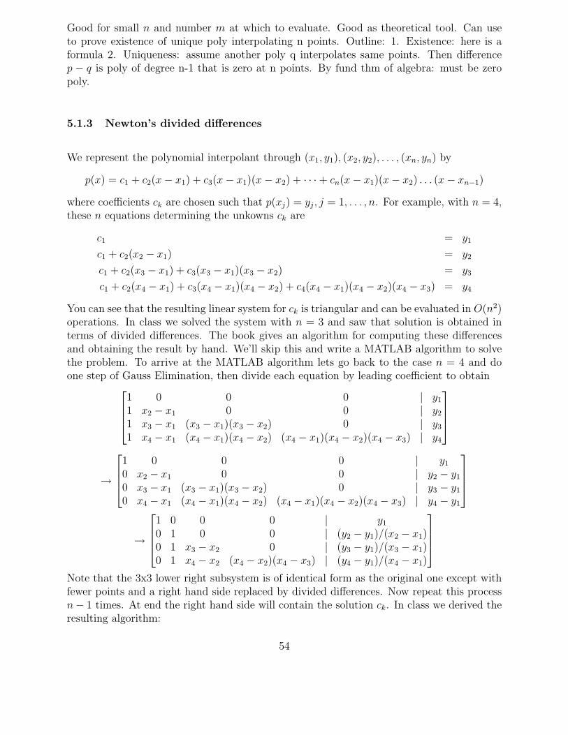
We represent the polynomial interpolant through (x1, y1), (x2, y2), . . . , (xn, yn) by

p(x) = c1 + c2(x − x1) + c3(x − x1)(x − x2) + · · · + cn(x − x1)(x − x2) . . . (x − xn−1)

where coefficients ck are chosen such that p(xj) = yj, j = 1, . . . , n. For example, with n = 4,these n equations determining the unkowns ck are

c1 = y1

c1 + c2(x2 − x1) = y2

c1 + c2(x3 − x1) + c3(x3 − x1)(x3 − x2) = y3

c1 + c2(x4 − x1) + c3(x4 − x1)(x4 − x2) + c4(x4 − x1)(x4 − x2)(x4 − x3) = y4

You can see that the resulting linear system for ck is triangular and can be evaluated in O(n2)operations. In class we solved the system with n = 3 and saw that solution is obtained interms of divided differences. The book gives an algorithm for computing these differencesand obtaining the result by hand. We’ll skip this and write a MATLAB algorithm to solvethe problem. To arrive at the MATLAB algorithm lets go back to the case n = 4 and doone step of Gauss Elimination, then divide each equation by leading coefficient to obtain

1 0 0 0 | y1

1 x2 − x1 0 0 | y2

1 x3 − x1 (x3 − x1)(x3 − x2) 0 | y3

1 x4 − x1 (x4 − x1)(x4 − x2) (x4 − x1)(x4 − x2)(x4 − x3) | y4

→

1 0 0 0 | y1

0 x2 − x1 0 0 | y2 − y1

0 x3 − x1 (x3 − x1)(x3 − x2) 0 | y3 − y1

0 x4 − x1 (x4 − x1)(x4 − x2) (x4 − x1)(x4 − x2)(x4 − x3) | y4 − y1

→

1 0 0 0 | y1

0 1 0 0 | (y2 − y1)/(x2 − x1)0 1 x3 − x2 0 | (y3 − y1)/(x3 − x1)0 1 x4 − x2 (x4 − x2)(x4 − x3) | (y4 − y1)/(x4 − x1)

Note that the 3x3 lower right subsystem is of identical form as the original one except withfewer points and a right hand side replaced by divided differences. Now repeat this processn− 1 times. At end the right hand side will contain the solution ck. In class we derived theresulting algorithm:

54

function c=interpnew(x,y)

n=length(x);

for k=1:n-1

y(k+1:n)=(y(k+1:n)-y(k))./(x(k+1:n)-x(k));

end

c=y;

So, coefficients can be obtained in O(n2) flops. (how many exactly?) Another advantage ofthis approach is that the polynomials in Newton representation can be evaluated in O(n)flops using a nested algorithm similar to the one for monomials. Write out Horner’s rule forthe Newton polynomial with n = 5. Deduce the following algorithm:

function p=evalpnew(c,xx,x)

n=length(c);

p=c(n)*ones(size(x));

for k=n-1:-1:1

p=p.*(x-xx(k))+c(k);

end

Pros: 1. O(n2) algorithm to find ck (faster than Vandermonde approach)2. O(n) nested algorithm to evaluate polynomial

Cons: condition numbers still large

Example: Use above to find interpolant through (0, 0), (1, 1), (3,−1), (4,−1). Plot polyno-mial on x ∈ [0, 5] using a fine mesh.

5.2 Accuracy of Polynomial interpolation

Here we get to the second question: How good is the polynomial interpolant? Suppose thepoints (xj, yj), j = 1, . . . , n satisfy yj = f(xj), where f may or may not be known a priori.Now you interpolate them by a polynomial pn(x), as discussed in previous section. Thispolynomial equals f at the gridpoints. But how close is it to f away from the gridpoints??

That is, how well does the p(x) approximate f(x) for all x? So we want to know somethingabout the maximum error difference between f and pn at any given point x.

Theorem: If pn is the (unique) polynomial of degree n − 1 that interpolates f at xj,j = 1, . . . , n (that is, f(xj) = p(xj)) then

f(x) − pn(x) =(x − x1)(x − x2) . . . (x − xn)

n!f (n)(c)

55

for some c ∈ (x1, xn) (assuming the xjs are in increasing order).

There are a few items to deduce from this

• If we know an upper bound |f (n)(x)| ≤ Mn for all x ∈ (x1, xn), then we know a boundfor the error

|f(x) − pn(x)| =Mn

n!|(x − x1)(x − x2) . . . (x − xn)|

• The error is a product of a terms that depend solely on the points xk, and a term thatdepends solely on the derivative of f .

• If we can choose the points xk, we can find the best polynomial pn for any given f , byfinding the points xk that minimize the maximum of

|(x − x1)(x − x2) . . . (x − xn)|

Example: Investigate the error graphically for f(x) = 11+25x2 for x ∈ [−1, 1], using n

uniformly spaced points. Plot f , f ′, f ′′. Plot (x − x1) . . . (x − xn), compare to f − pn.

5.2.1 Uniform points vs Tschebischeff points

Theorem: The set of points x1, . . . , xn that minimizes the maximum of |(x − x1)(x −x2) . . . (x − xn)| are the Tschebischeff points

xj = cos

(π(2j − 1)

2n

), j = 1, . . . , n

Note that the argument of the cosine is odd multiples 1, 3, . . . , (2n−1) of π/(2n), so it rangesfrom just a little above 0 to just below π. Therefore the xj range from just below 1 to justabove -1. Visualize the points as in book, by plotting semi-circle and marking x-coordinatesof points on semicircle at equally spaced arclength. Alternatively, figure (4) plots the cosvalues at equal spaced arguments, showing that they buch up at ±1. For an interval [a,b],the corresponding points would be

xj =a + b

2+

b − a

2cos

(π(2j − 1)

2n

), j = 1, . . . , n

[Side note : The way to prove this theorem requires properties of the Tschebyscheff (orChebichev) polynomials

Tn(x) = cos(n arccos x)

Pafnuti Lwowitsch Tschebyschow was an important Russian Mathematician in the 19thcenture, 1821-1894. Some of the properties of Tn: Tn(x) is the unique polynomial of degree

56

ππ/20x

−1

y

1

y=cos(x)

Figure 4: Image of equally spaced points under cosine map, showing how they bunch upnear ±1. These are the Tschebischeff points.

n that satisfies Tn(xj) = 0, where xj j = 1, . . . , n, are the Tschebyscheff points given above,and Tn(1) = 1. The fact that it is a polynomial of degree n follows from the recurrencerelation

Tn+1(x) = 2xTn(x) − Tn−1(x)

which can be deduced using trigonometric identities. Its values at xj and at 1 can be foundby inspections. The leading coefficient of xn is 2(n−1), which also follows from the recursiveformula. It thus follows that

Tn(x) = 2n−1(x − x1)(x − x2) . . . (x − xn) .

Finish side note.]

Example: Investigate the error f(x)− pn(x) graphically, for f(x) = 11+25x2 and x ∈ [−1, 1],

using n Tschebischeff points.

One can show that

• With equally spaced points, |(x − x1)(x − x2) . . . (x − xn)| ≤ (b − a)n (n − 1)!

(n − 1)n

(Does this term grow or decrease as n → ∞?)

• With Tschebischeff points, |(x − x1)(x − x2) . . . (x − xn)| ≤(

b − a

2

)n1

2n−1

(Does this term decrease any faster as n → ∞?)

57

5.3 Piecewise Polynomial interpolants

Here we discuss a different approach. Suppose we are given n points (xj, yj), j = 1, . . . , n,and we want to find an interpolant through the points. Instead of finding one function thatinterpolates all n points, we find a function on each interval that interpolates two consecutivepoints, with some matching conditions connecting the pieces from one interval to the next.The result is a piecewise interpolant

g(x) =

S1(x) , x1 ≤ x < x2

S2(x) , x2 ≤ x < x3...Sn−1(x) , xn−1 ≤ x < xn

5.3.1 Piecewise linear interpolant

The simplest case is when each Sj(x) is a linear function interpolating (xj, yj) and (xj+1, yj+1).This is what MATLAB plots when you type plot(x,y). That is,

Sj(x) = aj + bj(x − xj) , x ∈ [xj, xj+1]

where the two unknowns aj, bj are determined by the two conditions S(xj) = yj, S(xj+1) =yj+1.

5.3.2 Cubic splines

A cubic spline interpolant of the data (xj, yj), j = 1, . . . , n is a piecewise cubic functiondefined by

Sj(x) = aj + bj(x − xj) + cj(x − xj)2 + dj(x − xj)

3 , x ∈ [xj, xj+1] , j = 1, . . . , n − 1

such that

(0) Sj(xj) = yj j = 1, . . . , n − 1

(1) Sj(xj+1) = yj+1 j = 1, . . . , n − 1

(2) S ′j(xj+1) = S ′

j+1(xj+1) j = 1, . . . , n − 2

(3) S ′′j (xj+1) = S ′′

j+1(xj+1) j = 1, . . . , n − 2

Conditions (0),(1) ensure that the polynomials interpolate the data, while conditions (2),(3)enforce continuity of g′, g′′ at the interior data points, thereby ensuring that the interpolantg is not only continuous, but has continuous slope and curvature. This leads to a smooth-looking curve to the eye.

58

Condition (0) is trivially satisfied by setting aj = yj, leaving us with 3n − 3 unknownsbj, cj, dj, j = 1, . . . , n − 1. Conditions (1)-(3) give 3n − 5 equations, so that we still need2 more equations to uniquely solve for the 3n − 3 unknowns. Different conditions can bechosen. The natural spline consists of specifying zero curvature at the endpoints.

(4a) S ′′1 (x1) = 0

(4b) S ′′n−1(xn) = 0

The clamped spline consists of prescribing the derivatives at the endpoints.

(4a′) S ′1(x1) = α

(4b′) S ′n−1(xn) = β

The not-a-knot spline consists of prescribing continuous third derivative at the two interiorpoints closest to the end.

(4a”) S ′′′1 (x2) = S ′′′

2 (x2)

(4b”) S ′′′n−2(xn−1) = S ′′′

n−1(xn−1)

We now derive the equations for the coefficients of the natural spline. First, note that

Sj(x) = aj + bj(x − xj) + cj(x − xj)2 + dj(x − xj)

3

S ′j(x) = bj + 2cj(x − xj) + 3dj(x − xj)

2

S ′′j (x) = 2cj + 6dj(x − xj)

Conditions (1)-(3) are

(1) bj∆xj + cj∆x2j + dj∆x3

j = ∆yj j = 1, . . . , n − 1

(2) bj + 2cj∆xj + 3dj∆x2j = bj+1 j = 1, . . . , n − 2

(3) 2cj + 6dj∆xj = 2cj+1 j = 1, . . . , n − 2

where ∆xj = xj+1 − xj, ∆yj = yj+1 − yj. The goal now is to do some algebra by hand tocome up with a system of less unknowns that we then solve numerically. First, we introducea new variable cn = S ′′

n−1(xn)/2. As we showed in class, it follows that condition (3) aboveholds for j = 1, . . . , n − 1. Furthermore, conditions (4ab) can be simply stated as

(4a′) c0 = 0

(4b′) cn = 0

We now solve (3) for dj, to get dj in terms of cjs:

(3′) dj =cj+1 − cj

3∆xj

j = 1, . . . , n − 1

59

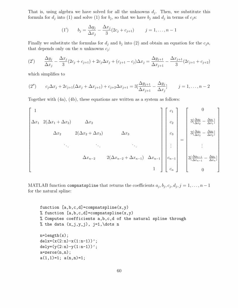
That is, using algebra we have solved for all the unknowns dj. Then, we substitute thisformula for dj into (1) and solve (1) for bj, so that we have bj and dj in terms of cjs:

(1′) bj =∆yj

∆xj

− ∆xj

3(2cj + cj+1) j = 1, . . . , n − 1

Finally we substitute the formulas for dj and bj into (2) and obtain an equation for the cjs,that depends only on the n unknowns cj:

(2′)∆yj

∆xj

− ∆xj

3(2cj + cj+1) + 2cj∆xj + (cj+1 − cj)∆xj =

∆yj+1

∆xj+1

− ∆xj+1

3(2cj+1 + cj+2)

which simplifies to

(2′′) cj∆xj + 2cj+1(∆xj + ∆xj+1) + cj+2∆xj+1 = 3[∆yj+1

∆xj+1

− ∆yj

∆xj

] j = 1, . . . , n − 2

Together with (4a), (4b), these equations are written as a system as follows:

1

∆x1 2(∆x1 + ∆x2) ∆x2

∆x2 2(∆x2 + ∆x3) ∆x3

. . . . . . . . .

∆xn−2 2(∆xn−2 + ∆xn−1) ∆xn−1

1

c1

c2

c3

...

cn−1

cn

=

0

3[∆y2

∆x2− ∆y1

∆x1]

3[∆y3

∆x3− ∆y2

∆x2]

...

3[∆yn−1

∆xn−1− ∆yn

∆xn]

0

MATLAB function compnatspline that returns the coefficients aj, bj, cj, dj, j = 1, . . . , n− 1for the natural spline:

function [a,b,c,d]=compnatspline(x,y)

% function [a,b,c,d]=compnatspline(x,y)

% Computes coefficients a,b,c,d of the natural spline through

% the data (x_j,y_j), j=1,\dots n

n=length(x);

delx=(x(2:n)-x(1:n-1))’;

dely=(y(2:n)-y(1:n-1))’;

a=zeros(n,n);

a(1,1)=1; a(n,n)=1;

60

r(1)=0; r(n)=0;

for row=2:n-1;

r(row)=3*(dely(row)/delx(row)-dely(row-1)/delx(row-1));

a(row,row-1)=delx(row-1);

a(row,row)=2*(delx(row-1)+delx(row));

a(row,row+1)=delx(row);

end

c=a\r’;

clear a

b(1:n-1)=dely./delx -delx/3.*(2*c(1:n-1)+c(2:n));

d(1:n-1)=(c(2:n)-c(1:n-1))./(3*delx(1:n-1));

a(1:n-1)=y(1:n-1);

c=c(1:n-1);

MATLAB function that plots the spline as well as the data using m points on each of then − 1 intervals [xj, xj+1], j = 1, n − 1, using Horner’s nested polynomial evaluation:

function plotspline(a,b,c,d,x,y,m)

% function plotspline(a,b,c,d,x,m)

% plots m points of spline through x_k, coeff a,b,c,d, on each

% interval

plot(x,y,’*r’)

hold on

n=length(x);

for j=1:n-1;

z=linspace(x(j),x(j+1),m)

arg=z-x(j);

y=a(j)+arg.*(b(j)+arg.*(c(j)+arg*d(j)));

plot(z,y)

end

hold off

Script that plots the 6 points (0, 3), (1, 1), (2, 4), (3, 1), (4, 2), (5, 0) and the cubic naturalspline on a fine mesh that has 10 points on each subinterval:

x=0:5; y=[3 1 4 1 2 0];

[a,b,c,d]=compnatspline(x,y);

plotspline(a,b,c,d,x,y,10)

61

5.4 Trigonometric interpolants

What if the data is viewed to be periodic? Then we want to use periodic basis functions(cos kx, sin kx). It turns out that this periodic interpolation works well if the data is uni-formly spaced in x, and the periodic extension of the data is smooth. (Note: any set of datamay be viewed to be periodic. The only problem is that the periodic extension may notcorrespond to a smooth function.)

For what follows, the total number of points n must be even.

So, let’s consider n points (xj, yj), j = 0, . . . , n − 1, where the xj are uniformly distributedin an interval [0, T ], n is even, and the yj correspond to a periodic function with period T .To begin with, we will assume T = 2π. That is, we are given data (xj, yj)

xj = j2π

n, yj = f(xj) , j = 0, . . . , n − 1

where f(x+2π) = f(x). Then it is natural to fit data using periodic basis functions, such as1, cos kx, sin kx. Note that these functions have period T = 2π with k oscillations per period.We call k the wavenumber and k/T the oscillation frequency (number of oscillationsper unit time). The oscillation period is T/k.

5.4.1 Using a basis of sines and cosines

As we did in §4.1 (and unlike the splines in §4.3) we will try to fit all the data using onelinear combination of n basis functions. Here we use the basis

1, cos x, cos 2x, . . . , cosn

2x, sin x, sin 2x, . . . , sin(

n

2− 1)x .

(The next sine mode, sin n2x, is zero at the gridpoints, and thus is no different from the zero

function and makes no contribution on the grid. Hence, no loss by excluding it, no gain fromincluding it.) Thus we want to approximate f(x) by a trigonometric polynomial

g(x) =

n/2∑

k=0

ak cos(kx) +

n/2−1∑

k=1

bk sin(kx) (12)

where the n coefficients ak, bk as chosen such that g(xj) = f(xj).

5.4.2 Using a basis of complex exponentials

Note that we can write cos kx and sin kx in terms of complex exponential functions eikx usingEuler’s formula

cos(kx) =eikx + e−ikx

2, sin(kx) =

eikx − e−ikx

2i

62

and similarly, we can write eikx in terms of sines and cosines

eikx = cos(kx) + i sin(kx) .

Hence, at the gridpoints, the basis of n sines and cosines is equivalent to the basis of nexponentials

eikx , k = −n/2, . . . , n/2 − 1

It turns out to be slightly more direct to use this basis for our trigonometric polynomials.So, instead of finding g as in (12) we will find

T (x) =

n/2−1∑

k=−n/2

ckeikx

such that T (xj) = f(xj), j = 0, . . . , n − 1. These n equations determine the n coefficientsck, which are called the Fourier coefficients.

In class we show that at the gridpoints we can rewrite T (xj) (using the change of summationindex l = k + n for one part of the sum) as

T (xj) =

n/2−1∑

k=−n/2

ckeikxj =

−1∑

k=−n/2

ckeikj2π/n +

n/2∑

k=0

ckeikj2π/n

=n−1∑

l=n/2

cl−nei(l−n)j2π/n +

n/2∑

k=0

ckeikj2π/n =

n−1∑

l=n/2

cl−neilj2π/ne−ij2π +

n/2∑

k=0

ckeikxj

=n−1∑

l=n/2

cleilj2π/n +

n/2∑

k=0

ckeikj2π/n =

n−1∑

k=n/2

ckeikj2π/n +

n/2∑

k=0

ckeikj2π/n

=n−1∑

k=0

ckeikxj

provided the coefficients are taken to be periodic, cl−n = cl, any l. In that case the equationsT (xj) = f(xj), or

fj =n−1∑

k=0

cke2πikj/n , j = 0, . . . , n − 1

where fj = f(xj), can be written as Fc = f where F = F (ω) is the Fourier matrix, given interms of nth unit root ω = e2πi/n as

F =

1 1 1 . . . 1 11 ω ω2 ω3 . . . ωn−1

1 ω2 ω4 ω6 . . . ω2(n−1)

......

... . . ....

1 ω(n−1) ω2(n−1) ω3(n−1) . . . ω(n−1)2

63

This matrix is invertible. It is easy to check that

F−1 =1

NF (ω−1) . =

1 1 1 . . . 1 11 ω−1 ω−2 ω−2 . . . ω−(n−1)

1 ω−2 ω−4 ω−6 . . . ω−2(n−1)

......

... . . ....

1 ω−(n−1) ω−2(n−1) ω3(n−1) . . . ω−(n−1)2

(13)

As a result we get a formula for the coefficients c = F−1f , or

cj =1

N

n−1∑

k=0

fke−2πikj/n , j = 0, . . . , n − 1

which also shows that they are indeed periodic (check that cj+n = cj).

The process of computing the Fourier coefficients from given values of fk is called the Fouriertransform and consists of evaluating a sum of the given form. The process of computingthe values fk from the coefficients ck is called the inverse Fourier transform and consistsof evaluating a very similar sum, where the negative sign in the exponent is replaced by aplus.

5.4.3 Using MATLABs fft and ifft

MATLABs functions fft and ifft compute these sums in a fast way using the Fast FourierTransform, which evaluates the sums in O(n log n) instead of O(n2) operations. We read theonline documentation to check this. In particular, fft(f,n) returns the vector of length nwith entries

∑n−1k=0 fke

−2πijk/n , j = 0, . . . , n− 1. That is, it returns the Fourier coefficientsup to a factor of 1/n.

To illustrate: Let f(x) = sin 3x =ei3x − e−i3x

2i. It has

c3 =1

2i, c−3 = cN−3 = − 1

2i, cj = 0 for j 6= ±3

The following matlab script computes the Fourier coefficients using N = 64 points. It thenplots both the function (sampled at the 64 points) and the absolute value of the Fouriercoefficients. You may want to print c(4) and c(62) to make sure they are the correctvalues. (Why 4 and 62 instead of 3 and -3 or 61?)

clear;clf % clear all data and the figure

n=64; % set n

x=[0:n-1]*2*pi/n; y=sin(3*x); % set x and y at gridpoints

c=fft(y,n)/n; % remember, need to divide by N

64

axis([0,2*pi,-2,2]); ylabel(’ f_j’)

plot(0:n-1,abs(c))

axis([0,n-1,-0.1,0.6]); ylabel(’abs(c_j)’)

We did this for various examples in class.

Examples: Look at ck and plot |ck| for: f(x) = 1, sin x, cos 8x, cos2 x, 1/(1 + sin2 x), x usingN = 64.

What happens when data is not periodic? Answer: decay rate of coefficients says somethingabout the smoothness of the periodic extension of the function f .

To plot the trigonometric interpolant T (x) =∑n/2−1

k=−n/2 ckeikx (on a fine mesh in between grid-

points) we need to correlate the Fourier coefficients MATLAB returns with indeces 1, . . . , nto the actual power in the exponential given by k = −n/2, . . . , n/2− 1. This can be done inMATLAB by specifying the correct mode k corresponding to a given MATLAB coefficient.For example, the coefficient indexed by 1 corresponds to mode k = 0, the coefficient indexedby n/2 corresponds to mode k = n/2 − 1, the coefficient indexed by n/2+1 corresponds tomode k = −n/2, the coefficient indexed by n corresponds to mode k = −1:

function trigplot(x,y,m)

%function trigplot(x,y,m)

%plots trigonometric interpolant of data x,y

%assumed to have period 2pi, on [-pi,3pi]

%using m points per interval [x_i,x_{i+1}]

n=length(x);

c=fft(y,n)/n;

k(1:n/2)=0:(n/2-1);

k(n/2+1:n)=-n/2:-1;

z=linspace(-pi,3*pi,2*m*n);

T=c(1)*ones(size(z));

for ind=2:n;

T = T+c(ind)*exp(j*k(ind)*z);

end

plot(x,y,’r*’,z,real(T),’-’)

Example: Plot |ck|, f and interpolant, for sin 4x, n = 6, 8, 10, 16. (See fig 5.4.3)

Example: Plot |ck|, f and interpolant, for f(x) = 1/(1 + sin2 x), n = 4, 8, 16, 32. (See fig5.4.3)

Example: Plot |ck|, f and interpolant, for f(x) = x, n = 8, 16, 32, 64. (See fig 5.4.3)

65

−2 0 2 4 6 8

−1

−0.5

0

0.5

1

y j, T(x

), f(

x)

x

n= 16

−2 0 2 4 6 8

−1

−0.5

0

0.5

1

x

n= 10

−2 0 2 4 6 8

−1

−0.5

0

0.5

1

x

n= 8

−2 0 2 4 6 8

−1

−0.5

0

0.5

1

x

n= 6

0 5 10 15

0

0.2

0.4

abs(

c j)

j0 2 4 6 8

0

0.2

0.4

j0 2 4 6

0

0.2

0.4

j0 1 2 3 4 5

0

0.2

0.4

j

Figure 5: Coefficients |ck|, function f , data, and interpolant, for sin 4x, n = 16, 10, 8, 6. Thisfunction has only one sine mode k = 8. Here we see, first that if n/2 > k the function isidentical to the trigonometric interpolant, since the interpolant captures all of the functionsnonzero modes. However, if n/2 ≤ k then the kth mode is undersampled and it showsup as a lower order Fourier coefficients. This is called aliasing error and occurs when afunction has modes bigger than n/2 that are not resolved by the mesh of n points. Thesemodes show up as lower order Fourier coefficients!

−2 0 2 4 6 80.4

0.5

0.6

0.7

0.8

0.9

1

1.1

y j, T(x

), f(

x)

x

n= 4

−2 0 2 4 6 80.4

0.6

0.8

1

x

n= 8

−2 0 2 4 6 80.4

0.6

0.8

1

x

n= 16

−2 0 2 4 6 80.4

0.6

0.8

1

x

n= 32

0 0.5 1 1.5 2 2.5 310

−1

100

abs(

c j)

j0 2 4 6

10−2

10−1

100

j0 5 10 15

10−4

10−3

10−2

10−1

100

j0 10 20 30

10−6

10−4

10−2

100

j

Figure 6: Coefficients |ck|, data, function f and interpolant, for f(x) = 1/(1 + sin2 x), n =8, 16, 32, 64. In this example the function is not represented exactly by a finite trigonometricpolynomial since the exact function has infinitely many modes. However the trigonometricinterpolants are increasingly better approximations as the number of points n increases.

66

−2 0 2 4 6 8

0

2

4

6

y j, T(x

), f(

x)

x

n= 4

−2 0 2 4 6 8

0

2

4

6

x

n= 8

−2 0 2 4 6 8

0

2

4

6

x

n= 16

−2 0 2 4 6 8

0

2

4

6

x

n= 32

0 0.5 1 1.5 2 2.5 310

−1

100

101

abs(

c j)

j0 1 2 3 4 5 6 7

10−1

100

101

j0 5 10 15

10−1

100

101

j0 5 10 15 20 25 30

10−1

100

101

j

Figure 7: Coefficients |ck|, data, function f and interpolant, for f(x) = x, n = 8, 16, 32, 64.In this example the periodic extension of f is discontinuous. As a result the coefficientdecay very slowly and the trigonometric interpolant contains oscillations near the jump thatdo not disappear as n increases. This phenomenon is called Gibbs phenomena. Gibbsshowed that the oscillations do not disappear as n → ∞ and found the precise size of theoscillations in this limit. So if the function is discontinuous then the trig interpolant is nota good approximation of the function near jump.

Example: (homework) Plot |ck| for f(x) = 1/(1 + sin2 x), N = 8, 64. Plot |ck| for hatfunction. Plot |ck| for f(x) = x. Compare decay rates of coefficients. Note that the smootherthe funtion, the faster the decay rate as k increases.

Example: Plot polynomial interpolant and trig interpolant on uniform (periodic) data. (SeeFigure 8

67

−1

−0.5

0

0.5

1

1.5

2

y

n= 4

−1 −0.5 0 0.5 1−1

−0.5

0

0.5

1

1.5

2

x

y

n= 8

−1 −0.5 0 0.5 1x

n= 16

−1 −0.5 0 0.5 1x

Figure 8: Function f(x) = 1/(1 + 25 sin2 x) (red) sampled at n equally spaced points (bluestars), and the polynomial interpolant (top row, in blue), and trigonometric interpolant(bottom row, in blue). Note: if periodic extension of f smooth, then as n increases triginterpolants are increasingly good approximations of f , whereas poly interpolant shows rungephenomena.

Time permitting: Prove that F−1 is as listed.

Summary:

• Isolated modes k < n/2 are recovered exactly by trig interpolant.

• Modes k > n/2 show up as lower order modes in trig interpolant and contaminate lowmodes, ⇒ aliasing error

• The smoothness of the periodic extension of f is reflected in the decay rate of theFourier modes.

• If the periodic extension of f is discontinuous, the coefficients decay slowly and theinterpolant is oscillatory near discontinuity.

• For large n, trig interpolants good for uniform points if periodic extension of f issmooth.

• For large n, polynomial interpolants bad for uniform points (Runge phenomena), butgood for Tschebichef points.

68

5.4.4 What if period τ 6= 2π?

Then need basis functions with period τ , such as

sin(k?x), cos(k?x), eik?x

So then find a trig interpolant of the form

T (x) =

n/2−1∑

k=−n/2

ckeik?x

and xj =?, j = 0, . . . , n − 1 (they must be equally spaced in [0, τ ]) such that

T (xj) = yj

What do these equations look like? What is the resulting linear system for cj? What changesbetween this case and the case τ = 2π we already discussed?

5.4.5 Music and Compression

Examples shown in class illustrate the following main points.

• We hear oscillatory pressure waves in the air hitting our ear. An oscillation of a givenfrequency corresponds to a clean tone. Frequency of 440 Hz (number of oscillation persecond) corresponds to a pure A. An A an octave higher would be at 880 Hz.

• Usually what we hear is a sum of various frequencies. Compare pure tone A and tuningfork, which is much richer with many frequencies accompanying the dominant one.

• The component at a certain frequency is captured by the Fourier coefficient for thatwavenumber. Its magnitude is typically measured in decibels, wich equals the logarithmof the magnitude relative to some basemeasure.

• For compression, we want to capture the dominant frequency content in a small timeinterval and represent it by as few coefficients as possible.

• How do we isolate a small time interval? Chopping it off (multiplying by hat function)introduces large high mode frequencies corresponding to discontinuous functions thatcant be ignored (the reconstruction would not sound like the origingal if not ignored).Thus not good compression.

• Sudden onset of sound (such in castanets) have similar problem. Exact fourier spec-trum has many large modes, and simply ignoring them distorts reconstruction signif-icantly. Again, we need to isolate a small time interval. (This is a classic testcase forcompression algorithms: if they reconstruct this signal well, then pretty good.)

69

• Multiplying by a smooth function that goes from 0 to 1 and back to zero gives you arelatively nice /compact fourier mode spectrum, but is not invertible (cannot recoversignal from these modes since basis not orthogonal)

• There is a “modified cosine transform” that does the trick. Wavelets are an alternativebut not used for sound, bur rather to compress images.

70

6 Least Squares Solutions to Ax = b

Example: The systems

1 11 −11 1

[xy

]=

213

,

[1 11 1

] [xy

]=

[21

], (14)

obviously don’t have a solution. Yet Matlab gives a solution to the first. What is it? It doesnot give solution to second. Why not?

6.1 Least squares solution to Ax = b

If An×mxm×1 = bn×1 has no solution, then the vector b is not in the set of all Ax, for anyx. What does the set of all possible Ax look like?

Note thatAx = a1x1 + a2x2 + · · · + anxn ∈ ℜn

where aj are the columns of A. So the set of all possible Ax is the set of all linear combinationsof the columns of A. Called the Span of A.

Definition: span(A) = {Ax : all x ∈ ℜm} ⊆ ℜn Note:

• The span of A is a vector space (contains origin, and any linear combination of vectorsin this space is in the space).

• It is contained in ℜn, and may be equal to ℜn (if the columns contain a linearlyindependent set of n vectors) or be a proper subspace of ℜn.

• If span(A) is a proper subspace of ℜn, span(A) ⊂ ℜn, then there are right hand sidesb ∈ ℜn which are not in the span(A) and for those right hand sides Ax = b has nosolution. (There are also right hand sides in the span for which the equation has asolution.) This scenario (span is proper subset) is illustrated geometrically in figure 9.For illustration, we depict the span as a 2-dimensional subspace (a plane) of the biggerspace ℜ3.

Definition: If b /∈ span(A), the least squares solution of Ax = b is defined to be thevector x ∈ ℜm such that ||Ax − b||2 is minimal. Here ||y||2 =

√∑mi=1 y2

i . The value of Axis illustrated in figure 10.

71

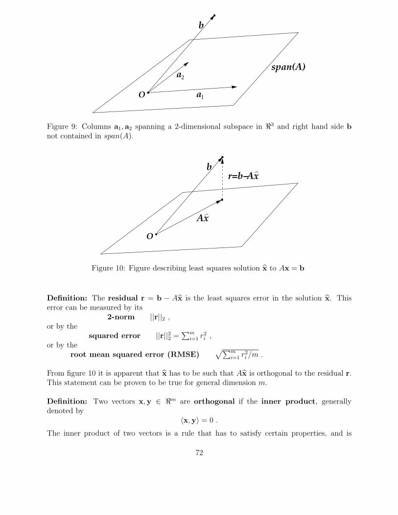
a1

a2

O

b

span(A)

Figure 9: Columns a1, a2 spanning a 2-dimensional subspace in ℜ3 and right hand side bnot contained in span(A).

Ax

Ax

O

br=b−

Figure 10: Figure describing least squares solution x to Ax = b

Definition: The residual r = b − Ax is the least squares error in the solution x. Thiserror can be measured by its

2-norm ||r||2 ,or by the

squared error ||r||22 =∑m

i=1 r2i ,

or by theroot mean squared error (RMSE)

√∑mi=1 r2

i /m .

From figure 10 it is apparent that x has to be such that Ax is orthogonal to the residual r.This statement can be proven to be true for general dimension m.

Definition: Two vectors x,y ∈ ℜm are orthogonal if the inner product, generallydenoted by

〈x,y〉 = 0 .

The inner product of two vectors is a rule that has to satisfy certain properties, and is

72

corresponds to an associated vector norm. We have already seen that there are manynorms. Since we are trying to minimize the 2-norm of the residual, this is the norm ofinterest here, and the corresponding inner product is the one you already know well

〈x,y〉 = xTy =m∑

i=1

xiyi

If two vectors x,y are orthogonal this is often denoted by x ⊥ y.

How do we find the least squares solution x? The solution x for which ||b − Ax||2is minimal satifies that the residual is normal to any vector in span(A). That is, for anyx ∈ ℜn

Ax ⊥ (b − Ax)

⇒ (Ax)T (b − Ax) = 0

⇒ xT AT (b − Ax) = 0

(Here we used the property that for any two commensurate matrices A,B, (AB)T = BT AT .)Since this must hold for all x ∈ ℜn, it follows that the n × 1 vector

AT (b − Ax) = 0

This yields the normal equations

AT Ax = ATb

Thus, the least squares solution x solves the normal equations.

Do the normal equations always have a solution? Yes, by construction. However,they can have multiple solutions. (In the latter case, we define the least squares solution tobe the one with smallest 2-norm ||x||2.)

Examples: Find the least squares solutions to the systems

1 11 −11 1

[xy

]=

213

,

[1 11 1

] [xy

]=

[21

], (15)

by setting up and solving the normal equations. (Solve them using Gauss Elimination andback substitution.) What is the 2-norm of the residual? What is the RSME? Can we nowanswer the questions we posed at the beginning of this chapter?

Problem with the normal equations: AT A usually has much larger condition numberthan A. Therefore solving the normal equations is often ill-posed. This problem is remediedif we use the QR factorization of a matrix, discussed in Section 4.xx.

73

6.2 Approximating data by model functions

6.2.1 Linear least squares approximation

Problem statement: Given data {xi, yi}ni=1, find the linear function f(x) = a + bx that

minimizes the least squares errorn∑

i=1

(yi − f(xi))2

This function is called the linear least squares approximation to the data.

• Draw sketch showing points and least squares line (graph of y = f(x)). (See Figure4.2 on page 198 of text.)

• Set up equations we’d like to solve a + bxi = yi, i = 1, . . . , n. Write them in matrixform. Note: the unknowns are c = (a, b).

• Find the least squares solution to the resulting system Ac = y. Note that this is thesolution that we want since it minimizes ||y−Ac||2, and Ac is the vector with entriesf(xi).

Example: Find the linear least squares approximation to (−1, 1), (0, 0), (1, 0), (2,−2). Graphin matlab. Find 2-norm of error.

Note: the approach described in this section works because the resulting system is linearin the unknowns a, b. We can use the same approach for slightly different problems, threeexamples of which will be given next. For another example, see bottom of page 214 - 215 inSauer.

6.2.2 Quadratic least squares approximation

Problem statement: Given data {xi, yi}ni=1, find the quadratic function f(x) = a+bx+cx2

that minimizes the least squares error∑n

i=1(yi−f(xi))2 This function is called the quadratic

least squares approximation to the data.

• Draw sketch showing points and least squares parabola (graph of y = f(x)). (SeeFigure 4.4 on page 201 of text.)

• Set up equations we’d like to solve a + bxi + cx2i = yi, i = 1, . . . , n. Write them in

matrix form. Note: the unknowns are c = (a, b, c).

74

• Find the least squares solution to the resulting system Ac = y. Note that this is thesolution that we want since it minimizes ||y−Ac||2, and Ac is the vector with entriesf(xi).

Example: Find the quadratic least squares approximation to (−1, 1), (0, 0), (1, 0), (2,−2).Graph in matlab. Find 2-norm of error.

6.2.3 Approximating data by an exponential function

Problem statement: Given data {xi, yi}ni=1, find an exponential function f(x) = aebx that

best approximates the data

• Problem: the equations we’d like to solve aebxi = yi, i = 1, . . . , n. are NOT linear inthe unknowns c = (a, b).

• Fix: instead, solve ln(a) + b ln(xi) = ln(yi), i = 1, . . . , n. This system is linear in theunknowns ln(a), b. The least squares solution of this linear system minimizes the leastsquares error

∑ni=1(ln(yi) − ln(f(xi)))

2.

Example: The world automobile supply data between 1950 and 1980 is given in the followingtable (Sauer, Ex 4.8, page 211). Find the exponential function that best approximates thedata. What is the error?

year cars(×106)1950 53.051955 73.041960 98.311965 139.781970 193.481975 260.201980 320.39

6.2.4 Approximating data by an algebraic function

Problem statement: Given data {xi, yi}ni=1, find an algebraic function f(x) = axp that

best approximates the data

• Problem: the equations we’d like to solve axpi = yi, i = 1, . . . , n. are NOT linear in

the unknowns c = (a, p).

75

• Fix: instead, solve ln(a) + p ln(xi) = yi, i = 1, . . . , n. This system is linear in theunknowns ln(a), p.

Example: The mean height and weight of boys ages 2-11 collected in 2002 is given in thefollowing table. Find an exponential function that relates weight and height as W = aHp.What is the error?

age(yrs) height(m) weight(kg)2 0.9120 13.73 0.9860 15.94 1.0600 18.55 1.1300 21.36 1.1900 23.57 1.2600 27.28 1.3200 32.79 1.3800 36.010 1.4100 38.611 1.4900 43.7

6.2.5 Periodic approximations

Problem statement: Given data {xi, yi}ni=1, find a trigonometric polynomials of degree d

that best approximates the data.

Solution: Find the trigonometric interpolant of degree n − 1 that we found in section4.4, and truncate it, using only the lowest order d terms. (This turns out to be the bestapproximation in the least squares sense. This fact follows from the orthogonality of thebasis functions eikx, which is discussed in §10.3 of the book.)

Example: Apply to solve example 4.6 (Sauer, page 207), and compare with their solution.

6.3 QR Factorization

76

7 Numerical Integration (Quadrature)

7.1 Newton-Cotes Rules

This section: Given f(x), integrate interpolating polynomial using as many points as needed.

n=2 points: integrate linear interpolant using 2 points on an interval of size h. We derivedthe error

∫ x0+h

x0f(x) dx −

∫ x0+h

x0p1(x) dx = O(h3) .

n=3 points: integrate quadrating interpolant using 3 points on an interval of size 2h. Weoutlined the derivation of the error

∫ x0+2h

x0f(x) dx −

∫ x0+2h

x0p2(x) dx = O(h5) .

General results: integrate a polynomial interpolant of degree n using n+1 points on intervalof size nh. The error is

∫ x0+nh

x0

f(x) dx −∫ x0+nh

x0

p2(x) dx =

{O(hn+2) if n oddO(hn+3) if n even

These formulas are exact for polynomials of degree n if n is odd, and n+1 if n is even. Thisis called the degree of precision of the quadrature rule.

7.2 Composite Newton-Cotes Rules

Here we combine the Newton-Cotes Rules to integrate over a larger interval [a, b].

Using piecewise linear interpolants, linear on intervals of size h: get trapezoid rule witherror

∫ b

af(x) dx −

∫ b

ap(x) dx = O(h2) .

Using piecewise quadratic interpolants, quadratic on consecutive intervals of size 2h: getSimpson’s rule with error

∫ b

af(x) dx −

∫ b

ap(x) dx = O(h4) .

Using piecewise polynomial interpolant, of degree n on consecutive intervals of size nh: getcomposite Newton Cotes rule with error is

∫ b

a

f(x) dx −∫ b

a

p2(x) dx =

{O(hn+1) if n oddO(hn+2) if n even

We implemented the trapezoid rule in MATLAB and tested it using

function z = trapez(f,a,b,n)

77

% Computes trapezoid rule approximation of integral of f from a to b using n intervals

% sum_{k=0}^n w_k f(x_k) where w_k are the trapezoid weights and x_k are equally spaced

% Input: f (function name), a,b (interval of integration), n (number of subintervals)

% Output: z=sum_{k=0}^n w_k f(x_k) where w_k are the trapezoid weights

% and x_k are equally spaced points spanning [a,b]

h=(b-a)/n;

x=a+(0:n)*h; %x has n+1 elements

y=f(x);

z = (y(1)+y(n+1))/2;

for i=2:n

z = z + y(i);

end

z = z*h;

(Note: can replace loop by z=z+sum(y(2:n)).) The calling script we used to apply and testthis function is

clear

f=inline(’1./(1+x.^2)’); a=0; b=4; ex=atan(4); fpa=0; fpb=-8/17^2;

for i=1:7

n(i)=2^i;

approx=trapez(f,a,b,n(i));

err(i) = abs(approx-ex);

end

m=length(err);

ratio=err(1:m-1)./err(2:m); ratio’

h=(b-a)./n;

figure(1), set(gca,’FontSize’,20)

loglog(h,err,’*-’), xlabel(’h’), ylabel(’error’)

axis([10^(-2),10,10^(-12),1])

7.3 More on Trapezoid Rule

Euler-Mc Laurin Formula for error.

Consequence for periodic integrands. (Actually, trapezoid exact for trig polys of degree n.)

Corrected trapezoid rules.

78

Richardson extrapolation to obtain a 4th order scheme (which happens to be Simpsons).

7.4 Gauss Quadrature

The Newton-Cotes formulas we have looked at so far are of the form

∫ x0+nh

x0

f(x) dx ≈n∑

k=0

wkf(xk)

where the points xk, k = 0, . . . n are prescribed (they are equally spaced). We find n + 1weights to integrate polynomials with n + 1 coefficients (of degree n) exactly.

Gauss quadrature refers to finding quadrature rules of the form

∫ xn

x0

f(x) dx ≈n∑

k=0

wkf(xk)

where we choose the n + 1 weights wk and the n + 1 points xk to find formulas as accurateas possible. These turn out to be exact for polynomials with 2(n + 1) coefficients (of degree2n + 1). For details see section §5.5 in book.

79

x

t

Figure 11: Slopefield x′ = f(t, x) (short line segments) and some integral curves (dashed)

8 Numerical Methods for ODEs

8.1 Problem statement

Find a numerical approximation for the solution to

dx

dt= f(x, t) , x(t0) = x0 (16)

for t0 ≤ t ≤ T , where x(t) is a scalar function or a vector valued function. Notice that thisdifferential equation states the slope at any point t, x in the x-t plane. We can thus drawa slopefield or direction field as shown in the figure. The solution x(t) is everywheretangent to the slopefield (it has the given slope) and the solution curves are also calledintegral curves.

Two different solution curves dont touch, assuming f is sufficiently nice. This is the resultof a uniqueness theorem:

Theorem: If f is continuous and has continuous first derivatives ∂f/∂t,∂f/∂x, then the initial value problem (16) has a unique solution.

In class we drew direction fields for three examples: x′ = t, x′ = x, x′ = x2, all of which canbe solved exactly. The difference between the third and the other two is that in that case f isnonlinear. From exact solutions we see that slope grows so fast as x increases that solutionsblow up in finite time. This is an example why in general we cannot guarantee solutions formore than just a little neighbourhood of t0. This is the statement of the following existencetheorem:

Theorem: If f is continuous and has continuous first derivatives, then asolution to the initial value problem (16) exists in some neigh-bourhood of t0.

80

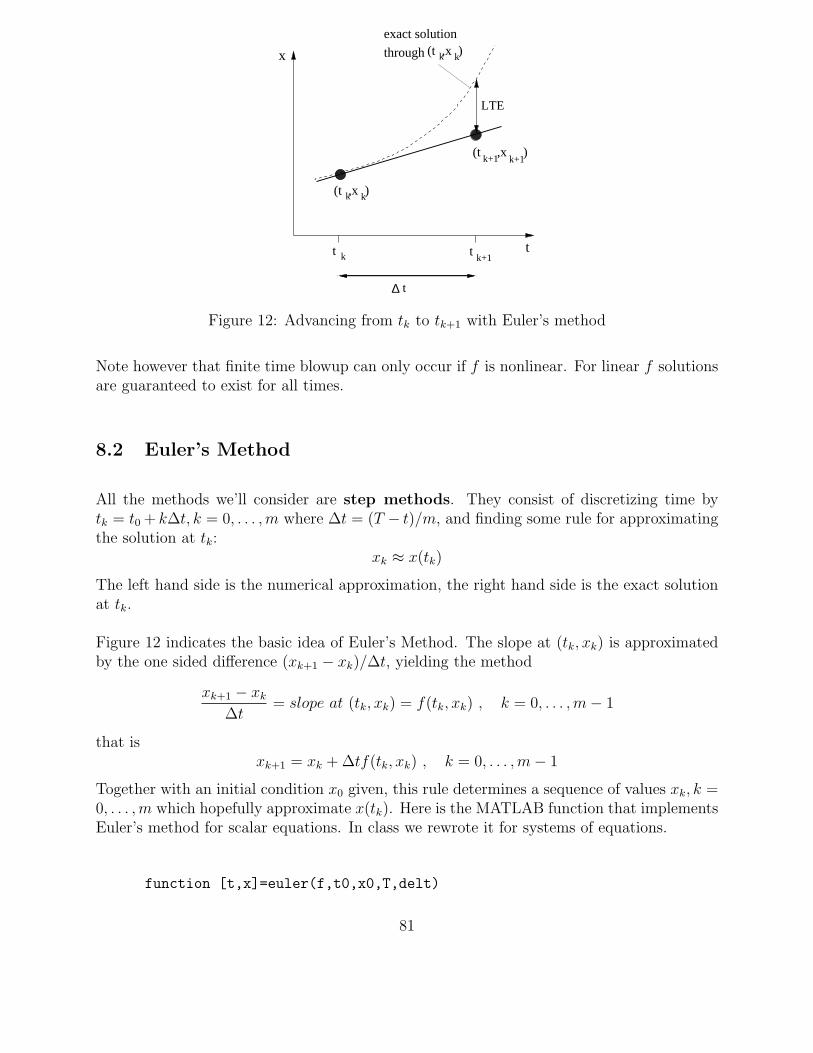
LTE

exact solution

through k k(t ,x )

k k

k+1 k+1

k+1k

x

(t ,x )

(t ,x )

t t

t∆

t

Figure 12: Advancing from tk to tk+1 with Euler’s method

Note however that finite time blowup can only occur if f is nonlinear. For linear f solutionsare guaranteed to exist for all times.

8.2 Euler’s Method

All the methods we’ll consider are step methods. They consist of discretizing time bytk = t0 + k∆t, k = 0, . . . ,m where ∆t = (T − t)/m, and finding some rule for approximatingthe solution at tk:

xk ≈ x(tk)

The left hand side is the numerical approximation, the right hand side is the exact solutionat tk.

Figure 12 indicates the basic idea of Euler’s Method. The slope at (tk, xk) is approximatedby the one sided difference (xk+1 − xk)/∆t, yielding the method

xk+1 − xk

∆t= slope at (tk, xk) = f(tk, xk) , k = 0, . . . ,m − 1

that isxk+1 = xk + ∆tf(tk, xk) , k = 0, . . . ,m − 1

Together with an initial condition x0 given, this rule determines a sequence of values xk, k =0, . . . ,m which hopefully approximate x(tk). Here is the MATLAB function that implementsEuler’s method for scalar equations. In class we rewrote it for systems of equations.

function [t,x]=euler(f,t0,x0,T,delt)

81

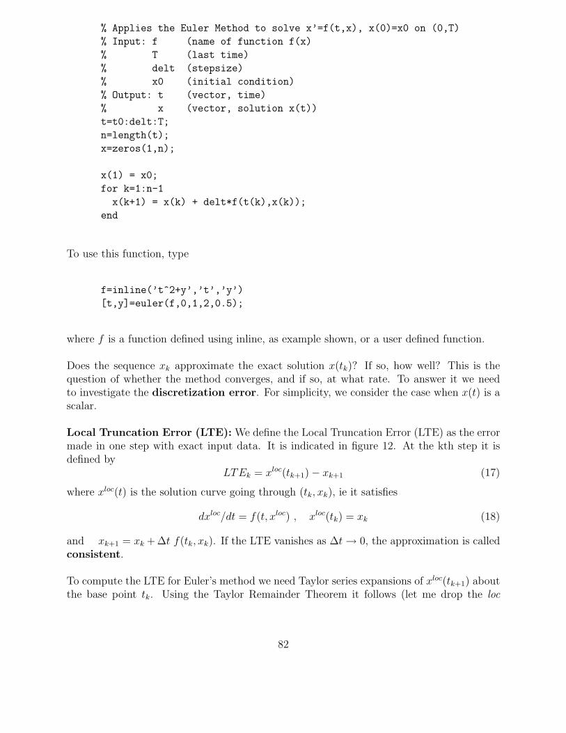
% Applies the Euler Method to solve x’=f(t,x), x(0)=x0 on (0,T)

% Input: f (name of function f(x)

% T (last time)

% delt (stepsize)

% x0 (initial condition)

% Output: t (vector, time)

% x (vector, solution x(t))

t=t0:delt:T;

n=length(t);

x=zeros(1,n);

x(1) = x0;

for k=1:n-1

x(k+1) = x(k) + delt*f(t(k),x(k));

end

To use this function, type

f=inline(’t^2+y’,’t’,’y’)

[t,y]=euler(f,0,1,2,0.5);

where f is a function defined using inline, as example shown, or a user defined function.

Does the sequence xk approximate the exact solution x(tk)? If so, how well? This is thequestion of whether the method converges, and if so, at what rate. To answer it we needto investigate the discretization error. For simplicity, we consider the case when x(t) is ascalar.

Local Truncation Error (LTE): We define the Local Truncation Error (LTE) as the errormade in one step with exact input data. It is indicated in figure 12. At the kth step it isdefined by

LTEk = xloc(tk+1) − xk+1 (17)

where xloc(t) is the solution curve going through (tk, xk), ie it satisfies

dxloc/dt = f(t, xloc) , xloc(tk) = xk (18)

and xk+1 = xk + ∆t f(tk, xk). If the LTE vanishes as ∆t → 0, the approximation is calledconsistent.

To compute the LTE for Euler’s method we need Taylor series expansions of xloc(tk+1) aboutthe base point tk. Using the Taylor Remainder Theorem it follows (let me drop the loc

82

(t ,x )0 0

(t ,x )1 1

(t ,x )2 2

(t ,x(t ))22

LTE2

LTE1

x

t

GTE

Figure 13: Local and global truncation errors

superscript for now) that:

xloc(tk+1) = x(tk + ∆t)

= x(tk) + ∆tx′(tk) + ∆t2x′′(η)/2

= xk + ∆tf(tk, xk) + ∆t2x′′(η)/2

= xk+1 + ∆t2tx′′(η)/2

where η ∈ [tk, tk+1] and we used the differential equation 18 for the third equality. Thus thelocal truncation error at the kth step is

LTEk = xloc(tk+1) − xk+1 = ∆t2x′′(η)/2

The value of η is not known, but IF x′′(t) is known to be bounded above, ie there existssome M such that |x′′| ≤ M for all a ≤ t ≤ b, then

LTEk ≤ ∆t2M/2 = O(∆t2) (19)

Global Truncation Error (GTE): What we are really interested in is the Global trunca-tion error

GTE = |x(tm) − xm|that is the (absolute) difference between the exact and the numerical solution at the lasttime. One may think that the global error is roughly the sum of the local truncation errors.One has to beware however. It may be that the local truncation errors, ie the differencebetween the solution curves through (tk, xk) and (tk+1, xk+1) increases in time (see sketch13), so that

GTE >∑

k

LTEk

As can be seen from the figure, this happens when the solution curves “feather out”, orequivalently, when the slope of f increases as x increases, ie when ∂f/∂x > 0. Indeed, it isfairly easy to show that

83

Theorem: If∂f

∂x≤ 0 then GTE ≤

m∑

k=1

LTEk.

If we now use Equation 19 and the fact that m = (T − t0)/∆t then

GTE ≤∑

k

LTEk ≤m∑

k=1

∆t2M/2

= M∆t2m/2

= M(T − t0)∆t/2 = O(∆t)

If ∂f/∂x > 0 the result that GTE = O(∆t) also holds but the proof is more complex (seeGear, Numerical IVPs in ODEs, 1971).

Order of convergence. A method with global error O(hp) is called a method of orderp. The Euler method is thus a first order method. That is, the method converges (thediscretization errors → 0 as ∆t → 0) but relatively slowly, namely to first order.

In summary, since there are of the order m = O(1/∆t) timesteps and the global error isroughly the sum of the local errors, we loose one power of ∆t in the decay rate of the globalerror. This is true in general: for a method of order p the LTE = O(hp+1). For example, ifwe want to find a second order method then the LTE needs to be O(∆t3), etc.

8.3 Second order Method obtained by Richardson Extrapolation

For the Euler method it can be shown specifically that

e∆t = x(tk) − x∆tk = ∆tg(t) + O(∆t2) (20)

where t = k∆t. Richardson extrapolation consists of using the solution obtained with twoor more values of ∆t to eliminate the highest order term in the error. For example using atime step of 2∆t one obtains

e2∆t = x(tk) − x2∆tk = 2∆tg(t) + O(∆t2) (21)

and taking the two times Equation (20) minus Equation (21) we obtain

2e∆t − e2∆t = x(tk) − (2x∆tk − x2∆t

k ) = O(∆t2)

So get second order approximation of solution. This is a way of using a coarse mesh and afine mesh solution to obtain a higher order approximation at a fixed time.

One can now imagine a method which consists of applying Euler’s method and Richardsonextrapolation at every timestep. That is, at each time tk we obtain the solution at tk+1

from a linear combination of a coarse mesh and a fine mesh result. The fine mesh result is

84

obtained by doing two steps of Euler of size ∆t/2. The coarse mesh result is obtained bydoing one step of Euler of size ∆t.

x∆t/2k+1/2 = xk +

∆t

2f(tk, xk)

x∆t/2k+1 = x

∆t/2k+1/2 +

∆t

2f(tk+1/2, x

∆t/2k+1/2)

x∆tk+1 = xk + ∆tf(tk, xk)

We now take the appropriate linear combination

xk+1 = 2x∆t/2k+1 − x∆t

k+1 (22)

This can be summarized ask1 = ∆tf(tk, xk)

k2 = ∆tf(tk +∆t

2, xk +

k1

2)

xk+1 = xk + k2

This is called the Midpoint method, since it is an approximation to xk+1−xk

∆t= x′

k+1/2, which isa second order approximation to the derivative, as opposed to the first order approximationwe used to derive the Euler method. The method can be shown to be of second order (thiswill also follow from next section).

8.4 Second order Method obtained using Taylor Series

In general, can look for scheme of the form

k1 = ∆tf(tk, xk)

k2 = ∆tf(tk + αh, xk + βk1)

xk+1 = xn + ak1 + bk2

Choose α, β, a, b such that LTE as small as possible. Write Taylor expansion for actualsolution x(tk+1) of the PDE x′ = f(x, t).

x(tk+1) = x(tk) + ∆tx′(tk) +∆t2

2x′′(tk) + O(∆t3)

= x(tk) + ∆tf(tk, xk) +∆t2

2

[∂f

∂t(tk, xk) +

∂f

∂x(tk, xk)f(tk, xk)

]+ O(∆t3)

Write Taylor expansion for a solution xk+1 of the difference scheme.

xk+1 = xk + a∆tf(tk, xk) + b∆t[f(tk, xk) +

∂f

∂t(tk, xk)α∆t +

∂f

∂x(tk, xk)β∆tf(tk, xk) + O(∆t2)

]

= xk + (a + b)∆tf(tk, xk) + ∆t2[bα

∂f

∂t(tk, xk) + bβ

∂f

∂x(tk, xk)f(tk, xk)

]+ O(∆t3)

85

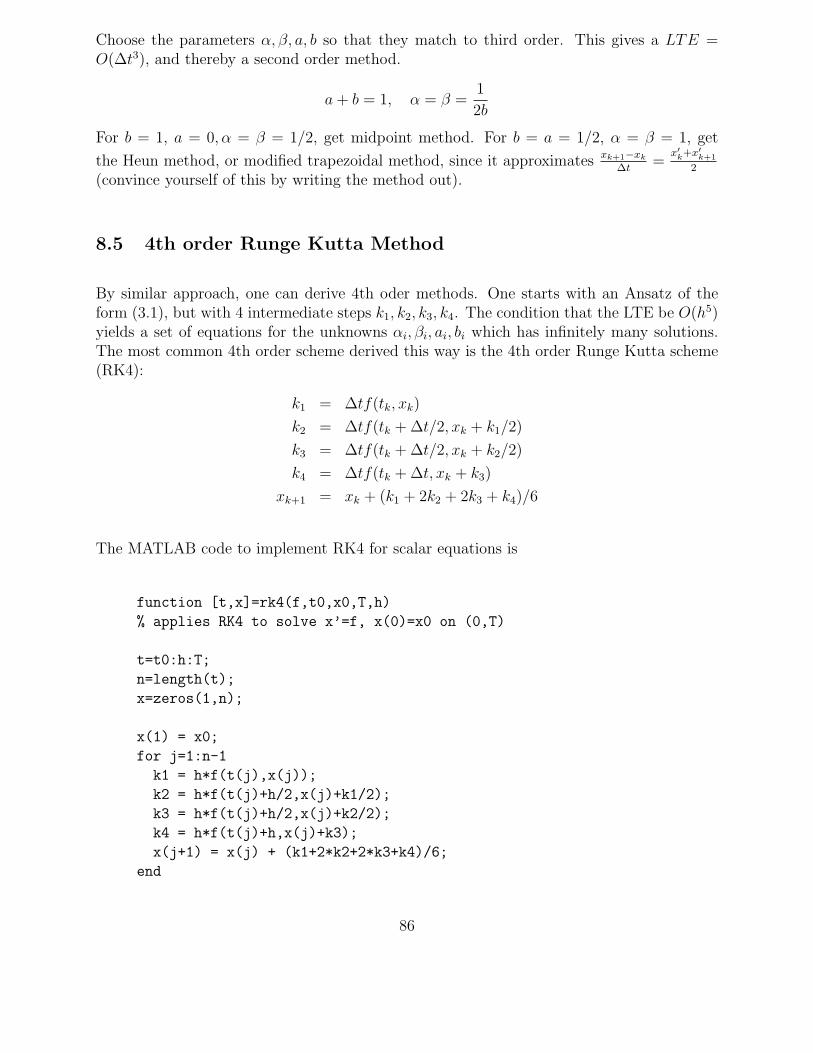
Choose the parameters α, β, a, b so that they match to third order. This gives a LTE =O(∆t3), and thereby a second order method.

a + b = 1, α = β =1

2b

For b = 1, a = 0, α = β = 1/2, get midpoint method. For b = a = 1/2, α = β = 1, get

the Heun method, or modified trapezoidal method, since it approximates xk+1−xk

∆t=

x′k+x′

k+1

2

(convince yourself of this by writing the method out).

8.5 4th order Runge Kutta Method

By similar approach, one can derive 4th oder methods. One starts with an Ansatz of theform (3.1), but with 4 intermediate steps k1, k2, k3, k4. The condition that the LTE be O(h5)yields a set of equations for the unknowns αi, βi, ai, bi which has infinitely many solutions.The most common 4th order scheme derived this way is the 4th order Runge Kutta scheme(RK4):

k1 = ∆tf(tk, xk)

k2 = ∆tf(tk + ∆t/2, xk + k1/2)

k3 = ∆tf(tk + ∆t/2, xk + k2/2)

k4 = ∆tf(tk + ∆t, xk + k3)

xk+1 = xk + (k1 + 2k2 + 2k3 + k4)/6

The MATLAB code to implement RK4 for scalar equations is

function [t,x]=rk4(f,t0,x0,T,h)

% applies RK4 to solve x’=f, x(0)=x0 on (0,T)

t=t0:h:T;

n=length(t);

x=zeros(1,n);

x(1) = x0;

for j=1:n-1

k1 = h*f(t(j),x(j));

k2 = h*f(t(j)+h/2,x(j)+k1/2);

k3 = h*f(t(j)+h/2,x(j)+k2/2);

k4 = h*f(t(j)+h,x(j)+k3);

x(j+1) = x(j) + (k1+2*k2+2*k3+k4)/6;

end

86