math 635: chapter 4 notesanderson/635s12/lectures/635_ch4_lec.… · math 635: chapter 4 notes...
TRANSCRIPT

Math 635: Chapter 4 Notes
David F. Anderson∗
Department of Mathematics
University of Wisconsin - Madison
Spring Semester 2012

Section 4.2
Definition (Precise definition of conditional expectation)Let
I X be a random variable with E|X | <∞ on (Ω,F ,P) andI G ⊂ F be a σ-field (think of it as “generated” by Z , i.e. G = σ(Z )).
We say that Y is the conditional expectation of X wrt G if Y is G measurableand
E(X1A) = E(Y 1A) for all A ∈ G
Notation: Y = E(X |G).

Conditional Expectation: Properties
Properties of Conditional Expectations:
1. E(X + Y |G) = E(X |G) + E(Y |G)
Proof.Must show that for A ∈ G:
E [E[X + Y |G]1(A)] = E[(
E[X |G] + E[Y |G]
)1(A)
].
Let A ∈ G.
E [E[X + Y |G]1(A)] = E[(X + Y )1(A)] (by definition of Cond. Exp.)
= E[X1(A)] + E[Y 1(A)] (by linearity of usual expec.)
= E[E[X |G]1(A)] + E[E[Y |G]1(A)] (by def. of cond. Exp.)
= E[(
E[X |G] + E[Y |G]
)1(A)
], (by linearity)
and done by uniqueness.
Conditional Expectation: Properties
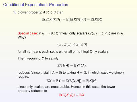
1. (Tower property) if H ⊂ G then
E(E(X |G)|H) = E(E(X |H)|G) = E(X |H)
Special case: if H = ∅,Ω trivial, only scalars (Z (ω) = c, ∀ω) are in H.Why?
ω : Z (ω) ≤ x ∈ H
for all x , means each set is either all or nothing! Only scalars.
Then, requiring Y to satisfy
EX1(A) = EY 1(A),
reduces (since trivial if A = ∅) to taking A = Ω, in which case we simplyrequire,
EX = EY = E(E[X |H]) = E[X |H],
since only scalars are measurable. Hence, in this case, the towerproperty reduces to
E(E(X |G)) = EX .

Conditional Expectation: Properties
1. If X and XY are integrable (in L1) and Y ∈ G then
E(XY |G) = YE(X |G)
2. Essentially all properties of expectations: i.e. E[aX |G] = aE[X |G].
Group project: Prove the Tower Property: if H ⊂ G then
E(E(X |G)|H) = E(E(X |H)|G) = E(X |H)

Section 4.3: Uniform Integrability
Note: important for proving that Mt∧τ is a martingale if τ is stopping time.
DefinitionWe say that a collection C of random variables is uniformly integrable if
ρ(x) = supZ∈C
E(|Z |1|Z |>x), satisfes ρ(x)→ 0 as x →∞.
Why? Recall that for integrable X (i.e. in L1), we have
E[|X |] = E[|X |1|X |>x] + E[|X |1|X |≤x],
with first term going to zero as x →∞.
Hence, for each Xi ∈ L1, there is a ρi such that
ρi (x) = E(|Xi |1|Xi |>x), satisfes ρi (x)→ 0 as x →∞.
Uniformly integrable says there is only one ρ for *all* the RVs in C.

Section 4.3: Uniform Integrability
LemmaIf C ⊂ L1 is finite then it is U.I.
Follows since for Z ∈ C
E(|Z |1|Z |>x) ≤ maxZi∈C
E(|Zi |1|Zi |>x) = maxiρi (x)
def= ρ(x)→ 0, as x →∞.
LemmaIf for Z ∈ C we have |Z | ≤ |X | ∈ L1 with a fixed X then C is U.I.

Section 4.3: Uniform Integrability
Lemma (4.1 in book, Uniform integrability and L1 convergence)If Zn → Z a.s. and Zn is U.I. then Zn → Z in L1.
Proof.By Fatou Z ∈ L1 and E |Z | ≤ ρ(x − ε) + x (for any x and ε > 0) since
E|Z | = E|Z |1|Z |>x + E|Z |1|Z |≤x ≤ E|Z |1|Z |>x + x
and
E|Z |1|Z |>x ≤ E lim supn→∞
|Zn|1|Zn|>x−ε
≤ lim infn→∞
E|Zn|1|Zn|>x−ε
≤ ρ(x − ε).

Section 4.3: Uniform Integrability
Lemma (4.1 in book, Uniform integrability and L1 convergence)If Zn → Z a.s. and Zn is U.I. then Zn → Z in L1.
Proof.We write
|Zn − Z | = |Zn − Z |1|Zn≤x + |Zn − Z |1|Zn>x
≤ |Zn − Z |1|Zn|≤x + |Z |1|Zn|>x + |Zn|1|Zn|>x
Must show that each term converges to zero:
1. First term: Dominated Convergence Thm (DCT) with |Z |+ x .
2. Second term: DCT with |Z | as the majorant: limit is ρ(x).
3. Third term: at most ρ(x).
So, we have that for any x
limn→∞
E|Zn − Z | ≤ 0 + ρ(x) + ρ(x).
By letting x →∞ we are done.

Section 4.3: Uniform Integrability
LemmaConditional expectation is a contraction:
E|E(Z |G)| ≤ E|Z |
Proof.Easy: consider Z = Z+ − Z−. Then,
E|E[Z |G]| = E|E[Z+|G]− E[Z−|G]|≤ E|E[Z+|G] + E[Z−|G]|= E[E[|Z ||G]]
= E|Z |.
Question: Lp, for p ≥ 1, contraction?
Section 4.3: Uniform Integrability
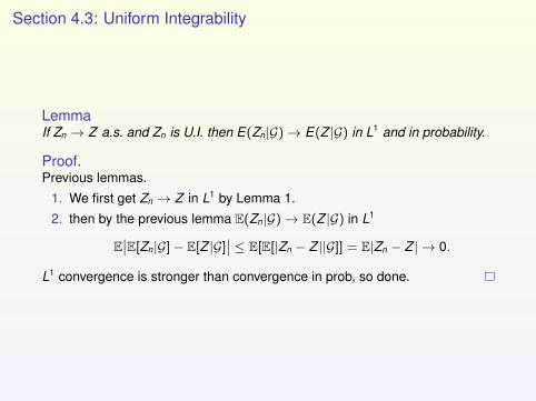
LemmaIf Zn → Z a.s. and Zn is U.I. then E(Zn|G)→ E(Z |G) in L1 and in probability.
Proof.Previous lemmas.
1. We first get Zn → Z in L1 by Lemma 1.
2. then by the previous lemma E(Zn|G)→ E(Z |G) in L1
E∣∣E[Zn|G]− E[Z |G]
∣∣ ≤ E[E[|Zn − Z ||G]] = E|Zn − Z | → 0.
L1 convergence is stronger than convergence in prob, so done.

Conditions for Uniform IntegrabilityHow to check for uniform integrability?
LemmaIf φ(x)/x →∞ as x →∞ and Eφ(|Z |) ≤ B <∞ for Z ∈ C, then C is U.I.
Proof.
1. Let Ψ(x) =φ(x)
x=⇒ x = φ(x)/Ψ(x).
2. For any Z ∈ C,
E(|Z |1|Z |≥x) = E[φ(|Z |)Ψ(|Z |) 1|Z |≥x
]≤ 1
minΨ(y) : y ≥ xE[φ(|Z |)1|Z |≥x]
≤ BminΨ(y) : y ≥ x
But, Ψ(x)→∞ as x →∞.
Example: φ(x) = x2. Says that if E|Zn|2 ≤ B for all n, then U.I. (we alreadyknew about convergence!)
More generally: if C ⊂ Lp with p > 1, then it is U.I.

Conditions for Uniform Integrability
LemmaIf Z is in L1 then there exists convex φ with φ(x)/x →∞ and E(φ(|Z |)) <∞.
Proof.Omit.
LemmaIf C = E(Z |G) : G ⊂ F then C is U.I.
Proof.Use the previous lemma: Eφ(|Z |) <∞ and also by Jensen’s inequality
Eφ(|E(Z |G)|) ≤ E(Eφ(|Z |)|G)) = Eφ(|Z |) ≤ ∞.
This is enough for the U.I. by previous Lemma (using this specific φ).

Section 4.4: Martingales in Continuous Time
DefinitionIf the collection
Ft : 0 ≤ t <∞
of sub σ-fields of F (so Ft ⊂ F) satisfies
s ≤ t =⇒ Fs ⊂ Ft ,
then the collection is called a filtration.
DefinitionIf the process Xt is such that Xt is Ft measurable,
ω : Xt (ω) ≤ x ∈ Ft ,
then we say that Xt is adapted to the filtration Ft.

Section 4.4: Martingales in Continuous Time
DefinitionWe say that Xt is a martingale with respect to Ft if it is adapted to it,E|Xt | <∞ and
E[Xt |Fs] = Xs for t > s,
and we say it is a submartingale if all assumptions hold with
E[Xt |Fs] ≥ Xs, for t ≥ s.
We will be interested in continuous martingales: i.e. there exists Ω0 ⊂ Ω suchthat Xt is continuous on Ω0:
ω ∈ Ω0 =⇒ t → Xt (ω) is continuous,
and P(Ω0) = 1.

Section 4.4: Martingales in Continuous TimeImportant filtration: the one associated to the Brownian motion, Bt .
Natural choice: Ft = σ(Bs : s ≤ t).
It turns out that this is not the nicest choice, so we also include all theprobability zero events from [0,T ] and also any subsets of these (null sets).(This is denoted by N .)
Then F0 = σ(N ) and
Ft = smallest σ − algebra containing N and σ(Bs : s ≤ t).
we have the nice property that
Ft =⋂s:s>t
Fs = Ft+ right continuity property
These
1. Having all sets of measure zero in filtration
2. Right continuity
are called the ”usual conditions”.
Section 4.4: Martingales in Continuous Time
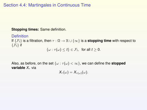
Stopping times: Same definition.
DefinitionIf Ft is a filtration, then τ : Ω→ R∪ ∞ is a stopping time with respect toFt if
ω : τ(ω) ≤ t ∈ Ft , for all t ≥ 0.
Also, as before, on the set ω : τ(ω) <∞, we can define the stoppedvariable Xτ via
Xτ (ω) = Xτ(ω)(ω).
Section 4.4: Martingales in Continuous Time
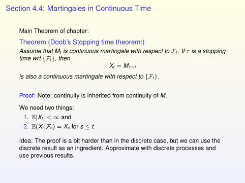
Main Theorem of chapter:
Theorem (Doob’s Stopping time theorem:)Assume that Mt is continuous martingale with respect to Ft . If τ is a stoppingtime wrt Ft, then
Xt = Mτ∧t
is also a continuous martingale with respect to Ft.
Proof: Note: continuity is inherited from continuity of M.
We need two things:
1. E|Xt | <∞ and
2. E(Xt |Fs) = Xs for s ≤ t .
Idea: The proof is a bit harder than in the discrete case, but we can use thediscrete result as an ingredient. Approximate with discrete processes anduse previous results.

Section 4.4: Martingales in Continuous Time
Recall:Xt = Mτ∧t
First show: E|Xt | <∞.
Fix s < t (for now take s = 0). For any n ≥ 1, define random time τn to besmallest element of
S(n) =
s + (t − s)k
12n : 0 ≤ k <∞
such that
τ ≤ τn.
and takes∞ if τ(ω) =∞.
We have that (i) τn(ω)→ τ(ω) for all ω (mesh size gets finer and finer) and(ii) τn is a stopping time (you know when you hit it): for x ∈ [ui , ui+1) (each inS(n))
τn ≤ x = minu ∈ S(n) : τ ≤ u ≤ x= τ ≤ ui ∈ Fui ⊂ Fx .

Section 4.4: Martingales in Continuous Time
We restrict M,F to the set S(n):
Mu,FuS(n).
Then we get a discrete martingale Mu,FuS(n), and similarly |Mu| is adiscrete time submartingale.
Since |Mu| is a (discrete) submartingale on S(n), and t , τn ∈ S(n), we have
E|Mt∧τn | ≤ E|Mt | <∞.
Letting n→∞ and using Fatou we get for all t ≥ 0
E|Xt | = E|Mt∧τ | ≤ lim infn→∞
E|Mt∧τn | ≤ E|Mt | <∞,
which proves the integrability of Xt .

Section 4.4: Martingales in Continuous Time
To prove the martingale identity, we again use the fact that Mu is a discretemartingale on S(n) to get
E(Mt∧τn |Fs) = Ms∧τn . (∗)
where we used that s, t , τn ∈ S(n).
Now we need to show that as n→∞ both sides converge to the right thing.
By the a.s. continuity of Mt and τn → τ we haveI Mt∧τn → Mt∧τ = Xt andI Ms∧τn → Ms∧τ = Xs
almost surely.
But we need convergence
E(Mt∧τn |Fs)→ E(Mt∧τ |Fs),
which will follow if we prove that Mt∧τn is U.I.

Section 4.4: Martingales in Continuous TimeFor this we use the trick introduced at the end of the U.I. section: there existsa convex φ with φ(x)/x →∞ s.t. Eφ(|Mt |) <∞ (t is fixed!).
By the convexity of φ (Jensen) and Eφ(|Mt |) <∞ we get that φ(|Mu|) is adiscrete submartingale on S(n).
So by the discrete version of the stopping time thm (used for submartingales)we get
Eφ(|Mt∧τn |) ≤ Eφ(|Mt |) <∞
1. By lemma from last class (Lemma 4.4): we have the U.I. property forMt∧τn , which converges a.s. to Mt∧τ .
2. SoLemma 4.3 gives the L1 convergence
E(Mt∧τn |Fs)L1→ E(Mt∧τ |Fs)
and this is enough to prove the martingale identity.
I E(Mt∧τn |Fs)→ E(Mt∧τ |Fs) in L1 and (if we look at the other side of theequation (∗)) we have
I E(Mt∧τn |Fs)→ Ms∧τ a.s.
which means E(Mt∧τ |Fs) = Ms∧τ a.s. (exercise 4.2 c).
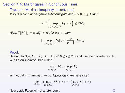
Section 4.4: Martingales in Continuous TimeTheorem (Maximal inequality in cont. time)If Mt is a cont. nonnegative submartingale and λ > 0, p ≥ 1 then
λpP
(sup
t :0≤t≤TMt > λ
)≤ EMp
T
Also: if ‖MT‖p = E|MpT | <∞, for p > 1, then
|| supt :0≤t≤T
Mt ||p ≤p
p − 1||MT ||p
Proof.Restrict to S(n,T ) = ti : ti = tT/2n, 0 ≤ i ≤ 2n and use the discrete resultswith Fatou’s lemma. Basic idea:
supt∈S(n,T )
Mt ≈ sup0≤t≤T
Mt
with equality in limit as n→∞. Specifically, we have (a.s.)
limn→∞
1( supt∈S(n,T )
Mt > λ) = 1( sup0≤t≤T
Mt > λ)
Now apply Fatou with discrete result.

Section 4.4: Martingales in Continuous TimeTheorem (Martingale convergence theorems in continuous time)If
1. Mt is a continuous martingale,
2. p > 1 and E|Mt |p ≤ B <∞ for all t ,
then Mt → M∞ a.s and in Lp
E|Mt −M∞|p → 0, as t →∞,
and E|M∞|p ≤ B.
If Mt is a cont martingale and E|Mt | ≤ B <∞ for all t then Mt → M∞ a.sand E|M∞| ≤ B.
Proof: Use the discrete result to get that Mn → M∞ (n ∈ 0, 1, 2, . . . ), thenwe only need to show that the fluctuations (in non-integer parts) are small.
Note that for any integer m ≤ t , we have
|Mt −M∞| ≤ |Mm −M∞|+ supt :m≤t<∞
|Mt −M∞|.
First term is trivial as m→∞, it goes to zero with prob. 1. Need limit ofsecond term.
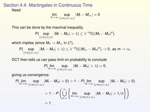
Section 4.4: Martingales in Continuous TimeNeed
limm→∞
supt :m≤t<∞
|Mt −M∞| = 0
This can be done by the maximal inequality.
P( supt :m≤t≤n
|Mt −Mm| > λ) ≤ λ−pE(|Mn −Mm|p).
which implies (since Mn → M∞ in Lp),
P( supt :m≤t<∞
|Mt −Mm| > λ) ≤ λ−pE(|M∞ −Mm|p)→ 0, as m→∞.
DCT then tells us can pass limit on probability to conclude
P( limm→∞
supt :m≤t<∞
|Mt −Mm| > λ) = 0,
giving us convergence:
P( limm→∞
supt :m≤t<∞
|Mt −Mm| = 0) = 1− P( limm→∞
supt :m≤t<∞
|Mt −Mm| > 0)
= 1− P
(∞⋃
n=1
lim
m→∞sup
t :m≤t<∞|Mt −Mm| > 1/n
)= 1.

Section 4.4: Martingales in Continuous Time
For Lp convergence: for all integers m ≤ t , we have
‖Mt −M∞‖p ≤ ‖Mt −Mm‖p + ‖Mm −M∞‖p.
Since St = |Mt −Mm| is a submartingale, we have for t < n,
‖Mt −Mm‖p ≤ ‖Mn −Mm‖p,
yielding‖Mt −M∞‖p ≤ ‖Mm −M∞‖p + sup
n:n≥m‖Mn −Mm‖p.
Above is independent of t , so:
lim supt→∞
‖Mt −M∞‖p ≤ ‖Mm −M∞‖p + supn:n≥m
‖Mn −Mm‖p → 0, as m→∞.
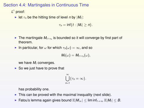
Section 4.4: Martingales in Continuous TimeL1 proof:
I let τn be the hitting time of level n by |Mt |:
τn = inft : |Mt | ≥ n.
I The martingale Mt∧τn is bounded so it will converge by first part oftheorem.
I In particular, for ω for which τn(ω) =∞, and so
Mt (ω) = Mt∧τn (ω),
we have Mt converges.I So we just have to prove that
∞⋃n=1
τn =∞.
has probability one.I This can be proved with the maximal inequality (next slide).I Fatou’s lemma again gives bound E|M∞| ≤ lim inft→∞ E|Mt | ≤ B.

Section 4.4: Martingales in Continuous TimeSo we just have to prove that
∞⋃n=1
τn =∞.
has probability one.
From Maximal:P( sup
0≤t≤T|Mt | ≥ λ) ≤ E(|MT |)/λ ≤
Bλ.
Implying (DCT on f (T ) = 1(sup0≤t≤T |Mt | ≥ λ)),
P
(sup
0≤t≤∞|Mt | ≥ λ
)≤ Bλ.
Converting to τn this is
P(τn =∞) = 1− P( sup0≤t≤∞
|Mt | ≥ n) ≥ 1− Bn.
taking unions and using continuity of probability function (note:τm =∞ ⊂ τm+1 =∞):
P (∪∞n=1ω : τn =∞) = P( limm→∞
τm =∞) = limm→∞
P(τm =∞)
= 1.

Section 4.5: Classic Brownian Motion martingales
We now have:
1. Brownian motion.
2. Notion of martingale in continuous time.
3. Stopping time theorem: Mt∧τ is a Martingale if τ is a stopping time.
4. Convergence theorems: martingales converge! “Given ω,Mt (ω)→ M∞(ω) in classical sense.”
We can start using this to compute things pertaining to Brownian motion.

Section 4.5: Classic Brownian Motion martingales
LemmaEach of the following process is a continuous martingale with respect to thestandard Brownian filtration:
1. Bt ,
2. B2t − t ,
3. exp(αBt − α2t/2), for α ∈ R.
Proof: Continuity, adapted, integrability are immediate. Only really checkMartingale identity. For example, if s < t ,
E[Bt |Fs] = E[Bt − Bs + Bs|Fs] = E[Bt − Bs|Fs] + E[Bs|Fs] = Bs.
E[B2t − t |Fs] = E[(Bt − Bs + Bs)2 − t |Fs]
= E[(Bt − Bs)2 + 2Bs(Bt − Bs) + B2s − t |Fs]
= (t − s) + B2s − t
= B2s − s.

Section 4.5: Classic Brownian Motion martingales
Finally, letXt = exp(αBt − α2t/2).
Bt is N(0, t), so
EXt = e−α2t/2
∫ ∞−∞
eαx 1√2πt
e−x22t dx = 1,
and for s < t ,
E[Xt |Fs] = E[exp(αBt − α2t/2)|Fs]
= E[exp(α(Bt − Bs)− α2(t − s)/2) exp(αBs − α2s/2)|Fs]
= XsE[exp(α(Bt − Bs)− α2(t − s)/2)]
= Xs.

Section 4.5: Classic Brownian Motion martingales
We have a similar theorem as in random walk.
TheoremLet Bt be a standard Brownian motion. If A,B > 0 and
τ = mint : Bt = −B or Bt = A,
then P(τ <∞) = 1 and
P(Bτ = A) =B
A + Band E(τ) = AB.
Proofs are similar. To prove finiteness, use geometric random variableargument:
P( supn≤t≤n+1
|Bn+1 − Bn| > A + B) = ε < 1
Events En = supn≤t≤n+1 |Bn+1 − Bn are independent, so
P(τ > n + 1) ≤ (1− ε)n =⇒ P(τ <∞) = 1.

Section 4.5: Classic Brownian Motion martingales
Rest of proof is same too.
EBτ = A · P(Bτ = A)− B · P(Bτ = −B)
= A · P(Bτ = A)− B · (1− P(τ = A)).
However,
1. Bt∧τ is a martingale.
2. EBt∧τ = 0 for all t .
3. |Bt∧τ | ≤ A + B.
So, by dominated convergence theorem,
EBτ = E limt→∞
Bt∧τ = limt→∞
EBt∧τ = 0.
Solving yields
P(Bτ = A) =B
A + B.

Section 4.5: Classic Brownian Motion martingales
Consider hitting time of one-sided boundary:
τa = inft : Bt = a.
Will show P(τa <∞) = 1 and Eτa =∞ for all a.
Proof.Suppose a > 0. Let b > 0 be arbitrary. Then,
P(τa <∞) ≥ P(Bτa∧τ−b = a) =b
a + b.
b is arbitrary and right hand side→ 1 as b →∞.
Next, and as before,
Eτa ≥ Eτa ∧ τ−b = ab →∞, as b →∞.

Section 4.5: Classic Brownian Motion martingales
TheoremLet f ∈ C3
b (R) (the bounded continuous functions with three boundedcontinuous derivatives. If Bt is a standard Brownian motion with respect toFt, then
f (Bt )− f (0)−∫ t
0
12
f ′′(Bs)ds
is a Ft-martingale.
Notes:
1. This is a Riemannian integral (calculus) since Bt is continuous.
2. Taking f (x) = x shows Bt is a martingale.
3. Taking f (x) = x2 shows B2t − t is a martingale.
4. Taking f (x) = x3 shows
B3t − 3
∫ t
0Bsds,
is a martingale.

Section 4.5: Classic Brownian Motion martingales
TheoremLet f ∈ C3
b (R) (the bounded continuous functions with three boundedcontinuous derivatives. If Bt is a standard Brownian motion with respect toFt, then
f (Bt )− f (0)−∫ t
0
12
f ′′(Bs)ds
is a Ft-martingale.
Proof.Let r < t . And consider
E[f (Bt )− f (0)− (f (Br )− f (0))|Fr ] = E[f (Bt )− f (Br )|Fr ].