math boundary-value
DESCRIPTION
Differential Equations with Boundary ValuesTRANSCRIPT
to accompany
ELEMENTARY DIFFERENTIAL
EQUATIONS WITH
BOUNDARY VALUE PROBLEMS
Werner KohlerVirginia Tech
Lee JohnsonVirginia Tech
INSTRUCTOR’S
SOLUTIONS MANUAL
LEE JOHNSONVirginia Tech
JEREMY BOURDONVirginia Tech
Reproduced by Pearson Addison-Wesley from electronic files supplied by the authors.
Copyright © 2004 Pearson Education, Inc.Publishing as Pearson Addison-Wesley, 75 Arlington Street, Boston, MA 02116
All rights reserved. No part of this publication may be reproduced, stored in a retrieval system, or transmitted,in any form or by any means, electronic, mechanical, photocopying, recording, or otherwise, without the priorwritten permission of the publisher. Printed in the United States of America.
ISBN 0-321-17323-6
2 3 4 5 6 SC 08 07 06 05
This work is protected by United States copyright laws and is provided solelyfor the use of instructors in teaching their courses and assessing student
learning. Dissemination or sale of any part of this work (including on theWorld Wide Web) will destroy the integrity of the work and is not permit-
ted. The work and materials from it should never be made available tostudents except by instructors using the accompanying text in their
classes. All recipients of this work are expected to abide by theserestrictions and to honor the intended pedagogical purposes and the needs ofother instructors who rely on these materials.
CONTENTS
Chapter 1: Introduction to 1Differential Equations
Chapter 2: First Order Linear 5Differential Equations
Chapter 3: First Order Nonlinear 26Differential Equations
Chapter 4: Second Order Linear 51Differential Equations
Chapter 5: Higher Order Linear 101Differential Equations
Chapter 6: First Order Linear Systems 115
Chapter 7: Laplace Transforms 178
Chapter 8: Nonlinear Systems 214
Chapter 9: Numerical Methods 250
Chapter 10: Series Solutions of Linear 268Differential Equations
Chapter 11: Second Order Partial Differential ??Equations and Fourier Series
Chapter 12: First Order Partial DifferentialEquations and the Method of Characteristics
Chapter 13: Linear Two-Point Boundary Value Problems
Chapter 1Introduction to Differential Equations
Section 1.1
1. This D.E. is of order two because the highest derivative in the equation is ¢¢y .
2. Order is 1.
3. This D.E. is of order one because the highest derivative in the equation is ¢y . (Note:
( )¢ π ¢¢¢y y3 )
4. Order is 3.
5 (a). y Cet=2
. Differentiating gives us ¢ = ◊ =y Ce t tyt 2
2 2 . Therefore, ¢ - =y ty2 0 for
any value of C .
5 (b). Substituting into the differential equation yields y Ce Ce( )1 12
= = . Using the initial condition,
y Ce( )1 2= = . Solving for C , we find C e= -2 1.
6. ¢¢¢ = ¢¢ = + = + + = + + +y y t c y t c t c yt
ct
c t c2 23 21
1 21 2
3
1
2
2 3. , , .
Order = 3 3 arbitrary constants
7 (a). y C t C t= +1 22 2sin cos . Differentiating gives us ¢ = -y C t C t2 2 2 21 2cos sin and
¢¢ = - - = - + = -y C t C t C t C t y4 2 4 2 4 2 2 41 2 1 2sin cos ( sin cos ) . Therefore,
¢¢ + = - + =y y y y4 4 4 0 and thus y t C t C t( ) sin cos= +1 22 2 is a solution of the D.E.
¢¢ + =y y4 0.
7 (b). y C C Cp4 1 2 11 0 3( ) = + = =( ) ( ) and ¢( ) = - = - = - fi =y C C C Cp
4 1 2 2 22 0 2 1 2 2 1( ) ( ) .
8. y e y ky e ke k et t t t= ¢ + = - + = - =- - - -2 8 2 2 4 04 4 4 4. ( )
\ = = = \ = = . ( ) . , .k y y k y4 0 2 4 20 0
9. y ct= -1. Differentiating gives us ¢ = - -y ct 2 . Thus ¢ + = - + = - =- - -y y ct c t c c t2 2 2 2 2 2 0( ) .
Solving this for c , we find that c c c c2 1 0- = - =( ) . Therefore, c = 0 1, .
10. y e tt= - +- sin ¢ + = =y y g t y y( ), ( ) .0 0 ¢ = +-y e tt cos
¢ + = + - + = \ = + = - =- -y y e t e t g g t t t y yt tcos sin ( ) cos sin , ( )0 1 0
2 • Chapter 1 Introduction to Differential Equations
11. y tr= . Differentiating gives us ¢ = -y rtr 1 and ¢¢ = - -y r r tr( )1 2. Thus
t y ty y r r t rt t r r r tr r r r2 2 2 1 2 2 1 2 2 0¢¢ - ¢ + = - - + = - - + =( ) [ ( ) ] . Solving this for r , we find
that r r r r r r r( ) ( )( )- - + = - + = - - =1 2 2 3 2 2 1 02 . Therefore, r = 1 2, .
12. y c e c e y c e c e y c e c e yt t t t t t= + ¢ = - ¢¢ = + =- - -1
22
21
22
21
22
22 2 4 4 4. ,
\ ¢¢ - = .y y4 0
13. From (12), y C e C et t= + -1
22
2 , which we differentiate to get ¢ = - -y C e C et t2 212
22 . Using the
initial conditions, y( )0 2= and ¢ =y ( )0 0, we have two equations containing C1 and C2:
C C1 2 2+ = and 2 2 01 2C C- = . Solving these simultaneous equations gives us C C1 2 1= = .
Thus, the solution to the initial value problem is y e e tt t= + =-2 2 2 2cosh( ).
14. y c c c c c c y t e t( ) , , ( )0 1 2 2 2 1 01 2 1 2 1 22= + = - = \ = = = .
15. From (12), y t C e C et t( ) = + -1
22
2 . Using the initial condition y( )0 3= , we find that C C1 2 3+ = .
From the initial condition lim ( )t
y tÆ •
= 0 and the equation for y t( ) given to us in (12), we can
conclude that C1 0= (if C1 0π , then limtÆ •
= ±•). Therefore, C2 3= and y t e t( ) = -3 2 .
16. c c y t c c y t et
t1 2 2 1
210 0 0 10 10+ = = fi = \ = =Æ -•
lim ( ) & ( ) .
17. From the graph, we can see that ¢ = -y 1 and that y( )1 1= . Thus m y= ¢ - = - - = -1 1 1 2 and
y y0 1 1= =( ) .
18. ¢ = fi = + = - = \ =y mt ymt c y t t . .
21 0 02
0From graph, only at
Also From graph . ( ) . c ym
m= - = - \ - = - fi =1 1 0 512 2
1 1.
19. We know that this is a freefall problem, so we can begin with the generic equation for freefall
situations: y tgt v t y( ) = - + +
22
0 0 . The object is released from rest, so v0 0= . The impact time
corresponds to the time at which y = 0, so we are left with the following equation for the
impact time t: 02
20= - +
gt y . Solving this for t yields t
y
g=
2 0 . For the velocity at the time
of impact: v y gt v gt gy= ¢ = - + = - = -0 02 .
20. ¢¢ = ¢ = + = = fi = +x a x at v v x xat
, 0 0 0
2
02
0 .
88 8 11 8 11642
3522= fi = = = ÊËÁ
ˆ¯ =a a ft t x ft( ) / sec . , .At
Chapter 1 Introduction to Differential Equations • 3
21. a yt
= ¢¢ = - ÊËÁ
ˆ¯32
4e p
sin . Integrating gives us ¢ = - - ÊËÁ
ˆ¯ +y tt
C324
4pe p
cos . The object is
dropped from rest, so ¢ = = - +y C( )0 04p
e . Solving for C yields C =4p
e , and putting this
value back into the equation for ¢y and simplifying gives us ¢ = - + - ÊËÁ
ˆ¯
ÊËÁ
ˆ¯
y tt
324
14p
e pcos .
Integrating again gives us y t tt
C= - + - ÊËÁ
ˆ¯
ÊËÁ
ˆ¯ + ¢16
4 44
22
pe
pe p
sin . Since the object is dropped
from a height of 252 ft. (at t = 0), y C( )0 252= ¢ = and thus
y t tt
= - + - ÊËÁ
ˆ¯
ÊËÁ
ˆ¯ +16
4 44
25222
pe
pe p
sin . Finally, since y( )4 0= ,
y( ) sin( )4 0 16 44
44
25222
= = - ◊ + ◊ - ÊËÁ
ˆ¯ +
ep p
e p . Solving for e yields e p=
4.
Section 1.2
1 (a). The equation is autonomous because ¢y depends only on y .
1 (b). Setting ¢ =y 0, we have 0 1= - +y . Solving this for y yields the equilibrium solution: y = 1.
2 (a). not autonomous
2 (b). no equilibrium solutions, isoclines are t = constant.
3 (a). The equation is autonomous because ¢y depends only on y .
3 (b). Setting ¢ =y 0, we have 0 = sin y . Solving this for y yields the equilibrium solutions: y n= ± p .
4 (a). autonomous
4 (b). y y y( ) , , - = =1 0 0 1.
5 (a). The equation is autonomous because ¢y does not depend explicitly on t.
5 (b). There are no equilibrium solutions because there are no points at which ¢ =y 0.
6 (a). not autonomous
6 (b). y = 0 is equilibrium solution, isoclines are hyperbolas.
7 (a). c = -1: Setting c = -1 gives us - + = -y 1 1 which, solved for y , reads y = 2. This is the
isocline for c = -1.
c = 0: Setting c = 0 gives us - + =y 1 0 which, solved for y , reads y = 1. This is the isocline
for c = 0.
c = 1: Setting c = 1 gives us - + =y 1 1 which, solved for y , reads y = 0, the isocline for c = 1.
4 • Chapter 1 Introduction to Differential Equations
8 (a). - + = - fi = +y t y t1 1
- + = fi =y t y t0
- + = fi = -y t y t1 1
9 (a). c = -1: Setting c = -1 gives us y t2 2 1- = - which can be simplified to t y2 2 1- = (a
hyperbola). This is the isocline for c = -1.
c = 0: Setting c = 0 gives us y t2 2 0- = which can be simplified to y t= ± . This is the isocline
for c = 0.
c = 1: Setting c = 1 gives us y t2 2 1- = (a hyperbola). This is the isocline for c = 1.
10. f f y y y( ) ( ) ( ) 0 2 0 2= = ¢ = -
¢ > < < ¢ < - • < < < < •y y y y y0 0 2 0 0 2 , for for and .
11. One example that would fit these criteria is ¢ = - -y y( )1 2 . For this autonomous D.E., ¢ =y 0 at
y = 1 and ¢ <y 0 for -• < <y 1 and 1 < < •y .
12. ¢ =y 1.
13. One example that would fit these criteria is ¢ =y ysin( )2p . For this autonomous D.E., ¢ =y 0 at
yn
=2
.
14. c.
15. f.
16. a.
17. b.
18. d.
19. e.
Chapter 2First Order Linear Differential Equations
Section 2.1
1. This equation is linear because it can be written in the form ¢ + =y p t y g t( ) ( ). It is
nonhomogeneous because when it is put in this form, g t( ) π 0.
2. nonlinear
3. This equation is nonlinear because it cannot be written in the form ¢ + =y p t y g t( ) ( ).
4. nonlinear
5. This equation is nonlinear because it cannot be written in the form ¢ + =y p t y g t( ) ( ).
6. linear, homogeneous
7. This equation is nonlinear because it can be written in the form ¢ + =y p t y g t( ) ( ).
8. nonlinear
9. This equation is linear because it cannot be written in the form ¢ + =y p t y g t( ) ( ). It is
nonhomogeneous because when it is put in this form, g t( ) π 0.
10. linear, homogeneous
11 (a). Theorem 2.1 guarantees a unique solution for the interval ( , )-• • , since t
t2 1+ and sin( )t are
both continuous for all t and -2 is on this interval.
11 (b). Theorem 2.1 guarantees a unique solution for the interval ( , )-• • , since t
t2 1+ and sin( )t are
both continuous for all t and 0 is on this interval.
11 (c). Theorem 2.1 guarantees a unique solution for the interval ( , )-• • , since t
t2 1+ and sin( )t are
both continuous for all t and p is on this interval.
12 (a). 2 < < •t
12 (b). - < <2 2t
12 (c). - < <2 2t
12 (d). -• < < -t 2
6 • Chapter 2 First Order Linear Differential Equations
13 (a). For this equation, p t( ) is continuous for all t π -2 2, and g t( ) is continuous for all t π 3.
Therefore, Theorem 2.1 guarantees a unique solution for ( , )3 • , the largest interval that
includes t = 5.
13 (b). For this equation, p t( ) is continuous for all t π -2 2, and g t( ) is continuous for all t π 3.
Therefore, Theorem 2.1 guarantees a unique solution for ( , )-2 2 , the largest interval that
includes t = -32
.
13 (c). For this equation, p t( ) is continuous for all t π -2 2, and g t( ) is continuous for all t π 3.
Therefore, Theorem 2.1 guarantees a unique solution for ( , )-2 2 , the largest interval that
includes t = 0.
13 (d). For this equation, p t( ) is continuous for all t π -2 2, and g t( ) is continuous for all t π 3.
Therefore, Theorem 2.1 guarantees a unique solution for ( , )-• -2 , the largest interval that
includes t = -5.
13 (e). For this equation, p t( ) is continuous for all t π -2 2, and g t( ) is continuous for all t π 3.
Therefore, Theorem 2.1 guarantees a unique solution for ( , )-2 2 , the largest interval that
includes t =32
.
14.ln lnt t
t t
tt+
-=
-
- +1 1
2 2
2
undefined at t = 0 2, .
14 (a). 2 < < •t .
14 (b). 0 2< <t .
14 (c). -• < <t 0 .
14 (d). -• < <t 0 .
15. y t et( ) = 32
. Differentiating gives us ¢ = =y e t tyt3 2 22
( ) . Substituting these values into the given
equation yields 2 0ty p t y+ =( ) . Solving this for p t( ) , we find that p t t( ) = -2 . Putting t = 0
into the equation for y gives us y0 3= .
16(a). y Ctr= ¢ = -y Crtr 1 2 6 0ty y¢ - =
\ - = - = fi - = fi - = fi = ( ) ( ) 2 6 2 6 0 2 6 0 2 6 0 3Crt Ct r Ct r y r rr r r
y C C C Cr( ) ( ) ( )- = - = fi π \ - = fi = -2 2 8 0 2 8 13
16 (b). -• < <t 0 since p tt
( ) =-3
16 (c). y t t t( ) , = - - • < < •3 .
Chapter 2 First Order Linear Differential Equations • 7
17. y t( ) = 0 satisfies all of these conditions.
Section 2.2
1 (a). First, we will integrate p t( ) = 3 to find P t t( ) = 3 . The general solution, then, is
y t Ce CeP t t( ) ( )= =- -3 .
1 (b). y C( )0 3= = - . Therefore, the solution to the initial value problem is y e t= - -3 3 .
2 (a). ¢ - =y y12
0 ( ) , e y y Cet t- ¢ = =2 20 .
2 (b). y Ce C e( ) , - = = =-1 2 21
21
2 y t et
( )( )
=+
21
2
3 (a). We can rewrite this equation into the conventional form: ¢ - =y ty2 0. Then we will integrate
p t t( ) = -2 to find P t t( ) = - 2 . The general solution, then, is y t Ce CeP t t( ) ( )= =- 2
.
3 (b). y Ce( )1 3= = . Solving for C yields C e= -3 1. Therefore, the solution to the initial value
problem is y t e e et t( ) ( )= =- -3 31 12 2
.
4 (a). ty y yty¢ - = fi ¢ - =4 0
40 . - = - = - \ =Ú
44
144t
dt t tt
ln ln( ) m
1 404 5
4
ty
ty t y¢ - = ¢ =-( ) y Ct= 4 .
4 (b). y C y t t( ) ( )1 1 4= = \ = .
5 (a). We can rewrite this equation into the conventional form: ¢ + =yty
40. Then we will integrate
p tt
( ) =4
to find P t t t( ) ln ln= =4 4 . The general solution, then, is
y t Ce Ce Ce CtP t t t( ) ( ) ln ln= = = =- - --4 4 4 .
5 (b). y C( )1 1= = . Therefore, the solution to the initial value problem is y t t( ) = -4 .
6 (a). m = - \ = - -exp( cos ) ( ) ( cos )t t y t Ce t t .
6 (b). y Cep p
212
ÊËÁ
ˆ¯ = =- C e= p
2 y e e et t t t= =- - - +p p2 2( cos ) cos .
7 (a). First, we will integrate p t t( ) cos( )= -2 2 to find P t t( ) sin( )= - 2 . The general solution, then, is
y t Ce CeP t t( ) ( ) sin( )= =- 2 .
7 (b). y C( )p = = -2. Therefore, the solution to the initial value problem is y t e t( ) sin( )= -2 2 .
8 (a). (( ) )t y2 1 0+ ¢ = yC
t=
+2 1.
8 • Chapter 2 First Order Linear Differential Equations
8 (b). y C y tt
( ) ( )0 33
12= = \ =+
.
9 (a). We can rewrite this equation into the conventional form: ¢ - + =y t y3 1 02( ) . Then we will
integrate p t t( ) ( )= - +3 12 to find P t t t( ) = - -3 3 . The general solution, then, is
y t Ce CeP t t t( ) ( )= =- +3 3 .
9 (b). y Ce( )1 44= = . Solving for C yields C e= -4 4 . Therefore, the solution to the initial value
problem is y t et t( ) = + -43 3 4 .
10 (a). ¢ + = \ = -- - -Úy e y e dt et t t0 ( )- ¢ =-
e ye t
0 y Ceet
=-
.
10 (b). y Ce( )0 21= = C e= -2 1 y t eet
( ) =- -2 1.
11 (a). #2
11 (b). #3
11 (c). #1
12. y t y e t( ) = -0
a 4 10 03= =- -y e y ea a, Divide: 4
12
4 22= fi = =e a a ln ln
and y e e e y t e t0
3 4 8 232 8 8= = = = \ = -a ln ln( ) (ln ). ( ) .
13. First, we should put the equation into our conventional form: ¢ - =yty
a0. Integrating
p tt
( ) = -a
gives us P t t t( ) ln ln= - = -a a . The general solution, then, is
y t Ce Ce Ce CtP t t t( ) ( ) ln ln= = = =- - -a a
a . Using the general solution and the point ( , )2 1 , we can
solve for C in terms of a : y C( )2 1 2= = ◊ a ; C = -2 a . We can then substitute this value for C
into the general solution at the point ( , )4 4 : y( ) / /4 4 2 4 4 4 42 2= = ◊ = ◊ =- -a a a a a . Setting the
exponents equal to each other yields 12
2= =a a; . Finally, solving for y0 ,
y y02 21 2 1
14
= = ◊ =-( ) .
14. ¢ = = + \ = - + = fi = = + \ = - +z z z y z z e y y et t2 2 0 1 2 1 2 22 2, ( )
15. Putting this equation into a form more like #14, we have ¢ = - + = - -y ty t t y2 6 2 3( ). We will
then let z y= - 3 (and ¢ = ¢z y , accordingly). Substituting into our modified original equation
yields an equation for z t( ) : ¢ = -z tz2 , or put in a more conventional form, ¢ + =z tz2 0. Using
the same substitution for the initial condition yields z( )0 4 3 1= - = . Integrating p t t( ) = 2 gives
us P t t( ) = 2 . The general solution is then z t Ce t( ) = - 2
. Our initial condition requires that C = 1,
Chapter 2 First Order Linear Differential Equations • 9
so the solution for z t( ) is z t e t( ) = - 2
. In terms of y t( ), this solution reads y e t- = -32
. Solved
for y t( ), this solution is y t e t( ) = +- 2
3.
16 (a).dB
dckB B A= - = -, ( ) *0
16 (b). B c A e A c A A c A ekc kc( ) ( ) ( ) ( )* * *= - = - \ = -- -1 No. A c A c( ) *≠ ≠ •as
16 (c). 0 95 1 0 05 20120. ( ) . ln( ) ln( )* *A A e e kckc kc= - fi - = - fi - = = -- -
\ = ln( ).c k0 95
120 .
17. Solving the equation ¢ + =y cy 0 with our method yields the general solution y t y e ct( ) = -0 .
Looking at the graph, we can see that y y( )0 2 0= = and y y e ec c( . ) ( . ) .- = = =- -0 4 3 200 4 0 4 .
Solving for c gives us c = ÊËÁ
ˆ¯ ª
52
32
1 01ln . .
18. ¢ = -y Ce ct y Ce y C y e y y ec c c t( ) ( )1 0 0 01= = fi = \ =- - -
y y( )1 10= = - y e cc( . ) . ln( . )0 312
12
0 712
0 7ª - \ - = - = ª ÊËÁ
ˆ¯
- -
c cª - = - \ = -1
0 72 0 990 1
.ln( ) . .
19 (a). The general solution to this D.E. is y t y e t( ) = -0 , which can be rewritten as ln( )y t c= - + .
Thus, this D.E. corresponds to graph #2 with y y e ey0
0 20= = =( ) ln( ( )) .
19 (b). The general solution to this D.E. is y t y et t( ) sin= 04 , which can be rewritten as
ln( ) siny t t c= +4 . Thus, this D.E. corresponds to graph #1 with y y e y0
00 1= = =( ) ln( ( )) .
19 (c). The general solution to this D.E. is y t y e t( ) = -0
22
, which can be rewritten as ln( )yt
c= - +2
2.
Thus, this D.E. corresponds to graph #4 with y y e ey0
00= = =( ) ln( ( )) .
19 (d). The general solution to this D.E. is y t y et t( ) sin= -0
4 , which can be rewritten as
ln( ) siny t t c= - +4 . Thus, this D.E. corresponds to graph #3 with y y e y0
00 1= = =( ) ln( ( )) .
20. ln ( ) ( ) ln( ( ))y t tt
p td
dty t=
--
+ = + \ = =3 14 0
12
112
y e0 = .
21 (a). Integrating p t tn( ) = gives us P tt
n
n
( ) =+
+1
1. Thus the solution to this initial value problem is
y t y e t nn
( ) = - ++
011
which can be rewritten as ln lny yt
n
n
= -+
+
0
1
1.
10 • Chapter 2 First Order Linear Differential Equations
Substituting values from the table gives us the necessary equations to solve for y0 and n . First,
- = -+
14
110ln y
n and - = -
+
+
42
10
1
ln yn
n
can be combined to solve for n :
414
154
2 11
1
- = =-
+
+n
n, so n = 3. - = -
14
140ln y by substitution, and therefore y0 1= .
21 (b). y t y e e y etn
nt
( ) ( )= = ◊ fi - =- - -++
0
11
44
141 1 .
Section 2.3
1. For this D.E., p t( ) = 2. Integrating gives us P t t( ) = 2 . An integrating factor is, then, m( )t e t= 2 .
Multiplying the D.E. by m( )t , we obtain e y e y e y et t t t2 2 2 22¢ + = ¢ =( ) . Integrating both sides
yields e y e Ct t2 212
= + . Therefore, the general solution is y t Ce t( ) = + -12
2 .
2. ¢ + = fi ¢ = fi = + fi = +- - -y y e e y e e y e C y e Cet t t t t t t2 2 2 2 ( ) .
3. For this D.E., p t( ) = 2. Integrating gives us P t t( ) = 2 . An integrating factor is, then, m( )t e t= 2 .
Multiplying the D.E. by m( )t , we obtain e y e y e yt t t2 2 22 1¢ + = ¢ =( ) . Integrating both sides yields
e y t Ct2 = + . Therefore, the general solution is y t te Cet t( ) = +- -2 2 .
4. ¢ + = fi ¢ = fi = + fi = + -y ty t e y te e y e C y Cet t t t t212
12
2 2 2 2 2
( ) .
5. Putting this equation into the conventional form gives us ¢ + =yty t
2. For this D.E., p t
t( ) =
2.
Integrating gives us P t t( ) ln= 2 . An integrating factor is, then, m( ) lnt e tt= =2 2. Multiplying
the D.E. by m( )t , we obtain t y ty t y t2 2 32¢ + = ¢ =( ) . Integrating both sides yields
t y t C2 414
= + . Therefore, the general solution is y t t Ct( ) = + -14
2 2.
6. ( ) ( ) , ln( )t y ty t t yt
ty t e tt2 2 2
22 4 24 2 4
24
42
+ ¢ + = + fi ¢ ++
= = = ++m
\ + ¢ = + = + fi + = + + (( ) ) ( ) ( )t y t t t t t yt t
C2 2 2 4 2 25 3
4 4 4 45
43
yC
t
t t
=+ +
+
5 3
54
32 4( )
.
7. For this D.E., p t( ) = 1. Integrating gives us P t t( ) = . An integrating factor is, then, m( )t et= .
Multiplying the D.E. by m( )t , we obtain e y e y e y tet t t t¢ + = ¢ =( ) . Integrating both sides yields
e y te e Ct t t= - + . Therefore, the general solution is y t t Ce t( ) = - + -1 .
Chapter 2 First Order Linear Differential Equations • 11
8. ¢ + = fi ¢ =y y t e y e tt t2 3 32 2cos ( ) cos
u e t= 2 dv tdt= cos3
du e dtt= 2 2 v t=13
3sin e tdte
t e tdttt
t22
233
323
3cos sin sin= - ÚÚ
u e t= 2 dv tdt= sin3
du e dtt= 2 2 v t= -13
3cos e tdte
t e tdttt
t22
233
323
3sin cos cos= - + ÚÚ
\ = - - +ÏÌÓ
¸˝˛
fi + = + sin cos ( ) (sin cos )Ie
te
t I Ie
t tt t t2 2 2
33
23 3
323
149 3
3 2 3
\ = + (sin cos )I e t tt313
3 2 32
\ = + + fi = + + - (sin cos ) (sin cos )e y e t t C y t t Cet t t2 2 2313
3 2 33
133 2 3
9. For this D.E., p t( ) = -3. Integrating gives us P t t( ) = -3 . An integrating factor is, then,
m( )t e t= -3 . Multiplying the D.E. by m( )t , we obtain e y e y e y et t t t- - - -¢ - = ¢ =3 3 3 33 6( ) .
Integrating both sides yields e y e Ct t- -= - +3 32 . Solving for y gives us y Ce t= - +2 3 , and with
our initial condition, y C( )0 1 2= = - + . Solving for C yields C = 3, and thus our final solution
is y e t= - +2 3 3 .
10. ¢ - = =y y e yt2 0 33 , ( ) . ( ) e y e e y e C y e Cet t t t t t- -¢ = fi = + fi = +2 2 3 2
y C C y e et t( ) , 0 1 3 2 23 2= + = fi = = + .
11. Putting this D.E. in the conventional form, we have ¢ + =y y et32
12
. For this D.E., p t( ) =32
.
Integrating gives us P t t( ) =32
. An integrating factor is, then, m( )t et
=3
2 . Multiplying the D.E.
by m( )t , we obtain e y e y e y et t t t
3
2
3
2
3
2
5
232
12
¢ + = ¢ =( ) . Integrating both sides yields
e y e Ct t
3
2
5
215
= + . Solving for y gives us y e Cet t= +
-15
3
2 , and with our initial condition,
y C( )0 015
= = + . Solving for C yields C = -15
, and thus our final solution is y e et t= -
-15
15
3
2 .
12 • Chapter 2 First Order Linear Differential Equations
12. ¢ + = + = \ ¢ = +-y y e t y e y e tt t t1 2 2 0 2 22cos( ), ( ) ( ) cosp
e y e t C y e t Cet t t t= + + fi = + +- -sin sin2 1 2
y Ce C e y e t et t( ) ; sin ( )p p p p
2 1 0 1 22 2 2= + = fi = - = + -- - - - .
13. Putting this D.E. in the conventional form, we have ¢ + = -yty t
cos( )cos( )
232
. For this D.E.,
p tt
( )cos( )
=2
. Integrating gives us P tt
( )sin( )
=2
. An integrating factor is, then, m( )sin( )
t et
= 2 .
Multiplying the D.E. by m( )t , we obtain e yte y e y
te
t t t tsin( ) sin( ) sin( ) sin( )cos( )( )
cos( )2 2 2 2
23
2¢ + = ¢ = - .
Integrating both sides yields e y e Ct tsin( ) sin( )
2 23= - + . Solving for y gives us y Cet
= - +-
3 2
sin( )
,
and with our initial condition, y C( )0 4 3= - = - + . Solving for C yields C = -1, and thus our
final solution is y et
= - --
3 2
sin( )
.
14. ¢ + = + + - = ¢ = + +-y y e t y e e y e te et t t t t2 1 1 2 2 2, ( ) , ( )
ye e te e e C y et
Cet t t t t t t2 2 2 2 212
14
12 2
14
= + - + + fi = + + +- -
y e Ce e C e( ) - = - + + = fi = -112
14
14
2 2
\ = + + +- - + ( )y et
et t
214
14
2 1 .
15. Putting this D.E. in the conventional form, we have ¢ + = +yty
t
31
1. For this D.E., p t
t( ) =
3.
Integrating gives us P t t( ) ln( )= 3 . An integrating factor is, then, m( ) ln( ) ln( )t e e tt t= = =3 33
.
Multiplying the D.E. by m( )t , we obtain t y t y t y t t3 2 3 3 23¢ + = ¢ = +( ) . Integrating both sides
yields t y t t C3 4 314
13
= + + . Solving for y gives us yt
Ct= + + -
413
3 , and with our initial
condition, y C( )- = = - + -113
14
13
. Solving for C yields C = -14
, and thus our final solution
is yt
t= + - -
413
14
3 . The t-interval on which this solution exists is -• < <t 0 .
Chapter 2 First Order Linear Differential Equations • 13
16. ¢ + = =yty t t
4 4a m,
t y t y t t y t yt
C yt
Ct4 3 5 4 46 2
446 6
¢ + = = ¢ fi = + fi = + -a a a( )
y C C yt
( ) , 113 6
13 6
0 23
2
= - = + fi = - - ∫ fi = - = -a a a .
17. Multiplying both sides of the equation by the integrating factor, m( )t e t= 2 , we have
e y e Ce t e t Ct t t t2 2 2 21 1= + + = + +-( ) ( ) . Differentiating gives us
( ) ( ) ( ) ( )e y e e t e tt t t t2 2 2 21 2 1 2 3¢ = + + = + . Therefore,
( ) ( ( ) ) ( ) ( ) ( ) ( )e y t y t g t e t g t tt t2 2 2 3 2 3¢ = ¢ = ◊ = + fi = +m m and
m( ) ( ) ( )( )t e e P t t p tt P t= = fi = fi =2 2 2 .
18. 2 0 22 2
tCe pCe p t tt t+ = fi = -( ) . Substituting, ( ) ( ) ( )Ce t Ce t g t tt t2 2
2 2 2 4 4+ ¢ - + = - fi = - .
19. Multiplying both sides of the equation by the integrating factor, m( )t t= , we have
ty t Ct t C= + = +-( )1 1 . Differentiating gives us ( )ty ¢ = 1. Therefore,
( ) ( ( ) ) ( ) ( ) ( )( ) ( )ty t y t g t t t g t t¢ = ¢ = ◊ = = fi =- -m m 1 1 1 and
m( ) ( ) ln ( )( )t t e P t t p tt
tP t= = fi = fi = = -1 1.
20. ( ) ( ) ( ) , e t e t t g t t yt t- -+ - ¢ + + - = fi = =1 1 00 .
21. y t e e t y yt t( ) sin ( )= - + + fi = = - + + = --2 0 2 1 0 10 .
If y t e e tt t( ) sin= - + +-2 , then ¢ = + +-y e e tt t2 cos .
Substituting in ¢ + =y y g t( ) , ( cos ) ( sin ) cos sin ( )2 2 2e e t e e t e t t g tt t t t t- -+ + + - + + = + + = .
22. ¢ + + = + = = +y t y t y et t( cos ) cos , ( ) , sin1 1 0 3 m .
( ) ( cos ) ( )sin sin sin sin sin ( sin )e y t e e e y e C y Cet t t t t t t t t t t t+ + + + + - +¢ = + = ¢ fi = + fi = +1 1 .
y C C y e y tt t
t( ) lim ( )( sin )0 1 3 2 1 2 1= + = fi = \ = + =- +
Æ • and .
23. Putting this D.E. in the conventional form, we have ¢ + = --y y e t2 2. For this D.E., p t( ) = 2.
An integrating factor is, then, m( )t e t= 2 . Multiplying the D.E. by m( )t , we obtain
e y e y e y e et t t t t2 2 2 22 2¢ + = ¢ = -( ) . Integrating both sides yields e y e e Ct t t2 2= - + . Solving for
y gives us y e Cet t= - +- -1 2 , and with our initial condition, y C( )0 2 1 1= - = - + . Solving for
C yields C = -2 , and thus our final solution is y e et t= - -- -1 2 2 . Therefore, lim ( )t
y tÆ •
= -1.

14 • Chapter 2 First Order Linear Differential Equations
24. On [ , ]1 2 :
¢ + = =yty t y
13 1 1, ( ) . An integrating factor is m( )t t= . Multiplying the D.E. by m( )t , we
obtain ( ) , ( )ty t ty t C y t Ct y C C¢ = fi = + fi = + = + = fi =-3 1 1 1 02 3 2 1 . Therefore, the
solution for 1 2£ £t is y t= 2 and y( )2 4= .
On [ , ]2 3 :
¢ + = =yty y
10 2 4, ( ) . An integrating factor is m( )t t= . Multiplying the D.E. by m( )t , we
obtain ( ) , ( )ty ty C y Ct yC
C¢ = fi = fi = = = fi =-0 22
4 81 . Therefore, the solution for
2 3£ £t is yt
=8
.
25. On [ , ]0 p :
¢ + = =y t y t y(sin ) sin , ( )0 3. An integrating factor is m( ) cost e t= - . Multiplying the D.E. by
m( )t , we obtain e y e t y e y t et t t t- - - -¢ + = ¢ =cos cos cos cos(sin ) ( ) (sin ) . Integrating both sides yields
e y e Ct t- -= +cos cos . Solving for y gives us y Ce t= +1 cos , and with our initial condition,
y Ce C e( )0 3 1 2 1= = + fi = - . Therefore, the solution for 0 £ £t p is y e t= + -1 2 1cos and
y e( )p = + -1 2 2 .
On [ , ]p p2 :
¢ + = - = + -y t y t y e(sin ) sin , ( )p 1 2 2. Multiplying the D.E. by m( ) cost e t= - , we obtain
e y e t y e y t et t t t- - - -¢ + = ¢ = -cos cos cos cos(sin ) ( ) ( sin ) . Integrating both sides yields
e y e Ct t- -= - +cos cos . Solving for y gives us y Ce t= - +1 cos , and with our initial condition,
y e Ce C e e( )p = + = - + fi = +- - -1 2 1 2 22 1 1 1. Therefore, the solution for p p£ £t 2 is
y e et t= - + ++ -1 2 21 1cos cos .
26. On [ , ]0 1 : ¢ = =y y2 0 1, ( ) .
y t C y C C= + = = fi =2 0 1 1, ( ) .
Therefore, the solution for 0 1£ £t is y t= +2 1 and y( )1 3= .
On [ , ]1 2 : ¢ + = =yty y
12 1 3, ( ) . An integrating factor is m( )t t= . Multiplying the D.E. by
m( )t , we obtain ( ) , ( )ty t ty t C y t Ct y C C¢ = fi = + fi = + = + = fi =-2 1 1 3 22 1 . Therefore,
the solution for 1 2£ £t is y tt
= +2
.
Chapter 2 First Order Linear Differential Equations • 15
27. On [ , ]0 1 :
¢ + - = =y t y y( ) , ( )2 1 0 0 3. An integrating factor is m( )t et t= -2
. Multiplying the D.E. by m( )t ,
we obtain e y e t y e yt t t t t t2 2 2
2 1 0- - -¢ + - = ¢ =( ) ( ) . Integrating both sides yields e y Ct t2 - = .
Solving for y gives us y Cet t= - 2
, and with our initial condition, y C( )0 3= = . Therefore, the
solution for 0 1£ £t is y et t= -32
and y( )1 3= .
On [ , ]1 3 :
¢ + = ¢ = =y y y y( ) , ( )0 0 1 3. Integrating gives us y C= = 3. Therefore, the solution for 1 3£ £t
is y = 3 and y( )3 3= .
On [ , ]3 4 :
¢ + -( ) = =y y yt1 0 3 3, ( ) . An integrating factor is m( ) lnt e t
t= =- 1 . Multiplying the D.E. by m( )t ,
we obtain 1 1 12 0t t ty y y¢ - = ¢ =( ) . Integrating both sides yields 1
t y C= . Solving for y gives us
y Ct= , and with our initial condition, y C C( ) ( )3 3 3 1= = fi = . Therefore, the solution for
3 4£ £t is y t= .
28. y t t Si t Si( ) ( ) ( )= - +{ }1 3
Section 2.4
1. P t A e ert t( ) .= =0055000 . Thus, P e( ) ..30 5000 22408 4505 30= =◊ .
2. P tr
At22
012
( ) ( )= + P26030 1 025 5000( ) ( . )= ◊
\ = + = ln ( ) ln( . ) ln .P2 30 60 1 025 5000 9 999 P2 30 21999( ) ª
3 (a). P t r A At t1 0 01 1 06( ) ( ) ( . )= + = . Setting P t A1 02( ) = yields 2 1 06= . t , and solving for t gives us
t ª 11 9. years.
3 (b). P tr
A At t2
20
201
21 03( ) ( ) ( . )= + = . Setting P t A2 02( ) = yields 2 1 032= . t , and solving for t gives us
t ª 11 72. years.
3 (c). P t A e A ert t( ) .= =0 006 . Setting P t A( ) = 2 0 yields 2 06= e t. , and solving for t gives us t ª 11 55.
years.
4. With r = .05 P t e At( ) .= 050 P e A( ) .10 0 5
0=
With unknown r, P e A e Ar( ) .8 80
0 50= =
\ = fi = ª . . ( . %)8 0 5 0 0625 6 25116r r
16 • Chapter 2 First Order Linear Differential Equations
5 (a). P t PB B¢ = +( . . )0 04 0 004 ; P AB ( )0 0= .
5 (b). P A eBt t= +
004 002 2. . . This can be verified easily through differentiation.
5 (c). For Plan A, P t A eAt( ) .= 0
06 . To find the time t at which Plan B “catches up” with Plan A, let us
set P t P tA B( ) ( )= : A e A et t t0
060
04 002 2. . .= + . Dividing by A0 and taking the natural logarithm of both
sides yields . . .06 04 002 2t t t= + , and solving for t gives us t = 0 (the time of the initial
investment) and t = 10 years (the time at which Plan B “catches up”).
6. After 4 yrs, P e P e e( ) , ( ) .. ( ) . ( ) . ( ) . .4 1000 10 1000 1000 1858 9305 4 05 4 07 6 2 42= = = =+ +
7. We can simplify this problem by considering the two deposits separately and then adding the
principals of each deposit together at a time of twelve years. We have, then,
1000 1000 400012 6e er r+ = . Introducing a new variable x e r∫ 6 , we have x x2 4 0+ - = .
Solving this with the quadratic formula yields one positive value of x : x e rª =1 5616 6. .
Solving for r yields r ª 0 0743. .
8. 11 000 000 10 000 000 5, , , ,= e k . Solving for k yields k = ÊËÁ
ˆ¯
15
1110
ln .
P e e( ) , , , , , ,ln ( ) ln30 10 000 000 10 000 000 17 715 61015
1110
1110
630= = =( ) ( ) .
9. 2 = ekt , and thus tk
= = ªln ln
ln.
25
21110
36 36 days.
10. 1 312
1 32. ln( . ).= fi =e kk 33 2 3
1 38 375= fi = = ªe t
kkt
ln ln( )ln( . )
. wks.
11. 80 000 100 000 6, ,= e k . Solving for k yields k =16
8ln(. ). Using this value for k , we have
( , , ) , . ,ln( . )80 000 50 000 130 000 0 8 104 0000 8+ = ◊ =e .
12 (a). ¢ = + =P kP M P P, ( )0 0 ¢ - = ¢ =- -P kP M e P Mekt kt, ( )
e PM
ke C P
M
kCe P
M
kCkt kt kt- -= - + fi = - + = - + , 0
\ = - + + ( ) ( )P tM
kP
M
kekt0
12 (b). PM
k0 = - . P PM
k0 0 .and must be nonnegative fi - ≥ If net immigration rate M > 0,
net growth rate k < 0 and vice versa.
12 (c). Set kP M PM
k+ = fi = -0 . P t P
M
k( ) = = -0 in this case.
Chapter 2 First Order Linear Differential Equations • 17
13 (a). For Strategy I, we have M kPI = 0 . For Strategy II, we have M P eIIk= -0 1( ).
13 (b). The net profit for each strategy would equal ( )( )M profitfish , and so the profit for Strategy I
is, then: Pr , (. )(. ) ,I = =500 000 3172 75 118 950, and the profit for Strategy II
is:Pr , ( )( . ) ,.II e= - ª500 000 1 0 6 111 9833172 . Strategy I would be more profitable for the farm.
14 (a). PM
kP
M
ke P P e
M
ke P
M
kek k k k
1 0 1 1 021 2 1( ) ( ) , ( ) ( ) ( )= - + + = = - + +
P P e PM
kP e
M
kek k k
2 0 2 01 2( ) , ( ) ( )= = - + +
14 (b). P PM
ke P e
M
ke
M
kP e
M
ke
M
ke ek k k k k k k
1 2 02 2
02 22 2 2 1( ) ( ) ( )- = - + + + - - = - +
= -M
kek( ) .1 2 Since M P P k P P k> > > < <0 2 2 0 2 2 01 2 1 2, ( ) ( ) ( ) ( ) if and if .
14 (c). If k > 0, introduce the immigrants as early as possible. If k < 0, introduce as late as possible.
15 (a). From the general solution of the radioactive decay equation, Q t Ce kt( ) = - , we can use the data
given to find C and k . Q Ce k( )1 100= =- and Q Ce k( )4 304= =- , so combining these
equations, we find that e k- =3 310
and therefore, k = ÊËÁ
ˆ¯ ª
13
103
0 4013ln . . Using this value of k
with the t = 1 data, we find that C Q mg= =0 149 4. . C Q= 0, since the exponential falls off the
expression for Q at t = 0.
15 (b). t = ªln
.2
1 727k
months.
15 (c). 0 01. = -e kt . Solving for t, we have tk
= - ªln( . )
.0 01
11 475 months.
16 (a). t = = fi =ln
ln
.2
57302
5730kk 0 3
0 3.
ln( . )= fi =
--e tk
kt
t = ◊ =ÊËÁ
ˆ¯
ªln( )ln
ln( )ln
103
103
2 29953
t t yr.
16 (b). From (a) t t= \ - £ £ +ln( )ln
ln( )ln
( )ln( )ln
( )103
103
103
2 230
230t t t
or 9901 10005£ £t yrs.
16 (c).Q
Qe ek( , )
( )., , ln60 000
02 83 1060 000 60 000 52
5730= = ª ( )- - ( ) - .
18 • Chapter 2 First Order Linear Differential Equations
17. ¢ = - +Q kQ M . Writing this D.E. in the conventional form, we have ¢ + =Q kQ M . For this
D.E., p t k( ) = and P t kt( ) = , which yields an integrating factor of m( )t ekt= . Thus,
e Q ke Q e Q e Mkt kt kt kt¢ + = ¢ =( ) . Integrating both sides gives us e Q eM
kCkt kt= + . Solving for Q,
we have QM
kCe kt= + - . Q
M
kC0 = + , so our equation for Q in terms of Q0 now reads
Q tM
kQ
M
ke e
M
kekt kt kt( ) = + -Ê
ËÁˆ¯ = + -( )- - -
0 50 1 . Setting Q( )2 100= and substituting
k = = ªln ln
.2 2
30 231
t, we have 100 50 1 31 5
2310 372 2= + -( ) = +- -e
M
ke
Mk k ..
( . ). Solving for
M , we find M = 42 78. (mg/yr.).
18. t = =ln
2
8k
days. Q t Q e Q ekt t
( ) ln= =- -0 0
2t
30 30 38 902
023
838= fi = ª-Q e Q eln ln . mg
19. 0 99 0 0. Q Q e kt= - . Solving for t in terms of k , we have
tk
= ÊËÁ
ˆ¯ = Ê
ËÁˆ¯ = ◊ ◊ ª ◊
1 10099 2
10099
4 10 0 0145 0 058 109 9lnln
ln . .t
=58 million years.
20. Contact angle is 180 30 45 195- + = ∞ or q q2 1 3 403- = . rad.
\ = ª ( ) . . ( . )T e20 3 3 403 100 277 6 lb.
21. The contact angle, q q p p p p2 1 2 2 5- = + + = . T e e20 1 0 1 52 1 100 9 8 980 4714= ◊ = ª- ◊. ( ) .( . ) ( )q q p N.
22. Contact – ∞ + + + ∞ = ∞: 90 90 240a a where sin a a= = fi = ∞a
a212
30
q q p p2 1 3 2
43
23
- = for and for T T
T e22100 152
23= ª( ).
plb.
T e32100 231
43= ª( ).
plb.
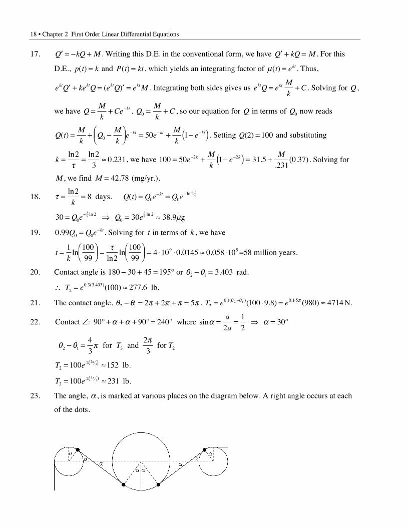
23. The angle, a , is marked at various places on the diagram below. A right angle occurs at each
of the dots.
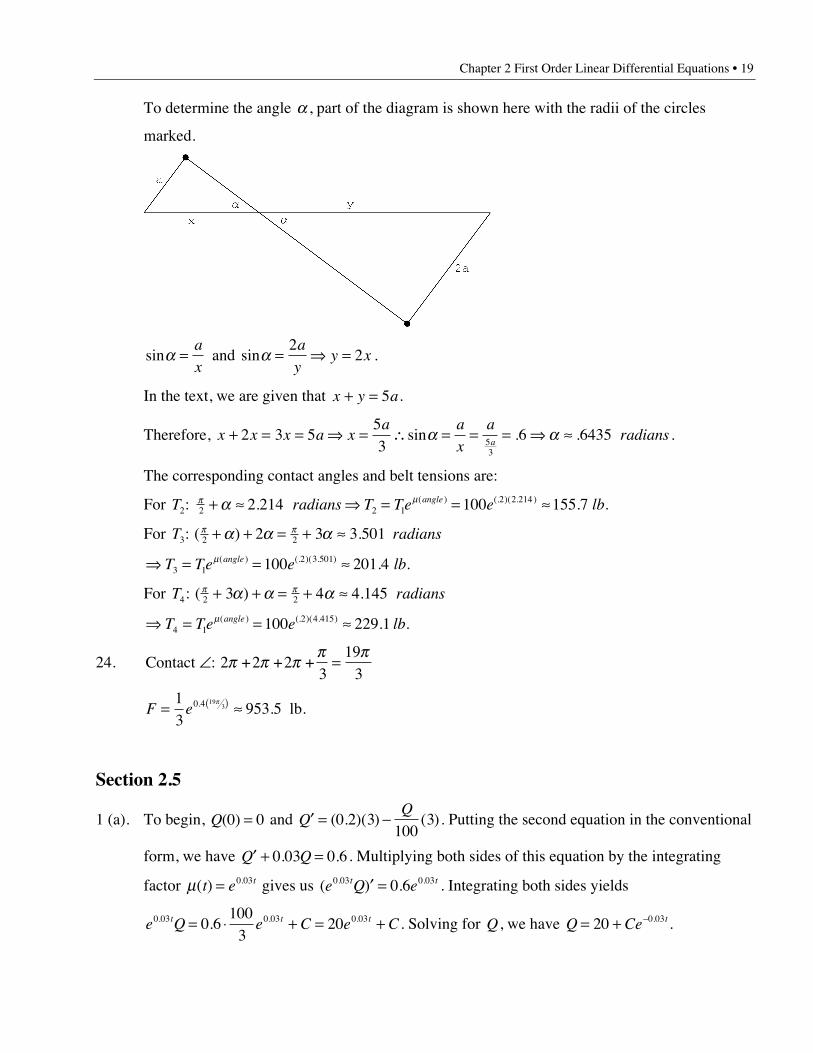
Chapter 2 First Order Linear Differential Equations • 19
To determine the angle a , part of the diagram is shown here with the radii of the circles
marked.
sin sina a= = fi =a
x
a
yy xand
22 .
In the text, we are given that x y a+ = 5 .
Therefore, x x x a xa a
x
aradians
a+ = = fi = \ = = = fi ª2 3 5
53
6 643553
sin . . a a .
The corresponding contact angles and belt tensions are:
For T radians T Te e lbangle2 2 2 1
2 2 2142 214 100 155 7: . . .( ) (. )( . )p ma+ ª fi = = ª
For T radians3 2 22 3 3 501: ( ) . p pa a a+ + = + ª
fi = = ªT Te e lbangle3 1
2 3 501100 201 4m( ) (. )( . ) . .
For T radians4 2 23 4 4 145: ( ) . p pa a a+ + = + ª
fi = = ªT Te e lbangle4 1
2 4 415100 229 1m( ) (. )( . ) . .
24. Contact : 2 +2 +2 +3
– =p p p p p193
F e= ª( )13
953 50 4 193. .
plb.
Section 2.5
1 (a). To begin, Q( )0 0= and ¢ = -QQ
( . )( ) ( )0 2 3100
3 . Putting the second equation in the conventional
form, we have ¢ + =Q Q0 03 0 6. . . Multiplying both sides of this equation by the integrating
factor m( ) .t e t= 0 03 gives us ( ) .. .e Q et t0 03 0 030 6¢ = . Integrating both sides yields
e Q e C e Ct t t0 03 0 03 0 030 6100
320. . ..= ◊ + = + . Solving for Q, we have Q Ce t= + -20 0 03. .
20 • Chapter 2 First Order Linear Differential Equations
Q C( )0 0 20= = + , so C = -20 . With this value for C , our final equation for Q is
Q e t= - -20 1 0 03( ). . Thus, Q e( ) ( ) ..10 20 1 5 180 3= - ª- lb.
1 (b). lim ( )t
Q tÆ •
= 20lb and the limiting concentration is 0 2. lb/gal.
2. V m= =100 70 20 140 000 3( )( ) , . ¢ = - fi = -QQ
vr Q Q e
rv t0 0
0 01130
0 0130
1000 030. ln( . ) ln( )Q Q e
r
vr
vrv= fi - = fi =- .
r = ª140 000
30100 21 491
3,ln( ) , min
m . r
v= = ª
130
100 0 1535 15 4ln( ) . ( . %).
3 (a). To begin, Q( )0 5= and ¢ = -Q rQ
r0 25200
. . Putting the second equation in the conventional
form, we have ¢ + =Q rQ r0 005 0 25. . . Multiplying both sides of this equation by the integrating
factor m( ) .t e rt= 0 005 gives us ( ) .. .e Q rert rt0 005 0 0050 25¢ = . Integrating both sides yields
e Q e C e Crt rt rt0 005 0 005 0 0050 25 200 50. . .. ( )= + = + . Solving for Q, we have Q Ce rt= + -50 0 005. .
Q C( )0 5 50= = + , so C = -45 . With this value for C , our equation for Q now reads
Q e rt= - -50 45 0 005. . We know that Q er
( )20 30 50 4520
200= = --
, and solving for r yields
r =-Ê
ËÁˆ¯ - = Ê
ËÁˆ¯ ªln
( )( ) ln .
50 3045
10 1094
8 11gal/min.
3 (b). This would be impossible, since Q t( ) < 50lb for all 0 £ < •t .
4 (a). ¢ = --Q te
Qt
( )( ) ( )10 1005000
10050 Q( )0 0=
¢ = - + fi ¢ =-Q Q te Qe tt t1
501000 100050 50 ( )
Qe t C Q t e Cet t t50 50 50500 5002 2= + fi = +- - . Q C( ) .0 0= = \ = - ( ) Q t t e
t
500 2 50 oz.
4 (b). ¢ = -( ) = fi = fi =-Q t e t t tt t
500 2 0 100 1002
5050
2 min.,
Qe e
( ) ( ).
1005000
500 1005000
1000 135 32
2 2= = ª- - ozgal
4 (c). Plot c t( ) vs t. Yes.
5 (a). To begin, Q( )0 10= , V ( )0 100= , and V t t( ) = +100 . Since the tank has a capacity of 700
gallons, 100 700+ =t . Solving for t yields t = 600 minutes.
Chapter 2 First Order Linear Differential Equations • 21
5 (b). ¢ = -+
t( . )( ) ( )0 5 3
1002 . Putting this in the conventional form, we have ¢ +
+=Q
tQ
2100
32
.
Multiplying both sides of the equation by the integrating factor m( ) ( )ln( )t e tt= = ++2 100 2100
gives us (( ) ) ( )10032
1002 2+ ¢ = +t Q t . Integrating both sides yields ( )( )
100100
22
3
+ =+
+t Qt
C ,
and solving for Q, we have Qt C
t=
++
+100
2 100 2( ). Q
C( )0 10 50
1002= = + , and solving for C
yields C = - = -40 100 400 0002( ) , .
Substituting this value of C back into our equation for Q gives us our final equation for Q,
Q tt
t( )
,( )
=+
-+
1002
400 000100 2 . V t( ) = 400 at t = 300, so Q( )
,( )
.3004002
400 000400
197 52= - = lb. The
concentration, then, is 197 5400
. lb/gal.
5 (c). Q( ),
( ).600
7002
400 000700
349 22= - ª lb. The concentration, then, is 349 2700
4988.
.ª lb/gal.
6 (a). ¢ = -QQ Qa
50015
50015( ) ( )
6 (b). Q Q( ) .180 0 01 0= ¢ =- -
Q Q( )
( )1500
15a
Q Q e t= - -0
03 1. ( )a
. .. ( )( ) . ( )01 0103 1 180 5 4 1= fi =- - - -e ea a
5 4 1 100 1 0 8528 0 1472. ( ) ln( ) . .- = fi - = fi =a a a .
7 (a). QA ( )0 1000= , QB ( )0 0= , QQ
AA¢ = - Ê
ËÁˆ¯0 1000
500 000,, and
QQ Q
BA B¢ = Ê
ËÁˆ¯ - Ê
ËÁˆ¯1000
500 0001000
200 000, ,.
7 (b). Putting the equation for QA¢ into the conventional form, we have Q QA A
¢ = -1
500. Thus,
Q eA
t
=-
1000 500 . Putting the equation for QB¢ into the conventional form, we have
Q Q eB B
t
¢ + =-1
2002 500 . Multiplying both sides by the integrating factor m( )t e
t
= 200 yields
( )Q e e eB
t t t
200
1
200
1
5003
10002 2¢ = =-Ê
ËÁˆ¯ . Integrating both sides gives us Q e e CB
t t
200
3
10002000
3= + , and
22 • Chapter 2 First Order Linear Differential Equations
solving for QB , Q e CeB
t t
= +- -2000
3500 200 . Q CB ( )0 0
20003
= = + , so C = -2000
3. Substituting
this value back into our equation, we have Q e eB
t t
= ÊËÁ
ˆ¯ -
ÊËÁ
ˆ¯
- -20003
500 200
7 (c). Setting QB¢ = 0, we have 0
20003
1500
1200
500 200= ÊËÁ
ˆ¯ - +
ÊËÁ
ˆ¯
- -e e
t t
. Since et t
- +=500 200
500200
,
31000
52
t = ÊËÁ
ˆ¯ln , and thus t = Ê
ËÁˆ¯ ª
10003
52
305 4ln . hours.
7 (d). Here, we want to determine tA such that Q tA A( ) =12
lb and tB such that Q tB ( ) .£ 0 2 lb where
t tB£ . This can be solved via plotting: tA ª 3800 hours and tB ª 4056 hours. Therefore,
t ª 4056 hours.
8 (a). r r t Vi = = + fi =0 3 sin constant.
8 (b). Expect lim ( ) . ( ) t
Q tÆ •
= =5 200 100 lb.
The tank is being “flushed out”, albeit in a pulsating manner.
8 (c). ¢ = + - + =Q tQ
t Q. ( sin ) ( sin ), ( )5 3200
3 0 10
¢ ++
= + fi ¢ = +- -
QtQ t Qe t e
t t t t3200
12
312
33
2003
200sin
( sin ) ( ) ( sin )( cos ) ( cos )
Qe e C Q Cet t t tt t( cos ) ( cos )cos
3200
3200100 1003- - -
= + fi = +-
Q Ce C e Q t et t
( ) ( )( cos )
0 10 100 90 100 901
2001
2003 1
200= = + fi = - fi = -- - - +
.
8(d). lim lim ( ) ( cos )
t te Q t
t t
Æ • Æ •
- - +
= fi =3 1
200 0 100 lb.
9. f t t( ) sin= +3 . Therefore, t = + = - = - +Ú ( sin ) [ cos ] cos3 3 3 10
0s ds s s t tt
t . Now,
dQ
dQ
t= -0 5
1200
. and Q( )0 10= . Putting the first equation into the conventional form, we
have dQ
dQ
t+ =
1200
0 5. , and multiplying both sides by the integrating factor mt
( )t e= 200 gives
us e Q et t
200 2000 5ÊËÁ
ˆ¯
¢= . . Integrating both sides yields e Q e C
t t200 200100= + , and solving for Q,
Q Ce= +-
100 200
t
. Now, Q C( )t = = = +0 10 100 , and therefore, C = -90 .
Chapter 2 First Order Linear Differential Equations • 23
Substituting this back into our equation for Q yields Q e= --
100 90 200
t
, which in terms of t
reads Q et t
= --
- +
100 903 1
200
cos
.
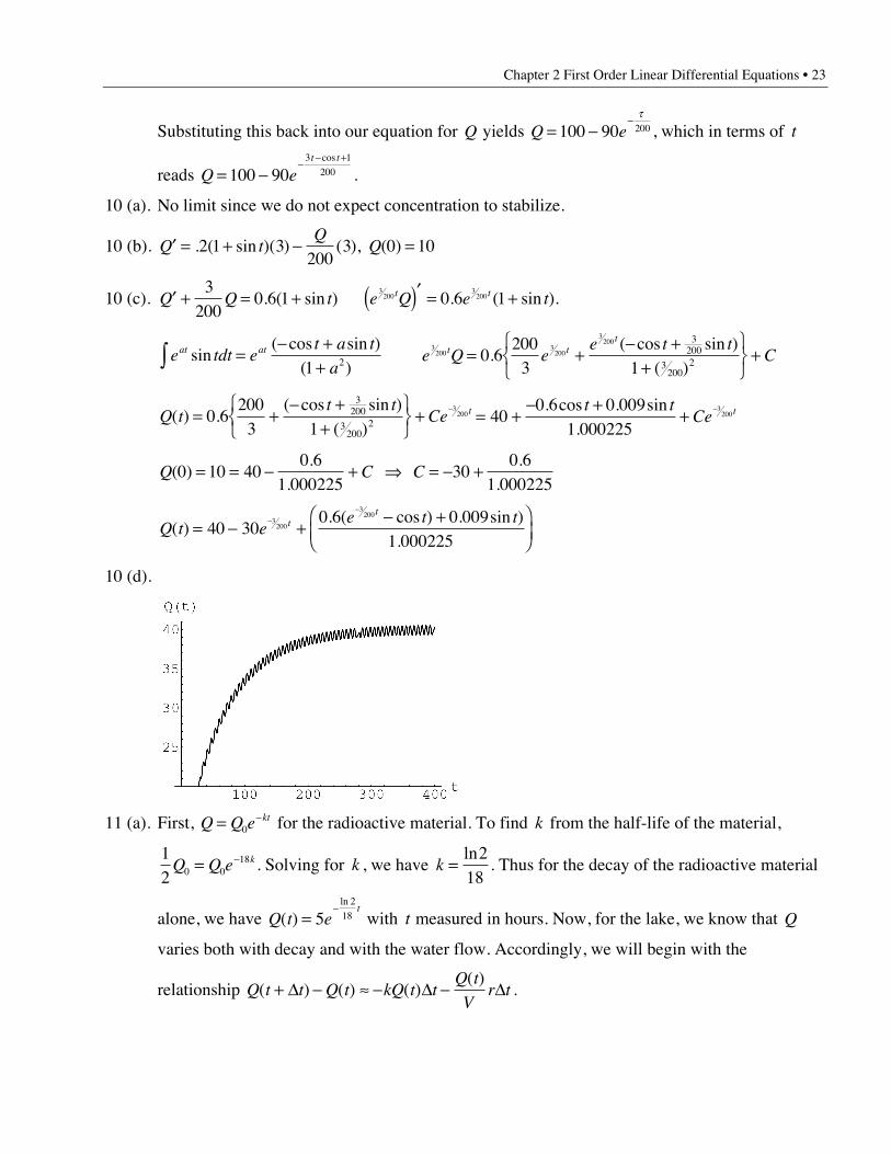
10 (a). No limit since we do not expect concentration to stabilize.
10 (b). ¢ = + - =Q tQ
Q. ( sin )( ) ( ), ( )2 1 3200
3 0 10
10 (c). ¢ + = +Q Q t3
2000 6 1. ( sin ) e Q e tt t3
2003
2000 6 1( )¢ = +. ( sin ).
e tdt et a t
aat atsin
( cos sin )( )
=- +
+Ú 1 2 e Q ee t t
Ct tt
3200
3200
3200
0 6200
3 1
3200
3200
2= +- +
+ÏÌÓ
¸˝˛
+.( cos sin )
( )
Q tt t
Ce t( ) .( cos sin )
( )= +
- ++
ÏÌÓ
¸˝˛
+ -0 6
2003 1
3200
3200
2
3200 = +
- ++ -
400 6 0 009
1 0002253
200. cos . sin
.t t
Ce t
Q C C( ).
.
..
0 10 400 6
1 00022530
0 61 000225
= = - + fi = - +
Q t ee t tt
t
( ). ( cos ) . sin )
.= - +
- +ÊËÁ
ˆ¯
--
40 300 6 0 009
1 0002253
200
3200
10 (d).
11 (a). First, Q Q e kt= -0 for the radioactive material. To find k from the half-life of the material,
12 0 0
18Q Q e k= - . Solving for k , we have k =ln218
. Thus for the decay of the radioactive material
alone, we have Q t et
( )ln
=-
52
18 with t measured in hours. Now, for the lake, we know that Q
varies both with decay and with the water flow. Accordingly, we will begin with the
relationship Q t t Q t kQ t tQ t
Vr t( ) ( ) ( )
( )+ - ª - -D D D .
24 • Chapter 2 First Order Linear Differential Equations
Using a form of the definition of the derivative and solving for Q©, we have
Q kr
VQ Q Q©
ln ,, ,
.= - +ÊËÁ
ˆ¯ = - +Ê
ËÁˆ¯ ª -
218
60 0001 200 000
0 0885 . We know that Q Q0 0 5= =( ) lb, so our
final equation for Q reads Q t e t( ) .= -5 0 0885 .
11 (b). Here, ( . )( ) .0 0001 5 5 0 0885= -e t . Thus, t = 104 07. hours.
12. ¢ = -q qk S( ), S = 72, q( )0 350= , q( )10 290=
¢ + = fi ¢ = fi = + fi = + -q q q q qk kS e ke S e e S C S Cekt kt kt kt kt ( )
q q q q q( ) ( )0 0 0 0= = + fi = - fi = + - -S C C S S S e kt
290 72 350 72 218 27810 10= + - fi =- -( ) ( )e ek k , 10278218
k = ÊËÁ
ˆ¯ln
k = ÊËÁ
ˆ¯
110
278218
ln ; 120 72 350 7248
278= + - fi =- -( ) e ekt kt
tk
= - ÊËÁ
ˆ¯ = ( )
( ) = ª1 48
278
10 10 1 7560 243
72 227848
278218
lnln
ln( . ).
. min.
13. To begin,q q= + - -S S e kt( )0 . With our substitutions for the time the food was in the oven, this
equation reads 120 350 40 350 10= + - -( )e k . Solving for k , we have
k = ---
ÊËÁ
ˆ¯ ª
110
350 120350 40
02985ln . . The temperature of the food after 20 minutes in the oven is,
then,q( ) ( ) ( )( . ) .20 350 40 350 350 310 0 550 179 520= + - = - ª-e k degrees. Finally, the food is
cooled at room temperature, so q( ) ( . ) .t e t= = + - -110 72 179 5 72 0 02985 . Solving for t yields
t ª --
-ÊËÁ
ˆ¯ ª
10 02985
110 72179 5 72
34 8.
ln.
. minutes.
14. q q= + - -S S e kt( )0 ; 170 212 72 212 5= + - -( )e k
k = ÊËÁ
ˆ¯ = Ê
ËÁˆ¯
15
14042
15
103
1ln ln min.-
¢ = -ÊËÁ
ˆ¯P r
Q tP1
140( )
, P P r t s dst
= -Ê
ËÁˆ
¯
ÏÌÔ
ÓÔ
¸˝ÔÔÚ0
0
1140
exp ( )q
q( ) ( )t e ekt kt= + - = -- -212 72 212 212 140
qds tk
et
kt
0
212140
1Ú = - -( )-
\ = - - -( )ÈÎÍ
˘˚
ÊËÁ
ˆ¯
ÏÌÓ
¸˝˛
- . exp0 01 101
1402120
1401 10r
ke k
Chapter 2 First Order Linear Differential Equations • 25
1100
1021214
11 10= - + -( )Ê
ËÁˆ¯
ÏÌÓ
¸˝˛
-exp rk
e k
- = - + ( ) -( )Ê
ËÁˆ
¯= - +( )ln( ) .
ln. . .100 10 15 143
51 09 5 143 3 78
103
r r
- ª - fi ª4 6052 1 363 3 379. ( . ) . r r min-1
15. For the first cup, q1 72 34 72= + - -( )e kt . Thus, with the proper substitutions, 53 72 38 1= - -e kt .
e kt- 1 , then, is equal to 1938
. For the second cup, q2 34 72 34= + - -( )e kt . With the proper
substitutions, we have 53 34 38 2= + -e kt . e kt- 2 , then, is equal to 1938
. Thus, the two times are
equal.
16. q q= + - -S S e kt( )0 For casserole, 45 72 40 72 2= + - -( )e k
- = - -27 32 2e k , k = ÊËÁ
ˆ¯
12
3227
ln
S t e t( ) = + -( )-72 228 1 a S e( )2 150 72 228 1 2= = + -( )-a
178
228150228
12
228150
2 2- = fi = fi = ÊËÁ
ˆ¯
- -e ea a a ln
¢ = - fi ¢ + = fi ¢ =q q q q qk S t k kS t e ke S tkt kt( ( ) ) ( ) ( ) ( )
= + - = -- -ke e ke ekt t kt t( ) ( )72 228 228 300 228a a
e ek
ke C
k
ke Cekt kt k t t ktq
aq
aa a= -
-+ fi = -
-+- - -300
228300
228( )
qa a
( ) 0 45 300228 228
255= = --
+ fi =-
-k
kC C
k
k
qa a
a( )8 300228 228
2558 8= --
+-
-ÊËÁ
ˆ¯
- -k
ke
k
ke k
e e- -= ( ) = ÊËÁ
ˆ¯ ª8 2 4
4150228
1873a a . , e ek k- -= ( ) = ÊËÁ
ˆ¯ =8 2 4
42732
5068.
k = ÊËÁ
ˆ¯ ª
12
3227
0 08495ln . a = ÊËÁ
ˆ¯ ª
12
228150
0 2094ln .
k - ª -a 0 1244. k
k -= -
a0 682843.
q( ) ( . )(. ) ( ( . ) )(. )8 300 228 0 682843 1873379 228 682843 255 5068216= - - + - -
= + - = ∞300 29 166 208 14565 121 02. . .
Chapter 3First Order Nonlinear Differential Equations
Section 3.1
1 (a). Solving for ¢y , we have ¢ = -y t y13
1 2( cos ) . Thus, f t y t y( , ) ( cos )= -13
1 2 .
1 (b).∂∂
= + =f
yt y t y
13
0 223
( sin ) sin . f and ∂∂f
y are continuous in the entire ty plane.
1 (c). The largest open rectangle is the entire ty plane, since f and ∂∂f
y are continuous in the entire
ty plane.
2 (a). f t yt
y( , ) ( cos )= -13
1 2 .
2 (b).∂∂
=f
y ty
23
sin . f and ∂∂f
y are continuous when t t< >0 0, .
2 (c). R t y t y= > -• < < •{ }( , ): ,0 .
3 (a). Solving for ¢y , we have ¢ = -+
yt
y
21 2 . Thus, f t y
t
y( , ) = -
+2
1 2 .
3 (b).∂∂
= - - + =+
-f
yt y y
ty
y( )( )( ) ( )
( )2 1 1 2
41
2 22 2 . f and
∂∂f
y are continuous in the entire ty plane.
3 (c). The largest open rectangle is the entire ty plane, since f and ∂∂f
y are continuous in the entire
ty plane.
4 (a). f t yt
y( , ) =
-+2
1 3 .
4 (b).∂∂
=+
f
y
ty
y
61
2
3 2( ). f and
∂∂f
y are continuous everywhere in the ty -plane except on the line
y = -1.
4 (c). R t y t y= -• < < • > -{ }( , ): , 1 .
5 (a). Solving for ¢y , we have ¢ = -y t tytan1
3 . Thus, f t y t ty( , ) tan= -1
3 .
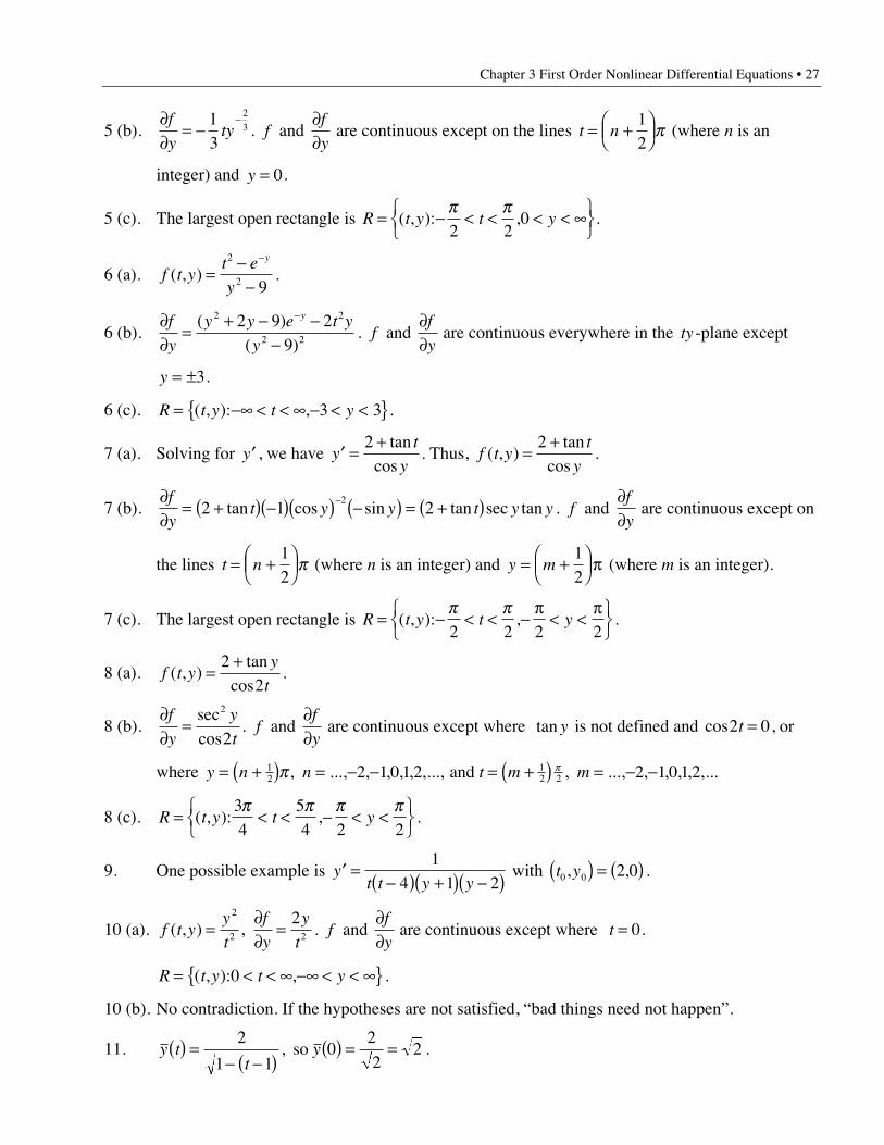
Chapter 3 First Order Nonlinear Differential Equations • 27
5 (b).∂∂
= --f
yty
13
2
3 . f and ∂∂f
y are continuous except on the lines t n= +Ê
ËÁˆ¯
12
p (where n is an
integer) and y = 0.
5 (c). The largest open rectangle is R t y t y= - < < < < •ÏÌÓ
¸˝˛
( , ): ,p p2 2
0 .
6 (a). f t yt e
y
y
( , ) =-
-
-2
2 9.
6 (b).∂∂
=+ - -
-
-f
y
y y e t y
y
y( )( )
2 2
2 2
2 9 29
. f and ∂∂f
y are continuous everywhere in the ty -plane except
y = ±3.
6 (c). R t y t y= -• < < • - < <{ }( , ): , 3 3 .
7 (a). Solving for ¢y , we have ¢ =+
yt
y
2 tancos
. Thus, f t yt
y( , )
tancos
=+2
.
7 (b).∂∂
= +( ) -( )( ) -( ) = +( )-f
yt y y t y y2 1 2
2tan cos sin tan sec tan . f and
∂∂f
y are continuous except on
the lines t n= +ÊËÁ
ˆ¯
12
p (where n is an integer) and y m= +ÊËÁ
ˆ¯ p
12
(where m is an integer).
7 (c). The largest open rectangle is R t y t y= - < < -p
< <pÏ
ÌÓ
¸˝˛
( , ): ,p p2 2 2 2
.
8 (a). f t yy
t( , )
tancos
=+2
2.
8 (b).∂∂
=f
y
y
t
seccos
2
2. f and
∂∂f
y are continuous except where tan y is not defined and cos2 0t = , or
where y n n t m m= +( ) = - - = +( ) = - -12
12 22 1 0 1 2 2 1 0 1 2p p, ..., , , , , ,..., , ..., , , , , ,... and
8 (c). R t y t y= < < - < <ÏÌÓ
¸˝˛
( , ): ,34
54 2 2
p p p p.
9. One possible example is ¢ =-( ) +( ) -( )y
t t y y
14 1 2
with t y0 0 2 0, ,( ) = ( ) .
10 (a). f t yy
t
f
y
y
t( , ) , =
∂∂
=2
2 2
2. f and
∂∂f
y are continuous except where t = 0.
R t y t y= < < • -• < < •{ }( , ): ,0 .
10 (b). No contradiction. If the hypotheses are not satisfied, “bad things need not happen”.
11. y tt
y( ) =- -( )
( ) = =2
1 10
2
22, so .

28 • Chapter 3 First Order Nonlinear Differential Equations
12. y t t t y t t( ) = + - ( ) = - = fi =( ( )) , ( )4 0 4 1 30 0 0
32
32so .
13 (a). z t y t z y1 12 5 3 2( ) = +( ) -( ) = -( ) =, so .
13 (b). z t y t z y2 22 3 1 0( ) = -( ) ( ) = ( ) =, so .
Section 3.2
1 (a). Antidifferentiation gives us y
t C2
2+ =cos . From the initial condition, we have
-( )+
p= =
22 2
22
cos C . Then we have y t y t2 4 2 4 2= - = - -cos , cos .
1 (b). -• < < •t
2 (a). y yy
t C23
13
¢ = - =, so . From the initial condition, we have 83
153
- = = C . Then we have
y t y t3 3 5 3 513= + fi = +( ) .
2 (b). -• < < •t
3 (a). y yy
y t C+( ) ¢ + = + + =1 1 02
2
, so . From the initial condition, we have 0 0 1+ + = C . Then we
have y
y t y y t yt2
2
21 2 2 1 0
2 4 8 1
2+ + = fi + + - = =
- ± - -( )( ) , . Since y 1 0( ) = , we only
want the plus sign. Finally, yt
t=- + - -( )
= - + -2 4 8 1
21 3 2 .
3 (b). -• < £t 32
4 (a). y y t t C- ¢ - = - - =2 22 0, so y-1 . From the initial condition, we have 1 0- = C . Then we have
- = + fi =-+
-y t yt
1 221
11
.
4 (b). -• < < •t
5 (a). y y ty t
C--
¢ - =-
- =32 2
02 2
, so . From the initial condition, we have C = -18
. Then we have
y t yt t
- + = =-
=-
2 2
2 2
14
1
14
2
1 4, .
5 (b). - < <12
12
t
Chapter 3 First Order Nonlinear Differential Equations • 29
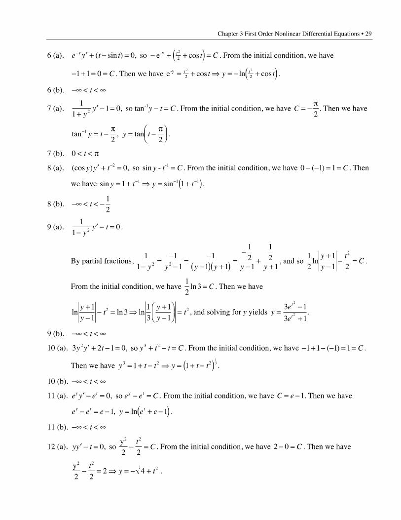
6 (a). e y t t t Cy t- ¢ + - = - + +( ) =( sin ) , cos02
2so e-y . From the initial condition, we have
- + = =1 1 0 C . Then we have e-y = + fi = - +( )t tt y t2 2
2 2cos ln cos .
6 (b). -• < < •t
7 (a).1
11 02+
¢ - = - =y
y y t C, so tan-1 . From the initial condition, we have C = -p2
. Then we have
tan , tan- = -p
= -pÊ
ËÁˆ¯
1
2 2y t y t .
7 (b). 0 < < pt
8 (a). (cos ) , siny y t y t C¢ + = =-2 10 so - - . From the initial condition, we have 0 1 1- - = =( ) C . Then
we have sin siny t y t= + fi = +( )- - -1 11 1 1 .
8 (b). -• < < -t12
9 (a).1
102-
¢ - =y
y t .
By partial fractions, 1
11
11
1 1
121
12
12 2-=
--
=-
-( ) +( ) =-
-+
+y y y y y y, and so
12
11 2
2
lny
y
tC
+-
- = .
From the initial condition, we have 12
3ln = C . Then we have
ln ln lny
yt
y
yt
+-
- = fi+-
ÊËÁ
ˆ¯
=11
313
11
2 2, and solving for y yields ye
e
t
t=
-+
3 1
3 1
2
2 .
9 (b). -• < < •t
10 (a). 3 2 1 02 2y y t y t t C¢ + - = + - =, so 3 . From the initial condition, we have - + - - = =1 1 1 1( ) C .
Then we have y t t y t t3 2 21 113= + - fi = + -( ) .
10 (b). -• < < •t
11 (a). e y e e e Cy t t¢ - = - =0, so y . From the initial condition, we have C e= - 1. Then we have
e e e y e ey t t- = - = + -( )1 1, ln .
11 (b). -• < < •t
12 (a). yy tt
C¢ - = - =02 2
2
, so y2
. From the initial condition, we have 2 0- = C . Then we have
y2
2 22 4
22- = fi = - +
ty t .
30 • Chapter 3 First Order Nonlinear Differential Equations
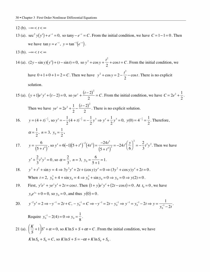
12 (b). -• < < •t
13 (a). sec , 2 0y y e e Ct t¢( ) + = - =- -so tany . From the initial condition, we have C = - =1 1 0. Then
we have tan , tany e y et t= = ( )- - -1 .
13 (b). -• < < •t
14 (a). ( sin ) ( sin ) , cos cos2 02
2
y y y t t y yt
t C- ¢( ) + - = + + + =so 2 . From the initial condition, we
have 0 1 0 1 2+ + + = = C . Then we have 2y yt
t+ = - -cos cos22
2
. There is no explicit
solution.
15 (a). y e y t yet
Cy y+( ) ¢ + -( ) = +-( )
=1 2 02
2
2
, so . From the initial condition, we have C e= +212
2 .
Then we have ye ety = + -
-( )2
12
22
22
. There is no explicit solution.
16. y t y t y y y y= + ¢ = - + = - fi ¢ + = = =- - -( ) ( ) , ( )412
412
12
0 0 412
12
32
123 3, so . Therefore,
a = = =12
3120, , n y .
17. yt
y t tt
tt
yt y=
+( ) ¢ = -( ) +( ) ( ) =-
+( )= - Ê
ËÁˆ¯ = -
-6
56 1 5 4
24
524
6234
4 2 33
4 23
23 2, so . Then we have
¢ + =y t y23
03 2 , so a = = =+
=23
36
5 110, , n y .
18. y t y y y t y y y y y t3 2 2 24 3 2 0 3 2 0+ + = fi ¢ + + ¢ = fi + ¢ + =sin (cos ) ( cos ) .
When t y y y y y y= + + = fi + = fi = fi =2 4 4 0 0 2 003
0 03
0 0, sin sin ( ) .
19. First, ¢ + ¢ + =y e ye y t ty y 2 cos . Then 1 2 0+( ) ¢ + -( ) =y e y t ty cos . At t0 0= , we have
y e yy0 0
0 0 0 0+ = =, so , and thus y 0 0( ) = .
20. y y y t C y C y t y y y t yy t
- - - - - - --¢ = fi - = + - = fi - = - fi = - fi =
-2 1
01 1
01 1
01
012 2 2 21
2, .
Require y y01
02 4 018
- - = fi =( ) .
21 (a).K
SS K S S t C+Ê
ËÁˆ¯ ¢ + = + + =1 0a a, so ln . From the initial condition, we have
K S S C K S S t K S Sln ln ln0 0 0 0+ = + = - + +, so a .
Chapter 3 First Order Nonlinear Differential Equations • 31
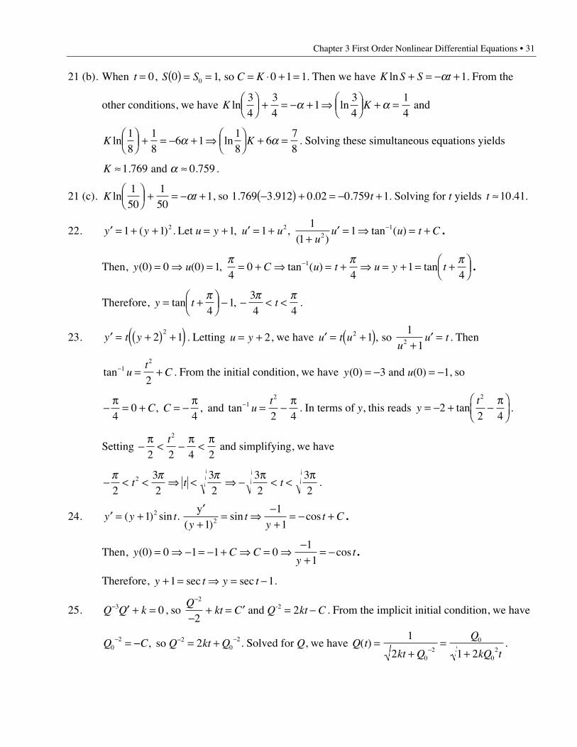
21 (b). When t = 0, S S C K0 1 0 1 10( ) = = = ◊ + =, so . Then we have K S S tln + = - +a 1. From the
other conditions, we have K Kln ln34
34
134
14
ÊËÁ
ˆ¯ + = - + fi Ê
ËÁˆ¯ + =a a and
K Kln ln18
18
6 118
678
ÊËÁ
ˆ¯ + = - + fi Ê
ËÁˆ¯ + =a a . Solving these simultaneous equations yields
K ª ª1 769 0 759. . and a .
21 (c). K tln1
501
501
ÊËÁ
ˆ¯ + = - +a , so 1 769 3 912 0 02 0 759 1. . . .-( ) + = - +t . Solving for t yields t ª 10 41. .
22. ¢ = + + = + ¢ = ++
¢ = fi = +-y y u y u uu
u u t C1 1 1 11
112 2
21( ) . , ,
( )tan ( ) Let .
Then, y u C u t u y t( ) ( ) , tan ( ) tan0 0 0 14
04
14
1= fi = = + fi = + fi = + = +ÊËÁ
ˆ¯
-p p p.
Therefore, y t t= +ÊËÁ
ˆ¯ - - < <tan ,
p p p4
134 4
.
23. ¢ = +( ) +( )y t y 2 12
. Letting u y= + 2, we have ¢ = +( ) +¢ =u t u
uu t2
211
1, so . Then
tan- = +12
2u
tC . From the initial condition, we have y u( ) ( )0 3 0 1= - = - and , so
-p
= + = -p
= -p-
40
4 2 41
2
C C ut
, , tanand . In terms of y, this reads yt
= - + -pÊ
ËÁˆ¯
22 4
2
tan .
Setting -p
< -p
<p
2 2 4 2
2t and simplifying, we have
- < < fi < fi -p
< <pp p p
232
32
32
32
2t t t .
24. ¢ = +¢
+= fi
-+
= - +y y ty
ty
t C( ) sin .( )
sin cos11
11
22
y.
Then, y C Cy
t( ) cos0 0 1 1 011
= fi - = - + fi = fi-
+= - .
Therefore, y t y t+ = fi = -1 1sec sec .
25. Q Q k- ¢ + =3 0 , so Q
kt C Q kt C-
-+ = ¢ = -
2
22 and -2 . From the implicit initial condition, we have
Q C Q kt Q02 2
022- - -= - = +, so . Solved for Q, we have Q t
kt Q
Q
kQ t( ) =
+=
+-
1
2 1 202
0
02
.

32 • Chapter 3 First Order Nonlinear Differential Equations
Thus 12 1 2
00
02
kQ=
+ t, where t is the half-life of the reactant. Therefore,
2 1 2 02= + kQ t t, which, solved for , gives t =
32 0
2kQ. Thus the half-life depends upon Q0 .
26. ¢ = - = ¢ = - fi - = - + = -- - -Q kQ Q Q Q Q k Q kt C C Q20
2 10
10, ( ) ; , . Therefore,
Q kt Q Qkt Q
Q
kQ tQ Q- -
-= + fi =+
=+
=10
1
01
0
00
11
10 0 4, ( ) . . Then,
0 41 10
0 4 4 1 0 151 150
0
00 0
0.( )
. . .
kQkQ kQ Q
Q
t=
+fi + = fi = =
+and .
Set Q Qt
t= =+
fi =0 25 0 251
1 15200. . .
. min. Then,
27 (a). The equation is nonlinear and separable. 1
1 0y
y¢ - = .
27 (b). yy y
y y=
≥- <
ÏÌÓ
,
,
0
0. Thus
dy
y
y y
y yy t
y e y
y e y
t
tÚ =>
- <ÏÌÓ
fi =><
ÏÌÓ
-
ln ,
ln , ( )
( ) ,
( ) ,
0
0
0 0
0 0.
Since y( )0 1 0= > , the solution y t et( ) = of ¢ = =y y y, ( )0 1 will be identical to that of
¢ = =y y y, ( )0 1 as long as y t et( ) = ≥ 0. This is true for all t, however, and so the two solution
curves agree.
27 (c). If y( )0 1 0= - < , then the solution of ¢ = = -y y y, ( )0 1, is y t e t( ) = - - , but the solution of
¢ = = -y y y, ( )0 1, is y t et( ) = - .
28. ¢ = -y y 2 is graph c. ¢ =y y 3 is graph a. ¢ = -y y y( )4 is graph b.
29. This is a translation three units to the right of graph (a) in problem 28.
30. Yes. 1
1 0f y
y( )
¢ - = .
31. ¢ + ( ) ¢ - = fi ¢ =+
=y y y y y yy y y
f ysin cossin cos
( )3 03
. The solution of
¢ = = +y f y H y t C( ) ( ) is , where H yf y
dy( )( )
= Ú1
. The solution of ¢ =y t f y2 ( ) is therefore
H yt
C( ) = +3
23. From the initial condition, we know that H C C H( ) ( )0 1 0 1= + fi = - , and
H C( )013 2= + . Thus C C2
23
= + . Now we have H y t C( ) = + and y y tsin - + =3 3 0, so
y y t y y t H y y y Csin ( ) sin ( ) ( ) sin= - fi = + - fi = = -3 1 1 113
13 , and .
Chapter 3 First Order Nonlinear Differential Equations • 33
Therefore, C C2
23
123
13
= + = - + = - and the implicit solution of the initial value problem is
y y ty y t
sinsin
3 313
1 03
3= - fi - + = .
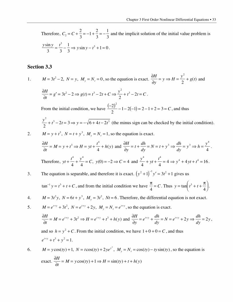
Section 3.3
1. M t N y M Ny t= - = = =3 2 02 , , , so the equation is exact. ∂∂
= fi = +H
yy H
yg t
2
2( ) and
∂∂
= ¢ = - fi = - + fi + - =H
tg t g t t t C
yt t C3 2 2
222 3
23( ) .
From the initial condition, we have -( )
- - -( ) = - + = =22
1 2 1 2 1 2 32
C , and thus
yt t y t t
23 3
22 3 6 4 2+ - = fi = - + - (the minus sign can be checked by the initial condition).
2. M y t N t y M Ny t= + = + = =3 3 1, , , so the equation is exact.
∂∂
= = + fi = + +H
tM y t H yt
th y3
4
4( ) and
∂∂
= + = = + fi = fi =H
yt
dh
dyN t y
dh
dyy h
y3 34
4.
Therefore, ytt y
C y C+ + = = - fi =4 4
4 40 2 4, ( ) and
yyt
ty yt t
4 44 4
4 44 4 16+ + = fi + + = .
3. The equation is separable, and therefore it is exact. y y t2 1 21 3 1+( ) ¢ = +-
gives us
tan- = + +1 3y t t C , and from the initial condition we have p
=4
C . Thus y t t= + +pÊ
ËÁˆ¯tan 3
4.
4. M t y N t y M t Nty= = + = =3 6 3 62 3 2, , , . Therefore, the differential equation is not exact.
5. M e t N e y M N et y t yy t
t y= + = + = =+ + +3 22, , , so the equation is exact.
∂∂
= = + fi = + ++ +H
tM e t H e t h yt y t y3 2 3 ( ) and
∂∂
= + = = + fi =+ +H
ye
dh
dyN e y
dh
dyyt y t y 2 2 ,
and so h y C= +2 . From the initial condition, we have 1 0 0+ + = C , and thus
e t yt y+ + + =3 2 1.
6. M y ty N t ty ye M N ty ty tyyy t= + = + = = -cos( ) , cos( ) , cos( ) sin( )1 2
2
, so the equation is
exact. ∂
∂= = + fi = + +
H
tM y ty H ty t h ycos( ) sin( ) ( )1
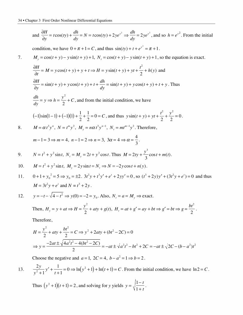
34 • Chapter 3 First Order Nonlinear Differential Equations
and ∂∂
= + = = + fi =H
yt ty
dh
dyN t ty ye
dh
dyyey ycos( ) cos( ) 2 2
2 2
, and so h ey= 2. From the initial
condition, we have 0 1+ + =p C , and thus sin( )ty t ey+ + = +2
1p .
7. M t y y t y N t y y t yy t= + - + + = + - + +cos( ) sin( ) , cos( ) sin( )1 1, so the equation is exact.
∂∂
= = + + + fi = + + + +H
tM y t y y t H y t y yt
th ycos( ) sin( ) ( )
2
2 and
∂∂
= + + + + + = + + + + +H
yt y y t y t
dh
dyt y y t y t ysin( ) cos( ) sin( ) cos( ) . Thus
dh
dyy h
yC= fi = +
2
2, and from the initial condition, we have
-( ) -( ) + -( )( ) + + = =1 1 1 1 112
12
0sin C , and thus y t y ytt y
sin( )+ + + + =2 2
2 20.
8. M t y N t y M n t y N mt yn my
nt
m= = = =- -a a3 2 3 1 1 2, , , . Therefore,
m m n n- = fi = - = fi = = fi =1 3 4 1 2 3 3 443
, , a a .
9. N t y t N M t y tt y= + = = +2 2 22sin , cos . Thus M tyy
t m t= + +23
3
cos ( ).
10. M t y t M y t N N y t n yy t= + = = fi = - +2 2 2 2sin , sin cos ( ).
11. 0 1 5 202
0+ + = fi = ±y y . 3 2 02 3t y t y e yyt+ ¢ + + ¢ = , so ( ) ( )t y y t y et3 22 3 0+ ¢ + + = and thus
M t y e N t yt= + +3 22 3 and = .
12. y t t y y= - - - fi = - =4 0 220( ) . Also, N a Mt y= = fi exact.
Then, H y at Hy
aty g t H at g ay bt g bt gbt
y t= + fi = + + = + ¢ = + fi ¢ = fi =2 2
2 2( ), .
Therefore,
Hy
atybt
C y aty bt C
yat a t bt C
at a t bt C at C b a t
= + + = fi + + - =
fi =- ± - -
= - ± - + = - ± - -
2 22 2
2 2 22 2 2 2 2
2 22 2 0
2 4 4 22
2 2
( )
( )( )
Choose the negative and a C b a b= = - = fi =1 2 4 1 22, , .
13.2
11
10 1 12
2y
yy
ty t C
+¢ +
+= fi +( ) + +( ) =ln ln . From the initial condition, we have ln2 = C .
Thus y t2 1 1 2+( ) +( ) = , and solving for y yields yt
t=
-+
11
.
Chapter 3 First Order Nonlinear Differential Equations • 35
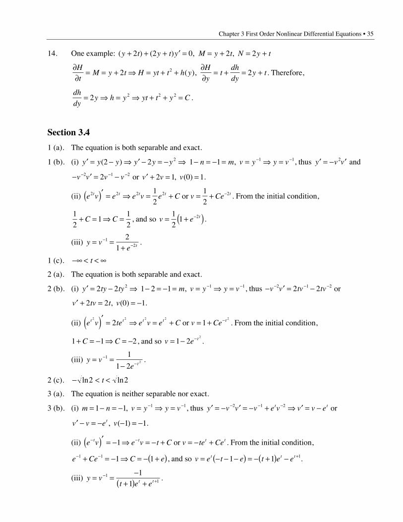
14. One example: ( ) ( ) , , y t y t y M y t N y t+ + + ¢ = = + = +2 2 0 2 2
∂∂
= = + fi = + +∂∂
= + = +H
tM y t H yt t h y
H
yt
dh
dyy t2 22 ( ), . Therefore,
dh
dyy h y yt t y C= fi = fi + + =2 2 2 2 .
Section 3.4
1 (a). The equation is both separable and exact.
1 (b). (i) ¢ = - fi ¢ - = - fiy y y y y y( )2 2 2 1 1 1 1- = - = = fi =- -n m v y y v, , thus ¢ = - ¢y v v2 and
- ¢ = -- - -v v v v2 1 22 or ¢ + = =v v v2 1 0 1, ( ) .
(ii) e v e e v e C v Cet t t t t2 2 2 2 212
12
( )¢ = fi = + = + - or . From the initial condition,
12
112
+ = fi =C C , and so v e t= +( )-12
1 2 .
(iii) y ve t= =
+-
-1
2
21
.
1 (c). -• < < •t
2 (a). The equation is both separable and exact.
2 (b). (i) ¢ = - fiy ty ty2 2 2 1 2 1 1 1- = - = = fi =- -m v y y v, , thus - ¢ = -- - -v v tv tv2 1 22 2 or
¢ + = = -v tv t v2 2 0 1, ( ) .
(ii) e v te e v e C v Cet t t t t2 2 2 2 2
2 1( )¢ = fi = + = + - or . From the initial condition,
1 1 2+ = - fi = -C C , and so v e t= - -1 22
.
(iii) y ve t
= =-
--
1 1
1 22 .
2 (c). - < <ln ln2 2t
3 (a). The equation is neither separable nor exact.
3 (b). (i) m n v y y v= - = - = fi =- -1 1 1 1, , thus ¢ = - ¢ = - + fi ¢ = -- - -y v v v e v v v et t2 1 2 or
¢ - = - - = -v v e vt , ( )1 1.
(ii) e v e v t C v te Cet t t t- -( )¢ = - fi = - + = - +1 or . From the initial condition,
e Ce C e- -+ = - fi = - +( )1 1 1 1 , and so v e t e t e et t t= - - -( ) = - +( ) - +1 1 1.
(iii) y vt e et t= =
-+( ) +
-+
11
11
.
36 • Chapter 3 First Order Nonlinear Differential Equations
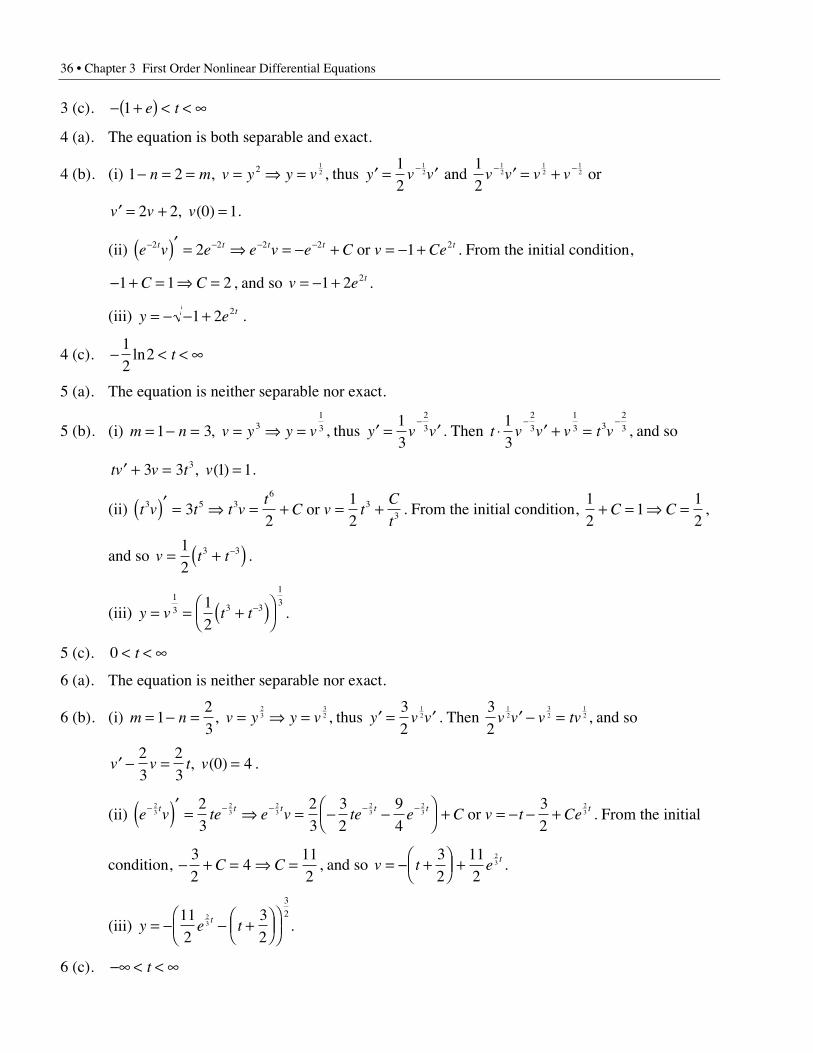
3 (c). - +( ) < < •1 e t
4 (a). The equation is both separable and exact.
4 (b). (i) 1 2 2 12- = = = fi =n m v y y v, , thus ¢ = ¢-y v v
12
12 and
12
12
12
12v v v v- -¢ = + or
¢ = + =v v v2 2 0 1, ( ) .
(ii) e v e e v e C v Cet t t t t- - - -( )¢ = fi = - + = - +2 2 2 2 22 1 or . From the initial condition,
- + = fi =1 1 2C C , and so v e t= - +1 2 2 .
(iii) y e t= - - +1 2 2 .
4 (c). - < < •12
2ln t
5 (a). The equation is neither separable nor exact.
5 (b). (i) m n v y y v= - = = fi =1 3 31
3, , thus ¢ = ¢-
y v v13
2
3 . Then t v v v t v◊ ¢ + =- -1
3
2
3
1
3 32
3 , and so
tv v t v¢ + = =3 3 1 13, ( ) .
(ii) t v t t vt
C v tC
t3 5 3
63
332
12
( )¢ = fi = + = + or . From the initial condition, 12
112
+ = fi =C C ,
and so v t t= +( )-12
3 3 .
(iii) y v t t= = +( )ÊËÁ
ˆ¯
-1
3 3 3
1
312
.
5 (c). 0 < < •t
6 (a). The equation is neither separable nor exact.
6 (b). (i) m n v y y v= - = = fi =123
23
32, , thus ¢ = ¢y v v
32
12 . Then
32
12
32
12v v v tv¢ - = , and so
¢ - = =v v t v23
23
0 4, ( ) .
(ii) e v te e v te e C v t Cet t t t t t- - - - -( )¢ = fi = - -ÊËÁ
ˆ¯ + = - - +
23
23
23
23
23
23
23
23
32
94
32
or . From the initial
condition, - + = fi =32
4112
C C , and so v t e t= - +ÊËÁ
ˆ¯ +
32
112
23 .
(iii) y e tt= - - +ÊËÁ
ˆ¯
ÊËÁ
ˆ¯
112
32
23
3
2
.
6 (c). -• < < •t
Chapter 3 First Order Nonlinear Differential Equations • 37
7. First, let u ey= . Then y u yu
u= ¢ =
¢ln and . Therefore,
¢= + fi ¢ - =-u
ut
uu
tu2
1 211 which gives
us 1 2 12 3 2t
ut
ut
¢ - = . Then we have t u t t u t C- - - -( )¢ = fi = - +2 2 2 1 . Solving for u gives us
u t Ct= - + 2 . From the initial condition, we have y u( ) ( )1 0 1 1= fi = , and so
u t t y t t t= - + fi = -( ) >2 212
2 2ln , .
8. First, let u y u u tu n= + ¢ = - + - =-1 1 31, , . Therefore,
v u u v u v v v v v tv= = ¢ = ¢ fi ¢ + =- - -3 13
23
23
13
23
13
13
, , . Then,
¢ + = = fi = fi =v v t y u v3 3 0 1 0 2 0 8, ( ) ( ) ( ) and
v Ce at b a at b t a bt= + + + + = fi = = --3 3 3 113
, ( ) , . Therefore,
v Ce t v C Ct= + - = - = fi =-3 13
013
8253
, ( ) . Then,
v e t y u v e t tt t= + - = - = - = + -ÊËÁ
ˆ¯ - - • < < •- -25
313
1 1253
13
13 3
1
313, , .
9. y0 3= by substitution. Differentiating yields
¢ =-
-+
--( )
Ê
ËÁˆ
¯-( ) = -
-+
-( )Ê
ËÁˆ
¯= - +
--y
e
te
t t ee
t ey e y
tt
tt
t
t31 3
31
1 33
31 3
9
1 32 2 2
2
( ).
Thus q t et( ) = .
Section 3.5
1. 1 1 1 1- = - = =- -n v P P v, , . Thus - ¢ - = -- - -v v rvr
Pv
e
2 1 2, or ¢ + = = -v rvr
Pv P
e
, ( )0 01. Then
v CeP
vP
CP
rt
e e
= + = = +- 10
1 1
0
, ( ) . Solving for C yields C P Pe= -- -0
1 1, so we have
v P P P e Pert
e= = -( ) +- - - - -10
1 1 1. Thus PP e P e
P P
P P P erte
rte
ert=
- -( ) =- -( )- - - - -
1
101 1
0
0 0
.
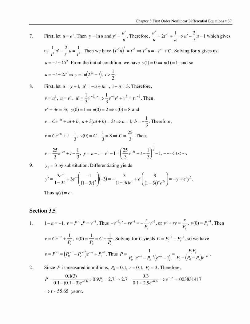
2. Since P is measured in millions, P r Pe0 0 1 0 1 3= = =. , . , . Therefore,
Pe
Pe
et e tt=
- -= fi =
+fi ª- -
-0 1 30 1 0 1 3
0 9 2 7 2 70 3
0 1 2 90038314170 1 0 1
1. ( ). ( . )
, . . ..
. ... .
.
fi ªt years55 65. .

38 • Chapter 3 First Order Nonlinear Differential Equations
3 (a). Setting rP
PP M
e
1 0-ÊËÁ
ˆ¯
+ = , we have - + + =P
PP
M
re
2
0. Then
P P P PM
rP
P P P Mr
e e
e e e2
2
04
2- - = fi =
± +. This makes sense; migration would alter the
equilibrium state.
3 (b). 2 1 1 412
14
22
P x P x-( ) = + fi -ÊËÁ
ˆ¯ = + , where x
M
r= . This is a parabola with vertex -Ê
ËÁˆ¯
14
12
, .
For x > 0, there is one nonnegative equilibrium solution. Two such solutions exist for
- < £14
0x .
3 (c). When x = -14
, the two nonnegative equilibrium solutions coalesce into a single equilibrium
value. There are no equilibrium solutions for x < -14
. This makes sense, since if the migration
out of the colony is too large relative to reproduction, equilibrium could not be achieved.
4. Equilibrium values at 4 2 and - . PP M
P rP Pe
ee e= ± +
Ê
ËÁˆ
¯fi + - = fi =
21 1
44 2 2( ) .
4 2 6 14
3 12
82
4- - = = + + = = fi =( ) PM
P r
M
r
M
r
M
ree
or .
5. ¢ = -( ) - =P P P P13
160
12
, ( ) . Then ¢ = - + - = - -ÊËÁ
ˆ¯ -Ê
ËÁˆ¯P P P P P2 3
1634
14
. Then we have
114
34
1 0P P
P-Ê
ËÁˆ¯ -Ê
ËÁˆ¯
¢ + = , and by partial fractions, we have -
-+
-
Ê
Ë
ÁÁÁ
ˆ
¯
˜˜˜
¢ + =2
14
234
1 0P P
P . Then
-
-ÊËÁ
ˆ¯
+-Ê
ËÁˆ¯
È
Î
ÍÍÍÍ
˘
˚
˙˙˙˙
+ =Ú2
14
234
P PdP t C , and so 2
3414
lnP
Pt C
-
-+ = .
From the initial condition, we have C = 0, so
P
Pe P P P
P
Pe
t t-
-= < < fi - = - -( ) fi
-
-=
- -
3414
14
34
34
14
2 34
34
2. But , and then P te
e
t
t( ) =+
+
-
-
34
14
1
2
2
.
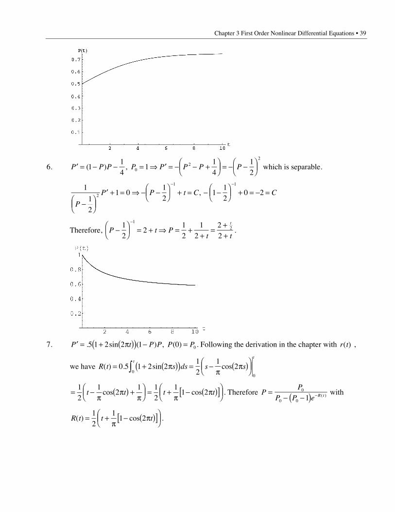
Chapter 3 First Order Nonlinear Differential Equations • 39
6. ¢ = - - = fi ¢ = - - +ÊËÁ
ˆ¯ = - -Ê
ËÁˆ¯P P P P P P P P( ) , 1
14
114
120
22
which is separable.
1
12
1 012
112
0 22
1 1
P
P P t C C
-ÊËÁ
ˆ¯
¢ + = fi - -ÊËÁ
ˆ¯ + = - -Ê
ËÁˆ¯ + = - =
- -
,
Therefore, P t Pt t
t
-ÊËÁ
ˆ¯ = + fi = +
+=
++
-12
212
12
22
1
2 .
7. ¢ = + p( )( ) - =P t P P P P. sin ( ) , ( )5 1 2 2 1 0 0. Following the derivation in the chapter with r t( ) ,
we have R t s ds s st
t
( ) . sin cos= + p( )( ) = -p
p( )ÊËÁ
ˆ¯Ú0 5 1 2 2
12
12
00
= -p
p( ) +p
ÊËÁ
ˆ¯ = +
p- p( )[ ]Ê
ËÁˆ¯
12
12
1 12
11 2t t t tcos cos . Therefore P
P
P P e R t=- -( ) -
0
0 0 1 ( ) with
R t t t( ) cos= +p
- p( )[ ]ÊËÁ
ˆ¯
12
11 2 .
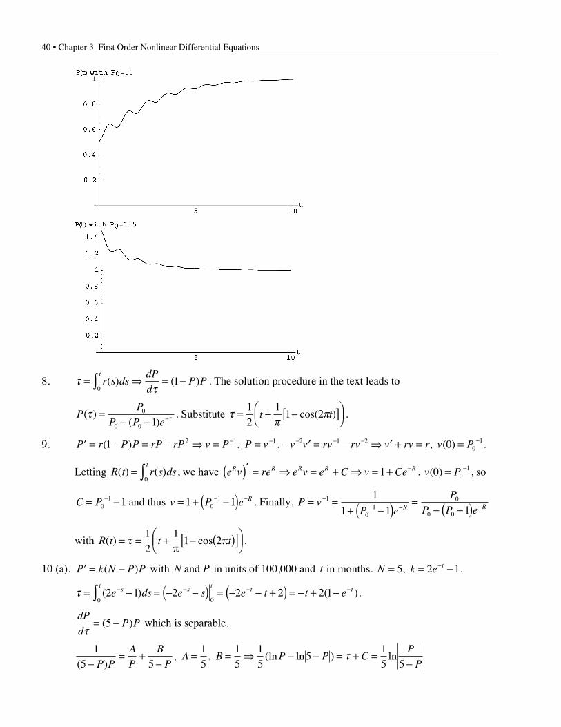
40 • Chapter 3 First Order Nonlinear Differential Equations
8. tt
= fi = -Ú r s dsdP
dP P
t( ) ( )
01 . The solution procedure in the text leads to
PP
P P e( )
( )t t=
- - -0
0 0 1. Substitute t
pp= + -[ ]Ê
ËÁˆ¯
12
11 2t tcos( ) .
9. ¢ = - = - fi = =- -P r P P rP rP v P P v( ) , 1 2 1 1, - ¢ = - fi ¢ + = =- - - -v v rv rv v rv r v P2 1 20
10, ( ) .
Letting R t r s dst
( ) ( )= Ú0, we have e v re e v e C v CeR R R R R( )¢ = fi = + fi = + -1 . v P( )0 0
1= - , so
C P= --0
1 1 and thus v P e R= + -( )- -1 101 . Finally, P v
P e
P
P P eR R= =+ -( ) =
- -( )-
- - -1
01
0
0 0
1
1 1 1
with R t t t( ) cos= = +p
- p( )[ ]ÊËÁ
ˆ¯t 1
21
1 2 .
10 (a). ¢ = -P k N P P( ) with N P and in units of 100,000 and t in months. N k e t= = --5 2 1, .
t = - = - -( ) = - - +( ) = - + -- - - -Ú ( ) ( )2 1 2 2 2 2 10 0
e ds e s e t t est
st
t t .
dP
dP P
t= -( )5 which is separable.
15 5
15
15
15
515 5( )
, , (ln ln ) ln-
= +-
= = fi - - = + =-P P
A
P
B
PA B P P C
P
Pt
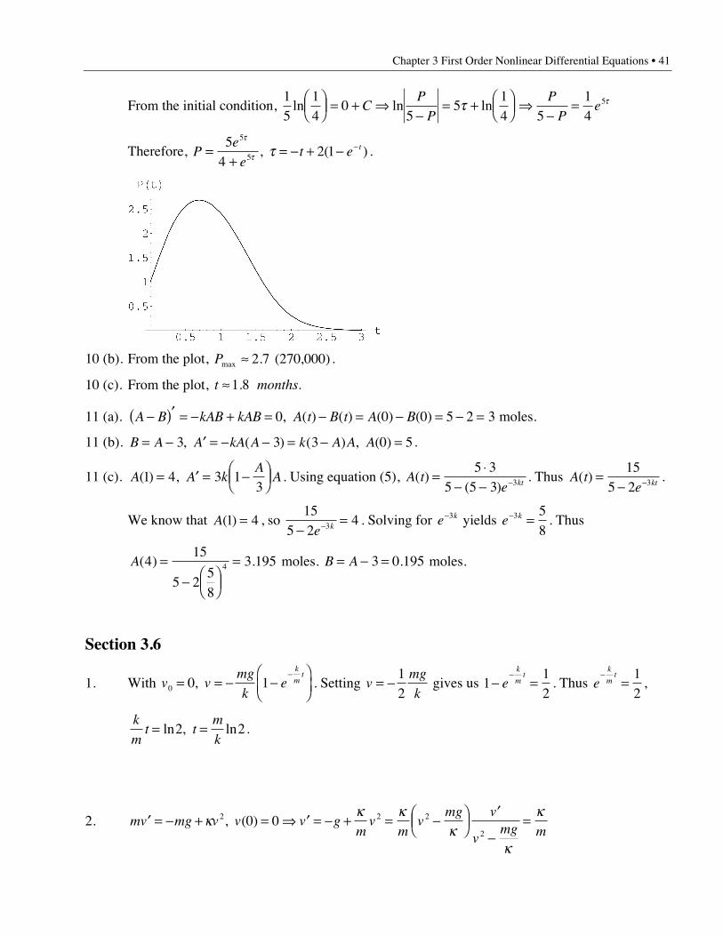
Chapter 3 First Order Nonlinear Differential Equations • 41
From the initial condition, 15
14
05
514 5
14
5ln ln lnÊËÁ
ˆ¯ = + fi
-= + Ê
ËÁˆ¯ fi
-=C
P
P
P
Pet t
Therefore, Pe
et e t=
+= - + - -5
42 1
5
5
t
t t, ( ) .
10 (b). From the plot, Pmax . ( , )ª 2 7 270 000 .
10 (c). From the plot, t monthsª 1 8. .
11 (a). A B kAB kAB A t B t A B-( )¢ = - + = - = - = - =0 0 0 5 2 3, ( ) ( ) ( ) ( ) moles.
11 (b). B A A kA A k A A A= - ¢ = - - = - =3 3 3 0 5, ( ) ( ) , ( ) .
11 (c). A A kA
A( ) , 1 4 3 13
= ¢ = -ÊËÁ
ˆ¯ . Using equation (5), A t
e kt( )( )
=◊
- - -5 3
5 5 3 3 . Thus A te kt( ) =
- -15
5 2 3 .
We know that A( )1 4= , so 15
5 243-
=-e k . Solving for e k-3 yields e k- =3 58
. Thus
A( ) .415
5 258
3 1954=- Ê
ËÁˆ¯
= moles. B A= - =3 0 195. moles.
Section 3.6
1. With v vmg
ke
k
mt
0 0 1= = - -ÊËÁ
ˆ¯
-, . Setting v
mg
k= -
12
gives us 112
- =-
ek
mt
. Thus ek
mt-
=12
,
k
mt t
m
k= =ln , ln2 2.
2. mv mg v v v gm
vm
vmg v
vmg m
¢ = - + = fi ¢ = - + = -ÊËÁ
ˆ¯
¢
-=k k k
kk
k2 2 2
20 0, ( )

42 • Chapter 3 First Order Nonlinear Differential Equations
1 1
2
1
22v
mgA
vmg
B
vmg
Amg
Bmg-
=-
++
fi = = -
k k k k k
, . Therefore,
1
2
0 0 0 0mg
vmg
vmg m
t C v Cmg
v
k
k
k
kk
ln , ( )-
+= + = fi = < £ and - . Then,
vmg
vmg
mgv
mgv
e vmg e
e
mg g
mt
g
mt
g
mt
g
mt
-
+=
-
+= fi = -
-
+
Ê
Ë
ÁÁÁ
ˆ
¯
˜˜ = -
ÊËÁ
ˆ¯
-
-
k
k
k
kk k
kkk
k
22
2
1
1
tanh .
3. 10 1052803600
14 67mi hr/ .= ÊËÁ
ˆ¯ = ft/sec. Then 14 67
200929. .= fi ª
◊k
k lb secft
2
2 .
4 (a). mdv
dtkv v t v e m slug
km t+ = fi = =-0
3000320( ) ,
v
ve kk( )
ln4 50
220225
12830000
4323000= = fi Ê
ËÁˆ¯ =- ◊ ◊ . Then, k lb ft= Ê
ËÁˆ¯ = ◊
3000128
225
34 725ln . sec/ .
4 (b). d v t dt v e dt vm
ke
mv
ke
km
km
kmt t= = = -Ê
ËÁˆ¯ = -( )Ú Ú - - -( )
0
4
0 0
4
0
0
4
0 14
= ◊ÊËÁ
ˆ¯
ÊËÁ
ˆ¯
ÊËÁ
ˆ¯ ª
300032
22052803600
134 725
170220
673.
.ft
5. mv vv
v mv
mt C¢ + = fi
¢= - fi - = - +-k k k2
210 , C v= - -
01. Then we have
vm
t v vv
mv t
- -= + fi =+
10
1 0
01
kk . From the condition provided, we have
v
vm
v mv
( )4 50220
1
1 44
1522
522
1750
0
0= =+
fi =-
=kk
. Solving for k yields
k = = ◊ ∏ ÊËÁ
ˆ¯
ÊËÁ
ˆ¯
ª◊17
5 4175
300032
14
22052803600
2470
m
v.
lb secft
2
2 .
For the distance traveled, d v t dt vdt
v
mt
vdt
tv t= =
+=
+= Ê
ËÁˆ¯ +Ê
ËÁˆ¯Ú Ú Ú( ) ln
0
4
000
4
0 0
4
0
0
4
1 11720
2017
11720k
= ÊËÁ
ˆ¯
ÊËÁ
ˆ¯ +Ê
ËÁˆ¯ =220
52803600
2017
1175
562 4ln . ft.
Chapter 3 First Order Nonlinear Differential Equations • 43
6. mv kv mg v v v tmg
kv
mg
ke
km t¢ + = - = fi = - + +Ê
ËÁˆ¯
-, ( ) ( )0 0 0 . Set
vmg
k
mg
k
kv
mge
k
mt
kv
mgt
m
k
kv
mg
km mt
m m= = +ÊËÁ
ˆ¯
fi = +ÊËÁ
ˆ¯
fi = +ÊËÁ
ˆ¯
-0 1 1 10 0 0: ln ln .
7. h v t dtmg
kv
mg
ke dt
tk
mttm m= = - + +Ê
ËÁˆ¯
È
ÎÍ
˘
˚˙Ú Ú
-( )
0 00 = - - +Ê
ËÁˆ¯
È
ÎÍ
˘
˚˙
-mg
kt
m
kv
mg
ke
k
mt
tm
0
0
= - + +ÊËÁ
ˆ¯ -
ÊËÁ
ˆ¯
-mg
kt
m
kv
mg
kem
k
mtm
0 1 .
8. mv mg v g v v¢ = - fi ¢ = - =, ( )0 0. Therefore, v t v gt y gt
v t tv
gm( ) , = - = - + =0
2
00
2 and . The
impact time is given by - + = fi - + = fi = =gt
v tg
t v tv
gti
i i i m
2
0 00
20
20
22 .
9 (a). ¢ = - = fi = - = ¢ fi = - +v g v v gt y y gt y, 02
0012
. We want to find the time t at which y=7.
Thus 7322
5552= - +t , and solving for t yields t ª 5 852. sec. At that time,
v = - ª -32 5 852 187 3( . ) . ft/sec.
9 (b). mv kv mg vkv
mg v¢ + = - fi ¢ + = - =, 0 0. Thus ve ge
k
mt
k
mtÊ
ËÁˆ¯
¢= - fi = - +ve
mg
ke C
k
mt
k
mt
. From
the initial condition, we have Cmg
k= , and so
vmg
ke y y v s ds y
mg
ks
m
ke
k
mt t
k
ms
t
= - -ÊËÁ
ˆ¯
fi = + = - +ÊËÁ
ˆ¯
- -
Ú1 0 0 0
0
( ) = - + -ÊËÁ
ˆ¯
Ê
ËÁˆ
¯-
ymg
kt
m
ke
k
mt
0 1 .
m = =◊ ◊
51
816
3241
8 16 32 slug, so
m
k= ( )( )( ) ª
418 16 32 0 0018
5 56098.
. sec-1.
mg = ( ) ª41
8 160 3203125. lb, and so solving for t yields
7 555 177 95139 5 56098 1 7 085135 56098= - - -È
ÎÍ
˘
˚˙
Ê
ËÁˆ
¯fi =
-
. . ..t e tt
sec. Substitution gives us
v e=-
-È
ÎÍ
˘
˚˙ ª -
-0 32031250 0018
1 128 187 08513
5 56098..
..
. ft/sec.
44 • Chapter 3 First Order Nonlinear Differential Equations
10. mg lb t v g v= £ £ ¢ = - =180 0 10 0 0 . , , ( ) . For
For 0 <1 14 14 0t mv kv mg y£ ¢ + = - =, , ( ) .
For g = 200, 200k
m k= fi = =1052803600
3600 2005280 10
13 63636364( )( )
. .
10 (a). v gt t v ft= - = = - , / sec.At 10 320
10 (b). Solve ¢ + = - = -vk
mv g v, ( )0 320 , for v( ).4
v tmg
kv
mg
ke v e
km t( ) ( )
. .
. ( ) ( )= - + +ÊËÁ
ˆ¯ fi = - + - +Ê
ËÁˆ¯
- -0
44180
13 63320
18013 63
13 63 32180
= - - = -13 2 306 8 000061469 13 219. . (. ) . / secft (basically the terminal velocity).
10 (c). h v t dtmg
kt v
mg
k
m
ke
mg
k
m
kv
mg
ke
km
kmt= - = - +È
Î͢˚
-ÊËÁ
ˆ¯
ÊËÁ
ˆ¯
= + +ÊËÁ
ˆ¯ -( )Ú - -( ) ( )
0
4
0
0
4
04 14
= - +ÊËÁ
ˆ¯ -( ) = - - +Ê
ËÁˆ¯ -Ê
ˈ¯
- -41
4 18013 63
18032 13 63
320180
13 6310
4 4 13 63 32180
mg
k
m
kv
mg
ke e
km
( ). ( . ) .
( . )
= - - =52 8 0 4125 306 8 0 99994 179 347. . ( . )( . ) . .ft
10 (d). h h g ftballoon = + = + =12
10 179 347 1600 1779 3472( ) . . .
11. For the first situation, mv kv v v e m kk
mt
1 1 1 00300032
25¢ + = = = =-
, , , . Then
50220
300025 32
225
5 55625 32
30001
1= fi = ( ) ª- ◊
e tt
ln . sec.
For the second situation, mv k t v vk
mt v2 2 2 20 0¢ + = ¢ + ( ) =(tanh ) , tanh . This is a first order
linear equation. Letting m = = ( )e tk
mt k
mln(cosh )
cosh , we have
v t v C tk
m
k
m2 20cosh cosh( )Ê
ËÁˆ¯
¢= fi = ( )-
.
From the initial condition, we have cosh( )0 1 0= fi =C v . Then
v
vt t
v
v
k
m
m
k2
02
0
2
3000
32 2522050
= ( ) fi =ÊËÁ
ˆ¯
= ÊËÁ
ˆ¯
- ◊cosh cosh .
ln(cosh ) . ln . cosh .t t2 23 75225
5 55602 258 79= ÊËÁ
ˆ¯ ª fi ª , so t2
1 258 79 6 249ª ª-cosh ( . ) . sec.
This would be expected, since the size of the drag coefficient would be less for the second
situation. Comparing the two values gives us t t1 20 89ª . . These values do not seem appreciably
Chapter 3 First Order Nonlinear Differential Equations • 45
different. However, it can be shown that this difference in stopping time leads to a difference in
stopping distance of approximately 110 ft. If this distance is important for a certain situation,
then the idealization is not reasonable.
Section 3.7
1.dv
dt
k
mx v v
dv
dx
k
mx v
dv
dx
k
mx= - fi = - fi = -2 2 2 fi = - +v
k
m
xC
3
3. When x = 0, v v= 0 .
Therefore, v C0 = , and so vk
m
xv= - +
3
03 and x
m
kv x
m
kvf f
30 0
1
33 3= fi = Ê
ËÁˆ¯ .
2. mvdv
dxkxv
dv
dx
k
mxv
dv
dx
k
mxv= - fi = - fi + =2 0 (first order linear).
d
dxe v v Ce C v v v e
km
x kxm
kxm
2
2
2
2
2
20 0 0ÊË
ˆ¯ = fi = = fi =- -, . Since v x x f> £ < • = •0 0, , .
3. mvdv
dxke v
dv
dx
k
me
v k
me Cx x x= - fi + = fi - =- - -0
2
2
. Then Cv k
m= -0
2
2, and so
vv k
m
k
me v v
k
mex x2 0
2
02
1
22
22 1= - +
È
ÎÍ
˘
˚˙ fi = - -( )È
Î͢˚
- - . If vk
m02 2
≥ , then v>0 for all nonnegative
x and x f = •. If vk
m02 2
< , then we have vk
me x f
02 2
1= -( )- , which, solved for x f , yields
xmv
kf = - -ÊËÁ
ˆ¯
ln 12
02
.
4. mvdv
dx
kv
x
dv
dx
k
m xv
k
mx C v C= -
+fi = -
+ÊËÁ
ˆ¯ fi = - + + =
11
11 0ln( ) , . Therefore,
v vk
mx
mv
kx x ef f
mvk= - + = + fi = -0
01 1 10
ln( ) ln( ) and .
5. mdv
dtkv v v x+ = = =2
00 0 0 0, ( ) , ( ) . We want to find v when x=d.
mvdv
dxkv
dv
dx
k
mv v Ce
k
mx
+ = fi + = fi =-2 0 0 . From the initial condition, v v e
k
mx
=-
0 , and so at
x=d, v v ek
md
=-
0 .
46 • Chapter 3 First Order Nonlinear Differential Equations
6. mdv
dtmg kv v v x mv
dv
dymg kv
dv
dy
k
mv gv= - - = = fi = - - fi = - - -2
02 10 0 0, ( ) , ( )
fi + = - -dv
dy
k
mv gv 1 (Bernoulli).
1 212
12
2 12
12
12
12
12- = = fi = = fi + = -- - -n u v v u
dv
dyu
du
dyu
du
dy
k
mu gu, , . Therefore,
du
dy
k
mu g u v y
d
dye u ge e u
mg
ke C C v
mg
k
kym
kym
kym
kym+ = - = = ( ) = - fi = - + = +
22 0 20
202
2 2 2 2
, . , when
Therefore, umg
kv
mg
ke v v
mg
kv
mg
ke
kym
kym= - + +Ê
ËÁˆ¯ = fi = - + +Ê
ËÁˆ¯
ÈÎÍ
˘˚
- -02 2
02
1
22 2
. This equation is
valid for 0 £ £ =y h h, where maximum height.
- + +ÊËÁ
ˆ¯ = fi - =
+È
ÎÍ
˘
˚˙ fi = +
È
ÎÍ
˘
˚˙
-mg
kv
mg
ke h
vh
m
k
kv
mg
km h k
m
mgk
mgk
02 2
02
02
2
02
1ln ln .
7. With x measured as shown and vdx
dt= , we have - =m
dv
dtF cosq . Defining
cosq =+( )x
x h2 21
2
, we have - =+( )
fi - = +( ) +mvdv
dx
Fx
x hm
vF x h C
2 21
2
22 2
1
2
2. We know that
v x D= =0 when , so C F D h= - +( )2 21
2 . Then we have vm
F D h F x h2 2 21
2 2 21
22
= +( ) - +( )ÊËÁ
ˆ¯
.
When xD
=3
, vF
mD h
Dh= - + - +
Ê
ËÁ
ˆ
¯˜
Ê
ËÁ
ˆ
¯˜
29
2 22
2
1
2
.
8. P Fv mdv
dtF
P
vmv
dv
dx
P
vv
dv
dx
P
m
v P
mx C= = = fi = fi = fi = +, 2
3
3
v P
mx C C
v P
mx
v P
mx
v P
mx1
3
113
123
213
13 3 3 3= + fi = - = + -, . Therefore,
x xm
P
v v m
Pv v m P ft lb2 1
23
13
23
13
3 3 33000
32200 550- = -
ÊËÁ
ˆ¯
= -( ) = = ◊, , ( ) / sec
v ft v v x2 1 2
3 3
5052803600
25
300032
13
1200 550
50 52803600
123
= = fi = ◊ ◊ ÊËÁ
ˆ¯ - Ê
ËÁˆ¯
Ê
ËÁˆ
¯/ sec,
( )( )
D
fi = ªDx ft112 04 936 104 87. (. ) . .
9 (a). mvdv
dxxv v v x+ = = =k 0
200 0, when .

Chapter 3 First Order Nonlinear Differential Equations • 47
9 (b).dv
dx mxv e v v v e
x
m
x
m+ = fiÊ
ËÁ
ˆ
¯˜
¢= fi =
-k k k0 2
020 0
02
02
. Setting x d= and v v= 0 01 0. , we have
0 012
1000 02 0
202
. lnv v ed
m
d
m= fi =-
k k. Solving for k 0 yields k 0 2
2100=
m
dln .
10 (a). mvdv
dr
GmM
rv
dv
dr mv
GM
rv v r R he e
e= - + fi = - = = +-2
22
1 0k k, . when
10 (b). Bernoulli equation: 1 1 212
22
12
12
12
12- = - fi = = fi = fi = = -- -n n u v v u
dv
dru
du
dr mu
GM
rue,
k
fi = -du
dr mu
GM
re2 2
2
k. Therefore,
e u GMe
re u e u GM
e
rdrm
m
m e
e
m e
e
m
e
ere
rR h
r R h
R
r Re
r
R
R h--
- +
= +
-
=
-+( )¢ = fi - - Ú2
2
2 2
2
2 22 2
kk
k kk
( ) ( )
= - --
=
-+
Ú0 22
2
2e u GMe
rdrm e
e
m
e
eR
r Re
r
R
R hkk
( ) .
Since u v vdr
dtv e GM
e
rdrimpact
Re
r
R
R hm e
m
e
e= = < = -È
ÎÍÍ
˘
˚˙˙
-+
Ú22
1
2
0 2
2
, , ( )kk
. Let
r R s v GMe
R sdse impact e
s
e
h m
= + = -+( )
È
ÎÍÍ
˘
˚˙˙
-
Ú. Then 2
2
20
1
2k
.
11. mdv
dt
GM m
rv
dv
dr
GM
rv ve e= - fi = - =2 2 0, when r Re= . Thus
v G
rM Ce
2
2= + , and from our
initial condition, v G
RM C
v vGM
r Ree e
e
02 2
02
2 2 21 1
= + fi = + -ÊËÁ
ˆ¯
. Since v = 0 when r R he= + ,
v GMR R he
e e0
2 21 1
= -+
ÊËÁ
ˆ¯
. Thus
v GMR R he
e e0
1
2 11 24
6
1
2
21 1 2 6 673 10 5 976 10
101
6 3711
6 5912044= -
+ÊËÁ
ˆ¯
È
ÎÍ
˘
˚˙ =
( )( )( )( )-Ê
ËÁˆ¯
È
ÎÍÍ
˘
˚˙˙
ª-. .
. .m/sec.
12 (a). m mg md
dtm
d
dmgl l l l l2 2 2¢¢ = - = fi = -q q w w w
qqsin sin
md
dmgl l2w w
qq w w q p= - =sin . and = - when 0
12 (b). m mg C m mg C m mg m mgl l l l l l l l22
2 02
22
2 02
2 2 2 2w q w w q w
= + = - + fi - = +cos , cos .
48 • Chapter 3 First Order Nonlinear Differential Equations
12 (c). When q w w w w w= - = + fi = + ÊËÁ
ˆ¯ = +0
2 22
2 422
2 02
202
2 02, m mg m mg mg
m
gl l l l l
l l
fi = +w w02 4g
l.
13. m mg Cl l22
020
w q w w q= + = =cos , when . Therefore, C m mg= -l l2 02
2w
, and so
m mg m mgl l l l22
2 02
2 2w q w
= + -cos . We know that w q= =p
034
when , so
- + - = fi = +ÊËÁ
ˆ¯ = +( )mg m
mgm
mggl l
ll
ll2 2
02
11
22 2
20
2
02
2
w w . Thus
w0 2 2 16 2 2 7 391= +( ) = +( ) ªg
l. rad/sec.
Section 3.8
Note: for exercises 1-5, h=0.1
1 (a). y t t C y C y t t= - + = = fi = -2 21 0, ( )
1 (b). y y h tk k k+ = + -( )1 2 1
1 (c). y y y1 2 30 1 0 22 0 36= = =. , . , .
1 (d). y y y( . ) . , ( . ) . , ( . ) .1 1 0 11 1 2 0 24 1 3 0 39= = =
2 (a). y Ce y C y et t= = = fi =- -, ( )0 1
2 (b). y y hyk k k+ = -1
2 (c). y y y1 2 30 9 0 81 0 729= = =. , . , .
2 (d). y y y( . ) . , ( . ) . , ( . ) .0 1 0 90484 0 2 0 81873 0 3 0 74082= = =
3 (a). y Ce y C y et t
= = = fi =- -
2 2
2 20 1, ( )
3 (b). y y h t yk k k k+ = - ( )1
3 (c). y y y1 2 31 0 99 0 9702= = =, . , .
3 (d). y y y( . ) . , ( . ) . , ( . ) .0 1 0 99501 0 2 0 98020 0 3 0 955997= = =
4 (a). y Ce t y C y e tt t= + - = - = fi = + -- -1 0 1 0 1, ( )
4 (b). y y h y tk k k k+ = + - +( )1
4 (c). y y y1 2 30 0 01 0 029= = =, . , .
4 (d). y y y( . ) . , ( . ) . , ( . ) .0 1 0 0048374 0 2 0 01873075 0 3 0 040818= = =
Chapter 3 First Order Nonlinear Differential Equations • 49
5 (a). y y y t C C yt
- -¢ = - = + = - fi =-
2 11 11
1, ,
5 (b). y y h yk k k+ = + ( )12
5 (c). y y y1 2 31 1 1 221 1 3700841= = =. , . , .
5 (d). y y y( . ) . , ( . ) . , ( . ) .0 1 1 111111 0 2 1 25 0 3 1 4285714= = =
6. y y tk k k+ = + +( )1 0 1. a b . From k=0, t y0 00 1= = -, .
For k y y t= = + +( ) fi - = - + +( ) fi = fi =0 0 1 0 9 1 1 0 0 1 1 11 0 0, . . . . .a b b b b .
For k y y t= = + +( ) fi - = - + +( ) fi - = fi = -1 0 1 0 81 0 9 1 0 1 1 0 01 01 12 1 1, . . . . ( . ) . .a b a a a .
7. y y yk k kn
+ = + +( )1 0 1. a . From k=0, t y0 01 1= =, .
For k y y y n n n= = + +( ) fi = + +( ) fi +( ) = - fi = -0 1 0 9 1 1 1 1 1 21 0 0, . . .a a a a .
For k y y y n n n= = + -( ) fi = + -( ) fi -( ) = -1 1 2 0 781 0 9 1 9 2 9 2 1 192 1 1, . . . . . . .
fi = fi =. .9 81 2n n .
8 (a). (i)Euler’s method will underestimate the exact solution.
(ii)Euler’s method will overestimate the exact solution.
(iii)Euler’s method will underestimate the exact solution.
(iv)Euler’s method will overestimate the exact solution.
8 (b). Exercise 2: decreasing, concave up, underestimates
Exercise 3: decreasing, concave down, overestimates
Exercise 5: increasing, concave up, underestimates
8 (c). Euler’s method should initially underestimate (when solution curves are concave up) and then
tend to “catch up” (when solution curves become concave down).
9. y y h t y t y h kk k k k k+ = + + p( )( ) = = =1 02 1 0 01 0 1 99sin , , . , , ,..., .
10. V V t t V T T t( ) , ( ) , ( )0 90 90 5 100 2 0 2= = + = = fi £ £ when
dQ
dtt
Q
tQ= -( ) - ◊
+=6 2 1
90 50 0cos( ) , ( )p
Q Q h tQ
tQ h kk k k
k
k+ = + -( ) -
+È
ÎÍ
˘
˚˙ = = =1 06 2
90 50 0 01 0 1 2 199cos( ) , , . , , , ,,...,p
Result: Q lb( ) . ... .2 23 7556=
11. ¢ = -ÊËÁ
ˆ¯ + =-P
PP e Pt0 1 1
30
12
. , ( ) . P P h P P e Pk k k ktk
+-= + -Ê
ËÁˆ¯ +
ÈÎÍ
˘˚
=1 00 1 113
0 5. , . . With
h k t kk= = =0 01 0 1 199 0 01. , , ,..., , . , P( ) .2 1 502477= million.
50 • Chapter 3 First Order Nonlinear Differential Equations
12 (a). y Ce C y et t= - = fi = -1 1 1, .
12 (b). y y h y yk k k+ = + + =1 01 0( ), . For y h kk( ), . , , ,...1 0 02 0 1 49= =
For y h kk( ), . , , ,...2 0 01 0 1 99= = .
13 (a). ¢ - = ( )¢ = = = =-y y e y C y Ce y C yt tl l l0 0 0, , , ( ) . Thus y e yt= l0 .
13 (b). y y h y h yk k k k+ = + = +( )1 1l l . Therefore
y h y y h y h y y h yn
n
1 0 2 1
2
0 01 1 1 1= +( ) = +( ) = +( ) = +( )l l l l, , ,
13 (c). yt
nyn
n
= +ÊËÁ
ˆ¯1 0
l. Since lim
n
naa
ne
Æ •+Ê
ËÁˆ¯ =1 , the result follows.
14 (a). y y y t C C yt
t- -¢ = - = + = - =-
- • < <2 11 11
11, , , ,
14 (b). y y hy y h kk k k+ = + = = =12
0 1 0 1 0 1 11, , . , , ,...
14 (c). Numerical solution becomes worse as tk ≠ 1. The numerical solution gives the mistaken
impression that the interval of existence extends to t ≥ 1.
Chapter 4Second Order Linear Differential Equations
Introduction
1 (a). The block’s weight is Wb = p = p( . ) ( )( )0 5 2 50 252 lb. Therefore, we have
25 0 5 62 42p = p( . ) ( )( . )Y . Solving for Y yields Y = 1 60256. feet.
1 (b). y0
14
= - , ¢ =y0 0, and w rr
2 62 450
322
19 968= = = =lg
L
W
W
g
Lb
.. . Therefore, w = 4 469. , and thus
our equation for y t( ) is y t t( ) cos( . )= -14
4 469 .
1 (c). The maximum depth to which the block sinks would be Y y+ = + =0 1 603 0 25 1 853. . . . feet.
2. y ty
t Yy
y Y ft( ) sin . ( ) . .=¢
+¢
= fi ¢ = - ª0 002 2 1 77596
ww
ww
3 (a). We know that the frequency of oscillation is given by w rr
2 = lg
L. We can see that the density
for the second drum is greater than that of the first. Since all the other variables determining w
would be the same for both drums, r r2 1> means that w w2 1< , which in turn means that
T T2 1> . Thus the first drum bobs more rapidly.
3 (b). By the same rationale as in the first part, L L2 1> means that w w2 1< , which in turn means that
T T2 1> . Thus the first drum bobs more rapidly.
4 (a). y T0 0 2= =,
4 (b). ¢ = =y ft y t t0
12
12
. ( ) sin ,w with w p w p p◊ = fi = \ =2 212
. ( ) sin ,y t t
4 (c). w pw
p p2 22
233
25
454
= = fi = = ÊËÁ
ˆ¯ ◊ =
W
W
g
LW
W g
LV ftl
bb
l ;
W lbb = ÊËÁ
ˆ¯ = ◊ ◊ ª62 4
454
1 325
62 49
8 1430 12. . . .p
p p
5 (a). Using the model provided, my mg Vg¢¢ = - rl . We can rewrite this equation with m in terms of
V and r: r r rVy Vg Vg¢¢ = - l . Simplifying this equation and solving for ¢¢y , we have
¢¢ =-Ê
ËÁˆ¯
y gr r
rl . We need not restrict this equation to the motion of cylindrical objects.
52 • Chapter 4 Second Order Linear Differential Equations
5 (b). Using these initial conditions, antidifferentiation yields the general solution
y gt
y t y=-Ê
ËÁˆ¯
+ ¢ +r r
rl
2
0 02.
6.r r
r-
=-
= -l 30 62 462 4
51923.
.. .
\ = - ◊ ◊ + + fi = fi = . . . ... sec.0 51923 322
0 99 8 30769 99 11 91662
2tt t
Section 4.1
1. All the relevant functions are continuous everywhere, so Theorem 4.1 guarantees a unique
solution for the interval ( , )-• • .
2. t0 = p . Since g t t t( ) tan , = < <p p2
32
.
3. Dividing the equation by et yields the functions p t( ) = 0, q te tt( )
( )=
-1
12 , and g ttet( ) =4
.
These functions are discontinuous at the points ±1 and 0, and since t0 2= - , the largest t-
interval on which Theorem 4.1 guarantees a unique solution is ( , )-• -1 .
4. p tt
t tq t
tt( )
sin, ( ) , =
-( ) = < <2
9
20 32
.
5. ¢¢ + =y y 0, y t y y t y( ) , ( )0 0 0 0= ¢ = ¢ for any t y y0 0 0, , ¢ .
6. ¢¢ +-
= = ¢ = ¢ > ¢yt
y y t y y t y t y y1
30 30 0 0 0 0 0 0, ( ) , ( ) , , , any (not both 0) .
7. ¢¢ +¢
-+
+=y
y
t
y
t5 10, - < < = ¢ = ¢1 50 0 0 0 0t y t y y t y, ( ) , ( ) . y y0 0 and ¢ cannot both be zero.
8 (a). ¢¢ -¢
+ = = < < •yy
t
y
tt t2 00 1 0, . .
8 (b). t t t2 0 1 0( ) ( )- + = .
8 (c). No.
9. Theorem 4.1 guarantees a unique solution on the interval ( , )-4 4 , so it is not possible for the
limit to hold.
10. Theorem 4.1 guarantees a unique solution on the interval ( , )-• 3 , so it is not possible for the
limit to hold.
Chapter 4 Second Order Linear Differential Equations • 53
11 (a). B
11 (b). D
11 (c). A
11 (d). C
Section 4.2
1 (a). y e y y e yt t1
21 2
224 4 8 4¢¢ = = ¢¢ = =- and , so both equations are solutions.
1 (b). We e
e e
t t
t t=
-= - π
-
-
2 2
2 2
2
2 48 0 , so yes, the functions do form a fundamental set of solutions.
1 (c). The general solution would be y c e c et t= + ◊ -1
22
22 . Differentiating yields ¢ = - -y c e c et t2 412
22 .
y c c y c c( ) ( )0 2 1 0 2 4 21 2 1 2= + = ¢ = - = - and , and solving these two simultaneous equations
yields c c1 2012
= = and . Thus the unique solution for this initial value problem is y t e t( ) = -2 .
2 (a). y e y y e yt t1 1 2
322¢¢ = = ¢¢ = =- + and , so both equations are solutions.
2 (b). We e
e ee
t t
t t=
-= - π
- +
- +
2
24 0
3
33 , so yes, the functions do form a fundamental set of solutions.
2 (c). The general solution would be y c e c et t= ◊ + ◊ - +1 2
32 . Differentiating yields ¢ = - - +y c e c et t2 1 23.
y c e c e y c e c e( ) ( )- = + = ¢ - = - =- -1 2 1 1 2 011
24
11
24 and , and solving these two simultaneous
equations yields ce
ce1 2 441
2= = and . Thus the unique solution for this initial value problem is
y te et t
( ) = ++ - -1 1
2 2.
3 (a). y1 is not a solution. y2 is a solution.
4 (a). Both equations are solutions.
4 (b). Wt t
t t=
-= π
cos sin
sin cos1 0, so yes, the functions do form a fundamental set of solutions.
4 (c). The general solution would be y c t c t= +1 2cos sin . Differentiating yields
¢ = - +y c t c t1 2sin cos . y c y cp p2 2
12 1
ÊËÁ
ˆ¯ = = ¢Ê
ËÁˆ¯ = - = fi = -1 and 1 c1 . Thus the unique solution
for this initial value problem is y t t t( ) cos sin= - + .
54 • Chapter 4 Second Order Linear Differential Equations
5 (a). y e y y e yt t1
21 1
212 2 4 4¢ = = ¢¢ = = and . Thus y y y y y y1 1 1 1 1 14 4 4 8 4 0¢¢ - ¢ + = - + = .
y te e y te e e te et t t t t t t2
2 22
2 2 2 2 22 4 2 2 4 4¢ = + ¢¢ = + + = + and . Thus
y y y te e te e tet t t t t2 2 2
2 2 2 2 24 4 4 4 8 4 4 0¢¢ - ¢ + = + - - + = , and so both equations are solutions.
5 (b). We te
e t ee
t t
t tt=
+= π
2 2
2 24
2 2 10
( ), so yes, the functions do form a fundamental set of solutions.
5 (c). The general solution would be y c e c tet t= +12
22 . Differentiating yields
¢ = + +y c e c te c et t t2 212
22
22 . y c y c c c( ) ( )0 0 2 0 41 1 2 2= = ¢ = + = fi = -2 and .
Thus the unique solution for this initial value problem is y t e tet t( ) = -2 42 2 .
6 (a). Both equations are solutions.
6 (b). We
ee
t
t
t= = π1
00
2
2
2
12
12 , so yes, the functions do form a fundamental set of solutions.
6 (c). The general solution would be y c c et= +1 22 . Differentiating yields ¢ =y c e
t12 2
2.
y c c e y c e c( ) ( )2 2 41 212 2 2= + = ¢ = = fi = -0 and 2 = 4e and c-1
1 . Thus the unique solution for
this initial value problem is y t et
( ) = - +-
4 42
2 .
7 (a). yt
yt
1 1
12 2 3
14 2 3
¢ = +pÊ
ËÁˆ¯
¢¢ = - +pÊ
ËÁˆ¯cos sin . and Thus 4
2 3 2 301 1y y
t t¢¢ + = - +pÊ
ËÁˆ¯ + +
pÊËÁ
ˆ¯ =sin sin .
yt
yt
2 2
12 2 3
14 2 3
¢ = -pÊ
ËÁˆ¯
¢¢ = - -pÊ
ËÁˆ¯cos sin . and Thus 4
2 3 2 302 2y y
t t¢¢ + = - -pÊ
ËÁˆ¯ + -
pÊËÁ
ˆ¯ =sin sin ,
and so both equations are solutions.
7 (b). W
t t
t t=
+pÊ
ËÁˆ¯ -
pÊËÁ
ˆ¯
+pÊ
ËÁˆ¯ -
pÊËÁ
ˆ¯
sin sin
cos cos
2 3 2 312 2 3
12 2 3
= +pÊ
ËÁˆ¯ -
pÊËÁ
ˆ¯ - -
pÊËÁ
ˆ¯ +
pÊËÁ
ˆ¯
ÈÎÍ
˘˚
12 2 3 2 3 2 3 2 3
sin cos sin cost t t t
= +p
- +pÊ
ËÁˆ¯ =
pÊËÁ
ˆ¯ π
12 2 3 2 3
12
23
0sin sint t
, so yes, the two equations do form a fundamental set
of solutions.
7 (c). The general solution would be y ct
ct
= +pÊ
ËÁˆ¯ + -
pÊËÁ
ˆ¯1 22 3 2 3
sin sin . Differentiating yields
¢ = +pÊ
ËÁˆ¯ + -
pÊËÁ
ˆ¯y c
tc
t12 2 3
12 2 31 2cos cos .
Chapter 4 Second Order Linear Differential Equations • 55
Using the first initial condition, y c c( ) sin sin03 3
01 2=pÊ
ËÁˆ¯ + -
pÊËÁ
ˆ¯ = , and so c c1 2= . From the
second initial condition, ¢ =pÊ
ËÁˆ¯ + -
pÊËÁ
ˆ¯ = + =y c c c c( ) cos cos0
12 3
12 3
14
14
11 2 1 2 . Thus c c1 2 2= = ,
and the unique solution is yt t t t
= +pÊ
ËÁˆ¯ + -
pÊËÁ
ˆ¯ = Ê
ËÁˆ¯
pÊËÁ
ˆ¯ = Ê
ËÁˆ¯2
2 32
2 34
2 32
2sin sin sin cos sin .
8 (a). Both equations are solutions.
8 (b). We e
e ee
t t
t tt= = π
2
2 22 0
2
23 , so yes, the functions do form a fundamental set of solutions.
8 (c). The general solution would be y c e c et t= ◊ + ◊1 222 . Differentiating yields ¢ = +y c e c et t2 21 2
2 .
y c e c e y c e c e( ) ( )- = + = ¢ - = + =- - - -1 2 1 1 2 2 011
22
11
22 and , and solving these two simultaneous
equations yields c e c e1 22= = - and . Thus the unique solution for this initial value problem is
y t e et t( ) ( )= -+ +2 1 2 1 .
9 (a). yt
yt t
yt1 1 2 2 2
1 1 1 1¢ = ¢¢ = - ¢ = ¢¢ = -, , y , and 2 . Thus ty y ty y1 1 2 2 0¢¢ + ¢ = ¢¢ + ¢ = , and so both
equations are solutions.
9 (b). Wt t
t t tt t t t t t= = -( ) = - -( ) = - π- -
ln lnln ln ln ln ln ln
31 1 1
3 3 3 01 1 on ( , )0 • , so yes, the two
equations do form a fundamental set of solutions.
9 (c). The general solution would be y c t c t c c t c= + = + +1 2 1 2 23 3ln ln ( )ln ln . Differentiating yields
¢ =+
yc c
t1 2 . From the first initial condition, y c c c c c( ) ( )ln ln ,3 3 3 0 2 01 2 2 1 2= + + = + = so .
From the second initial condition, ¢ =+
=yc c
( )33
31 2 . Thus c c1 218 9= = - and , and so the
unique solution is y t t t= - < < •18 9 3 0ln ln , .
10 (a). Both equations are solutions.
10 (b). Wt
tt
= =-
πln ln ln3
03
01 , so yes, the functions do form a fundamental set of solutions.
10 (c). The general solution would be y c t c= ◊ + ◊1 2 3ln ln . Differentiating yields ¢ = +yc
t1 0.
y c y c( ) ln ( )1 0 3 0 1 32 1= + = ¢ = = and , and solving these two simultaneous equations yields
c c1 23 0= = and . Thus the unique solution for this initial value problem is
y t t t( ) ln , = < < •3 0 .
56 • Chapter 4 Second Order Linear Differential Equations
11 (a). y t y t t y t12
12
233 6 2¢ = ¢¢ = ¢ = ¢¢ = -- -, , y , and 2 . Thus t y ty y t y ty y2
1 1 12
2 2 23 3 0¢¢ - ¢ - = ¢¢ - ¢ - = ,
and so both equations are solutions.
11 (b). Wt t
t tt t t=
-= + = π -•
-
-
3 1
2 233 4 0 0 on ( , ) , so yes, the two equations do form a fundamental
set of solutions.
11 (c). The general solution would be y c t c t= - -1
32
1. Differentiating yields ¢ = + -y c t c t3 12
22. From
the first initial condition, y c c( )- = - + =1 01 2 . From the second initial condition,
¢ - = + = -y c c( )1 3 21 2 . Thus c c1 2
12
= = - , and so the unique solution is
y t t t= - - • < <12
12
03 1+ , - .
12 (a). Both equations are solutions.
12 (b). We e
e e
t t
t t=
- -=
- -
- -
2
20
1
1, Therefore, the Wronskian calculation does not establish that y y1 2 and
form a fundamental set.
13 (a). y y y1 1 21 0 1 0¢ = ¢¢ = ¢ = - ¢¢ =, , y , and 2 . Thus both equations are solutions.
13 (b). Wt t
t t=+ - +
-= - - + - = - π
1 2
1 11 2 3 0, so yes, the two equations do form a fundamental set
of solutions.
13 (c). The general solution would be y c t c t= + + -1 21 2( ) ( ). Differentiating yields ¢ = -y c c1 2. From
the first initial condition, y c c( )1 2 41 2= + = . From the second initial condition,
¢ = - = -y c c( )1 11 2 . Thus c c1 21 2= = and , and so the unique solution is
y t t t= + + - = - +1 4 2 5.
14 (a). Both equations are solutions.
14 (b). Wt t t t
t t t t=
+ -- +
sin cos sin cos
cos sin cos sin
p p p pp p p p p p p p
=2 22 2 2 2p p p p p p p p p p p psin cos (sin cos ) sin cos (sin cos )t t t t t t t t+ + - + + ,
= π2 0p so yes, the functions do form a fundamental set of solutions.
14 (c). The general solution would be y c t t c t t= + + -1 2(sin cos ) (sin cos )p p p p . Differentiating yields
¢ = - + +y c t t c t tp p p p p p1 2(cos sin ) (cos sin ) .
y c c y c c c12
121 2 1 2 2
12
ÊËÁ
ˆ¯ = + = ¢Ê
ËÁˆ¯ = - + = fi = =1 and 0 c1p p .
Chapter 4 Second Order Linear Differential Equations • 57
Thus the unique solution for this initial value problem is
y t t t t t= + + - =12
12(sin cos ) (sin cos ) sinp p p p p .
15 (a). y1 is not a solution. y2 is not a solution.
16 (b). y t t t t= ( ) ÊËÁ
ˆ¯ + ( ) Ê
ËÁˆ¯ = ( ) + ( )sin cos cos sin cos sin2
42
41
2 22 2
1
22
p p.
Thus c c1 2
1
2 2
1
2= = and .
17 (a). ¢ = + + = + ¢¢ =y t t yt
2 1 3 3 31
ln ln , . Thus t y ty y t t t t t t t2 3 3 2 3 0¢¢ - ¢ + = - - + + =ln ln .
17(b). y t t t t t t= + + = + +2 3 2 3(ln ln ) ( ln ) ln . Thus c c1 22 3 1= + =ln and .
18 (b). y e e e et t t t t= ( ) = + = ◊ + -( ) ◊ -( )- -2 1 2212
2 2 2 2cosh .
Thus c c1 2121= = - and .
19. Substituting y1 into the equation yields 9 3 0 3 93 3 3e e et t t+ + = + = -a b a b; . Substituting y2
into the equation yields 9 3 0 3 93 3 3e e et t t- - -- + = + = -a b a b; - . Solving the two simultaneous
equations gives us a b= = -0 9 and .
20 (a). y t t y t y t y t e y t y t et t1 1 1 2 2 21 0( ) , ( ) , ( ) , ( ) , ( ) ( )= ¢ = ¢¢ = = ¢ = ¢¢ = .
0 1 0 0+ ◊ + ◊ = + ◊ + ◊ =p t q t t e p t e q t et t t( ) ( ) , ( ) ( )
p qt e p q p qt+ = + + = fi + = -0 1 0 1, ( )
\ - = fi =-
=--
( ) , t q qt
pt
t1 1
11 1
20 (b). Both p and q continuous on ( , ) ( , )-• •1 1and .
20 (c). Wt e
et e
t
tt= = -
11( ) W on andπ -• •0 1 1 ( , ) ( , )
20 (d). Yes, W π 0 on the two intervals on which p and q are both continuous.
21. From Abel’s Theorem, we have W t W e W e e esds sds
t
( ) ( ) ( ) ( )= Ú fi = Ú = =- - - - -1 2 4 4 41 1
2
4 1 2 3 2.
22. Substitute, 4 2 0 2 42 2 2e e et t t+ + = fi + = -a b a b .
Also, W e p tt= fi = =- ( ) .a 1 \ = = - ¢¢ + ¢ - =a b1 6 6 0, ( )y y y .
23. p t( ) = 0. From Abel’s Theorem, W t W t( ) ( )= 0 , which is a constant. Therefore, W ( )4 3= - .
24. ¢¢ + ¢ + = = Ú =- -y py y W W t e e
pdstt
t
3 0 00
2
, ( ) .
\ = ( ) =p td
dtt t( ) 2 2 .
58 • Chapter 4 Second Order Linear Differential Equations
Section 4.3
1 (a). W ( )12 1
2 10=
--
= , so the two solutions do not form a fundamental set.
1 (b). Since -12 1 2y y and satisfy identical initial conditions, we can conclude from Theorem 4.1 that
- ∫12 1 2y t y t( ) ( ). Therefore,
12
01 2y t y t t( ) , + = - • < < •( ) .
2 (a). W ( )- = = π21 0
2 11 0, so the two solutions do form a fundamental set.
2 (b). Yes (Theorem 4.7)
3 (a). W ( )00 1
1 01 0=
-= π , so the two solutions do form a fundamental set.
3 (b). From Theorem 4.7, the two solutions do form a linearly independent set of functions on
- • < < •t .
4 (a). W ( )30 1
0 20= = , so the two solutions do not form a fundamental set.
4 (b). By Theorem 4.1, y t1 0( ) ∫ . Therefore, 1 0 01 2◊ + ◊ =y t y t( ) ( ) and y t y t1 2( ), ( ) are linearly
dependent.
5 (a). y y e e y y e et t t t1 1
2 22 2
2 24 4 4 0 4 4 4 0¢¢ - = - = ¢¢ - = - =- -, , so yes, both are solutions to the
differential equation.
5 (b). y e y e y e y e12
12
22
221 1 2 1 1 2( ) ( ) ( ) ( )= ¢ = = ¢ = -- -, , , .
5 (c). We e
e e( )1
2 24 0
2 2
2 2=
-= - π
-
- , so the solutions do form a fundamental set.
6 (a). 4 4 0 4 2 01 114 2 2
12
2 2 2 2y y e e y y e et t t t¢¢ - = ( ) - = ¢¢ - = ( ) - -( ) =- - -
, 4 ,
6 (b). y e y y e y e11
112 2 22 2 2 2 2( ) ( ) ( ) ( )- = ¢ - = - = - ¢ - =- , e , , -1 .
6 (c). We ee
e( )- =
-= π
-
-22
22 0
1
1 , so the solutions do form a fundamental set.
7 (a). y y t t1 19 9 3 1 9 3 1 0¢¢ + = - -( )( ) + -( )( ) =sin sin ,
y y t t2 29 9 2 3 1 9 2 3 1 0¢¢ + = - -( )( )( ) + -( )( )( ) =cos cos , so yes, both are solutions to the
differential equation.
Chapter 4 Second Order Linear Differential Equations • 59
7 (b). y y y y1 1 2 21 0 1 3 1 2 1 0( ) ( ) ( ) ( )= ¢ = = ¢ =, , , .
7 (c). W ( )10 2
3 06 0= = - π , so the solutions do form a fundamental set.
8 (a). ¢ = - - ¢¢= +- -y e t t y e t tt t1
21
22 3 4( cos sin ), ( cos sin )
y y y e t t t t tt1 1 1
24 5 3 4 8 4 5 0¢¢ + ¢ + = + - - + =- ( cos sin cos sin cos )
¢ = - + ¢¢ = -- -y e t t y e t tt t2
22
22 3 4( sin cos ), ( sin cos )
y y y e t t t t tt2 2 2
24 5 3 4 8 4 5 0¢¢ + ¢ + = - - + + =- ( sin cos sin cos sin )
8 (b). y y y y1 1 2 20 1 0 2 0 0 0 1( ) ( ) ( ) ( )= ¢ = - = ¢ =, , , .
8 (c). W ( )01 0
2 11 0=
-= π , so the solutions do form a fundamental set.
9 (a). y y y e e et t t1 1 1
3 3 32 3 9 6 3 0¢¢ + ¢ - = - - =- - - ,
y y y e e et t t2 2 2
3 2 3 2 3 22 3 9 6 3 0¢¢ + ¢ - = - - =- - - - - -( ) ( ) ( ) , so yes, both are solutions to the differential
equation.
9 (b). y e y e y y16
16
2 22 2 3 2 1 2 3( ) ( ) ( ) ( )= ¢ = - = ¢ = -- -, , , .
9 (c). We
e( )2
1
3 30
6
6=
- -=
-
- , so the solutions do not form a fundamental set.
10 (a). y y y e t1 1 1
3 26 9 9 18 9 0¢¢ - ¢ + = - + =+( )( )
y y y e t t tt2 2 2
3 26 9 9 6 6 3 1 9 0¢¢ - ¢ + = + - + + =+( )( ( ) ))
10 (b). y y y y1 1 2 22 1 2 3 2 2 2 5( ) ( ) ( ) ( )- = ¢ - = - = - ¢ - = -, , , .
10 (c). W ( )- =--
= π21 2
3 51 0, so the solutions do form a fundamental set.
11. y y y y1 2 1 2
2 1
1 1[ ] = [ ] -
È
ÎÍ
˘
˚˙;
2 1
1 13 0
-= π , so y y1 2{ } is a fundamental set.
12. y y y y1 2 1 2
2 1
2 1[ ] = [ ] - -
È
ÎÍ
˘
˚˙ ;
2 1
2 10
- -= , so y y1 2{ } is not a fundamental set.
13. y y y y1 2 1 2
0 2
1 1[ ] = [ ] -
È
ÎÍ
˘
˚˙;
0 2
1 12 0
-= - π , so y y1 2{ } is a fundamental set.
14. The set is linearly independent since one function is not a constant multiple of the other.
15. f t t f22
12 2= = =ln ln , so the set is linearly dependent 2 01 2f f- =( ) .
60 • Chapter 4 Second Order Linear Differential Equations
16. The set is linearly independent since one function is not a constant multiple of the other.
17. The set is linearly independent since one function is not a constant multiple of the other.
18. Set k k t k t1 2 322 0◊ + ◊ + ◊ - =( ) and evaluate at t = -1 0 1, , .
2 1 1
2 0 0
2 1 1
0
0
0
1
2
3
- -
-
È
Î
ÍÍÍ
˘
˚
˙˙˙
È
Î
ÍÍÍ
˘
˚
˙˙˙
=È
Î
ÍÍÍ
˘
˚
˙˙˙
k
k
k
.
2 1 1
2 0 0
2 1 1
21 1
1 14 0
- -
-= -
- --
= - π .
Therefore, k k k1 2 3 0= = = and the set is linearly independent.
19. f f t f t1 22
322 2= = =, , sin cos . Therefore, 2 0 3 22 3 1f f f t+ - = - < < on , so the set is linearly
dependent.
20. f e f e f tt t1 2 32= = =-, , sinh . Therefore, 1
2 114 2 3 0f f f- - = , so the set is linearly dependent.
21 (a). f t f t f1 2 12 2= = =, , so the functions form a linearly dependent set.
21 (b). f t f t f1 2 1= = - = -, , so the functions form a linearly dependent set.
21 (c). f t f t1 2 1= = -, . These functions form a linearly independent set since one function is not a
constant multiple of the other.
22 (a). If f cf f cf1 2 1 2 0= - =, then . Therefore, the set is linearly dependent.
22 (b). Assume { ,f f1 2} is a linearly dependent set. Then
k f t k f t k k1 1 2 2 1 20( ) ( )+ = with and not both zero. Assume that k1 0π . Then f t f tkk1 2
2
1( ) ( )= -( ) on
the domain.
23 (a). If f f f f f f2 1 3 1 2 33 2 3 2 0= - - - =, then on the domain. Therefore, the set is linearly
dependent.
23 (b). Assume { , ,f f f1 2 3} is a linearly dependent set. Then
k f t k f t k f t k k k1 1 2 2 3 3 1 2 30( ) ( ) ( ) , ,+ + = with not all zero. Assume, without loss of generality, that
k1 0π . Then f t f t f tkk
kk1 2 3
2
1
3
1( ) ( ) ( ).= -( ) - ( )
24. Any set of functions containing the zero function is linearly dependent.
Consider { , , ,..., }.0 2 3f f fn Then 1 0 0 0 0 02 3◊ + ◊ + ◊ + + ◊ =f f fn... .
25. Suppose that f a f a f f b f b f3 1 1 2 2 3 1 1 2 2= + = + and . Then ( ) ( )a b f a b f1 1 1 2 2 2 0- + - = . Since the
functions are linearly independent, a b a b a b a b1 1 2 2 1 1 2 20- = - = = =; , .
26. On 0 02 1 1 2 1 2< < • = = = \ - =t f t t f f f f f, . { , } and is linearly dependent.
On -• < < • + = + =t k f k f k t k t, let 1 1 2 2 1 2 0 and evaluate at
t k k k k k k= ± + = - + = fi = =1 0 0 01 2 1 2 1 2. , Then and this is a linearly independent set.
Chapter 4 Second Order Linear Differential Equations • 61
27.2 1
1 1-È
ÎÍ
˘
˚˙
28.- -È
ÎÍ
˘
˚˙
1 3
2 1
Section 4.4
1 (a). l l l l2 2 2 1 0+ - = + - =( )( ) . Thus y c e c et t= +-1
22 .
1 (b). y c c y c c( ) ( )0 3 0 2 31 2 1 2= + = ¢ = - + = -, . Solving these simultaneous equations yields
c c1 22 1= = and . Thus the unique solution to the initial value problem is y e et t= +-2 2 .
1 (c). lim limt t
y yÆ -• Æ •
= • = • and .
2 (a). l l2 14 0
12
- = fi = ± . Thus y c e c et t= +-
1 22 2 .
2 (b). y c e c e y c e c e( ) ( )2 1 2 011
21 1
2 11 1
2 21= + = ¢ = - + =- -, . Therefore,
c e c e ce
ce
2 11
1 2
112 2 2
= = fi = =--
and . Thus the unique solution to the initial value problem is
y e et t
= +- - -1
212
22
22
( ) ( )
.
2 (c). lim limt t
y yÆ -• Æ •
= • = • and .
3 (a). l l l l2 4 3 3 1 0- + = - - =( )( ) . Thus y c e c et t= +13
2 .
3 (b). y c c y c c( ) ( )0 1 0 3 11 2 1 2= + = - ¢ = + =, . Solving these simultaneous equations yields
c c1 21 2= = - and . Thus the unique solution to the initial value problem is y e et t= -3 2 .
3 (c). lim limt t
y yÆ -• Æ •
= = •0 and .
4 (a). 2 5 2 2 1 2 02l l l l- + = - - =( )( ) . Thus y c e c et t= +1 2
22 .
4 (b). y c c y c c( ) ( )0 1 0 2 51 212 1 2= + = - ¢ = + = -, . Solving these simultaneous equations yields
c c1 22 3= = - and . Thus the unique solution to the initial value problem is y e et t= -2 32 2 .
4 (c). lim limt t
y yÆ -• Æ •
= = -•0 and .
5 (a). l l l2 1 1 1 0- = + - =( )( ) . Thus y c e c et t= +-1 2 .
5 (b). y c c y c c( ) ( )0 1 0 11 2 1 2= + = ¢ = - + = -, . Solving these simultaneous equations yields
c c1 21 0= = and . Thus the unique solution to the initial value problem is y e t= - .
5 (c). lim limt t
y yÆ -• Æ •
= • = and 0 .
6 (a). l l l l2 2 2 0+ = + =( ) . Thus y c e ct= +-1
22.

62 • Chapter 4 Second Order Linear Differential Equations
6 (b). y c e c y c e( ) ( )- = + = ¢ - = - =1 0 1 2 212
2 12, . Therefore, c e c1
22 1= - =- and , and y e t= - - - +1 2 1( ).
6 (c). lim limt t
y yÆ -• Æ •
= -• = and 1.
7 (a). l l l l2 5 6 2 3 0+ + = + + =( )( ) . Thus y c e c et t= +- -1
32
2 .
7 (b). y c c y c c( ) ( )0 1 0 3 2 11 2 1 2= + = ¢ = - - = -, . Solving these simultaneous equations yields
c c1 21 2= - = and . Thus the unique solution to the initial value problem is y e et t= - +- -3 22 .
7 (c). lim limt t
y yÆ -• Æ •
= -• = and 0.
8 (a). l l l l2 5 6 2 3 0- + = - - =( )( ) . Thus y c e c et t= +12
23 .
8 (b). c c c c1 2 1 21 2 3 1+ = + = -, . Therefore, c c1 24 3= = - and , and y e et t= -4 32 3 .
8 (c). lim limt t
y yÆ -• Æ •
= = -•0 and .
9 (a). l l l2 4 2 2 0- = + - =( )( ) . Thus y c e c et t= +-1
22
2 .
9 (b). y c e c e y c e c e( ) ( )3 0 3 2 2 016
26
16
26= + = ¢ = - + =- -, . Solving these simultaneous equations yields
c c1 20 0= = and . Thus the unique solution to the initial value problem is y = 0.
9 (c). lim limt t
y yÆ -• Æ •
= =0 0 and .
10 (a). 8 6 1 4 1 2 1 02l l l l- + = - - =( )( ) . Thus y c e c et t= +1 24 2 .
10 (b). c e c e c e c e1 2 112 2
32
14
12
14
124+ = + =, 1
4 . Therefore, c e c e1 22 21
41
2= =- - and , and
y e et t
= +- -
2 21
41
2( ) ( )
.
10 (c). lim limt t
y yÆ -• Æ •
= = •0 and .
11 (a). 2 3 2 3 02l l l l- = - =( )( ) . Thus y c c et
= +1 2
3
2 .
11 (b). y c c e y c e( ) ( )- = + = ¢ - = =- -2 3 232
01 23
23, . Solving these simultaneous equations yields
c c1 23 0= = and . Thus the unique solution to the initial value problem is y = 3.
11 (c). lim limt t
y yÆ -• Æ •
= =3 3 and .
12 (a). l l l l2 6 8 2 4 0- + = - - =( )( ) . Thus y c e c et t= +12
24 .
12 (b). c e c e c e c e12
24
12
242 4 8+ = + = -, 2 . Therefore, c e c e1
22
48 6= = -- - and , and
y e et t= -- -8 62 1 4 1( ) ( ).
12 (c). lim limt t
y yÆ -• Æ •
= = -•0 and .
13 (a). l l2 4 2 0+ + = . Thus l =- ± -
= - ±4 16 8
22 2 and y c e c et t= +- - - +
12 2
22 2( ) ( ) .
Chapter 4 Second Order Linear Differential Equations • 63
13 (b). y c c y c c( ) ( ) ( ) ( )0 0 0 2 2 2 2 41 2 1 2= + = ¢ = - - + - + =, . Solving these simultaneous equations
yields c c1 22 2= - = and . Thus the unique solution to the initial value problem is
y e et t= - +- - - +2 22 2 2 2( ) ( ) .
13 (c). lim limt t
y yÆ -• Æ •
= -• = and 0.
14 (a). l l l2 4 1 04 16 4
22 5- - = fi =
± += ± . Thus y c e c et t= +- +
12 5
22 5( ) ( ) .
14 (b). c c c c1 2 1 21+ = + =, (2 - 5 (2 + 5 2 + 5) ) . Therefore, c c1 20 1= = and , and y e t= +( )2 5 .
14 (c). lim limt t
y yÆ -• Æ •
= = •0 and .
15 (a). 2 1 02l - = . Thus l = ±1
2 and y c e c e
t t
= +-
12
22 .
15 (b). y c c y c c( ) ( )0 2 01
2
1
221 2 1 2= + = - ¢ = - + =, . Solving these simultaneous equations yields
c c1 22 0= - = and . Thus the unique solution to the initial value problem is y et
= --
2 2 .
15 (c). lim limt t
y yÆ -• Æ •
= -• = and 0.
16. Since lim , ( ) , ( )t
t te y t c e y c cÆ •
- -= = + = + = fi = -31
31 10 2 0 2 1 1. Therefore,
y t e y yt( ) , ( ) , ( ) .= - + + = + fi = = ¢ = ¢ =-2 3 3 0 0 33 20l al b l l a b and
17 (a). We ce
e cece e
t t
t tt t=
-= + =
-
--
l
ll
ll
2
2
2
22
1 21 4( ) ( ) . Thus l2 3 1= = and c . The second member of the
fundamental set is then y e t2
3= .
17 (b). l al b l l2 1 3+ + = + -( )( ) . Therefore a b= - = -2 3 and .
17 (c). The general solution is y c e c et t= +-1 2
3 . Using the initial conditions, we have
y c c y c c( ) ( )0 3 0 3 51 2 1 2= + = ¢ = - + =, . Solving these simultaneous equations yields
c c1 21 2= = and . The unique solution to the initial value problem is y e et t= +- 2 3 .
18 (a). l l l2 2 0 0 2+ = fi = -, . Graph (C) since it is the only equation admitting a nonzero limit as
t Æ • .
18 (b). 6 5 1 3 1 2 1 013
12
2l l l l l- + = - - = fi =( )( ) , . Graph (B)
18 (c). l l2 1 0 1 1- = fi = -, . Graph (A).
19. Utilizing the hint given, we can make the substitution u t y t( ) ( )= ¢ . The equation then becomes
¢¢ - ¢ + =u u u5 6 0.
64 • Chapter 4 Second Order Linear Differential Equations
The characteristic equation of this new differential equation is l l l l2 5 6 3 2 0- + = - - =( )( ) .
Thus u t c e c e y tt t( ) ( )= ¢ + ¢ = ¢12
23 . Antidifferentiation gives us
y c e c e c c e c e ct t t t= ¢ + ¢ + = + +12
131
22
33 1
22
33.
20 (a). mx kx m k mk
mkm¢¢ + ¢ = + = +( ) = fi = -0 0 02, ,l l l l l . Thus x t c e c
km t( ) = +-
1 2.
20 (b). ¢ = - \ + = - = fi = - = +-x c e c c x c v c v c x vkm
t km
mk
mk
km
1 1 2 0 1 0 1 0 2 0 0 ,, .
x t e x x emvk
t mvk
mvk
tkm
km( ) ( )= - + + = + -- -0 0 0
0 0 1 .
20 (c). lim ( )t
mvkx t x
Æ •= +0
0 .
21 (a). l l l2 2 0- = + - =W W W( )( ) . Thus r t c e c et t( ) = +-1 2
W W . From the initial conditions,
r c c r r c c r( ) ( )0 01 2 0 1 2 0= + = ¢ = - + = ¢ and W W . Solving these simultaneous equations yields
c r r c r r1 01
0 2 01
0
12
12
= - ¢( ) = + ¢( )- -W W and . Thus the unique solution is
r r r e r r e r t r tt t= - ¢( ) + + ¢( ) = + ¢- - - -12
120
10 0
10 0
10W W W W WW W cosh( ) sinh( ) . When r r0 0 0= ¢ = ,
r t( ) = 0 and the particle remains at rest at the pivot.
21 (b). r r0 0015
330 2
60= ¢ = = =
p= p, , , l W
( ). We need to find t when r t( ) = =l 3. With this condition,
we have r t t( ) sinh( )= =p
◊ p31 1
5. Solved for t, t = 1 44705. seconds.
22 (a). l l2 2 0+ - =k
mW . Thus l± =
- ± ( ) +k
mk
m2
24
2
W and the general solution to the differential
equation is r c e c et t= +- +1 2
l l . From the initial conditions, we have
c c c c r1 2 1 2 00+ = + = ¢- + and l l . Solving these simultaneous equations yields
c cr
km
2 10
224
= - =¢
( ) + W, and thus r t
r e km t
km
k
mt
( )
sinh
=¢ ◊ ( ) +Ê
ËÁˆ¯
È
ÎÍ
˘
˚˙
( ) +
-
02
22
22
212
4
4
W
W
22 (b). m R k Rk
m Rª ª \ ª3 2 1
, would decrease.
Chapter 4 Second Order Linear Differential Equations • 65
22 (c). W = = = ¢ = = -20 20 2 6023
1 401rev
minrad
sec( ) / , , p pr
k
ms
k
m
k
mr
ÊËÁ
ˆ¯ + = +
ÊËÁ
ˆ¯
= = ¢ =2
22
04 16 44
95 79189
22 1W
p. , , .
\ =◊ ◊
=-
r te t
r cmt
( )sinh[ . ].
, ( ) . .1 2 2 89594
5 791892 1 03605
2
23 (a). r c e et t= -[ ] > <+ -+ -2 0 0l l l l where and (from question 22). For the positive limit,
l+ = = - + ( ) +ÊËÁ
ˆ¯
WW
212
42
2k
mk
m . Therefore
W W W W W+ = ( ) + + + ÊËÁ
ˆ¯ = Ê
ËÁˆ¯ +
k
mk
mk
m
k
m
k
m
22 2
2 224 2 4, and . Then
2 332
2k
m
k
mW W W= =, and .
23 (b). Using the relation reached in part (a), k
mÊËÁ
ˆ¯ + = + =
22 2 2 24
94
4254
W W W W . Therefore
km( ) + =
224
52
W W and l- = - - ( ) +ÈÎÍ
˘˚
= - -ÈÎÍ
˘˚
= -12
412
32
52
22
2k
mk
m W W W W.
l+ = - +ÈÎÍ
˘˚
=12
32
52 2
W WW
, and so r tr
e et t( ) =
¢-
È
ÎÍ
˘
˚˙
-0 2 2
52
W
WW .
Section 4.5
1 (a). l l l2 22 1 1 0+ + = + =( ) . Thus y c e c tet t= +- -1 2 .
1 (b). ¢ = - + -- -y c e c t et t1 2 1( ) . From the initial conditions, we have
c e c e c e c c c e11
21
11
2 1 21 0 0 0- - -+ = - + ◊ = = = and , and thus and . The unique solution is then
y t te t( ) ( )= - -1 .
1 (c). lim limt t
y yÆ -• Æ •
= -• = and 0.
2 (a). 9 6 1 3 1 02 2l l l- + = - =( ) . Thus y c e c tet t= +1 23 3 .
2 (b). ¢ = + +y c e c et tt1
3 1 2 33 31( ) . c e c e c e c e c e c e1 2
13 1 2
53 1
12
13 2 2+ = - + = - fi = = -- - and and . The
unique solution is then y t e te t et t t
( ) ( )( ) ( ) ( )
= - = -- - -3
33
33
31 .
2 (c). lim limt t
y yÆ -• Æ •
= = -•0 and .
3 (a). l l l2 26 9 3 0+ + = + =( ) . Thus y c e c tet t= +- -1
32
3 .
66 • Chapter 4 Second Order Linear Differential Equations
3 (b). ¢ = - + -- -y c e c t et t3 1 313
23( ) . From the initial conditions, we have
c c c c1 1 2 22 3 2 4= - + = - = and , thus . The unique solution is then y t t e t( ) ( )= + -2 4 3 .
3 (c). lim limt t
y yÆ -• Æ •
= -• = and 0.
4 (a). 25 20 4 5 2 02 2l l l+ + = + =( ) . Thus y c e c tet t= +- -1 2
25
25 .
4 (b). ¢ = + -- - -y c e c et t t25 1 2
25
25
251( ) .
c e c e e c e c e e c c12
22 2 2
5 12
22 3
52
1 25 4 1 2 1 1- - - - - - -+ = + - = - fi = - = and and ( ) .
The unique solution is then y t t e t( ) ( )= - -125 .
4 (c). lim limt t
y yÆ -• Æ •
= -• = and 0.
5 (a). 4 4 1 2 1 02 2l l l- + = - =( ) . Thus y c e c tet t
= +12
22 .
5 (b). ¢ = + +y c e ct
et t1
21
212
22( ) . From the initial conditions, we have
c e c e c e c e c e c e1
1
22
1
21
1
22
1
21
1
22
1
2432
0 6 2+ = - + = = - =- -
and 12
, and thus and . The unique
solution is then y t t et
( ) ( )= - +-
6 21
2 .
5 (c). lim limt t
y yÆ -• Æ •
= = •0 and .
6 (a). l l l2 24 4 2 0- + = - =( ) . Thus y c e c tet t= +12
22 .
6 (b). c e c e c e c e c e c e12
22
12
22
12
222 2 1 2 1 3- - - -- = + - = fi = - = - and and ( )
The unique solution is then y t t e t( ) ( ) ( )= - - +1 3 2 1 .
6 (c). lim limt t
y yÆ -• Æ •
= = -•0 and .
7 (a). 16 8 1 4 1 02 2l l l- + = - =( ) . Thus y c e c tet t
= +14
24 .
7 (b). From the initial conditions, we have y c y c c( )0 4 31 0 1 2= = - ¢ = + = and 14
. Thus c2 4= , and so
the unique solution is y t t et
( ) ( )= - +4 4 4 .
7 (c). lim limt t
y yÆ -• Æ •
= = •0 and .
8 (a). l l l2 22 2 2 2 0+ + = + =( ) . Thus y c e c tet t= +- -1
22
2 .
8 (b). c c c c c1 1 2 1 20 1 1 0 0 1 2+ = - + - = fi = = and 2 and ( )
The unique solution is then y t t e t( ) ( )= + -1 2 2 .
8 (c). lim limt t
y yÆ -• Æ •
= -• = and 0.
Chapter 4 Second Order Linear Differential Equations • 67
9 (a). l l l22
5 6 2552
0- + = -ÊËÁ
ˆ¯ =. . Thus y c e c te
t t= +1
5
22
5
2 .
9 (b). ¢ = + +ÊËÁ
ˆ¯y c e c t e
t t52
1521
5
22
5
2 . From the initial conditions, we have
c e c e c e c e c e c e15
25
15
25
15
252 0 4 1 2- - - -- = - = = = and
52
, and thus and . The unique solution is
then y t t et
( ) ( )= ++( )
25
22
.
9 (c). lim limt t
y yÆ -• Æ •
= = •0 and .
10 (a). 3 2 3 1 3 1 02 2l l l+ + = + =( ) . Thus y c e c tet t= +- -
1 2
13
13 .
10 (b). ¢ = + -- - -y c e c e
t t t13 1 2 3
13
131( ) . c c c c c1
13 1 2 1 20 2 3 1 0 3 2 3 5+ = + - = fi = =- and and ( ) .
The unique solution is then y t t et
( ) ( )= + -2 3 5
13 .
10 (c). lim limt t
y yÆ -• Æ •
= -• = and 0.
11. l al a l a2 2 22 0- + = -( ) = . Thus y c e c tet t= +1 2
a a . From the initial conditions and the graph
provided, y c( )0 01= = and at the maximum, ¢ = + =y c t e t2 1 0( )a a . Solving for the t coordinate
at the maximum gives us tmax = - =12
a, and thus a = - 1
2.
Solving for the y coordinate at the maximum gives us y c e c e emax = -ÊË
ˆ¯ = =- - -
21
21 11
2 8a
, and
thus c2 4= . Finally, the equation for y t y t tet
( ) ( ) is =-
4 2 , and a = - = ¢ =12
0 40 0, , .y y
12. ¢¢ = \ = = ¢ + = = = ¢ + = fi ¢ = -y y y t y y y y y y0 0 0 2 4 4 2 0120 0 0 0 0 , , ( ) , ( ) ( )( )a .
Therefore, y t t y y( ) , , , = - + = = ¢ = -12 0 02 0 2
12
a .
13. 4 4 1 2 1 02 2l l l+ + = +( ) = . Thus y c e c tet t
= +- -
12
22 . From the first point given, we have
y c e c e e( )1 1
1
22
1
2
1
2= + =- - -
. From the second, we have y c e c e( )2 2 011
21= + =- - . Solving these
two simultaneous equations yields c c1 22 1= = - and . Finally, we have y t e tet t
( ) = -- -
2 2 2 , and
differentiation gives us ¢ = - - -- -
y e t et t
2 212
2( ) . Thus y y( ) ( )0 2 0 2= ¢ = - and .
68 • Chapter 4 Second Order Linear Differential Equations
14 (a). y e y e e y e v e v et t t t t t2 2 2 2= ¢ = + ¢ ¢¢ = + ¢ + ¢¢u u u u, , . Therefore
t v t v t( ) ( )( ) ( )¢¢ + ¢ + - + ¢ + + + = fiu u u u2 2 1 1 0
t t t t t t v t¢¢ + - - ¢ + - - + + = ¢¢ - ¢ =u u u u( ) ( )2 2 1 2 1 1 0 ;
u v u t u t u u ct v ct
y t et= ¢ ¢ - = ( )¢ = = fi = \ =- -, , , 1 12
220 0
2
14 (b). We t e
e t t ete
t t
t tt=
+= π -• •
2
22
22 0 0 0
( )( , ) ( , ). on and
14 (c). p tt
tq t
t
t( )
( ), ( ) , ( , ) ( , ).= -
+=
+-• •
2 1 10 0continuous on and
15 (a). y t y t y t2 2 2 2= ¢ = + ¢ ¢¢ = ¢¢ + ¢u u u u u, , . Therefore
t t t t t t t t tv v2 3 2 22 0( ) ( )¢¢ + ¢ - + ¢ + = ¢¢ + ¢ = ¢¢ + ¢( ) =u u u u u u u , and so
tc
t¢( )¢ = ¢ =u u0, which means that . Antidifferentiation yields u = + ¢c t cln , and thus
y t t2 = ln .
15 (b). Wt t t
tt=
+= π -• •
ln
ln( , ) ( , ).
1 10 0 0 on and
15 (c). p tt
q tt
( ) , ( ) , ( , ) ( , ).= - = -• •1 10 02 continuous on and
16 (a). y t y t t y v t v t v t2 2 2 2= ¢ = ¢ + ¢¢ = ¢¢ + ¢ -u u usin sin cos , sin cos sin, . Therefore
( sin cos sin ) ( cot )( sin cos ) ( cot )sin¢¢ + ¢ - - ¢ + + + = fiu ut t v t t v t v t t v2 2 1 2 02
¢¢ + ¢ - + - - + + =u u(sin ) ( cos cot sin ) ( sin cot cos sin cot sin )t t t t v t t t t t t2 2 2 2 02
fi ¢¢ = fi ¢¢ = = + \ =v t v v c t c y t tsin , sin0 0 1 2 2 .
16 (b). Wt t t
t t t tt=
+= π
sin sin
cos sin cossin ( .2 0 on n ,(n +1) ),n = ...,-2,-1,0,1,2,...p p
16 (c). p t t q t t s( ) cot , ( ) cot , .= - = +2 1 2 2 continuous on ame intervals
17 (a). y t y t t y t t22
22
221 2 1 1 1 4 1 2= + ¢ = + + + ¢ ¢¢ = + ¢¢ + + ¢ +( ) ( ) ( ) , ( ) ( )u u u u u u, . Therefore
( ) ( ) ( ) ( ) ( ) ( )t t t t t t v+ ¢¢ + + ¢ + + - + + + ¢[ ] + +1 4 1 2 1 4 2 1 1 6 14 3 2 2 3 2u u u u u
= + ¢¢ =( )t 1 04 u , and so ¢¢ =u 0. Antidifferentiation yields u = + +c t c1 21( ) , and thus
y t231= +( ) .
17 (b). Wt t
t tt=
+ ++ +
= + π -• - - •( ) ( )
( ) ( )( ) ( , ) ( , ).
1 1
2 1 3 11 0 1 1
2 3
24 on and
Chapter 4 Second Order Linear Differential Equations • 69
17 (c). p tt
q tt
( ) , ( )( )
, ( , ) ( , ).= -+
=+
-• - - •41
61
1 12 continuous on and
18 (a). y e y te et t t2 2
2 2 2
2= ¢ = - + ¢- - -u u u, , .
¢¢ = - + - ¢ - ¢ + ¢¢- - - - -y e v t e v te v te v et t t t t2
22 4 2 22 2 2 2 2
u .
Therefore, ¢¢ - ¢ + - + + - + ¢ + + = fi ¢¢ =u u u u4 2 4 4 2 2 4 0 02 2t t v t tv t v( ) ( ) ( ) ;
\ = + = -v c t c y te t1 2 2
2
, .
18 (b). We te
te e t ee
t t
t t t
t=- -
= π -• •- -
- - --
2 2
2 2 2
2
2 20
2
2 on ( , ).
18 (c). p t t q t t( ) , ( ) , ( , ).= = + -• •4 2 4 2 continuous on
19 (a). y t y t t y t t22
22
222 2 2 2 2 4 2 2= - ¢ = - + - ¢ ¢¢ = - ¢¢ + - ¢ +( ) ( ) ( ) , ( ) ( )u u u u u u, . Therefore
( ) ( ) ( ) ( ) ( ) ( )t t t t t t- ¢¢ + - ¢ + - + - + - ¢ - - =2 4 2 2 2 2 2 2 4 2 04 3 2 2 3 2u u u u u u , and so
¢¢ +-
¢ =u u52
0( )t
. Thus ( )t - ¢( )¢ =2 05u , and antidifferentiation yields u = --
+c
tc1
4 24 2( ),
and thus y t222= - -( ) .
19 (b). Wt t
t t t=
- -- - -
= --
π -• •-
-
( ) ( )
( ) ( ) ( )( , ) ( , ).
2 2
2 2 2 2
42
0 2 22 2
3 on and
19 (c). p tt
q tt
( ) , ( )( )
, ( , ) ( , ).=-
= --
-• •12
42
2 22 continuous on and
20 (a). y e y e e y e v e v et t t t t t2 2 2 2= ¢ = + ¢ ¢¢ = + ¢ + ¢¢u u u u, , . Therefore
¢¢ + ¢ + - +-Ê
ËÁˆ¯ ¢ + + +
-ÊËÁ
ˆ¯ = fiu u u u2 2
11
10v
n
tv
n
t( )
¢¢ --
¢ = fi ¢( )¢ = fi ¢ = fi = \ =- - -u n
tv t v v c t v t y t en n c
nn n t1
0 011
12
1( ) ,
20 (b). We t e
e nt t ent e
t n t
t n n tn t=
+=-
-
( ).
11 2
If on If on n W n W= π -• • ≥ π -• •1 0 2 0 0 0, ( , ). , ( , ),( , ).
20 (c). p tn
tq t
n
ts( ) , ( ) , .= - +
-ÊËÁ
ˆ¯ = +
-ÊËÁ
ˆ¯2
11
1continuous on ame intervals
70 • Chapter 4 Second Order Linear Differential Equations
Section 4.6
1 (a). 2 23 3
1 33e i ii p = p + pÊË
ˆ¯ = +cos sin
1 (b). - = - -p + -pÊË
ˆ¯ = - +- p2 2 2 2
4 42 24e i ii cos sin
1 (c). ( ) ( )( )2 2 1 23 2- = - - = - -pi e i i ii .
1 (d).1
2 21
2 276
76
34 2
14 2
7 6e i ii p = p + pÊË
ˆ¯ = - -cos sin
1 (e). 2 4 423
23
412
32
2 2 36 4 2 3e e i i ii ip p( ) = = p + pÊË
ˆ¯ = - +
ÊËÁ
ˆ¯
= - +cos sin
2 (a). 2 2 2 2cos( ) sin( )t i t+
2 (b). 2 2 2 23 3p pe t i e tt t- --cos( ) sin( )
2 (c). - + + + = +12
2 12
2 12
2e t i t e t i e tt t t[cos( ) sin( )] cos sinp p .
2 (d). 3 3 3 3 3 33 3e t i e tt tcos( ) sin( )+
2 (e). - + = - -24
24
243 3 3 3(cos sin ) cos( ) sin( )p p p pt i t t i t
3 (a). l2 4 0+ = , and thus l = ±i2 .
3 (b). y c t c t= +1 22 2cos( ) sin( )
3 (c). ¢ = - +y c t c t2 2 2 21 2sin( ) cos( ). Using the initial conditions, we have
y c y c( ) ( )p = = - ¢ p = - =4 2 4 2 12 1and . Thus
c c y t t1 2
12
212
2 2 2= - = - = - -, , cos( ) sin( )and .
4 (a). l l l2 2 2 02 4 8
21+ + = fi =
- ± -= - ± i .
4 (b). y c e t c e tt t= +- -1 2cos sin
4 (c). ¢ = - - - +- - - -y c e t c e t c e t c e tt t t t1 1 2 2cos sin sin cos . y c y c c( ) ( )0 3 0 11 1 2= = ¢ = - + = -and .
Thus c c y e t e tt t1 23 2 3 2= = = +- -, , cos sinand .
5 (a). 9 1 02l + = , and thus l = ±i13
.
5 (b). y ct
ct= Ê
ˈ¯ + Ê
ˈ¯1 23 3
cos sin
Chapter 4 Second Order Linear Differential Equations • 71
5 (c). ¢ = - ÊË
ˆ¯ + Ê
ˈ¯y c
tc
t13 3
13 31 2sin cos . Using the initial conditions, we have
y c c y c c( ) ( )p = + = ¢ p = - ÊË
ˆ¯ +
ÊËÁ
ˆ¯
=23
212
4 213
12
13
32
01 2 1 2and .
Solving these simultaneous equations gives us
c c yt t
1 22 3 2 2 33
23
= = = ÊË
ˆ¯ + Ê
ˈ¯, , cos sinand .
6 (a). 2 2 1 02 4 8
412
12
2l l l- + = fi =± -
= ± i .
6 (b). y c e c et t
t t= ( ) + ( )1 2 2 22 2cos sin
6 (c). ¢ = ( ) - ( ) + ( ) + ( )y c e c e c e c et t t t
t t t t12 1 2
12 1 2
12 2 2
12 2 2
2 2 2 2cos sin sin cos .
y c e y c e c e( ) ( ) ( ) ( )- = - = ¢ - = - - + - = -- - -p pp p p
212 1
12 2
2 2 21 1 1 1and . Thus
c e c e y e et t
t t1 2 2 23 32 2 2 2= - = - = - ( ) - ( )+ +p p p p
, , cos sinand .
7 (a). l l2 1 0+ + = , and thus l = - ±12
32
i .
7 (b). y c e t c e tt t
=ÊËÁ
ˆ¯
+ÊËÁ
ˆ¯
- -
12
223
23
2cos sin
7 (c). ¢ = -ÊËÁ
ˆ¯
-ÊËÁ
ˆ¯
- -y c e t c e t
t t12
32
32
321
21
2cos sin
-ÊËÁ
ˆ¯
+ÊËÁ
ˆ¯
- -12
32
32
322
22
2c e t c e tt t
sin cos .
Using the initial conditions, we have y c y c c( ) ( )0 2 012
32
21 1 2= = - ¢ = - + = -and .
Solving these simultaneous equations gives us
c c y e t e tt t
1 22 22 2 3 2
32
2 33
2= - = - = -
ÊËÁ
ˆ¯
-ÊËÁ
ˆ¯
- -, , cos sinand .
8 (a). l l l2 4 5 04 16 20
22+ + = fi =
- ± -= - ± i .
8 (b). y c e t c e tt t= +- -1
22
2cos sin
8 (c). ¢ = - - - +- - - -y c e t c e t c e t c e tt t t t2 212
12
22
22cos sin sin cos .
y c e y c e c ep p p p p2 2
12 2 1 22 2( ) = = ¢( ) = - - = -- - - and . Thus
c e c e y e t tt1 2
12
2 12
2= = = +- -( )p p p
, , (cos sin )and .
72 • Chapter 4 Second Order Linear Differential Equations
9 (a). 9 6 2 02l l+ + = , and thus l = - ±13
13
i .
9 (b). y c et
c ett t
= ÊË
ˆ¯ + Ê
ˈ¯
- -
13
23
3 3cos sin
9 (c). ¢ = - ÊËÁ
ˆ¯ - Ê
ËÁˆ¯ - Ê
ËÁˆ¯ + Ê
ËÁˆ¯
- - - -y c e
tc e
tc e
tc e
tt t t t13 3
13 3
13 3
13 31
31
32
32
3cos sin sin cos . Using the initial
conditions, we have y c e c y c e( ) ( )3 0 313
131 1 2p = - fi = ¢ p = - =-p -pand . Solving these
simultaneous equations gives us c c e y e ett
1 230
3= = - = - Ê
ˈ¯
p - p, , sinand .
10 (a). l p l p2 24 0 2+ = fi = ± i.
10 (b). y c t c t= +1 22 2cos( ) sin( )p p
10 (c). ¢ = - +y c t c t2 2 2 21 2p p p psin( ) cos( ).
y c y c c1 2 1 2 11
21 2 2( ) = = ¢( ) = = fi = and pp
.
Thus y t t= +2 21
22cos( ) sin( )p
pp .
11 (a). l l2 2 2 3 0- + = , and thus l = ±2 i .
11 (b). y c e t c e tt t= ( ) + ( )12
22cos sin
11 (c). ¢ = ( ) - ( ) + ( ) + ( )y c e t c e t c e t c e tt t t t2 212
12
22
22cos sin sin cos . Using the initial conditions,
we have y c y c c( ) ( )012
0 2 21 1 2= = - ¢ = + =and .
Solving these simultaneous equations gives us
c c y e t e tt t1 2
2 212
3 22
12
3 22
= - = = - ( ) + ( ), , cos sinand .
12 (a). 9 03
2 2l p l p+ = fi = ± i.
12 (b). y c t c t= ( ) + ( )1 3 2 3cos sinp p
12 (c). ¢ = - ( ) + ( )y c t c tp pp p
3 31 3 2 3sin cos .
y c y c c c3 2 33
2 31 2 1 2( ) = - = ¢( ) = - = - fi = - = , andp p .
Thus y t t= - ( ) + ( )2 33 3cos sinp p
Chapter 4 Second Order Linear Differential Equations • 73
13. l = ±i, so the characteristic equation must be l2 1 0+ = . Thus a b= =0 1 and .
y y y y0 0412
1 412
1= p = - ¢ = ¢ p = +( ) ( ) and .
14. l = ±2i, so the characteristic equation must be l2 4 0+ = . Thus a b= =0 4 and .
y y y y0 04 2 4 2= p = ¢ = ¢ p = -( ) ( ) and .
15. l = - ±2 i , so the characteristic equation must be l l2 4 5 0+ + = . Thus a b= =4 5 and .
y y y y0 00 1 0 2 1 3= = ¢ = ¢ = - - = -( ) ( ) and .
16. l = ±1 2i , so the characteristic equation must be ( )l l l- + = - + =1 4 2 5 02 2 . Thus
a b= - =2 5 and . y y y y0 0612 2
612
3 32
= p = ¢ = ¢ p = - -( ) ( )-3
and .
17. l = ± pi , so the characteristic equation must be l2 2 0+ p = . Thus a b= = p0 2 and .
y y y y0 01 2 1 1 2 3= = - ¢ = ¢ = - p( ) ( ) and .
18. y t t= + =sin cos , so = and a b0 1. R Rcos sind d= =1 1 and , so R = =p
24
and d . Thus
y t= -pÊ
ËÁˆ¯2
4cos .
19. y t t= p - p = pcos sin , so = and a b0 . R Rcos sind d= = -1 1 and , so R = = p2
74
and d .
Thus y t= p - pÊË
ˆ¯2
74
cos .
20. y e t e tt t= + =cos sin3 1 1, so = and a b . R Rcos sind d= =1 3 and , so R = =p
23
and d .
Thus y e tt= -pÊ
ËÁˆ¯3
3cos .
21. y e t e tt t= - + - =- -cos sin3 1 1, so = and a b . R Rcos sind d= - =1 3 and , so
R = = p2
23
and d . Thus y e tt= - pÊË
ˆ¯
-223
cos .
22. y e t e tt t= - - =- -2 22 2 2 2cos sin , so = and a b . R Rcos sind d= = -1 1 and , so
R = =p
274
and d . Thus y e tt= -pÊ
ËÁˆ¯
-2 274
2 cos .
23. y t t a b y y( ) cos , , , , = pÊË
ˆ¯ = = p = ¢ =2
20
42 0
2
0 0 .
24. y t t a b y y( ) cos , , , cos , sin= -ÊËÁ
ˆ¯ = = = Ê
ËÁˆ¯ ¢ = Ê
ËÁˆ¯
32 8
094 8
32 80 0
p p p.
74 • Chapter 4 Second Order Linear Differential Equations
25. y t t a b y y( ) cos , , , cos , sin= - pÊË
ˆ¯ = = = p ¢ = p1
22
56
0 412
56
560 0 .
26 (a). l ml w2 2 0+ + = . lm m w m w m=
- ± -= - ± -
2 22 24
2 2 24
i
y c e t c e tt t= -ÊË
ˆ¯ + -Ê
ˈ¯
- -1
24 2
24
22
22m m
w wm mcos sin .
26 (b). y c y c c c( ) , ( )0 2 02
01 12
4 2 22
4
2
2= = ¢ = - + - = fi =
-
m w m
wm
m.
y e t tt= -ÊË
ˆ¯ +
--Ê
ˈ¯
È
Î
ÍÍ
˘
˚
˙˙
- m
w m
wwm
m
m22
2
2
2 24
24
24cos sin .
26 (c). a m b w m= - = -2
24
2
, .
R R22
24
2
24
24
24
2 24
4 2
2 42 2 2 2
= +-
=-
fi =-
=-
=-
mw
ww
w
wd m
w
mw mm m m m
, tan .
27 (a). e t e e e tie
iet i t i t t i t i ta a b a b a a b a bb bcos , sin= + = -+( ) -( ) +( ) -( )1
212
12
12
.
27 (b). e t e t e e i
i
t t i t i ta a a b a bb bcos , sin , [ ] = [ ]-
È
Î
ÍÍÍ
˘
˚
˙˙˙
+( ) -( )
12
12
12
12
.
27 (c). det Ai
= - 12
, so A i i ii i
- = -- -
-
È
Î
ÍÍÍ
˘
˚
˙˙˙
=-
ÈÎÍ
˘˚
1 2
12
12
12
12
1 1.
e e e t e ti i
i t i t t ta b a b a ab b+( ) -( )[ ] = [ ] -ÈÎÍ
˘˚
, cos , sin1 1
, so
e e t ie t e e t ie ti t t t i t t ta b a a a b a ab b b b+( ) -( )= + = -cos sin cos sin and .
28. From Abel’s Theorem, a y c t c t= \ = +0 3 31 2 cos sin .
29. l l2 4 5 0+ + =i , and thus l = - ± - - = -4 16 202
5i
i i, . Thus y c e c eit it= + -1 2
5 .
Chapter 4 Second Order Linear Differential Equations • 75
Section 4.7
2 (a). ky mg k N m N mm= = =, . ( ).
. / . /9 8 100 030
3266 67 3 2667 or .
2 (b). my ky y y y y¢¢ + = ¢¢ + = = ¢ =0 326 67 0 0 0 07 0 0, . , ( ) . , ( ) .
2 (c). w w w= = = +km y c t c t18 0739 1 2. ..., cos sin .
y c c y t( ) . , . cos( . )0 0 07 0 0 0 07 18 07392 2= = fi = \ =w .
3. my ky y y¢¢ + = = ¢ =0 0 0 0 2, ( ) , ( ) . The general solution to this differential equation is
y c t c t= +1 2cos sinw w , where w = k
m. From the initial conditions, we have
y c y c c( ) ( )0 0 0 22
1 2 2= = ¢ = = = and , and thus ww
. The unique solution is then y t= 2w
wsin .
We know that yk
max .= = = =0 22
1020w
w, so . Solving for k yields k = 2000 N/m.
4 (a). T s= -( ) =4 254
34 .
4 (b). fT
Hz f rad s= = = =1 1
22 , / .w p p
4 (c). R = 3; the first maximum occurs at
t y t cm= - -ÊËÁ
ˆ¯ = \ ( ) - = fi = = -( )3
454
34
14
04
314 4 , cos .w d d p p p
4 (d). y cm y cm s( ) cos . ... , ( ) sin . ... / .0 3 2 1213 0 33
26 66434 4= ( ) = ¢ = - -( ) = =p pp p
5 (a). my y ky m k y y¢¢ + ¢ + = = = = = ¢ =g g0 10 7 100 0 0 5 0 1 with , , , ( ) . , ( ) . Thus with numerical
constants the initial value problem reads ¢¢ + ¢ + = = ¢ =y y y y y0 7 10 0 0 0 5 0 1. , ( ) . , ( ) .
5 (b). l l2 0 7 10 0+ + =. , and thus l a b= - ± = - ±0 35 3 14285. .i i . The general solution is then
y c e t c e tt t= +- -1
0 352
0 353 14285 3 14285. .cos . sin . . From the initial conditions, we have
y c y c c( ) . ( ) . .0 0 5 0 0 35 3 14285 11 1 2= = ¢ = - + = and . Solving these simultaneous equations
yields c c1 20 5 0 37386= =. . and . Thus the unique solution to the initial value problem is
y e t tt= +( )-0 35 0 5 3 14285 0 37386 3 14285. . cos( . ) . sin( . ) . lim ( )t
y tÆ •
= 0, which means that the
damping dissipates the energy of the system, causing the motion to decrease.
6 (a). my y ky m kmk
m¢¢ + ¢ + = + + = fi =
- ± -g l gl l
g g0 0
4
22
2
, . Critical damping: g 2 4= mk .
76 • Chapter 4 Second Order Linear Differential Equations
6 (b). y c e c te y c y cm mt t= + = = ¢ = =- -1 2 1 2
2 2 0 0 0 4g g
, ( ) , ( ) .
¢ = -( ) ¢ = =-y t c t e y t tm
mt
mm( ) , ( ) .2 21 0
22g g
g when
y t cm
em e m e
m( ) .= = \ = fi =-2
12 12
42
2 16g g g
m slug e lb ft km
lb ft= = ª ◊ = =-1 16 5 8864
8 661412
, . ... sec/ , . ... / .g g
7 (a). my y ky y y y¢¢ + ¢ + = = ¢ =g 0 0 0 00 with ( ) , ( ) . m kl gl2 0+ + = , and thus lg g
=- ± -2 4
2
mk
m.
We can rewrite this as lg g
1
2 4
2=
- - - mk
m and l
g g2
2 4
2=
- + - mk
m. The general solution
to this initial value problem is y c e c et t= +1 21 2l l . From the initial conditions, we have
y c c y( )0 1 2 0= + = and ¢ = + =y c c( )0 01 1 2 2l l . Solving these simultaneous equations for
c c1 2 and gives us cy
cy
12 0
2 11
1 0
2 1
=-
= --
ll l
ll l
and , and thus the unique solution is
ye e
yt t
=-( )-
l ll l
l l2 1
2 10
1 2
.
7 (b).
l l g g g g g g1 2
2 2 2
2
2
22
4
2 2
4
2 44
4= - -
-Ê
ËÁ
ˆ
¯˜ - +
-Ê
ËÁ
ˆ
¯˜ = -
-m
mk
m m
mk
m m
mk
m
l l ll g g1 2 2 2
12
44
2
4= = fi = = -
+ -mk
m
k
m
k
mk
km . Therefore, lim
gl
Æ •=2 0 .
Then, since l l g g l g lg g1 2 1 22
2+ =
-ÊËÁ
ˆ¯ = - = - -Ê
ËÁˆ¯ = -•
Æ • Æ •m m m, lim lim .
7 (c). lim ( ) lim limg g
l l
g
l ll ll l
ll l
ll lÆ • Æ • Æ •
=--
ÊËÁ
ˆ¯
È
ÎÍ
˘
˚˙ =
--
-ÊËÁ
ˆ¯
È
ÎÍ
˘
˚˙y t
e ey y
e et t t t2 1
2 10 0
2
2 1
1
2 1
1 2 1 2
= --
È
ÎÍÍ
˘
˚˙˙
= --
ÈÎÍ
˘˚
=Æ •
ye
y yt
0 0 001
10 1
2
2
1
limg
l
ll
. As damping increases, the motion becomes suppressed;
the system “locks up” and tends to stay at its initial displacement.
8 (a). ¢¢ + ¢ + = = ¢ = + + = fi =- ± -
y y y y yg l gl lg g
0 0 1 0 0 1 04
22
2
, ( ) , ( ) , ,
g gcrit crit2 4 0 2- = fi = .
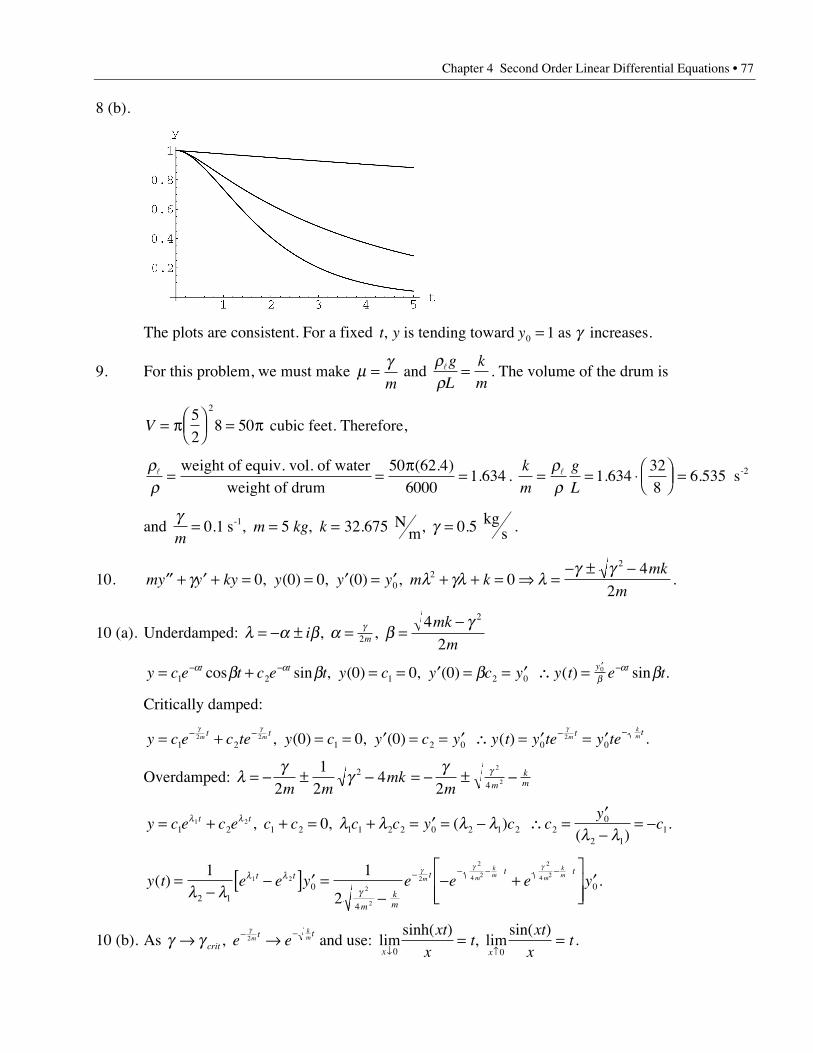
Chapter 4 Second Order Linear Differential Equations • 77
8 (b).
The plots are consistent. For a fixed t y y, is tending toward as increases.0 1= g
9. For this problem, we must make m g=m
and rr
lg
L
k
m= . The volume of the drum is
V = pÊËÁ
ˆ¯ = p
52
8 502
cubic feet. Therefore,
rrl = =
p=
weight of equiv. vol. of waterweight of drum
50 62 46000
1 634( . )
. . k
m
g
L= = ◊ Ê
ËÁˆ¯ =
rrl 1 634
328
6 535. . s-2
and g gm
m kg k= = = =0 1 5 32 675 0 5. , , . , . s Nm kg
s-1 .
10. my y ky y y y m kmk
m¢¢ + ¢ + = = ¢ = ¢ + + = fi =
- ± -g l gl l
g g0 0 0 0 0
4
202
2
, ( ) , ( ) , .
10 (a). Underdamped: l a b a bgg= - ± = =
-i
mk
mm, , 2
24
2
y c e t c e t y c y c y y t e tt t y t= + = = ¢ = = ¢ \ =- - ¢ -1 2 1 2 00 0 0 0a a
bab b b bcos sin , ( ) , ( ) ( ) sin .
Critically damped:
y c e c te y c y c y y t y te y tem m mkmt t t t= + = = ¢ = = ¢ \ = ¢ = ¢- - - -
1 2 1 2 0 0 02 2 20 0 0g g g
, ( ) , ( ) ( ) .
Overdamped: l g g g g= - ± - = - ± -2
12
42
2
4
2
2
m mmk
m mkm
y c e c e c c c c y c cy
ct t= + + = + = ¢ = - \ =¢
-= -1 2 1 2 1 1 2 2 0 2 1 2 2
0
2 11
1 2 0l l l l l ll l
, , ( ) ( )
.
y t e e y e e e yt t
mkm
t t tm m
km m
km( )
=
--[ ] ¢ =
-- +
È
ÎÍÍ
˘
˚˙˙
¢- - - -1 1
22 10
4
01 2
2
2
2
2
4 2
2
4 2
l ll l
g
g g g
.
10 (b). As g gg
Æ Æ = =- -
Ø ≠critt t
x xe e
xt
xt
xt
xtm
km, lim
sinh( ), lim
sin( )2
0 0 and use: .
78 • Chapter 4 Second Order Linear Differential Equations
Section 4.8
1 (a). ¢ = ¢¢ = - - - = - - + = - -y y t t tP P3 0 0 2 3 3 3 1 9 6 3 9 3, , ( ) ( ) .
1 (b). l l l l2 2 3 3 1 0- - = -( ) +( ) = , and thus y c e c eCt t= +-
1 23 .
1 (c). y c e c e tt t= + + --1 2
3 3 1. From the initial conditions, we have
y c c y c c( ) ( )0 1 1 0 3 3 31 2 1 2= + - = ¢ = - + + = and . Solving these simultaneous equations yields
c c1 2
32
12
= = and , and so y e e tt t= + + --32
12
3 13 .
2 (b). y c e c eCt t= +-
1 23 .
2 (c). y c e c e et t t= + --1 2
3 213
.
y c c y c c c c( ) ( )0 1 0 3 056
121 2
13 1 2
23 1 2= + - = ¢ = - + - = fi = = and and , and so
y e e et t t= + --56
12
3 13
2 .
3 (a). ¢ = ¢¢ = - - =y e y e e ePt
Pt t t8 32 32 8 2 2 204 4 4 4, , ( ( )) .
3 (b). l l l l2 2 2 1 0- - = -( ) +( ) = , and thus y c e c eCt t= +-
1 22 .
3 (c). y c e c e et t t= + +-1 2
2 42 . From the initial conditions, we have
y c c y c c( ) ( )0 2 0 0 2 8 11 2 1 2= + + = ¢ = - + + = and . Solving these simultaneous equations yields
c c1 21 3= = - and , and so y e e et t t= - +- 3 22 4 .
4 (b). y c e c eCt t= +-
1 22 .
4 (c). y c e c et t= + --1 2
2 5 .
y c e c e y c e c e c e c e( ) ( )- = + - = ¢ - = - + = fi = =- - -1 5 0 1 2 1 3 211
22
11
22
11
22 and and , and so
y e et t= + -- + +3 2 51 2 1( ) ( ) .
5 (a). 2 2 2 2+ - =( )t t .
5 (b). l l l l2 1 0+ = +( ) = , and thus y c e cCt= +-
1 2.
5 (c). y c e c t tt= + + --1 2
2 2 . From the initial conditions, we have
y c e c y c e( ) ( )1 1 1 1 2 2 211
2 11= + - = ¢ = - + - = -- - and . Solving these simultaneous equations
yields c e c1 22 0= = and , and so y e t tt= + -- -2 21 2( ) .
6 (b). y c e cCt= +-
1 2.
6 (c). y c e c tet t= + -- -1 2 2 .
y c c y c c c( ) ( )0 2 0 2 2 4 61 2 1 1 2= + = ¢ = - - = fi = - = and and , and so y e tet t= - + -- -4 6 2 .
7 (a). ¢ = - ¢¢ = - - + + = -y t y t t t t t tP P2 2 2 4 2 4 2 2 2 2 3 2sin , cos , cos ( cos ) cos .
Chapter 4 Second Order Linear Differential Equations • 79
7 (b). l2 1 0+ = , and thus y c t c tC = +1 2cos sin .
7 (c). y c t c t t t= + + +1 2 2 2cos sin cos . From the initial conditions, we have
y c y c( ) ( )0 1 0 0 2 01 2= + = ¢ = + = and . Solving these simultaneous equations yields
c c1 21 2= - = - and , and so y t t t t= - - + +cos sin cos2 2 2 .
8 (b). y c t c tC = +1 22 2cos sin .
8 (c). y c t c t et= + + -1 22 2 2cos sin p .
y c y c c c( ) ( )p p= + = ¢ = + = fi = = -1 2 1 22 2 2 2 0 0 1 and and , and so y t et= - + -sin2 2 p .
9 (a). 10 2 10 1 10 1 10 20 20 10 20 10 102 2 2- + + + = - - + + + =( ( )) ( )t t t t t t .
9 (b). l l l2 2 2 0 1- + = ±, so = i , and thus y c e t c e tCt t= +1 2cos sin .
9 (c). y c e t c e t tt t= + + +1 225 1cos sin ( ) . From the initial conditions, we have
y c y c c( ) ( )0 5 0 0 10 01 1 2= + = ¢ = + + = and . Solving these simultaneous equations yields
c c1 25 5= - = - and , and so y e t e t tt t= - - + +5 5 5 1 2cos sin ( ) .
10 (b). y c e t c e tCt t= +1 2cos sin .
10 (c). y c e t c e t t tt t= + + +1 2 2cos sin cos sin .
y c e y c e c e c e cp pp p p p
2 2 2 1 2 1 22 2 2 21 1 2 0 2 0( ) = + = ¢( ) = - + - = fi = - =- and and , and so
y e t t tt= - + +-2 22p
cos cos sin .
11 (a). ¢ = + ¢¢ = + +y t t e y t t ePt
Pt1
22
12
2 42 2( ) , ( ) , and t
t e t t et
e et t t t2
22
22 1 2
12
22
+ +ÊËÁ
ˆ¯
- ◊ +( ) + = .
11 (b). l l l2 22 1 1 0- + = - =( ) , and thus y c e c teCt t= +1 2 .
11 (c). y c e c tet
et t t= + +1 2
2
2. From the initial conditions, we have
y c y c c( ) ( )0 0 21 1 2= = ¢ = + =-2 and . Solving these simultaneous equations yields
c c1 22 4= - = and , and so y e tet
et t t= - + +2 42
2
.
12 (b). y c e c teCt t= +1 2 .
12 (c). y c e c te t t tt t= + + + + +1 22 4 10 cos .
y c y c c c c( ) ( )0 10 1 1 0 4 3 10 91 1 2 1 2= + + = ¢ = + + = fi = - = and and , and so
y e te t t tt t= - + + + + +10 9 4 102 cos .
13. First, y a u a vP = +1 2 . Now we have
¢¢ + ¢ + = ¢¢ + ¢ +( ) + ¢¢ + ¢ +( ) = +y p t y q t y a u p t u q t u a v p t v q t v a g a gP P P( ) ( ) ( ) ( ) ( ) ( )1 2 1 1 2 2
80 • Chapter 4 Second Order Linear Differential Equations
14. e t e tt t+ + = +[ ] + [ ]212
12
2 123
3 . Thus y u uP = +12
231 3.
15. 4 2 2 2 123
3e e t tt t- -- = - -[ ] + [ ]. Thus y u uP = +2232 3 .
16. cosh t e e e e t tt t t t= + = +[ ] + - -[ ] + [ ]- -12
12
14
2 114
2 11
123 . Thus y u u uP = + +
14
14
1121 2 3.
17. Differentiation gives us ¢ = - ¢¢ = -y e t y ePt
Pt2 2 4 22 2, . From the given differential equation, we
have g t e e t e t e t tt t t t( ) = - + - - + = + - -4 2 2 2 5 2 22 2 2 2 2 2 .
18. Differentiation gives us ¢ = + ¢¢ = -- -y t y tP P312
14
12
32, . From the given differential equation, we
have g t t t t t( ) = - - +ÊËÁ
ˆ¯ = - - -- - - -1
42 3
12
614
32
12
12
32 .
19. Differentiation gives us ¢ = ¢¢ =y yP P3 0, . From the given differential equation, we have
g t t e t e tt t( ) = ◊ + ◊ + ◊ = +0 3 2 3 3 6 .
20. Differentiation gives us ¢ =+
¢¢ = -+
yt
ytP P
11
11 2, ( )
. From the given differential equation, we
have g tt
t t( )( )
ln( ), = -+
+ + > -1
11 12 .
21. Differentiation gives us ¢ = - ¢¢ = -y t y tP Psin , cos . From the given differential equation, we have
g t t t t t t t t( ) cos sin cos cos sin= - - + = -( ) -2 22 2 1 .
22. ( )( ) , l l l l a b- - = - + = fi = - =1 2 3 2 0 3 22 . Differentiation gives us
¢ = - ¢¢ =- -y e y ePt
Pt4 82 2, , and so g t e e e et t t t( ) = - -( ) + ( ) =- - - -8 3 4 2 2 242 2 2 2 .
23. l l l l l a b= - fi + = + = = =1 0 1 0 0 1 02, ( ) , , so and . Differentiation gives us
¢ = ¢¢ =y t yP P2 2, , and so g t t( ) = +2 2 .
24. ( ) , l l l a b- = - + = fi = - =1 2 1 0 2 12 2 . Differentiation gives us
¢ = +( ) ¢¢ = + +( )y t t e y t t ePt
Pt2 22 4 2, , and so g t t t e t t e t e et t t t( ) = + +( ) - +( ) + =2 2 24 2 2 2 2 .
25. l l l l a b= ± fi -( ) = - - + = = - =1 1 1 2 2 0 2 22 2i , , so and . Differentiation gives us
¢ = + ¢¢ = -y e t y e tPt
Ptcos , sin , and so
g t e t e t e t e t tt t t t( ) sin cos sin cos sin= - - +[ ] + +[ ] = - +2 2 2 .
26. l a b2 4 0 0 4+ = fi = = , . Differentiation gives us ¢ = ¢¢ = -y t y tP Pcos , sin , and so
g t t t t( ) sin ( sin ) sin= - + - + = -4 1 3 4 .
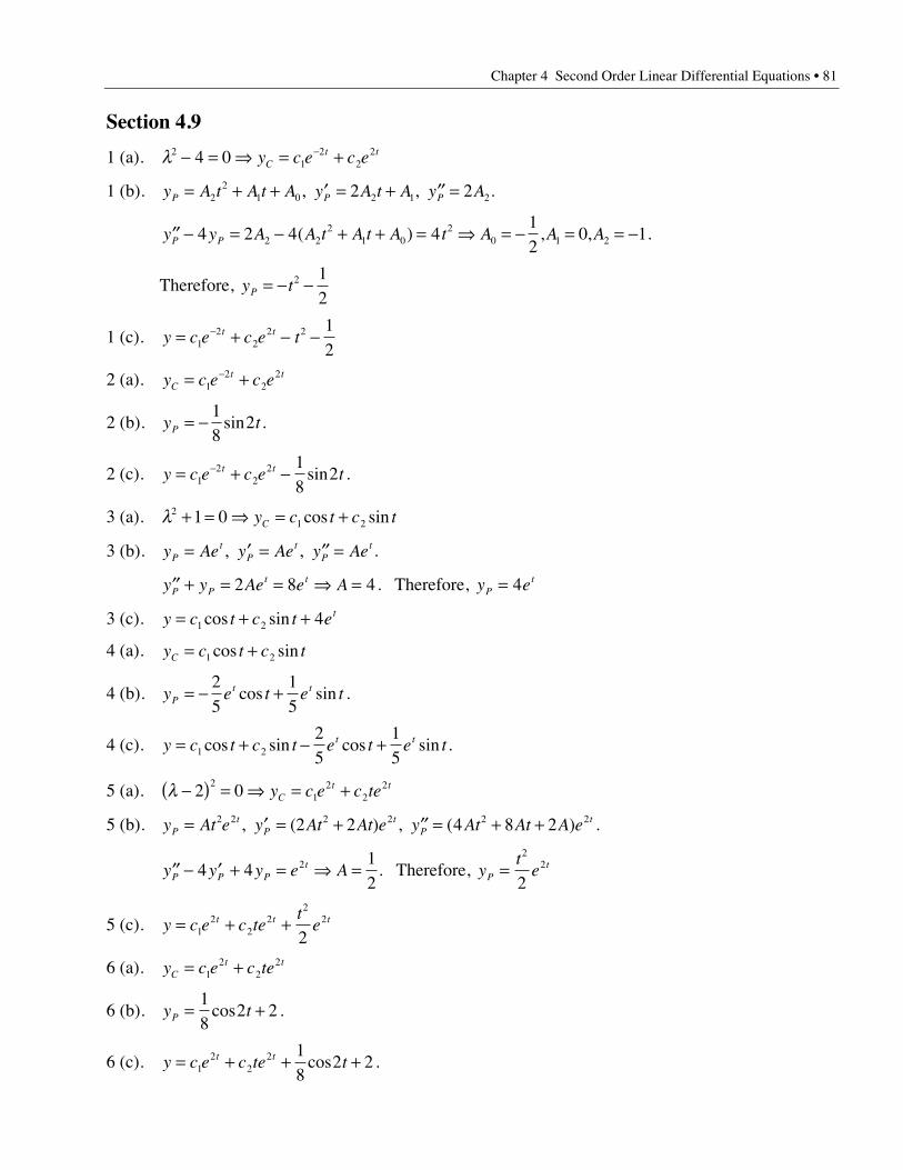
Chapter 4 Second Order Linear Differential Equations • 81
Section 4.9
1 (a). l21
22
24 0- = fi = +-y c e c eCt t
1 (b). y A t A t A y A t A y AP P P= + + ¢ = + ¢¢ =22
1 0 2 1 22 2, , .
¢¢ - = - + + = fi = - = = -y y A A t A t A t A A AP P4 2 4 412
0 12 22
1 02
0 1 2( ) , , .
Therefore, y tP = - -2 12
1 (c). y c e c e tt t= + - --1
22
2 2 12
2 (a). y c e c eCt t= +-
12
22
2 (b). y tP = -18
2sin .
2 (c). y c e c e tt t= + --1
22
2 18
2sin .
3 (a). l21 21 0+ = fi = +y c t c tC cos sin
3 (b). y Ae y Ae y AePt
Pt
Pt= ¢ = ¢¢ =, , .
¢¢ + = = fi =y y Ae e AP Pt t2 8 4. Therefore, y eP
t= 4
3 (c). y c t c t et= + +1 2 4cos sin
4 (a). y c t c tC = +1 2cos sin
4 (b). y e t e tPt t= - +
25
15
cos sin .
4 (c). y c t c t e t e tt t= + - +1 2
25
15
cos sin cos sin .
5 (a). l -( ) = fi = +2 02
12
22y c e c teC
t t
5 (b). y At e y At At e y At At A ePt
Pt
Pt= ¢ = + ¢¢ = + +2 2 2 2 2 22 2 4 8 2, ( ) , ( ) .
¢¢ - ¢ + = fi =y y y e AP P Pt4 4
12
2 . Therefore, yt
ePt=
22
2
5 (c). y c e c tet
et t t= + +12
22
22
2
6 (a). y c e c teCt t= +1
22
2
6 (b). y tP = +18
2 2cos .
6 (c). y c e c te tt t= + + +12
22 1
82 2cos .
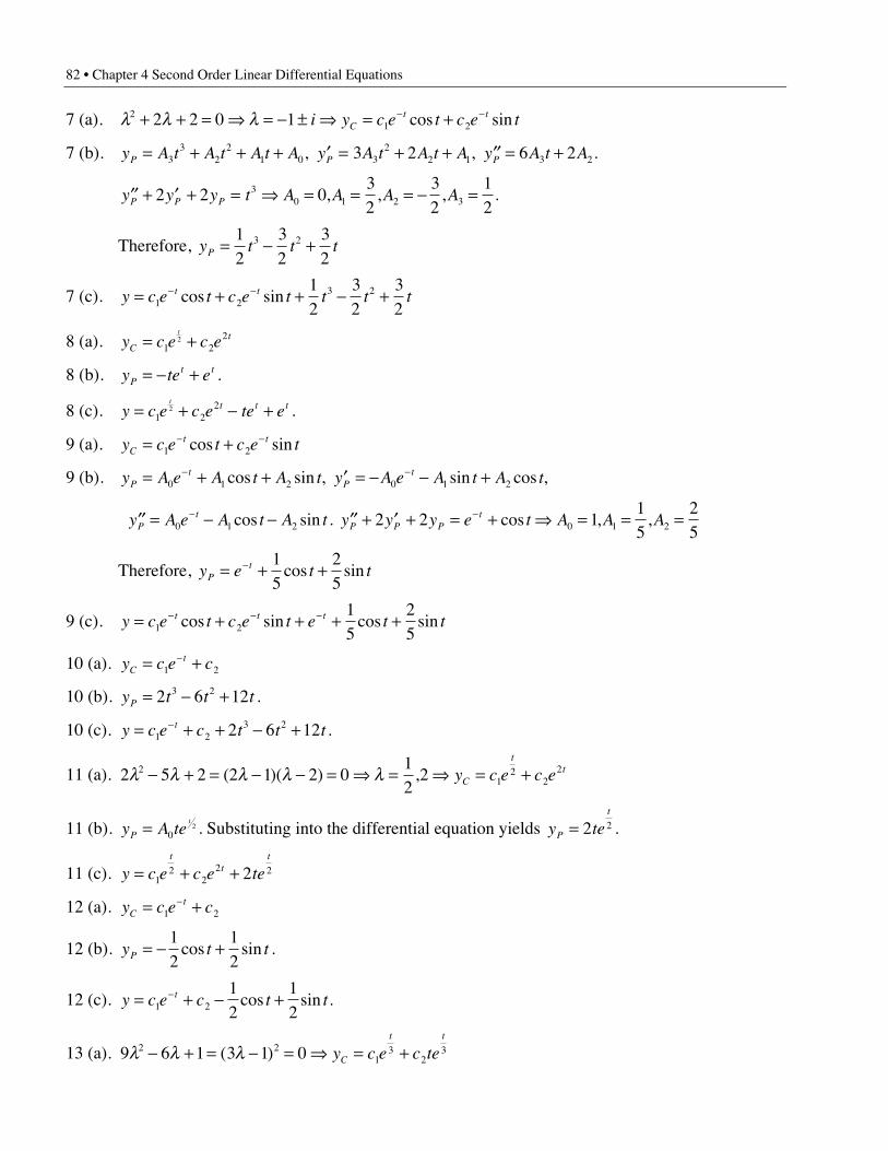
82 • Chapter 4 Second Order Linear Differential Equations
7 (a). l l l21 22 2 0 1+ + = fi = - ± fi = +- -i y c e t c e tC
t tcos sin
7 (b). y A t A t A t A y A t A t A y A t AP P P= + + + ¢ = + + ¢¢ = +33
22
1 0 32
2 1 3 23 2 6 2, , .
¢¢ + ¢ + = fi = = = - =y y y t A A A AP P P2 2 032
32
12
30 1 2 3, , , .
Therefore, y t t tP = - +12
32
32
3 2
7 (c). y c e t c e t t t tt t= + + - +- -1 2
3 212
32
32
cos sin
8 (a). y c e c eCtt
= +1 222
8 (b). y te ePt t= - + .
8 (c). y c e c e te et t t t= + - +1 2
22 .
9 (a). y c e t c e tCt t= +- -
1 2cos sin
9 (b). y A e A t A t y A e A t A tPt
Pt= + + ¢ = - - +- -
0 1 2 0 1 2cos sin , sin cos ,
cos sin¢¢ = - --y A e A t A tPt
0 1 2 . ¢¢ + ¢ + = + fi = = =-y y y e t A A AP P Pt2 2 1
15
250 1 2cos , ,
Therefore, y e t tPt= + +- 1
525
cos sin
9 (c). y c e t c e t e t tt t t= + + + +- - -1 2
15
25
cos sin cos sin
10 (a). y c e cCt= +-
1 2
10 (b). y t t tP = - +2 6 123 2 .
10 (c). y c e c t t tt= + + - +-1 2
3 22 6 12 .
11 (a). 2 5 2 2 1 2 012
221
22
2l l l l l- + = - - = fi = fi = +( )( ) , y c e c eC
tt
11 (b). y A teP
t= 02 . Substituting into the differential equation yields y teP
t
= 2 2 .
11 (c). y c e c e tet
tt
= + +12
22 22
12 (a). y c e cCt= +-
1 2
12 (b). y t tP = - +12
12
cos sin .
12 (c). y c e c t tt= + - +-1 2
12
12
cos sin .
13 (a). 9 6 1 3 1 02 21
32
3l l l- + = - = fi = +( ) y c e c teC
t t
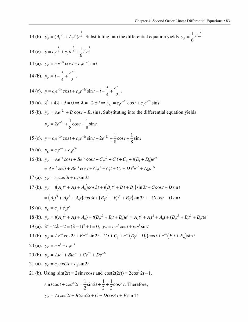
Chapter 4 Second Order Linear Differential Equations • 83
13 (b). y A t A t eP
t
= +( )13
02 3 . Substituting into the differential equation yields y t eP
t
=16
3 3
13 (c). y c e c te t et t t
= + +13
23 3 3
16
14 (a). y c e t c e tCt t= +- -
12
22cos sin
14 (b). y te
P
t
= - +-5
4 2.
14 (c). y c e t c e t tet t
t
= + + - +- --
12
22 5
4 2cos sin .
15 (a). l l l21
22
24 5 0 2+ + = fi = - ± fi = +- -i y c e t c e tCt tcos sin
15 (b). y Ae B t B tPt= + +-2
1 2cos sin . Substituting into the differential equation yields
y e t tPt= + +-2
18
18
2 cos sin .
15 (c). y c e t c e t e t tt t t= + + + +- - -1
22
2 2218
18
cos sin cos sin
16 (a). y c e c eCt t= +-
1 23
16 (b). y Ae t Be t C t C t C t D D ePt t t= + + + + + +- -cos cos ( )2
21 0 1 0
3
= + + + + + +- -Ae t Be t C t C t C D t e D tet t t tcos cos 22
1 0 12 3
03
17 (a). y c t c tC = +1 23 3cos sin
17 (b). y t A t A t A t t B t B t B t C t D tP = + +( ) + + +( ) + +22
1 0 22
1 03 3cos sin cos sin
= + +( ) + + +( ) + + +A t A t A t t B t B t B t t C t D t23
12
0 23
12
03 3cos sin cos sin
18 (a). y c c eCt= +1 2
18 (b). y t A t A t A t B t B t B e A t A t A t B t B t B t ePt t= + + + + + = + + + + +( ) ( ) ( )2
21 0 2
21 0 2
31
20 2
31
20
19 (a). l l l2 22 2 1 1 0- + = - + =( ) ; y c e t c e tCt t= +1 2cos sin
19 (b). y Ae t Be t C t C e D t D t e E t E tPt t t t= + + + + +( ) + +( )- - - -cos sin cos sin2 2 1 0 1 0 1 0
20 (a). y c e c eCt t= + -
1 2
20 (b). y Ate Bte Ce DePt t t t= + + +- -2 2
21 (a). y c t c tC = +1 22 2cos sin
21 (b). Using sin( ) sin cos cos( ( )) cos2 2 2 2 2 2 12t t t t t= = - and ,
sin cos cos sin cost t t t t+ = + +2 212
212
12
4 . Therefore,
y At t Bt t C D t E tP = + + + +cos sin cos sin2 2 4 4
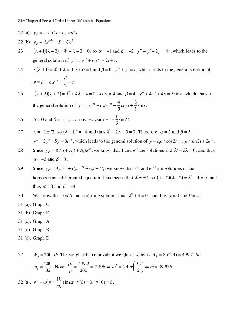
84 • Chapter 4 Second Order Linear Differential Equations
22 (a). y c t c tC = +1 22 2sin cos
22 (b). y Ae B CePt t= + +-2 2
23. l l l l+( ) -( ) = - - =1 2 2 02 , so a b= - = -1 2 and . ¢¢ - ¢ - =y y y t2 4 , which leads to the
general solution of y c e c e tt t= + - +-1 2
2 2 1.
24. l l l l+( ) = + =1 02 , so a b= =1 0 and . ¢¢ + ¢ =y y t, which leads to the general solution of
y c c et
tt= + + --1 2
2
2.
25. l l l l+( ) +( ) = + + =2 2 4 4 02 , so a b= =4 4 and . ¢¢ + ¢ + =y y y t4 4 5sin , which leads to
the general solution of y c e c te t tt t= + - +- -1
22
2 45
35
cos sin .
26. a b= =0 1 and , y c t c t t t= + + -1 2
13
2cos sin sin .
27. l l l l= - ± +( ) = - + + =1 2 1 4 2 5 02 2i , so and thus . Therefore. a b= =2 5 and .
¢¢ + ¢ + = -y y y e t2 5 8 , which leads to the general solution of y c e t c e t et t t= + +- - -1 22 2 2cos sin .
28. Since y t A t A B tePt= + +( )1 0 0
3 , we know that 1 3 and e t are solutions and l l2 3 0- = , and thus
a b= - =3 0 and .
29. Since y A te B te C t CPt t= + + +-
02
02
1 0, we know that e et t2 2 and - are solutions of the
homogeneous differential equation. This means that l = ±2, so l l l+( ) -( ) = - =2 2 4 02 , and
thus a b= = -0 4 and .
30. We know that cos sin2 2t t and are solutions and l2 4 0+ = , and thus a b= =0 4 and .
31 (a). Graph C
31 (b). Graph E
31 (c). Graph A
31 (d). Graph B
31 (e). Graph D
32. W lbb = 200 . The weight of an equivalent weight of water is W lbb = =8 62 4 499 2( . ) . .
mb =20032
. Note: r w wl
p= = fi = Ê
ËÁˆ¯ fi =
499 2200
2 496 2 496322
39 9362.. . . .
32 (a). ¢¢ + = = ¢ =y ym
t y yb
w w2 100 0 0 0sin , ( ) , ( ) .
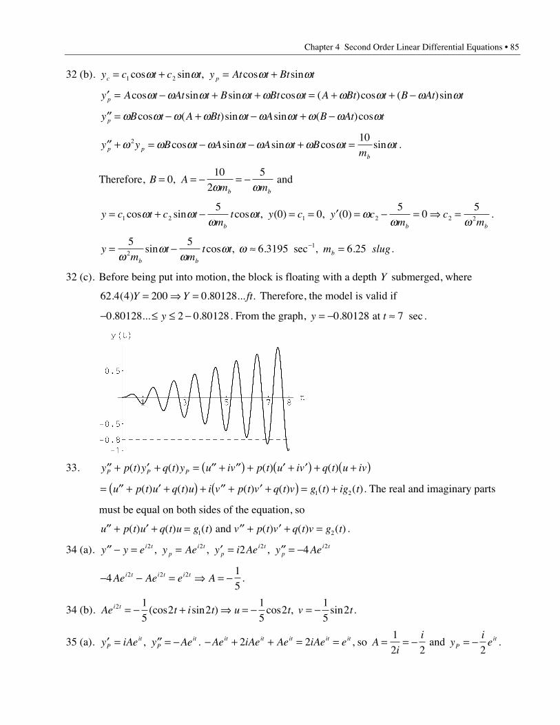
Chapter 4 Second Order Linear Differential Equations • 85
32 (b). y c t c t y At t Bt tc p= + = +1 2cos sin , cos sinw w w w
¢ = - + + = + + -y A t At t B t Bt t A Bt t B At tp cos sin sin cos ( )cos ( )sinw w w w w w w w w w
¢¢ = - + - + -y B t A Bt t A t B At tp w w w w w w w w w wcos ( )sin sin ( )cos
¢¢ + = - - + =y y B t A t A t B tm
tp pb
w w w w w w w w w w2 10cos sin sin cos sin .
Therefore, B Am mb b
= = - = -010
25
, w w
and
y c t c tm
t t y c y cm
cmb b b
= + - = = ¢ = - = fi =1 2 1 2 2 2
50 0 0
50
5cos sin cos , ( ) , ( )w w
ww w
w w.
ym
tm
t t m slugb b
b= - ª =-5 56 3195 6 252
1
ww
ww wsin cos , . sec , . .
32 (c). Before being put into motion, the block is floating with a depth Y submerged, where
62 4 4 200 0 80128. ( ) . ... . Y Y ft= fi = Therefore, the model is valid if
- £ £ -0 80128 2 0 80128. ... .y . From the graph, y t= - ª0 80128 7. sec. at
33. ¢¢ + ¢ + = ¢¢ + ¢¢( ) + ¢ + ¢( ) + +( )y p t y q t y u iv p t u iv q t u ivP P P( ) ( ) ( ) ( )
= ¢¢ + ¢ +( ) + ¢¢ + ¢ +( ) = +u p t u q t u i v p t v q t v g t ig t( ) ( ) ( ) ( ) ( ) ( )1 2 . The real and imaginary parts
must be equal on both sides of the equation, so
¢¢ + ¢ + = ¢¢ + ¢ + =u p t u q t u g t v p t v q t v g t( ) ( ) ( ) ( ) ( ) ( )1 2 and .
34 (a). ¢¢ - = = ¢ = ¢¢ = -y y e y Ae y i Ae y Aei tp
i tp
i tp
i t2 2 2 22 4, , ,
- - = fi = -415
2 2 2Ae Ae e Ai t i t i t .
34 (b). Ae t i t u t v ti t2 15
2 215
215
2= - + fi = - = -(cos sin ) cos , sin .
35 (a). ¢ = ¢¢ = -y iAe y AePit
Pit, . - + + = =Ae iAe Ae iAe eit it it it it2 2 , so A
i
i= = -
12 2
and yi
ePit= -
2.
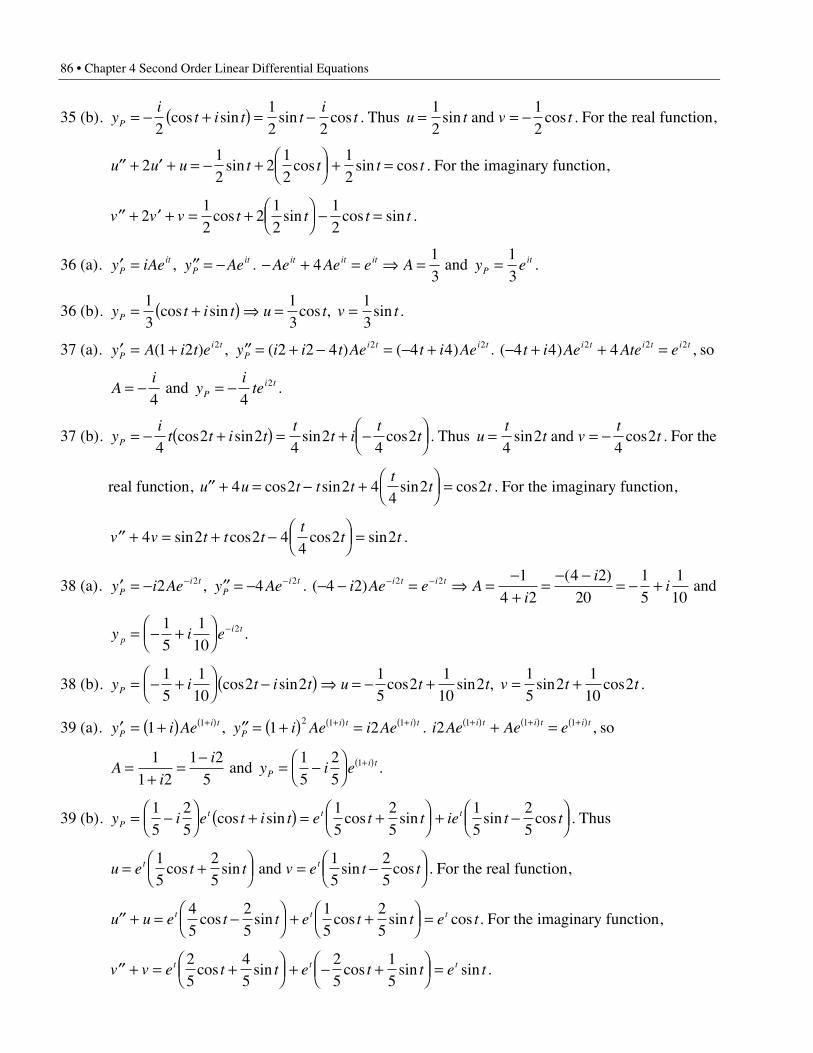
86 • Chapter 4 Second Order Linear Differential Equations
35 (b). yi
t i t ti
tP = - +( ) = -2
12 2
cos sin sin cos . Thus u t v t= = -12
12
sin cos and . For the real function,
¢¢ + ¢ + = - + ÊËÁ
ˆ¯ + =u u u t t t t2
12
212
12
sin cos sin cos . For the imaginary function,
¢¢ + ¢ + = + ÊËÁ
ˆ¯ - =v v v t t t t2
12
212
12
cos sin cos sin .
36 (a). ¢ = ¢¢ = -y iAe y AePit
Pit, . - + = fi =Ae Ae e Ait it it4
13
and y ePit=
13
.
36 (b). y t i t u t v tP = +( ) fi = =13
13
13
cos sin cos , sin .
37 (a). ¢ = + ¢¢ = + - = - +y A i t e y i i t Ae t i AePi t
Pi t i t( ) , ( ) ( )1 2 2 2 4 4 42 2 2 . ( )- + + =4 4 42 2 2t i Ae Ate ei t i t i t , so
Ai
= -4
and yi
tePi t= -
42 .
37 (b). yi
t t i tt
t it
tP = - +( ) = + -ÊËÁ
ˆ¯4
2 24
24
2cos sin sin cos . Thus ut
t vt
t= = -4
24
2sin cos and . For the
real function, ¢¢ + = - + ÊËÁ
ˆ¯ =u u t t t
tt t4 2 2 4
42 2cos sin sin cos . For the imaginary function,
¢¢ + = + - ÊËÁ
ˆ¯ =v v t t t
tt t4 2 2 4
42 2sin cos cos sin .
38 (a). ¢ = - ¢¢ = -- -y i Ae y AePi t
Pi t2 42 2, . ( )
( )- - = fi =
-+
=- -
= - +- -4 21
4 24 220
15
110
2 2i Ae e Ai
iii t i t and
y i epi t= - +Ê
ËÁˆ¯
-15
110
2 .
38 (b). y i t i t u t t v t tP = - +ÊËÁ
ˆ¯ -( ) fi = - + = +
15
110
2 215
21
102
15
21
102cos sin cos sin , sin cos .
39 (a). ¢ = +( ) ¢¢ = +( ) =+( ) +( ) +( )y i Ae y i Ae i AePi t
Pi t i t1 1 21 2 1 1, . i Ae Ae ei t i t i t2 1 1 1+( ) +( ) +( )+ = , so
Ai
i=
+=
-11 2
1 25
and y i ePi t= -Ê
ËÁˆ¯
+( )15
25
1 .
39 (b). y i e t i t e t t ie t tPt t t= -Ê
ËÁˆ¯ +( ) = +Ê
ËÁˆ¯ + -Ê
ËÁˆ¯
15
25
15
25
15
25
cos sin cos sin sin cos . Thus
u e t t v e t tt t= +ÊËÁ
ˆ¯ = -Ê
ËÁˆ¯
15
25
15
25
cos sin sin cos and . For the real function,
¢¢ + = -ÊËÁ
ˆ¯ + +Ê
ËÁˆ¯ =u u e t t e t t e tt t t4
525
15
25
cos sin cos sin cos . For the imaginary function,
¢¢ + = +ÊËÁ
ˆ¯ + - +Ê
ËÁˆ¯ =v v e t t e t t e tt t t2
545
25
15
cos sin cos sin sin .
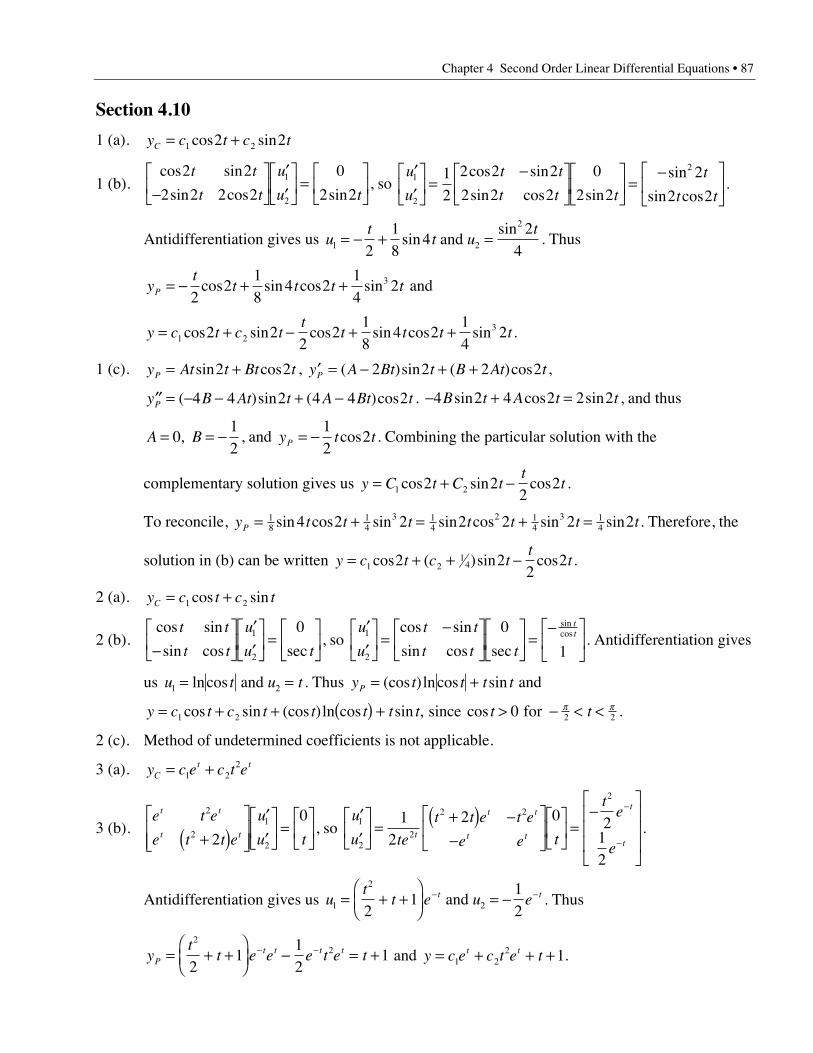
Chapter 4 Second Order Linear Differential Equations • 87
Section 4.10
1 (a). y c t c tC = +1 22 2cos sin
1 (b).cos sin
sin cos sin
2 2
2 2 2 2
0
2 21
2
t t
t t
u
u t-È
ÎÍ
˘
˚˙
¢¢
È
ÎÍ
˘
˚˙ =
È
ÎÍ
˘
˚˙, so
¢¢
È
ÎÍ
˘
˚˙ =
-È
ÎÍ
˘
˚˙
È
ÎÍ
˘
˚˙ =
-È
ÎÍ
˘
˚˙
u
u
t t
t t t
t
t t1
2
212
2 2 2
2 2 2
0
2 2
2
2 2
cos sin
sin cos sin
sin
sin cos.
Antidifferentiation gives us ut
t ut
1 2
2
218
42
4= - + =sin
sin and . Thus
yt
t t t tP = - + +2
218
4 214
23cos sin cos sin and
y c t c tt
t t t t= + - + +1 232 2
22
18
4 214
2cos sin cos sin cos sin .
1 (c). y At t Bt tP = +sin cos2 2 , ¢ = - + +y A Bt t B At tP ( )sin ( )cos2 2 2 2 ,
¢¢ = - - + -y B At t A Bt tP ( )sin ( )cos4 4 2 4 4 2 . - + =4 2 4 2 2 2B t A t tsin cos sin , and thus
A B= = -012
, , and y t tP = -12
2cos . Combining the particular solution with the
complementary solution gives us y C t C tt
t= + -1 22 22
2cos sin cos .
To reconcile, y t t t t t t tP = + = + =18
14
3 14
2 14
3 144 2 2 2 2 2 2sin cos sin sin cos sin sin . Therefore, the
solution in (b) can be written y c t c tt
t= + + -1 21
42 22
2cos ( )sin cos .
2 (a). y c t c tC = +1 2cos sin
2 (b).cos sin
sin cos sec
t t
t t
u
u t-È
ÎÍ
˘
˚˙
¢¢
È
ÎÍ
˘
˚˙ =
È
ÎÍ
˘
˚˙
1
2
0, so
¢¢
È
ÎÍ
˘
˚˙ =
-È
ÎÍ
˘
˚˙
È
ÎÍ
˘
˚˙ =
-È
ÎÍ
˘
˚˙
u
u
t t
t t t
tt1
2
0
1
cos sin
sin cos sec
sincos . Antidifferentiation gives
us u t u t1 2= =lncos and . Thus y t t t tP = +(cos )lncos sin and
y c t c t t t t t t t= + + ( ) + > - < <1 2 2 20cos sin (cos )ln cos sin , cos since for p p .
2 (c). Method of undetermined coefficients is not applicable.
3 (a). y c e c t eCt t= +1 2
2
3 (b).e t e
e t t e
u
u t
t t
t t
2
21
22
0
+( )È
ÎÍÍ
˘
˚˙˙
¢¢
È
ÎÍ
˘
˚˙ =
È
ÎÍ
˘
˚˙, so
¢¢
È
ÎÍ
˘
˚˙ =
+( ) --
È
ÎÍ
˘
˚˙
È
ÎÍ
˘
˚˙ =
-È
Î
ÍÍÍ
˘
˚
˙˙˙
-
-
u
u te
t t e t e
e e t
te
et
t t
t t
t
t
1
22
2 2
2
12
2 0 212
.
Antidifferentiation gives us ut
t e u et t1
2
221
12
= + +ÊËÁ
ˆ¯
= -- - and . Thus
yt
t e e e t e tPt t t t= + +
ÊËÁ
ˆ¯
- = +- -2
2
21
12
1 and y c e c t e tt t= + + +1 22 1.
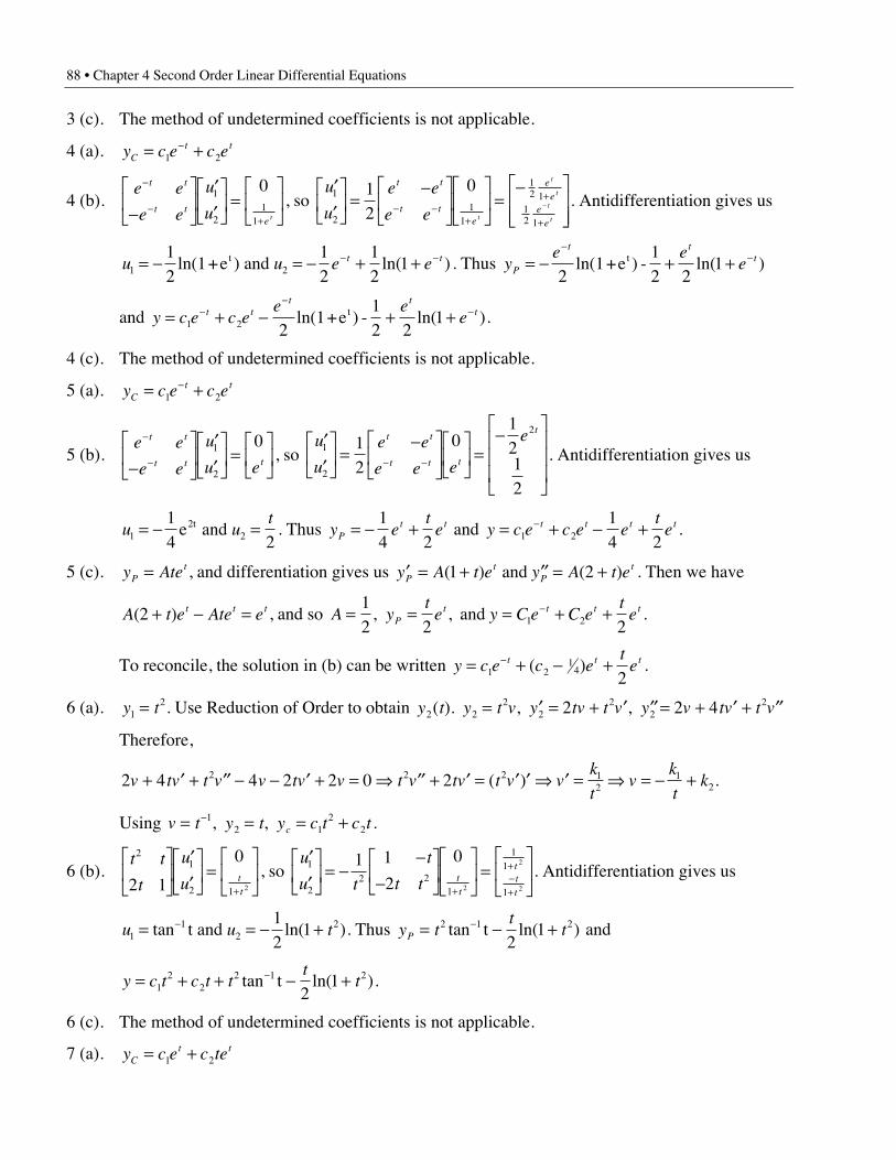
88 • Chapter 4 Second Order Linear Differential Equations
3 (c). The method of undetermined coefficients is not applicable.
4 (a). y c e c eCt t= +-
1 2
4 (b).e e
e e
u
u
t t
t te t
-
-+-
È
ÎÍ
˘
˚˙
¢¢
È
ÎÍ
˘
˚˙ =
È
ÎÍ
˘
˚˙
1
21
1
0, so
¢¢
È
ÎÍ
˘
˚˙ =
-È
ÎÍ
˘
˚˙
È
ÎÍ
˘
˚˙ =
-È
ÎÍÍ
˘
˚˙˙- -
+
+
+
-
u
u
e e
e e
t t
t te
ee
ee
t
t
t
t
t
1
21
1
12 1
12 1
12
0. Antidifferentiation gives us
u u e et t1 2
12
12
12
1= - = - + +- -ln(1+e ) and t ln( ) . Thus ye e
eP
t tt= - + +
--
2 21ln(1+e ) -
12
t ln( )
and y c e c ee e
et tt t
t= + - + +--
-1 2 2 2
1ln(1+e ) -12
t ln( ).
4 (c). The method of undetermined coefficients is not applicable.
5 (a). y c e c eCt t= +-
1 2
5 (b).e e
e e
u
u e
t t
t t t
-
--È
ÎÍ
˘
˚˙
¢¢
È
ÎÍ
˘
˚˙ =
È
ÎÍ
˘
˚˙
1
2
0, so
¢¢
È
ÎÍ
˘
˚˙ =
-È
ÎÍ
˘
˚˙
È
ÎÍ
˘
˚˙ =
-È
Î
ÍÍÍ
˘
˚
˙˙˙
- -
u
u
e e
e e e
et t
t t t
t
1
2
2
12
01212
. Antidifferentiation gives us
u ut
1 2
14 2
= - =e and 2t . Thus y et
ePt t= - +
14 2
and y c e c e et
et t t t= + - +-1 2
14 2
.
5 (c). y AtePt= , and differentiation gives us ¢ = + ¢¢ = +y A t e y A t eP
tP
t( ) ( )1 2 and . Then we have
A t e Ate et t t( )2 + - = , and so A yt
e y C e C et
ePt t t t= = = + +-1
2 2 21 2, and , .
To reconcile, the solution in (b) can be written y c e c et
et t t= + - +-1 2
14
2( ) .
6 (a). y t12= . Use Reduction of Order to obtain y t y t v y tv t v y v tv t v2 2
22
22
22 2 4( ). , , = ¢ = + ¢ ¢¢ = + ¢ + ¢¢
Therefore,
2 4 4 2 2 0 22 2 2 12
12v tv t v v tv v t v tv t v v
k
tv
k
tk+ ¢ + ¢¢ - - ¢ + = fi ¢¢ + ¢ = ¢ ¢ fi ¢ = fi = - +( ) .
Using v t y t y c t c tc= = = +-12 1
22, , .
6 (b).t t
t
u
u tt
21
2 12 1
0
2
È
ÎÍ
˘
˚˙
¢¢
È
ÎÍ
˘
˚˙ =
È
ÎÍ
˘
˚˙
+
, so ¢¢
È
ÎÍ
˘
˚˙ = -
--
È
ÎÍ
˘
˚˙
È
ÎÍ
˘
˚˙ =
È
ÎÍ
˘
˚˙
+
+-+
u
u t
t
t t tt
ttt
1
22 2
1
11
1
1 1
2
0
2
2
2
. Antidifferentiation gives us
u u t11
221
21= = - +-tan ln( )t and . Thus y t
ttP = - +-2 1 2
21tan ln( )t and
y c t c t tt
t= + + - +-1
22
2 1 2
21tan ln( )t .
6 (c). The method of undetermined coefficients is not applicable.
7 (a). y c e c teCt t= +1 2
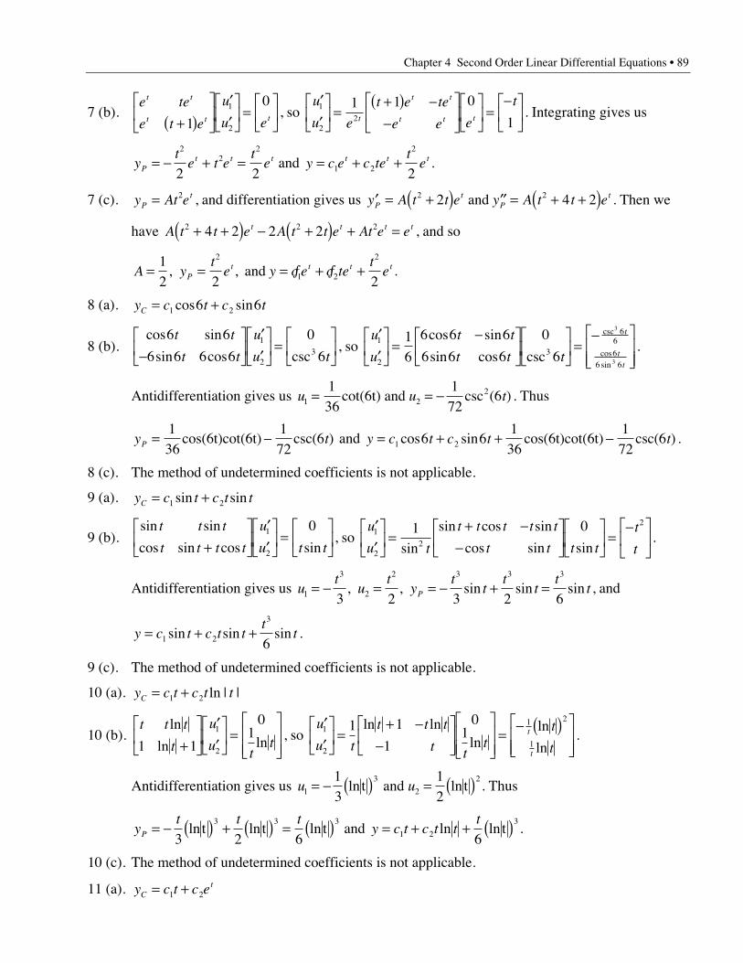
Chapter 4 Second Order Linear Differential Equations • 89
7 (b).e te
e t e
u
u e
t t
t t t+( )È
ÎÍ
˘
˚˙
¢¢
È
ÎÍ
˘
˚˙ =
È
ÎÍ
˘
˚˙1
01
2
, so ¢¢
È
ÎÍ
˘
˚˙ =
+( ) --
È
ÎÍ
˘
˚˙
È
ÎÍ
˘
˚˙ =
-È
ÎÍ
˘
˚˙
u
u e
t e te
e e e
tt
t t
t t t1
22
1 1 0
1. Integrating gives us
yt
e t et
ePt t t= - + =
22
2
2 2 and y c e c te
tet t t= + +1 2
2
2.
7 (c). y At ePt= 2 , and differentiation gives us ¢ = +( ) ¢¢ = + +( )y A t t e y A t t eP
tP
t2 22 4 2 and . Then we
have A t t e A t t e At e et t t t2 2 24 2 2 2+ +( ) - +( ) + = , and so
A yt
e y c e c tet
ePt t t t= = = + +
12 2 2
2
1 2
2
, and , ƒ ƒ .
8 (a). y c t c tC = +1 26 6cos sin
8 (b).cos sin
sin cos csc
6 6
6 6 6 6
0
61
23
t t
t t
u
u t-È
ÎÍ
˘
˚˙
¢¢
È
ÎÍ
˘
˚˙ =
È
ÎÍ
˘
˚˙ , so
¢¢
È
ÎÍ
˘
˚˙ =
-È
ÎÍ
˘
˚˙
È
ÎÍ
˘
˚˙ =
-È
ÎÍÍ
˘
˚˙˙
u
u
t t
t t t
t
tt
1
23
66
66 6
16
6 6 6
6 6 6
0
6
3
3
cos sin
sin cos csc
csc
cossin
.
Antidifferentiation gives us u u t1 221
36172
6= = -cot(6t) and csc ( ) . Thus
y tP = -136
172
6cos(6t)cot(6t) csc( ) and y c t c t t= + + -1 26 6136
172
6cos sin csc( )cos(6t)cot(6t) .
8 (c). The method of undetermined coefficients is not applicable.
9 (a). y c t c t tC = +1 2sin sin
9 (b).sin sin
cos sin cos sin
t t t
t t t t
u
u t t+È
ÎÍ
˘
˚˙
¢¢
È
ÎÍ
˘
˚˙ =
È
ÎÍ
˘
˚˙
1
2
0, so
¢¢
È
ÎÍ
˘
˚˙ =
+ --
È
ÎÍ
˘
˚˙
È
ÎÍ
˘
˚˙ =
-È
ÎÍ
˘
˚˙
u
u t
t t t t t
t t t t
t
t1
22
21 0
sin
sin cos sin
cos sin sin.
Antidifferentiation gives us ut
ut
yt
tt
tt
tP1
3
2
2 3 3 3
3 2 3 2 6= - = = - + =, , sin sin sin , and
y c t c t tt
t= + +1 2
3
6sin sin sin .
9 (c). The method of undetermined coefficients is not applicable.
10 (a). y c t c t tC = +1 2 ln | |
10 (b).t t t
t
u
u tt
ln
ln ln1 1
011
2+È
ÎÍ
˘
˚˙
¢¢
È
ÎÍ
˘
˚˙ =
È
ÎÍÍ
˘
˚˙˙, so
¢¢
È
ÎÍ
˘
˚˙ =
+ --
È
ÎÍ
˘
˚˙
È
ÎÍÍ
˘
˚˙˙
= - ( )È
ÎÍÍ
˘
˚˙˙
u
u t
t t t
t tt
t
tt
t
1
2
1 2
1
1 1
1
01
ln lnln
ln
ln.
Antidifferentiation gives us u u1 2
13
12
= - ( ) = ( )ln t and ln t3 2
. Thus
yt t t
P = - ( ) + ( ) = ( )3 2 6
ln t ln t ln t3 3 3
and y c t c t tt
= + + ( )1 2 6ln ln t
3.
10 (c). The method of undetermined coefficients is not applicable.
11 (a). y c t c eCt= +1 2
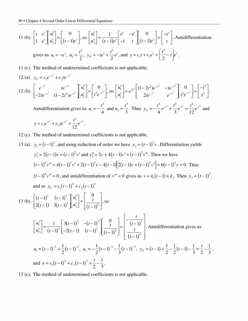
90 • Chapter 4 Second Order Linear Differential Equations
11 (b).t e
e
u
u t e
t
t t1
0
11
2
È
ÎÍ
˘
˚˙
¢¢
È
ÎÍ
˘
˚˙ =
-( )È
ÎÍ
˘
˚˙ , so
¢¢
È
ÎÍ
˘
˚˙ =
-( )-
-È
ÎÍ
˘
˚˙ -( )
È
ÎÍ
˘
˚˙ =
-È
ÎÍ
˘
˚˙
u
u t e
e e
t t e
e
tt
t t
t
t1
2
11 1
0
1. Antidifferentiation
gives us u e ut
y tet
etP
t t1 2
2 2
2 2= - = = - +, , , and y c t c e
tt et t= + + -
ÊËÁ
ˆ¯1 2
2
2.
11 (c). The method of undetermined coefficients is not applicable.
12 (a). y c e c teCt t= +- -
1 2
2 2
12 (b).e te
te t e
u
u t e
t t
t t t
- -
- - -- -
È
ÎÍÍ
˘
˚˙˙
¢¢
È
ÎÍ
˘
˚˙ =
È
ÎÍ
˘
˚˙
2 2
2 2 2
2 1 2
02
1
22
( ), so
¢¢
È
ÎÍ
˘
˚˙ =
- -È
ÎÍÍ
˘
˚˙˙
È
ÎÍ
˘
˚˙ =
-È
ÎÍ
˘
˚˙
- -
- - -
u
ue
t e te
te e t e
t
tt
t t
t t t1
2
22
2
3
2
2
2 2
2 2 2
1 2
2
0( ).
Antidifferentiation gives us ut
ut
1
4
2
3
4 3= - = and . Thus y
te
te
teP
t t t= - + =4 4 4
4 3 12
2 2 2- - - and
y c e c tet
et t t= + +1 2
42 2 2
12- - - .
12 (c). The method of undetermined coefficients is not applicable.
13 (a). y t1
21= -( ) , and using reduction of order we have y t v2
21= -( ) . Differentiation yields
¢ = -( ) + -( ) ¢ ¢¢ = + -( ) ¢ + -( ) ¢¢y t v t v y v t v t v2
2
2
22 1 1 2 4 1 1 and . Then we have
t v t v t v t t v t v t v-( ) ¢¢ + -( ) ¢ + -( ) - -( ) -( ) + -( ) ¢[ ] + -( ) =1 4 1 2 1 4 1 2 1 1 6 1 04 3 2 2 2
. Thus
t v-( ) ¢¢ =1 04
, and antidifferentiation of ¢¢ =v 0 gives us v k t k= -( ) +1 21 . Then y t2
31= -( ) ,
and so y c t c tC = -( ) + -( )1
2
2
31 1
13 (b).t t
t t
u
ut
t
-( ) -( )-( ) -( )
È
ÎÍÍ
˘
˚˙˙
¢¢
È
ÎÍ
˘
˚˙ =
-( )
È
ÎÍÍ
˘
˚˙˙
1 1
2 1 3 1
0
1
2 3
21
22
, so
¢¢
È
ÎÍ
˘
˚˙ =
-( )-( ) - -( )
- -( ) -( )È
ÎÍÍ
˘
˚˙˙ -( )
È
ÎÍÍ
˘
˚˙˙
=-
-( )
-( )
È
Î
ÍÍÍÍ
˘
˚
˙˙˙˙
u
u t
t t
t tt
t
t
tt
t
1
24
2 3
2 2
3
4
1
1
3 1 1
2 1 1
0
1
1
1
. Antidifferentiation gives us
u t t u t t1
1 2
2
2 31
12
112
113
1= -( ) + -( ) = - -( ) - -( )- - - -, , y t t
tP = -( ) + - -( ) - = -1
12
12
113 2
13
,
and y c t c tt
= -( ) + -( ) + -1
2
2
31 1
213
.
13 (c). The method of undetermined coefficients is not applicable.
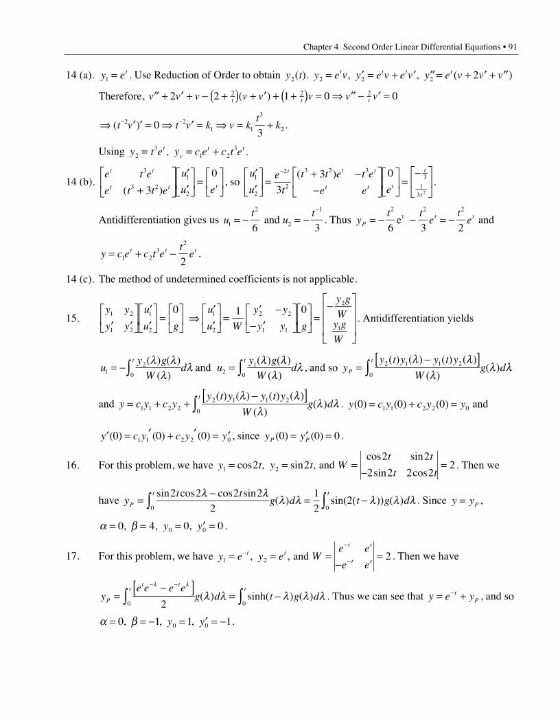
Chapter 4 Second Order Linear Differential Equations • 91
14 (a). y et1 = . Use Reduction of Order to obtain y t y e v y e v e v y e v v vt t t t
2 2 2 2 2( ). , , ( )= ¢ = + ¢ ¢¢ = + ¢ + ¢¢
Therefore, ¢¢ + ¢ + - +( ) + ¢ + +( ) = fi ¢¢ - ¢ =v v v v v v v vt t t2 2 1 0 02 2 2( )
fi ¢ ¢ = fi ¢ = fi = +- -( )t v t v k v kt
k2 21 1
3
203
.
Using y t e y c e c t etc
t t2
31 2
3= = +, .
14 (b).e t e
e t t e
u
u e
t t
t t t
3
3 2
1
23
0
( )+È
ÎÍ
˘
˚˙
¢¢
È
ÎÍ
˘
˚˙ =
È
ÎÍ
˘
˚˙ , so
¢¢
È
ÎÍ
˘
˚˙ =
+ --
È
ÎÍ
˘
˚˙
È
ÎÍ
˘
˚˙ =
-È
ÎÍ
˘
˚˙
-u
ue
t
t t e t e
e e e
t t t
t t t
t
t
1
2
2
2
3 2 33
13
3
3 0
2
( ).
Antidifferentiation gives us ut
ut
1
2
2
1
6 3= - = -
-
and . Thus yt t
et
ePt t= - - = -
2 2 2
6 3 2e t and
y c e c t et
et t t= + -1 23
2
2.
14 (c). The method of undetermined coefficients is not applicable.
15.y y
y y
u
u g1 2
1 2
1
2
0
¢ ¢È
ÎÍ
˘
˚˙
¢¢
È
ÎÍ
˘
˚˙ =
È
ÎÍ
˘
˚˙ fi
¢¢
È
ÎÍ
˘
˚˙ =
¢ -- ¢
È
ÎÍ
˘
˚˙
È
ÎÍ
˘
˚˙ =
-È
Î
ÍÍÍ
˘
˚
˙˙˙
u
u W
y y
y y g
y g
Wy g
W
1
2
2 2
1 1
2
1
1 0. Antidifferentiation yields
uy g
Wd u
y g
Wd
t t
12
0 21
0= - =Ú Ú
( ) ( )( )
( ) ( )
( )l l
ll l l
ll and , and so y
y t y y t y
Wg dP
t=
-[ ]Ú 2 1 1 2
0
( ) ( ) ( ) ( )
( )( )
l ll
l l
and y c y c yy t y y t y
Wg d
t= + +
-[ ]Ú1 1 2 22 1 1 2
0
( ) ( ) ( ) ( )
( )( )
l ll
l l . y c y c y y( ) ( ) ( )0 0 01 1 2 2 0= + = and
¢ = ¢ + ¢ = ¢y c y c y y( ) ( ) ( )0 0 01 1 2 2 0 , since y yP P( ) ( )0 0 0= ¢ = .
16. For this problem, we have y t y t Wt t
t t1 22 22 2
2 2 2 22= = =
-=cos , sin
cos sin
sin cos, and . Then we
have yt t
g d t g dP
t t=
-= -Ú Ú
sin cos cos sin( ) sin( ( )) ( )
2 2 2 22
12
20 0
l l l l l l l . Since y yP= ,
a b= = = ¢ =0 4 0 00 0, , , y y .
17. For this problem, we have y e y e We e
e et t
t t
t t1 2 2= = =-
=--
-, , and . Then we have
ye e e e
g d t g dP
t tt t
=-[ ] = -
- -
Ú Úl l
l l l l l20 0
( ) sinh( ) ( ) . Thus we can see that y e ytP= +- , and so
a b= = - = ¢ = -0 1 1 10 0, , , y y .
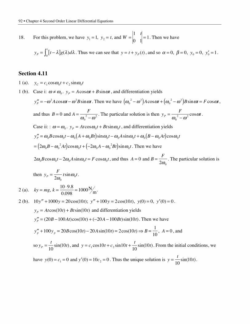
92 • Chapter 4 Second Order Linear Differential Equations
18. For this problem, we have y y t Wt
1 211
0 11= = = =, , and . Then we have
y t g dP
t= -[ ]Ú l l l( )
0. Thus we can see that y t y tP= + ( ) , and so a b= = = ¢ =0 0 0 10 0, , , y y .
Section 4.11
1 (a). y c t c tC = +1 0 2 0cos sinw w
1 (b). Case i: w wπ 0 . y A t B tP = +cos sinw w , and differentiation yields
¢¢ = - -y A t B tP w w w w2 2cos sin . Then we have w w w w w w w02 2
02 2-( ) + -( ) =A t B t F tcos sin cos ,
and thus B AF
= =-
00
2 2 and w w
. The particular solution is then yF
tP =-w w
w0
2 2 cos .
Case ii: : w w= 0 . y At t Bt tP = +cos sinw w0 0 , and differentiation yields
¢¢ = - +( ) - + -( )y B t A Bt t A t B At tP w w w w w w w w w w0 0 0 0 0 0 0 0 0 0cos sin sin cos
= -( ) + - -( )2 20 02
0 0 02
0w w w w w wB At t A Bt tcos sin . Then we have
2 20 0 0 0 0w w w w wB t A t F tcos sin cos- = , and thus A BF
= =02 0
and w
. The particular solution is
then yF
t tP =2 0
0wwsin .
2 (a). ky mg k= =◊
=, Nm
10 9 80 098
1000.
..
2 (b). 10 1000 20 10 100 2 10 0 0 0 0¢¢ + = ¢¢ + = = ¢ =y y t y y t y ycos( ); cos( ), ( ) , ( ) .
y At t Bt tP = +cos( ) sin( )10 10 and differentiation yields
¢¢ = - + - -y B At t A Bt tP ( )cos( ) ( )sin( )20 100 10 20 100 10 . Then we have
¢¢ + = - = fi = =y y B t A t t B Ap p100 20 10 20 10 2 101
100cos( ) sin( ) cos( ) , , and
so yt
tP =10
10sin( ), and y c t c tt
t= + +1 210 1010
10cos sin sin( ). From the initial conditions, we
have y c y c( ) ( )0 0 0 10 01 2= = ¢ = = and . Thus the unique solution is yt
t=10
10sin( ).
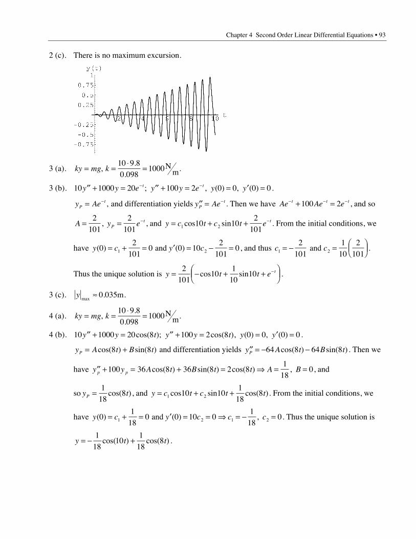
Chapter 4 Second Order Linear Differential Equations • 93
2 (c). There is no maximum excursion.
3 (a). ky mg k= =◊
=, Nm
10 9 80 098
1000.
..
3 (b). 10 1000 20 100 2 0 0 0 0¢¢ + = ¢¢ + = = ¢ =- -y y e y y e y yt t; , ( ) , ( ) .
y Ae y AePt
Pt= ¢¢ =- -, and differentiation yields . Then we have Ae Ae et t t- - -+ =100 2 , and so
A =2
101, y eP
t= -2101
, and y c t c t e t= + + -1 210 10
2101
cos sin . From the initial conditions, we
have y c y c( ) ( )02
1010 0 10
2101
01 2= + = ¢ = - = and , and thus c c1 2
2101
110
2101
= - = ÊËÁ
ˆ¯ and .
Thus the unique solution is y t t e t= - + +ÊËÁ
ˆ¯
-2101
101
1010cos sin .
3 (c). ymax
.ª 0 035m.
4 (a). ky mg k= =◊
=, Nm
10 9 80 098
1000.
..
4 (b). 10 1000 20 8 100 2 8 0 0 0 0¢¢ + = ¢¢ + = = ¢ =y y t y y t y ycos( ); cos( ), ( ) , ( ) .
y A t B tP = +cos( ) sin( )8 8 and differentiation yields ¢¢ = - -y A t B tP 64 8 64 8cos( ) sin( ) . Then we
have ¢¢ + = + = fi = =y y A t B t t A Bp p100 36 8 36 8 2 81
180cos( ) sin( ) cos( ) , , and
so y tP =1
188cos( ), and y c t c t t= + +1 210 10
118
8cos sin cos( ). From the initial conditions, we
have y c y c c c( ) ( ) , 01
180 0 10 0
118
01 2 1 2= + = ¢ = = fi = - = and . Thus the unique solution is
y t t= - +1
1810
118
8cos( ) cos( ) .
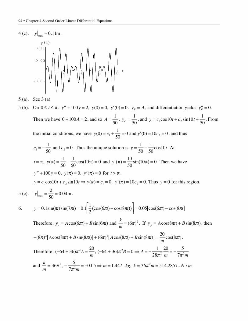
94 • Chapter 4 Second Order Linear Differential Equations
4 (c). ymax
.ª 0 11m.
5 (a). See 3 (a)
5 (b). On 0 £ £ pt : ¢¢ + = = ¢ =y y y y100 2 0 0 0 0, ( ) , ( ) . y AP = , and differentiation yields ¢¢ =yP 0.
Then we have 0 100 2+ =A , and so A =1
50, yP =
150
, and y c t c t= + +1 210 101
50cos sin . From
the initial conditions, we have y c y c( ) ( )0150
0 0 10 01 2= + = ¢ = = and , and thus
c c1 2
150
0= - = and . Thus the unique solution is y t= -1
501
5010cos . At
t y= p p = - p =, ( ) cos( )150
150
10 0 and ¢ p = p =y ( ) sin( )1050
10 0 . Then we have
¢¢ + = p = ¢ p =y y y y100 0 0 0, ( ) , ( ) for t > p .
y c t c t y c y c= + fi = = ¢ = =1 2 1 210 10 0 10 0cos sin ( ) , ( ) .p p Thus y = 0 for this region.
5 (c). ymax
.= =2
500 04m.
6. y t t t t t t= = -ÈÎÍ
˘˚
= -[ ]0 1 7 0 112
6 8 0 05 6 8. sin( )sin( ) . (cos( ) cos( )) . cos( ) cos(p p p p p p
Therefore, y A t B tk
mc = + =cos( ) sin( ) ( )6 6 6 2p p p and . If y A t B tp = +cos( ) sin( )8 8p p , then
- +[ ] + +[ ] =( ) cos( ) sin( ) ( ) cos( ) sin( ) cos( )8 8 8 6 8 820
82 2p p p p p p pA t B t A t B tm
t .
Therefore, ( ) , ( )- + = - + = fi = - = -64 3620
64 36 01
2820 5
72 2
2 2p pp p
Am
B Am m
and k
m mm kg k m N m= - = - fi = = =36
57
0 05 1 447 36 514 285722
2pp
p, . . ... , . ... / .
Chapter 4 Second Order Linear Differential Equations • 95
7 (a). 2 8 80 20 8 0 0 0 0¢¢ + ¢ + = = ¢ =y y y t y ycos , ( ) , ( ) . For the complementary solution, we have
l l l2 4 40 0 2 6+ + = = - ±, and so i . Thus y c e t c e tCt t= +- -
12
226 6cos sin . For the particular
solution, we have y A t B tP = +cos sin8 8 , and differentiation yields ¢ = - +y A t B tP 8 8 8 8sin cos and
¢¢ = - -y A t B tP 64 8 64 8cos sin . Then we have
- - + - + + + =64 8 64 8 4 8 8 8 8 40 8 8 10 8A t B t A t B t A t B t tcos sin ( sin cos ) ( cos sin ) cos . Solving for
A B A B and yields and = - =3
2015
. Thus y c e t c e t t tt t= + - +- -1
22
26 63
208
15
8cos sin cos sin . From
the initial conditions, we have y c y c c( ) ( )03
200 0 2 6
85
01 1 2= - = ¢ = - + + = and . Solving these
simultaneous equations yields c c1 2
320
1360
= = - and , so
y e t e t t tt t= - - +- -320
61360
63
208
15
82 2cos sin cos sin .
7 (b). For sufficiently large t, y t t t( ) cos sinª - +3
208
15
8 , and so the limit does not exist. This equation is
called the steady state solution.
8 (a). y c e t c e tCt t= +- -
12
226 6cos sin . For the particular solution, we have y AeP
t= - ,
¢¢ + ¢ + = fi - + = fi =-y y y e A A A Ap p pt4 40 10 4 40 10
1037
. Thus
y c e t c e t et t t= + +- - -1
22
26 61037
cos sin . From the initial conditions, we have
y c y c c c c( ) ( ) , 01037
0 0 2 61037
01037
51111 1 2 1 2= + = ¢ = - + - = fi = - = - and .
y e t e t et t t= - - +- - -1037
65
1116
1037
2 2cos sin .
8 (b). lim ( )t
y tÆ •
= 0.
9 (a). y c e t c e tCt t= +- -
12
226 6cos sin . For the particular solution, we have y A t B tP = +cos sin6 6 , and
differentiation yields ¢ = - +y A t B tP 6 6 6 6sin cos and ¢¢ = - -y A t B tP 36 6 36 6cos sin . Then we have
- - + - + + + =36 6 36 6 4 6 6 6 6 40 6 6 10 6A t B t A t B t A t B t tcos sin ( sin cos ) ( cos sin ) sin . Solving for
A B A B and yields and = - =3074
574
. Thus y c e t c e t t tt t= + - +- -1
22
26 63074
6574
6cos sin cos sin .
From the initial conditions, we have y c y c c( ) ( )03074
0 0 2 63074
01 1 2= - = ¢ = - + + = and .
96 • Chapter 4 Second Order Linear Differential Equations
Solving these simultaneous equations yields c c1 2
3074
574
= = and , so
y e t e t t tt t= + - +- -3074
65
746
3074
6574
62 2cos sin cos sin .
9 (b). For sufficiently large t, y t t t( ) cos sinª - +3074
6574
6 , and so the limit does not exist. This equation
is called the steady state solution.
10 (a). On 0 2£ £t p :
y c e t c e tCt t= +- -
12
226 6cos sin . For the particular solution, we have yP =
14
. Thus
y c e t c e tt t= + +- -1
22
26 614
cos sin . From the initial conditions, we have
y c y c c c c( ) ( ) , 014
0 0 2 6 014
1121 1 2 1 2= + = ¢ = - + = fi = - = - and .
y e t e t y e y e et t= - - + ÊËÁ
ˆ¯ = + ¢Ê
ËÁˆ¯ = - + =- - - - -1
46
112
614 2
14
14 2
12
12
02 2cos sin , , p pp p p .
On p2 < < •t :
y d e t d e tt t= +- -1
22
26 6cos sin . From the initial conditions, we have
y d e e y d e d ep pp p p p
214
12
2 6 01 1 2
ÊËÁ
ˆ¯ = - = +( ) ¢Ê
ËÁˆ¯ = - =- - - - and
fi = - +( ) = - +( )d e d e1 2
14
11
121p p, . y e e t e tt t= - +( ) +È
Î͢˚
- -14
1 613
62 2p cos sin .
10 (b). lim ( )t
y tÆ •
= 0.
11 (a). ¢¢ + ¢ + = = ¢ =y y y F t y y2 0 0 0 002
0d w wcos , ( ) , ( ) . ld d w
d w d=- ± -
= - ± -2 4 4
2
20
2
02 2i . Thus
y c e t c e tCt t= -( ) + -( )- -
1 02 2
2 02 2d dw d w dcos sin . y A t B tP = +cos sinw w0 0 , and differentiation
yields ¢ = - +y A t B tP w w w w0 0 0 0sin cos and ¢¢ = - -y A t B tP w w w w02
0 02
0cos sin .
Then we have ¢¢ + ¢ + = - +[ ] =y y y A t B t F tP P P2 202
0 0 0 0 0d w d w w w w wsin cos cos . Solving for
A B A BF
and yields and = =02 0dw
. Thus
y c e t c e tF
tt t= -( ) + -( ) +- -1 0
2 22 0
2 2
002
d dw d w ddw
wcos sin sin .
Chapter 4 Second Order Linear Differential Equations • 97
From the initial conditions, we have y c y cF
( ) ( )0 0 02
01 2 02 2= = ¢ = - + = and w d
d. Thus
c cF
1 2
02 2
02
= = --
and d w d
, and so yF t e tt
= --( )
-
È
Î
ÍÍÍ
˘
˚
˙˙˙
-
20
0
02 2
02 2d
ww
w d
w d
dsin sin
.
11 (b). First, let us rewrite yF t e t F N
D
t
=- - -( )
-
È
Î
ÍÍÍ
˘
˚
˙˙˙
∫-
2 2
02 2
0 0 02 2
0 02 2
w d w w w d
dw w ddd
dsin sin ( )( )
. To use
L’Hopital’s Rule to find the limit, we need
dN
dt te tt
dw d d w w w dd= -( ) -( ) + -( )- -1
220
2 21
20 0 0
2 2sin sin
- -( ) ◊ -( ) -( )- -w w d w d dd
0 02 2
02 2
1
212
2e t tt cos . Thus dN
dt t
dw wÆ + +0 00 0sin as d Æ 0.
dD
ddw w d dw w d d= - + ◊ -( ) -( )-
0 02 2
0 02 2
1
212
2 . Thus dD
ddwÆ 0
2 as d Æ 0. Therefore,
lim( )( )
sind
dd w
wÆ +
=0 0
02 2F N
D
Ft t .
11 (c). For sufficiently large t, yF t
ª2
0
0dw
wsin
. Knowing m and k means that we know w0 =k
m.
Therefore, by measuring the amplitude F
2 0dw of the steady state solution and knowing F
F
m= , we
can determine d .
12 (a). ¢¢ + ¢ + = = ¢ =y y y F t y y2 0 0 0 002
1d w wcos , ( ) , ( ) .
y c e t c e tCt t= -( ) + -( )- -
1 02 2
2 02 2d dw d w dcos sin . y A t B tP = +cos sinw w1 1 , and differentiation
yields ¢ = - +y A t B tP w w w w1 1 1 1sin cos and ¢¢ = - -y A t B tP w w w w12
1 12
1cos sin .
Then we have
¢¢ + ¢ + = -( ) +[ ] + - +[ ] =y y y A t B t A t B t F tP P P2 202
02
12
1 1 1 1 1 1 1d w w w w w d w w w w wcos sin sin cos cos .
Solving for A B AF
BF
and yields and =-( )
-( ) + ( )=
-( ) + ( )w w
w w dwdw
w w dw0
212
02
12 2
1
21
02
12 2
1
22
2
2. Thus
y c e t c e t A t B tt t= -( ) + -( ) + +- -1 0
2 22 0
2 21 1
d dw d w d w wcos sin cos sin . From the initial conditions,
we have y c A y c c B( ) ( )0 0 0 01 1 2 02 2
1= + = ¢ = - + - + = and d w d w .
98 • Chapter 4 Second Order Linear Differential Equations
Thus c A cA B
1 21
02 2
= - = -+
- and
d ww d
, and so
yF
t t
Fet
tt
=-( ) + ( )
-( ) +[ ] -
-( ) + ( )-( ) -( ) + -( ) +[ ]
--
w w dww w w dw w
w w dww w w d d w w w dw
w dd
02
12 2
1
2 02
12
1 1 1
02
12 2
1
2 02
12
02 2
02
12
1 1
02 2
22
22
cos sin
cos ( )sin(( )
-
ÏÌÔ
ÓÔ
¸˝Ô
Ôw d02 2
12 (b). Using d w w w dw d w w02
12
1 1 02
122-( ) + = +( )( ) ,
lim ( ) sinsin
sin sin
w w
d
d
dwdw w
dwdw
w d
w d
dw
w
w d
w d
1 0 22
22
2
0
2 0 0
0
2 02 0
2 2
02 2
0
0
02 2
02 2
Æ
-
-
=( )
-( ) [ ]
-( )-
ÏÌÔ
ÓÔ
¸˝Ô
Ô
= --( )
-
ÏÌÔ
ÓÔ
¸˝Ô
Ô
y tF
tFe t
F te
t
t
t
12 (c).
lim ( ) cos cos
cos cos cos cos .
d w ww w w
w ww w w
w ww w
w ww w
Æ +=
-( )-( ){ } -
-( )-( ){ }
=-( ) -{ } =
-( ) -{ }
00
212 2 0
212
1
02
12 2 0
212
0
02
12 1 0
12
02 0 1
y tF
tF
t
Ft t
Ft t
13 (a). mx kx mg x x¢¢ = - -pÊ
ËÁˆ¯ = - ¢ =cos , ( ) , ( )
40 10 0 0.
13 (b). ¢¢ + = -xk
mx
g
2.
k
m= ( ) =
150150
3232s-2 . Thus the complementary solution is
x c t c tC = ( ) + ( )1 232 32cos sin . x Ak
mA
gP = = -, so
2, and so A = -
1
2 and
x c t c t= ( ) + ( ) -1 232 321
2cos sin .
From the initial conditions, we have x c x c( ) ( )01
210 0 32 01 2= - = - ¢ = = and . Thus
c c1 2
1
210 0= - =, , and x t= -Ê
ËÁˆ¯ ( ) -
1
210 32
1
2cos .
Chapter 4 Second Order Linear Differential Equations • 99
Differentiation gives us ¢ = -ÊËÁ
ˆ¯ ( )x t t( ) sin32 10
1
232 . We need ¢ =x x when 0, so
cos t 32
1
21
210
( ) =-
. Solving for sin . .t x32 9971 52 416( ) = ¢ =, and so ft.s .
13 (c). Letting x and y represent horizontal and vertical coordinates which have their origin at the mouth o
the “cannon,” we have ¢¢ = - = ¢ =y g y yv
, ( ) , ( )0 0 020 and ¢¢ = = ¢ =x x x
v0 0 0 0
20, ( ) , ( ) . For the y
initial value problem, we have ¢ = - +y gtv0
2 and antidifferentiation yields y
gt v t= - +
20
2 2. Setting
y = 0 gives us tv
g= 0
2 0, . Substituting the second value for t into the solution of the initial value
problem for x gives us x tv
tv v
g
v
g( )
( . ).= = = = =0 0 0 0
2 2
2 22
52 41632
85 857ft.
14 (b). (i). v
gy C C v gy v ft2
1
2
12
2302
0 2 900 2 900 128 77212= - + = + fi = - + = - =, , ( ) ( ) / sec .
(ii). v k
my g y C C v
k
my g y
22
2 22 2
2 22 2
7722
2 2 2 772= - - - - + = fi = - - - - +( ) ( ) , ( ) ( )
vk
mg
k
mm k lb ft( ) ,
( ). /3 0 0 2 772 772 64 708
32708
16 321 3828
116= fi = - - + fi = - = = fi = = .
15. V LdI
dt CI ds
t= + Ú
10
( )l l , so dV
dtLI
CI I Is = ¢¢ + = ¢ =
10 0 0 0, ( ) , ( ) , and therefore ¢¢ + =I I
dV
dts1
4.
V t I I ts = ¢¢ + =5 314
15 3sin , cosso . Thus I ct
ct
C = ÊËÁ
ˆ¯ + Ê
ËÁˆ¯1 22 2
cos sin and I A t B tP = +cos sin3 3 .
Differentiation gives us ¢¢ = - -I A t B tP 9 3 9 3cos sin , and then we have
- +ÊËÁ
ˆ¯ + - +Ê
ËÁˆ¯ =9
14
3 914
3 15 3A t B t tcos sin cos . Thus B A= = -0127
and , and so
I t I ct
ct
tP = - = ÊËÁ
ˆ¯ + Ê
ËÁˆ¯ -
127
32 2
127
31 2cos cos sin cos and . From the initial conditions, we have
I c I c( ) ( )0127
0 012
01 2= - = ¢ = = and . Thus c c1 2
127
0= = and and I tt
t( ) cos cos= -ÊËÁ
ˆ¯
127 2
3 .
100 • Chapter 4 Second Order Linear Differential Equations
16. ¢¢ + =I IdV
dts1
4. V te I I tes
t t= ¢¢ + =- -1014
10, so . Thus I ct
ct
C = ÊËÁ
ˆ¯ + Ê
ËÁˆ¯1 22 2
cos sin and
I At B ePt= + -( ) . Differentiation gives us ¢¢ = - + -I At A B eP
t( )2 , and then we have
At A B At B t A B- + + + = - + fi = - = -214
10 10 8245
( ) , .
Thus, I t e I ct
ct
t ePt t= - -Ê
ËÁˆ¯ = Ê
ËÁˆ¯ + Ê
ËÁˆ¯ + - -Ê
ËÁˆ¯8
245 2 2
82451 2
- - and cos sin . From the initial conditions,
we have I c I c( ) ( )0245
0 012
8245
01 2= - = ¢ = - + = and . Thus c c1 2
247
325
= = and and
I tt t
t e t( ) cos sin= ÊËÁ
ˆ¯ + Ê
ËÁˆ¯ - +Ê
ËÁˆ¯
245 2
325 2
8245
- .
17. IV
R LV d C
dV
dtS
t= + +Ú
10
( )l l , and then we have CVR
VL
VdI
dts¢¢ + ¢ + =
1 1, V V( ) , ( )0 0 0 0= ¢ = .
R L V V VdI
dts= = ¢¢ + ¢ + =1 1 2 2 2k H, C =
12
F, and so W, m . For this problem,
I edI
dtes
t s t= - fi =- -1 2 2 . For the complementary solution, we have l =- ± -
= - ±2 4 8
21 i , and
so V c e t c e tCt t= +- -
1 2cos sin . V AePt= - , and substituting this into the original differential equation,
we have A A A- + =2 2 2. Thus A = 2, and so V c e t c e t et t t= + +- - -1 2 2cos sin . From the initial
conditions, we have V c V c c( ) ( )0 2 0 0 2 01 1 2= + = ¢ = - + - = and . Solving these simultaneous
equations yields c c1 22 0= - = and , and so V e t et t= - +- -2 2cos .
18. ¢¢ + ¢ + =V V VdI
dts2 2 2 , V V( ) , ( )0 0 0 0= ¢ = . For this problem, I t
dI
dtts
s= fi =5 2 10sin cos . For the
complementary solution,V c e t c e tCt t= +- -
1 2cos sin .
V A t B t V A t B t V A t B tP P P= + ¢ = - + ¢¢ = - -cos sin , sin cos , cos sin , and substituting this into the
original differential equation, we have ( )sin ( )cos cos , - + + + = fi = =2 2 10 2 4A B t A B t t A B .
Thus, V c e t c e t t tt t= + + +- -1 2 2 4cos sin cos sin . From the initial conditions, we have
V c V c c( ) ( )0 2 0 0 4 01 1 2= + = ¢ = - + + = and . Solving these simultaneous equations yields
c c1 22 6= - = - and , and so V e t e t t tt t= - - + +- -2 6 2 4cos sin cos sin .
Chapter 5Higher Order Linear Differential Equations
Section 5.1
1-5 Verify by substituting into differential equation.
6. Discontinuities for the relevant functions exist at t = - -3 1 3, , .
¢¢¢ --
¢¢ + + ¢ + =yt
y t y ty1
91 02 ln( ) cos ; Initial condition at t = 0. - < <1 3t .
7. Discontinuities for the relevant functions exist at t n= - p +p
12
and . Since t0 0= , the largest
interval on which Theorem 5.1 guarantees a unique solution is - < <p
12
t .
8. Discontinuities for the relevant functions exist at t = ± ±p
42
and . t y y t y t2 4 216 2-( ) + ¢¢ + =( ) sec ;
Initial condition at t = 3. p2
4< <t .
9. There are no discontinuities for the relevant functions and t0 0= . Thus the largest interval on which
Theorem 5.1 guarantees a unique solution is -• < < •t .
10. y y y( )4 5 4 0- ¢¢ + = ; l l l l4 2 2 25 4 1 4 0- + = -( ) -( ) = l = - -1 1 2 2, , , .
11. l l l l l3 1 1 0- = - + =( )( ) , so l = ±0 1, .
12. ¢¢¢ - ¢¢ - ¢ + =y y y y2 2 0; l l l l l l l l3 2 2 22 2 2 2 2 1 0- - + = - - - = - - =( ) ( ) ( )( )
l = -1 1 2, , .
13. l l l l l4 2 2 2 2 22 1 1 1 1 0- + = - = - + =( ) ( ) ( ) , so l = ±1.
Section 5.2
1 (a). ¢¢¢ =y 0, and antidifferentiation yields ¢¢ = ¢ = + = + +y c y c t c yc
t c t c1 1 21 2
2 32, , and .
1 (b). W
t t
t= = π1
0 1 2
0 0 2
2 0
2
, and thus the three functions form a fundamental set of solutions.
102 • Chapter 5 Higher Order Linear Differential Equations
2. W
e e
e e
e e
t t
t t
t t
= - = = π
-
-
-
1
0
0
1 2 2 0( ) .
3. W
t e
e
e
e
t
t
t
t= - = π
-
-
-
-
1
0 1
0 0
0, and thus the three functions form a fundamental set of solutions.
4. W
t t t
t t
t t
t t
t t=-- -
-
= ◊ ◊ +( ) = π
1
0 1
0 0
0 0
1 1 1 02 2
cos sin
sin cos
cos sin
sin cos
cos sin .
5. W
t t
t
t
t t= - = π >
-
-
-
-
1
0 1
0 0 2
2 0 0
1
2
3
3 , , and thus the three functions form a fundamental set of solutions.
6. W
t t
t t
t
t t t=-
= ◊ = π >-
-
- -
1
0 2
0 2
1 3 3 0 0
2
1
2
1 1
ln
( ) , .
7. y c c e c et t= + + -1 2 3 , and differentiation yields ¢ = - -y c e c et t
2 3 and ¢¢ = + -y c e c et t2 3 . From the
initial conditions, we have y c c c( )0 31 2 3= + + = , ¢ = - = -y c c( )0 32 3 , and ¢¢ = + =y c c( )0 12 3 .
Solving these simultaneous equations yields c c c1 2 32 1 2= = - =, , and , and so the unique solution
is y e et t= - + -2 2 .
8. y c c t c e t= + + -1 2 3 , y c c c e( )1 41 2 3
1= + + =- , ¢ = - =-y c c e( )1 32 31 , ¢¢ = =-y c e( )1 03
1
\ = = = , , c c c3 2 10 3 1 and y t t( ) = +1 3 .
9. y c c t c t c t= + + +1 2 3 4cos sin , and differentiation yields ¢ = - +y c c t c t2 3 4sin cos ,
¢¢ = - -y c t c t3 4cos sin , and ¢¢¢ = -y c t c t3 4sin cos . From the initial conditions, we have
y c c cpÊ
ËÁˆ¯ = +
p+ = + p
2 221 2 4 , ¢
pÊËÁ
ˆ¯ = - =y c c
232 3 , ¢¢
pÊËÁ
ˆ¯ = - = -y c
234 , and ¢¢¢
pÊËÁ
ˆ¯ = =y c
213 .
Solving these simultaneous equations yields c c c c1 2 3 41 4 1 3= - - p = = =, , , and , and so the
unique solution is y t t t= - - p + + +1 4 3cos sin .
10. y c c t c t= + + -1 2 3
1, ¢ = - -y c c t2 32 , ¢¢ = -y c t2 3
3 , y c c c( )2 212
11 2 3= + + = - , ¢ = - =y c c( )214
322 3 ,
¢¢ = = - fi = -y c c( ) 228
12
23 3 , c2
32
12
1= - = , c c1 12 112
2 1 2+ + - = - fi = -( ) ( )
y t t= - + - -2 2 1.

Chapter 5 Higher Order Linear Differential Equations • 103
11. y c c t c t= + +1 2 32ln , and differentiation yields ¢ = +-y c t c t2
132 and ¢¢ = - +-y c t c2
232 . From the
initial conditions, we have y c c( )1 11 3= + = , ¢ = + =y c c( )1 2 22 3 , and ¢¢ = - + = -y c c( )1 2 62 3 .
Solving these simultaneous equations yields c c c1 2 32 4 1= = = -, , and , and so the unique solution
is y t t= + -2 4 ln .
12. ¢¢¢ - ¢ =y y 0; p t p tn - = =1 2 0( ) ( ) . Abel’s theorem predicts W t W t( ) ( ).= 0
If t0 1= - , then W t W( ) ( )= - =1 constant. From exercise 2, W t( ) .= 2
13. p t p tn - = =1 2 1( ) ( ) , and so Abel’s Theorem predicts W t W e t( ) ( )= -0 with t0 0= . From Exercise 3,
W t e W et t( ) ( )= =- -0 since W ( )0 1= .
14. y y( )4 0+ ¢¢ = ; p t p tn - = =1 3 0( ) ( ) . If t0 1= , Abel’s theorem predicts W t W( ) ( )= =1 constant. From
exercise 4, W t( ) .= 1
15. p t p ttn - = =1 2
3( ) ( ) , and so Abel’s Theorem predicts W t W e W e
W
ts
ds tt
( ) ( ) ( )( )ln ln= Ú = =
- - -[ ]{ }1 113
3 13
1
with t0 1= . From Exercise 5, W t t W t( ) ( )= =- -2 13 3 since W ( )1 2= .
16. t y ty y2 0¢¢¢ + ¢¢ - ¢ = ; p t p ttn - = =1 2
1( ) ( ) . With t0 2= , Abel’s theorem predicts
W t Wsds W t W
t
W
t
t
( ) ( )exp ( )exp ln ln ( )exp ln( )
= -ÏÌÓ
¸˝˛
= - +{ } = ÊËÁ
ˆ¯
ÏÌÓ
¸˝˛
=Ú21
2 2 22
22
2
.
From exercise 6, W t t W( ) ( )= \ =-3 232
1 and W tW
t( )
( )= 2
2.
17. p t p tn - = = -1 2 3( ) ( ) . W t W e eds t
t
( ) ( )( ) ( )= Ú =
- - -13 3 11 .
18. p t p t tn - = =1 2( ) ( ) sin . W t W sdst
( ) ( )exp sin= -ÏÌÓ
¸˝˛
=Ú1 01
since W ( ) .1 0=
19. p t p ttn - = =1 2
1( ) ( ) . W t W e t t
s dst
( ) ( ) , = Ú = >- -
-
1 3 01
1 1 .
20. p t p t W t Wn - = = \ = =1 2 0 1 3( ) ( ) . ( ) ( ) .
21. ¢¢ - =u u 0, so l l l2 1 1 1 0- = + - =( )( ) . Then we have u c e c e yt t= + = ¢-1 2 . Antidifferentiation
yields y c e c e c Ae Be Ct t t t= - + + ∫ + +- -1 2 3 1( ).
22 (a). u y= ¢ ; ¢¢ + ¢ = + = fi = -u u 0 0 0 12, , l l l u y c c e t= ¢ = + -1 2
\ = - + ∫ + + ◊- - y c t c e c c t c e ct t1 2 3 1 2 3 1
22 (b). v y= ¢¢ ¢ + = fi = ¢¢ = fi ¢ = - + fi = + +- - -v v v y k e y k e k y k e k t kt t t0 1 1 2 1 2 3 .
104 • Chapter 5 Higher Order Linear Differential Equations
23. ¢¢ + =v v 0, so we have v c t c t y= + = ¢¢1 2cos sin . Antidifferentiation twice yields
y c t c t c t c A t B t Ct D= - - + + ∫ + + +1 2 3 4cos sin cos sin .
24 (a). W
t t
t t
t
t t t= = ◊ -[ ] =1
0 2 4
0 2 12
1 24 8 16
2 4
3
2
3 3 3. Note that W ( )0 0= but W t( ) is not identically zero on
( , )-1 1 . If ¢¢¢ + ¢¢ + =y p t y p t y2 1 0( ) ( ) were to have 1 2 4, , t t solutions with p t p t2 1( ), ( )
continuous on ( , )-1 1 , we would contradict Abel’s theorem. \ No.
24 (b). If then y y p y p y= ¢¢¢ + ¢¢ + ¢ =1 02 1, is satisfied for any p p1 2, .
If y t y t y p tp p tp= ¢ = ¢¢ = fi + + = fi + =22 1 2 12 2 0 2 2 0 0, , .
If y t y t y t y t t t p t p tp t p= ¢ = ¢¢ = ¢¢¢ = fi + + = fi + + =4 3 2 22
31 2
214 12 24 24 12 4 0 6 3 0, , , .
Therefore, t
t t
p
p
p
p t
t
t tt
t
1
3
0
61
2
3 1 0
6
3
321
2
1
22 2
2È
ÎÍ
˘
˚˙
È
ÎÍ
˘
˚˙ =
-È
ÎÍ
˘
˚˙ fi
È
ÎÍ
˘
˚˙ =
--
È
ÎÍ
˘
˚˙ -
È
ÎÍ
˘
˚˙ = -
È
ÎÍÍ
˘
˚˙˙.
Both functions fail to be continuous at t = 0.
25 (a). Differentiation yields ¢ = - ¢¢ = +- -y c e c e y c e c et t t t2 3 2 3 and . From the initial conditions, we have
y c c c y c( ) ( )0 01 2 3 2= + + ¢ == , - c =3a b , and ¢¢ = + =y c c( )0 42 3 . Solving these simultaneous
equations in terms of a b and yields c c c1 2 34 212
212
= - = + = -a b b, , and . Then we have
y t e et t( ) ( )= - + +ÊËÁ
ˆ¯ + -Ê
ËÁˆ¯
-a b b4 212
212
. Since the third term goes to zero as t gets large, we
must set a b= = -4 4 and so that the first two terms also become zero (for all t).
25 (b). y will be bounded on 0 £ < •t if b = -4 (a can be arbitrary). No choice of a b and will produce
a solution that is bounded on -• < < •t since 212
212
+ -b b and cannot simultaneously be zero.
Section 5.3
1. Antidifferentiation yields y c c t c t= + +1 2 32. Since t0 0= , we have y y t y
t1 2 3
2
12
= = =, , and from
the initial conditions provided.
2. y c c t c t= + +1 2 32, ¢ = +y c c t2 32 , ¢¢ =y c2 3
t y c c c c c c c c c y t0 1 1 2 3 2 3 3 1 2 3 11 1 2 0 2 0 1 0 1= + + = + = = \ = = = =: : , , , , ( ) .
y c c c c c c c c c y t t2 1 2 3 2 3 3 3 2 1 20 2 1 2 0 0 1 1 1: , , , , , ( ) ,+ + = + = = fi = = - = - = -
Chapter 5 Higher Order Linear Differential Equations • 105
y c c c c c c c c c3 1 2 3 2 3 3 3 2 10 2 0 2 112
112
: , , , , + + = + = = fi = = - = y t t321
21( ) ( )= -
y t y t t y t t1 2 321 1
12
1( ) , ( ) , ( ) ( )= = - = - .
3. Since t0 0= , we have y c c y c c y c1 1 3 1 2 3 1 30 1 0 0 0( ) , ( ) , = + = ¢ = - = ¢¢= =and from the initial
conditions provided. Thus c c c1 2 31 0= = = and , and y t1 1( ) = . Similarly, we have
y c c y c c y c2 1 3 2 2 3 2 30 0 0 1 0( ) , ( ) , = + = ¢ = - = ¢¢ = =and from the initial conditions provided. Thus
c c c2 1 31 0= = = and , and y t t2( ) = . Finally, we have
y c c y c c y c3 1 3 3 2 3 3 30 0 0 0 1( ) , ( ) , = + = ¢ = - = ¢¢ = =and from the initial conditions provided. Thus
c c c1 2 31 1= - = = and , and y t t e t3 1( ) = - + + - .
4. y c c t c e y c c e y c et t t= + + ¢ = - ¢¢ =- - -1 2 3 2 3 3, ,
t c c c e c c e c e c c c y t0 1 2 31
2 31
31
1 2 3 11 1 0 0 1 0 1= + + = - = = fi = = = =- - -: , , , , ( )
y c c c e c c e c e c c c y t t2 1 2 31
2 31
31
3 2 1 20 1 0 0 1 1 1: , , , , , , ( )+ + = - = = = = = - = -- - -
y c c c e c c e c e c e c c3 1 2 31
2 31
31
3 2 10 0 1 1 2: , , , , + + = - = = fi = = = -- - - , y t t e t3
12( ) ( )= - + + - -
y t y t t y t t e t1 2 3
11 1 2( ) , ( ) , ( ) ( )= = - = - + + - - .
5 (a). cosh , sinh , sinht t t1 2- +{ } is a solution set.
5 (b). cosh sinh sinht e e t e e t e et t t t t t= ◊ + + - = - + + = + -- - -0 112
12
1 112
12
2 212
12
, , and . Thus
A = -
-
È
Î
ÍÍÍÍÍÍ
˘
˚
˙˙˙˙˙˙
0 1 212
12
12
12
12
12
.
5 (c). det A =-
--
-+
-= π0
12
12
12
12
1
12
12
12
12
2
12
12
12
12
32
0, so the three functions form a fundamental set.
6 (a). 1 2 2 2- +{ }- +t t e t, , ( ) is a solution set.
6 (b). 1 2 1 1 2 0 2 2 1 1 0 0 1 02 2- = ◊ - ◊ + ◊ + = ◊ + ◊ + ◊ = ◊ + ◊ + ◊- - - + - -t t e t t e e t e et t t t, , ( )
A
e
= -È
Î
ÍÍÍ
˘
˚
˙˙˙-
1 2 0
2 1 0
0 0 2
6 (c). det ( ) A e e= = π \- -2 25 5 0 fundamental set .

106 • Chapter 5 Higher Order Linear Differential Equations
7 (a). y t yt
t1 211
= + =+
and are solutions. However, y t3
11= +( )-
is not a solution and so
11
11+
++( )Ï
ÌÓ
¸˝˛
-t
t
tt, , is not a solution set.
8 (a). 2 1 32 3t t-{ }, , ln( ) is a solution set; ln( ) ln .t t3 3=
8 (b). 2 1 1 1 0 22 2t t t- = - ◊ + ◊ + ◊ln , 3 3 1 0 0 2= ◊ + ◊ + ◊ln t t , 3 0 1 3 0 2ln lnt t t= ◊ + ◊ + ◊
A =-È
Î
ÍÍÍ
˘
˚
˙˙˙
1 3 0
0 0 3
2 0 0
8 (c). det A = --È
ÎÍ
˘
˚˙ = π \3
1 3
2 018 0 fundamental set.
9. Setting c c t c t1 2 321 0◊ + + = and evaluating at t = -1 0 1, , we have
c c c c c c c1 2 3 1 1 2 30 0 0- + = = + + =, , and . Thus c c c1 2 3 0= = = , and the three functions are
linearly independent on the interval.
10. c c t c t t c c c c c t c t1 2 32
1 2 3 2 3 321 1 1 0 1 0◊ + ◊ + + + + = \ + +( ) ◊ + +( ) ◊ + ◊ =( ) ( )
The argument of 9 leads to c c c c c c c c c1 2 3 2 3 3 1 2 30 0 0 0+ + = + = = fi = = =, ,
\ - • < < • linearly independent on t .
11. Setting c t c t c t12
2 322 2 2 0cos cos sin+ + = and using the identity cos sin cos2 2 2t t t- = , we have
c t c t t c t c c t c c t12
22 2
32
1 22
2 322 2 2 2 2 0cos cos sin sin cos sin+ -( ) + = +( ) + - +( ) = . Taking
c c c3 2 11 1 2= = = -, , and to be one nontrivial solution, we can conclude that the three functions are
linearly dependent on the interval.
12. c t t c t c t c t c c c t c c12
2 3 12
1 2 3 2 32 1 2 0+( ) + +( ) + +( ) = + + +( ) + +( ) =a a a a
\ = + = + = , , c c c c c1 2 3 2 30 0 0a a or a
aa
1
1
0
012
3
2È
ÎÍ
˘
˚˙
È
ÎÍ
˘
˚˙ =
È
ÎÍ
˘
˚˙ = -
c
c. det
\ - • < < • = ± linearly dependent on if t a 1 and linearly independent on -• < < •t otherwise.
(nontrivial c c2 3 1, if a = ± ).
13. On 0 £ < •t , t t t+ = +1 12 . Then we have
c t c t c t c c t c t c c12
22
3 1 22
3 1 21 1 0+( ) + -( ) + = +( ) + + -( ) = . Thus c c c1 2 3 0= = = , and so the three
functions are linearly independent on the interval.
14. On -• < £t 0 , t t t t t t t+ = - + fi + + - + =1 1 1 1 1 1 0 02 2( ) ( ) ( ) , and so the three functions are
linearly dependent on the interval.
Chapter 5 Higher Order Linear Differential Equations • 107
15. Since the three functions are linearly independent on half of the interval (see 13), the functions are
linearly independent on the entire interval.
Section 5.4
1 (a). l l3 4 0- =
1 (b). l l l l l3 4 2 2 0- = +( ) -( ) = . Thus l = ±0 2, .
1 (c). y c c e c et t= + +-1 2
23
2 , since the roots are distinct.
2 (a). l l l3 2 1+ - -
2 (b). l l l l l2 21 1 1 1 0( ) ( )+ - + = -( ) +( ) = l = - -1 1 1, ,
2 (c). y c e c te c et t t= + +- -1 2 3 ; W
e te e
e t e e
e t e e
t t t
t t t
t t t
= - -- +
=
- -
- -
- -
( )
( )
1
2
e t te e t t e e t t et t t t t t- - - - --[ ] - -[ ] + - - +[ ] = - + +[ ] = π3 2 2 2 1 3 2 2 1 4 02
3 (a). l l l3 2 4 4 0+ + + =
3 (b). l l l l l l l l3 2 2 24 4 1 4 1 4 1 0+ + + = +( ) + +( ) = +( ) +( ) = . Thus l = - ±1 2, i .
3 (c). y c e c t c tt= + +-1 2 32 2cos sin , since W
e t t
e t t
e t t
e
t
t
t
t= - -- -
= π
-
-
-
-
cos sin
sin cos
cos sin
2 2
2 2 2 2
4 2 4 2
10 0.
4 (a). 16 8 14 2l l- +
4 (b). 4 1 02 2l -( ) = ; l = - -
12
12
12
12
, , ,
4 (c). y c e c te c e c tet t t t= + + +- -
1 2 3 42 2 2 2 W
e te e te
e e e e
e e e e
e e e e
t t t t
t t t t
t t t t
t t t t
t t
t t
t t
=- -( ) +( )
- +( ) +( )- -( ) +( )
- -
- -
- -
- -
2 2 2 2
2 2 2 2
2 2 2 2
2 2 2 2
12 2
12 2
14 4
14 4
18
34 8
18
34 8
1 1
1 1
W ( )0
1 0 1 0
1 1
1 1
1 0 1 0
0 1 1 1
0 1 0 1
0 0
1 0 1 0
0 1 1 1
0 0 1 2
0 0 0
1 132
012
12
14
14
18
34
18
34
34
34
34
=-
--
Æ-
Æ
-
= ◊ ÊËÁ
ˆ¯ π .
5 (a). 16 8 1 04 2l l+ + =
5 (b). 16 8 1 4 1 04 2 2 2l l l+ + = +( ) = . Thus l = ± ±
i i
2 2, .
108 • Chapter 5 Higher Order Linear Differential Equations
5 (c). y ct
c tt
ct
c tt
= + + +1 2 3 42 2 2 2cos cos sin sin . To verify this,
W
t tt t
t t
t t t t
t t t t t t
t t t t t t
t
=
( ) ( ) ( ) ( )- ( ) ( ) - ( ) ( ) ( ) + ( )- ( ) - ( ) - ( ) - ( ) ( ) - ( )
( )
cos cos sin sin
sin cos sin cos sin cos
cos sin cos sin cos sin
sin
2 2 2 2
2 2 2 2 2 2
2 2 2 2 2 2
2
12 2
12 2
14 4
14 4
18
-- ( ) + ( ) - ( ) - ( ) - ( )34 8
18
34 82 2 2 2 2cos sin cos sin cost t t t tt t
.
W ( )0
1 0 0 0
0 112
0
14
0 0 1
034
18
0
1 0 0
0 112
034
18
14
0= -
- -
= -
- -
= - π .
6 (a). l3 1-
6 (b). l lp p3 2 23 0 1 2= fi = =e e ki k
k
i k
, , , ; l p p= = - + - -1 112
32
12
32
23
43, , , , e e i i
i i
6 (c). y c e c e t c e tt t= +ÊËÁ
ˆ¯
+ÊËÁ
ˆ¯
- -1 2 3
12 2
32
32
cos sin
7 (a). l l l3 22 2 0- - + =
7 (b). l l l l l l l l l3 2 22 2 2 2 1 1 2- - + = -( ) - -( ) = +( ) -( ) -( ) . Thus l = ±2 1, .
7 (c). y c e c e c et t t= + +-1 2 3
2 , since the roots are distinct.
8 (a). l4 16+
8 (b). l lp p p p4 216 16 2 0 1 2 34 2= - = fi = =+ +( )e e ki kk
i k( ) , , , , ; l lp
1 22 2 24= = + =e ii ,
2 2 2 2 2 2 2 2 2 2 234
54
74
3 4e i e i e i ii i ip p p
l l l= - + = = - - = = - \ = ± ±, ,
y c e t c e t c e t c e tt t t t= ( ) + ( ) + ( ) + ( )- -1
22
23
24
22 2 2 2cos sin cos sin .
9 (a). l l3 4 0+ =
9 (b). l l l l3 24 4 0+ = +( ) = . Thus l = ±0 2, i .
9 (c). y c c t c t= + +1 2 32 2cos sin
9 (d). Differentiation gives us ¢ = - + ¢¢ = - -y c t c t y c t c t2 2 2 2 4 2 4 22 3 2 3sin cos cos sin and . From the initial
conditions, we have y c c y c y c( ) , ( ) ( )0 1 0 2 6 0 4 41 2 3 2= + = ¢ = = ¢¢ = - =, and . Thus
c c c1 2 32 1 3= = - =, , and , and so y t t= - +2 2 3 2cos sin
10 (a). l l l l3 2 33 3 1 1+ + + = +( )
Chapter 5 Higher Order Linear Differential Equations • 109
10 (b). l = - - -1 1 1, ,
10 (c). y c e c te c t et t t= + +- - -1 2 3
2
10 (d). y y y( ) , ( ) , ( )0 0 0 1 0 0= ¢ = ¢¢ =
¢ = - + - + -( ) ¢¢ = + - + + - +( )- - - - - -y c e c t e c t t e y c e c t e c t t et t t t t t1 2 3
21 2 3
21 2 2 4 2( ) , ( )
y c y c y c c c c( ) , ( ) , ( ) ( ) ( ) 0 0 0 1 0 2 2 0 11 2 2 3 3 2= = ¢ = = ¢¢ = - + = fi = = y t t e t= +( ) -2
11. l l l l2 2 4 29 9 0+( ) = + = . Thus the differential equation is y y( )4 9 0+ ¢¢ = , and so
a a a a3 2 1 00 9 0 0= = = =, , , and .
12. y c t c t c t c t= + + +1 2 3 42 2cos sin cos sin ; l l l l2 2 4 21 4 5 4 0+( ) +( ) = + + =
y y y( )4 5 4 0+ ¢¢ + = ; a a a a3 2 1 00 5 0 4= = = =, , , .
13. l l l l l-( ) +( ) = -( ) = - + =1 1 1 2 1 02 2 2 2 4 2 . Thus the differential equation is y y y( )4 2 0- ¢¢ + = , an
so a a a a3 2 1 00 2 0 1= = - = =, , , and .
14.
y c e t c e t c e t c e t i it t t t= + + + = - ± +- -1 2 3 4 1 1 1 1sin cos sin cos ; , .l
( )( ) ( ) ; ( )( ) ( )l l l l l l l l l l+ - + + = + + = + + - - - + = - + = - +1 1 1 1 1 1 2 2 1 1 1 1 1 1 2 22 2 2 2i i i i
l l l l l l l l l l2 2 2 2 2 4 2 2 42 2 2 2 2 4 4 4 4 4 0+ +( ) - +( ) = +( ) - = + + - = + =
y y a a a a( ) ; , , , .43 2 1 04 0 0 0 0 4+ = = = = =
15. l l l l l-( ) = - + - + =1 4 6 4 1 04 4 3 2 . Thus the differential equation is
y y y y y( )4 4 6 4 0- ¢¢¢ + ¢¢ - ¢ + = , and so a a a a3 2 1 04 6 4 1= - = = - =, , , and .
16 (a). n = 5
16 (b). 1, , , cos , sint e t tt{ }17 (a). n = 5
17 (b). e e t e t e t e tt t t t t, cos , sin , cos , sin2 2 2 2- -{ }18 (a). n = 8
18 (b). sin , cos , sin , cos , sin , cos , sin , cost t t t t t t t t t e t e tt t2 2{ }19 (a). n = 7
19 (b). sin , cos , sin , cos , , , t t t t t t e te t et t t2{ }20 (a). n = 4
20 (b). 1 2 2, , ,t t e t{ }21. n a y t Ce t= = = -1 1, , ( )
110 • Chapter 5 Higher Order Linear Differential Equations
22. n a y y y t Ce t= = ± ¢ ± = =1 2 2 0, ; , ( ) m
23. n a y t c c t c t c t= = = + + +4 0 1 2 32
43, , ( )
24. n a y y y c t c t= = ¢¢ + = = +2 4 4 0 2 21 2, ; , cos sin .
25. Three values for l must be 332
3 32
and - ± i . Using these values to reach the characteristic
equation gives us l l l l l l l l l-( ) + +( ) = + + - - - = -3 3 9 3 9 3 9 27 272 3 2 2 3 . Thus
n a= = -3 27 and .
Section 5.5
1 (a). l l l l l3 1 1 0- = +( ) -( ) = . Thus y c e c c eCt t= + +-
1 2 3 .
1 (b). y AePt= 2 , and substituting this into the original differential equation yields ( )8 2 2 2A A e et t- = .
Thus A y ePt= =
16
16
2 and so .
1 (c). y c e c c e et t t= + + +-1 2 3
216
2 (a). y c e c c ect t= + +-
1 2 3
2 (b). y At B t C t y A B t C t yp p= + + ¢ = - + ¢¢ =cos sin , sin cos , 2 2 2 2 2 2
- - ¢¢¢ = -4 2 4 2 8 2 8 2B t C t y B t C tpcos sin , sin cos
\ - - + - = + sin cos sin cos cos8 2 8 2 2 2 2 2 4 2 2B t C t A B t C t t
10 0 10 2 4 4 015
415
2B C A A B C y t tp= - = - = \ = - = = - = - -, , , , ; sin
2 (c). y c e c c e t tt t= + + - --1 2 3 4
15
2sin
3 (a). l l l l l3 1 1 0- = +( ) -( ) = . Thus y c e c c eCt t= + +-
1 2 3 .
3 (b). y t At B At BtP = + = +( ) 2 . Differentiation yields ¢ = + ¢¢ = ¢¢¢=y At B y A yP P P2 2 0, and , , and
substituting into the original differential equation yields 0 2 4- - =At B t . Thus
A B y tP= - = = -2 0 2 2 and and so .
3 (c). y c e c c e tt t= + + --1 2 3
22
4 (a). y c e c c ect t= + +-
1 2 3
4 (b). y Ate y A t e y A t e y A t ept
pt
pt
pt= ¢ = + ¢¢ = + ¢¢¢= +, ( ) , ( ) , ( )1 2 3 ;
¢¢¢- ¢ = + - -[ ] = - fi = - = - \ = -y y A t t e e A A y tep pt t
pt3 1 4 2 4 2 2 or
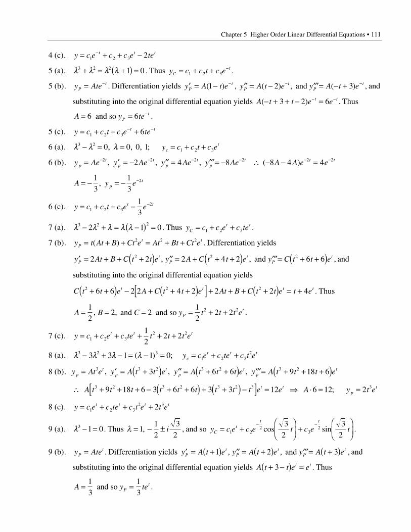
Chapter 5 Higher Order Linear Differential Equations • 111
4 (c). y c e c c e tet t t= + + --1 2 3 2
5 (a). l l l l3 2 2 1 0+ = +( ) = . Thus y c c t c eCt= + + -
1 2 3 .
5 (b). y AtePt= - . Differentiation yields ¢ = - -y A t eP
t( )1 , ¢¢ = - ¢¢¢= - +- -y A t e y A t ePt
Pt( ) , ( )2 3and , and
substituting into the original differential equation yields A t t e et t( )- + + - =- -3 2 6 . Thus
A y tePt= = -6 and so 6 .
5 (c). y c c t c e tet t= + + +- -1 2 3 6
6 (a). l l l3 21 2 30 0 0 1- = = = + +, , , ; y c c t c ec
t
6 (b). y Ae y Ae y Ae y Ae A A e ept
pt
pt
pt t t= ¢ = - ¢¢ = ¢¢¢= - \ - - =- - - - - -2 2 2 2 2 22 4 8 8 4 4, , , ( )
A y ept= - = - -1
313
2,
6 (c). y c c t c e et t= + + - -1 2 3
213
7 (a). l l l l l3 2 22 1 0- + = -( ) = . Thus y c c e c teC
t t= + +1 2 3 .
7 (b). y t At B Ct e At Bt Ct ePt t= + + = + +( ) 2 2 2 . Differentiation yields
¢ = + + +( ) ¢¢ = + + +( ) ¢¢¢= + +( )y At B C t t e y A C t t e y C t t ePt
Pt
Pt2 2 2 4 2 6 62 2 2, and , , and
substituting into the original differential equation yields
C t t e A C t t e At B C t t e t et t t t2 2 26 6 2 2 4 2 2 2 4+ +( ) - + + +( )[ ] + + + +( ) = + . Thus
A B C y t t t ePt= = = = + +
12
2 212
2 22 2, and and so , .
7 (c). y c c e c te t t t et t t= + + + + +1 2 32 21
22 2
8 (a). l l l l3 2 31 2 3
23 3 1 1 0- + - = - = = + +( ) ; y c e c te c t ect t t
8 (b). y At e y A t t e y A t t t e y A t t t ept
pt
pt
pt= ¢ = +( ) ¢¢ = + +( ) ¢¢¢= + + +( )3 3 2 3 2 3 23 6 6 9 18 6, , ,
\ + + + - + +( ) + +( ) -[ ] = fi ◊ = = ; A t t t t t t t t t e e A y t et tp
t3 2 3 2 3 2 3 39 18 6 3 6 6 3 3 12 6 12 2
8 (c). y c e c te c t e t et t t t= + + +1 2 32 32
9 (a). l3 1 0- = . Thus l = - ±112
32
, i , and so y c e c e t c e tCt
t t
= +ÊËÁ
ˆ¯
+ÊËÁ
ˆ¯
- -
1 22
32
32
32
cos sin .
9 (b). y AtePt= . Differentiation yields ¢ = +( ) ¢¢ = +( ) ¢¢¢= +( )y A t e y A t e y A t eP
tP
tP
t1 2 3, and , , and
substituting into the original differential equation yields A t t e et t+ -( ) =3 . Thus
A y tePt= =
13
13
and so .
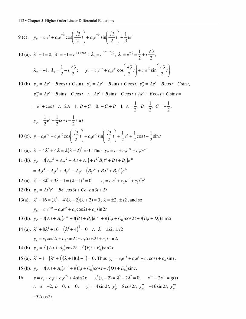
112 • Chapter 5 Higher Order Linear Differential Equations
9 (c). y c e c e t c e t teCt
t tt= +
ÊËÁ
ˆ¯
+ÊËÁ
ˆ¯
+- -
1 22
32
32
32
13
cos sin
10 (a). l l l lp p p p p3 3 211 0 1
12
32
23 3+ = = - = = = = ++ +
, , , , ( )( )
e e e ii kk
i k i
l l2 3 1 2 3112
32
32
32
2 2= - = - = +ÊËÁ
ˆ¯
+ÊËÁ
ˆ¯
-, ; cos sini y c e c e t c e tct t t
10 (b). y Ae B t C t y Ae B t C t y Ae B t C tpt
pt
pt= + + ¢ = - + ¢¢ = - -cos sin , sin cos , cos sin ,
¢¢¢= + - \ + - + + + =y Ae B t C t Ae B t C t Ae B t C tpt t tsin cos sin cos cos sin
= + \ = + = - + = = = = -e t A B C C B A B Ct cos , , , , , , 2 1 0 112
12
12
y e t tpt= + -
12
12
12
cos sin
10 (c). y c e c e t c e t e t tt tt t= +ÊËÁ
ˆ¯
+ÊËÁ
ˆ¯
+ + --1 2 3
2 23
23
212
12
12
cos sin cos sin
11 (a). l l l l l3 2 24 4 2 0- + = -( ) = . Thus y c c e c teC
t t= + +1 22
32 .
11 (b). y t A t A t A t A t B t B t B ePt= + + +( ) + + +( )3
32
21 0
22
21 0
2
= + + + + + +( )A t A t A t A t B t B t B t e t3
42
31
20 2
41
30
2 2
12 (a). l l l l3 2 31 2 3
23 3 1 1 0- + - = - = = + +( ) y c e c te c t ect t t
12 (b). y At e Be t Ce t Dpt t t= + + +3 3 3cos sin
13(a). l l l l4 216 4 2 2 0- = + -( ) + =( ) ( ) , l = ± ±2 2, i , and so
y c e c e c t c tCt t= + + +-
12
22
3 42 2cos sin .
13 (b). y t A t A e t B t B e t C t C t t D t D tPt t= +( ) + +( ) + +( ) + +( )-
1 02
1 02
1 0 1 02 2cos sin
14 (a). l l l l4 2 2 28 16 4 0 2 2+ + = +( ) = \ = ± ± , i i
y c t c t c t t c t tc = + + +1 2 3 42 2 2 2cos sin cos sin
14 (b). y t A t A t t B t B tp = +( ) + +( )21 0
21 02 2cos sin
15 (a). l l l l4 21 1 1 1 0- = +( ) +( ) -( ) = . Thus y c e c e c t c tCt t= + + +-
1 2 3 4cos sin .
15 (b). y t A t A e t C t C t t D t D tPt= +( ) + +( ) + +( )-
1 0 1 0 1 0cos sin .
16. y c c t c e t y y g tt= + + + - = - = ¢¢¢ - ¢¢ =1 2 32 2 3 24 2 2 2 0 2sin ; ( ) ; ( )l l l l
\ = - = = = ¢ = ¢¢ = - ¢¢¢= , , . sin , cos , sin , a b c y t y t y t yp p p p2 0 0 4 2 8 2 16 2
-32 2cos .t
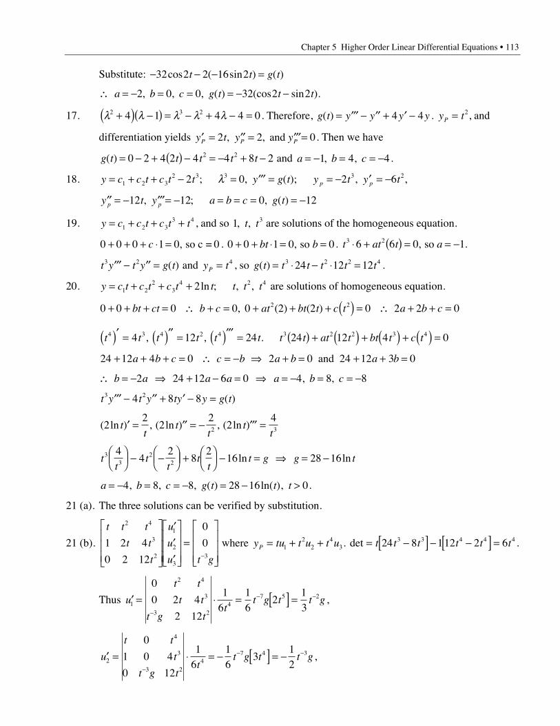
Chapter 5 Higher Order Linear Differential Equations • 113
Substitute: - - - =32 2 2 16 2cos ( sin ) ( ) t t g t
\ = - = = = - - , , , ( ) (cos sin ).a b c g t t t2 0 0 32 2 2
17. l l l l l2 3 24 1 4 4 0+( ) -( ) = - + - = . Therefore, g t y y y y( ) = ¢¢¢ - ¢¢ + ¢ -4 4 . y tP = 2, and
differentiation yields ¢ = ¢¢ = ¢¢¢=y t y yP P P2 2 0, , and . Then we have
g t t t t t( ) = - + ( ) - = - + -0 2 4 2 4 4 8 22 2 and a b c= - = = -1 4 4, , .
18. y c c t c t t y g t y t y tp p= + + - = ¢¢¢ = = - ¢ = -1 2 32 3 3 3 22 0 2 6; , ( ); , ,l
¢¢ = - ¢¢¢= - = = = = -y t y a b c g tp p12 12 0 12, ; , ( )
19. y c c t c t t= + + +1 2 33 4 , and so 1 3, , t t are solutions of the homogeneous equation.
0 0 0 1 0+ + + ◊ =c , so c = 0 . 0 0 1 0 0+ + ◊ = =bt b, so . t at t a3 26 6 0 1◊ + ( ) = = -, so .
t y t y g t3 2¢¢¢ - ¢¢ = ( ) and y tP = 4 , so g t t t t t t( ) = ◊ - ◊ =3 2 2 424 12 12 .
20. y c t c t c t t t t t= + + +1 22
34 2 42ln ; , , are solutions of homogeneous equation.
0 0 0 0 0 2 2 0 2 2 02 2+ + + = \ + = + + + ( ) = \ + + =bt ct b c at bt t c t a b c , ( ) ( )
t t t t t t t t at t bt t c t4 3 4 2 4 3 2 2 3 44 12 24 24 12 4 0( )¢ = ( )¢¢ = ( )¢¢¢ = ( ) + ( ) + ( ) + ( ) =, , .
24 12 4 0 2 0 24 12 3 0+ + + = \ = - fi + = + + =a b c c b a b a b and
\ = - fi + - = fi = - = = - , , b a a a a b c2 24 12 6 0 4 8 8
t y t y ty y g t3 24 8 8¢¢¢ - ¢¢ + ¢ - = ( )
( ln ) , ( ln ) , ( ln )22
22
24
2 3tt
tt
tt
¢ = ¢¢ = - ¢¢¢ =
tt
tt
tt
t g g t33
22
44
28
216 28 16
ÊËÁ
ˆ¯ - -Ê
ËÁˆ¯ + Ê
ËÁˆ¯ - = fi = -ln ln
a b c g t t t= - = = - = - >4 8 8 28 16 0, , , ( ) ln( ), .
21 (a). The three solutions can be verified by substitution.
21 (b).
t t t
t t
t
u
u
u t g
2 4
3
2
1
2
33
1 2 4
0 2 12
0
0
È
Î
ÍÍÍ
˘
˚
˙˙˙
¢¢¢
È
Î
ÍÍÍ
˘
˚
˙˙˙
=È
Î
ÍÍÍ
˘
˚
˙˙˙-
where y tu t u t uP = + +12
24
3. det = -[ ] - -[ ] =t t t t t t24 8 112 2 63 3 4 4 4 .
Thus ¢ = ◊ = [ ] =-
- -u
t t
t t
t g tt
t g t t g1
2 4
3
3 24
7 5 2
0
0 2 4
2 12
16
16
213
,
¢ = ◊ = - [ ] = --
- -u
t t
t
t g tt
t g t t g2
4
3
3 24
7 4 3
0
1 0 4
0 12
16
16
312
,
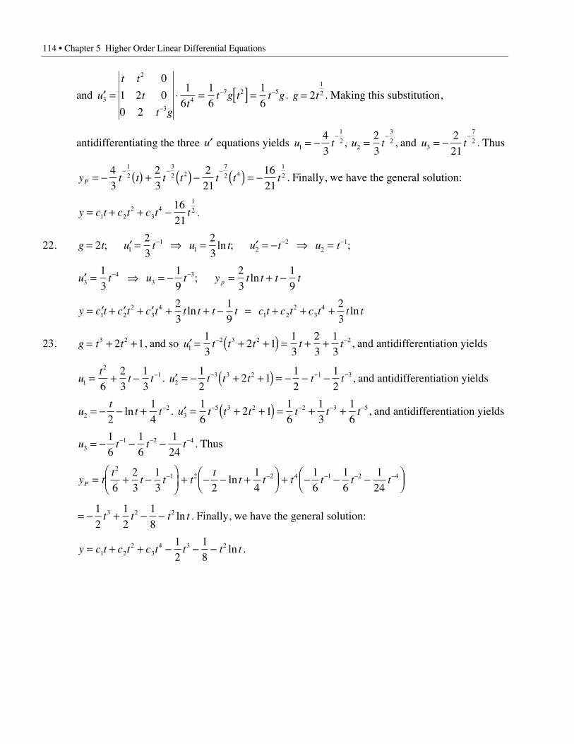
114 • Chapter 5 Higher Order Linear Differential Equations
and ¢ = ◊ = [ ] =-
- -u
t t
t
t gt
t g t t g3
2
34
7 2 5
0
1 2 0
0 2
16
16
16
. g t= 21
2 . Making this substitution,
antidifferentiating the three ¢u equations yields u t1
1
243
= --
, u t2
3
223
=-
, and u t3
7
2221
= --
. Thus
y t t t t t t tP = - ( ) + ( ) - ( ) = -- - -4
323
221
1621
1
2
3
2 27
2 41
2 . Finally, we have the general solution:
y c t c t c t t= + + -1 22
34
1
21621
.
22. g t u t u t u t u t= ¢ = fi = ¢ = - fi =- - -223
231
11 2
22
1; ln ; ;
¢ = fi = - = + -- -u t u t y t t t tp34
331
319
23
19
; ln
y c t c t c t t t t t c t c t c t t t= ¢ + ¢ + ¢ + + - = + + +1 22
34
1 22
342
319
23
ln ln
23. g t t= + +3 22 1, and so ¢ = + +( ) = + +- -u t t t t t12 3 2 21
32 1
13
23
13
, and antidifferentiation yields
ut
t t1
21
623
13
= + - - . ¢ = - + +( ) = - - -- - -u t t t t t23 3 2 1 31
22 1
12
12
, and antidifferentiation yields
ut
t t22
214
= - - + -ln . ¢ = + +( ) = + +- - - -u t t t t t t35 3 2 2 3 51
62 1
16
13
16
, and antidifferentiation yields
u t t t31 2 41
616
124
= - - -- - - . Thus
y tt
t t tt
t t t t t tP = + -ÊËÁ
ˆ¯
+ - - +ÊËÁ
ˆ¯ + - - -Ê
ËÁˆ¯
- - - - -2
1 2 2 4 1 2 4
623
13 2
14
16
16
124
ln
= - + - -12
12
18
3 2 2t t t tln . Finally, we have the general solution:
y c t c t c t t t t= + + - - -1 22
34 3 21
218
ln .
Chapter 6First Order Linear Systems
Section 6.1
1. 2 3 21
2 2 13
1
0 2
2 2 2
4 4 2
3 3
0 3 6
2 2 2
2A t tB t
t t
tt
t
t
t t
t
t t
t t( ) ( )- =
-+
È
ÎÍ
˘
˚˙ -
-+
È
ÎÍ
˘
˚˙ =
-+
È
ÎÍ
˘
˚˙ -
-+
È
ÎÍ
˘
˚˙
=- - +
- -È
ÎÍ
˘
˚˙
2 2 3 2 3
4 2 2 3
2 2
2
t t t t
t t
2. A t B t B t A tt t
( ) ( ) ( ) ( )- =+ +
- -È
ÎÍ
˘
˚˙
2 2 2
4 2
2
3. A t tt t
t
t t t t
t t( ) ( )
( )( ) ( )
( ) ( )( )c =
-+
È
ÎÍ
˘
˚˙
+-
È
ÎÍ
˘
˚˙ =
- + + -+ + + -
È
ÎÍ
˘
˚˙ =
-È
ÎÍ
˘
˚˙
1
2 2 1
1
1
1 1 1
2 1 2 1 1
1
1
2 2
4. det[ ( )]tA t t t= - -3 2
5. There are two natural ways to do this problem. We can form the matrix A t B t( ) ( )and then calculate det[ ( ) ( )]A t B t . Alternatively, we can separately calculate det[ ( )]A t anddet[ ( )]B t and use the fact that det[ ( ) ( )] det[ ( )]det[ ( )]A t B t A t B t= .Taking the latter course, det[ ( )] ( )( ) ( )A t t t t t= - + - = - +1 2 1 2 12 , and det[ ( )]B t =t t t t( )+ = +2 22 . Thus, det[ ( ) ( )] ( )( ) ( )A t B t t t t t t t= - + + = - + +1 2 3 22 3 2 .
6. det[ ( )]A t t= +2 1 and so the matrix A t( ) is invertible for every value t except t = -12
. The
inverse of A t( ) is given by A tt
t t
t tt- =
++ -
- +È
ÎÍ
˘
˚˙ π -1 1
2 1
1
112
( ) , .
7. As noted in Example 2, a square matrix is invertible if and only if its determinant is nonzero.Now, det[ ( )] ( ) ( )( )A t t t t t t t= - - = - - = - +3 4 3 4 4 12 and so the matrix A t( ) is invertible forevery value t except t t= = -4 1 and . The inverse of A t( ) is given by
A tt t
t
tt t- =
- +- -
-È
ÎÍ
˘
˚˙ π π -1 1
4 1
3 2
24 1( )
( )( ), , .

116 • Chapter 6 First Order Linear Systems
8. det[ ( )] sin cos sinA t t t t= =2 2 and so the matrix A t( ) is invertible for every value t except
22
0 1 2 3t n tn
n= fi = = ± ± ±p p, , , , ,.... The inverse of A t( ) i s g iven by
A tt t
t t
t t
t t
t tt
nn- =
-È
ÎÍ
˘
˚˙ =
-
È
Î
ÍÍÍ
˘
˚
˙˙˙
π = ± ± ±1 12
12
12
12
12
20 1 2 3( )
sin cos
cos cos
sin sin
csc csc
sec sec, , , , , ,...
p.
9. In this case, det[ ( )]A t e e e e e et t t t t t= - = -4 3 2 5 5 and so det[ ( )]A t is zero for every value of t.Hence, the given matrix A t( ) is never invertible.
10. lim ( ) lim
sincos
sect t t
A t
t
tt t
t
e tt
tÆ Æ
= +
-
È
Î
ÍÍÍ
˘
˚
˙˙˙
=È
ÎÍ
˘
˚˙
0 0 32
31
21
1 0 3
1 1 0.
11. lim ( ) limtan lim limtan
lim[ ] limsin sint t
t
tt
t
t
t t
tA tte t
t e
te t
t eÆ Æ
-Æ
-
Æ
Æ Æ
=-
È
ÎÍ
˘
˚˙ =
-
È
ÎÍÍ
˘
˚˙˙
=-
È
ÎÍ
˘
˚˙
0 0 20 0
0
2
02 2
0 0
2 1.
12. Differentiating A t( ) component wise, we have ¢ =È
ÎÍ
˘
˚˙A t
t
t( )
cos 3
2 0 and
¢¢ =-È
ÎÍ
˘
˚˙A t
t( )
sin 0
2 0. A t A t A t t( ), ( ) ( )¢ ¢¢ - • < < • and are defined for .
13. Differentiating A t( ) component wise, we have ¢ =- -
È
ÎÍ
˘
˚˙
-
-A tt
t e t( )
. ( ) /
0
0 5 1 3
1
1 2 3 and
¢¢ =-
- -È
ÎÍ
˘
˚˙
-
-A tt
t e t( )
. ( ) /
0
0 25 1 9
2
3 2 3. A t t t( ) is defined for and - • < < < £0 0 1.
¢ ¢¢ - • < < < <A t A t t t( ) ( ) and are defined for and 0 0 1.
14. P tt
t tt
t( )
sin( )
sec=
È
ÎÍ
˘
˚˙ =
-È
ÎÍ
˘
˚˙
2 3
5 and g .
15.¢¢
È
ÎÍ
˘
˚˙ =
+ + ++ +
È
ÎÍ
˘
˚˙ =
+ ++
È
ÎÍ
˘
˚˙ +
È
ÎÍ
˘
˚˙
-
-
-
-
y
y
t y t y t
y t y t t
t y t y
y t y
t
t t1
2
11
22
11
2
11
22
11
2
1
4 8
1
4 8
( )
ln
( )
ln=
t t
t
y
y
t
t t
-
-
+È
ÎÍ
˘
˚˙
È
ÎÍ
˘
˚˙ +
È
ÎÍ
˘
˚˙
1 2
1
1
2
1
4 8 ln. Therefore, P t
t t
tt
t
t t( ) ( )
ln=
+È
ÎÍ
˘
˚˙ =
È
ÎÍ
˘
˚˙
-
-
1 2
1
1
4 8 and g .
16. Let ¢ =È
ÎÍ
˘
˚˙A t
t
t t( )
cos
2 1
3 2 . Integrating component wise, we find
A tt C t C
t C t C( )
sin=
+ ++ +
È
ÎÍ
˘
˚˙
211 12
213
22
.
Chapter 6 First Order Linear Systems • 117
Since AC C
C C( )0
2 5
1 211 12
21 22
=È
ÎÍ
˘
˚˙ =
-È
ÎÍ
˘
˚˙ , we obtain A t
t t
t t( )
sin=
+ ++ -
È
ÎÍ
˘
˚˙
2
3
2 5
1 2.
17. Let ¢ =È
ÎÍ
˘
˚˙
-
A tt t
t( )
1
2
4
5 3. Integrating component wise, we find
A tt C t C
t C t C( )
ln=
+ ++ +
È
ÎÍ
˘
˚˙11
212
213
22
2
5. Since A
C C
C C( )1
2
5 1
2 5
1 211 12
21 22
=+
+ +È
ÎÍ
˘
˚˙ =
-È
ÎÍ
˘
˚˙ , we
obtain A tt t
t t( )
ln=
+ +- -
È
ÎÍ
˘
˚˙
2 2 3
5 4 3
2
3.
18. Let ¢¢ =È
ÎÍ
˘
˚˙A t
t( )
1
0 0. Integrating component wise, we find
¢ = + +È
Î
ÍÍ
˘
˚
˙˙
fi = + + + +
+ +
È
Î
ÍÍ
˘
˚
˙˙
A t t Ct
C
C CA t
tC t D
tC t D
C t D C t D( ) ( )11
2
12
21 22
2
11 11
3
12 12
21 21 22 22
2 2 6 .
Since A A( ) ( )01 1
2 11
1 2
2 3=
-È
ÎÍ
˘
˚˙ =
--
È
ÎÍ
˘
˚˙ and , we obtain A t
tt
tt
t( ) = - + + +
- +
È
Î
ÍÍ
˘
˚
˙˙
2 3
252
16
56
1
2 2 1.
19. Integrating component wise, we obtain
B s dssds sds ds
ds s ds s ds
t t t
t t t
t
t t t
t t t( )cos
( )
sin
ln0
0 0 0
0
1
0
2
0
2
3
2 2
5 1 3
2
5 1Ú Ú Ú ÚÚ Ú Ú
=+
È
Î
ÍÍÍ
˘
˚
˙˙˙
=+
È
ÎÍ
˘
˚˙
-.
20. Integrating component wise, we obtain B s dse t
t tt
t
( ) sin cos0
21 32
21 2
2Ú =
--
È
ÎÍÍ
˘
˚˙˙
pp
pp
.
21 (a). One example is At
t=
È
ÎÍ
˘
˚˙
1
02 .
22. One example is At
=È
ÎÍ
˘
˚˙
0
0 0.
Section 6.2
1. The given problem can be written as ¢ = + =y y g y y( ) ( ) ( ) ( ), ( )t P t t t 3 0
where P tt t
t ett( )
tan
ln, ( ) ,=
È
ÎÍ
˘
˚˙ =
È
ÎÍ
˘
˚˙ =
È
ÎÍ
˘
˚˙
-1
0
0
0
0
1g y . The coefficient functions
p t t p t t t111
21 0( ) ( ) ln .= = =- and are discontinuous at The coefficient function p t t12( ) tan=has discontinuities at ± ±p p/ , / ,2 3 2 K. The largest interval containing t0 3= but containingno discontinuities of any coefficient function is the interval p p/ /2 3 2< <t .
118 • Chapter 6 First Order Linear Systems
2. In standard form, the problem is ¢ =-
È
ÎÍ
˘
˚˙ +
+È
ÎÍ
˘
˚˙ =
È
ÎÍ
˘
˚˙
-
y y y1
2 4
1
00
0
02
2tan ( ), ( )
t
t
t.
tan /t t is discontinuous at = ±p 2 and (t +1) is discontinuous at -2 t = -1. The largest intervalcontaining t0 0= but containing no discontinuities of any coefficient function is the interval- < <1 2t p / .
3. In standard form, the problem is ¢ =È
ÎÍ
˘
˚˙ +
È
ÎÍ
˘
˚˙ =
È
ÎÍ
˘
˚˙y y y
(cos ) / / /
sec, ( )
t t t
t
t
t
2 2 21
2 4
11
0
2.
The only discontinuities of p t p t t g t11 12 20( ) ( ) , ( )and are at while = isdiscontinuous at t = ± ±p p/ , / ,2 3 2 K. The largest interval containing t0 1= but containing nodiscontinuities of any coefficient function is the interval 0 2< <t p / .
4. In standard form, the problem is ¢ = + +
- -
È
Î
ÍÍÍ
˘
˚
˙˙˙
=È
ÎÍ
˘
˚˙y y y
32
52
22
42
10
2
t
t t
t
t
t
, ( ) .
The largest interval containing t0 1= but containing no discontinuities of any coefficientfunction is the interval - < <2 2t .
5. Differentiating, ¢ = + ¢ = -y c e c e y c e c et t t t1 1
52
32 1
52
35 3 5 3 and . Calculating the right hand sides,4 4 5 31 2 1
52
31
52
31
52
31y y c e c e c e c e c e c e yt t t t t t+ = + + - = + = ¢( ) ( ) and
y y c e c e c e c e c e c e yt t t t t t1 2 1
52
31
52
31
52
324 4 5 3+ = + + - = - = ¢( ) ( ) .
7 (a). ¢ =È
ÎÍ
˘
˚˙y y
4 1
1 4
7 (b). y =È
ÎÍ
˘
˚˙ +
-È
ÎÍ
˘
˚˙c e c et t
15
23
1
1
1
1
8 (a). ¢ =-
È
ÎÍ
˘
˚˙y y
1 1
1 1
8 (b). y =-
È
ÎÍ
˘
˚˙ +
È
ÎÍ
˘
˚˙c
e t
e tc
e t
e t
t
t
t
t1 2
cos
sin
sin
cos
9. For y y=-
È
ÎÍ
˘
˚˙ +
-È
ÎÍ
˘
˚˙ ¢ =
-È
ÎÍ
˘
˚˙ +
-È
ÎÍ
˘
˚˙c e c e c e c et t t t
12
23
12
23
2
1
1
12
2
13
1
1, we have . On the other hand,
A A c e c e c e A c e At t t ty =-
È
ÎÍ
˘
˚˙ +
-È
ÎÍ
˘
˚˙
Ê
ËÁˆ
¯=
-È
ÎÍ
˘
˚˙ +
-È
ÎÍ
˘
˚˙1
22
31
22
32
1
1
1
2
1
1
1=
c e c e c e c et t t t1
22
31
22
31 2
1 4
2
1
1 2
1 4
1
1
4
2
3
3
-È
ÎÍ
˘
˚˙ -
È
ÎÍ
˘
˚˙ +
-È
ÎÍ
˘
˚˙ -
È
ÎÍ
˘
˚˙ =
-È
ÎÍ
˘
˚˙ +
-È
ÎÍ
˘
˚˙. Thus, ¢ =y yA for every choice of
c c1 2 and .
Chapter 6 First Order Linear Systems • 119
In order to solve the initial value problem, we first note that
y( )02
1
1
1
2 1
1 11 21
2
=-
È
ÎÍ
˘
˚˙ +
-È
ÎÍ
˘
˚˙ =
- -È
ÎÍ
˘
˚˙
È
ÎÍ
˘
˚˙c c
c
c. Thus, solving
2 1
1 1
4
31
2- -È
ÎÍ
˘
˚˙
È
ÎÍ
˘
˚˙ =
-È
ÎÍ
˘
˚˙
c
c, we obtain
c c1 2 2=1 and = . Therefore, y( )t e ee e
e et t
t t
t t=
-È
ÎÍ
˘
˚˙ +
-È
ÎÍ
˘
˚˙ =
+- -
È
ÎÍ
˘
˚˙2 3
2 3
2 3
2
12
1
1
2 2
2 is the solution of the
given initial value problem.
10. For ¢ =È
ÎÍ
˘
˚˙ +
-È
ÎÍ
˘
˚˙
-y c e c et t1
52
5
5
1
2, A c e c et ty =
++
È
ÎÍ
˘
˚˙ +
- +- +
È
ÎÍ
˘
˚˙
-1
52
3 2
4 1
3 4
4 2
Solving 1 1
1 2
1
81
2
-È
ÎÍ
˘
˚˙
È
ÎÍ
˘
˚˙ =
-È
ÎÍ
˘
˚˙
c
c, we obtain c c1 2 3= 2 and = . Therefore, y( )t
e e
e e
t t
t t=
-+
È
ÎÍ
˘
˚˙
-
-
2 3
2 6
5
5 is the
solution of the given initial value problem.
11. Let Y( )( )
( ).t
y t
y t=
¢È
ÎÍ
˘
˚˙ Calculating ¢Y ( )t , we find
¢ =¢
¢¢È
ÎÍ
˘
˚˙ =
¢- ¢ - +
È
ÎÍ
˘
˚˙ =
- -È
ÎÍ
˘
˚˙ ¢
È
ÎÍ
˘
˚˙ +
È
ÎÍ
˘
˚˙Y ( )
( )
( )
( )
( ) ( ) sin
( )
( ) sint
y t
y t
y t
t y t y t t t
y t
y t t2 24
0 1
4
0. Therefore, the scalar
equation can be written as ¢ = +Y Y GP t t( ) ( ) where P tt
tt
( ) ( )sin
=- -
È
ÎÍ
˘
˚˙ =
È
ÎÍ
˘
˚˙
0 1
4
02 and G .
12. Let Y( )( )
( ).t
y t
y t=
¢È
ÎÍ
˘
˚˙ Calculating ¢Y ( )t , we find
¢ =¢
¢¢È
ÎÍ
˘
˚˙ =
-È
ÎÍ
˘
˚˙ ¢
È
ÎÍ
˘
˚˙ +
+È
ÎÍ
˘
˚˙Y ( )
( )
( ) sec sec
( )
( ) ( )sect
y t
y t t t t t
y t
y t t t
0 1
3
0
12 . Therefore, the scalar equation can
be written as ¢ = +Y Y GP t t( ) ( ) where P tt t t t
tt t
( )sec sec
( )( )sec
=-
È
ÎÍ
˘
˚˙ =
+È
ÎÍ
˘
˚˙
0 1
3
0
12 and G .
13. Let Y( )
( )
( )
( )
t
y t
y t
y t
= ¢¢¢
È
Î
ÍÍÍ
˘
˚
˙˙˙. We solve for ¢¢¢y by multiplying the equation by e t- and find
¢ =¢
¢¢- ¢¢ - ¢ - +
È
Î
ÍÍÍ
˘
˚
˙˙˙- - - - -
Y ( )
( )
( )
( ) ( ) ( tan ) ( )
t
y t
y t
e y t e t y t e t y t et t t t5 1
. Expressing ¢Y ( )t in matrix terms, we
have ¢ =- - -
È
Î
ÍÍÍ
˘
˚
˙˙˙
¢¢¢
È
Î
ÍÍÍ
˘
˚
˙˙˙
+È
Î
ÍÍÍ
˘
˚
˙˙˙- - - - -
Y ( )
tan
( )
( )
( )
t
e t e t e
y t
y t
y t et t t t
0 1 0
0 0 1
5
0
01
. Therefore, the scalar equation can be
written as ¢ = +Y Y GP t t( ) ( ) where
P t
e t e t e
t
et t t t
( )
tan
( )=- - -
È
Î
ÍÍÍ
˘
˚
˙˙˙
=È
Î
ÍÍÍ
˘
˚
˙˙˙- - - - -
0 1 0
0 0 1
5
0
01
and G .

120 • Chapter 6 First Order Linear Systems
14. Let Y( )
( )
( )
( )
t
y t
y t
y t
= ¢¢¢
È
Î
ÍÍÍ
˘
˚
˙˙˙. ¢ =
-
È
Î
ÍÍÍ
˘
˚
˙˙˙
¢¢¢
È
Î
ÍÍÍ
˘
˚
˙˙˙
+È
Î
ÍÍÍ
˘
˚
˙˙˙
Y ( )
cos
( )
( )
( )
t
t t
y t
y t
y t e t
0 1 0
0 0 1
2
0
03
. Therefore, the scalar equation can
be written as ¢ = +Y Y GP t t( ) ( ) where P t
t t
t
e t
( )
cos
( )=-
È
Î
ÍÍÍ
˘
˚
˙˙˙
=È
Î
ÍÍÍ
˘
˚
˙˙˙
0 1 0
0 0 1
2
0
03
and G .
15. Let Y Y( )( )
( )( )
( )
( )t
y t
y tt
y t
y t=
¢È
ÎÍ
˘
˚˙ ¢ =
¢¢¢
È
ÎÍ
˘
˚˙ so that . We are given that
¢ =-
È
ÎÍ
˘
˚˙ ¢
È
ÎÍ
˘
˚˙ +
È
ÎÍ
˘
˚˙ =
¢- + ¢ +
È
ÎÍ
˘
˚˙Y ( )
( )
( ) cos
( )
( ) ( ) cost
y t
y t t
y t
y t y t t
0 1
3 2
0
2 2 3 2 2 2.
Therefore, equating components of the vector ¢Y ( )t , we see that the scalar equation is¢¢ = - + ¢ + - = ¢ - =y y y t y y3 2 2 2 1 1 1 4cos , ( ) , ( ) .
16. ¢¢¢ - ¢¢ + = = ¢ = - ¢¢ =y y y e y y yt4 2 0 1 0 2 0 33 , ( ) , ( ) , ( ) .
17. Let Y Y( )
( )
( )
( )
( )
( )
( )
( )
( )
( )
( )
( )
( )
( )( )
t
y t
y t
y t
y t
y t
y t
y t
y t
t
y t
y t
y t
y t
=
È
Î
ÍÍÍÍ
˘
˚
˙˙˙˙
=¢
¢¢¢¢¢
È
Î
ÍÍÍÍ
˘
˚
˙˙˙˙
¢ =
¢¢¢
¢¢¢
È
Î
ÍÍÍÍ
˘
˚
˙˙˙˙
1
2
3
44
so that . We are given that
¢ =
+ +
È
Î
ÍÍÍÍ
˘
˚
˙˙˙˙
=
¢¢¢
¢¢¢¢ + ¢¢ + ¢¢
È
Î
ÍÍÍÍ
˘
˚
˙˙˙˙
Y ( )
sin( ) sin( ) ( )
t
y
y
y
y y y y
y
y
y
y y y y
2
3
4
2 3 1 32 2
. Equating components of the vector
¢Y ( )t , we see that the scalar equation isy y y y y y y y y( ) sin( ) ( ) , ( ) , ( ) , ( ) , ( )4 2 1 0 1 0 1 1 1 2= ¢ + ¢¢ + ¢¢ = ¢ = ¢¢ = - ¢¢¢ = .
18. Making the indicated change of variables, the system of differential equations is¢ = + +¢ = + +
Y Y Y tY
Y tY Y Y2 2 3 4
4 1 2 42. Therefore, the system can be expressed in the form
¢ = +Y Y GP t t( ) ( ) where
P tt
t
t( ) ( )=
È
Î
ÍÍÍÍ
˘
˚
˙˙˙˙
=
È
Î
ÍÍÍÍ
˘
˚
˙˙˙˙
0 1 0 0
0 1 1
0 0 0 1
2 1 0 1
0
0
0
0
and G .
19. Making the indicated change of variables, the system of differential equations is¢ = + - + +¢ = -
-Y t Y Y tY t Y e
Y Y Y
t2
12 1 3 4
2
4 1 4
4
5
(sin ).
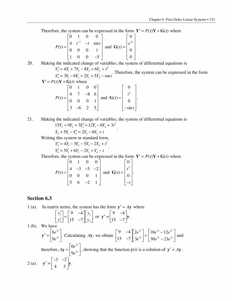
Chapter 6 First Order Linear Systems • 121
Therefore, the system can be expressed in the form ¢ = +Y Y GP t t( ) ( ) where
P tt t t
te t
( )sin
( )=-
-
È
Î
ÍÍÍÍ
˘
˚
˙˙˙˙
=
È
Î
ÍÍÍÍ
˘
˚
˙˙˙˙
-
0 1 0 0
4
0 0 0 1
1 0 0 5
0
0
0
1 2
and G .
20. Making the indicated change of variables, the system of differential equations is¢ = + - + +¢ = - + + -
Y Y Y Y Y t
Y Y Y Y Y t2 1 2 3 4
2
4 1 2 3 4
4 7 8 6
3 6 2 5 sin. Therefore, the system can be expressed in the form
¢ = +Y Y GP t t( ) ( ) where
P t tt
t
( ) ( )
sin
=-
-
È
Î
ÍÍÍÍ
˘
˚
˙˙˙˙
=
-
È
Î
ÍÍÍÍ
˘
˚
˙˙˙˙
0 1 0 0
4 7 8 6
0 0 0 1
3 6 2 5
0
0
2
and G .
21. Making the indicated change of variables, the system of differential equations is15 9 3 12 6 3
5 2 63 2 2 1 4
2
4 1 4 3 2
Y Y Y Y Y t
Y Y Y Y Y t
+ + ¢ = - ++ - ¢ = - +
.
Writing this system in standard form,¢ = - - - +¢ = + - + -
Y Y Y Y Y t
Y Y Y Y Y t2 1 2 3 4
2
4 1 2 3 4
4 3 5 2
5 6 2.
Therefore, the system can be expressed in the form ¢ = +Y Y GP t t( ) ( ) where
P t tt
t
( ) ( )=- - -
-
È
Î
ÍÍÍÍ
˘
˚
˙˙˙˙
=
-
È
Î
ÍÍÍÍ
˘
˚
˙˙˙˙
0 1 0 0
4 3 5 2
0 0 0 1
5 6 2 1
0
0
2
and G .
Section 6.3
1 (a). In matrix terms, the system has the form ¢ =y yA where¢¢
È
ÎÍ
˘
˚˙ =
--
È
ÎÍ
˘
˚˙
È
ÎÍ
˘
˚˙ ¢
--
È
ÎÍ
˘
˚˙
y
y
y
y1
2
1
2
9 4
15 7
9 4
15 7 or =y y.
1 (b). We have
¢ =È
ÎÍ
˘
˚˙
--
È
ÎÍ
˘
˚˙
È
ÎÍ
˘
˚˙ =
--
È
ÎÍ
˘
˚˙y y
6
9
9 4
15 7
2
3
18 12
30 21
3
3
3
3
3 3
3 3
e
eA
e
e
e e
e e
t
t
t
t
t t
t t. , Calculating we obtain and
therefore, Ae
e
t
ty =
È
ÎÍ
˘
˚˙
6
9
3
3, showing that the function y(t) is a solution of ¢ =y yA .
2 (a). =¢- -È
ÎÍ
˘
˚˙y y
3 2
4 3.
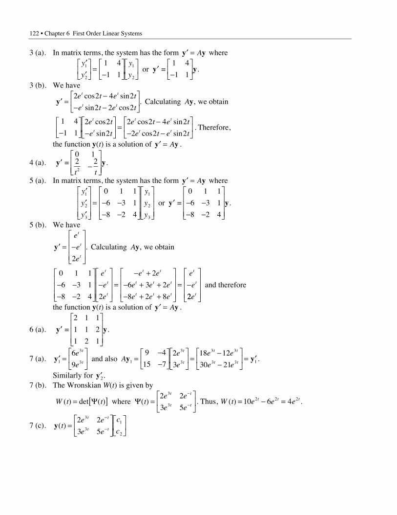
122 • Chapter 6 First Order Linear Systems
3 (a). In matrix terms, the system has the form ¢ =y yA where¢¢
È
ÎÍ
˘
˚˙ =
-È
ÎÍ
˘
˚˙
È
ÎÍ
˘
˚˙ ¢
-È
ÎÍ
˘
˚˙
y
y
y
y1
2
1
2
1 4
1 1
1 4
1 1 or =y y.
3 (b). We have
¢ =-
- -È
ÎÍ
˘
˚˙
-È
ÎÍ
˘
˚˙ -
È
ÎÍ
˘
˚˙ =
-- -
È
ÎÍ
˘
˚˙
y y2 2 4 2
2 2 2
1 4
1 1
2 2
2
2 2 4 2
2 2 2
e t e t
e t e tA
e t
e t
e t e t
e t e t
t t
t t
t
t
t t
t t
cos sin
sin cos. ,
cos
sin
cos sin
cos sin.
Calculating we obtain
Therefore,
the function y(t) is a solution of ¢ =y yA .
4 (a). =¢ -È
ÎÍÍ
˘
˚˙˙
y y0 12 22t t
.
5 (a). In matrix terms, the system has the form ¢ =y yA where¢¢¢
È
Î
ÍÍÍ
˘
˚
˙˙˙
= - -- -
È
Î
ÍÍÍ
˘
˚
˙˙˙
È
Î
ÍÍÍ
˘
˚
˙˙˙
¢ - -- -
È
Î
ÍÍÍ
˘
˚
˙˙˙
y
y
y
y
y
y
1
2
3
1
2
3
0 1 1
6 3 1
8 2 4
0 1 1
6 3 1
8 2 4
or =y y.
5 (b). We have
¢ = -È
Î
ÍÍÍ
˘
˚
˙˙˙
- -- -
È
Î
ÍÍÍ
˘
˚
˙˙˙
-È
Î
ÍÍÍ
˘
˚
˙˙˙
=- +
- + +- + +
È
Î
ÍÍÍ
˘
˚
˙˙˙
= -
y y
e
e
e
A
e
e
e
e e
e e e
e e e
e
e
t
t
t
t
t
t
t t
t t t
t t t
t
t
2
0 1 1
6 3 1
8 2 4 2
2
6 3 2
8 2 8
. , Calculating we obtain
22et
È
Î
ÍÍÍ
˘
˚
˙˙˙ and therefore
the function y(t) is a solution of ¢ =y yA .
6 (a). =
2 1 1
1 1 2
1 2 1
¢È
Î
ÍÍÍ
˘
˚
˙˙˙
y y.
7 (a). ¢ =È
ÎÍ
˘
˚˙ =
--
È
ÎÍ
˘
˚˙
È
ÎÍ
˘
˚˙ =
--
È
ÎÍ
˘
˚˙ = ¢y y y1
3
3 1
3
3
3 3
3 3 1
6
9
9 4
15 7
2
3
18 12
30 21
e
eA
e
e
e e
e e
t
t
t
t
t t
t t and also .
Similarly for ¢y2.7 (b). The Wronskian W(t) is given by
W t t te e
e e
t t
t t( ) det ( ) ( )= [ ] =
È
ÎÍ
˘
˚˙
-
-Y Y where 2 2
3 5
3
3. Thus, W t e e et t t( ) = - =10 6 42 2 2 .
7 (c). y( )te e
e e
c
c
t t
t t=
È
ÎÍ
˘
˚˙
È
ÎÍ
˘
˚˙
-
-
2 2
3 5
3
3
1
2
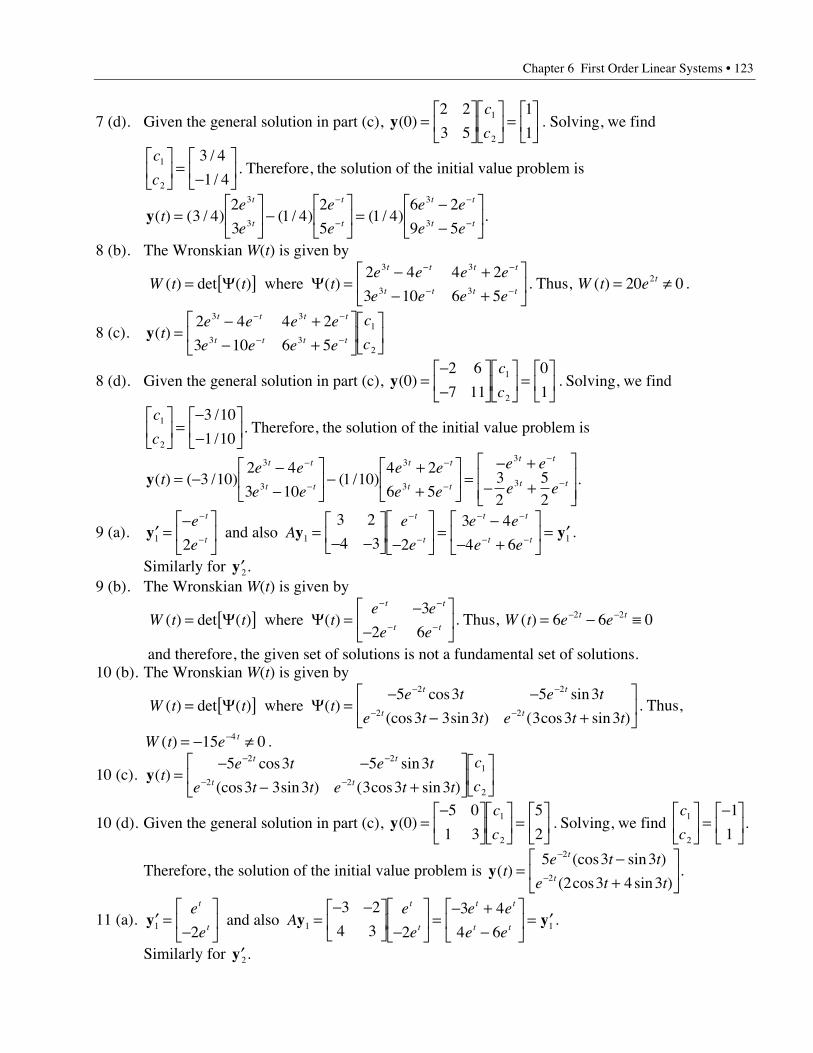
Chapter 6 First Order Linear Systems • 123
7 (d). Given the general solution in part (c), y( ) .02 2
3 5
1
11
2
=È
ÎÍ
˘
˚˙
È
ÎÍ
˘
˚˙ =
È
ÎÍ
˘
˚˙
c
c Solving, we find
c
c1
2
3 4
1 4
È
ÎÍ
˘
˚˙ =
-È
ÎÍ
˘
˚˙
/
/. Therefore, the solution of the initial value problem is
y( ) ( / ) ( / ) ( / )te
e
e
e
e e
e e
t
t
t
t
t t
t t=
È
ÎÍ
˘
˚˙ -
È
ÎÍ
˘
˚˙ =
--
È
ÎÍ
˘
˚˙
-
-
-
-3 42
31 4
2
51 4
6 2
9 5
3
3
3
3.
8 (b). The Wronskian W(t) is given by
W t t te e e e
e e e e
t t t t
t t t t( ) det ( ) ( )= [ ] =
- +- +
È
ÎÍ
˘
˚˙
- -
- -Y Y where 2 4 4 2
3 10 6 5
3 3
3 3. Thus, W t e t( ) = π20 02 .
8 (c). y( )te e e e
e e e e
c
c
t t t t
t t t t=
- +- +
È
ÎÍ
˘
˚˙
È
ÎÍ
˘
˚˙
- -
- -
2 4 4 2
3 10 6 5
3 3
3 3
1
2
8 (d). Given the general solution in part (c), y( ) .02 6
7 11
0
11
2
=--
È
ÎÍ
˘
˚˙
È
ÎÍ
˘
˚˙ =
È
ÎÍ
˘
˚˙
c
c Solving, we find
c
c1
2
3 10
1 10
È
ÎÍ
˘
˚˙ =
--
È
ÎÍ
˘
˚˙
/
/. Therefore, the solution of the initial value problem is
y( ) ( / ) ( / )te e
e e
e e
e e
e e
e e
t t
t t
t t
t t
t t
t t= --
-È
ÎÍ
˘
˚˙ -
++
È
ÎÍ
˘
˚˙ =
- +- +
È
ÎÍÍ
˘
˚˙˙
-
-
-
-
-
-3 102 4
3 101 10
4 2
6 532
52
3
3
3
3
3
3 .
9 (a). ¢ =-È
ÎÍ
˘
˚˙ =
- -È
ÎÍ
˘
˚˙ -
È
ÎÍ
˘
˚˙ =
-- +
È
ÎÍ
˘
˚˙ = ¢
-
-
-
-
- -
- -y y y1 1 12
3 2
4 3 2
3 4
4 6
e
eA
e
e
e e
e e
t
t
t
t
t t
t t and also .
Similarly for ¢y2.9 (b). The Wronskian W(t) is given by
W t t te e
e e
t t
t t( ) det ( ) ( )= [ ] =
--
È
ÎÍ
˘
˚˙
- -
- -Y Y where 3
2 6. Thus, W t e et t( ) = - ∫- -6 6 02 2
and therefore, the given set of solutions is not a fundamental set of solutions.10 (b). The Wronskian W(t) is given by
W t t te t e t
e t t e t t
t t
t t( ) det ( ) ( )
cos sin
(cos sin ) ( cos sin )= [ ] =
- -- +
È
ÎÍ
˘
˚˙
- -
- -Y Y where 5 3 5 3
3 3 3 3 3 3
2 2
2 2. Thus,
W t e t( ) = - π-15 04 .
10 (c). y( )cos sin
(cos sin ) ( cos sin )t
e t e t
e t t e t t
c
c
t t
t t=
- -- +
È
ÎÍ
˘
˚˙
È
ÎÍ
˘
˚˙
- -
- -
5 3 5 3
3 3 3 3 3 3
2 2
2 2
1
2
10 (d). Given the general solution in part (c), y( ) .05 0
1 3
5
21
2
=-È
ÎÍ
˘
˚˙
È
ÎÍ
˘
˚˙ =
È
ÎÍ
˘
˚˙
c
c Solving, we find
c
c1
2
1
1
È
ÎÍ
˘
˚˙ =
-È
ÎÍ
˘
˚˙.
Therefore, the solution of the initial value problem is y( )(cos sin )
( cos sin )t
e t t
e t t
t
t=
-+
È
ÎÍ
˘
˚˙
-
-
5 3 3
2 3 4 3
2
2.
11 (a). ¢ =-
È
ÎÍ
˘
˚˙ =
- -È
ÎÍ
˘
˚˙ -
È
ÎÍ
˘
˚˙ =
- +-
È
ÎÍ
˘
˚˙ = ¢y y y1 1 12
3 2
4 3 2
3 4
4 6
e
eA
e
e
e e
e e
t
t
t
t
t t
t t and also .
Similarly for ¢y2.
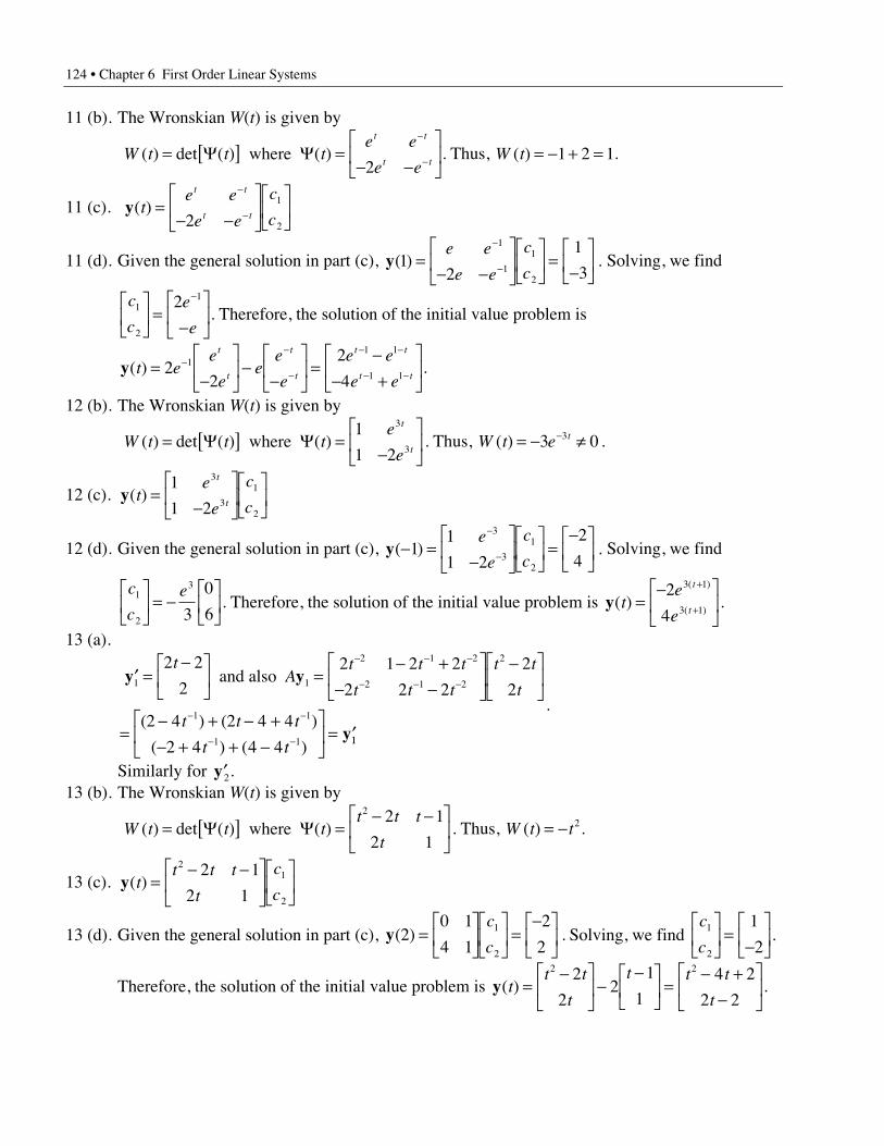
124 • Chapter 6 First Order Linear Systems
11 (b). The Wronskian W(t) is given by
W t t te e
e e
t t
t t( ) det ( ) ( )= [ ] =
- -È
ÎÍ
˘
˚˙
-
-Y Y where 2
. Thus, W t( ) = - + =1 2 1.
11 (c). y( )te e
e e
c
c
t t
t t=
- -È
ÎÍ
˘
˚˙
È
ÎÍ
˘
˚˙
-
-21
2
11 (d). Given the general solution in part (c), y( ) .12
1
3
1
1
1
2
=- -
È
ÎÍ
˘
˚˙
È
ÎÍ
˘
˚˙ =
-È
ÎÍ
˘
˚˙
-
-
e e
e e
c
c Solving, we find
c
c
e
e1
2
12È
ÎÍ
˘
˚˙ =
-È
ÎÍ
˘
˚˙
-
. Therefore, the solution of the initial value problem is
y( )t ee
ee
e
e
e e
e e
t
t
t
t
t t
t t=
-È
ÎÍ
˘
˚˙ -
-È
ÎÍ
˘
˚˙ =
-- +
È
ÎÍ
˘
˚˙-
-
-
- -
- -22
2
41
1 1
1 1.
12 (b). The Wronskian W(t) is given by
W t t te
e
t
t( ) det ( ) ( )= [ ] =
-È
ÎÍ
˘
˚˙Y Y where
1
1 2
3
3. Thus, W t e t( ) = - π-3 03 .
12 (c). y( )te
e
c
c
t
t=
-È
ÎÍ
˘
˚˙
È
ÎÍ
˘
˚˙
1
1 2
3
3
1
2
12 (d). Given the general solution in part (c), y( ) .- =-
È
ÎÍ
˘
˚˙
È
ÎÍ
˘
˚˙ =
-È
ÎÍ
˘
˚˙
-
-11
1 2
2
4
3
3
1
2
e
e
c
c Solving, we find
c
ce1
2
3
3
0
6
È
ÎÍ
˘
˚˙ = -
È
ÎÍ
˘
˚˙. Therefore, the solution of the initial value problem is y( )
( )
( )t
e
e
t
t=
-È
ÎÍ
˘
˚˙
+
+
2
4
3 1
3 1.
13 (a).
and also ¢ =-È
ÎÍ
˘
˚˙ =
- +- -
È
ÎÍ
˘
˚˙
-È
ÎÍ
˘
˚˙
=- + - +- + + -
È
ÎÍ
˘
˚˙ = ¢
- - -
- - -
- -
- -
y y
y
1 1
2 1 2
2 1 2
2
1 1
1 1
2 2
2
2 1 2 2
2 2 2
2
2
2 4 2 4 4
2 4 4 4
tA
t t t
t t t
t t
t
t t t
t t
( ) ( )
( ) ( ) 11
.
Similarly for ¢y2.13 (b). The Wronskian W(t) is given by
W t t tt t t
t( ) det ( ) ( )= [ ] =
- -È
ÎÍ
˘
˚˙Y Y where
2 2 1
2 1. Thus, W t t( ) = - 2.
13 (c). y( )tt t t
t
c
c=
- -È
ÎÍ
˘
˚˙
È
ÎÍ
˘
˚˙
21
2
2 1
2 1
13 (d). Given the general solution in part (c), y( ) .20 1
4 1
2
21
2
=È
ÎÍ
˘
˚˙
È
ÎÍ
˘
˚˙ =
-È
ÎÍ
˘
˚˙
c
c Solving, we find
c
c1
2
1
2
È
ÎÍ
˘
˚˙ =
-È
ÎÍ
˘
˚˙.
Therefore, the solution of the initial value problem is y( )tt t
t
t t t
t=
-È
ÎÍ
˘
˚˙ -
-È
ÎÍ
˘
˚˙ =
- +-
È
ÎÍ
˘
˚˙
2 22
22
1
1
4 2
2 2.
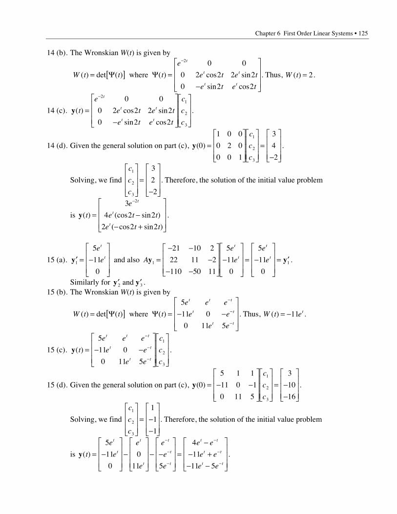
Chapter 6 First Order Linear Systems • 125
14 (b). The Wronskian W(t) is given by
W t t t
e
e t e t
e t e t
t
t t
t t
( ) det ( ) ( ) cos sin
sin cos
= [ ] =-
È
Î
ÍÍÍ
˘
˚
˙˙˙
-
Y Y where
2 0 0
0 2 2 2 2
0 2 2
. Thus, W t( ) = 2.
14 (c). y( ) cos sin
sin cos
t
e
e t e t
e t e t
c
c
c
t
t t
t t
=-
È
Î
ÍÍÍ
˘
˚
˙˙˙
È
Î
ÍÍÍ
˘
˚
˙˙˙
-21
2
3
0 0
0 2 2 2 2
0 2 2
.
14 (d). Given the general solution on part (c), y( )0
1 0 0
0 2 0
0 0 1
3
4
2
1
2
3
=È
Î
ÍÍÍ
˘
˚
˙˙˙
È
Î
ÍÍÍ
˘
˚
˙˙˙
=-
È
Î
ÍÍÍ
˘
˚
˙˙˙
c
c
c
.
Solving, we find
c
c
c
1
2
3
3
2
2
È
Î
ÍÍÍ
˘
˚
˙˙˙
=-
È
Î
ÍÍÍ
˘
˚
˙˙˙. Therefore, the solution of the initial value problem
is y( ) (cos sin )
( cos sin )
t
e
e t t
e t t
t
t
t
= -- +
È
Î
ÍÍÍ
˘
˚
˙˙˙
-3
4 2 2
2 2 2
2
.
15 (a). ¢ = -È
Î
ÍÍÍ
˘
˚
˙˙˙
=- -
-- -
È
Î
ÍÍÍ
˘
˚
˙˙˙
-È
Î
ÍÍÍ
˘
˚
˙˙˙
= -È
Î
ÍÍÍ
˘
˚
˙˙˙
= ¢y y y1 1 1
5
11
0
21 10 2
22 11 2
110 50 11
5
11
0
5
11
0
e
e A
e
e
e
e
t
t
t
t
t
t and also .
Similarly for ¢ ¢y y2 3 and .15 (b). The Wronskian W(t) is given by
W t t t
e e e
e e
e e
t t t
t t
t t
( ) det ( ) ( )= [ ] = - -È
Î
ÍÍÍ
˘
˚
˙˙˙
-
-
-
Y Y where
5
11 0
0 11 5
. Thus, W t et( ) = -11 .
15 (c). y( )t
e e e
e e
e e
c
c
c
t t t
t t
t t
= - -È
Î
ÍÍÍ
˘
˚
˙˙˙
È
Î
ÍÍÍ
˘
˚
˙˙˙
-
-
-
5
11 0
0 11 5
1
2
3
.
15 (d). Given the general solution on part (c), y( )0
5 1 1
11 0 1
0 11 5
3
10
16
1
2
3
= - -È
Î
ÍÍÍ
˘
˚
˙˙˙
È
Î
ÍÍÍ
˘
˚
˙˙˙
= --
È
Î
ÍÍÍ
˘
˚
˙˙˙
c
c
c
.
Solving, we find
c
c
c
1
2
3
1
1
1
È
Î
ÍÍÍ
˘
˚
˙˙˙
= --
È
Î
ÍÍÍ
˘
˚
˙˙˙. Therefore, the solution of the initial value problem
is y( )t
e
e
e
e
e
e
e
e e
e e
e e
t
t
t
t
t
t
t
t t
t t
t t
= -È
Î
ÍÍÍ
˘
˚
˙˙˙
-È
Î
ÍÍÍ
˘
˚
˙˙˙
- -È
Î
ÍÍÍ
˘
˚
˙˙˙
=-
- +- -
È
Î
ÍÍÍ
˘
˚
˙˙˙
-
-
-
-
-
-
5
11
0
0
11 5
4
11
11 5
.
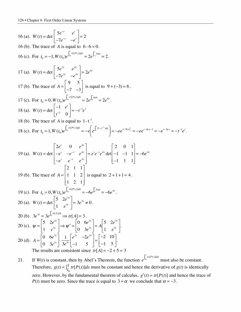
126 • Chapter 6 First Order Linear Systems
16 (a). W te e
e e
t t
t t( ) det=
- -È
ÎÍ
˘
˚˙ =
-
-
5
72
16 (b). The trace of A is equal to - 66 0= .
16 (c). For t W t e etr P s ds ds
t
t t
0 0
01 2 20 1= - Ú = Ú =-, ( )
[ ( )].
17 (a). W te e
e ee
t t
t tt( ) det=
- -È
ÎÍ
˘
˚˙ =
5
72
2 4
2 46
17 (b). The trace of A =- -
È
ÎÍ
˘
˚˙ + - =
9 5
7 39 3 6 is equal to ( ) .
17 (c). For t W t e e etr P s ds ds tt
t t
0 0
6 60 2 20 0= Ú = Ú =, ( )[ ( )]
.
18 (a). W te
tt e
tt( ) det=
-È
ÎÍ
˘
˚˙ = --
-1
011
18 (b). The trace of A is equal to - t -11 .
18 (c). For t W t e e e ee ee e t etr P s ds s ds s s t t t t tt
t tt
0 0
1 1 11 0
1
1 1= Ú = - ÚÊËÁ
ˆ¯
= - = - = - = -- - - - - -
-
, ( ) .[ ( )] ( ) ln ln ln
19 (a). W t
e e
e e e
e e e
e e e e
t t
t t t
t t t
t t t t( ) det det= - --
È
Î
ÍÍÍ
˘
˚
˙˙˙
= - --
È
Î
ÍÍÍ
˘
˚
˙˙˙
= --
-
-
2 0 2 0 1
1 1 1
1 1 1
6
4
4
4
4 4
19 (b). The trace of A =È
Î
ÍÍÍ
˘
˚
˙˙˙
+ + =2 1 1
1 1 2
1 2 1
1 1 4 is equal to 2 .
19 (c). For t W t e e etr P s ds ds tt
t t
0 0
4 40 6 60 0= Ú = - Ú = -, ( )[ ( )]
.
20 (a). W te
ee
t
tt( ) det=
È
ÎÍ
˘
˚˙ = π
5 2
13 0
3
33 .
20 (b). 3 3 33 0e e tr At tr A dst
= Ú fi =[ ]
[ ] .
20 (c). y y=È
ÎÍ
˘
˚˙ fi ¢ =
È
ÎÍ
˘
˚˙ =
È
ÎÍ
˘
˚˙
5 2
1
0 6
0 3
5 2
1
3
3
3
3
3
3
e
e
e
eA
e
e
t
t
t
t
t
t.
20 (d). Ae
e e
e et
t t
t t
=È
ÎÍ
˘
˚˙ ◊
--
È
ÎÍ
˘
˚˙ =
--
È
ÎÍ
˘
˚˙
0 6
0 3
13
2
1 5
2 10
1 5
3
3 3
3 3
.
The results are consistent since tr A[ ] = - + =2 5 3
21. If W(t) is constant, then by Abel’s Theorem, the function etr P s ds
t
t[ ( )]
0Ú must also be constant.
Therefore, g t tr P s dstt( ) [ ( )]= Ú0
must be constant and hence the derivative of g(t) is identically
zero. However, by the fundamental theorem of calculus, ¢ =g t tr P t( ) [ ( )] and hence the trace ofP(t) must be zero. Since the trace is equal to 3 3+ = -a a we conclude that .
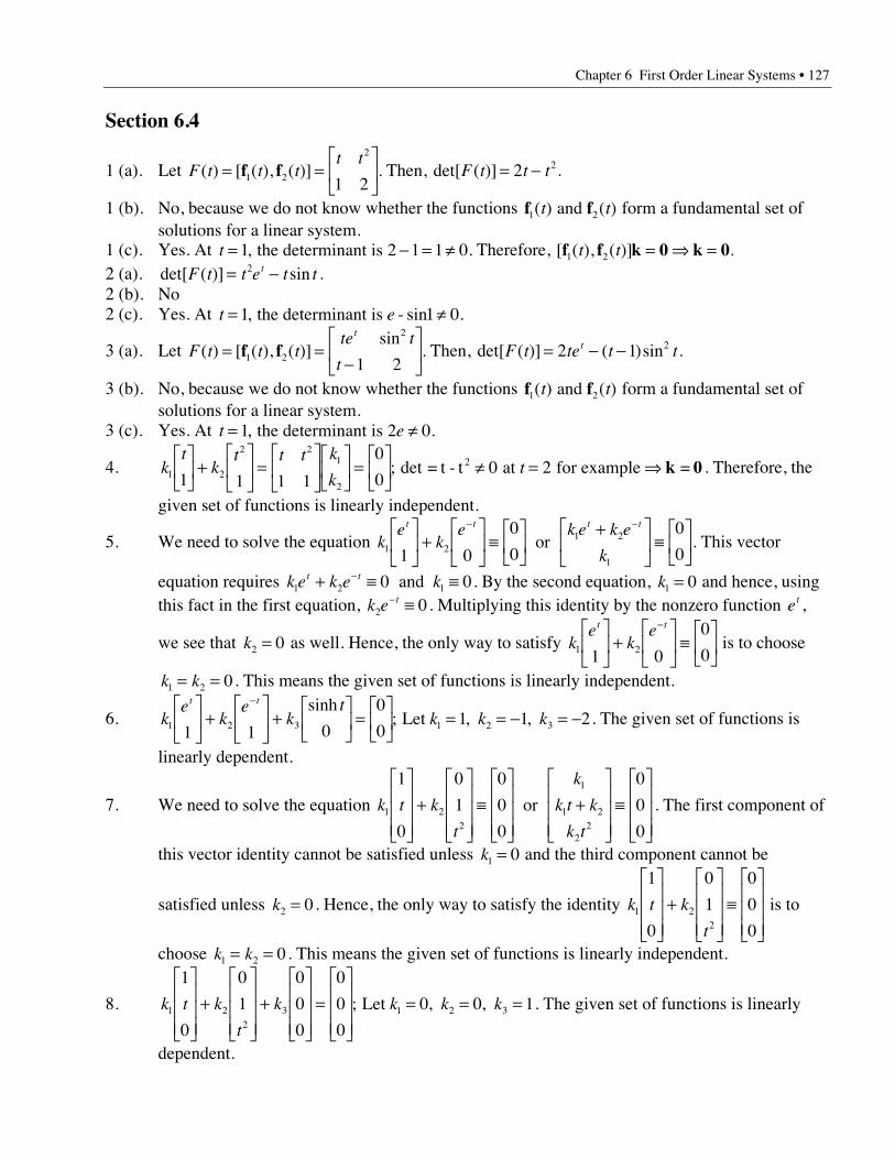
Chapter 6 First Order Linear Systems • 127
Section 6.4
1 (a). Let F t t tt t
( ) [ ( ), ( )] .= =È
ÎÍ
˘
˚˙f f1 2
2
1 2 Then, det[ ( )]F t t t= -2 2.
1 (b). No, because we do not know whether the functions f f1 2( ) ( )t t and form a fundamental set ofsolutions for a linear system.
1 (c). Yes. At t = - = π1 2 1 1 0, the determinant is . Therefore, [ ( ), ( )] .f f k 0 k 01 2t t = fi =2 (a). det[ ( )] sinF t t e t tt= -2 .2 (b). No2 (c). Yes. At t e= π1 1 0, the determinant is - sin .
3 (a). Let F t t tte t
t
t
( ) [ ( ), ( )]sin
.= =-
È
ÎÍ
˘
˚˙f f1 2
2
1 2 Then, det[ ( )] ( )sinF t te t tt= - -2 1 2 .
3 (b). No, because we do not know whether the functions f f1 2( ) ( )t t and form a fundamental set ofsolutions for a linear system.
3 (c). Yes. At t e= π1 2 0, the determinant is .
4. kt
kt t t k
kt1 2
2 21
21 1 1 1
0
00 2
È
ÎÍ
˘
˚˙ +
È
ÎÍ
˘
˚˙ =
È
ÎÍ
˘
˚˙
È
ÎÍ
˘
˚˙ =
È
ÎÍ
˘
˚˙ π = fi; det = t - t at for example =2 k 0 . Therefore, the
given set of functions is linearly independent.
5. We need to solve the equation ke
ke k e k e
k
t t t t
1 21 2
11 0
0
0
0
0
È
ÎÍ
˘
˚˙ +
È
ÎÍ
˘
˚˙ ∫
È
ÎÍ
˘
˚˙
+È
ÎÍ
˘
˚˙ ∫
È
ÎÍ
˘
˚˙
- -
or . This vector
equation requires k e k e kt t1 2 10 0+ ∫ ∫- and . By the second equation, k1 0= and hence, using
this fact in the first equation, k e t2 0- ∫ . Multiplying this identity by the nonzero function et ,
we see that k2 0= as well. Hence, the only way to satisfy ke
ket t
1 21 0
0
0
È
ÎÍ
˘
˚˙ +
È
ÎÍ
˘
˚˙ ∫
È
ÎÍ
˘
˚˙
-
is to choose
k k1 2 0= = . This means the given set of functions is linearly independent.
6. ke
ke
kt
k k kt t
1 2 3 1 2 31 1 0
0
01 1 2
È
ÎÍ
˘
˚˙ +
È
ÎÍ
˘
˚˙ +
È
ÎÍ
˘
˚˙ =
È
ÎÍ
˘
˚˙ = = - = -
- sinh, , ; Let . The given set of functions is
linearly dependent.
7. We need to solve the equation k t k
t
k
k t k
k t1 2
2
1
1 2
22
1
0
0
1
0
0
0
0
0
0
È
Î
ÍÍÍ
˘
˚
˙˙˙
+È
Î
ÍÍÍ
˘
˚
˙˙˙
∫È
Î
ÍÍÍ
˘
˚
˙˙˙
+È
Î
ÍÍÍ
˘
˚
˙˙˙
∫È
Î
ÍÍÍ
˘
˚
˙˙˙
or . The first component of
this vector identity cannot be satisfied unless k1 0= and the third component cannot be
satisfied unless k2 0= . Hence, the only way to satisfy the identity k t k
t1 2
2
1
0
0
1
0
0
0
È
Î
ÍÍÍ
˘
˚
˙˙˙
+È
Î
ÍÍÍ
˘
˚
˙˙˙
∫È
Î
ÍÍÍ
˘
˚
˙˙˙ is to
choose k k1 2 0= = . This means the given set of functions is linearly independent.
8. k t k
t
k k k k1 22
3 1 2 3
1
0
0
1
0
0
0
0
0
0
0 0 1
È
Î
ÍÍÍ
˘
˚
˙˙˙
+È
Î
ÍÍÍ
˘
˚
˙˙˙
+È
Î
ÍÍÍ
˘
˚
˙˙˙
=È
Î
ÍÍÍ
˘
˚
˙˙˙
= = =; Let , , . The given set of functions is linearly
dependent.
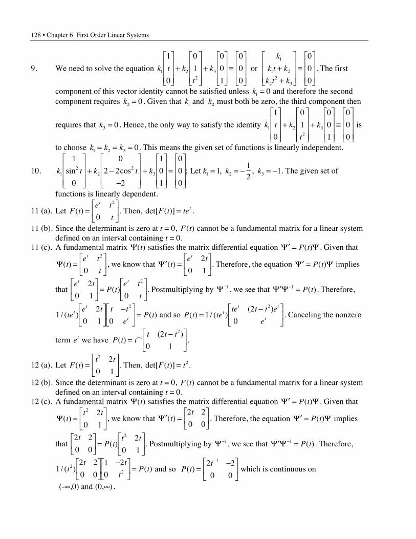
128 • Chapter 6 First Order Linear Systems
9. We need to solve the equation k t k
t
k
k
k t k
k t k1 2
23
1
1 2
22
3
1
0
0
1
0
0
1
0
0
0
0
0
0
È
Î
ÍÍÍ
˘
˚
˙˙˙
+È
Î
ÍÍÍ
˘
˚
˙˙˙
+È
Î
ÍÍÍ
˘
˚
˙˙˙
∫È
Î
ÍÍÍ
˘
˚
˙˙˙
++
È
Î
ÍÍÍ
˘
˚
˙˙˙
∫È
Î
ÍÍÍ
˘
˚
˙˙˙
or . The first
component of this vector identity cannot be satisfied unless k1 0= and therefore the secondcomponent requires k2 0= . Given that k k1 2 and must both be zero, the third component then
requires that k3 0= . Hence, the only way to satisfy the identity k t k
t
k1 22
3
1
0
0
1
0
0
1
0
0
0
È
Î
ÍÍÍ
˘
˚
˙˙˙
+È
Î
ÍÍÍ
˘
˚
˙˙˙
+È
Î
ÍÍÍ
˘
˚
˙˙˙
∫È
Î
ÍÍÍ
˘
˚
˙˙˙ is
to choose k k k1 2 3 0= = = . This means the given set of functions is linearly independent.
10. k t k t k k k k12
22
3 1 2 3
1
0
0
2 2
2
1
0
1
0
0
0
112
1sin cos , ,
È
Î
ÍÍÍ
˘
˚
˙˙˙
+ --
È
Î
ÍÍÍ
˘
˚
˙˙˙
+È
Î
ÍÍÍ
˘
˚
˙˙˙
=È
Î
ÍÍÍ
˘
˚
˙˙˙
= = - = -; Let . The given set of
functions is linearly dependent.
11 (a). Let F te t
t
t
( ) =È
ÎÍ
˘
˚˙
2
0. Then, det[ ( )]F t tet= .
11 (b). Since the determinant is zero at t = 0, F t( ) cannot be a fundamental matrix for a linear systemdefined on an interval containing t = 0.
11 (c). A fundamental matrix Y( )t satisfies the matrix differential equation ¢ =Y YP t( ) . Given that
Y( )te t
t
t
=È
ÎÍ
˘
˚˙
2
0, we know that ¢ =
È
ÎÍ
˘
˚˙Y ( )t
e tt 2
0 1. Therefore, the equation ¢ =Y YP t( ) implies
that e t
P te t
t
t t2
0 1 0
2È
ÎÍ
˘
˚˙ =
È
ÎÍ
˘
˚˙( ) . Postmultiplying by Y -1, we see that ¢ =-Y Y 1 P t( ). Therefore,
12
0 1 0
2
/ ( ) ( )tee t t t
eP tt
t
t
È
ÎÍ
˘
˚˙
-È
ÎÍ
˘
˚˙ = and so P t te
te t t e
et
t t
t( ) / ( )
( )=
-È
ÎÍ
˘
˚˙1
2
0
2
. Canceling the nonzero
term e P t tt t tt we have ( )
( )=
-È
ÎÍ
˘
˚˙-1
22
0 1.
12 (a). Let F tt t
( ) =È
ÎÍ
˘
˚˙
2 2
0 1. Then, det[ ( )]F t t= 2.
12 (b). Since the determinant is zero at t = 0, F t( ) cannot be a fundamental matrix for a linear systemdefined on an interval containing t = 0.
12 (c). A fundamental matrix Y( )t satisfies the matrix differential equation ¢ =Y YP t( ) . Given that
Y( )tt t
=È
ÎÍ
˘
˚˙
2 2
0 1, we know that ¢ =
È
ÎÍ
˘
˚˙Y ( )t
t2 2
0 0. Therefore, the equation ¢ =Y YP t( ) implies
that 2 2
0 0
2
0 1
2tP t
t tÈ
ÎÍ
˘
˚˙ =
È
ÎÍ
˘
˚˙( ) . Postmultiplying by Y -1, we see that ¢ =-Y Y 1 P t( ). Therefore,
12 2
0 0
1 2
02
2/ ( ) ( )tt t
tP t
È
ÎÍ
˘
˚˙
-È
ÎÍ
˘
˚˙ = and so P t
t( ) =
-È
ÎÍ
˘
˚˙
-2 2
0 0
1
which is continuous on
- ,0) and ( ( , )• •0 .
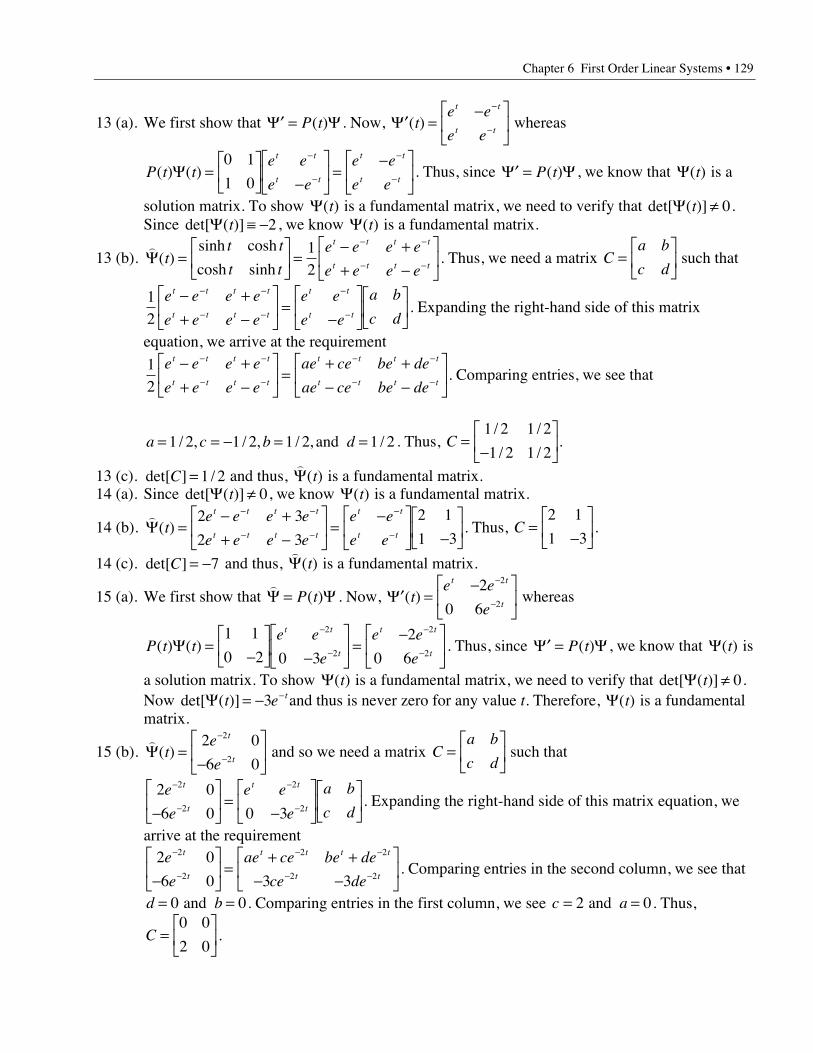
Chapter 6 First Order Linear Systems • 129
13 (a). We first show that ¢ =Y YP t( ) . Now, ¢ =-È
ÎÍ
˘
˚˙
-
-Y ( )te e
e e
t t
t t whereas
P t te e
e e
e e
e e
t t
t t
t t
t t( ) ( )Y =
È
ÎÍ
˘
˚˙ -
È
ÎÍ
˘
˚˙ =
-È
ÎÍ
˘
˚˙
-
-
-
-
0 1
1 0. Thus, since ¢ =Y YP t( ) , we know that Y( )t is a
solution matrix. To show Y( )t is a fundamental matrix, we need to verify that det[ ( )]Y t π 0.Since det[ ( )]Y t ∫ -2, we know Y( )t is a fundamental matrix.
13 (b). )
Y( )sinh cosh
cosh sinht
t t
t t
e e e e
e e e e
t t t t
t t t t=
È
ÎÍ
˘
˚˙ =
- ++ -
È
ÎÍ
˘
˚˙
- -
- -
12
. Thus, we need a matrix Ca b
c d=
È
ÎÍ
˘
˚˙ such that
12
e e e e
e e e e
e e
e e
a b
c d
t t t t
t t t t
t t
t t
- ++ -
È
ÎÍ
˘
˚˙ =
-È
ÎÍ
˘
˚˙
È
ÎÍ
˘
˚˙
- -
- -
-
- . Expanding the right-hand side of this matrix
equation, we arrive at the requirement
12
e e e e
e e e e
ae ce be de
ae ce be de
t t t t
t t t t
t t t t
t t t t
- ++ -
È
ÎÍ
˘
˚˙ =
+ +- -
È
ÎÍ
˘
˚˙
- -
- -
- -
- - . Comparing entries, we see that
a c b d= = - = =1 2 1 2 1 2 1 2/ , / , / , /and . Thus, C =-
È
ÎÍ
˘
˚˙
1 2 1 2
1 2 1 2
/ /
/ /.
13 (c). det[ ] /C = 1 2 and thus, )
Y( )t is a fundamental matrix.14 (a). Since det[ ( )]Y t π 0, we know Y( )t is a fundamental matrix.
14 (b). )
Y( )te e e e
e e e e
e e
e e
t t t t
t t t t
t t
t t=
- ++ -
È
ÎÍ
˘
˚˙ =
-È
ÎÍ
˘
˚˙ -
È
ÎÍ
˘
˚˙
- -
- -
-
-
2 3
2 3
2 1
1 3. Thus, C =
-È
ÎÍ
˘
˚˙
2 1
1 3.
14 (c). det[ ]C = -7 and thus, )
Y( )t is a fundamental matrix.
15 (a). We first show that )
Y Y= P t( ) . Now, ¢ =-È
ÎÍ
˘
˚˙
-
-Y ( )te e
e
t t
t
2
0 6
2
2 whereas
P t te e
e
e e
e
t t
t
t t
t( ) ( )Y =
-È
ÎÍ
˘
˚˙ -
È
ÎÍ
˘
˚˙ =
-È
ÎÍ
˘
˚˙
-
-
-
-
1 1
0 2 0 3
2
0 6
2
2
2
2. Thus, since ¢ =Y YP t( ) , we know that Y( )t is
a solution matrix. To show Y( )t is a fundamental matrix, we need to verify that det[ ( )]Y t π 0.Now det[ ( )]Y t e t= - -3 and thus is never zero for any value t. Therefore, Y( )t is a fundamentalmatrix.
15 (b). )
Y( )te
e
t
t=
-È
ÎÍ
˘
˚˙
-
-
2 0
6 0
2
2 and so we need a matrix C
a b
c d=
È
ÎÍ
˘
˚˙ such that
2 0
6 0 0 3
2
2
2
2
e
e
e e
e
a b
c d
t
t
t t
t
-
-
-
--È
ÎÍ
˘
˚˙ =
-È
ÎÍ
˘
˚˙
È
ÎÍ
˘
˚˙. Expanding the right-hand side of this matrix equation, we
arrive at the requirement2 0
6 0 3 3
2
2
2 2
2 2
e
e
ae ce be de
ce de
t
t
t t t t
t t
-
-
- -
- --È
ÎÍ
˘
˚˙ =
+ +- -
È
ÎÍ
˘
˚˙ . Comparing entries in the second column, we see that
d b= =0 0 and . Comparing entries in the first column, we see c a= =2 0 and . Thus,
C =È
ÎÍ
˘
˚˙
0 0
2 0.
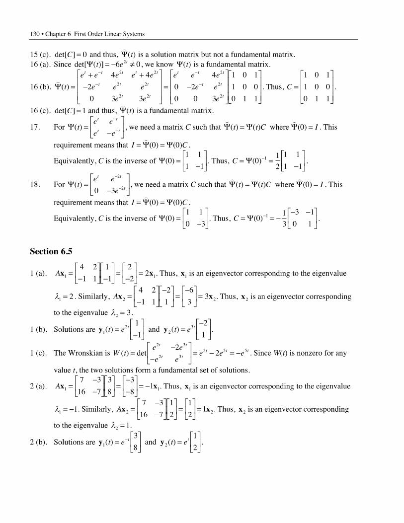
130 • Chapter 6 First Order Linear Systems
15 (c). det[ ]C = 0 and thus, )
Y( )t is a solution matrix but not a fundamental matrix.16 (a). Since det[ ( )]Y t e t= - π6 02 , we know Y( )t is a fundamental matrix.
16 (b). )
Y( )t
e e e e e
e e e
e e
e e e
e e
e
t t t t t
t t t
t t
t t t
t t
t
=+ +
-È
Î
ÍÍÍ
˘
˚
˙˙˙
= -È
Î
ÍÍÍ
˘
˚
˙˙˙
È
Î
ÍÍÍ
˘
˚
˙˙˙
-
-
-
-
4 4
2
0 3 3
4
0 2
0 0 3
1 0 1
1 0 0
0 1 1
2 2
2 2
2 2
2
2
2
. Thus, C =È
Î
ÍÍÍ
˘
˚
˙˙˙
1 0 1
1 0 0
0 1 1
.
16 (c). det[ ]C = 1 and thus, )
Y( )t is a fundamental matrix.
17. For Y( )te e
e e
t t
t t=
-È
ÎÍ
˘
˚˙
-
- , we need a matrix C such that ) )
Y Y Y( ) ( ) ( )t t C I= = where 0 . This
requirement means that I C= =)
Y Y( ) ( )0 0 .
Equivalently, C is the inverse of Y( )01 1
1 1=
-È
ÎÍ
˘
˚˙ . Thus, C = =
-È
ÎÍ
˘
˚˙
-Y( )012
1 1
1 11 .
18. For Y( )te e
e
t t
t=
-È
ÎÍ
˘
˚˙
-
-
2
20 3, we need a matrix C such that
) )Y Y Y( ) ( ) ( )t t C I= = where 0 . This
requirement means that I C= =)
Y Y( ) ( )0 0 .
Equivalently, C is the inverse of Y( )01 1
0 3=
-È
ÎÍ
˘
˚˙. Thus, C = = -
- -È
ÎÍ
˘
˚˙
-Y( )013
3 1
0 11 .
Section 6.5
1 (a). Ax x1 1
4 2
1 1
1
1
2
22=
-È
ÎÍ
˘
˚˙ -
È
ÎÍ
˘
˚˙ =
-È
ÎÍ
˘
˚˙ = . Thus, x1 is an eigenvector corresponding to the eigenvalue
l1 2= . Similarly, Ax x2 2
4 2
1 1
2
1
6
33=
-È
ÎÍ
˘
˚˙
-È
ÎÍ
˘
˚˙ =
-È
ÎÍ
˘
˚˙ = . Thus, x2 is an eigenvector corresponding
to the eigenvalue l2 3= .
1 (b). Solutions are y y12
23
1
1
2
1( ) ( )t e t et t=
-È
ÎÍ
˘
˚˙ =
-È
ÎÍ
˘
˚˙ and .
1 (c). The Wronskian is W te e
e ee e e
t t
t tt t t( ) det=
--
È
ÎÍ
˘
˚˙ = - = -
2 3
2 35 5 52
2 . Since W(t) is nonzero for any
value t, the two solutions form a fundamental set of solutions.
2 (a). Ax x1 1
7 3
16 7
3
8
3
81=
--
È
ÎÍ
˘
˚˙
È
ÎÍ
˘
˚˙ =
--
È
ÎÍ
˘
˚˙ = - . Thus, x1 is an eigenvector corresponding to the eigenvalue
l1 1= - . Similarly, Ax x2 2
7 3
16 7
1
2
1
21=
--
È
ÎÍ
˘
˚˙
È
ÎÍ
˘
˚˙ =
È
ÎÍ
˘
˚˙ = . Thus, x2 is an eigenvector corresponding
to the eigenvalue l2 1= .
2 (b). Solutions are y y1 2
3
8
1
2( ) ( )t e t et t=
È
ÎÍ
˘
˚˙ =
È
ÎÍ
˘
˚˙
- and .
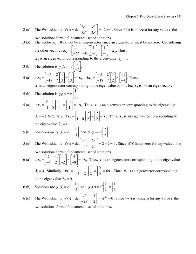
Chapter 6 First Order Linear Systems • 131
2 (c). The Wronskian is W te e
e e
t t
t t( ) det=
È
ÎÍ
˘
˚˙ = - π
-
-
3
8 22 0. Since W(t) is nonzero for any value t, the
two solutions form a fundamental set of solutions.3 (a). The vector x 01 = cannot be an eigenvector since an eigenvector must be nonzero. Considering
the other vector, Ax x2 2
11 5
22 10
1
2
1
2=
- -È
ÎÍ
˘
˚˙ -
È
ÎÍ
˘
˚˙ =
-È
ÎÍ
˘
˚˙ = . Thus,
x2 is an eigenvector corresponding to the eigenvalue l2 1= .
3 (b). The solution is y2
1
2( )t et=
-È
ÎÍ
˘
˚˙.
4 (a). Ax x1 1
5 2
18 7
1
3
1
31=
--
È
ÎÍ
˘
˚˙
È
ÎÍ
˘
˚˙ =
È
ÎÍ
˘
˚˙ = , Ax2
5 2
18 7
1
2
1
4=
--
È
ÎÍ
˘
˚˙
È
ÎÍ
˘
˚˙ =
--
È
ÎÍ
˘
˚˙. Thus,
x1 is an eigenvector corresponding to the eigenvalue l1 1= , but x2 is not an eigenvector.
4 (b). The solution is y1
1
3( )t et=
È
ÎÍ
˘
˚˙.
5 (a). Ax x1 1
0 1
1 0
1
1
1
1=
È
ÎÍ
˘
˚˙ -
È
ÎÍ
˘
˚˙ =
-È
ÎÍ
˘
˚˙ = - . Thus, x1 is an eigenvector corresponding to the eigenvalue
l1 1= - . Similarly, Ax x2 2
0 1
1 0
2
2
2
2=
È
ÎÍ
˘
˚˙
È
ÎÍ
˘
˚˙ =
È
ÎÍ
˘
˚˙ = . Thus, x2 is an eigenvector corresponding to
the eigenvalue l2 1= .
5 (b). Solutions are y y1 2
1
1
2
2( ) ( )t e t et t=
-È
ÎÍ
˘
˚˙ =
È
ÎÍ
˘
˚˙
- and .
5 (c). The Wronskian is W te e
e e
t t
t t( ) det=
-È
ÎÍ
˘
˚˙ = + =
-
-
2
22 2 4. Since W(t) is nonzero for any value t, the
two solutions form a fundamental set of solutions.
6 (a). Ax x1 1
2 1
4 2
1
2
4
84=
--
È
ÎÍ
˘
˚˙ -
È
ÎÍ
˘
˚˙ =
-È
ÎÍ
˘
˚˙ = . Thus, x1 is an eigenvector corresponding to the eigenvalue
l1 4= . Similarly, Ax x2 2
2 1
4 2
1
2
0
00=
--
È
ÎÍ
˘
˚˙
È
ÎÍ
˘
˚˙ =
È
ÎÍ
˘
˚˙ = . Thus, x2 is an eigenvector corresponding
to the eigenvalue l2 0= .
6 (b). Solutions are y y14
20
1
2
1
2
1
2( ) ( )t e t et=
-È
ÎÍ
˘
˚˙ =
È
ÎÍ
˘
˚˙ =
È
ÎÍ
˘
˚˙ and .
6 (c). The Wronskian is W te
ee
t
tt( ) det=
-È
ÎÍ
˘
˚˙ = π
4
441
2 24 0. Since W(t) is nonzero for any value t, the
two solutions form a fundamental set of solutions.
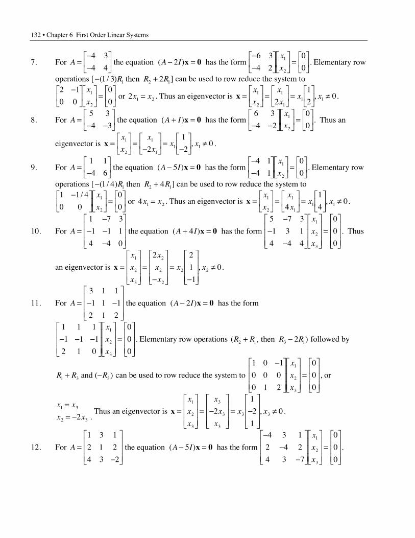
132 • Chapter 6 First Order Linear Systems
7. For A A Ix
x=
--
È
ÎÍ
˘
˚˙ - =
--
È
ÎÍ
˘
˚˙
È
ÎÍ
˘
˚˙ =
È
ÎÍ
˘
˚˙
4 3
4 42
6 3
4 2
0
01
2
the equation has the form ( )x 0 . Elementary row
operations [ - +( / )1 3 21 2 1R R R then ] can be used to row reduce the system to2 1
0 0
0
01
2
-È
ÎÍ
˘
˚˙
È
ÎÍ
˘
˚˙ =
È
ÎÍ
˘
˚˙
x
x or 2 1 2x x= . Thus an eigenvector is x =
È
ÎÍ
˘
˚˙ =
È
ÎÍ
˘
˚˙ =
È
ÎÍ
˘
˚˙ π
x
x
x
xx x1
2
1
11 12
1
20, .
8. For A A Ix
x=
- -È
ÎÍ
˘
˚˙ + =
- -È
ÎÍ
˘
˚˙
È
ÎÍ
˘
˚˙ =
È
ÎÍ
˘
˚˙
5 3
4 3
6 3
4 2
0
01
2
the equation has the form ( )x 0 . Thus an
eigenvector is x =È
ÎÍ
˘
˚˙ =
-È
ÎÍ
˘
˚˙ =
-È
ÎÍ
˘
˚˙ π
x
x
x
xx x1
2
1
11 12
1
20, .
9. For A A Ix
x=
-È
ÎÍ
˘
˚˙ - =
--
È
ÎÍ
˘
˚˙
È
ÎÍ
˘
˚˙ =
È
ÎÍ
˘
˚˙
1 1
4 65
4 1
4 1
0
01
2
the equation has the form ( )x 0 . Elementary row
operations [ - +( / )1 4 41 2 1R R R then ] can be used to row reduce the system to1 1 4
0 0
0
01
2
-È
ÎÍ
˘
˚˙
È
ÎÍ
˘
˚˙ =
È
ÎÍ
˘
˚˙
/ x
x or 4 1 2x x= . Thus an eigenvector is x =
È
ÎÍ
˘
˚˙ =
È
ÎÍ
˘
˚˙ =
È
ÎÍ
˘
˚˙ π
x
x
x
xx x1
2
1
11 14
1
40, .
10. For A A I
x
x
x
=-
- --
È
Î
ÍÍÍ
˘
˚
˙˙˙
+ =-
--
È
Î
ÍÍÍ
˘
˚
˙˙˙
È
Î
ÍÍÍ
˘
˚
˙˙˙
=È
Î
ÍÍÍ
˘
˚
˙˙˙
1 7 3
1 1 1
4 4 0
4
5 7 3
1 3 1
4 4 4
0
0
0
1
2
3
the equation has the form ( )x 0 . Thus
an eigenvector is x =È
Î
ÍÍÍ
˘
˚
˙˙˙
=-
È
Î
ÍÍÍ
˘
˚
˙˙˙
=-
È
Î
ÍÍÍ
˘
˚
˙˙˙
πx
x
x
x
x
x
x x1
2
3
2
2
2
2 2
2 2
1
1
0, .
11. For A A I= - -È
Î
ÍÍÍ
˘
˚
˙˙˙
- =3 1 1
1 1 1
2 1 2
2 the equation has the form( )x 0
1 1 1
1 1 1
2 1 0
0
0
0
1
2
3
- - -È
Î
ÍÍÍ
˘
˚
˙˙˙
È
Î
ÍÍÍ
˘
˚
˙˙˙
=È
Î
ÍÍÍ
˘
˚
˙˙˙
x
x
x
. Elementary row operations ( )R R R R2 1 3 12+ -, then followed by
R R R1 3 3+ - and ( ) can be used to row reduce the system to
1 0 1
0 0 0
0 1 2
0
0
0
1
2
3
-È
Î
ÍÍÍ
˘
˚
˙˙˙
È
Î
ÍÍÍ
˘
˚
˙˙˙
=È
Î
ÍÍÍ
˘
˚
˙˙˙
x
x
x
, or
x x
x x1 3
2 32
== - .
Thus an eigenvector is x =È
Î
ÍÍÍ
˘
˚
˙˙˙
= -È
Î
ÍÍÍ
˘
˚
˙˙˙
= -È
Î
ÍÍÍ
˘
˚
˙˙˙
πx
x
x
x
x
x
x x1
2
3
3
3
3
3 32
1
2
1
0, .
12. For A A I
x
x
x
=-
È
Î
ÍÍÍ
˘
˚
˙˙˙
- =-
--
È
Î
ÍÍÍ
˘
˚
˙˙˙
È
Î
ÍÍÍ
˘
˚
˙˙˙
=È
Î
ÍÍÍ
˘
˚
˙˙˙
1 3 1
2 1 2
4 3 2
5
4 3 1
2 4 2
4 3 7
0
0
0
1
2
3
the equation has the form ( )x 0 .
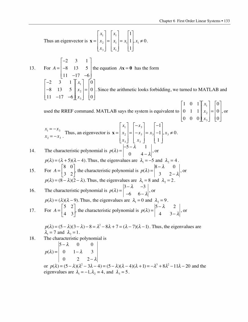
Chapter 6 First Order Linear Systems • 133
Thus an eigenvector is x =È
Î
ÍÍÍ
˘
˚
˙˙˙
=È
Î
ÍÍÍ
˘
˚
˙˙˙
=È
Î
ÍÍÍ
˘
˚
˙˙˙
πx
x
x
x
x
x
x x1
2
3
1
1
1
1 1
1
1
1
0, .
13. For A A=--
- -
È
Î
ÍÍÍ
˘
˚
˙˙˙
=2 3 1
8 13 5
11 17 6
the equation has the formx 0
--
- -
È
Î
ÍÍÍ
˘
˚
˙˙˙
È
Î
ÍÍÍ
˘
˚
˙˙˙
=È
Î
ÍÍÍ
˘
˚
˙˙˙
2 3 1
8 13 5
11 17 6
0
0
0
1
2
3
x
x
x
. Since the arithmetic looks forbidding, we turned to MATLAB and
used the RREF command. MATLAB says the system is equivalent to
1 0 1
0 1 1
0 0 0
0
0
0
1
2
3
È
Î
ÍÍÍ
˘
˚
˙˙˙
È
Î
ÍÍÍ
˘
˚
˙˙˙
=È
Î
ÍÍÍ
˘
˚
˙˙˙
x
x
x
, or
x x
x x1 3
2 3
= -= - .
Thus, an eigenvector is x =È
Î
ÍÍÍ
˘
˚
˙˙˙
=--
È
Î
ÍÍÍ
˘
˚
˙˙˙
=--
È
Î
ÍÍÍ
˘
˚
˙˙˙
πx
x
x
x
x
x
x x1
2
3
3
3
3
3 3
1
1
1
0, .
14. The characteristic polynomial is p( )ll
l=
- --
5 1
0 4, or
p( ) ( )( ). .l l l l l= + - = - =5 4 5 41 2 Thus, the eigenvalues are and
15. For the characteristic polynomial is A p=È
ÎÍ
˘
˚˙ =
--
8 0
3 2
8 0
3 2, ( )l
ll
, or
p( ) ( )( ). .l l l l l= - - = =8 2 8 21 2 Thus, the eigenvalues are and
16. The characteristic polynomial is p( )ll
l=
- -- -
3 3
6 6, or
p( ) ( )( ). .l l l l l= - = =9 0 91 2 Thus, the eigenvalues are and
17. For the characteristic polynomial is A p=È
ÎÍ
˘
˚˙ =
--
5 2
4 3
5 2
4 3, ( )l
ll
, or
p( ) ( )( ) ( )( ).l l l l l l l= - - - = - + = - -5 3 8 8 7 7 12 Thus, the eigenvalues arel l1 27 1= = and .
18. The characteristic polynomial is
p( )ll
ll
=-
--
5 0 0
0 1 3
0 2 2
or p( ) ( )( ) ( )( )( )l l l l l l l l l l= - - - = - - + = - + - -5 3 4 5 4 1 8 11 202 3 2 and theeigenvalues are l l l1 2 31 5= - =, .= 4, and
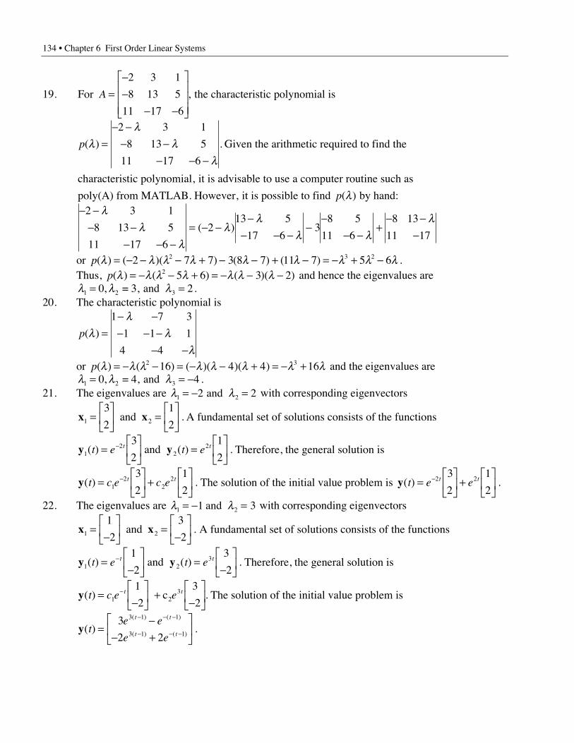
134 • Chapter 6 First Order Linear Systems
19. For the characteristic polynomial isA =--
- -
È
Î
ÍÍÍ
˘
˚
˙˙˙
2 3 1
8 13 5
11 17 6
,
p
p
( ) .
( )
ll
ll
l
=- -
- -- - -
2 3 1
8 13 5
11 17 6
Given the arithmetic required to find the
characteristic polynomial, it is advisable to use a computer routine such as
poly(A) from MATLAB. However, it is possible to find by hand:- -
- -- - -
= - --
- - --
-- -
+- -
-
2 3 1
8 13 5
11 17 6
213 5
17 63
8 5
11 6
8 13
11 17
ll
ll
ll l
l( )
or p( ) ( )( ) ( ) ( )l l l l l l l l l= - - - + - - + - = - + -2 7 7 3 8 7 11 7 5 62 3 2 .Thus, p( ) ( ) ( )( )l l l l l l l= - - + = - - -2 5 6 3 2 and hence the eigenvalues arel l l1 2 30 2= =, .= 3, and
20. The characteristic polynomial is
p( )ll
ll
=- -- - -
- -
1 7 3
1 1 1
4 4
or p( ) ( ) ( )( )( )l l l l l l l l= - - = - - + = - +2 316 4 4 16 and the eigenvalues arel l l1 2 30 4= = -, .= 4, and
21. The eigenvalues are l l1 22 2= - = and with corresponding eigenvectors
x x1 2
3
2
1
2=
È
ÎÍ
˘
˚˙ =
È
ÎÍ
˘
˚˙ and . A fundamental set of solutions consists of the functions
y y12
22
3
2
1
2( ) ( ) .t e t et t=
È
ÎÍ
˘
˚˙ =
È
ÎÍ
˘
˚˙
- and Therefore, the general solution is
y( ) .t c e c et t=È
ÎÍ
˘
˚˙ +
È
ÎÍ
˘
˚˙
-1
22
23
2
1
2 The solution of the initial value problem is y( ) .t e et t=
È
ÎÍ
˘
˚˙ +
È
ÎÍ
˘
˚˙
-2 23
2
1
222. The eigenvalues are l l1 21 3= - = and with corresponding eigenvectors
x x1 2
1
2
3
2=
-È
ÎÍ
˘
˚˙ =
-È
ÎÍ
˘
˚˙ and . A fundamental set of solutions consists of the functions
y y1 23
1
2
3
2( ) ( ) .t e t et t=
-È
ÎÍ
˘
˚˙ =
-È
ÎÍ
˘
˚˙
- and Therefore, the general solution is
y( ) .t c e et t=-
È
ÎÍ
˘
˚˙ +
-È
ÎÍ
˘
˚˙
-1
31
2
3
2 c2 The solution of the initial value problem is
y( ) .( ) ( )
( ) ( )t
e e
e e
t t
t t=
-- +
È
ÎÍ
˘
˚˙
- - -
- - -
3
2 2
3 1 1
3 1 1
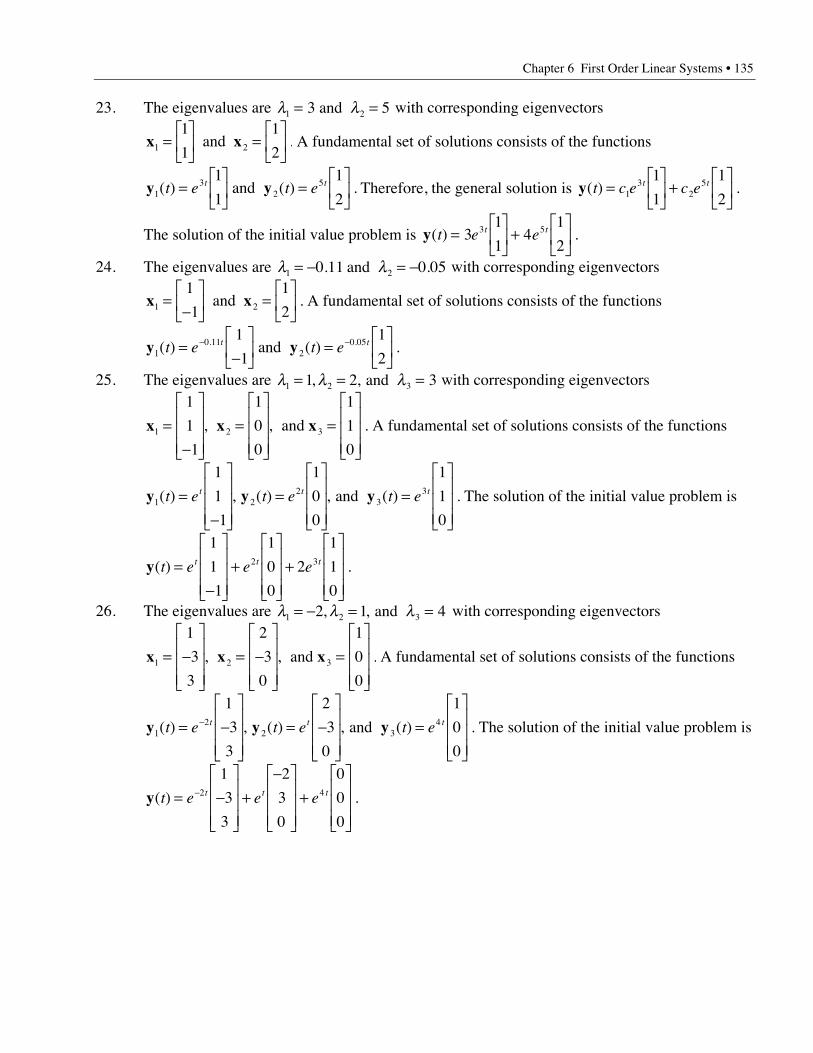
Chapter 6 First Order Linear Systems • 135
23. The eigenvalues are l l1 23 5= = and with corresponding eigenvectors
x x1 2
1
1
1
2=
È
ÎÍ
˘
˚˙ =
È
ÎÍ
˘
˚˙ and . A fundamental set of solutions consists of the functions
y y13
25
1
1
1
2( ) ( ) .t e t et t=
È
ÎÍ
˘
˚˙ =
È
ÎÍ
˘
˚˙ and Therefore, the general solution is y( ) .t c e c et t=
È
ÎÍ
˘
˚˙ +
È
ÎÍ
˘
˚˙1
32
51
1
1
2
The solution of the initial value problem is y( ) .t e et t=È
ÎÍ
˘
˚˙ +
È
ÎÍ
˘
˚˙3
1
14
1
23 5
24. The eigenvalues are l l1 20 11 0 05= - = -. . and with corresponding eigenvectors
x x1 2
1
1
1
2=
-È
ÎÍ
˘
˚˙ =
È
ÎÍ
˘
˚˙ and . A fundamental set of solutions consists of the functions
y y10 11
20 05
1
1
1
2( ) ( ) .. .t e t et t=
-È
ÎÍ
˘
˚˙ =
È
ÎÍ
˘
˚˙
- - and
25. The eigenvalues are l l l1 2 31 2 3= = =, , and with corresponding eigenvectors
x x x1 2 3
1
1
1
1
0
0
1
1
0
=-
È
Î
ÍÍÍ
˘
˚
˙˙˙
=È
Î
ÍÍÍ
˘
˚
˙˙˙
=È
Î
ÍÍÍ
˘
˚
˙˙˙
, , and . A fundamental set of solutions consists of the functions
y y y1 22
33
1
1
1
1
0
0
1
1
0
( ) ( ) ( ) .t e t e t et t t=-
È
Î
ÍÍÍ
˘
˚
˙˙˙
=È
Î
ÍÍÍ
˘
˚
˙˙˙
=È
Î
ÍÍÍ
˘
˚
˙˙˙
, , and The solution of the initial value problem is
y( ) .t e e et t t=-
È
Î
ÍÍÍ
˘
˚
˙˙˙
+È
Î
ÍÍÍ
˘
˚
˙˙˙
+È
Î
ÍÍÍ
˘
˚
˙˙˙
1
1
1
1
0
0
2
1
1
0
2 3
26. The eigenvalues are l l l1 2 32 1 4= - = =, , and with corresponding eigenvectors
x x x1 2 3
1
3
3
2
3
0
1
0
0
= -È
Î
ÍÍÍ
˘
˚
˙˙˙
= -È
Î
ÍÍÍ
˘
˚
˙˙˙
=È
Î
ÍÍÍ
˘
˚
˙˙˙
, , and . A fundamental set of solutions consists of the functions
y y y12
2 34
1
3
3
2
3
0
1
0
0
( ) ( ) ( ) .t e t e t et t t= -È
Î
ÍÍÍ
˘
˚
˙˙˙
= -È
Î
ÍÍÍ
˘
˚
˙˙˙
=È
Î
ÍÍÍ
˘
˚
˙˙˙
- , , and The solution of the initial value problem is
y( ) .t e e et t t= -È
Î
ÍÍÍ
˘
˚
˙˙˙
+-È
Î
ÍÍÍ
˘
˚
˙˙˙
+È
Î
ÍÍÍ
˘
˚
˙˙˙
-2 4
1
3
3
2
3
0
0
0
0
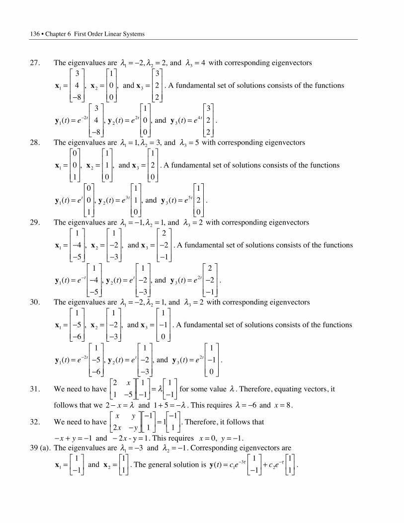
136 • Chapter 6 First Order Linear Systems
27. The eigenvalues are l l l1 2 32 2 4= - = =, , and with corresponding eigenvectors
x x x1 2 3
3
4
8
1
0
0
3
2
2
=-
È
Î
ÍÍÍ
˘
˚
˙˙˙
=È
Î
ÍÍÍ
˘
˚
˙˙˙
=È
Î
ÍÍÍ
˘
˚
˙˙˙
, , and . A fundamental set of solutions consists of the functions
y y y12
22
34
3
4
8
1
0
0
3
2
2
( ) ( ) ( ) .t e t e t et t t=-
È
Î
ÍÍÍ
˘
˚
˙˙˙
=È
Î
ÍÍÍ
˘
˚
˙˙˙
=È
Î
ÍÍÍ
˘
˚
˙˙˙
- , , and
28. The eigenvalues are l l l1 2 31 3 5= = =, , and with corresponding eigenvectors
x x x1 2 3
0
0
1
1
1
0
1
2
0
=È
Î
ÍÍÍ
˘
˚
˙˙˙
=È
Î
ÍÍÍ
˘
˚
˙˙˙
=È
Î
ÍÍÍ
˘
˚
˙˙˙
, , and . A fundamental set of solutions consists of the functions
y y y1 23
35
0
0
1
1
1
0
1
2
0
( ) ( ) ( ) .t e t e t et t t=È
Î
ÍÍÍ
˘
˚
˙˙˙
=È
Î
ÍÍÍ
˘
˚
˙˙˙
=È
Î
ÍÍÍ
˘
˚
˙˙˙
, , and
29. The eigenvalues are l l l1 2 31 1 2= - = =, , and with corresponding eigenvectors
x x x1 2 3
1
4
5
1
2
3
2
2
1
= --
È
Î
ÍÍÍ
˘
˚
˙˙˙
= --
È
Î
ÍÍÍ
˘
˚
˙˙˙
= --
È
Î
ÍÍÍ
˘
˚
˙˙˙
, , and . A fundamental set of solutions consists of the functions
y y y1 2 32
1
4
5
1
2
3
2
2
1
( ) ( ) ( ) .t e t e t et t t= --
È
Î
ÍÍÍ
˘
˚
˙˙˙
= --
È
Î
ÍÍÍ
˘
˚
˙˙˙
= --
È
Î
ÍÍÍ
˘
˚
˙˙˙
- , , and
30. The eigenvalues are l l l1 2 32 1 2= - = =, , and with corresponding eigenvectors
x x x1 2 3
1
5
6
1
2
3
1
1
0
= --
È
Î
ÍÍÍ
˘
˚
˙˙˙
= --
È
Î
ÍÍÍ
˘
˚
˙˙˙
= -È
Î
ÍÍÍ
˘
˚
˙˙˙
, , and . A fundamental set of solutions consists of the functions
y y y12
2 32
1
5
6
1
2
3
1
1
0
( ) ( ) ( ) .t e t e t et t t= --
È
Î
ÍÍÍ
˘
˚
˙˙˙
= --
È
Î
ÍÍÍ
˘
˚
˙˙˙
= -È
Î
ÍÍÍ
˘
˚
˙˙˙
- , , and
31. We need to have 2
1 5
1
1
1
1
x
-È
ÎÍ
˘
˚˙ -
È
ÎÍ
˘
˚˙ =
-È
ÎÍ
˘
˚˙l for some value l . Therefore, equating vectors, it
follows that we 2 1 5- = + = -x l land . This requires l = -6 and x = 8.
32. We need to have x y
x y2
1
11
1
1-È
ÎÍ
˘
˚˙
-È
ÎÍ
˘
˚˙ =
-È
ÎÍ
˘
˚˙. Therefore, it follows that
- + = - - =x y x1 2 1and - y . This requires x y= = -0 1, .39 (a). The eigenvalues are l l1 23 1= - = - and . Corresponding eigenvectors are
x x1 2
1
1
1
1=
-È
ÎÍ
˘
˚˙ =
È
ÎÍ
˘
˚˙ and . The general solution is y( ) .t c e c e=
-È
ÎÍ
˘
˚˙ +
È
ÎÍ
˘
˚˙
- -1
32
1
1
1
1t t
Chapter 6 First Order Linear Systems • 137
39 (b). The solution of the initial value problem is y( ) .tQ
eQ
e= --
È
ÎÍ
˘
˚˙ +
È
ÎÍ
˘
˚˙
- -0 3 0
2
1
13
2
1
1t t
Therefore, Q tQ
e e Q tQ
e e10 3
20 3
23
23( ) ( )= - +( ) = +( )- - - -t t t t and .
Note that 0 1 2< <Q Q( ) ( )t t . Therefore, we need t such thatQ
e e Q e e0 30
3
23 01 3 02( ) . ( ) .- - - -+ < fi + <t t t t . Graphically, we find that a value t ª 5 011. will
suffice. Since t V r= =( / )t t50 , we obtain a value of t tª ª250 55 4 18. sec . min or .40 (a). The eigenvalues are l l l1 2 31 4= - = = - and . Corresponding eigenvectors are
x x x1 2 3
1
1
1
1
1
0
1
0
1
=È
Î
ÍÍÍ
˘
˚
˙˙˙
= -È
Î
ÍÍÍ
˘
˚
˙˙˙
=-
È
Î
ÍÍÍ
˘
˚
˙˙˙
, , and . The general solution is
Q( ) .t c e c e c e=È
Î
ÍÍÍ
˘
˚
˙˙˙
+ -È
Î
ÍÍÍ
˘
˚
˙˙˙
+-
È
Î
ÍÍÍ
˘
˚
˙˙˙
- - -1 2
43
4
1
1
1
1
1
0
1
0
1
t t t
40 (b). The solution of the initial value problem is y( ) .t Q e Q e=È
Î
ÍÍÍ
˘
˚
˙˙˙
--
È
Î
ÍÍÍ
˘
˚
˙˙˙
- -2
1
1
1
1
0
10 0
4t t
Therefore, Q( )t Q
e e
e
e e
rv
rv
rv
rv
rv
t t
t
t t
=-
+
È
Î
ÍÍÍ
˘
˚
˙˙˙
- -
-
- -0
4
4
2
2
2
.
Section 6.6
1. For A =-
È
ÎÍ
˘
˚˙
2 1
1 2, the characteristic polynomial is p( )l
ll
l l=-
- -= - +
2 1
1 24 52 .
Therefore, the eigenvalues are l1 2= + i and l2 2= - i . We find an eigenvector x1 by solving( )A I- =l1 x 0 or2 2 1
1 2 2
0
01
2
- +- - +
È
ÎÍ
˘
˚˙
È
ÎÍ
˘
˚˙ =
È
ÎÍ
˘
˚˙
( )
( )
i
i
x
x. This equation reduces to
-- -
È
ÎÍ
˘
˚˙
È
ÎÍ
˘
˚˙ =
È
ÎÍ
˘
˚˙
i
i
x
x
1
1
0
01
2
. The
elementary row operation R iR2 1+ reduces the system to -È
ÎÍ
˘
˚˙
È
ÎÍ
˘
˚˙ =
È
ÎÍ
˘
˚˙
i x
x
1
0 0
0
01
2
or - + =ix x1 2 0.
Thus, an eigenvector is x =È
ÎÍ
˘
˚˙ =
È
ÎÍ
˘
˚˙ =
È
ÎÍ
˘
˚˙ π
x
x
x
ixx
ix1
2
1
11 1
10, . Since the eigenvalues and eigenvectors
occur in conjugate pairs, the eigenpairs are
l l1 1 2 221
21
= + =È
ÎÍ
˘
˚˙ = - =
-È
ÎÍ
˘
˚˙i
ii
i, ,x x and .
138 • Chapter 6 First Order Linear Systems
2. The characteristic polynomial is p( )ll
ll=
- --
= +9
192 . Therefore, the eigenvalues are
l1 3= i and l2 3= - i . We find an eigenvector x1 by solving ( )A I- =l1 x 0 or- -
-È
ÎÍ
˘
˚˙
È
ÎÍ
˘
˚˙ =
È
ÎÍ
˘
˚˙
3 9
1 3
0
01
2
i
i
x
x. Thus, an eigenvector is x1
1
2
2
22 2
3 3
10=
È
ÎÍ
˘
˚˙ =
È
ÎÍ
˘
˚˙ =
È
ÎÍ
˘
˚˙ π
x
x
ix
xx
ix, . Since the
eigenvalues and eigenvectors occur in conjugate pairs, the eigenpairs are
l l1 1 2 233
13
3
1= =
È
ÎÍ
˘
˚˙ = - =
-È
ÎÍ
˘
˚˙i
ii
i, ,x x and .
3. For A =-È
ÎÍ
˘
˚˙
6 13
1 0, the characteristic polynomial is p( )l
ll
l l=- -
-= - +
6 13
16 132 .
Therefore, the eigenvalues are l1 3 2= + i and l2 3 2= - i . We find an eigenvector x1 bysolving ( )A I- =l1 x 0 or
6 3 2 13
1 3 2
0
01
2
- + -- +
È
ÎÍ
˘
˚˙
È
ÎÍ
˘
˚˙ =
È
ÎÍ
˘
˚˙
( )
( )
i
i
x
x. This equation reduces to
3 2 13
1 3 2
0
01
2
- -- -
È
ÎÍ
˘
˚˙
È
ÎÍ
˘
˚˙ =
È
ÎÍ
˘
˚˙
i
i
x
x. The
elementary row operations R R R i R1 2 2 13 2´ - -, then ( ) reduces the system to1 3 2
0 0
0
01
2
- +È
ÎÍ
˘
˚˙
È
ÎÍ
˘
˚˙ =
È
ÎÍ
˘
˚˙
( )i x
x or x i x1 23 2 0- + =( ) . Thus, an eigenvector is
x =È
ÎÍ
˘
˚˙ =
+È
ÎÍ
˘
˚˙ =
+È
ÎÍ
˘
˚˙ π
x
x
i x
xx
ix1
2
2
22 2
3 2 3 2
10
( ), . Choosing x2 1= , we obtain the eigenvector
x1
3 2
1=
+È
ÎÍ
˘
˚˙
i. Since the eigenvalues and eigenvectors occur in conjugate pairs, the eigenpairs
are
l l1 1 2 23 23 2
13 2
3 2
1= + =
+È
ÎÍ
˘
˚˙ = - =
-È
ÎÍ
˘
˚˙i
ii
i, ,x x and .
4. The characteristic polynomial is p( ) ( )ll
ll=
-- -
= - +3 1
2 12 12 . Therefore, the eigenvalues
are l1 2= + i and l2 2= - i . We find an eigenvector x1 by solving ( )A I- =l1 x 0 or1 1
2 1
0
01
2
-- - -
È
ÎÍ
˘
˚˙
È
ÎÍ
˘
˚˙ =
È
ÎÍ
˘
˚˙
i
i
x
x. Thus, an eigenvector is x1
1
1=
- +È
ÎÍ
˘
˚˙i. Since the eigenvalues and
eigenvectors occur in conjugate pairs, the eigenpairs are
l l1 1 2 221
12
1
1= + =
- +È
ÎÍ
˘
˚˙ = - =
- -È
ÎÍ
˘
˚˙i
ii
i, ,x x and .
5. Using the EIG command in MATLAB, we find eigenvalues l l1 21 1= = +, i , and l3 1= - i .For each eigenvalue l , we use the RREF command in MATLAB to solve ( )A I- =l x 0,
finding x x x1 2 3
3
0
1
3 2
1
1
3 2
1
1
=-È
Î
ÍÍÍ
˘
˚
˙˙˙
=+
- -
È
Î
ÍÍÍ
˘
˚
˙˙˙
=-
- +
È
Î
ÍÍÍ
˘
˚
˙˙˙
, , .
i
i
i
i
and
Chapter 6 First Order Linear Systems • 139
Note that another possible eigenvector for l2 is x2 1
3 2
1
1
5
1
2
= - ++
- -
È
Î
ÍÍÍ
˘
˚
˙˙˙
=- +- +
È
Î
ÍÍÍ
˘
˚
˙˙˙
( ) .i
i
i
i
i
6. The eigenvalues are l l l1 2 32 2 3 2 3= = + = -, , i iand . The corresponding eigenvectors are
x x x1 2 3
1
0
1
4
3
1
4
3
1
=-
È
Î
ÍÍÍ
˘
˚
˙˙˙
=- -
+
È
Î
ÍÍÍ
˘
˚
˙˙˙
=- +
--
È
Î
ÍÍÍ
˘
˚
˙˙˙
, , .
i
i
i
i
i
i
and
7. As in Example 1, y( ) (cos sin )( )t ei
e t i ti
i t t=- +
È
ÎÍ
˘
˚˙ = +
- +È
ÎÍ
˘
˚˙
+4 2 44
12 2
4
1 is one solution of ¢ =y yA .
Expanding and collecting real and imaginary parts, we obtain
y( )cos
cos sin
sin
cos sint e
t
t tie
t
t tt t=
- -È
ÎÍ
˘
˚˙ +
-È
ÎÍ
˘
˚˙
4 44 2
2 2
4 2
2 2. Thus, a fundamental set of solutions can be
formed from y14
4 2
2 2( )
cos
cos sint e
t
t tt=
- -È
ÎÍ
˘
˚˙ and y2
44 2
2 2( )
sin
cos sint e
t
t tt=
-È
ÎÍ
˘
˚˙ .
8. y( ) (cos sin )t ei
t i ti
it=- +È
ÎÍ
˘
˚˙ = +
- +È
ÎÍ
˘
˚˙
2
5
2
5 is one solution of ¢ =y yA . Expanding and collecting
real and imaginary parts, we obtain y( )cos sin
cos
cos sin
sint
t t
ti
t t
t=
- -È
ÎÍ
˘
˚˙ +
-È
ÎÍ
˘
˚˙
2
5
2
5. Thus, a
fundamental set of solutions can be formed from y1
2
5( )
cos sin
cost
t t
t=
- -È
ÎÍ
˘
˚˙ and
y2
2
5( )
cos sin
sint
t t
t=
-È
ÎÍ
˘
˚˙ .
9. As in Example 1, y( ) (cos sin )t ei
t i ti
it=- -È
ÎÍ
˘
˚˙ = +
- -È
ÎÍ
˘
˚˙
21
12 2
1
1 is one solution of ¢ =y yA .
Expanding and collecting real and imaginary parts, we obtain
y( )cos sin
cos
cos sin
sint
t t
ti
t t
t=
- +È
ÎÍ
˘
˚˙ +
- -È
ÎÍ
˘
˚˙
2 2
2
2 2
2. Thus, a fundamental set of solutions can be
formed from y1
2 2
2( )
cos sin
cost
t t
t=
- +È
ÎÍ
˘
˚˙ and y2
2 2
2( )
cos sin
sint
t t
t=
- -È
ÎÍ
˘
˚˙ .
10. y( ) (cos sin )t e t i ti
it= +
- +È
ÎÍ
˘
˚˙
1 is one solution of ¢ =y yA . Expanding and collecting real and
imaginary parts, we obtain y( )cos sin
sin
cos sin
cost e
t t
tie
t t
tt t=
- --
È
ÎÍ
˘
˚˙ +
-È
ÎÍ
˘
˚˙. Thus, a fundamental set
of solutions can be formed from y1( )cos sin
sint e
t t
tt=
- --
È
ÎÍ
˘
˚˙ and y2( )
cos sin
cost e
t t
tt=
-È
ÎÍ
˘
˚˙.
140 • Chapter 6 First Order Linear Systems
11. As in Example 1, y( ) (cos sin )( )t e
i
i e t i t
i
ii t t=- +
+È
Î
ÍÍÍ
˘
˚
˙˙˙
= +- +
+È
Î
ÍÍÍ
˘
˚
˙˙˙
+2 3 2
5 3
3 3
2
3 3
5 3
3 3
2
is one solution of
¢ =y yA . Expanding and collecting real and imaginary parts, we obtain
y( )
cos sin
cos sin
cos
cos sin
cos sin
sin
t e
t t
t t
t
ie
t t
t t
t
t t=- -
-È
Î
ÍÍÍ
˘
˚
˙˙˙
+-+
È
Î
ÍÍÍ
˘
˚
˙˙˙
2 2
5 3 3 3
3 3 3 3
2 3
3 3 5 3
3 3 3 3
2 3
. Thus, two linearly independent solutions
are y12
5 3 3 3
3 3 3 3
2 3
( )
cos sin
cos sin
cos
t e
t t
t t
t
t=- -
-È
Î
ÍÍÍ
˘
˚
˙˙˙ and y2
2
3 3 5 3
3 3 3 3
2 3
( )
cos sin
cos sin
sin
t e
t t
t t
t
t=-+
È
Î
ÍÍÍ
˘
˚
˙˙˙. The third solution needed
to complete the fundamental set is obtained from the real eigenvalue l = 2, y32
1
0
1
( )t e t=-
È
Î
ÍÍÍ
˘
˚
˙˙˙.
12. e t i t
i
e
t
tie
t
tt t t(cos sin )
sin
cos
cos
sin5 5
1
0
0
5
5
0
0
5
5
0
0
+
È
Î
ÍÍÍÍ
˘
˚
˙˙˙˙
=
-È
Î
ÍÍÍÍ
˘
˚
˙˙˙˙
+
È
Î
ÍÍÍÍ
˘
˚
˙˙˙˙. Also,
e t i ti
et
t
iet
t
t t t(cos sin )sin
cos
cos
sin
2 2
0
0
1
0
0
2
2
0
0
2
2
+
È
Î
ÍÍÍÍ
˘
˚
˙˙˙˙
=-
È
Î
ÍÍÍÍ
˘
˚
˙˙˙˙
+
È
Î
ÍÍÍÍ
˘
˚
˙˙˙˙ Thus, a fundamental set of solutions can be
formed from e
t
te
t
te
t
t
et
t
t t t t
-È
Î
ÍÍÍÍ
˘
˚
˙˙˙˙
È
Î
ÍÍÍÍ
˘
˚
˙˙˙˙
-
È
Î
ÍÍÍÍ
˘
˚
˙˙˙˙
È
Î
ÍÍÍÍ
˘
˚
˙˙˙˙
sin
cos,
cos
sin,
sin
cos
, cos
sin
5
5
0
0
5
5
0
0
0
0
2
2
0
0
2
2
.
13. Proceeding as in Exercises 7-12, we find the general solution of ¢ =y yA is
y( )cos
sin
sin
cost c e
t
tc e
t
tt t=
-È
ÎÍ
˘
˚˙ +
È
ÎÍ
˘
˚˙1
22
2 . Imposing the initial condition, y( )01
0
0
1
4
71 2=È
ÎÍ
˘
˚˙ +
È
ÎÍ
˘
˚˙ =
È
ÎÍ
˘
˚˙c c , we
obtain the solution y( )cos sin
sin cost e
t t
t tt=
+- +
È
ÎÍ
˘
˚˙
24 7
4 7.
14. Proceeding as in Exercises 7-12, we find the general solution of ¢ =y yA is
y( )sin
cos
cos
sint c
t
tc
t
t=
È
ÎÍ
˘
˚˙ +
È
ÎÍ
˘
˚˙1 2
3 3
3
3 3
3. Imposing the initial condition, y( )0
0
1
3
0
6
21 2=È
ÎÍ
˘
˚˙ +
È
ÎÍ
˘
˚˙ =
È
ÎÍ
˘
˚˙c c , we
obtain the solution y( )sin cos
cos sint
t t
t t=
- ++
È
ÎÍ
˘
˚˙
6 3 6 3
2 3 2 3.
Chapter 6 First Order Linear Systems • 141
15. Proceeding as in Exercises 7-12, we find the general solution of ¢ =y yA is
y( )cos sin
cos
cos sin
sint c e
t t
tc e
t t
tt t=
-È
ÎÍ
˘
˚˙ +
+È
ÎÍ
˘
˚˙1
32
33 2 2 2
2
2 2 3 2
2. Imposing the initial condition,
y( )03
1
2
0
1
31 2=È
ÎÍ
˘
˚˙ +
È
ÎÍ
˘
˚˙ =
È
ÎÍ
˘
˚˙c c , we find c c1 23 4= = - and and the solution is
y( )cos sin
cos sint e
t t
t tt=
--
È
ÎÍ
˘
˚˙
32 18 2
3 2 4 2.
16. Proceeding as in Exercises 7-12, we find the general solution of ¢ =y yA is
y( )cos
cos sin
sin
cos sint c e
t
t tc e
t
t tt t=
- -È
ÎÍ
˘
˚˙ +
-È
ÎÍ
˘
˚˙1
22
2 . Imposing the initial condition,
y( )01
1
0
1
8
61 2=-
È
ÎÍ
˘
˚˙ +
È
ÎÍ
˘
˚˙ =
È
ÎÍ
˘
˚˙c c , we obtain the solution y( )
cos sin
cos sint e
t t
t tt=
+-
È
ÎÍ
˘
˚˙
28 14
6 22.
17. Proceeding as in Exercises 7-12, we find the general solution of ¢ =y yA is
y( )
cos sin
cos
cos sin
cos sin
sin
cos sin
t c e c e
t t
t
t t
c e
t t
t
t t
t t t=-È
Î
ÍÍÍ
˘
˚
˙˙˙
+-
- +
È
Î
ÍÍÍ
˘
˚
˙˙˙
++
- -
È
Î
ÍÍÍ
˘
˚
˙˙˙
1 2 3
3
0
1
3 2 2 3
.
Imposing the initial condition, y( )0
3
0
1
3
1
1
2
0
1
6
1
21 2 3=
-È
Î
ÍÍÍ
˘
˚
˙˙˙
+-
È
Î
ÍÍÍ
˘
˚
˙˙˙
+-
È
Î
ÍÍÍ
˘
˚
˙˙˙
=È
Î
ÍÍÍ
˘
˚
˙˙˙
c c c , we find
c c c1 2 39 1 12= - = = -, , and , and the solution y( )
cos sin
cos sin
cos sin
t e
t t
t t
t t
t=- -
-- + +
È
Î
ÍÍÍ
˘
˚
˙˙˙
27 21 38
12
9 11 13
.
18. Proceeding as in Exercises 7-12, we find the general solution of ¢ =y yA is
y( )
cos sin
sin
cos sin
cos sin
cos
cos sin
t c e c e
t t
t
t t
c e
t t
t
t t
t t t=-
È
Î
ÍÍÍ
˘
˚
˙˙˙
+- +
--
È
Î
ÍÍÍ
˘
˚
˙˙˙
+- -
+
È
Î
ÍÍÍ
˘
˚
˙˙˙
12
22
32
1
0
1
4 3 3
3 3
3 3
3 4 3
3 3
3 3
.
Imposing the initial condition, y( )0
1
0
1
4
0
1
1
3
1
1
9
41 2 3=
-
È
Î
ÍÍÍ
˘
˚
˙˙˙
+-È
Î
ÍÍÍ
˘
˚
˙˙˙
+-È
Î
ÍÍÍ
˘
˚
˙˙˙
=-È
Î
ÍÍÍ
˘
˚
˙˙˙
c c c , we find
c c c1 2 32 1 3= - = - =, , and , and the solution y( )
cos sin
cos sin
cos sin
t e
t t
t t
t t
t=- + -
++ +
È
Î
ÍÍÍ
˘
˚
˙˙˙
2
2 3 13 3
9 3 3 3
2 2 3 4 3
.
22. The eigenvalues of A are l m= - ± +( )1 9 12 2/ . If 9 12 012
0+ < = - ± πm l b b, ( )i ,
therefore distinct and y t( ) Æ 0. If 0 9 12 1< + <m , , the eigenvalues are distinct, real and
negative. Therefore, -• - • < < -< 9 +12 < 1 m m 23
.
142 • Chapter 6 First Order Linear Systems
23. The eigenvalues of A are l m= - ± +( )5 1 4 2/ . In order that both components of y( )t go to
zero as t Æ • , we need each of these (real) eigenvalues to be negative. Therefore, we need
- + +( ) <5 1 4 2 0m / or 1 4 5+ <m . This inequality holds if and only if
1 4 25 6+ < - • < <m m or .
24. The eigenvalues of A are l m m= - ± -( ) = - ± -2 16 4 2 1 42 2/ . Require
-• < - < fi < < •4 1 32 2m m . Therefore, -• < < - < < •m m3 3 and .
25. The eigenvalues of A are l m= - ± +1 4 2 . In order that both components of y( )t go to zeroas t Æ • , we need each of these (real) eigenvalues to be negative. Therefore, we need
- + + <1 4 02m or 4 12+ <m . This inequality cannot hold for any real value of m .
26 (a).d
dtt
t t
t t
c
cv v v=
-È
ÎÍ
˘
˚˙ fi =
-È
ÎÍ
˘
˚˙
È
ÎÍ
˘
˚˙
0 1
1 01
2
( )cos sin
sin cos.
26 (b). v v( ) ( )cos sin
sin cos0
1
2
2
21
2
=È
ÎÍ
˘
˚˙ =
È
ÎÍ
˘
˚˙ fi =
+- +
È
ÎÍ
˘
˚˙
c
ct
t t
t t. r( )
sin cos
cos sint
t t
t t
d
d=
-+
È
ÎÍ
˘
˚˙ +
È
ÎÍ
˘
˚˙
2
21
2
.
r r( ) ( )sin cos
cos sin0
2
1
2
1
2 4
21
2
=- +
+È
ÎÍ
˘
˚˙ =
È
ÎÍ
˘
˚˙ fi =
- ++
È
ÎÍ
˘
˚˙
d
dt
t t
t t. v r
32
2
132
3
2p pÊ
ËÁˆ¯ =
-È
ÎÍ
˘
˚˙
ÊËÁ
ˆ¯ =
-È
ÎÍ
˘
˚˙ and .
27 (d). If the charged particle is launched with initial velocity parallel to the magnetic field, it willmove with constant velocity.
28 (b). The eigenpairs are - + - + - +g l g l g lm m m1 1 2 2 3 3, , ,x x x and and .
The corresponding fundamental matrix is e tm t- g
y ( ).
Section 6.7
1 (a). For A =È
ÎÍ
˘
˚˙
2 1
0 2, the characteristic polynomial is p( ) ( ) .l l= - 2 2 The eigenvalue l1 2= has
algebraic multiplicity 2. Corresponding eigenvectors are obtained by solving ( )A I- =2 x 0 or0 1
0 0
0
01
2
È
ÎÍ
˘
˚˙
È
ÎÍ
˘
˚˙ =
È
ÎÍ
˘
˚˙
x
x. Therefore, all the eigenvectors corresponding to l1 2= have the form
x =È
ÎÍ
˘
˚˙ =
È
ÎÍ
˘
˚˙ π
xx x1
1 10
1
00, . The geometric multiplicity of l1 2= is 1.
1 (b). We find a generalized eigenvector corresponding to l1 2= by solving the equation
( )A I- = =È
ÎÍ
˘
˚˙2
1
01 1x x x where . The solution is x =È
ÎÍ
˘
˚˙
x1
1 where x1 is arbitrary. Choosing x1 0= ,
we obtain the generalized eigenvector x2
0
1=
È
ÎÍ
˘
˚˙.
Chapter 6 First Order Linear Systems • 143
Thus, we have solutions y x12
1( )t e t= and, as in equation (6), y x x22
12
2( )t te et t= + . A
fundamental matrix is Y( ) [ ( ), ( )]t t te te
e
t t
t= =
È
ÎÍ
˘
˚˙y y1 2
2 2
20.
1 (c). The general solution is Y( )t c . Imposing the initial condition, Y( )0 0c y= . We find1 0
0 1
1
1
1
11
2
È
ÎÍ
˘
˚˙
È
ÎÍ
˘
˚˙ =
-È
ÎÍ
˘
˚˙ =
-È
ÎÍ
˘
˚˙
c
c or c . Thus, the solution of the initial value problem is
y( )t et
t=-
-È
ÎÍ
˘
˚˙
21
1.
2 (a). The characteristic polynomial is p( ) ( ) .l l= -3 2 The eigenvalue l1 3= has algebraicmultiplicity 2. Corresponding eigenvectors are obtained by solving ( )A I- =3 x 0. Therefore,
all the eigenvectors corresponding to l1 3= have the form x =È
ÎÍ
˘
˚˙ =
È
ÎÍ
˘
˚˙ π
xx x1
1 10
1
00, . The
geometric multiplicity of l1 3= is 1.
2 (b). y13
1
0( )t e t=
È
ÎÍ
˘
˚˙ and y2
3 312
312
1
0
0( )t te e e
tt t t=
È
ÎÍ
˘
˚˙ +
È
ÎÍ
˘
˚˙ =
È
ÎÍ
˘
˚˙. A fundamental matrix is
Y( ) [ ( ), ( )]t t te te
e
t t
t= =
È
ÎÍ
˘
˚˙y y1 2
3 3
12
30.
2 (c). The general solution is Y( )t c . Imposing the initial condition, Y( )0 0c y= . We find1 0
0
4
1
4
212
1
2
È
ÎÍ
˘
˚˙
È
ÎÍ
˘
˚˙ =
È
ÎÍ
˘
˚˙ =
È
ÎÍ
˘
˚˙
c
c or c . Thus, the solution of the initial value problem is
y( )t et
t=+È
ÎÍ
˘
˚˙
32 4
1.
3 (a). For A =È
ÎÍ
˘
˚˙
6 0
2 6, the characteristic polynomial is p( ) ( ) .l l= - 6 2 The eigenvalue l1 6= has
algebraic multiplicity 2. Corresponding eigenvectors are obtained by solving ( )A I- =6 x 0 or0 0
2 0
0
01
2
È
ÎÍ
˘
˚˙
È
ÎÍ
˘
˚˙ =
È
ÎÍ
˘
˚˙
x
x. Therefore, all the eigenvectors corresponding to l1 6= have the form
x =È
ÎÍ
˘
˚˙ =
È
ÎÍ
˘
˚˙ π
0 0
10
22 2x
x x, . The geometric multiplicity of l1 6= is 1.
3 (b). We find a generalized eigenvector corresponding to l1 6= by solving the equation
( )A I- = =È
ÎÍ
˘
˚˙6
0
11 1x x x where . The solution is x =È
ÎÍ
˘
˚˙
0 5
2
.
x where x2 is arbitrary. Choosing
x2 0= , we obtain the generalized eigenvector x2
0 5
0=
È
ÎÍ
˘
˚˙
.. Thus, we have solutions y x1
61( )t e t=
and, as in equation (6), y x x26
16
2( )t te et t= + . A fundamental matrix is
Y( ) [ ( ), ( )].
t t te
e te
t
t t= =
È
ÎÍ
˘
˚˙y y1 2
6
6 6
0 0 5.
144 • Chapter 6 First Order Linear Systems
3 (c). The general solution is Y( )t c . Imposing the initial condition requires Y( )0 0c y= . We find0 0 5
1 0
2
0
0
41
2
.È
ÎÍ
˘
˚˙
È
ÎÍ
˘
˚˙ =
-È
ÎÍ
˘
˚˙ =
-È
ÎÍ
˘
˚˙
c
c or c . Thus, the solution of the initial value problem is
y( )t et
t=-
-È
ÎÍ
˘
˚˙
62
4.
4 (a). The characteristic polynomial is p( ) ( ) .l l= -3 2 The eigenvalue l1 3= has algebraicmultiplicity 2. Corresponding eigenvectors are obtained by solving ( )A I- =3 x 0. Therefore,
all the eigenvectors corresponding to l1 3= have the form x =È
ÎÍ
˘
˚˙ =
È
ÎÍ
˘
˚˙ π
0 0
10
22 2x
x x, . The
geometric multiplicity of l1 3= is 1.
4 (b). y13
0
1( )t e t=
È
ÎÍ
˘
˚˙ and y2
3 3 30
1
1
0
1( )t te e e
tt t t=
È
ÎÍ
˘
˚˙ +
È
ÎÍ
˘
˚˙ =
È
ÎÍ
˘
˚˙. A fundamental matrix is
Y( ) [ ( ), ( )]t t te
e te
t
t t= =
È
ÎÍ
˘
˚˙y y1 2
3
3 3
0.
4 (c). The general solution is Y( )t c . Imposing the initial condition, Y( )0 0c y= . We find0 1
1 0
2
3
3
21
2
È
ÎÍ
˘
˚˙
È
ÎÍ
˘
˚˙ =
-È
ÎÍ
˘
˚˙ =
-È
ÎÍ
˘
˚˙
c
c or c . Thus, the solution of the initial value problem is
y( )t et
t=-
È
ÎÍ
˘
˚˙
32
2 3.
5 (a). For A =-È
ÎÍ
˘
˚˙
5 1
4 1, the characteristic polynomial is p( ) ( ) .l l= - 3 2 The eigenvalue l1 3= has
algebraic multiplicity 2. Corresponding eigenvectors are obtained by solving ( )A I- =3 x 0 or2 1
4 2
0
01
2
--
È
ÎÍ
˘
˚˙
È
ÎÍ
˘
˚˙ =
È
ÎÍ
˘
˚˙
x
x. Therefore, all the eigenvectors corresponding to l1 3= have the form
x =È
ÎÍ
˘
˚˙ =
È
ÎÍ
˘
˚˙ π
x
xx x1
11 12
1
20, . The geometric multiplicity of l1 3= is 1.
5 (b). We find a generalized eigenvector corresponding to l1 3= by solving the equation
( )A I- = =È
ÎÍ
˘
˚˙3
1
21 1x x x where . The solution is x =+È
ÎÍ
˘
˚˙
. .5 52
2
x
x where x2 is arbitrary. Choosing
x2 0= , we obtain the generalized eigenvector x2
5
0=
È
ÎÍ
˘
˚˙
.. Thus, we have solutions y x1
31( )t e t=
and, as in equation (6), y x x23
13
2( )t te et t= + . A fundamental matrix is
Y( ) [ ( ), ( )]( . )
t t te t e
e te
t t
t t= =
+È
ÎÍ
˘
˚˙y y1 2
3 3
3 3
5
2 2.
Chapter 6 First Order Linear Systems • 145
5 (c). The general solution is Y( )t c . Imposing the initial condition requires Y( )0 0c y= . We find1 5
2 0
1
1
5
11
2
. .È
ÎÍ
˘
˚˙
È
ÎÍ
˘
˚˙ =
È
ÎÍ
˘
˚˙ =
È
ÎÍ
˘
˚˙
c
c or c . Thus, the solution of the initial value problem is
y( )t et
tt=
++
È
ÎÍ
˘
˚˙
31
2 1.
6 (a). The characteristic polynomial is p( ) ( ) .l l= -3 2 The eigenvalue l1 3= has algebraicmultiplicity 2. Corresponding eigenvectors are obtained by solving ( )A I- =3 x 0. Use
x1
6
1=
-È
ÎÍ
˘
˚˙. The geometric multiplicity of l1 3= is 1.
6 (b). y13
6
1( )t e t=
-È
ÎÍ
˘
˚˙ and y2
3 3 36
1
1
0
6 1( )t te e e
t
tt t t=
-È
ÎÍ
˘
˚˙ +
-È
ÎÍ
˘
˚˙ =
--
È
ÎÍ
˘
˚˙. A fundamental matrix is
Y( ) [ ( ), ( )]( )
t t te t e
e te
t t
t t= =
-- -
È
ÎÍ
˘
˚˙y y1 2
3 3
3 3
6 6 1.
6 (c). The general solution is Y( )t c . Imposing the initial condition, Y( )0 0c y= . We find6 1
1 0
0
2
2
121
2
--
È
ÎÍ
˘
˚˙
È
ÎÍ
˘
˚˙ =
È
ÎÍ
˘
˚˙ =
--
È
ÎÍ
˘
˚˙
c
c or c . Thus, the solution of the initial value problem is
y( )t et
tt=
-+
È
ÎÍ
˘
˚˙
372
12 2.
7 (a). For A =-È
ÎÍ
˘
˚˙
1 1
1 3, the characteristic polynomial is p( ) ( ) .l l= - 2 2 The eigenvalue l1 2= has
algebraic multiplicity 2. Corresponding eigenvectors are obtained by solving ( )A I- =2 x 0 or- -È
ÎÍ
˘
˚˙
È
ÎÍ
˘
˚˙ =
È
ÎÍ
˘
˚˙
1 1
1 1
0
01
2
x
x. Therefore, all the eigenvectors corresponding to l1 2= have the form
x =-
È
ÎÍ
˘
˚˙ =
-È
ÎÍ
˘
˚˙ π
x
xx x1
11 1
1
10, . The geometric multiplicity of l1 2= is 1.
7 (b). We find a generalized eigenvector corresponding to l1 2= by solving the equation
( )A I- = =-
È
ÎÍ
˘
˚˙2
1
11 1x x x where . The solution is x =- -È
ÎÍ
˘
˚˙
1 2
2
x
x where x2 is arbitrary. Choosing
x2 0= , we obtain the generalized eigenvector x2
1
0=
-È
ÎÍ
˘
˚˙ . Thus, we have solutions y x1
21( )t e t=
and, as in equation (6), y x x22
12
2( )t te et t= + . A fundamental matrix is
Y( ) [ ( ), ( )]( )
t t te t e
e te
t t
t t= =
-- -
È
ÎÍ
˘
˚˙y y1 2
2 2
2 2
1.
7 (c). The general solution is Y( )t c . Imposing the initial condition requires Y( )0 0c y= . We find1 1
1 0
4
1
1
31
2
--
È
ÎÍ
˘
˚˙
È
ÎÍ
˘
˚˙ =
-È
ÎÍ
˘
˚˙ =
-È
ÎÍ
˘
˚˙
c
c or c . Thus, the solution of the initial value problem is
y( )t et
tt=
--
È
ÎÍ
˘
˚˙
24 3
3 1.
146 • Chapter 6 First Order Linear Systems
8 (a). The characteristic polynomial is p( ) ( ) .l l= - 5 2 The eigenvalue l1 5= has algebraicmultiplicity 2. Corresponding eigenvectors are obtained by solving ( )A I- =5 x 0. Use
x1
1
1=
-È
ÎÍ
˘
˚˙. The geometric multiplicity of l1 5= is 1.
8 (b). y15
1
1( )t e t=
-È
ÎÍ
˘
˚˙ and y2
5 5 51
1
1
0
1( )t te e e
t
tt t t=
-È
ÎÍ
˘
˚˙ +
È
ÎÍ
˘
˚˙ =
+-
È
ÎÍ
˘
˚˙. A fundamental matrix is
Y( ) [ ( ), ( )]( )
t t te t e
e te
t t
t t= =
+- -
È
ÎÍ
˘
˚˙y y1 2
5 5
5 5
1.
8 (c). The general solution is Y( )t c . Imposing the initial condition, Y( )0 0c y= . We find1 1
1 0
4
4
4
01
2-È
ÎÍ
˘
˚˙
È
ÎÍ
˘
˚˙ =
-È
ÎÍ
˘
˚˙ =
È
ÎÍ
˘
˚˙
c
c or c . Thus, the solution of the initial value problem is
y( )t e t=-
È
ÎÍ
˘
˚˙
54
4.
9 (a). For A =È
Î
ÍÍÍ
˘
˚
˙˙˙
2 1 0
0 2 1
0 0 2
, the characteristic polynomial is p( ) ( ) .l l= - 2 3 The eigenvalue l1 2= has
algebraic multiplicity 3. Corresponding eigenvectors are obtained by solving ( )A I- =2 x 0 or0 1 0
0 0 1
0 0 0
0
0
0
1
2
3
È
Î
ÍÍÍ
˘
˚
˙˙˙
È
Î
ÍÍÍ
˘
˚
˙˙˙
=È
Î
ÍÍÍ
˘
˚
˙˙˙
x
x
x
. Therefore, all the eigenvectors corresponding to l1 2= have the form
x =È
Î
ÍÍÍ
˘
˚
˙˙˙
=È
Î
ÍÍÍ
˘
˚
˙˙˙
πx
x x1
1 10
0
1
0
0
0, . The geometric multiplicity of l1 2= is 1.
9 (b). For A =È
Î
ÍÍÍ
˘
˚
˙˙˙
2 1 0
0 2 0
0 0 2
, the characteristic polynomial is p( ) ( ) .l l= - 2 3 The eigenvalue l1 2= has
algebraic multiplicity 3. Corresponding eigenvectors are obtained by solving ( )A I- =2 x 0 or0 1 0
0 0 0
0 0 0
0
0
0
1
2
3
È
Î
ÍÍÍ
˘
˚
˙˙˙
È
Î
ÍÍÍ
˘
˚
˙˙˙
=È
Î
ÍÍÍ
˘
˚
˙˙˙
x
x
x
. Therefore, all the eigenvectors corresponding to l1 2= have the form
x =È
Î
ÍÍÍ
˘
˚
˙˙˙
=È
Î
ÍÍÍ
˘
˚
˙˙˙
+È
Î
ÍÍÍ
˘
˚
˙˙˙
x
x
x x1
3
1 30
1
0
0
0
0
1
, where x is nonzero. The geometric multiplicity of l1 2= is 2.
13. For A =È
Î
ÍÍÍ
˘
˚
˙˙˙
5 0 0
1 5 0
1 1 5
, the characteristic polynomial is p( ) ( ) .l l= - 5 3 The eigenvalue l1 5= has
algebraic multiplicity 3.
Chapter 6 First Order Linear Systems • 147
Corresponding eigenvectors are obtained by solving ( )A I- =5 x 0 or
0 0 0
1 0 0
1 1 0
0
0
0
1
2
3
È
Î
ÍÍÍ
˘
˚
˙˙˙
È
Î
ÍÍÍ
˘
˚
˙˙˙
=È
Î
ÍÍÍ
˘
˚
˙˙˙
x
x
x
.
Therefore, all the eigenvectors corresponding to l1 5= have the form
x =È
Î
ÍÍÍ
˘
˚
˙˙˙
=È
Î
ÍÍÍ
˘
˚
˙˙˙
π0
0
0
0
1
0
3
3 3
x
x x, . The geometric multiplicity of l1 5= is 1, so A does not have a full
set of eigenvectors.14. The characteristic polynomial is p( ) ( ) .l l= - 5 3 The eigenvalue l1 5= has algebraic
multiplicity 3. Corresponding eigenvectors are obtained by solving ( )A I- =5 x 0. Use
x x1 2
0
1
0
0
0
1
=È
Î
ÍÍÍ
˘
˚
˙˙˙
=È
Î
ÍÍÍ
˘
˚
˙˙˙
, . The geometric multiplicity of l1 5= is 2, so A does not have a full set of
eigenvectors.
15. For A =È
Î
ÍÍÍ
˘
˚
˙˙˙
5 0 1
0 5 0
0 0 5
, the characteristic polynomial is p( ) ( ) .l l= - 5 3 The eigenvalue l1 5= has
algebraic multiplicity 3. Corresponding eigenvectors are obtained by solving ( )A I- =5 x 0 or0 0 1
0 0 0
0 0 0
0
0
0
1
2
3
È
Î
ÍÍÍ
˘
˚
˙˙˙
È
Î
ÍÍÍ
˘
˚
˙˙˙
=È
Î
ÍÍÍ
˘
˚
˙˙˙
x
x
x
. Therefore, all the eigenvectors corresponding to l1 5= have the form
x =È
Î
ÍÍÍ
˘
˚
˙˙˙
=È
Î
ÍÍÍ
˘
˚
˙˙˙
+È
Î
ÍÍÍ
˘
˚
˙˙˙
x
x x x1
2 1 2
0
1
0
0
0
1
0
, where x is nonzero. The geometric multiplicity of l1 5= is 2, so A
does not have a full set of eigenvectors.16. The characteristic polynomial is p( ) ( ) .l l= - 5 3 The eigenvalue l1 5= has algebraic
multiplicity 3. Corresponding eigenvectors are obtained by solving ( )A I- = =5 0x x 0. Use
x x x1 2 3
1
0
0
0
1
0
0
0
1
=È
Î
ÍÍÍ
˘
˚
˙˙˙
=È
Î
ÍÍÍ
˘
˚
˙˙˙
=È
Î
ÍÍÍ
˘
˚
˙˙˙
, , . The geometric multiplicity of l1 5= is 3, so A does have a full
set of eigenvectors.
17. For A =
È
Î
ÍÍÍÍ
˘
˚
˙˙˙˙
2 0 0 0
1 2 0 0
0 0 3 0
0 0 1 3
, the characteristic polynomial is p( ) ( ) ( ) .l l l= - -2 32 2 The
eigenvalue l1 2= has algebraic multiplicity 2 as does l2 3= .
148 • Chapter 6 First Order Linear Systems
Corresponding eigenvectors for l1 2= have the form x =
È
Î
ÍÍÍÍ
˘
˚
˙˙˙˙
=
È
Î
ÍÍÍÍ
˘
˚
˙˙˙˙
π
0
0
0
0
1
0
0
022 2
xx x, . Therefore, the
geometric multiplicity of l1 2= is 1. Similarly, eigenvectors corresponding to l2 3= have the
form x =
È
Î
ÍÍÍÍ
˘
˚
˙˙˙˙
=
È
Î
ÍÍÍÍ
˘
˚
˙˙˙˙
π
0
0
0
0
0
0
1
0
4
4 4
x
x x, and so l2 3= has geometric multiplicity 1. A does not have a
full set of eigenvectors.18. The characteristic polynomial is p( ) ( ) .l l= -2 4 The eigenvalue l1 2= has algebraic
multiplicity 4. Corresponding eigenvectors are obtained by solving ( )A I- =2 x 0. Use
x x x1 2 3
1
0
0
0
0
1
0
0
0
0
0
1
=
È
Î
ÍÍÍÍ
˘
˚
˙˙˙˙
=
È
Î
ÍÍÍÍ
˘
˚
˙˙˙˙
=
È
Î
ÍÍÍÍ
˘
˚
˙˙˙˙
, , . The geometric multiplicity of l = 2 is 3, so A does not have a full
set of eigenvectors.
19. For A =
È
Î
ÍÍÍÍ
˘
˚
˙˙˙˙
2 0 0 0
0 2 0 0
0 0 2 0
0 0 1 3
, the characteristic polynomial is p( ) ( ) ( ).l l l= - -2 33 The eigenvalue
l1 2= has algebraic multiplicity 3 while l2 3= has algebraic multiplicity 1. Corresponding
eigenvectors for l1 2= have the form x =
-
È
Î
ÍÍÍÍ
˘
˚
˙˙˙˙
=
È
Î
ÍÍÍÍ
˘
˚
˙˙˙˙
+
È
Î
ÍÍÍÍ
˘
˚
˙˙˙˙
+
-
È
Î
ÍÍÍÍ
˘
˚
˙˙˙˙
x
x
x
x
x x x
1
2
3
3
1 2 3
1
0
0
0
0
1
0
0
0
0
1
1
. Therefore, the
geometric multiplicity of l1 2= is 3. Eigenvectors corresponding to l2 3= have the form
x =
È
Î
ÍÍÍÍ
˘
˚
˙˙˙˙
=
È
Î
ÍÍÍÍ
˘
˚
˙˙˙˙
π
0
0
0
0
0
0
1
0
4
4 4
x
x x, and so l2 3= has geometric multiplicity 1. Since every eigenvalue
of A has geometric multiplicity equal to its algebraic multiplicity, A has a full set ofeigenvectors.
20. A must have l l1 2= + = -a ib a ib and as two distinct eigenvalues. Therefore, A cannot havea repeated eigenvalue and cannot be defective.
21. In order for A to be symmetric, a x12 = must be the same as a21 9= . Thus, x = 9. Similarly,a y a23 32 4= = must equal .
22. x y= =6 1, .
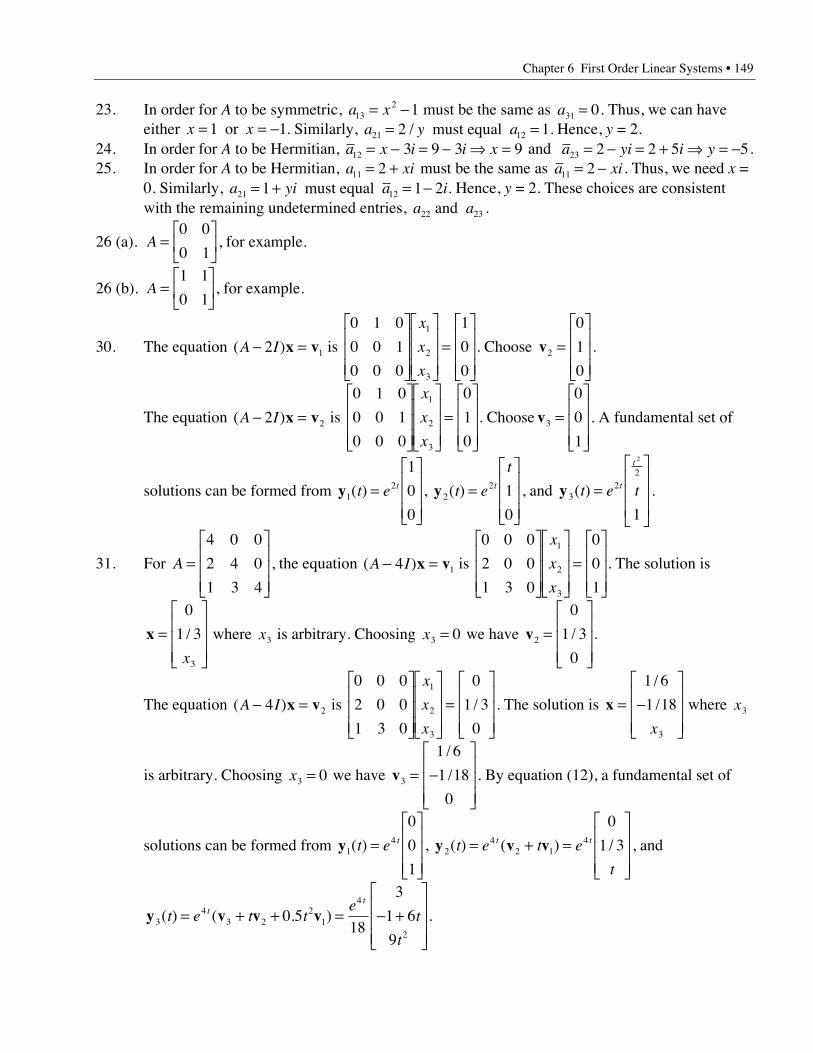
Chapter 6 First Order Linear Systems • 149
23. In order for A to be symmetric, a x132 1= - must be the same as a31 0= . Thus, we can have
either x x= = -1 1 or . Similarly, a y a21 122 1= =/ . must equal Hence, y = 2.24. In order for A to be Hermitian, a x i i x12 3 9 3 9= - = - fi = and a yi i y23 2 2 5 5= - = + fi = - .25. In order for A to be Hermitian, a xi11 2= + must be the same as a xi11 2= - . Thus, we need x =
0. Similarly, a yi a i21 121 1 2= + = - must equal . Hence, y = 2. These choices are consistentwith the remaining undetermined entries, a a22 23 and .
26 (a). A =È
ÎÍ
˘
˚˙
0 0
0 1, for example.
26 (b). A =È
ÎÍ
˘
˚˙
1 1
0 1, for example.
30. The equation ( )A I- =2 1x v is
0 1 0
0 0 1
0 0 0
1
0
0
1
2
3
È
Î
ÍÍÍ
˘
˚
˙˙˙
È
Î
ÍÍÍ
˘
˚
˙˙˙
=È
Î
ÍÍÍ
˘
˚
˙˙˙
x
x
x
. Choose v2
0
1
0
=È
Î
ÍÍÍ
˘
˚
˙˙˙.
The equation ( )A I- =2 2x v is
0 1 0
0 0 1
0 0 0
0
1
0
1
2
3
È
Î
ÍÍÍ
˘
˚
˙˙˙
È
Î
ÍÍÍ
˘
˚
˙˙˙
=È
Î
ÍÍÍ
˘
˚
˙˙˙
x
x
x
. Choose v3
0
0
1
=È
Î
ÍÍÍ
˘
˚
˙˙˙. A fundamental set of
solutions can be formed from y12
1
0
0
( )t e t=È
Î
ÍÍÍ
˘
˚
˙˙˙, y2
2 1
0
( )t e
tt=
È
Î
ÍÍÍ
˘
˚
˙˙˙, and y3
22
2
1
( )t e tt
t
=
È
Î
ÍÍÍ
˘
˚
˙˙˙.
31. For A =È
Î
ÍÍÍ
˘
˚
˙˙˙
4 0 0
2 4 0
1 3 4
, the equation ( )A I- =4 1x v is
0 0 0
2 0 0
1 3 0
0
0
1
1
2
3
È
Î
ÍÍÍ
˘
˚
˙˙˙
È
Î
ÍÍÍ
˘
˚
˙˙˙
=È
Î
ÍÍÍ
˘
˚
˙˙˙
x
x
x
. The solution is
x =È
Î
ÍÍÍ
˘
˚
˙˙˙
0
1 3
3
/
x
where x3 is arbitrary. Choosing x3 0= we have v2
0
1 3
0
=È
Î
ÍÍÍ
˘
˚
˙˙˙
/ .
The equation ( )A I- =4 2x v is
0 0 0
2 0 0
1 3 0
0
1 3
0
1
2
3
È
Î
ÍÍÍ
˘
˚
˙˙˙
È
Î
ÍÍÍ
˘
˚
˙˙˙
=È
Î
ÍÍÍ
˘
˚
˙˙˙
x
x
x
/ . The solution is x = -È
Î
ÍÍÍ
˘
˚
˙˙˙
1 6
1 18
3
/
/
x
where x3
is arbitrary. Choosing x3 0= we have v3
1 6
1 18
0
= -È
Î
ÍÍÍ
˘
˚
˙˙˙
/
/ . By equation (12), a fundamental set of
solutions can be formed from y14
0
0
1
( )t e t=È
Î
ÍÍÍ
˘
˚
˙˙˙, y v v2
42 1
4
0
1 3( ) ( ) /t e t e
t
t t= + =È
Î
ÍÍÍ
˘
˚
˙˙˙, and
y v v v34
3 22
1
4
2
0 518
3
1 6
9
( ) ( . )t e t te
t
t
tt
= + + = - +È
Î
ÍÍÍ
˘
˚
˙˙˙.
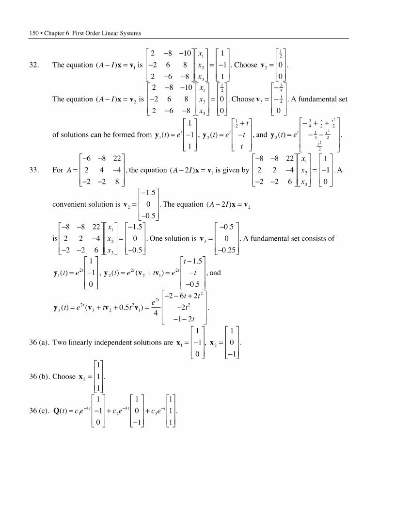
150 • Chapter 6 First Order Linear Systems
32. The equation ( )A I- =x v1 is
2 8 10
2 6 8
2 6 8
1
1
1
1
2
3
- --
- -
È
Î
ÍÍÍ
˘
˚
˙˙˙
È
Î
ÍÍÍ
˘
˚
˙˙˙
= -È
Î
ÍÍÍ
˘
˚
˙˙˙
x
x
x
. Choose v2
12
0
0
=È
Î
ÍÍÍ
˘
˚
˙˙˙.
The equation ( )A I- =x v2 is
2 8 10
2 6 8
2 6 8
0
0
1
2
3
12- -
-- -
È
Î
ÍÍÍ
˘
˚
˙˙˙
È
Î
ÍÍÍ
˘
˚
˙˙˙
=È
Î
ÍÍÍ
˘
˚
˙˙˙
x
x
x
. Choose v3
34
14
0
=--
È
Î
ÍÍÍ
˘
˚
˙˙˙. A fundamental set
of solutions can be formed from y1
1
1
1
( )t et= -È
Î
ÍÍÍ
˘
˚
˙˙˙, y2
12
( )t e
t
t
t
t=+
-È
Î
ÍÍÍ
˘
˚
˙˙˙, and y3
34 2 2
14 2
2
2
2
2
( )t et
t t
t
t
=- + +
- -
È
Î
ÍÍÍ
˘
˚
˙˙˙.
33. For A =- -
-- -
È
Î
ÍÍÍ
˘
˚
˙˙˙
6 8 22
2 4 4
2 2 8
, the equation ( )A I- =2 1x v is given by
- --
- -
È
Î
ÍÍÍ
˘
˚
˙˙˙
È
Î
ÍÍÍ
˘
˚
˙˙˙
= -È
Î
ÍÍÍ
˘
˚
˙˙˙
8 8 22
2 2 4
2 2 6
1
1
0
1
2
3
x
x
x
. A
convenient solution is v2
1 5
0
0 5
=-
-
È
Î
ÍÍÍ
˘
˚
˙˙˙
.
.
. The equation ( )A I- =2 2x v
is
- --
- -
È
Î
ÍÍÍ
˘
˚
˙˙˙
È
Î
ÍÍÍ
˘
˚
˙˙˙
=-
-
È
Î
ÍÍÍ
˘
˚
˙˙˙
8 8 22
2 2 4
2 2 6
1 5
0
0 5
1
2
3
x
x
x
.
.
. One solution is v3
0 5
0
0 25
=-
-
È
Î
ÍÍÍ
˘
˚
˙˙˙
.
.
. A fundamental set consists of
y12
1
1
0
( )t e t= -È
Î
ÍÍÍ
˘
˚
˙˙˙, y v v2
22 1
2
1 5
0 5
( ) ( )
.
.
t e t e
t
tt t= + =-
--
È
Î
ÍÍÍ
˘
˚
˙˙˙, and
y v v v32
3 22
1
2
2
20 54
2 6 2
2
1 2
( ) ( . )t e t te
t t
t
t
tt
= + + =- - +
-- -
È
Î
ÍÍÍ
˘
˚
˙˙˙.
36 (a). Two linearly independent solutions are x x1 2
1
1
0
1
0
1
= -È
Î
ÍÍÍ
˘
˚
˙˙˙
=-
È
Î
ÍÍÍ
˘
˚
˙˙˙
, .
36 (b). Choose x3
1
1
1
=È
Î
ÍÍÍ
˘
˚
˙˙˙.
36 (c). Q( )t c e c e c et t t= -È
Î
ÍÍÍ
˘
˚
˙˙˙
+-
È
Î
ÍÍÍ
˘
˚
˙˙˙
+È
Î
ÍÍÍ
˘
˚
˙˙˙
- - -1
42
43
1
1
0
1
0
1
1
1
1
.
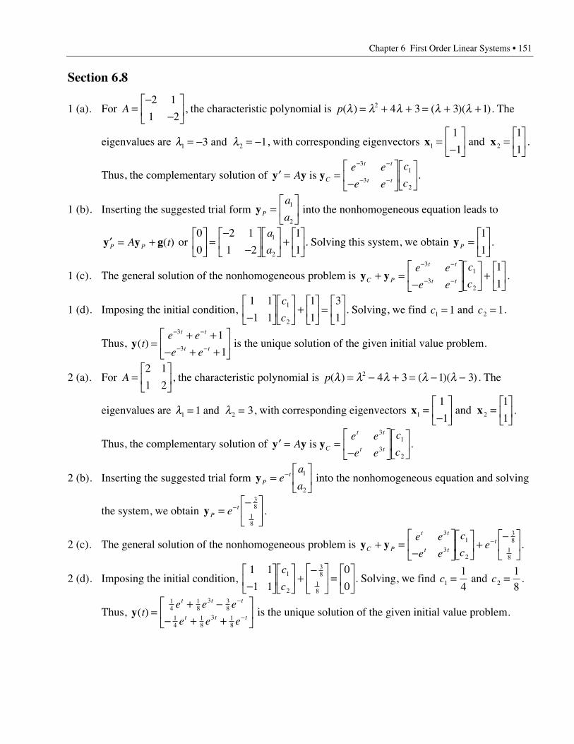
Chapter 6 First Order Linear Systems • 151
Section 6.8
1 (a). For A =-
-È
ÎÍ
˘
˚˙
2 1
1 2, the characteristic polynomial is p( ) ( )( )l l l l l= + + = + +2 4 3 3 1 . The
eigenvalues are l l1 23 1= - = - and , with corresponding eigenvectors x x1 2
1
1
1
1=
-È
ÎÍ
˘
˚˙ =
È
ÎÍ
˘
˚˙ and .
Thus, the complementary solution of ¢ = =-
È
ÎÍ
˘
˚˙
È
ÎÍ
˘
˚˙
- -
- -y y yAe e
e e
c
cC
t t
t t is
3
3
1
2
.
1 (b). Inserting the suggested trial form yP
a
a=
È
ÎÍ
˘
˚˙
1
2
into the nonhomogeneous equation leads to
¢ = +y y gP PA t( ) or 0
0
2 1
1 2
1
11
2
È
ÎÍ
˘
˚˙ =
--
È
ÎÍ
˘
˚˙
È
ÎÍ
˘
˚˙ +
È
ÎÍ
˘
˚˙
a
a. Solving this system, we obtain yP =
È
ÎÍ
˘
˚˙
1
1.
1 (c). The general solution of the nonhomogeneous problem is y yC P
t t
t t
e e
e e
c
c+ =
-È
ÎÍ
˘
˚˙
È
ÎÍ
˘
˚˙ +
È
ÎÍ
˘
˚˙
- -
- -
3
3
1
2
1
1.
1 (d). Imposing the initial condition, 1 1
1 1
1
1
3
11
2-È
ÎÍ
˘
˚˙
È
ÎÍ
˘
˚˙ +
È
ÎÍ
˘
˚˙ =
È
ÎÍ
˘
˚˙
c
c. Solving, we find c1 1= and c2 1= .
Thus, y( )te e
e e
t t
t t=
+ +- + +
È
ÎÍ
˘
˚˙
- -
- -
3
3
1
1 is the unique solution of the given initial value problem.
2 (a). For A =È
ÎÍ
˘
˚˙
2 1
1 2, the characteristic polynomial is p( ) ( )( )l l l l l= - + = - -2 4 3 1 3 . The
eigenvalues are l l1 21 3= = and , with corresponding eigenvectors x x1 2
1
1
1
1=
-È
ÎÍ
˘
˚˙ =
È
ÎÍ
˘
˚˙ and .
Thus, the complementary solution of ¢ = =-
È
ÎÍ
˘
˚˙
È
ÎÍ
˘
˚˙y y yA
e e
e e
c
cC
t t
t t is
3
3
1
2
.
2 (b). Inserting the suggested trial form yPte
a
a=
È
ÎÍ
˘
˚˙
- 1
2
into the nonhomogeneous equation and solving
the system, we obtain yPte=
-È
ÎÍ
˘
˚˙
-38
18
.
2 (c). The general solution of the nonhomogeneous problem is y yC P
t t
t tte e
e e
c
ce+ =
-È
ÎÍ
˘
˚˙
È
ÎÍ
˘
˚˙ +
-È
ÎÍ
˘
˚˙
-3
3
1
2
38
18
.
2 (d). Imposing the initial condition, 1 1
1 1
0
01
2
38
18-
È
ÎÍ
˘
˚˙
È
ÎÍ
˘
˚˙ +
-È
ÎÍ
˘
˚˙ =
È
ÎÍ
˘
˚˙
c
c. Solving, we find c1
14
= and c2
18
= .
Thus, y( )te e e
e e e
t t t
t t t=
+ -- + +
È
ÎÍ
˘
˚˙
-
-
14
18
3 38
14
18
3 18
is the unique solution of the given initial value problem.
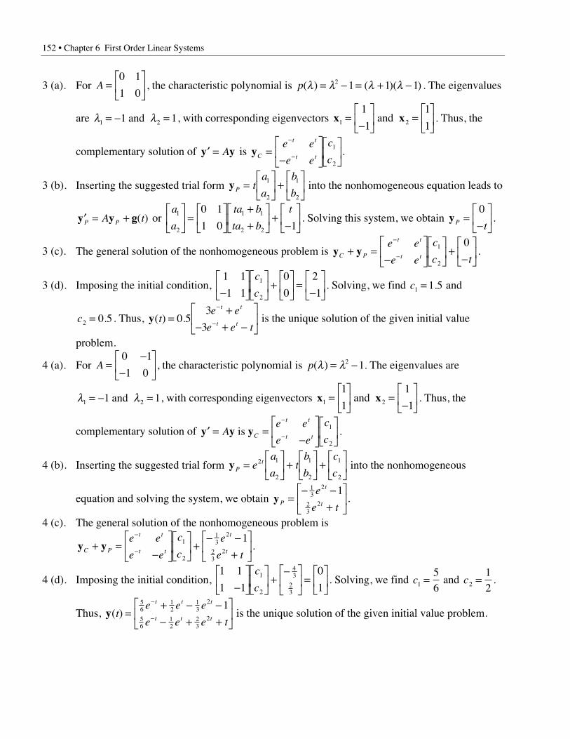
152 • Chapter 6 First Order Linear Systems
3 (a). For A =È
ÎÍ
˘
˚˙
0 1
1 0, the characteristic polynomial is p( ) ( )( )l l l l= - = + -2 1 1 1 . The eigenvalues
are l l1 21 1= - = and , with corresponding eigenvectors x x1 2
1
1
1
1=
-È
ÎÍ
˘
˚˙ =
È
ÎÍ
˘
˚˙ and . Thus, the
complementary solution of ¢ =y yA is yC
t t
t t
e e
e e
c
c=
-È
ÎÍ
˘
˚˙
È
ÎÍ
˘
˚˙
-
-1
2
.
3 (b). Inserting the suggested trial form yP ta
a
b
b=
È
ÎÍ
˘
˚˙ +
È
ÎÍ
˘
˚˙
1
2
1
2
into the nonhomogeneous equation leads to
¢ = +y y gP PA t( ) or a
a
ta b
ta b
t1
2
1 1
2 2
0 1
1 0 1
È
ÎÍ
˘
˚˙ =
È
ÎÍ
˘
˚˙
++
È
ÎÍ
˘
˚˙ +
-È
ÎÍ
˘
˚˙ . Solving this system, we obtain yP t
=-
È
ÎÍ
˘
˚˙
0.
3 (c). The general solution of the nonhomogeneous problem is y yC P
t t
t t
e e
e e
c
c t+ =
-È
ÎÍ
˘
˚˙
È
ÎÍ
˘
˚˙ +
-È
ÎÍ
˘
˚˙
-
-1
2
0.
3 (d). Imposing the initial condition, 1 1
1 1
0
0
2
11
2-È
ÎÍ
˘
˚˙
È
ÎÍ
˘
˚˙ +
È
ÎÍ
˘
˚˙ =
-È
ÎÍ
˘
˚˙
c
c. Solving, we find c1 1 5= . and
c2 0 5= . . Thus, y( ) .te e
e e t
t t
t t=
+- + -
È
ÎÍ
˘
˚˙
-
-0 53
3 is the unique solution of the given initial value
problem.
4 (a). For A =-
-È
ÎÍ
˘
˚˙
0 1
1 0, the characteristic polynomial is p( )l l= -2 1. The eigenvalues are
l l1 21 1= - = and , with corresponding eigenvectors x x1 2
1
1
1
1=
È
ÎÍ
˘
˚˙ =
-È
ÎÍ
˘
˚˙ and . Thus, the
complementary solution of ¢ = =-
È
ÎÍ
˘
˚˙
È
ÎÍ
˘
˚˙
-
-y y yAe e
e e
c
cC
t t
t t is 1
2
.
4 (b). Inserting the suggested trial form yPte
a
at
b
b
c
c=
È
ÎÍ
˘
˚˙ +
È
ÎÍ
˘
˚˙ +
È
ÎÍ
˘
˚˙
2 1
2
1
2
1
2
into the nonhomogeneous
equation and solving the system, we obtain yP
t
t
e
e t=
- -+
È
ÎÍ
˘
˚˙
13
2
23
2
1.
4 (c). The general solution of the nonhomogeneous problem is
y yC P
t t
t t
t
t
e e
e e
c
c
e
e t+ =
-È
ÎÍ
˘
˚˙
È
ÎÍ
˘
˚˙ +
- -+
È
ÎÍ
˘
˚˙
-
-1
2
13
2
23
2
1.
4 (d). Imposing the initial condition, 1 1
1 1
0
11
2
43
23-
È
ÎÍ
˘
˚˙
È
ÎÍ
˘
˚˙ +
-È
ÎÍ
˘
˚˙ =
È
ÎÍ
˘
˚˙
c
c. Solving, we find c1
56
= and c2
12
= .
Thus, y( )te e e
e e e t
t t t
t t t=
+ - -- + +
È
ÎÍ
˘
˚˙
-
-
56
12
13
2
56
12
23
2
1 is the unique solution of the given initial value problem.
Chapter 6 First Order Linear Systems • 153
5 (a). For A =- -È
ÎÍ
˘
˚˙
3 2
4 3, the characteristic polynomial is p( ) ( )( )l l l l= - = + -2 1 1 1 . The
eigenvalues are l l1 21 1= - = and , with corresponding eigenvectors x x1 2
1
1
1
2=
-È
ÎÍ
˘
˚˙ =
-È
ÎÍ
˘
˚˙ and .
Thus, the complementary solution of ¢ =y yA is yC
t t
t t
e e
e e
c
c=
- -È
ÎÍ
˘
˚˙
È
ÎÍ
˘
˚˙
-
- 21
2
.
5 (b). Inserting the suggested trial form yP ta
at
b
b=
È
ÎÍ
˘
˚˙ +
È
ÎÍ
˘
˚˙sin cos1
2
1
2
into the nonhomogeneous equation
leads to ¢ = +y y gP PA t( ) or a t b t
a t b t
a t b t
a t b t
t1 1
2 2
1 1
2 2
3 2
4 3 0
cos sin
cos sin
sin cos
sin cos
sin--
È
ÎÍ
˘
˚˙ =
- -È
ÎÍ
˘
˚˙
++
È
ÎÍ
˘
˚˙ +
È
ÎÍ
˘
˚˙ . Solving
this system, we obtain yP
t t
t=
--
È
ÎÍ
˘
˚˙0 5
3
4.
sin cos
sin.
5 (c). The general solution of the nonhomogeneous problem is
y yC P
t t
t t
e e
e e
c
c
t t
t+ =
- -È
ÎÍ
˘
˚˙
È
ÎÍ
˘
˚˙ +
--
È
ÎÍ
˘
˚˙
-
- 20 5
3
41
2
.sin cos
sin.
5 (d). Imposing the initial condition, 1 1
1 2
5
0
0
01
2- -È
ÎÍ
˘
˚˙
È
ÎÍ
˘
˚˙ +
-È
ÎÍ
˘
˚˙ =
È
ÎÍ
˘
˚˙
c
c
.. Solving, we find c1 1= and
c2 0 5= - . . Thus, y( ) .sin cos
sint
e e t t
e e t
t t
t t=
- + -- + -
È
ÎÍ
˘
˚˙
-
-0 52 3
2 2 4 is the unique solution of the given initial
value problem.
6 (a). For A =È
ÎÍ
˘
˚˙
1 1
1 1, the characteristic polynomial is p( )l l l= -2 2 . The eigenvalues are
l l1 20 2= = and , with corresponding eigenvectors x x1 2
1
1
1
1=
-È
ÎÍ
˘
˚˙ =
È
ÎÍ
˘
˚˙ and . Thus, the
complementary solution of ¢ = =-
È
ÎÍ
˘
˚˙
È
ÎÍ
˘
˚˙y y yA
e
e
c
cC
t
t is
1
1
2
2
1
2
.
7. Given y( )sin
cost
t
e tt=++
È
ÎÍ
˘
˚˙
1 2
2 it follows that y y0 2 22
1 1
1= =
++
È
ÎÍ
˘
˚˙ =
-È
ÎÍ
˘
˚˙( / )
sin
cos/ /pp
pp pe e. Inserting
y( )t into the differential equation, we see that ¢ = +y y g( ) ( ) ( )t A t t and thus2 2
2 2
0 2
2 0
1 2
2
cos
sin
sin
cos( )
t
e t
t
e ttt t-
È
ÎÍ
˘
˚˙ =
-È
ÎÍ
˘
˚˙
++
È
ÎÍ
˘
˚˙ + g . Solving for g(t), we obtain g( )t
e
e
t
t=
-+
È
ÎÍ
˘
˚˙
2
2.
8. Given y( )tt
t=
++
È
ÎÍ
˘
˚˙
ab2 it follows that y( ) , 1
1
1
2
11 2=
++
È
ÎÍ
˘
˚˙ =
-È
ÎÍ
˘
˚˙ fi = = -
ab
a b . Inserting y( )t into
the differential equation, we see that ¢ = +y y g( ) ( ) ( )t A t t and thus
¢ =È
ÎÍ
˘
˚˙ =
È
ÎÍ
˘
˚˙
+-
È
ÎÍ
˘
˚˙ +y g
1
2
1
1
1
22 2t
t
t
t
tt( ) . Solving for g(t), we obtain g( )t
t t
t t t=
- +- - + +
È
ÎÍ
˘
˚˙
3
3 22 2 2.
154 • Chapter 6 First Order Linear Systems
9. Following the hint, we form [ , ] ( )[ , ] [ ( ), ( )]¢ ¢ = +y y y y g g1 2 1 2 1 2P t t t which has the form
0
0
1
1
2
0 1
e
eP t
e
e
et
t
t
t
t
-È
ÎÍ
˘
˚˙ =
-È
ÎÍ
˘
˚˙ +
--
È
ÎÍ
˘
˚˙- -( ) . Solving for P(t), we have
P te
e
e e
e
e
et
t
t t
t
t
t
( ) ( / )=-
È
ÎÍ
˘
˚˙ -
È
ÎÍ
˘
˚˙ =
-È
ÎÍ
˘
˚˙ -
- --
È
ÎÍ
˘
˚˙ =
-È
ÎÍ
˘
˚˙- -
-
- -
2 0
1
1
1
2 0
11 2
1
1
1
0 1
1
.
10. If A-1 exists, y b21= - -A is the unique solution.
If A-1 does not exist, the matrix equation Ay b= - will either have no solution or a non-unique solution. Therefore, either no equilibrium solution or a non-unique equilibriumsolution.
11. An equilibrium solution of ¢ = +y y bA is a constant solution. Therefore, since ¢ =y 0 we need
A ey b= - . For A =- -
È
ÎÍ
˘
˚˙ =
È
ÎÍ
˘
˚˙
1 4
1 3
2
1 and b we see that y be A= - = -
- -È
ÎÍ
˘
˚˙
È
ÎÍ
˘
˚˙ =
-È
ÎÍ
˘
˚˙
-13 4
1 1
2
1
10
3.
12. A-1 exists and y e =È
ÎÍ
˘
˚˙
-È
ÎÍ
˘
˚˙ =
-È
ÎÍ
˘
˚˙
1 1
1 2
2
1
1
0.
13. As noted in the solution of Exercise 11, we need A ey b= - . For A =-
-È
ÎÍ
˘
˚˙ =
-È
ÎÍ
˘
˚˙
1 1
1 1
2
2 and b we
see that y e a=È
ÎÍ
˘
˚˙ +
È
ÎÍ
˘
˚˙
0
2
1
1 where a is arbitrary.
14. A-1 exists and
1 1 0
0 1 2
0 0 1
2
3
2
1
1
2
-È
Î
ÍÍÍ
˘
˚
˙˙˙
=---
È
Î
ÍÍÍ
˘
˚
˙˙˙
fi =---
È
Î
ÍÍÍ
˘
˚
˙˙˙
y ye e .
15. As noted in the solution of Exercise 11, we need A ey b= - . For A =È
Î
ÍÍÍ
˘
˚
˙˙˙
=-È
Î
ÍÍÍ
˘
˚
˙˙˙
1 0 0
0 1 1
0 1 1
2
0
0
and b
we see that y e a=È
Î
ÍÍÍ
˘
˚
˙˙˙
+ -È
Î
ÍÍÍ
˘
˚
˙˙˙
2
0
0
0
1
1
where a is arbitrary.
16. The characteristic polynomial is p( )l l l= -2 2 . The eigenvalues are l l1 20 2= = and , with
corresponding eigenvectors x x1 2
1
1
1
1=
È
ÎÍ
˘
˚˙ =
-È
ÎÍ
˘
˚˙ and .
Thus, one fundamental matrix is )
Y( )te
e
t
t=
-È
ÎÍ
˘
˚˙
1
1
2
2. Set
Y Y Y Y Y= = = \ = =-
È
ÎÍ
˘
˚˙ =
-È
ÎÍ
˘
˚˙
-
-
- -
) ) )C I C C
e
e e e. ( ) ( ) . ( )1 1 1
1
11
2
2
1 12
12
12
2 12
2 .
Y( )( ) ( )
( ) ( )te
e e e
e e
e e
t
t
t t
t t=-
È
ÎÍ
˘
˚˙ -
È
ÎÍ
˘
˚˙ =
+( ) -( )-( ) +( )
È
ÎÍÍ
˘
˚˙˙
- -
- -
- -
1
1
1 1
1 1
2
2
12
12
12
2 12
2
12
2 1 12
2 1
12
2 1 12
2 1 .
Chapter 6 First Order Linear Systems • 155
17. For A =-
È
ÎÍ
˘
˚˙
0 2
2 0, the characteristic polynomial is p i i( ) ( )( )l l l l= + = + -2 4 2 2 . The
eigenvalues are l l1 22 2= - =i i and , with corresponding eigenvectors
x x1 2
1 1=
-È
ÎÍ
˘
˚˙ =
--
È
ÎÍ
˘
˚˙i i
and . Converting to real solutions, we have
y( ) (cos sin )t ei
t i ti
it=-È
ÎÍ
˘
˚˙ = -
-È
ÎÍ
˘
˚˙
-21
2 21
. Therefore, a fundamental set of solutions is
y y1 2
2
2
2
2( )
cos
sin( )
sin
cost
t
tt
t
t=
-È
ÎÍ
˘
˚˙ =
È
ÎÍ
˘
˚˙ and .
Thus, one fundamental matrix is Y( )cos sin
sin cost
t t
t t=
-È
ÎÍ
˘
˚˙
2 2
2 2. The solution of the given initial
value problem has the form )
Y Y( ) ( )cos sin
sin cost t C
t t
t tC= =
-È
ÎÍ
˘
˚˙
2 2
2 2 where C is a ( )2 2¥ matrix
chosen so that )
Y( / )p 41 1
0 1=
-È
ÎÍ
˘
˚˙ . Imposing this condition, we have
1 1
0 14
0 1
1 0
-È
ÎÍ
˘
˚˙ = =
È
ÎÍ
˘
˚˙Y( / )p C C . Solving for C, we obtain C =
È
ÎÍ
˘
˚˙
-È
ÎÍ
˘
˚˙ =
-È
ÎÍ
˘
˚˙
0 1
1 0
1 1
0 1
0 1
1 1 and
thus )
Y( )cos sin
sin cost
t t
t t=
-È
ÎÍ
˘
˚˙ -
È
ÎÍ
˘
˚˙
2 2
2 2
0 1
1 1 or
)Y( )
sin cos sin
cos sin cost
t t t
t t t=
- --
È
ÎÍ
˘
˚˙
2 2 2
2 2 2.
18. The characteristic polynomial is p( )l l l= -2 2 . The eigenvalues are l l1 20 2= = and , with
corresponding eigenvectors x x1 2
1
1
1
1=
È
ÎÍ
˘
˚˙ =
-È
ÎÍ
˘
˚˙ and .
Thus, one fundamental matrix is )
Y( )te
e
t
t=
-È
ÎÍ
˘
˚˙
1
1
2
2. Set
Y Y Y Y Y Y= =È
ÎÍ
˘
˚˙ = \ = =
-È
ÎÍ
˘
˚˙
È
ÎÍ
˘
˚˙ =
- -È
ÎÍ
˘
˚˙
--
) ) )C C C. ( ) ( ) . ( ) ( )0
1 0
2 10 0 0
1 1
1 1
1 0
2 11
1 32
12
12
12
.
Y( )te
e
e e
e e
t
t
t t
t t=
-È
ÎÍ
˘
˚˙ - -
È
ÎÍ
˘
˚˙ =
- -+ +
È
ÎÍ
˘
˚˙
1
1
2
2
32
12
12
12
32
12
2 12
12
2
32
12
2 12
12
2.
19. For A =--
È
ÎÍ
˘
˚˙
3 4
2 3, the characteristic polynomial is p( ) ( )( )l l l l= - = + -2 1 1 1 . The
eigenvalues are l l1 21 1= - = and , with corresponding eigenvectors x x1 2
1
1
2
1=
È
ÎÍ
˘
˚˙ =
È
ÎÍ
˘
˚˙ and .
Therefore, a fundamental set of solutions is y y1 2
1
1
2
1( ) ( )t e t et t=
È
ÎÍ
˘
˚˙ =
È
ÎÍ
˘
˚˙
- and . Thus, one
fundamental matrix is Y( )te e
e e
t t
t t=
È
ÎÍ
˘
˚˙
-
-
2.
156 • Chapter 6 First Order Linear Systems
The solution of the given initial value problem has the form )
Y Y( ) ( )t t Ce e
e eC
t t
t t= =
È
ÎÍ
˘
˚˙
-
-
2
where C is a ( )2 2¥ matrix chosen so that )
Y( )01 0
0 1=
È
ÎÍ
˘
˚˙. Imposing this condition, we have
1 0
0 10
1 2
1 1
È
ÎÍ
˘
˚˙ = =
È
ÎÍ
˘
˚˙Y( )C C . Solving for C, we obtain C =
--
È
ÎÍ
˘
˚˙
1 2
1 1 and thus
)Y( )t
e e
e e
t t
t t=
È
ÎÍ
˘
˚˙
--
È
ÎÍ
˘
˚˙
-
-
2 1 2
1 1 or
)Y( )t
e e e e
e e e e
t t t t
t t t t=
- + -- + -
È
ÎÍ
˘
˚˙
- -
- -
2 2 2
2.
20. The characteristic polynomial is p( )l l l= - +2 2 5. The eigenvalues are
l l1 21 2 1 2= + = -i i and , with corresponding eigenvectors x =-È
ÎÍ
˘
˚˙
2
1
i. Then
y( ) (cos sin )sin
cos
cos
sint e t i t
i e t
e ti
e t
e tt
t
t
t
t= +
-È
ÎÍ
˘
˚˙ =
È
ÎÍ
˘
˚˙ +
-È
ÎÍ
˘
˚˙2 2
2
1
2 2
2
2 2
2.
Thus, one fundamental matrix is )
Y( )sin cos
cos sint
e t e t
e t e t
t t
t t=
-È
ÎÍ
˘
˚˙
2 2 2 2
2 2. Set
Y Y Y= ÊËÁ
ˆ¯ =
È
ÎÍ
˘
˚˙ =
È
ÎÍÍ
˘
˚˙˙
\ =È
ÎÍÍ
˘
˚˙˙
-
-
)C
e
eC C
e
e. .
pp
p
p
p4
1 0
0 12 0
0
0
0
4
4
4
4
12 .
Y( )sin cos
cos sint
e t e t
e t e t
t t
t t= -È
ÎÍÍ
˘
˚˙˙
-( ) -( )-( ) -( )
p p
p p
4 4
4 4
2 2 2
2 212
.
21. For A =È
ÎÍ
˘
˚˙
1 1
1 1, the characteristic polynomial is p( ) ( )l l l l l= - = -2 2 2 . The eigenvalues are
l l1 20 2= = and , with corresponding eigenvectors x x1 2
1
1
1
1=
-È
ÎÍ
˘
˚˙ =
È
ÎÍ
˘
˚˙ and . Therefore, a
fundamental set of solutions is y y1 22
1
1
1
1( ) ( )t t e t=
-È
ÎÍ
˘
˚˙ =
È
ÎÍ
˘
˚˙ and . A fundamental matrix is
Y( )te
e
t
t=
-È
ÎÍ
˘
˚˙
1
1
2
2 and therefore, Y - -
- -=-È
ÎÍ
˘
˚˙ =
-È
ÎÍ
˘
˚˙
1 22 2
2 20 51 1
0 51 1
( ) . .s ee e
e es
s s
s s . From equation
(11), the solution is y y g( ) ( ) ( ) ( ) ( ) ( )t t t t s s dst
t= +- -ÚY Y Y Y1
0 01
0
. Since y 00 0 0= = and t , we
have
y g( ) ( ) ( ) ( ) . .
.( )
t t s s dse
e
eds
e
e
e
t
e te
e te
tt
t
st
t
t
t
t t
t t
= =-
È
ÎÍ
˘
˚˙
È
ÎÍ
˘
˚˙ =
-È
ÎÍ
˘
˚˙
-È
ÎÍ
˘
˚˙
=- +
- - +È
Î
-Ú ÚY Y 1
0
2
2
2
0
2
2
2
2 2
2 2
1
10 5
1
1
10 25
1
2
0 251 2
1 2ÍÍ
˘
˚˙.
Chapter 6 First Order Linear Systems • 157
22. For A =--
È
ÎÍ
˘
˚˙
9 4
15 7, the characteristic polynomial is p( ) ( )( )l l l l l= - - = - +2 2 3 3 1 . The
eigenvalues are l l1 21 3= - = and , with corresponding eigenvectors x x1 2
2
5
2
3=
È
ÎÍ
˘
˚˙ =
È
ÎÍ
˘
˚˙ and .
A fundamental matrix is Y( )te e
e e
t t
t t=
È
ÎÍ
˘
˚˙
-
-
2 2
5 3
3
3 and therefore,
Y - -- - - -= -
--
È
ÎÍ
˘
˚˙ =
--
È
ÎÍ
˘
˚˙1 2
3 3 34
12
54
3 12
3
14
3 2
5 2( )s e
e e
e e
e e
e es
s s
s s
s s
s s.
Y -- -=
-È
ÎÍ
˘
˚˙ =
- -( )- -( )
È
ÎÍÍ
˘
˚˙˙ÚÚ 1
34
2
54
200
38
2
58
2
1
1( ) ( )s s ds
e
eds
e
e
s
s
ttt
tg .
Y Y( ) ( ) ( )( ) ( )
( ) ( )t s s ds
e e e e
e e e e
e e e
e e e
tt t t t
t t t t
t t t
t t t-
-
-
-
-Ú =- - - -
- - - -È
ÎÍ
˘
˚˙ =
- +- +
È
ÎÍ
˘
˚˙1
0
34
54
3
158
158
3
34
54
3
158
154
158
3
2g .
Then, y y g y y 0( ) ( ) ( ) ( ) ( ) , ( ) ( )t t t s s dst
= + = + =È
ÎÍ
˘
˚˙ fi-ÚY Y Y Y0
1
0 00 02
5
2
5
2 2
5 3
1
01
2
1
2
È
ÎÍ
˘
˚˙ =
È
ÎÍ
˘
˚˙
È
ÎÍ
˘
˚˙ fi
È
ÎÍ
˘
˚˙ =
È
ÎÍ
˘
˚˙
c
c
c
c. Therefore,
y( )te
e
e e e
e e e
e e e
e e e
t
t
t t t
t t t
t t t
t t t=
È
ÎÍ
˘
˚˙ +
- +- +
È
ÎÍ
˘
˚˙ =
- +- +
È
ÎÍ
˘
˚˙
-
-
-
-
-
-
2
5
2 234
54
3
158
154
158
3
114
54
3
558
154
158
3.
23. For A =-
È
ÎÍ
˘
˚˙
0 1
1 0, the characteristic polynomial is p i i( ) ( )( )l l l l= + = - +2 1 . The
eigenvalues are l l1 2= = -i i and , with corresponding eigenvectors x x1 2
1 1=
È
ÎÍ
˘
˚˙ =
-È
ÎÍ
˘
˚˙i i
and .
x x1 2
1 1=
-È
ÎÍ
˘
˚˙ =
--
È
ÎÍ
˘
˚˙i i
and . Converting to real solutions, we have y( ) (cos sin )t ei
t i ti
it=È
ÎÍ
˘
˚˙ = +
È
ÎÍ
˘
˚˙
1 1.
Therefore, a fundamental set of solutions is y y1 2( )cos
sin( )
sin
cost
t
tt
t
t=
-È
ÎÍ
˘
˚˙ =
È
ÎÍ
˘
˚˙ and . A fundamental
matrix is Y( )cos sin
sin cost
t t
t t=
-È
ÎÍ
˘
˚˙ . We have Y - =
-È
ÎÍ
˘
˚˙
1( )cos sin
sin coss
s s
s s.
From equation (11), the solution is y y g( ) ( ) ( ) ( ) ( ) ( )t t t t s s dst
t= +- -ÚY Y Y Y1
0 01
0
. Since
y g0 0
0
1
2
10=
È
ÎÍ
˘
˚˙ =
È
ÎÍ
˘
˚˙ =, , and ( )s t , we have
y y g( ) ( ) ( ) ( ) ( ) ( )t t t t s s dst
= +- -ÚY Y Y Y10 0
1
0=
È
ÎÍ
˘
˚˙ +
-È
ÎÍ
˘
˚˙
-+
È
ÎÍ
˘
˚˙Ú
sin
cos
cos sin
sin cos
cos sin
sin cos
t
t
t t
t t
s s
s sds
t 2
20
=È
ÎÍ
˘
˚˙ +
-È
ÎÍ
˘
˚˙
+ -- + +
È
ÎÍ
˘
˚˙ =
- +- + +
È
ÎÍ
˘
˚˙
sin
cos
cos sin
sin cos
sin cos
cos sin
cos sin
cos sin.
t
t
t t
t t
t t
t t
t t
t t
2 1
2 2
1 3
2 3

158 • Chapter 6 First Order Linear Systems
24. For A =È
ÎÍ
˘
˚˙
1 1
0 1, the characteristic polynomial is p( ) ( )l l= -1 2 . The eigenvalue is l = 1, with
corresponding eigenvector x =È
ÎÍ
˘
˚˙
1
0. Then
y y v v v v y1 2 1 2 1 2 20
1
0
0
1 1=
È
ÎÍ
˘
˚˙ = +( ) =
È
ÎÍ
˘
˚˙ =
È
ÎÍ
˘
˚˙ fi =
È
ÎÍ
˘
˚˙
ee t e
ttt t. . , Let .
A fundamental matrix is Y( )te te
e
t t
t=
È
ÎÍ
˘
˚˙
0 and therefore,
Y - -- -
-=-È
ÎÍ
˘
˚˙ =
-È
ÎÍ
˘
˚˙1 2
0 0( )s e
e se
e
e se
es
s s
s
s s
s. Y -
-
-
-
-=-È
ÎÍ
˘
˚˙ =
-È
ÎÍ
˘
˚˙ÚÚ 1
00
1
1( ) ( )
( )s s ds
e s
eds
te
e
s
s
ttt
tg .
Since y( )00
0=
È
ÎÍ
˘
˚˙, y g( ) ( ) ( ) ( )t t s s ds
t te t
e
te
e
tt
t
t
t= =
+ --
È
ÎÍ
˘
˚˙ =
-È
ÎÍ
˘
˚˙-ÚY Y 1
0 1 1.
25 (a). Q( )t is an equilibrium solution if r
V
cr--
È
ÎÍ
˘
˚˙ +
È
ÎÍ
˘
˚˙ =
2 1
1 2 0Q 0. Solving for Q, we obtain
Qe tCv
( ) =È
ÎÍ
˘
˚˙3
2
1.
25 (b). The characteristic polynomial is p r V r V r V r V( ) ( / ) / ( / )( / )l l l l l= + + = + +2 2 24 3 3 . Theeigenvalues are l l1 23= - = -r V r V/ / and , with corresponding eigenvectors
x x1 2
1
1
1
1=
-È
ÎÍ
˘
˚˙ =
È
ÎÍ
˘
˚˙ and . Therefore, a fundamental set of solutions is
y y13
2
1
1
1
1( ) ( )/ /t e t ert V rt V=
-È
ÎÍ
˘
˚˙ =
È
ÎÍ
˘
˚˙
- - and . The complementary solution is
QC
rt V rt V
rt V rt Vt
e e
e e
c
c( )
/ /
/ /=
-È
ÎÍ
˘
˚˙
È
ÎÍ
˘
˚˙
- -
- -
3
3
1
2
.
25 (c). Finding a constant particular solution is equivalent to finding an equilibrium solution, as in part(a).
25 (d). The general solution is Q Q Q( ) ( ) ( )/ /
/ /t t t
e e
e e
c
ccV
C e
rt V rt V
rt V rt V= + =
-È
ÎÍ
˘
˚˙
È
ÎÍ
˘
˚˙ +
È
ÎÍ
˘
˚˙
- -
- -
3
3
1
2 3
2
1. Imposing the
initial condition leads to Q 0( )0 = or 1 1
1 1 3
2
1
0
01
2-È
ÎÍ
˘
˚˙
È
ÎÍ
˘
˚˙ +
È
ÎÍ
˘
˚˙ =
È
ÎÍ
˘
˚˙
c
ccV
. The solution of the initial
value problem is Q( )/ /
/ /t
cV e e
e e
rt V rt V
rt V rt V=
- -+ -
È
ÎÍ
˘
˚˙
- -
- -6
4 3
2 3
3
3.
25 (e).1
3
2
1Vt
ctlim ( )
Æ •=
È
ÎÍ
˘
˚˙Q .
Chapter 6 First Order Linear Systems • 159
26 (a). - + ¢ + + - = - + + ¢ =V I I I I I I I Is
12
2 0 212
01 1 1 2 2 1 2 2( ) , ( ) . Therefore,
d
dt
I
I
I I V
I I
I
I
Vt
I
Is s¢
¢È
ÎÍ
˘
˚˙ =
- + +-
È
ÎÍ
˘
˚˙ =
--
È
ÎÍ
˘
˚˙
È
ÎÍ
˘
˚˙ +
È
ÎÍ
˘
˚˙ >
È
ÎÍ
˘
˚˙ =
È
ÎÍ
˘
˚˙
1
2
1 2
1 2
1
2
1
2
6 4 2
4 6
6 4
4 6
2
00
0
0
0
0, ,
( )
( )
26 (b). The characteristic polynomial is p( ) ( )( )l l l l l= + + = + +2 12 20 10 2 . The eigenvalues are
l l1 210 2= - = - and , with corresponding eigenvectors x x1 2
1
1
1
1=
-È
ÎÍ
˘
˚˙ =
È
ÎÍ
˘
˚˙ and . Therefore, a
fundamental matrix is Y( )te e
e e
t t
t t=
-È
ÎÍ
˘
˚˙
- -
- -
10 2
10 2.
26 (c). I I 0( ) ( ) ( ) ( )t t sV
dsst=
È
ÎÍ
˘
˚˙ =-ÚY Y 1
0
2
00 since . Y -
-
- -
- -=-È
ÎÍ
˘
˚˙ =
-È
ÎÍ
˘
˚˙1
12
2 2
10 10
10 10
2 2
12
12
( )se
e e
e e
e e
e es
s s
s s
s s
s s.
With V t t sV
dse
esst
t
t( ) , , ( )
( )
( )= >
È
ÎÍ
˘
˚˙
È
ÎÍ
˘
˚˙ =
--
È
ÎÍ
˘
˚˙- ÚÚ1 0
2
0
1
11
0
110
10
12
2Y =
e
e
10s
2s0
t, Therefore,
I( )( ) ( )
( ) ( )t
e e
e e
e e
e e
t t
t t
t t
t t=
- + -- - + -
È
ÎÍ
˘
˚˙ =
- - +- +
È
ÎÍ
˘
˚˙
- -
- -
- -
- -
110
10 12
2
110
10 12
2
110
10 12
2 35
110
10 12
2 25
1 1
1 1.
27 (a). In the vector system ¢ = - + ¥ +v v v k f( ) , the term v k¥ is given by
( )v v v vx y x yi j k j i+ ¥ = - + . Therefore, the system is ¢¢
È
ÎÍ
˘
˚˙ =
-- -
È
ÎÍ
˘
˚˙
È
ÎÍ
˘
˚˙ +
È
ÎÍ
˘
˚˙
v
v
v
v
f
fx
y
x
y
x
y
1 1
1 1.
27 (b). For f =È
ÎÍ
˘
˚˙0 5
1
3. , we seek a constant solution v; that is, an equilibrium solution. Thus, we need
to solve, if possible, -- -
È
ÎÍ
˘
˚˙
È
ÎÍ
˘
˚˙ +
È
ÎÍ
˘
˚˙ =
È
ÎÍ
˘
˚˙
1 1
1 10 5
1
3
0
0
v
vx
y
. . This system does indeed have a solution,
namely ve =+
- +
È
ÎÍ
˘
˚˙0 25
1 3
1 3. . If we choose the initial velocity equal to the “equilibrium
velocity,” ve , then the particle will move at that constant velocity.28 (b). The characteristic polynomial is p c( ) ( )l l l w= - +2 2 . The eigenvalues are
l l w l w1 2 30= = = -, , i ic c , with corresponding eigenvectors x x1
0
0
1
1
0
=È
Î
ÍÍÍ
˘
˚
˙˙˙
=È
Î
ÍÍÍ
˘
˚
˙˙˙
and i . Therefore,
A fundamental matrix is Y( )
cos sin
sin cost
t t
t tc c
c c= -È
Î
ÍÍÍ
˘
˚
˙˙˙
0
0
1 0 0
w ww w .
160 • Chapter 6 First Order Linear Systems
28 (c). F Y Y( ) ( ) ( )
cos sin
sin cost t
t t
t tc c
c c= = -È
Î
ÍÍÍ
˘
˚
˙˙˙
È
Î
ÍÍÍ
˘
˚
˙˙˙
=-
-
1
1
0
0
0
1 0 0
0 1 0
0 0 1
1 0 0
w ww w
0
0
1 0 0
0 0 1
1 0 0
0 1 0
0
0
0 0 1
cos sin
sin cos
cos sin
sin cos
w ww w
w ww w
c c
c c
c c
c c
t t
t t
t t
t t-È
Î
ÍÍÍ
˘
˚
˙˙˙
È
Î
ÍÍÍ
˘
˚
˙˙˙
= -È
Î
ÍÍÍ
˘
˚
˙˙˙.
28 (d). From equation 11, v v g( ) ( ) ( ) ( ) ( )t t t s s dst
= + -ÚF F F01
0, using F( )t as a fundamental matrix
and noting that F - =1 0( ) I . Therefore, v v f( ) ( ) ( )t t t= +F 0 .
28 (e). r v v f r v r f( ) ( ) ( ) ( ) . ( ) ( )t t dt t dt t dt t dt t dt= = ÈÎÍ
˘˚ + = \ È
Î͢˚ = -Ú Ú Ú Ú Ú0 0 0 0 0 0 0
t t t t tF F) )
F( )
sin ( cos )
( cos ) sint dt
t t
t tc c c c
c c c c0
1 1
1 1
1 0
1 0
0 0
tw w w w
w w w wt
Ú =-
- -È
Î
ÍÍÍ
˘
˚
˙˙˙
- -
- - .
D t dt nn
cc
c
c c
c
= { } = -( ) = ÊËÁ
ˆ¯ \ π fi πÚdet ( ) cos sin F
0 2 222
14
2 22t t
ww t t
ww t w t p t p
w.
Section 6.9
1 (a). For ¢ = + =y y g y yP t t t( ) ( ), ( )0 0, Euler’s method has the form y y y gn n n n nh P t t+ = + +[ ]1 ( ) ( ) .
For P t t( ) ( ) ,=È
ÎÍ
˘
˚˙ =
È
ÎÍ
˘
˚˙
-È
ÎÍ
˘
˚˙
1 2
2 3
1
1
10, =
1g y , and t0 0= the iteration is
y y y yn n nh+ = +È
ÎÍ
˘
˚˙ +
È
ÎÍ
˘
˚˙
È
ÎÍ
˘
˚˙ =
-È
ÎÍ
˘
˚˙1 0
1 2
2 3
1
1
1
1, .
1 (b). In general, t t kh kk = + =0 0 1, , ,K. Since t0 0= , we have t kh kk = =, , ,0 1 K. In general,h b a N= -( ) / . So, for a b h= = =0 1 0 01, , . and , we obtain N h= =1 100/ .
2 (a). y y y yn nn
nn
n
ht
t t+ = ++
È
ÎÍ
˘
˚˙ +
È
ÎÍ
˘
˚˙
È
ÎÍ
˘
˚˙ =
È
ÎÍ
˘
˚˙1 0
1
2 2
1 2
1, .
2 (b). t kh kk = + =1 0 1, , ,K. N h= =. /5 50.3 (a). For ¢ = + =y y g y yP t t t( ) ( ), ( )0 0, Euler’s method has the form y y y gn n n n nh P t t+ = + +[ ]1 ( ) ( ) .
For P tt t
tt
t( ) ( ) ,=
--
È
ÎÍ
˘
˚˙ =
È
ÎÍ
˘
˚˙
È
ÎÍ
˘
˚˙
2
02 0
1 2, =
0,g y and t0 1= the iteration is
y y y yn nn n
nn
n
ht t
t t+ = +-
-È
ÎÍ
˘
˚˙ +
È
ÎÍ
˘
˚˙
È
ÎÍÍ
˘
˚˙˙
=È
ÎÍ
˘
˚˙1
2
02 0
1 2
0, .
3 (b). In general, t t kh kk = + =0 0 1, , ,K. Since t0 1= , we have t kh kk = + =1 0 1, , ,K. In general,h b a N= -( ) / . So, for a b h= = =1 4 0 01, , . and , we obtain N h= =3 300/ .
Chapter 6 First Order Linear Systems • 161
4 (a). y y y yn n n
n
h
t+ = +
È
Î
ÍÍÍ
˘
˚
˙˙˙
+È
Î
ÍÍÍ
˘
˚
˙˙˙
È
Î
ÍÍÍ
˘
˚
˙˙˙
=È
Î
ÍÍÍ
˘
˚
˙˙˙
1 0
1 0 1
3 2 1
1 2 0
0
2
0
0
1
, .
4 (b). t kh kk = - + =1 0 1, , ,K. N h= =1 100/ .5 (a). For ¢ = + =y y g y yP t t t( ) ( ), ( )0 0, Euler’s method has the form y y y gn n n n nh P t t+ = + +[ ]1 ( ) ( ) .
For P tt t
tt
t( )
sin( ) ,=
-È
ÎÍ
˘
˚˙ =
È
ÎÍ
˘
˚˙
È
ÎÍ
˘
˚˙
-1
2 01 1
0 0, =
0,g y and t0 1= the iteration is
y y y yn nn n
nn
n
ht t
t t+
-
= +-
È
ÎÍ
˘
˚˙ +
È
ÎÍ
˘
˚˙
È
ÎÍÍ
˘
˚˙˙
=È
ÎÍ
˘
˚˙1
1
2 01 1
0 0
0
sin, .
5 (b). In general, t t kh kk = + =0 0 1, , ,K. Since t0 1= , we have t kh kk = + =1 0 1, , ,K. In general,h b a N= -( ) / . So, for a b h= = =1 6 0 01, , . and , we obtain N h= =5 500/ .
6. y1
1
10 01
1 2
2 3
1
1
1
1
0 98
1 02=
-È
ÎÍ
˘
˚˙ +
È
ÎÍ
˘
˚˙
-È
ÎÍ
˘
˚˙ +
È
ÎÍ
˘
˚˙
È
ÎÍ
˘
˚˙ =
-È
ÎÍ
˘
˚˙.
.
. and
y2
0 98
1 020 01
1 2
2 3
0 98
1 02
1
1
0 9594
1 041=
-È
ÎÍ
˘
˚˙ +
È
ÎÍ
˘
˚˙
-È
ÎÍ
˘
˚˙ +
È
ÎÍ
˘
˚˙
È
ÎÍ
˘
˚˙ =
-È
ÎÍ
˘
˚˙
.
..
.
.
.
.
7. The iteration has the form y y y yn nn
nn
n
ht
t t+ = ++
È
ÎÍ
˘
˚˙ +
È
ÎÍ
˘
˚˙
È
ÎÍ
˘
˚˙ =
È
ÎÍ
˘
˚˙1 0
1
2 2
1 2
1, where
t t0 11 1 01= = and . . Therefore, y1
2
10 01
1 1
3 2
2
1
1
1
2
10 01
4
9
2 04
1 09=
È
ÎÍ
˘
˚˙ +
È
ÎÍ
˘
˚˙
È
ÎÍ
˘
˚˙ +
È
ÎÍ
˘
˚˙
È
ÎÍ
˘
˚˙ =
È
ÎÍ
˘
˚˙ +
È
ÎÍ
˘
˚˙ =
È
ÎÍ
˘
˚˙. .
.
. and
y2
2 04
1 090 01
1 1 01
3 01 2
2 04
1 09
1
1 01
2 04
1 090 01
4 1409
9 3304
2 081409
1 183304
=È
ÎÍ
˘
˚˙ +
È
ÎÍ
˘
˚˙
È
ÎÍ
˘
˚˙ +
È
ÎÍ
˘
˚˙
È
ÎÍ
˘
˚˙ =
È
ÎÍ
˘
˚˙ +
È
ÎÍ
˘
˚˙
=È
ÎÍ
˘
˚˙
.
..
.
.
.
. .
.
..
.
.
.
..
8. y1
2
00 01
1 1
1 0
2
0
1
1
1 99
0 03=
È
ÎÍ
˘
˚˙ +
-È
ÎÍ
˘
˚˙
È
ÎÍ
˘
˚˙ +
È
ÎÍ
˘
˚˙
È
ÎÍ
˘
˚˙ =
È
ÎÍ
˘
˚˙.
.
. and
y2
21 99
0 030 01
1 01 1 01
2 1 01 0
1 99
0 03
1
1 01
1 9800030
0 059801=
È
ÎÍ
˘
˚˙ +
--
È
ÎÍ
˘
˚˙
È
ÎÍ
˘
˚˙ +
È
ÎÍ
˘
˚˙
È
ÎÍÍ
˘
˚˙˙
=È
ÎÍ
˘
˚˙
.
..
( . ) .
.
.
. .
.
.
9. The iteration has the form y y y yn n n
n
h
t+ = +
È
Î
ÍÍÍ
˘
˚
˙˙˙
+È
Î
ÍÍÍ
˘
˚
˙˙˙
È
Î
ÍÍÍ
˘
˚
˙˙˙
=È
Î
ÍÍÍ
˘
˚
˙˙˙
1 0
1 0 1
3 2 1
1 2 0
0
2
0
0
1
, where
t t0 11 0 99= - = - and . . Therefore,
y1
0
0
1
0 01
1 0 1
3 2 1
1 2 0
0
0
1
0
2
1
0
0
1
0 01
1
3
1
0 01
0 03
0
=È
Î
ÍÍÍ
˘
˚
˙˙˙
+È
Î
ÍÍÍ
˘
˚
˙˙˙
È
Î
ÍÍÍ
˘
˚
˙˙˙
+-
È
Î
ÍÍÍ
˘
˚
˙˙˙
È
Î
ÍÍÍ
˘
˚
˙˙˙
=È
Î
ÍÍÍ
˘
˚
˙˙˙
+-
È
Î
ÍÍÍ
˘
˚
˙˙˙
=. .
.
.
..99
È
Î
ÍÍÍ
˘
˚
˙˙˙
162 • Chapter 6 First Order Linear Systems
and
y2
0 01
0 03
0 99
0 01
1 0 1
3 2 1
1 2 0
0 01
0 03
0 99
0
2
0 99
0 01
0 03
0 99
0 01
1
=È
Î
ÍÍÍ
˘
˚
˙˙˙
+È
Î
ÍÍÍ
˘
˚
˙˙˙
È
Î
ÍÍÍ
˘
˚
˙˙˙
+-
È
Î
ÍÍÍ
˘
˚
˙˙˙
È
Î
ÍÍÍ
˘
˚
˙˙˙
=È
Î
ÍÍÍ
˘
˚
˙˙˙
+.
.
.
.
.
.
. .
.
.
.
. 33 08
0 92
0 02
0 0608
0 9808
.
.
.
.
.
.
-
È
Î
ÍÍÍ
˘
˚
˙˙˙
=È
Î
ÍÍÍ
˘
˚
˙˙˙
10. y1
0
00 01
1 1
0 1
0
0
0
1
0
0 01=
È
ÎÍ
˘
˚˙ +
È
ÎÍ
˘
˚˙
È
ÎÍ
˘
˚˙ +
È
ÎÍ
˘
˚˙
È
ÎÍ
˘
˚˙ =
È
ÎÍ
˘
˚˙.
sin( )
. and
y2
11 01
2
0
0 010 01
1 01
1 1 01 1
0
0 01
0
1 01
0 00008468318
0 020301=
È
ÎÍ
˘
˚˙ +
-È
ÎÍ
˘
˚˙
È
ÎÍ
˘
˚˙ +
È
ÎÍ
˘
˚˙
È
ÎÍÍ
˘
˚˙˙
=È
ÎÍ
˘
˚˙.
.sin( . )
. . ( . )
.
..
11 (a). Let z( )( )
( )
( )
( )t
z t
z t
y t
y t=
È
ÎÍ
˘
˚˙ =
¢È
ÎÍ
˘
˚˙
1
2
. With this,
¢ =¢¢
È
ÎÍ
˘
˚˙ =
¢¢¢
È
ÎÍ
˘
˚˙ =
- +È
ÎÍ
˘
˚˙ =
-È
ÎÍ
˘
˚˙
È
ÎÍ
˘
˚˙ +
È
ÎÍ
˘
˚˙ =
È
ÎÍ
˘z z( )
( )
( )
( )
( )
( )
( )
( )
( ), ( )/ /t
z t
z t
y t
y t
z t
z t t
z t
z t t1
2
2
13 2
1
23 2
0 1
1 0
00
1
0˚˙ .
11 (b). Thus, the iteration has the form z z z zn n nn
ht+ = +
-È
ÎÍ
˘
˚˙ +
È
ÎÍ
˘
˚˙
È
ÎÍ
˘
˚˙ =
È
ÎÍ
˘
˚˙1 3 2 0
0 1
1 0
0 1
0/ , where
t t0 10 0 01= = and . .
11 (c). Therefore, z1
1
00 01
0 1
1 0
1
0
0
0
1
00 01
0
1
1
0 01=
È
ÎÍ
˘
˚˙ +
-È
ÎÍ
˘
˚˙
È
ÎÍ
˘
˚˙ +
È
ÎÍ
˘
˚˙
È
ÎÍ
˘
˚˙ =
È
ÎÍ
˘
˚˙ +
-È
ÎÍ
˘
˚˙ =
-È
ÎÍ
˘
˚˙. .
. and
z2
1
0 010 01
0 1
1 0
1
0 01
0
0 001
1
0 010 01
01
999
9999
01999
=-
È
ÎÍ
˘
˚˙ +
-È
ÎÍ
˘
˚˙ -
È
ÎÍ
˘
˚˙ +
È
ÎÍ
˘
˚˙
È
ÎÍ
˘
˚˙ =
-È
ÎÍ
˘
˚˙ +
--
È
ÎÍ
˘
˚˙
=-
È
ÎÍ
˘
˚˙
..
. . ..
.
.
.
..
12 (a). ¢ =¢¢
È
ÎÍ
˘
˚˙ =
- - +È
ÎÍ
˘
˚˙ =
- -È
ÎÍ
˘
˚˙
È
ÎÍ
˘
˚˙ +
È
ÎÍ
˘
˚˙ =
È
ÎÍ
˘
˚˙z z( )
( )
( )
( )
( ) ( )
( )
( ), ( )t
z t
z t
z t
t z t z t t
z t
z t1
2
22
1 22
1
22
0 1
1
0
21
1
1.
12 (b). z z z zn n nht+ = +
- -È
ÎÍ
˘
˚˙ +
È
ÎÍ
˘
˚˙
È
ÎÍ
˘
˚˙ =
È
ÎÍ
˘
˚˙1 2 0
0 1
1
0
2
1
1, where t0 1= .
12 (c). z1
1
10 01
0 1
1 1
1
1
0
2
1 01
1=
È
ÎÍ
˘
˚˙ +
- -È
ÎÍ
˘
˚˙
È
ÎÍ
˘
˚˙ +
È
ÎÍ
˘
˚˙
È
ÎÍ
˘
˚˙ =
È
ÎÍ
˘
˚˙.
. and
z2 2
1 01
10 01
0 1
1 01 1
1 01
1
0
2
1 02
0 999696699=
È
ÎÍ
˘
˚˙ +
- -È
ÎÍ
˘
˚˙
È
ÎÍ
˘
˚˙ +
È
ÎÍ
˘
˚˙
È
ÎÍ
˘
˚˙ =
È
ÎÍ
˘
˚˙
..
( . )
. .
.
Chapter 6 First Order Linear Systems • 163
13 (a). Let z =È
Î
ÍÍÍ
˘
˚
˙˙˙
= ¢¢¢
È
Î
ÍÍÍ
˘
˚
˙˙˙
z
z
z
y
y
y
1
2
3
. With this,
¢ =¢¢¢
È
Î
ÍÍÍ
˘
˚
˙˙˙
=¢
¢¢¢¢¢
È
Î
ÍÍÍ
˘
˚
˙˙˙
=- - + +
È
Î
ÍÍÍ
˘
˚
˙˙˙
=- -
È
Î
ÍÍÍ
˘
˚
˙˙˙
È
Î
ÍÍÍ
˘
˚
˙˙˙
++
È
Î
ÍÍÍ
z
z
z
z
y
y
y
z
z
z tz t t
z
z
z t
1
2
3
2
3
2 1
1
2
32 1
0 1 0
0 0 1
2 0
0
0
1
˘
˚
˙˙˙
= -È
Î
ÍÍÍ
˘
˚
˙˙˙
, ( )z 0
1
1
0
.
13 (b). Thus, the iteration has the form z z z zn n
n
n
n
h
t t+ = +
- -
È
Î
ÍÍÍ
˘
˚
˙˙˙
++
È
Î
ÍÍÍ
˘
˚
˙˙˙
È
Î
ÍÍÍ
˘
˚
˙˙˙
= -È
Î
ÍÍÍ
˘
˚
˙˙˙
1 0
0 1 0
0 0 1
2 0
0
0
1
1
1
0
, where
t t0 10 0 01= = and . .
13 (c). Therefore, z1
1
1
0
0 01
0 1 0
0 0 1
0 2 0
1
1
0
0
0
1
1
1
0
0 01
1
0
3
0 99
= -È
Î
ÍÍÍ
˘
˚
˙˙˙
+-
È
Î
ÍÍÍ
˘
˚
˙˙˙
-È
Î
ÍÍÍ
˘
˚
˙˙˙
+È
Î
ÍÍÍ
˘
˚
˙˙˙
È
Î
ÍÍÍ
˘
˚
˙˙˙
= -È
Î
ÍÍÍ
˘
˚
˙˙˙
+-È
Î
ÍÍÍ
˘
˚
˙˙˙
= -. .
.
11
0 03.
È
Î
ÍÍÍ
˘
˚
˙˙˙ and
z2
0 99
1
0 03
0 01
0 1 0
0 0 1
0 01 2 0
0 99
1
0 03
0
0
1 01
0 99
1
0 03
0 01
1
= -È
Î
ÍÍÍ
˘
˚
˙˙˙
+- -
È
Î
ÍÍÍ
˘
˚
˙˙˙
-È
Î
ÍÍÍ
˘
˚
˙˙˙
+È
Î
ÍÍÍ
˘
˚
˙˙˙
È
Î
ÍÍÍ
˘
˚
˙˙˙
= -È
Î
ÍÍÍ
˘
˚
˙˙˙
+-.
.
.
.
.
. .
.
.
. 00 03
3 0001
0 98
0 9997
0 060001
.
.
.
.
.
.
È
Î
ÍÍÍ
˘
˚
˙˙˙
= -È
Î
ÍÍÍ
˘
˚
˙˙˙
14 (a). ¢ =¢¢
È
ÎÍ
˘
˚˙ =
- - +È
ÎÍ
˘
˚˙ =
- -È
ÎÍ
˘
˚˙
È
ÎÍ
˘
˚˙ +
È
ÎÍ
˘
˚˙ =
-È
ÎÍ
˘
˚˙- -z z( )
( )
( )
( )
( ) ( )
( )
( ), ( )t
z t
z t
z t
e z t z t e
z t
z tt t1
2
2
1 2
1
22
0 1
1
0
20
1
1.
14 (b). z z z zn n t nhe+ -= +
- -È
ÎÍ
˘
˚˙ +
È
ÎÍ
˘
˚˙
È
ÎÍ
˘
˚˙ =
-È
ÎÍ
˘
˚˙1 0
0 1
1
0
2
1
1, where t0 0= .
14 (c). z1
1
10 01
0 1
1 1
1
1
0
2
0 99
1 02=
-È
ÎÍ
˘
˚˙ +
- -È
ÎÍ
˘
˚˙
-È
ÎÍ
˘
˚˙ +
È
ÎÍ
˘
˚˙
È
ÎÍ
˘
˚˙ =
-È
ÎÍ
˘
˚˙.
.
. and
z2 0 01
0 99
1 020 01
0 1
1
0 99
1 02
0
2
0 9798
1 039601493=
-È
ÎÍ
˘
˚˙ +
- -È
ÎÍ
˘
˚˙
-È
ÎÍ
˘
˚˙ +
È
ÎÍ
˘
˚˙
È
ÎÍ
˘
˚˙ =
-È
ÎÍ
˘
˚˙-
.
..
.
.
.
..e
18. Actual error: y y( ).
. ...1
0 00807508729
0 0759433736200- =-È
ÎÍ
˘
˚˙
Estimated error: y y200 100
0 0086591617
0 0764878206- =
-È
ÎÍ
˘
˚˙
. ...
. ...
20. Actual error: y y( ). ...
. ...1
0 0027112167
0 0027112167200- =-
È
ÎÍ
˘
˚˙
Estimated error: y y200 100
0 0027202379
0 0027202379- =
-È
ÎÍ
˘
˚˙
. ...
. ...
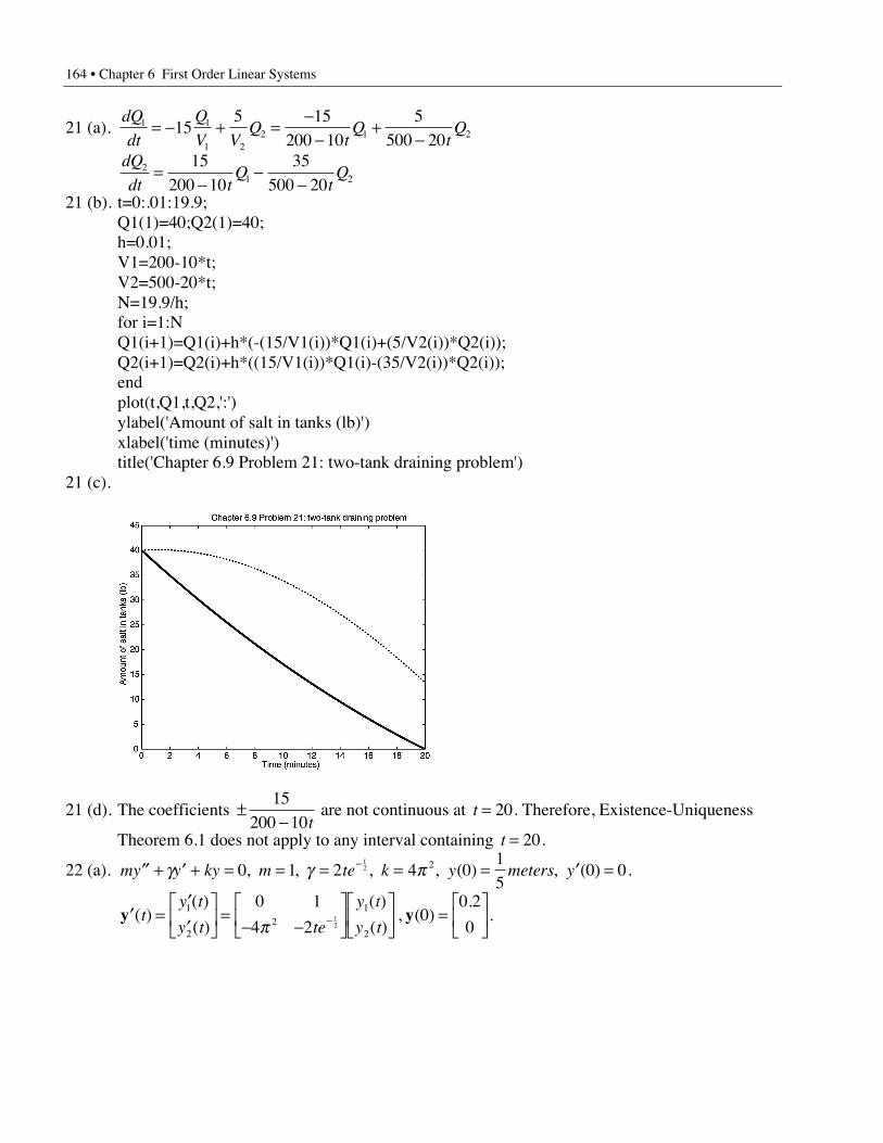
164 • Chapter 6 First Order Linear Systems
21 (a).dQ
dt
Q
V VQ
tQ
tQ1 1
1 22 1 215
5 15200 10
5500 20
= - + =-
-+
-dQ
dt tQ
tQ2
1 2
15200 10
35500 20
=-
--
21 (b). t=0:.01:19.9;Q1(1)=40;Q2(1)=40;h=0.01;V1=200-10*t;V2=500-20*t;N=19.9/h;for i=1:NQ1(i+1)=Q1(i)+h*(-(15/V1(i))*Q1(i)+(5/V2(i))*Q2(i));Q2(i+1)=Q2(i)+h*((15/V1(i))*Q1(i)-(35/V2(i))*Q2(i));endplot(t,Q1,t,Q2,':')ylabel('Amount of salt in tanks (lb)')xlabel('time (minutes)')title('Chapter 6.9 Problem 21: two-tank draining problem')
21 (c).
21 (d). The coefficients ±-
15200 10t
are not continuous at t = 20. Therefore, Existence-Uniqueness
Theorem 6.1 does not apply to any interval containing t = 20.
22 (a). my y ky m te k y meters yt
¢¢ + ¢ + = = = = = ¢ =-g g p0 1 2 4 015
0 02 2, , , , ( ) , ( ) .
¢ =¢¢
È
ÎÍ
˘
˚˙ =
- -È
ÎÍ
˘
˚˙
È
ÎÍ
˘
˚˙ =
È
ÎÍ
˘
˚˙-y y( )
( )
( )
( )
( ), ( )
.t
y t
y t te
y t
y tt
1
22
1
2
0 1
4 20
0 2
02p.
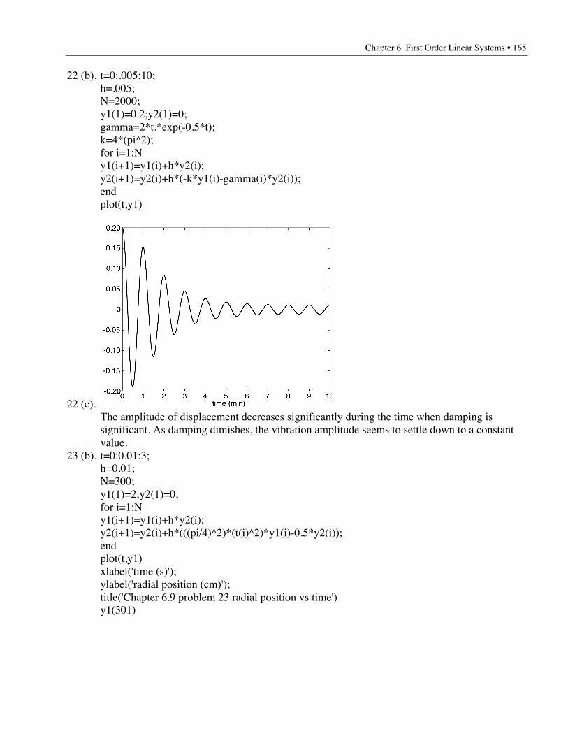
Chapter 6 First Order Linear Systems • 165
22 (b). t=0:.005:10;h=.005;N=2000;y1(1)=0.2;y2(1)=0;gamma=2*t.*exp(-0.5*t);k=4*(pi^2);for i=1:Ny1(i+1)=y1(i)+h*y2(i);y2(i+1)=y2(i)+h*(-k*y1(i)-gamma(i)*y2(i));endplot(t,y1)
22 (c). The amplitude of displacement decreases significantly during the time when damping issignificant. As damping dimishes, the vibration amplitude seems to settle down to a constantvalue.
23 (b). t=0:0.01:3;h=0.01;N=300;y1(1)=2;y2(1)=0;for i=1:Ny1(i+1)=y1(i)+h*y2(i);y2(i+1)=y2(i)+h*(((pi/4)^2)*(t(i)^2)*y1(i)-0.5*y2(i));endplot(t,y1)xlabel('time (s)');ylabel('radial position (cm)');title('Chapter 6.9 problem 23 radial position vs time')y1(301)

166 • Chapter 6 First Order Linear Systems
23 (c).
r cm( ) . ...3 15 2268=
Section 6.10
1. For A =--
È
ÎÍ
˘
˚˙
5 6
3 4 the characteristic polynomial is p( )l l l= - -2 2 . Eigenvalues are
l l1 21 2= - = and . Corresponding eigenvectors are x x1 2
1
1
2
1=
È
ÎÍ
˘
˚˙ =
È
ÎÍ
˘
˚˙ and . As in Example 1,
we can construct a diagonalizing matrix T from the eigenvectors of A, T =È
ÎÍ
˘
˚˙
1 2
1 1. The
corresponding matrix of eigenvalues, D =-È
ÎÍ
˘
˚˙
1 0
0 2, is such that T AT D- =1 .
2. The characteristic polynomial is p( )l l= -2 1. Eigenvalues are l l1 21 1= - = and .
Corresponding eigenvectors are x x1 2
1
1
2
1=
-È
ÎÍ
˘
˚˙ =
-È
ÎÍ
˘
˚˙ and . Therefore, T =
- -È
ÎÍ
˘
˚˙
1 2
1 1 and
D =-È
ÎÍ
˘
˚˙
1 0
0 1.
3. For A =È
ÎÍ
˘
˚˙
1 1
1 1 the characteristic polynomial is p( )l l l= -2 2 . Eigenvalues are
l l1 20 2= = and . Corresponding eigenvectors are x x1 2
1
1
1
1=
-È
ÎÍ
˘
˚˙ =
È
ÎÍ
˘
˚˙ and . As in Example 1,
we can construct a diagonalizing matrix T from the eigenvectors of A, T =-È
ÎÍ
˘
˚˙
1 1
1 1. The
corresponding matrix of eigenvalues, D =È
ÎÍ
˘
˚˙
0 0
0 2, is such that T AT D- =1 .
Chapter 6 First Order Linear Systems • 167
4. The characteristic polynomial is p( )l l l= -2 5 . Eigenvalues are l l1 20 5= = and .
Corresponding eigenvectors are x x1 2
3
2
1
1=
-È
ÎÍ
˘
˚˙ =
È
ÎÍ
˘
˚˙ and . Therefore, T =
-È
ÎÍ
˘
˚˙
3 1
2 1 and
D =È
ÎÍ
˘
˚˙
0 0
0 5.
5. For A =È
ÎÍ
˘
˚˙
2 3
3 2 the characteristic polynomial is p( )l l l= - -2 4 5. Eigenvalues are
l l1 21 5= - = and . Corresponding eigenvectors are x x1 2
1
1
1
1=
-È
ÎÍ
˘
˚˙ =
È
ÎÍ
˘
˚˙ and . As in Example 1,
we can construct a diagonalizing matrix T from the eigenvectors of A, T =-È
ÎÍ
˘
˚˙
1 1
1 1. The
corresponding matrix of eigenvalues, D =-È
ÎÍ
˘
˚˙
1 0
0 5, is such that T AT D- =1 .
6. The characteristic polynomial is p( ) ( )( )l l l l l= - - = + -2 2 3 1 3 . Eigenvalues are
l l1 21 3= - = and . Corresponding eigenvectors are x x1 2
1
1
1
1=
-È
ÎÍ
˘
˚˙ =
È
ÎÍ
˘
˚˙ and . Therefore,
T =-
È
ÎÍ
˘
˚˙
1 1
1 1 and D =
-È
ÎÍ
˘
˚˙
1 0
0 3.
7. For A =È
ÎÍ
˘
˚˙
2 0
1 1 the characteristic polynomial is p( )l l l= - +2 3 2. Eigenvalues are
l l1 21 2= = and . Corresponding eigenvectors are x x1 2
0
1
1
1=
È
ÎÍ
˘
˚˙ =
È
ÎÍ
˘
˚˙ and . As in Example 1, we
can construct a diagonalizing matrix T from the eigenvectors of A, T =È
ÎÍ
˘
˚˙
0 1
1 1. The
corresponding matrix of eigenvalues, D =È
ÎÍ
˘
˚˙
1 0
0 2, is such that T AT D- =1 .
8. The characteristic polynomial is p( ) ( )( )l l l l l= - - = + -2 6 2 3 . Eigenvalues are
l l1 22 3= - = and . Corresponding eigenvectors are x x1 2
1
0
2
1=
È
ÎÍ
˘
˚˙ =
È
ÎÍ
˘
˚˙ and . Therefore,
T =È
ÎÍ
˘
˚˙
1 2
0 1 and D =
-È
ÎÍ
˘
˚˙
2 0
0 3.
9. For A =--
- -
È
Î
ÍÍÍ
˘
˚
˙˙˙
25 8 30
24 7 30
12 4 14
, the eigenvalues are l l1 21 2= = and . From the characteristic
polynomial given, it follows that l1 has algebraic multiplicity 2 and l2 has algebraicmultiplicity 1.
168 • Chapter 6 First Order Linear Systems
In order to find the eigenvectors corresponding to l1, we solve ( )A I- =l1 x 0 or24 8 30
24 8 30
12 4 15
0
0
0
1
2
3
--
- -
È
Î
ÍÍÍ
˘
˚
˙˙˙
È
Î
ÍÍÍ
˘
˚
˙˙˙
=È
Î
ÍÍÍ
˘
˚
˙˙˙
x
x
x
. This system reduces to
12 4 15
0 0 0
0 0 0
0
0
0
1
2
3
-È
Î
ÍÍÍ
˘
˚
˙˙˙
È
Î
ÍÍÍ
˘
˚
˙˙˙
=È
Î
ÍÍÍ
˘
˚
˙˙˙
x
x
x
and hence
eigenvectors corresponding to l1 all have the form
x =-È
Î
ÍÍÍ
˘
˚
˙˙˙
=È
Î
ÍÍÍ
˘
˚
˙˙˙
+-È
Î
ÍÍÍ
˘
˚
˙˙˙
( ) / / /4 15 12 3
0
5 4
02 3
2
3
2
2
3
3
x x
x
x
x
x
x
x
. Thus, we find two linearly independent
eigenvectors, x x1 2
1
3
0
5
0
4
=È
Î
ÍÍÍ
˘
˚
˙˙˙
=-È
Î
ÍÍÍ
˘
˚
˙˙˙
and corresponding to l1 and therefore, l1 has geometric
multiplicity 2. Since l2 has algebraic multiplicity 1, it also has geometric multiplicity 1. Thus,A is not defective (that is, A is diagonalizable). In order to find the eigenvectors corresponding
to l2, we solve ( )A I- =l2 x 0 or
23 8 30
24 9 30
12 4 16
0
0
0
1
2
3
--
- -
È
Î
ÍÍÍ
˘
˚
˙˙˙
È
Î
ÍÍÍ
˘
˚
˙˙˙
=È
Î
ÍÍÍ
˘
˚
˙˙˙
x
x
x
. Solving this system, we obtain
an eigenvector corresponding to l2, x =-
È
Î
ÍÍÍ
˘
˚
˙˙˙
2
2
1
. Therefore, if T =-
-
È
Î
ÍÍÍ
˘
˚
˙˙˙
1 5 2
3 0 2
0 4 1
, and
D =È
Î
ÍÍÍ
˘
˚
˙˙˙
1 0 0
0 1 0
0 0 2
, then T AT D- =1 .
10. l1 1= - has algebraic multiplicity 1 and l2 3= has algebraic multiplicity 2. The corresponding
eigenvectors are x =-
È
Î
ÍÍÍ
˘
˚
˙˙˙
1
2
2
for l1 and x x1 2
1
0
2
1
2
0
=-
È
Î
ÍÍÍ
˘
˚
˙˙˙
=È
Î
ÍÍÍ
˘
˚
˙˙˙
and for l2. Therefore, l1 has
geometric multiplicity 1 and l2 has geometric multiplicity 2. A is diagonalizable and
T =- -
È
Î
ÍÍÍ
˘
˚
˙˙˙
1 1 1
2 0 2
2 2 0
, and D =-È
Î
ÍÍÍ
˘
˚
˙˙˙
1 0 0
0 3 0
0 0 3
.
11. For A = -È
Î
ÍÍÍ
˘
˚
˙˙˙
1 0 1
2 2 3
0 0 1
, the eigenvalues are l l1 21 2= = and . From the characteristic polynomial
given, it follows that l1 has algebraic multiplicity 2 and l2 has algebraic multiplicity 1.
Chapter 6 First Order Linear Systems • 169
In order to find the eigenvectors corresponding to l1, we solve ( )A I- =l1 x 0 or0 0 1
2 1 3
0 0 0
0
0
0
1
2
3
-È
Î
ÍÍÍ
˘
˚
˙˙˙
È
Î
ÍÍÍ
˘
˚
˙˙˙
=È
Î
ÍÍÍ
˘
˚
˙˙˙
x
x
x
. This system reduces to
0 0 1
2 1 0
0 0 0
0
0
0
1
2
3
È
Î
ÍÍÍ
˘
˚
˙˙˙
È
Î
ÍÍÍ
˘
˚
˙˙˙
=È
Î
ÍÍÍ
˘
˚
˙˙˙
x
x
x
and hence eigenvectors
corresponding to l1 all have the form x = -È
Î
ÍÍÍ
˘
˚
˙˙˙
= -È
Î
ÍÍÍ
˘
˚
˙˙˙
x
x x1
1 12
0
1
2
0
.
Thus, there is only one linearly independent eigenvector corresponding to l1. Therefore, l1
has geometric multiplicity 1 and consequently A is defective (not diagonalizable).
12. l1 2= has algebraic multiplicity 2 and l2 3= has algebraic multiplicity 1. The corresponding
eigenvectors are x =È
Î
ÍÍÍ
˘
˚
˙˙˙
1
4
1
for l1 and x =È
Î
ÍÍÍ
˘
˚
˙˙˙
0
1
1
for l2. Therefore, l1 has geometric multiplicity
1 and l2 has geometric multiplicity1 and A is not diagonalizable.
13. For A =--
È
Î
ÍÍÍ
˘
˚
˙˙˙
4 1 1
10 2 3
1 0 1
, the only eigenvalue is l1 1= . From the characteristic polynomial given,
it follows that l1 has algebraic multiplicity 3. In order to find the eigenvectors corresponding
to l1, we solve ( )A I- =l1 x 0 or
3 1 1
10 3 3
1 0 0
0
0
0
1
2
3
--
È
Î
ÍÍÍ
˘
˚
˙˙˙
È
Î
ÍÍÍ
˘
˚
˙˙˙
=È
Î
ÍÍÍ
˘
˚
˙˙˙
x
x
x
. This system reduces to
1 0 0
0 1 1
0 0 0
0
0
0
1
2
3
-È
Î
ÍÍÍ
˘
˚
˙˙˙
È
Î
ÍÍÍ
˘
˚
˙˙˙
=È
Î
ÍÍÍ
˘
˚
˙˙˙
x
x
x
and hence eigenvectors corresponding to l1 all have the form
x =È
Î
ÍÍÍ
˘
˚
˙˙˙
=È
Î
ÍÍÍ
˘
˚
˙˙˙
0 0
1
13
3
3x
x
x . Thus, there is only one linearly independent eigenvector corresponding to
l1. Therefore, l1 has geometric multiplicity 1 and consequently A is defective (notdiagonalizable).
14. All four matrices are diagonalizable.Matrices (a) and (d) have distinct eigenvalues.Matrix (b) is a real, symmetric matrix.Matrix (c) is lower triangular and has distinct eigenvalues.
15. For A =--
È
ÎÍ
˘
˚˙
6 6
2 1 the eigenvalues are l l1 22 3= = and with corresponding eigenvectors
x x1 2
3
2
2
1=
È
ÎÍ
˘
˚˙ =
È
ÎÍ
˘
˚˙ and . Make the substitution y z z= =
È
ÎÍ
˘
˚˙T
3 2
2 1 to obtain T AT t¢ = +z z g( ) .
170 • Chapter 6 First Order Linear Systems
Multiplying by T T AT T t- - -¢ = +1 1 1 gives z z g( ) or
¢ = + =È
ÎÍ
˘
˚˙ +
--
È
ÎÍ
˘
˚˙
++
È
ÎÍ
˘
˚˙ =
È
ÎÍ
˘
˚˙ +
È
ÎÍ
˘
˚˙-z z g z zD T t
e
e
et
t
t1
2 0
0 3
1 2
2 3
4 3
2 2
2 0
0 3 2( ) . Thus, the system uncouples
into ¢¢
È
ÎÍ
˘
˚˙ =
++
È
ÎÍ
˘
˚˙
z
z
z e
z
t1
2
1
2
2
3 2. Solving these uncoupled first order equations, we obtain
z =- +
- +È
ÎÍ
˘
˚˙
e c e
c e
t t
t1
2
232 3( / )
. Finally, forming y z= T , we obtain the general solution
y =È
ÎÍ
˘
˚˙
- +- +
È
ÎÍ
˘
˚˙ =
È
ÎÍ
˘
˚˙
È
ÎÍ
˘
˚˙ -
++
È
ÎÍ
˘
˚˙
3 2
2 1 2 3
3 2
2
3 4 3
2 2 31
2
23
2 3
2 3
1
2
e c e
c e
e e
e e
c
c
e
e
t t
t
t t
t t
t
t( / )
/
/.
16. The eigenvalues are l l1 21 2= - = and with corresponding eigenvectors x1
2
1=
-È
ÎÍ
˘
˚˙ and
x1
1
1=
-È
ÎÍ
˘
˚˙. Make the substitution y z z= =
- -È
ÎÍ
˘
˚˙T
2 1
1 1.
¢ = + =-È
ÎÍ
˘
˚˙ +
- -È
ÎÍ
˘
˚˙
-- +
È
ÎÍ
˘
˚˙ =
-È
ÎÍ
˘
˚˙-z z g zD T t
e e
e e
e
e
t t
t t
t
t1
2
2 2
1 0
0 2
1 1
1 2
2( ) .
Solving these first order equations, we obtain z =- +
+È
ÎÍ
˘
˚˙
-( / )1 2 12
22
e c e
te c e
t t
t t. Finally, forming y z= T ,
we obtain the solution y =- -
È
ÎÍ
˘
˚˙
- ++
È
ÎÍ
˘
˚˙ =
- -È
ÎÍ
˘
˚˙
È
ÎÍ
˘
˚˙ +
- +-
È
ÎÍ
˘
˚˙
- -
-
2 1
1 1
1 2 212
22
2
2
1
2
2
12
2
( / )e c e
te c e
e e
e e
c
c
e te
e te
t t
t t
t t
t t
t t
t t.
17. For A =È
ÎÍ
˘
˚˙
1 1
2 2 the eigenvalues are l l1 20 3= = and with corresponding eigenvectors
x1
1
1=
-È
ÎÍ
˘
˚˙ and x1
1
2=
È
ÎÍ
˘
˚˙ . Make the substitution y z z= =
-È
ÎÍ
˘
˚˙T
1 1
1 2 to obtain T AT t¢ = +z z g( ) .
Multiplying by T T AT T t- - -¢ = +1 1 1 gives z z g( ) or
¢ = + =È
ÎÍ
˘
˚˙ +
-È
ÎÍ
˘
˚˙ -
È
ÎÍ
˘
˚˙ =
È
ÎÍ
˘
˚˙ +
-È
ÎÍ
˘
˚˙
-z z g z zD T tt
t
t1
0 0
0 3
2 3 1 3
1 3 1 3 3
0 0
0 3
1
1( )
/ /
/ /.
Thus, the system uncouples into ¢¢
È
ÎÍ
˘
˚˙ =
-+
È
ÎÍ
˘
˚˙
z
z
t
z1
2 2
1
3 1. Solving these uncoupled first order
equations, we obtain z =- +
- +È
ÎÍ
˘
˚˙
( / )
( / )
1 2
1 3
21
23
t t c
c e t. Finally, forming y z= T , we obtain the solution
y =-
È
ÎÍ
˘
˚˙
- +- +
È
ÎÍ
˘
˚˙ =
-È
ÎÍ
˘
˚˙
È
ÎÍ
˘
˚˙ -
- -- + -
È
ÎÍ
˘
˚˙
1 1
1 2
1 2
1 3
1
1 2
1 2 1 3
1 2 2 3
21
23
3
3
1
2
2
2
( / )
( / )
( / ) ( / )
( / ) ( / )
t t c
c e
e
e
c
c
t t
t tt
t
t.
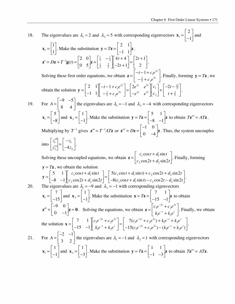
Chapter 6 First Order Linear Systems • 171
18. The eigenvalues are l l1 22 5= = and with corresponding eigenvectors x1
2
1=
-È
ÎÍ
˘
˚˙ and
x1
1
1=
È
ÎÍ
˘
˚˙ . Make the substitution y z z= =
-È
ÎÍ
˘
˚˙T
2 1
1 1.
¢ = + =È
ÎÍ
˘
˚˙ +
-È
ÎÍ
˘
˚˙
+- +
È
ÎÍ
˘
˚˙ =
+È
ÎÍ
˘
˚˙
-z z g zD T tt
t
t1
13
13
13
23
2 0
0 5
4 4
2 1
2 1
2( ) .
Solving these first order equations, we obtain z =- - +
- +È
ÎÍ
˘
˚˙
t c e
c e
t
t
1 12
25 2
5. Finally, forming y z= T , we
obtain the solution y =-
È
ÎÍ
˘
˚˙
- - +- +
È
ÎÍ
˘
˚˙ =
-È
ÎÍ
˘
˚˙
È
ÎÍ
˘
˚˙ +
- -+
È
ÎÍ
˘
˚˙
2 1
1 1
1 2 212
25 2
5
2 5
2 5
1
2
125
35
t c e
c e
e e
e e
c
c
t
t
t
t
t t
t t.
19. For A =- -È
ÎÍ
˘
˚˙
9 5
8 4 the eigenvalues are l l1 21 4= - = - and with corresponding eigenvectors
x x1 2
5
8
1
1=
-È
ÎÍ
˘
˚˙ =
-È
ÎÍ
˘
˚˙ and . Make the substitution y z z= =
- -È
ÎÍ
˘
˚˙T
5 1
8 1 to obtain T AT¢¢ =z z .
Multiplying by T T AT- -¢¢ =1 1 gives z z or ¢¢ = =-
-È
ÎÍ
˘
˚˙z z zD
1 0
0 4. Thus, the system uncouples
into ¢¢¢¢
È
ÎÍ
˘
˚˙ =
--
È
ÎÍ
˘
˚˙
z
z
z
z1
2
1
24.
Solving these uncoupled equations, we obtain z =++
È
ÎÍ
˘
˚˙
c t d t
c t d t1 1
2 22 2
cos sin
cos sin. Finally, forming
y z= T , we obtain the solution
y =- -
È
ÎÍ
˘
˚˙
++
È
ÎÍ
˘
˚˙ =
+ + +- + - -
È
ÎÍ
˘
˚˙
5 1
8 1 2 2
5 2 2
8 2 21 1
2 2
1 1 2 2
1 1 2 2
c t d t
c t d t
c t d t c t d t
c t d t c t d t
cos sin
cos sin
( cos sin ) cos sin
( cos sin ) cos sin.
20. The eigenvalues are l l1 29 1= - = - and with corresponding eigenvectors
x x1 2
7
15
1
1=
-È
ÎÍ
˘
˚˙ =
-È
ÎÍ
˘
˚˙ and . Make the substitution x z z= =
- -È
ÎÍ
˘
˚˙T
7 1
15 1 to obtain
¢¢ +-
-È
ÎÍ
˘
˚˙ =z z 0
9 0
0 1. Solving the equations, we obtain z =
++
È
ÎÍ
˘
˚˙
-
-
c e c e
k e k e
t t
t t1
32
3
1 2
. Finally, we obtain
the solution x =- -
È
ÎÍ
˘
˚˙
++
È
ÎÍ
˘
˚˙ =
+ + +- + - +
È
ÎÍ
˘
˚˙
-
-
- -
- -
7 1
15 1
7
151
32
3
1 2
13
23
1 2
13
23
1 2
c e c e
k e k e
c e c e k e k e
c e c e k e k e
t t
t t
t t t t
t t t t
( )
( ) ( ).
21. For A =- -È
ÎÍ
˘
˚˙
2 1
3 2 the eigenvalues are l l1 21 1= - = and with corresponding eigenvectors
x x1 2
1
1
1
3=
-È
ÎÍ
˘
˚˙ =
-È
ÎÍ
˘
˚˙ and . Make the substitution y z z= =
- -È
ÎÍ
˘
˚˙T
1 1
1 3 to obtain T AT¢¢ =z z .
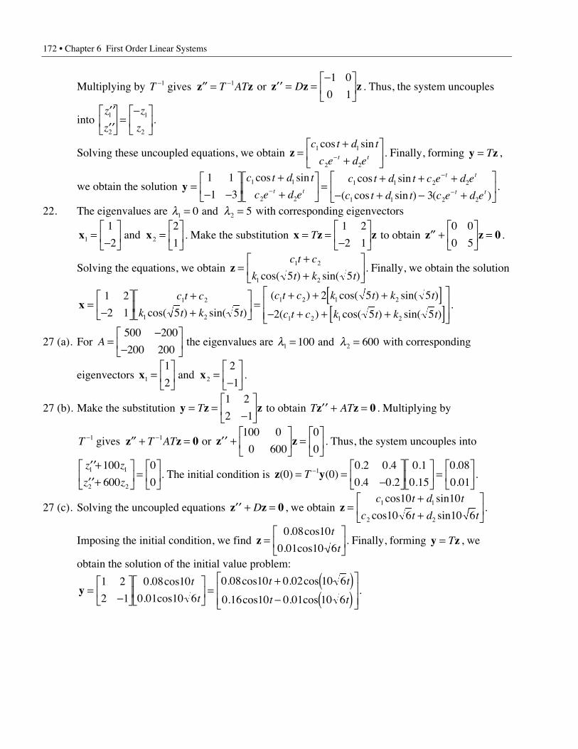
172 • Chapter 6 First Order Linear Systems
Multiplying by T T AT- -¢¢ =1 1 gives z z or ¢¢ = =-È
ÎÍ
˘
˚˙z z zD
1 0
0 1. Thus, the system uncouples
into ¢¢¢¢
È
ÎÍ
˘
˚˙ =
-È
ÎÍ
˘
˚˙
z
z
z
z1
2
1
2
.
Solving these uncoupled equations, we obtain z =++
È
ÎÍ
˘
˚˙-
c t d t
c e d et t1 1
2 2
cos sin. Finally, forming y z= T ,
we obtain the solution y =- -
È
ÎÍ
˘
˚˙
++
È
ÎÍ
˘
˚˙ =
+ + +- + - +
È
ÎÍ
˘
˚˙-
-
-
1 1
1 3 31 1
2 2
1 1 2 2
1 1 2 2
c t d t
c e d e
c t d t c e d e
c t d t c e d et t
t t
t t
cos sin cos sin
( cos sin ) ( ).
22. The eigenvalues are l l1 20 5= = and with corresponding eigenvectors
x x1 2
1
2
2
1=
-È
ÎÍ
˘
˚˙ =
È
ÎÍ
˘
˚˙ and . Make the substitution x z z= =
-È
ÎÍ
˘
˚˙T
1 2
2 1 to obtain ¢¢ +
È
ÎÍ
˘
˚˙ =z z 0
0 0
0 5.
Solving the equations, we obtain z =++
È
ÎÍ
˘
˚˙
c t c
k t k t1 2
1 25 5cos( ) sin( ). Finally, we obtain the solution
x =-
È
ÎÍ
˘
˚˙
++
È
ÎÍ
˘
˚˙ =
+ + +[ ]- + + +[ ]
È
ÎÍÍ
˘
˚˙˙
1 2
2 1 5 5
2 5 5
2 5 51 2
1 2
1 2 1 2
1 2 1 2
c t c
k t k t
c t c k t k t
c t c k t k tcos( ) sin( )
( ) cos( ) sin( )
( ) cos( ) sin( ).
27 (a). For A =-
-È
ÎÍ
˘
˚˙
500 200
200 200 the eigenvalues are l l1 2100 600= = and with corresponding
eigenvectors x x1 2
1
2
2
1=
È
ÎÍ
˘
˚˙ =
-È
ÎÍ
˘
˚˙ and .
27 (b). Make the substitution y z z= =-
È
ÎÍ
˘
˚˙T
1 2
2 1 to obtain T AT¢¢ + =z z 0 . Multiplying by
T T AT- -¢¢ + =1 1 gives z z 0 or ¢¢ +È
ÎÍ
˘
˚˙ =
È
ÎÍ
˘
˚˙z z
100 0
0 600
0
0. Thus, the system uncouples into
¢¢+¢¢+
È
ÎÍ
˘
˚˙ =
È
ÎÍ
˘
˚˙
z z
z z1 1
2 2
100
600
0
0. The initial condition is z y( ) ( )
. .
. .
.
.
.
.0 0
0 2 0 4
0 4 0 2
0 1
0 15
0 08
0 011= =
-È
ÎÍ
˘
˚˙
È
ÎÍ
˘
˚˙ =
È
ÎÍ
˘
˚˙
-T .
27 (c). Solving the uncoupled equations ¢¢ + =z z 0D , we obtain z =++
È
ÎÍ
˘
˚˙
c t d t
c t d t1 1
2 2
10 10
10 6 10 6
cos sin
cos sin.
Imposing the initial condition, we find z =È
ÎÍ
˘
˚˙
0 08 10
0 01 10 6
. cos
. cos
t
t. Finally, forming y z= T , we
obtain the solution of the initial value problem:
y =-
È
ÎÍ
˘
˚˙
È
ÎÍ
˘
˚˙ =
+ ( )- ( )
È
ÎÍÍ
˘
˚˙˙
1 2
2 1
0 08 10
0 01 10 6
0 08 10 0 02 10 6
0 16 10 0 01 10 6
. cos
. cos
. cos . cos
. cos . cos
t
t
t t
t t.
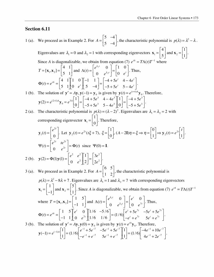
Chapter 6 First Order Linear Systems • 173
Section 6.11
1 (a). We proceed as in Example 2. For A =--
È
ÎÍ
˘
˚˙
5 4
5 4, the characteristic polynomial is p( )l l l= -2 .
Eigenvalues are l l1 20 1= = and with corresponding eigenvectors x x1 2
4
5
1
1=
È
ÎÍ
˘
˚˙ =
È
ÎÍ
˘
˚˙ and .
Since A is diagonalizable, we obtain from equation (7) e T t TtA = -L( ) 1 where
T = =È
ÎÍ
˘
˚˙[ , ]x x1 2
4 1
5 1 and L( )t
e
e e
t
t t=È
ÎÍ
˘
˚˙ =
È
ÎÍ
˘
˚˙
l
l
1
2
0
0
1 0
0. Thus,
F( )t ee
e e
e etA
t
t t
t t= =
È
ÎÍ
˘
˚˙
È
ÎÍ
˘
˚˙
--
È
ÎÍ
˘
˚˙ =
- + -- + -
È
ÎÍ
˘
˚˙
4 1
5 1
1 0
0
1 1
5 4
4 5 4 4
5 5 5 4.
1 (b). The solution of ¢ = - =y y y yA , ( )1 0 is given by y y( ) ( )t e t A= +10. Therefore,
y y( ) ( )21
0
4 5 4 4
5 5 5 4
1
0
4 5
5 52 1
03
3 3
3 3
3
3= =
È
ÎÍ
˘
˚˙ =
- + -- + -
È
ÎÍ
˘
˚˙
È
ÎÍ
˘
˚˙ =
- +- +
È
ÎÍ
˘
˚˙+e e
e e
e e
e
eA A .
2 (a). The characteristic polynomial is p( ) ( )l l= - 2 2 . Eigenvalues are l l1 2 2= = with
corresponding eigenvector x1
1
0=
È
ÎÍ
˘
˚˙ . Therefore,
y y I y1
2
22
22
07
1
02
0
1 1( ) . ( ) ( ), , ( ) ( )t
et e t A t e
ttt t=
È
ÎÍ
˘
˚˙ = + =
È
ÎÍ
˘
˚˙ - = fi =
È
ÎÍ
˘
˚˙ fi =
È
ÎÍ
˘
˚˙ Let x x h x h .
Y F Y( ) ( ) ( ) .te te
et
t t
t=
È
ÎÍ
˘
˚˙ = =
2 2
200 since I
2 (b). y y( ) ( ) ( )2 1 10
1
2
3
2
2 2
2
2
2= =
È
ÎÍ
˘
˚˙
È
ÎÍ
˘
˚˙ =
È
ÎÍ
˘
˚˙F
e e
e
e
e.
3 (a). We proceed as in Example 2. For A =È
ÎÍ
˘
˚˙
6 5
1 2, the characteristic polynomial is
p( )l l l= - +2 8 7. Eigenvalues are l l1 21 7= = and with corresponding eigenvectors
x x1 2
1
1
5
1=
-È
ÎÍ
˘
˚˙ =
È
ÎÍ
˘
˚˙ and . Since A is diagonalizable, we obtain from equation (7) e T t TtA = -L( ) 1
where T = =-
È
ÎÍ
˘
˚˙[ , ]x x1 2
1 5
1 1 and L( )t
e
e
e
e
t
t
t
t=
È
ÎÍ
˘
˚˙ =
È
ÎÍ
˘
˚˙
l
l
1
2
0
0
0
0 7. Thus,
F( )/ /
/ /( / )t e
e
e
e e e e
e e e etA
t
t
t t t t
t t t t= =
-È
ÎÍ
˘
˚˙
È
ÎÍ
˘
˚˙
-È
ÎÍ
˘
˚˙ =
+ - +- + +
È
ÎÍ
˘
˚˙
1 5
1 1
0
0
1 6 5 6
1 6 1 61 6
5 5 5
57
7 7
7 7.
3 (b). The solution of ¢ = =y y y yA , ( )0 0 is given by y y( )t etA= 0. Therefore,
y( ) ( / ) ( / )( )- =È
ÎÍ
˘
˚˙ =
+ - +- + +
È
ÎÍ
˘
˚˙
È
ÎÍ
˘
˚˙ =
- ++
È
ÎÍ
˘
˚˙-
- - - -
- - - -
- -
- -11
11 6
5 5 5
5
1
11 6
4 10
4 21
1 7 1 7
1 7 1 7
1 7
1 7e
e e e e
e e e e
e e
e eA .
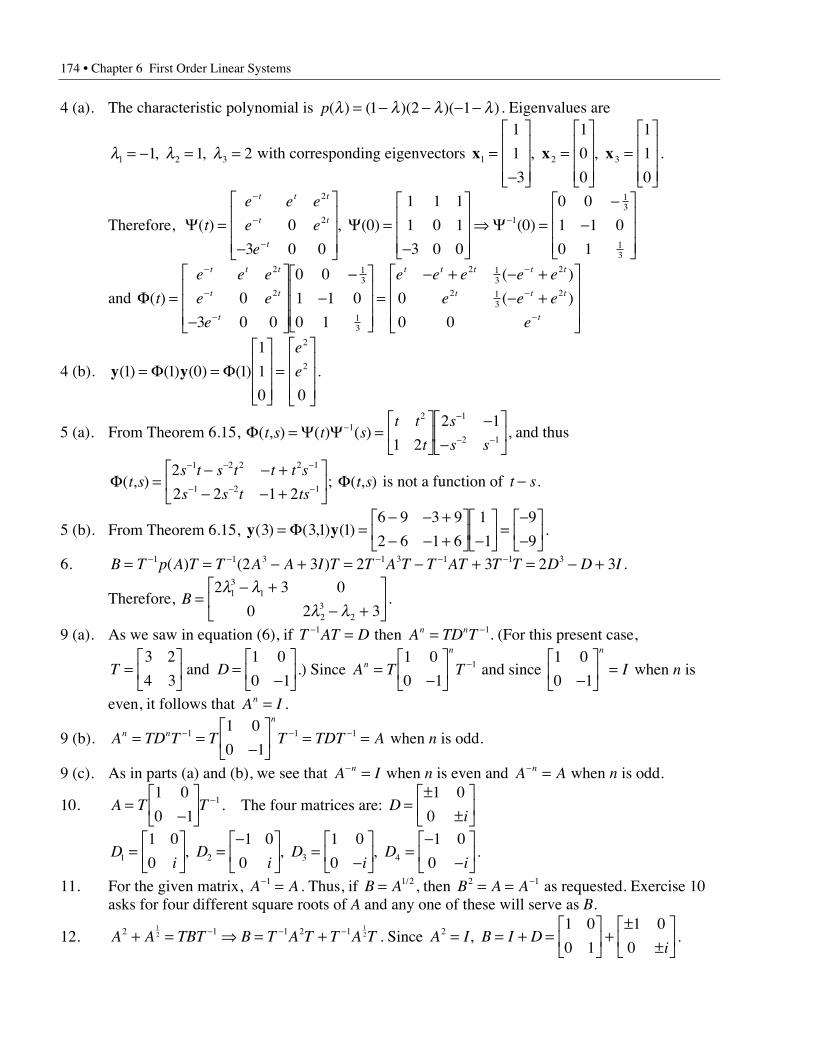
174 • Chapter 6 First Order Linear Systems
4 (a). The characteristic polynomial is p( ) ( )( )( )l l l l= - - - -1 2 1 . Eigenvalues are
l l l1 2 31 1 2= - = =, , with corresponding eigenvectors x x x1 2 3
1
1
3
1
0
0
1
1
0
=-
È
Î
ÍÍÍ
˘
˚
˙˙˙
=È
Î
ÍÍÍ
˘
˚
˙˙˙
=È
Î
ÍÍÍ
˘
˚
˙˙˙
, , .
Therefore, Y Y Y( ) , ( ) ( )t
e e e
e e
e
t t t
t t
t
=-
È
Î
ÍÍÍ
˘
˚
˙˙˙
=-
È
Î
ÍÍÍ
˘
˚
˙˙˙
fi =-
-È
Î
ÍÍÍ
˘
˚
˙˙˙
-
-
-
-
2
2 1
13
13
0
3 0 0
0
1 1 1
1 0 1
3 0 0
0
0 0
1 1 0
0 1
and F( )
( )
( )t
e e e
e e
e
e e e e e
e e e
e
t t t
t t
t
t t t t t
t t t
t
=-
È
Î
ÍÍÍ
˘
˚
˙˙˙
--
È
Î
ÍÍÍ
˘
˚
˙˙˙
=- + - +
- +È
Î
ÍÍÍ
˘
˚
˙˙˙
-
-
-
-
-
-
2
2
13
13
2 13
2
2 13
20
3 0 0
0 0
1 1 0
0 1
0
0 0
4 (b). y y( ) ( ) ( ) ( )1 1 0 1
1
1
0 0
2
2= =È
Î
ÍÍÍ
˘
˚
˙˙˙
=È
Î
ÍÍÍ
˘
˚
˙˙˙
F Fe
e .
5 (a). From Theorem 6.15, F Y Y( , ) ( ) ( )t s t st t
t
s
s s= =
È
ÎÍ
˘
˚˙
--
È
ÎÍ
˘
˚˙-
-
- -1
2 1
2 11 2
2 1, and thus
F( , )t ss t s t t t s
s s t ts=
- - +- - +
È
ÎÍ
˘
˚˙
- - -
- - -
2
2 2 1 2
1 2 2 2 1
1 2 1; F( , )t s is not a function of t s- .
5 (b). From Theorem 6.15, y y( ) ( , ) ( )3 31 16 9 3 9
2 6 1 6
1
1
9
9= =
- - +- - +
È
ÎÍ
˘
˚˙ -
È
ÎÍ
˘
˚˙ =
--
È
ÎÍ
˘
˚˙F .
6. B T p A T T A A I T T A T T AT T T D D I= = - + = - + = - +- - - - -1 1 3 1 3 1 1 32 3 2 3 2 3( ) ( ) .
Therefore, B =- +
- +È
ÎÍ
˘
˚˙
2 3 0
0 2 313
1
23
2
l ll l
.
9 (a). As we saw in equation (6), if T AT D- =1 then A TD Tn n= -1. (For this present case,
T D=È
ÎÍ
˘
˚˙ =
-È
ÎÍ
˘
˚˙
3 2
4 3
1 0
0 1 and .) Since A T Tn
n
=-
È
ÎÍ
˘
˚˙
-1 0
0 11 and since
1 0
0 1-È
ÎÍ
˘
˚˙ =
n
I when n is
even, it follows that A In = .
9 (b). A TD T T T TDT An n
n
= =-
È
ÎÍ
˘
˚˙ = =- - -1 1 1
1 0
0 1 when n is odd.
9 (c). As in parts (a) and (b), we see that A In- = when n is even and A An- = when n is odd.
10. A T T=-
È
ÎÍ
˘
˚˙
-1 0
0 11. The four matrices are: D
i=
±±
È
ÎÍ
˘
˚˙
1 0
0
Di
Di
Di
Di1 2 3 4
1 0
0
1 0
0
1 0
0
1 0
0=
È
ÎÍ
˘
˚˙ =
-È
ÎÍ
˘
˚˙ =
-È
ÎÍ
˘
˚˙ =
--
È
ÎÍ
˘
˚˙, , , .
11. For the given matrix, A A- =1 . Thus, if B A= 1 2/ , then B A A2 1= = - as requested. Exercise 10asks for four different square roots of A and any one of these will serve as B.
12. A A TBT B T A T T A T2 1 1 2 112
12+ = fi = +- - - . Since A I B I D
i2
1 0
0 1
1 0
0= = + =
È
ÎÍ
˘
˚˙ +
±±
È
ÎÍ
˘
˚˙, .
Chapter 6 First Order Linear Systems • 175
13. Since A TDT= -1, it follows that A TD T3 3 1
31 1
2 1
2 0
0 2
1 1
2 1
24 16
32 24= =
È
ÎÍ
˘
˚˙
-È
ÎÍ
˘
˚˙
--
È
ÎÍ
˘
˚˙ =
--
È
ÎÍ
˘
˚˙
- .
14. f A A T T T T11
2
1 10
0
2 1
5 3
3 1
5 2( ) cos( )
cos( )
cos( ). , = =
È
ÎÍ
˘
˚˙ =
È
ÎÍ
˘
˚˙ =
--
È
ÎÍ
˘
˚˙
- -ppl
pl.
cos( ) cos , cos( ) cospl p pl p1 24
1
2 20= Ê
ËÁˆ¯ = = Ê
ËÁˆ¯ = . Therefore,
f A A1
12
152
52
2 1
5 3
0
0 0
3 1
5 2
3 2 2
2 2( ) cos( )= =
È
ÎÍ
˘
˚˙
È
ÎÍ
˘
˚˙
--
È
ÎÍ
˘
˚˙ =
--
È
ÎÍ
˘
˚˙p .
sin( ) sin , sin( ) sinpl p pl p1 24
1
2 21= Ê
ËÁˆ¯ = = Ê
ËÁˆ¯ = . Therefore,
f A A2
12
152
52
2 1
5 3
0
0 1
3 1
5 2
3 2 5 2 2
2 15 2 6( ) sin( )= =
È
ÎÍ
˘
˚˙
È
ÎÍ
˘
˚˙
--
È
ÎÍ
˘
˚˙ =
- - +- - +
È
ÎÍ
˘
˚˙p .
15. As we saw following Theorem 6.16, cos( )cos
costA T
t
tT=
È
ÎÍ
˘
˚˙
-ll
1
2
10
0 when A is a ( )2 2¥
diagonalizable matrix with eigenvalues l l1 2 and . Thus, with t = p and the given eigenvalues,
we have
cos( )cos( / )
cos( / )
/
/
( / ) ( / ) .
pp
pA T T T T
T T I
=È
ÎÍ
˘
˚˙ =
È
ÎÍ
˘
˚˙
=È
ÎÍ
˘
˚˙ =
- -
-
3 0
0 7 3
1 2 0
0 1 2
1 21 0
0 11 2
1 1
1
Similarly, we find sin( ) ( / ) .pA I= 3 2
16. Let T =- -
È
ÎÍ
˘
˚˙
1 1
2 1. Make the substitution y z= T . Premultiplying by
T D T D- -È
ÎÍ
˘
˚˙ ¢¢ + =
È
ÎÍ
˘
˚˙ =
-È
ÎÍ
˘
˚˙ =
-È
ÎÍ
˘
˚˙
1 11
0
1
2
1 0
0 1=
-1 -1
2 1 gives z z , . The solution is
z( )cos sin
tc e c e
k t k t
t t
=+ +
+ +È
ÎÍ
˘
˚˙
-1 2
1 2
1
2. Converting to the original variables, we obtain
y z( ) ( )cos sin
cos sin
cos sint T t
c e c e
k t k t
c e c e k t k t
c e c e k t k t
t t t t
t t= =
- -È
ÎÍ
˘
˚˙
+ ++ +
È
ÎÍ
˘
˚˙ =
+ + + +- - - - -
È
ÎÍ
˘
˚˙
- -
-
1 1
2 1
1
2
3
2 2 41 2
1 2
1 2 1 2
1 2 1 2
.
17. Let T =- -
È
ÎÍ
˘
˚˙
1 1
2 1. Making the substitution y z= T , the system becomes AT T¢ + =
È
ÎÍ
˘
˚˙z z
1
1.
Premultiplying by T T AT- -È
ÎÍ
˘
˚˙ ¢ + =
-È
ÎÍ
˘
˚˙
1 12
3=
-1 -1
2 1 gives z z or
-È
ÎÍ
˘
˚˙ ¢ + =
-È
ÎÍ
˘
˚˙
1 0
0 1
2
3z z . Thus, the
system uncouples into - ¢ +
¢ +È
ÎÍ
˘
˚˙ =
-È
ÎÍ
˘
˚˙
z z
z z1 1
2 2
2
3. The solution is z( )t
c e
c e
t
t=
-+
È
ÎÍ
˘
˚˙-
1
2
2
3. Converting to the
original variables, we obtain y z= =- -
È
ÎÍ
˘
˚˙
-+
È
ÎÍ
˘
˚˙ =
+ +- - +
È
ÎÍ
˘
˚˙-
-
-Tc e
c e
c e c e
c e c e
t
t
t t
t t
1 1
2 1
2
3
1
2 11
2
1 2
1 2
.
176 • Chapter 6 First Order Linear Systems
18. Make the substitution y z= T . ¢¢ + ¢ + =z z z 0D .. The solution is
z( )cos sin
tc e c e
k e t k e t
t t
t t= +
( ) + ( )È
ÎÍÍ
˘
˚˙˙
- -( ) - +( )- -
1 2
13
2 23
2
12
52
12
52
2 2. Converting to the original variables, we obtain
y z( ) ( )cos sin
cos sint T t
c e c e k e t k e t
c e c e k e t k e t
t t
t t
t t
t t= =
+ + ( ) + ( )- - - ( ) - ( )
È - -( ) - +( ) - -
- -( ) - +( ) - -
1 2 13
2 23
2
1 2 13
2 23
2
12
52
12
52 2 2
12
52
12
52 2 22 2ÎÎ
ÍÍ
˘
˚
˙˙.
19. Let T =- -
È
ÎÍ
˘
˚˙
1 1
2 1. Making the substitution y z= T , the system becomes T AT¢¢ + ¢ =z z 02 .
Premultiplying by T T AT- -È
ÎÍ
˘
˚˙ ¢¢ + ¢ =1 12=
-1 -1
2 1 gives z z 0 or ¢¢ +
-È
ÎÍ
˘
˚˙ ¢ =
È
ÎÍ
˘
˚˙z z2
1 0
0 1
0
0. Thus, the
system uncouples into ¢¢- ¢
¢¢+ ¢È
ÎÍ
˘
˚˙ =
È
ÎÍ
˘
˚˙
z z
z z1 1
2 2
2
2
0
0. The solution is z( )t
c c e
d d e
t
t=
++
È
ÎÍ
˘
˚˙-
1 22
1 22
. Converting to the
original variables, we obtain
y z( ) ( )( ) ( )
t T tc c e
d d e
c c e d d e
c c e d d e
t
t
t t
t t= =
- -È
ÎÍ
˘
˚˙
++
È
ÎÍ
˘
˚˙ =
+ + +- + - +
È
ÎÍ
˘
˚˙-
-
-
1 1
2 1 21 2
2
1 22
1 22
1 22
1 22
1 22
.
20 (a). m x k x x m x k x x k x x m x k x x1 1 1 2 1 2 2 2 3 2 1 2 1 3 3 2 3 2¢¢= - ¢¢ = - - - ¢¢ = - -( ); ( ) ( ); ( ). Therefore,m x k x x m x k x k k x k x m x k x k x1 1 1 1 2 2 2 1 1 1 2 2 2 3 3 3 2 2 2 30 0 0¢¢+ - = ¢¢ - + + - = ¢¢ - + =( ) ; ( ) ; .The result follows.
20 (b). Kv 00 = , where v0 is any nonzero multiple of
1
1
1
È
Î
ÍÍÍ
˘
˚
˙˙˙. Therefore, 0
1
1
1
,
È
Î
ÍÍÍ
˘
˚
˙˙˙ is an eigenpair.
20 (c). Let x v x x v v 0= ¢¢ + = ¢¢ + =f t M K M f t Kf t( ) . ( ( ) ) ( )0 0 0 . Therefore, sinceK f t f t K Mf t or m f t j f tj( ( ) ) ( ) , ( ) ( ) , , , ( ) .v v 0 v 00 0 0 0 1 2 3 0= = ¢¢ = ¢¢ = = fi ¢¢ = Therefore,
f t c t c t c t c c c t c c( ) ( ) . ( ) , ( ) .= + = +( ) = = fi = = = fi =1 2 1 2 0 2 0 2 1 0 0 10 0 1 and x v x v 0 x v vTherefore, x v( )t t= 0. The system is executing motion at constant velocity v0 . There is norelative motion; the three-mass system is translating like a rigid body.
21 (a). For this case, we have A M Kk
m= =
-- -
-
È
Î
ÍÍÍ
˘
˚
˙˙˙
-1
1 1 0
1 2 1
0 1 1
. Using MATLAB, we find the
eigenvalues of B =-
- --
È
Î
ÍÍÍ
˘
˚
˙˙˙
1 1 0
1 2 1
0 1 1
are g g g1 2 30 1 3= = =, , and with corresponding
eigenvectors u u u1 2 3
1
1
1
1
0
1
1
2
1
=È
Î
ÍÍÍ
˘
˚
˙˙˙
=-
È
Î
ÍÍÍ
˘
˚
˙˙˙
= -È
Î
ÍÍÍ
˘
˚
˙˙˙
, , and . Since A k m B= ( / ) , the eigenvalues of A are
multiples of k/m times the eigenvalues of B while corresponding eigenvectors can be chosen tobe the same as those of B.
Chapter 6 First Order Linear Systems • 177
21 (b). Making the substitution x z= T , the system becomes T AT¢¢ + =z z 0 . Premultiplying by
gives ¢¢ + =-z z 0T AT1 or ¢¢ +È
Î
ÍÍÍ
˘
˚
˙˙˙
=È
Î
ÍÍÍ
˘
˚
˙˙˙
-
-
z z
0 0 0
0 0
0 0 3
0
0
0
1
1
km
km
. Thus, the system uncouples into
¢¢¢¢+
¢¢+
È
Î
ÍÍÍ
˘
˚
˙˙˙
=È
Î
ÍÍÍ
˘
˚
˙˙˙
-
-
z
z km z
z km z
1
21
2
31
33
0
0
0
. The solution is z( ) cos sin
cos sin
,t
c t c
d t d t
e t e t
km=+++
È
Î
ÍÍÍ
˘
˚
˙˙˙
= -1 2
1 2
1 2
1
3 3
w ww w
w where .
Converting to the original variables, we obtain
x( ) cos sin
cos sin
cos sin cos sin
( cos
t
c t c
d t d t
e t e t
c t c d t d t e t e t
c t c e t e
= --
È
Î
ÍÍÍ
˘
˚
˙˙˙
+++
È
Î
ÍÍÍ
˘
˚
˙˙˙
=+ + + + +
+ - +
1 1 1
1 0 2
1 1 1 3 3
3 3
2 3
1 2
1 2
1 2
1 2 1 2 1 2
1 2 1
w ww w
w w w ww 22
1 2 1 2 1 2
3
3 3
sin )
( cos sin ) cos sin
.ww w w w
t
c t c d t d t e t e t+ - + + +
È
Î
ÍÍÍ
˘
˚
˙˙˙
Chapter 7Laplace Transforms
Section 7.1
1. L{ } lim lim lim , 1 11
11
00
0
= ◊ =-
= -( ) = >Æ •
-
Æ •
-
Æ •
-ÚT
stT
T
st T
T
sTe dte
s se
ss
2. L{ } lim lim lim lim( ) ( )e e e dt e dts
es
et
T
t stT
T
s tT
T
s t T
T
s T3 3
0
3
0
3
0
313
13
1= ◊ = = --
=-
-( )Æ •
-
Æ •
- -( )Æ •
- -
Æ •
- -Ú Ú
=-
>1
33
ss, .
3. L{ } lim limte te e dt te dtt
T
t stT
T
s tT-
Æ •
- -
Æ •
- +( )= ◊ =Ú Ú0
1
0. For integration by parts, we will use
u t du dt dv e dt ve
ss t
s t
= = = = -+
- +( )- +( )
, , , 11
1and . Then we have
lim lim limT
s tT
T
s t T
s tT
T
s Ts Tte dt
te
s se dt
Te
s se
Æ •
- +( )Æ •
- +( )- +( )
Æ •
- +( )- +( )Ú Ú=
-+
++
ÏÌÔ
ÓÔ
¸˝ÔÔ
=-
++
+( )-( )Ï
ÌÓ
¸˝˛
1
0
1
0
1
0
1
21
11
1 11
11
=+( )
> -1
112
ss, .
4. L{ } lim ( )t t e dtT
stT
- = - ◊Æ •
-Ú5 50
. For integration by parts, we will use
u t du dt dv e dt ve
sst
st
= - = = = ---
5, , , and . Then we have
lim ( ) lim( )
lim( )
T
stT
T
st T
stT
T
sT st T
t e dtt e
s se dt
T e
s
e
sÆ •
-
Æ •
--
Æ •
- -
- =- -
+ÏÌÔ
ÓÔ
¸˝ÔÔ
=- - +
-ÏÌÔ
ÓÔ
¸˝ÔÔÚ Ú5
5 1 5 50
00 2
0
= - >1 5
02s ss, .
5. L{ ( )}f t does not exist because limt
t t stte eÆ •
- = • for all s > 0.
6. L{ ( )}f t does not exist because lim ( )
t
t ste eÆ •
- - = •1 2
for all s > 0.
Chapter 7 Laplace Transforms • 179
7. L t t e dt t e dtst st-{ } = -( ) + -( )- -•
Ú Ú1 1 10
1
1
1
2( ) ( )1 244 344 1 244 344
.
(1): u t du dt dv e dt ve
sst
st
= - = - = = ---
1 , , , . Then we have
( )1 11 1 1 1
10
1
0
1
20
1
2= - -( ) - = + = + -( )- -
- -Úte
s
e
sdt
s se
s se
st stst s
(2): u t du dt dv e dt ve
sst
st
= - = = = ---
1, , , . Then we have
( )21 1
11 2= -
-+ =-
•-• -
Út
se
se dt
e
sst st
s
( ) ( ) , 1 21 1 2
02 2+ = - + >-
s s se ss .
8. L{( ) } lim ( )t t e dtT
stT
- = - ◊Æ •
-Ú2 22 2
0. Using
u t du t dt dv e dt ve
sst
st
= - = - = = ---
( ) , ( ) , , 2 2 22 and , we have
lim ( ) lim( )
( ) lim ( ) .T
stT
T
st T
stT
T
Tstt e dt
t e
s st e dt
s st e dt
Æ •
-
Æ •
--
Æ •
-- ◊ =- -
+ -ÏÌÔ
ÓÔ
¸˝ÔÔ
= + -Ú Ú Ú22 2
24 2
22
0
2
00 0
Using
parts with u t du dt dv e dt ve
sst
st
= - = = = ---
2, , , and , we have
lim ( ) lim( )
, .T
stT
T
stst
T
t e dts s
t e
s se
s s ss
Æ •
-
Æ •
--- ◊ = +
- -+
ÊËÁ
ˆ¯
ÏÌÔ
ÓÔ
¸˝Ô
Ô= - + >Ú 2
4 2 2 1 4 4 202
0 2
0
2 3
9. L{ ( )} lim lim lim , f t e dte
s se e
e
ss
T
stT
T
st T
T
s sTs
= ◊ =-
= -( ) = >Æ •
-
Æ •
-
Æ •
- --
Ú 11
01
1
.
10. L{ ( )}f t =
lim ( ) lim( )
lim( )
T
stT
T
st T
stT
T
sT s sT
t e dtt e
s se dt
T e
s
e e
sÆ •
-
Æ •
--
Æ •
- - -
- ◊ =- -
+ÏÌÔ
ÓÔ
¸˝ÔÔ
= --
+-Ï
ÌÓ
¸˝˛
Ú Ú11 1 1
11
1 2
= >-e
ss
s
2 0, .
11. L{ ( )} , ; , f t e dte
s se e s sst
sts s= ◊ =
-= -( ) π = =-
-- -Ú 1
10 1 0
1
2
1
2
2 .
180 • Chapter 7 Laplace Transforms
12. L{ ( )} ( )( )
, .f t t e dtt e
s se dt
e
s se e sst
stst
ss s= - ◊ =
- -+ = - + -( ) π-
--
-- -Ú Ú1
1 1 10
1
2
1
2
1
2 2
22
13. t e dtn st-Ú . u t du nt dt dv e dt ve
sn n st
st
= = = = -- --
, , , 1 and . Then we have
- + >-
- -Út e
s
n
st e dt s
n stn st1 0, .
14 (a). Since lim lim , limt
n
t
st
t
n stt e t eÆ Æ
-
Æ
-+ + +
= = =0 0 0
0 1 0 and .
14 (b). Using L’Hopital’s rule:
lim lim lim ... lim!
.t
n st
t
n
st t
n
st t n stt et
e
nt
se
n
s eÆ •
-
Æ • Æ •
-
Æ •= = = = =
1
0
15 (a). Using 13 and 14,
L L{ } lim lim { }, tt e
s
n
st e dt
n
st e dt
n
st sn
T
n st T
n stT
T
n stT
n=-
+ÏÌÔ
ÓÔ
¸˝ÔÔ
= + = >Æ •
-- -
Æ •
- - -Ú Ú0
1
0
1
0
10 0 .
15 (b).
L L L L L{ } { } , { } { }!, { } { }
!, t
st
st
st
st
st
s2
33 2
44 3
5
2 2 3 3 4 4= = = = = =L
L L{ } { }!, t
st
ss5 4
6
5 50= = > .
15 (c). L{ }!
, tm
ssm
m= >+1 0.
16. L{ ( )} limcos sin
, .f t es t t
s
s
ss
T
st
T
=- -
+ÊËÁ
ˆ¯
ÏÌÔ
ÓÔ
¸˝ÔÔ
=+
>Æ •
- w w ww w2 2
02 2 0
17. L{ ( )} limsin cos
, f t es t t
s ss
T
st
T
=- -
+ÊËÁ
ˆ¯
ÏÌÔ
ÓÔ
¸˝ÔÔ
=+
>Æ •
- w w ww
ww2 2
02 2 0.
18. f t t t t( ) cos( ( )) cos( )cos( ) sin( )sin( )= - = +w w w w w2 2 2 . Using 16 and 17,
L{ ( )}cos( ) sin( )
, f ts
ss=
++
>2 2
02 2
w w ww
.
19. f t t t t( ) = -( )( ) = -sin sin cos cos sinw w w w w2 2 2 . Then we have
L{ ( )}cos sin
, f ts
ss=
-+
>w w w
w2 2
02 2 .
20. L{ ( )} lim sin lim( )sin cos
( ) ( ), ( ) ( )f t e t dt e
s t t
s ss
T
s tT
T
s t
T
= =- - -
- +ÊËÁ
ˆ¯
ÏÌÔ
ÓÔ
¸˝ÔÔ
=- +
>Æ •
- -
Æ •
- -Ú 3
0
32
0
2
33 1
13 1
3.
Chapter 7 Laplace Transforms • 181
21. L{ ( )} lim cos limcos sin
f t e tdt es t t
sT
s tT
T
s t
T
= =- +( ) +
+( ) +
Ê
ËÁˆ
¯
ÏÌÔ
ÓÔ
¸˝Ô
ÔÆ •
- +( )Æ •
- +( )Ú 2
0
22
0
42 4 4 4
2 16
=+
+( ) +> -
s
ss
2
2 1622 , .
22. L{ } , 22
555e
sst- =
+> - . L{ } , 6
602t
ss= > . Then L{ ( )} , r t
s ss=
++ >
25
602 .
23. L{ } , 55
777e
sst- =
+> - . L{ } , t
ss= >
102 , and L{ } , 2
22
22es
st =-
> . Then
L{ ( )} , r ts s s
s=+
+ +-
>5
71 2
222 .
24 (a). The function is discontinuous on 0 £ < •t because the one-sided limits do not exist at the
vertical asymptotes.
24 (b). The function is not exponentially bounded on 0 £ < •t .
25 (a). The function is continuous on 0 £ < •t .
25 (b). The function is exponentially bounded on 0 £ < •t . f t et( ) £ , so we can take M a= =1 1, .
26 (a). The function is continuous on 0 £ < •t .
26 (b). The function is exponentially bounded on 0 £ < •t .
If then f t t e f t t t e tt t( ) , ( ) ( )= ¢ = - = fi =- -2 22 0 2, is a maximum point, so we can take
M f e a= = =-( ) , 2 4 02 .
27 (a). The function is continuous on 0 £ < •t .
27 (b). The function is exponentially bounded on 0 £ < •t , since cosh21
2
22t
ee
tt£
+£ on 0 £ < •t ,
so we can take M a= =1 2, .
28 (a). The function is piecewise continuous on 0 £ < •t .
28 (b). Consider g t te g t t e t tt t( ) , ( ) ( ) . = ¢ = - = fi = \ =- -1 0 1 1 is a maximum and
g t e t e e tt( ) , .£ fi £ £ < •- -1 1 0 Since t t t[ ][ ] £ £ < •, 0 , the function is exponentially
bounded on 0 £ < •t , taking M e a= =-1 1, .
29 (a). The function is piecewise continuous on 0 £ < •t .
29 (b). f t e t( ) £ 2 , and so the function is exponentially bounded on 0 £ < •t , taking M a= =1 2, .
30 (a). The function is continuous on 0 £ < •t .
182 • Chapter 7 Laplace Transforms
30 (b). The function is not exponentially bounded on 0 £ < •t because
f te
e ee e e t
t
t tt t t t t
( ) , .≥+
= > >- -2
2 2 2
2
2 22 21
24 and
31 (a). The function is discontinuous and not piecewise continuous on 0 £ < •t .
31 (b). The function is not exponentially bounded on 0 £ < •t .
32. lim lim tan lim tanT
T
T
T
Ttdt t T
Æ • Æ •
-
Æ •
-
+= ( ) = ( ) =Ú
11 220
1
0
1 p, so the improper integral converges.
33.t
tdt t T
TT
112
112
120
2
0
2
+= +( ) = +( )Ú ln ln . Since lim ln
TT
Æ •+( ) = •
12
1 2 , the improper integral
diverges.
34. lim cos( ) lim cos( ) cos sin sin( )T
t tT
T
ee e dt u du udu u
T
Æ •
- -
Æ •- = - = = =Ú Ú Ú
-
0 1 0
1
0
11 , so the improper
integral converges.
35. te dt te dt e du e dut
T
tT
T
uT
T
uT-•
Æ •
-
Æ •
-
Æ •
-Ú Ú Ú Ú= = ÊËÁ
ˆ¯ =
2 22 2
0 0 0 0
12
12
lim lim lim = -( ) =Æ •
-limT
Te12
112
2
, so the
integral converges to 12
.
36. f ts
e tt( ) , =-
ÏÌÓ
¸˝˛
= ≥-31
23 01 2
L .
37. f ts s
t e tt( ) , = - ÏÌÓ
¸˝˛
++
ÏÌÓ
¸˝˛
= - + ≥- - -21 1
12 01
21
L L .
38. f ts s
e e t tt t( ) cosh( ), =+
ÏÌÓ
¸˝˛
+-
ÏÌÓ
¸˝˛
= + = ≥- - -21
22
12
2 2 4 2 01 1 2 2L L .
39. f ts s
e e t tt t( ) sinh , =-
ÏÌÓ
¸˝˛
-+
ÏÌÓ
¸˝˛
= - = ≥- - -L L
1 111
11
2 0.
Section 7.2
1. L{ ( )} , f ts s s s s s
s= ÊËÁ
ˆ¯ + + = + + >3
2 2 1 6 2 103 2 3 2
2. L{ ( )} , f ts s
s=-
+ >2
15
1
3. L{ ( )} , f ts s
s= ++
>1 3
902
4. L L{ ( )} { } , f t e ee
sss t
s
= =-
>--
3
33
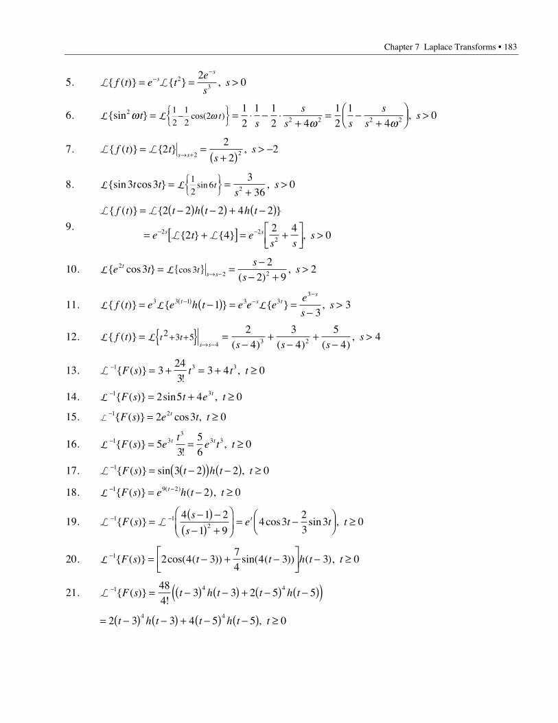
Chapter 7 Laplace Transforms • 183
5. L L{ ( )} { } , f t e te
sss
s
= = >--
23
20
6. L L{sin } , cos( )22 2 2 2
1
2
1
22
12
1 12 4
12
14
0ww w
wts
s
s s
s
sst= = ◊ - ◊
+= -
+ÊËÁ
ˆ¯ >-ÏÌ
Ó¸˛
7. L L{ ( )} { } , f t ts
ss s
= =+( )
> -Æ +
22
22
2 2
8. L L{sin cos } , sin3 33
3601
26 2t t
sst= =
+>ÏÌ
Ó¸˛
9.
L L
L L
{ ( )} { }
{ } { } ,
f t t h t h t
e t es s
ss s
= -( ) -( ) + -( )
= +[ ] = +ÈÎÍ
˘˚
>- -
2 2 2 4 2
2 42 4
02 22
10. L L{ cos }( )
, cose ts
sst
s st22 23
22 9
23= =-
- +>{ } Æ -
11. L L L{ ( )} { } { } , f t e e h t e e ee
sst s t
s
= -( ) = =-
>-( ) --
3 3 1 3 33
13
3
12. L L{ ( )}( ) ( ) ( )
, f ts s s
st ts s
= =-
+-
+-
>+ +{ }Æ -
2 3 54 3 2
24
34
54
4
13. L- = + = + ≥1 3 33
243
3 4 0{ ( )}!
, F s t t t
14. L- = + ≥1 32 5 4 0{ ( )} sin , F s t e tt
15. L- = ≥1 22 3 0{ ( )} cos , F s e t tt
16. L- = = ≥1 3
33 35
356
0{ ( )}!
, F s et
e t tt t
17. L- = -( )( ) -( ) ≥1 3 2 2 0{ ( )} sin , F s t h t t
18. L- -= - ≥1 9 2 2 0{ ( )} ( ), ( )F s e h t tt
19. L L- -=
-( ) --( ) +
Ê
ËÁˆ
¯= -Ê
ËÁˆ¯ ≥1 1
2
4 1 2
1 94 3
23
3 0{ ( )} cos sin , F ss
se t t tt
20. L- = - + -È
Î͢˚
- ≥1 2 4 374
4 3 3 0{ ( )} cos( ( )) sin( ( )) ( ), F s t t h t t
21. L- = -( ) -( ) + -( ) -( )( )1 4 448
43 3 2 5 5{ ( )}
!F s t h t t h t
= -( ) -( ) + -( ) -( ) ≥2 3 3 4 5 5 04 4
t h t t h t t,
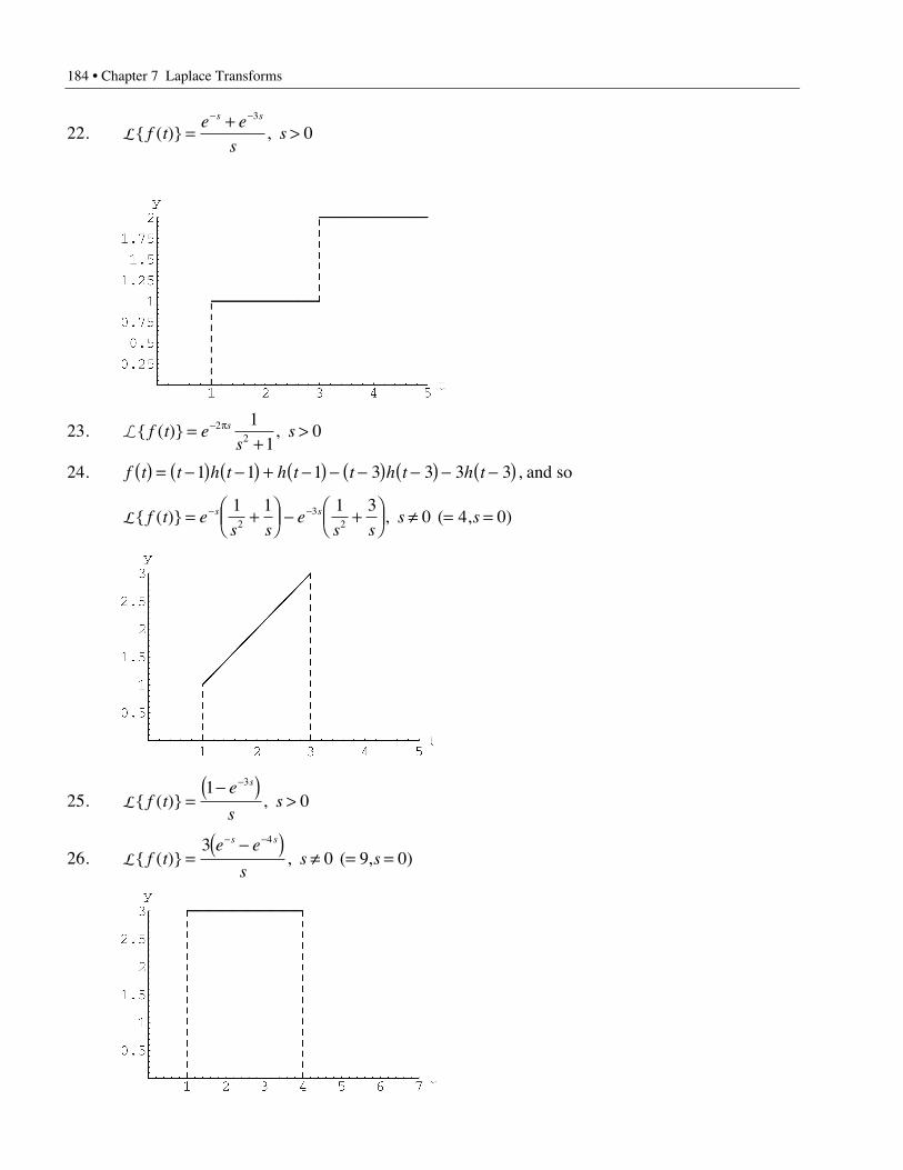
184 • Chapter 7 Laplace Transforms
22. L{ ( )} , f te e
ss
s s
=+
>- -3
0
23. L{ ( )} , f t es
ss=+
>- p22
11
0
24. f t t h t h t t h t h t( ) = -( ) -( ) + -( ) - -( ) -( ) - -( )1 1 1 3 3 3 3 , and so
L{ ( )} , ( , )f t es s
es s
s ss s= +ÊËÁ
ˆ¯ - +Ê
ËÁˆ¯ π = =- -1 1 1 3
0 4 023
2
25. L{ ( )} , f te
ss
s
=-( )
>-1
03
26. L{ ( )} , ( , )f te e
ss s
s s
=-( )
π = =- -3
0 9 04
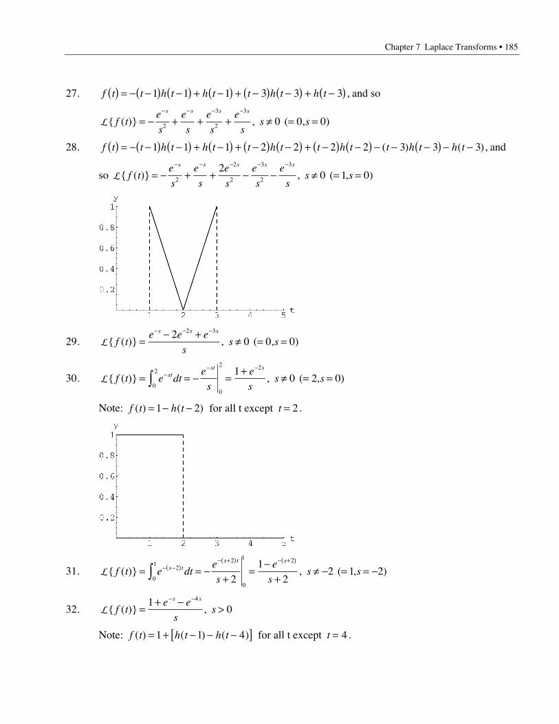
Chapter 7 Laplace Transforms • 185
27. f t t h t h t t h t h t( ) = - -( ) -( ) + -( ) + -( ) -( ) + -( )1 1 1 3 3 3 , and so
L{ ( )} , ( , )f te
s
e
s
e
s
e
ss s
s s s s
= - + + + π = =- - - -
2
3
2
3
0 0 0
28. f t t h t h t t h t t h t t h t h t( ) = - -( ) -( ) + -( ) + -( ) -( ) + -( ) -( ) - - -( ) - -1 1 1 2 2 2 2 3 3 3( ) ( ), and
so L{ ( )} , ( , )f te
s
e
s
e
s
e
s
e
ss s
s s s s s
= - + + - - π = =- - - - -
2
2
2
3
2
320 1 0
29. L{ ( )} , ( , )f te e e
ss s
s s s
=- +
π = =- - -2
0 0 02 3
30. L{ ( )} , ( , )f t e dte
s
e
ss sst
st s
= = - =+
π = =-- -
Ú0
2
0
2 210 2 0
Note: f t h t t( ) ( )= - - =1 2 2 for all t except .
31. L{ ( )} , ( , )f t e dte
s
e
ss ss t
s t s
= = -+
=-
+π - = = -- -( )
- +( ) - +( )
Ú 2
0
1 2
0
1 2
21
22 1 2
32. L{ ( )} , f te e
ss
s s
=+ -
>- -1
04
Note: f t h t h t t( ) ( ) ( )= + - - -[ ] =1 1 4 4 for all t except .
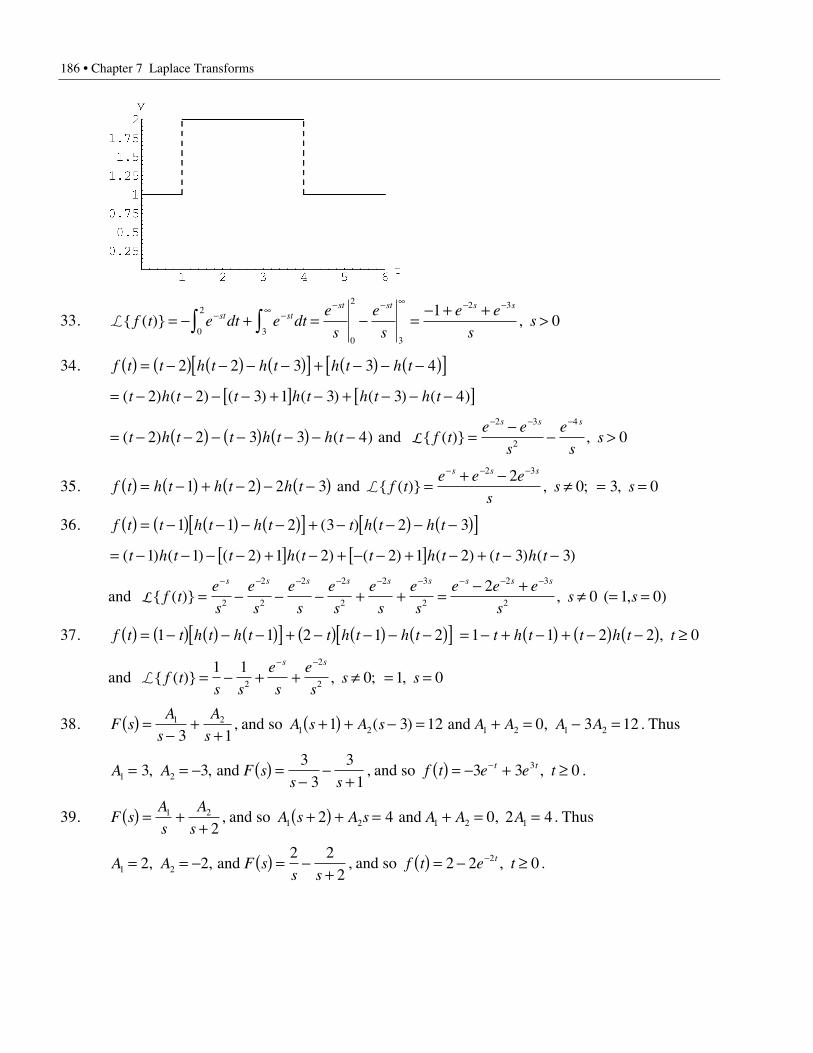
186 • Chapter 7 Laplace Transforms
33. L{ ( )} , f t e dt e dte
s
e
s
e e
ssst st
st st s s
= - + = - =- + +
>- -• - - • - -
Ú Ú0
2
30
2
3
2 310
34. f t t h t h t h t h t( ) = -( ) -( ) - -( )[ ] + -( ) - -( )[ ]2 2 3 3 4
= - - - - +[ ] - + - - -[ ]( ) ( ) ( ) ( ) ( ) ( )t h t t h t h t h t2 2 3 1 3 3 4
= - -( ) - -( ) -( ) - -( ) ( )t h t t h t h t2 2 3 3 4 and L{ ( )} , f te e
s
e
ss
s s s
=-
- >- - -2 3
2
4
0
35. f t h t h t h t( ) = -( ) + -( ) - -( )1 2 2 3 and L{ ( )} , ; , f te e e
ss s
s s s
=+ -
π = =- - -2 32
0 3 0
36. f t t h t h t t h t h t( ) = -( ) -( ) - -( )[ ] + - -( ) - -( )[ ]1 1 2 3 2 3( )
= - - - - +[ ] - + - - +[ ] - + - -( ) ( ) ( ) ( ) ( ) ( ) ( ) ( )t h t t h t t h t t h t1 1 2 1 2 2 1 2 3 3
and L{ ( )} , ( , )f te
s
e
s
e
s
e
s
e
s
e
s
e e e
ss s
s s s s s s s s s
= - - - + + =- +
π = =- - - - - - - - -
2
2
2
2 2
2
2 3
2
2 3
2
20 1 0
37. f t t h t h t t h t h t( ) = -( ) ( ) - -( )[ ] + -( ) -( ) - -( )[ ]1 1 2 1 2 = - + -( ) + -( ) -( ) ≥1 1 2 2 0t h t t h t t,
and L{ ( )} , ; , f ts s
e
s
e
ss s
s s
= - + + π = =- -1 1
0 1 02
2
2
38. F sA
s
A
s( ) =
-+
+1 2
3 1, and so A s A s A A A A1 2 1 2 1 21 3 12 0 3 12+( ) + - = + = - =( ) , and . Thus
A A F ss s1 23 3
33
31
= = - ( ) =-
-+
, , and , and so f t e e tt t( ) = - + ≥-3 3 03 , .
39. F sA
s
A
s( ) = +
+1 2
2, and so A s A s A A A1 2 1 2 12 4 0 2 4+( ) + = + = = and , . Thus
A A F ss s1 22 22 2
2= = - ( ) = -
+, , and , and so f t e tt( ) = - ≥-2 2 02 , .
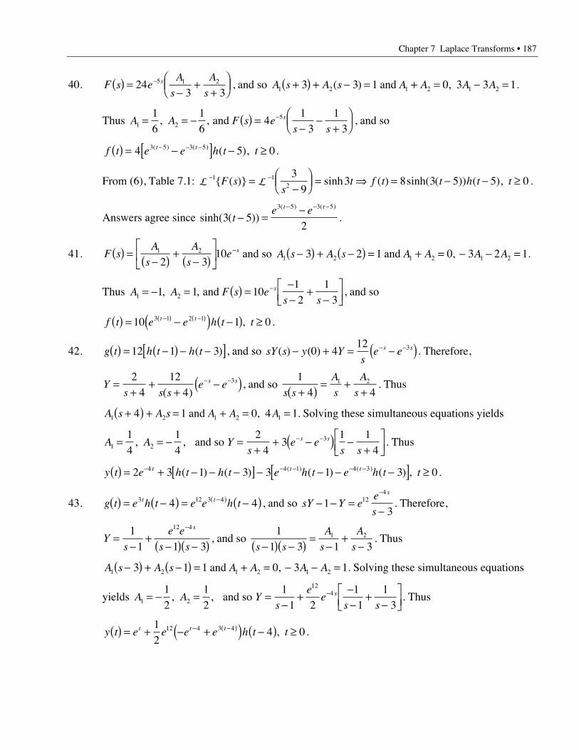
Chapter 7 Laplace Transforms • 187
40. F s eA
s
A
ss( ) =
-+
+ÊËÁ
ˆ¯
-243 3
5 1 2 , and so A s A s A A A A1 2 1 2 1 23 3 1 0 3 3 1+( ) + - = + = - =( ) , and .
Thus A A F s es s
s1 2
516
16
41
31
3= = - ( ) =
--
+ÊËÁ
ˆ¯
-, , and , and so
f t e e h t tt t( ) = -[ ] - ≥- - -4 5 03 5 3 5( ) ( ) ( ), .
From (6), Table 7.1: L L- -=
-ÊËÁ
ˆ¯ = fi = - - ≥1 1
2
39
3 8 3 5 5 0{ ( )} sinh ( ) sinh( ( )) ( ), F ss
t f t t h t t .
Answers agree since sinh( ( ))( ) ( )
3 52
3 5 3 5
te et t
- =-- - -
.
41. F sA
s
A
se s( ) =
-( ) +-( )
È
ÎÍ
˘
˚˙
-1 2
2 310 and so A s A s A A A A1 2 1 2 1 23 2 1 0 3 2 1-( ) + -( ) = + = - - = and , .
Thus A A F s es s
s1 21 1 10
12
13
= - = ( ) =--
+-
ÈÎÍ
˘˚
-, , and , and so
f t e e h t tt t( ) = -( ) -( ) ≥-( ) -( )10 1 03 1 2 1 , .
42. g t h t h t( ) = -( ) - -[ ]12 1 3( ) , and so sY s y Ys
e es s( ) ( )- + = -( )- -0 412 3 . Therefore,
Ys s s
e es s=+
++
-( )- -24
124
3
( ), and so
14 4
1 2
s s
A
s
A
s+( ) = ++
. Thus
A s A s A A A1 2 1 2 14 1 0 4 1+( ) + = + = = and , . Solving these simultaneous equations yields
A A1 2
14
14
= = -, , and so Ys
e es s
s s=+
+ -( ) -+
ÈÎÍ
˘˚
- -24
31 1
43 . Thus
y t e h t h t e h t e h t tt t t( ) = + - - -[ ] - - - -[ ] ≥- - - - -2 3 1 3 3 1 3 04 4 1 4 3( ) ( ) ( ) ( ) , ( ) ( ) .
43. g t e h t e e h tt t( ) = -( ) = -( )-( )3 12 3 44 4 , and so sY Y ee
s
s
- - =-
-
13
124
. Therefore,
Ys
e e
s s
s
=-
+-( ) -( )
-11 1 3
12 4
, and so 1
1 3 1 31 2
s s
A
s
A
s-( ) -( ) =-
+-
. Thus
A s A s A A A A1 2 1 2 1 23 1 1 0 3 1-( ) + -( ) = + = - - = and , . Solving these simultaneous equations
yields A A1 2
12
12
= - =, , and so Ys
ee
s ss=
-+
--
+-
ÈÎÍ
˘˚
-11 2
11
13
124 . Thus
y t e e e e h t tt t t( ) = + - +( ) -( ) ≥- -( )12
4 012 4 3 4 , .
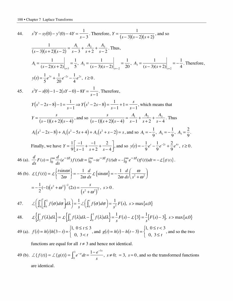
188 • Chapter 7 Laplace Transforms
44. s Y sy y Ys
2 0 0 41
3- ( ) - ¢ - =
-( ) . Therefore, Y
s s s=
-( ) -( ) +( )1
3 2 2, and so
13 2 2 3 2 2
1 2 3
s s s
A
s
A
s
A
s-( ) +( ) -( ) =-
++
+-
. Thus,
As s
As s
As ss s s
13
22
32
12 2
15
13 2
120
13 2
14
=- +
= =- -
= =- +
= -= = - =( )( )
, ( )( )
, ( )( )
. Therefore,
y t e e e tt t t( ) = + - ≥-15
120
14
03 2 2 , .
45. s Y s sY Ys
2 0 1 2 0 81
1- ( ) - - -( ) - =
-. Therefore,
Y s ss
Y s ss
s
s2 22 8 1
11
2 81
11
1- -( ) - =
-fi - -( ) =
-+ =
-, which means that
Ys
s s s=
-( ) +( ) -( )1 2 4, and so
s
s s s
A
s
A
s
A
s-( ) +( ) -( ) =-
++
+-1 2 4 1 2 4
1 2 3 . Thus
A s s A s s A s s s12
22
322 8 5 4 2- -( ) + - +( ) + + -( ) = , and so A A A1 2 3
19
19
29
= - = - =, , .
Finally, we have Ys s s
=--
+-+
+-
ÈÎÍ
˘˚
19
11
12
24
, and so y t e e e tt t t( ) = - - + ≥-19
19
29
02 4 , .
46 (a).d
dsF s
d
dse st f t dt te st f t dt e st tf t dt tf t( ) ( ) ( ) ( ) ( ( )) ( )= -•Ú = - -•Ú -•Ú = -= - { }0 0 0 L .
46 (b). L L L{ ( )}sin
sinf tt t d
dst
d
ds s= Ï
ÌÓ
¸˝˛
= - { } = -+
ÊËÁ
ˆ¯
ww w
ww
ww2
12
12 2 2
= - - +( ) =+( )
>-1
21 2 02 2 2
2 2 2( ) ( ) , s ss
ssw
w.
47. L Lf d ds
f ds
F s s at t
s s l s sl ( )È
Î͢˚
ÊË
ˆ¯ = ( )Ê
ˈ¯ = ( ) > { }ÚÚ Ú00 0 2
1 10, max ,
48. L L Lf d f d f ds
F ss
F s s at t
l l l l l l( ){ } = ( ) - ( ){ } = ( ) - { } = ( ) -[ ] > { }Ú ÚÚ2 0
2
0
13
13 0, max ,
49 (a). f t h t h tt
t( ) = ( ) -( ) =
£ £<
ÏÌÓ
31 0 3
0 3
,
, , and g t h t h t
t
t( ) = ( ) - -( ) =
£ <£
ÏÌÓ
31 0 3
0 3
,
, , and so the two
functions are equal for all t π 3 and hence not identical.
49 (b). L L{ ( )} { ( )} , ; , f t g t e dte
ss sst
s
= = =-
π = =--
Ú0
3 310 3 0, and so the transformed functions
are identical.
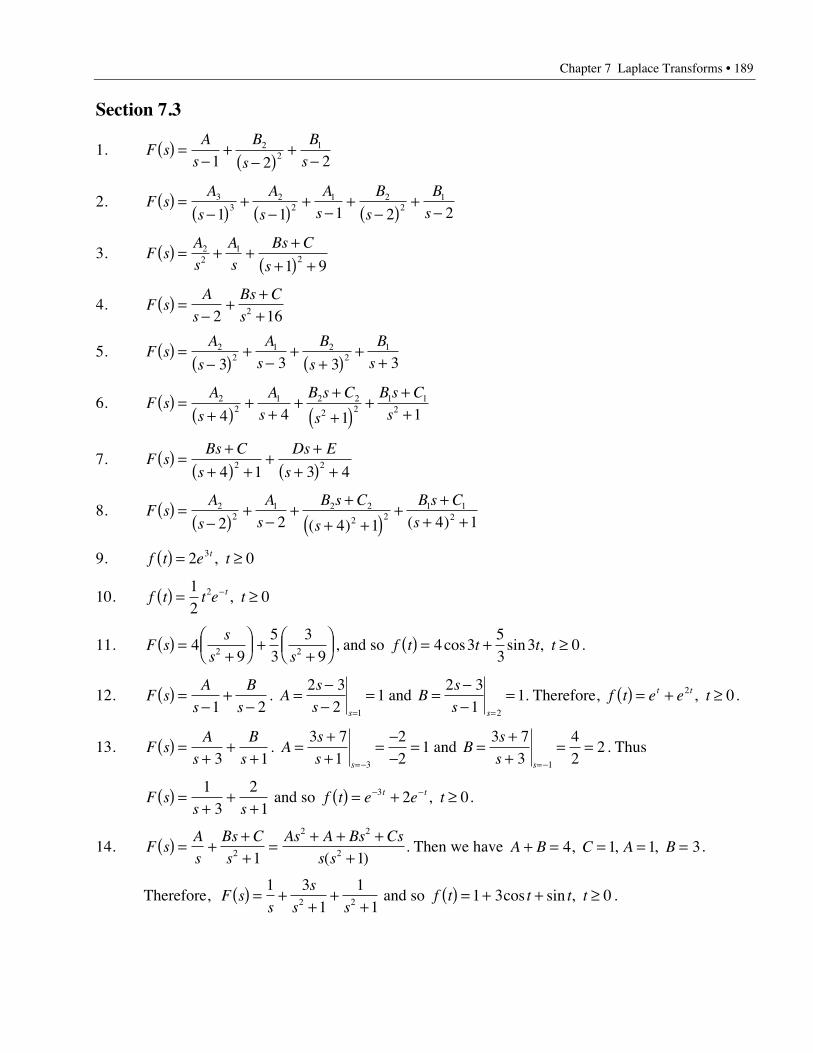
Chapter 7 Laplace Transforms • 189
Section 7.3
1. F sA
s
B
s
B
s( ) =
-+
-( )+
-1 2 22
21
2. F sA
s
A
s
A
s
B
s
B
s( ) =
-( )+
-( )+
-+
-( )+
-3
32
21 2
21
1 1 1 2 2
3. F sA
s
A
s
Bs C
s( ) = + +
++( ) +
22
12
1 9
4. F sA
s
Bs C
s( ) =
-+
++2 162
5. F sA
s
A
s
B
s
B
s( ) =
-( )+
-+
+( )+
+2
21 2
21
3 3 3 3
6. F sA
s
A
s
B s C
s
B s C
s( ) =
+( )+
++
++( )
+++
22
1 2 2
2 21 1
24 4 1 1
7. F sBs C
s
Ds E
s( ) =
++( ) +
++
+( ) +4 1 3 42 2
8. F sA
s
A
s
B s C
s
B s C
s( ) =
-( )+
-+
++ +( )
++
+ +2
21 2 2
2 21 1
22 2 4 1 4 1( ) ( )
9. f t e tt( ) = ≥2 03 ,
10. f t t e tt( ) = ≥-12
02 ,
11. F ss
s s( ) =
+ÊËÁ
ˆ¯ +
+ÊËÁ
ˆ¯4
953
392 2 , and so f t t t t( ) = + ≥4 3
53
3 0cos sin , .
12. F sA
s
B
s( ) =
-+
-1 2. A
s
s s
=-
-=
=
2 32
11
and Bs
s s
=-
-=
=
2 31
12
. Therefore, f t e e tt t( ) = + ≥2 0, .
13. F sA
s
B
s( ) =
++
+3 1. A
s
s s
=+
+=
--
== -
3 71
22
13
and Bs
s s
=+
+= =
= -
3 73
42
21
. Thus
F ss s
( ) =+
++
13
21
and so f t e e tt t( ) = + ≥- -3 2 0, .
14. F sA
s
Bs C
s
As A Bs Cs
s s( ) = +
++
=+ + +
+2
2 2
21 1( ). Then we have A B C A B+ = = = =4 1 1 3, , , .
Therefore, F ss
s
s s( ) = +
++
+1 3
11
12 2 and so f t t t t( ) = + + ≥1 3 0cos sin , .
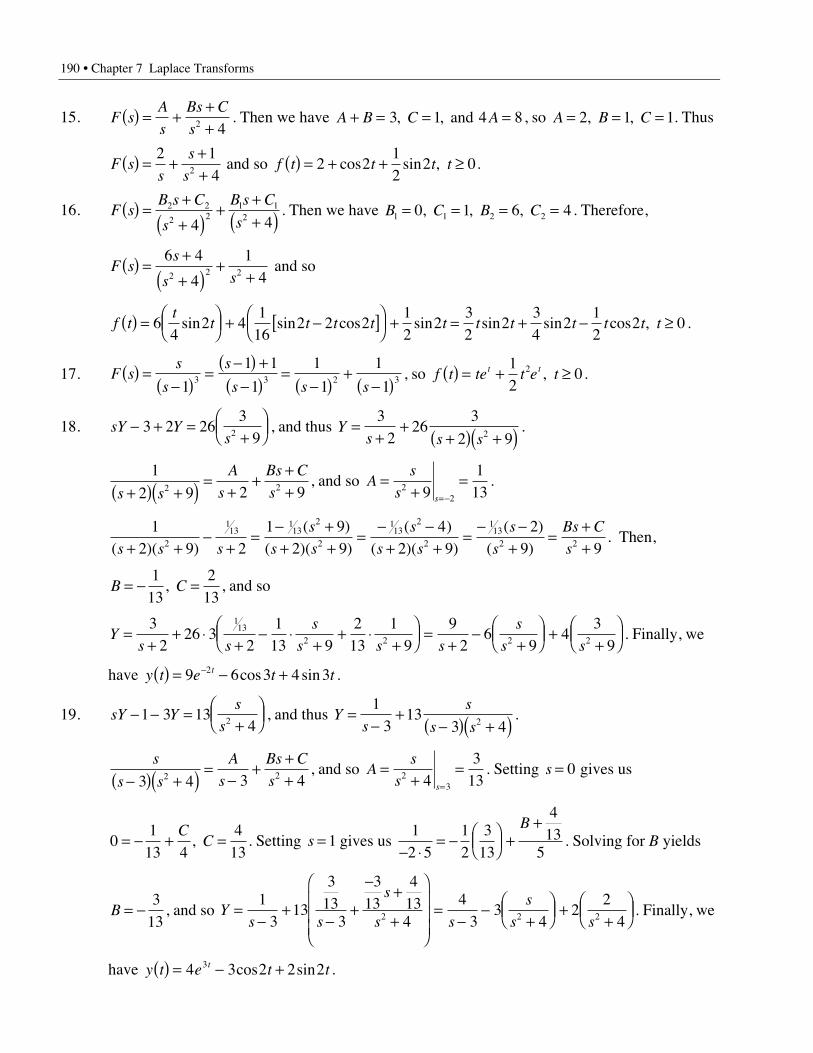
190 • Chapter 7 Laplace Transforms
15. F sA
s
Bs C
s( ) = +
++2 4
. Then we have A B C A+ = = =3 1 4 8, , and , so A B C= = =2 1 1, , . Thus
F ss
s
s( ) = +
++
2 142 and so f t t t t( ) = + + ≥2 2
12
2 0cos sin , .
16. F sB s C
s
B s C
s( ) =
++( )
+++( )
2 2
2 21 12
4 4. Then we have B C B C1 1 2 20 1 6 4= = = =, , , . Therefore,
F ss
s s( ) =
++( )
++
6 4
4
142 2 2 and so
f tt
t t t t t t t t t t t( ) = ÊËÁ
ˆ¯ + -[ ]Ê
ËÁˆ¯ + = + - ≥6
42 4
116
2 2 212
232
234
212
2 0sin sin cos sin sin sin cos , .
17. F ss
s
s
s s s( ) =
-( )=
-( ) +-( )
=-( )
+-( )1
1 1
1
1
1
1
13 3 2 3 , so f t te t e tt t( ) = + ≥
12
02 , .
18. sY Ys
- + =+
ÊËÁ
ˆ¯3 2 26
392 , and thus Y
s s s=
++
+( ) +( )3
226
3
2 92.
1
2 9 2 92 2s s
A
s
Bs C
s+( ) +( ) =+
+++
, and so As
s s
=+
== -
229
113
.
12 9 2
1 92 9
42 9
29 92
113
113
2
2
113
2
2
113
2 2( )( )( )
( )( )( )
( )( )( )
( )s s s
s
s s
s
s s
s
s
Bs C
s+ +-
+=
- ++ +
=- -
+ +=
- -+
=++
. Then,
B C= - =1
132
13, , and so
Ys s
s
s s s
s
s s=
++ ◊
+- ◊
++ ◊
+ÊËÁ
ˆ¯ =
+-
+ÊËÁ
ˆ¯ +
+ÊËÁ
ˆ¯
32
26 32
113 9
213
19
92
69
43
9
113
2 2 2 2 . Finally, we
have y t e t tt( ) = - +-9 6 3 4 32 cos sin .
19. sY Ys
s- - =
+ÊËÁ
ˆ¯1 3 13
42 , and thus Ys
s
s s=
-+
-( ) +( )1
313
3 42.
s
s s
A
s
Bs C
s-( ) +( ) =-
+++3 4 3 42 2 , and so A
s
s s
=+
==
234
313
. Setting s = 0 gives us
01
13 44
13= - + =
CC, . Setting s = 1 gives us
12 5
12
313
413
5- ◊= - Ê
ËÁˆ¯ +
+B. Solving for B yields
B = -3
13, and so Y
s s
s
s s
s
s s=
-+
-+
-+
+
Ê
Ë
ÁÁÁ
ˆ
¯
˜˜˜
=-
-+
ÊËÁ
ˆ¯ +
+ÊËÁ
ˆ¯
13
13
313
3
313
4134
43
34
22
42 2 2 . Finally, we
have y t e t tt( ) = - +4 3 2 2 23 cos sin .
Chapter 7 Laplace Transforms • 191
20. sY Ys
- + =3 242 , and thus Y
s s s
s
s s
A
s
B
s
C
s=
++
+=
++
= + ++
32
42
3 42 22
2
2 2( ) ( ), and so
Cs
sA
s
ss s
=+
= =+
+=
= - =
3 44
3 42
22
2
2
2
0
, . Setting s = 1 gives us 73
243
1= + + fi = -B B .
Therefore, Ys s s
= - ++
2 1 422 . Finally, we have y t e tt( ) = + --4 2 12 .
21. sY Ys
- - =-
1 31
3, so Y
s s=
-+
-( )1
31
32 and thus y t e tet t( ) = +3 3 .
22. s Y s sY Ys
2 1 2 3 1 26
1- - + - + =
+( ) ( ) , and thus Y
s
s s s s=
++ +
++ +
51 2
61 22( )( ) ( ) ( )
.
s s
s s
A
s
B
s
C
s
2
2 2
6 111 2 2 1 1
+ ++ +
=+
++
++( )( ) ( )
, and so
As s
sC
s s
ss s
=+ +
+= =
+ ++
== - = -
2
2
2
2
1
6 111
36 11
26
( ), . Setting s = 0 gives us
112
32
6 2= + + fi = -B B . Therefore, Ys s s
=+
-+
++
32
21
61 2( )
. Finally, we have
y t e e tet t t( ) = - +- - -3 2 62 .
23. s Y s Ys
222 6 4
8- ( ) - + = , so Y
s
s s s=
++
++( )
2 64
8
42 2 2.
If 8
4 42 2 2 2s s
A
s
B
s
Cs D
s( )+= + +
++
, then A s Bs s Cs Ds
s s s s
2 2 3 2
2 2 2 2
4 4
4
8
4
+( ) + +( ) + ++( ) =
+( ) , and so
we have B C A D B A+ = + = = =0 0 4 0 4 8, , , , which means that B C A D= = = = -0 2 2, , .
Then Ys
s s s s=
+ÊËÁ
ˆ¯ +
+ÊËÁ
ˆ¯ + -
+ÊËÁ
ˆ¯2
43
24
2 242 2 2 2 and y t t t t( ) = + +2 2 2 2 2cos sin .
24. s Y s Ys
s2
21 1 44
- ( ) - + =+
, so Ys
s
s
s=
++
++( )
14 4
2 2 2 . Therefore,
y t t tt
t( ) = + +cos sin sin212
24
2 .
25. s Y s Ys
221 0 42
4- ( ) - + =
+, so Y
s
s s=
++
+( )2 2 242
4. Therefore,
y t t t t t t tt
t( ) = +◊
-( ) = + -cos sin cos cos sin cos22
2 82 2 2 2
18
24
2 .
192 • Chapter 7 Laplace Transforms
26. s Y s sY Ys
2 0 0 2 01
2- - - - + =
-( ) ( ) , and thus Y
s s
A
s
B
s
C
s=
- -=
-+
-+
-( )1
2 1 2 1 12 2( )( ), and
so As
Css s
=-
= =-
= -= =
11
11
212
2 1( ), . Setting s = 0 gives us - = - - - fi = -
12
12
1 1B B .
Therefore, Ys s s
=-
--
--
12
11
11 2( )
. Finally, we have y t e e tet t t( ) = - -2 .
27. s Y sY Ys
2 1 2 01
1- + - + =
+, so Y
s s=
+( )+
+( )1
1
1
12 3 . Therefore, y t te
tet t( ) = +- -
2
2.
28. g t h t h t( ) = - -( )[ ]6 ( ) p , and then we have s Y s Ys
e s2 1 3 96
1- ( ) - + = -( )-p , so
Ys
s s se s=
++
++( ) -( )-3
96
912 2
p . 6
9 99
92 2
2 2
2s s
A
s
Bs C
s
As A Bs Cs
s s+( ) = +++
=+ + +
+( ) . Thus
A B C A B+ = = = = -0 023
23
, , , , and so Ys
s s s
s
se s=
++
++ - ◊
+ÊËÁ
ˆ¯ -( )-
2 2
23
293
923 9
1 p . Then,
y t t t t t h t( ) = + + -( ) - - -( ) -cos sin cos cos ( ) ( )3 323
1 323
1 3 p p
= + + -( ) - +( ) -cos sin cos cos ( )3 323
1 323
1 3t t t t h t p .
29. g t t h t t t h t h t( ) = - -( )[ ] = - - - - -1 2 2 2 2 2( ) ( ) ( ) , and then we have
s Y s Ys s
es
es s22 2
2 21 01 1 2
- ( ) - + = - -- - , so Ys
s s se
s ses s=
++
+( ) -( ) -+( )
- -2 2 2
22
2
11
11
2
1.
1
1
1 112 2 2 2s s s s+( ) = -
+ and
-+( ) = +
++
=+ + +
+( )2
1 1 12 2
2 2
2s s
A
s
Bs C
s
As A Bs Cs
s s. Thus
A B C A B+ = = = - fi =0 0 2 2, , , and so
Ys
s s se
s
s
ses s=
++ -
+ÊËÁ
ˆ¯ -( ) + - +
+ÊËÁ
ˆ¯
- -2 2 2
22
2
11 1
11
2 21
. The inverse Laplace transform yields
y t t t t h t t t h t h t t h t( ) = + - -( ) -( ) - + -( ) -( ) - -( ) + -( ) -( )cos sin sin cos2 2 2 2 2 2 2 2 2= - + + - -( ) + -( ) - + -( )[ ] -( )cos sin sin cost t t t t t h t2 2 2 2 2 2
= - + + - + -( ) + -( )[ ] -( )cos sin sin cost t t t t t h t2 2 2 2 .
30. s Y sy y sY y Y Ysy y y
s s
s
s s2
0 0 00 0 0
2 202 1
2- - ¢ + - + = fi =
+ ¢ +( )+ +
=-
+ +a b
aa b
( ) , so
a b a= = = ¢ + = ¢ + = - fi ¢ = -1 2 2 1 2 1 30 0 0 0 0, , , ( )y y y y y .
31.sy y y
s s s0 0 0
2 2
34
+ ¢ +( )+ +
=-
aa b
, so a b= = - = ¢ =0 4 0 30 0, , , y y .
Chapter 7 Laplace Transforms • 193
32.sy y y
s s
s
s0 0 0
2 21
+ ¢ +( )+ +
=+
aa b ( )
, so a b= = = ¢ = -2 1 1 20 0, , , y y .
Section 7.4
1. T e dt e dte
s
e
s se e est st
st sts s s= - =
--
-
È
ÎÍÍ
˘
˚˙˙
= - + -[ ]- -- -
- - -Ú Ú4 3 3 33
10
2
2
4
0
2
2
4
2 4 2. = -( )-31 2 2
se s .
Therefore, L{ }fs
e
e s
e
e
s
s
s
s=-( )-
=-+
ÊËÁ
ˆ¯
-
-
-
-3 1
13 1
1
2 2
4
2
2 .
2. T e dt e dte
s
e
s se e est st
st sts s s= + =
-+
-= - + -( )- -
- -- - -Ú Ú2 3 3
13 3
0
1
1
2
0
1
1
2
2. = - -( )- -13 2 2
se es s .
Therefore, L{ }( ) ( )
fe e
s e
e
s e
s s
s
s
s=- -
-=
- +-
- -
-
-
-3 2
131
2
2 .
3. T e dt e dts
es
est st st st= - + = -- - - -Ú Ú4 3 23 2
0
2
2
4
0
2
2
4
. = -( ) - -( )- - -31
22 4 2
se
se es s s
= - + -( )- -12 5 34 2
se es s . Therefore, L{ }f
e e
s e
e
s e
s s
s
s
s=
- + --( ) =
- ++( )
- -
-
-
-
2 5 3
1
3 2
1
4 2
4
2
2.
4. T e dt e dte
s
e
s se e est st
st sts s s= + =
-+
-= - + -( )- -
- -- - -Ú Ú4 2 2
12 2
0
1
1
3
0
1
1
3
3. = - -( )- -12 3
se es s .
Therefore, L{ }( ) ( )( )
fe e
s e
e e
s e e
s s
s
s s
s s=- -
-=
+ ++ +
- -
-
- -
- -2
12
1 1
3
4
2
2 .
5. T te dt t e dts
st es
st es
est st st st st= + -( ) = - +( ) + +( ) +-
- - - - -Ú Ú2 21
11
12
0
1
1
2
20
1
21
2
1
2
.
= - +( ) -[ ] + +( ) - +( )[ ] + -[ ]- - - - -11 1
12 1 1
22 2
2 2
ss e
ss e s e
se es s s s s = -( )-1
12
2
se s . Therefore,
L{ }fs
e
e
e
s e
s
s
s
s=
-( )-
=-
+( )-
-
-
-
1 1
11
12
2
2 2.
6. T t e dt ue du e ue due
ssu e
e
ss est s u s su
ssu
ss= -( ) = = =
-+ =
-+ -[ ]- - + - -
--
--Ú Ú Ú2 1 1 1 1
1
21
0
1
0
1
2
0
1
2. ( ) ( )( ) .
Therefore, L{ }( )
fe s e
s e
s s
s=
- +[ ]-( )
- -
-
1 1
12 2.
194 • Chapter 7 Laplace Transforms
7. T t e dts
s t st s est st= -( ) = + + -[ ]- -Ú2 11
2 22
0
1
32 2 2
0
1
.
= + + -( ) - +[ ]-12 2 23
2 2 2
ss s s e ss = +( ) + -[ ]-1
2 2 232
ss e ss . Therefore,
L{ }fs e s
s e
s
s=
+( ) + -( )[ ]-( )
-
-
2 2 2
1
2
3 2.
8. T te dts
st es
s est st s= =-
+ =-
+ -[ ]- - -Ú21
11
2 1 10
2
20
2
22. ( ) ( ) . Therefore, L{ }
( )f
s e
s e
s
s=
- +-( )
-
-
1 2 1
1
2
2 2.
9. T fe
s e
s
s=
p=
+
+( ) -ÊËÁ
ˆ¯
-p
-p2
2 2
4 1
2
2 2
, { }L
10. T fe
s e s e
s
s s= =
++( ) -( ) =
+( ) -( )-
- -21
1 1
1
1 12 2 2pp
p p, { }L
11. T e e dte
s se f
e
s et st
s ts
s
s= = -
+=
+-( ) =
-+( ) -( )
- -- +( )
- +( )- +( )
-Ú11
11
11
1 10
1 1
0
1
11
, , { }L .
12. T e e dte
s
e
s se
set st
st s ts s= - =
-+
+= -( ) -
+-( )- -
- - +( )- - +( )Ú2 1
11
11
11
0
2
0
2 1
0
2
2 2 1, ( )
L{ }fs
e
s e
s
s= -
-+( ) -( )
- +( )
-
1 1
1 1
2 1
2.
13. L L-
-
--
-- - -
-( )Ê
ËÁ
ˆ
¯˜ = + + + +( )Ê
ËÁˆ¯
1 1 2 3
11
e
s e
e
se e e
s
s
ss s s
a
a
aa a a ...
= + + +ÊËÁ
ˆ¯
= -( ) + -( ) +-- - -
L1
2 3
2e
s
e
s
e
sh t h t
s s sa a a
a a... ...,
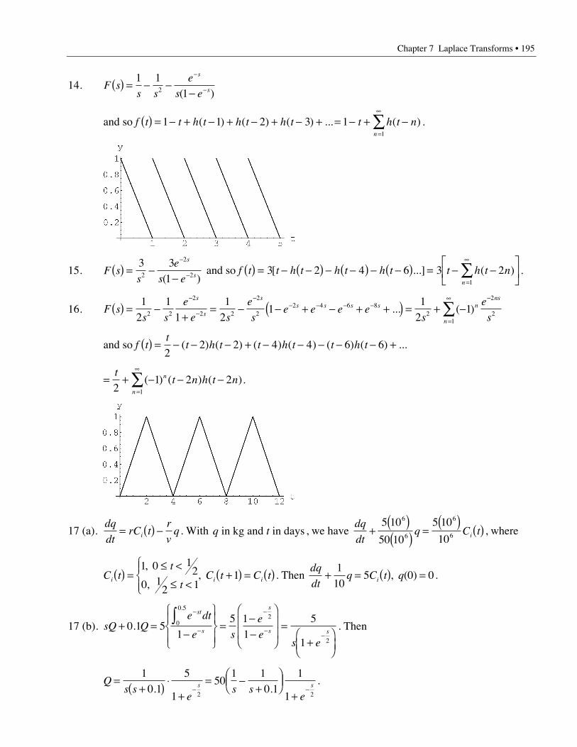
Chapter 7 Laplace Transforms • 195
14. F ss s
e
s e
s
s( ) = - --
-
-1 1
12 ( )
and so f t t h t h t h t t h t nn
( ) = - + - + - + - + = - + -=
•
Â1 1 2 3 11
( ) ( ) ( ) ... ( ) .
15. F ss
e
s e
s
s( ) = --
-
-3 3
12
2
2( ) and so f t t h t h t h t t h t n
n
( ) = - -( ) - -( ) - -( ) = - -È
ÎÍ
˘
˚˙
=
•
Â3 2 4 6 3 21
[ ...] ( ) .
16. F ss s
e
e s
e
se e e e
s
e
s
s
s
ss s s s n
n
ns
( ) = -+
= - - + - + +( ) = + --
-
-- - - -
=
• -
Â12
11
12
11
212 2
2
2 2
2
22 4 6 8
21
2
2... ( )
and so f tt
t h t t h t t h t( ) = - - - + - - - - - +2
2 2 4 4 6 6( ) ( ) ( ) ( ) ( ) ( ) ...
= + - - -=
•
Âtt n h t nn
n21 2 2
1
( ) ( ) ( ).
17 (a).dq
dtrC t
r
vqi= ( ) - . With q t in kg and in days , we have
dq
dtq C ti+
( )( ) =
( ) ( )5 10
50 10
5 10
10
6
6
6
6 , where
C tt
tC t C ti i i( ) =
£ <
£ <
ÏÌÔ
ÓÔ+( ) = ( )
1 0 12
0 12 1
1,
, , . Then
dq
dtq C t qi+ = ( ) =
110
5 0 0, ( ) .
17 (b). sQ Qe dt
e s
e
es e
st
s
s
s s+ =
-
ÏÌÔ
ÓÔ
¸˝Ô
Ô=
--
Ê
Ë
ÁÁ
ˆ
¯
˜˜
=+
ÊËÁ
ˆ¯
-
-
-
--
Ú0 1 5
15 1
15
1
0
0 52
2
.
.
. Then
Qs s
es s
es s=
+( ) ◊+
= -+
ÊËÁ
ˆ¯
+- -
10 1
5
150
1 10 1
1
12 2. .
.
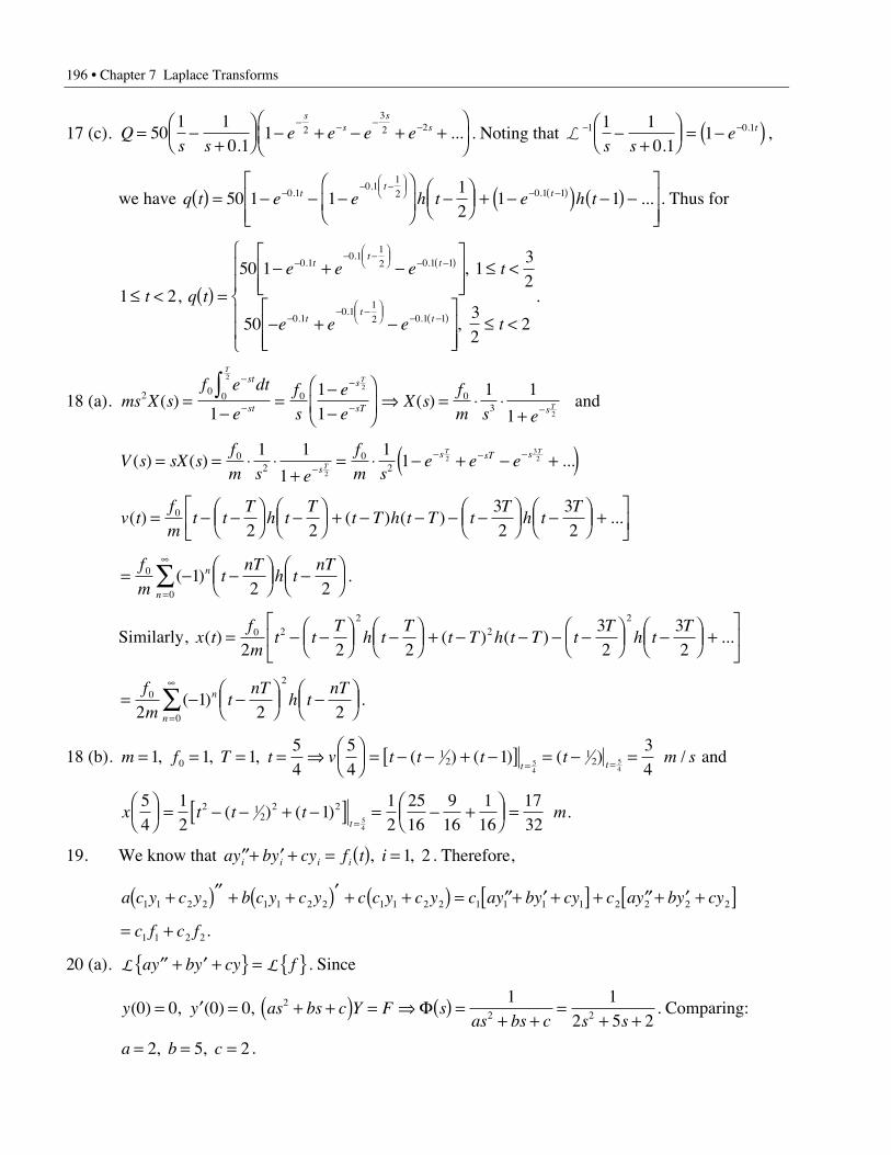
196 • Chapter 7 Laplace Transforms
17 (c). Qs s
e e e es
ss
s= -+
ÊËÁ
ˆ¯ - + - + +
ÊËÁ
ˆ¯
- - - -501 1
0 11 2
3
2 2
.... . Noting that L
- --+
ÊËÁ
ˆ¯ = -( )1 0 11 1
0 11
s se t
.. ,
we have q t e e h t e h ttt
t( ) = - - -Ê
ËÁˆ
¯-Ê
ËÁˆ¯ + -( ) -( ) -
È
ÎÍÍ
˘
˚˙˙
-- -Ê
ËÁˆ¯ - -( )50 1 1
12
1 10 10 1
1
2 0 1 1..
. ... . Thus for
1 2£ <t , q t
e e e t
e e e t
tt
t
tt
t
( ) =- + -
È
ÎÍÍ
˘
˚˙˙
£ <
- + -È
ÎÍÍ
˘
˚˙˙
£ <
Ï
Ì
ÔÔ
Ó
ÔÔ
-- -Ê
ËÁˆ¯ - -( )
-- -Ê
ËÁˆ¯ - -( )
50 1 132
5032
2
0 10 1
1
2 0 1 1
0 10 1
1
2 0 1 1
..
.
..
.
,
,
.
18 (a). ms X sf e dt
e
f
s
e
eX s
f
m s e
st
st
s
sT s
TT
T
2 0 0 0 03
22
2111
1 1
1( ) ( )=
-=
--
Ê
ËÁˆ
¯fi = ◊ ◊
+
-
-
-
- -
Ú and
V s sX sf
m s e
f
m se e e
s
s sT sT
T T
( ) ( ) ...= = ◊ ◊+
= ◊ - + - +( )-- - -0
20
2
1 1
1
11
2
232
v tf
mt t
Th t
Tt T h t T t
Th t
T( ) ( ) ( ) ...= - -Ê
ËÁˆ¯ -Ê
ËÁˆ¯ + - - - -Ê
ËÁˆ¯ -Ê
ËÁˆ¯ +
ÈÎÍ
˘˚
0
2 232
32
= - -ÊËÁ
ˆ¯ -Ê
ËÁˆ¯=
•
Âf
mt
nTh t
nTn
n
0
0
12 2
( ) .
Similarly, x tf
mt t
Th t
Tt T h t T t
Th t
T( ) ( ) ( ) ...= - -Ê
ËÁˆ¯ -Ê
ËÁˆ¯ + - - - -Ê
ËÁˆ¯ -Ê
ËÁˆ¯ +
È
ÎÍ
˘
˚˙0 2
22
2
2 2 232
32
= - -ÊËÁ
ˆ¯ -Ê
ËÁˆ¯=
•
Âf
mt
nTh t
nTn
n
0
2
021
2 2( ) .
18 (b). m f T t v t t t t m st t= = = = fi Ê
ËÁˆ¯ = - - + -[ ] = - =
= =1 1 154
54
1340
12
125
454
, , , ( ) ( ) ( ) / and
x t t t mt
54
12
112
2516
916
116
1732
2 12
2 254
ÊËÁ
ˆ¯ = - - + -[ ] = - +Ê
ËÁˆ¯ =
=( ) ( ) .
19. We know that ay by cy f t ii i i i¢¢+ ¢ + = ( ) =, , 1 2 . Therefore,
a c y c y b c y c y c c y c y c ay by cy c ay by cy1 1 2 2 1 1 2 2 1 1 2 2 1 1 1 1 2 2 2 2+( )¢¢ + +( )¢ + +( ) = ¢¢+ ¢ +[ ] + ¢¢ + ¢ +[ ]= +c f c f1 1 2 2.
20 (a). L Lay by cy f¢¢ + ¢ +{ } = { }. Since
y y as bs c Y F sas bs c s s
( ) , ( ) , 0 0 0 01 1
2 5 22
2 2= ¢ = + +( ) = fi ( ) =+ +
=+ +
F . Comparing:
a b c= = =2 5 2, , .
Chapter 7 Laplace Transforms • 197
20 (b). If f t e F ss
Y ss s s
t( ) , ( ) , ( )( )
= =+
=+ +( ) +
- 11
1
2 5 2 12. Since
2 5 2 2 212
12 1
12 2 1
2 12 1
21
2
s s s s Y ss s s
A
s
B
s
C
s+ + = + + =
+( ) + +È
ÎÍ
˘
˚˙ =
++
++
+ÈÎÍ
˘˚
( )( ), ( )( )( )
. Then
As s
Bs s
Cs ss s s
=+ +
= =+ +
= - =+ +
== - = - = -
11
23
12
21
2 1431
2 21
2 1 12
( )( ),
( )( ),
( )( ) and
y t e e et t t
( ) = - +- - -13
23
2 2 .
21. f t t( ) = , F ss
( ) =12 , y t e t et t( ) = -( ) + +( )- -2 1 1 ,
Y ss s s s
s s s s
s s s s( ) =
+- +
+( )+ =
- +( ) + + ++( )
=+( )
21
2 1
1
1 2 2 2 1
1
1
12 2
2 2
2 2 2 2 . Since Y s s F s( ) = ( ) ( )F ,
F ss
( ) =+( )1
12 .
22. From 21, F ss
( ) =+( )1
12 . If f t h t F s
sY s
s s
A
s
B
s
C
s( ) ( ), ( ) ( )
( ) ( )= = =
+= +
++
+1 1
1 1 12 2 and
As
Css s
=+
= = = -= = -
11
11
120 1( )
, . Setting sB
B= = + - fi = -114
12
14
1, . Therefore,
Y ss s s
y t e tet t( )( )
( )= -+
-+
fi = - -- -1 11
11
12 .
23 (a). s Y Y F2 4+ = , so F =+( )1
42s.
23 (b). Fs
Ys s
= =+( )
2 2
43 3 2, so .
24 (a). s Y sY Y F2 + + = , so F =+ +( )1
12s s.
24 (b). e f t dt e dt e dte
s
e
s se
se e
sest st st
st sts s s s- - -
- -- - - -= - =
--
-= - + - = -Ú Ú Ú( ) ( ) ( ) ( )
0
2
0
1
0
1
1
2
1
22 21
11 1
1 .
Therefore, Fe
s e
e
s eY
e
s e s s
s
s
s
s
s
s=-
--+
=-
+ + +
-
-
-
-
-
-( )( )
( )( )
( )( )( )
11
11
11 1
2
2 2= , so .
25 (a). s Y sY Y F2 4 4+ + = , so F =+ +( ) =
+( )1
4 4
1
22 2s s s.
198 • Chapter 7 Laplace Transforms
25 (b). te dts
st es
s est st s- - -Ú = - +( ) = - +( )[ ]0
1
20
1
2
11
11 1 , so F
s e
s eY
s e
s e s
s
s
s
s=
- +( )-( ) =
- +( )-( ) +( )
-
-
-
-
1 1
1
1 1
1 22 2 2 and .
26 (a). s Y Y F3 4- = , so F =-( )1
43s.
26 (b). Fs
s
s sY
s
s s s=
-+ -
-=
+ -- -
11
11
11 42 2 3+
1s
=s
, so s
2
2 2
( ) ( )( ).
27 (a). s Y sY F3 4+ = , so F =+( )1
43s s.
27 (b). Fs
sY
s
s s s s=
+=
+( ) +( ) =+( )2 2 3 2 24 4 4
1
4, so .
28. ¢¢ + ¢ + = fi - - ¢ + - + =y by cy f s Y sy y b sY y cY F2 0 0 0( ) ( ) ( ( )) . Therefore,
( )s bs c Y sy y by F Ysy y by
s bs c
F s
s bs c2
0 0 00 0 02 2+ + - - ¢ - = fi =
+ ¢ ++ +
+( )
+ +. If
f t h t F ss
Y ss y s y by
s bs cs
s s
s s s( ) = ( ) = fi =
+ ¢ + ++ +
=+ +
+ +( ), ( )
( )1 1 2 13 2
20 0 0
3 2
2
3 2 . Therefore,
b c y y by y y= = ¢ + = ¢ + = fi ¢ = -3 2 3 2 10 0 0 0 0, , =1, .
29. Ysy y by
s bs c
F s
s bs c=
+ ¢ ++ +
+( )
+ +0 0 02 2 . If f t e F s
st( ) = ( ) =
+- ,
11
and
s sy y by
s s bs c
s s
s s
+( ) + ¢ +( ) ++( ) + +( ) =
+ ++( ) +( )
1 1
1
1
1 40 0 0
2
2
2. Therefore,
b c s sy y s y sy sy y s s= = +( ) + ¢( ) + = + ¢ + + ¢ = + +0 4 1 1 10 02
0 0 0 02, , and . Finally, y y0 01 0= ¢ =, .
Section 7.5
1. L
cos t
t
te
s
s
s
s
t
È
Î
ÍÍÍ
˘
˚
˙˙˙
Ï
ÌÔ
ÓÔ
¸
˝Ô
˛Ô
=+
-( )
È
Î
ÍÍÍÍÍÍ
˘
˚
˙˙˙˙˙˙
2
2
2
11
1
1
2. L Ld
dt
e t
t e
sd
dt
e t
t e
s
s
s
s s
t
t
t
t
- -
+
È
Î
ÍÍÍ
˘
˚
˙˙˙
Ï
ÌÔ
ÓÔ
¸
˝Ô
˛Ô
=+
È
Î
ÍÍÍ
˘
˚
˙˙˙
Ï
ÌÔ
ÓÔ
¸
˝Ô
˛Ô
-È
Î
ÍÍÍ
˘
˚
˙˙˙
=
++ +
+-
È
Î
ÍÍÍÍÍ
˘
˚
˙˙
cos cos ( )2
0
2
0
1
0
1
11 40
1 11
2
2
˙˙˙
-È
Î
ÍÍÍ
˘
˚
˙˙˙
=
++ +
-
+-
-
È
Î
ÍÍÍÍÍ
˘
˚
˙˙˙˙˙
1
0
1
11 4
1
01
11
2
s s
s
s
s
s
( )( )
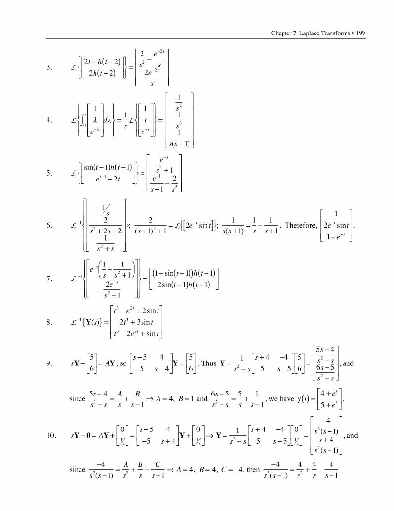
Chapter 7 Laplace Transforms • 199
3. L2 2
2 2
2
2
2
2
2
t h t
h ts
e
se
s
s
s
- -( )-( )
È
ÎÍ
˘
˚˙
ÏÌÔ
ÓÔ
¸˝ÔÔ
=-
È
Î
ÍÍÍÍ
˘
˚
˙˙˙˙
-
-
4. L L
11
1
1
1
11
0
2
3l lle
ds
t
e
s
s
s s
t
t- -
È
Î
ÍÍÍ
˘
˚
˙˙˙
Ï
ÌÔ
ÓÔ
¸
˝Ô
˛Ô
=È
Î
ÍÍÍ
˘
˚
˙˙˙
Ï
ÌÔ
ÓÔ
¸
˝Ô
˛Ô
=
+
È
Î
ÍÍÍÍÍÍ
˘
˚
˙˙˙˙˙˙
Ú
( )
5. Lsin t h t
e t
e
se
s s
t
s
-( ) -( )-
È
ÎÍ
˘
˚˙
ÏÌÔ
ÓÔ
¸˝ÔÔ
= +
--
È
Î
ÍÍÍÍ
˘
˚
˙˙˙˙
-
-
-
1 1
21
121
2
1
2
6. L L- -
+ +
+
È
Î
ÍÍÍÍÍÍ
˘
˚
˙˙˙˙˙˙
Ï
Ì
ÔÔÔ
Ó
ÔÔÔ
¸
˝
ÔÔÔ
˛
ÔÔÔ
+ += [ ]{ } +
= -+
12
2
2
1
22 21
21 1
21
11 1
1
s
s s
s s
se t
s s s st;
( )sin ;
( ). Therefore,
1
2
1
e t
e
t
t
-
--
È
Î
ÍÍÍ
˘
˚
˙˙˙
sin .
7. L-
-
-
-+
ÊËÁ
ˆ¯
+
È
Î
ÍÍÍÍ
˘
˚
˙˙˙˙
Ï
ÌÔÔ
ÓÔÔ
¸
˝ÔÔ
˛ÔÔ
=- -( )( ) -( )
-( ) -( )È
ÎÍ
˘
˚˙1
2
2
1 11
21
1 1 1
2 1 1
es s
e
s
t h t
t h t
s
s
sin
sin
8. L- { } =
- ++
- +
È
Î
ÍÍÍ
˘
˚
˙˙˙
1
3 2
3
3 2
2
2 3
2
Y( )
sin
sin
sin
s
t e t
t t
t e t
t
t
9. s AY Y-È
ÎÍ
˘
˚˙ =
5
6, so
s
s
-- +
È
ÎÍ
˘
˚˙ =
È
ÎÍ
˘
˚˙
5 4
5 4
5
6Y . Thus Y =
-+ -
-È
ÎÍ
˘
˚˙
È
ÎÍ
˘
˚˙ =
----
È
Î
ÍÍÍ
˘
˚
˙˙˙
1 4 4
5 5
5
6
5 4
6 52
2
2s s
s
s
s
s ss
s s
, and
since 5 4
14 12
s
s s
A
s
B
sA B
--
= +-
fi = =, and 6 5 5 1
12
s
s s s s
--
= +-
, we have y te
e
t
t( ) =
++
È
ÎÍ
˘
˚˙
4
5.
10. s As
s s s
s
ss s
s
s ss s s
Y 0 Y Y Y- = +È
ÎÍ
˘
˚˙ =
-- +
È
ÎÍ
˘
˚˙ +
È
ÎÍ
˘
˚˙ fi =
-+ -
-È
ÎÍ
˘
˚˙
È
ÎÍ
˘
˚˙ =
--
+-
È
Î
ÍÍÍÍ
˘
˚
˙˙˙˙
0 5 4
5 4
0 1 4 4
5 5
04
141
1 1 2 1
2
2
( )
( )
, and
since -
-= + +
-fi = = = -
41 1
4 4 42 2s s
A
s
B
s
C
sA B C
( ), , . then
--
= + --
41
4 4 412 2s s s s s( )
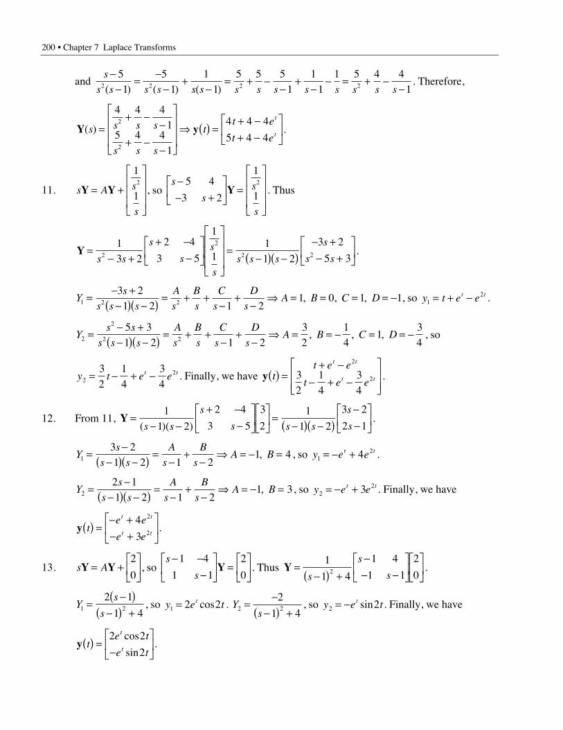
200 • Chapter 7 Laplace Transforms
and s
s s s s s s s s s s s s s s
--
=-
-+
-= + -
-+
-- = + -
-51
51
11
5 5 51
11
1 5 4 412 2 2 2( ) ( ) ( )
. Therefore,
Y y( )s s s s
s s s
tt e
t e
t
t=
+ --
+ --
È
Î
ÍÍÍ
˘
˚
˙˙˙
fi ( ) =+ -+ -
È
ÎÍ
˘
˚˙
4 4 41
5 4 41
4 4 4
5 4 4
2
2
.
11. s A s
s
Y Y= +
È
Î
ÍÍÍ
˘
˚
˙˙˙
1
12
, so s
ss
s
-- +
È
ÎÍ
˘
˚˙ =
È
Î
ÍÍÍ
˘
˚
˙˙˙
5 4
3 2
1
12
Y . Thus
Y =- +
+ --
È
ÎÍ
˘
˚˙
È
Î
ÍÍÍ
˘
˚
˙˙˙
=-( ) -( )
- +- +
È
ÎÍ
˘
˚˙
13 2
2 4
3 5
1
111 2
3 2
5 32
2
2 2s s
s
ss
ss s s
s
s s.
Ys
s s s
A
s
B
s
C
s
D
sA B C D1 2 2
3 21 2 1 2
1 0 1 1=- +
-( ) -( ) = + +-
+-
fi = = = = -, , , , so y t e et t1
2= + - .
Ys s
s s s
A
s
B
s
C
s
D
sA B C D2
2
2 2
5 31 2 1 2
32
14
134
=- +-( ) -( ) = + +
-+
-fi = = - = = -, , , , so
y t e et t2
232
14
34
= - + - . Finally, we have y tt e e
t e e
t t
t t( ) =+ -
- + -È
ÎÍÍ
˘
˚˙˙
2
232
14
34
.
12. From 11, Y =- -
+ --
È
ÎÍ
˘
˚˙
È
ÎÍ
˘
˚˙ =
-( ) -( )--
È
ÎÍ
˘
˚˙
11 2
2 4
3 5
3
21
1 2
3 2
2 1( )( )s s
s
s s s
s
s.
Ys
s s
A
s
B
sA B1
3 21 2 1 2
1 4=-
-( ) -( ) =-
+-
fi = - =, , so y e et t1
24= - + .
Ys
s s
A
s
B
sA B2
2 11 2 1 2
1 3=-
-( ) -( ) =-
+-
fi = - =, , so y e et t2
23= - + . Finally, we have
y te e
e e
t t
t t( ) =
- +- +
È
ÎÍ
˘
˚˙
4
3
2
2.
13. s AY Y= +È
ÎÍ
˘
˚˙
2
0, so
s
s
- --
È
ÎÍ
˘
˚˙ =
È
ÎÍ
˘
˚˙
1 4
1 1
2
0Y . Thus Y =
-( ) +-
- -È
ÎÍ
˘
˚˙
È
ÎÍ
˘
˚˙
1
1 4
1 4
1 1
2
02s
s
s.
Ys
s1 2
2 1
1 4=
-( )-( ) +
, so y e tt1 2 2= cos . Y
s2 2
2
1 4=
--( ) +
, so y e tt2 2= - sin . Finally, we have
y te t
e t
t
t( ) =
-È
ÎÍ
˘
˚˙
2 2
2
cos
sin.
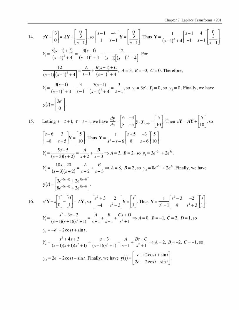
Chapter 7 Laplace Transforms • 201
14. s As
Y Y-È
ÎÍ
˘
˚˙ = +
-
È
ÎÍÍ
˘
˚˙˙
3
0
03
1, so
s
s s
- --
È
ÎÍ
˘
˚˙ =
-
È
ÎÍÍ
˘
˚˙˙
1 4
1 1
03
1Y . Thus Y =
-( ) +-
- -È
ÎÍ
˘
˚˙
-
È
ÎÍÍ
˘
˚˙˙
1
1 4
1 4
1 1
03
12
s
s
s s.
Ys
s
s
s s ss
1
121
2 2 2
3 1
1 4
3 1
1 4
12
1 1 4=
-( ) +-( ) +
=-( )
-( ) ++
- -( ) +[ ]-
( ). For
12
1 1 4 11
1 43 3 02 2
( )
( ), , , .
s s
A
s
B s C
sA B C
- -( ) +[ ] =-
+- +
-( ) += = - = Therefore,
Ys
s s
s
s s1 2 2
3 1
1 4
31
3 1
1 4
31
=-( )
-( ) ++
--
--( ) +
=-
( ), so y et
1 3= . Y2 0= , so y2 0= . Finally, we have
y tet
( ) =È
ÎÍ
˘
˚˙
3
0.
15. Letting t t= + = -t t1 1; , we have d
d
yy y
t t=--
È
ÎÍ
˘
˚˙ =
È
ÎÍ
˘
˚˙=
6 3
8 5
5
100, . Then s AY Y= +
È
ÎÍ
˘
˚˙
5
10, so
s
s
-- +
È
ÎÍ
˘
˚˙ =
È
ÎÍ
˘
˚˙
6 3
8 5
5
10Y . Thus Y =
- -+ -
-È
ÎÍ
˘
˚˙
È
ÎÍ
˘
˚˙
16
5 3
8 6
5
102s s
s
s.
Ys
s s
A
s
B
sA B1
5 53 2 2 3
3 2=-
-( ) +( ) =+
+-
fi = =, , so y e e12 33 2= +- t t .
Ys
s s
A
s
B
sA B2
10 203 2 2 3
8 2=-
-( ) +( ) =+
+-
fi = =, , so y e e22 38 2= +- t t .Finally, we have
y te e
e e
t t
t t( ) =
++
È
ÎÍ
˘
˚˙
- -( ) -( )
- -( ) -( )3 2
8 2
2 1 3 1
2 1 3 1.
16. s s A21
0
0
1Y Y-
È
ÎÍ
˘
˚˙ -
È
ÎÍ
˘
˚˙ = , so
s
s
s2
2
3 2
4 3 1
+- -
È
ÎÍ
˘
˚˙ =
È
ÎÍ
˘
˚˙Y . Thus Y =
-- -
+È
ÎÍ
˘
˚˙
È
ÎÍ
˘
˚˙
11
3 2
4 3 14
2
2s
s
s
s.
Ys s
s s s
A
s
B
s
Cs D
sA B C D1
3
2 2
3 21 1 1 1 1 1
0 1 2 1=- -
- + +=
++
-+
++
fi = = - = =( )( )( )
, , , , so
y e t tt1 2= - + +cos sin .
Ys s
s s s
s
s s
A
s
Bs C
sA B C2
2
2 2 2
4 31 1 1
31 1 1 1
2 2 1=+ +
- + +=
+- +
=-
+++
fi = = - = -( )( )( ) ( )( )
, , , so
y e t tt2 2 2= - -cos sin . Finally, we have y t
e t t
e t t
t
t( ) =
- + +- -
È
ÎÍ
˘
˚˙
2
2 2
cos sin
cos sin.
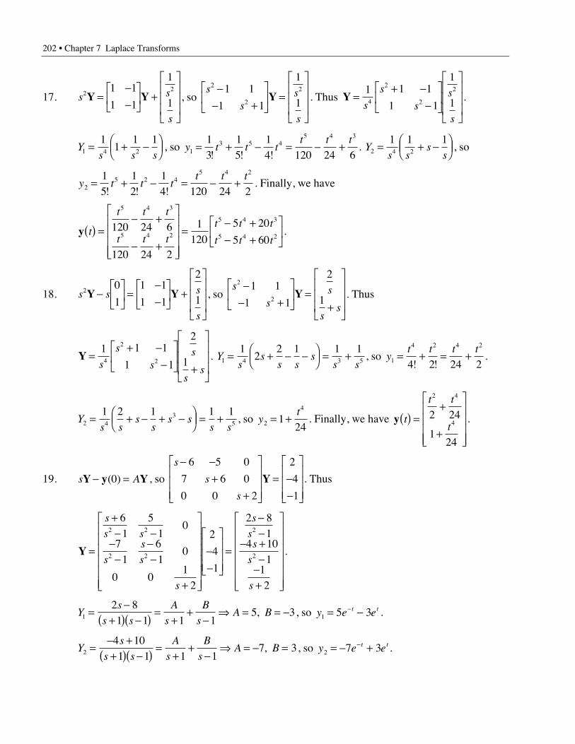
202 • Chapter 7 Laplace Transforms
17. s s
s
221 1
1 1
1
1Y Y=--
È
ÎÍ
˘
˚˙ +
È
Î
ÍÍÍ
˘
˚
˙˙˙, so
s
ss
s
2
2
21 1
1 1
1
1-
- +È
ÎÍ
˘
˚˙ =
È
Î
ÍÍÍ
˘
˚
˙˙˙
Y . Thus Y =+ -
-È
ÎÍ
˘
˚˙
È
Î
ÍÍÍ
˘
˚
˙˙˙
1 1 1
1 1
1
14
2
2
2
s
s
ss
s
.
Ys s s1 4 2
11
1 1= + -Ê
ËÁˆ¯ , so y t t t
t t t1
3 5 45 4 31
315
14 120 24 6
= + - = - +! ! !
. Ys s
ss2 4 2
1 1 1= + -Ê
ËÁˆ¯ , so
y t t tt t t
25 2 4
5 4 215
12
14 120 24 2
= + - = - +! ! !
. Finally, we have
y t
t t t
t t t
t t t
t t t( ) =
- +
- +
È
Î
ÍÍÍÍ
˘
˚
˙˙˙˙
=- +- +
È
ÎÍ
˘
˚˙
5 4 3
5 4 2
5 4 3
5 4 2120 24 6
120 24 2
1120
5 20
5 60.
18. s s s
s
20
1
1 1
1 1
2
1Y Y-È
ÎÍ
˘
˚˙ =
--
È
ÎÍ
˘
˚˙ +
È
Î
ÍÍÍ
˘
˚
˙˙˙, so
s
ss
ss
2
2
1 1
1 1
2
1-
- +È
ÎÍ
˘
˚˙ =
+
È
Î
ÍÍÍ
˘
˚
˙˙˙
Y . Thus
Y =+ -
-È
ÎÍ
˘
˚˙
+
È
Î
ÍÍÍ
˘
˚
˙˙˙
1 1 1
1 1
2
14
2
2s
s
ss
ss
. Ys
ss s
ss s1 4 3 5
12
2 1 1 1= + - -Ê
ËÁˆ¯ = + , so y
t t t t1
4 2 4 2
4 2 24 2= + = +
! !.
Ys s
ss
s ss s2 4
35
1 2 1 1 1= + - + -Ê
ËÁˆ¯ = + , so y
t2
4
124
= + . Finally, we have y t
t t
t( ) =
+
+
È
Î
ÍÍÍÍ
˘
˚
˙˙˙˙
2 4
42 24
124
.
19. s AY y Y- =( )0 , so
s
s
s
- -+
+
È
Î
ÍÍÍ
˘
˚
˙˙˙
= --
È
Î
ÍÍÍ
˘
˚
˙˙˙
6 5 0
7 6 0
0 0 2
2
4
1
Y . Thus
Y =
+- -
--
--
+
È
Î
ÍÍÍÍÍÍ
˘
˚
˙˙˙˙˙˙
--
È
Î
ÍÍÍ
˘
˚
˙˙˙
=
--
- +-
-+
È
Î
ÍÍÍÍÍÍ
˘
˚
˙˙˙˙˙˙
s
s s
s
s
s
s
s
ss
s
s
61
51
0
71
61
0
0 01
2
2
4
1
2 81
4 101
12
2 2
2 2
2
2 .
Ys
s s
A
s
B
sA B1
2 81 1 1 1
5 3=-
+( ) -( ) =+
+-
fi = = -, , so y e et t1 5 3= -- .
Ys
s s
A
s
B
sA B2
4 101 1 1 1
7 3=- +
+( ) -( ) =+
+-
fi = - =, , so y e et t2 7 3= - +- .
Chapter 7 Laplace Transforms • 203
Ys3
12
=-+
, so y e t3
2= - - . Finally, we have y t
e e
e e
e
t t
t t
t
( ) =-
- +-
È
Î
ÍÍÍ
˘
˚
˙˙˙
-
-
-
5 3
7 32
.
20. s A
s
s
s
Y Y= +-
-
È
Î
ÍÍÍÍÍÍ
˘
˚
˙˙˙˙˙˙
11
1
22
, so
s
s
s
s
s
s
-+ -
-
È
Î
ÍÍÍ
˘
˚
˙˙˙
=-
-
È
Î
ÍÍÍÍÍÍ
˘
˚
˙˙˙˙˙˙
1 0 0
0 1 1
0 0 2
11
1
22
Y . Thus
Y =-
+ + -
-
È
Î
ÍÍÍÍÍÍ
˘
˚
˙˙˙˙˙˙
-
-
È
Î
ÍÍÍÍÍÍ
˘
˚
˙˙˙˙˙˙
11
0 0
01
11
1 2
0 01
2
11
1
22
s
s s s
s
s
s
s
( )( ). Y
s1 2
1
1=
-( ), so y tet
1 = .
Ys s
s s s
A
s
B
s
C
s
D
sA B C D2 2 2
2 21 2 1 2
112
13
16
=- -
+( ) -( ) = + ++
+-
fi = = = - = -( )
, , , , so
y t e et t2
212
13
16
= + - -- .
Ys s
A
s
B
s
C
sA B C3 2 2
22 2
112
12
=-
-= + +
-fi = = = -
( ), , , so y t e t
321
212
= + - . Finally, we have
y t
te
t e e
t e
t
t t
t
( ) = + - -
+ -
È
Î
ÍÍÍÍÍÍ
˘
˚
˙˙˙˙˙˙
-12
13
16
12
12
2
2
.
21 (a). s s s s2 9 18 3 6 0 3 6- + = -( ) -( ) = fi =l , .
21 (b). s A sI AY y Y Y y- = fi = -( )-( )0
1
0 . Then - =- -
-È
ÎÍ
˘
˚˙ fi =
-È
ÎÍ
˘
˚˙
- -A A1 1118
2 1
4 71
18
2 1
4 7, and
det A- = ÊËÁ
ˆ¯ ◊ =1
21
1818
118
. Thus A A= ( ) =-È
ÎÍ
˘
˚˙ =
-È
ÎÍ
˘
˚˙
- -1 1 1818
7 1
4 2
7 1
4 2.
22 (a). s A s s A sI A sI AY Y G Y Y Y Y G Y Y1 1 2 2 1 11
21
1= + = + fi = - = -- -( ), ( ) , ( ) and
Y G22 2= - \ = -- -( ) ( ) ( ) ( )sI A s s sI AW .

204 • Chapter 7 Laplace Transforms
22 (b). ( ) ( )sI As
ssI A
s
s
s- =
-- +
È
ÎÍ
˘
˚˙ fi - =
+ --
È
ÎÍ
˘
˚˙
-1 1
1 11 1 1
1 11
2 and
W( ) ( )s sI As
s
s
s
s s
s s s
s s s= - =
+ --
È
ÎÍ
˘
˚˙
+ --
È
ÎÍ
˘
˚˙ =
+ --
È
ÎÍ
˘
˚˙-2
4 4
2
2
1 1 1
1 1
1 1
1 11 2 2
2 2.
G Y( ) ( )s s
s
ss
ss
s
s s s
s s
=
È
Î
ÍÍÍ
˘
˚
˙˙˙
fi =+ -
+ -
È
Î
ÍÍÍ
˘
˚
˙˙˙
=- + +
- +
È
Î
ÍÍÍ
˘
˚
˙˙˙
1
11 2
2
2 12
2 2 1
2 32
2 4
5 4 3
5 4
Therefore,
Y2
4 3 2
4 3
4 3 2
4 3
24
23 2
24
33
12 3 2
12 2
( ) ! ! !
! !
t
t t t
t t
t t t
t t=
- + +
- +
È
Î
ÍÍÍÍ
˘
˚
˙˙˙˙
=- + +
- +
È
Î
ÍÍÍÍ
˘
˚
˙˙˙˙
.
23. Y Y1 2
13
1
1
32
33
82
33
152 3
5 302 3
=-
È
ÎÍ
˘
˚˙ = +
--
+-
-
È
Î
ÍÍÍ
˘
˚
˙˙˙
=
-+( ) -( )
-+( ) -( )
È
Î
ÍÍÍÍ
˘
˚
˙˙˙˙
ss s
s s
s ss
s s
, . Therefore,
13
152 3
13
5 302 3
1 0
1 51s s s
s
s
s s
sI A-
-+( ) -( )
--
+( ) -( )
È
Î
ÍÍÍÍ
˘
˚
˙˙˙˙
= -( ) È
ÎÍ
˘
˚˙
-, and so
-
-
È
Î
ÍÍÍ
˘
˚
˙˙˙
= -È
ÎÍ
˘
˚˙
-
13
52
13
5
1 0
1 51A . Thus
A = -È
ÎÍ
˘
˚˙
-
-
È
Î
ÍÍÍ
˘
˚
˙˙˙
=
-
-
È
Î
ÍÍÍ
˘
˚
˙˙˙
=--
È
ÎÍ
˘
˚˙
-
1 0
1 5
13
52
13
5
65
55
2203
256
6 3
8 5
1
.
24. Y Y G1
2
2
12
12
1
0
2
0= +
+
È
Î
ÍÍÍ
˘
˚
˙˙˙
=È
ÎÍÍ
˘
˚˙˙
=È
ÎÍÍ
˘
˚˙˙
( ) , , ( )s
s
s s s . Therefore,
12
1
12
0
0 12
1 0
21( )s s
s
sI A s+
+
È
Î
ÍÍÍ
˘
˚
˙˙˙
= -( ) +È
ÎÍÍ
˘
˚˙˙
- , and so
( ) ( ) ( )
( )
sI As
ss s
s
s ss
ss
s s
- =+È
ÎÍÍ
˘
˚˙˙
+
+
È
Î
ÍÍÍ
˘
˚
˙˙˙
= - ++È
ÎÍÍ
˘
˚˙˙
-
-+ +
È
Î
ÍÍÍ
˘
˚
˙˙˙
-
02
1 0
12
1
12
02 0
2
1 0
01
12
12
2
1
2
= - +-
+
-
È
Î
ÍÍÍ
˘
˚
˙˙˙
=+ -
+È
ÎÍ
˘
˚˙ = -
--
È
ÎÍ
˘
˚˙ =
--
È
ÎÍ
˘
˚˙s s s s s
s
s
ssI A( ) ( ) ; 2
1 12
01
2 1
0 2
2 1
0 2
2 1
0 2.
Chapter 7 Laplace Transforms • 205
25 (a). - ( ) + + + -( ) =V s R I LsI R I I1 1 1 1 2 1 2 0, R I ICs
I R I V s2 2 1 2 3 2 2
10-( ) + + + ( ) = .
R R sL R
R R RCs
I
I
V
V
1 2 2
2 2 3
1
2
1
2
1+ + -
- + +
È
ÎÍÍ
˘
˚˙˙
È
ÎÍ
˘
˚˙ =
-È
ÎÍ
˘
˚˙ , so
I
IR R sL R R
CsR
R RCs
R
R R R sL
V
V1
21 2 2 3 2
2
2 3 2
2 1 2
1
2
11
1È
ÎÍ
˘
˚˙ =
+ +( ) + +ÊËÁ
ˆ¯ -
+ +
+ +
È
ÎÍÍ
˘
˚˙˙ -
È
ÎÍ
˘
˚˙.
25 (b).I
Is
s
ss
s
s
s
ss
s
ss
1
2
2
2
21
2 21
1
21
1
1 2
1
11
1
1
4 22
1
1
È
ÎÍ
˘
˚˙ =
+( ) +ÊËÁ
ˆ¯ -
+
+
È
ÎÍÍ
˘
˚˙˙
+( )-+( )
È
Î
ÍÍÍÍ
˘
˚
˙˙˙˙
=+( )
+ +
+
- +( )
È
ÎÍÍ
˘
˚˙˙
-
=+( )
+
- +( )
È
ÎÍÍ
˘
˚˙˙
s
s
s
ss2 1
1
14 .
I ss
i tt
e t1 3 1
21
2 1 4( ) =
+( )fi ( ) = - and
I ss
s
s
s s si t
te
tet t
2 3 3 2 3 2
2
2 1
1 1
2 1
1
2 1
1
2 1 2 4( ) =
-+( )
=- +( ) +
+( )=
-+( )
++( )
fi ( ) = - +- - .
Section 7.6
1. First, let s l= -t , and differentiation yields d ds l= - . Then,
f g f t g d f g t d g t f d g ft
t
t* *= -( ) ( ) = ( ) -( ) -( ) = -( ) ( ) =Ú Ú Úl l l s s s s s s
0
0
0.
2 (a). f g h t h d d tt t
* ( )= -( ) = =Ú Úl l l l0 0
1
2 (b). F Gs
f gs
t= = = ÊËÁ
ˆ¯ =-1 11
2, so * L
3 (a). f g t d t ttt
t
* = -( ) = -ÊËÁ
ˆ¯
= -ÊËÁ
ˆ¯ =Ú l l l l l2
0
3 4
0
44
3 413
14 12
3 (b). Fs
Gs
f gs
t t= = = Ï
ÌÓ
¸˝˛
= =-1 2 2 24 122 3
15
4 4
, *!
, so L
4 (a). f g e e d ee e
ee et
tt
tt
tt t
* = =-
ÊËÁ
ˆ¯
= -( ) =--( ) -
--
-
Ú l ll
l2
0
3
0
32
3 31
3
4 (b). Fs
Gs
f gs s s s
e et t=-
=+
=- +
ÏÌÓ
¸˝˛
=-
-+
ÊËÁ
ˆ¯
ÏÌÓ
¸˝˛
= -( )- - -11
12
11 2
13
11
12
13
1 1 2, *( )( )
, so L L
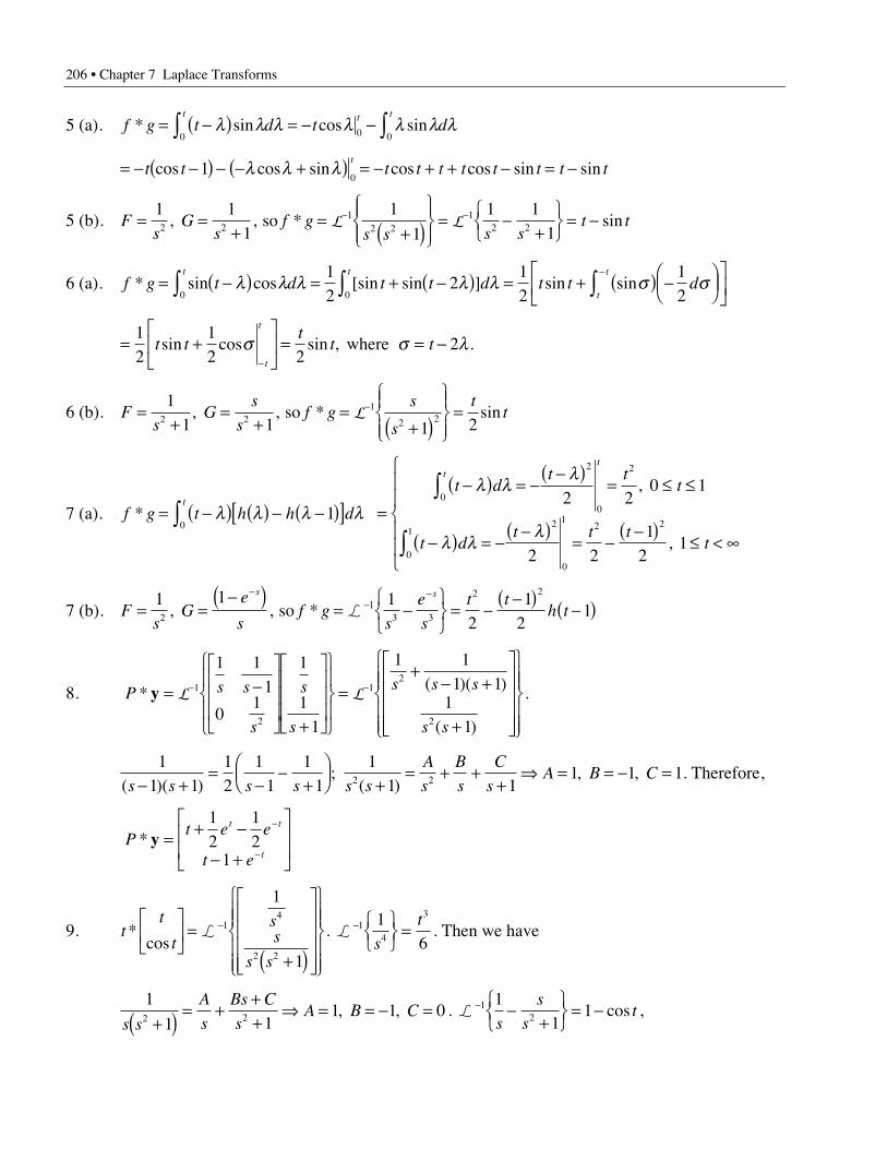
206 • Chapter 7 Laplace Transforms
5 (a). f g t d t dt t t
* sin cos sin= -( ) = - -Ú Úl l l l l l l0 0 0
= - -( ) - - +( )t tt
cos cos sin10
l l l = - + + - = -t t t t t t t tcos cos sin sin
5 (b). Fs
Gs
f gs s s s
t t= =+
=+( )
ÏÌÔ
ÓÔ
¸˝ÔÔ
= -+
ÏÌÓ
¸˝˛
= -- -1 11
1
1
1 112 2
12 2
12 2, * sin, so L L
6 (a). f g t d t t d t t dt t
t
t* sin cos [sin sin ] sin sin= -( ) = + -( ) = + ( ) -Ê
ËÁˆ¯
ÈÎÍ
˘˚Ú Ú Ú
-l l l l l s s
0 0
12
212
12
= +È
ÎÍ
˘
˚˙ = = -
-
12
12 2
2t tt
t tt
t
sin cos sin , .s s lwhere
6 (b). Fs
Gs
sf g
s
s
tt=
+=
+=
+( )ÏÌÔ
ÓÔ
¸˝Ô
Ô=-1
1 1 1 22 21
2 2, * sin, so L
7 (a). f g t h h dt
* = -( ) ( ) - -( )[ ]Ú l l l l10
=-( ) = -
-( )= £ £
-( ) = --( )
= --( )
£ < •
Ï
Ì
ÔÔ
Ó
ÔÔ
Ú
Ú
t dt t
t
t dt t t
t
tt
l l l
l l l
0
2
0
2
0
12
0
12 2
2 20 1
2 21
21
,
,
7 (b). Fs
Ge
sf g
s
e
s
t th t
s s
= =-( )
= -ÏÌÓ
¸˝˛
= --( )
-( )-
--1 1 1
21
212
13 3
2 2
, *, so L
8. P s s
s
s
s
s s s
s s
* ( )( )
( )
y = -È
Î
ÍÍÍ
˘
˚
˙˙˙
+
È
Î
ÍÍÍ
˘
˚
˙˙˙
Ï
ÌÔ
ÓÔ
¸
˝Ô
˛Ô
=+
- +
+
È
Î
ÍÍÍÍ
˘
˚
˙˙˙˙
Ï
ÌÔÔ
ÓÔÔ
¸
˝ÔÔ
˛ÔÔ
- -L L
1
2
12
2
1 11
01
1
11
1 11 1
11
.
11 1
12
11
11
11 1
1 1 12 2( )( );
( ), ,
s s s s s s
A
s
B
s
C
sA B C
- +=
--
+ÊËÁ
ˆ¯ +
= + ++
fi = = - = . Therefore,
Pt e e
t e
t t
t* y = + -
- +
È
Î
ÍÍ
˘
˚
˙˙
-
-
12
12
1
9. tt
tss
s s
*cos
È
ÎÍ
˘
˚˙ =
+( )
È
Î
ÍÍÍÍ
˘
˚
˙˙˙˙
Ï
ÌÔÔ
ÓÔÔ
¸
˝ÔÔ
˛ÔÔ
-L
14
2 2
1
1
. L - ÏÌÓ
¸˝˛
=14
316s
t. Then we have
1
1 11 1 02 2s s
A
s
Bs C
sA B C
+( ) = +++
fi = = - =, , . L - -+
ÏÌÓ
¸˝˛
= -12
11
1s
s
stcos ,
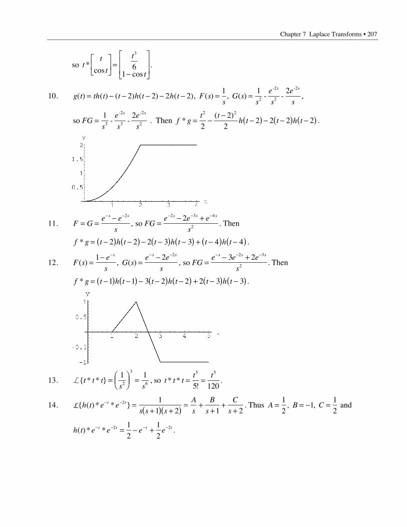
Chapter 7 Laplace Transforms • 207
so tt
t
t
t*
cos cos
È
ÎÍ
˘
˚˙ =
-
È
Î
ÍÍ
˘
˚
˙˙
3
61
.
10. g t th t t h t h t F ss
G ss
e
s
e
s
s s
( ) ( ) ( ) ( ) ( ), ( ) , ( )= - - - - - = =2 2 2 21 1 2
2
2
2
2
- - , - -
so - -- -
FGs
e
s
e
s
s s
=1 23
2
3
2
2 . Then f gt t
h t t h t*( )
= --
-( ) - -( ) -( )2 2
22
22 2 2 2 .
11. F Ge e
sFG
e e e
s
s s s s s
= =-
=- +- - - - -2 2 3 4
2
2, so . Then
f g t h t t h t t h t* = -( ) -( ) - -( ) -( ) + -( ) -( )2 2 2 3 3 4 4 .
12. F se
sG s
e e
sFG
e e e
s
s s s s s s
( ) , ( )=-
=-
=- +- - - - - -1 2 3 22 2 3
2, so . Then
f g t h t t h t t h t* = -( ) -( ) - -( ) -( ) + -( ) -( )1 1 3 2 2 2 3 3 .
13. L{ * * }t t ts s
= ÊËÁ
ˆ¯ =
1 12
3
6 , so t t tt t
* *!
= =5 5
5 120.
14. L{ ( ) * * }h t e es s s
A
s
B
s
C
st t- - =
+( ) +( ) = ++
++
2 11 2 1 2
. Thus A B C= = - =12
112
, , and
h t e e e et t t t( ) * *- - - -= - +2 212
12
.
208 • Chapter 7 Laplace Transforms
15. L{ * * }t e es s s
A
s
B
s
C
s
D
st t- =
+( ) -( ) = + +-
++
11 1 1 12 2 . Thus A B C D= - = = = -1 0
12
12
, , ,
and t e es s s
t e et t t t* *- - -=-
+-
-+
Ï
ÌÔ
ÓÔ
¸
˝Ô
˛Ô
= - + -( )L1
2
112
1
12
112
.
16. L L{ ( ) * ( ) * ...* ( )}( )!
h t h t h ts
t
nn
n
sn= =
-- Ï
ÌÓ
¸˝˛
-11
1 11
and .
Therefore, t
nCt n C
n -
-= fi = =
18
19
18( )!
, ! .
17. L Le e es s
t
ne Ct et t t
n n
nt t- - - -
--Ï
ÌÓ
¸˝˛
=+( ) +( )
ÏÌÓ
¸˝˛
=-( ) =* * ...* ,
!n times1 244 344
1
1
1
1 11
14 a . Thus
n C= = = -514
1, !, a .
18. sin sin *t y d t t yt
-( ) ( ) = =Ú l l l0
2 . Therefore,
2 11
2 1 2 223 2
2
3 32
s sY Y
s
s s sy t t=
+fi =
+( )= + fi = +( ) .
19. t e t y d t ytt
2
0
- = -( ) ( ) =Ú cos cos *l l l . Therefore,
2
1 1
2 1
1 1 1 13 2
2
3 2 3s
s
sY Y
s
s s
A
s
B
s
C
s
D
s+( )=
+fi =
+( )+( )
= ++
++( )
++( )
. Thus
A B C D= = - = = -2 2 0 4, , , , and so we have Ys s s
= -+
-+( )
2 21
4
13 . Finally,
y t e t et t( ) = - -- -2 2 2 2 .
20. y t e y d t y e y t Ys
Ys
tt
t( ) , - ( ) = fi - * = --
=-Ú l l l0 2
11
1. Therefore,
1 21
12 22 2 2s
s
sY Y
s
s s
A
s
B
s
C
s=
--
fi =-
-= + +
-( ). Thus A B C= - = =
14
12
14
, , , and so we have
Ys s s
=-
+ +-
14
122
14
2. Finally, y t
te t( ) = - + +
14 2
14
2 .
21. y t y d t y y Ys s
Ys
t-( ) ( ) = = fi = ( ) = fi = ±Ú l l l
0
3 24 4 26 6
3 36 6*
! and y t t( ) = ±6 .
Chapter 7 Laplace Transforms • 209
22.1 2 2
12 2
12 3 3
2
3sY
s sY
s
s
s= -
+fi = -
+( ) ( ).
s s s s s s s s2 2 2 22 1 2 1 1 2 2 1 1 2 1 1= + + - + = + - + - = + - + +( ) ( ) ( ) ( ) ( ) ( ) . Therefore,
Ys s s s
= -+
-+( )
++
Ê
ËÁˆ
¯2
21
12
1
112 3( )
, so y t e tet
e tt
et t t t( ) = - - +ÊËÁ
ˆ¯
= - - +ÊËÁ
ˆ¯
- - - -2 2 22
2 2 1 22
2 2
.
23. sYs
Ys
Ys
s
s
A
s
B
s
C
s- +
+= fi =
++( )
Ê
ËÁˆ
¯= +
++
+( )0
12
1 1 2
1 1 12 2 . Thus A B C= = - = -2 2 1, , , and
Ys s s
= -+
-+( )
2 21
1
12 , so y t e tet t( ) = - -- -2 2 .
24. ss
ss
s
s s sY Y Y Y-
È
ÎÍ
˘
˚˙ = fi -Ê
ËÁˆ¯ =
È
ÎÍ
˘
˚˙ fi =
-È
ÎÍ
˘
˚˙ =
-+
+ÊËÁ
ˆ¯
È
ÎÍ
˘
˚˙
1
21 1 1
2 1
1
212
11
11
1
22 , so
y t e e tt t( ) = +( )È
ÎÍ
˘
˚˙ =
È
ÎÍ
˘
˚˙
-12
1
2
1
2cosh .
25. sYs s
Ys s
y tt t
- = ◊ fi = + fi ( ) = + = +11 1 1 1
14
1242 2 5
4 4
!.
26. sY Ys s
s Ys s
Ys s s
- - - = ◊-
fi - = - +-
fi =--
+-
( ) ( )( ) ( )
11 1
11 1
11
11
112 2 2 2 .
11 1 1
2 1 2 12 2 2 2s s
A
s
B
s
C
s
D
sA B C D
( ), , ,
-= + +
-+
-( )fi = = = - = . Thus,
Ys s s s s s s s s
= --
+ + --
+-( )
= + --
+-( )
11
2 1 21
1
1
2 1 31
1
12 2 2 2 , so y t t e tet t( ) = + - +2 3 .
Section 7.7
1 (a). 1 2 10
32+( ) -( ) = +- -Ú e t dt et d
1 (b). 1 2 02
1+( ) -( ) =-
-Ú e t dtt d since t=2 lies outside the integration interval.
1 (c).cos2 1
01
2 t
tet dtt--
È
ÎÍ
˘
˚˙ ( ) =
È
ÎÍ
˘
˚˙Ú d
1 (d). e t
t
t
t
dt
e
et2
3
2
4
2
2
1
3
2
1
0
+( )+( )-( )-( )
È
Î
ÍÍÍ
˘
˚
˙˙˙
=-+
È
Î
ÍÍÍ
˘
˚
˙˙˙
-
-
Úddd
2. From Equation 7b, f f t* =d ( ).
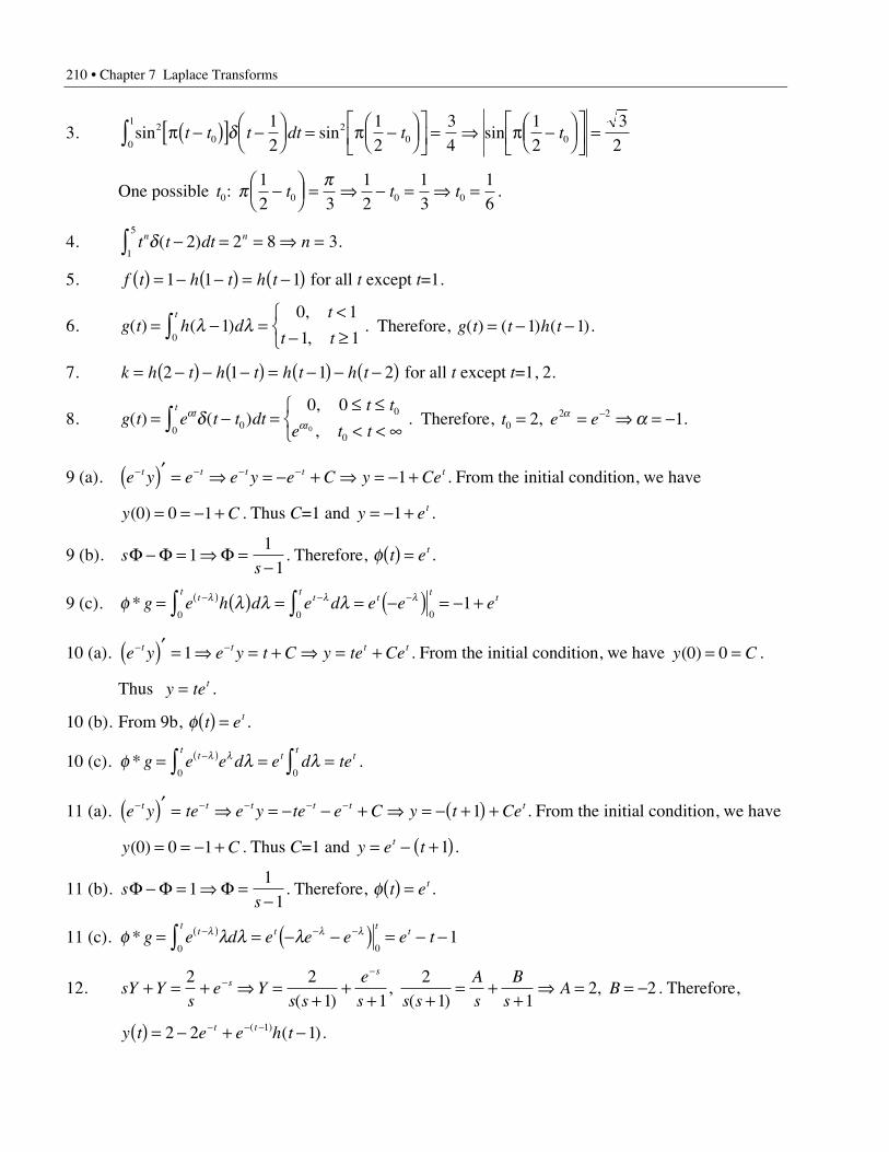
210 • Chapter 7 Laplace Transforms
3. sin sin sin200
12
0 0
12
12
34
12
32
p -( )[ ] -ÊËÁ
ˆ¯ = p -Ê
ËÁˆ¯
ÈÎÍ
˘˚
= fi p -ÊËÁ
ˆ¯
ÈÎÍ
˘˚
=Ú t t t dt t td
One possible t t t t0 0 0 0
12 3
12
13
16
: p p-Ê
ËÁˆ¯ = fi - = fi = .
4. t t dt nn nd( ) .- = = fi =Ú 2 2 8 31
5
5. f t h t h t( ) = - -( ) = -( )1 1 1 for all t except t=1.
6. g t h dt
t t
t( ) ( )
,= - =
<- ≥
ÏÌÓÚ l l1
0 1
1 10
,
. Therefore, g t t h t( ) ( ) ( )= - -1 1 .
7. k h t h t h t h t= -( ) - -( ) = -( ) - -( )2 1 1 2 for all t except t=1, 2.
8. g t e t t dtt t
e t tt
t
t( ) ( ),
= - =£ £< < •
ÏÌÓÚ a
ad 00
0
0
0 00
,
. Therefore, t e e0
2 22 1= = fi = --, a a .
9 (a). e y e e y e C y Cet t t t t- - - -( )¢ = fi = - + fi = - +1 . From the initial condition, we have
y C( )0 0 1= = - + . Thus C=1 and y et= - +1 .
9 (b). ss
F F F- = fi =-
11
1. Therefore, f t et( ) = .
9 (c). f l l ll l l* g e h d e d e e ett
tt
tt
t= ( ) = = -( ) = - +-( ) - -Ú Ú0 0 01
10 (a). e y e y t C y te Cet t t t- -( )¢ = fi = + fi = +1 . From the initial condition, we have y C( )0 0= = .
Thus y tet= .
10 (b). From 9b, f t et( ) = .
10 (c). f l ll l* g e e d e d tett
tt
t= = =-( )Ú Ú0 0.
11 (a). e y te e y te e C y t Cet t t t t t- - - - -( )¢ = fi = - - + fi = - +( ) +1 . From the initial condition, we have
y C( )0 0 1= = - + . Thus C=1 and y e tt= - +( )1 .
11 (b). ss
F F F- = fi =-
11
1. Therefore, f t et( ) = .
11 (c). f l l ll l l* g e d e e e e ttt
tt
t= = - -( ) = - --( ) - -Ú0 01
12. sY Ys
e Ys s
e
s s s
A
s
B
sA Bs
s
+ = + fi =+
++ +
= ++
fi = = ---2 2
1 12
1 12 2
( ),
( ), . Therefore,
y t e e h tt t( ) = - + -- - -2 2 11( ) ( ).

Chapter 7 Laplace Transforms • 211
13. sY Y e e Ye
s
e
ss s
s s
+ = - fi =+
-+
- -- -
22
1 1. Therefore, y t e h t e h tt t( ) = -( ) - -( )- -( ) - -( )1 21 2 .
14. s Y e e Ye
s
e
ss s
s s2 3
2
3
2= - fi = -- -- -
. Therefore, y t t h t t h t( ) = - -( ) - - -( )( ) ( )1 1 3 3 .
15. s Y e Ys
es s2 2 22 2
24 22
4+ p( ) = p fi =
p+ p
- - . Therefore, y t t h t( ) = p -( )( ) -( )sin 2 2 2 .
16. s Y s sY e Ys
s s
e
s s s
e
s ss
s s2 2 1
22 2
12
- - - = fi =--
+-
= +-
-- -
( )( ) ( ) ( )
.
12 2
12
12s s
A
s
B
sA B
( ),
-= +
-fi = - = . Therefore, Y
se
s s ss= + - +
-ÊËÁ
ˆ¯
-1 12
12( )
and
y t h t e h tt( ) = - - + --112
112
12 1( ) ( )( ) .
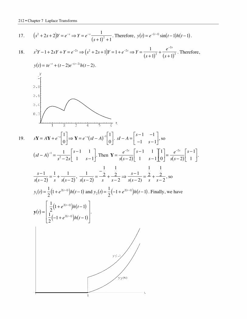
212 • Chapter 7 Laplace Transforms
17. s s Y e Y es
s s222 2
1
1 1+ +( ) = fi =
+( ) +- - . Therefore, y t e t h tt( ) = -( ) -( )- -( )1 1 1sin .
18. s Y sY Y e s s Y e Ys
e
ss s
s2 2 2 2
2
2
21 2 2 1 11
1 1- + + = fi + +( ) = + fi =
+( )+
+( )- -
-
. Therefore,
y t te t e h tt t( ) = + - -- - -( ) ( )( )2 22 .
19. s A e e sI As sY Y Y= +È
ÎÍ
˘
˚˙ fi = -( ) È
ÎÍ
˘
˚˙
- - -1
0
1
01
. sI As
s- =
- -- -
È
ÎÍ
˘
˚˙
1 1
1 1, so
sI As s
s
s-( ) =
--
-È
ÎÍ
˘
˚˙
-1
2
12
1 1
1 1. Then Y =
-( )-
-È
ÎÍ
˘
˚˙
È
ÎÍ
˘
˚˙ =
-( )-È
ÎÍ
˘
˚˙
- -e
s s
s
se
s s
ss s2 2
2
1 1
1 1
1
0 2
1
1.
s
s s s s s s s s s
s
s s s s
--( ) = +
-( ) -( ) =-
+-
fi--
= +-
12
1 12
12
12
12
212
12
12
2,
( ), so
y t e h t y t e h tt t1
2 12
2 112
1 112
1 1( ) = +( ) -( ) ( ) = - +( ) -( )-( ) -( ) and . Finally, we have
y te h t
e h t
t
t( ) =
+( ) -( )
- +( ) -( )
È
Î
ÍÍÍ
˘
˚
˙˙˙
-( )
-( )
12
1 1
12
1 1
2 1
2 1.
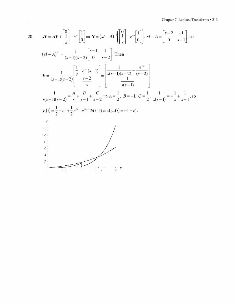
Chapter 7 Laplace Transforms • 213
20. s As
e sI As
es sY Y Y= +È
ÎÍÍ
˘
˚˙˙
-È
ÎÍ
˘
˚˙ fi = -( )
È
ÎÍÍ
˘
˚˙˙
-È
ÎÍ
˘
˚˙
Ê
ËÁÁ
ˆ
¯˜- - -
01
1
0
01
1
01
. sI As
s- =
- --
È
ÎÍ
˘
˚˙
2 1
0 1, so
sI As s
s
s-( ) =
- --
-È
ÎÍ
˘
˚˙
-1 11 2
1 1
0 2( )( ). Then
Y =- -( )
- -
-
È
Î
ÍÍÍ
˘
˚
˙˙˙
= - --
-
-
È
Î
ÍÍÍÍ
˘
˚
˙˙˙˙
--
11 2
11
2
11 2 2
11
( )
( )( )( ) ( )
( )s s
se s
s
s
s s s
e
s
s s
ss
.
11 2 1 2
12
112
11
1 11s s s
A
s
B
s
C
sA B C
s s s s( ), , ;
- -( ) = +-
+-
fi = = - =-( ) = - +
-, so
y t e e e h t y t et t t t1
2 2 12
12
12
1 1( ) = - ( ) = - ++ - ( - ) and ( - ) .
Chapter 8Nonlinear Systems
Section 8.1
1 (a). F o r ¢¢ + = ¢ = ¢ =y ty y y ysin , ( ) , ( )0 0 0 1, l e t y( )( )
( )
( )
( )t
y t
y t
y t
y t=
È
ÎÍ
˘
˚˙ =
¢È
ÎÍ
˘
˚˙
1
2
. T h u s ,
¢ =¢¢
È
ÎÍ
˘
˚˙ =
¢¢¢
È
ÎÍ
˘
˚˙ =
¢- + ¢
È
ÎÍ
˘
˚˙ =
- +È
ÎÍ
˘
˚˙ =
È
ÎÍ
˘
˚˙ =
¢È
ÎÍ
˘
˚˙ =
È
ÎÍ
˘
˚˙y y
y
y
y
y
y
ty y
y
ty y
y
y
y
y1
2
2
1 2
1
2
00
0
0
0
0
1sin sin, ( )
( )
( )
( )
( ).
1 (b). From part (a), f y( , )( , , )
( , , ) sint
f t y y
f t y y
y
ty y=
È
ÎÍ
˘
˚˙ =
- +È
ÎÍ
˘
˚˙
1 1 2
2 1 2
2
1 2
. Therefore, the requested partial
derivatives are ∂∂
=∂
∂=
∂∂
= -∂∂
=f
y
f
y
f
yt
f
yy1
1
1
2
2
1
2
220 1, , , cos .
1 (c). There are no points in 3-dimensional space where the hypotheses of Theorem 8.1 fail to besatisfied.
2 (a). For ¢¢ + ¢ + = = ¢ = -y y y t y y( ) tan( / ), ( ) , ( )/3 1 3 2 1 1 1 2, let y( )( )
( )
( )
( )t
y t
y t
y t
y t=
È
ÎÍ
˘
˚˙ =
¢È
ÎÍ
˘
˚˙
1
2
. Thus,
¢ =¢¢
È
ÎÍ
˘
˚˙ =
- -È
ÎÍ
˘
˚˙ =
-È
ÎÍ
˘
˚˙y y
y
y
y
t y y1
2
2
11 3
232
11
2tan( / ), ( )/ .
2 (b). F o r f y( , )( , , )
( , , )t
f t y y
f t y y=
È
ÎÍ
˘
˚˙
1 1 2
2 1 2
, t h e r e q u e s t e d p a r t i a l d e r i v a t i v e s a r e
∂∂
=∂
∂=
∂∂
= -∂∂
= --f
y
f
y
f
yy
f
yy1
1
1
2
2
11
2 3 2
2220 1
13
3, , ,/ .
2 (c). The hypotheses of Theorem 8.1 are not satisfied at t n y= ± + =( ) /2 1 2 01p and .3 (a). For ¢¢ + + + ¢ = = ¢ =- - - -y t y y t e y yt1 1 11 2 2 2 2 1( ) , ( ) , ( ) , let
y( )( )
( )
( )
( )t
y t
y t
y t
y t=
È
ÎÍ
˘
˚˙ =
¢È
ÎÍ
˘
˚˙
1
2
. Thus,
¢ =¢¢
È
ÎÍ
˘
˚˙ =
¢¢¢
È
ÎÍ
˘
˚˙ =
¢- + + ¢ +
È
ÎÍ
˘
˚˙ =
- + + +È
ÎÍ
˘
˚˙
=È
ÎÍ
˘
˚˙ =
- - - - - - - -y
y
y
y
y
y
y
t y y t e
y
t y y t e
y
y
y
t t1
21 1 1
21
1 21 1
1
2
1 2 1 2
22
2
2
( ) ( ),
( )( )
( )
( )
¢¢È
ÎÍ
˘
˚˙ =
È
ÎÍ
˘
˚˙y ( )
.2
2
1
3 (b). From part (a), f y( , )( , , )
( , , ) ( )t
f t y y
f t y y
y
t y y t e t=È
ÎÍ
˘
˚˙ =
- + + +È
ÎÍ
˘
˚˙- - - -
1 1 2
2 1 2
21
1 21 11 2
.
Therefore, the requested partial derivatives are∂∂
=∂
∂=
∂∂
= + +∂∂
= + +- - - -f
y
f
y
f
yt y y
f
yt y y1
1
1
2
2
1
11 2
2 2
2
11 2
20 1 1 2 2 1 2, , ( ) , ( ) .
Chapter 8 Nonlinear Systems • 215
3 (c). The hypotheses of Theorem 8.1 are satisfied everywhere except on the planes t = 0 and1 2 01 2+ + =y y .
4 (a). For ¢¢¢ + ¢ = ¢¢ = ¢ = ¢¢ = -y ty t y y y ycos( ) ( ) , ( ) , ( ) , ( )2 0 1 0 1 0 2, let
y( )( )( )
( )
( )( )
( )t
y ty t
y t
y ty t
y t=
È
Î
ÍÍ
˘
˚
˙˙ = ¢
¢¢
È
Î
ÍÍ
˘
˚
˙˙
1
2
3
. Thus, ¢ =¢¢¢
È
Î
ÍÍ
˘
˚
˙˙ =
- +
È
Î
ÍÍÍ
˘
˚
˙˙˙
=-
È
Î
ÍÍ
˘
˚
˙˙y y
yy
y
y
yty y
1
2
3
2
3
2 32
01
12cos( )
, ( ) .
4 (b). For f y( , )( , , , )( , , , )
( , , , )t
f t y y yf t y y y
f t y y y=
È
Î
ÍÍ
˘
˚
˙˙
1 1 2 3
2 1 2 3
3 1 2 3
, the requested partial derivatives are
∂∂
=∂
∂=
∂∂
=∂∂
=∂∂
=∂∂
=
∂∂
=∂∂
=∂∂
=
f
y
f
y
f
y
f
y
f
y
f
y
f
y
f
yt ty
f
yty
1
1
1
2
1
3
2
1
2
2
2
3
3
1
3
22
3
33
0 1 0 0 0 1
0 2
, , , , , ,
, sin( ),.
4 (c). The hypotheses of Theorem 8.1 are satisfied in all of ty y y1 2 3 - space .5 (a). For ¢¢¢ + - ¢¢ + = = ¢ = ¢¢ =- -y t y y y y y2 2 2 0 0 0 0 2 0 21 3 1 1/ ( ) ( ) , ( ) , ( ) , ( ) , let
y( )
( )
( )
( )
( )
( )
( )
t
y t
y t
y t
y t
y t
y t
=È
Î
ÍÍÍ
˘
˚
˙˙˙
= ¢¢¢
È
Î
ÍÍÍ
˘
˚
˙˙˙
1
2
3
. Thus,
¢ =¢¢¢
È
Î
ÍÍÍ
˘
˚
˙˙˙
=¢
¢¢¢¢¢
È
Î
ÍÍÍ
˘
˚
˙˙˙
=¢
¢¢- - ¢¢ +
È
Î
ÍÍÍ
˘
˚
˙˙˙
=- - +
È
Î
ÍÍÍ
˘
˚
˙˙˙- - - -
y
y
y
y
y
y
y
y
y
t y y
y
y
t y y
1
2
31 3 1 1
2
31 3
11
312 2 2 2 2 2/ /( ) ( ) ( ) ( )
,,
( )
( )
( )
( )
( )
( )
( )
.y 0
0
0
0
0
0
0
0
2
2
1
2
3
=È
Î
ÍÍÍ
˘
˚
˙˙˙
= ¢¢¢
È
Î
ÍÍÍ
˘
˚
˙˙˙
=È
Î
ÍÍÍ
˘
˚
˙˙˙
y
y
y
y
y
y
5 (b). From part (a), f y( , )
( , , , )
( , , , )
( , , , ) ( ) ( )/
t
f t y y y
f t y y y
f t y y y
y
y
t y y
=È
Î
ÍÍÍ
˘
˚
˙˙˙
=- - +
È
Î
ÍÍÍ
˘
˚
˙˙˙- -
1 1 2 3
2 1 2 3
3 1 2 3
2
31 3
11
212 2 2
.
Therefore, the requested partial derivatives are∂∂
=∂
∂=
∂∂
=
∂∂
=∂∂
=∂∂
=
∂∂
= - +∂∂
=∂∂
= - +- - - -
f
y
f
y
f
y
f
y
f
y
f
y
f
yt y y
f
y
f
yt y y
1
1
1
2
1
3
2
1
2
2
2
3
3
1
1 31
23
1 3
2
3
3
1 31
13
0 1 0
0 0 1
2 2 2 0 2 2 2
, ,
, ,
( ) ( ) , , ( ) ( )/ / 22
.
5 (c). The hypotheses of Theorem 8.1 are satisfied everywhere except on the “hyperplanes” y1 2=and y3 2= - .
6. Since ¢ = - +y t y y t22
2 143cos ( ) , it follows that the scalar problem is ¢¢ = ¢ - +y t y y tcos ( )2 43 ,
y y( ) , ( )2 1 2 1= ¢ = - .7. Since ¢ = +y y y ey
2 2 12tan , it follows that the scalar problem is ¢¢ = ¢ + ¢y y y eytan ,
y y( ) , ( )0 0 0 1= ¢ = .
216 • Chapter 8 Nonlinear Systems
8. Since ¢ = +y y y y3 1 2 32 , it follows that the scalar problem is ¢¢¢ = ¢ + ¢¢y yy y( )2,
y y y( ) , ( ) , ( )- = - ¢ - = ¢¢ - = -1 1 1 2 1 4 .9. Since ¢ = +y y y t3 2 3
2 1 2( ) / , it follows that the scalar problem is ¢¢¢ = ¢ ¢¢ +y y y t( ) /2 1 2,y y y( ) , ( ) / , ( )1 1 1 1 2 1 3= ¢ = ¢¢ = .
11. Laplace transforms cannot be productively used because the equation is nonlinear.14 (a). Let Then a ax ax a x a x= = + + +p d/ ( ). tan ( / ) ( / )2 1 3 2 153 3 5 5 L . Retaining the
first term of the Maclaurin series in equation (7), we havemx k x mx k x mx kx¢¢ + ª ¢¢ + = ¢¢ +( / )tan( / ) ( / )( / )2 2 2 2d p p d d p p d .
14 (b). As in part (a), retaining the first two terms of the Maclaurin series in equation (7)results in equation (8).
14 (c). Equation (7) becomes ¢ =¢¢
È
ÎÍ
˘
˚˙ =
-È
ÎÍ
˘
˚˙y
y
y
y
k m y1
2
2
12 2( / )tan( / )d p p d.
Equation (8) becomes ¢ =¢¢
È
ÎÍ
˘
˚˙ =
- +È
ÎÍ
˘
˚˙y
y
y
y
k m y y1
2
2
12 2
1312( / )( ( / ) )p d
.
14 (d). The system version of equation (7) satisfies the hypotheses of Theorem 8.1everywhere except along y n1 2 1 2= ± +( ) /p . The system version of equation (8)satisfies the hypotheses of Theorem 8.1 everywhere in ty y1 2 - space
15 (a). Adding equations 3 and 4, we obtain dc
dt
de
dt+ = 0. Thus, using the linearity of differentiation,
d c e
dt
( )+= 0 and hence, c t e t e( ) ( )+ ∫ 0 is a constant function.
15 (b). Substituting e t e c t( ) ( )= -0 in equations 1 and 3, we findda
dtk e a t k c t a t k c t= - + + ¢1 0 1 1( ) ( ) ( ) ( ) and
dc
dtk e a t k c t a t k k c t= - - ¢ +1 0 1 1 2( ) ( ) ( ) ( ) ( ) .
15 (c). The hypotheses of Theorem 8.1 are satisfied for all points in ( , , )t a c - space .16 (a). At the instant shown in the figure,
V R r dy R R y dy
R R y t y t
y t y t
sub = + = + -
= + -
Ú Ú( / ) ( / ) ( )
( / ) [ ( ) ( / )( ( )) ] .
( ) ( )2 3 2 3
2 3 1 3
3 2
0
3 2 2
0
3 2 3
p p p p
p p16 (b). Equation (10) is physically relevant as long as - £ £R y t R( ) .
Section 8.2
1. For¢ = - +¢ = -
x x y
y y x
( )
( ) ,
1
1we see that ¢ =x 0 if (a) or (b) x y= =0 1. In Case (a), we have ¢ =y 0 only if y = 0, yieldingthe equilibrium point ( , ) ( , )x y = 0 0 . In Case (b), we have ¢ =y 0 only if x = 1, yielding theequilibrium point ( , ) ( , )x y = 11 .

Chapter 8 Nonlinear Systems • 217
2. For¢ = +¢ = - -
x y x
y x y
( )
( )( ) ,
3
1 2we see that ¢ =x 0 if (a) or (b) x y= - =3 0. In Case (a), we have ¢ =y 0 only if y = 2,yielding the equilibrium point ( , ) ( , )x y = -3 2 . In Case (b), we have ¢ =y 0 only if x = 1,yielding the equilibrium point ( , ) ( , )x y = 1 0 .
3. For¢ = - +
¢ = - +
x x y
y x x
( )( )
,
2 1
4 32
we see that ¢ =x 0 if (a) or (b) x y= = -2 1. In Case (a), we cannot have ¢ =y 0. In Case (b),we have ¢ =y 0 only if x x= =1 3 or , yielding the equilibrium points( , ) ( , ) ( , ) ( , )x y x y= - = -1 1 3 1 and .
4. For¢ = - +¢ = -
x x y
y x y
( )( )
( ) ,
1 1
2we see that ¢ =x 0 if (a) or (b) x y= = -1 1. In Case (a), we have ¢ =y 0 only if y = 0,yielding the equilibrium point ( , ) ( , )x y = 1 0 . In Case (b), we have ¢ =y 0 only if x = 2, yieldingthe equilibrium point ( , ) ( , )x y = -2 1 .
5. For¢ = -¢ = -
x x x y
y y x y
( )
( ) ,
2
3we see that ¢ =x 0 if (a) or (b) x x y= =0 2 . In Case (a), we have ¢ =y 0 only if y = 0,yielding the equilibrium point ( , ) ( , )x y = 0 0 . In Case (b), we have ¢ =y 0 only if y = 0, yieldingthe same equilibrium point as in Case (a), ( , ) ( , )x y = 0 0 .
6. For¢ = -¢ = +
x y y x
y x x y
( )
( ) ,2we see that ¢ =x 0 if (a) y or (b) = =0 y x . In Case (a), we have ¢ =y 0 only if x = 0, yieldingthe equilibrium point ( , ) ( , )x y = 0 0 . In Case (b), we have ¢ =y 0 only if x = 0, yielding thesame equilibrium point ( , ) ( , )x y = 0 0 .
7. For¢ = + -
¢ = -
x x y
y x y
2 2
2 2
8
,
we see that ¢ =y 0 if x y2 2= . Using this requirement in the first equation, we see that ¢ =x 0requires 2 8 02x - = or x = ±2 . Since y x= ± , we find 4 equilibrium points,( , ), ( , ), ( , ), ( , ).2 2 2 2 2 2 2 2- - - -and
8. For¢ = + -
¢ = + -
x x y
y x y
2 2
2 2
2 3
2 3 ,
we see that ¢ =x 0 if x y2 23 2= - . In this event, we have ¢ =y 0 only if 2 3 2 3 02 2( )- + - =y y .Solving for y we obtain y = ±1. Then, since x y2 23 2= - , we see that x = ±1 for each choiceof y. The equilibrium points are( , ) ( , ), ( , ), ( , ), ( , )x y = - - - -11 1 1 1 1 1 1 .

218 • Chapter 8 Nonlinear Systems
9. For¢ = -¢ = +
¢ = -
x y
y x y x
z y z
1
2
( )
( ) ,we see that ¢ =x 0 requires y = 1. Using this requirement in the second equation, we see that
¢ =y 0 requires x x( )1 0+ = . Thus, we need in Case (a) x = 0 or in Case (b), x = -1. Finally,¢ =z 0 requires z = 2 since y is nonzero. We obtain 2 equilibrium points,
( , , ) ( , , ) ( , , ) ( , , )x y z x y z= = -0 1 2 11 2 and .10. For
¢ = -¢ = - +
¢ = - - -
x z
y z x y
z x y
2
2
1
1 2
1
( )
( ) ,we see that ¢ =x 0 requires z = ±1. Using this requirement in the second equation, we see that
¢ =y 0 requires 1 2 0- + =x y while ¢ =z 0 requires 1 0- - =x y . Satisfying ¢ =y 0 and ¢ =z 0therefore requires x y= =2 3 1 3/ / and . Combining this requirement with z = ±1, we obtain 2equilibrium points,( , , ) ( / , / , ) ( , , ) ( / , / , )x y z x y z= = -2 31 31 2 31 3 1 and .
11. Making the substitution y y y y1 2= = ¢ and the scalar equation can be expressedas the system
¢ =
¢ = - -
y y
y y y
1 2
2 1 13
Since ¢ = - +y y y2 1 121( ), we cannot have ¢ =y2 0 unless y1 0= . Similarly, from the first equation,
¢ =y1 0 requires y2 0= . Thus, the only equilibrium point is ( , ) ( , ) ( , )y y y y1 2 0 0= ¢ = .12. Making the substitution y y y y1 2= = ¢ and the scalar equation can be expressed
as the system¢ =
¢ = - -
y y
y e y yy
1 2
2 22
11 1 sin ( )pThus, the equilibrium points are ( , ) ( , ) ( . , ), , , ,y y y y n n1 2 0 5 0 0 1 2= ¢ = + = ± ± K .
13. Making the substitution y y y y1 2= = ¢ and the scalar equation can be expressedas the system
¢ =
¢ = - - + -
y y
y y y y
1 2
2 12
14 1
21 2 1( )From the first equation, ¢ =y1 0 requires y2 0= . Thus, in the second equation, ¢ =y2 0 requires1 0 11
21- = = ±y y or . There are two equilibrium points
( , ) ( , ) ( , )y y y y1 2 1 0= ¢ = and ( , ) ( , ) ( , )y y y y1 2 1 0= ¢ = - .14. Making the substitution y y y y y y1 2 3= = ¢ = ¢¢, , and the scalar equation can be expressed as
the system¢ =¢ =¢ = + -
y y
y y
y y y
1 2
2 3
3 3 11 2sinThus, the equilibrium points are
( , , ) (( / ) , , )
( , , ) (( / ) , , ), , , , .
y y y n
y y y n n1 2 3
1 2 3
6 2 0 0
5 6 2 0 0 0 1 2
= += + = ± ±
p pp p
and
K
Chapter 8 Nonlinear Systems • 219
15. Making the substitution y y y y y y1 2 3= = ¢ = ¢¢, and , the scalar equation can be expressed asthe system
¢ =¢ =
¢ = + - + -
y y
y y
y y y y
1 2
2 3
3 22
12
22 14 2( )( ) .
From the first equation, ¢ =y1 0 requires y2 0= while (by the second equation) ¢ =y2 0 requiresy3 0= . Having these requirements, the third equation tells us that ¢ =y3 0 only if y1 2= ± .Hence, There are two equilibrium points( , , ) ( , , ) ( , , )y y y y y y1 2 3 2 0 0= ¢ ¢¢ = and ( , , ) ( , , ) ( , , )y y y y y y1 2 3 2 0 0= ¢ ¢¢ = - .
16. Since ( , )0 0 is an equilibrium point, we know b d= =0 0 and . Similarly, since ( , )2 1 is anequilibrium point, we know 2 2 0a + = and g - =6 0. Thus, a = -1 and g = 6.
17. Since ( , )11 is an equilibrium point, we know a b g d+ + = + - =2 0 1 0 and . Similarly, since( , )2 0 is an equilibrium point, we know 2 2 0a + = and 2g - =1 0. Thus, a = -1 and g = 1 2/ .Using the equations derived from the equilibrium point ( , )11 , we have- + + = + - =1 2 0 1 0b d and (1 / 2) . Therefore, b = -1 and d = 1 2/ .
18. The slope of a phase plane trajectory is given by ¢ ¢ =y x g x y f x y/ ( , ) / ( , ), see equation (9). Asgiven, g f( , ) / ( , )2 1 2 1 1= and g f( , ) / ( , )1 1 1 1 0- - = . Therefore, g( , )1 1 0- = and so b = 2.Knowing b = 2 and g f( , ) / ( , )2 1 2 1 1= , we obtain ( ) / ( ) / ( )3 2 1 2 1+ + = + =b a a or 5 . Thus,we obtain a = 3.
19. The slope of a phase plane trajectory is given by ¢ ¢ =y x g x y f x y/ ( , ) / ( , ), see equation (9). Asgiven, g f( , ) / ( , )11 11 0= and g f( , ) / ( , )1 1 1 1 4- - = . Therefore, g( , )11 0= and so2 0 2+ = = -g g or . Knowing g = -2 and g f( , ) / ( , )1 1 1 1 4- - = , we obtain( ) / ( )2 1 4- - + =g a b or 1 1 1/ ( )a b- + = . Finally, since there is a vertical tangent at ( , )0 1-we know f ( , )0 1 0- = , and thus - + =b 1 0. Using b = 1 along with the prior equation1 1 1/ ( )a b- + = , we obtain a = 1.
20. The slope of a phase plane trajectory is given by ¢ ¢ =y x g x y f x y/ ( , ) / ( , ), see equation (9). Asgiven, g f( , ) / ( , ) /1 2 1 2 1 6= and thus1 6 1 2 1 2 1 0 5 5 2/ ( , ) / ( , ) ( . ) / ( )= = - + -g f n . Solving for n, we obtain n = 3.
21. Making the substitution y y y y1 2= = ¢ and the scalar equation can be expressedas the system
¢ =
¢ = - +
y y
y y y
1 2
2 2 122 a .
Since ( , ) ( , )y y1 2 2 0= is an equilibrium point, it follows that 2 812y = = a .
22 (a). v i j= -4 322 (b). v i j= +1522 (a). v j= -
24. For A =-
-È
ÎÍ
˘
˚˙
9 1
1 9, the eigenvalues are l l1 210 8= - = - and with corresponding eigenvectors
u u1 2
1
1
1
1=
-È
ÎÍ
˘
˚˙ =
È
ÎÍ
˘
˚˙ and . The general solution is
y( )t c e c et t=-
È
ÎÍ
˘
˚˙ +
È
ÎÍ
˘
˚˙
- -1
102
81
1
1
1 and hence all solution points are attracted to the origin. Thus, the
direction field corresponding to the given matrix is C.
220 • Chapter 8 Nonlinear Systems
25. For A =- -- -
È
ÎÍ
˘
˚˙
1 3
3 1, the eigenvalues are l l1 24 2= - = and with corresponding eigenvectors
u u1 2
1
1
1
1=
È
ÎÍ
˘
˚˙ =
-È
ÎÍ
˘
˚˙ and . The general solution is
y( )t c e c et t=È
ÎÍ
˘
˚˙ +
-È
ÎÍ
˘
˚˙
-1
42
21
1
1
1 and hence solution points that begin on the line y x= are attracted
to the origin whereas those that begin on the line y x= - are repelled away from the origin.Thus, the direction field corresponding to the given matrix is B.
26. For A =-
-È
ÎÍ
˘
˚˙
4 6
6 4, the eigenvalues are l l1 210 2= - = and with corresponding eigenvectors
u u1 2
1
1
1
1=
-È
ÎÍ
˘
˚˙ =
È
ÎÍ
˘
˚˙ and . The general solution is
y( )t c e c et t=-
È
ÎÍ
˘
˚˙ +
È
ÎÍ
˘
˚˙
-1
102
21
1
1
1 and hence solution points that begin on the line y x= are repelled
away from the origin whereas those that begin on the line y x= - are attracted to the origin.Thus, the direction field corresponding to the given matrix is D.
27. For A =È
ÎÍ
˘
˚˙
4 2
2 4, the eigenvalues are l l1 26 2= = and with corresponding eigenvectors
u u1 2
1
1
1
1=
È
ÎÍ
˘
˚˙ =
-È
ÎÍ
˘
˚˙ and . The general solution is
y( )t c e c et t=È
ÎÍ
˘
˚˙ +
-È
ÎÍ
˘
˚˙1
62
21
1
1
1 and hence solution points that begin on the line y x= are repelled
away from the origin as are those that begin on the line y x= - . Thus, the direction fieldcorresponding to the given matrix is A.
28. The phase plane point ( , )a 0 is an equilibrium point when a is a root off y( ) = 0.
29 (a). Making the substitution y y y y1 2= = ¢ and the scalar equation can be expressedas the system
¢ =
¢ = - -
y y
y y y
1 2
2 1 13 .
The nullclines are the lines y y1 20 0= = and . The only equilibrium point is the point ( , )0 0 .30 (a). Making the substitution y y y y1 2= = ¢ and the scalar equation can be expressed
as the system¢ =
¢ = - -
y y
y y y
1 2
2 1 121( ) .
The nullclines are the lines y y y1 1 20 0= ± =, = 1, and . The equilibrium points are( , ), ( , ), ( , )0 0 1 0 1 0- .
Chapter 8 Nonlinear Systems • 221
31 (a). Making the substitution y y y y1 2= = ¢ and the scalar equation can be expressedas the system
¢ =
¢ = -
y y
y y
1 2
22
11 2sin .The nullclines are the lines y n n1 4 0 1 2= ± + = ± ±( / ) , , , ,p p Kand the line y2 0= Theequilibrium points are ( ( / ) , ), , , ,± + = ± ±p p4 0 0 1 2n n K.
32 (a). The nullclines are the lines y x y x= - =3 2 and . These lines intersect at the point ( , )11yielding the only equilibrium point.
33 (a). The nullclines are the lines y x y x= - =2 and . These lines intersect at the point ( , )11 yieldingthe only equilibrium point.
34 (a). The nullclines are the lines y x y x f= - = - =2 2 4 0and where and the liney x g= =( / )1 2 0 where . The lines f g= =0 0 and intersect at the points( / , / ) ( / , / )4 3 2 3 8 3 4 3 and yielding the only equilibrium points.
35 (a). The nullclines are the lines y x y x f= - = =2 6 0 and where , and the liney x g= - =, where 0. The lines f g= =0 0 and intersect at the points ( , ) ( , )0 0 2 2 and -yielding the only equilibrium points.
36 (a). The nullclines are the curves y x y x= - = - +1 12 2and . These curves intersect at theequilibrium points ( , ) ( , )-1 0 1 0 and .
Section 8.3
1 (a). Given ¢¢ + =x x4 0, multiply by ¢x to obtain ¢ ¢¢ + ¢ =x x x x4 0 . Integrating, we obtain
0 5 22 2. ¢( ) + =x x C .
1 (b). The equation ¢¢ + =x x4 0 can be expressed as ¢ =¢ = -
x y
y x4 . With this notation, the conserved
quantity found in part (a) is 0 5 22 2. y x C+ = . The graph passes through the point ( , ) ( , )x y = 11when C = 2 5. .
1 (c). At ( , )11 , the velocity vector is v i j i j= ¢ + ¢ = -x y 4 . The velocity vector is tangent to the graphand indicates that the graph is traversed in the clockwise direction as t increases.
2 (a). Given ¢¢ - + =x x( )1 0, multiply by ¢x to obtain ¢ ¢¢ - ¢ + =x x x x( )1 0. Integrating, we obtain( ) ( )¢ - + =x x C2 21 .
2 (b). The equation ¢¢ - + =x x( )1 0 can be expressed as ¢ =¢ = +
x y
y x 1. With this notation, the conserved
quantity found in part (a) is y x C2 21- + =( ) . The graph passes through the point ( , ) ( , )x y = 11when C = -3.
2 (c). At ( , )11 , the velocity vector is v i j i j= ¢ + ¢ = +x y 2 . The velocity vector indicates that thesolution point moves upward and to the right along the right branch of the hyperbola as tincreases.
3 (a). Given ¢¢ + =x x 3 0, multiply by ¢x to obtain ¢ ¢¢ + ¢ =x x x x 3 0 . Integrating, we obtain
0 5 0 252 4. .¢( ) + =x x C .
222 • Chapter 8 Nonlinear Systems
3 (b). The equation ¢¢ + =x x 3 0 can be expressed as ¢ =
¢ = -
x y
y x 3. With this notation, the conserved
quantity found in part (a) is 0 5 0 252 4. .y x C+ = . The graph passes through the point( , ) ( , )x y = 11 when C = 0 75. .
3 (c). At ( , )11 , the velocity vector is v i j i j= ¢ + ¢ = -x y . The velocity vector is tangent to the graphand indicates that the graph is traversed in the clockwise direction as t increases.
4 (a). Given ¢¢ - + =x x x( sin )3 0p p , multiply by ¢x to obtain¢ ¢¢ - ¢ + =x x x x x( sin )3 0p p . Integrating, we obtain 2 42 4( ) ( cos )¢ - - =x x x Cp .
4 (b). The equation ¢¢ - + =x x x( sin )3 0p p can be expressed as ¢ =
¢ = +
x y
y x x3 p psin . With this notation,
the conserved quantity found in part (a) is 2 42 4y x x C- - =( cos )p .The graph passes through the point ( , ) ( , )x y = 11 when C = -3.
4 (c). At ( , )11 , the velocity vector is v i j i j= ¢ + ¢ = +x y . The velocity vector indicates that thesolution point moves upward and to the right along the right branch of the graph as t increases.
5 (a). Given ¢¢ + =x x 2 0, multiply by ¢x to obtain ¢ ¢¢ + ¢ =x x x x 2 0 . Integrating, we obtain
0 5 1 32 3. ( / )¢( ) + =x x C .
5 (b). The equation ¢¢ + =x x 2 0 can be expressed as ¢ =
¢ = -
x y
y x 2. With this notation, the conserved
quantity found in part (a) is 0 5 1 32 3. ( / )y x C+ = . The graph passes through the point( , ) ( , )x y = 11 when C = 5 6/ .
5 (c). At ( , )11 , the velocity vector is v i j i j= ¢ + ¢ = -x y . The velocity vector is tangent to the graphand indicates that the solution point moves “down the graph” as t increases.
6 (a). Given ¢¢ + + =x x x/ ( )1 02 , multiply by ¢x to obtain ¢ ¢¢ + ¢ + =x x x x x/ ( )1 02 . Integrating, weobtain ( ) ln( )¢ + + =x x C2 21 .
6 (b). The equation ¢¢ + + =x x x/ ( )1 02 can be expressed as ¢ =
¢ = - +
x y
y x x/ ( ).1 2 With this notation, the
conserved quantity found in part (a) is y x C2 21+ + =ln( ) .The graph passes through the point ( , ) ( , )x y = 11 when C = +1 2ln .
6 (c). At ( , )11 , the velocity vector is v i j i j= ¢ + ¢ = -x y 0 5. . The velocity vector indicates that thesolution point moves clockwise along the curve as t increases.
7. Rewriting the conservation law in terms of x x and ¢ , we have ( ) cos¢ + =x x x C2 2 .Differentiating with respect to t, we obtain 2 2 02¢ ¢¢ + ¢ - ¢ =x x x x x x x xcos sin or
¢ ¢¢ + - =x x x x x x( cos sin )2 2 02 . Therefore, the differential equation is¢¢ + - =x x x x xcos . sin0 5 02 .
8. Rewriting the conservation law in terms of x x and ¢ , we have ( )¢ - =-x e Cx2 2
. Differentiating
with respect to t, we obtain 2 2 02
¢ ¢¢ - - ¢ =-x x e xxx( )( ) . Therefore, the differential equation is
¢¢ + =-x xe x 2
0.
9 (a). The equation ¢¢ + + =x x x 3 0 can be expressed as ¢ =
¢ = - -
x y
y x x 3. The nullclines are the lines
defined by y = 0 and - + =x x( )1 02 ; the lines y x= =0 0 and . Thus, the only equilibriumpoint is the point ( , ) ( , )x y = 0 0 .
Chapter 8 Nonlinear Systems • 223
9 (b). The velocity vector has the form v i j( , ) ( )x y y x x= - + 3 . Thus, we obtain v i j( , )11 2= - ,v i j( , )1 1 2- = - - , v i j( , )- = +11 2 , and v i j( , )- - = - +1 1 2 .
9 (c). Multiplying by ¢x , the equation becomes ¢ ¢¢ + ¢ + =x x x x x( )3 0 . Integrating, we obtain0 5 0 5 0 252 2 4. ( ) . .¢ + + =x x x C or 2 22 2 4
1y x x C+ + = . The graph of the conserved quantitypasses through the point ( , )11 when C1 5= . The graph passes through the other three points andis consistent with the sketch in part (b).
10. Since ¢¢ + =x xa 0 it follows that 0 5 0 52 21
2 2. ( ) .¢ + = + =x x C x y Ca a and hence .10 (a). Figure A is a circle of radius 2 and thus a = + =1 42 2 and x y .
Figure B is a hyperbola with asymptotes y x= ± . Since (0, 2) is on the graph, we see thata = - - =1 42 2 and y x .Figure C shows horizontal lines, y = ±2 . Thus, a = 0.
10 (b). The solution point in Figure A travels clockwise around the circle. Solution points in Figure Bmove to the right on the upper branch and to the left on the lower branch. Solutions points inFigure C move to the right on the upper line and to the left on the lower line.
11. In analogy with Exercise 9, multiply the equation ¢¢¢ + ¢ = ¢¢y f y y( ) 0 by , obtaining¢¢ ¢¢¢ + ¢¢ ¢ =y y y f y( ) 0. Integrating, we find 0 5. ( )¢¢ + ¢ =y F y C where F u( ) is an antiderivative
of f u( ). Thus, the differential equation has a conservation law given by 0 5 2. ( ) ( )¢¢ + ¢ =y F y C .
12. (a) From the definition of E(t), it follows that dE
dtmx x kxx mx kx x= ¢ ¢¢ + ¢ = ¢¢ + ¢( ) . From the
differential equation, mx x kx¢¢ + ¢ + =g 0 and hence mx kx x¢¢ + = - ¢g . Therefore,dE
dtx x= - ¢ ¢ £( )g 0.
(b) Energy is not conserved. On t-intervals where ¢ πx t( ) 0, E(t) is a decreasing function of tand energy is being lost.
13 (a). For the system¢ =¢ = -
x x
y y
2
2we have f x y x g x y y( , ) ( , )= = -2 2 and . Thus, f gx y= = -2 2 and . Since f gx y= - , the
system is Hamiltonian.13 (b). Let H x y( , ) denote the Hamiltonian function. Thus, H x y g x y yx ( , ) ( , )= - = 2 . Integrating with
respect to x, we obtain H x y xy p y( , ) ( )= +2 . Differentiating with respect to y in order todetermine p y( ) , we find H x y x p y f x y xy ( , ) ( ) ( , )= + ¢ = =2 2 . Therefore, ¢ =p y( ) 0 and hencep y C( ) = is a constant function. Dropping the constant, we obtain a Hamiltonian function,H x y xy( , ) = 2 .
13 (c). From part (b), the phase-plane trajectories are defined by 2xy C= . If a phase-plane trajectorypasses through the point ( , )11 , then C = 2 and the trajectory is given by xy = 1.
14 (a). For the system¢ =
¢ = -
x xy
y y
22
we have f x y xy g x y y( , ) ( , )= = -2 2 and . Thus, f y g yx y= = -2 2 and . Since f gx y= - , the
system is Hamiltonian.14 (b). Let H x y( , ) denote the Hamiltonian function. Thus, H x y g x y yx ( , ) ( , )= - = 2 . Integrating with
respect to x, we obtain H x y xy p y( , ) ( )= +2 . Differentiating with respect to y in order todetermine p y( ) , we find H x y xy p y f x y xyy ( , ) ( ) ( , )= + ¢ = =2 2 .
224 • Chapter 8 Nonlinear Systems
Therefore, ¢ =p y( ) 0 and hence p y C( ) = is a constant function. Dropping the constant, weobtain a Hamiltonian function, H x y xy( , ) = 2.
14 (c). From part (b), the phase-plane trajectories are defined by xy C2 = . If a phase-plane trajectorypasses through the point ( , )11 , then C = 1 and the trajectory is given by xy 2 1= .
15 (a). For the system¢ = - +¢ = - + +
x x x
y y xy x
2 1
2 4we have f x y x x g x y y xy x( , ) ( , )= - = - + +2 2 4+1 and . Thus, f x g xx y= - = - +1 2 1 2 and .
Since f gx y= - , the system is Hamiltonian.
15 (b). Let H x y( , ) denote the Hamiltonian function. Thus, H x y g x y y xy xx ( , ) ( , )= - = - -2 4 .Integrating with respect to x, we obtain H x y xy x y x p y( , ) ( )= - - +2 22 . Differentiating withrespect to y in order to determine p y( ) , we findH x y x x p y f x y x xy ( , ) ( ) ( , )= - + ¢ = = - +2 2 1. Therefore, ¢ =p y( ) 1 and hence p y y C( ) = + .
Dropping the additive constant, we obtain a Hamiltonian function,H x y xy x y x y( , ) = - - +2 22 .
15 (c). From part (b), the phase-plane trajectories are defined by xy x y x y C- - + =2 22 . If a phase-plane trajectory passes through the point ( , )11 , then C = -1 and the trajectory is given byxy x y x y- - + + =2 22 1 0.
16 (a). For the system¢ = -¢ =
x y
y x
8
2we have f x y g x y x( , ) ( , )= - =8 2 and . Thus, f gx y= =0 0 and . Since f gx y= - , the system
is Hamiltonian.16 (b). Let H x y( , ) denote the Hamiltonian function. Thus, H x y f x y yy ( , ) ( , )= = -8 . Integrating with
respect to y, we obtain H x y y q x( , ) ( )= - +4 2 . Differentiating with respect to x in order todetermine q x( ), we find H x y q x xx ( , ) ( )= ¢ = -2 . Therefore, q x x C( ) = - +2 . Dropping theadditive constant, we obtain a Hamiltonian function, H x y x y( , ) = - -2 24 .
16 (c). From part (b), the phase-plane trajectories are defined by - - =x y C2 24 . If a phase-planetrajectory passes through the point ( , )11 , then C = -5 and the trajectory is given byx y2 24 5+ = .
17 (a). For the system¢ =
¢ =
x y x
y y x
22
cos
sinwe have f x y y x g x y y x( , ) cos ( , ) sin= =2 2 and . Thus, f y x g y xx y= - =2 2sin sin and . Since
f gx y= - , the system is Hamiltonian.
17 (b). Let H x y( , ) denote the Hamiltonian function. Thus, H x y g x y y xx ( , ) ( , ) sin= - = - 2 . Integratingwith respect to x, we obtain H x y y x p y( , ) cos ( )= +2 . Differentiating with respect to y in orderto determine p y( ) , we find H x y y x p y f x y y xy ( , ) cos ( ) ( , ) cos= + ¢ = =2 2 . Therefore,
¢ =p y( ) 0 and hence p y C( ) = is a constant function. Dropping the constant, we obtain aHamiltonian function, H x y y x( , ) cos= 2 .
Chapter 8 Nonlinear Systems • 225
17 (c). From part (b), the phase-plane trajectories are defined by y x C2 cos = . If a phase-planetrajectory passes through the point ( , )11 , then C = cos1 and the trajectory is given byy x2 1cos cos= .
18 (a). For the system¢ = - +
¢ = + -
x y x
y y x x
2 3
4 23
we have f gx y= - =1 1 and . Since f gx y= - , the system is Hamiltonian.
18 (b). Let H x y( , ) denote the Hamiltonian function. Thus, H x y f x y y xy ( , ) ( , )= = - +2 3. Integrating
with respect to y, we obtain H x y y xy y q x( , ) ( )= - - +2 3 . Differentiating with respect to x inorder to determine q x( ), we find H x y y q x y x xx ( , ) ( )= - + ¢ = - - +4 23 . Therefore,q x x x C( ) = - + +4 2 . Dropping the additive constant, we obtain a Hamiltonian function,H x y y xy y x x( , ) = - + - +2 4 23 .
18 (c). If a phase-plane trajectory H x y C( , ) = passes through the point ( , )11 , then the trajectory isgiven by y xy y x x2 4 23 8- + - + = .
19 (a). For the system¢ = -
¢ =
x y
y x
2
3 2
we have f x y y g x y x( , ) ( , )= - =2 3 2 and . Thus, f gx y= =0 0 and . Since f gx y= - , the
system is Hamiltonian.19 (b). Let H x y( , ) denote the Hamiltonian function. Thus, H x y g x y xx ( , ) ( , )= - = -3 2. Integrating
with respect to x, we obtain H x y x p y( , ) ( )= - +3 . Differentiating with respect to y in order todetermine p y( ) , we find H x y p y f x y yy ( , ) ( ) ( , )= ¢ = = -2 . Therefore, ¢ = -p y y( ) 2 and hence
p y y C( ) = - +2 is a constant function. Dropping the additive constant, we obtain aHamiltonian function, H x y x y( , ) = - -3 2 .
19 (c). From part (b), the phase-plane trajectories are defined by - - =x y C3 2 . If a phase-planetrajectory passes through the point ( , )11 , then C = -2 and the trajectory is given byx y3 2 2+ = .
20 (a). For the system¢ =
¢ = - -
x xe
y x ye
xy
xy2we have f e xye g e xyex
xy xyy
xy xy= + = - - and . Since f gx y= - , the system is Hamiltonian.
20 (b). Let H x y( , ) denote the Hamiltonian function. Thus, H x y f x y xeyxy( , ) ( , )= = . Integrating with
respect to y, we obtain H x y e q xxy( , ) ( )= + . Differentiating with respect to x in order todetermine q x( ), we find H x y ye q x x yex
xy xy( , ) ( )= + ¢ = +2 . Therefore, q x x C( ) = +2 .Dropping the additive constant, we obtain a Hamiltonian function, H x y e xxy( , ) = + 2 .
20 (c). If a phase-plane trajectory H x y C( , ) = passes through the point ( , )11 , then the trajectory isgiven by e x exy + = +2 1 .
226 • Chapter 8 Nonlinear Systems
21. Consider the system¢ = + +
¢ = - - +
x x x y
y x y x y
3
2
3 2 3
3 2 2 3
sin( )
sin( ) .
Calculating the partial derivatives, we have f x x yx = + +3 6 2 32 cos( ) andg x x yy = - - +3 6 2 32 cos( ) . Since f gx y= - , the system is Hamiltonian.
Let H x y( , ) denote the Hamiltonian function. Thus,H x y g x y x y x yx ( , ) ( , ) sin( )= - = + +3 2 2 32 . Integrating with respect to x, we obtainH x y x y x y p y( , ) cos( ) ( )= - + +3 2 3 . Differentiating with respect to y in order to determinep y( ) , we find H x y x x y p y f x y x x yy ( , ) sin( ) ( ) ( , ) sin( )= + + + ¢ = = + +3 33 2 3 3 2 3 . Therefore,
¢ =p y( ) 0 and hence p y C( ) = is a constant function. We obtain a Hamiltonian function,H x y x y x y( , ) cos( )= - +3 2 3 .
22. Consider the system¢ = +
¢ = - -
x e y
y e x
xy
xy
3
3 .
Calculating the partial derivatives, we have f yexxy= and g xey
xy= - . Since f gx yπ - , the
system is not Hamiltonian.23. Consider the system
¢ = - -¢ = +
x xy x
y xy y
sin( )
sin( ) .
2
2Calculating the partial derivatives, we have f y xyx = - -2 2 1cos( ) and g x xyy = +2 2 1cos( ) .
Since f gx yπ - , the system is not Hamiltonian.
24. Consider the system¢ = - +
¢ = + -
x x xe
y xy x e
y
y
3
6 3
2
.
Calculating the partial derivatives, we have f x exy= - +6 and g x ey
y= -6 . Since f gx y= - , thesystem is Hamiltonian. Let H x y( , ) denote the Hamiltonian function. Thus,H x y g x y xy x ex
y( , ) ( , )= - = - - +6 3 . Integrating with respect to x, we obtainH x y x y x p y( , ) ( / ) ( )= - - +3 3 22 2 . Differentiating with respect to y in order to determine p y( ) ,we find H x y x p y f x y x xey
y( , ) ( ) ( , )= - + ¢ = = - +3 32 2 . Therefore, ¢ =p y xey( ) and hence
p y xe Cy( ) = + . Dropping the additive constant, we obtain a Hamiltonian function,H x y x y x xey( , ) ( / )= - - +3 3 22 2 .
25. Consider the system¢ =
¢ = -
x y
y x x 2 .Calculating the partial derivatives, we have fx = 0 and gy = 0. Since f gx y= - , the system is
Hamiltonian.Let H x y( , ) denote the Hamiltonian function. Thus, H x y g x y x xx ( , ) ( , )= - = -2 . Integratingwith respect to x, we obtain H x y x x p y( , ) ( / )( ) ( )= - +1 6 2 33 2 . Differentiating with respect to yin order to determine p y( ) , we find H x y p y f x y yy ( , ) ( ) ( , )= ¢ = = . Therefore, ¢ =p y y( ) and
hence p y y C( ) .= +0 5 2 . Dropping the additive constant, we obtain a Hamiltonian function,H x y x x y( , ) ( / )( )= - +1 6 2 3 33 2 2 .
Chapter 8 Nonlinear Systems • 227
26. Consider the system¢ = +
¢ = - +
x x y
y x x y
2
23 .Calculating the partial derivatives, we have fx = 1 and gy = 1. Since f gx yπ - , the system is not
Hamiltonian.27. Consider the system
¢ =¢ =
x f y
y g x
( )
( ) .Calculating the partial derivatives, we have ∂ =x f y[ ( )] 0 and ∂ =y g x[ ( )] 0 . Since
∂ = -∂x yf y g x[ ( )] [ ( )], the system is Hamiltonian.Let H x y( , ) denote the Hamiltonian function. Thus, H x y g xx ( , ) ( )= - . Integrating with respectto x, we obtain H x y G x p y( , ) ( ) ( )= - + . Differentiating with respect to y in order to determinep y( ) , we find H x y p y f yy ( , ) ( ) ( )= ¢ = . Therefore, p y F y C( ) ( )= + . Dropping the additiveconstant, we obtain a Hamiltonian function, H x y F y G x( , ) ( ) ( )= - .
28. Consider the system¢ = +¢ = +
x f y y
y g x x
( )
( ) .
2
6Calculating the partial derivatives, we have ∂ + =x f y y[ ( ) ]2 0 and ∂ + =y g x x[ ( ) ]6 0. Since
∂ + = -∂ +x yf y y g x x[ ( ) ] [ ( ) ]2 6 , the system is Hamiltonian. Let H x y( , ) denote theHamiltonian function. Thus, H x y g x xx ( , ) ( )= - - 6 . Integrating with respect to x, we obtainH x y G x x p y( , ) ( ) ( )= - - +3 2 . Differentiating with respect to y in order to determine p y( ) , wefind H x y p y f y yy ( , ) ( ) ( )= ¢ = + 2 . Therefore, p y F y y C( ) ( )= + +2 . Dropping the additive
constant, we obtain a Hamiltonian function, H x y G x x F y y( , ) ( ) ( )= - - + +3 2 2.29. Consider the system
¢ = -
¢ = + +
x f y xy
y g x y
3 2
12
( )
( ) .Calculating the partial derivatives, we have ∂ - = -x f y xy y[ ( ) ]3 2 2 and ∂ + + =y g x y y[ ( ) ]2 1 2 .
Since ∂ - = -∂ + +x yf y xy g x y[ ( ) ] [ ( ) ]3 2 12 , the system is Hamiltonian.
Let H x y( , ) denote the Hamiltonian function. Thus, H x y g x yx ( , ) ( )= - - -2 1. Integrating withrespect to x, we obtain H x y G x y x x p y( , ) ( ) ( )= - - - +2 . Differentiating with respect to y inorder to determine p y( ) , we find H x y yx p y f y xyy ( , ) ( ) ( )= - + ¢ = -2 3 2 . Therefore,p y F y C( ) ( )= +3 . Dropping the additive constant, we obtain a Hamiltonian function,H x y F y G x y x x( , ) ( ) ( )= - - -3 2 .
30. Consider the system¢ = - +¢ = -
x f x y y
y f x y
( )
( ) .
2
Calculating the partial derivatives, we have ∂ - + = ¢ -x f x y y f x y[ ( ) ] ( )2 and∂ - = - ¢ -y f x y f x y[ ( )] ( ). Since ∂ - + = -∂ -x yf x y y f x y[ ( ) ] [ ( )]2 , the system is Hamiltonian.Let H x y( , ) denote the Hamiltonian function. Thus, H x y f x yx ( , ) ( )= - - . Integrating withrespect to x, we obtain H x y F x y p y( , ) ( ) ( )= - - + . Differentiating with respect to y in order todetermine p y( ) , we find H x y f x y p y f x y yy ( , ) ( ) ( ) ( )= - + ¢ = - + 2 .

228 • Chapter 8 Nonlinear Systems
Therefore, p y y C( ) = +2 . Dropping the additive constant, we obtain a Hamiltonian function,H x y F x y y( , ) ( )= - - + 2 .
31. Consider the composition K x t y t( ( ), ( )). Differentiating with respect to t, we obtaind
dtK x t y t
K
x
dx
dt
K
y
dy
dtg f f g( ( ), ( )) ( ) ( )=
∂∂
+∂∂
= - + =m m 0 . Therefore, K x t y t( ( ), ( )) is a conserved
quantity.
Section 8.4
1 (a). All points lying within the ellipse E having semi-major axis e and semi-minor axis e / 2 liewithin the circle of radius e . Likewise, all points lying within the circle of radius e / 2 liewithin the ellipse E. Therefore, given e > 0, choose d e= / 2.
1 (b). The origin is not an asymptotically stable equilibrium point since the solution points remain onan ellipse and do not approach the origin as t Æ • .
2. The origin is an unstable equilibrium point. Any solution point starting near the origin willfollow a branch of the hyperbola and will eventually exit any circle centered at the origin.
3 (a). Making the substitution y x= ¢ , the scalar equation ¢¢ + ¢ + =x x xg 0 can be expressed as thesystem
¢ =¢ = - -
x y
y x yg .The origin is the only equilibrium point for this system.
3 (b). We analyze stability by appealing to Theorem 8.3. The system in part (a) has the form ¢ =y yA
where A =- -
È
ÎÍ
˘
˚˙
0 1
1 g. The characteristic polynomial for A is p( )l l gl= + +2 1 and thus the
eigenvalues of A are l g g120 5 4= - - -( ). and l g g2
20 5 4= - + -( ). . When g 2 4 0- ≥ , we
see that l l1 2£ . Thus, if 2 £ g , then l l1 2 0£ < which shows the origin is asymptoticallystable. On the other hand, if g £ -2 , then 0 1 2< £l l which shows the origin is an unstableequilibrium point. For - < <2 2g , the eigenvalues are complex with nonzero imaginary parts.For - < <2 0g , the real parts of l l1 2 and are positive, which shows the origin is an unstableequilibrium point. Likewise, for 0 2< <g , the origin is an asymptotically stable equilibriumpoint. When g = 0, the origin is a stable (but not asymptotically stable) equilibrium point.
4. For the system ¢ =- -È
ÎÍ
˘
˚˙y y
3 2
4 3, the coefficient matrix has eigenvalues l l1 21 1= - = and .
Thus, by Theorem 8.3, the origin is an unstable equilibrium point.
5. For the system ¢ =-
-È
ÎÍ
˘
˚˙y y
5 14
3 8, the coefficient matrix has eigenvalues l l1 21 2= - = - and .
Thus, by Theorem 8.3, the origin is an asymptotically stable equilibrium point.
6. For the system ¢ =-È
ÎÍ
˘
˚˙y y
0 2
2 0, the coefficient matrix has eigenvalues l l1 22 2= = -i i and .
Thus, by Theorem 8.3, the origin is a stable equilibrium point but not an asymptotically stableequilibrium point.
Chapter 8 Nonlinear Systems • 229
7. For the system ¢ =-
È
ÎÍ
˘
˚˙y y
1 4
1 1, the coefficient matrix has eigenvalues
l l1 21 2 1 2= + = -i i and . Thus, by Theorem 8.3, the origin is an unstable equilibrium point.
8. For the system ¢ =- -È
ÎÍ
˘
˚˙y y
7 3
5 1, the coefficient matrix has eigenvalues l l1 24 2= - = - and .
Thus, by Theorem 8.3, the origin is an asymptotically stable equilibrium point.
9. For the system ¢ =- -
È
ÎÍ
˘
˚˙y y
9 5
7 3, the coefficient matrix has eigenvalues l l1 22 4= = and .
Thus, by Theorem 8.3, the origin is an unstable equilibrium point.
10. For the system ¢ =- -
-È
ÎÍ
˘
˚˙y y
3 5
2 1, the coefficient matrix has eigenvalues
l l1 22 3 2 3= - + = - -i i and . Thus, by Theorem 8.3, the origin is an asymptotically stableequilibrium point.
11. For the system ¢ =--
È
ÎÍ
˘
˚˙y y
9 4
15 7, the coefficient matrix has eigenvalues l l1 23 1= = - and .
Thus, by Theorem 8.3, the origin is an unstable equilibrium point.
12. For the system ¢ =- -È
ÎÍ
˘
˚˙y y
13 8
15 9, the coefficient matrix has eigenvalues l l1 23 1= - = - and .
Thus, by Theorem 8.3, the origin is an asymptotically stable equilibrium point.
13. For the system ¢ =--
È
ÎÍ
˘
˚˙y y
3 2
5 3, the coefficient matrix has eigenvalues l l1 2= = -i i and . Thus,
by Theorem 8.3, the origin is a stable (but not asymptotically stable) equilibrium point.
14. For the system ¢ =--
È
ÎÍ
˘
˚˙y y
1 5
1 3, the coefficient matrix has eigenvalues
l l1 21 1= - + = - -i i and . Thus, by Theorem 8.3, the origin is an asymptotically stableequilibrium point.
15. For the system ¢ =-
-È
ÎÍ
˘
˚˙y y
3 3
1 5, the coefficient matrix has eigenvalues l l1 26 2= - = - and .
Thus, by Theorem 8.3, the origin is an asymptotically stable equilibrium point.16. Eigenvalues are l l1 22 3= - = and . Since one of the eigenvalues is real and positive, the
origin is an unstable equilibrium point.17. Eigenvalues are l l1 22 3= = and . Since the eigenvalues are real and positive, the origin is an
unstable equilibrium point.18. Eigenvalues are l l1 24 2= - = - and . Since the eigenvalues are real and negative, the origin is
an asymptotically stable equilibrium point.19. Eigenvalues are l l1 21 2 1 2= - = +i i and . Since the eigenvalues are complex with positive
real parts, the origin is an unstable equilibrium point.20. Eigenvalues are l l1 22 2= - =i i and . Since the eigenvalues are purely imaginary, the origin is
a stable equilibrium point but it is not an asymptotically stable equilibrium point.21. Eigenvalues are l l1 22 2 2 2= - - = - +i i and . Since the eigenvalues are complex with
negative real parts, the origin is an asymptotically stable equilibrium point.22. Eigenvalues are l l1 22 3= - = and . Since one of the eigenvalues is real and positive, the
origin is an unstable equilibrium point.
230 • Chapter 8 Nonlinear Systems
23. Eigenvalues are l l1 22 3= - = - and . Since the eigenvalues are real and negative, the origin isan asymptotically stable equilibrium point.
24 (a). Solving 0 y g= +A e 0, it follows that y ge = - -A 10 is the unique equilibrium point.
24 (b). Let z y y( ) ( )t t= - e . Then, ¢ = ¢ = + = - =z y y g y y zA A A A0 e . Theorem 8.3 can be applied tothe new system ¢ =z zA .
25. For the system ¢ =-
-È
ÎÍ
˘
˚˙ +
-È
ÎÍ
˘
˚˙y y
2 1
1 2
4
2, the unique equilibrium point is
y e A= --È
ÎÍ
˘
˚˙ = -
- -- -
È
ÎÍ
˘
˚˙
-È
ÎÍ
˘
˚˙ =
-È
ÎÍ
˘
˚˙
-14
21 3
2 1
1 2
4
2
2
0( / ) . With the change of variable z y y( ) ( )t t e= - the
system becomes ( ) ( )z y z y+ ¢ =-
-È
ÎÍ
˘
˚˙ + +
-È
ÎÍ
˘
˚˙e e
2 1
1 2
4
2 or ¢ =
--
È
ÎÍ
˘
˚˙ +
--
È
ÎÍ
˘
˚˙ +
-È
ÎÍ
˘
˚˙z z y
2 1
1 2
2 1
1 2
4
2e .
This last system reduces to the homogeneous system ¢ =-
-È
ÎÍ
˘
˚˙z z
2 1
1 2. The coefficient matrix
has eigenvalues l l1 23 1= - = - and . By Theorem 8.3, the origin is an asymptotically stableequilibrium point of ¢ =z zA and therefore, y e is an asymptotically stable equilibrium point of
the nonhomogeneous system ¢ =-
-È
ÎÍ
˘
˚˙ +
-È
ÎÍ
˘
˚˙y y
2 1
1 2
4
2.
26. For the system ¢ =-
È
ÎÍ
˘
˚˙ +
È
ÎÍ
˘
˚˙y y
0 1
1 0
2
1, the unique equilibrium point is y e A= -
È
ÎÍ
˘
˚˙ =
-È
ÎÍ
˘
˚˙
-12
1
1
2. With
the change of variable z y y( ) ( )t t e= - the system reduces to the homogeneous system
¢ =-
È
ÎÍ
˘
˚˙z z
0 1
1 0. The coefficient matrix has eigenvalues l l1 2= = -i i and . By Theorem 8.3, the
origin is a stable but not an asymptotically stable equilibrium point of ¢ =z zA . Therefore, y e isa stable but not an asymptotically stable equilibrium point of the nonhomogeneous system.
27. For the system ¢ =- -
È
ÎÍ
˘
˚˙ +
-È
ÎÍ
˘
˚˙y y
3 2
4 3
2
2, the unique equilibrium point is
y e A= --È
ÎÍ
˘
˚˙ =
- -È
ÎÍ
˘
˚˙
-È
ÎÍ
˘
˚˙ =
-È
ÎÍ
˘
˚˙
-12
2
3 2
4 3
2
2
2
2. With the change of variable z y y( ) ( )t t e= - the system
becomes ( ) ( )z y z y+ ¢ =- -
È
ÎÍ
˘
˚˙ + +
-È
ÎÍ
˘
˚˙e e
3 2
4 3
2
2 or ¢ =
- -È
ÎÍ
˘
˚˙ +
- -È
ÎÍ
˘
˚˙ +
-È
ÎÍ
˘
˚˙z z y
3 2
4 3
3 2
4 3
2
2e . This
last system reduces to the homogeneous system ¢ =- -
È
ÎÍ
˘
˚˙z z
3 2
4 3. The coefficient matrix has
eigenvalues l l1 21 1= - = and . By Theorem 8.3, the origin is an unstable equilibrium point of¢ =z zA and therefore, y e is an unstable equilibrium point of the nonhomogeneous system
¢ =- -
È
ÎÍ
˘
˚˙ +
-È
ÎÍ
˘
˚˙y y
3 2
4 3
2
2.
28. For the system ¢ =-
-È
ÎÍ
˘
˚˙ +
È
ÎÍ
˘
˚˙y y
1 1
10 5
1
2, the unique equilibrium point is y e A= -
È
ÎÍ
˘
˚˙ =
--
È
ÎÍ
˘
˚˙
-11
2
3 5
8 5
/
/.
With the change of variable z y y( ) ( )t t e= - the system reduces to the homogeneous system
Chapter 8 Nonlinear Systems • 231
¢ =-
-È
ÎÍ
˘
˚˙z z
1 1
10 5. The coefficient matrix has eigenvalues l l1 22 2= + = -i i and . By Theorem
8.3, the origin is an unstable equilibrium point of ¢ =z zA . Therefore, y e is an unstableequilibrium point of the nonhomogeneous system.
29. For the system ¢ =È
Î
ÍÍÍ
˘
˚
˙˙˙
y y
2 1 1
1 1 2
1 2 1
, the coefficient matrix has eigenvalues
l l l1 2 31 2 3= - = =, , and . Thus, by the discussion following Theorem 8.3, the origin is anunstable equilibrium point.
30. For the system ¢ =--
-
È
Î
ÍÍÍ
˘
˚
˙˙˙
+È
Î
ÍÍÍ
˘
˚
˙˙˙
y y
1 1 0
0 1 2
0 0 1
2
0
3
, the unique equilibrium point is y e A= -È
Î
ÍÍÍ
˘
˚
˙˙˙
=È
Î
ÍÍÍ
˘
˚
˙˙˙
-1
2
0
3
4
6
3
.
With the change of variable z y y( ) ( )t t e= - the system reduces to the homogeneous system
¢ =- -- -
-
È
Î
ÍÍÍ
˘
˚
˙˙˙
z z
1 1 2
0 1 2
0 0 1
. The coefficient matrix has eigenvalues l l l1 1 31 1 1= = - = -, , and . By
Theorem 8.3, the origin is an unstable equilibrium point of ¢ =z zA . Therefore, y e is anunstable equilibrium point of the nonhomogeneous system.
31. For the system ¢ =
- --
-
È
Î
ÍÍÍÍ
˘
˚
˙˙˙˙
y y
3 5 0 0
2 1 0 0
0 0 0 2
0 0 2 0
, the coefficient matrix has eigenvalues
l l l l1 2 3 42 3 2 3 2 2= - + = - - = = -i i i i, , , and . Thus, by the discussion following Theorem8.3, the origin is a stable (but not asymptotically stable) equilibrium point.
32. For the system ¢ =-
-
È
Î
ÍÍÍÍ
˘
˚
˙˙˙˙
+
-È
Î
ÍÍÍÍ
˘
˚
˙˙˙˙
y y
0 1 0 0
1 0 0 0
0 0 1 0
0 0 0 1
1
2
1
0
, unique equilibrium point is given by
y e = -
-È
Î
ÍÍÍÍ
˘
˚
˙˙˙˙
=
-È
Î
ÍÍÍÍ
˘
˚
˙˙˙˙
-A 1
1
2
1
0
2
1
1
0
. With the change of variables z y y( ) ( )t t e= - , the system reduces to the
homogeneous system ¢ =-
-
È
Î
ÍÍÍÍ
˘
˚
˙˙˙˙
z z
0 1 0 0
1 0 0 0
0 0 1 0
0 0 0 1
. The coefficient matrix has eigenvalues
l l l l1 2 3 41 1 1 1= - = - = - =, , , and . Thus, by the discussion following Theorem 8.3, theorigin is an unstable equilibrium point.
34 (a). Since the coefficient matrix A is real and symmetric, it has real eigenvalues and a full set ofeigenvectors.
232 • Chapter 8 Nonlinear Systems
34 (b). From the discussion following Theorem 8.3, the equilibrium point y 0e = is isolated if andonly if det[ ]A π 0. Now, det[ ]A = -1 2a and therefore, y 0e = is an isolated equilibrium pointif and only if a π ±1.
34 (c). When a = 1 the equilibrium points lie on the line y x= . When a = -1 the equilibrium pointslie on the line y x= - .
34 (d). No, since the eigenvalues of A are real and not purely imaginary; see Theorem 8.3.34 (e). The eigenvalues of A are l a l a1 21 1= - + = - -, and . By part (b), if y 0e = is an isolated
equilibrium point, then a π ±1. Clearly, both eigenvalues are negative when - < <1 1awhereas one of the eigenvalues is positive when a > 1.
35. Since 1 1
22
1
212
21 22
a
a a
È
ÎÍ
˘
˚˙
È
ÎÍ
˘
˚˙ =
È
ÎÍ
˘
˚˙, it follows that 1 2 212+ =a and a a21 222 4+ = . From the first
equation, we have a12 1 2= / . Since y 0= is not an isolated equilibrium point, it follows thatdet[ ]A = 0. Thus, a a a22 12 21 0- = or a a22 211 2 0- =( / ) . This last equation, together with the
prior equation a a21 222 4+ = tells us that a a21 222 1= = and . Thus, A =È
ÎÍ
˘
˚˙
1 1 2
2 1
/.
Section 8.5
1 (a). For the system¢ = + -¢ = -
x x y
y y x
2 2 32
,
the equilibrium points are y ye e=È
ÎÍ
˘
˚˙ =
--
È
ÎÍ
˘
˚˙
4
4
4
4 and .
1 (b). At an equilibrium point, the linearized system ¢ =z zA has coefficient matrix Ax y
=-
È
ÎÍ
˘
˚˙
2 2
1 1.
Thus, the linearized systems are (i) ¢ =-
È
ÎÍ
˘
˚˙z z
8 8
1 1
and (ii) ¢ =- --
È
ÎÍ
˘
˚˙z z
8 8
1 1.
1 (c). In case (i), the eigenvalues are l l1 22 438 6 561= =. .K K and and thus the nonlinear system isunstable at the corresponding equilibrium point y e. For case (ii), the eigenvalues arel l1 28 815 1 815= - =. .K K and and thus the nonlinear system is unstable at thecorresponding equilibrium point y e.
2 (a). For the system¢ = + -¢ =
x x y
y x
2 29 9
,
the equilibrium points are y ye e=È
ÎÍ
˘
˚˙ =
-È
ÎÍ
˘
˚˙
0
1
0
1 and .
Chapter 8 Nonlinear Systems • 233
2 (b). At an equilibrium point, the linearized system ¢ =z zA has coefficient matrix Ax y
=È
ÎÍ
˘
˚˙
2 18
1 0.
Thus, the linearized systems are (i) ¢ =È
ÎÍ
˘
˚˙z z
0 18
1 0 and (ii) ¢ =
-È
ÎÍ
˘
˚˙z z
0 18
1 02 (c). In case (i), the eigenvalues are l l1 24 242 4 242= = -. .K K and and thus the nonlinear system
is unstable at the corresponding equilibrium point y e. For case (ii), the eigenvalues are ±3 2 iand thus nothing can be inferred about the stability of the nonlinear system.
3 (a). For the system¢ = -
¢ = + -
x x
y x y
1
2
2
2 2 ,
the equilibrium points are y y y ye e e e=È
ÎÍ
˘
˚˙ =
-È
ÎÍ
˘
˚˙ =
--
È
ÎÍ
˘
˚˙ =
-È
ÎÍ
˘
˚˙
1
1
1
1
1
1
1
1, , , and .
3 (b). At an equilibrium point, the linearized system ¢ =z zA has coefficient matrix Ax
x y=
-È
ÎÍ
˘
˚˙
2 0
2 2.
Thus, the linearized systems are (i) ¢ =-È
ÎÍ
˘
˚˙z z
2 0
2 2,
(ii) ¢ =-
È
ÎÍ
˘
˚˙z z
2 0
2 2, (iii) ¢ =
- -È
ÎÍ
˘
˚˙z z
2 0
2 2, and (iv) ¢ =
--
È
ÎÍ
˘
˚˙z z
2 0
2 2.
3 (c). In cases (i) – (iii), l = 2 is an eigenvalue and thus the nonlinear system is unstable at each ofthe corresponding equilibrium points y e. For case (iv), the eigenvalues arel l1 22 2= - = - and and thus the nonlinear system is asymptotically stable at thecorresponding equilibrium point y e.
4 (a). For the system¢ = - -
¢ = - +
x x y
y x y
1
12 2 ,
the equilibrium point is y e =-
È
ÎÍ
˘
˚˙
0
1.
4 (b). At the equilibrium point, the linearized system ¢ =z zA has coefficient matrix Ax y
=-
-È
ÎÍ
˘
˚˙
1 1
2 2.
Thus, the linearized system is ¢ =-È
ÎÍ
˘
˚˙z z
1 1
0 2.
4 (c). The eigenvalues are l l1 21 2= = and and thus the nonlinear system is unstable at theequilibrium point y e.
234 • Chapter 8 Nonlinear Systems
5 (a). For the system¢ = - -¢ = + -
x x y
y x y y
( )( )
( )( ) ,
2 3
2 1
the equilibrium points are y y ye e e=-
È
ÎÍ
˘
˚˙ =
È
ÎÍ
˘
˚˙ =
-È
ÎÍ
˘
˚˙
2
1
2
1
6
3, , and .
5 (b). At an equilibrium point, the linearized system ¢ =z zA has coefficient matrix
Ay x
y x y=
- -- + -
È
ÎÍ
˘
˚˙
3 2
1 4 2. Thus, the linearized systems are (i) ¢ =
-- -
È
ÎÍ
˘
˚˙z z
4 0
2 4,
(ii) ¢ =-È
ÎÍ
˘
˚˙z z
2 0
0 4, and (iii) ¢ =
-È
ÎÍ
˘
˚˙z z
0 8
2 4.
5 (c). In case (i), the eigenvalues are l l1 24 4= - = - and and thus the nonlinear system isasymptotically stable at the corresponding equilibrium point y e. For case (ii), the eigenvaluesare l l1 22 4= - = and and thus the nonlinear system is unstable at the corresponding
equilibrium point y e. In case (iii), the eigenvalues are l l1 22 2 3 2 2 3= + = -i i and . Thusthe nonlinear system is unstable at the corresponding equilibrium point y e.
6 (a). For the system¢ = - +¢ = + -
x x y y
y x y
( )( )
( )( ) ,
1
2 4
the equilibrium points are y y ye e e=--
È
ÎÍ
˘
˚˙ =
È
ÎÍ
˘
˚˙ =
--
È
ÎÍ
˘
˚˙
2
2
4
4
2
1, , and .
6 (b). At an equilibrium point, the linearized system ¢ =z zA has coefficient matrix
Ay x y
y x=
+ - -- +
È
ÎÍ
˘
˚˙
1 2 1
4 2. Thus, the linearized systems are (i) ¢ =
--
È
ÎÍ
˘
˚˙z z
1 1
6 0,
(ii) ¢ =-È
ÎÍ
˘
˚˙z z
5 5
0 6, and (iii) ¢ =
--
È
ÎÍ
˘
˚˙z z
0 1
5 0.
6 (c). In case (i), the eigenvalues are - ±0 5 0 5 23. . i and thus the nonlinear system is asymptoticallystable at the corresponding equilibrium point y e. For case (ii), the eigenvalues arel l1 25 6= = and and thus the nonlinear system is unstable at the corresponding equilibrium
point y e. In case (iii), the eigenvalues are ± 5 . Thus the nonlinear system is unstable at thecorresponding equilibrium point y e.
7 (a). For the system¢ = - +¢ = -
x x y y
y x y
( )( )
,
2 4
2
the equilibrium points are y ye e=È
ÎÍ
˘
˚˙ =
--
È
ÎÍ
˘
˚˙
0
0
2
4 and .
7 (b). At an equilibrium point, the linearized system ¢ =z zA has coefficient matrix
Ay x y
=+ - -
-È
ÎÍ
˘
˚˙
4 4 8
2 1. Thus, the linearized systems are (i) ¢ =
--
È
ÎÍ
˘
˚˙z z
4 8
2 1,
and (ii) ¢ =-
È
ÎÍ
˘
˚˙z z
0 6
2 1.
Chapter 8 Nonlinear Systems • 235
7 (c). In case (i), the eigenvalues are l l1 20 5 3 39 0 5 3 39= + = -. ( ) . ( )i i and and thus thenonlinear system is unstable at the corresponding equilibrium point y e. For case (ii), theeigenvalues are l l1 24 3= - = and and thus the nonlinear system is unstable at thecorresponding equilibrium point y e.
8 (a). For the system¢ = -¢ = + -
x xy
y x y x
1
4 1( )( ) ,
the equilibrium point is y e =È
ÎÍ
˘
˚˙
1
1.
8 (b). At the equilibrium point, the linearized system ¢ =z zA has coefficient matrix
Ay x
x y x=
+ - -È
ÎÍ
˘
˚˙2 4 1 4 1( ). Thus, the linearized system is ¢ =
È
ÎÍ
˘
˚˙z z
1 1
5 0.
8 (c). The eigenvalues are 0 5 1 21. ±( ) and thus the nonlinear system is unstable at the equilibrium
point y e.9 (a). For the system
¢ = -
¢ = -
x y x
y x y
2
2 ,
the equilibrium points are y ye e=È
ÎÍ
˘
˚˙ =
È
ÎÍ
˘
˚˙
0
0
1
1 and .
9 (b). At an equilibrium point, the linearized system ¢ =z zA has coefficient matrix Ay
x=
--
È
ÎÍ
˘
˚˙
1 2
2 1.
Thus, the linearized systems are (i) ¢ =-
-È
ÎÍ
˘
˚˙z z
1 0
0 1,
and (ii) ¢ =-
-È
ÎÍ
˘
˚˙z z
1 2
2 1.
9 (c). In case (i), the eigenvalues are l l1 21 1= - = - and and thus the nonlinear system isasymptotically stable at the corresponding equilibrium point y e. For case (ii), the eigenvaluesare l l1 23 1= - = and and thus the nonlinear system is unstable at the correspondingequilibrium point y e.
10. At an equilibrium point, the linearized system ¢ =z zA has coefficient matrix
Ax y x
y x y=
- - -- - -
È
ÎÍ
˘
˚˙
( / )[ ( / ) ] ( / )
( / ) ( / )[ ( / ) ( / ) ]
1 2 1 1 2 1 4
1 12 1 4 1 1 3 4 3. Thus, the linearized systems are: (i) at
0
0
È
ÎÍ
˘
˚˙, ¢ =
È
ÎÍ
˘
˚˙z z
1 2 0
0 1 4
/
/, (ii) at
0
3 2/
È
ÎÍ
˘
˚˙ , ¢ =
- -È
ÎÍ
˘
˚˙z z
1 8 0
1 8 1 4
/
/ /,
(iii) at 2
0
È
ÎÍ
˘
˚˙, ¢ =
- -È
ÎÍ
˘
˚˙z z
1 2 1 2
0 1 12
/ /
/. Thus, in all three of these cases, the system is
unstable at the corresponding equilibrium point.
236 • Chapter 8 Nonlinear Systems
11 (c). By Taylor’s theorem, f z f f z f z( ) ( ) ( ) ( ) /= + ¢ + ¢¢0 0 22g where g is between z and 0. Forf z z( ) sin= , we have sin ( sin ) /z z z1 1 1
2 2- = - g where g is between z1 and 0. Now,
g z z( ) / sin / sin /= - + £ -z z z z z z z1 1 12
22
1 1 1 . So, by the remarks above,
g z z( ) / / / /£ =z z z12
1 12 2. Hence, since z1 2/ goes to 0 as z goes to 0, the system is
almost linear at both equilibrium points.
12 (a). For the given system ¢ = +z z g zA ( ), the coefficient matrix A is A =--
È
ÎÍ
˘
˚˙
9 4
15 7, while
g z( ) =È
ÎÍ
˘
˚˙
z22
0.
12 (b). g z( ) = z22 , or using polar coordinates with z r z r1 2= =cos sinq q and , we obtain
g z( ) sin= r2 2 q .
12 (c). From part (b), g z z( ) / sin / sin= =r r r2 2 2q q . Thus, g z z( ) / Æ 0 as z Æ 0. Inaddition to the limit requirement, the system satisfies the other necessary conditions to be analmost linear system.
12 (d). The eigenvalues of A are l l1 21 3= - = and . Thus, by Theorem 8.4, z 0= is an unstableequilibrium point.
13 (a). For the system ¢ = +z z g zA ( ),¢ = - +
¢ = - + +
z z z z z
z z z z z
1 1 2 1 2
2 1 2 12
22
5 14
3 8 ,
the coefficient matrix A is given by A =-
-È
ÎÍ
˘
˚˙
5 14
3 8, while g z( ) =
+È
ÎÍ
˘
˚˙
z z
z z1 2
12
22 .
13 (b). Using polar coordinates with z r z r1 2= =cos sinq q and , we obtain
g z( ) cos sin= ( ) + +( ) = ( ) + ( )z z z z r r1 2
2
12
22 2 2 2 2 2
q q or g z( ) (cos sin )= +r4 2 2 1q q .
(Also note that z = r .)
13 (c). From part (b), g z z( ) / (cos sin ) / /= + £ =r r r r r4 2 2 21 2 2q q . Thus, g z z( ) / Æ 0
as z Æ 0. In addition to the limit requirement, the system satisfies the other necessaryconditions to be an almost linear system.
13 (d). The eigenvalues of A are l l1 22 1= - = - and . Thus, by Theorem 8.4, z 0= is anasymptotically stable equilibrium point.
14 (a). For the given system ¢ = +z z g zA ( ), the coefficient matrix A is A =-
-È
ÎÍ
˘
˚˙
3 1
2 2, while
g z( )( ) /
=+
+È
ÎÍ
˘
˚˙
z z
z z12
22
12
22 1 3
.
14 (b). Using polar coordinates with z r z r1 2= =cos sinq q and , we obtain g z( ) / /= +r r2 3 8 31 .
14 (c). From part (b), g z z( ) / / // / / /= + = +r r r r r2 3 8 3 8 3 1 31 1 . Thus,
g z z( ) / does not exist as z Æ 0. The system is not almost linear at z = 0.
Chapter 8 Nonlinear Systems • 237
15 (a). For the system ¢ = +z z g zA ( ),
¢ = - + + +
¢ = - - + +
z z z z z z
z z z z z z
1 1 2 2 12
22
2 1 2 1 12
22
3
5
cos
cos ,
the coefficient matrix A is given by A =-- -
È
ÎÍ
˘
˚˙
1 3
1 5, while g z( )
cos
cos=
++
È
ÎÍÍ
˘
˚˙˙
z z z
z z z2 1
222
1 12
22
.
15 (b). Using polar coordinates with z r z r1 2= =cos sinq q and , we obtain
g z( ) cos cos= +( ) + =z z z z r r12
22 2
12
22 2 2 or g z( ) cos= r r . (Also note that z = r .)
15 (c). From part (b), g z z( ) / cos / cos= =r r r r . Thus, g z z( ) / Æ 1 as z Æ 0. Therefore,the system is not an almost linear system.
16 (a). For the given system ¢ = +z z g zA ( ), the coefficient matrix A is A =-
-È
ÎÍ
˘
˚˙
2 2
1 3, while
g z( )cos
sin=
È
ÎÍ
˘
˚˙
z z z
z z z1 2 2
1 2 2
.
16 (b). Using polar coordinates with z r z r1 2= =cos sinq q and , we obtain g z( ) cos sin= r2 q q .
16 (c). From part (b), g z z( ) / sin cos /= £r r r2 q q . Thus, g z z( ) / Æ 0 as z Æ 0. Inaddition to the limit requirement, the system satisfies the other necessary conditions to be analmost linear system.
16 (d). The eigenvalues of A are l l1 24 1= - = - and . Thus, by Theorem 8.4, z 0= is anasymptotically stable equilibrium point.
17 (a). For the system ¢ = +z z g zA ( ),
¢ = +¢ = - +
z z z
z z z z1 2 2
2
2 1 1 2
2
2 ,
the coefficient matrix A is given by A =-
È
ÎÍ
˘
˚˙
0 2
2 0, while g z( ) =
È
ÎÍ
˘
˚˙
z
z z22
1 2
.
17 (b). Using polar coordinates with z r z r1 2= =cos sinq q and , we obtain
g z( ) cos sin sin= ( ) + = ( ) +z z z r r1 2
2
24 2 2 4 4q q q or
g z( ) sin (cos sin ) sin= + =r r4 2 2 2 2q q q q . (Also note that z = r .)
17 (c). From part (b), g z z( ) / sin / sin= =r r r2 q q . Thus, g z z( ) / Æ 0 as z Æ 0. Inaddition to the limit requirement, the system satisfies the other necessary conditions to be analmost linear system.(d) The eigenvalues of A are l l1 22 2= - =i i and . No conclusion can be drawn from Theorem8.4 relative to the stability of ¢ = +z z g zA ( ).
18 (a). For the given system ¢ = +z z g zA ( ), the coefficient matrix A is A =- -
-È
ÎÍ
˘
˚˙
3 5
2 1, while
g z( ) =È
ÎÍÍ
˘
˚˙˙
- +
- +
z e
z e
z z
z z
1
2
12
22
12
22 .
18 (b). Using polar coordinates with z r z r1 2= =cos sinq q and , we obtain g z( ) = -re r .
238 • Chapter 8 Nonlinear Systems
18 (c). From part (b), g z z( ) / = -e r . Thus, g z z( ) / Æ 1 as z Æ 0; the system is not almostlinear at z = 0.
19 (a). For the system ¢ = +z z g zA ( ),¢ = + +
¢ = - - +
z z z z z
z z z z
1 1 2 1 2
2 1 2 12
9 5
7 3 ,
the coefficient matrix A is given by A =- -
È
ÎÍ
˘
˚˙
9 5
7 3, while g z( ) =
È
ÎÍ
˘
˚˙
z z
z1 2
12 .
19 (b). Using polar coordinates with z r z r1 2= =cos sinq q and , we obtain
g z( ) cos sin cos= ( ) + = ( ) +z z z r r1 2
2
14 2 2 4 4q q q or
g z( ) cos (cos sin ) cos= + =r r4 2 2 2 2q q q q . (Also note that z = r .)
19 (c). From part (b), g z z( ) / cos / cos= =r r r2 q q . Thus, g z z( ) / Æ 0 as z Æ 0. Inaddition to the limit requirement, the system satisfies the other necessary conditions to be analmost linear system.(d) The eigenvalues of A are l l1 22 4= = and . Thus, by Theorem 8.4, z 0= is an unstableequilibrium point of the system.
20 (a). For the given system ¢ = +z z g zA ( ), the coefficient matrix A is A =- -
È
ÎÍ
˘
˚˙
2 2
5 2, while
g z( ) =È
ÎÍ
˘
˚˙
0
12z
.
20 (b). Using polar coordinates with z r z r1 2= =cos sinq q and , we obtain g z( ) cos= r2 2 q .
20 (c). From part (b), g z z( ) / cos= r 2 q . Thus, g z z( ) / Æ 0 as z Æ 0. In addition to thelimit requirement, the system satisfies the other necessary conditions to be an almost linearsystem.
20 (d). The eigenvalues of A are l l1 26 6= = -i i and . Thus, no conclusions can be drawn byusing Theorem 8.4.
21 (a). The system¢ = - + +¢ = - -
x x xy y
y x xy y2
can be expressed as ¢ = +z z g zA ( ) where the coefficient matrix A is given by A =-
-È
ÎÍ
˘
˚˙
1 1
1 2,
z =È
ÎÍ
˘
˚˙ =
È
ÎÍ
˘
˚˙
z
z
x
y1
2
, and g z( ) =-
È
ÎÍ
˘
˚˙
z z
z z1 2
1 2
. Since A is invertible, the solutions of
A Ae ez g z 0 z 0 g z+ = = - -( ) ( ) are vectors such that 1 and therefore, we need g z 0( )e = . Clearly,the only solution of g z 0 z 0( ) = = is e .
21 (b). The linearized system is ¢ =z zA and we find that A has eigenvaluesl l1 22 618 0 382= - = -. .K K and we see that z 0= is an asymptotically stable equilibriumpoint of ¢ =z zA .
Chapter 8 Nonlinear Systems • 239
21 (c). Using polar coordinates with z r z r1 2= =cos sinq q and , we obtain
g z( ) cos sin cos sin= ( ) = =2 2 21 2
2 4 2 2 2z z r rq q q q . (Also note that z = r .) Therefore,
g z z( ) / cos sin / cos= =2 22r r rq q q . Thus, g z z( ) / Æ 0 as z Æ 0. Inaddition to the limit requirement, the system satisfies the other necessary conditions to be analmost linear system.
21 (d). By Theorem 8.4, z 0= is an asymptotically stable equilibrium point of the original system.22 (a). The system has the form
¢ =
¢ = - +
x y
y x1 1 3 2( ) ./
22 (c). At an equilibrium point, the linearized system ¢ =z zA has coefficient matrix
Ax
=- +
È
ÎÍ
˘
˚˙
0 1
3 2 1 01 2( / )( ) / . Thus, at z = 0, A =-
È
ÎÍ
˘
˚˙
0 1
3 2 0/. The eigenvalues of A are
l l1 23 2 3 2= = -i i/ / and and hence the linearized system is stable but not asymptoticallystable at z = 0.
22 (d). Theorem 8.4 does not provide any information about the stability of the nonlinear system sincethe eigenvalues of the linearized system ¢ =z zA are purely imaginary.
23 (a). Multiplying by ¢x we obtain ¢ ¢¢ = ¢ - +x x x x[ ( ) ]/1 1 3 2 . Integrating, we obtain0 5 0 4 12 5 2. ( ) . ( ) /¢ = - +x x x . Therefore, with y x= ¢ we have y x x C2 5 22 0 8 1= - + +. ( ) / .
24 (a). At the equilibrium point (0, 0), the linearized system ¢ =z zA has coefficient matrix
A =-
-È
ÎÍ
˘
˚˙
1 1
1 1. Since A is not invertible, Theorem 8.4 does not apply.
24 (b). Let z =È
ÎÍ
˘
˚˙ =
È
ÎÍ
˘
˚˙
z
z
x
y1
2
. For the given system ¢ = +z z g zA ( ), g z( )/
/=
-È
ÎÍ
˘
˚˙
z
z12 3
21 32
. Using polar
coordinates, g z z( ) / cos sin/ / / /= +- -r r2 3 4 3 4 3 2 34q q . Thus, the limit of g z z( ) / does
not exist as z Æ 0; The system is not almost linear at (0, 0).
27. In this case, a a a a g r g r11 12 21 22 13
230 1 1 0= = = - = = =, , , , cos , sina q a qand . Thus, h r r( ) = a 2
and we obtain the system¢ =¢ = -
r raq
3
1 .Solving, r t C t t t C( ) ( ) ( ) ./= - = - +-
11 2
22a q and Hence, x C t t C= - - +-( ) cos( )/1
1 222a and
y C t t C= - - +-( ) sin( )/1
1 222a .
28. So, a a a a g r g r11 12 21 22 12
221 0 0 1= = = = = =, , , , cos , sinq qand . Thus, h r r( ) = and we obtain
the initial value problem¢ = + =
¢ = =
r r r r2 0 1
0 0 3
, ( )
, ( ) .q qThe solution is r e et t= - =( / ) / [ ( / ) ] , /2 3 1 2 3 3q p . However, the denominator in theexpression for r, 1 2 3- ( / )et , vanishes at 3 2/ = et . Solving for t, we have t = =ln . .1 5 0 405K.Thus, the solution does not exist at t = 1.
240 • Chapter 8 Nonlinear Systems
29. So, a a a a g r r g r r11 12 21 22 12
220 1 1 0= = = - = = - = -, , , , cos ln , sin lnq qand . Thus, h r r( ) ln= - 2
and we obtain the initial value problem¢ = - =¢ = =
r r r r2 0 1
1 0 4
ln , ( )
, ( ) / .q q pThe general solution is r C e t Ct= = +-
12
2exp( ) , q . Imposing the initial conditions we arrive atr e tt= - = +-exp( ) , /2 1 4q p . Hence, at t = 1, we findx e= - + ª --exp( )cos( / ) .2 1 1 4 0 0896p K and y e= - + ª-exp( )sin( / ) .2 1 1 4 0 411p K
Section 8.6
1 (a). Since the eigenvalues are real and have opposite signs, y 0= is an unstable saddle point.
1 (d). We have Y( ) [ , ]t e ee e
e et t
t t
t t= =
-È
ÎÍ
˘
˚˙
-
-l l1 2
1 2
2
2x x and ¢ =
-È
ÎÍ
˘
˚˙
-
-Y ( )te e
e e
t t
t t
2
2
2
2.
Therefore, A t te e
e e
e e
e e
t t
t t
t t
t t= ¢ =
-È
ÎÍ
˘
˚˙ -
È
ÎÍ
˘
˚˙ =
È
ÎÍ
˘
˚˙
--
-
- -
Y Y( ) ( ). .
. .
. .
. .1
2
2
2 22
2
0 5 0 5
0 5 0 5
0 5 1 5
1 5 0 5.
2 (a). Since the eigenvalues are real and positive, y 0= is an unstable node.
2 (d). We have Y( ) [ , ]t e ee e
e et t
t t
t t= =
-È
ÎÍ
˘
˚˙l l1 2
1 2
2
2
2
2x x and ¢ =
-È
ÎÍ
˘
˚˙Y ( )t
e e
e e
t t
t t
4
2 2
2
2.
Therefore, A t t= ¢ =-
-È
ÎÍ
˘
˚˙
-Y Y( ) ( )/ /
/ /1
9 5 2 5
2 5 6 5.
3 (a). Since both eigenvalues are real and positive, y 0= is an unstable improper node.
3 (d). We have Y( ) [ , ]t e ee
et t
t
t= =
È
ÎÍ
˘
˚˙l l1 2
1 2
22 0
0 2x x and ¢ =
È
ÎÍ
˘
˚˙Y ( )t
e
e
t
t
4 0
0 2
2
.
Therefore, A t te
e
e
e
t
t
t
t= ¢ =
È
ÎÍ
˘
˚˙
È
ÎÍ
˘
˚˙ =
È
ÎÍ
˘
˚˙
--
-Y Y( ) ( ).
.1
2 24 0
0 2
0 5 0
0 0 5
2 0
0 1.
4 (a). Since the eigenvalues are real and negative, y 0= is an asymptotically stable node.
4 (d). We have Y( ) [ , ]t e ee e
et t
t t
t= =
È
ÎÍ
˘
˚˙
- -
-l l1 2
1 2
2
0x x and ¢ =
- --
È
ÎÍ
˘
˚˙
- -
-Y ( )te e
e
t t
t
2
0
2
.
Therefore, A t t= ¢ =-
-È
ÎÍ
˘
˚˙
-Y Y( ) ( )12 1
0 1.
5 (a). Since the eigenvalues are real and have opposite signs, y 0= is an unstable saddle point.
5 (d). We have Y( ) [ , ]t e ee e
et t
t t
t= =
È
ÎÍ
˘
˚˙
-
-l l1 2
1 2
2
0x x and ¢ =
--
È
ÎÍ
˘
˚˙
-
-Y ( )te e
e
t t
t
2
0.
Therefore, A t te e
e
e e
e
t t
t
t t
t= ¢ =
--
È
ÎÍ
˘
˚˙
-È
ÎÍ
˘
˚˙ =
--
È
ÎÍ
˘
˚˙
--
-
- -
Y Y( ) ( )1 2
0
2
0
1 4
0 1.
6 (a). For A =--
È
ÎÍ
˘
˚˙
1 6
1 4, the eigenvalues are l l1 21 2= - = - and .
6 (b). Since the eigenvalues are real and negative, y 0= is an asymptotically stable improper node.
Chapter 8 Nonlinear Systems • 241
7 (a). For A =-
-È
ÎÍ
˘
˚˙
6 10
2 3, the eigenvalues are l l1 21 2= = and .
7 (b). Since the eigenvalues are real and positive, y 0= is an unstable improper node.
8 (a). For A =--
È
ÎÍ
˘
˚˙
6 14
2 5, the eigenvalues are l l1 21 2= = - and .
8 (b). Since the eigenvalues have opposite sign, y 0= is an unstable saddle point.
9 (a). For A =- -
È
ÎÍ
˘
˚˙
1 2
5 1, the eigenvalues are l l1 23 3= = -i i and .
9 (b). Since the eigenvalues are complex with zero real part, y 0= is a stable, but not asymptoticallystable, center.
10 (a). For A =-- -
È
ÎÍ
˘
˚˙
1 1
1 1, the eigenvalues are l l1 21 1= - + = - -i i and .
10 (b). Since the eigenvalues are complex with negative real part, y 0= is an asymptotically stablespiral point.
11 (a). For A =--
È
ÎÍ
˘
˚˙
1 6
2 6, the eigenvalues are l l1 23 2= - = - and .
11 (b). Since the eigenvalues are real and negative, y 0= is an asymptotically stable improper node.
12 (a). For A =-È
ÎÍ
˘
˚˙
2 3
3 2, the eigenvalues are l l1 22 3 2 3= + = -i i and .
12 (b). Since the eigenvalues are complex with positive real part, y 0= is an unstable spiral point.
13 (a). For A =- -È
ÎÍ
˘
˚˙
2 4
5 2, the eigenvalues are l l1 24 4= = -i i and .
13 (b). Since the eigenvalues are complex with zero real part, y 0= is a stable, but not asymptoticallystable, center.
14 (a). For A =-
-È
ÎÍ
˘
˚˙
7 24
2 7, the eigenvalues are l l1 21 1= = - and .
14 (b). Since the eigenvalues are real with opposite sigen, y 0= is an unstable saddle point.
15 (a). For A =--
È
ÎÍ
˘
˚˙
1 8
1 5, the eigenvalues are l l1 21 3= = and .
15 (b). Since the eigenvalues are real and positive, y 0= is an unstable improper node.
16 (a). For A =-- -
È
ÎÍ
˘
˚˙
2 1
1 2, the eigenvalues are l l1 22 2= - + = - -i i and .
16 (b). Since the eigenvalues are complex with negative real part, y 0= is an asymptotically stablespiral point.
17 (a). For A =- -
È
ÎÍ
˘
˚˙
2 4
4 6, the eigenvalues are l l1 22 2= - = - and .
17 (b). Since the eigenvalues are real and negative and A is not a multiple of the identity, y 0= is anasymptotically stable improper node.
18 (a). For A =È
ÎÍ
˘
˚˙
3 0
0 3, the eigenvalues are l l1 23 3= = and .
242 • Chapter 8 Nonlinear Systems
18 (b). Since the eigenvalues are real and positive and A is a multiple of the identity, y 0= is anunstable proper node.
19 (a). For A =-
È
ÎÍ
˘
˚˙
1 2
8 1, the eigenvalues are l l1 21 4 1 4= + = -i i and .
19 (b). Since the eigenvalues are complex with positive real part, y 0= is an unstable spiral point.
20 (a). For A =- -È
ÎÍ
˘
˚˙
1 2
2 3, the eigenvalues are l l1 21 1= = and .
20 (b). Since the eigenvalues are real and positive and A is not a multiple of the identity, y 0= is anunstable improper node.
21 (a). For A1
2 1
1 2=
--
È
ÎÍ
˘
˚˙, the eigenvalues are l l1 23 1= - = - and . Since the eigenvalues are real
and negative, y 0= is an asymptotically stable equilibrium point. Therefore, A1 corresponds toDirection Field 2.
21 (b). For A2
1 2
2 1=
- -È
ÎÍ
˘
˚˙, the eigenvalues are l l1 23 3= - =i i and . Since the eigenvalues are
complex with zero real part, y 0= is a stable, but not asymptotically stable, center. Therefore,A2 corresponds to Direction Field 4.
21 (c). For A3
2 1
1 2=
- -È
ÎÍ
˘
˚˙, the eigenvalues are l l1 23 3= - = and . Since the eigenvalues are real
and have opposite sign, y 0= is an unstable saddle point. Therefore, A3 corresponds toDirection Field 1.
21 (d). For A4
1 2
2 1=
-È
ÎÍ
˘
˚˙ , the eigenvalues are l l1 21 2 1 2= - = +i i and . Since the eigenvalues are
complex with positive real part, y 0= is an unstable spiral point. Therefore, A4 corresponds toDirection Field 3.
22. For a center, eigenvalues are purely imaginary. Therefore, a = -2.
23. Consider A =--
È
ÎÍ
˘
˚˙
4
2 2
a. The characteristic polynomial is p( ) ( )l l l a= + + -2 2 2 8 . Thus, the
eigenvalues are l a= - ± -1 9 2 . In order to have an asymptotically stable spiral point aty 0= , we need complex eigenvalues with negative real parts. Thus, we need 9 2 0- <a or9 2/ < a .
24. Note that l l1 22 2= - = - and no matter the value of a . Thus, y = 0 is always anasymptotically stable equilibrium point; it will be a proper node if a = 0.
25. Consider A =--
È
ÎÍ
˘
˚˙
4 2
4a. The characteristic polynomial is p( ) ( )l l a= + -2 2 16 . Thus, the
eigenvalues are l a= ± -16 2 . In order to have a saddle point at y 0= , we need realeigenvalues with opposite signs. Thus, we need 16 2 0- >a or a < 8.

Chapter 8 Nonlinear Systems • 243
26. Consider the nonhomogeneous system ¢ =-
È
ÎÍ
˘
˚˙ +
È
ÎÍ
˘
˚˙y y
1 4
1 1
3
2. The system has a unique
equilibrium point given by y e =-
È
ÎÍ
˘
˚˙
1
1. Making the substitution z y y= - e, we obtain
¢ =-
-È
ÎÍ
˘
˚˙z z
1 4
1 1. The eigenvalues of the coefficient matrix are l l1 21 2 1 2= + = -i i and .
Therefore, z 0= is an unstable spiral point and consequently, y y= e is an unstable spiral pointof the original system.
27. Consider the nonhomogeneous system ¢ =- -
È
ÎÍ
˘
˚˙ +
-È
ÎÍ
˘
˚˙y y
6 5
7 6
4
6. The system has a unique
equilibrium point given by y e = -- -
È
ÎÍ
˘
˚˙ -
È
ÎÍ
˘
˚˙ =
- -È
ÎÍ
˘
˚˙ -
È
ÎÍ
˘
˚˙ =
-È
ÎÍ
˘
˚˙
-6 5
7 6
4
6
6 5
7 6
4
6
6
8
1
. Making the
substitution z y y= - e, we obtain ¢ =- -
È
ÎÍ
˘
˚˙z z
6 5
7 6. The eigenvalues of the coefficient matrix
are l l1 21 1= - = and . Therefore, z 0= is an unstable saddle point and consequently, y y= e
is an unstable saddle point of the original system.
28. Consider the nonhomogeneous system ¢ =-
-È
ÎÍ
˘
˚˙ +
È
ÎÍ
˘
˚˙y y
5 14
3 8
2
1. The system has a unique
equilibrium point given by y e =È
ÎÍ
˘
˚˙
1
0 5.. Making the substitution z y y= - e, we obtain
¢ =-
-È
ÎÍ
˘
˚˙z z
5 14
3 8. The eigenvalues of the coefficient matrix are l l1 22 1= - = - and . Therefore,
z 0= is an asymptotically stable improper node and consequently, y y= e is an asymptoticallystable improper node of the original system.
29. Consider the nonhomogeneous system ¢ =-È
ÎÍ
˘
˚˙ +
-È
ÎÍ
˘
˚˙y y
1 0
0 2
2
4. The system has a unique
equilibrium point given by y e = --È
ÎÍ
˘
˚˙ -
È
ÎÍ
˘
˚˙ =
-È
ÎÍ
˘
˚˙ -
È
ÎÍ
˘
˚˙ =
È
ÎÍ
˘
˚˙
-1 0
0 2
2
4
1 0
0 0 5
2
4
2
2
1
.. Making the
substitution z y y= - e, we obtain ¢ =-È
ÎÍ
˘
˚˙z z
1 0
0 2. The eigenvalues of the coefficient matrix are
l l1 21 2= - = and . Therefore, z 0= is an unstable saddle point and consequently, y y= e is anunstable saddle point of the original system.
30 (a). The characteristic equation is l l211 22 11 22 12 21 0- + + - =( )a a a a a a . The origin is a center if the
roots are purely imaginary. That is, if a a11 22 0+ = and a a a a11 22 12 21 0- < .30 (b). Note that f x y a x a y( , ) = +11 12 and g x y a x a y( , ) = +21 22 . Thus, f ax = 11 and g ay = 22 . By part
(a), f gx y= - and hence the system is Hamiltonian.30 (c). The converse is not true since the system can be Hamiltonian even though a a a a11 22 12 21 0- = .
32 (a). The eigenvalues of the coefficient matrix A =-È
ÎÍ
˘
˚˙
2 1
5 2 are l l1 23 3= = - and .
32 (b). Since the eigenvalues are real with opposite sign, y 0= is an (unstable) saddle point.
244 • Chapter 8 Nonlinear Systems
32 (c). Since the system is Hamiltonian, we know that H x y x yy ( , ) = - +2 . Therefore,
H x y xy y q x( , ) . ( )= - + +2 0 5 2 . We determine q x( ) by differentiating H x y( , ) with respect to x,finding H x y y q x x yx ( , ) ( )= - + ¢ = - -2 5 2 . Thus, ¢ = -q x x( ) 5 and so q x x C( ) .= - +2 5 2 .Dropping the additive constant, we obtain a Hamiltonian function,H x y x xy y( , ) . .= - - +2 5 2 0 52 2. The conservation law for the system is H x y C( , ) = .
33 (a). The eigenvalues of the coefficient matrix A =- -
È
ÎÍ
˘
˚˙
1 3
3 1 are l l1 22 2 2 2= - = -i i and .
33 (b). Since the eigenvalues are complex with zero real part, y 0= is a stable, but not asymptoticallystable, center.
33 (c). Since the system is Hamiltonian, we know that H x y x yy ( , ) = + 3 . Therefore,
H x y xy y q x( , ) . ( )= + +1 5 2 . We determine q x( ) by differentiating H x y( , ) with respect to x,finding - - = - = - - ¢3x y H x y y q xx ( , ) ( ) . Thus, ¢ =q x x( ) 3 and so q x x C( ) .= +1 5 2 . Droppingthe additive constant, we obtain a Hamiltonian function, H x y xy x y( , ) . ( )= + +1 5 2 2 . Theconservation law for the system is H x y C( , ) = .
34 (a). The eigenvalues of the coefficient matrix A =-
È
ÎÍ
˘
˚˙
2 1
0 2 are l l1 22 2= = - and .
34 (b). Since the eigenvalues are real with opposite sign, y 0= is an (unstable) saddle point.34 (c). Since the system is Hamiltonian, we know that H x y x yy ( , ) = +2 . Therefore,
H x y xy y q x( , ) . ( )= + +2 0 5 2 . We determine q x( ) by differentiating H x y( , ) with respect to x,finding H x y y q x yx ( , ) ( )= + ¢ =2 2 . Thus, ¢ =q x( ) 0 and so q x C( ) = . Dropping the additiveconstant, we obtain a Hamiltonian function, H x y xy y( , ) .= +2 0 5 2. The conservation law forthe system is H x y C( , ) = .
Section 8.7
1 (a). Consider the system¢ = - -
¢ = - -
x x x xy
y y y xy
2
23 0 5. .If y = 0, then all direction field filaments on the positive x-axis point towardsx = 1. Thus, x approaches an equilibrium value of xe = 1 as t increases. Similarly, if x = 0, theny approaches an equilibrium value of ye = 1 3/ as t increases.In each case, the presence of the xy term causes the derivative to decrease. Therefore, thepresence of the other species is harmful in each case.
1 (b). Rewriting the system as¢ = - -¢ = - -
x x x y
y y y x
( )
( . ) ,
1
1 3 0 5we see that ¢ = = - - =x x x y0 0 1 0 if (i) or (ii) . In case (i), ¢ =y 0 if y y= =0 1 3 or / . Thus,two equilibrium points are ( , ) ( , )x y = 0 0 and ( , ) ( , / )x y = 0 1 3 . In case (ii), ¢ =y 0 if y = 0 (andhence, x = 1) or if 1 3 0 5 0- - =y x. (and hence x y x y+ = + =1 0 5 3 1 and . ). Thus, case (ii)leads us to two more equilibrium points ( , ) ( , )x y = 1 0 and ( , ) ( . , . )x y = 0 8 0 2 .
Chapter 8 Nonlinear Systems • 245
1 (c). At the equilibrium point z 0= , the linearized system takes the form ¢ =È
ÎÍ
˘
˚˙z z
1 0
0 1. The
eigenvalues of the coefficient matrix are l l1 21 1= = and . Since, z 0= is an unstable propernode of the linearized system, the original system is also unstable at y 0= .
2 (a). Consider the system¢ = - -¢ = - +
x x x
y y xy
2
.If y = 0, then x approaches an equilibrium value of xe = 0 as t increases. If x = 0, then yapproaches an equilibrium value of ye = 0 as t increases.The presence of y is a matter of indifference to x. The presence of x is beneficial to y.
2 (b). The only equilibrium point in the first quadrant is ( , ) ( , )x y = 0 0 .
2 (c). At the equilibrium point z 0= , the linearized system takes the form ¢ =-
-È
ÎÍ
˘
˚˙z z
1 0
0 1. The
eigenvalues of the coefficient matrix are l l1 21 1= - = - and . Since, z 0= is an asymptoticallystable proper node of the linearized system, the original system is also asymptotically stable aty 0= .
3 (a). Consider the system¢ = - -
¢ = - - +
x x x xy
y y y xy
2
2 .If y = 0, then all direction field filaments on the positive x-axis point towards x = 1. Thus, xapproaches an equilibrium value of xe = 1 as t increases. Similarly, if x = 0, then y approachesan equilibrium value of ye = 0 as t increases. The presence of the xy term in the first equationcauses the derivative to decrease. Therefore, the presence of y is harmful to x. On the otherhand, the presence of the xy term in the second equation causes the derivative to increase.Therefore, the presence of x is beneficial to y.
3 (b). Rewriting the system as¢ = - -¢ = - + -
x x x y
y y y x
( )
( ) ,
1
1we see that ¢ = = - - =x x x y0 0 1 0 if (i) or (ii) . In case (i), ¢ =y 0 if y y= = -0 1 or . Thelatter possibility has been excluded and thus case (i) leads to a single equilibrium point,( , ) ( , )x y = 0 0 . In case (ii), ¢ =y 0 if y = 0 (and hence, x = 1) or if 1 0+ - =y x (and hencex y x y+ = - =1 1 and ). This second set of equations also has solution x = 1 and y = 0. Thus,case (ii) leads us to one more equilibrium point ( , ) ( , )x y = 1 0 .
3 (c). At the equilibrium point z 0= , the linearized system takes the form ¢ =-
È
ÎÍ
˘
˚˙z z
1 0
0 1. The
eigenvalues of the coefficient matrix are l l1 21 1= - = and . Since, z 0= is an unstable saddlepoint of the linearized system, the original system is also unstable at y 0= .
246 • Chapter 8 Nonlinear Systems
4 (a). Consider the system¢ = - +
¢ = - +
x x x xy
y y y xy
2
2 .If y = 0, then x approaches an equilibrium value of xe = 1 as t increases. If x = 0, then yapproaches an equilibrium value of ye = 1 as t increases.In both cases, the presence of one species is beneficial to the other species.
4 (b). The only equilibrium points in the first quadrant are ( , ) ( , )x y = 0 0 , ( , ) ( , )x y = 0 1 , and( , ) ( , )x y = 1 0 .
4 (c). At the equilibrium point z 0= , the linearized system takes the form ¢ =È
ÎÍ
˘
˚˙z z
1 0
0 1. The
eigenvalues of the coefficient matrix are l l1 21 1= = and . Since, z 0= is an unstable propernode of the linearized system, the original system is also unstable at y 0= .
5 (a). When y = 0, the assumed model reduces to ¢ = +x r x x1 11( )a . In this case, we see from the
figure, that ln ( ) . ln ( )x t t x= +0 5 0 . Differentiating, we obtain ¢
=x t
x t
( )( )
.0 5 or ¢ =x x0 5. . Thus,
a1 10 0 5= = and r . . Similarly, when x = 0, the model reduces to ¢ = +y r y y2 21( )a . In this case,
we see from the figure, that ln ( ) ln ( )y t t y= - + 0 . Differentiating, we obtain ¢
= -y t
y t
( )( )
1 or
¢ = -y y . Thus, a 2 20 1= = - and r . So far, we have deduced that the assumptions of thepopulation model imply it has the form
¢ = +¢ = - +
x y x
y x y
0 5 1
11
2
. ( )
( ) .
bb
Knowing the equilibrium point ( , ) ( , )x ye e = 2 3 , allows us to determine the last remainingmodel parameters, b b1 2 and . In particular, we know from the first equation that0 5 1 3 2 01. ( )+ =b while the second equation gives - + =( )1 2 3 02b . Consequently,b b1 21 3 1 2= - = -/ / . and
5 (b). From part (a), the model is given by¢ = -¢ = - +
x x xy
y y xy
( / ) ( / )
( / ) .
1 2 1 6
1 2The presence of y causes ¢x to decrease and hence y is harmful to x. The presence of x causes
¢y to increase and hence x is beneficial to y.6 (a). Consider the system
¢ = - - +¢ = - -
x r x y x x
y r y x y
( )
( ) .
1
1
a b ma b
The equilibrium points are ( , ) ( , )x y = 0 0 , ( , ) ( , )x y = -0 1a , ( , ) ( ( ), )x y r= +- -a m1 11 0 , and( , ) ( ( ) , ( ))x y r r= + - - +- - -d a m b a b m1 1 11 1 where d a b= -2 2.
6 (b). If m is chosen large enough so that b m a( )1 1+ >-r then we see from part (a) that the“coexisting species” equilibrium point is moved into the fourth quadrant and is thereforephysically irrelevant.
Chapter 8 Nonlinear Systems • 247
6 (c). At z 0= , the linearized system has the form ¢ =+È
ÎÍ
˘
˚˙z z
r
r
m 0
0. The point z 0= is an unstable
improper node. At the equilibrium point z =È
ÎÍ
˘
˚˙
0
1 / a, the linearized system is
¢ =+ -
- -È
ÎÍ
˘
˚˙
- -
-z zr r
r r
( )1 01 1
1
m baba
. The eigenvalues are l l m ba1 21 11= - = + -- -r r r and ( ). Since
the eigenvalues have opposite sign, the equilibrium point is an unstable saddle point. Theequilibrium point ( , ) ( ( ), )x y r= +- -a m1 11 0 is an asymptotically stable improper node since theeigenvalues of the linearized system are negative and different:l m l bm a ba1
12
1 11 1= - + = - -- - -r r r r( [ ( ) ]) and .6 (d). For the nonlinear system, ( , )0 0 and ( , )0 1a - are unstable equilibrium points. The equilirium
point ( , ) ( ( ), )x y r= +- -a m1 11 0 is stable.6 (e). It appears that the y species will be driven to extinction with the x species approaching the
limiting value a m- -+1 11( )r .7 (a). Consider the system
¢ = - -¢ = - - -
x r x y x
y r y x y y
( )
( ) .
1
1
a ba b m
We see that ¢ = = - - =x x x y0 0 1 0 if (i) or (ii) a b . In case (i), ¢ =y 0 ify y r r= = -0 or ( ) / ( )m a . Thus case (i) leads to two equilibrium points, ( , ) ( , )x y = 0 0 and( , ) ( ,( ) / ( ))x y r r= -0 m a . In case (ii), ¢ =y 0 if y = 0 or if 1 0- - - =( / )m a br y x . Thus case (ii)leads to two equilibrium points, ( , ) ( / , )x y = 1 0a and( , ) ( [ ( )], [ ( )])x y r r= - - - + -- - - -d a b m d b a m1 1 1 11 1 where d a b= -2 2.
7 (b). If m > r, then 1 01- <-mr . In this case, we see from part (a) that the only physically relevantequilibrium points are ( , ) ( , )x y = 0 0 and ( , ) ( / , )x y = 1 0a .
7 (c). At z 0= , the linearized system has the form ¢ =-
È
ÎÍ
˘
˚˙z z
r
r
0
0 m. Since we are assuming m > r,
the point z 0= is an unstable saddle point. At the equilibrium point z =È
ÎÍ
˘
˚˙
1
0
/ a, the linearized
system is ¢ =- -
- -È
ÎÍ
˘
˚˙
-
-z zr r
r r
bam ba
1
10. The eigenvalues are l l m ba1 2
1= - = - - -r r r and .
Since both eigenvalues are negative, the equilibrium point is an asymptotically stable impropernode.
7 (d). For the nonlinear system, ( , )0 0 is unstable and ( , )a -1 0 is stable.7 (e). If m > r, it appears that the y species will be driven to extinction with the x species approaching
the limiting value a -1.8. The strategy of nurturing the desirable species leads to an equilibrium
x-population of a m- -+1 11( )r . This is greater than the equilibrium x-population of a -1 thatresults from harvesting the undesirable species.
248 • Chapter 8 Nonlinear Systems
9. Consider the population model¢ = ± ± ± ±
¢ = ± ± ± ±¢ = ± ± ±
x a x b x c xy d xz
y a y b y c xy d yz
z a z c xz d yz
1 12
1 1
2 22
2 2
3 3 3 .Since x and y are mutually competitive, we need to choose a negative sign for c c1 2 and (thepresence of x reduces the growth rate ¢y and similarly the presence of y reduces the growthrate ¢x ). The same argument applies to the signs of d d1 2 and since the predator is harmful to xand to y. The presence of the prey is beneficial to the predator z and thus we need to choose apositive sign for c d3 3 and .So far, we have deduced
¢ = ± ± - -
¢ = ± ± - -¢ = ± + +
x a x b x c xy d xz
y a y b y c xy d yz
z a z c xz d yz
1 12
1 1
2 22
2 2
3 3 3 .We also know that, in the absence of the other two species, x and y each evolve towards anonzero equilibrium value. Thus, from the first equation, we know the term± ± = ± ±a x b x x a b x1 1
21 1( ) has a positive zero, as does the corresponding term in the second
equation, ± ± = ± ±a y b y y a b y2 22
2 2( ) . From this fact, we infer that a b1 1 and have oppositesigns, as do a b2 2 and . The general solution of an equation of the form ¢ = +u au bu2 isu Ae Bt Ct Dat= + + +- 2 . If a is negative, then u t t( ) Æ • Æ • as . Hence, there cannot be anonzero equilibrium solution when a is negative. Applying this observation to the equations
¢ = ± ±x a x b x1 12 and ¢ = ± ±y a y b y2 2
2 , we deduce that a a1 2 and are positive and b b1 2 and arenegative. Likewise, in order that z decrease to zero in the absence of x and y, we need to havea3 negative. In summary, we arrive at the following model which will support theobservations:
¢ = - - -
¢ = - - -¢ = - + +
x a x b x c xy d xz
y a y b y c xy d yz
z a z c xz d yz
1 12
1 1
2 22
2 2
3 3 3 .10 (a). Consider the system
¢ = - +¢ = -¢ = -
s si r
i si i
r i r
a ga bb g .
Summing these three equations, we obtain ¢ + ¢ + ¢ =s t i t r t( ) ( ) ( ) 0. Hence, s t i t r t( ) ( ) ( )+ + isconstant, say s t i t r t N( ) ( ) ( )+ + = where N denotes the size of the population.
10 (b). If those who recover are permanently immunized, then¢ = -
¢ = -¢ =
s si
i si i
r i
aa bb .
As in part (a), we can sum these equations and again conclude that s t i t r t N( ) ( ) ( )+ + = .

Chapter 8 Nonlinear Systems • 249
10 (c). If some infected members perish, then¢ = -
¢ = -¢ = -
s si
i si i
r i r
aa bb g .
In this case, ¢ + ¢ + ¢ = -s t i t r t r t( ) ( ) ( ) ( )g . Thus, the population is not constant but rather isdecreasing.
11 (a). Consider the system¢ = - +
¢ = -¢ = -
s si r
i si i
r i r
a ga bb g .
Using the fact, from Exercise 10, that s i r N+ + = , we obtain a reduced system,¢ = - + - -
¢ = -s si N i s
i si i
a ga b
( )
.11 (b). For the given values, a b g= = = =1 9 and N , the reduced system has the form
¢ = - + - -¢ = -s si i s
i si i
( )
.
9
Rewriting this system slightly,¢ = - + - -
¢ = -s si i s
i i s
9
1( ) .We see that ¢ = = =i i s0 0 1 if (i) or (ii) . In case (i), ¢ =s 0 if s = 9. Thus case (i) leads to theequilibrium point ( , ) ( , )s i = 9 0 . In case (ii), ¢ =s 0 if i = 4 . Thus case (ii) leads to theequilibrium point ( , ) ( , )s i = 1 4 .
11 (c). At z =È
ÎÍ
˘
˚˙
9
0, the linearized system has the form ¢ =
- -È
ÎÍ
˘
˚˙z z
1 10
0 8. The eigenvalues are
l l1 21 8= - = and . This equilibrium point is an unstable saddle point. At z =È
ÎÍ
˘
˚˙
1
4, the
linearized system has the form ¢ =- -È
ÎÍ
˘
˚˙z z
5 2
4 0. The eigenvalues are
l1 5 7 2 5 7 2= - - - +( ) / ( ) /i i and . This equilibrium point is an asymptotically stable spiralpoint.
11 (d). ( , )9 0 is an unstable equilibrium point while ( , )1 4 is stable.
Chapter 9Numerical Methods
Section 9.1
Unless indicated by K, all results are rounded to the places shown.
1 (a). Integrating ¢ = -y t2 1, we find y t t C= - +2 . Imposing the initial condition y( )1 0= , weobtain y t t= -2 .
1 (b). Since f t y t( , ) = -2 1, it follows that f t h y hf t y t h( , ( , )) ( )+ + = + -2 1. Therefore, Heun’smethod takes the form
y y h t tn n n n+ += + - + -1 12 2 1 2 1( / )[( ) ( )].1 (c). As in part (b), we find the modified Euler’s method takes the form
y y h t hn n n+ = + + -1 2 2 1( ( / ) ).
1 (d). 1.0000 0 1.1000 0.1100 1.2000 0.2400 1.3000 0.3900
1 (e). 1.0000 0 1.1000 0.1100 1.2000 0.2400 1.3000 0.3900
1 (f). 1.0000 0 1.1000 0.1100 1.2000 0.2400 1.3000 0.3900
2 (a). Integrating ¢ = -y y and imposing the initial condition, we obtain y e t= - .2 (b). Heun’s method takes the form y h h yn n+ = - +1
21 0 5( . ) .2 (c). The modified Euler’s method takes the form y h h yn n+ = - +1
21 0 5( . ) .
2 (d). 0.0000 1.0000 0.1000 0.9050 0.2000 0.8190 0.3000 0.7412
Chapter 9 Numerical Methods • 251
2 (e). 0.0000 1.0000 0.1000 0.9050 0.2000 0.8190 0.3000 0.7412
2 (f). 0.0000 1.0000 0.1000 0.9048 0.2000 0.8187 0.3000 0.7408
3 (a). Solving the separable equation ¢ = -y ty , we find y Ce t= - 2 2/ . Imposing the initial condition
y( )0 1= , we obtain y e t= - 2 2/ .3 (b). Since f t y ty( , ) = - , it follows that f t h y hf t y t h y h ty( , ( , )) ( )[ ( )]+ + = - + + - . Therefore,
Heun’s method takes the formy y h t y t y ht yn n n n n n n n+ += + - - -1 12( / )[ ( )].
3 (c). As in part (b), we find the modified Euler’s method takes the formy y h t h y ht yn n n n n n+ = - + -1 0 5 0 5( . )( . ).
3 (d). 0 1.0000 0.1000 0.9950 0.2000 0.9802 0.3000 0.95603 (e). 0 1.0000 0.1000 0.9950 0.2000 0.9801 0.3000 0.95593 (f). 0 1.0000 0.1000 0.9950 0.2000 0.9802 0.3000 0.9560
4 (a). Integrating ¢ = - +y y t and imposing the initial condition, we obtain y t e t= - + -1 .4 (b). Heun’s method takes the form y y h y t y h y t tn n n n n n n n+ += + - + - + - + +1 10 5. [ ( ( )) ].4 (c). The modified Euler’s method takes the form y y h y h y t t hn n n n n n+ = + - + - + + +1 0 5 0 5[ ( . ( )) . ].
4 (d). 0.0000 0.0000 0.1000 0.0050 0.2000 0.0190 0.3000 0.0412
4 (e). 0.0000 0.0000 0.1000 0.0050 0.2000 0.0190 0.3000 0.0412
252 • Chapter 9 Numerical Methods
4 (f). 0.0000 0.0000 0.1000 0.0048 0.2000 0.0187 0.3000 0.0408
5 (a). Solving the separable equation y y t2 0¢ + = , we find y t C3 21 5= - +. . Imposing the initialcondition y( )0 1= , we obtain y t3 21 5 1= - +. or y t= -( . ) /1 1 5 2 1 3.
5 (b). Since f t y ty( , ) = - -2, it follows that f t h y hf t y t h y h ty( , ( , )) ( )[ ( )]+ + = - + + - -2 . Therefore,Heun’s method takes the form
y y h t y t y ht yn n n n n n n n+-
+- -= + - - -1
21
2 22( / )[ ( ) ].5 (c). As in part (b), we find the modified Euler’s method takes the form
y y h t h y ht yn n n n n n+- -= - + -1
2 20 5 0 5( . )( . ) .5 (d). 0 1.0000 0.1000 0.9950 0.2000 0.9796 0.3000 0.95295 (e). 0 1.0000 0.1000 0.9950 0.2000 0.9797 0.3000 0.95315 (f). 0 1.0000 0.1000 0.9950 0.2000 0.9796 0.3000 0.9528
Chapter 9 Numerical Methods • 253
6 (a). Solving the separable equation ¢ = +y y1 2 and imposing the initial condition we obtainy t= -tan( / )p 4 .
6 (b). T E H IE 0.0000 -1.0000 -1.0000 -1.0000
0.0500 -0.9000 -0.9047 -0.9049 0.1000 -0.8095 -0.8177 -0.8179 0.1500 -0.7267 -0.7375 -0.7378 0.2000 -0.6503 -0.6630 -0.6634 0.2500 -0.5792 -0.5933 -0.5937 0.3000 -0.5124 -0.5276 -0.5280 0.3500 -0.4493 -0.4653 -0.4657 0.4000 -0.3892 -0.4058 -0.4062 0.4500 -0.3316 -0.3486 -0.3491 0.5000 -0.2761 -0.2934 -0.2940 0.5500 -0.2223 -0.2399 -0.2404 0.6000 -0.1698 -0.1876 -0.1881 0.6500 -0.1184 -0.1362 -0.1368 0.7000 -0.0677 -0.0856 -0.0862 0.7500 -0.0175 -0.0354 -0.0360 0.8000 0.0326 0.0147 0.0140 0.8500 0.0826 0.0648 0.0641 0.9000 0.1329 0.1152 0.1145 0.9500 0.1838 0.1662 0.1654 1.0000 0.2355 0.2181 0.2173
The errors at t = 1 are, respectively, 0.0176, 1.6495e-004,and 6.8239e-004.
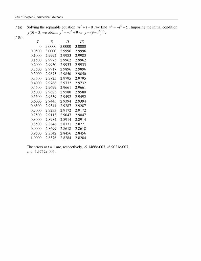
254 • Chapter 9 Numerical Methods
7 (a). Solving the separable equation yy t¢ + = 0, we find y t C2 2= - + . Imposing the initial conditiony( )0 3= , we obtain y t2 2 9= - + or y t= -( ) /9 2 1 2.
7 (b). T E H IE
0 3.0000 3.0000 3.0000 0.0500 3.0000 2.9996 2.9996 0.1000 2.9992 2.9983 2.9983 0.1500 2.9975 2.9962 2.9962 0.2000 2.9950 2.9933 2.9933 0.2500 2.9917 2.9896 2.9896 0.3000 2.9875 2.9850 2.9850 0.3500 2.9825 2.9795 2.9795 0.4000 2.9766 2.9732 2.9732 0.4500 2.9699 2.9661 2.9661 0.5000 2.9623 2.9580 2.9580 0.5500 2.9539 2.9492 2.9492 0.6000 2.9445 2.9394 2.9394 0.6500 2.9344 2.9287 2.9287 0.7000 2.9233 2.9172 2.9172 0.7500 2.9113 2.9047 2.9047 0.8000 2.8984 2.8914 2.8914 0.8500 2.8846 2.8771 2.8771 0.9000 2.8699 2.8618 2.8618 0.9500 2.8542 2.8456 2.8456 1.0000 2.8376 2.8284 2.8284
The errors at t = 1 are, respectively, -9.1466e-003, -6.9021e-007,and -1.3752e-005.
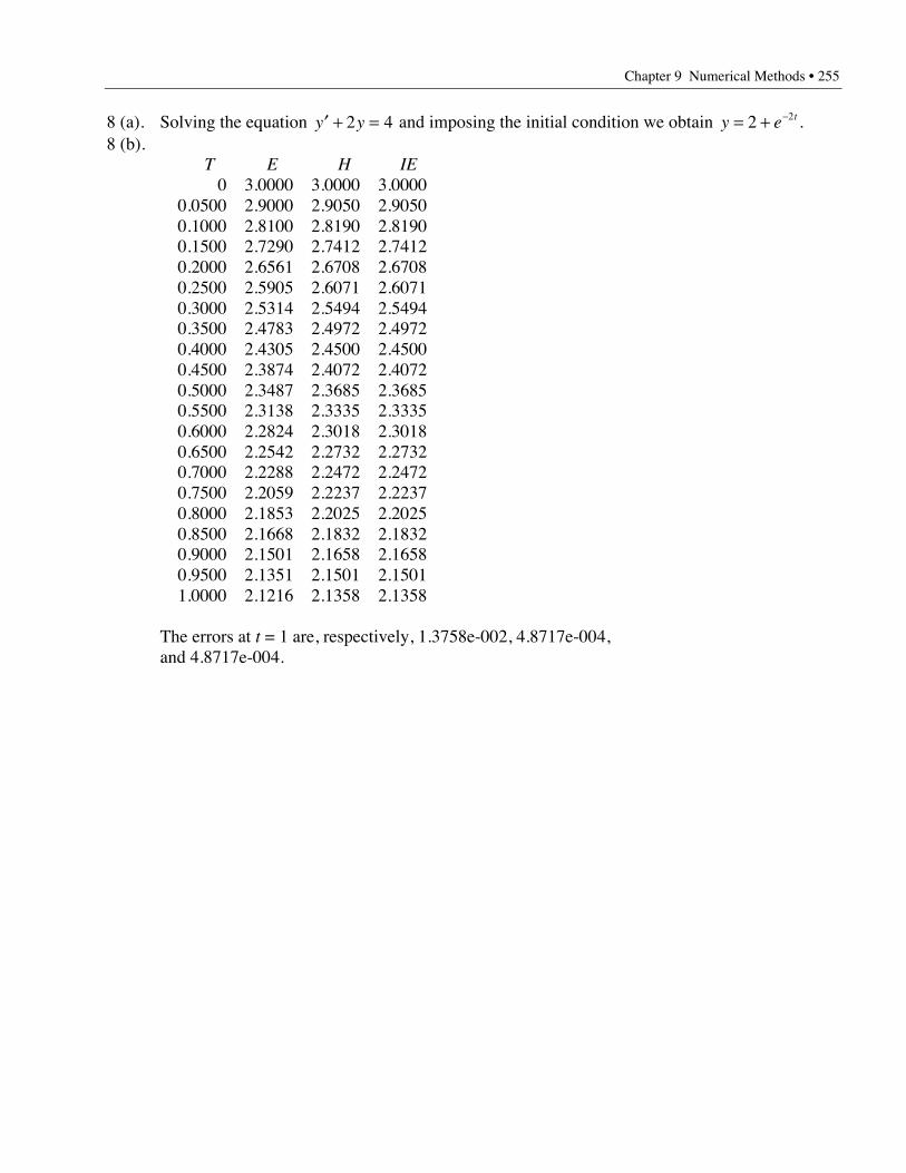
Chapter 9 Numerical Methods • 255
8 (a). Solving the equation ¢ + =y y2 4 and imposing the initial condition we obtain y e t= + -2 2 .8 (b).
T E H IE 0 3.0000 3.0000 3.0000 0.0500 2.9000 2.9050 2.9050 0.1000 2.8100 2.8190 2.8190 0.1500 2.7290 2.7412 2.7412 0.2000 2.6561 2.6708 2.6708 0.2500 2.5905 2.6071 2.6071 0.3000 2.5314 2.5494 2.5494 0.3500 2.4783 2.4972 2.4972 0.4000 2.4305 2.4500 2.4500 0.4500 2.3874 2.4072 2.4072 0.5000 2.3487 2.3685 2.3685 0.5500 2.3138 2.3335 2.3335 0.6000 2.2824 2.3018 2.3018 0.6500 2.2542 2.2732 2.2732 0.7000 2.2288 2.2472 2.2472 0.7500 2.2059 2.2237 2.2237 0.8000 2.1853 2.2025 2.2025 0.8500 2.1668 2.1832 2.1832 0.9000 2.1501 2.1658 2.1658 0.9500 2.1351 2.1501 2.1501 1.0000 2.1216 2.1358 2.1358
The errors at t = 1 are, respectively, 1.3758e-002, 4.8717e-004,and 4.8717e-004.
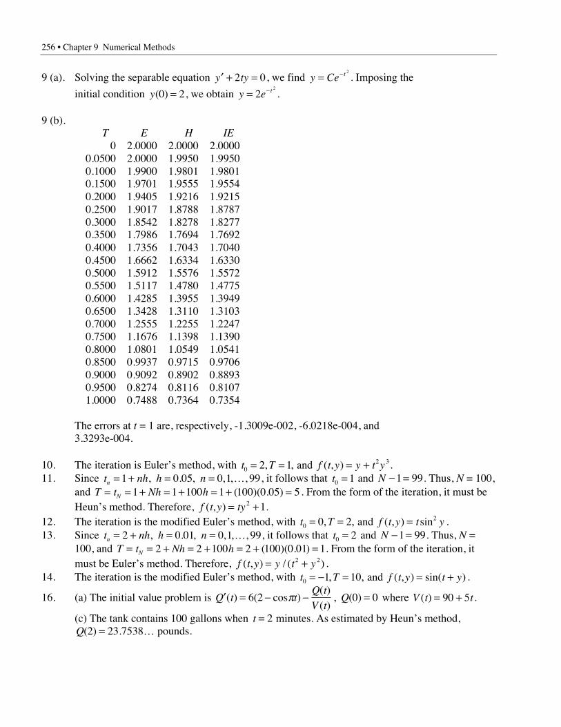
256 • Chapter 9 Numerical Methods
9 (a). Solving the separable equation ¢ + =y ty2 0, we find y Ce t= - 2
. Imposing the
initial condition y( )0 2= , we obtain y e t= -22
.
9 (b). T E H IE
0 2.0000 2.0000 2.0000 0.0500 2.0000 1.9950 1.9950 0.1000 1.9900 1.9801 1.9801 0.1500 1.9701 1.9555 1.9554 0.2000 1.9405 1.9216 1.9215 0.2500 1.9017 1.8788 1.8787 0.3000 1.8542 1.8278 1.8277 0.3500 1.7986 1.7694 1.7692 0.4000 1.7356 1.7043 1.7040 0.4500 1.6662 1.6334 1.6330 0.5000 1.5912 1.5576 1.5572 0.5500 1.5117 1.4780 1.4775 0.6000 1.4285 1.3955 1.3949 0.6500 1.3428 1.3110 1.3103 0.7000 1.2555 1.2255 1.2247 0.7500 1.1676 1.1398 1.1390 0.8000 1.0801 1.0549 1.0541 0.8500 0.9937 0.9715 0.9706 0.9000 0.9092 0.8902 0.8893 0.9500 0.8274 0.8116 0.8107 1.0000 0.7488 0.7364 0.7354
The errors at t = 1 are, respectively, -1.3009e-002, -6.0218e-004, and3.3293e-004.
10. The iteration is Euler’s method, with t T f t y y t y02 32 1= = = +, , ( , ) and .
11. Since t nh h nn = + = =1 0 05 0 1 99, . , , , ,K , it follows that t0 1= and N - =1 99. Thus, N = 100,and T t Nh hN= = + = + = + =1 1 100 1 100 0 05 5( )( . ) . From the form of the iteration, it must beHeun’s method. Therefore, f t y ty( , ) = +2 1.
12. The iteration is the modified Euler’s method, with t T f t y t y020 2= = =, , ( , ) sin and .
13. Since t nh h nn = + = =2 0 01 0 1 99, . , , , ,K , it follows that t0 2= and N - =1 99. Thus, N =100, and T t Nh hN= = + = + = + =2 2 100 2 100 0 01 1( )( . ) . From the form of the iteration, itmust be Euler’s method. Therefore, f t y y t y( , ) / ( )= +2 2 .
14. The iteration is the modified Euler’s method, with t T f t y t y0 1 10= - = = +, , ( , ) sin( ) and .
16. (a) The initial value problem is ¢ = - - =Q t tQ t
V tQ( ) ( cos )
( )( )
, ( )6 2 0 0p where V t t( ) = +90 5 .
(c) The tank contains 100 gallons when t = 2 minutes. As estimated by Heun’s method,Q( ) .2 23 7538= K pounds.
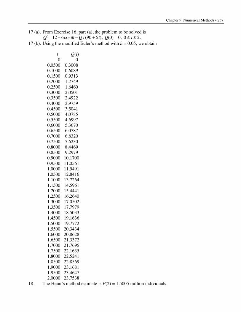
Chapter 9 Numerical Methods • 257
17 (a). From Exercise 16, part (a), the problem to be solved is¢ = - - + = £ £Q t Q t Q t12 6 90 5 0 0 0 2cos / ( ), ( ) ,p .
17 (b). Using the modified Euler’s method with h = 0.05, we obtain
t Q(t) 0 0
0.0500 0.3008 0.1000 0.6089 0.1500 0.9313 0.2000 1.2749 0.2500 1.6460 0.3000 2.0501 0.3500 2.4922 0.4000 2.9759 0.4500 3.5041 0.5000 4.0785 0.5500 4.6997 0.6000 5.3670 0.6500 6.0787 0.7000 6.8320 0.7500 7.6230 0.8000 8.4469 0.8500 9.2979 0.9000 10.1700 0.9500 11.0561 1.0000 11.9491 1.0500 12.8416 1.1000 13.7264 1.1500 14.5961 1.2000 15.4441 1.2500 16.2640 1.3000 17.0502 1.3500 17.7979 1.4000 18.5033 1.4500 19.1636 1.5000 19.7772 1.5500 20.3434 1.6000 20.8628 1.6500 21.3372 1.7000 21.7695 1.7500 22.1635 1.8000 22.5241 1.8500 22.8569 1.9000 23.1681 1.9500 23.4647 2.0000 23.7538
18. The Heun’s method estimate is P(2) = 1.5005 million individuals.
258 • Chapter 9 Numerical Methods
19. Using the modified Euler’s method, we estimate P(2) = 1.5003 million individuals.20 (a). The results are listed below. The columns headed H1, H2, and H3 are the results obtained
using step sizes h h h= = =0 05 0 025 0 0125. , . , .and respectively. t H1 H2 H3 True
0.0000 1.0000 1.0000 1.0000 1.0000 0.0500 1.0526 1.0526 1.0526 1.0526 0.1000 1.1109 1.1111 1.1111 1.1111 0.1500 1.1762 1.1764 1.1765 1.1765 0.2000 1.2495 1.2499 1.2500 1.2500 0.2500 1.3326 1.3332 1.3333 1.3333 0.3000 1.4275 1.4283 1.4285 1.4286 0.3500 1.5370 1.5381 1.5384 1.5385 0.4000 1.6645 1.6661 1.6665 1.6667 0.4500 1.8151 1.8174 1.8180 1.8182 0.5000 1.9954 1.9988 1.9997 2.0000 0.5500 2.2153 2.2204 2.2218 2.2222 0.6000 2.4894 2.4972 2.4993 2.5000 0.6500 2.8402 2.8527 2.8560 2.8571 0.7000 3.3049 3.3257 3.3314 3.3333 0.7500 3.9488 3.9860 3.9964 4.0000 0.8000 4.8975 4.9714 4.9925 5.0000 0.8500 6.4264 6.5969 6.6480 6.6667 0.9000 9.2615 9.7669 9.9353 10.0000 0.9500 15.9962 18.4267 19.5053 20.0000
The error ratios are denoted, respectively, by R1 and R2 whereR H True H True1 1 2= - -( ) / ( ) and R H True H True2 2 3= - -( ) / ( )
t R1 R2 0.0500 3.8916 3.9471 0.1000 3.8879 3.9454 0.1500 3.8838 3.9436 0.2000 3.8791 3.9414 0.2500 3.8737 3.9390 0.3000 3.8674 3.9362 0.3500 3.8601 3.9329 0.4000 3.8513 3.9291 0.4500 3.8408 3.9244 0.5000 3.8279 3.9187 0.5500 3.8117 3.9117 0.6000 3.7909 3.9026 0.6500 3.7634 3.8907 0.7000 3.7255 3.8743 0.7500 3.6707 3.8503 0.8000 3.5860 3.8126 0.8500 3.4428 3.7459 0.9000 3.1683 3.6039 0.9500 2.5450 3.1800
Chapter 9 Numerical Methods • 259
20 (b). An error monitor is y t y y yn n n( ) ( ) /* - = -) )2 2 3.
20 (c). The column headed est gives the estimated error using the error monitor from part (b). Thecolumn headed true gives the actual error. The error monitor used step sizes of h = 0.025 and h= 0.0125.
t est true0.0500 4.4179e-006 4.4972e-006
0.1000 1.0382e-005 1.0574e-005 0.1500 1.8466e-005 1.8820e-005 0.2000 2.9497e-005 3.0084e-005 0.2500 4.4686e-005 4.5614e-005 0.3000 6.5850e-005 6.7281e-005 0.3500 9.5774e-005 9.7965e-005 0.4000 1.3886e-004 1.4222e-004 0.4500 2.0228e-004 2.0751e-004 0.5000 2.9820e-004 3.0650e-004 0.5500 4.4818e-004 4.6178e-004 0.6000 6.9264e-004 7.1587e-004 0.6500 1.1126e-003 1.1547e-003 0.7000 1.8854e-003 1.9679e-003 0.7500 3.4446e-003 3.6255e-003 0.8000 7.0273e-003 7.4956e-003 0.8500 1.7050e-002 1.8628e-002 0.9000 5.6137e-002 6.4677e-002 0.9500 3.5951e-001 4.9473e-001
Section 9.2
Unless indicated by K, all results are rounded to the places shown.
1 (a). From the given equation ¢ = - +y y 2, we know ¢ = - +y t y t( ) ( ) 2, ¢¢ = - ¢y t y t( ) ( ) ,¢¢¢ = - ¢¢y t y t( ) ( ) , and y t y t( )( ) ( )4 = - ¢¢¢ . We also know that y( )0 1= . Therefore,¢ = - + = - + =y y( ) ( )0 0 2 1 2 1, ¢¢ = - ¢ = -y y( ) ( )0 0 1, ¢¢¢ = - ¢¢ =y y( ) ( )0 0 1, and
y y( )( ) ( )4 0 0 1= - ¢¢¢ = - . Thus,P t t t t t4
2 3 41 1 2 1 6 1 24( ) ( / ) ( / ) ( / )= + - + - .2 (a). From the given equation ¢ =y ty2 , we know, ¢ =y ( )0 0, ¢¢ =y ( )0 2, ¢¢¢ =y ( )0 0, and
y( )( )4 0 12= . Thus,P t t t4
2 41 1 2( ) ( / )= + + .3 (a). From the given equation ¢ =y ty 2 , we know ¢ =y t ty t( ) ( )2 , ¢¢ = + ¢y t y t ty t y t( ) ( ) ( ) ( )2 2 ,
¢¢¢ = ¢ + ¢ ¢ + ¢¢y t y t y t ty t y t ty t y t( ) ( ) ( ) ( ) ( ) ( ) ( )4 2 2 , andy t y t y t y t y t ty t y t ty t y t( )( ) ( ) ( ) ( ) ( ) ( ) ( ) ( ) ( )4 6 6 6 2= ¢ ¢ + ¢¢ + ¢ ¢¢ + ¢¢¢ . We also know that y( )0 1= .Therefore, ¢ =y ( )0 0, ¢¢ =y ( )0 1, ¢¢¢ =y ( )0 0, and y( )( )4 0 6= . Thus,
P t t t42 41 1 2 1 4( ) ( / ) ( / )= + + .
260 • Chapter 9 Numerical Methods
4 (a). From the given equation ¢ = +y t y2 , we know, ¢ =y ( )0 1, ¢¢ =y ( )0 1, ¢¢¢ =y ( )0 3, andy( )( )4 0 3= . Thus,
P t t t t t42 3 41 1 2 1 2 1 8( ) ( / ) ( / ) ( / )= + + + + .
5 (a). From the given equation ¢ =y y1 2/ , we know ¢ =y t y t( ) ( )/1 2 , ¢¢ = ¢-y t y t y t( ) ( / ) ( ) ( )/1 2 1 2 ,¢¢¢ = - ¢ + ¢¢- -y t y t y t y t y t( ) ( / ) ( ) ( ) ( / ) ( ) ( )/ /1 4 1 23 2 1 2 , and
y t y t y t y t y t y t y t y t y t( ) / / /( ) ( / ) ( ) ( ) ( ) ( / ) ( ) ( ) ( ) ( / ) ( ) ( )4 5 2 3 2 1 23 8 3 4 1 2= ¢ ¢ - ¢¢ ¢ + ¢¢¢- - - . We also knowthat y( )0 1= . Therefore, ¢ =y ( )0 1, ¢¢ =y ( ) /0 1 2, ¢¢¢ = - + =y ( ) ( / ) ( / )( / )0 1 4 1 2 1 2 0, andy( )( ) ( / ) ( / )( / )4 0 3 8 3 4 1 2 0= - = . Thus,
P t t t421 1 4( ) ( / )= + + .
6 (a). From the given equation ¢ = -y ty 1, we know, ¢ =y ( )0 0, ¢¢ =y ( )0 1, ¢¢¢ =y ( )0 0, andy( )( )4 0 3= - . Thus,
P t t t42 41 1 2 1 8( ) ( / ) ( / )= + - .
7 (a). From the given equation ¢ = +y y tsin , we know ¢ = +y t y t t( ) ( ) sin , ¢¢ = ¢ +y t y t t( ) ( ) cos ,¢¢¢ = ¢¢ -y t y t t( ) ( ) sin , and y t y t t( )( ) ( ) cos4 = ¢¢¢ - . We also know that y( )0 1= . Therefore,¢ =y ( )0 1, ¢¢ = + =y ( )0 1 1 2, ¢¢¢ = - =y ( )0 2 0 2, and y( )( )4 0 2 1 1= - = . Thus,
P t t t t t42 3 41 1 3 1 24( ) ( / ) ( / )= + + + + .
8 (a). From the given equation ¢ =y y 3 4/ , we know, ¢ =y ( )0 1, ¢¢ =y ( ) /0 3 4 , ¢¢¢ =y ( ) /0 3 8, andy( )( ) /4 0 3 32= . Thus,
P t t t t t42 3 41 3 8 1 16 1 256( ) ( / ) ( / ) ( / )= + + + + .
9 (a). From the given equation ¢ = +y y1 2, we know ¢ = +y t y t( ) ( )1 2 , ¢¢ = ¢y t y t y t( ) ( ) ( )2 ,¢¢¢ = ¢ ¢ + ¢¢y t y t y t y t y t( ) ( ) ( ) ( ) ( )2 2 , and y t y t y t y t y t( )( ) ( ) ( ) ( ) ( )4 6 2= ¢¢ ¢ + ¢¢ . We also know that
y( )0 1= . Therefore, ¢ =y ( )0 2, ¢¢ = =y ( ) ( )( )( )0 2 1 2 4 , ¢¢¢ = + =y ( ) ( )( )( ) ( )( )( )0 2 2 2 2 1 4 16, andy( )( ) ( )( )( ) ( )( )( )4 0 6 4 2 2 1 16 80= + = . Thus,
P t t t t t42 3 41 2 2 8 3 10 3( ) ( / ) ( / )= + + + + .
10 (a). From the given equation ¢ = -y t y4 3 , we know, ¢ =y ( )0 0, ¢¢ =y ( )0 0, ¢¢¢ =y ( )0 0, andy( )( )4 0 24= - . Thus,
P t t441( ) = - .
11 (a). From the given equation ¢¢ = ¢ -y y y3 2 , we know ¢¢ = ¢ -y t y t y t( ) ( ) ( )3 2 ,¢¢¢ = ¢¢ - ¢y t y t y t( ) ( ) ( )3 2 , y t y t y t( )( ) ( ) ( )4 3 2= ¢¢¢ - ¢¢ , and y t y t y t( ) ( )( ) ( ) ( )5 43 2= - ¢¢¢ . We also
know that y y( ) ( )0 1 0 0= ¢ = and . Therefore, ¢¢ = - = -y ( ) ( )( ) ( )( )0 3 0 2 1 2,¢¢¢ = - - = -y ( ) ( )( ) ( )( )0 3 2 2 0 6, y( )( ) ( )( ) ( )( )4 0 3 6 2 2 14= - - - = - , and
y( )( ) ( )( ) ( )( )5 0 3 14 2 6 30= - - - = - . Thus,P t t t t t5
2 3 4 51 7 12 1 4( ) ( / ) ( / )= - - - - .12 (a). From the given equation ¢¢ - ¢ =y y 0, we know, ¢¢ =y ( )1 2, ¢¢¢ =y ( )1 2, y( )( )4 1 2= , and
y( )( )5 1 2= . Thus,P t t t t t t5
2 3 4 51 2 1 1 1 3 1 1 12 1 1 60 1( ) ( ) ( ) ( / )( ) ( / )( ) ( / )( )= + - + - + - + - + - .13 (a). From the given equation ¢¢¢ = ¢y y , we know ¢¢¢ = ¢y t y t( ) ( ), y t y t( )( ) ( )4 = ¢¢ , and y t y t( )( ) ( )5 = ¢¢¢ .
We also know that y y y( ) , ( ) ( )0 1 0 2 0 0= ¢ = ¢¢ = and . Therefore, ¢¢¢ =y ( )0 2, y( )( )4 0 0= ,y( )( )5 0 2= . Thus,
P t t t t53 51 2 1 3 1 60( ) ( / ) ( / )= + + + .
Chapter 9 Numerical Methods • 261
14 (a). From the given equation ¢¢ + + =y y y 3 0, we know, ¢¢ = -y ( )0 2, ¢¢¢ =y ( )0 0, y( )( )4 0 8= , andy( )( )5 0 0= . Thus,
P t t t52 41 1 3( ) ( / )= - + .
15. The function q h h( ) sin= 2 has a Maclaurin expansion given by sin ( / )( )2 2 1 6 2 3h h h= - + L.Therefore, q h O h( ) ( )= .
16. q h O h( ) ( )= .17. The function q h h( ) cos= -1 has a Maclaurin expansion given by
1 1 1 1 2 1 24 1 22 4 2- = - - + + = +cos ( ( / ) ( / ) ( / )h h h hL L. Therefore, q h O h( ) ( )= 2 .18. The function q h e hh( ) ( )= - +1 has a Maclaurin expansion given by
e h h h h hh - + = + + + - + = +( ) [ ( / ) ] ( ) ( / )1 1 1 2 1 1 22 2L L. Therefore, q h O h( ) ( )= 2 .20 (a).
t ts-1 ts-2 ts-3 0.0000 1.0000 1.0000 1.0000 0.0500 1.0000 1.0006 1.0006 0.1000 1.0013 1.0025 1.0025 0.1500 1.0037 1.0056 1.0056 0.2000 1.0075 1.0100 1.0100 0.2500 1.0125 1.0156 1.0156 0.3000 1.0187 1.0224 1.0224 0.3500 1.0261 1.0304 1.0304 0.4000 1.0348 1.0396 1.0396 0.4500 1.0446 1.0500 1.0500 0.5000 1.0556 1.0616 1.0616 0.5500 1.0677 1.0743 1.0742 0.6000 1.0810 1.0881 1.0881 0.6500 1.0955 1.1030 1.1030 0.7000 1.1110 1.1190 1.1190 0.7500 1.1276 1.1360 1.1360 0.8000 1.1452 1.1541 1.1541 0.8500 1.1638 1.1732 1.1731 0.9000 1.1835 1.1932 1.1932 0.9500 1.2041 1.2142 1.2142 1.0000 1.2256 1.2361 1.236120 (b). At t = 1, the errors are (respectively): -1.0441e-002, 5.5071e-005, and
-1.0500e-006.
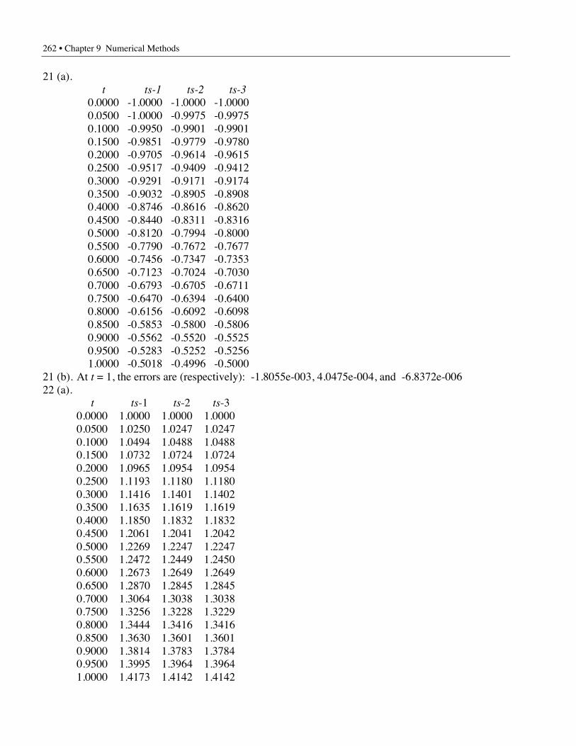
262 • Chapter 9 Numerical Methods
21 (a). t ts-1 ts-2 ts-3 0.0000 -1.0000 -1.0000 -1.0000 0.0500 -1.0000 -0.9975 -0.9975 0.1000 -0.9950 -0.9901 -0.9901 0.1500 -0.9851 -0.9779 -0.9780 0.2000 -0.9705 -0.9614 -0.9615 0.2500 -0.9517 -0.9409 -0.9412 0.3000 -0.9291 -0.9171 -0.9174 0.3500 -0.9032 -0.8905 -0.8908 0.4000 -0.8746 -0.8616 -0.8620 0.4500 -0.8440 -0.8311 -0.8316 0.5000 -0.8120 -0.7994 -0.8000 0.5500 -0.7790 -0.7672 -0.7677 0.6000 -0.7456 -0.7347 -0.7353 0.6500 -0.7123 -0.7024 -0.7030 0.7000 -0.6793 -0.6705 -0.6711 0.7500 -0.6470 -0.6394 -0.6400 0.8000 -0.6156 -0.6092 -0.6098 0.8500 -0.5853 -0.5800 -0.5806 0.9000 -0.5562 -0.5520 -0.5525 0.9500 -0.5283 -0.5252 -0.5256 1.0000 -0.5018 -0.4996 -0.5000
21 (b). At t = 1, the errors are (respectively): -1.8055e-003, 4.0475e-004, and -6.8372e-00622 (a).
t ts-1 ts-2 ts-3 0.0000 1.0000 1.0000 1.0000 0.0500 1.0250 1.0247 1.0247 0.1000 1.0494 1.0488 1.0488 0.1500 1.0732 1.0724 1.0724 0.2000 1.0965 1.0954 1.0954 0.2500 1.1193 1.1180 1.1180 0.3000 1.1416 1.1401 1.1402 0.3500 1.1635 1.1619 1.1619 0.4000 1.1850 1.1832 1.1832 0.4500 1.2061 1.2041 1.2042 0.5000 1.2269 1.2247 1.2247 0.5500 1.2472 1.2449 1.2450 0.6000 1.2673 1.2649 1.2649 0.6500 1.2870 1.2845 1.2845 0.7000 1.3064 1.3038 1.3038 0.7500 1.3256 1.3228 1.3229 0.8000 1.3444 1.3416 1.3416 0.8500 1.3630 1.3601 1.3601 0.9000 1.3814 1.3783 1.3784 0.9500 1.3995 1.3964 1.3964 1.0000 1.4173 1.4142 1.4142
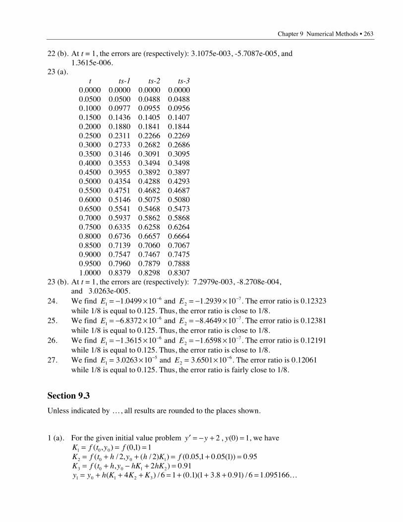
Chapter 9 Numerical Methods • 263
22 (b). At t = 1, the errors are (respectively): 3.1075e-003, -5.7087e-005, and1.3615e-006.
23 (a). t ts-1 ts-2 ts-3 0.0000 0.0000 0.0000 0.0000 0.0500 0.0500 0.0488 0.0488 0.1000 0.0977 0.0955 0.0956 0.1500 0.1436 0.1405 0.1407 0.2000 0.1880 0.1841 0.1844 0.2500 0.2311 0.2266 0.2269 0.3000 0.2733 0.2682 0.2686 0.3500 0.3146 0.3091 0.3095 0.4000 0.3553 0.3494 0.3498 0.4500 0.3955 0.3892 0.3897 0.5000 0.4354 0.4288 0.4293 0.5500 0.4751 0.4682 0.4687 0.6000 0.5146 0.5075 0.5080 0.6500 0.5541 0.5468 0.5473 0.7000 0.5937 0.5862 0.5868 0.7500 0.6335 0.6258 0.6264 0.8000 0.6736 0.6657 0.6664 0.8500 0.7139 0.7060 0.7067 0.9000 0.7547 0.7467 0.7475 0.9500 0.7960 0.7879 0.7888 1.0000 0.8379 0.8298 0.8307
23 (b). At t = 1, the errors are (respectively): 7.2979e-003, -8.2708e-004,and 3.0263e-005.
24. We find E161 0499 10= - ¥ -. and E2
71 2939 10= - ¥ -. . The error ratio is 0.12323while 1/8 is equal to 0.125. Thus, the error ratio is close to 1/8.
25. We find E166 8372 10= - ¥ -. and E2
78 4649 10= - ¥ -. . The error ratio is 0.12381while 1/8 is equal to 0.125. Thus, the error ratio is close to 1/8.
26. We find E161 3615 10= - ¥ -. and E2
71 6598 10= - ¥ -. . The error ratio is 0.12191while 1/8 is equal to 0.125. Thus, the error ratio is close to 1/8.
27. We find E153 0263 10= ¥ -. and E2
63 6501 10= ¥ -. . The error ratio is 0.12061while 1/8 is equal to 0.125. Thus, the error ratio is fairly close to 1/8.
Section 9.3
Unless indicated by K, all results are rounded to the places shown.
1 (a). For the given initial value problem ¢ = - + =y y y2 0 1, ( ) , we haveK f t y f1 0 0 0 1 1= = =( , ) ( , )K f t h y h K f2 0 0 12 2 0 05 1 0 05 1 0 95= + + = + =( / , ( / ) ) ( . , . ( )) .K f t h y hK hK3 0 0 1 22 0 91= + - + =( , ) .y y h K K K1 0 1 2 34 6 1 0 1 1 3 8 0 91 6 1 095166= + + + = + + + =( ) / ( . )( . . ) / . K
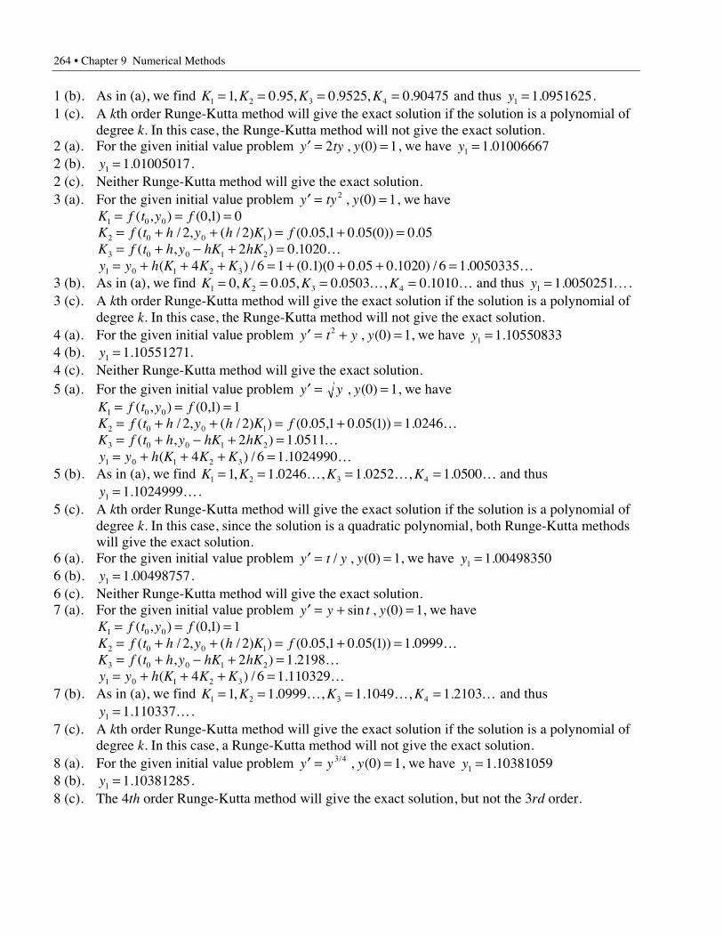
264 • Chapter 9 Numerical Methods
1 (b). As in (a), we find K K K K1 2 3 41 0 95 0 9525 0 90475= = = =, . , . , . and thus y1 1 0951625= . .1 (c). A kth order Runge-Kutta method will give the exact solution if the solution is a polynomial of
degree k. In this case, the Runge-Kutta method will not give the exact solution.2 (a). For the given initial value problem ¢ = =y ty y2 0 1, ( ) , we have y1 1 01006667= .2 (b). y1 1 01005017= . .2 (c). Neither Runge-Kutta method will give the exact solution.3 (a). For the given initial value problem ¢ = =y ty y2 0 1, ( ) , we have
K f t y f1 0 0 0 1 0= = =( , ) ( , )K f t h y h K f2 0 0 12 2 0 05 1 0 05 0 0 05= + + = + =( / , ( / ) ) ( . , . ( )) .K f t h y hK hK3 0 0 1 22 0 1020= + - + =( , ) . Ky y h K K K1 0 1 2 34 6 1 0 1 0 0 05 0 1020 6 1 0050335= + + + = + + + =( ) / ( . )( . . ) / . K
3 (b). As in (a), we find K K K K1 2 3 40 0 05 0 0503 0 1010= = = =, . , . , .K K and thus y1 1 0050251= . K.3 (c). A kth order Runge-Kutta method will give the exact solution if the solution is a polynomial of
degree k. In this case, the Runge-Kutta method will not give the exact solution.4 (a). For the given initial value problem ¢ = + =y t y y2 0 1, ( ) , we have y1 1 10550833= .4 (b). y1 1 10551271= . .4 (c). Neither Runge-Kutta method will give the exact solution.5 (a). For the given initial value problem ¢ = =y y y, ( )0 1, we have
K f t y f1 0 0 0 1 1= = =( , ) ( , )K f t h y h K f2 0 0 12 2 0 05 1 0 05 1 1 0246= + + = + =( / , ( / ) ) ( . , . ( )) . KK f t h y hK hK3 0 0 1 22 1 0511= + - + =( , ) . Ky y h K K K1 0 1 2 34 6 1 1024990= + + + =( ) / . K
5 (b). As in (a), we find K K K K1 2 3 41 1 0246 1 0252 1 0500= = = =, . , . , .K K K and thusy1 1 1024999= . K.
5 (c). A kth order Runge-Kutta method will give the exact solution if the solution is a polynomial ofdegree k. In this case, since the solution is a quadratic polynomial, both Runge-Kutta methodswill give the exact solution.
6 (a). For the given initial value problem ¢ = =y t y y/ , ( )0 1, we have y1 1 00498350= .6 (b). y1 1 00498757= . .6 (c). Neither Runge-Kutta method will give the exact solution.7 (a). For the given initial value problem ¢ = + =y y t ysin , ( )0 1, we have
K f t y f1 0 0 0 1 1= = =( , ) ( , )K f t h y h K f2 0 0 12 2 0 05 1 0 05 1 1 0999= + + = + =( / , ( / ) ) ( . , . ( )) . KK f t h y hK hK3 0 0 1 22 1 2198= + - + =( , ) . Ky y h K K K1 0 1 2 34 6 1 110329= + + + =( ) / . K
7 (b). As in (a), we find K K K K1 2 3 41 1 0999 1 1049 1 2103= = = =, . , . , .K K K and thusy1 1 110337= . K.
7 (c). A kth order Runge-Kutta method will give the exact solution if the solution is a polynomial ofdegree k. In this case, a Runge-Kutta method will not give the exact solution.
8 (a). For the given initial value problem ¢ = =y y y3 4 0 1/ , ( ) , we have y1 1 10381059= .8 (b). y1 1 10381285= . .8 (c). The 4th order Runge-Kutta method will give the exact solution, but not the 3rd order.
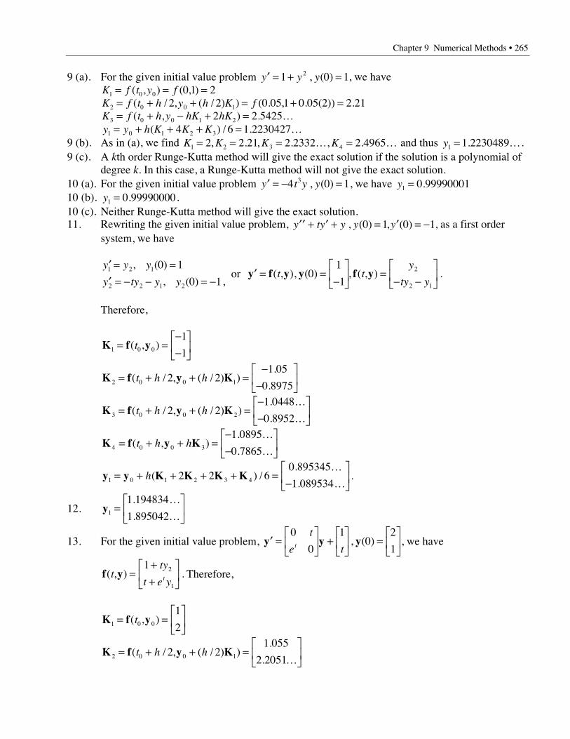
Chapter 9 Numerical Methods • 265
9 (a). For the given initial value problem ¢ = + =y y y1 0 12 , ( ) , we haveK f t y f1 0 0 0 1 2= = =( , ) ( , )K f t h y h K f2 0 0 12 2 0 05 1 0 05 2 2 21= + + = + =( / , ( / ) ) ( . , . ( )) .K f t h y hK hK3 0 0 1 22 2 5425= + - + =( , ) . Ky y h K K K1 0 1 2 34 6 1 2230427= + + + =( ) / . K
9 (b). As in (a), we find K K K K1 2 3 42 2 21 2 2332 2 4965= = = =, . , . , .K K and thus y1 1 2230489= . K.9 (c). A kth order Runge-Kutta method will give the exact solution if the solution is a polynomial of
degree k. In this case, a Runge-Kutta method will not give the exact solution.10 (a). For the given initial value problem ¢ = - =y t y y4 0 13 , ( ) , we have y1 0 99990001= .10 (b). y1 0 99990000= . .10 (c). Neither Runge-Kutta method will give the exact solution.11. Rewriting the given initial value problem, ¢¢ + ¢ + = ¢ = -y ty y y y, ( ) , ( )0 1 0 1, as a first order
system, we have
¢ = =¢ = - - = -
y y y
y ty y y1 2 1
2 2 1 2
0 1
0 1
, ( )
, ( ) , or ¢ = =
-È
ÎÍ
˘
˚˙ =
- -È
ÎÍ
˘
˚˙y f y y f y( , ), ( ) , ( , ) .t t
y
ty y0
1
12
2 1
Therefore,
K f y1 0 0
1
1= =
--
È
ÎÍ
˘
˚˙( , )t
K f y K2 0 0 12 21 05
0 8975= + + =
--
È
ÎÍ
˘
˚˙( / , ( / ) )
.
.t h h
K f y K3 0 0 22 21 0448
0 8952= + + =
--
È
ÎÍ
˘
˚˙( / , ( / ) )
.
.t h h
K
K
K f y K4 0 0 3
1 0895
0 7865= + + =
--
È
ÎÍ
˘
˚˙( , )
.
.t h h
K
K
y y K K K K1 0 1 2 3 42 2 60 895345
1 089534= + + + + =
-È
ÎÍ
˘
˚˙h( ) /
.
.
K
K.
12. y1
1 194834
1 895042=
È
ÎÍ
˘
˚˙
.
.
K
K
13. For the given initial value problem, ¢ =È
ÎÍ
˘
˚˙ +
È
ÎÍ
˘
˚˙ =
È
ÎÍ
˘
˚˙y y y
0
0
10
2
1
t
e tt , ( ) , we have
f y( , ) .tty
t e yt=+
+È
ÎÍ
˘
˚˙
1 2
1
Therefore,
K f y1 0 0
1
2= =
È
ÎÍ
˘
˚˙( , )t
K f y K2 0 0 12 21 055
2 2051= + + =
È
ÎÍ
˘
˚˙( / , ( / ) )
.
.t h h
K
266 • Chapter 9 Numerical Methods
K f y K3 0 0 22 21 0555
2 2079= + + =
È
ÎÍ
˘
˚˙( / , ( / ) )
.
.t h h
K
K
K f y K4 0 0 3
1 1220
2 4269= + + =
È
ÎÍ
˘
˚˙( , )
.
.t h h
K
K
y y K K K K1 0 1 2 3 42 2 62 105718
1 220886= + + + + =
È
ÎÍ
˘
˚˙h( ) /
.
.
K
K.
14. y1
0 900625
0 809968=
-È
ÎÍ
˘
˚˙
.
.
K
K
15. Rewriting the given initial value problem, ¢¢¢ = = ¢ = ¢¢ = -y ty y y y, ( ) , ( ) , ( )0 1 0 0 0 1, as a firstorder system, we have
¢ = =¢ = =¢ = = -
y y y
y y y
y ty y
1 2 1
2 3 2
3 1 3
0 1
0 0
0 1
, ( )
, ( )
, ( ) ,
or ¢ = =-
È
Î
ÍÍ
˘
˚
˙˙ =
È
Î
ÍÍ
˘
˚
˙˙y f y y f y( , ), ( ) , ( , ) .t t
y
yty
01
01
2
3
1
Therefore,
K f y1 0 0
0
10
= = -È
Î
ÍÍ
˘
˚
˙˙( , )t
K f y K2 0 0 12 20 05
1 00 05
= + + =--
È
Î
ÍÍ
˘
˚
˙˙( / , ( / ) )
.
..
t h h
K f y K3 0 0 22 20 05
0 99750 0498
= + + =--
È
Î
ÍÍ
˘
˚
˙˙( / , ( / ) )
.
..
t h hK
K f y K4 0 0 3
0 0997
0 99500 0995
= + + =--
È
Î
ÍÍ
˘
˚
˙˙( , )
.
..
t h hK
K
y y K K K K1 0 1 2 3 42 2 60 995004
0 0998330 995012
= + + + + = --
È
Î
ÍÍ
˘
˚
˙˙h( ) /
.
.
.
K
KK
.
16. y1
1 1996371 988834
0 114991=
È
ÎÍÍ
˘
˚˙˙
.
.
.
KK
K
19 (a). For the given initial value problem ¢ = + =y t y y/ ( ) , ( )1 0 1 and for the step size h = 0 05. , weobtain y20 1 2360679786= . K as our estimate of y( )1 .
19 (b). The actual value of the solution is y( ) .1 1 2360679749= K.20 (a). For the given initial value problem ¢ = = -y ty y2 0 12 , ( ) and for the step size h = 0 05. , we
obtain y20 0 5000000409= - . K as our estimate of y( )1 .20 (b). The actual value of the solution is y( ) .1 0 5= - .
Chapter 9 Numerical Methods • 267
21 (a). For the given initial value problem ¢ = =y y y1 2 0 1/ ( ) , ( ) and for the step size h = 0 05. , weobtain y20 1 4142135632= . K as our estimate of y( )1 .
21 (b). The actual value of the solution is y20 1 4142135623= . K.22 (a). For the given initial value problem ¢ = + + =y y t y( ) / ( ) , ( )1 1 0 02 and for the step size h = 0 05. ,
we obtain y20 0 83064092= . K as our estimate of y( )1 .22 (b). The actual value of the solution is y( ) .1 0 83064087= K.23 (a). Rewriting the given initial value problem, ¢¢ + ¢ + = - = ¢ =y y y y y2 2 2 0 0 0 1, ( ) , ( ) , as a first
order system, we have¢ = =¢ = - - - =
y y y
y y y y1 2 1
2 2 1 2
0 0
2 2 2 0 1
, ( )
, ( ) , or ¢ = =
È
ÎÍ
˘
˚˙ =
- - -È
ÎÍ
˘
˚˙y f y y f y( , ), ( ) , ( , ) .t t
y
y y0
0
1 2 2 22
2 1
23 (b). Using the step size h = 0 1. , we obtain y20
0 810202
0 425496=
--
È
ÎÍ
˘
˚˙
.
.
K
K as our estimate to the solution
value y( ).
.2
0 810199
0 425499=
--
È
ÎÍ
˘
˚˙
K
K.
24 (b). Using the step size h = 0 1. , we obtain y10
0 829662
0 383398=
È
ÎÍ
˘
˚˙
.
.
K
K as our estimate to the solution value
y( ).
.1
0 829660
0 383400=
È
ÎÍ
˘
˚˙
K
K.
25 (a). Rewriting the given initial value problem, t y ty y t y y2 2 1 2 1 2¢¢ - ¢ + = = ¢ =, ( ) , ( ) , as a first ordersystem, we have
¢ = =
¢ = - + =
y y y
y ty y t t y
1 2 1
2 2 12 2
2
1 2
1 2
, ( )
( ) / , ( ) , or
¢ = =È
ÎÍ
˘
˚˙ =
- +È
ÎÍ
˘
˚˙y f y y f y( , ), ( ) , ( , )
( ) /.t t
y
ty y t t0
2
22
2 12 2
25 (b). Using the step size h = 0 1. , we obtain y10
4 6137054
3 3068527=
È
ÎÍ
˘
˚˙
.
.
K
K as our estimate to the solution
value y10
4 6137056
3 3068528=
È
ÎÍ
˘
˚˙
.
.
K
K.
Chapter 10Series Solutions of Linear Differential Equations
Section 10.1
1. Consider the power series tn
nn 20=
•
 . Applying the ratio test at an arbitrary value of t, t π 0, we
obtain lim limn
n n
n n n
t
t
t tÆ •
+
+ Æ •= =
22 2 2
1
1 . The limiting ratio is less than 1 if
t < 2 . Therefore, the radius of convergence is R = 2.
2. lim( )
limn
n
n nn
t n
t n
tt
Æ •
+
Æ •+=
+( )=
1 2
2 1 21 1. Therefore, the radius of convergence is R = 1.
3. Consider the power series ( )t n
n
-=
•
 20
. Applying the ratio test at an arbitrary value of t, t π 2,
we obtain lim( )( )
limn
n
n n
t
tt t
Æ •
+
Æ •
--
= - = -22
2 21
. The limiting ratio is less than 1 if t - <2 1.
Therefore, the radius of convergence is R = 1.
4. lim( )( )n
n
n
t
tt t t
Æ •
+--
= - < fi - < - < fi < <3 13 1
3 1 1 1 3 1 1 023
1
. Therefore, the radius of
convergence is R =13
.
5. Consider the power series ( )
!t
n
n
n
-=
•
 1
0
. Applying the ratio test at an arbitrary value of t, t π 1, we
obtain lim!( )
( )!( )lim
n
n
n n
n t
n t
t
nÆ •
+
Æ •
-+ -
=-+
=1
1 111
01
. The limiting ratio is less than 1 for all t, t π 1.
Therefore, the radius of convergence is R = • .
6. lim( )!( )
!( )lim ( )( ) ,
n
n
n n
n t
n tn t t
Æ •
+
Æ •
+ --
= + - = • π1 1
11 1 1
1
. Therefore, the radius of convergence is
R = 0.
7. Consider the power series ( )-
=
•
 1
1
n n
n
t
n. Applying the ratio test at an arbitrary value of t, t π 0,
we obtain lim( )
limn
n
n n
nt
n t
nt
nt
Æ •
+
Æ •+=
+=
1
1 1. The limiting ratio is less than 1 if t < 1. Therefore,
the radius of convergence is R = 1.
Chapter 10 Series Solutions of Linear Differential Equations • 269
8. lim( ) ( )( ) ( )n
n n n
n n n
t
t
tt t
Æ •
+ +
+- -
- -=
-< fi - < - < fi - < <
1 3 41 3 4
34
1 4 3 4 1 71 1
1 . Therefore, the radius of
convergence is R = 4.
9. Consider the power series (ln )( )n t n
n
+=
•
 21
. Applying the ratio test at an arbitrary value of t,
t π -2, we obtain
lim(ln( ))( )
(ln )( )lim
(ln( ))( )ln
limln( )
lnn
n
n n n
n t
n t
n t
nt
n
nt
Æ •
+
Æ • Æ •
+ ++
=+ +
= ++
= +1 2
21 2
21
21
. (The last limit
can be found using L’Hôpital’s Rule.) The limiting ratio is less than 1 if t + <2 1. Therefore,the radius of convergence is R = 1.
10. lim( ) ( )
( )n
n
n
n t
n tt t t
Æ •
++ --
= - < fi - < - < fi < <1 1
11 1 1 1 1 0 2
3 1
3 . Therefore, the radius of
convergence is R = 1.
11. Consider the power series n t n
nn
( )-=
•
 421
. Applying the ratio test at an arbitrary value of t,
t π 4, we obtain lim( )
( )lim
( )n
n n
n n n
n t
n t
n t
n
tÆ •
+
+ Æ •
+ --
=+ -
=-2 1 4
2 4
1 4
2
42
1
1. The limiting ratio is
less than 1 if t - <4 2. Therefore, the radius of convergence is R = 2.
12. lim( ) arctan( )
( ) arctan( ) lim arctan( )
n
n
n n
t n
t nt t t n
Æ •
+
Æ •
-- +
= - < fi - < - < fi < < =ÊËÁ
ˆ¯
22 1
2 1 1 2 1 1 32
1
recall p
.
Therefore, the radius of convergence is R = 1.13. Applying the ratio test, we see the power series for f(t) and g(t) both have radius of
convergence R = 1. Therefore, each series converges in the interval - < <1 1t .(a) f t t t t t t( ) = + + + + + +1 2 3 4 5 L
g t t t t t t( ) = + + + + + +0 4 9 16 252 3 4 5 L
(b) f t g t t t t t t( ) ( )+ = + + + + + +1 2 5 10 17 262 3 4 5 L
(c) f t g t t t t t( ) ( )- = - - - - -1 3 8 15 242 3 4 5 L
(d) ¢ = + + + + + +f t t t t t t( ) 1 2 3 4 5 62 3 4 5 L
(e) ¢¢ = + + + + + +f t t t t t t( ) 2 6 12 20 30 422 3 4 5 L14. Applying the ratio test, we see the power series for f(t) and g(t) both have radius of
convergence R = 1. Therefore, each series converges in the interval - < <1 1t .(a) f t t t t t t t( ) = + + + + + +2 3 4 5 62 3 4 5 6 L
g t t t t t t t( ) = - + - + - + -2 3 4 5 62 3 4 5 6 L
(b) f t g t t t t t t( ) ( )+ = + + + + +4 8 12 16 202 4 6 8 10 L
(c) f t g t t t t t t t( ) ( )- = + + + + + +2 6 10 14 18 223 5 7 9 11 L
(d) ¢ = + + + + + +f t t t t t t( ) 1 4 9 16 25 362 3 4 5 L
(e) ¢¢ = + + + + + +f t t t t t t( ) 4 18 48 100 180 2942 3 4 5 L
270 • Chapter 10 Series Solutions of Linear Differential Equations
15. Applying the ratio test, we see the power series for f(t) has radius of convergence R = 1 2/while the series for g(t) has radius of convergence R = 1. Therefore, each series converges inthe interval t - <1 1 2/ , or 1 2 3 2/ /< <t .
(a) f t t t t t t( ) ( ) ( ) ( ) ( ) ( )= - - + - - - + - - - +1 2 1 4 1 8 1 16 1 32 12 3 4 5 L
g t t t t t t( ) ( ) ( ) ( ) ( ) ( )= + - + - + - + - + - +1 1 1 1 1 12 3 4 5 L
(b) f t g t t t t t t( ) ( ) ( ) ( ) ( ) ( ) ( )+ = - - + - - - + - - - +2 1 5 1 7 1 17 1 31 12 3 4 5 L
(c) f t g t t t t t t( ) ( ) ( ) ( ) ( ) ( ) ( )- = - - + - - - + - - - +3 1 3 1 9 1 15 1 33 12 3 4 5 L
(d) ¢ = - + - - - + - - - + -f t t t t t t( ) ( ) ( ) ( ) ( ) ( )2 8 1 24 1 64 1 160 1 384 12 3 4 5L
(e) ¢¢ = - - + - - - + - - -f t t t t t t( ) ( ) ( ) ( ) ( ) ( )8 48 1 192 1 640 1 1920 1 5376 12 3 4 5L16. Applying the ratio test, we see the power series for f t( ) is 1/2 and g t( ) is 1. Therefore,
R =12
.
(a) f t t t t t t( ) ( ) ( ) ( ) ( ) ( )= + + + + + + + + + + +1 2 1 4 1 8 1 16 1 32 12 3 4 5 L
g t t t t t t t( ) ( ) ( ) ( ) ( ) ( ) ( )= + + + + + + + + + + + +1 2 1 3 1 4 1 5 1 6 12 3 4 5 6 L
(b) f t g t t t t t t( ) ( ) ( ) ( ) ( ) ( ) ( )+ = + + + + + + + + + + +1 3 1 6 1 11 1 20 1 37 12 3 4 5 L
(c) f t g t t t t t t( ) ( ) ( ) ( ) ( ) ( ) ( )- = + + + + + + + + + + +1 1 2 1 5 1 12 1 27 12 3 4 5 L
(d) ¢ = + + + + + + + + + + +f t t t t t t( ) ( ) ( ) ( ) ( ) ( )2 8 1 24 1 64 1 160 1 384 12 3 4 5 L
(e) ¢¢ = + + + + + + + + + + +f t t t t t t( ) ( ) ( ) ( ) ( ) ( )8 48 1 192 1 640 1 1920 1 5376 12 3 4 5 L
17. Consider the power series 2 2
0
n n
n
t +
=
•
 . Make the change of index k n= + 2. With this change,
the lower limit of n = 0 transforms to k = 2 while the upper limit remains at • . Thus, the
power series can be rewritten as 2 2
2
k k
k
t-
=
•
 . Finally, changing to the original summation index,
n, we obtain 2 2
2
n n
n
t-
=
•
 .
18. Make the change of index k n= + 3. The power series can be rewritten as ( )( )k k tk
k
- -=
•
 2 13
.
Finally, changing to the original summation index, n, we obtain ( )( )n n tn
n
- -=
•
 2 13
.
19. Consider the power series a tnn
n
+
=
•
 2
0
. Make the change of index k n= + 2. With this change,
the lower limit of n = 0 transforms to k = 2 while the upper limit remains at • . Thus, the
power series can be rewritten as a tkk
k-
=
•
 22
. Finally, changing to the original summation index,
n, we obtain a tnn
n-
=
•
 22
.
20. Make the change of index k n= - 1. The power series can be rewritten as ( )k a tkk
k
+ +=
•
 1 10
.
Finally, changing to the original summation index, n, we obtain ( )n a tnn
n
+ +=
•
 1 10
.
Chapter 10 Series Solutions of Linear Differential Equations • 271
21. Consider the power series n n a tnn
n
( )- -
=
•
 1 2
2
. Make the change of index k n= - 2. With this
change, the lower limit of n = 2 transforms to k = 0 while the upper limit remains at • .
Thus, the power series can be rewritten as ( )( )k k a tkk
k
+ + +=
•
 2 1 20
. Finally, changing to the
original summation index, n, we obtain ( )( )n n a tnn
n
+ + +=
•
 2 1 20
.
22. Make the change of index k n= + 3. The power series can be rewritten as ( )- --
=
•
 1 33
3
kk
k
k
a t .
Finally, changing to the original summation index, n, we obtain ( )- --
=
•
 1 33
3
nn
n
n
a t .
23. Consider the power series ( ) ( )- ++ +
=
•
 1 11 2
0
nn
n
n
n a t . Make the change of index k n= + 2. With
this change, the lower limit of n = 0 transforms to k = 2 while the upper limit remains at • .
Thus, the power series can be rewritten as ( ) ( )- ---
=
•
 1 112
2
kk
k
k
k a t . Finally, changing to the
original summation index, n, we obtain ( ) ( )- ---
=
•
 1 112
2
nn
n
n
n a t .
24. Let f t t t t( ) ( sin )= -2 . t tt
n
n n
n
- = --
+
+
=
•
Âsin( )( )!
12 1
2 1
1
. Therefore, f tt
n
n n
n
( )( )
( )!=
-+
+ +
=
•
 12 1
1 2 3
1
.
lim( ) ( )!( )( ) ( )!( )n
n n
n n
n t
n tÆ •
+ +
+ +- +- +
=1 2 11 2 3
02 2 5
1 2 3 . Thus, the radius of convergence is R = • .
25. Let f t t( ) cos= -1 3 . From the Maclaurin series for cosu we have cos ( )( )!
uu
nn
n
n
= -=
•
 12
2
0
.
Therefore, cos! ! !
3 192
814
7296
2 4 6
tt t t
= - + - + L . Hence,
f tt t t t
nn
n
n
( )! ! !
( )( )( )!
= - + - = - +
=
•
Â92
814
7296
132
2 4 61
2
1
L . We calculate the radius of convergence by
using the ratio test. For an arbitrary value of t, t π 0, we have
lim( )!( )
( )!( )lim
( )( )n
n
n n
n t
n t
t
n nÆ •
+
Æ •+=
+ +=
2 32 2 3
92 2 2 1
02 2
2
2
. Thus, the radius of convergence is R = • .
26. Let f tt t
( )( )
=+
=- -
11 2
11 2
. 1
1 22 2
0 0- -= - = -
=
•
=
•
 Â( )( ) ( )
tt tn
n
n
n
n . lim( )( )n
n
n
t
tt
Æ •
+--
= <22
2 11
.
Thus, the radius of convergence is R =12
.
27. Let f t t( ) / ( )= -1 1 2 . From the Maclaurin series for 1 1/ ( )- u we have 1
1 0-=
=
•
Âuun
n
. Therefore,
11
122 4 6
-= + + + +
tt t t L. Hence, f t t n
n
( ) ==
•
 2
0
.
272 • Chapter 10 Series Solutions of Linear Differential Equations
We calculate the radius of convergence by using the ratio test. For an arbitrary value of t, t π 0,
we have lim limn
n
n n
t
tt t
Æ •
+
Æ •= =
2 2
22 2. Thus, the radius of convergence is R = 1.
28 (a). et
nt
t t t ttn
n
= = + + + + + +=
•
 ! ! ! ! !...
0
2 3 4 5
12 3 4 5
.
et
nt
t t t ttn
n
-
=
•
=-
= - + - + - +Â ( )! ! ! ! !
...0
2 3 4 5
12 3 4 5
28 (b). sinh( )! ! ! !
...! ! ! !
...! !
...t tt t t t
tt t t t
tt t
= + + + + + +ÊËÁ
ˆ¯
- - + - + - +ÊËÁ
ˆ¯
ÏÌÓ
¸˝˛
= + + +12
12 3 4 5
12 3 4 5 3 5
2 3 4 5 2 3 4 5 3 5
.
cosh( )! ! ! !
...! ! ! !
...! !
...t tt t t t
tt t t t t t
= + + + + + +ÊËÁ
ˆ¯
+ - + - + - +ÊËÁ
ˆ¯
ÏÌÓ
¸˝˛
= + + +12
12 3 4 5
12 3 4 5
12 4
2 3 4 5 2 3 4 5 2 4
29 (a). Consider the differential equation ¢¢ - =y yw 2 0 and assume there is solution of the form
y t a tnn
n
( ) ==
•
Â0
. Differentiating, we obtain ¢ = ¢¢ = --
=
•-
=
•
 Ây t na t y t n n a tnn
nn
n
n
( ) ( ) ( )1
1
2
2
1 and .
Inserting these series into the differential equation, we have n n a t a tnn
nn
n
n
( )- - =-
=
•
=
•
 Â1 02
2
2
0
w .
Making the change of index k n= - 2 in the series for ¢¢y t( ), we obtain
( )( )n n a t a tnn
nn
n
n
+ + - =+=
•
=
•
 Â2 1 020
2
0
w , or [( )( ) ]n n a a tnn
nn+ + - =+
=
•
 2 1 020
2w . Equating the
coefficients to zero, we find the recurrence relation aa
n nnn
n+ =
+ +=2
2
2 10 1
w( )( )
, , ,K
29 (b). The recurrence relation in part (a) leads us to a a a a a a a a2
20 4
22
40 6
24
602 12 24 30 720= = = = =w w w w w/ , / / , / / , K
a a a a a a a a32
1 52
34
1 72
56
16 20 120 42 5040= = = = =w w w w w/ , / / , / / , K
Thus, y t at t t
( ) [( ) ( ) ( )
]= + + + +0
2 4 6
12 24 720
w w wL +
at
t t t13 5 7
6 120 5040ww w w w
[( ) ( ) ( )
]+ + + + L .
By Exercise 28, y t t y t t1 2( ) cosh ( ) sinh= =w w and .
30 (a). y t n d C t C y C y t t tn
n
tn
n
n
n
n
n
( ) , ( ) ( )= + = + = = fi = + =-
=
•
=
•
=
•
=
•
ÂÚ Â Â Âl l1
10
1 1 0
0 1 1 .
30 (b). R = 1.
30 (c). y tt
( ) =-1
1.
31 (a). Consider the function given by ¢ =-
==
•
Ây tt
ny
n
n
( )( )
!, ( )
11 1
0
. Integrating the series termwise,
we obtain y t Ct
n
n
n
( )( )( )!
= +-
+
+
=
•
 11
1
0
. Imposing the condition y( )1 1= , it follows that C = 1.
Adjusting the index of summation, we can write y tt
n
t
n
n
n
n
n
( )( )
!( )
!= +
-=
-=
•
=
•
 Â11 1
1 0
.
Chapter 10 Series Solutions of Linear Differential Equations • 273
31 (b). Applying the ratio test, lim!( )
( )!( )lim
n
n
n n
n t
n t
t
nÆ •
+
Æ •
-+ -
=-+
=1
1 111
01
. Therefore, the radius of
convergence is R = • .31 (c). From the power series (7a), we see that y t et( ) = -1.
32 (a). ¢ = - + - = - + -+
= - + - = - + -ÏÌÓ
¸˝˛=
• +
=
•-
=
•
=
•
 ÂÚ ÂÂy tn
dt
n
t
n
t
nn
n
n
nn
n
tn
nn
n
nn
( ) ( )!
( )( )!
( )!
( )!
1 1 1 11
1 1 1 10
1
00
1
11
l l
¢ = - -=
•
Âyt
nn
n
n
( )!
10
. Then, y tt
n
t
n
t
nn
n
n
nn
n
nn
n
( ) ( )( )!
( )( )!
( )!
= - -+
+ = + -+
= -+
=
•+
+
=
•
=
•
  Â11
1 1 11
11
0
11
0 0
.
32 (b). R = • .32 (c). y t e t( ) = - .
33 (a). Consider the function given by ¢ = --
==
•
Ây tt
nyn
n
n
( ) ( )( )
!, ( )1
11 0
2
. Integrating the series
termwise, we obtain y t Ct
nn
n
n
( ) ( )( )( )!
= + --
+
+
=
•
 11
1
1
2
. Imposing the condition y( )1 0= , it follows
that C = 0. Adjusting the index of summation, we can write
y tt
n
t
nn
n
n
nn
n
( ) ( )( )
!( )
( )!
= --
= - --+
=
•
=
•
 Â11
111
3 3
.
33 (b). Applying the ratio test, lim( ) !( )
( ) ( )!( )lim
n
n n
n n n
n t
n t
t
nÆ •
+ +
Æ •
- -- + -
=-+
=1 1
1 1 111
01 1
. Therefore, the radius of
convergence is R = • .
33 (c). From the power series (7a), we see that ( )( )
!( )-
-=
=
•- -Â 1
1
0
1nn
n
tt
ne . Thus,
11
11
21
12
3
1--
+-
+ --
==
•- -Â( )
!( )
!( )
( )!
( )t t t
nen
n
n
t . Or, using the results of part (a),
11
11
2
21-
-+
-- =- -( )
!( )
!( )( )t t
e y tt .
34 (a). y t s dst
nn n
n
tn
n
n
( ) ( ) ( )= - = -+=
• +
=
•
ÂÚ Â1 12 1
2
00
2 1
0
.
34 (b). lim( ) ( )( ) ( )n
n n
n n
t n
t nt R
Æ •
+ +
+- +
- += < fi =
1 2 11 2 3
1 11 2 3
2 12 .
34 (c). y t t( ) tan ( )= -1 .
35 (a). Consider the function y(t) where y s dst
n
t n
n
( )0
1Ú Â=
=
•
. Differentiating both sides, we obtain
y t tn
n
( ) = -
=
•
 1
1
. Adjusting the index of summation, we can write y t tn
n
( ) ==
•
Â0
.
35 (b). Applying the ratio test, limn
n
n
t
tt
Æ •
+
=1
. Therefore, the radius of convergence is R = 1.
35 (c). From the power series (7d), we see that y t tt
n
n
( ) = =-=
•
Â0
11
.
274 • Chapter 10 Series Solutions of Linear Differential Equations
36. Assume there is solution of the form y t a tnn
n
( ) ==
•
Â0
. Differentiating, we obtain
¢ = ¢¢ = - = + + ¢ =-
=
•-
=
•
+=
•
=
•
   Ây t na t y t n n a t n n a t ty na tnn
nn
n
nn
n
nn
n
n
( ) ( ) ( ) ( )( ) , 1
1
2
22
0 0
1 2 1 and .
Therefore, [( )( ) ( ) ]n n a n a tnn
nn+ + - + =+
=
•
 2 1 1 020
. Equating the coefficients to zero, we find
the recurrence relation an a
n n
a
nnn n
+ =+
+ +=
+2
12 1 2
( )( )( )
The recurrence leads us to
aa
aa
aa a
aa a
20
31
42 0
53 1
2 3 4 8 5 15= = = = = =, , ,
Therefore, y t at t
a tt t
y a y a( ) ... ... , ( ) , ( )= + + +ÏÌÓ
¸˝˛
+ + + +ÏÌÓ
¸˝˛
= = ¢ = = -0
2 4
1
3 5
0 112 8 3 15
0 1 0 1.
Finally, y tt t
tt t
( ) ... ...= + + +ÏÌÓ
¸˝˛
- + + +ÏÌÓ
¸˝˛
12 8 3 15
2 4 3 5
.
37. Consider the initial value problem ¢¢ + ¢ - = = ¢ =y ty y y y2 0 0 0 0 1, ( ) , ( ) and assume there is
solution of the form y t a tnn
n
( ) ==
•
Â0
. Differentiating, we obtain
¢ = ¢¢ = --
=
•-
=
•
 Ây t na t y t n n a tnn
nn
n
n
( ) ( ) ( )1
1
2
2
1 and . Inserting these series into the differential
equation, we have n n a t t na t a tnn
nn
nn
n
nn
( )- + - =-
=
•-
=
•
=
•
 ÂÂ1 2 02
2
1
01
. Making the change of index
k n= - 2 in the series for ¢¢y t( ), we obtain ( )( )n n a t na t a tnn
nn
nn
n
nn
+ + + - =+=
•
=
•
=
•
 ÂÂ2 1 2 020 01
, or
[( )( ) ( ) ]n n a n a tnn
nn+ + + - =+
=
•
 2 1 2 020
. Equating the coefficients to zero, we find the
recurrence relation an a
n nnn
n+ =
- -+ +
=2
22 1
0 1( )
( )( ), , ,K The recurrence leads us to
a a a a a a a2 0 0 4 2 6 42 2 0 12 0 2 30 0= = = = = - =/ , / , / , K a a a a a a a a3 1 5 3 1 7 5 16 20 120 3 42 1680= = - = - = - =/ , / / , / / , KImposing the initial conditions, we have a a0 10 1= = and . Thus,
y t tt t t
( ) = + - + +3 5 7
6 120 1680L.
38. Assume there is solution of the form y t a tnn
n
( ) ==
•
Â0
. Differentiating, we obtain
¢ = ¢¢ = - = + + = =-
=
•-
=
•
+=
•+
=
•
-=
•
    Ây t na t y t n n a t n n a t ty a t a tnn
nn
n
nn
n
nn
n
nn
n
n
( ) ( ) ( ) ( )( ) ,1
1
2
22
0
1
01
1
1 2 1 and
Therefore, 2 2 1 02 21
1a n n a a tnn
nn+ + + + =+
=
•
-Â[( )( ) ] . Equating the coefficients to zero, we find
the recurrence relation aa
n nnn
n+
-=-
+ +=2
1
2 11 2
( )( ), , ,...
Chapter 10 Series Solutions of Linear Differential Equations • 275
The recurrence leads us to
aa
aa
aa
30
41
52
3 2 4 3 5 40=
-◊
=-
◊=
-◊
=, ,
Therefore, y t at
a tt
a a( ) ... ... , , = - +ÏÌÓ
¸˝˛
+ - +ÏÌÓ
¸˝˛
= =0
3
1
4
0 116 12
1 2.
Finally, y tt
tt
( ) ... ...= - +ÏÌÓ
¸˝˛
+ - +ÏÌÓ
¸˝˛
16
212
3 4
.
39. Consider the initial value problem ¢¢ + + ¢ + = = - ¢ =y t y y y y( ) , ( ) , ( )1 0 0 1 0 1 and assume there
is solution of the form y t a tnn
n
( ) ==
•
Â0
. Differentiating, we obtain
¢ = ¢¢ = --
=
•-
=
•
 Ây t na t y t n n a tnn
nn
n
n
( ) ( ) ( )1
1
2
2
1 and . Inserting these series into the differential
equation, we have n n a t t na t a tnn
nn
nn
n
nn
( ) ( )- + + + =-
=
•-
=
•
=
•
 ÂÂ1 1 02
2
1
01
or
n n a t na t n a tnn
nn
nn
n
nn
( ) ( )- + + + =-
=
•-
=
•
=
•
 ÂÂ1 1 02
2
1
01
. Making the change of index k n= - 2 in the
series for ¢¢y t( ) and k n= - 1 in the series for ¢y t( ) , we obtain
( )( ) ( ) ( )n n a t n a t n a tnn
nn
nn
n
nn
+ + + + + + =+=
•
+=
•
=
•
 ÂÂ2 1 1 1 020
100
, or
[( )( ) ( ) ( ) ]n n a n a n a tn nn
nn+ + + + + + =+ +
=
•
 2 1 1 1 02 10
. Equating the coefficients to zero, we find
the recurrence relation an a n a
n n
a a
nnn n n n
++ +=
- + - ++ +
=- -
+21 11 1
2 1 2( ) ( )
( )( ). The recurrence leads us to
a a a a a a a a a a a a2 0 1 3 2 1 4 3 2 5 4 32 3 4 0 5= - + = - + = - + = = - +( ) / , ( ) / , ( ) / , ( ) / .Imposing the initial conditions, we have a a0 11 1= - = and . Thus,a a a a2 3 4 50 1 3 1 12 1 20= = - = =, / , / , / and so we find
y t t t t t( ) = - + - + + +113
112
120
3 4 5 L.
40. Assume there is solution of the form y t a tnn
n
( ) ==
•
Â0
. Differentiating, we obtain
¢ = + ¢¢ = + ++=
•
+=
•
 Ây t n a t y t n n a tnn
nn
n
n
( ) ( ) ( ) ( )( )1 2 110
20
and . Inserting these series into the
differential equation, we have ( )( ) ( )n n a n a a tn n nn
n
+ + - + +{ } =+ +=
•
 2 1 5 1 6 02 10
. Equating the
coefficients to zero, we find the recurrence relation an a a
n nnn
n n+
+=+ -
+ +=2
15 1 62 1
0 1 2( )( )( )
, , , ,.... The
recurrence leads us to
aa a
aa a
21 0
32 15 6
25 2 6 1
22
5 2 63 2
10 2 6 26
43
=-
=-
= =-
◊=
-=
( ) ( ),
( ) ( ) ( ).
aa a
aa a
43 2
54 35 3 6
4 315 4 3 6 2
1223
5 4 65 4
20 2 3 6 4 320
415
=-
◊=
-= =
-◊
=-
=( ) ( / ) ( )
, ( ) ( / ) ( / )
276 • Chapter 10 Series Solutions of Linear Differential Equations
Therrefore, y t t t t t t( ) = + + + + + +1 2 243
23
415
2 3 4 5 L.
41. Consider the initial value problem ¢¢ - ¢ + = = ¢ =y y y y y2 0 0 0 0 2, ( ) , ( ) and assume there is
solution of the form y t a tnn
n
( ) ==
•
Â0
. Differentiating, we obtain
¢ = ¢¢ = --
=
•-
=
•
 Ây t na t y t n n a tnn
nn
n
n
( ) ( ) ( )1
1
2
2
1 and . Inserting these series into the differential
equation, we have n n a t na t a tnn
nn
nn
n
nn
( )- - + =-
=
•-
=
•
=
•
 ÂÂ1 2 02
2
1
01
. Making the change of index
k n= - 2 in the series for ¢¢y t( ) and k n= - 1 in the series for ¢y t( ) , we obtain
( )( ) ( )n n a t n a t a tnn
nn
nn
n
nn
+ + - + + =+=
•
+=
•
=
•
 ÂÂ2 1 2 1 020
100
, or
[( )( ) ( ) ]n n a n a a tn nn
nn+ + - + + =+ +
=
•
 2 1 2 1 02 10
. Equating the coefficients to zero, we find the
recurrence relation an a a
n nnn n
++=
+ -+ +2
12 12 1
( )( )( )
. The recurrence leads us to
a a a a a a a a a a a a2 1 0 3 2 1 4 3 2 5 4 32 2 4 6 6 12 8 20= - = - = - = -( ) / , ( ) / , ( ) / , ( ) / .Imposing the initial conditions, we have a a0 10 2= = and . Thus,
a a a a2 3 4 52 1 1 3 1 12= = = =, , / , / and so we find y t t t t t t( ) = + + + + +2 213
112
2 3 4 5 L.
Section 10.2
1. Consider the differential equation ¢¢ + ¢ + - =-y t y t t y(sec ) ( )2 14 0. The coefficient functionp t t( ) sec= is not analytic at odd integer multiples of p / 2. Thus, in the interval - < <10 10t ,
p t( ) , , is not analytic at 2 2 2
± ± ±p p p3 5
. Similarly, the coefficient function q t t t( ) ( )= - -2 14 is
not analytic at t = ±2 . These 8 points are the only singular points in - < <10 10t .
2. The function p t t( ) =23 is not analytic at t = 0. The function q t t( ) sin= is analytic everywhere.
Therefore, t = 0 is the only singular point in - < <10 10t .3. Consider the differential equation ( ) (csc )1 02- ¢¢ + ¢ + =t y ty t y . Putting the differential
equation into the form of equation (1), we see that the coefficient function p t t t( ) ( )= - -1 2 1 isnot analytic at t = ±1. Similarly, the coefficient function q t t t( ) (csc )( )= - -1 2 1 is not analytic atinteger multiples of p or at t = ±1. Thus, in the interval - < <10 10t , the singular points aregiven by t = ± ± ± ±0 1 2 3, , , ,p p p .
4. The function p te
t
t
( )sin
=2
is not analytic at t = ± ± ± ± ± ±02
32
252
3, , , , , , p p p p p p . The
function q tt
t t( )
( )sin=
-25 22 is also not analytic at t = ±5 . Therefore,
t = ± ± ± ± ± ± ±02
32
252
3 5, , , , , , , p p p p p p are the singular points in - < <10 10t .
Chapter 10 Series Solutions of Linear Differential Equations • 277
5. Consider the differential equation ( ln ) ( )1 1 02+ ¢¢ + ¢ + + =t y y t y . Putting the differential
equation into the form of equation (1), we see that the coefficient function p t t( ) ( ln )= + -1 1 is
not analytic at t t e= = ± -0 1 or at . Similarly, the coefficient function q t t t( ) ( )( ln )= + + -1 12 1
is not analytic t t e= = ± -0 1 or at . These three points are the only singular points in the interval- < <10 10t .
6. The function p tt
t( ) =
+1 is not analytic at t = 0. The function q t t( ) tan= is not analytic at
t = ± ± ± , , ,...p p p2
32
52
. Therefore, t = ± ± ± , , , 02
32
52
p p pare the singular points in
- < <10 10t .7. Consider the differential equation ¢¢ + + ¢ + - =- -y t y t t y( ) ( )1 2 1 01 2 1 . Since the coefficient
functions are rational functions, each is analytic with a radius of convergence R equal to thedistance from t0 0= to its nearest singularity; see Figure 10.2. The only singularity ofp t t( ) ( )= + -1 2 1 is t = -1 2/ while the only singularities of q t t t( ) ( )= - -1 2 1 are t = ±1. Thus, theradius of convergence of the series for p(t) is R = 1 2/ while the series for q(t) has radius ofconvergence R = 1. The given initial value problem is guaranteed to have a unique solution thatis analytic in the interval - < <1 2 1 2/ /t .
8. p t t( ) ( )= - -4 1 9 2 1 and q t t t( ) ( )= - -1 9 2 1 are not analytic at t = ±1 3/ . Thus, for t0 1= , R =23
.
9. Consider the differential equation ¢¢ + - ¢ + + =- -y t y t t y( ) ( )4 3 3 5 30 01 1 . Since the coefficientfunctions are rational functions, each is analytic with a radius of convergence R equal to thedistance from t0 1= - to its nearest singularity; see Figure 10.2. The only singularity ofp t t( ) ( )= - -4 3 1 is t = 4 3/ while the only singularity of q t t t( ) ( )= + -3 5 30 1 is t = -1 6/ . Thus,
the radius of convergence of the series for p(t) is R = - - =1 4 3 7 3( / ) / while the series for
q(t) has radius of convergence R = - - - =1 1 6 5 6( / ) / . The given initial value problem isguaranteed to have a unique solution that is analytic in the interval - < + <5 6 1 5 6/ /t .
10. p t t( ) ( )= + -1 4 2 1 is not analytic at ti
= ±2
and q t t t( ) ( )= + -4 1 is not analytic at t = -4 . Thus,
for t0 0= , R =12
.
11. Consider the differential equation ¢¢ + + - ¢ + =-y t y t y( ( )) (sin )1 3 2 01 . The coefficient functionp t t( ) ( )= - -3 5 1 is a rational function and is analytic with a radius of convergence R equal to
the distance from t0 2= to its nearest singularity; see Figure 10.2. The only singularity ofp t t( ) ( )= - -3 5 1 is t = 5 3/ . The other coefficient function, q t t( ) sin= , is analytic everywhere
with an infinite radius of convergence. The radius of convergence of the series for p(t) isR = - =2 5 3 1 3( / ) / . Therefore, the given initial value problem is guaranteed to have a uniquesolution that is analytic in the interval - < - <1 3 2 1 3/ /t .
12. p t t t( ) ( )( )= + + -3 1 2 1 is not analytic at t i= ± and q t t( ) = 2 is analytic everywhere. Thus, for
t0 1= , R = 2 .
13 (a). Consider the differential equation ¢¢ + ¢ + =y ty y 0. Let the solution be given by y t a tnn
n
( ) ==
•
Â0
.
Differentiating, we obtain ¢ = ¢¢ = --
=
•-
=
•
 Ây t na t y t n n a tnn
nn
n
n
( ) ( ) ( )1
1
2
2
1 and .
278 • Chapter 10 Series Solutions of Linear Differential Equations
Inserting these series into the differential equation, we have
n n a t t na t a tnn
nn
n
nn
n
n
( )- + + =-
=
•-
=
•
=
•
  Â1 02
2
1
1 0
or n n a t na t a tnn
nn
n
nn
n
n
( )- + + =-
=
•
=
•
=
•
  Â1 02
2 1 0
.
Adjusting the indices, we obtain ( )( )n n a t na t a tnn
nn
n
nn
n
n
+ + + + =+=
•
=
•
=
•
  Â2 1 020 1 0
or
2 2 1 1 02 0 21
a a n n a n a tnn
nn+ + + + + + =+
=
•
Â[( )( ) ( ) ] . Consequently, the recurrence relation is
given by a a a a n nn n2 0 22 2 1 2= - = - + =+/ / ( ), , , and K.13 (b). The recurrence leads us to
a a a a a2 0 4 2 02 4 8= - = - =/ , / / ,K a a a a a3 1 5 3 13 5 15= - = - =/ , / / ,KThus, the general solution is
y t at t
a tt t
y t y t( ) [ ] [ ] ( ) ( )= - + - + - + - = +0
2 4
1
3 5
1 212 8 3 15
L L .
13 (c). Since the coefficient functions are analytic for -• < < •t , the series converges for -• < < •t .13 (d). The coefficient function p t t( ) = is odd and the coefficient function q t( ) = 1 is even. Therefore,
Theorem 10.2 guarantees that the given equation has even solutions and odd solutions.
14 (a). [( )( ) ]n n a na a tn n nn
n+ + + + =+=
•
 2 1 2 3 020
. Consequently, the recurrence relation is given by
an a
n nnn
n+ =
- ++ +
=2
2 32 1
0 1 2( )
( )( ), , , ,K.
14 (b). The recurrence leads us to a a a a a a a a a a2 0 3 1 4 2 0 5 3 13 2 5 6 7 12 7 8 9 20 3 8= - = - = - = = - =/ , / , / / , / / K a a a a a3 1 5 3 13 5 15= - = - =/ , / / ,KThus, the general solution is
y t at t
a tt t
( ) [ ] [ ]= - + - + - + -0
2 4
1
3 5
132
78
56
38
L L .
14 (c). Since the coefficient functions are analytic for -• < < •t , R = • .14 (d). p t t( ) = 2 is odd and q t( ) = 3 is even. Therefore, Theorem 10.2 guarantees that the given
equation has even solutions and odd solutions.15 (a). Consider the differential equation ( )1 2 02+ ¢¢ + ¢ + =t y ty y . Let the solution be given by
y t a tnn
n
( ) ==
•
Â0
. Differentiating, we obtain ¢ = ¢¢ = --
=
•-
=
•
 Ây t na t y t n n a tnn
nn
n
n
( ) ( ) ( )1
1
2
2
1 and .
Inserting these series into the differential equation, we have
( ) ( )1 1 2 02 2
2
1
1 0
+ - + + =-
=
•-
=
•
=
•
  Ât n n a t t na t a tnn
nn
n
nn
n
n
or
n n a t n n a t na t a tnn
nn
nnn
n
nn
n
n
( ) ( )- + - + + =-
=
•
=
•
=
•
=
•
ÂÂ Â Â1 1 2 02
22 1 0
. Adjusting the indices, we obtain
( )( ) ( )n n a t n n a t na t a tnn
nn
n
nn
n
nn
n
n
+ + + - + + =+=
•
=
•
=
•
=
•
   Â2 1 1 2 020 2 1 0
. Consequently, the recurrence
relation is given by a a a a a n a n n nn n2 0 3 1 22 2 2 1 2 3= - = - = - + + + =+, / 2, and ( ) / [( )( )], , ,K.
Chapter 10 Series Solutions of Linear Differential Equations • 279
15 (b). The recurrence leads us to a a a a a2 0 4 2 02 2= - = - =, / / ,K a a a a a3 1 5 3 12 11 20 11 40= - = - =/ , / / ,KThus, the general solution is
y t a tt
a tt t
y t y t( ) [ ] [ ] ( ) ( )= - + - + - + - = +02
4
1
3 5
1 212 2
1140
L L .
15 (c). The coefficient functions p t t t( ) ( )= + -1 2 1 and q t t( ) ( )= + -2 1 2 1 fail to be analytic at t i= ± .Therefore, the radius of convergence for each coefficient function is R = 1. Consequently,Theorem 10.1 guarantees that the power series solution converges in the interval - < <1 1t .
15 (d). The coefficient function p t t t( ) ( )= + -1 2 1 is odd and the coefficient function q t t( ) ( )= + -2 1 2 1 iseven. Therefore, Theorem 10.2 guarantees that the given equation has even solutions and oddsolutions.
16 (a). [( )( ) ( ) ]n n a n a a tn n nn
n+ + - + + =+ +=
•
 2 1 5 1 6 02 10
. Consequently, the recurrence relation is given
by an a a
n nnn
n n+
+=+ -
+ +=2
15 1 62 1
0 1 2( )( )( )
, , , ,K.
16 (b). The recurrence leads us to a a a a a a a a a a2 1 0 1 0 3 2 1 1 05 6 2 5 2 3 5 2 6 3 2 19 6 5= - = - = - ◊ = -( ) / / , ( ( ) ) / ( ) /Thus, the general solution is
y t a t t a tt t
( ) [ ] [ ]= - - - + + + +02 3
1
2 3
1 3 552
196
L L .
16 (c). Since the coefficient functions are analytic for -• < < •t , R = • .16 (d). p t( ) = -5 and q t( ) = 6 are both even. Therefore, Theorem 10.2 does not apply.17 (a). Consider the differential equation ¢¢ - ¢ + =y y y4 4 0. Let the solution be given by
y t a tnn
n
( ) ==
•
Â0
. Differentiating, we obtain ¢ = ¢¢ = --
=
•-
=
•
 Ây t na t y t n n a tnn
nn
n
n
( ) ( ) ( )1
1
2
2
1 and .
Inserting these series into the differential equation, we have
n n a t na t a tnn
nn
n
nn
n
n
( )- - + =-
=
•-
=
•
=
•
  Â1 4 4 02
2
1
1 0
. Adjusting the indices, we obtain
( )( ) ( )n n a t n a t a tnn
nn
n
nn
n
n
+ + - + + =+=
•
+=
•
=
•
  Â2 1 4 1 4 020
10 0
. Consequently, the recurrence relation
is given by a n a a n n nn n n+ += + - + + =2 14 1 4 2 1 0 1[ ( ) ] / [( )( )], , ,K.17 (b). The recurrence leads us to
a a a a a a a a a a a2 1 0 3 2 1 1 0 1 1 02 2 8 4 6 16 16 4 6 2 8 3= - = - = - - = -, ( ) / ( ) / ( / ) ,KThus, the general solution is
y t a tt
a t t t y t y t( ) [ ] [ ] ( ) ( )= - - + + + + = +02
3
12 3
1 21 283
2 2L L .
17 (c). The coefficient functions are constant and hence analytic everywhere. Consequently, Theorem10.1 guarantees that the power series solution converges in the interval -• < < •t .
17 (d). The coefficient function p t( ) = -4 is even and hence Theorem 10.2 does not apply.
280 • Chapter 10 Series Solutions of Linear Differential Equations
18 (a). [( )( ) ( ) ]n n a n na a tn n nn
n+ + + + + =+ +=
•
 2 1 1 02 10
. Consequently, the recurrence relation is given
by an na a
n nnn n
++=
- + +[ ]+ +2
11
2 1
( )
( )( ).
18 (b). The recurrence leads us to
aa
aa a a a
aa a a a
20
32 1 0 1
43 2 0 1
2
2 1
3 2 6 6
3 2
4 3 8 12=
-=
- +[ ]◊
= - =- +[ ]
◊= - +,
( )( ),
( )( )
Thus, the general solution is
y t at t
a tt t
( ) [ ] [ ]= - - - + - + +0
2 3
1
3 4
12 6 6 12
L L .
18 (c). q tt
( ) =+1
1 is not analytic at t = -1, R = 1.
18 (d). q tt
( ) =+1
1 is neither even nor odd. Therefore, Theorem 10.2 does not apply.
19 (a). Consider the differential equation ( )3 3 0+ ¢¢ + ¢ + =t y ty y . Let the solution be given by
y t a tnn
n
( ) ==
•
Â0
. Differentiating, we obtain ¢ = ¢¢ = --
=
•-
=
•
 Ây t na t y t n n a tnn
nn
n
n
( ) ( ) ( )1
1
2
2
1 and .
Inserting these series into the differential equation, we have
( ) ( )3 1 3 02
2
1
1 0
+ - + + =-
=
•-
=
•
=
•
  Ât n n a t t na t a tnn
nn
n
nn
n
n
or
3 1 1 3 02 1
22 1 0
n n a t n n a t na t a tnn
nn
nnn
n
nn
n
n
( ) ( )- + - + + =- -
=
•
=
•
=
•
=
•
ÂÂ Â Â . Adjusting the indices, we obtain
3 2 1 1 3 020
11 1 0
( )( ) ( )n n a t n na t na t a tnn
nn
n
nn
n
nn
n
n
+ + + + + + =+=
•
+=
•
=
•
=
•
    . Consequently, the
recurrence relation is given bya a a n n a n a n n nn n n2 0 2 11 3 1 3 2 1 1 2= - = - + + + + + =+ +/ 6 and [ ( ) ( ) ] / [ ( )( )], , ,K.
19 (b). The recurrence leads us to a a a a a a a a a2 0 3 2 1 0 1 0 16 2 4 18 2 6 4 18 12 54= - = - + = - - + = -/ , ( ) / ( / ) / ( ) / ,KThus, the general solution is
y t at t
a tt
y t y t( ) [ ] [ ] ( ) ( )= - + + + - + = +0
2 3
1
3
1 216 54
29
L L .
19 (c). The coefficient functions p t t t( ) ( )= + -3 3 1 and q t t( ) ( )= + -3 1 fail to be analytic at t = -3.Therefore, the radius of convergence for each coefficient function is R = 3. Consequently,Theorem 10.1 guarantees that the power series solution converges in the interval - < <3 3t .
19 (d). The coefficient function p t t t( ) ( )= + -3 3 1 is neither even nor odd. Therefore, Theorem 10.2does not apply.
20 (a). [ ( )( ) ( ) ]2 2 1 1 4 020
n n a n n a a tn n nn
n+ + + - + =+=
•
 . Consequently, the recurrence relation is given
by an n a
n nnn
+ =- - +[ ]
+ +2
1 42 2 1
( )( )( )
.
Chapter 10 Series Solutions of Linear Differential Equations • 281
20 (b). The recurrence leads us to
a a aa
aa
aa
2 0 31
40
51
3 4 12= - = - = =, , ,
Thus, the general solution is
y t a tt
a tt t
( ) [ ] [ ]= - + - + - + +02
4
1
3 5
14 3 12
L L .
20 (c). R = 2 .
20 (d). p t( ) = 0 can be considered odd and q tt
( ) =+4
22 is even. Therefore, Theorem 10.2 guarantees
that the given equation has even solutions and odd solutions.
21 (a). Consider the differential equation ¢¢ + =y t y2 0. Let the solution be given by y t a tnn
n
( ) ==
•
Â0
.
Differentiating, we obtain ¢ = ¢¢ = --
=
•-
=
•
 Ây t na t y t n n a tnn
nn
n
n
( ) ( ) ( )1
1
2
2
1 and . Inserting these
series into the differential equation, we have n n a t t a tnn
nn
n
n
( )- + =-
=
•
=
•
 Â1 02 2
2 0
or
n n a t a tnn
nn
n
n
( )- + =-
=
•+
=
•
 Â1 02
2
2
0
. Adjusting the indices, we obtain
( )( )n n a t a tnn
nn
n
n
+ + + =+=
•
-=
•
 Â2 1 020
22
. Consequently, the recurrence relation is given by
a a a a n n nn n2 3 2 20 0 2 1 2 3= = = - + + =+ -, , / [( )( )], , , and K.21 (b). The recurrence leads us to
a a a a a a2 3 4 0 5 10 0 12 20= = = - = -, , / , / ,KThus, the general solution is
y t at
a tt
y t y t( ) [ ] [ ] ( ) ( )= - + + - + = +0
4
1
5
1 2112 20
L L .
21 (c). The coefficient functions are polynomials and hence analytic everywhere. Consequently,Theorem 10.1 guarantees that the power series solution converges in the interval -• < < •t .
21 (d). The coefficient function p t( ) = 0 can be considered an odd function while q t t( ) = 2 is clearlyan even function. Therefore, Theorem 10.2 guarantees that the given equation has evensolutions and odd solutions.
22 (a). [( )( ) ]( )n n a na a tn n nn
n+ + + + - =+=
•
 2 1 1 020
. Consequently, the recurrence relation is given by
an a
n n
a
nnn
n n+ =
- ++ +
=-
+=2
12 1 2
0 1 2( )
( )( ), , , ,....
22 (b). The recurrence leads us to
aa
aa
aa a
aa a
20
31
42 0
53 1
2 3 4 8 5 15= - = - = - = = - =, , ,
Thus, the general solution is
y t at t
a tt t
( ) [( ) ( )
] [( )( ) ( )
]= --
+-
+ + - --
+-
+0
2 4
1
3 5
11
21
81
13
115
L L .
22 (c). The coefficient functions are analytic everywhere. Consequently, R = • .
282 • Chapter 10 Series Solutions of Linear Differential Equations
23 (a). Consider the differential equation ¢¢ + =y y 0. Let the solution be given by
y z a z tnn
n
( ) = = -=
•
Â0
1 where z . Differentiating, we obtain
¢ = ¢¢ = --
=
•-
=
•
 Ây z na z y z n n a znn
nn
n
n
( ) ( ) ( )1
1
2
2
1 and . Inserting these series into the differential
equation, we have n n a z a znn
nn
n
n
( )- + =-
=
•
=
•
 Â1 02
2 0
. Adjusting the indices, we obtain
( )( )n n a z a znn
nn
n
n
+ + + =+=
•
=
•
 Â2 1 020 0
. Consequently, the recurrence relation is given by
a a n n nn n+ = - + + =2 2 1 0 1/[( )( )], , ,K.23 (b). The recurrence leads us to
a a a a a2 0 4 2 02 12 24= - = - =/ , / / ,K a a a a a3 1 5 3 16 20 120= - = - =/ , / / ,KThus, the general solution is
y t at t
a tt t
( ) [( ) ( )
] [( )( ) ( )
]= --
+-
+ + - --
+-
+0
2 4
1
3 5
11
21
241
16
1120
L L .
23 (c). The coefficient functions are constants and hence analytic everywhere. Consequently, Theorem10.1 guarantees that the power series solution converges in the interval -• < - < •t 1 .
24 (a). [( ) ( )( ) ( ) ]( )n na n n a n a a tn n n nn
n+ - + + + + + - =+ + +=
•
 1 2 1 1 1 01 2 10
. Consequently, the recurrence
relation is given by an a a
n nnn
n n+
+=+ +
+ +=2
211
2 10 1 2
( )( )( )
, , , ,....
24 (b). The recurrence leads us to
aa a a a
aa a a a
21 0 1 0
32 1 1 0
2 2 24
3 2 2 3=
+= + =
+◊
= +,
Thus, the general solution is
y t at t
a tt t
( ) [( ) ( )
] [( )( ) ( )
]= +-
+-
+ + - --
+-
+0
2 3
1
2 3
11
21
31
12
12
L L .
24 (c). p t q tt
( ) ( )= =-1
2 are not analytic at t = 2. Consequently, R = 1.
25 (a). Consider the differential equation ¢¢ + ¢ + - =y y t y( )2 0 or ¢¢ + ¢ + - - =y y t y[( ) ]1 1 0. Let the
solution be given by y z a z tnn
n
( ) = = -=
•
Â0
1 where z . Differentiating, we obtain
¢ = ¢¢ = --
=
•-
=
•
 Ây z na z y z n n a znn
nn
n
n
( ) ( ) ( )1
1
2
2
1 and . Inserting these series into the differential
equation, we have n n a z na z a z a znn
nn
nn
n
nnn
n
n
( )- + + - =- -
=
•+
=
•
=
•
=
•
 Â Â1 02 1
1
1
02 0
. Adjusting the
indices, we obtain ( )( ) ( )n n a z n a z a z a znn
nn
nn
n
nnn
n
n
+ + + + + - =+ +=
•
-=
•
=
•
=
•
 Â Â2 1 1 02 10
110 0
.
Consequently, the recurrence relation is given bya a a a n a a a n n nn n n n2 0 1 2 1 12 1 2 1 1 2= - = - + - + + + =+ + -( ) / [( ) ] / [( )( )], , , and K.
Chapter 10 Series Solutions of Linear Differential Equations • 283
25 (b). The recurrence leads us to a a a a a a3 2 1 0 0 12 6 3= - - + = - -( ) / ( ) / ,KThus, the general solution is
y t at t
a tt t
( ) [( ) ( )
] [( )( ) ( )
]= +-
--
+ + - --
+-
+0
2 3
1
2 3
11
21
31
12
13
L L .
25 (c). The coefficient functions are polynomials and hence analytic everywhere. Consequently,Theorem 10.1 guarantees that the power series solution converges in the interval-• < - < •t 1 .
26. an a
n nnn
n+ =
-+ +
=2
2 2
2 10 1 2
( )( )( )
, , , ,...m
For m = = - = = = = = - +5 4165
0 43 1 5 1 7 9 5 13 16
55, , , ... , ( ) [ ]a a a a a a T t a t t t .
Set T a a5 1165 11 1 4 1 5( ) [ ]= - + = fi = . Therefore, T t t t t5
5 316 20 5( ) = - +For m = = - = = - = - + - = -6 18 48 32 1 18 48 32 12 0 4 0 6 0 6 0
2 4 60, , , , ( ) [ ]; a a a a a a T t a t t t a .
Therefore, T t t t t66 4 232 48 18 1( ) = - + -
27 (c).
27 (d). T t tN ( ) £ - < <1 1 1 for . For t ≥ = •Æ ±•
1, lim ( )t
NT t .
28 (a). [( )( ) ( ) ( ) ]n n a n n a na a tn n n nn
n+ + - - - + + =+=
•
 2 1 1 2 1 020
m m . Therefore the recurrence relation
is an n a
n nnn
n+ =
+ - ++ +
=2
1 12 1
0 1 2[ ( ) ( )]
( )( ), , , ,...
m m
28 (b). When m = = = = =+ + +N a a aN N N, ... .2 4 6 0 Therefore, if m = 2M , a polynomial solution of theform a a t a tM
M0 2
22
2+ + +... exists, while if m = +2 1M , a polynomial solution of the forma t a t a tM
M1 3
32 1
2 1+ + + ++... exists.

284 • Chapter 10 Series Solutions of Linear Differential Equations
28 (c). If m = = - - + =0 1 1 0 2 0 0 1 02 and y t t, ( )( ) ( ) ( ) .If m = = - - + =1 1 0 2 1 1 2 02 and y t t t t, ( )( ) ( ) ( )( ) .
28 (d). If m = =+ -
+ +fi = -2
1 62 1
32
122 2
2, [ ( ) ]( )( )
( ) +an n a
n nP t tn
n .
If m = =+ -
+ +fi = -3
1 122 1
52
322 3
3, [ ( ) ]
( )( )( ) +a
n n a
n nP t t tn
n .
If m = =+ -
+ +fi = - +4
1 202 1
358
154
382 4
4 2, [ ( ) ]
( )( )( ) +a
n n a
n nP t t tn
n .
If m = =+ -
+ +fi = - +5
1 302 1
638
354
1582 5
5 3, [ ( ) ]
( )( )( ) +a
n n a
n nP t t t tn
n .
29 (a). Consider the differential equation ¢¢ - ¢ + =y ty y2 2 0m . Let the solution be given by
y t a tnn
n
( ) ==
•
Â0
. Differentiating, we obtain ¢ = ¢¢ = --
=
•-
=
•
 Ây t na t y t n n a tnn
nn
n
n
( ) ( ) ( )1
1
2
2
1 and .
Inserting these series into the differential equation, we have
n n a t na t a tnn
nn
nn
n
nn
( )- - + =-
=
•
=
•
=
•
 Â 1 2 2 02
1 02
m . Adjusting the indices, we obtain
( )( )n n a t na t a tnn
nn
nn
n
nn
+ + - + =+=
•
=
•
=
•
 Â 2 1 2 2 021 00
m . Consequently, the recurrence relation is
given by a a a n a n n nn n2 0 2 2 2 2 1 1 2= - = - + + =+m m and ( ) / [( )( )], , ,K.29 (d). For m = 2, the even indexed coefficients an vanish when n > 2. From the recurrence relation,
H t a a t a t2 0 02
022 2 1( ) ( )= - = - - . Choosing a0 2= - leads us to H t t2
24 2( ) = - . For m = 3, theodd indexed coefficients an vanish when n > 3. From the recurrence relation,H t a t a t a t t3 1 1
31
32 3 2 3( ) ( / ) [( / ) )= - = - - . Choosing a1 12= - leads us to H t t t338 12( ) = - .
Similarly, H t t t44 216 48 12( ) = - + and H t t t t5
5 332 160 120( ) = - + .
30 (a). Try y t a t n na n a a tnn
nn n n
n
n( ) [( ) ( ) ]= fi + + + - ==
•
+ +=
•
 Â0
1 10
1 1 0 .
fi =+
fi =++
=
•
Âaa
ny t a
t
nnn
n
n1 2 0 2
01 1( )( )
( ). By the ratio test, lim
( )( )n
n
n
t n
t nt
Æ •
+ ++
=1 2
2
12
and the series
converges in - < <1 1t .
30 (b). Try y t a t n n a t n n ann
nn
n
nn( ) [ ( ) ] [ ( ) ]= fi - + = fi - + =
=
•
=
•
 Â0 0
1 1 0 1 1 0.
The polynomial x x2 1- + has roots 1 1 4
2± -
. Since there are no positive integer roots, the
factor [ ( ) ]n n - +1 1 is nonzero for all n = 0 1 2, , ,... Therefore, a n y tn = = =0 0 1 2 0, , , ,... ( ) , and The trivial solution results.
33. The coefficient function p t t( ) sin= is odd and analytic everywhere. The coefficient functionq t t( ) = 2 is even and analytic everywhere. Thus, Theorem 10.2(b) applies. The differentialequation has a general solution of the form (15).
34. No. p t t( ) cos= is even; q t t( ) = is odd.35. The coefficient function p t( ) = 0 can be regarded as a function that is odd and analytic
everywhere. The coefficient function q t t( ) = 2 is even and analytic everywhere. Thus, Theorem10.2(b) applies. The differential equation has a general solution of the form (15).
Chapter 10 Series Solutions of Linear Differential Equations • 285
36. No. p t( ) = 1 and q t t( ) = 2 are both even.37. The coefficient function q t t( ) = is odd. Thus, Theorem 10.2(b) does not apply.38. No. p t et( ) = is neither even nor odd and q t( ) = 1 is even.39. Consider the differential equation ¢¢ + ¢ + =y ay by 0. The coefficient function p t a( ) = can be
regarded as an odd function if a = 0, but is even if a is nonzero. The coefficient functionq t b( ) = is even. Both coefficient functions are analytic everywhere. Thus, Theorem 10.2(b)applies if a = 0 and b is arbitrary.
40 (a). p t q tt
( ) , ( )= =+
01
1 2 . The denominator of q t( ) vanishes at t i R= ± fi = 1.
40 (b). y t a t n n a n n a a tnn
nn n n
n
n( ) [( )( ) ( ) ]= fi + + + - + ==
•
+=
•
 Â0
20
2 1 1 0
fi = + + = - +r n n n s n n n( ) ( )( ), ( ) ( )2 1 1 1. Then lim lim( )
( )( )n
n
nn
a
a
n n
n nÆ •
+
Æ •=
- ++ +
=2 1 12 1
1. Therefore,
the series diverges for t t2 1 1> fi > by the Ratio Test.
40 (c). No contradiction. The unique solution of the initial value problem exists for -• < < •t , but itsMaclaurin series has a radius of convergence R = 1.
Section 10.3
1 (a). l a l a l al a2 2 2 22 1 1 2 0+ - + - + = - + =( )1 (b). Using the technique in Section 4.5, the general solution is y c t c t t t= + >1 2 0a a ln , .
2. Wt t t t
t t t t t tt=
- += π- -
-g g
g ggd d
g d d d g d d dd
cos( ln ) sin( ln )
[ cos( ln ) sin( ln )] [ sin( ln ) cos( ln )]1 12 1 0
in since 0 0< < • πt d .3. When put in standard form, the differential equation is ¢¢ - ¢ + =- -y t y t y4 6 01 2 . Thus, t0 0= is
the only singular point. The characteristic equation is l l2 5 6 0- + = which has rootsl l1 22 3= = and . Hence, the general solution is y c t c t t= + π1
22
3 0, .4. t0 0= . The characteristic equation is l l2 6 0- - = which has roots l l1 22 3= - = and .
Hence, the general solution is y c t c t t= + π-1
22
3 0, .5. When put in standard form, the differential equation is ¢¢ - ¢ + =- -y t y t y3 4 01 2 . Thus, t0 0= is
the only singular point. The characteristic equation is l l2 4 4 0- + = which has rootsl l1 22 2= = and . Hence, the general solution is y c t c t t t= + π1
22
2 0ln , .
6. t0 0= . The characteristic equation is l l2 2 5 0- + = which has rootsl l1 21 2 1 2= + = -i i and . Hence, the general solution is y c t t c t t t= + π1 22 2 0cos( ln ) sin( ln ), .
7. When put in standard form, the differential equation is ¢¢ - ¢ + =- -y t y t y3 29 01 2 . Thus, t0 0= isthe only singular point. The characteristic equation is l l2 4 29 0- + = which has rootsl l1 22 5 2 5= + = -i i and . Hence, the general solution isy c t t c t t t= + π1
22
25 5 0cos( ln ) sin( ln ), .
8. t0 0= . The characteristic equation is l l2 6 9 0- + = which has roots l l1 2 3= = . Hence, thegeneral solution is y c t c t t t= + π1
32
3 0ln , .
286 • Chapter 10 Series Solutions of Linear Differential Equations
9. When put in standard form, the differential equation is ¢¢ + ¢ + =- -y t y t y1 29 0. Thus, t0 0= isthe only singular point. The characteristic equation is l2 9 0+ = which has rootsl l1 23 3= = -i i and . Hence, the general solution is y c t c t t= + π1 23 3 0cos( ln ) sin( ln ), .
10. t0 0= . The characteristic equation is l l2 2 1 0+ + = which has roots l l1 2 1= = - . Hence, thegeneral solution is y c t c t t t= + π- -
11
21 0ln , .
11. When put in standard form, the differential equation is ¢¢ + ¢ + =- -y t y t y3 17 01 2 . Thus, t0 0= isthe only singular point. The characteristic equation is l l2 2 17 0+ + = which has rootsl l1 21 4 1 4= - + = - -i i and . Hence, the general solution isy c t t c t t t= + π- -
11
214 4 0cos( ln ) sin( ln ), .
12. t0 0= . The characteristic equation is l l2 10 25 0+ + = which has roots l l1 2 5= = - . Hence,the general solution is y c t c t t t= + π- -
15
25 0ln , .
13. Consider the differential equation ¢¢ + ¢ + =- -y t y t y5 40 01 2 . We see that, t0 0= is the onlysingular point. The characteristic equation is l l2 4 40 0+ + = which has rootsl l1 22 6 2 6= - + = - -i i and . Hence, the general solution isy c t t c t t t= + π- -
12
226 6 0cos( ln ) sin( ln ), .
14. t0 0= . The characteristic equation is l l2 3 0- = which has roots l l1 20 3= =, . Hence, thegeneral solution is y c c t t= + π1 2
3 0, .15. When put in standard form, the differential equation is ¢¢ - - ¢ - - =- -y t y t y( ) ( )1 3 1 01 2 . Thus,
t0 1= is the only singular point. The characteristic equation is l l2 2 3 0- - = which has rootsl l1 23 1= - = and . Hence, the general solution is y c t c t t= - + - π-
13
211 1 1( ) ( ) , .
16. t0 1= . The characteristic equation is l l2 2 17 0+ + = which has rootsl l1 21 4 1 4= - + = - -i i, . Hence, the general solution isy c t t c t t t= - - + - - π- -
11
211 4 1 1 4 1 1( ) cos( ln ) ( ) sin( ln ), .
17. When put in standard form, the differential equation is ¢¢ + + ¢ + + =- -y t y t y6 2 6 2 01 2( ) ( ) .Thus, t0 2= - is the only singular point. The characteristic equation is l l2 5 6 0+ + = whichhas roots l l1 23 2= - = - and . Hence, the general solution isy c t c t t= + + + π -- -
13
222 2 2( ) ( ) , .
18. t0 2= . The characteristic equation is l2 4 0+ = which has roots l l1 22 2= = -i i, . Hence, thegeneral solution is y c t c t t= - + - π1 22 2 2 2 2cos( ln ) sin( ln ), .
19. From the form of the general solution, t0 2= - and the characteristic equation has rootsl l1 21 2= = - and . Therefore, the characteristic equation is l l2 2 0+ - = . Matching thecharacteristic equation with the general form given in equation (3), we see thata b- = = -1 1 2 and . Thus, the differential equation is ( ) ( )t y t y y+ ¢¢ + + ¢ - =2 2 2 2 02 .
20. t021 0 0 0 1 0= = \ = fi = =, , . , l l a b .
21. From the form of the general solution, t0 0= and the characteristic equation has rootsl l1 22 2= + = -i i and . Therefore, the characteristic equation is l l2 4 5 0- + = . Matchingthe characteristic equation with the general form given in equation (3), we see thata b- = - =1 4 5 and . Thus, the differential equation is t y ty y2 3 5 0¢¢ - ¢ + = .
22. The characteristic equation has roots l l1 22 1= = - and . Therefore, the characteristic equationis l l a b2 2 0 0 2- - = fi = = -, . Thus, the differential equation is t y ty y g t2 ¢¢ + ¢ - = ( ) . Wecan determine the nonhomogenous term g(t) by inserting the given particular solutiony t tP ( ) = +2 1. Doing so, we obtain t t t t g t2 0 2 2 2 1 2 2( ) ( ) ( ) ( )+ - + = - - = .
Chapter 10 Series Solutions of Linear Differential Equations • 287
23. From the form of the general solution, the characteristic equation has roots l l1 22 3= = and .Therefore, the characteristic equation is l l2 5 6 0- + = . Matching the characteristic equationwith the general form given in equation (3), we see that a b- = - =1 5 6 and .Thus, the differential equation is t y ty y g t2 4 6¢¢ - ¢ + = ( ). We can determine thenonhomogenous term g(t) by inserting the given particular solution y t tP ( ) ln= . Doing so, weobtain t y ty y g tP P P
2 4 6¢¢ - ¢ + = ( ) or t t t t t g t2 2 14 6( ) ( ) ln ( )- - + =- - . Thus, g t t( ) ln= - +5 6 .24. Under the change of variable t ez= , the differential equation transforms into
¢¢ - ¢ - =Y z Y z Y z( ) ( ) ( )2 2. The general solution is Y z c e c e y c t c tz z( ) = + - fi = + -- -1 2
21
12
21 1.25. Under the change of variable t ez= , the differential equation t y ty y t2 1¢¢ - ¢ + = - transforms
into ¢¢ - ¢ + = -Y z Y z Y z ez( ) ( ) ( ) ( )2 1 or ¢¢ - ¢ + = -Y z Y z Y z e z( ) ( ) ( )2 . Solving this constantcoefficient equation using the techniques of Chapter 4, we find the general solutionY z c e c ze ez z z( ) .= + + -
1 2 0 25 . Since z t= ln , the solution can be converted toy t c t c t t t( ) ln .= + + -
1 210 25 .
26. Under the change of variable t ez= , the differential equation transforms into¢¢ + =Y z Y z ez( ) ( )9 10 .
The general solution is Y z c z c z e y c t c t tz( ) cos( ) sin( ) cos( ln ) sin( ln )= + + fi = + +1 2 1 23 3 3 3 .27. Under the change of variable t ez= , the differential equation t y y t2 26 10 6¢¢ - = -- transforms
into ¢¢ - ¢ - = --Y z Y z Y z ez( ) ( ) ( ) ( )6 10 62 or ¢¢ - ¢ - = --Y z Y z Y z e z( ) ( ) ( )6 10 62 . Solving thisconstant coefficient equation using the techniques of Chapter 4, we find the general solutionY z c e c e zez z z( ) = + - +- -
13
22 22 1. Since z t= ln , the solution can be converted to
y t c t c t t t( ) ln= + - +- -1
32
2 22 1.28. Under the change of variable t ez= , the differential equation transforms into
¢¢ - ¢ + =Y z Y z Y z z( ) ( ) ( )5 6 3 . Therefore, Y c e c e Y Az B zcz z
p= + = + = +12
23 1
25
12, .
The general solution is Y z c e c e z y c t c t tz z( ) ln= + + + fi = + + +12
23
12
231
25
1212
512
.
29. Under the change of variable t ez= , the differential equation t y ty y t t2 18 10 36¢¢ + ¢ + = + -( )transforms into ¢¢ + ¢ + = + -Y z Y z Y z e ez z( ) ( ) ( ) ( )7 10 36 . Solving this constant coefficientequation using the techniques of Chapter 4, we find the general solutionY z c e c e e ez z z z( ) = + + +- - -
15
22 2 9 . Since z t= ln , the solution can be converted to
y t c t c t t t( ) = + + +- - -1
52
2 12 9 .30. The complementary solution is y t c t c tC ( ) = +-
11
23. For a particular solution, use
y t At BP ( ) = + . Then, the general solution is y t c t c t t( ) = + - --1
12
3 2 2. Imposing the initialconditions, we obtain y c c( )1 2 2 11 2= + - - = and ¢ = - + - =y c c( )1 3 2 31 2 . Solving, we find
the solution of the initial value problem is y t t t t( ) = + - --52
52
2 21 3 . The interval of existence
is 0 < < •t .31. Consider the initial value problem t y ty y y y2 5 5 10 1 4 1 6¢¢ - ¢ + = = ¢ =, ( ) , ( ) . The complementary
solution is y t c t c tC ( ) = +15
2 . By inspection, a particular solution is y tP ( ) = 2. Thus, the generalsolution is y t c t c t( ) = + +1
52 2 . Imposing the initial conditions, we obtain y c c( )1 2 41 2= + + =
and ¢ = + =y c c( )1 5 61 2 . Solving, we find the solution of the initial value problem isy t t t( ) = + +5 2. The interval of existence is the entire t-axis.
288 • Chapter 10 Series Solutions of Linear Differential Equations
32. The complementary solution is y t c t c t tC ( ) ln( )= + -- -1
12
1 . For a particular solution, usey t At BP ( ) = + . Then, the general solution is y t c t c t t tC ( ) ln( )= + - + +- -
11
21 2 9 . Imposing the
initial conditions, we obtain y c( )- = - - + =1 2 9 11 and ¢ - = - + + =y c c( )1 2 01 2 .Solving, we find the solution of the initial value problem is y t t t t t( ) ln( )= + - + +- -6 4 2 91 1 .The interval of existence is -• < <t 0 .
33. Consider the initial value problem t y ty y t y y2 13 2 1 2 1 1¢¢ + ¢ + = = - ¢ =- , ( ) , ( ) . Thecomplementary solution is y t c t c t tC ( ) ln= +- -
11
21 . Using the change of variable t ez= as in
Example 2, we find a particular solution y t t tP ( ) (ln )= -1 2 . Thus, the general solution isy t c t c t t t t( ) ln (ln )= + +- - -
11
21 1 2 . Imposing the initial conditions, we obtain y c( )1 21= = - and
¢ = - + =y c c( )1 11 2 . Solving, we find the solution of the initial value problem isy t t t t t t( ) ln (ln )= - - +- - -2 1 1 1 2 . The interval of existence is the positive t-axis.
34.dy
dt
dy
dz
dz
dt t
dy
dz
d y
dt t
dy
dz t
d y
dz t t
d y
dz
dy
dz= = = - + = -
ÊËÁ
ˆ¯
1 1 1 1 12
2 2
2
2 2
2
2; .
d y
dt t
d y
dz
dy
dz t
d y
dz
d y
dz t
d y
dz
d y
dz
dy
dz
3
3 3
2
2 3
3
3
2
2 3
3
3
2
2
2 1 13 2= - -
ÊËÁ
ˆ¯
+ -ÊËÁ
ˆ¯
= - +ÊËÁ
ˆ¯
. Therefore,
t y t y ty yd Y
dz
d Y
dz
dY
dz
d Y
dz
dY
dz
dY
dzY3 2
3
3
2
2
2
23 2 0¢¢¢ + ¢¢ + ¢ + = - + + -ÊËÁ
ˆ¯
+ ÊËÁ
ˆ¯ + =a b g a b g
fi + - + - + + =d Y
dz
d Y
dz
dY
dzY
3
3
2
23 2 0( ) ( )a b a g .
35. Consider the differential equation t y t y ty3 23 3 0¢¢¢ + ¢¢ - ¢ = . Assuming a solution of the formy t t( ) = l , we obtain the characteristic equation l l3 4 0- = . The roots arel l l1 2 30 2 2= = = -, and . The general solution is y t c c t c t( ) = + + -
1 22
32 , t π 0.
36. a b g= = = - fi ¢¢¢ - ¢¢ + ¢ - =0 1 1 3 3 0, , Y Y Y Y . The characteristic equation isl l l l3 2 33 3 1 1 0- + - = - =( ) . The roots are l l l1 2 3 1= = = . Therefore,Y c e c ze c z e y c t c t t c t tz z z= + + fi = + +1 2 3
21 2 3
2ln (ln ) .37. Consider the differential equation t y t y ty t3 2 23 8 12¢¢¢ + ¢¢ + ¢ = + . Using the change of variable
t ez= as suggested in Exercise 34, the differential equation transforms to ¢¢¢ = +Y z e z( ) 8 122 .The general solution is Y z c c z c z e zz( ) = + + + +1 2 3
2 2 32 . Using the fact that z t= ln , the generalsolution becomes y t c c t c t t t t( ) ln (ln ) (ln ) , = + + + + >1 2 3
2 2 32 0.38. a b g= = = fi ¢¢¢ + ¢¢ + ¢ + =6 7 1 3 3 0, , Y Y Y Y . The characteristic equation is ( )l + =1 03 . The
roots are l l l1 2 3 1= = = - . Therefore,Y c e c ze c z e Y Az B Y c e c ze c z e zc
z z zp
z z z= + + = + fi = + + + -- - - - - -1 2 3
21 2 3
2 1,
fi = + + + -- - -y c t c t t c t t t11
21
31 2 1ln (ln ) ln .
Section 10.4
1. When put in standard form, the differential equation is ¢¢ + ¢ + =- -y t t y t y1 1 0(cos ) .Thus, t = 0 is the only singular point. The coefficient functions are p t t t( ) (cos )= -1 andq t t( ) = -1. Clearly tp t t( ) cos= and t q t t2 ( ) = are analytic. Therefore, t = 0 is a regular singularpoint.
Chapter 10 Series Solutions of Linear Differential Equations • 289
2. p tt
t( )
sin= 2 and q t
t( ) =
12 . Since tp t
t
t
t t t( )
sin! ! !
...= = - + - +13 5 7
2 4 6
and t q t2 1( ) = are both
analytic at t = 0, then t = 0 is a regular singular point.3. When put in standard form, the differential equation is ¢¢ + + ¢ + - =- -y t y t y( ) ( )1 1 01 2 1 . Thus,
t t= = -1 1 and are singular points. The coefficient functions are p t t( ) ( )= + -1 1 andq t t( ) ( )= - -2 11 . Clearly ( ) ( ) ( )( )t p t t t- = - + -1 1 1 1 and ( ) ( ) ( )( )t q t t t- = - + -1 1 12 1 are analytic att = 1. Therefore, t = 1 is a regular singular point. Similarly, t = -1 is also a regular singularpoint.
4. p tt
t t t( )
( ) ( ) ( )=
+-
=- +
11
11 12 2 2 and q t
t t( )
( ) ( )=
- +1
1 12 2 .
At t t p tt
t q tt
t= - + =-
Æ + =-
Æ Æ -1 111
14
111
14
122
2, ( ) ( )( )
( ) ( )( )
and as . Therefore, t = -1
is a regular singular point.
At t t p tt tt t
= - =- +Æ Æ
1 11
1 11 1, lim( ) ( ) lim
( )( ) does not exist.. Therefore, t = 1 is an irregular singular
point.5. When put in standard form, the differential equation is ¢¢ + - ¢ + =- -y t t y t y2 21 0( cos ) . Thus,
t = 0 is the only singular point. The coefficient functions are p t t t( ) ( cos )= --2 1 and q t t( ) = -2.
Using a Maclaurin series, tp t t tt t t
( ) ( cos )! ! !
= - = - + --13 5
12 4 6
L is analytic at t = 0 as is
t q t2 1( ) = . Therefore, t = 0 is a regular singular point.
6. p t q tt
( ) ( )= =1
. Since neither tp tt
tt q t
t
t( ) ( )= = nor 2
2
are analytic at t = 0, there is an irregular
singular point at t = 0.7. When put in standard form, the differential equation is ¢¢ + - ¢ + - =- -y e y e yt t( ) ( )1 1 01 1 . Thus,
t = 0 is the only singular point. The coefficient functions are p t et( ) ( )= - -1 1 andq t et( ) ( )= - -1 1. Using a Maclaurin series,
tp t t e t tt t t tt( ) ( )! ! ! !
= - = - - - -ÊËÁ
ˆ¯
= - - - -ÊËÁ
ˆ¯
-- -
12 3
12 3
12 3 1 2 1
L L is analytic at t = 0 as is t q t2 ( )..
Therefore, t = 0 is a regular singular point.
8. p tt
t t t( )
( )( ) ( )=
+- +
=--
22 2
12
and q tt t t
( )( ) ( ) ( )
=-
=- +
14
12 22 2 2 2 .
At t t p tt
tt q t
tt= - + =
- +-
Æ + =-
Æ Æ -2 22
20 2
12
116
222, ( ) ( )
( )( )
( ) ( )( )
and as . Therefore,
t = -2 is a regular singular point.
At t t p t t q tt
t= - = - - =+
Æ Æ2 2 1 212
116
222, ( ) ( ) ( ) ( )
( ) and as . Therefore, t = 2 is a regular
singular point.9. When put in standard form, the differential equation is ¢¢ + - ¢ + - =- -y t y t ty( ) ( )/ /1 1 02 1 3 2 1 3 .
Thus, t t= = -1 1 and are singular points. The coefficient functions are p t t( ) ( ) /= - -1 2 1 3 andq t t t( ) ( ) /= - -1 2 1 3 . Neither of the functions ( ) ( )t p t± 1 or ( ) ( )t q t± 1 2 is analytic at t = ±1.Therefore, t = 1 is an irregular singular point as is t = -1.
290 • Chapter 10 Series Solutions of Linear Differential Equations
10. p t q t t( ) , ( )= =113 . Since tp t t( ) = is analytic at t = 0, but t q t t2 7
3( ) = is not, there is an irregularsingular point at t = 0.
11. For this problem, p t t P t( ) (sin ) / ( )= 2 . Since we know there are singular points att t= = ±0 1 and , we know that P t( ) must be zero at those points. Since tp t( ) is analytic att = 0 and since (sin ) /2t t tends to 2 as t Æ 0, it follows that t2 is a factor of P t( ) . Similarly,( ) ( )t p t- 1 is not analytic at t = 1 and thus ( )t - 1 2 must be a factor of P t( ) . The same argumentapplies at t = -1 and thus ( )t + 1 2 must be a factor of P t( ) . In summary,P t t t t t t( ) ( ) ( ) ( )= - + = -2 2 2 2 2 21 1 1 .
12. P t( ) = 1.13. For this problem, p t tP t( ) [ ( )]= -1. Since we know there are singular points at t = ±1, we know
that P t( ) must be zero at t = ±1. Since t q t t2 1( ) /= , it follows [without any assumptions onP t( )] that t = 0 is an irregular singular point. Since, ( ) ( )t p t- 1 is not analytic at t = 1 it followsthat ( )t - 1 2 must be a factor of P t( ) . The same argument applies at t = -1 and thus ( )t + 1 2
must be a factor of P t( ) . In summary, P t t t t( ) ( ) ( ) ( )= - + = -1 1 12 2 2 2 .14(a). t = 0 is a regular singular point if n = 1.14(b). t = 0 is an irregular singular point if n ≥ 2.15. For this problem, tp t t t( ) / (sin )= and t q t tn2 21( ) /= - . Since t t/ (sin ) is analytic at t = 0, it
follows that t = 0 is a regular singular point if n = 0 1 2, , and an irregular singular point if n > 2.
16 (a). tp t( ) = -12
and t q tt
t2 12
12
0( ) =+
Æ Æ as . Thus, t = 0 is a regular singular point.
16 (b). Substituting the series y a tnn
n
= +
=
•
 l
0
into the differential equation, we obtain
[ ( ) ] [( ( )( ) ( ) ) ]2 1 1 2 1 1 00 11
l l l l l ll l- - + + + + - - + + + =-+
=
•
Âa t n n n a a tn nn
n
. Therefore, the
indicial equation is F F( ) ( )l l l l= = - +0 2 3 12 where . The roots of the indicial equation are
l l1 2
12
1= = and .
16 (c). aa
F n
a
n nnn
n n=-
+=
-+ - + +
=- -1 122 3 1
1 2( ) ( ) ( )
, , ,l l l
K
For l2 1= , the recurrence relation is aa
n nnn
n=-
+ - + +=-1
22 1 3 1 11 2
( ) ( ), , ,K..
16 (d). y t a tt t
( ) = - + +È
ÎÍ
˘
˚˙0
2 3
3 30L .
17 (a). For this problem, tp t( ) = 1 and t q t t2 1 4( ) ( ) /= - . Thus, t = 0 is a regular singular point.
17 (b). Substituting the series y a tnn
n
= +
=
•
 l
0
into the differential equation 4 4 1 02t y ty t y¢¢ + ¢ + - =( ) ,
we obtain ( ) [( ( ) ) ]4 1 4 1 020
21
1
l ll l- + + - + =-+
=
•
Âa t n a a tn nn
n
. Therefore, the indicial equation
is F F( ) ( )l l l= = -0 4 12 where . The roots of the indicial equation arel l1 21 2 1 2= - =/ / and .
Chapter 10 Series Solutions of Linear Differential Equations • 291
17 (c). aa
F n
a
nnn
n n=-
+=
-+ -
=- -1 124 1
1 2( ) ( )
, , ,l l
K
For l = 1 2/ , the recurrence relation is a a n nn n= - + - =-124 0 5 1 1 2/[ ( . ) ], , ,K..
17 (d). y t a t t t( ) [ ( / ) ( / ) ]/ / /= - + -01 2 3 2 5 21 8 1 192 L .
18 (a). tp tt
( ) =16
and t q t2 316
( ) = . Both limits exist as t Æ 0 . Thus, t = 0 is a regular singular point.
18 (b). Substituting the series y a tnn
n
= +
=
•
 l
0
into the differential equation, we obtain
[ ( ) ] [( ( )( ) ) ( ) ]16 1 3 16 1 3 1 00 11
l l l l ll l- + + + + - + + + - =-+
=
•
Âa t n n a n a tn nn
n
. Therefore, the
indicial equation is F F( ) ( )l l l l= = - +0 16 16 32 where . The roots of the indicial equation
are l l1 2
14
34
= = and .
18 (c). an a
F n
n a
n nnn
n n=- + -
+=
- + -+ + - +
=- -( )( )
( )( )( )
, , ,l
ll
l l1 1
16 1 31 21 1 K
For l2
34
= , the recurrence relation is an a
n nnn
n=- + -
+ + - +=-( / )
( / )( / ), , , ,
3 4 116 3 4 3 4 1 3
1 21 K ..
18 (d). y t a tt t
t( ) , = - + +È
ÎÍÍ
˘
˚˙˙
>0
34
74
114
327
102400L .
19 (a). For this problem, tp t( ) = 1 and t q t t2 9( ) = - . Thus, t = 0 is a regular singular point.
19 (b). Substituting the series y a tnn
n
= +
=
•
 l
0
into the differential equation t y ty t y2 9 0¢¢ + ¢ + - =( ) , we
obtain ( ) [(( ) ) ]l ll l20
21
1
9 9 0- + + - + =-+
=
•
Âa t n a a tn nn
n
. Therefore, the indicial equation is
F F( ) ( )l l l= = -0 92 where . The roots of the indicial equation are l l1 23 3= - = and .
19 (c). aa
F n
a
nnn
n n=-
+=
-+ -
=- -1 12 9
1 2( ) ( )
, , ,l l
K
For l = 3, the recurrence relation is a a n nn n= - + - =-123 9 1 2/[( ) ], , ,K..
19 (d). y t a t t t( ) [ ( / ) ( / ) ]= - + -03 4 51 7 1 112 L .
20 (a). tp t t( ) = + 2 and t q t t2 ( ) = - . Both limits exist as t Æ 0 . Thus, t = 0 is a regular singular point.
20 (b). Substituting the series y a tnn
n
= +
=
•
 l
0
into the differential equation, we obtain
[ ( ) ] {[( )( ) ( )] ( ) }l l l l l l ll l- + + + + + + + + + + - =-+
+
=
•
Â1 2 1 2 1 1 001
10
a t n n n a n a tn nn
n
.
Therefore, the indicial equation is F F( ) ( )l l l l= = +0 2 where . The roots of the indicialequation are l l1 21 0= - = and .
20 (c). an a
n nnn
n+ =
- + -+ + + +
=1
12 1
0 1 2( )
( )( ), , , ,
ll l
K
For l2 0= , the recurrence relation is an a
n nnn
n=- -
+ +=
( )( )( )
, , , , ,1
2 10 1 2 K ..
292 • Chapter 10 Series Solutions of Linear Differential Equations
20 (d). y t at
( ) = +ÈÎÍ
˘˚0 1
2.
21 (a). For this problem, tp t( ) = 3 and t q t t2 2 1( ) = + . Thus, t = 0 is a regular singular point.
21 (b). Substituting the series y a tnn
n
= +
=
•
 l
0
into the differential equation t y ty t y2 3 2 1 0¢¢ + ¢ + + =( ) ,
we obtain ( ) [(( ) ( ) ) ]l l l ll l20
21
1
2 1 2 1 2 0+ + + + + + + + =-+
=
•
Âa t n n a a tn nn
n
. Therefore, the
indicial equation is F F( ) ( )l l l l= = + +0 2 12 where . The roots of the indicial equation arel l1 2 1= = - .
21 (c). aa
F n
a
nnn
n n=-
+=
-+ +
=- -2 21
1 21 12( ) (( ) ), , ,
l lK
For l = -1, the recurrence relation is a a n nn n= - =-2 1 212/ , , ,K..
21 (d). y t a t t( ) [ ]= - + --0
1 2 L .22 (a). Both limits exist as t Æ 0 . Thus, t = 0 is a regular singular point.
22 (b). Substituting the series y a tnn
n
= +
=
•
 l
0
into the differential equation, we obtain
[ ( ) ] {[( ) ( ) )] ( ) }l l l l l ll l- - - + + - + - + + - =-+
=
•
Â1 3 2 3 1 002
11
a t n n a n a tn nn
n
. Therefore, the
indicial equation is F F( ) ( )l l l l= = - -0 2 32 where . The roots of the indicial equation arel l1 21 3= - = and .
22 (c). an a
F n
n a
n nnn
n n=- + -
+=
- + -+ - + -
=- -( )( )
( )( ) ( )
, , ,l
ll
l l1 1
2 31 21 1
2 K
For l2 3= , the recurrence relation is an a
n nnn
n=- +
+=-( )
( ), , , ,
24
1 21 K ..
22 (d). y t a tt t
( ) = - + +È
ÎÍ
˘
˚˙0
34 53
5 5L .
23 (a). For this problem, tp t t( ) = - 2 and t q t t2 ( ) = . Thus, t = 0 is a regular singular point.
23 (b). Substituting the series y a tnn
n
= +
=
•
 l
0
into the differential equation ty t y y¢¢ + - ¢ + =( )2 0 , we
obtain ( ) ( )[( ) ]l l l ll l20
11
0
3 1 2 0- + + + + - + =--
+
=
•
Âa t n n a a tn nn
n
. Therefore, the indicial
equation is F F( ) ( )l l l l= = -0 32 where . The roots of the indicial equation arel l1 20 3= = and .
23 (c). an a
F n
n a
n n
a
nnn
n n n+ =
- + ++
=- + +
+ + + -=
-+ -
=1
1 11 2 2
0 1 2( )
( )( )
( )( ) ( ), , , ,
ll
ll l l
K
For l = 3, the recurrence relation is a a n nn n= - + =-1 1 0 1/ ( ), , ,K..23 (d). y t a t t t( ) [ ( / ) ]= - + -0
3 4 51 2 L .
24 (a). tp tt
tt( )
sin= - Æ - Æ
22 0 as and t q t t t2 2 2 0( ) = + Æ Æ as . Thus, t = 0 is a regular singular
point.
Chapter 10 Series Solutions of Linear Differential Equations • 293
24 (b). t y ty t y a t a t a t20 1
12
22 2 1 1 2 1¢¢ - ¢ + + = - + + + + + +[ ]+ +sin ( ) ( ) ( ) ( )( )l l l l l ll l l L
- - +È
ÎÍ
˘
˚˙ + + + + +[ ] + + + + +[ ] =- + + +2
31 2 2 0
3
01
1 21
0 11
22t
ta t a t a t t a t a t a t
!... ( ) ( ) ( ) ...l l ll l l l l lL .
For t a a a a al l l l l l l l: ( ) ( ) ( )( )- - + = - + = - - =1 2 2 3 2 1 2 00 0 02
0 0 .For t a a a a a al l l l l l+ + - + + + = + - + + =1
1 1 1 0 1 01 2 1 2 1 2 2 0: ( ) ( ) [( )( ) ] .
For t a a a a al l l l l+ + + - + + + + =22 2 0 2 12 1 2 2
23
2 0: ( )( ) ( )!
.
Therefore, the indicial equation is F( ) ( )( )l l l= - - =1 2 0 . The roots of the indicial equationare l l1 21 2= = and .
24 (c). y t a tt t
( ) [ ]= - - -02
3 4
2 6L
25 (a). For this problem, tp t( ) = 4 and t q t tet2 ( ) = . Thus, t = 0 is a regular singular point.
25 (b). Given the series y a tnn
n
= +
=
•
 l
0
, we have ty a t a t¢¢ = - + + +-l l l ll l( ) ( )1 101
1 L,
- ¢ = + + +-4 101
1y a t a tl ll l( ) L, ande y t t a t a t a t a tt = + + + + + = + + ++ +[ ( / !) ][ ] ( )1 1 2 12
0 11
0 11L L Ll l l l .
Therefore, substituting the series into the differential equation ty y e yt¢¢ - ¢ + =4 0, we obtainl l l ll l( ) [( )( ) ]- + + - + + =-5 1 4 00
10a t a t L . Therefore, the indicial equation is l l2 5 0- = .
The roots of the indicial equation are l l1 20 5= = and .25 (c). y t a t t t( ) [ ( / ) ( / ) ]= - - -0
5 6 71 6 5 84 L
26 (a). tp tt
tt( )
sin= - Æ - Æ1 0 as and t q t
t
tt2
2
0 0( )sin
= Æ Æ as . Thus, t = 0 is a regular singular
point.26 (b). (sin )t y y y¢¢ - ¢ + =
tt t
a t a t a t a t- +È
ÎÍ
˘
˚˙ - + + + + + + + + +[ ]- - +
3 5
02
11
2 31
3 51 1 2 1 3 2
! !... ( ) ( ) ( )( ) ( )( )l l l l l l l ll l l l L
- + + + + +[ ] + + + +[ ] =- + + +l l ll l l l l la t a t a t a t a t a t01
1 21
0 11
221 2 0( ) ( ) L L ..
For t a a a al l l l l l l l- - - = - = - =10 0
20 01 2 2 0: ( ) ( ) ( ) .
For t a a a a al l l l l l: ( ) ( ) ( )( )+ - + + = + - + =1 1 1 1 01 1 0 1 0 .
For t a a a a a a al l l l l l l l l+ + + + + - - + = + + - - =12 2 0 1
22 1 02 1 2
13
1 216
1 0: ( )( ) ( )!
( ) ( ) ( ) .
Therefore, the indicial equation is F( ) ( )l l l= - =2 0 . The roots of the indicial equation arel l1 20 2= = and .
26 (c). y t a tt t
( ) [ ]= - + +02
3 4
3 24L
27 (a). For this problem, tp t t et( ) / ( )= -2 2 and t q t t et2 2 1( ) / ( )= - . Thus, t = 0 is a regular singularpoint.
27 (b). Given the series y a tnn
n
= +
=
•
 l
0
, we have
( ) ( ) [ . ( ) ( ) ]1 1 0 5 1 101
0 1- ¢¢ = - - - - - + +-e y a t a a tt l l l l l ll l L,0 5 0 5 10
11. . [ ( ) ]¢ = + + +-y a t a tl ll l L .
294 • Chapter 10 Series Solutions of Linear Differential Equations
Therefore, substituting the series into the differential equation ( ) ( / )1 1 2 0- ¢¢ + ¢ + =e y y yt , weobtain - - + - + - + - + + + =-l l l l l ll l( . ) [ ( )( . ) . ( ) ]1 5 1 0 5 0 5 2 00
11
20a t a a t L . Therefore, the
indicial equation is l l2 1 5 0- =. . The roots of the indicial equation are l l1 20 1 5= = and . .27 (c). y t a t t t( ) [ ( / ) ( / ) ]/ / /= + - +0
3 2 5 2 7 21 2 17 96 L
Section 10.5
1 (a). When put in standard form, the differential equation is ¢¢ - + ¢ + =- -y t t y t y( ) ( )2 1 01 1 .Therefore, t = 0 is a regular singular point.
1 (b). Substituting the series y a tnn
n
= +
=
•
 l
0
into the differential equation, we obtain
( ) [( )( ( ) ) ( ) ]2 3 1 2 1 2 020
11
0
l l l l ll l- + + + + - - + - =-+
+
=
•
Âa t n n a n a tn nn
n
.
Therefore, the exponents at the singularity are l1 0= and l2 1 5= . .1 (c). The recurrence relation is a n a n nn n+ = + - + + + -1 2 1 2 2 1[( ) ] / [( )( )]l l l , n = 0 1, ,K.1 (d). For l1 0= , y a t t= + -0
21 2[ ] is a polynomial solution.For l2 3 2= / , y a t t t= - - -0
3 2 5 2 7 21 10 1 280[ ( / ) ( / ) ]/ / / L .1 (e). Note that tp t t q t( ) ( ) and 2 are analytic everywhere. Thus, see equations (18)-(21), the second
series found in part (d) converges for 0 < t.2 (b). Substituting the series into the differential equation, we obtain
2 1 5 2 1 5 1 2 1 5 2 301
1 1 11
l l l l l l l ll l l( ) ( ) ( ) [ ( )( / ) ]- +[ ] + + + +[ ] + + + + + +-+ -
+
=
•
Âa t a t n n a a tn nn
n
= 0. Therefore, F( ) ( / ) , l l l l l= + fi = - =2 3 232
01 2 .
2 (c). The recurrence relation is aa
n nn an
n+
-=-
+ + + += + + =1
11
32 1 5 2
1 2 1 2 5 0( )( / )
, , ,... ( )( )l l
l l and
2 (d). For l1
32
= - , y a t t t= - + +-0
3 2 1 2 5 23 2 9 40[ ( / ) ( / ) ]/ / / L .
For l2 0= , y a t t= - + -02 41 3 14 9 616[ ( / ) ( / ) ]L .
2 (e). The series converges for 0 < t.3 (a). When put in standard form, the differential equation is ¢¢ - ¢ + + =- -y t y t t y( ) ( ) ( )3 3 1 01 2 1 .
Therefore, t = 0 is a regular singular point.
3 (b). Substituting the series y a tnn
n
= +
=
•
 l
0
into the differential equation, we obtain
( ) {[ ( )( ) ] }3 4 1 3 1 1 020 1
1
l l l l ll l- + + + + - - - + + =-+
=
•
Âa t n n n a a tn nn
n
.
Therefore, the exponents at the singularity are l1 1 3= / and l2 1= .3 (c). The recurrence relation is a a n n nn n= - + + - - - +-1 3 1 1/[ ( )( ) ]l l l , n = 1 2, ,K.3 (d). For l1 1 3= / , y a t t t= - + +0
1 3 4 3 7 31 8[ ( / ) ]/ / / L .For l2 1= , y a t t t= - + +0
2 31 5 1 80[ ( / ) ( / ) ]L .3 (e). Note that tp t t q t( ) ( ) and 2 are analytic everywhere. Thus, see equations (18)-(21), the series
found in part (d) converge for 0 < t.
Chapter 10 Series Solutions of Linear Differential Equations • 295
4 (b). Substituting the series into the differential equation, we obtain
6 1 1 6 1 1 00 11
l l l l l ll l( ) {[ ( )( ) ( ) ] }- + +[ ] + + + - + + + - =-+
=
•
Âa t n n n a a tn nn
n
. Therefore,
F( ) , l l l l l= - + fi = =6 5 113
12
21 2 .
4 (c). The recurrence relation is aa
n n nnn
n=+ + - + + +
=-1
6 1 11 2
( )( ) ( ), , ,...
l l l
4 (d). For l1
13
= , y a t t t= + + +01 3 4 3 7 31 5 1 110[ ( / ) ( / ) ]/ / / L .
For l2
12
= , y a t t t= + + +01 2 3 2 5 21 7 1 182[ ( / ) ( / ) ]/ / / L .
4 (e). The series converges for 0 < t.5 (a). When put in standard form, the differential equation is ¢¢ - ¢ + + =- -y t y t t y5 9 01 2 2( ) .
Therefore, t = 0 is a regular singular point.
5 (b). Substituting the series y a tnn
n
= +
=
•
 l
0
into the differential equation, we obtain
( ) [( ) ( ) ]
{[( )( ) ( ) ] }
l l l l l
l l l
l l
l
20 1
1
12
6 9 1 5 1 9
1 5 9 0
- + + + - + + +
+ + - - + + + =
+
-+
=
•
Â
a t a t
n n n a a tn nn
n
.
Therefore, the exponents at the singularity are l l1 2 3= = .5 (c). The recurrence relation is a a nn n= - + -- 2
23/ ( )l , n = 2 3, ,K.5 (d). For l1 3= , y a t t t= - + +0
3 5 71 4 1 64[ ( / ) ( / ) ]L .5 (e). Note that tp t t q t( ) ( ) and 2 are analytic everywhere. Thus, see equations (18)-(21), the series
found in part (d) converges for 0 < t.6 (b). Substituting the series into the differential equation, we obtain
4 1 8 1 4 4 1 2 021
1
l l l l ll l( ) [ ( ) ( ) ]- + +[ ] + + + + + -{ } =-+
=
•
Âa t n n a a tn n nn
n
. Therefore,
F( )l l l l l= + + fi = = -4 4 112
21 2 .
6 (c). The recurrence relation is aa
nnn
n=+ +( )
=-2
2 11 21
2( )
, , ,...l
6 (d). For l1
12
= - , y a t t t= + + +-0
1 2 1 2 3 21 2 1 8[ ( / ) ( / ) ]/ / / L .
6 (e). The series converges for 0 < t.7 (a). When put in standard form, the differential equation is ¢¢ - ¢ + + =- -y t y t t y2 2 01 2( ) . Therefore,
t = 0 is a regular singular point.
7 (b). Substituting the series y a tnn
n
= +
=
•
 l
0
into the differential equation, we obtain
( ) {[( ) ( ) ] }l l l ll l20
21
1
3 2 3 2 0- + + + - + + + =-+
=
•
Âa t n n a a tn nn
n
.
Therefore, the exponents at the singularity are l1 1= and l2 2= .7 (c). The recurrence relation is a a n nn n= - + - + --1 1 2/[( )( )]l l , n = 1 2, ,K.7 (d). For l2 2= , y a t t t= - + +0
2 3 41 2 1 12[ ( / ) ( / ) ]L .
296 • Chapter 10 Series Solutions of Linear Differential Equations
7 (e). Note that tp t t q t( ) ( ) and 2 are analytic everywhere. Thus, see equations (18)-(21), the seriesfound in part (d) converges for 0 < t.
8 (b). Substituting the series into the differential equation, we obtain
l l l l l l l ll l l( ) ( ) ( ) [( )( )]- +[ ] + + + +[ ] + + + + + -{ } =++ -
+
=
•
Â1 4 1 4 1 1 4 2 00 11
1 11
a t a t n n a a tn nn
n
Therefore, F( ) , l l l l l= + fi = - =21 23 3 0 .
8 (c). The recurrence relation is aa
n nn an
n+
-=+ + + +
= + + =11
1
21 4
1 2 1 4 0( )( )
, , ,... ( )( )l l
l l and
8 (d). For l2 0= , y a t t= + + +02 41 1 5 1 70[ ( / ) ( / ) ]L .
8 (e). The series converges for 0 < t.9 (a). When put in standard form, the differential equation is ¢¢ + ¢ - + =- -y t y t t y1 2 21 0( ) . Therefore,
t = 0 is a regular singular point.
9 (b). Substituting the series y a tnn
n
= +
=
•
 l
0
into the differential equation, we obtain
( ) [( ) ] {[( ) ] }l l ll l l20
21
1 22
2
1 1 1 1 0- + + - + + - - =+-
+
=
•
Âa t a t n a a tn nn
n
.
Therefore, the exponents at the singularity are l1 1= - and l2 1= .9 (c). The recurrence relation is a a nn n= + -- 2
2 1/[( ) ]l , n = 2 3, ,K.9 (d). For l2 1= , y a t t t= + + +0
3 41 8 1 192[ ( / ) ( / ) ]L .9 (e). Note that tp t t q t( ) ( ) and 2 are analytic everywhere. Thus, see equations (18)-(21), the series
found in part (d) converges for 0 < t.10 (b). Substituting the series into the differential equation, we obtain
l l l l l ll l( ) ( ) ( )- + +[ ] + + + + +[ ] +1 5 4 1 5 1 40 11a t a t
+ + + + + -{ } =-+
=
•
 [( )( ) ]l l ln n a a tn nn
n
4 4 022
. Therefore, F( )l l l l l= + + fi = = -21 24 4 2 .
10 (c). The recurrence relation is aa
nn an
n=+ +
= + + =- 22 12
2 3 1 5 0( )
, , ,... ( )( )l
l l and
10 (d). For l = -2 , y a t t= + + +-0
2 21 4 1 64[ ( / ) ( / ) ]L .10 (e). The series converges for 0 < t.11 (a). When put in standard form, the differential equation is ¢¢ + ¢ - + =- -y t y t t y1 2 16 0( ) . Therefore,
t = 0 is a regular singular point.
11 (b). Substituting the series y a tnn
n
= +
=
•
 l
0
into the differential equation, we obtain
( ) {[( ) ] }l ll l20
21
1
16 16 0- + + - - =-+
=
•
Âa t n a a tn nn
n
.
Therefore, the exponents at the singularity are l1 4= - and l2 4= .11 (c). The recurrence relation is a a nn n= + --1
2 16/[( ) ]l , n = 1 2, ,K.11 (d). For l2 4= , y a t t t= + + +0
4 5 61 9 1 180[ ( / ) ( / ) ]L .11 (e). Note that tp t t q t( ) ( ) and 2 are analytic everywhere. Thus, see equations (18)-(21), the series
found in part (d) converges for 0 < t.
Chapter 10 Series Solutions of Linear Differential Equations • 297
12 (b). Substituting the series into the differential equation, we obtain
8 2 1 8 2 1 020
21
1
l l l ll l- -[ ] + + - + - +{ } =-+
=
•
Âa t n n a a tn nn
n
[ ( ) ( ) ] . Therefore,
F( ) , l l l l l= - - fi = - =8 2 114
12
21 2 .
12 (c). The recurrence relation is aa
n nnn
n=-
+ + + -=-1
4 1 2 11 2
( ( ) )( ( ) ), , ,...
l l
12 (d). For l1
14
= - , y a t t t= - + +-0
1 4 3 4 7 41 2 1 40[ ( / ) ( / ) ]/ / / L .
For l2
12
= , y a t t t= - + +01 2 3 2 5 21 14 1 616[ ( / ) ( / ) ]/ / / L ..
12 (e). The series converges for 0 < t.13 (a). When put in standard form, the differential equation is
¢¢ - + + ¢ + + =- - - -y t t t y t t y1 2 1 1 2 11 1 1 0( ) ( ) ( ) . Therefore, t = 0 is a regular singular point and allother points are ordinary points.
13 (b). Substituting the series y a tnn
n
= +
=
•
 l
0
into the differential equation, we obtain
( )( ) ( )( )l l l ll l+ - + - + + + + --+
++
= -
•
=
•
ÂÂ n n a t n n a tnn
nn
nn
1 2 1 11 111
- + - =+
=
•
Â( )l ln a tnn
n
1 00
Therefore, indicial equation is l l2 2 0- = . The exponents at the singularity are l1 0= andl2 2= .
14 (a). tp tt
tt( )
sin= Æ Æ
33 0 as and t q t t t2 1 0( ) cos= Æ Æ as . Thus, t = 0 is a regular singular
point.
14 (b). t y tt
yt
y23 2
333
12
0¢¢ + - +ÊËÁ
ˆ¯
¢ + - +ÊËÁ
ˆ¯
=( )
!...
!... .
Therefore, indicial equation ( )l l l+ = fi = = -1 0 121 2 .
15 (a). When put in standard form, the differential equation is ¢¢ - - ¢ + - =- -y t y t y( ) ( )2 2 2 24 4 0.Therefore, t t= = -2 2 and are irregular singular points. All other points are ordinary points.
16 (a). tp tt
t( )( )
=-
Æ Æ1
11 01
3 as and t q t
tt2 1
11 01
3( )
( )= -
-Æ - Æ as . Thus, t = 0 is a regular
singular point.Neither ( ) ( ) ( )t p t t q t- 1 1 2 nor ( - ) are analytical at t = 1, so t = 1 is an irregular singular point.
16 (b). ( ) ... ...1 113
19
113
19
013 2 2 2- = - - + fi - - +Ê
ËÁˆ¯ ¢¢ + ¢ - =t t t t t t y ty y .
Therefore, indicial equation l l l21 21 0 1 1- = fi = - =, .

298 • Chapter 10 Series Solutions of Linear Differential Equations
17 (a). We need to substitute the series y a tnn
n
= - +
=
•
 ( )10
l into the differential equation. Before doing
so, let us make the change of variable t = -t 1. We now substitute the series y ann
n
= +
=
•
 t l
0
into
the transformed equation, - + ¢¢ - + ¢ + + =t t t a a( ) ( ) ( )2 2 1 1 0y y y , obtaining
- + - + - + + + - + + =-+
+
=
•
Â2 1 2 1 020
1 2 21
0
l t l l a a l tl la n n a n an nn
n
{[ ( ) ( ) ( )] ( ) .
Thus, the exponents at the singularity are l l1 2 0= = .17 (b). For l = 0, the recurrence relation is a n n a nn n+ = - - + + +1
2 21 2 1[ ( )] / [ ( ) ]a a .
Thus, y t a t t( )( )
( )( )[ ( )]
( )= ++
- ++ - + +
- +ÈÎÍ
˘˚0
211
21
1 2 116
1a a a a a a
L .
17 (c). When a = 1, y t a t( ) = 0 .18 (a). ( ) ( )( ) ( )(( ) ), ( ) .1 1 1 1 1 2 1 12- = - - + = - - - + = - +t t t t t t t Let t = -t 1. We now substitute the
series into the transformed equation, - + ¢¢ - + ¢ + =t t t a( ) ( )2 1 02y y y , obtaining
- - +[ ] + - + + + + + + + - + +-+
+
=
•
Â2 1 2 1 101
12 2
0
l l l t l l l l a tl l( ) { [ ( )( ) ( )] [ ( ) ] }a n n n a n an nn
n
.
Thus, F( )l l l= - =2 02 and the exponents at the singularity are l1 0= and l2
12
= .
18 (b). For l1 0= , the recurrence relation is an a
n nnn
+ =- +[ ]
+ +1
2 2
1 2 1
a( )( )
.
and y t a t t( ) ( )( )
( )= + - +-
- +È
ÎÍ
˘
˚˙0
22 2
21 11
61a a a
L .
For l2
12
= , the recurrence relation is an a
n nnn
+ =- + +[ ]
+ +1
2 21 2
3 2 2 2
( / )
( / )( )
a.
and y t a t t t t( ) ( )( )
( )( )( )
( ) , = - +-
- +- -
- +È
ÎÍ
˘
˚˙ - >0
2 14
2 14
2 941
31
301 1 0
12
32
52
a a aL .
18 (c). By the Ratio Test, lim lim( )
( )( )n
n
nn
a
a
n
n nÆ •
+
Æ •=
- + ++ + + +
=12 2
1 2 2 112
l al l
fi < - < \ =convergence for or 12
1 1 2 2t t R .
18 (d). When a =12
, one solution (with l =12
) reduces to y t a t( ) ( )= -0 112 .
19 (a). Substituting the series y a tnn
n
= +
=
•
 l
0
into the differential equation, we obtain
l l l al l20
1 21
0
1 0a t n a n a tn nn
n
-+
+
=
•
+ + + - + - =Â{( ) ( ) } .
19 (b). The recurrence relation is a n a nn n+ = - +121( ) / ( )a . For a = 5, the solution is
y t a t t t t t( ) [ ( / ) ( / ) ( / ) ]= - + - + -02 3 4 51 5 5 5 3 5 24 1 120 .
19 (c). y t( ) is neither an even nor an odd function. Theorem 10.2 does not apply.20. The indicial equation is l l al b l a l b( ) ( )- + + = + - + =1 1 02 . Since l l1 21 2= =, , then
l a l b l l l l a b2 21 1 2 3 2 2 2+ - + = - - = - + fi = - =( ) ( )( ) , .
Chapter 10 Series Solutions of Linear Differential Equations • 299
21. The indicial equation is l a l b2 1 0+ - + =( ) . In order to have l1 1 2= + i and l2 1 2= - i , weneed ( )( ) ( )l l l l l l l l l l l l- - = - + + = - +1 2
21 2 1 2
2 2 5. Therefore, a b= - =1 5 and .22. The indicial equation is l l al( )- + + =1 2 0 has l = 2 as a root. Therefore,
2 1 2 2 0 2( ) + + = fi = -a a . Therefore,
t y ty t y n n n a t a tnn
nn
n
n
2
01
1
2 2 1 2 2 0¢¢ - ¢ + + = + + - - + + + =+
=
•
-+
=
•
 Â( ) {( )( ) ( ) }b l l l bl l
fi - - + + + - + + + ==
•
-+Â[ ( ) ] {[( ) ( ) ] }l l l l l bl l1 2 2 3 2 00
2
11a t n n a a tn
nn
n .
For l = 2, the recurrence relation becomes ( ) ( ) , , ,...n n a a nn n+ - + +[ ] + = =-2 3 2 2 0 1 221b
Therefore, n n n a a n n a an n n n2
12
14 4 3 6 2 0 4+ + - - +[ ] + = + + = fi = -- -b b b( ) .
23. The indicial equation is l2 0= and the corresponding recurrence relation is( )n a na an n n+ + + =+ -1 02
1 1a b . Therefore, a b= - =1 3 and .24 (a). p t( ) is odd and q t( ) is even, so we expect even and odd solutions.24 (b). The indicial equation is l l l u l l u l u l u( ) ( ) , - + - = = - fi = - =1 02 2 2
1 2 or F .For the Bessel equation, l l l u l l u( ) ( )- + - = = -1 02 2 2 or F .The indicial equation and exponents at the singularity are the same for both equations.
24 (c). [ ] [( ) ] {[( ) ] }l u l u l ul l l2 20
2 21
1 2 22
2
1 0- + + - + + - - =--
+
=
•
Âa t a t n a a tn nn
n
fi =+ -
=-aa
nnn
n 22 2 2 3
( ), , ,...
l u
For Bessel’s equation, aa
nnn
n=-
+ -=- 2
2 2 2 3( )
, , ,...l u
The minus sign creates a “term-to-term”
change of sign in the series solution. This sign alteration is not present in the series solutions ofthe modified Bessel equation.
Chapter 11Second Order Partial Differential Equations and Fourier Series
Chapter 11 Introduction
1. Differentiation gives us u u x ut x xx= = - = -4 2 2, , a a . Substitution yieldsu ut xx- = + =4 2 0a , and thus a = -2.
2. u e x u e x u e xtt
xt
xxt= - = = -- - -a a a asin , cos , sin2 2 2 4 2 .
u u e x e xt xxt t- = - + =- -a a asin sin2 4 2 0. a = 4.
3. Differentiation gives us u e x u e x u e xtt
xt
xxt= - = - = -- - -2 2 2 2 2a a a a a aa a acos , sin , cos .
Substitution yields u u e xt xxt- = - +( ) =-2 02 2a a aa cos , and thus a = 0 2, .
4. u x t u x t u x t u x tt tt x xx= +( ) = - +( ) = +( ) = - +( )a a a a a acos , sin cos , sin2 .
u u x tt xx- = - +( ) +( ) =4 4 02a asin . a = ±2 .
5. Differentiation gives us u x t u x t u x tt tt x= - +( ) = - +( ) = - +( )2 2 22a a a a asin , cos , sin ,
u x txx = - +( )2cos a . Substitution yields u u u x ttt xx- + = - + +( ) +( ) =2 2 2 4 02a acos , and thus
a = ± 3 .6. u e y u e yxx
xyy
x= = -sin , sina a a2 . u u e yxx yyx+ = -( ) =1 02a asin . a = ±1.
7. Differentiation gives us u e z u e z u e zxxx y
yyx y
zzx y= = = -+ + +a a aasin , sin , sin2 . Substitution yields
u u u e zxx yy zzx y+ + + -( ) =+1 1 02a a sin , and thus a = 0.
8. u u u e x yxx yy tt+ - = - - -( ) =1 4 2 0a a sin cos . a = -5.
9. Differentiation gives us u x t u x txx tt= - = -a a a2 2 4 2sin cos , sin cos . Substitution yields
u u u x txx tt- - = - - -( )4 4 4 22a a a asin cos , and thus a a= - =2 0 or .
10. u u u e y e y e yxx yyx x x+ - - = - - - - π- - -2 4 2 2 4 0cos cos cosa . There is no possible choice for
a .11 (b). u x c x c x x x, sin sin sin sin0 2 3 21 2( ) = + = - . Therefore, c c1 21 3= - =, .12 (b). u x c c x c x x, cos cos cos0 2 2 21 2 3( ) = + + = - . c c c1 2 32 0 1= = = -, , .13 (b). u x c x x u x c x xt, sin sin , , sin sin0 2 0 2 62 1( ) = = - ( ) = = . Therefore, c c1 23 2= = -, .14 (b). u x c x c x x x, sin sin sin sin0 2 4 21 2( ) = + = - . c c1 21 4= = -, .15 (b). u x c c c x x u x c ct, , ,0 1 2 0 01 2 3 2 3( ) = + +( ) = + ( ) = - + = . Solving these simultaneous equations
yields c c c1 2 3 1= = = .
18. 4 4 2 2 2 82u u x t t t f x txx tt- = - p p p -( ) = - = ( )sin cos , .
19. u u y x y x y x y x y y f x yxx yy+ = + + - = + = ( )4 2 12 2 12 43 2 2 3sinh sin sinh sin , .
20. u u u e e x y e e x y e x yxx yy tx y t x y t t+ - = - + - - -( )+ - + - -2 5 2 5 52 4 4 2 5 2sin sin sin sin sin sin
= = ( )+5 2e f x y tx y , , .
21. u u y x y f x yxx yy+ = - - = ( )2 63 2 , .
302 • Chapter 11 Second Order Partial Differential Equations and Fourier Series
Section 11.1
2. u x t x x u x t x x x x x u x t xx xx, , , , ,02
02 2
02 2 2 3 4 6 4( ) = -( ) ( ) = -( ) - = - + ( ) = - + . On
0 2 0< < >x uxx, k on 023
,ÊËÁ
ˆ¯ , uxx = 0 at x =
23
, uxx < 0 on 23
2< <x .
2 (a). u x t xt , 0 023
2( ) < < < on
2 (b). u x t xt , 0 023
( ) = = at
2 (c). u x t xt , 0 0 023
( ) > < < on
3 (c). Noting that k = Æ3 5 and u u , we obtain u x t e xt, sin( ) = p- p5 3 2
.
4 (b). k = 2. c c x x u e xt1 2
23 32
+ p = - p fi = - p- pcos cos cos .6 (a). (i) u x c x c u c u c c c c u x( ) = + ( ) = = ( ) = + = = fi = fi ( ) =1 2 2 1 2 1 10 0 0 0 0, , l l l .
(ii) u x c x c u c u u c u x cx( ) = + = ¢( ) = ¢( ) = fi = fi ( ) =1 2 1 1 20 0 0, , l .6 (b). The conjectured forms of the limiting distributions agree with the forms of the equilibrium
solutions.7 (a). If u e wt= d , then we have u e w e wt
t tt= +d d d . Since u e wxx
txx= d , we have
d k ad d de w e w w e wt tt xx
t+ = + which leads us to w w w wt xx xx= + -( ) =k a d k if d a= .
7 (c). a = 4, so u x t e e x e xt t t, cos cos( ) = =- p - p -( )4 4 4 12 2
2 2p p .
8. XT X TT
T
X
XX X T T¢ = ¢¢ fi
¢=
¢¢= fi ¢¢ - = ¢ - =k
ks s sk0 0, .
u t X T t u t X T t X Xx x0 0 0 0 0 0, ,( ) = ¢( ) ( ) = ( ) = ¢( ) ( ) = fi ¢( ) = ¢( ) = and l l l .9 (a). u x t u x t x t u t u l t tt xx x, , , , ; , , , , ;( ) = ( ) < < < < • ( ) = ( ) = ≥k 0 0 0 0 0 0l u x f x x, , 0 0( ) = ( ) £ £ l.9 (b). ¢¢ - = < < ( ) = ¢( ) = ¢ - = >X X x X X T T ts sk0 0 0 0 0 0 0, , , ; , l l .
10. u u u u XTt xx x= + =; . XT X T X T¢ = ¢¢ + ¢ . ¢
=¢¢ + ¢
∫T
T
X X
Xs .
¢¢ + ¢ - = ¢ - =X X X T Ts s0 0 and .11. u u x u u XTt xx= + =2 ; . Substitution and differentiation yields XT X T x XT¢ = ¢¢ + 2 . Division by
XT gives us ¢
=¢¢ +
∫T
T
X x X
X
2
s . Thus the appropriate separation equations are
¢¢ + -( ) = ¢ - =X x X T T2 0 0s s and .
12. u t x u u XTt xx= +( ) +( ) =1 12 2 ; . XT t x X T¢ = +( ) +( ) ¢¢1 12 2 . ¢
+( ) =¢¢ +( )
∫T
t T
X x
X1
12
2
s .
1 0 1 02 2+( ) ¢¢ - = ¢ - +( ) =x X X T t Ts s and .
13. u c u u XTtt xx= =2 ; . Substitution and differentiation yields XT c X T¢¢ = ¢¢2 . Division by c XT2
gives us ¢¢
=¢¢
∫T
c T
X
X2 s . Thus the appropriate separation equations are ¢¢ - =X Xs 0
and ¢¢ - =T c Ts 2 0 .
14. u u u u XTtt t xx- = =; . XT XT X T¢¢ - ¢ = ¢¢ . ¢¢ - ¢
=¢¢
∫T T
T
X
Xs .
¢¢ - = ¢¢ - ¢ - =X X T T Ts s0 0 and .
Chapter 11 Second Order Partial Differential Equations and Fourier Series • 303
15. u u xu u XTtt xx x= + =; . Substitution and differentiation yields XT X T xX T¢¢ = ¢¢ + ¢ . Division
by XT gives us ¢¢
=¢¢ + ¢
∫T
T
X xX
Xs . Thus the appropriate separation equations are
¢¢ + ¢ - =X xX Xs 0 and ¢¢ - =T Ts 0 .
16. u u u XYxx yy+ = =0; . ¢¢ + ¢¢ =X Y XY 0 . - ¢¢
=¢¢
∫Y
Y
X
Xs . ¢¢ - = ¢¢ + =X X Y Ys s0 0 and .
17. u e u u XYxxx y
yy+ = =+ 0; . Substitution and differentiation yields ¢¢ + ¢¢ =X Y e e XYx y 0 . Division
by e XYx and subtraction gives us ¢¢
= -¢¢
∫X
e X
e Y
Yx
y
s . Thus the appropriate separation
equations are ¢¢ - =X e Xxs 0 and e Y Yy ¢¢ + =s 0.18. u e u u XYxx
xyyy+ = =0; . ¢¢ + ¢¢ =X Y e XYxy 0. The variables cannot be separated.
19. u rr
ru
ru RTt =
∂∂
∂∂
ÊËÁ
ˆ¯ =-1 ; . Substitution and differentiation yields RT r rR T¢ = ¢( )¢-1 . Division
by RT gives us ¢
=¢( )¢Ê
ËÁÁ
ˆ
¯˜ ∫
T
T r
rR
R
1 s . Thus the appropriate separation equations are
r rR R- ¢( )¢ - =1 0s and ¢ - =T Ts 0.
20. u R= q . rRr
R¢( )¢ + ¢¢ =q q10.
r rR
R
¢( )¢=
- ¢¢∫
s . rRr
R¢( )¢ - = ¢¢ + =s q sq0 0 and .
21 (a). ¢ - =T Ts 0.
21 (b). We manipulate the given equation to read ¢¢
= -¢¢
∫X
X
Y
Ys h . The resulting separation
equations are then ¢¢ - = ¢¢ + -( ) =X X Y Yh h s0 0 and .
22. u u u u XYZxx yy zz+ + = =0; . ¢¢ + ¢¢ + ¢¢ =X YZ XY Z XYZ 0. -¢¢
-¢¢
=¢¢
∫X
X
Y
Y
Z
Zs . ¢¢ - =Z Zs 0.
¢¢= -
¢¢- = ¢¢ - = ¢¢ + +( ) =
X
X
Y
YX X Y Ys h h s h, 0 0 and .
Section 11.2
1. From (13), u x t a en x
n
n t
n
, sin( ) =pÊ
ËÁˆ¯
- p( )=
•
 l
l
2
1
. For t = 0, we have
f xx
an x
nn
( ) =pÊ
ËÁˆ¯ =
pÊËÁ
ˆ¯=
•
Âsin sin2
1l l. Thus a n a nn n= = = π1 2 0 2, ; , , and so
u ext=
pÊËÁ
ˆ¯
- p( )2 2 2l
lsin .
2. f xx
an x
nn
( ) =pÊ
ËÁˆ¯ =
pÊËÁ
ˆ¯=
•
Â33
1
sin sinl l
. a a nn3 3 0 3= = π; , , and so u ext=
pÊËÁ
ˆ¯
- p( )333 2
l
lsin .
304 • Chapter 11 Second Order Partial Differential Equations and Fourier Series
3. From (13), u x t a en x
n
n t
n
, sin( ) =pÊ
ËÁˆ¯
- p( )=
•
 l
l
2
1
. For t = 0, we have
f xx x
an x
nn
( ) =pÊ
ËÁˆ¯ -
pÊËÁ
ˆ¯ =
pÊËÁ
ˆ¯=
•
Âsin sin sinl l l
22
1
. Thus a a a nn1 21 2 0 2= = - = >, ; , , and so
u ex
ext t=
pÊËÁ
ˆ¯ -
pÊËÁ
ˆ¯
- p( ) - p( )l l
l l
2 2
222
sin sin .
4. f x x x a nxnn
( ) = + = ( )=
•
Âsin sin sin4 21
. a a a nn1 21 4 0 2= = = >, ; , , and so
u e x e xt t= +- -sin sin4 24 .
5. First, we note that 4 22
sin cos sinpÊ
ËÁˆ¯
pÊËÁ
ˆ¯ =
pÊËÁ
ˆ¯
x x x
l l l. From (13),
u x t a en x
n
n t
n
, sin( ) =pÊ
ËÁˆ¯
- p( )=
•
 l
l
2
1
. For t = 0, we have f xx
an x
nn
( ) =pÊ
ËÁˆ¯ =
pÊËÁ
ˆ¯=
•
Â22
1
sin sinl l
. Thus
a a nn2 2 0 2= = π; , , and so u ext=
pÊËÁ
ˆ¯
- p( )222 2
l
lsin .
6. f x x x x x a n xnn
( ) = p p = p + p = p( )=
•
Â2 3 4 21
sin cos sin sin sin . a a a nn2 4 1 0 2 4= = = π; , , , and so
u e x e xt t= p + p- p( ) - p( )2 42 2
2 4sin sin .
7. From (13), u x t a en x
n
n t
n
, sin( ) =pÊ
ËÁˆ¯
- p( )=
•
 l
l
2
1
. For t = 0, we have
f x n n x a n xn
nn
( ) = p( ) = p( )-
= =
•
 Â1
1
3
1
sin sin . Thus a a a a nn1 2 3112
13
0 3= = = = >, , ; , , and so
u e x e x e xt t t= p( ) + p( ) + p- p( ) - p( ) - p( )2 2 212
213
32 3sin sin sin .
8. f x x x x a n xnn
( ) = p = p - p = p( )=
•
Âsin sin sin sin3
1
34
14
3 . a a a nn1 3
34
14
0 1 3= = - = π, ; , , , and
so u e x e xt t= p - p- p( ) - p( )34
14
32 23sin sin .
9. From (14), u x t a en x
n
n t
n
, cos( ) =pÊ
ËÁˆ¯
- p( )=
•
 l
l
2
0
. For t = 0, we have
f xx
an x
nn
( ) = +pÊ
ËÁˆ¯ =
pÊËÁ
ˆ¯=
•
Â3 20
cos cosl l
. Thus a a a nn0 13 2 0 1= = = >, ; , , and so
u ext= +
pÊËÁ
ˆ¯
- p( )3 22
l
lcos .
10. f xx x
an x
nn
( ) = -pÊ
ËÁˆ¯ +
pÊËÁ
ˆ¯ =
pÊËÁ
ˆ¯=
•
Â4 22
0
cos cos cosl l l
. a a a a nn0 1 24 1 2 0 2= = - = = >, , ; , .
u ex
ext t= -
pÊËÁ
ˆ¯ +
pÊËÁ
ˆ¯
- p( ) - p( )4 222 22
l l
l lcos cos .
Chapter 11 Second Order Partial Differential Equations and Fourier Series • 305
11. From (14), u x t a en x
n
n t
n
, cos( ) =pÊ
ËÁˆ¯
- p( )=
•
 l
l
2
0
. For t = 0, we have
f xx
x an x
nn
( ) =pÊ
ËÁˆ¯ + p( ) =
pÊËÁ
ˆ¯=
•
Âcos cos cos2
220
. Thus a a a a nn0 1 20 1 2 0 2= = = = >, , ; , , and
so u ex
e xt t=
pÊËÁ
ˆ¯ + p( )- p( ) -p2
22
22cos cos .
12. f x x a nxnn
( ) = ==
•
Â30
cos cos . a a nn1 3 0 1= = π; , . u e xt= -3 cos .
13. First, we note that cos cos cos cosp + p = + p + px x x x2 12
12
2 . From (14),
u x t a e n xn
n t
n
, cos( ) = p( )- p( )=
•
 l2
0
. For t = 0, we have
f x x x a n xnn
( ) = + p( ) + p( ) = p( )=
•
Â12
12
20
cos cos cos . Thus a a a a nn0 1 2
12
112
0 2= = = = >, , ; , ,
and so u e x e xt t= + p( ) + p( )-p - p( )12
12
22 22cos cos .
14. f x x x an x
nn
( ) = - p = + p =pÊ
ËÁˆ¯=
•
Â232
12
22
2
0
sin cos cos . a a a nn0 4
32
12
0 0 4= = = π, ; , , .
u e xt= + p- p( )32
12
22 2
cos .
15. From (14), u x t a en x
n
n t
n
, cos( ) =pÊ
ËÁˆ¯
- p( )=
•
 l
l
2
0
. For t = 0, we have
f xn x
an x
nn
n
( ) = +pÊ
ËÁˆ¯ =
pÊËÁ
ˆ¯= =
•
 Â12 1
3
0
cos cosl l
. Thus a a a a a nn0 1 2 3
12
1 0 3= = = = = >, ; , , and
so u en x
nt
n
= +pÊ
ËÁˆ¯
-pÊ
ËÁˆ¯
=Â1
2
2
1
3l
lcos .
16. f xx x x
an x
nn
( ) =pÊ
ËÁˆ¯ =
pÊËÁ
ˆ¯ +
pÊËÁ
ˆ¯ =
pÊËÁ
ˆ¯=
•
Â232
12
33
0
cos cos cos cosl l l l
.
a a a nn1 3
32
12
0 1 3= = = π, ; , , . u ex
ext t=
pÊËÁ
ˆ¯ +
pÊËÁ
ˆ¯
- p( ) - p( )32
12
32 23l l
l lcos cos .
17 (a). From the given conditions, we have u x t ext
, sin( ) =pÊ
ËÁˆ¯
- p( )1002
22
k. Imposing the condition
u e11 70 100 22
,( ) = = - p( ) k and solving for k gives us k =
pª
4 107
0 144552 ln . .
17 (b). Differentiation gives us u ex
x
t= ◊p pÊ
ËÁˆ¯
- p( )1002 2
22
kcos , and substitution yields
ux 2 1 702
109 95, .( ) = -pÊ
ËÁˆ¯ ª - .
18 (a). u x t ext
, cos( ) = +pÊ
ËÁˆ¯
- p( )10 1004
42
k. u e11 60 10 100
44
2
, cos( ) = = +pÊ
ËÁˆ¯
- p( ) k. k =
pª
82 0 56182 ln . .
18 (b). u 0 1 80 71, .( ) = .
18 (c). u t et
0 10 100 4042
,( ) = + =- p( ) k. t = 3 4739.
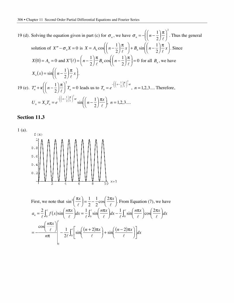
306 • Chapter 11 Second Order Partial Differential Equations and Fourier Series
19 (d). Solving the equation given in part (c) for s n , we have s n n= - -ÊËÁ
ˆ¯
pÊËÁ
ˆ¯
12
2
l. Thus the general
solution of ¢¢ - =X Xns 0 is X A n x B n xn n= -ÊËÁ
ˆ¯
pÊËÁ
ˆ¯
+ -ÊËÁ
ˆ¯
pÊËÁ
ˆ¯
cos sin12
12l l
. Since
X A X n B nn n0 012
12
0( ) = = ¢( ) = -ÊËÁ
ˆ¯
p-Ê
ËÁˆ¯
pÊËÁ
ˆ¯
= and ll l
cos for all Bn , we have
X x n xn ( ) = -ÊËÁ
ˆ¯
pÊËÁ
ˆ¯
sin12 l
.
19 (e). ¢ + -ÊËÁ
ˆ¯
pÊËÁ
ˆ¯
=T n Tn nk 12
02
l leads us to T e nn
n t
= =- -Ê
ËÁˆ¯
pÊËÁ
ˆ¯
1
2
2
1 2 3lk
, , , .... Therefore,
U X T e nx
nn n n
n t
= = -ÊËÁ
ˆ¯
pÊËÁ
ˆ¯
=- -Ê
ËÁˆ¯
pÊËÁ
ˆ¯
1
2
2
12
1 2 3l
l
ksin , , , ....
Section 11.3
1 (a).
First, we note that sin cos .2 12
12
2pÊËÁ
ˆ¯ = -
pÊËÁ
ˆ¯
x x
l l From Equation (7), we have
a f xn x
dxn x
dxn x x
dxn = ( ) pÊËÁ
ˆ¯ =
pÊËÁ
ˆ¯ -
pÊËÁ
ˆ¯
pÊËÁ
ˆ¯Ú Ú Ú
2 1 1 20 0 0l l l l l l l
l l l
sin sin sin cos
= -
pÊËÁ
ˆ¯
p-
+( )pÊËÁ
ˆ¯
+-( )pÊ
ËÁˆ¯
È
ÎÍ
˘
˚˙Ú
cossin sin
n x
n
n x n xdx
l
l l l
l
l
0
0
12
2 2
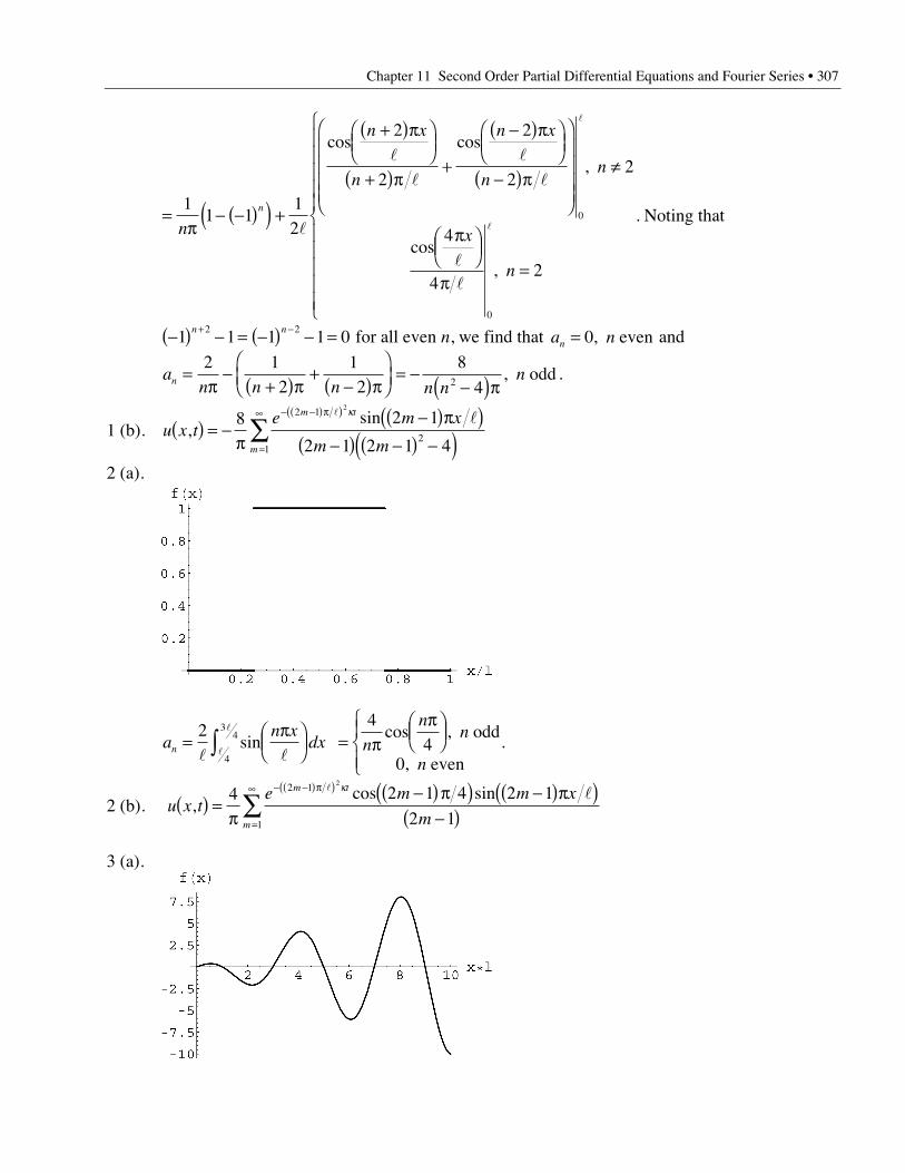
Chapter 11 Second Order Partial Differential Equations and Fourier Series • 307
=p
- -( )( ) +
+( )pÊËÁ
ˆ¯
+( )p+
-( )pÊËÁ
ˆ¯
-( )p
Ê
Ë
ÁÁÁÁ
ˆ
¯
˜˜˜˜
π
pÊËÁ
ˆ¯
p=
Ï
Ì
ÔÔÔÔÔ
Ó
ÔÔÔÔÔ
11 1
12
2
2
2
22
4
42
0
0
n
n x
n
n x
nn
x
n
n
l
l
l
l
l
l
l
l
l
cos cos,
cos,
. Noting that
-( ) - = -( ) - =+ -1 1 1 1 0
2 2n n for all even n, we find that a nn = 0, even and
an n n n n
nn =p
-+( )p
+-( )p
ÊËÁ
ˆ¯
= --( )p
2 12
12
8
42 , odd .
1 (b). u x te m x
m m
m t
m
,sin( ) = -
p-( )p( )
-( ) -( ) -( )- -( ) p( )
=
•
Â8 2 1
2 1 2 1 4
2 1
21
2l lk
2 (a).
an x
dxn =pÊ
ËÁˆ¯Ú
2
4
34
l ll
l
sin = ppÊ
ËÁˆ¯
ÏÌÔ
ÓÔ
44
0n
nn
n
cos ,
,
odd
even.
2 (b). u x te m m x
m
m t
m
,cos sin( ) =
p-( ) p( ) -( )p( )
-( )- -( ) p( )
=
•
Â4 2 1 4 2 1
2 1
2 1
1
2l lk
3 (a).
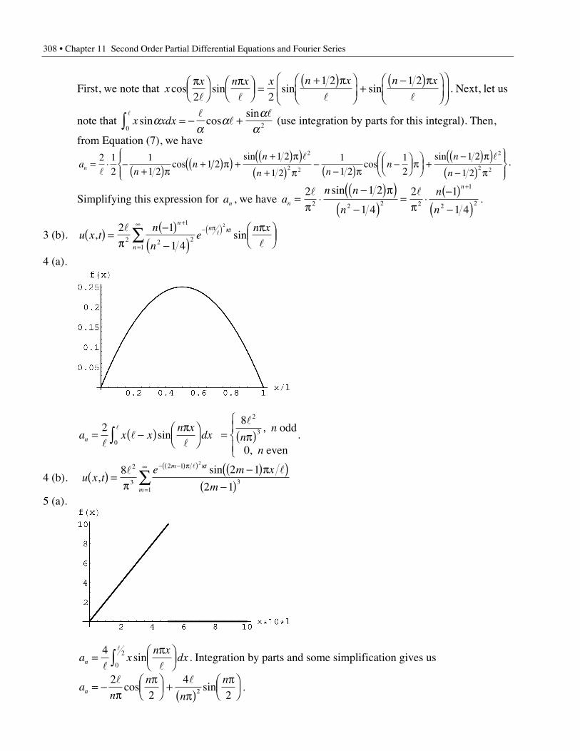
308 • Chapter 11 Second Order Partial Differential Equations and Fourier Series
First, we note that xx n x x n x n x
cos sin sin sinpÊ
ËÁˆ¯
pÊËÁ
ˆ¯ =
+( )pÊËÁ
ˆ¯
+-( )pÊ
ËÁˆ¯
Ê
ËÁˆ
¯2 2
1 2 1 2
l l l l. Next, let us
note that x xdxsin cossina
aa a
a0 2
l ll
lÚ = - + (use integration by parts for this integral). Then,
from Equation (7), we have
an
nn
n nn
n
nn = ◊ -
+( )p+( )p( ) +
+( )p( )+( ) p
--( )p
-ÊËÁ
ˆ¯ p
ÊËÁ
ˆ¯
+-( )p( )
-( ) p
ÏÌÔ
ÓÔ
¸˝ÔÔ
2 12
11 2
1 21 2
1 2
11 2
12
1 2
1 2
2
2 2
2
2 2l
l lcos
sincos
sin .
Simplifying this expression for an , we have an n
n
n
nn
n
=p
◊-( )p( )
-( )=
p◊
-( )-( )
+2 1 2
1 4
2 1
1 42 2 2 2
1
2 2
l lsin.
3 (b). u x tn
ne
n xn
n t
n
, sin( ) =p
-( )-( )
pÊËÁ
ˆ¯
+- p( )
=
•
Â2 1
1 42
1
2 21
2l
ll k
4 (a).
a x xn x
dxn = -( ) pÊËÁ
ˆ¯Ú
20l
ll
l
sin = p( )ÏÌÔ
ÓÔ
8
0
2
3
l
nn
n
,
,
odd
even.
4 (b). u x te m x
m
m t
m
,sin( ) =
p-( )p( )
-( )- -( ) p( )
=
•
Â8 2 1
2 1
2
3
2 1
31
2
l ll k
5 (a).
a xn x
dxn =pÊ
ËÁˆ¯Ú
40
2
l l
l
sin . Integration by parts and some simplification gives us
an
n
n
nn = -
ppÊ
ËÁˆ¯ +
p( )pÊ
ËÁˆ¯
22
422
l lcos sin .
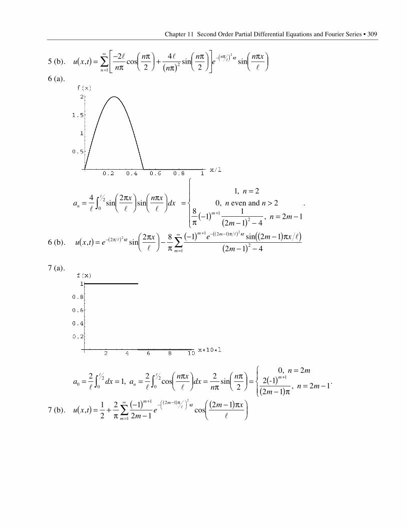
Chapter 11 Second Order Partial Differential Equations and Fourier Series • 309
5 (b). u x tn
n
n
ne
n xn t
n
, cos sin sin( ) =-
ppÊ
ËÁˆ¯ +
p( )pÊ
ËÁˆ¯
È
ÎÍ
˘
˚˙
pÊËÁ
ˆ¯
- p( )=
•
 22
422
1
2l l
ll k
6 (a).
ax n x
dxn =pÊ
ËÁˆ¯
pÊËÁ
ˆ¯Ú
4 20
2
l l l
l
sin sin ==
>
p-( )
-( ) -= -
Ï
Ì
ÔÔ
Ó
ÔÔ
+
1 2
0 28
11
2 1 42 1
1
2
,
,
,
n
n n
mn m
m
even and .
6 (b). u x t ex e m x
mt
m m t
m
, sinsin( ) =
pÊËÁ
ˆ¯ -
p-( ) -( )p( )
-( ) -- p( )
+ - -( ) p( )
=
•
Â2
1 2 1
21
2
2
2 8 1 2 1
2 1 4l
l
l
lkk
7 (a).
a dx an x
dxn
nn m
mn mn
m
0 0
2
0
2 121
2 22
0 2
2 12 1
= = =pÊ
ËÁˆ¯ =
ppÊ
ËÁˆ¯ =
=( )
-( )p= -
ÏÌÔ
ÓÔÚ Ú +
l l l
l l
, cos sin,
, 2 -1 .
7 (b). u x tm
em x
m m t
m
, cos( ) = +p
-( )-
-( )pÊËÁ
ˆ¯
+- -( ) pÊ
ˈ¯
=
•
Â12
2 12 1
2 11 2 1
1
2
l
l
k
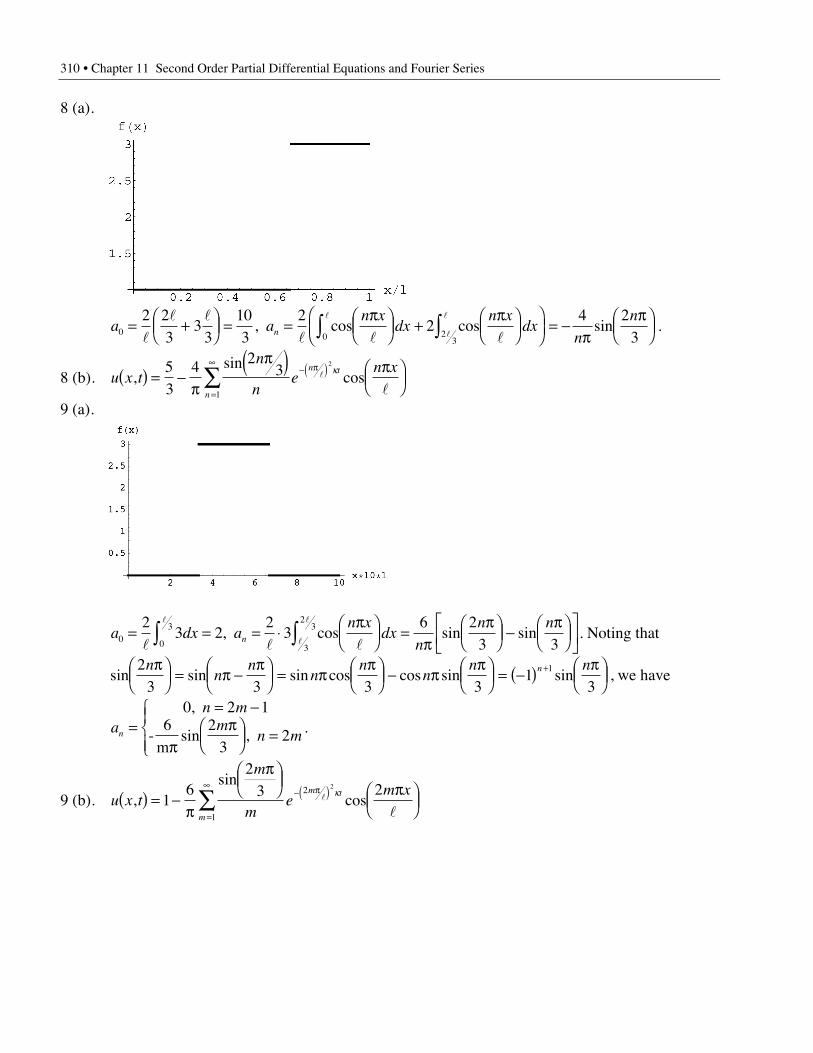
310 • Chapter 11 Second Order Partial Differential Equations and Fourier Series
8 (a).
a an x
dxn x
dxn
nn0 0 2
3
2 23
33
103
22
4 23
= +ÊËÁ
ˆ¯ = =
pÊËÁ
ˆ¯ +
pÊËÁ
ˆ¯
ÊËÁ
ˆ¯
= -p
pÊËÁ
ˆ¯Ú Úl
l l
l l l
l
l
l
, cos cos sin .
8 (b). u x tn
ne
n xn t
n
,sin
cos( ) = -p
p( ) pÊËÁ
ˆ¯
- p( )=
•
Â53
4 23
2
1
l
l
k
9 (a).
a dx an x
dxn
n nn0 0
3
3
232
3 22
36 2
3 3= = = ◊
pÊËÁ
ˆ¯ =
ppÊ
ËÁˆ¯ -
pÊËÁ
ˆ¯
ÈÎÍ
˘˚Ú Úl l l
l
l
l
, cos sin sin . Noting that
sin sin sin cos cos sin sin2
3 3 3 31
31n
nn
nn
nn nnpÊ
ËÁˆ¯ = p -
pÊËÁ
ˆ¯ = p
pÊËÁ
ˆ¯ - p
pÊËÁ
ˆ¯ = -( ) pÊ
ËÁˆ¯
+, we have
an m
mn mn =
= -
ppÊ
ËÁˆ¯ =
ÏÌÔ
ÓÔ
0 2 12
32
,
sin , -6
m.
9 (b). u x t
m
me
m xm t
m
,sin
cos( ) = -p
pÊËÁ
ˆ¯ pÊ
ËÁˆ¯
- p( )=
•
Â16
23 22
1
2
l
l
k
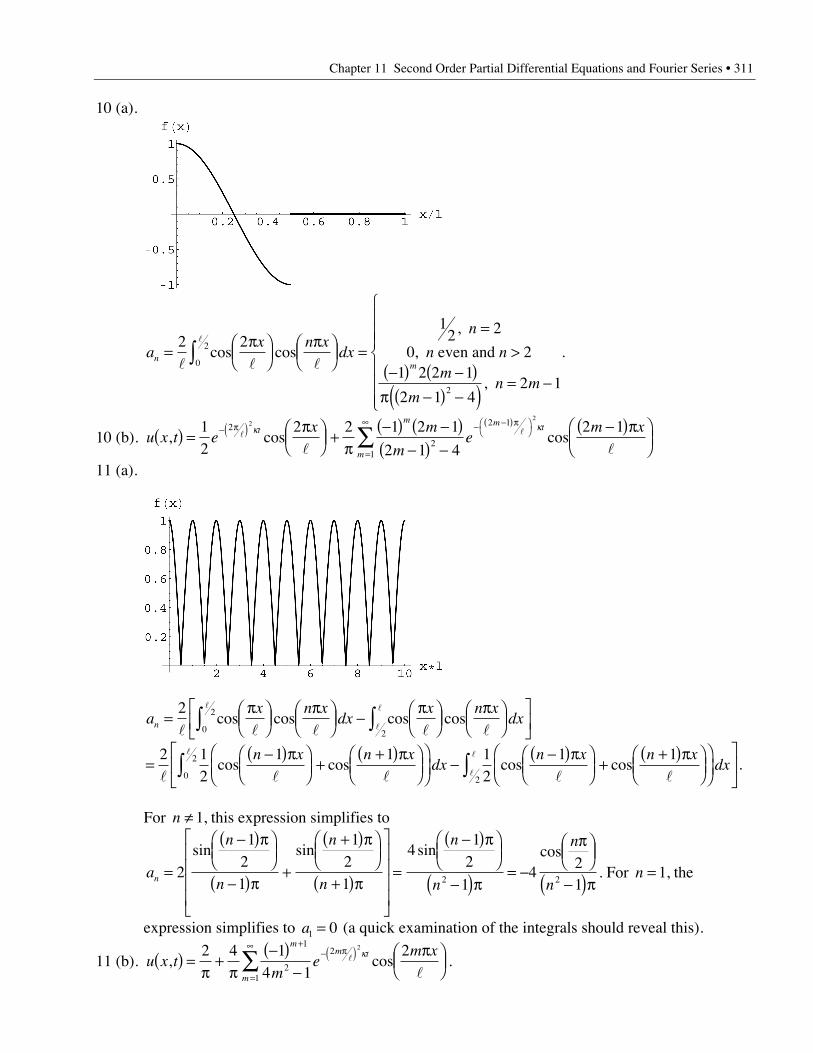
Chapter 11 Second Order Partial Differential Equations and Fourier Series • 311
10 (a).
ax n x
dx
n
n nm
mn m
nm
=pÊ
ËÁˆ¯
pÊËÁ
ˆ¯ =
=>
-( ) -( )p -( ) -( ) = -
Ï
Ì
ÔÔÔ
Ó
ÔÔÔ
Ú2 2
12 2
0 21 2 2 1
2 1 42 1
0
2
2
l l l
l
cos cos
,
,
,
even and .
10 (b). u x t ex m
me
m xtm m t
m
, cos cos( ) =pÊ
ËÁˆ¯ +
p-( ) -( )
-( ) --( )pÊ
ËÁˆ¯
- p( ) - -( ) pÊË
ˆ¯
=
•
Â12
2 2 1 2 1
2 1 4
2 12
2
2 1
1
22
l l
l l
k k
11 (a).
ax n x
dxx n x
dxn =pÊ
ËÁˆ¯
pÊËÁ
ˆ¯ -
pÊËÁ
ˆ¯
pÊËÁ
ˆ¯
ÈÎÍ
˘˚Ú Ú
20
2
2l l l l l
l
l
l
cos cos cos cos
=-( )pÊ
ËÁˆ¯
++( )pÊ
ËÁˆ¯
ÊËÁ
ˆ¯
--( )pÊ
ËÁˆ¯
++( )pÊ
ËÁˆ¯
ÊËÁ
ˆ¯
È
ÎÍ
˘
˚˙Ú Ú
2 12
1 1 12
1 10
2
2l l l l l
l
l
l
cos cos cos cosn x n x
dxn x n x
dx .
For n π 1, this expression simplifies to
a
n
n
n
n
n
n
n
nn =
-( )pÊËÁ
ˆ¯
-( )p+
+( )pÊËÁ
ˆ¯
+( )p
È
Î
ÍÍÍÍ
˘
˚
˙˙˙˙
=
-( )pÊËÁ
ˆ¯
-( )p= -
pÊËÁ
ˆ¯
-( )p2
121
121
41
2
14
212 2
sin sin sin cos. For n = 1, the
expression simplifies to a1 0= (a quick examination of the integrals should reveal this).
11 (b). u x tm
em x
mm t
m
, cos( ) =p
+p
-( )-
pÊËÁ
ˆ¯
+- p( )
=
•
Â2 4 14 1
21
2
2
1
2
l
l
k.
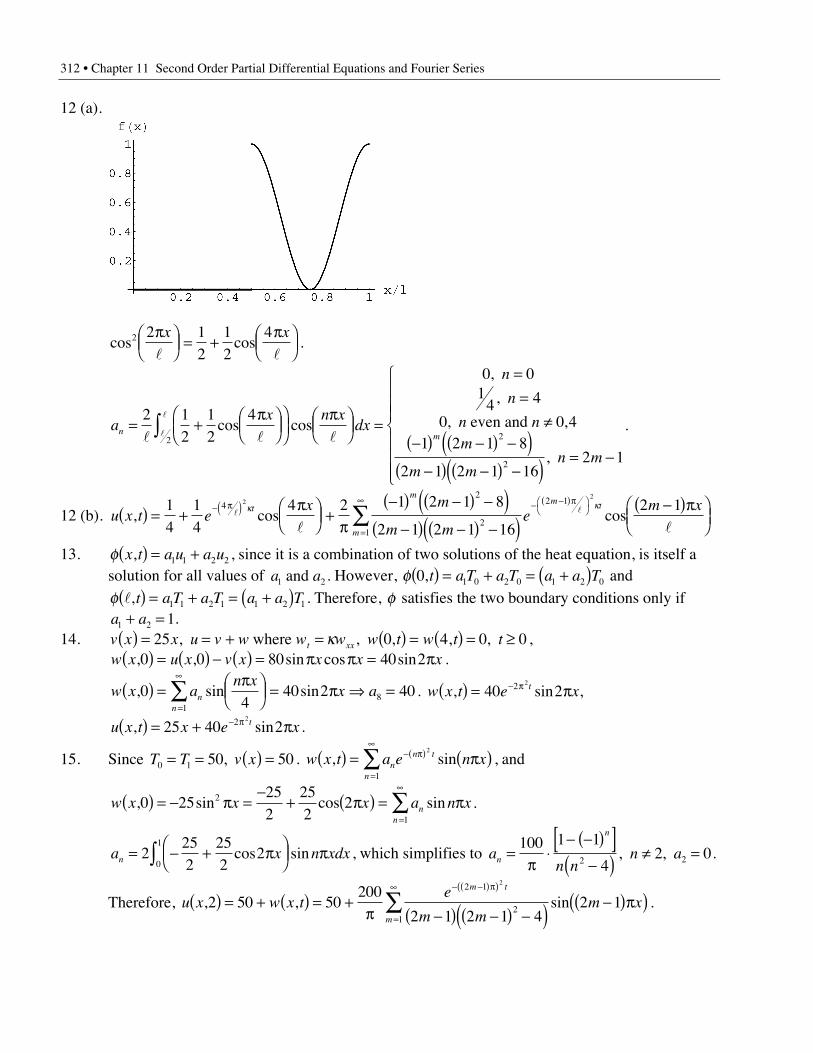
312 • Chapter 11 Second Order Partial Differential Equations and Fourier Series
12 (a).
cos cos2 2 12
12
4pÊËÁ
ˆ¯ = +
pÊËÁ
ˆ¯
x x
l l.
ax n x
dx
n
n
n nm
m mn m
nm
= +pÊ
ËÁˆ¯
ÊËÁ
ˆ¯
pÊËÁ
ˆ¯ =
==
π-( ) -( ) -( )
-( ) -( ) -( ) = -
Ï
Ì
ÔÔÔ
Ó
ÔÔ
Ú2 1
212
4
0 01
4 4
0 0 41 2 1 8
2 1 2 1 162 1
2 2
2
l l ll
l
cos cos
,
,
, ,
,
even and
ÔÔ
.
12 (b). u x t ex m
m me
m xt
mm t
m
, cos cos( ) = +pÊ
ËÁˆ¯ +
p-( ) -( ) -( )
-( ) -( ) -( )-( )pÊ
ËÁˆ¯
- p( ) - -( ) pÊË
ˆ¯
=
•
Â14
14
4 2 1 2 1 8
2 1 2 1 16
2 142
2
2 1
1
22
l l
l l
k k
13. f x t a u a u,( ) = +1 1 2 2 , since it is a combination of two solutions of the heat equation, is itself asolution for all values of a a1 2 and . However, f 0 1 0 2 0 1 2 0,t a T a T a a T( ) = + = +( ) and
f l,t a T a T a a T( ) = + = +( )1 1 2 1 1 2 1. Therefore, f satisfies the two boundary conditions only ifa a1 2 1+ = .
14. v x x u v w w w w t w t tt xx( ) = = + = ( ) = ( ) = ≥25 0 4 0 0, , , , , where k ,w x u x v x x x x, , sin cos sin0 0 80 40 2( ) = ( ) - ( ) = p p = p .
w x an x
x ann
, sin sin04
40 2 401
8( ) =pÊ
ËÁˆ¯ = p fi =
=
•
 . w x t e xt, sin , ( ) = p- p40 22 2
u x t x e xt, sin( ) = + p- p25 40 22 2
.
15. Since T T v x0 1 50 50= = ( ) =, . w x t a e n xnn t
n
, sin( ) = p( )- p( )
=
•
 2
1
, and
w x x x a n xnn
, sin cos sin0 25252
252
22
1
( ) = - p =-
+ p( ) = p=
•
 .
a x n xdxn = - + pÊËÁ
ˆ¯ pÚ2
252
252
20
1cos sin , which simplifies to a
n nn an
n
=p
◊- -( )[ ]
-( ) π =100 1 1
42 02 2, , .
Therefore, u x w x te
m mm x
m t
m
, , sin2 50 50200
2 1 2 1 42 1
2 1
21
2
( ) = + ( ) = +p -( ) -( ) -( ) -( )p( )
- -( ) p( )
=
•
 .
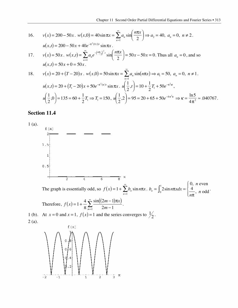
Chapter 11 Second Order Partial Differential Equations and Fourier Series • 313
16. v x x( ) = -200 50 . w x x an x
a a nnn
n, sin sin , , 0 402
40 0 21
2( ) = p =pÊ
ËÁˆ¯ fi = = π
=
•
 .
u x t x e xt, sin.( ) = - + p-p ( )200 50 402 0 1 .
17. v x x( ) = 50 . w x t a en x
x xn
n t
n
, sin .( ) =pÊ
ËÁˆ¯ = - =- p( )
=
•
 2
1
2
250 50 0 Thus all an = 0, and so
u x t x x,( ) = + =50 0 50 .
18. v x T x( ) = + -( )20 20 . w x x a n x a a nnn
n, sin sin , , 0 50 50 0 11
1( ) = p = p( ) fi = = π=
•
 .
u x t T x e xt, sin( ) = + -( ) + p-p ( )20 20 501
2 k . u t T e t12
1012
501
2
,ÊËÁ
ˆ¯ = + + -p k ,
u T T12
0 135 6012
1501 1,ÊËÁ
ˆ¯ = = + fi = , u e
12
2 95 20 65 505
40407674
2
2
,ln
.ÊËÁ
ˆ¯ = = + + fi =
pª- p k k .
Section 11.4
1 (a).
The graph is essentially odd, so f x b n xnn
( ) = + p=
•
Â11
sin . b n xdxn
nnn = p =
p
ÏÌÔ
ÓÔÚ 2
04
0
1sin
,
,
even
odd.
Therefore, f xm x
mm
( ) = +p
-( )p( )-=
•
Â14 2 1
2 11
sin.
1 (b). At x x= =0 1 and , f x( ) = 1 and the series converges to 12 .
2 (a).
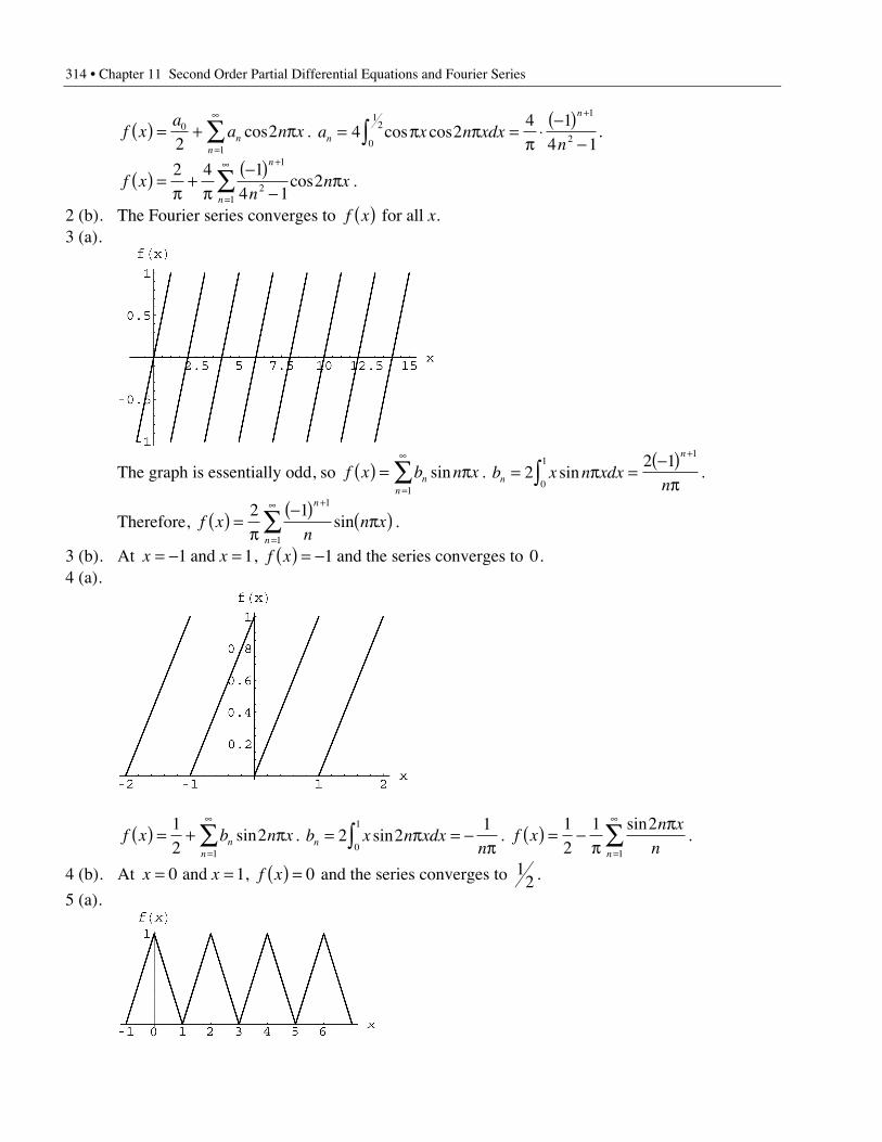
314 • Chapter 11 Second Order Partial Differential Equations and Fourier Series
f xa
a n xnn
( ) = + p=
•
Â0
122cos . a x n xdx
nn
n
= p p =p
◊-( )
-Ú+
4 24 1
4 10
12
1
2cos cos .
f xn
n xn
n
( ) =p
+p
-( )-
p+
=
•
Â2 4 14 1
21
21
cos .
2 (b). The Fourier series converges to f x( ) for all x.3 (a).
The graph is essentially odd, so f x b n xnn
( ) = p=
•
 sin1
. b x n xdxnn
n
= p =-( )
pÚ+
22 1
0
11
sin .
Therefore, f xn
n xn
n
( ) =p
-( )p( )
+
=
•
Â2 11
1
sin .
3 (b). At x x= - =1 1 and , f x( ) = -1 and the series converges to 0.4 (a).
f x b n xnn
( ) = + p=
•
Â12
21
sin . b x n xdxnn = p = -
pÚ2 21
0
1sin . f x
n x
nn
( ) = -p
p=
•
Â12
1 2
1
sin.
4 (b). At x x= =0 1 and , f x( ) = 0 and the series converges to 12 .
5 (a).
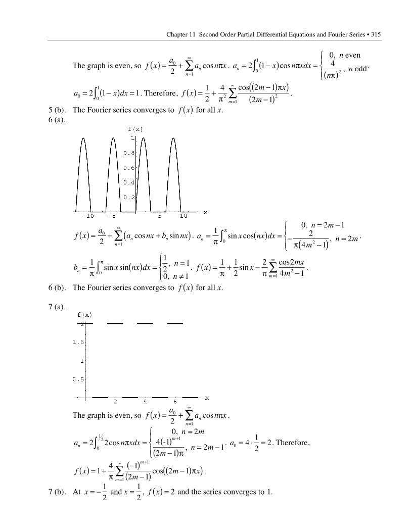
Chapter 11 Second Order Partial Differential Equations and Fourier Series • 315
The graph is even, so f xa
a n xnn
( ) = + p=
•
Â0
12cos . a x n xdx
n
nnn = -( ) p =
p( )
ÏÌÔ
ÓÔÚ2 1
0
0
1
2cos
,
,
even4
odd.
a x dx0 0
12 1 1= -( ) =Ú . Therefore, f x
m x
mm
( ) = +p
-( )p( )-( )=
•
Â12
4 2 1
2 12 21
cos.
5 (b). The Fourier series converges to f x( ) for all x.6 (a).
f xa
a nx b nxn nn
( ) = + +( )=
•
Â0
12cos sin . a x nx dx
n m
mn mn =
p( ) =
= -
-p -( ) =
ÏÌÔ
ÓÔ
p
Ú1
0 2 12
4 120 2
sin cos,
, .
b x nx dx n
nn =
p( ) = =
π
ÏÌÔ
ÓÔ
p
Ú1 1
21
0 10sin sin ,
, . f x x
mx
mm
( ) =p
+ -p -=
•
Â1 12
2 24 12
1
sincos
.
6 (b). The Fourier series converges to f x( ) for all x.
7 (a).
The graph is even, so f xa
a n xnn
( ) = + p=
•
Â0
12cos .
a n xdx
n m
mn mn
m= p = ( )
-( )p= -
ÏÌÔ
ÓÔÚ +
2 20 2
2 12 10
12 1
cos,
,
=4 -1 . a0 4
12
2= ◊ = . Therefore,
f xm
m xm
m
( ) = +p
-( )-( ) -( )p( )
+
=
•
Â14 1
2 12 1
1
1
cos .
7 (b). At x x= - =12
12
and , f x( ) = 2 and the series converges to 1.
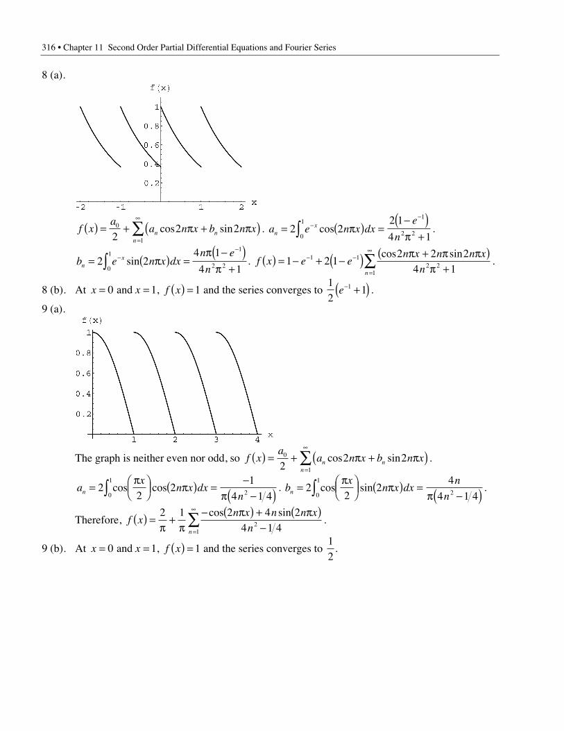
316 • Chapter 11 Second Order Partial Differential Equations and Fourier Series
8 (a).
f xa
a n x b n xn nn
( ) = + p + p( )=
•
Â0
122 2cos sin . a e n x dx
e
nnx= p( ) =
-( )p +
--
Ú2 22 1
4 10
11
2 2cos .
b e n x dxn e
nnx= p( ) =
p -( )p +
--
Ú2 24 1
4 10
11
2 2sin . f x e en x n n x
nn
( ) = - + -( ) p + p p( )p +
- -
=
•
Â1 2 12 2 2
4 11 1
2 21
cos sin.
8 (b). At x x= =0 1 and , f x( ) = 1 and the series converges to 12
11e- +( ) .
9 (a).
The graph is neither even nor odd, so f xa
a n x b n xn nn
( ) = + p + p( )=
•
Â0
122 2cos sin .
ax
n x dxnn =
pÊËÁ
ˆ¯ p( ) =
-p -( )Ú2
22
1
4 1 40
1
2cos cos . bx
n x dxn
nn =pÊ
ËÁˆ¯ p( ) =
p -( )Ú22
24
4 1 40
1
2cos sin .
Therefore, f xn x n n x
nn
( ) =p
+p
- p( ) + p( )-=
•
Â2 1 2 4 24 1 42
1
cos sin.
9 (b). At x x= =0 1 and , f x( ) = 1 and the series converges to 12
.

Chapter 11 Second Order Partial Differential Equations and Fourier Series • 317
10 (a).
f x b n xnn
( ) = + p=
•
Â21
sin . b x n xdxnn
n
= -( ) p =-( )
p-Ú 22 1
1
1sin . f x
nn x
n
n
( ) = +p
-( )p( )
=
•
Â22 1
1
sin .
10 (b). At x x= - =1 1 and , f x( ) = 3 and the series converges to 2.11 (a).
11 (b). x = 1 2,12 (a).
12 (b). x = 1 2,
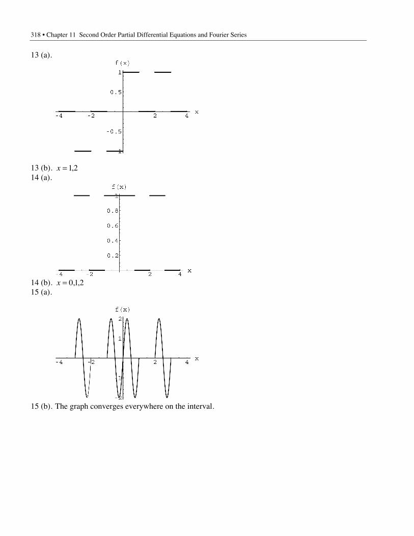
318 • Chapter 11 Second Order Partial Differential Equations and Fourier Series
13 (a).
13 (b). x = 1 2,14 (a).
14 (b). x = 0 1 2, ,15 (a).
15 (b). The graph converges everywhere on the interval.
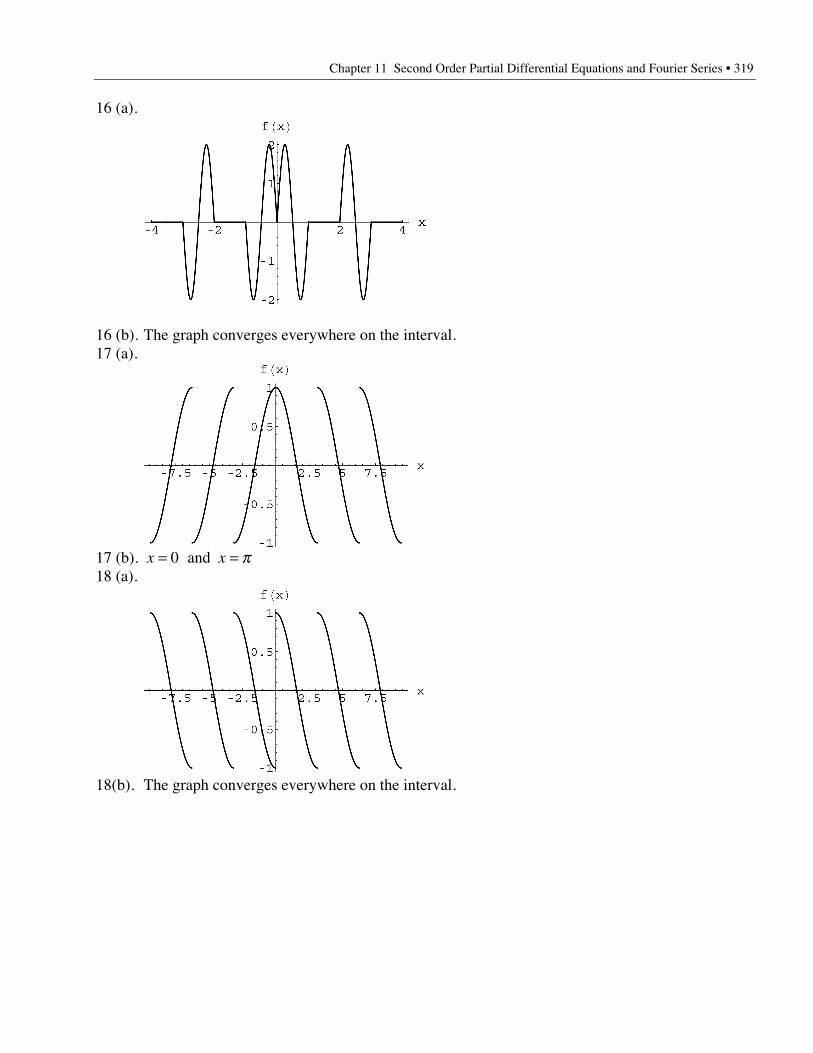
Chapter 11 Second Order Partial Differential Equations and Fourier Series • 319
16 (a).
16 (b). The graph converges everywhere on the interval.17 (a).
17 (b). x x= =0 and p18 (a).
18(b). The graph converges everywhere on the interval.
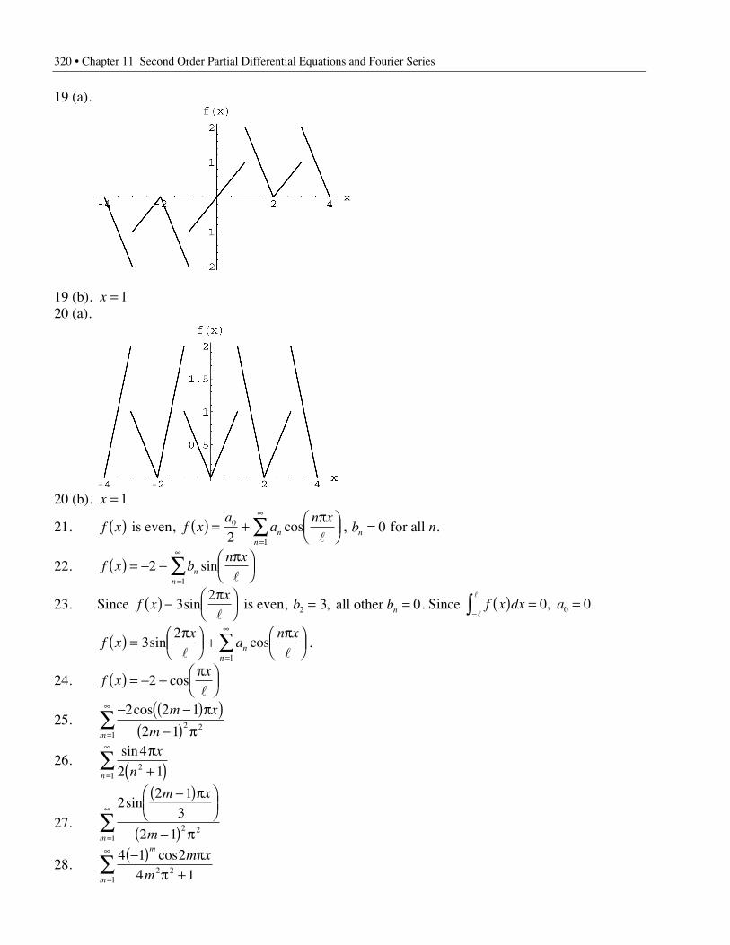
320 • Chapter 11 Second Order Partial Differential Equations and Fourier Series
19 (a).
19 (b). x = 120 (a).
20 (b). x = 1
21. f x( ) is even, f xa
an x
nn
( ) = +pÊ
ËÁˆ¯=
•
Â0
12cos
l, bn = 0 for all n.
22. f x bn x
nn
( ) = - +pÊ
ËÁˆ¯=
•
Â21
sinl
23. Since f xx( ) -
pÊËÁ
ˆ¯3
2sin
l is even, b bn2 3 0= =, all other . Since f x dx a( ) = =
-Ú l
l
0 00, .
f xx
an x
nn
( ) =pÊ
ËÁˆ¯ +
pÊËÁ
ˆ¯=
•
Â32
1
sin cosl l
.
24. f xx( ) = - +
pÊËÁ
ˆ¯2 cos
l
25.- -( )p( )
-( ) p=
•
 2 2 1
2 12 2
1
cos m x
mm
26.sin4
2 121
p+( )=
•
 x
nn
27.
22 1
3
2 12 2
1
sinm x
mm
-( )pÊËÁ
ˆ¯
-( ) p=
•
Â
28.4 1 2
4 12 21
-( ) pp +=
•
Âm
m
m x
m
cos
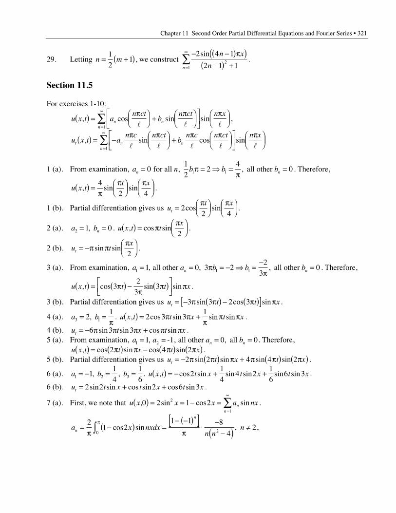
Chapter 11 Second Order Partial Differential Equations and Fourier Series • 321
29. Letting n m= +( )12
1 , we construct - -( )p( )
-( ) +=
•
 2 4 1
2 1 12
1
sin n x
nn
.
Section 11.5
For exercises 1-10:
u x t an ct
bn ct n x
n nn
, cos sin sin( ) =pÊ
ËÁˆ¯ +
pÊËÁ
ˆ¯
ÈÎÍ
˘˚
pÊËÁ
ˆ¯=
•
Âl l l1
,
u x t an c n ct
bn c n ct n x
t n nn
, sin cos sin( ) = -p pÊ
ËÁˆ¯ +
p pÊËÁ
ˆ¯
ÈÎÍ
˘˚
pÊËÁ
ˆ¯=
•
Âl l l l l1
1 (a). From examination, a n b b bn n= p = fi =p
=012
24
01 1 for all all other , , . Therefore,
u x tt x
, sin sin( ) =p
pÊËÁ
ˆ¯
pÊËÁ
ˆ¯
42 4
.
1 (b). Partial differentiation gives us ut x
t =pÊ
ËÁˆ¯
pÊËÁ
ˆ¯2
2 4cos sin .
2 (a). a bn2 1 0= =, . u x t tx
, cos sin( ) = ppÊ
ËÁˆ¯2
.
2 (b). u tx
t = -p ppÊ
ËÁˆ¯sin sin
2.
3 (a). From examination, a a b b bn n1 1 11 0 3 22
30= = p = - fi =
-p
=, , , all other all other . Therefore,
u x t t t x, cos sin sin( ) = p( ) -p
p( )ÈÎÍ
˘˚
p32
33 .
3 (b). Partial differentiation gives us u t t xt = - p p( ) - p( )[ ] p3 3 2 3sin cos sin .
4 (a). a b3 121
= =p
, . u x t t x t x, cos sin sin sin( ) = p p +p
p p2 3 31
.
4 (b). u t x t xt = - p p p + p p6 3 3sin sin cos sin .5 (a). From examination, a a a bn n1 21 0 0= = =, , = -1, all other all . Therefore,
u x t t x t x, cos sin cos sin( ) = p( ) p - p( ) p( )2 4 2 .5 (b). Partial differentiation gives us u t x t xt = - p p( ) p + p p( ) p( )2 2 4 4 2sin sin sin sin .
6 (a). a b b1 2 3114
16
= - = =, , . u x t t x t x t x, cos sin sin sin sin sin( ) = - + +214
4 216
6 3 .
6 (b). u t x t x t xt = + +2 2 2 6 3sin sin cos sin cos sin .
7 (a). First, we note that u x x x a nxnn
, sin cos sin0 2 1 22
1
( ) = = - ==
•
 .
a x nxdxn n
nn
n
=p
-( ) =- -( )[ ]
p◊
--( ) π
p
Ú2
1 21 1 8
42
0 2cos sin , ,
322 • Chapter 11 Second Order Partial Differential Equations and Fourier Series
a x x dx2 0
22
12
4 0=p
-ÈÎÍ
˘˚
=p
Ú sin sin . From examination, all bn = 0. Therefore,
u x tm t m x
m mm
,cos sin( ) =
-p
-( )( ) -( )( )-( ) -( ) -( )=
•
Â16 2 1 2 1
2 1 2 1 421
.
7 (b). Partial differentiation gives us u x tm t m x
mt
m
,sin sin( ) =
p-( )( ) -( )( )
-( ) -=
•
Â16 2 1 2 1
2 1 42
1
.
8 (a). a bn
x nxdxn
nnn n= = - ◊
p-Ê
ËÁˆ¯ =
p -( )ÏÌÔ
ÓÔ
p
Ú04 2 1
212
20
40 2 2
, cos sin,
,
even32
n odd.
u x tm t m x
m mm
,sin sin( ) =
p-( )( ) -( )( )
-( ) -( ) -( )=
•
Â32 2 1 2 1
2 1 2 1 42 2
1
.
8 (b). um t m x
m mt
m
=p
-( )( ) -( )( )-( ) -( ) -( )=
•
Â32 2 1 2 1
2 1 2 1 42
1
cos sin.
9 (a). From examination, a an1 1 0= =, all other .
n b x n xdx n nn
nnp = - pÊ
ËÁˆ¯ p =
-p
◊-( )
ÏÌÔ
ÓÔÚ2
12
12
2
8 1
40
12cos sin
, odd
0, even. Therefore,
u x t t xm t m x
m mm
, cos sinsin sin( ) = p p -
p-( )p( ) -( )p( )-( ) -( ) -[ ]=
•
Â8 2 1 2 1
2 1 2 1 42 2 2
1
.
9 (b). Partial differentiation gives us u x t t xm t m x
m mt
m
, sin sincos sin( ) = -p p p -
p-( )p( ) -( )p( )-( ) -( ) -[ ]=
•
Â8 2 1 2 1
2 1 2 1 42
1
.
10 (a). a x n xdxn
n nnn = - pÊ
ËÁˆ¯ p = -
p -( )ÏÌÔ
ÓÔÚ2
12
12
208
40
1
2cos sin
,
,
even
odd. b2
12
= -p
.
u x t t xm t m x
m mm
, sin sincos sin( ) = -
pp p -
p-( )p( ) -( )p( )-( ) -( ) -( )=
•
Â12
2 28 2 1 2 1
2 1 2 1 42
1
.
10 (b). u t xm t m x
mt
m
= - p p +p
-( )p( ) -( )p( )-( ) -=
•
Âcos sinsin sin
2 28 2 1 2 1
2 1 42
1
11 (a). x tc
a a bc
bc
= +( ) = - +( ) fi = = = =-1
212
12
12
12
121 2 1 2x h x h, , , , .
12 (a). u x t x t e x t ex t x t,( ) = -( ) + +( )( )- -( ) - +( )5 2 22 2 2 22 2
.
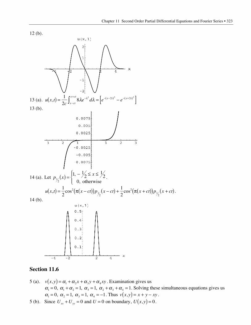
Chapter 11 Second Order Partial Differential Equations and Fourier Series • 323
12 (b).
13 (a). u x tc
e d e ex ct
x ctx t x t,( ) = = -[ ]-
-
+ - -( ) - +( )Ú12
82 2 22 2l ll
13 (b).
14 (a). Let p xx
12
1 12
12
0( ) = - £ £Ï
ÌÔ
ÓÔ,
, otherwise.
u x t x ct p x ct x ct p x ct, cos cos( ) = p -( )( ) -( ) + p +( )( ) +( )12
12
21
2
21
2.
14 (b).
Section 11.6
5 (a). v x y x y xy,( ) = + + +a a a a1 2 3 4 . Examination gives usa a a a a a a1 1 2 3 2 3 40 1 1 1= + = = + + =, , , . Solving these simultaneous equations gives usa a a a1 2 3 40 1 1 1= = = = -, , , . Thus v x y x y xy,( ) = + - .
5 (b). Since U U U U x yxx yy+ = = ( ) =0 0 0 and on boundary, , .
324 • Chapter 11 Second Order Partial Differential Equations and Fourier Series
5 (c). u x y v x y x y xy, ,( ) = ( ) = + - .
6 (a). v x y x y xy,( ) = + + +a a a a1 2 3 4 . a a a a1 2 3 42 2 2 0 2 2 4 2 2 2 4 2= + = + = - + + =, , , .
a a a a1 2 3 42 1 1 0= = - = =, , , . v x y x y,( ) = - +2 .
6 (b). U U U U x yxx yy+ = = fi ( ) =0 0 0 and on boundary , .
6 (c). u x y v x y x y, ,( ) = ( ) = - +2 .
7 (a). v x y x y xy,( ) = + + +a a a a1 2 3 4 . Examination gives us
a a a a a1 2 3 4 40 0 0 0 2 8 4= = = + = fi =, , , . Thus v x y xy,( ) = 4 .
7 (b). Since U U U U x yxx yy+ = = ( ) =0 0 0 and on boundary, , .
7 (c). u x y v x y xy, ,( ) = ( ) = 4 .
8 (a). Since all of the corner values are 0, v x y,( ) = 0.
8 (b). u x y U x y b n x n ynn
, , sin sinh( ) = ( ) = p( ) p=
•
Â21
.
u x b n n x x bnn
, sinh sin sinsinh
1 4 24
212( ) = p p = p fi =
p=
•
 . U x y x y,sinh
sin sinh( ) =p
p( ) p4
22 2 .
8 (c). u x y U x y,sinh
sin sinh( ) = + =p
p( ) p04
22 2 .
9 (a). Since all of the corner values are 0, v x y,( ) = 0.
9 (b). u x y U x y c n x n ynn
, , sinh sin( ) = ( ) = p -( )( ) p=
•
Â31
1 . u y c n n y ynn
0 21
, sinh sin sin( ) = p p = p=
•
 .
Therefore, c cn1 2 0sinh , p = =all other , and so U x y x y,sinh
sinh sin( ) =p
p -( )( ) p2
1 .
9 (c). u x y U x y,sinh
sinh sin( ) = + =p
p -( )( ) p02
1 .
10 (a). v x y x y xy,( ) = + + +a a a a1 2 3 4 . a a a a1 2 3 41 1 2 1 1 1 1 0 0 2 1= + = + = + + + =, , , .
a a a a1 2 3 41 0 0 0= = = =, , , . v x y,( ) = 1.
10 (b). U U x y dn x n
y xnn
= ( ) =pÊ
ËÁˆ¯
p-( )Ê
ËÁˆ¯ = p -
=
•
Â41 2 2
1 2 1, sin sinh cos .
dn
xn x
dx
n m
m mn mn sinh cos sin
,
, pÊ
ËÁˆ¯ = p -( ) pÊ
ËÁˆ¯ =
=
p -( ) -( ) -( ) = -ÏÌÔ
ÓÔÚ2
2 12
0 264
2 1 2 1 162 10
2
2.
U x ym x m y
m m mm
,sin sinh
sinh( ) =
p
-( ) p( ) -( ) p -( )( )-( ) p( ) -( ) -( ) -( )=
•
Â64 2 1 2 2 1 2 1
2 1 2 2 1 2 1 162
1
.
10 (c). u x y Um x m y
m m mm
,sin sinh
sinh( ) = + = +
p
-( ) p( ) -( ) p -( )( )-( ) p( ) -( ) -( ) -( )=
•
Â1 164 2 1 2 2 1 2 1
2 1 2 2 1 2 1 162
1
.
11 (a). Since all of the corner values are 1, v x y,( ) = 1.
Chapter 11 Second Order Partial Differential Equations and Fourier Series • 325
11 (b). U U U U Uxx yy+ = = +0 1 2, so . U x y an x n y
nn
11 2 2
, sinh sin( ) =pÊ
ËÁˆ¯
pÊËÁ
ˆ¯=
•
 .
an n y
ynn
sinh sin sin3
2 21
pÊËÁ
ˆ¯
pÊËÁ
ˆ¯ = p
=
•
 . Therefore, a an2 3 1 0sinh , p = =all other .
U x y bn x n y
nn
21 3 3
, sinh sin( ) =pÊ
ËÁˆ¯
pÊËÁ
ˆ¯=
•
 . bn n y x
nn
sinh sin sin2
32
32
31
pÊËÁ
ˆ¯
pÊËÁ
ˆ¯ = -
pÊËÁ
ˆ¯=
•
 . Therefore,
b bn1
23
2 0sinh , pÊ
ËÁˆ¯ = - =all other , and so U x y
x yx y
,sinh sin
sinh
sin sinh
sinh( ) =
p pp
-
pÊËÁ
ˆ¯
pÊËÁ
ˆ¯
pÊËÁ
ˆ¯
3
23 3
23
.
11 (c). u x y U vx y
x y
,sinh sin
sinh
sin sinh
sinh( ) = + = +
p pp
-
pÊËÁ
ˆ¯
pÊËÁ
ˆ¯
pÊËÁ
ˆ¯
13
23 3
23
.
12 (a). Since all of the corner values are 0, v x y,( ) = 0.12 (b). U U U U U= + + +1 2 3 4
=p p
p+
p pp
+p -( )( ) p
p+
p p -( )p
sinh sinsinh
sin sinhsinh
sinh sin
sinh
sin sinh
sinh2 2
23 3
3
2 1 2
2
3 3 1
3x y x y x y x y
.
12 (c). u x yx y x y x y x y
,sinh sin
sinhsin sinh
sinh
sinh sin
sinh
sin sinh
sinh( ) =
p pp
+p p
p+
p -( )( ) pp
+p p -( )
p2 2
23 3
3
2 1 2
2
3 3 1
3.
14. u ra
r a n b nnn n
n
, cos sinq q q( ) = + +[ ]=
•
Â0
12. a bn2
49
0= =, . u rr
, cosq q( ) = ÊËÁ
ˆ¯4
32
2
.
15. u ra
r a n b nnn n
n
, cos sinq q q( ) = + +[ ]=
•
Â0
12. Examination gives us
ab0 1
122 3 1= = -, , all other
a bn n, = 0, and so u rr
, sinq q( ) = - ÊËÁ
ˆ¯2
3.
16. u ra
r a n b nnn n
n
, cos sinq q q( ) = + +[ ]=
•
Â0
12. a a a bn0 2 44
12
12
0= = - = - =, , , .
u rr r
, cos cosq q q( ) = - -22
22
42 4
.
17. Let fa
a n b nnn n
n
q q q( ) = + +[ ]=
•
Â0
122 cos sin . a n d
n
nn n=p
==≥
ÏÌÓÚ
12
1 0
0 10cos
,
, q q
p.
b n dn m
mn mn n
m=
p=
=
-( )p= -
ÏÌÔ
ÓÔÚ
-
12
0 21
2 1 22 10 2 2
sin,
, q qp
. Therefore,
u rr m
m
m
m
,sin
( )q
q( ) = +p
ÊËÁ
ˆ¯
-( )( )-
-
=
•
Â12
22
2 1
2 1
2 1
1
.
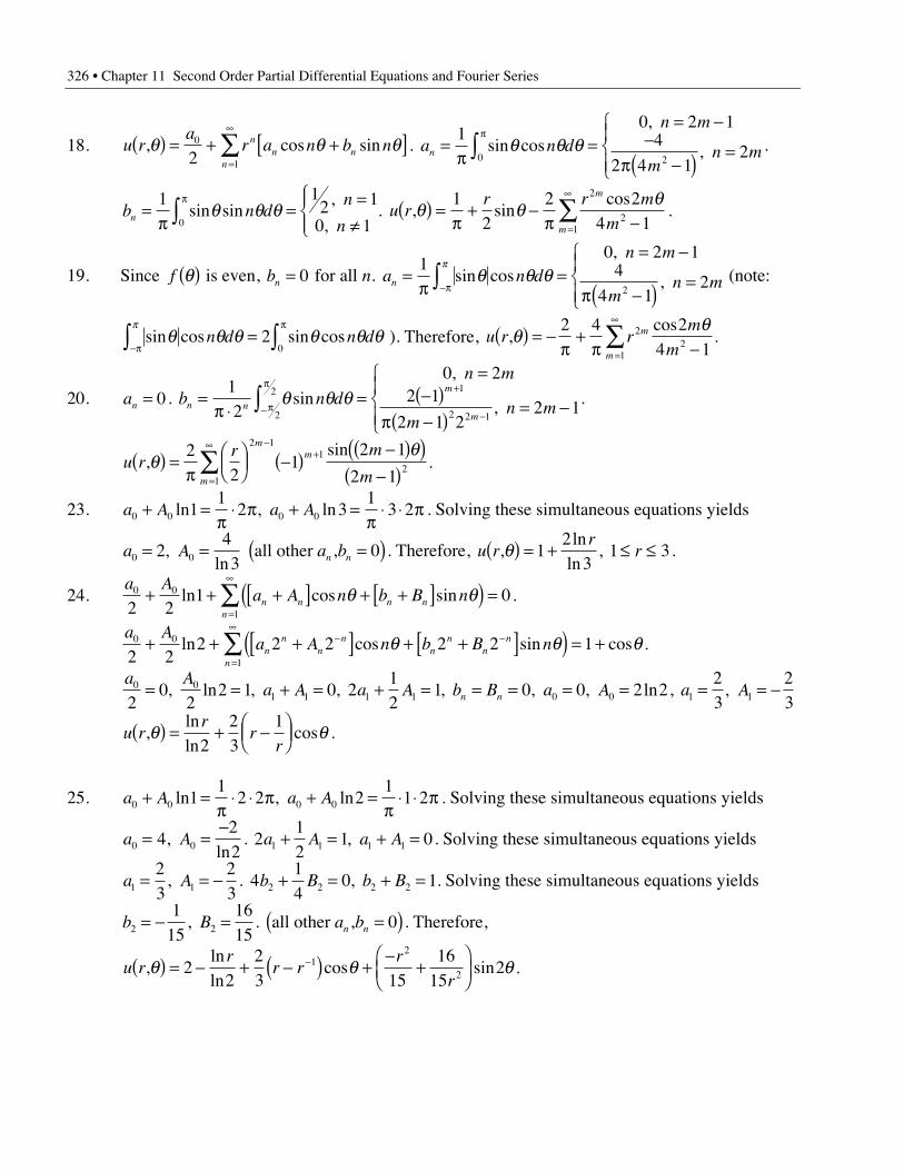
326 • Chapter 11 Second Order Partial Differential Equations and Fourier Series
18. u ra
r a n b nnn n
n
, cos sinq q q( ) = + +[ ]=
•
Â0
12. a n d
n m
mn mn =
p=
= --
p -( ) =ÏÌÔ
ÓÔ
p
Ú1
0 2 14
2 4 120 2
sin cos,
, q q q .
b n dn
nn =
p= =
π
ÏÌÔ
ÓÔp
Ú1 1
2 1
0 10sin sin
,
, q q q . u r
r r m
m
m
m
, sincosq q q( ) =
p+ -
p -=
•
Â12
2 24 1
2
21
.
19. Since f q( ) is even, bn = 0 for all n. a n dn m
mn mn =
p=
= -
p -( ) =ÏÌÔ
ÓÔ-pÚ
10 2 1
4
4 122
sin cos,
, q q qp
(note:
sin cos sin cosq q q q q qp
n d n d-p
p
Ú Ú= 20
). Therefore, u r rm
mm
m
,cosq q( ) = -
p+
p -=
•
Â2 4 24 1
22
1
.
20. an = 0. b n d
n m
mn mn n
m
m
=p ◊
==
-( )p -( )
= -
ÏÌÔ
ÓÔ- p
p +
-Ú
12
0 22 1
2 1 22 12
2 1
2 2 1
q q qsin
,
, .
u rr m
m
mm
m
,sin
qq( ) =
pÊËÁ
ˆ¯ -( ) -( )( )
-( )
-+
=
•
Â22
12 1
2 1
2 11
21
.
23. a A a A0 0 0 011
2 31
3 2+ =p
◊ p + =p
◊ ◊ pln , ln . Solving these simultaneous equations yields
a A0 0243
= =, ln
all other a bn n, =( )0 . Therefore, u rr
r,ln
ln, q( ) = + £ £1
23
1 3.
24.a A
a A n b B nn n n nn
0 0
12 21 0+ + +[ ] + +[ ]( ) =
=
•
Âln cos sinq q .
a Aa A n b B nn
nn
nn
nn
n
n
0 0
12 22 2 2 2 2 1+ + +[ ] + +[ ]( ) = +- -
=
•
Âln cos sin cosq q q .
a Aa A a A b B a An n
0 01 1 1 1 0 02
02
2 1 0 212
1 0 0 2 2= = + = + = = = = =, ln , , , , , ln , a A1 1
23
23
= = -,
u rr
rr
,lnln
cosq q( ) = + -ÊËÁ
ˆ¯2
23
1.
25. a A a A0 0 0 011
2 2 21
1 2+ =p
◊ ◊ p + =p
◊ ◊ pln , ln . Solving these simultaneous equations yields
a A0 0422
= =-
, ln
. 212
1 01 1 1 1a A a A+ = + =, . Solving these simultaneous equations yields
a A1 1
23
23
= = -, . 414
0 12 2 2 2b B b B+ = + =, . Solving these simultaneous equations yields
b B2 2
115
1615
= - =, . all other a bn n, =( )0 . Therefore,
u rr
r rr
r,
lnln
cos sinq q q( ) = - + -( ) +-
+ÊËÁ
ˆ¯
-22
23 15
1615
212
2 .

Chapter 11 Second Order Partial Differential Equations and Fourier Series • 327
26. a A a A A a0 0 0 0 0 021
2 6 023
22 2
3+ =
pp + = fi = - = +ln , ln
ln,
lnln
.
414
1 36136
01296320
13202 2 2 2 2 0a A a A A a+ = - + = fi = - =, , .
u rr
rr
rr
r,
lnln
lnln
cosln ln
lncosq q q( ) = + - + -Ê
ËÁˆ¯ =
-+ -Ê
ËÁˆ¯1
23 3
1320
12962
63
1320
129622
22
2 .
Section 11.7
1. f x yx
a
y
bc
m x
a
n y
bmn, sin sin sin sin( ) =pÊ
ËÁˆ¯
pÊËÁ
ˆ¯ =
pÊËÁ
ˆ¯
pÊËÁ
ˆ¯ÂÂ4 . Examination shows us that
c11 4 0= , otherwise. Thus u x y t ex
a
y
ba b t
, , sin sin( ) =pÊ
ËÁˆ¯
pÊËÁ
ˆ¯
- p( ) + p( )ÈÎÍ
˘˚4
2 2k
.
2. f x yx
a
y
b
x
a
y
bc
m x
a
n y
bmn, sin sin sin sin sin sin( ) =pÊ
ËÁˆ¯
pÊËÁ
ˆ¯ -
pÊËÁ
ˆ¯
pÊËÁ
ˆ¯ =
pÊËÁ
ˆ¯
pÊËÁ
ˆ¯ÂÂ8
2 3.
c c11 238 1= = -, .
u x y t ex
a
y
be
x
a
y
ba b t a b t
, , sin sin sin sin( ) =pÊ
ËÁˆ¯
pÊËÁ
ˆ¯ -
pÊËÁ
ˆ¯
pÊËÁ
ˆ¯
- p( ) + p( )ÈÎÍ
˘˚
- p( ) + p( )ÈÎÍ
˘˚8
2 32 2 2 22 3k k
.
3. First, we note that
f x yx
a
y
b
x
a
y
bc
m x
a
n y
bmn, sin sin cos sin sin sin( ) =pÊ
ËÁˆ¯
pÊËÁ
ˆ¯ = -
pÊËÁ
ˆ¯
ÊËÁ
ˆ¯
pÊËÁ
ˆ¯ =
pÊËÁ
ˆ¯
pÊËÁ
ˆ¯ÂÂ2 1
22 .
ca
x
a
m x
adx cm
a
mn1 0
21
20= -
pÊËÁ
ˆ¯
ÊËÁ
ˆ¯
pÊËÁ
ˆ¯ =Ú cos sin , otherwise. Working through this integral yields
c
m k
k km km1 2
0 216
2 1 2 1 42 1=
=-
p -( ) -( ) -[ ] = -ÏÌÔ
ÓÔ
,
, . Therefore,
u x y t
ek x
a
y
b
k k
ka b t
k
, ,sin sin
( ) = -p
-( )pÊËÁ
ˆ¯
pÊËÁ
ˆ¯
-( ) -( ) -[ ]
- -( ) pÊË
ˆ¯ + p( )È
ÎÍ
˘
˚˙
=
•
Â162 1
2 1 2 1 4
2 1
21
2 2k
.
4. f x yx
a
y
bc
m x
a
n y
bmn, sin sin sin sin( ) =pÊ
ËÁˆ¯
pÊËÁ
ˆ¯ =
pÊËÁ
ˆ¯
pÊËÁ
ˆ¯ÂÂ8 2 2 .
cab
x
a m x
adx
y
b n y
bdymn
a b=
-pÊ
ËÁˆ¯
Ê
Ë
ÁÁÁ
ˆ
¯
˜˜˜
pÊËÁ
ˆ¯
-pÊ
ËÁˆ¯
Ê
Ë
ÁÁÁ
ˆ
¯
˜˜˜
pÊËÁ
ˆ¯Ú Ú8
41
2
2
12
20 0
cossin
cossin
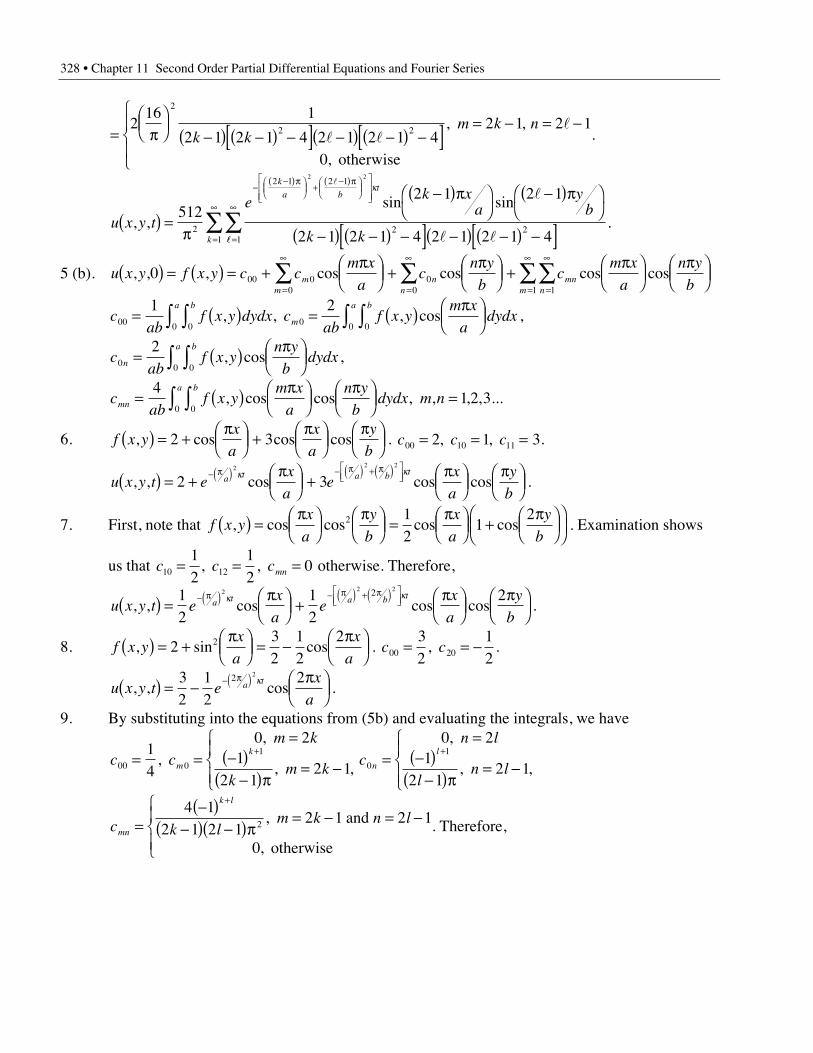
328 • Chapter 11 Second Order Partial Differential Equations and Fourier Series
= pÊËÁ
ˆ¯ -( ) -( ) -[ ] -( ) -( ) -[ ] = - = -
Ï
ÌÔ
ÓÔ
216 1
2 1 2 1 4 2 1 2 1 42 1 2 1
0
2
2 2k k
m k nl l
l, ,
, otherwise
.
u x y te k x
ay
b
k k
k
a bt
, ,sin sin
( ) =p
-( )pÊË
ˆ¯
-( )pÊË
ˆ¯
-( ) -( ) -[ ] -( ) -( ) -[ ]
--( ) pÊ
ËÁˆ¯
+-( ) pÊ
ËÁˆ¯
È
ÎÍÍ
˘
˚˙˙
5122 1 2 1
2 1 2 1 4 2 1 2 1 42
2 1 2 1
2 2
2 2l
l
l l
k
ll =
•
=
•
ÂÂ11k
.
5 (b). u x y f x y c cm x
ac
n y
bc
m x
a
n y
bmm
nn
mnnm
, , , cos cos cos cos0 00 00
00 11
( ) = ( ) = +pÊ
ËÁˆ¯ +
pÊËÁ
ˆ¯ +
pÊËÁ
ˆ¯
pÊËÁ
ˆ¯=
•
=
•
=
•
=
•
  ÂÂ
cab
f x y dydx cab
f x ym x
adydx
ba
m
ba
00 00 0 00
1 2= ( ) = ( ) pÊ
ËÁˆ¯ÚÚ ÚÚ, , , cos ,
cab
f x yn y
bdydxn
ba
0 00
2= ( ) pÊ
ËÁˆ¯ÚÚ , cos ,
cab
f x ym x
a
n y
bdydx m nmn
ba= ( ) pÊ
ËÁˆ¯
pÊËÁ
ˆ¯ =ÚÚ
41 2 3
00, cos cos , , , , ...
6. f x yx
a
x
a
y
b, cos cos cos( ) = +
pÊËÁ
ˆ¯ +
pÊËÁ
ˆ¯
pÊËÁ
ˆ¯2 3 . c c c00 10 112 1 3= = =, , .
u x y t ex
ae
x
a
y
ba t a b t
, , cos cos cos( ) = +pÊ
ËÁˆ¯ +
pÊËÁ
ˆ¯
pÊËÁ
ˆ¯
- p( ) - p( ) + p( )ÈÎÍ
˘˚2 3
2 2 2
k k.
7. First, note that f x yx
a
y
b
x
a
y
b, cos cos cos cos( ) =
pÊËÁ
ˆ¯
pÊËÁ
ˆ¯ =
pÊËÁ
ˆ¯ +
pÊËÁ
ˆ¯
ÊËÁ
ˆ¯
2 12
12
. Examination shows
us that c c cmn10 12
12
12
0= = =, , otherwise. Therefore,
u x y t ex
ae
x
a
y
ba t a b t
, , cos cos cos( ) =pÊ
ËÁˆ¯ +
pÊËÁ
ˆ¯
pÊËÁ
ˆ¯
- p( ) - p( ) + p( )ÈÎÍ
˘˚1
212
22 2 22k k.
8. f x yx
a
x
a, sin cos( ) = +
pÊËÁ
ˆ¯ = -
pÊËÁ
ˆ¯2
32
12
22 . c c00 20
32
12
= = -, .
u x y t ex
aa t
, , cos( ) = -pÊ
ËÁˆ¯
- p( )32
12
22 2k
.
9. By substituting into the equations from (5b) and evaluating the integrals, we have
c c
m k
km k
c
n l
ln lm
k
n
l
00 0
1
0
114
0 21
2 12 1
0 21
2 12 1
= ==
-( )-( )p
= -
ÏÌÔ
ÓÔ=
=-( )
-( )p= -
ÏÌÔ
ÓÔ
+ +,
,
, ,
,
, ,
c k lm k n l
mn
k l
=-( )
-( ) -( )p= - = -
ÏÌÔ
ÓÔ
+4 1
2 1 2 12 1 2 1
0
2 ,
,
and
otherwise. Therefore,
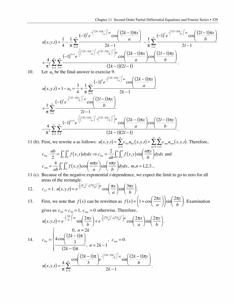
Chapter 11 Second Order Partial Differential Equations and Fourier Series • 329
u x y t
ek x
a
k
kk
a t
k
, ,cos
( ) = -p
-( ) -( )pÊËÁ
ˆ¯
-
- -( ) pÊË
ˆ¯
=
•
Â14
11
2 1
2 1
2 1
1
2
k
-p
-( ) -( )pÊËÁ
ˆ¯
-
- -( ) pÊË
ˆ¯
=
•
Â11
2 1
2 1
2 1
1
2
ll
b t
l
el x
b
l
kcos
+p
-( ) -( )pÊËÁ
ˆ¯
-( )pÊËÁ
ˆ¯
-( ) -( )
+- -( ) pÊ
ˈ¯ + -( ) pÊ
ˈ¯
È
ÎÍ
˘
˚˙
=
•
=
•
ÂÂ41
2 1 2 1
2 1 2 12
2 1 2 1
11
2 2
k lk
al
b t
lk
ek x
a
l y
b
k l
kcos cos
.
10. Let u9 be the final answer to exercise 9.
u x y t u
ek x
a
k
kk
a t
k
, ,cos
( ) = - = +p
-( ) -( )pÊËÁ
ˆ¯
-
- -( ) pÊË
ˆ¯
=
•
Â134
11
2 1
2 19
2 1
1
2
k
+p
-( ) -( )pÊËÁ
ˆ¯
-
- -( ) pÊË
ˆ¯
=
•
Â11
2 1
2 1
2 1
1
2
ll
b t
l
el x
b
l
kcos
-p
-( ) -( )pÊËÁ
ˆ¯
-( )pÊËÁ
ˆ¯
-( ) -( )
+- -( ) pÊ
ˈ¯ + -( ) pÊ
ˈ¯
È
ÎÍ
˘
˚˙
=
•
=
•
ÂÂ41
2 1 2 1
2 1 2 12
2 1 2 1
11
2 2
k lk
al
b t
lk
ek x
a
l y
b
k l
kcos cos
.
11 (b). First, we rewrite u as follows: u x y t c u x y t c u x y tn nn
mn mnnm
, , , , , ,( ) = ( ) + ( )=
•
=
•
=
•
 ÂÂ0 01 11
. Therefore,
cab
f x y dydx cab
f x yn y
bdydxn
ba
n
ba
0 00 0 0022
◊ = ( ) fi = ( ) pÊËÁ
ˆ¯ÚÚ ÚÚ, , sin and
cab
f x ym x
a
n y
bdydx m nmn
ba= ( ) pÊ
ËÁˆ¯
pÊËÁ
ˆ¯ =ÚÚ
41 2 3
00, cos sin , , , , ...
11 (c). Because of the negative exponential t-dependence, we expect the limit to go to zero for allareas of the rectangle.
12. c13 1= . u x y t ex
a
y
ba b t
, , cos sin( ) =pÊ
ËÁˆ¯
pÊËÁ
ˆ¯
- p( ) + p( )ÈÎÍ
˘˚
2 23 3k.
13. First, we note that f x( ) can be rewritten as f xx
a
y
b( ) = +
pÊËÁ
ˆ¯
ÊËÁ
ˆ¯
pÊËÁ
ˆ¯1
2 2cos sin . Examination
gives us c c cmn02 22 1 0= = =, otherwise. Therefore,
u x y t ey
be
x
a
y
bb
ta b t
, , sin cos sin( ) =pÊ
ËÁˆ¯ +
pÊËÁ
ˆ¯
pÊËÁ
ˆ¯
-pÊ
ËÁˆ¯ - p( ) + p( )È
Î͢˚
2 2 22
2 22 2 2k k
.
14. c
n kk
kn k
n0
0 2
42 1
32 1
2 1=
=-( )pÊ
ËÁˆ¯
-( )p= -
Ï
ÌÔÔ
ÓÔÔ
,
cos,
, cmn = 0.
u x y t
ke
k y
b
k
kb t
k
, ,cos sin
( ) =p
-( )pÊËÁ
ˆ¯
-( )pÊËÁ
ˆ¯
-
- -( ) pÊË
ˆ¯
=
•
Â42 1
32 1
2 1
2 1
1
2
k
.
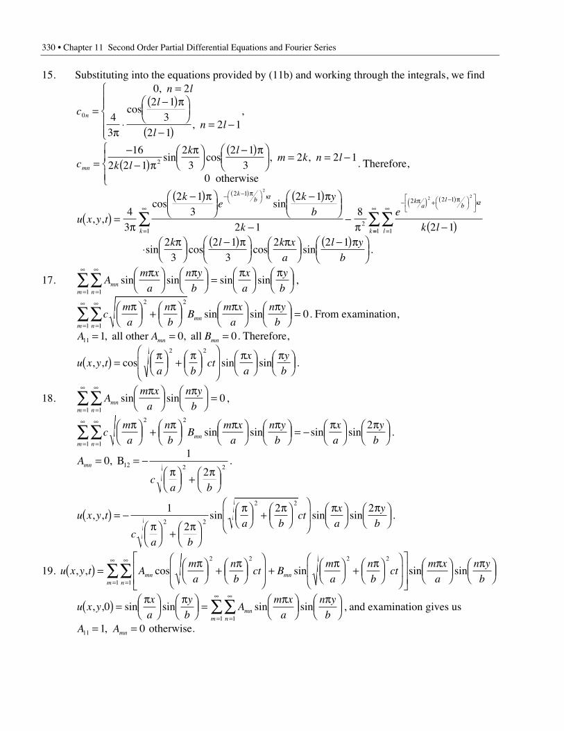
330 • Chapter 11 Second Order Partial Differential Equations and Fourier Series
15. Substituting into the equations provided by (11b) and working through the integrals, we find
c
n ll
ln l
n0
0 2
43
2 13
2 12 1
=
=
p◊
-( )pÊËÁ
ˆ¯
-( ) = -
Ï
ÌÔÔ
ÓÔÔ
,
cos,
,
c k l
k lm k n l
mn =-
-( )ppÊ
ËÁˆ¯
-( )pÊËÁ
ˆ¯
= = -ÏÌÔ
ÓÔ
162 2 1
23
2 13
2 2 1
0
2 sin cos , ,
otherwise. Therefore,
u x y t
ke
k y
b
k
e
k l
kb t
k
ka
lb t
lk
, ,cos sin
( ) =p
-( )pÊËÁ
ˆ¯
-( )pÊËÁ
ˆ¯
--
p -( )
- -( ) pÊË
ˆ¯
=
•- p( ) + -( ) pÊ
ˈ¯
È
ÎÍ
˘
˚˙
=
•
 Â43
2 13
2 1
2 18
2 1
2 1
12
2 2 1
1
2
2 2kk
==
•
Â1
◊pÊ
ËÁˆ¯
-( )pÊËÁ
ˆ¯
pÊËÁ
ˆ¯
-( )pÊËÁ
ˆ¯
sin cos cos sin2
32 1
32 2 1k l k x
a
l y
b.
17. Am x
a
n y
b
x
a
y
bmnnm
sin sin sin sinpÊ
ËÁˆ¯
pÊËÁ
ˆ¯ =
pÊËÁ
ˆ¯
pÊËÁ
ˆ¯=
•
=
•
ÂÂ11
,
cm
a
n
bB
m x
a
n y
bmnnm
pÊËÁ
ˆ¯ +
pÊËÁ
ˆ¯
pÊËÁ
ˆ¯
pÊËÁ
ˆ¯ =
=
•
=
•
ÂÂ2 2
11
0sin sin . From examination,
A A Bmn mn11 1 0 0= = =, , all other all . Therefore,
u x y ta b
ctx
a
y
b, , cos sin sin( ) =
pÊËÁ
ˆ¯ +
pÊËÁ
ˆ¯
Ê
ËÁ
ˆ
¯˜
pÊËÁ
ˆ¯
pÊËÁ
ˆ¯
2 2
.
18. Am x
a
n y
bmnnm
sin sinpÊ
ËÁˆ¯
pÊËÁ
ˆ¯ =
=
•
=
•
ÂÂ11
0,
cm
a
n
bB
m x
a
n y
b
x
a
y
bmnnm
pÊËÁ
ˆ¯ +
pÊËÁ
ˆ¯
pÊËÁ
ˆ¯
pÊËÁ
ˆ¯ = -
pÊËÁ
ˆ¯
pÊËÁ
ˆ¯=
•
=
•
ÂÂ2 2
11
2sin sin sin sin .
A
ca b
mn = = -pÊ
ËÁˆ¯ +
pÊËÁ
ˆ¯
01
212 2 2
, B .
u x y t
ca b
a bct
x
a
y
b, , sin sin sin( ) = -
pÊËÁ
ˆ¯ +
pÊËÁ
ˆ¯
pÊËÁ
ˆ¯ +
pÊËÁ
ˆ¯
Ê
ËÁ
ˆ
¯˜
pÊËÁ
ˆ¯
pÊËÁ
ˆ¯
1
2
2 22 2
2 2
.
19. u x y t Am
a
n
bct B
m
a
n
bct
m x
a
n y
bmn mnnm
, , cos sin sin sin( ) =pÊ
ËÁˆ¯ +
pÊËÁ
ˆ¯
Ê
ËÁ
ˆ
¯˜ +
pÊËÁ
ˆ¯ +
pÊËÁ
ˆ¯
Ê
ËÁ
ˆ
¯˜
È
ÎÍÍ
˘
˚˙˙
pÊËÁ
ˆ¯
pÊËÁ
ˆ¯=
•
=
•
ÂÂ2 2 2 2
11
u x yx
a
y
bA
m x
a
n y
bmnnm
, , sin sin sin sin011
( ) =pÊ
ËÁˆ¯
pÊËÁ
ˆ¯ =
pÊËÁ
ˆ¯
pÊËÁ
ˆ¯=
•
=
•
ÂÂ , and examination gives us
A Amn11 1 0= =, otherwise.
Chapter 11 Second Order Partial Differential Equations and Fourier Series • 331
u x yx
a
y
bc
m
a
n
bB
m x
a
n y
bt mnnm
, , sin sin sin sin0 22 2
11
( ) = -pÊ
ËÁˆ¯
pÊËÁ
ˆ¯ =
pÊËÁ
ˆ¯ +
pÊËÁ
ˆ¯
pÊËÁ
ˆ¯
pÊËÁ
ˆ¯=
•
=
•
ÂÂ , and
examination gives us pÊ
ËÁˆ¯ +
pÊËÁ
ˆ¯ = - =
a bcB Bmn
2 2
11 2 0, otherwise. Therefore,
u x y ta b
ct
a bc
a bct
x
a, , cos sin sin sin( ) =
pÊËÁ
ˆ¯ +
pÊËÁ
ˆ¯
Ê
ËÁ
ˆ
¯˜
-
pÊËÁ
ˆ¯ +
pÊËÁ
ˆ¯
Ê
Ë
ÁÁÁÁ
ˆ
¯
˜˜˜˜
pÊËÁ
ˆ¯ +
pÊËÁ
ˆ¯
Ê
ËÁ
ˆ
¯˜
Ê
ËÁÁ
ˆ
¯˜
pÊËÁ
ˆ¯
p2 2
2 2
2 22 yy
bÊËÁ
ˆ¯ .
20. f x yx
a
y
b
x
a
y
b, sin sin cos sin( ) =
pÊËÁ
ˆ¯
pÊËÁ
ˆ¯ = -
pÊËÁ
ˆ¯
ÈÎÍ
˘˚
pÊËÁ
ˆ¯2 1
22 .
B Aab
x
a
y
b
m x
a
n y
bdydxmn mn
ba= = -
pÊËÁ
ˆ¯
ÈÎÍ
˘˚
pÊËÁ
ˆ¯
pÊËÁ
ˆ¯
pÊËÁ
ˆ¯ÚÚ0
41
200
, cos sin sin sin
=-
p -( ) -( ) -[ ] = - =ÏÌÔ
ÓÔ
16
2 1 2 1 42 1 1
0
2k k
m k n, ,
, otherwise
.
u x y t
k
a bct
k x
a
y
b
k kk
, ,
cos sin sin
( ) = -p
-( )pÊËÁ
ˆ¯
+pÊ
ËÁˆ¯
Ê
ËÁÁ
ˆ
¯˜
-( )pÊËÁ
ˆ¯
pÊËÁ
ˆ¯
p -( ) -( ) -[ ]=
•
Â16
2 1 2 1
2 1 2 1 4
2 2
21
.
21 (a). Making the substitution
Tn x n
Tn x
U h tx
nn
nn
s¢ pÊ
ËÁˆ¯ - -
pÊËÁ
ˆ¯
pÊËÁ
ˆ¯ = -( ) ◊ -
pÊËÁ
ˆ¯
ÊËÁ
ˆ¯=
•
=
•
 Âcos cos cosl l l l0
2
1
12
12k t gives us
TU
h t T T U h tss0 2
2
222 1
2¢ = -( ) ¢ +
pÊËÁ
ˆ¯ = - -( )t k t,
l, T
nT nn n
¢ +pÊ
ËÁˆ¯ = πk
l
2
0 0 2, , . Imposing the
initial condition u x,0 0( ) = gives us Tn = 0 for all n π 0 2, .
For T0: TU
t
t
s
0 20
0¢ = £ £
>
ÏÌÔ
ÓÔ,
,
tt
, and antidifferentiation gives us T
Ut t
Ut
s
s0
20
2
=£ £
>
Ï
ÌÔ
ÓÔ
,
,
t
t t.
For T2: T T U t
t
s2
2
2
2 12
0
0¢ +
pÊËÁ
ˆ¯ = - £ £
>
ÏÌÔ
ÓÔk t
tl,
, . Therefore,
T
Ue t
Ue t
s t
s2
22
22
2 21 0
2 21
2
2=
-p
ÊËÁ
ˆ¯ -È
Î͢˚
£ £
-p
ÊËÁ
ˆ¯ -È
Î͢˚
>
Ï
ÌÔÔ
ÓÔÔ
- p( )
- p( )k
t
kt
k
k t
l
l
l
l
,
,
.
332 • Chapter 11 Second Order Partial Differential Equations and Fourier Series
21 (b). u x t T Tx
, cos( ) = +pÊ
ËÁˆ¯0 2
2l
. Therefore, u t T Tl
2 0 2,ÊËÁ
ˆ¯ = - .
For 0 £ £t t : u tU
tU
e t es s t tl ll
2 2 2 21 75
7515 79
12
2 15 792
,.
.ÊËÁ
ˆ¯ = +
pÊËÁ
ˆ¯ -È
Î͢˚
ª + -[ ]- p( ) -
kk
. Setting this
equal to zero and solving for t yields t = 0 936674. hours.
22 (a). Tn x
Tn n x
Ux
nn
nn
s¢ pÊ
ËÁˆ¯ +
pÊËÁ
ˆ¯
pÊËÁ
ˆ¯ =
pÊËÁ
ˆ¯=
•
=
•
 Âsin sin sinl l l l1
2
1
k .
T T U Tn
Ts n n1
2
1
2
0¢ +pÊ
ËÁˆ¯ = ¢ +
pÊËÁ
ˆ¯ =k k
l l, . T
UCe U
UCs s
1
2
0
22
=p
ÊËÁ
ˆ¯ + =
pÊËÁ
ˆ¯ +- p( )l l
l
k kk
, ,
TU
UU
e Ts s t
n1
2
0
2 2
0=p
ÊËÁ
ˆ¯ + -
pÊËÁ
ˆ¯
Ê
ËÁˆ
¯=- p( )l l
l
k kk
, . u x t Tx U xs, sin sin( ) =
pÊËÁ
ˆ¯ =
pÊËÁ
ˆ¯
pÊËÁ
ˆ¯1
2
l
l
lk.
22 (b). Assume u Ux
=pÊ
ËÁˆ¯0 sin
l. 0
2
0- -pÊ
ËÁˆ¯
Ê
ËÁˆ
¯pÊ
ËÁˆ¯ =
pÊËÁ
ˆ¯k
l l lU
xU
xssin sin . k pÊ
ËÁˆ¯ =
l
2
0U Us .
24. T cct
cct
C1 1 2=pÊ
ËÁˆ¯ +
pÊËÁ
ˆ¯cos sin
l l. T A t B t
P1 = +cos sinw w .
Tc
T Ac
t Bc
t tP P1
2
12
22
2
¢¢ +pÊ
ËÁˆ¯ = - +
pÊËÁ
ˆ¯
Ê
ËÁˆ
¯+ - +
pÊËÁ
ˆ¯
Ê
ËÁˆ
¯=
l l lw w w w wcos sin cos
fi =- +
pÊËÁ
ˆ¯
Ê
ËÁˆ
¯
=Ac
B1
02
2
wl
, . T cct
cct
A t1 1 2=pÊ
ËÁˆ¯ +
pÊËÁ
ˆ¯ +cos sin cos
l lw . T
cc1 20 0¢ ( ) =
p=
l,
T c A1 10 0( ) = + = . Tt
ct
c1 2
2
=-
pÊËÁ
ˆ¯
pÊËÁ
ˆ¯ -
cos cosw
w
l
l
, u x t Tx
u t Tt t
, sin , ,cos cos( ) =
pÊËÁ
ˆ¯
ÊËÁ
ˆ¯ = =
- p( )p -1 1 22
2 24 4l
l.
25. The complementary solution is T c t c tC1 1 2= p( ) + p( )cos sin . The particular solution is
T t A t B tP1 = p + p[ ]cos sin . Differentiation gives us
T A t B t t A t B tP1
¢ = p + p[ ] + -p p + p p[ ]cos sin sin cos and
T A t B t A t B t t A t B tP1
2 2¢¢ = -p p + p p[ ] + -p p + p p[ ] + -p p - p p[ ]sin cos sin cos cos sin .
T T A t B t t A BP P1
21 2 2 0
12
¢¢ + p = - p p + p p = p fi = =p
sin cos cos , . Thus
Tt
t T c t c tt
tP1 1 1 22 2
=p
p = p + p +p
psin , cos sin sinand so . Imposing the conditions
T c1 10 0( ) = = and T c1 20 0¢ ( ) = = p gives us Tt
t1 2=
ppsin , and so
u x t Tx t
tx
, sin sin sin( ) =pÊ
ËÁˆ¯ =
pp
pÊËÁ
ˆ¯1 2l l
.
Chapter 11 Second Order Partial Differential Equations and Fourier Series • 333
26 (b). u y Xn y
bu a y X a
n y
bX X an
nn
nn n0 0 0 0
1 1
, sin , , sin , ( ) = ( ) pÊËÁ
ˆ¯ ( ) = ( ) pÊ
ËÁˆ¯ ( ) = ( ) =
=
•
=
•
  .
X x c e c e Xx
bx
bP2 1
2
2
2
2( ) = + +p - p
.
X Ax Bb
Ax B x X x c e c eb
xP
xb
xb
2
2
2 1
2
2
22
02
2= + fi -
pÊËÁ
ˆ¯ +( ) = fi ( ) = + -
pÊËÁ
ˆ¯
p - p.
c c c e c eb
a c ca b
e e
ab
ab
ab
ab
1 2 1
2
2
22
1 2
2
2 202
2+ = + =p
ÊËÁ
ˆ¯ fi = - = p( )
-
p - p
p - p, . X nn = π0 2, .
u x ya b e e
e e
bx
y
b
xb
xb
ab
ab
, sin( ) = p( ) -( )-
-p
ÊËÁ
ˆ¯
È
Î
ÍÍÍ
˘
˚
˙˙˙
pÊËÁ
ˆ¯
p - p
p - p2
22
2 2 2
2 2
2
.
27. u x y n x Ynn
, sin( ) = p( )=
•
Â1
. Making this substitution, we have
- p( ) p( ) + p( ) ¢¢= p=
•
=
•
 Ân n x Y n x Y e xnn
nn
y2
1 1
sin sin sin . From this equation, we can obtain two initial
value problems: Y Y e Y Yy1
21 1 10 1 0¢¢ - p = ( ) = ( ) =, and Y Y Y Y nn n n n
¢¢ - p = ( ) = ( ) = ≥2 0 0 1 0 2, , .For the first, IVP, the complementary solution is Y c e c e
C
y y1 1 2= +p -p , and the particular solution
is Y Ae A AP
y1
221 1
11
= fi - p( ) = fi =-
p -. Therefore, we have Y c e c e
ey yy
1 1 2 2 1= + -
p -p -p .
Imposing the initial conditions gives us c c e c e ce
1 2 2 1 2 2
11 1
+ =p -
+ =p -
p -p, , and solving
these simultaneous equations yields ce e
e ec
e e
e e1 2 2 2
11
11
=p -
--
ÊËÁ
ˆ¯
=p -
- +-
ÊËÁ
ˆ¯
-p
-p p
p
-p p, . Thus
Ye e e e e e
e ee
y yy
1 2
11
=p -
-( ) - -( )-
-Ê
ËÁ
ˆ
¯˜
-p p p -p
p -p . For the second IVP, we can quickly see that the
only unique solution is trivial, and so Y nn = ≥0 2, . Finally, we have
u x y Y xx e e e e e e
e ee
y yy, sin
sin( ) = p =p
p --( ) - -( )
--
Ê
ËÁ
ˆ
¯˜
-p p p -p
p -p1 2 1.
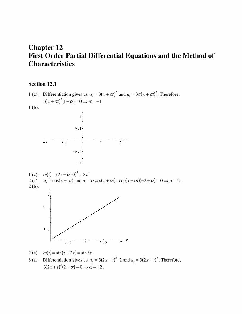
Chapter 12First Order Partial Differential Equations and the Method ofCharacteristics
Section 12.1
1 (a). Differentiation gives us u x t u x tx t= +( ) = +( )3 32 2a a a and . Therefore,
3 1 0 12
x t+( ) +( ) = fi = -a a a .1 (b).
1 (c). w t a tt( ) = + ◊( ) =2 0 83 3
2 (a). u x t u x tx t= +( ) = +( )cos cosa a a and . cos x t+( ) - +( ) = fi =a a a2 0 2.2 (b).
2 (c). w t t tt( ) = +( ) =sin sin2 3 .
3 (a). Differentiation gives us u x t u x tx t= +( ) ◊ = +( )3 2 3 22 2
2 and . Therefore,
3 2 2 0 22
x t+( ) +( ) = fi = -a a .
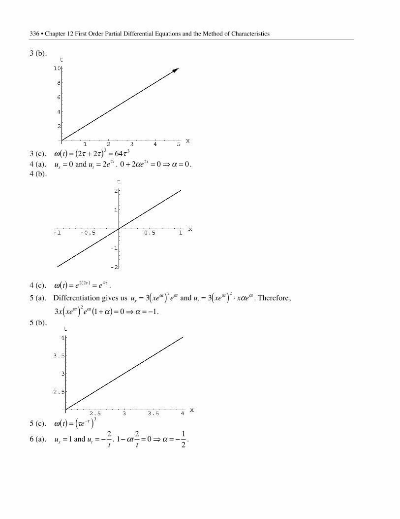
336 • Chapter 12 First Order Partial Differential Equations and the Method of Characteristics
3 (b).
3 (c). w t t tt( ) = +( ) =2 2 643 3
4 (a). u u ex tt= =0 2 2 and . 0 2 0 02+ = fi =a ae t .
4 (b).
4 (c). w t tt e e( ) = =( )2 2 4 .
5 (a). Differentiation gives us u xe e u xe x ext t
tt t= ( ) = ( ) ◊3 3
2 2a a a aa and . Therefore,
3 1 0 12
x xe et ta a a a( ) +( ) = fi = - .
5 (b).
5 (c). w t tt e( ) = ( )- 3
6 (a). u utx t= = -12
and . 12
012
- = fi = -a att
.
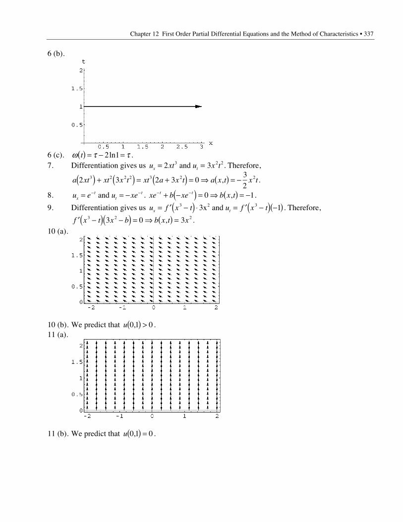
Chapter 12 First Order Partial Differential Equations and the Method of Characteristics • 337
6 (b).
6 (c). w t tt( ) = - =2 1ln .7. Differentiation gives us u xt u x tx t= =2 33 2 2 and . Therefore,
a xt xt x t xt a x t a x t x t2 3 2 3 032
3 2 2 2 3 2 2( ) + ( ) = +( ) = fi ( ) = -, .
8. u e u xext
tt= = -- - and . xe b xe b x tt t- -+ -( ) = fi ( ) = -0 1, .
9. Differentiation gives us u f x t u f x tx t= ¢ -( ) ◊ = ¢ -( ) -( )3 2 3 13x and . Therefore,
¢ -( ) -( ) = fi ( ) =f x t x b b x t x3 2 23 0 3, .
10 (a).
10 (b). We predict that u 0 1 0,( ) > .11 (a).
11 (b). We predict that u 0 1 0,( ) = .
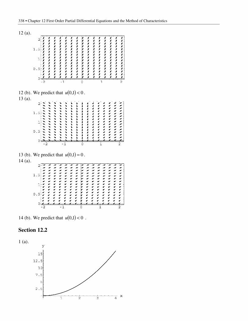
338 • Chapter 12 First Order Partial Differential Equations and the Method of Characteristics
12 (a).
12 (b). We predict that u 0 1 0,( ) < .13 (a).
13 (b). We predict that u 0 1 0,( ) = .14 (a).
14 (b). We predict that u 0 1 0,( ) < .
Section 12.2
1 (a).
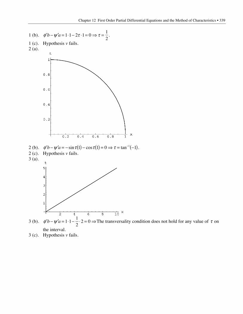
Chapter 12 First Order Partial Differential Equations and the Method of Characteristics • 339
1 (b). ¢ - ¢ = ◊ - ◊ = fi =f y t tb a 1 1 2 1 012
.
1 (c). Hypothesis v fails.2 (a).
2 (b). ¢ - ¢ = - ( ) - ( ) = fi = -( )-f y t t tb a sin cos tan1 1 0 11 .2 (c). Hypothesis v fails.3 (a).
3 (b). ¢ - ¢ = ◊ - ◊ = fif yb a 1 112
2 0 The transversality condition does not hold for any value of t on
the interval.3 (c). Hypothesis v fails.
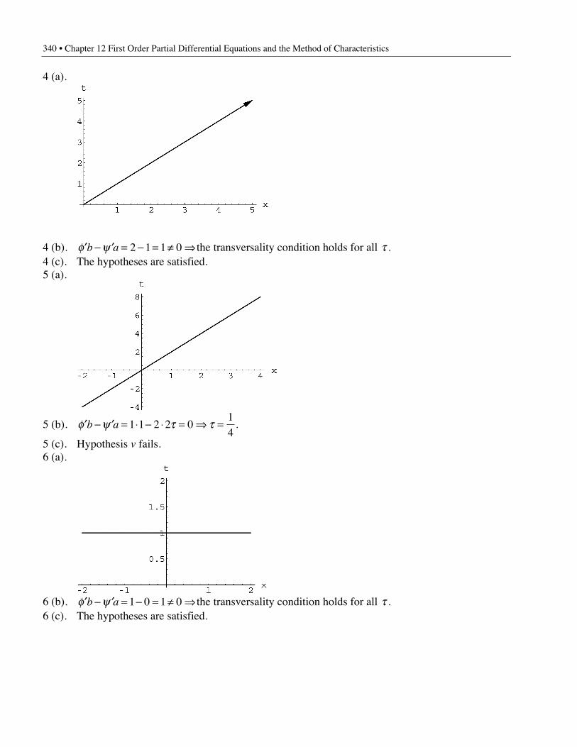
340 • Chapter 12 First Order Partial Differential Equations and the Method of Characteristics
4 (a).
4 (b). ¢ - ¢ = - = π fif yb a 2 1 1 0 the transversality condition holds for all t .4 (c). The hypotheses are satisfied.5 (a).
5 (b). ¢ - ¢ = ◊ - ◊ = fi =f y t tb a 1 1 2 2 014
.
5 (c). Hypothesis v fails.6 (a).
6 (b). ¢ - ¢ = - = π fif yb a 1 0 1 0 the transversality condition holds for all t .6 (c). The hypotheses are satisfied.
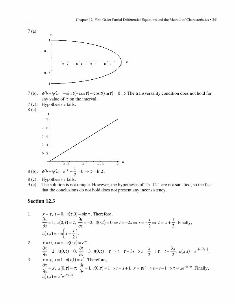
Chapter 12 First Order Partial Differential Equations and the Method of Characteristics • 341
7 (a).
7 (b). ¢ - ¢ = - -( ) - ( ) = fif y t t t tb a sin cos cos sin 0 The transversality condition does not hold forany value of t on the interval.
7 (c). Hypothesis v fails.8 (a).
8 (b). ¢ - ¢ = - = fi =-f y ttb a e12
0 2ln .
8 (c). Hypothesis v fails.9 (c). The solution is not unique. However, the hypotheses of Th. 12.1 are not satisfied, so the fact
that the conclusions do not hold does not present any inconsistency.
Section 12.3
1. x t u= = ( ) =t t t, , , sin0 0 . Therefore,∂∂
= ( ) =∂∂
= - ( ) = fi = - fi = - fi = +x
sx
t
st t s s
tx
t1 0 2 0 0 2
2 2, , ; , ,t t t t . Finally,
u x t xt
, sin( ) = +ÊËÁ
ˆ¯2
.
2. x t u e= = ( ) = -0 0, , ,t t t .∂∂
= ( ) =∂∂
= ( ) = fi = + fi = fi = -x
sx
t
st t s s
xt
x2 0 0 3 0 3
232
, , ; , ,t t t t t . u x t et x
,( ) = - -( )32 .
3. x t u= = ( ) =t t t, , ,1 1 2 . Therefore,∂∂
= ( ) =∂∂
= ( ) = fi = + = fi = - fi = - -( )x
sx x
t
st t s x e s t xes t, , ; , , , 0 1 0 1 1 1 1t t t t t . Finally,
u x t x e t, ( )( ) = - -2 2 1 .
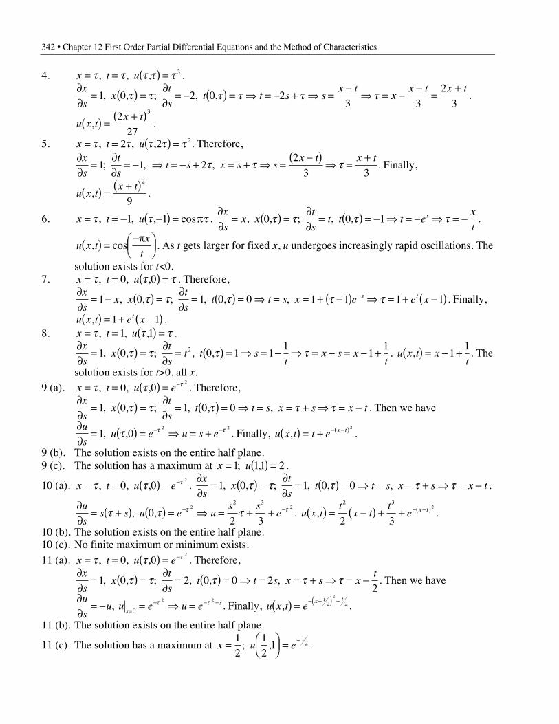
342 • Chapter 12 First Order Partial Differential Equations and the Method of Characteristics
4. x t u= = ( ) =t t t t t, , , 3 .∂∂
= ( ) =∂∂
= - ( ) = fi = - + fi =-
fi = --
=+x
sx
t
st t s s
x tx
x t x t1 0 2 0 2
3 32
3, , ; , ,t t t t t t .
u x tx t
,( ) =+( )2
27
3
.
5. x t u= = ( ) =t t t t t, , ,2 2 2. Therefore,∂∂
=∂∂
= - fi = - + = + fi =-( )
fi =+x
s
t
st s x s s
x t x t1 1 2
23 3
; , , t t t . Finally,
u x tx t
,( ) =+( )2
9.
6. x t u= = - -( ) = pt t t, , , cos1 1 . ∂∂
= ( ) =∂∂
= ( ) = - fi = - fi = -x
sx x
t
st t t e
x
ts, , ; , ,0 0 1t t t t .
u x tx
t, cos( ) =
-pÊËÁ
ˆ¯ . As t gets larger for fixed x, u undergoes increasingly rapid oscillations. The
solution exists for t<0.7. x t u= = ( ) =t t t, , ,0 0 . Therefore,
∂∂
= - ( ) =∂∂
= ( ) = fi = = + -( ) fi = + -( )-x
sx x
t
st t s x e e xs t1 0 1 0 0 1 1 1 1, , ; , , , t t t t t . Finally,
u x t e xt,( ) = + -( )1 1 .8. x t u= = ( ) =t t t, , ,1 1 .
∂∂
= ( ) =∂∂
= ( ) = fi = - fi = - = - +x
sx
t
st t s
tx s x
t1 0 0 1 1
11
12, , ; , ,t t t t . u x t xt
,( ) = - +11
. The
solution exists for t>0, all x.
9 (a). x t u e= = ( ) = -t t t, , ,0 02
. Therefore,∂∂
= ( ) =∂∂
= ( ) = fi = = + fi = -x
sx
t
st t s x s x t1 0 1 0 0, , ; , , , t t t t t . Then we have
∂∂
= ( ) = fi = +- -u
su e u s e1 0
2 2
, ,t t t . Finally, u x t t e x t,( ) = + - -( ) 2
.
9 (b). The solution exists on the entire half plane.9 (c). The solution has a maximum at x u= ( ) =1 11 2; , .
10 (a). x t u e= = ( ) = -t t t, , ,0 02
. ∂∂
= ( ) =∂∂
= ( ) = fi = = + fi = -x
sx
t
st t s x s x t1 0 1 0 0, , ; , , , t t t t t .
∂∂
= +( ) ( ) = fi = + +- -u
ss s u e u
s set t tt t, ,0
2 3
2 22 3
. u x tt
x tt
e x t,( ) = -( ) + + - -( )2 3
2 3
2
.
10 (b). The solution exists on the entire half plane.10 (c). No finite maximum or minimum exists.
11 (a). x t u e= = ( ) = -t t t, , ,0 02
. Therefore,∂∂
= ( ) =∂∂
= ( ) = fi = = + fi = -x
sx
t
st t s x s x
t1 0 2 0 0 2
2, , ; , , , t t t t t . Then we have
∂∂
= - = fi ==- - -u
su u e u es
s, 0
2 2t t . Finally, u x t ex t t
,( ) = - -( ) -2 22
.
11 (b). The solution exists on the entire half plane.
11 (c). The solution has a maximum at x u e= ÊËÁ
ˆ¯ = -1
212
11
2; , .
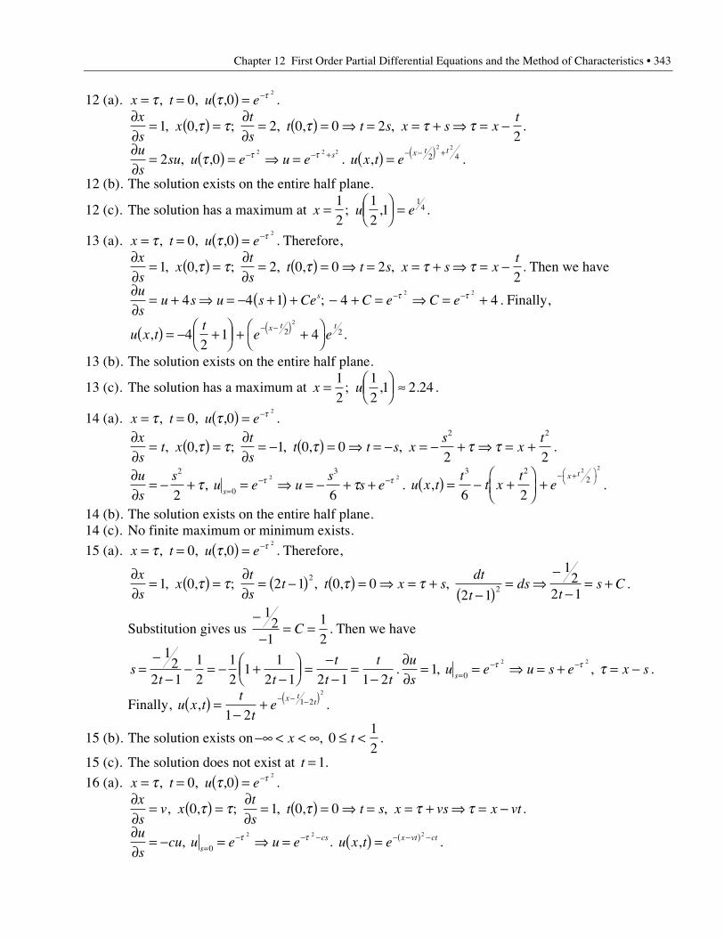
Chapter 12 First Order Partial Differential Equations and the Method of Characteristics • 343
12 (a). x t u e= = ( ) = -t t t, , ,0 02
.∂∂
= ( ) =∂∂
= ( ) = fi = = + fi = -x
sx
t
st t s x s x
t1 0 2 0 0 2
2, , ; , , , t t t t t .
∂∂
= ( ) = fi =- - +u
ssu u e u e s2 0
2 2 2
, ,t t t . u x t ex t t
,( ) = - -( ) +2 42 2
.
12 (b). The solution exists on the entire half plane.
12 (c). The solution has a maximum at x u e= ÊËÁ
ˆ¯ =
12
12
11
4; , .
13 (a). x t u e= = ( ) = -t t t, , ,0 02
. Therefore,∂∂
= ( ) =∂∂
= ( ) = fi = = + fi = -x
sx
t
st t s x s x
t1 0 2 0 0 2
2, , ; , , , t t t t t . Then we have
∂∂
= + fi = - +( ) + - + = fi = +- -u
su s u s Ce C e C es4 4 1 4 4
2 2
; t t . Finally,
u x tt
e ex t t
,( ) = - +ÊËÁ
ˆ¯ + +Ê
ˈ¯
- -( )42
1 42 22
.
13 (b). The solution exists on the entire half plane.
13 (c). The solution has a maximum at x u= ÊËÁ
ˆ¯ ª
12
12
1 2 24; , . .
14 (a). x t u e= = ( ) = -t t t, , ,0 02
.∂∂
= ( ) =∂∂
= - ( ) = fi = - = - + fi = +x
st x
t
st t s x
sx
t, , ; , , , 0 1 0 0
2 2
2 2
t t t t t .
∂∂
= - + = fi = - + +=- -u
s
su e u
ss es
2
0
3
2 6
2 2
t tt t, . u x tt
t xt
ex t
,( ) = - +ÊËÁ
ˆ¯
+- +Ê
ˈ¯
3 22
6 2
2 2
.
14 (b). The solution exists on the entire half plane.14 (c). No finite maximum or minimum exists.
15 (a). x t u e= = ( ) = -t t t, , ,0 02
. Therefore,
∂∂
= ( ) =∂∂
= -( ) ( ) = fi = +-( )
= fi-
-= +
x
sx
t
st t x s
dt
tds
ts C1 0 2 1 0 0
2 1
12
2 12
2, , ; , , , t t t t .
Substitution gives us -
-= =
12
112
C . Then we have
st t
t
t
t
t=
--
- = - +-
ÊËÁ
ˆ¯ =
--
=-
12
2 112
12
11
2 1 2 1 1 2.
∂∂
= = fi = + = -=- -u
su e u s e x ss1 0
2 2
, , t t t .
Finally, u x tt
te
x tt,( ) =
-+ - - -( )
1 21 2
2
.
15 (b). The solution exists on -• < < • £ <x t, 012
.
15 (c). The solution does not exist at t = 1.
16 (a). x t u e= = ( ) = -t t t, , ,0 02
.∂∂
= ( ) =∂∂
= ( ) = fi = = + fi = -x
sv x
t
st t s x vs x vt, , ; , , , 0 1 0 0t t t t t .
∂∂
= - = fi ==- - -u
scu u e u es
cs, 0
2 2t t . u x t e x vt ct,( ) = - -( ) -2
.
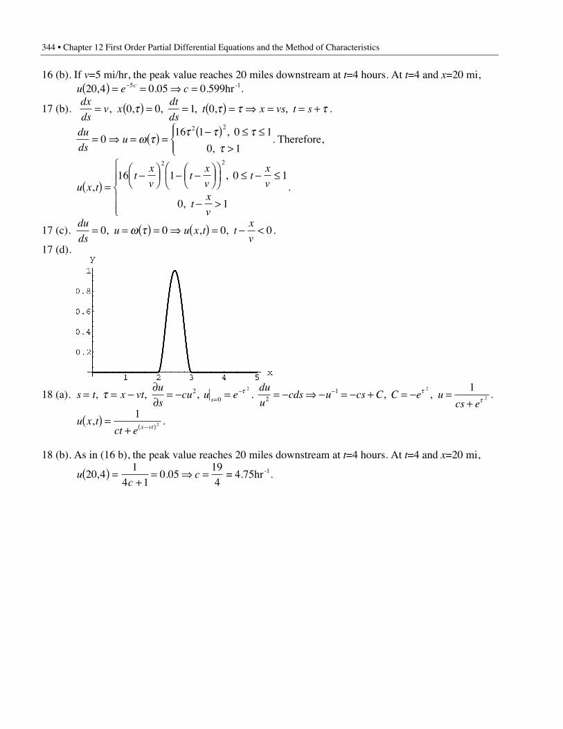
344 • Chapter 12 First Order Partial Differential Equations and the Method of Characteristics
16 (b). If v=5 mi/hr, the peak value reaches 20 miles downstream at t=4 hours. At t=4 and x=20 mi,u e cc20 4 0 05 0 5995, . .( ) = = fi =- hr-1.
17 (b). dx
dsv x
dt
dst x vs t s= ( ) = = ( ) = fi = = +, , , , , , 0 0 1 0t t t t .
du
dsu= fi = ( ) =
-( ) £ £>
ÏÌÔ
ÓÔ0
16 1 0 1
0 1
2 2
w t t t tt
,
, . Therefore,
u x tt
x
vt
x
vt
x
v
tx
v
,,
,
( ) =-Ê
ËÁˆ¯ - -Ê
ËÁˆ¯
ÊËÁ
ˆ¯
£ - £
- >
Ï
ÌÔÔ
ÓÔÔ
16 1 0 1
0 1
2 2
.
17 (c).du
dsu u x t t
x
v= = ( ) = fi ( ) = - <0 0 0 0, , , w t .
17 (d).
18 (a). s t x vtu
scu u es= = -
∂∂
= - ==-, , , t t2
0
2
. du
ucds u cs C C e u
cs e2
1 2
2
1= - fi - = - + = - =
+- , , t
t .
u x tct e x vt
,( ) =+ -( )
12 .
18 (b). As in (16 b), the peak value reaches 20 miles downstream at t=4 hours. At t=4 and x=20 mi,
uc
c20 41
4 10 05
194
, .( ) =+
= fi = = 4.75hr-1.
Chapter 13Linear Two-Point Boundary Value Problems
Section 13.1
Note: Part (a) of Exercises 1-7 are identical.
1 (a). y t ct
ct( ) = Ê
ËÁˆ¯ + Ê
ËÁˆ¯ +1 22 2
4cos sin
1 (b). Applying the boundary conditions, we have y c y c0 4 0 4 21 2( ) = + = p( ) = + =, . Solving thesesimultaneous equations yields c c1 24 2= - = - and . Thus there is a unique solution:
y tt t( ) = - Ê
ËÁˆ¯ - Ê
ËÁˆ¯ +4
22
24cos sin .
2 (b). ¢( ) = = ¢ p( ) = - =yc
yc
02
02
02 1, . c c1 2 0= = . Thus there is a unique solution: y t( ) = 4.
3 (b). Differentiation gives us ¢ = - ÊËÁ
ˆ¯ + Ê
ËÁˆ¯y
c t c t1 2
2 2 2 2sin cos . Applying the boundary conditions, we
have ¢( ) = = - p( ) = + =yc
y c02
2 4 022, . Solving these simultaneous equations yields
c c1 2 4 arbitrary and = - . Thus there are infinitely many solutions:
y t ct t( ) = Ê
ËÁˆ¯ - Ê
ËÁˆ¯ +1 2
42
4cos sin .
4 (b). y c yc
0 4 02
111( ) = + = ¢ p( ) = - =, . There is no solution.
5 (b). Differentiation gives us ¢ = - ÊËÁ
ˆ¯ + Ê
ËÁˆ¯y
c t c t1 2
2 2 2 2sin cos . Applying the boundary conditions, we
have y y c c y y c c0 2 0 4 0 2 4 01 2 2 1( ) + ¢( ) = + + = p( ) + ¢ p( ) = + - =, . Solving thesesimultaneous equations yields c c1 2 4= 0 and = - . Thus there is a unique solution:
y tt( ) = - Ê
ËÁˆ¯ +4
24sin .
6 (b). y y c c y y cc
0 2 0 4 0 2 4 22
01 2 21( ) + ¢( ) = + + = ( ) - ¢ p( ) = + - ( ) -
=, p . There are infinitely many
solutions: y ct
ct
= - +( ) +1 124
24cos sin .
7 (b). Differentiation gives us ¢ = - ÊËÁ
ˆ¯ + Ê
ËÁˆ¯y
c t c t1 2
2 2 2 2sin cos . Applying the boundary conditions, we
have y y c c y y c c0 2 0 4 4 2 4 01 2 2 1( ) + ¢( ) = + + = p( ) - ¢ p( ) = + + =, . These simultaneousequations cannot be solved, and so there are no solutions.
8. ¢¢ - = ( ) = ( ) =y y y y4 0 0 0 2 1, , . g a b= - = =4 0 1, , .9. Differentiation gives us ¢ = ¢¢ =y y2 0, . Thus g a b= = =0 2 1, , .
346 • Chapter 13 Linear Two-Point Boundary Value Problems
10. ¢¢ + = - + +( ) = ( ) =pÊ
ËÁˆ¯ = +
py y e t e t e y y et t tg gsin sin , , 2 0 1
212 . g a b= = = +
p1 1 1 2, , e .
11. The general solution is y c t c t= + +1 2 1cos sin . Differentiation gives us ¢ = - +y c t c t1 2sin cos .From the boundary conditions,
y a y c a c y y c c0 0 5 12 2
11 1 1 2 2 1( ) + ¢( ) = = + +pÊ
ËÁˆ¯ + ¢
pÊËÁ
ˆ¯ = = + -, b . From the graph, we can see
that y y0 12
3( ) =pÊ
ËÁˆ¯ =, , and so c c c c1 1 2 21 1 0 1 3 2+ = fi = + = fi =, . Finally,
0 2 4 2 0 2 1 31 1+ ◊ = fi = + = - fi =a a and b b .14 (a). t z tz z z z z z2 2 2 0 1 1 0 2 2 0¢¢ - ¢ + = ( ) + ¢( ) = ( ) - ¢( ) =, , 14 (b). z c t c t z c c t= + ¢ = +1 2
21 22, . c c c c c c c c1 2 1 2 1 2 1 22 0 2 4 4 0+[ ] + +[ ] = +[ ] - +[ ] =, .
c c z1 2 0 0= = =, .14 (c). The given problem has a unique solution.
14 (d). y c t c t y c c t= + ¢ = +1 22
1 22, . 2 3
1 0
9
31
2
È
ÎÍ
˘
˚˙
È
ÎÍ
˘
˚˙ =
È
ÎÍ
˘
˚˙
c
c. y t t= +3 2.
15 (a). t z tz z z z z z2 2 2 0 2 1 1 0 2 2 0¢¢ - ¢ + = ( ) - ¢( ) = ( ) - ¢( ) =, , 15 (b). z c t c t z c c t= + ¢ = +1 2
21 22, . Applying the boundary conditions gives us
2 2 0 2 4 4 01 2 1 2 1 2 1 2c c c c c c c c+[ ] - +[ ] = +[ ] - +[ ] =, . Solving these simultaneous equations
gives us z c t c= 22
2, arbitrary.15 (c). By the Fredholm Alternative Theorem, the given problem does not have a unique solution.15 (e). y c t c t y c c t= + ¢ = +1 2
21 22, . Applying the boundary conditions gives us
2 1 1 1 2 2 11 1y y c y y c( ) - ¢( ) = = ( ) - ¢( ) = =, . Solving these simultaneous equations gives usy t c t c= + 2
22, arbitrary.
16 (a). t z tz z z z z z2 2 2 0 3 1 2 1 0 5 2 6 2 0¢¢ - ¢ + = ( ) - ¢( ) = ( ) - ¢( ) =, , 16 (b). z c t c t z c c t= + ¢ = +1 2
21 22, . 3 2 2 0 5 2 4 6 4 01 2 1 2 1 2 1 2c c c c c c c c+[ ] - +[ ] = +[ ] - +[ ] =, . c c1 2= .
16 (c). By the Fredholm Alternative Theorem, the given problem does not have a unique solution.16 (e). y c t c t y c c t= + ¢ = +1 2
21 22, . 3 1 2 1 2 5 2 6 2 4 4 31 2 1 2y y c c y y c c( ) - ¢( ) = - = ( ) - ¢( ) = - =, . There
is no solution.17 (a). t z tz z z z z z2 2 2 0 1 2 1 0 2 2 2 0¢¢ - ¢ + = ( ) - ¢( ) = ( ) - ¢( ) =, , 17 (b). z c t c t z c c t= + ¢ = +1 2
21 22, . Applying the boundary conditions gives us
c c c c c c c c1 2 1 2 1 2 1 22 2 0 2 2 4 4 0+[ ] - +[ ] = +[ ] - +[ ] =, . Solving these simultaneous equationsgives us z c c= = =0 01 2, .
17 (c). By the Fredholm Alternative Theorem, the given problem has a unique solution.
17 (d). y c t c t y c c t= + ¢ = +1 22
1 22, . Applying the boundary conditions gives us - -È
ÎÍ
˘
˚˙
È
ÎÍ
˘
˚˙ =
-È
ÎÍ
˘
˚˙
1 3
3 4
5
71
2
c
c.
Solving this equation gives us y t t= +15
85
2.
18 (a). t z tz z z z z z2 2 2 0 1 1 0 2 2 2 0¢¢ - ¢ + = ( ) - ¢( ) = ( ) - ¢( ) =, , 18 (b). z c t c t z c c t= + ¢ = +1 2
21 22, . c c c c c c c c1 2 1 2 1 2 1 22 0 2 4 2 4 0+[ ] - +[ ] = +[ ] - +[ ] =, . c c2 10= ,
arbitrary.18 (c). By the Fredholm Alternative Theorem, the given problem does not have a unique solution.18 (e). y c t c t y c c t= + ¢ = +1 2
21 22, . y y c y y c1 1 1 2 2 2 4 42 2( ) - ¢( ) = - = ( ) - ¢( ) = - =, . y c t t c= -1
21,
arbitrary.
Chapter 13 Linear Two-Point Boundary Value Problems • 347
19 (a). t z tz z z z z z2 2 2 0 4 1 3 1 0 3 2 4 2 0¢¢ - ¢ + = ( ) - ¢( ) = ( ) - ¢( ) =, , 19 (b). z c t c t z c c t= + ¢ = +1 2
21 22, . Applying the boundary conditions gives us
4 3 2 0 3 2 4 4 4 01 2 1 2 1 2 1 2c c c c c c c c+[ ] - +[ ] = +[ ] - +[ ] =, . Solving these simultaneous equations
gives us z c t t c= +( )22
22 , arbitrary.
19 (c). By the Fredholm Alternative Theorem, the given problem does not have a unique solution.19 (e). y c t c t y c c t= + ¢ = +1 2
21 22, . Applying the boundary conditions gives us
4 1 3 1 2 1 3 2 4 2 2 4 31 2 1 2y y c c y y c c( ) - ¢( ) = - = ( ) - ¢( ) = - =, . These simultaneous equationscannot be solved, and thus there is no solution.
20 (a). Both Theorems guarantee a unique solution.
20 (b). c c c c y e et t1 2 1 24 7
12
2 4 7 2 4+ + = + + = fi = + +-, .
21 (a). Since a a0 1 0> , Theorem 13.2 is not applicable. Likewise, the form of the boundary conditionsmakes Theorem 13.3 not applicable.
21 (c). ¢¢ - = ( ) + ¢( ) = ( ) + ¢( ) =z z z z z z0 0 0 0 2 2 0, , ln ln . Thus z c e c e z c e c et t t t= + ¢ = - +- -1 2 1 2, . From
the boundary conditions, we have c c c c1 2 1 2 0+ - + = and 12
212
2 01 2 1 2c c c c+ - + = . Solving
these simultaneous equations yields c c2 10= , arbitrary. Therefore, there is no unique solutionto the given problem.
21 (e). y c e c e y c e c et t t t= + + ¢ = - +- -1 2 1 24, . From the boundary conditions, we have
c c c c1 2 1 24 5+ + - + = and 12
2 412
2 81 2 1 2c c c c+ + - + = . There is no solution to these
simultaneous equations, and so the problem has no solution.22 (a). Theorem 13.2 guarantees a unique solution.
22 (b). c c c c c c c c y e et t1 2 1 2 1 2 1 24 0
12
2 412
2 12 2 2 4+ + + - = + + - + = fi = - + +-, .
23 (a). Theorem 13.2 guarantees a unique solution.23 (b). y c e c e y c e c et t t t= + + ¢ = - +- -
1 2 1 24, . From the boundary conditions, we have c c1 2 4 11+ + =
and - + =12
2 41 2c c . Solving these simultaneous equations yields c c1 24 3= =, , and so
y t e et t( ) = + +-4 3 4 .24 (a). Since q t( ) > 0, neither theorem can guarantee a unique solution.24 (c). ¢¢ + = ( ) + ¢( ) = p( ) + ¢ p( ) =z z z z z z0 0 0 0 0, , . z c t c t z c t c t= + ¢ = - +1 2 1 2cos sin , sin cos .
c c1 2 0+ = . - - =c c1 2 0 . c c c1 2 2= - , arbitrary. There is no unique solution to the givenproblem.
24 (e). y c t c t y c t c t= + + ¢ = - +1 2 1 22cos sin , sin cos . c c c c1 2 1 22 7 2 3+ + = - + - = -, .y c t c t= -( ) + +5 22 2cos sin .
25 (a). Since q t( ) > 0, neither theorem can guarantee a unique solution.25 (c). ¢¢ + = ( ) + ¢( ) = p( ) + ¢ p( ) =z z z z z z0 0 0 0 0, , . Thus z c t c t z c t c t= + ¢ = - +1 2 1 2cos sin , sin cos .
From the boundary conditions, we have c c1 2 0+ = and - - =c c1 2 0 . Solving thesesimultaneous equations yields c c c1 2 2= - , arbitrary. Therefore, there is no unique solution tothe given problem.
25 (e). y c t c t y c t c t= + + ¢ = - +1 2 1 22cos sin , sin cos . From the boundary conditions, we havec c c c1 2 1 22 7 2 3+ + = - + - =, . There is no solution to these simultaneous equations, and sothe problem has no solution.
26 (a). Since q t( ) > 0, neither theorem can guarantee a unique solution.
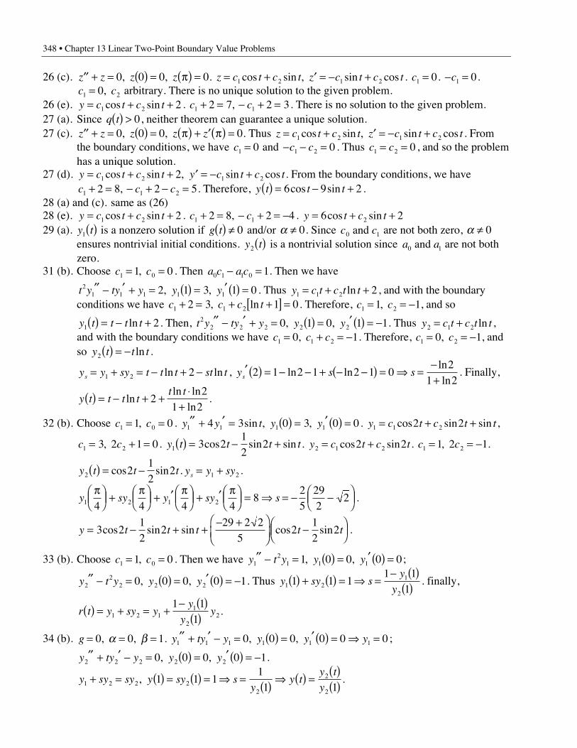
348 • Chapter 13 Linear Two-Point Boundary Value Problems
26 (c). ¢¢ + = ( ) = p( ) =z z z z0 0 0 0, , . z c t c t z c t c t= + ¢ = - +1 2 1 2cos sin , sin cos . c1 0= . - =c1 0.c c1 20= , arbitrary. There is no unique solution to the given problem.
26 (e). y c t c t= + +1 2 2cos sin . c c1 12 7 2 3+ = - + =, . There is no solution to the given problem.27 (a). Since q t( ) > 0, neither theorem can guarantee a unique solution.27 (c). ¢¢ + = ( ) = p( ) + ¢ p( ) =z z z z z0 0 0 0, , . Thus z c t c t z c t c t= + ¢ = - +1 2 1 2cos sin , sin cos . From
the boundary conditions, we have c1 0= and - - =c c1 2 0 . Thus c c1 2 0= = , and so the problemhas a unique solution.
27 (d). y c t c t y c t c t= + + ¢ = - +1 2 1 22cos sin , sin cos . From the boundary conditions, we havec c c1 1 22 8 2 5+ = - + - =, . Therefore, y t t t( ) = - +6 9 2cos sin .
28 (a) and (c). same as (26)28 (e). y c t c t= + +1 2 2cos sin . c c1 12 8 2 4+ = - + = -, . y t c t= + +6 22cos sin29 (a). y t1( ) is a nonzero solution if g t( ) π 0 and/or a π 0. Since c c0 1 and are not both zero, a π 0
ensures nontrivial initial conditions. y t2 ( ) is a nontrivial solution since a a0 1 and are not bothzero.
31 (b). Choose c c1 01 0= =, . Then a c a c0 1 1 0 1- = . Then we have
t y ty y y y21 1 1 1 12 1 3 1 0¢¢ - ¢ + = ( ) = ¢ ( ) =, , . Thus y c t c t t1 1 2 2= + +ln , and with the boundary
conditions we have c c c t1 1 22 3 1 0+ = + +[ ] =, ln . Therefore, c c1 21 1= = -, , and so
y t t t t1 2( ) = - +ln . Then, t y ty y y y22 2 2 2 20 1 0 1 1¢¢ - ¢ + = ( ) = ¢ ( ) = -, , . Thus y c t c t t2 1 2= + ln ,
and with the boundary conditions we have c c c1 1 20 1= + = -, . Therefore, c c1 20 1= = -, , andso y t t t2 ( ) = - ln .
y y sy t t t st ts = + = - + -1 2 2ln ln , y s ss¢ ( ) = - - + - -( ) = fi =
-+
2 1 2 1 2 1 02
1 2ln ln
lnln
. Finally,
y t t t tt t( ) = - + +
◊+
lnln ln
ln2
21 2
.
32 (b). Choose c c1 01 0= =, . y y t y y1 1 1 14 3 0 3 0 0¢¢ + ¢ = ( ) = ¢ ( ) =sin , , . y c t c t t1 1 22 2= + +cos sin sin ,
c c1 23 2 1 0= + =, . y t t t t1 3 212
2( ) = - +cos sin sin . y c t c t2 1 22 2= +cos sin . c c1 21 2 1= = -, .
y t t t2 212
2( ) = -cos sin . y y sys = +1 2 .
y sy y sy s1 2 1 24 4 4 48
25
292
2pÊ
ËÁˆ¯ +
pÊËÁ
ˆ¯ + ¢ pÊ
ËÁˆ¯ + ¢ pÊ
ËÁˆ¯ = fi = - -Ê
ËÁˆ¯ .
y t t t t t= - + +- +Ê
ËÁˆ¯
-ÊËÁ
ˆ¯3 2
12
229 2 2
52
12
2cos sin sin cos sin .
33 (b). Choose c c1 01 0= =, . Then we have y t y y y12
1 1 11 0 0 0 0¢¢ - = ( ) = ¢ ( ) =, , ;
y t y y y22
2 2 20 0 0 0 1¢¢ - = ( ) = ¢ ( ) = -, , . Thus y sy sy
y1 21
2
1 1 11 1
1( ) + ( ) = fi =
- ( )( ) . finally,
r t y sy yy
yy( ) = + = +
- ( )( )1 2 11
22
1 11
.
34 (b). g = = =0 0 1, , .a b y ty y y y y1 1 1 1 1 10 0 0 0 0 0¢¢ + ¢ - = ( ) = ¢ ( ) = fi =, , ;
y ty y y y2 2 2 2 20 0 0 0 1¢¢ + ¢ - = ( ) = ¢ ( ) = -, , .
y sy sy y sy sy
y ty t
y1 2 2 22
2
2
1 1 111 1
+ = ( ) = ( ) = fi = ( ) fi ( ) =( )( ), .
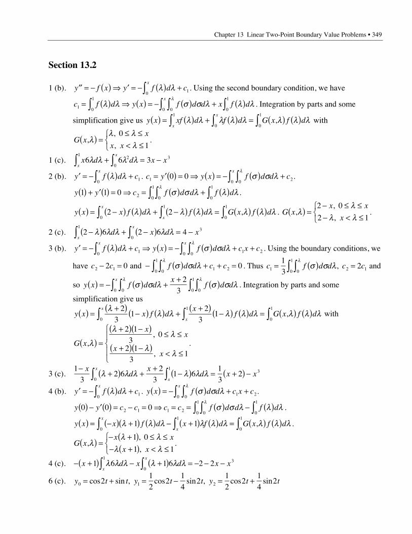
Chapter 13 Linear Two-Point Boundary Value Problems • 349
Section 13.2
1 (b). ¢¢ = - ( ) fi ¢ = - ( ) +Úy f x y f d cx
l l0 1. Using the second boundary condition, we have
c f d y x f d d x f dx
1 00 0
1
0
1= ( ) fi ( ) = - ( ) + ( )ÚÚ ÚÚ l l s s l l l
l. Integration by parts and some
simplification give us y x xf d f d G x f dx
x( ) = ( ) + ( ) = ( ) ( )Ú Ú Úl l l l l l l l1
0 0
1, with
G xx
x x,
,
, l
l ll
( ) =£ £< £
ÏÌÓ
0
1.
1 (c). x d d x xx
x6 6 3
12
0
3l l l lÚ Ú+ = -
2 (b). ¢ = - ( ) +Úy f d cx
l l0 1. c y y x f d d c
x
1 00 20 0= ¢( ) = fi ( ) = - ( ) +ÚÚ s s ll
.
y y c f d d f d1 1 0 2 00
1
0
1( ) + ¢( ) = fi = ( ) + ( )ÚÚ Ús s l l ll
.
y x x f d f d G x f dx
x( ) = -( ) ( ) + -( ) ( ) = ( ) ( )Ú Ú Ú2 2
0
1
0
1l l l l l l l l, . G x
x x
x,
,
, l
ll l
( ) =- £ £- < £
ÏÌÓ
2 0
2 1.
2 (c). 2 6 2 6 41
0
3-( ) + -( ) = -Ú Úl l l l ld x d xx
x
3 (b). ¢ = - ( ) + fi ( ) = - ( ) + +Ú ÚÚy f d c y x f d d c x cx x
l l s s ll
0 1 00 1 2 . Using the boundary conditions, we
have c c f d d c c2 1 00
1
1 22 0 0- = - ( ) + + =ÚÚ and s s ll
. Thus c f d d c c1 00
1
2 1
13
2= ( ) =ÚÚ s s ll
, and
so y x f d dx
f d dx( ) = - ( ) +
+ ( )ÚÚ ÚÚs s l s s ll l
00 00
123
. Integration by parts and some
simplification give us
y x x f dx
f d G x f dx
x( ) =
+( )-( ) ( ) +
+( )-( ) ( ) = ( ) ( )Ú Ú Ú
l l l l l l l l l23
12
31
0
1
0
1, with
G x
xx
xx
,,
, l
l l
l l( ) =
+( ) -( )£ £
+( ) -( )< £
Ï
ÌÔ
ÓÔ
2 13
0
2 13
1.
3 (c).1
32 6
23
1 613
20
13-
+( ) ++
-( ) = +( ) -Ú Úx
dx
d x xx
xl l l l l l
4 (b). ¢ = - ( ) +Úy f d cx
l l0 1. y x f d d c x c
x( ) = - ( ) + +ÚÚ s s ll
00 1 2.
y y c c c c f d d f d0 0 02 1 1 2 00
1
0
1( ) - ¢( ) = - = fi = = ( ) - ( )ÚÚ Ús s l l ll
.
y x x f d x f d G x f dx
x( ) = -( ) +( ) ( ) - +( ) ( ) = ( ) ( )Ú Ú Úl l l l l l l l l1 1
0
1
0
1, .
G xx x
x x,
,
, l
l ll l
( ) =- +( ) £ £- +( ) < £
ÏÌÓ
1 0
1 1.
4 (c). - +( ) - +( ) = - - -Ú Úx d x d x xx
x1 6 1 6 2 2
1
0
3l l l l l l
6 (c). y t t y t t y t t0 1 2212
214
212
214
2= + = - = +cos sin , cos sin , cos sin
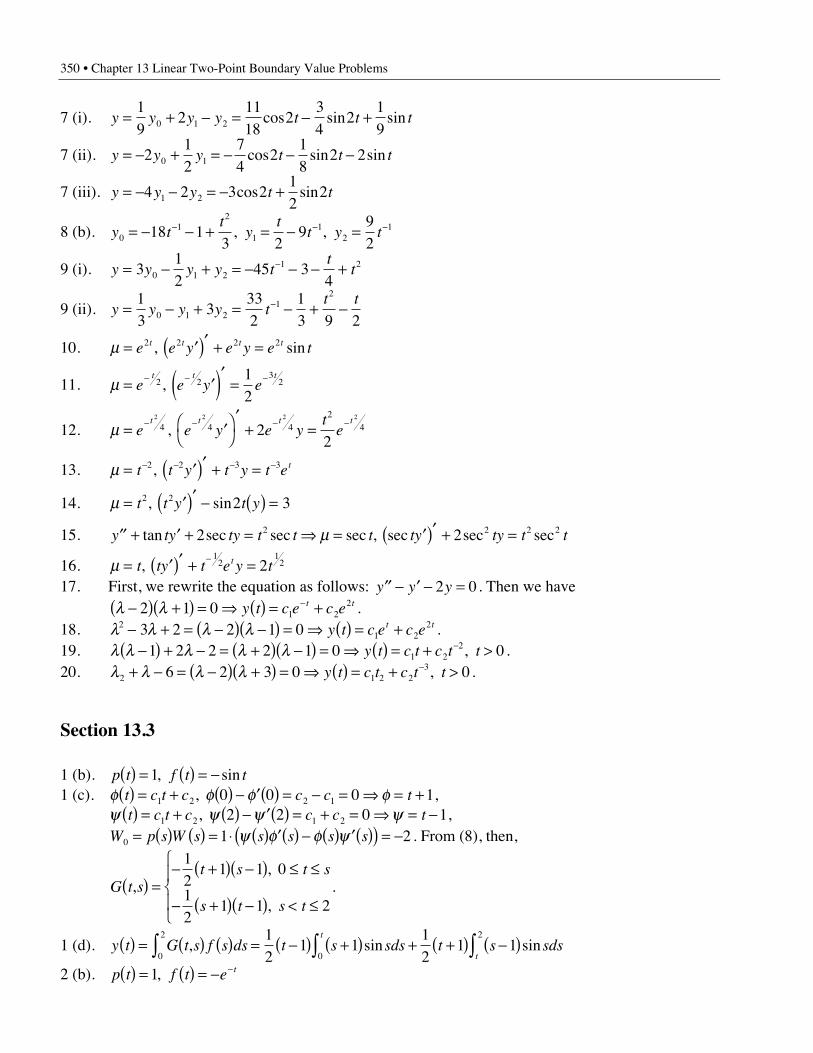
350 • Chapter 13 Linear Two-Point Boundary Value Problems
7 (i). y y y y t t t= + - = - +19
21118
234
2190 1 2 cos sin sin
7 (ii). y y y t t t= - + = - - -212
74
218
2 20 1 cos sin sin
7 (iii). y y y t t= - - = - +4 2 3 212
21 2 cos sin
8 (b). y tt
yt
t y t01
2
11
2118 1
3 29
92
= - - + = - =- - -, ,
9 (i). y y y y tt
t= - + = - - - +-312
45 340 1 2
1 2
9 (ii). y y y y tt t
= - + = - + --13
3332
13 9 20 1 2
12
10. m = ¢( )¢ + =e e y e y e tt t t t2 2 2 2, sin
11. m = ¢( )¢=- - -
e e y et t t2 2
32
12
,
12. m = ¢ÊË
ˆ¯
¢+ =- - - -
e e y e yt
et t t t2 2 2 2
4 4 42
422
,
13. m = ¢( )¢ + =- - - -t t y t y t et2 2 3 3,
14. m = ¢( )¢ - ( ) =t t y t y2 2 2 3, sin
15. ¢¢ + ¢ + = fi = ¢( )¢ + =y ty ty t t t ty ty t ttan sec sec sec , sec sec sec2 22 2 2 2m
16. m = ¢( )¢ + =-t ty t e y tt,
12
122
17. First, we rewrite the equation as follows: ¢¢ - ¢ - =y y y2 0. Then we havel l-( ) +( ) = fi ( ) = +-2 1 0 1 2
2y t c e c et t .18. l l l l2
1 223 2 2 1 0- + = -( ) -( ) = fi ( ) = +y t c e c et t .
19. l l l l l-( ) + - = +( ) -( ) = fi ( ) = + >-1 2 2 2 1 0 01 22y t c t c t t, .
20. l l l l2 1 2 236 2 3 0 0+ - = -( ) +( ) = fi ( ) = + >-y t c t c t t, .
Section 13.3
1 (b). p t f t t( ) = ( ) = -1, sin1 (c). f f f ft c t c c c t( ) = + ( ) - ¢( ) = - = fi = +1 2 2 10 0 0 1, ,
y y y yt c t c c c t( ) = + ( ) - ¢( ) = + = fi = -1 2 1 22 2 0 1, ,W p s W s s s s s0 1 2= ( ) ( ) = ◊ ( ) ¢( ) - ( ) ¢( )( ) = -y f f y . From (8), then,
G t st s t s
s t s t,
,
, ( ) =
- +( ) -( ) £ £
- +( ) -( ) < £
Ï
ÌÔ
ÓÔ
12
1 1 0
12
1 1 2.
1 (d). y t G t s f s ds t s sds t s sdst
t( ) = ( ) ( ) = -( ) +( ) + +( ) -( )Ú Ú Ú, sin sin
0
2
0
212
1 112
1 1
2 (b). p t f t e t( ) = ( ) = - -1,
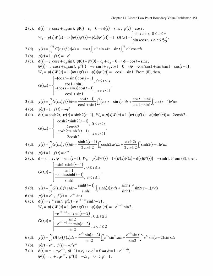
Chapter 13 Linear Two-Point Boundary Value Problems • 351
2 (c). f f ft c t c t c t t( ) = + ( ) = = fi ( ) =1 2 10 0cos sin , sin , y t t( ) = cos ,
W p s W s s s s s0 1 1= ( ) ( ) = ◊ ( ) ¢( ) - ( ) ¢( )( ) =y f f y . G t st s t s
s t s t,
sin cos ,
sin cos , ( ) =
£ £< £ p
ÏÌÓ
0
2.
2 (d). y t G t s f s ds t e sds t e sdsst
s
t( ) = ( ) ( ) = - -
p- -
p
Ú Ú Ú, cos sin sin cos0
2
0
2
3 (b). p t f t et( ) = ( ) = -1, 3 (c). f f f ft c t c t c c t t( ) = + ( ) + ¢( ) = + = fi = -1 2 1 20 0 0cos sin , cos sin ,
y y yt c t c t c c t t t( ) = + ¢( ) = - + = fi = + = -( )1 2 1 21 1 1 0 1 1 1cos sin , sin cos cos cos sin sin cos ,W p s W s s s s s0 1 1 1= ( ) ( ) = ◊ ( ) ¢( ) - ( ) ¢( )( ) = - -y f f y cos sin . From (8), then,
G t s
t t st s
s s ts t
,
cos sin coscos sin
,
cos sin coscos sin
, ( ) =
- -( ) -( )+
£ £
- -( ) -( )+
< £
Ï
ÌÔ
ÓÔ
11 1
0
11 1
1.
3 (d). y t G t s f s dst
s s e dst t
s e dsst
s
t( ) = ( ) ( ) =
-( )+
-( ) +-+
-( )Ú Ú Ú,cos
cos sincos sin
cos sincos sin
cos0
1
0
111 1 1 1
1
4 (b). p t f t et( ) = ( ) = -1, 4 (c). f t t( ) = cosh ,2 y t t( ) = -( )sinh2 1 , W p s W s s s s s0 1 2 2= ( ) ( ) = ◊ ( ) ¢( ) - ( ) ¢( )( ) = -y f f y cosh .
G t s
t st s
s ts t
,
cosh sinhcosh
,
cosh sinhcosh
, ( ) =
--( )
£ £
--( )
< £
Ï
ÌÔ
ÓÔ
2 2 12 2
0
2 2 12 2
1.
4 (d). y t G t s f s dst
se dst
s e dsst
s
t( ) = ( ) ( ) =
-( )+ -( )Ú Ú Ú,
sinhcosh
coshcoshcosh
sinh0
1
0
12 12 2
22
2 22 1
5 (b). p t f t e t( ) = ( ) = -12
, 5 (c). f = sinh t , y = -( )sinh t 1 , W p s W s s s s s0 1 1= ( ) ( ) = ◊ ( ) ¢( ) - ( ) ¢( )( ) = -y f f y sinh . From (8), then,
G t s
t st s
s ts t
,
sinh sinhsinh
,
sinh sinhsinh
, ( ) =
- -( )£ £
- -( )< £
Ï
ÌÔ
ÓÔ
11
0
11
1.
5 (d). y t G t s f s dst
s s dst
s s dst
t( ) = ( ) ( ) =
-( ) ( ) + -( )Ú Ú Ú,sinh
sinhsinh
sinhsinh
sinh0
12
0
211
1 11
6 (b). p t e f t e tt t( ) = ( ) = -4 4, sin6 (c). f t e tt( ) = -2 sin , y t e tt( ) = -( )- -( )2 2 2sin ,
W p s W s s s s s e t s0
2 21 2= ( ) ( ) = ◊ ( ) ¢( ) - ( ) ¢( )( ) = - +y f f y sin .
G t s
e t st s
e s ts t
t s
t s,
sin sinsin
,
sin sinsin
, ( ) =
- -( )£ £
- -( )< £
Ï
ÌÔÔ
ÓÔÔ
- +( )
- +( )
2
2
22
0
22
2.
6 (d). y t G t s f s dse t
e sdse t
e s sdst
st t
s
t( ) = ( ) ( ) =
-( )+ -( )Ú Ú Ú
- -
,sinsin
sinsin
sinsin sin
0
2 22 2
0
22
222 2
2
7 (b). p t e f t t et t( ) = ( ) = -2 3 2, 7 (c). f f ft c c e c c e et t( ) = + -( ) = + = fi = -- - +( )
1 22
1 22 2 11 0 1, ,
y y yt c c e ct( ) = + ¢( ) = - = fi =-1 2
221 2 0 1, ,
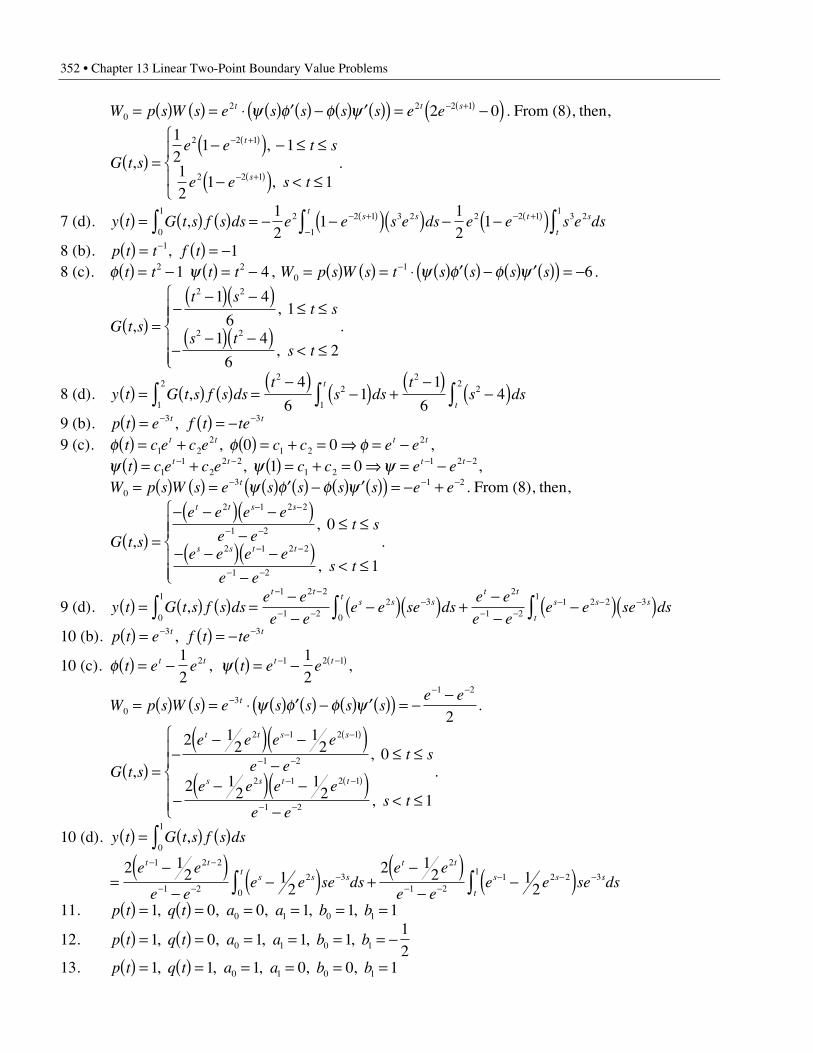
352 • Chapter 13 Linear Two-Point Boundary Value Problems
W p s W s e s s s s e et t s0
2 2 2 12 0= ( ) ( ) = ◊ ( ) ¢( ) - ( ) ¢( )( ) = -( )- +( )y f f y . From (8), then,
G t se e t s
e e s t
t
s,
,
, ( ) =
-( ) - £ £
-( ) < £
Ï
ÌÔ
ÓÔ
- +( )
- +( )
12
1 1
12
1 1
2 2 1
2 2 1.
7 (d). y t G t s f s ds e e s e ds e e s e dss st
t s
t( ) = ( ) ( ) = - -( )( ) - -( )Ú Ú Ú- +( )
-
- +( ),0
12 2 1 3 2
1
2 2 1 3 211
21
12
1
8 (b). p t t f t( ) = ( ) = --1 1, 8 (c). f t t( ) = -2 1 y t t( ) = -2 4 , W p s W s t s s s s0
1 6= ( ) ( ) = ◊ ( ) ¢( ) - ( ) ¢( )( ) = -- y f f y .
G t s
t st s
s ts t
,,
,
( ) =-
-( ) -( )£ £
--( ) -( )
< £
Ï
ÌÔÔ
ÓÔÔ
2 2
2 2
1 4
61
1 4
62
.
8 (d). y t G t s f s dst
s dst
s dst
t( ) = ( ) ( ) =
-( )-( ) +
-( )-( )Ú Ú Ú,
1
22
2
1
22
24
61
1
64
9 (b). p t e f t tet t( ) = ( ) = -- -3 3, 9 (c). f f ft c e c e c c e et t t t( ) = + ( ) = + = fi = -1 2
21 2
20 0, ,y y yt c e c e c c e et t t t( ) = + ( ) = + = fi = -- - - -
11
22 2
1 21 2 21 0, ,
W p s W s e s s s s e et0
3 1 2= ( ) ( ) = ( ) ¢( ) - ( ) ¢( )( ) = - +- - -y f f y . From (8), then,
G t s
e e e e
e et s
e e e e
e es t
t t s s
s s t t,,
,
( ) =
- -( ) -( )-
£ £
- -( ) -( )-
< £
Ï
ÌÔÔ
ÓÔÔ
- -
- -
- -
- -
2 1 2 2
1 2
2 1 2 2
1 2
0
1
.
9 (d). y t G t s f s dse e
e ee e se ds
e e
e ee e se ds
t ts s s
t t ts s s
t( ) = ( ) ( ) =
--
-( )( ) +--
-( )( )Ú Ú Ú- -
- --
- -- - -,
0
1 1 2 2
1 22 3
0
2
1 21 2 2 3
1
10 (b). p t e f t tet t( ) = ( ) = -- -3 3,
10 (c). f t e et t( ) = -12
2 , y t e et t( ) = -- -( )1 2 112
,
W p s W s e s s s se et
03
1 2
2= ( ) ( ) = ◊ ( ) ¢( ) - ( ) ¢( )( ) = -
--- -
y f f y .
G t s
e e e e
e et s
e e e e
e es t
t t s s
s s t t,
,
,
( ) =-
-( ) -( )-
£ £
--( ) -( )
-< £
Ï
ÌÔÔ
ÓÔÔ
- -( )
- -
- -( )
- -
2 12
12 0
2 12
12 1
2 1 2 1
1 2
2 1 2 1
1 2
.
10 (d). y t G t s f s ds( ) = ( ) ( )Ú ,0
1
=-( )
--( ) +
-( )-
-( )- -
- --
- -- - -Ú Ú
2 12 1
22 1
2 12
1 2 2
1 22 3
0
2
1 21 2 2 3
1e e
e ee e se ds
e e
e ee e se ds
t t
s s st
t t
s s s
t
11. p t q t a a b b( ) = ( ) = = = = =1 0 0 1 1 10 1 0 1, , , , ,
12. p t q t a a b b( ) = ( ) = = = = = -1 0 1 1 1120 1 0 1, , , , ,
13. p t q t a a b b( ) = ( ) = = = = =1 1 1 0 0 10 1 0 1, , , , ,
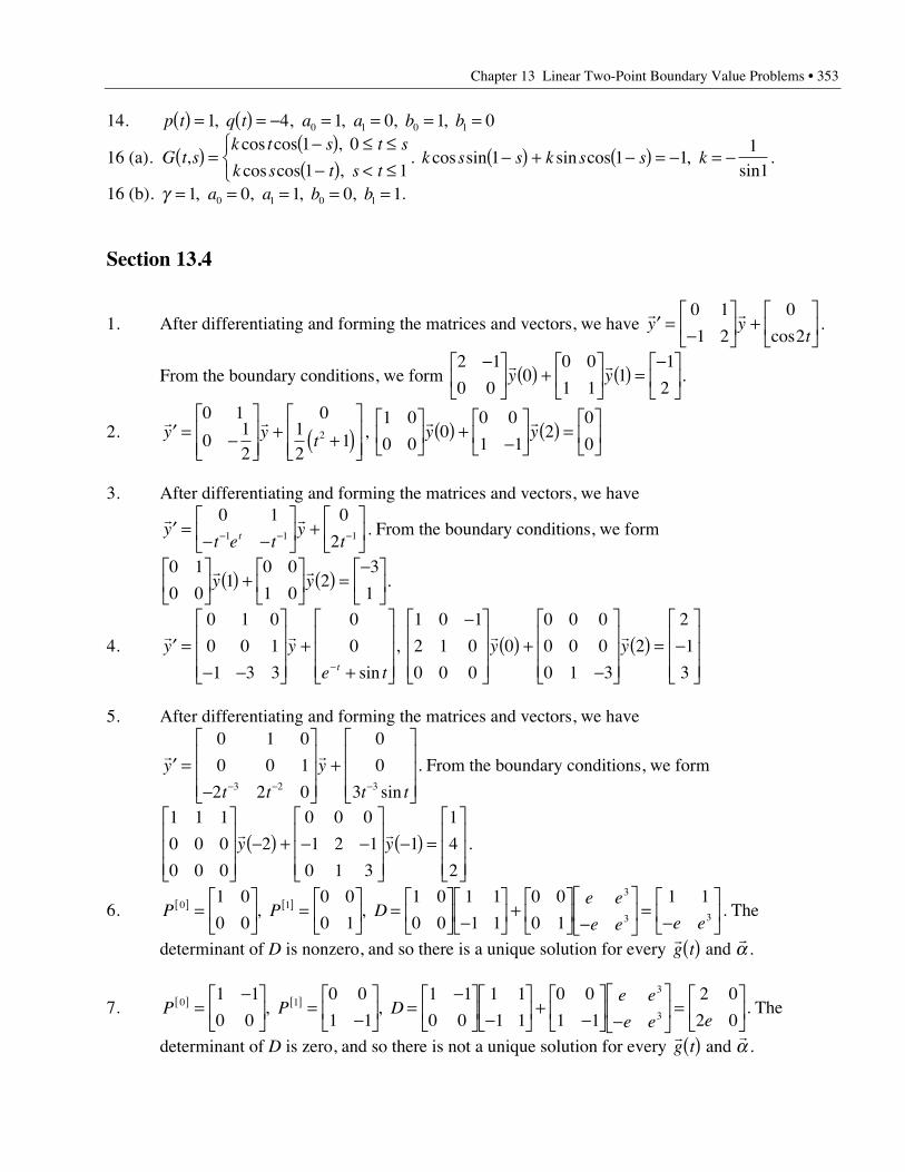
Chapter 13 Linear Two-Point Boundary Value Problems • 353
14. p t q t a a b b( ) = ( ) = - = = = =1 4 1 0 1 00 1 0 1, , , , ,
16 (a). G t sk t s t s
k s t s t,
cos cos ,
cos cos , ( ) =
-( ) £ £-( ) < £
ÏÌÓ
1 0
1 1. k s s k s s kcos sin sin cos ,
sin1 1 1
11
-( ) + -( ) = - = - .
16 (b). g = = = = =1 0 1 0 10 1 0 1, , , , a a b b .
Section 13.4
1. After differentiating and forming the matrices and vectors, we have ¢ =-
È
ÎÍ
˘
˚˙ +
È
ÎÍ
˘
˚˙
r ry y
t
0 1
1 2
0
2cos.
From the boundary conditions, we form 2 1
0 00
0 0
1 11
1
2
-È
ÎÍ
˘
˚˙ ( ) +
È
ÎÍ
˘
˚˙ ( ) =
-È
ÎÍ
˘
˚˙
r ry y .
2. ¢ = -È
ÎÍÍ
˘
˚˙˙
+ +( )È
ÎÍÍ
˘
˚˙˙
r ry y t
0 1
012
012
12 , 1 0
0 00
0 0
1 12
0
0
È
ÎÍ
˘
˚˙ ( ) +
-È
ÎÍ
˘
˚˙ ( ) =
È
ÎÍ
˘
˚˙
r ry y
3. After differentiating and forming the matrices and vectors, we have
¢ =- -
È
ÎÍ
˘
˚˙ +
È
ÎÍ
˘
˚˙- - -
r ry
t e ty
tt
0 1 0
21 1 1 . From the boundary conditions, we form
0 1
0 01
0 0
1 02
3
1
È
ÎÍ
˘
˚˙ ( ) +
È
ÎÍ
˘
˚˙ ( ) =
-È
ÎÍ
˘
˚˙
r ry y .
4. ¢ =- -
È
Î
ÍÍÍ
˘
˚
˙˙˙
++
È
Î
ÍÍÍ
˘
˚
˙˙˙-
r ry y
e tt
0 1 0
0 0 1
1 3 3
0
0
sin
,
1 0 1
2 1 0
0 0 0
0
0 0 0
0 0 0
0 1 3
2
2
1
3
-È
Î
ÍÍÍ
˘
˚
˙˙˙
( ) +-
È
Î
ÍÍÍ
˘
˚
˙˙˙
( ) = -È
Î
ÍÍÍ
˘
˚
˙˙˙
r ry y
5. After differentiating and forming the matrices and vectors, we have
¢ =-
È
Î
ÍÍÍ
˘
˚
˙˙˙
+È
Î
ÍÍÍ
˘
˚
˙˙˙- - -
r ry
t t
y
t t
0 1 0
0 0 1
2 2 0
0
0
33 2 3 sin
. From the boundary conditions, we form
1 1 1
0 0 0
0 0 0
2
0 0 0
1 2 1
0 1 3
1
1
4
2
È
Î
ÍÍÍ
˘
˚
˙˙˙
-( ) + - -È
Î
ÍÍÍ
˘
˚
˙˙˙
-( ) =È
Î
ÍÍÍ
˘
˚
˙˙˙
r ry y .
6. P P De e
e e e e0 1
3
3 3
1 0
0 0
0 0
0 1
1 0
0 0
1 1
1 1
0 0
0 1
1 1[ ] [ ]=È
ÎÍ
˘
˚˙ =
È
ÎÍ
˘
˚˙ =
È
ÎÍ
˘
˚˙ -
È
ÎÍ
˘
˚˙ +
È
ÎÍ
˘
˚˙ -
È
ÎÍ
˘
˚˙ =
-È
ÎÍ
˘
˚˙, , . The
determinant of D is nonzero, and so there is a unique solution for every r rg t( ) and a .
7. P P De e
e e e0 1
3
3
1 1
0 0
0 0
1 1
1 1
0 0
1 1
1 1
0 0
1 1
2 0
2 0[ ] [ ]=
-È
ÎÍ
˘
˚˙ =
-È
ÎÍ
˘
˚˙ =
-È
ÎÍ
˘
˚˙ -
È
ÎÍ
˘
˚˙ +
-È
ÎÍ
˘
˚˙ -
È
ÎÍ
˘
˚˙ =
È
ÎÍ
˘
˚˙, , . The
determinant of D is zero, and so there is not a unique solution for every r rg t( ) and a .
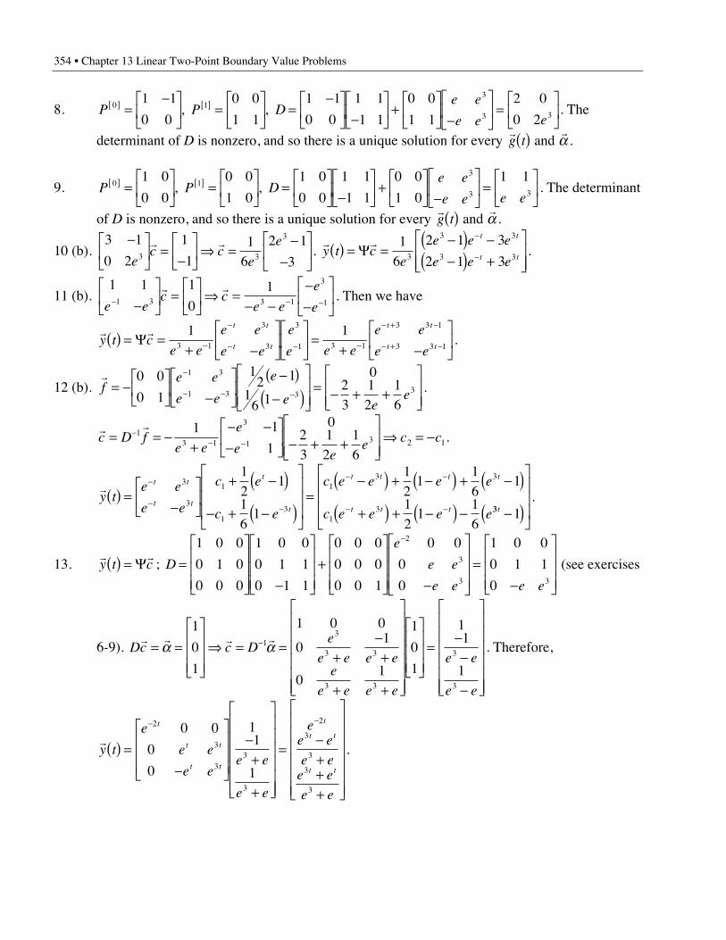
354 • Chapter 13 Linear Two-Point Boundary Value Problems
8. P P De e
e e e0 1
3
3 3
1 1
0 0
0 0
1 1
1 1
0 0
1 1
1 1
0 0
1 1
2 0
0 2[ ] [ ]=
-È
ÎÍ
˘
˚˙ =
È
ÎÍ
˘
˚˙ =
-È
ÎÍ
˘
˚˙ -
È
ÎÍ
˘
˚˙ +
È
ÎÍ
˘
˚˙ -
È
ÎÍ
˘
˚˙ =
È
ÎÍ
˘
˚˙, , . The
determinant of D is nonzero, and so there is a unique solution for every r rg t( ) and a .
9. P P De e
e e e e0 1
3
3 3
1 0
0 0
0 0
1 0
1 0
0 0
1 1
1 1
0 0
1 0
1 1[ ] [ ]=È
ÎÍ
˘
˚˙ =
È
ÎÍ
˘
˚˙ =
È
ÎÍ
˘
˚˙ -
È
ÎÍ
˘
˚˙ +
È
ÎÍ
˘
˚˙ -
È
ÎÍ
˘
˚˙ =
È
ÎÍ
˘
˚˙, , . The determinant
of D is nonzero, and so there is a unique solution for every r rg t( ) and a .
10 (b).3 1
0 2
1
11
6
2 1
33 3
3-È
ÎÍ
˘
˚˙ =
-È
ÎÍ
˘
˚˙ fi =
--
È
ÎÍ
˘
˚˙e
c ce
er r.
r ry t c
e
e e e
e e e
t t
t t( ) = =-( ) --( ) +
È
ÎÍÍ
˘
˚˙˙
-
-Y1
6
2 1 3
2 1 33
3 3
3 3 .
11 (b).1 1 1
01
1 3 3 1
3
1e ec c
e e
e
e- - --È
ÎÍ
˘
˚˙ =
È
ÎÍ
˘
˚˙ fi =
- --
-È
ÎÍ
˘
˚˙
r r. Then we have
r ry t c
e e
e e
e e
e
e e e
e e
e e
t t
t t
t t
t t( ) = =
+ -È
ÎÍ
˘
˚˙
È
ÎÍ
˘
˚˙ =
+ -È
ÎÍ
˘
˚˙-
-
- - -
- + -
- + -Y1 1
3 1
3
3
3
1 3 1
3 3 1
3 3 1.
12 (b).rf
e e
e e
e
e ee= -
È
ÎÍ
˘
˚˙ -
È
ÎÍ
˘
˚˙
-( )-( )
È
ÎÍÍ
˘
˚˙˙
= - + +È
ÎÍÍ
˘
˚˙˙
-
- - -
0 0
0 1
12 1
16 1
023
12
16
1 3
1 3 3 3 .
r rc D f
e e
e
e ee c c= = -
+- -
-È
ÎÍ
˘
˚˙ - + +
È
ÎÍÍ
˘
˚˙˙
fi = --- -
13 1
3
1 3 2 1
1 1
1
023
12
16
.
ry t
e e
e e
c e
c e
c e e e e
c e e e e
t t
t t
t
t
t t t t
t t t( ) =
-È
ÎÍ
˘
˚˙
+ -( )- + -( )
È
Î
ÍÍÍ
˘
˚
˙˙˙
=-( ) + -( ) + -( )+( ) + -( ) -
-
--
- -
- -
3
3
1
13
13 3
13
12
1
16
1
12
116
1
12
116
33 1t -( )
È
Î
ÍÍÍ
˘
˚
˙˙˙.
13.r ry t c( ) = Y ; D
e
e e
e e e e
=È
Î
ÍÍÍ
˘
˚
˙˙˙ -
È
Î
ÍÍÍ
˘
˚
˙˙˙
+È
Î
ÍÍÍ
˘
˚
˙˙˙ -
È
Î
ÍÍÍ
˘
˚
˙˙˙
=-
È
Î
ÍÍÍ
˘
˚
˙˙˙
-1 0 0
0 1 0
0 0 0
1 0 0
0 1 1
0 1 1
0 0 0
0 0 0
0 0 1
0 0
0
0
1 0 0
0 1 1
0
2
3
3 3
(see exercises
6-9). Dc c De
e e e ee
e e e e
e e
e e
r r r r= =
È
Î
ÍÍÍ
˘
˚
˙˙˙
fi = =+
-+
+ +
È
Î
ÍÍÍÍÍÍ
˘
˚
˙˙˙˙˙˙
È
Î
ÍÍÍ
˘
˚
˙˙˙
=-
-
-
È
Î
ÍÍÍÍÍÍ
˘
˚
˙˙˙˙˙˙
-a a1
0
1
1 0 0
01
01
1
0
1
11
1
13
3 3
3 3
3
3
. Therefore,
ry t
e
e e
e ee e
e e
ee e
e ee e
e e
t
t t
t t
t
t t
t t
( ) =-
È
Î
ÍÍÍ
˘
˚
˙˙˙
-+
+
È
Î
ÍÍÍÍÍÍ
˘
˚
˙˙˙˙˙˙
=-+++
È
Î
ÍÍÍÍÍÍ
˘
˚
˙˙˙˙˙˙
- -2
3
33
3
2
3
3
3
3
0 0
0
0
11
1
.
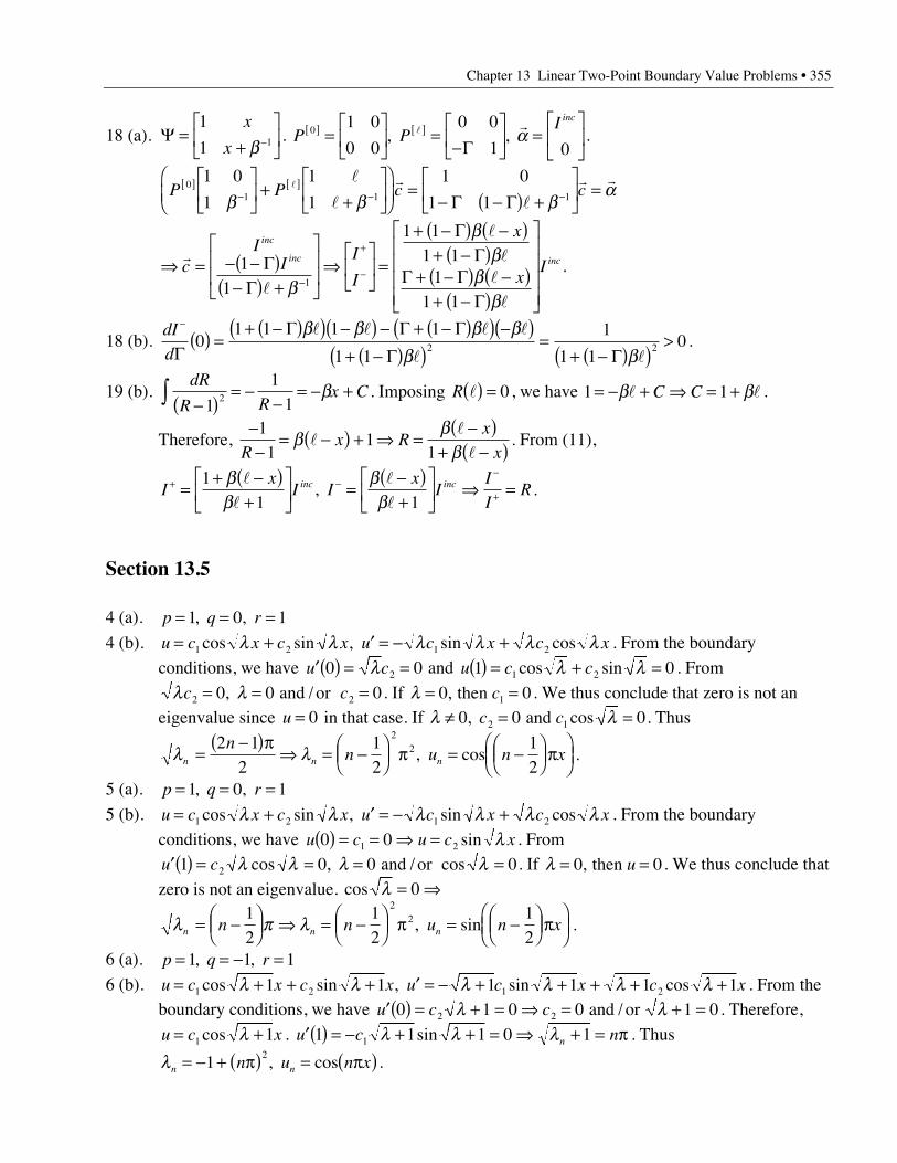
Chapter 13 Linear Two-Point Boundary Value Problems • 355
18 (a). Y =+
È
ÎÍ
˘
˚˙-
1
1 1
x
x b. P P
I inc0
1 0
0 0
0 0
1 0[ ] [ ]=
È
ÎÍ
˘
˚˙ =
-È
ÎÍ
˘
˚˙ =
È
ÎÍ
˘
˚˙, , l r
Ga .
P P c c01 1 1
1 0
1
1
1
1 0
1 1[ ]
-[ ]
- -
È
ÎÍ
˘
˚˙ +
+È
ÎÍ
˘
˚˙
Ê
ËÁˆ
¯=
- -( ) +È
ÎÍ
˘
˚˙ =
b b bal
l
l
r
l
r r
G G
fi = - -( )-( ) +
È
Î
ÍÍ
˘
˚
˙˙
fiÈ
ÎÍ
˘
˚˙ =
+ -( ) -( )+ -( )
+ -( ) -( )+ -( )
È
Î
ÍÍÍÍ
˘
˚
˙˙˙˙
-
+
-
r
l
l
ll
l
cI
II
I
x
xI
inc
inc inc11
1 11 1
11 1
1
GG
GG
G GG
b
bb
bb
.
18 (b).dI
d
-
( ) =+ -( )( ) -( ) - + -( )( ) -( )
+ -( )( )=
+ -( )( )>
GG G G
G G0
1 1 1 1
1 1
1
1 102 2
b b b bb b
l l l l
l l.
19 (b).dR
R Rx C
-( )= -
-= - +Ú 1
112 b . Imposing R l( ) = 0, we have 1 1= - + fi = +b bl lC C .
Therefore, -
-= -( ) + fi =
-( )+ -( )
11
11R
x Rx
xb b
bl
l
l. From (11),
Ix
I Ix
II
IRinc inc+ -
-
+=+ -( )
+È
ÎÍ
˘
˚˙ =
-( )+
È
ÎÍ
˘
˚˙ fi =
11 1
bb
bb
l
l
l
l, .
Section 13.5
4 (a). p q r= = =1 0 1, ,
4 (b). u c x c x u c x c x= + ¢ = - +1 2 1 2cos sin , sin cosl l l l l l . From the boundary
conditions, we have ¢( ) = =u c0 02l and u c c1 01 2( ) = + =cos sinl l . From
l lc c2 20 0 0= = =, and / or . If l = =0 01, then c . We thus conclude that zero is not an
eigenvalue since u = 0 in that case. If l lπ = =0 0 02 1, cosc c and . Thus
l ln n n
nn u n x=
-( )pfi = -Ê
ËÁˆ¯ p = -Ê
ËÁˆ¯ p
ÊËÁ
ˆ¯
2 12
12
12
22, cos .
5 (a). p q r= = =1 0 1, ,
5 (b). u c x c x u c x c x= + ¢ = - +1 2 1 2cos sin , sin cosl l l l l l . From the boundary
conditions, we have u c u c x0 01 2( ) = = fi = sin l . From
¢( ) = = = =u c1 0 0 02 l l l lcos , cos and / or . If l = =0 0, then u . We thus conclude that
zero is not an eigenvalue. cos l = fi0
l p ln n nn n u n x= -ÊËÁ
ˆ¯ fi = -Ê
ËÁˆ¯ p = -Ê
ËÁˆ¯ p
ÊËÁ
ˆ¯
12
12
12
22, sin .
6 (a). p q r= = - =1 1 1, ,
6 (b). u c x c x u c x c x= + + + ¢ = - + + + + +1 2 1 21 1 1 1 1 1cos sin , sin cosl l l l l l . From the
boundary conditions, we have ¢( ) = + = fi = + =u c c0 1 0 0 1 02 2l l and / or . Therefore,
u c x= +1 1cos l . ¢( ) = - + + = fi + = pu c nn1 1 1 0 11 l l lsin . Thus
ln nn u n x= - + p( ) = p( )12, cos .
356 • Chapter 13 Linear Two-Point Boundary Value Problems
7 (a). p q r= = =1 1 1, ,
7 (b). u c x c x u c x c x= - + - ¢ = - - - + - -1 2 1 21 1 1 1 1 1cos sin , sin cosl l l l l l . From the
boundary conditions, we have u c u c x0 0 11 2( ) = = fi = -sin l . From
u c nn2 1 2 0 2 12( ) = - ◊( ) = - = psin , l l . Thus ln n
nu
n x= +
pÊËÁ
ˆ¯ =
pÊËÁ
ˆ¯1
2 2
2
, sin .
8 (a). p q r= = =1 0 1, ,
8 (b). u c x c x u c x c x= + ¢ = - +1 2 1 2cos sin , sin cosl l l l l l . From the boundary
conditions, we have u c u c x0 01 2( ) = = fi = sin l . From
u u c u xn n n n1 1 02( ) + ¢( ) = +[ ] = = - =sin cos , tan , sinl l l l l l (or u would be
zero). From root-finding software, we obtain l l l1 2 34 11586 24 1393 63 6591= = =. , . , . .9 (a). p q r= = - =1 4 2, ,
9 (b). u c x c x= + + +1 22 4 2 4cos sinl l . From the boundary conditions, we have
u c u c x0 0 2 41 2( ) = = fi = +sin l . From u c nn3 2 4 3 0 3 2 42( ) = + ◊( ) = + = psin , l l .
Thus ln n
nu
n x=
pÊËÁ
ˆ¯ - =
pÊËÁ
ˆ¯
12 3
23
2
, sin .
10 (a). p e q e r ex x x= = - =2 2 22, ,
10 (b). r r r i2 2 2 02 4 4 2
21 1+ + +( ) = fi =
- ± - +( )= - ± -l
ll
fi = -( ) + -( )- -u c e x c e xx x1 21 1cos sinl l . From the boundary conditions, we have
u c u c e n nn n0 0 1 1 0 1 11 21 2( ) = = ( ) = - = fi - = p fi = + p( )-, sin l l l , u e n xn
x= p- sin .
11 (a). p e q e r ex x x= = - =, ,
11 (b). r r r i2 1 01 1 4 1
212
34
+ + +( ) = fi =- ± - +( )
= - ± +ll
l
fi = +ÊË
ˆ¯ + +Ê
ˈ¯
- -u c e x c e x
x x
12
223
43
4cos sinl l . From the boundary conditions, we have
u c u c e xx
0 0 341 2
2( ) = = fi = +ÊË
ˆ¯
-sin , l
¢ = - +ÊË
ˆ¯ + + +Ê
ˈ¯
ÈÎÍ
˘˚
-u c e x x
x
22
12
34
34
34sin cosl l l .
Also,
u u c e c e1 2 1 34 2
12
34
34
34 02
12
2
12( ) + ¢( ) = + + - +Ê
ˈ¯ + + +Ê
ˈ¯
ÈÎÍ
˘˚
=- -sin sin cosl l l l .
Therefore, l ln nn n+ = -ÊËÁ
ˆ¯ p fi = - + -Ê
ËÁˆ¯ p3
412
34
12
22 u e n xn
x= -Ê
ËÁˆ¯ p
ÊËÁ
ˆ¯
- 212
sin .
12 (a). p e q r ex x= = =- -, , 0
12 (b). r r r i2 01 1 4
212
14- + = fi =
± -= ± -l l l
fi = -ÊË
ˆ¯ + -Ê
ˈ¯u c e x c e x
x x
12
221
41
4cos sinl l .
Chapter 13 Linear Two-Point Boundary Value Problems • 357
From the boundary conditions, we have
u c u c en n
n n0 0 2 2 14 0 1
4 214 21 2
2
( ) = = ( ) = -ÊË
ˆ¯ = fi - =
pfi = +
pÊËÁ
ˆ¯, sin l l l ,
u en x
n
x=
pÊËÁ
ˆ¯
2
2sin .
13 (a). p e q r ex x= = =, , 0
13 (b). r r r i2 01 1 4
212
14+ + = fi =
- ± -= - ± -l l l
fi = - -( )ÊË
ˆ¯ + - -( )Ê
ˈ¯
- -( ) - -( )u c e x c e x
x x
1
12 1
2
12 11
4 1 14 1cos sinl l . From the boundary
conditions, we have
u c u c e n nn n1 0 2 14 0 1
4141 2
12 2( ) = = ( ) = -Ê
ˈ¯ = fi - = p fi = + p( )-
, sin l l l ,
u e n xn
x= p -( )( )- -( )12 1
1sin .
14 (a). p x q rx
= = =, , 01
14 (b). First, let u xr= . Now, r r r r r i-( ) + + = + = fi = ±1 02l l l . Thus
u c x c x= ( ) + ( )1 2cos ln sin lnl l . From the boundary conditions, we have
u c u c nn
n n1 0 4 4 0 441 2
2
( ) = = ( ) = ( ) = fi = p fi =pÊ
ËÁˆ¯, sin ln ln
lnl l l , u
n xn =
pÊËÁ
ˆ¯sin
lnln4
.
15 (a). From Problem 14, p x q rx
= = =, , 01
15 (b). u c x c x= ( ) + ( )1 2cos ln sin lnl l . From the boundary conditions, we have
¢( ) = = ¢( ) = - ( ) = fi = p fi =pÊ
ËÁˆ¯u c u c n
nn n1 0 3
33 0 3
32 1
2
l l l l l, sin ln lnln
,
un x
n =pÊ
ËÁˆ¯cos
lnln3
.
18. p q r= = - = fi ¢ = +( ) + = +1 1 1 1 12 2 2, , sin cos sinq l q q l q . ¢ = -R Rl q qsin cos .u R u R0 0 0 0 1 1 1 0 0 1 0( ) = ( ) ( ) = ( ) = ( ) ( ) = ( ) = ( ) =sin , sin , sin sinq q q q .
19. p q r= = = fi ¢ = -( ) +1 2 3 3 2 2 2, , sin cosq l q q .¢ = - +( ) = - -( )R R R1 3 2 3 1l q q l q qsin cos sin cos .
¢( ) = ( ) ( ) ( ) = ( ) = ( ) ( ) = ( ) = ( ) =up
R u R010
0 0 0 1 1 1 0 0 0 1 0cos , sin , cos , sinq q q q .
20. p e q r e e ex x x x= = = fi ¢ = +- - -2 2 2 2 2 20, , sin cosq l q q . ¢ = -( )-R e e Rx x2 2l q qsin cos .
u u0 2 0( ) = ( ) = . Therefore, sin , sinq q0 0 2 0( ) = ( ) =21. p e q e r e e ex x x x x= = - = fi ¢ = +( ) +- - - -2 2 2 2 2
1 2 2, , sin cosq l q q .
¢ = - +( )( )-R e e Rx x2 2
1l q qsin cos . u R up
R0 0 0 0 111
1 1 0( ) = ( ) ( ) = ¢( ) = ( ) ( ) ( ) =sin , cosq q .
Therefore, sin , cosq q0 0 1 0( ) = ( ) =