math 130 by paul... · math 130 © 2007 paul dawkins i ... in order to remind you how to simplify...
TRANSCRIPT
Math 130
Paul Dawkins
Math 130
© 2007 Paul Dawkins i http://tutorial.math.lamar.edu/terms.aspx
Table of Contents Review ............................................................................................................................................. 1
Introduction ................................................................................................................................................ 1 Review : Functions ..................................................................................................................................... 3 Review : Inverse Functions ...................................................................................................................... 13 Review : Trig Functions ........................................................................................................................... 20 Review : Solving Trig Equations ............................................................................................................. 27 Review : Solving Trig Equations with Calculators, Part I........................................................................ 36 Review : Solving Trig Equations with Calculators, Part II ...................................................................... 47 Review : Exponential Functions............................................................................................................... 52 Review : Logarithm Functions ................................................................................................................. 55 Review : Exponential and Logarithm Equations ...................................................................................... 61 Review : Common Graphs ....................................................................................................................... 67
Limits ............................................................................................................................................ 79 Introduction .............................................................................................................................................. 79 Rates of Change and Tangent Lines ......................................................................................................... 81 The Limit .................................................................................................................................................. 90 One-Sided Limits ................................................................................................................................... 100 Limit Properties ...................................................................................................................................... 106 Computing Limits .................................................................................................................................. 112 Infinite Limits......................................................................................................................................... 120 Limits At Infinity, Part I ......................................................................................................................... 130 Limits At Infinity, Part II ....................................................................................................................... 139 Continuity ............................................................................................................................................... 149 The Definition of the Limit .................................................................................................................... 156
Derivatives .................................................................................................................................. 171 Introduction ............................................................................................................................................ 171 The Definition of the Derivative ............................................................................................................ 173 Interpretations of the Derivative............................................................................................................. 179 Differentiation Formulas ........................................................................................................................ 188 Product and Quotient Rule ..................................................................................................................... 196 Derivatives of Trig Functions................................................................................................................. 202 Derivatives of Exponential and Logarithm Functions ............................................................................ 213 Derivatives of Inverse Trig Functions .................................................................................................... 218 Derivatives of Hyperbolic Functions ..................................................................................................... 224 Chain Rule .............................................................................................................................................. 226 Implicit Differentiation .......................................................................................................................... 236 Related Rates .......................................................................................................................................... 245 Higher Order Derivatives ....................................................................................................................... 259 Logarithmic Differentiation ................................................................................................................... 264
Applications of Derivatives ....................................................................................................... 267 Introduction ............................................................................................................................................ 267 Rates of Change ..................................................................................................................................... 269 Critical Points ......................................................................................................................................... 272 Minimum and Maximum Values ........................................................................................................... 278 Finding Absolute Extrema ..................................................................................................................... 286 The Shape of a Graph, Part I .................................................................................................................. 292 The Shape of a Graph, Part II ................................................................................................................. 301 The Mean Value Theorem ...................................................................................................................... 310 Optimization ........................................................................................................................................... 317 More Optimization Problems ................................................................................................................. 331 Indeterminate Forms and L’Hospital’s Rule .......................................................................................... 346 Differentials............................................................................................................................................ 352 Business Applications ............................................................................................................................ 355

Math 130
© 2007 Paul Dawkins ii http://tutorial.math.lamar.edu/terms.aspx
Integrals ...................................................................................................................................... 361 Introduction ............................................................................................................................................ 361 Indefinite Integrals ................................................................................................................................. 362
Extras .......................................................................................................................................... 368 Introduction ............................................................................................................................................ 368 Proof of Various Derivative Facts/Formulas/Properties ........................................................................ 369 Proof of Trig Limits ............................................................................................................................... 382 Proofs of Derivative Applications Facts/Formulas ................................................................................ 387 Types of Infinity ..................................................................................................................................... 398 Summation Notation .............................................................................................................................. 402
Math 130
© 2007 Paul Dawkins 1 http://tutorial.math.lamar.edu/terms.aspx
Review
Introduction Technically a student coming into a Calculus class is supposed to know both Algebra and Trigonometry. The reality is often much different however. Most students enter a Calculus class woefully unprepared for both the algebra and the trig that is in a Calculus class. This is very unfortunate since good algebra skills are absolutely vital to successfully completing any Calculus course and if your Calculus course includes trig (as this one does) good trig skills are also important in many sections. The intent of this chapter is to do a very cursory review of some algebra and trig skills that are absolutely vital to a calculus course. This chapter is not inclusive in the algebra and trig skills that are needed to be successful in a Calculus course. It only includes those topics that most students are particularly deficient in. For instance factoring is also vital to completing a standard calculus class but is not included here. For a more in depth review you should visit my Algebra/Trig review or my full set of Algebra notes at http://tutorial.math.lamar.edu. Note that even though these topics are very important to a Calculus class I rarely cover all of these in the actual class itself. We simply don’t have the time to do that. I do cover certain portions of this chapter in class, but for the most part I leave it to the students to read this chapter on their own. Here is a list of topics that are in this chapter. I’ve also denoted the sections that I typically cover during the first couple of days of a Calculus class. Review : Functions – Here is a quick review of functions, function notation and a couple of fairly important ideas about functions. Review : Inverse Functions – A quick review of inverse functions and the notation for inverse functions. Review : Trig Functions – A review of trig functions, evaluation of trig functions and the unit circle. This section usually gets a quick review in my class. Review : Solving Trig Equations – A reminder on how to solve trig equations. This section is always covered in my class. Review : Solving Trig Equations with Calculators, Part I – The previous section worked problem whose answers were always the “standard” angles. In this section we work some
Math 130
© 2007 Paul Dawkins 2 http://tutorial.math.lamar.edu/terms.aspx
problems whose answers are not “standard” and so a calculator is needed. This section is always covered in my class as most trig equations in the remainder will need a calculator. Review : Solving Trig Equations with Calculators, Part II – Even more trig equations requiring a calculator to solve. Review : Exponential Functions – A review of exponential functions. This section usually gets a quick review in my class. Review : Logarithm Functions – A review of logarithm functions and logarithm properties. This section usually gets a quick review in my class. Review : Exponential and Logarithm Equations – How to solve exponential and logarithm equations. This section is always covered in my class. Review : Common Graphs – This section isn’t much. It’s mostly a collection of graphs of many of the common functions that are liable to be seen in a Calculus class.
Math 130
© 2007 Paul Dawkins 3 http://tutorial.math.lamar.edu/terms.aspx
Review : Functions In this section we’re going to make sure that you’re familiar with functions and function notation. Both will appear in almost every section in a Calculus class and so you will need to be able to deal with them. First, what exactly is a function? An equation will be a function if for any x in the domain of the equation (the domain is all the x’s that can be plugged into the equation) the equation will yield exactly one value of y. This is usually easier to understand with an example. Example 1 Determine if each of the following are functions.
(a) 2 1y x= + (b) 2 1y x= +
Solution (a) This first one is a function. Given an x, there is only one way to square it and then add 1 to the result. So, no matter what value of x you put into the equation, there is only one possible value of y. (b) The only difference between this equation and the first is that we moved the exponent off the x and onto the y. This small change is all that is required, in this case, to change the equation from a function to something that isn’t a function. To see that this isn’t a function is fairly simple. Choose a value of x, say x=3 and plug this into the equation. 2 3 1 4y = + = Now, there are two possible values of y that we could use here. We could use 2y = or 2y = − . Since there are two possible values of y that we get from a single x this equation isn’t a function. Note that this only needs to be the case for a single value of x to make an equation not be a function. For instance we could have used x=-1 and in this case we would get a single y (y=0). However, because of what happens at x=3 this equation will not be a function. Next we need to take a quick look at function notation. Function notation is nothing more than a fancy way of writing the y in a function that will allow us to simplify notation and some of our work a little. Let’s take a look at the following function. 22 5 3y x x= − + Using function notation we can write this as any of the following.
Math 130
© 2007 Paul Dawkins 4 http://tutorial.math.lamar.edu/terms.aspx
( ) ( )( ) ( )( ) ( )
2 2
2 2
2 2
2 5 3 2 5 3
2 5 3 2 5 3
2 5 3 2 5 3
f x x x g x x x
h x x x R x x x
w x x x y x x x
= − + = − +
= − + = − +
= − + = − +
M
Recall that this is NOT a letter times x, this is just a fancy way of writing y. So, why is this useful? Well let’s take the function above and let’s get the value of the function at x=-3. Using function notation we represent the value of the function at x=-3 as f(-3). Function notation gives us a nice compact way of representing function values. Now, how do we actually evaluate the function? That’s really simple. Everywhere we see an x on the right side we will substitute whatever is in the parenthesis on the left side. For our function this gives,
( ) ( ) ( )
( )
23 2 3 5 3 3
2 9 15 336
f − = − − − +
= + +
=
Let’s take a look at some more function evaluation. Example 2 Given ( ) 2 6 11f x x x= − + − find each of the following.
(a) ( )2f [Solution]
(b) ( )10f − [Solution]
(c) ( )f t [Solution]
(d) ( )3f t − [Solution]
(e) ( )3f x − [Solution]
(f) ( )4 1f x − [Solution] Solution
(a) ( ) ( )22 2 6(2) 11 3f = − + − = − [Return to Problems]
(b) ( ) ( ) ( )210 10 6 10 11 100 60 11 171f − = − − + − − = − − − = −
Be careful when squaring negative numbers! [Return to Problems]
(c) ( ) 2 6 11f t t t= − + −
Remember that we substitute for the x’s WHATEVER is in the parenthesis on the left. Often this will be something other than a number. So, in this case we put t’s in for all the x’s on the left.
[Return to Problems]
Math 130
© 2007 Paul Dawkins 5 http://tutorial.math.lamar.edu/terms.aspx
(d) ( ) ( ) ( )2 23 3 6 3 11 12 38f t t t t t− = − − + − − = − + −
Often instead of evaluating functions at numbers or single letters we will have some fairly complex evaluations so make sure that you can do these kinds of evaluations.
[Return to Problems]
(e) ( ) ( ) ( )2 23 3 6 3 11 12 38f x x x x x− = − − + − − = − + −
The only difference between this one and the previous one is that I changed the t to an x. Other than that there is absolutely no difference between the two! Don’t get excited if an x appears inside the parenthesis on the left.
[Return to Problems]
(f) ( ) ( ) ( )2 24 1 4 1 6 4 1 11 16 32 18f x x x x x− = − − + − − = − + −
This one is not much different from the previous part. All we did was change the equation that we were plugging into function.
[Return to Problems] All throughout a calculus course we will be finding roots of functions. A root of a function is nothing more than a number for which the function is zero. In other words, finding the roots of a function, g(x), is equivalent to solving ( ) 0g x = Example 3 Determine all the roots of ( ) 3 29 18 6f t t t t= − + Solution So we will need to solve, 3 29 18 6 0t t t− + = First, we should factor the equation as much as possible. Doing this gives,
( )23 3 6 2 0t t t− + = Next recall that if a product of two things are zero then one (or both) of them had to be zero. This means that,
2
3 0 OR,3 6 2 0tt t
=
− + =
From the first it’s clear that one of the roots must then be t=0. To get the remaining roots we will need to use the quadratic formula on the second equation. Doing this gives,

Math 130
© 2007 Paul Dawkins 6 http://tutorial.math.lamar.edu/terms.aspx
( ) ( ) ( )( )( )
( )( )
26 6 4 3 22 3
6 126
6 4 36
6 2 36
3 3311 33113
t− − ± − −
=
±=
±=
±=
±=
= ±
= ±
In order to remind you how to simplify radicals we gave several forms of the answer. To complete the problem, here is a complete list of all the roots of this function.
3 3 3 30, ,3 3
t t t+ −= = =
Note we didn’t use the final form for the roots from the quadratic. This is usually where we’ll stop with the simplification for these kinds of roots. Also note that, for the sake of the practice, we broke up the compact form for the two roots of the quadratic. You will need to be able to do this so make sure that you can. This example had a couple of points other than finding roots of functions. The first was to remind you of the quadratic formula. This won’t be the last time that you’ll need it in this class. The second was to get you used to seeing “messy” answers. In fact, the answers in the above list are not that messy. However, most students come out of an Algebra class very used to seeing only integers and the occasional “nice” fraction as answers. So, here is fair warning. In this class I often will intentionally make the answers look “messy” just to get you out of the habit of always expecting “nice” answers. In “real life” (whatever that is) the answer is rarely a simple integer such as two. In most problems the answer will be a decimal that came about from a messy fraction and/or an answer that involved radicals.
Math 130
© 2007 Paul Dawkins 7 http://tutorial.math.lamar.edu/terms.aspx
One of the more important ideas about functions is that of the domain and range of a function. In simplest terms the domain of a function is the set of all values that can be plugged into a function and have the function exist and have a real number for a value. So, for the domain we need to avoid division by zero, square roots of negative numbers, logarithms of zero and negative numbers (if not familiar with logarithms we’ll take a look at them a little later), etc. The range of a function is simply the set of all possible values that a function can take. Let’s find the domain and range of a few functions. Example 4 Find the domain and range of each of the following functions.
(a) ( ) 5 3f x x= − [Solution]
(b) ( ) 4 7g t t= − [Solution]
(c) ( ) 22 12 5h x x x= − + + [Solution]
(d) ( ) 6 3f z z= − − [Solution]
(e) ( ) 8g x = [Solution] Solution (a) ( ) 5 3f x x= −
We know that this is a line and that it’s not a horizontal line (because the slope is 5 and not zero…). This means that this function can take on any value and so the range is all real numbers. Using “mathematical” notation this is, ( )Range : ,−∞ ∞
This is more generally a polynomial and we know that we can plug any value into a polynomial and so the domain in this case is also all real numbers or, ( )Domain : or ,x− ∞ < < ∞ −∞ ∞
[Return to Problems] (b) ( ) 4 7g t t= −
This is a square root and we know that square roots are always positive or zero and because we can have the square root of zero in this case,
( ) ( )4 47 74 7 0 0g = − = =
We know then that the range will be, [ )Range : 0,∞
For the domain we have a little bit of work to do, but not much. We need to make sure that we don’t take square roots of any negative numbers and so we need to require that,
Math 130
© 2007 Paul Dawkins 8 http://tutorial.math.lamar.edu/terms.aspx
4 47 7
4 7 04 7t
tt t
− ≥≥≥ ⇒ ≤
The domain is then, (4 4
7 7Domain : or ,t ≤ −∞ [Return to Problems]
(c) ( ) 22 12 5h x x x= − + +
Here we have a quadratic which is a polynomial and so we again know that the domain is all real numbers or,
( )Domain : or ,x− ∞ < < ∞ −∞ ∞
In this case the range requires a little bit of work. From an Algebra class we know that the graph of this will be a parabola that opens down (because the coefficient of the 2x is negative) and so the vertex will be the highest point on the graph. If we know the vertex we can then get the range. The vertex is then,
( ) ( ) ( ) ( ) ( )212 3 3 2 3 12 3 5 23 3,23
2 2x y h= − = = = − + + = ⇒
−
So, as discussed, we know that this will be the highest point on the graph or the largest value of the function and the parabola will take all values less than this so the range is then, ( ]Range : ,23−∞
[Return to Problems] (d) ( ) 6 3f z z= − −
This function contains an absolute value and we know that absolute value will be either positive or zero. In this case the absolute value will be zero if 6z = and so the absolute value portion of this function will always be greater than or equal to zero. We are subtracting 3 from the absolute value portion and so we then know that the range will be, [ )Range : 3,− ∞
We can plug any value into an absolute value and so the domain is once again all real numbers or, ( )Domain : or ,x− ∞ < < ∞ −∞ ∞
[Return to Problems] (e) ( ) 8g x =
This function may seem a little tricky at first but is actually the easiest one in this set of examples. This is a constant function and so an value of x that we plug into the function will yield a value of

Math 130
© 2007 Paul Dawkins 9 http://tutorial.math.lamar.edu/terms.aspx
8. This means that the range is a single value or, Range : 8 The domain is all real numbers, ( )Domain : or ,x− ∞ < < ∞ −∞ ∞
[Return to Problems] In general determining the range of a function can be somewhat difficult. As long as we restrict ourselves down to “simple” functions, some of which we looked at in the previous example, finding the range is not too bad, but for most functions it can be a difficult process. Because of the difficulty in finding the range for a lot of functions we had to keep those in the previous set somewhat simple, which also meant that we couldn’t really look at some of the more complicated domain examples that are liable to be important in a Calculus course. So, let’s take a look at another set of functions only this time we’ll just look for the domain. Example 5 Find the domain of each of the following functions.
(a) ( ) 2
42 15
xf xx x
−=
− − [Solution]
(b) ( ) 26g t t t= + − [Solution]
(c) ( )2 9xh x
x=
− [Solution]
Solution
(a) ( ) 2
42 15
xf xx x
−=
− −
Okay, with this problem we need to avoid division by zero and so we need to determine where the denominator is zero which means solving, ( )( )2 2 15 5 3 0 3, 5x x x x x x− − = − + = ⇒ = − =
So, these are the only values of x that we need to avoid and so the domain is, Domain : All real numbers except 3 & 5x x= − =
[Return to Problems]
(b) ( ) 26g t t t= + −
In this case we need to avoid square roots of negative numbers and so need to require that, 2 26 0 6 0t t t t+ − ≥ ⇒ − − ≤ Note that we multiplied the whole inequality by -1 (and remembered to switch the direction of the inequality) to make this easier to deal with. You’ll need to be able to solve inequalities like this more than a few times in a Calculus course so let’s make sure you can solve these.

Math 130
© 2007 Paul Dawkins 10 http://tutorial.math.lamar.edu/terms.aspx
The first thing that we need to determine where the function is zero and that’s not too difficult in this case. ( ) ( )2 6 3 2 0t t t t− − = − + =
So, the function will be zero at 2t = − and 3t = . Recall that these points will be the only place where the function may change sign. It’s not required to change sign at these points, but these will be the only points where the function can change sign. This means that all we need to do is break up a number line into the three regions that avoid these two points and test the sign of the function at a single point in each of the regions. If the function is positive at a single point in the region it will be positive at all points in that region because it doesn’t contain the any of the points where the function may change sign. We’ll have a similar situation if the function is negative for the test point. So, here is a number line showing these computations.
From this we can see that in only region in which the quadratic (in its modified form) will be negative is in the middle region. Recalling that we got to the modified region by multiplying the quadratic by a -1 this means that the quadratic under the root will only be positive in the middle region and so the domain for this function is then, [ ]Domain : 2 3 or 2,3t− ≤ ≤ −
[Return to Problems]
(c) ( )2 9xh x
x=
−
In this case we have a mixture of the two previous parts. We have to worry about division by zero and square roots of negative numbers. We can cover both issues by requiring that, 2 9 0x − > Note that we need the inequality here to be strictly greater than zero to avoid the division by zero issues. We can either solve this by the method from the previous example or, in this case, it is easy enough to solve by inspection. The domain is this case is, ( ) ( )Domain : 3 & 3 or , 3 & 3,x x< − > −∞ − ∞
[Return to Problems]

Math 130
© 2007 Paul Dawkins 11 http://tutorial.math.lamar.edu/terms.aspx
The next topic that we need to discuss here is that of function composition. The composition of f(x) and g(x) is ( )( ) ( )( )f g x f g x=o In other words, compositions are evaluated by plugging the second function listed into the first function listed. Note as well that order is important here. Interchanging the order will usually result in a different answer. Example 6 Given ( ) 23 10f x x x= − + and ( ) 1 20g x x= − find each of the following.
(a) ( )( )5f go [Solution]
(b) ( )( )f g xo [Solution]
(c) ( )( )g f xo [Solution]
(d) ( )( )g g xo [Solution] Solution (a) ( )( )5f go
In this case we’ve got a number instead of an x but it works in exactly the same way.
( )( ) ( )( )
( )5 5
99 29512
f g f g
f
=
= − =
o
[Return to Problems]
(b) ( )( )f g xo
( )( ) ( )( )( )
( ) ( )( )
2
2
2
1 20
3 1 20 1 20 10
3 1 40 400 1 20 10
1200 100 12
f g x f g x
f x
x x
x x x
x x
=
= −
= − − − +
= − + − + +
= − +
o
Compare this answer to the next part and notice that answers are NOT the same. The order in which the functions are listed is important!
[Return to Problems]
(c) ( )( )g f xo
( )( ) ( )( )( )
( )
2
2
2
3 10
1 20 3 10
60 20 199
g f x g f x
g x x
x x
x x
=
= − +
= − − +
= − + −
o
And just to make the point. This answer is different from the previous part. Order is important in composition.
[Return to Problems]

Math 130
© 2007 Paul Dawkins 12 http://tutorial.math.lamar.edu/terms.aspx
(d) ( )( )g g xo
In this case do not get excited about the fact that it’s the same function. Composition still works the same way.
( )( ) ( )( )( )
( )1 20
1 20 1 20400 19
g g x g g x
g x
xx
=
= −
= − −
= −
o
[Return to Problems] Let’s work one more example that will lead us into the next section.
Example 7 Given ( ) 3 2f x x= − and ( ) 1 23 3
g x x= + find each of the following.
(a) ( )( )f g xo
(b) ( )( )g f xo Solution (a)
( )( ) ( )( )1 23 3
1 23 23 32 2
f g x f g x
f x
x
x x
=
= +
= + −
= + − =
o
(b)
( )( ) ( )( )( )
( )
3 21 23 23 3
2 23 3
g f x g f x
g x
x
x x
=
= −
= − +
= − + =
o
In this case the two compositions where the same and in fact the answer was very simple. ( )( ) ( ) ( )f g x g f x x= =o o This will usually not happen. However, when the two compositions are the same, or more specifically when the two compositions are both x there is a very nice relationship between the two functions. We will take a look at that relationship in the next section.

Math 130
© 2007 Paul Dawkins 13 http://tutorial.math.lamar.edu/terms.aspx
Review : Inverse Functions
In the last example from the previous section we looked at the two functions ( ) 3 2f x x= − and
( ) 23 3xg x = + and saw that
( )( ) ( ) ( )f g x g f x x= =o o and as noted in that section this means that there is a nice relationship between these two functions. Let’s see just what that relationship is. Consider the following evaluations.
( ) ( ) ( )
( )
5 2 33 1 23 3 3
2 2 43 2 4 23
5 5
4 4
1 1
2 23 33 3
f g
g f
− −= − − = ⇒ = + = =
= + = ⇒ = − = − =
− −−
−
In the first case we plugged 1x = − into ( )f x and got a value of -5. We then turned around and
plugged 5x = − into ( )g x and got a value of -1, the number that we started off with.
In the second case we did something similar. Here we plugged 2x = into ( )g x and got a value
of43
, we turned around and plugged this into ( )f x and got a value of 2, which is again the
number that we started with. Note that we really are doing some function composition here. The first case is really,
( )( ) ( ) [ ]1 1 5 1g f g f g− = − = − = − o
and the second case is really,
( )( ) ( ) 42 2 23
f g f g f = = = o
Note as well that these both agree with the formula for the compositions that we found in the previous section. We get back out of the function evaluation the number that we originally plugged into the composition. So, just what is going on here? In some way we can think of these two functions as undoing what the other did to a number. In the first case we plugged 1x = − into ( )f x and then plugged the
result from this function evaluation back into ( )g x and in some way ( )g x undid what ( )f x
had done to 1x = − and gave us back the original x that we started with.

Math 130
© 2007 Paul Dawkins 14 http://tutorial.math.lamar.edu/terms.aspx
Function pairs that exhibit this behavior are called inverse functions. Before formally defining inverse functions and the notation that we’re going to use for them we need to get a definition out of the way. A function is called one-to-one if no two values of x produce the same y. Mathematically this is the same as saying,
( ) ( )1 2 1 2wheneverf x f x x x≠ ≠
So, a function is one-to-one if whenever we plug different values into the function we get different function values. Sometimes it is easier to understand this definition if we see a function that isn’t one-to-one. Let’s take a look at a function that isn’t one-to-one. The function ( ) 2f x x= is not one-to-one
because both ( )2 4f − = and ( )2 4f = . In other words there are two different values of x that
produce the same value of y. Note that we can turn ( ) 2f x x= into a one-to-one function if we
restrict ourselves to 0 x≤ < ∞ . This can sometimes be done with functions. Showing that a function is one-to-one is often tedious and/or difficult. For the most part we are going to assume that the functions that we’re going to be dealing with in this course are either one-to-one or we have restricted the domain of the function to get it to be a one-to-one function. Now, let’s formally define just what inverse functions are. Given two one-to-one functions
( )f x and ( )g x if
( )( ) ( ) ( )ANDf g x x g f x x= =o o
then we say that ( )f x and ( )g x are inverses of each other. More specifically we will say that
( )g x is the inverse of ( )f x and denote it by
( ) ( )1g x f x−=
Likewise we could also say that ( )f x is the inverse of ( )g x and denote it by
( ) ( )1f x g x−= The notation that we use really depends upon the problem. In most cases either is acceptable. For the two functions that we started off this section with we could write either of the following two sets of notation.
( ) ( )
( ) ( )
1
1
23 23 3
2 3 23 3
xf x x f x
xg x g x x
−
−
= − = +
= + = −

Math 130
© 2007 Paul Dawkins 15 http://tutorial.math.lamar.edu/terms.aspx
Now, be careful with the notation for inverses. The “-1” is NOT an exponent despite the fact that is sure does look like one! When dealing with inverse functions we’ve got to remember that
( ) ( )1 1f x
f x− ≠
This is one of the more common mistakes that students make when first studying inverse functions. The process for finding the inverse of a function is a fairly simple one although there are a couple of steps that can on occasion be somewhat messy. Here is the process Finding the Inverse of a Function Given the function ( )f x we want to find the inverse function, ( )1f x− .
1. First, replace ( )f x with y. This is done to make the rest of the process easier. 2. Replace every x with a y and replace every y with an x. 3. Solve the equation from Step 2 for y. This is the step where mistakes are most often
made so be careful with this step. 4. Replace y with ( )1f x− . In other words, we’ve managed to find the inverse at this point!
5. Verify your work by checking that ( )( )1f f x x− =o and ( )( )1f f x x− =o are both true. This work can sometimes be messy making it easy to make mistakes so again be careful.
That’s the process. Most of the steps are not all that bad but as mentioned in the process there are a couple of steps that we really need to be careful with since it is easy to make mistakes in those steps.
In the verification step we technically really do need to check that both ( )( )1f f x x− =o and
( )( )1f f x x− =o are true. For all the functions that we are going to be looking at in this course
if one is true then the other will also be true. However, there are functions (they are beyond the scope of this course however) for which it is possible for only one of these to be true. This is brought up because in all the problems here we will be just checking one of them. We just need to always remember that technically we should check both. Let’s work some examples. Example 1 Given ( ) 3 2f x x= − find ( )1f x− . Solution Now, we already know what the inverse to this function is as we’ve already done some work with it. However, it would be nice to actually start with this since we know what we should get. This will work as a nice verification of the process.
Math 130
© 2007 Paul Dawkins 16 http://tutorial.math.lamar.edu/terms.aspx
So, let’s get started. We’ll first replace ( )f x with y.
3 2y x= − Next, replace all x’s with y and all y’s with x. 3 2x y= − Now, solve for y.
( )
2 31 23
23 3
x y
x y
x y
+ =
+ =
+ =
Finally replace y with ( )1f x− .
( )1 23 3xf x− = +
Now, we need to verify the results. We already took care of this in the previous section, however, we really should follow the process so we’ll do that here. It doesn’t matter which of the two that
we check we just need to check one of them. This time we’ll check that ( )( )1f f x x− =o is
true.
( )( ) ( )1 1
23 3
23 23 32 2
f f x f f x
xf
x
xx
− − = = +
= + −
= + −=
o
Example 2 Given ( ) 3g x x= − find ( )1g x− . Solution The fact that we’re using ( )g x instead of ( )f x doesn’t change how the process works. Here
are the first few steps.
3
3
y x
x y
= −
= −

Math 130
© 2007 Paul Dawkins 17 http://tutorial.math.lamar.edu/terms.aspx
Now, to solve for y we will need to first square both sides and then proceed as normal.
2
2
3
33
x y
x yx y
= −
= −
+ =
This inverse is then,
( )1 2 3g x x− = +
Finally let’s verify and this time we’ll use the other one just so we can say that we’ve gotten both down somewhere in an example.
( )( ) ( )
( )( )
1 1
1
2
3
3 3
3 3
g g x g g x
g x
x
xx
− −
−
=
= −
= − +
= − +=
o
So, we did the work correctly and we do indeed have the inverse. The next example can be a little messy so be careful with the work here.
Example 3 Given ( ) 42 5xh xx+
=−
find ( )1h x− .
Solution The first couple of steps are pretty much the same as the previous examples so here they are,
42 5
42 5
xyx
yxy
+=
−+
=−
Now, be careful with the solution step. With this kind of problem it is very easy to make a mistake here.
Math 130
© 2007 Paul Dawkins 18 http://tutorial.math.lamar.edu/terms.aspx
( )
( )
2 5 42 5 42 4 5
2 1 4 54 52 1
x y yxy x yxy y x
x y xxy
x
− = +
− = +− = +
− = +
+=
−
So, if we’ve done all of our work correctly the inverse should be,
( )1 4 52 1
xh xx
− +=
−
Finally we’ll need to do the verification. This is also a fairly messy process and it doesn’t really matter which one we work with.
( )( ) ( )1 1
4 52 1
4 5 42 14 52 52 1
h h x h h x
xhx
xx
xx
− − = + = − +
+−=
+ − −
o
Okay, this is a mess. Let’s simplify things up a little bit by multiplying the numerator and denominator by 2 1x − .
( )( )
( )
( )
( )( ) ( )
1
4 5 42 1 2 14 52 1 2 52 14 52 1 42 14 52 1 2 52 1
4 5 4 2 12 4 5 5 2 14 5 8 4
8 10 10 51313
xx xh h x
xxx
xxx
xxx
x xx x
x xx x
x x
−
++− −=
+− − − + − + − =
+ − − − + + −
=+ − −
+ + −=
+ − +
= =
o
Wow. That was a lot of work, but it all worked out in the end. We did all of our work correctly and we do in fact have the inverse.

Math 130
© 2007 Paul Dawkins 19 http://tutorial.math.lamar.edu/terms.aspx
There is one final topic that we need to address quickly before we leave this section. There is an interesting relationship between the graph of a function and the graph of its inverse. Here is the graph of the function and inverse from the first two examples.
In both cases we can see that the graph of the inverse is a reflection of the actual function about the line y x= . This will always be the case with the graphs of a function and its inverse.
Math 130
© 2007 Paul Dawkins 20 http://tutorial.math.lamar.edu/terms.aspx
Review : Trig Functions The intent of this section is to remind you of some of the more important (from a Calculus standpoint…) topics from a trig class. One of the most important (but not the first) of these topics will be how to use the unit circle. We will actually leave the most important topic to the next section. First let’s start with the six trig functions and how they relate to each other.
( ) ( )
( ) ( )( ) ( ) ( )
( ) ( )
( ) ( ) ( ) ( )
cos sinsin cos 1tan cotcos sin tan
1 1sec csccos sin
x xx x
x xx x x
x xx x
= = =
= =
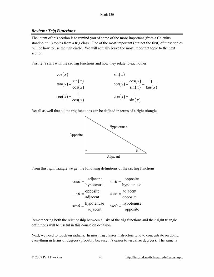
Recall as well that all the trig functions can be defined in terms of a right triangle.
From this right triangle we get the following definitions of the six trig functions.
adjacentcoshypotenuse
θ = oppositesin
hypotenuseθ =
oppositetanadjacent
θ = adjacentcotopposite
θ =
hypotenusesecadjacent
θ = hypotenusecsc
oppositeθ =
Remembering both the relationship between all six of the trig functions and their right triangle definitions will be useful in this course on occasion. Next, we need to touch on radians. In most trig classes instructors tend to concentrate on doing everything in terms of degrees (probably because it’s easier to visualize degrees). The same is

Math 130
© 2007 Paul Dawkins 21 http://tutorial.math.lamar.edu/terms.aspx
true in many science classes. However, in a calculus course almost everything is done in radians. The following table gives some of the basic angles in both degrees and radians.
Degree 0 30 45 60 90 180 270 360
Radians 0 6π
4π
3π
2π
π 32π
2π
Know this table! We may not see these specific angles all that much when we get into the Calculus portion of these notes, but knowing these can help us to visualize each angle. Now, one more time just make sure this is clear. Be forewarned, everything in most calculus classes will be done in radians! Let’s next take a look at one of the most overlooked ideas from a trig class. The unit circle is one of the more useful tools to come out of a trig class. Unfortunately, most people don’t learn it as well as they should in their trig class. Below is the unit circle with just the first quadrant filled in. The way the unit circle works is to draw a line from the center of the circle outwards corresponding to a given angle. Then look at the coordinates of the point where the line and the circle intersect. The first coordinate is the cosine of that angle and the second coordinate is the sine of that angle. We’ve put some of the basic angles along with the coordinates of their intersections on the unit circle. So, from the unit
circle below we can see that 3cos
6 2π =
and
1sin6 2π =
.
Math 130
© 2007 Paul Dawkins 22 http://tutorial.math.lamar.edu/terms.aspx
Remember how the signs of angles work. If you rotate in a counter clockwise direction the angle is positive and if you rotate in a clockwise direction the angle is negative. Recall as well that one complete revolution is 2π , so the positive x-axis can correspond to either an angle of 0 or 2π (or 4π , or 6π , or 2π− , or 4π− , etc. depending on the direction of rotation). Likewise, the angle 6
π (to pick an angle completely at random) can also be any of the following angles:
1326 6π π
π+ = (start at 6π
then rotate once around counter clockwise)
254
6 6π π
π+ = (start at 6π
then rotate around twice counter clockwise)
112
6 6π π
π− = − (start at 6π
then rotate once around clockwise)
234
6 6π π
π− = − (start at 6π
then rotate around twice clockwise)
etc.
In fact 6
π can be any of the following angles 6 2 , 0, 1, 2, 3,n nπ π+ = ± ± ± … In this case n is
the number of complete revolutions you make around the unit circle starting at 6π . Positive
values of n correspond to counter clockwise rotations and negative values of n correspond to clockwise rotations. So, why did I only put in the first quadrant? The answer is simple. If you know the first quadrant then you can get all the other quadrants from the first with a small application of geometry. You’ll see how this is done in the following set of examples. Example 1 Evaluate each of the following.
(a) 2sin3π
and 2sin3π −
[Solution]
(b) 7cos6π
and 7cos6π −
[Solution]
(c) tan4π −
and
7tan4π
[Solution]
(d) 25sec6π
[Solution]

Math 130
© 2007 Paul Dawkins 23 http://tutorial.math.lamar.edu/terms.aspx
Solution
(a) The first evaluation in this part uses the angle 23π
. That’s not on our unit circle above,
however notice that 23 3π π
π= − . So 23π
is found by rotating up 3π
from the negative x-axis.
This means that the line for 23π
will be a mirror image of the line for 3π
only in the second
quadrant. The coordinates for 23π
will be the coordinates for 3π
except the x coordinate will be
negative.
Likewise for 23π
− we can notice that 23 3π π
π− = − + , so this angle can be found by rotating
down 3π
from the negative x-axis. This means that the line for 23π
− will be a mirror image of
the line for 3π
only in the third quadrant and the coordinates will be the same as the coordinates
for 3π
except both will be negative.
Both of these angles along with their coordinates are shown on the following unit circle.
From this unit circle we can see that 2 3sin3 2π =
and
2 3sin3 2π − = −
.

Math 130
© 2007 Paul Dawkins 24 http://tutorial.math.lamar.edu/terms.aspx
This leads to a nice fact about the sine function. The sine function is called an odd function and so for ANY angle we have
( ) ( )sin sinθ θ− = − [Return to Problems]
(b) For this example notice that 76 6π π
π= + so this means we would rotate down 6π
from the
negative x-axis to get to this angle. Also 76 6π π
π− = − − so this means we would rotate up 6π
from the negative x-axis to get to this angle. So, as with the last part, both of these angles will be
mirror images of 6π
in the third and second quadrants respectively and we can use this to
determine the coordinates for both of these new angles. Both of these angles are shown on the following unit circle along with appropriate coordinates for the intersection points.
From this unit circle we can see that 7 3cos6 2π = −
and
7 3cos6 2π − = −
. In this case
the cosine function is called an even function and so for ANY angle we have
( ) ( )cos cosθ θ− = . [Return to Problems]
Math 130
© 2007 Paul Dawkins 25 http://tutorial.math.lamar.edu/terms.aspx
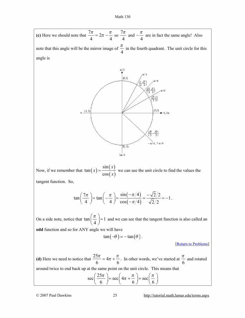
(c) Here we should note that 7 24 4π π
π= − so 74π
and 4π
− are in fact the same angle! Also
note that this angle will be the mirror image of 4π
in the fourth quadrant. The unit circle for this
angle is
Now, if we remember that ( ) ( )( )
sintan
cosx
xx
= we can use the unit circle to find the values the
tangent function. So,
( )( )
sin 47 2 2tan tan 14 4 cos 4 2 2
ππ ππ
− − = − = = = − − .
On a side note, notice that tan 14π =
and we can see that the tangent function is also called an
odd function and so for ANY angle we will have
( ) ( )tan tanθ θ− = − . [Return to Problems]
(d) Here we need to notice that 25 4
6 6π π
π= + . In other words, we’ve started at 6π
and rotated
around twice to end back up at the same point on the unit circle. This means that
25sec sec 4 sec6 6 6π π π
π = + =

Math 130
© 2007 Paul Dawkins 26 http://tutorial.math.lamar.edu/terms.aspx
Now, let’s also not get excited about the secant here. Just recall that
( ) ( )1sec
cosx
x=
and so all we need to do here is evaluate a cosine! Therefore,
25 1 1 2sec sec6 6 3 3cos 26
π ππ
= = = =
[Return to Problems] So, in the last example we saw how the unit circle can be used to determine the value of the trig functions at any of the “common” angles. It’s important to notice that all of these examples used the fact that if you know the first quadrant of the unit circle and can relate all the other angles to “mirror images” of one of the first quadrant angles you don’t really need to know whole unit circle. If you’d like to see a complete unit circle I’ve got one on my Trig Cheat Sheet that is available at http://tutorial.math.lamar.edu. Another important idea from the last example is that when it comes to evaluating trig functions all that you really need to know is how to evaluate sine and cosine. The other four trig functions are defined in terms of these two so if you know how to evaluate sine and cosine you can also evaluate the remaining four trig functions. We’ve not covered many of the topics from a trig class in this section, but we did cover some of the more important ones from a calculus standpoint. There are many important trig formulas that you will use occasionally in a calculus class. Most notably are the half-angle and double-angle formulas. If you need reminded of what these are, you might want to download my Trig Cheat Sheet as most of the important facts and formulas from a trig class are listed there.

Math 130
© 2007 Paul Dawkins 27 http://tutorial.math.lamar.edu/terms.aspx
Review : Solving Trig Equations In this section we will take a look at solving trig equations. This is something that you will be asked to do on a fairly regular basis in my class. Let’s just jump into the examples and see how to solve trig equations.
Example 1 Solve ( )2cos 3t = . Solution There’s really not a whole lot to do in solving this kind of trig equation. All we need to do is divide both sides by 2 and the go to the unit circle.
( )
( )
2cos 3
3cos2
t
t
=
=
So, we are looking for all the values of t for which cosine will have the value of 3
2. So, let’s
take a look at the following unit circle.
From quick inspection we can see that 6
t π= is a solution. However, as I have shown on the unit

Math 130
© 2007 Paul Dawkins 28 http://tutorial.math.lamar.edu/terms.aspx
circle there is another angle which will also be a solution. We need to determine what this angle is. When we look for these angles we typically want positive angles that lie between 0 and 2π . This angle will not be the only possibility of course, but by convention we typically look for angles that meet these conditions. To find this angle for this problem all we need to do is use a little geometry. The angle in the first
quadrant makes an angle of 6π
with the positive x-axis, then so must the angle in the fourth
quadrant. So we could use 6π
− , but again, it’s more common to use positive angles so, we’ll use
1126 6
t π ππ= − = .
We aren’t done with this problem. As the discussion about finding the second angle has shown
there are many ways to write any given angle on the unit circle. Sometimes it will be 6π
− that
we want for the solution and sometimes we will want both (or neither) of the listed angles. Therefore, since there isn’t anything in this problem (contrast this with the next problem) to tell us which is the correct solution we will need to list ALL possible solutions. This is very easy to do. Recall from the previous section and you’ll see there that I used
2 , 0, 1, 2, 3,6
n nππ+ = ± ± ± …
to represent all the possible angles that can end at the same location on the unit circle, i.e. angles
that end at 6π
. Remember that all this says is that we start at 6π
then rotate around in the
counter-clockwise direction (n is positive) or clockwise direction (n is negative) for n complete rotations. The same thing can be done for the second solution. So, all together the complete solution to this problem is
2 , 0, 1, 2, 3,
611 2 , 0, 1, 2, 3,
6
n n
n n
ππ
ππ
+ = ± ± ±
+ = ± ± ±
…
…
As a final thought, notice that we can get 6π
− by using 1n = − in the second solution.
Now, in a calculus class this is not a typical trig equation that we’ll be asked to solve. A more typical example is the next one.

Math 130
© 2007 Paul Dawkins 29 http://tutorial.math.lamar.edu/terms.aspx
Example 2 Solve ( )2cos 3t = on [ 2 ,2 ]π π− . Solution In a calculus class we are often more interested in only the solutions to a trig equation that fall in a certain interval. The first step in this kind of problem is to first find all possible solutions. We did this in the first example.
2 , 0, 1, 2, 3,
611 2 , 0, 1, 2, 3,
6
n n
n n
ππ
ππ
+ = ± ± ±
+ = ± ± ±
…
…
Now, to find the solutions in the interval all we need to do is start picking values of n, plugging them in and getting the solutions that will fall into the interval that we’ve been given. n=0.
( )
( )
2 0 26 611 112 0 2
6 6
π ππ π
π ππ π
+ = <
+ = <
Now, notice that if we take any positive value of n we will be adding on positive multiples of 2π onto a positive quantity and this will take us past the upper bound of our interval and so we don’t need to take any positive value of n. However, just because we aren’t going to take any positive value of n doesn’t mean that we shouldn’t also look at negative values of n. n=-1.
( )
( )
112 1 26 611 2 1 2
6 6
π ππ π
π ππ π
+ − = − > −
+ − = − > −
These are both greater than 2π− and so are solutions, but if we subtract another 2π off (i.e use 2n = − ) we will once again be outside of the interval so we’ve found all the possible solutions
that lie inside the interval [ 2 ,2 ]π π− .
So, the solutions are : 11 11, , ,
6 6 6 6π π π π
− − .
So, let’s see if you’ve got all this down.
Math 130
© 2007 Paul Dawkins 30 http://tutorial.math.lamar.edu/terms.aspx
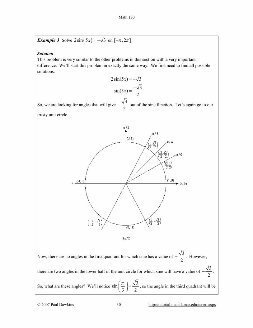
Example 3 Solve ( )2sin 5 3x = − on [ , 2 ]π π− Solution This problem is very similar to the other problems in this section with a very important difference. We’ll start this problem in exactly the same way. We first need to find all possible solutions.
2sin(5 ) 3
3sin(5 )2
x
x
= −
−=
So, we are looking for angles that will give 3
2− out of the sine function. Let’s again go to our
trusty unit circle.
Now, there are no angles in the first quadrant for which sine has a value of 3
2− . However,
there are two angles in the lower half of the unit circle for which sine will have a value of 3
2− .
So, what are these angles? We’ll notice 3sin
3 2π =
, so the angle in the third quadrant will be

Math 130
© 2007 Paul Dawkins 31 http://tutorial.math.lamar.edu/terms.aspx
3π
below the negative x-axis or 4
3 3π π
π + = . Likewise, the angle in the fourth quadrant will 3π
below the positive x-axis or 52
3 3π π
π − = . Remember that we’re typically looking for positive
angles between 0 and 2π . Now we come to the very important difference between this problem and the previous problems in this section. The solution is NOT
4 2 , 0, 1, 2,3
5 2 , 0, 1, 2,3
x n n
x n n
ππ
ππ
= + = ± ±
= + = ± ±
…
…
This is not the set of solutions because we are NOT looking for values of x for which
( ) 3sin2
x = − , but instead we are looking for values of x for which ( ) 3sin 52
x = − . Note the
difference in the arguments of the sine function! One is x and the other is 5x . This makes all the difference in the world in finding the solution! Therefore, the set of solutions is
45 2 , 0, 1, 2,3
55 2 , 0, 1, 2,3
x n n
x n n
ππ
ππ
= + = ± ±
= + = ± ±
…
…
Well, actually, that’s not quite the solution. We are looking for values of x so divide everything by 5 to get.
4 2 , 0, 1, 2,15 5
2 , 0, 1, 2,3 5
nx n
nx n
π π
π π
= + = ± ±
= + = ± ±
…
…
Notice that we also divided the 2 nπ by 5 as well! This is important! If we don’t do that you WILL miss solutions. For instance, take 1n = .
4 2 10 2 2 10 3sin 5 sin15 5 15 3 3 3 2
2 11 11 11 3sin 5 sin3 5 15 15 3 2
x
x
π π π π π π
π π π π π
= + = = ⇒ = = −
= + = ⇒ = = −
I’ll leave it to you to verify my work showing they are solutions. However it makes the point. If you didn’t divided the 2 nπ by 5 you would have missed these solutions! Okay, now that we’ve gotten all possible solutions it’s time to find the solutions on the given interval. We’ll do this as we did in the previous problem. Pick values of n and get the solutions.
Math 130
© 2007 Paul Dawkins 32 http://tutorial.math.lamar.edu/terms.aspx
n = 0.
( )
( )
2 04 4 215 5 15
2 02
3 5 3
x
x
ππ π π
ππ ππ
= + = <
= + = <
n = 1.
( )
( )
2 14 2 215 5 3
2 1 11 23 5 15
x
x
ππ π π
ππ ππ
= + = <
= + = <
n = 2.
( )
( )
2 24 16 215 5 15
2 2 17 23 5 15
x
x
ππ π π
ππ ππ
= + = <
= + = <
n = 3.
( )
( )
2 34 22 215 5 15
2 3 23 23 5 15
x
x
ππ π π
ππ ππ
= + = <
= + = <
n = 4.
( )
( )
2 44 28 215 5 15
2 4 29 23 5 15
x
x
ππ π π
ππ ππ
= + = <
= + = <
n = 5.
( )
( )
2 54 34 215 5 15
2 5 35 23 5 15
x
x
ππ π π
ππ ππ
= + = >
= + = >
Okay, so we finally got past the right endpoint of our interval so we don’t need any more positive n. Now let’s take a look at the negative n and see what we’ve got. n = –1 .
( )
( )
2 14 215 5 15
2 13 5 15
x
x
ππ π π
ππ ππ
−= + = − > −
−= + = − > −

Math 130
© 2007 Paul Dawkins 33 http://tutorial.math.lamar.edu/terms.aspx
n = –2.
( )
( )
2 24 815 5 15
2 2 73 5 15
x
x
ππ π π
ππ ππ
−= + = − > −
−= + = − > −
n = –3.
( )
( )
2 34 1415 5 15
2 3 133 5 15
x
x
ππ π π
ππ ππ
−= + = − > −
−= + = − > −
n = –4.
( )
( )
2 44 415 5 3
2 4 193 5 15
x
x
ππ π π
ππ ππ
−= + = − < −
−= + = − < −
And we’re now past the left endpoint of the interval. Sometimes, there will be many solutions as there were in this example. Putting all of this together gives the following set of solutions that lie in the given interval.
4 2 11 16 17 22 23 28 29, , , , , , , , ,15 3 3 15 15 15 15 15 15 15
2 7 8 13 14, , , , ,15 15 15 15 15 15
π π π π π π π π π π
π π π π π π− − − − − −
Let’s work another example.
Example 4 Solve ( ) ( )sin 2 cos 2x x= − on 3 3,2 2π π −
Solution This problem is a little different from the previous ones. First, we need to do some rearranging and simplification.
( )
sin(2 ) cos(2 )sin(2 ) 1cos(2 )tan 2 1
x xxxx
= −
= −
= −
So, solving sin(2 ) cos(2 )x x= − is the same as solving tan(2 ) 1x = − . At some level we didn’t need to do this for this problem as all we’re looking for is angles in which sine and cosine have the same value, but opposite signs. However, for other problems this won’t be the case and we’ll want to convert to tangent.

Math 130
© 2007 Paul Dawkins 34 http://tutorial.math.lamar.edu/terms.aspx
Looking at our trusty unit circle it appears that the solutions will be,
32 2 , 0, 1, 2,4
72 2 , 0, 1, 2,4
x n n
x n n
ππ
ππ
= + = ± ±
= + = ± ±
…
…
Or, upon dividing by the 2 we get all possible solutions.
3 , 0, 1, 2,8
7 , 0, 1, 2,8
x n n
x n n
ππ
ππ
= + = ± ±
= + = ± ±
…
…
Now, let’s determine the solutions that lie in the given interval. n = 0.
( )
( )
3 3 308 8 2
7 7 308 8 2
x
x
π π ππ
π π ππ
= + = <
= + = <
n = 1.
( )
( )
3 11 318 8 2
7 15 318 8 2
x
x
π π ππ
π π ππ
= + = <
= + = >
Unlike the previous example only one of these will be in the interval. This will happen occasionally so don’t always expect both answers from a particular n to work. Also, we should now check n=2 for the first to see if it will be in or out of the interval. I’ll leave it to you to check that it’s out of the interval. Now, let’s check the negative n. n = –1.
( )
( )
3 5 318 8 2
7 318 8 2
x
x
π π ππ
π π ππ
= + − = − > −
= + − = − > −
n = –2.
( )
( )
3 13 328 8 2
7 9 328 8 2
x
x
π π ππ
π π ππ
= + − = − < −
= + − = − > −
Again, only one will work here. I’ll leave it to you to verify that n = –3 will give two answers
Math 130
© 2007 Paul Dawkins 35 http://tutorial.math.lamar.edu/terms.aspx
that are both out of the interval. The complete list of solutions is then,
9 5 3 7 11, , , , ,8 8 8 8 8 8π π π π π π
− − −
Let’s work one more example so that I can make a point that needs to be understood when solving some trig equations. Example 5 Solve ( )cos 3 2x = . Solution This example is designed to remind you of certain properties about sine and cosine. Recall that
( )1 cos 1θ− ≤ ≤ and ( )1 sin 1θ− ≤ ≤ . Therefore, since cosine will never be greater that 1 it
definitely can’t be 2. So THERE ARE NO SOLUTIONS to this equation! It is important to remember that not all trig equations will have solutions. In this section we solved some simple trig equations. There are more complicated trig equations that we can solve so don’t leave this section with the feeling that there is nothing harder out there in the world to solve. In fact, we’ll see at least one of the more complicated problems in the next section. Also, every one of these problems came down to solutions involving one of the “common” or “standard” angles. Most trig equations won’t come down to one of those and will in fact need a calculator to solve. The next section is devoted to this kind of problem.
Math 130
© 2007 Paul Dawkins 36 http://tutorial.math.lamar.edu/terms.aspx
Review : Solving Trig Equations with Calculators, Part I In the previous section we started solving trig equations. The only problem with the equations we solved in there is that they pretty much all had solutions that came from a handful of “standard” angles and of course there are many equations out there that simply don’t. So, in this section we are going to take a look at some more trig equations, the majority of which will require the use of a calculator to solve (a couple won’t need a calculator). The fact that we are using calculators in this section does not however mean that the problems in the previous section aren’t important. It is going to be assumed in this section that the basic ideas of solving trig equations are known and that we don’t need to go back over them here. In particular, it is assumed that you can use a unit circle to help you find all answers to the equation (although the process here is a little different as we’ll see) and it is assumed that you can find answers in a given interval. If you are unfamiliar with these ideas you should first go to the previous section and go over those problems. Before proceeding with the problems we need to go over how our calculators work so that we can get the correct answers. Calculators are great tools but if you don’t know how they work and how to interpret their answers you can get in serious trouble. First, as already pointed out in previous sections, everything we are going to be doing here will be in radians so make sure that your calculator is set to radians before attempting the problems in this section. Also, we are going to use 4 decimal places of accuracy in the work here. You can use more if you want, but in this class we’ll always use at least 4 decimal places of accuracy. Next, and somewhat more importantly, we need to understand how calculators give answers to inverse trig functions. We didn’t cover inverse trig functions in this review, but they are just inverse functions and we have talked a little bit about inverse functions in a review section. The only real difference is that we are now using trig functions. We’ll only be looking at three of them and they are:
( ) ( )( ) ( )( ) ( )
1
1
1
Inverse Cosine : cos arccos
Inverse Sine : sin arcsin
Inverse Tangent : tan arctan
x x
x x
x x
−
−
−
=
=
=
As shown there are two different notations that are commonly used. In these notes we’ll be using the first form since it is a little more compact. Most calculators these days will have buttons on them for these three so make sure that yours does as well. We now need to deal with how calculators give answers to these. Let’s suppose, for example, that we wanted our calculator to compute ( )1 3
4cos− . First, remember that what the calculator is
actually computing is the angle, let’s say x, that we would plug into cosine to get a value of 34 , or

Math 130
© 2007 Paul Dawkins 37 http://tutorial.math.lamar.edu/terms.aspx
( )1 3 3cos cos4 4
x x− = ⇒ =
So, in other words, when we are using our calculator to compute an inverse trig function we are really solving a simple trig equation. Having our calculator compute ( )1 3
4cos− and hence solve ( ) 34cos x = gives,
1 3cos 0.72274
x − = =
From the previous section we know that there should in fact be an infinite number of answers to this including a second angle that is in the interval [ ]0, 2π . However, our calculator only gave us
a single answer. How to determine what the other angles are will be covered in the following examples so we won’t go into detail here about that. We did need to point out however, that the calculators will only give a single answer and that we’re going to have more work to do than just plugging a number into a calculator. Since we know that there are supposed to be an infinite number of solutions to ( ) 3
4cos x = the
next question we should ask then is just how did the calculator decide to return the answer that it did? Why this one and not one of the others? Will it give the same answer every time? There are rules that determine just what answer the calculator gives. All calculators will give answers in the following ranges.
( ) ( ) ( )1 1 10 cos sin tan2 2 2 2
x x xπ π π ππ− − −≤ ≤ − ≤ ≤ − < <
If you think back to the unit circle and recall that we think of cosine as the horizontal axis then we can see that we’ll cover all possible values of cosine in the upper half of the circle and this is exactly the range given above for the inverse cosine. Likewise, since we think of sine as the vertical axis in the unit circle we can see that we’ll cover all possible values of sine in the right half of the unit circle and that is the range given above. For the tangent range look back to the graph of the tangent function itself and we’ll see that one branch of the tangent is covered in the range given above and so that is the range we’ll use for inverse tangent. Note as well that we don’t include the endpoints in the range for inverse tangent since tangent does not exist there. So, if we can remember these rules we will be able to determine the remaining angle in [ ]0, 2π
that also works for each solution.

Math 130
© 2007 Paul Dawkins 38 http://tutorial.math.lamar.edu/terms.aspx
As a final quick topic let’s note that it will, on occasion, be useful to remember the decimal representations of some basic angles. So here they are,
31.5708 3.1416 4.7124 2 6.28322 2π π
π π= = = =
Using these we can quickly see that ( )1 3
4cos− must be in the first quadrant since 0.7227 is
between 0 and 1.5708. This will be of great help when we go to determine the remaining angles So, once again, we can’t stress enough that calculators are great tools that can be of tremendous help to us, but it you don’t understand how they work you will often get the answers to problems wrong. So, with all that out of the way let’s take a look at our first problem. Example 1 Solve ( )4cos 3t = on[-8,10]. Solution Okay, the first step here is identical to the problems in the previous section. We first need to isolate the cosine on one side by itself and then use our calculator to get the first answer.
( ) 13 3cos cos 0.72274 4
t t − = ⇒ = =
So, this is the one we were using above in the opening discussion of this section. At the time we mentioned that there were infinite number of answers and that we’d be seeing how to find them later. Well that time is now. First, let’s take a quick look at a unit circle for this example.
The angle that we’ve found is shown on the circle as well as the other angle that we know should also be an answer. Finding this angle here is just as easy as in the previous section. Since the

Math 130
© 2007 Paul Dawkins 39 http://tutorial.math.lamar.edu/terms.aspx
line segment in the first quadrant forms an angle of 0.7227 radians with the positive x-axis then so does the line segment in the fourth quadrant. This means that we can use either -0.7227 as the second angle or 2 0.7227 5.5605π − = . Which you use depends on which you prefer. We’ll pretty much always use the positive angle to avoid the possibility that we’ll lose the minus sign. So, all possible solutions, ignoring the interval for a second, are then,
0.7227 2
0, 1, 2,5.5605 2
t nn
t nππ
= += ± ±
= +…
Now, all we need to do is plug in values of n to determine the angle that are actually in the interval. Here’s the work for that.
2 : 11.8437n t= − = − and 7.00591 : 5.5605 and 0.7227
0 : 0.7227 and 5.5605
1 : 7.0059 and 11.8437
n tn t
n t
−= − = − −= =
= =
So, the solutions to this equation, in the given interval, are, 7.0059, 5.5605, 0.7227, 0.7227, 5.5605, 7.0059t = − − − Note that we had a choice of angles to use for the second angle in the previous example. The choice of angles there will also affect the value(s) of n that we’ll need to use to get all the solutions. In the end, regardless of the angle chosen, we’ll get the same list of solutions, but the value(s) of n that give the solutions will be different depending on our choice. Also, in the above example we put in a little more explanation than we’ll show in the remaining examples in this section to remind you how these work.
Example 2 Solve ( )10cos 3 7t− = on [-2,5]. Solution Okay, let’s first get the inverse cosine portion of this problem taken care of.
( ) 17 7cos 3 3 cos 2.346210 10
t t − = − ⇒ = − =
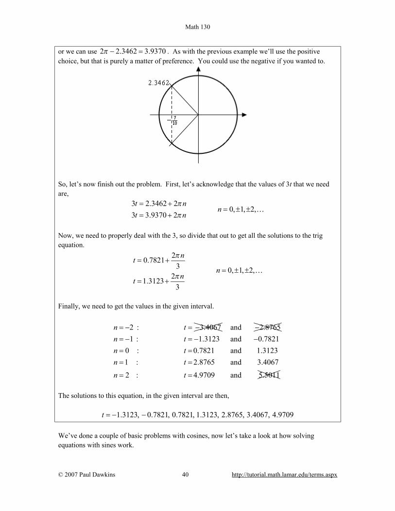
Don’t forget that we still need the “3”! Now, let’s look at a quick unit circle for this problem. As we can see the angle 2.3462 radians is in the second quadrant and the other angle that we need is in the third quadrant. We can find this second angle in exactly the same way we did in the previous example. We can use either -2.3462
Math 130
© 2007 Paul Dawkins 40 http://tutorial.math.lamar.edu/terms.aspx
or we can use 2 2.3462 3.9370π − = . As with the previous example we’ll use the positive choice, but that is purely a matter of preference. You could use the negative if you wanted to.
So, let’s now finish out the problem. First, let’s acknowledge that the values of 3t that we need are,
3 2.3462 2
0, 1, 2,3 3.9370 2t n
nt n
ππ
= += ± ±
= +…
Now, we need to properly deal with the 3, so divide that out to get all the solutions to the trig equation.
20.78213 0, 1, 2,
21.31233
ntn
nt
π
π
= += ± ±
= +…
Finally, we need to get the values in the given interval.
2 : 3.4067n t= − = − and 2.8765−1 : 1.3123 and 0.7821
0 : 0.7821 and 1.31231 : 2.8765 and 3.4067
2 : 4.9709 and 5.5011
n tn tn t
n t
= − = − −= == =
= =
The solutions to this equation, in the given interval are then, 1.3123, 0.7821, 0.7821, 1.3123, 2.8765, 3.4067, 4.9709t = − − We’ve done a couple of basic problems with cosines, now let’s take a look at how solving equations with sines work.
Math 130
© 2007 Paul Dawkins 41 http://tutorial.math.lamar.edu/terms.aspx
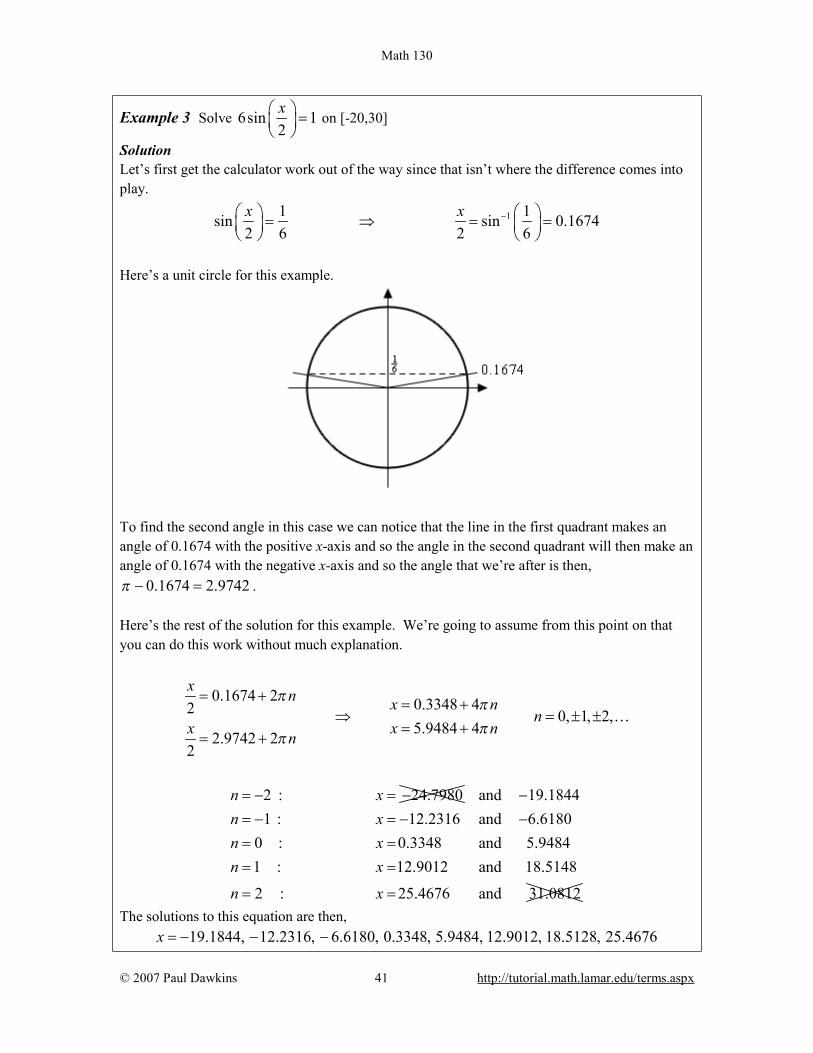
Example 3 Solve 6sin 12x =
on [-20,30]
Solution Let’s first get the calculator work out of the way since that isn’t where the difference comes into play.
11 1sin sin 0.16742 6 2 6x x − = ⇒ = =
Here’s a unit circle for this example.
To find the second angle in this case we can notice that the line in the first quadrant makes an angle of 0.1674 with the positive x-axis and so the angle in the second quadrant will then make an angle of 0.1674 with the negative x-axis and so the angle that we’re after is then,
0.1674 2.9742π − = . Here’s the rest of the solution for this example. We’re going to assume from this point on that you can do this work without much explanation.
0.1674 2 0.3348 42 0, 1, 2,
5.9484 42.9742 22
x n x nn
x x nn
π ππ
π
= + = +⇒ = ± ±
= += +
…
2 : 24.7980n x= − = − and 19.18441 : 12.2316 and 6.6180
0 : 0.3348 and 5.94841 : 12.9012 and 18.5148
2 : 25.4676 and 31.0812
n xn xn x
n x
−= − = − −= == =
= =
The solutions to this equation are then, 19.1844, 12.2316, 6.6180, 0.3348, 5.9484, 12.9012, 18.5128, 25.4676x = − − −

Math 130
© 2007 Paul Dawkins 42 http://tutorial.math.lamar.edu/terms.aspx
Example 4 Solve ( )3sin 5 2z = − on [0,1]. Solution You should be getting pretty good at these by now, so we won’t be putting much explanation in for this one. Here we go.
( ) 12 2sin 5 5 sin 0.72973 3
z z − = − ⇒ = − = −
Okay, with this one we’re going to do a little more work than with the others. For the first angle we could use the answer our calculator gave us. However, it’s easy to lose minus signs so we’ll instead use 2 0.7297 5.5535π − = . Again, there is no reason to this other than a worry about losing the minus sign in the calculator answer. If you’d like to use the calculator answer you are more than welcome to. For the second angle we’ll note that the lines in the third and fourth quadrant make an angle of 0.7297 with the x-axis and so the second angle is
0.7297 3.8713π + = . Here’s the rest of the work for this example.
21.11075 5.5535 2 5 0, 1, 2,5 3.8713 2 20.7743
5
nzz nn
z n nz
πππ π
= += +⇒ = ± ±
= += +
…
1 : 0.1460n x= − = − and 0.4823−
0 : 1.1107n x= = and 0.7743
So, in this case we get a single solution of 0.7743. Note that in the previous example we only got a single solution. This happens on occasion so don’t get worried about it. Also, note that it was the second angle that gave this solution and so if
Math 130
© 2007 Paul Dawkins 43 http://tutorial.math.lamar.edu/terms.aspx
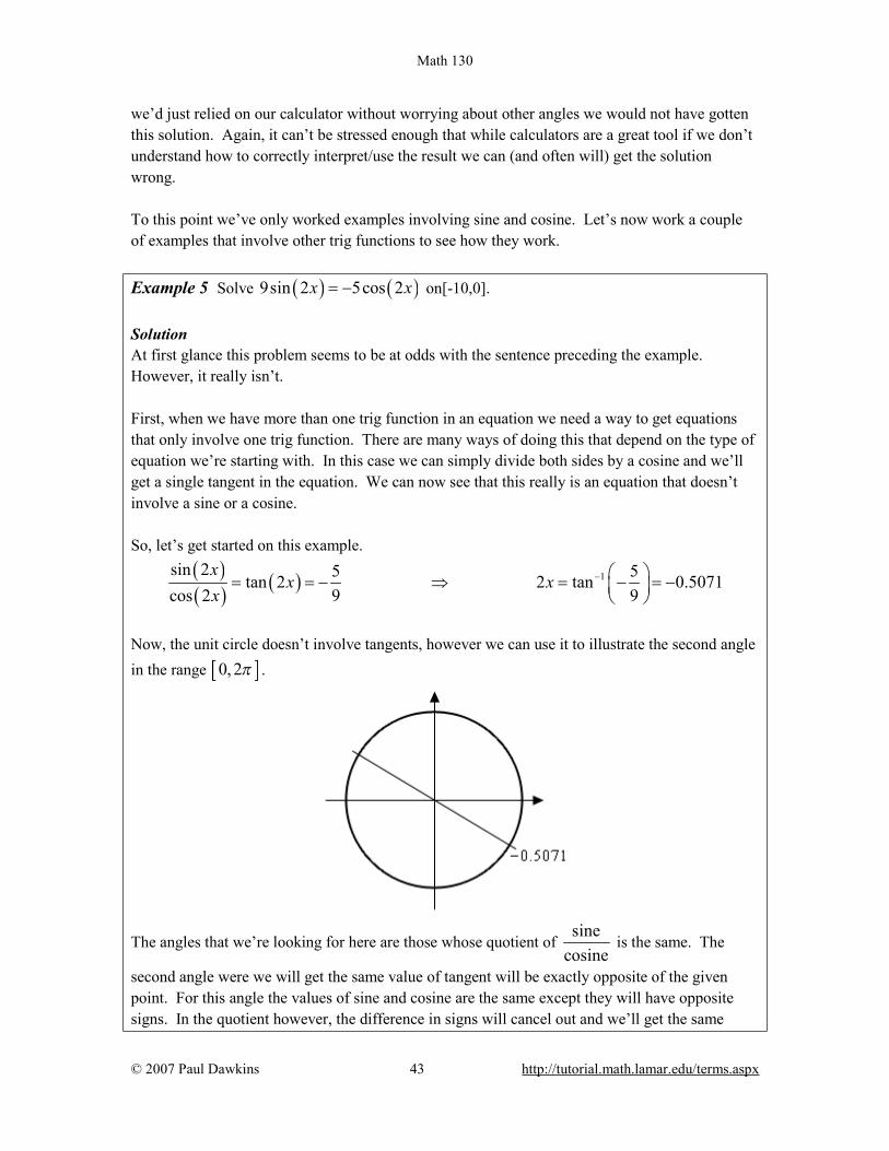
we’d just relied on our calculator without worrying about other angles we would not have gotten this solution. Again, it can’t be stressed enough that while calculators are a great tool if we don’t understand how to correctly interpret/use the result we can (and often will) get the solution wrong. To this point we’ve only worked examples involving sine and cosine. Let’s now work a couple of examples that involve other trig functions to see how they work. Example 5 Solve ( ) ( )9sin 2 5cos 2x x= − on[-10,0]. Solution At first glance this problem seems to be at odds with the sentence preceding the example. However, it really isn’t. First, when we have more than one trig function in an equation we need a way to get equations that only involve one trig function. There are many ways of doing this that depend on the type of equation we’re starting with. In this case we can simply divide both sides by a cosine and we’ll get a single tangent in the equation. We can now see that this really is an equation that doesn’t involve a sine or a cosine. So, let’s get started on this example.
( )( ) ( ) 1sin 2 5 5tan 2 2 tan 0.5071
cos 2 9 9x
x xx
− = = − ⇒ = − = −
Now, the unit circle doesn’t involve tangents, however we can use it to illustrate the second angle in the range [ ]0, 2π .
The angles that we’re looking for here are those whose quotient of sine
cosine is the same. The
second angle were we will get the same value of tangent will be exactly opposite of the given point. For this angle the values of sine and cosine are the same except they will have opposite signs. In the quotient however, the difference in signs will cancel out and we’ll get the same

Math 130
© 2007 Paul Dawkins 44 http://tutorial.math.lamar.edu/terms.aspx
value of tangent. So, the second angle will always be the first angle plus π . Before getting the second angle let’s also note that, like the previous example, we’ll use the 2 0.5071 5.7761π − = for the first angle. Again, this is only because of a concern about losing track of the minus sign in our calculator answer. We could just as easily do the work with the original angle our calculator gave us. Now, this is where is seems like we’re just randomly making changes and doing things for no reason. The second angle that we’re going to use is,
( )0.5071 0.5071 2.6345π π+ − = − =
The fact that we used the calculator answer here seems to contradict the fact that we used a different angle for the first above. The reason for doing this here is to give a second angle that is in the range [ ]0, 2π . Had we used 5.7761 to find the second angle we’d get
5.7761 8.9177π + = . This is a perfectly acceptable answer, however it is larger than 2π (6.2832) and the general rule of thumb is to keep the initial angles as small as possible. Here are all the solutions to the equation.
2 5.7761 2 2.8881
0, 1, 2,2 2.6345 2 1.3173
x n x nn
x n x nπ ππ π
= + = +⇒ = ± ±
= + = +…
4 : 9.6783 and 11.2491n x= − = − −3 : 6.5367 and 8.10752 : 3.3951 and 4.96591 : 0.2535 and 1.8243
0 : 2.8881
n xn xn x
n x
= − = − −= − = − −= − = − −
= = and 1.3173
The seven solutions to this equation are then, 0.2535, 1.8243, 3.3951, 4.9659, 6.5367, 8.1075, 9.6783− − − − − − − Note as well that we didn’t need to do the 0n = and computation since we could see from the given interval that we only wanted negative answers and these would clearly give positive answers. Most calculators today can only do inverse sine, inverse cosine, and inverse tangent. So, let’s see an example that uses one of the other trig functions.

Math 130
© 2007 Paul Dawkins 45 http://tutorial.math.lamar.edu/terms.aspx
Example 6 Solve ( )7sec 3 10t = − . Solution We’ll start this one in exactly the same way we’ve done all the others.
( ) 110 10sec 3 3 sec7 7
t t − = − ⇒ = −
Now we reach the problem. As noted above, most calculators can’t handle inverse secant so we’re going to need a different solution method for this one. To finish the solution here we’ll simply recall the definition of secant in terms of cosine and convert this into an equation involving cosine instead and we already know how to solve those kinds of trig equations.
( ) ( ) ( )1 10 7sec 3 cos 3
cos 3 7 10t t
t= = − ⇒ = −
Now, we solved this equation in the second example above so we won’t redo our work here. The solution is,
20.78213 0, 1, 2,
21.31233
ntn
nt
π
π
= += ± ±
= +…
We weren’t given an interval in this problem so here is nothing else to do here. For the remainder of the examples in this section we’re not going to be finding solutions in an interval to save some space. If you followed the work from the first few examples in which we were given intervals you should be able to do any of the remaining examples if given an interval. Also, we will no longer be including sketches of unit circles in the remaining solutions. We are going to assume that you can use the above sketches as guides for sketching unit circles to verify our claims in the following examples. The next three examples don’t require a calculator but are important enough or cause enough problems for students to include in this section in case you run across them and haven’t seen them anywhere else.

Math 130
© 2007 Paul Dawkins 46 http://tutorial.math.lamar.edu/terms.aspx
Example 7 Solve ( )cos 4 1θ = − . Solution There really isn’t too much to do with this problem. It is, however, different from all the others done to this point. All the others done to this point have had two angles in the interval [ ]0, 2π
that were solutions to the equation. This only has one. Here is the solution to this equation.
4 2 0, 1, 2,4 2
nn nπ πθ π π θ= + ⇒ = + = ± ± …
Example 8 Solve sin 07α =
.
Solution Again, not much to this problem. Using a unit circle it isn’t too hard to see that the solutions to this equation are,
0 2 147 0, 1, 2,
7 1427
n nn
nn
απ α π
α α π ππ π
= + =⇒ = ± ±
= += +
…
This next example has an important point that needs to be understood when solving some trig equations. Example 9 Solve ( )sin 3 2t = . Solution This example is designed to remind you of certain properties about sine and cosine. Recall that
( )1 sin 1θ− ≤ ≤ and ( )1 cos 1θ− ≤ ≤ . Therefore, since sine will never be greater that 1 it
definitely can’t be 2. So THERE ARE NO SOLUTIONS to this equation! It is important to remember that not all trig equations will have solutions. Because this document is also being prepared for viewing on the web we’re going to split this section in two in order to keep the page size (and hence load time in a browser) to a minimum. In the next section we’re going to take a look at some slightly more “complicated” equations. Although, as you’ll see, they aren’t as complicated as they may at first seem.

Math 130
© 2007 Paul Dawkins 47 http://tutorial.math.lamar.edu/terms.aspx
Review : Solving Trig Equations with Calculators, Part II Because this document is also being prepared for viewing on the web we split this section into two parts to keep the size of the pages to a minimum. Also, as with the last few examples in the previous part of this section we are not going to be looking for solutions in an interval in order to save space. The important part of these examples is to find the solutions to the equation. If we’d been given an interval it would be easy enough to find the solutions that actually fall in the interval.
In all the examples in the previous section all the arguments, the 3t , 7α
, etc., were fairly simple.
Let’s take a look at an example that has a slightly more complicated argument. Example 1 Solve ( )5cos 2 1 3x − = − . Solution Note that the argument here is not really all that complicated but the addition of the “-1” often seems to confuse people so we need to a quick example with this kind of argument. The solution process is identical to all the problems we’ve done to this point so we won’t be putting in much explanation. Here is the solution.
( ) 13 3cos 2 1 2 1 cos 2.21435 5
x x − − = − ⇒ − = − =
This angle is in the second quadrant and so we can use either -2.2143 or 2 2.2143 4.0689π − = for the second angle. As usual for these notes we’ll use the positive one. Therefore the two angles are,
2 1 2.2143 2
0, 1, 2,2 1 4.0689 2
x nn
x nππ
− = += ± ±
− = +…
Now, we still need to find the actual values of x that are the solutions. These are found in the same manner as all the problems above. We’ll first add 1 to both sides and then divide by 2. Doing this gives,
1.6072
0, 1, 2,2.5345
x nn
x nππ
= += ± ±
= +…
So, in this example we saw an argument that was a little different from those seen previously, but not all that different when it comes to working the problems so don’t get too excited about it.

Math 130
© 2007 Paul Dawkins 48 http://tutorial.math.lamar.edu/terms.aspx
We now need to move into a different type of trig equation. All of the trig equations solved to this point (the previous example as well as the previous section) were, in some way, more or less the “standard” trig equation that is usually solved in a trig class. There are other types of equations involving trig functions however that we need to take a quick look at. The remaining examples show some of these different kinds of trig equations. Example 2 Solve ( ) ( ) ( )2cos 6 11cos 6 sin 3 0y y y+ = . Solution So, this definitely doesn’t look like any of the equations we’ve solved to this point and initially the process is different as well. First, notice that there is a ( )cos 6y in each term, so let’s factor
that out and see what we have. ( ) ( )( )cos 6 2 11sin 3 0y y+ =
We now have a product of two terms that is zero and so we know that we must have, ( ) ( )cos 6 0 OR 2 11sin 3 0y y= + =
Now, at this point we have two trig equations to solve and each is identical to the type of equation we were solving earlier. Because of this we won’t put in much detail about solving these two equations. First, solving ( )cos 6 0y = gives,
6 2
12 32 0, 1, 2,36 22 4 3
nyy nn
ny n y
π πππ
π π ππ
= += +⇒ = ± ±
= + = +…
Next, solving ( )2 11sin 3 0y+ = gives,
22.03353 6.1004 2 3 0, 1, 2,3 3.3244 2 21.1081
3
nyy nn
y n ny
πππ π
= += +⇒ = ± ±
= += +
…
Remember that in these notes we tend to take positive angles and so the first solution here is in fact 2 0.1828π − where our calculator gave us -0.1828 as the answer when using the inverse sine function. The solutions to this equation are then,
Math 130
© 2007 Paul Dawkins 49 http://tutorial.math.lamar.edu/terms.aspx
12 3
4 3 0, 1, 2,22.0335
321.1081
3
ny
nyn
ny
ny
π π
π π
π
π
= +
= += ± ±
= +
= +
…
This next example also involves “factoring” trig equations but in a slightly different manner than the previous example.
Example 3 Solve 24sin 3sin 13 3t t − =
.
Solution Before solving this equation let’s solve an apparently unrelated equation.
( )( )2 2 14 3 1 4 3 1 4 1 1 0 ,14
x x x x x x x− = ⇒ − − = + − = ⇒ = −
This is an easy (or at least I hope it’s easy as this point) equation to solve. The obvious question then is, why did we do this? We’ll, if you compare the two equations you’ll see that the only real difference is that the one we just solved has an x everywhere the equation we want to solve has a sine. What this tells us is that we can work the two equations in exactly the same way. We, will first “factor” the equation as follows,
24sin 3sin 1 4sin 1 sin 1 03 3 3 3t t t t − − = + − =
Now, set each of the two factors equal to zero and solve for the sine,
1sin sin 1
3 4 3t t = − =
We now have two trig equations that we can easily (hopefully…) solve at this point. We’ll leave the details to you to verify that the solutions to each of these and hence the solutions to the original equation are,
18.0915 610.1829 6 0, 1, 2,3 62
t nt n n
t n
ππ
ππ
= += + = ± ±
= +
…
The first two solutions are from the first equation and the third solution is from the second equation.

Math 130
© 2007 Paul Dawkins 50 http://tutorial.math.lamar.edu/terms.aspx
Let’s work one more trig equation that involves solving a quadratic equation. However, this time, unlike the previous example this one won’t factor and so we’ll need to use the quadratic formula. Example 4 Solve ( ) ( )28cos 1 13cos 1 5 0x x− + − − = . Solution Now, as mentioned prior to starting the example this quadratic does not factor. However, that doesn’t mean all is lost. We can solve the following equation with the quadratic formula (you do remember this and how to use it right?),
2 13 3298 13 5 0 0.3211, 1.946116
t t t − ±+ − = ⇒ = = −
So, if we can use the quadratic formula on this then we can also use it on the equation we’re asked to solve. Doing this gives us,
( ) ( )cos 1 0.3211 OR cos 1 1.9461x x− = − = −
Now, recall Example 9 from the previous section. In that example we noted that
( )1 cos 1θ− ≤ ≤ and so the second equation will have no solutions. Therefore, the solutions to
the first equation will yield the only solutions to our original equation. Solving this gives the following set of solutions,
0.2439 20, 1, 2,
4.0393 2x n
nx n
ππ
= − −= ± ±
= − −…
Note that we did get some negative numbers here and that does seem to violate the general form that we’ve been using in most of these examples. However, in this case the “-” are coming about when we solved for x after computing the inverse cosine in our calculator. There is one more example in this section that we need to work that illustrates another way in which factoring can arise in solving trig equations. This equation is also the only one where the variable appears both inside and outside of the trig equation. Not all equations in this form can be easily solved, however some can so we want to do a quick example of one.

Math 130
© 2007 Paul Dawkins 51 http://tutorial.math.lamar.edu/terms.aspx
Example 5 Solve ( )5 tan 8 3x x x= . Solution First, before we even start solving we need to make one thing clear. DO NOT CANCEL AN x FROM BOTH SIDES!!! While this may seem like a natural thing to do it WILL cause us to lose a solution here. So, to solve this equation we’ll first get all the terms on one side of the equation and then factor an x out of the equation. If we can cancel an x from all terms then it can be factored out. Doing this gives, ( ) ( )( )5 tan 8 3 5 tan 8 3 0x x x x x− = − =
Upon factoring we can see that we must have either,
( ) 30 OR tan 85
x x= =
Note that if we’d canceled the x we would have missed the first solution. Now, we solved an equation with a tangent in it in Example 5 of the previous section so we’ll not go into the details of this solution here. Here is the solution to the trig equation.
0.0676
4 0, 1, 2,0.4603
4
nxn
nx
π
π
= += ± ±
= +…
The complete set of solutions then to the original equation are,
0
0.06764 0, 1, 2,
0.46034
xnx
nnx
π
π
=
= += ± ±
= +…

Math 130
© 2007 Paul Dawkins 52 http://tutorial.math.lamar.edu/terms.aspx
Review : Exponential Functions In this section we’re going to review one of the more common functions in both calculus and the sciences. However, before getting to this function let’s take a much more general approach to things. Let’s start with 0b > , 1b ≠ . An exponential function is then a function in the form, ( ) xf x b=
Note that we avoid 1b = because that would give the constant function, ( ) 1f x = . We avoid
0b = since this would also give a constant function and we avoid negative values of b for the following reason. Let’s, for a second, suppose that we did allow b to be negative and look at the following function.
( ) ( )4 xg x = − Let’s do some evaluation.
( ) ( ) ( )122
12 4 16 4 4 22
g g i = − = = − = − =
So, for some values of x we will get real numbers and for other values of x we well get complex numbers. We want to avoid this and so if we require 0b > this will not be a problem. Let’s take a look at a couple of exponential functions.
Example 1 Sketch the graph of ( ) 2xf x = and ( ) 12
x
g x =
Solution Let’s first get a table of values for these two functions.
x f(x) g(x)
-2 ( ) 2 12 24
f −− = = ( )212 4
2g
− − = =
-1 ( ) 1 11 22
f −− = = ( )111 2
2g
− − = =
0 ( ) 00 2 1f = = ( )010 1
2g = =
1 ( )1 2f = ( ) 112
g =
2 ( )2 4f = ( ) 124
g =
Here’s the sketch of both of these functions.

Math 130
© 2007 Paul Dawkins 53 http://tutorial.math.lamar.edu/terms.aspx
This graph illustrates some very nice properties about exponential functions in general. Properties of ( ) xf x b=
1. ( )0 1f = . The function will always take the value of 1 at 0x = .
2. ( ) 0f x ≠ . An exponential function will never be zero.
3. ( ) 0f x > . An exponential function is always positive. 4. The previous two properties can be summarized by saying that the range of an
exponential function is ( )0,∞ .
5. The domain of an exponential function is ( ),−∞ ∞ . In other words, you can plug every x into an exponential function.
6. If 0 1b< < then, a. ( ) 0 as f x x→ → ∞
b. ( ) as f x x→ ∞ → −∞ 7. If 1b > then,
a. ( ) as f x x→ ∞ → ∞
b. ( ) 0 as f x x→ → −∞ These will all be very useful properties to recall at times as we move throughout this course (and later Calculus courses for that matter…). There is a very important exponential function that arises naturally in many places. This function is called the natural exponential function. However, for must people this is simply the exponential function. Definition : The natural exponential function is ( ) xf x = e where,
2.71828182845905=e … .

Math 130
© 2007 Paul Dawkins 54 http://tutorial.math.lamar.edu/terms.aspx
So, since 1>e we also know that as x x→ ∞ → ∞e and 0 as x x→ → −∞e . Let’s take a quick look at an example.
Example 2 Sketch the graph of ( )1
21 5t
h t−
= − e Solution Let’s first get a table of values for this function.
t -2 -1 0 1 2 3
( )h t -35.9453 -21.4084 -12.5914 -7.2436 -4 -2.0327
Here is the sketch.
The main point behind this problem is to make sure you can do this type of evaluation so make sure that you can get the values that we graphed in this example. You will be asked to do this kind of evaluation on occasion in this class. You will be seeing exponential functions in pretty much every chapter in this class so make sure that you are comfortable with them.

Math 130
© 2007 Paul Dawkins 55 http://tutorial.math.lamar.edu/terms.aspx
Review : Logarithm Functions In this section we’ll take a look at a function that is related to the exponential functions we looked at in the last section. We will look logarithms in this section. Logarithms are one of the functions that students fear the most. The main reason for this seems to be that they simply have never really had to work with them. Once they start working with them, students come to realize that they aren’t as bad as they first thought. We’ll start with 0b > , 1b ≠ just as we did in the last section. Then we have log is equivalent to y
by x x b= = The first is called logarithmic form and the second is called the exponential form. Remembering this equivalence is the key to evaluating logarithms. The number, b, is called the base. Example 1 Without a calculator give the exact value of each of the following logarithms.
(a) 2log 16 [Solution] (b) 4log 16 [Solution] (c) 5log 625 [Solution]
(d) 91log
531441 [Solution]
(e) 16
log 36 [Solution]
(f) 32
27log8
[Solution]
Solution To quickly evaluate logarithms the easiest thing to do is to convert the logarithm to exponential form. So, let’s take a look at the first one. (a) 2log 16 First, let’s convert to exponential form. ?
2log 16 ? is equivalent to 2 16= = So, we’re really asking 2 raised to what gives 16. Since 2 raised to 4 is 16 we get,
42log 16 4 because 2 16= =
We’ll not do the remaining parts in quite this detail, but they were all worked in this way.
[Return to Problems] (b) 4log 16
24log 16 2 because 4 16= =
Note the difference the first and second logarithm! The base is important! It can completely change the answer.
[Return to Problems]

Math 130
© 2007 Paul Dawkins 56 http://tutorial.math.lamar.edu/terms.aspx
(c) 45log 625 4 because 5 625= =
[Return to Problems]
(d) 69 6
1 1 1log 6 because 9531441 9 531441
−= − = =
[Return to Problems]
(e) 2
216
1log 36 2 because 6 366
− = − = =
[Return to Problems]
(f) 3
32
27 3 27log 3 because8 2 8
= =
[Return to Problems] There are a couple of special logarithms that arise in many places. These are,
10
ln log This log is called the natural logarithmlog log This log is called the common logarithm
x xx x=
=e
In the natural logarithm the base e is the same number as in the natural exponential logarithm that we saw in the last section. Here is a sketch of both of these logarithms.
From this graph we can get a couple of very nice properties about the natural logarithm that we will use many times in this and later Calculus courses.
ln as ln as 0, 0
x xx x x
→ ∞ → ∞→ −∞ → >

Math 130
© 2007 Paul Dawkins 57 http://tutorial.math.lamar.edu/terms.aspx
Let’s take a look at a couple of more logarithm evaluations. Some of which deal with the natural or common logarithm and some of which don’t. Example 2 Without a calculator give the exact value of each of the following logarithms.
(a) 3ln e (b) log1000 (c) 16log 16 (d) 23log 1
(e) 72log 32
Solution These work exactly the same as previous example so we won’t put in too many details.
(a) 1
3 331ln because3
= =e e e
(b) 3log1000 3 because 10 1000= =
(c) 116log 16 1 because 16 16= =
(d) 023log 1 0 because 23 1= =
(e) ( )1 51
57 7 7 772
5log 32 because 32 32 2 27
= = = =
This last set of examples leads us to some of the basic properties of logarithms. Properties
1. The domain of the logarithm function is ( )0,∞ . In other words, we can only plug positive numbers into a logarithm! We can’t plug in zero or a negative number.
2. log 1b b = 3. log 1 0b =
4. log xb b x=
5. logb xb x= The last two properties will be especially useful in the next section. Notice as well that these last two properties tell us that,
( ) ( )and logxbf x b g x x= =
are inverses of each other. Here are some more properties that are useful in the manipulation of logarithms.

Math 130
© 2007 Paul Dawkins 58 http://tutorial.math.lamar.edu/terms.aspx
More Properties 6. log log logb b bxy x y= +
7. log log logb b bx x yy
= −
8. ( )log logrb bx r x=
Note that there is no equivalent property to the first two for sums and differences. In other words,
( )( )
log log log
log log logb b b
b b b
x y x y
x y x y
+ ≠ +
− ≠ −
Example 3 Write each of the following in terms of simpler logarithms.
(a) 3 4 5ln x y z [Solution]
(b) 4
39log x
y
[Solution]
(c) ( )
2 2
3log x yx y
+ −
[Solution]
Solution What the instructions really mean here is to use as many if the properties of logarithms as we can to simplify things down as much as we can. (a) 3 4 5ln x y z Property 6 above can be extended to products of more than two functions. Once we’ve used Property 6 we can then use Property 8.
3 4 5 3 4 5ln ln ln ln
3ln 4ln 5lnx y z x y z
x y z= + += + +
[Return to Problems]
(b) 4
39log x
y
When using property 7 above make sure that the logarithm that you subtract is the one that contains the denominator as its argument. Also, note that that we’ll be converting the root to fractional exponents in the first step.
144 2
3 3 3
14 2
3 3 3
3 3
9log log 9 log
log 9 log log12 4log log2
x x yy
x y
x y
= −
= + −
= + −
[Return to Problems]
Math 130
© 2007 Paul Dawkins 59 http://tutorial.math.lamar.edu/terms.aspx
(c) ( )
2 2
3log x yx y
+ −
The point to this problem is mostly the correct use of property 8 above.
( )( ) ( )
( ) ( )
2 232 2
3
2 2
log log log
log 3log
x y x y x yx y
x y x y
+= + − −
−
= + − −
You can use Property 8 on the second term because the WHOLE term was raised to the 3, but in the first logarithm, only the individual terms were squared and not the term as a whole so the 2’s must stay where they are!
[Return to Problems] The last topic that we need to look at in this section is the change of base formula for logarithms. The change of base formula is,
logloglog
ab
a
xxb
=
This is the most general change of base formula and will convert from base b to base a. However, the usual reason for using the change of base formula is to compute the value of a logarithm that is in a base that you can’t easily deal with. Using the change of base formula means that you can write the logarithm in terms of a logarithm that you can deal with. The two most common change of base formulas are
bln loglog and logln logb
x xx xb b
= =
In fact, often you will see one or the other listed as THE change of base formula! In the first part of this section we computed the value of a few logarithms, but we could do these without the change of base formula because all the arguments could be written in terms of the base to a power. For instance, 2
7log 49 2 because 7 49= = However, this only works because 49 can be written as a power of 7! We would need the change of base formula to compute 7log 50 .
7ln 50 3.91202300543log 50 2.0103821378ln 7 1.94591014906
= = =
OR
7log 50 1.69897000434log 50 2.0103821378log 7 0.845098040014
= = =

Math 130
© 2007 Paul Dawkins 60 http://tutorial.math.lamar.edu/terms.aspx
So, it doesn’t matter which we use, we will get the same answer regardless of the logarithm that we use in the change of base formula. Note as well that we could use the change of base formula on 7log 49 if we wanted to as well.
7ln 49 3.89182029811log 49 2ln 7 1.94591014906
= = =
This is a lot of work however, and is probably not the best way to deal with this. So, in this section we saw how logarithms work and took a look at some of the properties of logarithms. We will run into logarithms on occasion so make sure that you can deal with them when we do run into them.
Math 130
© 2007 Paul Dawkins 61 http://tutorial.math.lamar.edu/terms.aspx
Review : Exponential and Logarithm Equations In this section we’ll take a look at solving equations with exponential functions or logarithms in them. We’ll start with equations that involve exponential functions. The main property that we’ll need for these equations is, log x
b b x= Example 1 Solve 1 37 15 10z−+ =e . Solution The first step is to get the exponential all by itself on one side of the equation with a coefficient of one.
1 3
1 3
1 3
7 15 1015 3
15
z
z
z
−
−
−
+ =
=
=
ee
e
Now, we need to get the z out of the exponent so we can solve for it. To do this we will use the property above. Since we have an e in the equation we’ll use the natural logarithm. First we take the logarithm of both sides and then use the property to simplify the equation.
( )1 3 1ln ln
511 3 ln5
z
z
− = − =
e
All we need to do now is solve this equation for z.
11 3 ln5
13 1 ln5
1 11 ln 0.86981263723 5
z
z
z
− =
− = − +
= − − + =
Example 2 Solve 2
10 100t t− = . Solution Now, in this case it looks like the best logarithm to use is the common logarithm since left hand side has a base of 10. There’s no initial simplification to do, so just take the log of both sides and simplify.
Math 130
© 2007 Paul Dawkins 62 http://tutorial.math.lamar.edu/terms.aspx
2
2
log10 log1002
t t
t t
− =
− =
At this point, we’ve just got a quadratic that can be solved
( ) ( )
2 2 02 1 0t t
t t− − =
− + =
So, it looks like the solutions in this case are 2t = and 1t = − . Now that we’ve seen a couple of equations where the variable only appears in the exponent we need to see an example with variables both in the exponent and out of it. Example 3 Solve 5 2 0xx x +− =e . Solution The first step is to factor an x out of both terms. DO NOT DIVIDE AN x FROM BOTH TERMS!!!! Note that it is very tempting to “simplify” the equation by dividing an x out of both terms. However, if you do that you’ll miss a solution as we’ll see.
( )5 2
5 2
0
1 0
x
x
x x
x
+
+
− =
− =
e
e
So, it’s now a little easier to deal with. From this we can see that we get one of two possibilities.
5 2
0 OR1 0x
x+
=
− =e
The first possibility has nothing more to do, except notice that if we had divided both sides by an x we would have missed this one so be careful. In the second possibility we’ve got a little more to do. This is an equation similar to the first two that we did in this section.
5 2 15 2 ln15 2 0
25
x
xx
x
+ =+ =+ =
= −
e
Don’t forget that ln1 0= !
So, the two solutions are 0x = and 25
x = − .
Math 130
© 2007 Paul Dawkins 63 http://tutorial.math.lamar.edu/terms.aspx
The next equation is a more complicated (looking at least…) example similar to the previous one.
Example 4 Solve ( ) ( )2 2 75 4 4 xx x −− = − e . Solution As with the previous problem do NOT divide an 2 4x − out of both sides. Doing this will lose solutions even though it “simplifies” the equation. Note however, that if you can divide a term out then you can also factor it out if the equation is written properly. So, the first step here is to move everything to one side of the equation and then to factor out the
2 4x − .
( ) ( )
( )( )
2 2 7
2 7
5 4 4 0
4 5 0
x
x
x x
x
−
−
− − − =
− − =
e
e
At this point all we need to do is set each factor equal to zero and solve each.
( )( )
2 7
7
4 0 5 02 5
7 ln 5
7 ln 5 5.390562088
x
x
xx
x
x
−
−
− = − == ± =
− =
= − =
ee
The three solutions are then 2x = ± and 5.3906x = . As a final example let’s take a look at an equation that contains two different logarithms. Example 5 Solve 1 3 5 24 9 0x x+ −− =e e . Solution The first step here is to get one exponential on each side and then we’ll divide both sides by one of them (which doesn’t matter for the most part) so we’ll have a quotient of two exponentials. The quotient can then be simplified and we’ll finally get both coefficients on the other side. Doing all of this gives,
( )
1 3 5 2
1 3
5 2
1 3 5 2 94
5 4 94
4 994
x x
x
x
x x
x
+ −
+
−
+ −
−
−
=
=
=
=
e eee
e
e

Math 130
© 2007 Paul Dawkins 64 http://tutorial.math.lamar.edu/terms.aspx
Note that while we said that it doesn’t really matter which exponential we divide out by doing it the way we did here we’ll avoid a negative coefficient on the x. Not a major issue, but those minus signs on coefficients are really easy to lose on occasion. This is now in a form that we can deal with so here’s the rest of the solution.
( )
( )( )( )
5 4 94
94
94
915 4
5 4 ln
5 4 ln
4 ln 0.9621860432
x
x
x
x
− =
− =
= +
= + =
e
This equation has a single solution of 0.9622x = . Now let’s take a look at some equations that involve logarithms. The main property that we’ll be using to solve these kinds of equations is, logb xb x=
Example 6 Solve 3 2ln 3 47x + + = −
.
Solution This first step in this problem is to get the logarithm by itself on one side of the equation with a coefficient of 1.
2 ln 3 7
77ln 3
7 2
x
x
+ = − + = −
Now, we need to get the x out of the logarithm and the best way to do that is to “exponentiate” both sides using e. In other word,
7ln 3
7 2x + −
=e e So using the property above with e, since there is a natural logarithm in the equation, we get,
723
7x −
+ = e
Now all that we need to do is solve this for x.
72
72
72
37
37
7 3 20.78861832
x
x
x
−
−
−
+ =
= − +
= − + = −
e
e
e

Math 130
© 2007 Paul Dawkins 65 http://tutorial.math.lamar.edu/terms.aspx
At this point we might be tempted to say that we’re done and move on. However, we do need to be careful. Recall from the previous section that we can’t plug a negative number into a logarithm. This, by itself, doesn’t mean that our answer won’t work since its negative. What we
need to do is plug it into the logarithm and make sure that 37x
+ will not be negative. I’ll leave it
to you to verify that this is in fact positive upon plugging our solution into the logarithm and so 20.78861832x = − is in fact a solution to the equation.
Let’s now take a look at a more complicated equation. Often there will be more than one logarithm in the equation. When this happens we will need to use on or more of the following properties to combine all the logarithms into a single logarithm. Once this has been done we can proceed as we did in the previous example.
( )log log log log log log log logrb b b b b b b b
xxy x y x y x r xy
= + = − =
Example 7 Solve ( ) ( )2ln ln 1 2x x− − = .
Solution First get the two logarithms combined into a single logarithm.
( ) ( )
( )( ) ( )
( ) ( )
2
2ln ln 1 2
ln ln 1 2
ln ln 1 2
ln 21
x x
x x
x x
xx
− − =
− − =
− − =
= −
Now, exponentiate both sides and solve for x.
( )
( )
2
2
2 2
2 2
2
2
11
1
0.88079707801
xxx x
x x
x
x
=−
= −
= −
+ =
= =+
e
e
e e
e e
ee
Finally, we just need to make sure that the solution, 0.8807970780x = , doesn’t produce negative numbers in both of the original logarithms. It doesn’t, so this is in fact our solution to this problem. Let’s take a look at one more example.

Math 130
© 2007 Paul Dawkins 66 http://tutorial.math.lamar.edu/terms.aspx
Example 8 Solve ( )log log 3 1x x+ − = . Solution As with the last example, first combine the logarithms into a single logarithm.
( )
( )( )log log 3 1
log 3 1
x x
x x
+ − =
− =
Now exponentiate, using 10 this time instead of e because we’ve got common logs in the equation, both sides.
( )
( )( )
2log 3 1
2
2
10 103 10
3 10 05 2 0
x x
x xx x
x x
−=
− =
− − =
− + =
So, potential solutions are 5x = and 2x = − . Note, however that if we plug 2x = − into either of the two original logarithms we would get negative numbers so this can’t be a solution. We can however, use 5x = . Therefore, the solution to this equation is 5x = . When solving equations with logarithms it is important to check your potential solutions to make sure that they don’t generate logarithms of negative numbers or zero. It is also important to make sure that you do the checks in the original equation. If you check them in the second logarithm above (after we’ve combined the two logs) both solutions will appear to work! This is because in combining the two logarithms we’ve actually changed the problem. In fact, it is this change that introduces the extra solution that we couldn’t use! Also be careful in solving equations containing logarithms to not get locked into the idea that you will get two potential solutions and only one of these will work. It is possible to have problems where both are solutions and where neither are solutions.

Math 130
© 2007 Paul Dawkins 67 http://tutorial.math.lamar.edu/terms.aspx
Review : Common Graphs The purpose of this section is to make sure that you’re familiar with the graphs of many of the basic functions that you’re liable to run across in a calculus class.
Example 1 Graph 2 35
y x= − + .
Solution This is a line in the slope intercept form y mx b= + In this case the line has a y intercept of (0,b) and a slope of m. Recall that slope can be thought of as
riserun
m =
Note that if the slope is negative we tend to think of the rise as a fall. The slope allows us to get a second point on the line. Once we have any point on the line and the slope we move right by run and up/down by rise depending on the sign. This will be a second point on the line.
In this case we know (0,3) is a point on the line and the slope is 25
− . So starting at (0,3) we’ll
move 5 to the right (i.e. 0 5→ ) and down 2 (i.e. 3 1→ ) to get (5,1) as a second point on the line. Once we’ve got two points on a line all we need to do is plot the two points and connect them with a line. Here’s the sketch for this line.

Math 130
© 2007 Paul Dawkins 68 http://tutorial.math.lamar.edu/terms.aspx
Example 2 Graph ( )f x x= Solution There really isn’t much to this problem outside of reminding ourselves of what absolute value is. Recall that the absolute value function is defined as,
if 0if 0
x xx
x x≥
= − <
The graph is then,
Example 3 Graph ( ) 2 2 3f x x x= − + + . Solution This is a parabola in the general form.
( ) 2f x ax bx c= + +
In this form, the x-coordinate of the vertex (the highest or lowest point on the parabola) is
2bxa
= − and we get the y-coordinate is 2by fa
= −
. So, for our parabola the coordinates of
the vertex will be.
( )( ) ( ) ( )2
2 12 1
1 1 2 1 3 4
x
y f
= − =−
= = − + + =
So, the vertex for this parabola is (1,4). We can also determine which direction the parabola opens from the sign of a. If a is positive the parabola opens up and if a is negative the parabola opens down. In our case the parabola opens down.
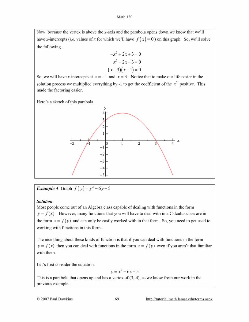
Math 130
© 2007 Paul Dawkins 69 http://tutorial.math.lamar.edu/terms.aspx
Now, because the vertex is above the x-axis and the parabola opens down we know that we’ll have x-intercepts (i.e. values of x for which we’ll have ( ) 0f x = ) on this graph. So, we’ll solve
the following.
( ) ( )
2
2
2 3 02 3 0
3 1 0
x xx x
x x
− + + =
− − =
− + =
So, we will have x-intercepts at 1x = − and 3x = . Notice that to make our life easier in the solution process we multiplied everything by -1 to get the coefficient of the 2x positive. This made the factoring easier. Here’s a sketch of this parabola.
Example 4 Graph ( ) 2 6 5f y y y= − + Solution Most people come out of an Algebra class capable of dealing with functions in the form
( )y f x= . However, many functions that you will have to deal with in a Calculus class are in the form ( )x f y= and can only be easily worked with in that form. So, you need to get used to working with functions in this form. The nice thing about these kinds of function is that if you can deal with functions in the form
( )y f x= then you can deal with functions in the form ( )x f y= even if you aren’t that familiar with them. Let’s first consider the equation. 2 6 5y x x= − + This is a parabola that opens up and has a vertex of (3,-4), as we know from our work in the previous example.

Math 130
© 2007 Paul Dawkins 70 http://tutorial.math.lamar.edu/terms.aspx
For our function we have essentially the same equation except the x and y’s are switched around. In other words, we have a parabola in the form, 2x ay by c= + + This is the general form of this kind of parabola and this will be a parabola that opens left or right
depending on the sign of a. The y-coordinate of the vertex is given by 2bya
= − and we find the
x-coordinate by plugging this into the equation. So, you can see that this is very similar to the type of parabola that you’re already used to dealing with. Now, let’s get back to the example. Our function is a parabola that opens to the right (a is positive) and has a vertex at (-4,3). The vertex is to the left of the y-axis and opens to the right so we’ll need the y-intercepts (i.e. values of y for which we’ll have ( ) 0f y = )). We find these just
like we found x-intercepts in the previous problem.
( ) ( )
2 6 5 05 1 0
y yy y
− + =
− − =
So, our parabola will have y-intercepts at 1y = and 5y = . Here’s a sketch of the graph.
Example 5 Graph 2 22 8 8 0x x y y+ + − + = . Solution To determine just what kind of graph we’ve got here we need complete the square on both the x and the y.
( ) ( )
2 2
2 2
2 2
2 8 8 02 1 1 8 16 16 8 0
1 4 9
x x y yx x y y
x y
+ + − + =
+ + − + − + − + =
+ + − =
Recall that to complete the square we take the half of the coefficient of the x (or the y), square this

Math 130
© 2007 Paul Dawkins 71 http://tutorial.math.lamar.edu/terms.aspx
and then add and subtract it to the equation. Upon doing this we see that we have a circle and it’s now written in standard form.
( ) ( )2 2 2x h y k r− + − = When circles are in this form we can easily identify the center : (h, k) and radius : r. Once we have these we can graph the circle simply by starting at the center and moving right, left, up and down by r to get the rightmost, leftmost, top most and bottom most points respectively. Our circle has a center at (-1, 4) and a radius of 3. Here’s a sketch of this circle.
Example 6 Graph ( ) ( )
222
4 2 19
xy
−+ + =
Solution This is an ellipse. The standard form of the ellipse is
( ) ( )2 2
2 2 1x h y k
a b− −
+ =
This is an ellipse with center (h, k) and the right most and left most points are a distance of a away from the center and the top most and bottom most points are a distance of b away from the center.
The ellipse for this problem has center (2, -2) and has 3a = and 12
b = . Note that to get the b
we’re really rewriting the equation as,
( ) ( )2 22 2
119 4
x y− ++ =
to get it into standard from.
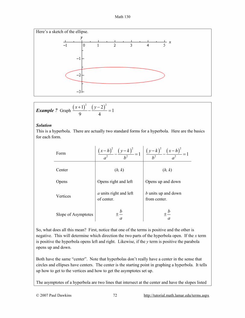
Math 130
© 2007 Paul Dawkins 72 http://tutorial.math.lamar.edu/terms.aspx
Here’s a sketch of the ellipse.
Example 7 Graph ( ) ( )2 21 2
19 4
x y+ −− =
Solution This is a hyperbola. There are actually two standard forms for a hyperbola. Here are the basics for each form.
Form ( ) ( )2 2
2 2 1x h y k
a b− −
− = ( ) ( )2 2
2 2 1y k x h
b a− −
− =
Center (h, k) (h, k) Opens Opens right and left Opens up and down
Vertices a units right and left of center.
b units up and down from center.
Slope of Asymptotes ba
± ba
±
So, what does all this mean? First, notice that one of the terms is positive and the other is negative. This will determine which direction the two parts of the hyperbola open. If the x term is positive the hyperbola opens left and right. Likewise, if the y term is positive the parabola opens up and down. Both have the same “center”. Note that hyperbolas don’t really have a center in the sense that circles and ellipses have centers. The center is the starting point in graphing a hyperbola. It tells up how to get to the vertices and how to get the asymptotes set up. The asymptotes of a hyperbola are two lines that intersect at the center and have the slopes listed
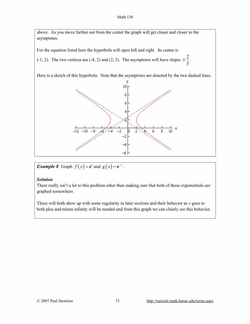
Math 130
© 2007 Paul Dawkins 73 http://tutorial.math.lamar.edu/terms.aspx
above. As you move farther out from the center the graph will get closer and closer to the asymptotes. For the equation listed here the hyperbola will open left and right. Its center is
(-1, 2). The two vertices are (-4, 2) and (2, 2). The asymptotes will have slopes 23
± .
Here is a sketch of this hyperbola. Note that the asymptotes are denoted by the two dashed lines.
Example 8 Graph ( ) xf x = e and ( ) xg x −= e . Solution There really isn’t a lot to this problem other than making sure that both of these exponentials are graphed somewhere. These will both show up with some regularity in later sections and their behavior as x goes to both plus and minus infinity will be needed and from this graph we can clearly see this behavior.

Math 130
© 2007 Paul Dawkins 74 http://tutorial.math.lamar.edu/terms.aspx
Example 9 Graph ( ) ( )lnf x x= . Solution This has already been graphed once in this review, but this puts it here with all the other “important” graphs.

Math 130
© 2007 Paul Dawkins 75 http://tutorial.math.lamar.edu/terms.aspx
Example 10 Graph y x= . Solution This one is fairly simple, we just need to make sure that we can graph it when need be.
Remember that the domain of the square root function is 0x ≥ . Example 11 Graph 3y x= Solution Again, there really isn’t much to this other than to make sure it’s been graphed somewhere so we can say we’ve done it.
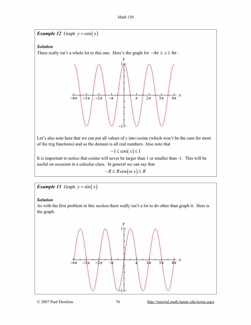
Math 130
© 2007 Paul Dawkins 76 http://tutorial.math.lamar.edu/terms.aspx
Example 12 Graph ( )cosy x= Solution There really isn’t a whole lot to this one. Here’s the graph for 4 4xπ π− ≤ ≤ .
Let’s also note here that we can put all values of x into cosine (which won’t be the case for most of the trig functions) and so the domain is all real numbers. Also note that ( )1 cos 1x− ≤ ≤ It is important to notice that cosine will never be larger than 1 or smaller than -1. This will be useful on occasion in a calculus class. In general we can say that
( )cosR R x Rω− ≤ ≤
Example 13 Graph ( )siny x= Solution As with the first problem in this section there really isn’t a lot to do other than graph it. Here is the graph.
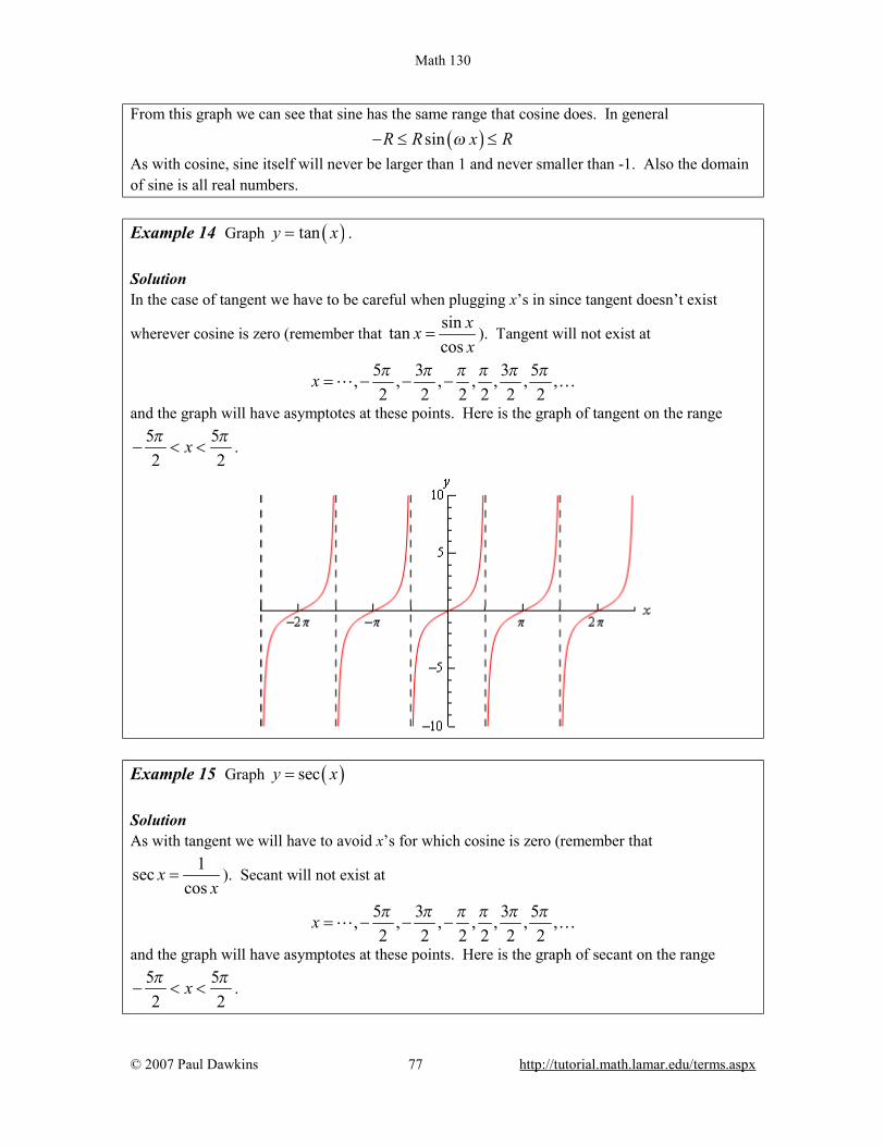
Math 130
© 2007 Paul Dawkins 77 http://tutorial.math.lamar.edu/terms.aspx
From this graph we can see that sine has the same range that cosine does. In general ( )sinR R x Rω− ≤ ≤ As with cosine, sine itself will never be larger than 1 and never smaller than -1. Also the domain of sine is all real numbers. Example 14 Graph ( )tany x= . Solution In the case of tangent we have to be careful when plugging x’s in since tangent doesn’t exist
wherever cosine is zero (remember that sintancos
xxx
= ). Tangent will not exist at
5 3 3 5, , , , , , ,2 2 2 2 2 2
x π π π π π π= − − −L …
and the graph will have asymptotes at these points. Here is the graph of tangent on the range 5 52 2
xπ π− < < .
Example 15 Graph ( )secy x= Solution As with tangent we will have to avoid x’s for which cosine is zero (remember that
1seccos
xx
= ). Secant will not exist at
5 3 3 5, , , , , , ,2 2 2 2 2 2
x π π π π π π= − − −L …
and the graph will have asymptotes at these points. Here is the graph of secant on the range 5 52 2
xπ π− < < .

Math 130
© 2007 Paul Dawkins 78 http://tutorial.math.lamar.edu/terms.aspx
Notice that the graph is always greater than 1 and less than -1. This should not be terribly surprising. Recall that ( )1 cos 1x− ≤ ≤ . So, one divided by something less than one will be
greater than 1. Also, 1 11 = ±± and so we get the following ranges for secant.
( ) ( )sec 1 and sec 1x xω ω≥ ≤ −
Math 130
© 2007 Paul Dawkins 79 http://tutorial.math.lamar.edu/terms.aspx
Limits
Introduction The topic that we will be examining in this chapter is that of Limits. This is the first of three major topics that we will be covering in this course. While we will be spending the least amount of time on limits in comparison to the other two topics limits are very important in the study of Calculus. We will be seeing limits in a variety of places once we move out of this chapter. In particular we will see that limits are part of the formal definition of the other two major topics. Here is a quick listing of the material that will be covered in this chapter. Tangent Lines and Rates of Change – In this section we will take a look at two problems that we will see time and again in this course. These problems will be used to introduce the topic of limits. The Limit – Here we will take a conceptual look at limits and try to get a grasp on just what they are and what they can tell us. One-Sided Limits – A brief introduction to one-sided limits. Limit Properties – Properties of limits that we’ll need to use in computing limits. We will also compute some basic limits in this section Computing Limits – Many of the limits we’ll be asked to compute will not be “simple” limits. In other words, we won’t be able to just apply the properties and be done. In this section we will look at several types of limits that require some work before we can use the limit properties to compute them. Infinite Limits – Here we will take a look at limits that have a value of infinity or negative infinity. We’ll also take a brief look at vertical asymptotes. Limits At Infinity, Part I – In this section we’ll look at limits at infinity. In other words, limits in which the variable gets very large in either the positive or negative sense. We’ll also take a brief look at horizontal asymptotes in this section. We’ll be concentrating on polynomials and rational expression involving polynomials in this section. Limits At Infinity, Part II – We’ll continue to look at limits at infinity in this section, but this time we’ll be looking at exponential, logarithms and inverse tangents.
Math 130
© 2007 Paul Dawkins 80 http://tutorial.math.lamar.edu/terms.aspx
Continuity – In this section we will introduce the concept of continuity and how it relates to limits. We will also see the Mean Value Theorem in this section. The Definition of the Limit – We will give the exact definition of several of the limits covered in this section. We’ll also give the exact definition of continuity.

Math 130
© 2007 Paul Dawkins 81 http://tutorial.math.lamar.edu/terms.aspx
Rates of Change and Tangent Lines In this section we are going to take a look at two fairly important problems in the study of calculus. There are two reasons for looking at these problems now. First, both of these problems will lead us into the study of limits, which is the topic of this chapter after all. Looking at these problems here will allow us to start to understand just what a limit is and what it can tell us about a function. Secondly, the rate of change problem that we’re going to be looking at is one of the most important concepts that we’ll encounter in the second chapter of this course. In fact, it’s probably one of the most important concepts that we’ll encounter in the whole course. So looking at it now will get us to start thinking about it from the very beginning. Tangent Lines The first problem that we’re going to take a look at is the tangent line problem. Before getting into this problem it would probably be best to define a tangent line. A tangent line to the function f(x) at the point x a= is a line that just touches the graph of the function at the point in question and is “parallel” (in some way) to the graph at that point. Take a look at the graph below.
In this graph the line is a tangent line at the indicated point because it just touches the graph at that point and is also “parallel” to the graph at that point. Likewise, at the second point shown, the line does just touch the graph at that point, but it is not “parallel” to the graph at that point and so it’s not a tangent line to the graph at that point. At the second point shown (the point where the line isn’t a tangent line) we will sometimes call the line a secant line. We’ve used the word parallel a couple of times now and we should probably be a little careful with it. In general, we will think of a line and a graph as being parallel at a point if they are both
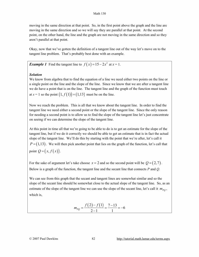
Math 130
© 2007 Paul Dawkins 82 http://tutorial.math.lamar.edu/terms.aspx
moving in the same direction at that point. So, in the first point above the graph and the line are moving in the same direction and so we will say they are parallel at that point. At the second point, on the other hand, the line and the graph are not moving in the same direction and so they aren’t parallel at that point. Okay, now that we’ve gotten the definition of a tangent line out of the way let’s move on to the tangent line problem. That’s probably best done with an example. Example 1 Find the tangent line to ( ) 215 2f x x= − at x = 1. Solution We know from algebra that to find the equation of a line we need either two points on the line or a single point on the line and the slope of the line. Since we know that we are after a tangent line we do have a point that is on the line. The tangent line and the graph of the function must touch at x = 1 so the point ( )( ) ( )1, 1 1,13f = must be on the line.
Now we reach the problem. This is all that we know about the tangent line. In order to find the tangent line we need either a second point or the slope of the tangent line. Since the only reason for needing a second point is to allow us to find the slope of the tangent line let’s just concentrate on seeing if we can determine the slope of the tangent line. At this point in time all that we’re going to be able to do is to get an estimate for the slope of the tangent line, but if we do it correctly we should be able to get an estimate that is in fact the actual slope of the tangent line. We’ll do this by starting with the point that we’re after, let’s call it
( )1,13P = . We will then pick another point that lies on the graph of the function, let’s call that
point ( )( ),Q x f x= .
For the sake of argument let’s take choose 2x = and so the second point will be ( )2,7Q = .
Below is a graph of the function, the tangent line and the secant line that connects P and Q. We can see from this graph that the secant and tangent lines are somewhat similar and so the slope of the secant line should be somewhat close to the actual slope of the tangent line. So, as an estimate of the slope of the tangent line we can use the slope of the secant line, let’s call it PQm ,
which is,
( ) ( )2 1 7 13 62 1 1PQ
f fm
− −= = = −
−

Math 130
© 2007 Paul Dawkins 83 http://tutorial.math.lamar.edu/terms.aspx
Now, if we weren’t too interested in accuracy we could say this is good enough and use this as an estimate of the slope of the tangent line. However, we would like an estimate that is at least somewhat close the actual value. So, to get a better estimate we can take an x that is closer to
1x = and redo the work above to get a new estimate on the slope. We could then take a third value of x even closer yet and get an even better estimate. In other words, as we take Q closer and closer to P the slope of the secant line connecting Q and P should be getting closer and closer to the slope of the tangent line. If you are viewing this on the web, the image below shows this process.
As you can see (if you’re reading this on the web) as we moved Q in closer and closer to P the secant lines does start to look more and more like the tangent line and so the approximate slopes (i.e. the slopes of the secant lines) are getting closer and closer to the exact slope. Also, do not

Math 130
© 2007 Paul Dawkins 84 http://tutorial.math.lamar.edu/terms.aspx
worry about how I got the exact or approximate slopes. We’ll be computing the approximate slopes shortly and we’ll be able to compute the exact slope in a few sections. In this figure we only looked at Q’s that were to the right of P, but we could have just as easily used Q’s that were to the left of P and we would have received the same results. In fact, we should always take a look at Q’s that are on both sides of P. In this case the same thing is happening on both sides of P. However, we will eventually see that doesn’t have to happen. Therefore we should always take a look at what is happening on both sides of the point in question when doing this kind of process. So, let’s see if we can come up with the approximate slopes I showed above, and hence an estimation of the slope of the tangent line. In order to simplify the process a little let’s get a formula for the slope of the line between P and Q, PQm , that will work for any x that we choose
to work with. We can get a formula by finding the slope between P and Q using the “general” form of ( )( ),Q x f x= .
( ) ( ) 2 21 15 2 13 2 2
1 1 1PQ
f x f x xmx x x
− − − −= = =
− − −
Now, let’s pick some values of x getting closer and closer to 1x = , plug in and get some slopes.
x PQm x PQm
2 -6 0 -2 1.5 -5 0.5 -3 1.1 -4.2 0.9 -3.8 1.01 -4.02 0.99 -3.98 1.001 -4.002 0.999 -3.998 1.0001 -4.0002 0.9999 -3.9998
So, if we take x’s to the right of 1 and move them in very close to 1 it appears that the slope of the secant lines appears to be approaching -4. Likewise, if we take x’s to the left of 1 and move them in very close to 1 the slope of the secant lines again appears to be approaching -4. Based on this evidence it seems that the slopes of the secant lines are approaching -4 as we move in towards 1x = , so we will estimate that the slope of the tangent line is also -4. As noted above, this is the correct value and we will be able to prove this eventually. Now, the equation of the line that goes through ( )( ),a f a is given by
( ) ( )y f a m x a= + −
Therefore, the equation of the tangent line to ( ) 215 2f x x= − at x = 1 is
( )13 4 1 4 17y x x= − − = − +
Math 130
© 2007 Paul Dawkins 85 http://tutorial.math.lamar.edu/terms.aspx
There are a couple of important points to note about our work above. First, we looked at points that were on both sides of 1x = . In this kind of process it is important to never assume that what is happening on one side of a point will also be happening on the other side as well. We should always look at what is happening on both sides of the point. In this example we could sketch a graph and from that guess that what is happening on one side will also be happening on the other, but we will usually not have the graphs in front of us or be able to easily get them. Next, notice that when we say we’re going to move in close to the point in question we do mean that we’re going to move in very close and we also used more than just a couple of points. We should never try to determine a trend based on a couple of points that aren’t really all that close to the point in question. The next thing to notice is really a warning more than anything. The values of PQm in this
example were fairly “nice” and it was pretty clear what value they were approaching after a couple of computations. In most cases this will not be the case. Most values will be far “messier” and you’ll often need quite a few computations to be able to get an estimate. Last, we were after something that was happening at 1x = and we couldn’t actually plug 1x = into our formula for the slope. Despite this limitation we were able to determine some information about what was happening at 1x = simply by looking at what was happening around
1x = . This is more important than you might at first realize and we will be discussing this point in detail in later sections. Before moving on let’s do a quick review of just what we did in the above example. We wanted the tangent line to ( )f x at a point x a= . First, we know that the point ( )( ),P a f a= will be
on the tangent line. Next, we’ll take a second point that is on the graph of the function, call it
( )( ),Q x f x= and compute the slope of the line connecting P and Q as follows,
( ) ( )PQ
f x f am
x a−
=−
We then take values of x that get closer and closer to x a= (making sure to look at x’s on both sides of x a= and use this list of values to estimate the slope of the tangent line, m. The tangent line will then be, ( ) ( )y f a m x a= + − Rates of Change The next problem that we need to look at is the rate of change problem. This will turn out to be one of the most important concepts that we will look at throughout this course.
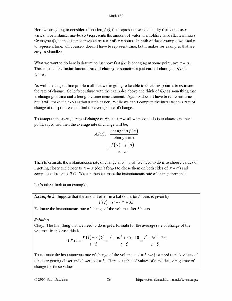
Math 130
© 2007 Paul Dawkins 86 http://tutorial.math.lamar.edu/terms.aspx
Here we are going to consider a function, f(x), that represents some quantity that varies as x varies. For instance, maybe f(x) represents the amount of water in a holding tank after x minutes. Or maybe f(x) is the distance traveled by a car after x hours. In both of these example we used x to represent time. Of course x doesn’t have to represent time, but it makes for examples that are easy to visualize. What we want to do here is determine just how fast f(x) is changing at some point, say x a= . This is called the instantaneous rate of change or sometimes just rate of change of f(x) at x a= . As with the tangent line problem all that we’re going to be able to do at this point is to estimate the rate of change. So let’s continue with the examples above and think of f(x) as something that is changing in time and x being the time measurement. Again x doesn’t have to represent time but it will make the explanation a little easier. While we can’t compute the instantaneous rate of change at this point we can find the average rate of change. To compute the average rate of change of f(x) at x a= all we need to do is to choose another point, say x, and then the average rate of change will be,
( )
( ) ( )
change in . . .
change in f x
A R Cx
f x f ax a
=
−=
−
Then to estimate the instantaneous rate of change at x a= all we need to do is to choose values of x getting closer and closer to x a= (don’t forget to chose them on both sides of x a= ) and compute values of A.R.C. We can then estimate the instantaneous rate of change from that. Let’s take a look at an example. Example 2 Suppose that the amount of air in a balloon after t hours is given by ( ) 3 26 35V t t t= − + Estimate the instantaneous rate of change of the volume after 5 hours. Solution Okay. The first thing that we need to do is get a formula for the average rate of change of the volume. In this case this is,
( ) ( ) 3 2 3 25 6 35 10 6 25. . .5 5 5
V t V t t t tA R Ct t t− − + − − +
= = =− − −
To estimate the instantaneous rate of change of the volume at 5t = we just need to pick values of t that are getting closer and closer to 5t = . Here is a table of values of t and the average rate of change for those values.

Math 130
© 2007 Paul Dawkins 87 http://tutorial.math.lamar.edu/terms.aspx
t A.R.C. t A.R.C. 6 25.0 4 7.0 5.5 19.75 4.5 10.75 5.1 15.91 4.9 14.11 5.01 15.0901 4.99 14.9101 5.001 15.009001 4.999 14.991001 5.0001 15.00090001 4.9999 14.99910001
So, from this table it looks like the average rate of change is approaching 15 and so we can estimate that the instantaneous rate of change is 15 at this point. So, just what does this tell us about the volume at this point? Let’s put some units on the answer from above. This might help us to see what is happening to the volume at this point. Let’s suppose that the units on the volume were in cm3. The units on the rate of change (both average and instantaneous) are then cm3/hr. We have estimated that at 5t = the volume is changing at a rate of 15 cm3/hr. This means that at 5t = the volume is changing in such a way that, if the rate were constant, then an hour later there would be 15 cm3 more air in the balloon than there was at 5t = . We do need to be careful here however. In reality there probably won’t be 15 cm3 more air in the balloon after an hour. The rate at which the volume is changing is generally not constant and so we can’t make any real determination as to what the volume will be in another hour. What we can say is that the volume is increasing, since the instantaneous rate of change is positive, and if we had rates of change for other values of t we could compare the numbers and see if the rate of change is faster or slower at the other points. For instance, at 4t = the instantaneous rate of change is 0 cm3/hr and at 3t = the instantaneous rate of change is -9 cm3/hr. I’ll leave it to you to check these rates of change. In fact, that would be a good exercise to see if you can build a table of values that will support my claims on these rates of change. Anyway, back to the example. At 4t = the rate of change is zero and so at this point in time the volume is not changing at all. That doesn’t mean that it will not change in the future. It just means that exactly at 4t = the volume isn’t changing. Likewise at 3t = the volume is decreasing since the rate of change at that point is negative. We can also say that, regardless of the increasing/decreasing aspects of the rate of change, the volume of the balloon is changing faster at 5t = than it is at 3t = since 15 is larger than 9. We will be talking a lot more about rates of change when we get into the next chapter.
Math 130
© 2007 Paul Dawkins 88 http://tutorial.math.lamar.edu/terms.aspx
Velocity Problem Let’s briefly look at the velocity problem. Many calculus books will treat this as its own problem. I however, like to think of this as a special case of the rate of change problem. In the velocity problem we are given a position function of an object, f(t), that gives the position of an object at time t. Then to compute the instantaneous velocity of the object we just need to recall that the velocity is nothing more than the rate at which the position is changing. In other words, to estimate the instantaneous velocity we would first compute the average velocity,
( ) ( )
change in position. .time traveled
AV
f t f at a
=
−=
−
and then take values of t closer and closer to t a= and use these values to estimate the instantaneous velocity. Change of Notation There is one last thing that we need to do in this section before we move on. The main point of this section was to introduce us to a couple of key concepts and ideas that we will see throughout the first portion of this course as well as get us started down the path towards limits. Before we move into limits officially let’s go back and do a little work that will relate both (or all three if you include velocity as a separate problem) problems to a more general concept. First, notice that whether we wanted the tangent line, instantaneous rate of change, or instantaneous velocity each of these came down to using exactly the same formula. Namely,
( ) ( )f x f ax a
−−
(1)
This should suggest that all three of these problems are then really the same problem. In fact this is the case as we will see in the next chapter. We are really working the same problem in each of these cases the only difference is the interpretation of the results. In preparation for the next section where we will discuss this in much more detail we need to do a quick change of notation. It’s easier to do here since we’ve already invested a fair amount of time into these problems. In all of these problems we wanted to determine what was happening at x a= . To do this we chose another value of x and plugged into (1). For what we were doing here that is probably most intuitive way of doing it. However, when we start looking at these problems as a single problem (1) will not be the best formula to work with.
Math 130
© 2007 Paul Dawkins 89 http://tutorial.math.lamar.edu/terms.aspx
What we’ll do instead is to first determine how far from x a= we want to move and then define our new point based on that decision. So, if we want to move a distance of h from x a= the new point would be x a h= + . As we saw in our work above it is important to take values of x that are both sides of x a= . This way of choosing new value of x will do this for us. If h>0 we will get value of x that are to the right of x a= and if h<0 we will get values of x that are to the left of x a= . Now, with this new way of getting a second x, (1) will become,
( ) ( ) ( ) ( ) ( ) ( )f x f a f a h f a f a h f ax a a h a h
− + − + −= =
− + − (2)
On the surface it might seem that (2) is going to be an overly complicated way of dealing with this stuff. However, as we will see it will often be easier to deal with (2) than it will be to deal with (1).

Math 130
© 2007 Paul Dawkins 90 http://tutorial.math.lamar.edu/terms.aspx
The Limit In the previous section we looked at a couple of problems and in both problems we had a function (slope in the tangent problem case and average rate of change in the rate of change problem) and we wanted to know how that function was behaving at some point x a= . At this stage of the game we no longer care where the functions came from and we no longer care if we’re going to see them down the road again or not. All that we need to know or worry about is that we’ve got these functions and we want to know something about them. To answer the questions in the last section we choose values of x that got closer and closer to x a= and we plugged these into the function. We also made sure that we looked at values of x that were on both the left and the right of x a= . Once we did this we looked at our table of function values and saw what the function values were approaching as x got closer and closer to x a= and used this to guess the value that we were after. This process is called taking a limit and we have some notation for this. The limit notation for the two problems from the last section is,
2 3 2
1 5
2 2 6 25lim 4 lim 151 5x t
x t tx t→ →
− − += − =
− −
In this notation we will note that we always give the function that we’re working with and we also give the value of x (or t) that we are moving in towards. In this section we are going to take an intuitive approach to limits and try to get a feel for what they are and what they can tell us about a function. With that goal in mind we are not going to get into how we actually compute limits yet. We will instead rely on what we did in the previous section as well as another approach to guess the value of the limits. Both of the approaches that we are going to use in this section are designed to help us understand just what limits are. In general we don’t typically use the methods in this section to compute limits and in many cases can be very difficult to use to even estimate the value of a limit and/or will give the wrong value on occasion. We will look at actually computing limits in a couple of sections. Let’s first start off with the following “definition” of a limit. Definition We say that the limit of f(x) is L as x approaches a and write this as ( )lim
x af x L
→=
provided we can make f(x) as close to L as we want for all x sufficiently close to a, from both sides, without actually letting x be a.

Math 130
© 2007 Paul Dawkins 91 http://tutorial.math.lamar.edu/terms.aspx
This is not the exact, precise definition of a limit. If you would like to see the more precise and mathematical definition of a limit you should check out the The Definition of a Limit section at the end of this chapter. The definition given above is more of a “working” definition. This definition helps us to get an idea of just what limits are and what they can tell us about functions. So just what does this definition mean? Well let’s suppose that we know that the limit does in fact exist. According to our “working” definition we can then decide how close to L that we’d like to make f(x). For sake of argument let’s suppose that we want to make f(x) no more that 0.001 away from L. This means that we want one of the following
( ) ( )
( ) ( )0.001 if is larger than L
0.001 if is smaller than L
f x L f x
L f x f x
− <
− <
Now according to the “working” definition this means that if we get x sufficiently close to we can make one of the above true. However, it actually says a little more. It actually says that somewhere out there in the world is a value of x, say X, so that for all x’s that are closer to a than X then one of the above statements will be true. This is actually a fairly important idea. There are many functions out there in the work that we can make as close to L for specific values of x that are close to a, but there will other values of x closer to a that give functions values that are nowhere near close to L. In order for a limit to exist once we get f(x) as close to L as we want for some x then it will need to stay in that close to L (or get closer) for all values of x that are closer to a. We’ll see an example of this later in this section. In somewhat simpler terms the definition says that as x gets closer and closer to x=a (from both sides of course…) then f(x) must be getting closer and closer to L. Or, as we move in towards x=a then f(x) must be moving in towards L. It is important to note once again that we must look at values of x that are on both sides of x=a. We should also note that we are not allowed to use x=a in the definition. We will often use the information that limits give us to get some information about what is going on right at x=a, but the limit itself is not concerned with what is actually going on at x=a. The limit is only concerned with what is going on around the point x=a. This is an important concept about limits that we need to keep in mind. An alternative notation that we will occasionally use in denoting limits is ( ) asf x L x a→ → How do we use this definition to help us estimate limits? We do exactly what we did in the previous section. We take x’s on both sides of x=a that move in closer and closer to a and we plug these into our function. We then look to see if we can determine what number the function values are moving in towards and use this as our estimate.

Math 130
© 2007 Paul Dawkins 92 http://tutorial.math.lamar.edu/terms.aspx
Let’s work an example. Example 1 Estimate the value of the following limit.
2
22
4 12lim2x
x xx x→
+ −−
Solution Notice that I did say estimate the value of the limit. Again, we are not going to directly compute limits in this section. The point of this section is to give us a better idea of how limits work and what they can tell us about the function. So, with that in mind we are going to work this in pretty much the same way that we did in the last section. We will choose values of x that get closer and closer to x=2 and plug these values into the function. Doing this gives the following table of values.
x f(x) x f(x) 2.5 3.4 1.5 5.0 2.1 3.857142857 1.9 4.157894737 2.01 3.985074627 1.99 4.015075377 2.001 3.998500750 1.999 4.001500750 2.0001 3.999850007 1.9999 4.000150008 2.00001 3.999985000 1.99999 4.000015000
Note that we made sure and picked values of x that were on both sides of 2x = and that we moved in very close to 2x = to make sure that any trends that we might be seeing are in fact correct. Also notice that we can’t actually plug in 2x = into the function as this would give us a division by zero error. This is not a problem since the limit doesn’t care what is happening at the point in question. From this table it appears that the function is going to 4 as x approaches 2, so
2
22
4 12lim 42x
x xx x→
+ −=
−.
Let’s think a little bit more about what’s going on here. Let’s graph the function from the last example. The graph of the function in the range of x’s that were interested in is shown below. First, notice that there is a rather large open dot at 2x = . This is there to remind us that the function (and hence the graph) doesn’t exist at 2x = . As we were plugging in values of x into the function we are in effect moving along the graph in towards the point as 2x = . This is shown in the graph by the two arrows on the graph that are moving in towards the point.

Math 130
© 2007 Paul Dawkins 93 http://tutorial.math.lamar.edu/terms.aspx
When we are computing limits the question that we are really asking is what y value is our graph approaching as we move in towards x a= on our graph. We are NOT asking what y value the graph takes at the point in question. In other words, we are asking what the graph is doing around the point x a= . In our case we can see that as x moves in towards 2 (from both sides) the function is approaching 4y = even though the function itself doesn’t even exist at 2x = . Therefore we can say that the limit is in fact 4. So what have we learned about limits? Limits are asking what the function is doing around x a= and are not concerned with what the function is actually doing at x a= . This is a good thing as many of the functions that we’ll be looking at won’t even exist at x a= as we saw in our last example. Let’s work another example to drive this point home. Example 2 Estimate the value of the following limit.
( ) ( )2
22
4 12 if 2lim where, 26 if 2
x
x x xg x g x x xx
→
+ −≠= −
=
Solution The first thing to note here is that this is exactly the same function as the first example with the exception that we’ve now given it a value for 2x = . So, let’s first note that ( )2 6g = As far as estimating the value of this limit goes, nothing has changed in comparison to the first example. We could build up a table of values as we did in the first example or we could take a quick look at the graph of the function. Either method will give us the value of the limit. Lets’ first take a look at a table of values and see what that tells us. Notice that the presence of the value for the function at 2x = will not change our choices for x. We only choose values of x

Math 130
© 2007 Paul Dawkins 94 http://tutorial.math.lamar.edu/terms.aspx
that are getting closer to 2x = but we never take 2x = . In other words the table of values that we used in the first example will be exactly the same table that we’ll use here. So, since we’ve already got it down once there is no reason to redo it here. From this table it is again clear that the limit is, ( )
2lim 4x
g x→
=
The limit is NOT 6! Remember from the discussion after the first example that limits do not care what the function is actually doing at the point in question. Limits are only concerned with what is going on around the point. Since the only thing about the function that we actually changed was its behavior at 2x = this will not change the limit. Let’s also take a quick look at this functions graph to see if this says the same thing.
Again, we can see that as we move in towards 2x = on our graph the function is still approaching a y value of 4. Remember that we are only asking what the function is doing around 2x = and we don’t care what the function is actually doing at 2x = . The graph then also supports the conclusion that the limit is, ( )
2lim 4x
g x→
=
Let’s make the point one more time just to make sure we’ve got it. Limits are not concerned with what is going on at x a= . Limits are only concerned with what is going on around x a= . We keep saying this, but it is a very important concept about limits that we must always keep in mind. So, we will take every opportunity to remind ourselves of this idea. Since limits aren’t concerned with what is actually happening at x a= we will, on occasion, see situations like the previous example where the limit at a point and the function value at a point are different. This won’t always happen of course. There are times where the function value and the limit at a point are the same and we will eventually see some examples of those. It is important however, to not get excited about things when the function and the limit do not take the same

Math 130
© 2007 Paul Dawkins 95 http://tutorial.math.lamar.edu/terms.aspx
value at a point. It happens sometimes and so we will need to be able to deal with those cases when they arise. Let’s take a look another example to try and beat this idea into the ground. Example 3 Estimate the value of the following limit.
( )0
1 coslimθ
θθ→
−
Solution First don’t get excited about the θ in function. It’s just a letter, just like x is a letter! It’s a Greek letter, but it’s a letter and you will be asked to deal with Greek letters on occasion so it’s a good idea to start getting used to them at this point. Now, also notice that if we plug in θ =0 that we will get division by zero and so the function doesn’t exist at this point. Actually, we get 0/0 at this point, but because of the division by zero this function does not exist at θ =0. So, as we did in the first example let’s get a table of values and see what if we can guess what value the function is heading in towards.
θ ( )f θ θ ( )f θ
1 0.45969769 -1 -0.45969769 0.1 0.04995835 -0.1 -0.04995835 0.01 0.00499996 -0.01 -0.00499996
0.001 0.00049999 -0.001 -0.00049999 Okay, it looks like the function is moving in towards a value of zero as θ moves in towards 0, from both sides of course. Therefore, the we will guess that the limit has the value,
( )0
1 coslim 0θ
θθ→
−=
So, once again, the limit had a value even though the function didn’t exist at the point we were interested in. It’s now time to work a couple of more examples that will lead us into the next idea about limits that we’re going to want to discuss.

Math 130
© 2007 Paul Dawkins 96 http://tutorial.math.lamar.edu/terms.aspx
Example 4 Estimate the value of the following limit.
0
lim cost t
π→
Solution Let’s build up a table of values and see what’s going on with our function in this case.
t f(t) t f(t) 1 -1 -1 -1
0.1 1 -0.1 1 0.01 1 -0.01 1 0.001 1 -0.001 1
Now, if we were to guess the limit from this table we would guess that the limit is 1. However, if we did make this guess we would be wrong. Consider any of the following function evaluations.
1 2 4 21 02001 2001 4001 2
f f f = − = =
In all three of these function evaluations we evaluated the function at a number that is less that 0.001 and got three totally different numbers. Recall that the definition of the limit that we’re working with requires that the function be approaching a single value (our guess) as t gets closer and closer to the point in question. It doesn’t say that only some of the function values must be getting closer to the guess. It says that all the function values must be getting closer and closer to our guess. To see what’s happening here a graph of the function would be convenient.
From this graph we can see that as we move in towards 0t = the function starts oscillating wildly and in fact the oscillations increases in speed the closer to 0t = that we get. Recall from our definition of the limit that in order for a limit to exist the function must be settling down in towards a single value as we get closer to the point in question. This function clearly does not settle in towards a single number and so this limit does not exist!

Math 130
© 2007 Paul Dawkins 97 http://tutorial.math.lamar.edu/terms.aspx
This last example points out the drawback of just picking values of x using a table of function values to estimate the value of a limit. The values of x that we chose in the previous example were valid and in fact were probably values that many would have picked. In fact they were exactly the same values we used in the problem before this one and they worked in that problem! When using a table of values there will always be the possibility that we aren’t choosing the correct values and that we will guess incorrectly for our limit. This is something that we should always keep in mind when doing this to guess the value of limits. In fact, this is such a problem that after this section we will never use a table of values to guess the value of a limit again. This last example also has shown us that limits do not have to exist. To this point we’ve only seen limits that have existed, but that just doesn’t always have to be the case. Let’s take a look at one more example in this section. Example 5 Estimate the value of the following limit.
( ) ( )0
0 if 0lim where,
1 if 0t
tH t H t
t→
<= ≥
Solution This function is often called either the Heaviside or step function. We could use a table of values to estimate the limit, but it’s probably just as quick in this case to use the graph so let’s do that. Below is the graph of this function.
We can see from the graph that if we approach 0t = from the right side the function is moving in towards a y value of 1. Well actually it’s just staying at 1, but in the terminology that we’ve been using in this section it’s moving in towards 1… Also, if we move in towards 0t = from the left the function is moving in towards a y value of 0. According to our definition of the limit the function needs to move in towards a single value as

Math 130
© 2007 Paul Dawkins 98 http://tutorial.math.lamar.edu/terms.aspx
we move in towards t a= (from both sides). This isn’t happening in this case and so in this example we will also say that the limit doesn’t exist. Note that the limit in this example is a little different from the previous example. In the previous example the function did not settle down to a single number as we moved in towards 0t = . In this example however, the function does settle down to a single number as 0t = on either side. The problem is that the number is different on each side of 0t = . This is an idea that we’ll look at in a little more detail in the next section. Let’s summarize what we (hopefully) learned in this section. In the first three examples we saw that limits do not care what the function is actually doing at the point in question. They only are concerned with what is happening around the point. In fact, we can have limits at x a= even if the function itself does not exist at that point. Likewise, even if a function exists at a point there is no reason (at this point) to think that the limit will have the same value as the function at that point. Sometimes the limit and the function will have the same value at a point and other times they won’t have the same value. Next, in the third and fourth examples we saw the main reason for not using a table of values to guess the value of a limit. In those examples we used exactly the same set of values, however they only worked in one of the examples. Using tables of values to guess the value of limits is simply not a good way to get the value of a limit. This is the only section in which we will do this. Tables of values should always be your last choice in finding values of limits. The last two examples showed us that not all limits will in fact exist. We should not get locked into the idea that limits will always exist. In most calculus courses we work with limits that almost always exist and so it’s easy to start thinking that limits always exist. Limits don’t always exist and so don’t get into the habit of assuming that they will. Finally, we saw in the fourth example that the only way to deal with the limit was to graph the function. Sometimes this is the only way, however this example also illustrated the drawback of using graphs. In order to use a graph to guess the value of the limit you need to be able to actually sketch the graph. For many functions this is not that easy to do. There is another drawback in using graphs. Even if you actually have the graph it’s only going to
be useful if the y value is approaching an integer. If the y value is approaching say 15
123−
there is
no way that you’re going to be able to guess that value from the graph and we are usually going to want exact values for our limits. So while graphs of functions can, on occasion, make your life easier in guessing values of limits they are again probably not the best way to get values of limits. They are only going to be useful if you can get your hands on it and the value of the limit is a “nice” number.

Math 130
© 2007 Paul Dawkins 99 http://tutorial.math.lamar.edu/terms.aspx
The natural question then is why did we even talk about using tables and/or graphs to estimate limits if they aren’t the best way. There were a couple of reasons. First, they can help us get a better understanding of what limits are and what they can tell us. If we don’t do at least a couple of limits in this way we might not get all that good of an idea on just what limits are. The second reason for doing limits in this way is to point out their drawback so that we aren’t tempted to use them all the time! We will eventually talk about how we really do limits. However, there is one more topic that we need to discuss before doing that. Since this section has already gone on for a while we will talk about this in the next section.
Math 130
© 2007 Paul Dawkins 100 http://tutorial.math.lamar.edu/terms.aspx
One-Sided Limits In the final two examples in the previous section we saw two limits that did not exist. However, the reason for each of the limits not existing was different for each of the examples. We saw that
0
lim cost t
π→
did not exist because the function did not settle down to a single value as t approached 0t = . The closer to 0t = we moved the more wildly the function oscillated and in order for a limit to exist the function must settle down to a single value. However we saw that
( ) ( )0
0 if 0lim where,
1 if 0t
tH t H t
t→
<= ≥
did not exist not because the function didn’t settle down to a single number as we moved in towards 0t = , but instead because it settled into two different numbers depending on which side of 0t = we were on. In this case the function was a very well behaved function, unlike the first function. The only problem was that, as we approached 0t = , the function was moving in towards different numbers on each side. We would like a way to differentiate between these two examples. We do this with one-sided limits. As the name implies, with one-sided limits we will only be looking at one side of the point in question. Here are the definitions for the two one sided limits. Right-handed limit We say ( )lim
x af x L
+→=
provided we can make f(x) as close to L as we want for all x sufficiently close to a and x>a without actually letting x be a. Left-handed limit We say ( )lim
x af x L
−→=
provided we can make f(x) as close to L as we want for all x sufficiently close to a and x<a without actually letting x be a. Note that the change in notation is very minor and in fact might be missed if you aren’t paying attention. The only difference is the bit that is under the “lim” part of the limit. For the right-handed limit we now have x a+→ (note the “+”) which means that we know will only look at
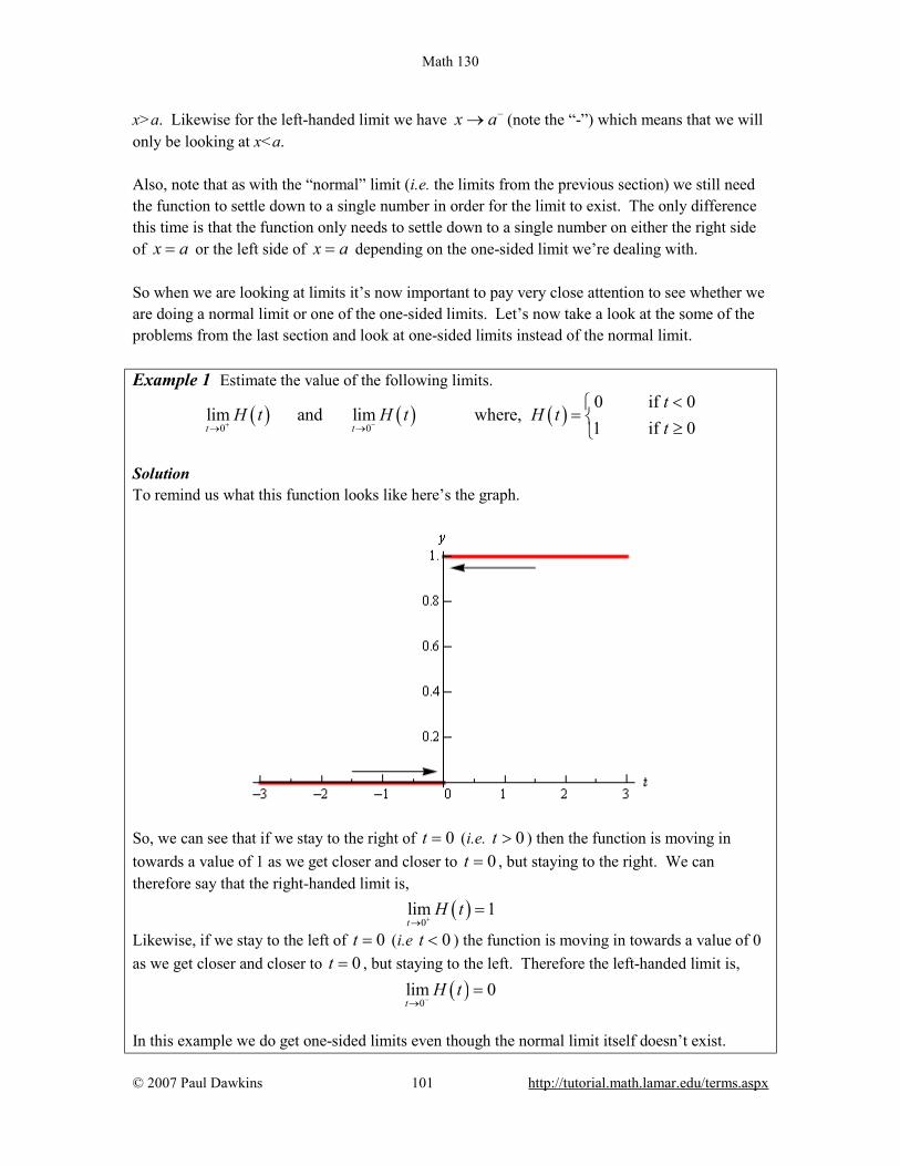
Math 130
© 2007 Paul Dawkins 101 http://tutorial.math.lamar.edu/terms.aspx
x>a. Likewise for the left-handed limit we have x a−→ (note the “-”) which means that we will only be looking at x<a. Also, note that as with the “normal” limit (i.e. the limits from the previous section) we still need the function to settle down to a single number in order for the limit to exist. The only difference this time is that the function only needs to settle down to a single number on either the right side of x a= or the left side of x a= depending on the one-sided limit we’re dealing with. So when we are looking at limits it’s now important to pay very close attention to see whether we are doing a normal limit or one of the one-sided limits. Let’s now take a look at the some of the problems from the last section and look at one-sided limits instead of the normal limit. Example 1 Estimate the value of the following limits.
( ) ( ) ( )0 0
0 if 0lim and lim where,
1 if 0t t
tH t H t H t
t+ −→ →
<= ≥
Solution To remind us what this function looks like here’s the graph.
So, we can see that if we stay to the right of 0t = (i.e. 0t > ) then the function is moving in towards a value of 1 as we get closer and closer to 0t = , but staying to the right. We can therefore say that the right-handed limit is, ( )
0lim 1t
H t+→
=
Likewise, if we stay to the left of 0t = (i.e 0t < ) the function is moving in towards a value of 0 as we get closer and closer to 0t = , but staying to the left. Therefore the left-handed limit is, ( )
0lim 0t
H t−→
=
In this example we do get one-sided limits even though the normal limit itself doesn’t exist.

Math 130
© 2007 Paul Dawkins 102 http://tutorial.math.lamar.edu/terms.aspx
Example 2 Estimate the value of the following limits.
0 0
lim cos lim cost tt t
π π+ −→ →
Solution From the graph of this function shown below,
we can see that both of the one-sided limits suffer the same problem that the normal limit did in the previous section. The function does not settle down to a single number on either side of
0t = . Therefore, neither the left-handed nor the right-handed limit will exist in this case. So, one-sided limits don’t have to exist just as normal limits aren’t guaranteed to exist. Let’s take a look at another example from the previous section. Example 3 Estimate the value of the following limits.
( ) ( ) ( )2
22 2
4 12 if 2lim and lim where, 26 if 2
x x
x x xg x g x g x x xx
+ −→ →
+ −≠= −
=
Solution So as we’ve done with the previous two examples, let’s remind ourselves of the graph of this function.

Math 130
© 2007 Paul Dawkins 103 http://tutorial.math.lamar.edu/terms.aspx
In this case regardless of which side of 2x = we are on the function is always approaching a value of 4 and so we get, ( ) ( )
2 2lim 4 lim 4x x
g x g x+ −→ →
= =
Note that one-sided limits do not care about what’s happening at the point any more than normal limits do. They are still only concerned with what is going on around the point. The only real difference between one-sided limits and normal limits is the range of x’s that we look at when determining the value of the limit. Now let’s take a look at the first and last example in this section to get a very nice fact about the relationship between one-sided limits and normal limits. In the last example the one-sided limits as well as the normal limit existed and all three had a value of 4. In the first example the two one-sided limits both existed, but did not have the same value and the normal limit did not exist. The relationship between one-sided limits and normal limits can be summarized by the following fact. Fact Given a function f(x) if, ( ) ( )lim lim
x a x af x f x L
+ −→ →= =
then the normal limit will exist and ( )lim
x af x L
→=
Likewise, if ( )lim
x af x L
→=
then, ( ) ( )lim lim
x a x af x f x L
+ −→ →= =

Math 130
© 2007 Paul Dawkins 104 http://tutorial.math.lamar.edu/terms.aspx
This fact can be turned around to also say that if the two one-sided limits have different values, i.e., ( ) ( )lim lim
x a x af x f x
+ −→ →≠
then the normal limit will not exist. This should make some sense. If the normal limit did exist then by the fact the two one-sided limits would have to exist and have the same value by the above fact. So, if the two one-sided limits have different values (or don’t even exist) then the normal limit simply can’t exist. Let’s take a look at one more example to make sure that we’ve got all the ideas about limits down that we’ve looked at in the last couple of sections. Example 4 Given the following graph,
compute each of the following. (a) ( 4)f − (b) ( )
4lim
xf x
−→− (c) ( )
4lim
xf x
+→− (d) ( )
4limx
f x→−
(e) ( )1f (f) ( )1
limx
f x−→
(g) ( )1
limx
f x+→
(h) ( )1
limx
f x→
(i) ( )6f (j) ( )6
limx
f x−→
(k) ( )6
limx
f x+→
(l) ( )6
limx
f x→
Solution (a) ( 4)f − doesn’t exist. There is no closed dot for this value of x and so the function doesn’t exist at this point. (b) ( )
4lim 2
xf x
−→−= The function is approaching a value of 2 as x moves in towards -4 from the
left. (c) ( )
4lim 2
xf x
+→−= The function is approaching a value of 2 as x moves in towards -4 from the
right.

Math 130
© 2007 Paul Dawkins 105 http://tutorial.math.lamar.edu/terms.aspx
(d) ( )4
lim 2x
f x→−
= We can do this one of two ways. Either we can use the fact here and notice
that the two one-sided limits are the same and so the normal limit must exist and have the same value as the one-sided limits or just get the answer from the graph. Also recall that a limit can exist at a point even if the function doesn’t exist at that point. (e) ( )1 4f = . The function will take on the y value where the closed dot is.
(f) ( )
1lim 4x
f x−→
= The function is approaching a value of 4 as x moves in towards 1 from the left.
(g) ( )
1lim 2x
f x+→
= − The function is approaching a value of -2 as x moves in towards 1 from the
right. Remember that the limit does NOT care about what the function is actually doing at the point, it only cares about what the function is doing around the point. In this case, always staying to the right of 1x = , the function is approaching a value of -2 and so the limit is -2. The limit is not 4, as that is value of the function at the point and again the limit doesn’t care about that! (h) ( )
1limx
f x→
doesn’t exist. The two one-sided limits both exist, however they are different and
so the normal limit doesn’t exist. (i) ( )6 2f = . The function will take on the y value where the closed dot is.
(j) ( )
6lim 5x
f x−→
= The function is approaching a value of 5 as x moves in towards 6 from the left.
(k) ( )
6lim 5x
f x+→
= The function is approaching a value of 5 as x moves in towards 6 from the
right. (l) ( )
6lim 5x
f x→
= Again, we can use either the graph or the fact to get this. Also, once more
remember that the limit doesn’t care what is happening at the point and so it’s possible for the limit to have a different value than the function at a point. When dealing with limits we’ve always got to remember that limits simply do not care about what the function is doing at the point in question. Limits are only concerned with what the function is doing around the point. Hopefully over the last couple of sections you’ve gotten an idea on how limits work and what they can tell us about functions. Some of these ideas will be important in later sections so it’s important that you have a good grasp on them.
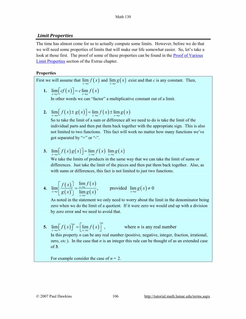
Math 130
© 2007 Paul Dawkins 106 http://tutorial.math.lamar.edu/terms.aspx
Limit Properties The time has almost come for us to actually compute some limits. However, before we do that we will need some properties of limits that will make our life somewhat easier. So, let’s take a look at those first. The proof of some of these properties can be found in the Proof of Various Limit Properties section of the Extras chapter. Properties First we will assume that ( )lim
x af x
→ and ( )lim
x ag x
→ exist and that c is any constant. Then,
1. ( ) ( )lim limx a x a
cf x c f x→ →
=
In other words we can “factor” a multiplicative constant out of a limit.
2. ( ) ( ) ( ) ( )lim lim limx a x a x a
f x g x f x g x→ → →
± = ±
So to take the limit of a sum or difference all we need to do is take the limit of the individual parts and then put them back together with the appropriate sign. This is also not limited to two functions. This fact will work no matter how many functions we’ve got separated by “+” or “-”.
3. ( ) ( ) ( ) ( )lim lim limx a x a x a
f x g x f x g x→ → →
=
We take the limits of products in the same way that we can take the limit of sums or differences. Just take the limit of the pieces and then put them back together. Also, as with sums or differences, this fact is not limited to just two functions.
4. ( )( )
( )( ) ( )
limlim , provided lim 0
limx a
x a x ax a
f xf xg x
g x g x→
→ →→
= ≠
As noted in the statement we only need to worry about the limit in the denominator being zero when we do the limit of a quotient. If it were zero we would end up with a division by zero error and we need to avoid that.
5. ( ) ( )lim lim , where is any real numbernn
x a x af x f x n
→ → =
In this property n can be any real number (positive, negative, integer, fraction, irrational, zero, etc.). In the case that n is an integer this rule can be thought of as an extended case of 3. For example consider the case of n = 2.

Math 130
© 2007 Paul Dawkins 107 http://tutorial.math.lamar.edu/terms.aspx
( ) ( ) ( )( ) ( )
( )
2
2
lim lim
lim lim using property 3
lim
x a x a
x a x a
x a
f x f x f x
f x f x
f x
→ →
→ →
→
=
=
=
The same can be done for any integer n.
6. ( ) ( )lim limn nx a x a
f x f x→ →
=
This is just a special case of the previous example.
( ) ( )
( )
( )
1
1
lim lim
lim
lim
n nx a x a
n
x a
nx a
f x f x
f x
f x
→ →
→
→
=
=
=
7. lim , is any real number
x ac c c
→=
In other words, the limit of a constant is just the constant. You should be able to convince yourself of this by drawing the graph of ( )f x c= .
8. lim
x ax a
→=
As with the last one you should be able to convince yourself of this by drawing the graph of ( )f x x= .
9. lim n n
x ax a
→=
This is really just a special case of property 5 using ( )f x x= .
Note that all these properties also hold for the two one-sided limits as well we just didn’t write them down with one sided limits to save on space. Let’s compute a limit or two using these properties. The next couple of examples will lead us to some truly useful facts about limits that we will use on a continual basis. Example 1 Compute the value of the following limit.
( )2
2lim 3 5 9x
x x→−
+ −
Solution This first time through we will use only the properties above to compute the limit.
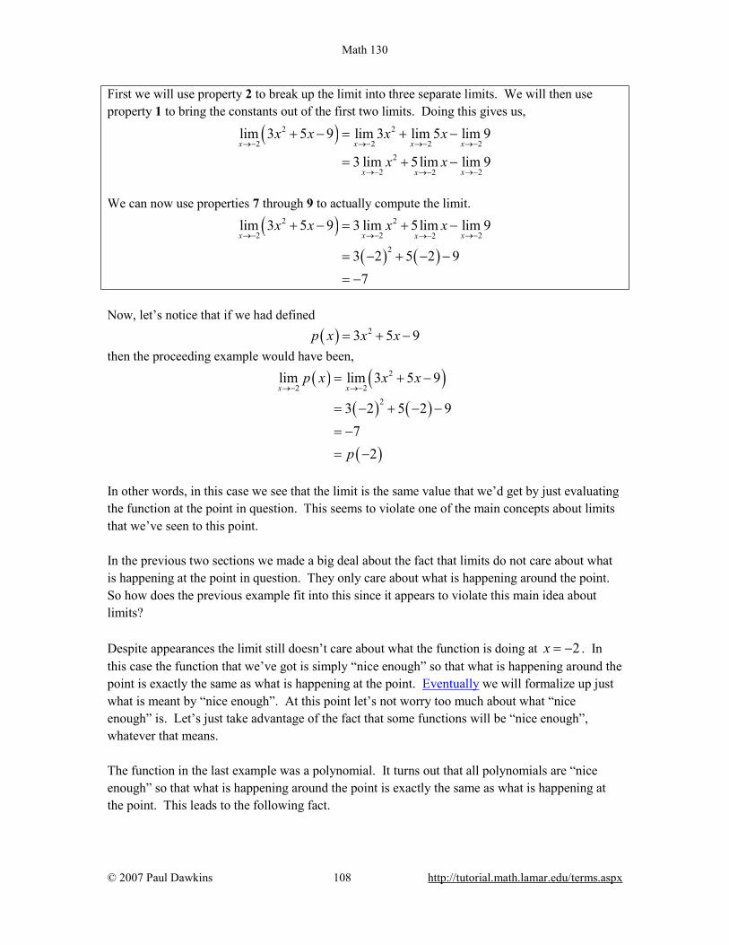
Math 130
© 2007 Paul Dawkins 108 http://tutorial.math.lamar.edu/terms.aspx
First we will use property 2 to break up the limit into three separate limits. We will then use property 1 to bring the constants out of the first two limits. Doing this gives us,
( )2 2
2 2 2 22
2 22
lim 3 5 9 lim 3 lim 5 lim 9
3 lim 5lim lim 9x x x x
x xx
x x x x
x x→− →− →− →−
→− →−→−
+ − = + −
= + −
We can now use properties 7 through 9 to actually compute the limit.
( )( ) ( )
2 2
2 2 222
lim 3 5 9 3 lim 5lim lim 9
3 2 5 2 97
x x xxx x x x
→− →− →−→−+ − = + −
= − + − −
= −
Now, let’s notice that if we had defined
( ) 23 5 9p x x x= + − then the proceeding example would have been,
( ) ( )( ) ( )
( )
2
2 22
lim lim 3 5 9
3 2 5 2 97
2
x xp x x x
p
→− →−= + −
= − + − −
= −
= −
In other words, in this case we see that the limit is the same value that we’d get by just evaluating the function at the point in question. This seems to violate one of the main concepts about limits that we’ve seen to this point. In the previous two sections we made a big deal about the fact that limits do not care about what is happening at the point in question. They only care about what is happening around the point. So how does the previous example fit into this since it appears to violate this main idea about limits? Despite appearances the limit still doesn’t care about what the function is doing at 2x = − . In this case the function that we’ve got is simply “nice enough” so that what is happening around the point is exactly the same as what is happening at the point. Eventually we will formalize up just what is meant by “nice enough”. At this point let’s not worry too much about what “nice enough” is. Let’s just take advantage of the fact that some functions will be “nice enough”, whatever that means. The function in the last example was a polynomial. It turns out that all polynomials are “nice enough” so that what is happening around the point is exactly the same as what is happening at the point. This leads to the following fact.
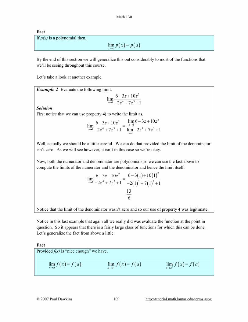
Math 130
© 2007 Paul Dawkins 109 http://tutorial.math.lamar.edu/terms.aspx
Fact If p(x) is a polynomial then, ( ) ( )lim
x ap x p a
→=
By the end of this section we will generalize this out considerably to most of the functions that we’ll be seeing throughout this course. Let’s take a look at another example. Example 2 Evaluate the following limit.
2
4 31
6 3 10lim2 7 1z
z zz z→
− +− + +
Solution First notice that we can use property 4) to write the limit as,
221
4 3 4 311
lim 6 3 106 3 10lim2 7 1 lim 2 7 1
zz
z
z zz zz z z z
→
→→
− +− +=
− + + − + +
Well, actually we should be a little careful. We can do that provided the limit of the denominator isn’t zero. As we will see however, it isn’t in this case so we’re okay. Now, both the numerator and denominator are polynomials so we can use the fact above to compute the limits of the numerator and the denominator and hence the limit itself.
( ) ( )( ) ( )
22
4 34 31
6 3 1 10 16 3 10lim2 7 1 2 1 7 1 1
136
z
z zz z→
− +− +=
− + + − + +
=
Notice that the limit of the denominator wasn’t zero and so our use of property 4 was legitimate. Notice in this last example that again all we really did was evaluate the function at the point in question. So it appears that there is a fairly large class of functions for which this can be done. Let’s generalize the fact from above a little. Fact Provided f(x) is “nice enough” we have, ( ) ( ) ( ) ( ) ( ) ( )lim lim lim
x a x a x af x f a f x f a f x f a
− +→ → →= = =

Math 130
© 2007 Paul Dawkins 110 http://tutorial.math.lamar.edu/terms.aspx
Again, we will formalize up just what we mean by “nice enough” eventually. At this point all we want to do is worry about which functions are “nice enough”. Some functions are “nice enough” for all x while others will only be “nice enough” for certain values of x. It will all depend on the function. As noted in the statement, this fact also holds for the two one-sided limits as well as the normal limit. Here is a list of some of the more common functions that are “nice enough”.
• Polynomials are nice enough for all x’s.
• If ( ) ( )( )
p xf x
q x= then f(x) will be nice enough provided both p(x) and q(x) are nice
enough and if we don’t get division by zero at the point we’re evaluating at. • ( ) ( )cos , sinx x are nice enough for all x’s
• ( ) ( )sec , tanx x are nice enough provided 5 3 3 5, , , , , ,2 2 2 2 2
x π π π π π≠ − −… … In other
words secant and tangent are nice enough everywhere cosine isn’t zero. To see why recall that these are both really rational functions and that cosine is in the denominator of both then go back up and look at the second bullet above.
• ( ) ( )csc , cotx x are nice enough provided , 3 , , 0, , 3 ,x π π π π≠ − −… … In other words cosecant and cotangent are nice enough everywhere sine isn’t zero.
• n x is nice enough for all x if n is odd. • n x is nice enough for 0x ≥ if n is even. Here we require 0x ≥ to avoid having to
deal with complex values. • ,x xa e are nice enough for all x’s. • log , lnb x x are nice enough for x>0. Remember we can only plug positive numbers
into logarithms and not zero or negative numbers. • Any sum, difference or product of the above functions will also be nice enough.
Quotients will be nice enough provided we don’t get division by zero upon evaluating the limit.
The last bullet is important. This means that for any combination of these functions all we need to do is evaluate the function at the point in question, making sure that none of the restrictions are violated. This means that we can now do a large number of limits. Example 3 Evaluate the following limit.
( ) ( ) ( )5
3lim sin cos
1 ln
x
xx x x
x→
− + + +
e
Solution This is a combination of several of the functions listed above and none of the restrictions are violated so all we need to do is plug in 3x = into the function to get the limit.
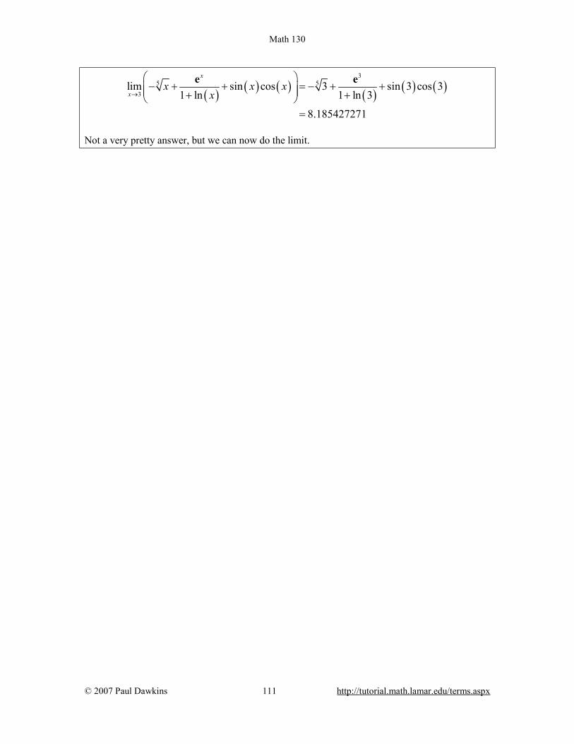
Math 130
© 2007 Paul Dawkins 111 http://tutorial.math.lamar.edu/terms.aspx
( ) ( ) ( ) ( ) ( ) ( )3
5 5
3lim sin cos 3 sin 3 cos 3
1 ln 1 ln 3
8.185427271
x
xx x x
x→
− + + = − + + + +
=
e e
Not a very pretty answer, but we can now do the limit.

Math 130
© 2007 Paul Dawkins 112 http://tutorial.math.lamar.edu/terms.aspx
Computing Limits In the previous section we saw that there is a large class of function that allows us to use ( ) ( )lim
x af x f a
→=
to compute limits. However, there are also many limits for which this won’t work easily. The purpose of this section is to develop techniques for dealing with some of these limits that will not allow us to just use this fact. Let’s first got back and take a look at one of the first limits that we looked at and compute its exact value and verify our guess for the limit. Example 1 Evaluate the following limit.
2
22
4 12lim2x
x xx x→
+ −−
Solution First let’s notice that if we try to plug in 2x = we get,
2
22
4 12 0lim2 0x
x xx x→
+ −=
−
So, we can’t just plug in 2x = to evaluate the limit. So, we’re going to have to do something else. The first thing that we should always do when evaluating limits is to simplify the function as much as possible. In this case that means factoring both the numerator and denominator. Doing this gives,
( ) ( )( )
2
22 2
2
2 64 12lim lim2 2
6lim
x x
x
x xx xx x x x
xx
→ →
→
− ++ −=
− −
+=
So, upon factoring we saw that we could cancel an 2x − from both the numerator and the denominator. Upon doing this we now have a new rational expression that we can plug 2x = into because we lost the division by zero problem. Therefore, the limit is,
2
22 2
4 12 6 8lim lim 42 2x x
x x xx x x→ →
+ − += = =
−
Note that this is in fact what we guessed the limit to be. On a side note, the 0/0 we initially got in the previous example is called an indeterminate form. This means that we don’t really know what it will be until we do some more work. Typically zero in the denominator means it’s undefined. However that will only be true if the numerator isn’t also zero. Also, zero in the numerator usually means that the fraction is zero, unless the
Math 130
© 2007 Paul Dawkins 113 http://tutorial.math.lamar.edu/terms.aspx
denominator is also zero. Likewise anything divided by itself is 1, unless we’re talking about zero. So, there are really three competing “rules” here and it’s not clear which one will win out. It’s also possible that none of them will win out and we will get something totally different from undefined, zero, or one. We might, for instance, get a value of 4 out of this, to pick a number completely at random. There are many more kinds of indeterminate forms and we will be discussing indeterminate forms at length in the next chapter. Let’s take a look at a couple of more examples. Example 2 Evaluate the following limit.
( )2
0
2 3 18limh
hh→
− + −
Solution In this case we also get 0/0 and factoring is not really an option. However, there is still some simplification that we can do.
( ) ( )2 2
0 0
2
0
2
0
2 9 6 182 3 18lim lim
18 12 2 18lim
12 2lim
h h
h
h
h hhh h
h hh
h hh
→ →
→
→
− + −− + −=
− + −=
− +=
So, upon multiplying out the first term we get a little cancellation and now notice that we can factor an h out of both terms in the numerator which will cancel against the h in the denominator and the division by zero problem goes away and we can then evaluate the limit.
( )
( )
2 2
0 0
0
0
2 3 18 12 2lim lim
12 2lim
lim 12 2 12
h h
h
h
h h hh h
h hh
h
→ →
→
→
− + − − +=
− +=
= − + = −
Example 3 Evaluate the following limit.
4
3 4lim4t
t tt→
− +−
Solution This limit is going to be a little more work than the previous two. Once again however note that we get the indeterminate form 0/0 if we try to just evaluate the limit. Also note that neither of the
Math 130
© 2007 Paul Dawkins 114 http://tutorial.math.lamar.edu/terms.aspx
two examples will be of any help here, at least initially. We can’t factor and we can’t just multiply something out to get the function to simplify. When there is a square root in the numerator or denominator we can try to rationalize and see if that helps. Recall that rationalizing makes use of the fact that ( ) ( ) 2 2a b a b a b+ − = − So, if either the first and/or the second term have a square root in them the rationalizing will eliminate the root(s). This might help in evaluating the limit. Let’s try rationalizing the numerator in this case.
( )
( )( )( )4 4
3 4 3 43 4lim lim4 4 3 4t t
t t t tt tt t t t→ →
− + + +− +=
− − + +
Remember that to rationalize we just take the numerator (since that’s what we’re rationalizing), change the sign on the second term and multiply the numerator and denominator by this new term. Next, we multiply the numerator out being careful to watch minus signs.
( )( ) ( )
( ) ( )
2
4 4
2
4
3 43 4lim lim4 4 3 4
3 4lim4 3 4
t t
t
t tt tt t t t
t tt t t
→ →
→
− +− +=
− − + +
− −=
− + +
Notice that we didn’t multiply the denominator out as well. Most students come out of an Algebra class having it beaten into their heads to always multiply this stuff out. However, in this case multiplying out will make the problem very difficult and in the end you’ll just end up factoring it back out anyway. At this stage we are almost done. Notice that we can factor the numerator so let’s do that.
( )( )( ) ( )4 4
4 13 4lim lim4 4 3 4t t
t tt tt t t t→ →
− +− +=
− − + +
Now all we need to do is notice that if we factor a “-1”out of the first term in the denominator we can do some canceling. At that point the division by zero problem will go away and we can evaluate the limit.
Math 130
© 2007 Paul Dawkins 115 http://tutorial.math.lamar.edu/terms.aspx
( ) ( )( ) ( )
( )
4 4
4
4 13 4lim lim4 4 3 4
1lim3 4
58
t t
t
t tt tt t t t
tt t
→ →
→
− +− +=
− − − + +
+=
− + +
= −
Note that if we had multiplied the denominator out we would not have been able to do this canceling and in all likelihood would not have even seen that some canceling could have been done. So, we’ve taken a look at a couple of limits in which evaluation gave the indeterminate form 0/0 and we now have a couple of things to try in these cases. Let’s take a look at another kind of problem that can arise in computing some limits involving piecewise functions. Example 4 Given the function,
( )2 5 if 2
1 3 if 2y y
g yy y
+ < −=
− ≥ −
Compute the following limits. (a) ( )
6limy
g y→
[Solution]
(b) ( )2
limy
g y→−
[Solution]
Solution (a) ( )
6limy
g y→
In this case there really isn’t a whole lot to do. In doing limits recall that we must always look at what’s happening on both sides of the point in question as we move in towards it. In this case
6y = is completely inside the second interval for the function and so there are values of y on both sides of 6y = that are also inside this interval. This means that we can just use the fact to evaluate this limit.
( )
6 6lim lim1 3
17y y
g y y→ →
= −
= −
[Return to Problems] (b) ( )
2limy
g y→−
This part is the real point to this problem. In this case the point that we want to take the limit for is the cutoff point for the two intervals. In other words we can’t just plug 2y = − into the second

Math 130
© 2007 Paul Dawkins 116 http://tutorial.math.lamar.edu/terms.aspx
portion because this interval does not contain values of y to the left of 2y = − and we need to know what is happening on both sides of the point. To do this part we are going to have to remember the fact from the section on one-sided limits that says that if the two one-sided limits exist and are the same then the normal limit will also exist and have the same value. Notice that both of the one sided limits can be done here since we are only going to be looking at one side of the point in question. So let’s do the two one-sided limits and see what we get.
( ) 2
2 2lim lim 5 since 2 implies 2
9y y
g y y y y− −
−
→− →−= + → < −
=
( )
2 2lim lim 1 3 since 2 implies 2
7y y
g y y y y+ +
+
→− →−= − → > −
=
So, in this case we can see that, ( ) ( )
2 2lim 9 7 lim
y yg y g y
− +→− →−= ≠ =
and so since the two one sided limits aren’t the same ( )
2limy
g y→−
doesn’t exist. [Return to Problems]
Note that a very simple change to the function will make the limit at 2y = − exist so don’t get in into your head that limits at these cutoff points in piecewise function don’t ever exist. Example 5 Evaluate the following limit.
( ) ( )2
2
5 if 2lim where,
3 3 if 2y
y yg y g y
y y→−
+ < −=
− ≥ −
Solution The two one-sided limits this time are,
( ) 2
2 2lim lim 5 since 2 implies 2
9y y
g y y y y− −
−
→− →−= + → < −
=
( )
2 2lim lim 3 3 since 2 implies 2
9y y
g y y y y+ −
+
→− →−= − → > −
=
The one-sided limits are the same so we get, ( )
2lim 9y
g y→−
=
Math 130
© 2007 Paul Dawkins 117 http://tutorial.math.lamar.edu/terms.aspx
There is one more limit that we need to do. However, we will need a new fact about limits that will help us to do this. Fact If ( ) ( )f x g x≤ for all x on [a, b] (except possibly at x c= ) and a c b≤ ≤ then,
( ) ( )lim limx c x c
f x g x→ →
≤
Note that this fact should make some sense to you if we assume that both functions are nice enough. If both of the functions are “nice enough” to use the limit evaluation fact then we have, ( ) ( ) ( ) ( )lim lim
x c x cf x f c g c g x
→ →= ≤ =
The inequality is true because we know that c is somewhere between a and b and in that range we also know ( ) ( )f x g x≤ .
Note that we don’t really need the two functions to be nice enough for the fact to be true, but it does provide a nice way to give a quick “justification” for the fact. Also, note that we said that we assumed that ( ) ( )f x g x≤ for all x on [a, b] (except possibly at
x c= ). Because limits do not care what is actually happening at x c= we don’t really need the inequality to hold at that specific point. We only need it to hold around x c= since that is what the limit is concerned about. We can take this fact one step farther to get the following theorem. Squeeze Theorem Suppose that for all x on [a, b] (except possibly at x c= ) we have, ( ) ( ) ( )f x h x g x≤ ≤ Also suppose that, ( ) ( )lim lim
x c x cf x g x L
→ →= =
for some a c b≤ ≤ . Then, ( )lim
x ch x L
→=
As with the previous fact we only need to know that ( ) ( ) ( )f x h x g x≤ ≤ is true around x c=
because we are working with limits and they are only concerned with what is going on around x c= and not what is actually happening at x c= . Now, if we again assume that all three functions are nice enough (again this isn’t required to make the Squeeze Theorem true, it only helps with the visualization) then we can get a quick
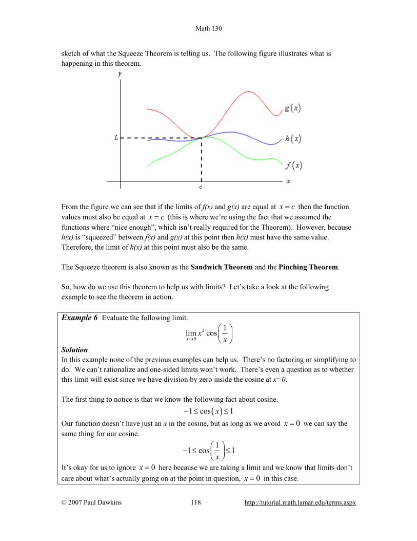
Math 130
© 2007 Paul Dawkins 118 http://tutorial.math.lamar.edu/terms.aspx
sketch of what the Squeeze Theorem is telling us. The following figure illustrates what is happening in this theorem.
From the figure we can see that if the limits of f(x) and g(x) are equal at x c= then the function values must also be equal at x c= (this is where we’re using the fact that we assumed the functions where “nice enough”, which isn’t really required for the Theorem). However, because h(x) is “squeezed” between f(x) and g(x) at this point then h(x) must have the same value. Therefore, the limit of h(x) at this point must also be the same. The Squeeze theorem is also known as the Sandwich Theorem and the Pinching Theorem. So, how do we use this theorem to help us with limits? Let’s take a look at the following example to see the theorem in action. Example 6 Evaluate the following limit.
2
0
1lim cosx
xx→
Solution In this example none of the previous examples can help us. There’s no factoring or simplifying to do. We can’t rationalize and one-sided limits won’t work. There’s even a question as to whether this limit will exist since we have division by zero inside the cosine at x=0. The first thing to notice is that we know the following fact about cosine. ( )1 cos 1x− ≤ ≤ Our function doesn’t have just an x in the cosine, but as long as we avoid 0x = we can say the same thing for our cosine.
11 cos 1x
− ≤ ≤
It’s okay for us to ignore 0x = here because we are taking a limit and we know that limits don’t care about what’s actually going on at the point in question, 0x = in this case.
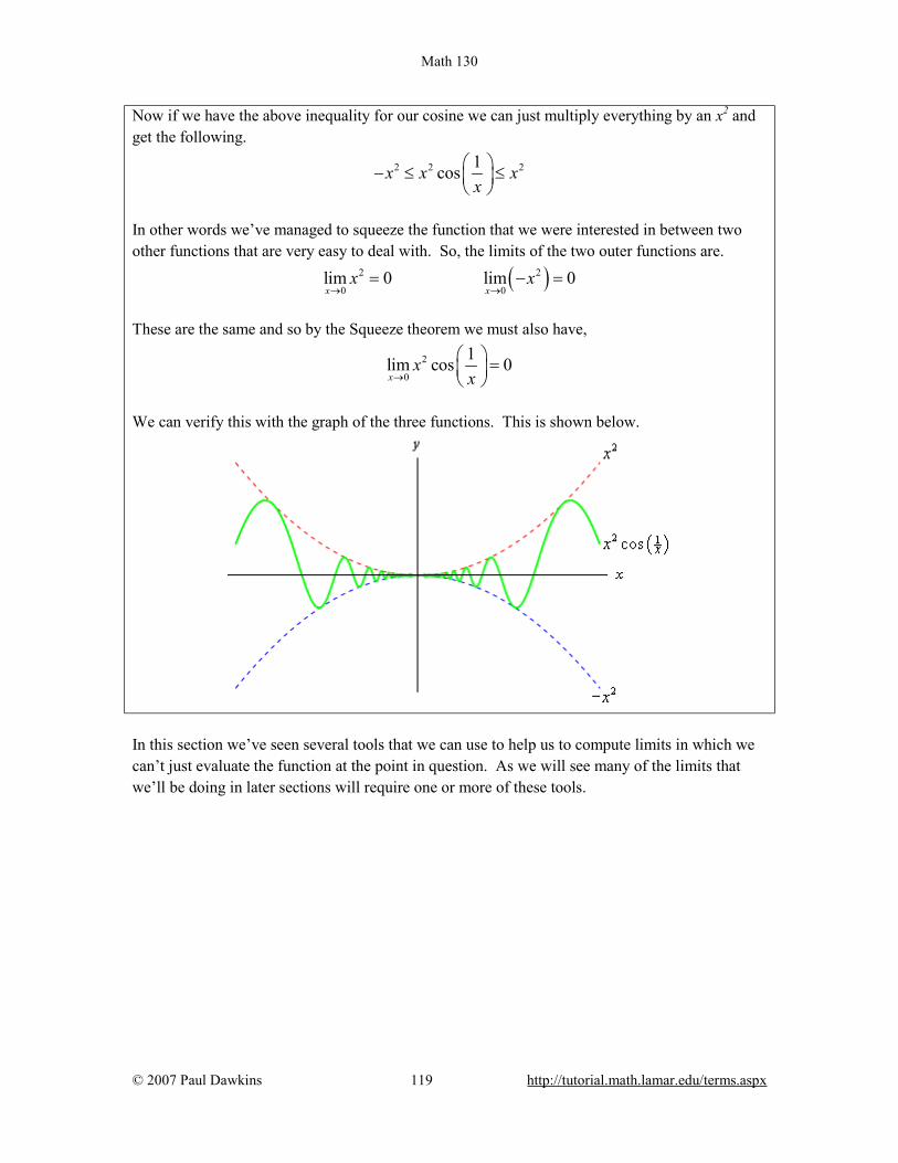
Math 130
© 2007 Paul Dawkins 119 http://tutorial.math.lamar.edu/terms.aspx
Now if we have the above inequality for our cosine we can just multiply everything by an x2 and get the following.
2 2 21cosx x xx
− ≤ ≤
In other words we’ve managed to squeeze the function that we were interested in between two other functions that are very easy to deal with. So, the limits of the two outer functions are.
( )2 2
0 0lim 0 lim 0x x
x x→ →
= − =
These are the same and so by the Squeeze theorem we must also have,
2
0
1lim cos 0x
xx→
=
We can verify this with the graph of the three functions. This is shown below.
In this section we’ve seen several tools that we can use to help us to compute limits in which we can’t just evaluate the function at the point in question. As we will see many of the limits that we’ll be doing in later sections will require one or more of these tools.
Math 130
© 2007 Paul Dawkins 120 http://tutorial.math.lamar.edu/terms.aspx
Infinite Limits In this section we will take a look at limits whose value is infinity or minus infinity. These kinds of limit will show up fairly regularly in later sections and in other courses and so you’ll need to be able to deal with them when you run across them. The first thing we should probably do here is to define just what we mean when we sat that a limit has a value of infinity or minus infinity. Definition We say ( )lim
x af x
→= ∞
if we can make f(x) arbitrarily large for all x sufficiently close to x=a, from both sides, without actually letting x a= . We say ( )lim
x af x
→= −∞
if we can make f(x) arbitrarily large and negative for all x sufficiently close to x=a, from both sides, without actually letting x a= . These definitions can be appropriately modified for the one-sided limits as well. To see a more precise and mathematical definition of this kind of limit see the The Definition of the Limit section at the end of this chapter. Let’s start off with a fairly typical example illustrating infinite limits. Example 1 Evaluate each of the following limits.
00 0
1 1 1lim lim limxx xx x x+ − →→ →
Solution So we’re going to be taking a look at a couple of one-sided limits as well as the normal limit here. In all three cases notice that we can’t just plug in 0x = . If we did we would get division by zero. Also recall that the definitions above can be easily modified to give similar definitions for the two one-sided limits which we’ll be needing here. Now, there are several ways we could proceed here to get values for these limits. One way is to plug in some points and see what value the function is approaching. In the proceeding section we said that we were no longer going to do this, but in this case it is a good way to illustrate just what’s going on with this function. So, here is a table of values of x’s from both the left and the right. Using these values we’ll be able to estimate the value of the two one-sided limits and once we have that done we can use the

Math 130
© 2007 Paul Dawkins 121 http://tutorial.math.lamar.edu/terms.aspx
fact that the normal limit will exist only if the two one-sided limits exist and have the same value.
x 1x
x 1x
-0.1 -10 0.1 10 -0.01 -100 0.01 100 -0.001 -1000 0.001 1000 -0.0001 -10000 0.0001 10000
From this table we can see that as we make x smaller and smaller the function 1x
gets larger and
larger and will retain the same sign that x originally had. It should make sense that this trend will continue for any smaller value of x that we chose to use. The function is a constant (one in this case) divided by an increasingly small number. The resulting fraction should be an increasingly large number and as noted above the fraction will retain the same sign as x. We can make the function as large and positive as we want for all x’s sufficiently close to zero while staying positive (i.e. on the right). Likewise, we can make the function as large and negative as we want for all x’s sufficiently close to zero while staying negative (i.e. on the left). So, from our definition above it looks like we should have the following values for the two one sided limits.
0 0
1 1lim limx xx x+ −→ →
= ∞ = −∞
Another way to see the values of the two one sided limits here is to graph the function. Again, in the previous section we mentioned that we won’t do this too often as most functions are not something we can just quickly sketch out as well as the problems with accuracy in reading values off the graph. In this case however, it’s not too hard to sketch a graph of the function and, in this case as we’ll see accuracy is not really going to be an issue. So, here is a quick sketch of the graph.

Math 130
© 2007 Paul Dawkins 122 http://tutorial.math.lamar.edu/terms.aspx
So, we can see from this graph that the function does behave much as we predicted that it would from our table values. The closer x gets to zero from the right the larger (in the positive sense) the function gets, while the closer x gets to zero from the left the larger (in the negative sense) the function gets. Finally, the normal limit, in this case, will not exist since the two one-sided have different values. So, in summary here are the values of the three limits for this example.
00 0
1 1 1lim lim lim doesn't existxx xx x x+ − →→ →
= ∞ = −∞
For most of the remaining examples in this section we’ll attempt to “talk our way through” each limit. This means that we’ll see if we can analyze what should happen to the function as we get very close to the point in question without actually plugging in any values into the function. For most of the following examples this kind of analysis shouldn’t be all that difficult to do. We’ll also verify our analysis with a quick graph. So, let’s do a couple more examples. Example 2 Evaluate each of the following limits.
2 2 200 0
6 6 6lim lim limxx xx x x+ − →→ →
Solution As with the previous example let’s start off by looking at the two one-sided limits. Once we have those we’ll be able to determine a value for the normal limit. So, let’s take a look at the right-hand limit first and as noted above let’s see if we can see if we can figure out what each limit will be doing without actually plugging in any values of x into the function. As we take smaller and smaller values of x, while staying positive, squaring them will only make them smaller (recall squaring a number between zero and one will make it smaller) and of course it will stay positive. So we have a positive constant divided by an increasingly small positive number. The result should then be an increasingly large positive number. It looks like we should have the following value for the right-hand limit in this case,
20
6limx x+→
= ∞
Now, let’s take a look at the left hand limit. In this case we’re going to take smaller and smaller values of x, while staying negative this time. When we square them we’ll get smaller, but upon squaring the result is now positive. So, we have a positive constant divided by an increasingly small positive number. The result, as with the right hand limit, will be an increasingly large positive number and so the left-hand limit will be,
20
6limx x−→
= ∞

Math 130
© 2007 Paul Dawkins 123 http://tutorial.math.lamar.edu/terms.aspx
Now, in this example, unlike the first one, the normal limit will exist and be infinity since the two one-sided limits both exist and have the same value. So, in summary here are all the limits for this example as well as a quick graph verifying the limits.
2 2 200 0
6 6 6lim lim limxx xx x x+ − →→ →
= ∞ = ∞ = ∞
With this next example we’ll move away from just an x in the denominator, but as we’ll see in the next couple of examples they work pretty much the same way. Example 3 Evaluate each of the following limits.
22 2
4 4 4lim lim lim2 2 2xx xx x x+ − →−→− →−
− − −+ + +
Solution Let’s again start with the right-hand limit. With the right hand limit we know that we have, 2 2 0x x> − ⇒ + > Also, as x gets closer and closer to -2 then 2x + will be getting closer and closer to zero, while staying positive as noted above. So, for the right-hand limit, we’ll have a negative constant divided by an increasingly small positive number. The result will be an increasingly large and negative number. So, it looks like the right-hand limit will be negative infinity. For the left hand limit we have, 2 2 0x x< − ⇒ + < and 2x + will get closer and closer to zero (and be negative) as x gets closer and closer to -2. In this case then we’ll have a negative constant divided by an increasingly small negative number. The result will then be an increasingly large positive number and so it looks like the left-hand limit will be positive infinity.

Math 130
© 2007 Paul Dawkins 124 http://tutorial.math.lamar.edu/terms.aspx
Finally, since two one sided limits are not the same the normal limit won’t exist. Here are the official answers for this example as well as a quick graph of the function for verification purposes.
22 2
4 4 4lim lim lim doesn't exist2 2 2xx xx x x+ − →−→− →−
− − −= −∞ = ∞
+ + +
At this point we should briefly acknowledge the idea of vertical asymptotes. Each of the three previous graphs have had one. Recall from an Algebra class that a vertical asymptote is a vertical line (the dashed line at 2x = − in the previous example) in which the graph will go towards infinity and/or minus infinity on one or both sides of the line. In an Algebra class they are a little difficult to define other than to say pretty much what we just said. Now that we have infinite limits under our belt we can easily define a vertical asymptote as follows, Definition The function f(x) will have a vertical asymptote at x a= if we have any of the following limits at x a= . ( ) ( ) ( )lim lim lim
x ax a x af x f x f x
− + →→ →= ± ∞ = ± ∞ = ± ∞
Note that it only requires one of the above limits for a function to have a vertical asymptote at x a= . Using this definition we can see that the first two examples had vertical asymptotes at 0x = while the third example had a vertical asymptote at 2x = − .
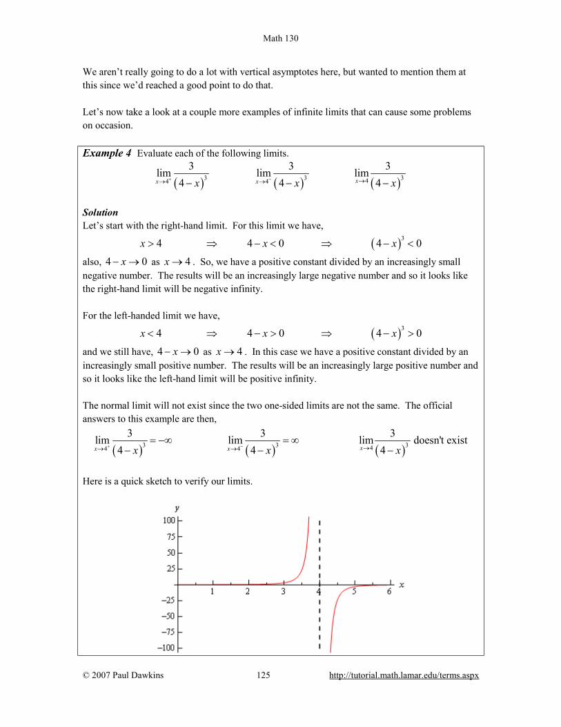
Math 130
© 2007 Paul Dawkins 125 http://tutorial.math.lamar.edu/terms.aspx
We aren’t really going to do a lot with vertical asymptotes here, but wanted to mention them at this since we’d reached a good point to do that. Let’s now take a look at a couple more examples of infinite limits that can cause some problems on occasion. Example 4 Evaluate each of the following limits.
( ) ( ) ( )3 3 344 4
3 3 3lim lim lim4 4 4xx xx x x+ − →→ →− − −
Solution Let’s start with the right-hand limit. For this limit we have,
( )34 4 0 4 0x x x> ⇒ − < ⇒ − <
also, 4 0x− → as 4x → . So, we have a positive constant divided by an increasingly small negative number. The results will be an increasingly large negative number and so it looks like the right-hand limit will be negative infinity. For the left-handed limit we have,
( )34 4 0 4 0x x x< ⇒ − > ⇒ − >
and we still have, 4 0x− → as 4x → . In this case we have a positive constant divided by an increasingly small positive number. The results will be an increasingly large positive number and so it looks like the left-hand limit will be positive infinity. The normal limit will not exist since the two one-sided limits are not the same. The official answers to this example are then,
( ) ( ) ( )3 3 344 4
3 3 3lim lim lim doesn't exist4 4 4xx xx x x+ − →→ →
= −∞ = ∞− − −
Here is a quick sketch to verify our limits.
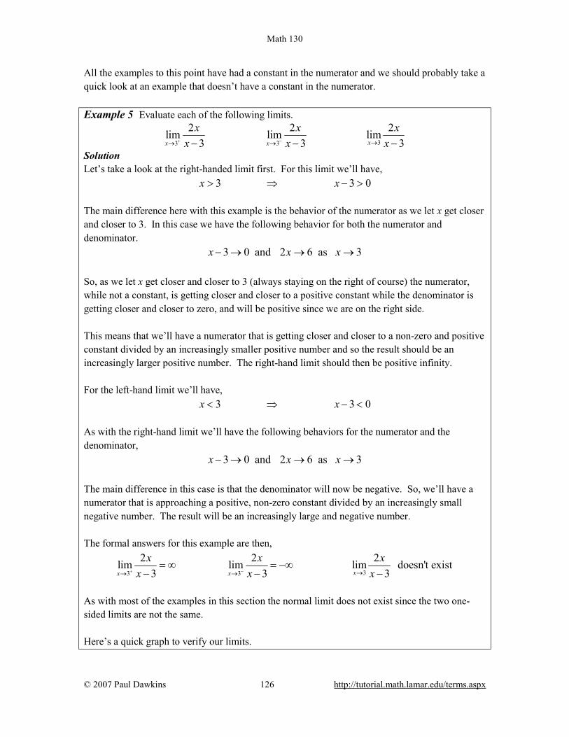
Math 130
© 2007 Paul Dawkins 126 http://tutorial.math.lamar.edu/terms.aspx
All the examples to this point have had a constant in the numerator and we should probably take a quick look at an example that doesn’t have a constant in the numerator. Example 5 Evaluate each of the following limits.
33 3
2 2 2lim lim lim3 3 3xx x
x x xx x x+ − →→ →− − −
Solution Let’s take a look at the right-handed limit first. For this limit we’ll have, 3 3 0x x> ⇒ − > The main difference here with this example is the behavior of the numerator as we let x get closer and closer to 3. In this case we have the following behavior for both the numerator and denominator. 3 0 and 2 6 as 3x x x− → → → So, as we let x get closer and closer to 3 (always staying on the right of course) the numerator, while not a constant, is getting closer and closer to a positive constant while the denominator is getting closer and closer to zero, and will be positive since we are on the right side. This means that we’ll have a numerator that is getting closer and closer to a non-zero and positive constant divided by an increasingly smaller positive number and so the result should be an increasingly larger positive number. The right-hand limit should then be positive infinity. For the left-hand limit we’ll have, 3 3 0x x< ⇒ − < As with the right-hand limit we’ll have the following behaviors for the numerator and the denominator,
3 0 and 2 6 as 3x x x− → → → The main difference in this case is that the denominator will now be negative. So, we’ll have a numerator that is approaching a positive, non-zero constant divided by an increasingly small negative number. The result will be an increasingly large and negative number. The formal answers for this example are then,
33 3
2 2 2lim lim lim doesn't exist3 3 3xx x
x x xx x x+ − →→ →
= ∞ = −∞− − −
As with most of the examples in this section the normal limit does not exist since the two one-sided limits are not the same. Here’s a quick graph to verify our limits.
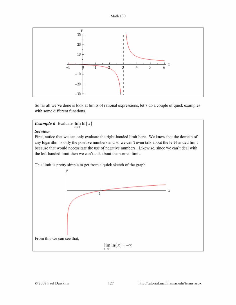
Math 130
© 2007 Paul Dawkins 127 http://tutorial.math.lamar.edu/terms.aspx
So far all we’ve done is look at limits of rational expressions, let’s do a couple of quick examples with some different functions. Example 6 Evaluate ( )
0lim lnx
x+→
Solution First, notice that we can only evaluate the right-handed limit here. We know that the domain of any logarithm is only the positive numbers and so we can’t even talk about the left-handed limit because that would necessitate the use of negative numbers. Likewise, since we can’t deal with the left-handed limit then we can’t talk about the normal limit. This limit is pretty simple to get from a quick sketch of the graph.
From this we can see that,
( )0
lim lnx
x+→
= −∞
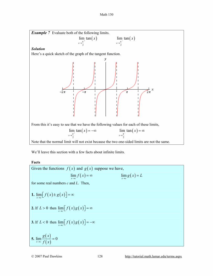
Math 130
© 2007 Paul Dawkins 128 http://tutorial.math.lamar.edu/terms.aspx
Example 7 Evaluate both of the following limits. ( ) ( )
2 2
lim tan lim tanx x
x xπ π+ −
→ →
Solution Here’s a quick sketch of the graph of the tangent function.
From this it’s easy to see that we have the following values for each of these limits, ( ) ( )
2 2
lim tan lim tanx x
x xπ π+ −
→ →
= −∞ = ∞
Note that the normal limit will not exist because the two one-sided limits are not the same. We’ll leave this section with a few facts about infinite limits. Facts Given the functions ( )f x and ( )g x suppose we have,
( ) ( )lim limx c x c
f x g x L→ →
= ∞ =
for some real numbers c and L. Then,
1. ( ) ( )limx c
f x g x→
± = ∞
2. If 0L > then ( ) ( )limx c
f x g x→
= ∞
3. If 0L < then ( ) ( )limx c
f x g x→
= −∞
5. ( )( )
lim 0x c
g xf x→
=

Math 130
© 2007 Paul Dawkins 129 http://tutorial.math.lamar.edu/terms.aspx
To see the proof of this set of facts see the Proof of Various Limit Properties section in the Extras chapter. Note as well that the above set of facts also holds for one-sided limits. They will also hold if
( )limx c
f x→
= −∞ , with a change of sign on the infinities in the first three parts. The proofs of
these changes to the facts are nearly identical to the proof of the original facts and so are left to the reader.

Math 130
© 2007 Paul Dawkins 130 http://tutorial.math.lamar.edu/terms.aspx
Limits At Infinity, Part I In the previous section we saw limits that were infinity and it’s now time to take a look at limits at infinity. By limits at infinity we mean one of the following two limits. ( ) ( )lim lim
x xf x f x
→∞ →−∞
In other words, we are going to be looking at what happens to a function if we let x get very large in either the positive or negative sense. Also, as we’ll soon see, these limits may also have infinity as a value. First, let’s note that the set of Facts from Infinite Limit section also hold if the replace the limx c→
with limx→∞
or limx→−∞
. The proof of this is nearly identical to the proof of the original set of
facts with only minor modifications to handle the change in the limit and so is left to the reader. We won’t need these facts much over the next couple of sections but they will be required on occasion. In fact, many of the limits that we’re going to be looking at we will need the following two facts. Fact 1 1. If r is a positive rational number and c is any real number then,
lim 0rx
cx→∞
=
2. If r is a positive rational number, c is any real number and xr is defined for 0x < then,
lim 0rx
cx→−∞
=
The first part of this fact should make sense if you think about it. Because we are requiring
0r > we know that xr will stay in the denominator. Next as we increase x then xr will also increase. So, we have a constant divided by an increasingly large number and so the result will be increasingly small. Or, in the limit we will get zero. The second part is nearly identical except we need to worry about xr being defined for negative x. This condition is here to avoid cases such as 1
2r = . If this r were allowed then we’d be taking the square root of negative numbers which would be complex and we want to avoid that at this level. Note as well that the sign of c will not affect the answer. Regardless of the sign of c we’ll still have a constant divided by a very large number which will result in a very small number and the larger x get the smaller the fraction gets. The sign of c will affect which direction the fraction approaches zero (i.e. from the positive or negative side) but it still approaches zero.
Math 130
© 2007 Paul Dawkins 131 http://tutorial.math.lamar.edu/terms.aspx
If you think about it this is really a special case of the last Fact from the Facts in the previous section. However, to see a direct proof of this fact see the Proof of Various Limit Properties section in the Extras chapter. Let’s start the off the examples with one that will lead us to a nice idea that we’ll use on a regular basis about limits at infinity for polynomials. Example 1 Evaluate each of the following limits.
(a) ( )4 2lim 2 8x
x x x→∞
− − [Solution]
(b) ( )5 3 213lim 2 8
tt t t
→−∞+ − + [Solution]
Solution (a) ( )4 2lim 2 8
xx x x
→∞− −
Our first thought here is probably to just “plug” infinity into the polynomial and “evaluate” each term to determine the value of the limit. It is pretty simple to see what each term will do in the limit and so this seems like an obvious step, especially since we’ve been doing that for other limits in previous sections. So, let’s see what we get if we do that. As x approaches infinity, then x to a power can only get larger and the coefficient on each term (the first and third) will only make the term even larger. So, if we look at what each term is doing in the limit we get the following,
( )4 2lim 2 8x
x x x→∞
− − = ∞ − ∞ − ∞
Now, we’ve got a small, but easily fixed, problem to deal with. We are probably tempted to say that the answer is zero (because we have an infinity minus an infinity) or maybe −∞ (because we’re subtracting two infinities off of one infinity). However, in both cases we’d be wrong. This is one of those indeterminate forms that we first started seeing in a previous section. Infinities just don’t always behave as real numbers do when it comes to arithmetic. Without more work there is simply no way to know what ∞ − ∞ will be and so we really need to be careful with this kind of problem. To read a little more about this see the Types of Infinity section in the Extras chapter. So, we need a way to get around this problem. What we’ll do here is factor the largest power of x out of the whole polynomial as follows,
( )4 2 42 3
1 8lim 2 8 lim 2x x
x x x xx x→∞ →∞
− − = − −
If you’re not sure you agree with the factoring above (there’s a chance you haven’t really been asked to do this kind of factoring prior to this) then recall that to check all you need to do is

Math 130
© 2007 Paul Dawkins 132 http://tutorial.math.lamar.edu/terms.aspx
multiply the 4x back through the parenthesis to verify it was done correctly. Also, an easy way to remember how to do this kind of factoring is to note that the second term is just the original polynomial divided by 4x . This will always work when factoring a power of x out of a polynomial. Now for each of the terms we have,
42 3
1 8lim lim 2 2x x
xx x→∞ →∞
= ∞ − − =
The first limit is clearly infinity and for the second limit we’ll use the fact above on the last two terms. Therefore using Fact 2 from the previous section we see value of the limit will be,
( )4 2lim 2 8x
x x x→∞
− − = ∞
[Return to Problems]
(b) ( )5 3 213lim 2 8
tt t t
→−∞+ − +
We’ll work this part much quicker than the previous part. All we need to do is factor out the largest power of t to get the following,
( )5 3 2 513 2 3 5
1 2 1 8lim 2 8 lim3t t
t t t tt t t→−∞ →−∞
+ − + = + − +
Remember that all you need to do to get the factoring correct is divide the original polynomial by the power of t we’re factoring out, 5t in this case. Now all we need to do is take the limit of the two terms. In the first don’t forget that since we’re going out towards −∞ and we’re raising t to the 5th power that the limit will be negative (negative number raised to an odd power is still negative). In the second term well again make heavy use of the fact above to see that is a finite number. Therefore, using the a modification of the Facts from the previous section the value of the limit is,
( )5 3 213lim 2 8
tt t t
→−∞+ − + = −∞
[Return to Problems] Okay, now that we’ve seen how a couple of polynomials work we can give a simple fact about polynomials in general. Fact 2 If ( ) 1
1 1 0n n
n np x a x a x a x a−−= + + + +L is a polynomial of degree n (i.e. 0na ≠ ) then,
Math 130
© 2007 Paul Dawkins 133 http://tutorial.math.lamar.edu/terms.aspx
( ) ( )lim lim lim limn nn nx x x x
p x a x p x a x→∞ →∞ →−∞ →−∞
= =
What this fact is really saying is that when we go to take a limit at infinity for a polynomial then all we need to really do is look at the term with the largest power and ask what that term is doing in the limit since the polynomial will have the same behavior. You can see the proof in the Proof of Various Limit Properties section in the Extras chapter. Let’s now move into some more complicated limits. Example 2 Evaluate both of the following limits.
4 2 4 2
4 4
2 8 2 8lim lim5 7 5 7x x
x x x x x xx x→∞ →−∞
− + − +− + − +
Solution First, the only difference between these two is that one is going to positive infinity and the other is going to negative infinity. Sometimes this small difference will affect then value of the limit and at other times it won’t. Let’s start with the first limit and as with our first set of examples it might be tempting to just “plug” in the infinity. Since both the numerator and denominator are polynomials we can use the above fact to determine the behavior of each. Doing this gives,
4 2
4
2 8lim5 7x
x x xx→∞
− + ∞=
− + −∞
This is yet another indeterminate form. In this case we might be tempted to say that the limit is infinity (because of the infinity in the numerator), zero (because of the infinity in the denominator) or -1 (because something divided by itself is one). There are three separate arithmetic “rules” at work here and without work there is no way to know which “rule” will be correct and to make matters worse it’s possible that none of them may work and we might get a
completely different answer, say 25
− to pick a number completely at random.
So, when we have a polynomial divided by a polynomial we’re going to proceed much as we did with only polynomials. We first identify the largest power of x in the denominator (and yes, we only look at the denominator for this) and we then factor this out of both the numerator and denominator. Doing this for the first limit gives,
44 2 2 3
44
4
1 822 8lim lim
75 7 5x x
xx x x x x
x xx
→∞ →∞
− + − + =− + − +
Once we’ve done this we can cancel the 4x from both the numerator and the denominator and

Math 130
© 2007 Paul Dawkins 134 http://tutorial.math.lamar.edu/terms.aspx
then use the Fact 1 above to take the limit of all the remaining terms. This gives,
4 2 2 3
4
4
1 822 8lim lim 75 7 5
2 0 05 0
25
x x
x x x x xx
x→∞ →∞
− +− +=
− + − +
+ +=
− +
= −
In this case the indeterminate form was neither of the “obvious” choices of infinity, zero, or -1 so be careful with make these kinds of assumptions with this kind of indeterminate forms. The second limit is done in a similar fashion. Notice however, that nowhere in the work for the first limit did we actually use the fact that the limit was going to plus infinity. In this case it doesn’t matter which infinity we are going towards we will get the same value for the limit.
4 2
4
2 8 2lim5 7 5x
x x xx→−∞
− += −
− +
In the previous example the infinity that we were using in the limit didn’t change the answer. This will not always be the case so don’t make the assumption that this will always be the case. Let’s take a look at an example where we get different answers for each limit. Example 3 Evaluate each of the following limits.
2 23 6 3 6lim lim
5 2 5 2x x
x xx x→∞ →−∞
+ +− −
Solution The square root in this problem won’t change our work, but it will make the work a little messier. Let’s start with the first limit. In this case the largest power of x in the denominator is just an x. So we need to factor an x out of the numerator and the denominator. When we are done factoring the x out we will need an x in both of the numerator and the denominator. To get this in the numerator we will have to factor an x2 out of the square root so that after we take the square root we will get an x. This is probably not something you’re used to doing, but just remember that when it comes out of the square root it needs to be an x and the only way have an x come out of a square is to take the square root of x2 and so that is what we’ll need to factor out of the term under the radical. Here’s the factoring work for this part,
Math 130
© 2007 Paul Dawkins 135 http://tutorial.math.lamar.edu/terms.aspx
222
22
633 6lim lim
55 2 2
63lim
5 2
x x
x
xxx
x xx
xx
xx
→∞ →∞
→∞
+ + =− −
+=
−
This is where we need to be really careful with the square root in the problem. Don’t forget that
2x x= Square roots are ALWAYS positive and so we need the absolute value bars on the x to make sure that it will give a positive answer. This is not something that most people every remember seeing in an Algebra class and in fact it’s not always given in an Algebra class. However, at this point it becomes absolutely vital that we know and use this fact. Using this fact the limit becomes,
2 2
633 6lim lim55 2 2
x x
xx xx x
x→∞ →∞
++=
− −
Now, we can’t just cancel the x’s. We first will need to get rid of the absolute value bars. To do this let’s recall the definition of absolute value.
if 0if 0
x xx
x x≥
= − <
In this case we are going out to plus infinity so we can safely assume that the x will be positive and so we can just drop the absolute value bars. The limit is then,
2 2
2
633 6lim lim55 2 2
63 3 0 3lim 5 0 2 22
x x
x
xx xx x
x
x
x
→∞ →∞
→∞
++=
− −
+ += = = −
−−
Let’s now take a look at the second limit (the one with negative infinity). In this case we will need to pay attention to the limit that we are using. The initial work will be the same up until we reach the following step.
Math 130
© 2007 Paul Dawkins 136 http://tutorial.math.lamar.edu/terms.aspx
2 2
633 6lim lim55 2 2
x x
xx xx x
x→−∞ →−∞
++=
− −
In this limit we are going to minus infinity so in this case we can assume that x is negative. So, in order to drop the absolute value bars in this case we will need to tack on a minus sign as well. The limit is then,
2 2
2
633 6lim lim55 2 2
63lim 5 2
32
x x
x
xx xx x
x
x
x
→−∞ →−∞
→−∞
− ++=
− −
− +=
−
=
So, as we saw in the last two examples sometimes the infinity in the limit will affect the answer and other times it won’t. Note as well that it doesn’t always just change the sign of the number. It can on occasion completely change the value. We’ll see an example of this later in this section. Before moving on to a couple of more examples let’s revisit the idea of asymptotes that we first saw in the previous section. Just as we can have vertical asymptotes defined in terms of limits we can also have horizontal asymptotes defined in terms of limits. Definition The function f(x) will have a horizontal asymptote at y=L if either of the following are true. ( ) ( )lim lim
x xf x L f x L
→∞ →−∞= =
We’re not going to be doing much with asymptotes here, but it’s an easy fact to give and we can use the previous example to illustrate all the asymptote ideas we’ve seen in the both this section and the previous section. The function in the last example will have two horizontal asymptotes. It will also have a vertical asymptote. Here is a graph of the function showing these.

Math 130
© 2007 Paul Dawkins 137 http://tutorial.math.lamar.edu/terms.aspx
Let’s work another couple of examples involving rational expressions. Example 4 Evaluate each of the following limits.
2 6 2 6
3 3
4 4lim lim1 5 1 5z z
z z z zz z→∞ →−∞
+ +− −
Solution Let’s do the first limit and in this case it looks like we will factor a z3 out of both the numerator and denominator. Remember that we only look at the denominator when determining the largest power of z here. There is a larger power of z in the numerator but we ignore it. We ONLY look at the denominator when doing this! So doing the factoring gives,
3 32 6
33
3
3
3
44lim lim
11 5 5
4
lim 1 5
z z
z
z zz z z
z zz
zz
z
→∞ →∞
→∞
+ + =− −
+=
−
When we take the limit we’ll need to be a little careful. The first term in the numerator and denominator will both be zero. However, the z3 in the numerator will be going to plus infinity in the limit and so the limit is,
2 6
3
4lim1 5 5z
z zz→∞
+ ∞= = −∞
− −
The final limit is negative because we have a quotient of positive quantity and a negative quantity. Now, let’s take a look at the second limit. Note that the only different in the work is at the final “evaluation” step and so we’ll pick up the work there.
Math 130
© 2007 Paul Dawkins 138 http://tutorial.math.lamar.edu/terms.aspx
32 6
3
3
44lim lim 11 5 55
z z
zz z zz
z→−∞ →−∞
++ −∞= = = ∞
− −−
In this case the z3 in the numerator gives negative infinity in the limit since we are going out to minus infinity and the power is odd. The answer is positive since we have a quotient of two negative numbers. Example 5 Evaluate the following limit.
2
4 3
5 9lim2 3t
t tt t→−∞
− −+
Solution In this case it looks like we will factor a 4t out of both the numerator and denominator. Doing this gives,
42 2 3 4
4 34
2 3 4
1 5 95 9lim lim
32 3 2
1 5 9
lim 32
020
t t
t
tt t t t t
t t tt
t t t
t
→−∞ →−∞
→−∞
− − − − =+ +
− −=
+
=
=
In this case using Fact 1 we can see that the numerator is zero and so since the denominator is also not zero the fraction, and hence the limit, will be zero. In this section we concentrated on limits at infinity with functions that only involved polynomials and/or rational expression involving polynomials. There are many more types of functions that we could use here. That is the subject of the next section. To see a precise and mathematical definition of this kind of limit see the The Definition of the Limit section at the end of this chapter.

Math 130
© 2007 Paul Dawkins 139 http://tutorial.math.lamar.edu/terms.aspx
Limits At Infinity, Part II In the previous section we looked at limits at infinity of polynomials and/or rational expression involving polynomials. In this section we want to take a look at some other types of functions that often show up in limits at infinity. The functions we’ll be looking at here are exponentials, natural logarithms and inverse tangents. Let’s start by taking a look at a some of very basic examples involving exponential functions. Example 1 Evaluate each of the following limits. lim lim lim limx x x x
x x x x
− −
→∞ →−∞ →∞ →−∞e e e e
Solution There are really just restatements of facts given in the basic exponential section of the review so we’ll leave it to you to go back and verify these. lim lim 0 lim 0 limx x x x
x x x x
− −
→∞ →−∞ →∞ →−∞= ∞ = = = ∞e e e e
The main point of this example was to point out that if the exponent of an exponential goes to infinity in the limit then the exponential function will also go to infinity in the limit. Likewise, if the exponent goes to minus infinity in the limit then the exponential will go to zero in the limit. Here’s a quick set of examples to illustrate these ideas. Example 2 Evaluate each of the following limits.
(a) 22 4 8lim
x
x x−
→∞
−e [Solution]
(b) 4 25 1lim
t
t t− +
→−∞e [Solution]
(c) 1
0lim zz +→
e [Solution]
Solution
(a) 22 4 8lim
x
x x−
→∞
−e
In this part what we need to note (using Fact 2 above) is that in the limit the exponent of the exponential does the following,
( )2lim 2 4 8x
x x→∞
− − = −∞
So, the exponent goes to minus infinity in the limit and so the exponential must go to zero in the limit using the ideas from the previous set of examples. So, the answer here is,
22 4 8lim 0
x
x x−
→∞
− =e
[Return to Problems]

Math 130
© 2007 Paul Dawkins 140 http://tutorial.math.lamar.edu/terms.aspx
(b) 4 25 1lim
t
t t− +
→−∞e
Here let’s first note that,
( )4 2lim 5 1t
t t→−∞
− + = ∞
The exponent goes to infinity in the limit and so the exponential will also need to go to infinity in the limit. Or,
4 25 1lim
t
t t− +
→−∞= ∞e
[Return to Problems]
(c) 1
0lim zz +→
e
On the surface this part doesn’t appear to belong in this section since it isn’t a limit at infinity. However, it does fit into the ideas we’re examining in this set of examples. So, let’s first note that using the idea from the previous section we have,
0
1limz z+→
= ∞
Remember that in order to do this limit here we do need to do a right hand limit. So, the exponent goes to infinity in the limit and so the exponential must also go to infinity. Here’s the answer to this part.
1
0lim zz +→
= ∞e
[Return to Problems] Let’s work some more complicated examples involving exponentials. In the following set of examples it won’t be that the exponents are more complicated, but instead that there will be more than one exponential function to deal with. Example 3 Evaluate each of the following limits.
(a) ( )10 6 2 15lim 4 3 2 9x
x x x x x− −
→∞− + + −e e e e e [Solution]
(b) ( )10 6 2 15lim 4 3 2 9x
x x x x x− −
→−∞− + + −e e e e e [Solution]
Solution So, the only difference between these two limits is the fact that in the first we’re taking the limit as we go to plus infinity and in the second we’re going to minus infinity. To this point we’ve been able to “reuse” work from the first limit in the at least a portion of the second limit. With exponentials that will often not be the case we we’re going to treat each of these as separate problems.

Math 130
© 2007 Paul Dawkins 141 http://tutorial.math.lamar.edu/terms.aspx
(a) ( )10 6 2 15lim 4 3 2 9x
x x x x x− −
→∞− + + −e e e e e
Let’s start by just taking the limit of each of the pieces and see what we get.
( )10 6 2 15lim 4 3 2 9 0 0x
x x x x x− −
→∞− + + − = ∞ − ∞ + ∞ + −e e e e e
The last two terms aren’t any problem (they will be in the next part however, do you see that?). The first three are a problem however as they present us with another indeterminate form. When dealing with polynomials we factored out the term with the largest exponent in it. Let’s do the same thing here. However, we now have to deal with both positive and negative exponents and just what do we mean by the “largest” exponent. When dealing with these here we look at the terms that are causing the problems and ask which is the largest exponent in those terms. So, since only the first three terms are causing us problems (i.e. they all evaluate to an infinity in the limit) we’ll look only at those. So, since 10x is the largest of the three exponents there we’ll “factor” an 10xe out of the whole thing. Just as with polynomials we do the factoring by, in essence, dividing each term by 10xe and remembering that to simply the division all we need to do is subtract the exponents. For example, let’s just take a look at the last term,
15
15 10 2510
9 9 9x
x x xx
−− −−−
= − = −e e e
e
Doing factoring on all terms then gives,
( ) ( )10 6 2 15 10 4 9 12 25lim 4 3 2 9 lim 1 4 3 2 9x x
x x x x x x x x x x− − − − − −
→∞ →∞ − + + − = − + + − e e e e e e e e e e
Notice that in doing this factoring all the remaining exponentials now have negative exponents and we know that for this limit (i.e. going out to positive infinity) these will all be zero in the limit and so will no longer cause problems. We can now take the limit of the two terms. The first is clearly infinity and the second is clearly a finite number (one in this case) and so the Facts from the Infinite Limits section gives us the following limit,
( )10 6 2 15lim 4 3 2 9x
x x x x x− −
→∞− + + − = ∞e e e e e
To simplify the work here a little all we really needed to do was factor the 10xe out of the “problem” terms (the first three in this case) as follows,
( ) ( )( )( )
10 6 10 4 9 2 15lim 4 3 lim 1 4 3 2 9
1 0 0x x
x x x x x x x x− − − −
→∞ →∞ − + = − + + −
= ∞ + −
= ∞
e e e e e e e e

Math 130
© 2007 Paul Dawkins 142 http://tutorial.math.lamar.edu/terms.aspx
We factored the 10xe out of all terms for the practice of doing the factoring and to avoid any issues with having the extra terms at the end. Note as well that while we wrote ( )( )1∞ for the
limit of the first term we are really using the Facts from the Infinite Limit section to do that limit. [Return to Problems]
(b) ( )10 6 2 15lim 4 3 2 9x
x x x x x− −
→−∞− + + −e e e e e
Let’s start this one off in the same manner as the first part. Let’s take the limit of each of the pieces. This time note that because our limit is going to negative infinity the first three exponentials will in fact go to zero (because their exponents go to minus infinity in the limit). The final two exponentials will go to infinity in the limit (because their exponents go to plus infinity in the limit). Taking the limits gives,
( )10 6 2 15lim 4 3 2 9 0 0 0x
x x x x x− −
→−∞− + + − = − + + ∞ − ∞e e e e e
So, the last two terms are the problem here as they once again leave us with an indeterminate form. As with the first example we’re going to factor out the “largest” exponent in the last two terms. This time however, “largest” doesn’t refer to the bigger of the two numbers (-2 is bigger than -15). Instead we’re going to use “largest” to refer to the exponent that is farther away from zero. Using this definition of “largest” means that we’re going to factor an 15x−e out. Again, remember that to factor this out all we really are doing is dividing each term by 15x−e and then subtracting exponents. Here’s the work for the first term as an example,
( )10
10 15 2515
xx x x
x− −
− = =e e ee
As with the first part we can either factor it out of only the “problem” terms (i.e. the last two terms), or all the terms. For the practice we’ll factor it out of all the terms. Here is the factoring work for this limit,
( ) ( )10 6 2 15 15 25 21 16 13lim 4 3 2 9 lim 4 3 2 9x x
x x x x x x x x x x− − −
→−∞ →−∞ − + + − = − + + − e e e e e e e e e e
Finally, after taking the limit of the two terms (the first is infinity and the second is a negative, finite number) and recalling the Facts from the Infinite Limit section we see that the limit is,
( )10 6 2 15lim 4 3 2 9x
x x x x x− −
→−∞− + + − = −∞e e e e e
[Return to Problems] So, when dealing with sums and/or differences of exponential functions we look for the exponential with the “largest” exponent and remember here that “largest” means the exponent farthest from zero. Also remember that if we’re looking at a limit at plus infinity only the

Math 130
© 2007 Paul Dawkins 143 http://tutorial.math.lamar.edu/terms.aspx
exponentials with positive exponents are going to cause problems so those are the only terms we look at in determining the largest exponent. Likewise, if we are looking at a limit at minus infinity then only exponentials with negative exponents are going to cause problems and so only those are looked at in determining the largest exponent. Finally, as you might have been able to guess from the previous example when dealing with a sum and/or difference of exponentials all we need to do is look at the largest exponent to determine the behavior of the whole expression. Again, remembering that if the limit is at plus infinity we only look at exponentials with positive exponents and if we’re looking at a limit at minus infinity we only look at exponentials with negative exponents. Let’s next take a look at some rational functions involving exponentials. Example 4 Evaluate each of the following limits.
(a) 4 2
4 2
6lim8 3x
x x
x x x
−
−→∞
−− +e e
e e e [Solution]
(b) 4 2
4 2
6lim8 3x
x x
x x x
−
−→−∞
−− +e e
e e e [Solution]
(c) 6 6
3 9 3
4lim2 5t
t t
t t t
−
− −→−∞
−− +
e ee e e
[Solution]
Solution As with the previous example, the only difference between the first two parts is that one of the limits is going to plus infinity and the other is going to minus infinity and just as with the previous example each will need to be worked differently.
(a) 4 2
4 2
6lim8 3x
x x
x x x
−
−→∞
−− +e e
e e e
The basic concept involved in working this problem is the same as with rational expressions in the previous section. We look at the denominator and determine the exponential function with the “largest” exponent which we will then factor out from both numerator and denominator. We will use the same reasoning as we did with the previous example to determine the “largest” exponent. In the case since we are looking at a limit at plus infinity we only look at exponentials with positive exponents. So, we’ll factor an 4xe out of both then numerator and denominator. Once that is done we can cancel the 4xe and then take the limit of the remaining terms. Here is the work for this limit,

Math 130
© 2007 Paul Dawkins 144 http://tutorial.math.lamar.edu/terms.aspx
( )( )
4 64 2
4 2 4 2 5
6
2 5
66lim lim8 3 8 3
6lim8 3
6 08 0 034
x x
x
x xx x
x x x x x x
x
x x
−−
− − −→∞ →∞
−
− −→∞
−−=
− + − +
−=
− +−
=− +
=
e ee ee e e e e e
ee e
[Return to Problems]
(b) 4 2
4 2
6lim8 3x
x x
x x x
−
−→−∞
−− +e e
e e e
In this case we’re going to minus infinity in the limit and so we’ll look at exponentials in the denominator with negative exponents in determining the “largest” exponent. There’s only one however in this problem so that is what we’ll use. Again, remember to only look at the denominator. Do NOT use the exponential from the numerator, even though that one is “larger” than the exponential in then denominator. We always look only at the denominator when determining what term to factor out regardless of what is going on in the numerator. Here is the work for this part.
( )( )
4 2
4 2
5
5 3
5
5 3
66lim lim8 3 8 3
6lim8 3
00 0 3
x x
x
x x xx x
x x x x x x
x x
x x
− −−
− −→−∞ →−∞
−
→−∞
−−=
− + − +
−=
− +− ∞
=− +
= −∞
e e ee ee e e e e e
e ee e
[Return to Problems]
(c) 6 6
3 9 3
4lim2 5t
t t
t t t
−
− −→−∞
−− +
e ee e e
We’ll do the work on this part with much less detail.
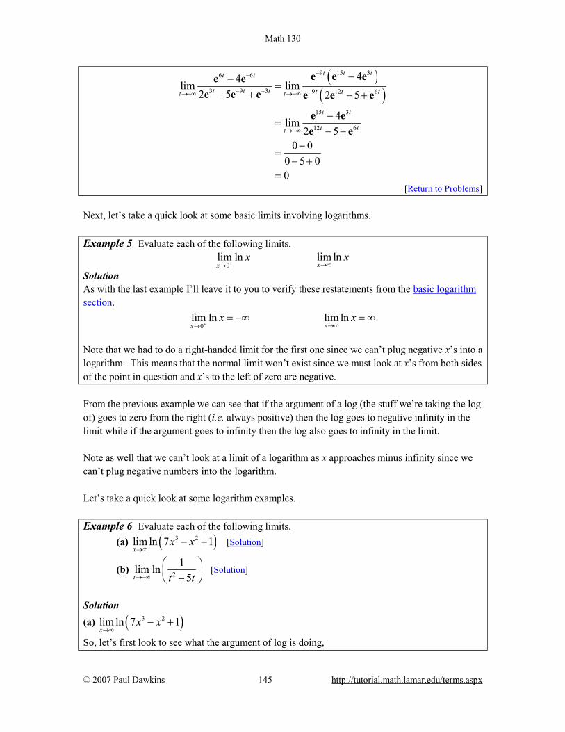
Math 130
© 2007 Paul Dawkins 145 http://tutorial.math.lamar.edu/terms.aspx
( )( )9 15 36 6
3 9 3 9 12 6
15 3
12 6
44lim lim2 5 2 5
4lim2 5
0 00 5 00
t t
t
t t tt t
t t t t t t
t t
t t
−−
− − −→−∞ →−∞
→−∞
−−=
− + − +
−=
− +−
=− +
=
e e ee ee e e e e e
e ee e
[Return to Problems] Next, let’s take a quick look at some basic limits involving logarithms. Example 5 Evaluate each of the following limits.
0lim ln lim ln
xxx x
+ →∞→
Solution As with the last example I’ll leave it to you to verify these restatements from the basic logarithm section.
0lim ln lim ln
xxx x
+ →∞→= −∞ = ∞
Note that we had to do a right-handed limit for the first one since we can’t plug negative x’s into a logarithm. This means that the normal limit won’t exist since we must look at x’s from both sides of the point in question and x’s to the left of zero are negative. From the previous example we can see that if the argument of a log (the stuff we’re taking the log of) goes to zero from the right (i.e. always positive) then the log goes to negative infinity in the limit while if the argument goes to infinity then the log also goes to infinity in the limit. Note as well that we can’t look at a limit of a logarithm as x approaches minus infinity since we can’t plug negative numbers into the logarithm. Let’s take a quick look at some logarithm examples. Example 6 Evaluate each of the following limits.
(a) ( )3 2lim ln 7 1x
x x→∞
− + [Solution]
(b) 2
1lim ln5t t t→−∞
−
[Solution]
Solution (a) ( )3 2lim ln 7 1
xx x
→∞− +
So, let’s first look to see what the argument of log is doing,

Math 130
© 2007 Paul Dawkins 146 http://tutorial.math.lamar.edu/terms.aspx
( )3 2lim 7 1x
x x→∞
− + = ∞
The argument of the log is going to infinity and so the log must also be going to infinity in the limit. The answer to this part is then,
( )3 2lim ln 7 1x
x x→∞
− + = ∞
[Return to Problems]
(b) 2
1lim ln5t t t→−∞
−
First, note that the limit going to negative infinity here isn’t a violation (necessarily) of the fact that we can’t plug negative numbers into the logarithm. The real issue is whether or not the argument of the log will be negative or not. Using the techniques from earlier in this section we can see that,
2
1lim 05t t t→−∞
=−
and let’s also not that for negative numbers (which we can assume we’ve got since we’re going to minus infinity in the limit) the denominator will always be positive and so the quotient will also always be positive. Therefore, not only does the argument go to zero, it goes to zero from the right. This is exactly what we need to do this limit. So, the answer here is,
2
1lim ln5t t t→−∞
= −∞ −
[Return to Problems]
As a final set of examples let’s take a look at some limits involving inverse tangents. Example 7 Evaluate each of the following limits.
(a) 1lim tanx
x−
→∞ [Solution]
(b) 1lim tanx
x−
→−∞ [Solution]
(c) ( )1 3lim tan 5 6x
x x−
→∞− + [Solution]
(d) 1
0
1lim tanx x−
−
→
[Solution]
Solution The first two parts here are really just the basic limits involving inverse tangents and can easily be found by examining the following sketch of inverse tangents. The remaining two parts are more

Math 130
© 2007 Paul Dawkins 147 http://tutorial.math.lamar.edu/terms.aspx
involved but as with the exponential and logarithm limits really just refer back to the first two parts as we’ll see.
(a) 1lim tanx
x−
→∞
As noted above all we really need to do here is look at the graph of the inverse tangent. Doing this shows us that we have the following value of the limit.
1lim tan2x
x π−
→∞=
[Return to Problems] (b) 1lim tan
xx−
→−∞
Again, not much to do here other than examine the graph of the inverse tangent.
1lim tan2x
x π−
→−∞= −
[Return to Problems]
(c) ( )1 3lim tan 5 6x
x x−
→∞− +
Okay, in part (a) above we saw that if the argument of the inverse tangent function (the stuff inside the parenthesis) goes to plus infinity then we know the value of the limit. In this case (using the techniques from the previous section) we have, 3lim 5 6
xx x
→∞− + = ∞
So, this limit is,
( )1 3lim tan 5 62x
x x π−
→∞− + =
[Return to Problems]

Math 130
© 2007 Paul Dawkins 148 http://tutorial.math.lamar.edu/terms.aspx
(d) 1
0
1lim tanx x−
−
→
Even though this limit is not a limit at infinity we’re still looking at the same basic idea here. We’ll use part (b) from above as a guide for this limit. We know from the Infinite Limits section that we have the following limit for the argument of this inverse tangent,
0
1limx x−→
= −∞
So, since the argument goes to minus infinity in the limit we know that this limit must be,
1
0
1lim tan2x xπ
−
−
→
= −
[Return to Problems] To see a precise and mathematical definition of this kind of limit see the The Definition of the Limit section at the end of this chapter.

Math 130
© 2007 Paul Dawkins 149 http://tutorial.math.lamar.edu/terms.aspx
Continuity Over the last few sections we’ve been using the term “nice enough” to define those functions that we could evaluate limits by just evaluating the function at the point in question. It’s now time to formally define what we mean by “nice enough”. Definition A function ( )f x is said to be continuous at x a= if
( ) ( )limx a
f x f a→
=
A function is said to be continuous on the interval [a, b] if it is continuous at each point in the interval. Note that this definition is also implicitly assuming that both ( )f a and ( )lim
x af x
→ exist. If
either of these do not exist then the function will not be continuous at x a= . This definition can be turned around into the following fact. Fact 1 If ( )f x is continuous at x a= then,
( ) ( ) ( ) ( ) ( ) ( )lim lim limx a x a x a
f x f a f x f a f x f a− +→ → →
= = =
This is exactly the same fact that we first put down back when we started looking at limits with the exception that we have replaced the phrase “nice enough” with continuous. It’s nice to finally know what we mean by “nice enough”, however, the definition doesn’t really tell us just what it means for a function to be continuous. Let’s take a look at an example to help us understand just what it means for a function to be continuous. Example 1 Given the graph of f(x), shown below, determine if f(x) is continuous at 2x = − ,
0x = , and 3x = .

Math 130
© 2007 Paul Dawkins 150 http://tutorial.math.lamar.edu/terms.aspx
Solution To answer the question for each point we’ll need to get both the limit at that point and the function value at that point. If they are equal the function is continuous at that point and if they aren’t equal the function isn’t continuous at that point. First 2x = − . ( ) ( )
22 2 lim doesn't exist
xf f x
→−− =
The function value and the limit aren’t the same and so the function is not continuous at this point. This kind of discontinuity in a graph is called a jump discontinuity. Jump discontinuities occur where the graph has a break in it is as this graph does. Now 0x = . ( ) ( )
00 1 lim 1
xf f x
→= =
The function is continuous at this point since the function and limit have the same value. Finally 3x = . ( ) ( )
33 1 lim 0
xf f x
→= − =
The function is not continuous at this point. This kind of discontinuity is called a removable discontinuity. Removable discontinuities are those where there is a hole in the graph as there is in this case. From this example we can get a quick “working” definition of continuity. A function is continuous on an interval if we can draw the graph from start to finish without ever once picking up our pencil. The graph in the last example has only two discontinuities since there are only two places where we would have to pick up our pencil in sketching it. In other words, a function is continuous if its graph has no holes or breaks in it. For many functions it’s easy to determine where it won’t be continuous. Functions won’t be continuous where we have things like division by zero or logarithms of zero. Let’s take a quick look at an example of determining where a function is not continuous.

Math 130
© 2007 Paul Dawkins 151 http://tutorial.math.lamar.edu/terms.aspx
Example 2 Determine where the function below is not continuous.
( ) 2
4 102 15
th tt t
+=
− −
Solution Rational functions are continuous everywhere except where we have division by zero. So all that we need to is determine where the denominator is zero. That’s easy enough to determine by setting the denominator equal to zero and solving. ( )( )2 2 15 5 3 0t t t t− − = − + = So, the function will not be continuous at t=-3 and t=5. A nice consequence of continuity is the following fact. Fact 2 If ( )f x is continuous at x b= and ( )lim
x ag x b
→= then,
( )( ) ( )( )lim limx a x a
f g x f g x→ →
=
To see a proof of this fact see the Proof of Various Limit Properties section in the Extras chapter. With this fact we can now do limits like the following example. Example 3 Evaluate the following limit.
0
sinlimx
x→
e
Solution Since we know that exponentials are continuous everywhere we can use the fact above.
0 0
0
lim sinsinlim 1x
x
xx →
→= = =e e e
Another very nice consequence of continuity is the Intermediate Value Theorem. Intermediate Value Theorem Suppose that f(x) is continuous on [a, b] and let M be any number between f(a) and f(b). Then there exists a number c such that,
1. a c b< < 2. ( )f c M=

Math 130
© 2007 Paul Dawkins 152 http://tutorial.math.lamar.edu/terms.aspx
All the Intermediate Value Theorem is really saying is that a continuous function will take on all values between f(a) and f(b). Below is a graph of a continuous function that illustrates the Intermediate Value Theorem.
As we can see from this image if we pick any value, M, that is between the value of f(a) and the value of f(b) and draw a line straight out from this point the line will hit the graph in at least one point. In other words somewhere between a and b the function will take on the value of M. Also, as the figure shows the function may take on the value at more than one place. It’s also important to note that the Intermediate Value Theorem only says that the function will take on the value of M somewhere between a and b. It doesn’t say just what that value will be. It only says that it exists. So, the Intermediate Value Theorem tells us that a function will take the value of M somewhere between a and b but it doesn’t tell us where it will take the value nor does it tell us how many times it will take the value. There are important idea to remember about the Intermediate Value Theorem. A nice use of the Intermediate Value Theorem is to prove the existence of roots of equations as the following example shows. Example 4 Show that ( ) 3 22 5 10 5p x x x x= − − + has a root somewhere in the interval [-1,2]. Solution What we’re really asking here is whether or not the function will take on the value ( ) 0p x = somewhere between -1 and 2. In other words, we want to show that there is a number c such that
1 2c− < < and ( ) 0p c = . However if we define 0M = and acknowledge that 1a = − and
2b = we can see that these two condition on c are exactly the conclusions of the Intermediate
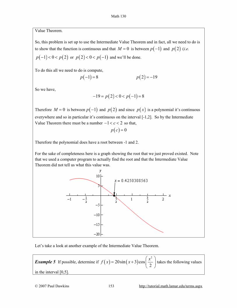
Math 130
© 2007 Paul Dawkins 153 http://tutorial.math.lamar.edu/terms.aspx
Value Theorem. So, this problem is set up to use the Intermediate Value Theorem and in fact, all we need to do is to show that the function is continuous and that 0M = is between ( )1p − and ( )2p (i.e.
( ) ( )1 0 2p p− < < or ( ) ( )2 0 1p p< < − and we’ll be done.
To do this all we need to do is compute, ( ) ( )1 8 2 19p p− = = − So we have, ( ) ( )19 2 0 1 8p p− = < < − = Therefore 0M = is between ( )1p − and ( )2p and since ( )p x is a polynomial it’s continuous
everywhere and so in particular it’s continuous on the interval [-1,2]. So by the Intermediate Value Theorem there must be a number 1 2c− < < so that, ( ) 0p c = Therefore the polynomial does have a root between -1 and 2. For the sake of completeness here is a graph showing the root that we just proved existed. Note that we used a computer program to actually find the root and that the Intermediate Value Theorem did not tell us what this value was.
Let’s take a look at another example of the Intermediate Value Theorem.
Example 5 If possible, determine if ( ) ( )2
20sin 3 cos2xf x x
= +
takes the following values
in the interval [0,5].

Math 130
© 2007 Paul Dawkins 154 http://tutorial.math.lamar.edu/terms.aspx
(a) Does ( ) 10f x = ? [Solution]
(b) Does ( ) 10f x = − ? [Solution] Solution Okay, so much as the previous example we’re being asked to determine, if possible, if the function takes on either of the two values above in the interval [0,5]. First, let’s notice that this is a continuous function and so we know that we can use the Intermediate Value Theorem to do this problem. Now, for each part we will let M be the given value for that part and then we’ll need to show that M lives between ( )0f and ( )5f . If it does then we can use the Intermediate Value Theorem to
prove that the function will take the given value. So, since we’ll need the two function evaluations for each part let’s give them here, ( ) ( )0 2.8224 5 19.7436f f= =
Now, let’s take a look at each part. (a) Okay, in this case we’ll define 10M = and we can see that, ( ) ( )0 2.8224 10 19.7436 5f f= < < =
So, by the Intermediate Value Theorem there must be a number 0 5c≤ ≤ such that ( ) 10f c =
[Return to Problems] (b) In this part we’ll define 10M = − . We now have a problem. In this part M does not live between ( )0f and ( )5f . So, what does this mean for us? Does this mean that ( ) 10f x ≠ −
in [0,5]? Unfortunately for us, this doesn’t mean anything. It is possible that ( ) 10f x ≠ − in [0,5], but is
it also possible that ( ) 10f x = − in [0,5]. The Intermediate Value Theorem will only tell us that
c’s will exist. The theorem will NOT tell us that c’s don’t exist. In this case it is not possible to determine if ( ) 10f x = − in [0,5] using the Intermediate Value
Theorem. [Return to Problems]
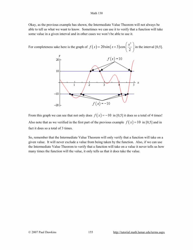
Math 130
© 2007 Paul Dawkins 155 http://tutorial.math.lamar.edu/terms.aspx
Okay, as the previous example has shown, the Intermediate Value Theorem will not always be able to tell us what we want to know. Sometimes we can use it to verify that a function will take some value in a given interval and in other cases we won’t be able to use it.
For completeness sake here is the graph of ( ) ( )2
20sin 3 cos2xf x x
= +
in the interval [0,5].
From this graph we can see that not only does ( ) 10f x = − in [0,5] it does so a total of 4 times!
Also note that as we verified in the first part of the previous example ( ) 10f x = in [0,5] and in
fact it does so a total of 3 times. So, remember that the Intermediate Value Theorem will only verify that a function will take on a given value. It will never exclude a value from being taken by the function. Also, if we can use the Intermediate Value Theorem to verify that a function will take on a value it never tells us how many times the function will the value, it only tells us that it does take the value.

Math 130
© 2007 Paul Dawkins 156 http://tutorial.math.lamar.edu/terms.aspx
The Definition of the Limit In this section we’re going to be taking a look at the precise, mathematical definition of the three kinds of limits we looked at in this chapter. We’ll be looking at the precise definition of limits at finite points that have finite values, limits that are infinity and limits at infinity. We’ll also give the precise, mathematical definition of continuity. Let’s start this section out with the definition of a limit at a finite point that has a finite value. Definition 1 Let f(x) be a function defined on an interval that contains x a= , except possibly at x a= . Then we say that,
( )limx a
f x L→
=
if for every number 0ε > there is some number 0δ > such that
( ) whenever 0f x L x aε δ− < < − <
Wow. That’s a mouth full. Now that it’s written down, just what does this mean? Let’s take a look at the following graph and let’s also assume that the limit does exist.
What the definition is telling us is that for any number 0ε > that we pick we can go to our graph and sketch two horizontal lines at L ε+ and L ε− as shown on the graph above. Then somewhere out there in the world is another number 0δ > , which we will need to determine, that will allow us to add in two vertical lines to our graph at a δ+ and a δ− . Now, if we take any x in the pink region, i.e. between a δ+ and a δ− , then this x will be closer to a than either of a δ+ and a δ− . Or, x a δ− <
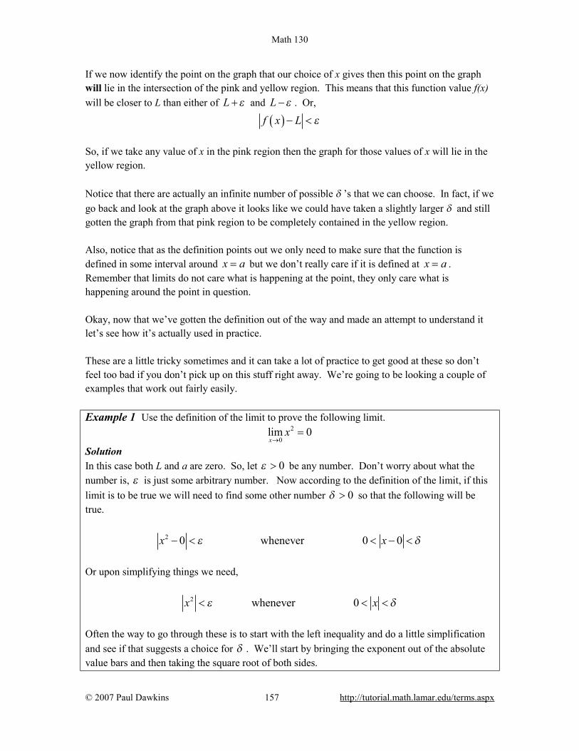
Math 130
© 2007 Paul Dawkins 157 http://tutorial.math.lamar.edu/terms.aspx
If we now identify the point on the graph that our choice of x gives then this point on the graph will lie in the intersection of the pink and yellow region. This means that this function value f(x) will be closer to L than either of L ε+ and L ε− . Or,
( )f x L ε− < So, if we take any value of x in the pink region then the graph for those values of x will lie in the yellow region. Notice that there are actually an infinite number of possible δ ’s that we can choose. In fact, if we go back and look at the graph above it looks like we could have taken a slightly larger δ and still gotten the graph from that pink region to be completely contained in the yellow region. Also, notice that as the definition points out we only need to make sure that the function is defined in some interval around x a= but we don’t really care if it is defined at x a= . Remember that limits do not care what is happening at the point, they only care what is happening around the point in question. Okay, now that we’ve gotten the definition out of the way and made an attempt to understand it let’s see how it’s actually used in practice. These are a little tricky sometimes and it can take a lot of practice to get good at these so don’t feel too bad if you don’t pick up on this stuff right away. We’re going to be looking a couple of examples that work out fairly easily. Example 1 Use the definition of the limit to prove the following limit. 2
0lim 0x
x→
=
Solution In this case both L and a are zero. So, let 0ε > be any number. Don’t worry about what the number is, ε is just some arbitrary number. Now according to the definition of the limit, if this limit is to be true we will need to find some other number 0δ > so that the following will be true.
2 0 whenever 0 0x xε δ− < < − < Or upon simplifying things we need,
2 whenever 0x xε δ< < < Often the way to go through these is to start with the left inequality and do a little simplification and see if that suggests a choice for δ . We’ll start by bringing the exponent out of the absolute value bars and then taking the square root of both sides.

Math 130
© 2007 Paul Dawkins 158 http://tutorial.math.lamar.edu/terms.aspx
2x xε ε< ⇒ < Now, the results of this simplification looks an awful lot like 0 x δ< < with the exception of
the “ 0 < ” part. Missing that however isn’t a problem, it is just telling us that we can’t take
0x = . So, it looks like if we choose δ ε= we should get what we want. We’ll next need to verify that our choice of δ will give us what we want, i.e.,
2 whenever 0x xε ε< < <
Verification is in fact pretty much the same work that we did to get our guess. First, let’s again
let 0ε > be any number and then choose δ ε= . Now, assume that 0 x ε< < . We need to
show that by choosing x to satisfy this we will get,
2x ε<
To start the verification process we’ll start with 2x and then first strip out the exponent from the
absolute values. Once this is done we’ll use our assumption on x, namely that x ε< . Doing
all this gives,
( )
22
2
strip exponent out of absolute value bars
< use the assumption that
simplify
x x
xε ε
ε
=
<
=
Or, upon taking the middle terms out, if we assume that 0 x ε< < then we will get, 2x ε<
and this is exactly what we needed to show. So, just what have we done? We’ve shown that if we choose 0ε > then we can find a 0δ > so that we have,
2 0 whenever 0 0x xε ε− < < − <
and according to our definition this means that, 2
0lim 0x
x→
=
These can be a little tricky the first couple times through. Especially when it seems like we’ve got to do the work twice. In the previous example we did some simplification on the left hand
Math 130
© 2007 Paul Dawkins 159 http://tutorial.math.lamar.edu/terms.aspx
inequality to get our guess for δ and then seemingly went through exactly the same work to then prove that our guess was correct. This is often how these work, although we will see an example here in a bit where things don’t work out quite so nicely. So, having said that let’s take a look at a slightly more complicated limit, although this one will still be fairly similar to the first example. Example 2 Use the definition of the limit to prove the following limit.
2lim5 4 6x
x→
− =
Solution We’ll start this one out the same way that we did the first one. We won’t be putting in quite the same amount of explanation however. Let’s start off by letting 0ε > be any number then we need to find a number 0δ > so that the following will be true.
( )5 4 6 whenever 0 2x xε δ− − < < − < We’ll start by simplifying the left inequality in an attempt to get a guess for δ . Doing this gives,
( )5 4 6 5 10 5 2 25
x x x x εε− − = − = − < ⇒ − <
So, as with the first example it looks like if we do enough simplification on the left inequality we
get something that looks an awful lot like the right inequality and this leads us to choose 5ε
δ = .
Let’s now verify this guess. So, again let 0ε > be any number and then choose 5ε
δ = . Next,
assume that 0 25
x εδ< − < = and we get the following,
( )5 4 6 5 10 simplify things a little
5 2 more simplification....
5 use the assumption 5 5
and some more simplification
x x
x
ε εδ
ε
− − = −
= −
< =
=
So, we’ve shown that
( )5 4 6 whenever 0 25
x x εε− − < < − <
and so by our definition we have,
2lim5 4 6x
x→
− =

Math 130
© 2007 Paul Dawkins 160 http://tutorial.math.lamar.edu/terms.aspx
Okay, so again the process seems to suggest that we have to essentially redo all our work twice, once to make the guess for δ and then another time to prove our guess. Let’s do an example that doesn’t work out quite so nicely. Example 3 Use the definition of the limit to prove the following limit. 2
4lim 11 9x
x x→
+ − =
Solution So, let’s get started. Let 0ε > be any number then we need to find a number 0δ > so that the following will be true.
( )2 11 9 whenever 0 4x x xε δ+ − − < < − <
We’ll start the guess process in the same manner as the previous two examples.
( ) ( )( )2 211 9 20 5 4 5 4x x x x x x x x ε+ − − = + − = + − = + − <
Okay, we’ve managed to show that ( )2 11 9x x ε+ − − < is equivalent to 5 4x x ε+ − < .
However, unlike the previous two examples, we’ve got an extra term in here that doesn’t show up in the right inequality above. If we have any hope of proceeding here we’re going need to find some way to get rid of the 5x + .
To do this let’s just note that if, by some chance, we can show that 5x K+ < for some number
K then, we’ll have the following, 5 4 4x x K x+ − < −
If we now assume that what we really want to show is 4K x ε− < instead of 5 4x x ε+ − <
we get the following,
4xKε
− <
This is starting to seem familiar isn’t it? All this work however, is based on the assumption that we can show that 5x K+ < for some K.
Without this assumption we can’t do anything so let’s see if we can do this. Let’s first remember that we are working on a limit here and let’s also remember that limits are only really concerned with what is happening around the point in question, 4x = in this case. So, it is safe to assume that whatever x is, it must be close to 4x = . This means we can safely assume that whatever x is, it is within a distance of, say one of 4x = . Or in terms of an

Math 130
© 2007 Paul Dawkins 161 http://tutorial.math.lamar.edu/terms.aspx
inequality, we can assume that, 4 1x − <
Why choose 1 here? There is no reason other than it’s a nice number to work with. We could just have easily chosen 2, or 5, or 1
3 . The only difference our choice will make is on the actual value of K that we end up with. You might want to go through this process with another choice of K and see if you can do it. So, let’s start with 4 1x − < and get rid of the absolute value bars and this solve the resulting
inequality for x as follows, 1 4 1 3 5x x− < − < ⇒ < < If we now add 5 to all parts of this inequality we get, 8 5 10x< + < Now, since 5 8 0x + > > (the positive part is important here) we can say that, provided
4 1x − < we know that 5 5x x+ = + . Or, if take the double inequality above we have,
8 5 10 5 10 10x x K< + < ⇒ + < ⇒ =
So, provided 4 1x − < we can see that 5 10x + < which in turn gives us,
410
xKε ε
− < =
So, to this point we make two assumptions about 4x − We’ve assumed that,
4 AND 4 110
x xε− < − <
It may not seem like it, but we’re now ready to chose a δ . In the previous examples we had only a single assumption and we used that to give us δ . In this case we’ve got two and they BOTH
need to be true. So, we’ll let δ be the smaller of the two assumptions, 1 and 10ε
.
Mathematically, this is written as,
min 1,10ε
δ =
By doing this we can guarantee that,
AND 110ε
δ δ≤ ≤
Now that we’ve made our choice for δ we need to verify it. So, 0ε > be any number and then

Math 130
© 2007 Paul Dawkins 162 http://tutorial.math.lamar.edu/terms.aspx
choose min 1,10ε
δ =
. Assume that 0 4 min 1,10
x εδ < − < =
. First, we get that,
0 4 410 10
x xε εδ< − < ≤ ⇒ − <
We also get, 0 4 1 4 1 5 10x x xδ< − < ≤ ⇒ − < ⇒ + <
Finally, all we need to do is,
( )2 211 9 20 simplify things a little
5 4 factor
10 4 use the assumption that 5 10
10 use the assumption that 410 10
a little final simplification
x x x x
x x
x x
xε ε
ε
+ − − = + −
= + −
< − + <
< − <
<
We’ve now managed to show that,
( )2 11 9 whenever 0 4 min 1,10
x x x εε + − − < < − <
and so by our definition we have, 2
4lim 11 9x
x x→
+ − =
Okay, that was a lot more work that the first two examples and unfortunately, it wasn’t all that difficult of a problem. Well, maybe we should say that in comparison to some of the other limits we could have tried to prove it wasn’t all that difficult. When first faced with these kinds of proofs using the precise definition of a limit they can all seem pretty difficult. Do not feel bad if you don’t get this stuff right away. It’s very common to not understand this right away and to have to struggle a little to fully start to understand how these kinds of limit definition proofs work. Next, let’s give the precise definitions for the right- and left-handed limits. Definition 2 For the right-hand limit we say that,
( )limx a
f x L+→
=
if for every number 0ε > there is some number 0δ > such that
( ) ( )whenever 0 or f x L x a a x aε δ δ− < < − < < < +
Math 130
© 2007 Paul Dawkins 163 http://tutorial.math.lamar.edu/terms.aspx
Definition 3 For the left-hand limit we say that,
( )limx a
f x L−→
=
if for every number 0ε > there is some number 0δ > such that
( ) ( )whenever 0 or f x L x a a x aε δ δ− < − < − < − < <
Note that with both of these definitions there are two ways to deal with the restriction on x and the one in parenthesis is probably the easier to use, although the main one given more closely matches the definition of the normal limit above. Let’s work a quick example of one of these, although as you’ll see they work in much the same manner as the normal limit problems do. Example 4 Use the definition of the limit to prove the following limit.
0lim 0x
x+→
=
Solution Let 0ε > be any number then we need to find a number 0δ > so that the following will be true.
0 whenever 0 0x xε δ− < < − <
Or upon a little simplification we need to show,
whenever 0x xε δ< < < As with the previous problems let’s start with the left hand inequality and see if we can’t use that to get a guess for δ . The only simplification that we really need to do here is to square both sides.
2x xε ε< ⇒ < So, it looks like we can chose 2δ ε= . Let’s verify this. Let 0ε > be any number and chose 2δ ε= . Next assume that 20 x ε< < . This gives,
2 2
0 some quick simplification
use the assumption that one final simplification
x x
xε εε
− =
< <<
We now shown that, 20 whenever 0 0x xε ε− < < − <
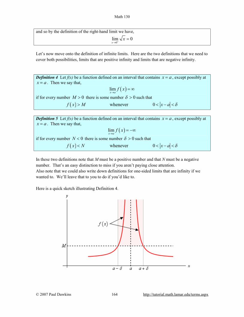
Math 130
© 2007 Paul Dawkins 164 http://tutorial.math.lamar.edu/terms.aspx
and so by the definition of the right-hand limit we have,
0lim 0x
x+→
=
Let’s now move onto the definition of infinite limits. Here are the two definitions that we need to cover both possibilities, limits that are positive infinity and limits that are negative infinity. Definition 4 Let f(x) be a function defined on an interval that contains x a= , except possibly at x a= . Then we say that,
( )limx a
f x→
= ∞
if for every number 0M > there is some number 0δ > such that
( ) whenever 0f x M x a δ> < − <
Definition 5 Let f(x) be a function defined on an interval that contains x a= , except possibly at x a= . Then we say that,
( )limx a
f x→
= −∞
if for every number 0N < there is some number 0δ > such that
( ) whenever 0f x N x a δ< < − <
In these two definitions note that M must be a positive number and that N must be a negative number. That’s an easy distinction to miss if you aren’t paying close attention. Also note that we could also write down definitions for one-sided limits that are infinity if we wanted to. We’ll leave that to you to do if you’d like to. Here is a quick sketch illustrating Definition 4.

Math 130
© 2007 Paul Dawkins 165 http://tutorial.math.lamar.edu/terms.aspx
What Definition 4 is telling us is that no matter how large we choose M to be we can always find an interval around x a= , given by 0 x a δ< − < for some number δ , so that as long as we
stay within that interval the graph of the function will be above the line y M= as shown in the graph. Also note that we don’t need the function to actually exist at x a= in order for the definition to hold. This is also illustrated in the sketch above. Note as well that the larger M is the smaller we’re probably going to need to make δ . To see an illustration of Definition 5 reflect the above graph about the x-axis and you’ll see a sketch of Definition 5. Let’s work a quick example of one of these to see how these differ from the previous examples. Example 5 Use the definition of the limit to prove the following limit.
20
1limx x→
= ∞
Solution These work in pretty much the same manner as the previous set of examples do. The main difference is that we’re working with an M now instead of an ε . So, let’s get going. Let 0M > be any number and we’ll need to choose a 0δ > so that,
2
1 whenever 0 0M x xx
δ> < − = <
As with the all the previous problems we’ll start with the left inequality and try to get something in the end that looks like the right inequality. To do this we’ll basically solve the left inequality
for x and we’ll need to recall that 2x x= . So, here’s that work.
22
1 1 1M x xx M M
> ⇒ < ⇒ <
So, it looks like we can chose 1M
δ = . All we need to do now is verify this guess.
Let 0M > be any number, choose 1M
δ = and assume that 10 xM
< < .
In the previous examples we tried to show that our assumptions satisfied the left inequality by working with it directly. However, in this, the function and our assumption on x that we’ve got actually will make this easier to start with the assumption on x and show that we can get the left inequality out of that. Note that this is being done this way mostly because of the function that we’re working with and not because of the type of limit that we’ve got.
Math 130
© 2007 Paul Dawkins 166 http://tutorial.math.lamar.edu/terms.aspx
Doing this work gives,
2
22 2
22
1
1 square both sides
1 acknowledge that
1 solve for
xM
xM
x x xM
M xx
<
<
< =
>
So, we’ve managed to show that,
2
1 1whenever 0 0M xx M
> < − <
and so by the definition of the limit we have,
20
1limx x→
= ∞
For our next set of limit definitions let’s take a look at the two definitions for limits at infinity. Again, we need one for a limit at plus infinity and another for negative infinity. Definition 6 Let f(x) be a function defined on an interval that contains x a= , except possibly at x a= . Then we say that,
( )limx
f x L→∞
=
if for every number 0ε > there is some number 0M > such that
( ) wheneverf x L x Mε− < >
Definition 7 Let f(x) be a function defined on an interval that contains x a= , except possibly at x a= . Then we say that,
( )limx
f x L→−∞
=
if for every number 0ε > there is some number 0N < such that
( ) wheneverf x L x Nε− < <
To see what these definitions are telling us here is a quick sketch illustrating Definition 6. Definition 6 tells us is that no matter how close to L we want to get, mathematically this is given
by ( )f x L ε− < for any chosen ε , we can find another number M such that provided we take
any x bigger than M, then the graph of the function for that x will be closer to L than either L ε− and L ε+ . Or, in other words, the graph will be in the shaded region as shown in the sketch below.
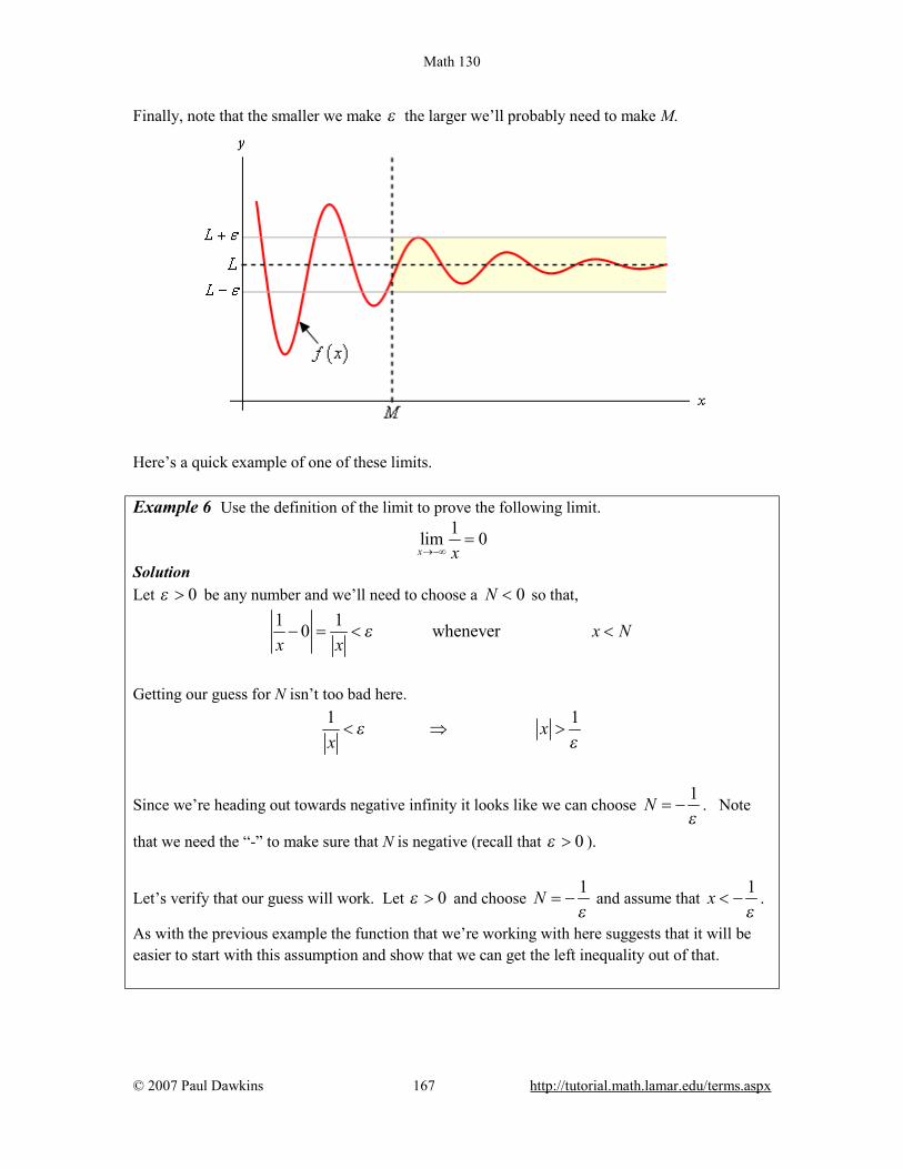
Math 130
© 2007 Paul Dawkins 167 http://tutorial.math.lamar.edu/terms.aspx
Finally, note that the smaller we make ε the larger we’ll probably need to make M.
Here’s a quick example of one of these limits. Example 6 Use the definition of the limit to prove the following limit.
1lim 0x x→−∞
=
Solution Let 0ε > be any number and we’ll need to choose a 0N < so that,
1 10 whenever x Nx x
ε− = < <
Getting our guess for N isn’t too bad here.
1 1xx
εε
< ⇒ >
Since we’re heading out towards negative infinity it looks like we can choose 1Nε
= − . Note
that we need the “-” to make sure that N is negative (recall that 0ε > ).
Let’s verify that our guess will work. Let 0ε > and choose 1Nε
= − and assume that 1xε
< − .
As with the previous example the function that we’re working with here suggests that it will be easier to start with this assumption and show that we can get the left inequality out of that.

Math 130
© 2007 Paul Dawkins 168 http://tutorial.math.lamar.edu/terms.aspx
1
1 take the absolute value
1 do a little simplification
1 solve for
1 0 rewrite things a little
x
x
x
xx
x
ε
ε
ε
ε
ε
< −
> −
>
<
− <
Note that when we took the absolute value of both sides we changed both sides from negative numbers to positive numbers and so also had to change the direction of the inequality. So, we’ve shown that,
1 1 10 whenever xx x
εε
− = < < −
and so by the definition of the limit we have, 1lim 0
x x→−∞=
For our final limit definition let’s look at limits at infinity that are also infinite in value. There are four possible limits to define here. We’ll do one of them and leave the other three to you to write down if you’d like to. Definition 8 Let f(x) be a function defined on an interval that contains x a= , except possibly at x a= . Then we say that,
( )limx
f x→∞
= ∞
if for every number 0N > there is some number 0M > such that
( ) wheneverf x N x M> >
The other three definitions are almost identical. The only differences are the signs of M and/or N and the corresponding inequality directions. As a final definition in this section let’s recall that we previously said that a function was continuous if,
( ) ( )limx a
f x f a→
=
So, since continuity, as we previously defined it, is defined in terms of a limit we can also now give a more precise definition of continuity. Here it is,
Math 130
© 2007 Paul Dawkins 169 http://tutorial.math.lamar.edu/terms.aspx
Definition 9 Let f(x) be a function defined on an interval that contains x a= . Then we say that f(x) is continuous at x a= if for every number 0ε > there is some number 0δ > such that
( ) ( ) whenever 0f x f a x aε δ− < < − <
This definition is very similar to the first definition in this section and of course that should make some sense since that is exactly the kind of limit that we’re doing to show that a function is continuous. The only real difference is that here we need to make sure that the function is actually defined at x a= , while we didn’t need to worry about that for the first definition since limits don’t really care what is happening at the point. We won’t do any examples of proving a function is continuous at a point here mostly because we’ve already done some examples. Go back and look at the first three examples. In each of these examples the value of the limit was the value of the function evaluated at x a= and so in each of these examples not only did we prove the value of the limit we also managed to prove that each of these functions are continuous at the point in question.

Math 130
© 2007 Paul Dawkins 170 http://tutorial.math.lamar.edu/terms.aspx
Math 130
© 2007 Paul Dawkins 171 http://tutorial.math.lamar.edu/terms.aspx
Derivatives
Introduction In this chapter we will start looking at the next major topic in a calculus class. We will be looking at derivatives in this chapter (as well as the next chapter). This chapter is devoted almost exclusively to finding derivatives. We will be looking at one application of them in this chapter. We will be leaving most of the applications of derivatives to the next chapter. Here is a listing of the topics covered in this chapter. The Definition of the Derivative – In this section we will be looking at the definition of the derivative. Interpretation of the Derivative – Here we will take a quick look at some interpretations of the derivative. Differentiation Formulas – Here we will start introducing some of the differentiation formulas used in a calculus course. Product and Quotient Rule – In this section we will look at differentiating products and quotients of functions. Derivatives of Trig Functions – We’ll give the derivatives of the trig functions in this section. Derivatives of Exponential and Logarithm Functions – In this section we will get the derivatives of the exponential and logarithm functions. Derivatives of Inverse Trig Functions – Here we will look at the derivatives of inverse trig functions. Derivatives of Hyperbolic Functions – Here we will look at the derivatives of hyperbolic functions. Chain Rule – The Chain Rule is one of the more important differentiation rules and will allow us to differentiate a wider variety of functions. In this section we will take a look at it. Implicit Differentiation – In this section we will be looking at implicit differentiation. Without this we won’t be able to work some of the applications of derivatives.
Math 130
© 2007 Paul Dawkins 172 http://tutorial.math.lamar.edu/terms.aspx
Related Rates – In this section we will look at the lone application to derivatives in this chapter. This topic is here rather than the next chapter because it will help to cement in our minds one of the more important concepts about derivatives and because it requires implicit differentiation. Higher Order Derivatives – Here we will introduce the idea of higher order derivatives. Logarithmic Differentiation – The topic of logarithmic differentiation is not always presented in a standard calculus course. It is presented here for those how are interested in seeing how it is done and the types of functions on which it can be used.

Math 130
© 2007 Paul Dawkins 173 http://tutorial.math.lamar.edu/terms.aspx
The Definition of the Derivative In the first section of the last chapter we saw that the computation of the slope of a tangent line, the instantaneous rate of change of a function, and the instantaneous velocity of an object at x a= all required us to compute the following limit.
( ) ( )limx a
f x f ax a→
−−
We also saw that with a small change of notation this limit could also be written as,
( ) ( )0
limh
f a h f ah→
+ − (1)
This is such an important limit and it arises in so many places that we give it a name. We call it a derivative. Here is the official definition of the derivative. Definition The derivative of ( )f x with respect to x is the function ( )f x′ and is defined as,
( ) ( ) ( )0
limh
f x h f xf x
h→
+ −′ = (2)
Note that we replaced all the a’s in (1) with x’s to acknowledge the fact that the derivative is really a function as well. We often “read” ( )f x′ as “f prime of x”.
Let’s compute a couple of derivatives using the definition. Example 1 Find the derivative of the following function using the definition of the derivative. ( ) 22 16 35f x x x= − + Solution So, all we really need to do is to plug this function into the definition of the derivative, (1), and do some algebra. While, admittedly, the algebra will get somewhat unpleasant at times, but it’s just algebra so don’t get excited about the fact that we’re now computing derivatives. First plug the function into the definition of the derivative.
( ) ( ) ( )
( ) ( ) ( )0
2 2
0
lim
2 16 35 2 16 35lim
h
h
f x h f xf x
hx h x h x x
h
→
→
+ −′ =
+ − + + − − +=
Be careful and make sure that you properly deal with parenthesis when doing the subtracting. Now, we know from the previous chapter that we can’t just plug in 0h = since this will give us a
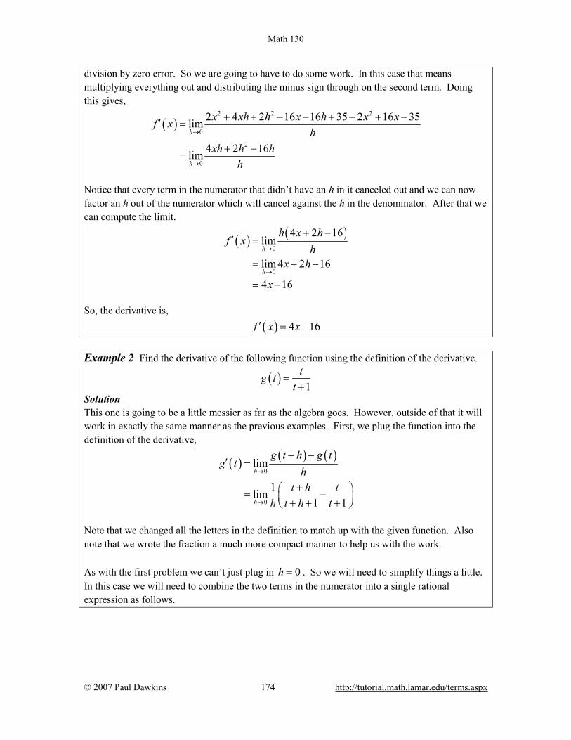
Math 130
© 2007 Paul Dawkins 174 http://tutorial.math.lamar.edu/terms.aspx
division by zero error. So we are going to have to do some work. In this case that means multiplying everything out and distributing the minus sign through on the second term. Doing this gives,
( )
2 2 2
0
2
0
2 4 2 16 16 35 2 16 35lim
4 2 16lim
h
h
x xh h x h x xf xh
xh h hh
→
→
+ + − − + − + −′ =
+ −=
Notice that every term in the numerator that didn’t have an h in it canceled out and we can now factor an h out of the numerator which will cancel against the h in the denominator. After that we can compute the limit.
( ) ( )0
0
4 2 16lim
lim 4 2 16
4 16
h
h
h x hf x
hx h
x
→
→
+ −′ =
= + −
= −
So, the derivative is, ( ) 4 16f x x′ = − Example 2 Find the derivative of the following function using the definition of the derivative.
( )1
tg tt
=+
Solution This one is going to be a little messier as far as the algebra goes. However, outside of that it will work in exactly the same manner as the previous examples. First, we plug the function into the definition of the derivative,
( ) ( ) ( )
0
0
lim
1lim1 1
h
h
g t h g tg t
ht h t
h t h t
→
→
+ −′ =
+ = − + + +
Note that we changed all the letters in the definition to match up with the given function. Also note that we wrote the fraction a much more compact manner to help us with the work. As with the first problem we can’t just plug in 0h = . So we will need to simplify things a little. In this case we will need to combine the two terms in the numerator into a single rational expression as follows.

Math 130
© 2007 Paul Dawkins 175 http://tutorial.math.lamar.edu/terms.aspx
( ) ( )( ) ( )( ) ( )
( )( ) ( )
( ) ( )
0
2 2
0
0
1 11lim1 1
1lim1 1
1lim1 1
h
h
h
t h t t t hg t
h t h t
t t th h t th th t h t
hh t h t
→
→
→
+ + − + +′ = + + +
+ + + − + + = + + +
= + + +
Before finishing this let’s note a couple of things. First, we didn’t multiply out the denominator. Multiplying out the denominator will just overly complicate things so let’s keep it simple. Next, as with the first example, after the simplification we only have terms with h’s in them left in the numerator and so we can now cancel an h out. So, upon canceling the h we can evaluate the limit and get the derivative.
( ) ( ) ( )
( )( )
( )
0
2
1lim1 1
11 1
11
hg t
t h t
t t
t
→′ =
+ + +
=+ +
=+
The derivative is then,
( )( )2
11
g tt
′ =+
Example 3 Find the derivative of the following function using the derivative. ( ) 5 8R z z= − Solution First plug into the definition of the derivative as we’ve done with the previous two examples.
( ) ( ) ( )
( )0
0
lim
5 8 5 8lim
h
h
R z h R zR z
hz h z
h
→
→
+ −′ =
+ − − −=
In this problem we’re going to have to rationalize the numerator. You do remember rationalization from an Algebra class right? In an Algebra class you probably only rationalized the denominator, but you can also rationalize numerators. Remember that in rationalizing the numerator (in this case) we multiply both the numerator and denominator by the numerator except we change the sign between the two terms. Here’s the rationalizing work for this problem,
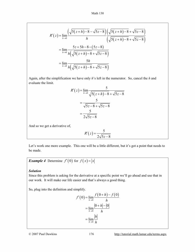
Math 130
© 2007 Paul Dawkins 176 http://tutorial.math.lamar.edu/terms.aspx
( )( )( ) ( )( )
( )( )( )
( )( )
( )( )
0
0
0
5 8 5 8 5 8 5 8lim
5 8 5 8
5 5 8 5 8lim
5 8 5 8
5lim5 8 5 8
h
h
h
z h z z h zR z
h z h z
z h z
h z h z
hh z h z
→
→
→
+ − − − + − + −′ =
+ − + −
+ − − −=
+ − + −
=+ − + −
Again, after the simplification we have only h’s left in the numerator. So, cancel the h and evaluate the limit.
( )( )0
5lim5 8 5 8
55 8 5 8
52 5 8
hR z
z h z
z z
z
→′ =
+ − + −
=− + −
=−
And so we get a derivative of,
( ) 52 5 8
R zz
′ =−
Let’s work one more example. This one will be a little different, but it’s got a point that needs to be made. Example 4 Determine ( )0f ′ for ( )f x x= Solution Since this problem is asking for the derivative at a specific point we’ll go ahead and use that in our work. It will make our life easier and that’s always a good thing. So, plug into the definition and simplify.
( ) ( ) ( )0
0
0
0 00 lim
0 0lim
lim
h
h
h
f h ff
hhh
hh
→
→
→
+ −′ =
+ −=
=

Math 130
© 2007 Paul Dawkins 177 http://tutorial.math.lamar.edu/terms.aspx
We saw a situation like this back when we were looking at limits at infinity. As in that section we can’t just cancel the h’s. We will have to look at the two one sided limits and recall that
if 0if 0
h hh
h h≥
= − <
( )0 0
0
lim lim because 0 in a left-hand limit.
lim 1
1
h h
h
h h hh h− −
−
→ →
→
−= <
= −
= −
0 0
0
lim lim because 0 in a right-hand limit.
lim 1
1
h h
h
h h hh h+ +
+
→ →
→
= >
=
=
The two one-sided limits are different and so
0
limh
hh→
doesn’t exist. However, this is the limit that gives us the derivative that we’re after. If the limit doesn’t exist then the derivative doesn’t exist either. In this example we have finally seen a function for which the derivative doesn’t exist at a point. This is a fact of life that we’ve got to be aware of. Derivatives will not always exist. Note as well that this doesn’t say anything about whether or not the derivative exists anywhere else. In fact, the derivative of the absolute value function exists at every point except the one we just looked at, 0x = . The preceding discussion leads to the following definition. Definition A function ( )f x is called differentiable at x a= if ( )f x′ exists and ( )f x is called
differentiable on an interval if the derivative exists for each point in that interval. The next theorem shows us a very nice relationship between functions that are continuous and those that are differentiable. Theorem If ( )f x is differentiable at x a= then ( )f x is continuous at x a= .

Math 130
© 2007 Paul Dawkins 178 http://tutorial.math.lamar.edu/terms.aspx
See the Proof of Various Derivative Formulas section of the Extras chapter to see the proof of this theorem. Note that this theorem does not work in reverse. Consider ( )f x x= and take a look at,
( ) ( )
0 0lim lim 0 0x x
f x x f→ →
= = =
So, ( )f x x= is continuous at 0x = but we’ve just shown above in Example 4 that
( )f x x= is not differentiable at 0x = .
Alternate Notation Next we need to discuss some alternate notation for the derivative. The typical derivative notation is the “prime” notation. However, there is another notation that is used on occasion so let’s cover that. Given a function ( )y f x= all of the following are equivalent and represent the derivative of
( )f x with respect to x.
( ) ( )( ) ( )df dy d df x y f x ydx dx dx dx
′ ′= = = = =
Because we also need to evaluate derivatives on occasion we also need a notation for evaluating derivatives when using the fractional notation. So if we want to evaluate the derivative at x=a all of the following are equivalent.
( ) x ax a x a
df dyf a ydx dx=
= =
′ ′= = =
Note as well that on occasion we will drop the (x) part on the function to simplify the notation somewhat. In these cases the following are equivalent. ( )f x f′ ′= As a final note in this section we’ll acknowledge that computing most derivatives directly from the definition is a fairly complex (and sometimes painful) process filled with opportunities to make mistakes. In a couple of section we’ll start developing formulas and/or properties that will help us to take the derivative of many of the common functions so we won’t need to resort to the definition of the derivative too often. This does not mean however that it isn’t important to know the definition of the derivative! It is an important definition that we should always know and keep in the back of our minds. It is just something that we’re not going to be working with all that much.

Math 130
© 2007 Paul Dawkins 179 http://tutorial.math.lamar.edu/terms.aspx
Interpretations of the Derivative Before moving on to the section where we learn how to compute derivatives by avoiding the limits we were evaluating in the previous section we need to take a quick look at some of the interpretations of the derivative. All of these interpretations arise from recalling how our definition of the derivative came about. The definition came about by noticing that all the problems that we worked in the first section in the chapter on limits required us to evaluate the same limit. Rate of Change The first interpretation of a derivative is rate of change. This was not the first problem that we looked at in the limit chapter, but it is the most important interpretation of the derivative. If
( )f x represents a quantity at any x then the derivative ( )f a′ represents the instantaneous rate
of change of ( )f x at x a= .
Example 1 Suppose that the amount of water in a holding tank at t minutes is given by
( ) 22 16 35V t t t= − + . Determine each of the following. (a) Is the volume of water in the tank increasing or decreasing at 1t = minute?
[Solution]
(b) Is the volume of water in the tank increasing or decreasing at 5t = minutes? [Solution]
(c) Is the volume of water in the tank changing faster at 1t = or 5t = minutes? [Solution]
(d) Is the volume of water in the tank ever not changing? If so, when? [Solution] Solution In the solution to this example we will use both notations for the derivative just to get you familiar with the different notations. We are going to need the rate of change of the volume to answer these questions. This means that we will need the derivative of this function since that will give us a formula for the rate of change at any time t. Now, notice that the function giving the volume of water in the tank is the same function that we saw in Example 1 in the last section except the letters have changed. The change in letters between the function in this example versus the function in the example from the last section won’t affect the work and so we can just use the answer from that example with an appropriate change in letters. The derivative is.
( ) 4 16 OR 4 16dVV t t tdt
′ = − = −
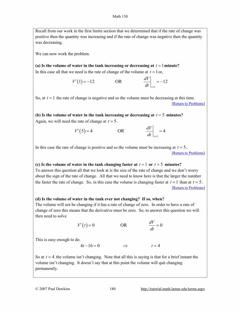
Math 130
© 2007 Paul Dawkins 180 http://tutorial.math.lamar.edu/terms.aspx
Recall from our work in the first limits section that we determined that if the rate of change was positive then the quantity was increasing and if the rate of change was negative then the quantity was decreasing. We can now work the problem. (a) Is the volume of water in the tank increasing or decreasing at 1t = minute? In this case all that we need is the rate of change of the volume at 1t = or,
( )1
1 12 OR 12t
dVVdt =
′ = − = −
So, at 1t = the rate of change is negative and so the volume must be decreasing at this time.
[Return to Problems] (b) Is the volume of water in the tank increasing or decreasing at 5t = minutes? Again, we will need the rate of change at 5t = .
( )5
5 4 OR 4t
dVVdt =
′ = =
In this case the rate of change is positive and so the volume must be increasing at 5t = .
[Return to Problems] (c) Is the volume of water in the tank changing faster at 1t = or 5t = minutes? To answer this question all that we look at is the size of the rate of change and we don’t worry about the sign of the rate of change. All that we need to know here is that the larger the number the faster the rate of change. So, in this case the volume is changing faster at 1t = than at 5t = .
[Return to Problems] (d) Is the volume of water in the tank ever not changing? If so, when? The volume will not be changing if it has a rate of change of zero. In order to have a rate of change of zero this means that the derivative must be zero. So, to answer this question we will then need to solve
( ) 0 OR 0dVV tdt
′ = =
This is easy enough to do. 4 16 0 4t t− = ⇒ = So at 4t = the volume isn’t changing. Note that all this is saying is that for a brief instant the volume isn’t changing. It doesn’t say that at this point the volume will quit changing permanently.
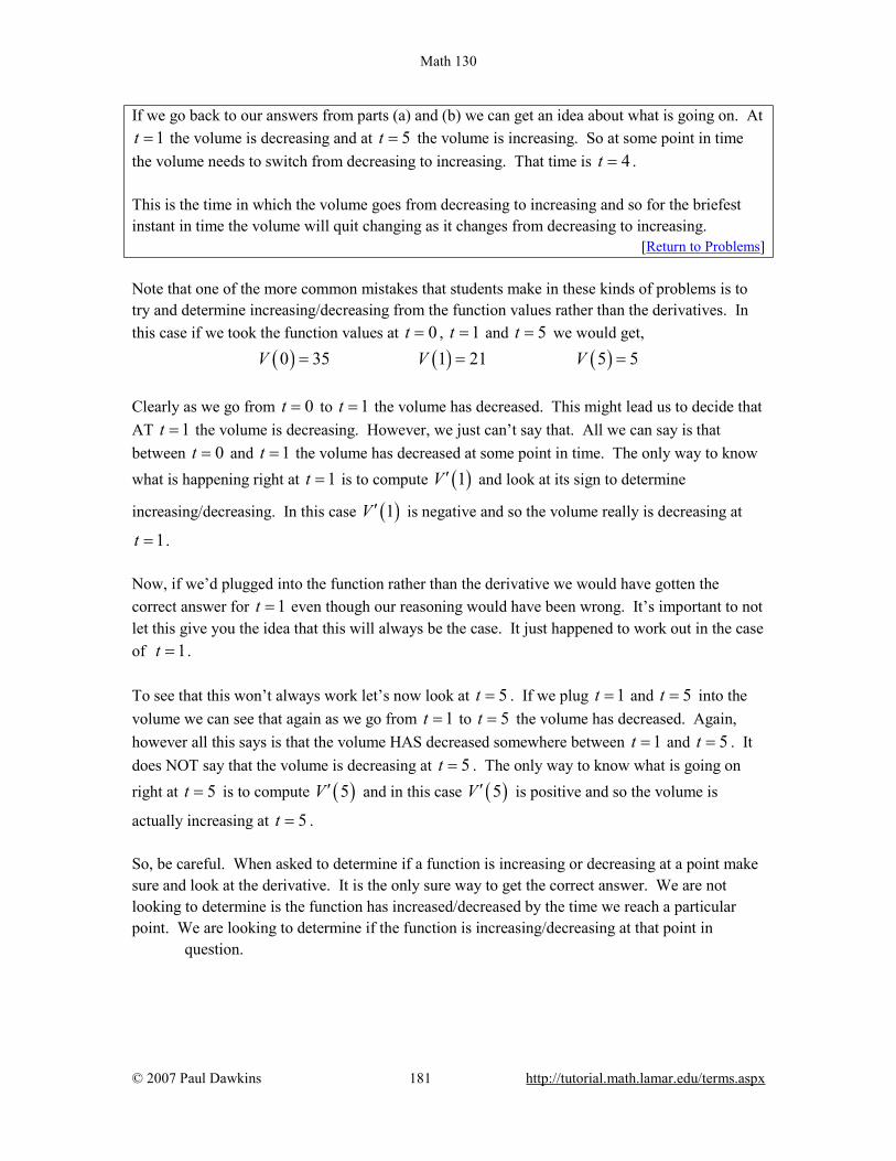
Math 130
© 2007 Paul Dawkins 181 http://tutorial.math.lamar.edu/terms.aspx
If we go back to our answers from parts (a) and (b) we can get an idea about what is going on. At 1t = the volume is decreasing and at 5t = the volume is increasing. So at some point in time
the volume needs to switch from decreasing to increasing. That time is 4t = . This is the time in which the volume goes from decreasing to increasing and so for the briefest instant in time the volume will quit changing as it changes from decreasing to increasing.
[Return to Problems] Note that one of the more common mistakes that students make in these kinds of problems is to try and determine increasing/decreasing from the function values rather than the derivatives. In this case if we took the function values at 0t = , 1t = and 5t = we would get, ( ) ( ) ( )0 35 1 21 5 5V V V= = = Clearly as we go from 0t = to 1t = the volume has decreased. This might lead us to decide that AT 1t = the volume is decreasing. However, we just can’t say that. All we can say is that between 0t = and 1t = the volume has decreased at some point in time. The only way to know what is happening right at 1t = is to compute ( )1V ′ and look at its sign to determine
increasing/decreasing. In this case ( )1V ′ is negative and so the volume really is decreasing at
1t = . Now, if we’d plugged into the function rather than the derivative we would have gotten the correct answer for 1t = even though our reasoning would have been wrong. It’s important to not let this give you the idea that this will always be the case. It just happened to work out in the case of 1t = . To see that this won’t always work let’s now look at 5t = . If we plug 1t = and 5t = into the volume we can see that again as we go from 1t = to 5t = the volume has decreased. Again, however all this says is that the volume HAS decreased somewhere between 1t = and 5t = . It does NOT say that the volume is decreasing at 5t = . The only way to know what is going on right at 5t = is to compute ( )5V ′ and in this case ( )5V ′ is positive and so the volume is
actually increasing at 5t = . So, be careful. When asked to determine if a function is increasing or decreasing at a point make sure and look at the derivative. It is the only sure way to get the correct answer. We are not looking to determine is the function has increased/decreased by the time we reach a particular point. We are looking to determine if the function is increasing/decreasing at that point in question.

Math 130
© 2007 Paul Dawkins 182 http://tutorial.math.lamar.edu/terms.aspx
Slope of Tangent Line This is the next major interpretation of the derivative. The slope of the tangent line to ( )f x at
x a= is ( )f a′ . The tangent line then is given by,
( ) ( )( )y f a f a x a′= + − Example 2 Find the tangent line to the following function at 3z = . ( ) 5 8R z z= − Solution We first need the derivative of the function and we found that in Example 3 in the last section. The derivative is,
( ) 52 5 8
R zz
′ =−
Now all that we need is the function value and derivative (for the slope) at 3z = .
( ) ( ) 53 7 32 7
R m R′= = =
The tangent line is then,
( )57 32 7
y z= + −
Velocity Recall that this can be thought of as a special case of the rate of change interpretation. If the position of an object is given by ( )f t after t units of time the velocity of the object at t a= is
given by ( )f a′ .
Example 3 Suppose that the position of an object after t hours is given by,
( )1
tg tt
=+
Answer both of the following about this object. (a) Is the object moving to the right or the left at 10t = hours? [Solution] (b) Does the object ever stop moving? [Solution]
Solution Once again we need the derivative and we found that in Example 2 in the last section. The derivative is,
( )( )2
11
g tt
′ =+
(a) Is the object moving to the right or the left at 10t = hours? To determine if the object is moving to the right (velocity is positive) or left (velocity is

Math 130
© 2007 Paul Dawkins 183 http://tutorial.math.lamar.edu/terms.aspx
negative) we need the derivative at 10t = .
( ) 110121
g′ =
So the velocity at 10t = is positive and so the object is moving to the right at 10t = .
[Return to Problems] (b) Does the object ever stop moving? The object will stop moving if the velocity is ever zero. However, note that the only way a rational expression will ever be zero is if the numerator is zero. Since the numerator of the derivative (and hence the speed) is a constant it can’t be zero. Therefore, the velocity will never stop moving. In fact, we can say a little more here. The object will always be moving to the right since the velocity is always positive.
[Return to Problems] We’ve seen three major interpretations of the derivative here. You will need to remember these, especially the rate of change, as they will show up continually throughout this course. Before we leave this section let’s work one more example that encompasses some of the ideas discussed here and is just a nice example to work. Example 4 Below is the sketch of a function ( )f x . Sketch the graph of the derivative of this
function, ( )f x′ .
Solution At first glance this seems to an all but impossible task. However, if you have some basic knowledge of the interpretations of the derivative you can get a sketch of the derivative. It will not be a perfect sketch for the most part, but you should be able to get most of the basic features
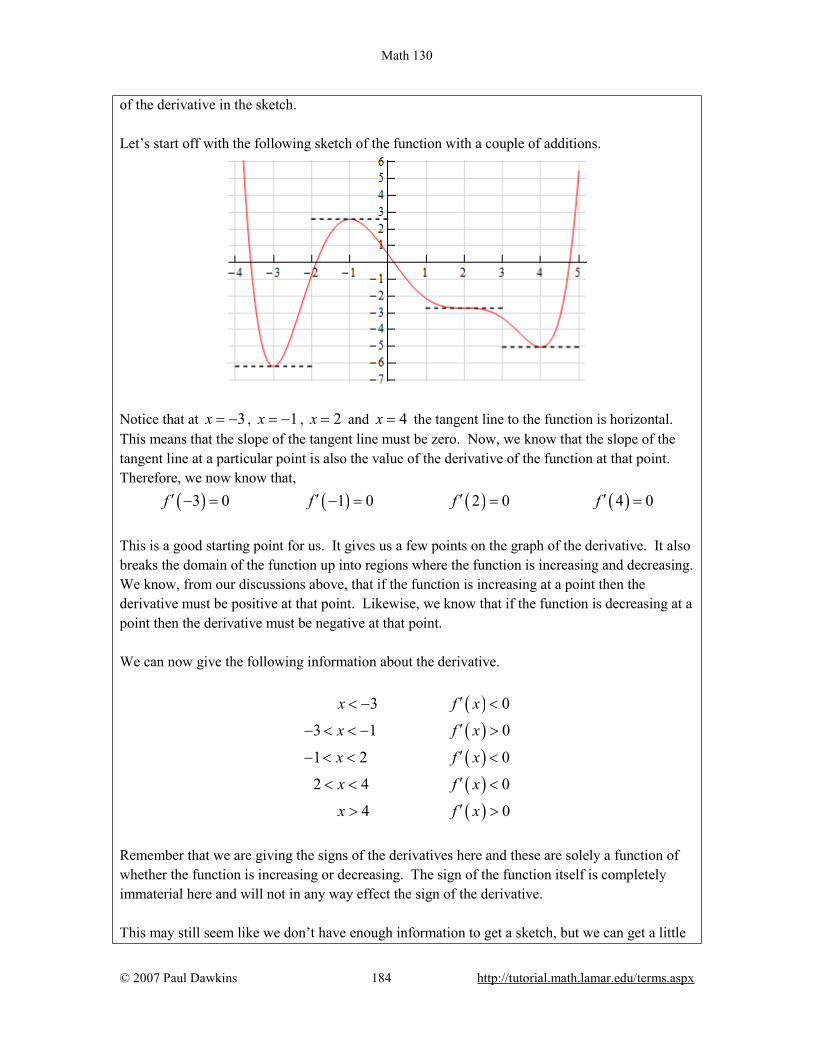
Math 130
© 2007 Paul Dawkins 184 http://tutorial.math.lamar.edu/terms.aspx
of the derivative in the sketch. Let’s start off with the following sketch of the function with a couple of additions.
Notice that at 3x = − , 1x = − , 2x = and 4x = the tangent line to the function is horizontal. This means that the slope of the tangent line must be zero. Now, we know that the slope of the tangent line at a particular point is also the value of the derivative of the function at that point. Therefore, we now know that, ( ) ( ) ( ) ( )3 0 1 0 2 0 4 0f f f f′ ′ ′ ′− = − = = =
This is a good starting point for us. It gives us a few points on the graph of the derivative. It also breaks the domain of the function up into regions where the function is increasing and decreasing. We know, from our discussions above, that if the function is increasing at a point then the derivative must be positive at that point. Likewise, we know that if the function is decreasing at a point then the derivative must be negative at that point. We can now give the following information about the derivative.
( )( )( )( )( )
3 0
3 1 0
1 2 0
2 4 0
4 0
x f x
x f x
x f x
x f x
x f x
′< − <
′− < < − >
′− < < <
′< < <
′> >
Remember that we are giving the signs of the derivatives here and these are solely a function of whether the function is increasing or decreasing. The sign of the function itself is completely immaterial here and will not in any way effect the sign of the derivative. This may still seem like we don’t have enough information to get a sketch, but we can get a little

Math 130
© 2007 Paul Dawkins 185 http://tutorial.math.lamar.edu/terms.aspx
bit more information about the derivative from the graph of the function. In the range 3x < − we know that the derivative must be negative, however we can also see that the derivative needs to be increasing in this range. It is negative here until we reach 3x = − and at this point the derivative must be zero. The only way for the derivative to be negative to the left of 3x = − and zero at 3x = − is for the derivative to increase as we increase x towards 3x = − . Now, in the range 3 1x− < < − we know that the derivative must be zero at the endpoints and positive in between the two endpoints. Directly to the right of 3x = − the derivative must also be increasing (because it starts at zero and the goes positive – therefore it must be increasing). So, the derivative in this range must start out increasing and must eventually get back to zero at
1x = − . So, at some point in this interval the derivative must start decreasing before it reaches 1x = − . Now, we have to be careful here because this is just general behavior here at the two
endpoints. We won’t know where the derivative goes from increasing to decreasing and it may well change between increasing and decreasing several times before we reach 1x = − . All we can really say is that immediately to the right of 3x = − the derivative will be increasing and immediately to the left of 1x = − the derivative will be decreasing. Next, for the ranges 1 2x− < < and 2 4x< < we know the derivative will be zero at the endpoints and negative in between. Also, following the type of reasoning given above we can see in each of these ranges that the derivative will be decreasing just to the right of the left hand endpoint and increasing just to the left of the right hand endpoint. Finally, in the last region 4x > we know that the derivative is zero at 4x = and positive to the right of 4x = . Once again, following the reasoning above, the derivative must also be increasing in this range. Putting all of this material together (and always taking the simplest choices for increasing and/or decreasing information) gives us the following sketch for the derivative.
Note that this was done with the actual derivative and so is in fact accurate. Any sketch you do

Math 130
© 2007 Paul Dawkins 186 http://tutorial.math.lamar.edu/terms.aspx
will probably not look quite the same. The “humps” in each of the regions may be at different places and/or different heights for example. Also, note that we left off the vertical scale because given the information that we’ve got at this point there was no real way to know this information. That doesn’t mean however that we can’t get some ideas of specific points on the derivative other than where we know the derivative to be zero. To see this let’s check out the following graph of the function (not the derivative, but the function).
At 2x = − and 3x = we’ve sketched in a couple of tangent lines. We can use the basic rise/run slope concept to estimate the value of the derivative at these points. Let’s start at 3x = . We’ve got two points on the line here. We can see that each seem to be about one-quarter of the way off the grid line. So, taking that into account and the fact that we go through one complete grid we can see that the slope of the tangent line, and hence the derivative, is approximately -1.5. At 2x = − it looks like (with some heavy estimation) that the second point is about 6.5 grids above the first point and so the slope of the tangent line here, and hence the derivative, is approximately 6.5. Here is the sketch of the derivative with the vertical scale included and from this we can see that in fact our estimates are pretty close to reality.

Math 130
© 2007 Paul Dawkins 187 http://tutorial.math.lamar.edu/terms.aspx
Note that this idea of estimating values of derivatives can be a tricky process and does require a fair amount of (possible bad) approximations so while it can be used, you need to be careful with it. We’ll close out this section by noting that while we’re not going to include an example here we could also use the graph of the derivative to give us a sketch of the function itself. In fact, in the next chapter where we discuss some applications of the derivative we will be looking using information the derivative gives us to sketch the graph of a function.
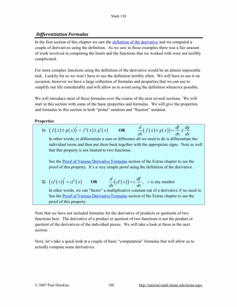
Math 130
© 2007 Paul Dawkins 188 http://tutorial.math.lamar.edu/terms.aspx
Differentiation Formulas In the first section of this chapter we saw the definition of the derivative and we computed a couple of derivatives using the definition. As we saw in those examples there was a fair amount of work involved in computing the limits and the functions that we worked with were not terribly complicated. For more complex functions using the definition of the derivative would be an almost impossible task. Luckily for us we won’t have to use the definition terribly often. We will have to use it on occasion, however we have a large collection of formulas and properties that we can use to simplify our life considerably and will allow us to avoid using the definition whenever possible. We will introduce most of these formulas over the course of the next several sections. We will start in this section with some of the basic properties and formulas. We will give the properties and formulas in this section in both “prime” notation and “fraction” notation. Properties
1) ( ) ( )( ) ( ) ( )f x g x f x g x′ ′ ′± = ± OR ( ) ( )( )d df dgf x g xdx dx dx
± = ±
In other words, to differentiate a sum or difference all we need to do is differentiate the individual terms and then put them back together with the appropriate signs. Note as well that this property is not limited to two functions. See the Proof of Various Derivative Formulas section of the Extras chapter to see the proof of this property. It’s a very simple proof using the definition of the derivative.
2) ( )( ) ( )cf x cf x′ ′= OR ( )( )d dfcf x cdx dx
= , c is any number
In other words, we can “factor” a multiplicative constant out of a derivative if we need to. See the Proof of Various Derivative Formulas section of the Extras chapter to see the proof of this property.
Note that we have not included formulas for the derivative of products or quotients of two functions here. The derivative of a product or quotient of two functions is not the product or quotient of the derivatives of the individual pieces. We will take a look at these in the next section. Next, let’s take a quick look at a couple of basic “computation” formulas that will allow us to actually compute some derivatives.
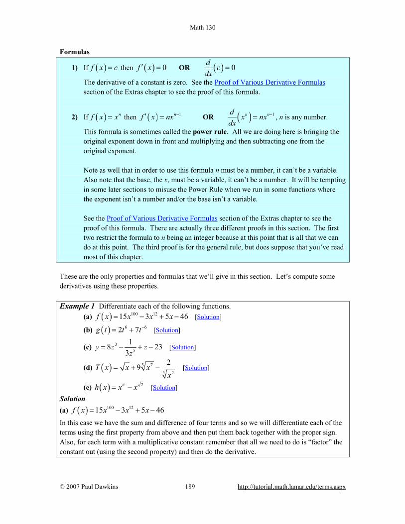
Math 130
© 2007 Paul Dawkins 189 http://tutorial.math.lamar.edu/terms.aspx
Formulas
1) If ( )f x c= then ( ) 0f x′ = OR ( ) 0d cdx
=
The derivative of a constant is zero. See the Proof of Various Derivative Formulas section of the Extras chapter to see the proof of this formula.
2) If ( ) nf x x= then ( ) 1nf x nx −′ = OR ( ) 1n nd x nxdx
−= , n is any number.
This formula is sometimes called the power rule. All we are doing here is bringing the original exponent down in front and multiplying and then subtracting one from the original exponent. Note as well that in order to use this formula n must be a number, it can’t be a variable. Also note that the base, the x, must be a variable, it can’t be a number. It will be tempting in some later sections to misuse the Power Rule when we run in some functions where the exponent isn’t a number and/or the base isn’t a variable. See the Proof of Various Derivative Formulas section of the Extras chapter to see the proof of this formula. There are actually three different proofs in this section. The first two restrict the formula to n being an integer because at this point that is all that we can do at this point. The third proof is for the general rule, but does suppose that you’ve read most of this chapter.
These are the only properties and formulas that we’ll give in this section. Let’s compute some derivatives using these properties. Example 1 Differentiate each of the following functions.
(a) ( ) 100 1215 3 5 46f x x x x= − + − [Solution]
(b) ( ) 6 62 7g t t t−= + [Solution]
(c) 35
18 233
y z zz
= − + − [Solution]
(d) ( ) 3 7
5 2
29T x x xx
= + − [Solution]
(e) ( ) 2h x x xπ= − [Solution] Solution (a) ( ) 100 1215 3 5 46f x x x x= − + −
In this case we have the sum and difference of four terms and so we will differentiate each of the terms using the first property from above and then put them back together with the proper sign. Also, for each term with a multiplicative constant remember that all we need to do is “factor” the constant out (using the second property) and then do the derivative.

Math 130
© 2007 Paul Dawkins 190 http://tutorial.math.lamar.edu/terms.aspx
( ) ( ) ( ) ( )99 11 0
99 11
15 100 3 12 5 1 0
1500 36 5
f x x x x
x x
′ = − + −
= − +
Notice that in the third term the exponent was a one and so upon subtracting 1 from the original exponent we get a new exponent of zero. Now recall that 0 1x = . Don’t forget to do any basic arithmetic that needs to be done such as any multiplication and/or division in the coefficients.
[Return to Problems] (b) ( ) 6 62 7g t t t−= +
The point of this problem is to make sure that you deal with negative exponents correctly. Here is the derivative.
( ) ( ) ( )5 7
5 7
2 6 7 6
12 42
g t t t
t t
−
−
′ = + −
= −
Make sure that you correctly deal with the exponents in these cases, especially the negative exponents. It is an easy mistake to “go the other way” when subtracting one off from a negative exponent and get 56t−− instead of the correct 76t−− .
[Return to Problems]
(c) 35
18 233
y z zz
= − + −
Now in this function the second term is not correctly set up for us to use the power rule. The power rule requires that the term be a variable to a power only and the term must be in the numerator. So, prior to differentiating we first need to rewrite the second term into a form that we can deal with.
3 518 233
y z z z−= − + −
Note that we left the 3 in the denominator and only moved the variable up to the numerator. Remember that the only thing that gets an exponent is the term that is immediately to the left of the exponent. If we’d wanted the three to come up as well we’d have written,
( )5
13z
so be careful with this! It’s a very common mistake to bring the 3 up into the numerator as well at this stage. Now that we’ve gotten the function rewritten into a proper form that allows us to use the Power Rule we can differentiate the function. Here is the derivative for this part.
2 6524 13
y z z−′ = + +
[Return to Problems]

Math 130
© 2007 Paul Dawkins 191 http://tutorial.math.lamar.edu/terms.aspx
(d) ( ) 3 7
5 2
29T x x xx
= + −
All of the terms in this function have roots in them. In order to use the power rule we need to first convert all the roots to fractional exponents. Again, remember that the Power Rule requires us to have a variable to a number and that it must be in the numerator of the term. Here is the function written in “proper” form.
( ) ( )( )
1 172 3
12 5
7132
25
7 213 52
29
29
9 2
T x x xx
x xx
x x x−
= + −
= + −
= + −
In the last two terms we combined the exponents. You should always do this with this kind of term. In a later section we will learn of a technique that would allow us to differentiate this term without combining exponents, however it will take significantly more work to do. Also don’t forget to move the term in the denominator of the third term up to the numerator. We can now differentiate the function.
( )
4 713 52
4 713 52
1 7 29 22 3 51 63 42 3 5
T x x x x
x x x
−−
−−
′ = + − −
= + +
Make sure that you can deal with fractional exponents. You will see a lot of them in this class.
[Return to Problems]
(e) ( ) 2h x x xπ= −
In all of the previous examples the exponents have been nice integers or fractions. That is usually what we’ll see in this class. However, the exponent only needs to be a number so don’t get excited about problems like this one. They work exactly the same.
( ) 1 2 12h x x xππ − −′ = − The answer is a little messy and we won’t reduce the exponents down to decimals. However, this problem is not terribly difficult it just looks that way initially.
[Return to Problems] There is a general rule about derivatives in this class that you will need to get into the habit of using. When you see radicals you should always first convert the radical to a fractional exponent and then simplify exponents as much as possible. Following this rule will save you a lot of grief in the future.

Math 130
© 2007 Paul Dawkins 192 http://tutorial.math.lamar.edu/terms.aspx
Back when we first put down the properties we noted that we hadn’t included a property for products and quotients. That doesn’t mean that we can’t differentiate any product or quotient at this point. There are some that we can do. Example 2 Differentiate each of the following functions.
(a) ( )3 2 22y x x x= − [Solution]
(b) ( )5 2
2
2 5t th tt
+ −= [Solution]
Solution
(a) ( )3 2 22y x x x= −
In this function we can’t just differentiate the first term, differentiate the second term and then multiply the two back together. That just won’t work. We will discuss this in detail in the next section so if you’re not sure you believe that hold on for a bit and we’ll be looking at that soon as well as showing you an example of why it won’t work. It is still possible to do this derivative however. All that we need to do is convert the radical to fractional exponents (as we should anyway) and then multiply this through the parenthesis.
( )2 5 8
23 3 32 2y x x x x x= − = − Now we can differentiate the function.
2 53 310 8
3 3y x x′ = −
[Return to Problems]
(b) ( )5 2
2
2 5t th tt
+ −=
As with the first part we can’t just differentiate the numerator and the denominator and the put it back together as a fraction. Again, if you’re not sure you believe this hold on until the next section and we’ll take a more detailed look at this. We can simplify this rational expression however as follows.
( )5 2
3 22 2 2
2 5 2 1 5t th t t tt t t
−= + − = + −
This is a function that we can differentiate. ( ) 2 36 10h t t t−′ = +
[Return to Problems]

Math 130
© 2007 Paul Dawkins 193 http://tutorial.math.lamar.edu/terms.aspx
So, as we saw in this example there are a few products and quotients that we can differentiate. If we can first do some simplification the functions will sometimes simplify into a form that can be differentiated using the properties and formulas in this section. Before moving on to the next section let’s work a couple of examples to remind us once again of some of the interpretations of the derivative.
Example 3 Is ( ) 33
3002 4f x xx
= + + increasing, decreasing or not changing at 2x = − ?
Solution We know that the rate of change of a function is given by the functions derivative so all we need to do is it rewrite the function (to deal with the second term) and then take the derivative.
( ) ( )3 3 2 4 24
9002 300 4 6 900 6f x x x f x x x xx
− −′= + + ⇒ = − = −
Note that we rewrote the last term in the derivative back as a fraction. This is not something we’ve done to this point and is only being done here to help with the evaluation in the next step. It’s often easier to do the evaluation with positive exponents. So, upon evaluating the derivative we get
( ) ( ) 900 1292 6 4 32.2516 4
f ′ − = − = − = −
So, at 2x = − the derivative is negative and so the function is decreasing at 2x = − .
Example 4 Find the equation of the tangent line to ( ) 4 8f x x x= − at 16x = . Solution We know that the equation of a tangent line is given by, ( ) ( )( )y f a f a x a′= + − So, we will need the derivative of the function (don’t forget to get rid of the radical).
( ) ( )1 12 2
12
44 8 4 4 4f x x x f x xx
−′= − ⇒ = − = −
Again, notice that we eliminated the negative exponent in the derivative solely for the sake of the evaluation. All we need to do then is evaluate the function and the derivative at the point in question, 16x = .
( ) ( ) ( ) 416 64 8 4 32 4 34
f f x′= − = = − =
The tangent line is then, ( )32 3 16 3 16y x x= + − = −

Math 130
© 2007 Paul Dawkins 194 http://tutorial.math.lamar.edu/terms.aspx
Example 5 The position of an object at any time t (in hours) is given by, ( ) 3 22 21 60 10s t t t t= − + − Determine when the object is moving to the right and when the object is moving to the left. Solution The only way that we’ll know for sure which direction the object is moving is to have the velocity in hand. Recall that if the velocity is positive the object is moving off to the right and if the velocity is negative then the object is moving to the left. So, we need the derivative since the derivative is the velocity of the object. The derivative is,
( ) ( ) ( ) ( )2 26 42 60 6 7 10 6 2 5s t t t t t t t′ = − + = − + = − − The reason for factoring the derivative will be apparent shortly. Now, we need to determine where the derivative is positive and where the derivative is negative. There are several ways to do this. The method that I tend to prefer is the following. Since polynomials are continuous we know from the Intermediate Value Theorem that if the polynomial ever changes sign then it must have first gone through zero. So, if we knew where the derivative was zero we would know the only points where the derivative might change sign. We can see from the factored form of the derivative that the derivative will be zero at 2t = and
5t = . Let’s graph these points on a number line.
Now, we can see that these two points divide the number line into three distinct regions. In reach of these regions we know that the derivative will be the same sign. Recall the derivative can only change sign at the two points that are used to divide the number line up into the regions. Therefore, all that we need to do is to check the derivative at a test point in each region and the derivative in that region will have the same sign as the test point. Here is the number line with the test points and results shown.

Math 130
© 2007 Paul Dawkins 195 http://tutorial.math.lamar.edu/terms.aspx
Here are the intervals in which the derivative is positive and negative.
positive : 2 & 5negative : 2 5
t tt
−∞ < < < < ∞< <
We included negative t’s here because we could even though they may not make much sense for this problem. Once we know this we also can answer the question. The object is moving to the right and left in the following intervals.
moving to the right : 2 & 5moving to the left : 2 5
t tt
−∞ < < < < ∞< <
Make sure that you can do the kind of work that we just did in this example. You will be asked numerous times over the course of the next two chapters to determine where functions are positive and/or negative. If you need some review or want to practice these kinds of problems you should check out the Solving Inequalities section of my Algebra/Trig Review.

Math 130
© 2007 Paul Dawkins 196 http://tutorial.math.lamar.edu/terms.aspx
Product and Quotient Rule In the previous section we noted that we had to be careful when differentiating products or quotients. It’s now time to look at products and quotients and see why. First let’s take a look at why we have to be careful with products and quotients. Suppose that we have the two functions ( ) 3f x x= and ( ) 6g x x= . Let’s start by computing the derivative of
the product of these two functions. This is easy enough to do directly.
( ) ( ) ( )3 6 9 89f g x x x x′ ′′ = = = Remember that on occasion we will drop the (x) part on the functions to simplify notation somewhat. We’ve done that in the work above. Now, let’s try the following.
( ) ( ) ( )( )2 5 73 6 18f x g x x x x′ ′ = =
So, we can very quickly see that.
( )f g f g′ ′ ′≠ In other words, the derivative of a product is not the product of the derivatives. Using the same functions we can do the same thing for quotients.
( )3
3 46 3 4
1 33f x x xg x x x
− −′′ ′ ′= = = = − = −
( )( )
2
5 3
3 16 2
f x xg x x x
′= =
′
So, again we can see that,
f fg g
′ ′ ≠ ′
To differentiate products and quotients we have the Product Rule and the Quotient Rule. Product Rule If the two functions f(x) and g(x) are differentiable (i.e. the derivative exist) then the product is differentiable and,
( )f g f g f g′ ′ ′= + The proof of the Product Rule is shown in the Proof of Various Derivative Formulas section of the Extras chapter.

Math 130
© 2007 Paul Dawkins 197 http://tutorial.math.lamar.edu/terms.aspx
Quotient Rule If the two functions f(x) and g(x) are differentiable (i.e. the derivative exist) then the quotient is differentiable and,
2
f f g f gg g
′ ′ ′ −=
Note that the numerator of the quotient rule is very similar to the product rule so be careful to not mix the two up! The proof of the Quotient Rule is shown in the Proof of Various Derivative Formulas section of the Extras chapter. Let’s do a couple of examples of the product rule. Example 1 Differentiate each of the following functions.
(a) ( )3 2 22y x x x= − [Solution]
(b) ( ) ( )( )36 10 20f x x x x= − − [Solution] Solution At this point there really aren’t a lot of reasons to use the product rule. As we noted in the previous section all we would need to do for either of these is to just multiply out the product and then differentiate. With that said we will use the product rule on these so we can see an example or two. As we add more functions to our repertoire and as the functions become more complicated the product rule will become more useful and in many cases required.
(a) ( )3 2 22y x x x= −
Note that we took the derivative of this function in the previous section and didn’t use the product rule at that point. We should however get the same result here as we did then. Now let’s do the problem here. There’s not really a lot to do here other than use the product rule. However, before doing that we should convert the radical to a fractional exponent as always.
( )2
23 2y x x x= − Now let’s take the derivative. So we take the derivative of the first function times the second then add on to that the first function times the derivative of the second function.
( ) ( )1 2
23 32 2 2 23
y x x x x x−
′ = − + −

Math 130
© 2007 Paul Dawkins 198 http://tutorial.math.lamar.edu/terms.aspx
This is NOT what we got in the previous section for this derivative. However, with some simplification we can arrive at the same answer.
2 5 2 5 2 53 3 3 3 3 34 2 10 82 2
3 3 3 3y x x x x x x′ = − + − = −
This is what we got for an answer in the previous section so that is a good check of the product rule.
[Return to Problems]
(b) ( ) ( )( )36 10 20f x x x x= − −
This one is actually easier than the previous one. Let’s just run it through the product rule.
( ) ( )( ) ( )( )2 3
3 2
18 1 10 20 6 20
480 180 40 10
f x x x x x
x x x
′ = − − + − −
= − + + −
Since it was easy to do we went ahead and simplified the results a little.
[Return to Problems] Let’s now work an example or two with the quotient rule. In this case, unlike the product rule examples, a couple of these functions will require the quotient rule in order to get the derivative. The last two however, we can avoid the quotient rule if we’d like to as we’ll see. Example 2 Differentiate each of the following functions.
(a) ( ) 3 92zW z
z+
=−
[Solution]
(b) ( ) 2
42
xh xx
=−
[Solution]
(c) ( ) 6
4f xx
= [Solution]
(d) 6
5wy = [Solution]
Solution
(a) ( ) 3 92zW z
z+
=−
There isn’t a lot to do here other than to use the quotient rule. Here is the work for this function.
( ) ( ) ( ) ( )
( )
( )
2
2
3 2 3 9 12
152
z zW z
z
z
− − + −′ =
−
=−
[Return to Problems]

Math 130
© 2007 Paul Dawkins 199 http://tutorial.math.lamar.edu/terms.aspx
(b) ( ) 2
42
xh xx
=−
Again, not much to do here other than use the quotient rule. Don’t forget to convert the square root into a fractional exponent.
( )( ) ( ) ( )
( )
( )
( )
1 121 2 2
222
3 1 32 2 2
22
3 12 2
22
4 2 4 2
2
2 4 8
2
6 4
2
x x x xh x
x
x x x
x
x x
x
−
−
−
− −′ =
−
− −=
−
− −=
−
[Return to Problems]
(c) ( ) 6
4f xx
=
It seems strange to have this one here rather than being the first part of this example given that it definitely appears to be easier than any of the previous two. In fact, it is easier. There is a point to doing it here rather than first. In this case there are two ways to do compute this derivative. There is an easy way and a hard way and in this case the hard way is the quotient rule. That’s the point of this example. Let’s do the quotient rule and see what we get.
( )( )( ) ( )
( )
6 5 5
2 12 76
0 4 6 24 24x x xf xx xx
− −′ = = = −
Now, that was the “hard” way. So, what was so hard about it? Well actually it wasn’t that hard, there is just an easier way to do it that’s all. However, having said that, a common mistake here is to do the derivative of the numerator (a constant) incorrectly. For some reason many people will give the derivative of the numerator in these kinds of problems as a 1 instead of 0! Also, there is some simplification that needs to be done in these kinds of problems if you do the quotient rule. The easy way is to do what we did in the previous section.
( ) 6 77
244 24f x x xx
− −′ = = − = −
Either way will work, but I’d rather take the easier route if I had the choice.
[Return to Problems]
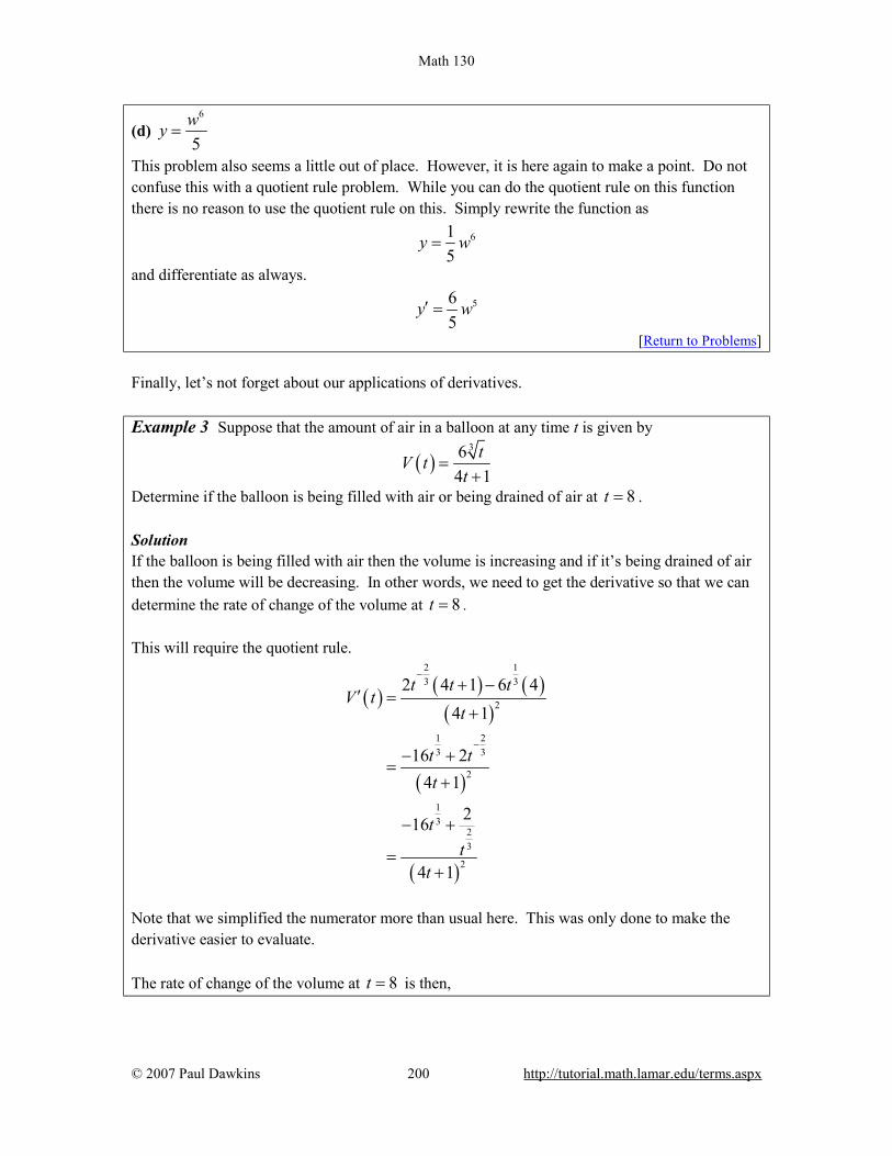
Math 130
© 2007 Paul Dawkins 200 http://tutorial.math.lamar.edu/terms.aspx
(d) 6
5wy =
This problem also seems a little out of place. However, it is here again to make a point. Do not confuse this with a quotient rule problem. While you can do the quotient rule on this function there is no reason to use the quotient rule on this. Simply rewrite the function as
615
y w=
and differentiate as always. 56
5y w′ =
[Return to Problems] Finally, let’s not forget about our applications of derivatives. Example 3 Suppose that the amount of air in a balloon at any time t is given by
( )36
4 1tV t
t=
+
Determine if the balloon is being filled with air or being drained of air at 8t = . Solution If the balloon is being filled with air then the volume is increasing and if it’s being drained of air then the volume will be decreasing. In other words, we need to get the derivative so that we can determine the rate of change of the volume at 8t = . This will require the quotient rule.
( ) ( ) ( )( )
( )
( )
2 13 3
2
1 23 3
2
13
23
2
2 4 1 6 44 1
16 24 1
216
4 1
t t tV t
t
t tt
tt
t
−
−
+ −′ =
+
− +=
+
− +
=+
Note that we simplified the numerator more than usual here. This was only done to make the derivative easier to evaluate. The rate of change of the volume at 8t = is then,
Math 130
© 2007 Paul Dawkins 201 http://tutorial.math.lamar.edu/terms.aspx
( )
( )
( )( ) ( ) ( ) ( )
21 2 1 23 3 3
2
216 248 8 2 8 8 2 4
3363 7
2178 242
V− + ′ = = = = =
= − = −
So, the rate of change of the volume at 8t = is negative and so the volume must be decreasing. Therefore air is being drained out of the balloon at 8t = . As a final topic let’s note that the product rule can be extended to more than two functions, for instance.
( )
( )
f g h f g h f g h f g h
f g h w f g h w f g h w f g h w f g h w
′ ′ ′ ′= + +
′ ′ ′ ′ ′= + + +
With this section and the previous section we are now able to differentiate powers of x as well as sums, differences, products and quotients of these kinds of functions. However, there are many more functions out there in the world that are not in this form. The next few sections give many of these functions as well as give their derivatives.
Math 130
© 2007 Paul Dawkins 202 http://tutorial.math.lamar.edu/terms.aspx
Derivatives of Trig Functions With this section we’re going to start looking at the derivatives of functions other than polynomials or roots of polynomials. We’ll start this process off by taking a look at the derivatives of the six trig functions. Two of the derivatives will be derived. The remaining four are left to the reader and will follow similar proofs for the two given here. Before we actually get into the derivatives of the trig functions we need to give a couple of limits that will show up in the derivation of two of the derivatives. Fact
0 0
sin cos 1lim 1 lim 0θ θ
θ θθ θ→ →
−= =
See the Proof of Trig Limits section of the Extras chapter to see the proof of these two limits. Before we start differentiating trig functions let’s work a quick set of limit problems that this fact now allows us to do. Example 1 Evaluate each of the following limits.
(a) 0
sinlim6θ
θθ→
[Solution]
(b) ( )0
sin 6limx
xx→
[Solution]
(c) ( )0
limsin 7x
xx→
[Solution]
(d) ( )( )0
sin 3lim
sin 8t
tt→
[Solution]
(e) ( )4
sin 4lim
4x
xx→
−−
[Solution]
(f) ( )0
cos 2 1limz
zz→
− [Solution]
Solution
(a) 0
sinlim6θ
θθ→
There really isn’t a whole lot to this limit. In fact, it’s only here to contrast with the next example so you can see the difference in how these work. In this case since there is only a 6 in the denominator we’ll just factor this out and then use the fact.
( )0 0
sin 1 sin 1 1lim lim 16 6 6 6θ θ
θ θθ θ→ →
= = =
[Return to Problems]

Math 130
© 2007 Paul Dawkins 203 http://tutorial.math.lamar.edu/terms.aspx
(b) ( )
0
sin 6limx
xx→
Now, in this case we can’t factor the 6 out of the sine so we’re stuck with it there and we’ll need to figure out a way to deal with it. To do this problem we need to notice that in the fact the argument of the sine is the same as the denominator (i.e. both θ ’s). So we need to get both of the argument of the sine and the denominator to be the same. We can do this by multiplying the numerator and the denominator by 6 as follows.
( ) ( ) ( )
0 0 0
sin 6 6sin 6 sin 6lim lim 6lim
6 6x x x
x x xx x x→ → →
= =
Note that we factored the 6 in the numerator out of the limit. At this point, while it may not look like it, we can use the fact above to finish the limit. To see that we can use the fact on this limit let’s do a change of variables. A change of variables is really just a renaming of portions of the problem to make something look more like something we know how to deal with. They can’t always be done, but sometimes, such as this case, they can simplify the problem. The change of variables here is to let 6xθ = and then notice that as
0x → we also have ( )6 0 0θ → = . When doing a change of variables in a limit we need to
change all the x’s into θ ’s and that includes the one in the limit. Doing the change of variables on this limit gives,
( ) ( )
( )
( )
0 0
0
sin 6 sin 6lim 6lim let 6
6sin
6lim
6 16
x x
x xx
x x
θ
θ
θθ
→ →
→
= =
=
=
=
And there we are. Note that we didn’t really need to do a change of variables here. All we really need to notice is that the argument of the sine is the same as the denominator and then we can use the fact. A change of variables, in this case, is really only needed to make it clear that the fact does work.
[Return to Problems]
(c) ( )0
limsin 7x
xx→
In this case we appear to have a small problem in that the function we’re taking the limit of here is upside down compared to that in the fact. This is not the problem it appears to be once we notice that,
Math 130
© 2007 Paul Dawkins 204 http://tutorial.math.lamar.edu/terms.aspx
( ) ( )
1sin 7sin 7
xxx
x
=
and then all we need to do is recall a nice property of limits that allows us to do ,
( ) ( )
( )
( )
0 0
0
0
0
1lim limsin 7sin 7
lim1
sin 7lim
1sin 7
lim
x x
x
x
x
xxx
x
xx
xx
→ →
→
→
→
=
=
=
With a little rewriting we can see that we do in fact end up needing to do a limit like the one we did in the previous part. So, let’s do the limit here and this time we won’t bother with a change of variable to help us out. All we need to do is multiply the numerator and denominator of the fraction in the denominator by 7 to get things set up to use the fact. Here is the work for this limit.
( ) ( )
( )
( ) ( )
0
0
0
1lim7sin 7sin 7 lim
71
sin 77 lim
71
7 117
x
x
x
xxx
x
xx
→
→
→
=
=
=
=
[Return to Problems]
(d) ( )( )0
sin 3lim
sin 8t
tt→
This limit looks nothing like the limit in the fact, however it can be thought of as a combination of the previous two parts by doing a little rewriting. First, we’ll split the fraction up as follows,
( )( )
( )( )0 0
sin 3 sin 3 1lim limsin 8 1 sin 8t t
t tt t→ →
=
Now, the fact wants a t in the denominator of the first and in the numerator of the second. This is
Math 130
© 2007 Paul Dawkins 205 http://tutorial.math.lamar.edu/terms.aspx
easy enough to do if we multiply the whole thing by tt (which is just one after all and so won’t
change the problem) and then do a little rearranging as follows,
( )( )
( )( )
( )( )
( )( )
0 0
0
0 0
sin 3 sin 3 1lim limsin 8 1 sin 8
sin 3lim
sin 8
sin 3lim lim
sin 8
t t
t
t t
t t tt t t
t tt t
t tt t
→ →
→
→ →
=
=
=
At this point we can see that this really is two limits that we’ve seen before. Here is the work for each of these and notice on the second limit that we’re going to work it a little differently than we did in the previous part. This time we’re going to notice that it doesn’t really matter whether the sine is in the numerator or the denominator as long as the argument of the sine is the same as what’s in the numerator the limit is still one. Here is the work for this limit.
( )( )
( )( )
( )( )
( )
0 0 0
0 0
sin 3 3sin 3 8lim lim limsin 8 3 8sin 8
sin 3 1 83lim lim3 8 sin 8
138
38
t t t
t t
t t tt t t
t tt t
→ → →
→ →
=
=
=
=
[Return to Problems]
(e) ( )
4
sin 4lim
4x
xx→
−−
This limit almost looks the same as that in the fact in the sense that the argument of the sine is the same as what is in the denominator. However, notice that, in the limit, x is going to 4 and not 0 as the fact requires. However, with a change of variables we can see that this limit is in fact set to use the fact above regardless. So, let xθ = − 4 and then notice that as 4x → we have 0θ → . Therefore, after doing the change of variable the limit becomes,
( )
4 0
sin 4 sinlim lim 14x
xx θ
θθ→ →
−= =
−
[Return to Problems]

Math 130
© 2007 Paul Dawkins 206 http://tutorial.math.lamar.edu/terms.aspx
(f) ( )
0
cos 2 1limz
zz→
−
The previous parts of this example all used the sine portion of the fact. However, we could just have easily used the cosine portion so here is a quick example using the cosine portion to illustrate this. We’ll not put in much explanation here as this really does work in the same manner as the sine portion.
( ) ( )( )
( )
( )
0 0
0
2 cos 2 1cos 2 1lim lim
2cos 2 1
2lim2
2 00
z z
z
zzz z
zz
→ →
→
−−=
−=
=
All that is required to use the fact is that the argument of the cosine is the same as the denominator.
[Return to Problems] Okay, now that we’ve gotten this set of limit examples out of the way let’s get back to the main point of this section, differentiating trig functions. We’ll start with finding the derivative of the sine function. To do this we will need to use the definition of the derivative. It’s been a while since we’ve had to use this, but sometimes there just isn’t anything we can do about it. Here is the definition of the derivative for the sine function.
( )( ) ( ) ( )0
sin sinsin lim
h
x h xd xdx h→
+ −=
Since we can’t just plug in 0h = to evaluate the limit we will need to use the following trig formula on the first sine in the numerator. ( ) ( ) ( ) ( ) ( )sin sin cos cos sinx h x h x h+ = + Doing this gives us,
( )( ) ( ) ( ) ( ) ( ) ( )
( ) ( )( ) ( ) ( )
( ) ( ) ( ) ( )
0
0
0 0
sin cos cos sin sinsin lim
sin cos 1 cos sinlim
cos 1 sinlimsin limcos
h
h
h h
x h x h xd xdx h
x h x hh
h hx x
h h
→
→
→ →
+ −=
− +=
−= +

Math 130
© 2007 Paul Dawkins 207 http://tutorial.math.lamar.edu/terms.aspx
As you can see upon using the trig formula we can combine the first and third term and then factor a sine out of that. We can then break up the fraction into two pieces, both of which can be dealt with separately. Now, both of the limits here are limits as h approaches zero. In the first limit we have a sin(x) and in the second limit we have a cos(x). Both of these are only functions of x only and as h moves in towards zero this has no affect on the value of x. Therefore, as far as the limits are concerned, these two functions are constants and can be factored out of their respective limits. Doing this gives,
( )( ) ( ) ( ) ( ) ( )0 0
cos 1 sinsin sin lim cos lim
h h
h hd x x xdx h h→ →
−= +
At this point all we need to do is use the limits in the fact above to finish out this problem.
( )( ) ( )( ) ( ) ( ) ( )sin sin 0 cos 1 cosd x x x xdx
= + =
Differentiating cosine is done in a similar fashion. It will require a different trig formula, but other than that is an almost identical proof. The details will be left to you. When done with the proof you should get,
( )( ) ( )cos sind x xdx
= −
With these two out of the way the remaining four are fairly simple to get. All the remaining four trig functions can be defined in terms of sine and cosine and these definitions, along with appropriate derivative rules, can be used to get their derivatives. Let’s take a look at tangent. Tangent is defined as,
( ) ( )( )
sintan
cosx
xx
=
Now that we have the derivatives of sine and cosine all that we need to do is use the quotient rule on this. Let’s do that.
( )( ) ( )( )
( ) ( ) ( ) ( )( )( )( )
( ) ( )( )
2
2 2
2
sintan
cos
cos cos sin sin
cos
cos sincos
xd dxdx dx x
x x x x
x
x xx
=
− −
=
+=

Math 130
© 2007 Paul Dawkins 208 http://tutorial.math.lamar.edu/terms.aspx
Now, recall that ( ) ( )2 2cos sin 1x x+ = and if we also recall the definition of secant in terms of
cosine we arrive at,
( )( ) ( ) ( )( )
( )( )
2 2
2
2
2
cos sintan
cos1
cos
sec
x xd xdx x
x
x
+=
=
=
The remaining three trig functions are also quotients involving sine and/or cosine and so can be differentiated in a similar manner. We’ll leave the details to you. Here are the derivatives of all six of the trig functions. Derivatives of the six trig functions
( )( ) ( ) ( )( ) ( )
( )( ) ( ) ( )( ) ( )
( )( ) ( ) ( ) ( )( ) ( ) ( )
2 2
sin cos cos sin
tan sec cot csc
sec sec tan csc csc cot
d dx x x xdx dxd dx x x xdx dxd dx x x x x xdx dx
= = −
= = −
= = −
At this point we should work some examples. Example 2 Differentiate each of the following functions.
(a) ( ) ( ) ( )3sec 10cotg x x x= − [Solution]
(b) ( ) ( )4 23 tanh w w w w−= − [Solution]
(c) ( ) ( ) ( )5sin cos 4cscy x x x= + [Solution]
(d) ( ) ( )( )
sin3 2cos
tP t
t=
− [Solution]
Solution (a) ( ) ( ) ( )3sec 10cotg x x x= −
There really isn’t a whole lot to this problem. We’ll just differentiate each term using the formulas from above.
( ) ( ) ( ) ( )( )
( ) ( ) ( )
2
2
3sec tan 10 csc
3sec tan 10csc
g x x x x
x x x
′ = − −
= +
[Return to Problems]
(b) ( ) ( )4 23 tanh w w w w−= −
In this part we will need to use the product rule on the second term and note that we really will need the product rule here. There is no other way to do this derivative unlike what we saw when
Math 130
© 2007 Paul Dawkins 209 http://tutorial.math.lamar.edu/terms.aspx
we first looked at the product rule. When we first looked at the product rule the only functions we knew how to differentiate were polynomials and in those cases all we really needed to do was multiply them out and we could take the derivative without the product rule. We are now getting into the point where we will be forced to do the product rule at times regardless of whether or not we want to. We will also need to be careful with the minus sign in front of the second term and make sure that it gets dealt with properly. There are two ways to deal with this. One way it to make sure that you use a set of parenthesis as follows,
( ) ( ) ( )( )
( ) ( )
5 2 2
5 2 2
12 2 tan sec
12 2 tan sec
h w w w w w w
w w w w w
−
−
′ = − − +
= − − −
Because the second term is being subtracted off of the first term then the whole derivative of the second term must also be subtracted off of the derivative of the first term. The parenthesis make this idea clear. A potentially easier way to do this is to think of the minus sign as part of the first function in the product. Or, in other words the two functions in the product, using this idea, are 2w− and
( )tan w . Doing this gives,
( ) ( ) ( )5 2 212 2 tan sech w w w w w w−′ = − − − So, regardless of how you approach this problem you will get the same derivative.
[Return to Problems] (c) ( ) ( ) ( )5sin cos 4cscy x x x= +
As with the previous part we’ll need to use the product rule on the first term. We will also think of the 5 as part of the first function in the product to make sure we deal with it correctly. Alternatively, you could make use of a set of parenthesis to make sure the 5 gets dealt with properly. Either way will work, but we’ll stick with thinking of the 5 as part of the first term in the product. Here’s the derivative of this function.
( ) ( ) ( ) ( )( ) ( ) ( )( ) ( ) ( ) ( )2 2
5cos cos 5sin sin 4csc cot
5cos 5sin 4csc cot
y x x x x x x
x x x x
′ = + − −
= − −
[Return to Problems]
(d) ( ) ( )( )
sin3 2cos
tP t
t=
−
In this part we’ll need to use the quotient rule to take the derivative.

Math 130
© 2007 Paul Dawkins 210 http://tutorial.math.lamar.edu/terms.aspx
( ) ( ) ( )( ) ( ) ( )( )( )( )
( ) ( ) ( )( )( )
2
2 2
2
cos 3 2cos sin 2sin
3 2cos
3cos 2cos 2sin
3 2cos
t t t tP t
t
t t t
t
− −′ =
−
− −=
−
Be careful with the signs when differentiating the denominator. The negative sign we get from differentiating the cosine will cancel against the negative sign that is already there. This appears to be done, but there is actually a fair amount of simplification that can yet be done. To do this we need to factor out a “-2” from the last two terms in the numerator and the make use of the fact that ( ) ( )2 2cos sin 1θ θ+ = .
( )( ) ( ) ( )( )
( )( )( )
( )( )
2 2
2
2
3cos 2 cos sin
3 2cos
3cos 2
3 2cos
t t tP t
t
t
t
− +′ =
−
−=
−
[Return to Problems] As a final problem here let’s not forget that we still have our standard interpretations to derivatives. Example 3 Suppose that the amount of money in a bank account is given by ( ) ( ) ( )500 100cos 150sinP t t t= + − where t is in years. During the first 10 years in which the account is open when is the amount of money in the account increasing? Solution To determine when the amount of money is increasing we need to determine when the rate of change is positive. Since we know that the rate of change is given by the derivative that is the first thing that we need to find. ( ) ( ) ( )100sin 150cosP t t t′ = − − Now, we need to determine where in the first 10 years this will be positive. This is equivalent to asking where in the interval [0, 10] is the derivative positive. Recall that both sine and cosine are continuous functions and so the derivative is also a continuous function. The Intermediate Value Theorem then tells us that the derivative can only change sign if it first goes through zero. So, we need to solve the following equation.

Math 130
© 2007 Paul Dawkins 211 http://tutorial.math.lamar.edu/terms.aspx
( ) ( )( ) ( )( )( )( )
100sin 150cos 0
100sin 150cos
sin1.5
cos
tan 1.5
t t
t t
tt
t
− − =
= −
= −
= −
The solution to this equation is,
2.1588 2 , 0, 1, 2,5.3004 2 , 0, 1, 2,
t n nt n n
ππ
= + = ± ±= + = ± ±
……
If you don’t recall how to solve trig equations go back and take a look at the sections on solving trig equations in the Review chapter. We are only interested in those solutions that fall in the range [0, 10]. Plugging in values of n into the solutions above we see that the values we need are,
2.1588 2.1588 2 8.44205.3004
t tt
π= = + ==
So, much like solving polynomial inequalities all that we need to do is sketch in a number line and add in these points. These points will divide the number line into regions in which the derivative must always be the same sign. All that we need to do then is choose a test point from each region to determine the sign of the derivative in that region. Here is the number line with all the information on it.
So, it looks like the amount of money in the bank account will be increasing during the following intervals. 2.1588 5.3004 8.4420 10t t< < < < Note that we can’t say anything about what is happening after 10t = since we haven’t done any work for t’s after that point. In this section we saw how to differentiate trig functions. We also saw in the last example that our interpretations of the derivative are still valid so we can’t forget those.

Math 130
© 2007 Paul Dawkins 212 http://tutorial.math.lamar.edu/terms.aspx
Also, it is important that we be able to solve trig equations as this is something that will arise off and on in this course. It is also important that we can do the kinds of number lines that we used in the last example to determine where a function is positive and where a function is negative. This is something that we will be doing on occasion in both this chapter and the next.
Math 130
© 2007 Paul Dawkins 213 http://tutorial.math.lamar.edu/terms.aspx
Derivatives of Exponential and Logarithm Functions The next set of functions that we want to take a look at are exponential and logarithm functions. The most common exponential and logarithm functions in a calculus course are the natural exponential function, xe , and the natural logarithm function, ( )ln x . We will take a more
general approach however and look at the general exponential and logarithm function. Exponential Functions We’ll start off by looking at the exponential function,
( ) xf x a=
We want to differentiate this. The power rule that we looked at a couple of sections ago won’t work as that required the exponent to be a fixed number and the base to be a variable. That is exactly the opposite from what we’ve got with this function. So, we’re going to have to start with the definition of the derivative.
( ) ( ) ( )
( )
0
0
0
0
lim
lim
lim
1lim
h
x h x
h
x h x
h
x h
h
f x h f xf x
ha a
ha a a
ha a
h
→
+
→
→
→
+ −′ =
−=
−=
−=
Now, the xa is not affected by the limit since it doesn’t have any h’s in it and so is a constant as far as the limit is concerned. We can therefore factor this out of the limit. This gives,
( )0
1limh
x
h
af x ah→
−′ =
Now let’s notice that the limit we’ve got above is exactly the definition of the derivative of
( ) xf x a= at 0x = , i.e. ( )0f ′ . Therefore, the derivative becomes,
( ) ( )0 xf x f a′ ′= So, we are kind of stuck we need to know the derivative in order to get the derivative! There is one value of a that we can deal with at this point. Back in the Exponential Functions section of the Review chapter we stated that 2.71828182845905=e … What we didn’t do however do actually define where e comes from. There are in fact a variety of ways to define e. Here are a three of them.

Math 130
© 2007 Paul Dawkins 214 http://tutorial.math.lamar.edu/terms.aspx
Some Definitions of e.
1. 1lim 1
n
n n→∞
= +
e
2. e is the unique positive number for which 0
1lim 1h
h
h→
−=
e
3. 0
1!n n
∞
=
= ∑e
The second one is the important one for us because that limit is exactly the limit that we’re working with above. So, this definition leads to the following fact, Fact 1
For the natural exponential function, ( ) xf x = e we have ( )0
10 lim 1h
hf
h→
−′ = =e
.
So, provided we are using the natural exponential function we get the following. ( ) ( )x xf x f x′= ⇒ =e e At this point we’re missing some knowledge that will allow us to easily get the derivative for a general function. Eventually we will be able to show that for a general exponential function we have, ( ) ( ) ( )lnx xf x a f x a a′= ⇒ = Logarithm Functions Let’s now briefly get the derivatives for logarithms. In this case we will need to start with the following fact about functions that are inverses of each other. Fact 2 If f(x) and g(x) are inverses of each other then,
( ) ( )( )1g x
f g x′ =
′
So, how is this fact useful to us? Well recall that the natural exponential function and the natural logarithm function are inverses of each other and we know what the derivative of the natural exponential function is! So, if we have ( ) xf x = e and ( ) lng x x= then,

Math 130
© 2007 Paul Dawkins 215 http://tutorial.math.lamar.edu/terms.aspx
( ) ( )( ) ( ) ln
1 1 1 1xg xg x
xf g x′ = = = =
′ ee
The last step just uses the fact that the two functions are inverses of each other. Putting this all together gives,
( ) 1ln 0d x xdx x
= >
Note that we need to require that 0x > since this is required for the logarithm and so must also be required for its derivative. In can also be shown that,
( ) 1ln 0d x xdx x
= ≠
Using this all we need to avoid is 0x = . In this case, unlike the exponential function case, we can actually find the derivative of the general logarithm function. All that we need is the derivative of the natural logarithm, which we just found, and the change of base formula. Using the change of base formula we can write a general logarithm as,
lnloglna
xxa
=
Differentiation is then fairly simple.
( )
( )
lnlogln
1 lnln
1ln
ad d xxdx dx a
d xa dx
x a
=
=
=
We took advantage of the fact that a was a constant and so ln a is also a constant and can be factored out of the derivative. Putting all this together gives,
( ) 1loglna
d xdx x a
=
Here is a summary of the derivatives in this section.
( ) ( )
( ) ( )
ln
1 1ln logln
x x x x
a
d d a a adx dxd dx xdx x dx x a
= =
= =
e e

Math 130
© 2007 Paul Dawkins 216 http://tutorial.math.lamar.edu/terms.aspx
Okay, now that we have the derivations of the formulas out of the way let’s compute a couple of derivatives. Example 1 Differentiate each of the following functions.
(a) ( ) 94 5logwR w w= −
(b) ( ) 33 10 lnxf x x x= +e
(c) 53 1
x
xy =+
ee
Solution (a) This will be the only example that doesn’t involve the natural exponential and natural logarithm functions.
( ) 54 ln 4ln 9
wR ww
′ = −
(b) Not much to this one. Just remember to use the product rule on the second term.
( ) 2 3
2 2
13 30 ln 10
3 30 ln 10
x
x
f x x x xx
x x x
′ = + +
= + +
e
e
(c) We’ll need to use the quotient rule on this one.
( ) ( )( )( )
( )
( )
2
2 2
2
2
5 3 1 5 3
3 1
15 5 15
3 1
5
3 1
x x x x
x
x x x
x
x
x
y+ −
=+
+ −=
+
=+
e e e e
e
e e e
e
e
e
There’s really not a lot to differentiating natural logarithms and natural exponential functions at this point as long as you remember the formulas. In later sections as we get more formulas under our belt they will become more complicated. Next, we need to do our obligatory application/interpretation problem so we don’t forget about them. Example 2 Suppose that the position of an object is given by ( ) ts t t= e Does the object ever stop moving? Solution First we will need the derivative. We need this to determine if the object ever stops moving since
Math 130
© 2007 Paul Dawkins 217 http://tutorial.math.lamar.edu/terms.aspx
at that point (provided there is one) the velocity will be zero and recall that the derivative of the position function is the velocity of the object. The derivative is, ( ) ( )1t t ts t t t′ = + = +e e e So, we need to determine if the derivative is ever zero. To do this we will need to solve, ( )1 0tt+ =e Now, we know that exponential functions are never zero and so this will only be zero at 1t = − . So, if we are going to allow negative values of t then the object will stop moving once at 1t = − . If we aren’t going to allow negative values of t then the object will never stop moving. Before moving on to the next section we need to go back over a couple of derivatives to make sure that we don’t confuse the two. The two derivatives are,
( )
( )
1 Power Rule
ln Derivative of an exponential function
n n
x x
d x nxdxd a a adx
−=
=
It is important to note that with the Power rule the exponent MUST be a constant and the base MUST be a variable while we need exactly the opposite for the derivative of an exponential function. For an exponential function the exponent MUST be a variable and the base MUST be a constant. It is easy to get locked into one of these formulas and just use it for both of these. We also haven’t even talked about what to do if both the exponent and the base involve variables. We’ll see this situation in a later section.
Math 130
© 2007 Paul Dawkins 218 http://tutorial.math.lamar.edu/terms.aspx
Derivatives of Inverse Trig Functions In this section we are going to look at the derivatives of the inverse trig functions. In order to derive the derivatives of inverse trig functions we’ll need the formula from the last section relating the derivatives of inverse functions. If f(x) and g(x) are inverse functions then,
( ) ( )( )1g x
f g x′ =
′
Recall as well that two functions are inverses if ( )( )f g x x= and ( )( )g f x x= .
We’ll go through inverse sine, inverse cosine and inverse tangent in detail here and leave the other three to you to derive if you’d like to. Inverse Sine Let’s start with inverse sine. Here is the definition of the inverse sine.
1sin sin for2 2
y x y x yπ π−= ⇔ = − ≤ ≤
So, evaluating an inverse trig function is the same as asking what angle (i.e. y) did we plug into the sine function to get x. The restrictions on y given above are there to make sure that we get a consistent answer out of the inverse sine. We know that there are in fact an infinite number of angles that will work and we want a consistent value when we work with inverse sine. When using the range of angles above gives all possible values of the sine function exactly once. If you’re not sure of that sketch out a unit circle and you’ll see that that range of angles (the y’s) will cover all possible values of sine. Note as well that since ( )1 sin 1y− ≤ ≤ we also have 1 1x− ≤ ≤ .
Let’s work a quick example.
Example 1 Evaluate 1 1sin2
−
Solution So we are really asking what angle y solves the following equation.
( ) 1sin2
y =
and we are restricted to the values of y above.
From a unit circle we can quickly see that 6
y π= .
We have the following relationship between the inverse sine function and the sine function.
Math 130
© 2007 Paul Dawkins 219 http://tutorial.math.lamar.edu/terms.aspx
( ) ( )1 1sin sin sin sinx x x x− −= = In other words they are inverses of each other. This means that we can use the fact above to find the derivative of inverse sine. Let’s start with, ( ) ( ) 1sin sinf x x g x x−= = Then,
( ) ( )( ) ( )1
1 1cos sin
g xf g x x−
′ = =′
This is not a very useful formula. Let’s see if we can get a better formula. Let’s start by recalling the definition of the inverse sine function. ( ) ( )1sin siny x x y−= ⇒ = Using the first part of this definition the denominator in the derivative becomes,
( ) ( )1cos sin cosx y− = Now, recall that
2 2 2cos sin 1 cos 1 siny y y y+ = ⇒ = − Using this, the denominator is now,
( ) ( )1 2cos sin cos 1 sinx y y− = = − Now, use the second part of the definition of the inverse sine function. The denominator is then,
( )1 2 2cos sin 1 sin 1x y x− = − = − Putting all of this together gives the following derivative.
( )1
2
1sin1
d xdx x
− =−
Inverse Cosine Now let’s take a look at the inverse cosine. Here is the definition for the inverse cosine. 1cos cos for 0y x y x y π−= ⇔ = ≤ ≤ As with the inverse since we’ve got a restriction on the angles, y, that we get out of the inverse cosine function. Again, if you’d like to verify this a quick sketch of a unit circle should convince you that this range will cover all possible values of cosine exactly once. Also, we also have
1 1x− ≤ ≤ because ( )1 cos 1y− ≤ ≤ .
Math 130
© 2007 Paul Dawkins 220 http://tutorial.math.lamar.edu/terms.aspx
Example 2 Evaluate 1 2cos2
− −
.
Solution As with the inverse sine we are really just asking the following.
2cos2
y = −
where y must meet the requirements given above. From a unit circle we can see that we must
have 34
y π= .
The inverse cosine and cosine functions are also inverses of each other and so we have, ( ) ( )1 1cos cos cos cosx x x x− −= = To find the derivative we’ll do the same kind of work that we did with the inverse sine above. If we start with ( ) ( ) 1cos cosf x x g x x−= = then,
( ) ( )( ) ( )1
1 1sin cos
g xf g x x−
′ = =′ −
Simplifying the denominator here is almost identical to the work we did for the inverse sine and so isn’t shown here. Upon simplifying we get the following derivative.
( )1
2
1cos1
d xdx x
− = −−
So, the derivative of the inverse cosine is nearly identical to the derivative of the inverse sine. The only difference is the negative sign. Inverse Tangent Here is the definition of the inverse tangent.
1tan tan for2 2
y x y x yπ π−= ⇔ = − < <
Again, we have a restriction on y, but notice that we can’t let y be either of the two endpoints in the restriction above since tangent isn’t even defined at those two points. To convince yourself that this range will cover all possible values of tangent do a quick sketch of the tangent function and we can see that in this range we do indeed cover all possible values of tangent. Also, in this case there are no restrictions on x because tangent can take on all possible values.

Math 130
© 2007 Paul Dawkins 221 http://tutorial.math.lamar.edu/terms.aspx
Example 3 Evaluate 1tan 1− Solution Here we are asking, tan 1y =
where y satisfies the restrictions given above. From a unit circle we can see that 4
y π= .
Because there is no restriction on x we can ask for the limits of the inverse tangent function as x goes to plus or minus infinity. To do this we’ll need the graph of the inverse tangent function. This is shown below.
From this graph we can see that
1 1lim tan lim tan2 2x x
x xπ π− −
→∞ →−∞= = −
The tangent and inverse tangent functions are inverse functions so,
( ) ( )1 1tan tan tan tanx x x x− −= = Therefore to find the derivative of the inverse tangent function we can start with ( ) ( ) 1tan tanf x x g x x−= = We then have,
( ) ( )( ) ( )2 1
1 1sec tan
g xf g x x−
′ = =′
Simplifying the denominator is similar to the inverse sine, but different enough to warrant showing the details. We’ll start with the definition of the inverse tangent. 1tan tany x y x−= ⇒ = The denominator is then,
( )2 1 2sec tan secx y− =

Math 130
© 2007 Paul Dawkins 222 http://tutorial.math.lamar.edu/terms.aspx
Now, if we start with the fact that 2 2cos sin 1y y+ = and divide every term by cos2 y we will get, 2 21 tan secy y+ = The denominator is then,
( )2 1 2 2sec tan sec 1 tanx y y− = = + Finally using the second portion of the definition of the inverse tangent function gives us,
( )2 1 2 2sec tan 1 tan 1x y x− = + = + The derivative of the inverse tangent is then,
( )12
1tan1
d xdx x
− =+
There are three more inverse trig functions but the three shown here the most common ones. Formulas for the remaining three could be derived by a similar process as we did those above. Here are the derivatives of all six inverse trig functions.
( ) ( )
( ) ( )
( ) ( )
1 1
2 2
1 12 2
1 1
2 2
1 1sin cos1 11 1tan cot
1 11 1sec csc
1 1
d dx xdx dxx xd dx xdx x dx xd dx xdx dxx x x x
− −
− −
− −
= = −− −
= = −+ +
= = −− −
We should probably now do a couple of quick derivatives here before moving on to the next section. Example 4 Differentiate the following functions.
(a) ( ) ( ) ( )1 14cos 10 tanf t t t− −= −
(b) ( )1siny z z−= Solution (a) Not much to do with this one other than differentiate each term.
( ) 22
4 1011
f ttt
′ = − −+−
Math 130
© 2007 Paul Dawkins 223 http://tutorial.math.lamar.edu/terms.aspx
(b) Don’t forget to convert the radical to fractional exponents before using the product rule.
( )1
122
1 sin2 1
zy z zz
− −′ = +−
Alternate Notation There is some alternate notation that is used on occasion to denote the inverse trig functions. This notation is,
1 1
1 1
1 1
sin arcsin cos arccostan arctan cot arccot sec arcsec csc arccsc
x x x xx x x xx x x x
− −
− −
− −
= =
= =
= =

Math 130
© 2007 Paul Dawkins 224 http://tutorial.math.lamar.edu/terms.aspx
Derivatives of Hyperbolic Functions The last set of functions that we’re going to be looking in this chapter at are the hyperbolic functions. In many physical situations combinations of xe and x−e arise fairly often. Because of this these combinations are given names. There are six hyperbolic functions and they are defined as follows.
sinh cosh2 2
sinh cosh 1tanh cothcosh sinh tanh
1 1sech cschcosh sinh
x x x x
x x
x xx xx x x
x xx x
− −− += =
= = =
= =
e e e e
Here are the graphs of the three main hyperbolic functions.
We also have the following facts about the hyperbolic functions.
( ) ( ) ( ) ( )
( ) ( ) ( ) ( )2 2 2 2
sinh sinh cosh cosh
cosh sinh 1 1 tanh sech
x x x x
x x x x
− = − − =
− = − =
You’ll note that these are similar, but not quite the same, to some of the more common trig identities so be careful to not confuse the identities here with those of the standard trig functions.

Math 130
© 2007 Paul Dawkins 225 http://tutorial.math.lamar.edu/terms.aspx
Because the hyperbolic functions are defined in terms of exponential functions finding their derivatives is fairly simple provided you’ve already read through the next section. We haven’t however so we’ll need the following formula that can be easily proved after we’ve covered the next section.
( )x xddx
− −= −e e
With this formula we’ll do the derivative for hyperbolic sine and leave the rest to you as an exercise.
( ) ( )sinh cosh
2 2 2
x xx x x xd dx xdx dx
−− −− − − += = = =
e ee e e e
For the rest we can either use the definition of the hyperbolic function and/or the quotient rule. Here are all six derivatives.
( ) ( )
( ) ( )
( ) ( )
2 2
sinh cosh cosh sinh
tanh sech coth csch
sech sech tanh csch csch coth
d dx x x xdx dxd dx x x xdx dxd dx x x x x xdx dx
= =
= = −
= − = −
Here are a couple of quick derivatives using hyperbolic functions. Example 1 Differentiate each of the following functions.
(a) ( ) 52 coshf x x x=
(b) ( ) sinh1th t
t=
+
Solution (a) ( ) 4 510 cosh 2 sinhf x x x x x′ = + (b)
( ) ( )( )2
1 cosh sinh1
t t th t
t+ −
′ =+

Math 130
© 2007 Paul Dawkins 226 http://tutorial.math.lamar.edu/terms.aspx
Chain Rule We’ve taken a lot of derivatives over the course of the last few sections. However, if you look back they have all been functions similar to the following kinds of functions.
( ) ( ) ( ) ( ) ( )50 tan lnwR z z f t t y x h w g x x= = = = =e These are all fairly simple functions in that wherever the variable appears it is by itself. What about functions like the following,
( ) ( ) ( )( ) ( )( )
( ) ( ) ( )4 2
50 33 2
3 9 4 4
5 8 2 cos tan 3 tan 5
lnw w
R z z f t t t y x x
h w g x x x− + −
= − = + = +
= = +e
None of our rules will work on these functions and yet some of these functions are closer to the derivatives that we’re liable to run into than the functions in the first set. Let’s take the first one for example. Back in the section on the definition of the derivative we actually used the definition to compute this derivative. In that section we found that,
( ) 52 5 8
R zz
′ =−
If we were to just use the power rule on this we would get,
( )12
1 15 82 2 5 8
zz
−− =−
which is not the derivative that we computed using the definition. It is close, but it’s not the same. So, the power rule alone simply won’t work to get the derivative here. Let’s keep looking at this function and note that if we define,
( ) ( ) 5 8f z z g z z= = − then we can write the function as a composition.
( ) ( ) ( ) ( )( ) 5 8R z f g z f g z z= = = −o and it turns out that it’s actually fairly simple to differentiate a function composition using the Chain Rule. There are two forms of the chain rule. Here they are. Chain Rule Suppose that we have two functions f(x) and g(x) and they are both differentiable.
1. If we define ( ) ( ) ( )F x f g x= o then the derivative of F(x) is,
( ) ( )( ) ( )F x f g x g x′ ′ ′=
2. If we have ( )y f u= and ( )u g x= then the derivative of y is,
dy dy dudx du dx
=
Math 130
© 2007 Paul Dawkins 227 http://tutorial.math.lamar.edu/terms.aspx
Each of these forms have their uses, however we will work mostly with the first form in this class. To see the proof of the Chain Rule see the Proof of Various Derivative Formulas section of the Extras chapter. Now, let’s go back and use the Chain Rule on the function that we used when we opened this section.
Example 1 Use the Chain Rule to differentiate ( ) 5 8R z z= − . Solution We’ve already identified the two functions that we needed for the composition, but let’s write them back down anyway and take their derivatives.
( ) ( )
( ) ( )
5 81 5
2
f z z g z z
f z g zz
= = −
′ ′= =
So, using the chain rule we get,
( ) ( )( ) ( )( ) ( )
( ) ( )
( )
12
5 81 5 8 52
1 52 5 8
52 5 8
R z f g z g z
f z g z
z
z
z
−
′ ′ ′=
′ ′= −
= −
=−
=−
And this is what we got using the definition of the derivative. In general we don’t really do all the composition stuff in using the Chain Rule. That can get a little complicated and in fact obscures the fact that there is a quick and easy way of remembering the chain rule that doesn’t require us to think in terms of function composition. Let’s take the function from the previous example and rewrite it slightly.
( ) ( ) 12
outside inside function function
5 8R z z= −14243
This function has an “inside function” and an “outside function”. The outside function is the square root or the exponent of 1
2 depending on how you want to think of it and the inside
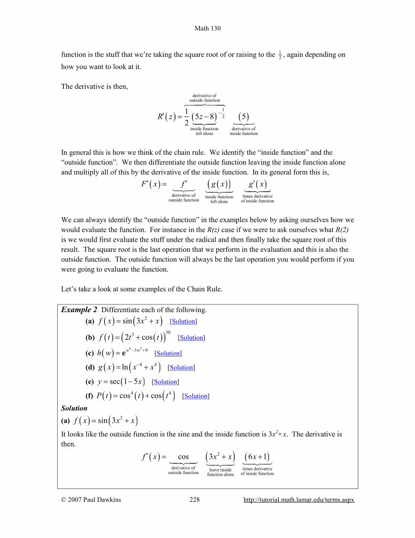
Math 130
© 2007 Paul Dawkins 228 http://tutorial.math.lamar.edu/terms.aspx
function is the stuff that we’re taking the square root of or raising to the 12 , again depending on
how you want to look at it. The derivative is then,
( ) ( ) ( )
derivative ofoutside function
12
inside function derivative ofleft alone inside function
1 5 8 52
R z z −′ = −
6447448
14243 123
In general this is how we think of the chain rule. We identify the “inside function” and the “outside function”. We then differentiate the outside function leaving the inside function alone and multiply all of this by the derivative of the inside function. In its general form this is, ( ) ( )( ) ( )
derivative of times derivativeinside functionoutside function of inside functionleft alone
F x f g x g x′ ′ ′= 123 1424314243
We can always identify the “outside function” in the examples below by asking ourselves how we would evaluate the function. For instance in the R(z) case if we were to ask ourselves what R(2) is we would first evaluate the stuff under the radical and then finally take the square root of this result. The square root is the last operation that we perform in the evaluation and this is also the outside function. The outside function will always be the last operation you would perform if you were going to evaluate the function. Let’s take a look at some examples of the Chain Rule. Example 2 Differentiate each of the following.
(a) ( ) ( )2sin 3f x x x= + [Solution]
(b) ( ) ( )( )5032 cosf t t t= + [Solution]
(c) ( ) 4 23 9w wh w − += e [Solution]
(d) ( ) ( )4 4lng x x x−= + [Solution]
(e) ( )sec 1 5y x= − [Solution]
(f) ( ) ( ) ( )4 4cos cosP t t t= + [Solution]
Solution
(a) ( ) ( )2sin 3f x x x= +
It looks like the outside function is the sine and the inside function is 3x2+x. The derivative is then.
( ) ( ) ( )2
derivative of times derivativeleave insideoutside function of inside functionfunction alone
cos 3 6 1f x x x x′ = + +14243 1424314243

Math 130
© 2007 Paul Dawkins 229 http://tutorial.math.lamar.edu/terms.aspx
Or with a little rewriting,
( ) ( ) ( )26 1 cos 3f x x x x′ = + + [Return to Problems]
(b) ( ) ( )( )5032 cosf t t t= +
In this case the outside function is the exponent of 50 and the inside function is all the stuff on the inside of the parenthesis. The derivative is then.
( ) ( )( ) ( )( )
( )( ) ( )( )
493 2
492 3
50 2 cos 6 sin
50 6 sin 2 cos
f t t t t t
t t t t
′ = + −
= − +
[Return to Problems]
(c) ( ) 4 23 9w wh w − += e
Identifying the outside function in the previous two was fairly simple since it really was the “outside” function in some sense. In this case we need to be a little careful. Recall that the outside function is the last operation that we would perform in an evaluation. In this case if we were to evaluate this function the last operation would be the exponential. Therefore the outside function is the exponential function and the inside function is its exponent. Here’s the derivative.
( ) ( )
( )
4 2
4 2
3 9 3
3 3 9
4 6
4 6
w w
w w
h w w w
w w
− +
− +
′ = −
= −
e
e
Remember, we leave the inside function alone when we differentiate the outside function. So, the derivative of the exponential function (with the inside left alone) is just the original function.
[Return to Problems]
(d) ( ) ( )4 4lng x x x−= +
Here the outside function is the natural logarithm and the inside function is stuff on the inside of the logarithm.
( ) ( )5 3
5 34 4 4 4
1 4 44 4 x xg x x xx x x x
−−
− −
− +′ = − + =+ +
Again remember to leave the inside function along when differentiating the outside function. So, upon differentiating the logarithm we end up not with 1/x but instead with 1/(inside function).
[Return to Problems] (e) ( )sec 1 5y x= −
In this case the outside function is the secant and the inside is the 1 5x− .
Math 130
© 2007 Paul Dawkins 230 http://tutorial.math.lamar.edu/terms.aspx
( ) ( )( )
( ) ( )sec 1 5 tan 1 5 5
5sec 1 5 tan 1 5
y x x
x x
′ = − − −
= − − −
In this case the derivative of the outside function is ( ) ( )sec tanx x . However, since we leave the
inside function alone we don’t get x’s in both. Instead we get 1 5x− in both. [Return to Problems]
(f) ( ) ( ) ( )4 4cos cosP t t t= +
There are two points to this problem. First, there are two terms and each will require a different application of the chain rule. That will often be the case so don’t expect just a single chain rule when doing these problems. Second, we need to be very careful in choosing the outside and inside function for each term. Recall that the first term can actually be written as,
( ) ( )( )44cos cost t= So, in the first term the outside function is the exponent of 4 and the inside function is the cosine. In the second term it’s exactly the opposite. In the second term the outside function is the cosine and the inside function is 4t . Here’s the derivative for this function.
( ) ( ) ( )( ) ( )( )
( ) ( ) ( )
3 4 3
3 3 4
4cos sin sin 4
4sin cos 4 sin
P t t t t t
t t t t
′ = − −
= − −
[Return to Problems] There are a couple of general formulas that we can get for some special cases of the chain rule. Let’s take a quick look at those. Example 3 Differentiate each of the following.
(a) ( ) ( ) nf x g x=
(b) ( ) ( )g xf x = e
(c) ( ) ( )( )lnf x g x= Solution (a) The outside function is the exponent and the inside is g(x).
( ) ( ) ( )1nf x n g x g x
−′ ′=
(b) The outside function is the exponential function and the inside is g(x).
( ) ( ) ( )g xf x g x′ ′= e

Math 130
© 2007 Paul Dawkins 231 http://tutorial.math.lamar.edu/terms.aspx
(c) The outside function is the logarithm and the inside is g(x).
( ) ( ) ( ) ( )( )
1 g xf x g x
g x g x′
′ ′= =
The formulas in this example are really just special cases of the Chain Rule but may be useful to remember in order to quickly do some of these derivatives. Now, let’s also not forget the other rules that we’ve got for doing derivatives. For the most part we’ll not be explicitly identifying the inside and outside functions for the remainder of the problems in this section. We will be assuming that you can see our choices based on the previous examples and the work that we have shown. Example 4 Differentiate each of the following.
(a) ( ) ( ) 31 2tan 2 1 3T x x x−= − [Solution]
(b) ( )( )
53
32
4
1 2
xy
x
+=
− [Solution]
Solution
(a) ( ) ( ) 31 2tan 2 1 3T x x x−= −
This requires the product rule and each derivative in the product rule will require a chain rule application as well.
( )( )
( ) ( ) ( ) ( ) ( )
( )( )
( ) ( )
1 22 1 23 3
2
12 3 2
2 132
1 12 1 3 tan 2 1 3 631 2
2 1 32 1 3 tan 2
1 2
T x x x x xx
xx x x
x
−−
− −
′ = − + − − +
−= − −
+
In this part be careful with the inverse tangent. We know that,
( )12
1tan1
d xdx x
− =+
When doing the chain rule with this we remember that we’ve got to leave the inside function alone. That means that where we have the 2x in the derivative of 1tan x− we will need to have
( )2inside function . [Return to Problems]

Math 130
© 2007 Paul Dawkins 232 http://tutorial.math.lamar.edu/terms.aspx
(b) ( )( )
53
32
4
1 2
xy
x
+=
−
In this case we will be using the chain rule in concert with the quotient rule.
( ) ( )( ) ( ) ( ) ( ) ( )
( )( )4 3 5 23 2 2 3 2
232
5 4 3 1 2 4 3 1 2 4
1 2
x x x x x xy
x
+ − − + − −′ =
−
These tend to be a little messy. Notice that when we go to simplify that we’ll be able to a fair amount of factoring in the numerator and this will often greatly simplify the derivative.
( ) ( ) ( )( ) ( )( )( )( )( )
( ) ( )( )
4 23 2 2 2 3
62
43 3
42
4 1 2 5 3 1 2 4 3 4
1 2
3 4 5 6 16
1 2
x x x x x xy
x
x x x x
x
+ − − − + −′ =
−
+ − +=
−
After factoring we were able to cancel some of the terms in the numerator against the denominator. So even though the initial chain rule was fairly messy the final answer is significantly simpler because of the factoring.
[Return to Problems] The point of this last example is to not forget the other derivative rules that we’ve got. Most of the examples in this section won’t involve the product rule or the quotient rule to make the problems a little shorter. However, in practice they will often be in the same problem. Now, let’s take a look at some more complicated examples. Example 5 Differentiate each of the following.
(a) ( )( )109
2
4 zh z
z −=
+ e [Solution]
(b) ( ) ( )322 3 4f y y y y= + + [Solution]
(c) ( )( )3 2 4tan 3 ln 5y x x= + [Solution]
(d) ( ) ( )( )3 1sin 3sin 6tg t t−= +e [Solution]
Solution We’re going to be a little more careful in these problems than we were in the previous ones. The reason will be quickly apparent.

Math 130
© 2007 Paul Dawkins 233 http://tutorial.math.lamar.edu/terms.aspx
(a) ( )( )109
2
4 zh z
z −=
+ e
In this case let’s first rewrite the function in a form that will be a little easier to deal with.
( ) ( ) 1092 4 zh z z−−= + e
Now, let’s start the derivative.
( ) ( ) ( )119 920 4 4z zdh z z zdz
−− −′ = − + +e e
Notice that we didn’t actually do the derivative of the inside function yet. This is to allow us to notice that when we do differentiate the second term we will require the chain rule again. Notice as well that we will only need the chain rule on the exponential and not the first term. In many functions we will be using the chain rule more than once so don’t get excited about this when it happens. Let’s go ahead and finish this example out.
( ) ( ) ( )119 920 4 4 9z zh z z−− −′ = − + −e e
Be careful with the second application of the chain rule. Only the exponential gets multiplied by the “-9” since that’s the derivative of the inside function for that term only. One of the more common mistakes in these kinds of problems is to multiply the whole thing by the “-9” and not just the second term.
[Return to Problems]
(b) ( ) ( )322 3 4f y y y y= + +
We’ll not put as many words into this example, but we’re still going to be careful with this derivative so make sure you can follow each of the steps here.
( ) ( )( ) ( )( )( )( ) ( ) ( )( )( )( ) ( )( )( )
13 322 2
13 222 2
13 222 2
1 2 3 4 2 3 42
1 2 3 4 2 3 3 4 3 82
1 2 3 4 2 9 24 3 42
df y y y y y y ydy
y y y y y y
y y y y y y
−
−
−
′ = + + + +
= + + + + +
= + + + + +
As with the first example the second term of the inside function required the chain rule to differentiate it. Also note that again we need to be careful when multiplying by the derivative of the inside function when doing the chain rule on the second term.
[Return to Problems]

Math 130
© 2007 Paul Dawkins 234 http://tutorial.math.lamar.edu/terms.aspx
(c) ( )( )3 2 4tan 3 ln 5y x x= +
Let’s jump right into this one.
( )( ) ( ) ( )
( )( ) ( ) ( )
( ) ( )( )
132 2 4 2 43
2 332 2 4 2 3
4
232 2 2 43
sec 3 ln 5 3 ln 5
1 20sec 3 ln 5 3 63 5
42 3 sec 3 ln 5
dy x x x xdx
xx x x xx
x x x xx
−
−
′ = + +
= + +
= + +
In this example both of the terms in the inside function required a separate application of the chain rule.
[Return to Problems]
(d) ( ) ( )( )3 1sin 3sin 6tg t t−= +e
We’ll need to be a little careful with this one.
( ) ( )( ) ( )( )
( )( ) ( )( ) ( )( )( )( ) ( )( ) ( ) ( )( )( )
( )( ) ( )( ) ( )( )
2 1 1
2 1 1 1
2 1 1 1
1 2 1 1
3sin 3sin 6 sin 3sin 6
3sin 3sin 6 cos 3sin 6 3sin 6
3sin 3sin 6 cos 3sin 6 1 3cos 6 6
3 18cos 6 sin 3sin 6 cos 3sin 6
t t
t t t
t t t
t t t
dg t t tdt
dt t tdt
t t t
t t t
− −
− − −
− − −
− − −
′ = + +
= + + +
= + + − +
= − + + +
e e
e e e
e e e
e e e
This problem required a total of 4 chain rules to complete.
[Return to Problems] Sometimes these can get quite unpleasant and require many applications of the chain rule. Initially, in these cases it’s usually best to be careful as we did in this previous set of examples and write out a couple of extra steps rather than trying to do it all in one step in your head. Once you get better at the chain rule you’ll find that you can do these fairly quickly in your head. Finally, before we move onto the next section there is one more issue that we need to address. In the Derivatives of Exponential and Logarithm Functions section we claimed that, ( ) ( ) ( )lnx xf x a f x a a′= ⇒ = but at the time we didn’t have the knowledge to do this. We now do. What we needed was the Chain Rule. First, notice that using a property of logarithms we can write a as, ln aa = e

Math 130
© 2007 Paul Dawkins 235 http://tutorial.math.lamar.edu/terms.aspx
This may seem kind of silly, but it is needed to compute the derivative. Now, using this we can write the function as,
( )( )
( )( )
ln
ln
ln
x
x
xa
a x
x a
f x a
a
=
=
=
=
=
e
ee
Okay, now that we’ve gotten that taken care of all we need to remember is that a is a constant and so ln a is also a constant. Now, differentiating the final version of this function is a (hopefully) fairly simple Chain Rule problem. ( ) ( )ln lnx af x a′ = e Now, all we need to do is rewrite the first term back as xa to get, ( ) ( )lnxf x a a′ = So, not too bad if you can see the trick to rewrite a and with the Chain Rule.

Math 130
© 2007 Paul Dawkins 236 http://tutorial.math.lamar.edu/terms.aspx
Implicit Differentiation To this point we’ve done quite a few derivatives, but they have all been derivatives of functions of the form ( )y f x= . Unfortunately not all the functions that we’re going to look at will fall
into this form. Let’s take a look at an example of a function like this. Example 1 Find y′ for 1xy = . Solution There are actually two solution methods for this problem. Solution 1 : This is the simple way of doing the problem. Just solve for y to get the function in the form that we’re used to dealing with and then differentiate.
2
1 1y yx x
′= ⇒ = −
So, that’s easy enough to do. However, there are some functions for which this can’t be done. That’s where the second solution technique comes into play. Solution 2 : In this case we’re going to leave the function in the form that we were given and work with it in that form. However, let’s recall from the first part of this solution that if we could solve for y then we will get y as a function of x. In other words, if we could solve for y (as we could in this case, but won’t always be able to do) we get ( )y y x= . Let’s rewrite the equation to note this.
( ) 1xy x y x= =
Be careful here and note that when we write ( )y x we don’t mean y times x. What we are noting
here is that y is some (probably unknown) function of x. This is important to recall when doing this solution technique. The next step in this solution is to differentiate both sides with respect to x as follows,
( )( ) ( )1d dx y xdx dx
=
The right side is easy. It’s just the derivative of a constant. The left side is also easy, but we’ve got to recognize that we’ve actually got a product here, the x and the ( )y x . So to do the
derivative of the left side we’ll need to do the product rule. Doing this gives,
( ) ( ) ( )( )1 0dy x x y xdx
+ =

Math 130
© 2007 Paul Dawkins 237 http://tutorial.math.lamar.edu/terms.aspx
Now, recall that we have the following notational way of writing the derivative.
( )( )d dyy x ydx dx
′= =
Using this we get the following, 0y xy′+ = Note that we dropped the ( )x on the y as it was only there to remind us that the y was a function
of x and now that we’ve taken the derivative it’s no longer really needed. We just wanted it in the equation to recognize the product rule when we took the derivative. So, let’s now recall just what were we after. We were after the derivative, y′ , and notice that there is now a y′ in the equation. So, to get the derivative all that we need to do is solve the equation for y′ .
yyx
′ = −
There it is. Using the second solution technique this is our answer. This is not what we got from the first solution however. Or at least it doesn’t look like the same derivative that we got from the first solution. Recall however, that we really do know what y is in terms of x and if we plug that in we will get,
2
1 1xyx x
′ = − = −
which is what we got from the first solution. Regardless of the solution technique used we should get the same derivative. The process that we used in the second solution to the previous example is called implicit differentiation and that is the subject of this section. In the previous example we were able to just solve for y and avoid implicit differentiation. However, in the remainder of the examples in this section we either won’t be able to solve for y or, as we’ll see in one of the examples below, the answer will not be in a form that we can deal with. In the second solution above we replaced the y with ( )y x and then did the derivative. Recall
that we did this to remind us that y is in fact a function of x. We’ll be doing this quite a bit in these problems, although we rarely actually write ( )y x . So, before we actually work anymore
implicit differentiation problems let’s do a quick set of “simple” derivatives that will hopefully help us with doing derivatives of functions that also contain a ( )y x .
Math 130
© 2007 Paul Dawkins 238 http://tutorial.math.lamar.edu/terms.aspx
Example 2 Differentiate each of the following.
(a) ( )535 7 1x x− + , ( ) 5f x , ( ) 5
y x [Solution]
(b) ( )sin 3 6x− , ( )( )sin y x [Solution]
(c) 2 9x x−e , ( )y xe [Solution]
Solution These are written a little differently from what we’re used to seeing here. This is because we want to match up these problems with what we’ll be doing in this section. Also, each of these parts has several functions to differentiate starting with a specific function followed by a general function. This again, is to help us with some specific parts of the implicit differentiation process that we’ll be doing.
(a) ( )535 7 1x x− + , ( ) 5f x , ( ) 5
y x
With the first function here we’re being asked to do the following,
( ) ( ) ( )5 43 3 25 7 1 5 5 7 1 15 7d x x x x xdx
− + = − + −
and this is just the chain rule. We differentiated the outside function (the exponent of 5) and then multiplied that by the derivative of the inside function (the stuff inside the parenthesis). For the second function we’re going to do basically the same thing. We’re going to need to use the chain rule. The outside function is still the exponent of 5 while the inside function this time is simply ( )f x . We don’t have a specific function here, but that doesn’t mean that we can’t at
least write down the chain rule for this function. Here is the derivative for this function,
( ) ( ) ( )5 45d f x f x f x
dx′=
We don’t actually know what ( )f x is so when we do the derivative of the inside function all we
can do is write down notation for the derivative, i.e. ( )f x′ .
With the final function here we simply replaced the f in the second function with a y since most of our work in this section will involve y’s instead of f’s. Outside of that this function is identical to the second. So, the derivative is,
( ) ( ) ( )5 45d y x y x y x
dx′=
[Return to Problems] (b) ( )sin 3 6x− , ( )( )sin y x
The first function to differentiate here is just a quick chain rule problem again so here is it’s derivative,

Math 130
© 2007 Paul Dawkins 239 http://tutorial.math.lamar.edu/terms.aspx
( ) ( )sin 3 6 6cos 3 6d x xdx
− = − −
For the second function we didn’t bother this time with using ( )f x and just jumped straight to
( )y x for the general version. This is still just a general version of what we did for the first
function. The outside function is still the sine and the inside is give by ( )y x and while we don’t
have a formula for ( )y x and so we can’t actually take its derivative we do have a notation for its
derivative. Here is the derivative for this function,
( )( ) ( ) ( )( )sin cosd y x y x y xdx
′=
[Return to Problems]
(c) 2 9x x−e , ( )y xe
In this part we’ll just give the answers for each and leave out the explanation that we had in the first two parts.
( ) ( ) ( )( ) ( ) ( )2 29 92 9 y x y xx x x xd dx y xdx dx
− − ′= − =e e e e
[Return to Problems]
So, in this set of examples we were just doing some chain rule problems where the inside function was ( )y x instead of a specific function. This kind of derivative shows up all the time in doing
implicit differentiation so we need to make sure that we can do them. Also note that we only did this for three kinds of functions but there are many more kinds of functions that we could have used here. So, it’s now time to do our first problem where implicit differentiation is required, unlike the first example where we could actually avoid implicit differentiation by solving for y. Example 3 Find y′ for the following function. 2 2 9x y+ = Solution Now, this is just a circle and we can solve for y which would give,
29y x= ± − Prior to starting this problem we stated that we had to do implicit differentiation here because we couldn’t just solve for y and yet that’s what we just did. So, why can’t we use “normal” differentiation here? The problem is the “ ± ”. With this in the “solution” for y we see that y is in fact two different functions. Which should we use? Should we use both? We only want a single function for the derivative and at best we have two functions here.

Math 130
© 2007 Paul Dawkins 240 http://tutorial.math.lamar.edu/terms.aspx
So, in this example we really are going to need to do implicit differentiation so we can avoid this. In this example we’ll do the same thing we did in the first example and remind ourselves that y is really a function of x and write y as ( )y x . Once we’ve done this all we need to do is
differentiate each term with respect to x.
( )( ) ( )22 9d dx y xdx dx
+ =
As with the first example the right side is easy. The left side is also pretty easy since all we need to do is take the derivative of each term and note that the second term will be similar the part (a) of the second example. All we need to do for the second term is use the chain rule. After taking the derivative we have,
( ) ( )12 2 0x y x y x′+ =
At this point we can drop the ( )x part as it was only in the problem to help with the
differentiation process. The final step is to simply solve the resulting equation for y′ .
2 2 0x yy
xyy
′+ =
′ = −
Unlike the first example we can’t just plug in for y since we wouldn’t know which of the two functions to use. Most answers from implicit differentiation will involve both x and y so don’t get excited about that when it happens. As always, we can’t forget our interpretations of derivatives. Example 4 Find the equation of the tangent line to 2 2 9x y+ =
at the point ( )2, 5 .
Solution First note that unlike all the other tangent line problems we’ve done in previous sections we need to be given both the x and the y values of the point. Notice as well that this point does lie on the graph of the circle (you can check by plugging the points into the equation) and so it’s okay to talk about the tangent line at this point. Recall that to write down the tangent line we need is slope of the tangent line and this is nothing more than the derivative evaluated at the given point. We’ve got the derivative from the previous example so as we need to do is plug in the given point.

Math 130
© 2007 Paul Dawkins 241 http://tutorial.math.lamar.edu/terms.aspx
2, 5
25x y
m y= =
′= = −
The tangent line is then.
( )25 25
y x= − −
Now, let’s work some more examples. In the remaining examples we will no longer write ( )y x
for y. This is just something that we were doing to remind ourselves that y is really a function of x to help with the derivatives. Seeing the ( )y x reminded us that we needed to do the chain rule
on that portion of the problem. From this point on we’ll leave the y’s written as y’s and in our head we’ll need to remember that they really are ( )y x and that we’ll need to do the chain rule.
There is an easy way to remember how to do the chain rule in these problems. The chain rule really tells us to differentiate the function as we usually would, except we need to add on a derivative of the inside function. In implicit differentiation this means that every time we are differentiating a term with y in it the inside function is the y and we will need to add a y′ onto the term since that will be the derivative of the inside function. Let’s see a couple of examples. Example 5 Find y′ for each of the following.
(a) 3 5 33 8 1x y x y+ = + [Solution] (b) ( ) ( )2 10tan sec 2x y y x x+ = [Solution]
(c) ( )2 3 2 3lnx y x xy+ = −e [Solution]
Solution (a) 3 5 33 8 1x y x y+ = +
First differentiate both sides with respect to x and remember that each y is really ( )y x we just
aren’t going to write it that way anymore. This means that the first term on the left will be a product rule. We differentiated these kinds of functions involving y’s to a power with the chain rule in the Example 2 above. Also, recall the discussion prior to the start of this problem. When doing this kind of chain rule problem all that we need to do is differentiate the y’s as normal and then add on a y′ , which is nothing more than the derivative of the “inside function”. Here is the differentiation of each side for this function. 2 5 3 4 23 5 3 24x y x y y y y′ ′+ + =

Math 130
© 2007 Paul Dawkins 242 http://tutorial.math.lamar.edu/terms.aspx
Now all that we need to do is solve for the derivative, y′ . This is just basic solving algebra that you are capable of doing. The main problem is that it’s liable to be messier than what you’re used to doing. All we need to do is get all the terms with y′ in them on one side and all the terms without y′ in them on the other. Then factor y′ out of all the terms containing it and divide both sides by the “coefficient” of the y′ . Here is the solving work for this one,
( )2 5 2 3 4
2 5 2 3 4
2 5
2 3 4
3 3 24 5
3 3 24 5
3 324 5
x y y y x y y
x y y x y y
x yyy x y
′ ′+ = −
′+ = −
+′ =−
The algebra in these problems can be quite messy so be careful with that.
[Return to Problems] (b) ( ) ( )2 10tan sec 2x y y x x+ =
We’ve got two product rules to deal with this time. Here is the derivative of this function. ( ) ( ) ( ) ( ) ( )2 2 9 102 tan sec 10 sec sec tan 2x y x y y y y x y x x′ ′+ + + = Notice the derivative tacked onto the secant! Again, this is just a chain rule problem similar to the second part of Example 2 above. Now, solve for the derivative.
( ) ( )( ) ( ) ( ) ( )
( ) ( ) ( )( ) ( )
2 2 9 10
10
2 2 9
sec 10 sec 2 sec tan 2 tan
2 sec tan 2 tansec 10 sec
x y y x y y x x x y
y x x x yy
x y y x
′+ = − −
− −′ =
+
[Return to Problems] (c) ( )2 3 2 3lnx y x xy+ = −e
We’re going to need to be careful with this problem. We’ve got a couple chain rules that we’re going to need to deal with here that are a little different from those that we’ve dealt with prior to this problem. In both the exponential and the logarithm we’ve got a “standard” chain rule in that there is something other than just an x or y inside the exponential and logarithm. So, this means we’ll do the chain rule as usual here and then when we do the derivative of the inside function for each term we’ll have to deal with differentiating y’s. Here is the derivative of this equation.

Math 130
© 2007 Paul Dawkins 243 http://tutorial.math.lamar.edu/terms.aspx
( )3 2
2 33
32 3 2x y y xy yy xxy
+ ′+′+ = −e
In both of the chain rules note that the y′ didn’t get tacked on until we actually differentiated the y’s in that term. Now we need to solve for the derivative and this is liable to be somewhat messy. In order to get the y′ on one side we’ll need to multiply the exponential through the parenthesis and break up the quotient.
( )
3 22 3 2 3
3 3
2 3 2 3
2 3 1 1 2 3
1 2 3
2 3 1
32 3 2
1 32 3 2
3 3 2 2
2 23 3
x y x y
x y x y
x y x y
x y
x y
y xy yy xxy xy
yy xx y
y y x x
x xyy
+ +
+ +
+ − − +
− +
+ −
′′+ = − −
′′+ = − −
′+ = − −
− −′ =+
e e
e e
e e
ee
Note that to make the derivative at least look a little nicer we converted all the fractions to negative exponents.
[Return to Problems] Okay, we’ve seen one application of implicit differentiation in the tangent line example above. However, there is another application that we will be seeing in every problem in the next section. In some cases we will have two (or more) functions all of which are functions of a third variable. So, we might have ( )x t and ( )y t , for example and in these cases we will be differentiating
with respect to t. This is just implicit differentiation like we did in the previous examples, but there is a difference however. In the previous examples we have functions involving x’s and y’s and thinking of y as ( )y x . In
these problems we differentiated with respect to x and so when faced with x’s in the function we differentiated as normal and when faced with y’s we differentiated as normal except we then added a y′ onto that term because we were really doing a chain rule. In the new example we want to look at we’re assume that ( )x x t= and that ( )y y t= and
differentiating with respect to t. This means that every time we are faced with an x or a y we’ll be doing the chain rule. This in turn means that when we differentiate an x we will need to add on an x′ and whenever we differentiate a y we will add on a y′ .

Math 130
© 2007 Paul Dawkins 244 http://tutorial.math.lamar.edu/terms.aspx
These new types of problems are really the same kind of problem we’ve been doing in this section. They are just expanded out a little to include more than one function that will require a chain rule. Let’s take a look at an example of this kind of problem. Example 6 Assume that ( )x x t= and ( )y y t= and differentiate the following equation with respect to t. ( )3 6 1 2cos 5xx y y y−+ − =e Solution So, just differentiate as normal and add on an appropriate derivative at each step. Note as well that the first term will be a product rule since both x and y are functions of t. ( )2 6 3 5 13 6 5 sin 5 2xx x y x y y x y y yy−′ ′ ′ ′ ′+ − + =e There really isn’t all that much to this problem. Since there are two derivatives in the problem we won’t be bothering to solve for one of them. When we do this kind of problem in the next section the problem will imply which one we need to solve for. At this point there doesn’t seem be any real reason for doing this kind of problem, but as we’ll see in the next section every problem that we’ll be doing there will involve this kind of implicit differentiation.

Math 130
© 2007 Paul Dawkins 245 http://tutorial.math.lamar.edu/terms.aspx
Related Rates In this section we are going to look at an application of implicit differentiation. Most of the applications of derivatives are in the next chapter however there are a couple of reasons for placing it in this chapter as opposed to putting it into the next chapter with the other applications. The first reason is that it’s an application of implicit differentiation and so putting right after that section means that we won’t have forgotten how to do implicit differentiation. The other reason is simply that after doing all these derivatives we need to be reminded that there really are actual applications to derivatives. Sometimes it is easy to forget there really is a reason that we’re spending all this time on derivatives. For these related rates problems it’s usually best to just jump right into some problems and see how they work. Example 1 Air is being pumped into a spherical balloon at a rate of 5 cm3/min. Determine the rate at which the radius of the balloon is increasing when the diameter of the balloon is 20 cm. Solution The first thing that we’ll need to do here is to identify what information that we’ve been given and what we want to find. Before we do that let’s notice that both the volume of the balloon and the radius of the balloon will vary with time and so are really functions of time, i.e. ( )V t and
( )r t .
We know that air is being pumped into the balloon at a rate of 5 cm3/min. This is the rate at which the volume is increasing. Recall that rates of change are nothing more than derivatives and so we know that, ( ) 5V t′ = We want to determine the rate at which the radius is changing. Again, rates are derivatives and so it looks like we want to determine,
( ) ( )? when 10cm2dr t r t′ = = =
Note that we needed to convert the diameter to a radius. Now that we’ve identified what we have been given and what we want to find we need to relate these two quantities to each other. In this case we can relate the volume and the radius with the formula for the volume of a sphere.
( ) ( ) 343
V t r tπ=
As in the previous section when we looked at implicit differentiation, we will typically not use the ( )t part of things in the formulas, but since this is the first time through one of these we will
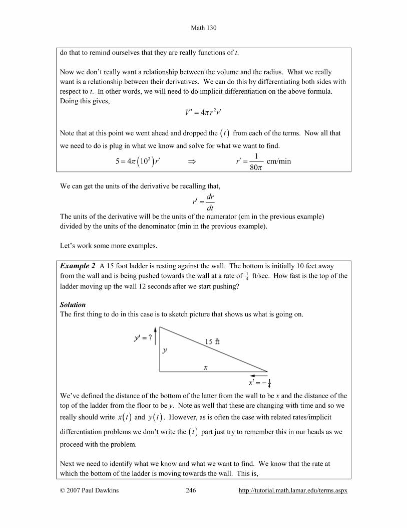
Math 130
© 2007 Paul Dawkins 246 http://tutorial.math.lamar.edu/terms.aspx
do that to remind ourselves that they are really functions of t. Now we don’t really want a relationship between the volume and the radius. What we really want is a relationship between their derivatives. We can do this by differentiating both sides with respect to t. In other words, we will need to do implicit differentiation on the above formula. Doing this gives, 24V r rπ′ ′= Note that at this point we went ahead and dropped the ( )t from each of the terms. Now all that
we need to do is plug in what we know and solve for what we want to find.
( )2 15 4 10 cm/min80
r rππ
′ ′= ⇒ =
We can get the units of the derivative be recalling that,
drrdt
′ =
The units of the derivative will be the units of the numerator (cm in the previous example) divided by the units of the denominator (min in the previous example). Let’s work some more examples. Example 2 A 15 foot ladder is resting against the wall. The bottom is initially 10 feet away from the wall and is being pushed towards the wall at a rate of 1
4 ft/sec. How fast is the top of the ladder moving up the wall 12 seconds after we start pushing? Solution The first thing to do in this case is to sketch picture that shows us what is going on.
We’ve defined the distance of the bottom of the latter from the wall to be x and the distance of the top of the ladder from the floor to be y. Note as well that these are changing with time and so we really should write ( )x t and ( )y t . However, as is often the case with related rates/implicit
differentiation problems we don’t write the ( )t part just try to remember this in our heads as we
proceed with the problem. Next we need to identify what we know and what we want to find. We know that the rate at which the bottom of the ladder is moving towards the wall. This is,

Math 130
© 2007 Paul Dawkins 247 http://tutorial.math.lamar.edu/terms.aspx
14
x′ = −
Note as well that the rate is negative since the distance from the wall, x, is decreasing. We always need to be careful with signs with these problems. We want to find the rate at which the top of the ladder is moving away from the floor. This is y′ . Note as well that this quantity should be positive since y will be increasing. As with the first example we first need a relationship between x and y. We can get this using Pythagorean theorem.
( )22 2 15 225x y+ = = All that we need to do at this point is to differentiate both sides with respect to t, remembering that x and y are really functions of t and so we’ll need to do implicit differentiation. Doing this gives an equation that shows the relationship between the derivatives. 2 2 0xx yy′ ′+ = (1) Next, let’s see which of the various parts of this equation that we know and what we need to find. We know x′ and are being asked to determine y′ so it’s okay that we don’t know that. However, we still need to determine x and y. Determining x and y is actually fairly simple. We know that initially 10x = and the end is being pushed in towards the wall at a rate of 1
4 ft/sec and that we are interested in what has happened after 12 seconds. We know that,
( )
distance rate time1 12 34
= ×
= =
So, the end of the ladder has been pushed in 3 feet and so after 12 seconds we must have 7x = . Note that we could have computed this in one step as follows,
( )110 12 74
x = − =
To find y (after 12 seconds) all that we need to do is reuse the Pythagorean Theorem with the values of x that we just found above.
2225 225 49 176y x= − = − = Now all that we need to do is plug into (1) and solve for y′ .

Math 130
© 2007 Paul Dawkins 248 http://tutorial.math.lamar.edu/terms.aspx
( ) ( )71 742 7 2 176 0 0.1319 ft/sec
4 176 4 176y y ′ ′− + = ⇒ = = =
Notice that we got the correct sign for y′ . If we’d gotten a negative then we’d have known that we had made a mistake and we could go back and look for it. Example 3 Two people are 50 feet apart. One of them starts walking north at a rate so that the angle shown in the diagram below is changing at a constant rate of 0.01 rad/min. At what rate is distance between the two people changing when 0.5θ = radians?
Solution This example is not as tricky as it might at first appear. Let’s call the distance between them at any point in time x as noted above. We can then relate all the known quantities by one of two trig formulas.
50cos sec50x
xθ θ= =
We want to find x′ and we could find x if we wanted to at the point in question using cosine since we also know the angle at that point in time. However, if we use the second formula we won’t need to know x as you’ll see. So, let’s differentiate that formula.
sec tan50x
θ θ θ′
′ =
As noted, there are no x’s in this formula. We want to determine x′ and we know that 0.5θ = and 0.01θ ′ = (do you agree with it being positive?). So, just plug in and solve. ( )( ) ( ) ( )50 0.01 sec 0.5 tan 0.5 0.311254 ft / minx x′ ′= ⇒ = So far we we’ve seen three related rates problems. While each one was worked in a very different manner the process was essentially the same in each. In each problem we identified what we were given and what we wanted to find. We next wrote down a relationship between all the various quantities and used implicit differentiation to arrive at a relationship between the various derivatives in the problem. Finally, we plugged into the equation to find the value we were after. So, in a general sense each problem was worked in pretty much the same manner. The only real difference between them was coming up with the relationship between the known and unknown
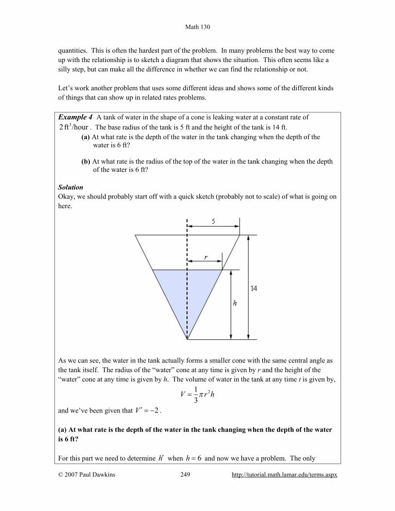
Math 130
© 2007 Paul Dawkins 249 http://tutorial.math.lamar.edu/terms.aspx
quantities. This is often the hardest part of the problem. In many problems the best way to come up with the relationship is to sketch a diagram that shows the situation. This often seems like a silly step, but can make all the difference in whether we can find the relationship or not. Let’s work another problem that uses some different ideas and shows some of the different kinds of things that can show up in related rates problems. Example 4 A tank of water in the shape of a cone is leaking water at a constant rate of
32ft /hour . The base radius of the tank is 5 ft and the height of the tank is 14 ft. (a) At what rate is the depth of the water in the tank changing when the depth of the
water is 6 ft?
(b) At what rate is the radius of the top of the water in the tank changing when the depth of the water is 6 ft?
Solution Okay, we should probably start off with a quick sketch (probably not to scale) of what is going on here.
As we can see, the water in the tank actually forms a smaller cone with the same central angle as the tank itself. The radius of the “water” cone at any time is given by r and the height of the “water” cone at any time is given by h. The volume of water in the tank at any time t is given by,
213
V r hπ=
and we’ve been given that 2V ′ = − . (a) At what rate is the depth of the water in the tank changing when the depth of the water is 6 ft? For this part we need to determine h′ when 6h = and now we have a problem. The only

Math 130
© 2007 Paul Dawkins 250 http://tutorial.math.lamar.edu/terms.aspx
formula that we’ve got that will relate the volume to the height also includes the radius and so if we were to differentiate this with respect to t we would get,
22 13 3
V rr h r hπ π′ ′ ′= +
So, in this equation we know V ′ and h and want to find h′ , but we don’t know r and r′ . As we’ll see finding r isn’t too bad, but we just don’t have enough information, at this point, that will allow us to find r′ and h′ simultaneously. To fix this we’ll need to eliminate the r from the volume formula in some way. This is actually easier than it might at first look. If we go back to our sketch above and look at just the right half of the tank we see that we have two similar triangles and when we say similar we mean similar in the geometric sense. Recall that two triangles are called similar if their angles are identical, which is the case here. When we have two similar triangles then ratios of any two sides will be equal. For our set this means that we have,
5 514 14
r r hh
= ⇒ =
If we take this and plug it into our volume formula we have,
2
2 31 1 5 253 3 14 588
V r h h h hπ π π = = =
This gives us a volume formula that only involved the volume and the height of the water. Note however that this volume formula is only valid for our cone, so don’t be tempted to use it for other cones! If we now differentiate this we have,
225196
V h hπ′ ′=
At this point all we need to do is plug in what we know and solve for h′ .
( )225 982 6 0.1386196 225
h hππ
−′ ′− = ⇒ = = −
So, it looks like the height is decreasing at a rate of 0.1386 ft/hr. (b) At what rate is the radius of the top of the water in the tank changing when the depth of the water is 6 ft? In this case we are asking for r′ and there is an easy way to do this part and a difficult (well, more difficult than the easy way anyway….) way to do it. The “difficult” way is to redo the work part (a) above only this time use,
14 145 5
h h rr
= ⇒ =

Math 130
© 2007 Paul Dawkins 251 http://tutorial.math.lamar.edu/terms.aspx
to get the volume in terms of V and r and then proceed as before. That’s not terribly difficult, but it is more work that we need to so. Recall from the first part that we have,
5 5
14 14r h r h′ ′= ⇒ =
So, as we can see if we take the relationship that relates r and h that we used in the first part and differentiate it we get a relationship between r′ and h′ . At this point all we need to do here is use the result from the first part to get,
5 98 7 0.04951
14 225 45r
π π− ′ = = − = −
Much easier that redoing all of the first part. Note however, that we were only able to do this the “easier” way because it was asking for r′ at exactly the same time that we asked for h′ in the first part. If we hadn’t been using the same time then we would have had no choice but to do this the “difficult” way. In the second part of the previous problem we saw an important idea in dealing with related rates. In order to find the asked for rate all we need is an equations that relates the rate we’re looking for to a rate that we already know. Sometimes there are multiple equations that we can use and sometimes one will be easier than another. Also, this problem showed us that we will often have an equation that contains more variables that we have information about and so, in these cases, we will need to eliminate one (or more) of the variables. In this problem we eliminated the extra variable using the idea of similar triangles. This will not always be how we do this, but many of these problems do use similar triangles so make sure you can use that idea. Let’s work some more problems. Example 5 A trough of water is 8 meters deep and its ends are in the shape of isosceles triangles whose width is 5 meters and height is 2 meters. If water is being pumped in at a constant rate of 36 m /sec . At what rate is the height of the water changing when the water has a height of 120 cm? Solution Note that an isosceles triangle is just a triangle in which two of the sides are the same length. In our case sides of the tank have the same length. We definitely need a sketch of this situation to get us going here so here. A sketch of the trough is shown below.

Math 130
© 2007 Paul Dawkins 252 http://tutorial.math.lamar.edu/terms.aspx
Now, in this problem we know that 36 m /secV ′ = and we want to determine h′ when
1.2 mh = . Note that because V ′ is in terms of meters we need to convert h into meters as well. So, we need an equation that will relate these two quantities and the volume of the tank will do it. The volume of this kind of tank is simple to compute. The volume is the area of the end times the depth. For our case the volume of the water in the tank is,
( ) ( )( )( )
( )
12
12
Area of End depth
base height depth
84
V
hwhw
=
= ×
=
=
As with the previous example we’ve got an extra quantity here, w, that is also changing with time and so we need to get eliminate it from the problem. To do this we’ll again make use of the idea of similar triangles. If we look at the end of the tank we’ll see that we again have two similar triangles. One for the tank itself and one formed by the water in the tank. Again, remember that with similar triangles ratios of sides must be equal. In our case we’ll use,
55 2 2w h w h= ⇒ =
Plugging this into the volume gives a formula for the volume (and only for this tank) that only involved the height of the water.
254 4 102
V hw h h h = = =
We can now differentiate this to get, 20V hh′ ′= Finally, all we need to do is plug in and solve for h′ .
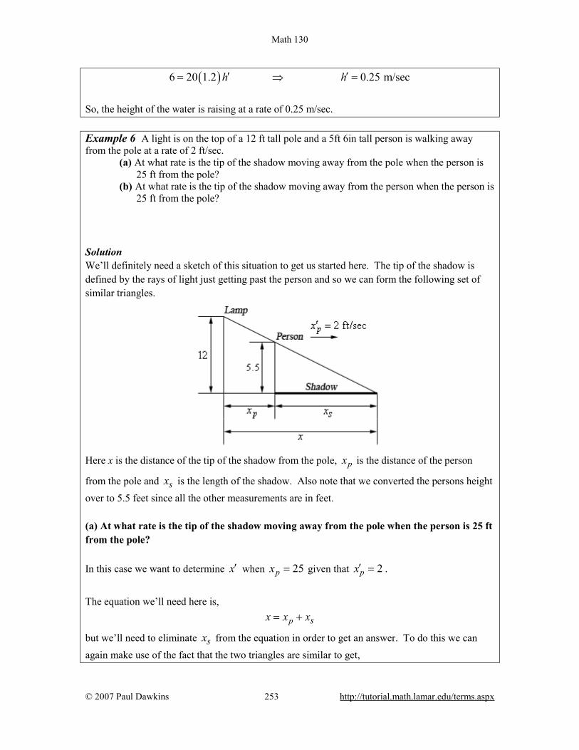
Math 130
© 2007 Paul Dawkins 253 http://tutorial.math.lamar.edu/terms.aspx
( )6 20 1.2 0.25 m/sech h′ ′= ⇒ =
So, the height of the water is raising at a rate of 0.25 m/sec. Example 6 A light is on the top of a 12 ft tall pole and a 5ft 6in tall person is walking away from the pole at a rate of 2 ft/sec.
(a) At what rate is the tip of the shadow moving away from the pole when the person is 25 ft from the pole?
(b) At what rate is the tip of the shadow moving away from the person when the person is 25 ft from the pole?
Solution We’ll definitely need a sketch of this situation to get us started here. The tip of the shadow is defined by the rays of light just getting past the person and so we can form the following set of similar triangles.
Here x is the distance of the tip of the shadow from the pole, px is the distance of the person
from the pole and sx is the length of the shadow. Also note that we converted the persons height over to 5.5 feet since all the other measurements are in feet. (a) At what rate is the tip of the shadow moving away from the pole when the person is 25 ft from the pole? In this case we want to determine x′ when 25px = given that 2px′ = .
The equation we’ll need here is, p sx x x= +
but we’ll need to eliminate sx from the equation in order to get an answer. To do this we can again make use of the fact that the two triangles are similar to get,

Math 130
© 2007 Paul Dawkins 254 http://tutorial.math.lamar.edu/terms.aspx
1125.5 5.5 11Note :
12 12 12 24p
s s
s
x xx x x
= = = =+
We’ll need to solve this for sx .
( )1124
11 1324 241113
p
p
p
s s
s
s
x x x
x x
x x
+ =
=
=
Our equation then becomes,
11 2413 13p p px x x x= + =
Now all that we need to do is differentiate this, plug in and solve for x′ .
( )24 24 2 3.6923 ft/sec13 13px x x′ ′ ′= ⇒ = =
The tip of the shadow is then moving away from the pole at a rate of 3.6923 ft/sec. Notice as well that we never actually had to use the fact that 25px = for this problem. That will happen
on rare occasions. (b) At what rate is the tip of the shadow moving away from the person when the person is 25 ft from the pole? This part is actually quite simple if we have the answer from (a) in hand, which we do of course. In this case we know that sx represents the length of the shadow, or the distance of the tip of the
shadow from the person so it looks like we want to determine sx′ when 25px = .
Again, we can use p sx x x= + , however unlike the first part we now know that 2px′ = and
3.6923 ft/secx′ = so in this case all we need to do is differentiate the equation and plug in for all the known quantities.
3.6923 2 1.6923 ft/sec
p s
s s
x x x
x x
′ ′ ′= +
′ ′= + =
The tip of the shadow is then moving away from the person at a rate of 1.6923 ft/sec.
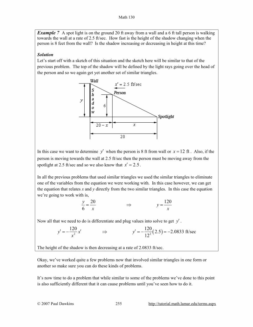
Math 130
© 2007 Paul Dawkins 255 http://tutorial.math.lamar.edu/terms.aspx
Example 7 A spot light is on the ground 20 ft away from a wall and a 6 ft tall person is walking towards the wall at a rate of 2.5 ft/sec. How fast is the height of the shadow changing when the person is 8 feet from the wall? Is the shadow increasing or decreasing in height at this time? Solution Let’s start off with a sketch of this situation and the sketch here will be similar to that of the previous problem. The top of the shadow will be defined by the light rays going over the head of the person and so we again get yet another set of similar triangles.
In this case we want to determine y′ when the person is 8 ft from wall or 12 ftx = . Also, if the person is moving towards the wall at 2.5 ft/sec then the person must be moving away from the spotlight at 2.5 ft/sec and so we also know that 2.5x′ = . In all the previous problems that used similar triangles we used the similar triangles to eliminate one of the variables from the equation we were working with. In this case however, we can get the equation that relates x and y directly from the two similar triangles. In this case the equation we’re going to work with is,
20 1206y y
x x= ⇒ =
Now all that we need to do is differentiate and plug values into solve to get y′ .
( )2 2
120 120 2.5 2.0833 ft/sec12
y x yx
′ ′ ′= − ⇒ = − = −
The height of the shadow is then decreasing at a rate of 2.0833 ft/sec. Okay, we’ve worked quite a few problems now that involved similar triangles in one form or another so make sure you can do these kinds of problems. It’s now time to do a problem that while similar to some of the problems we’ve done to this point is also sufficiently different that it can cause problems until you’ve seen how to do it.

Math 130
© 2007 Paul Dawkins 256 http://tutorial.math.lamar.edu/terms.aspx
Example 8 Two people on bikes are separated by 350 meters. Person A starts riding north at a rate of 5 m/sec and 7 minutes later Person B starts riding south at 3 m/sec. At what rate is the distance separating the two people changing 25 minutes after Person A starts riding? Solution There is a lot to digest here with this problem. Let’s start off with a sketch of the situation.
Now we are after z′ and we know that 5x′ = and 3y′ = . We want to know z′ after Person A had been riding for 25 minutes and Person B has been riding for 25 7 18− = minutes. After converting these times to seconds (because our rates are all in m/sec) this means that at the time we’re interested in each of the bike riders has rode, ( ) ( )5 25 60 7500 m 3 18 60 3240 mx y= × = = × =
Next, the Pythagorean theorem tells us that,
( )22 2350z x y= + + (2)
Therefore, 25 minutes after Person A starts riding the two bike riders are
( ) ( )2 22 2350 7500 3240 350 10745.7015 mz x y= + + = + + =
apart. To determine the rate at which the two riders are moving apart all we need to do then is differentiate (2) and plug in all the quantities that we know to find z′ .
Math 130
© 2007 Paul Dawkins 257 http://tutorial.math.lamar.edu/terms.aspx
( )( )( ) ( )( )
2 2
2 10745.7015 2 7500 3240 5 37.9958 m/sec
zz x y x y
zz
′ ′ ′= + +
′ = + +
′ =
So, the two riders are moving apart at a rate of 7.9958 m/sec. Every problem that we’ve worked to this point has come down to needing a geometric formula and we should probably work a quick problem that is not geometric in nature. Example 9 Suppose that we have two resistors connected in parallel with resistances 1R and
2R measured in ohms ( Ω ). The total resistance, R, is then given by,
1 2
1 1 1R R R
= +
Suppose that 1R is increasing at a rate of 0.4 Ω /min and 2R is decreasing at a rate of
0.7 Ω /min. At what rate is R changing when 1 80R = Ω and 2 105R = Ω ?
Solution Okay, unlike the previous problems there really isn’t a whole lot to do here. First, let’s note that we’re looking for R′ and that we know 1 0.4R′ = and 2 0.7R′ = − . Be careful with the signs
here. Also, since we’ll eventually need it let’s determine R at the time we’re interested in.
1 1 1 37 1680 45.4054
80 105 1680 37R
R= + = ⇒ = = Ω
Next we need to differentiate the equation given in the problem statement.
( ) ( )
( ) ( )
1 22 22
1 2
21 22 2
1 2
1 1 1
1 1
R R RR R R
R R R RR R
′ ′ ′− = − −
′ ′ ′= +
Finally, all we need to do is plug into this and do some quick computations.
( ) ( ) ( )22 2
1 145.4054 0.4 0.7 0.00204580 105
R ′ = + − = −
So, it looks like R is decreasing at a rate of 0.002045 Ω /min.

Math 130
© 2007 Paul Dawkins 258 http://tutorial.math.lamar.edu/terms.aspx
We’ve seen quite a few related rates problems in this section that cover a wide variety of possible problems. There are still many more different kinds of related rates problems out there in the world, but the ones that we’ve worked here should give you a pretty good idea on how to at least start most of the problems that you’re liable to run into.

Math 130
© 2007 Paul Dawkins 259 http://tutorial.math.lamar.edu/terms.aspx
Higher Order Derivatives Let’s start this section with the following function. ( ) 3 25 3 10 5f x x x x= − + − By this point we should be able to differentiate this function without any problems. Doing this we get, ( ) 215 6 10f x x x′ = − + Now, this is a function and so it can be differentiated. Here is the notation that we’ll use for that, as well as the derivative.
( ) ( )( ) 30 6f x f x x′′′ ′= = −
This is called the second derivative and ( )f x′ is now called the first derivative.
Again, this is a function so we can differentiate it again. This will be called the third derivative. Here is that derivative as well as the notation for the third derivative.
( ) ( )( ) 30f x f x ′′′′ ′′= = Continuing, we can differentiate again. This is called, oddly enough, the fourth derivative. We’re also going to be changing notation at this point. We can keep adding on primes, but that will get cumbersome after awhile.
( ) ( )( )(4) 0f x f x ′′′′= = This process can continue but notice that we will get zero for all derivatives after this point. This set of derivatives leads us to the following fact about the differentiation of polynomials. Fact If p(x) is a polynomial of degree n (i.e. the largest exponent in the polynomial) then,
( ) ( ) 0 for 1kp x k n= ≥ + We will need to be careful with the “non-prime” notation for derivatives. Consider each of the following.
( ) ( ) ( )
( ) ( )
2
22
f x f x
f x f x
′′=
=
The presence of parenthesis in the exponent denotes differentiation while the absence of parenthesis denotes exponentiation. Collectively the second, third, fourth, etc. derivatives are called higher order derivatives.

Math 130
© 2007 Paul Dawkins 260 http://tutorial.math.lamar.edu/terms.aspx
Let’s take a look at some examples of higher order derivatives. Example 1 Find the first four derivatives for each of the following.
(a) ( )1
2 23 8 tR t t t= + + e [Solution] (b) cosy x= [Solution] (c) ( ) ( ) ( )2sin 3 ln 7yf y y y−= + +e [Solution]
Solution
(a) ( )1
2 23 8 tR t t t= + + e
There really isn’t a lot to do here other than do the derivatives.
( )
( )
( )
( )
12
32
52
7(4) 2
6 4
6 2
3
152
t
t
t
t
R t t t
R t t
R t t
R t t
−
−
−
−
′ = + +
′′ = − +
′′′ = +
= − +
e
e
e
e
Notice that differentiating an exponential function is very simple. It doesn’t change with each differentiation.
[Return to Problems] (b) cosy x= Again, let’s just do some derivatives.
( )4
cossincos
sin
cos
y xy xy xy x
y x
=′ = −′′ = −′′′ =
=
Note that cosine (and sine) will repeat every four derivatives. The other four trig functions will not exhibit this behavior. You might want to take a few derivatives to convince yourself of this.
[Return to Problems] (c) ( ) ( ) ( )2sin 3 ln 7yf y y y−= + +e
In the previous two examples we saw some patterns in the differentiation of exponential functions, cosines and sines. We need to be careful however since they only work if there is just a t or an x in argument. This is the point of this example. In this example we will need to use the chain rule on each derivative.
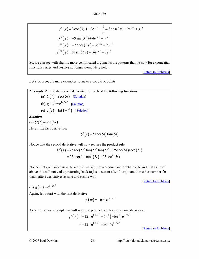
Math 130
© 2007 Paul Dawkins 261 http://tutorial.math.lamar.edu/terms.aspx
( ) ( ) ( )
( ) ( )( ) ( )
( ) ( ) ( )
2 2 1
2 2
2 3
4 2 4
13cos 3 2 3cos 3 2
9sin 3 4
27cos 3 8 2
81sin 3 16 6
y y
y
y
y
f y y y yy
f y y y
f y y y
f y y y
− − −
− −
− −
− −
′ = − + = − +
′′ = − + −
′′′ = − − +
= + −
e e
e
e
e
So, we can see with slightly more complicated arguments the patterns that we saw for exponential functions, sines and cosines no longer completely hold.
[Return to Problems] Let’s do a couple more examples to make a couple of points. Example 2 Find the second derivative for each of the following functions.
(a) ( ) ( )sec 5Q t t= [Solution]
(b) ( ) 31 2wg w −= e [Solution]
(c) ( ) ( )2ln 1f t t= + [Solution]
Solution (a) ( ) ( )sec 5Q t t=
Here’s the first derivative. ( ) ( ) ( )5sec 5 tan 5Q t t t′ = Notice that the second derivative will now require the product rule.
( ) ( ) ( ) ( ) ( ) ( )
( ) ( ) ( )
2
2 3
25sec 5 tan 5 tan 5 25sec 5 sec 5
25sec 5 tan 5 25sec 5
Q t t t t t t
t t t
′′ = +
= +
Notice that each successive derivative will require a product and/or chain rule and that as noted above this will not end up returning back to just a secant after four (or another other number for that matter) derivatives as sine and cosine will.
[Return to Problems]
(b) ( ) 31 2wg w −= e
Again, let’s start with the first derivative.
( ) 32 1 26 wg w w −′ = − e As with the first example we will need the product rule for the second derivative.
( ) ( )3 3
3 3
2 2
4
1 2 1 2
1 2 1 2
12 6 6
12 36
w w
w w
g w w w w
w w
− −
− −
′′ = − − −
= − +
e e
e e
[Return to Problems]

Math 130
© 2007 Paul Dawkins 262 http://tutorial.math.lamar.edu/terms.aspx
(c) ( ) ( )2ln 1f t t= +
Same thing here.
( ) 2
21
tf tt
′ =+
The second derivative this time will require the quotient rule.
( ) ( ) ( ) ( )( )
( )
2
22
2
22
2 1 2 2
1
2 2
1
t t tf t
t
t
t
+ −′′ =
+
−=
+
[Return to Problems] As we saw in this last set of examples we will often need to use the product or quotient rule for the higher order derivatives, even when the first derivative didn’t require these rules. Let’s work one more example that will illustrate how to use implicit differentiation to find higher order derivatives. Example 3 Find y′′ for 2 4 10x y+ = Solution Okay, we know that in order to get the second derivative we need the first derivative and in order to get that we’ll need to do implicit differentiation. Here is the work for that.
3
3
2 4 0
2
x y yxyy
′+ =
′ = −
Now, this is the first derivative. We get the second derivative by differentiating this, which will require implicit differentiation again.
( )( )
3
3 2
23
3 2
6
4
2
2 6
2
2 64
32
xyy
y x y y
y
y xy yy
y xyy
′ ′′ = −
′−= −
′−= −
′−= −
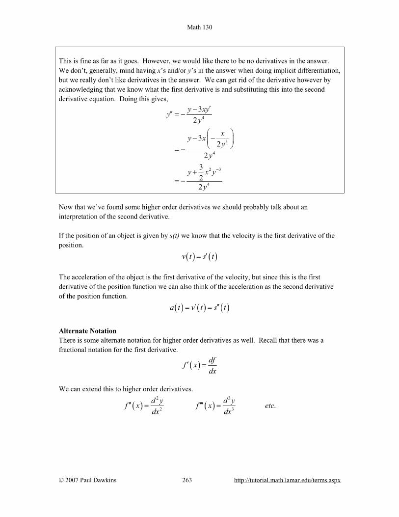
Math 130
© 2007 Paul Dawkins 263 http://tutorial.math.lamar.edu/terms.aspx
This is fine as far as it goes. However, we would like there to be no derivatives in the answer. We don’t, generally, mind having x’s and/or y’s in the answer when doing implicit differentiation, but we really don’t like derivatives in the answer. We can get rid of the derivative however by acknowledging that we know what the first derivative is and substituting this into the second derivative equation. Doing this gives,
4
3
4
2 3
4
32
32
2322
y xyyy
xy xy
y
y x y
y
−
′−′′ = −
− −
= −
+= −
Now that we’ve found some higher order derivatives we should probably talk about an interpretation of the second derivative. If the position of an object is given by s(t) we know that the velocity is the first derivative of the position. ( ) ( )v t s t′= The acceleration of the object is the first derivative of the velocity, but since this is the first derivative of the position function we can also think of the acceleration as the second derivative of the position function. ( ) ( ) ( )a t v t s t′ ′′= =
Alternate Notation There is some alternate notation for higher order derivatives as well. Recall that there was a fractional notation for the first derivative.
( ) dff xdx
′ =
We can extend this to higher order derivatives.
( ) ( )2 3
2 3 .d y d yf x f x etcdx dx
′′ ′′′= =

Math 130
© 2007 Paul Dawkins 264 http://tutorial.math.lamar.edu/terms.aspx
Logarithmic Differentiation There is one last topic to discuss in this section. Taking the derivatives of some complicated functions can be simplified by using logarithms. This is called logarithmic differentiation. It’s easiest to see how this works in an example. Example 1 Differentiate the function.
( )
5
21 10 2xy
x x=
− +
Solution Differentiating this function could be done with a product rule and a quotient rule. However, that would be a fairly messy process. We can simplify things somewhat by taking logarithms of both sides.
( )
5
2ln ln
1 10 2xy
x x
= − +
Of course, this isn’t really simpler. What we need to do is use the properties of logarithms to expand the right side as follows.
( ) ( )( )( ) ( ) ( )
5 2
5 2
ln ln ln 1 10 2
ln ln ln 1 10 ln 2
y x x x
y x x x
= − − +
= − − − +
This doesn’t look all the simple. However, the differentiation process will be simpler. What we need to do at this point is differentiate both sides with respect to x. Note that this is really implicit differentiation.
( ) ( )
( )
12 24
152 2
2
1 2 25 10 21 10 2
5 101 10 2
x xy xy x x x
y xy x x x
−+′ −
= − −−
+
′= + −
− +
To finish the problem all that we need to do is multiply both sides by y and the plug in for y since we do know what that is.
( )
2
5
22
5 101 10 2
5 101 10 21 10 2
xy yx x x
x xx x xx x
′ = + − − +
= + − − + − +
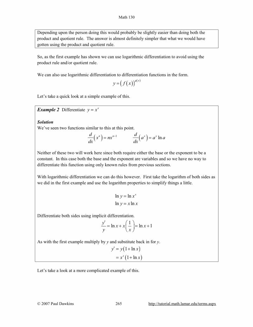
Math 130
© 2007 Paul Dawkins 265 http://tutorial.math.lamar.edu/terms.aspx
Depending upon the person doing this would probably be slightly easier than doing both the product and quotient rule. The answer is almost definitely simpler that what we would have gotten using the product and quotient rule. So, as the first example has shown we can use logarithmic differentiation to avoid using the product rule and/or quotient rule. We can also use logarithmic differentiation to differentiation functions in the form.
( )( ) ( )g xy f x=
Let’s take a quick look at a simple example of this. Example 2 Differentiate xy x= Solution We’ve seen two functions similar to this at this point.
( ) ( )1 lnn n x xd dx nx a a adx dx
−= =
Neither of these two will work here since both require either the base or the exponent to be a constant. In this case both the base and the exponent are variables and so we have no way to differentiate this function using only known rules from previous sections. With logarithmic differentiation we can do this however. First take the logarithm of both sides as we did in the first example and use the logarithm properties to simplify things a little.
ln lnln ln
xy xy x x
==
Differentiate both sides using implicit differentiation.
1ln ln 1y x x xy x′ = + = +
As with the first example multiply by y and substitute back in for y.
( )( )1 ln
1 lnx
y y x
x x
′ = +
= +
Let’s take a look at a more complicated example of this.
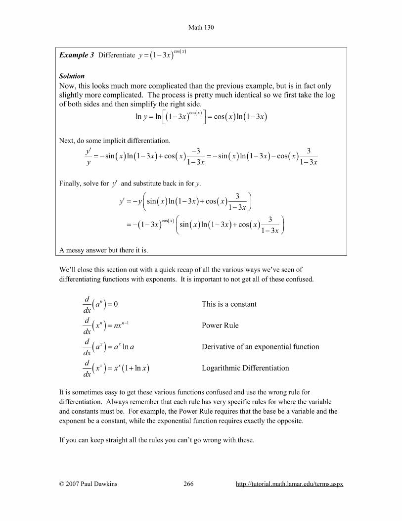
Math 130
© 2007 Paul Dawkins 266 http://tutorial.math.lamar.edu/terms.aspx
Example 3 Differentiate ( ) ( )cos1 3 xy x= − Solution Now, this looks much more complicated than the previous example, but is in fact only slightly more complicated. The process is pretty much identical so we first take the log of both sides and then simplify the right side. ( ) ( ) ( ) ( )cosln ln 1 3 cos ln 1 3xy x x x = − = −
Next, do some implicit differentiation.
( ) ( ) ( ) ( ) ( ) ( )3 3sin ln 1 3 cos sin ln 1 3 cos1 3 1 3
y x x x x x xy x x′ −
= − − + = − − −− −
Finally, solve for y′ and substitute back in for y.
( ) ( ) ( )
( ) ( ) ( ) ( ) ( )cos
3sin ln 1 3 cos1 3
31 3 sin ln 1 3 cos1 3
x
y y x x xx
x x x xx
′ = − − + − = − − − + −
A messy answer but there it is. We’ll close this section out with a quick recap of all the various ways we’ve seen of differentiating functions with exponents. It is important to not get all of these confused.
( )
( )
( )
( ) ( )
1
0 This is a constant
Power Rule
ln Derivative of an exponential function
1 ln Logarithmic Differentiation
b
n n
x x
x x
d adxd x nxdxd a a adxd x x xdx
−
=
=
=
= +
It is sometimes easy to get these various functions confused and use the wrong rule for differentiation. Always remember that each rule has very specific rules for where the variable and constants must be. For example, the Power Rule requires that the base be a variable and the exponent be a constant, while the exponential function requires exactly the opposite. If you can keep straight all the rules you can’t go wrong with these.

Math 130
© 2007 Paul Dawkins 267 http://tutorial.math.lamar.edu/terms.aspx
Applications of Derivatives
Introduction In the previous chapter we focused almost exclusively on the computation of derivatives. In this chapter will focus on applications of derivatives. It is important to always remember that we didn’t spend a whole chapter talking about computing derivatives just to be talking about them. There are many very important applications to derivatives. The two main applications that we’ll be looking at in this chapter are using derivatives to determine information about graphs of functions and optimization problems. These will not be the only applications however. We will be revisiting limits and taking a look at an application of derivatives that will allow us to compute limits that we haven’t been able to compute previously. We will also see how derivatives can be used to estimate solutions to equations. Here is a listing of the topics in this section. Rates of Change – The point of this section is to remind us of the application/interpretation of derivatives that we were dealing with in the previous chapter. Namely, rates of change. Critical Points – In this section we will define critical points. Critical points will show up in many of the sections in this chapter so it will be important to understand them. Minimum and Maximum Values – In this section we will take a look at some of the basic definitions and facts involving minimum and maximum values of functions. Finding Absolute Extrema – Here is the first application of derivatives that we’ll look at in this chapter. We will be determining the largest and smallest value of a function on an interval. The Shape of a Graph, Part I – We will start looking at the information that the first derivatives can tell us about the graph of a function. We will be looking at increasing/decreasing functions as well as the First Derivative Test. The Shape of a Graph, Part II – In this section we will look at the information about the graph of a function that the second derivatives can tell us. We will look at inflection points, concavity, and the Second Derivative Test. The Mean Value Theorem – Here we will take a look that the Mean Value Theorem.
Math 130
© 2007 Paul Dawkins 268 http://tutorial.math.lamar.edu/terms.aspx
Optimization Problems – This is the second major application of derivatives in this chapter. In this section we will look at optimizing a function, possible subject to some constraint. More Optimization Problems – Here are even more optimization problems. L’Hospital’s Rule and Indeterminate Forms – This isn’t the first time that we’ve looked at indeterminate forms. In this section we will take a look at L’Hospital’s Rule. This rule will allow us to compute some limits that we couldn’t do until this section. Differentials – We will look at differentials in this section as well as an application for them. Business Applications – Here we will take a quick look at some applications of derivatives to the business field.

Math 130
© 2007 Paul Dawkins 269 http://tutorial.math.lamar.edu/terms.aspx
Rates of Change The purpose of this section is to remind us of one of the more important applications of derivatives. That is the fact that ( )f x′ represents the rate of change of ( )f x . This is an
application that we repeatedly saw in the previous chapter. Almost every section in the previous chapter contained at least one problem dealing with this application of derivatives. While this application will arise occasionally in this chapter we are going to focus more on other applications in this chapter. So, to make sure that we don’t forget about this application here is a brief set of examples concentrating on the rate of change application of derivatives. Note that the point of these examples is to remind you of material covered in the previous chapter and not to teach you how to do these kinds of problems. If you don’t recall how to do these kinds of examples you’ll need to go back and review the previous chapter. Example 1 Determine all the points where the following function is not changing. ( ) ( )5 6 10cos 2g x x x= − − Solution First we’ll need to take the derivative of the function. ( ) ( )6 20sin 2g x x′ = − +
Now, the function will not be changing if the rate of change is zero and so to answer this question we need to determine where the derivative is zero. So, let’s set this equal to zero and solve.
( ) ( )6 20sin 2 0 sin 2 0.320
x x 6− + = ⇒ = =
The solution to this is then,
2 0.3047 2 OR 2 2.8369 2 0, 1, 2,
0.1524 OR 1.4185 0, 1, 2,x n x n nx n x n n
π ππ π
= + = + = ± ±= + = + = ± ±
……
If you don’t recall how to solve trig equations check out the Solving Trig Equations sections in the Review Chapter. Example 2 Determine where the following function is increasing and decreasing. ( ) 5 4 327 45 130 150A t t t t= − − + Solution As with the first problem we first need to take the derivative of the function.
( ) ( )4 3 2 2 2135 180 390 15 9 12 26A t t t t t t t′ = − − = − −
Next, we need to determine where the function isn’t changing. This is at,

Math 130
© 2007 Paul Dawkins 270 http://tutorial.math.lamar.edu/terms.aspx
( ) ( )0
12 144 4 9 26 12 1080 12 6 30 2 30 1.159, 2.49218 18 18 3
t
t
=
± − − ± ± ±= = = = = −
So, the function is not changing at three values of t. Finally, to determine where the function is increasing or decreasing we need to determine where the derivative is positive or negative. Recall that if the derivative is positive then the function must be increasing and if the derivative is negative then the function must be decreasing. The following number line gives this information.
So, from this number line we can see that we have the following increasing and decreasing information. Increasing : 1.159, 2.492 Decreasing : 1.159 0, 0 2.492t t t t− ∞ < < − < < ∞ < < < < If you don’t remember how to solve polynomial and rational inequalities then you should check out the appropriate sections in the Review Chapter. Finally, we can’t forget about Related Rates problems. Example 3 Two cars start out 500 miles apart. Car A is to the west of Car B and starts driving to the east (i.e. towards Car B) at 35 mph and at the same time Car B starts driving south at 50 mph. After 3 hours of driving at what rate is the distance between the two cars changing? Is it increasing or decreasing? Solution The first thing to do here is to get sketch a figure showing the situation.
In this figure y represents the distance driven by Car B and x represents the distance separating Car A from Car B’s initial position and z represents the distance separating the two cars. After 3

Math 130
© 2007 Paul Dawkins 271 http://tutorial.math.lamar.edu/terms.aspx
hours driving time with have the following values of x and y. ( ) ( )500 35 3 395 50 3 150x y= − = = =
We can use the Pythagorean theorem to find z at this time as follows,
2 2 2395 150 178525 178525 422.5222z z= + = ⇒ = = Now, to answer this question we will need to determine z′ given that 35x′ = − and 50y′ = . Do you agree with the signs on the two given rates? Remember that a rate is negative if the quantity is decreasing and positive if the quantity is increasing. We can again use the Pythagorean theorem here. First, write it down and the remember that x, y, and z are all changing with time and so differentiate the equation using Implicit Differentiation. 2 2 2 2 2 2z x y zz xx yy′ ′ ′= + ⇒ = + Finally, all we need to do is cancel a two from everything, plug in for the known quantities and solve for z′ .
( ) ( ) ( ) ( )( ) 6325422.5222 395 35 150 50 14.9696422.5222
z z −′ ′= − + ⇒ = = −
So, after three hours the distance between them is decreasing at a rate of 14.9696 mph. So, in this section we covered three “standard” problems using the idea that the derivative of a function gives its rate of change. As mentioned earlier, this chapter will be focusing more on other applications than the idea of rate of change, however, we can’t forget this application as it is a very important one.

Math 130
© 2007 Paul Dawkins 272 http://tutorial.math.lamar.edu/terms.aspx
Critical Points Critical points will show up throughout a majority of this chapter so we first need to define them and work a few examples before getting into the sections that actually use them. Definition We say that x c= is a critical point of the function f(x) if ( )f c exists and if either of the
following are true. ( ) ( )0 OR doesn't existf c f c′ ′= Note that we require that ( )f c exists in order for x c= to actually be a critical point. This is an
important, and often overlooked, point. The main point of this section is to work some examples finding critical points. So, let’s work some examples. Example 1 Determine all the critical points for the function. ( ) 5 4 36 33 30 100f x x x x= + − + Solution We first need the derivative of the function in order to find the critical points and so let’s get that and notice that we’ll factor it as much as possible to make our life easier when we go to find the critical points.
( )( )( ) ( )
4 3 2
2 2
2
30 132 90
6 5 22 15
6 5 3 5
f x x x x
x x x
x x x
′ = + −
= + −
= − +
Now, our derivative is a polynomial and so will exist everywhere. Therefore the only critical points will be those values of x which make the derivative zero. So, we must solve. ( )( )26 5 3 5 0x x x− + = Because this is the factored form of the derivative it’s pretty easy to identify the three critical points. They are,
35, 0,5
x x x= − = =
Polynomials are usually fairly simple functions to find critical points for provided the degree doesn’t get so large that we have trouble finding the roots of the derivative.

Math 130
© 2007 Paul Dawkins 273 http://tutorial.math.lamar.edu/terms.aspx
Most of the more “interesting” functions for finding critical points aren’t polynomials however. So let’s take a look at some functions that require a little more effort on our part. Example 2 Determine all the critical points for the function.
( ) ( )3 2 2 1g t t t= − Solution To find the derivative it’s probably easiest to do a little simplification before we actually differentiate. Let’s multiply the root through the parenthesis and simplify as much as possible. This will allow us to avoid using the product rule when taking the derivative.
( ) ( )2 5 23 3 32 1 2g t t t t t= − = −
Now differentiate.
( )2
2 1 33 3
13
10 2 10 23 3 3 3
tg t t tt
−′ = − = −
We will need to be careful with this problem. When faced with a negative exponent it is often best to eliminate the minus sign in the exponent as we did above. This isn’t really required but it can make our life easier on occasion if we do that. Notice as well that eliminating the negative exponent in the second term allows us to correctly identify why 0t = is a critical point for this function. Once we move the second term to the denominator we can clearly see that the derivative doesn’t exist at 0t = and so this will be a critical point. If you don’t get rid of the negative exponent in the second term many people will incorrectly state that 0t = is a critical point because the derivative is zero at 0t = . While this may seem like a silly point, after all in each case 0t = is identified as a critical point, it is sometimes important to know why a point is a critical point. In fact, in a couple of sections we’ll see a fact that only works for critical points in which the derivative is zero. So, we’ve found one critical point (where the derivative doesn’t exist), but we now need to determine where the derivative is zero (provided it is of course…). To help with this it’s usually best to combine the two terms into a single rational expression. So, getting a common denominator and combining gives us,
( ) 13
10 2
3
tg tt
−′ =
Notice that we still have 0t = as a critical point. Doing this kind of combining should never lose critical points, it’s only being done to help us find them. As we can see it’s now become much easier to quickly determine where the derivative will be zero. Recall that a rational expression will only be zero if its numerator is zero (and provided the denominator isn’t also zero at that

Math 130
© 2007 Paul Dawkins 274 http://tutorial.math.lamar.edu/terms.aspx
point of course).
So, in this case we can see that the numerator will be zero if 15
t = and so there are two critical
points for this function.
10 and5
t t= =
Example 3 Determine all the critical points for the function.
( )2
2
16
wR ww w
+=
− −
Solution We’ll leave it to you to verify that using the quotient rule we get that the derivative is,
( )( ) ( )
2 2
2 22 2
14 1 14 1
6 6
w w w wR ww w w w
− − + + −′ = = −− − − −
Notice that we factored a “-1” out of the numerator to help a little with finding the critical points. This negative out in front will not affect the derivative whether or not the derivative is zero or not exist but will make our work a little easier. Now, we have two issues to deal with. First the derivative will not exist if there is division by zero in the denominator. So we need to solve, ( ) ( )2 6 3 2 0w w w w− − = − + = We didn’t bother squaring this since if this is zero, then zero squared is still zero and if it isn’t zero then squaring it won’t make it zero. So, we can see from this that the derivative will not exist at 3w = and 2w = − . However, these are NOT critical points since the function will also not exist at these points. Recall that in order for a point to be a critical point the function must actually exist at that point. At this point we need to be careful. The numerator doesn’t factor, but that doesn’t mean that there aren’t any critical points where the derivative is zero. We can use the quadratic formula on the numerator to determine if the fraction as a whole is ever zero.
( ) ( ) ( )
( )
214 14 4 1 1 14 200 14 10 2 7 5 22 1 2 2
w− ± − − − ± − +
= = = = − ±
So, we get two critical points. Also, these are not “nice” integers or fractions. This will happen on occasion. Don’t get too locked into answers always being “nice”. Often they aren’t. Note as well that we only use real numbers for critical points. So, if upon solving the quadratic in the numerator, we had gotten complex number these would not have been considered critical points.

Math 130
© 2007 Paul Dawkins 275 http://tutorial.math.lamar.edu/terms.aspx
Summarizing, we have two critical points. They are,
7 5 2, 7 5 2w w= − + = − − Again, remember that while the derivative doesn’t exist at 3w = and 2w = − neither does the function and so these two points are not critical points for this function. So far all the examples have not had any trig functions, exponential functions, etc. in them. We shouldn’t expect that to always be the case. So, let’s take a look at some examples that don’t just involve powers of x. Example 4 Determine all the critical points for the function. ( )6 4cos 3y x x= − Solution First get the derivative and don’t forget to use the chain rule on the second term. ( )6 12sin 3y x′ = + Now, this will exist everywhere and so there won’t be any critical points for which the derivative doesn’t exist. The only critical points will come from points that make the derivative zero. We will need to solve,
( )
( )
6 12sin 3 01sin 32
x
x
+ =
= −
Solving this equation gives the following.
3 3.6652 2 , 0, 1, 2,3 5.7596 2 , 0, 1, 2,
x n nx n n
ππ
= + = ± ±= + = ± ±
……
Don’t forget the 2π n on these! There will be problems down the road in which we will miss solutions without this! Also make sure that it gets put on at this stage! Now divide by 3 to get all the critical points for this function.
21.2217 , 0, 1, 2,3
21.9199 , 0, 1, 2,3
nx n
nx n
π
π
= + = ± ±
= + = ± ±
…
…
Notice that in the previous example we got an infinite number of critical points. That will happen on occasion so don’t worry about it when it happens.

Math 130
© 2007 Paul Dawkins 276 http://tutorial.math.lamar.edu/terms.aspx
Example 5 Determine all the critical points for the function.
( ) 2310 th t t −= e Solution Here’s the derivative for this function.
( ) ( )2 2 2 23 3 3 2 310 10 2 10 20t t t th t t t t− − − −′ = + − = −e e e e Now, this looks unpleasant, however with a little factoring we can clean things up a little as follows,
( ) ( )23 210 1 2th t t−′ = −e This function will exist everywhere and so no critical points will come from that. Determining where this is zero is easier than it looks. We know that exponentials are never zero and so the only way the derivative will be zero is if,
2
2
2
1 2 01 212
tt
t
− =
=
=
We will have two critical points for this function.
12
t = ±
Example 6 Determine all the critical points for the function. ( ) ( )2 ln 3 6f x x x= + Solution Before getting the derivative let’s notice that since we can’t take the log of a negative number or zero we will only be able to look at 0x > . The derivative is then,
( ) ( )
( )( )( )
2 32 ln 33
2 ln 3
2ln 3 1
f x x x xx
x x x
x x
′ = +
= +
= +
Now, this derivative will not exist if x is a negative number or if 0x = , but then again neither will the function and so these are not critical points. Remember that the function will only exist if
0x > and nicely enough the derivative will also only exist if 0x > and so the only thing we

Math 130
© 2007 Paul Dawkins 277 http://tutorial.math.lamar.edu/terms.aspx
need to worry about is where the derivative is zero. First note that, despite appearances, the derivative will not be zero for 0x = . As noted above the derivative doesn’t exist at 0x = because of the natural logarithm and so the derivative can’t be zero there! So, the derivative will only be zero if,
( )
( )
2ln 3 1 01ln 32
x
x
+ =
= −
Recall that we can solve this by exponentiating both sides.
( )1
ln 3 2
12
12
3
1 13 3
x
x
x
−
−
−
=
=
= =
e e
e
ee
There is a single critical point for this function. Let’s work one more problem to make a point. Example 7 Determine all the critical points for the function. ( ) 2xf x x= e Solution Note that this function is not much different from the function used in Example 5. In this case the derivative is,
( ) ( ) ( )2 2 2 22 1 2x x xf x x x x′ = + = +e e e This function will never be zero for any real value of x. The exponential is never zero of course and the polynomial will only be zero if x is complex and recall that we only want real values of x for critical points. Therefore, this function will not have any critical points. It is important to note that not all functions will have critical points! In this course most of the functions that we will be looking at do have critical points. That is only because those problems make for more interesting examples. Do not let this fact lead you to always expect that a function will have critical points. Sometimes they don’t as this final example has shown.
Math 130
© 2007 Paul Dawkins 278 http://tutorial.math.lamar.edu/terms.aspx
Minimum and Maximum Values Many of our applications in this chapter will revolve around minimum and maximum values of a function. While we can all visualize the minimum and maximum values of a function we want to be a little more specific in our work here. In particular we want to differentiate between two types of minimum or maximum values. The following definition gives the types of minimums and/or maximums values that we’ll be looking at. Definition 1. We say that f(x) has an absolute (or global) maximum at x c= if ( ) ( )f x f c≤ for every x
in the domain we are working on. 2. We say that f(x) has a relative (or local) maximum at x c= if ( ) ( )f x f c≤ for every x in
some open interval around x c= . 3. We say that f(x) has an absolute (or global) minimum at x c= if ( ) ( )f x f c≥ for every x
in the domain we are working on. 4. We say that f(x) has a relative (or local) minimum at x c= if ( ) ( )f x f c≥ for every x in
some open interval around x c= . Note that when we say an “open interval around x c= ” we mean that we can find some interval
( ),a b , not including the endpoints, such that a c b< < . Or, in other words, c will be contained
somewhere inside the interval and will not be either of the endpoints. Also, we will collectively call the minimum and maximum points of a function the extrema of the function. So, relative extrema will refer to the relative minimums and maximums while absolute extrema refer to the absolute minimums and maximums. Now, let’s talk a little bit about the subtle difference between the absolute and relative in the definition above. We will have an absolute maximum (or minimum) at x c= provided f(c) is the largest (or smallest) value that the function will ever take on the domain that we are working on. Also, when we say the “domain we are working on” this simply means the range of x’s that we have chosen to work with for a given problem. There may be other values of x that we can actually plug into the function but have excluded them for some reason. A relative maximum or minimum is slightly different. All that’s required for a point to be a relative maximum or minimum is for that point to be a maximum or minimum in some interval of x’s around x c= . There may be larger or smaller values of the function at some other place, but relative to x c= , or local to x c= , f(c) is larger or smaller than all the other function values that are near it.

Math 130
© 2007 Paul Dawkins 279 http://tutorial.math.lamar.edu/terms.aspx
Note as well that in order for a point to be a relative extrema we must be able to look at function values on both sides of x c= to see if it really is a maximum or minimum at that point. This means that relative extrema do not occur at the end points of a domain. They can only occur interior to the domain. There is actually some debate on the preceding point. Some folks do feel that relative extrema can occur on the end points of a domain. However, in this class we will be using the definition that says that they can’t occur at the end points of a domain. It’s usually easier to get a feel for the definitions by taking a quick look at a graph.
For the function shown in this graph we have relative maximums at x b= and x d= . Both of these point are relative maximums since they are interior to the domain shown and are the largest point on the graph in some interval around the point. We also have a relative minimum at x c= since this point is interior to the domain and is the lowest point on the graph in an interval around it. The far right end point, x e= , will not be a relative minimum since it is an end point. The function will have an absolute maximum at x d= and an absolute minimum at x a= . These two points are the largest and smallest that the function will ever be. We can also notice that the absolute extrema for a function will occur at either the endpoints of the domain or at relative extrema. We will use this idea in later sections so it’s more important than it might seem at the present time. Let’s take a quick look at some examples to make sure that we have the definitions of absolute extrema and relative extrema straight. Example 1 Identify the absolute extrema and relative extrema for the following function. ( ) [ ]2 on 1,2f x x= − Solution Since this function is easy enough to graph let’s do that. However, we only want the graph on the interval [-1,2]. Here is the graph,

Math 130
© 2007 Paul Dawkins 280 http://tutorial.math.lamar.edu/terms.aspx
Note that we used dots at the end of the graph to remind us that the graph ends at these points. We can now identify the extrema from the graph. It looks like we’ve got a relative and absolute minimum of zero at 0x = and an absolute maximum of four at 2x = . Note that 1x = − is not a relative maximum since it is at the end point of the interval. This function doesn’t have any relative maximums. As we saw in the previous example functions do not have to have relative extrema. It is completely possible for a function to not have a relative maximum and/or a relative minimum. Example 2 Identify the absolute extrema and relative extrema for the following function. ( ) [ ]2 on 2, 2f x x= − Solution Here is the graph for this function.
In this case we still have a relative and absolute minimum of zero at 0x = . We also still have an absolute maximum of four. However, unlike the first example this will occur at two points,
2x = − and 2x = . Again, the function doesn’t have any relative maximums. As this example has shown there can only be a single absolute maximum or absolute minimum value, but they can occur at more than one place in the domain.

Math 130
© 2007 Paul Dawkins 281 http://tutorial.math.lamar.edu/terms.aspx
Example 3 Identify the absolute extrema and relative extrema for the following function. ( ) 2f x x= Solution In this case we’ve given no domain and so the assumption is that we will take the largest possible domain. For this function that means all the real numbers. Here is the graph.
In this case the graph doesn’t stop increasing at either end and so there are no maximums of any kind for this function. No matter which point we pick on the graph there will be points both larger and smaller than it on either side so we can’t have any maximums (or any kind, relative or absolute) in a graph. We still have a relative and absolute minimum value of zero at 0x = . So, some graphs can have minimums but not maximums. Likewise, a graph could have maximums but not minimums. Example 4 Identify the absolute extrema and relative extrema for the following function. ( ) [ ]3 on 2, 2f x x= − Solution Here is the graph for this function.
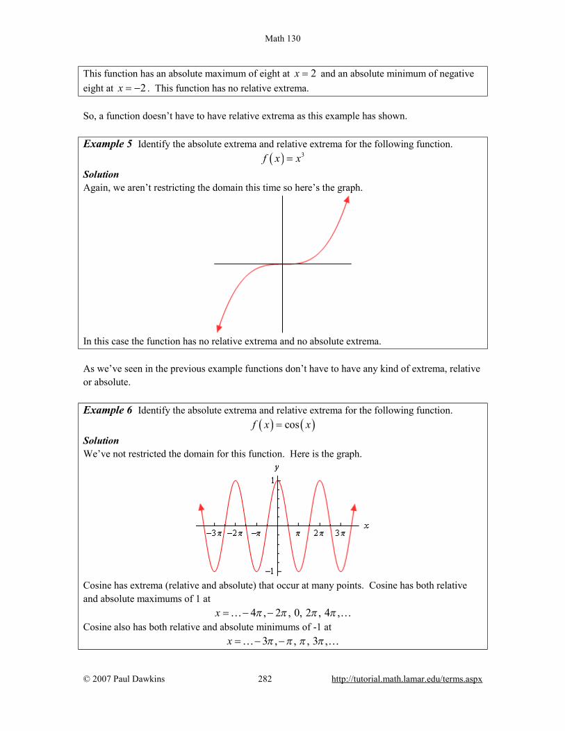
Math 130
© 2007 Paul Dawkins 282 http://tutorial.math.lamar.edu/terms.aspx
This function has an absolute maximum of eight at 2x = and an absolute minimum of negative eight at 2x = − . This function has no relative extrema. So, a function doesn’t have to have relative extrema as this example has shown. Example 5 Identify the absolute extrema and relative extrema for the following function. ( ) 3f x x= Solution Again, we aren’t restricting the domain this time so here’s the graph.
In this case the function has no relative extrema and no absolute extrema. As we’ve seen in the previous example functions don’t have to have any kind of extrema, relative or absolute. Example 6 Identify the absolute extrema and relative extrema for the following function. ( ) ( )cosf x x= Solution We’ve not restricted the domain for this function. Here is the graph.
Cosine has extrema (relative and absolute) that occur at many points. Cosine has both relative and absolute maximums of 1 at 4 , 2 , 0, 2 , 4 ,x π π π π= − −… … Cosine also has both relative and absolute minimums of -1 at 3 , , , 3 ,x π π π π= − −… …

Math 130
© 2007 Paul Dawkins 283 http://tutorial.math.lamar.edu/terms.aspx
As this example has shown a graph can in fact have extrema occurring at a large number (infinite in this case) of points. We’ve now worked quite a few examples and we can use these examples to see a nice fact about absolute extrema. First let’s notice that all the functions above were continuous functions. Next notice that every time we restricted the domain to a closed interval (i.e. the interval contains its end points) we got absolute maximums and absolute minimums. Finally, in only one of the three examples in which we did not restrict the domain did we get both an absolute maximum and an absolute minimum. These observations lead us the following theorem. Extreme Value Theorem Suppose that ( )f x is continuous on the interval [a,b] then there are two numbers ,a c d b≤ ≤ so
that ( )f c is an absolute maximum for the function and ( )f d is an absolute minimum for the
function. So, if we have a continuous function on an interval [a,b] then we are guaranteed to have both an absolute maximum and an absolute minimum for the function somewhere in the interval. The theorem doesn’t tell us where they will occur or if they will occur more than once, but at least it tells us that they do exist somewhere. Sometimes, all that we need to know is that they do exist. This theorem doesn’t say anything about absolute extrema if we aren’t working on an interval. We saw examples of functions above that had both absolute extrema, one absolute extrema, and no absolute extrema when we didn’t restrict ourselves down to an interval. The requirement that a function be continuous is also required in order for us to use the theorem. Consider the case of
( ) 2
1 on [ 1,1]f xx
= −
Here’s the graph.
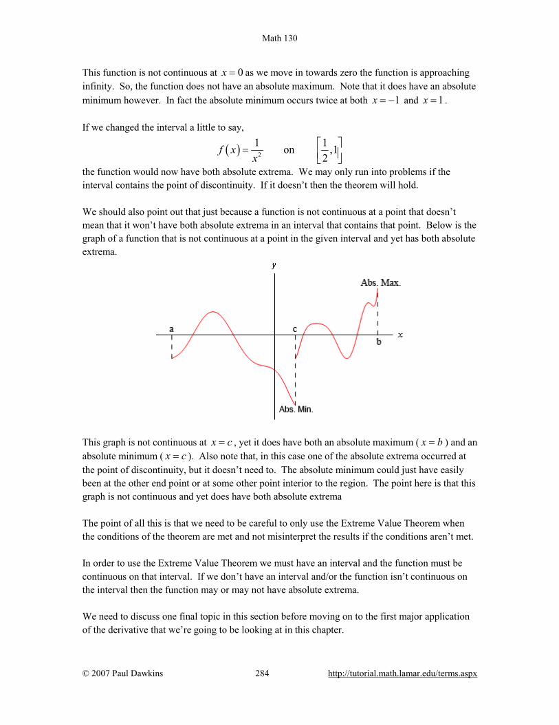
Math 130
© 2007 Paul Dawkins 284 http://tutorial.math.lamar.edu/terms.aspx
This function is not continuous at 0x = as we move in towards zero the function is approaching infinity. So, the function does not have an absolute maximum. Note that it does have an absolute minimum however. In fact the absolute minimum occurs twice at both 1x = − and 1x = . If we changed the interval a little to say,
( ) 2
1 1on ,12
f xx
=
the function would now have both absolute extrema. We may only run into problems if the interval contains the point of discontinuity. If it doesn’t then the theorem will hold. We should also point out that just because a function is not continuous at a point that doesn’t mean that it won’t have both absolute extrema in an interval that contains that point. Below is the graph of a function that is not continuous at a point in the given interval and yet has both absolute extrema.
This graph is not continuous at x c= , yet it does have both an absolute maximum ( x b= ) and an absolute minimum ( x c= ). Also note that, in this case one of the absolute extrema occurred at the point of discontinuity, but it doesn’t need to. The absolute minimum could just have easily been at the other end point or at some other point interior to the region. The point here is that this graph is not continuous and yet does have both absolute extrema The point of all this is that we need to be careful to only use the Extreme Value Theorem when the conditions of the theorem are met and not misinterpret the results if the conditions aren’t met. In order to use the Extreme Value Theorem we must have an interval and the function must be continuous on that interval. If we don’t have an interval and/or the function isn’t continuous on the interval then the function may or may not have absolute extrema. We need to discuss one final topic in this section before moving on to the first major application of the derivative that we’re going to be looking at in this chapter.

Math 130
© 2007 Paul Dawkins 285 http://tutorial.math.lamar.edu/terms.aspx
Fermat’s Theorem If ( )f x has a relative extrema at x c= and ( )f c′ exists then x c= is a critical point of
( )f x . In fact, it will be a critical point such that ( ) 0f c′ = .
Note that we can say that ( ) 0f c′ = because we are also assuming that ( )f c′ exists.
This theorem tells us that there is a nice relationship between relative extrema and critical points. In fact it will allow us to get a list of all possible relative extrema. Since a relative extrema must be a critical point the list of all critical points will give us a list of all possible relative extrema. Consider the case of ( ) 2f x x= . We saw that this function had a relative minimum at 0x = in
several earlier examples. So according to Fermat’s theorem 0x = should be a critical point. The derivative of the function is, ( ) 2f x x′ = Sure enough 0x = is a critical point. Be careful not to misuse this theorem. It doesn’t say that a critical point will be a relative extrema. To see this, consider the following case. ( ) ( )3 23f x x f x x′= = Clearly 0x = is a critical point. However we saw in an earlier example this function has no relative extrema of any kind. So, critical points do not have to be relative extrema. Also note that this theorem says nothing about absolute extrema. An absolute extrema may or may not be a critical point. To see the proof of this theorem see the Proofs From Derivative Applications section of the Extras chapter.
Math 130
© 2007 Paul Dawkins 286 http://tutorial.math.lamar.edu/terms.aspx
Finding Absolute Extrema It’s now time to see our first major application of derivatives in this chapter. Given a continuous function, f(x), on an interval [a,b] we want to determine the absolute extrema of the function. To do this we will need many of the ideas that we looked at in the previous section. First, since we have an interval and we are assuming that the function is continuous the Extreme Value Theorem tells us that we can in fact do this. This is a good thing of course. We don’t want to be trying to find something that may not exist. Next, we saw in the previous section that absolute extrema can occur at endpoints or at relative extrema. Also, from Fermat’s Theorem we know that the list of critical points is also a list of all possible relative extrema. So the endpoints along with the list of all critical points will in fact be a list of all possible absolute extrema. Now we just need to recall that the absolute extrema are nothing more than the largest and smallest values that a function will take so all that we really need to do is get a list of possible absolute extrema, plug these points into our function and then identify the largest and smallest values. Here is the procedure for finding absolute extrema. Finding Absolute Extrema of f(x) on [a,b].
0. Verify that the function is continuous on the interval [a,b]. 1. Find all critical points of f(x) that are in the interval [a,b]. This makes sense if you think
about it. Since we are only interested in what the function is doing in this interval we don’t care about critical points that fall outside the interval.
2. Evaluate the function at the critical points found in step 1 and the end points. 3. Identify the absolute extrema.
There really isn’t a whole lot to this procedure. We called the first step in the process step 0, mostly because all of the functions that we’re going to look at here are going to be continuous, but it is something that we do need to be careful with. This process will only work if we have a function that is continuous on the given interval. The most labor intensive step of this process is the second step (step 1) where we find the critical points. It is also important to note that all we want are the critical points that are in the interval. Let’s do some examples. Example 1 Determine the absolute extrema for the following function and interval. ( ) [ ]3 22 3 12 4 on 4, 2g t t t t= + − + − Solution All we really need to do here is follow the procedure given above. So, first notice that this is a polynomial and so in continuous everywhere and in particular is then continuous on the given

Math 130
© 2007 Paul Dawkins 287 http://tutorial.math.lamar.edu/terms.aspx
interval. Now, we need to get the derivative so that we can find the critical points of the function. ( ) ( ) ( )26 6 12 6 2 1g t t t t t′ = + − = + − It looks like we’ll have two critical points, 2t = − and 1t = . Note that we actually want something more than just the critical points. We only want the critical points of the function that lie in the interval in question. Both of these do fall in the interval as so we will use both of them. That may seem like a silly thing to mention at this point, but it is often forgotten, usually when it becomes important, and so we will mention it at every opportunity to make sure it’s not forgotten. Now we evaluate the function at the critical points and the end points of the interval.
( ) ( )( ) ( )
2 24 1 3
4 28 2 8
g g
g g
− = = −
− = − =
Absolute extrema are the largest and smallest the function will ever be and these four points represent the only places in the interval where the absolute extrema can occur. So, from this list we see that the absolute maximum of g(t) is 24 and it occurs at 2t = − (a critical point) and the absolute minimum of g(t) is -28 which occurs at 4t = − (an endpoint). In this example we saw that absolute extrema can and will occur at both endpoints and critical points. One of the biggest mistakes that students make with these problems is to forget to check the endpoints of the interval. Example 2 Determine the absolute extrema for the following function and interval. ( ) [ ]3 22 3 12 4 on 0,2g t t t t= + − + Solution Note that this problem is almost identical to the first problem. The only difference is the interval that we’re working on. This small change will completely change our answer however. With this change we have excluded both of the answers from the first example. The first step is to again find the critical points. From the first example we know these are
2t = − and 1t = .. At this point it’s important to recall that we only want the critical points that actually fall in the interval in question. This means that we only want 1t = since 2t = − falls outside the interval. Now evaluate the function at the single critical point in the interval and the two endpoints. ( ) ( ) ( )1 3 0 4 2 8g g g= − = = From this list of values we see that the absolute maximum is 8 and will occur at 2t = and the absolute minimum is -3 which occurs at 1t = .

Math 130
© 2007 Paul Dawkins 288 http://tutorial.math.lamar.edu/terms.aspx
As we saw in this example a simple change in the interval can completely change the answer. It also has shown us that we do need to be careful to exclude critical points that aren’t in the interval. Had we forgotten this and included 2t = − we would have gotten the wrong absolute maximum! This is the other big mistakes that students make in these problems. All too often they forget to exclude critical points that aren’t in the interval. If your instructor is anything like me this will mean that you will get the wrong answer. It’s not too hard to make sure that a critical point outside of the interval is larger or smaller than any of the points in the interval. Example 3 Suppose that the population (in thousands) of a certain kind of insect after t months is given by the following formula. ( ) ( )3 sin 4 100P t t t= + + Determine the minimum and maximum population in the first 4 months. Solution The question that we’re really asking is to find the absolute extrema of P(t) on the interval [0,4]. Since this function is continuous everywhere we know we can do this. Let’s start with the derivative. ( ) ( )3 4cos 4P t t′ = + We need the critical points of the function. The derivative exists everywhere so there are no critical points from that. So, all we need to do is determine where the derivative is zero.
( )
( )
3 4cos 4 03cos 44
t
t
+ =
= −
The solutions to this are,
0.6047 , 0, 1, 2,4 2.4189 2 , 0, 1, 2, 2
4 3.8643 2 , 0, 1, 2, 0.9661 , 0, 1, 2,2
nt nt n nt n n nt n
πππ π
= + = ± ±= + = ± ±⇒
= + = ± ±= + = ± ±
……… …
So, these are all the critical points. We need to determine the ones that fall in the interval [0,4]. There’s nothing to do except plug some n’s into the formulas until we get all of them.
0n = : 0.6047 0.9661t t= = We’ll need both of these critical points.
1n = :
Math 130
© 2007 Paul Dawkins 289 http://tutorial.math.lamar.edu/terms.aspx
0.6047 2.1755 0.9661 2.53692 2
t tπ π= + = = + =
We’ll need these.
2n = : 0.6047 3.7463 0.9661 4.1077t tπ π= + = = + = In this case we only need the first one since the second is out of the interval. There are five critical points that are in the interval. They are, 0.6047, 0.9661, 2.1755, 2.5369, 3.7463 Finally, to determine the absolute minimum and maximum population we only need to plug these values into the function as well as the two end points. Here are the function evaluations.
( ) ( )( ) ( )( ) ( )( )
0 100.0 4 111.7121
0.6047 102.4756 0.9661 102.2368
2.1755 107.1880 2.5369 106.9492
3.7463 111.9004
P P
P P
P P
P
= =
= =
= =
=
From these evaluations it appears that the minimum population is 100,000 (remember that P is in thousands…) which occurs at 0t = and the maximum population is 111,900 which occurs at
3.7463t = . Make sure that you can correctly solve trig equations. If we had forgotten the 2 nπ we would have missed the last three critical points in the interval and hence gotten the wrong answer since the maximum population was at the final critical point. Also, note that we do really need to be very careful with rounding answers here. If we’d rounded to the nearest integer, for instance, it would appear that the maximum population would have occurred at two different locations instead of only one. Example 4 Suppose that the amount of money in a bank account after t years is given by,
( )2
582000 10t
A t t−
= − e Determine the minimum and maximum amount of money in the account during the first 10 years that it is open. Solution Here we are really asking for the absolute extrema of A(t) on the interval [0,10]. As with the previous examples this function is continuous everywhere and so we know that this can be done. We’ll first need the derivative so we can find the critical points.
Math 130
© 2007 Paul Dawkins 290 http://tutorial.math.lamar.edu/terms.aspx
( )
2 2
2
5 58 8
258
10 104
10 14
t t
t
tA t t
t
− −
−
′ = − − −
= − +
e e
e
The derivative exists everywhere and the exponential is never zero. Therefore the derivative will only be zero where,
2
21 0 4 24t t t− + = ⇒ = ⇒ = ±
We’ve got two critical points, however only 2t = is actually in the interval so that is only critical point that we’ll use. Let’s now evaluate the function at the lone critical point and the end points of the interval. Here are those function evaluations. ( ) ( ) ( )0 2000 2 199.66 10 1999.94A A A= = = So, the maximum amount in the account will be $2000 which occurs at 0t = and the minimum amount in the account will be $199.66 which occurs at the 2 year mark. In this example there are two important things to note. First, if we had included the second critical point we would have gotten an incorrect answer for the maximum amount so it’s important to be careful with which critical points to include and which to exclude. All of the problems that we’ve worked to this point had derivatives that existed everywhere and so the only critical points that we looked at where those for which the derivative is zero. Do not get too locked into this always happening. Most of the problems that we run into will be like this, but they won’t all be like this. Let’s work another example to make this point. Example 5 Determine the absolute extrema for the following function and interval.
( ) ( ) [ ]233 4 on 5, 1Q y y y= + − −
Solution Again, as with all the other examples here, this function is continuous on the given interval and so we know that this can be done. First we’ll need the derivative and make sure you can do the simplification that we did here to make the work for finding the critical points easier.

Math 130
© 2007 Paul Dawkins 291 http://tutorial.math.lamar.edu/terms.aspx
( ) ( ) ( )
( )( )
( )( )
( )
2 13 3
23
13
13
13
23 4 3 43
23 44
3 4 2
45 12
4
Q y y y y
yyy
y y
yy
y
− ′ = + + +
= + ++
+ +=
+
+=
+
So, it looks like we’ve got two critical points.
4 Because the derivative doesn't exist here.12 Because the derivative is zero here.5
y
y
= −
= −
Both of these are in the interval so let’s evaluate the function at these points and the end points of the interval.
( )
( ) ( )
124 0 9.8495
5 15 1 6.241
Q Q
Q Q
− = − = −
− = − − = −
The function has an absolute maximum of zero at 4y = − and the function will have an absolute minimum of -15 at 5y = − . So, if we had ignored or forgotten about the critical point where the derivative doesn’t exist ( 4y = − ) we would not have gotten the correct answer. In this section we’ve seen how we can use a derivative to identify the absolute extrema of a function. This is an important application of derivatives that will arise from time to time so don’t forget about it.

Math 130
© 2007 Paul Dawkins 292 http://tutorial.math.lamar.edu/terms.aspx
The Shape of a Graph, Part I In the previous section we saw how to use the derivative to determine the absolute minimum and maximum values of a function. However, there is a lot more information about a graph that can be determined from the first derivative of a function. We will start looking at that information in this section. The main idea we’ll be looking at in this section we will be identifying all the relative extrema of a function. Let’s start this section off by revisiting a familiar topic from the previous chapter. Let’s suppose that we have a function, ( )f x . We know from our work in the previous chapter that the first
derivative, ( )f x′ , is the rate of change of the function. We used this idea to identify where a
function was increasing, decreasing or not changing. Before reviewing this idea let’s first write down the mathematical definition of increasing and decreasing. We all know what the graph of an increasing/decreasing function looks like but sometimes it is nice to have a mathematical definition as well. Here it is. Definition 1. Given any 1x and 2x from an interval I with 1 2x x< if ( ) ( )1 2f x f x< then ( )f x is
increasing on I. 2. Given any 1x and 2x from an interval I with 1 2x x< if ( ) ( )1 2f x f x> then ( )f x is
decreasing on I. This definition will actually be used in the proof of the next fact in this section. Now, recall that in the previous chapter we constantly used the idea that if the derivative of a function was positive at a point then the function was increasing at that point and if the derivative was negative at a point then the function was decreasing at that point. We also used the fact that if the derivative of a function was zero at a point then the function was not changing at that point. We used these ideas to identify the intervals in which a function is increasing and decreasing. The following fact summarizes up what we were doing in the previous chapter. Fact 1. If ( ) 0f x′ > for every x on some interval I, then ( )f x is increasing on the interval.
2. If ( ) 0f x′ < for every x on some interval I, then ( )f x is decreasing on the interval.
3. If ( ) 0f x′ = for every x on some interval I, then ( )f x is constant on the interval. The proof of this fact is in the Proofs From Derivative Applications section of the Extras chapter.

Math 130
© 2007 Paul Dawkins 293 http://tutorial.math.lamar.edu/terms.aspx
Let’s take a look at an example. This example has two purposes. First, it will remind us of the increasing/decreasing type of problems that we were doing in the previous chapter. Secondly, and maybe more importantly, it will now incorporate critical points into the solution. We didn’t know about critical points in the previous chapter, but if you go back and look at those examples, the first step in almost every increasing/decreasing problem is to find the critical points of the function. Example 1 Determine all intervals where the following function is increasing or decreasing.
( ) 5 4 35 40 52 3
f x x x x= − + + +
Solution To determine if the function is increasing or decreasing we will need the derivative.
( )( )( )( )
4 3 2
2 2
2
5 10 40
5 2 8
5 4 2
f x x x x
x x x
x x x
′ = − + +
= − − −
= − − +
Note that when we factored the derivative we first factored a “-1” out to make the rest of the factoring a little easier. From the factored form of the derivative we see that we have three critical points : 2x = − ,
0x = , and 4x = . We’ll need these in a bit. We now need to determine where the derivative is positive and where it’s negative. We’ve done this several times now in both the Review chapter and the previous chapter. Since the derivative is a polynomial it is continuous and so we know that the only way for it to change signs is to first go through zero. In other words, the only place that the derivative may change signs is at the critical points of the function. We’ve now got another use for critical points. So, we’ll build a number line, graph the critical points and pick test points from each region to see if the derivative is positive or negative in each region. Here is the number line and the test points for the derivative.
Math 130
© 2007 Paul Dawkins 294 http://tutorial.math.lamar.edu/terms.aspx
Make sure that you test your points in the derivative. One of the more common mistakes here is to test the points in the function instead! Recall that we know that the derivative will be the same sign in each region. The only place that the derivative can change signs is at the critical points and we’ve marked the only critical points on the number line. So, it looks we’ve got the following intervals of increase and decrease.
Increase : 2 0 and 0 4Decrease : 2 and 4
x xx x
− < < < <− ∞ < < − < < ∞
In this example we used the fact that the only place that a derivative can change sign is at the critical points. Also, the critical points for this function were those for which the derivative was zero. However, the same thing can be said for critical points where the derivative doesn’t exist. This is nice to know. A function can change signs where it is zero or doesn’t exist. In the previous chapter all our examples of this type had only critical points where the derivative was zero. Now, that we know more about critical points we’ll also see an example or two later on with critical points where the derivative doesn’t exist. Now that we have the previous “reminder” example out of the way let’s move into some new material. Once we have the intervals of increasing and decreasing for a function we can use this information to get a sketch of the graph. Note that the sketch, at this point, may not be super accurate when it comes to the curvature of the graph, but it will at least have the basic shape correct. To get the curvature of the graph correct we’ll need the information from the next section. Let’s attempt to get a sketch of the graph of the function we used in the previous example. Example 2 Sketch the graph of the following function.
( ) 5 4 35 40 52 3
f x x x x= − + + +
Solution There really isn’t a whole lot to this example. Whenever we sketch a graph it’s nice to have a few points on the graph to give us a starting place. So we’ll start by the function at the critical points. These will give us some starting points when we go to sketch the graph. These points are,
( ) ( ) ( )89 14232 29.67 0 5 4 474.333 3
f f f− = − = − = = =
Once these points are graphed we go to the increasing and decreasing information and start sketching. For reference purposes here is the increasing/decreasing information.
Increase : 2 0 and 0 4Decrease : 2 and 4
x xx x
− < < < <− ∞ < < − < < ∞
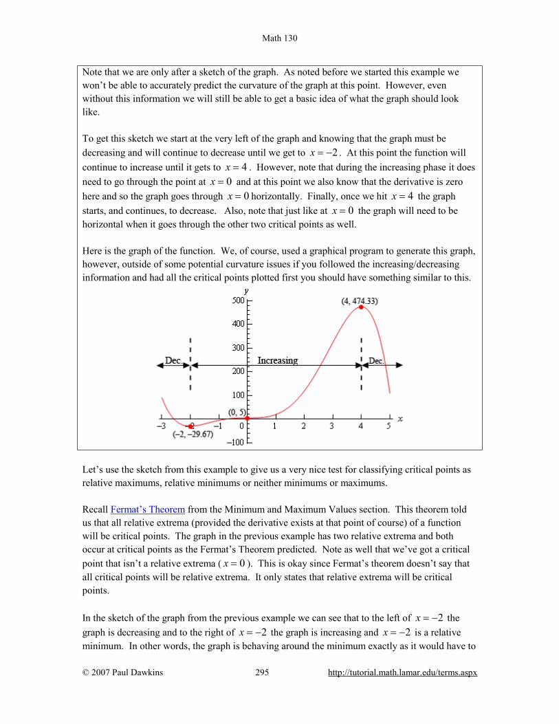
Math 130
© 2007 Paul Dawkins 295 http://tutorial.math.lamar.edu/terms.aspx
Note that we are only after a sketch of the graph. As noted before we started this example we won’t be able to accurately predict the curvature of the graph at this point. However, even without this information we will still be able to get a basic idea of what the graph should look like. To get this sketch we start at the very left of the graph and knowing that the graph must be decreasing and will continue to decrease until we get to 2x = − . At this point the function will continue to increase until it gets to 4x = . However, note that during the increasing phase it does need to go through the point at 0x = and at this point we also know that the derivative is zero here and so the graph goes through 0x = horizontally. Finally, once we hit 4x = the graph starts, and continues, to decrease. Also, note that just like at 0x = the graph will need to be horizontal when it goes through the other two critical points as well. Here is the graph of the function. We, of course, used a graphical program to generate this graph, however, outside of some potential curvature issues if you followed the increasing/decreasing information and had all the critical points plotted first you should have something similar to this.
Let’s use the sketch from this example to give us a very nice test for classifying critical points as relative maximums, relative minimums or neither minimums or maximums. Recall Fermat’s Theorem from the Minimum and Maximum Values section. This theorem told us that all relative extrema (provided the derivative exists at that point of course) of a function will be critical points. The graph in the previous example has two relative extrema and both occur at critical points as the Fermat’s Theorem predicted. Note as well that we’ve got a critical point that isn’t a relative extrema ( 0x = ). This is okay since Fermat’s theorem doesn’t say that all critical points will be relative extrema. It only states that relative extrema will be critical points. In the sketch of the graph from the previous example we can see that to the left of 2x = − the graph is decreasing and to the right of 2x = − the graph is increasing and 2x = − is a relative minimum. In other words, the graph is behaving around the minimum exactly as it would have to

Math 130
© 2007 Paul Dawkins 296 http://tutorial.math.lamar.edu/terms.aspx
be in order for 2x = − to be a minimum. The same thing can be said for the relative maximum at 4x = . The graph is increasing of the left and decreasing on the right exactly as it must be in
order for 4x = to be a maximum. Finally, the graph is increasing on both sides of 0x = and so this critical point can’t be a minimum or a maximum. These ideas can be generalized to arrive at a nice way to test if a critical point is a relative minimum, relative maximum or neither. If x c= is a critical point and the function is decreasing to the left of x c= and is increasing to the right then x c= must be a relative minimum of the function. Likewise, if the function is increasing to the left of x c= and decreasing to the right then x c= must be a relative maximum of the function. Finally, if the function is increasing on both sides of x c= or decreasing on both sides of x c= then x c= can be neither a relative minimum nor a relative maximum. These ideas can be summarized up in the following test. First Derivative Test Suppose that x c= is a critical point of ( )f x then,
1. If ( ) 0f x′ > to the left of x c= and ( ) 0f x′ < to the right of x c= then x c= is a relative
maximum. 2. If ( ) 0f x′ < to the left of x c= and ( ) 0f x′ > to the right of x c= then x c= is a relative
minimum. 3. If ( )f x′ is the same sign on both sides of x c= then x c= is neither a relative maximum
nor a relative minimum. It is important to note here that the first derivative test will only classify critical points as relative extrema and not as absolute extrema. As we recall from the Finding Absolute Extrema section absolute extrema are largest and smallest function values and may not even exist or be critical points if they do exist. The first derivative test is exactly that, a test using the first derivative. It doesn’t ever use the value of the function and so no conclusions can be drawn from the test about the relative “size” of the function at the critical points (which would be needed to identify absolute extrema) and can’t even begin to address the fact that absolute extrema may not occur at critical points. Let’s take at another example. Example 3 Find and classify all the critical points of the following function. Give the intervals where the function is increasing and decreasing.
( ) 3 2 4g t t t= −
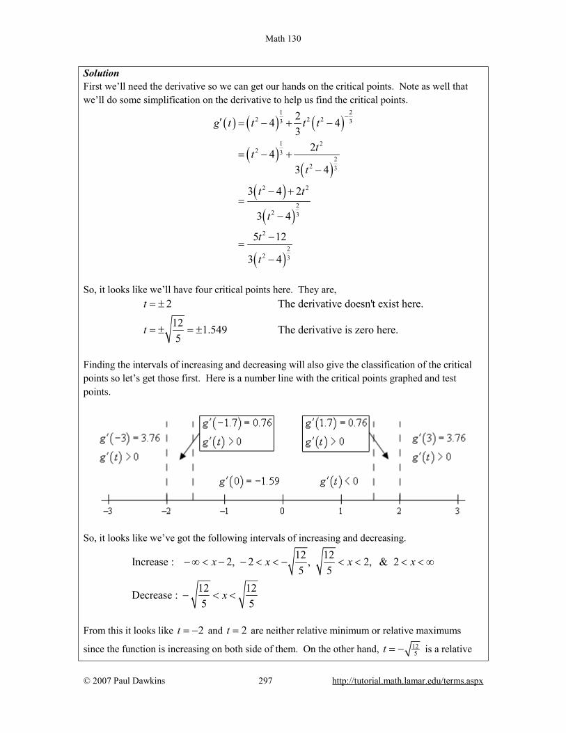
Math 130
© 2007 Paul Dawkins 297 http://tutorial.math.lamar.edu/terms.aspx
Solution First we’ll need the derivative so we can get our hands on the critical points. Note as well that we’ll do some simplification on the derivative to help us find the critical points.
( ) ( ) ( )
( )( )
( )( )
( )
1 22 2 23 3
1 22 3
22 3
2 2
22 3
2
22 3
24 43
243 4
3 4 2
3 4
5 12
3 4
g t t t t
ttt
t t
t
t
t
−′ = − + −
= − +−
− +=
−
−=
−
So, it looks like we’ll have four critical points here. They are,
2 The derivative doesn't exist here.
12 1.549 The derivative is zero here.5
t
t
= ±
= ± = ±
Finding the intervals of increasing and decreasing will also give the classification of the critical points so let’s get those first. Here is a number line with the critical points graphed and test points.
So, it looks like we’ve got the following intervals of increasing and decreasing.
12 12Increase : 2, 2 , 2, & 25 5
12 12Decrease : 5 5
x x x x
x
− ∞ < − − < < − < < < < ∞
− < <
From this it looks like 2t = − and 2t = are neither relative minimum or relative maximums
since the function is increasing on both side of them. On the other hand, 125t = − is a relative

Math 130
© 2007 Paul Dawkins 298 http://tutorial.math.lamar.edu/terms.aspx
maximum and 125t = is a relative minimum.
For completeness sake here is the graph of the function.
In the previous example the two critical points where the derivative didn’t exist ended up not being relative extrema. Do not read anything into this. They often will be relative extrema. Check out this example in the Absolute Extrema to see an example of one such critical point. Let’s work a couple more examples. Example 4 Suppose that the elevation above sea level of a road is given by the following function.
( ) 500 cos 3 sin4 4x xE x = + +
where x is in miles. Assume that if x is positive we are to the east of the initial point of measurement and if x is negative we are to the west of the initial point of measurement. If we start 25 miles to the west of the initial point of measurement and drive until we are 25 miles east of the initial point how many miles of our drive were we driving up an incline? Solution Okay, this is just a really fancy way of asking what the intervals of increasing and decreasing are for the function on the interval [-25,25]. So, we first need the derivative of the function.
( ) 1 3sin cos4 4 4 4
x xE x ′ = − +
Setting this equal to zero gives,

Math 130
© 2007 Paul Dawkins 299 http://tutorial.math.lamar.edu/terms.aspx
1 3sin cos 04 4 4 4
tan 34
x x
x
− + =
=
The solutions to this and hence the critical points are,
1.0472 2 , 0, 1, 2, 4.1888 8 , 0, 1, 2,4
16.7552 8 , 0, 1, 2,4.1888 2 , 0, 1, 2,4
x n n x n nx x n nn n
π ππ
π
= + = ± ± = + = ± ±⇒
= + = ± ±= + = ± ±
… ………
I’ll leave it to you to check that the critical points that fall in the interval that we’re after are, 20.9439, 8.3775, 4.1888, 16.7552− − Here is the number line with the critical points and test points.
So, it looks like the intervals of increasing and decreasing are,
Increase : 25 20.9439, 8.3775 4.1888 and 16.7552 25Decrease : 20.9439 8.3775 and 4.1888 16.7552
x x xx x
− < < − − < < < <− < < − < <
Notice that we had to end our intervals at -25 and 25 since we’ve done no work outside of these points and so we can’t really say anything about the function outside of the interval [-25,25]. From the intervals of we can actually answer the question. We were driving on an incline during the intervals of increasing and so the total number of miles is,
( )( ) ( )( ) ( )Distance 20.9439 25 4.1888 8.3775 25 16.7552
24.8652 miles
= − − − + − − + −
=
Even though the problem didn’t ask for it we can also classify the critical points that are in the interval [-25,25].
Relative Maximums : 20.9439, 4.1888Relative Minimums : 8.3775,16.7552
−−

Math 130
© 2007 Paul Dawkins 300 http://tutorial.math.lamar.edu/terms.aspx
Example 5 The population of rabbits (in hundreds) after t years in a certain area is given by the following function, ( ) ( )2 ln 3 6P t t t= + Determine if the population ever decreases in the first two years. Solution So, again we are really after the intervals and increasing and decreasing in the interval [0,2]. We found the only critical point to this function back in the Critical Points section to be,
1 0.2023
x = =e
Here is a number line for the intervals of increasing and decreasing.
So, it looks like the population will decrease for a short period and then continue to increase forever. Also, while the problem didn’t ask for it we can see that the single critical point is a relative minimum. In this section we’ve seen how we can use the first derivative of a function to give us some information about the shape of a graph and how we can use this information in some applications. Using the first derivative to give us information about a whether a function is increasing or decreasing is a very important application of derivatives and arises on a fairly regular basis in many areas.

Math 130
© 2007 Paul Dawkins 301 http://tutorial.math.lamar.edu/terms.aspx
The Shape of a Graph, Part II In the previous section we saw how we could use the first derivative of a function to get some information about the graph of a function. In this section we are going to look at the information that the second derivative of a function can give us a about the graph of a function. Before we do this we will need a couple of definitions out of the way. The main concept that we’ll be discussing in this section is concavity. Concavity is easiest to see with a graph (we’ll give the mathematical definition in a bit).
So a function is concave up if it “opens” up and the function is concave down if it “opens” down. Notice as well that concavity has nothing to do with increasing or decreasing. A function can be concave up and either increasing or decreasing. Similarly, a function can be concave down and either increasing or decreasing. It’s probably not the best way to define concavity by saying which way it “opens” since this is a somewhat nebulous definition. Here is the mathematical definition of concavity. Definition 1 Given the function ( )f x then
1. ( )f x is concave up on an interval I if all of the tangents to the curve on I are below the
graph of ( )f x .
2. ( )f x is concave down on an interval I if all of the tangents to the curve on I are above
the graph of ( )f x . To show that the graphs above do in fact have concavity claimed above here is the graph again (blown up a little to make things clearer).
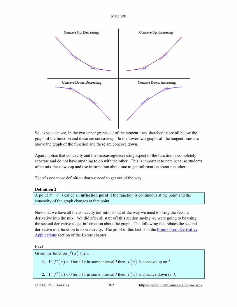
Math 130
© 2007 Paul Dawkins 302 http://tutorial.math.lamar.edu/terms.aspx
So, as you can see, in the two upper graphs all of the tangent lines sketched in are all below the graph of the function and these are concave up. In the lower two graphs all the tangent lines are above the graph of the function and these are concave down. Again, notice that concavity and the increasing/decreasing aspect of the function is completely separate and do not have anything to do with the other. This is important to note because students often mix these two up and use information about one to get information about the other. There’s one more definition that we need to get out of the way. Definition 2 A point x c= is called an inflection point if the function is continuous at the point and the concavity of the graph changes at that point. Now that we have all the concavity definitions out of the way we need to bring the second derivative into the mix. We did after all start off this section saying we were going to be using the second derivative to get information about the graph. The following fact relates the second derivative of a function to its concavity. The proof of this fact is in the Proofs From Derivative Applications section of the Extras chapter. Fact Given the function ( )f x then,
1. If ( ) 0f x′′ > for all x in some interval I then ( )f x is concave up on I.
2. If ( ) 0f x′′ < for all x in some interval I then ( )f x is concave down on I.
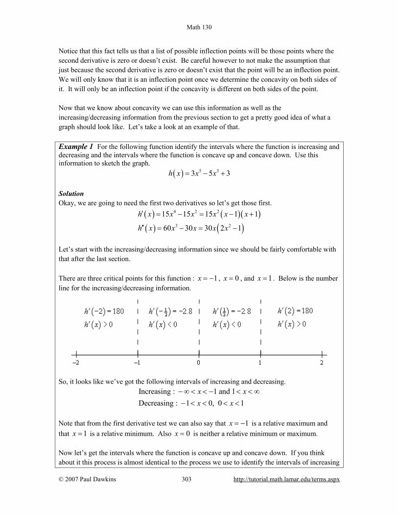
Math 130
© 2007 Paul Dawkins 303 http://tutorial.math.lamar.edu/terms.aspx
Notice that this fact tells us that a list of possible inflection points will be those points where the second derivative is zero or doesn’t exist. Be careful however to not make the assumption that just because the second derivative is zero or doesn’t exist that the point will be an inflection point. We will only know that it is an inflection point once we determine the concavity on both sides of it. It will only be an inflection point if the concavity is different on both sides of the point. Now that we know about concavity we can use this information as well as the increasing/decreasing information from the previous section to get a pretty good idea of what a graph should look like. Let’s take a look at an example of that. Example 1 For the following function identify the intervals where the function is increasing and decreasing and the intervals where the function is concave up and concave down. Use this information to sketch the graph. ( ) 5 33 5 3h x x x= − + Solution Okay, we are going to need the first two derivatives so let’s get those first.
( ) ( ) ( )( ) ( )
4 2 2
3 2
15 15 15 1 1
60 30 30 2 1
h x x x x x x
h x x x x x
′ = − = − +
′′ = − = −
Let’s start with the increasing/decreasing information since we should be fairly comfortable with that after the last section. There are three critical points for this function : 1x = − , 0x = , and 1x = . Below is the number line for the increasing/decreasing information.
So, it looks like we’ve got the following intervals of increasing and decreasing.
Increasing : 1 and 1Decreasing : 1 0, 0 1
x xx x
− ∞ < < − < < ∞− < < < <
Note that from the first derivative test we can also say that 1x = − is a relative maximum and that 1x = is a relative minimum. Also 0x = is neither a relative minimum or maximum. Now let’s get the intervals where the function is concave up and concave down. If you think about it this process is almost identical to the process we use to identify the intervals of increasing

Math 130
© 2007 Paul Dawkins 304 http://tutorial.math.lamar.edu/terms.aspx
and decreasing. This only difference is that we will be using the second derivative instead of the first derivative. The first thing that we need to do is identify the possible inflection points. These will be where the second derivative is zero or doesn’t exist. The second derivative in this case is a polynomial and so will exist everywhere. It will be zero at the following points.
10, 0.70712
x x= = ± = ±
As with the increasing and decreasing part we can draw a number line up and use these points to divide the number line into regions. In these regions we know that the second derivative will always have the same sign since these three points are the only places where the function may change sign. Therefore, all that we need to do is pick a point from each region and plug it into the second derivative. The second derivative will then have that sign in the whole region from which the point came from Here is the number line for this second derivative.
So, it looks like we’ve got the following intervals of concavity.
1 1Concave Up : 0 and 2 2
1 1Concave Down : and 02 2
x x
x x
− < < < < ∞
− ∞ < < − < <
This also means that
10, 0.70712
x x= = ± = ±
are all inflection points. All this information can be a little overwhelming when going to sketch the graph. The first thing that we should do is get some starting points. The critical points and inflection points are good starting points. So, first graph these points. Now, start to the left and start graphing the increasing/decreasing information as we did in the previous section when all we had was the increasing/decreasing information. As we graph this we will make sure that the concavity information matches up with what we’re graphing.

Math 130
© 2007 Paul Dawkins 305 http://tutorial.math.lamar.edu/terms.aspx
Using all this information to sketch the graph gives the following graph.
We can use the previous example to illustrate another way to classify some of the critical points of a function as relative maximums or relative minimums. Notice that 1x = − is a relative maximum and that the function is concave down at this point. This means that ( )1f ′′ − must be negative. Likewise, 1x = is a relative minimum and the
function is concave up at this point. This means that ( )1f ′′ must be positive.
As we’ll see in a bit we will need to be very careful with 0x = . In this case the second derivative is zero, but that will not actually mean that 0x = is not a relative minimum or maximum. We’ll see some examples of this in a bit, but we need to get some other information taken care of first. It is also important to note here that all of the critical points in this example were critical points in which the first derivative was zero and this is required for this to work. We will not be able to use this test on critical points where the derivative doesn’t exist. Here is the test that can be used to classify some of the critical points of a function. The proof of this test is in the Proofs From Derivative Applications section of the Extras chapter. Second Derivative Test Suppose that x c= is a critical point of ( )f c′ such that ( ) 0f c′ = and that ( )f x′′ is
continuous in a region around x c= . Then, 1. If ( ) 0f c′′ < then x c= is a relative maximum.
2. If ( ) 0f c′′ > then x c= is a relative minimum.
3. If ( ) 0f c′′ = then x c= can be a relative maximum, relative minimum or neither.

Math 130
© 2007 Paul Dawkins 306 http://tutorial.math.lamar.edu/terms.aspx
The third part of the second derivative test is important to notice. If the second derivative is zero then the critical point can be anything. Below are the graphs of three functions all of which have a critical point at 0x = , the second derivative of all of the functions is zero at 0x = and yet all three possibilities are exhibited. The first is the graph of ( ) 4f x x= . This graph has a relative minimum at 0x = .
Next is the graph of ( ) 4f x x= − which has a relative maximum at 0x = .
Finally, there is the graph of ( ) 3f x x= and this graph had neither a relative minimum or a
relative maximum at 0x = .

Math 130
© 2007 Paul Dawkins 307 http://tutorial.math.lamar.edu/terms.aspx
So, we can see that we have to be careful if we fall into the third case. For those times when we do fall into this case we will have to resort to other methods of classifying the critical point. This is usually done with the first derivative test. Let’s go back and relook at the critical points from the first example and use the Second Derivative Test on them, if possible. Example 2 Use the second derivative test to classify the critical points of the function, ( ) 5 33 5 3h x x x= − + Solution Note that all we’re doing here is verifying the results from the first example. The second derivative is, ( ) 360 30h x x x′′ = − The three critical points ( 1x = − , 0x = , and 1x = ) of this function are all critical points where the first derivative is zero so we know that we at least have a chance that the Second Derivative Test will work. The value of the second derivative for each of these are, ( ) ( ) ( )1 30 0 0 1 30h h h′′ ′′ ′′− = − = = The second derivative at 1x = − is negative so by the Second Derivative Test this critical point this is a relative maximum as we saw in the first example. The second derivative at 1x = is positive and so we have a relative minimum here by the Second Derivative Test as we also saw in the first example. In the case of 0x = the second derivative is zero and so we can’t use the Second Derivative Test to classify this critical point. Note however, that we do know from the First Derivative Test we used in the first example that in this case the critical point is not a relative extrema.
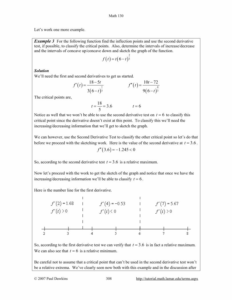
Math 130
© 2007 Paul Dawkins 308 http://tutorial.math.lamar.edu/terms.aspx
Let’s work one more example. Example 3 For the following function find the inflection points and use the second derivative test, if possible, to classify the critical points. Also, determine the intervals of increase/decrease and the intervals of concave up/concave down and sketch the graph of the function.
( ) ( )236f t t t= −
Solution We’ll need the first and second derivatives to get us started.
( )( )
( )( )
1 43 3
18 5 10 72
3 6 9 6
t tf t f tt t
− −′ ′′= =− −
The critical points are,
18 3.6 65
t t= = =
Notice as well that we won’t be able to use the second derivative test on 6t = to classify this critical point since the derivative doesn’t exist at this point. To classify this we’ll need the increasing/decreasing information that we’ll get to sketch the graph. We can however, use the Second Derivative Test to classify the other critical point so let’s do that before we proceed with the sketching work. Here is the value of the second derivative at 3.6t = . ( )3.6 1.245 0f ′′ = − < So, according to the second derivative test 3.6t = is a relative maximum. Now let’s proceed with the work to get the sketch of the graph and notice that once we have the increasing/decreasing information we’ll be able to classify 6t = . Here is the number line for the first derivative.
So, according to the first derivative test we can verify that 3.6t = is in fact a relative maximum. We can also see that 6t = is a relative minimum. Be careful not to assume that a critical point that can’t be used in the second derivative test won’t be a relative extrema. We’ve clearly seen now both with this example and in the discussion after
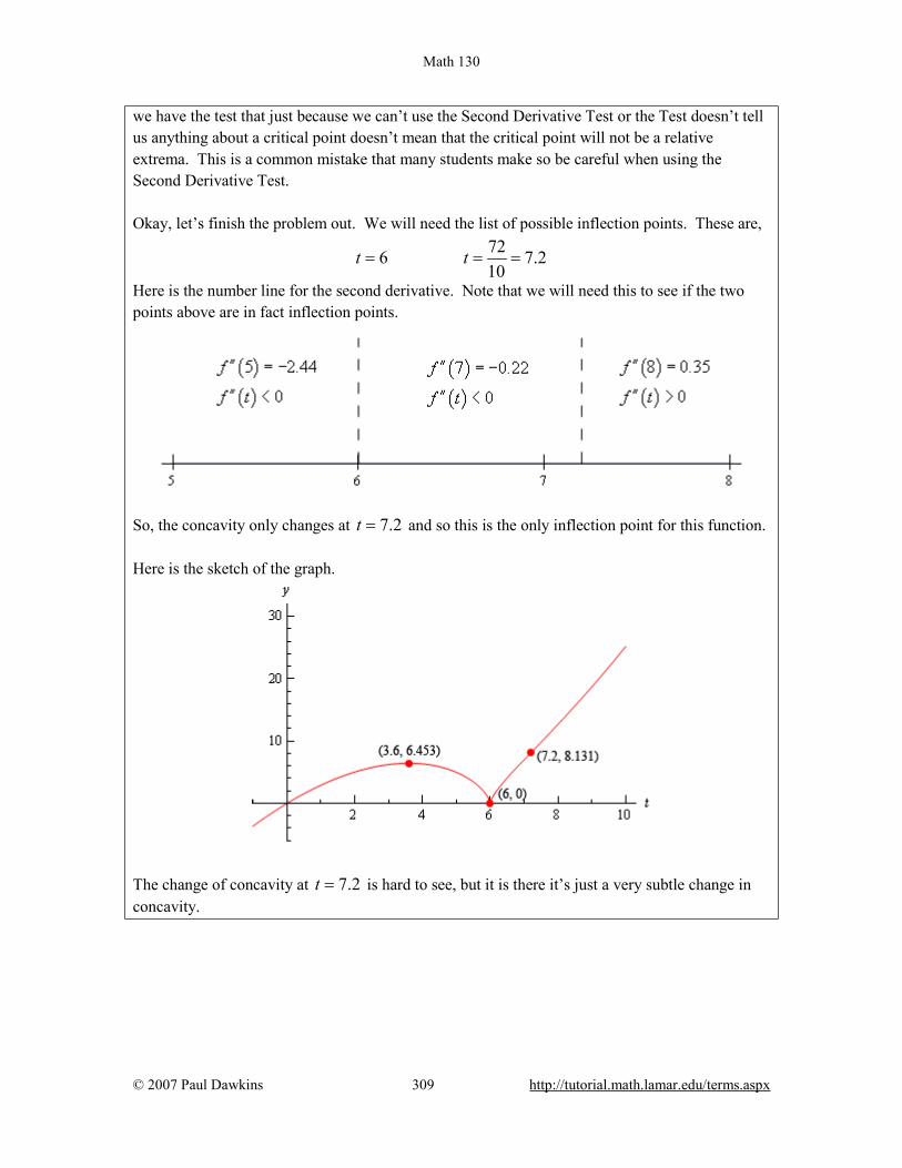
Math 130
© 2007 Paul Dawkins 309 http://tutorial.math.lamar.edu/terms.aspx
we have the test that just because we can’t use the Second Derivative Test or the Test doesn’t tell us anything about a critical point doesn’t mean that the critical point will not be a relative extrema. This is a common mistake that many students make so be careful when using the Second Derivative Test. Okay, let’s finish the problem out. We will need the list of possible inflection points. These are,
726 7.210
t t= = =
Here is the number line for the second derivative. Note that we will need this to see if the two points above are in fact inflection points.
So, the concavity only changes at 7.2t = and so this is the only inflection point for this function. Here is the sketch of the graph.
The change of concavity at 7.2t = is hard to see, but it is there it’s just a very subtle change in concavity.
Math 130
© 2007 Paul Dawkins 310 http://tutorial.math.lamar.edu/terms.aspx
The Mean Value Theorem In this section we want to take a look at the Mean Value Theorem. In most traditional textbooks this section comes before the sections containing the First and Second Derivative Tests because many of the proofs in those sections need the Mean Value Theorem. However, we feel that from a logical point of view it’s better to put the Shape of a Graph sections right after the absolute extrema section. So, if you’ve been following the proofs from the previous two sections you’ve probably already read through this section. Before we get to the Mean Value Theorem we need to cover the following theorem. Rolle’s Theorem Suppose ( )f x is a function that satisfies all of the following.
1. ( )f x is continuous on the closed interval [a,b].
2. ( )f x is differentiable on the open interval (a,b).
3. ( ) ( )f a f b=
Then there is a number c such that a c b< < and ( ) 0f c′ = . Or, in other words ( )f x has a
critical point in (a,b). To see the proof of Rolle’s Theorem see the Proofs From Derivative Applications section of the Extras chapter. Let’s take a look at a quick example that uses Rolle’s Theorem. Example 1 Show that ( ) 5 34 7 2f x x x x= + + − has exactly one real root. Solution From basic Algebra principles we know that since ( )f x is a 5th degree polynomial it will have
five roots. What we’re being asked to prove here is that only one of those 5 is a real number and the other 4 must be complex roots. First, we should show that it does have at least one real root. To do this note that ( )0 2f = − and
that ( )1 10f = and so we can see that ( ) ( )0 0 1f f< < . Now, because ( )f x is a polynomial
we know that it is continuous everywhere and so by the Intermediate Value Theorem there is a number c such that 0 1c< < and ( ) 0f c = . In other words ( )f x has at least one real root.
We now need to show that this is in fact the only real root. To do this we’ll use an argument that
Math 130
© 2007 Paul Dawkins 311 http://tutorial.math.lamar.edu/terms.aspx
is called contradiction proof. What we’ll do is assume that ( )f x has at least two real roots.
This means that we can find real numbers a and b (there might be more, but all we need for this particular argument is two) such that ( ) ( ) 0f a f b= = . But if we do this then we know from
Rolle’s Theorem that there must then be another number c such that ( ) 0f c′ = .
This is a problem however. The derivative of this function is, ( ) 4 220 3 7f x x x′ = + +
Because the exponents on the first two terms are even we know that the first two terms will always be greater than or equal to zero and we are then going to add a positive number onto that and so we can see that the smallest the derivative will ever be is 7 and this contradicts the statement above that says we MUST have a number c such that ( ) 0f c′ = .
We reached these contradictory statements by assuming that ( )f x has at least two roots. Since
this assumption leads to a contradiction the assumption must be false and so we can only have a single real root. The reason for covering Rolle’s Theorem is that it is needed in the proof of the Mean Value Theorem. To see the proof see the Proofs From Derivative Applications section of the Extras chapter. Here is the theorem. Mean Value Theorem Suppose ( )f x is a function that satisfies both of the following.
1. ( )f x is continuous on the closed interval [a,b].
2. ( )f x is differentiable on the open interval (a,b). Then there is a number c such that a < c < b and
( ) ( ) ( )f b f af c
b a−
′ =−
Or, ( ) ( ) ( )( )f b f a f c b a′− = − Note that the Mean Value Theorem doesn’t tell us what c is. It only tells us that there is at least one number c that will satisfy the conclusion of the theorem. Also note that if it weren’t for the fact that we needed Rolle’s Theorem to prove this we could think of Rolle’s Theorem as a special case of the Mean Value Theorem. To see that just assume that ( ) ( )f a f b= and then the result of the Mean Value Theorem gives the result of Rolle’s
Theorem.

Math 130
© 2007 Paul Dawkins 312 http://tutorial.math.lamar.edu/terms.aspx
Before we take a look at a couple of examples let’s think about a geometric interpretation of the Mean Value Theorem. First define ( )( ),A a f a= and ( )( ),B b f b= and then we know from
the Mean Value theorem that there is a c such that a c b< < and that
( ) ( ) ( )f b f af c
b a−
′ =−
Now, if we draw in the secant line connecting A and B then we can know that the slope of the secant line is,
( ) ( )f b f ab a
−−
Likewise, if we draw in the tangent line to ( )f x at x c= we know that its slope is ( )f c′ .
What the Mean Value Theorem tells us is that these two slopes must be equal or in other words the secant line connecting A and B and the tangent line at x c= must be parallel. We can see this in the following sketch.
Let’s now take a look at a couple of examples using the Mean Value Theorem. Example 2 Determine all the numbers c which satisfy the conclusions of the Mean Value Theorem for the following function. ( ) [ ]3 22 on 1,2f x x x x= + − − Solution There isn’t really a whole lot to this problem other than to notice that since ( )f x is a polynomial
it is both continuous and differentiable (i.e. the derivative exists) on the interval given. First let’s find the derivative.

Math 130
© 2007 Paul Dawkins 313 http://tutorial.math.lamar.edu/terms.aspx
( ) 23 4 1f x x x′ = + − Now, to find the numbers that satisfy the conclusions of the Mean Value Theorem all we need to do is plug this into the formula given by the Mean Value Theorem.
( ) ( ) ( )
( )2
2 12 1
14 2 123 4 1 43 3
f ff c
c c
− −′ =
− −
−+ − = = =
Now, this is just a quadratic equation,
2
2
3 4 1 43 4 5 0c cc c
+ − =
+ − =
Using the quadratic formula on this we get,
( )( )4 16 4 3 5 4 76
6 6c
− ± − − − ±= =
So, solving gives two values of c.
4 76 4 760.7863 2.11966 6
c c− + − −= = = = −
Notice that only one of these is actually in the interval given in the problem. That means that we will exclude the second one (since it isn’t in the interval). The number that we’re after in this problem is, 0.7863c = Be careful to not assume that only one of the numbers will work. It is possible for both of them to work. Example 3 Suppose that we know that ( )f x is continuous and differentiable on [6, 15]. Let’s
also suppose that we know that ( )6 2f = − and that we know that ( ) 10f x′ ≤ . What is the
largest possible value for ( )15f ? Solution Let’s start with the conclusion of the Mean Value Theorem. ( ) ( ) ( )( )15 6 15 6f f f c′− = − Plugging in for the known quantities and rewriting this a little gives, ( ) ( ) ( ) ( ) ( )15 6 15 6 2 9f f f c f c′ ′= + − = − +
Math 130
© 2007 Paul Dawkins 314 http://tutorial.math.lamar.edu/terms.aspx
Now we know that ( ) 10f x′ ≤ so in particular we know that ( ) 10f c′ ≤ . This gives us the
following,
( ) ( )
( )15 2 9
2 9 1088
f f c′= − +
≤ − +
=
All we did was replace ( )f c′ with its largest possible value.
This means that the largest possible value for ( )15f is 88.
Example 4 Suppose that we know that ( )f x is continuous and differentiable everywhere.
Let’s also suppose that we know that ( )f x has two roots. Show that ( )f x′ must have at least one root. Solution It is important to note here that all we can say is that ( )f x′ will have at least one root. We can’t
say that it will have exactly one root. So don’t confuse this problem with the first one we worked. This is actually a fairly simple thing to prove. Since we know that ( )f x has two roots let’s
suppose that they are a and b. Now, by assumption we know that ( )f x is continuous and
differentiable everywhere and so in particular it is continuous on [a,b] and differentiable on (a,b). Therefore, by the Mean Value Theorem there is a number c that is between a and b (this isn’t needed for this problem, but it’s true so it should be pointed out) and that,
( ) ( ) ( )f b f af c
b a−
′ =−
But we now need to recall that a and b are roots of ( )f x and so this is,
( ) 0 0 0f cb a
−′ = =−
Or, ( )f x′ has a root at x c= .
Again, it is important to note that we don’t have a value of c. We have only shown that it exists. We also haven’t said anything about c being the only root. It is completely possible for ( )f x′ to
have more than one root.

Math 130
© 2007 Paul Dawkins 315 http://tutorial.math.lamar.edu/terms.aspx
It is completely possible to generalize the previous example significantly. For instance if we know that ( )f x is continuous and differentiable everywhere and has three roots we can then
show that not only will ( )f x′ have at least two roots but that ( )f x′′ will have at least one root.
We’ll leave it to you to verify this, but the ideas involved are identical to those in the previous example. We’ll close this section out with a couple of nice facts that can be proved using the Mean Value Theorem. Note that in both of these facts we are assuming the functions are continuous and differentiable on the interval [a,b]. Fact 1 If ( ) 0f x′ = for all x in an interval ( ),a b then ( )f x is constant on ( ),a b .
This fact is very easy to prove so let’s do that here. Take any two x’s in the interval ( ),a b , say
1x and 2x . Then since ( )f x is continuous and differential on [a,b] it must also be continuous
and differentiable on [ ]1 2,x x . This means that we can apply the Mean Value Theorem for these
two values of x. Doing this gives, ( ) ( ) ( )( )2 1 2 1f x f x f c x x′− = −
where 1 2x c x< < . But by assumption ( ) 0f x′ = for all x in an interval ( ),a b and so in
particular we must have, ( ) 0f c′ = Putting this into the equation above gives, ( ) ( ) ( ) ( )2 1 2 10f x f x f x f x− = ⇒ = Now, since 1x and 2x where any two values of x in the interval ( ),a b we can see that we must
have ( ) ( )2 1f x f x= for all 1x and 2x in the interval and this is exactly what it means for a
function to be constant on the interval and so we’ve proven the fact. Fact 2 If ( ) ( )f x g x′ ′= for all x in an interval ( ),a b then in this interval we have ( ) ( )f x g x c= +
where c is some constant. This fact is a direct result of the previous fact and is also easy to prove. If we first define,
Math 130
© 2007 Paul Dawkins 316 http://tutorial.math.lamar.edu/terms.aspx
( ) ( ) ( )h x f x g x= −
Then since both ( )f x and ( )g x are continuous and differentiable in the interval ( ),a b then so
must be ( )h x . Therefore the derivative of ( )h x is,
( ) ( ) ( )h x f x g x′ ′ ′= − However, by assumption ( ) ( )f x g x′ ′= for all x in an interval ( ),a b and so we must have that
( ) 0h x′ = for all x in an interval ( ),a b . So, by Fact 1 ( )h x must be constant on the interval.
This means that we have,
( )
( ) ( )( ) ( )
h x c
f x g x c
f x g x c
=
− =
= +
which is what we were trying to show.
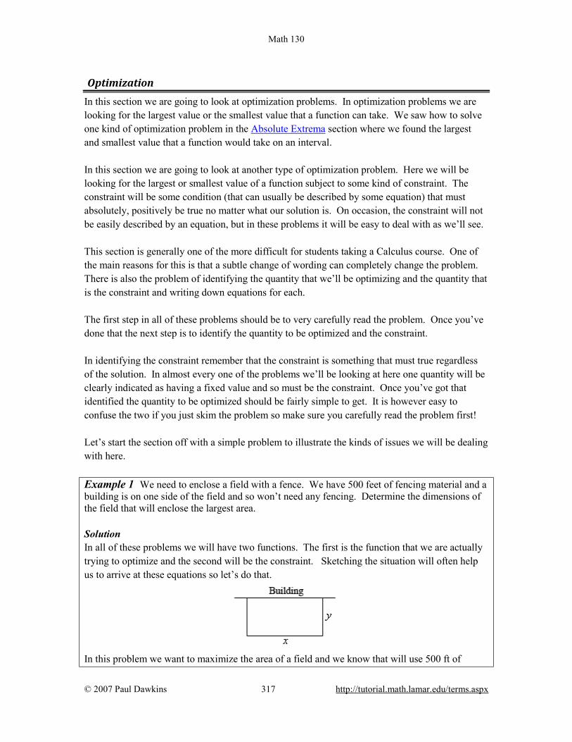
Math 130
© 2007 Paul Dawkins 317 http://tutorial.math.lamar.edu/terms.aspx
Optimization In this section we are going to look at optimization problems. In optimization problems we are looking for the largest value or the smallest value that a function can take. We saw how to solve one kind of optimization problem in the Absolute Extrema section where we found the largest and smallest value that a function would take on an interval. In this section we are going to look at another type of optimization problem. Here we will be looking for the largest or smallest value of a function subject to some kind of constraint. The constraint will be some condition (that can usually be described by some equation) that must absolutely, positively be true no matter what our solution is. On occasion, the constraint will not be easily described by an equation, but in these problems it will be easy to deal with as we’ll see. This section is generally one of the more difficult for students taking a Calculus course. One of the main reasons for this is that a subtle change of wording can completely change the problem. There is also the problem of identifying the quantity that we’ll be optimizing and the quantity that is the constraint and writing down equations for each. The first step in all of these problems should be to very carefully read the problem. Once you’ve done that the next step is to identify the quantity to be optimized and the constraint. In identifying the constraint remember that the constraint is something that must true regardless of the solution. In almost every one of the problems we’ll be looking at here one quantity will be clearly indicated as having a fixed value and so must be the constraint. Once you’ve got that identified the quantity to be optimized should be fairly simple to get. It is however easy to confuse the two if you just skim the problem so make sure you carefully read the problem first! Let’s start the section off with a simple problem to illustrate the kinds of issues we will be dealing with here. Example 1 We need to enclose a field with a fence. We have 500 feet of fencing material and a building is on one side of the field and so won’t need any fencing. Determine the dimensions of the field that will enclose the largest area. Solution In all of these problems we will have two functions. The first is the function that we are actually trying to optimize and the second will be the constraint. Sketching the situation will often help us to arrive at these equations so let’s do that.
In this problem we want to maximize the area of a field and we know that will use 500 ft of

Math 130
© 2007 Paul Dawkins 318 http://tutorial.math.lamar.edu/terms.aspx
fencing material. So, the area will be the function we are trying to optimize and the amount of fencing is the constraint. The two equations for these are,
Maximize : Contraint : 500 2
A xyx y
== +
Okay, we know how to find the largest or smallest value of a function provided it’s only got a single variable. The area function (as well as the constraint) has two variables in it and so what we know about finding absolute extrema won’t work. However, if we solve the constraint for one of the two variables we can substitute this into the area and we will then have a function of a single variable. So, let’s solve the constraint for x. Note that we could have just as easily solved for y but that would have led to fractions and so, in this case, solving for x will probably be best. 500 2x y= − Substituting this into the area function gives a function of y. ( ) ( ) 2500 2 500 2A y y y y y= − = − Now we want to find the largest value this will have on the interval [0,250]. Note that the interval corresponds to taking 0y = (i.e. no sides to the fence) and 250y = (i.e. only two sides and no width, also if there are two sides each must be 250 ft to use the whole 500ft). Note that the endpoints of the interval won’t make any sense from a physical standpoint if we actually want to enclose some area because they would both give zero area. They do, however, give us a set of limits on y and so the Extreme Value Theorem tells us that we will have a maximum value of the area somewhere between the two endpoints. Having these limits will also mean that we can use the process we discussed in the Finding Absolute Extrema section earlier in the chapter to find the maximum value of the area. So, recall that the maximum value of a continuous function (which we’ve got here) on a closed interval (which we also have here) will occur at critical points and/or end points. As we’ve already pointed out the end points in this case will give zero area and so don’t make any sense. That means our only option will be the critical points. So let’s get the derivative and find the critical points. ( ) 500 4A y y′ = − Setting this equal to zero and solving gives a lone critical point of 125y = . Plugging this into the area gives an area of 31250 ft2. So according to the method from Absolute Extrema section this must be the largest possible area, since the area at either endpoint is zero.

Math 130
© 2007 Paul Dawkins 319 http://tutorial.math.lamar.edu/terms.aspx
Finally, let’s not forget to get the value of x and then we’ll have the dimensions since this is what the problem statement asked for. We can get the x by plugging in our y into the constraint. ( )500 2 125 250x = − = The dimensions of the field that will give the largest area, subject to the fact that we used exactly 500 ft of fencing material, are 250 x 125. Don’t forget to actually read the problem and give the answer that was asked for. These types of problems can take a fair amount of time/effort to solve and it’s not hard to sometimes forget what the problem was actually asking for. In the previous problem we used the method from the Finding Absolute Extrema section to find the maximum value of the function we wanted to optimize. However, as we’ll see in later examples we won’t always have easy to find endpoints and/or dealing with the endpoints may not be easy to deal with. Not only that, but this method requires that the function we’re optimizing be continuous on the interval we’re looking at, including the endpoints, and that may not always be the case. So, before proceeding with the anymore examples let’s spend a little time discussing some methods for determining if our solution is in fact the absolute minimum/maximum value that we’re looking for. In some examples all of these will work while in others one or more won’t be all that useful. However, we will always need to use some method for making sure that our answer is in fact that optimal value that we’re after. Method 1 : Use the method used in Finding Absolute Extrema. This is the method used in the first example above. Recall that in order to use this method the range of possible optimal values, let’s call it I, must have finite endpoints. Also, the function we’re optimizing (once it’s down to a single variable) must be continuous on I, including the endpoints. If these conditions are met then we know that the optimal value, either the maximum or minimum depending on the problem, will occur at either the endpoints of the range or at a critical point that is inside the range of possible solutions. There are two main issues that will often prevent this method from being used however. First, not every problem will actually have a range of possible solutions that have finite endpoints at both ends. We’ll see at least one example of this as we work through the remaining examples. Also, many of the functions we’ll be optimizing will not be continuous once we reduce them down to a single variable and this will prevent us from using this method. Method 2 : Use a variant of the First Derivative Test. In this method we also will need a range of possible optimal values, I. However, in this case, unlike the previous method the endpoints do not need to be finite. Also, we will need to require that the function be continuous on the interior I and we will only need the function to be

Math 130
© 2007 Paul Dawkins 320 http://tutorial.math.lamar.edu/terms.aspx
continuous at the end points if the endpoint is finite and the function actually exists at the endpoint. We’ll see several problems where the function we’re optimizing doesn’t actually exist at one of the endpoints. This will not prevent this method from being used. Let’s suppose that x c= is a critical point of the function we’re trying to optimize, ( )f x . We
already know from the First Derivative Test that if ( ) 0f x′ > immediately to the left of x c=
(i.e. the function is increasing immediately to the left) and if ( ) 0f x′ < immediately to the right
of x c= (i.e. the function is decreasing immediately to the right) then x c= will be a relative maximum for ( )f x .
Now, this does not mean that the absolute maximum of ( )f x will occur at x c= . However,
suppose that we knew a little bit more information. Suppose that in fact we knew that ( ) 0f x′ >
for all x in I such that x c< . Likewise, suppose that we knew that ( ) 0f x′ < for all x in I such
that x c> . In this case we know that to the left of x c= , provided we stay in I of course, the function is always increasing and to the right of x c= , again staying in I, we are always decreasing. In this case we can say that the absolute maximum of ( )f x in I will occur at x c= .
Similarly, if we know that to the left of x c= the function is always decreasing and to the right of x c= the function is always increasing then the absolute minimum of ( )f x in I will occur at
x c= . Before we give a summary of this method let’s discuss the continuity requirement a little. Nowhere in the above discussion did the continuity requirement apparently come into play. We require that that the function we’re optimizing to be continuous in I to prevent the following situation.

Math 130
© 2007 Paul Dawkins 321 http://tutorial.math.lamar.edu/terms.aspx
In this case, a relative maximum of the function clearly occurs at x c= . Also, the function is always decreasing to the right and is always increasing to the left. However, because of the discontinuity at x d= , we can clearly see that ( ) ( )f d f c> and so the absolute maximum of
the function does not occur at x c= . Had the discontinuity at x d= not been there this would not have happened and the absolute maximum would have occurred at x c= . Here is a summary of this method. First Derivative Test for Absolute Extrema Let I be the interval of all possible optimal values of ( )f x and further suppose that ( )f x is
continuous on I , except possibly at the endpoints. Finally suppose that x c= is a critical point of ( )f x and that c is in the interval I. If we restrict x to values from I (i.e. we only consider
possible optimal values of the function) then,
1. If ( ) 0f x′ > for all x c< and if ( ) 0f x′ < for all x c> then ( )f c will be the
absolute maximum value of ( )f x on the interval I.
2. If ( ) 0f x′ < for all x c< and if ( ) 0f x′ > for all x c> then ( )f c will be the
absolute minimum value of ( )f x on the interval I. Method 3 : Use the second derivative. There are actually two ways to use the second derivative to help us identify the optimal value of a function and both use the Second Derivative Test to one extent or another. The first way to use the second derivative doesn’t actually help us to identify the optimal value. What it does do is allow us to potentially exclude values and knowing this can simplify our work somewhat and so is not a bad thing to do. Suppose that we are looking for the absolute maximum of a function and after finding the critical points we find that we have multiple critical points. Let’s also suppose that we run all of them through the second derivative test and determine that some of them are in fact relative minimums of the function. Since we are after the absolute maximum we know that a maximum (of any kind) can’t occur at relative minimums and so we immediately know that we can exclude these points from further consideration. We could do a similar check if we were looking for the absolute minimum. Doing this may not seem like all that great of a thing to do, but it can, on occasion, lead to a nice reduction in the amount of work that we need to do in later steps. The second of way using the second derivative can be used to identify the optimal value of a function and in fact is very similar to the second method above. In fact we will have the same requirements for this method as we did in that method. We need an interval of possible optimal
Math 130
© 2007 Paul Dawkins 322 http://tutorial.math.lamar.edu/terms.aspx
values, I and the endpoint(s) may or may not be finite. We’ll also need to require that the function, ( )f x be continuous everywhere in I except possibly at the endpoints as above.
Now, suppose that x c= is a critical point and that ( ) 0f c′′ > . The second derivative test tells
us that x c= must be a relative minimum of the function. Suppose however that we also knew that ( ) 0f x′′ > for all x in I. In this case we would know that the function was concave up in all
of I and that would in turn mean that the absolute minimum of ( )f x in I would in fact have to
be at x c= . Likewise if x c= is a critical point and ( ) 0f x′′ < for all x in I then we would know that the
function was concave down in I and that the absolute maximum of ( )f x in I would have to be
at x c= . Here is a summary of this method. Second Derivative Test for Absolute Extrema Let I be the range of all possible optimal values of ( )f x and further suppose that ( )f x is
continuous on I , except possibly at the endpoints. Finally suppose that x c= is a critical point of ( )f x and that c is in the interval I. Then,
1. If ( ) 0f x′′ > for all x in I then ( )f c will be the absolute minimum value of ( )f x on
the interval I. 2. If ( ) 0f x′′ < for all x in I then ( )f c will be the absolute maximum value of ( )f x on
the interval I. Before proceeding with some more examples we need to once again acknowledge that not every method discussed above will work for every problem and that, in some problems, more than one method will work. There are also problems were we may need to use a combination of these methods to identify the optimal value. Each problem will be different and we’ll need to see what we’ve got once we get the critical points before we decide which method might be best to use. Okay, let’s work some more examples. Example 2 We want to construct a box whose base length is 3 times the base width. The material used to build the top and bottom cost $10/ft2 and the material used to build the sides cost $6/ft2. If the box must have a volume of 50ft3 determine the dimensions that will minimize the cost to build the box. Solution First, a quick figure (probably not to scale…).
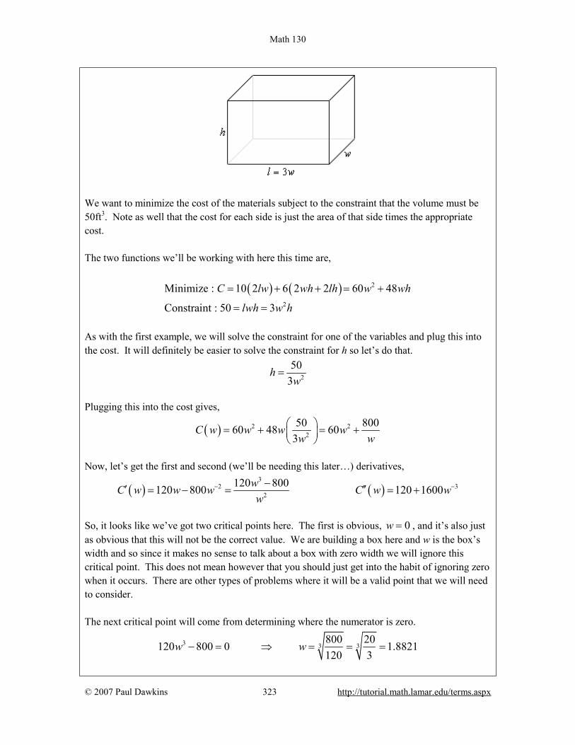
Math 130
© 2007 Paul Dawkins 323 http://tutorial.math.lamar.edu/terms.aspx
We want to minimize the cost of the materials subject to the constraint that the volume must be 50ft3. Note as well that the cost for each side is just the area of that side times the appropriate cost. The two functions we’ll be working with here this time are,
( ) ( ) 2
2
Minimize : 10 2 6 2 2 60 48
Constraint : 50 3
C lw wh lh w wh
lwh w h
= + + = +
= =
As with the first example, we will solve the constraint for one of the variables and plug this into the cost. It will definitely be easier to solve the constraint for h so let’s do that.
2
503
hw
=
Plugging this into the cost gives,
( ) 2 22
50 80060 48 603
C w w w ww w
= + = +
Now, let’s get the first and second (we’ll be needing this later…) derivatives,
( ) ( )3
2 32
120 800120 800 120 1600wC w w w C w ww
− −−′ ′′= − = = +
So, it looks like we’ve got two critical points here. The first is obvious, 0w = , and it’s also just as obvious that this will not be the correct value. We are building a box here and w is the box’s width and so since it makes no sense to talk about a box with zero width we will ignore this critical point. This does not mean however that you should just get into the habit of ignoring zero when it occurs. There are other types of problems where it will be a valid point that we will need to consider. The next critical point will come from determining where the numerator is zero.
3 3 3800 20120 800 0 1.8821120 3
w w− = ⇒ = = =
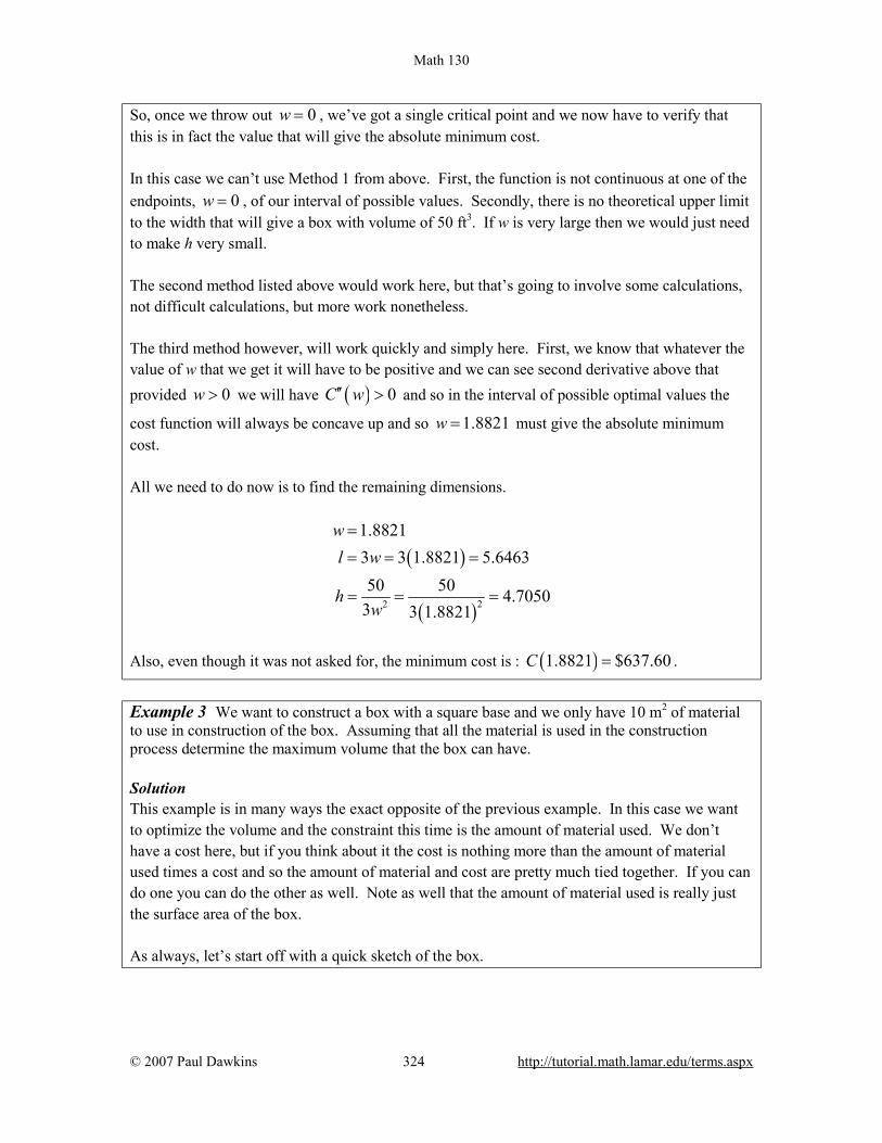
Math 130
© 2007 Paul Dawkins 324 http://tutorial.math.lamar.edu/terms.aspx
So, once we throw out 0w = , we’ve got a single critical point and we now have to verify that this is in fact the value that will give the absolute minimum cost. In this case we can’t use Method 1 from above. First, the function is not continuous at one of the endpoints, 0w = , of our interval of possible values. Secondly, there is no theoretical upper limit to the width that will give a box with volume of 50 ft3. If w is very large then we would just need to make h very small. The second method listed above would work here, but that’s going to involve some calculations, not difficult calculations, but more work nonetheless. The third method however, will work quickly and simply here. First, we know that whatever the value of w that we get it will have to be positive and we can see second derivative above that provided 0w > we will have ( ) 0C w′′ > and so in the interval of possible optimal values the
cost function will always be concave up and so 1.8821w = must give the absolute minimum cost. All we need to do now is to find the remaining dimensions.
( )
( )22
1.88213 3 1.8821 5.646350 50 4.7050
3 3 1.8821
wl w
hw
=
= = =
= = =
Also, even though it was not asked for, the minimum cost is : ( )1.8821 $637.60C = .
Example 3 We want to construct a box with a square base and we only have 10 m2 of material to use in construction of the box. Assuming that all the material is used in the construction process determine the maximum volume that the box can have. Solution This example is in many ways the exact opposite of the previous example. In this case we want to optimize the volume and the constraint this time is the amount of material used. We don’t have a cost here, but if you think about it the cost is nothing more than the amount of material used times a cost and so the amount of material and cost are pretty much tied together. If you can do one you can do the other as well. Note as well that the amount of material used is really just the surface area of the box. As always, let’s start off with a quick sketch of the box.
Math 130
© 2007 Paul Dawkins 325 http://tutorial.math.lamar.edu/terms.aspx
Now, as mentioned above we want to maximize the volume and the amount of material is the constraint so here are the equations we’ll need.
2
2
Maximize : Constraint : 10 2 2 2 2 4
V lwh w hlw wh lh w wh
= =
= + + = +
We’ll solve the constraint for h and plug this into the equation for the volume.
( ) ( )2 2 2
2 310 2 5 5 1 54 2 2 2
w w wh V w w w ww w w
− − −= = ⇒ = = −
Here are the first and second derivatives of the volume function.
( ) ( ) ( )212 5 3 3V w w V w w′ ′′= − = −
Note as well here that provided 0w > , which we know from a physical standpoint will be true, then the volume function will be concave down and so if we get a single critical point then we know that it will have to be the value that gives the absolute maximum. Setting the first derivative equal to zero and solving gives us the two critical points,
5 1.29103
w = ± = ±
In this case we can exclude the negative critical point since we are dealing with a length of a box and we know that these must be positive. Do not however get into the habit of just excluding any negative critical point. There are problems where negative critical points are perfectly valid possible solutions. Now, as noted above we got a single critical point, 1.2910, and so this must be the value that gives the maximum volume and since the maximum volume is all that was asked for in the problem statement the answer is then : ( ) 31.2910 2.1517 mV = .
Note that we could also have noted here that if 1.2910w < then ( ) 0V w′ > and likewise if
Math 130
© 2007 Paul Dawkins 326 http://tutorial.math.lamar.edu/terms.aspx
1.2910w > then ( ) 0V w′ < and so if we are to the left of the critical point the volume is always
increasing and if we are to the right of the critical point the volume is always decreasing and so by the Method 2 above we can also see that the single critical point must give the absolute maximum of the volume. Finally, even though these weren’t asked for here are the dimension of the box that gives the maximum volume.
( )25 1.29101.2910 1.2910
2 1.2910l w h −
= = = =
So, it looks like in this case we actually have a perfect cube. In the last two examples we’ve seen that many of these optimization problems can in both directions so to speak. In both examples we have essentially the same two equations: volume and surface area. However, in Example 2 the volume was the constraint and the cost (which is directly related to the surface area) was the function we were trying to optimize. In Example 3, on the other hand, we were trying to optimize the volume and the surface area was the constraint. It is important to not get so locked into one way of doing these problems that we can’t do it in the opposite direction as needed as well. This is one of the more common mistakes that students make with these kinds of problems. They see one problem and then try to make every other problem that seems to be the same conform to that one solution even if the problem needs to be worked differently. Keep an open mind with these problems and make sure that you understand what is being optimized and what the constraint is before you jump into the solution. Also, as seen in the last example we used two different methods of verifying that we did get the optimal value. Do not get too locked into one method of doing this verification that you forget about the other methods. Let’s work some another example that this time doesn’t involve a rectangle or box. Example 4 A manufacturer needs to make a cylindrical can that will hold 1.5 liters of liquid. Determine the dimensions of the can that will minimize the amount of material used in its construction. Solution In this problem the constraint is the volume and we want to minimize the amount of material used. This means that what we want to minimize is the surface area of the can and we’ll need to include both the walls of the can as well as the top and bottom “caps”. Here is a quick sketch to get us started off.
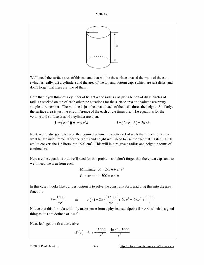
Math 130
© 2007 Paul Dawkins 327 http://tutorial.math.lamar.edu/terms.aspx
We’ll need the surface area of this can and that will be the surface area of the walls of the can (which is really just a cylinder) and the area of the top and bottom caps (which are just disks, and don’t forget that there are two of them). Note that if you think of a cylinder of height h and radius r as just a bunch of disks/circles of radius r stacked on top of each other the equations for the surface area and volume are pretty simple to remember. The volume is just the area of each of the disks times the height. Similarly, the surface area is just the circumference of the each circle times the. The equations for the volume and surface area of a cylinder are then,
( )( ) ( )( )2 2 2 2V r h r h A r h rhπ π π π= = = =
Next, we’re also going to need the required volume in a better set of units than liters. Since we want length measurements for the radius and height we’ll need to use the fact that 1 Liter = 1000 cm3 to convert the 1.5 liters into 1500 cm3. This will in turn give a radius and height in terms of centimeters. Here are the equations that we’ll need for this problem and don’t forget that there two caps and so we’ll need the area from each.
2
2
Minimize : 2 2Constraint : 1500
A rh rr h
π π
π
= +
=
In this case it looks like our best option is to solve the constraint for h and plug this into the area function.
( ) 2 22 2
1500 1500 30002 2 2h A r r r rr r r
π π ππ π
= ⇒ = + = +
Notice that this formula will only make sense from a physical standpoint if 0r > which is a good thing as it is not defined at 0r = . Next, let’s get the first derivative.
( )3
2 2
3000 4 30004 rA r rr r
ππ
−′ = − =

Math 130
© 2007 Paul Dawkins 328 http://tutorial.math.lamar.edu/terms.aspx
From this we can see that we have two critical points : 0r = and 7503 6.2035r π= = . The first
critical point doesn’t make sense from a physical standpoint and so we can ignore that one. So we only have a single critical point to deal with here and notice that 6.2035 is the only value for which the derivative will be zero and hence the only place (with 0r > of course) that the derivative may change sign. It’s not difficult to check that if 6.2035r < then ( ) 0A r′ < and
likewise if 6.2035r > then ( ) 0A r′ > . The variant of the First Derivative Test above then tells
us that the absolute minimum value of the area (for 0r > ) must occur at 6.2035r = . All we need to do this is determine height of the can and we’ll be done.
( )2
1500 12.40706.2035
hπ
= =
Therefore if the manufacturer makes the can with a radius of 6.2035 cm and a height of 12.4070 cm the least amount of material will be used to make the can. As an interesting side problem and extension to the above example you might want to show that for a given volume, L, the minimum material will be used if 2h r= regardless of the volume of the can. In the examples to this point we’ve put in quite a bit of discussion in the solution. In the remaining problems we won’t be putting in quite as much discussion and leave it to you to fill in any missing details. Example 5 We have a piece of cardboard that is 14 inches by 10 inches and we’re going to cut out the corners as shown below and fold up the sides to form a box, also shown below. Determine the height of the box that will give a maximum volume.
Solution In this example, for the first time, we’ve run into a problem where the constraint doesn’t really have an equation. The constraint is simply the size of the piece of cardboard and has already been factored into the figure above. This will happen on occasion and so don’t get excited about it when it does. This just means that we have one less equation to worry about. In this case we
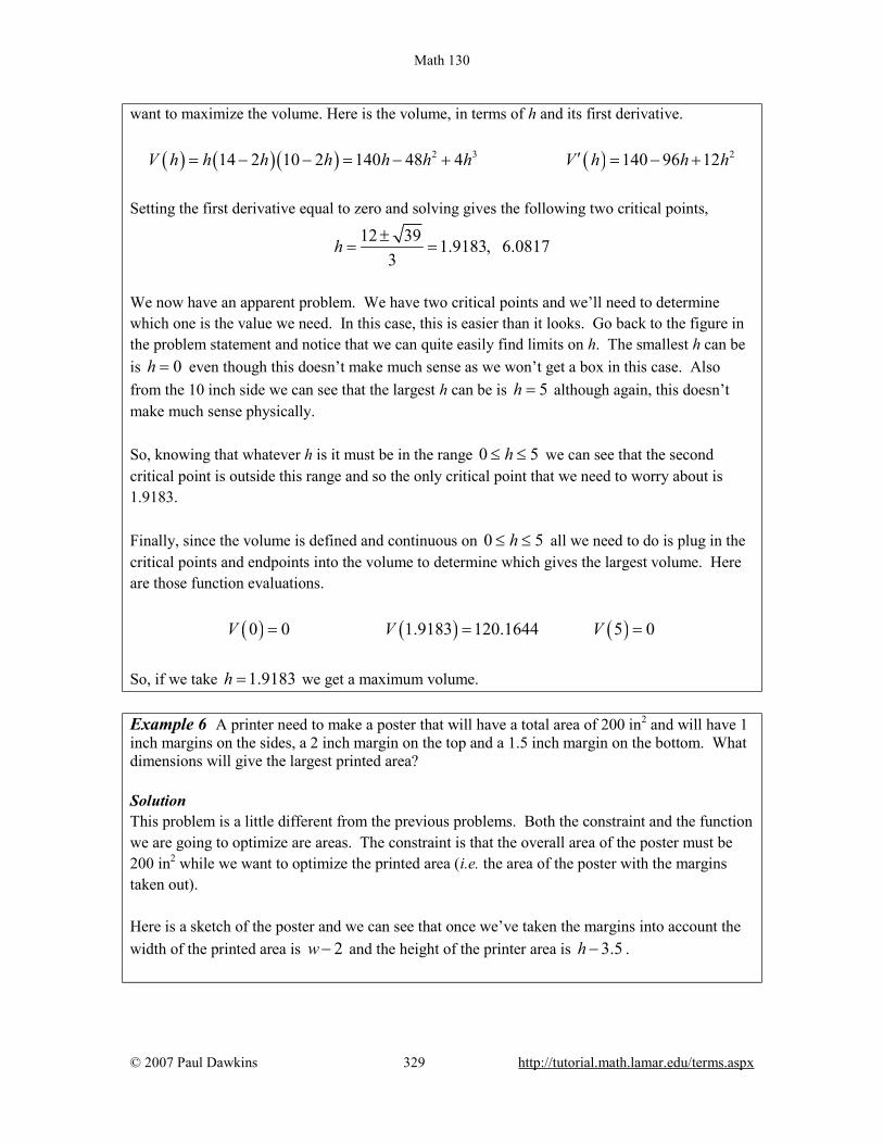
Math 130
© 2007 Paul Dawkins 329 http://tutorial.math.lamar.edu/terms.aspx
want to maximize the volume. Here is the volume, in terms of h and its first derivative. ( ) ( ) ( ) ( )2 3 214 2 10 2 140 48 4 140 96 12V h h h h h h h V h h h′= − − = − + = − +
Setting the first derivative equal to zero and solving gives the following two critical points,
12 39 1.9183, 6.0817
3h ±
= =
We now have an apparent problem. We have two critical points and we’ll need to determine which one is the value we need. In this case, this is easier than it looks. Go back to the figure in the problem statement and notice that we can quite easily find limits on h. The smallest h can be is 0h = even though this doesn’t make much sense as we won’t get a box in this case. Also from the 10 inch side we can see that the largest h can be is 5h = although again, this doesn’t make much sense physically. So, knowing that whatever h is it must be in the range 0 5h≤ ≤ we can see that the second critical point is outside this range and so the only critical point that we need to worry about is 1.9183. Finally, since the volume is defined and continuous on 0 5h≤ ≤ all we need to do is plug in the critical points and endpoints into the volume to determine which gives the largest volume. Here are those function evaluations.
( ) ( ) ( )0 0 1.9183 120.1644 5 0V V V= = =
So, if we take 1.9183h = we get a maximum volume. Example 6 A printer need to make a poster that will have a total area of 200 in2 and will have 1 inch margins on the sides, a 2 inch margin on the top and a 1.5 inch margin on the bottom. What dimensions will give the largest printed area? Solution This problem is a little different from the previous problems. Both the constraint and the function we are going to optimize are areas. The constraint is that the overall area of the poster must be 200 in2 while we want to optimize the printed area (i.e. the area of the poster with the margins taken out). Here is a sketch of the poster and we can see that once we’ve taken the margins into account the width of the printed area is 2w − and the height of the printer area is 3.5h − .
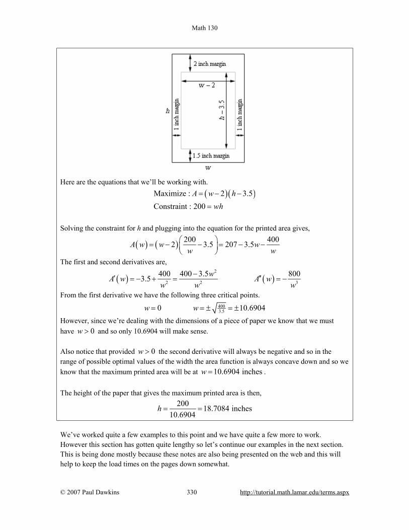
Math 130
© 2007 Paul Dawkins 330 http://tutorial.math.lamar.edu/terms.aspx
Here are the equations that we’ll be working with.
( ) ( )Maximize : 2 3.5Constraint : 200
A w hwh
= − −
=
Solving the constraint for h and plugging into the equation for the printed area gives,
( ) ( ) 200 4002 3.5 207 3.5A w w ww w
= − − = − −
The first and second derivatives are,
( ) ( )2
2 2 3
400 400 3.5 8003.5 wA w A ww w w
−′ ′′= − + = = −
From the first derivative we have the following three critical points. 4003.50 10.6904w w= = ± = ±
However, since we’re dealing with the dimensions of a piece of paper we know that we must have 0w > and so only 10.6904 will make sense. Also notice that provided 0w > the second derivative will always be negative and so in the range of possible optimal values of the width the area function is always concave down and so we know that the maximum printed area will be at 10.6904 inchesw = . The height of the paper that gives the maximum printed area is then,
200 18.7084 inches10.6904
h = =
We’ve worked quite a few examples to this point and we have quite a few more to work. However this section has gotten quite lengthy so let’s continue our examples in the next section. This is being done mostly because these notes are also being presented on the web and this will help to keep the load times on the pages down somewhat.

Math 130
© 2007 Paul Dawkins 331 http://tutorial.math.lamar.edu/terms.aspx
More Optimization Problems Because these notes are also being presented on the web we’ve broken the optimization examples up into several sections to keep the load times to a minimum. Do not forget the various methods for verifying that we have the optimal value that we looked at in the previous section. In this section we’ll just use them without acknowledging so make sure you understand them and can use them. So let’s get going on some more examples. Example 1 A window is being built and the bottom is a rectangle and the top is a semicircle. If there is 12 meters of framing materials what must the dimensions of the window be to let in the most light? Solution Okay, let’s ask this question again in slightly easier to understand terms. We want a window in the shape described above to have a maximum area (and hence let in the most light) and have a perimeter of 12 m (because we have 12 m of framing material). Little bit easier to understand in those terms. Here’s a sketch of the window. The height of the rectangular portion is h and because the semicircle is on top we can think of the width of the rectangular portion at 2r.
The perimeter (our constraint) is the lengths of the three sides on the rectangular portion plus half the circumference of a circle of radius r. The area (what we want to maximize) is the area of the rectangle plus half the area of a circle of radius r. Here are the equations we’ll be working with in this example.
21
2Maximize : 2Constraint : 12 2 2
A hr rh r r
ππ
= +
= + +
In this case we’ll solve the constraint for h and plug that into the area equation. ( ) ( ) 2 2 21 1 1 1
2 2 2 26 2 6 12 2h r r A r r r r r r r rπ π π π= − − ⇒ = − − + = − −
The first and second derivatives are,
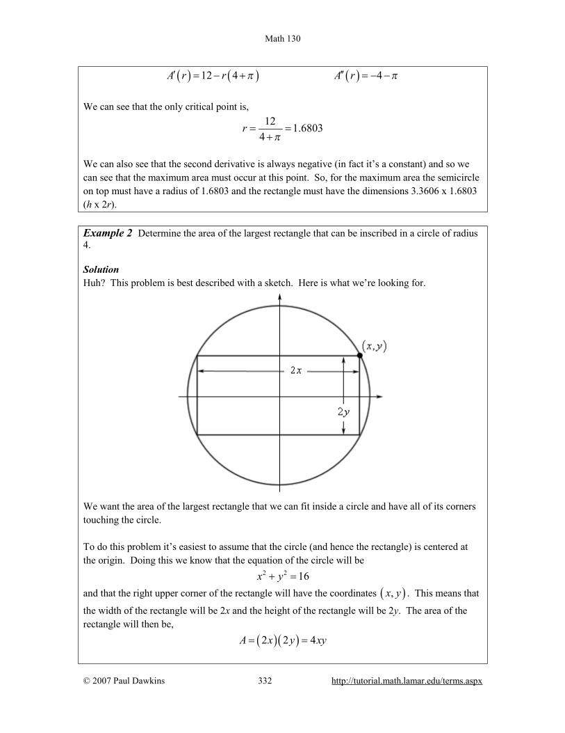
Math 130
© 2007 Paul Dawkins 332 http://tutorial.math.lamar.edu/terms.aspx
( ) ( ) ( )12 4 4A r r A rπ π′ ′′= − + = − −
We can see that the only critical point is,
12 1.68034
rπ
= =+
We can also see that the second derivative is always negative (in fact it’s a constant) and so we can see that the maximum area must occur at this point. So, for the maximum area the semicircle on top must have a radius of 1.6803 and the rectangle must have the dimensions 3.3606 x 1.6803 (h x 2r). Example 2 Determine the area of the largest rectangle that can be inscribed in a circle of radius 4. Solution Huh? This problem is best described with a sketch. Here is what we’re looking for.
We want the area of the largest rectangle that we can fit inside a circle and have all of its corners touching the circle. To do this problem it’s easiest to assume that the circle (and hence the rectangle) is centered at the origin. Doing this we know that the equation of the circle will be 2 2 16x y+ = and that the right upper corner of the rectangle will have the coordinates ( ),x y . This means that
the width of the rectangle will be 2x and the height of the rectangle will be 2y. The area of the rectangle will then be, ( )( )2 2 4A x y xy= =

Math 130
© 2007 Paul Dawkins 333 http://tutorial.math.lamar.edu/terms.aspx
So, we’ve got the function we want to maximize (the area), but what is the constraint? Well since the coordinates of the upper right corner must be on the circle we know that x and y must satisfy the equation of the circle. In other words, the equation of the circle is the constraint. The first thing to do then is to solve the constraint for one of the variables.
216y x= ± − Since the point that we’re looking at is in the first quadrant we know that y must be positive and so we can take the “+” part of this. Plugging this into the area and computing the first derivative gives,
( )
( )
2
2 22
2 2
4 16
4 64 84 1616 16
A x x x
x xA x xx x
= −
−′ = − − =− −
Before getting the critical points let’s notice that we can limit x to the range 0 4x≤ ≤ since we are assuming that x is in the first quadrant and must stay inside the circle. Now the four critical points we get (two from the numerator and two from the denominator) are,
2
2
16 0 4
64 8 0 2 2
x x
x x
− = ⇒ = ±
− = ⇒ = ±
We only want critical points that are in the range of possible optimal values so that means that we
have two critical points to deal with : 2 2x = and 4x = . Notice however that the second critical point is also one of the endpoints of our interval. Now, area function is continuous and we have an interval of possible solution with finite endpoints so,
( ) ( ) ( )0 0 2 2 32 4 0A A A= = =
So, we can see that we’ll get the maximum area if 2 2x = and the corresponding value of y is,
( )216 2 2 8 2 2y = − = =
It looks like the maximum area will be found if the inscribed rectangle is in fact a square. We need to again make a point that was made several times in the previous section. We excluded several critical points in the work above. Do not always expect to do that. There will often be physical reasons to exclude zero and/or negative critical points, however, there will be problems where these are perfectly acceptable values. You should always write down every possible critical point and then exclude any that can’t be possible solutions. This keeps you in the habit of
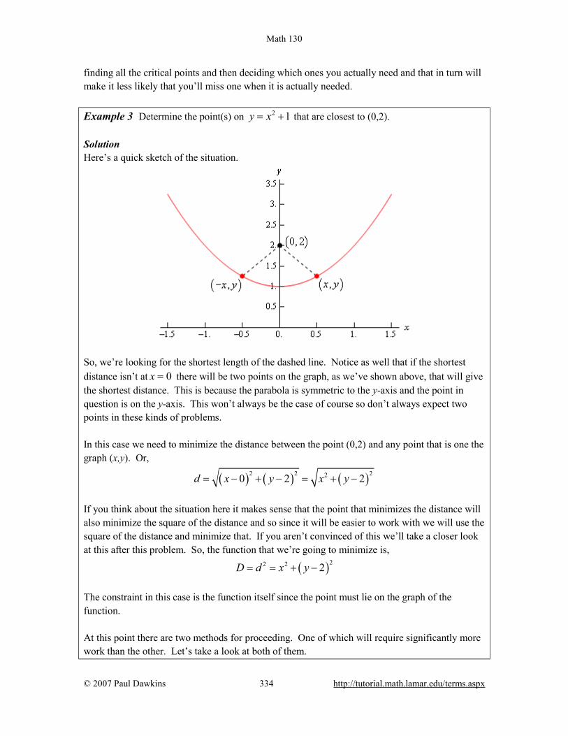
Math 130
© 2007 Paul Dawkins 334 http://tutorial.math.lamar.edu/terms.aspx
finding all the critical points and then deciding which ones you actually need and that in turn will make it less likely that you’ll miss one when it is actually needed. Example 3 Determine the point(s) on 2 1y x= + that are closest to (0,2). Solution Here’s a quick sketch of the situation.
So, we’re looking for the shortest length of the dashed line. Notice as well that if the shortest distance isn’t at 0x = there will be two points on the graph, as we’ve shown above, that will give the shortest distance. This is because the parabola is symmetric to the y-axis and the point in question is on the y-axis. This won’t always be the case of course so don’t always expect two points in these kinds of problems. In this case we need to minimize the distance between the point (0,2) and any point that is one the graph (x,y). Or,
( ) ( ) ( )2 2 220 2 2d x y x y= − + − = + − If you think about the situation here it makes sense that the point that minimizes the distance will also minimize the square of the distance and so since it will be easier to work with we will use the square of the distance and minimize that. If you aren’t convinced of this we’ll take a closer look at this after this problem. So, the function that we’re going to minimize is,
( )22 2 2D d x y= = + − The constraint in this case is the function itself since the point must lie on the graph of the function. At this point there are two methods for proceeding. One of which will require significantly more work than the other. Let’s take a look at both of them.

Math 130
© 2007 Paul Dawkins 335 http://tutorial.math.lamar.edu/terms.aspx
Solution 1 In this case we will use the constraint in probably the most obvious way. We already have the constraint solved for y so let’s plug that into the square of the distance and get the derivatives.
( ) ( )( ) ( )( )
22 2 4 2
3 2
2
1 2 1
4 2 2 2 1
12 2
D x x x x x
D x x x x x
D x x
= + + − = − +
′ = − = −
′′ = −
So, it looks like there are three critical points for the square of the distance and notice that this time, unlike pretty much every previous example we’ve worked, we can’t exclude zero or negative numbers. They are perfectly valid possible optimal values this time.
10,2
x x= = ±
Before going any farther, let’s check these in the second derivative to see if they are all relative minimums.
( ) 1 10 2 0 4 42 2
D D D ′′ ′′ ′′= − < = − =
So, 0x = is a relative maximum and so can’t possibly be the minimum distance. That means that we’ve got two critical points. The question is how do we verify that these give the minimum distance and yes we did mean to say that both will give the minimum distance. Recall from our sketch above that if x gives the minimum distance then so will –x and so if gives the minimum distance then the other should as well. None of the methods we discussed in the previous section will really work here. We don’t have an interval of possible solutions with finite endpoints and both the first and second derivative change sign. In this case however, we can still verify that they are the points that give the minimum distance.
First, notice that if we are working on the interval 1 12 2
, − then the endpoints of this interval
(which are also the critical points) are in fact where the absolute minimum of the function occurs in this interval. Next we can see that if 1
2x < − then ( ) 0D x′ < . Or in other words, if 1
2x < − the function is
decreasing until it hits 12
x = − and so must always be larger than the function at 12
x = − .
Similarly, 1
2x > then ( ) 0D x′ > and so the function is always increasing to the right of
Math 130
© 2007 Paul Dawkins 336 http://tutorial.math.lamar.edu/terms.aspx
12
x = − and so must be larger than the function at 12
x = − .
So, putting all of this together tells us that we do in fact have an absolute minimum at 1
2x = ± .
All that we need to do is to find the value of y for these points.
1 3:22
1 3:22
x y
x y
= =
= − =
So, the points on the graph that are closest to (0,2) are,
1 3 1 3, ,2 22 2
−
Solution 2 The first solution that we worked was actually the long solution. There is a much shorter solution to this problem. Instead of plugging y into the square of the distance let’s plug in x. From the constraint we get, 2 1x y= − and notice that the only place x show up in the square of the distance it shows up as x2 and let’s just plug this into the square of the distance. Doing this gives,
( ) ( )( )( )
2 21 2 3 3
2 3
2
D y y y y y
D y y
D y
= − + − = − +
′ = −
′′ =
There is now a single critical point, 3
2y = , and since the second derivative is always positive we know that this point must give the absolute minimum. So all that we need to do at this point is find the value(s) of x that go with this value of y.
2 3 1 112 2 2
x x= − = ⇒ = ±
The points are then,
1 3 1 3, ,2 22 2
−
So, for significantly less work we got exactly the same answer. This previous example had a couple of nice points. First, as pointed out in the problem, we couldn’t exclude zero or negative critical points this time as we’ve done in all the previous
Math 130
© 2007 Paul Dawkins 337 http://tutorial.math.lamar.edu/terms.aspx
examples. Again, be careful to not get into the habit of always excluding them as we do many of the examples we’ll work. Next, some of these problems will have multiple solution methods and sometimes one will be significantly easier than the other. The method you use is up to you and often the difficulty of any particular method is dependent upon the person doing the problem. One person may find one way easier and other person may find a different method easier. Finally, as we saw in the first solution method sometimes we’ll need to use a combination of the optimal value verification methods we discussed in the previous section. Now, before we move onto the next example let’s take a look at the claim above that we could find the location of the point that minimizes the distance by finding the point that minimizes the square of the distance. We’ll generalize things a little bit, Fact Suppose that we have a positive function, ( ) 0f x > , that exists everywhere then ( )f x and
( ) ( )g x f x= will have the same critical points and the relative extrema will occur at the same
points. This is simple enough to prove so let’s do that here. First let’s take the derivative of ( )g x and
see what we can determine about the critical points of ( )g x .
( ) ( ) ( ) ( )( )
11 22 2
f xg x f x f x
f x− ′
′ ′= =
Let’s plug x c= into this to get,
( ) ( )( )2
f cg c
f c
′′ =
By assumption we know that ( )f c exists and ( ) 0f c > and therefore the denominator of this
will always exist and will never be zero. We’ll need this in several places so we can’t forget this. If ( ) 0f c′ = then because we know that the denominator will not be zero here we must also have
( ) 0g c′ = . Likewise, if ( ) 0g c′ = then we must have ( ) 0f c′ = . So, ( )f x and ( )g x will
have the same critical points in which the derivatives will be zero. Next, if ( )f c′ doesn’t exist then ( )g c′ will also not exist and likewise if ( )g c′ doesn’t exist
then because we know that the denominator will not be zero then this means that ( )f c′ will also

Math 130
© 2007 Paul Dawkins 338 http://tutorial.math.lamar.edu/terms.aspx
not exist. Therefore, ( )f x and ( )g x will have the same critical points in which the derivatives
does not exist. So, the upshot of all this is that ( )f x and ( )g x will have the same critical points.
Next, let’s notice that because we know that ( )2 0f x > then ( )f x′ and ( )g x′ will have the
same sign and so if we apply the first derivative test (and recalling that they have the same critical points) to each of these functions we can see that the results will be the same and so the relative extrema will occur at the same points. Note that we could also use the second derivative test to verify that the critical points will have the same classification if we wanted to. The second derivative is (and you should see if you can use the quotient rule to verify this),
( ) ( ) ( ) ( ) ( )( )
1222
4f x f x f x f x
g xf x
−′′ ′− ′′ =
Then if x c= is a critical point such that ( ) 0f c′ = (and so we can use the second derivative
test) we get,
( ) ( ) ( ) ( ) ( )
( )
( ) ( ) [ ] ( )( )
( ) ( )( )
122
12 2
24
2 04 2
f c f c f c f cg c
f c
f c f c f c f c f cf c f c
−
−
′′ ′− ′′ =
′′ ′′− = =
Now, because we know that ( )2 0f c > and by assumption ( ) 0f c > we can see that ( )f c′′
and ( )g c′′ will have the same sign and so will have the same conclusion from the second
derivative test. So, now that we have that out of the way let’s work some more examples. Example 4 A 2 feet piece of wire is cut into two pieces and once piece is bent into a square and the other is bent into an equilateral triangle. Where should the wire cut so that the total area enclosed by both is minimum and maximum? Solution Before starting the solution recall that an equilateral triangle is a triangle with three equal sides and each of the interior angles are 3
π (or 60° ).
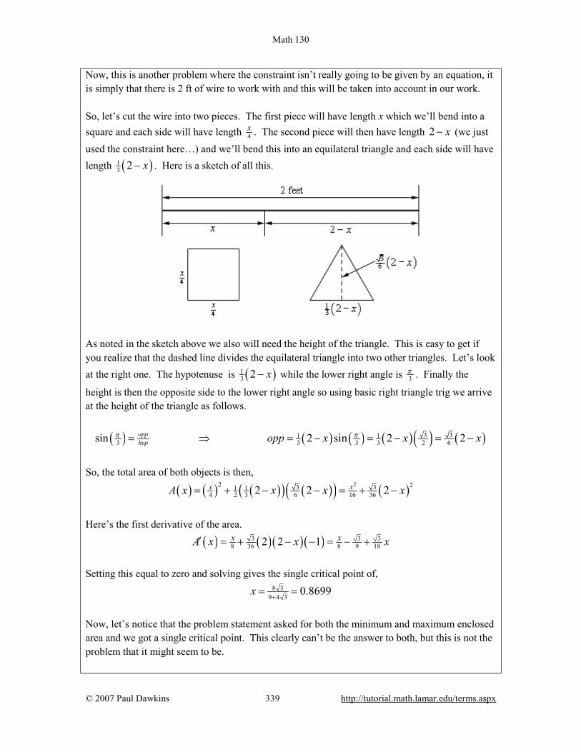
Math 130
© 2007 Paul Dawkins 339 http://tutorial.math.lamar.edu/terms.aspx
Now, this is another problem where the constraint isn’t really going to be given by an equation, it is simply that there is 2 ft of wire to work with and this will be taken into account in our work. So, let’s cut the wire into two pieces. The first piece will have length x which we’ll bend into a square and each side will have length 4
x . The second piece will then have length 2 x− (we just used the constraint here…) and we’ll bend this into an equilateral triangle and each side will have length ( )1
3 2 x− . Here is a sketch of all this.
As noted in the sketch above we also will need the height of the triangle. This is easy to get if you realize that the dashed line divides the equilateral triangle into two other triangles. Let’s look at the right one. The hypotenuse is ( )1
3 2 x− while the lower right angle is 3π . Finally the
height is then the opposite side to the lower right angle so using basic right triangle trig we arrive at the height of the triangle as follows.
( ) ( ) ( ) ( ) ( ) ( )3 31 13 3 3 3 2 6sin 2 sin 2 2opp
hyp opp x x xπ π= ⇒ = − = − = −
So, the total area of both objects is then,
( ) ( ) ( )( ) ( )( ) ( )22 23 31 14 2 3 6 16 362 2 2xxA x x x x= + − − = + −
Here’s the first derivative of the area.
( ) ( )( )( )3 3 38 36 8 9 182 2 1x xA x x x′ = + − − = − +
Setting this equal to zero and solving gives the single critical point of,
8 39 4 3
0.8699x+
= =
Now, let’s notice that the problem statement asked for both the minimum and maximum enclosed area and we got a single critical point. This clearly can’t be the answer to both, but this is not the problem that it might seem to be.
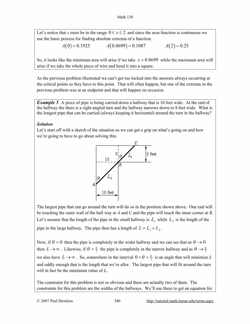
Math 130
© 2007 Paul Dawkins 340 http://tutorial.math.lamar.edu/terms.aspx
Let’s notice that x must be in the range 0 2x≤ ≤ and since the area function is continuous we use the basic process for finding absolute extrema of a function.
( ) ( ) ( )0 0.1925 0.8699 0.1087 2 0.25A A A= = =
So, it looks like the minimum area will arise if we take 0.8699x = while the maximum area will arise if we take the whole piece of wire and bend it into a square. As the previous problem illustrated we can’t get too locked into the answers always occurring at the critical points as they have to this point. That will often happen, but one of the extrema in the previous problem was at an endpoint and that will happen on occasion. Example 5 A piece of pipe is being carried down a hallway that is 10 feet wide. At the end of the hallway the there is a right-angled turn and the hallway narrows down to 8 feet wide. What is the longest pipe that can be carried (always keeping it horizontal) around the turn in the hallway? Solution Let’s start off with a sketch of the situation so we can get a grip on what’s going on and how we’re going to have to go about solving this.
The largest pipe that can go around the turn will do so in the position shown above. One end will be touching the outer wall of the hall way at A and C and the pipe will touch the inner corner at B. Let’s assume that the length of the pipe in the small hallway is 1L while 2L is the length of the
pipe in the large hallway. The pipe then has a length of 1 2L L L= + .
Now, if 0θ = then the pipe is completely in the wider hallway and we can see that as 0θ → then L → ∞ . Likewise, if 2
πθ = the pipe is completely in the narrow hallway and as 2πθ →
we also have L → ∞ . So, somewhere in the interval 20 πθ< < is an angle that will minimize L and oddly enough that is the length that we’re after. The largest pipe that will fit around the turn will in fact be the minimum value of L. The constraint for this problem is not so obvious and there are actually two of them. The constraints for this problem are the widths of the hallways. We’ll use these to get an equation for

Math 130
© 2007 Paul Dawkins 341 http://tutorial.math.lamar.edu/terms.aspx
L in terms of θ and then we’ll minimize this new equation. So, using basic right triangle trig we can see that, 1 28sec 10csc 8sec 10cscL L Lθ θ θ θ= = ⇒ = +
So, differentiating L gives, 8sec tan 10csc cotL θ θ θ θ′ = − Setting this equal to zero and solving gives,
23
8sec tan 10csc cotsec tan 10csc cot 8
sin tan 5 tan 1.25cos 4
θ θ θ θθ θθ θ
θ θθ
θ
=
=
= ⇒ =
Solving for θ gives,
( )13 3tan 1.25 tan 1.25 0.8226θ θ −= ⇒ = =
So, if 0.8226θ = radians then the pipe will have a minimum length and will just fit around the turn. Anything larger will not fit around the turn and so the largest pipe that can be carried around the turn is, ( ) ( )8sec 0.8226 10csc 0.8226 25.4033 feetL = + =
Example 6 Two poles, one 6 meters tall and one 15 meters tall, are 20 meters apart. A length of wire is attached to the top of each pole and it is also staked to the ground somewhere between the two poles. Where should the wire be staked so that the minimum amount of wire is used? Solution As always let’s start off with a sketch of this situation.

Math 130
© 2007 Paul Dawkins 342 http://tutorial.math.lamar.edu/terms.aspx
The total length of the wire is 1 2L L L= + and we need to determine the value of x that will
minimize this. The constraint in this problem is that the poles must be 20 meters apart and that x must be in the range 0 20x≤ ≤ . The first thing that we’ll need to do here is to get the length of wire in terms of x, which is fairly simple to do using the Pythagorean Theorem.
( )22 2 21 236 225 20 36 625 40L x L x L x x x= + = + − = + + − +
Not the nicest function we’ve had to work with but there it is. Note however, that it is a continuous function and we’ve got an interval with finite endpoints and so finding the absolute minimum won’t require much more work than just getting the critical points of this function. So, let’s do that. Here’s the derivative.
2 2
2036 625 40
x xLx x x
−′ = ++ − +
Setting this equal to zero gives,
( )
2 2
2 2
20 036 625 40
625 40 20 36
x xx x x
x x x x x
−+ =
+ − +
− + = − − +
It’s probably been quite a while since you’ve been asked to solve something like this. To solve this we’ll need to square both sides to get rid of the roots, but this will cause problems as well soon see. Let’s first just square both sides and solve that equation.
( ) ( ) ( )
( )( )
22 2 2
2 3 4 2 3 4
2
40 403 7
625 40 20 36
625 40 14400 1440 436 40189 1440 14400 0
9 3 40 7 40 0 ,
x x x x x
x x x x x x xx x
x x x x
− + = − +
− + = − + − +
+ − =
+ − = ⇒ = − =
Note that if you can’t do that factoring done worry, you can always just use the quadratic formula and you’ll get the same answers. Okay two issues that we need to discuss briefly here. The first solution above (note that I didn’t call it a critical point…) doesn’t make any sense because it is negative and outside of the range of possible solutions and so we can ignore it. Secondly, and maybe more importantly, if you were to plug 40
3x = − into the derivative you would not get zero and so is not even a critical point. How is this possible? It is a solution after all. We’ll recall that we squared both sides of the equation above and it was mentioned at the
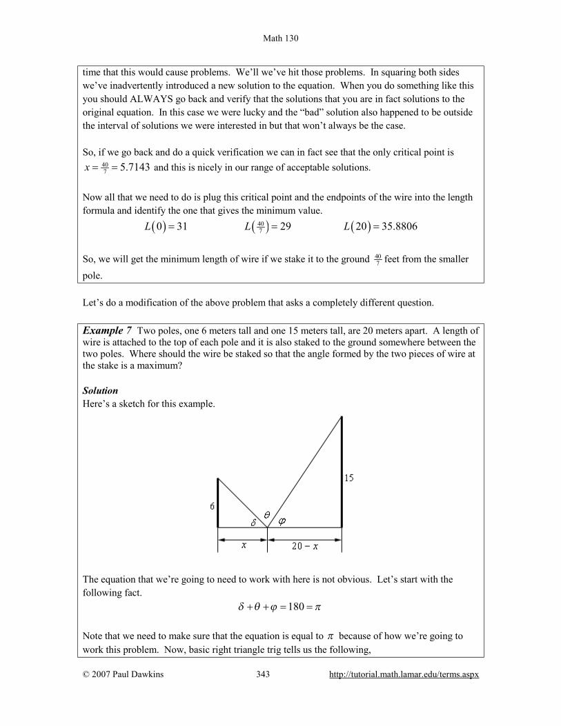
Math 130
© 2007 Paul Dawkins 343 http://tutorial.math.lamar.edu/terms.aspx
time that this would cause problems. We’ll we’ve hit those problems. In squaring both sides we’ve inadvertently introduced a new solution to the equation. When you do something like this you should ALWAYS go back and verify that the solutions that you are in fact solutions to the original equation. In this case we were lucky and the “bad” solution also happened to be outside the interval of solutions we were interested in but that won’t always be the case. So, if we go back and do a quick verification we can in fact see that the only critical point is
407 5.7143x = = and this is nicely in our range of acceptable solutions.
Now all that we need to do is plug this critical point and the endpoints of the wire into the length formula and identify the one that gives the minimum value. ( ) ( ) ( )40
70 31 29 20 35.8806L L L= = =
So, we will get the minimum length of wire if we stake it to the ground 40
7 feet from the smaller pole. Let’s do a modification of the above problem that asks a completely different question. Example 7 Two poles, one 6 meters tall and one 15 meters tall, are 20 meters apart. A length of wire is attached to the top of each pole and it is also staked to the ground somewhere between the two poles. Where should the wire be staked so that the angle formed by the two pieces of wire at the stake is a maximum? Solution Here’s a sketch for this example.
The equation that we’re going to need to work with here is not obvious. Let’s start with the following fact.
180δ θ ϕ π+ + = = Note that we need to make sure that the equation is equal to π because of how we’re going to work this problem. Now, basic right triangle trig tells us the following,

Math 130
© 2007 Paul Dawkins 344 http://tutorial.math.lamar.edu/terms.aspx
( )( )
16 6
115 1520 20
tan tan
tan tanx x
x x
δ δ
ϕ ϕ
−
−− −
= ⇒ =
= ⇒ =
Plugging these into the equation above and solving for θ gives, ( ) ( )1 16 15
20tan tan xxθ π − −−= − −
Note that this is the reason for the π in our equation. The inverse tangents give angles that are in radians and so can’t use the 180 that we’re used to in this kind of equation. Next we’ll need the derivative so hopefully you’ll recall how to differentiate inverse tangents.
( ) ( ) ( )
( )( )
( )( )
2 2 226 1520
22
2
2 2 2 2
1 6 1 15201 1
6 1536 20 225
3 3 80 10706 1536 40 625 36 40 625
xx x x
x x
x xx x x x x x
θ−
′ = − − − −+ +
= −+ − +
− + −= − =
+ − + + − +
Setting this equal to zero and solving give the following two critical points.
40 48103 36.4514, 9.7847x − ±= = −
The first critical point is not in the interval of possible solutions and so we can exclude it. It’s not difficult to show that if 0 9.7847x≤ ≤ that 0θ ′ > and if 9.7847 20x≤ ≤ that 0θ ′ < and so when 9.7847x = we will get the maximum value of θ . Example 8 A trough for holding water is be formed by taking a piece of sheet metal 60 cm wide and folding the 20 cm on either end up as shown below. Determine the angle θ that will maximize the amount of water that the trough can hold.
Solution Now, in this case we are being asked to maximize the volume that a trough can hold, but if you think about it the volume of a trough in this shape is nothing more than the cross-sectional area times the length of the trough. So for a given length in order to maximize the volume all you really need to do is maximize the cross-sectional area. To get a formula for the cross-sectional area let’s redo the sketch above a little.

Math 130
© 2007 Paul Dawkins 345 http://tutorial.math.lamar.edu/terms.aspx
We can think of the cross-sectional area as a rectangle in the middle with width 20 and height h and two identical triangles on either end with height h, base b and hypotenuse 20. Also note that basic geometry tells us that the angle between the hypotenuse and the base must also be the same angle θ that we had in our original sketch. Also, basic right triangle trig tells us that the base and height can be written as, 20cos 20sinb hθ θ= = The cross-sectional area for the whole trough, in terms of θ , is then,
( ) ( )( ) ( )1220 2 400sin 20cos 20sin 400 sin sin cosA h bh θ θ θ θ θ θ= + = + = +
The derivative of the area is,
( ) ( )( )( )
( )( )( )
2 2
2 2
2
400 cos cos sin
400 cos cos 1 cos
400 2cos cos 1
400 2cos 1 cos 1
A θ θ θ θ
θ θ θ
θ θ
θ θ
′ = + −
= + − −
= + −
= − +
So, we have either,
12 32cos 1 0 cos
cos 1 0 cos 1
πθ θ θθ θ θ π
− = ⇒ = ⇒ =
+ = ⇒ = − ⇒ =
However, we can see that θ must be in the interval 20 πθ≤ ≤ or we won’t get a trough in the proper shape. Therefore, the second critical point makes no sense and also note that we don’t need to add on the standard “ 2 nπ+ ” for the same reason. Finally, since the equation for the area is continuous all we need to do is plug in the critical point and the end points to find the one that gives the maximum area. ( ) ( ) ( )3 20 0 519.6152 400A A Aπ π= = =
So, we will get a maximum cross-sectional area, and hence a maximum volume, when 3
πθ = .

Math 130
© 2007 Paul Dawkins 346 http://tutorial.math.lamar.edu/terms.aspx
Indeterminate Forms and L’Hospital’s Rule Back in the chapter on Limits we saw methods for dealing with the following limits.
2 2
24
16 4 5lim lim4 1 3x x
x x xx x→ →∞
− −− −
In the first limit if we plugged in 4x = we would get 0/0 and in the second limit if we “plugged” in infinity we would get ∞ −∞ (recall that as x goes to infinity a polynomial will behave in the same fashion that it’s largest power behaves). Both of these are called indeterminate forms. In both of these cases there are competing interests or rules and it’s not clear which will win out. In the case of 0/0 we typically think of a fraction that has a numerator of zero as being zero. However, we also tend to think of fractions in which the denominator is going to zero as infinity or might not exist at all. Likewise, we tend to think of a fraction in which the numerator and denominator are the same as one. So, which will win out? Or will neither win out and they all “cancel out” and the limit will reach some other value? In the case of ∞ −∞ we have a similar set of problems. If the numerator of a fraction is going to infinity we tend to think of the whole fraction going to infinity. Also if the denominator is going to infinity we tend to think of the fraction as going to zero. We also have the case of a fraction in which the numerator and denominator are the same (ignoring the minus sign) and so we might get -1. Again, it’s not clear which of these will win out, if any of them will win out. With the second limit there is the further problem that infinity isn’t really a number and so we really shouldn’t even treat it like a number. Much of the time it simply won’t behave as we would expect it to if it was a number. To look a little more into this check out the Types of Infinity section in the Extras chapter at the end of this document. This is the problem with indeterminate forms. It’s just not clear what is happening in the limit. There are other types of indeterminate forms as well. Some other types are, ( )( ) 0 00 1 0∞± ∞ ∞ ∞ − ∞ These all have competing interests or rules that tell us what should happen and it’s just not clear which, if any, of the interests or rules will win out. The topic of this section is how to deal with these kinds of limits. As already pointed out we do know how to deal with some kinds of indeterminate forms already. For the two limits above we work them as follows.
( )2
4 4
16lim lim 4 84x x
x xx→ →
−= + =
−
Math 130
© 2007 Paul Dawkins 347 http://tutorial.math.lamar.edu/terms.aspx
2
2
2
544 5 4lim lim 11 3 33x x
x x xx
x→∞ →∞
−−= = −
− −
In the first case we simply factored, canceled and took the limit and in the second case we factored out an 2x from both the numerator and the denominator and took the limit. Notice as well that none of the competing interests or rules in these cases won out! That is often the case. So we can deal with some of these. However what about the following two limits.
20
sinlim limx
x x
xx x→ →∞
e
This first is a 0/0 indeterminate form, but we can’t factor this one. The second is an ∞ ∞
indeterminate form, but we can’t just factor an 2x out of the numerator. So, nothing that we’ve got in our bag of tricks will work with these two limits. This is where the subject of this section comes into play. L’Hospital’s Rule Suppose that we have one of the following cases,
( )( )
( )( )
0lim OR lim0x a x a
f x f xg x g x→ →
± ∞= =
± ∞
where a can be any real number, infinity or negative infinity. In these cases we have,
( )( )
( )( )
lim limx a x a
f x f xg x g x→ →
′=
′
So, L’Hospital’s Rule tells us that if we have an indeterminate form 0/0 or ∞ ∞ all we need to do is differentiate the numerator and differentiate the denominator and then take the limit. Before proceeding with examples let me address the spelling of “L’Hospital”. The more correct spelling is “L’Hôpital”. However, when I first learned Calculus I my teacher used the spelling that I use in these notes and the first text book that I taught Calculus out of also used the spelling that I use here. So, I’m used to spelling it that way and that is the way that I’ve spelled it here. Let’s work some examples.
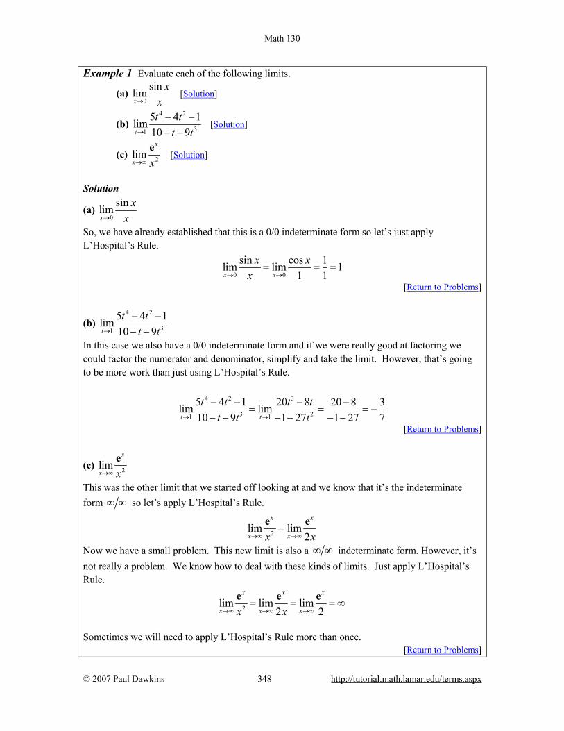
Math 130
© 2007 Paul Dawkins 348 http://tutorial.math.lamar.edu/terms.aspx
Example 1 Evaluate each of the following limits.
(a) 0
sinlimx
xx→
[Solution]
(b) 4 2
31
5 4 1lim10 9t
t tt t→
− −− −
[Solution]
(c) 2limx
x x→∞
e [Solution]
Solution
(a) 0
sinlimx
xx→
So, we have already established that this is a 0/0 indeterminate form so let’s just apply L’Hospital’s Rule.
0 0
sin cos 1lim lim 11 1x x
x xx→ →
= = =
[Return to Problems]
(b) 4 2
31
5 4 1lim10 9t
t tt t→
− −− −
In this case we also have a 0/0 indeterminate form and if we were really good at factoring we could factor the numerator and denominator, simplify and take the limit. However, that’s going to be more work than just using L’Hospital’s Rule.
4 2 3
3 21 1
5 4 1 20 8 20 8 3lim lim10 9 1 27 1 27 7t t
t t t tt t t→ →
− − − −= = = −
− − − − − −
[Return to Problems]
(c) 2limx
x x→∞
e
This was the other limit that we started off looking at and we know that it’s the indeterminate form ∞ ∞ so let’s apply L’Hospital’s Rule.
2lim lim2
x x
x xx x→∞ →∞=
e e
Now we have a small problem. This new limit is also a ∞ ∞ indeterminate form. However, it’s not really a problem. We know how to deal with these kinds of limits. Just apply L’Hospital’s Rule.
2lim lim lim2 2
x x x
x x xx x→∞ →∞ →∞= = = ∞
e e e
Sometimes we will need to apply L’Hospital’s Rule more than once.
[Return to Problems]
Math 130
© 2007 Paul Dawkins 349 http://tutorial.math.lamar.edu/terms.aspx
L’Hospital’s Rule works great on the two indeterminate forms 0/0 and ± ∞ ± ∞ . However, there are many more indeterminate forms out there as we saw earlier. Let’s take a look at some of those and see how we deal with those kinds of indeterminate forms. We’ll start with the indeterminate form ( )( )0 ± ∞ .
Example 2 Evaluate the following limit.
0lim lnx
x x+→
Solution Note that we really do need to do the right-hand limit here. We know that the natural logarithm is only defined for positive x and so this is the only limit that makes any sense. Now, in the limit, we get the indeterminate form ( ) ( )0 −∞ . L’Hospital’s Rule won’t work on
products, it only works on quotients. However, we can turn this into a fraction if we rewrite things a little.
0 0
lnlim ln lim 1x x
xx xx
+ +→ →=
The function is the same, just rewritten, and the limit is now in the form −∞ ∞ and we can now use L’Hospital’s Rule.
0 0 0
2
1lnlim ln lim lim1 1x x x
x xx xx x
+ + +→ → →= =
−
Now, this is a mess, but it cleans up nicely.
( )0 0 0
2
1lim ln lim lim 01x x x
xx x xx
+ + +→ → →= = − =
−
In the previous example we used the fact that we can always write a product of functions as a quotient by doing one of the following.
( ) ( ) ( )
( )( ) ( ) ( )
( )OR1 1
g x f xf x g x f x g x
f x g x= =
Using these two facts will allow us to turn any limit in the form ( )( )0 ± ∞ into a limit in the form
0/0 or ± ∞ ± ∞ . One of these two we get after doing the rewrite will depend upon which fact we
used to do the rewrite. One of the rewrites will give 0/0 and the other will give ± ∞ ± ∞ . It all depends on which function stays in the numerator and which gets moved down to the denominator.

Math 130
© 2007 Paul Dawkins 350 http://tutorial.math.lamar.edu/terms.aspx
Let’s take a look at another example. Example 3 Evaluate the following limit. lim x
xx
→−∞e
Solution So, it’s in the form ( )( )0∞ . This means that we’ll need to write it as a quotient. Moving the x
to the denominator worked in the previous example so let’s try that with this problem as well.
lim lim 1
xx
x xx
x→−∞ →−∞
=ee
Writing the product in this way gives us a product that has the form 0/0 in the limit. So, let’s use L’Hospital’s Rule on the quotient.
2 3 4
lim lim lim lim lim1 1 2 6
x x x xx
x x x x xx
x x x x→−∞ →−∞ →−∞ →−∞ →−∞
= = = = =− −
e e e ee L
Hummmm…. This doesn’t seem to be getting us anywhere. With each application of L’Hospital’s Rule we just end up with another 0/0 indeterminate form and in fact the derivatives seem to be getting worse and worse. Also note that if we simplified the quotient back into a product we would just end up with either ( )( )0∞ or ( )( )0−∞ and so that won’t do us any
good. This does not mean however that the limit can’t be done. It just means that we moved the wrong function to the denominator. Let’s move the exponential function instead.
lim lim lim1x
xx x xx
x xx −→−∞ →−∞ →−∞= =e
ee
Note that we used the fact that,
1 xx
−= ee
to simplify the quotient up a little. This will help us when it comes time to take some derivatives. The quotient is now an indeterminate form of −∞ ∞ and use L’Hospital’s Rule gives,
1lim lim lim 0xx xx x x
xx − −→−∞ →−∞ →−∞= = =
−e
e e
So, when faced with a product ( )( )0 ± ∞ we can turn it into a quotient that will allow us to use
L’Hospital’s Rule. However, as we saw in the last example we need to be careful with how we do that on occasion. Sometimes we can use either quotient and in other cases only one will work. Let’s now take a look at the indeterminate forms,

Math 130
© 2007 Paul Dawkins 351 http://tutorial.math.lamar.edu/terms.aspx
0 01 0∞ ∞ These can all be dealt with in the following way so we’ll just work one example. Example 4 Evaluate the following limit.
1
lim xx
x→∞
Solution In the limit this is the indeterminate form 0∞ . We’re actually going to spend most of this problem on a different limit. Let’s first define the following.
1xy x=
Now, if we take the natural log of both sides we get,
( )1 1 lnln ln lnx xy x x
x x
= = =
Let’s now take a look at the following limit.
( )1lnlim ln lim lim 01x x x
x xyx→∞ →∞ →∞
= = =
This limit was just a L’Hospital’s Rule problem and we know how to do those. So, what did this have to do with our limit? Well first notice that,
( )ln y y=e and so our limit could be written as,
( )1
lnlim lim lim yxx x x
x y→∞ →∞ →∞
= = e
We can now use the limit above to finish this problem.
( ) ( )1lim lnln 0lim lim lim 1x
yyxx x x
x y →∞
→∞ →∞ →∞= = = = =e e e
With L’Hospital’s Rule we are now able to take the limit of a wide variety of indeterminate forms that we were unable to deal with prior to this section.
Math 130
© 2007 Paul Dawkins 352 http://tutorial.math.lamar.edu/terms.aspx
Differentials In this section we’re going to introduce a notation that we’ll be seeing quite a bit in the next chapter. We will also look at an application of this new notation. Given a function ( )y f x= we call dy and dx differentials and the relationship between them is
given by, ( )dy f x dx′= Note that if we are just given ( )f x then the differentials are df and dx and we compute them the
same manner. ( )df f x dx′= Let’s compute a couple of differentials. Example 1 Compute the differential for each of the following.
(a) 3 24 7y t t t= − + (b) ( )2 sin 2w x x=
(c) ( ) 43 zf z −= e Solution Before working any of these we should first discuss just what we’re being asked to find here. We defined two differentials earlier and here we’re being asked to compute a differential. So, which differential are we being asked to compute? In this kind of problem we’re being asked to compute the differential of the function. In other words, dy for the first problem, dw for the second problem and df for the third problem. Here are the solutions. Not much to do here other than take a derivative and don’t forget to add on the second differential to the derivative.
(a) ( )23 8 7dy t t dt= − +
(b) ( ) ( )( )22 sin 2 2 cos 2dw x x x x dx= +
(c) 43 34 zdf z dz−= − e

Math 130
© 2007 Paul Dawkins 353 http://tutorial.math.lamar.edu/terms.aspx
There is a nice application to differentials. If we think of x∆ as the change in x then
( ) ( )y f x x f x∆ = + ∆ − is the change in y corresponding to the change in x. Now, if x∆ is
small we can assume that y dy∆ ≈ . Let’s see an illustration of this idea.
Example 2 Compute dy and y∆ if ( )2cos 1y x x= + − as x changes from 2x = to 2.03x = . Solution First let’s compute actual the change in y, y∆ .
( )( ) ( )( )2 2cos 2.03 1 2.03 cos 2 1 2 0.083581127y∆ = + − − + − =
Now let’s get the formula for dy.
( )( )22 sin 1 1dy x x dx= − + − Next, the change in x from 2x = to 2.03x = is 0.03x∆ = and so we then assume that
0.03dx x≈ ∆ = . This gives an approximate change in y of,
( ) ( )( )( )22 2 sin 2 1 1 0.03 0.085070913dy = − + − = We can see that in fact we do have that y dy∆ ≈ provided we keep x∆ small. We can use the fact that y dy∆ ≈ in the following way. Example 3 A sphere was measured and its radius was found to be 45 inches with a possible error of no more that 0.01 inches. What is the maximum possible error in the volume if we use this value of the radius? Solution First, recall the equation for the volume of a sphere.
343
V rπ=
Now, if we start with 45r = and use 0.01dr r≈ ∆ = then V dV∆ ≈ should give us maximum error. So, first get the formula for the differential. 24dV r drπ= Now compute dV.
( ) ( )2 34 45 0.01 254.47 inV dV π∆ ≈ = =

Math 130
© 2007 Paul Dawkins 354 http://tutorial.math.lamar.edu/terms.aspx
The maximum error in the volume is then approximately 254.47 in3. Be careful to not assume this is a large error. On the surface it looks large, however if we compute the actual volume for 45r = we get 3381,703.51 inV = . So, in comparison the error in the volume is,
254.47 100 0.067%
381703.51× =
That’s not much possible error at all!

Math 130
© 2007 Paul Dawkins 355 http://tutorial.math.lamar.edu/terms.aspx
Business Applications In the final section of this chapter let’s take a look at some applications of derivatives in the business world. For the most part these are really applications that we’ve already looked at, but they are now going to be approached with an eye towards the business world. Let’s start things out with a couple of optimization problems. We’ve already looked at more than a few of these in previous sections so there really isn’t anything all that new here except for the fact that they are coming out of the business world. Example 1 An apartment complex has 250 apartments to rent. If they rent x apartments then their monthly profit, in dollars, is given by,
( ) 28 3200 80,000P x x x= − + −
How many apartments should they rent in order to maximize their profit? Solution All that we’re really being asked to do here is to maximize the profit subject to the constraint that x must be in the range 0 250x≤ ≤ . First, we’ll need the derivative and the critical point(s) that fall in the range 0 250x≤ ≤ . ( ) 3200
1616 3200 3200 16 0 200P x x x x′ = − + ⇒ − = ⇒ = =
Since the profit function is continuous and we have an interval with finite bounds we can find the maximum value by simply plugging in the only critical point that we have (which nicely enough in the range of acceptable answers) and the end points of the range. ( ) ( ) ( )0 80,000 200 240,000 250 220,000P P P= − = =
So, it looks like they will generate the most profit if they only rent out 200 of the apartments instead of all 250 of them. Note that with these problems you shouldn’t just assume that renting all the apartments will generate the most profit. Do not forget that there are all sorts of maintenance costs and that the more tenants renting apartments the more the maintenance costs will be. With this analysis we can see that, for this complex at least, something probably needs to be done to get the maximum profit more towards full capacity. This kind of analysis can help them determine just what they need to do to move towards goal that whether it be raising rent or find a way to reduce maintenance costs. Note as well that because most apartment complexes have at least a few unit empty after a tenant moves out and the like that it’s possible that they would actually like the maximum profit to fall
Math 130
© 2007 Paul Dawkins 356 http://tutorial.math.lamar.edu/terms.aspx
slightly under full capacity to take this into account. Again, another reason to not just assume that maximum profit will always be at the upper limit of the range. Let’s take a quick look at another problem along these lines. Example 2 A production facility is capable of producing 60,000 widgets in a day and the total daily cost of producing x widgets in a day is given by,
( ) 200,000,000250,000 0.08C x xx
= + +
How many widgets per day should they produce in order to minimize production costs? Solution Here we need to minimize the cost subject to the constraint that x must be in the range 0 60,000x≤ ≤ . Note that in this case the cost function is not continuous at the left endpoint and so we won’t be able to just plug critical points and endpoints into the cost function to find the minimum value. Let’s get the first couple of derivatives of the cost function.
( ) ( )2 3
200,000,000 400,000,0000.08C x C xx x
′ ′′= − =
The critical points of the cost function are,
2
2
2
200,000,0000.08 0
0.08 200,000,000
2,500,000,000 2,500,000,000 50,000
xx
x x
− =
=
= ⇒ = ± = ±
Now, clearly the negative value doesn’t make any sense in this setting and so we have a single critical point in the range of possible solutions : 50,000. Now, as long as 0x > the second derivative is positive and so, in the range of possible solutions the function is always concave up and so producing 50,000 widgets will yield the absolute minimum production cost. Now, we shouldn’t walk out of the previous two examples with the idea that the only applications to business are just applications we’ve already looked at but with a business “twist” to them. There are some very real applications to calculus that are in the business world and at some level that is the point of this section. Note that to really learn these applications and all of their intricacies you’ll need to take a business course or two or three. In this section we’re just going to scratch the surface and get a feel for some of the actual applications of calculus from the business world and some of the main “buzz” words in the applications.

Math 130
© 2007 Paul Dawkins 357 http://tutorial.math.lamar.edu/terms.aspx
Let’s start off by looking at the following example. Example 3 The production costs per week for producing x widgets is given by,
( ) 2500 350 0.09 , 0 1000C x x x x= + − ≤ ≤
Answer each of the following questions.
(a) What is the cost to produce the 301st widget? (b) What is the rate of change of the cost at 300x = ?
Solution (a) We can’t just compute ( )301C as that is the cost of producing 301 widgets while we are
looking for the actual cost of producing the 301st widget. In other words, what we’re looking for here is, ( ) ( )301 300 97,695.91 97, 400.00 295.91C C− = − =
So, the cost of producing the 301st widget is $295.91. (b) In the part all we need to do is get the derivative and then compute ( )300C′ .
( ) ( )350 0.18 300 296.00C x x C′ ′= − ⇒ =
Okay, so just what did we learn in this example? The cost to produce an additional item is called the marginal cost and as we’ve seen in the above example the marginal cost is approximated by the rate of change of the cost function, ( )C x . So, we define the marginal cost function to be
the derivative of the cost function or, ( )C x′ . Let’s work a quick example of this.
Example 4 The production costs per day for some widget is given by, ( ) 2 32500 10 0.01 0.0002C x x x x= − − +
What is the marginal cost when 200x = , 300x = and 400x = ? Solution So, we need the derivative and then we’ll need to compute some values of the derivative.
( )
( ) ( ) ( )
210 0.02 0.0006
200 10 300 38 400 78
C x x x
C C C
′ = − − +
′ ′ ′= = =
So, in order to produce the 201st widget it will cost approximately $10. To produce the 301st widget will cost around $38. Finally, to product the 401st widget it will cost approximately $78.
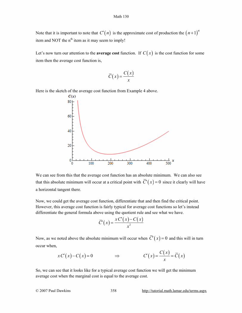
Math 130
© 2007 Paul Dawkins 358 http://tutorial.math.lamar.edu/terms.aspx
Note that it is important to note that ( )C n′ is the approximate cost of production the ( )st1n +
item and NOT the nth item as it may seem to imply! Let’s now turn our attention to the average cost function. If ( )C x is the cost function for some
item then the average cost function is,
( ) ( )C xC x
x=
Here is the sketch of the average cost function from Example 4 above.
We can see from this that the average cost function has an absolute minimum. We can also see that this absolute minimum will occur at a critical point with ( ) 0C x′ = since it clearly will have
a horizontal tangent there. Now, we could get the average cost function, differentiate that and then find the critical point. However, this average cost function is fairly typical for average cost functions so let’s instead differentiate the general formula above using the quotient rule and see what we have.
( ) ( ) ( )2
x C x C xC x
x′ −
′ =
Now, as we noted above the absolute minimum will occur when ( ) 0C x′ = and this will in turn
occur when,
( ) ( ) ( ) ( ) ( )0C x
xC x C x C x C xx
′ ′− = ⇒ = =
So, we can see that it looks like for a typical average cost function we will get the minimum average cost when the marginal cost is equal to the average cost.
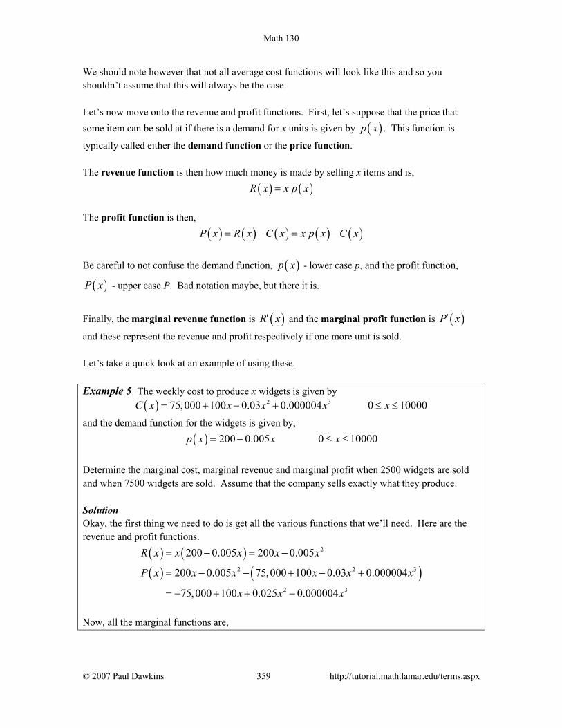
Math 130
© 2007 Paul Dawkins 359 http://tutorial.math.lamar.edu/terms.aspx
We should note however that not all average cost functions will look like this and so you shouldn’t assume that this will always be the case. Let’s now move onto the revenue and profit functions. First, let’s suppose that the price that some item can be sold at if there is a demand for x units is given by ( )p x . This function is
typically called either the demand function or the price function. The revenue function is then how much money is made by selling x items and is, ( ) ( )R x x p x= The profit function is then, ( ) ( ) ( ) ( ) ( )P x R x C x x p x C x= − = − Be careful to not confuse the demand function, ( )p x - lower case p, and the profit function,
( )P x - upper case P. Bad notation maybe, but there it is.
Finally, the marginal revenue function is ( )R x′ and the marginal profit function is ( )P x′
and these represent the revenue and profit respectively if one more unit is sold. Let’s take a quick look at an example of using these. Example 5 The weekly cost to produce x widgets is given by ( ) 2 375,000 100 0.03 0.000004 0 10000C x x x x x= + − + ≤ ≤
and the demand function for the widgets is given by, ( ) 200 0.005 0 10000p x x x= − ≤ ≤
Determine the marginal cost, marginal revenue and marginal profit when 2500 widgets are sold and when 7500 widgets are sold. Assume that the company sells exactly what they produce. Solution Okay, the first thing we need to do is get all the various functions that we’ll need. Here are the revenue and profit functions.
( ) ( )( ) ( )
2
2 2 3
2 3
200 0.005 200 0.005
200 0.005 75,000 100 0.03 0.000004
75,000 100 0.025 0.000004
R x x x x x
P x x x x x x
x x x
= − = −
= − − + − +
= − + + −
Now, all the marginal functions are,
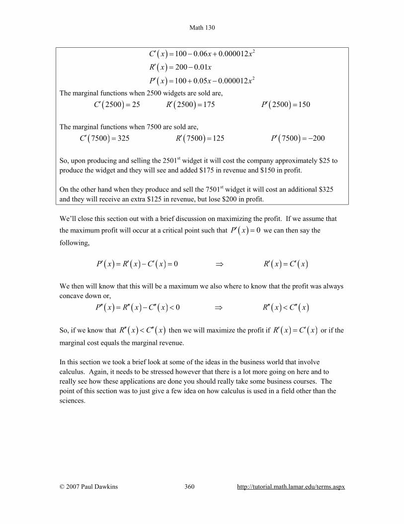
Math 130
© 2007 Paul Dawkins 360 http://tutorial.math.lamar.edu/terms.aspx
( )( )( )
2
2
100 0.06 0.000012
200 0.01
100 0.05 0.000012
C x x x
R x x
P x x x
′ = − +
′ = −
′ = + −
The marginal functions when 2500 widgets are sold are, ( ) ( ) ( )2500 25 2500 175 2500 150C R P′ ′ ′= = =
The marginal functions when 7500 are sold are, ( ) ( ) ( )7500 325 7500 125 7500 200C R P′ ′ ′= = = −
So, upon producing and selling the 2501st widget it will cost the company approximately $25 to produce the widget and they will see and added $175 in revenue and $150 in profit. On the other hand when they produce and sell the 7501st widget it will cost an additional $325 and they will receive an extra $125 in revenue, but lose $200 in profit. We’ll close this section out with a brief discussion on maximizing the profit. If we assume that the maximum profit will occur at a critical point such that ( ) 0P x′ = we can then say the
following,
( ) ( ) ( ) ( ) ( )0P x R x C x R x C x′ ′ ′ ′ ′= − = ⇒ =
We then will know that this will be a maximum we also where to know that the profit was always concave down or, ( ) ( ) ( ) ( ) ( )0P x R x C x R x C x′′ ′′ ′′ ′′ ′′= − < ⇒ < So, if we know that ( ) ( )R x C x′′ ′′< then we will maximize the profit if ( ) ( )R x C x′ ′= or if the
marginal cost equals the marginal revenue. In this section we took a brief look at some of the ideas in the business world that involve calculus. Again, it needs to be stressed however that there is a lot more going on here and to really see how these applications are done you should really take some business courses. The point of this section was to just give a few idea on how calculus is used in a field other than the sciences.

Math 130
© 2007 Paul Dawkins 361 http://tutorial.math.lamar.edu/terms.aspx
Integrals
Introduction In this chapter we will be looking at integrals. Integrals are the third and final major topic that will be covered in this class. This chapter includes a brief introduction to the idea of an anti-derivative / indefinite integral. Here is a quick listing of the material that is in this chapter. Indefinite Integrals – In this section we will start with the definition of indefinite integral. This section will be devoted mostly to the definition and properties of indefinite integrals.

Math 130
© 2007 Paul Dawkins 362 http://tutorial.math.lamar.edu/terms.aspx
Indefinite Integrals
In the past two chapters we’ve been given a function, ( )f x , and asking what the derivative of
this function was. Starting with this section we are not going to turn things around. We now want to ask what function we differentiated to get the function ( )f x .
Let’s take a quick look at an example to get us started. Example 1 What function did we differentiate to get the following function. ( ) 4 3 9f x x x= + − Solution Let’s actually start by getting the derivative of this function to help us see how we’re going to have to approach this problem. The derivative of this function is, ( ) 34 3f x x′ = + The point of this was to remind us of how differentiation works. When differentiating powers of x we multiply the term by the original exponent and then drop the exponent by one. Now, let’s go back and work the problem. In fact let’s just start with the first term. We got x4 by differentiating a function and since we drop the exponent by one it looks like we must have differentiated x5. However, if we had differentiated x5 we would have 5x4 and we don’t have a 5 in front our first term, so the 5 needs to cancel out after we’ve differentiated. It looks then like
we would have to differentiate 515
x in order to get x4.
Likewise for the second term, in order to get 3x after differentiating we would have to
differentiate 232
x . Again, the fraction is there to cancel out the 2 we pick up in the
differentiation. The third term is just a constant and we know that if we differentiate x we get 1. So, it looks like we had to differentiate -9x to get the last term. Putting all of this together gives the following function,
( ) 5 21 3 95 2
F x x x x= + −
Our answer is easy enough to check. Simply differentiate ( )F x .
( ) ( )4 3 9F x x x f x′ = + − =
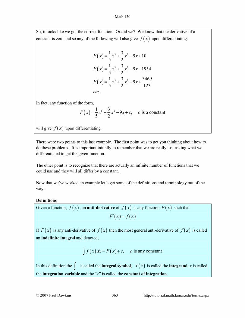
Math 130
© 2007 Paul Dawkins 363 http://tutorial.math.lamar.edu/terms.aspx
So, it looks like we got the correct function. Or did we? We know that the derivative of a constant is zero and so any of the following will also give ( )f x upon differentiating.
( )
( )
( )
5 2
5 2
5 2
1 3 9 105 21 3 9 19545 21 3 346995 2 123
.
F x x x x
F x x x x
F x x x x
etc
= + − +
= + − −
= + − +
In fact, any function of the form,
( ) 5 21 3 9 , is a constant5 2
F x x x x c c= + − +
will give ( )f x upon differentiating.
There were two points to this last example. The first point was to get you thinking about how to do these problems. It is important initially to remember that we are really just asking what we differentiated to get the given function. The other point is to recognize that there are actually an infinite number of functions that we could use and they will all differ by a constant. Now that we’ve worked an example let’s get some of the definitions and terminology out of the way. Definitions Given a function, ( )f x , an anti-derivative of ( )f x is any function ( )F x such that
( ) ( )F x f x′ = If ( )F x is any anti-derivative of ( )f x then the most general anti-derivative of ( )f x is called
an indefinite integral and denoted,
( ) ( ) , is any constantf x dx F x c c= +∫
In this definition the ∫ is called the integral symbol, ( )f x is called the integrand, x is called
the integration variable and the “c” is called the constant of integration.
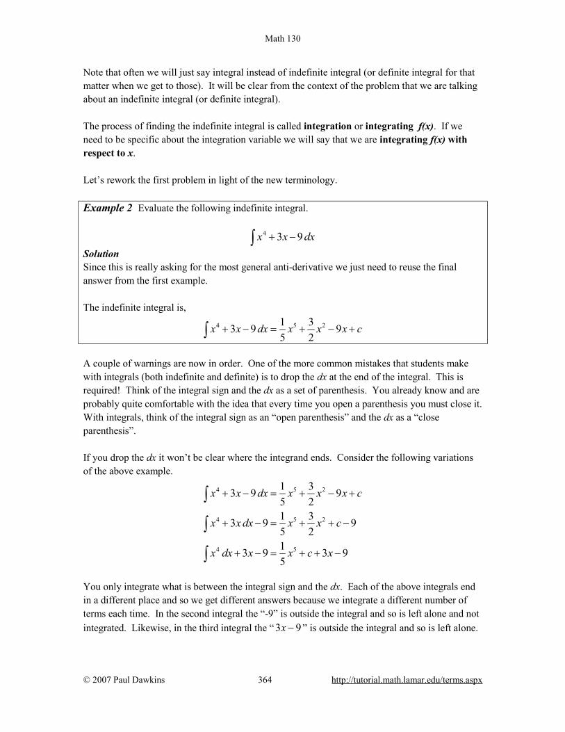
Math 130
© 2007 Paul Dawkins 364 http://tutorial.math.lamar.edu/terms.aspx
Note that often we will just say integral instead of indefinite integral (or definite integral for that matter when we get to those). It will be clear from the context of the problem that we are talking about an indefinite integral (or definite integral). The process of finding the indefinite integral is called integration or integrating f(x). If we need to be specific about the integration variable we will say that we are integrating f(x) with respect to x. Let’s rework the first problem in light of the new terminology. Example 2 Evaluate the following indefinite integral.
4 3 9x x dx+ −∫ Solution Since this is really asking for the most general anti-derivative we just need to reuse the final answer from the first example. The indefinite integral is,
4 5 21 33 9 95 2
x x dx x x x c+ − = + − +∫
A couple of warnings are now in order. One of the more common mistakes that students make with integrals (both indefinite and definite) is to drop the dx at the end of the integral. This is required! Think of the integral sign and the dx as a set of parenthesis. You already know and are probably quite comfortable with the idea that every time you open a parenthesis you must close it. With integrals, think of the integral sign as an “open parenthesis” and the dx as a “close parenthesis”. If you drop the dx it won’t be clear where the integrand ends. Consider the following variations of the above example.
4 5 2
4 5 2
4 5
1 33 9 95 21 33 9 95 213 9 3 95
x x dx x x x c
x x dx x x c
x dx x x c x
+ − = + − +
+ − = + + −
+ − = + + −
∫
∫
∫
You only integrate what is between the integral sign and the dx. Each of the above integrals end in a different place and so we get different answers because we integrate a different number of terms each time. In the second integral the “-9” is outside the integral and so is left alone and not integrated. Likewise, in the third integral the “ 3 9x − ” is outside the integral and so is left alone.

Math 130
© 2007 Paul Dawkins 365 http://tutorial.math.lamar.edu/terms.aspx
Knowing which terms to integrate is not the only reason for writing the dx down. In the Substitution Rule section we will actually be working with the dx in the problem and if we aren’t in the habit of writing it down it will be easy to forget about it and then we will get the wrong answer at that stage. The moral of this is to make sure and put in the dx! At this stage it may seem like a silly thing to do, but it just needs to be there, if for no other reason than knowing where the integral stops. On a side note, the dx notation should seem a little familiar to you. We saw things like this a couple of sections ago. We called the dx a differential in that section and yes that is exactly what it is. The dx that ends the integral is nothing more than a differential. The next topic that we should discuss here is the integration variable used in the integral. Actually there isn’t really a lot to discuss here other than to note that the integration variable doesn’t really matter. For instance,
4 5 2
4 5 2
4 5 2
1 33 9 95 2
1 33 9 95 2
1 33 9 95 2
x x dx x x x c
t t dt t t t c
w w dw w w w c
+ − = + − +
+ − = + − +
+ − = + − +
∫
∫
∫
Changing the integration variable in the integral simply changes the variable in the answer. It is important to notice however that when we change the integration variable in the integral we also changed the differential (dx, dt, or dw) to match the new variable. This is more important that we might realize at this point. Another use of the differential at the end of integral is to tell us what variable we are integrating with respect to. At this stage that may seem unimportant since most of the integrals that we’re going to be working with here will only involve a single variable. However, if you are on a degree track that will take you into multi-variable calculus this will be very important at that stage since there will be more than one variable in the problem. You need to get into the habit of writing the correct differential at the end of the integral so when it becomes important in those classes you will already be in the habit of writing it down. To see why this is important take a look at the following two integrals.
2 2x dx t dx∫ ∫ The first integral is simple enough.
22x dx x c= +∫

Math 130
© 2007 Paul Dawkins 366 http://tutorial.math.lamar.edu/terms.aspx
The second integral is also fairly simple, but we need to be careful. The dx tells us that we are integrating x’s. That means that we only integrate x’s that are in the integrand and all other variables in the integrand are considered to be constants. The second integral is then,
2 2t dx tx c= +∫ So, it may seem silly to always put in the dx, but it is a vital bit of notation that can cause us to get the incorrect answer if we neglect to put it in. Now, there are some important properties of integrals that we should take a look at. Properties of the Indefinite Integral
1. ( ) ( )k f x dx k f x dx=∫ ∫ where k is any number. So, we can factor multiplicative constants out of indefinite integrals. See the Proof of Various Integral Formulas section of the Extras chapter to see the proof of this property.
2. ( ) ( )f x dx f x dx− = −∫ ∫ . This is really the first property with 1k = − and so no proof of this property will be given.
3. ( ) ( ) ( ) ( )f x g x dx f x dx g x dx± = ±∫ ∫ ∫ . In other words, the integral of a sum or difference of functions is the sum or difference of the individual integrals. This rule can be extended to as many functions as we need. See the Proof of Various Integral Formulas section of the Extras chapter to see the proof of this property.
Notice that when we worked the first example above we used the first and third property in the discussion. We integrated each term individually, put any constants back in and then put everything back together with the appropriate sign. Not listed in the properties above were integrals of products and quotients. The reason for this is simple. Just like with derivatives each of the following will NOT work.
( ) ( ) ( ) ( ) ( )( )
( )( )
f x dxf xf x g x dx f x dx g x dx dx
g x g x dx≠ ≠
⌠⌡
∫∫ ∫ ∫ ∫
With derivatives we had a product rule and a quotient rule to deal with these cases. However, with integrals there are no such rules. When faced with a product and quotient in an integral we will have a variety of ways of dealing with it depending on just what the integrand is.

Math 130
© 2007 Paul Dawkins 367 http://tutorial.math.lamar.edu/terms.aspx
There is one final topic to be discussed briefly in this section. On occasion we will be given
( )f x′ and will ask what ( )f x was. We can now answer this question easily with an indefinite
integral.
( ) ( )f x f x dx′= ∫ Example 3 If ( ) 4 3 9f x x x′ = + − what was ( )f x ? Solution By this point in this section this is a simple question to answer.
( ) ( ) 4 5 21 33 9 95 2
f x f x dx x x dx x x x c′= = + − = + − +∫ ∫
In this section we kept evaluating the same indefinite integral in all of our examples. The point of this section was not to do indefinite integrals, but instead to get us familiar with the notation and some of the basic ideas and properties of indefinite integrals. The next couple of sections are devoted to actually evaluating indefinite integrals.

Math 130
© 2007 Paul Dawkins 368 http://tutorial.math.lamar.edu/terms.aspx
Extras
Introduction In this chapter material that didn’t fit into other sections for a variety of reasons. Also, in order to not obscure the mechanics of actually working problems, most of the proofs of various facts and formulas are in this chapter as opposed to being in the section with the fact/formula. This chapter contains those topics. Proof of Various Derivative Facts/Formulas/Properties – In this section we give the proof for several of the rules/formulas/properties of derivatives that we saw in Derivatives Chapter. Included are multiple proofs of the Power Rule, Product Rule, Quotient Rule and Chain Rule. Proof of Trig Limits – Here we give proofs for the two limits that are needed to find the derivative of the sine and cosine functions. Proofs of Derivative Applications Facts/Formulas – We’ll give proofs of many of the facts that we saw in the Applications of Derivatives chapter. Types of Infinity – This is a discussion on the types of infinity and how these affect certain limits. Summation Notation – Here is a quick review of summation notation.

Math 130
© 2007 Paul Dawkins 369 http://tutorial.math.lamar.edu/terms.aspx
Proof of Various Derivative Facts/Formulas/Properties In this section we’re going to prove many of the various derivative facts, formulas and/or properties that we encountered in the early part of the Derivatives chapter. Not all of them will be proved here and some will only be proved for special cases, but at least you’ll see that some of them aren’t just pulled out of the air.
Theorem, from Definition of Derivative If ( )f x is differentiable at x a= then ( )f x is continuous at x a= .
Proof Because ( )f x is differentiable at x a= we know that
( ) ( ) ( )limx a
f x f af a
x a→
−′ =
−
exists. We’ll need this in a bit. If we next assume that x a≠ we can write the following,
( ) ( ) ( ) ( ) ( )f x f af x f a x a
x a−
− = −−
Then basic properties of limits tells us that we have,
( ) ( )( ) ( ) ( ) ( )
( ) ( ) ( )
lim lim
lim lim
x a x a
x a x a
f x f af x f a x a
x a
f x f ax a
x a
→ →
→ →
− − = − −
−= −
−
The first limit on the right is just ( )f a′ as we noted above and the second limit is clearly zero
and so, ( ) ( )( ) ( )lim 0 0
x af x f a f a
→′− = ⋅ =
Okay, we’ve managed to prove that ( ) ( )( )lim 0
x af x f a
→− = . But just how does this help us to
prove that ( )f x is continuous at x a= ?
Let’s start with the following.
( ) ( ) ( ) ( )lim limx a x a
f x f x f a f a→ →
= + −

Math 130
© 2007 Paul Dawkins 370 http://tutorial.math.lamar.edu/terms.aspx
Note that we’ve just added in zero on the right side. A little rewriting and the use of limit properties gives,
( ) ( ) ( ) ( )
( ) ( ) ( )
lim lim
lim limx a x a
x a x a
f x f a f x f a
f a f x f a→ →
→ →
= + −
= + −
Now, we just proved above that ( ) ( )( )lim 0x a
f x f a→
− = and because ( )f a is a constant we
also know that ( ) ( )limx a
f a f a→
= and so this becomes,
( ) ( ) ( )lim lim 0x a x a
f x f a f a→ →
= + =
Or, in other words, ( ) ( )limx a
f x f a→
= but this is exactly what it means for ( )f x is continuous
at x a= and so we’re done.
Proof of Sum/Difference of Two Functions : ( ) ( )( ) ( ) ( )f x g x f x g x′ ′ ′± = ±
This is easy enough to prove using the definition of the derivative. We’ll start with the sum of two functions. First plug the sum into the definition of the derivative and rewrite the numerator a little.
( ) ( )( ) ( ) ( ) ( ) ( )( )
( ) ( ) ( ) ( )0
0
lim
lim
h
h
f x h g x h f x g xf x g x
hf x h f x g x h g x
h
→
→
+ + + − +′+ =
+ − + + −=
Now, break up the fraction into two pieces and recall that the limit of a sum is the sum of the limits. Using this fact we see that we end up with the definition of the derivative for each of the two functions.
( ) ( )( ) ( ) ( ) ( ) ( )
( ) ( )0 0
lim limh h
f x h f x g x h g xf x g x
h hf x g x→ →
+ − + −′+ = +
′ ′= +
The proof of the difference of two functions in nearly identical so we’ll give it here without any explanation.

Math 130
© 2007 Paul Dawkins 371 http://tutorial.math.lamar.edu/terms.aspx
( ) ( )( ) ( ) ( ) ( ) ( )( )
( ) ( ) ( ) ( )( )
( ) ( ) ( ) ( )
( ) ( )
0
0
0
lim
lim
lim
h
h
h
f x h g x h f x g xf x g x
hf x h f x g x h g x
hf x h f x g x h g x
h hf x g x
→
→
→
+ − + − −′− =
+ − − + −=
+ − + −= −
′ ′= −
Proof of Constant Times a Function : ( )( ) ( )cf x cf x′ ′=
This is property is very easy to prove using the definition provided you recall that we can factor a constant out of a limit. Here’s the work for this property.
( )( ) ( ) ( ) ( ) ( ) ( )0 0
lim limh h
cf x h cf x f x h f xcf x c cf x
h h→ →
+ − + −′ ′= = =
Proof of the Derivative of a Constant : ( ) 0d cdx
=
This is very easy to prove using the definition of the derivative so define ( )f x c= and the use
the definition of the derivative.
( ) ( ) ( )0 0 0
lim lim lim0 0h h h
f x h f x c cf xh h→ → →
+ − −′ = = = =
Power Rule : ( ) 1n nd x nxdx
−=
There are actually three proofs that we can give here and we’re going to go through all three here so you can see all of them. However, having said that, for the first two we will need to restrict n to be a positive integer. At the time that the Power Rule was introduced only enough information

Math 130
© 2007 Paul Dawkins 372 http://tutorial.math.lamar.edu/terms.aspx
has been given to allow the proof for only integers. So, the first two proofs are really to be read at that point. The third proof will work for any real number n. However, it does assume that you’ve read most of the Derivatives chapter and so should only be read after you’ve gone through the whole chapter. Proof 1 In this case as noted above we need to assume that n is a positive integer. We’ll use the definition of the derivative and the Binomial Theorem in this theorem. The Binomial Theorem tells us that,
( )
( ) ( )( )
0
1 2 2 3 3 1
1 2 2 3 3 1
1 2 3 1
1 1 22! 3!
nn n k k
k
n n n n n n
n n n n n n
na b a b
kn n n n n
a a b a b a b ab bn n
n n n n na na b a b a b nab b
−
=
− − − −
− − − −
+ =
= + + + + + + − − − −
= + + + + + +
∑
L
L
where,
( )
!! !
n nk k n k
= −
are called the binomial coefficients and ( )( ) ( )( )! 1 2 2 1n n n n= − − L is the factorial.
So, let’s go through the details of this proof. First, plug ( ) nf x x= into the definition of the
derivative and use the Binomial Theorem to expand out the first term.
( ) ( )
( )0
1 2 2 1
0
lim
12!
lim
n n
h
n n n n n n
h
x h xf x
hn n
x nx h x h nxh h x
h
→
− − −
→
+ −′ =
− + + + + + −
=L
Now, notice that we can cancel an nx and then each term in the numerator will have an h in them that can be factored out and then canceled against the h in the numerator. At this point we can evaluate the limit.
( )( )
( )
1 2 2 1
0
1 2 2 1
0
1
12!lim
1lim
2!
n n n n
h
n n n n
h
n
n nnx h x h nxh h
f xh
n nnx x h nxh h
nx
− − −
→
− − − −
→
−
−+ + + +
′ =
−= + + + +
=
L
L

Math 130
© 2007 Paul Dawkins 373 http://tutorial.math.lamar.edu/terms.aspx
Proof 2 For this proof we’ll again need to restrict n to be a positive integer. In this case if we define
( ) nf x x= we know from the alternate limit form of the definition of the derivative that the
derivative ( )f a′ is given by,
( ) ( ) ( )lim limn n
x a x a
f x f a x af ax a x a→ →
− −′ = =− −
Now we have the following formula,
( )( )1 2 2 3 3 2 2 1n n n n n n n nx a x a x ax a x a x a x a− − − − − −− = − + + + + + +L You can verify this if you’d like by simply multiplying the two factors together. Also, notice that there are a total of n terms in the second factor (this will be important in a bit). If we plug this into the formula for the derivative we see that we can cancel the x a− and then compute the limit.
( )( ) ( )1 2 2 3 3 2 2 1
1 2 2 3 3 2 2 1
1 2 2 3 3 2 2 1
1
lim
lim
n n n n n n
x a
n n n n n n
x an n n n n n
n
x a x ax a x a x a x af a
x ax ax a x a x a x a
a aa a a a a a a ana
− − − − − −
→
− − − − − −
→
− − − − − −
−
− + + + + + +′ =
−= + + + + + +
= + + + + + +
=
L
L
L
After combining the exponents in each term we can see that we get the same term. So, then recalling that there are n terms in second factor we can see that we get what we claimed it would be. To completely finish this off we simply replace the a with an x to get, ( ) 1nf x nx −′ =
Proof 3 In this proof we no longer need to restrict n to be a positive integer. It can now be any real number. However, this proof also assumes that you’ve read all the way through the Derivative chapter. In particular it needs both Implicit Differentiation and Logarithmic Differentiation. If you’ve not read, and understand, these sections then this proof will not make any sense to you. So, to get set up for logarithmic differentiation let’s first define ny x= then take the log of both sides, simplify the right side using logarithm properties and then differentiate using implicit differentiation.

Math 130
© 2007 Paul Dawkins 374 http://tutorial.math.lamar.edu/terms.aspx
ln lnln ln
1
ny xy n x
y ny x
==
′=
Finally, all we need to do is solve for y′ and then substitute in for y.
1n nn ny y x nxx x
− ′ = − =
Before moving onto the next proof, let’s notice that in all three proofs we did require that the exponent, n, be a number (integer in the first two, any real number in the third). In the first proof we couldn’t have used the Binomial Theorem if the exponent wasn’t a positive integer. In the second proof we couldn’t have factored n nx a− if the exponent hadn’t been a positive integer. Finally, in the third proof we would have gotten a much different derivative if n had not been a constant. This is important because people will often misuse the power rule and use it even when the exponent is not a number and/or the base is not a variable.
Product Rule : ( )f g f g f g′ ′ ′= +
As with the Power Rule above, the Product Rule can be proved either by using the definition of the derivative or it can be proved using Logarithmic Differentiation. We’ll show both proofs here. Proof 1 This proof can be a little tricky when you first see it so let’s be a little careful here. We’ll first use the definition of the derivative on the product.
( ) ( ) ( ) ( ) ( )0
limh
f x h g x h f x g xf g
h→
+ + −′ =
On the surface this appears to do nothing for us. We’ll first need to manipulate things a little to get the proof going. What we’ll do is subtract out and add in ( ) ( )f x h g x+ to the numerator.
Note that we’re really just adding in a zero here since these two terms will cancel. This will give us,

Math 130
© 2007 Paul Dawkins 375 http://tutorial.math.lamar.edu/terms.aspx
( ) ( ) ( ) ( ) ( ) ( ) ( ) ( ) ( )0
limh
f x h g x h f x h g x f x h g x f x g xf g
h→
+ + − + + + −′ =
Notice that we added the two terms into the middle of the numerator. As written we can break up the limit into two pieces. From the first piece we can factor a ( )f x h+ out and we can factor a
( )g x out of the second piece. Doing this gives,
( ) ( ) ( ) ( )( ) ( ) ( ) ( )( )
( ) ( ) ( ) ( ) ( ) ( )0 0
0 0
lim lim
lim lim
h h
h h
f x h g x h g x g x f x h f xf g
h hg x h g x f x h f x
f x h g xh h
→ →
→ →
+ + − + −′ = +
+ − + −= + +
At this point we can use limit properties to write,
( ) ( )( ) ( ) ( ) ( )( ) ( ) ( )0 0 0 0
lim lim lim limh h h h
g x h g x f x h f xf g f x h g x
h h→ → → →
+ − + − ′ = + +
The individual limits in here are,
( ) ( ) ( ) ( ) ( )
( ) ( ) ( ) ( ) ( )
0 0
0 0
lim lim
lim lim
h h
h h
g x h g xg x g x g x
hf x h f x
f x f x h f xh
→ →
→ →
+ −′= =
+ −′= + =
The two limits on the left are nothing more than the definition the derivative for ( )g x and
( )f x respectively. The upper limit on the right seems a little tricky, but remember that the limit
of a constant is just the constant. In this case since the limit is only concerned with allowing h to go to zero. The key here is to recognize that changing h will not change x and so as far as this limit is concerned ( )g x is a constant. Note that the function is probably not a constant, however
as far as the limit is concerned the function can be treated as a constant. We get the lower limit on the right we get simply by plugging 0h = into the function Plugging all these into the last step gives us,
( ) ( ) ( ) ( ) ( )f g f x g x g x f x′ ′ ′= +
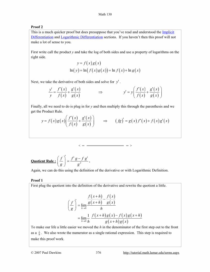
Math 130
© 2007 Paul Dawkins 376 http://tutorial.math.lamar.edu/terms.aspx
Proof 2 This is a much quicker proof but does presuppose that you’ve read and understood the Implicit Differentiation and Logarithmic Differentiation sections. If you haven’t then this proof will not make a lot of sense to you. First write call the product y and take the log of both sides and use a property of logarithms on the right side.
( ) ( )
( ) ( ) ( )( ) ( ) ( )ln ln ln ln
y f x g x
y f x g x f x g x
=
= = +
Next, we take the derivative of both sides and solve for y′ .
( )( )
( )( )
( )( )
( )( )
f x g x f x g xy y yy f x g x f x g x
′ ′ ′ ′′′= + ⇒ = +
Finally, all we need to do is plug in for y and then multiply this through the parenthesis and we get the Product Rule.
( ) ( ) ( )( )
( )( ) ( ) ( ) ( ) ( ) ( )f x g x
y f x g x fg g x f x f x g xf x g x
′ ′ ′ ′ ′= + ⇒ = +
Quotient Rule : 2
f f g f gg g
′ ′ ′ −=
.
Again, we can do this using the definition of the derivative or with Logarithmic Definition. Proof 1 First plug the quotient into the definition of the derivative and rewrite the quotient a little.
( )( )
( )( )
( ) ( ) ( ) ( )( ) ( )
0
0
lim
1lim
h
h
f x h f xg x h g xf
g hf x h g x f x g x h
h g x h g x
→
→
+−′ +
=
+ − +=
+
To make our life a little easier we moved the h in the denominator of the first step out to the front as a 1
h . We also wrote the numerator as a single rational expression. This step is required to make this proof work.

Math 130
© 2007 Paul Dawkins 377 http://tutorial.math.lamar.edu/terms.aspx
Now, for the next step will need to subtract out and add in ( ) ( )f x g x to the numerator.
( ) ( ) ( ) ( ) ( ) ( ) ( ) ( )( ) ( )0
1limh
f x h g x f x g x f x g x f x g x hfg h g x h g x→
′ + − + − + = +
The next step is to rewrite things a little,
( ) ( )
( ) ( ) ( ) ( ) ( ) ( ) ( ) ( )0
1limh
f x h g x f x g x f x g x f x g x hfg g x h g x h→
′ + − + − + = +
Note that all we did was interchange the two denominators. Since we are multiplying the fractions we can do this. Next, the larger fraction can be broken up as follows.
( ) ( )
( ) ( ) ( ) ( ) ( ) ( ) ( ) ( )0
1limh
f x h g x f x g x f x g x f x g x hfg g x h g x h h→
′ + − − + = + +
In the first fraction we will factor a ( )g x out and in the second we will factor a ( )f x− out.
This gives,
( ) ( ) ( ) ( ) ( ) ( ) ( ) ( )
0
1limh
f x h f x g x h g xf g x f xg g x h g x h h→
′ + − + − = − +
We can now use the basic properties of limits to write this as,
( ) ( ) ( )( ) ( ) ( )
( )( ) ( ) ( )
0 00 0
0 0
1 lim limlim lim
lim lim
h hh h
h h
f x h f xf g xg g x h g x h
g x h g xf x
h
→ →→ →
→ →
′ + − = − +
+ −
The individual limits are,
( ) ( ) ( ) ( ) ( ) ( ) ( )
( ) ( ) ( ) ( ) ( )
0 0 0
0 0
lim lim lim
lim lim
h h h
h h
g x h g xg x g x h g x g x g x
hf x h f x
f x f x f xh
→ → →
→ →
+ −′= + = =
+ −′= =
The first two limits in each row are nothing more than the definition the derivative for ( )g x and
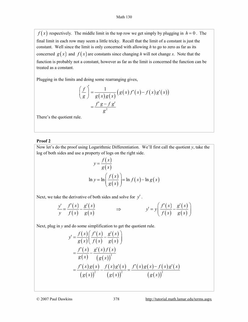
Math 130
© 2007 Paul Dawkins 378 http://tutorial.math.lamar.edu/terms.aspx
( )f x respectively. The middle limit in the top row we get simply by plugging in 0h = . The
final limit in each row may seem a little tricky. Recall that the limit of a constant is just the constant. Well since the limit is only concerned with allowing h to go to zero as far as its concerned ( )g x and ( )f x are constants since changing h will not change x. Note that the
function is probably not a constant, however as far as the limit is concerned the function can be treated as a constant. Plugging in the limits and doing some rearranging gives,
( ) ( ) ( ) ( ) ( ) ( )( )
2
1f g x f x f x g xg g x g x
f g f gg
′ ′ ′= −
′ ′−=
There’s the quotient rule.
Proof 2 Now let’s do the proof using Logarithmic Differentiation. We’ll first call the quotient y, take the log of both sides and use a property of logs on the right side.
( )( )
( )( ) ( ) ( )ln ln ln ln
f xy
g x
f xy f x g x
g x
=
= = −
Next, we take the derivative of both sides and solve for y′ .
( )( )
( )( )
( )( )
( )( )
f x g x f x g xy y yy f x g x f x g x
′ ′ ′ ′′′= − ⇒ = −
Next, plug in y and do some simplification to get the quotient rule.
( )( )
( )( )
( )( )
( )( )
( ) ( )( )( )
( ) ( )( )( )
( ) ( )( )( )
( ) ( ) ( ) ( )( )( )
2
2 2 2
f x f x g xy
g x f x g x
f x g x f xg x g x
f x g x f x g x f x g x f x g x
g x g x g x
′ ′′ = −
′ ′
= −
′ ′ ′ ′−= − =

Math 130
© 2007 Paul Dawkins 379 http://tutorial.math.lamar.edu/terms.aspx
Chain Rule If ( )f x and ( )g x are both differentiable functions and we define ( ) ( ) ( )F x f g x= o then the
derivative of F(x) is ( ) ( )( ) ( )F x f g x g x′ ′ ′= .
Proof We’ll start off the proof by defining ( )u g x= and noticing that in terms of this definition what
we’re being asked to prove is,
( ) ( )d duf u f udx dx
′=
Let’s take a look at the derivative of ( )u x (again, remember we’ve defined ( )u g x= and so u
really is a function of x) which we know exists because we are assuming that ( )g x is
differentiable. By definition we have,
( ) ( ) ( )0
limh
u x h u xu x
h→
+ −′ =
Note as well that,
( ) ( ) ( ) ( ) ( ) ( ) ( ) ( )
0 0 0lim lim lim 0h h h
u x h u x u x h u xu x u x u x u x
h h→ → →
+ − + − ′ ′ ′ ′− = − = − =
Now, define,
( )( ) ( ) ( ) if 0
0 if 0
u x h u xu x hv h h
h
+ −′− ≠=
=
and notice that ( ) ( )
0lim 0 0h
v h v→
= = and so ( )v h is continuous at 0h =
Now if we assume that 0h ≠ we can rewrite the definition of ( )v h to get,
( ) ( ) ( ) ( )( )u x h u x h v h u x′+ = + + (1)
Now, notice that (1) is in fact valid even if we let 0h = and so is valid for any value of h. Next, since we also know that ( )f x is differentiable we can do something similar. However,
we’re going to use a different set of letters/variables here for reasons that will be apparent in a bit.

Math 130
© 2007 Paul Dawkins 380 http://tutorial.math.lamar.edu/terms.aspx
So, define,
( )( ) ( ) ( ) if 0
0 if 0
f z k f zf z kw k k
k
+ −′− ≠=
=
we can go through a similar argument that we did above so show that ( )w k is continuous at
0k = and that, ( ) ( ) ( ) ( )( )f z k f z k w k f z′+ = + + (2)
Do not get excited about the different letters here all we did was use k instead of h and let x z= . Nothing fancy here, but the change of letters will be useful down the road. Okay, to this point it doesn’t look like we’ve really done anything that gets us even close to proving the chain rule. The work above will turn out to be very important in our proof however so let’s get going on the proof. What we need to do here is use the definition of the derivative and evaluate the following limit.
( ) ( ) ( )0
limh
f u x h f u xd f u xdx h→
+ − = (3)
Note that even though the notation is more than a little messy if we use ( )u x instead of u we
need to remind ourselves here that u really is a function of x. Let’s now use (1) to rewrite the ( )u x h+ and yes the notation is going to be unpleasant but
we’re going to have to deal with it. By using (1), the numerator in the limit above becomes,
( ) ( ) ( ) ( ) ( )( ) ( )f u x h f u x f u x h v h u x f u x ′+ − = + + −
If we then define ( )z u x= and ( ) ( )( )k h v h u x′= + we can use (2) to further write this as,
( ) ( ) ( ) ( ) ( )( ) ( )( ) ( ) ( )( ) ( ) ( )( ) ( )
( ) ( )( ) ( ) ( )( )
f u x h f u x f u x h v h u x f u x
f u x h v h u x w k f u x f u x
h v h u x w k f u x
′+ − = + + − ′ ′= + + + −
′ ′= + +
Notice that we were able to cancel a ( )f u x to simplify things up a little. Also, note that the
( )w k was intentionally left that way to keep the mess to a minimum here, just remember that
( ) ( )( )k h v h u x′= + here as that will be important here in a bit. Let’s now go back and
remember that all this was the numerator of our limit, (3). Plugging this into (3) gives,

Math 130
© 2007 Paul Dawkins 381 http://tutorial.math.lamar.edu/terms.aspx
( )
( ) ( )( ) ( ) ( )( )
( ) ( )( ) ( ) ( )( )0
0
lim
lim
h
h
h v h u x w k f u xd f u xdx h
v h u x w k f u x
→
→
′ ′+ + =
′ ′= + +
Notice that the h’s canceled out. Next, recall that ( ) ( )( )k h v h u x′= + and so,
( ) ( )( )0 0
lim lim 0h h
k h v h u x→ →
′= + =
But, if 0
lim 0h
k→
= , as we’ve defined k anyway, then by the definition of w and the fact that we
know ( )w k is continuous at 0k = we also know that,
( ) ( ) ( )0 0
lim lim 0 0h h
w k w k w→ →
= = =
Also, recall that ( )
0lim 0h
v h→
= . Using all of these facts our limit becomes,
( ) ( ) ( )( ) ( ) ( )( )( ) ( )
( )
0limh
d f u x v h u x w k f u xdx
u x f u x
duf u xdx
→ ′ ′= + +
′ ′=
′=
This is exactly what we needed to prove and so we’re done.

Math 130
© 2007 Paul Dawkins 382 http://tutorial.math.lamar.edu/terms.aspx
Proof of Trig Limits In this section we’re going to provide the proof of the two limits that are used in the derivation of the derivative of sine and cosine in the Derivatives of Trig Functions section of the Derivatives chapter.
Proof of : 0
sinlim 1θ
θθ→
=
This proof of this limit uses the Squeeze Theorem. However, getting things set up to use the Squeeze Theorem can be a somewhat complex geometric argument that can be difficult to follow so we’ll try to take it fairly slow. Let’s start by assuming that 20 πθ≤ ≤ . Since we are proving a limit that has 0θ → it’s okay to
assume that θ is not too large (i.e. 2πθ ≤ ). Also, by assuming that θ is positive we’re actually
going to first prove that the above limit is true if it is the right-hand limit. As you’ll see if we can prove this then the proof of the limit will be easy. So, now that we’ve got our assumption on θ taken care of let’s start off with the unit circle circumscribed by an octagon with a small slice marked out as shown below.
Points A and C are the midpoints of their respective sides on the octagon and are in fact tangent to the circle at that point. We’ll call the point where these two sides meet B. From this figure we can see that the circumference of the circle is less than the length of the octagon. This also means that if we look at the slice of the figure marked out above then the length of the portion of the circle included in the slice must be less than the length of the portion of the octagon included in the slice. Because we’re going to be doing most of our work on just the slice of the figure let’s strip that out and look at just it. Here is a sketch of just the slice.
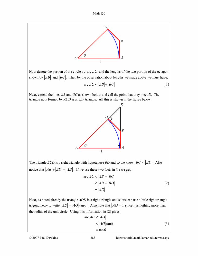
Math 130
© 2007 Paul Dawkins 383 http://tutorial.math.lamar.edu/terms.aspx
Now denote the portion of the circle by arc AC and the lengths of the two portion of the octagon shown by AB and BC . Then by the observation about lengths we made above we must have,
arc AC AB BC< + (1) Next, extend the lines AB and OC as shown below and call the point that they meet D. The triangle now formed by AOD is a right triangle. All this is shown in the figure below.
The triangle BCD is a right triangle with hypotenuse BD and so we know BC BD< . Also
notice that AB BD AD+ = . If we use these two facts in (1) we get,
arc AC AB BC
AB BD
AD
< +
< +
=
(2)
Next, as noted already the triangle AOD is a right triangle and so we can use a little right triangle trigonometry to write tanAD AO θ= . Also note that 1AO = since it is nothing more than
the radius of the unit circle. Using this information in (2) gives,
arc
tantan
AC AD
AO θ
θ
<
<
=
(3)

Math 130
© 2007 Paul Dawkins 384 http://tutorial.math.lamar.edu/terms.aspx
The next thing that we need to recall is that the length of a portion of a circle is given by the radius of the circle times the angle that traces out the portion of the circle we’re trying to measure. For our portion this means that, arc AC AO θ θ= = So, putting this into (3) we see that,
sinarc tancos
AC θθ θ
θ= < =
or, if we do a little rearranging we get,
sincos θθ
θ< (4)
We’ll be coming back to (4) in a bit. Let’s now add in a couple more lines into our figure above. Let’s connect A and C with a line and drop a line straight down from C until it intersects AO at a right angle and let’s call the intersection point E. This is all shown in the figure below.
Okay, the first thing to notice here is that, arcCE AC AC< < (5) Also note that triangle EOC is a right triangle with a hypotenuse of 1CO = . Using some right
triangle trig we can see that, sin sinCE CO θ θ= = Plugging this into (5) and recalling that arc AC θ= we get, sin arcCE ACθ θ= < = and with a little rewriting we get,
sin 1θθ
< (6)
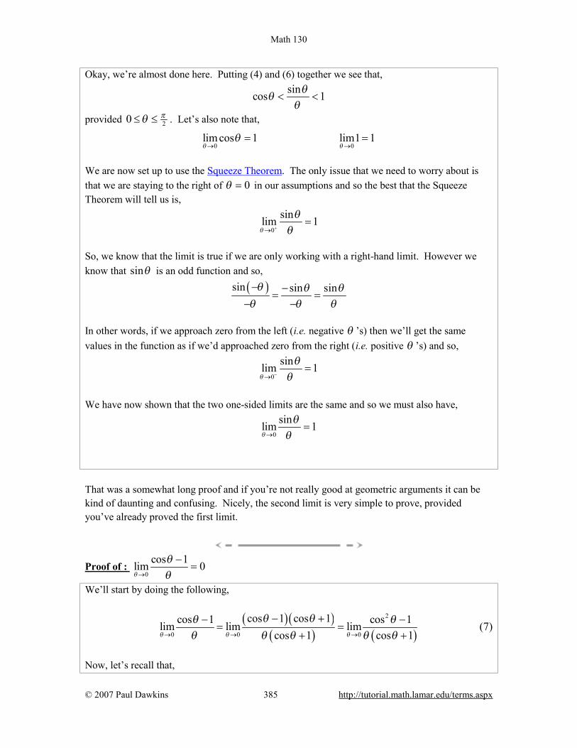
Math 130
© 2007 Paul Dawkins 385 http://tutorial.math.lamar.edu/terms.aspx
Okay, we’re almost done here. Putting (4) and (6) together we see that,
sincos 1θθ
θ< <
provided 20 πθ≤ ≤ . Let’s also note that,
0 0
lim cos 1 lim1 1θ θ
θ→ →
= =
We are now set up to use the Squeeze Theorem. The only issue that we need to worry about is that we are staying to the right of 0θ = in our assumptions and so the best that the Squeeze Theorem will tell us is,
0
sinlim 1θ
θθ+→
=
So, we know that the limit is true if we are only working with a right-hand limit. However we know that sinθ is an odd function and so,
( )sin sin sinθ θ θθ θ θ− −
= =− −
In other words, if we approach zero from the left (i.e. negative θ ’s) then we’ll get the same values in the function as if we’d approached zero from the right (i.e. positive θ ’s) and so,
0
sinlim 1θ
θθ−→
=
We have now shown that the two one-sided limits are the same and so we must also have,
0
sinlim 1θ
θθ→
=
That was a somewhat long proof and if you’re not really good at geometric arguments it can be kind of daunting and confusing. Nicely, the second limit is very simple to prove, provided you’ve already proved the first limit.
Proof of : 0
cos 1lim 0θ
θθ→
−=
We’ll start by doing the following,
( ) ( )( ) ( )
2
0 0 0
cos 1 cos 1cos 1 cos 1lim lim limcos 1 cos 1θ θ θ
θ θθ θθ θ θ θ θ→ → →
− +− −= =
+ + (7)
Now, let’s recall that,

Math 130
© 2007 Paul Dawkins 386 http://tutorial.math.lamar.edu/terms.aspx
2 2 2 2cos sin 1 cos 1 sinθ θ θ θ+ = ⇒ − = − Using this in (7) gives us,
( )2
0 0
0
0 0
cos 1 sinlim limcos 1
sin sinlimcos 1
sin sinlim limcos 1
θ θ
θ
θ θ
θ θθ θ θ
θ θθ θ
θ θθ θ
→ →
→
→ →
− −=
+
−=
+−
=+
At this point, because we just proved the first limit and the second can be taken directly we’re pretty much done. All we need to do is take the limits.
( ) ( )0 0 0
cos 1 sin sinlim lim lim 1 0 0cos 1θ θ θ
θ θ θθ θ θ→ → →
− −= = =
+
Math 130
© 2007 Paul Dawkins 387 http://tutorial.math.lamar.edu/terms.aspx
Proofs of Derivative Applications Facts/Formulas In this section we’ll be proving some of the facts and/or theorems from the Applications of Derivatives chapter. Not all of the facts and/or theorems will be proved here.
Fermat’s Theorem If ( )f x has a relative extrema at x c= and ( )f c′ exists then x c= is a critical point of
( )f x . In fact, it will be a critical point such that ( ) 0f c′ = .
Proof This is a fairly simple proof. We’ll assume that ( )f x has a relative maximum to do the proof.
The proof for a relative minimum is nearly identical. So, if we assume that we have a relative maximum at x c= then we know that ( ) ( )f c f x≥ for all x that are sufficiently close to x c= .
In particular for all h that are sufficiently close to zero (positive or negative) we must have, ( ) ( )f c f c h≥ + or, with a little rewrite we must have, ( ) ( ) 0f c h f c+ − ≤ (1) Now, at this point assume that 0h > and divide both sides of (1) by h. This gives,
( ) ( ) 0f c h f c
h+ −
≤
Because we’re assuming that 0h > we can now take the right-hand limit of both sides of this.
( ) ( )0 0
lim lim 0 0h h
f c h f ch+ +→ →
+ −≤ =
We are also assuming that ( )f c′ exists and recall that if a normal limit exists then it must be
equal to both one-sided limits. We can then say that,
( ) ( ) ( ) ( ) ( )0 0
lim lim 0h h
f c h f c f c h f cf c
h h+→ →
+ − + −′ = = ≤
If we put this together we have now shown that ( ) 0f c′ ≤ .
Okay, now let’s turn things around and assume that 0h < and divide both sides of (1) by h. This gives,
( ) ( ) 0f c h f c
h+ −
≥
Remember that because we’re assuming 0h < we’ll need to switch the inequality when we

Math 130
© 2007 Paul Dawkins 388 http://tutorial.math.lamar.edu/terms.aspx
divide by a negative number. We can now do a similar argument as above to get that,
( ) ( ) ( ) ( ) ( )0 0 0
lim lim lim 0 0h h h
f c h f c f c h f cf c
h h− −→ → →
+ − + −′ = = ≥ =
The difference here is that this time we’re going to be looking at the left-hand limit since we’re assuming that 0h < . This argument shows that ( ) 0f c′ ≥ .
We’ve now shown that ( ) 0f c′ ≤ and ( ) 0f c′ ≥ . Then only way both of these can be true at
the same time is to have ( ) 0f c′ = and this in turn means that x c= must be a critical point.
As noted above, if we assume that ( )f x has a relative minimum then the proof is nearly
identical and so isn’t shown here. The main differences are simply some inequalities need to be switched.
Fact, The Shape of a Graph, Part I 1. If ( ) 0f x′ > for every x on some interval I, then ( )f x is increasing on the interval.
2. If ( ) 0f x′ < for every x on some interval I, then ( )f x is decreasing on the interval.
3. If ( ) 0f x′ = for every x on some interval I, then ( )f x is constant on the interval. The proof of this fact uses the Mean Value Theorem which, if you’re following along in my notes has actually not been covered yet. The Mean Value Theorem can be covered at any time and for whatever the reason I decided to put where it is. Before reading through the proof of this fact you should take a quick look at the Mean Value Theorem section. You really just need the conclusion of the Mean Value Theorem for this proof however. Proof of 1 Let 1x and 2x be in I and suppose that 1 2x x< . Now, using the Mean Value Theorem on
[ ]1 2,x x means there is a number c such that 1 2x c x< < and,
( ) ( ) ( )( )2 1 2 1f x f x f c x x′− = −
Because 1 2x c x< < we know that c must also be in I and so we know that ( ) 0f c′ > we also
know that 2 1 0x x− > . So, this means that we have,
( ) ( )2 1 0f x f x− >
Math 130
© 2007 Paul Dawkins 389 http://tutorial.math.lamar.edu/terms.aspx
Rewriting this gives, ( ) ( )1 2f x f x<
and so, by definition, since 1x and 2x were two arbitrary numbers in I, ( )f x must be increasing
on I.
Proof of 2 This proof is nearly identical to the previous part. Let 1x and 2x be in I and suppose that 1 2x x< . Now, using the Mean Value Theorem on
[ ]1 2,x x means there is a number c such that 1 2x c x< < and,
( ) ( ) ( )( )2 1 2 1f x f x f c x x′− = −
Because 1 2x c x< < we know that c must also be in I and so we know that ( ) 0f c′ < we also
know that 2 1 0x x− > . So, this means that we have,
( ) ( )2 1 0f x f x− <
Rewriting this gives,
( ) ( )1 2f x f x>
and so, by definition, since 1x and 2x were two arbitrary numbers in I, ( )f x must be decreasing
on I.
Proof of 3 Again, this proof is nearly identical to the previous two parts, but in this case is actually somewhat easier. Let 1x and 2x be in I. Now, using the Mean Value Theorem on [ ]1 2,x x there is a number c such
that c is between 1x and 2x and,
( ) ( ) ( )( )2 1 2 1f x f x f c x x′− = −
Note that for this part we didn’t need to assume that 1 2x x< and so all we know is that c is
between 1x and 2x and so, more importantly, c is also in I. and this means that ( ) 0f c′ = . So,
this means that we have,

Math 130
© 2007 Paul Dawkins 390 http://tutorial.math.lamar.edu/terms.aspx
( ) ( )2 1 0f x f x− =
Rewriting this gives,
( ) ( )1 2f x f x=
and so, since 1x and 2x were two arbitrary numbers in I, ( )f x must be constant on I.
Fact, The Shape of a Graph, Part II Given the function ( )f x then,
1. If ( ) 0f x′′ > for all x in some interval I then ( )f x is concave up on I.
2. If ( ) 0f x′′ < for all x in some interval I then ( )f x is concave down on I. The proof of this fact uses the Mean Value Theorem which, if you’re following along in my notes has actually not been covered yet. The Mean Value Theorem can be covered at any time and for whatever the reason I decided to put it after the section this fact is in. Before reading through the proof of this fact you should take a quick look at the Mean Value Theorem section. You really just need the conclusion of the Mean Value Theorem for this proof however. Proof of 1 Let a be any number in the interval I. The tangent line to ( )f x at x a= is,
( ) ( )( )y f a f a x a′= + −
To show that ( )f x is concave up on I then we need to show that for any x, x a≠ , in I that,
( ) ( ) ( )( )f x f a f a x a′> + −
or in other words, the tangent line is always below the graph of ( )f x on I. Note that we require
x a≠ because at that point we know that ( ) ( )f x f a= since we are talking about the tangent
line. Let’s start the proof off by first assuming that x a> . Using the Mean Value Theorem on [ ],a x
means there is a number c such that a c x< < and, ( ) ( ) ( )( )f x f a f c x a′− = −
With some rewriting this is,
Math 130
© 2007 Paul Dawkins 391 http://tutorial.math.lamar.edu/terms.aspx
( ) ( ) ( ) ( )f x f a f c x a′= + − (2)
Next, let’s use the fact that ( ) 0f x′′ > for every x on I. This means that the first derivative,
( )f x′ , must be increasing (because its derivative, ( )f x′′ , is positive). Now, we know from the
Mean Value Theorem that a c< and so because ( )f x′ is increasing we must have,
( ) ( )f a f c′ ′< (3)
Recall as well that we are assuming x a> and so 0x a− > . If we now multiply (3) by x a− (which is positive and so the inequality stays the same) we get,
( ) ( ) ( )( )f a x a f c x a′ ′− < −
Next, add ( )f a to both sides of this to get,
( ) ( )( ) ( ) ( )( )f a f a x a f a f c x a′ ′+ − < + −
However, by (2), the right side of this is nothing more than ( )f x and so we have,
( ) ( )( ) ( )f a f a x a f x′+ − <
but this is exactly what we wanted to show. So, provided x a> the tangent line is in fact below the graph of ( )f x .
We now need to assume x a< . Using the Mean Value Theorem on [ ],x a means there is a
number c such that x c a< < and, ( ) ( ) ( )( )f a f x f c a x′− = −
If we multiply both sides of this by –1 and then adding ( )f a to both sides and we again arise at
(2). Now, from the Mean Value Theorem we know that c a< and because ( ) 0f x′′ > for every x on
I we know that the derivative is still increasing and so we have, ( ) ( )f c f a′ ′<
Let’s now multiply this by x a− , which is now a negative number since x a< . This gives,
( )( ) ( )( )f c x a f a x a′ ′− > −
Notice that we had to switch the direction of the inequality since we were multiplying by a

Math 130
© 2007 Paul Dawkins 392 http://tutorial.math.lamar.edu/terms.aspx
negative number. If we now add ( )f a to both sides of this and then substitute (2) into the
results we arrive at,
( ) ( ) ( ) ( ) ( ) ( )
( ) ( ) ( ) ( )f a f c x a f a f a x a
f x f a f a x a
′ ′+ − > + −
′> + −
So, again we’ve shown that the tangent line is always below the graph of ( )f x .
We’ve now shown that if x is any number in I, with x a≠ the tangent lines are always below the graph of ( )f x on I and so ( )f x is concave up on I.
Proof of 2 This proof is nearly identical to the proof of 1 and since that proof is fairly long we’re going to just get things started and then leave the rest of it to you to go through. Let a be any number in I . To show that ( )f x is concave down we need to show that for any x
in I, x a≠ , that the tangent line is always above the graph of ( )f x or,
( ) ( ) ( ) ( )f x f a f a x a′< + −
From this point on the proof is almost identical to the proof of 1 except that you’ll need to use the fact that the derivative in this case is decreasing since ( ) 0f x′′ < . We’ll leave it to you to fill in
the details of this proof.
Second Derivative Test Suppose that x c= is a critical point of ( )f c′ such that ( ) 0f c′ = and that ( )f x′′ is
continuous in a region around x c= . Then, 1. If ( ) 0f c′′ < then x c= is a relative maximum.
2. If ( ) 0f c′′ > then x c= is a relative minimum.
3. If ( ) 0f c′′ = then x c= can be a relative maximum, relative minimum or neither. The proof of this fact uses the Mean Value Theorem which, if you’re following along in my notes has actually not been covered yet. The Mean Value Theorem can be covered at any time and for whatever the reason I decided to put it after the section this fact is in. Before reading through the

Math 130
© 2007 Paul Dawkins 393 http://tutorial.math.lamar.edu/terms.aspx
proof of this fact you should take a quick look at the Mean Value Theorem section. You really just need the conclusion of the Mean Value Theorem for this proof however. Proof of 1 First since we are assuming that ( )f x′′ is continuous in a region around x c= then we can
assume that in fact ( ) 0f c′′ < is also true in some open region, say ( ),a b around x c= , i.e.
a c b< < . Now let x be any number such that a x c< < , we’re going to use the Mean Value Theorem on
[ ],x c . However, instead of using it on the function itself we’re going to use it on the first
derivative. So, the Mean Value Theorem tells us that there is a number x d c< < such that, ( ) ( ) ( ) ( )f c f x f d c x′ ′ ′′− = −
Now, because a x d c< < < we know that ( ) 0f d′′ < and we also know that 0c x− > so we
then get that,
( ) ( ) 0f c f x′ ′− <
However, we also assumed that ( ) 0f c′ = and so we have,
( ) ( )0 0f x f x′ ′− < ⇒ >
Or, in other words to the left of x c= the function is increasing. Let’s now turn things around and let x be any number such that c x b< < and use the Mean Value Theorem on [ ],c x and the first derivative. The Mean Value Theorem tells us that there is
a number c d x< < such that, ( ) ( ) ( ) ( )f x f c f d x c′ ′ ′′− = −
Now, because c d x b< < < we know that ( ) 0f d′′ < and we also know that 0x c− > so we
then get that,
( ) ( ) 0f x f c′ ′− <
Again use the fact that we also assumed that ( ) 0f c′ = to get,
( ) 0f x′ <
We now know that to the right of x c= the function is decreasing.

Math 130
© 2007 Paul Dawkins 394 http://tutorial.math.lamar.edu/terms.aspx
So, to the left of x c= the function is increasing and to the right of x c= the function is decreasing so by the first derivative test this means that x c= must be a relative maximum.
Proof of 2 This proof is nearly identical to the proof of 1 and since that proof is somewhat long we’re going to leave the proof to you to do. In this case the only difference is that now we are going to assume that ( ) 0f x′′ < and that will give us the opposite signs of the first derivative on either
side of x c= which gives us the conclusion we were after. We’ll leave it to you to fill in all the details of this.
Proof of 3 There isn’t really anything to prove here. All this statement says is that any of the three cases are possible and to “prove” this all one needs to do is provide an example of each of the three cases. This was done in The Shape of a Graph, Part II section where this test was presented so we’ll leave it to you to go back to that section to see those graphs to verify that all three possibilities really can happen.
Rolle’s Theorem Suppose ( )f x is a function that satisfies all of the following.
1. ( )f x is continuous on the closed interval [a,b].
2. ( )f x is differentiable on the open interval (a,b).
3. ( ) ( )f a f b=
Then there is a number c such that a c b< < and ( ) 0f c′ = . Or, in other words ( )f x has a
critical point in (a,b). Proof We’ll need to do this with 3 cases. Case 1 : ( )f x k= on [a,b] where k is a constant.
In this case ( ) 0f x′ = for all x in [a,b] and so we can take c to be any number in [a,b].
Math 130
© 2007 Paul Dawkins 395 http://tutorial.math.lamar.edu/terms.aspx
Case 2 : There is some number d in (a,b) such that ( ) ( )f d f a> .
Because ( )f x is continuous on [a,b] by the Extreme Value Theorem we know that ( )f x will
have a maximum somewhere in [a,b]. Also, because ( ) ( )f a f b= and ( ) ( )f d f a> we
know that in fact the maximum value will have to occur at some c that is in the open interval (a,b), or a c b< < . Because c occurs in the interior of the interval this means that ( )f x will
actually have a relative maximum at x c= and by the second hypothesis above we also know that ( )f c′ exists. Finally, by Fermat’s Theorem we then know that in fact x c= must be a
critical point and because we know that ( )f c′ exists we must have ( ) 0f c′ = (as opposed to
( )f c′ not existing…).
Case 3 : There is some number d in (a,b) such that ( ) ( )f d f a< .
This is nearly identical to Case 2 so we won’t put in quite as much detail. By the Extreme Value Theorem ( )f x will have minimum in [a,b] and because ( ) ( )f a f b= and ( ) ( )f d f a< we
know that the minimum must occur at x c= where a c b< < . Finally, by Fermat’s Theorem we know that ( ) 0f c′ = .
The Mean Value Theorem Suppose ( )f x is a function that satisfies both of the following.
1. ( )f x is continuous on the closed interval [a,b].
2. ( )f x is differentiable on the open interval (a,b). Then there is a number c such that a < c < b and
( ) ( ) ( )f b f af c
b a−
′ =−
Or,
( ) ( ) ( )( )f b f a f c b a′− = −

Math 130
© 2007 Paul Dawkins 396 http://tutorial.math.lamar.edu/terms.aspx
Proof For illustration purposes let’s suppose that the graph of ( )f x is,
Note of course that it may not look like this, but we just need a quick sketch to make it easier to see what we’re talking about here. The first thing that we need is the equation of the secant line that goes through the two points A and B as shown above. This is,
( ) ( ) ( ) ( )f b f ay f a x a
b a−
= + −−
Let’s now define a new function, ( )g x , as to be the difference between ( )f x and the equation
of the secant line or,
( ) ( ) ( ) ( ) ( ) ( ) ( ) ( ) ( ) ( ) ( )f b f a f b f ag x f x f a x a f x f a x a
b a b a− −
= − + − = − − − − −
Next, let’s notice that because ( )g x is the sum of ( )f x , which is assumed to be continuous on
[a,b], and a linear polynomial, which we know to be continuous everywhere, we know that ( )g x
must also be continuous on [a,b]. Also, we can see that ( )g x must be differentiable on (a,b) because it is the sum of ( )f x , which
is assumed to be differentiable on (a,b), and a linear polynomial, which we know to be differentiable. We could also have just computed the derivative as follows,
( ) ( ) ( ) ( )f b f ag x f x
b a−
′ ′= −−

Math 130
© 2007 Paul Dawkins 397 http://tutorial.math.lamar.edu/terms.aspx
at which point we can see that it exists on (a,b) because we assumed that ( )f x′ exists on (a,b)
and the last term is just a constant. Finally, we have,
( ) ( ) ( ) ( ) ( ) ( ) ( ) ( )
( ) ( ) ( ) ( ) ( ) ( ) ( ) ( ) ( ) ( )( )
0
0
f b f ag a f a f a a a f a f a
b a
f b f ag b f b f a b a f b f a f b f a
b a
−= − − − = − =
−
−= − − − = − − − =
−
In other words, ( )g x satisfies the three conditions of Rolle’s Theorem and so we know that
there must be a number c such that a c b< < and that,
( ) ( ) ( ) ( ) ( ) ( ) ( )0f b f a f b f a
g c f c f cb a b a
− −′ ′ ′= = − ⇒ =
− −

Math 130
© 2007 Paul Dawkins 398 http://tutorial.math.lamar.edu/terms.aspx
Types of Infinity Most students have run across infinity at some point in time prior to a calculus class. However, when they have dealt with it, it was just a symbol used to represent a really, really large positive or really, really large negative number and that was the extent of it. Once they get into a calculus class students are asked to do some basic algebra with infinity and this is where they get into trouble. Infinity is NOT a number and for the most part doesn’t behave like a number. However, despite that we’ll think of infinity in this section as a really, really, really large number that is so large there isn’t another number larger than it. This is not correct of course, but may help with the discussion in this section. Note as well that everything that we’ll be discussing in this section applies only to real numbers. If you move into complex numbers for instance things can and do change. So, let’s start thinking about addition with infinity. When you add two non-zero numbers you get a new number. For example, 4 7 11+ = . With infinity this is not true. With infinity you have the following.
where a a∞ + = ∞ ≠ −∞∞ + ∞ = ∞
In other words, a really, really large positive number ( ∞ ) plus any positive number, regardless of the size, is still a really, really large positive number. Likewise, you can add a negative number (i.e. 0a < ) to a really, really large positive number and stay really, really large and positive. So, addition involving infinity can be dealt with in an intuitive way if you’re careful. Note as well that the a must NOT be negative infinity. If it is, there are some serious issues that we need to deal with as we’ll see in a bit. Subtraction with negative infinity can also be dealt with in an intuitive way in most cases as well. A really, really large negative number minus any positive number, regardless of its size, is still a really, really large negative number. Subtracting a negative number (i.e. 0a < ) from a really, really large negative number will still be a really, really large negative number. Or,
where a a−∞ − = −∞ ≠ −∞−∞ − ∞ = −∞
Again, a must not be negative infinity to avoid some potentially serious difficulties. Multiplication can be dealt with fairly intuitively as well. A really, really large number (positive, or negative) times any number, regardless of size, is still a really, really large number we’ll just need to be careful with signs. In the case of multiplication we have
( ) ( ) ( )( )
( ) ( ) ( ) ( ) ( ) ( )if 0 if 0a a a a∞ = ∞ > ∞ = −∞ <
∞ ∞ = ∞ −∞ −∞ = ∞ −∞ ∞ = −∞
What you know about products of positive and negative numbers is still true here. Some forms of division can be dealt with intuitively as well. A really, really large number divided by a number that isn’t too large is still a really, really large number.
Math 130
© 2007 Paul Dawkins 399 http://tutorial.math.lamar.edu/terms.aspx
if 0, if 0,
if 0, if 0,
a a a aa a
a a a aa a
∞ ∞= ∞ > ≠ ∞ = −∞ < ≠ −∞
−∞ −∞= −∞ > ≠ ∞ = ∞ < ≠ −∞
Division of a number by infinity is somewhat intuitive, but there are a couple of subtleties that you need to be aware of. When we talk about division by infinity we are really talking about a limiting process in which the denominator is going towards infinity. So, a number that isn’t too large divided an increasingly large number is an increasingly small number. In other words in the limit we have,
0 0a a= =
∞ −∞
So, we’ve dealt with almost every basic algebraic operation involving infinity. There are two cases that that we haven’t dealt with yet. These are
? ?± ∞∞ − ∞ = =
± ∞
The problem with these two cases is that intuition doesn’t really help here. A really, really large number minus a really, really large number can be anything ( −∞ , a constant, or ∞ ). Likewise, a really, really large number divided by a really, really large number can also be anything ( ±∞ – this depends on sign issues, 0, or a non-zero constant). What we’ve got to remember here is that there are really, really large numbers and then there are really, really, really large numbers. In other words, some infinities are larger than other infinities. With addition, multiplication and the first sets of division we worked this wasn’t an issue. The general size of the infinity just doesn’t affect the answer in those cases. However, with the subtraction and division cases listed above, it does matter as we will see. Here is one way to think of this idea that some infinities are larger than others. This is a fairly dry and technical way to think of this and your calculus problems will probably never use this stuff, but this it is a nice way of looking at this. Also, please note that I’m not trying to give a precise proof of anything here. I’m just trying to give you a little insight into the problems with infinity and how some infinities can be thought of as larger than others. For a much better (and definitely more precise) discussion see, http://www.math.vanderbilt.edu/~schectex/courses/infinity.pdf Let’s start by looking at how many integers there are. Clearly, I hope, there are an infinite number of them, but let’s try to get a better grasp on the “size” of this infinity. So, pick any two integers completely at random. Start at the smaller of the two and list, in increasing order, all the integers that come after that. Eventually we will reach the larger of the two integers that you picked.

Math 130
© 2007 Paul Dawkins 400 http://tutorial.math.lamar.edu/terms.aspx
Depending on the relative size of the two integers it might take a very, very long time to list all the integers between them and there isn’t really a purpose to doing it. But, it could be done if we wanted to and that’s the important part. Because we could list all these integers between two randomly chosen integers we say that the integers are countably infinite. Again, there is no real reason to actually do this, it is simply something that can be done if we should chose to do so. In general a set of numbers is called countably infinite if we can find a way to list them all out. In a more precise mathematical setting this is generally done with a special kind of function called a bijection that associates each number in the set with exactly one of the positive integers. To see some more details of this see the pdf given above. It can also be shown that the set of all fractions are also countably infinite, although this is a little harder to show and is not really the purpose of this discussion. To see a proof of this see the pdf given above. It has a very nice proof of this fact. Let’s contrast this by trying to figure out how many numbers there are in the interval (0,1). By numbers, I mean all possible fractions that lie between zero and one as well as all possible decimals (that aren’t fractions) that lie between zero and one. The following is similar to the proof given in the pdf above, but was nice enough and easy enough (I hope) that I wanted to include it here. To start let’s assume that all the numbers in the interval (0,1) are countably infinite. This means that there should be a way to list all of them out. We could have something like the following,
1
2
3
4
0.6920960.1710340.9936710.045908
xxxx
====
LLLL
M M
Now, select the ith decimal out of ix as shown below
1
2
3
4
0.6920960.1710340.9936710.045908
xxxx
====
LLLL
M M
and form a new number with these digits. So, for our example we would have the number 0.6739x = L In this new decimal replace all the 3’s with a 1 and replace every other numbers with a 3. In the case of our example this would yield the new number

Math 130
© 2007 Paul Dawkins 401 http://tutorial.math.lamar.edu/terms.aspx
0.3313x = L Notice that this number is in the interval (0,1) and also notice that given how we choose the digits of the number this number will not be equal to the first number in our list, 1x , because the first digit of each is guaranteed to not be the same. Likewise, this new number will not get the same number as the second in our list, 2x , because the second digit of each is guaranteed to not be the
same. Continuing in this manner we can see that this new number we constructed, x , is guaranteed to not be in our listing. But this contradicts the initial assumption that we could list out all the numbers in the interval (0,1). Hence, it must not be possible to list out all the numbers in the interval (0,1). Sets of numbers, such as all the numbers in (0,1), that we can’t write down in a list are called uncountably infinite. The reason for going over this is the following. An infinity that is uncountably infinite is significantly larger than an infinity that is only countably infinite. So, if we take the difference of two infinities we have a couple of possibilities.
( ) ( )( ) ( )
uncountable countable
countable uncountable
∞ − ∞ = ∞
∞ − ∞ = −∞
Notice that we didn’t put down a difference of two infinities of the same type. Depending upon the context there might still have some ambiguity about just what the answer would be in this case, but that is a whole different topic. We could also do something similar for quotients of infinities.
( )( )( )( )
countable
uncountable
uncountable
countable
0∞
=∞
∞= ∞
∞
Again, we avoided a quotient of two infinities of the same type since, again depending upon the context, there might still be ambiguities about its value. So, that’s it and hopefully you’ve learned something from this discussion. Infinity simply isn’t a number and because there are different kinds of infinity it generally doesn’t behave as a number does. Be careful when dealing with infinity.
Math 130
© 2007 Paul Dawkins 402 http://tutorial.math.lamar.edu/terms.aspx
Summation Notation In this section we need to do a brief review of summation notation or sigma notation. We’ll start out with two integers, n and m, with n m< and a list of numbers denoted as follows, 1 2 2 1, , , , , ,n n n m m ma a a a a a+ + − −… We want to add them up, in other words we want, 1 2 2 1n n n m m ma a a a a a+ + − −+ + + + + +… For large lists this can be a fairly cumbersome notation so we introduce summation notation to denote these kinds of sums. The case above is denoted as follows.
1 2 2 1
m
i n n n m m mi n
a a a a a a a+ + − −=
= + + + + + +∑ …
The i is called the index of summation. This notation tells us to add all the ai’s up for all integers starting at n and ending at m. For instance,
( ) ( ) ( ) ( ) ( )
4
06
2 1 4 9 5 11 6 13 9 11 13
44
* * * * *1 2 3 4
1
0 1 2 3 4 163 2.716661 0 1 1 1 2 1 3 1 4 1 60
2 2 2 2 16 32 64
i
i i
i
ii
ii
x x x x x x x
f x f x f x f x f x
=
+
=
=
= + + + + = =+ + + + + +
= + + = + +
= + + +
∑
∑
∑
Properties Here are a couple of formulas for summation notation.
1. 0 0
n n
i ii i i i
ca c a= =
=∑ ∑ where c is any number. So, we can factor constants out of a summation.
2. ( )0 0 0
n n n
i i i ii i i i i i
a b a b= = =
± = ±∑ ∑ ∑ So we can break up a summation across a sum or difference.
Note that we started the series at 0i to denote the fact that they can start at any value of i that we
need them to. Also note that while we can break up sums and differences as we did in 2 above we can’t do the same thing for products and quotients. In other words,
( ) 0
0 0 0 0
0
n
in n n ni ii
i i i i ni i i i i i i i i
ii i
aaa b a bb b
=
= = = =
=
≠ ≠
∑∑ ∑ ∑ ∑
∑

Math 130
© 2007 Paul Dawkins 403 http://tutorial.math.lamar.edu/terms.aspx
Formulas Here are a couple of nice formulas that we will find useful in a couple of sections. Note that these formulas are only true if starting at 1i = . You can, of course, derive other formulas from these for different starting points if you need to.
1. 1
n
ic cn
=
=∑
2. ( )1
12
n
i
n ni
=
+=∑
3. ( ) ( )2
1
1 2 16
n
i
n n ni
=
+ +=∑
4. ( ) 23
1
12
n
i
n ni
=
+ =
∑
Here is a quick example on how to use these properties to quickly evaluate a sum that would not be easy to do by hand. Example 1 Using the formulas and properties from above determine the value of the following summation.
( )100
2
13 2
ii
=
−∑
Solution The first thing that we need to do is square out the stuff being summed and then break up the summation using the properties as follows,
( )100 100
2 2
1 1100 100 100
2
1 1 1100 100 100
2
1 1 1
3 2 9 12 4
9 12 4
9 12 4
i i
i i i
i i i
i i i
i i
i i
= =
= = =
= = =
− = − +
= − +
= − +
∑ ∑
∑ ∑ ∑
∑ ∑ ∑
Now, using the formulas, this is easy to compute,
( ) ( ) ( ) ( ) ( )1002
1
100 101 100 101 2013 2 9 100 12 4
2 61293700
ii
=
− = − +
=
∑
Doing this by hand would definitely taken some time and there’s a good chance that we might have made a minor mistake somewhere along the line.

Math 130
© 2007 Paul Dawkins 404 http://tutorial.math.lamar.edu/terms.aspx