math101 algebra and differential calculus lecture …mcs.une.edu.au/~math101/lectures/lecture notes...
TRANSCRIPT
University of New England
School of Science and Technology
MATH101
ALGEBRA AND
DIFFERENTIAL CALCULUS
Lecture Notes Part 1
Trimester 1, 2015
c©University of New England
CRICOS Provider No: 00003G

CONTENTS i
Contents
Preface . . . . . . . . . . . . . . . . . . . . . . . . . . . . . . . . . . . . . . iii
Lecture 1.1 Mathematical Language and Proof . . . . . . . . . . . . . . . 1
Lecture 1.2 Important Types of Theorems and Proof . . . . . . . . . . . 7
Lecture 1.3 Sets and Functions . . . . . . . . . . . . . . . . . . . . . . . . 14
Lecture 1.4 Numbers . . . . . . . . . . . . . . . . . . . . . . . . . . . . . 22
Lecture 1.5 Some Properties of Real Numbers . . . . . . . . . . . . . . . 27
Lecture 1.6 Complex Numbers . . . . . . . . . . . . . . . . . . . . . . . . 33
Lecture 1.7 Complex Numbers (continued) . . . . . . . . . . . . . . . . . 40
Lecture 1.8 Functions on R . . . . . . . . . . . . . . . . . . . . . . . . . . 48
Lecture 1.9 Limits . . . . . . . . . . . . . . . . . . . . . . . . . . . . . . . 56
Lecture 1.10 Limits and Continuous Functions . . . . . . . . . . . . . . . 63
Lecture 1.11 Continuous Functions . . . . . . . . . . . . . . . . . . . . . 69
Lecture 1.12 More on Continuity . . . . . . . . . . . . . . . . . . . . . . . 76
Lecture 1.13 Sequences . . . . . . . . . . . . . . . . . . . . . . . . . . . . 82
Lecture 1.14 Sequences and Series . . . . . . . . . . . . . . . . . . . . . . 88
Lecture 1.15 Series . . . . . . . . . . . . . . . . . . . . . . . . . . . . . . 94

ii CONTENTS

iii
Preface
Mathematics today is a vast enterprise. Advances and breakthroughs have been
painstakingly built on the structure(s) erected by earlier mathematicians. The his-
tory of mathematics is quite different from the that of other human endeavours. In
other fields, previously held views are typically extended or proved wrong with each
advance there is a process of correction and extension. “Only in mathematics is
there no significant correction – only extension”.
The work of Euclid has certainly been extended many times. Euclid, however,
has not been corrected – his theorems are valid today and for all time! The other
remarkable thing about mathematics is its extraordinary utility in describing and
quantifying the world around us. Mathematics is the language of the sciences, both
natural and social. This forces mathematics to be abstract, since it must embrace
theories from physics, economics, chemistry, psychology, etc. Mathematics is so
widely applicable precisely because of — not despite — its intrinsic abstractness.
MATH101 is the first half of the MATH101/102 sequence, which lays the founda-
tion for all further study and application of mathematics and statistics, presenting
an introduction to differential calculus, integral calculus, algebra, differential equa-
tions and statistics, providing sound mathematical foundations for further studies
not only in mathematics and statistics, but also in the natural and social sciences.
Achieving this, requires a brief, preliminary foray into the basics of mathematics,
because much of the material requires a high degree of abstract reasoning, rather
than rote learning of computational techniques.
A rigorous approach to the basics provides a deeper understanding of the whole
structure. The assumptions upon which the structure is built are thereby clarifed,
with both the scope and limitations of the intellectual framework made readily
understandable. Moreover, this deeper understanding, does not come at the expense
of applicability. Quite the contrary!
One consequence of providing sound fundamentals is that there is considerable
time devoted to matters whose importance and applicability is not immediately ob-
vious. But such study of these fundamental areas of mathematics is also stimulating.
If you enjoy puzzles here is an “intellectual game” par excellence. A game played
within a rigid framework of rules, but with unlimited scope for creativity in the
search for problems and the solutions to problems.
This is the first of three parts of the lecture notes which together constitute the
unit material for MATH101. These notes were originally prepared by Chris Radford
and have been revised by Shusen Yan and others.

iv Preface
The reader is invited and encouraged to point out any mistakes (s)he finds. I
hope you enjoy the challenges the unit offers and that you experience a sense of
achievement at the end.
Bea Bleile
UNE

Lecture 1.1 Mathematical Language and Proof 1
Lecture 1.1 Mathematical Language and Proof
Introduction
What is research in mathematics? A mathematician would answer “proving
theorems”. The language and etiquette of mathematics has evolved over a long
period of time. Terms such as theorem, axiom, definition and proof have a universal
and well understood meaning. It is these conventions and definitions we want to
examine in this lecture.
Basic Terminology
Statement: A statement is a sentence which is either true or false
(according to some previously accepted criteria). Statements do not
include exclamations, questions or orders. A statement cannot be
true and false at the same time.
A statement is simple when it cannot be broken down into other statements. A
statement is compound when it contains more than one simple statement.
�Example “I will have a BBQ and it will rain” is a compound statement consisting
of two simple statements. “I will have a BBQ” and “It will rain”.
Definition: A definition is a statement of the precise meaning of a
word, phrase, mathematical symbol or concept.
In trying to understand a piece of mathematics it is important to have a good
working understanding of the initial definitions. You need to look at examples which
satisfy and do not satisfy the definitions.
Theorem: A theorem is a mathematical statement that can be proved
true by a chain of logical argument based on assumptions that are
given or implied in the statement of the theorem.
A theorem will give a deeper insight into the structure of a piece of mathematics.
Lemma: A lemma is a preliminary theorem read in the proof of
another theorem.

2 Lecture 1.1 Mathematical Language and Proof
Some theorems can have proofs that are long and intricate. It is useful in such
cases to break the proof into intermediate steps which are separated out as lemmas
which lead into the main result.
Corollary: A corollary is a theorem that is a natural consequence
of a preceding theorem. Generally, a corollary will follow in a rel-
atively easy and straight-forward way from the previous theorem or
proposition.
Proof: A proof of a proposition, theorem, lemma or corollary is a
sequence of logical reasoning. It is based on the given assumptions
or hypothesis and aims to establish the truth of the proposition or
theorem.
Basic Techniques of Proof
Implication
Consider the following compound statement: “If I pass MATH101 then I will do
MATH 102”. Under what circumstances is this statement true or false?
Let’s have a look at the two simple statements making up this compound state-
ment.
A. I pass MATH101.
B. I will do MATH102.
For statement A there are two possibilities,
1. I do pass MATH101 (A is true).
2. I fail MATH101 (A is false).
There are also two possibilities for B,
1. I will enrol in MATH102 (B is true).
2. I will not enrol in MATH102 (B is false).

Lecture 1.1 Mathematical Language and Proof 3
So we have to consider four possibilities:
A B
1. True True
2. True False
3. False True
4. False False
As well as the truth or otherwise of A and B, individually, we must consider the
truth of the original compound statement which takes the form of an implication.
This compound statement is “If A then B”. We enlarge our table above to include a
column for “If A then B”. We must decide for each of the four cases if the compound
entry is True or False.
Case 1: I pass MATH101 and enrol in MATH 102. The implication is True.
Case 2: I pass 101 and do not enrol in 102. Implication is False.
Case 3: I do not pass 101 but still enrol in 102. My original statement is not a
lie, it is not a falsehood. Implication is True.
Case 4: I do not pass 101 and do not enrol in 102. Again, my original statement
is not a lie or a falsehood. Implication is True.
A B If A then B
1. True True True
2. True False False
3. False True True
4. False False True
There is only one case when the implication is false, ie. when A is true and B is
false.
The implication “If A then B” is true if we can prove that it is
impossible to have A true and B false at the same time.
This means if we assume “A implies B” to be true and we also assume that A is
true then we must conclude that B is true.
The statement “if A then B” is equivalent to the statement “A is a
sufficient condition for B” and to the statement “B is a necessary
condition for A”.

4 Lecture 1.1 Mathematical Language and Proof
Notice that in a statement of the form “A implies B” the hypothesis, part A, is
clearly distinguished from the conclusion, part B. A direct proof of a mathematical
implication, “A implies B”, proceeds on the assumption that the hypothesis A is
true. The proof will work via a series of logically connected steps to obtain the
conclusion B.
�Example Prove that the sum of two prime numbers larger than 2 is an even
number.
Solution We formulate this as an implication:
“If p and q are prime numbers larger than 2 then p+ q is even”.
The hypothesis “p and q are prime numbers larger than 2” assumes that we know
what prime numbers are. A prime number is a natural or counting number divisible
only by itself and one – 2, 3, 5, 7, 11, 13, 17, 19, 23 are prime numbers.
So we are to assume p and q are prime numbers bigger than 2. We must then
construct a series of arguments which lead directly to the conclusion that p + q is
divisible by 2 (i.e. p+ q is even).
Firstly, we see that p and q must be odd. We must be careful about this point
because 2 is prime but even! However, for primes greater than 2 we note that a
prime cannot be divisible by 2; so it must have remainder 1 after division by 2. So
there must be counting numbers n and m such that
p = 2n+ 1
q = 2m+ 1
This really just says that p and q are odd. We can now move to our conclusion,
p+ q = (2n+ 1) + (2m+ 1)
= 2n+ 2m+ 2
= 2(n+m+ 1).
We conclude that p+ q is divisible by 2 and so p+ q is even. 2
This is a direct proof as we moved directly from the (assumed true) hypothesis,
“p and q are prime numbers larger than 2” directly to the conclusion “p + q is an
even number”.

Lecture 1.1 Mathematical Language and Proof 5
Proof by Contradiction
Recall that the implication “If A then B” can only be false if we have A true
and B false. So if we were to assume B to be false and prove, as a consequence,
that A is necessarily false, then we have proved the implication is true. We would
have shown that the only possible case with B false is A false which contradicts the
assumed truth of the hypothesis. This is proof by contradiction.
In general one tries to avoid using a proof by contradiction. If a direct proof is
straightforward then this is to be preferred – a direct proof usually provides more
insight into the mathematical structure at hand.
�Example Prove that if p is a prime number larger than 2 then p+1 is not prime.
Solution We formulate this statement as an implication with hypothesis “p is a
prime number larger than 2” and conclusion “p+ 1 is not prime”.
We will use a proof by contradiction. Assume the conclusion is false. We need
the negative of the statement “p + 1 is not prime”. This means we must assume
that “p+ 1 is prime”.
So our starting assumptions are now
“p is a prime number larger than 2” (hypothesis)
“p+ 1 is prime” (negative of the conclusion).
We are now free to use any means at our disposal to find a contradiction based on
these two assumptions. If we can find such a contradiction then we have established
the truth of the original implication.
We will use the result established in the previous example.
We have two primes p and p+1 both larger than 2, so we know that p+ (p+1)
must be even (this is the result of our earlier exercise). But this is clearly false as
p+ (p+ 1) = 2p+ 1 is an odd number.
We have a contradiction. Our proof is complete, our assumption that the con-
clusion is false cannot hold, the conclusion must be true. 2
6 Lecture 1.1 Mathematical Language and Proof
♠ Exercises 1
1. Construct a direct proof for the last example, above.
2. Use a direct proof technique to prove that if (a + b)2 = a2 + b2 for all real
numbers b, then a = 0.
*3. Let n be a counting number. If 2n − 1 is a prime number prove that n is also
prime. Use a proof by contradiction to establish the truth of this statement.

Lecture 1.2 Important Types of Theorems and Proof 7
Lecture 1.2 Important Types of Theorems and Proof
In your mathematical reading you will find that there are certain types of theorem
whose statement and proof follow a standard pattern. Our aim here is to look at a
couple of the more important examples.
Equivalence or “If and Only If” Theorems.
The statement of theorems of this type takes one of the following possible forms
“A is true if and only if B is true”
“A is false if and only if B is false”
“A is equivalent to B”.
Notice that these forms are all basically equivalent – the truth (or falsity) of A
automatically implies the truth (or falsity) of B and vice versa. So to prove such a
theorem we have to produce two proofs:
one proof for “A implies B” and
one proof for “B implies A”.
The first proof says A is sufficient for B (or B is necessary for A). The second
proof says B is sufficient for A (or A is necessary for B). In fact another com-
mon statement of equivalence is a theorem which takes the following form, “A is a
necessary and sufficient condition for B”.
�Example Let n be a counting number. Then n is odd if and only if n2 is odd.
Solution Let A be the statement “n is odd” and let B be the statement “n2 is
odd”.
We have to prove two implications
1. A implies B
2. B implies A
Firstly, let’s examine A implies B. We’ll provide a direct proof. So we assume
A, that is, we assume n is an odd counting number. This means there is a counting
number r such that
n = 2r + 1
8 Lecture 1.2 Important Types of Theorems and Proof
(any odd number is one plus an even number). Then we have
n2 = (2r + 1)2 = 4r2 + 4r + 1
= 4(r2 + r) + 1,
which is again an odd number. The first implication has been proved.
We must now tackle “B implies A”. This is not easy to do using a direct proof.
Try it, you need to assume n2 is odd and then prove n is odd. Here we will use a
proof by contradiction. The conclusion of the implication is that n is odd, so we will
assume that n is even in order to produce a contradiction to our assumed hypothesis
(that n2 is odd). That is, we assume n2 is odd (hypothesis) and that n is even and
show that this leads to a contradiction.
Well, if n is even there is a counting number m such that n = 2m. In which case
we have
n2 = (2m)2
= 4m2.
But his means n2 is even. We have a contradiction with the hypothesis that n2 was
odd. We have a proof by contradiction.
We conclude that A is equivalent to B. 2
The way we have written the above proof contains much more verbiage than we
would normally expect in a mathematical proof. We needed it to explain what was
going on! So let’s rewrite the above theorem and proof in a more economical and
“cleaner” style.
Theorem Let n be a counting number. Then n is odd if and only if n2 is odd.
Proof First, we assume n is odd. Then n = 2r + 1, for some counting number r.
We have
n2 = (2r + 1)2
= 4r2 + 4r + 1
= 4(r2 + r) + 1,
so that n2 is odd, as required.
Next, assume n2 is odd. To prove that n is odd using a proof by contradiction,
assume n is even. Then n = 2m, for some counting number m.

Lecture 1.2 Important Types of Theorems and Proof 9
Thus
n2 = (2m)2
= 4m2,
so that n2 is even. This contradicts our hypothesis. We conclude that n is odd,
completing the proof. �
This “if and only if” type of theorem need not be restricted to the equivalence
of just two statements. A theorem might state the equivalence between three (or
more) statements. Something like
“The following statements are equivalent”
1. A
2. B
3. C.
might be found in the mathematical literature. In such a case it is not necessary
to prove directly that each statement is equivalent to each of the others. For example,
it would suffice to prove the following three implications “A implies B”, “B implies
C” and “C implies A”. Why is this true?
Mathematical Induction
Mathematical induction is used to prove theorems that would otherwise require
the checking of a large (usually infinite) number of cases. For example, consider the
following claim for any counting number n,
1 + 2 + 3 + . . .+ n =1
2n(n + 1).
It is certainly easy to check the veracity of this statement for, say, the first ten
counting numbers. After that it gets a bit tiresome! For example for n = 6 we have
L.H.S. = 1 + 2 + 3 + 4 + 5 + 6 = 21
and R.H.S. = 126(6 + 1) = 3× 7 = 21.
Here, L.H.S. is an abbreviation for left hand side of the equation and R.H.S. an
abbreviation for right hand side of the equation.
Our statement says the equation is true for all counting numbers n. Just because
we have checked a few examples does not mean we can conclude that the general
case is true. We cannot go from the particular to the general.
The usual way in which statements like this are proved is via the principle of
mathematical induction. This technique involves three steps

10 Lecture 1.2 Important Types of Theorems and Proof
1. Verify that the statement is true for the smallest number that can be used in
the statement.
2. Assume that the statement is true for an arbitrary counting number k. This
is called the inductive hypothesis.
3. Using 1 and 2 prove that the statement is true for the next counting number
k + 1. This is called the deductive step.
Suppose that we wish to prove that the statement P (n) is true for all counting
numbers n. For example P (n) might be the statement
1 + 2 + 3 + . . .+ n =1
2n(n+ 1),
of our example above. Our three step program would now read
Mathematical Induction.
1. Verify that P (1) is true (we have assumed n = 1 is the lowest
value of n for which P (n) makes sense).
2. Assume that P (k) is true.
3. Use the assumed truth of P (k) and the verified truth of P (1)
to prove P (k + 1) is true.
If we can complete these three steps then we have proved P (n) for all counting
numbers n. To see why this is true notice that steps 2 and 3 show the following: If
P (k) is true then P (k + 1) is also true. Well, we know that P (1) is true (step 1),
so P (2) must be true. But if P (2) is true then P (3) must be true. And so on ‘ad
infinitum’ !
We can now finally prove the statement of our working example, that the sum
of the first n counting numbers is 12n(1 + n).
Theorem For any counting number n
1 + 2 + 3 + . . .+ n =1
2n(1 + n).
Proof Let P (n) be the statement
1 + 2 + 3 + . . .+ n =1
2n(1 + n).

Lecture 1.2 Important Types of Theorems and Proof 11
We verify that P (1) is true.
L.H.S. P (1) = 1 and R.H.S. P (1) = 12· 1 · (1 + 1) = 1 so P (1) is true.
Now assume P (k) is true (inductive hypothesis). That is, assume
P (k) : 1 + 2 + 3 + . . .+ k =1
2k(1 + k).
Next we prove P (k + 1) is true using the assumed truth of P (k). We have
L.H.S. P (k + 1) = 1 + 2 + 3 + . . .+ k + (k + 1)
=1
2k(1 + k) + (k + 1), using P (k).
And,
R.H.S. P (k + 1) =1
2(k + 1)(1 + (k + 1))
=1
2(k + 1)(k + 2)
=1
2(k + 1)k +
1
2(k + 1)2
=1
2k(k + 1) + (k + 1).
Thus we conclude
L.H.S. P (k + 1) = R.H.S. P (k + 1),
so P (k + 1) is true.
Alternatively, we can rewrite the L.H.S. of P (k + 1) until we obtain the R.H.S.
using the assumed truth of P (k):
1 + 2 + 3 + . . .+ k + (k + 1)
=1
2k(1 + k) + (k + 1) using P (k)
=1
2k(k + 1) +
1
2(2(k + 1)) as
1
2× 2 = 1
=1
2(k(k + 1) + 2(k + 1)) by factorising
=1
2((k + 2)(k + 1)) again by factorising.
We have established, by the principle of mathematical induction, that P (n) is
true for all counting numbers n. �

12 Lecture 1.2 Important Types of Theorems and Proof
Theorem If n is a counting number greater than 9, then 2n > n3.
Proof Let P (n) be the statement 2n > n3.
Now n > 9, so we must verify P (10). We have
L.H.S. P (10) = 210 = 1024 and
R.H.S. P (10) = 103 = 1000.
We have established the truth of P (10).
Next, assume that P (k) is true, that is
P (k), 2k > k3.
We now prove P (k + 1). We have
L.H.S. P (k + 1) = 2k+1
= 2k · 2 > 2k3, usingP (k).
And,
R.H.S. P (k + 1) = (k + 1)3
= k3 + 3k2 + 3k + 1.
We note that 3k2 + 3k + 1 < 3k2 + 3k2 + k2 = 7k2, for k > 3. So if k > 9, we
have k3 > 7k2 > 3k2 + 3k + 1.
We can thus conclude
L.H.S. P (k + 1) = 2k+1 > 2k3 > k3 + 3k2 + 3k + 1 = R.H.S. P (k + 1).
So P (k + 1) is true.
So by the principle of mathematical induction, P (n) is true for all counting
numbers n. �
Lecture 1.2 Important Types of Theorems and Proof 13
♠ Exercises 2
1. Let m and n be counting numbers. Prove that the following statements are
equivalent:
(a) m > n.
(b) am > an, for all real numbers a > 1.
(c) am < an, for all positive real numbers a < 1.
2 For all counting numbers n prove that
1 + 2 + 22 + 23 + . . .+ 2n−1 = 2n − 1.
3. For all counting numbers n ≥ 1 prove that
13 + 23 + 33 + . . .+ n3 =
[1
2n(n+ 1)
]2
.
4. Let a be a real number with a > 0. Prove for any counting number n > 1 that
(1 + a)n > 1 + na.
5*. For all counting numbers n ≥ 1 prove that 32n − 1 is divisible by 8.

14 Lecture 1.3 Sets and Functions
Lecture 1.3 Sets and Functions
Basic Terminology
We do not attempt to define the word set. Intuitively a set is a collection,
aggregate or ensemble of objects which are called the elements or members of the
set. The set is completely determined by a knowledge of which objects are elements
of it.
Capital letters will be used to denote sets and lower case letters will denote
elements of the sets. The symbol ∈ is used to denote membership of a set. So
x ∈ S
reads “x is an element of the set S.” The statement “x is not an element of S” is
abbreviated to
x /∈ S.
Note that we do not exclude the possibility that x is a set in its own right, except
that x cannot be S: We explicitly exclude S ∈ S.
The statement that a set is completely determined by its elements can be thought
of in terms of the following equivalence.
If X and Y are sets then X = Y if and only if for all x ∈ X we
have x ∈ Y and for all y ∈ Y we have y ∈ X.
A set may be given by a property which defines the elements of the set. We
write
S = {x : “statement involving x”},
which reads S is the set of all x such that “statement involving x” holds. For
example,
N = {x : x is a natural number}= {0, 1, 2, 3, 4, 5, . . .}
is the set of natural numbers. The set of even natural numbers could be written as
{2n : n ∈ N} or {m ∈ N : m = 2n, for n ∈ N}.

Lecture 1.3 Sets and Functions 15
If X and Y are sets and every element of X is also an element of Y , then X is
a subset of Y . This is denoted symbolically by
X ⊂ Y, or Y ⊃ X.
So X ⊂ Y is shorthand for the statement “if x ∈ X then x ∈ Y ”. We see that
X = Y is equivalent to the two statements X ⊂ Y and Y ⊂ X . The negation of
the statement X ⊂ Y is written
X 6⊂ Y,
and read as “X is not a subset of Y ”. A set X is called a proper subset of another
set Y if X ⊂ Y but X 6= Y .
The empty set is the set with no elements. It is denoted by the symbol φ. Note
that φ ⊂ X , for any set X .
Operations on Sets
The intersection of two sets X and Y , denoted by X ∩ Y , is defined to be the
set of all objects which are elements of both X and Y . In symbols,
X ∩ Y = {x : x ∈ X and x ∈ Y }.
The union of sets X and Y is the set of all objects which are elements of X or
Y . Note that the “or” is inclusive, that is, x is contained in the union of X and Y
if and only if it is in X , in Y or both in X and in Y . Symbolically,
X ∪ Y = {x : x ∈ X or x ∈ Y }.
If X is a subset of a set S, then the complement of X in S is the set of elements
of S which are not in X . If it is understood or explicitly stated in the context what
the set S is, then the words “in S” are often omitted. In probability theory S is
often understood as “the universal set”. We denote the complement of X (in S) by
X ,
X = {x ∈ S : x /∈ X}.Venn diagrams provide a convenient diagrammatic way of representing the various
operations and relations on sets.
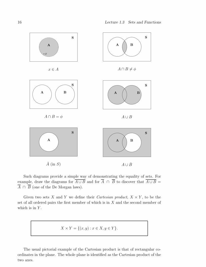
16 Lecture 1.3 Sets and Functions
A
x
S
x ∈ A
A B
S
A ∩B 6= φ
A B
S
A ∩B = φ
A B
S
A ∪ B
A
S
A (in S)
A B
S
A ∪ B
Such diagrams provide a simple way of demonstrating the equality of sets. For
example, draw the diagrams for A ∪B and for A ∩ B to discover that A ∪ B =
A ∩ B (one of the De Morgan laws).
Given two sets X and Y we define their Cartesian product, X × Y , to be the
set of all ordered pairs the first member of which is in X and the second member of
which is in Y .
X × Y = {(x, y) : x ∈ X, y ∈ Y }.
The usual pictorial example of the Cartesian product is that of rectangular co-
ordinates in the plane. The whole plane is identified as the Cartesian product of the
two axes.
Lecture 1.3 Sets and Functions 17
�Example Find, explicitly, the Cartesian product of the two setsX = {1, 7, 9, 21, 66}and Y = {2, 3}.
Solution The Cartesian product, X×Y , consists of all possible ordered pairs (x, y),
where x ∈ X and y ∈ Y . Hence
X × Y = {(1, 2), (1, 3), (7, 2), (7, 3), (9, 2), (9, 3), (21, 2), (21, 3), (66, 2), (66, 3)}
Notice in this example we can explicitly write down each element of X × Y . We
can do this here because the sets X and Y are finite. Of course this is not possible
if the sets are infinite. For example, the set of lattice points in the first quadrant of
the x− y plane is given by N×N – an infinite set of points (n,m) where n ∈ N and
m ∈ N.
Functions
If X and Y are sets a function from X to Y (or a function from X into Y , or
a function with values in Y ) is a rule which associates with each element of X a
unique element of Y . The words mapping or map are often used instead of function.
The function “rule” can be specified in many ways, but the important thing
is that to any given element of X we associate, somehow, a unique element of Y .
We indicate that we have a function or map between sets X and Y by the arrow
notation,
f : X −→ Y.
For any x ∈ X the element y of Y associated with x by the function f is denoted
f(x). Then f(x) ∈ Y and we write
y = f(x) or x 7−→ y.
This is a more general concept of a function than you have probably met before. The
familiar functions of calculus are functions from a subset, D, of the real numbers to
the real numbers. Denoting the set of real numbers by R, we obtain
f : D −→ R.
�Example We may use the formula f(x) = x2 + x+ 1 to define the function
f : R −→ R; x 7−→ x2 + x+ 1.
The graph of such a real valued function on D is the set of points (x, y) in the
plane such that y = f(x) for x ∈ D. In fact, this idea of graph is easy to generalise
to our more abstract setting.
18 Lecture 1.3 Sets and Functions
The graph of a function f : X −→ Y is the set of ordered pairs
{(x, y) ∈ X × Y : y = f(x)} or {(x, f(x)) ∈ X × Y : x ∈ X}
Another class of functions with which you should be familiar are the sequences.
A sequence {an} where n ∈ N can be thought of as a function
f : N −→ R.
This means for each n ∈ N the function f associates a real number f(n), which
by tradition we denote by a symbol such as an. In fact all your familiar functions
from calculus (quadratics, exponentials and so on) can be made into sequences if we
restrict ourselves to the subset N of R. For example, consider the quadratic
f : R −→ R, with f(x) = x2.
We may restrict this function to the subset of natural numbers, that is, we think of
f as acting only on the subset N of R. This is usually written as f |N, and read as “f
restricted to N”. The function f |N has exactly the same function rule as f , it simply
acts only on the subset N of R. This all sounds a bit abstract, but in practice it’s
very simple, we have
f |N : N −→ R, with f |N(n) = n2.
Similarly, restricting any function R −→ R we obtain a sequence. Our example,
f(x) = x2, defines the sequence {n2}n∈N = {1, 22, 32, 42, . . .}.
We will take a more detailed look at sequences later in these notes.
In our general setting with functions f : X −→ Y we make the following defini-
tions
The set X is called the domain and the set Y is called the codomain
of the function f . The set f(X) = {f(x) : x ∈ X} is called the
range or image of the function.
We should emphasise the importance of the domain in the definition of a function –
functions with different domains are different functions. Consider the following two
functions,
g : {x ∈ R : x ≥ 0} → {y ∈ R : y ≥ 0}, x 7−→ x2,
f : R → R, x 7−→ x2.

Lecture 1.3 Sets and Functions 19
They are given by the same formula, that is, f(x) = x2 and g(x) = x2, but they
are quite different functions – they have different domains. They also have different
properties, for example, g is one-to-one (see lecture 8), whereas f is not.
�Example What is the largest subset, D of R, such that
f : D −→ R, x 7−→√1− x2
is a function?
Solution As√u is defined if and only if u ≥ 0, we must have 1 − x2 ≥ 0, that is,
−1 ≤ x ≤ 1. Thus D = {x : −1 ≤ x ≤ 1}.
Suppose we have two functions f : X −→ Y and g : Y −→ Z, where X , Y and
Z are sets. Is there a natural way to go from X to Z using f and g? Well, we could
simply use f to take us from x ∈ X to y = f(x) ∈ Y and then use g to take us from
y to g(y) ∈ Z. This gives us a new function X −→ Z, the composition of f and g.
For functions f : X −→ Y and g : Y −→ Z the composition of f
and g, denoted g ◦ f , is defined to be the function
g ◦ f : X −→ Z
g ◦ f(x) = g(f(x)), for x ∈ X.
Notice the order of f and g in g ◦ f – we use the function f first and then we use g.
The expression g(f(x)) simply means g(y) where y = f(x).
�Example Find g ◦ f(x) and f ◦ g(x) where f, g : R −→ R are defined by
f(x) = x2 and g(x) = x2 + 1.
Solution
g ◦ f (x) = g(f(x))
= g(x2)
= (x2)2 + 1
= x4 + 1

20 Lecture 1.3 Sets and Functions
Perhaps this is a little easier to see if we introduce the intermediate step, y =
f(x) = x2, then
g ◦ f(x) = g(f(x)) = g(y)
= y2 + 1
= x4 + 1, as y = x2.
Furthermore,
f ◦ g (x) = f(g(x))
= f(x2 + 1)
= (x2 + 1)2
= x4 + 2x2 + 1
This shows that, in general, f ◦ g is not equal to g ◦ f . 2
�Example For functions h : N −→ R and g : R −→ R, where h(n) = 1nand
g(x) = 1x2+1
, find the equation for g ◦ h(n).
Solution
g ◦ h(n) = g(h(n))
= g(1
n)
=1
( 1n)2 + 1
=n2
1 + n2
2

Lecture 1.3 Sets and Functions 21
♠ Exercises 3
1. If A ⊂ S show that
(a) (A) = A
(b) A ∪ A = A ∩A = A ∪ φ = A
2. Use a Venn diagram to demonstrate the truth of the second De Morgan law
A ∩ B = A ∪B.
3. Consider the functions f : Df −→ R and g : Dg −→ R given by f(x) =√x2 − 4 and g(x) = x2 + 4.
(a) What are the largest subsets Df and Dg of R, such that f and g are
functions?
(b) What are the ranges (images) of f and g?
(c) Find the equation defining g ◦ f . What are the domain, codomain and
and range of g ◦ f?
4.Let f : X −→ Y be a function, let A and B be subsets of X . Prove that
(a) f(A ∪ B) = f(A) ∪ f(B).
(b) f(A ∩ B) ⊂ f(A) ∩ f(B).
22 Lecture 1.4 Numbers
Lecture 1.4 Numbers
The awareness of numbers, particularly the counting numbers, is in some ways a
fairly primitive sensibility – certain birds can distinguish sets containing up to four
elements. But it is this concept of number which is at the heart of the origins of
mathematics.
Number theory, even today, offers some of the deepest and most challenging
problems in mathematics. Our aim over the next couple of lectures will be quite
modest. We want to give a brief introduction to those ideas from the theory of
number which are required for a rigorous look at the differential calculus.
Integers
We will accept as given the counting numbers {1, 2, 3, 4, . . .} and the natural
numbers N = {1, 2, 3, 4, . . .}, stressing only the facts needed for extensions of this
number system.
Elements of N can be added or multiplied to give further elements of N. If
m,n ∈ N then m + n ∈ N and mn ∈ N. This is called closure under addition or
multiplication. There is a number 0 for which 0 +m = m + 0 = m and there is a
number 1 for which 1.m = m.1 = m, for all m ∈ N. We call 0 the neutral element
with respect to addition and 1 the neutral element with respect to multiplication.
We also have an order expressed by the symbols < (less than),> (greater than).
To deal, in a more complete fashion, with equations
m+ x = n; m,n ∈ N
we will need to introduce more numbers. Notice this equation can only be solved
in N (i.e. with x ∈ N) if n > m. We widen our number system to include the
“negatives” of the counting numbers.
The integers Z = {. . . ,−3,−2,−1, 0, 1, 2, 3, . . .}.
Notice that the properties of closure under addition and multiplication still hold
for Z, as does the ordering property.
Lecture 1.4 Numbers 23
If a and b are integers the equation
ax = b.
is not, in general, satisfied by an integral value of x. If this equation is to always
have a solution we need to again widen our number system to include the rationals
a/b (with a, b ∈ Z, b 6= 0).
Rational Numbers
The set of rational numbers, Q = {pq: q 6= 0; p, q ∈ Z}.
In the system of rationals the usual operations of arithmetic, addition, sub-
traction, multiplication and division all apply. The rationals can also be ordered
according to their “size” if we define
a
b>
c
d; a, b, c, d ∈ Z and b, d > 0
to mean ad > bc. Note the restriction b and d positive is not really a restriction at
all, if b < 0 then we can writea
b=
−a
−b.
The denominator is then positive.
The rationals have an important property not possessed by the integers:
Theorem Between any two rationals there are infinitely many other rationals.
Proof The proof is a simple direct “construction”.
We simply give an infinite set of rationals between aband c
d; a
b, ca∈ Q. As noted
above we can always take b and d to be positive integers. Then
a+mc
b+md
lies between a/b and c/d for any positive integer m. There are infinitely many
positive integers so we get infinitely many rationals between a/b and c/d. �

24 Lecture 1.4 Numbers
Irrational Numbers
It was realised by the Greeks more than 2000 years ago that there is an incom-
pleteness about the system of rational numbers. The diagonal of a square with
sides of unit length has a length which is not a rational number – it is an irrational
number. In algebraic language the equation for x,
x2 = a, a ∈ Q,
has a rational solution for x only for exceptional values of the rational number a.
For our unit square Pythagoras’ theorem says that the length of the diagonal, x, is
given by
x2 = 12 + 12 = 2.
We will now show that the formal solution to this equation, x =√2, cannot be a
rational number. We call√2 an irrational number.
Theorem No rational number has square 2.
Proof This is a very old theorem having been proved first by Pythagoras or one of
his school. It is a very simple and economical proof by contradiction.
Assume, on the contrary, that the rational p/q has square 2. We can also assume
that p and q are integers having no common factors – if they did have common factors
we would simply cancel them from the “fraction”. We have
p2
q2= 2, or
p2 = 2q2.
We see that p2 is divisible by 2 so p must be an even integer (see example in lecture
1.2). So we can write p = 2r, for some integer r. We now have
p2 = 4r2 = 2q2,
from which we see that q2 = 2r2 so that q must be even. This means that p and q
have the common factor 2, contradicting our hypothesis. The theorem is proved. �
It can be quite difficult to determine whether a given number is rational or not.
The fact that the number π (the ratio of the circumference of a circle to its diameter)
is not rational was only discovered at the end of the 18th century.
The rationals and irrationals together give us the real numbers – all possible
points on the number line.

Lecture 1.4 Numbers 25
The Real Numbers.
The irrationals fill in the “gaps” in the rationals. Given any irrational we can
find rational numbers arbitrarily close to it. This process is just the decimal approx-
imation to the infinite decimal expression for the irrational number. This is most
easily seen by looking at the irrational√2 = 1.4142 . . . (an infinite decimal). We
then simply look at successive decimal approximations to√2,
1, 1.4, 1.41, 1.414, 1.4142, . . . .
Each of these numbers is rational (any finite decimal is rational, e.g. 1.414 = 14141000
)
and they are in increasing order. All of these numbers are less than√2. However,
we can get arbitrarily close to√2.
We can also approximate√2 from above
2, 1.5, 1.42, 1.415, 1.4143, . . . .
This sequence is found by adding a one to the last decimal place of our approximation
from below. Notice that this latter sequence is a decreasing sequence of rationals.
The sequence approximating√2 from below has no greatest member – we simply
go to the next decimal place to get a bigger member of the sequence. The sequence
approximating√2 from above has no smallest member.
So the irrational number√2 can be defined by cutting the rationals into two
classes L and R. Where L has no greatest member and R which has no smallest
member.
L︷ ︸︸ ︷
R︷ ︸︸ ︷
0 1√2 2 3
This is Dedekind’s definition (1872) of the irrationals by a cut of the rationals.
The rationals and the reals satisfy the axioms for what is known in algebra as an
ordered field. The reals are distinguished from the rationals by one further axiom,
Dedekind’s Axiom. Suppose that the system of all real numbers
is divided into two classes L and R, every member ℓ of L being
less than every member r of R (neither class being empty). Then
there is a dividing number ξ with the property that every number
less than ξ belongs to L and every number greater than ξ belongs to
R. The number ξ may belong to either L or R. If it is in L, it is
the greatest member of L. If ξ is in R it is the least member of R.

26 Lecture 1.4 Numbers
Such a division of the real numbers into two classes by means of some rule is
called a Dedekind cut.
♠ Exercises 4
1. (a) Is 22371
greater than 227?
(b) Is 265153
greater than 1351780
?
2. If a, b ∈ R prove, that if a < b < 0, then
1
a>
1
b.
3. Prove that if m/n is a rational approximation to√2 from below then
m+ 2n
m+ n
is a closer approximation from above. Hence write down approximations to√2, obtaining two which differ by less than 1
10,000.
4*. The density property of the rationals amounts to saying that there is no ra-
tional which is next to another. The following plan for arranging the rationals
(not in order of magnitude) does assign a definite place to each
1
1,2
1,1
2,3
1,2
2,1
3,4
1,3
2,2
3,1
4,5
1, . . . .
What place does 61occupy? (Counting from the left, of course!)
Show that p/q occupies the {12(p + q − 1)(p + q − 2) + q}th place. (Notice
that each rational occurs infinitely often in this scheme; e.g. 2 appears as21, 42, 63, . . . .)

Lecture 1.5 Some Properties of Real Numbers 27
Lecture 1.5 Some Properties of Real Numbers
Basic Arithmetic
We assume the familiar properties of the real numbers: For all a, b, c ∈ R
• a+ b = b+ a (commutativity of addition);
• (a+ b) + c = a+ (b+ c) (associativity of addition);
• 0 + a = a+ 0 = a (0 is the neutral element with respect to addition);
• There exists y ∈ R such that a+y = y+a = 0 (existence of additive inverses);
• ab = ba (commutativity of multiplication);
• (ab)c = a(bc) (associativity of multiplication);
• 1a = a1 = a (1 is the neutral element with respect to multiplication);
• There exists z ∈ R such that az = za = 1 (existence of multiplicative inverses).
• (a+ b)c = ac+ bc (distributivity).
• One and only one of
a > b, a = b, a < b
is true.
• If a > b and b > c, then a > c.
• If a > b, then a+ c > b+ c.
• If a > b and c > 0, then ac > bc.
These properties are essentially the axioms for an ordered field. If we add the
Dedekind axiom of the last lecture then we have the axioms defining the real num-
bers.
From these basic rules or axioms all the well-known and well-used properties of
real numbers follow.
28 Lecture 1.5 Some Properties of Real Numbers
For example, defining
an = a · a . . . a︸ ︷︷ ︸
n times
and (for a 6= 0) a0 = 1, a−n =1
an,
we obtain the usual statements for exponentials of a
am · an = am+n
(am)n = amn
(ab)n = anbn,
with m,n ∈ Z. These index rules can, in fact, be extended to m,n ∈ R.
We can also impose a “distance measure” on R, this is the absolute value of a
real number – it measures the distance of that number from zero.
|a| ={
a, if a ≥ 0
−a, if a ≤ 0.
Theorem The absolute value has the following properties:
1. |a| ≥ 0 for all a ∈ R and |a| = 0 if and only if a = 0.
2. |ab| = |a| · |b|, for all a, b ∈ R.
3. |a|2 = a2, for all a ∈ R.
4. |a+ b| ≤ |a|+ |b|, for all a, b ∈,R.
5. |a− b| ≥ ||a| − |b||, for all a, b ∈ R.
Proof The first three properties are trivial consequences of the definition and are
left as exercises.
To prove (4) note that if a+ b ≤ 0 then
|a+ b| = −(a + b)
= −a− b
= −a + (−b)
≤ |a|+ |b|,
as −a ≤ |a| and −b ≤ |b|. On the other hand, if a + b ≥ 0 then
|a+ b| = a+ b
≤ |a|+ |b|.
Lecture 1.5 Some Properties of Real Numbers 29
And we have the required property.
To prove (5) note that
|a| = |(a− b) + b| ≤ |a− b|+ |b|,
so that
|a− b| ≥ |a| − |b|.Similarly,
|b| = |(b− a) + a| ≤ |b− a|+ |a|,so that
|b− a| = |a− b| ≥ |b| − |a|.Combine the two inequalities for |a− b|,
|a− b| ≥ ±(|a| − |b|).
So we have (5),
|a− b| ≥ ||a| − |b||.�
Bounded Sets of Numbers
Consider the following sets of numbers:
1. All prime numbers.
2. All integers greater than 1000 which are perfect squares.
3. All rational numbers x, with 1 ≤ x ≤ 2.
4. All real numbers x such that 1 ≤ x ≤ 2.
5. All real numbers x such that 1 < x < 2.
We first observe that all these sets are infinite. The examples 1 and 2 might give
the impression that an infinite set must contain elements which are unboundedly
large. However, examples 3, 4 and 5 correct that false impression!
The sets of examples 4 and 5 are of an important type, each is called an interval.
Example 4 in which the end points, x = 1 and 2, are members of the set is called a
closed interval and denoted by [1, 2]. In general, the closed interval from a to b with
a ≤ b is the set
[a, b] = {x ∈ R : a ≤ x ≤ b}.

30 Lecture 1.5 Some Properties of Real Numbers
The set in example 5, in which the end points are excluded from the set, is called an
open interval and denoted by (1, 2). In general, the open interval from a to b with
a ≤ b is the set
(a, b) = {x ∈ R : a < x < b}.
If a set consists of finitely many numbers then clearly we can distinguish a
greatest (and least) element of that set. However, if S is an infinite set of numbers
there may or may not be a greatest element.
For example, in the set S = [−1, 1] the number 1 is greater than any other
member of S. The set S also has a least member, −1.
On the other hand the set S = (−1, 1) does not have a largest member. Given
any element of S we can always find another member of S which is larger. Suppose
k ∈ S = (−1, 1), then −1 < 12(k + 1) < 1 so 1
2(k + 1) ∈ S. But, 1
2(k + 1) > k.
What both sets do have in common is the fact that they are bounded above (and
below). That is, there is a number K (not necessarily in the set S) such that x ≤ K
for all x ∈ S.
Let S be a set of real numbers. If there is a number K such that
for every x ∈ S, x ≤ K, we say S is bounded above. K is an upper
bound for S.
Similarly if there is a k ∈ R such that x ≥ k for all x ∈ S we say
S is bounded below. k is a lower bound for S.
A set which is both bounded above and below is said to be bounded.
�Example Is the set {12, 23, 34, . . . , n
n+1, . . .} bounded or unbounded?
Solution The set is clearly bounded. The number 12serves as a lower bound – or
any number less than 12. The number 1 (or any number greater than 1) serves as an
upper bound. Note that the set does have a least member, 12. However, the set does
not have a greatest member. The elements of the set form an increasing sequence
which is bounded above by 1. 2
If K is an upper bound of a set S ⊆ R then any number greater than K is also
an upper bound. If we want to make the sharpest possible statement by confining
S as closely as possible then we would aim at getting the least upper bound. That is
a number K which is an upper bound, but such that K − ε is not an upper bound
for any positive number ε, no matter how small ε is. Or, stated another way
K ≥ x for all x ∈ S and for any ε > 0 there is an s ∈ S such that s > K − ε.

Lecture 1.5 Some Properties of Real Numbers 31
In a similar fashion we may seek a greatest lower bound k with the properties
k ≤ x for all x ∈ S and for any ε > 0 there is an s ∈ S such that s < k + ε.
The least upper bound is usually called the supremum and we write
K = sup S, read as K is the supremum of the set S.
The greatest lower bound is usually called the infimum, and we write
k = inf S.
Using the Dedekind axiom we can prove that a (non-empty) set of real num-
bers which is bounded above must have a supremum. And in a similar way that a
nonempty set of real numbers which is bounded below must have an infimum. We
will not give the proof here – although we now certainly have the background to
tackle it. As illustrations consider the sets
1. S1 = {x ∈ Q : 0 ≤ x ≤ 12}
2. S2 = {x ∈ Q : x2 < 2}
3. S3 = {12, 23, 34, . . . , n
n+1, . . .}.
For S1 the least upper bound is 12, that is, sup S1 =
12. Note 1
2is also the greatest
member of S1.
The set S2 has a supremum of√2, i.e. sup S2 =
√2. In this case sup S2 /∈ S2.
Finally, for the set S3 the supremum is 1, sup S3 = 1. Again, sup S3 /∈ S3.
We also have inf S1 = 0, inf S2 = −√2 and inf S3 =
12.

32 Lecture 1.5 Some Properties of Real Numbers
♠ Exercises 5
1. If a, b ∈ R and
a < b+ ε, for any ε > 0,
prove a ≤ b.
[Hint: try a proof by contradiction. The negative of the statement a ≤ b is
a > b.]
2. Show, for any a, b ∈ R,
maximum {a, b} =a+ b+ |a− b|
2minimum {a, b} = − maximum {−a,−b}
=a+ b− |a− b|
2
3. Find (if they exist) the supremum and infimum of the following sets
(a) {1, 12, 13, 14, . . . , 1
n, . . .}
(b) {1.1, (1.1)2, (1.1)3, . . . , (1.1)n, . . .}
(c) {√2,√√
2,
√√√
2, . . .}
4. Given two bounded subsets A,B ⊆ R prove
sup (A ∪ B) = maximum {sup A, supB}.

Lecture 1.6 Complex Numbers 33
Lecture 1.6 Complex Numbers
Our system of real numbers R would appear to be perfectly adequate for mathe-
matics and indeed most applications. We feel comfortable with the fact that R can
be represented as the real number line every point of which is in R. We think of
rulers and other measuring devices as segments or intervals of the real number line.
Why would we want to extend further our system of numbers?
Well, curiosity would be one reason. If it is possible let’s try it! On the other
hand there are sound mathematical reasons why we might want to extend our num-
ber system. The extension to the complex numbers was first carried out by Gauss
in about 1795. Complex numbers are indispensable in modern mathematics and
physics. In Quantum theory in particular complex numbers are used in a funda-
mental way.
One motivation for the extension of the number system is to note that only
non-negative numbers have square roots. In all other respects there is complete
symmetry between positive and negative numbers. Another way of stating this is
to note that the equation
x2 = a, with a ∈ R,
has a solution x ∈ R if and only if a ≥ 0. If we write an equation such as
x2 = −1
then x 6∈ R. So there exist “numbers”, satisfying perfectly reasonable equations,
which are not in R.
We extend the field of real numbers to the field of complex numbers by adjoining
a new element, i, to the set. This element i is defined as a solution to the equation
i2 = −1.
It is traditional to write i =√−1 as the solution; note that x2 = −1 then has two
possible solutions x = ±i.
We also include in our set of complex numbers all numbers which can be formed
from i and R by use of the operations + and −. The elements of this field of complex
numbers then take the form a+ ib, where a, b ∈ R.
The Complex Numbers C = {a+ ib : a, b ∈ R}.

34 Lecture 1.6 Complex Numbers
All the axioms for multiplication and addition of the real number system listed
in the last lecture apply to C. However, the order axioms involving < and > no
longer apply. The real numbers can be included in C as a subset, namely R can be
identified with the complex numbers of the form a + i0. For this reason we write
a+ i0 = a.
So we may think of complex numbers as numbers of the form a+ ib, with a and
b real. We refer to the a as the real part and b as the imaginary part.
Any complex number z can be written as
z = a+ ib, with a, b ∈ R.
We write Re (z) = a for the real part of z and
Im (z) = b for the imaginary part of z.
Addition of Complex Numbers
For two complex numbers z1 = a1 + ib, and z2 = a2 + ib2, with
a1, a2, b1, b2 ∈ R, we have
z1 + z2 = (a1 + ib1) + (a2 + ib2) = (a1 + a2) + i(b1 + b2).
Notice that
Re (z1 + z2) = a1 + a2 = Re(z1) + Re(z2)
and Im (z1 + z2) = b1 + b2 = Im(z1) + Im(z2).
�Example
(a) (1 + 3i) + (3 + i) = 4 + 4i = 4(1 + i)
(b) (1 + 3i)− (3 + i) = −2 + 2i = 2(−1 + i)
(c) (π + i)− (1 +√2i) = (π − 1) + (1−
√2)i
(d)(12+ 1
3i)+(14− 1
6i)= 3
4+ 1
6i
Lecture 1.6 Complex Numbers 35
Multiplication of Complex Numbers
Multiplication for elements of C follows the same field axioms as multiplication
of real numbers. Let’s start with an example.
�Example What is (1 + i) · (1− 3i)?
Solution
We simply expand the brackets,
(1 + i) · (1− 3i) = 1 · (1− 3i) + i · (1− 3i)
= 1− 3i+ i− i · 3i= 1− 3i+ i− 3i2
= 1− 2i− 3 · (−1), as i2 = −1
i.e. (1 + i) · (1− 3i) = 4− 2i.
2
Now for the general case
For complex numbers z1 and z2 (as above) we have
z1z2 = (a1 + ib1)(a2 + ib2) = a1a2 − b1b2 + i(a1b2 + a2b1).
You should not bother memorising this formula, instead you simply multiply
out the brackets as per our example. In the general case we have
z1z2 = (a1 + ib)(a2 + ib2) = a1(a2 + ib2) + ib1)
= a1a2 + ia1b2 + ib1a2 + i2b1b2
= a1a2 − b1b2 + i(a1b2 + b1a2), as i2 = −1.
So the policy is expand everything in sight, use i2 = −1 and then collect terms into
two groups those with an i and those without an i. The terms without an i give the
real part of the product and the coefficient of the i gives the imaginary part. So,
Re (z1z2) = a1a2 − b1b2 and
Im (z1z2) = a1b2 + b1a2.
One thing worth emphasising Im (a + ib) = b is a real number, it is the coefficient
of i.

36 Lecture 1.6 Complex Numbers
�Example
(a) (3 + 4i)(6 + i) = 3 · (6 + i) + 4i · 6 + i)
= 18 + 3i+ 24i+ 4i2
= 18 + 3i+ 24i− 4
= 14 + 27i.
(b) (2− 7i)(3− 2i) = 2(3− 2i)− 7i(3− 2i)
= 6− 4i− 21i− 14
= −8− 25i.
(c) (√2 + i
√3)(1− i) =
√2(1− i) + i
√3(1− i)
=√2− i
√2 + i
√3 +
√3
= (√2 +
√3) + i(
√3−
√2).
(d) (√2− i)2 = (
√2)2 − 2
√2i+ i2
= 2− 2√2i− 1
= 1− 2√2i.
Equality of Complex Numbers
To specify a complex number we must give two real numbers, the real and imagi-
nary parts. So two complex numbers are equal if and only if their real and imaginary
parts are equal (respectively).
For complex numbers z1 = a1+ib1 and z2 = a2+ib2 we have z1 = z2if and only if a1 = a2 and b1 = b2.
�Example Find all complex numbers for which
z2 = −3 + 4i.
Solution We write z = x + iy, with x and y real. Substituting into the equation
we have
z2 = (x+ iy)2 = −3 + 4i
i.e. x2 − y2 + i2xy = −3 + 4i.

Lecture 1.6 Complex Numbers 37
Now equate real and imaginary parts – remember the complex number on the
left is equal to that on the right if and only if their real and imaginary parts are
(respectively) equal. We get
x2 − y2 = −3 and 2xy = 4.
From the second of these equations we have
y =2
x,
which we substitute into the first equation. This gives
x2 −(2
x
)2
= −3.
Multiplying this equation through by x2 gives as
x4 − 4 = −3x2
i.e. x4 + 3x2 − 4 = 0.
This is a quadratic in x2, we factorise
(x2 + 4)(x2 − 1) = 0,
so that x2 = 1 or x2 = −4. But x must be real, so we cannot have x2 = −4. So we
conclude x2 = 1, which gives x = ±1. We found earlier that y = 2/x, so we have
two possible solutions
(x, y) = (1, 2) or (−1,−2).
Giving two possible complex numbers z,
z = 1 + 2i or z = −1− 2i.
2
Division by Complex Numbers
If we have two complex numbers z1 = a1 + ib1 and z2 = a2 + ib2 6= 0 how do we
writez1z2
=a1 + ib1a2 + ib2
in the standard complex number form, i.e. as a + ib? To answer this question note
that what we really have to do is get rid of the complex number in the denominator.
Now recall that
(x+ iy)(x− iy) = x2 + y2
38 Lecture 1.6 Complex Numbers
is a real (positive) number. So if we multiply the denominator by a2 − ib2 we will
get a real number. But to keep the equality we will have to multiply the numerator
by a2 − ib2 as well. Here is the calculation
z1z2
=a1 + ib1a2 + ib2
=a1 + ib1a2 + ib2
· a2 − ib2a2 − ib2
=(a1 + ib1)(a2 − ib2)
(a2)2 + (b2)2
=a1a2 + b1b2 + i(b1a2 − a1b2)
(a2)2 + (b2)2
So the real and imaginary parts are
Re
(z1z2
)
=a1a2 + b1b2(a2)2 + (b2)2
and Im
(z1z2
)
=b1a2 − a1b2(a2)2 + (b2)2.
�Example Write 1+i3−2i
in the form a+ ib.
Solution1 + i
3− 2i=
1 + i
3− 2i· 3 + 2i
3 + 2i=
(1 + i)(3 + 2i)
32 + 22
=3 + 2i+ 3i− 2
9 + 4
=1 + 5i
13
i.e.1 + i
3− 2i=
1
13+ i
5
13
2
Solving Real Quadratic Equations
We can now solve all quadratic equations with real coefficients. For example we
solve
z2 + z + 1 = 0.
Using the usual quadratic formula
z =−1 ±
√12 − 4.1.1
2
=−1 ±
√−3
2.
Clearly the solutions are complex, we write them in the standard a+ ib format.
We note that √−3 =
√−1× 3 =
√−1 ·
√3 = i
√3.
So the solutions to the quadratic are
z =−1 ±
√−3
2= −1
2± i
√3
2.

Lecture 1.6 Complex Numbers 39
♠ Exercises 6
1. Express each of the following complex numbers in the form x+ iy.
(a) (2− i)(3 + 2i) (b) (6 + 5i)(2 + 7i)
(c) (3− 2i)2 (d) i3
(e)2− i
1 + i(f)
2
3 + i− 1 + i
1− i
(g)1− i
(2 + i)2(h) i7
2. Show that1 + sin θ + i cos θ
1 + sin θ − i cos θ= sin θ + i cos θ.
3. Solve the following equations for z, writing your solution in the form a+ ib
(a) (−1 + 2i)z − 1 = 3i
(b) z2 + 2i+ 5 = 0
(c) 5z2 − 4z + 1 = 0.
4. Find all solutions of the equation
z2 = 6− 8i.
40 Lecture 1.7 Complex Numbers (continued)
Lecture 1.7 Complex Numbers (continued)
Complex Conjungation
If z = x + iy (with x and y real) is a complex number we define
the complex conjugate of z by z = x− iy.
Notice that all we have to do to get the complex conjugate of a complex number
is to replace the imaginary part by its negative.
�Example
(a) If z = 3 + 2i then z = 3− 2i.
(b) If z = 27− 5i then z = 27 + 5i.
(c) If z = 5 then z = 5.
(d) If z = 6i then z = −6i.
Theorem If z1, z2 ∈ C then z1z2 = z1z2.
Proof Let z1 = x1+iy1, and z2 = x2+iy2. Then z1z2 = (x1x2−y1y2)+i(y1x2+y2x1).
So (z1z2) = (x1x2 − y1y2)− i(y1x2 + y2x1).
Now,
z1 = x1 − iy1, and z2 = x2 − iy2 so
z1z2 = (x1 − iy1)(x2 − iy2)
= (x1x2 − y1y2)− i(y1x2 + y2x1), as (−i)2 = −1.
Comparing our expressions for z1z2 and z1z2 we conclude that z1z2 = z1z2, as
required. �
In a similar vein we also have:
Theorem If z1 and z2 are complex numbers then
(a) z1 + z2 = z1 + z2
(b)
(z1z2
)
=z
1
z2, for z2 6= 0.

Lecture 1.7 Complex Numbers (continued) 41
Proof Exercise!
Taken together these two theorems tell us that if we wish to take the complex
conjugate of an expression involving complex numbers all we have to do is write
down the expression with each complex number replaced by its conjugate.
�Example
For z1, z2, z3 ∈ C we have
(z21 + 2z1z2 + z2 + 1− i
z3
)
=z21 + 2z1z2 + z2 + 1 + i
z3,
for z3 6= 0.
In the previous lecture we mentioned the method for writing a complex numberz1z2
(with z1, z2 ∈ C) in the form x + iy. If z2 = x2 + iy2 we had to multiply the
expression byx2 − iy2x2 − iy2
. We now see that the method is simply multiplying the
expression byz2z2. The method works because z2z2 is always a real number. This is
easily seen z2z2 = (x2 + iy2)(x2 − iy2) = (x2)2 + (y2)
2.
For any complex number z we have
zz = (Re(z))2 + (Im(z))2.
�Example
(a) For z = 2 + 3i we have zz = 22 + 32 = 13
(b) If z = 2 then zz = 22 = 4
(c) If z = −3i then zz = (−3)2 = 9.
Argand Diagrams
A complex number has two parts, its real part and its imaginary part. We can
think of a complex number z = x + iy (x, y ∈ R) as an ordered pair (x, y). In this
way we see that a complex number can be thought of as a point in the plane –
we simply plot the point (x, y) in the xy plane. The resulting picture is called an
Argand diagram. We represent z by the point (x, y) in the plane.

42 Lecture 1.7 Complex Numbers (continued)
y
x
3
2
1
−2 −1 1 2 3
(1, 3) or 1 + 3i
(1, 1) or 1 + i(−1, 1) or −1 + i
The real numbers (numbers with no imaginary part) simply lie on the x-axis.
The pure imaginary numbers (those with no real part) lie along the y-axis.
y
x
2
1
−1
−2
−2 −1 1 2 3
(3, 2) or 3 + 2i
(3,−2) or 3− 2i
(−1, 1) or −1 + i
(−1,−1) or −1− i
The complex conjugate of a complex number represented on the Argand diagram.
The distance of a complex number z = x + iy from the origin on an Argand
diagram is√
x2 + y2 =√zz.
Notice that when z is real (ie y = 0) we have the distance as
√x2 = |x|.
This motivates the definition
If z = x+ iy ∈ C we define the modulus of z (or the absolute value
of z) to be |z| =√
x2 + y2 =√zz.

Lecture 1.7 Complex Numbers (continued) 43
y
y
xx
|z|
z or (x, y)
�Example
(a) If z = 2− 3i then |z| =√
22 + (−3)2 =√13.
(b) If z = 3− 4i then |z| =√
32 + (−4)2 = 5.
(c) If z = 3 then |z| = 3.
(d) If z = −10 then |z| = 10.
(e) If z = 2i then |z| =√22 = 2.
Theorem
If z1, z2 ∈ C then
(i) |z1z2| = |z1||z2|.
(ii)
∣∣∣∣
z1z2
∣∣∣∣=
|z1||z2|
, for z2 6= 0.
Proof Both follow from the earlier theorem on the complex conjugate. We will
prove (ii) and leave (i) as an exercise. For (ii) we have
∣∣∣∣
z1z2
∣∣∣∣=
√(z1z2
)(z1z2
)
=
√z1z2.z1z2
=
√z1z1z2z2
=
√z1z1√z2z2
=|z1||z2|.
�

44 Lecture 1.7 Complex Numbers (continued)
Notice that, in general, |z1 + z2| 6= |z1| + |z2|. For example for z1 = 1 + i and
z2 = 1− i we get
|z1 + z2| = |2| = 2.
And
|z1|+ |z2| = |1 + i|+ |1− i|=
√12 + 12 +
√
12 + (−1)2
=√2 +
√2
= 2√2,
so |z1|+ |z2| > |z1 + z2|, in this case. In fact, we have
Theorem If z1, z2 ∈ C then
|z1 + z2| ≤ |z1|+ |z2|.
Proof Notice that |z1 + z2| and |z1| + |z2| are both non-negative so we can prove
the inequality by proving
|z1 + z2|2 ≤ (|z1|+ |z2|)2.
This is what we will now do.
|z1 + z2|2 = (z1 + z2)(z1 + z2)
= (z1 + z2)(z1 + z2)
= z1z1 + z2z2 + z1z2 + z1z2.
And (|z1|+ |z2|)2 = (√z1z1 +
√z2z2)
2
= z1z2 + z2z2 + 2√z1z1
√z2z2.
Hence,
(|z1|+ |z2|)2 − |z1 + z2|2 = 2√z1z1
√z2z2 − z1z2 − z1z2
= 2√
(z1z2)(z1z2)− z1z2 − z1z2.
Now Z = z1z2 is a complex number so we can write z1z2 = Z = X + iY , with
X, Y real.
Then√
(z1z2)(z1z2) =√ZZ =
√X2 + Y 2 and z1z2 + z1z2 = 2X . So
(|z1|+ |z2|)2 − |z1 + z2|2 = 2√X2 + Y 2 − 2X ≥ 2
√X2 − 2X ≥ 0.

Lecture 1.7 Complex Numbers (continued) 45
Thus
(|z1|+ |z2|)2 − |z1 + z2|2 ≥ 0
and our result follows. �
This result is also known as the triangle in equality. It can be thought of geo-
metrically as stating the old fact that the length of one side of a triangle is less than
the sum of the lengths of the other two sides.
De Moivre’s Theorem
To motivate de Moivre’s theorem we first introduce the polar form of a complex
number.
y
y
xxθ
r
z = x+ iy
From our diagram we have z = x+ iy = r cos θ + ir sin θ.
The polar form of a complex number is z = r(cos θ+ i sin θ), |z| = r.
If we wanted to look at powers of z we would need to look at expressions of the
form
zn = [r(cos θ + i sin θ)]n
= rn(cos θ + i sin θ)n.
What can we say about (cos θ + i sin θ)n? It is here that the remarkable de
Moivre’s theorem enters.
Theorem If θ ∈ R then
(cos θ + i sin θ)n = cos(nθ) + i sin(nθ),
for n any rational number.
Proof See the exercises!
46 Lecture 1.7 Complex Numbers (continued)
�Example
(a) 1 + i =√2
(1√2+ i
1√2
)
=√2(
cosπ
4+ i sin
π
4
)
.
(b) i = cos π2+ i sin π
2.
(c) 1 = cos 0 + i sin 0
= cos(2π) + i sin 2π.
Notice in this last example we have a phenomenon typical of trigonometric func-
tions – they are periodic,
cos(θ + 2π) = cos θ
sin(θ + 2π) = sin θ .
In fact for any integer m,
cos(θ + 2mπ) + i sin(θ + 2mπ) = cos θ + i sin θ.
♠ Exercises 7
1. For each of the following complex numbers write down the complex conjugate
and modulus
(a) 6 + 2i
(b) 1− 3i
(c) 1+i√2
(d) 11+i
(e) 2−3i1−i
(f) i.
2. Let z1, z2 ∈ C. Show that
|z1 + z2|2 + |z1 − z2|2 = 2|z1|2 + 2|z2|2.
3. For z1, z2 ∈ C prove that
(z1z2
)
=z1z2
, for z2 6= 0.
4. Use the addition formulae for the sine and cosine functions to deduce that
(cos θ + i sin θ)(cos φ+ i sin φ) = cos(θ + φ) + i sin(θ + φ).

Lecture 1.7 Complex Numbers (continued) 47
5. By induction, or otherwise, prove de Moivres theorem
(cos θ + i sin θ)n = cos(nθ) + i sin(nθ)
for n ∈ N.
6.* Extend de Moivre’s theorem taking n to be (i) a negative integer and then (ii)
n = p/q, a rational number.

48 Lecture 1.8 Functions on R
Lecture 1.8 Functions on R
In lecture 3 we introduced the idea of a function or mapping, f , consisting of set, A,
called the domain, a set B, called the codomain, and a rule which assigns to every
element a ∈ A a unique element b ∈ B. We write
f : A −→ B
and
f : a 7−→ b or f(a) = b.
In lecture 3 we also met the idea of composition of two functions f and g. For
f : A −→ B, a 7−→ b and
g : B −→ C, b 7−→ c
we define
g ◦ f : A −→ C, a 7−→ c
by
g ◦ f(a) = g(f(a)).
Before specialising to functions f : D −→ R with D ⊆ R, we examine two
general concepts. Firstly, the idea of a function being one-one:
A function f : A −→ B is one-one or injective if, for a, a′ ∈ A,
f(a) = f(a′) implies a = a′.
Another way of saying that f is injective is to say that, for every b ∈ B there is
at most one a ∈ A with f(a) = b. Or that, whenever a1 6= a2, with a1, a2 ∈ A, then
f(a1) 6= f(a2).
Our second concept of this type is that of surjectivity:
The function f : A −→ B is said to be onto or surjective if for
every b ∈ B there is at least one a ∈ A such that b = f(a).
An alternative statement is to say that f is surjective if f(A) = B, that is, the
codomain B is equal to the range of f .

Lecture 1.8 Functions on R 49
A function which is both injective and surjective is called bijective.
�Example
(a) f : N −→ R
f : n 7−→ f(n) =1
1 + n.
This function is one-one (injective) but not surjective.
(b) f : R −→ R
f(x) = x, x ∈ R.
This function is both injective and surjective – so its’ bijective.
(c) f : R −→ R
f(x) = x2.
The function is neither injective nor surjective. Note, however, that
g : R −→ [0,∞)
f(x) = x2.
is surjective (of course its’ still not injective).
(d) f : R −→ {0, 1}
f(x) =
{0, when x is irrational,
1, when x is rational.
The function is clearly not injective. It is surjective.
(e) f : [−1, 1] −→ [0, 1]
f(x) =√1− x2.
The function is not injective but it is surjective. Note however that
g : [0, 1] −→ [0, 1]
f(x) =√1− x2
is both injective and surjective and thus bijective.
Real Valued Functions on R
We now specialise our study to consider only functions f : D −→ R, with D ⊆ R.
All our previous discussions of things such as domain, codomain, range, composition,
being injective, surjective and bijective apply to these more specialised functions.

50 Lecture 1.8 Functions on R
The concepts of injective, surjective and bijective are now particularly easy to
deal with. They are basically about how many ”x-values” correspond to a given ”y-
value” – one or none for injective; one or more for surjective; and one and only one
for bijective. The easiest way to visualise this is to draw the graph of the function,
the question now becomes how many times does a horizontal line drawn at the given
y-value hit the graph? Try it on the following examples.
�Example Decide whether the following functions are injective or surjective justi-
fying your statements.
(a) f : N −→ R, n 7−→ n2 − 9
(b) f : [−1, 1] = {x ∈ R : −1 ≤ x ≤ 1} −→ R, x 7−→√1− x4
(c) f : R \ {1} −→ R \ {0}, x 7−→ 1
x− 1
Solution
(a) For n1, n2 ∈ N with f(n1) = f(n2) we obtain n21 − 9 = n2
2 − 9. Thus n21 = n2
2,
so that n1 = n2 as n1, n2 ≥ 0. Hence f is injective. As there is no natural
number n with f(n) = 2, the function is not surjective.
(b) As f(−x) = f(x) for x ∈ [−1, 1], the function is not injective. Note that the
function is well–defined as 1−x4 ≥ 0 for all x ∈ [−1, 1]. Since the square root
is always greater than or equal to 0, the function is not surjective.
(c) Take x1, x2 ∈ R \ {1} with f(x1) = f(x2). Then
1
x1 − 1=
1
x2 − 1⇐⇒ x2 − 1 = x1 − 1
⇐⇒ x2 = x1
and hence f is injective. Now take y ∈ R, y 6= 0. Then
y =1
x− 1⇐⇒ y(x− 1) = 1
⇐⇒ x− 1 =1
y
⇐⇒ x =1
y+ 1 =
1 + y
y
showing that f is surjective. Thus f is bijective.

Lecture 1.8 Functions on R 51
2
We should also recall the definition of the graph of a function f : D −→ R
as the set of ordered pairs {(x, y) ∈ R × R : y = f(x) for some x ∈ D}. We
identify the Cartesian product R × R as our usual x − y plane, R2. So the set
{(x, y) ∈ R× R : y = f(x), x ∈ D} is “identified” with our usual notion of the plot
of y = f(x). That is a very wordy way of saying that our usual idea of drawing the
graph of a function coincides (in the case f : D −→ R) with our more general idea
of a graph.
Your past experience with graph drawing will have taught you that the behaviour
of the function as x −→ ±∞, or as x approaches a singular point of the function, is
a most important feature of your sketch. To discuss such behaviour rigourously we
need to understand the notion of a limit.
A First Look at Limits
The idea we want to make precise is the following. Suppose we have a function
f : D −→ R with D ⊆ R and c ∈ R. Our question is does f(x) approach some
specific number, L, as x approaches c. If it does then we say f(x) has a limit at
x = c. We write this symbolically as
f(x) −→ L as x −→ c,
read as “f(x) approaches L as x approaches c”. Or as
limx−→c
f(x) = L,
read as the “limit of f(x) as x approaches c is L”. The idea here is that we can
make f(x) as close to L as we like simply by taking x sufficiently near to c.
You might like to think of this idea in terms of approximation. We can make the
difference f(x)− L as small as we like by simply taking x close enough to c. Well,
we can do this provided f(x) has limit L as x approaches c. We are saying that I
can always make |f(x)−L| smaller than any number you give me simply by taking
x close enough to c.
�Example f(x) = x2 has limit 1 as x −→ 1.
Give me any number, as small as you like, say 0.001. Then we can make |f(x)−1|smaller than 0.001 by taking x close enough to 1.
We want |x2 − 1| < 0.001. We can achieve this by making x just less than 1 or
just greater than 1.

52 Lecture 1.8 Functions on R
Let’s have a look at the value of x, x0 say for which x20 − 1 = 0.001, so
x0 = +√1.001. Because of the absolute value signs |x2 − 1| we also need the value
x1, x21 − 1 = −0.001 i.e. x1 =
√0.999. We conclude |x2 − 1| < 0.001 provided
x1 =√0.999 < x < x0 =
√1.001.
Now x0 + 1.0005 and x1 + 0.9095 so we can ensure |x2−1| < 0.001 by (for example)
0.9996 < x < 1.004.
No matter what number you give me, lets say it is ε, I can always find x0, x1 such
that
|x2 − 1| < ε provided
x1 < x < x0,
where x0 and x1 are near x = 1. Such a statement is just about right for the abstract
definition of a limit, we’ll say more about this in the next lecture.
�Example
limx−→0
2x = 1.
This just says 2x −→ 1 as x −→ 0. This means that given any number, no
matter how small, we can always make |2x − 1| smaller than this number by taking
x close enough to 0. For example lets take the number ε = 0.01, the claim is we
can make |2x − 1| < 0.01 by choosing x close enough to 0. We don’t have to find
precisely the values of x for which the inequality is true we just need to find an
interval about x = 0 for which it is true. Try some values on a calculator.
x 2x(4 decimal places) |2x − 1|-0.1 0.9330 0.0670
-0.05 0.9659 0.0341
-0.01 0.9931 0.0069
0.1 1.0718 0.0718
0.05 1.0070 0.0070
From this table of calculated values its clear that it would suffice to take −0.01 <
x < 0.01 to ensure that
|2x − 1| < 0.01.

Lecture 1.8 Functions on R 53
�Example Sketch the graph of the function f : R \ {−1} −→ R, x 7−→ 1
1 + x.
Solution. The first thing you notice is that f(x) is “badly behaved” near x = −1,
it’s undefined there. What happens as we approach x = −1? Suppose we approach
from below, i.e. consider x = −1 − δ where δ is small and positive. Then
f(−1− δ) =1
1 + (−1− δ)= −1
δ,
so if δ is small 1δis large. The function is large in magnitude and negative just below
x = −1. As we approach x = −1 from below, f(x) −→ −∞.
Next let’s see what happens when we approach from above, let x = −1 + δ, δ
small and positive. Then
f(−1 + δ) =1
1 + (−1 + δ)=
1
δ,
so f(x) −→ +∞ as we approach x = −1 from above. We have thus far
y
−1x
The behaviour of the function for x > −1 or x < −1 is easy to determine once
we know what happens as x −→ ±∞. For x large and positive 11+x
will be small
and positive. That is f(x) −→ 0+ as x −→ +∞. We use the notation f(x) −→ 0+
to indicate that f(x) is approaching zero from above, i.e. from the positive side.
For x large and negative 11+x
will be small and negative. That is f(x) −→ 0−
as x −→ −∞, f(x) approaches 0 from below (i.e. from the negative side). One
important point on the graph is where it cuts the y-axis, this is at x = 0 and
f(0) = 1; so the graph cuts the y-axis at (0, 1). This is enough information to give
us a reasonably accurate sketch.

54 Lecture 1.8 Functions on R
y
−1x
y = f(x) = 11+x
2

Lecture 1.8 Functions on R 55
♠ Exercises 8
1. What is the largest subset D ⊆ R such that f : D −→ R is a function, where
f is given by
(a) f(x) = 11+x2
(b) f(x) =√x2 − 9
(c) f(x) = x3 − 1
In each case find the range of f .
2. For each of the functions of question 1 state whether or not the function is
injective or surjective.
3. Find a δ > 0 such that |x3 − 1| < 110
whenever |x− 1| < δ.
[Hint: |x− 1| < δ means 1 − δ < x < 1 + δ. You have to find a δ > 0 which
ensures that
|x3 − 1| < 1
10.]
4. Sketch the graph of f(x) = 1x2−4
.
5*. Show that given any ε > 0 we can always find δ such that
∣∣∣∣
1
x+ 1− 1
∣∣∣∣< ε
whenever |x| < δ.
[Hint: The idea here is to explicitly give a relation which determines the
possible values of δ given ε. For example you may end up with something like
δ < 1 + ε (this doesn’t work here!).]

56 Lecture 1.9 Limits
Lecture 1.9 Limits
Formal Definition of a Limit
In the last lecture we began to discuss what is meant by a statement such as
“f(x) has limit L as x approaches c”. The statement
limx−→c
f(x) = L
means that given any number ε, no matter how small, we can ensure that the
distance, |f(x)−L|, between f(x) and L, is smaller than ε by taking x close enough
to c, that is, by making the distance |x− x| small enough. Let’s state this formally.
We will say limx−→c
f(x) = L, or f(x) −→ L as x −→ c or f(x) has
limit L as x −→ c, if, given any ε > 0 there exists a δ > 0 such
that |f(x)− L| < ε whenever 0 < |x− c| < δ.
Note that 0 < |x − c| < δ excludes x = c. For the limit we are only interested
in the behaviour of the function near c, not in f(c). In fact, we don’t even require
that c is in the domain of f .
To show that f(x) has limit L we have to demonstrate the existence of a δ > 0 for
any given ε. The idea is exactly that of the last lecture, you give me any number,
no matter how small, call it ε. Then I have to come up with a δ > 0 such that
|f(x)− L| <∈ whenever 0 < |x− c| < δ.
Lemma 1.1 Take a, c ∈ R. Then
(a) limx−→a c = c
(b) limx−→a x = a
Proof
Take a, c ∈ R and ε > 0.
(a) As |c− c| = 0 < ε no matter how far x is from a, we may choose any δ > 0,
for example, put δ = 231. Then |c − c| = 0 < ε whenever |x − a| < 231. Thus
limx−→a c = c.
(b) Put δ = ε. Then |x− a| < ε whenever |x− a| < δ = ε. Thus limx−→a x = a.
2

Lecture 1.9 Limits 57
�Example Prove that1
1 + x−→ 1 as x −→ 0.
Solution Let ε > 0 be given.
Our strategy has to be to find a δ > 0, depending on ε, such that if 0 < |x−0| < δ
then
∣∣∣∣
1
1 + x− 1
∣∣∣∣< ε.
Now we note that
∣∣∣∣
1
1 + x− 1
∣∣∣∣
=
∣∣∣∣
−x
1 + x
∣∣∣∣
=|x|
|1 + x|
≤ |x|1− |x| , for |x| < 1.
So for |x| < δ < 1 we have∣∣∣∣
1
1 + x− 1
∣∣∣∣<
δ
1− δ.
[Note we have increased the numerator |x| to δ and decreased the denominator
from 1− |x| to 1− δ. So the fraction|x|
1− |x| has been increased toδ
1− δ. ]
So we have to choose δ so thatδ
1− δ< ε ie. δ <
ε
1 + ε.
So given any ε > 0 we have∣∣∣∣
1
1 + x− 1
∣∣∣∣< ε whenever
|x− 0| < δ <ε
1 + ε.
We are finished. 2
As you can see there is quite an art in getting one of these proofs to work.
Remember you are given ε > 0 and you have to find an appropriate δ such that
|x− c| < δ implies |f(x)− L| < ε. Here is another example:
�Example Prove that limx−→0
(1 + x
1− x
)
= 1.
Solution Take x ∈ R \ {1} and ε > 0.

58 Lecture 1.9 Limits
And suppose 0 < |x| < δ, where δ > 0 is to be determined.
Now 1 + x ≤ 1 + |x| and 1− x ≥ 1− |x|, so we have that
1 + x
1− x≤ 1 + |x|
1− |x| .
[Remember: You increase the value of a fraction abby increasing the numerator
a or decreasing the denominator b (or both).]
And as 0 < |x| < δ we have
1 + x
1− x≤ 1 + |x|
1− |x| <1 + δ
1− δ.
Now, for |x| < δ < 1 we have |1− x| ≥ 1− |x| > 0 and hence
1
1− |x| ≥1
|1− x| .
We obtain∣∣∣∣
1 + x
1− x− 1
∣∣∣∣
=
∣∣∣∣
x
1− x
∣∣∣∣
=|x|
|1− x|
≤ |x|1− |x|
<δ
1− δ
To obtainδ
1− δ= ε we must have δ =
ε
1 + ε. Then δ < 1, so that
∣∣∣∣
1 + x
1− x− 1
∣∣∣∣< ε
whenever |x| < δ = ε/(1 + ε).
This is the formal definition of limx−→0
(1 + x
1− x
)
= 1. 2
One-Sided Limits
Implicit in our definition of limits, so far, is the notion that we approach the
point x = c from either side. That is f(x) −→ L whether we approach c from
above, ie. x −→ c+, or from below, x −→ c−. But there are cases where we can
approach from only one side. For example, the limit of√x as x −→ 0. This limit,
for real valued functions, must be from above, ie. we should really write x −→ 0+.
This is a one-side limit.
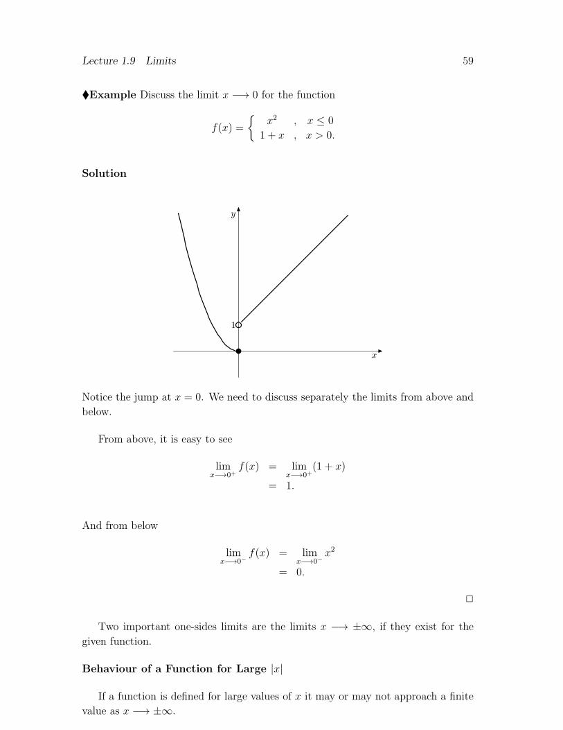
Lecture 1.9 Limits 59
�Example Discuss the limit x −→ 0 for the function
f(x) =
{x2 , x ≤ 0
1 + x , x > 0.
Solution
y
1
x
Notice the jump at x = 0. We need to discuss separately the limits from above and
below.
From above, it is easy to see
limx−→0+
f(x) = limx−→0+
(1 + x)
= 1.
And from below
limx−→0−
f(x) = limx−→0−
x2
= 0.
2
Two important one-sides limits are the limits x −→ ±∞, if they exist for the
given function.
Behaviour of a Function for Large |x|
If a function is defined for large values of x it may or may not approach a finite
value as x −→ ±∞.

60 Lecture 1.9 Limits
If f(x) does have a finite limit, L, as x −→ ±∞ then, in terms of our previous
understanding, we mean that given any ε > 0, |f(x)− L| < ε, whenever |x| is largeenough. Formally:
We say f(x) has finite limit L as x −→ ±∞, or
limx−→±∞
f(x) = L < ∞ or f(x) −→ L < ∞ as |x| −→ ∞, if given
ε > 0 there exists X > 0 such that |f(x)−L| < ε whenever |x| > X.
All this says is that if you give me any ε > 0 I can find a number X > 0 such
that |f(x)− L| is smaller than ε whenever |x| > X .
�Example
Prove that1√x−→ 0 as x −→ ∞.
Solution Let ε > 0 be given. We have to find an X > 0 such that
∣∣∣∣
1√x
∣∣∣∣< ε
whenever x > X . Well this is pretty easy, in this case.
Let x > X , with X to be determined. Then1√x<
1√X, as decreasing the
denominator increases the fraction. So
∣∣∣∣
1√x
∣∣∣∣=
1√x<
1√X
= ε, for X = 1ε2. We are
finished, we have
∣∣∣∣
1√x
∣∣∣∣< ε whenever x > 1
ε2. 2
�Example Prove that
√x+ 1−
√x− 1
x−→ 0 as x −→ ∞.
Solution The trick here is to make the troublesome numerator “look better”. We
rationalize the numerator (i.e. eliminate the square roots),(√
x+ 1−√x− 1
)(√x+ 1 +
√x− 1
)
= (x+ 1)− (x− 1), “difference of squares”.
= 2
Therefore√x+ 1−
√x− 1
x=
√x+ 1−
√x− 1
x·√x+ 1 +
√x− 1√
x− 1 +√x− 1
=2
x(√
x+ 1 +√x− 1
) .
It’s now clear that this expression tends to zero as x −→ ∞. We need to prove
it formally.

Lecture 1.9 Limits 61
We note that for x > 1,
√x+ 1 +
√x− 1 > 1,
so1√
x+ 1 +√x− 1
< 1.
Thus we have√x+ 1−
√x− 1
x=
2
x(√
x+ 1 +√x− 1
) <2
x.
So for x > X > 1, we have
∣∣∣∣
√x+ 1−
√x− 1
x
∣∣∣∣<
2
x<
2
X= ε,
for X = 2ε. We are done. 2

62 Lecture 1.9 Limits
♠ Exercises 9
1. Give a formal proof that x2 −→ 1 as x −→ 1.
2. Prove formally that
limx−→0
1 + x2
1− x2= 1.
3. Discuss the limit of 11−x2 as x −→ 1.
4. Prove that
limx−→∞
√
x+ 1
x− 1= 1.

Lecture 1.10 Limits and Continuous Functions 63
Lecture 1.10 Limits and Continuous Functions
In manipulating and calculating limits it is useful to have a set of rules for such
things as the limit of a sum or product. The following theorem provides just those
rules.
Theorem Take f, g : D −→ R with D ⊆ R. Suppose that
limx−→c
f(x) = L1 < ∞ and
limx−→c
g(x) = L2 < ∞.
Then
(a) limx−→c
[αf(x) + βg(x)] = αL1 + βL2 where α, β ∈ R.
(b) limx−→c
[f(x)g(x)] = L1L2
(c) limx−→c
[f(x)
g(x)
]
=L1
L2, for L2 6= 0.
Proof
(a) This just says that the “limit of a sum is the sum of the limits”.
Let ε > 0 be given. Assume one of α, β is non-zero. Now both f and g have
well defined limits as x −→ c so we know there exist a number δ such that
|f(x)− L1| <ε
|α|+ |β| and |g(x)− L2| <ε
|α|+ |β|
whenever |x− c| < δ. Then
|[αf(x) + βg(x)]− (αL1 + βL2)| = |α [f(x)− L1] + β [g(x)− L2]|≤ |α [f(x)− L1]|+ |β [g(x)− L2]| ,
by the triangle inequality. Combining this with our previous equations we
have
|[αf(x) + βg(x)]− (αL1 + βL2)| ≤ |α| |f(x)− L1|+ |β| |g(x)− L2|
<|α|ε
|α|+ |β| +|β|ε
|α|+ |β| = ε.
Whenever |x− c| < δ.
Which completes the proof of (a).

64 Lecture 1.10 Limits and Continuous Functions
(b) This is quite an intricate little proof.
Firstly we observe that
f(x)g(x)− L1L2 = (f(x)− L1)g(x) + (g(x)− L2)L1
so by the triangle inequality.
(∗) |f(x)g(x)− L1L2| ≤ |f(x)− L1| |g(x)|+ |g(x)− L2| |L1| .
Now f and g both have well-defined limits as x −→ c, so we have for any ε > 0
and some δ > 0
|f(x)− L1| < ε and |g(x)− L2| < ε,
whenever |x− c| < δ.
From the second of these inequalities we also have
−ε < g(x)− L2 < ε,
i.e.,
L2 − ε < g(x) < L2 + ε, whenever |x− c| < δ.
So, whenever |x− c| < δ, we have
|f(x)− L1| < ε, |g(x)− L2| < ε
and |g(x)| < maximum (|L2 + ε| , |L2 − ε|)< |L2|+ ε.
Put all this into (*)
|f(x)g(x)− L1L2| < ε (|L2|+ ε) + ε |L1| = ε (ε+ |L1|+ |L2|) .
This is true for any ε > 0, in particular for ε2 + ε (|L1|+ |L2|) = ε, i.e. for
ε =1
2
[
− (|L1|+ |L2|) +√
(|L1|+ |L2|)2 + 4ε
]
(use the quadratic formula). We have our proof,
|f(x)g(x)− L1L2| < ε
whenever |x− c| < δ.
(c) The proof is similar to that of (b). See Exercises. �

Lecture 1.10 Limits and Continuous Functions 65
�Example Evaluate the following limits
(i) limx−→0
3− 2x
x+ 6(ii) lim
x−→∞
3− 2x
x+ 6
(iii) limx−→0
x+ 1
x− 1cosx (iv) lim
x−→∞
(x+ 4
x
)
.
Solution
Recall that limx−→a c = c and limx−→a x = a for a, c ∈ R and use the Theorem
above.
(i)
limx−→0
3− 2x
x+ 6=
limx−→0
(3− 2x)
limx−→0
(x+ 6)
=limx−→0
(3)− limx−→0
(2x)
limx−→0
(x) + limx−→0
(6)
=3− lim
x−→0(2) lim
x−→0(x)
0 + 6
=3− 0
6=
1
2.
(ii) We cannot apply (c) directly as 3 − 2x −→ −∞ as x −→ ∞. We may
assume x 6= 0 and rewrite the expression so that we can apply (c):
limx−→∞
3− 2x
x+ 6= lim
x−→∞
3x− 2
1 + 6x
=
limx−→∞
(3
x− 2
)
limx−→∞
(
1 +6
x
)
=−2
1= −2.
(iii) Apply (b) and (c),
limx−→0
x+ 1
x− 1cosx =
limx−→0
(x+ 1)
limx−→0
(x− 1)limx−→0
cos x
=1
−1· 1
= −1.
66 Lecture 1.10 Limits and Continuous Functions
(iv) Again we cannot use (c) directly. We rewrite the expression so that we
can apply (c):
limx−→∞
(x+ 4
x
)
= limx−→∞
(
1 +4
x
)
= 1.
2
Continuity
You will have gained the impression that the common functions are what could
reasonably be called continuous, that is if you trace along the function by changing
x the graph of the function it does not have any breaks. We think, intuitively, of
a function being continuous if we can draw its graph without removing the pencil
from the paper.
We now refine these ideas and formalise them mathematically. In fact, a little
reflection should convince you that for a function to be continuous at x = c we
require two things:
1. f(c) is defined, that is, c ∈ D, where f : D −→ R, and
2. f(x) −→ f(c) as x approaches c.
But this is nothing more or less than a statement about limits.
A function f : D −→ R, D ⊆ R, is continuous at c ∈ D if
limx−→c
f(x) = f(c).
We say that f is continuous if it is continuous at all c ∈ D.
So to formally prove that f(x) is continuous at x = c we need to formally prove
that f(x) has limit f(c) at x = c.
�Example Prove that the identity function idR : R −→ R, x 7−→ x is continuous
at x for all x ∈ R.
Solution Recall that limx−→c x = c. Thus
limx−→c
idR(x) = limx−→c
x = c = idR(c).
So we are finished, idR is continuous on the whole real line. 2

Lecture 1.10 Limits and Continuous Functions 67
�Example Prove that f : R \ {0} −→ R, x 7−→ 1xis continuous at x for all
x ∈ (0,∞).
Solution We take x > 0 and let ε > 0 be given. Then for any c ∈ (0,∞),
∣∣∣∣
1
x− 1
c
∣∣∣∣=
|c− x|cx
.
Let |x− c| < δ for some δ > 0 to be determined. Then
∣∣∣∣
1
x− 1
c
∣∣∣∣<
δ
xc.
Now |x− c| < δ implies
−δ < x− c < δ,
i.e. c− δ < x < δ + c, we take δ ≤ c2so that
x ≥ c− c
2=
c
2.
Then ∣∣∣∣
1
x− 1
c
∣∣∣∣<
δ
xc<
δc2· c =
2δ
c2≤ ε,
for δ = minimum
(c
2,εc2
2
)
. We have our formal statement of continuity at any
point c ∈ (0,∞). 2
A trivial consequence of our definition of continuity and our previous theorem
on limits is the following.
Theorem Let f : Df −→ R and g : Dg −→ R be continuous at x = c ∈ Df ∩Dg.
Then
(a) αf(x) + βg(x) is continuous at x = c for all α, β ∈ R;
(b) f(x)g(x) is continuous at x = c;
(c)f(x)
g(x)is continuous at x = c for g(c) 6= 0.
Armed with this theorem we can considerably expand our list of continuous
functions. All polynomial functions f : R −→ R given by
f(x) = a0 + a1x+ a2x2 + . . .+ anx
n
where n ∈ N and ai ∈ R, i = 0, 1, 2, . . . are continuous.

68 Lecture 1.10 Limits and Continuous Functions
Furthermore, all rational functions f : D −→ R given by
f(x) = p(x)/q(x)
where p(x) and q(x) are polynomials, are continuous.
For continuity at x = c it is necessary and sufficient that limx−→c+
f(x) = f(c) = limx−→c−
f(x).
This typically fails when there is a jump in f(x) from one side of x = c to the other.
�Example The following functions are discontinuous:
(a)
f : R −→ R, x 7−→{
x2, x < 0
1 + x, x > 0.
Here continuity fails at x = 0.
(b)
f : R −→ R, x 7−→ [x],
where [x] is the greatest integer less than or equal to x. This function has
discontinuities at x = n for all n ∈ N.
♠ Exercises 10
1. Sketch the two functions of the last example, indicating the discontinuities.
2. Evaluate the following limits:
(a) limx−→0
√x2 + 1−
√x+ 1
x
(b) limx−→−∞
x2 − 1
x2 + 1
(c) limx−→∞
x2 + x+ 1
2x2 − x− 1
3. Investigate the limit as x −→ 1 of
x2 − 3x+ 2
x3 − 3x2 + 2.
4. Prove formally that f : (−1,∞] → R, x 7−→ 1
x+ 1is continuous.

Lecture 1.11 Continuous Functions 69
Lecture 1.11 Continuous Functions
A function f : D −→ R is continuous in an open interval (a, b) ⊆ D
if it is continuous at each point x ∈ (a, b).
A function f : D −→ R is continuous on a closed interval [a, b] ⊆ D
if
(i) f(x) is continuous for each x ∈ (a, b);
(ii) limx→a+
f(x) = f(a) and limx→b−
f(x) = f(b).
So f : R 7−→ R, x 7−→ |x|, for example, is continuous on (0, 1) (in fact, on
(0,∞)), but not continuous on [0.1].
Graphs of continuous functions have all the “nice” properties one would expect
of a curve that is drawn on paper without removing your pencil from the page. A
good example of such properties is the intermediate value theorem.
The Intermediate Value Property
Theorem Suppose f is continuous on [a, b] and that f(a) 6= f(b). Then f(x), x ∈(a, b), takes every value between f(a) and f(b).
Remark: As your pencil moves from f(a) to f(b) you must pass over every value
(every real number) between f(a) and f(b).
Proof We restrict our function f to [a, b] and suppose that there is a y ∈ ]f(a), f(b)[ \Im(f).
Put A := {x ∈ [a, b] | f(t) < y for all t ∈ [a, x]}.
Since a ∈ A, A 6= ∅. By the definition of A, b is an upper bound for A. Hence, by
the Completeness Axiom for the Real Numbers, A has a supremum, say s. Plainly,
s ∈ [a, b].
As f(s) 6= y, either f(s) < y, or f(s) > y. Put ε := |f(s)− y|, and take δ > 0.
If f(s) < y, then ε = y − f(s).
As s = supA, it follows from the definition of A that there is an x ∈ [s, s + δ[
with f(x) > y.
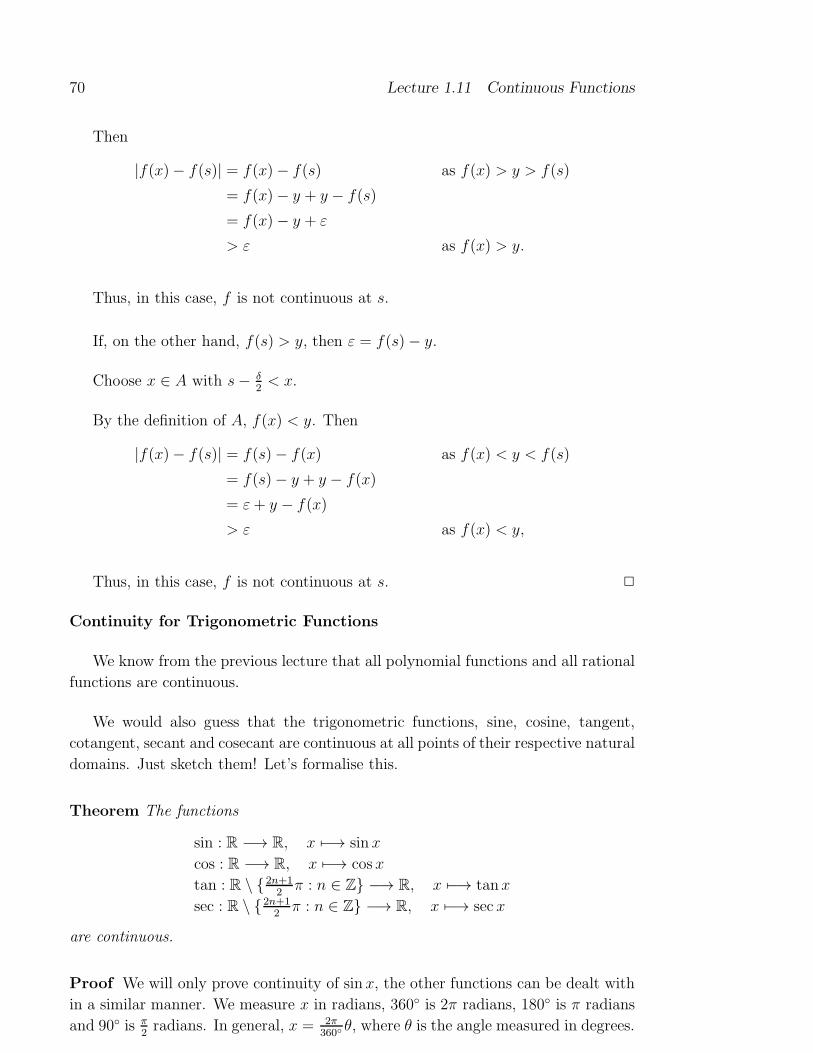
70 Lecture 1.11 Continuous Functions
Then
|f(x)− f(s)| = f(x)− f(s) as f(x) > y > f(s)
= f(x)− y + y − f(s)
= f(x)− y + ε
> ε as f(x) > y.
Thus, in this case, f is not continuous at s.
If, on the other hand, f(s) > y, then ε = f(s)− y.
Choose x ∈ A with s− δ2< x.
By the definition of A, f(x) < y. Then
|f(x)− f(s)| = f(s)− f(x) as f(x) < y < f(s)
= f(s)− y + y − f(x)
= ε+ y − f(x)
> ε as f(x) < y,
Thus, in this case, f is not continuous at s. 2
Continuity for Trigonometric Functions
We know from the previous lecture that all polynomial functions and all rational
functions are continuous.
We would also guess that the trigonometric functions, sine, cosine, tangent,
cotangent, secant and cosecant are continuous at all points of their respective natural
domains. Just sketch them! Let’s formalise this.
Theorem The functions
sin : R −→ R, x 7−→ sin x
cos : R −→ R, x 7−→ cosx
tan : R \ {2n+12
π : n ∈ Z} −→ R, x 7−→ tanx
sec : R \ {2n+12
π : n ∈ Z} −→ R, x 7−→ sec x
are continuous.
Proof We will only prove continuity of sin x, the other functions can be dealt with
in a similar manner. We measure x in radians, 360◦ is 2π radians, 180◦ is π radians
and 90◦ is π2radians. In general, x = 2π
360◦θ, where θ is the angle measured in degrees.
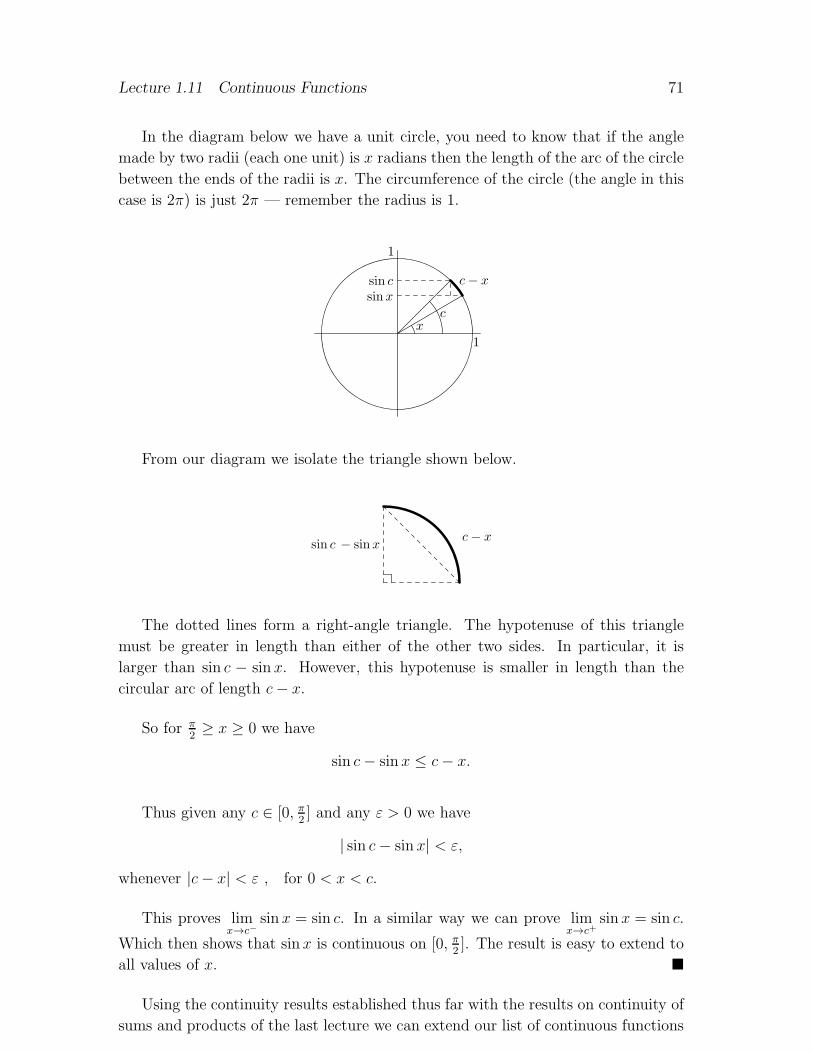
Lecture 1.11 Continuous Functions 71
In the diagram below we have a unit circle, you need to know that if the angle
made by two radii (each one unit) is x radians then the length of the arc of the circle
between the ends of the radii is x. The circumference of the circle (the angle in this
case is 2π) is just 2π — remember the radius is 1.
1
1
sinxsin c
x
c− x
c
From our diagram we isolate the triangle shown below.
sin c − sinxc− x
The dotted lines form a right-angle triangle. The hypotenuse of this triangle
must be greater in length than either of the other two sides. In particular, it is
larger than sin c − sin x. However, this hypotenuse is smaller in length than the
circular arc of length c− x.
So for π2≥ x ≥ 0 we have
sin c− sin x ≤ c− x.
Thus given any c ∈ [0, π2] and any ε > 0 we have
| sin c− sin x| < ε,
whenever |c− x| < ε , for 0 < x < c.
This proves limx→c−
sin x = sin c. In a similar way we can prove limx→c+
sin x = sin c.
Which then shows that sin x is continuous on [0, π2]. The result is easy to extend to
all values of x. �
Using the continuity results established thus far with the results on continuity of
sums and products of the last lecture we can extend our list of continuous functions

72 Lecture 1.11 Continuous Functions
in an obvious way to a large list of powers, products, of trigonometric and rational
functions.
We are also now in a position to establish many limits involving these functions.
A particularly useful way to establish these limits is the squeezing principle. It says
that, if two functions have limit L as x approaches c ∈ R, then any function in
between must also have limit L as x approaches c.
Theorem (Squeezing Principle)
Let f, g and h be functions whose domains contain the open interval (a, b), such
that
g(x) ≤ f(x) ≤ h(x)
for all x ∈ (a, c) and for all x ∈ (c, b) with a < c < b.
If limx→c
g(x) = limx→c
h(x) = L then
limx→c
f(x) = L.
Proof Let x ∈ (a, b). From the definition of the limit we know that for any ε > 0
there exists a δ > 0 such that
|g(x)− L| < ε and |h(x)− L| < ε
whenever |x− c| < δ. Thus
−ε < g(x)− L < ε and − ε < h(x)− L < ε
whenever |x− c| < δ. Now
g(x) ≤ f(x) ≤ h(x),
so
g(x)− L ≤ f(x)− L ≤ h(x)− L.
Combining this with the previous inequalities, we obtain
−ε ≤ g(x)− L ≤ f(x)− L ≤ h(x)− L ≤ ε,
so that, −ε ≤ f(x)− L ≤ ε, whenever |x− c| < δ.
This establishes limx→c
f(x) = L. 2
We now use this principle to establish two very well-known limits.
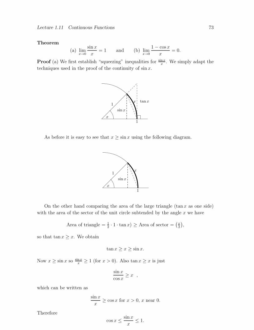
Lecture 1.11 Continuous Functions 73
Theorem
(a) limx→0
sin x
x= 1 and (b) lim
x→0
1− cosx
x= 0.
Proof (a) We first establish “squeezing” inequalities for sinxx. We simply adapt the
techniques used in the proof of the continuity of sin x.
1
1
sinx
x
x
tanx
As before it is easy to see that x ≥ sin x using the following diagram.
1
1
sinx
x
x
On the other hand comparing the area of the large triangle (tanx as one side)
with the area of the sector of the unit circle subtended by the angle x we have
Area of triangle = 12· 1 · tan x) ≥ Area of sector =
(x2
),
so that tanx ≥ x. We obtain
tanx ≥ x ≥ sin x.
Now x ≥ sin x so sinxx
≥ 1 (for x > 0). Also tan x ≥ x is just
sin x
cosx≥ x ,
which can be written as
sin x
x≥ cosx for x > 0, x near 0.
Therefore
cos x ≤ sin x
x≤ 1.

74 Lecture 1.11 Continuous Functions
Notice if x < 0 and x is near enough to 0 then
sin x
x=
sin(−x)
(−x)≥ cos(−x) = cos x, as sin(−x) = − sin x.
The same inequality applies either side of 0.
Now,
limx→0
cosx = 1 and limx→0
1 = 1.
We can apply the squeezing principle to get the result
limx→0
sin x
x= 1.
(b) We use the result from part (a), the identity sin2 x = 1− cos2 x and rewrite our
expression as follows
1− cos x
x=
1− cos x
x· 1 + cosx
1 + cosx
=1− cos2 x
x(1 + cosx)
=sin2 x
x(1 + cosx)=
[sin x
x
] [sin x
1 + cosx
]
.
Now take limits, remember we have proved the limit of product is the product of
the limits, etc.,
limx→0
(1− cosx
x
)
= limx→0
[sin x
x
]
limx→0
[sin x
1 + cosx
]
= (1)
(0
1 + 1
)
= 0.
�
Lecture 1.11 Continuous Functions 75
♠ Exercises 11
1. Evaluate the following limits:
(a) limh→0
sin h
2h(b) lim
x→0
x+ sin x
x
(c) limx→0
1− cos2 x
x(d) lim
y→0
sin(2y)
y
(e) limx→0
1− cosx
sin x(f) lim
h→0
h
tanh
(g) limx→0+
sin x
|x| (h) limx→0−
sin x
|x| .
2. Find the value of the constant k which makes
f : R −→ R, x −→{
sin 2xx
, x 6= 0
k, x = 0
a continuous function at x = 0.
3. Find limx→1sin(πx)x−1
.
4. Prove that if f : R −→ R is a continuous function then sin ◦f is also continu-
ous.
76 Lecture 1.12 More on Continuity
Lecture 1.12 More on Continuity
In this lecture we want to confirm the intuition that continuous functions on a closed
interval are “nice” functions.
Bounds of a Continuous Function
Theorem If f : D −→ R is continuous on [a, b] ⊆ D then it is bounded on the
interval, that is, {f(x) : x ∈ [a, b]} is bounded.
Remarks It is essential to the truth of the theorem that the interval is closed. The
function 1xis continuous in (0, 1], but is certainly not bounded as x −→ 0. We can
make 1xarbitrarily large by taking x near enough to 0.
Proof We first prove
Lemma 1.2 If the function f : R → R is continuous at a, then there is an r > 0
such that {f(x) | a− r < x < a+ r} is a bounded set of real numbers.
Proof Since f is continuous at a, and 1 > 0, there is an r > 0 with
f(a)− 1 < f(x) < f(a) + 1,
whenever a− r < x < a + r. 2
Now put A := {x ∈ [a, b] | f is bounded on [a, x]}. Since a ∈ A, A 6= ∅ and b is
an upper bound for A. Hence, A has a supremum, s ∈ [a, b].
Since f is continuous on [a, b], it follows by the Lemma above, that there is an
r > 0 such that f is bounded on the interval (s − r, s + r) ∩ [a, b], and so, in
particular, on [a, s+ r).
Since s = supA, this is only possible if (s, s+ r) ∩ [a, b] = ∅. Thus s = b. 2
This is again quite a subtle proof. Read it carefully to get the essential idea of
the argument.
Given a function, f : D −→ R, the supremum of f , supf , is the supremum of
the set {f(x)|x ∈ D}, that is, supf is the least upper bound of the image of f .
Similarly, the infimum of f , inff , is the infimum of {f(x)|x ∈ D}.
Lecture 1.12 More on Continuity 77
�Example If they exist, find supf and inff for the following:
(a) f : (0, 1) −→ R, x 7−→ x2;
(b) f : (0, 1) −→ R, x 7−→ 1x;
(c) f : [0, π2] −→ R, x 7−→ sin x.
Solution
(a) Here supf = 1 and inff = 0. Note that there is no x ∈ (0, 1) such that
f(x) = sup or f(x) = inf. We say that f(x) does not attain its bounds.
(b) Here inff(x) = 1 and supf does not exist as the function is unbounded above –1x→ ∞ as x −→ 0. Again we see there is no x ∈ (0, 1) such that f(x) = inff .
The function does not attain its lower bound.
(c) Here supf = 1 and inff = 0. In this case we see that f does attain its bounds
– note the interval is closed.
2
We already saw that a continuous function defined on a closed interval is bounded.
Thus it has a supremum and an infimum. We now show that it must attain its
bounds.
Theorem (The Extreme Value Theorem) Let f : [a, b] −→ R be a continuous
function with M = sup f and m = inf f . Then there exist x1, x2 ∈ [a, b] such that
f(x1) = M and f(x2) = m.
Proof We prove there exists an x1 ∈ [a, b] such that f(x1) = M . The proof for the
infinum is similar.
The proof we give is by contradiction – there is another proof using the so-called
method of bisection.
Proof by contradiction. Assume there is no x1 ∈ [a, b] for which f(x1) = M .
Then, as M is the supremum,
M − f(x) > 0 for all x ∈ [a, b].

78 Lecture 1.12 More on Continuity
Since M − f(x) 6= 0 for all x ∈ [a, b] we see, from Lecture 10, that
1
M − f(x)
is continuous on [a, b].
So, by our previous theorem, 1M−f(x)
is bounded on [a, b]. We have
1
M − f(x)< K, for some finite K ∈ R, and all x ∈ [a, b].
Then, as M − f(x) > 0,1
K< M − f(x)
or
f(x) < M − 1
Kfor x ∈ [a, b].
But this contradicts M = supf(x), M is the least upper bound, there cannot be a
smaller bound M − 1K! We have our proof by contradiction. �
We have had two reasonably difficult proofs for what would seem to be two
intuitively obvious facts!
�Example State whether or not the following functions meet the conditions of the
previous two theorems. If the function does, what are its supremum and infinum?
(a) f : (0, 1] −→ R, x 7−→ 1x;
(b) f : [1, 2] −→ R, x 7−→ 1x;
(c) f : [−1, 1] \ {0} −→ R, x 7−→ 1x2 ;
(d) f : [0, π] −→ R, x 7−→ cosx.
Solution The hypothesis for both theorems is that f is defined on a closed interval
[a, b] and continuous.
(a) Does not satisfy the hypothesis, the interval is not closed.
(b) Satisfies the hypothesis. Note that 1xdecreases from x = 1 to x = 2, so
sup
(1
x
)
= 1, on [1, 2] and
inf
(1
x
)
=1
2, on [1, 2].
Note that the function attains its bounds on [1, 2].

Lecture 1.12 More on Continuity 79
(c) The function does not satisfy the hypothesis as it is not defined on a closed
interval.
(d) The function cos is continuous and restricting a continuous function to a closed
interval we obtain another continuous function. Thus the hypothesis is satis-
fied.
sup f = 1 and inff = −1.
Monotone Functions
Consider a function f : D −→ R, D ⊆ R. We say that f is increasing if, given
any points x1, x2 ∈ S with x1 < x2, then f(x1) ≤ f(x2). If we have f(x1) < f(x2)
we say f is strictly increasing. Reversing the inequalities on f defines a decreasing
or strictly decreasing function.
A function which is either increasing or decreasing is said to be
monotone. A function which is strictly increasing or strictly de-
creasing is said to be strictly monotone.
It is easy to see that every strictly monotone function must be injective (one-one)
but it is by no means true that every injective function has to be strictly monotone.
�Example The following functions are monotone
(a) idR : R −→ R, x 7−→ x;
(b) f : [0,∞) −→ R, x 7−→ x2;
(c) f : R −→ R, x 7−→
x, x < 0
0, 0 ≤ x < 1
x− 1, x ≥ 1
;
(d) f : (0,∞) −→ R, x 7−→ 1x.
Note that the functions in (a), (b) and (d) are strictly monotone, continuous
and injective. The function in example (c) is not strictly monotone, though it is
monotone. The example (c) is continuous but not injective. You should draw the
graphs of these functions to convince yourself of these facts.

80 Lecture 1.12 More on Continuity
�Example The following functions are not monotone
(a) f : R −→ R, x 7−→ |x|;
(b) f : R −→ R, x 7−→ x2;
(c) f : R −→ R, x 7−→{
x, x < 0
x− 1, x ≥ 0;
(d) f : [0, π] −→ R, x 7−→ sin x.
The functions in (a), (b) and (d) are all continuous, but they are not injective.
Hence they cannot be monotone. The function in (c) is not continuous at x = 0
and not monotone. It is, however, injective. In fact, the function in (c) is monotone
on each of the intervals (−∞, 0) and [0,∞), separately. The same is also true for
the other functions – there exist subintervals on which the (restricted) function is
monotone.
Now for our main result on monotone functions.
Theorem Every injective and continuous function f : [a, b] −→ R is strictly mono-
tone.
Proof First we observe that f cannot be constant on any subinterval – if it was
there would be points x and y for which f(x) = f(y), which is not possible as f
is one-one. In fact it is not hard to see that if f is increasing on a subinterval it
must be strictly increasing (again use the fact that f is injective). Similarly, if f is
decreasing on a subinterval it must be strictly decreasing on that subinterval. Divide
[a, b] into subintervals on which f is either strictly increasing or strictly decreasing.
If there is only one subinterval (the whole of [a, b]) we are finished. So we assume
there are at least two. Hence there is a point c ∈ (a, b) such that for some δ > 0,
the function f is either strictly increasing on (c − δ, c) and strictly decreasing on
(c, c+ δ) or vice versa. Let us assume the former, so
f(y) > f(x) for x, y ∈ (c− δ, c) and y > x,
and f(y) < f(x) for x, y ∈ (c, c+ δ) and y > x.
Now f is continuous and so takes all values between f(c−δ) and f(c) for x ∈ (c−δ, c)
– note f(c) > f(c− δ). Similarly f must take all values between f(c+ δ) and f(c)
for x ∈ (c, c+ δ) – note f(c) > f(c+ δ).
Then either f(c − δ) > f(c + δ), in which case there is an x1 ∈ (c, c + δ) such
that f(c− δ) = f(x1). Or
f(c− δ) < f(c+ δ)
Lecture 1.12 More on Continuity 81
in which case there is an x2 ∈ (c− δ, c) such that f(c+ δ) = f(x2). Or
f(c− δ) = f(c+ δ).
However, each of these possibilities contradicts the fact that f is injective. We can
thus have only one subinterval – f is either strictly increasing on [a, b] or strictly
decreasing on [a, b]. It’s monotone. 2
♠ Exercises 12
1. Given functions f, g : R −→ R, suppose f is continuous at x = a whereas g is
discontinuous at x = a.
(a) Can one conclude f + g is not continuous at x = a?
(b) Can one conclude fg is not continuous at x = a?
2. Repeat question 1 this time assuming both f and g are discontinuous at x = a.
3. State whether or not the following functions are monotone. Also decide if
the functions are are injective, surjective or bijective. If they exist, find the
supremum and infimum in each case and state whether or not the function
attains its bounds.
(a) f : [0, 3] −→ R, x 7−→ x3;
(b) f : R −→ R, x 7−→ 11+x2 ;
(c) f : (0, π2) −→ R, x 7−→ sin( 1
x);
(d) f : (−1,∞) −→ R, x 7−→ 1−x1+x
.
4*. Let f : [a, b] −→ R be bounded, such that, for every pair of values x1, x2 with
a ≤ x1 ≤ x2 ≤ b
f
(x1 + x2
2
)
≤ 1
2[f(x1) + f(x2)] .
Prove f is continuous on (a, b).
82 Lecture 1.13 Sequences
Lecture 1.13 Sequences
A sequence is simply a function whose domain is N, the natural numbers.
f : N −→ R
f : n 7−→ f(n).
Of course this is not the notation you would be familiar with. The usual way of
specifying a sequence is to give the nth term, usually denoted by an. In function
notation the nth term is just f(n). Clearly any function f : R −→ R can be
restricted to the natural numbers to give a sequence.
�Example
(a) f(x) = 1x2 , when restricted to N gives the sequence an = 1
n2 .
(b) f(x) = sin x, when restricted to N gives the sequence an = sin n.
Another common way of specifying a sequence is to write down some of the early
terms. But, unless the nth term is given, this does not uniquely specify a sequence.
�Example Examples of notation for sequences
(a) 1, 12, 13, 14, . . . , 1
n, . . .
(b)
{1
n
}∞
n=1
=
{
1,1
2,1
3, . . . ,
1
n, . . .
}
(c) f(n) = 1n.
A sequence need not be infinite, {1, 2, 3} is a sequence. If, for each n ∈ N, we
are assigned a number an then the sequence is said to be an infinite sequence.
For an infinite sequence perhaps the most interesting question is “does the se-
quence tend to a finite limit as n −→ ∞?”.
�Example
(a)
{1
n
}∞
n=1
tends to the limiting value 0.
(b)1
2,2
3,3
4, . . . ,
n
n + 1, . . . approaches the value 1.
Lecture 1.13 Sequences 83
Formal Definition of Limits
We can define a limit for a sequence in much the same way as we defined the
one-sided limits for f(x) as x −→ ±∞.
A sequence with nth term an is said to have the limit a if, given
any ε > 0, there is an N such that
|an − a| < ε for all n > N.
We write limn−→∞
an = a or an −→ a as n −→ ∞.
Note that if a sequence an does have a limit then it must be bounded. For n > N
we have
−ε < an − a < ε
or a− ε < an < a+ ε.
Our definition of the limit can be abbreviated using some mathematical notation.
We introduce two symbols which replace commonly used mathematical phrases.
∃ . . . stands for the phrase “there exists”.
∀ . . . stands for the words “for all”.
So we can write our definition of the limit as,
an −→ a if
given ε > 0 ∃ N such that
|an − a| < ε, ∀ n > N.
The symbols ∃ and ∀ are not just used in the context of sequences, they may be used
in any (mathematical) situation in which the corresponding phrase is appropriate.
If a sequence does not tend to a finite limit it does not necessarily diverge to
±∞ – there are other types of behaviour.
�Example
(a) The sequence an = (−1)n oscillates.

84 Lecture 1.13 Sequences
(b) The sequence an = sin(n) oscillates.
(c) The sequence an =√n tends to infinity.
(d) The sequence an = sin(1n
)approaches 0.
Formally, we will define a diverging sequence as follows.
The sequence an is said to tend to infinity, or an −→ ∞ if given
any A > 0 (no matter how large) there exists on N such that
an > A for all n > N.
We have a similar definition for a sequence diverging to −∞.
The sequence an is said to tend to negative infinity, or an −→ −∞as n −→ ∞ if given A > 0 ∃ N such that
an < −A ∀ n > N.
Sequences such as an = (−1)n or bn = (−1)nn do not tend to a limit or ±∞.
Such sequences are said to oscillate.
From our earlier work on limits we would expect to have a theorem on the limit
sums and products of sequences. There is such a theorem.
Theorem Let an −→ a and bn −→ b as n −→ ∞ then
(a) αan + βbn −→ αa+ βb, ∀α, β ∈ R.
(b) anbn −→ ab
(c)anbn
−→ a
b, provided b 6= 0.
Proof The technique of proof is the same as for limits of functions. We will prove
(c).
Lecture 1.13 Sequences 85
Note that∣∣∣∣
anbn
− a
b
∣∣∣∣
=
∣∣∣∣
ban − abnbbn
∣∣∣∣
=
∣∣∣∣
b(an − a) + a(b− bn)
bbn
∣∣∣∣
≤ |b(an − a)|+ |a(b− bn)||bbn|
,
ie.
(∗)∣∣∣∣
anbn
− a
b
∣∣∣∣≤ |b| · |an − a|+ |a| · |bn − b|
|bbn|.
Now an −→ a and bn −→ b so for any given ε > 0 we can find an N such that
|an − a| < |b|4ε, |bn − b| < |b|2
4|a|ε
and |bn| >1
2|b|
for n > N.
If |a| = 0 then we do not need the inequality for |bn − b|. Putting these last three
inequalities into (*) we have
∣∣∣∣
anbn
− a
b
∣∣∣∣<
|b| · |b|4ε+ |a| · |b|2
4|a|ε
|b|12|b| = ε.
for n > N.
We have formally establishedanbn
−→ a
bas n −→ ∞.
�Example Discuss the behaviour of the following sequences as n −→ ∞ :
(a)
(n− 3
3n+ 1
)3
(b)
(3n+ 1
n− 3
)3
(c) cosn (d)(−1)n
n
Solution
(a) We need to use the trick of dividing out the n so as to apply our theorem onanbn
.
(n− 3
3n+ 1
)3
=
(1− 3
n
3 + 1n
)3
=
(1− 3
n
)3
(3 + 1
n
)3 .

86 Lecture 1.13 Sequences
Now apply the theorem to get
(n− 3
3n + 1
)3
−→ (1− 0)3
(3 + 0)3=
1
27.
(b) Similar to (a),
(3n+ 1
n− 3
)3
=
(3 + 1
n
1− 3n
)3
−→ 33
13= 27.
(c) The sequence oscillates through all numbers between −1 and +1.
(d) The sequence tends to the limit 0,
i.e.(−1)n
n−→ 0 as n −→ ∞.
2
Monotone Sequences
If an+1 ≥ an for all n we call an increasing.
If an > an ∀ n we say an is strictly increasing. If an+1 ≤ an ∀ n we
say an is decreasing and if an+1 < an we say an is strictly decreasing.
A sequence which is increasing or decreasing is called monotonic.
Monotonic sequences have the very important property that they must tend to
a limit or to +∞ or to −∞. Monotonic sequences cannot oscillate.
We will prove this property for an increasing sequence. This proof is easily
adapted to the decreasing case.
Theorem An increasing sequence either tends to a limit or +∞ as n −→ ∞. An
increasing sequence cannot oscillate.
Proof Let an be an increasing sequence.
We have two possibilities either the sequence is bounded above or its not. That is
either of the following must hold
1. a number K can be found such that
an ≤ K ∀n
or
2. for any number A we can find an N such that an > A.
Lecture 1.13 Sequences 87
Deal with possibility (2) first. As an is increasing an > A not just for n = N but
for all n ≥ N . So from our definition an −→ ∞ as n −→ ∞.
Now for (1). The number K is an upper bound for the set {a1, a2, . . . , an, . . .} =
{an}, so the set must have supremum a which satisfies
an ≤ a ∀n and
an > a− ε for some particular value n = N.
As an is increasing the second inequality must hold for all n ≥ N . So we have
an < a(< a+ ε) and
a− ε < an
for all n > N . We can write this as
|an − a| < ε ∀n > N.
Which just says an has limit a.
♠ Exercises 13
1. Discuss the behaviour of the sequences as n −→ ∞.
(a) sin
(1
n
)
(b) n sin
(1
n
)
(c) (n!)1
n
(d)n3 − n2 + n + 1
10− 3n+ 2n3(e)
n2 + 1
n(f)
2n2
n!
2. State which of the sequences are monotone. (Are they increasing or decreas-
ing?)
(a)n
n2 + 1(b) (−n)2 (c) nn
(d)n2 + 1
n(e) 2n+ (−1)n (f) n2−1
n3−1
3. Prove that if a > 0 then a1
n −→ 1 as n −→ ∞.
4. In relativistic quantum mechanics the solution of the Dirac equation for the
electron in the hydrogen atom gives energy levels
En =mc2
√
1 + γ2/c2[
n+√
κ2−γ2/c2]
where m is the electron mass, γ is a constant related to the electric charge,
κ is a constant related to the orbital quantum number and n is the principle
quantum number. Does En give a monotonic sequence? Does En have a limit
as n −→ ∞?
5*. Prove that an −→ 0 as n −→ ∞ if limn−→∞
an+1
an= L, where −1 < L < 1.

88 Lecture 1.14 Sequences and Series
Lecture 1.14 Sequences and Series
As a direct consequence of our last theorem (Lecture 13) we have the following useful
result.
Theorem A bounded monotone sequence tends to a limit.
Proof Direct consequence of previous theorem for an increasing sequence – case 1.
The same technique works for a decreasing sequence. Try it! 2
The Geometric Sequence
The geometric sequence has nth term an = an where a is a constant. The
behaviour of the sequence as n −→ ∞ depends upon the value of a. There are four
main cases to consider.
1. If a = 1, an = 1 for all n. Clearly limn−→∞
an = 1! There is also the trivial case
a = 0 to consider.
2. a > 1 let a = 1+ k, k > 0 then (1+ k)n > 1+ nk (Exercise 4 Lecture 2). Now
as n −→ ∞ 1 + nk −→ ∞ and so an = (1 + k)n −→ ∞.
3. 0 < a < 1. Let a =1
1 + k, k > 0. Then
1
an= (1 + k)n > 1 + nk. So
an =1
(1 + k)n<
1
1 + nk
Now1
1 + nk−→ 0 as n −→ ∞ so an =
1
(1 + k)n−→ 0 as n −→ ∞.
4. a < 0. Firstly, if −1 < a < 0 we use a similar argument to that in 3 to find
an −→ 0. If a = −1 then an = (−1)n = ±1 and the sequence oscillates finitely.
If a < −1 then (using a similar argument to 2) we see that the sequence
oscillates infinitely.
Summing up
an = an, a constant
a > 1, an −→ ∞a = 1 an −→ 1
−1 < a < 1 an −→ 0
a = −1 an oscillates finitely
a < −1 an oscillates infinitely.

Lecture 1.14 Sequences and Series 89
Infinite Series
Intuitively we think of an infinite series as a “sum to infinity” of an infinite
sequence {an}:a1 + a2 + a3 + . . .+ an + . . . .
We will use a shorthand notation for such a sum
∞∑
n=1
an ≡ a1 + a2 + a3 + . . .+ an + . . . ;
this is the sigma or summation notation. We just think of the∑
as standing for
sum over all counting number values between the given limits.
We have still not said what we mean by “sum to infinity”. This term is fraught
with danger and we need to say precisely what we mean by it. We will give the
appropriate definition below, but first an illustration of the dangers.
Consider∞∑
n=1
(−1)n = −1 + 1− 1 + 1− 1 + 1 . . . . We might want to “sum” this
by grouping terms as follows (−1 + 1) + (−1 + 1) + (−1 + 1) + . . . to conclude that
the sum is zero. This would be wrong. To see this we could also group the terms
as −1 + (1 − 1) + (1 − 1) + . . . , to get a sum of −1! There is clearly something
wrong with the process of “grouping terms” for such a series.
We will define our infinite sums in terms of a sequence, the sequence of partial
sums.
Let {an}∞n=1 be an infinite sequence. We define the nth partial sum
Sn of the sequence as
Sn = a1 + 12 + a3 + . . .+ an, or
Sn =n∑
r=1
ar.
We can now talk about the possible limit of the sequence {Sn}∞n=1.
If the sequence of partial sums {Sn} has a finite limit as n −→ ∞ we
say that the infinite series a1+a2+a3+ . . .+an+ . . . is convergent
or has a “sum to infinity” and that S = limn−→∞
Sn is its sum.
90 Lecture 1.14 Sequences and Series
A series which is not convergent is said to be divergent.
We think of the words “infinite sum” as applying only in the sense of a convergent
limit of the sequence of partial sums.
The Geometric Series
The geometric series is the “sum to infinity” of the geometric sequence. When
this sum exists!
Theorem The infinite geometric series
1 + a+ a2 + . . .+ an . . .
converges if and only if −1 < a < 1.
Proof The series has first term 1 so the nth term is an = an−1. We note that
Sn = 1 + a+ a2 + . . .+ an−1
and aSn = a+ a2 + . . .+ an.
So aSn − Sn = an − 1.
Therefore Sn = 1−an
1−a, for a 6= 1, if a = 1 Sn = n. We see that if a = 1 then
Sn −→ ∞ as n −→ ∞. For a 6= 1 we have
Sn =1− an
1− a=
1
1− a− 1
1− aan.
We see that the sequence of partial sums Sn, converges if and only if the sequence
an converges. But from our section on the geometric sequence we know an tends to
a finite limit (which is 0) if and only if −1 < a < 1. This proves the theorem. Note
that we also have the sum to infinity in the case −1 < a < 1, it is
Sn −→ 1
1− aas n −→ ∞.
�
The Harmonic Series∑
1n
Theorem The infinite series
∞∑
n=1
1
n= 1 +
1
2+
1
3+ . . .
diverges.

Lecture 1.14 Sequences and Series 91
Proof Consider the following
1
3+
1
4> 2× 1
4=
1
21
5+
1
6+
1
7+
1
8> 4× 1
8=
1
21
9+
1
10+ . . .+
1
15+
1
16> 8× 1
16=
1
2,
and so on. The sum of successive blocks of 2, 4, 8, 16 . . . terms is greater than 12.
Including the first two terms 1+ 12we have that the sum of the first 2 + 2+ 4+ 8+
16 + . . .+ 2m−1 = 2m terms of the series is greater than
1 + 12+ 1
2×(number of blocks) = 1 + 1
2+ 1
2(m− 1) = 1 + 1
2m.
So S2m > 1 + 12m, ie. the partial sums of the first 2m terms is greater than 1 + 1
2m.
Clearly, Sn −→ ∞ as n −→ ∞. The series diverges. �
The Comparison Test
Theorem If for every n > N (N finite),
(i) un ≥ 0, vn ≥ 0
(ii) un ≤ kvn, k > 0 is a constant,
then
(a) if∑
vn converges∑
un converges
or
(b) if∑
un diverges∑
vn diverges.
Proof
An exercise. Use the fact that the partial sums Sn =
n∑
r=1
un and Tn =
n∑
r=1
vn
form increasing sequences for n > N . Then use the results on monotone sequences.
�Example Discuss the convergence (or divergence) of the following infinite series.
(a)
∞∑
n=1
1√n
(b)
∞∑
n=1
n
3n
(c)
∞∑
n=1
n
n2 + 1(d)
∞∑
n=0
n2n + 1
5n + 1

92 Lecture 1.14 Sequences and Series
Solution
(a) For n ≥ 11√n≥ 1
n
The comparison test then shows that∑
1√ndiverges.
(b) For n ≥ 1 n < 2n so.n
3n<
2n
3n=
1
(1.5)n
Now∞∑
n=1
1
(1.5)
n
is a convergent geometric progression, so by the comparison
test∑ n
3nconverges.
(c)n
n2 + 1≥ n
n2 + n2, for n ≥ 1.
ie.n
n2 + 1≥ 1
2· 1n
∑1nis the divergent harmonic series so
∑ n
n2 + 1diverges by the comparison
test.
(d)n2n + 1
5n + 1<
n2n + n2n
5n + 1<
n2n+1
5n<
2n · 2n+1
5n
i.e.n2n + 1
5n + 1<
2 · (22)n5n
= 21
(1.25)n
So comparison with the convergent geometric series∑ 1
(1.25)nshows that
∑ n2n + 1
5n + 1converges.
2
♠ Exercises 14
1. A ball is dropped from a height of 20m. On each bounce the ball returns to a
height of 45of that of the previous bounce.
What is height of the 3rd bounce?
Give a formula for the height of the nth bounce.
Give a formula for the distance travelled by the ball up to and including the
nth bounce.
What is the total distance travelled by the ball from the time it is first dropped
till the time it comes to rest?
2. Discuss the convergence or otherwise of the following infinite series:

Lecture 1.14 Sequences and Series 93
(a)1
3+
2
5+
3
7+ . . .+
n
2n + 1+ . . .
(b) 1 +1
1+
1
2 · 1 +1
3 · ·1 + . . .+1
n!+ . . .
(c)∑ 2n + 1
3n + 1
(d)∑ 1√
n2 + 1
(e)∞∑
k=0
cos(kπ)
(f)∑ n2
2n.
3. Prove that if 0 ≤ an ≤ 1, then the series
∞∑
n=0
(anxn) converges for 0 ≤ x < 1.
4. If
an =
(
1 +1
n
)n
and bn =
(
1− 1
n
)−n
prove that an is an increasing and bn a decreasing sequence. Prove further
that as n −→ ∞, bn − an −→ 0, and that an and bn lead to the same limit.
(This limit is e the base of the natural logarithms.)

94 Lecture 1.15 Series
Lecture 1.15 Series
In the previous lecture we showed that the harmonic series∑ 1
ndiverges. We now
generalise this result.
Theorem The infinite series
∞∑
n=1
1
nk, k constant, converges if k > 1 and diverges if
k ≤ 1.
Proof We know the series diverges for k = 1 so for k ≤ 1 we can use the comparison
test. We have1
nk≥ 1
n, for k ≤ 1.
So the series diverges for k ≤ 1.
For the case k > 1 we use the same device we used in proving the divergence of∑
1n. Group terms of the series in blocks of length 2, 4, 8, . . . , to get
1
2k+
1
3k<
2
2k=
1
2k−1
1
4k+
1
5k+
1
6k+
1
7k<
4
4k=
1
4k−1=
1
(2k−1)2
1
8k+
1
9k+ . . .+
1
15k<
8
8k=
1
8k−1=
1
(2k−1)3.
The series 1 +1
2k−1+
1
(2k−1)2+
1
(2k−1)3+ . . . is a convergent geometric series,
(as a 0 <1
2k−1< 1, for k > 1) . The sequence of partial sums Sn =
n∑
r=1
1
rkis then
bounded by the sum to infinity of our geometric series ie.
Sn <1
1− 2k−1.
Now Sn is an increasing sequence so our theorem on monotone sequences (Lecture
14) tells us Sn must tend to a finite limit. Hence the series∑ 1
nkconverges for
k > 1. We are finished. �
�Example Discuss the convergence or otherwise of the following series
(a)∑ n2 + 1
n4 + 1

Lecture 1.15 Series 95
(b)∑ 1
3√n
Solution
(a) Noten2 + 1
n4 + 1<
n2 + n2
n4=
2
n2.
So, as∑ 1
n2, converges (see last theorem) we have from the comparison test
that∑ n2 + 1
n4 + 1converges.
(b) Straightforward application of last theorem with k =1
3.
∑ 13√n
diverges.
2
Properties of Infinite Series
Theorem For infinite series the following properties must hold.
1. The convergence or divergence of a series is unaffected if a finite number of
terms are inserted, or suppressed, or altered.
2. If∑
un converges then un −→ 0 as n −→ ∞.
3. If∑
un converges to s and∑
sn converges to t then∑
(un + vn) converges to
s+ t.
4. If∑
un is convergent then so is any series obtained from∑
un by bracketing
the terms in any manner. The two series have the same sum.
5. If un ≥ 0, for every n, the∑
un either converges or diverges to +∞.
Proof
1. Changing a finite number of terms, say we replace
N∑
n=1
an by some other num-
ber A, say. Then
∞∑
n=1
an =
N∑
n=1
an +
∞∑
n=N+1
an and the new sum to infinity is

96 Lecture 1.15 Series
A+∞∑
n=N+1
an. However∞∑
n=1
an converges (or diverges) if and only if∞∑
n=N+1
an
converges (or diverges) as
N∑
n=1
an is finite. Hence the result.
2. Note that un = Sn − Sn−1 where Sn =n∑
r=1
ur is the nth partial sum.
However, if∑
un converges to s then Sn −→ s and Sn−1 −→ s as n −→ ∞.
The result follows.
3. Let Sn =
n∑
r=1
ur and Tn =
n∑
r=1
vn. Then limn→∞
Sn = s and limn→∞
Tn = t. However
from lecture 13 we know that
limn→∞
(Sn + Tn) = s+ t.
But, Sn + Tn = Pn =
n∑
r=1
(un + vn) the nth partial sum of∑
(un + vn). The
result is proved.
4. Exercise.
5. With un ≥ 0 Sn =n∑
r=1
ur is an increasing sequence. The result then follows
from lecture 13.
�
�Example Discuss the convergence or otherwise of
(a)∑ (3n + 2n)
6n
(b)
∞∑
n=1
210−n
Solution
(a) The series∑ 1
2nand
∑ 1
3nboth converge so the series
∑(
1
2n+
1
3n
)
=∑
(3n + 2n
2n · 3n)
=∑ 2n + 3n
6n
must also converge by our last theorem.

Lecture 1.15 Series 97
(b) ∞∑
n=1
210−n =9∑
n=1
210−n +∞∑
n=10
210−n
∞∑
n=10
210−n = 1 +1
2+
1
22+
1
23+ . . .
=
∞∑
n′=0
1
2n′, where n′ = n− 10.
This last series is a convergent geometric series so the original series converges,
property 1 of the last theorem. 2
The Ratio Test
Theorem Let∑
uk be a series with positive terms and suppose that
ρ = limn−→∞
un+1
un
(a) if ρ < 1, the series converges;
(b) if ρ > 1 the series diverges;
(c) if ρ = 1 the series may converge or diverge.
Proof
(a) Nowun+1
un
≥ 0 ∀n ∈ N so we have 0 ≤ ρ < 1 in this case.
Asun+1
un−→ ρ < 1 we must have for n ≥ N , for some N ,
un+1
un< 1. So there
is an r < 1 such that for n ≥ N ,un+1
un< r. Consider the series
∞∑
n=N
un. Now,
usingun+1
un< r, for n ≥ N , we have
uN+1 < ruN
uN+2 < ruN+1 < r2uN
uN+3 < ruN+2 < r3uN
...
In general un < rn−NuN for n ≥ N . The series
∞∑
n=N
rn−NuN is a convergent
geometric series (as 0 < r < 1) so by the comparison test∑
un converges.
98 Lecture 1.15 Series
(b) In this case we haveuN+1
un
−→ ρ > 1 as n −→ ∞. So for some N we have
un+1
un
> 1 for all n ≥ N.
From which we have
uN+1 > uN
uN+2 > uN+1 > uN
...
In general un > uN for all n ≥ N . However, the series∞∑
n=N
uN = uN
∞∑
n=N
1 = uN(1 + 1 + 1 + · · · ) clearly diverges. Hence, by the com-
parison test∑
un must diverge.
(c) Consider the ratio test for un = 1nk , where 0 < k < ∞. We have
un+1un =nk
(n+ 1)k=
(n
n+ 1
)k
=1
(1 + 1
n
)k.
But1
(1 + 1
n
)k−→ 1 as n −→ ∞.
So for un = 1nk , ρ = 1. However,
∑un diverges if 0 < k ≤ 1 and converges for
k > 1.
�
�Example Determine whether the following series converge or diverge.
(a)∞∑
n=1
nn
n!(b)
∑ 3n
n!(c)
∑ 5n
n2
Solution
(a) un =nn
n!=
nn
n(n− 1) . . . 2.1, so
un+1
un=
(n + 1)n+1
(n + 1)!· n!nn
=(n + 1)n+1
(n+ 1)nn
=(n + 1)n
nn=
(
1 +1
n
)n
Lecture 1.15 Series 99
We know from an earlier exercise that
(
1 +1
n
)n
−→ e > 1 as n −→ ∞. So
the series∑ nn
n!diverges.
(b) un =3n
n!,un+1
un=
3n+1
(n+ 1)!
n!
3n=
3
n+ 1. So
un+1
un=
3
n+ 1−→ 0 as n −→ ∞.
The series converges.
(c) un =5n
n2,un+1
un
=5n2
(n+ 1)2= 5
(1
1 + 1n
)2
.
So,un+1
un=
5(1 + 1
n
)2 −→ 5 as n −→ ∞. The series diverges. 2
♠ Exercises 15
Determine the convergence or otherwise of these following infinite series.
1.∑ 1
5n2 − n2.
∑ 2
n2 + n
3.
∞∑
k=1
k
k3/2 − 12
4.∑ n10
3k
5.∑ k2
3k3 + 16.
∑ sin2 k
k2
7.∑ k2
5k8.
∑ (n!)2
(2n)!