MATH4406 (Control Theory)Unit 6: The Linear Quadratic Regulator (LQR)

andModel Predictive Control (MPC)

Prepared by Yoni Nazarathy, Artem Pulemotov,September 12, 2012

Unit Outline

Goal 1: Outline linear quadratic optimal control (LQR).

Goal 2: Introduce Concepts of Model Predictive Control (MPC).

Goal 3: A stability proof for linear quadratic MPC.

Auxiliary items:Background on positive (semi) definite matrices.Riccati equations.Quadratic Programming (convex optimization).

The Linear Quadratic Regulator (LQR)

The “L” part of LQR

The same old linear dynamics:

x(t) = Ax(t) + Bu(t), or x(k + 1) = Ax(k) + Bu(k),

A ∈ Rn×n, B ∈ Rn×m, x(0) = x0.

Assume,

rank(con(A,B) :=

[B,AB,A2B, . . . ,An−1B

])= n,

i.e., the system is controllable (reachable)

So in the continuous time case, we can drive the state from x0 toany state in any finite time, T . For the discrete time case it can bedone in at most n steps.

The “Q” part of LQR

A cost structure:

J(u) =

∫ T

0

(x(t)′Q x(t) + u(t)′ R u(t)

)dt + x(T )′Qf x(T ),

or,

J(u) =N−1∑k=0

(x(k)′Q x(k) + u(k)′ R u(k)

)+ x(N)′Qf x(N).

The time horizon, T or N, can be finite or infinite.

The cost matrices satisfy,

Q = Q ′ ≥ 0, Qf = Q ′f > 0, R = R ′ > 0.

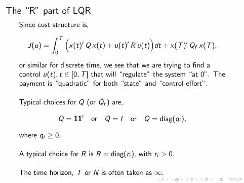
The “R” part of LQR

Since cost structure is,

J(u) =

∫ T

0

(x(t)′Q x(t) + u(t)′ R u(t)

)dt + x(T )′Qf x(T ),

or similar for discrete time, we see that we are trying to find acontrol u(t), t ∈ [0,T ] that will “regulate” the system “at 0”. Thepayment is “quadratic” for both “state” and “control effort”.

Typical choices for Q (or Qf ) are,

Q = 11′ or Q = I or Q = diag(qi ),

where qi ≥ 0.

A typical choice for R is R = diag(ri ), with ri > 0.

The time horizon, T or N is often taken as ∞.

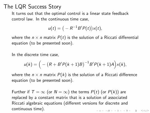
The LQR Success StoryIt turns out that the optimal control is a linear state feedbackcontrol law. In the continuous time case,

u(t) =(− R−1B ′P(t)

)x(t),

where the n × n matrix P(t) is the solution of a Riccati differentialequation (to be presented soon).

In the discrete time case,

u(k) =(−(R + B ′P(k + 1)B

)−1B ′P(k + 1)A

)x(k),

where the n × n matrix P(k) is the solution of a Riccati differenceequation (to be presented soon).

Further if T =∞ (or N =∞) the terms P(t) (or P(k)) arereplaced by a constant matrix that is a solution of associatedRiccati algebraic equations (different versions for discrete andcontinuous time).

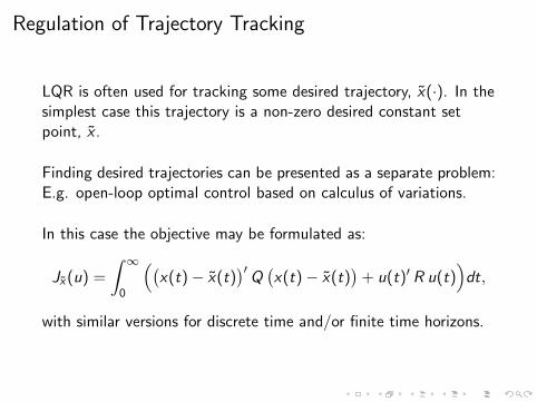
Regulation of Trajectory Tracking

LQR is often used for tracking some desired trajectory, x(·). In thesimplest case this trajectory is a non-zero desired constant setpoint, x .

Finding desired trajectories can be presented as a separate problem:E.g. open-loop optimal control based on calculus of variations.

In this case the objective may be formulated as:

Jx(u) =

∫ ∞0

((x(t)− x(t)

)′Q(x(t)− x(t)

)+ u(t)′ R u(t)

)dt,

with similar versions for discrete time and/or finite time horizons.

LQR Results

The Riccati Equation - Continuous Time

This is the Riccati matrix differential equation used to find thestate feedback control law of continuous time LQR. Solve it for{P(t), t ∈ [0,T ]}

−P(t) = A′P(t) + P(t)A− P(t)BR−1B ′P(t) + Q, P(T ) = Qf .

Observe that it is specified “backward in time”.

If T =∞ the steady state solution P of the Riccati differentialequation replaces P(t) in the optimal control law. This P is theunique positive definite solution of the algebraic Riccati equation,

0 = A′P + PA− PBR−1B ′P + Q.

The optimal control is:

u(t) =(− R−1B ′P(t)

)x(t) or u(t) =

(− R−1B ′P

)x(t).

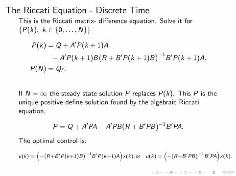
The Riccati Equation - Discrete TimeThis is the Riccati matrix- difference equation. Solve it for{P(k), k ∈ {0, . . . ,N}}

P(k) = Q + A′P(k + 1)A

− A′P(k + 1)B(R + B ′P(k + 1)B

)−1B ′P(k + 1)A,

P(N) = Qf .

If N =∞ the steady state solution P replaces P(k). This P is theunique positive define solution found by the algebraic Riccatiequation,

P = Q + A′PA− A′PB(R + B ′PB)−1B ′PA.

The optimal control is:

u(k) =(−(R+B′P(k+1)B

)−1B′P(k+1)A

)x(k), or u(k) =

(−(R+B′PB

)−1B′PA

)x(k).

Stability

When T =∞ (or N =∞) we see that the resulting system issimply a state-feedback controller,

u(t) = Fx(t) or u(k) = Fx(k).

with F =(− R−1B ′P

)or F =

(−(R + B ′PB

)−1B ′PA

).

Is it stable? In the continuous time case, the algebraic Riccatiequation is,

0 = A′P + PA− PBR−1B ′P + Q.

Recall the formula −(A′P + PA) > 0 from Yoni’s lecture onLyapunov functions. The presence of this term suggests that wecan hope to have stability. Indeed, we do under assumptions.

For the discrete time system, the analog of A′P + PA is P − A′PA.

A Solved ExampleConsider the continuous time (A,B,C ,D) system as studiedpreviously with,

A =

[0 1

0 0

], B =

[0

1

], C = [1 0] , D = 0.

We wish to find u(·) that minimizes,

J =

∫ ∞0

(y2(t) + ρu2(t)

)dt.

Then this can be formulated as an LQR problem with,

Q = C ′C , R = ρ.

The algebraic Riccati equation turns out to be a system of

equations for the elements of P =

[p1 p2

p2 p3

],

−1

ρp22 + 1 = 0, p1 −

1

ρp2p3 = 0, 2p2 −

1

ρp23 = 0.

A Solved Example - cont.

P =

[p1 p2

p2 p3

]

−1

ρp22 + 1 = 0, p1 −

1

ρp2p3 = 0, 2p2 −

1

ρp23 = 0.

We will have P > 0 if and only if p1 > 0 and p1p3 − p22 > 0.... Weget,

P =

[ √2√ρ

√ρ

√ρ

√2ρ√ρ.

]And the optimal feedback control law is,

u(t) = −1

ρ[√ρ√

2ρ√ρ]x(t).

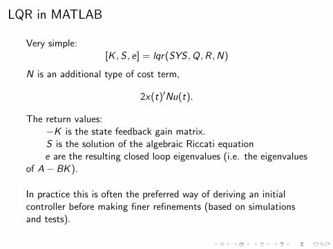
LQR in MATLAB

Very simple:[K ,S , e] = lqr(SYS ,Q,R,N)

N is an additional type of cost term,

2x(t)′Nu(t).

The return values:−K is the state feedback gain matrix.S is the solution of the algebraic Riccati equatione are the resulting closed loop eigenvalues (i.e. the eigenvalues

of A− BK ).

In practice this is often the preferred way of deriving an initialcontroller before making finer refinements (based on simulationsand tests).

Model Predictive Control

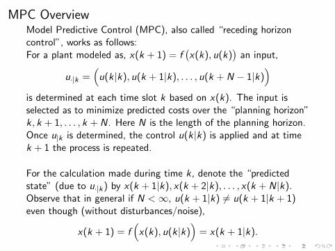
MPC OverviewModel Predictive Control (MPC), also called “receding horizoncontrol”, works as follows:For a plant modeled as, x(k + 1) = f

(x(k), u(k)

)an input,

u·|k =(u(k|k), u(k + 1|k), . . . , u(k + N − 1|k)

)is determined at each time slot k based on x(k). The input isselected as to minimize predicted costs over the “planning horizon”k , k + 1, . . . , k + N. Here N is the length of the planning horizon.Once u|k is determined, the control u(k |k) is applied and at timek + 1 the process is repeated.

For the calculation made during time k , denote the “predictedstate” (due to u·|k) by x(k + 1|k), x(k + 2|k), . . . , x(k + N|k).Observe that in general if N <∞, u(k + 1|k) 6= u(k + 1|k + 1)even though (without disturbances/noise),

x(k + 1) = f(x(k), u(k |k)

)= x(k + 1|k).

MPC Notes

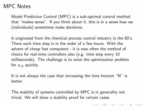
Model Predictive Control (MPC) is a sub-optimal control methodthat “makes sense”. If you think about it, this is in a sense how we(individuals) sometimes make decisions.

It originated from the chemical process control industry in the 80’s.There each time step is in the order of a few hours. With theadvent of cheap fast computers - it is now often the method ofchoice for real-time controllers also (e.g. time step every 10milliseconds). The challenge is to solve the optimization problemfor u·|k quickly.

It is not always the case that increasing the time horizon “N” isbetter.

The stability of systems controlled by MPC is in generality nottrivial. We will show a stability proof for certain cases.

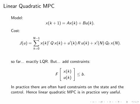
Linear Quadratic MPC

Model:x(k + 1) = Ax(k) + Bu(k).

Cost:

J(u) =N−1∑k=0

x(k)′Q x(k) + u′(k)R u(k) + x ′(N)Qf x(N).

so far... exactly LQR. But... add constraints:

F

[x(k)

u(k)

]≤ b.

In practice there are often hard constraints on the state and thecontrol. Hence linear quadratic MPC is in practice very useful.

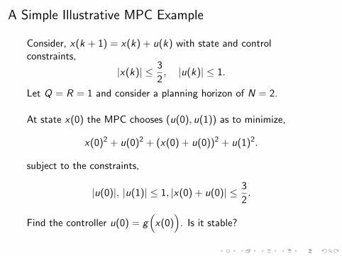
A Simple Illustrative MPC Example

Consider, x(k + 1) = x(k) + u(k) with state and controlconstraints,

|x(k)| ≤ 3

2, |u(k)| ≤ 1.

Let Q = R = 1 and consider a planning horizon of N = 2.

At state x(0) the MPC chooses (u(0), u(1)) as to minimize,

x(0)2 + u(0)2 + (x(0) + u(0))2 + u(1)2.

subject to the constraints,

|u(0)|, |u(1)| ≤ 1, |x(0) + u(0)| ≤ 3

2.

Find the controller u(0) = g(x(0)

). Is it stable?

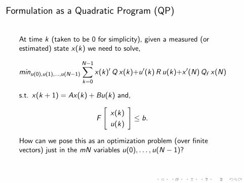
Formulation as a Quadratic Program (QP)

At time k (taken to be 0 for simplicity), given a measured (orestimated) state x(k) we need to solve,

minu(0),u(1),...,u(N−1)

N−1∑k=0

x(k)′Q x(k)+u′(k)R u(k)+x ′(N)Qf x(N)

s.t. x(k + 1) = Ax(k) + Bu(k) and,

F

[x(k)

u(k)

]≤ b.

How can we pose this as an optimization problem (over finitevectors) just in the mN variables u(0), . . . , u(N − 1)?

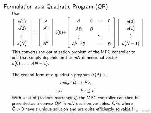
Formulation as a Quadratic Program (QP)Use

x(1)

x(2)...

x(N)

=

A

A2

...

AN

x(0)+

B 0 · · · 0

AB B...

.... . .

AN−1B · · · B

u(0)

u(1)...

u(N − 1)

This converts the optimization problem of the MPC controller toone that simply depends on the mN dimensional vectoru(0), . . . , u(N − 1).

The general form of a quadratic program (QP) is:

minzz′Qz + Pz ,

s.t. F z ≤ b.

With a bit of (tedious rearranging) the MPC controller can then bepresented as a convex QP in mN decision variables. QPs whereQ > 0 have a unique solution and are quite efficiently solvable!!!

The Closed Loop System is Non-Linear

MPC generates a “feedback” control law u(k) = g(x(k)

), where

the function g(·) is implicitly defined by the unique solution of theQP. The resulting controlled system,

x(k + 1) = Ax(k) + Bg(x(k)

),

is in general non-linear (it is linear if there are no-constraintsbecause then the problem is simply LQR).

Nevertheless, as will be seen in the HW (looking at parts ofBemporad, Morari, Dua and Pistikopoulus, 2002, “The explicitlinear quadratic regulator for constrained systems”), the resultingsystem is piece-wise linear.

Stability of MPC

Stability of MPC

A system controlled by MPC is generally not guaranteed to bestable.

It is thus important to see how to “modify” the optimizationproblem in the controller so that the resulting system is stable.

We now show one such method based on adding an “end-pointconstraint” that forces the optimized u·|k to drive the predictedsystem to state 0.

Our proof is for linear-quadratic MPC, yet this type of result existsfor general MPC applied to non-linear systems.

Generalizations of the “end-point constraint method” also exist.

The Constrained Controllability Assumption

Based on the constraints F

[x(k)

u(k)

]≤ b, denote by X ⊂ Rn the

state-space and by U(x) the allowable controls for every x ∈ X.

For our stability result, we assume:

1. Q > 0

2. 0 ∈ U(0)

3. Constrained Controllability Assumption: Assume ∃N0 suchthat for every initial condition x(0) ∈ X satisfying theconstraint set, ∃u(0), u(1), . . . , u(N0 − 1) that when appliedas input, results in x(N0) = 0.

In practice, verifying the constrained controllability assumption isnot much harder than verifying that the system is controllable. Forcontrollable unconstrained linear systems, N0 ≤ n.

The Modified Linear-Quadratic MPC

Add now an additional end-point constraint to the constraints ofthe optimization problem in the MPC controller:

x(N0) = 0.

The problem can again be solved by a quadratic program, yet atany time k (for any measured state x(k)) will result in u·|k thathas a predicted state of x(k + N0) = 0.

Observe that this does not imply that the system will actually beat state 0 after N0 steps. Why?

Simple Example RevisitedConsider again, x(k + 1) = x(k) + u(k) with constraints,|x(k)| ≤ 3

2 and |u(k)| ≤ 1, and with Q = R = 1 and a planninghorizon of N = 2. Add now an end point constraint at N = 2.

At state x(0) the MPC chooses (u(0), u(1)) as to minimize,

x(0)2 + u(0)2 + (x(0) + u(0))2 + u(1)2.

subject to the constraints,|u(0)|, |u(1)| ≤ 1, |x(0) + u(0)| ≤ 3/2,as well as the new end point constraint:

|x(0) + u(0) + u(1)| = 0

The minimization now requires u(1) = −(x(0) + u(0)) and thisimplies that u(0) = −2

3x(0). The controlled system is now:

x(k + 1) =1

3x(k).

Observe that it is asymp’ stable but does not reach 0 in finite time.

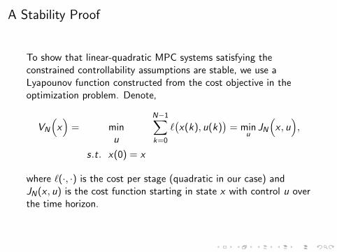
A Stability Proof

To show that linear-quadratic MPC systems satisfying theconstrained controllability assumptions are stable, we use aLyapounov function constructed from the cost objective in theoptimization problem. Denote,

VN

(x)

= minu

s.t. x(0) = x

N−1∑k=0

`(x(k), u(k)

)= min

uJN

(x , u),

where `(·, ·) is the cost per stage (quadratic in our case) andJN(x , u) is the cost function starting in state x with control u overthe time horizon.

A Stability Proof - cont.

Then a feasible trajectory (one satisfying the constraints) forhorizon N − 1 based on feasible controls u(0), . . . , u(N − 2), can be“prolonged” with no cost by setting u(N − 1) = 0. This is becausewith the new end point constraint, a feasible trajectory for horizonN − 1 has x(N − 1) = 0 and `

(x(N − 1), u(N − 1)

)= `(0, 0) = 0.

Thus all feasible u’s for the N − 1 horizon problem are feasible forthe problem with horizon N and further,

JN−1

(x(0), u

)= JN

(x(0), [u, 0]

).

Hence,VN(x) ≤ VN−1(x).

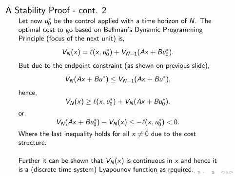
A Stability Proof - cont. 2Let now u∗0 be the control applied with a time horizon of N. Theoptimal cost to go based on Bellman’s Dynamic ProgrammingPrinciple (focus of the next unit) is,

VN(x) = `(x , u∗0) + VN−1(Ax + Bu∗0).

But due to the endpoint constraint (as shown on previous slide),

VN(Ax + Bu∗) ≤ VN−1(Ax + Bu∗),

hence,VN(x) ≥ `(x , u∗0) + VN(Ax + Bu∗0).

or,VN(Ax + Bu∗0)− VN(x) ≤ −`(x , u∗0) < 0.

Where the last inequality holds for all x 6= 0 due to the coststructure.

Further it can be shown that VN(x) is continuous in x and hence itis a (discrete time system) Lyapounov function as required.