mathematical and experimental modeling of reverse osmosis

366

Korean J. Chem. Eng., 38(2), 366-379 (2021)DOI: 10.1007/s11814-020-0697-9

INVITED REVIEW PAPER

pISSN: 0256-1115eISSN: 1975-7220

INVITED REVIEW PAPER

†To whom correspondence should be addressed.E-mail: [email protected] by The Korean Institute of Chemical Engineers.

Mathematical and experimental modeling of reverse osmosis (RO) process

Zeinab Hadadian*,†, Sina Zahmatkesh*, Mostafa Ansari*, Ali Haghighi*, and Eskandar Moghimipour**

*Faculty of Civil Engineering and Architecture, Shahid Chamran University of Ahvaz, Ahvaz, Iran**Nanotechnology Research Center, Ahvaz Jundishapur University of Medical Sciences, Ahvaz, Iran

(Received 13 May 2020 • Revised 26 September 2020 • Accepted 15 October 2020)

AbstractThis paper provides a mathematical simulation model for the reverse osmosis (RO) process with series ele-ments. A mathematical simulation model was developed based on the mass, material and energy balances consideringthe concentration polarization. The simulation model is open-source and easy to couple with other computational toolslike optimization algorithms and SCADA1 applications. An RO laboratory pilot was also set up in the Hydraulic Lab ofShahid Chamran University of Ahvaz to validate the simulation results. Comparing the results of the simulation modelwith the experiments and ROSA commercial software, the proposed simulation model functions well and is reliable. Thecomparisons indicate that the simulation results are over 96% close to ROSA and over 80% close to experimental results.Keywords: Desalination, Reverse Osmosis, Simulation, Experimental, Mathematical Modeling

INTRODUCTION

The reverse osmosis (RO) method for desalination is currentlythe most popular technology for seawater and brackish water desali-nation [1]. The RO process has several advantages over the otherdesalination methods, especially in terms of energy consumptionand efficiency. For each RO system, the membrane performanceshould be evaluated to determine the type of membrane, recovery,and number of membrane elements. The construction and opera-tion costs, as well as the permeate concentration and the permeateflux, are critical factors to determine for the design of an RO sys-tem. Commercial software, like ROSA and IMSDesign, has beenwidely used in many investigations and industrial projects for pre-dicting the performance of the RO systems [2]. These commercialmodels have been mostly released by the membrane manufacturersand therefore are useful for their productions. For research objec-tives, one needs to have an open-source model to extend the sim-ulations and couple the RO models with the optimization algorithmsand other mathematical techniques.

Villafafila and Mujtaba developed a simulation and optimizationmodel for seawater and brackish water. They optimized energy con-sumption, recovery, and the number of tubular membranes. Theyconsidered the number of pressure vessels, pressure values, mem-brane diameter, and feed water flux as the constraints [3]. Barelloet al. provided experimental data that examined the pure water per-meability and salt permeability constant for this type of membraneelement (tubular) [4]. Marcovecchio et al. optimized the simula-tion of seawater reverse osmosis (SWRO) system with a two-stagearrangement. That work included hollow fiber membranes and

energy recovery systems [5]. Geraldes et al. optimized the simula-tion of a two-stage desalination system and the considered spiralwound membrane (the most common type). They also used theexperimental data to identify specific parameters in design equa-tions. That paper focused on optimizing the pressure and flow offeed water for various recovery rates [6]. Guria et al. presented a mul-tiobjective optimization problem for seawater desalination, usingspiral wound and tubular membranes. That paper does not includeexperimental data [7]. An optimization model for different feedwater concentrations was presented by Lu et al. in 2007 [8]. Choiet al. presented an RO and forward osmosis (FO) computer pro-gram; the model was developed only for a one-stage system [9]. Duet al. presented a simulation-optimization model for seawater andbrackish water, using spiral wound membranes. They consideredthe permeate flux as a constraint in addition to the constraints onthe membrane manufacturer. The model also included a maximumof two-stage membrane and considered energy recovery systems[10-12]. Altaee estimated the performance of RO systems with sev-eral elements based on the solution-diffusion model, and most ofthe equations used in that paper were from the empirical equationspresented in the DOW design guide, which included single-stagesystems and has no experimental data. It was a model that wasunable to establish new constraints or to optimize the system [2].Saavedra et al. presented a design method for RO brackish waterplants, which was based on the application of maximum availablerecovery without scaling of any inorganic compounds presented inwater [13,14]. Choi and Kim presented a simulation and optimiza-tion model for RO systems with two stages, including spiral woundmembranes, but did not provide experimental work [15]. Kotb etal. examined an SWRO system with a maximum of three-stages[16]. Haluch et al. evaluated the experimental and semi-empiricalmodel of a small-capacity reverse osmosis desalination unit. Theyfound that the semi-empirical model predictions agreed with theirexperimental counterparts within the measurement uncertaintythreshold [17]. Chee et al. investigated the performance evaluation

1Supervisory Control And Data Acquisition

Mathematical and experimental modeling of reverse osmosis (RO) process 367

Korean J. Chem. Eng.(Vol. 38, No. 2)

of RO desalination pilot plants using the ROSA Simulation soft-ware. They found that in terms of flux and recovery ratio, the sim-ulated results and the experimental data showed a marginal dis-crepancy with deviations <2% and <8%, respectively. Their find-ings also confirmed the feasibility of adopting ROSA software toverify the performance of a pilot plant with all operational param-eters being ideally optimized [18]. Al-Obaidi et al. evaluated theperformance of a medium-sized industrial BWRO desalination plantof the Arab Potash Company using the mathematical model andthe real data [19]. Chen and Qin developed mathematical model-ing of glucose-water separation through reverse osmosis (RO) mem-brane to research the membrane’s performance during the masstransfer process. They validated the model using experimental resultsand found that the calculated results were consistent with the experi-mental data [20]. Maure and Mungkasi obtained a mathematicalmodel using numerical integration for the reverse osmosis system[21]. Li proposed a predictive mathematical model based on thesolution-diffusion theory for a commercial spiral wound SWROmodule. They concluded that the mathematical model with theparameters obtained from the experimental data can predict theflow of water and salt as well as the pressures under different feedconditions of temperature, flow, and pressure with a mean error4% [22]. Gaublomme et al. developed a generic steady-state modelfor RO and applied it to a unique three-year data set of a full-scaleRO process. They validated the model with online conductivity dataas input taking into account the uncertainty originating from onlinesensors and compared to the commercial software Winflows. Theyfound that the model has satisfactory results, i.e., an average devia-tion from the data at 2.7%, 12.7%, 34.1% and 18.7%, respectively,for the recovery, the concentrate pressure, the permeate, and con-centrate solute concentration [23]. Siegel et al. developed a mathe-matical model describing the RO enrichment process using a noveldevice. They created it in MATLAB Simulink software and vali-dated it with experimental results. Using the calculation of the meanrelative error between the model and the experimental results, theyconcluded that the model is useful for describing the RO systemand the RO device is suitable for the enrichment of estrogens priorto instrumental or in vitro analysis [24]. Ligaray et al. presented anovel energy self-sufficient desalination system design that incor-porates rechargeable seawater batteries as an additional energy stor-age system. They predicted the experimental data using the ROSAmodel to determine the configuration of the lowest energy con-sumption and highest charging rate. The results showed that theseawater battery achieved satisfactory desalination performance[25]. Mansour et al. focused on employing an energy recovery sys-tem (ERS) to enhance the performance of the small RO plant forremote areas using an experimental pilot and simulation model.Their obtained results showed good agreement between experi-mental and simulation model values. They evaluated the cost anal-ysis of the small RO desalination plant with and without ERS andshowed a significant reduction in total cost [26].

In this paper, we present a mathematical simulation programfor a multi-element RO system and consider multiple elements ineach pressure vessel. The output parameters of the program includethe feed pressure, the permeate concentration, the recovery of eachelement in the pressure vessel, and the permeate flow generated by

each element. Unlike other commercial software (ROSA, IMSDe-sign, etc.), the proposed model is open-source and easy to couplewith other computational tools like optimization algorithms, andsince it has been based on the mathematical equations of the ROprocess (the ROSA software utilizes experimental equations thatcontrol Filmtec membranes), it is capable of using all types of mem-branes manufactured in different companies. In existing commer-cial software, the total system recovery is considered as input, whilethe present model considers the recovery of each stage separately.An RO laboratory pilot with 50 m3/day production capacity hasbeen also set up in the Hydraulic Lab of Shahid Chamran Univ-ersity of Ahwaz to validate the simulation results. Two single-ele-ment and multi-element cases were simulated using the proposedsimulator model and the results were compared with the ROSAsoftware simulation and the experimental results which are dis-cussed.

MATERIALS AND METHODS

1. Model DevelopmentAn RO mathematical simulation model was developed based

on mass, material, and energy balances for a given configuration.For more realistic modeling, the concentration polarization is alsotaken into account. The related equations used to simulate the ROprocess are reported in Table 1.2. Membrane Characteristics

The full characteristics of the membranes provided by the man-ufacturers are critical parameters for the simulation of the RO sys-tems. The required data include the active membrane area, maximumoperating pressure, salt rejection, pure water permeability constant(Am), feed spacer, pressure drop in element, length of the element,diameter of the element, spacer diameter and thickness.3. Arrangements of a Multi-stage RO System

The schematic of a multi-stage RO unit is shown in Fig. 1.For a three-stage system, there are three splitter points (F, R1,

and R2) with three split ratios , and between 0 and 1 so thattheir summation at each point is 1. The flow rate of the feed solu-tion to each stage can be calculated by Eq. (16) [16].

(16)

where, QR1 is retentate flow rate from the first stage (m3/s), QR2

is retentate flow rate from the second stage (m3/s), QF1 is feed flowrate to the first stage (m3/s), QF2 is feed flow rate to the second stage(m3/s), QF3 is feed flow rate to the third stage (m3/s), is the frac-tion of stream branching to the left from a split point, is the frac-tion of stream branching to the right from a split point, and is thefraction of stream branching straight forward from a split point.4. The Calculation of Permeate Water at Each Stage

The purpose of the RO simulation is to determine the pressurerequired at each stage to obtain the required permeate water. Eachstage may include several pressure vessels in parallel, and each pres-sure vessel includes several membranes in a series. The number ofpressure vessels in each stage depends on the total number of the

Qf1 fQf

Qf2 fQf R1QR1

Qf3 fQf R1QR1 R2QR2

368 Z. Hadadian et al.

February, 2021

Table 1. Equations for the RO process simulationMeaning Equation No. Ref.

Feed flow rate (1) [1]Permeate flow rate (2) [1]

Temperature correction factor (3) [10]

Material balance (4) [1]Feed concentration (5) [2]Permeate water flux (6) [1]Residual transmembrane pressure (7) [1]

Van’t hoff ’s equationFor NaCl

(8) [2]

Concentration on the feed side membrane wall (9) [1]

Mass transfer coefficient (10) [9]

Density (11) [1]

Viscosity (12) [1]

Diffusivity (13) [1]

Effective membrane area (14) [23]

Number of pressure vessels in the ith stage (15)

QF QR QP

QP TCF jwA

TCF =

1, TF 25 Co

25,000R

---------------1

T0 273.15--------------------------

1TF 273.15--------------------------

,exp TF 25 Co

20,000R

---------------1

T0 273.15--------------------------

1TF 273.15--------------------------

,exp TF 25 Co

QF CF QP CP QR CR

CF CP/ 1 rejection

jw Am P AmPeff

Peff Pf Pp Pin Pf/2 w p

nMR T 273.15 103

2 C/0.0585 R T 273.15 103

Cw Cp

Cf Cp-----------------

JwdDS------- exp

Jw

k---- exp

Cw CP Cf Cp Jw/k exp

k 0.5510 Re 0.4 Sc 0.17 Cf/ 0.77 DS/d 0.77

498.4m 248,400m2 752.4mCf

m 1.0069 2.757 104Tf

1.234 106 0.00212Cf 1,965/Tf 273.15 exp

DS 6.725 106 0.1546 103Cf 2,513/Tf 273.15 exp

Aeff VT/l *

1 VSP/VT

NPVi Ni

Nei-------

Fig. 1. Schematic of multi-stage RO unit [16].



membranes and the number of membranes in each pressure ves-sel, which is obtained from Eq. (15). The system recovery dependson the permeate water (Qp) and the feed flow (Qf) as follows:

(17)

Since the amount of permeate water should be constant, bydetermining the system recovery the amount of feed flow is deter-mined. If we assume the recovery in the first, second, and thirdstages, respectively, rec1, rec2, and rec3, the amount of permeatewater at each stage can be calculated according to Eq. (16) as fol-lows:

(18)

(19)

By using Eqs. (18) and (19) along with the continuity equation,the values of productive permeate water are obtained at each stageas follows:

(20)

Finally, the feed rate intake at each stage can be determined byhaving Qp1, Qp2, Qp3, the recovery, and the coefficients of the split-ter points.5. The Calculation of Operating Parameters for Each Elementof Pressure Vessel

Given that there is uniformity of the pressure vessels at each stage,the feed flow and permeate flow rates are split equally among thepressure vessels and are obtained for each pressure vessel (QFPVj,QPPVj). In each pressure vessel permeate water produced by theelements is calculated using Eqs. (2), (6), and (7) as in the follow-ing equation:

(21)

By placing Eqs. (8), (9), and (5) in Eq. (21):

(22)

In each pressure vessel, the feed flow rate and feed pressure inletto each element are equal to the retentate flow rate and retentatepressure outlet from the previous element.

(23)

(24)

By using Eqs. (5), (23), and (24), the permeate concentration atthe z+1th element is obtained as follows:

(25)

For each pressure vessel, the summation of permeate flux of allelements is equal to the required permeate flux of the pressure vessel.

(26)

Then, for all elements in the pressure vessel, a set of nonlinearequations consisting of permeate flow rate (Eq. (22)) and concen-tration (Eq. (25)) as variables with Eq. (26) is formed, which is solvedby the Newton-Raphson method and obtained feed water pressureof that stage and permeate flow rate and concentration in each ele-ment.

Finally, the permeate concentration of the jth pressure vessel (Cppvj)is calculated as follows:

(27)

Total permeate concentration and recovery of the system are cal-culated as follows:

(28)

(29)

6. The Simulation AlgorithmThe solving procedure of the RO equations is illustrated in Fig.

2. The simulation model is mathematically nonlinear and implicitand should be iteratively solved. The proposed simulation algorithmconsists of the following steps:

Recovery Qp

Qf------

Qf1 fQf Qf Qf1

f-------

Qf2 R1QR1 fQf

Qf Qf1

f-------, QR1 1 rec1 Qf1

Qf2 Qf1 1 rec1 R1 f

f----

Qf Qp

rec------ Qp

rec2----------

Qp1

rec1---------- 1 rec1 R1

f

f----

Qf3 R2QR2 fQf R1QR1

R2 1 rec2 Qf2 R1 1 rec1 Qf1 f

f----Qf1

Qp3

rec3----------

R2 1 rec2 rec2

------------------------------Qp2 R1 1 rec1

rec1------------------------------

f

frec1---------------

Qp1

1 rec1 R1 f

f----

rec1---------------------------------------Qp1

Qp2

rec2---------- 0

R1 1 rec1 rec1

------------------------------ f

frec1---------------

Qp1

R2 1 rec2 rec2

------------------------------Qp2 Qp3

rec3---------- 0

Qi Qpi1

3

QPz A*TCF*Am Pf Ppz Pinz Pfz

2----------

wz pz


2----------

2R T 273.15

0.0585-----------------------------------*103 Cwz CPz


2----------

2R T 273.15

0.0585-----------------------------------*103 CPz Cfz Cpz

Jw

kz---- CPzexp


2----------

2R T 273.15

0.0585-----------------------------------*103

*CPz1

1 rejection---------------------------- 1

*

QPz

A*kz------------ exp

QFz1 CFz1 QFz CFz QPz CPz

QFz1 QFz QPz

CPz1 1 rejection QFz

CPz

1 rejection---------------------------- QPz CPz

QFz QPz-------------------------------------------------------------------

QPpvj QPzz1

Nei

CPpvj

QPz*CPz z1

Nei

QPpvj------------------------------

Cptotal

QPi*CPi i1

3

QP----------------------------

rectotal QP

Qf------

QP

Qf1/f--------------

QP

Qp1/ rec1*f ----------------------------------


February, 2021

Fig. 3. A graphical user interface (GUI) window.

Fig. 2. Flowchart of RO simulation model.



1. The input data include the feed water and membrane charac-teristics, recovery of each stage, required permeate water, numberof elements, the number of series element in each pressure vessel,and the split ratios for the membrane’s arrangement are introducedto the model.

2. QPi is calculated using Eq. (20) for each stage (i=1 : 3) thenQFi and QRi are obtained using Eqs. (17) and (1), respectively.

3. Set i=1 for the first stage4. QFPVj, QPPVj are calculated for each pressure vessel (j=1: NPVi)

in ith stage and because of the uniformity of the pressure vessels ateach stage, QFi and QPi are split equally among the pressure vessels.

5. z, z, Dsz, Rez, Scz, and kz are calculated using Eqs. (10)-(13)for each element.

6. Each pressure vessel assumes an initial value for the feed waterpressure (PFi) and permeate flow rate, and concentration in eachelement (z=1: Nei).

7. Due to the similarity of the pressure vessels in a stage, the pres-sure in all pressure vessels is equal to the pressure applied by thepump to the stage. The input pressure to the first element has beenalready assumed in step 6.

8. Solving Eqs. (22), (25), and (26) for all elements (z=1: Nei) ina pressure vessel in a set of nonlinear equations, which is solved bythe Newton-Raphson method.

9. Permeate concentration of pressure vessel (Cppvj) is calculatedusing Eq. (27).

10. Steps 4 to 9 are repeated for all stages.Based on the above algorithm, simulation software with a graph-

ical user interface (GUI) was designed in MATLAB. This algo-rithm makes it possible to do the RO simulation by entering theinitial data, feed water, and membrane characteristics to obtain therequired feed pressures for stages, feed flow rate, retentate flow rate,and the permeate concentration as displayed in Fig. 3.

EXPERIMENTAL

1. Experimental PilotAn RO experimental pilot with 50 m3/day production capacity

was constructed at the Hydraulic Lab of Shahid Chamran Universityof Ahwaz and used to validate the results of this simulation model.This pilot is shown in Figs. 4-5 and includes both pretreatment anddesalination units. The pretreatment unit consists of a booster pump(1.34kW), a carbon filter, a sand filter, four micro-filters (5microns),and a water tanker. The desalination unit consists of a water tankerwith a mixer, a booster pump (1.21kW), a high-pressure pump (3.06kW), and a BW30-400 membrane from DOW. The membrane’scharacteristics are given in Table 2. The pressure and flow through

Fig. 4. Flowchart of the RO pilot plant at Hydraulic Lab of Shahid Chamran University of Ahvaz.


February, 2021

the process are also measured by pressure gauges and flow metersin different parts in the system. The value of pure water permea-bility constant for the BW30-400 membrane was found 7.94e-9(m/s·kPa) through experimental data analysis and calibration.2. Test Cases and Methodology of the Experiments

To validate the simulation model, some RO experiments werecarried out at the pressures of 700 and 1,100 kPa for the brackishwater as feed solution with a concentration of 2-5 kg/m3 by the ROplant. For all tests feed water temperature was 15 oC and PH=7.3±0.1. Each RO experiment was performed by maintaining the feedpressures constantly and varying the concentration of the feed solu-tion from 2-5 kg/m3. The flow rate and concentration of permeateand retentate water were measured, and then the recovery of eachcase was calculated for the applied pressure.

RESULTS AND DISCUSSION

In this study, a simulator model for the RO process was devel-

oped and validated by the ROSA software and an experimentalpilot.1. Performance of the Experimental Pilot

The performance evaluation of the laboratory scale experimentswas conducted with various operating conditions, including oper-ating pressure (700 and 1,100 kPa) and feed concentration (2, 3, 4,5kg/m3). The experimental results are reported in Fig. 6. Our experi-ments were limited to operating pressures below 1,100 kPa and re-covery ratios below 50%.

As shown in Fig. 6(a), at constant pressure, the increase of thefeed concentration from 2 to 5 kg/m3 decreases the permeate flowrate from 9.55 to 3.75 (m3/min)*103 and 15.29 to 10.55 (m3/min)*103 for experimental pressure of 700 and 1,100 kPa, respectively.In addition, the decreasing trend was almost linear with correla-tion coefficients of 0.9888 and 0.9961 for experimental pressuresof 700 and 1,100 kPa, respectively. The highest permeate flow rate(15.29 (m3/min)*103) was obtained at pressures of 1,100 kPa andfeed concentration of 2 kg/m3. A higher permeate flow rate meansthat the membrane can produce a large amount of water per unitarea and time. At a constant feed concentration, with increasingpressure from 700 to 1,100 kPa, the permeate flow rate also in-creases by 5.74, 5.42, 6.64, and 6.8 (m3/min)*103) at feed concen-tration of 2, 3, 4, and 5, respectively. This is an acceptable issue andcan be justified using Eq. (6). According to this equation at con-stant pressure, the permeate flow rate decreases with increasingosmotic pressure due to increasing feed concentration. At a con-stant feed concentration, the permeate flow rate also increases whenincreasing the pressure.

Fig. 6(b) indicates that the highest recovery was obtained by48.58% at pressure of 1,100 kPa and feed concentration of 2 kg/m3.As shown in this figure, at constant pressure, the increase of thefeed concentration from 2 to 5 kg/m3 decreases the recovery from41.54% to 20.67% and 48.58% to 37.06% for experimental pressureof 700 and 1,100 kPa, respectively. At a constant feed concentra-tion, with increasing pressure from 700 to 1,100 kPa, the recoveryalso increases by 7.04%, 7.05%, 12.9%, and 16.39% at feed concen-trations of 2, 3, 4, and 5, respectively, and the average percentageof increased recovery was 10.85%. In other words, the higher theconcentration is the higher the percent recovery.

As shown in Fig. 6(c), at constant pressure, the increase in thefeed concentration from 2 to 5 kg/m3 decreases the salt rejectionfrom 96.6% to 94.58% and 97.45% to 96.52% for experimental pres-sure of 700 and 1,100 kPa, respectively. The salt rejection also in-creases by increasing the feed pressure at a constant feed concen-tration. It can also be justified using Eq. (5). The highest salt rejec-tion was obtained at 97.45% at pressures of 1,100kPa and feed con-centration of 2 kg/m3 and the average salt rejection was 96.36%.

Since energy consumption is a key factor that affects the cost ofthe RO system, the change of the specific energy consumption (SEC)values versus the feed concentration for experimental pressure of700 and 1,100kPa is shown in Fig. 6(d). The SEC is directly related

Fig. 5. The RO pilot plant at Hydraulic Lab of Shahid ChamranUniversity of Ahvaz.

Table 2. Characteristics of Filmtec spiral wound RO membrane element [27]Element type Size (m) Active surface area (m2) Feed spacer thickness (mil) Applied pressure (kPa) Salt rejection

BW30-400 0.203*1.02 37.2 28 1,551.32 99.5%



to the feed flow rate and pressure (pump power) and inverselyrelated to the permeate flow rate. As shown in this figure, at con-stant pressure, the increase of the feed concentration from 2 to5 kg/m3 increases the SEC. This is because according to Fig. 6(b),the permeate flow rate decreases when increasing the feed concen-tration and due to increases of SEC. The average SEC value was0.777 (kW hr/m3) and all SEC values were less than 1.04 (kW hr/m3).2. Performance of the Proposed Simulation Model2-1. Single Element Case

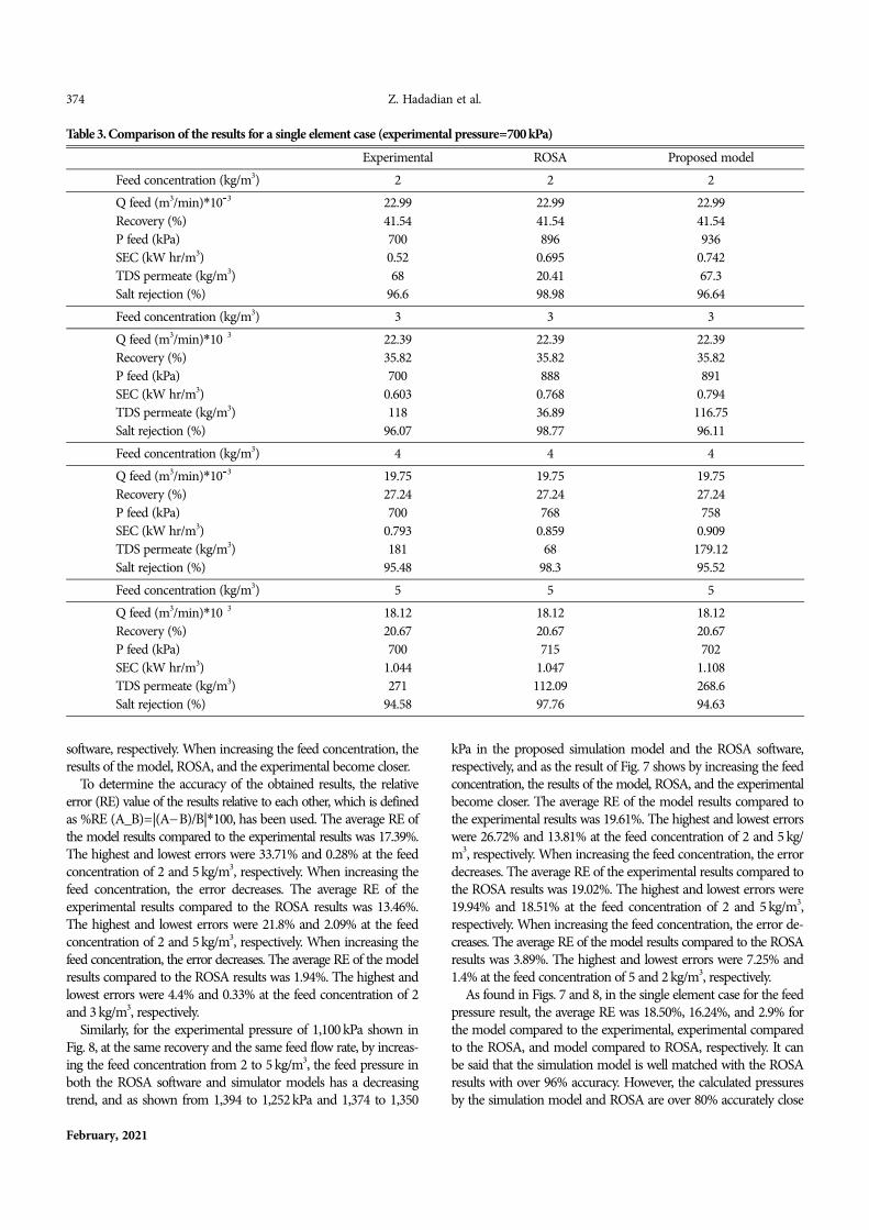
To validate the simulation model, the RO experiments (Fig. 6)were also simulated by the proposed simulation model as well asby the ROSA software version 9.1. Note that the temperature of thelaboratory was rectified using the temperature correction factor TFCin the simulation model equations (Eq. (3)). Tables 3 and 4 com-pare the results of the RO experimental pilot, the ROSA softwareestimation, and estimated by the proposed simulator model for thefeed concentration of 2, 3, 4, and 5 kg/m3 and experimental pres-

sure of 700 and 1,100kPa, respectively. These tables show how, underthe same conditions of feed flow rate and recovery, by increasingthe feed concentration, the feed pressure decreases in both theROSA software and simulator models and it can be justified usingEq. (6). The feed pressure estimated by the proposed model is alsocloser to the estimation by the ROSA software than the experi-mental. Since the feed pressure has a direct effect on the calcula-tion of energy consumption, this is also true for SEC. The highestSEC values were 1.115 and 1.047 (kW hr/m3) in the ROSA soft-ware and the proposed model, respectively.

To better understand the feed pressure trend, the data sets areshown in Figs. 7 and 8. As shown in Fig. 7, when the experimen-tal pressure was 700 kPa, at the same recovery and the same feedflow rate, by increasing the feed concentration from 2 to 5 kg/m3,the feed pressure in both the ROSA software and simulator mod-els has a decreasing trend and as shown from 936 to 702 kPa and896 to 714 kPa in the proposed simulation model and the ROSA

Fig. 6. Experimental result of (a): The permeate flow rate, (b) the recovery of system, (c) the salt rejection, and (d): The specific energy con-sumption (SEC) versus feed concentration.


February, 2021

software, respectively. When increasing the feed concentration, theresults of the model, ROSA, and the experimental become closer.

To determine the accuracy of the obtained results, the relativeerror (RE) value of the results relative to each other, which is definedas %RE (A_B)=|(AB)/B|*100, has been used. The average RE ofthe model results compared to the experimental results was 17.39%.The highest and lowest errors were 33.71% and 0.28% at the feedconcentration of 2 and 5 kg/m3, respectively. When increasing thefeed concentration, the error decreases. The average RE of theexperimental results compared to the ROSA results was 13.46%.The highest and lowest errors were 21.8% and 2.09% at the feedconcentration of 2 and 5 kg/m3, respectively. When increasing thefeed concentration, the error decreases. The average RE of the modelresults compared to the ROSA results was 1.94%. The highest andlowest errors were 4.4% and 0.33% at the feed concentration of 2and 3 kg/m3, respectively.

Similarly, for the experimental pressure of 1,100 kPa shown inFig. 8, at the same recovery and the same feed flow rate, by increas-ing the feed concentration from 2 to 5 kg/m3, the feed pressure inboth the ROSA software and simulator models has a decreasingtrend, and as shown from 1,394 to 1,252 kPa and 1,374 to 1,350

kPa in the proposed simulation model and the ROSA software,respectively, and as the result of Fig. 7 shows by increasing the feedconcentration, the results of the model, ROSA, and the experimentalbecome closer. The average RE of the model results compared tothe experimental results was 19.61%. The highest and lowest errorswere 26.72% and 13.81% at the feed concentration of 2 and 5 kg/m3, respectively. When increasing the feed concentration, the errordecreases. The average RE of the experimental results compared tothe ROSA results was 19.02%. The highest and lowest errors were19.94% and 18.51% at the feed concentration of 2 and 5 kg/m3,respectively. When increasing the feed concentration, the error de-creases. The average RE of the model results compared to the ROSAresults was 3.89%. The highest and lowest errors were 7.25% and1.4% at the feed concentration of 5 and 2 kg/m3, respectively.

As found in Figs. 7 and 8, in the single element case for the feedpressure result, the average RE was 18.50%, 16.24%, and 2.9% forthe model compared to the experimental, experimental comparedto the ROSA, and model compared to ROSA, respectively. It canbe said that the simulation model is well matched with the ROSAresults with over 96% accuracy. However, the calculated pressuresby the simulation model and ROSA are over 80% accurately close

Table 3. Comparison of the results for a single element case (experimental pressure=700 kPa)Experimental ROSA Proposed model

Feed concentration (kg/m3) 2 2 2Q feed (m3/min)*103 22.99 22.99 22.99Recovery (%) 41.54 41.54 41.54P feed (kPa) 700 896 936SEC (kW hr/m3) 0.52 0.695 0.742TDS permeate (kg/m3) 68 20.41 67.3Salt rejection (%) 96.6 98.98 96.64Feed concentration (kg/m3) 3 3 3Q feed (m3/min)*103 22.39 22.39 22.39Recovery (%) 35.82 35.82 35.82P feed (kPa) 700 888 891SEC (kW hr/m3) 0.603 0.768 0.794TDS permeate (kg/m3) 118 36.89 116.75Salt rejection (%) 96.07 98.77 96.11Feed concentration (kg/m3) 4 4 4Q feed (m3/min)*103 19.75 19.75 19.75Recovery (%) 27.24 27.24 27.24P feed (kPa) 700 768 758SEC (kW hr/m3) 0.793 0.859 0.909TDS permeate (kg/m3) 181 68 179.12Salt rejection (%) 95.48 98.3 95.52Feed concentration (kg/m3) 5 5 5Q feed (m3/min)*103 18.12 18.12 18.12Recovery (%) 20.67 20.67 20.67P feed (kPa) 700 715 702SEC (kW hr/m3) 1.044 1.047 1.108TDS permeate (kg/m3) 271 112.09 268.6Salt rejection (%) 94.58 97.76 94.63



to the laboratory results. This could be due to laboratory conditions,measurement errors, and uncertainties and the simplifications applied

to the simulation equations. Since the equations used in ROSA andthe proposed simulation model are slightly different, this little dif-

Table 4. Comparison of the results for a single element case (experimental pressure=1,100 kPa)Experimental ROSA Proposed model

Feed concentration (kg/m3) 2 2 2Q feed (m3/min)*103 31.47 31.47 31.47Recovery (%) 48.58 48.58 48.58P feed (kPa) 1100 1374 1394SEC (kW hr/m3) 0.699 0.892 0.886TDS permeate (kg/m3) 51 15 50.51Salt rejection (%) 97.45 99.25 97.47Feed concentration (kg/m3) 3 3 3Q feed (m3/min)*103 31.36 31.36 31.36Recovery (%) 42.87 42.87 42.87P feed (kPa) 1100 1350 1326SEC (kW hr/m3) 0.792 0.992 0.955TDS permeate (kg/m3) 80 25.7 79.32Salt rejection (%) 97.33 99.14 97.36Feed concentration (kg/m3) 4 4 4Q feed (m3/min)*103 29.94 29.94 29.94Recovery (%) 40.14 40.14 40.14P feed (kPa) 1100 1359 1291SEC (kW hr/m3) 0.846 1.072 0.992TDS permeate (kg/m3) 125 38.44 123.62Salt rejection (%) 96.88 99.04 96.91Feed concentration (kg/m3) 5 5 5Q feed (m3/min)*103 28.47 28.47 28.47Recovery (%) 37.06 37.06 37.06P feed (kPa) 1100 1350 1252SEC (kW hr/m3) 0.916 1.151 1.043TDS permeate (kg/m3) 174 52.17 172.46Salt rejection (%) 96.52 98.96 96.55

Fig. 7. Variation of feed pressure in RO system with feed concentration (experimental pressure=700 kPa) (*: Relative Error).


February, 2021

ference in results was expected. The ROSA software utilizes exper-imental equations that control Filmtec membranes, but in oursimulation model the mathematical equations that control the ROprocess - based on the mass, material, and energy balance equa-tions - are used. The equation that leads to significant differencesis the one used for calculating the pressure drop in the membranes.The BW30-400 pure water permeability constant and the salt rejec-tion used in the simulator model were obtained by laboratory dataanalysis (7.94e-9 (m/s·kPa) and 94.58-97.45%) that have a differ-ent quantity from the value set in ROSA (7.5e-9 (m/s·kPa) [8] and97.76-99.25%).

It is observed in Tables 3 and 4 that by increasing the feed con-centration, the permeate TDS estimated in both ROSA softwareand simulator model has a decreasing trend. It can also be justifiedusing Eq. (5). The permeate TDS estimated by the proposed modelis also closer (average ER: 1%) to the laboratory than estimated bythe ROSA software. This is because the salt rejection in the ROSAsoftware (97.76-99.25%) is different from our salt rejection in thelaboratory (94.58-97.45%) and the proposed simulator model (94.63-97.47). Thus, for permeate TDS estimation the simulation model isaccurate enough and well matched with the experimental results.2-2. Multi-element Case

Since the experimental pilot has only one element in each pres-sure vessel, for the multi-pressure vessel and multi-element test cases,the comparisons were done between the simulation model and theROSA software. For this purpose, a case study was simulated with

several pressure vessels and several elements in each pressure vesselaccording to Table 5. The simulated results, including the requiredfeed pressures, permeate flow rate and recovery of each element arefound in Figs. 9-11.

The calculated pressures are indicated in Fig. 9 where in eachelement by the simulation model and the ROSA software, showsthat the pressure values in the first to fifth elements were 1,003,988, 973, 958, and 943 in the proposed model and 912, 889, 869,853 and 840 in the Rosa model and have decreasing trends in both.The average difference in the results was 100kPa between the modeland ROSA, which is according to the results reported by Altaee[2]. The highest and lowest RE was 12.26% and 9.9% in the fifth

Fig. 8. Variation of Feed pressure in RO system with feed concentration (experimental pressure=1,100 kPa).

Table 5. Characteristics of case studies with two-pressure vessel and 5 elements in each pressure vesselNumber of elements in

each pressure vessel Element type Number ofpressure vessel

Temp(oC) Recovery QPermeate

(m3/h)Feed concentration

(kg/m3)5 BW30-400 2 25 0.5 8 2

Fig. 9. Feed pressure for each element in RO system.



element and the first element, respectively; the average RE was11.53%. The average pressure drop per element was 18 kPa and15 kPa in ROSA and the simulation model, respectively, which arealmost close to each other.

From Fig. 10, which shows the permeate flow rate in each ele-ment in the model and ROSA, it can be seen that the permeateflow rate value in the first to fifth elements was 0.93, 0.86, 0.8, 0.74,and 0.67 in ROSA and 0.88, 0.84, 0.8, 0.75, and 0.69 in the modelwhere the results are very close [2]. The average RE was 2.4%, thehighest RE was 5.3% in the first element, and the lowest RE was0% in the third element.

In Fig. 11, which shows the recovery in each element in themodel and ROSA, the recovery value in the first to fifth elementswas 0.12, 0.12, 0.13, 0.14, and 0.14 in ROSA, and 0.11, 0.12, 0.13,0.14, and 0.15 in the model where the results are very close [2].The average RE was 3.09%.

Based on these obtained average RE values, it can be said thatthe pressure, the permeate flow rate, and the recovery calculated bythe simulator model are (88.4%, 97.6%, 96.9%, respectively) accu-rately close to the calculated values by the ROSA software. Hence,the proposed algorithm functions well in the multi-elements ROsystems. The calculated pressures by the model are slightly higherthan the calculated pressures by ROSA. This could be due to labo-ratory conditions, measurement errors, and uncertainties and thesimplifications applied to the simulation equations. Since the equa-tions used in ROSA and the proposed simulation model are slightlydifferent, this little difference in results was expected. The ROSA

software utilizes experimental equations that control Filmtec mem-branes, but in our simulation model the mathematical equationsthat control the RO process are used. The equation that leads tosignificant differences is the one used for calculating the pressuredrop in the membranes.

Based on two single element and multi-element cases result andRE value, the proposed simulation model functions well and is reli-able. The calculated pressures by the simulation model are over 80%accurately close to the laboratory results and 96% accurately closeto the results of the ROSA software.

CONCLUSION

A mathematical simulation model for the RO process, consider-ing several series elements in each pressure vessel, was developedbased on the mass, material, and energy balances considering theconcentration polarization. Unlike other commercial software, theproposed model is open-source and since it is based on the math-ematical equations of the RO process, it is capable of using all typesof membranes manufactured by different companies. In the ROSAsoftware, the percentage of the feed flow cannot be assigned to stage2 and stage 3, and the feed flow first enters stage 1, and after treat-ment, the entire retentate from the first stage is considered as thefeed water for the second stage. This issue happens between stage2 and stage 3. However, in the proposed simulation model, giventhe three splitter points definition in the system, a certain percent-age of the feed flow can be assigned to each stage. A percentage ofthe retentate from the first stage can also be removed from thesystem and a percentage of it can be added to each of the secondand third stages. The former stream also happens between stage 2and stage 3. Accordingly, in the ROSA software, the feed pressureof high-pressure pumps is related to the first stage, and the feedpressure of the second stage is the summation of retentate pres-sure from the first stage and the accelerator pump pressure. In theproposed simulation model, according to the three splitter pointcoefficients, the value of the high-pressure pumps is first determinedin order to provide the pressure required for the first stage and ac-cording to the energy equation. Then, for the second and third stage,the amount of feed pressure is calculated by the energy equation.On the other hand, the retentate pressure considered as the feed foranother stage is calculated concerning the energy equation, andthe flow pressure prior to entering each stage is considered to bethe minimum of the inflows to that stage. In case there is any needfor a higher pressure, accelerator pumps are utilized.

An RO experimental pilot was constructed at the Hydraulic Labof Shahid Chamran University of Ahwaz and used to validate theresults of this simulation model. The performance of the laboratorypilot was evaluated and the results were discussed in detail.

The single element case was simulated using the proposed sim-ulator model, and the results (including feed pressure, SEC, TDSpermeate, and salt rejection) were compared with the ROSA soft-ware simulation and the experimental results. The multi-elementcase was simulated using the proposed simulator model, and theresults (including feed pressure, permeate flow rate, and recoveryin each element) were compared with ROSA.

Based on two single element and multi-element cases result and

Fig. 10. Permeate flow rate for each element in RO system.

Fig. 11. Recovery for each element in RO system.


February, 2021

RE value, it can be said that the comparison among the simula-tion model, the experiments, and the ROSA results indicates thereliability of the proposed simulation model. The calculated resultsby the simulation model are over 80% accurately close to the labo-ratory results and 96% accurately close to the ROSA software.

ACKNOWLEDGEMENTS

The authors would like to thank Ghadir Khuzestan Water Com-pany and Khuzestan Water and Power Authority for their finan-cial and technical support.

NOMENCLATURE

A : membrane surface area [m2]Aeff : effective surface area of membrane [m2]Am : pure water permeability constant [m/s·kPa]C : solution concentration [kg/m3]CF : feed concentration [kg/m3]CP : permeate concentration [kg/m3]CR : retentate concentration [kg/m3]Cw : concentration on the feed side of membrane wall [kg/m3]d : membrane channel diameter [m]Ds : solute diffusivity [m2/s]dsp : spacer diameter [m] i : stage counterj : pressure vessel counter in stagejw : water flux [m3/m2·s] k : mass transfer coefficient [m/s]lch : length of the membrane channel [m]M : molar concentration [mol/m3]n : van’t Hoff factorNei : number of the membrane element in pressure vessel of the

ith stageNi : number of membrane element in the ith stageNPVi : number of pressure vessel in the ith stagePeff : residual transmembrane pressure [kPa]Pf : feed pressure [kPa]Pp : permeate pressure [kPa]QF : feed flow rate [m3/s]QFPV : feed flow rate in the pressure vessel [m3/s]QF1 : feed flow rate to the first stage [m3/s]QF2 : feed flow rate to the second stage [m3/s]QF3 : feed flow rate to the third stage [m3/s]QP : permeate flow rate [m3/s]QPPV : permeate flow rate in the pressure vessel [m3/s]QR : retentate flow rate [m3/s]QR1 : retentate flow rate from the first stage [m3/s]QR2 : retentate flow rate from the second stage [m3/s]R : universal gases constant [8.314 m3·Pa/mol·oK]Re : Reynold’s numberRE : relative errorrec1 : recovery in the first stagerec2 : recovery in the second stagerec3 : recovery in the third stageSc : schmidt number

St : spacer thickness [m]T : temperature [oC]T0 : reference temperature [25 oC]TCF : temperature's correction factorTF : feed water temperature [oC]VSP : volume of the spacer [m3]VT : total volume [m3]z : element counter in the Pressure vessel : feed water viscosity [Pa·s] : fraction of the stream branching to the left from a split point : fraction of the stream branching to the right from a split point : fraction of the stream branching straight forward from a

split pointPf : pressure drop due to friction [kPa]Pin : pressure drop at inlet [kPa] : osmotic pressure [kPa]p : osmotic pressure on the permeate side [kPa]w : osmotic pressure on the feed side of membrane wall [kPa] : density [kg/m3] : Porosity

Subscriptsf : feedF : feed split ratiop : permeater : retentateR1 : retentate split ratio for first moduleR2 : retentate split ratio for second module

REFERENCES

1. H. Kotb, E. Amer and K. Ibrahim, Desalination, 357, 246 (2015).2. A. Altaee, Desalination, 291, 101 (2012).3. A. Villafafila and I. Mujtaba, Desalination, 155, 1 (2003).4. M. Barello, D. Manca, R. Patel and I. M. Mujtaba, Comput. Chem.

Eng., 83, 139 (2015).5. M. G. Marcovecchio, P. A. Aguirre and N. J. Scenna, Desalination,

184, 259 (2005).6. V. Geraldes, N. E. Pereira and M. Norberta de Pinho, Ind. Eng.

Chem. Res., 44, 1897 (2005).7. C. Guria, P. K. Bhattacharya and S. K. Gupta, Comput. Chem. Eng.,

29, 1977 (2005).8. Y.-Y. Lu, Y.-D. Hu, X.-L. Zhang, L.-Y. Wu and Q.-Z. Liu, J. Membr.

Sci., 287, 219 (2007).9. Y.-J. Choi, T.-M. Hwang, H. Oh, S.-H. Nam, S. Lee, J.-c. Jeon, S. J.

Han and Y. Chung, Desalination and Water Treatment, 33, 273(2011).

10. Y. Du, L. Xie, Y. Wang, Y. Xu and S. Wang, Ind. Eng. Chem. Res.,51, 11764 (2012).

11. Y. Du, L. Xie, J. Liu, Y. Wang, Y. Xu and S. Wang, Desalination, 333,66 (2014).

12. Y. Du, L. Xie, Y. Liu, S. Zhang and Y. Xu, Desalination, 365, 365(2015).

13. E. R. Saavedra, A. G. Gotor, S. O. Pérez Báez, A. R. Martín, A. Ruiz-García and A. C. González, Desalination and Water Treatment, 51,4790 (2013).



14. E. Ruiz-Saavedra, A. Ruiz-García and A. Ramos-Martín, Desalina-tion and Water Treatment, 55, 2562 (2015).

15. J.-S. Choi and J.-T. Kim, J. Ind. Eng. Chem., 21, 261 (2015).16. H. Kotb, E. Amer and K. Ibrahim, Energy, 103, 127 (2016).17. V. Haluch, E. F. Zanoelo and C. J. Hermes, Chem. Eng. Res. Des.,

122, 243 (2017).18. K. P. Chee, K. P. Wai, C. H. Koo and W. C. Chong, EDP Sciences,

E3S Web of Conferences, 65, 05022 (2018).19. M. Al-Obaidi, A. Alsarayreh, A. Al-Hroub, S. Alsadaie and I. M.

Mujtaba, Desalination, 443, 272 (2018).20. C. Chen and H. Qin, Processes, 7, 271 (2019).21. O. P. Maure and S. Mungkasi, AIP Publishing LLC, AIP Conference

Proceedings, 2202, 020043 (2019).

22. M. Li, Chem. Eng. Res. Des., 148, 440 (2019).23. D. Gaublomme, L. Strubbe, M. Vanoppen, E. Torfs, S. Mortier, E.

Cornelissen, B. De Gusseme, A. Verliefde and I. Nopens, Desali-nation, 490, 114509 (2020).

24. J. Siegel, C. Wangmo, J. Cuhorka, A. Otoupalíková and M. Bittner,Environ. Technol. Innovation, 17, 100584 (2020).

25. M. Ligaray, N. Kim, S. Park, J.-S. Park, J. Park, Y. Kim and K. H.Cho, Chem. Eng. J., 395, 125082 (2020).

26. T. M. Mansour, T. M. Ismail, K. Ramzy and M. Abd El-Salam,Alexandria Eng. J., 59, 3741 (2020).

27. DOW, FILMTEC Membranes, product information catalog, http://www.lenntech.com/feedback/feedback_uk.htm?ref_title=Filmtec/Filmtec-Reverse-Osmosis-Product-Catalog-L.pdf (2006).

mathematical and experimental modeling of reverse osmosis

Documents