J. Appl. Math. & Computing Vol. 21(2006), No. 1 - 2, pp. 509 - 523

MATHEMATICAL CHARACTERIZATION OF PETROLEUMRESERVOIR AND PREDICTION OF FUTURE OIL

PRODUCTION

HONGJOONG KIM

Abstract. Numerical solutions of the Darcy and Buckley-Leverett equa-tions for flows in porous media are considered. These solutions are charac-

terized by a random field, which represents the reservoir permeability. Amathematical model for numerical solution errors is introduced to predict

geology correlation lengths and future oil production, which translates ob-served oil cut versus time data into time versus oil cut. In addition, the

error model is screened based on whether the model predicts times cor-responding to observed oil cuts accurately. The introduced mathematical

model performs accurate uncertainty analysis and enhances the reliabilityof the prediction. The results from three methods are compared: the max-

imum likelihood method, the Bayesian analysis, and the Fourier analysis.The maximum likelihood method is more efficient than the others by re-

ducing the prediction error in oil production by about 20%, relative to theprior probabilityprediction. It is also effective for correlation identification.

AMS Mathematics Subject Classification: 76S05, 76T10, 76M35

Key words and phrases: Porous media, two-phase flow, upscaling, erroranalysis, uncertainty, prediction

1. Introduction

Flow in porous media such as fluids in an oil reservoir or groundwater withcontaminants is influenced by fine scale geological variability so that finely de-tailed specification of the geology is needed to obtain accurate flow description oncoarser length scales. Thus the computational problem of integration of the flowequations is prohibitively large if these geological details are included. Scaleupis intended to allow substitution of effective or equivalent averaged mes-o-scalegeological information with the same averaged flow behavior and much more

Received August 17, 2005.

c© 2006 Korean Society for Computational & Applied Mathematics and Korean SIGCAM .

509

510 Hongjoong Kim

rapid solution procedures. [20] shows a factor 10 scale up in linear dimensions,and [8] offers large problem asymptotic reduction of 104−107 in CPU utilizationand 102 in memory for three dimensional simulations. Extensive study on theeffects of parameters of the geological medium and flows on scaleup is performedin [10].

The scaleup is only one factor leading to the need for error models of math-ematical solutions for the flow equations. A second factor is that practical useof these simulations requires multiple solutions, as engineering parameters arevaried to find optimal flow regimes. A third factor lies in the fact that the geo-logical data is specified in a statistical sense only. Parts of the specification of thegeological data are thus expectations or probability measures on the ensembleof realizations of the geology. Thus an ensemble of computed porous media flowsolutions is needed to represent the statistical uncertainty associated with thegeological model. Deterministic geological data, from well logs, seismic signals,and well pressure and flow history production data serve to limit, or condition,the geostatistical ensemble [4, 11, 13, 15, 16]. Conditioning the ensemble meansthat the allowed realizations of the geology are reduced to a subset of all pos-sible random fields. Selection of the allowed geostatistical realizations is calledKriging, or history matching, depending on the specific method used. One wayto accomplish this selection is to select realizations at random until a sufficientensemble of confirming realizations is found. This restricted ensemble is calledthe conditioned ensemble. Even if the conditioned ensemble is small, multiplesimulations of the full ensemble are needed to find it, which is a fourth factorincreasing the computational burden. See [1, 3, 12, 17, 18].

We are going to solve several mathematical problems. First, we need to iden-tify the coefficients in the governing equations based on limited knowledge fromthe observed oil cut at the outlet. This parameter identification is solved usingthe scaleup [10]. The scale up reformulates the governing differential equationsby redefining variables in macro-scale, in which fine scale details are integratedout. In the present study, fine grid solutions are used for scaleup in place ofobservations of the solutions (the oil cut). Thus, the coarse grid equations aredefined by a fine grid geology, but are solved on a coarse grid through the scaleupof permeability. These coarse grid solutions are expected to duplicate observedoil production data from a geology specified on a fine grid but numerical errorsare included in the solutions. The present paper is concerned with the construc-tion of a mathematical model for the approximate solution errors and an initialexploration of the power of the model in differentiating geologies and predictingfuture oil production. This enables the prediction of future oil production andevaluates the reservoir. Various mathematical approaches have been developedand compared in [8]. The present study improves an error model found in [8]in order to obtain better accuracy and to reduce computational loads in bothcomputation time and storage requirement. See also [6, 7, 10, 20, 21].

Mathematical characterization of petroleum reservoir and prediction 511

Section 2 introduces governing equations and scaleup. Section 3 introducesmodified error models. Efficient numerical methods for the uncertainty analysisand results from them are presented in Section 4. Section 5 concludes the presentstudy and suggests future research directions.

2. Averaged Equations

Water is injected into a petroleum reservoir and the outflow is observedthrough production wells in the present study. The mixture of water and oilis governed in their simplest forms by following system of equations for two-phase flow:

v = −λK · ∇p (Darcy’s law)∇ · v = q (Incompressibility) (1)

st + v · ∇f = qwater (Buckley-Leverett)

where v is the seepage velocity and λ is the total relative mobility. K and prepresent the permeability and the pressure, respectively. qi are the volumetricsource terms for two phases, i = water and oil, and their sum q = qoil + qwater

is the total volumetric source term. s and f represent the saturation and thefractional flux of water, respectively. Gravity, molecular diffusion and capillarypressure are neglected and removed from the equations. Production of gas andof the different fractions of petroleum is ignored for simplicity. Porosity has asignificant effect on the speed of the front and hence on the saturation distri-bution and water and oil cuts at the outlet. In fact, for one-dimensional flowand constant rate injection, the saturation distribution, and hence water cut,calculated from the Buckley-Leverett model is directly related to the porosityfield and is independent of the permeability distribution. However, its variationis relatively small compared to that of the permeability. In order to character-ize solutions by the reservoir permeability, porosity is assumed to be a globalconstant and it has been removed from the equations. See [19] for more generalequations.

To illustrate the derivation of the upscaled equations, we consider the simplerproblem of Darcy’s equation for single phase flow with µ denoting single phaseviscosity,

v = −K

µ∇p, ∇ · v = 0 . (2)

The averaging process is denoted by an over-bar. The analysis below refers toeither a spatial or an ensemble average, or both. The averaged version of (2) is

v = −K

µ∇p, ∇ · v = 0 . (3)

This equation is not useful due to the fact that the right hand side of the firstequation in (3) is not a defined quantity. With µ regarded as a global constant,

512 Hongjoong Kim

K∇p 6= K∇p. To accommodate this fact, we introduce the quantity

Kren =K∇p

∇p

so that Kren∇p = K∇p and

v = −Kren

µ∇p . (4)

Here we have used the fact that ∇ is a linear operator. (4) only rearranges ourignorance. The essential step is closure, which is to find an approximation forKren in terms of basic averaged variables. A standard solution to this problemis to define Kren using solutions corresponding to a specific choice of boundaryconditions, e.g., periodic in ∇p, with p decreasing across this periodic domain inone of the coordinate directions. Three such problems, one for each of the threecoordinate directions, uniquely determines Kren as a tensor.

For two-phase flow, satisfactory results require scaleup of the Buckley Leverettequation as well. In the total mobility method, the total relative mobility λ andthe fractional flux f are scaled up using an analytic renormalization method:

v = −Krenλren∇p

andst + v∇fren = 0 ,

whereλren = Kλ∇p/(Kren∇p) and fren = vf/v.

These are then used to find effective relative permeabilities at the new scale.Choice of proper boundary conditions in the test problem which defines therelative mobility and the effective relative permeabilities is important at thesuccess of this method [14]. The scaleup of absolute and relative permeabilitieshas shown to give remarkably good results for both synthetic and actual fielddata in two and three dimensions [20].

3. Improved Error Models

A two-dimensional crosscut of porous medium is characterized by permeabil-ity, K = K(x), which is assumed to be a stationary log-normal random variable.That is, K(x) = exp(φ(x)) for a Gaussian φ(x), whose mean is constant andwhose covariance depends on spatial separation only. Each sample of K is calleda realization. Suppose that a permeability ensemble is defined by n x-directionalcorrelation lengths,

λx = λx1, λx2, . . . , λxn ,

while z-directional correlation length λz and the standard deviation σ are fixed.For each λxi, m realizations of permeability fields, Kij (j = 1, 2, . . . , m), havebeen observed. Kij is defined on a 100×100 grid. Let Fij(t) denote the exact oilcut observed at the outlet of a reservoir Kij. Kij is scaled up to three different

Mathematical characterization of petroleum reservoir and prediction 513

grids, 20× 20, 10× 10 and 5 × 5 grids, and corresponding solutions are denotedby C1

ij(t), C2ij(t), C

3ij(t), respectively.

Let us consider a fixed medium Kij whose x-directional correlation length λx

is unknown, and remove subscripts of the corresponding variables for notationalsimplicity. The oil cut s = F (t) is observed until it reaches a fixed value s∗. Anerror is the difference between the exact observation F (t) and its approximation,

(error) = (approximation) − (exact solution) .

Since λx for K is not known, it is impossible to identify the correspondingapproximations to F (t) out of 3mn scaleup solutions. Since we have such in-sufficient information, we need to apply a discrepancy instead of an error. Adiscrepancy is the difference between the exact solution and a scaleup solution

(discrepancy) = (scaleup solution) − (exact solution) .

That is, a discrepancy ∆kij(t) between a scaleup solution Ck

ij(t) and the obser-vation F (t) is defined by

∆kij(t) = Ck

ij(t) − F (t) .

Note that this scaleup solution may not be an approximation corresponding toF (t), but an approximation to another observation from a different permeability.

Let tb be the time when the breakthrough is observed for the oil cut F atthe outlet and let t∗ denote the moment when F reaches s∗. Because tb andt∗ are specific to F , Ck

ij may not have the breakthrough at tb and Ckij may

not reach the critical point s∗ at t∗, either. [8] neglects such facts and uses Fdirectly without any modification. In order to overcome this shortcoming, weuse the fact that the oil cut functions and their scaleup solutions are invertible,and translate observed oil cut versus time data into time versus oil cut. Inversemappings of those functions are computed to find t = ck

ij(s) and t = f(s),

where f(s) = F−1(s) and ckij(s) =

(Ck

ij

)−1 (s). Then, discrepancies δkij(s) are

re-defined as differences between f(s) and ckij(s),

δkij(s) = ck

ij(s) − f(s) . (5)

This change of view point is critical and results in improvements as seen in Sec-tion 4. Since i, j, and k are indices to rearrange scaleup solutions, let us denoteckij(s) by ci(s) for notational simplicity and change other variables similarly.

A solution space is constructed in [8] using all 3mn scaleup solutions as abasis, and takes 3mn degree of freedom. However, some scaleup solutions mayhave not similarities with any of observations due to sampling errors. If allthe scaleup solutions are directly used in the solution space, the reliability andaccuracy of predictions will decrease. Thus, we try to remove several samplingerrors. First, there is an error due to inaccuracies in the measurements, whichleads to an observation of a disturbed version. Such a noise decreases as thenumber of samples increases from the law of large numbers. However, there isanother type of error, which is not reduced even when large number of samples

514 Hongjoong Kim

are used. Those are outliers in the data. Outliers are samples, which havedifferent characteristics than the underlying distribution. Thus, given a scaleupsolution, it requires in-depth investigation of its characteristic to tell if it is anoutlier. One way to measure the characteristic is to compute the deviation fromthe mean. When samples are obtained from the same distribution, the differencebetween each sample and the mean will be small. If, however, one sample comesfrom a totally different distribution, the difference between this specific sampleand the mean will be relatively large. Thus, if the deviation from the mean islarge, the corresponding sample will be claimed as an outlier and removed fromconsideration. After outliers are discarded, means will be updated.

After sampling errors are removed, the first task is to identify unknown λx ofthe permeability corresponding to the observation f(s). We apply three methodsfor this inverse problem. First method is called the maximum likelihood method.Let H∞ be the Schwartz space of rapidly decreasing smooth (test) functions.Actual measurement is accomplished by means of integration using a kernelφ(t) ∈ H∞, e(φ) =

∫φ(t)e(t)dt. This allows the definition of a generalized

random process in terms of its expectation values only. In this respect, it iscomparable to a generalized function. The difference is that upon integrationwith a test function, a generalized function results in a real number while theintegral of a generalized random process results in a random variable.

Let angle brackets 〈·〉 denote expectation in the probability space on which arandom process e is defined. The mean and the covariance are defined as

e = 〈e(t)〉 and C =⟨(e(t) − e(t))(e(s) − e(s))

⟩.

For a generalized random process, C is a covariance operator defined on S =∩Hj = H∞, −∞ < j < ∞. Here Hj for j ≥ 0 is the Hilbert space of j-fold L2

differentiable functions φ with Pj(t)Qj( ∂∂t)φ ∈ L2 for any polynomials P and Q

of order j. H−j is defined by its dual pairing to Hj via the H0 space (= L2)inner product. C is assumed to be continuous and positive definite as a bilinearform on H∞ × H∞. H∞ is a nuclear space, a fact which leads to the existenceof a unique Gaussian measure on its dual S′ = ∪Hj = H−∞ having C as itscovariance operator [5]. Let dθC denote this Gaussian measure.

Let Σ(θ) ≡ (θ, C−1θ) for a continuous bilinear form C. The positive definiteoperator Σ defined by this bilinear form is called the precision operator. Itdetermines the relative likelihood of θ. The likelihood is the quantity, whichreflects how beliefs about obtaining the given data f vary over the differentunderlying hypotheses, thus defining the relative likelihoods Li of the latter [2].In fact, Σ(θ)is proportional to the negative log of the likelihood of θ as definedby the Gaussian measure dθC [9]. We use the White Noise measure C = I−1 = Iso that Σ(θ) is equivalent to the L2 norm [5]. That is, the likelihood Li of ascaleup solution t = ci(s) is

lnLi ∝ −‖δi(s)‖2 .

Mathematical characterization of petroleum reservoir and prediction 515

Large ‖δi(s)‖2 norm implies that a scaleup solution ci(s) differs much fromt = f(s), because the likelihood for ci(s) to be the best approximation fort = f(s) decreases as ‖δi(s)‖2 norm increases. Thus, the maximum likelihoodmethod finds a scaleup solution ci∗ from the solution space, which maximizesthe likelihood,

lnLi∗ = maxi

{lnLi}or

‖δi∗‖2 = mini

{‖δi(s)‖2} .

Then we use the corresponding λMLx = λi∗ as the correlation length of t = f(s)

and treat t = ci∗ (s) as an approximation to f(s). Values of t = ci∗(s) for s∗ ≤ sis used to predict t = f(s) for s∗ ≤ s.

The second method we apply is the Bayesian analysis. We denote a modelby the symbol m. The random variable aspects of m are uniquely specified bythe heterogeneous permeability field K. The discrete probability distributionfor one of five correlation lengths and the log normal distribution for K withgiven correlation length thus defines the prior distribution dm. The question ofthe level of detail to include in the stochastic variable m is a modeling issue.Whatever certainty is omitted or error committed in the description of m shouldbe included in the simulation error which we discuss below. Bayes’ theoremstates that

P (m|O) =P (O|m)P (m)∫P (O|m)P (m)dm

(6)

Here O is an observation, used to improve the specification of the prior proba-bility P (m) of the model m. Prior probabilities represent initial beliefs for eachscaleup solutions. The left hand side, P (m|O), is the posterior probability den-sity. The likelihood, P (O|m), is the conditional probability of an observation,given that the model is known to be exactly m. The likelihood is generated bya probability model for simulation errors. We focus specifically on numerical so-lution errors. On the basis of solution (and observational) errors, we will acceptmodels m for which the approximation s(m) and simulated observation O(s(m))satisfy O(s(m)) ≈ O. The likelihood of O given m is the likelihood of a solutionerror δs(m) for which

O(s(m) + δs(m)) ≡ O.

The stochastic model for the error δs found in [8] gives a likelihood for a givenerror, and serves as a necessary input to Bayes’ theorem. It allows definition ofthe likelihood of O and hence the posterior distribution, based on knowledge ofO, which we take here to be the history of the oil production, up to the specifiedtime. The posterior probability is a revised set of beliefs from initial beliefsmodified by the data using the likelihood, and is defined by (6), or simply

(posterior probability) ∝ (prior probability) × (likelihood) .

Given posterior probabilities for each scaleup solutions as weights, we computethe weighted average of correlation lengths from the solution space and use the

516 Hongjoong Kim

mean as the correlation length for t = f(s). We also find the weighted averageof t = ci(s) curves to predict t = f(s) for s∗ ≤ s.

Due to the availability of only finite number of ci’s, we seek solutions froma finite-dimensional subspace of the true solution space, whose dimension maybe possibly infinite. In fact, oil cuts are obtained from permeability fields withfinitely many λx values in the present study. The Fourier analysis implies thatwhen the basis functions are orthonormal, their Fourier coefficients are optimalin the sense that the finite sum of basis with those coefficients as weights will min-imizes the truncation error. Since ci functions are not necessarily orthonormal,or even orthogonal, we need to convert them into an orthogonal set first usingthe Gram-Schmidt method before the Fourier analysis is applied. Let {φi(s)} bea set of orthonormal functions, obtained from {ci(s)} using the Gram-Schmidtmethod. Then, the inner product

wFi = 〈f(s), φi(s)〉

will be the Fourier coefficient. The third method uses the weighted averageof λx,i’s using wF

i ’s as the correlation length for f(s). We also compute theweighted average of φi’s with wF

i ’s to predict the future values of t = f(s). TheFourier analysis was not used in [8].

4. Numerical Results

Oil cuts from the permeability fields having five different λx are observed:

λx = 0.2, 0.4, 0.6, 0.8,1.0 .

z-directional correlation length λz is set to 0.02, and the variance of the log per-meability is 2.0. Ten realizations of permeability fields for each λx are generatedon a 100× 100 grid using the moving ellipse averaging technique [20].

Figure 1 shows a realization of the permeability field. Top and bottom of themedium are assumed to be blocked by solids and no flow boundary conditionis imposed on those boundaries. A periodic boundary condition is imposed onright and left boundaries. The medium is initially filled with oil and water isinjected from the left boundary of the medium. Production wells are on theright boundary. Let s be the observed oil cut and t = f(s) is the first timewhen the oil cut reaches s. The outflow is equal in volume to the inflow sincethe incompressibility condition is assumed as a simplifying approximation. Thetime is non-dimensionalized by using the pore volume of water injected, denotedby PVI.

5 observed oil cuts corresponding to 5 different λx values are shown in Fig-ure 2. Different λx shows different characteristics. First difference is observedat the breakthrough. When λx is large and close to 1.0, early breakthrough isobserved. The breakthrough is delayed as λx increases. Another difference isseen at the rate of change of oil cuts. When λx is large, the rate of change is

Mathematical characterization of petroleum reservoir and prediction 517

Figure 1. A realization of the permeability field.

0 0.4 0.8 1.2

0.1

0.4

0.7

1

PVI

Oil

Cut

0.20.40.60.81.0

Figure 2. Oil cuts for different correlation lengths

large and the curve has steep slopes. For small λx, however, the curve dropsslowly. Notice also that oil cut curves are close each other when λx is small.This will make the identification of λx difficult for small λx, which is shownlater. Separation of observed oil cuts based on λx leads to Figure 3.

Figure 3 compares observed oil cuts from permeability fields when λx = 0.2and 1.0. Observations (considered as exact solutions of the model problem)are plotted in thicker lines (with different styles for different λx). Approxima-tions from the scaleup to three different grids are also plotted in Figure 3 forcomparison. Notice that approximations form bands around the corresponding

518 Hongjoong Kim

0 0.4 0.8 1.2

0.1

0.4

0.7

1

PVI

Oil

Cut

fine0.2

fine1.0

coarse0.2

coarse1.0

Figure 3. Observed oil cuts and their approximations on per-meability fields with two different correlation lengths.

observed oil cuts, which implies that approximations from different λx have dif-ferent characteristics, and that they have the power to discern parameters givenearly observations. This claim becomes clear in Figure 4.

0 0.2 0.4 0.6 0.80.1

0.4

0.7

1

PVI

Oil

Cut

coarse0.2

− fine1.0

coarse1.0

− fine1.0

Figure 4. Errors and discrepancies.

Figure 4 compares errors (solid lines) and discrepancies (dotted lines). Er-rors are the differences between the observed oil cut from a permeability withλx = 1.0 and corresponding scaleup solutions. Discrepancies are the differencesbetween the observed oil cut and scaleup solutions from a permeability fieldwith λx = 0.2. Errors are close to t = 0 axis, which means that an observa-tion and its corresponding approximations have almost identical characteristicsand thus produce similar amounts of oil in time. Discrepancies, on the otherhand, are far from the t = 0 line. It implies that scaleup solutions from differ-ent porous medium produce different amounts of oil in time. Figure 4 supportsthe claim that approximations have the power to distinguish permeability fields.

Mathematical characterization of petroleum reservoir and prediction 519

Notice also that the Figure 4 gives more reasonable approximations than thecorresponding figure in the previous study [8].

Let {ci, i = 1, 2, . . . , 3mn} be the collection of scaleup solutions. We computethe distinction between each solution and the sample mean using the L2 norm.If the distance to the sample mean is farther than three times the standarddeviation, the scaleup solution is considered as an outlier. That is, if

‖ci(s) − c(s)‖2 > 3‖σ(s)‖2 ,

where c and σ are the sample mean and the standard deviation of scaleup so-lutions, ci is discarded. After outliers are eliminated, taking an average withremaining scaleup solutions removes sample errors and re-defines the samplemeans.

Let the oil cut t = f(s) be observed on a permeability field K, whose x-directional correlation length λx is unknown. The oil cut is observed until itreaches a fixed value s∗ = 0.6. As explained in the previous section, threemethods are applied to solve the identification problem of λx for f(s), and theprediction of future oil-cut. First method computes the likelihood, Li, of eachscaleup solution ci,

Li ∝ e−‖δi‖2

where δi ≡ ci − f , and chooses λx,i∗ corresponding to the maximum likelihood.The prediction problem is solved similarly, by choosing the approximation ci∗(s)corresponding to the maximum likelihood and by treating its future value as thefuture oil cut.

Next two methods take weighted averages for the identification of λx and theprediction of the oil production. The Bayesian analysis uses posterior probabil-ities as weights. The weighted average of λx is considered as the x-directionalcorrelation length of the observed permeability field and the weighted averageof {ci} is used to approximate future values of f .

Last method uses the Fourier series after orthonormal basis is obtained by theGram-Schmidt method. Fourier analysis implies that the best approximation ofthe oil production is the Fourier series,

∑

i

wFi φi(s) ,

where wFi is the Fourier coefficient of f(s) with respect to {φi} and {φi} is the

set of orthonormal basis, which is generated from {ci} by the Gram-Schmidtmethod.

After λx is identified using three methods explained above, we validate thisidentification with the mean fractional error in geology correlation length pre-dictions. Let λML be the approximation for λx from the maximum likelihoodmethod. Then the relative error for λML is defined by

∣∣∣λML−λx

λx

∣∣∣. The mean frac-tional error for the maximum likelihood method is the average of this relativeerror from all the observed permeability fields. Similarly, letting λB and λF be

520 Hongjoong Kim

approximations for λx from the Bayesian analysis and the Fourier approxima-tion, we define the mean fractional errors for these two methods as averages ofrelative errors,

∣∣∣λB−λx

λx

∣∣∣ and∣∣∣λF−λx

λx

∣∣∣ , from all the permeability fields, respec-tively.

Maximum Bayesian Fourierλx likelihood analysis approximation0.2 0.80 1.99 0.090.4 0.55 0.50 0.510.6 0.23 0.01 0.670.8 0.08 0.24 0.721.0 0.18 0.39 0.78

Average 0.37 0.63 0.56

Table 1. Mean Fractional Errors in Geology CorrelationLength Prediction

Table 1 shows mean fractional errors from three methods in the predictionof λx. The maximum likelihood method gives much better results than theother methods. Especially when λx ≥ 0.5, the average of mean fractional errorsfrom the maximum likelihood method is only 0.16. The Fourier approximationmethod is very efficient when λx is small. Thus, when there is no informationon λx or when λx is known to be not small, the maximum likelihood methodwill be the method of choice. On the other hand, when λx is known to be verysmall, the Fourier approximation results in better. This has been anticipated inFigure 2, because oil cuts for small λx are not properly separated, and becausethe likelihood is based on L2-norm of differences. If it is assumed that eachλx would be equally likely, the predicted correlation length, denoted by λPrior,would be the arithmetic mean:

λPrior = λx = 0.63 .

The current method using the maximum likelihood method reduces this errorby 37%.

In [8], the maximum likelihood analysis resulted in 0.44 mean fractional er-ror when the correlation length of geology is predicted. The Bayesian analysishad 55% of error. The error from the maximum likelihood method from thepresent study is only 0.37. None of the non-parametric analysis or the Ornstein-Uhrenbeck model is superior to this and proves the improvement of the currentstudy compared to [8]. This enhancement results from the elimination of sam-pling errors and from the translation of observed oil cut versus time data intotime versus oil cut.

Similarly to the prediction of λx, we predict the future oil production for eachgeology based on three methods. The relative error of oil cut for the maximum

Mathematical characterization of petroleum reservoir and prediction 521

likelihood method is defined by∫ s∗

s−|cML(s) − f(s)|ds∫ s∗

s−|f(s)|ds

,

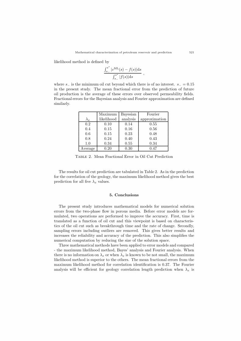
where s− is the minimum oil cut beyond which there is of no interest. s− = 0.15in the present study. The mean fractional error from the prediction of futureoil production is the average of these errors over observed permeability fields.Fractional errors for the Bayesian analysis and Fourier approximation are definedsimilarly.

Maximum Bayesian Fourierλx likelihood analysis approximation0.2 0.10 0.14 0.550.4 0.15 0.16 0.560.6 0.15 0.23 0.480.8 0.24 0.40 0.431.0 0.34 0.55 0.34

Average 0.20 0.30 0.47

Table 2. Mean Fractional Error in Oil Cut Prediction

The results for oil cut prediction are tabulated in Table 2. As in the predictionfor the correlation of the geology, the maximum likelihood method gives the bestprediction for all five λx values.

5. Conclusions

The present study introduces mathematical models for numerical solutionerrors from the two-phase flow in porous media. Before error models are for-mulated, two operations are performed to improve the accuracy. First, time istranslated as a function of oil cut and this viewpoint is based on characteris-tics of the oil cut such as breakthrough time and the rate of change. Secondly,sampling errors including outliers are removed. This gives better results andincreases the reliability and accuracy of the prediction. This also simplifies thenumerical computation by reducing the size of the solution space.

Three mathematical methods have been applied to error models and compared- the maximum likelihood method, Bayes’ analysis and Fourier analysis. Whenthere is no information on λx or when λx is known to be not small, the maximumlikelihood method is superior to the others. The mean fractional errors from themaximum likelihood method for correlation identification is 0.37. The Fourieranalysis will be efficient for geology correlation length prediction when λx is

522 Hongjoong Kim

small. The maximum likelihood method is also efficient in the prediction offuture oil production and its mean fractional error is only 0.20.

In this study, only first moments have been used as basis functions. Ourapproach is limited when the error bound is considered since it depends on thesecond moment. Efficient methods for the derivation of the second and highermoments are future research directions.

6. Acknowledgements

This research was supported by a Korea University Grant. This research usedthe data generated by the Los Alamos National Lab and I’d like to appreciateShuling Hou, David D. Sharp, and James Glimm for allowing me to use the data.Some of this research was conducted while I was in UNC Charlotte.

References

1. J. W. Barker, M. Cuypers, and L. Holden, Quantifying uncertainty in production forecasts:

Another look at the PUNQ-S3 problem, Tech. Rep, SPE 62925, 20002. J. M. Bernardo, and A. F. M. Smith, Bayesian Theory, John Wiley & Sons, 1994

3. L. Bonet-Cunha, D. S. Oliver, R. A. Redner, and A. C. Reynolds, A hybrid markov chainmonte carlo method for generating permeability fields conditioned to multiwell pressure data

and prior information, SPE Journal, v.3, no.3, p.261–271, 19984. C. V. Deusch, and A. G. Journel, Geostatistical Software Library and User’s Guide, Oxford

University Press, Oxford, 19925. I. Gelfand, and N. Vilenkin, Generalized Functions, Vol IV, Academic Press, New York,

19646. R. G. Ghanem, and P. Spanos, Stochastic Finite Elements: A Spectral Approach, Springer-

Verlag, N.Y., 19917. W. R. Gilks, S. Richardson, and D. J. Spiegelhalter, eds., Markov Chain Monte Carlo in

Practice, Chapman and Hall, London and New York, 19968. J. Glimm, S. Hou, H. Kim, Y. Lee, D. H. Sharp, K. Ye, and Q. Zou, Risk management

for petroleum reservoir production: a simulation-based study of prediction, ComputationalGeosciences, v.5, p.173–197, 2001

9. J. Glimm, and A. Jaffe, Quantum Physics: A Functional Integral Point of View, Springer-Verlag, New York, 1981

10. J. Glimm, H. Kim, D. Sharp, and T. Wallstrom, A stochastic analysis of the scale upproblem for flow in porous media, Comp. Appl. Math., v.17, no.1, p.67–79, 1998

11. H. H. Haldorsen, and L. W. Lake, A new approach to shale management in field scalemodels, SPE Journal, v.24, p.447–457, 1984

12. B. K. Hegstad, and H. Omre, Uncertainty assessment in history matching and forecasting:Geostatistics Wollongong ’96, E. Y. Baafi and N. A. Schofield, eds., v.1, Kluwer Academic

Publishers, p.585–59613. A. G. Journel, and Ch. J. Huijbregts, Mining Geostatistics, Academic Press, New York,

197814. P. R. King, A. H. Muggeridge, and W. G. Price, Renormalization calculations of immis-

cible flow, Transport in Porous Media, 12:237–260, 1993

Mathematical characterization of petroleum reservoir and prediction 523

15. L. W. Lake, and H. B. Carroll, Reservoir Characterization, Academic Press, New York,1986

16. L. W. Lake, H. B. Carroll, and T. C. Wesson, Reservoir Characterization II, Academic

Press, New York, 199117. D. S. Oliver, L. B. Cunha, and A. C. Reynolds, Markov chain monte carlo method for

conditioning a permeability field pressure data, Math. Geo., v.29, no.1, p.61–91, 199718. H. Omre, and H. Tjelmeland, Petroleum geostatistics, Geostatistics Wollongong ’96,

E. Y. Baafi and N. A. Schofield, eds., v.1, Kluwer Academic Publishers, p.41–52, 199719. D. W. Peaceman, Fundamentals of numerical reservoir simulation, Elsevier, Amsterdam-

New York, 197720. T. Wallstrom, S. Hou, M. A. Christie, L. J. Durlofsky, and D. H. Sharp, Accurate scale

up of two phase flow using renormalization and nonuniform coarsening, ComputationalGeoscience, v.3, p.69–87, 1999

21. D. Xiu, D. Lucor, C. H. Su, and G. E. Karniadakis, Stochastic modeling of flow-structureinteractions using generalized polynomial chaos, J. Fluids Eng., v.124, p.51–59, 2002

Hongjoong Kim, His research concerns computational fluid dynamics, scientific com-putation, stochastic partial differential equations and mathematical modeling of various

security-related aspects of the Internet.

Department of Mathematics, Korea University, 1, Anam-dong, Sungbuk-ku, Seoul, 136-701,Korea.

email: hongjoong@korea.ac.kr