mathematical combinatorics - university of …smarandache/ijmc-1-2011.pdfsmarandache geometries,...
TRANSCRIPT

ISSN 1937 - 1055
VOLUME 1, 2011
INTERNATIONAL JOURNAL OF
MATHEMATICAL COMBINATORICS
EDITED BY
THE MADIS OF CHINESE ACADEMY OF SCIENCES
March, 2011

Vol.1, 2011 ISSN 1937-1055
International Journal of
Mathematical Combinatorics
Edited By
The Madis of Chinese Academy of Sciences
March, 2011

Aims and Scope: The International J.Mathematical Combinatorics (ISSN 1937-1055)
is a fully refereed international journal, sponsored by the MADIS of Chinese Academy of Sci-
ences and published in USA quarterly comprising 100-150 pages approx. per volume, which
publishes original research papers and survey articles in all aspects of Smarandache multi-spaces,
Smarandache geometries, mathematical combinatorics, non-euclidean geometry and topology
and their applications to other sciences. Topics in detail to be covered are:
Smarandache multi-spaces with applications to other sciences, such as those of algebraic
multi-systems, multi-metric spaces,· · · , etc.. Smarandache geometries;
Differential Geometry; Geometry on manifolds;
Topological graphs; Algebraic graphs; Random graphs; Combinatorial maps; Graph and
map enumeration; Combinatorial designs; Combinatorial enumeration;
Low Dimensional Topology; Differential Topology; Topology of Manifolds;
Geometrical aspects of Mathematical Physics and Relations with Manifold Topology;
Applications of Smarandache multi-spaces to theoretical physics; Applications of Combi-
natorics to mathematics and theoretical physics;
Mathematical theory on gravitational fields; Mathematical theory on parallel universes;
Other applications of Smarandache multi-space and combinatorics.
Generally, papers on mathematics with its applications not including in above topics are
also welcome.
It is also available from the below international databases:
Serials Group/Editorial Department of EBSCO Publishing
10 Estes St. Ipswich, MA 01938-2106, USA
Tel.: (978) 356-6500, Ext. 2262 Fax: (978) 356-9371
http://www.ebsco.com/home/printsubs/priceproj.asp
and
Gale Directory of Publications and Broadcast Media, Gale, a part of Cengage Learning
27500 Drake Rd. Farmington Hills, MI 48331-3535, USA
Tel.: (248) 699-4253, ext. 1326; 1-800-347-GALE Fax: (248) 699-8075
http://www.gale.com
Indexing and Reviews: Mathematical Reviews(USA), Zentralblatt fur Mathematik(Germany),
Referativnyi Zhurnal (Russia), Mathematika (Russia), Computing Review (USA), Institute for
Scientific Information (PA, USA), Library of Congress Subject Headings (USA).
Subscription A subscription can be ordered by a mail or an email directly to
Linfan Mao
The Editor-in-Chief of International Journal of Mathematical Combinatorics
Chinese Academy of Mathematics and System Science
Beijing, 100190, P.R.China
Email: [email protected]
Price: US$48.00

Editorial Board
Editor-in-Chief
Linfan MAO
Chinese Academy of Mathematics and System
Science, P.R.China
Email: [email protected]
Editors
S.Bhattacharya
Deakin University
Geelong Campus at Waurn Ponds
Australia
Email: [email protected]
An Chang
Fuzhou University, P.R.China
Email: [email protected]
Junliang Cai
Beijing Normal University, P.R.China
Email: [email protected]
Yanxun Chang
Beijing Jiaotong University, P.R.China
Email: [email protected]
Shaofei Du
Capital Normal University, P.R.China
Email: [email protected]
Florentin Popescu and Marian Popescu
University of Craiova
Craiova, Romania
Xiaodong Hu
Chinese Academy of Mathematics and System
Science, P.R.China
Email: [email protected]
Yuanqiu Huang
Hunan Normal University, P.R.China
Email: [email protected]
H.Iseri
Mansfield University, USA
Email: [email protected]
M.Khoshnevisan
School of Accounting and Finance,
Griffith University, Australia
Xueliang Li
Nankai University, P.R.China
Email: [email protected]
Han Ren
East China Normal University, P.R.China
Email: [email protected]
W.B.Vasantha Kandasamy
Indian Institute of Technology, India
Email: [email protected]
Mingyao Xu
Peking University, P.R.China
Email: [email protected]
Guiying Yan
Chinese Academy of Mathematics and System
Science, P.R.China
Email: [email protected]
Y. Zhang
Department of Computer Science
Georgia State University, Atlanta, USA

ii International Journal of Mathematical Combinatorics
Achievement provides the only real pleasure in life.
By Thomas Edison, an American inventor.

International J.Math. Combin. Vol.1 (2011), 01-19
Lucas Graceful Labeling for Some Graphs
M.A.Perumal1, S.Navaneethakrishnan2 and A.Nagarajan2
1. Department of Mathematics, National Engineering College,
K.R.Nagar, Kovilpatti, Tamil Nadu, India
2. Department of Mathematics, V.O.C College, Thoothukudi, Tamil Nadu, India.
Email : [email protected], [email protected], [email protected]
Abstract: A Smarandache-Fibonacci triple is a sequence S(n), n ≥ 0 such that
S(n) = S(n − 1) + S(n − 2), where S(n) is the Smarandache function for integers
n ≥ 0. Clearly, it is a generalization of Fibonacci sequence and Lucas sequence. Let
G be a (p, q)-graph and S(n)|n ≥ 0 a Smarandache-Fibonacci triple. An bijection
f : V (G) → S(0), S(1), S(2), . . . , S(q) is said to be a super Smarandache-Fibonacci grace-
ful graph if the induced edge labeling f∗(uv) = |f(u) − f(v)| is a bijection onto the set
S(1), S(2), . . . , S(q). Particularly, if S(n), n ≥ 0 is just the Lucas sequence, such a label-
ing f : V (G) → l0, l1, l2, · · · , la (a ǫ N) is said to be Lucas graceful labeling if the induced
edge labeling f1(uv) = |f(u) − f(v)| is a bijection on to the set l1, l2, · · · , lq. Then G is
called Lucas graceful graph if it admits Lucas graceful labeling. Also an injective function
f : V (G) → l0, l1, l2, · · · , lq is said to be strong Lucas graceful labeling if the induced edge
labeling f1(uv) = |f(u) − f(v)| is a bijection onto the set l1, l2, ..., lq. G is called strong
Lucas graceful graph if it admits strong Lucas graceful labeling. In this paper, we show
that some graphs namely Pn, P+n − e, Sm,n, Fm@Pn, Cm@Pn, K1,n ⊙ 2Pm, C3@2Pn and
Cn@K1,2 admit Lucas graceful labeling and some graphs namely K1,n and Fn admit strong
Lucas graceful labeling.
Key Words: Smarandache-Fibonacci triple, super Smarandache-Fibonacci graceful graph,
Lucas graceful labeling, strong Lucas graceful labeling.
AMS(2010): 05C78
§1. Introduction
By a graph, we mean a finite undirected graph without loops or multiple edges. A path of
length n is denoted by Pn. A cycle of length n is denoted by Cn.G+ is a graph obtained from
the graph G by attaching a pendant vertex to each vertex of G. The concept of graceful labeling
was introduced by Rosa [3] in 1967.
A function f is a graceful labeling of a graph G with q edges if f is an injection from
1Received November 11, 2010. Accepted February 10, 2011.

2 M.A.Perumal, S.Navaneethakrishnan and A.Nagarajan
the vertices of G to the set 1, 2, 3, · · · , q such that when each edge uv is assigned the la-
bel |f(u) − f(v)|, the resulting edge labels are distinct. The notion of Fibonacci graceful
labeling was introduced by K.M.Kathiresan and S.Amutha [4]. We call a function, a Fi-
bonacci graceful labeling of a graph G with q edges if f is an injection from the vertices of
G to the set 0, 1, 2, ..., Fq, where Fq is the qth Fibonacci number of the Fibonacci series
F1 = 1, F2 = 2, F3 = 3, F4 = 5, ..., and each edge uv is assigned the label |f(u) − f(v)|. Based
on the above concepts we define the following.
Let G be a (p, q) -graph. An injective function f : V (G) → l0, l1, l2, · · · , la, (a ǫ N),
is said to be Lucas graceful labeling if an induced edge labeling f1(uv) = |f(u) − f(v)| is a
bijection onto the set l1, l2, · · · , lq with the assumption of l0 = 0, l1 = 1, l2 = 3, l3 = 4, l4 =
7, l5 = 11, · · · ,. Then G is called Lucas graceful graph if it admits Lucas graceful labeling. Also
an injective function f : V (G) → l0, l1, l2, · · · , lq is said to be strong Lucas graceful labeling if
the induced edge labeling f1(uv) = |f(u)−f(v)| is a bijection onto the set l1, l2, · · · , lq. Then
G is called strong Lucas graceful graph if it admits strong Lucas graceful labeling. In this paper,
we show that some graphs namely Pn, P+n − e, Sm,n, Fm@Pn, Cm@Pn, K1,n ⊙2Pm, C3@2Pn
and Cn@K1,2 admit Lucas graceful labeling and some graphs namely K1,n and Fn admit strong
Lucas graceful labeling. Generally, let S(n), n ≥ 0 with S(n) = S(n − 1) + S(n − 2) be a
Smarandache-Fibonacci triple, where S(n) is the Smarandache function for integers n ≥ 0. An
bijection f : V (G) → S(0), S(1), S(2), . . . , S(q) is said to be a super Smarandache-Fibonacci
graceful graph if the induced edge labeling f∗(uv) = |f(u) − f(v)| is a bijection onto the set
S(1), S(2), · · · , S(q).
§2. Lucas graceful graphs
In this section, we show that some well known graphs are Lucas graceful graphs.
Definition 2.1 Let G be a (p, q) -graph. An injective function f : V (G) → l0, l1, l2, · · · , la, ,(a ǫ N) is said to be Lucas graceful labeling if an induced edge labeling f1(uv) = |f(u) − f(v)| is
a bijection onto the set l1, l2, · · · , lq with the assumption of l0 = 0, l1 = 1, l2 = 3, l3 = 4, l4 =
7, l5 = 11, · · · ,. Then G is called Lucas graceful graph if it admits Lucas graceful labeling.
Theorem 2.2 The path Pn is a Lucas graceful graph.
Proof Let Pn be a path of length n having (n + 1) vertices namely v1, v2, v3, · · · , vn, vn+1.
Now, |V (Pn)| = n + 1 and |E(Pn)| = n. Define f : V (Pn) → l0, l1, l2, · · · , la, , a ǫ N by
f(ui) = li+1, 1 ≤ i ≤ n. Next, we claim that the edge labels are distinct. Let
E = f1(vivi+1) : 1 ≤ i ≤ n = |f(vi) − f(vi+1)| : 1 ≤ i ≤ n= |f(v1) − f(v2)| , |f(v2) − f(v3)| , · · · , |f(vn) − f(vn+1)| , = |l2 − l3| , |l3 − l4| , · · · , |ln+1 − ln+2| = l1, l2, · · · , ln.
So, the edges of Pn receive the distinct labels. Therefore, f is a Lucas graceful labeling.
Hence, the path Pn is a Lucas graceful graph.
Lucas Graceful Labeling for Some Graphs 3
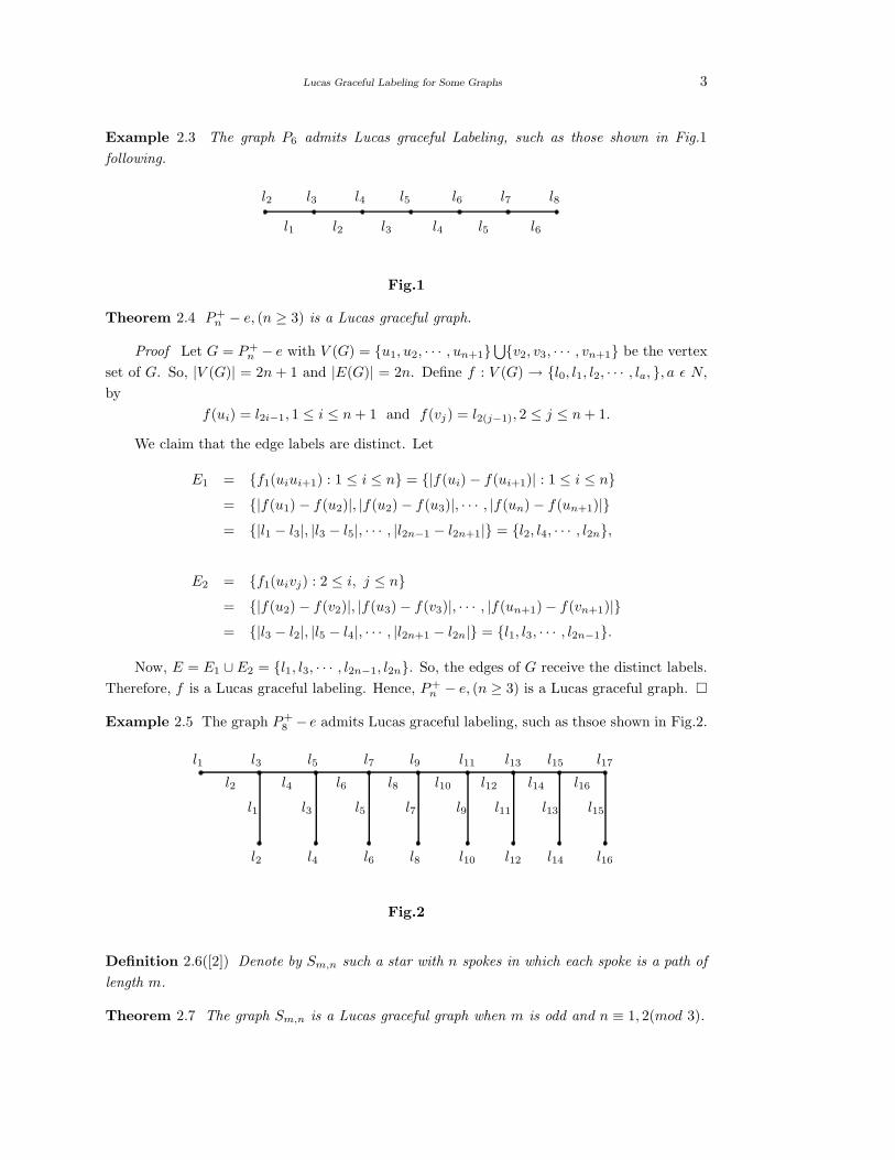
Example 2.3 The graph P6 admits Lucas graceful Labeling, such as those shown in Fig.1
following.
l2 l3 l4 l5 l6 l7 l8
l1 l2 l3 l4 l5 l6
Fig.1
Theorem 2.4 P+n − e, (n ≥ 3) is a Lucas graceful graph.
Proof Let G = P+n − e with V (G) = u1, u2, · · · , un+1
⋃v2, v3, · · · , vn+1 be the vertex
set of G. So, |V (G)| = 2n + 1 and |E(G)| = 2n. Define f : V (G) → l0, l1, l2, · · · , la, , a ǫ N,
by
f(ui) = l2i−1, 1 ≤ i ≤ n + 1 and f(vj) = l2(j−1), 2 ≤ j ≤ n + 1.
We claim that the edge labels are distinct. Let
E1 = f1(uiui+1) : 1 ≤ i ≤ n = |f(ui) − f(ui+1)| : 1 ≤ i ≤ n= |f(u1) − f(u2)|, |f(u2) − f(u3)|, · · · , |f(un) − f(un+1)|= |l1 − l3|, |l3 − l5|, · · · , |l2n−1 − l2n+1| = l2, l4, · · · , l2n,
E2 = f1(uivj) : 2 ≤ i, j ≤ n= |f(u2) − f(v2)|, |f(u3) − f(v3)|, · · · , |f(un+1) − f(vn+1)|= |l3 − l2|, |l5 − l4|, · · · , |l2n+1 − l2n| = l1, l3, · · · , l2n−1.
Now, E = E1 ∪ E2 = l1, l3, · · · , l2n−1, l2n. So, the edges of G receive the distinct labels.
Therefore, f is a Lucas graceful labeling. Hence, P+n − e, (n ≥ 3) is a Lucas graceful graph.
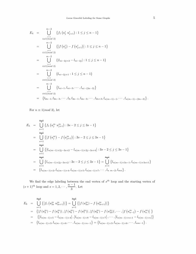
Example 2.5 The graph P+8 − e admits Lucas graceful labeling, such as thsoe shown in Fig.2.
l1 l3 l5 l7 l9 l11 l13 l15 l17
l2 l4 l6 l8 l10 l12 l14 l16
l1 l3 l5 l7 l9 l11 l13 l15
l2 l4 l6 l8 l10 l12 l14 l16
Fig.2
Definition 2.6([2]) Denote by Sm,n such a star with n spokes in which each spoke is a path of
length m.
Theorem 2.7 The graph Sm,n is a Lucas graceful graph when m is odd and n ≡ 1, 2(mod 3).

4 M.A.Perumal, S.Navaneethakrishnan and A.Nagarajan
Proof Let G = Sm,n and let V (G) =ui
j : 1 ≤ i ≤ m and 1 ≤ j ≤ n
be the vertex set of
Sm,n. Then |V (G)| = mn + 1 and |E(G)| = mn. Define f : V (G) → l0, l1, l2, · · · , la, , a ǫ N
by
f(u0) = l0 for i = 1, 2, · · · , m − 2 and i ≡ 1(mod 2);
f(ui
j
)= ln(i−1)+2j−1, 1 ≤ j ≤ n for i = 1, 2, · · · , m − 1 and i ≡ 0(mod 2);
f(ui
j
)= lni+2−2j , 1 ≤ j ≤ n and for s = 1, 2, · · · ,
n
3,
f(um
j
)= ln(m−1)+2(j+1)−3s, 3s − 2 ≤ j ≤ 3s.
We claim that the edge labels are distinct. Let
E1 =m⋃
i=1
i≡1(mod 2)
f1
(u0 ui
1
)=
m⋃
i=1
i≡1(mod 2)
∣∣f (u0) − f(ui
1
)∣∣
=
m⋃
i=1
i≡1(mod 2)
∣∣l0 − ln(i−1)+1
∣∣ =
m⋃
i=1
i≡1(mod 2)
ln(i−1)+1
=l1, l2n+1, l4n+1, · · · , ln(m−1)+1
,
E2 =
m−1⋃
i=1
i≡1(mod 2)
f1
(u0 ui
1
)=
m−1⋃
i=1
i≡1(mod 2)
∣∣f (u0) − f(ui
1
)∣∣
=
m−1⋃
i=1
i≡1(mod 2)
|l0 − lni| =
m−1⋃
i=1
i≡1(mod 2)
lni =l2n, l4n, · · · , ln(m−1)
E3 =m−2⋃
i=1
i≡1(mod 2)
f1
(ui
juij+1
): 1 ≤ j ≤ n − 1
=
m−2⋃
i=1
i≡1(mod 2)
∣∣f(ui
j
)− f
(ui
j+1
)∣∣ : 1 ≤ j ≤ n − 1
=
m−2⋃
i=1
i≡1(mod 2)
∣∣ln(i−1)+2j−1 − ln(i−1)+2j+1
∣∣ : 1 ≤ j ≤ n − 1
=
m−2⋃
i=1
i≡1(mod 2)
ln(i−1)+2j : 1 ≤ j ≤ n − 1
=m−2⋃
i=1
i≡1(mod 2)
ln(i−1)+2, ln(i−1)+4, · · · , : ln(i−1)+2(n−1)
=l2, l2n+2, ..., ln(m−3)+2
∪l4, l2n+4, · · · , ln(m−3)+4
∪ · · ·
∪l2n−2, l4n−2, ..., ln(m−3)+2n−2
,
Lucas Graceful Labeling for Some Graphs 5
E4 =
m−2⋃
i=1
i≡1(mod 2)
f1
(ui
j uij+1
): 1 ≤ j ≤ n − 1
=
m−2⋃
i=1
i≡1(mod 2)
∣∣f(ui
j
)− f
(ui
j+1
)∣∣ : 1 ≤ j ≤ n − 1
=m−2⋃
i=1
i≡1(mod 2)
|lni−2j+2 − lni−2j | : 1 ≤ j ≤ n − 1
=
m−2⋃
i=1
i≡1(mod 2)
lni−2j+1 : 1 ≤ j ≤ n − 1
=
m−2⋃
i=1
i≡1(mod 2)
lni−1, lni−3, · · · , lni−(2n−3)
=l2n−1, l2n−3, · · · , l3, l4n−1, l4n−3, · · · , l2n+3, ln(m−1)−1, · · · , ln(m−1)−(2n−3)
.
For n ≡ 1(mod 3), let
E5 =
n−1
3⋃
s=1
f1
(um
j umj+1
): 3s− 2 ≤ j ≤ 3s − 1
=
n−1
3⋃
s=1
∣∣f(um
j
)− f
(um
j+1
)∣∣ : 3s − 2 ≤ j ≤ 3s − 1
=
n−1
3⋃
s=1
∣∣ln(m−1)+2j−3s+2 − ln(m−1)+2j−3s+4
∣∣ : 3s − 2 ≤ j ≤ 3s − 1
=
n−1
3⋃
s=1
ln(m−1)+2j−3s+2 : 3s − 2 ≤ j ≤ 3s − 1
=
n−1
3⋃
s=1
ln(m−1)+3s−1, ln(m−1)+3s+1
=ln(m−1)+2, ln(m−1)+4, ln(m−1)+5, ln(m−1)+7, · · · , ln m−2, lmn
.
We find the edge labeling between the end vertex of sth loop and the starting vertex of
(s + 1)th loop and s = 1, 2, · · · ,n − 1
3. Let
E6 =
n−1
3⋃
s=1
∣∣f1
(um
3s um3s+1
)∣∣ =
n−1
3⋃
s=1
∣∣f (um3s) − f
(um
3s+1
)∣∣
=|f (um
3 ) − f (um4 )| , |f (um
6 ) − f (um7 )| , |f (um
9 ) − f (um10)| , · · · ,
∣∣f(um
n−1
)− f (um
n )∣∣
=∣∣ln(m−1)+5 − ln(m−1)+4
∣∣ ,∣∣ln(m−1)+8 − ln(m−1)+7
∣∣ , · · · ,∣∣ln(m−1)+n+1 − ln(m−1)+n
∣∣
=ln(m−1)+3, ln(m−1)+6, · · · , ln(m−1)+n−1
=ln(m−1)+3, ln(m−1)+6, · · · , lnm−1
.

6 M.A.Perumal, S.Navaneethakrishnan and A.Nagarajan
For n ≡ 2(mod 3), let
E′5 =
n−1
3⋃
s=1
f1
(um
j umj+1
): 3s− 2 ≤ j ≤ 3s − 1
=
n−1
3⋃
s=1
∣∣f(um
j
)− f
(um
j+1
)∣∣ : 3s − 2 ≤ j ≤ 3s − 1
=
n−1
3⋃
s=1
∣∣ln(m−1)+2j−3s+2 − ln(m−1)+2j−3s+4
∣∣ : 3s − 2 ≤ j ≤ 3s − 1
=
n−1
3⋃
s=1
ln(m−1)+2j−3s+3 : 3s − 2 ≤ j ≤ 3s − 1
=
n−1
3⋃
s=1
ln(m−1)+3s−1, ln(m−1)+3s+1
=ln(m−1)+2, ln(m−1)+4, ln(m−1)+5, ln(m−1)+7, · · · , ln(m−1)+n−2, ln(m−1)+n
.
We determine the edge labeling between the end vertex of sth loop and the starting vertex
of (s + 1)th loop and s = 1, 2, 3, ...,n − 1
3.
Let E′
6 =
n−1
3⋃
s=1
f1
(um
3s um3s+1
)=
n−1
3⋃
s=1
∣∣f (um3s) − f
(m3s+1
)∣∣
=|f (um
3 ) − f (um4 )| , |f (um
6 ) − f (um7 )| , |f (um
9 ) − f (um10)| , · · · ,
∣∣f(um
n−1
)− f (um
n )∣∣
=∣∣ln(m−1)+5 − ln(m−1)+4
∣∣ ,∣∣ln(m−1)+8 − ln(m−1)+7
∣∣ , · · · ,∣∣ln(m−1)+n+1 − ln(m−1)+n
∣∣
=ln(m−1)+3, ln(m−1)+6, · · · , lnm−1
.
Now,E =6⋃
i=1
Ei if n ≡ 1(mod 3) and E =
(6⋃
i=1
Ei
)⋃E
′
5
⋃E
′
6 if n ≡ 2(mod 3). So the
edges of Sm,n (when m is odd and n ≡ 1, 2(mod 3)), receive the distinct labels. Therefore, f is
a Lucas graceful labeling. Hence, Sm,n is a Lucas graceful graph if m is odd, n ≡ 1, 2(mod 3).
Example 2.8 The graphs S5,4 and S5,5 admit Lucas graceful labeling, such as those shown in
Fig.3 and Fig 4.
l1 l3 l5 l7
l8 l6 l7 l2
l9 l11 l13 l15
l16 l14 l12 l10
l17 l19 l21 l20
l2 l4 l6
l7 l5 l3
l10 l12 l14
l15 l13 l11
l18 l20 l19
l1
l8
l9
l16l17
l0
Fig.3

Lucas Graceful Labeling for Some Graphs 7
l1 l3 l5 l7 l9
l10 l8 l6 l4 l2
l11 l13 l15 l17 l19
l20 l18 l16 l14 l12
l21 l23 l25 l24 l26
l2 l4 l6 l8
l9 l7 l5 l3
l12 l14 l16 l18
l19 l17 l15 l13
l22 l24 l23 l25
l1
l10
l11
l20
l21
l0
Fig.4
Definition 2.9([2]) The graph G = Fm@Pn consists of a fan Fm and a path Pn of length n
which is attached with the maximum degree of the vertex of Fm.
Theorem 2.10 Fm@Pn is a Lucas graceful labeling when n ≡ 1, 2 (mod 3).
Proof Let v1, v2, ..., vm, vm+1 and u0 be the vertices of a fan Fm and u1, u2, · · · , un be the
vertices of a path Pn. Let G = Fm@Pn. Then |V (G)| = m + n + 2 and |E(G)| = 2m + n + 1.
Define f : V (G) → l0, l1, l2, · · · , la, , a ǫ N, by f(u0) = l0, f(vi) = l2i−1, 1 ≤ i ≤ m + 1.
For s = 1, 2, · · · ,n − 1
3or
n − 2
3according as n ≡ 1(mod 3) or n ≡ 2(mod 3), f(uj) =
l2m+2j−3s+3, 3s − 2 ≤ j ≤ 3s.
We claim that the edge labels are distinct. Let
E1 = f1(vi vi+1) : 1 ≤ i ≤ m = |f(vi) − f (vi+1)| : 1 ≤ i ≤ m= |l2i−1 − l2i+1| : 1 ≤ i ≤ m= l2i : 1 ≤ i ≤ m = l2, l4, · · · , l2m ,
E2 = f1 (u0vi) : 1 ≤ i ≤ m + 1 = |f(u0) − f(vi)| 1 ≤ i ≤ m + 1= |l0 − l2i−1| : 1 ≤ i ≤ m + 1= l2i−1 : 1 ≤ i ≤ m + 1 = l1, l3, · · · , l2m+1
and
E3 = f1 (u0u1) = |f(u0) − f(u1)| = |l0 − l2m+2| = l2m+2

8 M.A.Perumal, S.Navaneethakrishnan and A.Nagarajan
For s = 1, 2, 3, · · · ,n − 1
3and n ≡ 1(mod 3), let
E4 =
n−1
3⋃
s=1
f1 (uj , uj+1) : 3s − 2 ≤ j ≤ 3s − 1
=
n−1
3⋃
s=1
|f(uj) − f(uj+1)| : 3s − 2 ≤ j ≤ 3s − 1
=
n−1
3⋃
s=1
|l2m+2j+3−3s − l2m+2j+5−3s| : 3s − 2 ≤ j ≤ 3s − 1
=
n−1
3⋃
s=1
(l2m+2j+4−3s : 3s − 2 ≤ j ≤ 3s − 1)
= l2m+2j−2 : 4 ≤ j ≤ 5⋃
l2m+2j−5 : 7 ≤ j ≤ 8⋃
· · ·⋃
l2m+2j−n+4 : n − 3 ≤ j ≤ n − 2
= l2m+6, l2m+8 ∪ l2m+9, l2m+11⋃
· · ·⋃
l2m+n−2, l2m+n= l2m+6, l2m+8, l2m+9, l2m+11, · · · , l2m+n−2, l2m+n
We find the edge labeling between the end vertex of sth loop and the starting vertex of
(s + 1)th loop and s = 1, 2, 3, · · · ,n − 1
3, n ≡ 1(mod 3). Let
E5 =
n−1
3⋃
s=1
f1 (uj uj+1) : j = 3s =
n−1
3⋃
s=1
|f(uj) − f(uj+1)| : j = 3s
=
n−1
3⋃
s=1
|l2m+2j+3−3s − l2m+2j+5−3s| : j = 3s
= |l2m+2j − l2m+2j−1| : j = 3 ∪ |l2m+2j−3 − l2m+2j−4| : j = 6⋃
· · ·⋃
|l2m+2j − l2m+2j−1| : j = n − 1= l2m+2j−2 : j = 3 ∪ l2m+2j−5 : j = 6∪, · · · ,∪l2m+2j−n+3 : j = n − 1= l2m+4, l2m+7, · · · , l2m+n+1 .
For s = 1, 2, 3, · · · ,n − 2
3and n ≡ 2(mod 3), let
E′
4 =
n−2
3⋃
s=1
f1(uj uj+1) : 3s − 2 ≤ j ≤ 3s − 1
=
n−2
3⋃
s=1
|f(uj) − f(uj+1)| : 3s − 2 ≤ j ≤ 3s − 1
=
n−2
3⋃
s=1
|l2m+2j+3−3s − l2m+2j+5−3s| : 3s − 2 ≤ j ≤ 3s − 1

Lucas Graceful Labeling for Some Graphs 9
=
n−2
3⋃
s=1
(l2m+2j+4−3s : 3s − 2 ≤ j ≤ 3s− 1)
= l2m+2j−2 : 4 ≤ j ≤ 5⋃
l2m+2j−5 : 7 ≤ j ≤ 8⋃
· · ·⋃
l2m+2j−n+4 : n − 3 ≤ j ≤ n − 2
= l2m+6, l2m+8⋃
l2m+9, l2m+11⋃
· · ·⋃
l2m+n−2, l2m+n= l2m+6, l2m+8,2m+9 , l2m+11, · · · , l2m+n−2, l2m+n
We determine the edge labeling between the end vertex of sth loop and the starting vertex
of (s + 1)th loop and s = 1, 2, 3, ...,n − 2
3, n ≡ 2(mod 3). Let
E′
5 =
n−2
3⋃
s=1
f1 (uj, uj+1) : j = 3s
=
n−2
3⋃
s=1
|f(uj) − f(uj+1)| : j = 3s =
n−2
3⋃
s=1
|l2m+2j+3−3s − l2m+2j+5−3s| : j = 3s
= |l2m+2j − l2m+2j−1| : j = 3⋃
|l2m+2j−3 − l2m+2j−4| : j = 6⋃
· · ·⋃
|l2m+2j−n+4 − l2m+2j−n+5| : j = n − 1
= l2m+2j−2 : j = 3 ∪ l2m+2j−5 : j = 6⋃
· · ·⋃
l2m+2j−(n−3) : j = n − 1
= l2m+4, l2m+7, ..., l2m+n+1 .
Now, E =5⋃
i=1
Ei if n ≡ 1(mod 3) and E =
(5⋃
i=1
Ei
)⋃E
′
4
⋃E
′
5 if n ≡ 2(mod 3). So, the
edges of Fm@Pn (whenn ≡ 1, 2(mod 3)) are the distinct labels. Therefore, f is a Lucas graceful
labeling. Hence, G = Fm@Pn (if n ≡ 1, 2(mod 3)) is a Lucas graceful labeling.
Example 2.11 The graph F5@P4 admits a Lucas graceful labeling shown in Fig.5.
l1 l3 l5 l7 l9 l11
l0 l12 l14 l16 l15
l2 l4 l6 l8 l10
l12 l13 l15 l14
l1l3
l5 l7l9
l11
Fig.5
Definition 2.12 ([2]) The Graph G = Cm@Pn consists of a cycle Cm and a path of Pn of
length n which is attached with any one vertex of Cm.

10 M.A.Perumal, S.Navaneethakrishnan and A.Nagarajan
Theorem 2.13 The graph Cm@Pn is a Lucas graceful graph when m ≡ 0(mod 3) and n =
1, 2(mod 3).
Proof Let G = Cm@Pn and let u1, u2, · · · , um be the vertices of a cycle Cm and v1, v2, · · · , vn, vn+1
be the vertices of a path Pn which is attached with the vertex (u1 = v1) of Cm. Let V (G) =
u1 = v1 ∪ u2, u3, · · · , um ∪ v2, v3, ..., vn, vn+1 be the vertex set of G. So, |V (G)| = m + n
and |E(G)| = m + n. Define f : V (G) → l0, l1, · · · , la, a ǫ N by f(u1) = f(v1) = l0; f(ui) =
l2i−3s, 3s − 1 ≤ j ≤ 3s + 1 for s = 1, 2, 3, · · · ,m
3, i = 2, 3, · · · , m; f(vj) = lm+2j−3r, 3r − 1 ≤
j ≤ 3r + 1 for r = 1, 2, · · · ,n + 1
3and j = 2, 3, · · · , n + 1.
We claim that the edge labels are distinct. Let
E1 = f1 (u1 u2) = |f (u1) − f (u2)| = (|l0 − l1|) = l1,
E2 =
m3⋃
s=1
f1 (ui ui+1) : 3s − 1 ≤ i ≤ 3s and um+1 = u1
=
m3⋃
s=1
f1 (ui) − f(ui+1) : 3s − 1 ≤ i ≤ 3s and um+1 = u1
= |f(u2) − f(u3)| , |f(u3) − f(u4)| , ..., |f(um) − f(um+1)|= |l1 − l3| , |l3 − l5| , |l4 − l6| , |l6 − l8| , · · · , |lm − l0|= l2, l4, l5, l7, · · · , lm
We determine the edge labeling between the end vertex of sth loop and the starting vertex
of (s + 1)th loop and s = 1, 2, ...,m
3− 1. Let
E3 =
m3−1⋃
s=1
f1(u3s+1 u3s+2) =
m3−1⋃
s=1
|f(u3s+1) − f(u3s+2)|
= |f(u4) − f(u5)| , |f(u7) − f(u8)| , · · · , |f(um−2) − f(um−1)|= |l5 − l4| , |l8 − l7| , · · · , |lm−1 − lm−2|= l3, l6, · · · , lm−3 ,
E4 = f1(v1 v2) = |f(v1) − f(v2)| = |l0 − lm+4−3| |l0 − lm+4−3|= |l0 − lm+1| = |l0 − lm+1| = lm+1 .
For n ≡ 1(mod 3), let
E5 =
n−1
3⋃
r=1
f1(vj vj+1) : 3r − 1 ≤ j ≤ 3r
=
n−1
3⋃
r=1
|f(vj) − f(vj+1)| : 3r − 1 ≤ j ≤ 3r

Lucas Graceful Labeling for Some Graphs 11
= |f(v2) − f(v3)| , |f(v3) − f(v4)| , · · · , |f(vn−1) − f(vn)|= |lm+4−3 − lm+6−3| , |lm+6−3 − lm+8−3| , |lm+10−6 − lm+12−6| , |lm+12−6 − lm+14−6| ,
· · · , |lm+2n−2−n+1 − lm+2n−n+1|= |lm+1 − lm+3| , |lm+3 − lm+5| , |lm+4 − lm+6| , |lm+6 − lm+8| , · · · , |lm+n−1 − lm+n+1|= lm+2, lm+4, lm+5, lm+7, · · · , lm+n .
We calculate the edge labeling between the end vertex of rth loop and the starting vertex
of (r + 1)th loop and r = 1, 2, · · · ,n − 1
3. Let
E6 =
n−1
3⋃
r=1
f1(v3r+1 v3r+2) =
n−1
3⋃
r=1
|f(v3r+1) − f(v3r+2)|
= |f(v4) − f(v5)| , |f(v7) − f(v8)| , · · · , |f(vn−2) − f(vn−1)|= |lm+8−3 − lm+10−6| , |lm+14−6 − lm+16−9| , · · · , |lm+2n−4−n+2 − lm+2n−2−n+1|= |lm+5 − lm+4| , |lm+8 − lm+7| , · · · , |lm+n−2 − lm+n|= lm+3, lm+6, lm+9, · · · , lm+n−1
For n ≡ 2(mod 3), let
E′
5 =
n−1
3⋃
r=1
f1(vj vj+1) : 3r − 1 ≤ j ≤ 3r =
n−1
3⋃
r=1
|f(vj) − f(vj+1)| : 3r − 1 ≤ j ≤ 3r
= |f(v2) − f(v3)| , |f(v3) − f(v4)| , · · · , |f(vn−1) − f(vn)|= |lm+4−3 − lm+6−3| , |lm+6−3 − lm+8−3| , |lm+10−6 − lm+12−6| , |lm+12−6 − lm+14−6| ,
· · · , |lm+2n−2−2n+1 − lm+2n−n+1|= lm+2, lm+4, lm+5, lm+7, ..., lm+n .
We find the edge labeling between the end vertex of rth loop and the starting vertex of
(r + 1)th loop and r = 1, 2, · · · ,n − 2
3. Let
E′
6 =
n−2
3⋃
r=1
f1(v3r+1 v3r+2) =
n−2
3⋃
r=1
|f(v3r+1) − f(v3r+2)|
= |f(v4) − f(v5)| , |f(v7) − f(v8)| , · · · , |f(vn−2) − f(vn−1)|= |lm+8−3 − lm+10−6| , |lm+14−6 − lm+16−9| , · · · , |lm+2n−4−n+2 − lm+2n−2−n+1|= |lm+5 − lm+4| , |lm+8 − lm+7| , · · · , |lm+n−2 − lm+n|= lm+3, lm+6, lm+9, · · · , lm+n−1
Now, E =6⋃
i=1
Ei if n ≡ 1(mod 3) and E =
(4⋃
i=1
Ei
)⋃E
′
5
⋃E
′
6 if n ≡ 2(mod 3). So,
the edges of G receive the distinct labels. Therefore, f is a Lucas graceful labeling. Hence,
G = Cm@Pn is a Lucas graceful graph when m ≡ 0(mod 3) and n ≡ 1, 2(mod 3).

12 M.A.Perumal, S.Navaneethakrishnan and A.Nagarajan
Example 2.14 The graph C9@P7 admits a Lucas graceful labeling, such as those shown in
Fig.6.
l0
l1
l3
l5l4l6
l8
l7
l9 l1
l2
l4
l3l5
l7
l6
l8
l9 l10 l12 l14 l13 l15 l17 l16
l10 l11 l13 l12 l14 l16 l15
Fig.6
Definition 2.15 The graph K1,n ⊙2Pm means that 2 copies of the path of length m is attached
with each pendent vertex of K1,n.
Theorem 2.16 The graph K1,n ⊙ 2Pm is a Lucas graceful graph.
Proof Let G = K1,n ⊙ 2Pm with V (G) = ui : 0 ≤ i ≤ n⋃v(1)ij , v
(2)i,j : 1 ≤ i ≤ n, 1 ≤ j
≤ m − 1 and E(G) = u0 ui : 1 ≤ i ≤ n∪
ui v(1)i,j , ui v(2)i,j : 1 ≤ i ≤ n and 1 ≤ j ≤ m − 1
∪
v(1)i,j v
(1)i,j+1, v
(2)i,j v
(2)i,j+1 : 1 ≤ i ≤ n and 1 ≤ j ≤ m − 1
. Thus |V (G)| = 2mn + n + 1 and
|E(G)| = 2mn + n.
For i = 1, 2, · · · , n, define f : V (G) → l0, l1, l2, · · · , la , a ǫ N , by f(u0) = l0 f(ui) =
l(2m+1)(i−1)+2; f(v(1)i,j ) = l(2m+1)(i−1)+2j+1, 1 ≤ j ≤ m and f(v
(2)i,j ) = l(2m+1)(i−1)+2j+2, 1 ≤
j ≤ m.
We claim that the edge labels are distinct. Let
E1 =
n⋃
i=1
f1 (u0 ui) =
n⋃
i=1
|f (u0) − f (ui)|
=n⋃
i=1
∣∣l0 − l(2m+1)(i−1)+2
∣∣ =n⋃
i=1
l(2m+1)(i−1)+2
,
E2 =
n⋃
i=1
f1(uiv
(1)i,1 ), f1(uiv
(2)i,1 )
=
n⋃
i=1
∣∣∣f(ui) − f(v(1)i,1
∣∣∣ ,∣∣∣f(ui) − f(v
(2)i,1 )∣∣∣
Lucas Graceful Labeling for Some Graphs 13
=n⋃
i=1
∣∣l(2m+1)(i−1)+2 − l(2m+1)(i−1)+3
∣∣ ,∣∣l(2m+1)(i−1)+2 − l(2m+1)(i−1)+4
∣∣
=
n⋃
i=1
l(2m+1)(i−1)+1, l(2m+1)(i−1)+3
= l1, l3 ∪ l2m+2, l2m+4 ∪ l2mn+n−2m+1, l2mn+n−2m+3= l1, l2m+2, · · · , l2mn+n−2m+1, l3, l2m+4, · · · , l2mn+n−2m+3 ,
E3 =
n⋃
i=1
m−1⋃
j=1
f1(v
(1)i,j v
(1)i,j+1
=n⋃
i=1
m−1⋃
j=1
∣∣∣f(v(1)i,j ) − f(v
(1)i,j+1
∣∣∣
=n⋃
i=1
m−1⋃
j=1
∣∣l(2m+1)(i−1)+2j+1 − l(2m+1)(i−1)+2j+3
∣∣
=n⋃
i=1
m−1⋃
j=1
l(2m+1)(i−1)+2j+2
=n⋃
i=1
l(2m+1)(i−1)+4, l(2m+1)(i−1)+6, · · · , l(2m+1)(i−1)+2m
= l4, l6, · · · , l2m ∪l(2m+1)+4, l(2m+1)+6, · · · , l(2m+1)(i−1)+2m
⋃
· · ·⋃
l(2m+1)(n−1)+4, l(2m+1)(n−1)+6, · · · , l(2m+1)(n−1)+2m
=l4, · · · , l2m, l2m+5, · · · , l4m+1, · · · , l(2m+1)(n−1)+4, l(2m+1)(n−1)+6, · · · , l2mn+n−1
,
E4 =n⋃
i=1
m−1⋃
j=1
f1(v
(2)i,j v
(2)i,j+1
=
n⋃
i=1
m−1⋃
j=1
∣∣∣f(v(2)i,j ) − f(v
(2)i,j+1
∣∣∣
=
n⋃
i=1
m−1⋃
j=1
∣∣l(2m+1)(i−1)+2j+2 − l(2m+1)(i−1)+2j+4
∣∣
=
n⋃
i=1
m−1⋃
j=1
l(2m+1)(i−1)+2j+3
=
n⋃
i=1
l(2m+1)(i−1)+5, l(2m+1)(i−1)+7, · · · , l(2m+1)(i−1)+2m+1
= l5, · · · , l2m+1⋃
l2m+1+5, l2m+1+7, · · · , l2m+1+2m+1⋃
l(2m+1)(n−1)+5, l(2m+1)(n−1)+7, · · · , l(2m+1)(n−1)+(2m+1)
=l5, · · · , l2m+1, l2m+6, · · · , l4m+1, · · · , l(2m+1)(n−1)+5, l(2m+1(n−1)+7, · · · , l(2m+1)+n
.

14 M.A.Perumal, S.Navaneethakrishnan and A.Nagarajan
Now, E =4⋃
i=1
Ei =l1, l2, ..., l(2m+1)n
. So, the edge labels of G are distinct. Therefore,
f is a Lucas graceful labeling. Hence, G = K1,n ⊙ 2Pm is a Lucas graceful labeling.
Example 2.17 The graph K1,4 ⊙ 2P4 admits Lucas graceful labeling, such as those shown in
Fig.7.
l3 l5 l7 l9
l4 l6 l8 l10
l12
l14
l16
l18
l13
l15
l17
l19
l21l23l25l27
l28 l26 l24 l22
l30
l32
l34
l36
l31
l33
l35
l37
l2
l11
l20
l29
l4 l6 l8
l5 l7 l9
l13
l15
l17
l14
l16
l18
l22l24l26
l27 l25 l23
l31
l33
l35 l36
l34
l32
l1
l3
l10l12
l19
l21
l28 l30
l2l11
l20
l29
l0
Fig.7
Theorem 2.18 The graph C3@2Pn is Lucas graceful graph when n ≡ 1(mod 3).
Proof Let G = C3@2Pn with V (G) = wi : 1 ≤ i ≤ 3∪ui : 1 ≤ i ≤ n∪vi : 1 ≤ i ≤ nand the vertices w2 and w3 of C3 are identified with v1 and u1 of two paths of length n
respectively. Let E(G) = wiwi+1 : 1 ≤ i ≤ 2 ∪ uiui+1, vivi+1 : 1 ≤ i ≤ n be the edge set of
G. So, |V (G)| = 2n + 3 and |E(G)| = 2n + 3. Define f : V (G) → l0, l1, l2, · · · , la , a ǫ N
by f(w1) = ln+4; f(ui) = ln+3−i, 1 ≤ i ≤ n + 1; f(vj) = ln+4+2j−3s, 3s − 2 ≤ j ≤ 3s for
s = 1, 2, ...,n − 1
3and f(vj) = ln+4+2j−3s 3s − 2 ≤ j ≤ 3s − 1 for s =
n − 1
3+ 1.

Lucas Graceful Labeling for Some Graphs 15
We claim that the edge labels are distinct. Let
E1 =
n⋃
i=1
f1(uiui+1 =
n⋃
i=1
|f(ui) − f(ui+1)|
=n⋃
i=1
|ln+3−i − ln+3−i−1| =n⋃
i=1
|ln+3−i − ln+2−i|
=
n⋃
i=1
ln+1−i = ln, ln−1, · · · , l1 ,
E2 = f1(u1w1), f1(w1v1), f1(v1u1)= |f(u1) − f(w1)| , |f(w1 − f(v1)| , |f(v1) − f(u1)|= |ln+2 − ln+4| , |ln+4 − ln+3| , |ln+3 − ln+2| = ln+3, ln+2, ln+1 .
For s = 1, 2, · · · ,n − 1
3, let
E3 =
n−1
3⋃
s=1
f1 (vjvj+1) : 3s− 2 ≤ j ≤ 3s − 1
=
n−1
3⋃
s=1
|f(vj) − f(vj+1)| : 3s − 2 ≤ j ≤ 3s − 1
= |f(v1) − f(v2)| , |f(v2) − f(v3)| ∪ |f(v4) − f(v5)| , |f(v5) − f(v6)|⋃
· · ·⋃
|f(vn−3) − f(vn−2)| , |f(vn−2) − f(vn−1)|
= |ln+3 − ln+5| , |ln+5 − ln+7| ∪ |ln+6 − ln+8| , |ln+8 − ln+10|⋃
· · ·⋃
|l2n−1 − l2n+1| , |l2n+1 − l2n+3|
= ln+4, ln+6⋃
ln+7, ln+9⋃
· · ·⋃
l2n, l2n+2 .
We find the edge labeling between the end vertex of sth loop and the starting vertex of
(s + 1)th loop and 1 ≤ s ≤ n − 1
3. Let
E4 = f1(vjvj+1) : j = 3s = |f(vj) − f(vj+1)| : j = 3s= |f(v3) − f(v4)| , |f(v6) − f(v7)| , · · · , |f(vn−1) − f(vn)|= |ln+7 − ln+6| , |ln+10 − ln+9| , · · · , |l2n+3 − l2n+2| = l5, l8, · · · , l2n+1 .
For s =n − 1
3+ 1, let
E5 = f1(vjv(j+1) : j = 3s − 2 = |f(vj) − f(vj+1)| : j = n= |f(vn) − f(vn+1)| = |ln+4+2n−n−2 − ln+4+2n+2−n−2|= |l2n+2 − l2n+4| = l2n+3 .
Now, E =5⋃
s=1Ei = l1, l2, ..., l2n+3. So, the edge labels of G are distinct. Therefore, f is
a Lucas graceful labeling. Hence, G = C3@2Pn is a Lucas graceful graph if n ≡ 1(mod 3).

16 M.A.Perumal, S.Navaneethakrishnan and A.Nagarajan
Example 2.19 The graph C3@2P4 admits Lucas graceful labeling shown in Fig.8.
v1 v2 v3 v4 v5
l7 l9 l11 l10 l12
l8 l10 l9 l11
l5
l6 l5 l4 l3 l2
u1 u2 u3 u4 u5l4 l3 l2 l1w3
w2
w1
l6
l8
l7
Fig.8
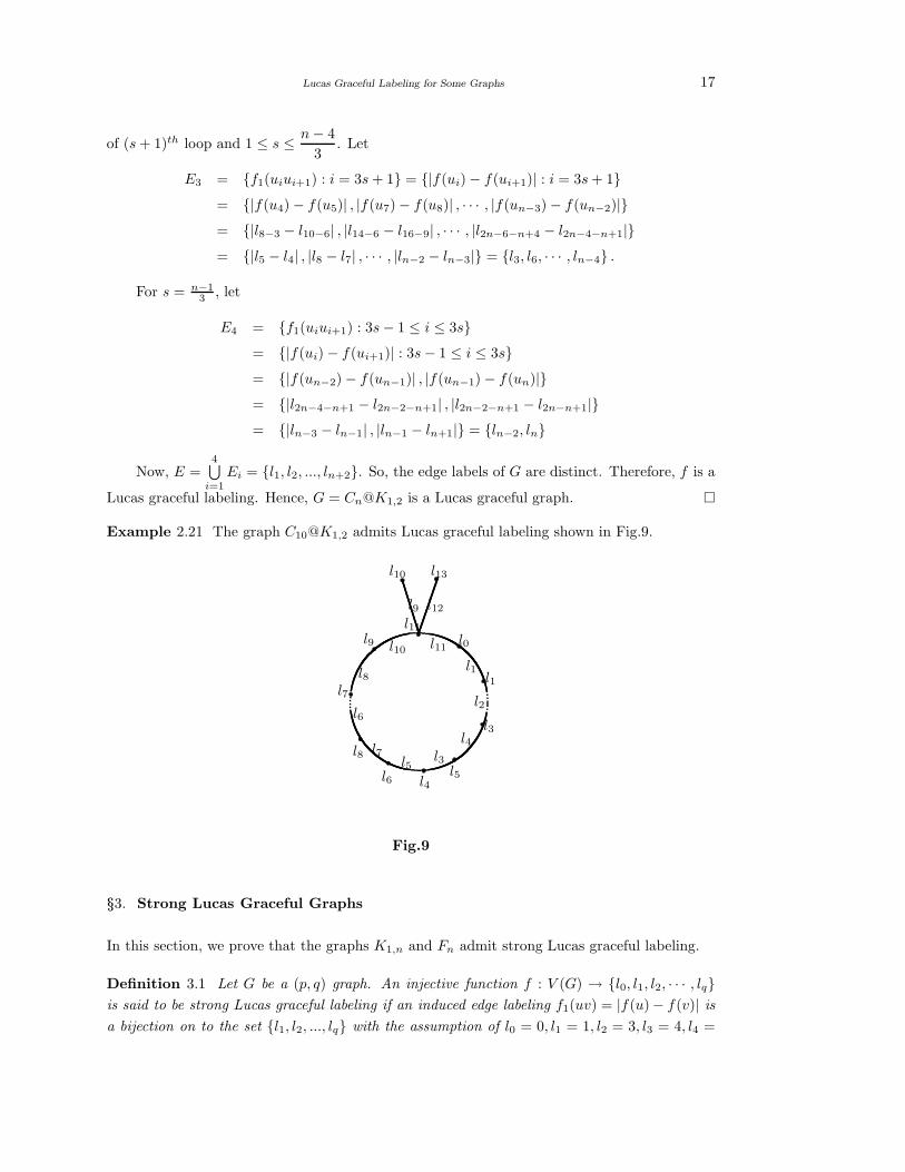
Theorem 2.20 The graph Cn@K1,2 is a Lucas graceful graph if n ≡ 1(mod 3).
Proof Let G = Cn@K1,2 with V (G) = ui : 1 ≤ i ≤ n ∪ v1, v2, E(G) = uiui+1 :
1 ≤ i ≤ n − 1∪unu1, unvn, unv2. So, |V (G)| = n+2 and |E(G)| = n+2. Define f : V (G) →l0, l1, l2, ..., la , a ǫ N by f(u1) = 0, f(v1) = ln, f(v2) = ln+3; f(ui) = l2i−3s, 3s − 1 ≤ i ≤3s + 1 for s = 1, 2, ...,
n − 4
3and f(ui) = l2i−3s, 3s − 1 ≤ i ≤ 3s for s =
n − 1
3. We claim that
the edge labels are distinct. Let
E1 = f1 (u1u2) , f1(unv1), f1(unv2), f1(unu1)= |f(u1) − f(u2)| , |f(un) − f(v1)| , |f(un) − f(v2)| , |f(un) − f(v1)|= |l0 − l1| , |ln+1 − ln| , |ln+1 − ln+3| , |ln+1 − l0|= l1, ln−1, ln+2, ln+1 ,
E2 =
n−4
3⋃
s=1
f1(uiui+1) : 3s − 1 ≤ i ≤ 3s
=
n−4
3⋃
s=1
|f(ui) − f(ui+1)| : 3s − 1 ≤ i ≤ 3s
= |f(u2) − f(u3)| , |f(u3) − f(u4)|⋃
|f(u5) − f(u6)| , |f(u6) − f(u7)|⋃
· · ·⋃
|f(un−5) − f(un−4)| , |f(un−4) − f(un−3)|
= |l1 − l3| , |l3 − l5|⋃
|l4 − l6| , |l6 − l8|⋃
· · ·⋃
|ln−6 − ln−4| , |ln−5 − ln−2|
= l2, l4⋃
l5, l7⋃
· · ·⋃
ln−5, ln−3 = l2, l4, l5, l7, · · · , ln−5, ln−3
We determine the edge labeling between the end vertex of sth loop and the starting vertex
Lucas Graceful Labeling for Some Graphs 17
of (s + 1)th loop and 1 ≤ s ≤ n − 4
3. Let
E3 = f1(uiui+1) : i = 3s + 1 = |f(ui) − f(ui+1)| : i = 3s + 1= |f(u4) − f(u5)| , |f(u7) − f(u8)| , · · · , |f(un−3) − f(un−2)|= |l8−3 − l10−6| , |l14−6 − l16−9| , · · · , |l2n−6−n+4 − l2n−4−n+1|= |l5 − l4| , |l8 − l7| , · · · , |ln−2 − ln−3| = l3, l6, · · · , ln−4 .
For s = n−13 , let
E4 = f1(uiui+1) : 3s − 1 ≤ i ≤ 3s= |f(ui) − f(ui+1)| : 3s − 1 ≤ i ≤ 3s= |f(un−2) − f(un−1)| , |f(un−1) − f(un)|= |l2n−4−n+1 − l2n−2−n+1| , |l2n−2−n+1 − l2n−n+1|= |ln−3 − ln−1| , |ln−1 − ln+1| = ln−2, ln
Now, E =4⋃
i=1
Ei = l1, l2, ..., ln+2. So, the edge labels of G are distinct. Therefore, f is a
Lucas graceful labeling. Hence, G = Cn@K1,2 is a Lucas graceful graph.
Example 2.21 The graph C10@K1,2 admits Lucas graceful labeling shown in Fig.9.
l0
l1
l3
l5l4l6
l8
l7
l9l11
l11
l1
l2
l4l3l5
l7
l6
l8
l10
l9
l10
l12
l13
Fig.9
§3. Strong Lucas Graceful Graphs
In this section, we prove that the graphs K1,n and Fn admit strong Lucas graceful labeling.
Definition 3.1 Let G be a (p, q) graph. An injective function f : V (G) → l0, l1, l2, · · · , lqis said to be strong Lucas graceful labeling if an induced edge labeling f1(uv) = |f(u)− f(v)| is
a bijection on to the set l1, l2, ..., lq with the assumption of l0 = 0, l1 = 1, l2 = 3, l3 = 4, l4 =

18 M.A.Perumal, S.Navaneethakrishnan and A.Nagarajan
7, l5 = 11, · · · ,. Then G is called strong Lucas graceful graph if it admits strong Lucas graceful
labeling.
Theorem 3.2 The graph K1,n is a strong Lucas graceful graph.
Proof Let G = K1,n and V = V1 ∪ V2 be the bipartition of K1,n with V1 = u1 and
V2 = u1, u2, ..., un. Then, |V (G)| = n+1 and |E(G)| = n. Define f : V (G) → l0, l1, l2, ..., lnby f(u0) = l0, f(u1) = l1, 1 ≤ i ≤ n. We claim that the edge labels are distinct. Notice that
E = f1(u0u1) : 1 ≤ i ≤ n = f(u0) − f(u1) : 1 ≤ i ≤ n= |f(u0) − f(u1)| , |f(u0) − f(u2)| , ..., |f(u0) − f(un)|= |l0 − l1| , |l0 − l2| , ..., |l0 − ln| = l1, l2, ..., ln
So, the edges of G receive the distinct labels. Therefore, f is a strong Lucas graceful labeling.
Hence, K1, n the path is a strong Lucas graceful graph.
Example 3.3 The graph K1,9 admits strong Lucas graceful labeling shown in Fig.10.
l0
l1l2 l3 l4 l5 l6 l7
l8l9
l1l2
l3l4 l5 l6 l7
l8l9
Fig.10
Definition 3.4([2]) Let u1, u2, ..., un, un+1 be the vertices of a path and u0 be a vertex which
is attached with u1, u2, ..., un, un+1. Then the resulting graph is called Fan and is denoted by
Fn = Pn + K1.
Theorem 3.5 The graph Fn = Pn + K1 is a Lucas graceful graph.
Proof Let G = Fn and u1, u2, ..., un, un+1 be the vertices of a path Pn with the central
vertex u0 joined with u1, u2, ..., un, un+1. Clearly, |V (G)| = n + 2 and |E(G)| = 2n + 1. Define
f : V (G) → l0, l1, l2, ..., l2n+1 by f(u0) = l0 and f(ui) = l2i−1, 1 ≤ i ≤ n + 1. We claim that
the edge labels are distinct.
Calculation shows that
E1 = f1(uiui+1) : 1 ≤ i ≤ n = |f(ui) − f(ui+1)| : 1 ≤ i ≤ n= |f(u1) − f(u2)|, |f(u2) − f(u3)|, ..., |f(un) − f(un+1)|= |l1 − l3|, |l3 − l5|, ..., |l2n−1 − l2n+1| = l2, l4, ..., l2n,

Lucas Graceful Labeling for Some Graphs 19
E2 = f1(u0ui) : 1 ≤ i ≤ n + 1 = |f(u0) − f(ui)| : 1 ≤ i ≤ n + 1= |f(u0) − f(u1)|, |f(u0) − f(u2)|, ..., |f(u0) − f(un+1)|= |l0 − l1|, |l0 − l3|, ..., |l0 − l2n+1| = l1, l3, ..., l2n+1.
Whence, E = E1 ∪ E2 = l1, l2, ..., l2n, l2n+1. Thus the edges of Fn receive the distinct labels.
Therefore, f is a Lucas graceful labeling. Consequently, Fn = Pn + K1 is a Lucas graceful
graph.
Example 3.6 The graph F7 = P7 + K1 admits Lucas graceful graph shown in Fig.11.
l1
l3
l5
l7
l9
l11
l13
l15
l0
l2
l4
l6
l8
l10
l12
l14
l1l3
l5
l7
l9
l11
l13l15
Fig.11
References
[1] David M.Burton, Elementary Number Theory( Sixth Edition), Tata McGraw - Hill Edition,
Tenth reprint 2010.
[2] G.A.Gallian, A Dynamic Survey of Graph Labeling, The Electronic Journal of Combina-
torics, 16(2009) # DS 6, pp 219.
[3] A.Rosa, On certain valuations of the vertices of a graph, Theory of Graphs International
Symposium, Rome, 1966.
[4] K.M.Kathiresan and S.Amutha, Fibonacci Graceful Graphs, Ph.D. thesis of Madurai Ka-
maraj University, October 2006.

International J.Math. Combin. Vol.1 (2011), 20-32
Sequences on Graphs with Symmetries
Linfan Mao
Chinese Academy of Mathematics and System Science, Beijing, 10080, P.R.China
Beijing Institute of Civil Engineering and Architecture, Beijing, 100044, P.R.China
E-mail: [email protected]
Abstract: An interesting symmetry on multiplication of numbers found by
Prof.Smarandache recently. By considering integers or elements in groups on graphs, we
extend this symmetry on graphs and find geometrical symmetries. For extending further,
Smarandache’s or combinatorial systems are also discussed in this paper, particularly, the
CC conjecture presented by myself six years ago, which enables one to construct more sym-
metrical systems in mathematical sciences.
Key Words: Smarandache sequence, labeling, Smarandache beauty, graph, group,
Smarandache system, combinatorial system, CC conjecture.
AMS(2010): 05C21, 05E18
§1. Sequences
Let Z+ be the set of non-negative integers and Γ a group. We consider sequences i(n)|n ∈ Z+and gn ∈ Γ|n ∈ Z+ in this paper. There are many interesting sequences appeared in literature.
For example, the sequences presented by Prof.Smarandache in references [2], [13] and [15]
following:
(1) Consecutive sequence
1, 12, 123, 1234, 12345, 123456, 1234567, 12345678, · · · ;
(2) Digital sequence
1, 11, 111, 1111, 11111, 11111, 1111111, 11111111, · · ·
(3) Circular sequence
1, 12, 21, 123, 231, 312, 1234, 2341, 3412, 4123, · · · ;
(4) Symmetric sequence
1, 11, 121, 1221, 12321, 123321, 1234321, 12344321, 123454321, 1234554321, · · · ;
(5) Divisor product sequence
1Reported at The 7th Conference on Number Theory and Smarandache’s Notion, Xian, P.R.China2Received December 18, 2010. Accepted February 18, 2011.

Sequences on Graphs with Symmetries 21
1, 2, 3, 8, 5, 36, 7, 64, 27, 100, 11, 1728, 13, 196, 225, 1024, 17, 5832, 19, · · · ;
(6) Cube-free sieve
2, 3, 4, 5, 6, 7, 9, 10, 11, 12, 13, 14, 15, 17, 18, 19, 20, 21, 22, 23, 25, 26, 28, 29, 30, · · · .
He also found three nice symmetries for these integer sequences recently.
First Symmetry
1 × 8 + 1 = 9
12 × 8 + 2 = 98
123 × 8 + 3 = 987
1234 × 8 + 4 = 9876
12345× 8 + 5 = 98765
123456× 8 + 6 = 987654
1234567× 8 + 7 = 9876543
12345678× 8 + 8 = 98765432
123456789× 8 + 9 = 987654321
Second Symmetry
1 × 9 + 2 = 11
12 × 9 + 3 = 111
123 × 9 + 4 = 1111
1234 × 9 + 5 = 11111
12345× 9 + 6 = 111111
123456× 9 + 7 = 1111111
1234567× 9 + 8 = 11111111
12345678× 9 + 9 = 111111111
123456789× 9 + 10 = 1111111111
Third Symmetry
1 × 1 = 1
11 × 11 = 121
111 × 111 = 12321
1111× 1111 = 1234321
11111× 11111 = 12345431

22 Linfan Mao
111111× 111111 = 12345654321
1111111× 1111111 = 1234567654321
11111111× 11111111 = 13456787654321
111111111× 111111111 = 12345678987654321
Notice that a Smarandache sequence is not closed under operation, but a group is, which
enables one to get symmetric figure in geometry. Whence, we also consider labelings on graphs
G by that elements of groups in this paper.
§2. Graphs with Labelings
A graph G is an ordered 3-tuple (V (G), E(G); I(G)), where V (G), E(G) are finite sets, called
vertex and edge set respectively, V (G) 6= ∅ and I(G) : E(G) → V (G) × V (G). Usually, the
cardinality |V (G)| is called the order and |E(G)| the size of a graph G.
A graph H = (V1, E1; I1) is a subgraph of a graph G = (V, E; I) if V1 ⊆ V , E1 ⊆ E and
I1 : E1 → V1 × V1, denoted by H ⊂ G.
Example 2.1 A graph G is shown in Fig.2.1, where, V (G) = v1, v2, v3, v4, E(G) =
e1, e2, e3, e4, e5, e6, e7, e8, e9, e10 and I(ei) = (vi, vi), 1 ≤ i ≤ 4; I(e5) = (v1, v2) = (v2, v1), I(e8)
= (v3, v4) = (v4, v3), I(e6) = I(e7) = (v2, v3) = (v3, v2), I(e8) = I(e9) = (v4, v1) = (v1, v4).
v1 v2
v3v4
e1 e2
e3e4
e5
e6e7
e8
e9 e10
Fig. 2.1
An automorphism of a graph G is a 1 − 1 mapping θ : V (G) → V (G) such that
θ(u, v) = (θ(u), θ(v)) ∈ E(G)
holds for ∀(u, v) ∈ E(G). All such automorphisms of G form a group under composition
operation, denoted by AutG. A graph G is vertex-transitive if AutG is transitive on V (G).
A graph family FP is the set of graphs whose each element possesses a graph property P .
Some well-known graph families are listed following.
Sequences on Graphs with Symmetries 23
Walk. A walk of a graph G is an alternating sequence of vertices and edges u1, e1, u2, e2,
· · · , en, un1with ei = (ui, ui+1) for 1 ≤ i ≤ n.
Path and Circuit. A walk such that all the vertices are distinct and a circuit or a cycle is
such a walk u1, e1, u2, e2, · · · , en, un1with u1 = un and distinct vertices. A graph G = (V, E; I)
is connected if there is a path connecting any two vertices in this graph.
Tree. A tree is a connected graph without cycles.
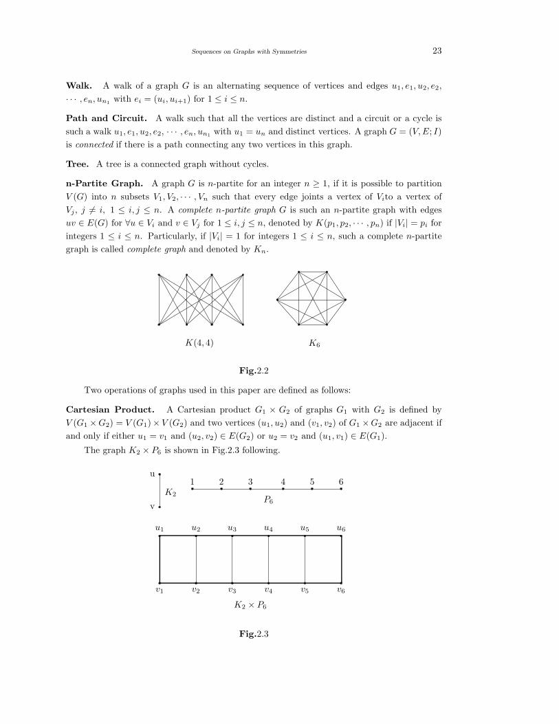
n-Partite Graph. A graph G is n-partite for an integer n ≥ 1, if it is possible to partition
V (G) into n subsets V1, V2, · · · , Vn such that every edge joints a vertex of Vito a vertex of
Vj , j 6= i, 1 ≤ i, j ≤ n. A complete n-partite graph G is such an n-partite graph with edges
uv ∈ E(G) for ∀u ∈ Vi and v ∈ Vj for 1 ≤ i, j ≤ n, denoted by K(p1, p2, · · · , pn) if |Vi| = pi for
integers 1 ≤ i ≤ n. Particularly, if |Vi| = 1 for integers 1 ≤ i ≤ n, such a complete n-partite
graph is called complete graph and denoted by Kn.
K(4, 4) K6
Fig.2.2
Two operations of graphs used in this paper are defined as follows:
Cartesian Product. A Cartesian product G1 × G2 of graphs G1 with G2 is defined by
V (G1 ×G2) = V (G1)× V (G2) and two vertices (u1, u2) and (v1, v2) of G1 ×G2 are adjacent if
and only if either u1 = v1 and (u2, v2) ∈ E(G2) or u2 = v2 and (u1, v1) ∈ E(G1).
The graph K2 × P6 is shown in Fig.2.3 following.
u
v
1 2 3 4 5K2
6
P6
K2 × P6
u1 u2 u3 u4 u5 u6
v1 v2 v3 v4 v5 v6
Fig.2.3
24 Linfan Mao
Union. The union G∪H of graphs G and H is a graph (V (G∪H), E(G∪H), I(G∪H)) with
V (G ∪ H) = V (G) ∪ V (H), E(G ∪ H) = E(G) ∪ E(H) and I(G ∪ H) = I(G) ∪ I(H).
Labeling. Now let G be a graph and N ⊂ Z+. A labeling of G is a mapping lG : V (G) ∪E(G) → N with each labeling on an edge (u, v) is induced by a ruler r(lG(u), lG(v)) with
additional conditions.
Classical Labeling Rulers. The following rulers are usually found in literature.
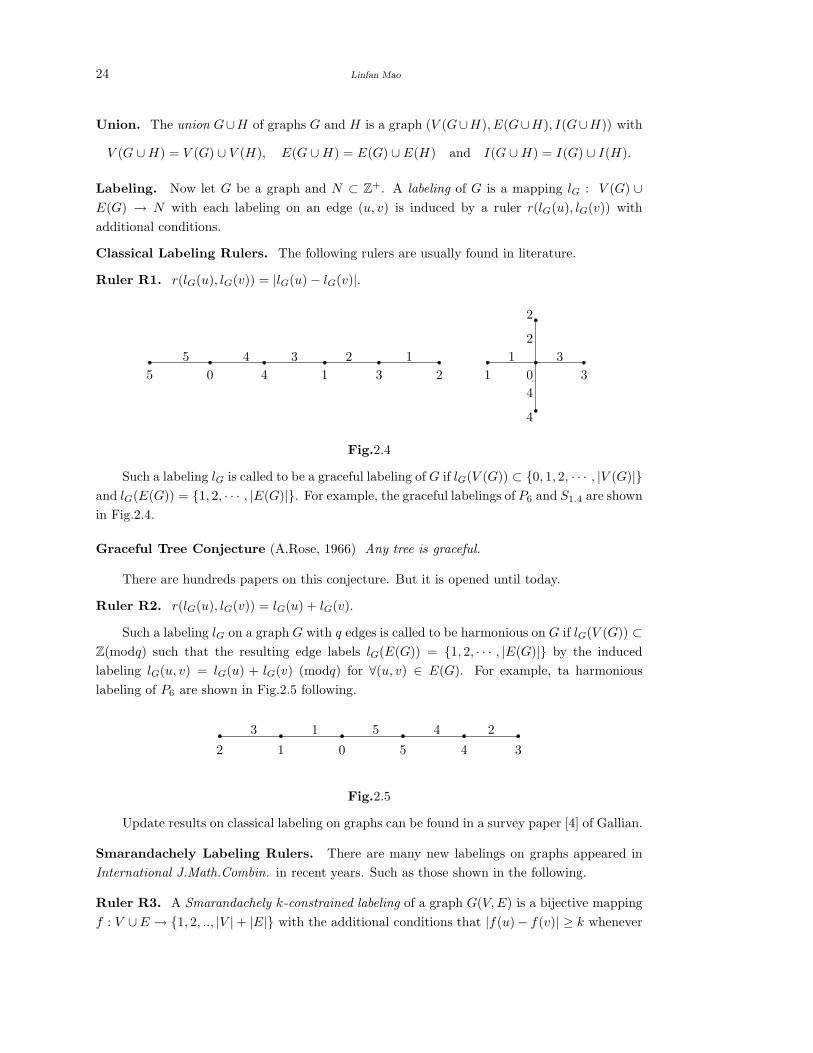
Ruler R1. r(lG(u), lG(v)) = |lG(u) − lG(v)|.
5 4 3 2 1
5 0 4 1 3 2 01
2
3
1
4
3
2
4
Fig.2.4
Such a labeling lG is called to be a graceful labeling of G if lG(V (G)) ⊂ 0, 1, 2, · · · , |V (G)|and lG(E(G)) = 1, 2, · · · , |E(G)|. For example, the graceful labelings of P6 and S1.4 are shown
in Fig.2.4.
Graceful Tree Conjecture (A.Rose, 1966) Any tree is graceful.
There are hundreds papers on this conjecture. But it is opened until today.
Ruler R2. r(lG(u), lG(v)) = lG(u) + lG(v).
Such a labeling lG on a graph G with q edges is called to be harmonious on G if lG(V (G)) ⊂Z(modq) such that the resulting edge labels lG(E(G)) = 1, 2, · · · , |E(G)| by the induced
labeling lG(u, v) = lG(u) + lG(v) (modq) for ∀(u, v) ∈ E(G). For example, ta harmonious
labeling of P6 are shown in Fig.2.5 following.
2 1 0 5 4 3
3 1 5 4 2
Fig.2.5
Update results on classical labeling on graphs can be found in a survey paper [4] of Gallian.
Smarandachely Labeling Rulers. There are many new labelings on graphs appeared in
International J.Math.Combin. in recent years. Such as those shown in the following.
Ruler R3. A Smarandachely k-constrained labeling of a graph G(V, E) is a bijective mapping
f : V ∪E → 1, 2, .., |V |+ |E| with the additional conditions that |f(u)− f(v)| ≥ k whenever

Sequences on Graphs with Symmetries 25
uv ∈ E, |f(u) − f(uv)| ≥ k and |f(uv) − f(vw)| ≥ k whenever u 6= w, for an integer k ≥ 2.
A graph G which admits a such labeling is called a Smarandachely k-constrained total graph,
abbreviated as k − CTG. An example for k = 5 on P7 is shown in Fig.2.6.
11 1 7 13 3 9 15 56 12 2 8 14 4 10
Fig.2.6
The minimum positive integer n such that the graph G ∪ Kn is a k − CTG is called k-
constrained number of the graph G and denoted by tk(G), the corresponding labeling is called
a minimum k-constrained total labeling of G. Update results for tk(G) in [3] and [12] are as
follows:
(1) t2(Pn)=
2 if n = 2,
1 if n = 3,
0 else.
(2) t2(Cn) = 0 if n ≥ 4 and t2(C3) = 2.
(3) t2(Kn) = 0 if n ≥ 4.
(4) t2(K(m, n))=
2 if n = 1 and m = 1,
1 if n = 1 and m ≥ 2,
0 else.
(5) tk(Pn)=
0 if k ≤ k0,
2(k − k0) − 1 if k > k0 and 2n ≡ 0(mod 3),
2(k − k0) if k > k0 and 2n ≡ 1 or 2(mod 3).
(6) tk(Cn) =
0 if k ≤ k0,
2(k − k0) if k > k0 and 2n ≡ 0 (mod 3),
3(k − k0) if k > k0 and 2n ≡ 1 or 2(mod 3),
where k0 = ⌊ 2n−13 ⌋. More results on tk(G) cam be found in references.
Ruler R4. Let G be a graph and f : V (G) → 1, 2, 3, · · · , |V | + |E(G)| be an injection.
For each edge e = uv and an integer m ≥ 2, the induced Smarandachely edge m-labeling f∗S is
defined by
f∗S(e) =
⌈f(u) + f(v)
m
⌉.
Then f is called a Smarandachely super m-mean labeling if f(V (G)) ∪ f∗(e) : e ∈ E(G) =
1, 2, 3, · · · , |V | + |E(G)|. A graph that admits a Smarandachely super mean m-labeling is
called Smarandachely super m-mean graph. Particularly, if m = 2, we know that
f∗(e) =
f(u) + f(v)
2if f(u) + f(v) is even;
f(u) + f(v) + 1
2if f(u) + f(v) is odd.

26 Linfan Mao
A Smarandache super 2-mean labeling on P 26 is shown in Fig.2.7.
1 2 3 5 7 8 9 11 13 14 15
4 6 10 12
Fig.2.7
Now we have know graphs Pn, Cn, Kn,K(2,n), (n ≥ 4), K(1, n) for 1 ≤ n ≤ 4, Cm × Pn
for n ≥ 1, m = 3, 5 have Smarandachely super 2-mean labeling. More results on Smarandachely
super m-mean labeling of graphs can be found in references in [1], [11], [17] and [18].
§3. Smarandache Sequences on Symmetric Graphs
Let lSG : V (G) → 1, 11, 111, 1111, 11111, 111111, 1111111, 11111111, 111111111 be a vertex la-
beling of a graph G with edge labeling lSG(u, v) induced by lSG(u)lSG(v) for (u, v) ∈ E(G) such that
lSG(E(G)) = 1, 121, 12321, 1234321, 123454321, 12345654321, 1234567654321, 123456787654321,
12345678987654321, i.e., lSG(V (G)∪E(G)) contains all numbers appeared in the Smarandachely
third symmetry. Denote all graphs with lSG labeling by L S . Then it is easily find a graph with
a labeling lSG in Fig.3.1 following.
1 111 11
111 1111111 1111
11111 11111111111 111111
1111111 111111111111111 11111111
111111111 111111111
1121
123211234321
12345432112345654321
1234567654321123456787654321
12345678987654321
Fig.3.1
Generally, we know the following result.
Theorem 3.1 Let G ∈ L S. Then G =n⋃
i=1
Hi for an integer n ≥ 9, where each Hi is a
connected graph. Furthermore, if G is vertex-transitive graph, then G = nH for an integer
n ≥ 9, where H is a vertex-transitive graph.
Proof Let C(i) be the connected component with a label i for a vertex u, where i ∈1, 11, 111, 1111, 11111, 111111, 1111111, 11111111, 111111111. Then all vertices v in C(i) must
be with label lSG(v) = i. Otherwise, if there is a vertex v with lSG(v) = j ∈ 1, 11, 111, 1111, 11111,
111111, 1111111, 11111111, 111111111\ i, let P (u, v) be a path connecting vertices u and v.

Sequences on Graphs with Symmetries 27
Then there must be an edge (x, y) on P (u, v) such that lSG(x) = i, lSG(y) = j. By definition,
i × j 6∈ lSG(E(G)), a contradiction. So there are at least 9 components in G.
Now if G is vertex-transitive, we are easily know that each connected component C(i) must
be vertex-transitive and all components are isomorphic.
The smallest graph in L Sv is the graph 9K2 shown in Fig.3.1. It should be noted that each
graph in L Sv is not connected. For finding a connected one, we construct a graph Qk following
on the digital sequence
1, 11, 111, 1111, 11111, · · · , 11 · · ·1︸ ︷︷ ︸k
.
by
V (Qk) = 1, 11, · · · , 11 · · ·1︸ ︷︷ ︸k
⋃
1′, 11′, · · · , 11 · · · 1′︸ ︷︷ ︸k
,
E(Qk) = (1, 11 · · ·1︸ ︷︷ ︸k
), (x, x′), (x, y)|x, y ∈ V (Q) differ in precisely one 1.
Now label x ∈ V (Q) by lG(x) = lG(x′) = x and (u, v) ∈ E(Q) by lG(u)lG(v). Then we have
the following result for the graph Qk.
Theorem 3.2 For any integer m ≥ 3, the graph Qm is a connected vertex-transitive graph of
order 2m with edge labels
lG(E(Q)) = 1, 11, 121, 1221, 12321, 123321, 1234321, 12344321, 12345431, · · ·,
i.e., the Smarandache symmetric sequence.
Proof Clearly, Qm is connected. We prove it is a vertex-transitive graph. For simplicity,
denote 11 · · · 1︸ ︷︷ ︸i
, 11 · · · 1′︸ ︷︷ ︸i
by i and i′, respectively. Then V (Qm) = 1, 2, · · · , m. We define an
operation + on V (Qk) by
k + l = 11 · · · 1︸ ︷︷ ︸k+l(modk)
and k′+ l
′= k + l
′, k
′′= k
for integers 1 ≤ k, l ≤ m. Then an element i naturally induces a mapping
i∗ : x → x + i, for x ∈ V (Qm).
It should be noted that i∗ is an automorphism of Qm because tuples x and y differ in precisely
one 1 if and only if x + i and y + i differ in precisely one 1 by definition. On the other hand,
the mapping τ : x → x′ for ∀x ∈ is clearly an automorphism of Qm. Whence,
G = 〈 τ, i∗ | 1 ≤ i ≤ m〉 AutQm,
which acts transitively on V (Q) because (y − x)∗(x) = y for x, y ∈ V (Qm) and τ : x → x′.
Calculation shows easily that
lG(E(Qm)) = 1, 11, 121, 1221, 12321, 123321, 1234321, 12344321, 12345431, · · ·,
28 Linfan Mao
i.e., the Smarandache symmetric sequence. This completes the proof.
By the definition of graph Qm, w consequently get the following result by Theorem 3.2.
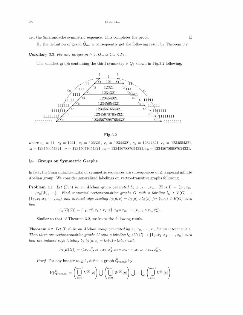
Corollary 3.3 For any integer m ≥ 3, Qm ≃ Cm × P2.
The smallest graph containing the third symmetry is Q9 shown in Fig.3.2 following,
c1 c111 11
111 111
1111 1111
11111 11111
111111 111111
1111111 1111111
11111111 11111111
111111111 111111111
1
121
12321
1234321
123454321
12345654321
1234567654321
123456787654321
12345678987654321
c2
11
c2
c3 c3
c4 c4
c5 c5
c6 c6
c7 c7
c8 c8
c9 c9
Fig.3.2
where c1 = 11, c2 = 1221, c3 = 123321, c4 = 12344321, c5 = 12344321, c5 = 1234554321,
c6 = 123456654321, c7 = 12345677654321, c8 = 1234567887654321, c9 = 123456789987654321.
§4. Groups on Symmetric Graphs
In fact, the Smarandache digital or symmetric sequences are subsequences of Z, a special infinite
Abelian group. We consider generalized labelings on vertex-transitive graphs following.
Problem 4.1 Let (Γ; ) be an Abelian group generated by x1, · · · , xn. Thus Γ = 〈x1, x2,
· · · , xn|W1, · · · 〉. Find connected vertex-transitive graphs G with a labeling lG : V (G) →1Γ, x1, x2, · · · , xn and induced edge labeling lG(u, v) = lG(u) lG(v) for (u, v) ∈ E(G) such
that
lG(E(G)) = 1Γ, x21, x1 x2, x
22, x2 x3, · · · , xn−1 xn, x2
n.
Similar to that of Theorem 3.2, we know the following result.
Theorem 4.2 Let (Γ; ) be an Abelian group generated by x1, x2, · · · , xn for an integer n ≥ 1.
Then there are vertex-transitive graphs G with a labeling lG : V (G) → 1Γ, x1, x2, · · · , xn such
that the induced edge labeling by lG(u, v) = lG(u) lG(v) with
lG(E(G)) = 1Γ, x21, x1 x2, x
22, x2 x3, · · · , xn−1 xn, x2
n.
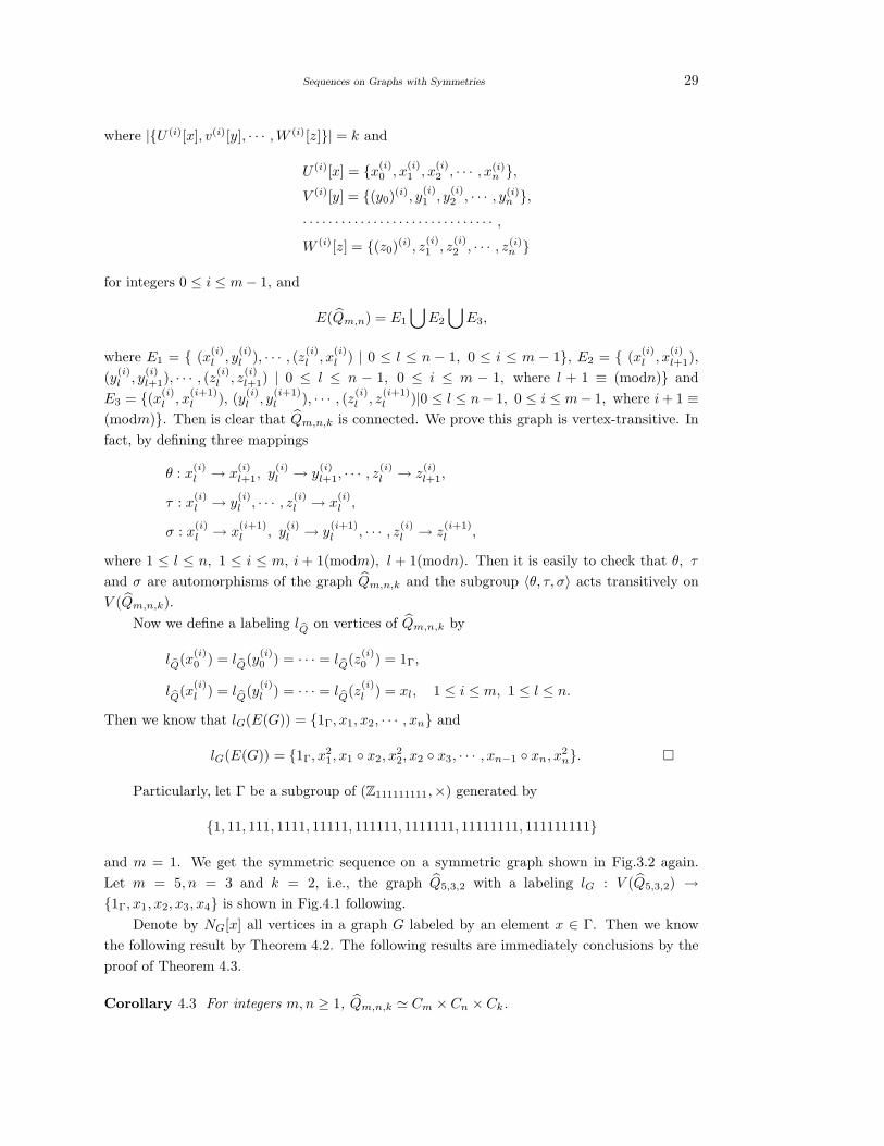
Proof For any integer m ≥ 1, define a graph Qm,n,k by
V (Qm,n,k) =
(m−1⋃
i=0
U (i)[x]
)⋃(
m−1⋃
i=0
W (i)[y]
)⋃
· · ·⋃(
m−1⋃
i=0
U (i)[z]
)
Sequences on Graphs with Symmetries 29
where |U (i)[x], v(i)[y], · · · , W (i)[z]| = k and
U (i)[x] = x(i)0 , x
(i)1 , x
(i)2 , · · · , x(i)
n ,V (i)[y] = (y0)
(i), y(i)1 , y
(i)2 , · · · , y(i)
n ,· · · · · · · · · · · · · · · · · · · · · · · · · · · · · · ,
W (i)[z] = (z0)(i), z
(i)1 , z
(i)2 , · · · , z(i)
n
for integers 0 ≤ i ≤ m − 1, and
E(Qm,n) = E1
⋃E2
⋃E3,
where E1 = (x(i)l , y
(i)l ), · · · , (z
(i)l , x
(i)l ) | 0 ≤ l ≤ n − 1, 0 ≤ i ≤ m − 1, E2 = (x
(i)l , x
(i)l+1),
(y(i)l , y
(i)l+1), · · · , (z
(i)l , z
(i)l+1) | 0 ≤ l ≤ n − 1, 0 ≤ i ≤ m − 1, where l + 1 ≡ (modn) and
E3 = (x(i)l , x
(i+1)l ), (y
(i)l , y
(i+1)l ), · · · , (z
(i)l , z
(i+1)l )|0 ≤ l ≤ n− 1, 0 ≤ i ≤ m− 1, where i + 1 ≡
(modm). Then is clear that Qm,n,k is connected. We prove this graph is vertex-transitive. In
fact, by defining three mappings
θ : x(i)l → x
(i)l+1, y
(i)l → y
(i)l+1, · · · , z
(i)l → z
(i)l+1,
τ : x(i)l → y
(i)l , · · · , z
(i)l → x
(i)l ,
σ : x(i)l → x
(i+1)l , y
(i)l → y
(i+1)l , · · · , z
(i)l → z
(i+1)l ,
where 1 ≤ l ≤ n, 1 ≤ i ≤ m, i + 1(modm), l + 1(modn). Then it is easily to check that θ, τ
and σ are automorphisms of the graph Qm,n,k and the subgroup 〈θ, τ, σ〉 acts transitively on
V (Qm,n,k).
Now we define a labeling lQ on vertices of Qm,n,k by
lQ(x(i)0 ) = lQ(y
(i)0 ) = · · · = lQ(z
(i)0 ) = 1Γ,
lQ(x(i)l ) = lQ(y
(i)l ) = · · · = lQ(z
(i)l ) = xl, 1 ≤ i ≤ m, 1 ≤ l ≤ n.
Then we know that lG(E(G)) = 1Γ, x1, x2, · · · , xn and
lG(E(G)) = 1Γ, x21, x1 x2, x
22, x2 x3, · · · , xn−1 xn, x2
n.
Particularly, let Γ be a subgroup of (Z111111111,×) generated by
1, 11, 111, 1111, 11111, 111111, 1111111, 11111111, 111111111
and m = 1. We get the symmetric sequence on a symmetric graph shown in Fig.3.2 again.
Let m = 5, n = 3 and k = 2, i.e., the graph Q5,3,2 with a labeling lG : V (Q5,3,2) →1Γ, x1, x2, x3, x4 is shown in Fig.4.1 following.
Denote by NG[x] all vertices in a graph G labeled by an element x ∈ Γ. Then we know
the following result by Theorem 4.2. The following results are immediately conclusions by the
proof of Theorem 4.3.
Corollary 4.3 For integers m, n ≥ 1, Qm,n,k ≃ Cm × Cn × Ck.

30 Linfan Mao
Corollary 4.4 |NQm,n,k[x]| = mk for ∀x ∈ 1Γ, x1, · · · , xn and integers m, n, k ≥ 1.
1Γ
1Γ
1Γ
1Γ
1Γ
1Γ
x1
x1
x1
x1
x1
x1
x2
x2
x2
x2
x2
x2
x3
x3
x3
x3
x3
x3
x4
x4
x4
x4
x4
x4
Fig.4.1
§5. Speculation
It should be noted that the essence we have done is a combinatorial notion, i.e., combining math-
ematical systems on that of graphs. Recently, Sridevi et al. consider the Fibonacci sequence
on graphs in [16]. Let G be a graph and F0, F1, F2, · · · , Fq, · · · be the Fibonacci sequence,
where Fq is the qth Fibonacci number. An injective labeling lG : V (G) → F0, F1, F2, · · · , Fqis called to be super Fibonacci graceful if the induced edge labeling by lG(u, v) = |lG(u)− lG(v)|is a bijection onto the set F1, F2, · · · , Fq with initial values F0 = F1 = 1. They proved a
few graphs, such as those of Cn ⊕ Pm, Cn ⊕ K1,m have super Fibonacci labelings in [18]. For
example, a super Fibonacci labeling of C6 ⊕ P6 is shown in Fig.5.1.
F0
F7F9
F11
F10 F12
F6 F4 F5 F3 F1 F2
F1F2F4F3F5F6
F7
F8
F10
F9
F11
F12
Fig.5.1
All of these are not just one mathematical system. In fact, they are applications of Smaran-
dache multi-space and CC conjecture for developing modern mathematics, which appeals one
to find combinatorial structures for classical mathematical systems, i.e., the following problem.
Problem 5.1 Construct classical mathematical systems combinatorially and characterize them.

Sequences on Graphs with Symmetries 31
For example, classical algebraic systems, such as those of groups, rings and fields by combina-
torial principle.
Generally, a Smarandache multi-space is defined by the following.
Definition 5.2([6],[14]) For an integer m ≥ 2, let (Σ1;R1), (Σ2;R2), · · · , (Σm;Rm) be m
mathematical systems different two by two. A Smarandache multi-space is a pair (Σ; R) with
Σ =
m⋃
i=1
Σi, and R =
m⋃
i=1
Ri.
Definition 5.3([10]) A combinatorial system CG is a union of mathematical systems (Σ1;R1),
(Σ2;R2), · · · , (Σm;Rm) for an integer m, i.e.,
CG = (
m⋃
i=1
Σi;
m⋃
i=1
Ri)
with an underlying connected graph structure G, where
V (G) = Σ1, Σ2, · · · , Σm, E(G) = (Σi, Σj) | Σi
⋂Σj 6= ∅, 1 ≤ i, j ≤ m.
We have known a few Smarandache multi-spaces in classical mathematics. For examples,
these rings and fields are group multi-space, and topological groups, topological rings and
topological fields are typical multi-space are both groups, rings, or fields and topological spaces.
Usually, if m ≥ 3, a Smarandache multi-space must be underlying a combinatorial structure G.
Whence, it becomes a combinatorial space in that case. I have presented the CC conjecture
for developing modern mathematical science in 2005 [5], then formally reported it at The 2th
Conference on Graph Theory and Combinatorics of China (2006, Tianjing, China)([7]-[10]).
CC Conjecture(Mao, 2005) Any mathematical system (Σ;R) is a combinatorial system
CG(lij , 1 ≤ i, j ≤ m).
This conjecture is not just an open problem, but more likes a deeply thought, which opens
a entirely way for advancing the modern mathematical sciences. In fact, it indeed means a
combinatorial notion on mathematical objects following for researchers.
(1) There is a combinatorial structure and finite rules for a classical mathematical system,
which means one can make combinatorialization for all classical mathematical subjects.
(2) One can generalizes a classical mathematical system by this combinatorial notion such
that it is a particular case in this generalization.
(3) One can make one combination of different branches in mathematics and find new
results after then.
(4) One can understand our WORLD by this combinatorial notion, establish combinatorial
models for it and then find its behavior, for example,
what is true colors of the Universe, for instance its dimension?
and · · · . For its application to geometry and physics, the reader is refereed to references [5]-[10],
particularly, the book [10] of mine.
32 Linfan Mao
References
[1] S.Avadayappan and R.Vasuki, New families of mean graphs, International J.Math. Com-
bin. Vol.2 (2010), 68-80.
[2] D.Deleanu, A Dictionary of Smarandache Mathematics, Buxton University Press, London
& New York, 2006.
[3] P.Devadas Rao, B. Sooryanarayana and M. Jayalakshmi, Smarandachely k-Constrained
Number of Paths and Cycles, International J.Math. Combin. Vol.3 (2009), 48-60.
[4] J.A.Gallian, A dynamic survey of graph labeling, The Electronic J.Combinatorics, # DS6,
16(2009), 1-219.
[5] Linfan Mao, Automorphism Groups of Maps, Surfaces and Smarandache Geometries, Amer-
ican Research Press, 2005.
[6] Linfan Mao, Smarandache Multi-Space Theory, Hexis, Phoenix, USA, 2006.
[7] Linfan Mao, Selected Papers on Mathematical Combinatorics, World Academic Union,
2006.
[8] Linfan Mao, Combinatorial speculation and combinatorial conjecture for mathematics,
International J.Math. Combin. Vol.1(2007), No.1, 1-19.
[9] Linfan Mao, An introduction to Smarandache multi-spaces and mathematical combina-
torics, Scientia Magna, Vol.3, No.1(2007), 54-80.
[10] Linfan Mao, Combinatorial Geometry with Applications to Field Theory, InforQuest, USA,
2009.
[11] A.Nagarajan, A.Nellai Murugan and S.Navaneetha Krishnan, On near mean graphs, In-
ternational J.Math. Combin. Vol.4 (2010), 94-99.
[12] ShreedharK, B.Sooryanarayana and RaghunathP, Smarandachely k-Constrained labeling
of Graphs, International J.Math. Combin. Vol.1 (2009), 50-60.
[13] F.Smarandache, Only Problems, Not Solutions! Xiquan Publishing House, Chicago, 1990.
[14] F.Smarandache, Mixed noneuclidean geometries, eprint arXiv: math/0010119, 10/2000.
[15] F.Smarandache, Sequences of Numbers Involved in Unsolved Problems, Hexis, Phoenix,
Arizona, 2006.
[16] R.Sridevi, S.Navaneethakrishnan and K.Nagarajan, Super Fibonacci graceful labeling, In-
ternational J.Math. Combin. Vol.3(2010), 22-40.
[17] R. Vasuki and A.Nagarajan, Some results on super mean graphs, International J.Math.
Combin. Vol.3 (2009), 82-96.
[18] R. Vasuki and A.. Nagarajan, Some results on super mean graphs, International J.Math.
Combin. Vol.3 (2009), 82-96.

International J.Math. Combin. Vol.1 (2011), 33-48
Supermagic Coverings of Some Simple Graphs
P.Jeyanthi
Department of Mathematics, Govindammal Aditanar College for Women, Tiruchendur-628 215
P.Selvagopal
Department of Mathematics,Cape Institute of Technology,
Levengipuram, Tirunelveli Dist.-627 114
E-mail: [email protected], [email protected]
Abstract: A simple graph G = (V, E) admits an H-covering if every edge in E belongs to
a subgraph of G isomorphic to H . We say that G is Smarandachely pair s, l H-magic if
there is a total labeling f : V ∪ E → 1, 2, 3, · · · , |V | + |E| such that there are subgraphs
H1 = (V1, E1) and H2 = (V2, E2) of G isomorphic to H , the sum∑
v∈V1
f(v) +∑
e∈E1
f(e) = s
and∑
v∈V2
f(v)+∑
e∈E2
f(e) = l. Particularly, if s = l, such a Smarandachely pair s, l H-magic
is called H-magic and if f(V ) = 1, 2, · · · , |V |, G is said to be a H-supermagic. In this
paper we show that edge amalgamation of a finite collection of graphs isomorphic to any
2-connected simple graph H is H-supermagic.
Key Words: H-covering, Smarandachely pair s, l H-magic, H-magic, H-supermagic.
AMS(2010): 05C78
§1. Introduction
The concept of H-magic graphs was introduced in [3]. An edge-covering of a graph G is a family
of different subgraphs H1, H2, . . . , Hk such that each edge of E belongs to at least one of the
subgraphs Hi, 1 ≤ i ≤ k. Then, it is said that G admits an (H1, H2, . . . , Hk) - edge covering.
If every Hi is isomorphic to a given graph H , then we say that G admits an H-covering.
Suppose that G = (V, E) admits an H-covering. We say that a bijective function f :
V ∪E → 1, 2, 3, · · · , |V |+ |E| is an H-magic labeling of G if there is a positive integer m(f),
which we call magic sum, such that for each subgraph H ′ = (V ′, E′) of G isomorphic to H ,
we have,f(H ′) =∑
v∈V ′ f(v) +∑
e∈E′ f(e) = m(f). In this case we say that the graph G
is H-magic. When f(V ) = 1, 2, |V |, we say that G is H-supermagic and we denote its
supermagic-sum by s(f).
We use the following notations. For any two integers n < m, we denote by [n, m], the set
of all consecutive integers from n to m. For any set I ⊂ N we write,∑
I =∑x∈I
x and for any
integers k, I+k = x+k : x ∈ I. Thus k+[n, m] is the set of consecutive integers from k+n to
1Received December 29, 2010. Accepted February 20, 2011.

34 P.Jeyanthi and P.Selvagopal
k+m. It can be easily verified that∑
(I+k) =∑
I+k|I|. If P = X1, X2, · · · , Xn is a partition
of a set X of integers with the same cardinality then we say P is an n-equipartition of X . Also
we denote the set of subsets sums of the parts of P by∑
P = ∑X1,∑
X2, · · · ,∑
Xn.Finally,
given a graph G = (V, E) and a total labeling f on it we denote by f(G) =∑
f(V ) +∑
f(E).
§2. Preliminary Results
In this section we give some lemmas which are used to prove the main results in Section 3.
Lemma 2.1 Let h and k be two positive integers and h is odd. Then there exists a k-
equipartition P = X1, X2, · · · , Xk of X = [1, hk] such that∑
Xr =(h − 1)(hk + k + 1)
2+ r
for 1 ≤ r ≤ k. Thus,∑
P is a set of consecutive integers given by∑
P =(h − 1)(hk + k + 1)
2+
[1, k].
Proof Let us arrange the set of integers X = [1, hk] in a h × k matrix A as given below.
A =
1 2 · · · k − 1 k
n + 1 n + 2 · · · 2k − 1 2k
2n + 1 2n + 2 · · · 3k − 1 3k...
......
......
(h − 1)k + 1 (h − 1)k + 2 · · · hk − 1 hk
h×k
That is, A = (ai,j)h×k where ai,j = (i − 1)k + j for 1 ≤ i ≤ h and 1 ≤ j ≤ k. For 1 ≤ r ≤ k,
define Xr = ai,r/1 ≤ i ≤ h+12 ∪ ai,k−r+1/
h+32 ≤ i ≤ h. Then
∑Xr =
h+1
2∑
i=1
ai,r +
h∑
i= h+3
2
ai,k−r+1
=
h+1
2∑
i=1
(i − 1)k + r
h∑
i= h+3
2
(i − 1)k + k − r + 1
=h2k + h − k − 1
2+ r
=(h − 1)(hk + k + 1)
2+ r for 1 ≤ r ≤ k.
Hence,∑
P =(h − 1)(hk + k + 1)
2+ [1, k].
Example 2.2 Let h = 9, k = 6 and X = [1, 54]. Then the partition subsets are X1 =
1, 7, 13, 19, 25, 36, 42, 48, 54, X2 = 2, 8, 14, 20, 26, 35, 41, 47, 53, X3 = 3, 9, 15, 21, 27, 34,
40, 46, 52, X4 = 4, 10, 16, 22, 28, 33, 39, 45, 51, X5 = 5, 11, 17, 23, 29, 32, 38, 44, 50 and X6 =
6, 12, 18, 24, 30, 31, 37, 43, 49. ∑Xr =(h − 1)(hk + k + 1)
2+ r = 244 + r for 1 ≤ r ≤ 6.

Supermagic Coverings of Some Simple Graphs 35
Lemma 2.3 Let h and k be two positive integers such that h is even and k ≥ 3 is odd.
Then there exists a k-equipartition P = X1, X2, · · · , Xk of X = [1, hk] such that∑
Xr =(h − 1)(hk + k + 1)
2+ r for 1 ≤ r ≤ k. Thus,
∑P is a set of consecutive integers given by
∑P =
(h − 1)(hk + k + 1)
2+ [1, k].
Proof Let us arrange the set of integers X = 1, 2, 3, · · · , hkin a h× k matrix A as given
below.
A =
1 2 · · · k − 1 k
n + 1 n + 2 · · · 2k − 1 2k
2n + 1 2n + 2 · · · 3k − 1 3k...
......
......
(h − 1)k + 1 (h − 1)k + 2 · · · hk − 1 hk
h×k
That is, A = (ai,j)h×k where ai,j = (i − 1)k + j for 1 ≤ i ≤ h and 1 ≤ j ≤ k. For 1 ≤ r ≤ k,
define Yr = ai,r/1 ≤ i ≤ h
2 ∪ ai,k−r+1/
h
2+ 1 ≤ i ≤ h − 1. Then
∑Yr =
h2∑
i=1
ai,r +
h−1∑
i= h2+1
ai,k−r+1
=
h2∑
i=1
(i − 1)k + r +
h−1∑
i= h2+1
(i − 1)k + k − r + 1
=k(h − 1)2 + h − k − 2
2+ r
For 1 ≤ r ≤ k, define Xr = Yσ(r) ∪ (h − 1)k + π(r), where σ and π denote the per-
mutations of 1, 2, · · · , k given by σ(r) =
k − 2r + 1
2for 1 ≤ r ≤ k − 1
23k − 2r + 1
2for
k + 1
2≤ r ≤ k
and π(r) =
2r for 1 ≤ r ≤ k − 1
2
2r − k fork + 1
2≤ r ≤ k
. Then
∑Xr =
∑Yσ(r) + (h − 1)k + π(r)
=k(h − 1)2 + h − k − 2
2+ σ(r) + (h − 1)k + π(r)
∑Xr =
k(h − 1)2 + h − k − 2
2+
k − 2r + 1
2+ (h − 1)k + 2r for 1 ≤ r ≤ k−1
2
k(h − 1)2 + h − k − 2
2+
3k − 2r + 1
2+ (h − 1)k + 2r − k for k+1
2 ≤ r ≤ k. On
simplification we get∑
Xr =(h − 1)(hk + k + 1)
2+ r for 1 ≤ r ≤ k. Hence,
∑P =
(h − 1)(hk + k + 1)
2+ [1, k].

36 P.Jeyanthi and P.Selvagopal
Example 2.4 Let h = 6,k = 5 and X = [1, 30]. Y1 = 1, 6, 11, 20, 25, Y2 = 2, 7, 12, 19, 24,Y3 = 3, 8, 13, 18, 23, Y4 = 4, 9, 14, 17, 22and Y5 = 5, 10, 15, 16, 21. By definition the parti-
tion subsets are, Xr = Yσ(r) ∪ (h − 1)k + π(r) for 1 ≤ r ≤ 5. X1 = 2, 7, 12, 19, 24, 27, X2 =
1, 6, 11, 20, 25, 29, X3 = 5, 10, 15, 16, 21, 26X4 = 4, 9, 14, 17, 22, 28X5 = 3, 8, 13, 18, 23, 30,Now,
∑Xr =
(h − 1)(hk + k + 1)
2+ r = 90 + r for 1 ≤ r ≤ 5.
Lemma 2.5 If h is even, then there exists a k-equipartition P = X1, X2, · · · , Xk of X =
[1, hk] such that∑
Xr =h(hk + 1)
2for 1 ≤ r ≤ k. Thus, the subsets sum are equal and is
equal toh(hk + 1)
2.
Proof Let us arrange the set of integers X = 1, 2, 3, · · · , hkin a h× k matrix A as given
below.
A =
1 2 · · · k − 1 k
n + 1 n + 2 · · · 2k − 1 2k
2n + 1 2n + 2 · · · 3k − 1 3k...
......
......
(h − 1)k + 1 (h − 1)k + 2 · · · hk − 1 hk
h×k
That is, A = (ai,j)h×k where ai,j = (i − 1)k + j for 1 ≤ i ≤ h and 1 ≤ j ≤ k. For 1 ≤ r ≤ k,
define Xr = ai,r/1 ≤ i ≤ h2 ∪ ai,k−r+1/
h2 + 1 ≤ i ≤ h − 1. Then
∑Xr =
h2∑
i=1
ai,r +
h∑
i= h2+1
ai,k−r+1
=
h2∑
i=1
(i − 1)k + r +
h∑
i= h2+1
(i − 1)k + k − r + 1 =h(hk + 1)
2
Thus, the subsets sum are equal and is equal toh(hk + 1)
2.
Example 2.6 Let h = 6, k = 5 and X = [1, 30]. Then the partition subsets are X1 =
1, 6, 11, 20, 25, 30, X2 = 2, 7, 12, 19, 24, 29, X3 = 3, 8, 13, 18, 23, 28, X4 = 4, 9, 14, 17,
22, 27 and X5 = 5, 10, 15, 16, 21, 26. Now,∑
Xr =h(hk + 1)
2= 93 for 1 ≤ r ≤ 5.
Lemma 2.7 Let h and k be two even positive integers and h ≥ 4. If X = [1, hk+1]−k
2+1 ,
there exists a k-equipartition P = X1, X2, · · · , Xk of X such that∑
Xr =h2k + 3h − k − 2
2+r
for 1 ≤ r ≤ k. Thus∑
P is a set of consecutive integersh2k + 3h − k − 2
2+ [1, k].
Proof First we prove this lemma for h = 2 and we generalize for any even integer h ≥ 4.
Case 1: h = 2.
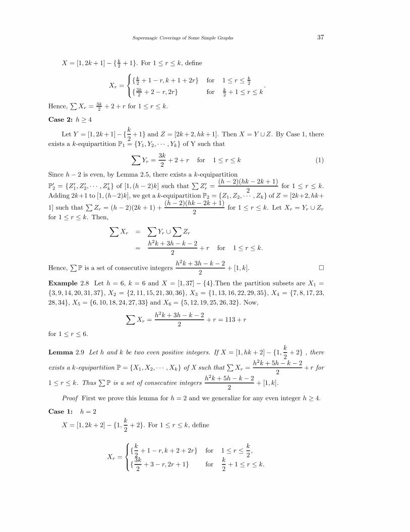
Supermagic Coverings of Some Simple Graphs 37
X = [1, 2k + 1] − k2 + 1. For 1 ≤ r ≤ k, define
Xr =
k
2 + 1 − r, k + 1 + 2r for 1 ≤ r ≤ k2
3k2 + 2 − r, 2r for k
2 + 1 ≤ r ≤ k.
Hence,∑
Xr = 3k2 + 2 + r for 1 ≤ r ≤ k.
Case 2: h ≥ 4
Let Y = [1, 2k + 1]−k
2+ 1 and Z = [2k + 2, hk+ 1]. Then X = Y ∪Z. By Case 1, there
exists a k-equipartition P1 = Y1, Y2, · · · , Yk of Y such that
∑Yr =
3k
2+ 2 + r for 1 ≤ r ≤ k (1)
Since h − 2 is even, by Lemma 2.5, there exists a k-equipartition
P′2 = Z ′
1, Z′2, · · · , Z ′
k of [1, (h − 2)k] such that∑
Z ′r =
(h − 2)(hk − 2k + 1)
2for 1 ≤ r ≤ k.
Adding 2k+1 to [1, (h−2)k], we get a k-equipartition P2 = Z1, Z2, · · · , Zk of Z = [2k+2, hk+
1] such that∑
Zr = (h − 2)(2k + 1) +(h − 2)(hk − 2k + 1)
2for 1 ≤ r ≤ k. Let Xr = Yr ∪ Zr
for 1 ≤ r ≤ k. Then,∑
Xr =∑
Yr ∪∑
Zr
=h2k + 3h − k − 2
2+ r for 1 ≤ r ≤ k.
Hence,∑
P is a set of consecutive integersh2k + 3h − k − 2
2+ [1, k].
Example 2.8 Let h = 6, k = 6 and X = [1, 37] − 4.Then the partition subsets are X1 =
3, 9, 14, 20, 31, 37, X2 = 2, 11, 15, 21, 30, 36, X3 = 1, 13, 16, 22, 29, 35, X4 = 7, 8, 17, 23,
28, 34, X5 = 6, 10, 18, 24, 27, 33 and X6 = 5, 12, 19, 25, 26, 32. Now,
∑Xr =
h2k + 3h − k − 2
2+ r = 113 + r
for 1 ≤ r ≤ 6.
Lemma 2.9 Let h and k be two even positive integers. If X = [1, hk + 2] − 1,k
2+ 2 , there
exists a k-equipartition P = X1, X2, · · · , Xk of X such that∑
Xr =h2k + 5h− k − 2
2+ r for
1 ≤ r ≤ k. Thus∑
P is a set of consecutive integersh2k + 5h − k − 2
2+ [1, k].
Proof First we prove this lemma for h = 2 and we generalize for any even integer h ≥ 4.
Case 1: h = 2
X = [1, 2k + 2] − 1,k
2+ 2. For 1 ≤ r ≤ k, define
Xr =
k
2+ 1 − r, k + 2 + 2r for 1 ≤ r ≤ k
2,
3k
2+ 3 − r, 2r + 1 for
k
2+ 1 ≤ r ≤ k.

38 P.Jeyanthi and P.Selvagopal
Hence,∑
Xr =3k
2+ 4 + r for 1 ≤ r ≤ k.
Case 2: h ≥ 4
Let Y = [1, 2k + 2] − 1,k
2+ 2 and Z = [2k + 3, hk + 2]. Then X = Y ∪ Z. By Case 1,
there exists a k-equipartition P1 = Y1, Y2, · · · , Yk of Y such that
∑Yr =
3k
2+ 4 + r for 1 ≤ r ≤ k (2)
Since h − 2 is even, by Lemma 2.5, there exists a k-equipartition
P′2 = Z ′
1, Z′2, · · · , Z ′
k of [1, (h − 2)k] such that∑
Z ′r =
(h − 2)(hk − 2k + 1)
2for 1 ≤ r ≤ k.
Adding 2k+2 to [1, (h−2)k], we get a k-equipartition P2 = Z1, Z2, · · · , Zk of Z = [2k+3, hk+
2] such that∑
Zr = (h − 2)(2k + 2) +(h − 2)(hk − 2k + 1)
2for 1 ≤ r ≤ k. Let Xr = Yr ∪ Zr
for 1 ≤ r ≤ k. Then,
∑Xr =
∑Yr ∪
∑Zr
=h2k + 5h − k − 2
2+ r for 1 ≤ r ≤ k.
Hence,∑
P is a set of consecutive integersh2k + 5h − k − 2
2+ [1, k].
Example 2.10 Let h = 6, k = 6 and X = [1, 38] − 1, 5.Then the partition subsets
are X1 = 4, 10, 15, 21, 32, 38, X2 = 3, 12, 16, 22, 31, 37, X3 = 2, 14, 17, 23, 30, 36, X4 =
8, 9, 18, 24, 29, 35, X5 = 7, 11, 19, 25, 28, 34 and X6 = 6, 13, 20, 26, 27, 33. Now,∑
Xr =h2k + 5h − k − 2
2+ r = 119 + r for 1 ≤ r ≤ 6.
§3. Main Results
Definition 3.1(Edge amalgamation of a finite collection of graphs, [1]) For any finite collection
(Gi, uivi) of graphs Gi, each with a fixed edge uivi, Carlson [1] defined the edge amalgamation
Edgeamal(Gi, uivi) as the graph obtained by taking the union of all the Gi’s and identifying
their fixed edges.
Definition 3.2( Generalized Book) If all the Gi’s are cycles then Edgeamal(Gi, uivi) is
called a generalized book.
Theorem 3.3 Let H be a 2-connected (p, q) simple graph. Then the edge amalgamation
Edgeamal(Hi, uivi) of any finite collection Hi, uivi of graphs Hi, each with a fixed edge
uivi isomorphic to H is H-supermagic for all values of p and q.
Proof Let Hi, uivi be a collection of n graphs Hi, each with a fixed edge uivi and
isomorphic to a 2-connected simple graph H .
Let G = Edgeamal(Hi, uivi) with vertex set V and edge set E. Note that |V | = n(p− 2) + 2
and |E| = n(q − 1) + 1. Let Hi = (Vi, Ei) for 1 ≤ i ≤ n. Label the common edge of G as
e = w1w2. Let V ′i = Vi − w1, w2 and E′
i = E − e for 1 ≤ i ≤ n.

Supermagic Coverings of Some Simple Graphs 39
Case 1: n is odd
Subcase (i): p is even and q is odd
Since p − 2 and q − 1 are even by Lemma 2.5 there exists n-equipartitions P′1 = X ′
1, X′2,
· · · , X ′n of [1, (p − 2)n] and P′
2 = Y ′1 , Y ′
2 , · · · , Y ′n of [1, (q − 1)n] such that
∑X ′
i =(p − 2)(pn − 2n + 1)
2,∑
Y ′i =
(q − 1)(qn − n + 1)
2.
Add 2 to each element of the set [1, (p−2)n] and (p−2)n+3 to each element of the set [1, (q−1)n].
We get n-equipartitions P1 = X1, X2, · · · , Xn of [3, pn − 2n + 3] and P2 = Y1, Y2, · · · , Ynof [pn − 2n + 4, (p + q − 3)n + 3] such that
∑Xi = (p−2)2+
(p − 2)(pn − 2n + 1)
2,∑
Yi = (q−1)(pn−2n+3)+(q − 1)(qn − n + 1)
2.
Define a total labeling f : V ∪ E → [1, (p + q − 3)n + 3] as follows:
f(w1) = 1 and f(w2) = 2.
f(e) = pn − 2n + 3.
f(V ′i ) = Xi for 1 ≤ i ≤ n.
f(E′i) = Yn−i+1 for 1 ≤ i ≤ n.
Then for 1 ≤ i ≤ n,
f(Hi) = f(w1) + f(w2) + f(e) +∑
f(V ′i ) +
∑f(E′
i)
= f(w1) + f(w2) + f(e) +∑
X ′i +∑
Y ′n−i+1
=n(p + q)2 + p + q + 5(n − 1)
2− (n − 1)(2p + 3q)
= constant.
Since Hi∼= H for 1 ≤ i ≤ n, G is H-supermagic.
Subcase (ii): p is odd and q is even
Since p−2 and q−1 are odd, by Lemma 2.1 there exists n-equipartitions P′1 = X ′
1, X′2, · · · ,
X ′n of [1, (p − 2)n] and P′
2 = Y ′1 , Y ′
2 , · · · , Y ′n of [1, (q − 1)n] such that
∑X ′
i =(p − 3)(pn − n + 1)
2+ i,
∑Y ′
i =(q − 2)(qn + 1)
2+ i
for 1 ≤ i ≤ n. Add 2 to each element of the set [1, (p − 2)n] and (p − 2)n + 3 to each element
of the set [1, (q − 1)n]. We get n-equipartitions P1 = X1, X2, · · · , Xn of [3, pn − 2n + 3] and
P2 = Y1, Y2, · · · , Yn of [pn − 2n + 4, (p + q − 3)n + 3] such that
∑Xi = (p−2)2+
(p − 3)(pn − n + 1)
2+ i,
∑Yi = (q−1)(pn−2n+3)+
(q − 2)(nq + 1)
2+ i
for 1 ≤ i ≤ n. Define a total labeling f : V ∪ E → [1, (p + q − 3)n + 3] as follows:
f(w1) = 1 and f(w2) = 2.
f(e) = pn − 2n + 3.
f(V ′i ) = Xi for 1 ≤ i ≤ n.
f(E′i) = Yn−i+1 for 1 ≤ i ≤ n.

40 P.Jeyanthi and P.Selvagopal
Then for 1 ≤ i ≤ n,
f(Hi) = f(w1) + f(w2) + f(e) +∑
f(V ′i ) +
∑f(E′
i)
= f(w1) + f(w2) + f(e) +∑
X ′i +∑
Y ′n−i+1
=n(p + q)2 + p + q + 5(n − 1)
2− (n − 1)(2p + 3q)
= constant.
Since Hi∼= H for 1 ≤ i ≤ n, G is H-supermagic.
Subcase (iii): p and q are odd
Since p − 2 is odd, by Lemma 2.1 there exists an n-equipartition P′1 = X ′
1, X′2, · · · , X ′
nof [1, (p− 2)n] such that
∑X ′
i =(p − 3)(pn − n + 1)
2+ i for 1 ≤ i ≤ n. Since q − 1 is even and
n is odd, by Lemma 2.3 there exists an n-equipartition P′2 = Y ′
1 , Y ′2 , · · · , Y ′
n of [1, (q − 1)n]
such that∑
Y ′i =
(q − 2)(qn + 1)
2+ i for 1 ≤ i ≤ n. Add 2 to each element of the set
[1, (p − 2)n] and (p − 2)n + 3 to each element of the set [1, (q − 1)n]. We get n-equipartitions
P1 = X1, X2, · · · , Xn of [3, pn−2n+3] and P2 = Y1, Y2, · · · , Yn of [pn−2n+4, (p+q−3)n+3]
such that
∑Xi = (p − 2)2 +
(p − 3)(np − n + 1)
2+ i,
∑Yi = (q − 1)(pn − 2n + 3) +
(q − 2)(qn + 1)
2+ i
for 1 ≤ i ≤ n. Define a total labeling f : V ∪ E → [1, (p + q − 3)n + 3] as follows:
f(w1) = 1 and f(w2) = 2.
f(e) = pn − 2n + 3.
f(V ′i ) = Xi for 1 ≤ i ≤ n.
f(E′i) = Yn−i+1 for 1 ≤ i ≤ n.
Then for 1 ≤ i ≤ n,
f(Hi) = f(w1) + f(w2) + f(e) +∑
f(V ′i ) +
∑f(E′
i)
= f(w1) + f(w2) + f(e) +∑
X ′i +∑
Y ′n−i+1
=n(p + q)2 + p + q + 5(n − 1)
2− (n − 1)(2p + 3q)
= constant.
Since Hi∼= H for 1 ≤ i ≤ n, G is H-supermagic.
Subcase (iv): p and q are even
Since p − 2 is even and n is odd, by Lemma 2.3 there exists an n-equipartition P′1 =
X ′1, X
′2, · · · , X ′
n of [1, (p − 2)n] such that∑
X ′i =
(p − 3)(pn − n + 1)
2+ i for 1 ≤ i ≤ n.
Since q − 1 is odd, by Lemma 2.1 there exists an n-equipartition P′2 = Y ′
1 , Y ′2 , · · · , Y ′
n of
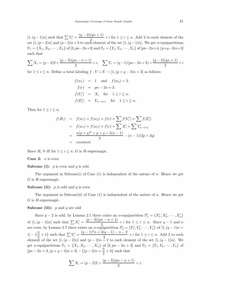
Supermagic Coverings of Some Simple Graphs 41
[1, (q − 1)n] such that∑
Y ′i =
(q − 2)(qn + 1)
2+ i for 1 ≤ i ≤ n. Add 2 to each element of the
set [1, (p−2)n] and (p−2)n+3 to each element of the set [1, (q−1)n]. We get n-equipartitions
P1 = X1, X2, · · · , Xn of [3, pn−2n+3] and P2 = Y1, Y2, · · · , Yn of [pn−2n+4, (p+q−3)n+3]
such that
∑Xi = (p−2)2+
(p − 3)(pn − n + 1)
2+ i,
∑Yi = (q−1)(pn−2n+3)+
(q − 2)(qn + 1)
2+ i
for 1 ≤ i ≤ n. Define a total labeling f : V ∪ E → [1, (p + q − 3)n + 3] as follows:
f(w1) = 1 and f(w2) = 2.
f(e) = pn − 2n + 3.
f(V ′i ) = Xi for 1 ≤ i ≤ n.
f(E′i) = Yn−i+1 for 1 ≤ i ≤ n.
Then for 1 ≤ i ≤ n,
f(Hi) = f(w1) + f(w2) + f(e) +∑
f(V ′i ) +
∑f(E′
i)
= f(w1) + f(w2) + f(e) +∑
X ′i +∑
Y ′n−i+1
=n(p + q)2 + p + q + 5(n − 1)
2− (n − 1)(2p + 3q)
= constant.
Since Hi∼= H for 1 ≤ i ≤ n, G is H-supermagic.
Case 2: n is even
Subcase (i): p is even and q is odd
The argument in Subcase(i) of Case (1) is independent of the nature of n. Hence we get
G is H-supermagic.
Subcase (ii): p is odd and q is even
The argument in Subcase(ii) of Case (1) is independent of the nature of n. Hence we get
G is H-supermagic.
Subcase (iii): p and q are odd
Since p − 2 is odd, by Lemma 2.1 there exists an n-equipartition P′1 = X ′
1, X′2, · · · , X ′
nof [1, (p − 2)n] such that
∑X ′
i =(p − 3)(pn − n + 1)
2+ i for 1 ≤ i ≤ n. Since q − 1 and n
are even, by Lemma 2.7 there exists an n-equipartition P′2 = Y ′
1 , Y ′2 , · · · , Y ′
n of [1, (q − 1)n +
1] − n
2+ 1 such that
∑Y ′
i =(q − 1)2n + 3(q − 1) − n − 2
2+ i for 1 ≤ i ≤ n. Add 2 to each
element of the set [1, (p − 2)n] and (p − 2)n + 2 to each element of the set [1, (q − 1)n]. We
get n-equipartitions P1 = X1, X2, · · · , Xn of [3, pn − 2n + 3] and P2 = Y1, Y2, · · · , Yn of
[pn − 2n + 3, (p + q − 3)n + 3] − (p − 2)n +n
2+ 3 such that
∑Xi = (p − 2)2 +
(p − 3)(pn − n + 1)
2+ i,

42 P.Jeyanthi and P.Selvagopal
∑Yi = (q − 1)(pn − 2n + 2) +
(q − 1)2n + 3(q − 1) − n − 2
2+ i
for 1 ≤ i ≤ n. Define a total labeling f : V ∪ E → [1, (p + q − 3)n + 3] as follows:
f(w1) = 1 and f(w2) = 2.
f(e) = (p − 2)n +n
2+ 3.
f(V ′i ) = Xi for 1 ≤ i ≤ n.
f(E′i) = Yn−i+1 for 1 ≤ i ≤ n.
Then for 1 ≤ i ≤ n,
f(Hi) = f(w1) + f(w2) + f(e) +∑
f(V ′i ) +
∑f(E′
i)
= f(w1) + f(w2) + f(e) +∑
X ′i +∑
Y ′n−i+1
=n(p + q)2 + p + q
2− (n − 1)(2p + 3q − 3)
= constant.
Since Hi∼= H for 1 ≤ i ≤ n, G is H-supermagic.
Subcase (iv): p and q are even
Since p − 2 and n are even, by Lemma 2.9 there exists an n-equipartition P1 = X1, X2,
· · · , Xn of [1, (p− 2)n +2]−1,n
2+2 such that
∑Xi =
(p − 2)2n + 5(p − 2) − n − 2
2+ i for
1 ≤ i ≤ n.
Since q − 1 is odd, by Lemma 2.1 there exists an n-equipartition P′2 = Y ′
1 , Y ′2 , · · · , Y ′
n of
[1, (q − 1)n] and∑
Y ′i = (q−2)(qn+1)
2 + i for 1 ≤ i ≤ n. Add (p− 2)n + 3 to each element of the
set [1, (q−1)n]. We get an n-equipartition P2 = Y1, Y2, · · · , Yn of [pn−2n+4, (p+q−3)n+3]
such that∑
Yi = (q − 1)(pn − 2n + 3) + (q−2)(qn+1)2 + i for 1 ≤ i ≤ n. Define a total labeling
f : V ∪ E → [1, (p + q − 3)n + 3] as follows:
f(w1) = 1 and f(w2) =n
2+ 2.
f(e) = pn − 2n + 3.
f(V ′i ) = Xi for 1 ≤ i ≤ n.
f(E′i) = Yn−i+1 for 1 ≤ i ≤ n.
Then for 1 ≤ i ≤ n,
f(Hi) = f(w1) + f(w2) + f(e) +∑
f(V ′i ) +
∑f(E′
i)
= f(w1) + f(w2) + f(e) +∑
X ′i +∑
Y ′n−i+1
=n(p + q)2 + p + q
2− (n − 1)(2p + 3q − 3)
= constant.
Since Hi∼= H for 1 ≤ i ≤ n, G is H-supermagic.

Supermagic Coverings of Some Simple Graphs 43
Hence, the edge amalgamation Edgeamal(Hi, uivi) of any finite collection Hi, uivi of
graphs Hi, each with a fixed edge uivi and isomorphic to H is H-supermagic for all values of
p and q.
Illustration 3.4 Let H1,H2,H3,H4 and H5 be five graphs isomorphic to the wheel W4 =
C4 + K1 and their fixed edges given by dotted lines. Then the Edge amalgamation graph
Edgeamal(Hi, uivi) of the given collection is W4-supermagic with supermagic sum 303.
1
2
1
2
1
2
1
25
10
15
7
8
17 16
9
6
4
11
14
12
3
21
3136
18 18
18
18
26
41
51
46
22
25
3235
42
45 52
23
24
3334
44
4353
19
28
2938
48
3949
40
5047
20
27
3037
13
Fig.1
Illustration 3.5 Let H1,H2,H3 and H4 be four graphs isomorphic to H and their fixed edges
given by dotted lines. Then the Edge amalgamation graph Edgeamal(Hi, uivi) of the given
collection is H-supermagic with supermagic sum 300.
1 419
40 47
39
32
183
31
24
38
3025
332
10 12
17
9
14 4
15
15
20
27
28
35
36
19
43
44
1
4
6 19
21
34 29
26
7
16
42
45
42
13
23
22
41
46
Fig.2

44 P.Jeyanthi and P.Selvagopal
Definition 3.6(Book with m-gon pages) Let n and m be any positive integers with n ≥ 1 and
m ≥ 3 . Then, n copies of the cycle Cm with an edge in common is called a book with n m-gon
pages. That is, if Gi, uivi is a collection of n copies of the cycle Cm each with a fixed edge
uivi then Edgeamal(Gi, uivi) is called a book with n m-gon pages.
A book with 3 pentagon pages is given below.
Fig.3
Corollary 3.7 Books with n m-gon pages are Cm -supermagic for every positive integers
n ≥ 1and m ≥ 3.
Illustration 3.8 C5-supermagic covering of a book with 3 hexagon pages is given below. The
supermagic sum is 167.
4
7
10
14
5
8
9
12
3
6
11
13
16 21
22
2728
17 20
23
2629
18 19
24
2530
2
15
1
Fig.4
Theorem 3.9 Let Hi = K1,k with vertex set V (Hi) = vi, vir : 1 ≤ r ≤ k and the edge set
E(Hi) = vivir : 1 ≤ r ≤ k where 1 ≤ i ≤ k and G be a graph obtained by joining a new vertex
w with v11, v21, · · · , vk1. Then G is K1,k-supermagic.
Proof Let Vi = vi, vir : 1 ≤ r ≤ k and Ei = Vivjr : 1 ≤ r ≤ k for 1 ≤ i ≤ k.
Then the vertex and edge set of G = (V, E) are given by V = ∪ki=1Vi ∪ v and E = ∪k
i=1Ei ∪vv1, vv2, · · · , vvk. Also |V | = k2 + k + 1 and |E| = k2 + k. Let Vk+1 = w, v1, v2, · · · , vkand Ek+1 = wv1, wv2, · · · , wvk and Hk+1 = (Vk+1, Ek+1) be the graph with vertex set Vk+1
and edge set Ek+1. Note that any edge of E belongs to at least one of the subgraphs Hi for
1 ≤ i ≤ k + 1. Since Hi∼= K1,k for 1 ≤ i ≤ k + 1, G admits a K1,k-covering.

Supermagic Coverings of Some Simple Graphs 45
Case 1: k is odd
Since k + 1 is even, by Lemma 2.3, there exists a k-equipartition P = X1, X2, · · · , Xk of
X = [1, (k + 1)k] such that
∑Xi =
k(k + 1)2
2+ i for 1 ≤ i ≤ k (3)
It can be easily verified from the definition of Xr in Lemma 2.3 that
(k + 1
2− 1
)k+σ(r) ∈ Xr
for 1 ≤ r ≤ k, where σ denotes the permutation of 1, 2, · · · , k given by
σ(r) =
k − 2r + 1
2for 1 ≤ r ≤ k − 1
23k − 2r + 1
2for
k + 1
2≤ r ≤ k
.
Construct Xk+1 = (
k + 1
2− 1
)k + σ(r) : 1 ≤ r ≤ k ∪ k2 + k + 1.
∑Xk+1 =
k∑
r=1
[(k + 1
2− 1
)k + σ(r)
]+ k2 + k + 1
=k2(k − 1)
2+
k(k + 1)
2+ k2 + k + 1
=k(k + 1)2
2+ k + 1 (4)
From (1) and (2) we have
∑Xi =
k(k + 1)2
2+ i for 1 ≤ i ≤ k + 1 (5)
As k is odd, by Lemma 1, there exists a k +1-equipartition Q′ = Y ′1 , Y ′
2 , · · · , Y ′k+1 of the
set Y = [1, k(k + 1)] such that∑
Y ′i =
(k − 1)[(k + 1)2 + 1]
2+ i for 1 ≤ i ≤ k + 1.
Adding k2 + k + 1 to [1, k(k + 1)], we get a k + 1-equipartition Q = Y1, Y2, · · · , Yk+1 of
the set Y = [k2 + k + 2, 2k2 + 2k + 1] such that
∑Yi = k(k2 + k + 1) +
(k − 1)[(k + 1)2 + 1]
2+ i for 1 ≤ i ≤ k + 1 (6)
Define a total labeling f : V ∪ E → [1, 2k2 + 2k + 1] as follows:
(i) f(w) = k2 + k + 1.
(ii) f(Vi) = Xi with f(vi1) =
(k + 1
2− 1
)k + σ(r) for 1 ≤ i ≤ k + 1.
(iii) f(Ei) = Yk+2−i for 1 ≤ i ≤ k + 1.
Then for 1 ≤ i ≤ k + 1,
f(Hi) =∑
f(Vi) +∑
f(Ei) =∑
Xi +∑
Yk+2−i
=4k3 + 5k2 + 5k + 2
2,
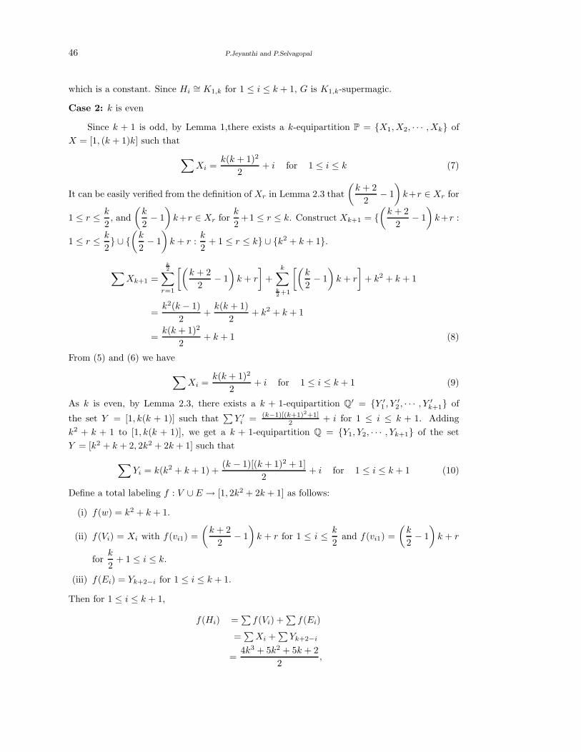
46 P.Jeyanthi and P.Selvagopal
which is a constant. Since Hi∼= K1,k for 1 ≤ i ≤ k + 1, G is K1,k-supermagic.
Case 2: k is even
Since k + 1 is odd, by Lemma 1,there exists a k-equipartition P = X1, X2, · · · , Xk of
X = [1, (k + 1)k] such that
∑Xi =
k(k + 1)2
2+ i for 1 ≤ i ≤ k (7)
It can be easily verified from the definition of Xr in Lemma 2.3 that
(k + 2
2− 1
)k+r ∈ Xr for
1 ≤ r ≤ k
2, and
(k
2− 1
)k+r ∈ Xr for
k
2+1 ≤ r ≤ k. Construct Xk+1 =
(k + 2
2− 1
)k+r :
1 ≤ r ≤ k
2 ∪
(k
2− 1
)k + r :
k
2+ 1 ≤ r ≤ k ∪ k2 + k + 1.
∑Xk+1 =
k2∑
r=1
[(k + 2
2− 1
)k + r
]+
k∑
k2+1
[(k
2− 1
)k + r
]+ k2 + k + 1
=k2(k − 1)
2+
k(k + 1)
2+ k2 + k + 1
=k(k + 1)2
2+ k + 1 (8)
From (5) and (6) we have
∑Xi =
k(k + 1)2
2+ i for 1 ≤ i ≤ k + 1 (9)
As k is even, by Lemma 2.3, there exists a k + 1-equipartition Q′ = Y ′1 , Y ′
2 , · · · , Y ′k+1 of
the set Y = [1, k(k + 1)] such that∑
Y ′i = (k−1)[(k+1)2+1]
2 + i for 1 ≤ i ≤ k + 1. Adding
k2 + k + 1 to [1, k(k + 1)], we get a k + 1-equipartition Q = Y1, Y2, · · · , Yk+1 of the set
Y = [k2 + k + 2, 2k2 + 2k + 1] such that
∑Yi = k(k2 + k + 1) +
(k − 1)[(k + 1)2 + 1]
2+ i for 1 ≤ i ≤ k + 1 (10)
Define a total labeling f : V ∪ E → [1, 2k2 + 2k + 1] as follows:
(i) f(w) = k2 + k + 1.
(ii) f(Vi) = Xi with f(vi1) =
(k + 2
2− 1
)k + r for 1 ≤ i ≤ k
2and f(vi1) =
(k
2− 1
)k + r
fork
2+ 1 ≤ i ≤ k.
(iii) f(Ei) = Yk+2−i for 1 ≤ i ≤ k + 1.
Then for 1 ≤ i ≤ k + 1,
f(Hi) =∑
f(Vi) +∑
f(Ei)
=∑
Xi +∑
Yk+2−i
=4k3 + 5k2 + 5k + 2
2,

Supermagic Coverings of Some Simple Graphs 47
which is a constant. Since Hi∼= K1,k for 1 ≤ i ≤ k + 1, G is K1,k-supermagic. Thus, in both
the cases G is K1,k-supermagic with supermagic sum s(f) =4k3 + 5k2 + 5k + 2
2.
Illustration 3.10
1112
13
14
1531
1
6
20
25
29 27
19 24
27
3
8
18
23
30
4
9
17
22
28
5
10
16
21
26
37
38
4950
61
36
3948
5160
3540
47
52
59 34
41
4653
58
33
42 45
54
5732
43
44
55
56
Fig.1. G- is K1,5-supermagic with supermagic sum 236.
19
20 21
16
1718
431
713
30
3642
2
8
14
29 35
41
39
15
28
34
40
4
10 22
27
3339
5
11
23
2632
38
6 12
2425
31
37
5461
68
7585
47
4855
62
6774
83
49
56
6366
73
81
50
57 64
65
79 72
44 51
58
7178
84
45
52
5970
77
82
46
53 60
69
7680
Fig.2. G- is K1,6-supermagic with supermagic sum 538.
48 P.Jeyanthi and P.Selvagopal
References
[1] K.Carlson, Generalized books and Cm-snakes are prime graphs, Ars Combin. 80(2006)
215-221.
[2] J.A.Gallian, A Dynamic Survey of Graph labeling(DS6), The Electronic Journal of Com-
binatorics, 5(2005).
[3] A.Gutierrez, A.Llado, Magic coverings, J. Combin. Math. Combin. Comput., 55(2005),
43-56.
[4] P.Selvagopal, P.Jeyanthi, On Ck-supermagic graphs, International Journal of Mathematics
and Computer Science, 3(2008), No. 1, 25-30.

International J.Math. Combin. Vol.1 (2011), 49-58
Elementary Abelian Regular Coverings of Cube
Furong Wang
(Beijing Wuzi University, Beijing 101149, P.R. China)
Lin Zhang
(Capital University of Economics and Business, Beijing 100070, P. R. China)
E-mail: [email protected], [email protected]
Abstract: For a give finite connected graph Γ, a group H of automorphisms of Γ and a finite
group A, a natural question can be raised as follows: Find all the connected regular coverings
of Γ having A as its covering transformation group, on which each automorphism in H can
be lifted. In this paper, we classify all the connected regular covering graphs of the cube
satisfying the following two properties: (1) the covering transformation group is isomorphic
to the elementary Abelian p-groups; (2) the group of fibre-preserving automorphisms acts
edge-transitively.
Key Words: Connected graph, graph covering, cube, Smarandachely covering, regular
covering.
AMS(2010):
§1. Introduction
All graphs considered in this paper are finite, undirected and simple. For a graph Γ, we use
V (Γ), E(Γ), A(Γ) and Aut(Γ) to denote its vertex set, edge set, arc set and full automorphism
group, respectively. For any v ∈ V (Γ), by N(v) we denote the neighborhood of v in Γ. For an
arc (u, v) ∈ A(Γ), we denote the corresponding undirected edge by uv.
A graph Γ is called a covering of the graph Γ with projection p : Γ → Γ if there is a
surjection p : V (Γ) → V (Γ) such that p|N(v) : N(v) → N(v) is a bijection for any vertex
v ∈ V (Γ) and v ∈ p−1(v). The graph Γ is called the covering graph and Γ is the base graph.
A p : Γ → Γ is called to be a Smarandachely covering of Γ if there exist u, v ∈ V (Γ) such that
|p−1(u)| 6= |p−1(v)|. Conversely, if |p−1(v)| = n for each v ∈ V (Γ), then such a covering p is
said to be n-fold. Each p−1(v) is called a fibre of Γ. An automorphism of Γ which maps a fibre
to a fibre is said to be fibre-preserving. The group K of all automorphisms of Γ which fix each
of the fibres setwise is called the covering transformation group. A covering p : Γ → Γ is said
to be regular (simply, A-covering) if there is a subgroup A of K acting regularly on each fibre.
Moreover, if Γ is connected, then A = K.
A purely combinatorial description of a covering was introduced through a voltage graph
1Supported by NNSF(10971144) and BNSF(1092010).2Received December 23, 2010. Accepted February 23, 2011.

50 Furong Wang and Lin Zhang
by Gross and Tucker [4,5] and also a very similar idea was appeared in Biggs’ monograph [1,2].
Let A be a finite group. An (ordinary) voltage assignment (or, A-voltage assignment) of Γ is
a function φ : A(Γ) → A with the property that φ(u, v) = φ(v, u)−1 for each (u, v) ∈ A(Γ).
The values of φ are called voltages, and A is called the voltage group. The graph Γ ×φ A
derived from φ is defined by V (Γ ×φ A) = V (Γ) × A and E(Γ ×φ A) = ((u, g), (v, φ(u, v)g))∣∣
(u, v) ∈ E(Γ), g ∈ A. Clearly, the graph Γ ×φ A is a covering of the graph Γ with the first
coordinate projection p : Γ×φ A → Γ, which is called the natural projection. For each u ∈ V (Γ),
(u, g)∣∣ g ∈ A is a fibre of Γ ×φ A. Moreover, by defining (u, g′)g := (u, g′g) for any g ∈ A
and (u, g′) ∈ V (Γ×φ A), A can be identified with a fibre-preserving automorphism subgroup of
Aut(Γ×φ A) acting regularly on each fibre. Therefore, p can be viewed as a A-covering. Given
a spanning tree T of the graph Γ, a voltage assignment φ is called T -reduced if the voltages
on the tree arcs are identity. Gross and Tucker ([4]) showed that every regular covering of a
graph Γ can be derived from an ordinary T -reduced voltage assignment φ with respect to an
arbitrary fixed spanning tree T of Γ.
An automorphism α of Γ can be lifted to an automorphism α of a covering graph Γ if
pα = αp, where p is the covering projection from Γ to Γ. We say a subgroup of H of Aut(Γ)
can be lifted if each element of H can be lifted.
For a given finite connected graph Γ, a group H of automorphisms of Γ and a finite group
A, a natural question can be raised as follows: Find all the connected regular coverings of Γ
having A as its covering transformation group, on which each automorphism in H can be lifted.
In [3], Du, Kawk and Xu investigate the regular coverings with A = Znp , an elementary Abelian
group and get some new matrix-theoretical characterizations for an automorphism of the base
graph to be lifted, and as one of the applications, they gave a classification of all connected
regular coverings of the Petersen graph with the covering transformation group Znp , whose
fibre-preserving automorphism subgroup acts arc-transitively.
In this paper, we use the same method to classify all the connected regular covering graphs
of the cube satisfying the following two properties: (1) the covering transformation group is
isomorphic to the elementary Abelian p-group; (2) the group of fibre-preserving automorphisms
acts edge-transitively.
The cube is identified with the graph Γ as shown in Figure (a). Fix a spanning tree T in
Γ as shown in Figure (b). Let V1 = 2, 6, 4, 7, 3, 5. Then the induced subgraph Γ(V1) is a line
as shown in Figure (c).
17
6
5
4
3
2
8 17
6
5
4
3
2
8
Figure (a): the graph Γ; (b) a spanning tree T of Γ.
2 6 4 7 3 5
Figure (c): the induced subgraph Γ(V1)

Elementary Abelian Regular Coverings of Cube 51
First, we introduce five families of covering graphs Γ×φZnp of cube Γ by giving a T -reduced
voltage assignment φ. Since φ is T -reduced, we only need to give the voltages on the cotree arcs
(see Figure (c)). Let t denote the transposition of a matrix.
(1) X(2, 1):=Γ×φ Z2, where φ26 = φ47 = φ35 = 1 and φ46 = φ37 = 0,
X(p, 1):=Γ×φ Zp, where p = 3 or p ≡ 1(mod 6), φ26 = φ37 = 1, φ46 = φ35 = 1+√−3
2 and
φ47 = 0.
(2) X(p, 2):=Γ×φ Z2p , where φ26 = φ37 = (0, 1), φ46 = φ35 = (1, 0) and φ47 = (0, 0).
(3) X(p, 3):=Γ ×φ Z3p , where ((φ26)
t, (φ47)t, (φ35)
t) = I3×3, φ46 = (0, 1,−1) and φ37 =
(−1, 1, 0).
(4) X(p, 4):=Γ×φ Z4p , where p = 3 or p ≡ 1(mod 6), ((φ26)
t, (φ46)t, (φ47)
t, (φ37)t) = I4×4
and φ35 = (1 −
√−3
2, −1,
1 +√−3
2,
1 −√−3
2).
(5) X(p, 5):=Γ×φ Z5p , where ((φ26)
t, (φ46)t, (φ47)
t, (φ37)t, (φ35)
t) = I5×5.
Now we state the main theorem of this paper.
Theorem 1.1 Let Γ be a connected regular covering of the cube Γ whose covering transformation
group is isomorphic to Znp and whose fibre-preserving automorphism subgroup G acts edge-
transitively on Γ. Then, Γ is isomorphic to one of the graphs in (1)-(5) listed above. Moreover,
for the graphs X(2, 1), X(3, 1), X(p, 2), X(p, 3), X(3, 4) and X(p, 5), Aut(Γ) can be lifted, and
so they are 2-arc-transitive; and for the graphs X(p, 1) and X(p, 4) for p ≡ 1(mod 6), the
subgroup isomorphic to A4×Z2 can be lifted but AutΓ cannot, and so they are arc-transitive, in
particular, all these five families of graphs are vertex transitive.
§2. Algorithm for the Lifting
In this section, we present the algorithm given by Du, Kwak and Xu [3], which deals with
the lifting problem for regular coverings of a graph Γ whose covering transformation group is
elementary Abelian.
Throughout this section, let Γ be a connected graph and let Γ = Γ ×φ Znp be a connected
regular covering of the Γ. The voltage group Znp will be identified with the additive group of
the n-dimensional vector space V (n, p) over the finite field GF (p). Since Γ is connected, the
number β(Γ) = |E(Γ)| − |V (Γ)|+ 1 is equal to the number of independent cycles in Γ and it is
referred to as the Betti number of Γ.
Let V (Γ) = 0, 1, . . . , |V (Γ)| − 1. For any arc (i, j) ∈ A(Γ), by φi,j we denote the voltage
on the arc, which is identified with a row vector in V (n, p). An arc (i, j) ∈ A(Γ) is called
positive (resp. negative) if i < j (resp. i > j). For each subset F in E(Γ), we denote the
set of its arcs, positive arcs and negative arcs by A(F ), A+(F ) and A−(F ), respectively, so
that A(F ) = A+(F ) ∪ A−(F ). In particular, if F = E(Γ), we prefer to use A(Γ), A+(Γ) and
A−(Γ) to denote A(F ), A+(F ) and A−(F ), respectively. Fix a spanning tree T in the graph

52 Furong Wang and Lin Zhang
Γ and let E0 = E(T ), so that |E(Γ) \ E0| is the Betti number β(Γ) of the graph Γ. From
now on, the voltage assignment φ is assumed to be T -reduced. By the connectedness of Γ,
φi,j | (i, j) ∈ A+(E(Γ) \ E0) generates the group Znp . Hence, we get n 6 β(Γ).
Let E1 be a set of edges such that φA+(E1) = φi,j
∣∣ (i, j) ∈ A+(E1) is a basis for the
vector space V (n, p), and let E2 = E(Γ) \ (E0 ∪ E1). Let
|E0| = k, |E1| = n and |E2| = m, (1)
so that the number of edges in Γ is k + n + m.
Let Φ0 (resp. Φ1 and Φ2) be the k×n (resp. n×n and m×n) matrix with the row vectors
φi,j for the arcs (i, j) in A+(E0) (resp. A+(E1) and A+(E2)), according to a fixed order of the
positive arcs. Since the row vectors of Φ1 form a basis for V (n, p), there exists an m×n matrix
M , called a voltage generating matrix of φ, such that
Φ2 = MΦ1. (2)
Let
Φ =
Φ0
Φ1
Φ2
, (3)
which is a (k+n+m)×n matrix over GF (p), called a voltage (assignment) matrix corresponding
to the voltage assignment φ. If we take φA+(E1) so that Φ0 = 0 and Φ1 = In×n, the n×n identity
matrix, then Φ is called a reduced form or a T-reduced form of the voltage assignment matrix
Φ. From now on one may assume that Φ is in a reduced form without loss of any generality.
Let V = V (k + n + m, p) be the (k + n + m)-dimensional row vector space over the field
GF (p). Hereafter, we denote a vector v in V by (v0,v1,v2) ∈ Zkp ⊕ Zn
p ⊕ Zmp , where the
coordinates of the vector v0 (resp. v1 and v2) are indexed by arcs in A+(E0) (resp. A+(E1)
and A+(E2)), according to the same order of row vectors in Φ0 (Φ1 and Φ2).
Given a graph Γ, its spanning tree T , and a positive cotree arc (u, v), there is a unique
path from v to u in T which is denoted by [v, · · · , u]. We call the closed walk (u, [v, · · · , u]) the
fundamental cycle belonging to (u, v), and denote it by C(u, v; T ). There are n+m fundamental
cycles in Γ, where n + m is the Betti number of Γ.
Given a graph Γ and its spanning tree T , we keep the same order for positive arcs as the
order of row vectors of the voltage matrix Φ. For each positive cotree arc (u, v), let pu,v be the
k-dimensional row vector over GF (p) whose (i, j)-coordinate pu,vi,j indexed by the positive tree
arc (i, j) of the given order is defined as follows:
pu,vi,j =
1 if (i, j) is in C(u, v; T ),
−1 if (j, i) is in C(u, v; T ),
0 otherwise.
(4)
Let P be the (n + m) × k matrix whose row vectors are pu,v, indexed by the positive cotree
arcs (u, v) of the given order. We call P the incidence matrix for the fundamental cycles of
the graph Γ with respect to the tree T .

Elementary Abelian Regular Coverings of Cube 53
Now we state the algorithm for solving lifting problem for the connected regular coverings
of a graph Γ whose covering transformation group is elementary Abelian.
(1st) Choose a fixed spanning tree T in Γ and write down the arcs in A+(E0), A+(E1) and
A+(E2) in a certain order so that Φ0 = 0, Φ1 = In×n and Φ2 = M.
(2nd) Calculate the incidence matrix P for the fundamental cycles of Γ with respect to T .
(3rd) Assume that the voltage generating matrix M = (aij)m×n, where the entries aij are
unknowns. Let ∆ = ((−M, Im×m)P,−M, Im×m), whose columns are indexed by the
arcs in A+(E0), A+(E1), A
+(E2) according to the given order. We call the matrix ∆
the discriminant matrix for a lift of φ. For convenience, we write ∆0 = (−M, Im×m)P ,
∆1 = −M and ∆2 = Im×m, so that ∆ = (∆0, ∆1, ∆2), as a block matrix.
(4th) Let ∆ = (· · · , ci,j , · · · ), where ci,j is the column indexed by (i, j) ∈ A+(Γ). For a given
σ ∈ Aut(Γ), let cσi,j = ciσ−1 ,jσ−1 , where we assume that ci,j = −cj,i for any arc (i, j). Let
∆σ = (· · · , cσi,j , · · · ) for any (i, j) ∈ A+(Γ), and let (∆σ)0, (∆σ)1 and (∆σ)2 denote the
first, the second and the third blocks of the matrix ∆σ respectively, as before. Then one
can say that
σ can be lifted ⇐⇒ (∆σ)1 + (∆σ)2M = 0 ⇐⇒ ∆σ1 + ∆σ
2M = 0. (5)
Proof of Theorem 1.1
Let E0 = E(T ) and E = E(Γ) \ E0. Give an ordering for the arcs in A+(E0) and A+(E) as
follows:
A+(E0) = 15, 16, 17, 25, 28, 38, 48,
A+(E) = 26, 46, 47, 37, 35.
Give fundamental cycles in Γ as follows:
C(2, 6; T ) = (2, 6, 1, 5, 2),
C(4, 6; T ) = (4, 6, 1, 5, 2, 8, 4),
C(4, 7; T ) = (4, 7, 1, 5, 2, 8, 4),
C(3, 7; T ) = (3, 7, 1, 5, 2, 8, 3),
C(3, 5; T ) = (3, 5, 2, 8, 3).
It is well-known that Aut(Γ) ∼= S4 × Z2. Take four automorphisms of Γ as follows: α =
(243)(567), β = (14)(23)(58)(67), γ = (18)(27)(36)(45) and δ = (23)(67).
It is easy to check that M =< α, β > is subgroup of Aut(Γ) isomorphic to A4, N =<
M, γ > is subgroup of Aut(Γ) isomorphic to A4×Z2, and < N, δ >= Aut(Γ). Thus we have:
(1) M can be lifted if and only if α and β can be lifted;
(2) N can be lifted if and only if α, β and γ can be lifted;
(3) Aut(Γ) can be lifted if and only if α, β, γ and δ can be lifted.

54 Furong Wang and Lin Zhang
Since β(Γ) = 5, we get n 6 5. If n = 5, then Γ is nothing but X(p, 5) and by [6, Theorem
2.11], Aut(Γ) can be lifted. So, in what follows, we assume n < 5 and divide our proof into
four cases for each n with 1 6 n 6 4.
3.1 The Case of n = 1
Suppose that n = 1. Then K = Zp = V (1, p). Since the element (18)(25)(36)(47) of Aut(Γ)
maps 2, 6, 4, 7, 3, 5 to 5, 3, 7, 4, 6, 2, respectively, without loss of any generality, we have the
following three essentially different cases for the set E1 and E2:
(1) E1 = 26 and E2 = 46, 47, 37, 35;
(2) E1 = 46 and E2 = 26, 47, 37, 35;
(3) E1 = 47 and E2 = 26, 46, 37, 35.
Case (1): E1 = 26 and E2 = 46, 47, 37, 35.
In this case, the incidence matrix is:
P =
(1,5) (1,6) (1,7) (2,5) (2,8) (3,8) (4,8)
(2,6) 1 −1 0 −1 0 0 0
(4,6) 1 −1 0 −1 1 0 −1
(4,7) 1 0 −1 −1 1 0 −1
(3,7) 1 0 −1 −1 1 −1 0
(3,5) 0 0 0 −1 1 −1 0
.
Let D = (D0, D1, D2) be the discriminant matrix with D0 = (−M, I4×4)P , D1 = (−M)
and D2 = (I4×4) with a voltage generating matrix M = (a, b, c, d)t. A direct computation gives
that D0 = (−M, I4×4)P is equal to
D0 =
(1, 5) (1, 6) (1, 7) (2, 5) (2, 8) (3, 8) (4, 8)
−a + 1 a − 1 0 a − 1 1 0 −1
−b + 1 b −1 b − 1 1 0 −1
−c + 1 c −1 c − 1 1 −1 0
−d d 0 d − 1 1 −1 0
.
For an automorphism σ of Γ can be lifted if and only if
∆σ1 + ∆σ
2M = (c26)σ + (c46c47c37c35)
σM = 0. (6)
Inserting α = (243)(567) to (6), we have
0 = Dα1 + Dα
2 M = (c26)α + (c46c47c37c35)
αM
= (c35) + (c25c26c46c47)M
=
a2 − a − ab + c
ab − a − b2 + d
ac − a − bc
ad − a − bd + 1
= (xi,j).

Elementary Abelian Regular Coverings of Cube 55
Inserting β = (14)(23)(58)(67) to (6), we have
0 = Dβ1 + Dβ
2 M = (c26)β + (c46c47c37c35)
βM
= (c37) + (c17c16c26c28)M
=
ab − b − ac + d
−a + b2 − bc + d
−a + bc − c2 + d + 1
bd − cd + d
= (yij).
Now assume that α and β can be lifted. By y41 = 0, we distinguish two cases: (1) d = 0;
(2) b − c + 1 = 0. If (1) happens, by x41 = 0 and x11 = 0, we have a = 1 and b = c. But it
doesn’t satisfy y21 = 0. If (2) happens, by y11 = 0 , we have −a − b + d = 0. By x21 = 0, we
distinguish two subcases: (i) a − b + 1 = 0; (ii) b = 0. If (i) happens, by (xij) = 0, we have
that either a = c = 0, b = d = 1 and p = 2 or a = d = 2, b = 0, c = 1 and p = 3. If (ii)
happens, we have c = 1 and a = d. By x11 = 0, we have a2 − a + 1 = 0. Thus the solution of
(xij) = (yij) = 0 are: a = c = 0, b = d = 1 and p = 2; or a = d = 1±√−3
2 , b = 0, c = 1 and
p = 3 or p ≡ 1(mod 6). Or equivalently,
M1 = (0, 1, 0, 1)t, p = 2;
M21 = (1 +
√−3
2, 0, 1,
1 +√−3
2)t, p = 3 or p ≡ 1(mod 6);
M22 = (1 −
√−3
2, 0, 1,
1 −√−3
2)t, p = 3 or p ≡ 1(mod 6).
By X(2, 1), X(p, 1) and X ′(p, 1), we denote the covering graphs determined by M1, M21
and M22, respectively. In particular, X(p, 1) and X ′(p, 1) are the same one if p = 3.
Inserting γ = (18)(27)(36)(45) to (6), we have
0 = Dγ1 + Dγ
2M = (c26)γ + (c46c47c37c35)
γM
= (c73) + (c53c52c62c64)M
=
b − ab + ac − d
b − b2 + bc
b − bc + c2 − 1
−a + b − bd + cd
.
Clearly, the matrices M1, M21 and M22 satisfy this equation and γ can be lifted, and so
the group N can be lifted.

56 Furong Wang and Lin Zhang
Inserting δ = (23)(67) to (6), we have
0 = Dδ1 + Dδ
2M = (c26)δ + (c46c47c37c35)
δM
= (c37) + (c47c46c26c25)M
=
b − ac + ad − d
a − bc + bd − d
−c2 + cd − d + 1
−cd + d2 − d
.
Clearly, the matrix M1 satisfy this equation and δ can be lifted. But the matrices M21 and
M22 satisfy this equation and δ can be lifted when p = 3. So, for graphs X(2, 1) and X(3, 1),
Aut(Γ) can be lifted.
Finally, we show that for p ≡ 1(mod 6), the graphs X(p, 1) and X ′(p, 1) are isomor-
phic as graphs. Let V := V (X(p, 1)) = V (X ′(p, 1)) = (i; x) | 1 ≤ i ≤ 8, x ∈ GF (p). Let
R = (−1+√−3
2 ), and let ζ = (18)(25)(36)(47) ∈Aut(Γ). Define a permutation Υ on V by
(i; x)Υ = (iζ ; (x)R). A direct checking shows that Υ is isomorphism from X(p, 1) to X ′(p, 1).
Cases (2) and (3): By a computation similar to case (1), we can get the graph X(p, 1) in
case (2) and the graph X(2, 1) in the case (3).
3.2 The case of n = 2, 3, and 4
In this subsection, the case n = 2, 3, and 4 will be described briefly.
Case n = 2. In the case, K = Z2p = V (2, p). As before, without loss we may assume one of the
following happens:
(1) E1 = 46, 37 and E2 = 26, 47, 35;
(2) E1 = 26, 46 and E2 = 47, 37, 35;
(3) E1 = 26, 47 and E2 = 46, 37, 35;
(4) E1 = 26, 37 and E2 = 46, 47, 35;
(5) E1 = 26, 35 and E2 = 46, 47, 37;
(6) E1 = 46, 47 and E2 = 26, 37, 35.
For the case of (1), let
M =
a1 b1
a2 b2
a3 b3
.

Elementary Abelian Regular Coverings of Cube 57
be a voltage generating matrix. Then a computation similar to case n = 1 gives that Aut(Γ)
can be lifted if and only if a1 = a2 = b2 = b3 and b1 = a3 = 1. Accordingly, we can get the
graph X(p, 2).
In the Cases of (2), (3), (4), (5) and (6), the group M can not be lifted.
Case n = 3. In this case, K = Z3p = V (3, p). Without any loss of generality, we may assume
one of the following happens:
(1) E1 = 26, 47, 35 and E2 = 46, 37;
(2) E1 = 26, 46, 47 and E2 = 37, 35;
(3) E1 = 26, 46, 37 and E2 = 47, 35;
(4) E1 = 26, 46, 35 and E2 = 47, 37;
(5) E1 = 46, 47, 37 and E2 = 26, 35;
(6) E1 = 26, 47, 37 and E2 = 46, 35.
For the case of (1), one can show that Aut(Γ) can be lifted if and only if the voltage
generation matrix
M =
0 1 −1
−1 1 0
.
Thus, we get the graph X(p, 3).
In the case (2), (3), (4), (5) and (6), the group M can not be lifted.
Case n = 4. In this case, K = Z4p = V (4, p). Without any loss of generality, we may divide our
discussion into mutually exclusive three cases as followings:
Case (1): E1 = 26, 46, 47, 37 and E2 = 35.Let D = (D0, D1, D2) be the discriminant matrix with D0 = (−M, I1×1)P , D1 = (−M)
and D2 = (I1×1) with a voltage generating matrix M = (a, b, c, d).
The group Aut(Γ) can be lifted if and only if
M1 = (1 −
√−3
2,−1,
1 +√−3
2,1 −
√−3
2), p = 3 or p ≡ 1(mod 6);
M2 = (1 +
√−3
2,−1,
1 −√−3
2,1 +
√−3
2), p = 3 or p ≡ 1(mod 6).
By X(p, 4) and X ′(p, 4), we denote the covering graphs determined by M1 and M2, respec-
tively. In particular, X(p, 4) and X ′(p, 4) are the same one if p = 3.
For p ≡ 1(mod 6), the graphs X(p, 4) and X ′(p, 4) are isomorphic as graphs. Let V :=

58 Furong Wang and Lin Zhang
V (X(p, 4)) = V (X ′(p, 4)) = (i; x, y, z, w) | 1 ≤ i ≤ 8, x, y, z, w ∈ GF (p). Let
R =
c2 − 1 1 −c2 c2 − 1
0 0 0 −1
0 0 −1 0
0 −1 0 0
.
And let and let ζ = (18)(25)(36)(47) ∈Aut(Γ). Define a permutation Υ on V by (i; x, y, z, w)Υ =
(iζ ; (x, y, z, w)R). A direct checking shows that Υ is isomorphism from X(p, 4) to X ′(p, 4).
Case (2): E1 = 26, 46, 47, 35 and E2 = 37, and φ26, φ46, φ47 φ37, φ46, φ47, φ37 φ35 are
linear dependant, hence letting
M = (0, b, c, 0).
Now, one can show that M cannot be lifted.
By a similar computation, in case (3) , E1 = 26, 46, 37, 35 and E2 = 47, and the group
M can not be lifted.
Combining subsection 3.1 and 3.2, we finish the proof of Theorem 1.1.
References
[1] N.L. Biggs, Algebraic graph theory, Cambridge University Press, Cambridge, 1974.
[2] N.L. Biggs, Homological coverings of graphs, J. London Math. Soc. 30(1984), 1–14.
[3] S.F. Du, J.H. Kwak and M.Y. Xu, Linear criteria for liftings of automorphisms of the
elementary abelian regular coverings, to appear in Linear Algebra and Its applications,
2003.
[4] J.L. Gross and T.W. Tucker, Generating all graph coverings by permutation voltage as-
signments, Discrete Math. 18(1977) 273–283.
[5] J.L. Gross and T.W. Tucker, Topological Graph Theory, Wiley-Interscience, New York,
1987.

International J.Math. Combin. Vol.1 (2011), 59-72
Super Fibonacci Graceful Labeling of
Some Special Class of Graphs
R.Sridevi1, S.Navaneethakrishnan2 and K.Nagarajan1
1. Department of Mathematics, Sri S.R.N.M.College, Sattur - 626 203, Tamil Nadu, India
2. Department of Mathematics, V.O.C.College, Tuticorin - 628 008, Tamil Nadu, India
E-mail: r.sridevi [email protected], [email protected], k nagarajan [email protected]
Abstract: A Smarandache-Fibonacci Triple is a sequence S(n), n ≥ 0 such that S(n) =
S(n − 1) + S(n − 2), where S(n) is the Smarandache function for integers n ≥ 0. Certainly,
it is a generalization of Fibonacci sequence. A Fibonacci graceful labeling and a super Fi-
bonacci graceful labeling on graphs were introduced by Kathiresan and Amutha in 2006.
Generally, let G be a (p, q)-graph and S(n)|n ≥ 0 a Smarandache-Fibonacci Triple. An bi-
jection f : V (G) → S(0), S(1), S(2), . . . , S(q) is said to be a super Smarandache-Fibonacci
graceful graph if the induced edge labeling f∗(uv) = |f(u)− f(v)| is a bijection onto the set
S(1), S(2), . . . , S(q). Particularly, if S(n), n ≥ 0 is just the Fibonacci sequence Fi, i ≥ 0,
such a graph is called a super Fibonacci graceful graph. In this paper, we show that some
special class of graphs namely F tn, Ct
n and Stm,n are super fibonacci graceful graphs.
Key Words: Smarandache-Fibonacci triple, graceful labeling, Fibonacci graceful labeling,
super Smarandache-Fibonacci graceful graph, super Fibonacci graceful graph.
AMS(2010): 05C78
§1. Introduction
By a graph, we mean a finite undirected graph without loops or multiple edges. A path of
length n is denoted by Pn+1. A cycle of length n is denoted by Cn. G+ is a graph obtained
from the graph G by attaching pendant vertex to each vertex of G. Graph labelings, where
the vertices are assigned certain values subject to some conditions, have often motivated by
practical problems. In the last five decades enormous work has been done on this subject [1].
The concept of graceful labeling was first introduced by Rosa [6] in 1967. A function f is
a graceful labeling of a graph G with q edges if f is an injection from the vertices of G to the
set 0, 1, 2, . . . , q such that when each edge uv is assigned the label |f(u)− f(v)|, the resulting
edge labels are distinct.
The notion of Fibonacci graceful labeling and Super Fibonacci graceful labeling were in-
troduced by Kathiresan and Amutha [5]. We call a function f , a fibonacci graceful labeling of a
graph G with q edges if f is an injection from the vertices of G to the set 0, 1, 2, . . . , Fq, where
1Received November 1, 2010. Accepted February 25, 2011.

60 R.Sridevi, S.Navaneethakrishnan and K.Nagarajan
Fq is the qth fibonacci number of the fibonacci series F1 = 1,F2 = 2,F3 = 3, F4 = 5,. . . , such that
each edge uv is assigned the labels |f(u)− f(v)|, the resulting edge labels are F1, F2, . . . , . . . Fq.
An injective function f : V (G) → F0, F1, . . . , Fq, where Fq is the qth fibonacci number, is said
to be a super fibonacci graceful labeling if the induced edge labeling |f(u)− f(v)| is a bijection
onto the set F1, F2, . . . , Fq. In the labeling problems the induced labelings must be distinct.
So to introduce fibonacci graceful labelings we assume F1 = 1, F2 = 2, F3 = 3, F4 = 5,. . . , as
the sequence of fibonacci numbers instead of 0, 1, 2, · · · [3].
Generally, a Smarandache-Fibonacci Triple is a sequence S(n), n ≥ 0 such that S(n) =
S(n− 1) + S(n− 2), where S(n) is the Smarandache function for integers n ≥ 0 ([2]). A (p, q)-
graph G is a super Smarandache-Fibonacci graceful graph if there is an bijection f : V (G) →S(0), S(1), S(2), . . . , S(q) such that the induced edge labeling f∗(uv) = |f(u) − f(v)| is a
bijection onto the set S(1), S(2), . . . , S(q). So a super Fibonacci graceful graph is a special
type of Smarandache-Fibonacci graceful graph by definition.
We have constructed some new types of graphs namely Fn ⊕K+1,m, Cn ⊕Pm, K1,n ⊘K1,2,
Fn ⊕ Pm and Cn ⊕K1,m and we proved that these graphs are super fibonacci graceful labeling
in [7]. In this paper, we prove that F tn, Ct
n and Stm,n are super fibonacci graceful graphs.
§2. Main Results
In this section, we show that some special class of graphs namely F tn, Ct
n and Stm,n are super
fibonacci graceful graphs.
Definition 2.1 Let G be a (p, q) graph. An injective function f : V (G) → F0, F1, F2, · · · , Fq,where Fq is the qth fibonacci number, is said to be a super fibonacci graceful graphs if the induced
edge labeling f∗(uv) = |f(u) − f(v)| is a bijection onto the set F1, F2, . . . , Fq.
Definition 2.2 The one point union of t copies of fan Fn is denoted by F tn.
The following theorem shows that the graph F tn is a super fibonacci graceful graph.
Theorem 2.3 F tn is a super fibonacci graceful graph for all n ≥ 2.
Proof Let u0 be the center vertex of F tn and uj
i , where i = 1, 2, . . . , t, j = 1, 2, . . . , n be
the other vertices of F tn. Also, |V (G)| = nt + 1 and |E(G)| = 2nt − t. Define f : V (F t
n) →F0, F1, . . . , Fq by f(u0) = F0, f(uj
1) = F2j−1, 1 ≤ j ≤ n. For i = 2, 3, . . . , t, f(uji ) =
F2n(i−1)+2(j−1)−(i−2), 1 ≤ j ≤ n. We claim that all these edge labels are distinct. Let E1 =
f∗(u0uj1) : 1 ≤ j ≤ n. Then
E1 = |f(u0) − f(uj1)| : 1 ≤ j ≤ n
= |f(u0) − f(u11)|, |f(u0) − f(u2
1)|, . . . , |f(u0) − f(un−11 )|, |f(u0) − f(un
1 )|= |F0 − F1|, |F0 − F3|, . . . , |F0 − F2n−3|, |F0 − F2n−1|= F1, F3, . . . , F2n−3, F2n−1.

Super Fibonacci Graceful Labeling of Some Special Class of Graphs 61
Let E2 = f∗(uj1u
j+11 ) : 1 ≤ j ≤ n − 1. Then
E2 = |f(uj1) − f(uj+1
1 )| : 1 ≤ j ≤ n − 1= |f(u1
1) − f(u21)|, |f(u2
1) − f(u31)|, . . . , |f(un−2
1 ) − f(un−11 )|, |f(un−1
1 ) − f(un1 )|
= |F1 − F3|, |F3 − F5|, . . . , |F2n−5 − F2n−3|, |F2n−3 − F2n−1|= F2, F4, . . . , F2n−4, F2n−2.
For i = 2, we know that
E3 = f∗(u0uj2) : 1 ≤ j ≤ n = |f(u0) − f(uj
2)| : 1 ≤ j ≤ n= |f(u0) − f(u1
2)|, |f(u0) − f(u22)|, . . . , |f(u0) − f(un−1
2 )|, |f(u0) − f(un2 )|
= |F0 − F2n|, |F0 − F2n+2|, . . . , |F0 − F4n−4|, |F0 − F4n−2|= F2n, F2n+2, . . . , F4n−4, F4n−2,
E4 = f∗(uj2u
j+12 ) : 1 ≤ j ≤ n − 1
= |f(uj2) − f(uj+1
2 )| : 1 ≤ j ≤ n − 1= |f(u1
2) − f(u22)|, |f(u2
2) − f(u32)|, . . . , |f(un−2
2 ) − f(un−12 )|, |f(un−1
2 ) − f(un2 )|
= |F2n − F2n+2|, |F2n+2 − F2n+4|, . . . , |F4n−6 − F4n−4|, |F4n−4 − F4n−2|= F2n+1, F2n+3, . . . , F4n−5, F4n−3.
For i = 3, let E5 = f∗(u0uj3) : 1 ≤ j ≤ n. Then
E5 = |f(u0) − f(uj3)| : 1 ≤ j ≤ n
= |f(u0) − f(u13)|, |f(u0) − f(u2
3)|, . . . , |f(u0) − f(un−13 )|, |f(u0) − f(un
3 )|= |F0 − F4n−1|, |F0 − F4n+1|, . . . , |F0 − F6n−5|, |F0 − F6n−3|= F4n−1, F4n+1, . . . , F6n−5, F6n−3.
Let E6 = f∗(uj3u
j+13 ) : 1 ≤ j ≤ n − 1. Then
E6 = |f(uj3) − f(uj+1
3 )| : 1 ≤ j ≤ n − 1= |f(u1
3) − f(u23)|, |f(u2
3) − f(u33)|, . . . , |f(un−2
3 ) − f(un−13 )|, |f(un−1
3 ) − f(un3 )|
= |F4n−1 − F4n+1|, |F4n+1 − F4n+3|, . . . , |F6n−7 − F6n−5|, |F6n−5 − F6n−3|= F4n, F4n+2, . . . , F6n−6, F6n−4
· · · · · · · · · · · · · · · ,
Now, for i = t − 1, let Et−1 = f∗(u0ujt−1) : 1 ≤ j ≤ n. Then
Et−1 = |f(u0) − f(ujt−1)| : 1 ≤ j ≤ n
= |f(u0) − f(u1t−1)|, |f(u0) − f(u2
t−1)|, . . . , |f(u0) − f(un−1t−1 )|, |f(u0) − f(un
t−1)|= |F0 − F2nt−4n−t+3|, |F0 − F2nt−4n−t+5|, . . . , |F0 − F2nt−2n−t−1|, |F0 − F2nt−2n−t+1|= F2nt−4n−t+3, F2nt−4n−t+5, . . . , F2nt−2n−t−1, F2nt−2n−t+1.

62 R.Sridevi, S.Navaneethakrishnan and K.Nagarajan
Let Et−1 = f∗(ujt−1u
j+1t−1) : 1 ≤ j ≤ n − 1. Then
Et−1 = |f(ujt−1) − f(uj+1
t−1)| : 1 ≤ j ≤ n − 1= |f(u1
t−1) − f(u2t−1)|, |f(u2
t−1) − f(u3t−1)|,
. . . , |f(un−2t−1 ) − f(un−1
t−1 )|, |f(un−1t−1 ) − f(un
t−1)|= |F2nt−4n−t+3 − F2nt−4n−t+5|, |F2nt−4n−t+5 − F2nt−4n−t+7|,
. . . , |F2nt−2n−t−3 − F2nt−2n−t−1|, |F2nt−2n−t−1 − F2nt−2n−t+1|= F2nt−4n−t+4, F2nt−4n−t+6, . . . , F2nt−2n−t−2, F2nt−2n−t.
F1
F8F10F12F14
F19
F21
F22 F26 F28
F0
F24F23 F25 F27
F22 F24 F28
F1
F3
F5
F8
F26
F7
F10F12F14
F15
F17
F19
F21
F3
F7
F5
F2
F4
F6
F9F11F13
F17
F15
F16
F18
F20
Fig.1
F 44 :
For i = t, let Et = f∗(u0ujt ) : 1 ≤ j ≤ n. Then
Et = |f(u0) − f(ujt)| : 1 ≤ j ≤ n
= |f(u0) − f(u1t )|, |f(u0) − f(u2
t )|, . . . , |f(u0) − f(un−1t )|,
|f(u0) − f(unt )|
= |F0 − F2nt−2n−t+2|, |F0 − F2nt−2n−t+4|, . . . , |F0 − F2nt−t−2|, |F0 − F2nt−t|= F2nt−2n−t+2, F2nt−2n−t+4, . . . , F2nt−t−2, F2nt−t.

Super Fibonacci Graceful Labeling of Some Special Class of Graphs 63
Let Et = f∗(ujtu
j+1t ) : 1 ≤ j ≤ n − 1. Then
Et = |f(ujt) − f(uj+1
t )| : 1 ≤ j ≤ n − 1= |f(u1
t ) − f(u2t )|, |f(u2
t ) − f(u3t )|, . . . , |f(un−2
t ) − f(un−1t )|, |f(un−1
t ) − f(unt )|
= |F2nt−2n−t+2 − F2nt−2n−t+4|, |F2nt−2n−t+4 − F2nt−2n−t+6|,. . . , |F2nt−t−4 − F2nt−t−2|, |F2nt−t−2 − F2nt−t|
= F2nt−2n−t+3, F2nt−2n−t+5, . . . , F2nt−t−3, F2nt−t−1.
Therefore, E = E1 ∪ E2∪, . . . ,∪Et−1 ∪ Et = F1, F2, . . . , F2nt−t Thus, the edge labels are
distinct. Therefore, F tn admits super fibonacci graceful labeling.
For example the super fibonacci graceful labeling of F 44 is shown in Fig.1.
Definition 2.4 The one point union of t cycles of length n is denoted by Ctn.
Theorem 2.5 Ctn is a super fibonacci graceful graph for n ≡ 0(mod3).
Proof Let u0 be the one point union of t cycles and u1, u2, . . . , ut(n−1) be the other vertices
of Ctn. Also, |V (G)| = t(n − 1) + 1, |E(G)| = nt. Define f : V (Ct
n) → F0, F1, . . . , Fq by
f(u0) = F0. For i = 1, 2, . . . , t, f(u(n−1)(i−1)+(j−1)+1) = Fnt−n(i−1)−2(j−1), 1 ≤ j ≤ 2. For s =
1, 2, · · · , n−33 , i = 1, 2, . . . , t, f(u(n−1)(i−1)+j) = Fnt−1−n(i−1)−2(j−s−2)+(s−1), 3s ≤ j ≤ 3s + 2.
Next, we claim that the edge labels are distinct.
We find the edge labeling between the vertex u0 and starting vertex of each copy of
(u(n−1)(i−1)+1). Let E1 = f∗(u0u(n−1)(i−1)+1) : 1 ≤ i ≤ t. Then
E1 = |f(u0) − f(u(n−1)(i−1)+1)| : 1 ≤ i ≤ t= |f(u0) − f(u1)|, |f(u0) − f(un)|, . . . , |f(u0) − f(unt−2n−t+3)|,
|f(u0) − f(unt−n−t+2)|= |F0 − Fnt|, |F0 − Fnt−n|, . . . , |F0 − F2n|, |F0 − Fn|= Fnt, Fnt−n, . . . , F2n, Fn
Now we determine the edge labelings between the vertex u(n−1)(i−1)+1 and the vertex
u(n−1)(i−1)+2 of each copy. Let E2 = f∗(u(n−1)(i−1)+1u(n−1)(i−1)+2) : 1 ≤ i ≤ t. Then
E2 = |f(u(n−1)(i−1)+1) − f(u(n−1)(i−1)+2)| : 1 ≤ i ≤ t= |f(u1) − f(u2)|, |f(un) − f(un+1)|, . . . ,
|f(unt−2n−t+3) − f(unt−2n−t+4)|, |f(unt−n−t+2) − f(unt−n−t+3)|= |Fnt − Fnt−2|, |Fnt−n − Fnt−n−2|, . . . , |F2n − F2n−2|, |Fn − Fn−2|= Fnt−1, Fnt−n−1, . . . , F2n−1, Fn−1
We calculate the edge labeling between the vertex u(n−1)(i−1)+2 and starting vertex u(n−1)(i−1)+3

64 R.Sridevi, S.Navaneethakrishnan and K.Nagarajan
of the first loop. Let E3 = f∗(u(n−1)(i−1)+2u(n−1)(i−1)+3) : 1 ≤ i ≤ t. Then
E3 = |f(u(n−1)(i−1)+2) − f(u(n−1)(i−1)+3)| : 1 ≤ i ≤ t= |f(u2) − f(u3)|, |f(un+1) − f(un+2)|, |f(u2n) − f(u2n+1)|, . . . ,
|f(unt−2n−t+4) − f(unt−2n−t+5)|, |f(unt−n−t+3) − f(unt−n−t+4)|= |Fnt−2 − Fnt−1|, |Fnt−n−2 − Fnt−n−1|, |Fnt−2n−2 − Fnt−2n−1|,
. . . , |F2n−2 − F2n−1|, |Fn−2 − Fn−1|= Fnt−3, Fnt−n−3, Fnt−2n−3, . . . , F2n−3, Fn−3.
Now, for s = 1, let E4 =t⋃
i=1
f∗(u(n−1)(i−1)+ju(n−1)(i−1)+j+1) : 3 ≤ j ≤ 4. Then
E4 = ∪ti=1|f(u(n−1)(i−1)+j) − f(u(n−1)(i−1)+j+1)| : 3 ≤ j ≤ 4
= |f(u3) − f(u4)|, |f(u4) − f(u5)|∪|f(un+2) − f(un+3)|, |f(un+3) − f(un+4)|∪, . . . ,
∪|f(unt−2n−t+5) − f(unt−2n−t+6)|, |f(unt−2n−t+6) − f(unt−2n−t+7)|∪|f(unt−n−t+4) − f(unt−n−t+5)|, |f(unt−n−t+5) − f(unt−n−t+6)|
= |Fnt−1 − Fnt−3|, |Fnt−3 − Fnt−5|∪|Fnt−n−1 − Fnt−n−3|, |Fnt−n−3 − Fnt−n−5|∪, . . . ,∪|F2n−1 − F2n−3|, |F2n−3 − F2n−5|∪|Fn−1 − Fn−3|, |Fn−3 − Fn−5|
= Fnt−2, Fnt−4 ∪ Fnt−n−2, Fnt−n−4∪, . . . ,
∪F2n−2, F2n−4 ∪ Fn−2, Fn−4
For the edge labeling between the end vertex (u(n−1)(i−1)+5) of the first loop and starting
vertex (u(n−1)(i−1)+6) of the second loop, calculation shows that
E14 = |f(u(n−1)(i−1)+5) − f(u(n−1)(i−1)+6)| : 1 ≤ i ≤ t
= |f(u5) − f(u6)|, |f(un+4) − f(un+5)|, . . . ,|f(unt−2n−t+7) − f(unt−2n−t+8)|, |f(unt−n−t+6) − f(unt−n−t+7)|
= |Fnt−5 − Fnt−4|, |Fnt−n−5 − Fnt−n−4|, . . . , |F2n−5 − F2n−4|, |Fn−5 − Fn−4|= Fnt−6, Fnt−n−6, . . . , F2n−6, Fn−6
For s = 2, let E5 = ∪ti=1f∗(u(n−1)(i−1)+ju(n−1)(i−1)+j+1) : 6 ≤ j ≤ 7. Then

Super Fibonacci Graceful Labeling of Some Special Class of Graphs 65
E5 = ∪ti=1|f(u(n−1)(i−1)+j) − f(u(n−1)(i−1)+j+1)| : 6 ≤ j ≤ 7
= |f(u6) − f(u7)|, |f(u7) − f(u8)|∪|f(un+5) − f(un+6)|, |f(un+6) − f(un+7)|∪, . . . ,
∪|f(unt−2n−t+8) − f(unt−2n−t+9)|, |f(unt−2n−t+9) − f(unt−2n−t+10)|∪|f(unt−n−t+7) − f(unt−n−t+8)|, |f(unt−n−t+8) − f(unt−n−t+9)|
= |Fnt−4 − Fnt−6|, |Fnt−6 − Fnt−8|∪|Fnt−n−4 − Fnt−n−6|, |Fnt−n−6 − Fnt−n−8|∪, . . . ,∪|F2n−4 − F2n−6|, |F2n−6 − F2n−8|∪|Fn−4 − Fn−6|, |Fn−6 − Fn−8|
= Fnt−5, Fnt−7 ∪ Fnt−n−5, Fnt−n−7∪, . . . ,
∪F2n−5, F2n−7 ∪ Fn−5, Fn−7
Similarly, for finding the edge labeling between the end vertex (u(n−1)(i−1)+8) of the second
loop and starting vertex (u(n−1)(i−1)+9) of the third loop, calculation shows that
E15 = |f(u(n−1)(i−1)+8) − f(u(n−1)(i−1)+9)| : 1 ≤ i ≤ t
= |f(u8) − f(u9)|, |f(un+7) − f(un+8)|, . . . ,|f(unt−2n−t+10) − f(unt−2n−t+11)|, |f(unt−n−t+9) − f(unt−n−t+10)|
= |Fnt−8 − Fnt−7|, |Fnt−n−8 − Fnt−n−7|, . . . , |F2n−8 − F2n−7|,|Fn−8 − Fn−7|
= Fnt−9, Fnt−n−9, . . . , F2n−9, Fn−9,
· · · · · · · · · · · · ,
For s =n − 3
3− 1, let En−3
3−1 = ∪t
i=1f∗(u(n−1)(i−1)+ju(n−1)(i−1)+j+1) : n − 6 ≤ j ≤ n − 5.Then
En−3
3−1 = ∪t
i=1|f(u(n−1)(i−1)+j) − f(u(n−1)(i−1)+j+1)| : n − 6 ≤ j ≤ n − 5= |f(un−6) − f(un−5)|, |f(un−5) − f(un−4)|
∪|f(u2n−7) − f(u2n−6)|, |f(u2n−6) − f(u2n−5)|∪, . . . ,
∪|f(unt−n−t−4) − f(unt−n−t−3)|, |f(unt−n−t−3) − f(unt−n−t−2)|∪|f(unt−t−5) − f(unt−t−4)|, |f(unt−t−4) − f(unt−t−3)|
= |Fnt−n+8 − Fnt−n+6|, |Fnt−n+6 − Fnt−n+4| ∪ |Fnt−2n+8 − Fnt−2n+6|,|Fnt−2n+6 − Fnt−2n+4|∪, . . . ,∪|Fn+8 − Fn+6|, |Fn+6 − Fn+4|∪|F8 − F6|, |F6 − F4|
= Fnt−n+7, Fnt−n+5 ∪ Fnt−2n+7, Fnt−2n+5∪, . . . ,∪Fn+7, Fn+5∪F7, F5

66 R.Sridevi, S.Navaneethakrishnan and K.Nagarajan
We calculate the edge labeling between the end vertex (u(n−1)(i−1)+n−4) of the (n−33 −1)th
loop and starting vertex (u(n−1)(i−1)+n−3) of the (n−33 )rd loop as follows.
E1n−3
3−1
= |f(u(n−1)(i−1)+n−4) − f(u(n−1)(i−1)+n−3)| : 1 ≤ i ≤ t= |f(un−4) − f(un−3)|, |f(u2n−5) − f(u2n−4)|, . . . ,
|f(unt−n−t+2) − f(unt−n−t−1)|, |f(unt−t−3) − f(unt−t−2)|= |Fnt−n+6 − Fnt−n+5|, |Fnt−2n+4 − Fnt−2n+5|, . . . ,
|Fn+4 − Fn+5|, |F4 − F5|= Fnt−n+4, Fnt−2n+3, . . . , Fn+3, F3
For s =n − 3
3, let En−3
3
=t⋃
i=1
f∗(u(n−1)(i−1)+ju(n−1)(i−1)+j+1) : n − 3 ≤ j ≤ n − 2.Then
En−3
3
= ∪ti=1|f(u(n−1)(i−1)+j) − f(u(n−1)(i−1)+j+1)| : n − 3 ≤ j ≤ n − 2
= |f(un−3) − f(un−2)|, |f(un−2) − f(un−1)|∪|f(u2n−4) − f(u2n−3)|, |f(u2n−3) − f(u2n−2)|∪, . . . ,
∪|f(unt−n−t−1) − f(unt−n−t)|, |f(unt−n−t) − f(unt−n−t+1)|∪|f(unt−t−2) − f(unt−t−1)|, |f(unt−t−1) − f(unt−t)|
= |Fnt−n+5 − Fnt−n+3|, |Fnt−n+3 − Fnt−n+1|∪|Fnt−2n+5 − Fnt−2n+3|, |Fnt−2n+3 − Fnt−2n+1|∪, . . . ,
∪|Fn+5 − Fn+3|, |Fn+3 − Fn+1| ∪ |F5 − F3|, |F3 − F1|= Fnt−n+4, Fnt−n+2 ∪ Fnt−2n+4, Fnt−2n+2∪, . . . ,
∪Fn+4, Fn+2 ∪ F4, F2
Calculation shows the edge labeling between the end vertex (u(n−1)(i−1)+n−1) of the (n−33 )rd
loop and the vertex u0 are
E∗ = |f(u(n−1)(i−1)+n−1) − f(u0)| : 1 ≤ i ≤ t= |f(un−1) − f(u0)|, |f(u2n−2) − f(u0)|, . . . ,
|f(unt−n−t+1) − f(u0)|, |f(unt−t) − f(u0)|= |Fnt−n+1 − F0|, |Fnt−2n+1 − F0|, . . . , |Fn+1 − F0|, |F1 − F0|= Fnt−n+1, Fnt−2n+1, . . . , Fn+1, F1.
Therefore,
E = (E1 ∪ E2∪, . . . ,∪En−3
3
) ∪ (E14 ∪ E1
5∪, . . . ,∪E1n−3
3−1
) ∪ E∗
= F1, F2, . . . , Fnt
Thus, the edge labels are distinct. Therefore, Ctn admits a super fibonacci graceful labeling.

Super Fibonacci Graceful Labeling of Some Special Class of Graphs 67
For example the super fibonacci graceful labeling of C29 is shown in Fig.2.
F1F3F5F4
F6 F8 F7 F9 F10 F13
F15
F7 F6 F8
F9
F10
F12 F14
F16 F17
F11 F13 F12
F14
F16F15F17F18
F18F1
F2F4F3
F5F0
C29 :
Fig.2
Definition 2.6([4]) Let Sm,n stand for a star with n spokes in which each spoke is a path of
length m.
Definition 2.7 The one point union of t copies of Sm,n is denoted by Stm,n.
Next theorem shows that the graph Stm,n is a super Fibonacci graceful graph.
Theorem 2.8 Stm,n is a super fibonacci graceful graph for all m, n, when n ≡ 1(mod3).
Proof Let v0 be the center of the star and vij , i = 1, 2, . . . , mt, j = 1, 2, . . . , n be the
other vertices of Stm,n. Also, |V (G)| = mnt + 1 and |E(G)| = mnt. Define f : V (St
m,n) →F0, F1, . . . , Fq by f(v0) = F0. For i = 1, 2, . . . , mt, f(vi
j) = Fmnt−n(i−1)−2(j−1), 1 ≤ j ≤ 2.
For i = 1, 2, . . . , mt, F (vij) = Fmnt−(2j−n−1)−n(i−1), n − 1 ≤ j ≤ n. For s = 1, 2, . . . , n−4
3 ,
i = 1, 2, . . . , mt
f(vij) = Fmnt−1−n(i−1)−2(j−s−2)+(s−1), 3s ≤ j ≤ 3s+2. We claim that all these edge labels are
distinct. Let E1 = f∗(v0vi1) : 1 ≤ i ≤ mt. Calculation shows that
E1 = |f(v0) − f(vi1)| : 1 ≤ i ≤ mt
= |f(v0) − f(v11)|, |f(v0) − f(v2
1)|, . . . , |f(v0) − f(vmt−11 )|,
|f(v0) − f(vmt1 )|
= |F0 − Fmnt|, |F0 − Fmnt−n|, . . . , |F0 − F2n|, |F0 − Fn|= Fmnt, Fmnt−n, . . . , F2n, Fn.
Let E2 = f∗(vi1v
i2) : 1 ≤ i ≤ mt. Then
E2 = |f(vi1) − f(vi
2)| : 1 ≤ i ≤ mt= |f(v1
1) − f(v12)|, |f(v2
1) − f(v22)|, . . . , |f(vmt−1
1 ) − f(vmt−12 )|,
|f(vmt1 ) − f(vmt
2 )|= |Fmnt − Fmnt−2|, |Fmnt−n − Fmnt−n−2|, . . . , |F2n − F2n−2|, |Fn − Fn−2|= Fmnt−1, Fmnt−n−1, . . . , F2n−1, Fn−1

68 R.Sridevi, S.Navaneethakrishnan and K.Nagarajan
For the edge labeling between the vertex vi2 and starting vertex vi
3 of the first loop, let
E3 = f∗(vi2v
i3) : 1 ≤ i ≤ mt. Calculation shows that
E3 = |f(vi2) − f(vi
3)| : 1 ≤ i ≤ mt= |f(v1
2) − f(v13)|, |f(v2
2) − f(v23)|, . . . , |f(vmt−1
2 ) − f(vmt−13 )|,
|f(vmt2 ) − f(vmt
3 )|= |Fmnt−2 − Fmnt−1|, |Fmnt−n−2 − Fmnt−n−1|, . . . , |F2n−2 − F2n−1|,
|Fn−2 − Fn−1|= Fmnt−3, Fmnt−n−3, . . . , F2n−3, Fn−3.
For s = 1, let E4 = ∪mti=1f∗(vi
jvij+1) : 3 ≤ j ≤ 4. Then
E4 = ∪mti=1|f(vi
j) − f(vij+1)| : 3 ≤ j ≤ 4
= |f(v13) − f(v1
4)|, |f(v14) − f(v1
5)| ∪ |f(v23) − f(v2
4)|, |f(v24) − f(v2
5)|∪, . . . ,∪|f(vmt−1
3 ) − f(vmt−14 )|, |f(vmt−1
4 ) − f(vmt−15 )|
∪|f(vmt3 ) − f(vmt
4 )|, |f(vmt4 ) − f(vmt
5 )|= |Fmnt−1 − Fmnt−3|, |Fmnt−3 − Fmnt−5|
∪|Fmnt−n−1 − Fmnt−n−3|, |Fmnt−n−3 − Fmnt−n−5|∪, . . . ,∪|F2n−1 − F2n−3|, |F2n−3 − F2n−5|∪|Fn−1 − Fn−3|, |Fn−3 − Fn−5|
= Fmnt−2, Fmnt−4 ∪ Fmnt−n−2, Fmnt−n−4∪, . . . ,∪F2n−2, F2n−4∪Fn−2, Fn−4.
We find the edge labeling between the vertex vi5 of the first loop and starting vertex vi
6 of
the second loop. Let E14 = f∗(vi
5vi6) : 1 ≤ i ≤ mt. Then
E14 = |f(vi
5) − f(vi6)| : 1 ≤ i ≤ mt
= |f(v15) − f(v1
6)|, |f(v25) − f(v2
6)|, . . . , |f(vmt−15 ) − f(vmt−1
6 )|,|f(vmt
5 ) − f(vmt6 )|
= |Fmnt−5 − Fmnt−4|, |Fmnt−n−5 − Fmnt−n−4|, . . . , |F2n−5 − F2n−4|,|Fn−5 − Fn−4|
= Fmnt−6, Fmnt−n−6, . . . , F2n−6, Fn−6.
For s = 2, let E5 = ∪mti=1f∗(vi
jvij+1) : 6 ≤ j ≤ 7. Then
Super Fibonacci Graceful Labeling of Some Special Class of Graphs 69
E5 = ∪mti=1|f(vi
j) − f(vij+1)| : 6 ≤ j ≤ 7
= |f(v16) − f(v1
7)|, |f(v17) − f(v1
8)| ∪ |f(v26) − f(v2
7)|, |f(v27) − f(v2
8)|∪, . . . , . . . , |f(vmt−1
6 ) − f(vmt−17 )|, |f(vmt−1
7 ) − f(vmt−18 )|
∪|f(vmt6 ) − f(vmt
7 )|, |f(vmt7 ) − f(vmt
8 )|= |Fmnt−4 − Fmnt−6|, |Fmnt−6 − Fmnt−8| ∪ |Fmnt−n−4 − Fmnt−n−6|,
|Fmnt−n−6 − Fmnt−n−8|∪, . . . ,∪|F2n−4 − F2n−6|, |F2n−6 − F2n−8|∪|Fn−4 − Fn−6|, |Fn−6 − Fn−8|
= Fmnt−5, Fmnt−7 ∪ Fmnt−n−5, Fmnt−n−7∪, . . . ,∪F2n−5, F2n−7∪Fn−5, Fn−7.
Let E15 = f∗(vi
8vi9) : 1 ≤ i ≤ mt. Calculation shows that the edge labeling between the
vertex vi8 of the second loop and starting vertex vi
9 of the third loop are
E15 = |f(vi
8) − f(vi9)| : 1 ≤ i ≤ mt
= |f(v18) − f(v1
9)|, |f(v28) − f(v2
9)|, . . . , |f(vmt−18 ) − f(vmt−1
9 )|,|f(vmt
8 ) − f(vmt9 )|
= |Fmnt−8 − Fmnt−7|, |Fmnt−n−8 − Fmnt−n−7|, . . . ,|F2n−8 − F2n−7|, |Fn−8 − Fn−7|
= Fmnt−9, Fmnt−n−9, . . . , F2n−9, Fn−9.
For s =n − 4
3− 1, let En−4
3−1 = ∪mt
i=1f∗(vijv
ij+1) : n − 7 ≤ j ≤ n − 6. Then
En−4
3−1 = ∪mt
i=1|f(vij) − f(vi
j+1)| : n − 7 ≤ j ≤ n − 6= |f(v1
n−7) − f(v1n−6)|, |f(v1
n−6) − f(v1n−5)|
∪|f(v2n−7) − f(v2
n−6)|, |f(v2n−6) − f(v2
n−5)|∪, . . . ,∪|f(vmt−1
n−7 ) − f(vmt−1n−6 )|, |f(vmt−1
n−6 ) − f(vmt−1n−5 )|
∪|f(vmtn−7) − f(vmt
n−6)|, |f(vmtn−6) − f(vmt
n−5)|= |Fmnt−n+9 − Fmnt−n+7|, |Fmnt−n+7 − Fmnt−n+5|
∪|Fmnt−2n+9 − Fmnt−2n+7|, |Fmnt−2n+7 − Fmnt−2n+5|∪, . . . ,∪|Fn+9 − Fn+7|, |Fn+7 − Fn+5|∪|F9 − F7|, |F7 − F5|
= Fmnt−n+8, Fmnt−n+6 ∪ Fmnt−2n+8, Fmnt−2n+6∪, . . . ,
∪Fn+8, Fn+6 ∪ F8, F6.
Similarly, for the edge labeling between the end vertex vin−5 of the (n−4
3 − 1)th loop and
starting vertex vin−4 of the (n−4
3 )rd loop, let E1n−4
3−1
= f∗(vin−5v
in−4) : 1 ≤ i ≤ mt. Calcula-

70 R.Sridevi, S.Navaneethakrishnan and K.Nagarajan
tion shows that
E1n−4
3−1
= |f(vin−5) − f(vi
n−4)| : 1 ≤ i ≤ mt= |f(v1
n−5) − f(v1n−4)|, |f(v2
n−5) − f(v2n−4)|, . . . ,
|f(vmt−1n−5 ) − f(vmt−1
n−4 )|, |f(vmtn−5) − f(vmt
n−4)|= |Fmnt−n+5 − Fmnt−n+6|, |Fmnt−2n+5 − Fmnt−2n+6|, . . . ,
|Fn+5 − Fn+6|, |F5 − F6|= Fmnt−n+4, Fmnt−2n+4, . . . , Fn+4, F4.
Now for s =n − 4
3, let En−4
3
=mt⋃i=1
f∗(vijv
ij+1) : n − 4 ≤ j ≤ n − 3. Then
En−4
3
= ∪mti=1|f(vi
j) − f(vij+1)| : n − 4 ≤ j ≤ n − 3
= |f(v1n−4) − f(v1
n−3)|, |f(v1n−3) − f(v1
n−2)|∪|f(v2
n−4) − f(v2n−3)|, |f(v2
n−3) − f(v2n−2)| ∪
, . . . , |f(vmt−1n−4 ) − f(vmt−1
n−3 )|, |f(vmt−1n−4 ) − f(vmt−1
n−3 )|∪|f(vmt
n−4) − f(vmtn−3)|, |f(vmt
n−3) − f(vmtn−2)|
= |Fmnt−n+6 − Fmnt−n+4|, |Fmnt−n+4 − Fmnt−n+2|∪|Fmnt−2n+6 − Fmnt−2n+4|, |Fmnt−2n+4 − Fmnt−2n+2|∪, . . . ,∪|Fn+6 − Fn+4|, |Fn+4 − Fn+2|∪|F6 − F4|, |F4 − F2|
= Fmnt−n+5, Fmnt−n+3 ∪ Fmnt−2n+5, Fmnt−2n+3∪, . . . ,
∪Fn+5, Fn+3 ∪ F5, F3.
We find the edge labeling between the end vertex vin−2 of the (n−4
3 )rd loop and the vertex
vin−1. Let E∗
1 = f∗(vin−2v
in−1) : 1 ≤ i ≤ mt. Then
E∗1 = |f(vi
n−2) − f(vin−1)| : 1 ≤ i ≤ mt
= |f(v1n−2) − f(v1
n−1)|, |f(v2n−2) − f(v2
n−1)|, . . . , |f(vmt−1n−2 ) − f(vmt−1
n−1 )|,|f(vmt
n−2) − f(vmtn−1)|
= |Fmnt−n+2 − Fmnt−n+3|, |Fmnt−2n+2 − Fmnt−2n+3|, . . . ,|Fn+2 − Fn+3|, |F2 − F3|
= Fmnt−n+1, Fmnt−2n+1, . . . , Fn+1, F1.
Let E∗2 = f∗(vi
n−1vin) : 1 ≤ i ≤ mt. Then
E∗2 = |f(vi
n−1) − f(vin)| : 1 ≤ i ≤ mt
= |f(v1n−1) − f(v1
n)|, |f(v2n−1) − f(v2
n)|, . . . ,|f(vmt−1
n−1 ) − f(vmt−1n )|, |f(vmt
n−1) − f(vmtn )|
= |Fmnt−n+3 − Fmnt−n+1|, |Fmnt−2n+3 − Fmnt−2n+1|, . . . ,|Fn+3 − Fn+1|, |F3 − F1|
= Fmnt−n+2, Fmnt−2n+2, . . . , Fn+2, F2.

Super Fibonacci Graceful Labeling of Some Special Class of Graphs 71
Therefore,
E = (E1 ∪ E2∪, . . . ,∪En−4
3
) ∪ (E14 ∪ E1
5∪, . . . ,∪E1n−4
3−1
) ∪ E∗1 ∪ E∗
2
= F1, F2, . . . , Fmnt
Thus, Stm,n admits a super fibonacci graceful labeling.
For example the super fibonacci graceful labeling of S23,7 is shown in Fig.3.
F42 F40F41 F41F39 F39F40 F37F38 F38F36 F36F37
F35
F35
F33F34F34F32
F32F33F30F31
F31F29F29F30
F28
F28
F26F27F27F25
F25F26F23F24
F24F22F22F23
F21
F21
F19
F20
F20
F18
F18
F19
F16
F17
F17
F15
F15
F16
F14
F14
F12
F13
F13
F11
F11
F12
F9
F10
F10
F8
F8
F9
F7
F7
F5
F6
F6
F4
F4
F5
F2
F3
F3
F1
F1
F2
F0
F42
Fig.3
Theorem 2.9 The complete graph Kn is a super fibonacci graceful graph if n ≤ 3.
Proof Let v0, v1, . . . , vn−1 be the vertex set of Kn. Then vi(0 ≤ i ≤ n − 1) is adjacent
to all other vertices of Kn. Let v0 and v1 be labeled as F0 and Fq respectively. Then v2 must
be given Fq−1 or Fq−2 so that the edge v1v2 will receive a fibonacci number Fq−2 or Fq−1.
Therefore, the edges will receive the distinct labeling. Suppose not, Let v0 and v1 be labeled as
F1 and Fq or F0 and Fq−2 respectively. Then v2 must be given Fq−1 or Fq−2 so that the edges
v0v2 and v1v2 will receive the same edge label Fq−2, which is a contradiction by our definition.
Hence, Kn is super fibonacci graceful graph if n ≤ 3.

72 R.Sridevi, S.Navaneethakrishnan and K.Nagarajan
References
[1] G.J.Gallian, A Dynamic survey of graph labeling, The electronic Journal of Combinotorics,
16(2009), #DS6, PP219.
[2] Henry Ibstedt, Surfing on the Ocean of Numbers a Few Smarandache Notions and Similar
Topics, Ethus University Press, Vail 1997.
[3] Ian Anderson, A First Course in Combinatorial Mathematics, Claridon Press-Oxford,
28(1989) 3-13.
[4] K.Kathiresan, Two classes of graceful graphs, Ars Combin., 55(2000) 129-132.
[5] K.M.Kathiresan and S.Amutha, Fibonacci Graceful Graphs, Ph.D.Thesis, Madurai Kama-
raj University, October 2006.
[6] A.Rosa, On certain valuations of the vertices of a graph, Theory of Graphs (International
Symposium, Rome), July (1966).
[7] R.Sridevi, S.Navaneethakrishnan and K.Nagarajan, Super Fibonacci graceful graphs, In-
ternational Journal of Mathematical Combinatorics, Vol.3(2010) 22-40.

International J.Math. Combin. Vol.1 (2011), 73-81
Surface Embeddability of Graphs via Tree-travels
Yanpei Liu
(Institute of Mathematics, Beijing Jiaotong University, Beijing 100044, P.R.China)
E-mail: [email protected]
Abstract: This paper provides a characterization for surface embeddability of a graph
with any given orientable and nonorientable genus not zero via a method discovered by the
author thirty years ago.
Key Words: Surface, graph,Smarandache λS-drawing, embeddability, tree-travel.
AMS(2010): 05C15, 05C25
§1. Introduction
A drawing of a graph G on a surface S is such a drawing with no edge crosses itself, no adjacent
edges cross each other, no two edges intersect more than once, and no three edges have a
common point. A Smarandache λS-drawing of G on S is a drawing of G on S with minimal
intersections λS . Particularly, a Smarandache 0-drawing of G on S, if existing, is called an
embedding of G on S. Along the Kurotowski research line for determining the embeddability
of a graph on a surface of genus not zero, the number of forbidden minors is greater than a
hundred even for the projective plane, a nonorientable surface of genus 1 in [1].
However, this paper extends the results in [3] which is on the basis of the method established
in [3-4] by the author himself for dealing with the problem on the maximum genus of a graph
in 1979. Although the principle idea looks like from the joint trees, a main difference of a tree
used here is not corresponding to an embedding of the graph considered.
Given a graph G = (V, E), let T be a spanning tree of G. If each cotree edge is added
to T as an articulate edge, what obtained is called a protracted tree of G, denoted by T . An
protracted tree T is oriented via an orientation of T or its fundamental circuits. In order to
guarantee the well-definedness of the orientation for given rotation at all vertices on G and
a selected vertex of T , the direction of a cotree edge is always chosen in coincidence with its
direction firstly appeared along the the face boundary of T . For convenience, vertices on the
boundary are marked by the ordinary natural numbers as the root vertex, the starting vertex,
by 0. Of course, the boundary is a travel on G, called a tree-travel.
In Fig.1, (a) A spanning tree T of K5(i.e., the complete graph of order 5), as shown by
bold lines; (b) the protracted tree T of T .
1Received December 25, 2010. Accepted February 22, 2011.

74 Yanpei Liu
0
1
2
34
a
b
c
d
α
βγ
λδ
σ
0
1
2
3
4
2
3
43
4
4
ab
cd
α
β
γ δ
λ
σ
Y(a) T (b) T
Fig.1
§2. Tree-Travels
Let C = C(V ; e) be the tree travel obtained from the boundary of T with 0 as the starting
vertex. Apparently, the travel as a edge sequence C = C(e) provides a double covering of
G = (V, E), denoted by
C(V ; e) = 0P0,i1vi1Pi1,i2vi2Pi2,i′1vi′
1Pi′
1,i′
2vi′
2Pi′
2,2ǫ0 (1)
where ǫ = |E|.For a vertex-edge sequence Q as a tree-travel, denote by [Q]eg the edge sequence induced
from Q missing vertices, then Ceg = [C(V ; e)]eg is a polyhegon(i.e., a polyhedron with only one
face).
Example 1 From T in Fig.1(b), obtain the thee-travel
C(V ; e) = 0P0,80P8,140P14,180P18,200
where v0 = v8 = v14 = v18 = v20 = 0 and
P0,8 = a1α2α−11β3β−11γ4γ−11a−1;
P8,14 = b2δ3δ−12λ4λ−12b−1;
P14,18 = c3σ4σ−13c−1;
P18,20 = d4d−1.
For natural number i, if avia−1 is a segment in C, then a is called a reflective edge and
then vi, the reflective vertex of a.

Surface Embeddability of Graphs via Tree-travels 75
Because of nothing important for articulate vertices(1-valent vertices) and 2-valent vertices
in an embedding, we are allowed to restrict ourselves only discussing graphs with neither 1-
valent nor 2-valent vertices without loss of generality. From vertices of all greater than or equal
to 3, we are allowed only to consider all reflective edges as on the cotree.
If vi1 and vi2 are both reflective vertices in (1), their reflective edges are adjacent in G and
vi′1
= vi1 and vi′2
= vi2 , [Pvi1,i2]eg ∩ [Pvi′
1,i′
2
]eg = ∅, but neither vi′1
nor vi′2
is a reflective vertex,
then the transformation from C to
vi1,vi2
C(V ; e) = 0P0,i1vi1Pi′1,i′
2vi2Pi2,i′
1vi′
1Pi1,i2vi′
2Pi′
2,00. (2)
is called an operation of interchange segments for vi1 , vi2.
Example 2 In C = C(V ; e)) of Example 1, v2 = 2 and v4 = 3 are two reflective vertices, their
reflective edges α and β, v9 = 2 and v15 = 3. For interchange segments once on C, we have
2,3C = 0P0,22P9,153P4,92P2,43P15,200 (= C1).
where
P0,2 = a1α (= P1;0,2);
P9,15 = δ3δ−12λ4λ−12b−10c3 (= P1;2,8);
P4,9 = β−11γ4γ−11a−10b2 (= P1;8,13);
P2,4 = α−11β (= P1;13,15);
P15,20 = σ4σ−13c−10d4d−1 (= P1;15,20).
Lemma 1 Polyhegon vi,vjCeg is orientable if, and only if, Ceg is orientable and the genus
of vi1,vi2
Ceg is exactly 1 greater than that of Ceg.
Proof Because of the invariant of orientability for -operation on a polyhegon, the first
statement is true.
In order to prove the second statement, assume cotree edges α and β are reflective edges
at vertices, respectively,vi1 and vi2 . Because of
Ceg = Aαα−1Bββ−1CDE
where
Aα = [P0,i1 ]eg; α−1Bβ = [Pi1,i2 ]eg;
β−1C = [Pi2,i′1]eg; D = [Pi′
1,i′
2]eg;
E = [Pi′2,iǫ
]eg,
we havevi1
,vi2Ceg = AαDβ−1Cα−1BβE
∼top ABCDEαβα−1β−1, (Theorem 3.3.3 in [5])
= Cegαβα−1β−1 (Transform 1, in §3.1 of [5]).

76 Yanpei Liu
Therefore, the second statement is true.
If interchange segments can be done on C successively for k times, then C is called a k-tree
travel. Since one reflective edge is reduced for each interchange of segments on C and C has at
most m = ⌊β/2⌋ reflective edges, we have 0 6 k 6 m where β = β(G) is the Betti number(or
corank) of G. When k = m, C is also called normal.
For a k-tree travel Ck(V ; e, e−1) of G, graph Gk is defined as
Gk = T⋃
[Eref
⋂ET −
k∑
j=1
ej, e′j] (3)
where T is a spanning tree, [X ] represents the edge induced subgraph by edge subset X , and
e ∈ Eref , e ∈ ET , ej, e′j are, respectively, reflective edge, cotree edge, pair of reflective edges
for interchange segments.
Example 3 On C1 in Example 2, v1;3 = 3 and v1;5 = 4 are two reflective vertices, v1;8 = 3
and v1;10 = 4. By doing interchange segments on C1, obtain
3,4C1 = 0P1;0,103P1;17,194P1;12,153P1;10.124P1;19,200 (= C2)
where
P1;0,10 = a1α2b−10c3β−11γ4γ−11a−10b2δ(= P2;0,10);
P1;17,19 = c−10d(= P2;10,12);
P1;12.17 = α−12α−11β3σ4σ−1(= P2;12,17);
P1;10,12 = δ−12λ(= P2;17,19);
P1;19,20 = d−1(= P2;19,20).
Because of [P2;6,16]eg ∩ [P2;12,19]eg 6= ∅ for v2;12 = 4 and v2;19 = 4, only v2;6 = 4 and
v2;16 = 4 with their reflective edges γ and σ are allowed for doing interchange segments on C2.
The protracted tree T in Fig.1(b) provides a 2-tree travel C, and then a 1-tree travel as well.
However, if interchange segments are done for pairs of cotree edges as β, γ, δ, λ and
α, σ in this order, it is known that C is also a 3-tree travel.
On C of Example 1, the reflective vertices of cotree edges β and γ are, respectively, v4 = 3
and v6 = 4, choose 4′ = 15 and 6′ = 19, we have
4,6C = 0P1;0,43P1;4,84P1;8,173P1;17,194P1;19,200(= C1)
where
P1;0,4 = P0,4; P1;4,8 = P15,19; P1;8,17 = P6,15;
P1;17,19 = P4,6; P1;19,20 = P19,20.
On C1, subindices of the reflective vertices for reflective edges δ and λ are 5 and 8, choose
5′ = 17 and 8′ = 19, find
5,8C1 = 0P2;0,53P2;5,74P2;7,163P2;16,194P2;19,200(= C2)

Surface Embeddability of Graphs via Tree-travels 77
where
P2;0,12 = P1;0,12; P2;12,14 = P1;17,19; P2;14,17 = P1;14,17;
P2;17,19 = P1;12,14; P2;19,20 = P1;19,20.
On C2, subindices of the reflective vertices for reflective edges α and σ are 2 and 5, choose
2′ = 18 and 5′ = 19, find
5,8C2 = 0P3;0,23P3;2,34P3;3,163P3;16,194P3;19,200(= C3)
where
P3;0,2 = P2;0,2; P2;2,3 = P2;18,19; P3;3,16 = P2;5,18;
P3;16,19 = P2;2,5; P3;19,20 = P2;19,20.
Because of β(K5) = 6, m = 3 = ⌊β/2⌋. Thus, the tree-travel C is normal.
This example tells us the problem of determining the maximum orientable genus of a graph
can be transformed into that of determining a k-tree travel of a graph with k maximum as shown
in [4].
Lemma 2 Among all k-tree travel of a graph G, the maximum of k is the maximum orientable
genus γmax(G) of G.
Proof In order to prove this lemma, the following two facts have to be known(both of
them can be done via the finite recursion principle in §1.3 of [5]!).
Fact 1 In a connected graph G considered, there exists a spanning tree such that any
pair of cotree edges whose fundamental circuits with vertex in common are adjacent in G.
Fact 2 For a spanning tree T with Fact 1, there exists an orientation such that on the
protracted tree T , no two articulate subvertices(articulate vertices of T ) with odd out-degree
of cotree have a path in the cotree.
Because of that if two cotree edges for a tree are with their fundamental circuits without
vertex in common then they for any other tree are with their fundamental circuits without
vertex in common as well, Fact 1 enables us to find a spanning tree with number of pairs of
adjacent cotree edges as much as possible and Fact 2 enables us to find an orientation such
that the number of times for dong interchange segments successively as much as possible. From
Lemma 1, the lemma can be done.
§3. Tree-Travel Theorems
The purpose of what follows is for characterizing the embeddability of a graph on a surface of
genus not necessary to be zero via k-tree travels.
Theorem 1 A graph G can be embedded into an orientable surface of genus k if, and only if,
there exists a k-tree travel Ck(V ; e) such that Gk is planar.

78 Yanpei Liu
Proof Necessity. Let µ(G) be an embedding of G on an orientable surface of genus k.
From Lemma 2, µ(G) has a spanning tree T with its edge subsets E0, |E0| = β(G) − 2k, such
that G = G − E0 is with exactly one face. By successively doing the inverse of interchange
segments for k times, a k-tree travel is obtained on G. Let K be consisted of the k pairs of
cotree edge subsets. Thus, from Operation 2 in §3.3 of [5], Gk = G−K = G−K +E0 is planar.
Sufficiency. Because of G with a k-tree travel Ck(V ; e), Let K be consisted of the k pairs of
cotree edge subsets in successively doing interchange segments for k times. Since Gk = G − K
is planar, By successively doing the inverse of interchange segments for k times on Ck(V ; e) in
its planar embedding, an embedding of G on an orientable surface of genus k is obtained.
Example 4 In Example 1, for G = K5, C is a 1-tree travel for the pair of cotree edges α and
β. And, G1 = K5 − α, β is planar. Its planar embedding is
[4σ−13c−10d4]eg = (σ−1c−1d);
[4d−10a1γ4]eg = (d−1aγ);
[3σ4λ−12δ3]eg = (σλ−1δ); [0c3δ−12b−10]eg = (cδ−1b−1);
[2λ4γ−11a−10b2]eg = (λγ−1a−1b).
By recovering α, β to G and then doing interchange segments once on C, obtain C1. From
C1 on the basis of a planar embedding of G1, an embedding of G on an orientable surface of
genus 1(the torus) is produced as
[4σ−13c−10d4]eg = (σ−1c−1d); [4d−10a1γ4]eg = (d−1aγ);
[3σ4λ−12δ3β−11a−10b2α−11β3]eg = (σλ−1δβ−1a−1b2α−1β);
[0c3δ−12b−10]eg = (cδ−1b−1); [2λ4γ−11α2]eg = (λγ−1α).
Similarly, we further discuss on nonorientable case. Let G = (V, E), T a spanning tree,
and
C(V ; e) = 0P0,iviPi,jvjPj,2ǫ0 (4)
is the travel obtained from 0 along the boundary of protracted tree T . If vi is a reflective vertex
and vj = vi, then
ξC(V ; e) = 0P0,iviP−1i,j vjPj,2ǫ0 (5)
is called what is obtained by doing a reverse segment for the reflective vertex vi on C(V ; e).
If reverse segment can be done for successively k times on C, then C is called a k-tree
travel. Because of one reflective edge reduced for each reverse segment and at most β reflective
edges on C, we have 0 6 k 6 β where β = β(G) is the Betti number of G(or corank). When
k = β, C(or G) is called twist normal.
Lemma 3 A connected graph is twist normal if, and only if, the graph is not a tree.
Proof Because of trees no cotree edge themselves, the reverse segment can not be done,
this leads to the necessity. Conversely, because of a graph not a tree, the graph has to be with
a circuit, a tree-travel has at least one reflective edge. Because of no effect to other reflective

Surface Embeddability of Graphs via Tree-travels 79
edges after doing reverse segment once for a reflective edge, reverse segment can always be
done for successively β = β(G) times, and hence this tree-travel is twist normal. Therefore,
sufficiency holds.
Lemma 4 Let C be obtained by doing reverse segment at least once on a tree-travel of a
graph. Then the polyhegon [iC]eg is nonorientable and its genus
g([ξC]eg) =
2g(C) + 1, when C orientable;
g(C) + 1, when C nonorientable. (6)
Proof Although a tree-travel is orientable with genus 0 itself, after the first time of doing
the reverse segment on what are obtained the nonorientability is always kept unchanged. This
leads to the first conclusion. Assume Ceg is orientable with genus g(C)(in fact, only g(C) = 0
will be used!). Because of
[iC]eg = AξB−1ξC
where [P0,i]eg = Aξ, [Pi,j ]eg = ξ−1B and [Pj,ǫ]eg = C, From (3.1.2) in [5]
[iC]eg ∼top ABCξξ.
Noticing that from Operation 0 in §3.3 of [5], Crseg ∼top ABC, Lemma 3.1.1 in [5] leads to
g([ξC]eg) = 2g([C]eg) + 1 = 2g(C) + 1.
Assume Ceg is nonorientable with genus g(C). Because of
Ceg = Aξξ−1BC ∼top ABC,
g([ξC]eg) = g(C) + 1. Thus, this implies the second conclusion.
As a matter of fact, only reverse segment is enough on a tree-travel for determining the
nonorientable maximum genus of a graph.
Lemma 5 Any connected graph, except only for trees, has its Betti number as the nonori-
entable maximum genus.
Proof From Lemmas 3-4, the conclusion can soon be done.
For a k-tree travel Ck(V ; e) on G, the graph Gk is defined as
Gk = T⋃
[Eref −k∑
j=1
ej] (7)
where T is a spanning tree, [X ] the induced graph of edge subset X , and e ∈ Eref and ej, e′j,
respectively, a reflective edge and that used for reverse segment.
Theorem 2 A graph G can be embedded into a nonorientable surface of genus k if, and
only if, G has a k-tree travel Ck(V ; e) such that Gk is planar.

80 Yanpei Liu
Proof From Lemma 3, for k, 1 6 k 6 β(G), any connected graph G but tree has a k-tree
travel.
Necessity. Because of G embeddable on a nonorientable surface Sk of genus k, let µ(G)
be an embedding of G on Sk. From Lemma 5, µ(G) has a spanning tree T with cotree edge
set E0, |E0| = β(G) − k, such that G = G − E0 has exactly one face. By doing the inverse of
reverse segment for k times, a k-tree travel of G is obtained. Let K be a set consisted of the k
cotree edges. From Operation 2 in §3.3 of [5], Gk = G − K = G − K + E0 is planar.
Sufficiency. Because of G with a k-tree travel Ck(V ; e), let K be the set of k cotree edges
used for successively dong reverse segment. Since Gk = G− K is planar, by successively doing
reverse segment for k times on Ck(V ; e) in a planar embedding of Gk, an embedding of G on a
nonorientable surface Sk of genus k is then extracted.
Example 5 On K3,3, take a spanning tree T , as shown in Fig.2(a) by bold lines. In (b), given
a protracted tree T of T . From T , get a tree-travel
C = 0P0,112P11,152P15,00 (= C0)
where v0 = v18 and
P0,11 = c4δ5δ−14γ3γ−14c−10d2e3β1β−13e−1;
P11,15 = d−10a1b5α;
P15,0 = α−15b−11a−1.
Because of v15 = 2 as the reflective vertex of cotree edge α and v11 = v15,
3C0 = 0P1;0,112P1;11,152P1;15,00 (= C1)
where
P1;0,11 = P0,11 = c4δ5δ−14γ3γ−14c−10d2e3β1β−13e−1;
P1;11,15 = P−111,15 = α−15b−11a−10d;
P1;15,0 = P15,0 = α−15b−11a−1.
Since G1 = K3,3 − α is planar, from C0 we have its planar embedding
f1 = [5P16,00P0,20]eg = (b−1a−1cδ);
f2 = [3P4,83]eg = (γ−1c−1de);
f3 = [1P13,145P2,43P8,91]eg = (δ−1γβb);
f4 = [1P9,131]eg = (β−1e−1d−1a).
By doing reverse segment on C0, get C1. On this basis, an embedding of K3,3 on the projective
plane(i.e., nonorientable surface S1 of genus 1) is obtained as
f1 = [5P1;16,00P1;0,20]eg = f1 = (b−1a−1cδ);
f2 = [3P1;4,83]eg = f2 = (γ−1c−1de);
f3 = [1P1;9,112P1;11,131]eg = be−1e−1α−1b−1);
f4 = [0P1;14,152P1;15,165P1;2,43P1;8,91P1;13,140]eg
= (dα−1δ−1γβa−1).

Surface Embeddability of Graphs via Tree-travels 81
01
2
34
5α
β
γ
δ
a
b
cd
e
0
1 2
345
2
5
3
1
a ib
cd
e
αδ
γ
β
(a) T (b) T
Fig.2
§4. Research Notes
A. For the embeddability of a graph on the torus, double torus etc or in general orientable
surfaces of genus small, more efficient characterizations are still necessary to be further con-
templated on the basis of Theorem 1.
B. For the embeddability of a graph on the projective plane(1-crosscap), Klein bottle(2-
crosscap), 3-crosscap etc or in general nonorientable surfaces of genus small, more efficient
characterizations are also necessary to be further contemplated on the basis of Theorem 2.
C. Tree-travels can be extended to deal with all problems related to embedings of a graph on
surfaces as joint trees in a constructive way.
References
[1] Archdeacon, D., A Kuratowski theorem for the projective plane, J. Comb. Theory, 5
(1981), 243–246.
[2] Liu, Yi. and Liu, Y.P., A characterization of the embeddability of graphs on the surface
of given genus, Chin. Ann. Math., 17B(1996), 457–462.
[3] Liu, Y.P., The nonorientable maximum genus of a graph(in Chinese with English abstract),
Scintia Sinica, Special Issue on Math. I(1979), 191–201.
[4] Liu, Y.P., The maximum orientable genus of a graph, Scientia Sinica, Special Issue on
Math. II(1979), 41–55.
[5] Liu, Y.P., Topological Theory on Graphs, USTC Press, 2008.

International J.Math. Combin. Vol.1 (2011), 82-87
Edge Maximal C3 and C5-Edge Disjoint Free Graphs
M.S.A. Bataineh1 and M.M.M. Jaradat1,2
1Department of Mathematics, Yarmouk University, Irbid-Jordan
2Department of Mathematics, Statistics and Physics, Qatar University, Doha-Qatar
E-mail: [email protected]; [email protected]
Abstract: For a positive integer k, let G(n; E2k+1) be the class of graphs on n vertices con-
taining no two 2k +1-edge disjoint cycles. Let f(n; E2k+1) = maxE(G) : G ∈ G(n; E2k+1).In this paper we determine f(n; E2k+1) and characterize the edge maximal members in
G(n; E2k+1) for k = 1 and 2.
Key Words: Extremal graphs; Edge disjoint: Cycles, Smarandache-Turan graph.
AMS(2010):
§1. Introduction
For our purposes a graph G is finite, undirected and has no loops or multiple edges. We denote
the vertex set of G by V (G) and edge set of G by E(G). The cardinalities of these sets are
denoted by ν(G) and E(G), respectively. The cycle on n vertices is denoted by Cn. Let G be
a graph and u ∈ V (G). The degree of u in G, denoted by dG(u), is the number of edges of G
incident to u. The neighbor set of u in G is a subgraph H of G, denoted by NH(u), consists of
the vertices of H adjacent to u; observe that dG(u) = |NH(u)|. For a proper subgraph H of G
we write G[V (H)] and G-V (H) simply as G[H ] and G − H respectively.
Let G1 and G2 be graphs. The union G1 ∪ G2 of G1 and G2 is a graph with vertex set
V (G1) ∪ V (G2) and edge set E(G1) ∪ E(G2). G1 and G2 are vertex disjoint if and only if
V (G1) ∩ V (G2) = ∅; G1 and G2 are edge disjoint if E(G1) ∩ E(G2) = ∅. If G1 and G2 are
vertex disjoint, we denote their union by G1 + G2. The intersection G1 ∩ G2 of graphs G1 and
G2 is defined similarly, but in this case we need to assume that V (G1) ∩ V (G2) 6= ∅. The
join G ∨ H of two disjoint graphs G and H is the graph obtained from G1 + G2 by joining
each vertex of G to each vertex of H . For a vertex disjoint subgraphs H1 and H2 of G we let
E(H1, H2) = xy ∈ E(G) : x ∈ V (H1), y ∈ V (H2) and E(H1, H2) = |E(H1, H2)|.Let F1,F2 be two graph families and n be a positive integer. Let G(n;F1,F2) be a
Smarandache-Turan graph family consisting of graphs being F1-free but containing a subgraph
isomorphic to a graph in F2 on n vertices. Define
f(n;F1,F2) = max|E(G)| : G ∈ G(n;F1,F2).
1Received August 25, 2010. Accepted February 25, 2011.

Edge Maximal C3 and C5-Edge Disjoint Free Graphs 83
The problem of determining f(n;F1,F2) is called the Smarandache-Turan-type extremal prob-
lem. It is well known that in case F2 = ∅ or F2 = edge the problem is called the Turan-type
extremal problem and abbreviated by f(n;F1) and the class by G(n;F1). In this paper we
consider the Turan-type extremal problem with the odd edge disjoint cycles being the forbid-
den subgraph. Since a bipartite graph contains no odd cycles, we only consider non-bipartite
graphs. For convenience, in the case when F1 consists of only one member Cr, where r is an
odd integer, we write
G(n; r) = G(n;F1), f(n; r) = f(n;F1).
An important problem in extremal graph theory is that of determining the values of the function
f(n;F1). Further, characterize the extremal graphs G(n;F1) where f(n;F1) is attained. For a
given r, the edge maximal graphs of G(n; r) have been studied by a number of authors [1, 2, 3,
6, 7, 8, 9, 11].
Let G(n; E2k+1) denote the class of graphs on n vertices containing no two (2k + 1)- edge
disjoint cycles. Let
f(n; E2k+1) = maxE(G) : G ∈ G(n; E2k+1).
In this paper we determine f(n; E2k+1) and characterize the edge maximal members in for
k = 1 and 2. Now, we state a number of results, which we use to prove our main results.
Lemma 1.1 ( Bondy and Murty, [4]) Let G be a graph on n vertices. If E(G) > n2/4, then G
contains a cycle of length r for each 3 ≤ r ≤ ⌊(n + 3)/2⌋.
Theorem 1.2 (Brandt, [5]) Let G be a non-bipartite graph with n vertices and more than⌊(n − 1)2/4 + 1
⌋edges. Then G contains all cycles of length between 3 and the length of the
longest cycle.
Let G∗(n) denote the class of graphs obtained by adding a triangle, two vertices of which
are new, to the complete bipartite graph K⌊(n−2)/2⌋,⌈(n−2)/2⌉. For an example of G∗(n), see
Figure 1.
Theorem 1.3 ( Jia, [10]) Let G ∈ G(n; 5), n ≥ 10 . Then
E(G) ≤⌊(n − 2)2/4
⌋+ 3.
Furthermore, equality holds if and only if G ∈ G∗(n).
In this paper we determine f(n, E2k+1) and characterize the edge maximal members in
G(n, E2k+1) for k = 1, 2, which is the first step toward solving the problem for each positive
integer k.
§2. Edge-Maximal C3-Disjoint Free Graphs
In this section we determine f(n, E3) and characterize the edge maximal members in G(n, E3).
We begin with some constructions. Let Ω(G) denote to the class of graphs obtained by adding

84 M.S.A. Bataineh and M.M.M. Jaradat
Figure 1: The figure represent a member of G∗(n).
an edge to the complete bipartite graph K⌊n/2⌋,⌈n/2⌉. Figure 2 displays a member of Ω(G).
Observe that Ω(G) ⊆ G(n, E2k+1) and every graph in Ω(G) contains⌊n2/4
⌋+ 1 edges. Thus,
we have established that
f(n; E2k+1) ≥⌊n2/4
⌋+ 1 (1)
We now establish that equality (1) holds for k = 1. Further we characterize the edge maximal
members in G(n; E3).
Figure 2: The figure represents a member of Ω(G).
In the following theorem we determine edge maximum members in G(n; E3).

Edge Maximal C3 and C5-Edge Disjoint Free Graphs 85
Theorem 2.1 Let G ∈ G(n; E3). For n ≥ 8,
f(n; E3) ≤⌊n2/4
⌋+ 1.
Furthermore, equality holds if and only if G ∈ Ω(G).
Proof Let G ∈ G(n, E3). If G contains no cycle of length three, then by Lemma 1.1,
E(G) ≤⌊n2/4
⌋. Thus, E(G) <
⌊n2/4
⌋+ 1. So, we need to consider the case when G has cycles
of length 3. Let xyzx be a cycle of length 3 in G. Let H = G − xy, xz, yz. Observe that H
cannot have cycles of length 3 as otherwise G would have two edge disjoint cycles of length 3.
To this end we consider the following two cases.
Case1: H is not a bipartite graph. Since H contains no cycles of length 3, by Theorem 1.2,
E(G) ≤⌊(n − 1)2/4
⌋+ 1.
Now,
E(H) = E(H) + 3
≤⌊
(n − 1)2
4
⌋+ 4 <
⌊n2
4
⌋+ 1,
for n ≥ 8.
Case 2: H is a bipartite graph. Let X and Y be the bipartition of V (H). Thus, E(H) ≤ |X ||Y |.Observe |X | + |Y | = n. The maximum of the above is when |X | = ⌊n/2⌋ and |Y | = ⌈n/2⌉.Thus, E(G) ≤
⌊n2/4
⌋. Now we divide our work into two subcases.
Subcase 2.1. All the edges xy, xz, and yz are edges in on of X and Y , say in X . Observe
that for any two vertices of Y , say u and v, we have that E(x, y, z, u, v) ≤ 5 as otherwise
G would have two edge disjoint cycles of length 3. Thus, E(x, y, z, Y ) ≤ 2|Y | + 1. Now,
E(G) = E(X − x, y, z, Y ) + E(x, y, z, Y ) + E(x, y, z)≤ (|X | − 3)|Y | + 2|Y | + 1 + 3
≤ |X ||Y | − |Y | + 4 ≤ (|X | − 1)|Y | + 4.
Observe |X | + |Y | = n. The maximum of the above equation is when |X | = ⌊(n + 1)/2⌋ and
|Y | = ⌈(n − 1)/2⌉, Thus,
E(G) ≤⌊
(n − 1)2
4
⌋+ 4 <
⌊n2
4
⌋+ 1.
Subcase 2.2. At most one of xy, xz and yz is an edge in X and Y . So,
E(G) = E(H) + 1 ≤⌊
n2
4
⌋+ 1.
This completes the proof of the theorem.
We now characterize the extremal graphs. Through the proof, we notice that the only time
we have equality is in case when G obtained by adding an edge to the complete bipartite graph
K⌊n/2⌋,⌈n/2⌉. This gives rise to the class Ω(G).

86 M.S.A. Bataineh and M.M.M. Jaradat
§3. Edge-Maximal C5-Disjoint Free Graphs
In this section we determine f(n; E2k+1) and characterize the edge maximal members in G(n; E2k+1)
for k = 2. We now establish that equality (1) holds for k = 2. Further we characterize the
edge maximal members in G(n; E5). To do that we employ the same method as in the above
theorem
Theorem 3.1 Let G ∈ G(n, E5). For n ≥ 9,
f(n; E5) ≤⌊n2/4
⌋+ 1.
Furthermore, equality holds if and only if G ∈ Ω(G).
Proof Let G ∈ G(n; E5). If G does not have a cycle of length 5, then by Lemma 1.1,
E(G) ≤⌊n2/4
⌋. Thus, E(G) <
⌊n2/4
⌋+ 1. Hence, we consider the case when G has cycles
of length 5. Assume x1x2 . . . x5x1 be a cycle of length 5 in G. As in the proof of the above
theorem, we consider H = G − e1 = x1x2, e2 = x2x3, . . . , e5 = x5x1. Observe that H cannot
have 5-cycles as otherwise G would have two 5 - edges disjoint cycles. Now, we consider two
cases.
Case 1: H is not a bipartite graph. Then, by Theorem 1.3, we have
E(H) ≤⌊(n − 2)2/4
⌋+ 1.
Now,
E(G) = E(H) + 5
≤⌊
(n − 2)2
4
⌋+ 8 <
⌊n2
4
⌋− n + 9,
for n ≥ 9, we have
E(G) <
⌊n2
4
⌋+ 1.
Case 2: H is a bipartite graph. Let X and Y be the bipartition of V (H). Thus, E(G) ≤|X ||Y |. Observe |X | + |Y | = n. The maximum of the above is when |X | = ⌊n/2⌋ and |Y | =
⌈n/2⌉. Thus, E(G) <⌊
n2
4
⌋. Now, we consider the following subcases.
Subcase 2.1. One of X and Y contains two edges. Observe that those two edges must be
consecutive, say e1 and e2. Let z be a vertex in X . If |NY (x1)∩NY (x2)∩NY (x3)∩NY (z)| ≥ 4,
then G contains two 5 edges disjoint cycles. Thus,
E(x1, x2, x3, z, Y ) ≤ 3|Y | + 3.
So,
E(G) = E(X − x1, x2, x3, z, Y ) + E(x1, x2, x3, z, Y ) + E(X) + E(Y )
≤ (|X | − 4)|Y | + 3|Y | + 3 + 2 + 3
≤ |X ||Y | − |Y | + 8 ≤ (|X | − 1)|Y | + 8

Edge Maximal C3 and C5-Edge Disjoint Free Graphs 87
Observe |X | + |Y | = n. The maximum of the above equation is when |Y | =⌈
n−12
⌉and
|X | − 1 =⌊
n−12
⌋. Thus,
E(G) ≤⌊
(n − 1)2
4
⌋+ 8
For n ≥ 9, we have
E(G) <
⌊n2
4
⌋+ 1.
Subcase 2.2. E(X) = 1 and E(Y ) = 0 or E(X) = 0 and E(Y ) = 1. Then
E(G) ≤ E(H) + 1 ≤⌊
n2
4
⌋+ 1
This completes the proof of the theorem.
We now characterize the extremal graphs. Through the proof, we notice that the only time
we have equality is in case when G obtained by adding an edge to the complete bipartite graph.
This gives rise to the class Ω(G).
References
[1] Bataineh, M. (2007), Some Extremal problems in graph theory, Ph.D Thesis, Curtin Uni-
versity of Technology, Australia.
[2] Bondy, J. (1971a), Large cycle in graphs, Discrete Mathematics 1, 121-132.
[3] Bondy, J. (1971b), Pancyclic graphs, J. Combin. Theory Ser. B 11, 80-84.
[4] Bondy J. & Murty U. (1976), Graph Theory with Applications, The MacMillan Press,
London.
[5] Brandt, S. (1997), A sufficient condition for all short cycles, Discrete Applied Mathematics
79, 63-66.
[6] Caccetta, L. (1976), A problem in extremal graph theory, Ars Combinatoria 2, 33-56.
[7] Caccetta, L. & Jia, R. (1997), Edge maximal non-bipartite hamiltonian graphs without
cycles of length 5, Technical Report.14/97,School of Mathematics and Statistics, Curtin
University of Technology, Australia.
[8] Caccetta, L. & Jia, R. (2002), Edge maximal non-bipartite graphs without odd cycles of
prescribed length, Graphs and Combinatorics, 18, 75-92.
[9] Furedi, Z. (1996), On the number of edges of quadrilateral-free graphs, J. Combin. Theory,
Series B 68, 1-6.
[10] Jia, R. (1998), Some extremal problems in graph theory, Ph.D Thesis, Curtin University of
Technology, Australia.
[11] Turan, P. (1941), On a problem in graph theory, Mat. Fiz. Lapok 48, 436-452.

International J.Math. Combin. Vol.1 (2011), 88-93
A Note on Admissible Mannheim Curves in Galilean Space G3
S.Ersoy, M.Akyigit AND M.Tosun
Department of Mathematics, Faculty of Arts and Sciences,
Sakarya University, Sakarya, 54187 Turkey
E-mail: [email protected], [email protected], [email protected]
Abstract: In this paper, the definition of the Mannheim partner curves in Galilean space
G3 is given. The relationship between the curvatures and the torsions of the Mannheim
partner curves with respect to each other are obtained.
Key Words: Galilean space, Mannheim curve, admissible curve.
AMS(2010): 53A35, 51M30
§1. Introduction
The theory of curves is a fundamental structure of differential geometry. An increasing interest
of the theory curves makes a development of special curves to be examined. A way for clas-
sification and characterization of curves is the relationship between the Frenet vectors of the
curves. The well known of such curve is Bertrand curve which is characterized as a kind of
corresponding relation between the two curves. A Bertrand curve is defined as a spatial curve
which shares its principal normals with another spatial curve (called Bertrand mate). Another
kind of associated curve has been called Mannheim curve and Mannheim partner curve. A
space curve whose principal normal is the binormal of another curve is called Mannheim curve.
The notion of Mannheim curve was discovered by A. Mannheim in 1878. The articles concern-
ing Mannheim curves are rather few. In [1], R. Blum studied a remarkable class of Mannheim
curves. O. Tigano obtained general Mannheim curves in Euclidean 3-space in [2]. Recently,
H.Liu and F. Wang studied the Mannheim partner curves in Euclidean 3-space and Minkowski
3-space and obtained the necessary and sufficient conditions for the Mannheim partner curves
in [3]. On the other hand, a range of new types of geometries have been invented and devel-
oped in the last two centuries. They can be introduced in a variety of manners. One possible
way is through projective manner, where one can express metric properties through projective
relations. For this purpose a fixed conic in infinity is taken and all metric relations with respect
to the absolute. This approach is due to A. Cayley and F. Klein who noticed that due to
the nature of the absolute, various geometries are possible. Among this geometries, there are
also Galilean and pseudo-Galilean geometries. They are very important in physics. Galilean
space-time plays the same role in non relativistic physics. The Geometry of the Galilean space
1Received October 12, 2010. Accepted February 26, 2011.

A Note an Admissible Mannheim Curves in Galilean Space G3 89
G3 has treated in detail in Roschel’s habilitiation, [4]. Furthermore, Kamenarovic and Sipus
studied about Galilean space, [5]-[6]. The properties of the curves in the Galilean space are
studied [7]-[9]. The aim of this paper is to study the Mannheim partner curves in Galilean
space G3 and give some characterizations for this curves.
§2. Preliminaries
The Galilean space G3 is a Cayley-Klein space equipped with the projective metric of signature
(0,0,+,+), as in [10]. The absolute figure of the Galilean Geometry consist of an ordered triple
w, f, I, where w is the ideal (absolute) plane, f is the line (absolute line) in w and I is the
fixed elliptic involution of points of f , [5]. In the non-homogeneous coordinates the similarity
group H8 has the form
x = a11 + a12x
y = a21 + a22x + a23y cosϕ + a23z sin ϕ
z = a31 + a32x − a23y sin ϕ + a23z cosϕ
(2.1)
where aij and ϕ are real numbers, [7].
In what follows the coefficients a12 and a23 will play the special role. In particular, for
a12 = a23 = 1, (2.1) defines the group B6 ⊂ H8 of isometries of Galilean space G3.
In G3 there are four classes of lines:
i) (proper) non-isotropic lines- they don’t meet the absolute line f .
ii) (proper) isotropic lines- lines that don’t belong to the plane w but meet the absolute
line f .
iii) un-proper non-isotropic lines-all lines of w but f .
iv) the absolute line f .
Planes x =constant are Euclidean and so is the plane w. Other planes are isotropic, [6].
The Galilean scalar product can be written as
< u1, u2 >=
x1x2 , if x1 6= 0 ∨ x2 6= 0
y1y2 + z1z2 , if x1 = 0 ∧ x2 = 0
where u1 = (x1, y1, z1) and u2 = (x2, y2, z2). It leaves invariant the Galilean norm of the vector
u = (x, y, z) defined by
‖u‖ =
x , x 6= 0√
y2 + z2 , x = 0.
Let α be a curve given in the coordinate form
(α : I → G3, I ⊂ R
t → α(t) = (x(t), y(t), z(t)) (2.2)
where x(t), y(t), z(t) ∈ C3 and t is a real interval. If x′(t) 6= 0, then the curve α is called
admissible curve.

90 S. Ersoy, M. Akyigit, M. Tosun
Let α be an admissible curve in G3 parameterized by arc length s and given by
α(s) = (s, y(s), z(s))
where the curvature κ(s) and the torsion τ(s) are
κ(s) =√
y′′2(s) + z′′2(s) and τ(s) =det [α′ (s) , α′′ (s) , α′′′ (s)]
κ2(s), (2.3)
respectively. The associated moving Frenet frame is
T (s) = α′(s) = (1, y′(s), z′(s))
N(s) = 1κ(s)α
′(s) = 1κ(s) (0, y′′(s), z′′(s))
B(s) = 1κ(s) (0,−z′′(s), y′′(s)).
(2.4)
Here T, N and B are called the tangent vector, principal normal vector and binormal vector
fields of the curve α, respectively. Then for the curve α, the following Frenet equations are given
by
T ′(s) = κ(s)N(s)
N ′(s) = τ(s)B(s)
B′(s) = −τ(s)N(s)
(2.5)
where T, N, B are mutually orthogonal vectors, [6].
§3. Admissible Mannheim Curves in Galilean Space G3
In this section, we defined the admissible Mannheim curve and gave some theorems related to
these curves in G3.
Definition 3.2 Let α and α∗ be an admissible curves with the Frenet frames along T, N, Band T ∗, N∗, B∗, respectively. The curvature and torsion of α and α∗, respectively, κ(s), τ(s)
and κ∗(s), τ∗(s) never vanish for all s ∈ I in G3. If the principal normal vector field N of α
coincidence with the binormal vector field B∗ of α∗ at the corresponding points of the admissible
curves α and α∗. Then α is called an admissible Mannheim curve and α∗ is an admissible
Mannheim mate of α. Thus, for all s ∈ I
α∗(s) = α(s) + λ(s)N(s). (3.1)
The mate of an admissible Mannheim curve is denoted by (α, α∗), (see Figure 1).

A Note an Admissible Mannheim Curves in Galilean Space G3 91
Figure 1. The admissible Mannheim partner curves
Theorem 3.1 Let (α, α∗) be a mate of admissible Mannheim pair in G3. Then function λ is
constant.
Proof Let α be an admissible Mannheim curve in G3 and α∗ be an admissible Mannheim
mate of α. Let the pair of α(s) and α∗(s) be corresponding points of α and α∗. Then the curve
α∗(s) is given by (3.1). Differentiating (3.1) with respect to s and using Frenet equations,
T ∗ ds∗
ds= T + λ′N + λτB (3.2)
is obtained.
Here and here after prime denotes the derivative with respect to s. Since N is coincident
with B∗ in the same direction, we have
λ′(s) = 0, (3.3)
that is, λ is constant. This theorem proves that the distance between the curve α and its
Mannheim mate α∗ is constant at the corresponding points of them. It is notable that if α∗
is an admissible Mannheim mate of α. Then α is also Mannheim mate of α∗ because the
relationship obtained in theorem between a curve and its Mannheim mate is reciprocal one.
Theorem 3.2 Let α be an admissible curve with arc length parameter s. The curve α is an
admissible Mannheim curve if and only if the torsion τ of α is constant.
Proof Let (α, α∗) be a mate of an admissible Mannheim curves, then there exists the
relation
T (s) = cos θT ∗(s) + sin θN∗(s)
B(s) = − sin θT ∗(s) + cos θN∗(s)(3.4)
and
T ∗(s) = cos θT (s) − sin θB(s)
N∗(s) = sin θT (s) + cos θB(s)(3.5)

92 S. Ersoy, M. Akyigit, M. Tosun
where θ is the angle between T and T ∗ at the corresponding points of α(s) and α∗(s), (see
Figure 1).
By differentiating (3.5) with respect to s, we get
τ∗B∗ ds∗
ds = d(sin θ)ds T + sin θκN + cos θτN + d(cos θ)
ds B. (3.6)
Since the principal normal vector field N of the curve α and the binormal vector field B∗ of its
Mannheim mate curve, then it can be seen that θ is a constant angle.
If the equations (3.2) and (3.5) is considered, then
λτ cot θ = 1 (3.7)
is obtained. According to Theorem 3.1 and constant angle θ, u = λ cot θ is constant. Then
from equation (3.7), τ = 1u is constant, too. Hence the proof is completed.
Theorem 3.3(Schell’s Theorem) Let (α, α∗) be a mate of an admissible Mannheim curves with
torsions τ and τ∗, respectively. The product of torsions τ and τ∗ is constant at the corresponding
points α(s) and α∗(s).
Proof Since α is an admissible Mannheim mate of α∗, then equation (3.1) also can be
given by
α = α∗ − λB∗. (3.8)
By taking differentiation of last equation and using equation (3.4),
τ∗ = 1λ tan θ (3.9)
can be given. By the helps of (3.7), the equation below is easily obtained;
ττ∗ = tan2θλ2 = constant (3.10)
This completes the proof.
Theorem 3.4 Let (α, α∗) be an admissible Mannheim mate with curvatures κ, κ∗ and torsions
τ, τ∗ of α and α∗, respectively. Then their curvatures and torsions satisfy the following relations
i) κ∗ = − dθds∗
ii) κ = τ∗ ds∗
ds sin θ
iii) τ = −τ∗ ds∗
ds cos θ.
Proof i) Let us consideration equation (3.4), then we have
< T, T ∗ >= cos θ. (3.11)
By differentiating last equation with respect to s∗ and using the Frenet equations of α and
α∗, we reach
< κ(s)N(s) dsds∗
, T ∗(s) > + < T (s), κ∗(s)N∗(s) >= − sin θ dθds∗
. (3.12)

A Note an Admissible Mannheim Curves in Galilean Space G3 93
Since the principal normal N of α and binormal B∗ of α∗ are linearly dependent. By
considering equations (3.4) and (3.12), we reach
κ∗(s) = − dθds∗
. (3.13)
If we take into consideration < T, B∗ >, < B, B∗ > scalar products and (2.5), (3.4), (3.5)
equations, then we can easily prove ii) and iii) items of the theorem, respectively.
The relations given in ii) and iii) of the last theorem, we obtain
κ
τ= − tan θ = constant.
References
[1] R. Blum, A remarkable class of Mannheim curves, Canad. Math. Bull. 9 (1966), 223–228.
[2] O. Tigano, Sulla determinazione delle curve di Mannheim, Matematiche Catania 3 (1948),
25–29.
[3] H. Liu and F. Wang, Mannheim partner curves in 3-space, Journal of Geometry, 88 (2008),
120–126.
[4] O. Roschel, Die Geometrie des Galileischen Raumes, Habilitationsschrift, Leoben, (1984).
[5] Z. M. Sipus, Ruled Weingarten surfaces in the Galilean space, Periodica Mathematica
Hungarica, 56 (2) (2008), 213–225.
[6] I. Kamenarovic, Existence theorems for ruled surfaces in the Galilean space G3, Rad HAZU
Math. 456 (10) (1991), 183–196.
[7] B. J. Pavkovic and I. Kamenarovic, The equiform differential geometry of curves in the
Galilean space G3, Glasnik Matematicki, 22 (42) (1987), 449–457.
[8] A. O. Ogrenmis, M. Bektas and M. Ergut, The characterizations for helices in the Galilean
space G3, Int. J. of Pure and Appl. Math., 16 (1) (2004), 31–36.
[9] A. O. Ogrenmis, M. Ergut and M. Bektas, On the helices in the Galilean space G3, Iranian
J. of Sci. Tec, Trans. A., 31 (2) (2007), 177–181.
[10] E. Molnar, The projective interpretation of the eight 3-dimensional homogeneous geome-
tries, Beitrage zur Algebra und Geometrie Contributions to Algebra and Geometry 38 (2)
(1997), 261–288.

International J.Math. Combin. Vol.1 (2011), 94-106
The Number of Spanning Trees in
Generalized Complete Multipartite Graphs of Fan-Type
Junliang Cai
Laboratory of Mathematics and Complex Systems, School of Mathematical Sciences,
Beijing Normal University, Beijing, 100875, P.R. China
Xiaoli Liu
Elementary Education College, Capital Normal University, Beijing, 100080, P.R.China
E-mail: [email protected]
Abstract: Let Kk,n be a complete k-partite graph of order n and let KF
k,n be a generalized
complete k-partite graph of order n spanned by the fan set F = Fn1, Fn2
, · · · , Fnk, where
n = n1, n2, · · · , nk and n = n1 + n2 + · · · + nk for 1 6 k 6 n. In this paper, we get the
number of spanning trees in Kk,n to be
t(Kk,n) = nk−2k∏
i=1
(n − ni)ni−1.
and the number of spanning trees in KFk,n to be
t(KF
k,n) = n2k−2k∏
i=1
αni−1i − βni−1
i
αi − βi
where αi = (di +√
d2i − 4)/2 and βi = (di −
√d2
i − 4)/2,di = n − ni + 3. In particular,
K1,n = Kcn with t(K1,n) = 0, Kn,n = Kn with t(Kn,n) = nn−2 which is just the Cayley’s
formula and KF1,n = Fn with t(KF
1,n) = (αn−1 − βn−1)/√
5 where α = (3 +√
5)/2 and
β = (3 −√
5)/2 which is just the formula given by Z.R.Bogdanowicz in 2008.
Key Words: Connected simple graph, k-partite graph, complete graph, tree, Smarandache
(E1, E2)-number of trees.
AMS(2010): 05C10
§1. Introduction
Graphs considered here are simple finite and undirected. A graph is simple if it contains neither
multiple edges nor loops. A graph is denoted by G = 〈V (G), E(G)〉 with n vertices and m edges
where V (G) = v1, v2, · · · , vn and E(G) = e1, e2, · · · , em denote the sets of its vertices and
1Sponsored by Priority Discipline of Beijing Normal University.2Received December 2, 2010. Accepted February 28, 2011.

The Number of Spanning Trees in GeneralizedComplete Multipartite Graphs 95
edges, respectively. The degree of a vertex v in a graph G is the number of edges incident with
v and is denoted by d(v) = dG(v).
For simple graphs Gi = 〈Vi(G), Ei(G)〉 with vertex set Vi = vi1, vi2, · · · , vini, the empty
graphs of order ni are denoted by Nni= 〈Vi, φ〉, i = 1, 2, · · · , k. A complete k-partite graph
Kk,n = Kn1,n2,··· ,nk= 〈V1, V2, · · · , Vk, E〉 is said to be one spanned by the empty graph set
N = Nn1, Nn2
, · · · , Nnk, denoted by KN
n1,n2,··· ,nkor KN
k,n where n = n1, n2, · · · , nk.In generally, for the graph set G = Gn1
, Gn2, · · · , Gnk
, the graph
KG
k,n = KN
k,n ∪ Gn1∪ Gn2
∪ · · · ∪ Gnk(1)
is said to be a generalized complete k-partite graph spanned by the graph set G .
For all graph theoretic terminology not described here we refer to [1]. Let G be a connected
graph and E1, E2 ⊂ E(E) with E1 6= E2. The Smarandache (E1, E2)-number tS(E1, E2) of trees
is the number of such spanning trees T in G with E(T )∩E1 6= ∅ but E(T )∩E2 = ∅. Particularly,
if E1 = E(G) and E2 = ∅, i.e., such number is just the number of labeled spanning trees of a
graph G, denoted by t(G). For a few special families of graphs there exist simple formulas that
make it much easier to calculate and determine the number of corresponding spanning trees.
One of the first such results is due to Cayley [2] who showed in 1889 that complete graph on n
vertices, Kn, has nn−2 spanning trees. That is
t(Kn) = nn−2 for n > 2. (2)
Another result is due to Sedlacek [3] who derived in 1970 a formula for the wheel on n + 1
vertices, Wn+1, which is formed from a cycle Cn on n vertices by adding a new vertex adjacent
to every vertex of Cn. That is
t(Wn+1) = (3 +
√5
2)n + (
3 −√
5
2)n − 2 for n > 3. (3)
Sedlacek [4] also later derived a formula for the number of spanning trees in a Mobius
ladder, Mn, is formed from a cycle C2n on 2n vertices ladder v1, v2, · · · , v2n by adding edges
vivn+i for every vertex vi, where i 6 n. That is
t(Mn) =n
2[(2 +
√3)n + (2 −
√3)n + 2] for n > 2. (4)
In 1985, Baron et al [5] derived the formula for the number of spanning trees in a square
of cycle, C2n, which is expressed as follows.
t(C2n) = nF−n, n > 5, (5)
where F−n is the n,th Fibonacci Number. Similar results can also be found in [6].
The next result is due to Boesch and Bogdanowicz [7] who derived in 1987 a formula for
the prism on 2n vertices, Rn, which is formed from two disjoint cycles Cn with vertex set
V (Cn) = v1, v2, · · · , vn and C′n with vertex set V (C′
n) = v′1, v′2, · · · , v′n by adding all edges
of the form viv′i. That is
t(Rn) =n
2[(2 +
√3)n + (2 −
√3)n − 2] for n > 3. (6)

96 Junliang Cai and Xiaoli Liu
In 2007, Bleller and Saccoman [8] derived a formula for a threshold graph on n vertices,
Tn, which is formed from that for all pairs of vertices u and v in Tn, N(u) − v ⊂ N(v) − u
whenever d(u) 6 d(v). That is
t(Tn) =
k∏
i=1
dni
i
s−1∏
j=k+2
(dj + 1)nj (dk+1 + l)nk+1−1(ds + 1)ns−1, (7)
where d(Tn) = (d(n1)1 , d
(n2)2 , · · · , d
(ns)s ) is the degree sequence of Tn, di < di+1 for i = 1, 2, · · · , s−
1, k = ⌊ s−12 ⌋ and s ≡ l(mod 2).
In 2008, Bogdanowicz [9] also derived a formula for an n-fan on n+1 vertices, Fn+1, which
is formed from a n-path Pn by adding an additional vertex adjacent to every vertex of Pn. That
is
t(Fn+1) =2
5 − 3√
5[(
3 −√
5
2)n+1 − (
3 +√
5
2)n−1] for n > 2. (8)
In this paper it is proved that: Let Kk,n be a complete k-partite graph of order n where
the vector n = n1, n2, · · · , nk and n = n1 + n2 + · · · + nk for 1 6 k 6 n, then the number of
spanning trees in Kk,n is
t(Kk,n) = nk−2k∏
i=1
(n − ni)ni−1. (9)
Moreover, let KFk,n be a generalized complete k-partite graph of order n spanned by the
fan set F = Fn1, Fn2
, · · · , Fnk where n = n1, n2, · · · , nk and n = n1 + n2 + · · · + nk for
1 6 k 6 n, then the number of spanning trees in KFk,n is
t(KF
k,n) = n2k−2k∏
i=1
αni−1i − βni−1
i
αi − βi(10)
where αi = (di +√
d2i − 4)/2 and βi = (di −
√d2
i − 4)/2,di = n − ni + 3.
In particular, from (9) we can obtain K1,n = Kcn with t(Kc
n) = 0 and Kn,n = Kn with
t(Kn) = nn−2 which is just the Cayley’s formula (2). From (10) we can also obtain KF1,n = Fn
with t(KF1,n) = (αn−1−βn−1)/
√5 where α = 1
2 (3+√
5) and β = 12 (3−
√5) which is the formula
(8), too.
§2. Some Lemmas
In order to calculate the number of spanning trees of G, we first denote by A(G), or A =
(aij)n×n, the adjacency matrix of G, which has the rows and columns corresponding to the
vertices, and entries aij = 1 if there is an edge between vertices vi and vj in V (G), aij = 0
otherwise.
In addition, let D(G) represent the diagonal matrix of the degrees of the vertices of G. We
denote by H(G), or H = (hij)n×n, the Laplacian matrix (also known as the nodal admittance
matrix ) D(G) − A(G) of G. From H(G) = D(G) − A(G), we can see that hii = d(vi) and
hij = −aij if i 6= j.

The Number of Spanning Trees in GeneralizedComplete Multipartite Graphs 97
A well-known result states the relationship between the number of spanning trees of a
graph and the eigenvalues of its nodal admittance matrix:
Lemma 2.1([10]) The value of t(G), the number of spanning trees of a graph G, is related to
the eigenvalues λ1(G), λ2(G), · · · , λn(G) of its nodal admittance matrix H = H(G) as follows:
t(G) =1
n
n∏
i=2
λi(G), 0 = λ1(G) 6 λ2(G) 6 · · · 6 λn(G). (11)
A classic result of Kirchhoff can be used to determine the number of spanning trees for G.
Next, we state the well-known theorem of Kirchhoff:
Lemma 2.2(Kirchhoff’s Matrix-Tree Theorem, [11]) All cofactors of H are equal and their
common value is the number of spanning trees.
Lemma 2.3 Let b > 2 be a constant, then the determinant of order m∣∣∣∣∣∣∣∣∣∣∣∣∣∣∣∣
1 1 1 · · · 1
−1 b −1 0...
0. . .
. . .. . . 0
... 0 −1 b −1
0 · · · 0 −1 b − 1
∣∣∣∣∣∣∣∣∣∣∣∣∣∣∣∣m×m
=αm − βm
α − β, (12)
where α = (b +√
b2 − 4)/2, β = (b −√
b2 − 4)/2.
Proof Let am stand for the determinant in (??) as above, by expending the determinant
according to the first column we then have
am =
∣∣∣∣∣∣∣∣∣∣∣∣∣∣∣∣
1 1 1 · · · 1
−1 b −1 0...
0. . .
. . .. . . 0
... 0 −1 b −1
0 · · · 0 −1 b − 1
∣∣∣∣∣∣∣∣∣∣∣∣∣∣∣∣m×m
= cm−1 + am−1, (13)
where
cm =
∣∣∣∣∣∣∣∣∣∣∣∣∣∣∣∣
b −1 0 · · · 0
−1 b −1 0...
0. . .
. . .. . . 0
... 0 −1 b −1
0 · · · 0 −1 b − 1
∣∣∣∣∣∣∣∣∣∣∣∣∣∣∣∣m×m
= bcm−1 − cm−2 (14)
in which c0 = 1, c1 = b − 1 and c2 = b2 − b − 1.
98 Junliang Cai and Xiaoli Liu
Constructing a function as follows:
f(x) =∑
m>0
cmxm, (15)
then
f(x) = 1 + (b − 1)x +∑
m>2
cmxm
= 1 + (b − 1)x +∑
m>2
(bcm−1 − cm−2)xm
= 1 + (b − 1)x + bx(f(x) − 1) − x2f(x),
i.e.
f(x) =1 − x
x2 − bx + 1=∑
m>0
αm+1 + βm
1 + αxm (16)
where α = (b +√
b2 − 4)/2 and β = (b −√
b2 − 4)/2 which is just the two solutions of the
equation x2 − bx + 1 = 0.
Thus, from (11.4) and (11.5) we have
cm =αm+1 + βm
1 + α. (17)
Since
a3 =
∣∣∣∣∣∣∣∣
1 1 1
−1 b −1
0 −1 b − 1
∣∣∣∣∣∣∣∣= b2 − 1 = c2 + c1 + c0, (18)
from (11.2),(11.6) and (11.7) we can obtain that
am =m−1∑
k=0
ck =m−1∑
k=0
αk+1 + βk
1 + α=
αm − βm
α − β.
§3 Complete Multipartite Graphs
For a complete k-partite graph Kk,n of order n where the vector n = n1, n2, · · · , nk and
n = n1 +n2 + · · ·+nk for 1 6 k 6 n with n1 > n2 > · · · > nk. Let V (Kk,n) = V1 ∪V2 ∪ · · · ∪Vk
be the k partitions of the graph Kk,n such that |Vi| = ni for i = 1, 2, · · · , k. It is clear that for
any vertex vi ∈ Vi, d(vi) = n−ni for i = 1, 2, · · · , k. So the degree sequence of vertices in Kk,n
d(Kk,n) = ((n − n1)n1 , (n − n2)
n2 , · · · , (n − nk)nk). (19)
Now, let Ei be an identity matrix of order i, Ii×j = (1)i×j a total module matrix of order
i × j and Oi×j = (0)i×j a total zero matrix of order i × j. Then the diagonal block matrix of
the degrees of the vertices of Kk,n corresponding to (12) is
D(Kk,n) = (Dij)k×k, (20)
The Number of Spanning Trees in GeneralizedComplete Multipartite Graphs 99
where Dii = (n − ni)Eniand Dij = Oni×nj
when i 6= j for 1 6 i, j 6 k. The adjacency matrix
of Kk,n corresponding to (??) is
A(Kk,n) = (Aij)k×k, (21)
where Aii = Oniand Aij = Ini×nj
when i 6= j for 1 6 i, j 6 k.
Thus, we have from (13) and (14) the Laplacian block matrix (or the nodal admittance
matrix ) of Kk,n
H(Kk,n) = D(Kk,n) − A(Kk,n) = (Hij)k×k, (22)
where Hii = (n − ni)Eniand Hij = −Ini×nj
when i 6= j for 1 6 i, j 6 k.
Theorem 3.1 Let Kk,n be a complete k-partite graph of order n where the vector n =
n1, n2, · · · , nk and n = n1 + n2 + · · · + nk for 1 6 k 6 n with n1 > n2 > · · · > nk.
Then the number of spanning trees of Kk,n is
t(Kk,n) = nk−2k∏
i=1
(n − ni)ni−1. (23)
Proof According to Lemma 2.1, we need to determine all eigenvalues of nodal admittance
matrix H(Kk,n) of Kk,n. From (15) we can get easily the characteristic polynomial of H(Kk,n)
as follows:
|H(Kk,n) − λE| =
∣∣∣∣∣∣∣∣∣∣∣
(n − n1 − λ)En1−In1×n2
· · · −In1×nk
−In2×n1(n − n2 − λ)En2
· · · −In2×nk
· · · · · · · · · · · ·−Ink×n1
−Ink×n2· · · (n − nk − λ)Enk
∣∣∣∣∣∣∣∣∣∣∣n×n
.
(24)
Since the summations of entries in every column in |H(Kk,n) − λE| all are −λ, by adding
the entries of all rows other than the first row to the first row in |H(Kk,n)− λE|, all entries of
the first row then become −λ. Thus, the determinant becomes
|H(Kk,n) − λE| =
−λ
∣∣∣∣∣∣∣∣∣∣∣
H+n1
∗ · · · ∗−In2×n1
(n − n2 − λ)En2· · · −In2×nk
· · · · · · · · · · · ·−Ink×n1
−Ink×n2· · · (n − nk − λ)Enk
∣∣∣∣∣∣∣∣∣∣∣n×n
,
(25)
where
H+n1
=
1 I1×(n1−1)
O(n1−1)×1 (n − n1 − λ)E(n1−1)
n1×n1
(26)
100 Junliang Cai and Xiaoli Liu
and the stars ”*” in (18) stand for the matrices with all entries in the first row being 1. By
adding the entries in the first row to the rows from row n1 + 1 to row n in the determinant
(18), it then becomes
|H(Kk,n) − λE| =
−λ
∣∣∣∣∣∣∣∣∣∣∣
H+n1
∗ · · · ∗On2×n1
(n − n2 − λ)En2+ In2
· · · On2×nk
· · · · · · · · · · · ·Onk×n1
Onk×n2· · · (n − nk − λ)Enk
+ Ink
∣∣∣∣∣∣∣∣∣∣∣n×n
,
i.e.
|H(Kk,n) − λE| = −λ|H+n1|∏
1<i6k
|(n − ni − λ)Eni+ Ini
|. (27)
From (19) we have
|H+n1| =
∣∣∣∣∣∣1 I1×n1
On1×1 (n − n1 − λ)En1
∣∣∣∣∣∣= (n − n1 − λ)n1−1. (28)
For 1 < i 6 k we have
|(n − ni − λ)Eni+ Ini
| =
∣∣∣∣∣∣n − λ (n − λ)I1×(ni−1)
I(ni−1)×1 (n − ni − λ)Eni−1 + Ini−1
∣∣∣∣∣∣
i.e.
|(n − ni − λ)Eni+ Ini
| = (n − λ)
∣∣∣∣∣∣1 I1×(ni−1)
O(ni−1)×1 (n − ni − λ)Eni−1
∣∣∣∣∣∣
= (n − λ)(n − ni − λ)ni−1.
(29)
By substituting (21),(22) to (20) we have
|H(Kk,n) − λE| = −λ(n − λ)k−1k∏
i=1
(n − ni − λ)ni−1. (30)
So, from (23) we derive all eigenvalues of H(Kk,n) as follows: λ1 = 0 and
(ni − 1)-multiple roots λi+1(Kk,n) = n − ni, i = 1, 2, · · · , k;
(k − 1)-multiple root λn(Kk,n) = n.
(31)
By substituting (24) to (11) we have
t(Kk,n) =1
n
n∏
i=2
λi(Kk,n) = nk−2k∏
i=1
(n − ni)ni−1. (32)

The Number of Spanning Trees in GeneralizedComplete Multipartite Graphs 101
This is just the theorem.
Corollary 3.2 (Cayley’s formula) The total number of spanning trees of complete graph Kn
is
t(Kn) = nn−2. (33)
Proof Let k = n, then n1 = n2 = · · · = nn = 1 and Kn,n = Kn. By substituting it to (25)
we then have
t(Kn) = t(Kn,n) = nn−2n∏
i=1
(n − 1)0 = nn−2.
§3. Generalized Complete Multipartite Graphs
For a generalized complete k-partite graph KFk,n of order n spanned by the fan set F =
Fn1, Fn2
, · · · , Fnk where n = n1 + n2 + · · ·+ nk with n1 > n2 > · · · > nk for 1 6 k 6 n. It is
clear that the degree sequence of vertices of the fan Fniin KF
k,n
d(Fni) = (n − ni + 2, (n − ni + 3)ni−3, n − ni + 2, n − 1) (34)
for i = 1, 2, · · · , k. So the degree sequence of vertices of KFk,n is
d(KF
k,n) = (d(Fn1), d(Fn2
), · · · , d(Fnk)). (35)
Now, the diagonal block matrix of the degrees of the vertices of KFk,n corresponding to (28)
is
D(KFk,n) = (Dij)k×k, (36)
where from (27) we have
Dii = diagn− ni + 2, n − ni + 3, · · · , n − ni + 3, n − ni + 2, n− 1 (37)
and Dij = Oni×njwhen i 6= j for 1 6 i, j 6 k.
The adjacency matrix of KFk,n corresponding to (28) is
A(KF
k,n) = (Aij)k×k, (38)
where
Aii =
0 1 1
1 0. . . 1
. . .. . .
. . ....
. . . 0 1
1 1 · · · 1 0
ni×ni
(39)
and Aij = Ini×njwhen i 6= j for 1 6 i, j 6 k.

102 Junliang Cai and Xiaoli Liu
Thus, we have from (29) ∼ (32) the Laplacian block matrix (or the nodal admittance
matrix ) of KFk,n
H(KF
k,n) = D(KF
k,n) − A(KF
k,n) = (Hij)k×k, (40)
where
Hii = Dii − Aii =
di − 1 −1 −1
−1 di −1 −1
. . .. . .
. . ....
−1 di −1
−1 di − 1 −1
−1 −1 · · · −1 n − 1
ni×ni
(41)
with di = n − ni + 3 and Hij = −Ini×njwhen i 6= j for 1 6 i, j 6 k.
Theorem 4.1 Let KFk,n be a generalized complete k-partite graph of order n spanned by the
fan set F = Fn1, Fn2
, · · · , Fnk where n = n1, n2, · · · , nk and n = n1 + n2 + · · · + nk for
1 6 k 6 n, then the number of spanning trees in KFk,n is
t(KF
k,n) = n2k−2k∏
i=1
αni−1i − βni−1
i
αi − βi(42)
where αi = (di +√
d2i − 4)/2 and βi = (di −
√d2
i − 4)/2,di = n − ni + 3.
Proof According to the Kirchhoff’s Matrix-Tree theorem, all cofactors of H(KFk,n) are
equal to the number of spanning trees t(KFk,n). Let H∗(KF
k,n) be the cofactor of H(KFk,n)
corresponding to the entry hnn of H(KFk,n), then
t(KFk,n) = |H∗(KF
k,n)| =
∣∣∣∣∣∣∣∣∣∣∣∣∣∣
H11 · · · −In1×ni· · · −In1×(nk−1)
· · · · · · · · · · · · · · ·−Ini×n1
· · · Hii · · · −Ini×(nk−1)
· · · · · · · · · · · · · · ·−I(nk−1)×n1
· · · −I(nk−1)×ni· · · H∗
kk
∣∣∣∣∣∣∣∣∣∣∣∣∣∣
(43)

The Number of Spanning Trees in GeneralizedComplete Multipartite Graphs 103
where
H∗kk =
dk − 1 −1
−1 dk −1
. . .. . .
. . .
−1 dk −1
−1 dk − 1
(nk−1)×(nk−1)
. (44)
Since the summations of entries in every column in |H∗(KFk,n)| all are 1 by adding the
entries of all rows other than the first row to the first row in |H∗(KFk,n)| the entries of the first
row become 1. By adding the entries in the first row to the rows from row n1 + 1 to row n− 1
in the last determinant, it becomes from (36) and (37)
|H∗(KF
k,n)| =
∣∣∣∣∣∣∣∣∣∣∣∣∣∣
H∗n1
· · · ∗ · · · ∗· · · · · · · · · · · · · · ·
Oni×n1· · · Hii + Ini
· · · ∗· · · · · · · · · · · · · · ·
O(nk−1)×n1· · · O(nk−1)×ni
· · · H∗nk−1
∣∣∣∣∣∣∣∣∣∣∣∣∣∣
,
i.e.
t(KF
k,n) = |H∗(KF
k,n)| = |H∗n1| ·∏
1<i<k
|Hii + Ini| · |H∗
nk−1|, (45)
where
|H∗n1| =
∣∣∣∣∣∣∣∣∣∣∣∣∣∣∣∣∣
1 1 1 · · · 1 1
−1 d1 −1 −1
. . .. . .
. . ....
−1 d1 −1 −1
−1 d1 − 1 −1
−1 −1 · · · −1 −1 n − 1
∣∣∣∣∣∣∣∣∣∣∣∣∣∣∣∣∣n1×n1
,
by adding the entries in the first row to the correspondence entries of the other row in |H∗n1|
we then have
|H∗n1| =
∣∣∣∣∣∣∣∣∣∣∣∣∣∣∣∣∣∣
1 1 1 · · · 1 1
0 d1 + 1 0 1... 0
1. . .
. . .. . . 1
...... 1 0 d1 + 1 0 0
1 · · · 1 0 d1 0
0 0 · · · 0 0 n
∣∣∣∣∣∣∣∣∣∣∣∣∣∣∣∣∣∣n1×n1
,

104 Junliang Cai and Xiaoli Liu
i.e.
|H∗n1| = n
∣∣∣∣∣∣∣∣∣∣∣∣∣∣∣∣
1 1 1 · · · 1
0 d1 + 1 0 1...
1. . .
. . .. . . 1
... 1 0 d1 + 1 0
1 · · · 1 0 d1
∣∣∣∣∣∣∣∣∣∣∣∣∣∣∣∣(n1−1)×(n1−1)
; (46)
It is clear that
|Hii + Ini| =
∣∣∣∣∣∣∣∣∣∣∣∣∣∣∣∣∣∣
di 0 1 · · · 1 0
0 di + 1 0 1...
1. . .
. . .. . . 1
...... 1 0 di + 1 0
1 · · · 1 0 di 0
0 · · · 0 n
∣∣∣∣∣∣∣∣∣∣∣∣∣∣∣∣∣∣ni×ni
,
i.e.
|Hii + Ini| = n
∣∣∣∣∣∣∣∣∣∣∣∣∣∣∣∣
di 0 1 · · · 1
0 di + 1 0 1...
1. . .
. . .. . . 1
... 1 0 di + 1 0
1 · · · 1 0 di
∣∣∣∣∣∣∣∣∣∣∣∣∣∣∣∣(ni−1)×(ni−1)
.
Since the summations of all entries in every column in the last determinant, we have
|Hii + Ini| = n2
∣∣∣∣∣∣∣∣∣∣∣∣∣∣∣∣
1 1 1 · · · 1
0 di + 1 0 1...
1. . .
. . .. . . 1
... 1 0 di + 1 0
1 · · · 1 0 di
∣∣∣∣∣∣∣∣∣∣∣∣∣∣∣∣(ni−1)×(ni−1)
; (47)
and
|H∗nk−1| =
∣∣∣∣∣∣∣∣∣∣∣∣∣∣∣∣
dk 0 1 · · · 1
0 dk + 1 0 1...
1. . .
. . .. . . 1
... 1 0 dk + 1 0
1 · · · 1 0 dk
∣∣∣∣∣∣∣∣∣∣∣∣∣∣∣∣(nk−1)×(nk−1)
,
Similarly, we have

The Number of Spanning Trees in GeneralizedComplete Multipartite Graphs 105
|H∗nk−1| = n
∣∣∣∣∣∣∣∣∣∣∣∣∣∣∣∣
1 1 1 · · · 1
0 dk + 1 0 1...
1. . .
. . .. . . 1
... 1 0 dk + 1 0
1 · · · 1 0 dk
∣∣∣∣∣∣∣∣∣∣∣∣∣∣∣∣(nk−1)×(nk−1)
. (48)
By substituting (39),(40) and (41) to (38), it becomes
t(KFk,n) = n2k−2
∏
16i6k
∣∣∣∣∣∣∣∣∣∣∣∣∣∣∣∣
1 1 1 · · · 1
0 di + 1 0 1...
1. . .
. . .. . . 1
... 1 0 di + 1 0
1 · · · 1 0 di
∣∣∣∣∣∣∣∣∣∣∣∣∣∣∣∣(ni−1)×(ni−1)
,
or
t(KF
k,n) = n2k−2∏
16i6k
∣∣∣∣∣∣∣∣∣∣∣∣∣∣∣∣
1 1 1 · · · 1
−1 di −1 0...
0. . .
. . .. . . 0
... 0 −1 di −1
0 · · · 0 −1 di − 1
∣∣∣∣∣∣∣∣∣∣∣∣∣∣∣∣(ni−1)×(ni−1)
. (49)
Thus, from (11.1) and (42) we have
t(KF
k,n) = n2k−2∏
16i6k
αni−1i − βni−1
i
αi − βi(50)
where αi = (di +√
d2i − 4)/2, βi = (di −
√d2
i − 4)/2 and di = n − ni + 3.
This is just the theorem.
Corollary 4.2 The total number of spanning trees of a fan graph Fn is
t(Fn) =1√5(αn−1 − βn−1) (51)
where α = (3 +√
5)/2 and β = (3 −√
5)/2.
Proof Let k = 1, then n1 = n and KF1,n = Fn. Substituting this fact into (35), this result
is followed.
106 Junliang Cai and Xiaoli Liu
References
[1] J.A.Bondy and U.S.R.Murty, Graph Theory with Applications. The Macmilan Press LTD,1976.
[2] G.A.Cayley, A Theorem on Trees. Quart. J. Math.,23,(1889),276-387.
[3] J.Sedlacek, Lucas Numbers in Graphs Theory. In: Mqthematics(Geometry and Graph
Theory)(Chech.). Univ.Karlova, Prague, (1970),111-115.
[4] J.Sedlacek, On the Skeleton of a graph or Digraph. In: Combinatorial Structures and
Their Applications(R.Guy,M.Hanani,N.Saver and J.Schonheim,eds.),Gordon and Breach,
New york(1970),387-391.
[5] G.Baron,F.Boesch,H.Prodinger,R.Tichy and J,Wang, The Number of spanning trees in the
Square of Cycle. The Fibonacci Quart., 23,(1985),258-264.
[6] G.J.F.Wang and C.S.Yang, On the Number of Spanning Trees of Circulant Graphs. Inter.
J. Comput.Math.,16,(1984),229-241.
[7] G.F.T.Boesch and Z.R.Bogdanowicz, The Number of Spanning Trees in a Prism. Inter. J.
Comput.Math.,21,(1987),229-243.
[8] S.K.Blelleer and J.T.Saccoman, A Correction in the Formula for the Number of Spanning
Trees in threshold graphs. Australasian of Combinatorics,37,(2007),205-213.
[9] Z.R.Bogdanowicz, Formulas for the Number of Spanning Trees in a Fan. Applied Mathe-
matical Sciences,2,(2008),781-786.
[10] V.M.Chelnokov and A.K.Kelmans, A Certain Polynomial of a Graph and Graphs with an
Extremal Number of Trees. J. Combin. Theory, Ser. B, 16,(1974),197-214.
[11] G.G.Kirhhoff, Uber die Auflosung der Gleichungen, auf welche man bei der Untersuchung
der linearen Verteilung galvanischer Strme gefhrt wird. Ann Phys. Chem., 72,(1847),497-
508.
International J.Math. Combin. Vol.1 (2011), 107-112
A Note on Antipodal Signed Graphs
P.Siva Kota Reddy, B.Prashanth and Kavita. S.Permi
Department of Mathematics, Acharya Institute of Technology
Soladevanahalli, Bangalore-560 090, India
E-mail: [email protected]
Abstract: A Smarandachely k-signed graph (Smarandachely k-marked graph) is an ordered
pair S = (G, σ) (S = (G, µ)) where G = (V, E) is a graph called underlying graph of S and
σ : E → (e1, e2, ..., ek) (µ : V → (e1, e2, ..., ek)) is a function, where each ei ∈ +,−.Particularly, a Smarandachely 1-signed graph or Smarandachely 1-marked graph is called
abbreviated a signed graph or a marked graph. Singleton (1968) introduced the concept of
the antipodal graph of a graph G, denoted by A(G), is the graph on the same vertices as of
G, two vertices being adjacent if the distance between them is equal to the diameter of G.
Analogously, one can define the antipodal signed graph A(S) of a signed graph S = (G, σ)
as a signed graph, A(S) = (A(G), σ′), where A(G) is the underlying graph of A(S), and
for any edge e = uv in A(S), σ′(e) = µ(u)µ(v), where for any v ∈ V , µ(v) =∏
u∈N(v)
σ(uv).
It is shown that for any signed graph S, its A(S) is balanced and we offer a structural
characterization of antipodal signed graphs. Further, we characterize signed graphs S for
which S ∼ A(S) and S ∼ A(S) where ∼ denotes switching equivalence and A(S) and S are
denotes the antipodal signed graph and complementary signed graph of S respectively.
Key Words: Smarandachely k-signed graphs, Smarandachely k-marked graphs, signed
graphs, marked graphs, balance, switching, antipodal signed graphs, complement, negation.
AMS(2010): 05C22
§1. Introduction
We consider only finite undirected graphs G = (V, E) without loops and multiple edges and
follow Harary [4] for notation and terminology.
A Smarandachely k-signed graph (Smarandachely k-marked graph) is an ordered pair S =
(G, σ) (S = (G, µ)) where G = (V, E) is a graph called underlying graph of S and σ : E →(e1, e2, ..., ek) (µ : V → (e1, e2, ..., ek)) is a function, where each ei ∈ +,−. Particularly, a
Smarandachely 1-signed graph or Smarandachely 1-marked graph is called abbreviated a signed
graph or a marked graph.
In 1953, Harary published “On the notion of balance of a signed graph”, [5], the first paper
to introduce signed graphs. In this paper, Harary defined a signed graph as a graph whose edge
1Received November 23, 2010. Accepted March 1, 2011.

108 P.Siva Kota Reddy, B.Prashanth and Kavita. S.Permi
set has been partitioned into positive and negative edges. He called a cycle positive if it had an
even number of negative edges, and he called a signed graph balanced if every cycle is positive.
Then he gave both necessary and sufficient conditions for balance.
Since then, mathematicians have written numerous papers on the topic of signed graphs.
Many of these papers demonstrate the connection between signed graphs and different subjects:
circuit design (Barahona [3], coding theory (Sole and Zaslavsky [20]), physics (Toulouse [22])
and social psychology (Abelson and Rosenberg [1]). While these subjects seem unrelated,
balance plays an important role in each of these fields.
Four years after Harary’s paper, Abelson and Rosenberg [1], wrote a paper in which they
discuss algebraic methods to detect balance in a signed graphs. It was one of the first papers
to propose a measure of imbalance, the “complexity” (which Harary called the “line index of
balance”). Abelson and Rosenberg introduced an operation that changes a signed graph while
preserving balance and they proved that this does not change the line index of imbalance. For
more new notions on signed graphs refer the papers ([7]-[11], [13]-[19]).
A marking of S is a function µ : V (G) → +,−; A signed graph S together with a
marking µ is denoted by Sµ. Given a signed graph S one can easily define a marking µ of S as
follows: For any vertex v ∈ V (S),
µ(v) =∏
uv∈E(S)
σ(uv),
the marking µ of S is called canonical marking of S. In a signed graph S = (G, σ), for any
A ⊆ E(G) the sign σ(A) is the product of the signs on the edges of A.
The following characterization of balanced signed graphs is well known.
Proposition 1(E. Sampathkumar, [9]) A signed graph S = (G, σ) is balanced if, and only if,
there exists a marking µ of its vertices such that each edge uv in S satisfies σ(uv) = µ(u)µ(v).
Let S = (G, σ) be a signed graph. Consider the marking µ on vertices of S defined
as follows: each vertex v ∈ V , µ(v) is the product of the signs on the edges incident at v.
Complement of S is a signed graph S = (G, σ′), where for any edge e = uv ∈ G, σ′(uv) =
µ(u)µ(v). Clearly, S as defined here is a balanced signed graph due to Proposition 1.
The idea of switching a signed graph was introduced in [1]in connection with structural
analysis of social behavior and also its deeper mathematical aspects, significance and connec-
tions may be found in [24].
Switching S with respect to a marking µ is the operation of changing the sign of every edge
of S to its opposite whenever its end vertices are of opposite signs (See also R. Rangarajan and
P. S. K. Reddy [8]). The signed graph obtained in this way is denoted by Sµ(S) and is called
µ-switched signed graph or just switched signed graph. Two signed graphs S1 = (G, σ) and
S2 = (G′, σ′) are said to be isomorphic, written as S1∼= S2 if there exists a graph isomorphism
f : G → G′ (that is a bijection f : V (G) → V (G′) such that if uv is an edge in G then
f(u)f(v) is an edge in G′) such that for any edge e ∈ G, σ(e) = σ′(f(e)). Further a signed
graph S1 = (G, σ) switches to a signed graph S2 = (G′, σ′) (or that S1 and S2 are switching
equivalent) written S1 ∼ S2, whenever there exists a marking µ of S1 such that Sµ(S1) ∼= S2.

A Note on Antipodal Signed Graphs 109
Note that S1 ∼ S2 implies that G ∼= G′, since the definition of switching does not involve change
of adjacencies in the underlying graphs of the respective signed graphs.
Two signed graphs S1 = (G, σ) and S2 = (G′, σ′) are said to be weakly isomorphic (see
[21]) or cycle isomorphic (see [23]) if there exists an isomorphism φ : G → G′ such that the
sign of every cycle Z in S1 equals to the sign of φ(Z) in S2. The following result is well known
(See [23]).
Proposition 2(T. Zaslavsky, [23]) Two signed graphs S1 and S2 with the same underlying
graph are switching equivalent if, and only if, they are cycle isomorphic.
§2. Antipodal Signed Graphs
Singleton [11] has introduced the concept of antipodal graph of a graph G as the graph A(G)
having the same vertex set as that of G and two vertices are adjacent if they are at a distance
of diam(G) in G.
Motivated by the existing definition of complement of a signed graph, we extend the notion
of antipodal graphs to signed graphs as follows: The antipodal signed graph A(S) of a signed
graph S = (G, σ) is a signed graph whose underlying graph is A(G) and sign of any edge uv is
A(S) is µ(u)µ(v), where µ is the canonical marking of S. Further, a signed graph S = (G, σ) is
called antipodal signed graph, if S ∼= A(S′) for some signed graph S′. The following result
indicates the limitations of the notion A(S) as introduced above, since the entire class of
unbalanced signed graphs is forbidden to be antipodal signed graphs.
Proposition 3 For any signed graph S = (G, σ), its antipodal signed graph A(S) is balanced.
Proof Since sign of any edge uv in A(S) is µ(u)µ(v), where µ is the canonical marking of
S, by Proposition 1, A(S) is balanced.
For any positive integer k, the kth iterated antipodal signed graph A(S) of S is defined as
follows:
A0(S) = S, Ak(S) = A(Ak−1(S))
Corollary 4 For any signed graph S = (G, σ) and any positive integer k, Ak(S) is balanced.
In [2], the authors characterized those graphs that are isomorphic to their antipodal graphs.
Proposition 5(Aravamudhan and Rajendran, [2]) For a graph G = (V, E), G ∼= A(G) if, and
only if, G is complete.
We now characterize the signed graphs that are switching equivalent to their antipodal
signed graphs.
Proposition 6 For any signed graph S = (G, σ), S ∼ A(S) if, and only if, G = Kp and S is
balanced signed graph.

110 P.Siva Kota Reddy, B.Prashanth and Kavita. S.Permi
Proof Suppose S ∼ A(S). This implies, G ∼= A(G) and hence G is Kp. Now, if S is any
signed graph with underlying graph as Kp, Proposition 3 implies that A(S) is balanced and
hence if S is unbalanced and its A(S) being balanced can not be switching equivalent to S in
accordance with Proposition 2. Therefore, S must be balanced.
Conversely, suppose that S is a balanced signed graph and G is Kp. Then, since A(S) is
balanced as per Proposition 3 and since G ∼= A(G), this follows from Proposition 2 again.
Proposition 7 For any two signed graphs S and S′ with the same underlying graph, their
antipodal signed graphs are switching equivalent.
Proposition 8(Aravamudhan and Rajendran, [2]) For a graph G = (V, E), G ∼= A(G) if, and
only if, i). G is diameter 2 or ii). G is disconnected and the components of G are complete
graphs.
In view of the above, we have the following result for signed graphs:
Proposition 9 For any signed graph S = (G, σ), S ∼ A(S) if, and only if, G satisfies
conditions of Proposition 8.
Proof Suppose that A(S) ∼ S. Then clearly we have A(G) ∼= G and hence G satisfies
conditions of Proposition 8.
Conversely, suppose that G satisfies conditions of Proposition 8. Then G ∼= A(G) by Propo-
sition 8. Now, if S is a signed graph with underlying graph satisfies conditions of Proposition
8, by definition of complementary signed graph and Proposition 3, S and A(S) are balanced
and hence, the result follows from Proposition 2.
The notion of negation η(S) of a given signed graph S defined in [6] as follows: η(S) has
the same underlying graph as that of S with the sign of each edge opposite to that given to it in
S. However, this definition does not say anything about what to do with nonadjacent pairs of
vertices in S while applying the unary operator η(.) of taking the negation of S.
Propositions 6 and 9 provides easy solutions to two other signed graph switching equiva-
lence relations, which are given in the following results.
Corollary 10 For any signed graph S = (G, σ), S ∼ A(η(S)).
Corollary 11 For any signed graph S = (G, σ), S ∼ A(η(S)).
Problem 12 Characterize signed graphs for which i) η(S) ∼ A(S) or ii) η(S) ∼ A(S).
For a signed graph S = (G, σ), the A(S) is balanced (Proposition 3). We now examine,
the conditions under which negation η(S) of A(S) is balanced.
Proposition 13 Let S = (G, σ) be a signed graph. If A(G) is bipartite then η(A(S)) is
balanced.
Proof Since, by Proposition 3, A(S) is balanced, if each cycle C in A(S) contains even

A Note on Antipodal Signed Graphs 111
number of negative edges. Also, since A(G) is bipartite, all cycles have even length; thus, the
number of positive edges on any cycle C in A(S) is also even. Hence η(A(S)) is balanced.
§3. Characterization of Antipodal Signed Graphs
The following result characterize signed graphs which are antipodal signed graphs.
Proposition 14 A signed graph S = (G, σ) is an antipodal signed graph if, and only if, S is
balanced signed graph and its underlying graph G is an antipodal graph.
Proof Suppose that S is balanced and G is a A(G). Then there exists a graph H such
that A(H) ∼= G. Since S is balanced, by Proposition 1, there exists a marking µ of G such
that each edge uv in S satisfies σ(uv) = µ(u)µ(v). Now consider the signed graph S′ = (H, σ′),
where for any edge e in H , σ′(e) is the marking of the corresponding vertex in G. Then clearly,
A(S′) ∼= S. Hence S is an antipodal signed graph.
Conversely, suppose that S = (G, σ) is an antipodal signed graph. Then there exists a
signed graph S′ = (H, σ′) such that A(S′) ∼= S. Hence G is the A(G) of H and by Proposition
3, S is balanced.
Acknowledgement
The authors would like to thank Sri. B. Premnath Reddy, Chairman, Acharya Institutes, for
his constant support and encouragement for research and development.
References
[1] R.P.Abelson and M. J.Rosenberg, Symbolic psychologic:A model of attitudinal cognition,
Behav. Sci., 3 (1958), 1-13.
[2] R.Arvamudhan and B.Rajendran, On antipodal graphs, Discrete Math., 58(1984), 193-195.
[3] F.Barahona, M.Grotschel, M.Junger, and G.Reinelt, An application of combinatorial opti-
mization to statistical physics and circuit layout design, Operations Research, 36 (3) (1988),
493-513.
[4] F.Harary, Graph Theory, Addison-Wesley Publishing Co., 1969.
[5] F.Harary, On the notion of balance of a signed graph, Michigan Math. J., 2(1953), 143-146.
[6] F.Harary, Structural duality, Behav. Sci., 2(4) (1957), 255-265.
[7] R.Rangarajan, M. S.Subramanya and P.S.K.Reddy, The H-Line Signed Graph of a Signed
Graph, International J. Math. Combin., 2 (2010), 37-43.
[8] R.Rangarajan and P. S. K.Reddy, The edge C4 signed graph of a signed graph, Southeast
Asain Bull. Math., 34 (6) (2010), 1077-1082.
[9] E.Sampathkumar, Point signed and line signed graphs, Nat. Acad. Sci. Letters, 7(3)
(1984), 91-93.
[10] E.Sampathkumar, P. S. K.Reddy and M. S.Subramanya, Directionally n-signed graphs,
Ramanujan Math. Soc., Lecture Notes Series (Proc. Int. Conf. ICDM 2008), 13 (2010),

112 P.Siva Kota Reddy, B.Prashanth and Kavita. S.Permi
155-162.
[11] E.Sampathkumar, P. S. K.Reddy and M. S.Subramanya, Directionally n-signed graphs-II,
International J. Math. Combin., 4 (2009), 89-98.
[12] R. Singleton, There is no irregular moore graph, Amer. Math. Monthly, 75(1968), 42-43.
[13] P. S. K.Reddy and M. S.Subramanya, Note on Path Signed Graphs, Notes on Number
Theory and Discrete Mathematics, 15(4) (2009), 1-6.
[14] P. S. K.Reddy and M. S.Subramanya, Signed graph equation Lk(S) ∼ S, International J.
Math. Combin., 4 (2009), 84-88.
[15] P. S. K.Reddy, S.Vijay and V.Lokesha, nth Power signed graphs, Proceedings of the Jang-
jeon Math. Soc., 12(3) (2009), 307-313.
[16] P. S. K.Reddy, S.Vijay and H. C.Savithri, A Note on Path Sidigraphs, International J.
Math. Combin., 1 (2010), 42-46.
[17] P. S. K.Reddy, S.Vijay and V.Lokesha, nth Power signed graphs-II, International J. Math.
Combin., 1 (2010), 74-79.
[18] P. S. K.Reddy and S.Vijay, Total minimal dominating signed graph, International J. Math.
Combin., 3 (2010), 11-16.
[19] P. S. K.Reddy, t-Path Sigraphs, Tamsui Oxford J. of Math. Sciences, 26(4) (2010), to
appear.
[20] P. Sole and T.Zaslavsky, A coding approach to signed graphs, SIAM J. Discrete Math., 4
(1994), 544-553.
[21] T.Sozansky, Enueration of weak isomorphism classes of signed graphs, J. Graph Theory,
4(2)(1980), 127-144.
[22] G.Toulouse. Theory of the frustration effect in spin glasses: I, Commun. on Phys., 2
(1977), 115-119.
[23] T.Zaslavsky, Signed Graphs, Discrete Appl. Math., 4(1)(1982), 47-74.
[24] T.Zaslavsky, A mathematical bibliography of signed and gain graphs and its allied areas,
Electronic J. Combin., 8(1)(1998), Dynamic Surveys (1999), No. DS8.

International J.Math. Combin. Vol.1 (2011), 113-118
Group Connectivity
of 1-Edge Deletable IM-Extendable Graphs
Keke Wang, Rongxia Hao
(Department of Mathematics, Beijing Jiaotong University, Beijing 100044, P.R. China)
Jianbing Liu
(Department of Mathematics, Northwest Normal University, Lanzhou 730070, P.R. China)
E-mail: [email protected]
Abstract: A graph G is called a k-edges deletable IM-extendable graph, if G − F is IM-
extendable for every F ⊆ E(G) with |F | = k. Denoted by ∧g(G) the group connectivity of
a graph G. In this paper, ∧g(G) = 3 is gotten if G is a 4-regular claw-free 1-edge deletable
IM-extendable graph.
Key Words: Graph, multi-group connectivity, group connectivity, induced matching.
AMS(2010): 05C75, 05C45
§1. Introduction and Lemmas
In 1950s, Tutte introduced the theory of nowhere-zero flows as a tool to investigate the coloring
problem of maps, together with his most fascinating conjectures on nowhere-zero flows. These
have been extended by Jaeger, Linial, Payan and Tarsil in 1992 to group connectivity, the
generalized form of nowhere-zero flows. Let G be an undirected graph and A = (m⋃
i=1
Ai; +i, 1 ≤
i ≤ m) be an Abelian multi-group. Let A∗ denote the set of non-zero elements of A. A function
b : V (G) → A is called an A-valued zero-sum function of G if∑
v∈V (G) b(v) = 0+i, 1 ≤ i ≤ m
in G. The set of all A-valued zero-sum function on G is denoted by Z(G, A). We define:
F (G, A) = f : E(G) → A and F ∗(G, A) = f : E(G) → A∗. Let G1 be an orientation of
a graph G. If an edge e ∈ E(G) is directed from a vertex u to a vertex v, then let tail(e) = u
and head(e) = v. For a vertex v ∈ V (G), let E−(v) = e ∈ E(G1) : v = tail(e), and
E+(v) = e ∈ E(G1) : v = head(e). Given a function f ∈ F (G, A), define ∂f : V (G) → A
by ∂f(v) =∑
e∈E+(v)
f(e) − ∑e∈E−(v)
f(e). A graph G is A-connected if G has an orientation G1
such that for every function b ∈ Z(G, A), there is a function f ∈ F ∗(G1, A) such that b = ∂f .
Let 〈A〉 be the family of graphs that are A-connected. The multi-group connectivity of G is
defined as: ∧g(G)=mink | if A is an Abelian group with |A| ≥ k, then G ∈ 〈A〉. Particularly,
1Supported by NNSFC No.10871021.2Received December 22, 2010. Accepted March 3, 2011.

114 Keke Wang, Rongxia Hao and Jianbing Liu
if m = 1, i.e., A = (A, +) an Abelian group, such connectivity is called group connectivity.
Let v be a vertex of G, denote N(v) by : N(v) = u ∈ V (G) − v : uv ∈ E(G). Let u
be a vertex of G, denote N2(u) = N(N(u))\(N(u) ∪ u). Graph G is called claw-free, if it
doesn’t contain k1,3 as an induced subgraph. Let Ckn denote the graph with V (Ck
n) = V (Cn),
E(Ckn) = uv : u, v ∈ V (Cn) and dcn
(u, v) ≤ k, where dcn(u, v) is a distance between u and v
in Cn. Let G be a graph. A triangle-path in G is a sequence of distinct triangles T1 T2 · ·· Tm
in G such that for 1 ≤ i ≤ m − 1, the following formula (*) holds:
|E(Ti) ∩ E(Ti+1)| = 1 and E(Ti) ∩ E(Tj) = Ω if j > i + 1. (*)
Furthermore, if m ≥ 3 and (*) holds for all i, 1 ≤ i ≤ m, with the additionally taken mod
m, then the sequence is called a triangle-cycle. The number m is the length of the triangle-
path(triangle-cycle). A connected graph G is triangularly connected if for any distinct e, e1 ∈E(G), which are not parallel, there is a triangle-path T1T2 · · · Tm such that e ∈ E(T1) and
e1 ∈ E(Tm).
Let G be a connected graph, V (G) and E(G) denote its sets of vertices and edges,
respectively. For S ⊆ V (G), let E(S) = uv ∈ E(G), u, v ∈ S. For M ⊆ E(G), let
V (M) = u ∈ V (G): there is v ∈ V (G) such that uv ∈ M. A set of edges M ⊆ E(G)
is called a matching of G if they are independent in G, and no two of them share a common
end vertex. A matching is called perfect if it covers all vertices of G. A matching M is called
induced matching if E(V (M)) = M . G is called induced matching extendable if every induced
matching M of G is contained in a perfect matching of G. For simplicity, induced matching
extendable will often be abbreviated as IM-extendable.
Notations undefined in this paper will follow [1]. In this paper, we give some properties of
the 4-regular claw-free 1-edge deletable IM-extendable and prove that its group connectivity is
3.
Lemma 1.1.([1]) A graph G has a perfect matching if and only if for every S ⊆ V (G), o(G−S) ≤|S|, Where o(H) is the number of odd components of H.
For group connectivity, some conclusions have reached. For example, complete graphs,
complete bipartite graphs and triangularly connected graphs etc in [2,3,4,5,6]. For more results
about IM-extendable graphs, one can see references [7,8,9,10].
A k-circuit is a circuit of k vertices. A wheel Wk is the graph obtained from a k-circuit
by adding a new vertex, called the center of the wheel, which is joined to every vertex of the
k-circuit. Wk is an odd(even) wheel if k is odd(even). For a technical reason, a single edge is
regarded as 1-circuit, and thus W1 is a triangle, called the trivial wheel.
Lemma 1.2([6]) (1)W2n ∈ 〈Z3〉.(2) Let G ∼= W2n+1, b ∈ Z(G, Z3). Then there exists a (Z3, b)-NZF f ∈ F ∗(G, Z3) if and only
if b 6= 0.
Lemma 1.3([4]) Let G be a connected graph with n vertices and m edges. Then ∧g(G)=2 if
and only if n = 1 (and so G has m loops).
Lemma 1.4([3]) Let H ≤ G be Zk-connected. If G/H is Zk-connected, then so is G.

Group Connectivity of 1-Edge Deletable IM-Extendable Graphs 115
§2. Main Results
Lemma 2.1 C26 is 4-regular claw-free 1-edge deletable connected IM-extendable graph.
Proof Obviously, C26 is 4-regular and claw-free. The following we will prove C2
6 is 1-edge
deletable IM-extendable graph. Supposing the vertices of C26 denoted by vi, 1 ≤ i ≤ 6, along a
clockwise. Supposing M is an induced matching of an induced graph G[N(u)]. Since G[N(u)]
has four vertices, so |M | ≤ 2. If |M | = 2, u is an isolated vertex of G − V (M), this conflict
with that G is 1-edge deletable IM-extendable graph, thus, |M | ≤ 1. Since E(C26 ) = E1 ∪ E2
where E1 = E(C6), E2 = E \ E1, the following discussions are divided into two cases.
Case 1 Deleting one edge in E1. Without loss of generality, suppose deleting edge v1v2.
From the structure of C26 , if M is an induced matching of C2
6 , then |M | < 2. If let M = v2v3
be an induced matching of G − v1v2, it extended to a perfect matching v2v3, v4v5, v6v1.Otherwise, let M = v2v4 be an induced matching of G − v1v2, it extended to a perfect
matching v2v4, v3v5, v6v1.
Case2 Deleting one edge in E2. Without loss of generality, let M = v2v3 be an induced
matching of G − v1v3, it extended to a perfect matching v2v3, v4v5, v6v1. Otherwise,
let M = v3v5 be an induced matching of G − v1v3 , it extended to a perfect matching
v3v5, v2v4, v6v1. So C26 is a 4-regular claw-free 1-edge deletable connected IM-extendable
graph.
Lemma 2.2 Let G be a 4-regular claw-free 1-edge deletable connected IM-extendable graph,
then G = C26 .
Proof For a given u ∈ V (G), since G is 4-regular, let N(u) = x1, x2, x3, x4, N2(u) =
N(N(u)) \ (N(u)∪u), f(u) = |E(N(u))|, g(N(u)) = |N2(u)|.Since G is 4-regular and claw-free, we have 2 ≤ f(u) ≤ 6. If f(u) = 6, G is isomorphic
to K5, there is no perfect matching in K5 which is a contradiction with 1-edge deletable IM-
extendable graph. If f(u) = 5, G[N(u)] is isomorphic to K4 − e. Without loss of generality, let
e = x2x4 and y1 ∈ N(x2) \ (u ∪ N(u)). Since G is 4-regular, there exists z ∈ N(y1) \ N(u).
Let M = y1z, ux1 be an induced matching of G − x2x3. It could not extend to a perfect
matching of G − x2x3 which is a contradiction. Next we discuss: 2 ≤ f(u) ≤ 4. There are
three cases according to the value of f(u).
Case 1 f(u) = 2.
Let x1, x2, x3, x4 be neighbor vertices of u, we have three different subcases: Subcase(a)
x1x2, x2x3 ∈ E(G); Subcase(b) x1x2, x3x4 ∈ E(G); Subcase(c) x1x2, x1x3 ∈ E(G).
For subcases (a), the induced subgraph of G by vertices u, x1, x3, x4 consists of an induced
subgraph k1,3 which contradict with the assumption. For subcase (b), M = x1x2, x3x4 is
an induced matching of G − ux2, however, u could not included in vertex set of any perfect
matching of G − ux2 which contradict with the assumption. For subcase (c), the induced
subgraph of G by vertices u, x2, x3, x4 consists of k1,3, which contradicts with the assumption.
Therefore f(u) 6= 2.

116 Keke Wang, Rongxia Hao and Jianbing Liu
Case 2 f(u) = 3.
G[N(u)] is isomorphic to P4 or K3 ∪ K1 or K1,3, where Pn is the path with n vertices.
If G[N(u)] is isomorphic to P4. Supposing x1x2, x2x3, x3x4 ∈ E(G), then M = x1x2, x3x4is an induced matching of G − x2x3, but it does not extended to a perfect matching of
G − x2x3.If G[N(u)] is isomorphic to k1,3, obviously G consists of k1,3 as its induced subgraph,
contradiction.
If G[N(u)] is isomorphic to K3 ∪ K1, supposing x1x2, x2x3, x1x3 ∈ E(G), then 3 ≤g(N(u)) ≤ 6, there are four subcases according to the value of g(N(u)).
Subcase 1. If g(N(u)) = 3, let N2(u) = y1, y2, y3 then yix4 ∈ E(G) (i = 1, 2, 3). Since
G is claw-free and 4-regular, then y1y2, y1y3, y2y3 ∈ E(G) and each vertex of xi is adjacent
to only one vertices of yj (where i, j ∈ 1, 2, 3 are distinct). Without loss of generality, let
x1, x2, x3 are adjacent to y1, y2, y3 respectively. Let M = x1x3, x4y2 be an induced matching
of G−ux2. It does not extended to a perfect matching of G−ux2 which is a contradiction.
Subcase 2. If g(N(u)) = 4, let yi ∈ N2(u), i = 1, 2, 3, 4. Since d(x4) = 4, there is three of
yi(1 ≤ i ≤ 4) adjacent to x4, without loss of generality, supposing yix4 ∈ E(G) (i = 2, 3, 4).
Because G is claw-free, one have y2y3, y3y4, y2y4 ∈ E(G). Obviously y1 is adjacent to at least
one vertex of xi (i=1,2,3).
If y1 is adjacent to each of xi (i=1,2,3), that is x1y1, x2y1, x3y1 ∈ E(G). If y1y4 6∈ E(G),
let M = x1y1, x4y4 be an induced matching of G − x2x3 which could not extended to a
perfect matching of G−x2x3. If y1y4 ∈ E(G), let M = x1y1, x4y3 be an induced matching
of G − x2x3 which could not extended to a perfect matching of G − x2x3.If y1 is adjacent to two vertices of xi (i=1,2,3), without loss of generality, let x1y1, x2y1 ∈
E(G) and x3y1 6∈ E(G), x3 is adjacent to one of yi (which i ∈ 2, 3, 4). If x3y3 6∈ E(G), let
M = x2x3, x4y3 be an induced matching of G−y2y4 which could not extended to a perfect
matching of G − y2y4. If x3y3 ∈ E(G), let M = x2x3, x4y4 be an induced matching of
G − ux1 which could not extended to a perfect matching of G − ux1.If y1 is adjacent to only one of xi (i=1,2,3), without loss of generality, let x1y1 ∈ E(G).
Supposing x2y2, x3y3 ∈ E(G), let M = x1x2, x4y3 be an induced matching of G − ux3which could not extended to a perfect matching of G − ux3.
Subcase 3. If g(N(u)) = 5, let N2(u) = y1, y2, y3, y4, y5 and supposing y3x4, y4x4, y5x4 ∈E(G). Because G is claw-free, y3y4, y4y5, y5y3 ∈ E(G). Since no more than two vertices of xi
(i = 1, 2, 3) is adjacent to yj (j = 1, 2), without loss of generality, let x1y1, x2y2 ∈ E(G).
If x3 is adjacent to y1 or y2, supposing x3y1 ∈ E(G). Let M = x1x3, x4y3 be an induced
matching of G − ux2. It does not extended to a perfect matching of G − ux2 which is a
contradiction.
If x3yi 6∈ E(G) (i=1,2). Without loss of generality, supposing x3y3 ∈ E(G). Let M =
x1x3, x4y5 be an induced matching of G − ux2 which could not extended to a perfect
matching of G − ux2.
Subcase 4. If g(N(u)) = 6, without loss of generality, supposing yix4 ∈ E(G) (i = 4, 5, 6).

Group Connectivity of 1-Edge Deletable IM-Extendable Graphs 117
Because each vertex of xi (i=1,2,3) has degree 3 in N(u), each of xi (i = 1, 2, 3) is adjacent
to only one of yj (j = 1, 2, 3), without loss of generality, let xiyi ∈ E(G) (i = 1, 2, 3). Let
M = x1x3, x4y4 be an induced matching of G−ux2 which could not extended to a perfect
matching of G − ux2. So f(u) 6= 3.
Case 3 If f(u) = 4, G[N(u)] is isomorphic to C4 or K1,3 + e.
If G[N(u)] is isomorphic to C4. Since there are only four edges between N(u) and N2(u),
then 1 ≤ g(N(u)) ≤ 4.
(3.1) If g(N(u)) = 1. Supposing v ∈ N2(u), there exists xiv ∈ E(G) (i = 1, 2, 3, 4), it is
isomorphic to C26 .
(3.2) If g(N(u)) = 2. Supposing y1, y2 ∈ N2(u). There are two subcases. Subcases 1,
there are two vertices adjacent to y1, two vertices adjacent to y2. Subcases 2, there are three
vertices adjacent to y1, only one vertex adjacent to y2.
Subcase 1. Supposing x1y1, x2y1, x3y2, x4y2 ∈ E(G), there exists z, satisfying y1z ∈ E(G).
Let M = x3x4, y1z be an induced matching of G − x1x2 which could not extended to a
perfect matching of G − x1x2.
Subcase 2. Supposing x1y1, x2y1, x3y1, x4y2 ∈ E(G). However, x4, x3, x1, y2 induced a K1,3
which is a contradiction.
(3.3) If g(N(u)) = 3. Supposing y1, y2, y3 ∈ N2(u). Obviously, only two vertices of xi
(i=1,2,3,4) are adjacent to one of yi (i=1,2,3). Without loss of generality, let xiyi, x4y3 ∈ E(G)
(i = 1, 2, 3). x2, x1, y2, x3 induced a K1,3 which is a contradiction.
(3.4) If g(N(u)) = 4. Supposing y1, y2, y3, y4 ∈ N2(u). Without loss of generality, let
xiyi ∈ E(G) (i = 1, 2, 3, 4). x2, x1, y1, x4 induced a K1,3 subgraph. If G[N(u)] is isomorphic to
C4, it does not extended to a perfect matching. If G[N(u)] is isomorphic to K1,3 + e, supposing
x1x2, x1x3, x1x4, x3x4 ∈ E(G), since there are only 4 edges between N(u) and N2(u), one have
2 ≤ g(N(u)) ≤ 4. There are three subcases according to the value of g(N(u)).
Subcase 1. If g(N(u)) = 2. Supposing N2(u) = y1, y2, then x2y1, x2y2 ∈ E(G). Because
G is claw-free, y1y2 ∈ E(G). If both of x3, x4 are adjacent to y1, let M = ux1, y1y2 be an
induced matching of G−x3x4 which could not extended to a perfect matching of G−x3x4.If x3y1, x4y2 ∈ E(G), let M = ux1, y1y2 be an induced matching of G − x3x4 which could
not extended to a perfect matching of G − x3x4.
Subcase 2. If g(N(u)) = 3, supposing N2(u) = y1, y2, y3. Without loss of generality, let
x2y1, x2y2 ∈ E(G). Because G is claw-free, y1y2 ∈ E(G). If both of x3, x4 are adjacent to
y3, let M = y1y2, x3x4 be an induced matching of G − x1x3. However, not all vertices of
x1, x2, u could be included in a perfect matching vertices of G−x1x3 which is a contradiction.
If x3y3, x4y2 ∈ E(G), let M = x1x3, y1y2 be an induced matching of G − x1x2. However,
not all vertices of x2, x4, u could be included in a vertex set of perfect matching of G − x1x1which is a contradiction.
Subcase 3. If g(N(u)) = 4, Supposing N2(u) = y1, y2, y3, y4. Without loss of generality,

118 Keke Wang, Rongxia Hao and Jianbing Liu
let x2y1, x2y2, x3y3, x4y4 ∈ E(G). Because G is claw-free, y1y2 ∈ E(G). Let M = x1x4, y1y2 ∈E(G) be an induced matching of G − ux2 which could not extended to a perfect matching
of G − ux2. The lemma 2.2 is proved.
Lemma 2.3 If n ≥ 5, then C2n is Z3-connected.
Proof By the definition of Ckn, for n ≥ 5, there exists a subgraph of C2
n isomorphic to W2k.
By lemma 1.2, W2k is Z3-connected. Since C2n is triangularly connected, by contracting W2k in
C2n and Lemma 1.4, we have C2
n is Z3-connected.
Theorem 2.4 The group connectivity of 4-regular claw-free 1-edge deletable IM-extendable
graph is 3.
Proof By applying lemma 2.1 and lemma2.2, 4-regular claw-free 1-edge deletable IM-
extendable graph is C26 . From Lemma 2.3, the group connectivity of 4-regular claw-free 1-edge
deletable IM-extendable graph is not more than 3. By lemma 1.3 we conclude the group con-
nectivity of 4-regular claw-free 1-edge deletable IM-extendable graph is more than 2. Therefore,
the group connectivity of 4-regular claw-free 1-edge deletable IM-extendable graph is 3. This
theorem is proved.
References
[1] J. A. Bondy and U. S. R. Murty, Graph Theory with Applications, American Elsevier, New
York, 1976.
[2] Jing-jing Chen, Elaine Eschen and Hong-Jian Lai, Group connectivity of certain graphs,
Ars Combinatoria, 141-158(2008).
[3] M. DeVos, R. Xu and G. Yu, Nowhere-zero Z3-flows through Z3-connectivity, Discrete
Math. 306(2006), 26-30.
[4] Genghua Fan, Hongjian Lai, Rui Xu, Cun-Quan Zhang, Chuixiang Zhou, Nowhere-zero
3-flows in triangularly connected graphs, Journal of Combin. Theory, Series B98(2008)
1325-1336.
[5] F. Jaeger, N. Linial, C. Payan and M. Tarsi, Group connectivity of graphs-a nonhomoge-
neous analogue of nowhere-zero flow properties, J.Combin.Theory Ser.B 56(1992) 165-182.
[6] H.-J. Lai, Group connectivity of 3-edge-connected chordal graphs, Graphs and Combina-
torics, 16(2000), 165-176.
[7] Y. Liu, J.-J. Yuan and S.-Y. Wang, Degree conditions of IM-extendable graphs, Appl.
Math. JCU, 15B 1 (2000) 1-6.
[8] Q. Wang and J.-J. Yuan, 4-regular claw-free IM-extendable graphs, Discrete Math., 294
(2005), 303-309.
[9] Q. Wang and J.-J. Yuan, Degree sum conditions of induced matching extendable graphs,
Zhengzhou Univ. 32 (1) (2000), 19-21.
[10] J.-J. Yuan, Induced matching extendable graph, J. Graph Theory, 28 (1998) 203-313.

International J.Math. Combin. Vol.1 (2011), 119-122
A Note On Line Graphs
P. Siva Kota Reddy, Kavita. S. Permi and B. Prashanth
Department of Mathematics, Acharya Institute of Technology
Soladevanahalli, Bangalore-560 090, India
E-mail: [email protected]
Abstract: In this note we define two generalizations of the line graph and obtain some
results. Also, we mark some open problems.
Key Words: Smarandachely (k, r) line graph, (k, r)-graphs, line graphs
AMS(2010): 05C75, 05C45
For standard terminology and notion in graph theory we refer the reader to Harary [2]; the
non-standard will be given in this paper as and when required. We treat only finite simple
graphs without self loops and isolates.
The line graph L(G) of a graph G is defined to have as its vertices the edges of G, with two
being adjacent if the corresponding edges share a vertex in G. Line graphs have a rich history.
The name line graph was first used by Harary and Norman [3] in 1960. But line graphs were
the subject of investigation as far back as 1932 in Whitney s paper [7], where he studied edge
isomorphism and showed that for connected graphs, edge-isomorphism implies isomorphism
except for K3 and K1,3. The first characterization (partition into complete subgraphs) was
given by Krausz [5]. Instead, we refer the interested reader to a somewhat older but still an
excellent survey on line graphs and line digraphs by Hemminger and Beineke [4]. An excellent
book by Prisner [6] describes many interesting generalizations of line graphs. In this note we
generalize the line graph L(G) of G as follows:
Let G = (V, E) be a graph of order p ≥ 3, k and r be integers with 1 ≤ r < k ≤ p. Let
U = S1, S2, ..., Sn be the set of all distinct connected acyclic subgraphs of G of order k and
U ′ = T1, T2, ..., Tm be the set of all distinct connected subgraphs of G with size k.
The vertex (k, r)-graph Lv(k,r)(G), where 1 ≤ r < k ≤ p is the graph has the vertex set
U where two vertices Si and Sj , i 6= j are adjacent if, and only if, Si ∩ Sj has a connected
subgraph of order r.
The edge (k, r)-graph Le(k,r)(G), where 0 ≤ r < k ≤ q is the graph has the vertex set U ′
where two vertices Ti and Tj , i 6= j are adjacent if, and only if, Ti∩Tj has a connected subgraph
of size r.
The Smarandachely (k, r) line graph LS(k,r)(G) of a graph G is such a graph with vertex
set U ′ and two vertices Ti and Tj , i 6= j are adjacent if and only if, Ti ∩ Tj has a connected
subgraph with order or size r. Clearly, Lv(k,r)(G) ≤ LS
(k,r)(G) and Le(k,r)(G) ≤ LS
(k,r)(G). In
1Received December 22, 2010. Accepted March 3, 2011.

120 P. Siva Kota Reddy, Kavita. S. Permi and B. Prashanth
Figure 1, we depicted L(G), Lv(k,r)(G) and Le
(k,r)(G) for the graph G.
Figure.1
One can easily verify that: L3(K1,3) = K3, L3(Cn) = Cn, for n ≥ 3, L3(Pn) = Pn−1 and
L3(K4) = L(K4 − e) = K4.
For any positive integer k, the kth iterated line graph L(G) of G is defined as follows:
L0(G) = G, Lk(G) = L(Lk−1(G)).
A graph G is a (3, 2)-graph if there exists a graph H such that L(3,2)(H) ∼= G. First we
prove the following result:
Proposition 1 For any graph G, L(3,2)∼= L2(G).
Proof First we show that L(3,2)(G) and L2(G) have the same number of vertices. Let S
be a vertex in L(3,2)(G). Then S corresponds to a subgraph of order 3 in G. Say, S consists
of two adjacent edges ab and bc. Then corresponding to S we have an edge in L(G) with end
vertices ab and bc, and corresponding this edge, we have a vertex say abc in L2(G). Similarly,
we can show that very vertex in L2(G) corresponds to a connected subgraph of order 3. This
proves that L(3,2)(G) and L2(G) have the same number of vertices. Now, let S1 and S2 be two
adjacent edges in L(3,2)(G). Then S1 and S2 correspond to two connected subgraphs of order
3 each, having a common edge. These in turn will give two adjacent edges, say e(S1) and e(S2)
in L(G) and this will give an edge in L2(G) with end vertices e(S1) and e(S2). This proves the
result.
In general one can establish the following result.
Proposition 2 Let G be a graph of order p and 2 ≥ r < k ≤ p. If (G) ≤ 2 then L(k,k−1)(G) ∼=Lk−1(G).
Note that this is true only when (G) ≤ 2. For example, we find Ln−1(n,n−1)(K1,n) = Kn =
L(K1,n).
Proposition 3 The star K1,3 is not a 3-line graph.

A Note On Line Graphs 121
Proof Let K1,3 be a 3-line graph. Then there exists a graph G such that L(K1,3) = G.
Since K1,3 has four vertices, G should have exactly four connected subgraphs each of order
three. All connected graphs having exactly four induced subgraphs are as follows: i) C4, ii) K4,
iii) K4 − e and iv) P6. None of these graphs have K1,3 as its 3-line graph.
Clearly, any graph having K1,3 as an induced subgraph is not a 3-line graph. Hence, we
have
Corollary 4 K1,n, n ≥ 3 is not a 3-line graph.
It is not true in general that the line graph L(G) of a graph G is a subgraph of L3(G). For
example, L3(K1,4) does not contain K4, the line graph of K1,4 as a subgraph.
Problem 5 Characterize 3-line graphs.
A graph G is a self 3-line graph, if it is isomorphic to its 3-line graph.
Problem 6 Characterize self 3-line graphs.
Proposition 7 Let L3(G) be the 3-line graph of a graph G of order p ≥ 3. The degree of a
vertex s in L3(G) is denoted by degs and is defined as follows:
Let S be the subgraph of G corresponding to the vertex s in L3(G). For an edge x = uv in
S, let d(x) = (degGu + degGv)− (degSu + degSv), where degGu and degSu are the degrees of u
in G and S respectively. Then d(s) =∑
x∈S
d(x).
Proof Consider an edge uv in S. Suppose y = uz is an edge of G at u which is not in S.
Then y belongs to a connected subgraph S1 of cardinality three containing the edge uv which
is distinct form S. Since S and S1 have common edge, ss1 is an edge in L3(G), where s1 is the
vertex in L3(G) corresponding to the subgraph S1 in G. Similarly, for any edge y1 = vz1 at v
in G which is not in S, we have an edge ss2 in L3(G). This implies that corresponding to the
edge x = uv in S, we have (degGu − degSu) + (degGv − degSv) edges in L3(G), and hence the
result follows.
Acknowledgement
The authors are grateful to Sri. B. Premnath Reddy, Chairman, Acharya Institutes, for his
constant support and encouragement for research and development.
References
[1] F.Barahona, M.Grotschel, M.Junger, and G.Reinelt, An application of combinatorial opti-
mization to statistical physics and circuit layout design, Operations Research, 36 (3) (1988),
493-513.
[2] F. Harary, Graph Theory, Addison-Wesley Publishing Co., 1969.

122 P. Siva Kota Reddy, Kavita. S. Permi and B. Prashanth
[3] F.Harary and R. Z. Norman, Some properties of line digraphs, Rend. Circ. Mat. Palermo,
(2) 9 (1960), 161-168.
[4] R. L.Hemminger and L. W. Beineke, Line graphs and line digraphs, Selected Topics in
Graph Theory (W. B. Lowell and R. J. Wilson, eds.), Academic Press, New York, 1978,
pp. 271-305.
[5] J.Krausz, Demonstration nouvelle d u ne theoreme de Whitney sur les reseaux, Mat. Fiz.
Lapok, 50 (1943), 75-85 (Hungarian).
[6] E. Prisner, Graph Dynamics, Pitman Research Notes in Mathematics Series, vol. 338,
Longman, Harlow, 1995.
[7] H. Whitney, Congruent graphs and the connectivity of graphs, Amer. J. Math., 54 (1932),
150-168.

International J.Math. Combin. Vol.1 (2011), 123-132
One-Mother Vertex Graphs
F. Salama
(Mathematics Department, Faculty of Science, Tanta University, Tanta, Egypt)
E-mail: [email protected]
Abstract: In this paper we will define a new type of graph. The idea of this definition
is based on when we illustrate the cardiovascular system by a graph we find that not all
vertices have the same important so we define this new graph and call it 1- mother vertex
graph.
Key Words: Smarandache mother-father graph, 1-mother graph, matrices
AMS(2010): 97K30, 94C15
§1. Introduction
Unlike other areas in mathematics, graph theory traces its beginning to definite time and place:
the problem of the seven bridges of Konigsberg, which was solved in 1736 by Leonhard Euler.
And in 1752 we find Euler’s Theorem for planer graph. However, after this development, little
was accomplished in this area for almost a century [4].
here are many physical systems whose performance depends not only on the characteristics
of the components but also on the relative locations of the elements. An obvious example is an
electrical network. One simple way of displaying a structure of a system is to draw a diagram
consisting of points called vertices and line segments called edges which connect these vertices so
that such vertices and edges indicate components and relationships between these components.
Such a diagram is called linear graph. A graph G is a triple consisting of a vertex-set V(G), an
edge-set E(G) and a relation that associated with each edge two vertices called its endpoints.
§2. Definitions and Background
Definition 2.1 An abstract graph G is a diagram consisting of finite non empty set of elements
called vertices denoted by V(G) together with a set of unordered pairs of these elements called
edges denoted by E(G). The set of vertices of the graph G is called the vertex-set of G and the
list of the edges is called the edge-list of G [1,5,9,10].
Definition 2.2 An oriented abstract graph is a pair (V,E) where V is finite non empty set
of vertices and E is a set of ordered pairs of distinct elements of E with the property that if
(v,w)∈E then (w,v)/∈E where the element (v,w) denote the edge from v to w [4,5].
1Received December 22, 2010. Accepted March 3, 2011.
124 F. Salama
Definition 2.3 An empty graph is a graph with no vertices and no edges [5].
Definition 2.4 A null graph is a graph containing no edges [9,10].
Definition 2.5 A multiple edges defined as two or more edges joining the same pair of vertices
[1,8,9,10].
Definition 2.6 A loop is an edge joining a vertex to itself [1,8,9,10].
Definition 2.7 A simple graph is a graph with no loops or multiple edges [9].
Definition 2.8 A multiple graph is a graph with allows multiple edges and loops [1,8,9,10].
Definition 2.9 A complete graph is a graph in which every two distinct vertices are joined by
exactly one edge [5,6,9,10].
Definition 2.10 A connected graph is a graph that in one piece, where as one which splits in
to several pieces is disconnected [9].
Definition 2.11 Given a graph G, a graph H is called a subgraph of G if the vertices of H are
vertices of G and the edges of H are edges of G [5,6,8].
Definition 2.12 Let v and w be two vertices of a graph. If v and w are joined by an edges,
then v and w are said to be adjacent. Also, v and w are said to be incident with e then e is said
to be incident with v and w [10].
Definition 2.13 Let G be a graph without loops, with n-vertices labeled 1, 2, 3, ..., n. The
adjacency matrix A(G) is the n × n matrix in which the entry in row i and column j is the
number of edges joining the vertices i and j [10].
Definition 2.14 Let G be a graph without loops, with n- vertices labeled 1,2,3,. . . ., n and m
edges labeled 1,2,3,. . . .,m. The incidence matrix I(G) is the n×m matrix in which the entry in
row i and column j is l if vertex i is incident with edge j and 0 otherwise [10].
§3. Main Results
In this article, we will define new types of graphs as follows:
Definition 3.1 A Smarandache mother-father graph is a graph G in which there are vertices
u1m, u2
m, · · · , unm, v1
m, v2m, · · · , vn
m in G with a partition of V1, v2, · · · , Vn of V (G) such that vim
is important than vi1, vi
1 is important than vi2 · · · , and vi
j is important than vij+1, · · · , important
than uim for ∀1 ≤ i ≤ n, j > 1 , we call vi
m, uim, 1 ≤ i ≤ n mother vertices and father vertices.
Particularly, if n = 1 and there are no father vertices in a graph G, we call such a graph G
1-mother graph, seeing Figure 1.

One-Mother Vertex Graphs 125
vm v1 v2 v3 v4
Figure 1
Now we will classify the 1-mother vertex graph with respect to the number of the family
which contacts with the mother vertex as follows:
Definition 3.2 A 1-mother vertex graph with n families of vertices is a graph Gm which it’s
vertex-set has the form Vvm; v1
1 , v12 , v
13 , · · · ; v2
1 , v22 , v2
3 , · · · ; · · · ; vn1 , vn
2 , vn3 , · · ·
, where vi
1, vi2, v
i3, · · ·
is the i-th family, seeing Figure 2.
vm v1 v2 v3 v4
(a) 1 family (b) 2 families
vmv1v2v3v4 v1 v2 v3 v4
(c) 3 families
vm v11 v1
2
v21
v22
v31
v32
(d) n families
vmv11v1
2 v21
v22
v41
v32
v31
v42
vn1
vn2
Figure 2
Definition 3.3 Any edge has vm as a vertex is called a mother edge.
In Figure 2, there is a one mother edge in (a), two mother edges in (b), three mother edges
in (c) and n mother edges in (d).
Note 1) The families of vertices in a 1-mother vertex graph with n families not necessary have
the same number of vertices , seeing Figure 3.
1 family 3 families 2 families
vm v1 vm v11v2
1v22v2
3
v31
v32
vm v11 v1
2v21v2
2v23
Figure 3
2) The following graph is not 1-mother vertex graph, seeing Figure 4.

126 F. Salama
v
Figure 4
Definition 3.4 An empty 1-mother vertex graph is an 1-mother vertex graph with no vertices
and no edges.
Definition 3.5 A simple 1-mother vertex graph is an 1-mother vertex graph with no loops and
no multiple edges, seeing Figure 3.
Definition 3.6 A multiple 1-mother vertex graph is an 1-mother vertex graph allows multiple
edges and loops, seeing Figure 5.
1 family 3 families 2 families
vm v1 vm v11v2
1v22v2
3
v31
v32
vm v11 v1
2v21v2
2v23
Figure 5
Definition 3.7 A connected 1-mother vertex graph is 1-mother vertex graph that in one piece
and the one which splits into several pieces is disconnected,seeing Figure 6.
vm v11 v1
2v21v2
2v23
(a) A connected1-mother vertex graph with 2 families
vm v21 v2
2v31v3
2v33
(a) A connected1-mother vertex graph with 2 families
v11
Figure 6
Note The following graph is not disconnected 1-mother vertex graph and also is not 1-mother
vertex graph.
vm v11 v1
2v21v2
2v23
Figure 7
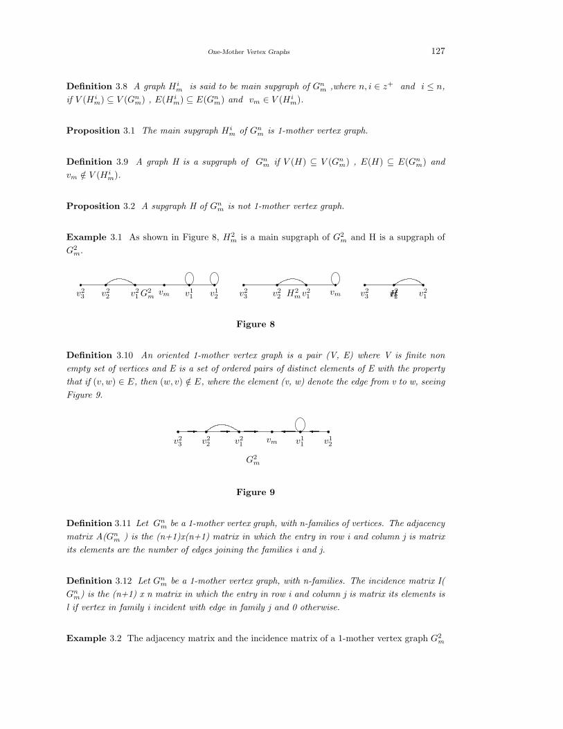
One-Mother Vertex Graphs 127
Definition 3.8 A graph Him is said to be main supgraph of Gn
m ,where n, i ∈ z+ and i ≤ n,
if V (Him) ⊆ V (Gn
m) , E(Him) ⊆ E(Gn
m) and vm ∈ V (Him).
Proposition 3.1 The main supgraph Him of Gn
m is 1-mother vertex graph.
Definition 3.9 A graph H is a supgraph of Gnm if V (H) ⊆ V (Gn
m) , E(H) ⊆ E(Gnm) and
vm /∈ V (Him).
Proposition 3.2 A supgraph H of Gnm is not 1-mother vertex graph.
Example 3.1 As shown in Figure 8, H2m is a main supgraph of G2
m and H is a supgraph of
G2m.
vm v21v2
1v22v2
3 v22v2
3vm v1
1 v12v2
1v22v2
3 G2m H2
m H
Figure 8
Definition 3.10 An oriented 1-mother vertex graph is a pair (V, E) where V is finite non
empty set of vertices and E is a set of ordered pairs of distinct elements of E with the property
that if (v, w) ∈ E, then (w, v) /∈ E, where the element (v, w) denote the edge from v to w, seeing
Figure 9.
vm v11 v1
2v21v2
2v23
- - - G2
m
Figure 9
Definition 3.11 Let Gnm be a 1-mother vertex graph, with n-families of vertices. The adjacency
matrix A(Gnm ) is the (n+1)x(n+1) matrix in which the entry in row i and column j is matrix
its elements are the number of edges joining the families i and j.
Definition 3.12 Let Gnm be a 1-mother vertex graph, with n-families. The incidence matrix I(
Gnm) is the (n+1) x n matrix in which the entry in row i and column j is matrix its elements is
l if vertex in family i incident with edge in family j and 0 otherwise.
Example 3.2 The adjacency matrix and the incidence matrix of a 1-mother vertex graph G2m

128 F. Salama
as shown in Figure 9 are given by
A(G2m) =
0 1 0 1 0 0
1 1 1 0 0 0
0 1 0 0 0 0
1 0 0 0 2 0
0 0 0 2 0 1
0 0 0 0 1 0
I(G2m) =
1 11 0 0 0 0
0 1 1 0 0 0
1 0 0 1 0 0
0 0 0 1 1 0
0 0 0 1 1 0
0 0 0 0 1 1
where the symbol 11in the matrix in the row 1 and column 2 of the incidence matrix means
that there exists a loop at the vertex v11with the edge e1
1.
Theorem A A complete 1-mother vertex graph is not defined.
Proof Let there exist a complete 1-mother vertex graph. Then this mean that every two
distinct vertices are joined which is contradict with the definition of the 1-mother vertex graph.
Hence the complete 1-mother vertex graph is not define.
New we will define the union of any 1-mother vertex graphs as follows:
Definition 3.13 The union of Gsm and Gv
m , denoted Gsm∪ Gv
m is the graph with vertex set
V1 ∪ V2 and edge set E1 ∪ E2.
Proposition 3.3 The union of any 1-mother vertex graphs is 1-mother vertex graph if vm ∈V1∩V2.
Proof Let we have two 1-mother vertex graphs, the union of these graphs has one of two
types.
1) If vm ∈V1 ∩ V2 , i.e. the new graph has one mother vertex, then the new graph is
1-mother vertex graph, seeing Figure 10.a.
2) If vm /∈V1 ∩ V2, i.e. the new graph has more than one mother vertex, then the new
graph is not 1-mother vertex graph, seeing Figure 10-b.
vm v11v2
1v22v2
3
H2m
G2m
-v21v2
2v23
vm v11 v1
2
union
v41v4
2v43 v3
1 v32
v23
v22
v21
v11
vm
H2m ∪ G2
m
Figure 10-a
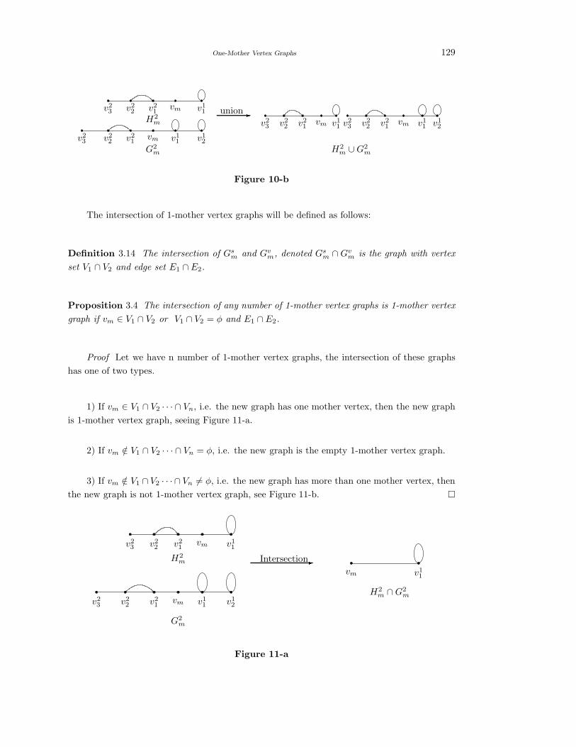
One-Mother Vertex Graphs 129
vm v11v2
1v22v2
3
H2m
G2m
-v21v2
2v23
vm v11 v1
2
unionvm v1
1v21v2
2v23 v2
3 v22 v2
1vm v1
1 v12
H2m ∪ G2
m
Figure 10-b
The intersection of 1-mother vertex graphs will be defined as follows:
Definition 3.14 The intersection of Gsm and Gv
m, denoted Gsm ∩ Gv
m is the graph with vertex
set V1 ∩ V2 and edge set E1 ∩ E2.
Proposition 3.4 The intersection of any number of 1-mother vertex graphs is 1-mother vertex
graph if vm ∈ V1 ∩ V2 or V1 ∩ V2 = φ and E1 ∩ E2.
Proof Let we have n number of 1-mother vertex graphs, the intersection of these graphs
has one of two types.
1) If vm ∈ V1 ∩ V2 · · · ∩ Vn, i.e. the new graph has one mother vertex, then the new graph
is 1-mother vertex graph, seeing Figure 11-a.
2) If vm /∈ V1 ∩ V2 · · · ∩ Vn = φ, i.e. the new graph is the empty 1-mother vertex graph.
3) If vm /∈ V1 ∩ V2 · · · ∩ Vn 6= φ, i.e. the new graph has more than one mother vertex, then
the new graph is not 1-mother vertex graph, see Figure 11-b.
vm v11v2
1v22v2
3
vm v11 v1
2v21v2
2v23
-H2m
G2m
Intersection
vm v11
H2m ∩ G2
m
Figure 11-a

130 F. Salama
vm v11v2
1v22v2
3
vm v11 v1
2v21v2
2v23
-H2m
G2m
Intersection
H2m ∩ G2
m
v21v2
2v23
Figure 11-b
In this section we will define special types of 1-mother vertex graphs.
Definition 3.15 A spider mother graph Snm is 1-mother vertex graph has the form as shown
in Figure 12.
vm
v11
v12
v13
v21
v22
v23
v31
v32
v33
vm v11
v12
v13
v14
v21
v22
v23
v24
v31
v32
v33
v34
v41
v42
v43
v44
(a) Spider mother graph with 3 families (b) Spider mother graph with 4 families
Figure 12
Note The least number of families which the spider graph has is three.
Definition 3.16 A tree mother graph T nm is 1-mother vertex graph has the form as shown in
Figure 13.
T 1m T 2
m T 3m T 4
m T 5m
Figure 13

One-Mother Vertex Graphs 131
Example 3.3 The adjacency matrix of the spider graph as shown in Figure 12-a are given by
0 1 0 0 1 0 0 1 0 0
1 0 1 0 1 0 0 1 0 0
0 1 0 1 0 1 0 0 1 0
0 0 1 0 0 0 1 0 0 1
1 1 0 0 0 1 0 1 0 0
0 0 1 0 1 0 1 0 1 0
0 0 0 1 0 1 0 0 0 1
1 1 0 0 1 0 0 0 1 0
0 0 1 0 0 1 0 1 0 1
0 0 0 1 0 0 1 0 1 0
the existence of the unit matrix in column I and raw j means that the family in the column I
and the family in the raw j have the relation between the vertices which have the same order.
Definition 3.17 An orbit mother graph is 1-mother vertex graph is a 1-mother vertex graph
containing no edges and the elements in the same family have the same distance from the mother
vertex, seeing Figure 14.
vm
v11
v12
v13
v21 v2
2
v31
v32
Figure 14
§4. Applications
(1) The solar system is orbit mother graph.
(2) If we illustrate the nervous system by using the graph we find that the nervous system is
1-mother vertex graph, seeing Figure 16.

132 F. Salama
Figure 16
References
[1] L. W. Beineke and R. J. Wilson, Selected Topics in Graph Theory(2), Academic press Inc.
LTD, London, 1983.
[2] A. Gibbons, Algorithmic Graph Theory, Cambridge University Press, com bridge, UK,
1985.
[3] P. J. Giblin, Graphs, Surfaces and Homology, an introduction to algebraic topology, Chap-
man and Hall I, td, London 1977.
[4] R. P. Grimaldi, Discrete and Combinatorial Mathematics, Addison-Wesley publishing Com-
pany. Inc,New York,1994.
[5] J. L. Gross and T. W. Tucker, Topological Graph Theory, Jon Wiley & Sons. Inc, Canada,
1987.
[6] A. T. White, Graph, Groups and Surfaces, Amsterdam, North-Holland, Publishing Com-
pany, 1973.
[7] R. J. Wilson, Introduction to Graph Theory, Oliver & Boyed, Edinburgh, 1972.
[8] R. J. Wilson, J. J. Watkins, Graphs, an introductory approach, a first course in discrete
mathematics, Jon Wiley & Sons Inc, Canada, 1990.

Perfect understanding will sometimes almost extinguish pleasure.
By A.E.Housman, a British scholar and poet

Author Information
Submission: Papers only in electronic form are considered for possible publication. Papers
prepared in formats, viz., .tex, .dvi, .pdf, or.ps may be submitted electronically to one member
of the Editorial Board for consideration in the International Journal of Mathematical
Combinatorics (ISSN 1937-1055). An effort is made to publish a paper duly recommended
by a referee within a period of 3 months. Articles received are immediately put the refer-
ees/members of the Editorial Board for their opinion who generally pass on the same in six
week’s time or less. In case of clear recommendation for publication, the paper is accommo-
dated in an issue to appear next. Each submitted paper is not returned, hence we advise the
authors to keep a copy of their submitted papers for further processing.
Abstract: Authors are requested to provide an abstract of not more than 250 words, lat-
est Mathematics Subject Classification of the American Mathematical Society, Keywords and
phrases. Statements of Lemmas, Propositions and Theorems should be set in italics and ref-
erences should be arranged in alphabetical order by the surname of the first author in the
following style:
Books
[4]Linfan Mao, Combinatorial Geometry with Applications to Field Theory, InfoQuest Press,
2009. [12]W.S. Massey, Algebraic topology: an introduction, Springer-Verlag, New York 1977.
Research papers
[6]Linfan Mao, Combinatorial speculation and combinatorial conjecture for mathematics, In-
ternational J.Math. Combin., Vol.1, 1-19(2007).
[9]Kavita Srivastava, On singular H-closed extensions, Proc. Amer. Math. Soc. (to appear).
Figures: Figures should be drawn by TEXCAD in text directly, or as EPS file. In addition,
all figures and tables should be numbered and the appropriate space reserved in the text, with
the insertion point clearly indicated.
Copyright: It is assumed that the submitted manuscript has not been published and will not
be simultaneously submitted or published elsewhere. By submitting a manuscript, the authors
agree that the copyright for their articles is transferred to the publisher, if and when, the
paper is accepted for publication. The publisher cannot take the responsibility of any loss of
manuscript. Therefore, authors are requested to maintain a copy at their end.
Proofs: One set of galley proofs of a paper will be sent to the author submitting the paper,
unless requested otherwise, without the original manuscript, for corrections after the paper is
accepted for publication on the basis of the recommendation of referees. Corrections should be
restricted to typesetting errors. Authors are advised to check their proofs very carefully before
return.

March 2011
Contents
Lucas Graceful Labeling for Some Graphs
BY M.A.PERUMAL, S.NAVANEETHAKRISHNAN AND A.NAGARAJAN . . . . . . . . . 01
Sequences on Graphs with Symmetries
BY LINFAN MAO . . . . . . . . . . . . . . . . . . . . . . . . . . . . . . . . . . . . . . . . . . . . . . . . . . . . . . . . . . . . . . . . . . 20
Supermagic Coverings of Some Simple Graphs
BY P.JEYANTHI AND P.SELVAGOPAL . . . . . . . . . . . . . . . . . . . . . . . . . . . . . . . . . . . . . . . . . . . 33
Elementary Abelian Regular Coverings of Cube
BY FURONG WANG AND LIN ZHANG. . . . . . . . . . . . . . . . . . . . . . . . . . . . . . . . . . . . . . . . . . . .49
Super Fibonacci Graceful Labeling of Some Special Class of Graphs
BY R.SRIDEVI, S.NAVANEETHAKRISHNAN AND K.NAGARAJAN. . . . . . . . . . . . . . 59
Surface Embeddability of Graphs via Tree-travels
BY YANPEI LIU. . . . . . . . . . . . . . . . . . . . . . . . . . . . . . . . . . . . . . . . . . . . . . . . . . . . . . . . . . . . . . . . . . . . 73
Edge Maximal C3 and C5-Edge Disjoint Free Graphs
BY M.S.A.BATAINEH AND M.M.M.JARADAT . . . . . . . . . . . . . . . . . . . . . . . . . . . . . . . . . . . . 82
A Note on Admissible Mannheim Curves in Galilean Space G3
BY S.ERSOY, M.AKYIGIT AND M.TOSUN . . . . . . . . . . . . . . . . . . . . . . . . . . . . . . . . . . . . . . . . 88
The Number of Spanning Trees in Generalized Complete Multipartite Graphs
of Fan-Type BY JUNLIANGE CAI AND XIAOLI LIU . . . . . . . . . . . . . . . . . . . . . . . . . . . 94
A Note on Antipodal Signed Graphs
BY P.SIVA KOTA REDDY, B.PRASHANTH AND KAVITA S.PERMI . . . . . . . . . . . . 107
Group Connectivity of 1-Edge Deletable IM-Extendable Graphs
BY KEKE WANG, RONGXIA HAO AND JIANBING LIU . . . . . . . . . . . . . . . . . . . . . . . . 113
A Note On Line Graphs
BY P.SIVA KOTA REDDY, KAVITA. S. PERMI AND B.PRASHANTH . . . . . . . . . . . 119
One-Mother Vertex Graphs
BY F.SALAMA . . . . . . . . . . . . . . . . . . . . . . . . . . . . . . . . . . . . . . . . . . . . . . . . . . . . . . . . . . . . . . . . . . . . 123
An International Journal on Mathematical Combinatorics