mathematical ecology - lehr- und forschungseinheit …kuttler/script_mathoek.pdf · model is e.g....
TRANSCRIPT

Mathematical Ecology
Christina Kuttler
Sommersemester 2010

Contents
1 Unstructured Population Models 21.1 Single-Species Models . . . . . . . . . . . . . . . . . . . . . . . . . . . . . . . . . . . . . . 2
1.1.1 Basics: Exponential, logistic and Gompertz growth . . . . . . . . . . . . . . . . . . 21.1.2 Sigmoid growth, fitting . . . . . . . . . . . . . . . . . . . . . . . . . . . . . . . . . 41.1.3 Allee effect . . . . . . . . . . . . . . . . . . . . . . . . . . . . . . . . . . . . . . . . 111.1.4 Harvest models: bifurcations and breakpoints; optimal control theory . . . . . . . 151.1.5 Stochastic birth and death processes . . . . . . . . . . . . . . . . . . . . . . . . . . 301.1.6 Metapopulations / Island-Mainland Model . . . . . . . . . . . . . . . . . . . . . . 341.1.7 Discrete-time models . . . . . . . . . . . . . . . . . . . . . . . . . . . . . . . . . . . 371.1.8 Delay models . . . . . . . . . . . . . . . . . . . . . . . . . . . . . . . . . . . . . . . 41
1.2 Interacting Populations . . . . . . . . . . . . . . . . . . . . . . . . . . . . . . . . . . . . . 451.2.1 Aquatic population interacting with a polluted environment . . . . . . . . . . . . . 451.2.2 Interactions between two populations: the prototypes . . . . . . . . . . . . . . . . 531.2.3 Some classics: Predator-prey; cycles, global bifurcations . . . . . . . . . . . . . . . 541.2.4 Competition models . . . . . . . . . . . . . . . . . . . . . . . . . . . . . . . . . . . 651.2.5 Mutualism models . . . . . . . . . . . . . . . . . . . . . . . . . . . . . . . . . . . . 69
2 Structured Population Models 712.1 Spatially structured models . . . . . . . . . . . . . . . . . . . . . . . . . . . . . . . . . . . 71
2.1.1 Mathematical treatment of biological diffusion . . . . . . . . . . . . . . . . . . . . 712.1.2 Spatial steady states . . . . . . . . . . . . . . . . . . . . . . . . . . . . . . . . . . . 732.1.3 Models of spread / Examples of Animal Diffusion . . . . . . . . . . . . . . . . . . . 792.1.4 Animal movements in Home range . . . . . . . . . . . . . . . . . . . . . . . . . . . 822.1.5 Some ideas for the dynamics of animal grouping . . . . . . . . . . . . . . . . . . . 89
2.2 Age-Structured models . . . . . . . . . . . . . . . . . . . . . . . . . . . . . . . . . . . . . . 922.2.1 Overview . . . . . . . . . . . . . . . . . . . . . . . . . . . . . . . . . . . . . . . . . 922.2.2 Difference equation . . . . . . . . . . . . . . . . . . . . . . . . . . . . . . . . . . . . 922.2.3 Leslie matrix . . . . . . . . . . . . . . . . . . . . . . . . . . . . . . . . . . . . . . . 932.2.4 Lotka integral equation . . . . . . . . . . . . . . . . . . . . . . . . . . . . . . . . . 932.2.5 McKendrick- von Foerster PDE . . . . . . . . . . . . . . . . . . . . . . . . . . . . . 942.2.6 Comparison of these modelling approaches . . . . . . . . . . . . . . . . . . . . . . . 97
2.3 Sex-structured models . . . . . . . . . . . . . . . . . . . . . . . . . . . . . . . . . . . . . . 972.3.1 Two-sex models . . . . . . . . . . . . . . . . . . . . . . . . . . . . . . . . . . . . . . 97
Literature 97
1

Chapter 1
Unstructured Population Models
In some ecological problems, it is sufficient to consider populations without further structure.
1.1 Single-Species Models
1.1.1 Basics: Exponential, logistic and Gompertz growth
[6]
In this section, we deal with the most simple population models: just one homogeneous populationis considered.Let N(t) describe the number of individuals which belong to the population. Then dN/dt denotes the“rate of change” and 1
N dN/dt denotes the “per capita rate of change”.
First model assumption: Only births and deaths influence the change of population. The two ratesb (for the per capita birth rate) and d (for the per capita death rate) are constant:
1
N
dN
dt= b − d.
By introducing the so-called “intrinsic rate of growth” r = b − d, this equation can be reformulated:
dN
dt= rN.
Including an initial conditionN(0) = N0
(which describes the number of individuals which are present at the beginning of the observation) leadsto an initial value problem, with a unique solution:
N(t) = N0ert.
Three cases can be distinguished:
• r > 0: exponential growth
• r < 0: exponential decay
• r = 0: constant population size
It can be interesting to consider the dependency of e.g. the per capita growth rate and the (whole)population growth rate:
Population growth rateper capita growth rate
NN
rrN
2

We observe: The per capita growth rate is constant - which means: there is no influence of the populationsize on the individuals and their “behaviour”. The population growth rate is always increasing (which isnot realistic for long times)!
There is just one stationary point: N∗ = 0, which is obviously stable (even asympotically stable) forr < 0, respectively unstable for r > 0.
Obviously, there are several problems with this approach:
• unlimited growth
• stochastic effects (especially for small population sizes) were ignored
• time lags were ignored (the population growth may depend on the population size some time ago)
• further structure (like temporal and spatial variability) was ignored
During the lecture, we will try to find more realistic models which address also these problems.In the next step we want to include a limitation of growth into the model. But how? In the historicaldevelopment two main hypotheses were considered:
• the main limiting influence is caused by “biotic factors” like competition for ressources - they havea bigger influence in case of large populations
• the abiotic factors like weather changes play a major role - they influence small populations in thesame way as large populations.
In the next step, we deal with the hypothesis of intraspecies competition for ressources. Simple approach:The per capita growth rate decreases linearly with the size of the population, or (ending up in the samemathematical model) the per capita death rate increases (linearly) for an increasing population size:d = d0 + d · N . Introducing the so-called carrying capacity K allows another notation: d = r/K, so weend up with the model equation
1
N
dN
dt= r
(
1 − N
K
)
Correspondingly, the population growth rate reads
dN
dt= rN
(
1 − N
K
)
=: f(N), (1.1)
with the graph
NK
Equation (1.1) is called the “Verhulst equation” or the “logistic equation”. The explicit solution can becomputed:
N(t) =K
1 +(
KN0
− 1)
e−rt
Some more properties:Obviously, the logistic growth model has two stationary points N1 = 0 and N2 = K, we check also theirstability:
3

N’ = f(N)
NK/2 K
Zeros of f(N) stationary pointsf(N) positive: Arrow to the rightf(N) negative: Arrow to the left.
This is the “visualisation” of the well-known analytical criterion: Let N a stationary point.
f ′(N) < 0: N stable stationary pointf ′(N) > 0: N unstable stationary point.
Remark: Near N = 0, there is dNdt ≈ rN , i.e. nearly exponential growth. The saturation/limitation of
growths starts to play a role only for larger values of N ; near N = K, there is dNdt ≈ 0, nearly no growth
anymore.
The Verhulst equation belongs to a more general class of models, the so-called Bernoulli’s equation:
dN
dt= r(t)N − d(t)NΘ+1,
where r(t) = b(t) − d0(t) is again an intrinsic rate of growth.
An alternative approach is the so-called Gompertz equation:
dN
dt= r0e
−αtN,
where it is assumed that the intrinsic rate of growth decays exponentially. In the ecological context, thismodel is e.g. used for the growth of plants, or for some fishery ecology problems.Remark: The Gompertz equation is a non-autonomous ODE, i.e. there is a parameter which dependsexplicitely on time t. So, some typical tools for the analysis cannot be used since they are only valid oruseful for autonomous ODEs.
Of course, there are many other approaches for a limited population growth, which are used for spe-cial cases - not all can be considered here in detail, e.g.
• Beverton-Holt:
N = N1 − N
1 + αN, where α ≥ 0
• Ricker:
N = Neγ(1−N) − 1
eγ − 1, where γ ≥ 0
1.1.2 Sigmoid growth, fitting
(aus Thieme) [10]
All models for limited population growth which we considered up to now (Verhulst, Beverton-Holt,Ricker), show an S-shaped growth (also called “sigmoid growth”). Furthermore, there exist two station-ary points: N = 0 and a further N > 0; first with a convex increase, later with a concave increase. Thus,one can consider a more general class of growth models, for sigmoid growth. Hence, we consider specialcases of the ODE
N = f(N),
where f has the following properties:
4

1. f is continuous on [0,∞) and continuously differentiable of (0,∞).
2. f(0) = 0 (no population ; no growth)
3. f(N) < 0 for some N > 0 (i.e. decrease happens for (large) populations)
4. there is at most one N > 0 where f ′(N) = 0 (only one change from convex to concave shapepossible)
5. ρ := limx→0+(f(x)/x) exists (but possibly infinite), and f(N)/N < ρ for all N > 0. (ρ correspondsto the intrinsic rate of natural increase, which appears here for N ≈ 0; i.e. corresponding to r inthe preceding section).
Next, we mention a theorem which will be useful to find some properties of the model solutions:
Theorem 1 Let f : (0,∞) → R be continuously differentiable, the initial value N0 ∈ (0,∞). Then, thereexists an interval (a, b) (with a ∈ [−∞, 0) and b ∈ (0,∞]) and a strictly positive, unique solution N ofthe initial value problem
N = f(N) ( on (a, b))
N(0) = N0,
with the following properties:
(i) If f(N0) = 0, then N is constant.If f(N0) > 0, then N is strictly monotone increasing on (a, b).If f(N0) < 0, then N is strictly monotone decreasing.
(ii) If c ∈ a, b is finite, then N(t) → ∞ or N(t) → 0 as t → c, t ∈ (a, b).
(iii) If c ∈ a, b is not finite, then N(t) → ∞, or N(t) → 0, or N(t) → K ∈ (0,∞).
Proof: Due to the properties of the right hand side function f , local existence and uniqueness of solution(N) follows immediately. Furthermore, there is an interval (a, b) with a < 0 < b, such that this solutionN (with N(0) = N0) is strictly positive inside that interval.In case of f(N0) = 0, then N(t) = N0 on (a, b), the solution can be extended to R.In case of f(N0) > 0, then we find f(N(t)) > 0 for all t ∈ (a, b) (this follows from the intermediate valuetheorem: If not, then there were a value t0 ∈ (a, b) such that f(N(t0)) = 0; by the uniqueness theoremit would follow that N = N(t0) on (a, b), but 6= N0, which is a contradiction).Thus we get: N ′ = f(N) is strictly positive, by that N is strictly increasing on (a, b). Furthermore, thelimits of N(t) for t → b or t → a exist in [0,∞].If these limits are in (0,∞), then the solution can be extended beyond a or b, respectively (due to thelocal existence and uniqueness theorem) - iterating this process and taking the union of all open intervals(around 0), for which solutions of the initial value problem N ′ = f(N), N(0) = N0 exist, we end up witha unique solution N on an interval (a, b) which cannot be extended anymore to a larger interval. Twopossibilities:
• a and b are not finite (corresponds to (iii)) OR
• the limits of N in a and b are 0 or ∞ (corresponds to (ii)).
In case (iii): One possibility is b = ∞, limt→∞ N(t) = K ∈ (0,∞). Due to f(N(t)) > 0 for all t ∈ (a,∞),we have f(K) ≥ 0. Assume that f(K) > 0. Then we can find a r > a and ǫ ∈ (0, f(K)), such thatN ′(t) = f(N(t)) ≥ ǫ for all t ≥ r. By that, we would get for all t ≥ r:
N(t) ≥ N(r) +
∫ t
r
N ′(s) ds ≥ N(r) + ǫ(t − r),
which means N(t) → ∞ for t → ∞ - this is a contradiction to the assumption, by that only f(K) = 0 ispossible.In the same way, the case a = −∞ can be considered.And the proof can be done similarly for the case of f(N0) < 0, just with an decreasing N .
2
5

The next lemma helps to find the influence of the “intrinsic rate of natural increase”, ρ, on the behaviourof the system.
Lemma 1 Let f show the properties of sigmoid growth.
(a) If ρ ≤ 0, then f(N) < 0 for all N > 0.If ρ < 0, then f ′(N) < 0 for all N > 0 with the possible exception of one point.
(b) If ρ > 0, then there exist uniquely determined numbers
K > L > 0 such that f(K) = 0 and f ′(L) = 0.
Moreover, f is strictly positive on (0,K) and strictly negative on (K,∞), while f ′ is strictly positiveon (0, L) and strictly negative on (L,∞).
(The proof can be done with similar arguments as Theorem 1, is left out here)
Remark 1 (Carrying capacity and population size with maximum growth) K is already knownas “carrying capacity”. L is called the “population size with maximum growth”.What is a typical ratio of K and L in our model examples?
• Verhulst equation: K/L = 2
• Beverton-Holt: K/L > 2
• Gompertz: K/L = e
Up to now, we still do not know, if N = f(N) with the right hand side f satisfying the properties 1.-5.really shows sigmoid growth. This will be checked in the next theorem!
Theorem 2 Let f satisfy the properties 1.-5., where ρ > 0, and N = f(N). Then the following state-ments hold:
(a) Let N(0) ∈ (0,K). Then, there exists a unique nonnegative solution N (defined on R) with theproperties
N(t) → 0 for t → −∞ and N(t) → K for t → ∞,
it is nondecreasing in t, and strictly increasing in case of N > 0.Furthermore, N(t) is
• strictly convex, if 0 < N(t) < L and
• strictly concave, if L < N(t) < K.
(b) Let N(0) > K. Then, there exists a unique solution N (defined on an interval (a,∞)), with
N(t) → ∞ for t → a, and N(t) → K for t → ∞.
N(t) is a strictly decreasing, convex function of t.
This means: N indeed has a graph like this:
K
L
t
N(t)
a
6

Proof: For the proof, we need several times theorem 1.Let N(0) > 0. From the theorem, we know that there exists a unique strictly positive and strictlymonotone solution N(t), which is defined on (a, b) with a ∈ [−∞, 0) and b ∈ (0,∞], N behaves at theendpoints as described in the theorem.
(a) Case N(0) ∈ (0,K). Obviously, N = K (constant) is a solution of N ′ = f(N), and f is continuouslydifferentiable in a neighborhood of K. So, uniqueness of solutions yields that N(t) < K for allt ∈ (a, b).We know that f(N) > 0 for N ∈ (0,K); so since N ′ = f(N) we get that N is strictly monotoneincreasing. Furthermore, it has an upper bound at K on (a, b). The theorem yields then: b = ∞and limt→∞ N(t) = K.For a = −∞, one gets limt→−∞ N(t) = 0 (in a similar way).For a > −∞, the theorem yields N(a+) = 0 and N is strictly increasing. The solution can beextended by setting N(t) = 0 for t ≤ a (then N is continuously differentiable on R, and satisfiesthe ODE.Furthermore,
N ′′ = (f(N))′ = f ′(N)N ′ = f ′(N)f(N).
Due to Lemma 1 (and f(N) > 0 for N ∈ (0,K)), f ′ is strictly positive on (0, L) and strictly negativeon (L,∞) with L < K.; N ′′ = f ′(N)f(N) > 0 as long as N ∈ (0, L); respectively N ′′ < 0 as soon as N ∈ (L,K).
(b) Case N(0) > K. Uniqueness yields N(t) > K for all t ∈ (a, b) ; f(N(t)) < 0 for all t ∈ (a, b) andN(t) is strictly decreasing. Theorem 1 implies then b = ∞. In a similar way to above, one canshow that limt→∞ N(t) = K. Due to N > K > L (hence f(N) < 0 and f ′(N) < 0), we get
N ′′ = f ′(N)f(N) > 0,
which means that N is strictly convex.In case of a > −∞, theorem 1 yields limt→a+
N(t) → ∞.In case of a = −∞, it is limt→−∞ N(t) → ∞ (N is strictly decreasing AND strictly convex on R).
2
A short “excurs”, concerning integrability:As we have seen above (part (a) of the preceding theorem), it is possible to have a solution N on theinterval (a,∞), a < 0, such that N is strictly positive on (a,∞) and limt→a+ N(t) = 0. Question: Is itpossible to determine a somehow?For that, we use the following approach (separating the variables):
∫ N(t)
N(0)
1
f(x)dx =
∫ t
0
N ′(s)
f(N(s))ds = t, where a < t < 0.
Here we take the limit t → a and get:
a =
∫ 0
N(0)
1
f(x)dx. (1.2)
Obviously, a is finite in case of the improper integral being finite. Vice versa, if the integral is infinite, Nis strictly positive in R.Terminology:1/f(x) is called integrable at 0, if there is a M (> N0) > 0, such that f doesn’t change sign on (0,M)and ∫ M
0
dx
|f(x)| < ∞.
So, this “criterion” helps to decide what happens with the solution:
• If 1/f(x) is not integrable at 0, then all these solutions are positive on R.
• If 1/f(x) is integrable at 0, then all solutions are 0 on some interval (−∞, a) (a depends on theinitial data, can be computed by (1.2)).
7

On the other hand (referring to part (b) of the preceding theorem), the solution is defined on an interval(a,∞), where a < 0 and limt→a+ N(t) → ∞. Again, we have
∫ N(t)
N(0)
dx
f(x)= t, where a < t < 0.
We take the limit t → a and get:
a =
∫ ∞
N(0)
dx
f(x).
Finding a finite value a by the integral, means, that there is “blow-up” at a finite backward time (namelya). In case of an infinite integral, N is defined on R. Again we can distinguish between the two cases,using a similar terminology for integrability as above. We say:
• 1/f(x) is integrable at ∞, if there exists a (N0 >) M > 0 such that f doesn’t change its sign on(M,∞) and
∫ ∞
M
dx
|f(x)| < ∞. (1.3)
• 1/f(x) is not integrable at ∞, if M exists as before, but with an infinite integral (1.3).
So, the following two cases can be distinguished for initial data > K:
• If 1/f(x) is integrable at ∞, then there is a finite a with limt→a+ N(t) → ∞ (i.e. there is a blow-upat a finite backward time).
• If 1/f(x) is not integrable at ∞, then limt→−∞ N(t) → ∞ (i.e. the solutions exist for complete R).
The next lemma provides a nice criterion, how to check for that integrability by using ρ.
Lemma 2 If ρ = limx→0+f(x)
x is finite, then 1/f(x) is not integrable at 0.
(The proof is left out here, but can be found in [10])
Taken together, we end up with the following useful theorem:
Theorem 3 Let N ′ = f(N), f satisfying the conditions 1.-5. (as above). Let ρ ≤ 0 and N(0). Then, aunique solution exists on the interval (a,∞), where a ∈ [−∞, 0), such that
N(t) → ∞ for t → a + and N(t) → 0 for t → ∞.
N(t) is strictly decreasing in t.In case of ρ < 0, then N is also strictly convex.a > −∞ is true if and only if 1/f(x) is integrable at ∞.
Up to now, we collected a lot of (theoretical) knowledge and examples of models which show sigmoidgrowth.
Question: Do these models have anything to do with reality? What happens, if we consider real worlddata, is it possible to fit such models to data?
Another property of populations with sigmoid growth: They can be rewritten in the following form:
N = Ng(N), N > 0,
where the function g(N) = f(N)/N is strictly decreasing for N > 0.Thus, d
dt ln(N(t) is strictly decreasing ⇔ lnN(t) is strictly concave (the so-called “logarithmic convex-ity”) ⇔ N(t + h)/N(t) is strictly decreasing in t (for an arbitrary h > 0).By checking the logarithmic convexity of N , we can get a guess, if the data can be expected to be fittedwell (by a model for sigmoid growth).
Test data (from McKendrick / Kesava Pai, 1911; taken from [10]): Population growth of Escherichiacoli (bacteria)
8

time (h) 0 0.5 1 2 3 4 5 6 7 8number (millions) 0.176 0.280 0.608 3.87 28.2 74.2 127 150 149 154
First, we consider the corresponding data plots:
0 1 2 3 4 5 6 7 80
20
40
60
80
100
120
140
160
0 1 2 3 4 5 6 7 810
−1
100
101
102
103
On the left hand side: original data; on the right hand side: natural logarithm of the data .
Observation: The logarithmic data plot is convex (and not concave) at the beginning. This means: Inthe early stage of the experiment, the bacteria grow “slower than expected”. But since the deviationis not very large (and can be explained e.g. by adaptation processes), it might be still possible to fit asigmoid growth model to the data.K can be guessed (to some extent) directly from the data, e.g. K ≈ 154.By just looking at the data, it seems that L (the value where the growth curve switches from convexityto concavity) is aroung K/2. So, no contradiction to the logistic growth, which will be used as a firstapproach:
N = ρN
(
1 − N
K
)
(using now the notation with ρ).
We use y = N/K in the following (which means: normalise the population by the capacity K), thisyields
y =N
K=
1
KρN
(
1 − N
K
)
= ρy(1 − y)
In the next step, we rewrite this equation by separating the variables and using partial fractions:
y = ρy(1 − y) ⇔ y
y(1 − y)= ρ
⇔ y(1 − y) + yy
y(1 − y)= ρ
⇔ ρ =y
y+
y
1 − y
Advantage: The last equation can be easily integrated and yields
k + ρt = ln y − ln(1 − y)
What does that mean? If we take the normalised data (i.e. divide them by K) and insert them into theright hand side of the last equation, they should be plotted more or less on a straight line. The plot:
0 1 2 3 4 5 6 7 8−8
−6
−4
−2
0
2
4
6
8
9

Remark: There seems to be one data point (7.149), which seems to be “extraordinary” - maybe it canbe left out for the fitting procedure. In the “original data plot”, the deviation is not so clear to see.
Advantage: (Least square) Fitting of a straight line is much easier that fitting of a nonlinear equa-tion; and simpler than fitting of an ODE-solution, which is maybe not explicitely available.
By such a fitting procedure (e.g. using MATLAB), we get the following parameter values:
k ≈ −7.00438 and ρ = 1.727
resulting in the following plot:
0 1 2 3 4 5 6 7 8−8
−6
−4
−2
0
2
4
6
8
0 1 2 3 4 5 6 7 80
20
40
60
80
100
120
140
160
(left hand side: fitting of the straight line; right hand side: resulting solution curve)
In the next step, we want to check, if an even better fit is possible. So we test, if the Beverton-Holtequation could fit better to the data. The model can be formulated e.g. by
N = ρN
(1 − N
K
)
(1 − αN)
We use the same procedure as above: first normalise the population size by K, i.e. y = NK (and introduce
a = 1 + αK as short notation):
y =ρy(1 − y)
(1 + αKy)=
ρy(1 − y)
(1 − αKy)
In the next step, the variables are separated:
ρ =y(1 − y) + a · yy
y(1 − y))=
y
y+ a
y
1 − y
Integration yields in this case:k + ρt + a ln(1 − y) = ln y.
Applying again a least-squares fit results in the following parameter values:
k ≈ −7.0577, ρ ≈ 1.7654, a ≈ 1.05.
The resulting plot is
0 1 2 3 4 5 6 7 80
20
40
60
80
100
120
140
160
Of course, one could try also other (sigmoid growth) models in the same way.Question: Why is the Gompertz equation no suitable approach for these data? ; Exercises
10
1.1.3 Allee effect
Reference: [10]
There are two works of Allee (1931, 1951) which gave the name to the Allee effect. The basic ideais a kind of “fine tuning” for the dependency of the population growth for small population levels. Up tonow, the basic assumption was that an increasing population density has a negative effect on reproduction/ survival of a single individual. But for some cases it makes sense that for low population densities anincrease in density is beneficial. Models, which take that into account, are called “Allee type models”.
Where does this effect come from? There are two possibilities:
• It may be necessary to find a mate for reproduction, but the meeting probability may be low incase of small populations
• It may be necessary to defense the group against a (so-called “generalist”) predator, for that alarger group has advantages.
The model structure is based on a sigmoid growth model plus an extra trem describing the extra mortality,which decreases with increasing population density.Taking the Verhulst model as basis, the model can look like that:
N ′ = φN
(
1 − N
K− η
1 + γN
)
.
Next we follow that first idea, including the search for a mate.Model assumption: The sex ratio in the population is around 1:1. Let N denote the female populationsize. It is splitted into two subpopulations:
• N1: female population with a mate ; able to reproduce
• N2: female population without a mate ; no reproduction possible at the moment
(of course N = N1 + N2). We need to introduce some reproduction and mortality rates:β : per capita reproduction rate for N1 (only female offspring is considered)µ + νN : per capita mortality of N1
µ + λ + νN : per capita mortality of N2.(λ is a kind of “extra mortality rate” for the females searching for a mate: she has to move more and isexposed to higher risks like predation or accidents)
Further processes: Switch from N1 to N2 is assumed to happen at a constant rate σ (leading to anexponentially distributed stay in the “reproductive phase”, mean time 1/σ).Vice versa, the switch from N2 to N1 depends on the probability to meet one of N males, i.e. the percapita rate for the meeting can be formulated as ξN . We get the following basic system:
N ′1 = βN1 − (µ + νN)N1 − σN1 + ξNN2
N ′2 = −(µ + λ + νN)N2 + σN1 − ξNN2.
(Not so clear: Why is reproduction only for N1?)The system can be reformulated in terms of N and N2:
N ′ = βN − (µ + νN)N − (β + σ)N2,
N ′2 = −(µ + λ + νN)N2 + σ(N − N2) − ξNN2.
As for the logistic model, we introduce the carrying capacity K = νβ−µ (under the assumption that
β > µ), then the system reads
N ′ = (β − µ)N
(
1 − N
K
)
− (β + λ)N2,
N ′2 = −(µ + λ + νN)N2 + σ(N − N2) − ξNN2.
In the next step, we nondimensionalise the system (i.e. the goal is to use dimensionless variables andparameters). For that, we use
N = xK, N2 = yK,
11

(the new variables are x and y, which are dimensionless variables, in relation to the carrying capacityK).Also the time can be rescaled, using s = µt as new dimensionless time (1/µ as reference time is the lifeexpectancy under ideal conditions). Notation: x, y as derivatives with respect to s. Furthermore two“short notations” are used:
ε =µ
σ, R0 =
β
µ
The resulting rescaled system reads
x = R0 − 1)x(1 − x) − β + λ
µy
εy = −εy − λ
σy − ν + ξ
σKxy + x − y
Some ecological considerations: The average time to be reproductive after mating and the average timefor finding a mate at condition N = K are very short, compared to the average life expectancy of afemale. In mathematical terms:
1
σ,
1
ξK≪ 1
µ
equivalent toσ, ξK ≫ µ
The number of female offspring per female during lifetime (R0) is assumed not to be very large. Theseassumptions result in
0 < ε ≪ 1
In the next step, we use the so-called “quasi-steady-state” approximation ε → 0, which means that they population adapts more or less immediately to the given value of x (which evolves much more slowly).(The theory behind this procedure is the singular perturbation theory; here we use it only formally - inprinciple, the analysis could also be done with the 2D ODE system). The system reads
x = (R0 − 1)x(1 − x) − β + λ
µy
0 = x − y − λ
σy − (ν + ξ)K
σxy.
The second equation is solved for y:
y =x
1 + (λ/σ) + (ν + ξ)(K/σ)x
and inserted into the x equation:
x = (R0 − 1)x(1 − x) − β + λ
µ
x
1 + (λ/σ + ((ν + ξ)K/σ)x.
scaling back to the original variable N and time t yields the above-mentioned
N ′ = φN
(
1 − N
K− η
1 + γN
)
, (1.4)
with the short notations
φ = β − µ, η =β + λ
µ
1
1 + (σ/σ)=
β + λ
µ + ελ, γ =
ν + ξ
σ + λ.
The same model structure is gained by an approach, where a generalist predator is present (generalistpredator means, that he “eats” the considered population as prey, but not as the one and only foodsource. I.e. the generalist predator does not die out in case of vanishing prey of that certain species).
Now we consider the Allee type model from a mathematical point of view.Again, we us a rescaling:
x = γN
12

Using x, the equation (1.4) becomes
x′ = φx
(
1 − x
γK− η
1 + x
)
.
Also the time variable is rescaled, we use (as before) s = tφ respectively s = t/φ. Differentiation withrespect to the new time s is denoted by x, so we end up at
x = x
(
1 − x
M− η
1 + x
)
=: f(x) (with M = γK) (1.5)
Stationary points:
x = 0 or 0 = 1 − x
M− η
1 + x.
It depends on η, if there are further solutions x > 0 of this equation. In order to examine that, we solveup the right equation for η:
η =(
1 − x
M
)
· (1 + x) =1
M(M − x)(1 + x),
a concave parabola (as function of x). We can also find out the maximum of the parabola, e.g. bydifferentiating η with respect to x:
dη
dx= −2x
M+ 1 − 1
M,
thus
0 =dη
dx⇔ 1 =
2xmax
M+
1
M⇔ xmax =
1
2(M − 1)
The corresponding η is
ηmax =1
M
(1
2(M + 1)
)2
The plot x over η looks like that:
x
η
turning point
1
Equilibria over extra mortality
It shows the position of stationary points (=equilibria), dependent on the parameter η (the extra mor-tality).Remark: The η value which corresponds to x = 0 (i.e. η = 1) is quite interesting, since there, two branchesof equilibria intersect: the branch of positive equilibria and the “extinct population equilibrium”. Thus,the point (1, 0) in the (η, x) plane is called a bifurcation point. (ηmax, xmax) is called “turning point”,since the branch of nontrivial solutions obviously changes its direction at that point.In the following, we consider only the case, where M > 1 - otherwise, there is no significant effect, justat most one positive equilibrium.¿From the graph / the properties of η(x) we get the following Lemma:
13

Lemma 3 Let M > 1.Case 1: η > ηmax. Then there exists no positive equilibrium.Case 2: 1 < η < ηmax. Then there exist two positive equilibria.Case 3: 0 ≤ η ≤ 1. Then there exists exactly one positive equilibrium.
Some more analysis of the qualitative behaviour for the case 1 < η < ηmax. There, we have two positiveequilibria, which are denoted by x1 and x2 (without loss of generality, they are sorted as 0 < x1 < xmax <x2).Observation: Due to
f ′(0) =
(
x
(
1 − x
M− η
1 + x
))′
|x=0 = 1 − η
we find: ρ = f ′(0) < 0.Of course, also the equilibria can be computed, dependent on η. We get:
0 = 1 − x
M− η
1 + x⇔ M(1 + x) − x(1 − x) − Mη = 0
⇔ x2 + (1 − M)x + M(η − 1) = 0
⇔ x1,2 =M − 1 ±
√
(1 − M)2 − 4M(η − 1)
2.
With these explicit formula, one can compute:
x1 + x2 + 1 = M and (similarly) η = 1 +x1x2
1 + x1 + x2
Hence, equation (1.5) can be rewritten:
x =x
M(1 + x)((M − x)(1 + x) − Mη)
=x
1 + x
(x2 − x)(x − x1)
1 + x1 + x2. (1.6)
In this formulation, the qualitative behaviour can be seen quite directly:For x ∈ (0, x1), the right-hand side of (1.6) is strictly negative.For x ∈ (x1, x2), the right-hand side of (1.6) is strictly positive.For x > x2 it is again strictly negative.Due to the locally Lipschitz continuous right-hand side of (1.6), there is uniqueness of solutions, thus theequilibrium solutions cannot be crossed somehow.So, the behaviour for t → ∞ can be described, dependent on the initial values (denoted by x0):x0 ∈ (0, x1) ; solutions tend to 0x0 ∈ (x1,∞) ; solutions tend to x2.Since the solution branch x1 “separates” two types of solutions, it is called “separatrix”, or also “wa-tershed equilibrium”. (Or, in case of a disease as “population”, like the pest, it is called the breakpointdensity).The situation shows up bistability, which means: there are two stable equilibria present in the system.The initial data “decide” two which one of the stable equilibria the solution will tend to in the long timerun.
Let’s have a look at the solution curves!
x
x2
x1
t
14

In case of x0 ∈ (x1, x2), the solution has the shape of a sigmoid function. This can also be shown,similarly to the preceding section.
A short observation for the limit case η = ηmax: Obviously, there is just one equilibrium > 0 present,which corresponds to the turning point xmax. The solution behaviour looks as follows in that case:
x
x2
t
x1xmax
For x0 ∈ [xmaxm∞), the solution approaches xmax.For x0 ∈ [0, xmax), the solution approaches 0.So, there is no surprise, how this kind of equilibrium is called: semistable.
The last remaining case is quite boring: 0 ≤ η ≤ 1. There, the solutions always tend to the oneand only nontrivial equilibrium, similar to the standard logistic model.
Remark: Of course, also other sigmoid growth models can be taken as basis model, where the extramortality is added!
1.1.4 Harvest models: bifurcations and breakpoints; optimal control theory
In this section we want to deal with the situation of a population (underlying again a sigmoid growth),which is additionally harvested. In this context, we do not consider the situation of a predator population,which depends solely on the harvested population, but have in mind for example the situation of fishery:people like to eat fishes, but have also further food. The goal is to examine the consequences of harvestingon the harvested population.As basis for the sigmoid growth, we choose the logistic equation - mainly for reasons of simplicity. Ofcourse, also other approaches can be chosen, dependent on the behaviour of the population.
Bifurcations and Breakpoints
First, we need a short excurs in the meaning of bifurcations: As shortly seen in the section concerningthe Allee effect, equilibria can change their positions, exchange stability behaviour, or also vanish orappear. The resulting (qualitative) changes in the behaviour of the considered dynamical system arecalled bifurcations.As an example we consider a very simple fish population, which grows according to the logistic growth,and which is harvested. A further variable is introduced: E, the so-called fishing effort. First assumption:The catch of fish per unit effort is proportional to the availably amount of fish, N : Thus, a very simplemodel reads:
dN
dt= rN
(
1 − N
K
)
− qEN
The proportionality constant q describes, how “easy” the fished can be harvested. Then, qE correspondsto the “fishing mortality”, caused by the harvesting. (Remark: it has the same dimension as r).First, we compute the equilibria N∗:
rN∗
(
1 − N∗
K
)
= qEN∗.
Obviously, there are two equilibria:
N∗ = K
(
1 − qE
r
)
and N∗ = 0.
15

The following figure helps to understand about the stability behaviour:
dN/dt
NK
qEN
rN(1−N/K)
N*
It shows the case of a quite small fishing mortality. It reduces the population level, below the carryingcapacity K, but still alows survival of the population. The nontrivial N∗ is stable (which can be computedby considering the derivative, or just seen here in the figure). Vice versa, N∗ = 0 is unstable.Now we increase the fishing mortality. This means in the figure: The straight line qEN becomes steeper.So, the position of the nontrivial N∗ moves to the left, but still stays positive and stable, if qE is not toolarge (i.e. if there is still the positive intersection point with the parabola). This works in that way, aslong as qE < r. In the limit case qE = r, they only intersect in N∗ = 0 - the situation stays like this, incase of qE is increased further.
dN/dt
NK
rN(1−N/K)
qEN
N*
This situation corresponds to a severe overfishing!Obviously, the behaviour depends on the size of qE. In a similar way as in the preceding section, we canplot the corresponding bifurcation diagram:
N*
qEr
K
(green: stable branch; red: unstable branch) Obviously, a transcritical bifurcation happens at qE = r,there the two branches intersect each other and exchange their stability. From the ecological point of
16

view, the graph shows the dependency of the equilibrial level of the fish population on the fishing mortality.
In the next step, we consider, how much is harvested in the equilibrium situation (also called “sustainableyield”):
Y = qEN∗ = qEK
(
1 − qE
r
)
.
Plotting this function over qE (a parabola) yields the so-called “Yield-effort curve”:
qEr
rK/4
Y
¿From that, we can see: If the fishing effort is increased, the sustainable yields increases, too, but onlyup to a certain point. Further increasing diminuishes the sustainable yield again, for the harvestedpopulation it means: it is overexploited and depleted. Of course, we can also compute the optimal levelof effort. For that we assume, that q (the catchability) is fixed; the maximum sustainable yield (calledshortly MSY) satisfies the condition
dY
dE= qK
(
1 − 2qE
r
)
= 0,
which leads to
EMSY =r
2qand MSY =
rK
4
Up to now, our harvesting model was based on the assumption of logistic growth of the non-harvestedpopulation. Of course, further processes like the Allee effect may play a role ; see the exercises.
The bifurcations we hve considered here, are all of codimension 1. (Remark: The codimension describesthe minimum number of control parameters = bifurcation parameters, which are essential to describethe bifurcation). There are also codimension-1 bifurcations which are not “robust” in the sense of theso-called “structural stability”. What happens to the bifurcations, if small perturbations are introducedto the underlying ODE system? The ODE can be formulated as
dN
dt= f(N,µ)
(µ is taken as the bifurcation or control parameter). For the analysis of the structural stability, the ODEis perturbed, i.e.
dN
dt= f(N,µ) + εg(N).
g(N) can be chosen (arbitrary function); ε is the (small) amplitude of the structural perturbation. Ingeneral, g(N) (which is also called sometimes “imperfection”) can be expanded in a Taylor series aboutthe bifurcation point. Then, one can decide for the order, and thus only keep the lower-order terms.Simple example: We take the well-known harvesting model and add a small constant I to it:
dN
dt= rN
(
1 − N
K
)
+ I − qEN
Ecological meaning for the “imperfection” g:
• I > 0: there is a constant immigration to the present population
• I < 0: there is a constant emigration to the present population
17

Examplary bifurcation diagrams for I = −0.02K, I = 0K, I = +0.02K:
N*
qEr
K
N*
r
K I=0
qE
I=−0.02K I=+0.02K
N*
qEr
K
We see:
• Case of emigration: Instead of the transcritical bifurcation, there are two saddle-node bifurcations.There are regions, where no (real-valued) stationary point is present ; catastrophic collapse of thefishery! (Positivity of solution is not conserved!)
• Case of immigration: There is no bifurcation at all!
Obviously, the qualitative behaviour of the bifuration changes very much, dependent on the parameterI. This is the reason, why the transcritical bifurcation is considered to be “structurally unstable”.
Harvest models and optimal theory
Taken from: [6]
Up to now, we considered harvesting as an additional influence on the dynamics of a population. Inreality, harvesting is also an ”economic” factor - e.g. in the context of fishing: The fishermen (and thebig fishing companies) are interested in fishing as much fish as possible - but by that the fish populationsare reduced and may even die out. A typical example of overexploitation is the tuna. Thus, the questionfor optimal harvesting strategies appears. We will deal with that from a mathematical point of view.
In the following, we still use E as the level of fishing effort, but now it can be varied and also adapted tothe actual population size N (which is called stock level in the context of fishery).
We start with three typical examples:
Example: Open-access fisheryAssumption: Open-access fishery means: the fishermen just do what they like, without regulations.A simple model for that situation:
dN
dt= rN
(
1 − N
K
)
− qEN,
dE
dt= k(pqEN − cE),
Meaning of the parameters: r: intrinsic growth rate of the stock, K carrying capacity, q catchability;p price per fish, c cost per unit effort, k proportionality constant. The harvesting term is just mass-action in this case. For the fishing effort, the rate of change is proportional to the profit.Remark: The structure of the model equations is well-known: Predator-prey model with logisticgrowth for the prey (just another interpretation). So we know about the dynamical behaviour (andcan compute easily by the well-known standard techniques):The stationary points are
(N1, E1) = (0, 0), (N2, E2) = (K, 0),
(c
pq,r
q
(
1 − c
Kpq
))
(for the ”coexistence point”: from the second equation, we get for E 6= 0: N = cpq , inserting that
into the first equation gives the desired results).
18

The Jacobian matrix reads in general:(
r − 2 rK N − qE −qNkpqE k(pqN − c)
)
We need the Jacobian matrix in the stationary points:In (0, 0):
(r 00 −kc
)
,
thus there is one positive, one negative eigenvalue, which corresponds to a saddle.In (K, 0):
(−r −qK0 k(pqK − c)
)
.
There, we have λ1 = −r, λ2 = k(pqK − c). If K > cpq ; saddle, if K < c
pq ; asymptoticallystable.In
(cpq , r
q
(
1 − cKpq
))
:
r − 2 r
Kcpq − r
(
1 − cKpq
)
−q cpq
kpq rq
(
1 − cKpq
)
k(pq cpq − c)
=
( − rcKpq − c
p
kpr(
1 − cKpq
)
0
)
.
The trace is < 0, the determinant is −kpr(
1 − cKpq
)
·(
− cp
)
= krc(
1 − cKpq
)
. In case of K > cpq ,
it is asymptotically stable, in case of K < cpq , it is a saddle.
So, there happens an exchange of stability (bifurcation!) , dependent on the parameters K, c, p, q.There are two possible outcomes in the fishery system: Either the fishery is not economically viable,then the fishing effort will tend to zero, correspondingly the stock level to its carrying capacity. Orthere is a “coexistence”, where the level for the fishes is mainly determined by economic factors.Remark: This level can correspond to to an overfishing situation, which means: the stock level maybe below the optimum (optimum for the sustainable yield of fish). Also oscillations can appear - asexpected from predator-prey models!
Example: Sole-owner fisheryHere we assume: there is just one “individual” fishing (and regulating the fishery), the goal is tomaximize the (long-term) profit. The dynamics of the fish population is still
dN
dt= rN
(
1 − N
K
)
− qEN,
(initial condition N(0) = N0), the fishery owner wants to obtain
max0≤E(t)≤Emax
∫ T
0
e−δt[pqE(t)N(t) − cE(t)]dt.
This means: The fishing effort E(t) should be chosen such that the maximum profit will come out.The underlying assumptions are: The net economic rent is considered over a certain time period T .The term e−δt takes into account that future rents are not that useful as current rents (e.g. currentrents can be invested now, for further rents in the future). Emax corresponds to a maximum fishingeffort which can be done (e.g. number of fishing boats etc.).Both equations influence each other.This is a new type of problem: from optimal control theory!
Example: OligopolyIn this situation, there is a small number of competitive firms which control the market. As in theexample of sole-owner fishery, each firm wants to obtain maximum rent. Now, they are “connected”in their success via the stock level N . So mathematically, the problem reads:
max0≤Ei(t)≤Emax
∫ T
0
e−δt[pqEi(t)N(t) − cEi(t)] dt,
which is subject to
dN
dt= rN
(
1 − N
K
)
− q
(∑
i
Ei
)
N,
19

with the initial condition N(0) = N0.The difference to above is: Due to the fact, that there are several “players” involved in that problem,this is problem in “differential game theory”. We will not deal with that here.
In the following, we want to deal with the problem of the sole-owner fishery.
For a typical optimal control problem, the following “ingredients” are needed:
1. state variables x(t)
2. control variables u(t) ∈ U
3. a set U of admissible controls
4. an objective functional J [x(t), u(t)] (it describes something like the performance index or payoff)
There are different types of formulations for such problems. Here we consider three formulations!
Lagrange problemHere, the so-called objective functional is an integral, with the underlying assumption that the payoffaccumulates through the time. In case of a single state variable and a single control variable, one wantsto obtain
maxu∈U
J [x, u],
where
J [x, u] =
∫ t1
t0
F [x(t), u(t), t] dt.
It is subject todx
dt= f(x, u, t).
Furthermore, initial and/or terminal conditions may be given:
x(t0) = x0, x(t1) = x1.
Remark: The sole-owner fishery problem, as stated above, was formulated as Lagrange problem!
Another example (the exhaustible resources): Similar to the sole-owner fishery, but the resource doesnot renew itself. Hence, the goal is to find
maxu(t)∈U
∫ T
0
e−δtp[u(t)]x(t) dt,
which is subject todx
dt= −u,
the initial condition isx(0) = x0
Meaning of the variables: u (the control variable) is the rate, by which the resource is used up / harvested.Furthermore, there is a price p(u) included, this depends on the extraction rate (the usual market laws:if there is much on the market, the price may be lower etc.). How does the schedule have to be, in orderto get maximum gain?
Mayer problem Here, the typical property is that the payoff occurs completely at the initial or terminaltime. The typical Mayer problem with one state variable and one control variable is thus formulated asfollows:The goal is to obtain
maxu(t)∈U
J [x, u],
whereJ [x, u] = G[t0, x(t0), t1, x(t1)],
20
(G is sometimes called the “salvage function”), this is subject to the ODE
dx
dt= f(x, u, t).
As usual, intial and/or terminal conditions can be prescribed:
x(t0) = x0, x(t1) = x1.
Example: We want to describe the problem of getting to class.x is used to describe the distance to the classroom. Assuming, we can accelerate or decelerate (the bikeor the walking speed or the car, maybe not the U-Bahn), up to a certain maximum rate, called umax,then
d2x
dt2= u, with |u| ≤ umax.
Goal: We want to go from(
x,dx
dt
)
= (a, b)
to (
x,dx
dt
)
= (0, 0)
in minimum time.A suitable mathematical formulation contains two state variables and one control variable (u). The stateequations can be formulated as follows:
dx
dt= y,
dy
dt= u,
with the initial conditionsx(0) = a, y(0) = b
(as mentioned above). Here, there are also terminal conditions prescribed:
x(T ) = 0, y(T ) = 0.
The mathematical goal is to find
min|u(t)|≤umax
T ⇔ max|u(t)|≤umax
−T.
(We will not solve the problem, just have a look how to formulate a Mayer problem).
Bolza problem The Bolza problem is in some sense a combination of the Lagrange problem and theMayer problem. The payoff consists of two parts: an integral and an initial or terminal function. Goal isto obtain
maxu∈U
J [x, u],
where
J [x, u] =
∫ t1
t0
F [x(t), u(t), t] dt + G[t0, x(t0), t1, x(t1)],
this is subject todx
dt= f(x, u, t).
Initial and/or terminal conditions can be prescribed:
x(t0) = x0, x(t1) = x1.
Now we have seen three different types of formulations for an optimal control problem. In literature,results are stated for the different formulations. Luckily, the following is true:
The three formulations, Lagrange problem, Mayer problem and Bolza problem are equivalent!So, all results can be used, since reformulation as a problem of another type is always possible. There is
21

one main result of optimal control theory, which will be useful for us. We will state is for the multidimen-sional Bolza problem (because it can be applied straightfowardly also to Lagrange and Mayer problems;the multidimensional version is not more complicated to formulate than the problem with one state andone control variable).In the multidimensional problem, we deal with a vector x of n state variables and a vector u of m controlvariables. Goal is to determine
maxu∈U
J [x, u],
where
J [x, u] =
∫ t1
t0
F [x(t), u(t), t] dt + G[t0, x(t0), t1, x(t1)],
which is subject todxi
dt= fi(x, u, t), i = 1, . . . n.
Again, there may be initial or terminal conditions for all state variables:
xi(t0) = xi0, xi(t1) = xi1.
Further assumption: Each control variable is piecewise continuous; and F , G and fi are “suitably wellbehaved”.
Further concepts which will be used in the following:
• Adjoint variables:
λ0 = const.
λi = λi(t), i = 1, . . . , n
• a Hamiltonian:
H(x, u, λ, t) = λ0F +n∑
i=1
λi(t)fi(x, u, t)
• a maximised Hamiltonian:
M [x(t), λ(t), t] = supu∈U
H[x(t), u(t), λ(t), t].
In the next step, we can state Pontryagin’s Maximum Principle:
Theorem 4 (Pontryagin‘s Maximum Principle) If u(t) is an optimal control and x(t) the corre-sponding response, then it holds:
1. There exist adjoint variablesλ(t) = [λ0, λ1(t), . . . , λn(t)], (1.7)
satisfyingλ(t) 6= 0, t0 ≤ t ≤ t1, (1.8)
such that the so-called canonical equations
dxi
dt=
∂H
∂λi, (1.9)
dλi
dt= −∂H
∂xi, (1.10)
are satisfied for each i = 1, . . . , n.
2. u(t) satisfiesH[x(t), u(t), λ(t), t] = M [x(t), λ(t), t]. (1.11)
3. The transversality condition
λ0dG +
[
M(t1)dt1 −n∑
i=1
λi(t1)dxi1
]
−[
M(t0)dt0 −n∑
i=1
λi(t0)dxi0
]
= 0 (1.12)
is satisfied.
22

Some explanation to this Maximum Principle:
• Equation (1.8): It is impossible that all adjoint variables vanish simultaneously. For n = 1, it isalways λ0 6= 0; without loss of generality λ0 = 1 for n = 1 can be chosen. (In case of n > 1, thecase λ0 = 0 is “pathological”: too many constrains for the variables).
• What does λ mean (e.g. in economic terms)?For a better understanding we define
w(t, x) = maxu∈U
J [x(t), u(t)],
which means: w(t, x) represents the current value of the fish population (assuming optimal exploita-tion which starts at x(t) = x and ends at x(t1) = x1). Thus, initial time and state are variable,only the endpoints are fixed. w is called (amongst others) the optimal-return function. Besides theproperties of λ in the maximum principle, one can show that
λ =∂w
dx.
In that context λ (the adjoint variable) can be considered as the “shadow price of capital” - an-swering the question: If one more fish is added to the population, how will the value of fishery beaffected by that?
• Meaning of the Hamiltonian H in economic terms: In our typical examples here (e.g. H = pqEN +λ[f(N) − qEN ], as we will see later), it can be interpreted as “flow of dividends” (the first term)and the “rate of change of capital” (the second term) - thus, we are maximizing the rate of changeof assets.
• Equations (1.9) and (1.10) form an ODE system of dimension 2n, for the state variables and theadjoint variables.
• In equation (1.11), m aditional conditions for the control variables are contained.
• Transversality condition: supplies missing initial or terminal conditions.For better understanding, we consider the special case of a single state variable and a single controlvariable, i.e.
dG + [M(t1) dt1 − λ(t1)dx1] − [M(t0)dt0 − λ(t0)dx0] = 0.
Special case: Initial and terminal time is fixed, initial value for the state variable given, but not theterminal value for the state variable, then the transversality condition claims
dG
dx1− λ(t1) = 0 ⇔ λ(t1) =
∂G
∂x1.
¿From that we can see also: In case of G = 0 (no “salvage function”), the strategy is: Bring theshadow price of capital to 0 at the terminal time (corresponding to “everything is used up until theend of the interesting period of time”).
Another special case: Initial time, initial state and terminal state are specified, but not the terminaltime. Here, the transversality condition claims:
∂G
∂t1+ M(t1) = 0
In case of G = 0, this reduces to M(t1) = 0. This means: The terminal time is chosen, when youare no longer adding to your assets!
We will use that Maximum Principle below.
Next, we consider a very simple example: A fish population is harvested at a constant rate:
dN
dt= f(N) − h.
23
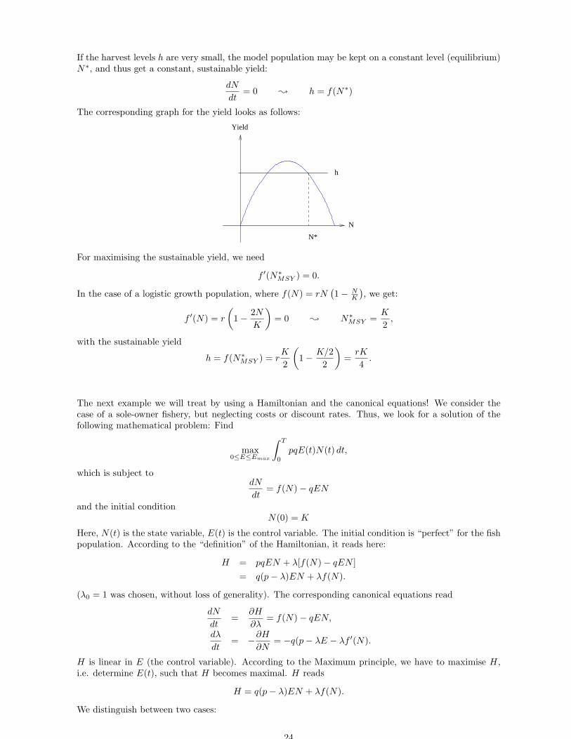
If the harvest levels h are very small, the model population may be kept on a constant level (equilibrium)N∗, and thus get a constant, sustainable yield:
dN
dt= 0 ; h = f(N∗)
The corresponding graph for the yield looks as follows:
h
Yield
N
N*
For maximising the sustainable yield, we need
f ′(N∗MSY ) = 0.
In the case of a logistic growth population, where f(N) = rN(1 − N
K
), we get:
f ′(N) = r
(
1 − 2N
K
)
= 0 ; N∗MSY =
K
2,
with the sustainable yield
h = f(N∗MSY ) = r
K
2
(
1 − K/2
2
)
=rK
4.
The next example we will treat by using a Hamiltonian and the canonical equations! We consider thecase of a sole-owner fishery, but neglecting costs or discount rates. Thus, we look for a solution of thefollowing mathematical problem: Find
max0≤E≤Emax
∫ T
0
pqE(t)N(t) dt,
which is subject todN
dt= f(N) − qEN
and the initial conditionN(0) = K
Here, N(t) is the state variable, E(t) is the control variable. The initial condition is “perfect” for the fishpopulation. According to the “definition” of the Hamiltonian, it reads here:
H = pqEN + λ[f(N) − qEN ]
= q(p − λ)EN + λf(N).
(λ0 = 1 was chosen, without loss of generality). The corresponding canonical equations read
dN
dt=
∂H
∂λ= f(N) − qEN,
dλ
dt= −∂H
∂N= −q(p − λE − λf ′(N).
H is linear in E (the control variable). According to the Maximum principle, we have to maximise H,i.e. determine E(t), such that H becomes maximal. H reads
H = q(p − λ)EN + λf(N).
We distinguish between two cases:
24

• If λ(t) > p, then E = 0 is needed (in order to avoid the first term to become negative).
• If λ(t) < p, then choose Emax.
Hence:
E(t) =
Emax for λ(t) < p0 for λ(t) > p
maximises the Hamiltonian H.What happens in case of λ(t) = p on an entire interval? In that case, from the second canonical equationit follows directly that
f ′(N) = 0,
which means that the population has to be kept on MSY-Level,
N(t) = N∗MSY .
Vice versa, the control variable E has to be chosen in such a way that the fish population is kept on thatlebel, i.e.
E∗(t) =f(N∗
MSY )
qN∗MSY
(1.13)
(due to dNdt = f(N) − qEN).
Thus: Harvesting must happen with maximum rate, not at all, or according to (1.13), dependent on theadjoint variable λ(t). But that one we don’t know yet!We have to deal with that problem: An ODE for λ(t) is there, but no initial condition for this variable. Thetransversality condition (of the Maximum principle) should provide missing initial or terminal conditions.In our case: no initial or terminal payoff, the initial and terminal times are fixed (dt0 = 0, dt1 = 0), andthe state variable is a fixed constant at t0 = 0 (i.e. dN0 = 0). There is no condition on the state variableat t1 = T , so dN1 is arbitrary. Under these conditions, the transversality condition reduces to
λ(T ) = 0.
This corresponds to an terminal condition on the adjoint variable, not an initial condition.The situation is as follows: We have an initial condition on the state variable and a terminal conditionon the adjoint variable, which corresponds more to a boundary value problem (and not an initial valueproblem). Typical for optimal control problems!Problem: there is no possibility to compute exactly λ(0) - only numerical methods. But at least, we canfind a range of possible values for λ(0). We check different regions:
λ(0) > p: In that case, the control variable has to satisfy
E(t) = 0
(at least initially). Consequently, the adjoint equation reduces to
dλ
dt= −λf ′(N).
Due to f ′(K) < 0 we get dλdt > 0, λ would increase ; no harvesting at any time, continuous invrease
of λ for all times, but then λ(T ) (from the transversality condition) can never be satisfied. Thus,λ(0) > is impossible.
0 < λ(0) < p: In that case, we start with E(t) = Emax. The canonical equation
dλ
dt= −q(p − λ)E − λf ′(N)
has a negative term (the first one), and a positive term (the second one).Case λ(0) near 0: first term dominatesCase λ(0) near p: second term dominates
The choice of λ(0) still is not clear: It depends on the available time T :In case of T small, λ(0) is chosen close to 0,then λ(t) decays to zero in that time (according to thetransversality condition). This means: Owning the fishery only for a short time, leads to the best
25

strategy to fish as hard as possible (don’t mind about later generations ...)In case of T large, λ(0) is chosen closer to p, then λ(t) will increase to p - here the maximumsustainable yield can be used - and some time before the ownership ends, increase the harvest rate(to Emax), by that λ(t) is decreased to λ(T ) = 0.The typical behaviour can be seen also in the following figures:
t
T
t
T
t
T
t
T
E E
N N
Small T Large T
Emax
K
N MSY
Emax
E*
λ(0) < 0: left as exercise
Next example: We consider again the problem with the discounting (future gain is not as good as currentgain), i.e. we look for
max0≤E≤Emax
∫ T
0
e−δtpqE(t)N(t) dt,
which is subject todN
dt= f(N) − qEN,
and the initial conditionN(0) = K.
We follow the ideas from above, just use the modified equations. The Hamiltonian reads
H = e−δtpqEN + λ[f(N) − qEN ]
= q(pe−δt − λ)EN + λf(N).
Again, it is linear in the control variable E; there may be a change of sign in the coefficient of E, itdepends on
σ = pe−δt − λ
(called “switching function”).The canonical equations read here:
dN
dt=
∂H
∂λ= f(N) − qEN
dλ
dt= −∂H
∂N= −q(pe−δt − λ)E − λf ′(N).
26

Again, the Hamiltonian has to be maximized with respect to E (the control variable); similar to abovewe have to distinguish two cases:
E(t) =
Emax for λ < pe−δt
0 for λ > e−δt.
Similar to above, also here it is possible that σ = 0 on an interval, i.e. λ = pe−δt. In that case we have
dλ
dt= −δpe−δt = −δλ.
¿From the canonical equation we get in that case
dλ
dt= −λf ′(N)
Comparison of these two equations yieldsf ′(N) = δ.
Question: Which population level should be kept by the fishery owner to satisfy this condition? Thegraph of f(N) helps us to understand what happens:
N
f(N)
δf’(N) =
NMSY KN*
The maximum sustainable yield is attained when f ′(N) = 0. In case of a “nice” growth function (e.g. thelogistic equation), the slope of f is monotonic decreasing and the slope is > 0 only in case of N < NMSY .Obviously: The higher the value of δ is, the lower is the corresponding N∗.By that, we find the so-called “fundamental principle of renewable resources”:
Larger discount rates ⇔ Less biological conservation
In the extreme case: If δ > r, the owner will bring the population to extinction (at least if he justinterested in economic success).The reason behind is: The population grows too slowly, it makes sense (for the economically interestedowner) to fully consume the resource and invest the money he gets for that in something else, with ahigher rate of return.Example from the real world: The baleen whale (Bartenwal), which grows quite slowly (growth rate of2 − 5% per year suffers under extreme overexploitation.
Next step: We want to consider the case of a nonlinear revenue, which means: the earnings by har-vesting depend in a nonlinear way on the harvest h = qEN , described by a function R. R is assumed tobe increasing and concave, i.e.
R′(h) > 0 and R′′(h) < 0,
the graph looks like
qEN
R(h)
27

This means: The revenues increases with catch, but at decreasing rates.Goal of the sole owner (still underlying discounted revenues) is to find
max0≤h≤hmax
∫ T
0
e−δtR(h) dt,
which is subject todN
dt= f(N) − h
with the initial conditionN(0) = K
(the population is under best conditions at the beginning of the harvesting process). In the following his taken as the control variable (instead of dealing with the fishing effort, as before). The Hamiltonianreads for this problem:
H = e−δtR(h) + λ[f(N) − h].
Obviously, the Hamiltonian is now a nonlinear function of the harvest rate h; thus we look for a localmaximum by
∂H
∂h= e−δtR′(h) − λ = 0
which corresponds toλ = e−δtR′(h).
(Please notice that∂2H
∂h2= e−δtR′′(h) < 0,
i.e. we deal indeed with a maximum, not with a minimum).¿From λ = e−δtR′(h), it follows that
∂λ
dt= −δe−δtR′(h) + e−δtR′′(h)
dh
dt.
The adjoint equation yields
dλ
dt= −∂H
∂N= −λf ′(N) = −e−δtR′(h)f ′(N).
Comparing these two equations, we get:
dh
dt= [δ − f ′(N)]
R′(h)
R′′(h).
Hence, we have an autonomous ODE system (first order) for the stock level N and the harvest rate h:
dN
dt= f(N) − h
dh
dt= [δ − f ′(N)]
R′(h)
R′′(h)
(Remark: The adjoint variable doesn’t appear here anymore - no problem, we are not interested in itdirectly, we just use it)For that ODE system, we can use our classical methods for the analysis!Stationary points:
dN
dt= 0 ⇔ f(N) = h
dh
dt= 0 ⇔ f ′(N) = δ ; N = N∗
; h∗ = f(N∗).
The intersection point of these two isoclines (N = 0 and h = 0) corresponds to the stationary point, thephase plane looks as follows:
28

NN*
(N*,h*)
h
f’(N) = δ
h=f(N)
The general Jacobian matrix reads:
J =
(f ′(N) −1
−f ′′(N) R′(h)R′′(h) (δ − f ′(N))
(R′(h)R′′(h)
)′
)
Inserting the coordinates of the stationary point, N = N∗, h = f(N∗), yields (due to f ′(N∗) = δ):
J =
(
δ −1
−f ′′(N∗) R′(h∗)R′′(h∗) 0
)
The sign of the determinant is (due to R′(h) > 0, R′′(h) < 0 and f ′′(N∗) < 0):
detJ = −f ′′(N∗)R′(h∗)
R′′(h∗)< 0,
hence the stationary point is a saddle.
Via the directions of the eigenvectors, we can determine the “position” of the saddle in the phase plane,the typical flow near the equilibrium looks as follows:
N
h
NT N0
E.g., if we prescribe initial and terminal conditions for the state variable (N(0) = N0, N(T ) = NT ), asshown in the graph, we are looking for a solution curve (also called orbit), which connects N0 to NT
in the prescribed time T . For an increasing T , this leads to the choice of an orbit which comes nearerand nearer to the stationary point (N∗, h∗), since in the neighbourhood the “flow” becomes slower andslower. In opposite to the examples before, here we really have a graded control (not just off - on withfull effort).
Of course, we could also consider possible costs in our approaches (corresponding e.g. to
max0≤E≤Emax
∫ T
0
e−δt[pqN(t) − c]E(t) dt),
but for the lecture, we will not consider that case.
29

1.1.5 Stochastic birth and death processes
Reference: [6]
As mentioned before, by using deterministic equations like dNdt = rN or the logistic growth model
dNdt = rN
(1 − N
K
), random influences are ignored, but they may be important for the growth of popu-
lations, especially, if the size of the population is quite small (then the influence of single individuals islarge).We start with a very simple linear birth process: the Yule-Furry process (introduced by Yule (1924) andFurry (1937)). It is a Markov process, which means the future is independent of the past (only the presentplays a role). The time is a continuous parameter.State space for this process: The potential number of individuals in the population at any instant of time(this is countable; thus it can be called a continuous-time Markov chain).
Random variable N(t): number of individuals at time tpn(t) = P [N(t) = n], n = 0, 1, 2, . . . (Probabilty that N(t) takes value n).
Birth process
First approach: only births, no deaths.Asumption: No internal population structure, the individuals act independently of each other, everyindividual can give birth to new ones. The classical assumption for a single individual is:
P (1 birth in (t, t + ∆t] |N(t) = 1) = β∆t + o(∆t)
P (more than 1 birth in (t, t + ∆t] |N(t) = 1) = o(∆t)
P (0 birth in (t, t + ∆t] |N(t) = 1) = 1 − β∆t + o(∆t)
(Notation: lim∆t→0o(∆t)∆t = 0). Remark: The idea behind is a small ∆t, e.g. such that β∆t < 1, later
we consider ∆t → 0.
This approach can be easily generalised for the situation with n individuals:
P (1 birth in (t, t + ∆t] |N(t) = n) = n[β∆t + o(∆t)][1 − β∆t + o(∆t)]n−1
= nβ∆t + o(∆t)
P (more than 1 birth in (t, t + ∆t] |N(t) = n) = o(∆t)
P (0 birth in (t, t + ∆t] |N(t) = n) = 1 − nβ∆t + o(∆t)
Using this knowledge we can formulate an equation for pn(t):
pn(t + ∆t) = pn−1P (1 birth in (t, t + ∆t] |N(t) = n − 1+pn(t)P (0 births in (t, t + ∆t] |N(t) = n) + o(∆t)
= (n − 1)β∆tpn−1(t) + (1 − nβ∆t)pn(t) + o(∆t).
Reformulating yields:
pn(t + ∆t) − pn(t)
∆t= −nβpn(t) + (n − 1)βpn−1(t) +
o(∆t)
∆t,
respectively with the limit ∆t → 0
dpn
dt= −nβpn + (n − 1)βpn−1
(which is a chain of ordinary differential equations).Initial condition:
pn(0) =
1, for n = n0
0, for n 6= n0
(this means: we start with N(0) = n0).Due to the fact that we neglect deaths at the moment and consider a pure birth process, it holds:
pn(t) = 0 for n < n0.
A lot of statements can be derived directly from these equations. Some examples:
30

• Probabilty of staying at the initial condition?
Due todpn0
dt = −βn0pn0and pn0
(0) = 1, we get the solution
pn0(t) = e−βn0t.
• Probability of being at n0 + 1?
Due todpn0+1
dt = −β(n0+1)pn0+1+βn0e−βn0t and pn0+1(0) = 0, we still can get an explicit solution:
pn0+1(t) = n0e−βn0t(1 − e−βt)
Observation: First, there is an increase in probability, later a decrease (by further births). Thepeak can be found (using the first derivative):
p′n0+1(t) = n0(−βn0)e−βn0t(1 − e−βt) + n0e
−βn0t(βe−βt) = 0
⇔ ln
(n0
n0 + 1
)
= −βt
⇔ t =1
βln
(n0 + 1
n0
)
.
By induction, one can find e.g.
pn0+m(t) =
(n0 + m − 1
n0 − 1
)
e−βn0t(1 − e−βt
)m
pn(t) =
(n − 1
n0 − 1
)
e−βn0t(1 − e−βt
)n−n0
for n ≥ n0. Remark: This corresponds to the so-called “negative binomial distribution” where thechance of success in a single trial deceases exponentially with time, due to e−βt (in general, thenegative binomial distribution describes the number of attempts which are necessary in a Bernoulliprocess to reach a given number of successes; it is e.g. very important in the context of insurances).We can compute expected value and variance easily:
E[N(t)] =
∞∑
n=0
npn(t) = n0eβt,
V ar[N(t)] =∞∑
n=0
n2pn(t) − E2[N(t)] = n0(1 − e−βt)e2βt.
Remark: For β > 0 the mean population size grows exponentially (the variance also increases withtime). So, the mean population in this approach behaves like the deterministic exponential growth;but here we get an additional information, concerning the variance.It is also interesting to consider a size called the “coefficient of variation”:
V [N(t)] =
√
V ar[N(t)]
E[N(t)]=
√
1 − e−βt
n0.
Obviously, this has the property
limt→∞
V [N(t)] =
√1
n0.
It compares somehow the variance with the current population size. Remark: It depends only onthe intial population size. In case of a large initial population, the coefficient of variation is small; incase of a small initial population, it is large. From that we find: In case of small initial populations,the stochasticity plays a big role, the runs of the stochastic process may differ greatly from thecorresponding deterministic process.
Linear birth and death process
in the same way, we can introduce an additional death process, assuming that an living individual diesat time t with the probability µ∆t + o(∆t) in the time interval (t, t + ∆t]. As before, the individuals act
31

independently of each other and the probability of several events is o(∆t). Following the same ideas asabove, we get a set of ODEs, which looks now as follows:
dpn
dt= β(n − 1)pn−1 + µ(n + 1)pn+1 − (β + µ)npn
with initial conditions
pn(0) =
1, for n = n0
0, for n 6= n0,
(and we set pn(t) = 0 for n < 0). In opposite to the simple birth process, we need more effort to solve it(due to it is not a clear chain with a direction, also the step from n+1 (still unknown) to n is important).This can be treated by using the so-called probability generating function
F (t, x) =∞∑
n=0
pn(t)xn.
Due to pn(t) ≤ 1, the generating function converges for all |x| < 1 (and even for x = 1, due to∑
n pn(t) =1). (Remark: It is also possible to introduce a moment generating function instead, this will be consideredin the exercises).Some properties of the probability generating function F (t, x):
1. p0(t) = F (t, 0) describes the probability of being extinct at time t
2. Also the probability of having n individuals in the population at time t can be described by theprobability generating function:
pn(t) =1
n!
∂nF
∂xn|x=0
3. The expected value of N(t) can be computed by
E[N(t)] =
∞∑
n=0
npn(t) =∂F
∂x|x=1
4. Even the variance of N(t) can be described by using the probability generating function. Due to
∂2F
∂x2|x=1 =
∑
n=0
(n2 − n)pn(t) = E[N2(t)] − E[N(t)]
and the fact thatV ar[N(t)] = E[N2(t)] − E2[N(t)],
yields
V ar[N(t)] =
[
∂2F
∂x2+
∂F
∂x−
(∂F
∂x
)2]
x=1
.
Taken together, we see: the probability-generating function is very useful. But: How to find it? One caneasily compute, that the probability generating function satisfies the following PDE
∂F
∂t= [βx2 − (β + µ)x + µ]
∂F
∂x
with initial conditionF (0, x) = xn0
(as shown in “Math.Models in Biol. I”). Using the “method of characteristics”, the solution can bedetermined (we do not consider the details here again) and reads:
F (t, x) =
[µ(1−x)ert−(µ−βx)β(1−x)ert−(µ−βx)
]n0
for β 6= µ[
βt+(1−βt)x(1+βt)−βtx
]n0
, for β = µ.
Please recall also the most important properties:
32

• Probability of being extinct at time t:
p0(t) = F (t, 0) =
[µ(ert−1)βert−µ
]n0
for β 6= µ[
βt1+βt
]n0
, for β = µ.
• In the limit t → ∞ (i.e. the asymptotic probability of extinction):
limt→∞
p0(t) =
(µβ
)n0
, for β > µ
1, for β ≤ µ.
Remark: Even if the birth rate is larger than the death rate, there is a finite probability probabilitythat the population goes extinct (especially for populations with small initial numbers n0). Differentto deterministic models!
• Expected value and variance of the population (where r = β − µ):
E[N(t)] =∂F
∂x|x=1 = n0e
rt
V ar[N(t)] =
n0(β+µ)(β−µ)e
rt(ert − 1), for β 6= µ
2n0βt, for β = µ.
Remark: Both grow exponentially in case of β > µ. The variance increases linearly in case of β = µand in case of β < µ, the variance increases first, but later decreases exponentially (due to theextinction).
• Coefficient of variation:
V [N(t)] =
√
1
n0
(β + µ)
β − µ(1 − e−rt), β > µ
Remark: It increases monotonically, but tends to a constant.
Nonlinear birth and death processes
Until now, we had constant per capita birth and death rates β and µ. Analogously to the deterministicgrowth models, it may make sense to introduce birth and death rates which depend on the populationsize, i.e. βn and µn for n = 0, 1, 2, . . .. A model for a density-dependent growth looks as follows:
dp0
dt= µ1p1 (1.14)
dp1
dt= 2µ2p2 − (β1 + µ1)p1 (1.15)
dpn
dt= [(n − 1)βn−1]pn−1 + [(n + 1)µn+1]pn+1 − n(βn + µn)pn, n > 1. (1.16)
βn and µn should be chosen in such a way that they prevent an unlimited growth.Short observation: In the case of (nonlinear) deterministic models, one is always interested in the sta-tionary points. Now we are in the situation of a stochastic model. The stochastic analog of a stationarypoint is the so-called “statistically stationary state”. Let us consider the example above:¿From the first equation it follows, that p1(t) has to be = 0, if p0(t) is constant. But for p1(t) = 0, weneed also that p2(t) = 0 and so on, i.e. pn(t) = 0 for all n > 0. This means: For a closed population(where no migration takes place), the only finite stationary state is “extinction”. From that it followsdirectly: A closed and bounded population will tend to the absorbing state N = 0 and will go extinctwith probability 1.BUT: It may take a long time until the extinction really happens (i.e. more precisely: The expected timeto extinction may be longer than the time for typical population changes). Maybe a so-called statisticallyquasistationary state exists: this means, that in the long term run, it goes to extinction, but in the shortterm, that statistically quasistationary state is approached by the population. For making that conceptmore clear, we introduce conditional probabilities:
qn(t) =pn(t)
1 − p0(t)
33

“conditional on no extinction”. Its derivative reads:
dqm
dt=
1
1 − p0(t)
dpn
dt+
pn(t)
[1 − p0(t)]2dp0
dt.
Using the model equations and the definition of qn(t) yields a system of ODEs:
dq1
dt= 2µ2q2 − (β1 + µ1)q1 + µ1q
21
dqn
dt= [(n − 1)βn−1]qn−1 + [(n + 1)µn+1]qn+1 − [n(βn + µ2)]qn + µ1q1qn for n > 1.
That system may possess a set of stationary states q∗n.A iterative procedure for the computation of the quasistationary states (recommended by Nisbet andGurney, 1982):
(1) Guess q∗1 .
(2) Set dqn/dt to 0 and calculate by repeatedly applying the right hand sides of the ODEs q∗2 , q∗3 , . . ..For the maximum n, choose such a value, that q∗n is already negligible.
(3) Calculate the value q∗1/∑
q∗n and compare it to the old value of q∗1 . If the difference is large, repeatstep (2) with the new value of q∗1 - until the desired accuracy is reached.
These density-dependent birth and death processes are quite difficult to analyse and simulate. But wecan consider at least a special case:Assume that an ensemble of populations approaches quickly its quasistationary distribution. This corre-sponds to
p1(t)
1 − p0(t)≈ q∗1
(which describes the probability of N(t) = 1, under the condition that no extinction has occured). Inthat case we get from (1.14):
dp0
dt≈ µ1q
∗1(1 − p0),
i.e.p0(t) ≈ 1 − e−µ1q∗
1 t.
By definition, p0(t) describes the probability of being extinct at time t. Then dp0/dt corresponds tothe probability density of extinction at time t. By that approach, the mean time to extinction can becomputed via
Textinction =
∫ ∞
0
tdp0
dtdt ≈
∫ ∞
0
tµ1q∗1e−µ1q∗
1 t dt =1
µ1q∗1
(by applying partial integration).One can see: In case of µ1 and q∗1 both small, the extinction time will be large, as expected.
1.1.6 Metapopulations / Island-Mainland Model
Reference: [4]
Short “review” of mathematical models in biology: Most populations do not just live in one habitat,but are spread over several habitats. Even though if such “small populations” may go extinct locally,the total population survives in many cases since individuals from neighbouring surviving habitats caninvade and thus reoccupy it again. This type of problems is considered in the metapopulation theory.Typical questions are:
• Is a certain patchwork of local habitats able to support a population for a long time?
• Which factors play a role?
In the simple approach here, we do not deal with the sizes of a population, but only with persistence.This means: there are only two possible values for a populations size: 0 (which corresponds to localextinction) or 1 (which corresponds to local persistence).
34

¿From a metapopulations perspective, it has to be distinguished between local extinction (a single pop-ulation disappears) and regional extinction (all populations in the system die out).Let pe describe the probability of local extinction (Remark: in a discrete time scale! typically years ordecades). By that we can describe the probability that the population will survive for n years by
Pn,loc = (1 − pe)n.
This was a statement for one single poplation. But we want to consider a metapopulation, with populationacting independent of each other. Special case: two subpopulations; the probability of regional persistencefor one year can be described by
P2,reg = 1 − p2e,
since p2e is the probability that both subpopulations go extinct in one year.
For a simple metapopulation model we make the following assumptions:
• constant probabilities
• no time lags
• no explicit spatial structure
• the patches are treated as ”homogeneous” in size, quality etc, concerning the probabilities
• large number of patches ...
Let f describe the fraction of sites which is occupied (i.e. the proportion of patches where populationslive - thus, 0 ≤ f ≤ 1). Using a immigration rate I (proportion of sites which are successfully colonisedper unit time) and an extinction rate E (proportion of sites which go extinct per unit time), the basicequation can be formulated by
df
dt= I − E
(compare to the population growth models, which were similarly introduced; wo we reach an equilibriumin case of I = E).Simple assumptions for that:
Immigration: depends on probability of local colonisation (denoted by pi, may depend on f , but alsoon physical and biological conditions), and the availability of unoccupied sites (1 − f).
Extinction: depends on the probability of local extinction pe and the fraction of occupied sites f .
Thus:
I = pi(1 − f)
E = pef
and the general metapopulation model reads
df
dt= pi(1 − f) − pef
Now we step more into the direction of an island-mainland model.
Mainland
Islands
35

Simple assumptions:Constant pe means: the probability of extinction is independent of f (the fraction of occupied sites). (Insome sense, this corresponds to the density-indepentent death rate in a simple population growth modellike the exponential growth).Constant pi means: there is something like a continuous source of migrants which can colonise an emptysite. This proporty is also called “propagule rain”. It can be provided by a large stable mainlandpopulation.
Mainland
Islands
With these assumptions, we look for the stationary state of our model dfdt = pi(1 − f) − pef :
0 = pi − pif − pef ⇔ f =pi
pi + pe
Remark: Even in case of a large probability of extinction pe and a small probability of colonisation pi,there will be no complete regional extinction (f > 0 in the equilibrium case, which corresponds to theexpected value). The reason is indeed the propagule rain!
To be more realistic, usually also internal colonisation between the population sites is possible. With asimple assumption, this corresponds to
pi = i · f,
where i (constant) describes the increas of colonisation probability of empty sizes by an additional occu-pied patch.
Mainland
Islands
It can be interpreted as a contribute of individuals to a kind of pool of propagules by each population.In case of neglecting the mainland, here the probability of colonisation is 0 in case of f = 0. The modelequation reads:
df
dt= if(1 − f) − pef
Equilibrium:
pef = if(1 − f) ⇔ f = 1 − pe
i
36

Remark: Here, a complete extinction is possible (f ≤ 0), dependent on the strength of internal coloniza-tion effect i compared to the probability of local extinction.
Another “refinement”: Inclusion of a so-called rescue effect. pe might also depend on f .The idea behind is: Each occupied site produces propagules - if they arrive at empty sites, they canestablish a new population there (as already considered). But also arriving at occupied sites may help,by increasing the population size and therefore reducing the probability of extinction. This is called the“rescue effect”. How to include that effect into the model?Simple approach:
pe = e(1 − f),
the parameter e controls the strength of the rescue effect. The complete model for an external propagulerain and a rescue effect reads then:
df
dt= pi(1 − f) − ef(1 − f).
We compute the equilibrium:
0 = pi(1 − f) − ef(1 − f) ⇔ ef = pi ⇔ f =pi
e.
Remark: Also here, persistence of the metapopulation is guaranteed. If e < pi, then all population sitesare occupied at equilibrium.
Alternatively, one can combine the internal colonisation with the rescue effect (corresponding to a situa-tion which is completely separated from external influences). The model equations read
df
dt= if(1 − f) − ef(1 − f).
Computation of the equilibrium:0 = (i − e)(f(1 − f)
(remark: same structure like the Verhulst model!). The equilibria are f = 0 and f = 1. Concerningstability:
Case i > e: (immigration > extinction), f = 1 is stable, f = 0 is unstable; this leads to “landscapesaturation”.
Case i < e: (immigration < extinction), f = 0 is stable, f = 1 is unstable; this leads to “regionalextinction”.
Case i = e: (immigration = extinction), there is a continuum of equilibria, f will not change at all. Inreality, there may be stochastic variations in i and e, so fluctuation between the two equilibria ispossible, respectively slight changes in f near the last case.
Summary: Here, we considered only very simple metapopulation situations, neglecting explicit spatialstructure or population sizes, interactions with other species ... but ok to see the basic problems andapproaches.Remark that the considered models deal with probabilities, these are not deterministic. As a consequence,they are the basis for stochastic simulations, which may behave differently in different runs!
1.1.7 Discrete-time models
References: [6], [2]
In this lecture, we only step very fast through a different type of modelling approach: the discrete-time models. There are examples of populations which are easy (and appropriate) to describe by discretetimes. An important criterion can be: Do the birth occur in regular time-intervals, e.g. caused by typical“breeding seasons”?Advantages:
• easy to formulate and to simulate
• Phenomena like delays much more easy to describe (in some cases at least)
37

• can show oscillations (in opposite to deterministic, autonomous, one-species models)
¿From an more ecological point of view, typical special which are well-suited for a discrete-time descrip-tion:
Plants, especially so-called monocarpic plants: they grow, flower (i.e. produce seeds) and then die.Many of these monocarps are annuals (like the sun-flowers), but there are also some which live formany years, e.g. Bamboos (with life times in the range of 20 years). Advantage: Organisms whichsubsists on bamboo, have difficulties in surviving the symchronised death phase; this also concernedthe pandas in China in 1983).
Insects, especially so-called semelparour insects: analogously to the monocarpic plants, they lay downeggs once in their live (after that they die). Typical ecamples: Mayflies, day-flies ... . There arealso examples for long-living species, like some cicaded in eastern USA, with time intervals of 13 or17 years.
Fishes, some also show semeparous behaviour and dies soon after spawning. The most well-knownspecies are salmons and eels (additionally they migrate between freshwater and marine habitats).
Birds usually show iteroparous behaviour (i.e. they can breed in more than one season), but due tooften clearly-defined breedings seasons, can often be described also by discrete-time models (maybewith an additional age structure).
Mammals: There are not many, but at least some species showing semelparous behaviour. (Examplesare marsupials of the genus Antechinus). In this case, typically the males die after mating.
Short review of the basics of disrete-time models (i.e. difference equations, which are used here): Ingeneral: Generally:
xn+1 = f(xn) is denoted to be a difference equation of first order.
As usual, we are interested in stationary points and their stability:
Definition 1 x is called stationary point of the system xn+1 = f(xn), if
x = f(x).
x is also called fixed point or steady state.
For difference equations, the stability is defined via convergence of sequences:
Definition 2 Let x be a stationary point of the system xn+1 = f(xn).x is called locally asymptotically stable, if there exists a neighbourhood U of x such that for each startingvalue x0 ∈ U we get:
limn→∞
xn = x.
x is called unstable, if x is not (locally asymptotically) stable.
A practical criterion for checking the stability yields the following proposition:
Proposition 1 Let f be differentiable. A stationary point x of xn+1 = f(xn) is
• locally asymptotically stable, if |f ′(x)| < 1
• unstable, if |f ′(x)| > 1
Remark: These criteria are sufficient, but not necessary!
One can also use graphical methods like cobwebbing for fast checks for stationary points and theirstability!
Now let’s look for some typical examples for population growth!
38

Density-independent growth
Let Nt denote the size a population in generation t (can be years or something else which is appropriatefor the considered species). Let R0 be the offspring per individual (also called net reproductive rate). Inthe most simple case, neglecting all other effects, we get as model
Nt+1 = R0Nt.
This can be easily solved (Nt = Rt0N0), but is obviously not realistic to an unlimited growth in case of
R0 > 0.
Density-dependent growth
First idea could be to find the analogue of the logistic differential equation. This means: Taking thelogistic differential equation,
dN
dt= rN
(
1 − N
K
)
,
the left-hand side is approximated by a finite-difference quotient,
∆N
∆t= rN
(
1 − N
K
)
.
The time-step is assumed to cover one generation, ∆t = 1, then it can be rewritten as
Nt+1 − Nt = rNt
(
1 − Nt
K
)
. ⇔ Nt+1 = (1 + r)Nt −r
KN2
t
or in the rescaled version something like
xt+1 = µxt(1 − xt).
The graph of Nt+1, dependent on Nt looks as follows:
N t
Nt+1
K
K
We can see: there is a overcompensation, this means the recruitment for the total population decreaseswith increasing population size. Furthermore, several other problems appear, like loss of positivity, chaoticbehaviour. Some of these topics will be treated in the exercises.
Trying to make it better!Idea: The “function”
1 + [(R0 − 1)/K]Nt
R0
is linearly increasing in Nt The per capita number of offspring is assumed to be inversely proportional tothis function, i.e.
Nt+1
Nt=
R0
1 + [(R0 − 1)/K]Nt⇔ Nt+1 =
R0Nt
1 + [(R0 − 1)/K]Nt
This difference equation is called the Beverton-Holt stock-recruitment curve. The graph looks as follows:
39

N t
Nt+1
K
K
We see: Here, no overcompensation happens; the increase in population density leads to a decrease ofthe per capita reproduction, but not of the total population size.Let us consider the equilibria N∗ and their stability:
N∗ =R0N
∗
1 + [(R0 − 1)/K]N∗⇔ N∗ = 0 or N∗ = K.
The first derivative reads
f ′(N∗) =R0
[1 +
(R0−1
K
)N∗
]2 ,
thus:
In N∗ = 0: f ′(0) = R0, i.e. unstable for R0 > 1 and asymptotically stable for R0 < 1, what can beexpected also from the meaning of R0.
In N∗ = K: f ′(K) = 1R0
, i.e. asymptotically stable for R0 > 1
(of course having in mind only values R0 > 0)
Bifurcation diagrams
In a lot of models, the qualitative behaviour depends heavily on the parameter values. Typical exampleis the discrete logistic model, but also other models show similar dependencies.The qualitative behaviour can be represented by a so-called bifurcation diagram. In each case, the “stableobjects” will be plotted.Example: discrete logistic model, bifurcation parameter r
Creating such a diagram with the aid of a computer:
• Choose a parameter value (here it is done for r)
• Run 1000 steps of iteration (from an arbitrary starting value).
• Plot the next 1000 values (of the iteration) in the line above the chose r.
• Do the same procedure for other values of r
40

1.1.8 Delay models
Reference: [6]
In some sense, the difference equations from the section above already include a kind of implicit delay,as they cannot react instantaneously on changes, one after a discrete time. This may lead to phenomenalike overshooting of equilibria, chaotic orbits etc.Additionally, explicit delays can be included in models, also in difference equations. In this context, theycorrespond to higher-order difference equations. We consider examples of the following form:
Nt+1 = f(Nt, Nt−T ) = NtF (Nt−T ), (1.17)
T is called the explicit lag in density dependence. Typical examples are:
• Lagged Beverton-Holt model:
Nt+1 =R0Nt
1 + [(R0 − 1)/K]Nt−T
• Lagged logistic difference equation:
Nt+1 =
[
1 + r
(
1 − Nt−T
K
)]
Nt
• Lagged Ricker curve:
Nt+1 = Nt exp
[
r
(
1 − Nt−T
K
)]
These exemplary models were formulated in such a way that they satisfy
F (K) = 1 and thus Nt = Nt−T = K,
which means: the capacity corresponds to an equilibrium. Let us check the stability of this equilibrium!Usual approach: Let xt = Nt−K (i.e. consider the deviation from the equilibrium). Then the linearisationof the standard equation (1.17) reads:
xt+1 =∂f
∂Nt|K xt +
∂f
∂Nt−T|K xt−T .
(using the total differential).Both, the lagged logistic difference equation and the lagged Ricker curve, as examples, satisfy
xt+1 = xt − rxt−T ,
which is a linear equation. Approach for the solution to be of the form
xt = x0λt.
This approach is applied in the linear equation and yields
x0λt+1 = x0λ
t − rx0λt−T
⇔ λ = 1 − rλ−T
⇔ rλ−T = 1 − λ
⇔ r = λT (1 − λ).
There are T + 1 roots λi of this algebraic equation. If all these roots satisfy the condition
|λi| < 1,
then the equilibrium N = K is asymptotically stable. (Recall the stability conditions for discrete systemsand the fact that a higher-order difference equation can be reformulated as a system of first-order differenceequations)The root with the largest absolute value is called the “dominant root” (and chosen to be λ1, without lossof generality) - in some sense, it dominates the behaviour of the system:
41

• If λ1 is ∈ R, λ1 > 0 and λ1 < 1, then small perturbations around N = K are expected to decaymonotocally to 0.
• If λ1 ∈ R but −1 < λ1 < 0, or λ1 ∈ C \ R, then small perturbations around N = K are expectedto show dampled oscillations.
• If |λ1| > 1, then the equilibrium N = K is unstable.
In our example, the characteristic equation was r = λT (1 − λ). In a graphical approach, the real rootscorrespond to the intersection points of the curve λT (1 − λ) with the straight line r:
λ
r
r0
1
Obviously, there are two positive roots in case of a small positive r (it can be shown: the larger one is thedominant). There is a critical value r = r0 where they meet and disappear, simultaneously, oscillationsstart at that critical value r = r0. Determination of r0: it corresponds to the maximum of r(λ), i.e.
0 =dr
dλ= T · λT−1 − (T + 1)λT ⇔ λmax =
T
T + 1,
thus
r0 = r(λmax) =
(T
T + 1
)T (
1 − T
T + 1
)
=TT
(T + 1)T+1.
Remark: The critical value r0 is monotonically decreasing in T , for large delays it tends to zero:
limT→∞
r0(T ) = 0.
This means also: The larger the delay T is, the easier oscillations can appear. In the graph, we can seethe critical values for instability, dependent on T .
r0
T5
1
2
In general, explicit time lags often cause instability, also e.g. for the lagged Beverton-Holt model andothers. Remark: There is a big problem with these approaches from an ecological point of view: Thedelay is often included in the death term. But the major influence of an delay should concern the birthterm, as it may take some time until the offspring will be available, dependent on the population sizesome time ago!
42

Delay in Continuous-time models
Of course, there are also situation, where continuous-time models are more appropriate to describe apopulation growth, but nevertheless a delay plays a major role.Question: Do explicit time lags also destabilise the behaviour in continuous-time models?
We start with the logistic differential equation,
dN
dt= rN
(
1 − N
K
)
.
Let τ be the delay in time.The first idea to introduce that delay into the basic model of logistic growth was
dN
dt= rN(t)
(
1 − N(t − τ)
K
)
,
the so-called Hutchinson-Wright equation (due to Hutchinson, a well-known lomnologist and ecologist,and Wright, a number-theorist).Remark, that instead of an intial condition at a time point (e.g. t = 0), here a so-called history functionhas to be given for an entire interval of length τ (otherwise, the solution wouldn’t be defined uniquely):
N(t) = N0(t) for − τ ≤ t ≤ 0.
Important remark: Also the Hutchinson-Wright model includes the problem with the delay in the deathterm instead of the birth term! Nevertheless, it is used here to show the basic procedure for analysingthese systems.There are two equilibria (similar to the non-delayed logistic equation).:
N = 0 and N = K.
Looking for their stability:
• near N = 0: there we have approximately
dN
dt≈ rN,
so, if r > 0 the population will grow exponentially fast ; N = 0 is unstable.
• Near N = K: As usual, we consider the deviation from the carrying capacity, which can be definedby
x(t) = N(t) − K.
Linearisation yields:
dx
dt=
∂f
∂N(t)|N=Kx(t) +
∂f
∂N(t − τ)|N=Kx(t − τ)
= r
(
1 − N(t − τ)
K
)
|N=Kx(t) − rN(t)
K|N=Kx(t − τ)
= −rx(t − τ),
which is a linear delay-differential equation.Approach with an exponential solution:
x(t) = x0eλt.
Inserting that into the linear delay-differential equation, we get:
λx0eλt = −rx0e
λ(t−τ) ⇔ λ = −re−λt,
obviously, this is a transcendental equation, which has an infinite number of complex roots λ.Nevertheless, a statement concerning the stability of the equilibrium N = K can be given; thereare three different regimes (dependent on the product rτ):
43

0 < rτ < 1e : N = K is a monotonically dampled stable equilibrium
1e < rτ < π
2 : N = K is an oscillatorily dampled stable equilibrium
rτ > π2 : N = K is an unstable equilibrium
How to get this result?Let µ = λτ , then the characteristic equation reads
µ = −rτe−µ. (1.18)
In our case, the delay τ is positive, so the real part of µ has the same sign as the real part of λ.For a better understanding, we use a “trick”: Plot the left hand side and the right hand side ofequation (1.18) separately (but in the same coordinate system), so we look for intersection points.Dependent on rτ , there may be 0, 1 or 2 intersection points of −rτe−µ with the diagonal line(which corresponds to the left hand side). They correspond to real-valued solutions of (1.18). Thetransition from two distinct real roots to one with no real roots corresponds to the transition fromexponential to oscillatory decay (and is a double root). The reason behind is: there is no crossing ofthe imaginary axis, so the real part stays negative. At this double root, the two curves are tangent,i.e.
1 = rτe−µ.
Together with (1.18), we get:
µ = −1 ; rτ =1
e.
Looking for the transition from damped oscillations to “growing oscillations” (i.e. loosing stability):There, a pair of complex conjugate roots crosses the imaginary acis. We take
µ = iω
(i.e. a root on the imaginary axis), the equation (1.18) reduces to
iω = −rτe−iω = −rτ(cos ω − i sin ω)
We consider separately the real and the imaginary parts, thus
0 = −rτ cos ω ; ω = (n +1
2)π, n = 0, 1, 2, . . .
ω = rτ sinω ; rτ =ω
sin ω.
The first transversal of the imaginary axis is the “relevant” one: thus choose n = 0 ; N = K losesits stability at rτ = π
2 .
Thusm we have the basic qualitative behaviour of the Hutchinson-Wright equation!
Don’t forget: From an ecological point of view, one should take another approach for including thedelay into the birth term. This is the case, e.g. in Nicholson’s blowfly equation:
dN
dt= αN(t − τ)e−βN(t−τ) − δN(t).
Here, an instantaneous death takes place, while the birth may be delayed. It was applied to describesome periodic oscillations which were observed in experiments with the Australian sheep blowfly Luciliacuprina (experiments were done by Nicholson in 1954).Another applied model:
dN
dt= µN(t − τ)
(
1 + q
(
1 −[N(t − τ)
K
]z))
− µN(t),
it was introduced by May in 1980 and applied to describe the population dynamics of baleen whales.(Remark: the parameter z is free to choose; a sufficiently high z can lead to chaotic dynamics).
44

1.2 Interacting Populations
1.2.1 Aquatic population interacting with a polluted environment
Toxic impact
Reference: [5]
First, we consider a very simple example: How does a population “react” on a toxic impact, i.e. how isthe population dynamics influenced?Example: Daphnia galeata mendotae (a crustacea), with impact of cadmium.Goal: Analyse the relations between “level of stress” (i.e. toxicant input), population size, birth rate anddeath rate.Let D describe the number of toxicant-induced deaths, N the population size and Z the toxicant-inducedmortality rate per individual. Thus, a sample approach for a so-called “mortality equation“ reads:
dD
dt= ZN.
Usually, Z is assumed to depend on the toxicant concentration; simple approach:
Z =
h · (C − C0) for C ≥ C0
0 for C < C0
thusdD
dt= h(C − C0)N for C ≥ C0,
with the parameters with dimensions
• toxicant-induced mortality coefficient h, [h] =(time · µg
L
)−1
• toxicant concentration C, [C] = µgL
• threshold toxiant concentration C0, [C0] = µgL
(The assumption behind is: the crustacea can tolerate the toxicant up to a certain threshold, only whenexceeding it, there is an impact on the death rate; but also C0 = 0µg
L is possible)Simple approach for the population size:
dN
dt= rN
(
1 − N
K
)
− h(C − C0)N
(As usual: r as basic growth rate with [r] = 1time , K the carrying capacity, e.g. [K] = number of individuals).
Compute the stationary state for the population size:
dN
dt= 0 ⇔ N = 0 or N = K − h(C − C0)K
r
Obviously, it depends on the toxicant concentration C, if there exists a nontrivial equilibrium > 0:Condition is
r > h(C − C0) ⇔ C <r
h+ C0.
Of course, the toxicant-induced mortality is not necessarily zero, when reaching the equilibrium popula-tion, in detail:
dD
dt= h(C − C0)N
= h(C − C0)
(
K − h(C − C0)K
r
)
= hK(C − C0) −Kh2(C − C0)
2
rfor C ≥ C0
We see: The toxicant-induced death rate dDdt has the shape of a parabola, dependent on C: first it in-
creases to a maximum at C = C0 + r2h , then decreases again.
45

Even though this model approach looks very simple, it fits well to experimental observations! Thetoxicant concentration was varied, dependent on that several magnitudes were measured, like equilibriumpopulation sizes, birth rate, death rate ...Fitting (with least squares approach) yields the following results for the parameter values:
C0 ≈ 0µg/L
h = 0.018(day µg/L)−1
K = 147 individuals
r = 0.29 day−1,
the curve e.g. for the toxicant-induced death rate, dependent on the Cadmium impact in microgram/literlooks as follows (in comparison with the experimental data):
model output experimental dataC
0 5 10 150
2
4
6
8
10
12
Interpretation: The increase is clear to understand: the more Cadmium is brought into the system, thehigher the death rate. But later, i.e. in the range of high Cadmium levels, the equilibrium populationsize becomes smaller and smaller, so also less individuals are dying per time unit.
Population interacting with toxicant
Reference: [10]
Up to now, we only considered the influence of the toxicant on the development of the population.But in reality, there are also a lot of examples, where the population influences also the toxicant; e.g.some bacteria are able to degrade chemical pollutants. From a mathematical point of view, we need thena system of ordinary differential equations (still assuming a homogeneous distribution, without relevantspatial structure of the players). In the following, we use as dependent variables:
M(t) concentration of biomass of the population at time tCE(t) concentration of toxicant in the environment at time tCI(t) amount of toxicant in the (population) biomass at time ty(t) = CI(t)/M(t) concentration of toxicant per unit population biomass at time t
46

(y(t) is also called the “body burden”; subscript “E” denotes “environmental”, “I” means “internal”)A simple basic model is formulated as follows:
M = M(β(M,y) − µ) (1.19)
CI = aCEM − (µ + η + κ)CI (1.20)
CE = −aCEM + (pµ + η)CI − θCE + u(t) (1.21)
y = CI/M (1.22)
Meaning of these equations:
• the first equation describes the population growth under the influence of the toxicant: µ is thedeath rate; β(M,y) the “birth rate” - dependent on the current population size and the bodyburden (assuming that y doesn’t influence the death rate directly)
• The second and the third equations concern the toxicants - there is an exchange possible(the “tox-icant uptake rate”, aCEM , due to the law of mass action).The death of an individual also influences (i.e. reduces) the internal toxicant concentration, by rate−µCI . A fixed fraction of that (0 ≤ p ≤ 1) is recycled in the environment and thus appears in thethird equation.The population can egest and depurate toxicants by metabolic processes, described by the constantsη and κ.
• In the third equation we take into account, that in the environment further (abiotic) processescan lead to a degradation of the toxicant, introduced by the rate θ > 0 (called “per unit rate ofenvironmental detoxification”).The term u(t) allows an exogeneous input of toxicants into the environment.
Remark: The total concentration of the toxicant, C = CE + CI is not conserved:
C = u(t) − (κ + (1 − p)µ)CI − θCE
= u(t) − (κ + (1 − p)µ)(C − CE) − θCE ,
the reason is that here an input of toxicants may happen, and the toxicant can be degraded by envi-ronmental and population-based processes. We consider the body burden equation (y = CI/M); weget
y =CI
M− y
M
M= aCE − (µ + η + κ)y − y(β(M,y) − µ)
= aCE − (η + κ + β(M,y))y.
Obviously, β(M,y) can be interpreted as a kind of dilution by the biomass gain. How should the functionβ(M,y) “behave” for a realistic model?Typically the following four assumptions are made:
1. β : [0,∞)2 → R is locally Lipschitz continuous, i.e. for every constant c > 0 there exists a Lipschitzconstant L > 0, such that
|β(M,y) − β(N, z)| ≤ L(|M − N | + |y − z|) for all 0 ≤ y, z,M,N ≤ c.
(no biological meaning; just in order to guarantee uniqueness of solutions)
2. β(M,y) is monotonely decreasing (in both arguments); strictly decreasing if β(0, y) > 0.For an arbitrary but fixed M ≥ 0, β(M, ·) is bounded on [0,∞)(an increasing toxicant concentration reduces food uptake / growth; an increasing population in-creases also intraspecies competition for ressources, thus reducing growth, too)
3. β(0, 0) > 0, β(0, y) ≥ 0 for all y > 0, and limM→∞ β(M, 0) < µ(for positivity of the population under optimal conditions; and limited growth)
4. ∀ ε > 0 ∃ δ > 0:β(M,y) ≥ −ε for M ≤ δ, y ≥ 0.
(mathematically useful; also for high body burden of toxicant hardly any starvation effects)
47

Typical example for β satisfying these conditions:
β(M,y) =ρ(y)
1 + cM,
where ρ in monotonely non-increasing, c positive constant. The linear dose response for the per unitbiomass production rate is a special case:
ρ(y) = α1(1 − α2y)+,
where α1, α2 are positive constants, [r]+ = max0, r is the positive part of a real number.
Open Loop Toxicant Input
In this case, the input of toxicant, u, is prescribed, and the goal is to determine the resulting total toxicantconcentration in the system.We can use tools from “fluctuation theory” for examining the qualitative behaviour.The first theorem concerns the existence of a nonnegative solution:
Theorem 5 (Existence and uniqueness of solution) Let u be continuous and nonnegative on [0,∞).Then for nonnegative initial data and M(0) > 0, there exists a unique solution M , CE, CI of system(1.19)-(1.21) on [0,∞) which is also nonnegative and M(t) > 0 for all t ≥ 0. M is bounded on [0,∞).
The proof is left out here.
The next corollary allows an estimation of the total toxicant concentration in the system:
Corollary 1 Let u satisfy the assumptions of Theorem 5 and be bounded on [0,∞). Then CE and CI
are also bounded and for C = CE + CI the following estimation holds:
C(t) ≤ maxC(0),u
ξ∗,
whereu = sup
[0,∞)
u, ξ∗ = minκ + (1 − p)µ, θ.
The proof of the corollary is also left out (it uses two theorems from the theory of ODEs, concerningpreservation of positivity and for the boundedness of solutions on finite intervals; including a lot of esti-mations)
The large-time estimates for the total toxicant concentrations are given in the next proposition:
Proposition 2 Let u : [0,∞) → R be bounded. Then the following estimates hold:
lim supt→∞
C(t) =: C∞ ≤ u∞
ξ∗, lim inf
t→∞C(t) =: C∞ ≥ u∞
ξ∗.
(Remember the formal definition of the Limes inferior: Let f : Ω → R be a bounded function, Ω ⊆ Rm
closed. Then for x ∈ Ω:
lim supy→x
f(y) = suplim supN→∞
f(yN ) | yN,Ω → x,
Ω → x means: x is accumulation point of the sequence yN , which is in Ω;according to Bolzano-Weierstraß a bounded sequence (yN ) has a largest (lim sup) and a smallest (lim inf)accumulation point)
Before we consider the proof of proposition 2, we introduce a proposition from fluctuation theory:For the method of fluctuations, bounded differentiable functions f : (a,∞) → R are considered, one isinterested in the relation between the asymptotic behaviour of f and f ′.The following notation will be used for the next steps:
f∞ : lim supt→∞
f(t), f∞ : lim inft→∞
f(t).
48

Proposition 3 There exist sequences sn, tn → ∞ with the following properties:
f(sn) → f∞, f ′(sn) → 0,
f(tn) → f∞, f ′(tn) → 0,
for n → ∞.
This helps us now:Proof of Proposition 2: According to Proposition 3, choose a sequence tn → ∞ such that C(tn) → C∞
and C ′(tn) → 0 as n → ∞. From C ′ = u(t) − (κ + (1 − p)µ)CI − θCE , one can find the inequalities
C ′ ≤ u(t) − ξ∗C
C ′ ≥ u(t) − ξ∗C,
whereξast = minκ + (1 − p)µ, θ and ξ∗ = maxκ + (1 − p)µ, θ.
Then we get:0 = lim sup
n→∞C ′(tn) ≤ lim sup
n→∞u(tn) − ξ∗C
∞ ≤ u∞ − ξ∗C∞
; C∗ ≤ u∞ξast (the first estimate). The second estimate can be deduced analogously.
2
¿From this proposition it follows immediately that the total toxicant concentration C(t) tends to 0 incase of the toxicant input u(t) tends to 0. The reason behind is that the toxicant is degraded abioticallyin the environment and within the biomass of the species.
Corollary 2 If u(t) → 0 for t → ∞, then CE(t) + CI(t) = C(t) → 0 for t → ∞. Also the body burdeny(t) converges to 0 for t → ∞.If 0 < β(0, 0) ≤ µ, then the biomass M(t) converges to 0 for t → ∞.If β(0, 0) > µ, then the biomass M(t) converges to M , where β(M) = µ.
(The proof is omitted again, a little bit too long for the lecture; but it can be found in the book of Thieme[10]).
Feedback Loop Toxicant Input
In the next step, the goal is to construct the toxicant input u in such a way, that the environmentalconcentration of the toxicant, CE converges to a chosen target value T . Processes like these are e.g.applied in sewage plants (Klarwerken) - with the idea to reduce the toxicant to an acceptable level.Mathematically, u should neutralise the other terms in the equation for the environmental toxicant CE ,and a term with the sign of T − CE is added, i.e.
u(t) = aCEM − (pµ + η)CI + θCE − v
(CE
T− 1
)
.
Here, v : R → R is continuous, v(0) = 0 and zv(z) ≥ 0 for all z ∈ R.Remark: u(t) can become negative now; this means: it is necessary to “clean” the environment in orderto reach the target value (in practice it could mean e.g. dilution).Then the equation for CE looks as follows:
C ′E = −v
(CE
T− 1
)
.
Let CE := T (1 + z) respectively z = CE
T − 1, and a := aT . We use the equation for y′ instead of theequation for C ′
I , furthermore let σ := η + κ. We obtain the reformulated system:
M ′ = M(β(M,y) − µ)
y′ = a(1 + z) − (σ + β(M,y))y
z′ =C ′
E
T= − 1
Tv(z)
49

Special choice for v:v(z) = αzζ , z ≥ 0.
with a constant ζ > 0.E.g. for ζ = 1 we get
z(t) = z(0) · e− αT
t
(check:
z′ = −α
Tz
In the following, we consider as simplification z = 0. This means: we consider a limiting system, withthe idea behind that it behaves similar to the large-time-behaviour of solutions of the original system.The details to such an approach are provided by the theory of asymptotically autonomous differentialequations. The limiting system is 2D and reads
M ′ = M(β(M,y) − µ) (1.23)
y′ = a − (σ + β(M,y))y (1.24)
For the limiting system, some statements concerning boundedness and positivity are collected in thefollowing theorem:
Theorem 6 Let all initial data (at time 0) be nonnegative. Then all solutions of (1.23)-(1.24) exist forall forward times and are nonnegative and bounded.In case of M(0) = 0, then M(t) = 0 for all t ≥ 0.In case of M(0) > 0, then M(t) > 0 for all t ≥ 0.In case of y(0) ≥ 0, then y(t) > 0 for all t > 0.The following large-time estimates hold true:
y∞ ≥ a
σ + β(0, 0)
M(t) ≤ M(0)e(β(0,0)−µ)t for all t ≥ 0.
In case of β(0, 0) > µ, the large-time behaviour of M can be estimated by
M∞ ≤ M,
where M is characterised by β(M, 0) = µ.There exists a c0 > 0 such that y∞ ≤ c0
Remark: System (1.23)-(1.24) is called dissipative. This means: There exists a constant c > 0, such thatthere is a time r > 0 with ‖M(t), y(t)‖ ≤ c for all t ≥ r, nonnegative solutions of (1.23)-(1.24). (‖ · ‖ isany norm of R
2).
The proof (which is not considered here in detail) uses again arguments from fluctuation theory andtheorems concerning the conservation of positivity for special types of ODE systems.
Of course, we are interested in possible stationary states!In the following, we assume: β(M,y) to be continuously differential in points M,y ≥ 0, where β(M,y) > 0,and the partial derivatives (denoted by βM = ∂β
∂M and βy = ∂β∂y ) are strictly negative there.
The equilibrium equations read:
0 = M(β(M,y) − µ)
0 = a − (σ + β(M,y))y.
Two different types of equilibria are distinguished:
• “boundary equilibria”: x∗ = (M∗, y∗) = (0, y∗) (so they are also called “extinction equilibria”. Thefirst equation has the solution M = 0 (not necessarily the only one), this is inserted into the secondequilibrium equation and yields
a = (σ + β(0, y∗)y∗ =: φ(y∗).
50

Properties of φ: φ(0) = 0 and φ(y) → ∞ for y → ∞). This means: the equation a = φ(y∗) hasalways a positive solution, thus there is at least one boundary equilibrium (or several; it is evenpossible to have an uncountable continuum of boundary equilibria, if φ = a on a nongenerate in-terval).
• “interior equilibrium”: M∗ > 0, this means the second term from the first equilibrium equationyields the zero, β(M∗, y) = µ (it is also called “survival equilibrium”. We substitute β(M∗, y∗) = µinto the second equilibrium equation:
y∗ =a
σ + µ.
The y∗ is taken and substituted into the first condition: β(M∗, y∗) = µ. Remember property (3)for β, which saidβ(0, 0) > 0, β(0, y) ≥ 0 for all y > 0 , and limM→∞ β(M, 0) < µ.Thusm we can get a positive solution M∗ if and only if the so-called threshold condition
β(0, y∗) > µ
is satisfied (due to the intermediate value theorem).Result: If the threshold condition is not satisfied, the population necessarily will die out. (can beshown also).
Next, we consider some properties concerning stability:Assumptions here for β:
• β is continuously differentiable on (0,∞)2
• the partial derivatives of β are strictly negative and bounded on every bounded subset of (0,∞)2.
• the partial derivatives βy(0, y) exist and are continuous in y.
For being able to analyse our system also for M = 0 (since boundary equilibria may play an importantrole), β is extended to R
2 by
β(M,y) = β(M+, y+), where e.g.M+ = maxM, 0
(i.e. the + in the index denotes the positive part).By property (1) of β, β is locally Lipschitz on R
2.Useful observation:
∂
∂M(Mβ(M,y)) =
β(M,y) + MβM (M,y), for M > 0,β(M,y), for M ≤ 0.
The vector field, consisting of the two right hand sides of the 2D limiting system (what we consider here),
F (M,y) =
(M(β(M,y) − µ)
a − (σ + β(M,y))y
)
,
is continuously differentiable on R × (0,∞).¿From Theorem 6 we know: A solution which starts at nonnegative initial data, will enter and stay in acompact subset of [0,∞) × (0,∞).For checking the stability, the standard approach is to consider the Jacobian matrix of F . For M ≥ 0,y > 0 it reads:
DF (M,y) =
(β(M,y) − µ + MβM (M,y) Mβy(M,y)
−yβM (M,y) −σ − β(M,y) − yβy(M,y)
)
,
where MβM (M,y) := 0 for M = 0.
Let’s start with a boundary equilibrium, i.e. (M∗, y∗) = (0, y∗), then we have a lower triangle formfor the Jacobian matrix:
DF (0, y∗) =
(β(0, y∗) − µ 0−y∗βM (0, y∗) −σ − β(0, y∗) − y∗βy(0, y∗)
)
.
51

We can find the two eigenvalues:
λ1 = β(0, y∗) − µ =a
y∗− σ − µ
λ2 = −σ − β(0, y∗) − y∗βy(0, y∗) = −φ′(y∗).
Remark: The y-coordinate of the interior equilibrium (in case of its existence) is yint = aσ+µ . Thus we
can rewrite
λ1 = a
(1
y∗− 1
yint
)
and observe, that the sign of λ1 obviously depends on the position of the boundary equilibrium comparedto the position of yint.If λ1 > 0, then the boundary equilibrium is unstable, solutions will not converge to the boundary equi-librium.
Consider now the interior equilibrium (M∗, y∗) (if it exists). The Jacobian matrix reads in this case(using β(M∗, y∗))µ):
DF (M∗, y∗) =
(M∗βM (M∗, y∗) M∗βy(M∗, y∗)−y∗βM (M∗, y∗) −σ − β(M∗, y∗) − y∗βy(M∗, y∗)
)
.
Here, we compute trace and determinant:
tr(DF )(M∗, y∗) = M∗βM (M∗, y∗) − σ − β(Mast, y∗) − y∗βy(M∗, y∗)
= M∗βM (M∗, y∗) − σ − µ − y∗βy(M∗, y∗)
det(DF )(M∗, y∗) = M∗βM (M∗, y∗)(−σ − µ − y∗)βy(M∗, y∗)) + y∗βM (M∗, y∗) · M∗βy(M∗, y∗)
= −(σ + µ) · M∗βM (M∗, y∗) > 0
Thus, 0 is never an eigenvalue, and both eigenvalues have real parts of the same sign; if the trace isnegative, the equilibrium is locally asymptotically stable. This results in:
Theorem 7 Assume that the interior equilibrium (M∗, y∗) exists. It is locally asymptotically stable, if
σ + µ + y∗βy(M∗, y∗) − M∗βM (M∗, y∗) > 0,
if this expression is < 0, then it is unstable.
As last part of the analysis of this system, we want to exclude periodic orbits (at least under somecondition). For that the concept of an orbitally stable periodic solution, respectively a nice criterion tocheck for that, can be useful:
Definition 3 A periodic solution x of a system x′ = F (x) is called orbitally stable, if the associated orbitis a locally stable set.It is called locally asymptotically orbitally stable, if the associated orbit is locally asymptotically stable.It is called locally asymptotically orbitally stable with asymtotic phase, if it is orbitally stable and thereexists a neighbourhood U of the orbit such that for any solution y′ = F (y) with y(0) ∈ U , there exists as > 0 such that
|y(t) − x(t + s)| → 0 for t → ∞
Proposition 4 Let x : R → R2 be a periodic solution of a planar ODE
x′ = F (x)
with period τ > 0. Then it is locally asymptotically orbitally stable (with asymptotic phase) if
∫ τ
0
div F (x(t)) dt < 0.
If the integral is strictly positive, the periodic solution is unstable.
52

How to use that?Let us assume, that we are in a situation where the interior equilibrium is locally asymptotically stable.If one can show additionally, that all periodic orbits are locally asymptotically orbitally stable, we canrule out that periodic orbits show up by a contradiction argument:Assume there is a periodic orbit ξ, it necessarily has to surround the unique interior equilibrium and islocally asymptotically orbitally stable. There is a point in the region R which is surrounded by ξ whichdoes not lie on a periodic orbit - we take this as starting point for a solution. This solution is clearlydefined for all times (since it stays bounded; no chance to leave the surrounded region. The interiorequilibrium is locally asymptotically stable, which prevents that the solution can get arbitrarily close tothe interior equilibrium in backward time. There is not other equilibrium in region R, so the theoremof Poincare-Bendixson “forces” that the solution converges toa periodic orbit. But this is impossiblebecause this periodic orbit is also orbitally stable in our assumption.
Using these arguments, we can show the following Lemma:
Lemma 4 If σ + β + yβy − MβM > 0 for all M,y > 0, then there are no periodic solutions.
Proof:The assumption says: σ + β + yβy − MβM > 0 for all M,y > 0; if this is true for all M,y > 0, then alsofor the coordinates of the interior equilibrium Mast, y∗ (if it exists), according to Theorem 7, it is locallyasymptotically stable. It holds: β(M∗, y∗) = µ.Thus, we have to check if all periodic orbits are locally asymptotically orbitally stable. According toProposition 4, we check if
∫ τ
0
div F (x(t)) dt < 0,
x(t) = (M(t), y(t)) a periodic solution of the ODE system, period τ > 0. Then we find:
div F (M(t), y(t)) = β(M,y) − µ + M(βM (M,y))
−(σ + β(M,y)) − y(βy(M,y))
=M ′(t)
M(t)+ MβM (M,y) − σ − β(M,y) − yβy(M,y)
︸ ︷︷ ︸
<0
thus∫ τ
0
div F (x(t)) dt <
∫ τ
0
M ′(t)
M(t)dt
= lnM(τ) − lnM(0) = 0.
Proposition 4 yields: any periodic orbit is locally asymptotically orbitally stable. With the argumentationfrom the lecture, we can thus exclude periodic orbits.
2
1.2.2 Interactions between two populations: the prototypes
Reference: [1]
As a prototype of interactions between populations, one considers the situation of two species, x andy, thus (classically) a 2D ODE system as a mathematical model (neglecting e.g. spatial effects, stochas-ticity, delay effects ...):
x = f(x, y)
y = g(x, y)
Typical “types of interaction” are:
• predator-prey
• competition (e.g. for a common source of food)
• symbiosis,
53

it shows up in typical properties of the functions f and g.
Special kind of formulation for a two-species interaction model:
x = αx + βxy
y = γy + δxy.
Here, we can easily check for the meaning of these terms:
• αx respectively γy describe exponential growth / decay (dependent on the sign) in case of anisolated population
• interactions terms βxy, δxy, according to the law of mass action,for positive parameter: the other species “helps”for negative parameter: the other species “harms”
So, different combinations of signs are possible, the most usual ones are:
• β > 0, δ < 0 (or vice versa): predator-prey
• β > 0, δ > 0: symbiosis
• β < 0, δ < 0: competition
1.2.3 Some classics: Predator-prey; cycles, global bifurcations
Reference: [6]
The historically first predator-prey model was introduced by Volterra:
dN
dt= rN − cNP
dP
dt= bNP − mP
Goal was to describe some fish population in the Adriatic sea, especially the termporarily increase ofsharks during the First World War:
Before the first world war: The fraction of sharks at fishing in the Adriatic Sea: ∼ 11 %during ¨ ∼ 36 %after ¨ ∼ 11 %
The complete data set looks as follows (years / percentages of predators in the fish catches in Fiume(Italian port):
1914 1915 1916 1917 1918 1919 1920 1921 1922 192312 21 22 21 36 27 16 16 15 11
Analysis of the system above shows (see “Mathematical models in Biology I” or [2]): the solutions oscillate,but always around the same average number (which corresponds to the equilibrium). The observed effectcan be expained only by introducing a harvest rate h:
dN
dt= (r − h)N − cNP
dP
dt= bNP (m + h)P.
Problem with the model itself: It shows oscillations (as predator-prey systems do often in reality), butthese are structurally unstable. This means: A small perturbation of the model equations can changethe qualitative behaviour completely (e.g. the periodic solutions disappear), in the sense of
54

Goal: We want to find a predator-prey model with (stable) limit cycles.Idea: Choose a more realistic “functional response”, i.e. the rate at which each predator captures prey- instead of a linearly increasing function of prey density, there must be a kind of “saturation” (thepredators cannot eeat unlimited amounts of food at once, catching and consuming needs some time ...)
There are four different types of functional responses:
Type I: The number of prey which is eaten per predator per unit time (also called intake rate) dependslinearly on the prey density (possibly with a fixed maximum)
Type II: The intake rate decelerates and approaches a maximum (i.e. saturation of the food uptake),because the predators need time to handle the prey and eat it up.How to find a suitable function? We introduce the following variables / parameters:
T = total time for an observation
Th = handling time for each prey item
N = number of potential prey
V = number of prey caught (i.e. the “victims”)
Assumption: V is proportional to N and additionally proportional to the time which is availablefor searching, i.e.
V = α(T − V Th)N ; V =αTN
1 + αThN,
thus we can rewrite the functional response type II as
Φ(N) =cN
α + N
(Remark: This equation is related to the Monod equation for the growth of microorganisms or theMichaelis-Menten equation for the rate of reactions performed by enzymes)
Type III: Similar to type II, but for low prey densities, it increases faster than linear (e.g. the predatorshave to learn how to catch the prey). Typical approach:
Φ(N) =cN2
α2 + N2
Type IV: For high prey densities, the per capita predation rate decreases (e.g. due to prey interferenceor prey toxicity). Typical approach:
Φ(N) =cN
N2
i + N + a
(where c, i, a > 0 constant).
55

Type I
Type II
Type III
Type IV
Example: The predator-prey model according to Rosenzweig-MacArthur (1963) reads:
dN
dT= rN
(
1 − N
K
)
− cNP
a + N
dP
dT=
bNP
a + N− mP.
(i.e. here an functional response of type II is applied)Nondimensionalisation (by choosing the new variables x = N
a , y = car P and t = rT ) yields:
dx
dt= x
(
1 − x
γ
)
− xy
1 + x
dy
dt= β
(x
1 + x− α
)
y,
where α = mb , β = b
r , γ = Ka . There are three stationary points:
(x0, y0) = (0, 0)
(x1, y1) = (γ, 0)
(x2, y2) =
(
x∗, (1 + x∗)(1 − x∗
γ)
)
, where x∗ =α
1 − α.
Trick: rewrite the rescaled differential equations as
dx
dt= f(x)(g(x) − y)
dy
dt= β(f(x) − α)y,
where
f(x) =x
1 + x, g(x) = (1 + x)
(
1 − x
γ
)
.
Then the Jacobian matrix is quite easy to write:
J =
(f(x)g′(x) + f ′(x)g(x) − yf ′(x) −f(x)
βf ′(x)y β(f(x) − α)
)
.
Now we can check it in the stationary points:
(0, 0):
J =
(1 00 −αβ
)
,
with the eigenvalues λ1 = 1, λ2 = −αβ ; saddle point.
56

(γ, 0): Obviously g(γ) = 0, then the Jacobian matrix reads:
J =
(−1 −f(γ)0 β(f(γ) − α)
)
,
with the eigenvalues λ1 = −1, λ2 = β(
γ1+γ − α
)
.
Thus, this equilibrium is stable (a node) if
γ
1 + γ< α ⇔ x∗ > γ,
otherwise a saddle point.
(x∗, g(x∗)): (it is f(x∗) = α). Then the Jacobian matrix reads:
J =
(αg′(x∗) −α
βf ′(x∗)g(x∗) 0
)
The corresponding characteristic equation is
λ2 − αg′(x)λ + αβf ′(x∗)g(x∗) = 0.
We can use the Routh-Hurwitz criterion to check for stability: For the case n = 2, we need bothcoefficients to be > 0. The constants α and β satisfy this condition; also f ′(x) is strictly positive.In case of −1 < x∗ < γ the g(x∗) is also positive (this is satisfied if the coexistence point is in thepositive area). All in all, this means: the stability of the coexistence point (equilibrium) dependson the sign of g′(x∗):If g′(x∗) < 0, then the coexistence point is stableIf g′(x∗) > 0, then the coexistence point is unstable.Remark that the eigenvalues are purely imaginary, if g′(x∗) = 0. ; here we have the situation ofa Hopf bifurcation! So, we expect (at least) one stable periodic orbit to show up up.Let us consider the dependency of the carrying capacity of the prey, K: If K increases (which iscorresponding to an increasing dimensionless parameter γ), then the 0-Isocline of the prey, and itspeak, is moved to the right.Remark: g′(x∗) corresponds to the slope of the 0-isocline of the prey, at that point where it intersectsthe 0-isocline of the predators. The region, where this slope is > 0 is also increased, when K isincreased. Thus, increasing K to sufficiently large values, destabilises the coexistence point (i.e.the coexistence point looses its stability and a stable periodic orbit shows up; by Hopf bifurcation).
x
y
γα/(1−α)
This phenomenon is called the “paradox of enrichment”: it means: increasing the capacity of anecosystem may destabilise the whole system. Thus, be careful in enriching ecosystems!
The next example for a predator-prey model is based on a model of Freedman & Wolkowicz (1986), witha type IV functional response:
N = rN
(
1 − N
K
)
− cNN2
i + N + aP
P = bφ(N)P − mP
57

The system can be nondimensionalised (by introducing the parameters x = Na , y = c
raP , t = rT ):
x = x
(
1 − x
γ
)
− xyx2
α + x + 1
y =βδxy
x2
α + x + 1− δy
(where α = ia , β = bc
m , γ = Ka , δ = m
r ).Simpler notation:
x = f(x)(g(x) − y),
y = δh(x)y,
where
f(x) =x
x2
α + x + 1
g(x) =
(
1 − x
γ
)(x2
α+ x + 1
)
h(x) = βf(x) − 1 =−x2
α + (β − 1)x − 1x2
α + x + 1.
First, we consider the isoclines:
• x = 0: x = 0 and y = g(x).Remark: g(x) has a local maximum in [0, γ], this is called M :
x
g(x)
γ
M
• γ = 0: y = 0 and the roots of h(x),
x2,3 =α
2
(
(β − 1) ±√
(β − 1)2 − 4
α
)
,
(if they are both positive and real, i.e. for β > 1 and α > 4/(β − 1)2 ; x = x2 and x = x3)The sign of h(x) will be important for our stability analysis:
For β < 1 or α < 4/(β − 1)2: h(x) < 0 for all x ≥ 0.
For β > 1 and α > 4/(β − 1)2:
h(x)
> 0 for x2 < x < x3
< 0 for 0 < x < x2 or x > x3
; h′(x2) > 0, h′(x3) < 0.
The stationary points are at the intersection points of (x = 0)− and (y = 0) isoclines:
Equilibrium Coordinates Conditions for exist. MeaningE0 (0, 0) both species extinctE1 (γ, 0) prey at capacity, pred. extinctE2 (x2, g(x2)) β > 1, α > 4/(β − 1)2, γ > x2 coexistenceE3 (x3, g(x3)) β > 1, α > 4(β − 1)2, γ > x3 coexistence
58

General Jacobian matrix:
J(x, y) =
(f ′(x)(g(x) − y) + f(x)g′(x) −f(x)
δh′(x)y δh(x)
)
In E0:
J(0, 0) =
(1 00 δ
)
; saddle point (unstable)
In E1:
J(γ, 0) =
(−1 −f(γ)0 δh(γ)
)
; stable node for β < 1 or α < 4/(β − 1)2,other possibility to be stable: β > 1 and α > 4/(β − 1)2 and 0 < γ < x2 or γ > x3;analogously: unstable for β > 1 and α > 4/(β − 1)2 and x2 < γ < x3.
In E2:
J(x2, g(x2)) =
( 1β g′(x2) − 1
β
δh′(x2)g(x2) 0
)
,
with the characteristic equation
λ2 − 1
βg′(x2)λ +
δ
βh′(x2)g(x2) = 0
(remark: h′(x2) > 0 and g(x2) > 0).One can observe: E2 is asymptotially stable for g′(x2) < 0 and unstable for g′(x2) > 0. Moreprecisely, E2 is a stable focus right of and near to M , respectively a unstable focus left of and nearto M . So, the Hopf bifurcation theorem guides us to expect a limit cycle close to g′(x2) = 0.
In E3:
J(x3, g(x3)) =
( 1β g′(x3) − 1
β
δh′(x3)g(x3) 0
)
,
with the characteristic equation
λ2 − 1
βg′(x3)λ +
δ
βh′(x3)g(x3) = 0.
(remark: h′(x3) < 0 and g(x3) > 0. One can show: the two eigenvalues are real and have oppositesign, thus E3 is a saddle point.
A lot of different nice situations and bifurcations may appear, dependent on the parameter values.Maybe the most interesting is the so-called “homoclinic bifurcation”: there a limit cycle runs into asaddle point. (It is also called “saddle separatrix loop” or “Andronov-Leontovich-Bifurcation”).
59

We consider a few phase plane graphs as examples:α = 5.2, β = 2.0, δ = 2.5, γ is varying
• γ = 1.1
x1 2 3 4 5
y
0
1
2
3
4
5
• γ = 2.5
x1 2 3 4 5
y
0
1
2
3
4
5
60

• γ = 3.5
x1 2 3 4 5
y
0
1
2
3
4
5
• γ = 4.1
x1 2 3 4 5
y
0
1
2
3
4
5
61

• γ = 4.24
x1 2 3 4 5
y
0
1
2
3
4
5
• γ = 4.6
x1 2 3 4 5
y
0
1
2
3
4
5
How to find such a homoclinic bifurcation in the parameter space?The idea is to find homoclinic orbits, but in general, this is difficult; the differential equation is typicallyintegrated numerically.For small δ a “relaxation oscillator”, the homoclinic orbit can be approximated analytically; for detailssee [6].
Kolmogorov Model
Reference: [3]
The idea for the Kolmogorov model is to find a quite “general” description of meaningful predator-prey models, and not to go into much details, concerning the choice of functional responses etc. Whichproperties should such a model have?Let x denote the prey, y the predators. The model equation read:
x = xf(x, y) (1.25)
y = yf(x, y) (1.26)
62

(Underlying assumption: the growth rate of each species is proportional to the present population size).The following conditions on f and g are introduced to guarantee a predator-prey system. Let f and g becontinuously differentiable.
1. ∂f∂y < 0 (predators diminish the prey growth rate)
2. x∂f(x,y)∂x + y ∂f(x,y)
∂y < 0. We consider a fixed ratio off predators to prey. Increasing the number of
predators reduces neertheless the growth rate of the prey (because the encounters between the twospecies are increased). This corresponds to the change in f in direction (x, y)T .
3. f(0, 0) > 0 (the prey population is able to grow)
4. There exists an A > 0 such that f(0, A) = 0 (a sufficiently large predator population inhibits anygrowth of prey)
5. There exists a B > 0 wuch that f(B, 0) = 0 (carrying capacity for the prey)
6. ∂g(x,y)∂y ≤ 0 (the growth of predators is lower for increasing predator population)
7. x∂g(x,y)∂x + y ∂g(x,y)
∂y > 0 (see 2. for the explanation)
8. There exists a C > 0 such that g(C, 0) = 0 (the predators grow if enough prey is available, butdecrease if there is not enough prey available - even if the predator population is small)
9. B > C (otherwise the predators always go extinct)
(Remark: Condition 1., 2., 6., 7. are assumed to hold in the interior of the first quadrant only).Additional conditions:
10. (x − B)f(x, 0) < 0
11. (y − A)f(0, y) < 0
12. (x − C)g(x, 0) > 0
(the last three conditions concern the uniqueness of the boundary equilibria).
The next theorem gives information about the general behaviour of such a model system.
Theorem 8 (Kolmogorov) Let conditions 1.-12. hold. Then the Kolmogorov model has a uniquecoexistence equilibrium. If this coexistence equilibrium is not asymptotically stable, there is a limit cycle(in the interior of the first quadrant), which is asymptotically stable from the outside.
Sketch of proof:Step 1: Show the existence of a function y = φ(x), such that
f(x, φ(x)) = 0, φ(0) = A, φ(B) = 0.
Obviously, for each fixed x ≥ 0, there exist at most one y > 0 such that f(x, y) = 0 (follows from 1. forx > 0 / from 11. for x = 0).IF x > B, then from 10. we get f(x, 0) < 0 ; the domain of φ(x) is contained in [0, B]. From 5. weknow: φ(0) = A. f is continuous, thus there exists a δ > 0 wuchthat for 0 ≤ x ≤ ε we find f(x,A+δ) < 0and f(x,A − δ) > 0 (for x = 0 this is clear due to 4. and 1.). Hence, in this intervall [0, ε] the desiredφ(x) exists. Again from 1. we know: fy(ε, y) < 0. Due to the implicit function theorem, it can be solvedfor y as a function x in a neighbourhood of x = ε, which corresponds to φ(x). The solution exists as longas fy does not vanish (due to 1., this is true on 0 < x < B). fy is continuous, then also φ(x) (it is evencontinuously differentiable).We know f(A, 0) = f(0, B) = 0, thus the end points are included. Conditions 10. and 11. yield thatthere are no other points on the axes as part of the solution set of f(x, y) = 0.Let y = φ(x) describe a curve Cf (the prey isocline),
63

B
Cf
y
x
A
Step 2: Similarly, we can show the existence of a function x = ψ(y) such that
g(ψ(y), y) = 0, ψ(0) = C, limy→∞
ψ(y) → ∞
the corresponding curve (the predator isocline) is denoted as Cg. The properties of φ(x) and ψ(y) yield:Cf and Cg intersect exactly once (due to 9.) ; coexistence equilibrium (x∗, y∗).
B
Cf
y
x
A
Cg
C
(x*,y*)
Step 3: Consider the change of signs!11. yields f(0, y) > 0 for y < A and f(0, y) < 0 for y > A. For fixed y, the only possibility for f(x, y) tochange sign due to continuity is at y = φ(x). Hence:
x = f(x, y)
< 0 for y > φ(x)> 0 for y < φ(x)
Similarly we get
y = g(x, y)
< 0 for y > ψ(x)> 0 for y < ψ(x)
In the figure:
B
Cf
y
x
A
Cg
C
(x*,y*)
IV
I
II
III
(the first quadrant is divided into the axes and four zones).Step 4: Introduce another curve, Ck, where
dy
dx=
yg(x, y)
xf(x, y)= k.
64

For the slope k, we choose
k =g(B, 0)
Bfy(B, 0).
Obviously, the curve passes through (B, 0) and k < 0. Similarly to above, one can show: this Ck is acontinuous curve, representing x as a function of y. Furthermore it must lie to the right of Cg (due tok < 0 the arrows point upwards), and the range of y is [0,∞).We choose a point (x0, y0) on Ck, where y0 > sup0≤x≤By|y = φ(x). Let Γ be the solution through(x0, y0).
B
Cf
y
x
A
Cg
C
(x*,y*)
IV
I
II
III
(x0,y0)
Ck
Γ must cross Cg (with zero slope), then it continuues to the left, but with negative slope. It cannotintersect the axes, in zone II it only can tend to the left and down, similarly in III down and right,in IV righ and up,in I left and up.; i.e. a kind of rotation counterclockwise through the zones. Whenintersecting Cg for the second time, we get a “inward spiraling” ; a bounded closed set.There are two possibilities, by Poincare-Bendixson: either the solution tends to (x∗, y∗), or (if the first isnot possible) to a periodic orbit.
2
Remark: We do not have an information what happens from “inside” of a possible limit cycle - it mustn’tbe unique!
1.2.4 Competition models
References: [6, 7]
Apart from predation, competition plays a big role in ecological communities.The classical model from Lotka-Volterra (1926/1932) is based on the following assumptions:
• in absence of the other, each species (N1 and N2) grow logistically
• interference competition: the two speces diminish each other’s net per capita growth rate by directinterference.
In the notation with per capita growth rate:
1
N1
dN1
dt= r1
(
1 − (N1 + α12N2)
K1
)
1
N2
dN2
dt= r2
(
1 − N2 + α21N1)
K2
)
or rewritten e.g. as
dN1
dt=
r1
K1N1(K1 − N1 − α12N2)
dN2
dt=
r2
K2N2(K2 − N2 − α21N1)
There are two isoclines for each species, allowing for up to four stationary states (number and stability aredependent on the parameter values) - this was already analysed thoroughly in Math. Models in Biology(see e.g. [7]).The remarkable fact is: Only in one case (where the interspecific effects are small compared to the in-traspecific effects, α12 < K1
K2, α21 < K2
K1), one finds a stable coexistecne point
65

; “Principle of Competitive Exclusion” (first mentioned by Gause 1934/35, later again by Hardin, 1960):Two species cannot coexist if they are too minilar. This is a little bit “vague” - what means “similar”,and how to quantify similarity?Other problem: the competition coefficients are difficult to measure ...
New idea: Take the common resource also into account, i.e. the two species are competing with re-spect to their efficiency at exploiting a common resource ; exploitation model
First example: There is a abiotic resource for both species, e.g. in a chemostat; the uptake of sub-strate is assumed to be of type II functional response.The model equations read (S. substrate, N1: species 1, N2. species 2):
dS
dT= D(Si − S) − 1
Y1
m1SN1
K1 + S− 1
Y2
m2SN2
K2 + SdN1
dT=
m1SN1
K1 + S− DN1
dN2
dT=
m2SN2
K2 + S− DN2
(m1,m2: maximum growth rates; Y1, Y2: yield coefficients, K1,K2: half saturation constants; D: dilutionrate, Si: inflowing substrate concentration).The model is non-dimensionalised by introducing the new variables
s =S
Si, x =
N1
Y1Si, y =
N2
Y2Si, t = DT,
then
ds
dt= 1 − s − A1sx
a1 + s− A2sy
a2 + sdx
dt=
A1sx
a1 + s− x
dy
dt=
A2sy
a2 + s− y
(with A1 = m1
D , a1 = K1
Si, A2 = m2
D , a2 = K2
Si)
Adding these equations yields:ds
dt+
dx
dt+
dy
dt= 1 − s − x − y (1.27)
One can see: for t → ∞ we find s + x + y → 1. This means: The asymptotic behaviour can be studieson the plane s + x + y = 1.The main interest are the competitors x and y, so we replace s by 1 − x − y, resulting in the 2D systemfor the asymptotic concentrations:
dx
dt=
A1(1 − x − y)x
a1 + 1 − x − y− x =: f(x, y)
dy
dt=
A2(1 − x − y)y
a2 + 1 − x − y− y =: g(x, y)
Now we can use our standard techniques for phase plane analysis.Trivial stationary state (0, 0):In the neighbourhood of (0, 0) we find approximately:
df
∂x=
(−A1x + A1(1 − x − y))(a1 + 1 − x − y) − A1(1 − x − y)x(−1)
(a1 + 1 − x − y)2− 1,
thus in (x, y) = (0, 0):∂f
∂x(0, 0) =
A1(a1 + 1)
(a1 + 1)2− 1 =
A1
a1 + 1− 1.
If we consider the spingle species behaviour of x, we find
dx
dt≈
(A1
a1 + 1− 1
)
x,
66

analogously for y as single speciesdy
dt≈
(A2
a2 + 1− 1
)
y.
Assumption: Both species should be able to survive as single species, thus the right hand side coefficientshave to be positive, respectively
a1
A1 − 1< 1,
a2
A2 − 1< 1.
Now we can consider the isoclines:
For x = 0:x = 0 and x + y = 1 − a1
A1 − 1
For y = 0:
y = 0 and x + y = 1 − a2
A2 − 1
The two “nontrivial” isoclines are parallel straight lines, so we may have three stationary points. Onecould check stability as usual, but it is already sufficient here, to deal with the isoclines:
x
y
1
1
x
y
1
1
Left picture: a1
A1−1 < a2
A2−1 , then x excludes y.Right picture: a2
A2−1 < a1
A1−1 , then y excludes x.Coexistence ist only possible, if
a1
A1 − 1=
a2
A2 − 1,
which is very unlikely (if it indeed happens, then there is a line of equilibria). So, also with this approach,it is “difficult” to get coexistence.Remark: Experimental findings (with a chemostat on an abiotic substracte, with the bacterial speciesEscherichia coli and Pseudomonas aeruginosa, indeed showed the expected behaviour - i.e. exclusion orcoexistence - dependent on the parameters which could be modified - was correctly predicted.
How to find coexistence?Next example: Instead of an abiotic substrate, as above, we consider now biotic prey. Thus the questionis: Can two predators, which both live on the same biotic prey, coexist?Such a system was introduced and considered by Koch / Hsu / Waltman, 1974/1978/1983), let N denotethe biotic prey, and P1 and P2 the two predators.:
dN
dt= rN
(
1 − N
K0
)
− 1
Y1
m1NP1
K1 + N− 1
Y2
m2NP2
K2 + N
dP1
dT=
m1NP1
K1 + N− d1P1
dP2
dT=
m2NP2
K2 + N− d2P2.
(again with functional response of type II; the other terms and the meanings of the parameters as usual).Nondimensionalisation by introducing the new variables
x =N
K0, y =
P1
Y1K0, z =
P2
Y2K0, t = rT
67

yields
dx
dt= x(1 − x) − A1xy
a1 + x− A2xz
a2 + xdy
dt=
A1xy
a1 + x− D1y
dz
dt=
A2xz
a2 + x− D2z,
with
A1 =m1
r, a1 =
K1
K0, D1 =
d1
r, A2 =
m2
r, a2 =
K2
K0, D2 =
d2
r.
Similar to above, we requireA1
a1 + 1> D1,
A2
a2 + 1> D2.
(This guarantees that the single predator species can survive)
Now we look for a possible coexistence point:For the y equation we need
y = 0 or x =a1D1
A1 − D1
For the z equation we need
z = 0 or x =a2D2
A2 − D2
Obviously, it is not possible to find a coexistence point, except for
a1D1
A1 − D1=
a2D2
A2 − D2.
Until now, we only considered equilibria.If we consider the system without the second predator, it has the form
dx
dt= x(1 − x) − A1xy
a1 + xdy
dt=
A1xy
a1 + x− D1y.
Remark: this corresponds to the Rosenzweig Predator-Prey model! There we saw, that a Hopf bifurcationis possible, i.e. limit cycles in the (x, y) plane showed up.Thusm also here, in the x-y-z system limiti cycles could be possible, in the (x, y) plane; these limit cyclesare stable to perturbations in the (x, y) plane.Big question: are they also stable to perturbations in the z direction? If not, and if the correspondingequilibria (or limit cycles) in the (x, z) plane are also unstable, we may find coexistence of the two preda-tors, not in an equilibrium situation, but on a periodic orbit in the interior of the first octant.
How to proceed with such an analysis?We can rewrite our 3D system in the following form:
dx
dt= xf(x, y, z)
dy
dt= yg(x)
dz
dt= zh(x).
Let [xp(t), yp(t), 0] denot the periodic (x, y) limit cycle. Now we linearize the system about this periodiclimit cycle and get:
J =
x∂f∂x + f ∂f
∂y∂f∂z
y ∂g∂x g 0
z ∂h∂x 0 h
[xp(t),yp(t),0]
=
x∂f∂x + f ∂f
∂y∂f∂z
y ∂g∂x g 00 0 h
[xp(t),yp(t),0]
68

Obviously, this matrix is reducible, we can decouple the behaviour in the z direction:
dz
dt≈ h[xp(t)]z =
(A2xp(t)
a2 + xp(t)− D2
)
z,
which can be solved:
z(t) ≈ z0eR
t
0
A2xp(s)
a2+xp(s)−D2 ds
.
xp(t) is periodic, so we can consider the relative change of the perturbation over one period (called τ):
µ = z0eR
τ
0
A2xp(s)
a2+xp(s)−D2 ds
.
This relative change µ is called “Floquet multiplier”.We do not consider the theory behind in detail here, but can have a short look at it:If a2 is large, we can get µ < 1, then the small perturbations in the z direction decay.Vice versa, if a2 is “sufficiently” small, then µ > 1, the perturbations grow!
Thus: If we look for coexistence for the two predators, we can start with a stable limit cycle in the(x, y) plane and the gradually decrease a2, until this limit cycle looses its stability.One can observe (e.g. numerically): Indeed it is possible to find limit cycles in the interior of the firstoctant (when reducing a2 graudally, e.g. a transcritical bifurcation of limit cycles happens, then the (x, y)limit cycle exchanges its stability with another periodic orbit ...
1.2.5 Mutualism models
Reference: [6]
Mutualism means: There is an interaction of (two) species, the help one another.
“Classification” of mutualism types in nature:
• Seed-dispersal mutualism: Animals eat (or bury) fruits and nuts and by that carry the seeds toother places.
• Pollination mutualism: e.g. by insects
• Digestive mutualism: e.g. bacteria (or yeast, protozoa) help to break down food for the host -for cattle, deer, sheep, otherwise plant cellulose and hemicelluloses are undigestible, vice versa thehosts provide a protected (and partially nutrient-rich) environment for the microorganisms. Oranother example: Legumes (plants) use bacteria (Rhizobium) to turn atmospheric nitrogen intousable ammonia.
• Protection mutualism: e.g. ants and acacias (the ants protext against herbivorous predators; theants have a nest site and often also food)Other example: Clown fishes (→ Nemo! ,) protect the anemones against other predators, theanemones provide a protected area for the Clown fishes which are not the best swimmers.
For the modelling approach, other classifications are also important
• diffuse ↔ specialised mutualism? (how many species are involved?)
• obligate ↔ facultative mutualism? (is the interaction essential or only helpful?)
The model structure can be done analogously to the competition models, but with different sign forthe interaction terms. So, a basic model (logistic growth for each population N1 and N2 ; mutualismsamelioreates intraspecific competition) reads e.g.
dN1
dt=
r1
K1N1(K1 − N1 + α12N2)
dN2
dt=
r2
K2N2(K2 − N2 + α21N1)
(cf. the so-called model of May on Exercise sheet 8)The meaning of the parameters is as usual; α12 and α21 describe the strength of the positive effect of onespecies on the other one.The analysis of this system is also standard and left out here; just remark, that there are two main casesfor the qualitative behaviour:
69

• If α12α21 < 1, then the isoclines cut each other in the first quadrant, we find a coexistence point,which is stable (remark that its coordinates are above the single species carrying capacities).
• If α12α21 > 1, then the isoclines do not intersect in the first quadrant ; no coexistence equilibrium;even unlimitied growth (could be called “orgy of mutual benefaction”
How to prevent such an unlimited growth?The benefits of mutualisms have to be limited! There are several possibilities to do that, e.g. by limitingthe per capita birth and death rates; or by introducing a resource-based formalism. Here, we only men-tion shortly two models into that direction:
The model of Wolin and Lawlor (1984):
dN1
dt=
(
r1 −b1N1
1 + α12N2− d1N1
)
N1
dN2
dt=
(
r2 −b2N2
1 + α21N1− d2N2
)
N2.
Considering the isoclines, one finds, that they are always intersecting in the “desired” way, thus prevent-ing an orgy of mutual benefaction.
Another possibility was considered by Lee et al. (1976): the idea behind is to introduce un unlim-ited growth.They considered a special situation: production of Emmental cheese! The biology behind: There isan interaction between two bacterial species, Lactobacillus plantarum and Propionibacterium shermanii.The first grows on glucose and produces lactic acid. The second one takes lactate (a salt of lactic acid)and produces propionic acid and carbon dioxide (resulting in the holes of the cheese).Let S denote the substrate (glucose), P the product (lactate), N1 L. plantarum and N2 P. shermanii.The model reads:
dS
dT= D(Si − S) − 1
Y1
µ1SN1
K1 + SdN1
dT=
µ1SN1
K1 + S− DN1
dP
dT= a
µ1SN1
K1 + S+ bN1 −
1
Y2
µ1PN2
K2 + P− DP
dN2
dT=
µ1PN2
K2 + P− DN2
(in this formulation it is a model for commensalism, but can be easily extended to mutualism).There are three nonnegative equilibria for this system:
• washout of both species
• the lactic acid bacterium, but not the propionic acid bacterium survives
• coexistence
Analysis of this system shows: there is no unlimited growth; the concentration of glucose limits bothpopulations.
70

Chapter 2
Structured Population Models
There are a lot of realistical situations, where the assumption of homogenous population(s) is not sufficientanymore. The typical structures, which may play a role, are:
• Space (i.e. the population(s) is/are heterogeneously distributed in space);
• Age (i.e. it is important to consider different birth/death rates for different ages of the individuals);
• Sex (i.e. the number of male and female is not in the same range, the distribution plays a big role).
In the following, we will deal with problems of these types.In many situations, the modelling approaches are done by using partial differential equations, which allowfor changes not only e.g. in time direction, but also in space, age ...But of course, also discrete models, stochastic effects could be considered in that context.
2.1 Spatially structured models
In this section, we deal with models with an additional space structure. The importance of consideringthe spatial structure can be caused by a heterogeneous environment, but also (in case of a homogeneousenvironment) by a heterogeneous initial distribution of the population. This concerns e.g. problems ofinvasion of a species in a “new territory”. Additionally, in case of interaction of several populations, thedifferent species may have different rates of spread; leading to patterns.
2.1.1 Mathematical treatment of biological diffusion
The classical approach for the modelling of spatially structured populations are reaction-diffusion equa-tions.Basic ideas:
• the spatial distribution is done by a flux J , which “transports” the individuals, under “conservationof total population”
• growth/death of individuals is described by a reaction term f
The basic equation can be formulated by
∂n
∂t= f −∇ · J,
where n describes the population density, f the net growth rate of the population, J the flux.Typical examples for the reaction term:
• no births/deaths: f = 0
• exponential growth: f = rn
• logistic growth: f = rn(1 − n
K
)
• logistic growth with non-constant parameters: f = r(x)n(x, t)(
1 − n(x,t)K(x)
)
71

• Allee effect: f = rn(
nK0
− 1) (
1 − nK
)
Typical examples for the flux J :
• Advection/convection: Organisms move with velocity v = v(x, y, z), the corresponding flux is
JA = v(x, y, z)n,
and the general balance equation∂n
∂t+ ∇ · (nv) = f(n),
which is a scalar reaction-advection equation.
• Diffusion (random motion): Organisms move down a density gradient, i.e. from regions of highconcentration to regions of low concentration. According to Fick’s law, the diffusive flux is
JD = −D∇n.
The general balance is then
∂n
∂t= f(n) −∇ · (−D∇n) = f(n) + D∆n,
a scalar reaction-diffusion equation.(this formulation is possible for the desired dimension; for more details see the script for Math.modelsin Biology)There are a lot of typical examples for reaction-diffusion equations:
– KISS-model (Kierstead, Slobodkin, Skellam):
∂n
∂t= rn + D
∂2n
∂x2,
it is often used e.g. for the description of spread of Algae
– Fisher equation:∂n
∂t= rn
(
1 − n
K
)
+ D∂2n
∂x2.
(logistic growth and diffusion; typical example with a simple traveling wave solution)
– Nagumo equation:∂n
∂t= n(n − a)(1 − n) + D
∂2n
∂x2
(containing the Allee effect, in combination with diffusion)
• Density-dependent diffusion: The diffusivity D may be dependent, e.g. on the density of theorganism, e.g. D = D0n
m, then the diffusive flux is written as
JDD = −D0nm∇n,
and the balance equation reads
∂n
∂t= f(n) + D0∇ · (nm∇n).
• Chemotaxis: movement of the organisms with a velocity which is proportional to the gradient of asubstance a (could be food or a chemical signal in the environment). The flux reads
JC = χ(a)∇an
and the general balance equation
∂n
∂t= f(n) −∇ · (nχ(a)∇a).
Of course, also more than one flux type may appear in reality, no problem to combine several types!
72

2.1.2 Spatial steady states
Simple example: We consider a population which lives in a patch of length L, 0 ≤ x ≤ L, it does notgrow, but underlies diffusion:
∂n(x, t)
∂t= D
∂2n
∂x2, (2.1)
with an initial conditionn(x, 0) = n0(x).
Assumption: the region outside the patch does not allow to live there, so we can assume Dirichletboundary conditions:
n(0, t) = 0 and n(L, t) = 0
This population will sooner or later die out (no growth, and organisms which leave the patch “die”, resp.are lost for the system. How to describe the time course for the population’s collapse?We use the separation of variables technique (d’Alembert, 1752 / Fourier, 1822). For that we assumethat the solution can be separated into a product of spatial and temporal terms,
n(x, t) = S(x)T (t). (2.2)
Insert (2.2) into (2.1), we get then:T S = DTS′′
The notation is used as follows: the dot means a time derivative and the primes means the spacederivatives. We can separate the two variables, just rearranging:
1
D
T
T=
S′′
S.
Here, the left hand-side is a function of time and the right hand side a function of space. They areindependent variables, so if this equality should hold for all t and x, the only possibility is to have bothsides constant. Thus we can write:
1
D
T
T=
S′′
S= −λ
(from the boundary conditions it follows that only a negative constant may yield a nontrivial solution,we neglect here the details)So, we can take the two sides separately from each other, yielding two ODEs:
T = −λDT, S′′ + λS = 0.
For λ positive, the solutions of these ODEs can be written as
T (t) = ce−λDt
S(x) = a sin√
λx + b cos√
λx,
the combination thereof yields (since n(x, t) = S(x)T (t),
n(x, t) = e−λDt(A sin√
λx + B cos√
λx)
as a potential solution (choose A = c · a, B = c · b).Is it possible to satisfy the boundary conditions?Obviously, we need
B = 0 and A sin√
λL = 0
For nontrivial solutions, we can assume A 6= 0, then it follows:
√λ =
kπ
L,
for an integer k. This means: there are (contable) infinitely many solutions of the form
nk(x, t) = Ake−D(kπ/L)2t sin
(kπx
L
)
.
73

A more general solution can be found by applying the superposition principle (i.e. use a linear combina-tions of these solutions):
n(x, t) =∞∑
k=1
Aje−D(kπ/L)2t sin
(kπx
L
)
.
This means: The solution consists of independent “spatial modes”, each spatial mode decays with itsown characteristic decay constant - obviously the high frequency (short wavelength; large k) modes decaymore rapidly than the low frequency modes.We still have undetermined Ak. For determining these, we use the initial condition: it is necessary tohave
n0(x) =
∞∑
k=1
Ak sin
(kπx
L
)
.
This means: the initial function is written as a Fourier sinus series and its coefficients are also thecoefficients of the solution.The sinus functions can be considered as basis vectors, as they are orthogonal:
∫ L
0
sin
(jπx
L
)
sin
(kπx
L
)
dx =
0 j 6= kL/2 j = k
So the coefficients can be thought of as coordinates for these basis vectors.We take the Fourier sinus series for the initial condition, multiply the equation by a sinus and thenintegrate the result from 0 to L:
∫ L
0
n0(x) sin
(jπx
L
)
dx =
∞∑
k=1
∫ L
0
Ak sin
(jπx
L
)
sin
(kπx
L
)
dx =L
2Ak,
which can also be solved up for Ak:
Ak =2
L
∫ L
0
n0(x) sin
(kπx
L
)
dx.
So, we have an explicit formula for the coefficients!
Now, we consider the KISS model as an example!
KISS model
As an example for a steady state problem, we consider the KISS-model with homogeneous Dirichlet-boundary conditions:
∂n
∂t= rn + D
∂2n
∂x2for 0 < x < L (2.3)
n(0, t) = 0 and n(L, t) = 0 (2.4)
n(x, 0) = n0(x) (2.5)
Idea: In case of no diffusion, the population grows exponentially. So, it might make sense to use thefollowing approach for the solution:
n(x, t) = ertu(x, t).
This is substituted into (2.3):
ert ∂u
∂t+ rertu = rertu + Dert ∂
2u
∂x2,
hence
∂u
∂t= D
∂2u
∂x2for 0 < x < L
u(0, t) = 0 and u(L, t) = 0
u(x, 0) = n0(x)
74

Remark: This is exactly the diffusion equation with homogeneous Dirichlet boundary conditions whichwe solved already:
u(x, t) =
∞∑
k=1
Ake−D(kπ/L)2t sin
(kπx
L
)
,
hence
n(x, t) =
∞∑
k=1
Ake(r−D(kπ/L)2)t sin
(kπx
L
)
Question: Does this population grow or collapse? Obviously, if
r − D(kπ/L)2 > 0
for some k, it will grow. The “dominant” or slowest decaying spatial mode corresponds to k = 1. Thatmeans: If
r − D(π
L
)2
< 0 ⇔ L < P√
D/r︸ ︷︷ ︸
“KISS size”
,
the population indeed will die out.The so-called KISS-size corresponds to the critical length: E.g., the KISS-model is often used to describephytoplankton populations. If it is larger than the KISS-size, a “bloom” occurs. If the patch size isincreased (starting with a small size), a bifurcation shows up: The “trivial steady state” n = 0 looses itsstability at this bifurcations point.Example: KISS-size for dinoflagellates: ∼ 1-50 km.The same idea can be transferred to many other problems, including
√D as an important parameter.
Remark that the diffusion coefficients can vary a lot for different species:
Swarming midges 1 · 101 cm2/sOaks 1.8 · 10−1 km2/generation
Another example: The (nonlinear) Fisher-equation with homogeneour Dirichlet boundary conditions:
∂n
∂t= rn
(
1 − n
K
)
+ D∂2n
∂x2for 0 < x < L (2.6)
n(0, t) = 0 and n(L, t) = 0 (2.7)
n(x, 0) = n0(x) (2.8)
Also here, we want to consider spatial steady states. For simplifying the system, we use
u(x, t) = n(x, t)/K,
thus
∂u
∂t= ru(1 − u) + D
∂2u
∂x2for 0 < x < L
u(0, t) = 0 and u(L, t) = 0
u(x, 0) = u0(x)
The steady-state solutions satisfy
ru(1 − u) + Du′′ = 0 (2.9)
u(0) = 0 and u(L) = 0 (2.10)
For ecology, only solutions with u(x) ≥ 0 are of interest. Obviously, u(x) = 0 is a trivial one, but arethere also nontrivial solutions?We rewrite (2.9) into a system of first-order ODEs:
u′ = v
v′ = − r
Du(1 − u)
(Remark: the space is here the independent variable, not the time, as often usual).Stationary states: (0, 0) and (1, 0)Linearisation:
75

In (0, 0):(
u′
v′
)
=
(0 1
− rD 0
) (uv
)
; λ = ±i√
r/D,
i.e. a center, but not necessarily in the nonlinear system, too, because Hartman-Grobman does notapply!
In (1, 0):(
0 1rD 0
)
; λ = ±√
r/D,
i.e. a saddle, also in the original nonlinear system.
So we look for another method to determine the type of (0, 0): Take (2.9) and multiply that equation byu′:
Du′′u′ + ru(1 − u)u′ = 0.
Integration (over x) yields:D
2(u′)2 + r(
1
2u2 − 1
3u3) = c
Again use v instead of u′, rewrite
E(u, v) :=1
2v2 +
r
D
(1
2u2 − 1
3u3
)
= c/D = c1 (2.11)
Thus, (2.11) is an invariant of motion, since it satisfies
d
dtE(u, v) =
∂E
∂uu +
∂E
∂vv
=r
D(u − u2) · v + v · (− r
Du(1 − u)) = 0
This means: The level curves of E(u, v) = c1 correspond to the solution curves in the (u, v) phase plane.Obviously, the phase portrait is symmetricc in v = u′
; the origin is indeed a centre.
In the next step we look for such orbits which satisfy the boundary conditions (2.10).At least, (0, 0) satisfies these conditions.Question: Are there other solutions? These have to start on the positive v axis (corresponding to u = 0)at x = 0 and end at x = L on the negative v-axis.Idea: Near the saddle point, the solution curves “slow down”, near the center the invariant of motion is“similar” to that of the harmonic oscillator, so the half-period could be expected close to π
√
D/r. So for
each patch size L > π√
D/r there is one solution curve. We take equation (2.11) and rewrite it in thefollowing form:
1
2v2 +
r
DF (u) =
r
DF (µ),
i.e. F (u) = 12u2 − 1
3u3. In this notation one needs u = µ when v = 0 at x = L2 (remark: µ corresponds
to the maximum density). Hence:
v =du
dx=
+√
2rD (F (µ) − F (u)) for 0 < x < L
2
−√
2rD (F (µ) − F (u)) for L
2 < x < L
We take the first half, i.e. 0 < x < L2 , there integration yields
√
D
2r
∫ µ
0
du√
F (µ) − F (u)=
∫ L/2
0
dx.
In the same way we can integrate over the second half:
√
D
2r
∫ 0
µ
−du√
F (µ = −F (u)=
∫ L
L/2
dx
76

Both times we get
L =
√
2D
r
∫ µ
0
du√
F (µ) − F (u).
Substitute z = u/µ then
L =
√
2D
r
∫ 1
0
µ√
F (µ) − F (µz)dz
By further analytical methods one can find the following properties for L (as function of µ):
(1) L is increasing in µ for 0 ≤ µ < 1
(2) L is convex for 0 ≤ µ < 1
(3) limµ→1− L(µ) → ∞
(4) limµ→0+ L(µ) = π√
D/r =: Lc
Property (4) has to do with the “KISS size”. We find:
Lc = limµ→0
√
2D
r
∫ 1
0
µ√
F (µ) − F (µz)dz
= limµ→0
√
2D
r
∫ 1
0
µ√
12µ2(1 − z)(1 + z + 2
3µ(1 + z + z2))dz
= 2
√
D
r
∫ 1
0
1√1 − z2
dz
= 2
√
D
r[arcsin z]10
= π√
Dr
Taken together: If L > π√
Dr, then there exists a unique, nonuniform stationary solution; additionallywe have the trivial solution u(x) = 0.
Now we consider the stability of these stationary solutions:
Trivial solution: Linearisation around u(x) = 0 yields the KISS problem, there we already found:For L < π
√
D/r it is stable,
For L > π√
D/r it is unstable.
Non-trivial solution : One can also use a linearisation, then separation of variables, which leads to aregular Sturm-Liouville problem - the theory for that yields:The non-uniform stationary solution is stable (if it exists).
Remark: Thus, a bifurcation takes place at Lc = π√
D/r. The bifurcation diagram is of the followingform:
stable
L
sqrt(D/r)π
µ
77
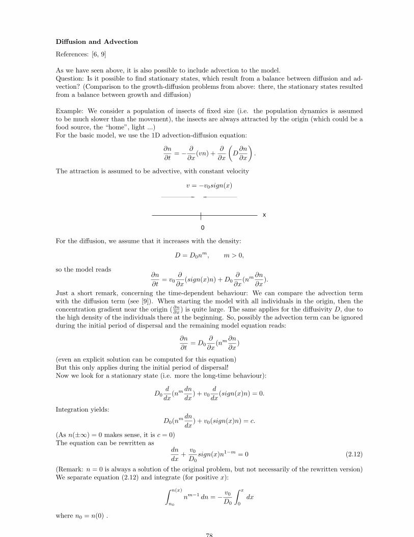
Diffusion and Advection
References: [6, 9]
As we have seen above, it is also possible to include advection to the model.Question: Is it possible to find stationary states, which result from a balance between diffusion and ad-vection? (Comparison to the growth-diffusion problems from above: there, the stationary states resultedfrom a balance between growth and diffusion)
Example: We consider a population of insects of fixed size (i.e. the population dynamics is assumedto be much slower than the movement), the insects are always attracted by the origin (which could be afood source, the “home”, light ...)For the basic model, we use the 1D advection-diffusion equation:
∂n
∂t= − ∂
∂x(vn) +
∂
∂x
(
D∂n
∂x
)
.
The attraction is assumed to be advective, with constant velocity
v = −v0sign(x)
0
x
For the diffusion, we assume that it increases with the density:
D = D0nm, m > 0,
so the model reads∂n
∂t= v0
∂
∂x(sign(x)n) + D0
∂
∂x(nm ∂n
∂x).
Just a short remark, concerning the time-dependent behaviour: We can compare the advection termwith the diffusion term (see [9]). When starting the model with all individuals in the origin, then theconcentration gradient near the origin (∂n
∂x ) is quite large. The same applies for the diffusivity D, due tothe high density of the individuals there at the beginning. So, possibly the advection term can be ignoredduring the initial period of dispersal and the remaining model equation reads:
∂n
∂t= D0
∂
∂x(nm ∂n
∂x)
(even an explicit solution can be computed for this equation)But this only applies during the initial period of dispersal!Now we look for a stationary state (i.e. more the long-time behaviour):
D0d
dx(nm dn
dx) + v0
d
dx(sign(x)n) = 0.
Integration yields:
D0(nm dn
dx) + v0(sign(x)n) = c.
(As n(±∞) = 0 makes sense, it is c = 0)The equation can be rewritten as
dn
dx+
v0
D0sign(x)n1−m = 0 (2.12)
(Remark: n = 0 is always a solution of the original problem, but not necessarily of the rewritten version)We separate equation (2.12) and integrate (for positive x):
∫ n(x)
n0
nm−1 dn = − v0
D0
∫ x
0
dx
where n0 = n(0) .
78

Case 1: m = 0 (simple diffusion), then
ln
(n
n0
)
= − v0
D0x ; n(x) = n0 · e−
v0D0
x (positive x)
We look for symmetric solution, so the whole solution can be written as
n(x) = n0e−
v0D0
|x|
(Remark: the total population size is conserved)
Case 2: m 6= 0:1
m(nm(x) − nm
0 ) = − v0
D0x ; n(x) = (nm
0 − mv0
D0x)1/m
Remark: This makes sense only for positive values for n(x). This can be avoided by setting the restof the solution to n = 0, which is also solution. A symmetric solution of this type can be written as
n(x) =
(nm0 − mv0
D0|x|)1/m, for |x| ≤ nm
0 D0
mv0
0 for |x| >nm
0 D0
mv0.
Remark: The steady-state solution here is only a weak solution, since the derivatives which areneeded for the PDE may not exist on the boundary of the support of n.
Sketch of the solutions:
0
xm=0
m=1/2m=1
m=2
One can observe: the larger m, the more “clumped” the solution looks. Although a large m leads to anincrease of diffusion at high densities, it also decreases the diffusion at low densities ; this can explainthe observed behaviour.
Of course, the modelling results were also compared to experimental findings. E.g. a kind of swarmof Mosquitoes was observed, respectively the spatial distribution of the insects within such a swarm, andthe distribution looked quite similar to the case of m = 1
2 .
2.1.3 Models of spread / Examples of Animal Diffusion
Reference: [6]
In this section we deal with the problem how to descrie the spread of invading populations., Again,we use Reaction-diffusion equations as modelling approaches.We shouldn’t forget that the diffusion equation leads to infinite speed of individuals, which is not realistic.There are several ideas how to circumvent that problem, respectively how to describe spread by usefulapproaches.
79
Threshold
One idea is to introduce a threshold, only a population density above that threshold is considered to bepresent at that place. This may lead to finite speed for the spread of the population.Example: Spread of muscrats (which escaped in Bohemia in 1905). It can be described very well by aradially symmetric spread, in combination with exponential growth:
∂n
∂t= αn + D
1
r
∂
∂r
(
r∂n
∂r
)
(α: intrinsic rate of growth; r radial coordinate). Assumed that the population starts with n0 individualswhich are concentrated at r = 0 at t = 0 (which corresponds exactly to the situation for the muskrats),the explicit solution can be computed, it reads
n(r, t) =n0
4πDteαt− r2
2Dt .
Assumption: A population can be detected, if it reaches the threshold density nc. We can approach thisproblem by computing the position r (dependent on time t), where the population density reaches thatlevel, respectively the velocity of this expansion, r/t. So we find:
r
t=
√
4αD − 4D
tln
(
4πnc
n0Dt
)
.
For large times t, this average velocity tends to
r
t= 2
√αD.
Travelling wave approach
Instead of a steady-state solution, we look for a solution which moves with constant speed c. For that,the so-called wave variable z is introduced,
z = x − ct,
one is interested e.g. in a moving wage (to the right) of the form
u(x, t) = u(x − ct) = u(z),
hence
∂u
∂t=
∂u
∂z
∂z
∂t= −cu′
∂u
∂x=
∂u
∂z
∂z
∂x= u′.
Typical example: the Fisher equation
∂n
∂t= rn
(
1 − n
K
)
+ D∂2n
∂x2,
We rescaleu = n/K, t = rt, x =
√
r/Dx,
(for reasons of simplicity, drop the tildes again), this yields
∂u
∂t= u(1 − u) +
∂2u
∂x2
. So the travelling wave approach leads to
−cu′ = u(1 − u) + u′′
(an ODE of 2nd order). Analogously to above, it can be reformulated as system of two first-order ODEs:
u′ = v
v′ = −cv − u(1 − u).
80

Additionally there are conditions for the wave
limz→−∞
(u, v) → (1, 0)
limz→+∞
(u, v) → (0, 0),
Stationary points:(0, 0) is stable; a focus for 0 < c < 2 respectively a stable node for c ≥ 2.(1, 0) a saddle point.A travelling wave corresponds to a heteroclinic orbit which connects (1, 0) to (0, 0). For populations onlynonnegative solutions make sense ; only c ≥ 2 yields meaningful solutions.This means: c ≥ 2 is a necessary condition for a travelling wave; c = 2 is the minimum wave speed. Inoriginal coordinates this corresponds to a speed
dx
dt= 2
√Dr
Until now, we only know that c ≥ 2 is necessary, we do not now, if it is also a sufficient condition. But,indeed, using the properties of the vector field shows that the solution curve which leaves the saddle point(1, 0) ends up in the stable node (0, 0). (We neglect the details here, it is not complicated, but a littlebit lengthy). This corresponds to the heteroclinic orbit for what we are looking.Sketch of the phase plane and the heteroclinic orbit:
u
v
(Remark: the yellow curve shows the behaviour in case of c < 2, with the stable focus in (0, 0))Next question: How to determine the profile of the travelling wave solution?¿From the ODE system we get directly: a solution v(u) satisfies
dv
du=
−cv − u(1 − u)
v, (2.13)
thus also the heteroclinic orbit.Let v = 1
cy, then we can rewrite equation (2.13):
εydy
du= −y + u(u − 1), (2.14)
where ε = 1c2 . At least we know that ε is not too big (due to c ≥ 2, so it might make sense to expand y
as a power series in ε:y(u, ε) = y0(u) + εy1(u) + ε2y2(u) + . . .
This is inserted into (2.14):
ε(y0(u) + εy1(u) + ε2y2(u) + . . .) · (dy0
du+ ε
dy1
du+ ε2 dy2
du+ . . .)
= −(y0(u) + εy1(u) + ε2y2(u) + . . .) + u(u − 1).
We split up that equation into the different orders (i.e. powers) in ε:
ε0: y0(u) = u(u − 1)
81

ε1: y1(u) = y0(u) · dy0
du
ε2: y2(u) = y1(u) · dy0
du + y0(u) · dy1
du ,
So, the heteroclinic orbit can be written as
y(u) = y0(u) + ε y0(u)dy0
du︸ ︷︷ ︸
y1(u)
+ε2 y1(u)dy0
du+ y0(u)
dy1
du)
︸ ︷︷ ︸
y2(u)
= u(u. − 1) − εu(u − 1)(2u − 1) + . . .
Of course, this can be written also in the original variables u and v:
v(u) = ε1/2(u2 − u) − ε3/2(2u3 − 3u2 + u) + . . .
Now, we have a description in variables u and v. But of course, one is interested more in a solution foru dependent e.g. on z. We can use a similar idea:Let s = z
c , then the wave equation (the ODE of 2nd order) is transformed into
εu′′ + u′ + u(1 − u) = 0. (2.15)
Even though the ε appears in the term with the highest derivative, also for ε = 0 both “additional waveconditions” can be satisfied also for ε = 0, i.e. we really deal with a regular perturbation problem. Nowwe can expand u in terms (powers) of ε:
u(s, ε) = u0(s) + εu1(s) + . . . ,
this is substituted in (2.15), we split up the different powers of ε and get:
ε0: u′0 = −u0(1 − u0)
ε1: u′1 + (1 − 2u0)u1 = −u′′
0
s can be chosen arbitrarily, since the equation (2.15) and the traveling wave solution both are invariantto translations in s. Thus, we choose s = as point where u = 1/2 for all ε, i.e.
u0 =1
2ui = 0 for i = 1, 2, 3, . . .
Hence, we can solve the equations for the single orders in ε step by step and get
u0(s) =1
1 + es
u1(s) =es
(1 + es)2ln
(4es
(1 + es)2
)
,
and rewritten in the original variable z:
u(z, ε) =1
1 + ez/c+
1
c2
ez/c
(1 + ez/c)2ln
(
4ez/c
(1 + ez/c)
2)
+ O(c−4)
One can also show that the traveling wave solution for the Fisher equation is stable, but this is left outhere.
2.1.4 Animal movements in Home range
Reference: [8]As a famous example, we consider here the ecology of wolves. They have “home ranges”, i.e. territories,where packs live. A pack is a family with 3-15 wolves as members. (Also other species have suchterritories, e.g. lions, hyenas, badgers ...). In many cases, the pack territories remain unchanged formany years, and there is rarely an overlap of two such territories. Between the territories, there areso-called “buffer zones”, around 2 km wide. These buffer zones reduce e.g. interpack conflicts (and thusreduce the probability of death of the pack leaders, which might lead to pack disintegration).Several questions arise in that context:
82

• How are these territories determined?
• How can the territories be maintained?
• How can predators (wolves) and prey (mainly moose and deer, in Northern America) coexist incase of predator territories?
Some more background information about wolves:
• They can cover around 50km per day, even though, they cannot cover the whole territory bycontinuing physical presence.
• Exchange of information can be done on two ways:
– Howling yields a temporary information on the location of the pack, also on the pack size
– Scent marking (denoted by RLU) is more useful for territorial claims, even in absence of theanimals; but does not yield precise information about the pack size since only a few individualsare involved in marking. Important for the modelling approach!
• Reproduction of wolves mainly takes place in April or May. The whole pack is involved in feedingthe pups; the pups usually stay near the den.
• The prey, deer, reproduce usually in early summer. Outside these seasons, population changes onlyoccur by mortality, emigration or immigration.
Goal: Put up a mechanistic model, which is spatially explicit.
A lot of data are available from the observation of wolves in northeastern Minnesota; gained b ra-diomarking studies over 25 years.
Home range model for a single wolf pack
We start with a very simple model just for the wolf population; in order to learn how terrotories can bebuilt and maintained.Assumptions: no birth processes included, enough food available, just consider the territory formationand maintenance during the summer months. The territories are assumed to be marked by RLU as maindelineation method.Two mechanisms guide the spatial wolf movement:
• dispersal for search of food and e.g. marking
• movement back to the den (bringing food, taking care for the pups)
We look for densitities for the wolves at point x and time t. (Remark: Direct field observation will notprovides these data very exactly due to the small numbers of individuals).
In case of a two wolf pack model, the following state variables could be used:
u(x, t) = expected density of wolves from pack 1
v(x, t) = expected density of wolves from pack 2
p(x, t) = expected density of RLUs from wolf pack 1
q(x, t) = expected density of RLUs from wolf pack 2
(for a probabilistic approach, due to the small numbers of animals)
For the movement back towards the den we assume that it happens on a straight line, described mathe-matically by directed motion (in form of a flux),
Ju|convection = −cu(x − xu)u.
xu: location of the den; cu(x−xu) space-dependent velocity of movement (compare to the movement forthe insects, there the speed of movement was constant, discontinuous in 0).A typical approach for the velocity, including a slow-down and stopping at the den site, reads
cu(x − xu) = cu tanh(βr)x − xu
r
83
Here, r = ‖x − xu‖, cu maximum speed of the wolf in direction to the den, β change in the rate ofconvective movement as the den is approached (remark again: β → ∞ corresponds to the discontinuousform).
If enough food is available (and uniformly distributed throughout the region), we can assume a randomwalk process, maybe density-dependent; thus this kind of movement can be represented by a diffusionflux:
Ju|Diffusion = −D(u)∇u,
where D(u) = duun (n > 0, du constant). Interpretation: a positive n means that the wolf pack prefersto move to regions which are more familiar to the wolf pack.Hence, a very simple model for a single isolated wolf pack reads:
∂u
∂t+ ∇ · Ju = 0 ⇒ ∂u
∂t= ∇ · (cu(x − xu)u + Du(u)∇u).
(Remark: conservation of population!).Let Ω denote the “domain of interest” (not yet determined). Assumption: No emigration or immigrationof Ω ; zero-flux boundary condition
Ju · n = 0 on ∂Ω,
where n is the outward unit normal to the boundary ∂Ω.Initial condition:
u(x, t) = u0(x).
The total number of wolves, Q in Ω is
Q =
∫
Ω
u(x, t) dx,
for all times t. Indeed:
∂
∂t
∫
Ω
u(x, t) dx =
∫
Ω
∂
∂tu(x, t) dx = −
∫
Ω
∇ · Ju dx = −∫
∂Ω
Ju · nds = 0,
so the number of wolves inside Ω stays constant.The average density of wolves in Ω can be computed by
U0 =1
A
∫
Ω
u0(x) dx,
where A is the area of Ω.
In the next step, we consider the steady state problem (i.e. time-independent). The basic equationbecomes
0 = ∇ · (cu(x − xu)u + Du(u)∇u),
in the following we use Du(u) = d0un and cu(x− xu) = cu tanh(βr)x−xu
r , and consider the 1D situation.This leads to the equation
cuu tanhβ(x − xu) + duun du
dx= const.
Two cases:
Linear diffusion, n = 0: This corresponds to D(u) = du constant. Integration yields directly the steadystate solution us():
us(x) =B
(cosh β(x − xu))cu/(duβ),
B is a constant of integration, determined by
B
∫
Ω
dx
(cosh β(x − xu)cu/(duβ)= Q
(from the conservation condition)
84

Nonlinear diffusion, n > 0: In this case, integration yields:
us(x) =
(cunduβ ln
(cosh βxb
cosh β(x−xu)
))1/n
for |x − xu| ≤ xb
0 else
xb, the range radius of the pack, is implicitly given by
∫ xu+xb
xu−xb
(cun
duβln
(cosh βxb
cosh β(x − xu)
))1/n
dx = Q.
Remark: Here we have a “weak solution” which satisfies the equation at all points except forx = ±xb.
Big difference: in case of n > 0, there are territories with finite boundaries formed; but not in case ofn = 0.
Territorial model for two wolf packs
We take the main ideas from above. The exchange of information between two packs mainly happens viaRLU marking. It is not yet clear, how exactly the response is. Two ideas:
• Presence of foreign RLU marks increases the speed of movement back to the den (as central terri-tory); additionally the production of familiar RLU is increased.
• The movement of the wolves is along the gradients of foreign RLU marking (away from high density);additionally the production of familiar RLU is increased.
For both approaches, it is necessary to introduce both RLU densities into the model. Now, three mecha-nisms guid the spatial wolf movement; additional to the “standard dispersal” and the “standard movementto the den” there is a movement away from the RLUs from the other pack. According to the two ideasfrom above, there are two typical approaches for the movement caused by the RLU marking of the otherpack:
• The presence of foreign RLUs just increases the (always present) rate of movement back to the den,i.e. by a convection flux:
Jcu= −cu(x − xu, q)u
It is assumed that dcu
dq ≥ 0; typically the function cu(x−xu, q) is a bounded monitonically increasing
function of q, e.g. of the form Aq/(B + q).
• For the movement down the gradients of foreign RLU density, a suitable modelling approach reads
Jau= −au(q)u∇q,
where au(q) is a monotonically non-decreasing function.
Taken together, the conservation equation for the wolves in pack 1 reads
∂u
∂t+ ∇ · (Jcu
+ Jdu+ Jau
) = 0,
with the fluxes
Jcu= −ucu(x − xu, q), cu(0) ≥ 0,
∂cu
∂q≥ 0
Jdu= −du(u)∇u, du(0) ≥ 0,
ddu
du≥ 0
Jau= −au(q)u∇q, au(0) ≥ 0,
dau
dq≥ 0.
In the same way, the equations for wolf pack 2 can be introduced:
∂v
∂t+ ∇ · (Jcv
+ Jdv+ Jav
) = 0,
85

with the fluxes
Jcv= −vcv(x − xv, p), cv(0) ≥ 0,
∂cv
∂p≥ 0
Jdv= −dv(v)∇v, dv(0) ≥ 0,
ddv
dv≥ 0
Jav= −av(q)v∇p, av(0) ≥ 0,
dav
dp≥ 0.
In the next step, we have to introduce equations for the RLU densities p and q. Assumption (guidedby experimental observation): The wolfes do RLU marking throughout the territory on a low level (lpresp. lq); foreign RLU marking increases the marking activities. The RLU decays with a constant ratefp respectively fq. So a plausible assumption for p (RLU marking by pack 1) and q (RLU marking bypack 2) is formulated as follows:
∂p
∂t= u(lp + mp(q)) − fpp
∂q
∂t= v(lq + mq(p)) − fqq
For the boundary conditions we assume again that no immigration or emigration of Ω takes place; thuswe have zero-flux boundary conditions for u and v on the boundary ∂Ω:
(Jcu+ Jdu
+ Jau) · n = 0 on ∂Ω
(Jcv+ Jdv
+ Jav) · n = 0 on ∂Ω
(again n is the outward unit normal to ∂Ω).Initial conditions are given for the spatial distribution of the wolves and the two types of RLU marking:
u(x, 0) = u0(x), v(x, 0) = v0(x), p(x, 0) = p0(x), q(x, 0) = q0(x)
Again one can show (by using the zero-flux boundary conditions and the divergence theorem): the totalnumber of wolves of each wolf pack remains constant.Using the area A =
∫
Ωdx, the average densities of the wolves can be computed by
U0 =1
A
∫
Ω
u0(x) dx, V0 =1
A
∫
Ω
v0(x) dx
For reasons of simplicity, the whole model system can be nondimensionalised. Let L = A1/m where mdenotes the dimension of the solution domain, i.e. m = 1 or m = 2. A lot of new dimensionless quantitiesare introduced; for tat we have to assume U0, V0 > 0 (both packs are present), L > 0 (domain size greaterthan zero), lp, lq > 0 (nonzero low level of RLU marking for both packs), fp, fq > 0 (nonvanishing decayof RLU).
u∗ = uU0
, v∗ = vV0
, p∗ =pfp
U0lp, q∗ =
qfp
V0lq, t∗ = tfp, x∗ = x/L
c∗u = cu
Lfp, c∗v = cv
Lfp, d∗u = du
L2fp, d∗v = dv
L2fp
a∗u =
auV0lqL2f2
p, a∗
v =avU0lpL2f2
q, m∗
p =mp
lp, m∗
q =mq
lq, φ =
fq
fp.
The asteriscs are dropped (for a better notation), nevertheless we end up with the nondimensionalisedsystem:
∂u
∂t+ ∇ · (Jcu
+ Jdu+ Jau
) = 0
∂v
∂t+ ∇ · (Jcv
+ Jdv+ Jav
) = 0
∂p
∂t= u(1 + mp(q)) − p
∂q
∂t= v(1 + mq(p)) − φq,
86

the fluxes are given by
Jcu= −ucu(x − xu, q), Jdu
= −du(u)∇u, Jau= −au(q)u∇q
Jcv= −ucv(x − xv, p), Jdv
= −dv(v)∇v, Jav= −av(p)v∇p,
all functions cu, cv, du, dv, au, av are assumed to be nonnegative (or constants), as described above.The boundary conditions remain unchanged; the initial conditions (after omitting the asteriscs) look thesame as before, just with the new notation.For the nondimensionalised variables we get
∫
Ω
u(x, t) dx =
∫
Ω
v(x, t) dx = 1,
this allows us to interpret u(x, t) and v(x, t) as probability density functions for the location of wolves.For the next steps of analysis, we consider the 1D version of the equations above; the position of the densis assumed to be at the opposite ends of the domain (xu = 0, xv = 1). Steady state solutions for thathave to satisfy
0 = [Ju]x, Ju = −duux − cu(ru, q)u,
0 = [Jv]x, Jv = −dvvx + cv(rv, p)v,
0 = u(1 + mp(q)) − p,
0 = v(1 + mq(p)) − φq.
(again, ru and rv denote the distances to the dens).The boundary conditions read
Ju, Jv = 0 at x = 0, 1
and ∫ 1
0
u(x) dx =
∫ 1
0
v(x) dx = 1.
Remark that the functions m should be chosen as described above, then it guarantees that no blow-uphappens to the solution. This makes also sense from an ecological point of view: preventing an arbitrarilyhigh marking rate).
In the next step we look for the existence of a “buffer zone” between the packs.From a mathematical point of view, such a buffer zone corresponds to an interior minimum for u + v.We do the analysis for the 1D case and assume that the two interacting packs behave identical, i.e.du = dv = d, φ = 1 etc.; for the movement response function c it is assumed not to be explicitly spatialdependent (just for reasons of simplicity for the computations and to understand the principle). Hence,we use the equations
du
dx= −1
dc(q)u,
dv
dx=
1
dc(p)v,
p = u(1 + m(q)),
q = v(1 + m(p)),
the integrals over u and v still yielding 1.The solution of this system is invariant to x → 1 − x, u ↔ v, p ↔ q, and thus symmetric about themidpoint x = 1
2 . This also means that at x = 1/2 we have
u = v, p = q
0 >du
dx= −dv
dx,
dp
dx= − dq
dx,
d(u + v)
dx= 0,
dq
dx=
1 + m(p)
1 + vm′(p)
dv
dx> 0,
87

furthermore
(u + x)xx =1
d(c(p)v − c(q)u)x
=2
d(c′(p)upx − c(p)ux)
=2u2
d
d
dx
(c(p)
p
p
u
)
=2u2
d
d
dx
(c(p)
p(1 + m(q))
)
=2u2
d
(d
dp
(c(p)
p
)
(1 + m(q))px +c(p)
pm′(q)qx
)
The property of c(p) being convex is sufficient for the right-hand side of the last line to be positive. Thenx = 1/2 is a minimum for u + v, which corresponds to a buffer zone for the interacting packs.Of course, also assumptions can be made and analysed, some examples can be found in the literatureand the references in there.
Special case: Foreign RLU causes increased movement back to the den (and an increased productionof the own RLU), without additional movement along the foreign RLU gradient. Goal is to determine amore or less explicit solution. Then our equations read
∂u
∂t= ∇ · (cu(x − xu, q)u + du∇u)
∂v
∂t= ∇ · (cv(x − xv, p)v + dv∇v)
∂p
∂t= u(1 + mp(q)) − p
∂q
∂t= v(1 + mq(p)) − φq
Simple assumption for the functions c and m: they are assumed to be piecewise linear, i.e.
cu(q) =
γq for 0 ≤ q ≤ c∞/γc∞ for q ≥ c∞/γ
mp(q) =
µq for 0 ≤ q ≤ m∞/γm∞ for q ≥ m∞/γ
similarly for cv and mq.One can show: There are interior maxima for p(x) and q(x) only if u(x) = 1
µ and v(x) = 1µ . Due to the
fact that u(x) and v(x) are monotonically decreasing functions (with respect to the distance to their densite), it is necessary to have u(0) ≥ 1/µ ≥ u(1) and v(0) ≤ 1/µ ≤ v(1). In that case, the solutions lookqualitatively as follows:
0 1
blue: pack 1; solid line - wolf density, dashed line - RLU densityred: pack 2; solid line - wolf density, dashed line - RLU density
88

Wolf-Deer Predator-Prey model
Until now, we neglected any dynamics or spatial distribution of the prey (e.g. deer).Simplest assumption: The wolves prefer to move to regions of higher deer density, which correspondsmathematically to a movement along a “deer gradient”. Let h denote the deer density and σu a kind of“strength of the taxis”, then the flux, caused by the deer, can be formulated by
Jdeer = σuu∇h
Remark: There is the same idea as in the chemotaxis behind!Asumptions for the deer dynamics: We only consider the situation in sumer, i.e. the deer do not move ona large spatial scale; furthermore the deer do not seem to “avoid” actively places where wolves are present(as long as they are not predated in a certain moment). So a simple model for the deer population canbe introduced as follows:
∂h
∂t= −(αuu + αvv)g(h),
where αu, αv constants, g(h) could be a typical saturating function like g = ahm/(1 + bhm) with m = 1or m > 1. The “natural mortality” during summer can be neglected - the big part of mortality in thattime is caused by the predation by wolves. Taken together, a basic model for the wolf-deer interactioncan be formulated as follows:
∂u
∂t= ∇ · (cu(x − xu)u − σuu∇h),
∂v
∂t= ∇ · (cv(x − xv)v − σvv∇h),
∂p
∂t= u(lp + mp(q, h)) − fpp,
∂q
∂t= v(lq + mq(p, h)) − fqq,
∂h
∂t= −(αuu + αvv)g(h).
Possible improvements for the basic models, which are neglected up to now:
• What happens if not enough prey is available? Starvation could be introduced by an additionalterm of the form −αuufu(h), where fu is a positive function, which is decreasing in h
• How to include interpack conflicts? As this could arise if both packs are present at certain places,it could be introduced by an additional term −kujuv.
As these effectly usually play a minor role during the summer period, they are often neglected in thiskind of modelling approach.
Another limitiation of the model approach as considered here: The simulations are valid only for alimited period of time:
• a lot of assumptions were made which limit the model to the summer period
• the prey population could die out under these assumptions
• seasonal deer reproduction (or also wolf reproduction) is not included
• ...
Nevertheless, simulations look qualitatively similar to the experimental observation, and by that, theapproach is “justified”!
2.1.5 Some ideas for the dynamics of animal grouping
Simple Simulation model for Animal grouping
Reference: [9]
89

The idea was developed in 1973 by Sakai and Suzuki: The motion of individual animals is guided by aequation of the type of Newton’s equation of motion:
md2x
dt2= R + K + A,
where R denotes a kind of frictional force, which is proportional to the velocity, K is a kind of force, whichis attractive toward the center of the “herd”/group of animals, and which is assumed to be proportionalto the distance from the center. and A = A(t) a kind of random force, which just depends on the time t.So we can write N equations for a group of N individuals:
md2xi
dt2+ mk
dxi
dt= Ki + Ai(t)
The forces Ki may consist of three typical types of forces:
1. Forward thrust Kf : Animals tend to continue moving forward with their velocity; it can be ex-pressed as
(Kf )i = adxi
dt
/|dxi
dt|,
a > 0 const. (called the “coefficient of thrust”).
2. Mutual interaction Km: An individual underlies attraction respectively repulsion from the otherindividuals which belong to the group; this mechanism is assumed to depend on the distance betweentwo individuals and can be formulated as follows:
(Km)i =1
N − 1
N∑
j=1,j 6=i
Q(Rij)(xj − xi)/Rij ,
Rij = |xj − xi| denotes the distance between individual i and j. Assumption for Q (introduced bySakai and Suzuki):
Q(Rij) =
−c0Rij for 0 < Rij < R0
c for R0 < Rij < R1
0 for R1 < Rij
This means: If an individual is very close to another one (i.e. closer than R0), then there isa repulsive force (this is assumed to be linearly dependent on the distance); in an intermediatedistance, there is a constant attractive force, and if the distance is too larger, there is no interactionassumed.
3. Arrayal force Ka: Two neighbouring animals prefer to have the same velocity. This only happens,if they are sufficiently close to each other (i.e. within a sphere of influence); the so-called meanarrayal force of the i-th individual is formulated as
(Ka)i =1
Mi
∑
xj∈Vi
h
(dxj
dt− dxi
dt
)
,
where h denotes to so-called coefficient of arrayal force, Vi = 43πl3i the sphere of influence around
individual i (and li is the radius of the sphere), Mi the number of animals within the sphere ofinfluence.
Taken together, the equation of motion for individual i in a group, reads:
md2xi
dt2+ mk
dxi
dt= a
dxi
dt
/|dxi
dt| + 1
N − 1
N∑
j=1,j 6=i
Q(Rij)xj − xi
|xj − xi|+
1
Misumxj∈Vi
h
(dxj
dt− dxi
dt
)
+ Ai(t).
(2.16)Of course, equation (2.16) can be solved only in very simple special cases analytically, but it is veryuseful for computer simulations. Dependent on the chosen parameter, typical group movements can beobserved:
Amoebic movement: For this situation, the random force dominates the forward thrust, which leadsto a more or less circular pattern (with fluctuating shape of the group), around a centre (of massof the animals) which hardly moves.
90

Doughnut pattern: For this situation, the forward ghrust dominates the random force, then a group ofanimals may itself around an empty centre (it looks somehow like a doughnut)
Rectilinear movement: For this situation, the arrayal force is added, then the animal group may performa rectilinear movement as a whole.
Of course, combined effects are also possible and occuring in reality!
The split and Amalgamation of Herds
Reference: [9]
In nature, there is only limited space, i.e. herds which wander around may meet other herds (allow-ing for interaction between herds). It is possible that two herds amalgamates, or vice versa, that a largeherd splits up into two smaller herds.Typical example: Elephants!
From a modelling point of view, a simple model can be introduced by a small stochastic model deal-ing with the size of elephant herds. Such a model was introduced in 1967 by Holgate.
Situation: We have an area with N elephants living in there. We introduce a probability Pk(t) thatthe elephants are grouped into k herds at time t (necessarily 1 ≤ k ≤ N).
Amalgamation:
If k = 1: no chance for amalgamation, but increasing chance for meeting and amalgamation of two herdsfor increasing k.Approach: probability of an amalgamation occuring in (t, t + ∆t) in presence of k herds is µ(k + 1)∆t (µis called “coefficient of amalgamation”)(An alternative model introduced by Boyd in 1979 assumes for this probability µk(k − 1), guided by theidea that the meeting chance of the herds plays a big role).
Splitting:
The probability of splitting of a herd may increase dependent on the herd size xi. Assumption: it isproportional to xi − 1 (as obviously a herd with size xi = 1 cannot split).So the probability that splitting of one existing herd in the time interval (t, t + ∆t) reads
λ
k∑
i=1
(xi − 1)∆t = λ(N − k)∆t
(λ is called the “coefficient of splitting”).
As in the simple stochastic population models also here the probability of two events (amalgamation
91

or splitting) during the small time interval (t, t + ∆t) is ignored (higher order).Hence, we obtain for the rate of change of the Pk(t):
dP1(t)
dt= µP2 − λ(N − 1)P1
dPk(t)
dt= λ(N − (k − 1))Pk−1 + µkPk+1 − (µ(k − 1) + λ(N − k))Pk for 1 < k < N
dPN (t)
dt= λPN−1 − µ(N − 1)PN .
We do not consider many details here, but it may be interesting to look for the coresponding stationaryprobability distribution (denoted by the P ∗
k for the stationary probability):
P ∗k =
(N − 1)!
(N − k(!(k − 1)!
(a
1 + a
)k−1 (1
1 + a
)N−k
,
where a = λµ (compare to the Binomial distribution!)
One can also compute the expected value for N/k which corresponds to the average herd size:
q =N∑
k=1
(N/k)P ∗k =
(1 + a)N − 1
a(1 + a)N−1
From that we get the influence of the parameter a on the behaviour of the population:In case of a → 0, the value q tends to N (Rule of de l’Hospital!), which means that the whole populationforms one herd.In case of a → ∞, the value q tends to 1, which means that the whole population is divided in singleindividual herds.
2.2 Age-Structured models
Reference: [6]
2.2.1 Overview
In many species, the age of the individuals play a big role, concerning fertility and/or mortality. Ofcourse, there may be also consequences for the survival of the population as a whole.From a modelling point of view, there are mainly four typical approaches, which are used in literature:
discrete in time ↔ continuous in timeresulting birth rate ↔ age structure of the population
Here, we only have a very short overview over the different approaches.Remark: Only the females in a population are considered in this context.
2.2.2 Difference equation
The approach is already well-known, remark that by difference equation, different ages can be modelledvery easily. The basic idea is as follows: Let
Bt = number of female births at time t
na,t = number of females of age a at time t
la = fraction of females surviving from birth to age a
ma = average number of females vorn to a female of age a
(in this context, a and t have to be integers) .Let ω denote the maximum age of survivorship. Using this notation, the number of births can be describedby
Bt =
t∑
a=1
Bt−alama + Gt,
92

where
Gt =ω−t∑
a=1
na,0la+t
lama+t
Interpretation: The first term in the birth equation describes the number of births given by individu-als which were born during the “run of the model”, which weren’t already present when starting themodel/the observation (i.e. of birth time t ≥ 0). The second term concerns those individuals which werealready born at time t = 0 and still alive (or being more precise: still reproductively active).Remark: In the approach, the number of births at a certain time t is of interest, not the age structure ofthe whole population.
Typical application: growth rates etc. for population which live in clearly defined generations
2.2.3 Leslie matrix
The Leslie matrix is also a discrete-time model, but focuses on the age distributon of the population, notso much on the birth rate. With the same notation as before, we can formulate:
n0,t+1 = l1m1n0,t +l2l1
m2n1,t + . . . +lω
lω−1mωnω−1,t.
na,t+1 =la
la−1na−1,t, for a = 1, 2, . . . , ω − 1.
For a simpler notation we introduce
Pa =la+1
la,
which describes the survival probabilities from year to year. Additionally, one can introduce a fertilityfor each age class:
Fa = Pama+1
The model equations are linear, so they can be easily collected in a matrix vector notation:
n0
n1
...nω−1
=
F0 F1 F2 · · · Fω1
P0 0 0 · · · 00 P1 0 · · · 0... · · ·
.... . .
...0 0 · · · Pω2
0
n0
n1
......
nΩ1
,
or even shorter asnt+1 = Lnt,
L is called the Leslie matrix.
Typical application: Populations with clearly defined age classes (can be easily extended to stage struc-tured approaches), with questions concerning age distributions.
2.2.4 Lotka integral equation
The Lotka model is a continuous-time model which considers especially the birth rate of a population.In the continuous-time approach, we use the following notations:
B(t) dt = number of female births during [t, t + dt)
n(a, t) da = number of females of age a to a + da at time t
l(a) = fraction of newborn females surviving to age a
m(a) da = average number of females born to a female during the ages a to a + da
Assumptions: l(a) is continuous and (piecewise) smooth; nonincreasing.m(a), the so-called maternity function is assumed to be continuous and (piecewise) smooth, as well; witha minimum age of reproduction α and a maximum age of reproduction β. Typical graphs for l(a) andm(a) look as follows:
93

a a
l(a) m(a)
1
ω α β
Lotka’s basic model for the rate of births reads:
B(t) =
∫ t
0
B(t − a)l(a)m(a) da + G(t),
where
G(t) =
∫ ω−t
0
n(a, 0)l(a + t)
l(a)m(a + t) da.
Similar as in the discrete model approach one has to distinguish between “younger individuals” whichwere born at time t ≥ 0, and “elder individuals” which were born before t = 0 (they are included intothe model via initial conditions).Remark that the equation for B(t) is formulated as a nonhomogeneous Volterra integral equation ofsecond kind.
Typical applications: Computation of intrinsic rate of growth of continuously reproducing populations(also human populations), doubling times ...
2.2.5 McKendrick- von Foerster PDE
The McKendrick- von Foerster PDE is a continuous-time model, which considers in details the agedistribution. We use again
n(a, t) = number of females of age (a, a + da) at time t.
The rate of change of number of females in a given age interval can be formulated as
∂
∂t(n(a, t)∆a) = + rate of entry of a
− rate of departure at (a + ∆a)
− deaths
, in mathematical terms
∂n
∂t∆a = J(a, t) − J(a + ∆a, t) − µ(a, t)n(a, t)∆a
µ(a, t) denotes the per capita mortality rate for individuals of age a at time t. J(a, t) is a kind of fluxof individuals of age a at time t (we deal with that in a few steps).Division by ∆a yields
∂n
∂t= −
(J(a + ∆a, t) − J(a, t)
∆a
)
− µ(a, t)n,
respectively in the limit ∆a → 0∂n
∂t= −∂J
∂a− µ(a, t)n.
This looks like a “conservation law” for the density of individuals! Question: Hoew to introduce ameaningful flux J?In our context, the “flux” J is a movement of individuals in age! As all individuals become older (andall in the same way), the flux can be assumed to be proportional to the density of individuals, includinga characteristic velocity v(a, t) of aging:
J(a, t) = n(a, t)v(a, t)
94

In the standard approach, the aging corresponds one-to-one to the passage of time, i.e.
v =∂a
∂t= 1.
(Remark: When using a size-structured approach instead of an age-structured one, this “velocity” canbe more complicated, since increase in size mustn’t be proportional to the time)In the standard case, we get:
∂n
∂t+
∂n
∂a= −µ(a, t)n.
How to include births to this model? Here, it corresponds to a boundary condition at age a = 0:
n(0, t) =
∫ ω
0
n(a, t)m(a, t) da.
(Compare to the birth rate B(t) in the Lotka integral equation!)The maternity function m(a, t) may depend on the age and also explicitely on the time; ω is again themaximum attainable age.Initial age distribution is introduced as
n(a, 0) = n0(a)
So, the model here consists of a first-order PDE, which is not too complicated, but the boundary condi-tion is not so easy to “use”.
Typical application: description of age-dependent phenomena for “continuous-time populations”, agedistributions, population dynamics, easy to extend to nonlinear situations
For the solution fo the McKendrick- von Foerster PDE in general, one can use the so-called methodof characteristics (we do not consider it here in detail, as it was treated in the lecture Math. Modelsin Biology). The idea is: Information is transported via characteristics; in our model the characteristicscorrespond to straight lines with slope 1:
Bou
ndar
y co
nditi
ons
Initial conditions
t
a
This method allows to transform the PDE into a system of three ODEs.We have to distinguish if the characteristics intersect with the initial conditions (a-axis) or the theboundary conditions (t-axis).
Case 1: a ≤ t (green region in the figure)
n(a, t) = n(0, t − a)︸ ︷︷ ︸
B(t−a)
· e−R
a
0µ(ξ) dξ
︸ ︷︷ ︸
l(a)
(Idea behind: Take the number of births a years ago, this is multiplied by the probability ofsurviving to age a)
Case 2: a ≥ t (blue region in the figure)
n(a, t) = n0(a − t)︸ ︷︷ ︸
n(a−t,0)
· e−R
t
a−tµ(ξ) dξ
︸ ︷︷ ︸
l(a)l(a−t)
(Idea behind: Take the number of females which were present at t = 0; this is multiplied by theprobability of surviving from age a − t to age a)
95

Example: Age-dependent harvesting
We consider a population with an age-structure; only individuals with age a ≥ c are harvested (with afraction δ, 0 < δ < 1); additional to the natural mortality. The model reads (in form of a McKendrick-von Foerster PDE):
∂n
∂t+
∂n
∂a= −µ(a)n − δH(a − c)n,
with the Heaviside step function
H(a) =
1, for a ≥ 00, for a < 0.
It can be considered e.g. with the method of characteristics, the resulting density can be written as
n(a, t) =
n(0, t − a)l(a) for a ≤ c, tn(0, t − a)l(a)e−δ(a−c) for c < a < t
n(a − t, 0) l(a)l(a−t) for t ≤ a < c
n(a − t, 0) l(a)l(a−t)e
−δ(a−c) for a ≥ t, a ≥ c, a ≤ t + c
n(a − t, 0) l(a)l(a−t)e
−δt for a > c − t
This means:1.row: females born since the start of the problem, too young to be harvested2.row: females born since the start of the problem, old enough to be harvested for a − c years3.row: females present at the start of the problem, too young to be harvested4.row: females present at the start of the problem, being harvested for a − c years5.row: females present at the start of the problem, being harvested for the complete time
Remark: There is an incompatibility included: Either we have t ≤ c or t > c, but it is impossiblethat there are females which were born after the start of the problem and already harvested, and at thesame time females which were already present at the start and never harvested. So, either the second orthe third line have to be “dropped”.
It is often useful to assume that birth and death rates do no depend explicitely on time, but on ageand the total population size. The total population size at time t reads
N(t) =
∫ ∞
0
n(a, t) da,
and the age-structured model can be formulated as
∂n
∂t+
∂n
∂a= −µ(a,N)n
n(0, t) =
∫ ∞
0
n(a, t)m(a,N) da
n(a, 0) = n0(a)
Special case: Gurtin-MacCamy models, with an age-independent mortality µ(a,N) = µ(N), and anatality of the following form:
m(a,N) = β(N)ane−γa
Example: Tribbles
The tribbles are originally from the planet Iota Geminorum IV ; Star Trek. They are born alreadypregnant and are potentially infinitely long living. Their age specific birth rate decreases exponentiallywith age, i.e. m(a,N) = m0 · eγa. The model reads
∂n
∂t+
∂n
∂a= −µ(N)n (2.17)
n(0, t) =
∫ ∞
0
m0e−γan(a, t) da (2.18)
n(a, 0) = n0(a) (2.19)
96

2.2.6 Comparison of these modelling approaches
The models look quite different, but there are also a lot of similarities:
• all models need an initial age distribution
• all models need a detailed description of the age-specific mortality
• all models need a detailed description of the age-specific natality
One can also find for all of these models:
• an “intrinsic rate of growth” of the population (by a so-called dominant eigenvalue)
• a stable age distribution (by an eigenvector)
So, the preferences for one or another model are guided more by the applications; in addition to historicalreasons this led to the dominance of each model in different areas of mathematical ecology.
2.3 Sex-structured models
2.3.1 Two-sex models
97
Bibliography
[1] G. de Vries, T. Hillen, M. Lewis, J. Muller, and B. Schonfisch. A Course in Mathematical Biology.SIAM, 2006.
[2] L. Edelstein-Keshet. Mathematical Models in Biology. SIAM, 2005.
[3] H. Freedman. Deterministic mathematical models in Population Ecology. Marcel Dekker, Inc., 1980.
[4] N. Gotelli. A Primer of Ecology. Sinauer Ass., 2001.
[5] A. Jensen and J. Marshall. Toxicant-induced fecundity compensation: A model of population re-sponses. Environmental Management, 7:171–175, 1983.
[6] M. Kot. Elements of Mathematical Ecology. Cambridge University Press, 2001.
[7] C. Kuttler. Lecture Script “Mathematical models in Biology I”. TU Munchen, 2008/2009.
[8] J. Murray. Mathematical biology II: Spatial Models and Biomedical Applications. Springer-Verlag,2003.
[9] A. Okubo. Diffusion and Ecological Problems: Mathematical Models. Springer-Verlag, 1980.
[10] H. Thieme. Mathematics in Population Biology. Princeton University Press, 2003.
98