mathematical economics: lecture 13econren.weebly.com/uploads/9/0/1/5/9015734/lecture13.pdf ·...
TRANSCRIPT

Mathematical Economics:Lecture 13
Yu Ren
WISE, Xiamen University
November 7, 2012
math
Chapter 18: Constrained Optimization I
Outline
1 Chapter 18: Constrained Optimization I
Yu Ren Mathematical Economics: Lecture 13

math
Chapter 18: Constrained Optimization I
New Section
Chapter 18:Constrained
Optimization I
Yu Ren Mathematical Economics: Lecture 13
math
Chapter 18: Constrained Optimization I
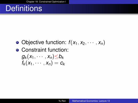
Definitions
Objective function: f (x1, x2, · · · , xn)
Constraint function:gk(x1, · · · , xn)≤bkfk(x1, · · · , xn) = ck
Yu Ren Mathematical Economics: Lecture 13

math
Chapter 18: Constrained Optimization I
Example 18.1
Example 18.1 (Utility Maximization Problem) Inthis most basic problem, Xi represents theamount of commodity i and f (x1, . . . , xn), usuallywritten as U(x1, . . . , xn), measures theindividual’s level of utility or satisfaction withconsuming x1 units of good 1, x2 units of good2, and so on. Let p1, . . . ,pn denote the prices ofthe commodities and let I denote the individual’sincome.
Yu Ren Mathematical Economics: Lecture 13

math
Chapter 18: Constrained Optimization I
Example 18.1
The consumer wants to
maximize U(x1, . . . , xn)
subject to p1x1 + p2x2 + · · ·+ pnxn ≤ I
To be consistent with the general format in (1),the nonnegativity constraints xi ≥ 0 should bewritten as −xi ≤ 0 so that all inequalityconstraints are written with ≤ signs.
Yu Ren Mathematical Economics: Lecture 13

math
Chapter 18: Constrained Optimization I
Example 18.2Example 18.2 (Utility Maximization withLabor/Leisure Choice) Let U, x1, . . . , xn,p1, . . . ,pn be as in the preceding example. Inaddition, let w denote the wage rate, I ′ theconsumer’s nonwage income, l0 hours of labor,and l1 hours of leisure. The consumer hasI ′ + wl0 dollars to spend and wants to
maximize U(x1, . . . , xn, l1)
subject to p1x1 + p2x2 + · · ·+ pnxn ≤ I ′ + wl0,l0 + l1 = 24,x1 ≥ 0, . . . , xn ≥ 0, l0 ≥ 0, l1 ≥ 0
Yu Ren Mathematical Economics: Lecture 13
math
Chapter 18: Constrained Optimization I
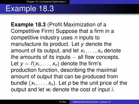
Example 18.3
Example 18.3 (Profit Maximization of aCompetitive Firm) Suppose that a firm in acompetitive industry uses n inputs tomanufacture its product. Let y denote theamount of its output, and let x1, . . . , xn denotethe amounts of its inputs − all flow concepts.Let y = f (x1, . . . , xn) denote the firm’sproduction function, describing the maximalamount of output that can be produced frombundle (x1, . . . , xn). Let p be the unit price of theoutput and let wi denote the cost of input i .
Yu Ren Mathematical Economics: Lecture 13

math
Chapter 18: Constrained Optimization I
Example 18.3
The firm’s goal is to choose (x1, . . . , xn) tomaximize its profit
Π(x1, . . . , xn) = pf (x1, . . . , xn)−n∑1
wixi
Yu Ren Mathematical Economics: Lecture 13

math
Chapter 18: Constrained Optimization I
Example 18.3
under the constraints
pf (x1, . . . , xn)−n∑1
wixi ≥ 0,
g1(x) ≤ b1, . . . ,gk(x) ≤ bk ,
x1 ≥ 0, . . . , xn ≥ 0.
The first inequality constraints reflects therequirement that the firm make a nonnegativeprofit. The gj−constraints represent constraintson the availability of the inputs.
Yu Ren Mathematical Economics: Lecture 13

math
Chapter 18: Constrained Optimization I
Equality Constraints
Two variables and one equality constraintSetup:
max f (x1, x2)
s.t .h(x1, x2) = c
(2) (3) (4) (5) (6) in Page 414Figure 18.1
Yu Ren Mathematical Economics: Lecture 13
math
Chapter 18: Constrained Optimization I
NDCQ
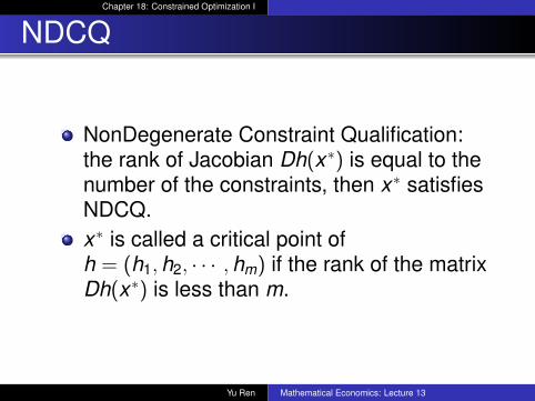
NonDegenerate Constraint Qualification:the rank of Jacobian Dh(x∗) is equal to thenumber of the constraints, then x∗ satisfiesNDCQ.x∗ is called a critical point ofh = (h1,h2, · · · ,hm) if the rank of the matrixDh(x∗) is less than m.
Yu Ren Mathematical Economics: Lecture 13

math
Chapter 18: Constrained Optimization I
Equality ConstraintsSolution (Theorem 18.1):Suppose (x∗1 , x
∗2) is not
a critical point of h. Then there is a real numberµ∗ such that (x∗1 , x
∗2 , µ
∗)
L(x1, x2, µ) ≡ f (x1, x2)− µ(h(x1, x2)− c)
∂f∂x1
(x)− µ ∂h∂x1
(x) = 0
∂f∂x2
(x)− µ ∂h∂x2
(x) = 0
h(x1, x2)− c = 0
µ is called a Lagrangian multiplierYu Ren Mathematical Economics: Lecture 13
math
Chapter 18: Constrained Optimization I
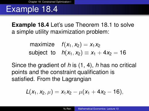
Example 18.4
Example 18.4 Let’s use Theorem 18.1 to solvea simple utility maximization problem:
maximize f (x1, x2) = x1x2
subject to h(x1, x2) ≡ x1 + 4x2 = 16
Since the gradient of h is (1, 4), h has no criticalpoints and the constraint qualification issatisfied. From the Lagrangian
L(x1, x2, µ) = x1x2 − µ(x1 + 4x2 − 16),
Yu Ren Mathematical Economics: Lecture 13

math
Chapter 18: Constrained Optimization I
Example 18.4
and set its partial derivatives equal to zero:
∂L∂x1
= x2 − µ = 0∂L∂x2
= x1 − 4µ = 0∂L∂µ = −(x1 + 4x2 − 16) = 0
we conclude the solution of this system is
x1 = 8, x2 = 2, µ = 2.
Theorem 18.1 states that the only candidate fora solution is x1 = 8, x2 = 2.
Yu Ren Mathematical Economics: Lecture 13

math
Chapter 18: Constrained Optimization I
Example 18.5
Example 18.5 Let’s work out a more complexexample:
maximize f (x1, x2) = x21 x2
subject to Ch = {(x1, x2) : 2x21 + x2
2 = 3}.
To check the constraint qualification, wecompute the critical points ofh(x1, x2) = 2x2
1 + x22 . The only such critical point
at (x1, x2)=(0, 0) − a point which is not in theconstraint set Ch.
Yu Ren Mathematical Economics: Lecture 13

math
Chapter 18: Constrained Optimization I
Example 18.5
Now, from the Lagrangian
L(x1, x2, µ) = x21 x2 − µ(2x2
1 + x22 − 3),
compute its partial derivatives, and set themequal to 0:
∂L∂x1
= 2x1x2 − 4µx1 = 2x1(x2 − 2µ) = 0∂L∂x2
= x21 − 2µx2 = 0
∂L∂µ = −2x2
1 − x22 + 3 = 0
Yu Ren Mathematical Economics: Lecture 13

math
Chapter 18: Constrained Optimization I
Example 18.5
The first equation yields x1 = 0 or x2 = 2µ.If x1 = 0, therefore (0,
√3, 0) and (0, −
√3, 0)
are two solutions of the system.If x1 6= 0, then x2 = 2µ, thenx2
1 = x22 ⇒ x1 = ±1, x2 = ±1.
If x2 = +1, and µ = 0.5. If x2 = −1, andµ = −0.5. Then we obtain four more solutions ofthe system
(1,1,0.5), (-1, -1, -0.5), (1,−1,−0.5), (-1, 1, 0.5) .
Yu Ren Mathematical Economics: Lecture 13

math
Chapter 18: Constrained Optimization I
Example 18.5
Sincef (1,1) = f (−1,1) = 1,
f (1,−1) = f (−1,−1) = −1,
f (0,√
3) = f (0,−√
3) = 0.
the max occurs at (1, 1) and (-1, 1). Note that(1, -1) and (-1, -1) minimize f on Ch.
Yu Ren Mathematical Economics: Lecture 13

math
Chapter 18: Constrained Optimization I
Equality Constraints
Several equality constraintsSetup:
max f (x1, x2, · · · , xn)
s.t .h1(x) = a1; · · · ,hm(x) = am
Yu Ren Mathematical Economics: Lecture 13

math
Chapter 18: Constrained Optimization I
Equality ConstraintsSolution (Theorem 18.2): Lagrangian Function:NDCQ
L(x , µ) ≡ f (x)− µ1(h1(x)− a1)− µ2(h2(x)− a2)
− · · · − µm(hm(x)− am)
∂L∂x1
(x∗, µ∗) = 0, · · · , ∂L∂xn
(x∗, µ∗) = 0
∂L∂µ1
(x∗, µ∗) = 0, · · · , ∂L∂µn
(x∗, µ∗) = 0
Yu Ren Mathematical Economics: Lecture 13

math
Chapter 18: Constrained Optimization I
Example 18.6
Example 18.6 Consider the problem:
maximize f (x , y , z) = xyzsubject to h1(x , y , z) = x2 + y2 = 1
and h2(x , y , z) = x + z = 1.
First compute the Jacobian matrix of theconstraint functions
Dh(x , y , z) =
(2x 2y 01 0 1
)
Yu Ren Mathematical Economics: Lecture 13
math
Chapter 18: Constrained Optimization I
Example 18.6
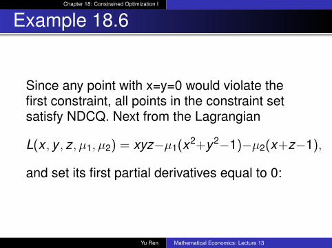
Since any point with x=y=0 would violate thefirst constraint, all points in the constraint setsatisfy NDCQ. Next from the Lagrangian
L(x , y , z, µ1, µ2) = xyz−µ1(x2+y2−1)−µ2(x+z−1),
and set its first partial derivatives equal to 0:
Yu Ren Mathematical Economics: Lecture 13

math
Chapter 18: Constrained Optimization I
Example 18.6
∂L∂x = yz − 2µ1x − µ2 = 0∂L∂y = xz − 2µ1y = 0∂L∂z = xy − µ2 = 0∂L∂µ2
= 1− x2 − y2 = 0∂L∂µ1
= 1− x − z = 0
Yu Ren Mathematical Economics: Lecture 13
math
Chapter 18: Constrained Optimization I
Example 18.6
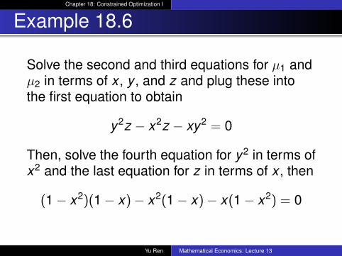
Solve the second and third equations for µ1 andµ2 in terms of x , y , and z and plug these intothe first equation to obtain
y2z − x2z − xy2 = 0
Then, solve the fourth equation for y2 in terms ofx2 and the last equation for z in terms of x , then
(1− x2)(1− x)− x2(1− x)− x(1− x2) = 0
Yu Ren Mathematical Economics: Lecture 13

math
Chapter 18: Constrained Optimization I
Example 18.6
so x = 16(−1±
√13), approximately -0.7676 and
0.4343. We obtain the four solution candidates
x ' 0.4343, y ' ±0.9008, z ' 0.5657;x ' −.07676, y ' ±0.6409, z ' 1.7676;
Evaluate the objective functions at these fourpoints, we find that the maximizer is
x ' −.07676, y ' −0.6409, z ' 1.7676
Yu Ren Mathematical Economics: Lecture 13

math
Chapter 18: Constrained Optimization I
Inequality Constraints
Figure 18.4 Figure 18.5One inequality constraint:Setup:
max f (x , y)
s.t .g(x , y) ≤ b
Yu Ren Mathematical Economics: Lecture 13

math
Chapter 18: Constrained Optimization I
Inequality ConstraintsSolution (Theorem 18.3): If ∂g
∂x (x∗, y∗) 6= 0 or∂g∂y (x∗, y∗) 6= 0 Lagrangian Function:
L(x , y , λ) ≡ f (x , y)− λ[g(x , y)− b]
∂L∂x
(x∗, y∗, λ∗) = 0
∂L∂y
(x∗, y∗, λ∗) = 0
λ∗[g(x∗, y∗)− b] = 0λ∗ ≥ 0
g(x∗, y∗) ≤ b
Yu Ren Mathematical Economics: Lecture 13

math
Chapter 18: Constrained Optimization I
Example 18.7Example 18.7 Consider the problem:
maximize f (x , y) = xysubject to g(x , y) = x2 + y2 ≤ 1
The only critical point of g occurs at the origin −far away from the boundary of the constraint setx2 + y2 = 1. So the constraint qualification willbe satisfied any candidate for a solution. Fromthe lagrangian
L(x , y , λ) = xy − λ(x2 + y2 − 1),
and write out the first order conditions describedin Theorem 18.3:
Yu Ren Mathematical Economics: Lecture 13
math
Chapter 18: Constrained Optimization I
Example 18.7
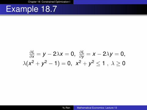
∂L∂x = y − 2λx = 0, ∂L
∂y = x − 2λy = 0,
λ(x2 + y2 − 1) = 0, x2 + y2 ≤ 1 , λ ≥ 0
Yu Ren Mathematical Economics: Lecture 13

math
Chapter 18: Constrained Optimization I
Example 18.7
The first two equations yield
λ =y2x
=x
2yor x2 = y2.
If λ = 0, then x = y = 0, which is a candidate fora solution.If λ 6= 0, then x2 + y2 − 1 = 0⇒ x2 = y2 = 1
2 ⇒x = ± 1√
2, x = ± 1√
2, then we find the following
four candidates:
Yu Ren Mathematical Economics: Lecture 13

math
Chapter 18: Constrained Optimization I
Example 18.7
x = + 1√2, y = + 1√
2, λ = +1
2x = − 1√
2, y = − 1√
2, λ = +1
2x = + 1√
2, y = − 1√
2, λ = −1
2x = − 1√
2, y = + 1√
2, λ = −1
2
Yu Ren Mathematical Economics: Lecture 13

math
Chapter 18: Constrained Optimization I
Example 18.7
We disregard the last two candidates since theyinvolve a negative multiplier. Plugging the leftthree candidates into the object function, we findthat
x = 1√2, y = 1√
2and x = − 1√
2, y = − 1√
2
are the solutions of our original problem. Thetwo points with the negative multipliers are thesolutions of the problem of minimizing xy on theconstraint set x2 + y2 ≤ 1.
Yu Ren Mathematical Economics: Lecture 13

math
Chapter 18: Constrained Optimization I
Inequality Constraints
Several Inequality Constraint:Setup:
max f (x)
s.t .g1(x) ≤ b1, · · · ,gk(x) ≤ bk
Yu Ren Mathematical Economics: Lecture 13

math
Chapter 18: Constrained Optimization I
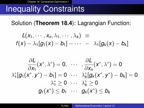
Inequality Constraints
Solution (Theorem 18.4): NDCQ conditionAssume the first k0 constraints are binding at x∗and the last k − k0 are not binding. NDCQ holdsif the rank of
∂g1∂x1
(x∗) · · · ∂g1∂xn
(x∗)... ... ...
∂gk0∂x1
(x∗) · · · ∂gk0∂xn
(x∗)
is k0
Yu Ren Mathematical Economics: Lecture 13
math
Chapter 18: Constrained Optimization I
Inequality Constraints
Solution (Theorem 18.4): Lagrangian Function:
L(x1, · · · , xn, λ1, · · · , λk) ≡f (x)− λ1[g1(x)− b1]− · · · − λ1[gk(x)− bk ]
∂L∂x1
(x∗, λ∗) = 0, · · · , ∂L∂xn
(x∗, λ∗) = 0
λ∗1[g1(x∗, y∗)− b1] = 0 · · · λ∗k [gk(x∗, y∗)− bk ] = 0λ∗1 ≥ 0 · · · λ∗k ≥ 0
g1(x∗) ≤ b1 · · · gk(x∗) ≤ bk
Yu Ren Mathematical Economics: Lecture 13

math
Chapter 18: Constrained Optimization I
Example 18.8
Example 18.8 Consider again the standardutility maximization problem of Example 18.1.We continue to ignore the nonnegativityconstraints but do not force the budgetconstraint to be binding in the statement of theproblem.
maximize U(x1, x2)
subject to p1x1 + p2x2 ≤ I
Yu Ren Mathematical Economics: Lecture 13

math
Chapter 18: Constrained Optimization I
Example 18.8We assume that for each commodity bundle(x1, x2),
x = ∂U∂x1
(x1, x2) > 0 or x = ∂U∂x2
(x1, x2) > 0
This is a version of the usual monotonicity ornonsatiation assumption. It states that thecommodities under study are goods in thatincreasing consumption increases utility. Sincethe usual constraint qualification is satisfied, sofrom the lagrangian
L(x1, x2, λ) = U(x1, x2)− λ(p1x1 + p2x2 − I)
Yu Ren Mathematical Economics: Lecture 13

math
Chapter 18: Constrained Optimization I
Example 18.8
and compute its x1− and x2− critical points:
∂L∂x1
(x1, x2) = ∂U∂x1
(x1, x2)− λp1 = 0,∂L∂x2
(x1, x2) = ∂U∂x1
(x1, x2)− λp2 = 0.
Yu Ren Mathematical Economics: Lecture 13

math
Chapter 18: Constrained Optimization I
Example 18.8
At the maximizer, the multiplier λ cannot bezero; otherwise both ∂U
∂x1and ∂U
∂x2would be zero
− a contradiction to our monotonicityassumption. Since
λ > 0 and λ(p1x1 + p2x2 − I) = 0,
it follows that p1x1 + p2x2 = I; the consumer willspend all available income and we can treat thebudget constraint as an equality constraint.
Yu Ren Mathematical Economics: Lecture 13

math
Chapter 18: Constrained Optimization I
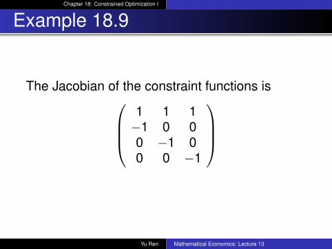
Example 18.9
Example 18.9 Consider the problem:
max f (x , y , z) = xyzs.t x + y + z ≤ 1, x ≥ 0, y ≥ 0, z ≥ 0
Yu Ren Mathematical Economics: Lecture 13

math
Chapter 18: Constrained Optimization I
Example 18.9
we rewrite the three nonnegatitivity constraintsas
−x ≤ 0, −y ≤ 0, and −z ≤ 0.
Yu Ren Mathematical Economics: Lecture 13
math
Chapter 18: Constrained Optimization I
Example 18.9
The Jacobian of the constraint functions is1 1 1−1 0 00 −1 00 0 −1
Yu Ren Mathematical Economics: Lecture 13

math
Chapter 18: Constrained Optimization I
Example 18.9
Since the NDCQ holds at any solutioncandidate. From the lagrangian
L(x , y , z, λ1, λ2, λ3, λ4) = xyz − λ1(x + y + z − 1)
−λ2(−x)− λ3(−y)− λ4(−z).
we can rewrite it more aesthetically as
L(x , y , z, λ1, λ2, λ3, λ4) = xyz − λ1(x + y + z − 1)
+ λ2x + λ3y + λ4z.
Yu Ren Mathematical Economics: Lecture 13

math
Chapter 18: Constrained Optimization I
Example 18.9
according to Theorem 18.4:
(1) ∂L∂x = yz − λ1 + λ2 = 0,
(2) ∂L∂y = xz − λ1 + λ3 = 0,
(3) ∂L∂z = xy − λ1 + λ4 = 0,
Yu Ren Mathematical Economics: Lecture 13

math
Chapter 18: Constrained Optimization I
Example 18.9
(4) λ1(x + y + z − 1) = 0, (5) λ2x = 0,(6) λ3y = 0, (7) λ4z = 0,(8) λ1 ≥ 0, (9) λ2 ≥ 0,
(10) λ3 ≥ 0, (11) λ4 ≥ 0,(12) x + y + z − 1 ≤ 1, (13) x ≥ 0,(14) y ≥ 0, (15) z ≥ 0.
Yu Ren Mathematical Economics: Lecture 13

math
Chapter 18: Constrained Optimization I
Example 18.9Rewrite conditions 1, 2, and 3, without minussigns, as
λ1 = yz + λ2 = xz + λ3 = xy + λ4
If λ1 = 0, then yz = xz = xy = 0 andλ1 = λ2 = λ3 = λ4 = 0If λ1 > 0, suppose x = 0, thenλ1 = λ3 = λ4 > 0⇒ y = z = 0− a contradictionto x + y + z = 1, so x > 0. Similarlyy > 0, z > 0⇒ λ2 = λ3 = λ4 = 0 andyz = xz = xy = 1
3. Since f (13 ,
13 ,
13) = 1
27 > 0, isthe solution of the constraint maximizationproblem.
Yu Ren Mathematical Economics: Lecture 13

math
Chapter 18: Constrained Optimization I
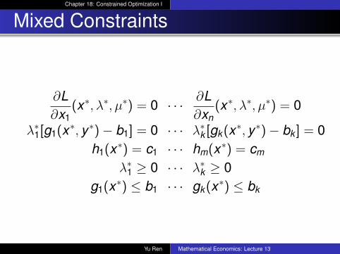
Mixed Constraints
Setup:max f (x)
s.t .
g1(x) ≤ b1, · · · ,gk(x) ≤ bk
h1(x) = c1, · · · ,hm(x) = cm
Yu Ren Mathematical Economics: Lecture 13

math
Chapter 18: Constrained Optimization I
Mixed Constraints
Solution (Theorem 18.5): NDCQ conditionAssume the first k0 constraints are binding at x∗and the last k − k0 are not binding.
r
∂g1∂x1
(x∗) · · · ∂g1∂xn
(x∗)... ... ...
∂gk0∂x1
(x∗) · · · ∂gk0∂xn
(x∗)∂h1∂x1
(x∗) · · · ∂h1∂xn
(x∗)... ... ...
∂hm∂x1
(x∗) · · · ∂hm∂xn
(x∗)
=?
Yu Ren Mathematical Economics: Lecture 13

math
Chapter 18: Constrained Optimization I
Mixed Constraints
Solution (Theorem 18.5): Lagrangian Function:
L(x1, · · · , xn, λ1, · · · , λk , µ1, · · · , µm) ≡f (x)− λ1[g1(x)− b1]− · · · − λk [gk(x) − bk ]
−µ1[h1(x)− c1]− · · · − µm[hm(x) − cm]
Yu Ren Mathematical Economics: Lecture 13
math
Chapter 18: Constrained Optimization I
Mixed Constraints
∂L∂x1
(x∗, λ∗, µ∗) = 0 · · · ∂L∂xn
(x∗, λ∗, µ∗) = 0
λ∗1[g1(x∗, y∗)− b1] = 0 · · · λ∗k [gk(x∗, y∗)− bk ] = 0h1(x∗) = c1 · · · hm(x∗) = cm
λ∗1 ≥ 0 · · · λ∗k ≥ 0g1(x∗) ≤ b1 · · · gk(x∗) ≤ bk
Yu Ren Mathematical Economics: Lecture 13

math
Chapter 18: Constrained Optimization I
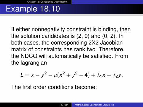
Example 18.10
Example 18.10 Consider the problem:
maximize x − y2
subject to x2 + y2 = 4, x ≥ 0, y ≥ 0.
Checking the NDCQ, first note that the gradientof x2 + y2 is zero only at the origin, a pointwhich is not in the constraint set.
Yu Ren Mathematical Economics: Lecture 13
math
Chapter 18: Constrained Optimization I
Example 18.10
If either nonnegativity constraint is binding, thenthe solution candidates is (2, 0) and (0, 2). Inboth cases, the corresponding 2X2 Jacobianmatrix of constraints has rank two. Therefore,the NDCQ will automatically be satisfied. Fromthe lagrangian
L = x − y2 − µ(x2 + y2 − 4) + λ1x + λ2y .
The first order conditions become:
Yu Ren Mathematical Economics: Lecture 13
math
Chapter 18: Constrained Optimization I
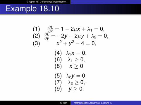
Example 18.10
(1) ∂L∂x = 1− 2µx + λ1 = 0,
(2) ∂L∂y = −2y − 2µy + λ2 = 0,
(3) x2 + y2 − 4 = 0,
(4) λ1x = 0,(6) λ1 ≥ 0,(8) x ≥ 0
(5) λ2y = 0,(7) λ2 ≥ 0,(9) y ≥ 0.
Yu Ren Mathematical Economics: Lecture 13

math
Chapter 18: Constrained Optimization I
Example 18.10
Write 1 as 1 + λ1 = 2µx .Sinceλ1 ≥ 0,1 + λ1 > 0. Therefore,µ > 0, x > 0, λ1 = 0. Write 2 as 2y(1 + µ) = λ2.Since 1 + λ1 > 0, either both y and λ2 are zeroor both are positive. By 5, both cannot bepositive. Therefore, λ2 = y = 0. Now, x = 2 by 3and 8, λ1 = 0 by 4, and µ = 1/4 by 1. This leadsto the solution
(x , y , µ, λ1, λ2) = (2,0,1/4,0,0).
Yu Ren Mathematical Economics: Lecture 13

math
Chapter 18: Constrained Optimization I
Example 18.11
Example 18.11 Consider the problem:
minimize f (x , y) = 2y − x2
subject to x2 + y2 ≤ 1, x ≥ 0, y ≥ 0.
From the lagrangian
L(x , y , λ1, λ2, λ3) = 2y − x2
− λ1(−x2 − y2 + 1)− λ2x − λ3y .
Yu Ren Mathematical Economics: Lecture 13

math
Chapter 18: Constrained Optimization I
Example 18.11
The first order conditions are:
∂L∂x
= −2x + 2λ1x − λ2 = 0,
∂L∂y
= 2 + 2λ1y − λ3 = 0,
λ1(−x2 − y2 + 1) = 0,λ2x = 0,λ3y = 0
λ1, λ2, λ3 ≥ 0,
Yu Ren Mathematical Economics: Lecture 13

math
Chapter 18: Constrained Optimization I
Example 18.11
rewrite the ∂L∂x = 0 equations, then
2x + λ2 = 2λ1x , 2 + 2λ1y = λ3. Sinceλ3 ≥ 2 > 0, we conclude that y = 0 and λ3 = 2.Next, if x + 0⇒ λ1 = 0, y = 0 and λ2 = 0, thusf (0,0) = 0.If x > 0⇒ λ2 = 0, λ1 = 1, y = 0, x = 1, thusf (1,0) = −1.We conclude that (x , y) = (1,0) minimizesf (x , y) = 2y − x2 on the constraint set.
Yu Ren Mathematical Economics: Lecture 13
math
Chapter 18: Constrained Optimization I
Example 18.12
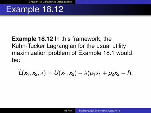
Example 18.12 In this framework, theKuhn-Tucker Lagrangian for the usual utilitymaximization problem of Example 18.1 wouldbe:
L̃(x1, x2, λ) = U(x1, x2)− λ(p1x1 + p2x2 − I),
Yu Ren Mathematical Economics: Lecture 13
math
Chapter 18: Constrained Optimization I
Example 18.12
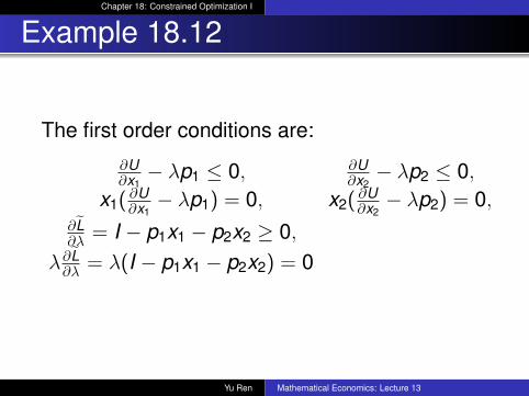
The first order conditions are:
∂U∂x1− λp1 ≤ 0, ∂U
∂x2− λp2 ≤ 0,
x1( ∂U∂x1− λp1) = 0, x2( ∂U
∂x2− λp2) = 0,
∂L̃∂λ = I − p1x1 − p2x2 ≥ 0,
λ∂L̃∂λ = λ(I − p1x1 − p2x2) = 0
Yu Ren Mathematical Economics: Lecture 13

math
Chapter 18: Constrained Optimization I
Example 18.13
Example 18.13 Consider the problem:
minimize f (x , y) = x2 + x + 4y2
subject to 2x + 2y ≤ 1, x ≥ 0, y ≥ 0.
The Jacobian of the constraint functions is 2 2−1 00 −1
Yu Ren Mathematical Economics: Lecture 13

math
Chapter 18: Constrained Optimization I
Example 18.13
At most two constraints can be binding at thesame time, and any 2X2 submatrix of theJacobian has rank two. Therefore, the NDCQwill hold at any solution candidate. From thelagrangian
L(x , y , λ1, λ2, λ3) = x2 + x + 4y2
− λ1(2x + 2y − 1) + λ2x + λ3y .
Yu Ren Mathematical Economics: Lecture 13

math
Chapter 18: Constrained Optimization I
Example 18.13
The first order conditions are:
∂L∂x
= −2x + 1− 2λ1 + λ2 = 0,
∂L∂y
= 8y − 2λ1 + λ3 = 0,
λ1(2x + 2y − 1) = 0, λ2x = 0, λ3y = 0,λ1 ≥ 0, λ2 ≥ 0 , λ3 ≥ 0,
2x + 2y ≤ 1, x ≥ 0, y ≥ 0.
Yu Ren Mathematical Economics: Lecture 13
math
Chapter 18: Constrained Optimization I
Example 18.13
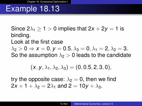
Since 2λ1 ≥ 1 > 0 implies that 2x + 2y = 1 isbinding.Look at the first caseλ2 > 0⇒ x = 0, y = 0.5, λ3 = 0, λ1 = 2, λ2 = 3.So the assumption λ2 > 0 leads to the candidate
(x , y , λ1, λ2, λ3) = (0,0.5,2,3,0),
try the opposite case: λ2 = 0, then we find2x + 1 + λ2 = 2λ1 and 2 = 10y + λ3.
Yu Ren Mathematical Economics: Lecture 13

math
Chapter 18: Constrained Optimization I
Example 18.13
So this leads to the conclusion that either y = 0or λ3 = 0, and we get two candidates:(x , y , λ1, λ2, λ3) = (0.5,0,1,0,2) or(x , y , λ1, λ2, λ3) = (0.3,0.2,0.8,0,0) byevaluating the objective function at each ofthese three candidates, we find that theconstrained maximum occurs at the pointx = 0, y = 0.5, where λ1 = 2, λ2 = 3 and λ3 = 0.
Yu Ren Mathematical Economics: Lecture 13