Mathematical Foundations of Game Theory

By: Michael Bianco

Submitted To:

The Mathematics & Economics Departments of Franciscan University

Bianco P. 2

Table of Contents:

I. Abstract 3

II. Introduction 4

A. Basic Definition 4

B. Historical Development 5

i. Antoine-Augustine Cournot 5

ii. Neumann, Nash, and Others 6

III. Game Setup 7

A. Strategies & Payoffs 7

B. Graphical Display 10

i. Extensive Form 9

ii. Normal Form 12

C. Game Characteristics 13

i. Constant & Zero-Sum 13

ii. Cooperative & Repeated 14

D. Characterizing Solutions 15

i. Nash Equilibrium 15

ii. Dominance 17

iii. Pareto Optimality 17

IV. Mathematical Analysis 19

A. Two-Person, 3 x 3, Zero Sum Game 19

i. Solving Using the Minimax Algorithm 19

ii. Solving Using Iterated Dominance 20

iii. Solving Graphically 20

B. Minimax Theorem 21

i. Definition 21

ii. Proof 23

C. Zero-Sum, 2 x 2 Game with Mixed Strategy Nash Equilibrium 27

i. Solving Using Systems of Linear Equations 27

ii. Solving Using Numerical Estimation 28

V. Conclusion 30

Bianco P. 3

Abstract:

The recently developed field of Game Theory has occupied the minds of many

contemporary mathematicians and economists alike. This paper will explore the

mathematical foundations of Game Theory, solutions to common strategic situations, as

well as provide some application to specific economic situations.

Bianco P. 4

I. Introduction

A. Basic Definition

In order to assist our inquiry into the mathematical foundations and economic

application of game theory a definition of terms is necessary. Despite the fact the fact that

the word ‘game’ exists in the title of the field of study, the application of game theory is

not restricted exclusively to what we would think of as games (i.e. chess, checkers, etc).

According to Library of Economics and Liberty the object of game theory is to

“determine mathematically and logically the actions that ‘players’ should take to secure

the best outcomes for themselves in a wide array of ‘games.’” (Dixit & Nalebuff, 2008).

Games are interactions between two or more players that are characterized by situations

in which a player’s outcome at the of the game is dependent on the decisions of the other

players. An individual decision or choice of a player is defined as a move, a series of

moves of a given player is a strategy. A unique combination of players’ strategies will

result in a game outcome. The result of a game for a given player is defined as the payoff

(Straffin, 1996, P.3). A player is defined as a rational agent (not necessarily a person,

could be a institution or firm) where rationality consists of “complete knowledge of one’s

interests, and flawless calculation of what actions will best serve those interests” (Dixit,

Reiley, and Skeath, 2009, P. 30). With knowledge of possible game outcomes and

payoffs associated with those outcomes, it is often possible to find a equilibrium (more

specifically a nash equilibrium) for that game. There are many types of equilibrium but in

a broad sense it can be defined as the state when “each player is using the strategy that is

Bianco P. 5

the best response to the strategies of the other players” (Dixit, Reiley, and Skeath, 2009,

P. 33).

B. Historical Development

Antoine-Augustine Cournot

Although many would claim that the development of game theory is rooted in the

20th century work of John von Neumann, others would argue that the father of game

theory is Antoine-Augustine Cournot (Morrison, 1998). Cournot initially began his career

as a mathematician, publishing many papers that caught the attention of fellow

mathematician Poisson, and eventually secured professorship at the University of Lyons.

His mathematical background uniquely positioned him to approach the study of

Economics with a symbolic and graphical representation of thought, enabling him to

present clear definitions of ideas that previously were imprecisely elucidated using the

literary form of economic explanation. Although Cournot was not the first to bring

mathematics to the study of economics, he is the first to popularize and defend its use.

Cournot “originated an early form of game theory” (Ekelund & Hebert , 2007, P.

571) in his 1838 publication of Researches into the Mathematical Principles of the

Theory of Wealth through his discussion of competition between mineral water sellers

(Ekelund & Hebert, 2007, P.268). He developed the reaction curve, a tool used to predict

the output of a firm based on given knowledge of a competing firm’s output level. By

partially differentiating a firm’s output function by the quantity produced of the

competing firm and setting the resulting equation equal to zero, he was able to determine

the stable equilibrium (outcome) of competing players (firms) in a competitive situation

Bianco P. 6

(Morrison, 1998). This inquiry into interactions between competing agents was the first

of much analysis undertaken to understand the nature of competitive environments.

Neumann, Nash, and Others

Although there were a couple thinkers (such as Joseph Bertrand in 1883 and

Francis Ysidro Edgeworth in 1897) who continued to build upon the foundation which

Cournot created, substantial strides in the development of game theory were not made

until John von Neumann starting publishing his work. A brilliant man, Neumann earned a

doctorate in chemistry and mathematics at the same time before the age of twenty-four.

He took a professorship position for a short time at the University of Berlin before

becoming the youngest member of the Institute for Advanced Study at Princeton

(Fonseca). In 1937 Neumann, with the encouragement and help of Oskar Morgenstern,

published Theory of Games and Economic Behavior which was the first work to assert

that “any economic situation could be defined as the outcome of a game between two or

more players” (“John von Neumann”, 2008). In addition to making critical contributions

to game theory (such as the minimax theorem), Neumann also assisted in the

development of the first computer and was a key member of the Manhattan Project

(Myhrvold, 1999).

John Forbes Nash Jr., popularized by the recent movie A Beautiful Mind, was

another pivotal contributor to the field of game theory in the twentieth century. From

1950 – 1953 he published a series of four papers, which eventually won him the Nobel

Prize in 1994, in which he proved that in non-cooperative (i.e. competitive) games “at

least one equilibrium exists as long as mixed strategies are allowed” (“John F. Nash Jr”,

2008). This specific type of equilibrium that can be found in non-cooperative games was

Bianco P. 7

later coined the nash equilibrium. In addition to his work on non-cooperative games, he

also made great strides in the area of cooperative games (i.e. bargaining or auction

situations). Nash’s work, along with those who built upon his work, was used in the fairly

recent electromagnetic spectrum auction: “a multiple-round procedure was carefully

designed by experts in the game theory of auctions…The result was highly successful,

bringing more than $10 billion to the government while guaranteeing an efficient

allocation of resources” (Milnor, 1998). Correctly applied game theoretic principals to

real-world situations can yield great results.

II. Game Setup

A. Strategies & Payoffs

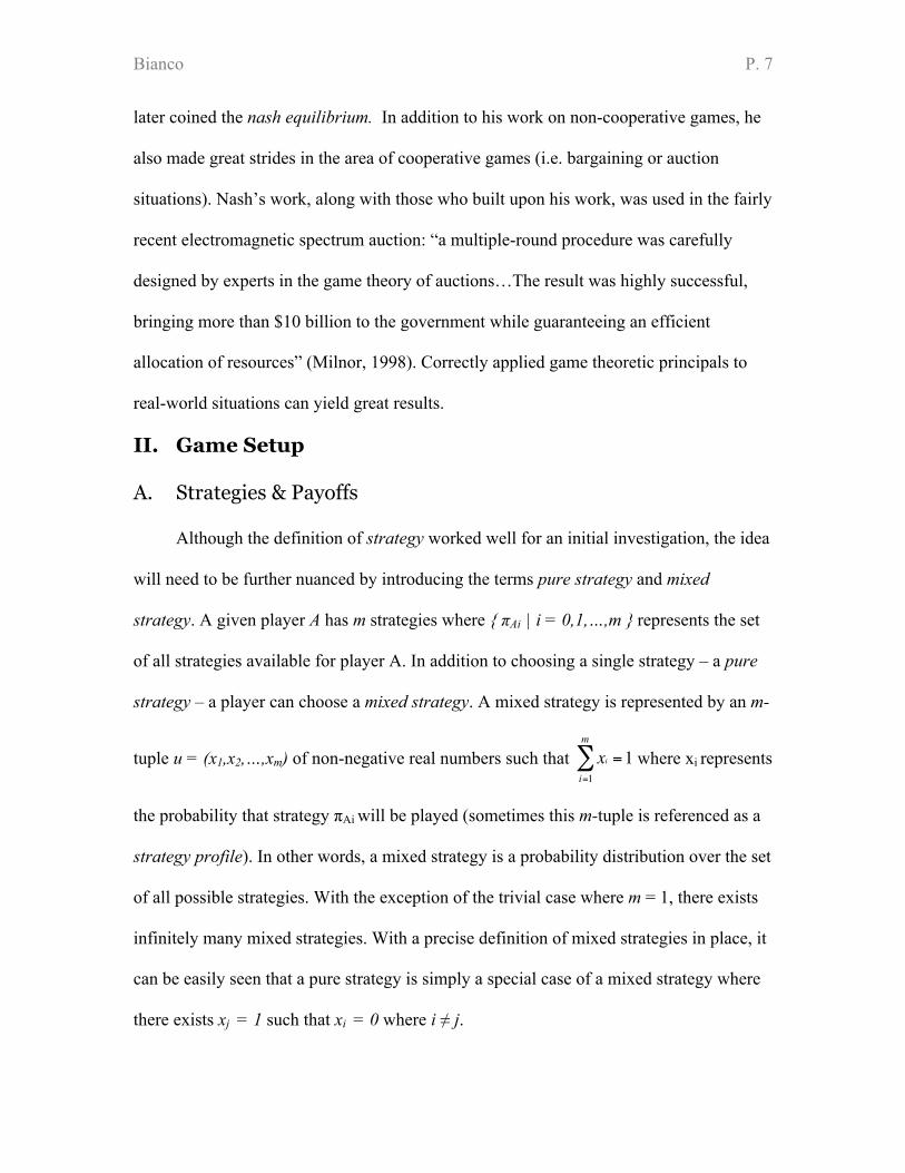
Although the definition of strategy worked well for an initial investigation, the idea

will need to be further nuanced by introducing the terms pure strategy and mixed

strategy. A given player A has m strategies where { !Ai | i = 0,1,…,m } represents the set

of all strategies available for player A. In addition to choosing a single strategy – a pure

strategy – a player can choose a mixed strategy. A mixed strategy is represented by an m-

tuple u = (x1,x2,…,xm) of non-negative real numbers such that

!

xii=1

m

" =1 where xi represents

the probability that strategy !Ai will be played (sometimes this m-tuple is referenced as a

strategy profile). In other words, a mixed strategy is a probability distribution over the set

of all possible strategies. With the exception of the trivial case where m = 1, there exists

infinitely many mixed strategies. With a precise definition of mixed strategies in place, it

can be easily seen that a pure strategy is simply a special case of a mixed strategy where

there exists xj = 1 such that xi = 0 where i " j.

Bianco P. 8

These distinctions between strategy types might seem a bit abstract, but some

investigation will reveal their operation in real world situations. Encouraging students to

learn can be seen as a game between teachers and students. Teachers want students to

come to class, but they would rather not spend time taking roll and calculating an

attendance grade at the end of the year. In order to minimize time spent on punishing

students for lack of attendance and maximize the number of students in the class, teachers

will often check attendance sporadically – utilizing a mixed strategy – in order to achieve

their desired result. If a teacher used a pure strategy – checking attendance using some

fixed pattern – students would detect the pattern and simply skip class when teacher did

not check attendance, ultimately lowering attendance and creating more work for the

teacher.

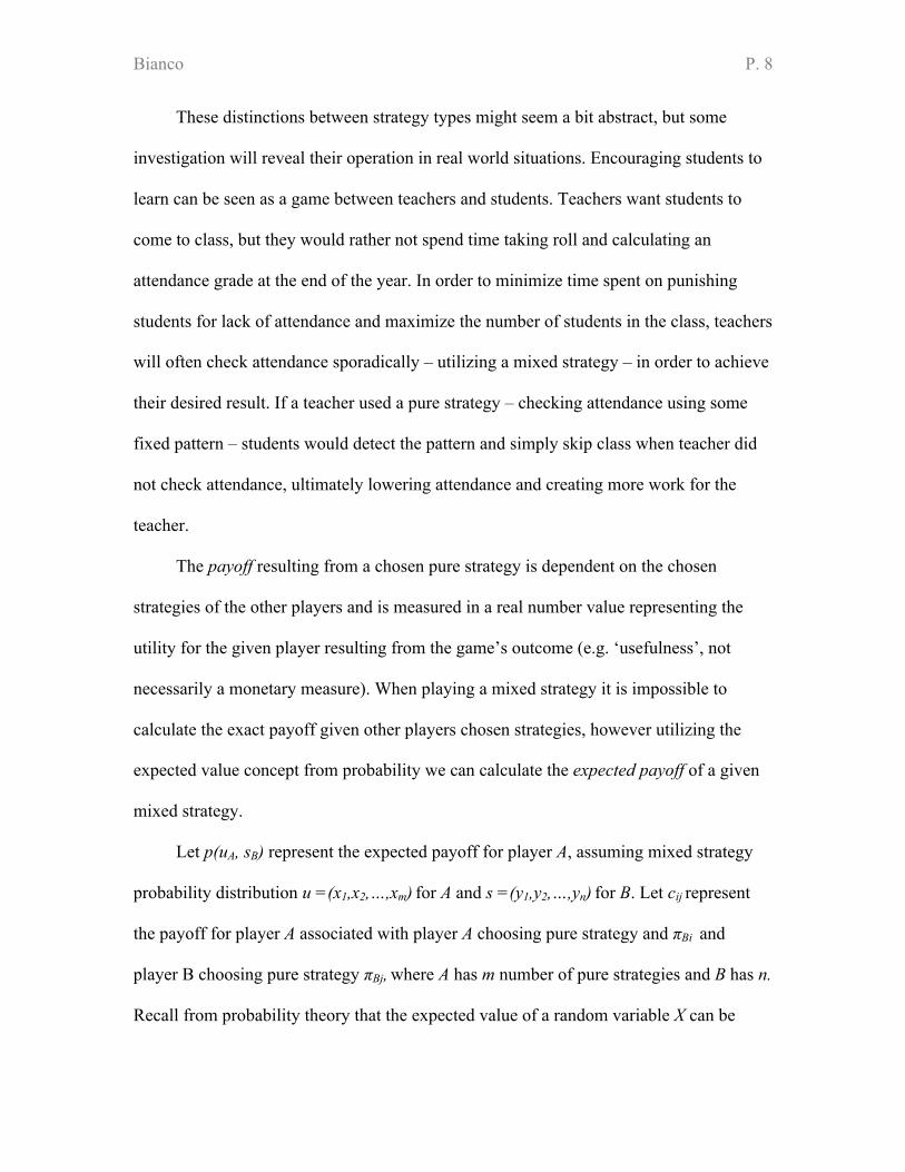
The payoff resulting from a chosen pure strategy is dependent on the chosen

strategies of the other players and is measured in a real number value representing the

utility for the given player resulting from the game’s outcome (e.g. ‘usefulness’, not

necessarily a monetary measure). When playing a mixed strategy it is impossible to

calculate the exact payoff given other players chosen strategies, however utilizing the

expected value concept from probability we can calculate the expected payoff of a given

mixed strategy.

Let p(uA, sB) represent the expected payoff for player A, assuming mixed strategy

probability distribution u =(x1,x2,…,xm) for A and s =(y1,y2,…,yn) for B. Let cij represent

the payoff for player A associated with player A choosing pure strategy and !Bi and

player B choosing pure strategy !Bj, where A has m number of pure strategies and B has n.

Recall from probability theory that the expected value of a random variable X can be

Bianco P. 9

represented as

!

E(X) = P(X = xi)xii=1

n

" assuming the number of trials approaches infinity

(Mendelson, 2004, P.214). Let X = { cij | i =0…m, j =0…n } and P(X = xi) = P(X = cij) =

xiyj, given u and s the expected payoff would be

!

E(X) = cijxiyjcij"X# . A general definition

for the expected payoff can now be provided from the perspective of player A:

!

p(u,s) = cijxiyji=1

m

"j=1

n

" .

To notation above is a bit restricted because it is examining the game from the

perspective of player A. To differentiate the payoff function between A and B, pA(u,s) will

be used to represent the payoff function for A and pB(u,s) for B. When dealing with the

payoff function, all mixed strategy distributions for all other players will be given or

previously defined. With this in mind, notational simplifications can be made to the

payoff function, defining the payoff function for a player i as pi(u). The set of all possible

mixed strategies (remember that a pure strategy is just a special case of a mixed strategy)

for a player i will be defined as Si.

Bianco P. 10

B. Graphical Display

Extensive Form

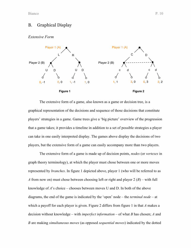
The extensive form of a game, also known as a game or decision tree, is a

graphical representation of the decisions and sequence of those decisions that constitute

players’ strategies in a game. Game trees give a ‘big picture’ overview of the progression

that a game takes; it provides a timeline in addition to a set of possible strategies a player

can take in one easily interpreted display. The games above display the decisions of two

players, but the extensive form of a game can easily accompany more than two players.

The extensive form of a game is made up of decision points, nodes (or vertexes in

graph theory terminology), at which the player must chose between one or more moves

represented by branches. In figure 1 depicted above, player 1 (who will be referred to as

A from now on) must chose between choosing left or right and player 2 (B) – with full

knowledge of A’s choice – chooses between moves U and D. In both of the above

diagrams, the end of the game is indicated by the ‘open’ node – the terminal node – at

which a payoff for each player is given. Figure 2 differs from figure 1 in that A makes a

decision without knowledge – with imperfect information – of what B has chosen; A and

B are making simultaneous moves (as opposed sequential moves) indicated by the dotted

L R

0, -1

U D

0, 0

Figure 1

1, -1

Player 1 (A)

Player 2 (B)

1, 0

U D

C D

1, 1

c d

3, 0

Figure 2

0, 3

Player 1 (A)

Player 2 (B)

2, 2

c d

Bianco P. 11

line connecting the nodes. The moves that B must choose from in figure 2 are said to be

in the same information set. If all information sets contain only one element (as in figure

1) then the game is said to have perfect information (Kuhn, 1953).

Making the distinction between games with perfect and imperfect information is

crucial to determining if a equilibrium exists. For instance, a game with perfect

information “always has an equilibrium point in pure strategies” (Kuhn, 1953, P. 209).

Understanding what information is available can enable you determine the outcome of a

game with a much higher level of accuracy.

The level of information available to a player completely changes the decision

making process – information is one of the most valuable assets one can possess. One of

the most interesting games playing itself out in the market is the ‘phone war’ between

Google, Apple, RIM, and others. Few firms have the know-how, leadership, capital, and

monopoly power required in order to create a competitively priced smart phone with

accompanying software and adequate feature set. Additionally, the labor pool with

adequate education and experience in designing both the software and hardware end of a

smartphone is limited. This unique situation creates an environment where the price on

intellectual property, talented employees, and product secrecy soars. Employees working

on new projects at Apple are often video monitored and “must pass through a maze of

security doors, swiping their badges again and again and finally entering a numeric code

to reach their offices” (Stone & Vance, 2009). Apple has a dedicated “Worldwide

Loyalty Team” to ensure product secrecy and eliminate information leaks.

Misinformation about products is intentionally spread internally and bloggers who leak

product information are quickly sued.

Bianco P. 12

In order to attract talented employees and keep hired talent, Google recently gave

“all its employees a $1,000 holiday bonus in addition to pay increases of at least 10

percent” (Comlay, 2010). The amount of capital invested in the attainment and protection

of information in oligopoly markets is enormous, game theory gives us key insights into

what information is valuable and helps determine how to properly value that information.

Normal Form

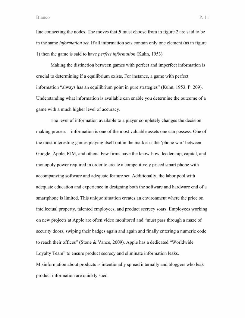
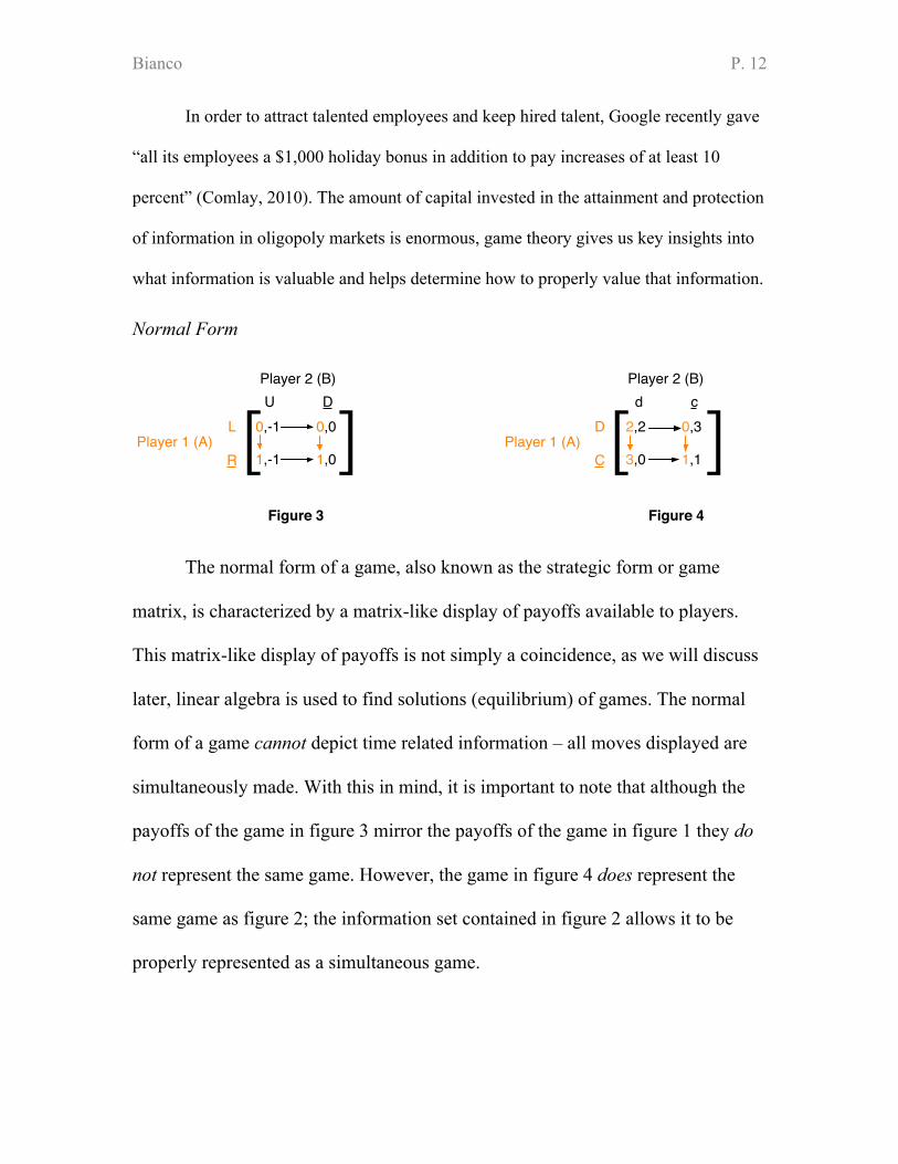
The normal form of a game, also known as the strategic form or game

matrix, is characterized by a matrix-like display of payoffs available to players.

This matrix-like display of payoffs is not simply a coincidence, as we will discuss

later, linear algebra is used to find solutions (equilibrium) of games. The normal

form of a game cannot depict time related information – all moves displayed are

simultaneously made. With this in mind, it is important to note that although the

payoffs of the game in figure 3 mirror the payoffs of the game in figure 1 they do

not represent the same game. However, the game in figure 4 does represent the

same game as figure 2; the information set contained in figure 2 allows it to be

properly represented as a simultaneous game.

[ ]Player 2 (B)

Player 1 (A)

U D

L

R

0,-1 0,0

1,-1 1,0

Figure 3

[ ]Player 2 (B)

Player 1 (A)

d c

D

C

2,2 0,3

3,0 1,1

Figure 4

Bianco P. 13

C. Game Characteristics

Constant and Non-Constant Games

How payoffs change when other players’ strategies change determines whether

we classify a game as constant or non-constant. All the games depicted thus far have

been non-constant sum games: a increase in the payoff of one player did not necessarily

require a decrease in the other player’s payoff. In constant-sum games there is some fixed

net payoff amount, increase in one player’s payoff necessitates a payoff decrease for

other players’. A special case of the constant-sum game is the zero-sum game, where the

sum of the players’ payoffs is zero. The terms constant & zero-sum are often used

interchangeably since a constant-sum game can be translated to a zero-sum game by

simply adjusting the utility scale. Zero-sum games are commonly found in what one

would traditionally consider a game: chess, checkers, soccer, basketball, etc. In games

such as chess or basketball there cannot be two winners: one team wins the other loses.

Zero-sum games have a very special implication: they are strictly competitive.

Because there can only be one winner, players have no incentive to cooperate.

Characterizing a game as zero-sum has both effects on mathematical analysis as well as a

players’ mindset. Mathematically, classifying a game as zero-sum allows certain analysis

(such as minimax analysis, which will be discussed later) to be performed and enabled

certain judgments to be made about the equilibrium. Understanding how you – and your

competitors – are classifying a situation will change the strategies players’ will chose and

change the way you should predict other players’ decisions. For instance, many people

falsely characterize the interaction of entrepreneurs in the free market economy as a zero-

sum game. This changes how a given entrepreneur will view and interact with others;

Bianco P. 14

instead of viewing them as potential future business partners they are categorized as

competition to be beaten. The free market is not a zero-sum game, although there are

some businesses that will directly compete with each other, for the most part businesses

can interact and collaborate in order to increase wealth rather than ‘steal’ it from each

other.

Cooperative & Repeated Games

Although we will not explore these concepts in detail it is useful to give a brief

overview of these two important concepts. A cooperative game is one in which

communication between players is allowed, they are “permitted to communicate prior to

playing the game, to make binding agreements” (Luce & Raffia, 1957, P. 152) in addition

to many other communication tactics. Cooperative games are characteristic of many

political situations and contract negotiations between businesses.

The number of times a game is played can greatly effect the strategies which

players will choose to employ. When a player repeatedly plays a board game against the

same opponent the player will start to notice certain patterns in his opponent’s thought

and utilize strategies that will work well against his opponent. The notion of finitely

repeated and infinitely repeated games are crucial to comprehensive game theoretic

analysis. All games presented here will be assumed to be one-shot games (played only

once).

Bianco P. 15

D. Characterizing Solutions

Nash Equilibrium

A general and broad definition of equilibrium was given earlier, the concept of a

nash equilibrium will now be fleshed out in more detail. Remember that a strategy that is

a nash equilibrium is not always equivalent to the strategy choice that will result in the

highest possible payoff for players’. However, it is the best possible response to the

expected choices of all other players involved in the game. In other words, a nash

equilibrium exists if, for every player, a change in that player’s strategy will not improve

his payoff holding all other players’ strategy choices constant.

The idea of a nash equilibrium can be furthered by introducing a mixed strategy

nash equilibrium and pure strategy nash equilibrium. These distinctions highlight the fact

that a nash equilibrium is not always a pure strategy, but can be an optimal mix of many

pure strategies engineered to generate a maximum expected payoff. Although every every

game has a one or more mixed strategy nash equilibrium, it is possible for a game not to

have any pure strategy nash equilibrium. Often a nash equilibrium strategy will be called

a equilibrium point or (for two player games) an equilibrium pair.

Mathematical methods of finding the nash equilibria of a game will be

investigated later, but for now it is helpful to see the logic of the nash equilibrium

operating in figure 3 and figure 4. The arrows represent A & B’s ‘thinking’, they

graphically describe the logic used in making the best decision, each player will want to

chose the option that will provide them with the highest payoff. Notationally, the nash

equilibrium of A choosing strategy R and B choosing D (in figure 3) will be denoted as

(D, R).

Bianco P. 16

Looking closer at the chosen strategies, it becomes apparent that in figure 4 both

players receive the best result possible, but in figure 4 the chosen strategies (c, C) result

in a less than optimal outcome (the best possible outcome would have been (d, D)). This

type of game is called the prisoner’s dilemma. Both players (prisoners) chose what is best

for them (confess) and both end up receiving a lower payoff.

Aside from the jailhouse, we can see the prisoner’s dilemma operating in

oligopoly markets. In a market with few sellers, some amount of monopoly power exists

allowing the firm to charge more for their product than they would if there were many

sellers. In other words, the firm’s marginal revenue exceeds its marginal cost for each

product or service sold. However, competitors in a oligopoly have a natural incentive to

decrease prices in order steal customers from the other firm, ultimately benefiting

consumers. The perceptive firm realizes that if they could come to a price fixing

agreement then both firms would benefit in the long run (and consumers would lose).

This is why, in order to protect consumers, there are anti-trust laws in place – to decrease

the potential gains of collusion by associating penalties to the strategy of price-fixing

(Hawkins, 2009).

Thus far a colloquial definition of the nash equilibrium has been given, a precise

mathematically definition will now be given. Let q be the number of players in a game, i

be an integer such that 0<i # q, Si be the set of available mixed strategies for player i, ui !

Si. Let (u1,…,uq) be an q-tuple corresponding to another q-tuple (c1,…,cq) where ci=pi(ui).

A q-tuple (u1,…,uq) (which represents all players’ chosen strategies) is a nash equilibrium

if "i, " ui* ! Si , pi(ui*) $ pi(ui).

Bianco P. 17

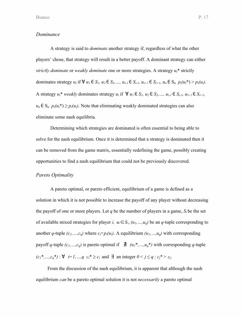
Dominance

A strategy is said to dominate another strategy if, regardless of what the other

players’ chose, that strategy will result in a better payoff. A dominant strategy can either

strictly dominate or weakly dominate one or more strategies. A strategy ui* strictly

dominates strategy ui if " u1 ! S1, u2 ! S2,…, ui-1 ! Si-1, ui+1 ! Si+1, un ! Sn pi(ui*) > pi(ui).

A strategy ui* weakly dominates strategy ui if " u1 ! S1, u2 ! S2,…, ui-1 ! Si-1, ui+1 ! Si+1,

un ! Sn pi(ui*) " pi(ui). Note that eliminating weakly dominated strategies can also

eliminate some nash equilibria.

Determining which strategies are dominated is often essential to being able to

solve for the nash equilibrium. Once it is determined that a strategy is dominated then it

can be removed from the game matrix, essentially redefining the game, possibly creating

opportunities to find a nash equilibrium that could not be previously discovered.

Pareto Optimality

A pareto optimal, or pareto efficient, equilibrium of a game is defined as a

solution in which it is not possible to increase the payoff of any player without decreasing

the payoff of one or more players. Let q be the number of players in a game, Si be the set

of available mixed strategies for player i,

!

ui" Si, (u1,…,uq) be an q-tuple corresponding to

another q-tuple (c1,…,cq) where ci=pi(ui). A equilibrium (u1,…,uq) with corresponding

payoff q-tuple (c1,…,cq) is pareto optimal if # (u1*,…,uq*) with corresponding q-tuple

(c1*,…,cq*) : " i=1,…,q ci* $ ci and $ an integer 0 < j # q : cj* > cj.

From the discussion of the nash equilibrium, it is apparent that although the nash

equilibrium can be a pareto optimal solution it is not necessarily a pareto optimal

Bianco P. 18

solution. For example, take the case of the prisoner’s dilemma in figure 4: although (c,

C) is the nash equilibrium it is not a pareto optimal solution (every other possible pure

strategy choice in that game is pareto optimal). This underscores the fact that the nash

equilibrium, in many cases, is not the outcome that both parties should desire. If the nash

equilibrium is not pareto optimal this could be a sign of a coordination problem, signaling

players involved that cooperation should be engaged in order to eliminate any

coordination issues that are preventing one or more players from increasing their payoffs

without expense to other players involved.

The nash equilibrium, combined with the notion of pareto efficiency, in the case of

the prisoner’s dilemma highlights an interesting moral issue: self-interest does not always

result in the optimal result for both parties. For the hedonist who is strictly concerned

about himself, the “pursuit of self-interest backfires, and prevents us from conforming to

collectively advantageous social arrangements” (Luper, 2001). The hedonist can take a

well-needed lesson from our above discussion; sacrifice and concern for others might

result in a higher level of utility for all.

Bianco P. 19

III. Mathematical Analysis

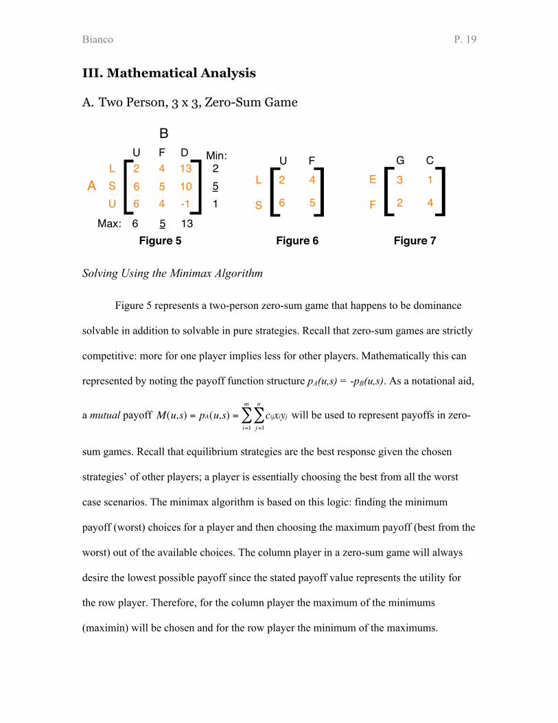
A. Two Person, 3 x 3, Zero-Sum Game

Solving Using the Minimax Algorithm

Figure 5 represents a two-person zero-sum game that happens to be dominance

solvable in addition to solvable in pure strategies. Recall that zero-sum games are strictly

competitive: more for one player implies less for other players. Mathematically this can

represented by noting the payoff function structure pA(u,s) = -pB(u,s). As a notational aid,

a mutual payoff

!

M(u,s) = pA(u,s) = cijxiyjj=1

n

"i=1

m

" will be used to represent payoffs in zero-

sum games. Recall that equilibrium strategies are the best response given the chosen

strategies’ of other players; a player is essentially choosing the best from all the worst

case scenarios. The minimax algorithm is based on this logic: finding the minimum

payoff (worst) choices for a player and then choosing the maximum payoff (best from the

worst) out of the available choices. The column player in a zero-sum game will always

desire the lowest possible payoff since the stated payoff value represents the utility for

the row player. Therefore, for the column player the maximum of the minimums

(maximin) will be chosen and for the row player the minimum of the maximums.

B

A

U F DL

Figure 5

2SU

66

454

1310-1

6 5 13Max:

251

Min:

[ ]U F

L

S

2 4

6 5

Figure 6

[ ]G C

E

F

Figure 7

3 1

2 4

Bianco P. 20

Examining figure 5 it is easy to see that for A the maximin is 5 and for B the

minimax is 5 resulting in an equilibrium pair (F, S). It is not a coincidence that both

values are equal – this is a property of the minimax theorem that will be explored in more

detail later. The equilibrium pair that we have found is a pure strategy nash equilibrium.

Not every zero-sum game has a pure strategy nash equilibrium, but (as will be shown

later) every zero-sum game has a mixed strategy nash equilibrium.

Solving Using Iterated Dominance

Although not always the case, in figure 5 the nash equilibrium can also be found

by eliminating dominated strategies and choosing the best remaining strategy. Comparing

strategies S & U of player B it is apparent that S weakly dominated U. Examining A finds

that both U & F strictly dominate D. The new resulting matrix (depicted in figure 6)

makes it clear that L is dominated and thus F is the best choice for B resulting in (F, S) as

the equilibrium pair – the same result found using minimax analysis.

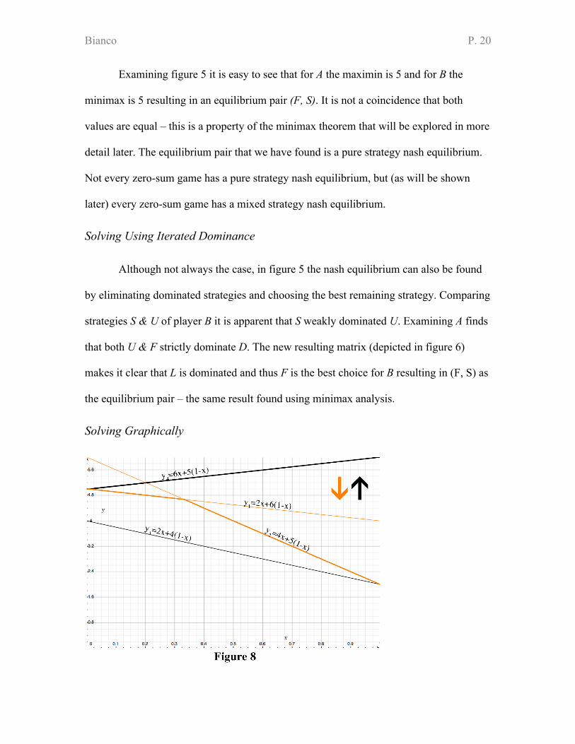
Solving Graphically

Bianco P. 21

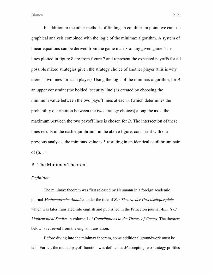
In addition to the other methods of finding an equilibrium point, we can use

graphical analysis combined with the logic of the minimax algorithm. A system of

linear equations can be derived from the game matrix of any given game. The

lines plotted in figure 8 are from figure 7 and represent the expected payoffs for all

possible mixed strategies given the strategy choice of another player (this is why

there is two lines for each player). Using the logic of the minimax algorithm, for A

an upper constraint (the bolded ‘security line’) is created by choosing the

minimum value between the two payoff lines at each x (which determines the

probability distribution between the two strategy choices) along the axis; the

maximum between the two payoff lines is chosen for B. The intersection of these

lines results in the nash equilibrium, in the above figure, consistent with our

previous analysis, the minimax value is 5 resulting in an identical equilibrium pair

of (S, F).

B. The Minimax Theorem

Definition

The minimax theorem was first released by Neumann in a foreign academic

journal Mathematische Annalen under the title of Zur Theorie der Gesellschaftsspiele

which was later translated into english and published in the Princeton journal Annals of

Mathematical Studies in volume 4 of Contributions to the Theory of Games. The theorem

below is retrieved from the english translation.

Before diving into the minimax theorem, some additional groundwork must be

laid. Earlier, the mutual payoff function was defined as M accepting two strategy profiles

Bianco P. 22

as arguments. In addition to accepting strategy profiles, M can accept a pure strategy

argument in place of either strategy profile such that

!

M("Ai,s) = M("i,s) = cijyjj=1

n

# (recall

that cij is the payoff from the perspective of A, thus B’s payoff in a zero-sum game is -cij).

With this notational addition in place, the two part minimax theorem can now be stated.

Theorem 1: For two-person zero-sum games each of the following three conditions

implies the other two.

Condition 1:

An equilibrium pair exists

Condition 2:

!

v1 = maxu " SA

mins " SB

M(u,s) = mins " SB

maxu " SA

M(u,s) = v2

Condition 3:

There exists a real number %, mixed strategy u*=(x1,…,xm) and mixed strategy

s*=(y1,…,ym) such that:

(a)

!

cijxii=1

m

" # v, j =1,...,n

(b)

!

cijyij=1

n

" # v,i =1,...,m

Theorem 2: For every finite, two-person, zero-sum game, there exists an equilibrium

strategy.

Condition 2 states algorithmically how the minimax & maximin are calculated,

also implying that

!

v = v1 = v 2 . Condition 3(a) states that there does not exist another

strategy available to player A that could be chosen to ensure a greater worst-case or

‘security’ payoff (3(b) ensures the same for player B). The proof for theorem one is rather

Bianco P. 23

simplistic and follows directly from the previous definitions that have been made, for this

reason the proof for part two of the theorem will be the focus.

Proof

The following proof for the minimax theorem is adapted from appendix two of

Luce & Raiffa’s Games and Decisions. Recall the definition of a fixed point for a

mapping. A mapping T : X ! X has the fixed point property if $ x ! X : T(x) = x.

Let u ! SA, s ! SB, u* ! SA, s* ! SB

Let T be a transformation that maps mixed strategy pairs into mixed strategy pairs

!

T : SA " SB #SA " SB

!

T(u,s) = (u',s') = ((x1,...,xm'),(yi,...,yn'))

It will be proved that T has two properties:

(a) u* and s* are maximin & minimax strategies if and only if T(u*,s*) = (u*,s*)

(b) T has at least one fixed point

T is defined as:

!

xi'= xi + ci(u,s)

1+ ck(u,s)k=1

m

"

!

yi'= yi + di(u,s)

1+ dk(u,s)k=1

n

"

!

ci(u,s) =M("i,s) #M(u,s) if M("i,s) #M(u,s) > 00 otherwise$ % &

!

dj(u,s) =M(u,s) "M(u,#j) if M(u,s) "M(u,#j) > 00 otherwise$ % &

Bianco P. 24

Note that ci , di are greater that zero if the pure strategy !Ai, !Bi results in a better

payoff (remember that numerically lower is better for B) than the mixed strategy u, s for

players A and B respectively. Building on ci and di, xi " xi' and yi "ysi' if there exists some

pure strategy that would result in a better payoff for A given B’s mixed strategy (or B

given A’s strategy). If xi = xi' then we know that A is making the best strategy choice

possible given s (and when yi =yi' B is making the best strategy choice possible given u).

A couple conclusions come out of this analysis:

!

if T(u*,s*) = (u*',s*') = (u*,s*) then (u*,s*) is an equilibrium pair

!

if (u*,s*) is an equilibrium pair then

!

"i, ci(u*,s*) = 0

!

and "j, dj(u*,s*) = 0

The following proof is ‘nested’ in the sense that it a multi-part and multi-level proof. To

assist in following the logic of the proof the three main sections of the proof will be

separated into A, B, C. Part B is separated into I & II.

A. Prove: u' & s' are Probability Distributions

Before going any further it must first be proved that the mapping T results in a

pair of probability distributions. Recall that for a m-tuple (x1,x2,…,xm) to be a probability

distribution

!

xii=1

m

" =1.

!

ui'= xi + ci(u,s)

1+ ck(u,s)k=1

m

"i=1

m

"i=1

m

" =

xii=1

m

" + ci(u,s)i=1

m

"

1+ ck(u,s)k=1

m

"

Bianco P. 25

!

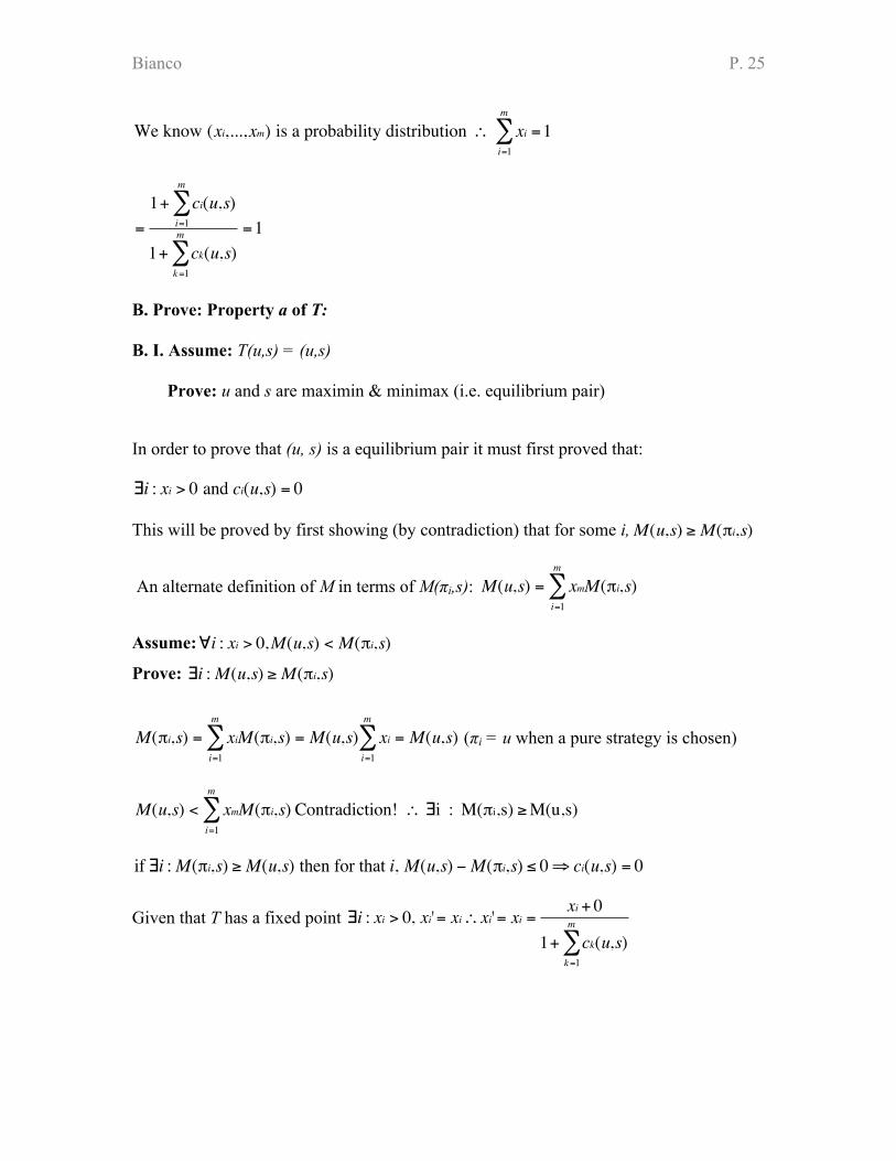
We know (xi,...,xm) is a probability distribution " xii=1

m

# =1

!

=

1+ ci(u,s)i=1

m

"

1+ ck(u,s)k=1

m

"=1

B. Prove: Property a of T:

B. I. Assume: T(u,s) = (u,s)

Prove: u and s are maximin & minimax (i.e. equilibrium pair)

In order to prove that (u, s) is a equilibrium pair it must first proved that:

!

"i : xi > 0 and ci(u,s) = 0

This will be proved by first showing (by contradiction) that for some i,

!

M(u,s) "M(#i,s)

An alternate definition of M in terms of M(!i,s):

!

M(u,s) = xmM("i,s)i=1

m

#

Assume:

!

"i : xi > 0,M(u,s) < M(#i,s)

Prove:

!

"i :M(u,s) #M($i,s)

!

M("i,s) = xiM("i,s)i=1

m

# = M(u,s) xii=1

m

# = M(u,s) (!i = u when a pure strategy is chosen)

!

M(u,s) < xmM("i,s)i=1

m

# Contradiction! $ %i : M("i,s) &M(u,s)

!

if "i : M(#i,s) $M(u,s) then for that i, M(u,s) %M(#i,s) & 0' ci(u,s) = 0

Given that T has a fixed point

!

"i : xi > 0, xi'= xi# xi'= xi =xi + 0

1+ ck(u,s)k=1

m

$

Bianco P. 26

!

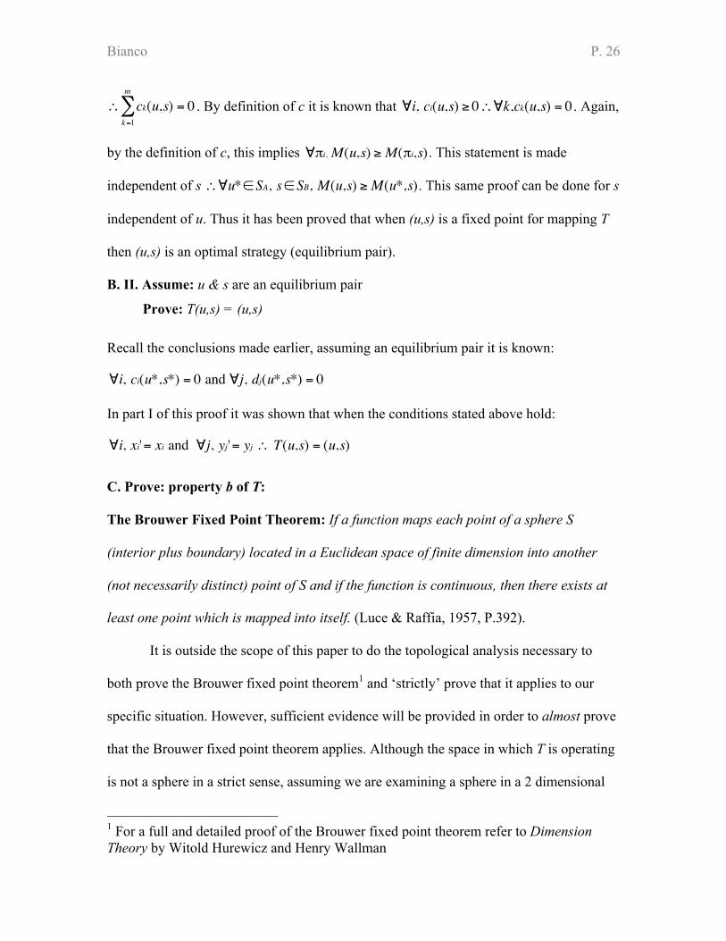
" ck(u,s)k=1

m

# = 0 . By definition of c it is known that

!

"i, ci(u,s) # 0$"k,ck(u,s) = 0 . Again,

by the definition of c, this implies

!

"#i, M(u,s) $M(#i,s). This statement is made

independent of s

!

"#u*$ SA, s$ SB, M(u,s) %M(u*,s). This same proof can be done for s

independent of u. Thus it has been proved that when (u,s) is a fixed point for mapping T

then (u,s) is an optimal strategy (equilibrium pair).

B. II. Assume: u & s are an equilibrium pair

Prove: T(u,s) = (u,s)

Recall the conclusions made earlier, assuming an equilibrium pair it is known:

!

"i, ci(u*,s*) = 0 and "j, dj(u*,s*) = 0

In part I of this proof it was shown that when the conditions stated above hold:

!

"i, xi'= xi and "j, yj'= yj # T(u,s) = (u,s)

C. Prove: property b of T:

The Brouwer Fixed Point Theorem: If a function maps each point of a sphere S

(interior plus boundary) located in a Euclidean space of finite dimension into another

(not necessarily distinct) point of S and if the function is continuous, then there exists at

least one point which is mapped into itself. (Luce & Raffia, 1957, P.392).

It is outside the scope of this paper to do the topological analysis necessary to

both prove the Brouwer fixed point theorem1 and ‘strictly’ prove that it applies to our

specific situation. However, sufficient evidence will be provided in order to almost prove

that the Brouwer fixed point theorem applies. Although the space in which T is operating

is not a sphere in a strict sense, assuming we are examining a sphere in a 2 dimensional

1 For a full and detailed proof of the Brouwer fixed point theorem refer to Dimension Theory by Witold Hurewicz and Henry Wallman

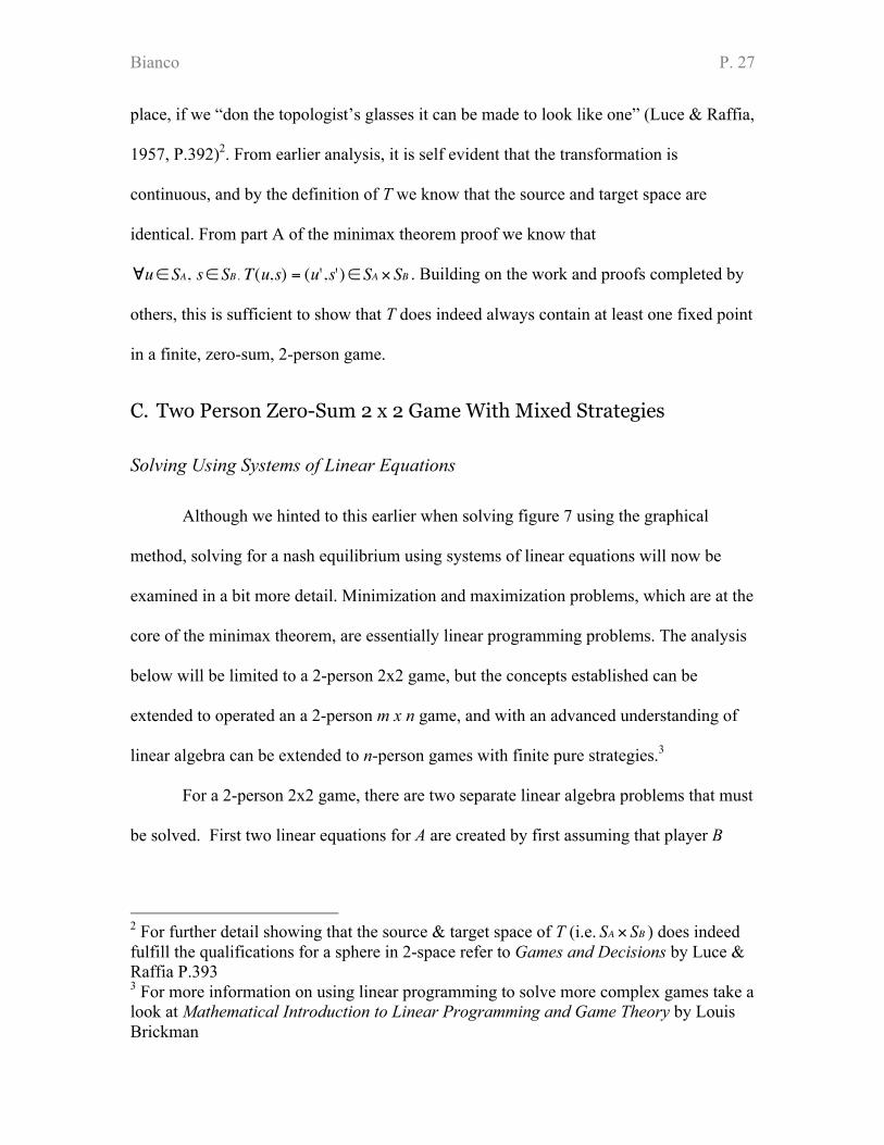
Bianco P. 27

place, if we “don the topologist’s glasses it can be made to look like one” (Luce & Raffia,

1957, P.392)2. From earlier analysis, it is self evident that the transformation is

continuous, and by the definition of T we know that the source and target space are

identical. From part A of the minimax theorem proof we know that

!

"u# SA, s# SB , T(u,s) = (u',s')# SA $ SB . Building on the work and proofs completed by

others, this is sufficient to show that T does indeed always contain at least one fixed point

in a finite, zero-sum, 2-person game.

C. Two Person Zero-Sum 2 x 2 Game With Mixed Strategies

Solving Using Systems of Linear Equations

Although we hinted to this earlier when solving figure 7 using the graphical

method, solving for a nash equilibrium using systems of linear equations will now be

examined in a bit more detail. Minimization and maximization problems, which are at the

core of the minimax theorem, are essentially linear programming problems. The analysis

below will be limited to a 2-person 2x2 game, but the concepts established can be

extended to operated an a 2-person m x n game, and with an advanced understanding of

linear algebra can be extended to n-person games with finite pure strategies.3

For a 2-person 2x2 game, there are two separate linear algebra problems that must

be solved. First two linear equations for A are created by first assuming that player B

2 For further detail showing that the source & target space of T (i.e.

!

SA " SB ) does indeed fulfill the qualifications for a sphere in 2-space refer to Games and Decisions by Luce & Raffia P.393 3 For more information on using linear programming to solve more complex games take a look at Mathematical Introduction to Linear Programming and Game Theory by Louis Brickman

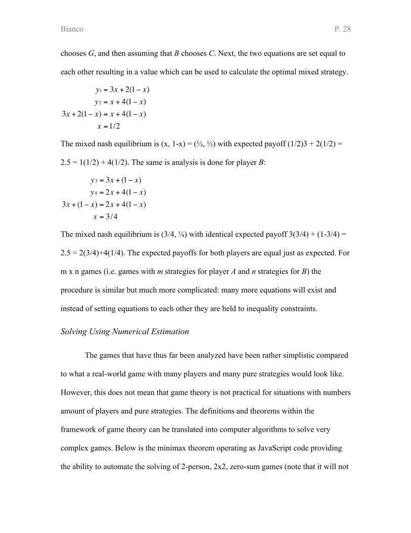
Bianco P. 28

chooses G, and then assuming that B chooses C. Next, the two equations are set equal to

each other resulting in a value which can be used to calculate the optimal mixed strategy.

!

y1 = 3x + 2(1" x)y 2 = x + 4(1" x)

3x + 2(1" x) = x + 4(1" x)x =1/2

The mixed nash equilibrium is (x, 1-x) = (#, #) with expected payoff (1/2)3 + 2(1/2) =

2.5 = 1(1/2) + 4(1/2). The same is analysis is done for player B:

!

y3 = 3x + (1" x)y4 = 2x + 4(1" x)

3x + (1" x) = 2x + 4(1" x)x = 3/4

The mixed nash equilibrium is (3/4, $) with identical expected payoff 3(3/4) + (1-3/4) =

2.5 = 2(3/4)+4(1/4). The expected payoffs for both players are equal just as expected. For

m x n games (i.e. games with m strategies for player A and n strategies for B) the

procedure is similar but much more complicated: many more equations will exist and

instead of setting equations to each other they are held to inequality constraints.

Solving Using Numerical Estimation

The games that have thus far been analyzed have been rather simplistic compared

to what a real-world game with many players and many pure strategies would look like.

However, this does not mean that game theory is not practical for situations with numbers

amount of players and pure strategies. The definitions and theorems within the

framework of game theory can be translated into computer algorithms to solve very

complex games. Below is the minimax theorem operating as JavaScript code providing

the ability to automate the solving of 2-person, 2x2, zero-sum games (note that it will not

Bianco P. 29

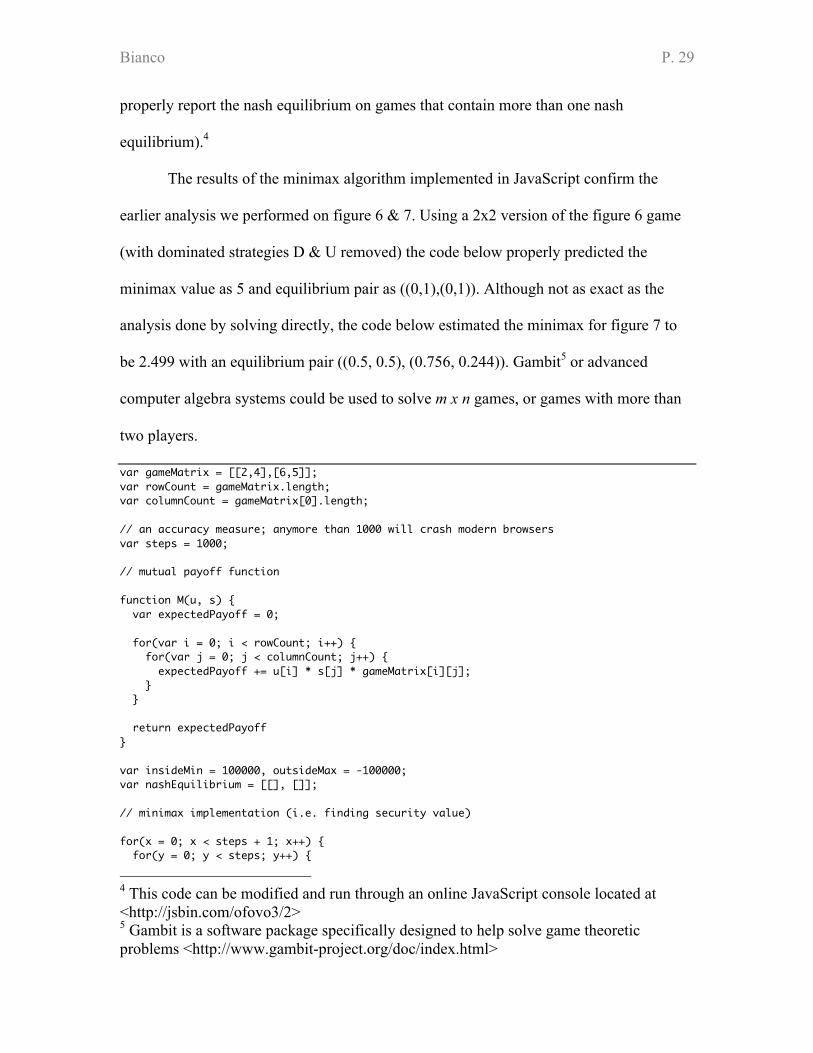
properly report the nash equilibrium on games that contain more than one nash

equilibrium).4

The results of the minimax algorithm implemented in JavaScript confirm the

earlier analysis we performed on figure 6 & 7. Using a 2x2 version of the figure 6 game

(with dominated strategies D & U removed) the code below properly predicted the

minimax value as 5 and equilibrium pair as ((0,1),(0,1)). Although not as exact as the

analysis done by solving directly, the code below estimated the minimax for figure 7 to

be 2.499 with an equilibrium pair ((0.5, 0.5), (0.756, 0.244)). Gambit5 or advanced

computer algebra systems could be used to solve m x n games, or games with more than

two players.

var gameMatrix = [[2,4],[6,5]]; var rowCount = gameMatrix.length; var columnCount = gameMatrix[0].length; // an accuracy measure; anymore than 1000 will crash modern browsers var steps = 1000; // mutual payoff function function M(u, s) { var expectedPayoff = 0; for(var i = 0; i < rowCount; i++) { for(var j = 0; j < columnCount; j++) { expectedPayoff += u[i] * s[j] * gameMatrix[i][j]; } } return expectedPayoff } var insideMin = 100000, outsideMax = -100000; var nashEquilibrium = [[], []]; // minimax implementation (i.e. finding security value) for(x = 0; x < steps + 1; x++) { for(y = 0; y < steps; y++) {

4 This code can be modified and run through an online JavaScript console located at <http://jsbin.com/ofovo3/2> 5 Gambit is a software package specifically designed to help solve game theoretic problems <http://www.gambit-project.org/doc/index.html>

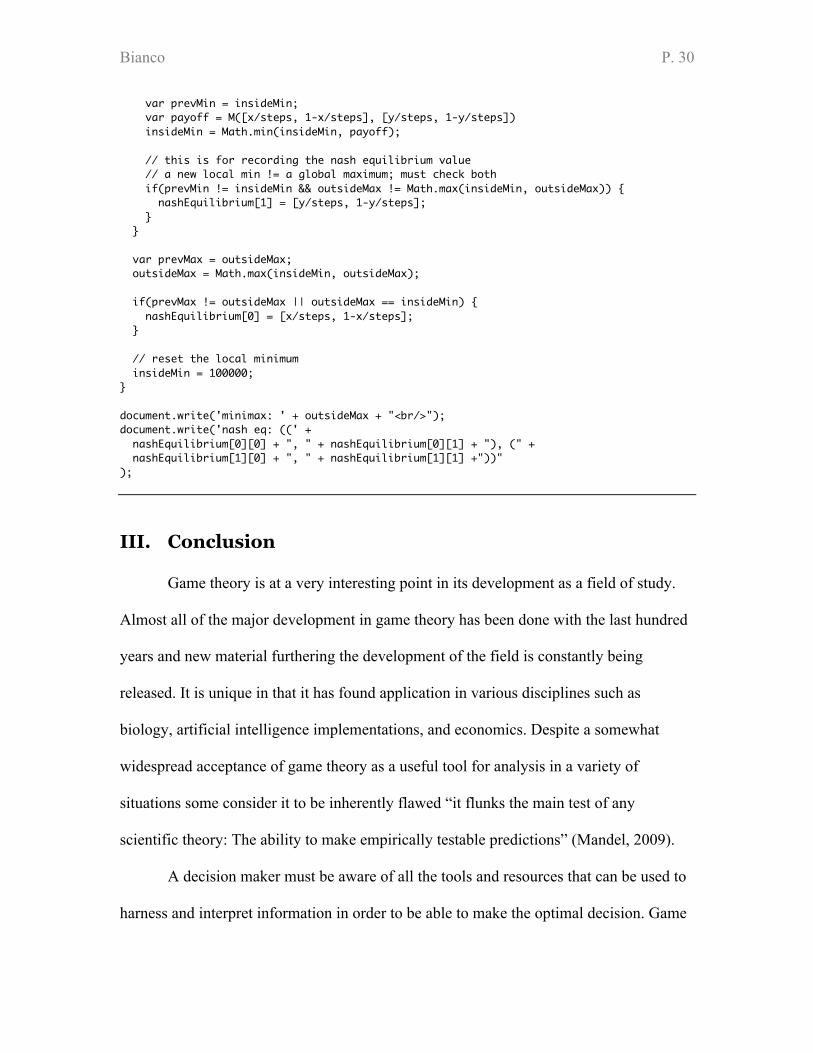
Bianco P. 30

var prevMin = insideMin; var payoff = M([x/steps, 1-x/steps], [y/steps, 1-y/steps]) insideMin = Math.min(insideMin, payoff); // this is for recording the nash equilibrium value // a new local min != a global maximum; must check both if(prevMin != insideMin && outsideMax != Math.max(insideMin, outsideMax)) { nashEquilibrium[1] = [y/steps, 1-y/steps]; } } var prevMax = outsideMax; outsideMax = Math.max(insideMin, outsideMax); if(prevMax != outsideMax || outsideMax == insideMin) { nashEquilibrium[0] = [x/steps, 1-x/steps]; } // reset the local minimum insideMin = 100000; } document.write('minimax: ' + outsideMax + "<br/>"); document.write('nash eq: ((' + nashEquilibrium[0][0] + ", " + nashEquilibrium[0][1] + "), (" + nashEquilibrium[1][0] + ", " + nashEquilibrium[1][1] +"))" );

III. Conclusion

Game theory is at a very interesting point in its development as a field of study.

Almost all of the major development in game theory has been done with the last hundred

years and new material furthering the development of the field is constantly being

released. It is unique in that it has found application in various disciplines such as

biology, artificial intelligence implementations, and economics. Despite a somewhat

widespread acceptance of game theory as a useful tool for analysis in a variety of

situations some consider it to be inherently flawed “it flunks the main test of any

scientific theory: The ability to make empirically testable predictions” (Mandel, 2009).

A decision maker must be aware of all the tools and resources that can be used to

harness and interpret information in order to be able to make the optimal decision. Game

Bianco P. 31

theory should not be thought of a standalone tool used to make decisions or determine

outcomes. The conclusions that the theoretical mathematics upon which game theory is

based bring us to, allow us to assign certain attributes to specific strategic situations in

order to aid one in understanding what is beneficial for both himself and his opponent (or

ally). These attributes and characteristics which game theory allows us to ascertain from a

situation enable additional facets of a given competitive situation to be revealed, making

game theory an indispensible tool for a decision maker to have in his intellectual toolbox.

References: Antoine Augustin Cournot. (2004). Encyclopedia of World Biography. Encyclopedia.com.

Retrieved November from http://www.encyclopedia.com/doc/1G2-3404701543.html Avinash Dixit and Barry Nalebuff. (2008). Game Theory. The Concise Encyclopedia of

Economics. Library of Economics and Liberty. Retrieved from http://econlib.org/library/Enc/GameTheory.html

Comlay, E. (2010, November 10). Google to give staff a 10 percent pay rise: reports .

Business & Financial News, Breaking US & International News. Retrieved from http://www.reuters.com/article/idUSTRE6A90LT20101110

Dixit, A. K., Skeath, S., & Reiley, D. (2009). Games of Strategy (3rd ed.). New York: W. W.

Norton & Co.. Ekelund, R. B., & Hébert, R. F. (2007). A History of Economic Theory and Method (5th ed.).

Long Grove, Ill.: Waveland Press. Luce, R. D., & Raiffa, H. (1957). Games and Decision: Introduction and Critical Survey.

New York: John Wiley & Sons, Inc. Fonseca, G. L. (n.d.). John von Neumann. New School of Economics. Retrieved from

http://homepage.newschool.edu/het/profiles/neumann.htm Hawkins, A. (2009, June 3). Prisoner's Dilemma. Forbes. Retrieved November 26, 2010,

from http://www.forbes.com/forbes/2009/0622/trustbusters-consumers-monopolies-heads-up.html

John von Neumann. (2008). The Concise Encyclopedia of Economics. Library of Economics

and Liberty. Retrieved http://www.econlib.org/library/Enc/bios/Neumann.html John F. Nash Jr. (2008). The Concise Encyclopedia of Economics. Library of Economics and

Liberty. Retrieved from http://www.econlib.org/library/Enc/bios/Nash.html Kuhn, H. W. (1953). Extensive Games and the Problem of Information. Annals of

Mathematical Studies, 2, 189 - 216. Luper, S. (n.d.). Ethical Egoism: Is Duty a Matter of Self-Enhancement?. Trinity University.

Retrieved from http://www.trinity.edu/departments/philosophy/sluper/CHAPTER%207guidetoethics.htm

Mandel, M. (2005, September 11). A Nobel Letdown in Economics. Business Week.

Retrieved from http://www.businessweek.com/bwdaily/dnflash/oct2005/nf20051011_3028_db084.htm

Mendelson, E. (2004). Introducing Game Theory and Its Applications . Boca Raton: Chapman & Hall/Crc.

Milnor, J. (1998). John Nash and “A Beautiful Mind”. Notices, 45(10). Retrieved from

http://www.ams.org/notices/199810/milnor.pdf Mandel, M. (2005, September 11). A Nobel Letdown in Economics. Business Week.

Retrieved from http://www.businessweek.com/bwdaily/dnflash/oct2005/nf20051011_3028_db084.htm

Myhrvold, N. (1999, March 21). John von Neumann. TIME.com. Retrieved from

http://www.time.com/time/magazine/article/0,9171,21839,00.html Stone, B., & Vance, A. (2009, May 22). Apple’s Management Obsessed With Secrecy.

Breaking News, World News & Multimedia. Retrieved November 10, 2010, from http://www.nytimes.com/2009/06/23/technology/23apple.html?hp

Straffin, P. D. (1996). Game Theory and Strategy (New Mathematical Library). Washington:

The Mathematical Association Of America