MATHEMATICAL FOUNDATIONS OF MACHINELEARNING

(NMAG 469, FALL TERM 2018-2019)

HONG VAN LE ∗

Contents

1. Learning, machine learning and artificial intelligence 31.1. Learning, inductive learning and machine learning 31.2. A brief history of machine learning 51.3. Current tasks and types of machine learning 71.4. Basic questions in mathematical foundations of machine

learning 101.5. Conclusion 112. Statistical models and frameworks for supervised learning 112.1. Discriminative model of supervised learning 112.2. Generative model of supervised learning 152.3. Empirical Risk Minimization and overfitting 172.4. Conclusion 193. Statistical models and frameworks for unsupervised learning and

reinforcement learning 193.1. Statistical models and frameworks for density estimation 203.2. Statistical models and frameworks for clustering 233.3. Statistical models and frameworks for dimension reduction and

manifold learning 243.4. Statistical model and framework for reinforcement learning 253.5. Conclusion 264. Fisher metric and maximum likelihood estimator 264.1. The space of all probability measures and total variation norm 264.2. Fisher metric on a statistical model 284.3. The Fisher metric, MSE and Cramer-Rao inequality 304.4. Efficient estimators and MLE 334.5. Consistency of MLE 334.6. Conclusion 345. Consistency of a learning algorithm 345.1. Consistent learning algorithm and its sample complexity 355.2. Uniformly consistent learning and VC-dimension 38

Date: February 1, 2019.∗ Institute of Mathematics of ASCR, Zitna 25, 11567 Praha 1, email: hvle@math.cas.cz.

1

2 HONG VAN LE ∗

5.3. Fundamental theorem of binary classification 405.4. Conclusions 426. Generalization ability of a learning machine and model selection 426.1. Covering number and sample complexity 426.2. Rademacher complexities and sample complexity 456.3. Model selection 476.4. Conclusion 497. Support vector machines 497.1. Linear classifier and hard SVM 497.2. Soft SVM 527.3. Sample complexities of SVM 547.4. Conclusion 568. Kernel based SVMs 568.1. Kernel trick 568.2. PSD kernels and reproducing kernel Hilbert spaces 588.3. Kernel based SVMs and their generalization ability 618.4. Conclusion 629. Neural networks 629.1. Neural networks as computing devices 639.2. The expressive power of neural networks 669.3. Sample complexities of neural networks 679.4. Conclusion 6910. Training neural networks 6910.1. Gradient and subgradient descend 6910.2. Stochastic gradient descend (SGD) 7110.3. Online gradient descend and online learnability 7310.4. Conclusion 7411. Bayesian machine learning 7411.1. Bayesian concept of learning 7411.2. Estimating decisions using posterior distributions 7511.3. Bayesian model selection 7711.4. Conclusion 77Appendix A. Some basic notions in probability theory 77A.1. Dominating measures and the Radon-Nikodym theorem 77A.2. Conditional expectation and regular conditional measure 78A.3. Joint distribution and Bayes’ theorem 79A.4. Transition measure, Markov kernel, and parameterized

statistical model 80Appendix B. Concentration-of-measure inequalities 81B.1. Markov’s inequality 82B.2. Hoeffding’s inequality 82B.3. Bernstein’s inequality 82B.4. McDiarmid’s inequality 82References 82

MACHINE LEARNING 3

It is not knowledge, but the act of learning ... which grants the greatestenjoyment.

Carl Friedrich Gauss

Machine learning is an interdisciplinary field in the intersection of math-ematical statistics and computer sciences. Machine learning studies sta-tistical models and algorithms for deriving predictors or meaningful pat-terns from empirical data. Machine learning techniques are applied insearch engine, speech recognition and natural language processing, imagedetection, robotics etc.. In our course we address the following questions:What is the mathematical model of learning? How to quantify the diffi-culty/hardness/complexity of a learning problem? How to choose a learningalgorithm? How to measure success of machine learning?

The syllabus of our course:1. Supervised learning and unsupervised learning.2. Generalization ability of machine learning.3. Fisher metric and stochastic gradient descend.4. Support vector machine, Kernel machine and Neural network.Recommended Literature.1. F. Cucker and S. Smale, On mathematical foundations of learning,

Bulletin of AMS, 39(2001), 1-49.2. K. P. Murphy, Machine learning: a probabilistic perspective (MIT

press, 2012).3. M. Sugiyama, Introduction to Statistical Machine Learning, Elsevier,

2016.4. S. Shalev-Shwartz, and S. Ben-David, Understanding Machine Learn-

ing: From Theory to Algorithms, Cambridge University Press, 2014.

1. Learning, machine learning and artificial intelligence

Machine learning is the foundation of countless important applicationsincluding speech recognition, image detection, self-driving car and manything more which I shall discuss today in my lecture. Machine learningtechniques are developed using many mathematical theories. In my lecturecourse I shall explain the mathematical model of machine learning and howdo we design a machine which shall learn successfully.

In my today lecture I shall discuss the following topics.1. What are learning, inductive learning and machine learning.2. History of machine learning and artificial intelligence.3. Current tasks and main types of machine learning.4. Basic questions in mathematical foundation of machine learning.

1.1. Learning, inductive learning and machine learning. To start ourdiscussion on machine learning let us begin first with the notion of learning.Every one from us know what is learning from our experiences at the veryearly age.

4 HONG VAN LE ∗

(a) Small children learn to speak by observing, repeating and mimickingadults’ phrases. At the beginning their language is very simple and often er-roneous. Gradually they speak freely with less and less mistakes. Their wayof learning is inductive learning: from examples of words and phrases theylearn the rules of combinations of these words and phrases into meaningfulsentences.

(b) In school we learn mathematics, physics, biology, chemistry by fol-lowing the instructions of our teachers and those in textbooks. We learngeneral rules and apply them to particular cases. This type of learning isdeductive learning. Of course we also learn inductively in school by search-ing similar patterns in new problems and then apply the most appropriatemethods possibly with modifications for solving the problem.

(c) Experimental physicists design experiments and observe the outcomesof the experiments to validate/support or dispute/refute a statement/conjectureon the nature of the observables. In other words experimental physicistslearn about the dependence of certain features of the observables from em-pirical data which are outcomes of the experiments. This type of learningis inductive learning.

In mathematical theory of machine learning, or more general, in mathe-matical theory of learning we consider only inductive learning. Deductivelearning is not very interesting; essentially it is equivalent to performing a setof computations using a finite set of rules and a knowledge database. Clas-sical computer programs learn or gain some new information by deductivelearning.

Let me suggest a definition of learning, that will be updated later to bemore and more precise.

Definition 1.1. A learning is a process of gaining new knowledge, moreprecisely, new correlations of features of observable by examination of em-pirical data of the observable. Furthermore a learning is successful if thecorrelations can be tested in examination of new data and will be moreprecise with the increase of data.

The above definition is an expansion of Vapnik’s mathematical postula-tion: “Learning is a problem of function estimation on the basis of empiricaldata”.

Example 1.2. A classical example of learning is that of learning a physicallaw by curve fitting to data. In mathematical terms, a physical law isexpressed by a function f , and data are the value yi of f at observablepoints xi. Usually we also know that (or assume that) the desired functionbelongs to a finite dimensional space. The goal of learning in this case isto estimate the unknown f from a set of pairs (x1, y1), · · · , (xm, ym). Forinstance, if f is assumed to be a polynomial of degree d over R, then fbelongs to a N -dimensional linear space RN , where N = d + 1, and to

MACHINE LEARNING 5

estimate f is the same as to estimate the unknown coefficients w0, · · · , wdof monomial components in f , observing the data (xi, yi).

The most popular method of curve fitting is the least square methodwhich quantifies the error of the estimation of the coefficients (w0, · · · , wd)in terms of the value

(1.1)

m∑i=1

(fw(xi)− yi)2 with fw(x) =

d∑j=0

wjxj

which the desired function f should minimize. If the measurements gener-ating the data (xi, yi) were exact, then f(xi) would be equal to yi and thelearning problem is an interpolation problem. But in general one expectsthe values yi to be affected by noise.

The least square technique, going back to Gauss and Legendre 1, whichis computational efficient and relies on numerical linear algebra, solves thisminimization problem.

In the case of measurement noise, which is the reality according to quan-tum physics, we need to use the language of probability theory to modelthe noise and therefore to use tools of mathematical statistics in learningtheory. That is why statistical learning theory is important part of machinelearning theory.

1.2. A brief history of machine learning. Machine learning was bornas a domain of artificial intelligence and it was reorganized as a separatedfield only in the 1990s. Below I recall several important events when theconcept of machine learning has been discussed by famous mathematiciansand computer scientists.• In 1948 John von Neumann suggested that machine can do any thing

that peoples are able to do.• In 1950 Alan Turing asked “Can machines think?” in “Computing Ma-

chine and Intelligence” and proposed the famous Turing test. The Turingtest is carried out as imitation game. On one side of a computer screen sitsa human judge, whose job is to chat to an unknown gamer on the otherside. Most of those gamers will be humans; one will be a chatbot with thepurpose of tricking the judge into thinking that it is the real human.• In 1956 John McCarthy coined the term “artificial intelligence”.• In 1959, Arthur Samuel, the American pioneer in the field of com-

puter gaming and artificial intelligence, defined machine learning as a fieldof study that gives computers the ability to learn without being explicitlyprogrammed. The Samuel Checkers-playing Program appears to be theworld’s first self-learning program, and as such a very early demonstrationof the fundamental concept of artificial intelligence (AI).

1The least-squares method is usually credited to Carl Friedrich Gauss (1809), but itwas first published by Adrien-Marie Legendre (1805)

6 HONG VAN LE ∗

In the early days of AI, statistical and probabilistic methods were em-ployed. Perceptrons which are simple models used in statistics were usedfor classification problems in machine learning. Perceptrons were later de-veloped into more complicated neural networks. Because of many theoret-ical problems and because of small capacity of hardware memory and slowspeed of computers statistical methods were out of favour. By 1980, ex-pert systems, which were based on knowledge database, and inductive logicprogramming had come to dominate AI. Neural networks returned back tomachine learning with success in the mid-1980s with the reinvention of anew algorithm and thanks to increasing speed of computers and increasinghardware memory.

Machine learning, reorganized as a separate field, started to flourish inthe 1990s. The current trend is benefited from Internet.

In the book by Russel and Norvig “Artificial Intelligence a modern Ap-proach” (2010) AI encompass the following domains:- natural language processing,- knowledge representation,- automated reasoning to use the stored information to answer questionsand to draw new conclusions;- machine learning to adapt to new circumstances and to detect and extrap-olate patterns,- computer vision to perceive objects,- robotics.

All the listed above domains of artificial intelligence except knowledgerepresentation and robotics are now considered domains of machine learning.Pattern detection and recognition were and are still considered to be domainof data mining but they become more and more part of machine learning.Thus AI = knowledge representation + ML + robotics.• representation learning, a new word for knowledge representation but

with a different flavor, is a part of machine learning.• Robotics = ML + hardware.Why did such a move from artificial intelligence to machine learning hap-

pen?The answer is that we are able to formalize most concepts and model

problems of artificial intelligence using mathematical language and representas well as unify them in such a way that we can apply mathematical methodsto solve many problems in terms of algorithms that machine are able toperform.

As a final remark on the history of machine learning I would like tonote that data science, much hyped in 2018, has the same goal as machinelearning: Data science seeks actionable and consistent pattern for predictiveuses. 2.

2according to Dhar, V. (2013). “Data science and prediction”. Communications of theACM. 56 (12): 64. doi:10.1145/2500499, see also wiki site on data science

MACHINE LEARNING 7

1.3. Current tasks and types of machine learning. Now I shall de-scribe what current machine learning can perform and how they do it.

1.3.1. Main tasks of current machine learning. Let us give a short descrip-tion of current applications of machine learning.

Classification task assigns a “category” 3 to each item. In mathematicallanguage, a category is an element in a countable set. For example, docu-ment classification may assign items with categories such as politics, emailspam, sports, or weather while image classification may assign items withcategories such as landscape, portrait, or animal. The number of categoriesin such tasks can be unbounded as in OCR, text classification, or speechrecognition. In short, a classification task is a construction of a function onthe set of items that takes value in a countable set of categories.

As we have remarked in the classical example of learning (Example 1.2),usually we have ambiguous/incorrect measurement and we have to add a“noise” to our measurement. If every thing would be exact, the classificationtask is the classical interpolation function problem in mathematics.

Regression task predicts a real value, i.e., a value in R, for each item.Examples of regression tasks include learning physical law by curve fittingto data (Example 1.2) with application to predictions of stock values orvariations of economic variables. In this problem, the error of the prediction,which is also called estimation in Example 1.2, depends on the magnitudeof the distance between the true and predicted values, in contrast with theclassification problem, where there is typically no notion of closeness betweenvarious categories. In short, a regression task is a construction of a functionon the set of items that takes value in R. As in the classification task,in regression problems we also need to take into account a “noise” fromincorrect measurement for the regression problem. 4

Density estimation task finds the distribution of inputs in some space.Over one hundred year ago Karl Pearson (1980-1962), the founder of themodern statistics, 5 proposed that all observations come from some proba-bility distribution and the purpose of sciences is to estimate the parameter

3the term “category” used in machine learning has another meaning than the term“category” in mathematics. In what follows we use the term “category” accepted in MLcommunity without bracket.

4The term “regression” was coined by Francis Galton in the nineteenth century todescribe a biological phenomenon. The phenomenon was that the heights of descendantsof tall ancestors tend to regress down towards a normal average (a phenomenon alsoknown as regression toward the mean of population). For Galton, regression had only thisbiological meaning, but his work was later extended by Udny Yule and Karl Pearson to amore general statistical context: movement toward the mean of a statistical population.Galton’s method of investigation is non-standard at that time: first he collected the data,then he guessed the relationship model of the events.

5 He founded the world’s first university statistics department at University CollegeLondon in 1911, the Biometrical Society and Biometrika, the first journal of mathematicalstatistics and biometry.

8 HONG VAN LE ∗

of these distributions. A particular case of parameter estimation is den-sity estimation problem. Density estimation problem has been proposedby Ronald Fisher (1980-1962), the father of modern statistics and experi-ment designs, 6 as a key element of his simplification of statistical theory,namely he assumed the existence of a density function p(ξ) that governs therandomness (the noise) of a problem of interest.

Digression. The measure ν is called dominated by µ (or absolutely contin-uous with respect to µ), if ν(A) = 0 for every set A with µ(A) = 0. Notation:ν << µ. By Radon-Nykodym theorem, see Appendix, Subsection A.1, wecan write

ν = f · µand f is the density function of ν w.r.t. µ.

For example, the Gaussian distribution on the real line is dominated bythe canonical measure dx and we express the standard normal distributionin terms of its density

f(x) =1√2π

exp(−1

2x2).

The classical problem of density estimation is formulated as follows. Leta statistical model A be a class of densities subjected to a given dominantmeasure. Let the unknown density p(x, ξ) we need to estimate belong tothe statistical model A, which is parameterized by ξ. The problem is toestimate the parameter ξ of p(x, ξ) using i.i.d. data X1, · · · , Xl distributedaccording to this unknown density.

Ranking task orders items according to some criterion. Web search, e.g.,returning web pages relevant to a search query, is the canonical rankingexample. If the number of ranking is finite, then this task is close to theclassification problem, but not the same, since in the ranking task we needto specify each rank during the task and not before the task as in the clas-sification problem.

Clustering task partitions items into (homogeneous) regions. Clusteringis often performed to analyze very large data sets. Clustering is one of themost widely used techniques for exploratory data analysis. In all disciplines,from social sciences to biology to computer science, people try to get afirst intuition about their data by identifying meaningful groups among thedata points. For example, computational biologists cluster genes on thebasis of similarities in their expression in different experiments; retailerscluster customers, on the basis of their customer profiles, for the purposeof targeted marketing; and astronomers cluster stars on the basis of theirspacial proximity.

6Fisher introduced the main models of statistical inference in the unified framework ofparametric statistics. He described different problems of estimating functions from givendata (the problems of discriminant analysis, regression analysis, and density estimation)as the problems of parameter estimation of specific (parametric) models and suggested themaximum likelihood method for estimating the unknown parameters in all these models.

MACHINE LEARNING 9

Dimensionality reduction or manifold learning transforms an initial repre-sentation of items in high dimensional space into a space of lower dimensionwhile preserving some properties of the initial representation. A commonexample involves pre-processing digital images in computer vision tasks.Many of dimensional reduction techniques are linear. When the techniqueis non-linear we speak about manifold learning technique. We can regardclustering as dimension reduction too.

1.3.2. Main types of machine learning. The type of a machine learning taskis defined by the type of interaction between the learner and the environment.More precisely we consider types of training data, i.e., the data available tothe learner before making decision and prediction, the outcomes and the testdata that are used to evaluate and apply the learning algorithm.

Main types of machine learning are supervised, unsupervised and rein-forcement.• In supervised learning a learning machine is a device that receives labeled

training data, i.e., the pair of a known instance and its feature, also calledlabel. Examples of labeled data are emails that are labeled “spam” or “nospam” and medical histories that are labeled with the occurrence or absenceof a certain disease. In these cases the learners output would be a spamfilter and a diagnostic program, respectively. Most of classification andregression problems of machine learning belong to supervised learning. Wealso interpret a learning machine in supervised learning as a student whogives his supervisor a known instance and the supervisor answers with theknown feature.• In unsupervised learning there is no additional label attached to the

data and the task is to describe structure of data. Since the examples (theavailable data) given to the learning algorithm are unlabeled, there is nostraightforward way to evaluate the accuracy of the structure that is pro-duced by the algorithm. Density estimation, clustering and dimensionalityreduction are examples of unsupervised learning problems. Most importantapplications of unsupervised learning are finding association rules that areimportant in market analysis, banking security and consists of importantpart of pattern recognition, which is important for understand advanced AI.Regarding a learning machine in unsupervised learning as a student, thenthe student has to learn by himself without teacher. This learning is harderbut happens more often in life. At the current time, except few tasks, whichI shall consider in the next lecture, unsupervised learning is primarily de-scriptive and experimental whereas supervised learning is more predictive(and has deeper theoretical foundation).• Reinforcement learning is the type of machine learning where a learner

actively interacts with the environment to achieve a certain goal. Moreprecisely, the learner collects information through a course of actions byinteracting with the environment. This active interaction justifies the ter-minology of an agent used to refer to the learner. The achievement of the

10 HONG VAN LE ∗

agent’s goal is typically measured by the reward he receives from the en-vironment and which he seeks to maximize. For examples, reinforcementlearning is used in self-driving car. Reinforcement learning is aimed at ac-quiring the generalization ability in the same way as supervised learning,but the supervisor does not directly give answers to the students questions.Instead, the supervisor evaluates the students behavior and gives feedbackabout it.

1.4. Basic questions in mathematical foundations of machine learn-ing. Let me recall that a learning is a process of gaining knowledge on afeature of observables by examination of partially available data. The learn-ing is successful if we can make a prediction on unseen data, which improveswhen we have more data. For example, in classification problem, the learn-ing machine has to predict the category of a new item from a specific set,after seeing a lot of labeled data consisting of items and their categories.The classification task is a typical task in supervised learning where we canexplain how and why a learning machine works and how and why machinelearns successfully. Mathematical foundations of machine learning aim toanswer these questions in mathematical language.

Question 1.3. What is the mathematical model of learning?

To answer Question 1.3 we need to specify our definition of learning in amathematical language which can be used to build instructions for machines.

Question 1.4. How to quantify the difficulty/complexity of a learning prob-lem?

We quantify the difficulty of a problem in terms of its time complexity,which is the minimum time needed for performing computer program tosolve a problem, and in term of its resource complexity which measure thecapacity of data storage and energy resource needed to solve the problem.If the complexity of a problem is very large then we cannot not learn it. SoQuestion 1.4 contains the sub-question “ why can we learn a problem?”

Question 1.5. How to choose a learning algorithm?

Clearly we want to have a best learning algorithm, once we know a modelof a machine learning which specifies the set of possible predictors (decisions)and the associated error/reward function.

By Definition 1.1, a learning process is successful, if its prediction/estimationimproves with the increase of data. Thus the notion of success of learn-ing process requires a mathematical treatment of asymptotic rate of er-ror/reward in the presence of complexity of the problem.

Question 1.6. Is there a mathematical theory underlying intelligence?

I shall discuss this speculative question in the last lecture.

MACHINE LEARNING 11

1.5. Conclusion. Machine learning is automatized learning, whose perfor-mance is improves with increasing volume of empirical data. Machine learn-ing uses mathematical statistics to model incomplete information and therandom nature of the observed data. Machine learning is the core part of ar-tificial intelligence. Machine learning is very successful experimentally andthere are many open questions concerning its mathematical foundations.Mathematical foundations of machine learning is necessary for building gen-eral purpose artificial intelligence, also called Artificial General Intelligence(AGI), or Universal Artificial Intelligence (UAI). The importance of math-ematical foundations for AGI shall be clarified in the third lecture.

Finally I recommend some sources for further reading.

• F. Cucker and S. Smale, On mathematical foundations of learning,Bulletin of AMS, 39(2001), 1-49.• B. M. Lake, T. D. Ullman, J. B. Tenenbaum, and S. J. Gershman,

Building machines that learn and think like people. Behavioral andBrain Sciences,(2016) 24:1-101, arXiv:1604.00289.• S. J. Russell and P. Norvig, Artificial Intelligence A Modern Ap-

proach, Prentice Hall, 2010.

2. Statistical models and frameworks for supervised learning

Last week we discussed the concept of learning and examined severalexamples. Today I shall specify the concept of learning by presenting basicmathematical models of supervised learning.

A model is simply a compact representation of possible data one couldobserve. Modeling is central to the sciences. Models allow one to makepredictions, to understand phenomena, and to quantify, compare and falsifyhypotheses. A model for machine learning must be able to make predictionsand improves their ability to make predictions in light of new data.

The model of supervised learning I present today is based on Vapnik’sstatistical learning theory, which starts from the following concise conceptof learning.

Definition 2.1. ([Vapnik2000, p. 17]) Learning is a problem of functionestimation on the basis of empirical data.

There are two main model types for machine learning: discriminativemodels and generative models. They are distinguished by the type of func-tions we want to estimate for understanding the feature of observable.

2.1. Discriminative model of supervised learning. Let us consider atoy example of a classification task, which like regression tasks (Example1.2), is a typical example of supervised learning.

Example 2.2 (Toy example). A ML firm wants to estimate the potentialof applicants to new positions of developers of algorithms in ML of its firm

12 HONG VAN LE ∗

based on its experience that the potential of a software developer depends onthree qualities of an applicant: his/her analytical mathematical skill ratedby the mark (from 1 to 20) in his/her graduate diploma, his/her computersciences skill, rated by the mark (from 1 to 20) in his/her graduate diploma,and his/her communication skill rated by the firm test (scaled from 1 to 5).The potential of an applicant for the open position is evaluated in scale 1-10. Since the position of a developer of algorithm in ML will be periodicallyre-opened and therefore they want to design a ML program to predict thepotential of applicants such that the program automatically will be improvedwith time.

A discriminative model of supervised learning consists of the followingcomponents.• A domain set X (also called an input space) consists of elements, whose

features we like to learn. Elements x ∈ X are called random inputs (or ran-dom instances) 7 which are distributed by an unknown probability measureµX . In other words, the probability that x belongs to a subset A ⊂ X isµX (A). The probability distribution µX models our incomplete informationabout elements x ∈ X . In general we don’t know the distribution µX .

(In the toy example of a ML firm the domain set X is the set of allapplicants, more precisely, their representing features: the marks in math,in CS, and in communication test. Hence X = [1, 20] × [1, 20] × [1, 5]. Inthe regression example of learning a physical law (Example 1.2) the domainset X is the set of all polynomials of degree at most d, hence X is identifiedwith Rd.)

• An output space Y, also called a label set, consists of possible features(also called labels) y of inputs x ∈ X . We are interested in finding a predic-tor/mapping h : X → Y such that a feature of x is h(x). If such a mappingh exists and is measurable, the feature h(x) is distributed by the measureh∗(µX ). In general such a function does not exist, and we assume that thereexists only a probability measure µX×Y on the space (X×Y) that defines theprobability that y is a feature of x, i.e., the probability of (x, y) ∈ A ⊂ X×Ybeing a labeled pair is equal to µX×Y(A). In general we don’t know µX×Y .

(In the toy example the label set Y = [1, 10] is the set of all possiblepotentials scaled from 1 to 10. In the example of learning a physical law(Example 1.2) the label set is the set R of all possible value of f(x).)

• A training data is a sequence S = (x1, y1), · · · , (xn, yn) ∈ (X ×Y)n ofobserved labeled pairs, which are usually assumed to be i.i.d. (independently

7classically, elements of X are considered as (values of) random variables, where theword “variable” means “unknown”. When X is an input space (resp. an output space)its elements are also called independent (resp. dependent) variables. Since nowadaysthe word variable has a different meaning, like [Ghahramani2013, p. 4], I would avoid“random variable” in this situation. Some authors, e.g. [Billingsley1999, p.24] use theterminology “random elements” for measurable mappings.

MACHINE LEARNING 13

identically distributed). In this case S is distributed by the product measureµnX×Y on (X × Y)n. The number n is called the size of S. S is thought asgiven by a “supervisor”.

• A hypothesis space H ⊂ YX of possible predictors h : X → Y.(In Example 2.2 we may wish to choose

H := h : X → Y|h(x, y, z) = ax+ by + cz for some a, b, c ∈ Z≥0and in Example 1.2 we chooseH := h : R→ R| h is a polynomial of degree at most d ∼= Rd+1

to simplify our search for a best prediction.)

• The aim of a learner is to find a best prediction rule A that assigns atraining data S to a prediction hS ∈ H. In other words the learner needs tofind a rule, more precisely, an algorithm

(2.1) A :⋃n∈N

(X × Y)n → H, S → hS

such that hS(x) predicts the label of (unseen) instance x with the less error.

• The error function, also called a risk function, measures the discrepancybetween a hypothesis h ∈ H and an ideal predictor. The error function isa central notion in learning theory. This function should be defined asthe averaged discrepancy of h(x) and y, where (x, y) runs over X × Y.The averaging is calculated using the probability measure µ := µX×Y thatgoverns the distribution of labeled pair (x, y). Thus a risk function R mustdepend on µ, so we denote it by Rµ. It is accepted that the risk functionRµ : H → R is defined as follows.

(2.2) RLµ(h) :=

∫X×Y

L(x, y, h) dµ

where L : X × Y ×H → R is an instantaneous loss function that measuresthe discrepancy between the value of a prediction/hypothesis h at x and thepossible feature y:

(2.3) L(x, y, h) := d(y, h(x)).

Here d : Y × Y is a non-negative function that vanishes at the diagonal(y, y)| y ∈ Y of Y × Y. For example d(y, y′) = |y − y′|2. By takingaveraging over (X × Y) using µ, we effectively count only the points (x, y)which are correlated as labeled pairs.

Note the expected risk function is well defined on H only if L(x, y, h) ∈L1(X × Y, µ) for all h ∈ H.

• The main question of learning theory is to find necessary and sufficientconditions for the existence of a prediction rule A in (2.1) such that the errorof hS converges to the error of an ideal predictor, or more precisely, to theinfimum of the error of h over h ∈ H, and then to construct such A.

14 HONG VAN LE ∗

Remark 2.3. (1) In our discriminative model of supervised learning wemodel the random nature of training data S ∈ (X × Y)n via a probabilitymeasure µn on (X × Y)n, where µn = µn1 is the training data are i.i.d..We don’t need a probability measure on X to model the random nature ofx ∈ X . The main difficulty in search for the best prediction rule A is thatwe don’t know µn, we know only training data S distributed by µn.

(2) Note the expected risk function is well defined onH only if L(x, y, h) ∈L1(X × Y, µ) for all h ∈ H. Since we don’t know µ, we should assume thatL ∈ L1(X×Y, ν) for any ν ∈ P0, where P0 is a family of probability measureson X × Y that contains the unknown µ.

(3) The quasi-distance function d : Y × Y → R induces a quasi-distancefunction dn : Yn × Yn → R as follows

(2.4) dn([y1, · · · , yn], [y′1, · · · , y′n]) =n∑i=1

d(yi, y′i),

and therefore it induces the expected loss function RL(dn)µn : H → R as follows

RL(dn)µn (h) =

∫(X×Y)n

dn([y1, · · · , yn], [h(x1), · · · , h(xn)])dµn

= n

∫X×Y

L(x, y, h)dµ.(2.5)

Thus it suffices to consider only Rµ(h), if S is a sequence of i.i.d. observables.(4) Now we show that the classical case of learning a physical law by fitting

to data, assuming exact measurement, is a “classical limit” of our discrimi-native model of supervised learning. In the classical learning problem, sincewe know the exact position S := (x1, y1), · · · , (xn, yn) ∈ (X ×Y)n, we as-sign the Dirac (probability measure) µS := δx1,y1 × · · · × δxn,yn to the space(X × Y)n 8. Now let d(y, y′) = |y − y′|2, it is not hard to see that

(2.6) RL(dn)µS

(h) =n∑i=1

|h(xi)− yi|2

coincides with the error of estimation in (1.1).

Example 2.4 (0-1 loss). Let us take H = YX - the subset of all mappingX → Y. The 0-1 instantaneous loss function L : X × Y × H → 0, 1 isdefined as follows: L(x, y, h) := d(y, h(x)) = 1 − δyh(x). The corresponding

expected 0-1 loss determines the probability of the answer h(x) that doesnot correlate with x:

(2.7) R(0−1)µX×Y (h) = µX×Y(x, y) ∈ X ×Y|h(x) 6= y = 1−µX×Y(x, h(x)).

Example 2.5. Assume that x ∈ X is distributed by a probability measureµX and its feature y is defined by y = h(x) where h : X → Y is a measurable

8the probability that A contains S is δS(A)

MACHINE LEARNING 15

mapping. Denote by Γh : X → X × Y, x 7→ (x, y), the graph of h. Then(x, y) is distributed by the push-forward measure µh := (Γh)∗(µX ), where

(2.8) (Γh)∗µX (A) = µX(Γ−1h (A)

)= µX

(Γ−1h (A ∩ Γh(X )

)).

Let us compute the expected 0-1 loss function for a mapping f ∈ H = YXw.r.t. the measure µh. By (2.7) and by (2.8) we have

(2.9) R(0−1)µh

(f) = 1− µX (x|f(x) = h(x)).

Hence R(0−1)µh (f) = 0 iff f = h µX -a. e..

2.2. Generative model of supervised learning. In many cases a dis-criminative model of supervised learning may not yield a successful learningalgorithm because the hypothesis space H is too small and cannot approx-imate a desired prediction for a feature ∈ Y of instance x ∈ X with asatisfying accuracy, i.e., the optimal performance error of the class H

(2.10) RLµ,H := infh∈H

RLµ(h)

that represents the optimal performance of a learner using H is quite large.One of possible reasons of this failure is that, a feature y ∈ Y of x cannot

be accurately approximated (using an instantaneous loss function L) by anyfunction h : X → Y.

In general case we may wish to estimate the probability that y ∈ Y isa feature of x. This is expressed in term of the conditional probabilityP (y ∈ B|x) - the probability that a feature y of x ∈ X belongs to B ⊂ ΣY .

Digression. Conditional probability is one of most basic concepts in prob-ability theory. In general we always have a prior information before takingdecision, e.g. before estimating the probability of a future event. Condi-tional probability P (A|B) formalizes the probability of an event A given theknowledge that event B happens. Here we assume that A,B are elementsof the sigma-algebra ΣX of a measurable space (X ,ΣX ). If X is countable,the concept of conditional probability can be defined straightforward:

(2.11) P (A|B) :=P (A ∩B)

P (B).

It is not hard to see that, given B, the conditional probability P (·|B) definedin (2.11) is a probability measure on X , A 7→ P (A|B), which is called theconditional probability measure given B. In its turn, by taking integrationover X using the conditional probability P (·|B), we obtain the notion ofconditional expectation, given B, which shall be denoted by EP (·|B)Thereforethe conditional expectation given B is a function on ΣX .

In general case when X is not countable the definition of conditionalprobability is more subtle, especially when we have to define P (A|B), whereB has null-measure. A typical situation is the case B = h−1(z0), where

16 HONG VAN LE ∗

h : X → Z is a random variable (a measurable mapping). To treat this im-portant case we need to define first the notion of conditional expectation, seeSubsection A.2 in Appendix. What is important for our applications in manycase is the notion of conditional distribution P (A|h(x) = z0), which can beexpressed by a function on Z moreover we also require that P (·|h(x) = z0)is dominated by a measure µX for all z0 ∈ Z, i.e., there exists a densityfunction f(x|z0) on X such that by (A.5) we have

P (A|h(x) = z0) =

∫Af(x|z0)µX .

We may also wish to estimate the joint distribution µ := µX×Y of i.i.d.labeled pairs (x, y). By Formula (A.7) the joint distribution µX×Y can berecovered from conditional probability µ(y|x), see also Subsection A.3. Oncewe know µ we know the expected risk RLµ for an instantaneous loss function

L, and hence a minimizing sequence hi ∈ H of RLµ

limn→∞

RLµ(hi) = RLµ,H

can be determined. In many cases we can find an explicit formula for theBayes optimal predictor that minimizes the expected risk value RLµ , once µis known.

Exercise 2.6 (The Bayes Optimal Predictor). ([SSBD2014, p. 46]) If Y =Z2 there is an explicit formula for a Bayes classifier, called the Bayes optimalpredictor. Given any probability distribution D over X × 0, 1, the bestlabel predicting function from X to 0, 1 will be

fD(x) =

1 if r(x) := D[y = 1|x] ≥ 1/20 otherwise

Show that for every probability distribution D, the Bayes optimal predictorfD is optimal. In other words for every classifier g we have RD(fD) ≤ RD(g).

Exercise 2.7 (Regression optimal Bayesian estimator). In regression prob-lem the output space Y is R. Let us define the following embedding

i1 : RX → RX×Y : [i1(f)](x, y) := f(x),

i2 : RY → RX×Y : [i2(f)](x, y) := f(y).

(These embeddings are adjoint to the projections: X : X × R ΠX→ X and

X × R ΠR→ R.) For a given probability measure µ on X × R we set

L2(X , (ΠX )∗µ) = f ∈ RX | i1(f) ∈ L2(X × R, µ),L2(R, (ΠR)∗µ) = f ∈ RR| i2(f) ∈ L2(X × R, µ).

Now we let F := L2(X ,Π∗(µ)). Let Y denote the function on R such thatY (y) = y. Assume that Y ∈ L2(R, (ΠR)∗µ) and define the quadratic lossfunction L : X × Y × F → R(2.12) L(x, y, h) := |y − h(x)|2,

MACHINE LEARNING 17

(2.13) RLµ(h) = Eµ(|Y (y)− h(x)|2

)= |i2(Y )− i1(h)|2L2(X×R,µ).

The expected risk RLµ is called the L2-risk, also known as mean squared error

(MSE). Show that the regression function r(x) := Eµ(i2(Y )|X = x

)belongs

to F and minimizes the L2(µ)-risk.

Definition 2.8. A model of supervised learning with the aim to estimatethe conditional distribution P (y ∈ B|x), in particular, a conditional densityfunction p(y|x), or joint distribution of (x, y) is called a generative model ofsupervised learning.

Remark 2.9. Generative models give us more complete information of thecorrelation between a feature y and an instance x but they are more com-plicated, since even in the regular case, a conditional density function is afunction of two variables x and y and we cannot express this correlationas a dependence of y from x. In fact, we could interpret a density func-tion p(y|x) as a probabilistic mapping from X to Y: p(y|x) indicates theprobability that the value of a mapping in consideration at x is equal to y.In many practical cases, following Fisher suggestion, [Vapnik2006, p. 481],[Sugiyama2016, p. 236], we often assume that y can be expressed in termsof a function of x up to a white noise, i.e.

(2.14) y = f(x) + ε

where ε is a random error (a measurable function on X ) with zero expecta-tion i.e., Eµ(ε) = 0.

This simplified setting of a supervised learning is a discriminative model.

2.3. Empirical Risk Minimization and overfitting. In a discriminativemodel of supervised learning our aim is to construct a prediction rule A thatassigns a predictor hS to each sequence

S = (x1, y1), · · · , (xn, yn) ∈ (X × Y)n

of i.i.d. labeled data such that the expected error RLµ(hS) tends to the

optimal performance error RLµ,H of the class H. One of most popular waysto find a prediction rule A is to use the Empirical Risk Minimization.

For a loss function

L : X × Y ×H → R,and a training data S ∈ (X ×Y)n we define the empirical risk of a predictorh as follows

(2.15) RLS(h) :=1

n

n∑i=1

L(xi, yi, h) ∈ R.

If L is fixed, then we also omit the superscript L.The empirical risk is a function of two variables: the “empirical data” S

and the predictor h. Given S a learner can compute RS(h) for any function

18 HONG VAN LE ∗

h : X → Y. A minimizer of the empirical risk should have also “approxi-mately” minimize the expected risk. This is the empirical risk minimizationprinciple, abbreviated as ERM.

Remark 2.10. We note that

(2.16) RL(d)S (h) =

1

nRL(dn)µS

(h)

where µS is the Dirac measure on (X × Y)n associated to S, see (2.6). If his fixed, by the weak law of large numbers, the RHS of (2.16) converges inprobability to the expected risk RLµ(h), so we could hope to find a conditionunder which the RHS of (2.16) for a sequence of hS , instead of h, convergesto RLµ,H.

Example 2.11. In this example we shall show the failure of ERM in certaincases. The 0-1 empirical risk corresponding to 0-1-loss function L : X ×Y ×YX → 0, 1 is defined as follows

(2.17) R0−1S (h) :=

|i ∈ [n] : h(xi) 6= yi|n

for a training data S = (x1, y1), · · · , (xn, yn) and a function h : X → Y.We also often call R0−1

S (h) - the training error or the empirical error.Now we assume that labeled data (x, y) is generated by a map f : X → Y,

i.e., y = f(x), and further more, x is distributed by a measure µX on X as inExample 2.5. Then (x, f(x)) is distributed by the measure µf = (Γf )∗(µX ).

Let H = YX . Then f ∈ H and R0−1µf

(f) = 0. For any given ε > 0 and

any n we shall find a map f , a measure µX , and a predictor hSn such that

R0−1Sn

(hSn) = 0 and R0−1µf

(hSn) = ε, which shall imply that the ERM is

invalid in this case.Set

(2.18) hSn(x) =

f(xi) if there exists i ∈ [n] s.t. xi = x0 otherwise.

Clearly R0−1Sn

(hSn) = 0. We also note that hSn(x) = 0 except finite (atmost n) points x in X .

Let X be the unit cube Ik in Rk and Y = Z2. Let µ0 be the Lebesguemeasure on Ik, k ≥ 1.We decompose X into a disjoint union of two measur-able subsets A1 and A2 such that µX (A1) = ε. Let f : X → Z2 be equal 1A1

- the indicator function of A1. By (2.7) we have

(2.19) Rµf (hSn) = µX (x ∈ X |hSn(x) 6= 1A1(x)).

Since hSn(x) = 0 a.e. on X it follows from (2.19) that

Rµf (hSn) = µX (A1) = ε.

Such a predictor hSn is said to be overfitting, i.e., it fits well to trainingdata but not real life.

MACHINE LEARNING 19

Exercise 2.12 (Empirical risk minimization). Let X × Y = Rd × R andF := h : X → Y| ∃v ∈ Rd : h(x) = 〈v, x〉 be the class of linear functions inYX . For S =

((xi, yi)

)ni=1∈ (X × Y)n and the quadratic loss L (defined in

(2.12)), find the hypothesis hS ∈ F that minimizes the empirical risk RLS .

The phenomenon of overfitting suggests the following questions concern-ing ERM principle [Vapnik2000, p.21]

1) Can we learn in discriminative model of supervised learning using theERM principle?

2) If we can learn, we would like to know the rate of convergence of thelearning process as well as construction method of learning algorithms.

We shall address these questions later in our course and recommend thebooks by Vapnik on statistical learning theory for further reading.

2.4. Conclusion. In this lecture we learn a discriminative model of super-vised learning which consists of a hypothesis space H of functions X → Yand an expected risk function RLµ on H where L is an instantaneous lossfunction and µ ∈ P(X × Y) is a unknown probability distribution of la-beled pairs on X × Y. The aim of a learner is to find a prediction ruleA : S 7→ hS ∈ H such that (x, hS(x)) approximates the labeled trainingdata best, assuming that S is a sequence of i.i.d. labeled training data. TheERM principle suggests that we could choose hS to be the minimizer of theempirical risk RS and we hope that as the size of S increases the expectederror RLµ(hS) converges to the optimal performance error RLµ,H. Withoutfurther condition on H and L the ERM principle does not work.

3. Statistical models and frameworks for unsupervisedlearning and reinforcement learning

Last week we learned discriminative and generative models of supervisedlearning. The starting point of our models is Vapnik’s postulate: learningis a problem of function estimation on the basis of empirical data. In super-vised learning we are given i.i.d. labeled data and the problem is to predictthe label of a new/unseen instance. If we regard this prediction as a functionX → Y (up to a negligible noise) then we have to find/estimate a functionfrom a hypothesis space H ⊂ YX such that its expected error is as smallas possible, using labeled data. If we wish instead to estimate the condi-tional probability p(y|x) or the joint distribution of the labeled data thenour model is generative. The error function is a central notion of learningtheory that specifies the idea of “best approximation”, “best predictor”.

Today we shall study statistical models of machine learning for severalimportant tasks in unsupervised learning: density estimation, clustering,dimension reduction, manifold learning and a mathematical model for rein-forcement learning. The key problem is to specify the error function thatmeasures the accuracy of an estimator or the fitness of a decision.

20 HONG VAN LE ∗

3.1. Statistical models and frameworks for density estimation. LetX be a measurable space and denote by P(X ) the space of all probabilitymeasures on X . In a density estimation problem we are given a sequenceof observables Sn = (x1, · · · , xn) ∈ X n, which are i.i.d. by unknown proba-bility measure µu. We have to estimate the measure µu ∈ P(X ). Further-more, having a prior information, we assume that µu belongs to a subsetP ⊂ P(X ), which is also called a statistical model. Simplifying further, weassume that P consists of probability measures that are dominated by ameasure µ0 ∈ P(X ). Thus we regard P as a family of density functionson X . If P is finite dimensional, then estimating µu ∈ P is called a para-metric problem of density estimation, otherwise it is called a nonparametricproblem. The density estimation problem encompasses the problem of esti-mating the joint distribution in the generative model of supervised learningas particular case.• In the parametric density estimation problem we assume that P ⊂ P(X )

is parameterized by a nice parameter set Θ, e.g. Θ is an open set of Rn.That is, there exists a surjective map p : Θ→ P, θ 7→ pθµ0, which is usually(in classical statistics) assumed to be a 1-1 map. 9 In this lecture we shallassume that Θ is an open subset of Rn and p is a 1-1 map. Thus we shallidentify P with Θ and the parametric density estimation in this case isequivalent to estimating the parameter p−1(µu) ∈ Θ. As in mathematicalmodels for supervised learning, we define an expected risk function Rµ :Θ → R by averaging an instantaneous loss function L : X × Θ → R usingthe unknown probability measure µu which we have to estimate. Usually thissetting of density estimation L given by the minus log-likelihood function

(3.1) L(x, θ) = − log pθ(x).

Hence the expected risk function Rµ : Θ → R is the expected log-likelihoodfunction:

(3.2) Rµ(θ) = RLµu(θ) = −∫X

log pθ(x)pu(x)dµ0

where µu = puµ0. Given a data Sn = (x1, · · · , xn) ∈ X n, by (3.1), thecorresponding empirical risk function is

(3.3) RLSn(θ) = −n∑i=1

log pθ(xi) = − log[pnθ (Sn)],

where pnθ (Sn) is the density of the probability measure µnθ on X n. It follows

that the minimizer θ of the empirical risk RLSn is the maximizer of the log-likelihood function log[pnθ (Sn)]. According to ERM principle, the minimizer

θ of RLSn should provide an “approximation” of the density pu of the unknownprobability measure µu.

9For many important statistical models in machine learning the condition 1-1 map doesnot hold and we refer to [AJLS2017] for a general treatment.

MACHINE LEARNING 21

Remark 3.1. (1) For X = R the ERM principle for the expected log-likelihood function holds. Namely one can show that the minimum of therisk functional in (3.2), if exists is attained at a function p∗u which may differfrom pu only on a set of zero measure, see [Vapnik1998, p.30] for a proof.

(2) Note that minimizing the expected log-likelihood function Rµ(θ) isthe same as minimizing the following modified risk function [Vapnik2000,p.32]

(3.4) R∗µ(θ) := Rµ(θ) +

∫X

log pu(x)pu(x)dµ0 = −∫X

logpθ(x)

pu(x)pu(x)dµ0.

The expression on the RHS of (3.4) is the Kullback-Leibler divergenceKL(pθµ0|µu)that is used in statistics for measuring the divergence between pθµ0 andµu = puµ0. The Kullback-Leibler divergence KL(µ|µ′) is dedined for prob-ability measures (µ, µ′) ∈ P(X )×P(X ) such that µ << µ′, see also Remark4.9 below. It is a quasi-distance, i.e., it satisfies the following properties:

(3.5) KL(µ|µ′) ≥ 0 and KL(µ|µ′) = 0 iff µ = µ′.

Thus a maximizer of the expected log-likelihood function minimizes the KL-divergence. This justifies the choice of the expected risk function RLµu .

(3) It is important to find quasi-distance functions on P(Ω) that satisfyingcertain natural statistical requirement. This problem has been consideredin information geometry, see [Amari2016, AJLS2017] for further reading.

(4) Traditionally in statistics people consider only measures that can beexpressed as a density function w.r.t. a given (dominant) measure. Thisassumption holds in classical situations, when we consider only finite di-mensional families of probability measures. Currently in machine learningone also uses infinite dimensional family of probability measures on X thatcannot be dominated by any measure on X , for examples, the infinite di-mensional family of posterior distributions of Dirichlet processes which areused in clustering.

• A popular nonparametric technique for estimating density functions onX = Rm‘ using empirical data Sn ∈ X n is the kernel density estimation(KDE) [Tsybakov2009, p. 2]. For understanding the idea of KDE we shallconsider only the case X = R and µ0 = dx. Let

F (t) =

∫ t

−∞pu(x)dx

be the corresponding cumulative distribution function. Consider the empir-ical distribution function

FSn(t) =1

n

n∑i=1

1(xi≤t).

By the strong law of large numbers we have

limn→∞

FSn(t)a.s.= F (t).

22 HONG VAN LE ∗

How can we estimate the density pu? Note that for sufficiently smallh > 0 we can write an approximation

pu(t) ∼=F (t+ h)− F (t− h)

2h.

Replacing F by FSn we define the Rosenblatt estimator

(3.6) pRSn(t) :=FSn(t+ h)− FSn(t− h)

2h,

which can be rewritten in the following form

(3.7) pRSn(t) =1

2nh

n∑i=1

1(t−h≤xi≤t+h) =1

nh

n∑i=1

K0(xi − th

)

where K0(u) := 121(−1≤u≤1). A simple generalization of the Rosenblatt

estimator is given by

(3.8) pPRSn (t) =1

nh

n∑i=1

K(xi − th

)

where K : R→ R is an integrable function satisfying∫K(u)du = 1. Such a

function K is called kernel and the parameter h is called bandwidth of thekernel density estimator (3.8), also called the Parzen-Rosenblatt estimator.

To measure the accuracy of the estimator pPRSn we use a trick, namelyinstead of using the L2-estimation

MSE(fPRSn ) :=

∫R|pPRSn (x)− pu(x)|2dx,

we consider MSE(fPR, x0) of fPRSn w.r.t. a given point x0 ∈ R, averagingover the population of all possible data Sn ∈ Rn:

(3.9) MSE(fPR, x0) := Epnu [(pPRSn (x0)− pu(x0))2]dSn.

Note that the RHS measures the accuracy of pPRSn (x0) probably w.r.t. Sn ∈Rn. This is an important concept of accuracy in the presence of uncertainty.

It has been proved that under certain condition on the kernel function Kand the infinite dimensional statistical model P of densities theMSE(fPR, x0)converges to zero uniformly on R as h goes to zero [Tsybakov2009, Theorem1.1, p. 9].

Remark 3.2. In this Subsection we discuss two popular models of machinelearning for density estimation using ERM principle, which works under cer-tain conditions. We postpone important Bayesian model of machine learningand stochastic approximation method for finding minimizer of the expectedrisk function using i.i.d. data to later parts of our course.

MACHINE LEARNING 23

3.2. Statistical models and frameworks for clustering. Clustering isthe process of grouping similar objects x ∈ X together. There are twopossible types of grouping: partitional clustering, where we partition theobjects into disjoint sets; and hierarchical clustering, where we create anested tree of partitions. To formalize the notion of similarity we introducea quasi-distance function on X . That is, a function d : X ×X → R+ that issymmetric, satisfies d(x, x) = 0 for all x ∈ X .

A popular approach to clustering starts by defining a cost function overa parameterized set of possible clusterings and the goal of the clusteringalgorithm is to find a partitioning (clustering) of minimal cost. Under thisparadigm, the clustering task is turned into an optimization problem. Thefunction to be minimized is called the objective function, which is a functionG from pairs of an input (X , d), and a proposed clustering solution C =(C1, · · · , Ck), to positive real numbers. Given G, the goal of a clusteringalgorithm is defined as finding, for a given input (X , d), a clustering Cso that G((X, d), C) is minimized. In order to reach that goal, one hasto apply some appropriate search algorithm. As it turns out, most of theresulting optimization problems are NP-hard, and some are even NP-hardto approximate.

Example 3.3. The k-means objective function is one of the most popularclustering objectives. In k-means the data is partitioned into disjoint setsC1, · · · , Ck where each Ci is represented by a centroid µi := µi(Ci). Itis assumed that the input set X is embedded in some larger metric space(X ′, d) and µi ⊂ X ′. We define µi as follows

µi(Ci) := arg minµ∈X ′

∑x∈Ci

d(x, µ).

The k-means objective function Gk is defined as follows

(3.10) Gk((X, d), (C1, · · · , Ck)) =

k∑i=1

∑x∈Ci

d(x, µi(Ci)).

The k-means objective function G is used in digital communication tasks,where the members of X may be viewed as a collection of signals that have tobe transmitted. For further reading on k-means algorithms, see [SSBD2014,p. 313].

Remark 3.4. The above formulation of clustering is deterministic. Weconsider also more complicated probabilistic clustering, where the output is afunction assigning to each domain point x ∈ X , a vector (p1(x), · · · , pk(x)),where pi(x) = P [x ∈ Ci] is the probability that x belongs to cluster Ci.

24 HONG VAN LE ∗

3.3. Statistical models and frameworks for dimension reductionand manifold learning. A central cause of the difficulties with unsuper-vised learning is the high dimensionality of the random variables being mod-eled. As the dimensionality of input x grows, any learning problem signifi-cantly gets harder and harder. Handling high-dimensional data is cumber-some in practice, which is often referred to as the curse of dimensionality.Hence various methods of dimensionality reduction are introduced. Dimen-sion reduction is the process of taking data in a high dimensional space andmapping it into a new space whose dimension is much smaller.• Classical (linear) dimension reduction methods. Given original data

Sm := xi ∈ Rd| i ∈ [1,m] we want to embed it into Rn, n < d, then wewould like to find a linear transformation W ∈ Hom(Rd,Rn) such that

W (Sm) := W (xi) ⊂ Rn.

To find the “best” transformation W = W(Sm) we define an error function

on the space Hom(Rd,Rn) and solve the associated optimization problem.

Example 3.5. A popular linear method for dimension reduction is calledPrincipal Component Analysis (PCA), which has another name SVD (sin-gular value decomposition.) Given Sm ⊂ Rd, we use a linear transforma-tion W ∈ Hom(Rd,Rn), where n < d, to embed Sm into Rd. Then, asecond linear transformation U ∈ Hom(Rn,Rd) can be used to (approxi-mately) recover Sm from its compression W (Sm). In PCA, we search forW and U to be a minimizer of the following reconstruction error functionRSm : Hom(Rd,Rn)×Hom(Rn,Rd)→ R

(3.11) RSm(W,U) =m∑i=1

||xi − UW (xi)||2

where ||, || denotes the quadratic norm.

Exercise 3.6. ([SSBD2014, Lemma 23.1, p.324]) Let (W,U) be a minimizer

of RSm defined in (3.11). Show that U can be chosen as an orthogonalembedding and W U = Id|Rn .

Hint. First we show that if a solution (W,U) of (3.11) exists, then thereis a solution (W ′, U ′) of (3.11) such that dim ker(U ′W ′) = d− n.

Let Homg(Rd,Rn) denotes the set of all ort hogonal projections from Rdto Rn and Homg(Rn,Rd) the set of all orthogonal embeddings from Rmto Rd. Let F ⊂ Homg(Rd,Rn) × Homg(Rn,Rd) be the subset of all pairs(W,U) of transformations such that W U = Id|Rn . Exercise 3.6 implies

that any minimizer (W,U) of RSm is an element of F .

MACHINE LEARNING 25

Exercise 3.7. ([SSBD2014, Theorem 3.23, p. 325]) Let C(Sm) ∈ End(Rd)be defined as follows

C(Sm)(v) :=

m∑i=1

〈xi, v〉xi.

Assume that ξ1, · · · , ξd ∈ Rd are eigenvectors of C(Sm) with eigenvaluesλ1 ≥ · · · ≥ λd ≥ 0. Show that any (W,U) ∈ F with W (xj) = 0 for allj ≥ m+ 1 is a solution of (3.11).

Thus a PCA problem can be solved using linear algebra method.

•Manifold learning and autoencoder. In real life data are not concentratedon a linear subspace of Rd but around a submanifold M ⊂ Rd. The currentchallenge in ML community is that to reduce representation of data in Rdusing all the data in Rd but only use only data concentrated around M . Forthat purpose we use autoencoder, which is a non-linear analogue of PCA.

In an auto-encoder we learn a pair of functions: an encoder functionψ : Rd → Rn, and a decoder function ϕ : Rn → Rd. The goal of the learningprocess is to P find a pair of functions (ψ,ϕ) such that the reconstructionerror

RSm(ψ,ϕ) :=

m∑i=1

||xi − ϕ(ψ(xi))||2

is small. We therefore must restrict ψ and ϕ in some way. In PCA, weconstrain k < d and further restrict ψ and ϕ to be linear functions.

Remark 3.8. Modern autoencoders have generalized the idea of an encoderand a decoder beyond deterministic functions to stochastic mappings pstoch :X → Y, (x, y) 7→ p(y|x). For further reading I recommend [SSBD2014],[GBC2016] and [Bishop2006, §12.2, p.570].

3.4. Statistical model and framework for reinforcement learning. Areinforcement learning agent interacts with its environment in discrete timesteps. At each time t, the agent receives an observation ot, which typicallyincludes the reward rt. It then chooses an action at from a set A of availableactions, which is subsequently sent to the environment. The environmentmoves to a new state st+1 in a set S of available states and the reward rt+1

associated with the transition ot+1 := (st, at, st+1) is determined. The goalof a reinforcement learning agent is to collect as much reward as possible.The agent can (possibly randomly) choose any action as a function of thehistory. The uncertainly in reinforcement learning is expressed in termsof a transition probability Pr[s′|s, a] - distribution over destination statess′ = δ(s, a) and in terms of a reward probability Pr[r′|s, a] - distributionover rewards returned r′ = r(s, a). Thus the mathematical model of rein-forcement learning is a Markov decision process. For further reading, see[MRT2012, chapter 14].

26 HONG VAN LE ∗

3.5. Conclusion. In this lecture we learned mathematical models for un-supervised learning, where for each empirical data Sn ∈ X n we choose anempirical risk/error function RSn on a space of possible hypotheses as aquasi-distance between a hypothesis and the true (desired) hypothesis. Insome case (e.g. in parametric density estimation) we can interpret this em-pirical risk function to be derived from an expected risk/error function asin the models of supervised learning. The main problem is to show the con-vergence of minimizers of RSn to the desired hypothesis as n goes to zeroand Sn are i.i.d. by an unknown measure on X n.

4. Fisher metric and maximum likelihood estimator

In the last lecture we considered several mathematical models in unsuper-vised learning. The most important problem among them is the problem ofdensity estimation, which is also a problem in generative models of super-vised learning and an important problem of classical statistics. The errorfunction in density estimation problem can be defined as the expected log-likelihood function, which combining with the ERM principle leads to thewell known maximum likelihood estimator. The popularity of this estima-tor stems from its asymptotic accuracy, also called consistency, which holdsunder mild conditions. Today we shall study MLE using the Fisher metric,the associated MSE function and the Cramer-Rao inequality.

We also clarify the relation between the Fisher metric and the Kullback-Leibler divergence.

4.1. The space of all probability measures and total variation norm.We begin today lecture with our investigation of natural geometry of P(X )for an arbitrary measurable space (X ,Σ). This geometry induces the Fishermetric on any statistical model P ⊂ P(X ) satisfying a mild condition.

Let us fix some notations. Recall that a signed finite measure µ on X isa function µ : Σ → R which satisfies all axioms of a measure except that µneeds not take non-negative value. Now we set

M(X ) := µ : µ a finite measure on X,S(X ) := µ : µ a signed finite measure on X.

It is known that S(X ) is a Banach space whose norm is given by the totalvariation of a signed measure, defined as

‖µ‖TV := supn∑i=1

|µ(Ai)|

where the supremum is taken over all finite partitions X = A1∪ . . . ∪An withdisjoint sets Ai ∈ Σ(X ) (see e.g. [Halmos1950]). Here, the symbol ∪ standsfor the disjoint union of sets.

Let me describe the total variation norm using the Jordan decompositiontheorem for signed measures, which is an analogue of the decompositiontheorem for a measurable function. For a measurable function φ : X →

MACHINE LEARNING 27

[−∞,∞] we define φ+ := max(φ, 0) and φ− := max(−φ, 0), so that φ± ≥ 0are measurable with disjoint support, and

(4.1) φ = φ+ − φ− |φ| = φ+ + φ−.

Similarly, by the Jordan decomposition theorem, each measure µ ∈ S(X ) canbe decomposed uniquely as

(4.2) µ = µ+ − µ− with µ± ∈M(X ), µ+ ⊥ µ−.That is, there is a Hahn decomposition X = X+∪X− with µ+(X−) =µ−(X+) = 0 (in this case the measures µ+ and µ− are called mutuallysingular). Thus, if we define

|µ| := µ+ + µ− ∈M(X ),

then (4.2) implies

(4.3) |µ(A)| ≤ |µ|(A) for all µ ∈ S(X ) and A ∈ Σ(X ),

so that‖µ‖TV = ‖ |µ| ‖TV = |µ|(X ).

In particular,P(X ) = µ ∈M(X ) : ‖µ‖TV = 1.

Next let us consider important subsets of dominated measures and equiv-alent measures in the Banach space S(X ) which are most frequently usedsubsets in statistics and ML.

Given a measure µ0 ∈M(X ), we let

S(X , µ0) := µ ∈ S(X ) : µ is dominated by µ0.By the Radon-Nikodym theorem, we may canonically identify S(X , µ0)

with L1(X , µ0) by the correspondence

(4.4) ıcan : L1(X , µ0) −→ S(X , µ0), φ 7−→ φ µ0.

Observe that ıcan is an isomorphism of Banach spaces, since evidently

‖φ‖L1(X ,µ0) =

∫X|φ| dµ0 = ‖φ µ0‖TV .

Example 4.1. Let Xn := ω1, · · · , ωn be a finite set of n elementary events.Let δωi denote the Dirac measure concentrated at ωi. Then

S(Xn) = µ =n∑i=1

xiδωi |xi ∈ R = Rn(x1, · · · , xn)

and

M(Xn) = n∑i=1

xiδωi |xi ∈ R≥0 = Rn≥0.

For µ ∈M(Xn) of the form

µ =

k∑i=1

ciδi, ci > 0

28 HONG VAN LE ∗

we have ||µ||TV =∑ci. Thus the space L1(Xn, µ) with the total variation

norm is isomorphic to Rk with the l1-norm. The space P(Xn) with theinduced total variation topology is homeomorphic to a (n− 1)-dimensionalsimplex (c1, · · · , cn) ∈ Rn+|

∑i ci = 1.

Exercise 4.2. ([JLS2017]) For any countable family of signed measuresµn ∈ S(X ) show that there exists a measure µ ∈ M(X ) dominating allmeasures µn.

Remark 4.3. On (possibly infinite dimensional) Banach spaces we can doanalysis, since we can define the notion of differentiable mappings. Let Vand W be Banach spaces and U ⊂ V an open subset. Denote by Lin(V,W )the space of all continuous linear map from V to W . A map φ : U → W iscalled differentiable at x ∈ U , if there is a bounded linear operator dxφ ∈Lin(V,W ) such that

(4.5) limh→0

‖φ(x+ h)− φ(x)− dxφ(h)‖W‖h‖V

= 0.

In this case, dxφ is called the (total) differential of φ at x. Moreover, φ iscalled continuously differentiable or shortly a C1-map, if it is differentiableat every x ∈ U , and the map dφ : U → Lin(V,W ), x 7→ dxφ, is continuous.Furthermore, a differentiable map c : (−ε, ε)→W is called a curve in W.

A map φ from an open subset Θ of a Banach space V to a subset X of aBanach space W is called differentiable, if the composition i φ : Θ→W isdifferentiable.

4.2. Fisher metric on a statistical model. Given a statistical modelP ⊂ P(X ) we shall show that P is endowed with a nice geometric structureinduced from the Banach space (S(X ), ||, ||TV ). Under a mild condition thisimplies the existence of the Fisher metric on P . Then we shall compare theFisher metric and the Kullback-Leibler divergence.

We study P by investigating the space of functions on P (which is a linearinfinite dimensional vector space) and by investigating its dual version: thespace of all curves on P . The tangent fibration of P describes the first orderapproximation of the later space.

Definition 4.4. ([AJLS2017, Definition 3.2, p. 141]) (1) Let (V, ‖ · ‖) be aBanach space, X ⊂ V an arbitrary subset and x0 ∈ X . Then v ∈ V is calleda tangent vector of X at x0, if there is a curve c : (−ε, ε) → X ⊂ V suchthat c(0) = x0 and c(0) = v.

(2) The tangent (double) cone CxX at a point x ∈ X is defined as thesubset of the tangent space TxV = V that are tangent to a curve lying inX . The tangent space TxX is the linear hull of the tangent cone CxX .

(3) The tangent cone fibration CX (resp. the tangent fibration TX ) isthe union ∪x∈XCxX (resp. ∪x∈XTxX ) is a subset of V × V and therefore isendowed with the induced topology.

MACHINE LEARNING 29

Exercise 4.5. (cf. [AJLS2018, Theorem 2.1]) Let P be a statistical model.Show that any v ∈ TξP is dominated by ξ. Hence the logarithmic represen-tation of v

log v := dv/dξ

is an element of L1(X , ξ).

Example 4.6. Assume that a statistical model P consists of measures dom-inated by a measure µ0 and therefore P is regarded as a family of densityfunctions on X , namely

(4.6) P = f · µ0| f ∈ L1(X , µ0).

Then a tangent vector v ∈ TξP has the form v = f(0) ·µ0, where ξ = f(0)µ0,and its logarithmic representation is expressed as follows

(4.7) log v =dv

dξ=f(0)

f(0)=

d

dt |t=0log f(t).

Next we want to put a Riemannian metric on P i.e., to put a positivequadratic form g on each tangent space TξP . By Exercise 4.5, the logarith-mic representation log(TξP ) of TξP is a subspace in L1(X , ξ). The spaceL1(X , ξ) does not have a natural metric but its subspace L2(X , ξ) is a Hilbertspace.

Definition 4.7. (1) A statistical model P that satisfies

(4.8) log(TξP ) ⊂ L2(X , ξ)

for all ξ ∈ P is called almost 2-integrable.(2) Assume that P is an almost 2-integrable statistical model. For each

v, w ∈ CξP the Fisher metric on P is defined as follows

(4.9) g(v, w) := 〈log v, logw〉L2(X ,ξ) =

∫X

log v · logw dξ.

(3) An almost 2-integrable statistical model P is called 2-integrable, if thefunction v 7→ |v|g is continuous on CP .

Since TξP is a linear hull of CξP , the formula (4.9) extends uniquely toa positive quadratic form on TξP , which is also called the Fisher metric.

Example 4.8. Let P ⊂ P(X ) be a 2-integrable statistical model that isparameterized by a differentiable map p : Θ→ P, θ 7→ pθµ0, where Θ is anopen subset in Rn. It follows from (4.7) that the Fisher metric on P has thefollowing form

(4.10) g|p(θ)(dp(v), dp(w)) =

∫X

∂vpθpθ· ∂wpθpθ

pθdµ0,

for any v, w ∈ TθΘ.

30 HONG VAN LE ∗

Remark 4.9. (1) The Fisher metric has been defined by Fisher in 1925 tocharacterize “information” of a statistical model. One of most notable ap-plications of the Fisher metric is the Cramer-Rao inequality which measuresour ability to have a good density estimator in terms of geometry of theunderlying statistical model, see Theorem 4.13 below.

(2) The Fisher metric gp(θ)(dp(v), dp(v)) of a parametrized statisticalmodel P of dominated measures in Example 4.8 can be obtained from theTaylor expansion of the Kullback-Leibler divergence I(p(θ),p(θ + εv)), as-suming that log pθ is continuously differentiable in all partial derivative in θup to order 3. Indeed we have

I(p(θ),p(θ + εv)) =

∫Xpθ(x) log

pθ(x)

pθ+εv(x)dµ0

(4.11) = −ε∫Xpθ(x)∂v log pθ(x)dµ0

(4.12) − ε2

∫Xpθ(x)(∂v)

2 log pθ(x)dµ0 +O(ε3).

Since logθ(x) is continuously differentiable in θ up to order 3, we can applydifferentiation under the integral sign, see e.g. [Jost2005, Theorem 16.11, p.213] to (4.11), which then must vanish, and integration by part to (4.12).Hence we obtain

I(p(θ),p(θ + εv)) = ε2gp(θ)(dp(v), dp(v)) +O(ε3)

what is required to prove.

4.3. The Fisher metric, MSE and Cramer-Rao inequality. As welearned with the regression problem in Exercise 2.7, it is important to narrowa hypothesis class to define a good loss/risk function, namely the L2-risk,which is also called MSE.

We also wish to measure the efficiency of our estimator σ : Ω → P viaMSE. For this purpose we need further formalization. In general case P isa subset of an infinite dimensional space P(Ω) and to define a point ξ ∈ Pwe need its coordinates, or certain features of ξ ∈ P which is formalized asa vector valued map ϕ : P → Rn. 10.

Definition 4.10. A ϕ-estimator is a composition of an estimator σ : Ω→ Pand a map ϕ : P → Rn.

Set ϕl : l ϕ for any l ∈ (Rn)∗ and

L2ϕ(P,X ) := σ : X → P |ϕlσ ∈ L2(X , ξ) for all ξ ∈ P and for all l ∈ (Rn)∗.

10see [MFSS2016] for examples of ϕ : P(X ) → H, where H is a RKHS (see alsoDefinition 8.9) which is a generalization of the method of moment, see e.g. [Borovkov1998,p. 56]

MACHINE LEARNING 31

If σ ∈ L2ϕ(P,X ), then the following L2-risk function, also called MSE, is

well-defined for any l, k ∈ (Rn)∗

(4.13) MSEϕξ [σ](l, k) := Eξ[(ϕl σ − ϕl ξ) · (ϕk σ − ϕk ξ)].

Thus the function MSEϕξ [σ](l, l) on P is the expected risk of the quadratic

instantaneous loss function

Ll : X × P → R, Ll(x, ξ) = |ϕl σ(x)− ϕl ξ|2.

Next we define the mean value ϕσ of a ϕ-estimator ϕ σ as a Rn-valuedfunction on P :

(4.14) 〈ϕσ(ξ), l〉 := Eξ(ϕl σ) =

∫Xϕl σ dξ

for any l∗ ∈ (Rn)∗.

Definition 4.11. (1) The difference

(4.15) bϕσ := ϕσ − ϕ ∈ (Rn)P

will be called the bias of the estimator σ w.r.t. the map ϕ.(2) Given an estimator σ ∈ L2

ϕ(P,X ) the estimator σ will be called ϕ-

unbiased, if ϕσ = ϕ, equivalently, bϕσ = 0.

Using the mean value ϕσ, we define the variance of σ w.r.t. ϕ as thederivation of ϕ σ from its mean value ϕσ. We set for all l ∈ (Rn)∗

(4.16) V ϕξ [σ](l, l) := Eξ[(ϕl σ − ϕlσ) · (ϕl σ − ϕlσ)].

The RHS of (4.16) is well-defined, since σ ∈ L2ϕ(P,X ). It is a quadratic

form on (Rn)∗ and will be denoted by V ϕξ [σ].

Exercise 4.12. ([JLS2017]) Prove the following formula

(4.17) MSEϕξ [σ](l, k) = V ϕξ [σ](l, k) + 〈bϕσ(ξ), l〉 · 〈bϕσ(ξ), k〉

for all ξ ∈ P and all l, k ∈ (Rn)∗.

By Proposition 3.3 in [JLS2017], since P is 2-integrable, the functionϕlσ := 〈ϕσ(ξ), l〉 is differentiable, i.e., there is differential dϕlσ ∈ T ∗ξ P for any

ξ ∈ P such that ∂vϕlσ(ξ) = dϕlσ(v) for all v ∈ TξP . Here for a function f

on P we define ∂vf(ξ) := f(c(t)) where c(t) ⊂ P is a curve with c(0) = ξand c(0) = v. The differentiability of ϕlσ is proved by differentiation underintegral

(4.18) ∂vϕlσ =

∫X∂v(ϕ

l σ dξ) =

∫X

(ϕl σ(x)− Eξ(ϕl σ)) · log v dξ,

see [AJLS2017, JLS2017] for more detail.

32 HONG VAN LE ∗

Recall that the Fisher metric on any 2-integrable statistical model is non-degenerate. 11 We now regard ‖dϕlσ‖2g−1(ξ) as a quadratic form on (Rn)∗.

Theorem 4.13 (The Cramer-Rao inequality). (cf. [AJLS2017, JLS2017])Let P be a finite dimensional 2-integrable statistical model with non-degenerateFisher metric, ϕ a Rn-valued function on P and σ ∈ L2

ϕ(P,X ) a ϕ-estimator.Then for all l ∈ (Rn)∗ we have

V ϕξ [σ](l, l)− ‖dϕlσ‖2g−1(ξ) ≥ 0.

If σ is unbiased then its MSE is equal to its variance. In this case theCramer-Rao inequality asserts that we can never construct an exact estima-tor.

Remark 4.14. Let us consider the following quadratic instantaneous lossfunction for ϕ : P → Rn

(4.19) Lϕ : X × L2ϕ(P,X )× P → R : (x, σ, ξ) 7→ ||ϕ(σ(x))− ϕ(ξ)||2

which defines the expected risk on L2ϕ(P,X ) a follows

(4.20) RLϕξ (σ) := EξL(x, σ, ξ) = Eξ||ϕ σ(x)− ϕ(ξ)||2.

Clearly RLϕξ (σ) is equal to the mean square error MSEϕξ (σ) :=∑n

i=1MSEϕξ [σ](e∗i , e∗i ), where e∗i is an orthonormal dual basis of (Rn)∗.

Outline of the proof of the Cramer-Rao inequality. Since P is 2-integrableand finite dimensional, the logarithmic representation log(TξP ) := log v| v ∈TξP is a closed subspace of the Hilbert space L2(X , ξ). Denote by Πlog(TξP )

the orthogonal projection of L2(X , ξ) to log(TξP ) and by ∇gf the gradientof a function f on P w.r.t. the Fisher metric g. To prove the Cramer-Raoinequality it suffices to show the following geometric identity

(4.21) Πlog(TξP )(ϕl σ − Eξ(ϕl σ)) = log(∇gϕ

lσ) ∈ L2(X , ξ),

since the square of the L2-norm of the term in the RHS of (4.21) is equal to||dϕlσ||2g−1 and the square of the L2-norm of the term in the LHS is equal to

V ϕξ [σ](l, l).

Next, we reduce the proof of equality (4.21) to the proof of the followingequality for all v ∈ TξP

(4.22) 〈ϕl σ − Eξ(ϕl σ), log v〉L2 = 〈∇gϕlσ(ξ), v〉g

which is obtained easily from (4.18).

11In literature, e.g., [Amari2016, AJLS2017, Borovkov1998], one considers the Fishermetric on a parametrized statistical model, i.e., the metric obtained by pull-back theFisher metric on P via the parameterization map p : Θ → P . This “parameterized”Fisher metric may be degenerate.

MACHINE LEARNING 33

Remark 4.15. The Cramer-Rao inequality in Theorem 4.13 is non-parametric,i.e. P is not assumed to be parameterized by a smooth manifold, as inJanssen’s version of Cramer-Rao inequality [Janssen2003]. The conditionof 2-integrability of P is an adaptation of the 2-integrability condition ofparametrized measure models in [AJLS2017, JLS2017], which is equivalentto the differentiability condition in [Janssen2003], see [JLS2017] for com-ments and history of the Cramer-Rao inequality.

Example 4.16. Assume that ϕ is a differentiable coordinate mapping, i.e.,there is a differentiable parameterization p from an open subset Θ of Rnsuch that ϕ p = Id. Assume that σ is an unbiased estimator. Then theterms involving bσ := bϕσ vanishes. Since ϕσ = ϕ we have ||dϕl||g−1(ξ) =

||dϕlσ||2g−1(ξ). Hence the Cramer-Rao inequality in Theorem 4.13 becomes

the well-known Cramer-Rao inequality for an unbiased estimator

(4.23) Vξ := Vξ[σ] ≥ g−1(ξ).

4.4. Efficient estimators and MLE.

Definition 4.17. Assume that P ⊂ P(X ) is a 2-integrable statistical modeland ϕ : P → Rn is a feature map. An estimator σ ∈ L2

ϕ(P,X ) is called effi-

cient, if the Cramer-Rao inequality for σ becomes an equality, i.e., V ϕξ [σ] =

||dϕσ||2g−1(ξ) for any ξ ∈ P .

Theorem 4.18. Let P be a 2-integrable statistical model parameterized bya differentiable map p : Θ→ P(X ), θ 7→ pθµ0, where Θ is an open subset ofRn, and ϕ : P → Rn a differentiable coordinate mapping, i.e., p ϕ = Id.Assume that the function p(x, θ) := pθ(x) has continuous partial derivativesup to order 3. If σ : X → P is an unbiased efficient estimator then σ is amaximum likelihood estimator (MLE), i.e.,

(4.24) ∂v log p(θ, x)|θ=ϕσ(x) = 0

for all x ∈ X and all v ∈ TθΘ.

Proof. Assume that σ is efficient. Since ϕ is a coordinate mapping, we obtainfrom (4.21)

log(∇gϕlσ)|ξ=σ(x) = ϕl σ − Eσ(x)(ϕ

l σ = 〈l, bϕσ(x)〉 = 0

since σ is unbiased. Comparing the LHS of the above equality with theLHS of (4.24) for dp(v) = ∇gdϕ

l = ∇gdϕlσ we obtain immediately Theorem

4.18.

4.5. Consistency of MLE. Assume that P1 = P ⊂ P(X ) is a 2-integrablestatistical model that contains an unknown probability measure µu govern-ing distribution of random instance xi ∈ X . Then Pn = µn|µ ∈ P ⊂P(X n) is a 2-integrable statistical model containing probability measure µnuthat governs the distribution of i.i.d. of random instances (x1, · · · , xn) ∈ X n.Denote by gn the Fisher metric on the statistical model Pn. The map

34 HONG VAN LE ∗

λn : P1 → Pn, µ 7→ µn, is a 1-1 map, it is the restriction of the differentiablemap, also denoted by λn

λn : S(X )→ S(X n), λn(µ) = µn.

It is easy to see that for any v ∈ TµP we have

(4.25) gn(dλn(v), dλn(v)) = n · g1(v, v).

This implies that the lower bound in the Cramer-Rao inequality (4.23) forunbiased estimators σ∗n := λ−1

n σn : (X )n → P converges to zero and thereis a hope that MLE is asymptotically accurate as n goes to infinity. Nowwe shall give a concept of a consistent sequence ϕ-estimators that formalizesthe notion of asymptotically accurate sequence of estimators σ∗k : X k → P1

and using it to examine MLE. 12.

Definition 4.19. (cf. [IH1981, p. 30], [Borovkov1998, Definition 1, p. 53])Let P ⊂ P(X ) be a statistical model and ϕ a Rn-valued function on P .A sequence of ϕ-estimators σ∗k : (X )k → P → Rn is called a consistentsequence of ϕ-estimators for the value ϕ(µu) if for all δ > 0 we have

(4.26) limk→∞

µku(x ∈ X k : |ϕ σ∗k(x)− ϕ(µu)| > δ) = 0.

Under quite general conditions on the density functions of a statisticalmodel P ⊂ P(X ) of dominated measures, see e.g. [IH1981, Theorem 4.3, p.36] the sequence of MLE’s is consistent.

4.6. Conclusion. In this lecture we derive a natural geometry on a statis-tical model P ⊂ P(X ) regarding it as a subset in the Banach space S(X )with the total variation norm. Since P is non-linear, we linearize estimatorσ∗k : X k → Pk = λk(P ) by composing it with a map ϕk := λ−1

k ϕ : Pk → Rn.Then we define the MSE and variance of ϕk-estimator ϕk σk, which can beestimated using the Cramer-Rao inequality. It turns out that the efficientunbiased estimator w.r.t. MSE is MLE. The notion of a ϕ-estimator allowsto define the notion of a consistent sequence of ϕ-estimators that formalizesthe notion of asymptotically accurate estimators.

5. Consistency of a learning algorithm

In the last lecture we learned the important concept of a consistent se-quence of ϕ-estimators, which formalizes the notion of the asymptotic accu-racy of a sequence of estimators, and applied this concept to MLE.

In this lecture we extend the concept of a consistent sequence of estimatorsto the notion of consistency of a learning algorithm in a unified learningmodel that encompasses models for density estimation and discriminativemodels of supervised learning. The concept of consistency of a learningalgorithm formalizes the notion of learnability of a learning machine. In

12the notion of a consistent sequence of estimators that is asymptotically accurate hasbeen suggested by Fisher in [Fisher1925]

MACHINE LEARNING 35

particular we relate this notion with the problem of overfitting. 13 Then weshall apply this concept to examine the success of ERM algorithm in binaryclassification problems.

5.1. Consistent learning algorithm and its sample complexity.In a unified learning model (Z,H, L, P ) we are given a measurable space

Z (e.g. Z = X × Y in classification and regression problems), a hypothesisclass H (e.g., the domain Θ in the density estimation problem in Subsection3.1) together with an instantaneous loss function L : Z×H×P → R+, whereP ⊂ P(Z) is a statistical model. We define the expected risk function asfollows

RL : H× P → R+, (h, µ) 7→ EµL(z, h, µ).

We also set for µ ∈ PRLµ : H → R, h 7→ RL(h, µ).

A learning algorithm is a map

A :⋃n

Zn → H, S 7→ hS

where S is distributed by some unknown µn ∈ Pn = λn(P ), cf. (2.1).

Example 5.1. In a unified learning model (Z,H, L, P ) there is always alearning algorithm using ERM, if H is compact. For an element Sn =(z1, · · · , zn) ∈ Zn we denote by [Sn] the subset z1, · · · , zn ⊂ Z. For

Sn ∈ Zn we define the empirical risk RLSn : H → R by the formula: RLSn(h) =∑z∈[Sn] L(z, h). The ERM algorithm Aerm for (Z,H, L, P ) is defined as

follows

(5.1) Aerm(Sn) := argh∈Hmin RLSn(h).

Observe that argh∈Hmin RLSn(h) may not exist if H is not compact. Inthis case we denote by Aerm(Sn) any hypothesis that satisfies the inequality

RLS(Aerm(Sn)) − infh∈H RLSn

(h) = O(n−k), where k ≥ 1 depends on thecomputational complexity of defining Aerm. In other words, Aerm is onlyasymptotically ERM. 14

Note that the ERM algorithm Aerm does not depend on P but the knowl-edge of P is important for defining and understanding the expected lossfunction RLµ . In general we expect a close relationship between H, a repre-sentation of a discriminative model, and P , a representation of a generativemodel.

Recall that RLµ,H = infh∈HRLµ(h), see (2.10).

13In ML community, one says that a learning algorithm is consistent if it may commitno error on the example of the training data [MRT2012, p.5].

14Vapnik considered ERM algorithm also for the case that RLSnmay not reach infimum,

using slightly different language than ours. In [SSBD2014] the authors assumed that a

minimizer of RLSnalways exists.

36 HONG VAN LE ∗

Definition 5.2. A learning algorithm A in a model (Z,H, L, P ) is calledconsistent, if for any ε ∈ (0, 1) and for every probability measure µ ∈ P ,

(5.2) limn→∞

µnS ∈ Zn : |RLµ(A(S))−RLµ,H| ≥ ε = 0

(2) A learning algorithm A is called uniformly consistent, if (5.2) convergesto zero uniformly on P , i.e., for any (ε, δ) ∈ (0, 1)2 there exists a numbermA(ε, δ) such that for any µ ∈ P and any m ≥ mA(ε, δ) we have

(5.3) µmS ∈ Zm : |RLµ(A(S))−RLµ,H| ≤ ε ≥ 1− δ.

If(5.3) holds we say that A predicts with accuracy ε and confidence 1− δusing m samples.

We characterize the uniform consistency of a learning algorithm A via thenotion of the sample complexity function of A.

Definition 5.3. Let A be an algorithm on (Z,H, L, P ) and mA(ε, δ) theminimal number m0 ∈ R+ ∪∞ such that (5.3) holds for any m ≥ m0. Thenthe function mA : (ε, δ) 7→ mA(ε, δ) is called the sample complexity functionof algorithm A.

Clearly a learning algorithm A is uniformly consistent if and only if mA

takes value in R+. Furthermore, A is consistent if and only if the samplefunction of A on the sub-model (Z,H, L, µ) takes values in R+ for all µ ∈ P .

Example 5.4. Let (Z,H, L, P ) be a unified learning model. Denote byπn : Z∞ → Zn the map (z1, · · · , z∞) 7→ (z1, · · · , zn). A sequence S∞ ∈Z∞ of i.i. instances distributed by µ ∈ P is called overfitting, if there existε ∈ (0, 1) such that for all n we have

(5.4) |RLµ(Aerm(πn(S∞))−RLµ,H| ≥ ε.Thus Aerm is consistent, if and only if the set of all overfitting sequencesS∞ ∈ Z∞ has µ∞-zero measure 15, equivalently, if (5.2) holds, for any µ ∈ P .In Example 2.11 we showed the existence of a measure µf on Z = X × Ysuch that any sequence S∞ ∈ Z∞ distributed by µ∞f is overfitting. Hence

the unified learning model in Example 2.11) for any P containing µf is notconsistent using Aerm.

The following simple Lemma reduces a proof of the uniform consistencyof Aerm to the proof of the convergence in probability of RLS(h) to RLµ(h)(the weak law of large numbers) that is uniform on H.

Lemma 5.5. Assume that for any (ε, δ) ∈ (0, 1)2 there exists a functionmH(ε, δ) taking value in R+ such that for all m ≥ mH(ε, δ) for all µ ∈ Pand for all h ∈ H we have

(5.5) µmS ∈ Zm : |RLS(h)−RLµ(h)| < ε ≥ 1− δthen Aerm is uniformly consistent.

15we refer to [AJLS2017, p. 293] and [Bogachev2007, p. 188] for definition of µ∞

MACHINE LEARNING 37

Proof. For the simplicity of the exposition we assume first that Aerm(Sn) =arg minh∈HR

LSn

(h). The argument for the general case can be easily adaptedfrom this simple case.

Given m ≥ mH(ε/2, δ/2), µ ∈ P and hε ∈ H such that RLµ(hε) ≤ RLµ,H+εwe have

µmS ∈ Zm : |RLµ(Aerm(S))−Rµ,H| ≤ 2ε ≥µmS ∈ Zm : RLµ(Aerm(S)) ≤ RLµ(hε) + ε ≥

µmS ∈ Zm : RLµ(Aerm(S)) ≤ RLS(hε) +ε

2& |RLS(hε)−RLµ(hε)| <

ε

2 ≥

µnS ∈ Zm : RLµ(Aerm(S)) ≤ RLS(hε) + ε − δ

2≥

µnS ∈ Zn : |RLµ(Aerm(S))− RLS(A(S))| ≤ ε

2 − δ

2≥ 1− δ

since RLS(A(S)) < RLS(hε). This completes the proof of Lemma 5.5.

Theorem 5.6. (cf. [SSBD2014, Corollary 4.6, p.57]) Let (Z,H, L,P(Z))be a unified learning model. If H is finite and L(Z ×H) ⊂ [0, c] 63 ∞ thenthe ERM algorithm is uniformly consistent.

Proof. By Lemma 5.5, it suffices to find for each (ε, δ) ∈ (0, 1) × (0, 1) anumber mH(ε, δ) such that for all m ≥ mH(ε, δ) and for all µ ∈ P(Z) wehave

(5.6) µm( ⋂h∈HS ∈ Zm : |RLS(h)−RLµ(h)| ≤ ε

)≥ 1− δ.

In order to prove (5.6) it suffices to establish the following inequality

(5.7)∑h∈H

µm(S ∈ Zm| |RLS(h)−RLµ(h)| > ε

)< δ.

Since #H < ∞, it suffices to find mH(ε, δ) such that when m ≥ mH(ε, δ)each summand in RHS of (5.7) is small enough. For this purpose we shallapply the well-known Hoeffding inequality, which specifies the rate of con-vergence in the week law of large numbers, see Subsection B.2.

To apply Hoeffding’s inequality to the proof of Theorem 5.6 we observethat for each h ∈ H

θhi (z) := L(h, z) ∈ [0, c]are i.i.d. R-valued random variables on Z. Furthermore we have for anyh ∈ H and S = (z1, · · · , zm)

RLS(h) =1

m

m∑i=1

θhi (zi),

RLµ(h) = θh.

Hence the Hoeffding inequality implies

(5.8) µmS ∈ Zm : |RLS(h)−RLµ(h)| > ε ≤ 2 exp(−2mε2c−2).

38 HONG VAN LE ∗

Now pluging

m ≥ mH(ε, δ) :=log(2#(H)/δ)

2ε2c−2

in (5.8) we obtain (5.7). This completes the proof of Theorem 5.6.

Definition 5.7. The function mH : (0, 1)2 → R defined by the requirementthat mH(ε, δ) is the least number for which (5.6) holds is called the samplecomplexity of a (unified) learning model (Z,H, L, P ).

Remark 5.8. (1) We have proved that the sample complexity of the algo-rithm Aerm is upper bounded by the sample complexity mH of (Z,H, L, P ).

(2) The definition of the sample complexity mH in our lecture is differentfrom the definition of the sample complexity mH in [?, Definition 3.1, p. 43],which is equivalent to the notion of the sample complexity mA of a learningalgorithm in our lecture.

5.2. Uniformly consistent learning and VC-dimension. In this sub-section we shall examine sufficient and necessary conditions for the existenceof a uniformly consistent learning algorithm on a unified learning model withinfinite hypothesis class H ⊂ YX . First we prove a version of No-Free-Lunchtheorem which asserts that there is no uniformly consistent learning algo-rithm on a learning model with a very large hypothesis class and a verylarge statistical model. Denote by PX (X ×Y) the set of all probability mea-sures (Γf )∗(µX ) ∈ P(X × Y) where f : X → Y is a measurable map andµX ∈ P(X ).

Theorem 5.9. Let X be an infinite domain set, Y = 0, 1 and L(0−1) the0-1 loss function. Then there is no uniformly consistent learning algorithmon a unified learning model (X × Y,H, L(0−1),PX (X × Y)).

Proof. To prove Theorem 5.9 it suffices to show that mA(ε, δ) = ∞ for(ε, δ) = (1/8, 1/8) and any learning algorithm A. Assume the opposite, i.e.,mA(1/8, 1/8) = m < ∞. Then we shall find µ(m) ∈ PX (X × Y) such thatEquation (5.3) violates for m, µ(m) and (ε, δ) = (1/8, 1/8).

To describe the measure µ(m) we need some notations. For a subset

C[k] ⊂ X of k-elements let µC[k]X ∈ P(X ) be defined by

(5.9) µC[k]X (B) :=

#(B ∩ C[k])

kfor any B ⊂ X .

For a map f : X → Y we set

µC[k]f := (Γf )∗µ

C[k]X ∈ PX (X × Y).

Lemma 5.10. Assume that X , Y are finite sets and #X ≥ n + 1. Forf ∈ YX set µf := µXf ∈ PX (X × Y). Then for any learning algorithm

A : S 7→ AS, any f ∈ YX we have

(5.10)

∫YX

∫(X×Y)n

R(0−1)µf

(AS) d(µnf )(S)dµYX

YX (f) ≥ (1− 1

#Y)(1− n

#X)

MACHINE LEARNING 39

Proof of Lemma 5.10. We set for S ∈ (X × Y)n

Pri : (X × Y)n → X , (x1, y1), · · · , (xn, yn) 7→ xi ∈ X ,

XS :=

n⋃i+1

Pri(S).

Note that S is distributed by µnf means that S = (x1, f(x1)), · · · , (xn, f(xn)),

so S is essentially distributed by the uniform probability measure (µXX )n. Letus compute and estimate the double integral in the LHS of (5.10) using (2.9)and the Fubini theorem.

EµYXYX

(Eµnf

(R(0−1)µf

(AS)))

=1

#XEµYXYX

(E(µXX )n

(∑x∈X

(1− δAS(x)f(x) )

))≥ 1

#XEµYXYX

(E(µXX )n

(∑x 6∈XS

(1− δAS(x)f(x) )

))=

1

#XE(µXX )n

(∑x 6∈XS

EµYXYX

(1− δAS(x)f(x) )

)=

1

#XE(µXX )n

(#[X \ XS ] ·

(1− 1

#Y))

since #[X\XS ]≥#X−n≥ (1− 1

#Y)(1− n

#X).(5.11)

This completes the proof of Lemma 5.10.

Continuation of the proof of Theorem 5.9. It follows from Lemma 5.10

that there exists f ∈ YX such that, denoting µ := µC[2m]f , we have

(5.12)

∫(X×Y)m

R(0−1)µ (AS) dµm =

∫(C[2m]×Y)m

R(0−1)µ (AS) d(µm)(S) ≥ 1

4.

Since 0 ≤ R(0−1)µ ≤ 1 we obtain from (5.12)

µmS ∈ (X × Y)m|R(0−1)µ

(A(S)

)≥ 1

8 > 1

8.

This implies that (5.3) does not hold for (ε, δ) = (1/8, 1/8), for any m and

µ(m) = µC[m]f . This proves Theorem 5.9.

Remark 5.11. In the proof of Theorem 5.9 we showed that if there is asubset C ⊂ X of size 2m and the restriction of H to C is the full set offunctions in 0, 1C then (5.3) does not hold for any learning algorithm A,m ∈ N and (ε, δ) = (1/8, 1/8). In other words we cannot predict a hypothesis

in H = YX of a learning model (X ,H, L(0−1),PX (X × Y)) with accuracy εand confidence 1 − δ using sample of size m if #X ≥ 2m. This motivatesthe following Definition.

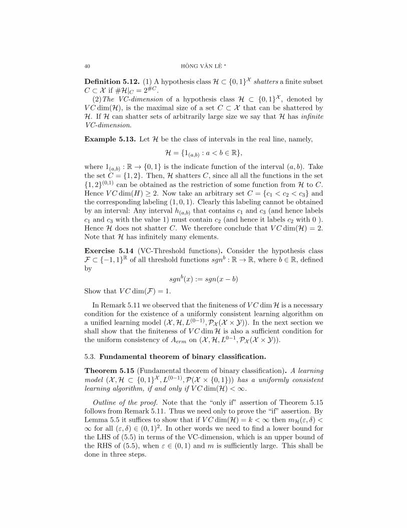
40 HONG VAN LE ∗

Definition 5.12. (1) A hypothesis class H ⊂ 0, 1X shatters a finite subsetC ⊂ X if #H|C = 2#C .

(2)The VC-dimension of a hypothesis class H ⊂ 0, 1X , denoted byV C dim(H), is the maximal size of a set C ⊂ X that can be shattered byH. If H can shatter sets of arbitrarily large size we say that H has infiniteVC-dimension.

Example 5.13. Let H be the class of intervals in the real line, namely,

H = 1(a,b) : a < b ∈ R,

where 1(a,b) : R→ 0, 1 is the indicate function of the interval (a, b). Takethe set C = 1, 2. Then, H shatters C, since all all the functions in the set

1, 2(0,1) can be obtained as the restriction of some function from H to C.Hence V C dim(H) ≥ 2. Now take an arbitrary set C = c1 < c2 < c3 andthe corresponding labeling (1, 0, 1). Clearly this labeling cannot be obtainedby an interval: Any interval h(a,b) that contains c1 and c3 (and hence labelsc1 and c3 with the value 1) must contain c2 (and hence it labels c2 with 0 ).Hence H does not shatter C. We therefore conclude that V C dim(H) = 2.Note that H has infinitely many elements.

Exercise 5.14 (VC-Threshold functions). Consider the hypothesis classF ⊂ −1, 1R of all threshold functions sgnb : R→ R, where b ∈ R, definedby

sgnb(x) := sgn(x− b)Show that V C dim(F) = 1.

In Remark 5.11 we observed that the finiteness of V C dimH is a necessarycondition for the existence of a uniformly consistent learning algorithm ona unified learning model (X ,H, L(0−1),PX (X × Y)). In the next section weshall show that the finiteness of V C dimH is also a sufficient condition forthe uniform consistency of Aerm on (X ,H, L0−1,PX (X × Y)).

5.3. Fundamental theorem of binary classification.

Theorem 5.15 (Fundamental theorem of binary classification). A learning

model (X ,H ⊂ 0, 1X , L(0−1),P(X × 0, 1)) has a uniformly consistentlearning algorithm, if and only if V C dim(H) <∞.

Outline of the proof. Note that the “only if” assertion of Theorem 5.15follows from Remark 5.11. Thus we need only to prove the “if” assertion. ByLemma 5.5 it suffices to show that if V C dim(H) = k <∞ then mH(ε, δ) <∞ for all (ε, δ) ∈ (0, 1)2. In other words we need to find a lower bound forthe LHS of (5.5) in terms of the VC-dimension, which is an upper bound ofthe RHS of (5.5), when ε ∈ (0, 1) and m is sufficiently large. This shall bedone in three steps.

MACHINE LEARNING 41

In step 1, setting Z = X×Y, and omitting superscript of the risk functionR, we use the Markov inequality to obtain

(5.13) µmS ∈ Zm : |Rµ(h)− RS(h)| < a ≤ Eµm |Rµ(h)−RS(h)|a

for any a > 0 and any h ∈ H.

In step 2 we define the growth function ΓH(m) : N → N and use it toupper bound the RHS of (5.13). Namely we shall prove the following

(5.14) Eµm(suph∈H|Rµ(h)− RS(h)| ≤

4 +√

log(ΓH(2m)

)δ√

2m) ≥ 1− δ

for every µ ∈ P(X × Y) and any δ ∈ (0, 1). The proof of (5.14) is delicateand can be found in [SSBD2014, p. 76-77].

Definition 5.16 (Growth function). Let F ⊂ YX be a class of functionswith finite target space Y. The growth function ΓF assigned to F is thendefined for all n ∈ N as

ΓF (n) := maxΣ⊂X|#Σ=n

#F|Σ.

We also set Γ(0) = 1.

Example 5.17. Consider the set F : signb| b ∈ R of all threshold func-tions. Given a set of distinct points x1, · · · , xn = Σ ⊂ R, there are n+ 1functions in F|Σ corresponding to n + 1 possible ways of placing b relativeto the xi s. Hence, in this case ΓF (n) ≥ n+ 1.

Exercise 5.18. Show that ΓF (n) = n + 1 for the set F of all thresholdfunctions.

In step 3 we use the following Vapnik-Chervonenski-Lemma, also knownas Sauer’s Lemma, whose proof can be found in [SSBD2014, p. 74-75].

Lemma 5.19. Let H ⊂ 0, 1X be a hypothesis class with V C dim(H) =d <∞. Then, for all n ∈ N we have

ΓH(n) ≤d∑i=0

(n

i

).

In particular, if n > d+ 1 then ΓH(n) ≤ (en/d)d.

It follows from Lemma 5.19 that for any (ε, δ) ∈ (0, 1)2 there exists msuch that

4 +√

log(ΓH(2m)

)δ√

2m< ε

and therefore by (5.14) for any (ε, δ) ∈ (0, 1)2 the value mH(ε, δ) is finite.This completes the proof of Theorem 5.15.

42 HONG VAN LE ∗

5.4. Conclusions. In this lecture we define the notion of the (uniform) con-sistency of a learning algorithm A on a unified learning model (Z,H, L, P )and characterize this notion via the sample complexity of A. We relatethe consistency of the ERM algorithm with the uniform convergence of thelaw of large numbers over the parameter space H and use it to prove theuniform consistency of ERM in the binary classification problem (X ,H ⊂0, 1X , L(0−1),P(X × 0, 1). We show that the finiteness of the VC-dimension of H is a necessary and sufficient condition for the existence ofa uniform consistent learning algorithm on a binary classification problem(X × 0, 1,H ⊂ 0, 1X , L(0−1),PX (X × 0, 1).

6. Generalization ability of a learning machine and modelselection

In the last lecture we measured the consistency of a learning algorithm Ain a unified learning model (Z,H, L, P ) via the sample complexity functionmA : (0, 1)2 → R+ ∪∞. The sample complexity mA(ε, δ) is the less numberof samples that A requires in order to make a prediction with ε accuracyand (1− δ) confidence. In 1984 Valiant suggested a PAC-model of learning,which corresponds to the notion of uniform (w.r.t. P ) consistency of A,which has moreover to be efficiently computable, i.e. the function mA(ε, δ)must be polynomial in ε−1 and δ−1. Furthermore Valiant also requiresthat A is efficiently computable, which can be expressed in terms of thecomputational complexity of A, see [SSBD2014, Chapter 8] for discussionon running time of A.

Thus, given a learning machine (Z,H, L, P,A), where A is a learningalgorithm, the generalization ability of (Z,H, L, P,A) is measured in termsof the family of sample complexities mA,µ(ε, δ)| µ ∈ P of the learningmachines (Z,H, L, µ ∈ P,A) and the computational complexity of A. Inthe previous lecture, Lemma 5.5, we gave upper bounds for the samplecomplexity mAerm(ε, δ) in terms of the sample complexity mH(ε/2, δ/2) ofthe learning model. Then we showed that in a binary classification problemthe sample complexity mH takes finite values if and only if the VC-dimensionof H is finite.

Today we shall discuss two further methods of upper bounds for the sam-ple complexities mH and mAerm of some important learning models. Thenwe discuss the problem of learning model selection.

6.1. Covering number and sample complexity. In the binary classifi-cation problem of supervised learning the VC-dimension is a combinatorialcharacterization of the hypothesis class H, which carries no topology, sincethe domain X and the target space Y are discrete. The expected zero-one loss function is therefore the preferred choice of a risk function. In[CS2001] Cucker-Smale estimated the sample complexity mH of a discrim-inative model for a regression problem with the MSE as the expected lossfunction.

MACHINE LEARNING 43

Before stating Cucker-Smale’s results we introduce necessary notations.• X is a topological space and ρ denotes a Borel measure on X × Rn.• Let Cn(X ) be the Banach space of continuous bounded Rn-valued func-

tions on X with the norm 16

||f ||C0 = supx∈X||f(x)||.

• For f ∈ Cn(X ) let fY ∈ Cn(X × Rn) denote the function

fY (x, y) := f(x)− y.Then MSEρ(f) = Eρ(||fY ||2), see (2.2) and (2.3).• For a function g ∈ Cn(X ×Rn) denote by Vρ(g) its variance, see (4.16),

Vρ(g) = Eρ(||g − Eρ(g)||2) = Eρ(||g||2)− ||Eρg||2.• For a compact hypothesis class H ⊂ Cn(X ) define the following quan-

tities

(6.1) MSEρ,H(f) := MSEρ(f)−minf∈H

MSEρ(f),

which is called the estimation error of f , or the sample error of f [CS2001],and

Vρ(H) := supf∈H

Vρ(fY ),

N (H, s) := minl ∈ N| there exists l disks in H with radius s covering H.• For S = (z1, · · · , zm) ∈ Zm := (X ×Y)m, where zi = (xi, yi), denote by

fS the minimizer of the function MSES : H → R such that

MSES(f) :=1

m

m∑i=1

||f(xi)− yi||2.

The existence of fS follows from the compactness of H and the continuityof the functional MSES on H.

Theorem 6.1. ([CS2001, Theorem C]) Let H be a compact subset of C(X ) :=C1(X ). Assume that for all f ∈ H we have |f(x)− y| ≤M ρ-almost every-where, where ρ is a probability measure on X × R. Then for all ε > 0

(6.2) ρmS ∈ Zm|MSEρ,H(fS) ≤ ε ≥ 1−N (H, ε

16M)2e− mε2

8(4Vρ(H)+ 13M

2ε) .

Theorem 6.1 implies that for any n <∞ the ERM algorithm is consistenton the unified learning model (X ,H ⊂ Cn(X ), L2,PB(X × Rn)), where L2

is the quadratic loss function, and PB(X × Rn) denotes the space of Borelmeasures on the topological space X × Rn, if H is compact. To increasethe accuracy of the estimate in (6.2) we need to decrease the radius of thecovering balls and therefore increase the number of the covering ball.

16In [CS2001, p.8] the authors used the L∞-norm, but they considered only the sub-space of continuous functions

44 HONG VAN LE ∗

The proof of Theorem 6.1 is based on Lemma 5.5. To prove that thesample complexity of Aerm is bounded it suffices to prove that the samplecomplexity mH of the learning model (X ,H ⊂ C(X ), L2,PB(X × Rn)) isbounded.

Outline of the proof of the Cucker-Smale theorem. The strategy of theproof of Theorem 6.1 is similar to that of Fundamental Theorem of binaryclassification (Theorem 5.15).

In the first step we prove the following Lemma, which gives a lower boundon the rate of the convergence in probability of empirical risk MSES(f) tothe expected risk MSEρ(f) for a given f ∈ H.

Lemma 6.2. ([CS2001, Theorem A, p.8]) Let M > 0 and f ∈ C0(X ) suchthat |f(x)− y| ≤M ρ-a.e.. Then for all ε > 0 we have

ρmS ∈ Zm : |MSEρ(f)−MSES(f)| ≤ ε ≥ 1− 2e(− mε2

2(σ2+13M

2ε))

where σ2 = Vρ(f2Y ).

Lemma 6.2 is a version of the inequality (5.8), for which we used theHoeffding inequality. The Hoeffding inequality does not involve the varianceand Cucker-Smale used the Bernstein inequality instead of the Hoeffdinginequality, see Appendix B.

In the second step, we reduce the problem of estimating upper bound forthe sample complexity mH to the problem of estimating upper bound forthe sample complexities mDj , where Dj | j ∈ [1, l] is a cover of H, andusing the covering number. Namely we have the following easy inequality

ρmS ∈ Zm| supf∈H|MSEρ(f)−MSES(f)| ≥ ε ≤

l∑j=1

ρmS ∈ Zm| supf∈Dj

|MSEρ(f)−MSES(f)| ≥ ε.(6.3)

In the last third step we proof the following

Lemma 6.3. ([CS2001, Proposition 3, p. 12]) Let f1, f2 ∈ C(X ). If |fj(x)−y| ≤ M on a set U ⊂ Z of full measure for j = 1, 2 then for any S ∈ Umwe have

|MSES(f1)−MSES(f2)|| ≤ 4M ||f1 − f2||C0 .

Lemma 6.3 implies that for all S ∈ Um

supf∈Dj

|MSEρ(f)−MSES(f)| ≥ 2ε =⇒ |MSEρ(fj)−MSES(fj)| ≥ ε.

Combining the last relation with (6.3), we derive the following desired upperestimate for the sample complexity mH.

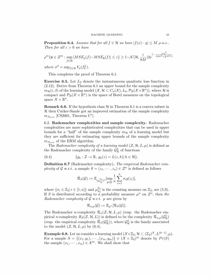
MACHINE LEARNING 45

Proposition 6.4. Assume that for all f ∈ H we have |f(x)−y| ≤M ρ-a.e..Then for all ε > 0 we have

ρmz ∈ Zm : supf∈H|MSEρ(f)−MSEz(f)| ≤ ε ≥ 1−N (H, ε

8M)2e

(− mε2

4(2σ2+13M

2ε)

where σ2 = supf∈H Vρ(f2Y ).

This completes the proof of Theorem 6.1.

Exercise 6.5. Let L2 denote the instantaneous quadratic loss function in(2.12). Derive from Theorem 6.1 an upper bound for the sample complexitymH(ε, δ) of the learning model (X ,H ⊂ Cn(X ), L2,PB(X ×Rn)), where H iscompact and PB(X ×Rn) is the space of Borel measures on the topologicalspace X × Rn.

Remark 6.6. If the hypothesis class H in Theorem 6.1 is a convex subset inH then Cucker-Smale got an improved estimation of the sample complexitymAerm [CS2001, Theorem C∗].

6.2. Rademacher complexities and sample complexity. Rademachercomplexities are more sophisticated complexities that can be used in upperbounds for a “half” of the sample complexity mH of a learning model butthey are sufficient for estimating upper bounds of the sample complexitymAerm of the ERM algorithm.

The Rademacher complexity of a learning model (Z,H, L, µ) is defined asthe Rademacher complexity of the family GLH of functions

(6.4) gh : Z → R, gh(z) = L(z, h)|h ∈ H.

Definition 6.7 (Rademacher complexity). The empirical Rademacher com-plexity of G w.r.t. a sample S = (z1, · · · , zn) ∈ Zn is defined as follows

RS(G) := E(µ

Z2Z2

)n[supg∈G

1

n

n∑i=1

σig(zi)],

where σi ∈ Z2| i ∈ [1, n] and µZ2Z2

is the counting measure on Z2, see (5.9).If S is distributed according to a probability measure µn on Zn, then theRademacher complexity of G w.r.t. µ are given by

Rn,µ(G) := Eµn [RS(G)].

The Rademacher n-complexity Rn(Z,H, L, µ) (resp. the Rademacher em-pirical n-complexity RS(Z,H, L)) is defined to be the complexity Rn,µ(GLH)

(resp. the empirical complexity RS(GLH)), where GLH is the family associatedto the model (Z,H, L, µ) by (6.4).

Example 6.8. Let us consider a learning model (X×Z2,H ⊂ (Z2)X , L(0−1), µ).For a sample S = (x1, y1), · · · , (xm, ym) ∈ (X × Z2)m denote by Pr(S)the sample (x1, · · · , xm) ∈ Xm. We shall show that

46 HONG VAN LE ∗

(6.5) RS(G(0−1)H ) =

1

2RPr(S)(H).

Using the identity

L(0−1)(x, y, h) = 1− δh(x)y =

1

2(1− yih(xi))

we compute

RS(G(0−1)H ) = E

(µZ2Z2

)m[suph∈H

1

m

m∑i=1

σiδh(xi)yi ]

= E(µ

Z2Z2

)m[suph∈H

1

m

m∑i=1

σi1− yih(xi)

2]

E(µ

Z2Z2

)mσi=0

=1

2E

(µZ2Z2

)m[suph∈H

1

m

m∑i=1

−σiyih(xi)]

=1

2E

(µZ2Z2

)m[suph∈H

1

m

m∑i=1

σih(xi)] =1

2RPr(S)(H)

which is required to prove.

We have the following relation between the empirical Rademacher com-plexity and the Rademacher complexity, using the McDiarmid concentrationinequality, see (B.4) and [MRT2012, (3.14), p.36]

(6.6) µnS ∈ Zn|Rn,µ(GLH) ≤ RS(GLH) +

√ln(2/δ)

2m ≥ 1− δ/2.

Theorem 6.9. (see e.g. [SSBD2014, Theorems 26.3, 26.5, p. 377- 378])Assume that (Z,H, L, µ) is a learning model with |L(z, h)| < c for all z ∈ Zand all h ∈ H. Then for any δ > 0 and any h ∈ H we have

(6.7) µnS ∈ Zn|RLµ(h)−RLS(h) ≤ Rn,µ(GLH) + c

√2 ln(2/δ)

n ≥ 1− δ,

(6.8) µnS ∈ Zn|RLµ(h)−RLS(h) ≤ RS(GLH) + 4c

√2 ln(4/δ)

n ≥ 1− δ.

(6.9)

µnS ∈ Zn|RLµ(Aerm(S))−RLµ(h) ≤ 2RrS(GLH) + 5c

√2 ln(8/δ)

δ ≥ 1− δ.

(6.10) Eµn(RLµ(Aerm(S))−RLµ,H) ≤ 2Rrn,µ(GLH).

It follows from (6.10), using the Markov inequality, the following boundfor the sample complexity mAerm in terms of Rademacher complexity

(6.11) µnS ∈ Zn|RLµ(Aerm)−RLµ,H ≤2RLn,µ(GLH)

δ ≥ 1− δ.

MACHINE LEARNING 47

Remark 6.10. (1) The first two assertions of Theorem 6.9 give an upperbound of a “half” of the sample complexity mH of a unified learning model(Z,H, L, µ) by the (empirical) Rademacher complexity Rn(G) of the associ-ated family G. The last assertion of Theorem 6.9 is derived from the secondassertion and the Hoeffding inequality.

(2) For the binary classification problem (X×0, 1,H ⊂ 0, 1X , L(0−1),P(X×0, 1) there exists a close relationship between the Rademacher complexityand the growth function ΓH(m), see [MRT2012, Lemma 3.1, Theorem 3.2,p. 37] for detailed discussion.

6.3. Model selection. The choice of a right prior information in machinelearning is often interpreted as the choice of a right class H in a learningmodel (Z,H, L, P ) which is also called a model selection. A right choice ofH should make balance between the approximation error and the estimationerror of H defined in the error decomposition of H.

6.3.1. Error decomposition. We assume that the maximum domain of theexpected loss function RLµ is a subspace HL,µ ⊃ H, given L and a probabilitymeasure µ ∈ P .

We define the Bayes risk of the learning problem RLµ on the maximaldomain HL,µ as follows

RLb,µ := infh∈HL,µ

RLµ(h)

Recall that RLµ,H := infh∈HRLµ(h) quantify the optimal performance of a

learner in H. Then we decompose the difference between the expected riskof a predictor h ∈ H and the Bayes risk as follows:

(6.12) RLµ(h)−RLb,µ = (RLµ(h)−RLµ,H) + (RLµ,H −RLb,µ).

The first term in the RHS of (6.12) is called the estimation error of h, cf.(6.1), and the second term is called the approximation error. If h = Aerm(S)

is a minimizer of the empirical risk RLS , then the estimation error of Aerm(S)is also called the sample error [CS2001, p. 9].

The approximation error quantifies how well the hypothesis class H issuited for the problem under consideration. The estimation error measureshow well the hypothesis h performs relative to best hypotheses in H. Typi-cally, the approximation error will decrease when enlargingH but the sampleerror will increase as demonstrated in No-Free-Lunch Theorem 5.9, becauseP should be enlarged as H will be enlarged.

Example 6.11. (cf. [Vapnik2000, p. 19], [CS2001, p. 4, 5]) Let uscompute the error decomposition of a discriminative model (X × R,H ⊂RX , L2,PB(X × R) for regression problem. Let π : X × R → X denotethe natural projection. Then the measure ρ, the push-forward measureπ∗(ρ) ∈ P(X ) and the conditional probability measure ρ(y|x) on each fiber

48 HONG VAN LE ∗

π−1(x) = R are related as follows∫X×R

ϕ(x, y)dρ =

∫X

(

∫Rϕ(x, y)dρ(y|x))dπ∗(ρ)

for ϕ ∈ L1(ρ), similar to the Fubini theorem, see Subsection A.4.Let us compute the Bayes risk RLb,µ for L = L2. The maximal subspace

HL,µ where the expected loss RLµ is well defined is the space L2(X , π∗(ρ)).We claim that the regression function of ρ, see Exercise 2.7,

rρ(x) := Eρ(i2(Y )|X = x) =

∫Rydρ(y|x)

minimizes the MSEπ∗(ρ) defined on the space L2(X , π∗(ρ)). Indeed, for any

f ∈ L2(X , π∗(ρ)) we have

(6.13) MSEπ∗(ρ)(f) =

∫X

(f(x)− rρ(x))2dπ∗(ρ) +MSEπ∗(ρ)(rρ).

The equation (6.13) implies that the Bayes risk RLb,π∗(ρ) is MSEπ∗(ρ)(rρ). It

follows that the approximation error of a hypothesis class H is equal

MSEπ∗(ρ)(fmin) =

∫X

(fmin − rρ(x))2dπ∗(ρ) +MSEπ∗(ρ)(rρ),

where fmin is a minimizer of MSE in H. Since MSEπ∗(ρ)(rρ) is a constant,if H is compact, fmin exists and satisfies the condition

(6.14) fmin = argming∈H

d(g, rρ),

where d is the L2-distance on L2(X , π∗(ρ)).

6.3.2. Validation and cross-validation. An important empirical approach inmodel selection is validation and its refinement - (k-fold) cross-validation.Validation is used for model selection as follows. We first train differentalgorithms (or the same algorithm with different parameters) on the giventraining set S. Let H := h1, · · · , hr be the set of all output predictors ofthe different algorithms. Now, to choose a single predictor fromH we samplea fresh validation set S′ ∈ Zm and choose the predictor hi that minimizesthe error over the validation set.

The basic idea of cross-validation is to partition the training set S =(z1, · · · , zn) ∈ Zn into two sets S = S1 ∪ S2 where S1 ∈ Zk and S2 ∈ Zn−k.The set S1 is used for training each of the candidate models, and the secondset S2 is used for deciding which of them yields the best results.

The n-cross validation is a refinement of cross-validation by partition ofthe training set into n-subsets and use one of them for testing the and repeatthe procedure (n− 1)-time for other testing subsets.

MACHINE LEARNING 49

6.4. Conclusion. In this lecture we use several complexities of a learningmodel (Z,H, L, P ) for obtaining upper bounds of the sample complexity ofthe ERM algorithm Aerm. Among them Rademacher complexities are themost sophisticated ones that measure the capacity of a hypothesis class on aspecific sample, which can be used to bound the difference between empiricaland expected error, and thus the excess generalization error of empirical riskminimization. To find an ideal hypothesis class H for a learning problemwe have to take into account the error decomposition of a learning modeland the resulting bias-variance trade-off and use empirical cross validationmethods.

7. Support vector machines

In this lecture we shall consider a class of simple supervised learningmachines for binary classification problems and apply results in the previ-ous lectures on consistent learning algorithms. Our learning machines are(V ×Z2,Hlin, L,P(V ×Z2), A) where V is a real Hilbert space, Hlin consistsof linear classifiers, defined below, L is a (0 − 1) loss function (resp. regu-larized (0 − 1) loss function) and A is a hard SVM algorithm (resp. a softSVM algorithm), which we shall learn in today lecture. The original SVMalgorithm is the hard SVM algorithm, which was invented by Vapnik andChervonenkis in 1963. The current standard incarnation (soft margin) wasproposed by Cortes and Vapnik in 1993 and published in 1995.

7.1. Linear classifier and hard SVM. For (w, b) ∈ V × R we set

(7.1) f(w,b)(x) := 〈w, x〉+ b.

Definition 7.1. A linear classifier is a function sign f(w,b) : V → Z2,x 7→ signf(w,b)(x) ∈ −1, 1 = Z2.

We identify each linear classifier with the half spaceH+(w,b) := signf−1

(w,b)(1) =

f−1(w,b)(R≥0) ⊂ V and set H(w,b) := f−1

(w,b)(0) ⊂ V . Note that each hyperplane

H(w,b) ⊂ V defines H+(w,b) up to a reflection of V around H(w,b) and therefore

defines the affine function f(w,b) up to a multiplicative factor λ ∈ R∗. Denoteby HA(V ) the set of of all hyperplanes in the affine space V . Then Hlin isa double cover of HA(V ) with the natural projection π : Hlin → HA(V )defined above.

Definition 7.2. A training sample S = (x1, y1), · · · , (xm, ym) ∈ (V ×±1)m is called separable, if there is a half space H+

(w,b) ⊂ V that cor-

rectly classifies S, i.e. for all i ∈ [1,m] we have xi ∈ H+(w,b) iff yi = 1. In

other words, the linear classifier signf(w,b) is a minimizer of the empirical

risk function R0−1S : Hlin → R associated to the zero one loss function L(0−1).

50 HONG VAN LE ∗

Remark 7.3. (1) A half space H+(w,b) correctly classifies S if and only if the

empirical risk function R(0−1)S (f(w,b)) = 0 and sign f(w,b) is a linear classifier

associated to H+(w,b).

(2) Write S = S+ ∪ S− where

S± := (x, y) ∈ S| y = ±1.

Let Pr : (V × ±1)m → V m denote the canonical projection. Then Sis separable if and only if there exists a hyper-plane H(w,b) that separates[Pr(S+)] and [Pr(S−)], where recall that [(x1, · · · , xm)] = ∪mi=1xi ⊂ V . Inthis case we say that H(w,b) correctly separates S.

(3) If a training sample S is separable then the separating hyperplaneis not unique, and hence there are many minimizers of the empirical risk

function R(0−1)S . Thus, given S, we need to find a strategy for selecting one

of these ERM’s, or equivalently for selecting a separating hyperplane H(w,b),

since the associated half-space H+(w,b) is defined by H(w,b) and any training

value (xi, yi). The standard approach in the SVM framework is to chooseH(w,b) that maximizes the distance to the closest points xi ∈ [Pr(S)]. Thisapproach is called the hard SVM rule. To formulate the hard SVM rule weneed a formula for the distance of a point to a hyperplane H(w,b).

Lemma 7.4 (Distance to a hyperplane). Let V be a real Hilbert space andH(w,b) := z ∈ V | 〈z, w〉 + b = 0. The distance of a point x ∈ V to H(w,b)

is given by

(7.2) ρ(x,H(w,b)) := infz∈H(w,b)

||x− z|| = |〈x,w〉+ b|||w||

.

Proof. Since H(w,b) = H(w,b)/λ for all λ > 0, it suffices to prove (7.2) for thecase ||w|| = 1 and hence we can assume that w = e1. Now formula (7.2)follows immediately, noting that H(e1,b) = H(e1,0) − be1.

Let H(w,b) separate S = (x1, y1), · · · , (xm, ym) correctly. Then we have

yi = sign(〈xi, w〉+ b),

=⇒ |〈xi, w〉+ b| = yi(〈x,w〉+ b).

Hence, by Lemma 7.4, the distance between H(w,b) and S is

(7.3) ρ(S,H(w,b)) := miniρ(xi, H(w,b)) =

mini yi(〈xi, w〉+ b)

||w||.

The distance ρ(S,H(w,b)) is also called the margin of a hyperplane H(w,b)

w.r.t. S. The hyperplanes, that are parallel to the separating hyperplaneand passing through the closest points on the negative or positive sides arecalled marginal.

MACHINE LEARNING 51

Denote byHS the subset of π(Hlin) = HA(V ) that consists of hyperplanesseparating S. Set

(7.4) A∗hs(S) := arg maxH(w,b)′∈HS

ρ(S,H(w,b)′).

Now we define a map Ahs : ∪m(V × Z2)m → Hlin by letting Ahs(S) ∈π−1A∗hs(S) to be the linear classifier that correctly classifies S.

Definition 7.5. A hard SVM is a learning machine (V × Z2,Hlin, L(0−1),P(V × Z2), Ahs).

The domain of the optimization problem in (7.4) is HS , which is not easyto determine. So we replace this problem by another optimization problemover a larger convex domain as follows.

Lemma 7.6. For S = (x1, y1), · · · , (xm, ym) we have

(7.5) Ahs(S) = H+(w,b) where (w, b) = arg max

(w,b):||w||≤1miniyi(〈w, xi〉+ b).

Proof. If H(w,b) separates S then ρ(S,H(w,b)) = mini yi(〈w, xi〉 + b). Sincethe constraint ||w|| ≤ 1 does not effect on H(w,b), which is invariant under apositive rescaling, (7.3) implies that

(7.6) max(w,b):||w||≤1

miniyi(〈w, xi〉+ b) ≥ max

H(w,b)′∈HSρ(S,H(w,b)′).

Next we observe that if H(w,b) 6∈ HS then

miniyi(〈w, xi〉+ b) < 0.

Combining this with (7.6) we obtain

max(w,b):||w||≤1

miniyi(〈w, xi〉+ b) = max

(w,b):H(w,b)∈HSminiyi(〈w, xi〉+ b).

This completes the proof of Lemma 7.6.

A solution Ahs(S) of the equation (7.5) maximizes the enumerator of thefar RHS of (7.3) under the constraint ||w|| ≤ 1. In the Proposition below weshall show that Ahs(S) can be found as a solution to the dual optimizationproblem of minimizing the dominator of the RHS (7.3) under the constraintthat the enumerator of the far RHS of (7.3) has to be fixed.

Proposition 7.7. A solution to the following optimization problem, whichis called Hard-SVM,

(7.7) (w0, b0) = argminw,b||w||2 : yi(〈w, xi〉+ b) ≥ 1 for all i

produces a solution (w, b) := (w0/||w0||, b0/||w0||) of the optimization prob-lem (7.5).

52 HONG VAN LE ∗

Proof. Let (w0, b0) be a solution of (7.7). We shall show that (w0/||w0||, b0/||w0||)is a solution of (7.5). It suffices to show that the margin of the hyperplaneH(w0,b0) is greater than or equal to the margin of the hyperplane associatedto a (and hence any) solution of (7.5).

Let (w∗, b∗) be a solution of Equation (7.5). Set

γ∗ := miniyi(〈w∗, xi〉+ b∗)

which is the margin of the hyperplane H(w∗,b∗) by (7.3). Therefore for all iwe have

yi(〈w∗, xi〉+ b∗) ≥ γ∗

or equivalently

y∗i (〈w∗

γ∗, xi〉+

b∗

γ∗) ≥ 1.

Hence the pair (w∗

γ∗ ,b∗

γ∗ ) satisfies the condition of the quadratic optimization

problem in (7.7). It follows that

||w0|| ≤ ||w∗

γ∗|| = 1

γ∗.

Hence for all i we have

yi(w0

||w0||+

b0||w0||

) =yi(〈w0, xi〉+ b0)

||w0||≥ 1

||w0||≥ γ∗.

This implies that the margin of H(w0,b0) satisfies the required condition. Thiscompletes the proof of Proposition 7.7.

Remark 7.8. (1) The optimization problem of (7.4) is a specific instanceof quadratic programming (QP), a family of problems extensively studied inoptimization. A variety of commercial and open-source solvers are availablefor solving convex QP problems. It is well-known that there is a uniquesolution of (7.4).

(2) In practice, when we have a sample set S of large size, then S is notseparable, thus the application of hard SVM is limited.

Exercise 7.9. (1) Show that the vector w0 of the solution (w0, b0) in (7.7)of the SVM problem is a linear combination of the training set vectorsx1, · · · , xm.

(2) Show that xi lies on the marginal hyperplanes 〈w0, x〉+ b0 = ±1.

A vector xi appears in the linear expansion of the weight vector w0 inExercise 7.9 is called a support vector.

7.2. Soft SVM. Now we consider the case when the sample set S is not sep-arable. There are at least two possibilities to overcome this difficulty. Thefirst one is to find a nonlinear embedding of patterns into a high-dimensionalspace. To realize this approach we use a kernel trick that embeds the pat-terns in an infinite dimensional Hilbert space space, which we shall learn inthe next lecture. The second way is to seek a predictor sign f(w,b) such that

MACHINE LEARNING 53

H(w,b) = f−1(w,b)(0) still has maximal margin in some sense. More precisely,

we shall relax the hard SVM rule (7.7) by replacing the constraint

(7.8) yi(〈w, xi〉+ b) ≥ 1

by the relaxed constraint

(7.9) yi(〈w, xi〉) + b ≥ 1− ξiwhere ξi ≥ 0 are called the slack variables. The slack variables are commonlyused in optimization to define relaxed versions of some constraints. In ourcase a slack variable ξi measures the distance by which vector xi violatesthe original inequality in the LHS of (7.8).

The relaxed hard SVM rule is called the soft SVM rule.

Definition 7.10. The soft SVM algorithm Ass : (Rd × Z2)m → Hlin withslack variables ξ ∈ Rm≥0 is defined as follows

Ass(S) = sign f(w0,b0)(S)

where (w0, b0) satisfies the following equation with ξ = (ξ1, · · · , ξm)

(w0, b0, ξ) = argminw,b,ξ

(λ||w||2 +1

m||ξ||l1)(7.10)

s. t. ∀i, yi(〈w, xi〉+ b) ≥ 1− ξi and ξi ≥ 0.(7.11)

In what follows we shall show that the soft SVM algorithm Ass is a so-lution of a regularized loss minimization rule, which is a refinement of theERM rule.

Digression Regularized Loss Minimization (RLM) is a learning algorithmon a learning model (Z,H, L, P ) in which we jointly minimize the empirical

risk RLS and a regularization function. Formally, a regularization functionis a mapping R : H → R and the regularized loss minimization rule is amap Arlm : Zn → H such that Arlm(S) is a minimizer of the empirical

regularized loss function RLS := RLS +R : H → R.As the ERM algorithm works under certain condition, the RLM algorithm

also works under certain conditions, see e.g. [SSBD2014, Chapter 13] fordetailed discussion.

The loss function for the soft SVM learning machine is the hinge lossfunction Lhinge : Hlin × (V × ±1)→ R defined as follows

(7.12) Lhinge(h(w,b), (x, y)) := max0, 1− y(〈w, x〉+ b).

Hence the empirical hinge risk function is defined as follows for S =(x1, y1) · · · , (xm, ym)

RhingeS (h(w,b)) =1

m

m∑i=1

max0, 1− yi(〈w, xi〉+ b.

54 HONG VAN LE ∗

Lemma 7.11. The Equation (7.10) with constraint (7.11) for Ass is equiv-alent to the following regularized risk minimization problem, which does notdepend on the slack variables ξ:

(7.13) Ass(S) = arg minf(w,b)

(λ||w||2 +RhingeS (f(w,b))

)∈ Hlin.

Proof. Let us fix (w0, b0) and minimize the RHS of (7.10) under the con-straint (7.11). It is straightforward to see that ξi = Lhinge

((w, b), (xi, yi)

).

Using this and comparing (7.10) with (7.13), we complete the proof ofLemma 7.11.

From Lemma 7.11 we obtain immediately the following

Corollary 7.12 (Definition). A soft SVM is a learning machine (V ×Z2,Hlin,Lhinge,P(V × Z2), Arlm).

Remark 7.13. The hinge loss function Lhinge enjoys several good propertiesthat justify the preference of Lhinger as a loss function over the zero-one lossfunction L(0−1), see [SSBD2014, Subsection 12.3, p. 167] for discussion.

7.3. Sample complexities of SVM.

Exercise 7.14. Prove that V C dimHlin = dimV + 1.

From the Fundamental Theorem of binary classification 5.15 and Exercise(7.14) we obtain immediately the following

Proposition 7.15. The binary classification problem (V×Z2,Hlin, L(0−1),P(V×Z2)) ha a uniformly consistent learning algorithm if and only if V is finitedimensional.

In what follow we shall show the uniform consistent of hard SVM andsoft SVM replacing the statistical model P(Rd × Z2) by a smaller class.

Definition 7.16. ([SSBD2014, Definition 15.3]) Let µ be a distribution onV × Z2. We say that µ is separable with a (γ, ρ)-margin if there exists(w∗, b∗) ∈ V × R such that ‖w‖ = 1 and such that

µ(x, y) ∈ V × Z2| y(〈w∗, x〉+ b∗) ≥ γ and ||x|| ≤ ρ = 1.

Similarly, we say that µ is separable with a (γ, ρ)-margin using a homoge-neous half-space if the preceding holds with a half-space defined by a vector(w∗, 0).

Definition 7.16 means that the set of labeled pairs (x, y) ∈ V × Z2 thatsatisfy the condition

y(〈w∗, x〉+ b∗) ≥ γ and ||x|| ≤ ρ

has a full µ-measure, where µ is a separable measure on with (γ, ρ)-margin.

MACHINE LEARNING 55

Remark 7.17. (1) We regard an affine function f(w,b) : V → R as a linearfunction fw′ : V ′ → R where V ′ = 〈e1〉⊗R ⊕ V , i.e., we incorporate thebias term b of f(w,b) in (7.1) into the term w as an extra coordinate. Moreprecisely we set

w′ := be1 + v and x′ := e1 + x.

Thenf(w,b)(x) = fw′(x

′).

Note that the natural projection of the zero set f−1w′ (0) ⊂ V ′ to V is the zero

set H(w,b) of f(w,b).(2) By Remark 7.17 (1), we can always assume that a separable measure

with (γ, ρ)-margin is a one that uses a homogeneous half-space by enlargingthe instance space V .

Denote by P(γ,ρ)(V ×Z2) the subset of P(V ×Z2) that consists of separablemeasures with a (γ, ρ)-margin using a homogeneous half-space. Using theRademacher complexity, see [SSBD2014, Theorem 26.13, p. 384], we havethe following estimate of the sample complexity of the learning machine(V × Z2,Hlin, L(0−1), P(γ,ρ)(V × Z2), Ahs).

Theorem 7.18. ([SSBD2014, Theorem 15.4, p. 206]) Let µ ∈ P(γ,ρ)(V ×Z2). Then we have

µmS ∈ (V × Z2)m|R(0−1)µ (Ahs(S)) ≤

√4(ρ/γ)2

m+

√2 log(2/δ)

m ≥ 1− δ.

Denote by Pρ(V ×Z2) the set of of probability measures on V ×Z2 whosesupport lies in B(0, ρ)×Z2 where B(0, ρ) is the ball of radius ρ centered atthe origin of V . Now we shall examine the sample complexity of the softSVM learning machine (V ×Z2,Hlin, Lhinge, Pρ(V ×Z2), Ass). The followingtheorem is a a consequence of Lemma 7.11 and a general result on the samplecomplexity of RLM under certain conditions, see [SSBD2014, Corollary 13.8,p. 179].

Theorem 7.19. ([SSBD2014, Corollary 15.7, p. 208]) Let µ ∈ Pρ(V ×Z2).Then for every r > 0 we have

Eµm(R(0−1)µ

(Ass(S)

))≤ Eµm

(Rhingeµ

(Ass(S)

))≤ min

w∈B(0,r)Rhingeµ (hw) +

√8ρ2r2

m.(7.14)

Exercise 7.20. Using the Markov inequality, derive from Theorem 7.19 anupper bound for the sample complexity of the soft SVM.

Theorem 7.19 and Exercise 7.20 imply that we can control the samplecomplexity of a soft SVM algorithm as a function of the norm of the under-lying Hilbert space V , independently of the dimension of V . This becomeshighly significant when we learn classifiers h : V → Z2 via embeddings intohigh dimensional feature spaces.

56 HONG VAN LE ∗

7.4. Conclusion. In this section we consider two classes of learning ma-chines for binary classification. The first class consists of learning models(V ×Z2,Hlin, L(0−1),P(V ×Z2)) with finite VC-dimension iff and only if V isfinite dimensional. If µ ∈ P(V ×Z2) is separable with (γ, ρ)-margin then wecan upper bound the sample complexity of the hard SVM algorithm Ahs for(V ×Z2,Hlin, L(0−1), µ) using the ration ρ/γ and Rademacher’s complexity.The second class consists of learning machines (V ×Z2,Hlin, Lhinge,Pρ(V ×Z2), Ass). The soft SVM algorithm Ass is a solution of a regularized ERMand therefore we can apply here general results on sample complexity ofregularized ERM algorithms.

8. Kernel based SVMs

In the previous lecture we considered the hypothesis class Hlin of linearclassifiers. A linear classifier sign f(w,b) correctly classifies a training sam-ple S ⊂ (V × ±1)m iff the zero set H(w,b) of f(w,b) separates the subsets[Pr(S−)] and [Pr(S+)]. By Radon’s theorem any set of distinct (d+2) pointsin Rd can be partitioned into two subsets that cannot be separated by a hy-perplane in Rd. Thus it is reasonable to enlarge the hypothesis class Hlinby adding polynomial classifiers. Now we observe that any (polynomial)function f on Rd can be regarded as the restriction of a new coordinatefunction y on Rd × R(y) to the image of the graph Γf (Rd) ⊂ Rd × R off , i.e., f(x) = y(Γf (x)). However, the computational complexity of SVM

with learning by polynomial embedding (x, f(x))| x ∈ Rd may be compu-tationally expensive. The common solution to this concern is kernel basedlearning. The term “kernels” is used in this context to describe inner prod-ucts in the feature space. Namely we are interested in classifiers of theform

sign h : X → Z2, h(x) := 〈h, ψ(x)〉,

where h is an element in a Hilbert space W , ψ : X →W is a “feature map”and the kernel function Kϕ : X × X → R is defined

(8.1) Kψ(x, y) := 〈ψ(x), ψ(y)〉.

We shall see that to solve the hard SVM optimization problem (7.7) forh ∈ W it suffices to learn K. This kernel trick requires less computationalcomplexity than the one for learning ψ : X →W .

8.1. Kernel trick. It is known that a solution of a hard SVM can be ex-pressed as a linear combination of support vectors (Exercise 7.9). If thenumber of support vectors is less than the dimension of the instance space,then this property simplifies the search for a solution of the hard SVM.Below we shall show that this property is a consequence of the Represen-ter Theorem concerning solutions of a special optimization problem. The

MACHINE LEARNING 57

optimization problem we are interested in is of the following form:

(8.2) w0 = arg minw∈W

(f(〈w,ψ(x1)〉, · · · , 〈w,ψ(xm)〉

)+R(‖w‖)

)where xi ∈ X , w and ψ(xi) are elements of a Hilbert space W , f : Rm → Ris an arbitrary function and R : R+ → R is a monotonically non-decreasingfunction. The map ψ : X → W is often called the feature map, and W iscalled the feature space.

The following examples show that the optimization problem for the hard(resp. soft) SVM algorithm is an instance of the optimization problem (8.2).

Example 8.1. Let S = (x1, y1), · · · , (xm, ym) ∈ (V × Z2)m.(1) Plugging in Equation (8.2)

R(a) := a2,

f(a1, · · · , am) :=

0 if yi(ai) ≥ 1 for all i∞ otherwise

we obtain Equation (7.7) of hard SVM for homogeneous vectors (w,0), re-placing ai by 〈w, xi〉. The general case of non-homogeneous solutions (w, b)is reduced to the homogeneous case by Remark 7.17.

(2) Plugging in Equation (8.2)

R(a) := λa2,

f(a1, · · · , am) :=1

m

m∑i=1

max0, 1− yiai

we obtain Equation (7.13) of soft SVM for a homogeneous solution Ass(S),identifying Ass(S) with its parameter (w, 0), S with (x1, y1) · · · (xm, ym)and replacing ai with 〈w, xi〉.

Theorem 8.2 (Representer Theorem). Let ψ : X →W be a feature mappingfrom an instance space X to a Hilbert space W and w0 a solution of (8.2).Then the projection of w0 to the subspace 〈ψ(x1), · · · , ψ(xm)〉⊗R in W isalso a solution of (8.2).

Proof. Assume that w0 is a solution of (8.2). Then we can write

w0 =m∑i=1

αiψ(xi) + u

where 〈u, ψ(xi)〉 = 0 for all i. Set w0 := w0 − u. Then

(8.3) ‖w0‖ ≤ ‖w0‖and since 〈w0, ψ(xi)〉 = 〈w0, ψ(xi)〉 we have

(8.4) f(〈w0, ψ(x1)〉, · · · , 〈w0, ψ(xm)〉

)= f

(〈w0, ψ(x1)〉, · · · , 〈w0, ψ(xm)〉

).

From (8.3), (8.4) and taking into account the monotonicity of R, we concludethat w0 is also a solution of (8.2). This completes the proof of Theorem8.2.

58 HONG VAN LE ∗

The Representer Theorem implies that it suffices to find a solution ofEquation (8.2) in a finite dimensional subspace W1 ⊂ W . In what followswe shall describe a method to solve the minimization problem of (8.2) onW1, which is called the kernel trick.

Let• K : X × X → R, K(x, x′) := 〈ψ(x), ψ(x′)〉 be a kernel function,• G = (Gij) := K(xi, xj) - a Gram matrix,• w0 =

∑mi=1 αjψ(xj) ∈W1 - a solution of Equation (8.2).

Then α = (α1, · · · , αm) is a solution of the following minimization prob-lem

(8.5) arg minα∈Rm

f( m∑j=1

αjGj1, · · · ,m∑j=1

αjGjm)

+R(√√√√ m∑

i,j=1

αiαjGji

).

Recall that the solution w0 =∑m

i=1 αjψ(xj) of the hard (resp. soft) SVMoptimization problem, where (α1, · · · , αm) is a solution of (8.5), produces a“nonlinear” classifier w0 : X → Z2 associated to as follows

w0(x) := signw0(x)

where

(8.6) w0(x) := 〈w0, ψ(x)〉 =m∑i=1

αj〈ψ(xj), ψ(x)〉 =m∑j=1

αjK(xj , x).

To compute (8.6) we need to know only the kernel function K and not themapping ψ, nor the inner product 〈, 〉 on the Hilbert space W .

This motivates the following question.

Problem 8.3. Find a sufficient and necessary condition for a kernel func-tion, also called a kernel, K : X × X → R such that K can be written asK(x, x′) = 〈ψ(x), ψ(x′)〉 for a feature mapping ψ : X → W , where W is areal Hilbert space.

Definition 8.4. If K satisfies the condition in Problem 8.3 we shall saythat K is generated by a (feature) mapping ψ. The target Hilbert space isalso called a feature space.

8.2. PSD kernels and reproducing kernel Hilbert spaces.

8.2.1. Positive semi-definite kernel.

Definition 8.5. Let X be an arbitrary set. A map K : X × X → R iscalled positive semi-definite kernel (PSD kernel) iff for all x1, · · · , xm theGram matrix Gij = K(xi, xj) is positive semi-definite.

Theorem 8.6. A kernel K : X × X → R is induced by a feature map to aHilbert space if and only if it is positive semi-definite.

MACHINE LEARNING 59

Proof. 1) First let us prove the “only if” assertion of Theorem 8.6. Assumethat K(x, x′) = 〈ψ(x), ψ(x′)〉 for a mapping ψ : X → W , where W is aHilbert space. Given m points x1, · · · , xm ∈ X we consider the subspaceWm ⊂W generated by ψ(x1), · · · , ψ(xm). Using the positive definite of theinner product on Wm, we conclude that the Gram matrix Gij = K(xi, xj)is positive semi-definite. This proves the “only if” part of Theorem 8.6

2) Now let us prove the “if” part. Assume that K : X ×X → R is positivesemi-definite. For each x ∈ X let Kx ∈ RX be the function defined by

Kx(y) := K(x, y).

Denote by

W := f ∈ RX | f =

N(f)∑i=1

aiKxi , ai ∈ R and N(f) <∞.

Then W is equipped with the following inner-product

〈∑i

αiKxi ,∑j

βjKyj 〉 :=∑i,j

αiβjK(xi, yj).

The PSD property of K implies that the inner product is positive semi-definite, i.e.

〈∑i

αiKxi ,∑j

αiKxi〉 ≥ 0.

Since the inner product is positive semi-definite, the Cauchy-Schwarz in-equality implies for f ∈W and x ∈ X

(8.7) 〈f,Kx〉2 ≤ 〈f, f〉〈Kx,Kx〉.

Since for all x, y we have Ky(x) = K(y, x) = 〈Ky,Kx〉 , it follows that forall f ∈W we have

(8.8) f(x) = 〈f,Kx〉.

Using (8.8), we obtain from (8.7) for all x ∈ X

|f(x)|2 ≤ 〈f, f〉K(x, x).

This proves that the inner product on W is positive definite and hence Wis a pre-Hilbert space. Let H be the completion of W . The map x 7→ Kx

is the desired mapping from X to H. This completes the proof of Theorem8.6.

Example 8.7. (1) (Polynomial kernels). Assume that P is a polynomial inone variable with non-negative coefficients. Then the polynomial kernel ofthe form K : Rd×Rd → R, (x, y) 7→ P (〈x, y)〉 is a PSD kernel. This followsfrom the observations that if Ki : X ×X → R, i = 1, 2, are PDS kernel then(K1+K2)(x, y) := K1(x, y)+K2(x, y) is a PSD kernel, and (K1 ·K2)(x, y) :=K1(x, y) ·K2(x, y) is a PSD kernel. In particular, K(x, y) := (1 + 〈x, y〉)2 isa PSD kernel.

60 HONG VAN LE ∗

(2) (Exponential kernel). For any γ > 0 the kernel K(x, y) := exp(γ ·

〈x, y〉)

is a PSD kernel, since it is the limit of a polynomials in 〈x, y〉 withnon-negative coefficients.

Exercise 8.8. (1) Show that the Gaussian kernel K(x, y) := exp(−γ

2 ||x −y||2) is a PSD kernel.

(2) Let X = B(0, 1) - the open ball of radius 1 centered at the origin0 ∈ Rd. Show that K(x, y) := (1−〈x, y〉)−p is a PSD kernel for any p ∈ N+.

8.2.2. Reproducing kernel Hilbert space. Given a PSD kernel K : X×X → Rthere exist many feature maps ϕ : X → W such that K is generated by afeature map ϕ : X → W . Indeed, if K(x, x) = 〈ϕ(x), ϕ(x)〉 then K(x, x) =〈e ϕ(x), e ϕ(x)〉 for any isometric embedding e : W → W ′. However,there is a canonical choice for the feature space, a so-called reproducingkernel Hilbert space.

Definition 8.9 (Reproducing kernel Hilbert space). Let X be an instanceset and H ⊂ RX a real Hilbert space of functions on X with the uniquevector space structure such that for x ∈ X the evaluation map

evx : H → R , evx(f) := f(x)

is a linear map. 17 Then H is called a reproducing kernel Hilbert space(RKHS) on X if for all x ∈ X the linear map evx is bounded i.e.,

supf∈B(0,1)⊂H

evx(f) <∞.

Remark 8.10. Let H be a RKHS on X and x ∈ X . Since evx is bounded,by the Riesz representation theorem there is a function kx ∈ H so thatf(x) = 〈f, kx〉 for all f ∈ H. Then the kernel

K(x, y) := 〈kx, ky〉is a PSD kernel. K is called the reproducing kernel of H.

Thus every RKHS H on X produces a PSD kernel K : X × X → R.Conversely, Theorem 8.11 below asserts that every PSD kernel reproducesa RKHS H.

Theorem 8.11. Let K : X × X → R be a PSD kernel. There there existsa unique RKHS H such that K is the reproducing kernel of H.

Proof. By Theorem 8.6, given a PSD kernel K : X ×X → R, there exists aRKHS

H := Kx|Kx(y) = K(x, y) for all x, y ∈ Xsuch that

(8.9) ∀x, y ∈ X we have K(x, y) = 〈Kx,Ky〉.17In other words, the vector structure on H is induced from the vector structure on R

via the evaluation map.

MACHINE LEARNING 61

From (8.9) we conclude that the evaluation map evx : H → R, evx(Ky) =K(y, x) is a linear bounded map for all x, y, since

||evx|| = max||Ky ||=1

evx(Ky) = max||Ky ||=1

K(y, x) ≤√K(x, x).

Hence H is a RKHS.To show the uniqueness of a RKHS H such that K is the reproducing

kernel of H we assume that there exists another RKHS H′ such that for allx, y ∈ X there exist kx, ky ∈ H′ with the following properties

K(x, y) = 〈kx, ky〉 and f(x) = 〈f, kx〉 for all f ∈ H.

We define a map g : H → H′ by setting g(Kx) = kx. It is not hard to seethat g is an isometric embedding. To show that g extends to an isometryit suffices to show that the set kx is dense in H′. Assume the opposite, i.e.there exists f ∈ H′ such that 〈f, kx〉 = 0 for all x. But this implies thatf(x) = 0 for all x and hence f = 0. This completes the proof of Theorem8.11.

8.3. Kernel based SVMs and their generalization ability.

8.3.1. Kernel based SVMs. Let K : X × X → R be a PSD kernel. Denoteby H(K) the RHKS of functions on X that produces K. Each functionh ∈ H(K) defines a binary classifier

sign h : X → Z2.

Denote by Klin the set of all binary classifiers sign h where h ∈ H(K). Usingthe Representer Theorem 8.2 and Example 8.1 (1), we replace the algorithmAhs of a hard SVM by a kernel based algorithm.

Definition 8.12. A kernel based hard SVM is a learning machine(X×Z2,Klin, L

(0−1),P(X×Z2), Ahk), where for S = (x1, y1), · · · , (xm, ym)∈ (X × Z2)m and any x ∈ X we have

Ahk(S)(x) = signm∑i=1

αjK(xj , x) ∈ Z2,

and α := (α1, · · · , αm) is the solution of the following optimization problem(8.10)

α = argmin(f( m∑j=1

αjK(xj , x1), · · · ,m∑j=1

αjK(xj , xm))+R(

√√√√ m∑i,j=1

αiαjK(xi, xj))),

where R and f are defined in Example 8.1(1).

Using the Representer Theorem 8.2 and Example 8.1 (2) , we replace thealgorithm Ass of a soft SVM by a kernel based algorithm.

62 HONG VAN LE ∗

Definition 8.13. A kernel based soft SVM is a learning machine(X×Z2,Klin, L

hinge,P(X×Z2), Ask), where for S = (x1, y1), · · · , (xm, ym)∈ (X × Z2)m and any x ∈ X we have

Ask(S)(x) = sign

m∑i=1

αjK(xj , x) ∈ Z2,

and α := (α1, · · · , αm) is the solution of the following optimization problem(8.11)

α = argmin(f( m∑j=1

αjK(xj , x1), · · · ,m∑j=1

αjK(xj , xm))+R(

√√√√ m∑i,j=1

αiαjK(xi, xj))),

where R and f are defined in Example 8.1(2).

8.3.2. Generalization ability of kernel based SVMs.• The advantage of working with kernels rather than directly optimizing in

the feature space is that in some situations the dimension of the feature spaceis extremely large while implementing the kernel function is very simpleand in many case the computational time complexity of solving (8.10) is apolynomial on the variable of the size of xi, i ∈ [1,m], see [SSBD2014, p.221-223].• The upper bound for the sample complexity of hard SVM in Theorem

7.18 is also valid for the sample complexity of the kernel based hard SVM[SSBD2014, Theorem 26.3, p. 384] after adapting the condition of separa-bility with (γ, ρ)-margin of a measure µ ∈ P(X ×Z2) in terms of the kernelfunction.• The upper bound for the sample complexity of soft SVM in Theorem

7.19 is also valid for the sample complexity of the kernel based soft SVM,after adapting the support condition a measure µ ∈ P(X × Z2) in terms ofthe kernel function.

8.4. Conclusion. In this section we learn the kernel trick, which simplifiesthe algorithm of solving hard SVM and soft SVM optimization problem,using embedding of patterns into a Hilbert space. The kernel trick is basedon the theory of RKHS and has many applications, e.g., for defining a featuremap ϕ : P(X ) → V , where V is a RHKS, see e.g. [MFSS2016]. The maindifficulty of the kernel method is that we still have no general method ofselecting a suitable kernel for a concrete problem. Another open problem isto improve the upper bound for sample complexity of SVM algorithm, i.e.,to find new conditions on µ ∈ P such that the sample complexity of Ahk,Ask which is computed w.r.t. µ is bounded.

9. Neural networks

In the last lecture we examined kernel based SVMs which are generaliza-tions of linear classifiers, which are also called perceptrons.

MACHINE LEARNING 63

Today we shall examine other generalizations of linear classifiers whichare artificial neural networks, shortened as neural networks (otherwise, non-artificial neural networks are (called) biological neural networks). The ideabehind neural networks is that many neurons can be joined together bycommunication links to carry out complex computations. Neural networksachieve outstanding performance on many important problems in computervision, speech recognition, and natural language processing.

Note that under “a neural network” one may think of a computing de-vice, a learning model, or a hypothesis class of a learning model, a class of(sequences of) multivariable functions.

In today lecture we shall investigate several types of neural networks,their expressive power, i.e., the class of functions that can be realized aselements in a hypothesis class of a neural network. In the next lecture weshall discuss the current learning algorithm -stochastic gradient descend -on neural networks.

9.1. Neural networks as computing devices. A neural network has agraphical representation for multivariate functions of multi-variables hV,E,σ,w :Rn → Rm or a sequence of multivariate functions of multi-variables hiV,E,σ,w :

Rn → Rm| i ∈ N.• The quadruple (V,E, σ, w) consists of+ the network graph (V,E), also called the underlying graph of the net-

work, where V is the set of nodes n, also called neurons, and E is the set ofdirected edges connecting nodes of

+ σ - a family of functions σn : R→ R, also called the activation functionof neuron n. Usually σn = σ is independent of n. Most common activationfunctions are:- the sign function σ(x) = sign(x),- the threshold function σ(x) = 1R+(x),- the sigmoid function σ(x) := 1

1+e−x , which is a smooth approximation tothe threshold function;

+ w : E → R - the weight function of the network.

64 HONG VAN LE ∗

• The networks architecture of a neural network is the triple G = (V,E, σ).

• A weight w : E → R endows each neuron n with a computing instruction oftype “ input-output”. The input I(n) of a neuron n is equal to the weightedsum of the outputs of all the neurons connected to it: I(n) =

∑w(n′n)O(n′),

where n′n ∈ E is a directed edge and O(n′) is the output of the neuron n′ inthe network.• The output O(n) of a neuron n is obtained from the input I(n) as follows:

O(n) = σ(I(n)).• The i-th input nodes give the output xi. If the input space is Rn then

we have n + 1 input-nodes, one of them is the “constant” neuron, whoseoutput is 1.• There is a neuron in the hidden layer that has no incoming edges. This

neuron will output the constant σ(0).• A feedforward neural network (FNN) has underlying acyclic directed

graph. Each FNN (E, V,w, σ) represents a multivariate multivariable func-tion hV,E,σ,w : Rn → Rm which is obtained by composing the computinginstruction of each neuron on directed paths from input neurons to outputneurons. For each architecture (V,E, σ) of a FNN we denote by

HV,E,σ = hV,E,σ,w : w ∈ RE

the underlying hypothesis class of functions from the input space to theoutput space of the network.• A recurrent network (RNN) has underlying directed graph with a cycle.

By unrolling cycles in a RNN in discrete time n ∈ N, a RNN defines a map r :N+ :→ FNN such that [r(n)] ⊂ [r(n+ 1)], where [r(n)] is the underlying

MACHINE LEARNING 65

graph of r(n), see [GBC2016, §10.2, p. 368] and [Graves2012, §3.2, p. 22].Thus a RNN can be regarded as a sequence of multivariate multivariablefunctions which serves as in a discriminative model for supervised sequencelabelling.

Digression The goal of supervised sequence labelling is to assign sequencesof labels, drawn from a label space, to sequences of input data. For example,one might wish to transcribe a sequence of acoustic features with spokenwords (speech recognition), or a sequence of video frames with hand gestures(gesture recognition). Although such tasks commonly arise when analysingtime series, they are also found in domains with non-temporal sequences,such as protein secondary structure prediction.

If the sequences are assumed to be independent and identically distributed,we recover the basic framework of pattern classification, only with sequencesin place of patterns (of course the data-points within each sequence are notassumed to be independent). In practice this assumption may not be thecase.

Example 9.1. A multilayer perceptron (MLP) is a type of FNN that hasvertices arranged in a disjoint union of layers V = ∪nl=0Vi such that everyedge in E connects nodes in neighboring layers Vi, Vi+1. The depth of theMLP is m. V0 is called the input layer, Vn is called the output layer, theother layer is called hidden.

66 HONG VAN LE ∗

Remark 9.2. Neural networks are abstraction of biological neural networks,the connection weights w represent the strength of the synapses between theneurons and the activation function σ is usually an abstraction representingthe rate of action potential firing in the cell. In its simplest form, thisfunction is binary, that is, either the neuron is firing or not. We can consideractivation function as a filter of relevant information, or introducing the non-linearlity in regression problems.

In the remaining of today lecture we consider only FNNs. In particularunder NN’s we mean FNNs.

9.2. The expressive power of neural networks. In this section we wantto address the following

Question 9.3. What type of functions can be implemented using neuralnetworks.

First we consider representation of Boolian functions by neural networks.

Proposition 9.4 (Representation of Boolean functions). ( [SSBD2014, Claim20.1, p. 271]) Every Boolean function f : Zd2 → Z2 can be represented exactlyby a feedforward neural network HV,E, sign with a single hidden layer contain-

ing at most 2d + 1 neurons and with the activation function σ(x) = sign(x).

Proof. Let (V,E) be a two-layer FNN with #V0 = d + 1, #V1 = 2d + 1,#V2 = 1 and E consist of all possible edges between adjacent layers. Asbefore Z2 = ±1. Now let f : Zd2 → Z2. Let ui ∈ f−1(1) ⊂ Zd2 andk := #f−1(1). Set

gi(x) := sign(〈x, ui〉 − d+ 1).

Then gi| i ∈ [1, k] are linear classifiers and therefore can be implementedby the neurons in V1. Now set

f(x) := sign(k∑i=1

gi(x) + k − 1)

which is also a linear classifier. This completes the proof of Proposition9.4

In general case we have the following Universal Approximation Theorem,see e.g. [Haykin2008, p. 167].

Theorem 9.5. Let ϕ be a nonconstant, bounded and monotone increas-ing continuous function. For any m ∈ N, ε > 0 and any function F ∈C0([0, 1]m) there exists an integer m1 ∈ N and constants ai, bj , wij wherei ∈ [1,m1], j ∈ [1,m] such that

f(x1, · · · , xm) :=

m1∑i=1

αiϕ(m∑j=1

wijxj + bi)

MACHINE LEARNING 67

for all (x1, · · · , xm) ∈ [0, 1]m we have

|F (x1, · · · , xm)− f(x1, · · · , xm)| < ε.

9.3. Sample complexities of neural networks. A learning model (X ×Y,HV,E,σ, L, P ) is called a neural network if HV,E,σ is a neural network and

HV,E,σ ⊂ YX .

9.3.1. Neural networks for binary classification problem. In neural networkswith hypothesis class HV,E,σ for binary classification problems one oftenchoose the activation function σ to be the sign function, and the loss functionL to be L(0−1).

Proposition 9.6. ([SSBD2014, Theorem 20.6, p. 274]) Let HV,E,sign be aMLP. The VC-dimension of HV,E,sign is O(|E| log |E|).

Outline of the proof If H := HV,E,sign consists of exactly one percep-tron, then Proposition 9.6 is valid since in this case V C dimH = |Ein| =O(|E| log |E|), where Ein denotes the set of directed edges coming into theperceptron.

We want to reduce the proof for the general case of a neural network tothe case of a single perceptron, using the known VC-dimension of a singleperceptron. Let m := V C dim(H). Using

(9.1) ΓH(m) = 2m,

to prove Proposition 9.6, it suffices to show that

(9.2) ΓHV,E,σ(m) ≤ (em)|E|,

since log2(em) < 4 log(E) by (9.2) and ((9.1)).Let V0, · · · , VT be the layers of (E, V ). For t ∈ [1, T ] denote by Ht the

neural network HWt,Et,sign where Wt consists of inputs neurons in Vt−1 andoutput neurons in Vt and Et consists of edges of H that connect Vt−1 withVt. Now we decompose

(9.3) H = HT · · · H1.

Lemma 9.7 (Exercises). (1) ([SSBD2014, Exercise 4, p. 282]) Let F1 ⊂ ZXand F2 ⊂ YZ . Set H := F2 F1. Then ΓH(n) ≤ ΓF2(n)ΓF1(n).

(2) ([SSBD2014, Exercise 3, p. 282]) Let Fi be a set of function from Xto Yi for i = 1, 2. Then ΓF1×F2(n) ≤ ΓF1(n)ΓF2(n).

By Lemma 9.7 (1) we have

ΓH(m) ≤ ΠTt=1ΓHt(m).

Next we observe that

(9.4) Ht = Ht,1 × · · · ×Ht,|Vt|.

68 HONG VAN LE ∗

Each neuron ni on Vt has dt,i heading edges presenting the number of theinputs for the linear classifier ni. Hence V C dimHt,i = dt,i < m − 1. ByLemma 9.7 and by Vapnik-Chervonenski-Sauer-Lemma we have

ΓH(m) ≤ ΠTt=1Π

|Vt|i=1(

em

dt,i)dt,i < (em)|E|,

which completes the proof of Proposition 9.6.

It follows from Proposition 9.6 that the sample complexity of the ERMalgorithm for (V ×Z2,HV,E,sign, L(0−1),P(V ×Z2)) is finite. But the runningtime for ERM algorithm in a neural networkHV,E,sign is non-polynomial andtherefore it is impractical to use it [SSBD2014, Theorem 20.7, p. 276]. Thesolution is to use the stochastic gradient descend, which we shall learn inthe next lecture.

9.3.2. Neural networks for regression problem. In neural networks with hy-pothesis class HV,E,σ for regression problems one often chooses the activa-tion function σ to be the sigmoid function σ(a) := (1 + e−a)−1, and the lossfunction L to be L2, i.e., L(x, y, hw) := 1

2 ||hw(x)− y||2 for hw ∈ HV,E,σ andx ∈ X = Rn, y ∈ Y = Rm.

9.3.3. Neural networks for generative models in supervised learning. In gen-erative models of supervised learning we need to estimate the conditionaldistribution p(t|x). In many regression problems p is chosen as follows[Bishop2006, (5.12), p. 232]

(9.5) p(t|x) = N (t|y(x,w), β−1) =β√2π

exp−β2

(t− y(x,w)),

where β is unknown parameter and y(x,w) is the expected value of t. Thusthe learning model is of the form (X ,H, L, P ) where H := y(t, x, w) pa-rameterized by a parameter w, β, and a statistical model P is a subset ofP(X ), since the joint distribution µ(x, y) is completely defined by µX andthe conditional distribution µ(y|x).

Now assume that X = (x1, · · · , xn) are i.i.d. by µ ∈ P along with labels(t1, · · · , tn). Then (9.5) implies

(9.6) − log p(t|X,w, β) = −n2

log β +n

2log(2π) +

β

2

n∑i=1

|tn − y(xn, w)|2.

As in the density estimation problem we want to minimize the LHS of (9.5).Leaving β = const we minimize first the β -independent component of theloss function

(9.7) LS(w) =1

2

n∑i−1

|y(xn, w)2 − tn|2.

MACHINE LEARNING 69

Once we know a solution wML of the equation minimizing LS(w), the valueof β can be found by the following formula

(9.8)1

βML=

1

n

n∑i=1

|y(xi, wML)− ti|2.

9.4. Conclusion. In this lecture we considered learning machines whosehypothesis class consisted of functions or sequence of functions that canbe graphical represented by neural networks. Neural networks have goodexpressive power and finite VC-dimension in binary classification problemsbut the ERM algorithm in these networks has very high computational com-plexity and therefore they are unpractical.

10. Training neural networks

Training a neural network is a popular name for running a learning al-gorithm in a neural network learning model. We consider in this lectureonly the case where the input space and the output space of a network areEuclidean spaces Rn and Rm respectively. Our learning model is of the form(Rn×Rm,HV,E,σ, L, P ) and the learning algorithm is stochastic gradient de-scend (SGD), which aims to find a minimizer of the expected risk functionRLµ : HV,E,σ → R. Since HV,E,σ is parameterized by the weight function

w ∈ RE ∼= R|E|, we regard RLµ as a function of variable w on RN , whereN = |E|. We begin with classical (deterministic) gradient and subgradientdescend of a function on RN and then analyze the SGD if the loss functionL is convex. In this case we get an upper bound for the sample complexityof SGD. Finally we discuss SGD in general FNNs.

10.1. Gradient and subgradient descend. For any differentiable func-tion f on a RN denote by ∇gf the gradient of f w.r.t. a Riemannian metricg on RN , i.e., for any x ∈ RN and any V ∈ RN we have

(10.1) df(V ) = 〈∇gf,X〉.

If g is fixed, for instance g is the standard Euclidean metric on RN , we justwrite ∇f instead of ∇gf .

The negative gradient flow of f on RN is a dynamic system on RN definedby the following ODE with initial value w0 ∈ RN

(10.2) w(0) = w0 ∈ RN and w(t) = −∇f(w(t)).

If w(t) is a solution of (10.2) then f(w(t)) < f(w(t′)) for any t′ > t unless∇f(w(t)) = 0, i.e., w(t) is a critical point of f .

If f is not differentiable we modify the notion of the gradient of f asfollows.

Definition 10.1. Let f : S → R be a function on an open convex setS ⊂ RN . A vector v ∈ RN is called a subgradient of f at w ∈ S if

(10.3) ∀u ∈ S, f(u) ≥ f(w) + 〈u− w, v〉.

70 HONG VAN LE ∗

The set of subgradients of f at w is called the differential set and denotedby ∂f(w).

Exercise 10.2. (1) Show that if f is differentiable at w then ∂f(w) containsa single element ∇f(w).

(2) Find a subgradient of the generalized hinge loss function fa,b,c(w) =

maxa, 1− b〈w, c〉 where a, b ∈ R and w, c ∈ RN and 〈·, ·〉 a scalar product.

Remark 10.3. It is known that a subgradient of a function f on a con-vex open domain S exists at every point w ∈ S iff f is convex, see e.g.[SSBD2014, Lemma 14.3].

• Gradient descend algorithm discretizes the solution of the gradient flowequation (10.2). We begin with an arbitrary initial point x0 ∈ RN . We set

(10.4) wn+1 = wn − γn∇f(wn),

where γn ∈ R+ is a constant, called a “learning rate” in machine learning, tobe optimized. This algorithm can be slightly modified. For example, afterT iterations we set the output point wT to be

(10.5) wT :=1

T

T∑i=1

wi,

or

(10.6) wT := arg mini∈[1,T ]

f(wi).

If a function f on RN has a critical point which is not the minimizer off , then the gradient flow (10.2) and its discrete version (10.4) may not yieldthe required minimizer of f . If f is convex, then f has only a unique criticalpoint w0 which is also the minimizer of f . In fact we have the followingstronger assertion.

(10.7) f(w)− f(u) ≤ 〈w − u,∇f(w)〉 for any w, u ∈ RN .

It also follows from (10.7) that there exists a unique minimizer of f , andhence the gradient flow (10.2) works. Its discrete version (10.4) also works,as stated in the following.

Proposition 10.4. ([SSBD2014, Corollary 14.2, p. 188]) Let f be a convexρ-Lipschitz function on RN ,18 and let w∗ ∈ arg minw∈B(0,r)⊂RN f(w). If

we run the GD algorithm (10.4) on f for T steps with γt = η = rρ√T

for

t ∈ [1, T ], then the output wT defined by (10.5) satisfies

f(wT )− f(w∗) ≤ rρ√T.

18i.e., |f(w)− f(u)| ≤ ρ |w − u|

MACHINE LEARNING 71

Under the conditions in Proposition 10.4, for every ε > 0, to achievef(wT ) − f(w∗) ≤ ε, it suffices to run the GD algorithm for a number ofiterations that satisfies

T ≥ r2ρ2

ε2.

Lemma 10.5. ([SSBD2014, Lemma 14.1, p. 187]) Let w∗, v1, · · · , vT ∈ RN .Any algorithm with an initialization w1 = 0 and

(10.8) wt+1 = wt − ηvtsatisfies

(10.9)

T∑i=1

〈wt − w∗, vt〉 ≤||w∗||2

2η+η

2

T∑t=1

||vt||2.

In particular, for every r, ρ > 0, if for all t ∈ [1, T ] we have ||vt|| ≤ ρ and if

we set η = (r/ρ)T−1/2 then if ||w∗|| ≤ r we have

(10.10)1

T

T∑t=1

〈wt − w∗, vt〉 ≤rρ√T.

To apply Lemma 10.5 to Proposition 10.4 we set vt := ∇f(wt) and notethat ||∇f(wt)|| ≤ ρ since f is ρ-convex, moreover

f(wT )− f(w∗) = f(1

T

T∑t=1

wt)− f(w∗)

since f is convex≤ 1

T

T∑t=1

f(wt)− f(w∗) =1

T

T∑i=1

(f(wt)− f(w∗))

by(10.7)

≤ 1

T

T∑i=1

〈wt − w∗,∇f(wt)〉.

• Subgradient descend algorithm. Comparing (10.3) with (10.7), takinginto account the technical Lemma 10.5, we conclude that the gradient de-scend algorithm can be applied the case of non-differentiable function f thathas subgradient at every point.

10.2. Stochastic gradient descend (SGD). Let (Z,H, L, P ) be a learn-ing model. Given a sample S := (z1, · · · , zn) ∈ Zn consisting of observableszi that are i.i.d. by µ ∈ P , a SGD searches for an approximate minimizerhS ∈ H of the function RLµ : H → R using the following formula of “differ-entiation under integration”

(10.11) ∇RLµ(h) =

∫Z∇hL(h, z) dµ(z)

72 HONG VAN LE ∗

if L is differentiable. Thus ∇RLµ(h) can be computed in two steps. First wecompute ∇hL(h, zi) for zi ∈ S. Then we approximate the RHS of (10.11)by the empirical gradient 1

n

∑zi∈S ∇hL(h, zi) which is equal to the gradient

of the empirical risk function.

∇RLS(h) =1

n

∑zi∈S∇hL(h, zi).

Next we apply the algorithm for gradient flow described above to ∇RLS(h).The weak law of large numbers ensures the convergence in probability of∇RLS(h) to RHS of (10.11), and heuristically the convergence of the empiricalgradient descend algorithm to the gradient descend of the expected riskfunction RLµ .

There are several versions of SGD with minor modifications.For simplicity and applications in NN we assume Z = Rn × Rm, H :=

HE,V,σ is parameterized by w ∈ RN and L is differentiable in w. A versionof SGD works as follows.1) Choose a parameter η > 0 and T > 0.2) Assume that S = (z1, z2, · · · , zn) ∈ Zn. Take arbitrary z ∈ S.3) Set w1 = 0 ∈ RN .4) wt+1 := wt − η∇wL(wt, z).5) Set the output wT (z) := 1

n

∑nt=1wt.

Proposition 10.6. ([SSBD2014, Corollary 14.12, p. 197]) Assume L is aconvex function in variable w and µ ∈ P governs the probability distributionof i.i.d. zi ∈ S ∈ (Rn × Rm). Assume that r, ρ ∈ R+ are given with thefollowing properties.

1) w∗ ∈ arg minw∈B(0,r)RLµ

(w).

2) The SGD is run for T iterations with η =√

r2

ρ2T.

3) For all t ∈ [1, T ] we have Eµ(||∇wL(wt, z)||

)≤ ρ (e.g., ||∇wL(wt, z)|| ≤

ρ for all z).

4) Assume that T ≥ r2ρ2

ε2.

Then

(10.12) Eµ(RLµ(wT (z)

))≤ RLµ

(h(w∗)

)+ ε.

Exercise 10.7. Find an upper bound for the sample complexity of the SGDin Proposition 10.6.

Example 10.8. Let us consider layered FNN with H = HE,V,σ where V =V0 ∪ V1 ∪ · · · ∪ VT . For the loss function

L(x, y, w) :=1

2||hw(x)− y||2

MACHINE LEARNING 73

and a vector v ∈ RN on Rn we compute the gradient of L w.r.t. the Eu-clidean metric on RN , regarding x, y as parameters:

〈∇L(x, y, w), v〉 = 〈hw(x)− y,∇vhw(x)〉.To compute ∇vhw(x) = dh(v) we decompose hw = hT · · · h1 as in (9.3)and using the chain rule

d(hT · · · h1)(v) = dhT · · · dh1(v).

To compute dhi we use the decomposition (9.4)

d(ht,1 × · · · × ht,|Vt|) = dht,1 × · · · × dht,|Vt|.

Finally for ht,j = σ(∑ajxj) we have

dht,j = dσ (∑

ajdxj).

The algorithm for computing the gradient ∇L w.r.t. w efficiently is calledbackpropogation. 19

Remark 10.9. (1) In a general FNN the loss function L is not convex there-fore we cannot apply Proposition 10.6. Training FNN is therefore subjectto experimental tuning.

(2) Training a RNN is reduced to training of sequence of FNN given asequence of labelled data, see [Haykin2008, §15.6, p. 806] for more details.

10.3. Online gradient descend and online learnability. For trainingneural networks one also use Online Gradient Descend (OGD), which worksas an alternative method of SGD [SSBD2014, p. 300]. Let L : RN ×Z → Rbe a loss function. A version of OGD works almost like SGD1) We choose a parameter η > 0 and T > 0.2) A sample S = (z1, · · · , · · · zT ) ∈ ZT is given.3) Set w1 = 0.4) For t∈ [1, T ] set vt := ∇wf(wt, zt).5) Set wt := wt − ηvt.

Despite on their similarity, at the moment there is no sample complex-ity analysis of OGD. Instead, ML community develops a concept of onlinelearnability for understanding OGD.

10.3.1. Setting of online-learning. Let (X×Y,H, L, P ) be a supervised learn-ing model. The general on-line learning setting involves T rounds. At thet-th round, 1 ≤ t ≤ T , the algorithm A receives an instance xt ∈ X andmakes a prediction A(xt) ∈ Y. It then receives the true label yt ∈ Y andcomputes a loss L(A(yt), yt), where L : Y ×Y → R+ is a loss function. Thegoal of A is to find a predictor A(xt) that minimizes the cumulative loss,which is an analogue of the notion of empirical risk in our unified learningmodel RA(T ) :=

∑Ti=1 L(A(xt), yt) over T rounds [MRT2012, p. 148].

19According to [Bishop2006, p. 241] the term “backpropogation” is used in the neuralcomputing literature to mean a variety of different things.

74 HONG VAN LE ∗

In the case of 0-1 loss function L(0−1) the value RA(T ) is called the numberof mistakes that A makes after T rounds.

Definition 10.10 (Mistake Bounds, Online Learnability). ([SSBD2014,Definition 21.1, p. 288]) Given any sequence S = (x1, h

∗(y1)), · · · , (xT , h∗(yT )),where T is any integer and h∗ ∈ H, let MA(S) be the number of mistakes Amakes on the sequence S. We denote by MA(H) the supremum of MA(S)over all sequences of the above form. A bound of the form MA(H) ≤ B <∞is called a mistake bound. We say that a hypothesis class H is online learn-able if there exists an algorithm A for which MA(H) ≤ B <∞.

Remark 10.11. 1) Similarly we also have the notion of a successful onlinelearner in regression problems [SSBD2014, p. 300] and within this conceptonline gradient descent is a successful online learner whenever the loss func-tion is convex and Lipschitz.

2) In the online learning setting the notion of certainty and therefore thenotion of probability measure are absent. In particular we do not have thenotion of expected risk. So there is an open question if we can make explainit using statistical learning theory.

10.4. Conclusion. In this section we study stochastic gradient descend asa learning algorithm which works if the loss function is convex. To applystochastic gradient flow as a learning algorithm in FNN where the loss func-tion is not convex one needs experimentally modify the algorithm so it doesnot stay in a critical point which is not the minimizer of the empirical riskfunction. One also trains NN with online gradient descends for which weneed a new concept of online learnability which has not yet interpreted usingprobability framework.

11. Bayesian machine learning

Under “Bayesian learning” one means application of Bayesian statisticsto statistical learning theory. Bayesian inference is an approach to statis-tics in which all forms of uncertainty are expressed in terms of probability.Ultimately in Bayesian statistics we regard all unknown quantities as ran-dom variables and we consider a joint probability distribution for all of them,which contains the most complete information about the correlation betweenthe unknown quantities.

11.1. Bayesian concept of learning. A Bayesian approach to a problemstarts with the formulation of a model that we hope is adequate to describethe situation of interest. We then formulated a prior distribution over theunknown parameters of the model, which is meant to capture our beliefsabout the situation before seeing the data. After observing some data,we apply Bayes’ Theorem A.6, to obtain a posterior distribution for theseunknowns, which takes account of both the prior and the data. From thisposterior distribution we can compute predictive distributions for futureobservations using (11.1).

MACHINE LEARNING 75

To predict the value of an unknown quantity zn+1, given a sample (z1, · · · , zn),a prior distribution dθ ∈ P(Θ), one uses the following formula

(11.1) P (zn+1| z1, · · · , zn) =

∫P (zn+1|θ)P (θ|z1, · · · , zn)dθ

which is a consequence of formula (A.8). The conditional distribution P (zn+1|θ)is called sampling distribution of data zn+1 which is assumed to known, theconditional probability P (θ|z1, · · · , zn) is called posterior distribution of θafter observing (z1, · · · , zn).

Example 11.1 (Bayesian neural networks). ([Neal1996, §1.1.2, p. 5]) InBayesian neural network the aim of a learner is to find a conditional prob-ability P (y|xn+1, (x1, y1), · · · , (xn, yn)), where y is a label, xn+1 is a newinput and (xi, yi)| i = 1, n is training data. Let θ be a parameter of theneural network. Then we have(11.2)

P (y|xn+1, (x1, y1), · · · , (xn, yn)) =

∫P (y|xn+1, θ)P (θ| (x1, y1), · · · , (xn, yn)) dθ.

The conditional sampling probability P (y|xn+1, θ) is assumed to known.Hence we can compute the LHS of (11.2), which is called predictive distri-bution of y.

11.2. Estimating decisions using posterior distributions. In statisti-cal decision theory we consider the problem of making optimal decisions,that is, decisions or actions that minimize our expected loss. For example,in our unified learning model (Z,H, L, P ) our learning algorithm A shouldminimize the expected loss RLµ : H → R, which is the average of the instan-taneous loss function L : H × Z → R over the sample space Z using theunknown probability measure µ that governs the distribution of observablez ∈ Z. Since we shall not consider asymptotic theory in Bayesian decisiontheory and in Bayesian machine learning, see Remark 11.7 below, our discus-sion of Bayesian optimal decisions should be compared with our discussionon efficient estimators in Subsection 4.4.

In Bayesian decision theory we consider a decision model (or learningmodel) (X ,Θ,D, L, π ∈ P(Θ)) where• X is a sample space, also called observation space,• a family of conditional sampling distributions Pθ ∈ P(X ), | θ ∈ Θ is

given• Θ is the parameter space with given a prior distribution π(θ),• D is a decision space (e.g., D = h(Θ) is a “feature space” of Θ) we are

interested to learn, observing x ∈ X ,• L : Θ×D → R is an instantaneous loss that measures the discrepancy

between θ ∈ Θ and d ∈ D,• the posterior expected loss is defined as follows

(11.3) ρL(π, d|x) :=

∫ΘL(θ, d)dπ(θ|x)

76 HONG VAN LE ∗

• the integrated risk is defined as follows

(11.4) rL(π, δ) =

∫Θ

∫XL(θ, δ(x)) dµ(x|θ)dπ(θ),

where δ : X → D is an estimator.

Theorem 11.2. ([Robert2007, Theorme 2.3.2]) An estimator minimizingthe integrated risk rL(π, δ) can be obtained by selecting for every x ∈ X thevalue δ(x) which minimizes the posterior expected risk ρL(π, δ|x).

Theorem 11.2 says that the posterior loss function and the integrated riskfunction lead to the same decision and the Bayesian approach agrees withthe classical approach. It also leads to the following definition.

Definition 11.3. A Bayes estimator associated with a prior distribution πand a loss function L is any estimator δπ which minimizes r(π, δ). For everyx ∈ X it is given by δπ := arg min ρ(π, d|x). The value r(π) := r(π, δπ) iscalled the Bayes risk.

Example 11.4. The most common risk function used for Bayesian estima-tion is the mean square error (MSE), which is defined by L(θ, d) = |θ− d|2.In this case the Bayes estimator is defined the mean of the posterior distri-bution (cf. Exercise 2.7)

(11.5) δπ(x) = Eπ[θ|x].

Exercise 11.5. (cf. [Robert2007, Proposition 2.5.7, p. 81]) Prove that theBayes optimal predictor in exercise 2.6 is a Bayes estimator.

Remark 11.6. Following Bayesian ultimately probabilistic approach wealso define the notion of randomized estimators, also called statistical deci-sion rule [Chentsov1972, Definition 5.1, p. 65], which is a stochastic/probabilisticmap from a sample space X taking value in the space D. Fortunately wedon’t need to consider randomized estimators since there is a known theoremthat the Bayes risk on the set of randomized estimators is the same as theBayes risk on the set of nonrandomized estimators [Robert2007, Theorem2.4.2, p. 66].

Remark 11.7 (Asymptotic properties of Bayes learning algorithm). ([Robert2007,p. 48]) In Bayesian decision theory one did not consider asymptotic theory.Firstly, the Bayesian point of view is intrinsically conditional. When condi-tioning on the observation S ∈ X n, there is no reason to wonder what mighthappen if n goes to infinity since n is fixed by the sample size. Theorizing onfuture values of the observations thus leads to a frequentist analysis, oppo-site to the imperatives of the Bayesian perspective. Secondly, even thoughit does not integrate asymptotic requirements, Bayesian procedures performwell in a vast majority of cases under asymptotic criteria. In a general con-text, Ibragimov and Hasminskii show that Bayes estimators are consistent[IH1981, chapter 1].

MACHINE LEARNING 77

11.3. Bayesian model selection. In Example 11.1 we gives an exampleof using Bayesian methods to learning using neural network. Another ap-plication of Bayesian methods is model selection. First we enumerate allreasonable models of the data and assigning a prior belief µi to each of thesemodels Mi. Then, upon observing the data x you evaluate how probablethe data was under each of these models to compute P (x|µi). To comparetwo models Mi with Mj , we need to compute their relative probability giventhe data: µiP (x|Mi)/µjP (x|Mj).

11.4. Conclusion. In our lecture we considered main ideas and some appli-cations of Bayesian methods in machine learning. Bayesian machine learningis an emerging promising trend in machine learning that is well suitable forsolving complex problems on one hand and consistent with most basic tech-niques of non-Bayesian machine learning. There are several problems inimplementing Bayesian approach, for instance to translating our subjectiveprior beliefs into a mathematically formulated model and prior. There mayalso computational difficulties with the Bayesian approach.

Appendix A. Some basic notions in probability theory

Basis objects in probability theory (and mathematical statistics) are mea-surable spaces (X ,Σ), where Σ is a σ-algebra of subsets of a space X . Acountably additive measure µ on Σ is called a probability measure if µ ≥ 0and µ(X ) = 1.

For this Appendix I use [Bogachev2007] as my main reference on mea-sure theory and [Schervish1997] for theoretical statistics, see also the book[JP2003] for a clear and short exposition of probability theory and [AJLS2015,AJLS2017, AJLS2018] for geometric approach in statistics.

A.1. Dominating measures and the Radon-Nikodym theorem. Letµ and ν be countably additive measures on a measurable space (X ,Σ)(i) The measure ν is called absolutely continuous with respect to µ (or domi-nated by µ) if |ν|(A) = 0 for every set A with |µ|(A) = 0. Notation: ν << µ.(ii) The measure ν is called singular with respect to µ, if there exists a setΩ ∈ Σ such that

|µ|(Ω) = 0 and |ν|(X \ Ω) = 0.

Notation: ν ⊥ µ.

Theorem A.1. (cf. [Bogachev2007, Theorem 3.2.2, vol 1, p. 178]) Let µand ν be two finite measures on a measurable space (X ,Σ). The measureν is dominated by the measure µ precisely when there exists a µ-integrablefunction f such that ν is given by

(A.1) ν(A) =

∫Af dµ

for each A ∈ Σ.

78 HONG VAN LE ∗

We denote ν by fµ for µ, ν, f satisfying the equation (A.1). The functionf is called the (Radon-Nikodym) density (or the Radon-Nikodym derivative)of ν w.r.t. µ. The function f is denoted by dν/dµ.

A.2. Conditional expectation and regular conditional measure.

A.2.1. Conditional expectation. In this section we define the notion of con-ditional expectation using the Radon-Nykodym theorem. We note that anysub-σ-algebra B ⊂ Σ can be written as B = Id−1(B) where Id : (X ,Σ) →(X ,B) is the identity mapping. In what follow we let B := σ(η) whereη : (X ,Σ)→ (Y,Σ′) is a measurable map.

(X ,Σ)η //

Idη

(Y,Σ′)

(X , η−1(Σ′))

η88

Definition A.2. Let µ ∈ P(X ) and f ∈ L1(X , µ). The conditional expec-

tation Eσ(η)f is defined as follows

(A.2) Eσ(η)µ f := (Idη)

µ∗f :=

d(Idη)∗(fµ)

d(Idη)∗(µ)∈ L1(X , η−1(Σ′), (Idη)∗µ).

It follows immediately from (A.2) that for all x ∈ X we have

(A.3) Eσ(η)f(x) = g(η(x)) where g = ηµ∗ f :=dη∗(fµ)

dη∗(µ)∈ L1(Y,Σ′, η∗µ).

In the probabilistic literature for B = σ(η) one uses the notation

E(f |B) := EBµf.

Remark A.3. There are many approaches to conditional expectations. For-mula (A.2), defined in [AJLS2015], and Formula (A.7) defined in [Halmos1950,p. 207] using the Radon-Nykodym theorem, are the simplest.

A.2.2. Conditional measure and conditional probability. Given a measure µon (X ,Σ) the conditional measure (or conditional probability in the case ofprobability measure µ) of A ∈ Σ w.r.t. B, is defined as follows

(A.4) µ(A|B) := Eµ(1A|B).

In probabilistic literature one omits µ in (A.4) and writes instead

P (A|B) := µ(A|B).

If B = η−1(Σ′) where η : (X ,Σ) → (Y,Σ′) is a measurable map, one usesthe notation

P (A|η) := µ(A|η) := µ(A|B).

For any A ∈ Σ and B ∈ B = η−1(Σ′) formulas (A.2) and (A.1) imply

(A.5) µ(A ∩B) =

∫Bµ(A|B)dµ.

MACHINE LEARNING 79

By (A.3) the measurable function ζA := ηµ∗ (1A) : Y → R satisfies thefollowing relation

µ(A|η)(x) = ζA(η(x))

for all x ∈ X . Then one sets for y ∈ Y

(A.6) µB(A|y) := µB(A|η(x) = y) := ζA(y).

The RHS of (A.6) is called the measure of A under conditioning η = y.We also rewrite formula (A.6) as follows for E ∈ Σ′

(A.7) µ(A ∩ η−1(E)) =

∫Eµy(A) dη∗(µ)(y)

where µy(A) := µB(A|y) is a Σ′-measurable function.Note that it is not always the case that for η∗(µ)-almost all y ∈ Y the

set function µy(A) is countably addictive measure, see Example 10.4.9 in[Bogachev2007, p. 367, v.2]. Nevertheless this becomes possible undersome additional conditions on set-theoretic or topological character, see[Bogachev2007, Theorems 10.4.5, 10.4.8, v. 2].

A.2.3. Regular conditional measure.

Definition A.4. [Bogachev2007, Definition 10.4.1, p. 357]) Suppose we aregiven a sub-σ-algebra B ⊂ Σ. A function

µB(·, ·) : Σ×X → R

is called a regular conditional measure on Σ w.r.t. B if(1) for every x ∈ X the function A 7→ µB(A, x) is a measure on Σ,(2) for every A ∈ Σ the function x 7→ µB(A, x) is B-measurable and µ-integrable,(3) For all A ∈ Σ, B ∈ B the following formula holds, cf (A.5)

(A.8) µ(A ∩B) =

∫BµB(A, x)dµ(x).

Remark A.5. Assume that µB(A, x) is a regular conditional measure. For-mulas (A.8) and (A.5) imply that µB(A, x) : X → R is a representative ofthe conditional measure µ(A|B) ∈ L1(X ,B, (Idη)∗(µ)). Thus one also usesthe notation µ(A|x) instead of µ(A, x).

A.3. Joint distribution and Bayes’ theorem. Till now we define condi-tional probability measure µ(A|B) on a measurable space (X ,Σ, µ) where Bis a sub σ-algebra of Σ. We can also define conditional probability measureµX×Y(A|B) where A is a subset of the σ-algebra ΣX of a measurable spaceX and B is a sub-σ algebra of the σ-algebra ΣY of a measurable space Y,if a joint probability measure µX×Y on (X × Y,ΣX × ΣY) is given. Thiscan be done by push forwarding the measure µX×Y to X and Y and liftingas in Exercise 2.7. There are several sufficient conditions on ΣX for theexistence of regular conditional measure µ(A|y) for any A ∈ ΣX and y ∈ Y,

80 HONG VAN LE ∗

see Corollaries A.9, A.10 below and Theorem 10.4.14 in [Bogachev2007, p.364, v. 2].

The Bayes theorem stated below assumes the existence of regular con-ditional measure µX|Θ(A|θ), 20 where µ is a joint distribution of randomelements x ∈ X and θ ∈ Θ. Furthermore we also assume the condition thatthere exists a measure ν ∈ P(X ) such that ν dominates µθ := µ(·|θ) for allθ ∈ Θ.

Theorem A.6. [Bayes’ theorem]([Schervish1997, Theorem 1.31, p. 16])Suppose that X has a parametric family Pθ| θ ∈ Θ such that Pθ << ν forsome ν ∈ P(X ) for all θ ∈ Θ. Let fX|Θ(x|θ) denotes the conditional densityof Pθ w.r.t. ν. Let µΘ be the prior distribution of Θ and let µΘ|X (·|x) theconditional distribution of Θ given x. Then µΘ|X << µΘ ν- a.s. and theRadon-Nykodim derivative is

dµΘ|X

dµΘ(θ|x) =

fX|Θ(x|θ)∫Θ fX|Θ(x|t) dµΘ(t)

for those x s.t. the dominator is neither 0 or infinite. The prior predictiveprobability of the set of x values s.t. the dominator is 0 or infinite is 0,hence the posterior can be defined arbitrary for such x values.

A.4. Transition measure, Markov kernel, and parameterized statis-tical model. Regular conditional measures in Definition A.4 are examplesof transitions measures for which we shall have a generalized version of Fu-bini theorem (Theorem A.8)

Definition A.7. ([Bogachev2007, Definition 10.7.1, vol. 2, p. 384]) Let(X1,B1) and (X ,B2) be a pair of measurable spaces. A transition measurefor this pair is a function P (·|·) : X1×B2 → R with the following properties:

(i) for every fixed x ∈ X1 the function B 7→ P (x|B) is a measure on B2;(ii) for every fixed B ∈ B2 the function x 7→ P (x|B) is measurable w.r.t.

B1.

In the case where transition measures are probabilities in the second ar-gument, they are called transition probabilities. In probabilistic literaturetransition probability is also called Markov kernel, or (probability) kernel[Kallenberg2002, p. 20].

Theorem A.8. ([Bogachev2007, Theorem 10.7.2, p. 384, vol. 2]) Let P (·|·)be a transition probability for spaces (X1,B1) and (X2,B2) and let ν be aprobability measure on B1. Then there exists a unique probability measure µon (X1 ×X2,B1 ⊗ B2) with

(A.9) µ(B1 ×B2) =

∫B1

P (x|B2)dν(x) for all B1 ∈ B1, B2 ∈ B2.

20Schervish considered only parametric family of conditional distributions[Schervish1997, p.13]

MACHINE LEARNING 81

In addition, given any f ∈ L1(µ) for ν- a.e. x1 ∈ X1 the function x2 7→f(x1, x2) on X2 is measurable w.r.t. the completed σ-algebra (B2)P (x1|·) andP (x1|·)-integrable, the function

x1 7→∫X2

f(x1, x2)dP (x1|x2)

is measurable w.r.t. (B1)ν , and ν-integrable, and one has

(A.10)

∫X1×X2

f(x1, x2)dµ(x1, x2) =

∫X1

∫X2

f(x1, x2)dP (x1|x2)dν(x1).

Corollary A.9. If a parametrization (Θ,ΣΘ) → P(X ), θ 7→ pθ, defines atransition measure then pθ can be regarded as a regular conditional proba-bility measure µ(·|θ) for µ defined by (A.9).

Recall that P(X ) as a subset of the Banach space S(X ) has a naturaltopology which is called strong topology.

Corollary A.10. Assume that Θ is a topological space and ΣΘ is a Borel σ-algebra. If the parametrization mapping Θ → P(X ), θ 7→ pθ, is continuousw.r.t. the strong topology, then pθ can be regarded as a regular conditionalprobability measure.

Proof. Since the parametrization is continuous, for any A ∈ ΣX the functionθ 7→ pθ(A) is continuous and bounded, and hence measurable. Hence theparametrization Θ → P(X ) defines a transition probability measure andapplying Theorem A.8 we obtain Corollary A.10.

It can be shown that for any measurable space (X ,ΣX ) the space P(X )has a unique smallest σ-algebra ΣP(X ) such that the pairing (P(X ),ΣX )→R, (µ,A) 7→ µ(A), defines a probabilistic mapping Ev : (P(X ),ΣP(X )) →(X ,ΣX ) and hence any statistical model P ⊂ (P(X ),ΣP(X )) can be regardedas a family of regular conditional probability measures on (X ,ΣX ).

Appendix B. Concentration-of-measure inequalities

In probability theory, the concentration of measure is a property of alarge number of variables, such as in laws of large numbers. Concentration-of-measure inequalities provide bounds on the probability that a randomvariable X deviates from its mean, median or other typical value by a givenamount. Very roughly speaking, the concentration of measure phenomenoncan be stated in the following simple way: “A random variable that dependsin a smooth way on many independent random variables (but not too muchon any of them) is essentially constant”. For the proofs of concentration-ofmeasure inequalities in this Appendix we refer to [Lugosi2009]. I also recom-mend [Ledoux2001, Shioya2016] for more advanced treatment the concentration-of-measure theory.

82 HONG VAN LE ∗

B.1. Markov’s inequality. For any nonnegative random variableX : (X , µ)→(R+, dt), and any t > 0 we have

(B.1) µx ∈ X |X(x) > t ≤ EµXt

.

B.2. Hoeffding’s inequality. ([Hoeffding1963]) Let θ = (θ1, · · · , θn) be asequence of i.i.d. R-valued random variables on Z and µ ∈ P(Z). Assumethat Eµ(θi(z)) = θ for all i and µz ∈ Z| [ai ≤ θi(z) ≤ b] = 1. Then forany ε > 0 we have

(B.2) µmz ∈ Zm :∣∣ 1

m

m∑i=1

θi(zi)− θ∣∣ > ε ≤ 2 exp

( −2mε2

(b− a)2

),

where z = (z1, · · · , zm).

B.3. Bernstein’s inequality. Let θ be a R-valued random variable on aprobability space (Z, µ) with the mean Eµ(θ) = θ and variance σ2 = Vµ(θ).If |ξ − Eµ(ξ)| ≤M then for all ε > 0 we have

(B.3) µmz ∈ Zm :∣∣ 1

m

m∑i=1

θi(zi)− θ∣∣ > ε ≤ 2 exp

( −mε2

2(σ2 + 13Mε

)),

where z = (z1, · · · , zm).

B.4. McDiarmid’s inequality. (or Bounded Differences or Hoeffding/AzumaInequality). Let X1, · · · , Xm ∈ X are i.i.d. by a probability measure µ. As-sume that f : Xm → R satisfies the following property form some c > 0.For all i ∈ [1,m] and for all x1, · · · , xm, x′i ∈ X we have

|f(x1, · · · , xm)− f(x1, · · · , xi−1, x′i, xi+1, · · · , xm)| ≤ c.

Then we have for all δ ∈ (0, 1)

(B.4) µmS ∈ Xm| |f(S)− Eµmf(S)| ≤ c√

ln(2/δ)

m ≥ 1− δ.

References

[Amari2016] S. Amari, Information Geometry and its applications, Springer, 2016.[AJLS2015] N. Ay, J. Jost, H. V. Le, and L. Schwachhofer, Information geometry

and sufficient statistics, Probability Theory and related Fields, 162 (2015), 327-364, arXiv:1207.6736.

[AJLS2017] N. Ay, J. Jost, H. V. Le and L. Schwachhofer, Information Geometry,Springer, 2017.

[AJLS2018] N. Ay, J. Jost, H. V. Le and L. Schwachhofer, Parametrized measuremodels, Bernoulli vol. 24 Nr 3 (2018), 1692-1725, arXiv:1510.07305.

[Billingsley1999] P. Billingsley, Convergence of Probability measures, 2nd edition, JohnWiley ans Sohns, 1999.

[Bishop2006] C. M. Bishop, Pattern Recognition and Machine Learning, Springer, 2006.[Bogachev2007] V. I. Bogachev, Measure theory I, II, Springer, 2007.[Bogachev2010] V. I. Bogachev, Differentiable Measures and the Malliavin Calculus,

AMS, 2010.

MACHINE LEARNING 83

[Borovkov1998] A. A. Borovkov, Mathematical statistics, Gordon and Breach SciencePublishers, 1998.

[Chentsov1972] N. N. Chentsov, Statistical Decision Rules and Optimal Inference,Translation of mathematical monographs, AMS, Providence, Rhode Island, 1982,translation from Russian original, Nauka, Moscow, 1972.

[CS2001] F. Cucker and S. Smale, On mathematical foundations of learning, Bulletinof AMS, 39(2001), 1-49.

[Fisher1925] R. A. Fisher, Theory of statistical estimation, Proceedings of the CambridgePhilosophical Society, 22(1925), 700-725.

[GBC2016] I. Goodfellow, Y. Bengio, A. Courville, Deep Learning, MIT, 2016.[Ghahramani2013] Z. Ghahramani, Bayesian nonparametrics and the probabilistic ap-

proach to modelling. Philosophical Transactions of the Royal Society A 371 (2013),20110553.

[Ghahramani2015] Z. Ghahramani, Probabilistic machine learning and artificial intelli-gence, Nature, 521(2015), 452-459.

[Graves2012] A. Graves, Supervised Sequence Labelling with Recurrent Neural Net-works, Springer, 2012.

[JLS2017] J. Jost, H. V. Le and L. Schwachhofer, The Cramer-Rao inequality onsingular statistical models, arXiv:1703.09403.

[Halmos1950] P.R. Halmos, Measure theory, Van Nostrand 1950.[Haykin2008] S. Haykin, Neural Networks and Learning Machines, 2008.[Hoeffding1963] W. Hoeffding, Probability inequalities for sums of bounded random

variables, J. Am. Stat. Assoc., 58(301):13-30, 1963.[IH1981] I. A. Ibragimov and R. Z. Has’minskii, Statistical Estimation: Asymptotic

Theory, Springer, 1981.[Janssen2003] A. Janssen, A nonparametric Cramer-Rao inequality, Statistics & Proba-

bility letters, 64(2003), 347-358.[Jaynes2003] E. T. Jaynes, Probability Theory The Logic of Sciences, Cambridge Uni-

versity Press, 2003.[Jost2005] J. Jost, Postmodern Analysis, Springer, 2005.[JP2003] J. Jacod and P. Protter, Probability Essentials, Springer, 2. edition, 2004.[Kallenberg2002] O. Kallenberg, Foundations of modern Probability, Springer, 2002.[Kallenberg2017] O. Kallenberg, Random measures, Springer, 2017.[Kullback1959] S. Kullback, Information theory and statistics, John Wiley and Sons,

1959.[Ledoux2001] M. Ledoux, The concentration of measure phenomenon, AMS, 2001.[Lugosi2009] G. Lugosi, Concentration of measure inequalities - lecture notes, 2009, avail-

able at http://www.econ.upf.edu/∼lugosi/anu.pdf.[LC1998] E. L. Lehmann and G. Casella, Theory of Point Estimation, Springer, 1998.[MFSS2016] K. Muandet, K. Fukumizu, B. Sriperumbudur and B. Scholkopf, Ker-

nel Mean Embedding of Distributions: A Review and Beyonds, arXiv:1605.09522.[MRT2012] M. Mohri, A. Rostamizadeh, A. Talwalkar, Foundations of Machine

Learning, MIT Press, 2012.[Murphy2012] K. P. Murphy, Machine Learning: A Probabilistic Perspective, MIT

Press, 2012.[Neal1996] R. M. Neal, Bayesian Learning for Neural Networks, Springer, 1996.[RN2010] S. J. Russell and P. Norvig, Artificial Intelligence A Modern Approach,

Prentice Hall, 2010.[Robert2007] C. P. Robert, The Bayesian Choice, From Decision-Theoretic Foundations

to Computational Implementation, Springer, 2007.[Shioya2016] T. Shioya, Metric Measure Geometry Gromov’s Theory of Convergence and

Concentration of Metrics and Measures, EMS, 2016.

84 HONG VAN LE ∗

[SSBD2014] S. Shalev-Shwartz and S. Ben-David, Understanding Machine Learning:From Theory to Algorithms, Cambridge University Press, 2014.

[Schervish1997] M. J. Schervish, Theory of Statistics, Springer, 2d corrected printing,1997.

[Sugiyama2016] M. Sugiyama, Introduction to Statistical Machine Learning, Elsevier,2016.

[Tsybakov2009] A. B. Tsybakov, Introduction to Nonparametric Estimation, Springer,2009.

[Valiant1984] L. Valiant, A theory of the learnable, Communications of the ACM, 27,1984.

[Vapnik1998] V. Vapnik, Statistical learning theory, John Willey and Sons, 1998.[Vapnik2000] V. Vapnik, The nature of statistical learning theory, Springer, 2000.[Vapnik2006] V. Vapnik, Estimation of Dependences Based on Empirical Data, Springer,

2006.