mathematical methods (10/24.539) ii. linear differential ... · mathematical methods (10/24.539)...

Mathematical Methods (10/24.539)

II. Linear Differential Equations

Introduction

Many systems can be represented in mathematical form using Linear Differential Equations. This subject is the main focus of most introductory courses in Differential Equations. In addition, linear ODEs with constant coefficients can be solved using relatively simple analytical approaches, and the characteristic solutions that are obtained are simple elementary functions (sinusoids, exponentials, etc.) and they give significant insight into the physical behavior of the systems under study. Also, much of the mathematical notation and terminology (i.e. linear independence, homogeneous, particular, general, and unique solutions, etc.) associated with all differential equations can be introduced concisely and logically through the discussion of linear ODEs. Thus, this is an important subject that warrants a brief review here -- just to make sure everyone has the same base background.

Note: Although this section of notes will not be treated in detail in this class, you should be sure you are quite comfortable with all the concepts reviewed here…

In particular, this section overviews the key terminology and analytical procedures needed to solve linear ODEs (of second and higher order). This material is broken into a number of subsections, as follows:

General Characteristics of Linear ODEs

Homogeneous Equations with Constant Coefficients

Linear Independence

Reduction of Order

Second Order Systems

• Constant Coefficients

• Euler-Cauchy Equations

Finding Particular Solutions

• Undetermined Coefficients (UC)

• Overview of Variation of Parameters (VOP)

• Development of VOP Equations for 2nd Order System

Operator Notation (ON)

Examples of Analytical Solution Methods

• Example 2.1 - Solve using the UC method 2y '' 4y x 8cos2x+ = +

• Example 2.2 - Solve Example 2.1 again using the VOP method

• Example 2.3 - Solve ( ) 2xxy '' 2x 3 y ' 4y e+ + + = by simplification using ON

Math Methods -- Section II: Linear Differential Equations 2

The reader should also see the additional modeling and simulation examples involving linear ODEs under the Illustrative Applications link at my website for my undergraduate Differential Equation Course at UMass-Lowell (see www.profjrwhite.com/courses.htm). These extra examples simply provide a larger inventory of worked problems and they also illustrate some additional application areas for the methods reviewed in Section II of these notes.

Lecture Notes for Math Methods by Dr. John R. White, UMass-Lowell (updated July 2003)

http://www.profjrwhite.com/courses.htm


General Characteristics

In general, a linear nth order differential equation can be written as

(2.1) ( ) ( )n n 1n 1 1 oy p (x)y p (x)y ' p (x)y r(x)−

−+ + + + =

where the pi(x) coefficients and right hand side forcing function, r(x), are continuous functions. For example, the standard form for a second order system is

(2.2) y '' p(x)y ' q(x)y r(x)+ + =

The General Solution to a problem of this type (i.e. linear ODE) can be written as the sum of a homogeneous solution and a particular solution,

(2.3) h py(x) y (x) y (x)= +

where y(x) is the general solution, yh(x) is the homogeneous solution (sometimes referred to as the complementary solution) containing n arbitrary constants, and yp(x) is the particular solution containing no arbitrary constants.

The Unique Solution is generated by specifying n unique conditions that must be satisfied, thereby identifying the arbitrary constants within the homogeneous solution. The manner in which the conditions are specified puts the linear ODE within one of two categories:

Initial Value Problems (IVPs): For this class of problems, there is only one boundary point location, which is typically referred to as the initial point. With n initial conditions specified at this single point, one can uniquely define n constants.

Boundary Value Problems (BVPs): For this category, two or more boundary points are specified. With a total of n boundary conditions at these two or more boundary locations, one can at least define n-1 constants, with the final constant sometimes representing an arbitrary normalization (the difference here is specific to eigenvalue versus fixed-source problems -- to be discussed later).

We will discuss various analytical solution methods for linear ODEs and other related topics in this section of notes. Some of the topics highlighted, and their inter-relationships, are as follows:

Homogeneous Equations:

Constant coefficient equations -- assume solutions of the form xhy (x) eλ≈

Euler-Cauchy equations -- assume solutions of the form mhy (x) x≈

Variable coefficient case - use power series solution (done later)

Particular Solutions: Undetermined Coefficients -- useful for simple r(x) and constant coefficient equations

Variation of Parameter -- a more general method (also more difficult to use)

Reduction of Order: A technique for obtaining a second solution given one known solution -- let . 2 1y (x) u(x)y (x)=



Linear Independence: A method for addressing whether n solutions are linearly independent and form a basis. If the Wronskian is nonzero, ( )1 2, y 0W y ≠ , then y1 and y2 are linearly independent.

Differential Operators: This section develops a new notation, which is often convenient and, sometimes, it can lead to important simplifications in special situations.



Homogeneous Equations with Constant Coefficients

A general constant coefficient homogeneous linear ODE can be written as

(2.4) ( ) ( )n n 1n 1 1 oy a y a y ' a y−

−+ + + + 0=

One usually assumes a solution of the form xz(x) eλ= (for constant λ). Substitution of this expression into the original equation gives

n x n 1 x x xn 1 1 0e a e a e a eλ − λ λ λ

−λ + λ + + λ + = 0

a 0

Dividing by gives the characteristic equation xeλ

(2.5) n n 1n 1 1 0a a−

−λ + λ + + λ + =

and the roots of the characteristic polynomial represent values of λ that satisfy the assumed form for z(x). For an nth order system, there will be n roots (not necessarily distinct) to the nth order characteristic equation.

The general solution becomes a linear combination of the individual solutions to the homogeneous equation with the restriction that the n solutions must be linearly independent. For n distinct roots, the homogeneous solution can be written as

(2.6) in n

xh i i

i 1 i 1y (x) c z (x) c eλ

= =

= =∑ ∑ i

The n linearly independent solutions form the basis of solutions on the interval of interest.



Linear Independence

General Discussion

The subject of linear independence is very important since n linearly independent solutions are needed to form the homogeneous solution to an nth order linear ODE. Here we will restrict our arguments to a second order system and then generalize for the nth order case.

Let’s define y1(x) and y2(x) as two solutions to a 2nd order linear ODE. Simply stated, if y1/y2 = constant, then these two functions are linearly dependent. However, if y1/y2 = f(x), then y1(x) and y2(x) are linearly independent, since their ratio varies with x.

This check on linear independence is often quite straightforward for 2nd order systems, but for the general case, simply looking at ratios of functions is usually not sufficient. However, this check can be generalized as shown below.

General Check for Linear Independence

Second Order Systems The homogeneous solution is a linear combination of the two linearly independent individual solutions, y1(x) and y2(x), or

1 1 2 2y(x) k y (x) k y (x)= + (2.7)

Now, if y1(x) and y2(x) are really linearly independent, then this is a valid homogeneous solution. As such, we can take the derivative of this expression, giving

(2.8) 1 1 2 2y '(x) k y '(x) k y '(x)= +

Writing these two equations, evaluated at any value 0x x= on the interval of interest, as a matrix equation gives

( ) ( )( ) ( )

( )( )

1 0 2 0 01

1 0 2 0 02

y x y x y xky ' x y ' x y ' xk

=

(2.9)

For this (assumed to be valid) system to have a non-trivial solution, the coefficient matrix must not be singular (i.e. its determinant must be non-zero). Thus we have the condition that

( ) ( )( ) ( ) ( )

0

1 0 2 01 2 1 2 x x

1 0 2 0

y x y xy y ' y ' y 0

y ' x y ' x == − ≠ (2.10)

implies linear independence.

This particular determinant appears frequently and is called the Wronskian of y1 and y2 and is denoted as W(y1, y2). Therefore,

(2.11) ( )1 2W y , y 0≠

implies that y1 and y2 are linearly independent.



Higher Order Systems The above result extends nicely to nth order systems. In particular,

( )( ) ( ) ( )

1 2 n

1 2 n1 2 n

n 1 n 1 n 11 2 n

y y yy ' y ' y '

W y , y , , y 0

y y y− − −

= ≠ (2.12)

implies that are all linearly independent. 1 2 ny , y , , y



Reduction of Order

General Discussion

One often needs to obtain a second solution when one solution is already known. This occurs, for example, if the two individual solutions to a 2nd order system are linearly dependent, or if one solution is known by inspection of the equations (or by some other means). In these cases, the Reduction of Order Method can be used to find a second linearly independent solution.

Development of the Method

Given a valid solution to a homogeneous linear 2nd order differential equation, one can obtain a second linearly independent solution by letting

(2.13) 2y (x) u(x)y (x)= 1

=

1

1

1

=

) =

) =

where y1(x) is known and u(x) is to be determined. This technique applied to a 2nd order system is as follows:

Given the original differential equation

(2.14) y ''(x) p(x)y '(x) q(x)y(x) 0+ +

with known solution y1(x), we let

2 1y uy=

2 1y ' u ' y uy '= +

2 1 1 1y '' u '' y u ' y ' u ' y ' uy ''= + + +

or

2 1 1y '' u '' y 2u ' y ' uy ''= + +

Now, substitution into the original equation gives

( )1 1 1 1 1 1u '' y 2u ' y ' uy '' p u ' y uy ' quy 0+ + + + +

or

( ) (1 1 1 1 1 1u '' y u ' 2y ' py u y '' py ' qy 0+ + + + +

Letting z = u’ and noting that the third term vanishes from definition of the original ODE, we have

(2.15) (1 1 1z ' y z 2y ' py 0+ +

Now, separating variables and integrating gives

1

1

z ' 2y ' pz y

= − +



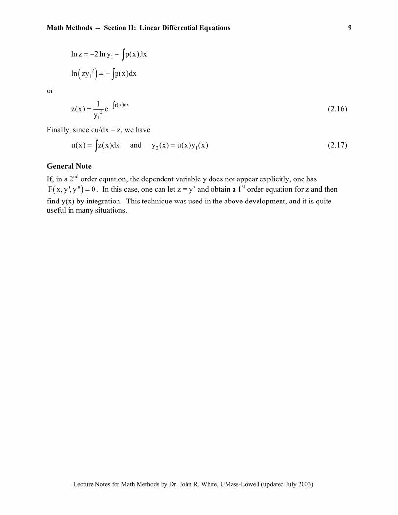
1ln z 2ln y p(x)dx= − − ∫ ( )2

1ln zy p(x)dx= −∫or

( )p x dx2

1

1z(x) ey

−∫= (2.16)

Finally, since du/dx = z, we have

(2.17) 2u(x) z(x)dx and y (x) u(x)y (x) = ∫ 1=

General Note

If, in a 2nd order equation, the dependent variable y does not appear explicitly, one has . In this case, one can let z = y’ and obtain a 1( )F x, y ', y '' 0= st order equation for z and then

find y(x) by integration. This technique was used in the above development, and it is quite useful in many situations.



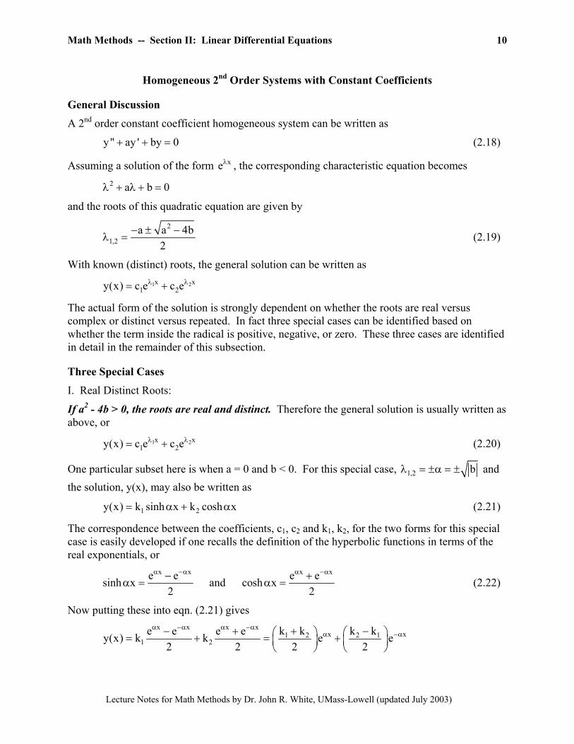
Homogeneous 2nd Order Systems with Constant Coefficients

General Discussion

A 2nd order constant coefficient homogeneous system can be written as

(2.18) y '' ay ' by 0+ + =

Assuming a solution of the form , the corresponding characteristic equation becomes xeλ

2 a bλ + λ + = 0

and the roots of this quadratic equation are given by

2

1,2a a 4

2− ± −

λ =b

2xλ

(2.19)

With known (distinct) roots, the general solution can be written as

1 2x x1 2y(x) c e c eλ λ= +

The actual form of the solution is strongly dependent on whether the roots are real versus complex or distinct versus repeated. In fact three special cases can be identified based on whether the term inside the radical is positive, negative, or zero. These three cases are identified in detail in the remainder of this subsection.

Three Special Cases

I. Real Distinct Roots:

If a2 - 4b > 0, the roots are real and distinct. Therefore the general solution is usually written as above, or

(2.20) 1x1 2y(x) c e c eλ= +

One particular subset here is when a = 0 and b < 0. For this special case, 1,2 bλ = and the solution, y(x), may also be written as

±α = ±

(2.21) 1 2y(x) k sinh x k cosh x= α + α

The correspondence between the coefficients, c1, c2 and k1, k2, for the two forms for this special case is easily developed if one recalls the definition of the hyperbolic functions in terms of the real exponentials, or

x x xe e e esinh x and cosh x

2 2

α −α α −α−α = α =

x+ (2.22)

Now putting these into eqn. (2.21) gives x x x x

x x1 2 2 11 2

e e e e k k k ky(x) k k e e2 2 2 2

α −α α −αα −α− + + − = + = +



and, from the last relationship, it is obvious that the correspondence among the coefficients is given by

1 2 21 2

k k k kc and c2 2+

= 1−= (2.23)

II. Complex Conjugate Roots:

If a2 - 4b < 0, the roots are complex conjugates. In this case the roots can be written as

21,2

a 1i with and a 4b2 2

λ = α ± β α = − β = − (2.24)

Recalling the definition of the complex exponential and the complex form of the sine and cosine functions,

(2.25) i xe cos x isin± β = β ± βx

i x i x i x i xe e e esin x and cos x

2i 2

β − β β − β−β = β =

+

β

β

)β

) i

(2.26)

the standard form of the solution, y(x), can be rewritten using

( )1x x i x x1 1 1c e c e e c e cos x isin xλ α β α= = β +

( )2x x i x x2 2 2c e c e e c e cos x isin xλ α − β α= = β −

to get

(2.27) (x1 2y(x) e k cos x k sin xα= β +

where now the relationship between the two formulations is

(2.28) (1 1 2 2 1 2k c c and k c c = + = −

III. Repeated Roots:

If a2 - 4b = 0, one obtains repeated roots. For this situation, the double root is given by

1,2a2

λ = − (2.29)

Therefore, there is only one independent solution,

ax 21y (x) e−= (2.30)

To find a second basis solution, let’s use the Reduction of Order Method. For the general case,

y '' p(x)y ' q(x)y 0+ + =

we have from eqns. (2.16) and (2.17) that

( )p x dx2 12

1

1z(x) e with u(x) z(x)dx and y (x) u(x)y (x)y

−∫= = ∫ =



For the present case, p(x) = a and ax 21y (x) e−= , therefore z(x) becomes

ax axz(x) e e 1− = =

and u(x) is given by

(2.31) u(x) (1)dx x= ∫ =

Therefore,

( )ax 2 ax 22y (x) xe and y(x) c c x e −= = +1 2

− (2.32)

Special Note

This technique of multiplying by some power of x is quite useful for Linear Constant Coefficient Equations with repeated roots. This is also true for particular solutions to constant coefficient ODEs when the forcing function is of the same form as the homogeneous solution (to be discussed later).



Homogeneous 2nd Order Euler-Cauchy Equations

General Discussion

In general, variable coefficient linear ODEs are rather difficult to solve analytically. In a subsequent section we will use the Power Series Method to address this problem from an analytical viewpoint, and we will use a numerical scheme for the general case. However, there is one special case of a variable coefficient system, called the Euler-Cauchy equation, that occurs quite frequently in applications and has a solution scheme very similar to that of constant coefficient systems. This subsection is devoted to developing the solution method for this special system - the homogeneous 2nd order Euler-Cauchy equation.

For 2nd order, the standard Euler-Cauchy equation has the form

(2.33) 2x y '' axy ' by 0+ + =

where a and b are constants. We assume a solution of the form

(2.34) my x=

Therefore,

( )m 1 m 2y ' mx and y '' m m 1 x −= = −− (2.35)

Upon substitution into the original ODE given in eqn. (2.33), we get

[ ] mm(m 1) am b x 0− + + =

and dividing by xm gives the characteristic equation,

( )2m a 1 m b+ − + = 0

The roots of this quadratic equation are given by

( ) ( )2

1,2a 1 a 1 4b

m2

− − ± − −= (2.36)

As for the case of constant coefficients, the actual form of the solution is strongly dependent on whether the roots are real versus complex or distinct versus repeated. In fact three special cases can be identified based on whether the term inside the radical is positive, negative, or zero. These three cases, for the Euler Cauchy equation, are identified in detail in the remainder of this subsection.

Three Special Cases

I. Real Distinct Roots:

If (a-1)2 - 4b > 0, the roots are real and distinct. Therefore the general solution is simply written as

(2.37) 1m1 2y(x) c x c x= + 2m



II. Complex Conjugate Roots:

If (a-1)2 - 4b < 0, the roots are complex conjugates. In this case the roots can be written as

( )21,2

a 1 1m i with and a 12 2

4b−= α ± β α = − β = − − (2.38)

Before writing the general solution in terms of complex roots, however, let’s look at alternate ways to write xm. The goal here is to write the solution in terms of real functions, if possible. First consider the following form for xm,

(2.39) ( )mm ln x mlx e e= = n x

)

Now, if , then m i= α + β

( ) (m i i i ln xx x x x x e x cos ln x isin ln xα+ β α β α β α = = = = β + β (2.40)

and similarly

( ) ( )m ix x x cos ln x isin ln xα− β α= = β − β (2.41)

Therefore,

( ) ( ) ( ) ( )m m1 2 1 2 1 2y(x) c x c x x c c cos ln x c c isin ln xα= + = + β + − β

or

( ) ( )1 2y(x) x k cos ln x k sin ln xα= β + β

) i

(2.42)

where (2.43) (1 1 2 2 1 2k c c and k c c = + = −

Note also that the following expressions are often useful in justifying the relationship of the standard solution in eqn. (2.37) and the form given in eqn. (2.42):

( )i ln x i ln x i ie e x xsin ln x

2i 2i

β − β β −− −β = =

β

(2.44)

( )i ln x i ln x i ie e x xcos ln x

2 2

β − β β −+ +β = =

β

(2.45)

III. Repeated Roots:

If (a-1)2 - 4b = 0, one obtains repeated roots. For this situation, the double root is given by

1,2m (1 a)= − 2 (2.46)

Therefore, there is only one independent solution,

m (1 a)1y (x) x x −= = 2 (2.47)

To find a second basis solution, let’s use the Reduction of Order Method again. For the general case,



y '' p(x)y ' q(x)y 0+ + =

we have from eqns. (2.16) and (2.17) that

( )p x dx2 12

1

1z(x) e with u(x) z(x)dx and y (x) u(x)y (x)y

−∫= = ∫ =

For the present case, p(x) = a/x , q(x) = b/x2, and m (1 a)1y (x) x x −= = 2 . Therefore z(x) becomes

a dx2m 2m a ln x 2m axz(x) x e x e x x

−− − − −∫= = = −

−

but m = (1-a)/2, thus , and 2m a 1x x− = ( )( )a 1 a 1 1z(x) x x xx

− − −= = =

Finally,

dxu(x) ln xx

= =∫ (2.48)

Therefore,

( )m2y (x) x ln x and y(x) c c ln x x = = + m

1 2 (2.49)

Special Note

This technique of multiplying by ln(x) is quite useful for Euler-Cauchy equations with repeated roots. This is also true for particular solutions when the forcing function for the Euler-Cauchy equation is of the same form as the homogeneous solution (to be discussed shortly).



Finding Particular Solutions

Undetermined Coefficients (UC)

The method of undetermined coefficients is rather straightforward but it is generally useful only for constant coefficient linear systems. In addition, the forcing function, r(x), must be a relatively simple function that has a finite number of linearly independent derivatives (exponentials, polynomials, sinusoids, or a linear combination of such functions usually work nicely).

General rule: Choose yp(x) to have the same form as the RHS forcing function and all its linearly independent derivatives. Evaluate the unknown coefficients within yp(x) by substitution into the original inhomogeneous ODE, and simply equate the coefficients of the like terms on both sides of the equations.

Special rule: If yp(x) via the general rule contains terms that are solutions to the homogeneous equations, one then multiplies this choice by x (from the Reduction of Order Method).

Example 2.1 provides an example of the method of Undetermined Coefficients.

Variation of Parameters (VOP)

A more general method for finding particular solutions is the variation of parameter technique. The method can be summarized as follows:

Given

(2.50) ( ) ( )n n 1n 1 1 0y p (x)y p (x)y ' p (x)y r(x)−

−+ + + + =

+

with homogeneous solution

(2.51) h 1 1 2 2 3 3y (x) c y (x) c y (x) c y (x)= + + +

one can write the particular solution as

(2.52) p 1 1 2 2 3 3y (x) u (x)y (x) u (x)y (x) u (x)y (x)= + +

where

1 21 2

W (x) W (x)u (x) r(x)dx and u (x) r(x)dxW(x) W(x)

= =∫ ∫

or, in general,

ii

W (x)u (x) r(x)dxW(x)

= ∫ (2.53)

where the Wronskian for an nth order system is given by

( ) ( ) ( )

1 2

1 2 n

n 1 n 1 n 11 2 n

y y yy ' y ' y '

W(x)

y y y− −

=

n

−

(2.54)



and Wi(x) is the determinant obtained after replacing the ith column of the right hand side of W(x) with the vector [ ]T0 0 0 1 . For example, in a 3rd order system, W2(x) is given by

1 3

2 1

1 3

y 0 yW (x) y ' 0 y '

y '' 1 y ''= 3

The development of these equations for the specific case of a second order system is given in the next subsection. Generalization to higher order systems is straightforward.

Example 2.2 illustrates the Variation of Parameters method using the same problem statement as given in Example 2.1 (which used the Undetermined Coefficients approach).

Variation of Parameters - Detailed Development for 2nd Order Systems

This subsection derives the summary equations presented above for the Variation of Parameters method. The development here is specific to a second order system, but it is easily extended to higher order linear ODEs.

Let’s start with the general 2nd order equation written in standard form,

(2.55) y '' p(x)y ' q(x)y r(x)+ + =

with homogeneous solution

(2.56) h 1 1 2 2y (x) c y (x) c y (x)= +

Now assume yp of the form

(2.57) p 1 1 2 2y (x) u (x)y (x) u (x)y (x)= +

which gives

p 1 1 2 2 p 1 1 1 1 2 2 2 2y u y u y and y ' u y ' u ' y u y ' u ' y = + = + + + (2.58)

At this point we recognize that an additional constraint, beyond the original balance equation, will be needed because we are trying to find two unknowns, u1 and u2. For simplicity, let’s choose the following relationship,

(2.59) 1 1 2 2u ' y u ' y 0+ =

which greatly simplifies the above equation for yp’, giving

p 1 1 2 2y ' u y ' u y '= + (2.60)

Now the second derivative becomes

p 1 1 1 1 2 2 2 2y '' u y '' u ' y ' u y '' u ' y= + + + ' (2.61)

Substitution of these expressions into the original equation gives

1 1 1 1 2 2 2 2 1 1 2 2 1 1 2 2u y '' u ' y ' u y '' u ' y ' pu y ' pu y ' qu y qu y r+ + + + + + + =

Rearranging gives



( ) ( )1 1 1 1 2 2 2 2 1 1 2 2u y '' py ' qy u y '' py ' qy u ' y ' u ' y ' r+ + + + + + + =

Therefore, since both the first and second terms vanish (because y1 and y2 are solutions to the homogeneous equation), we have

(2.62) 1 1 2 2u ' y ' u ' y ' r + =

Writing eqns. (2.59) and (2.62) in matrix form (two equations with two unknowns) gives

(2.63) 1 2 1

1 2 2

y y u ' 0y ' y ' u ' r

=

Using Cramer’s rule the solution to this system can be written as

2 2

2 2 11

1 2

1 2

0 y 0 yr y ' 1 y ' Wu ' r ry y W Wy ' y '

= = = (2.64)

1

1 22

y 0y ' 1 Wu ' r r

W W= = (2.65)

Finally, integrating these latter expressions to give u1 and u2 allows one to write the desired expression for yp(x) as

1 2p 1 2

W Wy (x) y r(x)dx y r(x)dxW W

= +∫ ∫ (2.66)

This result is consistent with the general relationships given above.



Operator Notation

General Discussion

Linear ODEs are very common in engineering analysis. Because they occur so frequently, it is often convenient to use a shorthand notation to simplify the sometimes lengthy and very detailed differential equations that are characteristic of many real systems. In particular, let’s define the common derivative operation with the following notation:

2 n

22

dy d y d yDy D y , D ydx dx dx

, and = = =nn

n

(2.67)

The quantities are called differential operators and they have properties analogous to algebraic quantities. For example, a general 2

2D, D , , D nd order linear ODE can be written

simply as Ly = r, where the L operator is the combination of three operators and is given by

( )2 2L D pD q and Ly D pD q y r = + + = + + = (2.68)

This simplified notation is very convenient once one becomes comfortable with the interpretation of the operators utilized.

Two Points About Linear Operators

1. Linear operators with constant coefficients can be factored and the order of the operation is unimportant. For example, the following operator expressions are all equivalent:

( ) ( ) ( ) ( ) ( )2D 3D 2 y D 2 D 1 y D 1 D 2+ + = + + = + + y

2. Linear operators with variable coefficients can also be factored, but the order of operation is extremely important. To see this, consider the following two operator expressions that are nearly identical, except for the order of operation:

Case 1:

( ) ( ) ( ) ( )

( ) ( )xD 1 D 2 y xD 1 y ' 2y

xD y ' 2y y ' 2yxy '' 2xy ' y ' 2y

+ − = + −

= − + −

= − + −

Case 2:

( ) ( ) ( ) ( )( ) ( )

D 2 xD 1 y D 2 xy ' y

D xy ' y 2 xy ' yxy '' y ' y ' 2xy ' 2yxy '' 2y ' 2xy ' 2y

− + = − +

= + − +

= + + − −= + − −

Thus, it is clear that Case 1 and Case 2 lead to different results. Therefore,

( ) ( ) ( ) ( )xD 1 D 2 y D 2 xD 1 y+ − ≠ − +



Summary Note

The point here is that linear operator notation can be very useful at times, and it is used extensively in the literature -- so the student must become familiar with its use. In addition, proper factorization of linear operators can also help in the solution of some very complicated systems. Example 2.3 further explains this approach. However, for variable coefficient systems, the order of operation is very important and care must be exercised when working with such systems!



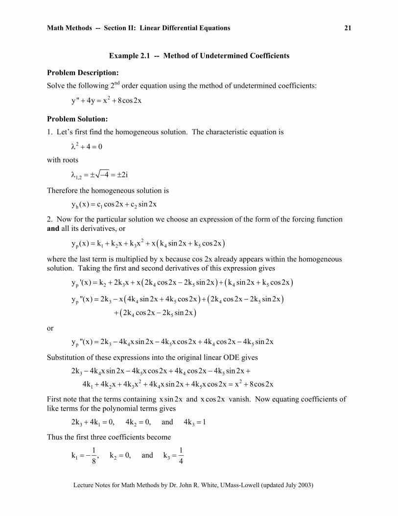
Example 2.1 -- Method of Undetermined Coefficients

Problem Description:

Solve the following 2nd order equation using the method of undetermined coefficients:

2y '' 4y x 8cos2x+ = +

Problem Solution:

1. Let’s first find the homogeneous solution. The characteristic equation is

2 4 0λ + =

with roots

1,2 4 2λ = ± − = ± i

Therefore the homogeneous solution is

h 1 2y (x) c cos2x c sin 2x= +

2. Now for the particular solution we choose an expression of the form of the forcing function and all its derivatives, or

( )2p 1 2 3 4 5y (x) k k x k x x k sin 2x k cos2x= + + + +

where the last term is multiplied by x because cos 2x already appears within the homogeneous solution. Taking the first and second derivatives of this expression gives

( ) ( )p 2 3 4 5 4 5y '(x) k 2k x x 2k cos2x 2k sin 2x k sin 2x k cos2x= + + − + +

( ) ( )( )

p 3 4 5 4 5

4 5

y ''(x) 2k x 4k sin 2x 4k cos2x 2k cos2x 2k sin 2x

2k cos2x 2k sin 2x

= − + + −

+ −

or

p 3 4 5 4 5y ''(x) 2k 4k x sin 2x 4k x cos2x 4k cos2x 4k sin 2x= − − + −

Substitution of these expressions into the original linear ODE gives

3 4 5 4 52 2

1 2 3 4 5

2k 4k x sin 2x 4k x cos2x 4k cos2x 4k sin 2x

4k 4k x 4k x 4k x sin 2x 4k x cos2x x 8cos2x

− − + − +

+ + + + = +

First note that the terms containing and vanish. Now equating coefficients of like terms for the polynomial terms gives

x sin 2x x cos2x

3 1 2 32k 4k 0, 4k 0, and 4k 1 + = = =

Thus the first three coefficients become

1 21 1k , k 0, and k8 4

= − = =3



Similarly for the sinusoidal terms, we have

4 54k 8 and 4k 0 = − =

0or 4 5k 2 and k = =

Therefore, the particular solution is

2p

1 1y (x) x 2x sin 2x8 4

= − + +

3. Finally, combining the homogeneous and particular solutions gives the desired general solution, or

2h p 1 2

1 1y(x) y (x) y (x) c cos2x c sin 2x x 2x sin 2x8 4

= + = + − + +

Example 2.2 explores a different approach to this equation using the Variation of Parameters method.



Example 2.2 -- Variation of Parameters


Solve the following 2nd order equation using the variation of parameter method:

2y '' 4y x 8cos2x+ = +

Problem Solution:

1. The homogeneous solution for this problem was derived previously (see Example 2.1) as

h 1 2y (x) c cos2x c sin 2x= +

2. Now for the particular solution, assume that yp(x) can be written as

p 1 1 2 2y (x) u y u y= +

where

1 2y cos2x and y sin 2 = = x

From our previous development for the Variation of Parameter technique (note that the system is already in standard form), we have

1 2p 1 2

W Wy (x) y r(x)dx y r(x)dxW W

= +∫ ∫

where

1 2 2 2

1 2

y y cos2x sin 2xW 2cos

y ' y ' 2sin 2x 2cos2x= = = +

−2x 2sin 2x 2=

21

2

0 y 0 sin 2xW s

1 y ' 1 2cos2x= = = − in 2x

12

1

y 0 cos2x 0W c

y ' 1 2sin 2x 1= = =

−os2x

and

2r(x) x 8cos2x= +

For performing the integrals and various manipulations, note the following integral relationships and trigonometric identities:

2 x sin 2axcos axdx2 4a

= +∫

21sin ax cosaxdx sin ax2a

=∫



2

22 3

2x 2 xx sin axdx sin ax cosax cosaxaa a

= + −∫

2

22 3

2x 2 xx cosaxdx cosax sin ax sin axaa a

= − +∫

and

( ) ( )1 1sin cos sin sin2 2

α β = α + β + α − β

sin 2 2sin cosα = α α

Now, with these expressions and relationships, the integrands and actual integrals become:

( )21W 1r x sin 2x 8sin 2x cos2xW 2

= − +

2 21

2 2

W 1 2x 2 x sinr(x)dx sin 2x cos2x cos2x 8W 2 4 8 2 4

1 1 1x sin 2x cos2x x cos2x sin 2x4 8 4

= − + − +

= − − + −

∫2x

2 22W 1r x cos2x 8cos 2xW 2

= +

22

2

W 1 2x 2 x x 1r(x)dx cos2x sin 2x sin 2x 8 sin 4xW 2 4 8 2 2 8

1 1 1 1x cos2x sin 2x x sin 2x 2x sin 4x4 8 4 2

= − + + +

= − + + +

∫

Therefore, yp(x) becomes

2 2 2p

2 2

2 2

1 1 1y x sin 2x cos2x cos 2x x cos 2x4 8 4

1 1sin 2x cos2x x sin 2x cos2x sin 2x4 8

1 1x sin 2x 2x sin 2x sin 4x sin 2x4 2

= − − +

− + −

+ + +

or

2 2p

1 1 1y x sin 2x cos2x 2x sin 2x sin 4x sin 2x8 4 2

= − + − + +

Therefore, using the last trigonometric identity given above, one final simplification gives

2p

1 1y (x) x 2x sin 2x8 4

= − + +



Finally, combining this with the homogeneous solution gives

21 2

1 1y(x) c cos2x c sin 2x x 2x sin 2x8 4

= + − + +

which is the same solution as that from Example 2.1.

Clearly, Examples 2.1 and 2.2 show that, if possible, the method of undetermined coefficients should be used, since its application is usually much easier than the current variation of parameters approach. A word of advice is “Use the Variation of Parameters method when necessary, but only when necessary!”



Example 2.3 -- Solution via Operator Factorization


Solve the following variable coefficient 2nd order equation by operator factorization:

( ) 2xxy '' 2x 3 y ' 4y e+ + + =

Problem Solution:

1. First let’s write the original equation in operator form,

2 2xD (2x 3)D 4 y e + + + = x

2. Now factor the operator L(D) as follows:

( ) ( )2Ly xD (2x 3)D 4 y D 2 xD 2 y = + + + = + +

Checking this (just to be sure) shows that indeed this is the correct factorization (always be careful here), or

( ) ( ) ( ) ( )

( )2

2

D 2 xD 2 y D 2 xDy 2y

xD y Dy 2Dy 2xDy 4y

xD (2x 3)D 4 y

+ + = + +

= + + + +

= + + +

3. Now, let ( . Therefore, we have )xD 2 y z+ =

( ) 2xD 2 z e+ =

or

2xdz 2z edx

+ =

But this is a linear 1st order ODE with integrating factor . Therefore, 2xg(x) e=

( )2x 2x 4xdz de 2z zedx dx

+ = =

e

and integration gives

2x 4x 4x 2x 2x1 1

1 1ze e dx e c or z(x) e c e4 4

−= = + = +∫

4. Now we must solve

( ) 2x 2x1

1xD 2 y e c e4

−+ = +

or



2x 2x

1dy 2 1 e ey cdx x 4 x x

−

+ = +

Again this is a linear 1st order ODE with integrating factor

2dx 2ln x 2xg(x) e e x∫= = =

Therefore,

( )2 2 2x 2x1

dy 2 d 1x y yx xe c xdx x dx 4

e− + = = +

Integrating both sides of this expression gives (see detailed integration by parts below):

2 2x 2x1

2x 2x1 2

1yx xe dx c xe dx4

1 1 1 1 1e x c e x4 2 2 2 2

−

−

= +

= − + − +

∫ ∫

c+

or 2 2x 2x1 2

1 1 1 1yx e x c e x c8 2 2 2

− = − − +

+

Thus, the final solution to this rather complex problem is

2x 2x1 22

1 1 1 1 1y e x c e x8 2 2 2x

− = − − + c+

x

-------------------------

Note: Let’s do an example of integration by parts. Consider the following integral,

axI xe d= ∫Now let’s put this into the following form

udv uv vdu= −∫ ∫where axu x dv e dx, = =

ax1du dx, v ea

= =

Therefore, we have

ax ax ax ax2

1 1 1 1I xe e dx xe ea a a a

= − = −∫

or

ax1 1I e xa a

= −


mathematical methods (10/24.539) ii. linear differential ... · mathematical methods (10/24.539)...

Documents