HAL Id: hal-01377994https://hal.archives-ouvertes.fr/hal-01377994

Submitted on 8 Oct 2016

HAL is a multi-disciplinary open accessarchive for the deposit and dissemination of sci-entific research documents, whether they are pub-lished or not. The documents may come fromteaching and research institutions in France orabroad, or from public or private research centers.

L’archive ouverte pluridisciplinaire HAL, estdestinée au dépôt et à la diffusion de documentsscientifiques de niveau recherche, publiés ou non,émanant des établissements d’enseignement et derecherche français ou étrangers, des laboratoirespublics ou privés.

Mathematical modeling of tumor and metastatic growthwhen treated with sunitinib

Simon Evain, Sebastien Benzekry

To cite this version:Simon Evain, Sebastien Benzekry. Mathematical modeling of tumor and metastatic growth whentreated with sunitinib. [Research Report] Inria Bordeaux Sud-Ouest. 2016. �hal-01377994�

Internship report

Mathematical modeling of tumorand metastatic growth when

treated with sunitinib

Simon Evain

supervised bySebastien Benzekry

October 8, 2016

Abstract

The effect of the antiangiogenic drug sunitinib on the tumor sizeand the metastatic burden evolution are studied statistically and math-ematically. For this, a new model SunitinibTGI is built, which allowsto model with accuracy the phenomenon, thus giving us more informa-tion on the behavior of a tumor treated with sunitinib, distinguishinga phase of resistance to sunitinib under certain conditions. Togetherwith some correlations that are noted on the data set, these tools allowus to better understand the metastatic response to sunitinib adminis-tration, notably in a neoadjuvant setting.

1

Contents

1 Abstract 1

2 Introduction 7

3 Description of the problem 93.1 Nature of the issue . . . . . . . . . . . . . . . . . . . . . . . . 9

3.1.1 A brief summary on sunitinib . . . . . . . . . . . . . . 93.1.2 Controversy on the effect of sunitinib in a neo-adjuvant

setting . . . . . . . . . . . . . . . . . . . . . . . . . . . 93.2 Data description . . . . . . . . . . . . . . . . . . . . . . . . . 103.3 Benchmark of optimization algorithms . . . . . . . . . . . . . 13

4 Classical models of tumor growth without treatment ([1]) 144.1 Exponential model . . . . . . . . . . . . . . . . . . . . . . . . 144.2 Exponential-linear model . . . . . . . . . . . . . . . . . . . . 154.3 Gompertz model . . . . . . . . . . . . . . . . . . . . . . . . . 164.4 Gomp-Exp model . . . . . . . . . . . . . . . . . . . . . . . . . 174.5 Power Law model . . . . . . . . . . . . . . . . . . . . . . . . . 174.6 Logistic model . . . . . . . . . . . . . . . . . . . . . . . . . . 184.7 Dynamic CC model . . . . . . . . . . . . . . . . . . . . . . . 184.8 Comparison of the accuracy of the untreated growth models . 19

5 Implementation of the treatment in a tumor growth model 205.1 Shape of the treated data . . . . . . . . . . . . . . . . . . . . 205.2 Approach based on pharmacokinetics ([15]) . . . . . . . . . . 225.3 Classical models of tumor growth with treatment . . . . . . . 24

5.3.1 Exp-log kill . . . . . . . . . . . . . . . . . . . . . . . . 245.3.2 Gompertz-Norton-Simon model . . . . . . . . . . . . . 255.3.3 SimeoniAA model . . . . . . . . . . . . . . . . . . . . 255.3.4 Simeoni2004 model . . . . . . . . . . . . . . . . . . . . 265.3.5 Treated dynamic CC model . . . . . . . . . . . . . . . 265.3.6 Hahnfeldt model . . . . . . . . . . . . . . . . . . . . . 285.3.7 Limits . . . . . . . . . . . . . . . . . . . . . . . . . . . 29

5.4 SunitinibTGI model . . . . . . . . . . . . . . . . . . . . . . . 295.4.1 Required features . . . . . . . . . . . . . . . . . . . . . 295.4.2 Shape of the selected model . . . . . . . . . . . . . . . 305.4.3 Expression of the model SunitinibTGI . . . . . . . . . 315.4.4 Smoothing of the model . . . . . . . . . . . . . . . . . 325.4.5 Parameter identifiability in the model SunitinibTGI . 335.4.6 Comparison with classical models . . . . . . . . . . . . 345.4.7 Notable results related to the model ([14]) . . . . . . . 345.4.8 Limits of the model . . . . . . . . . . . . . . . . . . . 39

2

6 Data correlations 40

7 Computing the metastatic burden ([7], [18]) 437.1 General equation . . . . . . . . . . . . . . . . . . . . . . . . . 437.2 Conclusions . . . . . . . . . . . . . . . . . . . . . . . . . . . . 447.3 Prospects . . . . . . . . . . . . . . . . . . . . . . . . . . . . . 45

8 Conclusion 46

9 Annex 479.1 Cancer biology ([9]) . . . . . . . . . . . . . . . . . . . . . . . 47

9.1.1 Overview . . . . . . . . . . . . . . . . . . . . . . . . . 479.1.2 Detailed description of the disease . . . . . . . . . . . 479.1.3 Current treatments . . . . . . . . . . . . . . . . . . . . 52

9.2 Statistical tools . . . . . . . . . . . . . . . . . . . . . . . . . . 549.2.1 Sum of squared errors (SSE) . . . . . . . . . . . . . . 549.2.2 Root mean squared error (RMSE) . . . . . . . . . . . 549.2.3 Akaike Information Criterion (AIC) . . . . . . . . . . 549.2.4 R2 coefficient . . . . . . . . . . . . . . . . . . . . . . . 559.2.5 Log-likelihood ratio . . . . . . . . . . . . . . . . . . . 55

9.3 Optimization methods for the Gompertz model . . . . . . . . 569.3.1 Introduction . . . . . . . . . . . . . . . . . . . . . . . 569.3.2 Optimization problem . . . . . . . . . . . . . . . . . . 579.3.3 Optimization algorithms . . . . . . . . . . . . . . . . . 599.3.4 Statistical comparison of the optimization algorithms . 849.3.5 Numerical implementation of the Levenberg-Marquardt

algorithm . . . . . . . . . . . . . . . . . . . . . . . . . 879.4 Numerical methods for the Gompertz model . . . . . . . . . . 88

9.4.1 Introduction . . . . . . . . . . . . . . . . . . . . . . . 889.4.2 Analysis of numerical methods for the Gompertz dif-

ferential equation . . . . . . . . . . . . . . . . . . . . . 899.4.3 Derivation of the order of the methods . . . . . . . . . 91

10 Thanks and acknowledgments 92

11 Bibliography 94

3

List of Figures

1 Description of the effect of sunitinib . . . . . . . . . . . . . . 82 Presentation of the 2009 article by J. Ebos et al. . . . . . . . 103 Description of the experimental process for a group of mice . 114 Description of the experimental process . . . . . . . . . . . . . 115 Summary of all breast-related data that were dealt with during

the internship . . . . . . . . . . . . . . . . . . . . . . . . . . . 126 Summary of all melanoma-related data that were dealt with

during the internship . . . . . . . . . . . . . . . . . . . . . . . 127 Surface of the objective function to be optimized for a Gom-

pertz function . . . . . . . . . . . . . . . . . . . . . . . . . . . 138 Fit of the average data of the group 3 by the exponential model 149 Fit of the average data of the group 3 by the exponential-linear

model . . . . . . . . . . . . . . . . . . . . . . . . . . . . . . . 1510 Fit of the average data of the group 3 by the Gompertz model 1611 Fit of the average data of the group 3 by the Gomp-Exp model 1712 Fit of the average data of the group 3 by the Power Law model 1813 Fit of the average data of the group 3 by the Logistic model . 1914 Comparison of the accuracy of the untreated growth models . 2015 Shape of the treated data for breast cancer [’behavior breast 1

and 2’] . . . . . . . . . . . . . . . . . . . . . . . . . . . . . . . 2116 Shape of the treated data for melanoma [’behavior melanoma’] 2217 Unicompartmental model (absorption rate ka and elimination

rate k . . . . . . . . . . . . . . . . . . . . . . . . . . . . . . . 2318 Fit of the average data of the group 31 by the Exp-log kill model 2419 Fit of the average data of the group 31 by the Gompertz-

Norton-Simon model (3 degrees of freedom) . . . . . . . . . . 2520 Fit of the average data of the group 31 by the SimeoniAA

model (3 degrees of freedom) . . . . . . . . . . . . . . . . . . . 2621 Fit of the average data of the group 31 by the Simeoni2004

model (4 degrees of freedom) . . . . . . . . . . . . . . . . . . . 2722 Fit of the average data of the group 31 by the dynamic CC

model (2 degrees of freedom) . . . . . . . . . . . . . . . . . . . 2723 Fit of the average data of the group 31 by the Hahnfeldt model

(3 degrees of freedom) . . . . . . . . . . . . . . . . . . . . . . 2824 Parameter identifiability for the SunitinibTGI model [the first

table shows the maximal uncertainty for τ ] . . . . . . . . . . . 3325 Comparison of the SunitinibTGI model with classical models . 3526 SunitinibTGI modeling for an individual mouse injected with

breast cancer . . . . . . . . . . . . . . . . . . . . . . . . . . . 3627 SunitinibTGI modeling for an individual mouse injected with

breast cancer . . . . . . . . . . . . . . . . . . . . . . . . . . . 37

4

28 SunitinibTGI modeling for an individual mouse injected withmelanoma . . . . . . . . . . . . . . . . . . . . . . . . . . . . . 37

29 Correlations overall survival - tumor size pre-resection forcontrol groups . . . . . . . . . . . . . . . . . . . . . . . . . . . 40

30 Correlations overall survival - tumor size pre-resection fortreated groups . . . . . . . . . . . . . . . . . . . . . . . . . . . 41

31 Correlations tumor size pre-resection - metastatic burden forcontrol groups . . . . . . . . . . . . . . . . . . . . . . . . . . . 42

32 Correlations tumor size pre-resection - metastatic burden fortreated groups . . . . . . . . . . . . . . . . . . . . . . . . . . . 42

33 Evolution of the metastatic burden (control groups) . . . . . . 4434 Evolution of the metastatic burden (treated groups) . . . . . . 4535 Data provided . . . . . . . . . . . . . . . . . . . . . . . . . . . 5736 Solution to the Gompertz differential equation, with V0 = 1,

α = 1, β = 0.1 . . . . . . . . . . . . . . . . . . . . . . . . . . 5837 F depending on α and β . . . . . . . . . . . . . . . . . . . . . 6038 Zoom on one part of the pseudo-minimum ”valley” from the

surface of F . . . . . . . . . . . . . . . . . . . . . . . . . . . . 6139 Contour lines of log(F) . . . . . . . . . . . . . . . . . . . . . . 6240 Extreme values of F for a range of α and β . . . . . . . . . . 6341 Solution obtained for the optimized parameters, starting from

(0.8, 0.13) (gradient with constant step). . . . . . . . . . . . . 6442 Solution obtained for the optimized parameters, starting from

(1.0, 0.20) (gradient with constant step). . . . . . . . . . . . . 6443 Value of the criterion as the constant gradient algorithm is

carried out (depending on the number of the considered iter-ation) . . . . . . . . . . . . . . . . . . . . . . . . . . . . . . . 65

44 Value of the parameters α and β in the course of the constantgradient algorithm, compared with the contour lines of log(F )for a starting point (0.7, 0.1) . . . . . . . . . . . . . . . . . . 66

45 Solution obtained for the optimized parameters, starting from(0.8, 0.13) (gradient with variable step). . . . . . . . . . . . . 68

46 Solution obtained for the optimized parameters, starting from(1.0, 0.20) (gradient with variable step). . . . . . . . . . . . . 69

47 Value of the criterion as the variable gradient algorithm iscarried out (depending on the number of the considered iter-ation) for a starting point (0.7, 0.1) . . . . . . . . . . . . . . 70

48 Value of the parameters α and β in the course of the variablegradient algorithm, compared with the contour lines of log(F )for a starting point (0.7, 0.1) . . . . . . . . . . . . . . . . . . 71

49 Solution obtained for the optimized parameters, starting from(1.7, 0.2) (Gauss-Newton). . . . . . . . . . . . . . . . . . . . . 73

50 Solution obtained for the optimized parameters, starting from(1.0, 0.13) (Gauss). . . . . . . . . . . . . . . . . . . . . . . . . 73

5

51 Value of the criterion as the Gauss-Newton algorithm is car-ried out (depending on the number of the considered iteration) 74

52 Value of the parameters α and β in the course of the Gauss-Newton algorithm, compared with the contour lines of log(F )for a starting point (0.7, 0.1) . . . . . . . . . . . . . . . . . . 75

53 Solution obtained for the optimized parameters, starting from(0.8, 0.13) (Gauss-Newton). . . . . . . . . . . . . . . . . . . . 76

54 Solution obtained for the optimized parameters, starting from(0.7, 0.1) (Levenberg-Marquardt). . . . . . . . . . . . . . . . . 82

55 Solution obtained for the optimized parameters, starting from(1.7, 0.2) (Levenberg-Marquardt). . . . . . . . . . . . . . . . . 82

56 Solution obtained for the optimized parameters, starting from(0.8, 0.13) (Levenberg-Marquardt). . . . . . . . . . . . . . . . . 83

57 Value of the criterion as the Levenberg-Marquardt algorithmis carried out (depending on the number of the considerediteration) for a starting point (0.7, 0.1) . . . . . . . . . . . . 96

58 Value of the parameters α and β in the course of the Levenberg-Marquardt algorithm, compared with the contour lines of log(F )for a starting point (0.7, 0.1) . . . . . . . . . . . . . . . . . . 96

59 Average error and calculation time for the considered opti-mization algorithms . . . . . . . . . . . . . . . . . . . . . . . 97

60 Results obtained, by comparison with the Nelder-Mead algorithm 9761 Solution to the Gompertz differential equation, with V0 =

1mm3, α = 1, β = 0.1 . . . . . . . . . . . . . . . . . . . . . . 9762 RK4 approximation for h = 6. . . . . . . . . . . . . . . . . . . 9863 RK4 approximation for h = 4. . . . . . . . . . . . . . . . . . . 9864 RK4 approximation for h = 2. . . . . . . . . . . . . . . . . . . 9865 Relative errors and calculation times for the RK4 approxima-

tion depending on the value of the step h . . . . . . . . . . . . 9966 Euler approximation for h = 2. . . . . . . . . . . . . . . . . . 10067 Euler approximation for h = 1. . . . . . . . . . . . . . . . . . 10068 Euler approximation for h = 0.5 . . . . . . . . . . . . . . . . . 10069 Relative errors and calculation times for the RK4 approxima-

tion depending on the value of the step h . . . . . . . . . . . . 10170 Euler approximation and RK4 approximation for h = 3.5 . . . 10171 Bigger steps allowing to get a specific relative error for the

two numerical methods and corresponding calculation times . 10172 Evaluation of the order of the RK4 method . . . . . . . . . . 10273 Evaluation of the order of the Euler method . . . . . . . . . . 102

6

1 Introduction

Cancer is, in France, the first cause of mortality ([12]). In spite of the con-stant progress of medical research, cancer is still an illness which is poorlyunderstood in a lot of aspects.

Cancer is a disease which is born when some cells of the organism breakfree from the genetic rules and undergo limitless mitosis. This leads to thecreation of a mass of cells with uncontrollable growth within the organs,which have no utility whatsoever for the organism: the primary tumor. Atsome stage, the tumor cannot grow more due to the lack of nutrients. Butsome primary tumors find themselves able to induce what is called angio-genesis, which allows to stimulate its own vascularization. This way, thetumor can access more nutrients and grow even more.

Some tumor cells may be able to escape the organ, through the bloodor the lymph nodes, giving the possibility of a dissemination of tumor cellsinside the whole organism. These cells are then able to settle in a new organ(colonization), and to grow inside the organ to form a secondary tumor.This latest process is called metastatic process, and is the least understoodand the most lethal part in most cancers.

One of the possible ways to treat cancer is therefore to block angiogen-esis, in order to deprive the tumor from its nutrients, thus weakening it.Among the most well-known antiangiogenic drugs, we can quote the Su-tent (or sunitinib, for the name of the molecule), which has recently beenthe object of a controversy. One of the main goals for the administrationof such a medicine is the size reduction of the primary tumor, allowing toremove the tumor through surgery much easier later. And if, indeed, thisspecific consequence has been evidenced by several experiments, John Ebos,in [6], has made a connection between the administration of the drug andthe metastatic acceleration for mice. Administering such a drug could leadto an acceleration of the metastatic process for mice, and ultimately reduc-ing their life expectancy.

During this six-month-long internship carried out at inria Bordeaux,within the monc team, the main objective was to study the connection be-tween these two factors, through the analysis of Mr John Ebos’ data. Thefirst objective was to try and describe as accurately as possible the evolutionof the size of the primary tumor in those experiments, when treated and un-treated. A benchmark of classical models had to be performed, to comparetheir relative efficiency to fit the data. The fitting process itself had to bestudied in order to pick the best (most stable, accurate and quicker) opti-mization algorithm. Faced with rather unsatisfying results when fitting the

7

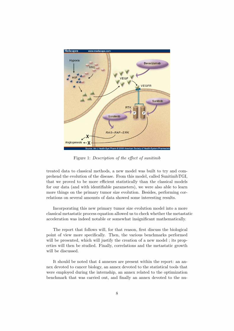
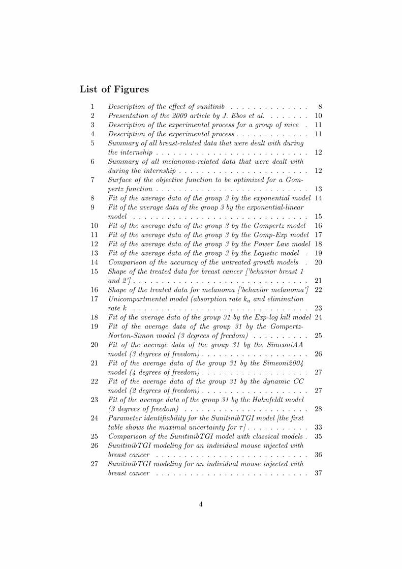
Figure 1: Description of the effect of sunitinib

treated data to classical methods, a new model was built to try and com-prehend the evolution of the disease. From this model, called SunitinibTGI,that we proved to be more efficient statistically than the classical modelsfor our data (and with identifiable parameters), we were also able to learnmore things on the primary tumor size evolution. Besides, performing cor-relations on several amounts of data showed some interesting results.

Incorporating this new primary tumor size evolution model into a moreclassical metastatic process equation allowed us to check whether the metastaticacceleration was indeed notable or somewhat insignificant mathematically.

The report that follows will, for that reason, first discuss the biologicalpoint of view more specifically. Then, the various benchmarks performedwill be presented, which will justify the creation of a new model ; its prop-erties will then be studied. Finally, correlations and the metastatic growthwill be discussed.

It should be noted that 4 annexes are present within the report: an an-nex devoted to cancer biology, an annex devoted to the statistical tools thatwere employed during the internship, an annex related to the optimizationbenchmark that was carried out, and finally an annex devoted to the nu-

8

merical methods employed. All the code used for the internship was writtenusing Matlab, and the internship was an extension of the work carried outpreviously by Mr Aristoteles Camillo ([12]).

2 Description of the problem

2.1 Nature of the issue

2.1.1 A brief summary on sunitinib

Sunitinib (marketed by Pfitzer as Sutent) is a drug that was approved in2006 by the Food and Drug Administration simultaneously for two diseases:metastatic kidney cancer, and GIST (Gastro-Intestinal Stromal Tumor) asa second-line drug (after the potential failure of imatinib). This drug actslike a targeted bio-therapy: it does not attack straightly the cells, but at-tacks instead a specific biological action mechanism used for the growthof tumor cells. That action mechanism is angiogenesis, the biological pro-cess by which new blood vessels are created from pre-existing ones, allowingthe tumor to grow beyond a certain size to be able to eventually metastasize.

Sunitinib acts as an inhibitor for Tyrosine Kinase Receptors, the enzymeswhich receive the signals emitted by the primary tumor allowing the furthergrowth of the vasculature within the primary tumor. Among the recep-tors that are inhibited by the drug are the VEGFRs (Vascular EndothelialGrowth Factor Receptors) and PDGFRs (Platelet-Derived Growth FactorReceptors).

Besides, sunitinib is a small molecule, and is therefore able to enter intothe cells, unlike most antibodies.

2.1.2 Controversy on the effect of sunitinib in a neo-adjuvantsetting

In 2009, the American biologist John Ebos and his associated co-workerspublished an article [6], that was seen as a major breakthrough. In thisarticle, Ebos showed that a metastatic acceleration could occur for a mousetreated with sunitinib in a neo-adjuvant perspective (before tumor resec-tion). These results seem to indicate that a treatment of sunitinib in aneo-adjuvant setting can reduce the life expectancy of mice.

This matter of the exact effect of sunitinib on tumor and metastatic ki-netics is absolutely crucial, for it is a very common and widespread antian-giogenic drug. For that reason, other studies were led on human patients,which tended to show that there was no clear metastatic acceleration and

9

Figure 2: Presentation of the 2009 article by J. Ebos et al.

overall survival reduction when administered with sunitinib.

This issue was central in the internship.

2.2 Data description

All the data this internship is built upon were provided by Dr Ebos, theAmerican biologist who first assumed the idea of connection between suni-tinib administration and metastatic acceleration.

The data is extracted from mice, and all are drawn from two differentcell lines: breast and melanoma, both treated with sunitinib.

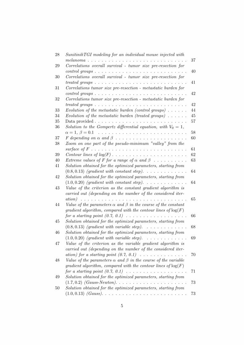
The breast data are data on primary tumor size and, for some groups,metastatic burden. 88 mice were subject to the experiment, and, amongthem, 33 were used as control individuals (so they were injected with the can-cer cells, but not with the treatment). Six various groups, differing by theirscheduling, can be distinguished. For four out of six groups, the primarytumor was resected, allowing to evaluate the evolution of the metastaticburden when sunitinib is administered in a neo-adjuvant perspective. Forthe two remaining groups (31 and 32), the primary tumor was not resected; these groups are useful for they permit to study tumor growth kinetics on

10

Figure 3: Description of the experimental process for a group of mice

Figure 4: Description of the experimental process

11

Group number Dose injected (mg.kg−1) Treatment days Resection day

1 120 24-30 32

2 60 24-38 39

31 60 11-60 -

32 120 2-19 -

51 60 20-33 34

6 60 20-33 34

Figure 5: Summary of all breast-related data that were dealt with during theinternship

Group number Drug employed Cell line Treatment days

1A 516 regular 1-41

1B sunitinib regular 1-41

2A 516 resistant 1-41

2B sunitinib resistant 1-41

Figure 6: Summary of all melanoma-related data that were dealt with duringthe internship

a longer scale. Figure 5 displays the different treatments for each group.

Another data set corresponds to melanoma-related cells. 38 mice aresubject to such an experiment, among which 22 are exploited for controlanalysis (so, untreated) and the 16 remaining mice can be divided into 4groups. All these data have in common the fact that they only show pri-mary tumor growth. Besides, all tumors are treated from day 1 to day 41,and the treatment is then stopped. These pieces of data, thus, allow toevaluate the impact of a stop of the treatment. Two various drugs (516 andsunitinib) were used on two different cell lines (regular or sunitinib-resistantcells). All the useful information regarding this data set are indicated onfigure 6.

All primary tumor growth volume data are expressed in mm3. Thevolume is calculated thanks to the formula: V = 0.5width2.length, wherelength and width of the tumor cells are measured using a caliper. Themetastatic burden is measured using bio-luminescence, and is therefore ex-pressed in photons per second.

12

Figure 7: Surface of the objective function to be optimized for a Gompertzfunction

2.3 Benchmark of optimization algorithms

Our objective during this internship is to model the evolution of tumorgrowth. On a mathematical point of view, we need to solve the followingleast-square minimization problem (yi designates the data, p the parametersof the model and M the chosen model):

minp(∑

i(yi −M(ti; p))2)

To address this issue, a test case was carried out on a Gompertz modeland the data for mice which were not administered any treatment.

Several algorithms and methods were implemented to be compared.Were tested the constant gradient, variable gradient, Gauss-Newton andLevenberg-Marquardt algorithms. The results are described in the annexdevoted to Optimization in this report, but only its outcome will be dis-played here.

We concluded that the Nelder-Mead and the Levenberg-Marquardt al-gorithms were to be favoured in terms of stability and efficiency.

One important point that needs to be understood is that, no matterhow accurate our optimization process is, there is still a huge influence ofthe initial condition. For that reason, for each data fitting that will be

13

Figure 8: Fit of the average data of the group 3 by the exponential model

performed in the subsequent parts of the report, the optimization algorithmwas launched a significant number of times, with various starting points.

3 Classical models of tumor growth without treat-ment ([1])

The first data that needs to be fitted with models is the evolution of thesize of the primary tumor of mice for control groups (so when the mice arenot treated). For that reason, all the following models were implementedon MATLAB, and the Nelder-Mead algorithm was used each time, on theobjective function described in the previous part. This allowed us to findthe parameters of each model which were able to describe as accurately aspossible the evolution of the primary tumor. We then computed the resultthat was obtained to see how close it was from the actual data. This way,we were able to compare all the following models.

3.1 Exponential model

Tumor growth in this model is supposed to be exponential.

dV

dt= λV (1)

where λ is the growth rate of the primary tumor.

14

Figure 9: Fit of the average data of the group 3 by the exponential-linearmodel

3.2 Exponential-linear model

This model takes into account more elements, when compared with theexponential model. It follows 2 successive phases:

• an exponential growth with a constant rate a0.

• a linear growth with a constant rate a1.

dV

dt= a0V (t), t ≤ τ

dV

dt= a1, t ≥ τ

V (t = 0) = V0

(2)

To use the model, we often resort to a single differential equation, whichapproximates the behavior described by the previous equations:

dV

dt=

a0V (t)

(1 + (a0V (t)a1

)ψ)1ψ

(3)

ψ is often chosen equal to 20 (value taken from [1]). We notice that whenV is small, the growth of the model is very close to the exponential growth

15

Figure 10: Fit of the average data of the group 3 by the Gompertz model

; when V is large, the model gets closer to a linear one.

Besides, if we want the solution to be continuously differentiable, we seethat we necessarily have τ = 1

log(a1a0V0

).

On a biological point of view, the model represents the fact that thegrowth of the tumor is almost unlimited at first, but that as the nutrientsgo scarce, its growth will then necessarily be restricted, and become linear.

3.3 Gompertz model

In this model, tumor growth is written this way:

dV

dt= (a− b ln(V ))V (4)

In the equation, a is the tumor proliferation rate, and b is the rate ofexponential decay of the proliferation rate.

Biologically, the model is based on the same reasoning as the exponential-linear model, but with the supplementary assumption that the tumor sizehas an upper boundary: the carrying capacity V0 exp(ab ). It cannot growuntil infinity.

16

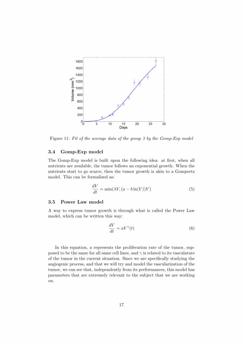
Figure 11: Fit of the average data of the group 3 by the Gomp-Exp model

3.4 Gomp-Exp model

The Gomp-Exp model is built upon the following idea: at first, when allnutrients are available, the tumor follows an exponential growth. When thenutrients start to go scarce, then the tumor growth is akin to a Gompertzmodel. This can be formalized as:

dV

dt= min(λV, (a− b ln(V ))V ) (5)

3.5 Power Law model

A way to express tumor growth is through what is called the Power Lawmodel, which can be written this way:

dV

dt= aV γ(t) (6)

In this equation, a represents the proliferation rate of the tumor, sup-posed to be the same for all same cell lines, and γ is related to its vasculatureof the tumor in the current situation. Since we are specifically studying theangiogenic process, and that we will try and model the vascularization of thetumor, we can see that, independently from its performances, this model hasparameters that are extremely relevant to the subject that we are workingon.

17

Figure 12: Fit of the average data of the group 3 by the Power Law model

3.6 Logistic model

In this model, the carrying capacity K is considered as a constant in theproblem. We can then write the model as:

dV

dt= aV (t)(1− V (t)

K) (7)

In this expression, a is considered as a rate controlling the velocity of thegrowth. In this model, as the tumor volume reaches the carrying capacity,the growth is gradually reduced.

3.7 Dynamic CC model

This model considers the carrying capacity K as a variable representing thetumor vasculature. The dynamic can then be written as:

dV

dt= aV (t) log(

K(t)

V (t))

dK

dt= bV (t)

23

V (t = 0) = V0,K(t = 0) = K0

(8)

The biological reasoning behind such a model is close from the reasoningguiding the other models. We can note that the factor 2

3 is chosen because

18

Figure 13: Fit of the average data of the group 3 by the Logistic model

it is assumed that the carrying capacity growth is proportional to the tumorsurface.

3.8 Comparison of the accuracy of the untreated growthmodels

We implemented all the previous models and fit the data from control groupswith them, using the Nelder-Mead algorithm as the optimization method.The parameters are the result of the optimization problem of minimizationof the SSE. The results for this statistical comparison are summed up onfigure 14 (the meaning of each one of the statistical tools employed are de-scribed in the Annex Statistics).

For the statistical tools SSE, AIC and RMSE, it is more interesting tohave a small value (see the Annex Statistics to understand why) ; as for theR2, the closer it is to 1, the better the actual fit is.

We notice that for all criteria, two models seem to have to be favored:the Gompertz model and the Power Law model. We can note that sinceour work aims at modeling the effect of anti-angiogenic drugs, the biologicalmeaning of the parameters related to the Power Law model, notably throughtheir modeling of vascularization, could be quite useful.

19

Figure 14: Comparison of the accuracy of the untreated growth models

4 Implementation of the treatment in a tumor growthmodel

4.1 Shape of the treated data

Before performing any analysis, it is important to focus on the treated tumordata (volume) graphically. We can separate all the data set into 3 differ-ent kinds of behavior, 2 for breast-related data and a specific behavior formelanoma-related data.

’Behavior breast 1’, as displayed in figure 15, shows a tumor growthwhich can be distinguished into 3 phases.

• Phase 1 (pre-treatment): the tumor grows and no treatment is ad-ministered yet. We can consider this growth as identical to the tumorgrowth for control groups, when absolutely no treatment is adminis-tered.

• Phase 2 (growth arrest): this phase begins when the treatment startsto be administered, and it lasts for a certain duration which does notseem to always coincide with the duration of the treatment. During

20

Figure 15: Shape of the treated data for breast cancer [’behavior breast 1 and2’]

21

Figure 16: Shape of the treated data for melanoma [’behavior melanoma’]

this phase, the treatment seems to be extremely efficient, and to stopnearly all tumor growth.

• Phase 3 (resistance phase): after a certain duration, the tumor re-grows, and the treatment, while still administered at the same dose,seems to be far less effective.

’Behavior breast 2’ corresponds to the same data, but for mice that hadtheir tumor resected sooner, and they then only exhibit the first two phasesof the previous behavior.

The third one, ’behavior melanoma’, can be divided into two phases.First, there is no pre-treatment phase, for the treatment begins the day af-ter the tumor is implanted. Then, we notice in the data a first phase of tumorgrowth, which seems to last for about the same duration as the administra-tion of the treatment. A second phase seems to occur when the treatmentstops, with a tumor growth that is accelerated. But these observations, asfor the exact duration of this phase, need to be verified mathematically andstatistically.

4.2 Approach based on pharmacokinetics ([15])

Most models in the literature are built upon the idea of pharmacokinetics.Here, in this specific framework, we can see the whole human body, and in

22

Figure 17: Unicompartmental model (absorption rate ka and eliminationrate k

particular the blood system, as a compartment, as shown in figure 17 (uni-compartmental model with absorption). First, the drug enters the body, itsamount is given by a variable Xa. The drug reaches the gut, in which an ab-sorption occurs, the absorption being defined by the variable ka. The drugis then spread in the body, and is eliminated, the elimination being modeledby a variable k. We call CAA the concentration of drugs actually in thebody, and we call Tadmin(m), the times at which the drug is administered,at a dose Dm. Besides, we call V1 the fictive volume of the compartment.

We have the following equations:

{dX(t)dt = kaXa(t)− kX(t)

dXa(t)dt = −kaXa(t)

First, let us suppose that the drug is only administered once at a timeTadm and a dose D. We obtain Xa(t) = X0a exp(−ka(t − Tadm)). Whichleads us to

dXdt = (kaX0a exp(−ka(t− Tadm))).(t > Tadm).

Using the variation of constants, we finally find

X(t) = D kaka−k (exp(−k(t− Tadm))− exp(−ka(t− Tadm))).(t > Tadm).

Now, if we suppose that we administer the drug at times Tadmin(m),every time with the dose Dm, we obtain the following result:

X(t) =∑

mDmka

ka−k (exp(−k(t−Tadm(m)))−exp(−ka(t−Tadm(m)))).(t >Tadm(m)).

Since X(t) is the amount of drug in the body, we have X(t) = CAA(t)V1.

23

Figure 18: Fit of the average data of the group 31 by the Exp-log kill model

cAA(t) =∑

mDmV1

kaka−k (exp(−k(t−Tadm(m)))−exp(−ka(t−Tadm(m)))).(t >

Tadm(m)).

In what will ensue, cAA will be calculated this way.

4.3 Classical models of tumor growth with treatment

The optimization of the objective function described in the ”Optimization”subsection is once more computed, but with a different data set (treatedtumor) and with new models, supposedly more able to describe the data.

4.3.1 Exp-log kill

The Exp-log kill model can be expressed with the following equation:

dV

dt= (α− βcAA(t))V (t) (9)

The idea behind this model is that the natural tumor growth (illustratedby the parameter α) is compensated by the effect of the treatment (param-eter β). It can be noted that the effect of the treatment is assumed to beproportional to the drug concentration in the organism and to the tumorvolume (assumed to be proportional to the total number of tumor cells).

24

Figure 19: Fit of the average data of the group 31 by the Gompertz-Norton-Simon model (3 degrees of freedom)

4.3.2 Gompertz-Norton-Simon model

The Gompertz-Norton-Simon model can be written as:

dV

dt= (α− β ln(V (t)))V (t)(1− ecAA(t)) (10)

It can be noted that this model is an adaptation of the Gompertz modelused for control groups, where a simple pharmacokinetic term was added,partly determined by the parameter e, which needs to be fitted as a supple-mentary parameter.

4.3.3 SimeoniAA model

This model is an adaptation of the Simeoni model used for control data. Itcan be expressed as:

dV

dt=

a0V (t)

(1 + (a0a1V (t))ψ)1ψ

(1− cAA(t)

cAA(t) + IC50) (11)

The pharmacokinetics is this time implemented by a somewhat differentterm, which allows once more to evaluate the drug effect through its con-centration in the organism (IC50, in this model, corresponds biologically tothe required drug concentration to halve tumor growth).

25

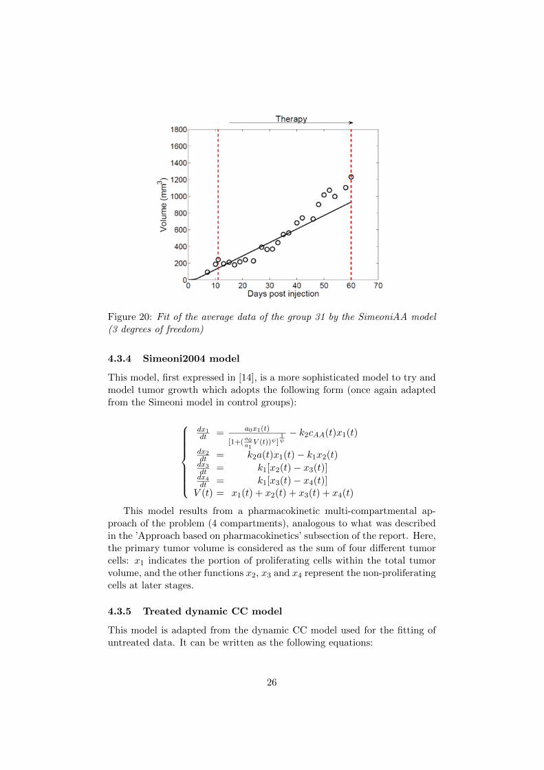
Figure 20: Fit of the average data of the group 31 by the SimeoniAA model(3 degrees of freedom)

4.3.4 Simeoni2004 model

This model, first expressed in [14], is a more sophisticated model to try andmodel tumor growth which adopts the following form (once again adaptedfrom the Simeoni model in control groups):

dx1dt = a0x1(t)

[1+(a0a1V (t))ψ ]

1ψ− k2cAA(t)x1(t)

dx2dt = k2a(t)x1(t)− k1x2(t)dx3dt = k1[x2(t)− x3(t)]dx4dt = k1[x3(t)− x4(t)]V (t) = x1(t) + x2(t) + x3(t) + x4(t)

This model results from a pharmacokinetic multi-compartmental ap-proach of the problem (4 compartments), analogous to what was describedin the ’Approach based on pharmacokinetics’ subsection of the report. Here,the primary tumor volume is considered as the sum of four different tumorcells: x1 indicates the portion of proliferating cells within the total tumorvolume, and the other functions x2, x3 and x4 represent the non-proliferatingcells at later stages.

4.3.5 Treated dynamic CC model

This model is adapted from the dynamic CC model used for the fitting ofuntreated data. It can be written as the following equations:

26

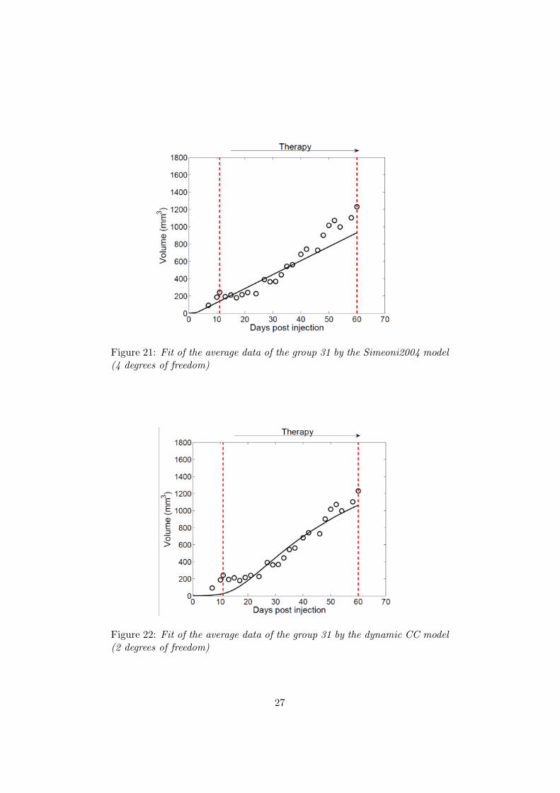
Figure 21: Fit of the average data of the group 31 by the Simeoni2004 model(4 degrees of freedom)

Figure 22: Fit of the average data of the group 31 by the dynamic CC model(2 degrees of freedom)

27

Figure 23: Fit of the average data of the group 31 by the Hahnfeldt model(3 degrees of freedom)

{dVdt = aV (t) ln(K(t)

V (t) )dKdt = aV (t)

23 − ecAA(t)V (t)

As a reminder, K represents here the carrying capacity (upper boundaryof tumor size), which is taken as a variable. We note that the pharma-cokinetic adaptation of the model considers the effect of the treatment as aterm which reduces the carrying capacity of the tumor. This last statementmakes sense biologically, for the antiangiogenic effect of sunitinib is indeedsupposed to reduce the vasculature of the tumor and thus the carrying ca-pacity in this model.

4.3.6 Hahnfeldt model

This model was first pitched in [17].

{dVdt = aV (t) ln(K(t)

V (t) )dKdt = bV (t)− dV (t)

23 − ecAA(t)K(t)

The differences are notable in the evolution of the carrying capacity. In-deed, unlike the treated dynamic CC model, the influence of tumor volumeon carrying capacity growth is decomposed into two phenomena (birth anddeath) illustrated by two distinct parameters (b for birth rate and d fordeath rate). Besides, the effect of the treatment on the carrying capacity isthis time proportional to the carrying capacity instead of the tumor volume.

28

This model actually causes several issues. First an issue of parameteridentifiability: indeed, b and d can be easily compensated, and thereforenone of them can be found to be identifiable. For that reason, and sincethe only element that matters is not the exact value, but the proportionbetween the different parameters in this equation, we decide to set b as 1.This way, we manage to obtain a model for which parameters are identifiable.

A second issue is a stability one when we want to optimize the differentparameters. Indeed, for an important range of starting points, the algo-rithm will converge very slowly. The starting points for parameters in ouralgorithm therefore need to be chosen very carefully.

4.3.7 Limits

If the models that were previously defined seem totally consistent theoreti-cally, they are faced with some difficulty when confronted with actual data.Indeed, as it can be noted in figures 18 to 23, the models do not seem ableto fit the data properly, in particular the early phases. Notably, the wholepre-treatment and growth arrest phases described on figure 15 can not befitted efficiently. This is a true problem, for it necessarily reduces the rele-vance of all the models to fit this kind of data.

This observed result is actually rather unsurprising, for the effect of thetreatment is in these models only considered by the drug concentration inthe organism. The more drug concentration is in the organism, the moretumor growth should be reduced, according to these models, which, as wesaw in the ’Shape of the treated data’ subsection, does not seem to be thecase. Therefore, no model is able to predict a change in the kinetic responsewhen the treatment does not change ; yet, it is the case in the data we areworking on. Besides, a good part of these models include parameters thatare not identifiable when confronted with actual data.

Since no model in the studied literature seems to be able to model thesevarious phases, it appears useful to create a new model that will be betterat evaluating the primary tumor kinetic response to treatment.

4.4 SunitinibTGI model

4.4.1 Required features

Before starting to actually build the model, it is important to detail thefeatures that our model will have to contain to be deemed satisfying.

• Ability to perform a better fit on the early stages of the treatment:

29

this is precisely the reason we build this new model for.

• Better overall fit quality: we want this new model to bring overallbetter statistical results on the fit of all phases, compared with modelsin the literature.

• Simplicity of the model: we want the model to contain mathematicalexpressions as simple as possible, so that the calculation time to finda solution to the model is as short as possible.

• Biological meaning of the parameters: we want this model to includeparameters conceived so that their values may bring us biological in-formation on the situation and the problem we are working on.

• Parameter identifiability: we want this model to have parameters beingidentifiable. We set a tolerance maximum threshold of 50 % on theerror (NSE) as our limit for parameter identifiability.

4.4.2 Shape of the selected model

The model is built upon 3 phases: during the first phase, ’pre-treatment’the growth is controlled by two parameters (a and γ1). When the treatmentstarts and is efficient, a second phase ’growth arrest’ begins ; the growth iscontrolled by 2 parameters (a, γ1) , and the duration of this phase is con-trolled by a parameter τ . Then, when the tumor regrows and the efficacyof the treatment seems to gradually fade, a new phase, called ’resistancephase’ starts, controlled itself by two parameters (a, γ2).

We can note the differences in growth kinetics between the three typesof data that we had distinguished in the part ’Shape of the treated data’:

• For the data sets that follow ’behavior breast 1’, we can see that thethree phases are represented and that the parameter a can be chosenequal to 0.

• For the data sets that follow ’behavior breast 2’, we can note that onlythe first two phases are represented (hence, no need to consider the γ2parameter), and that a is there, also, equal to 0.

30

• For the data sets that follow ’behavior melanoma’, we can note thatonly the last two phases are represented, and that a, in this case,cannot be picked as equal to 0.

4.4.3 Expression of the model SunitinibTGI

The conceived model, a 5-parameter model, can be written this way:

dV

dt=

aV γ1 if t ≤ tstartaV γ1 if tstart < t ≤ tstart + τaV γ2 if t > tstart + τ

(12)

where tstart is the day at which the treatment starts to be administered.

The choice to use three successive Power Law models can be justified bythe analysis performed in the part ’Comparison of the accuracy of the un-treated tumor growth models’, which showed that this model was satisfyingto fit untreated data, and that it had biological relevance.

Besides, it is a simple model (an explicit solution can be very easily

found for each one of the 3 phases: V (t) = (V 1−γ10 + a(1− γ1) t)

11−γ1 ), with

parameters that have a biological meaning, relevant to the context.

A biological interpretation possible for this model is the following.

Of course, when no treatment is administered, the situation is exactlythe same as for the control groups. When the treatment starts and is stillefficient (second phase), we suppose that it prevents the cells from prolifer-ating and will modify the value of the proliferating rate a into a a. Whenthe treatment loses a part of its efficacy (third phase), we suppose that it isrelated to the fact that the tumor cells have developed a form of resistanceto sunitinib. This resistance may be biologically related to the openingof a another way to pursue angiogenesis. Among the hypotheses that wecould draw is that when the antiangiogenic drug is administered at first, itcompletely blocks and starves the tumor cells that would otherwise growthrough the receptors (RTKs) blocked by sunitinib. But not all cells growthanks to these receptors. Some of them may grow through other cellularpathways. Some may notably grow through hypoxia, and do not require thesame amount of nutrients. This way, the angiogenesis would start over whenthose hypoxic cells would get more significant in the whole pool of tumorcells. Unaffected by the antiangiogenic drug, they would be able to grow inspite of the administered treatment. But, since their vasculature is muchless stable, their growth would be less strong than tumor cells that would

31

grow through RTKs. Anyway, this change in vasculature could help us jus-tify this switch of γ between the two phases. Of course, this interpretationcan not be confirmed, but is one way of seeing the model with biologicalrelevance.

Still, on a mathematical point of view, two major problems seem to risewith that definition of the model.

4.4.4 Smoothing of the model

First, the function that is calculated is not continuously differentiable, forits derivative is of course discontinuous.

This causes a problem, notably related to parameter identifiability. In-deed, statistical analyses that were performed showed that the lack in differ-entiability for the model led to significantly larger NSEs for all parameters,preventing parameter identifiability in all cases.

For that reason, we decided to smooth the model to make it continuouslydifferentiable, and in particular the explicit solution, since a statistical anal-ysis that was performed showed that it was the smoothing that led to thebest improvement in stability. With this new smoothing, the model writesas:

V1 + (Vτ − V1)RTd + (V2 − Vτ )Rτ (13)

where V1 is the explicit solution of the model in the first phase, Vτ theexplicit solution of the model in the second phase and V2 the explicit solu-tion of the model in the third phase. As for the smoothing terms, they canbe expressed as:

RTd = 0.5(1 + tanh(pcont(t− tstart))

Rτ = 0.5(1 + tanh(pcont(t− tstart − τ))

In this smoothing term, pcont is chosen by trial and error (here, its valueis set to 2.1). The logic behind the use of the smoothing term RTd is that,when t << tstart, RTd ≈ 0. When t draws near tstart, RTd draws near1, and it remains close to 1 ∀t ≥ tstart. Thanks to this, we thus obtain acontinuously differentiable model. This mathematical process is only therefor parameter identifiability, and so that it checks mathematical propertiesthat will make it easier to be used.

32

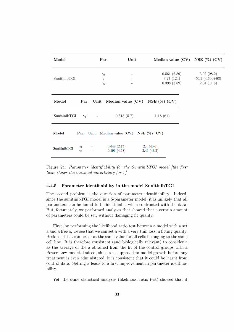
Figure 24: Parameter identifiability for the SunitinibTGI model [the firsttable shows the maximal uncertainty for τ ]

4.4.5 Parameter identifiability in the model SunitinibTGI

The second problem is the question of parameter identifiability. Indeed,since the sunitinibTGI model is a 5-parameter model, it is unlikely that allparameters can be found to be identifiable when confronted with the data.But, fortunately, we performed analyses that showed that a certain amountof parameters could be set, without damaging fit quality.

First, by performing the likelihood ratio test between a model with a seta and a free a, we see that we can set a with a very thin loss in fitting quality.Besides, this a can be set at the same value for all cells belonging to the samecell line. It is therefore consistent (and biologically relevant) to consider aas the average of the a obtained from the fit of the control groups with aPower Law model. Indeed, since a is supposed to model growth before anytreatment is even administered, it is consistent that it could be learnt fromcontrol data. Setting a leads to a first improvement in parameter identifia-bility.

Yet, the same statistical analyses (likelihood ratio test) showed that it

33

was not interesting to set γ1 to the average of the control groups γ fittedwith a Power Law model, for it led to a dramatic decrease in fit quality. Thisresult can be explained by individual variability between mice, and becausethe influence of γ1 on the trajectory of our graph is much more important.For that reason, individual variability can really make major differences. Itis possible however to set an a priori on γ1, to pick it as a variable followingthe γ control distribution fitted with Power Law model. This makes sensebiologically, for the same reason as the fact of setting a ; these parameterscontrol the pre-treatment tumor growth, and it is thus relevant to considerthat they can be learnt from the control groups. There again, restrictingthe range in which we can choose γ1 leads to an improvement in parameteridentifiability.

The third step towards an even better parameter identifiability is thesetting of a. This decision is not really motivated by a biological reasoning,but rather by data analysis, and statistical analyses analogous to the oneswho led to the setting of a and the restrictions on γ1. They showed that acould be set at the same value for all cells from the same cell line. a con-trolling tumor growth in the early stages of the treatment administration,it would not be consistent at all to learn it from control groups. For breastcancer cells, since we have a clear arrest in tumor growth during this phase,we quite simply choose a equal to 0. For melanoma cells, we first fit a modelwith a free a. The median value of a obtained by this process is then thevalue to which we will set a in ulterior analyses.

This way, we end up obtaining a model with only 2 parameters left totallyfree (τ and γ2), and one parameter constrained in a specific distribution (γ1).We therefore improve quite significantly the parameter identifiability of themodel [see figure 24].

4.4.6 Comparison with classical models

This model was compared, for each data set, to the other classical models fortreated tumor growth ; the results are displayed on figure 25. We can notethat for all data sets, and for all statistical tools, the SunitibTGI modelsseems better fitted to model the process of treated tumor growth.

4.4.7 Notable results related to the model ([14])

Now that the model has been shown to be both efficient in terms of fittingcapacity and in terms of parameter identifiability, we can try and evaluatethe values of its parameters on the various data sets, and hence note a fewinteresting elements on the biology of the problem.

34

Figure 25: Comparison of the SunitinibTGI model with classical models

35

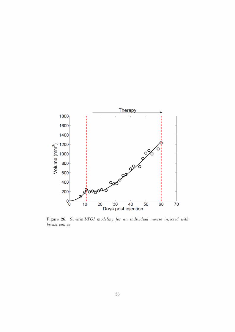
Figure 26: SunitinibTGI modeling for an individual mouse injected withbreast cancer

36

Figure 27: SunitinibTGI modeling for an individual mouse injected withbreast cancer

Figure 28: SunitinibTGI modeling for an individual mouse injected withmelanoma

37

1. We notice that during the ’resistance’ part of the treatment for breastcancer, tumor growth is significantly weaker than growth without atreatment at all. Indeed, if we perform for instance the analysis ongroups 31, we notice that we obtain medians γ1 = 0.56 (for a NSE of3%) and γ2 = 0.40 (for a NSE of 2%).

It seems to imply that even after the treatment has its efficacy clearlyreduced, it still has an impact, and a noteworthy influence to reducetumor growth. The interpretation based on hypoxia that was describedin the ’Expression of the model SunitinibTGI’ subsection could be anexplanation of it.

2. We do not have a sufficient amount of data to be able to model andcompute the optimal drug scheduling, as we would want to. Indeed,since a scheduling rests on two significant elements (dose and adminis-tration time), to be able to perform a proper analysis, we would needto have examples with one of those two features (only) as commonelements, and the data sets that were provided, did not allow us toobtain this kind of result. Still, the parameters that are computed bythe model can help us make a decision between 2 different scheduling.

For instance, we can note that for group 31, which has the follow-ing scheduling (60 mg/kg on 40 days), we have medians γ1 = 0.56(NSE = 2%) and γ2 = 0.40 (NSE = 3%) ; for group 32, with the fol-lowing scheduling (120 mg/kg on 7 days), we have medians γ1 = 0.57and γ2 = 0.52 (NSE = 2%).

We may note that a larger dose in a shorter time period, leads toa ultimate tumor growth much higher later, and to a similar tumorgrowth during treatment. Therefore, if we are interested in reducingas much as possible the tumor size before surgery, for instance, we cansee that we should, generally, privilege treatment 31.

3. For the melanoma data, and the sunitinib-resistant cells, we first noticethat is is statistically, and in terms of fitting capacity, advantageous toset τ at the value for the time of end of the treatment. We can concludefrom it that in this specific situation (melanoma/sunitinib-resistantcells), the end of the efficacy phase coincides exactly with the end ofthe treatment. We then deduce that in the case of melanoma, thereis no post-treatment efficacy phase ; once the treatment is stopped,

38

tumor automatically regrows without any delay. And, more impor-tantly, the treatment does not look as if its efficacy were significantlyreduced during its whole administration.

4. We also note that the higher the tumor volume is at the beginningof the treatment, the higher τ will be. Indeed, for the group 31 forinstance, which has an initial tumor volume of 196.7 mm3 we haveτ = 5.28 days (NSE = 39%) ; and for group 51 (initial tumor volume:439.5 mm3), we have τ ≥ 14.

Hence, the higher the initial tumor volume is, the longer the growtharrest phase will last. This result tends to give credit to the hypoxiainterpretation of our model that we had made in the subsection ’Ex-pression of the model SunitinibTGI’: the higher the number of cellsthat would grow with the RTK pathway is, the longer the antiangio-genic drug will have to proceed to completely eliminate those cells togive place to the hypoxic ones (related to treatment resistance).

4.4.8 Limits of the model

This model is not exempt from problems and limits. Among them, wecan note that no direct and explicit connection to pharmacokineticshas been clearly established. The impact of pharmacokinetics is obvi-ously in the parameters, but the exact relationship that connects, forinstance, drug concentration and the value of some of the parameters,is not obvious at all.

One idea that was developed during this internship to connect themturned out to be fruitless.

Considering the formula τ = inf{t,∫D(t) ≥ s} (where D is the admin-

istered dose, and s a parameter to be optimized) was meaningful, forit implied that above a certain threshold of concentration, the drugpartly lost its efficiency, and the tumor cold grow again. Unfortu-nately, as it can be evidenced with the fact that τ depends on theinitial tumor volume, obviously completely unrelated to the adminis-tered dose, this was not a correct way of seeing the problem.

Establishing an explicit connection with pharmacokinetics would bringa supplementary layer to the model, but during this internship, it didnot look that obvious to make.

39

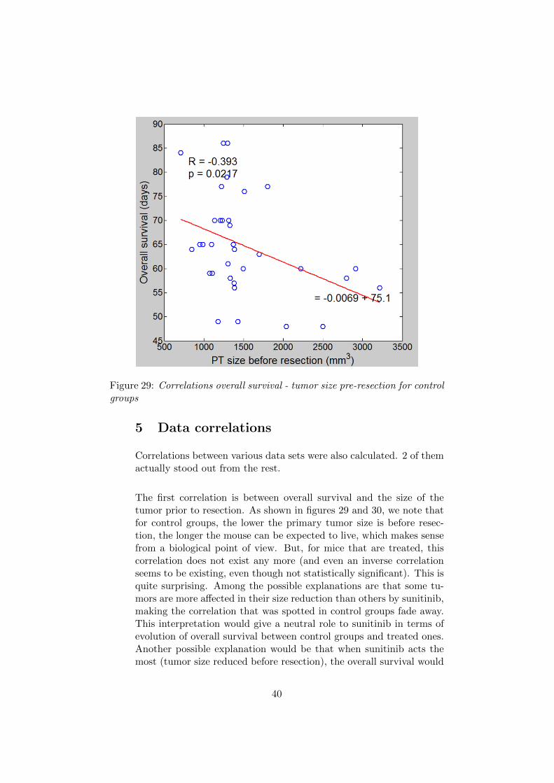
Figure 29: Correlations overall survival - tumor size pre-resection for controlgroups

5 Data correlations

Correlations between various data sets were also calculated. 2 of themactually stood out from the rest.

The first correlation is between overall survival and the size of thetumor prior to resection. As shown in figures 29 and 30, we note thatfor control groups, the lower the primary tumor size is before resec-tion, the longer the mouse can be expected to live, which makes sensefrom a biological point of view. But, for mice that are treated, thiscorrelation does not exist any more (and even an inverse correlationseems to be existing, even though not statistically significant). This isquite surprising. Among the possible explanations are that some tu-mors are more affected in their size reduction than others by sunitinib,making the correlation that was spotted in control groups fade away.This interpretation would give a neutral role to sunitinib in terms ofevolution of overall survival between control groups and treated ones.Another possible explanation would be that when sunitinib acts themost (tumor size reduced before resection), the overall survival would

40

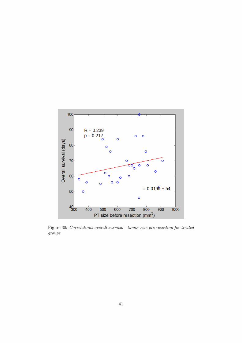
Figure 30: Correlations overall survival - tumor size pre-resection for treatedgroups

41

Figure 31: Correlations tumor size pre-resection - metastatic burden forcontrol groups

Figure 32: Correlations tumor size pre-resection - metastatic burden fortreated groups

42

tend to decrease, which would give a harmful role to sunitinib. Fromthis analysis only, we cannot choose a perfect interpretation, but it isstill an interesting result to consider.

The second correlation which is interesting to consider (figures 31 and32) is between the size of the primary tumor before resection, andthe metastatic burden 15 days after resection. What we can noteis that for the control groups, the higher the primary tumor size is,the higher the metastatic burden will be, which, once more, makessense biologically. But for mice that were treated with sunitinib, thecorrelation does not exist anymore (and even seems to be, even thoughstatistically insignificant, inverse). This can also be explained with anasymmetrical influence of sunitinib: it would affect some tumors morethan others all while not modifying the related metastatic burden, itsrole would therefore be neutral in the issue. Or we can see it as, whenthe tumor size is lower, then the sunitinib has acted more, and a moresignificant metastatic burden can be found, which would, under thosecircumstances, show that the sunitinib would indeed provoke moremetastatic burden. It would then be harmful. But once more, fromthose singular experiments, we cannot know which interpretation issound.

6 Computing the metastatic burden ([7], [18])

Our model for primary tumor growth SunitinibTGI can then be used totry and describe the metastatic burden, as evidenced by the followingsection.

6.1 General equation

Based on [7], we see that the evolution of the metastatic burden canbe evaluated thanks to the following transport equation:

∂ρ∂t + ∂(ρg)

∂V = 0g(V0)ρ(t, V0) = µVp(t)ρ(0, V ) = 0

where ρ(V, t) is the metastatic density that rules the metastatic popu-lation, for a given volume V at a specific time t ; g is the function thatdescribes the growth ; Vp(t) describes the volume of the primary tumor; µ is a parameter that describes the metastatic process (colonization

43

Figure 33: Evolution of the metastatic burden (control groups)

and dissemination).

Thanks to the analyses that were led in the previous part, we knowthat we have obtained a model allowing to evaluate the volume ofthe primary tumor Vp(t) more precisely than classical models. Here,we then choose Vp(t) following the SunitinibTGI model, g followinga Gomp-Exp model, and we approximate this equation numericallyusing the method of characteristics.

6.2 Conclusions

When numerically solved with the method of characteristics, this equa-tion returns us a ρ, which can be displayed in the graphs on figures33 and 34. What we can note is that no clear acceleration is actu-ally found computationally between the cases where no treatment isadministered, and the cases where sunitinib is actually administered.This tends to show that the results of metastatic acceleration do notlook like they actually have a total relevance on a statistical point ofview.

44

Figure 34: Evolution of the metastatic burden (treated groups)

6.3 Prospects

Some work still needs to be done in order to improve the metastaticprocess modeling. For instance, being able to distinguish (through ananalysis of µ) the dissemination and the colonization in the metastaticprocess could lead us to more insightful results. Indeed, if we wereable to distinguish these two parts of the metastatic process, we wouldtherefore be able to see how each one of those two phenomena can beaffected with external parameters independently, instead of consider-ing the whole process as one.

In particular, in this case, to be able to model the impact of hypoxia,it could prove to be interesting to try and express µ as a function of KV ,where K is the vascularization and V the volume. This way, a possi-ble connection between hypoxia and metastatic acceleration could beshown (or dismissed).

Finally, we have made sure all along that all of our parameters werestatistically significant (low NSE,...). This also gives us hope that itmay be possible to build, from that basis, a predictive model, whichwould be able, from a given number of input points for primary tumor

45

size and metastatic burden, to predict with a relative accuracy theevolution of the disease.

7 Conclusion

As a summary, we could say that the mathematical data analysisof the primary tumor and the metastatic burden evolution for micedoes not show a clear connection between sunitinib administrationand metastatic acceleration.

This result was obtained after an optimization algorithm benchmarkshowed that the Nelder-Mead or the Levenberg-Marquardt algorithmswere the most fitted to deal with the problem. Among the classi-cal models of untreated tumor growth, the Power Law seemed to beone of the most interesting in terms of statistical results and biologi-cal meaning. When working on treated tumor data, we saw that noclassical model was really able to describe accurately the evolution ofthe primary tumor. For that reason, a new model, whose propertieswere checked, was built. This new, more efficient model, allowed tofind new interesting results on the evolution and the primary tumor,and on correlations between some elements of data. Incorporating thismodel into a classical metastatic equation helped show that the accel-eration was clearly not obvious from a mathematical point of view.

46

8 Annex

8.1 Cancer biology ([9])

8.1.1 Overview

Cancer is, in France, the first cause of mortality: about 30% of peopledie from this disease. In spite of the intensive research that is beingcarried out, cancer remains a disease that is not entirely understood.The aim of this annex is to describe, as a complement to the rest ofthe internship report, the basements of cancer biology.

To describe it in a few words, cancer is a disease which induces theuncontrolled growth of a group of cells, the primary tumor, within anorgan. At a certain stage, some cells from the primary tumor man-age to leave the original organ through the blood vessels or the lymphnodes of the organ, to settle in a new organ. The cells that carry outthis trip through the body are called metastases. Metastases are, inmost cancers, the main cause of death, and they also explain the dif-ficulty in treating cancers ; fighting the primary tumor is not enoughto cure the patient, since other tumors may grow in other parts of thebody.

This annex deals with two different subjects: a description of thedisease itself and of its biological mechanisms, and a little summary ofthe possible treatments.

8.1.2 Detailed description of the disease

During a cancer, some cells will grow and divide abnormally. The newstructure that then rises from this uncontrolled growth is called a tu-mor. But for the tumor to actually trigger a cancer, it must satisfy acertain range of conditions, such as:

• the ability to sustain proliferative signals. The cancer cells are notcontrolled in their proliferation by the environment, as opposedto normal cells in organism.

• the ability to evade growth suppressors. The cancer cells havethe ability to ignore the signals that restrict cell growth and pro-liferation.

• the ability to resist cell death, in particular apoptosis. Apoptosisis the programmed cell death, which notably occurs when the cell

47

is abnormal. The deactivation of the signal can then prevent theorganism from destroying cancer cells.

• the ability to get replicative immortality. Unlike all normal cells,cancer cells can process an unlimited number of cell cycles, andundergo mitosis an unlimited number of times.

• the ability to induce angiogenesis: the primary tumor can senditself signals to create blood vessels, which will supply the tumorin nutrients, and will allow it to grow even more.

• the ability to invade the full body (with metastases) throughblood vessels and the lymph system.

All these properties, common to all cancers, are the core ideas of whatthe disease is capable of, and of how it proceeds. In the following sec-tions, we will focus more precisely on the evolution of the disease.

Genetics

Like all biological phenomena, cancer is a disease in which geneticsplays an important part. Indeed, cancer is born from mutations whichaffect specific genes, and which lead to malfunctions in various phasesof the cell cycle. The three main genes responsible for it are:

Oncogenes: oncogenes are mutated genes, which send signals to causeuncontrolled cell growth. The said cells are then liberated from theconstraint of limited cell proliferation. If an oncogene appears after agene mutation, the first step to cancer is reached.

Tumor suppressor genes: even once the oncogenes have appeared, de-fense mechanisms against cancer still exist in the organism. Amongthese mechanisms, we can count tumor suppressor genes. These aregenes which have the ability to slow down (or even arrest) the cell cy-cle. This way, even if a cell proliferates too much because of oncogenes,the tumor suppressor genes still retain control on how it divides, andcan stop the process or even induce the apoptosis (programmed celldeath) of the cell. But if a mutation occurs, reducing (or erasing) thepower of the gene, then the first defense mechanism of the organismis neutralized. In most cancers, the mutation of these genes occurs inthe early stages of the disease.

DNA repair genes: another defense mechanism in the organism. Thesegenes code for proteins which will solve the errors due to a mutation.

48

Therefore, they widely reduce the development of tumor cells. Butthey only reduce it, because these genes have limited repairing power,and if the error rate is considerably larger than the repairing capacityof the gene, the cells will still uncontrollably grow. And of course, amutation of these genes, if it leads to a reduced power or a vanishedpower, greatly accelerates the development of the tumor cell.

If those conditions are verified, we have then reached the first stage ofcancer. Due to these genetic mutations, the cells will grow uncontrol-lably in the organ, and give birth to a large cell structure, the tumor.Yet, at this point, the tumor can still be benign, and can fail to de-velop more. For it to happen, several events need to occur.

Development of the tumor inside the organ

The first thing that comes to mind is the fact that to grow, the tumorneeds to be supplied in nutrients through the blood. In some cases, thetumor cells, perceived as abnormal by the organism, are not supplied.This way, the tumor cells cannot live long, and are destroyed not longafter they are created. Thus, even if the tumor cells undergo uncon-trollable growth, since they can not stay alive, it is not an immediateproblem.

The issue is raised when the tumor is supplied in blood and nutrients.This is related to the fact that the tumor, in most situations, is notmade of cells which are all abnormal. Indeed, the tumor often managesto include normal cells in the structure (the normal cell tissue within atumor is called the stroma). This way, the organism, recognizing thesecells as normal ones, will supply the tumor in nutrients and blood. Thetumor will then be able to grow, while being fed by the organism itself.

It is good to note that at this stage, the tumor can still be consideredas benign. Therefore, it is not -yet- really dangerous for the patient,unless the tumor is located in a very fragile and specific organ (suchas the brain for instance). If the illness is treated at this step, it canbe cured with no problem.

The tumor has then managed to grow to a much larger size (gener-ally around 1mm3). But it is still limited in its development by theamount of blood that is supplied; as it is now, it is still not a dangerfor the individual. For it to grow more, the tumor has to receive morenutrients. The tumor, in all cancers, ends up being able to induce aphenomenon called angiogenesis.

49

Angiogenesis is a physiological process through which new blood ves-sels are created. It is a normal and vital process (crucial for woundhealing for instance), but it may be impeded by the tumor so thatit can grow more. In all cancers, the tumor will be able to induceangiogenesis, leading to the development of a vascular system withinthe tumor. This way, the tumor will be supplied in more nutrients,and will be able to grow even more and to considerably develop. Oncethis step has been reached, the likelihood of cancer development con-siderably rises and the illness needs to be treated as quickly as possible.

On a biological level, angiogenesis in induced by the tumor throughthe VEGF protein (Vascular Endothelial Growth Factor). This proteinis part of the system that restores the supply in oxygen when bloodcirculation is inadequate. Signals leading to the production of VEGFproteins are emitted by the tumor itself. The tumor, through previousmutations, carries VEGF-R, receptors for the VEGF proteins. Thisway, the tumor stimulates the production of VEGF proteins for itself,which makes the local vascular system expand. The tumor, being sup-plied in more nutrients, can therefore grow again. It is noteworthythat all the receptors related to this type of protein signals can becalled receptor tyrosine kinases (RTKs).

We have then reached the second stage of cancer.

Metastatic process

The tumor is now a very large cell structure located inside an organ,and which is able to grow because of angiogenesis. Yet, the cancer isnot (unless it is located near the brain) a deadly threat for now on. Itwill become one if it is capable to metastasize.

Metastatic dissemination is the process by which some cells from thetumor will leave the organ in which they are located to reach a neworgan (through the blood vessels or the lymphatic system), where theywill settle and create a new tumor. This way, the cancer can dissemi-nate in the entire organism. This metastatic process is responsible for90 % of patients’ death. For this reason, many studies are carried outto try and understand te phenomenon.

Epithelial to Mesenchymal Transition

50

The EMT (Epithelial to Mesenchymal Transition) is a recent discov-ery, which may explain the process by which cells from the tumor canleave it to join a blood vessel or a lymph node.

Epithelium is a type of organic tissue, which lines the surface of bloodvessels and organs. It is made of a large number of epithelial cellsbound together. The epithelial cells are not free to move, they are allconnected with very tight junctions.

On the other hand, mesenchyme is a type of tissue which is character-ized by associated cells (mesenchymal cells), loosely bound together.The mesenchymal cells can move rather freely and are not tightly con-nected to one another.

It has recently been shown that some cancerous cells, mostly locatedin the periphery of the tumor, were able to move from an epithelialcell state to a mesenchymal one. Thanks to this transition, the cellsare able to move more freely, and they can then join blood vesselsor the lymph nodes, in order to reach another organ. They becomemetastases. Once this step has been reached, we are at the third stageof cancer.

Dissemination and colonization

Once in the blood vessels, the metastases have to escape the immunesystem (few cells will actually survive), which often perceives them asstranger cells, and then destroys them. What ensues can be dividedinto two parts: dissemination and colonization.

During the dissemination phase, the metastases will be in the bloodor the lymph nodes.

At some point, the metastases can reach a new organ and settle there,through MET (Mesenchymal to Epithelial Transition), the inverse ofthe EMT process. Thanks to this, the metastases can form a newstructure (secondary tumor) where they will be jointly bound (as anepithelial tissue) in the new organ. They have thus colonized the or-gan, and the secondary tumor will start to grow again, and eventuallyto metastasize. Once an organ has been colonized, we have reachedthe fourth stage of cancer.

51

It can be interesting to note that the early stages of the colonizationphase can be very long, and even seem like dormancy. Indeed, for awhile, at the beginning of the colonization, the size of the tumors donot change, and the health of the patient does not worsen either.

But once this dormancy phase is over, metastases will grow more andmore aggressive, and the health of the patient will just go declining.

8.1.3 Current treatments

Some treatments exist to improve the life and the health of ill patients.If they are presented separately in this part, they are very often com-bined for more efficacy.

Chirurgy

The first - and seemingly more obvious - treatment is the resection(surgical removal) of the primary tumor. It seems like a pretty in-tuitive step, but the effects of such an operation are contrasted. Iffor some patients, a notable improvement in health was noticed, itis not the case for all in general. Indeed, one interesting aspect con-cerning the primary tumor is that it both sends proliferative signalsto itself, but that it also sends inhibition signals. Removing it hasled, in some cases, to a notable acceleration of metastatic growth, andthen a worsening of the state of the patient. Therefore, the issue ofwhether removing surgically the tumor is the best option, when it isnot located in an organ where it is directly lethal, is still an open one.

Chemotherapy

The chemotherapy is the administration of the combination of sev-eral drugs, which will have as a common behaviour, to target the cellsthat divide very quickly. Of course, the idea is this way to destroythe tumor and metastatic cells, which divide uncontrollably. But notonly cancerous cells are destroyed through this process: some bloodcells, hair cells, among others, will also be targeted. For that reason,chemotherapy is a very important type of treatment, but with a lot ofadverse effects.

Targeted therapies

52

The idea of targeted therapies is, instead of destroying the cells di-rectly, to attack it through its biological mechanisms, through extra-cellular (outside the cell) or intracellular pathway. One of the mostuseful ways to fight cancer is to combat angiogenesis, with what iscalled antiangiogenic drugs. Let us consider the example of sunitinib.

The sunitinib is a molecule which inhibits cellular signaling by tar-geting receptor tyrosine kinases (RTKs), including receptors for vas-cular endothelial growth factor receptors (VEGF-Rs). The inhibitionof these targets allow to reduce tumor vascularization, and can leadto the apoptosis of several cancer cells. This may allow to shrink thetumor.

53

8.2 Statistical tools

We display here a little overview of the various statistical tools usedfor data analysis in the report.

Let us consider a data set (yi)i∈[1,n] and f the model considered to fitthe data (with (ti)i∈[1,n] the time range)

8.2.1 Sum of squared errors (SSE)

The sum of squared errors (SSE) can be defined as:

SSE =n∑i=1

(yi − f(xi))2 (14)

This statistical value is then simply the error, added for all points,committed by considering the model instead of the data. The bestmodel, in that regard, is then the model for which the error is thesmallest.

But the criterion, as helpful as it may be, is often insufficient to fullycompare 2 different models.

8.2.2 Root mean squared error (RMSE)

The root mean squared error (RMSE) can be written as:

RMSE =

√∑ni=1(yi − f(xi))2

n(15)

RMSE is a criterion which is very close to SSE.

8.2.3 Akaike Information Criterion (AIC)

Let L be the maximum value of the likelihood function for the model,and k its number of parameters. The AIC is then defined as:

AIC = 2k − 2 ln(L) (16)

The model that has the lowest AIC is then the model that has to befavored. We notice that as the likelihood maximum is high, the AICgoes down, and that AIC grows with the number of parameters. This

54

criterion is then a way to choose the best model, all while penalizingthe number of parameters. Indeed, the more parameters we add, thelowest the error will be ; but the number of parameters is also an im-portant criterion to consider. This criterion takes it into account, byconsidering it as a penalty for a model.

This criterion is therefore adapted to the comparison of models withdifferent number of parameters.

8.2.4 R2 coefficient

Let us denote

y = 1n

∑ni=1 yi

SStot =∑

i(yi − y)2

SSreg =∑

i(f(ti)− y)2

SSres =∑

i(yi − f(ti))2

R2 = 1− SSresSStot

(17)

The R2 coefficient is then a measure of how much better it is to con-sider the model to fit the data instead of simply choosing the constantfunction, equal to the average of all data. R2 can be negative ; in thatcase, it means that it is better to consider the constant function to fitthe data. A negative R2 is a sign that the model considered is notable to fit the data at all.

8.2.5 Log-likelihood ratio

The likelihood ratio test is a statistical test which allows to compare 2models, when they do not have the same number of parameters. Letus call Ln the likelihood for the model with fewer parameters, La thelikelihood for the model with more parameters. Then, the likelihoodratio is calculated this way:

D = −2 ln(LnLa

) (18)

The likelihood ratio allows therefore to evaluate which one of the twomodels considered is to be favored.

55

8.3 Optimization methods for the Gompertz model

8.3.1 Introduction

Setting of the problem

As of today, the phenomenon of tumor growth is still an open prob-lem. Indeed, no equation is considered as the equation which wouldperfectly model the data. Yet, for, notably, biological reasons, theGompertz model is one of the most acclaimed models to describe thisgrowth ([1], [2]). During this project, a simplified model of Gompertzgrowth, depending on 2 parameters, α and β, was considered. Thegoal of this project was to compute several optimization algorithms inorder to find the values of α and β that allowed the best fit for thetumor growth data provided. This work is interesting for the resultsthat were found about the efficiency of the optimization algorithms fora rather simple model can be extended to more complicated ones.

All the following results were computed using Python and its numeri-cal (numpy) and graphical (matplotlib) libraries.

The Gompertz model

The Gompertz model is a model which is commonly used in the liter-ature to describe tumor growth. It can be written as follows:

dV

dt= (α− β ln(V ))V

V (0) = V0

(19)

We notice that the form of the solution curve (figure 35) is compatiblewith a phenomenon of tumor growth. During the early stages of can-cer, there are very few tumor cells, restricting, therefore, the growthrate. Once the number of tumor cells rises, the growth rate will un-doubtedly increase until a certain stage. Indeed, since the resourcesfor all cells are limited, the scarcity of the nutrients when there are toomany tumor cells tends to gradually decrease the growth rate. Thisfunction seems to fit well the phenomenon of tumor growth.

In this project, we made the assumption that the tumor is 1mm3-longinitially (V0 = 1). Our work was to try and estimate the parameters

56

α and β which allowed the best fit for the data provided.

Data provided

The data that was provided to calibrate the model represent the growthof a tumor made from a lung cell line (LLC: Lewis Lung Carcinoma),subcutaneously injected into mice. The volumes were measured usinga caliper. The largest (L) and smallest (w) diameters were measuredsubcutaneously using calipers and the formula V = π

6w2L was used to

compute the volume (ellipsoid).

4 6 8 10 12 14 16 18 20

Time(days)

0

200

400

600

800

1000

1200

1400

Tum

or

volu

me (mm

3)

Data provided

Figure 35: Data provided

8.3.2 Optimization problem

Optimization criterion

We want, in this project, to find the values of α and β that will leadus to a solution as close as possible to the data. For this reason, wechoose our optimization criterion F as (with n the number of dataprovided, yi the volume attained in ti in the data, and M the exactsolution to the Gompertz ODE):

57

F (α, β) =

n∑i=1

(yi −M(ti;α, β))2 (20)

We will consider log(F ) as the criterion instead of F for the gradientdescent algorithms, since it makes convergence easier. We will thentry to find the α and β minimizing the criterion.

Analytic solution to the Gompertz ODE

In this section, we calculate the function which solves the GompertzODE. By carrying out a variable separation method (function of theform − 1

βu′

u ), we end up obtaining the analytic solution, displayed onfigure 36:

M(t;α, β) = exp(α− exp(−βt)(α− β ln(V0))

β) (21)

0 5 10 15 20 25 30 35

Time (days)

0

2000

4000

6000

8000

10000

12000

14000

Tum

or

volu

me (mm

3)

Exact solution

Figure 36: Solution to the Gompertz differential equation, with V0 = 1,α = 1, β = 0.1

Analysis of the optimization criterion

58

We plot on figure 37 the optimization criterion depending on the twoparameters α and β. We can notice that there is a large number of lo-cal minima (”valley” of pseudo-minima), especially on figure 38, whichwill be a problem for some optimization algorithms that we will useafterwards.

This problem is clearly illustrated on figure 39, since we see that thecontour lines of F depict very thin areas close to the global minimum,which may cause the algorithm to stop even if the point reached is notthe one we wanted.

Besides, if we get a little further from the area with the more commonvalues of α and β, we notice that the function is somewhat trouble-some. Indeed, figure 40 shows that log(F ) can take extreme values,which will make F impossible to evaluate numerically. This issue willbe addressed in the part devoted to the Levenberg-Marquard algo-rithm.

8.3.3 Optimization algorithms

All the optimization algorithms which are studied in this report in-duce a propagation of the considered point in the descent directionof the optimization criterion. A descent direction is a direction alongwhich the criterion has a strictly negative directional derivative; fol-lowing it will then undoubtedly lead to a minimization of the function.

Gradient descent with constant step

Theory

The algorithm of gradient descent draws its logic from the fact thata function F will decrease the most in the direction that is opposedto the direction of the gradient. It takes for input an initial valuex0, which will be the starting point of the algorithm. The gradientdescent algorithm generates a sequence of iterated points x1, x2, ... andis stopped when a test is satisfied, sending as output the last point xngenerated. It follows 4 phases:

(a) Simulation: we first calculate ∇F (xk).

(b) Test: we check if ||∇F (xk)|| ≤ ε. If this is the case, then thealgorithm stops, and the output xk is returned.

(c) Calculation of the step: here, we consider a constant step αk.

59

0.50.6

0.70.8

0.91

1.11.2

1.3

0.05

0.1

0.15

0.2

10

15

20

25

30

35

40

alpha valuesbeta values

log(

F)

Figure 37: F depending on α and β

(d) New point: we consider a new point xk+1 = xk−αk∇F (xk), andwe start over to phase 1.

This way, we end up reaching a local extremum. But nothing, in thisalgorithm, can guarantee us than the value returned is a global mini-mum.

Analysis of the results

This algorithm was implemented (αk = 0.01, ε = 0.0001), and appliedto the function log(F ).

60

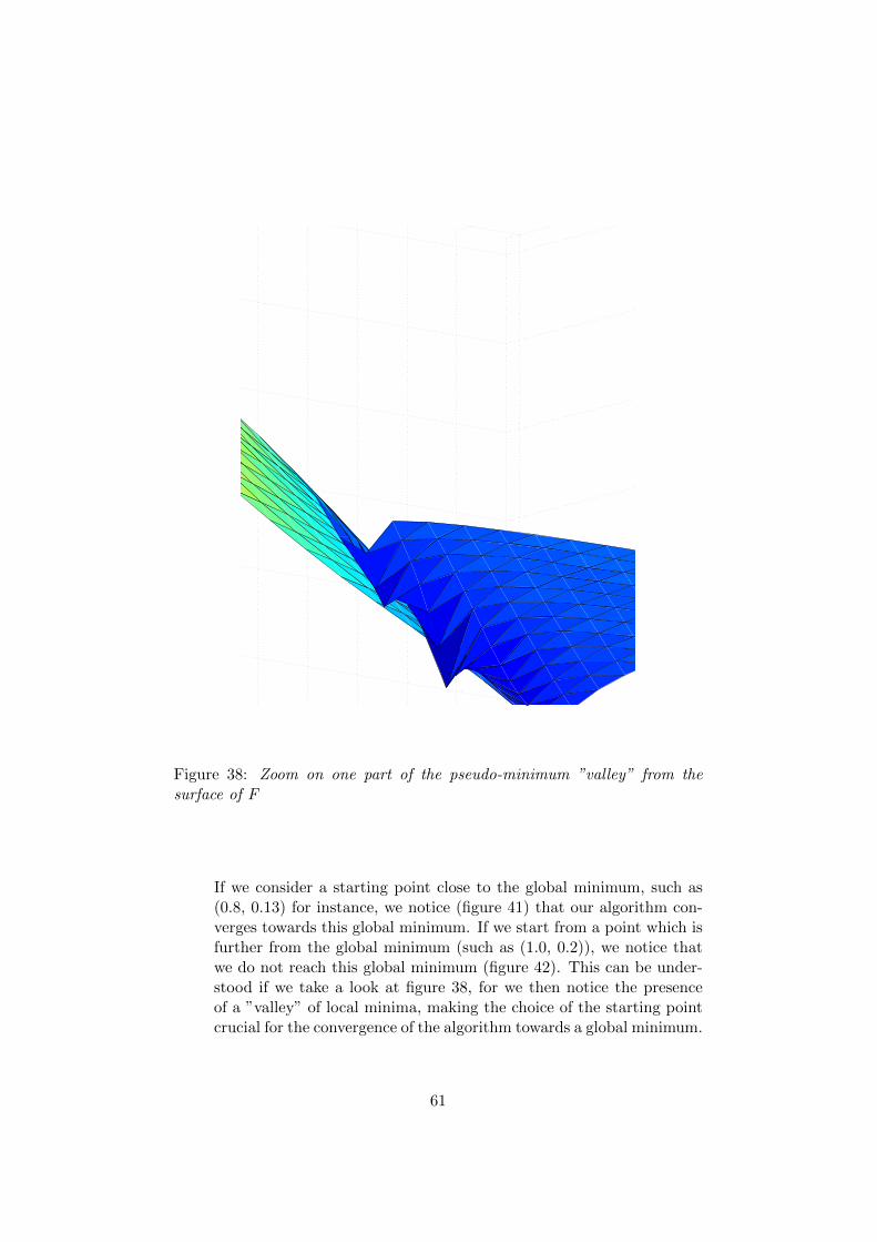
Figure 38: Zoom on one part of the pseudo-minimum ”valley” from thesurface of F

If we consider a starting point close to the global minimum, such as(0.8, 0.13) for instance, we notice (figure 41) that our algorithm con-verges towards this global minimum. If we start from a point which isfurther from the global minimum (such as (1.0, 0.2)), we notice thatwe do not reach this global minimum (figure 42). This can be under-stood if we take a look at figure 38, for we then notice the presenceof a ”valley” of local minima, making the choice of the starting pointcrucial for the convergence of the algorithm towards a global minimum.

61

0.6 0.8 1.0 1.2 1.4

alpha

0.06

0.08

0.10

0.12

0.14

0.16

0.18

0.20beta

2.16

2.32

2.48

2.64

2.80

2.96

3.12

3.28

3.44

3.60

Figure 39: Contour lines of log(F)

Besides, we notice that the calculation time is quite important com-pared to the other algorithms studied. Indeed, for an initial point (0.8,0.13), the convergence time is about 0.142 s.

Moreover, as it can be seen from figure 43, we notice that for a start-ing point (1.0, 0.1), the algorithm converges after about 750 iterations(which is a lot, compared to the other optimization algorithms). Wealso notice a bigger fall as the function gets closer to its extremum.

All these conclusions can be confirmed if we watch figure 44, whichshows the trajectory of the parameters α and β on the contour linesof F. Indeed, we see that there is a high number of iterations, andthat the algorithm does not necessarily converge towards the globalminimum. Besides, we can note the “oscillations” in the value of theparameters, which may explain the lack of efficiency of the algorithm.

More details concerning the comparison of the optimization methodsare given in part IV.

Gradient descent with variable step

In order to improve the efficiency of the algorithm and to reduce the

62

−0.5

0

0.5

1

1.5

2 0 0.2 0.4 0.6 0.8 1 1.2 1.4

0

20

40

60

80

100

120

beta values

alpha values

log(

F)

Figure 40: Extreme values of F for a range of α and β

calculation time, we start to consider a variable step, which will beiterated with the sequence of points xi at phase 3 of each iteration.To determine the value of the step, we perform line search, with theFletcher-Lemarechal algorithm, and the Wolfe conditions.

Theory

The main issue with the gradient descent with constant step is that thestep does not adapt with the context and the course of the function.This may be a problem: indeed, on the one hand, a too large stepvalue will have a hard time getting closer, with accuracy, to the global

63

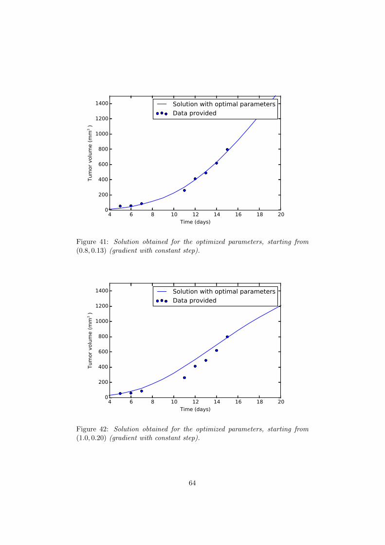
4 6 8 10 12 14 16 18 20

Time (days)

0

200

400

600

800

1000

1200

1400

Tum

or

volu

me (

mm

3)

Solution with optimal parameters

Data provided

Figure 41: Solution obtained for the optimized parameters, starting from(0.8, 0.13) (gradient with constant step).

4 6 8 10 12 14 16 18 20

Time (days)

0

200

400

600

800

1000

1200

1400

Tum

or

volu

me (

mm

3)

Solution with optimal parameters

Data provided

Figure 42: Solution obtained for the optimized parameters, starting from(1.0, 0.20) (gradient with constant step).

64

0 100 200 300 400 500 600 700 800

Number of iterations

10

11

12

13

14

15

16

17

18V

alu

e o

f th

e c

rite

rion

Figure 43: Value of the criterion as the constant gradient algorithm is carriedout (depending on the number of the considered iteration)

minimum, since every iteration will keep the point to a non-negligibledistance from the minimum. But on the other hand, a too small stepmight converge very slowly (or not converge towards an extremum !)and lead to a tremendous calculation time. The problem being that“too small” or “too large” is not a global point of view, but a localone ; at each iteration, the algorithm must make sure that the step,compared to the context of the function, remains moderate.

These two check-up in our algorithm are carried out at each iterationthrough the 2 Wolfe conditions, defined as follows (where αk is theconsidered step, dk is the descent direction, which is for the gradientalgorithm −∇F (xk), ω1 and ω2 real values such as 0 < ω1 < ω2 < 1):

F (xk + αkdk)− F (xk) ≤ ω1αk〈∇F (xk), dk〉 (22)

〈∇F (xk + αkdk), dk〉 ≥ ω2〈∇F (xk), dk〉 (23)

The first Wolfe condition (4), called “sufficient decrease condition” or“Armijo rule”, forces the step αk to reduce sufficiently the optimiza-tion criterion F between two iterations of the optimization algorithm.

65

0.6 0.8 1.0 1.2 1.4

alpha

0.06

0.08

0.10

0.12

0.14

0.16

0.18

0.20beta

2.16

2.32

2.48

2.64

2.80

2.96

3.12

3.28

3.44

3.60

Figure 44: Value of the parameters α and β in the course of the constantgradient algorithm, compared with the contour lines of log(F ) for a startingpoint (0.7, 0.1)

It can be noted in this rule that for a minimization problem, boththe left-hand term and right-hand terms are negative (for dk is a de-scent direction). Hence, this condition states that the choice of thestep value αk must induce a decrease in the optimization criterion atleast equal to ω1αk〈∇F (xk), dk〉. This “sufficient decrease condition”forces to choose a step value that ensures that a minimal decrease inF actually takes place.

The right-hand term (the minimal decrease in F) depends on the gra-dient of F, which means that the minimal decrease is decided locally:if the gradient is small, the condition will expect a small minimal de-crease in F, and if it is large, then we can expect a larger decrease in F.More precisely, we can understand the “sufficient decrease condition”as: the step αk must be chosen so that the minimal decrease in Fbetween two iterations is at least a fraction ω1 of what would happenif we could neglect all second-order terms in the Taylor developmentof F. This specific choice of right-hand term is interesting, for, as saidbefore, it involves the presence of the gradient of F, but also becauseit guarantees that for some values of step, the condition is necessarilysatisfied. Indeed, when αk is “small enough”, then the second order

66

terms in the Taylor development can be neglected. Therefore, we havethe equality:

F (xk + αkdk)− F (xk) = αk〈∇F (xk), dk〉+ o(||α2k||). (24)

Since the right-hand term is negative, if we multiply it by ω1 < 1 weindeed get a value which is larger than the difference in F.

The point of this rule is that it chooses a step αk that allows a minimaldecrease in F between 2 iterations. This minimal decrease is definedlocally (gradient at this point), and there is always a step value thatsatisfies the inequality. There is still a problem: we are sure that astep value satisfies the equation, but as we have seen before, an ex-tremely small step can then be chosen. This might of course reducethe convergence speed. For this reason, this rule is combined with thesecond Wolfe condition, called the “curvature condition” (5).

This second condition ensures that the step αk chosen is “large enough”.The idea is this time to check the directional derivative of F (dependingon the descent direction dk) for the two successive values of consideredpoints. If the difference is not large enough, which implies that thestep is too small (the two successive points are too close), inequalityis not satisfied. This allows us to solve the problem caused by theprevious rule, of a too small step value.

To calculate the proper step, and use the two previous Wolfe condi-tions, we use the Fletcher-Lemarechal algorithm, which is describedbelow:

(a) We first consider two values αb and αh, which will represent re-spectively the lower boundary, and the upper boundary of ourpossible step value. They will be updated as the algorithm iscarried out. We start with αb = 0, αh = +∞. We consider aninitial step α.

(b) We check if, with the step α, the first Wolfe condition is sat-isfied. While this is not the case, we proceed to the followinginstructions: αh = α, α = αb+αh

2 .

(c) The first condition is satisfied, now we check whether the secondcondition is satisfied. If not, we choose αb = α. We have twopossibilities: if αh = +∞ (the first condition was directly satis-fied), then α = 2αb. Else, we pick α = αb+αh

2 . We check if the

67

second condition is satisfied with this step ; if it is not the case,we restart this phase.

(d) We return the step α obtained: it is an optimal step.

Analysis of the results

This algorithm was implemented, and applied to the function log(F )(ε = 0.0001, ω1 = 0.001, ω2 = 0.99) for several starting points (figure45).

4 6 8 10 12 14 16 18 20

Time (days)

0

200

400

600

800

1000

1200

1400

Tum

or

volu

me (

mm

3)

Solution with optimal parameters

Data provided

Figure 45: Solution obtained for the optimized parameters, starting from(0.8, 0.13) (gradient with variable step).

We notice that we are faced with the same problem as in the case of thegradient descent algorithm with constant step: if we choose a startingpoint too far from the global minimum, then the algorithm will stopat an extremum which is not the global minimum (as illustrated onfigure 46).

Though, we notice on figure 47 that the algorithm converges in only 6iterations for the starting point (0.7, 0.1), and even if each iteration isfar more costly than in the case of the constant gradient algorithm, itstill leads to a calculation time significantly reduced (divided by 10).Besides, the value of the criterion is slightly diminished as we use thisvariable gradient algorithm instead of the constant gradient one for

68

4 6 8 10 12 14 16 18 20

Time (days)

0

200

400

600

800

1000

1200

1400

Tum

or

volu

me (

mm

3)

Solution with optimal parameters

Data provided

Figure 46: Solution obtained for the optimized parameters, starting from(1.0, 0.20) (gradient with variable step).

the considered points. This algorithm is therefore to be favored com-pared with the constant gradient one.

Once more, these results are confirmed if we look at figure 48, whichshows the trajectory of (α, β) on the contour lines of log(F ) for thestarting point (0.7, 0.1). We can see that the algorithm converges aftera very small number of iterations, to a point which is not the globalminimum.

More details concerning the comparison of the optimization methodsare given in part IV.

The Gauss-Newton algorithm

Even though the variable gradient algorithm seems better than theconstant gradient algorithm, an important issue remains: the algo-rithm does not necessarily return the global minimum that we arelooking for. To try and correct this situation, a new algorithm is stud-ied in the following section: the Gauss-Newton algorithm.

Theory

69

0 1 2 3 4 5 6

Number of iterations

10

11

12

13

14

15

16

17

18V

alu

e o

f th

e c

rite

rion

Figure 47: Value of the criterion as the variable gradient algorithm is carriedout (depending on the number of the considered iteration) for a starting point(0.7, 0.1)

The Gauss-Newton algorithm is an optimization algorithm which isapplied on a specific set of problems: the minimization of the sum ofsquared functions. It is, therefore, totally adapted to our situation.

Let us consider m functions ri (i = 1...m) (written in a matrix r), de-pending on n variables γ = (γ1, ...γn). The Gauss-Newton algorithmallows to find the γ that will minimize

∑mi=1 r

2i (γ). Here of course,

ri = yi − M(ti;α, β), γ = (α, β) and the function that we want tominimize is F. We will call Y the vector (y1, ..., ym) afterwards.

The Gauss-Newton method is based on expanding M(ti; γ) as a Taylorseries for a small variation in γ, and keeping only the first-order terms.It gives us:

M(ti; γ + δ) = M(ti; γ) +n∑j=1

∂M(ti; γ)

∂γjδj + o(||δ||2) (25)

Or, if we write is as a matrix equation ((M0)i = M(ti; γ), and Ji being

70

0.6 0.8 1.0 1.2 1.4

alpha

0.06

0.08

0.10

0.12

0.14

0.16

0.18

0.20beta

2.16

2.32

2.48

2.64

2.80

2.96

3.12

3.28

3.44

3.60

Figure 48: Value of the parameters α and β in the course of the variablegradient algorithm, compared with the contour lines of log(F ) for a startingpoint (0.7, 0.1)

the i-th line of J the Jacobian matrix of M(t; γ) depending on γ):

M(ti; γ + δ) = (M0)i + Ji.δ (26)

We want to select the δ that will minimize F. For this reason, wecalculate the δ that will solve the equation ∂F

∂δ = 0. We obtain:

∂F

∂δ= 2

m∑i=1

∂M(ti; γ + δ)

∂δ(yi −M(ti; γ + δ)) (27)

Or:

2

m∑i=1

JTi (yi − (M0)i − Jiδ) = 0 (28)

It leads to:

m∑i=1

JTi Ji.δ =

m∑i=1

JTi (yi − (M0)i) (29)

71

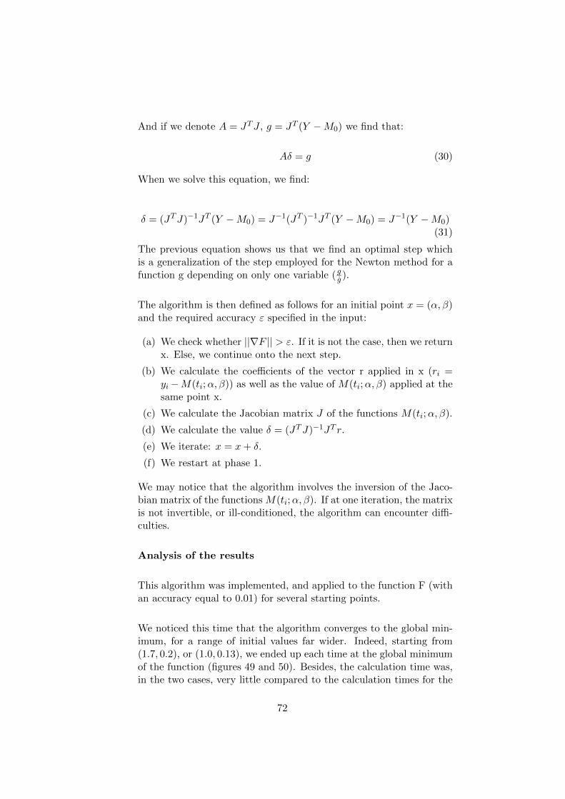
And if we denote A = JTJ , g = JT (Y −M0) we find that:

Aδ = g (30)

When we solve this equation, we find:

δ = (JTJ)−1JT (Y −M0) = J−1(JT )−1JT (Y −M0) = J−1(Y −M0)(31)

The previous equation shows us that we find an optimal step whichis a generalization of the step employed for the Newton method for afunction g depending on only one variable (gg ).

The algorithm is then defined as follows for an initial point x = (α, β)and the required accuracy ε specified in the input:

(a) We check whether ||∇F || > ε. If it is not the case, then we returnx. Else, we continue onto the next step.

(b) We calculate the coefficients of the vector r applied in x (ri =yi−M(ti;α, β)) as well as the value of M(ti;α, β) applied at thesame point x.

(c) We calculate the Jacobian matrix J of the functions M(ti;α, β).

(d) We calculate the value δ = (JTJ)−1JT r.

(e) We iterate: x = x+ δ.

(f) We restart at phase 1.

We may notice that the algorithm involves the inversion of the Jaco-bian matrix of the functions M(ti;α, β). If at one iteration, the matrixis not invertible, or ill-conditioned, the algorithm can encounter diffi-culties.

Analysis of the results

This algorithm was implemented, and applied to the function F (withan accuracy equal to 0.01) for several starting points.

We noticed this time that the algorithm converges to the global min-imum, for a range of initial values far wider. Indeed, starting from(1.7, 0.2), or (1.0, 0.13), we ended up each time at the global minimumof the function (figures 49 and 50). Besides, the calculation time was,in the two cases, very little compared to the calculation times for the

72

4 6 8 10 12 14 16 18 20

Time (days)

0

200

400

600

800

1000

1200

1400

Tum

or

volu

me (

mm

3)

Solution with optimal parameters

Data provided

Figure 49: Solution obtained for the optimized parameters, starting from(1.7, 0.2) (Gauss-Newton).

4 6 8 10 12 14 16 18 20

Time (days)

0

200

400

600

800

1000

1200

1400

Tum

or

volu

me (

mm

3)

Solution with optimal parameters

Data provided

Figure 50: Solution obtained for the optimized parameters, starting from(1.0, 0.13) (Gauss).

73

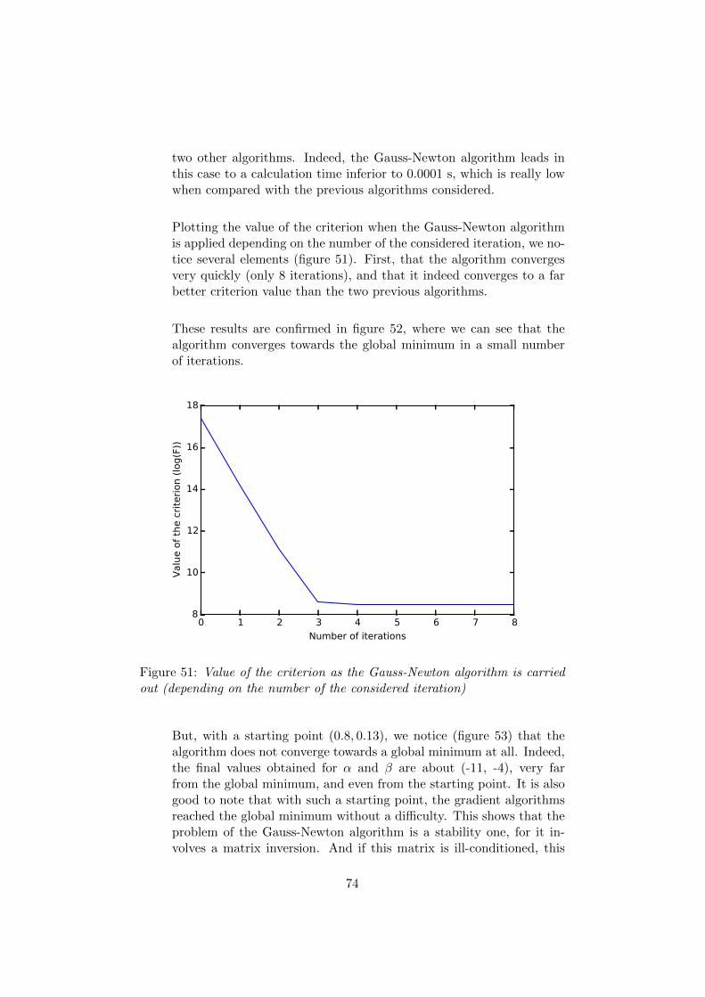
two other algorithms. Indeed, the Gauss-Newton algorithm leads inthis case to a calculation time inferior to 0.0001 s, which is really lowwhen compared with the previous algorithms considered.

Plotting the value of the criterion when the Gauss-Newton algorithmis applied depending on the number of the considered iteration, we no-tice several elements (figure 51). First, that the algorithm convergesvery quickly (only 8 iterations), and that it indeed converges to a farbetter criterion value than the two previous algorithms.

These results are confirmed in figure 52, where we can see that thealgorithm converges towards the global minimum in a small numberof iterations.

0 1 2 3 4 5 6 7 8

Number of iterations

8

10

12

14

16

18

Valu

e o

f th

e c

rite

rion (

log(F

))

Figure 51: Value of the criterion as the Gauss-Newton algorithm is carriedout (depending on the number of the considered iteration)

But, with a starting point (0.8, 0.13), we notice (figure 53) that thealgorithm does not converge towards a global minimum at all. Indeed,the final values obtained for α and β are about (-11, -4), very farfrom the global minimum, and even from the starting point. It is alsogood to note that with such a starting point, the gradient algorithmsreached the global minimum without a difficulty. This shows that theproblem of the Gauss-Newton algorithm is a stability one, for it in-volves a matrix inversion. And if this matrix is ill-conditioned, this

74

0.6 0.8 1.0 1.2 1.4

alpha

0.06

0.08

0.10

0.12

0.14

0.16

0.18

0.20beta

2.16

2.32

2.48

2.64

2.80

2.96

3.12

3.28

3.44

3.60

Figure 52: Value of the parameters α and β in the course of the Gauss-Newton algorithm, compared with the contour lines of log(F ) for a startingpoint (0.7, 0.1)

may lead to a far higher step value that what would be the optimalstep. And since the step value is very high, the approximation carriedout in the beginning of the theoretical framework of the algorithm(that all second-order terms in the Taylor development could be ne-glected) becomes of course a wrong assumption. The algorithm canthus diverge.

The Gauss-Newton algorithm is therefore a very efficient algorithm,but which lacks of stability : some starting points can make the algo-rithm diverge.

More details concerning the comparison of the optimization methodsare given in part IV.

The Levenberg-Marquardt algorithm

The Gauss-Newton algorithm is a very powerful algorithm, but whichlacks of stability depending on the starting points. Not all startingpoints lead to convergence. For that reason, Levenberg and Marquardt([3], [4]) developed an optimization algorithm which allows to combine

75

0 5 10 15 20 25 30

Time(days)

0.0

0.2

0.4

0.6

0.8

1.0Tum

or

volu

me (mm

3)

Figure 53: Solution obtained for the optimized parameters, starting from(0.8, 0.13) (Gauss-Newton).

the efficiency of the Gauss-Newton algorithm and the stability of thegradient algorithms.

Theory

Outline of the method

Let us choose the same notations as the ones used in the section de-voted to the Gauss-Newton algorithm. The descent direction δt sat-isfies the following equation in the case of a Gauss-Newton algorithm(as a reminder, A = JTJ , g = JT (Y −M0)):

Aδt = g (32)

We also notice that g = −12∇F . Since the orientation of the direction

is the element that will really matter in our algorithm, we will considerfrom now on that g = −∇F . Therefore, we can write that, in the caseof a gradient descent algorithm, the direction δg satisfies the followingequation:

76

δg = g (33)

The idea of Marquardt in [4] is to try and combine the two previousdirection equations, to create a third equation that will be used tocalculate the direction δ0 in this algorithm, with λ ≥ 0:

(A+ λI)δ0 = g (34)

The relevance of the parameter λ can be seen quite easily: when λ isclose to 0, then the equation that needs to satisfy the direction is veryclose to equation (14). Therefore, the calculated direction δ0 will beclose to the one calculated for a Gauss-Newton algorithm δt. On theopposite, when λ is extremely high, we see that the equation will becloser to equation (15), and that the direction δ0 calculated will bevery close to the opposite of the gradient. This intuitive thought isrigorously shown in [4], where it is even stated that as λ grows, thecalculated direction δ0, starting at δt turns more and more towards δg.In the same article, is also shown that as λ grows, the norm of thedirection decreases.

Relevance of the method

One interrogation that may legitimately arise is whether the directioncalculated thanks to equation (16) is a descent direction ∀λ. Basingourselves on [4], we will demonstrate properly this through the follow-ing theorem:

Theorem : For any positive λ, if δ0 satisfies the equation (16), thenδ0 minimizes F (γ + δ) on the sphere of radius ||δ0||.

Proof : The function C that we want to minimize can be written asC(γ, δ) = ||Y − M0 − Jδ||2 for any direction δ. The minimizationproblem described in the theorem can therefore be written this way:

minδ

||Y −M0 − Jδ||2

subject to ||δ||2 = ||δ0||2

77

To solve the optimization problem, we consider the Lagrangian, withλ a Lagrange multiplier:

u(δ, λ) = ||Y −M0 − Jδ||2 + λ(||δ||2 − ||δ0||2) (35)

By the method of Lagrange, we know that a stationary point neces-sarily satisfies the equations ∂u

∂δ = 0, ∂u∂λ = 0.

Thus, we have:

−2JT (Y −M0 − Jδ) + 2λδ = 0 (36)

and

||δ||2 = ||δ0||2 (37)

From equation (18), we find:

(JTJ + λI)δ0 = JT (Y −M0) (38)

This means that if δ0 satisfies equation (16), then it is a stationarypoint for F (γ+ δ). Since A+λI is a definite positive matrix, then the

calculation of ∂2u∂δ2

and of ∂2u∂λ2

shows us that the stationary point δ0 isindeed a minimum.

This way, we are able to show that the δ0 direction is indeed a direc-tion that minimizes F (γ + δ).

Rescaling

The solution of Gauss-Newton, δt, is invariant under linear transfor-mation, but it is not the case for the solution of the gradient algorithm.For this reason, we will scale the definition space, by considering thestandard deviation of the gradient function as unit. More explanations

78

about this procedure are given in [4]. This leads us to consider thefollowing formulas, where * represents the rescaled values (aj,j′ beingthe coefficients of the matrix A, and gj the coefficients of the vector gas defined in equation (16)):

A∗ = (a∗j,j′) =aj,j′√

aj,j√aj′,j′

(39)

g∗ = (g∗j ) =gj√aj

(40)

δ0 =δ∗0√aj,j

(41)

Evaluation of F

Before describing precisely the method, it is crucial to be able to under-stand exactly how the λ parameter intervenes. For this, let us supposewe are at the p-th iteration. We then have to solve the equation, andcalculate the δ∗0 such as:

(A∗ + λ(p)I)δ∗0 = g∗ (42)

Once δ∗0 is calculated, we calculate δ0 using equation (23). We thenconsider a new point γnew (in the next part, γ will be called the “start-ing point”):

γnew = γ + δ0 (43)

The next step is then to evaluate F (γnew). The previous algorithmwill be what we will refer to when, in the precise description of thealgorithm that will be displayed in the next section, we will talk aboutevaluating F.

Course of the algorithm

The algorithm takes as inputs a real number ν > 1 and the first valueof λ considered, λ0, the accuracy ε and a starting point γ0. We supposethat we are currently at the p-th iteration of the algorithm (so, we haveas values λp−1, γp and F p, which is the value of F finally obtained forλ = λp−1 in equation (24) and a starting point γp−1):

79

(a) We check whether ||∇F || < ε. If it is the case, then we return γp.Else, we proceed onto the following phases.

(b) We rescale A and g, as stated in the subsection “Rescaling”.

(c) Let us call F pλ the value of F finally obtained for λ = λp−1 inequation (24) and a starting point γp. Let us call F pν the value

of F finally obtained for λ =λp−1

ν in equation (24) and a startingpoint γp.

(d) We compare F p and F pν : if F pν ≤ F p, then we set λp =λp−1

ν , andF p+1 = F pν . γp+1 is also valued with the final value of γ in theevaluation of F pν . We then return to phase 1 for a new iterationor the end of the algorithm.

(e) If not, we compare F p and F pλ : if F pλ ≤ Fp, then we set λp = λp−1

and F p+1 = F pλ . γp+1 is also valued with the final value of γ in theevaluation of F pλ . We then return to phase 1 for a new iterationor the end of the algorithm.

(f) Else, we will increase the value of λ. For this, let us call F pwthe value of F finally obtained for λ = λp−1ν in equation (24)and a starting point γp. If F pw ≤ F p then we set λp = λp−1νand F p+1 = F pw. Else, we consider F pw as the F obtained for aλp−1ν2, and we compare once more. While F pw > F p, we increaseλ by multiplying it by ν. When this condition is not verifiedanymore (let us say it is after w iterations), we set λp = λp−1ν

w,F p+1 = F pw and γp+1 is valued with the final value of γ in theevaluation of F pw. We then return to phase 1 for a new iterationor the end of the algorithm.

The relevance of the algorithm is quite clear. First, we notice thatwe consider a new iteration only when the optimization criterion Fis reduced, which makes sense in the framework of a minimizationproblem. But we notice that we do not try to compute the maximaldecrease in F between two iterations (indeed, as stated in [4], this localminimal decrease would be a poor choice from a global point of view).Instead, we try whenever it is possible, and when we are sure that itwill lead to a local decrease in F, to decrease λ. This is quite logical ;indeed, the smaller λ is, the more the algorithm gets closer from theGauss-Newton algorithm, which is very efficient as shown in previousparts.

But the point of the algorithm is that when it is not possible to de-crease λ without increasing the optimization criterion (typically areaswhere the Gauss-Newton algorithm would not be stable), then otheroptions are considered. We can keep the same values of λ or, when

80

there is no other choice if we want to minimize F, increase it untilreaching a stage where we have a local decrease of F.

We know that, if we are not already at an extremum (where the con-dition on the norm of the gradient in the algorithm would be satisfiedanyway), we will necessarily reach, for some high value of λ, a localdecrease in F. Indeed, for this range value of λ, we are closer to thegradient algorithms, which are stable.

Marquardt, in [4], stated that default values of 0.01 for λ and 10 for νwere often a good choice.

Analysis of the results

This algorithm was implemented and applied to the function F (ε =0.001, ν = 10, and if not explicitly defined, λ0 = 0.01). Applied tothe starting point (0.7, 0.1), we notice that, like the Gauss-Newtonalgorithm, it converges towards the global minimum (figure 54). If wechoose a starting point even further from the global minimum, suchas (1.7, 0.2) for instance, we notice a convergence towards the globalminimum as well (figure 55).

But one interesting feature of the algorithm is that, starting from apoint which made the Gauss-Newton algorithm diverge (such as (0.8,0.13) for instance), we really reach the global minimum required. TheLevenberg-Macquardt algorithm seems to have corrected the stabilityof the Gauss-Newton algorithm, while keeping the ability to convergetowards a global minimum from a wide range of starting points (figure56).

One interesting aspect which can be studied is the evolution of λ as thealgorithm goes on. We notice that, depending on the starting point,the evolution will be extremely different. When the starting point is apoint that is totally fit for a Gauss-Newton algorithm, then λ decreasesvery quickly: it is indeed in this case better to get closer to the Gauss-Newton algorithm. On the other hand, when we start with a pointsuch as (0.8, 0.13), which leads to a divergence for Gauss-Newton, λwill increase a lot in the early stages of the algorithm, denoting thefact that it is necessary to copy the properties of the gradient descentalgorithms to attain a proper minimum value.

81

4 6 8 10 12 14 16 18 20

Time(days)

0

200

400

600

800

1000

1200

1400

Tum

or

volu

me (mm

3)

Figure 54: Solution obtained for the optimized parameters, starting from(0.7, 0.1) (Levenberg-Marquardt).

4 6 8 10 12 14 16 18 20

Time(days)

0

200

400

600

800

1000

1200

1400

Tum

or

volu

me (mm

3)

Figure 55: Solution obtained for the optimized parameters, starting from(1.7, 0.2) (Levenberg-Marquardt).

82

4 6 8 10 12 14 16 18 20

Time(days)

0

200

400

600

800

1000

1200

1400

Tum

or

volu

me (mm

3)

Figure 56: Solution obtained for the optimized parameters, starting from(0.8, 0.13) (Levenberg-Marquardt).

If we study the calculation time, we notice that it is far better than thegradient descent algorithms for these starting points, but slightly lessgood than the Gauss-Newton algorithm, which makes perfect sense: inthe best-case scenario as far as efficiency is concerned, λ will be closeto 0 (but will never really reach it), which will make the algorithm assimilar as possible to the Gauss-Newton, without equalizing its out-standing performance in this specific situation.

Yet, the choice of some starting points still leads to numerical prob-lems for the algorithm (notably (1,2)). We notice that the points thatseem to challenge the algorithm were also troublesome for the Gauss-Newton algorithm.

Indeed, if we consider figure 39, we notice that the function F canhave extreme values, which can create a numerical error if it has to beevaluated by the program. The issue is the evaluation of F 1λ and F 1

ν ,since the first value λ0 is given by the user and not, like all the other λ,evaluated by the algorithm depending on the optimization criterion.If the first λ is badly chosen as an input, then we can reach a F whichwill be impossible to calculate numerically. Indeed, we can see that ifwe increase the initial value of λ0 for these troublesome starting points,

83

then the Levenberg-Marquardt actually converges towards the globalminimum. But the fact that the convergence depends on the value ofλ0 is an element that should not be neglected.

If we study the evolution of the optimization criterion (figure 57), andof the parameters related to the contour lines of F (figure 58), we no-tice a very fast and accurate convergence, even though the algorithmis rather less efficient (but considerably more stable) than the Gauss-Newton algorithm.

More details concerning the comparison of the optimization methodsare given in part IV.

8.3.4 Statistical comparison of the optimization algorithms

Theoretical framework

In this part, we will compare the various optimization algorithms morerigorously: instead of comparing the results of the algorithm on arather restricted number of points, we will apply a statistical proce-dure in order to get an approximation of the average error (value ofthe optimization criterion) and calculation time of the algorithm.

To do that, we will use a Monte Carlo method: we will simulate alarge number of times the algorithm that we want to study, for a givenrequired accuracy and for various starting points, and we will considerthe global calculation time as the average of the calculation time ofevery simulation. We will do the same thing for the error.

One issue remains: which starting points do we have to consider, sothat the results are really significant ? The first matter is: how manypoints should we consider ? The second one is related to the fact thatchoosing only random coordinates for the starting points could be aproblem. Indeed, since many algorithms (like the gradient descents)have an important dependence on the starting point, a random drawcan then lead to very close points, which will not represent well thetrue properties of the algorithm. For that reason, we tried and per-form a statistical analysis more representative.

To carry out the analysis, we followed the advice from [5]. Basing our-selves on the experiments carried out in the article, we decided to per-form 100 successive simulations. Besides, as [5] suggests, to choose our

84

starting points, we used a multi-start strategy based on latin squaresampling. This strategy is developed in the following paragraph.

Let us suppose that we want n independent points. The idea of thelatin square sampling is to divide the range of values that can takeour point coordinates in n smaller domains of equal size. Then, eachpoint is picked randomly within a different domain. This way, we endup getting n points, which are able to represent the whole coordinatesrange. Besides, since the points are still picked randomly, every sta-tistical analysis will return a different average value.

Results of the statistical analysis

We performed the previous statistical analysis of the 4 optimizationalgorithms, for the same 100 starting points defined by latin squaresampling, an accuracy of 0.01, and we obtained the results displayedon figure 59 (for the Levenberg-Marquardt algorithm, λ0 = 1000). Theanalysis was performed on Python 2.7, on a computer having an IntelCore processor with a 2 GHz frequency and a 16 Go RAM. The initialconditions were chosen within an arbitrary range: [0.5, 1.5] for α and[0.05, 0.2] for β. The function does not have extreme values on thisrange, hence the decision to choose it.

We noticed several useful pieces of information. First, we saw how hardit is to perform a statistical analysis on the Gauss-Newton method,since its instability leads very often to a numerical error for at least1 of the 100 simulations. As for the results themselves, we noticedthat most of what we had seen and concluded from a reduced set ofpoints seems to be verified. Indeed, the constant gradient algorithm isclearly the slowest algorithm, whereas the Gauss-Newton algorithm isthe fastest. As for the error, the gradient descents are far less efficientthan the other two algorithms. We also noted that the Levenberg-Marquardt algorithm is the algorithm which combines the best, amongthe 4 presented algorithms, stability and efficiency.

Still, some surprises arose: the variable gradient algorithm is not moreaccurate on average than the constant gradient algorithm. This is dueto the fact that for some starting points, the variable gradient algo-rithm will lead to much higher errors than the constant gradient one.But for a high majority of starting points, we still saw that the variablegradient algorithm is seemingly better than the constant gradient one.Moreover, they had a very significant difference as far as calculation

85

time was concerned.

Another noticeable thing is the difference in accuracy between theGauss-Newton algorithm and the Levenberg-Marquardt one. This isdue to the instability of the first algorithm. Indeed, for some startingpoints, we reach values which may induce very important errors. But,there again, for nearly all the starting points which do not induce in-stability, the accuracy obtained is very similar.

The table 59 can quite clearly show us why the Levenberg-Marquardtalgorithm is generally favored in the least-squares minimization forbiological data. Accurate, robust and fast, it is clearly the best opti-mization algorithm to solve our problem.

Comparison to a pre-implemented algorithm: the Nelder-Mead algorithm

The Levenberg-Marquardt algorithm was then integrated into a least-squares minimization code used by the team at inria. So far, the op-timization algorithm that was used was the Nelder-Mead algorithm.Integrating the Levenberg-Marquardt algorithm into the code was auseful step (the algorithm is not in the standard library of numpy, sohaving a functional code of it was helpful), and was also the opportu-nity to compare the performance of the two algorithms for the samedata set. In this section, the considered data set is independent fromthe data studied before.

A statistical analysis analogous to the one carried out in the previ-ous part (for, when not specified, λ0 = 100 and an accuracy of 10−6

for Levenberg-Marquardt) led to the following results. On the stud-ied data, the average calculation time of the Levenberg-Marquardtalgorithm was slightly more significant. As for the average error com-mitted, we noticed that the Nelder-Mead algorithm was a little lessaccurate, but the difference is extremely small (and could almost beneglected): we have indeed an average difference of 2.31.10−6 for de-fault parameters.

As for the parameters of Levenberg-Marquardt, obviously, reducingthe required accuracy increases the error, and reduces the calculationtime. Increasing the starting value of λ0 increases the calculationtime, but if it is too small, the error sharply increases. All theseresults are summed up on table 60. If we have a negative value in thesecond column (average relative difference between the method and the

86

Nelder-Mead algorithm), then this means that for those parameters,the Levenberg-Marquardt algorithm is less efficient than the Nelder-Mead algorithm. In this figure, LM stands for Levenberg-Marquardtand N-M for Nelder-Mead.

8.3.5 Numerical implementation of the Levenberg-Marquardtalgorithm

All these algorithms were coded using Python 2.7. The previous anal-ysis showed that the Levenberg-Marquardt algorithm was the mostefficient and interesting to use.

For this reason, an easy-to-handle version of the Levenberg-Marquardtfunction had to be implemented from the version that had alreadybeen coded within the framework of the previous analysis. The writ-ten code was integrated into a research numerical code developed bythe MONC team at inria, aiming at the analysis of preclinical data inoncology. This part of the work was quite challenging, for it required aclean-up, series of tests and an optimization of the code, so that a userwho did not know how it was coded could find it easy to use and effi-cient, and for a good understanding of the research code was necessary.

To integrate it into the code, several elements had to be added ormodified. Among them, the functionality of automatic calculation ofthe Jacobian matrix through finite differences was added. The variousLevenberg parameters were also grouped within a class. The code wasfinally integrated into the research numerical code, and was functional.

87

8.4 Numerical methods for the Gompertz model

8.4.1 Introduction

Setting of the problem

As of today, the phenomenon of tumor growth is still an open prob-lem. Indeed, no equation is considered as the equation which wouldperfectly model the data. Yet, for, notably, biological reasons, theGompertz model is one of the most acclaimed models to describe thisgrowth ([1], [2]). During this project, a simplified model of tumorgrowth was considered, deriving from the Gompertz model, from whichan exact solution can be found rather easily . The work was to tryseveral numerical methods to see how close their results were to theexact solution, and how various parameters affected this difference.This work is interesting for the results that were found about the effi-ciency of various numerical methods for a rather simple model can beextended to more complicated ones.

All the following results were computed using Python and its numeri-cal (numpy) and graphical (matplotlib) libraries.

The Gompertz model

The Gompertz model is a model which is commonly used in the liter-ature to describe tumor growth. It can be written as follows:

∂V

∂t= (α− β ln(V ))V

V (0) = V0

(44)

We notice that the form of the solution curve (figure 61) is compatiblewith a phenomenon of tumor growth. During the early stages of can-cer, there are very few tumor cells, restricting, therefore, the growthrate. Once the number of tumor cells rises, the growth rate will un-doubtedly increase until a certain stage. Indeed, since the resourcesfor all cells are limited, the scarcity of the nutrients when there are toomany tumor cells tends to gradually decrease the growth rate. Thisfunction seems to fit well the phenomenon of tumor growth.

α and β (and sometimes even V0) are usually parameters which are notgiven, and which have to be found through estimations. Since what

88

we want in this project is to evaluate the accuracy of several methods,we will consider a reference, fixed model with α = 1, V0 = 1mm3 andβ = 0.1. Besides, it was decided to consider a time span of 30 days.

8.4.2 Analysis of numerical methods for the Gompertz dif-ferential equation

Runge-Kutta method

Description of the method

The Runge-Kutta method (which will be called RK4 from now on) isan iterative method, which allows to find the approximation of time-depending solutions y of ordinary differential equations (which can bewritten as follows): {

y = f(t, y)

y(t0) = y0(45)

The RK4 method is defined, for a step h, a time span [t0, tn] and∀i ∈ {0, ..., n}, an approximation yi = y(ti) , such as: yi+1 = yi +

h

6(k1 + 2k2 + 2k3 + k4)

ti+1 = ti + h(46)

where:

k1 = f(ti, yi)

k2 = f(ti +h

2, yi +

h

2k1)

k3 = f(ti +h

2, yi +

h

2k2)

k4 = f(ti +h

2, yi +

h

2k3)

(47)

The RK4 method is a fourth-order method ; the error is on the orderof O(h4).

Comparison of the RK4 approximation to the exact solution

We then computed the RK4 method and plotted the approximationobtained, for various steps h (figures 62, 63, 64).

89

We calculate the relative error L∞ (the maximal relative differencebetween the values of the exact solution, and the one of the RK4 ap-proximation). We obtain the results displayed figure 65.

We notice of course that the relative error decreases with the step, butthat the calculation time rises, for a smaller step involves more calcu-lations. We also notice that the relative error decreases very quicklywith the step. Therefore, even a rather important step value (2) canlead to very accurate results.

Euler method

Description of the method

Using the same notations as the ones that were used in the previouspart, the approximations yi are defined, for the Euler method, as:{

yi+1 = yi + hf(ti, yi)

ti+1 = ti + h(48)

The Euler method is a first-order method ; the error is on the orderof O(h).

Comparison of the Euler approximation to the exact solution

We then computed the Euler method and plotted the approximationobtained, for various steps h (figures 66, 67, 68). We also calculatedthe error (defined as before) figure 69.

We may notice that the Euler method is clearly less accurate than theRK4 method to approximate the solution. It is less accurate, but thecalculation time is shorter.

Comparison of the two methods

We now try and compare the two methods. For this, we seek for themaximal step that we can choose in each method to obtain a relativeerror inferior to various tolerance thresholds. These steps being chosen,

90

we compare the calculation time, and we can therefore find the fastermethod to reach a given relative error.

We choose 3 error thresholds (10 %, 1 %, 0.1 %) and we compute aheuristic method which allows us to approximate each time the biggerstep that leads to a relative error inferior to these thresholds. Then, byperforming several tests in the neighborhood of the step given by theheuristic, we end up finding the bigger step that leads to this specificerror threshold. We also write the calculation time. We get the resultsdisplayed on figure 71.

We notice that for the same relative error, the RK4 method is fasterthan the Euler method. Nevertheless, we also see, by comparing fig-ures 65 and 69, that for a given step value (2 for instance), withoutconsidering the accuracy of the method at all, the Euler method is con-siderably faster. This seems to indicate that when the same numberof steps is performed in the two methods, the Euler method is faster,which leads to the logical conclusion that one iteration in the Eulermethod is considerably faster than one iteration in the RK4 method.The RK4 method is nevertheless to be favored ; this is due to the factthat the number of steps that need to be carried out in the RK4 modelto attain a certain accuracy is far lower than for the Euler method,since the step value is higher.

To approximate this type of problem, it is therefore better to use theRK4 method.

8.4.3 Derivation of the order of the methods

In this part, we try and determine the order of the two methods em-ployed from the calculations that we have performed.

Theoretical reasoning

The consistency error of a numerical method is a sequence which canbe defined as (where y is the exact solution of the ODE):

en = y(tn+1)− yn+1 (49)

91

A method is defined as a p-th order method if en = o(hp+1).

The simplest way to evaluate the order of a numerical method is toconsider the following relationship, deduced from the definition of en:

ln(y(tn+1)− yn+1) = ln(en(h)) (50)

So, if we plot ln(y(tn+1)−yn+1)) depending on ln(h), we should obtaina line, the slope being the order of the method.

Numerical results

Order of the RK4 method

We plot this graph, and we obtain the result displayed figure 72.

A linear interpolation gives a slope coefficient of 3.71. We find, indeed,that the RK4 method is a fourth-order method.

Order of the Euler method

The same thing is done for the Euler method, with the result displayedfigure 73.

A linear interpolation gives a slope coefficient of 0.87. We thereforefind, indeed, that the Euler method is a first-order method.

9 Thanks and acknowledgments

This internship was, for me, an amazing experience, and I would re-ally like to thank Sebastien for his patience throughout the internship(and long after), for his kindness, support, guidance and good advicethroughout the six months. Scientifically and humanly, this internshipwas an extremely positive experience for me, and I am very gratefulto Sebastien for it.

I would also like to thank Thierry Colin for accepting me into the teamand for his everyday human warmth. I am also very grateful to OlivierSaut for his guidance and help throughout those six months. I would

92

also like to thank Etienne, Thomas and Cynthia, for their kindness,and their contribution to some of the scientific contents of this report.Finally, I would also like to thank all other members of the monc teamfor their warmful welcome in Bordeaux.

93

10 Bibliography

[1] Benzekry S., Lamont C., Beheshti A., Tracz A., Ebos J., et al.(2014) Classical Mathematical Models for Description and Predictionof Experimental Tumor Growth. PLoS Computational Biology, 10(8):e1003800. doi:10.1371/journal.pcbi.1003800

[2] Gerlee P. (2013) The model muddle: in search of tumor growthlaws. Cancer Research, 73(8), 2407-11.

[3] Levenberg K. (1944) A method for the solution of certain non-linear problems in least squares. Quarterly Appl Math 2:1648

[4] Marquardt D. (1963) An Algorithm for Least-Squares Estimationof Nonlinear Parameters. Journal of the Society for Industrial andApplied Mathematics, Vol 11, no2, 431-441

[5] Raue A., Schilling M., Bachmann J., Matteson A, Schelke M, etal. (2013) Lessons Learned from Quantitative Dynamical Modeling inSystems Biology. PLoS

[6] Ebos J., Lee C., Crus-Munoz W., Bjarnason G., Christensen J.(2009) Accelerated metastasis after short-term treatment with a po-tent inhibitor of tumor angiogenesis. Cancer Cell, 15 :232-239.

[7] Benzekry S. (2011). Modelisation et analyse mathematique detherapies anti-cancereuses pour les cancers metastatiques, PhD the-sis, Universite d’Aix-Marseille.

[8] Ebos J., Mastri M., Lee C., Tracz A., Hudson J. et al. (2014),Neoadjuvant antiangiogenic therapy reveals contrasts in primary andmetastatic tumor efficacy, EMBO Molecular Medicine

[9] Hanahan D., Weinberg R. (2000). The Hallmarks of Cancer, Cell.

[10] Iwata K., Kawasaki K., Shigesada N. (2000). A dynamical modelfor the growth and size distribution of multiple metastatic tumors,Journal of theoretical biology, 203, 177-86.

[11] Wheldon T. (1988) Mathematical models in cancer research.

[12] Camillo A. (2014), An experimentally-based modeling study of theeffect of anti-angiogenic therapies on primary tumor kinetics for data

94

analysis on clinically relevant animal models of metastasis, internshipreport.

[13] Morais C. (2014) Sunitinib resistance in renal cell carcinoma.Journal of Kidney Cancer and VHL.

[14] Simeoni M., Magni P., Cammia C. et al (2004). Predictive pharmacokinetics-pharmacodynamic modeling of tumor growth kinetics in xenograftmodels after administration of anticancer agents. Cancer research.

[15] Dhillon S. (2006) Clinical pharmacokinetics.

[16] Aouba A. (2007). Les causes medicales de deces en France etleur evolution 1980-2004. Bulletin epistemiologique hebdomadaire

[17] Hahnfeldt P., Panigrahy D., Folkman J., Hlatky L. (1999). Tu-mor Development under Angiogenic Signaling: A Dynamical Theoryof Tumor Growth, Treatment Response, and Postvascular Dormancy.Cancer Research, 4770-5.

[18] Benzekry S., Tracz A., Mastri M., Corbelli R., Barbolosi D., EbosJ. (2016). Modeling Spontaneous Metastasis following Surgery: An InVivo-In Silico approach. Cancer Research, 76(3), 535-547.

95

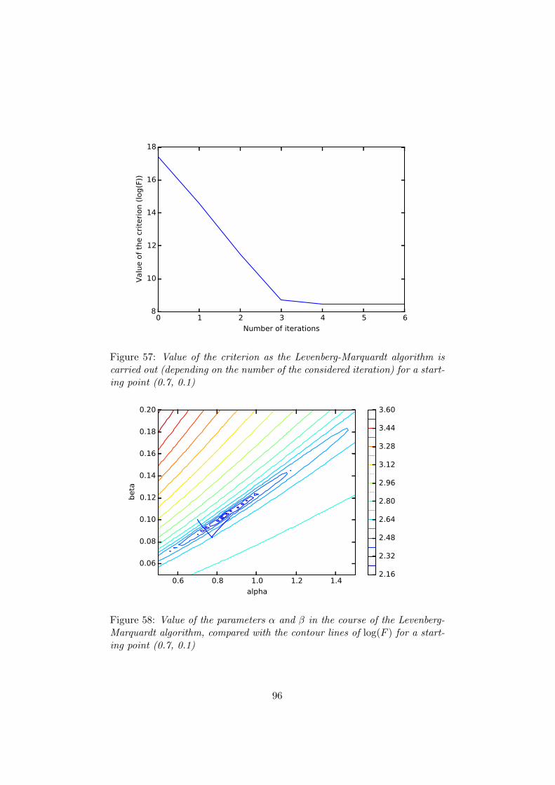
0 1 2 3 4 5 6

Number of iterations

8

10

12

14

16

18V

alu

e o

f th

e c

rite

rion (

log(F

))

Figure 57: Value of the criterion as the Levenberg-Marquardt algorithm iscarried out (depending on the number of the considered iteration) for a start-ing point (0.7, 0.1)

0.6 0.8 1.0 1.2 1.4

alpha

0.06

0.08

0.10

0.12

0.14

0.16

0.18

0.20

beta

2.16

2.32

2.48

2.64

2.80

2.96

3.12

3.28

3.44

3.60

Figure 58: Value of the parameters α and β in the course of the Levenberg-Marquardt algorithm, compared with the contour lines of log(F ) for a start-ing point (0.7, 0.1)

96

Method Average error (log(F )) Average calculation time (s)

Constant gradient 14.729 0.2286

Variable gradient 15.629 0.0079

Gauss-Newton 10.423 0.0024

Levenberg-Marquardt 8.478 0.0073

Figure 59: Average error and calculation time for the considered optimiza-tion algorithms

Method and parameters Relative difference with the NM method (%) Calculation time (s)

L-M (default values) 2.31.10−6 2.67

L-M (accuracy: 1E-3) −2.82.10−6 2.66

L-M (λ0 = 1000) 6.81.10−6 2.71

L-M (λ0 = 0.01) -81,56 2.67

N-M / 2.64

Figure 60: Results obtained, by comparison with the Nelder-Mead algorithm

0 5 10 15 20 25 30 35

Time (days)

0

2000

4000

6000

8000

10000

12000

14000

Tum

or

volu

me (mm

3)

Exact solution

Figure 61: Solution to the Gompertz differential equation, with V0 = 1mm3,α = 1, β = 0.1

97

0 5 10 15 20 25 30

Time (days)

0

2000

4000

6000

8000

10000

12000

14000Tum

or

volu

me (mm

3)

Exact solution

RK4 approximation

Figure 62: RK4 approximation for h = 6.

0 5 10 15 20 25 30 35

Time (days)

0

2000

4000

6000

8000

10000

12000

14000

16000

Tum

or

volu

me (mm

3)

Exact solution

RK4 approximation

Figure 63: RK4 approximation for h = 4.

0 5 10 15 20 25 30

Time (days)

0

2000

4000

6000

8000

10000

12000

14000

Tum

or

volu

me (mm

3)

Exact solution

RK4 approximation

Figure 64: RK4 approximation for h = 2.

98

Value of the step Relative error Calculation time (s)

6 10.1 % < 0.0001

4 4.2 % < 0.0001

2 0.7 % 0.001

Figure 65: Relative errors and calculation times for the RK4 approximationdepending on the value of the step h

99

0 5 10 15 20 25 30

Time (days)

0

2000

4000

6000

8000

10000

12000

14000Tum

or

volu

me (mm

3)

Exact solution

Euler approximation

Figure 66: Euler approximation for h = 2.

0 5 10 15 20 25 30

Time (days)

0

2000

4000

6000

8000

10000

12000

14000

Tum

or

volu

me (mm

3)

Exact solution

Euler approximation

Figure 67: Euler approximation for h = 1.

0 5 10 15 20 25 30

Time (days)

0

2000

4000

6000

8000

10000

12000

14000

Tum

or

volu

me (mm

3)

Exact solution

Euler approximation

Figure 68: Euler approximation for h = 0.5

100

Value of the step Relative error Calculation time (s)

2 46.2 % < 0.0001

1 26.4 % < 0.0001

0.5 14.8 % < 0.0001

Figure 69: Relative errors and calculation times for the RK4 approximationdepending on the value of the step h

0 5 10 15 20 25 30 35

Time (days)

0

2000

4000

6000

8000

10000

12000

14000

16000

Tum

or

volu

me (mm

3)

Exact solution

RK4 approximation

Euler approximation

Figure 70: Euler approximation and RK4 approximation for h = 3.5

Relative error Bigger step (RK4 / Euler) Calculation time (s) (RK4 / Euler)

10 % 6.85 / 0.32 < 0.0001 / < 0.0001

1 % 2.2 / 0.03 < 0.0001 / 0.003

0.1 % 1.07 / 0.003 < 0.001 / 0.004

Figure 71: Bigger steps allowing to get a specific relative error for the twonumerical methods and corresponding calculation times

101

3.5 3.0 2.5 2.0 1.5 1.0 0.5 0.0

ln(h)

18

16

14

12

10

8

6

4

ln(y

(tn

+1)

- yn

+1)

Figure 72: Evaluation of the order of the RK4 method

3.5 3.0 2.5 2.0 1.5 1.0 0.5 0.0

ln(h)

3.5

3.0

2.5

2.0

1.5

1.0

0.5

ln(y

(tn

+1)

- yn

+1)

Figure 73: Evaluation of the order of the Euler method

102