mathematical modeling, simulation and identification...

Journal of KONES Powertrain and Transport, Vol. 19, No. 2 2012

MATHEMATICAL MODELING, SIMULATION AND IDENTIFICATION OF MICRO COAXIAL HELICOPTER

Hari Muhammad, Huynh Phuoc Thien and Taufiq Mulyanto

Institut Teknologi Bandung

Faculty of Mechanical and Aerospace Engineering Department of Aeronautics and Astronautics

Jl. Ganeca 10, Bandung 40132, Indonesia tel.: +62 22 2504243, fax: +62 22 2534099

e-mail: [email protected]

Abstract

Micro Coaxial Helicopter with compact size and vertical takeoff ability offers a good Micro Aerial Vehicle (MAV) configuration to handle indoor mission such as search, rescue and surveillance. An autonomous MAV helicopter equipped with micro vision devices could provide more information of the scene, in which the human present is risky. Toward an autonomous flight, mathematical model of the helicopter should be obtained before controller design takes place. This paper will discuss the mathematical modelling, simulation and identification of a micro coaxial helicopter. The mathematical model of the micro coaxial helicopter will be presented, in which total forces and moment are expressed as a Taylor series expansion as function of the state and control variables. The mathematical model will be used to simulate the helicopter responses due to control input. The simulation was used to obtain better understanding of the characteristics of the helicopter before flight test program are performed. Flight test program dedicated to identify the parameter of the micro coaxial helicopter have been carried out. The micro coaxial helicopter was instrumented with sensory system to measure some input and output variables. The use of Kalman filter to estimate the state and total least squares to estimate the aerodynamic parameter of micro coaxial helicopter based on the flight test data will be presented. Some identification results and model validation will be given in this paper.

Keywords: micro coaxial helicopter, mathematical modelling, flight simulation, parameter identification

1. Introduction

Micro Aerial Vehicle (MAV) offers excellent tool to support missions in indoor environment. With certain onboard, intelligent the MAV can be used to perform tasks that may be dangerous for human or tasks in which human presence is not possible, e.g. search and rescue, surveillance in unstable contraction, in underground tunnel. In order to operate in indoor environments with limited space and rich of obstacles of different size and shape, the MAV should be inherently stable to simplify the control. Control system should be designed and implemented to autonomously control the MAV.

System identification approach is properly one of the good solutions to achieve an appropriate mathematical model. In detail, flight test data will be used to identify the parameters in the model. Unfortunately, due to the small size of the helicopter, and the use of low cost sensory system, data obtained from flight test are corrupted by noise. These inaccurate data could make the estimation of parameters become improper. In order to handle this issue, one of the solutions is using the Kalman filter followed by the total least square in the identification process.

The present paper starts with discussion of a mathematical model of a micro coaxial helicopter. Next, the numerical simulation prior to the flight test will be given to obtain proper values of control inputs during real flight test program. Parameter identification technique to estimate both the state and the aerodynamic parameters will be described. Estimation of the aerodynamic parameter based on real flight data will be presented and discussed. Some conclusions will be given in this paper.

H. Muhammad, H. P. Thien, T. Mulyanto

2. Mathematical model of micro coaxial helicopter

A typical micro coaxial helicopter is shown in Fig. 1. Two pairs of 50 cm diameter rotor blade are used to generate lift. These rotors are driven in opposite direction by two electric motors to counter the torque generated by rotor system [1].

Fig. 1. Lama 400D coaxial helicopter [1]

In general, control of this type of rotorcraft is done by main motors and swash-plate system,

both inactive and passive way. In upper rotor, a fly-bar is attached to the driven shaft. Through the mechanical linkages with rotor blade, this fly-bar will provide passive control into the upper rotor input. In lower rotor, swash-plate system with servomotors is used to control pitch and roll of the helicopter. To activate a motion in vertical direction, motor rotational speed should simultaneously be varied, while differential variation of these RPM will lead to a yaw motion. 2.1. The longitudinal equations of motion

The kinematics model of a Micro Coaxial Helicopter is a set of differential equations relating the forces and moments acting on the helicopter. This model can be derived from equation of motion of the helicopter. In the body-fixed reference frame, this equation can be written as follows, only the longitudinal equations are considered here [2].

.cossin

,

,

,cos

,sin

wuh

I

Mq

q

m

Zgquw

m

Xgqwu

y

(1)

In equation (1), u and w indicate the velocity components of the helicopter along the X and Z axes respectively, q is the pitch rate, denotes the angle of pitch, h is the altitude, g is the acceleration due to gravity, m is mass, and Iy is the moment of inertia.

354

Mathematical Modeling, Simulation and Identification of Micro Coaxial Helicopter

2.2. The rotor dynamic model

The rotor dynamic model here is derived for the flapping angle of the lower rotor and the fly-bar, which are defined as follows [3, 4]:

(2) .

,

q

qk

fff

lon

in which and f are the flapping angle of the lower rotor and the fly-bar respectively, lon denotes the deflection of the longitudinal control surface, and q is the pitch rate. In equation (2), ,

f, and k are constants. The upper rotor flapping angle u is modelled as a linear function of the flapping angle of the

fly-bar as follows [2]:

ffu k . (3)

The flapping angle of both the upper and the lower rotors will be used to develop the aerodynamic-propulsion model of the micro coaxial helicopter. 2.3. The aerodynamic-propulsion model

The total aerodynamic-propulsion force along the longitudinal axis X, the total aerodynamic-propulsion force along the vertical axis Z, and the total aerodynamic-propulsion pitching moment in the lateral axis M, can be expressed as follows [5]:

.2

1

,2

1

,2

1

2

2

2

RSCVM

SCVZ

SCVX

m

Z

X

(4)

where Cx, Cz, and Cm denote the coefficients of the aerodynamic-propulsion forces along the X and Z-axes, and pitching moment about Y-axis respectively, V is the forward speed, is the air density.

By substituting V= R and S= R2 into equation (4), where and R are the rotational speed and radius of the rotor respectively, it follows that:

.2

1

,2

1

,2

1

52

42

42

m

Z

X

CRM

CRZ

CRX

(5)

The aerodynamic forces and moment coefficients can be expressed in terms of several state and control variables of the vehicle, for example the lower and upper flapping angles, pitch rate, deflection of the longitudinal control surface, and the thrust coefficient Tc defined as

42

21 R

TTc. (6)

The dependency of those coefficients on these variables can be expressed as follows:

355


),,,,(;; clonumZX TqfCCC . (7)

Each coefficient in equation (7) can be expressed in a Taylor series expansion as a function of the state and control variables as well as thrust coefficient. If terms up to the first order are included, these coefficients can be expressed as follows [6, 7]:

.

,

,

0

0

0

cmlonmmummmm

cZlonZZuZZZZ

cXlonXXuXXXX

TCCqCCCCC

TCCqCCCCC

TCCqCCCCC

cTlonqu

cTlonqu

cTlonqu

(8)

In equation (8), are the aerodynamic and control

parameters, and lonlonqu

mmZXXXX CCCCCCC ,,...,,,,

andT Tc c c

x z mC ,C , C are the thrust parameters expressing the effect of the thrust on

the total aerodynamic forces and moment. These parameters can be determined from both theoretical prediction or experimental. In this paper, these parameters will be estimated from flight test experiment.

Substitution of equation (8) into (4) and the result is substituted into (1) yields the differential equation of motion of the micro coaxial helicopter as follows.

.cossin

,)(2

1

,

,)(2

1cos

,)(2

1sin

0

0

0

52

42

42

wuh

TCCqCCCCI

Rq

q

TCCqCCCCm

Rgquw

TCCqCCCCm

Rgqwu

cmlonmmummmy

cZlonZZuZZZ

cXlonXXuXXX

cTlonqu

cTlonqu

cTlonqu

(9)

In principle, the differential equations (2) and (9) can be used to simulate the flight test scenarios as will be explained in the following section. 3. Flight simulation of micro coaxial helicopter

The purpose of the flight simulation is to test the mathematical model of the helicopter as well as to obtain the reference values of control input for later use in flight test program. The mathematical model of the helicopter given in equations (2) and (9) is implemented into the MATLAB/Simulink software. Fig. 2 shows the schematic diagram of the implementation of the equations of motion of the micro coaxial helicopter [2].

The physical parameters of the micro coaxial helicopter used in the simulation are presented in Tab. 1, see also Fig. 1.

Tab. 1. Micro coaxial helicopter data

Characteristics Data

Main rotor radius 25 cm

Total weight 800 g

Engine type Electric motor

Distance between rotor 80 mm

Endurance 10 minutes

356


,lon lat Micro Coaxial Helicopter

Mathematical Model

Environmental Data: , g

Helicopter Parameters: m, R, l fus, wfus, du, dl, Ixx, Iyy, Izz, Ju, Jl, Jf,

Kb, Kq, Kp,

,l u

State: u, v, w p, q, r

,

,l l

f f

, , xE,yE, h

Sensor Model

V, h, p, q, r ax, ay, az

Observation

, , ,

, , ,

V h p q

r a a ax y z

Fig. 2. Schematic diagram of the implementation of the mathematical model of micro coaxial helicopter

The simulation was carried out within 20 seconds and time step of 0.01 s. The total forces X

and Z as well as the total moment M in equation (4) are assumed known [2]. The time history of the control input for the rotor and the servo system in longitudinal simulation are shown in Fig. 3. The corresponding response in term of translational velocity (u, w), angular rate about Y-axis (q), pitch angle ( ) and altitude (h) are depicted in Fig. 4.

2000

2200

2400

0 2 4 6 8 1RP

M_l

ower

rot

or

0

-10-505

10

0 2 4 6 8dlo

n (d

eg)

10

1800

2000

2200

0 2 4 6 8RP

M_u

pper

rot

or

10 -10

-5

0

5

10

0 2 4 6 8dla

t (d

eg)

Time (s)10

Fig. 3. Control input of rotor and servo system in longitudinal maneuver

-2

0

2

0 2 4 6 8u(m

/s)

10

-5

0

5

0 2 4 6 8

(deg

)

10

-1

0

1

0 2 4 6 8w(m

/s)

10

0.5

1.5

2.5

0 2 4 6 8

h(m

)

Time (s) 10

-20

0

20

40

0 2 4 6 8q(d

eg/s

)

10

Fig. 4. Response of the helicopter to the control input in term of translational velocity (u, w), angular rate about Y-axis (q), pitch angle ( ), and altitude (h)

357


Figure 5 shows the observed speed (Vm) and altitude (hm). Also presented in Fig. 5 are the accelerations along the longitudinal and vertical axes (ax, az), pitch rate (q), and upper and lower flapping angles u l, . In this simulated flight data, it is assumed that noise was presence in the

observed data.

-2-10123

0 2 4 6 8Vm

(m/s

)

-10.5

-10

-9.5

-9

0 2 4 6 8a z(d

eg/s

)

Time (s)10

10

0.5

1.5

2.5

0 2 4 6 8

h m(m

)

-5

0

5

0 2 4 6 8 1al(d

eg)

0

10

-0.4

-0.2

0

0.2

0.4

0 2 4 6 8

a x(d

eg/s

)

10

-5

0

5

0 2 4 6 8 1

au

(deg

)

0

Fig. 5. The observed response of the helicopter due to control input: airspeed, altitude, vertical acceleration, rate of pitch, lower, and upper flapping angles. Noise is added in these observed responses

The simulated flight data as given in Fig. 3 and Fig. 5 can be used to obtain proper values of

control inputs during real flight test program [2, 7]. Also, the simulated flight data was used to validate the software of the Kalman filter and the total least squares [6, 9].

4. Identification of micro coaxial helicopter parameters

In the identification of micro coaxial helicopter parameters, two steps parameter estimation are

used. In the first step, Extended Kalman Filter was used to estimate the states of the helicopter. The Total Least Square was then applied to estimate the parameters of the aerodynamic force and moment models.

4.1. The flight instrumentation system and data

Flight test program aimed to identify the aerodynamic-propulsion parameter was carried out using modified micro coaxial helicopter. The helicopter was instrumented with three navigation sensors: 6 DOF Inertial Measurement Unit (IMU) from SparKFun Electronic to provide the

measurement of the airframe accelerations (ax, ay, az), measured range of 6 g, and angular rates (p, q, r), measured range of 500 deg/s; Data rate of this IMU is up to 200 Hz,

Digital magnetic compass (DMC) with tilt compensated OS500-S from Ocean Server for sensing heading attitude, tilt angle in longitudinal and lateral direction (resolution: 0.10, data rate: 40 Hz),

Sonar Range Finder sensor for measuring the helicopter altitude (range: 15 cm–650 cm).

358


Also, two optical shaft encoders are used to record the rotational speed of rotor system. Two microcontrollers are selected to read the servo’s control input, to collect, and to encode the entire sensor reading into data packages. The architecture of the sensory system is depicted in Fig. 1.

Fig. 1. Schematic diagram of overall structure of flight test instrumentation system

Fig. 2 shows typical example of input-output flight test data obtained in longitudinal maneuver.

In this figure, the time history of control inputs is shown in the left side; while the helicopter responses are shown in the right side. It can be seen that the measured data obtained from the sensory system are noisy with high noise to signal ratio. Therefore, the filtering of data was carried out to obtain appropriate data for further processing [7].

-8

-4

0

4

8

0 2 4 6 8d lon

(deg

)

-20

-10

0

10

20

0 2 4 6 8q (de

g/s)

1010

-8

-4

0

4

8

0 2 4 6 8

Time (s)

d lat

(deg

)

-10

-5

0

5

10

0 2 4 6 8a x (m/s2 )

1010

2000

2100

2200

2300

Uppe

r Rot

or R

PM

5

10

15

0 2 4 6 8a z (m/s2 )

10

1800

1900

2000

2100

2200

Lowe

r Rot

or R

PM

0

1

2

3

0 2 4 6 8 1

h(m

)

Time(s)

0

Fig. 2. Control input and measured data obtained from longitudinal flight test maneuver.

4.2. State estimation

Assuming that the measurement of accelerations and angular rates of the micro coaxial

helicopter can be performed using IMU with sufficient accuracy. By replacing the total forces in

359


equation (1) with the specific forces mZ

zmX

x mmaa ; , the equations of longitudinal motion of the

micro coaxial helicopter can be expressed as follows [8]:

sin xagqwum

0

cossin

cos

z

m

zz

wuh

q

agquwm

(10)

In equation (10), the bias in the vertical acceleration is considered and it is assumed constant so that the derivative with respect to time is zero. Also, the subscript m in equation (10) denotes the me

slational acceleration

asured variable. In principle, Extended Kalman Filter (EKF) can be applied to estimate the state in . (10) as the

input in term of tranmxa , a

mz m

the flapping angle of the upper and lower rotor can be obtained by integrating equation with

lon

, q are known from the flight test. In addition,

and qm acquired in the flight test and using equation (3).

Results on the estimation of translational velocity (u, v), pitch angle bias in vertical

leration and altitude in longitudinal maneuver are showacce n in Fig. 3. The estimated flapping ang .

c

le of the upper and lower rotor in longitudinal maneuver is depicted in Fig. 4

Fig. 3. Estimated of translational velocity (u, v), pit h angle bias in vertical acceleration and altitude

Fig. 4. Estimated of the flapping angle of the lower and upper rotor in longitudinal maneuver

-0.5

0

0.5

1

0 2 4 6 8 10

u(m

/s)

Time (s)

1.5

Estimation of Longitudinal Velocity Using Kalman Filter on Longitudinal Maneuver Flight Test Data

-0.2

-0.1

00 2 4 6 8 10

az(m

/s2 )

Time (s)

0.1

an Filter on Estimation of Bias in Vertical Accleration Using KalmLongitudinal Flight Test Data

-0.5

0

0.5

0 2 4 6 8 1

w(m

/s)

Time (s)

1

0

Estimation of Vertical Velocity Using Kalman Filter on Longitudinal Maneuver Flight Test Data

0

0.5

1

1.5

0 2 4 6 8 10

h(m

)

Time (s)

-2

-1

0

1

0 2 4 6 8 10

(deg

)

Time (s)

2

Estimation of Pitch Angle Using Kalman Filter on Longitudinal Maneuver Flight Test Data

2

2.5Estimation - Extended Kalman Filter Measurement

Estimation of Altitude Using Kalman Filter on Longitudinal Maneuver Flight Test Data

0.2

Difference Between Measured and Estimated Altitude using Extended Kalman Filter

-0.2

-0.1

0

0.1

0 2 4 6 8 10

resi

dual

(m)

Time (s)

-2

-1

0

1

2

0 2 4 6 8 10au

(deg

)

Time (s)

Estimation of Upper Rotor Flapping Using Kalman Filter on Longitudinal Maneuver Flight Test Data

-8

-4

0

4

8

0 2 4 6 8 10al(d

eg)

Time (s)

Estimation of Lower Rotor Flapping Using Kalman Filter on Longitudinal Maneuver Flight Test Data

,

,

,

,

.

360


4.3. Parameter estimation

The aerodynamic-propulsion model given in eq

uations (5) and (8) can be rewritten as:

cmlonmmummmmy

m TCCqCCCCRR

MC

cTlonqu0521521

cZlonZZuZZZz

TCCqCCCCR

ZcTlonqu

m

042

XXx

X

am

CCR

am

R

XC m

0422142

21 cXlonXXuX TCCqCC

cTlonqu

ZR 2

14221

qI

C

22

(11)

The force coefficients CX and CZ in equation (11) can be obtained from measurement of longitudinal and vertical accelerations. The moment coefficient Cm is obtained from numerical

qm by taking the 4 points Lagrange time derivative [8]. From the flight test data, the value of angular rate q, the control input of pitch servo lon

rotor system thrust coefficient Tc are obtained. The flapping angles of the upper and lower rotor can be reconstructed as discussed in 0. The principle of the regression method can be explained in short as follows. The aerodynamic model in equation (11) can be expressed as follows:

differentiation of and the

)()(...)()()( 22110 iixixixiy pp , (12)

where y(i) is the dependent variable, i.e. the aerodynamic force and moment coefficients, x (i) den

p

ote the independent variables, i.e. the (estimated) state and control variables, p is the vector of the aerodynamic parameters, and (i) am the stochastic equation error, accounting for measurement as well as model errors on the dependent variable. In the compact matrix form, equation (12) can be written as follows:

Xy . (13)

The matrix of independent variables X is assumed known exactly from the state estimation, i.e. using EKF, or from direct measurement with highest accuracy of the instrumentation system. Using the Least Squares (LS) method [10], the parameter vector can be estimated from:

yXXXX TTLS

1. (14)

However, due to the limited accuracy of the instconstruction of the flapping angle or the upper and t

the

rumentation system in the measurement or re he lower: u and l, pitch rate q, deflection of

longitudinal control surface lon, and thrust coefficient Tc, the data matrix X has also error. Therefore, equation (13) can be written as follows:

][ XXy . (15)

In equation (15), not only the observation y has error bwe

ut also the data matrix X has error as ll. Again, with the assumption that the dependent variable y can be measured with finite

accuracy, equation (15) can be written as follows:

][ XXy . (16)

Denote C = [X y] is a compound matrix that contains both observation quation (16). This matrix C could be decomposed into:

, (17)

y and data matrix X in e

TVUC

.

,

,

361


wh

artitioned based on n and d as follows

Solution of total least square exists if and only if Vo exi

(19)

ere =diag( 1, 2, … n+d) is a single value decomposition of C, 1> 2 >…> n+d be the singular values of C, n and d is the number of independent variables and number of observation respectively. The element matrix in (17) could be p

n

n

dn

VV 0 n

d

ddVVV

2

1

22

12

21

11

0. (18)

22 is non-singularity. This solution is unique if iven by and nly if n n+1.The sted solution could be g

1

2212 VVTLS .

,

rameters in the presence of noise in the measured data [9]. Tab. 2 presents the results on estimation of parameters in the longitudinal force and moment coefficient by applying the Total Least Squares n the flight test data.

Tab. 2. Estimated parameters in aerodynamic-propulsion model of micro coaxial helicopter

rameters Value Standard Deviation Parameters Value Standard Deviation

TLS was chosen as the estimator due to its ability in giving consistent estimation of pa

o

Pa

0.0134 0.0042 -0.1802 0.0108 lon

ZC0XC

uXC -0.0655 0.0149

TlZC 0.0004 0.0009

lXC

0.3900 0.0218 Tu

ZC -0.0057 0.0007

qXC

0.05 0.0039 69 0.0189 0.0068

0.0201 0mC

lonXC

-0.3569 u

mC

0.2370 0.0241

0.0016 Tl

XC

0.0041 l

mC

C

-0

-0

.6448 0.0354

TuXC

.0063 0.0012

qm -0.0833 0.0063

0ZC

0.0495 0.0022 Lon

mC

0.5995 0.0326

uZC 0.0124 0.008 -0.0066 0.0026 Tl

mC

lZC

0.2034 0.0117 0.0009 0.002 TumC

qZC

0.0285 0.0021

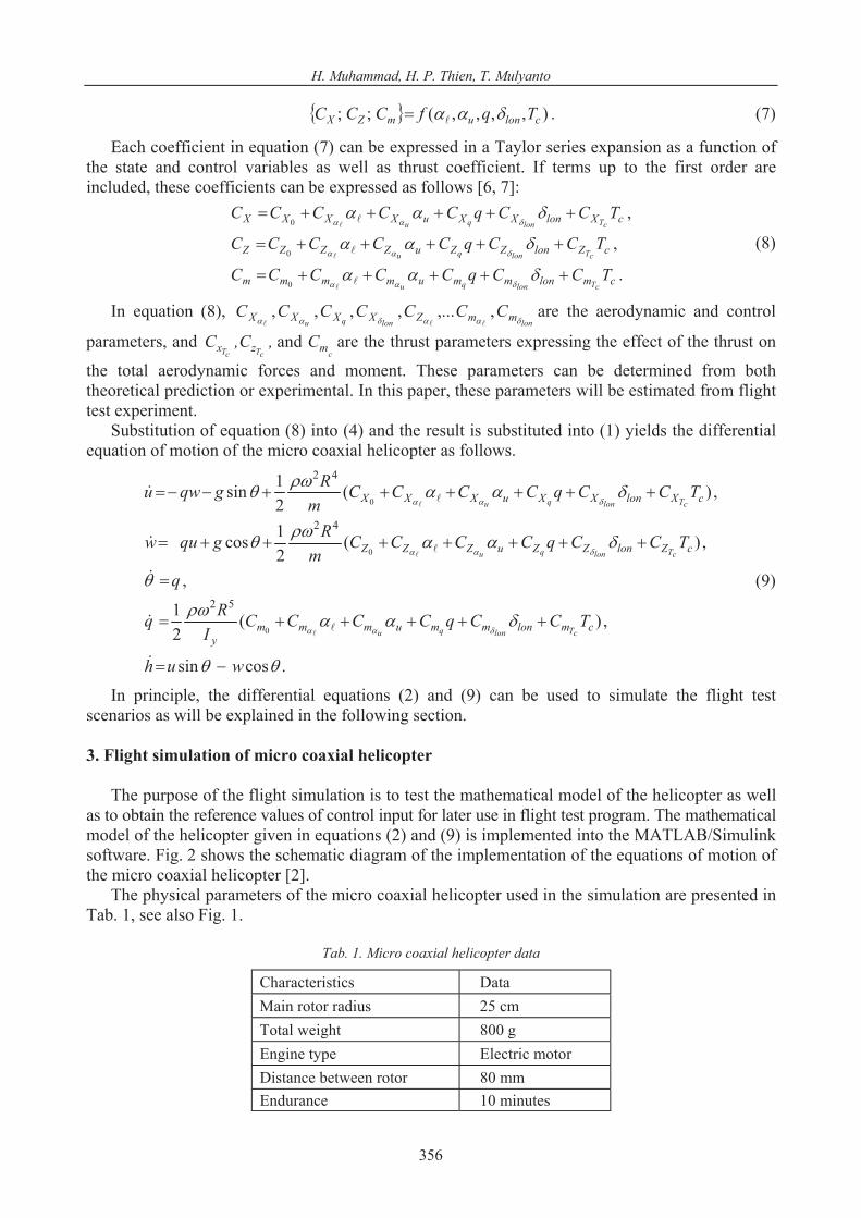
The comparison n the estim f CX, C , Cm and the corr g measu es are

shown in Fig. 5. In g the estima es of C , CZ, and Cm fit w easured except some periods in which transition of control input were made, i.e. at t = 2, t = 4, t = 8 s, see also

betwee ation o Z espondin red valueneral, ted valu X ell the m values,

lon in

Fig. 2. To evaluate the of the es n of fo ce and moment ents usin Least

Squares, the goodness of fit coeffi used.coefficient as follows:

quality timatio r coeffici g Totalcient is This coefficient is defined as the correlation

][][ yyyy eT

e

in which ym and ye are the measured and estimated values of CX, CZ and Cm respectively, and

][][2 yyyyR , em

Tem (20)

y is the mean value of y . The correlation coefficients of C , C and C obtained from analysis of the flight te

e X Z m

st data as presented in Fig. 10. are 0.91, 0.92 and 0.97, receptively.

362


Fi va ce

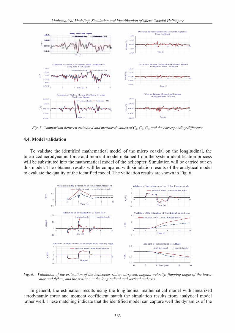
To inal, the

l o will be t ied out on this m ared w odel to evalu odel. The validation

Fig. 6. Validation of the estimation of the helicopter states: airspeed, angular velocity, flapping angle of the lower rotor and flybar, and the position in the longitudinal and vertical and axis

In general, the estimation results using the longitudinal mathematical model with linearized

aerodynamic force and moment coefficient match the simulation results from analytical model rather well. These matching indicate that the identified model can capture well the dynamics of the

g. 5. Comparison between estimated and measured

4.4. Model validation

lued of CX, CZ, Cm and the corresponding differen

validate the identified mathematical mlinearized aerodynamic force and moment mode

substituted into the mathematical model ofodel. The obtained results will be comp

ate the quality of the identified m

odel of the micro coaxial on the longitudbtained from the system identification processhe helicopter. Simulation will be carr

ith simulation results of the analytical mresults are shown in Fig. 6.

-4.E-03

-2.E-03

0.E+000 2 4 6 8 10

Res

idua

l [-

2.E-03

4.E-03

]

Difference Between Measured and Estimated Longitudinal Force Coefficient

Time (s)

2.3E-02

2.4E-02

2.5E-02

2.6E-02

2.7E-02

2.8E-02

C Z [-

]

0 2 4 6 8 10Time (s)

Measured data Estimated - TLS

Estimation of Vertical Aerodynamic Force Coefficient by using Total Least Square

-2.E-03

0.E+00

2.E-03

4.E-03

0 2 4Resi

dual

[-]

Difference Between Measured and Estimated Vertical Aerodynamic Force Coefficient

6 8 10

Time (s)-4.E-03

-8.0E-03Time (s)

-4.0E-03

0.0E+00

4.0E-03

8.0E-03

0 2 4 6 8 10

C m [-

]

Measured data Estimated - TLS

Estimation of Pitching Moment Coefficient by using Total Least Square

-2.0E-03

0.0E+00

2.0E-03

4.0E-03

0 2 4 6 8 10

resi

dual

[-]

Difference Between Measured and EstimatedPitching Moment Coefficient

-4.0E-03Time (s)

-0.5

0 2 4 6 8 10Time (s)

0

1

V(m

Validation in the Estimation of Helicopter Airspseed

0.5

/s)

Analytical model Identified model

-10

0 2 4 6 8 10

Time (s)

0

10

20

q(d

eg/s

)

Validation of the Estimation of Pitch Rate


-4

-2

0

2

4

0 2 4 6 8 10al(

deg)

Time (s)


Validation of the Estimation of the Upper Rotor Flapping Angle

-4

-2

a

Time (s)

0

2

4

0 2 4 6 8 10f(de

g)


Validation of the Estimation of the Fly-bar Flapping Angle

-2

0 2 4 6 8 10Time (s)

0

2

4

x(m

)


Validation of the Estimation of Translational along X-axis

1.6

1.8

2.0

2.2

0 2 4 6 8 10

h(m

)

Time (s)


Validation of the Estimation of Altitude

363


helicopter. It is a good starting point for further imathematical model of the coaxial helic

provement towards the obtaining of hipter.

gh accuracy m o

5. Conclusion

The m odel

was used to ma y the paramete licopter derived from on result showed in good agreem odel obtained

ic model, repe r tent

ode, i.e. lateral, vertical mkind of m References

[1] w -metal-edition.html, last visited: January 26, 2012.

[2]

ot System, pp. 27-47, 2010. [4] Shin, J., Fujiwara, D., Nonami, K., Hazawa, K., Model-based optimal attitude and positioning

small-scale unmanned helicopter, Journal of Robotica, Vol. 23, pp. 51–63, 2005. [5] Leishman, J. G., Principle of Helicopter Aerodynamics. Cambridge University Press, pp. 134-

ammad, H., Suzuki, S., Mathematical modelling and

echnology, pp. 468-475, Ho Chi Minh City, Vietnam 2012. ] Muhammad, H., Thien, H. P., Mulyanto, T., Total least squares estimation of aerodynamic

ter of micro coaxial helicopter from flight data, International Journal of Basic & Applied Science IJBAS-IJENS, Vol. 12, No. 02, pp. 44-52, April 2012.

n 2003.

athematical model of micro coaxial he simulate the helicopter. Also, the

r from the real flight test data. The ma the identificati

from the analytical approach. In the future work, more flight tests should

licopter has been derived in this paper. The mthematical model has been used to identif

thematical model of the micro coaxial heent with mathematical m

be performed to validate the identified dynamating flight test run (execution) in ce

result of the parameters. Mathematical model aneuver should also be develope

icro coaxial helicopter.

tain number is necessary to ensure the consisof the micro coaxial helicopter in other m

d to obtain the full mathematical model of this

ww.helipal.com/walkera-hm-lama-400d-helicopter-yellow-2-4g

Thien, H. P., System modelling and identification of coaxial rotor micro aerial vehicle, Ph.D. Dissertation, Department of Aeronautics and Astronautics, Institut Teknologi Bandung, Bandung, Indonesia 2012.

[3] Schafroth, D., Boaubdallah, S., Bermes, C., Siegwart, R., Modelling and system identification of muFly micro helicopter, Journal of Intelligent Rob

control of

138, 2000.

[6] Muhammad, H., Thien, H. P., Mulyanto, T., Estimation of aerodynamic parameter of micro aerial vehicle using total least squares, Proceedings of the 4th Regional Conference on Mechanical and Aerospace Technology, pp. 441-447, Ho Chi Minh City, Vietnam 2012.

[7] Thien, H. P., Mulyanto, T., Muhexperimental system identification of micro coaxial helicopter dynamics, International Journal of Basic & Applied Science IJBAS-JENS, Vol. 12, No. 02, pp. 88-102, April 2012.

[8] Thien, H. P., Mulyanto, T., Muhammad, H., Modelling and identification of longitudinal dynamic model of micro coaxial helicopter, Proceedings of the 4th Regional Conference on Mechanical and Aerospace T

[9parame

[10] Mettler, B., Identification modelling and characteristics of miniature rotorcraft, Kluwer Academic Publishers, Bosto

[11] Laban, M., Masui, K., Total least square estimation of aerodynamics model parameters from flight data, Journal of Aircraft, Vol. 30, No. 1, pp. 150-152, 1992.

364

mathematical modeling, simulation and identification...

Documents