mathematical optimization of biological systems · 2014-12-28 · mathematical optimization of...
TRANSCRIPT

Mathematical optimization of biological systems
by
Laurence Yang
A thesis submitted in conformity with the requirementsfor the degree of Doctor of Philosophy
Graduate Department of Chemical EngineeringUniversity of Toronto
Copyright c© 2012 by Laurence Yang

Abstract
Mathematical optimization of biological systems
Laurence Yang
Doctor of Philosophy
Graduate Department of Chemical Engineering
University of Toronto
2012
System-level design and optimization of cell metabolism is becoming increasingly important
for the renewable production of fuels, chemicals, and pharmaceuticals. Mathematical models
of the metabolism of biological systems are improving in terms of their accuracy and scope of
predictions, but are also growing in complexity. Consequently, efficient and scalable algorithms
are needed for performing simulations and metabolic system design using these models. Such
algorithms are being actively developed and are used in industry today. However, many of
the existing algorithms scale poorly to the genome-scale, due to an exponential increase in
computational effort with model size or design scope. Therefore, there is difficulty in applying
these algorithms for the identification of more complex designs using detailed models. This
thesis is aimed at meeting these challenges. First, we present EMILiO, a strain design algorithm
that identifies individually fine-tuned flux levels with unprecedented speed via successive linear
programming. To test the algorithm, we efficiently generate over 100 strain designs for several
industrially important biochemicals. We then develop a framework to assess the robustness of
strain designs to industrially relevant perturbations and uncertainties. We then explore how
metabolomics, an emerging technology for high-throughput measurement of many metabolites,
can be used to improve model precision, despite the high variability typically found in these data
sets. Accordingly, we develop an algorithm to randomly sample both fluxes and concentrations
and use the algorithm to design a sequence of experiments, in which high-variance metabolomics
data are used to identify a subset of metabolites needing more precise measurements. Finally,
we evaluate some approaches for extending the methods developed in this thesis for strain
design to the identification of optimal enzyme manipulations using nonlinear kinetic models of
ii

cell metabolism. The methods developed in this thesis should aid metabolic engineers for the
efficient design of robust microbial strains.
iii

Acknowledgements
My Doctoral program at the University of Toronto has been rewarding in large part due to
many individuals. First and foremost, my sincerest gratitude goes to my two supervisors,
Professor Cluett and Professor Mahadevan. In a unique synergy, my mentors enabled me
to explore problems in science to my heart’s content while providing valuable guidance. I
also thank the members of my reading committee. Professor Edwards raised my awareness
of biological tractability and the importance of maintaining cohesiveness. Professor Frances
provided valuable insight and fundamental inquiries on the optimization techniques that are
so integral to this thesis. I also thank my colleagues in the Laboratory for Metabolic Systems
Engineering and the Process Control Group. In particular, Nik Anesiadis, with whom I have
shared the office for the past seven years, has been a valuable friend and colleague.
Many talented and interesting individuals at the University have enriched my PhD program.
Dan Tomchyshyn, despite his challenging schedule as Head of IT in the department, was always
generous in sharing his vast knowledge of networking, file systems, and all things IT. Without his
help, I would not have become the avid Linux user I am today. Paul Jowlabar is irreplaceable in
the department due to his unmatched experience in and dedication towards the proper education
of young engineers. Glenn Wilson provided me with valuable input on industrial challenges for
process control. Fred with both humor and professionalism has been an important part of my
stay at the University.
I also extend gratitude to the friends and family outside of the lab. Yaser provided inspiration
and information on matters of science and the world over expensive, and sometimes exotic,
meals. Virgil helped me to think about scientific advancement within the broader context of
socioeconomic, political, and legal systems. The talented Andrei introduced me to practical
issues in the computer industry and to various programming languages. Charlie, with his
singular intellect, unwavering loyalty, and an unparalleled aptitude to enjoy life will continue
to be a source of inspiration to me. I owe my parents many thanks for their unwavering trust
in all of my endeavors and for enabling me to graduate debt-free.
Finally, I gratefully acknowledge financial support from the Natural Sciences and Engineering
Research Council of Canada, Genome Canada, and the University of Toronto.
iv

Contents
1 Introduction 1
1.1 Motivation . . . . . . . . . . . . . . . . . . . . . . . . . . . . . . . . . . . . . . . 1
1.2 Challenges and objectives . . . . . . . . . . . . . . . . . . . . . . . . . . . . . . . 3
1.3 Contributions . . . . . . . . . . . . . . . . . . . . . . . . . . . . . . . . . . . . . . 4
1.3.1 EMILiO: a fast algorithm for genome-scale strain design . . . . . . . . . . 5
1.3.2 Robust strain design . . . . . . . . . . . . . . . . . . . . . . . . . . . . . . 6
1.3.3 Experiment design using noisy metabolomics data . . . . . . . . . . . . . 6
1.3.4 Additional contributions . . . . . . . . . . . . . . . . . . . . . . . . . . . . 7
2 Literature Review 8
2.1 Constraint-based modeling . . . . . . . . . . . . . . . . . . . . . . . . . . . . . . . 8
2.1.1 Fundamentals . . . . . . . . . . . . . . . . . . . . . . . . . . . . . . . . . . 8
2.1.2 Extensions and applications of flux balance analysis . . . . . . . . . . . . 10
2.1.3 Opportunities for advancement . . . . . . . . . . . . . . . . . . . . . . . . 12
2.2 Computer-aided strain design . . . . . . . . . . . . . . . . . . . . . . . . . . . . . 13
2.2.1 Bilevel optimization-based strain design . . . . . . . . . . . . . . . . . . . 13
2.2.2 Extensions of the bilevel optimization framework . . . . . . . . . . . . . . 16
2.2.3 Alternative approaches . . . . . . . . . . . . . . . . . . . . . . . . . . . . . 18
2.2.4 Opportunities for advancement . . . . . . . . . . . . . . . . . . . . . . . . 19
2.3 Simulation and design using kinetic models of metabolism . . . . . . . . . . . . . 22
2.3.1 Optimization approaches to metabolic engineering using kinetic models . 23
2.3.2 Stability of kinetic models . . . . . . . . . . . . . . . . . . . . . . . . . . . 25
v

2.3.3 Mechanistic versus generalized rate equations . . . . . . . . . . . . . . . . 25
2.3.4 Opportunities for advancement . . . . . . . . . . . . . . . . . . . . . . . . 28
2.4 Synthesis and summary of the literature . . . . . . . . . . . . . . . . . . . . . . . 29
2.4.1 Constraint-based modeling . . . . . . . . . . . . . . . . . . . . . . . . . . 29
2.4.2 Computer-aided strain design . . . . . . . . . . . . . . . . . . . . . . . . . 30
2.4.3 Simulation and design using kinetic models of metabolism . . . . . . . . . 30
2.5 On the chapters to follow . . . . . . . . . . . . . . . . . . . . . . . . . . . . . . . 31
2.5.1 A Unifying Theme of this Thesis . . . . . . . . . . . . . . . . . . . . . . . 31
2.5.2 Outline of the remainder of the thesis . . . . . . . . . . . . . . . . . . . . 33
2.5.3 Types of models used in the thesis . . . . . . . . . . . . . . . . . . . . . . 33
3 EMILiO: A fast algorithm for genome-scale strain design 35
3.1 Abstract . . . . . . . . . . . . . . . . . . . . . . . . . . . . . . . . . . . . . . . . . 35
3.2 Introduction . . . . . . . . . . . . . . . . . . . . . . . . . . . . . . . . . . . . . . . 36
3.3 Materials and Methods . . . . . . . . . . . . . . . . . . . . . . . . . . . . . . . . . 38
3.3.1 Flux balance analysis, model reduction, and in silico strain design verifi-
cation . . . . . . . . . . . . . . . . . . . . . . . . . . . . . . . . . . . . . . 38
3.3.2 The formulation of EMILiO . . . . . . . . . . . . . . . . . . . . . . . . . . 39
3.3.3 Solution of the MPCC using ILP . . . . . . . . . . . . . . . . . . . . . . . 41
3.3.4 Pruning the Design Using LP . . . . . . . . . . . . . . . . . . . . . . . . . 43
3.3.5 Minimal and Alternate Optimal Designs Using MILP . . . . . . . . . . . 44
3.3.6 Modified OptReg and Local Search . . . . . . . . . . . . . . . . . . . . . . 46
3.3.7 Local search implementation of modified OptReg . . . . . . . . . . . . . . 48
3.3.8 Determining minimum flux magnitudes . . . . . . . . . . . . . . . . . . . 51
3.4 Results and Discussion . . . . . . . . . . . . . . . . . . . . . . . . . . . . . . . . . 51
3.4.1 Comparison of the strain design algorithms . . . . . . . . . . . . . . . . . 51
3.4.2 Large-scale exploration of the strain design space . . . . . . . . . . . . . . 54
3.4.3 Increasing production beyond knockout strains . . . . . . . . . . . . . . . 60
3.5 Conclusions . . . . . . . . . . . . . . . . . . . . . . . . . . . . . . . . . . . . . . . 61
vi

4 Genome-scale robust strain design 63
4.1 Abstract . . . . . . . . . . . . . . . . . . . . . . . . . . . . . . . . . . . . . . . . . 63
4.2 Introduction . . . . . . . . . . . . . . . . . . . . . . . . . . . . . . . . . . . . . . . 63
4.3 Robust strain design . . . . . . . . . . . . . . . . . . . . . . . . . . . . . . . . . . 64
4.4 Materials and Methods . . . . . . . . . . . . . . . . . . . . . . . . . . . . . . . . . 66
4.4.1 Flux balance analysis, model reduction, and in silico strain design verifi-
cation . . . . . . . . . . . . . . . . . . . . . . . . . . . . . . . . . . . . . . 66
4.4.2 EMILiO . . . . . . . . . . . . . . . . . . . . . . . . . . . . . . . . . . . . . 67
4.4.3 Strain design using EMILiO . . . . . . . . . . . . . . . . . . . . . . . . . . 69
4.4.4 Escaping from local optima . . . . . . . . . . . . . . . . . . . . . . . . . . 70
4.4.5 Generating alternate strain designs . . . . . . . . . . . . . . . . . . . . . . 71
4.4.6 Sensitivity analysis of a strain design . . . . . . . . . . . . . . . . . . . . . 72
4.4.7 Determining the perturbation size . . . . . . . . . . . . . . . . . . . . . . 74
4.4.8 Sensitivity of succinate strains without aerobic fumarate reductase activity 74
4.4.9 Modeling the metabolic response to osmotic stress . . . . . . . . . . . . . 75
4.4.10 Modeling byproduct secretion and re-consumption with molecular crowd-
ing and membrane occupancy constraints . . . . . . . . . . . . . . . . . . 76
4.4.11 Mean-variance portfolio optimization . . . . . . . . . . . . . . . . . . . . . 76
4.5 Results and Discussion . . . . . . . . . . . . . . . . . . . . . . . . . . . . . . . . . 77
4.5.1 Computational strain design . . . . . . . . . . . . . . . . . . . . . . . . . 77
4.5.2 Pathway diversification improves robustness against flux perturbations . . 80
4.5.3 Diversity increases sensitivity to small perturbations . . . . . . . . . . . . 84
4.5.4 Enhanced robustness of L-serine production via low-yield pathways . . . . 86
4.5.5 Assessing robustness against industrially relevant perturbations . . . . . . 90
4.6 Conclusions . . . . . . . . . . . . . . . . . . . . . . . . . . . . . . . . . . . . . . . 98
5 Designing experiments using noisy metabolomics data 102
5.1 Abstract . . . . . . . . . . . . . . . . . . . . . . . . . . . . . . . . . . . . . . . . . 102
5.2 Introduction . . . . . . . . . . . . . . . . . . . . . . . . . . . . . . . . . . . . . . . 103
vii

5.3 Preliminaries . . . . . . . . . . . . . . . . . . . . . . . . . . . . . . . . . . . . . . 104
5.3.1 Constraint-Based Modeling . . . . . . . . . . . . . . . . . . . . . . . . . . 104
5.3.2 Randomly Sampling the Solution Space . . . . . . . . . . . . . . . . . . . 107
5.4 Sampling the non-convex solution space . . . . . . . . . . . . . . . . . . . . . . . 108
5.5 Identifying Important Metabolites . . . . . . . . . . . . . . . . . . . . . . . . . . 109
5.6 Results . . . . . . . . . . . . . . . . . . . . . . . . . . . . . . . . . . . . . . . . . . 110
5.6.1 Sampling the Non-Convex Solution Space . . . . . . . . . . . . . . . . . . 110
5.6.2 Computational Performance of the Sampling Algorithm . . . . . . . . . . 112
5.6.3 Example: Simplified Model of E. coli Central Metabolism . . . . . . . . . 112
5.7 Conclusions . . . . . . . . . . . . . . . . . . . . . . . . . . . . . . . . . . . . . . . 115
6 Scalable methods for strain design using kinetic models 118
6.1 Abstract . . . . . . . . . . . . . . . . . . . . . . . . . . . . . . . . . . . . . . . . . 118
6.2 Introduction . . . . . . . . . . . . . . . . . . . . . . . . . . . . . . . . . . . . . . . 119
6.3 Design of optimal enzyme manipulations using approximative kinetic models . . 119
6.4 Methods . . . . . . . . . . . . . . . . . . . . . . . . . . . . . . . . . . . . . . . . . 121
6.4.1 Solution using successive linear programming . . . . . . . . . . . . . . . . 121
6.4.2 Escaping local optima with convex relaxations . . . . . . . . . . . . . . . 122
6.5 Result: serine synthesis in E. coli . . . . . . . . . . . . . . . . . . . . . . . . . . . 123
6.6 Conclusions . . . . . . . . . . . . . . . . . . . . . . . . . . . . . . . . . . . . . . . 125
7 Conclusions 128
8 Recommendations for Future Work 131
Bibliography 136
A The Robust Strain Design Algorithm 152
A.1 Succinate overproduction strains . . . . . . . . . . . . . . . . . . . . . . . . . . . 152
A.2 Simple example of the portfolio effect . . . . . . . . . . . . . . . . . . . . . . . . . 168
viii

B Simulation and Design using Kinetic Models of Metabolism 169
B.1 Reference state and elasticity matrix . . . . . . . . . . . . . . . . . . . . . . . . . 169
C Strain design for balanced yield, titer, and productivity 174
C.1 Introduction . . . . . . . . . . . . . . . . . . . . . . . . . . . . . . . . . . . . . . . 175
C.2 Results . . . . . . . . . . . . . . . . . . . . . . . . . . . . . . . . . . . . . . . . . . 176
C.2.1 Succinate strains using GDLS . . . . . . . . . . . . . . . . . . . . . . . . . 176
C.2.2 Butanediol strains using GDLS . . . . . . . . . . . . . . . . . . . . . . . . 177
C.3 Methods . . . . . . . . . . . . . . . . . . . . . . . . . . . . . . . . . . . . . . . . . 178
ix

List of Tables
1.1 Global renewable chemicals market sizes by year ($ millions) . . . . . . . . . . . 1
2.1 Comparison of some of the existing strain design algorithms . . . . . . . . . . . . 21
2.2 Models used in this thesis. GAR: gene-associated reactions (if genes are not
present in the model, GAR refers to metabolic reactions excluding transport and
biomass synthesis), NGAR: non-gene-associated reactions. . . . . . . . . . . . . . 34
3.1 Modified bound definitions for OptReg’ . . . . . . . . . . . . . . . . . . . . . . . 49
3.2 Reactions whose minimum flux magnitude (see Section 3.3.8) deviated from that
of the wild-type. Reference is made to experimental evidence. . . . . . . . . . . . 59
4.1 Perturbations and model uncertainties investigated . . . . . . . . . . . . . . . . . 65
4.2 Mean and maximum succinate yields through three controlled pathways based
on 1,000 random samples . . . . . . . . . . . . . . . . . . . . . . . . . . . . . . . 77
4.3 Covariance matrix for the three controlled pathway fluxes based on 1,000 random
samples . . . . . . . . . . . . . . . . . . . . . . . . . . . . . . . . . . . . . . . . . 77
4.4 Critical perturbation size, δ∗(n), indicating the perturbation size at which robust-
ness of diversified strains (with n pathways) exceeds that of the most efficient
strain. . . . . . . . . . . . . . . . . . . . . . . . . . . . . . . . . . . . . . . . . . . 98
B.1 Elasticity matrix at the reference state in sparse format. The full elasticity
matrix can be constructed by creating an n ×m matrix (n = number of fluxes
and m = number of metabolites) of zeros and filling in the non-zero entries at
the row (reaction) and column (metabolite) indices specified in the table below. . 170
x

B.2 Reference flux for the model of E. coli central metabolism (Chassagnole et al.,
2002) . . . . . . . . . . . . . . . . . . . . . . . . . . . . . . . . . . . . . . . . . . . 172
B.3 Reference concentrations for the model of E. coli central metabolism (Chassag-
nole et al., 2002) . . . . . . . . . . . . . . . . . . . . . . . . . . . . . . . . . . . . 173
C.1 Knockout strategies for succinate overproduction identified using GDLS . . . . . 177
C.2 Knockout strategies for BDO overproduction identified using GDLS . . . . . . . 178
xi

List of Figures
3.1 Schematic of the definition of up- or down-regulation in OptReg’, based on mod-
ified flux bounds. . . . . . . . . . . . . . . . . . . . . . . . . . . . . . . . . . . . . 49
3.2 Comparison of succinate production strains identified by EMILiO, OptReg’LS,
and OptReg’. Succinate production envelopes for OptReg’, OptReg’LS, and
EMILiO using the iAF1260 genome-scale model of E. coli metabolism (top).
CPU times for strain design using EMILiO, OptReg’LS, and OptReg’ (bottom).
OptReg’LS converged in two iterations. CPU time is shown in log scale. . . . . . 52
3.3 Summary of strategies (i.e., the individual reactions being modified) identified by
EMILiO for succinate production and comparison to existing literature. While
many strategies are supported by previous experimental and/or computational
literature, many more unvalidated predictions have been generated in this work.
Strategies were identified for aerobic, anaerobic, or both conditions. Some of the
frequently used strategies are annotated. Nodes are linked if the strategies are
used together frequently. . . . . . . . . . . . . . . . . . . . . . . . . . . . . . . . . 55
3.4 The landscape of strategies for succinate production. Squares indicate modifica-
tions having a large impact on strain performance. Diamonds indicate modifica-
tions identified frequently in the 234 alternate strain designs. . . . . . . . . . . . 56
xii

3.5 The 234 strains grouped into 15 clusters using affinity propagation. (A) Clusters
are formed based on the deviation of minimum flux magnitudes, relative to those
of the wild-type. These deviations represent changes in physiology of each strain.
Larger rectangles represent clusters with a larger number of strain design mem-
bers. (B) The fluxes that deviate consistently across the 15 strains are shown
in yellow, while those fluxes distinguishing cluster 5 from cluster 1 are shown in
magenta. . . . . . . . . . . . . . . . . . . . . . . . . . . . . . . . . . . . . . . . . . 58
4.1 Nominal and mean succinate yields of the 98 strains generated using EMILiO.
(A) Succinate yield of each strain when no perturbations are present (i.e., the
nominal yields). Dashed red line denotes the maximal (nominal) yield at a growth
rate of 0.1 h−1, the minimum required growth rate for the strain designs. The
red vertical bars are used to indicate the three succinate strains referred to as
strain I, II, and III in the main text. (B) Succinate yield of each strain when gene
expression noise is present, based on 1,000 random samples for each strain (see
Section 4.4.6 for the procedure). Blue dots show the mean of the 1,000 samples
of succinate yield for each strain, while the red line shows the median. Black
lines show the minimum and maximum succinate yield for each strain, while the
minimum and maximum values in the green area correspond to the 25th and
75th percentiles of succinate yield, for each strain. Strains are sorted in order
of descending mean yield (in (A) as well). (C) Histogram of succinate yields
across the 98 strains when no perturbations are present. (D) Histogram of mean
succinate yields across the 98 strains when gene expression noise is present. 52%
of the 98 strains achieved a nominal yield above 99% of the maximum succinate
yield. In contrast, only 1% of strains achieved a mean yield above 99% of the
highest mean yield, which was 88% of the maximal nominal succinate yield. . . . 79
xiii

4.2 Robustness of three succinate strains. (A) Histograms of succinate yield, relative
to glucose uptake flux, for strains I to III. (B-D) histograms of controlled fluxes,
relative to glucose uptake flux. (E) Strains I to III use one to three alternative
routes to succinate production, respectively: the reductive branch of the citric
acid (TCA) cycle (1), the glyoxylate shunt (2), and the oxidative branch of the
TCA cycle (3). (F) Mean succinate yield. (G) Standard deviation of succinate
yield. (H) Robustness, R, of succinate yield, calculated according to Eq. 4.1.
The simultaneous use of a large number of pathways improves robustness against
variations in the controlled fluxes. FRD2: fumarate reductase, MALS: malate
synthase, AKGDH: α-ketoglutarate dehydrogenase. . . . . . . . . . . . . . . . . . 81
4.3 Example of portfolio optimization for three succinate strains I, II, and III. Based
on 1,000 random samples, we calculated the mean flux (Table 4.2) through each
of the three succinate producing pathways (reductive TCA, glyoxylate shunt,
and oxidative TCA). Based on the random samples, we determined the covari-
ance matrix (Table 4.3) between these three pathways. Due to mass balance
constraints and the topological arrangement of the three pathways, the covari-
ance matrix has negative elements. Therefore, the weighted combination of the
three pathways can have a smaller variance than that of individual pathways.
A quadratic program is formulated to identify the optimal fluxes through the
pathways to maximize the mean yield for a specified variance of succinate yield,
or risk (see Section 4.4.11). Strain I only uses only the highest-yield pathway, so
its risk (standard deviation of yield) and return (mean succinate yield) are the
highest of the three strains. Strain II uses two pathways, so flux through each
pathway can be adjusted to achieve a lower risk than any individual pathway,
albiet for an intermediate level of return. Strain III uses three pathways, all of
them showing a weak negative correlation, so it is possible to achieve an even
lower risk for an intermediate return. Additionally, strain III achieves a higher
return than strain II for the same level of risk. . . . . . . . . . . . . . . . . . . . 83
xiv

4.4 Robustness of three succinate strains as functions of perturbation size. (A) Mean
product yield versus perturbation size. Error bars represent one standard devi-
ation. (B) Standard deviation of product yield versus perturbation size. (C)
Robustness (R) versus perturbation size. Critical perturbation sizes for strains
II (δ∗(2) = 0.395) and III (δ∗(3) = 0.415) are indicated by dotted lines. Strains
I, II, and III each use, one, two, and three succinate production pathways, re-
spectively. Strain I uses only the highest-yield pathway; therefore, its mean yield
is highest when perturbations are small. However, the robustness of strain I
deteriorates rapidly as perturbation size increases, while strain III is the most
robust. Strain II is the most robust for only a narrow range of perturbation sizes
(i.e., for 0.395 ≤ δ ≤ 0.415). . . . . . . . . . . . . . . . . . . . . . . . . . . . . . . 85
4.5 L-serine production pathways and strains. (A) Two pathways are available for L-
serine production: (1) the PSP route and (2) the GHMT route. (B) We designed
three strains (strains I, II, and III), using one or both of these pathways. In
addition, strain III inhibits NDPK3 and CTPS2 fluxes. . . . . . . . . . . . . . . . 87
4.6 Robustness of three L-serine strains as functions of perturbation size. (A) Mean
yields of three L-serine strains as functions of perturbation size. Error bars
represent one standard deviation. (B) Standard deviation of L-serine yield for
the three strains. (C) Robustness values of the three L-serine strains as functions
of perturbation size. Strain I uses one L-serine synthesis pathway, while strains II
and III use two pathways. Strain III inhibits two additional reactions, compared
to strain II, which results in improved nominal yield but decreased robustness. . 89
xv

4.7 Histograms showing the simulated response of succinate strains to industrially-
relevant perturbations. All controlled fluxes are perturbed due to gene expres-
sion noise. Industrially-relevant perturbations include variations in glucose up-
take rate (a-b), oxygen uptake rate (c-d), osmotic stress (e-f), byproduct secre-
tion due to overflow metabolism (g-k), and re-consumption of byproducts (l-p).
While simulating byproduct secretion, membrane occupancy coefficients were
subjected to parameter uncertainty (g). While simulating byproduct consump-
tion, molecular crowding coefficients were subjected to parameter uncertainty
(l). For oxygen and substrates (glucose, acetate, formate, and ethanol), negative
fluxes correspond to uptake while positive fluxes correspond to secretion. ATPM:
non-growth-associated ATP maintenance, kMemFRD: membrane crowding coef-
ficient of fumarate reductase, kVol: molecular crowding coefficient. . . . . . . . . 92
4.8 Respiration and succinate production. (1) Reductive branch of the citric acid
(TCA) cycle. (2) Glyoxylate shunt. (3) Oxidative branch of the TCA cycle.
When fumarate reductase (FRD) is repressed (A), the quinol-dependent NADH
dehydrogenase activity dominates and oxygen is the terminal electron acceptor.
In contrast, when FRD is activated (B), fumarate is available as an additional
terminal electron acceptor. Accordingly, the production of succinate becomes
insensitive to fluctuations in oxygen availability. . . . . . . . . . . . . . . . . . . . 94
xvi

4.9 Nominal and mean succinate yield of 98 strains without aerobic fumarate re-
ductase (FRD) and anaerobic pyruvate dehydrogenase (PDH) activities. (A)
Succinate yield of each strain when no perturbations are present. All yields were
calculated without aerobic FRD and anaerobic PDH activities. However, to eas-
ily compare results with Fig. 1, the dashed red line denotes the maximal yield
at a growth rate of 0.1 h−1 when aerobic FRD and anaerobic PDH activities
are enabled. (B) Succinate yield of each strain when gene expression noise is
present, based on 1,000 random samples for each strain. Blue dots show the
mean of the 1,000 samples of succinate yield for each strain, while the red line
shows the median. Black lines show the minimum and maximum succinate yield
for each strain, while the minimum and maximum values in the green area corre-
spond to the 25th and 75th percentiles of succinate yield, for each strain. Strains
are sorted in order of descending mean yield (in (A) as well). (C) Histogram
of succinate yield across the 98 strains when no perturbations are present. (D)
Histogram of mean succinate yield across the 98 strains when gene expression
noise is present. Mean succinate yields ranged from 0% to 66% of the maximal
yield, and had a median of 42% of the maximal yield. . . . . . . . . . . . . . . . 95
4.10 Correlation between succinate production and oxygen uptake for strain III. Col-
ors are proportional to growth rate as shown in the colorbar. When fumarate
reductase (FRD) is active under aerobic conditions, maximum succinate flux is
insensitive to changes in oxygen uptake flux due to the availability of fumarate
respiration (A). When FRD is inactive under aerobic conditions, maximum suc-
cinate flux is affected by oxygen uptake rate (B). . . . . . . . . . . . . . . . . . . 96
5.1 Metabolomics data serve as the launchpad for iterative model refinement. Our
computational algorithm, outlined in Section 5.5, allows researchers to identify
metabolites needing more precise concentration measurements to make precise
predictions of the output variables of interest. . . . . . . . . . . . . . . . . . . . . 105
xvii

5.2 The flux and concentration space of a toy reaction cycle. Random samples and
reduction of solution space with (A) no measurements, (B) high-variance mea-
surements, and (C) precise measurements. Four representative pair-wise scatter-
plot patterns: disjoint flux and ∆rG′ regions (v < 0 & ∆rG
′ > 0, and v > 0
& ∆rG′ < 0) (D), relation between ∆rG
′ and metabolite concentrations due
to Equation (5.4) (E), correlation between fully coupled fluxes (Burgard et al.,
2004) (F), and non-convex regions between fluxes constrained by thermodynam-
ics (G). The layout of scatterplots is inspired by the COBRA Toolbox (Becker
et al., 2007). . . . . . . . . . . . . . . . . . . . . . . . . . . . . . . . . . . . . . . . 111
5.3 Comparison of computational speed non-convex sampling on the simplified model
of E. coli central metabolism on the CPU and GPU. Parallelized code was more
efficient than a single long chain on the CPU. For the largest number of samples,
parallel code on the GPU was faster than that on the CPU by >20X. . . . . . . 113
5.4 Determining the metabolite concentrations needing precise measurements. The
global sensitivity of the variability of each output prediction was assessed relative
to each metabolite concentration. Without experimental data (top two figures),
several metabolite concentrations require measurements to reduce output vari-
ability. Once high-variance data are provided for metabolites 5, 7, and 10, other
metabolite measurements become important for reducing output variability (bot-
tom two figures). . . . . . . . . . . . . . . . . . . . . . . . . . . . . . . . . . . . . 114
5.5 Comparison of model prediction error when, in addition to a partial set of noisy
data, precise metabolites are unavailable (top), chosen randomly (middle) and
chosen by design using our algorithm (bottom). The relative error in model
predictions is reduced over 10X using the designed experiment compared to the
purely random experiment. . . . . . . . . . . . . . . . . . . . . . . . . . . . . . . 116
xviii

6.1 Dynamic and steady-state simulations of E. coli central metabolism subject to
optimal enzyme manipulations. (A) Optimal enzyme fold-changes identified us-
ing the design algorithm. (B–C) Dynamic profiles of SERS flux (B) and concen-
trations of the 18 metabolites (C), both relative to reference values. The profiles
are based on dynamic simulations of the full kinetic model (Chassagnole et al.,
2002) where enzyme levels are fixed to the optimal levels identified by the algo-
rithm at the start of the simulation (i.e,. Time=0). Initial concentrations are
the reference concentrations, and initial fluxes are perturbed from the reference
values due to the enzyme perturbations at Time=0. . . . . . . . . . . . . . . . . 124
A.1 Simple demonstration of the portfolio effect. . . . . . . . . . . . . . . . . . . . . . 168
xix

Chapter 1
Introduction
1.1 Motivation
Chemicals have been largely derived from petroleum for the past 150 years. With the increas-
ing volatility of oil prices, expanding efforts towards environmental sustenance, and increasing
global demand for greener industries, the renewable chemicals market has been steadily increas-
ing (Table 1.1). While the market may indeed be growing, most renewable chemical building
Table 1.1: Global renewable chemicals market sizes by year ($ millions)
Product 2007 2008 2009 2014
Alcohols 40,819 43,125 45,586 58,894
Organic acids 56 60 65 94
Ketones 12 13 14 21
Polymers 73 81 91 152
Others 11 12 14 22
Total 40,971 43,291 45,770 59,183
Source: Chemicals Market Research Report. MarketsandMarkets (2009), p17.
blocks are currently too expensive to directly replace their conventional counterparts. Accord-
ing to the US Department of Energy, (Top Value Added Chemicals from Biomass, 2004) a
minimum volumetric productivity of 2.5 g/L/hr would be required for certain renewable chemi-
cals to be economically competitive with existing petroleum-derived counterparts. Considering
1

Chapter 1. Introduction 2
that this number is valid when inexpensive media are used for culturing the organisms (e.g.,
minimal media), existing production pipelines that use expensive media components like yeast
extract would require higher productivity. Furthermore, fluctuating or high feedstock costs
makes product yield an important consideration. Product titer factors into overall production
costs as it affects the costs for separating and concentrating the final product.
Metabolic engineering, as well as molecular and synthetic biology are important technologies
for lowering costs and adding value to renewable chemicals. Such technologies, however, are not
critical to the production of all renewable chemicals. For example, the DOE Top Value Added
Chemicals from Biomass (2004) report highlights twelve building block chemicals that have the
greatest potential to penetrate into large or diverse markets. Glycerol, sorbitol, xylitol and
arabinose are produced efficiently using chemical transformations with few technical barriers.
Meanwhile, succinic, fumaric, and malic acids, 3-hydroxypropionic acid (3-HPA), glutamic acid,
and itaconic acid are produced more efficiently using biotransformation routes. However, their
overall production costs must decrease for them to be directly competitive with conventional,
petroleum-based chemicals. This demonstrates that certain chemicals may experience greater
acceleration in cost-competitiveness and value as the techniques of metabolic engineering con-
tinue to develop.
An important component of metabolic engineering, and which will be the main focus of this
thesis, is computational modeling and model-based design of microbial metabolic networks.
Computational methods are important for metabolic engineering in part due to the great com-
plexity of biological systems coupled with the need to systematically design and optimize the
organisms that serve as chemical production platforms. Currently, genome-scale models of cell
metabolism are being constructed for various organisms with increasing ease–in fact, they are
now constructed almost automatically (Henry et al., 2010a). These constraint-based models
(CBM) contain information on the reaction stoichiometry of an organism’s metabolic network,
based on the annotated genome-sequence (Edwards et al., 2002). Typically, the rates, or fluxes
of more than a thousand reactions involving hundreds of metabolites are simulated–sometimes
with reasonable accuracy under specific growth conditions (Edwards et al., 2001; Ibarra et al.,
2002). While this great level of detail and complexity enables us to understand cell metabolism
Chapter 1. Introduction 3
at the systems-level, it also presents difficulties when we wish to (re-)design and (re-)optimize
these systems for engineering objectives.
Accordingly, computational algorithms have been developed to aid in the systematic design
of engineered strains with the use of constraint-based models. Early algorithms used mixed-
integer linear programming (MILP) to design knockout strains (Burgard et al., 2003). In some
cases, experimental observations showed a close agreement with predicted strain behavior (Fong
et al., 2005). Later algorithms also included up- and down-regulation of gene expression to ar-
bitrary levels (Pharkya and Maranas, 2006), as well as the inclusion of heterologous pathways
(Pharkya et al., 2004). An increasing number of experiments have demonstrated, however, that
in addition to knockouts, fine-tuned gene expression levels are necessary to optimize production
(Alper et al., 2005; Lee et al., 2007). The computational problem of designing strains with fine-
tuned gene expression levels, however, is significantly more complex than designing knockout
or even up- and down-regulation strategies. Certainly, the prevalent methods involving integer
optimization could not be efficiently applied to the problem of exploring the continuous spec-
trum of gene expression levels due to the inherent computational complexity. Accordingly, this
thesis will address a number of challenges facing the development of computational methods
for metabolic engineering, as outlined in the next section.
1.2 Challenges and objectives
As stated above, a pressing challenge for metabolic engineering is to overcome the computa-
tional complexity inherent in existing computational algorithms for designing optimal genetic
manipulations to maximize microbial production of biochemicals. This challenge is addressed in
Chapter 3. A closely related challenge is to not only design microbial strains that are optimal
under controlled environments, but to also design strains that are robust against both genetic
and environmental perturbations that are encountered in industrial settings. A computational
algorithm is developed to address this problem in Chapter 4.
Next, the thesis addresses a fundamental problem in model-based design of microbial strains:

Chapter 1. Introduction 4
the practical utility of a design depends on the precision of the model. A model that makes
precise predictions can be used to generate a focused set of strain designs that are predicted to
behave in a precise fashion. This focused set of designs can then be tested experimentally, and
if there is discrepancy between the predicted and observed cell behaviors, this discrepancy can
be used constructively to improve the accuracy of the original model. One source of impreci-
sion, or variability, in model predictions is the presence of parameters that are themselves not
precisely defined (i.e., the parameters involve uncertainty). One method for improving model
precision when such uncertain parameters are present is to perform sensitivity analysis on the
parameters. Furthermore, the results of the sensitivity analysis can be incorporated in an algo-
rithm for efficiently improving model precision by identifying a subset of the parameters that
needs to be measured more precisely. In Chapter 5, we address this problem using a model
of metabolism that describes both reaction fluxes and metabolite concentrations. The methods
developed are expected to be particularly useful for interpreting metabolomics data sets which
include measurements for a large number of metabolites, but typically involve much variability
in the measurements.
Finally, in Chapter 6, the methods developed in this thesis for the optimal design of microbial
strains is extended to kinetic models of metabolism, which incorporate kinetic rate equations.
The use of kinetic models for strain design is challenging, especially for large-scale kinetic mod-
els, since the kinetic rate equations typically involve complex nonlinear terms. In alignment
with the direction of this thesis, we develop an efficient algorithm for strain design using kinetic
models, which has the potential to be scalable to large-scale kinetic models.
1.3 Contributions
As outlined above, this thesis addresses four main challenges that are addressed in Chapters 3
to 6. In this section, the contributions stemming from the work presented in each chapter are
outlined.

Chapter 1. Introduction 5
1.3.1 EMILiO: a fast algorithm for genome-scale strain design
To address the need for an efficient, computational algorithm to design strains having fine-tuned
reaction fluxes, the EMILiO (Enhancing Metabolism with Iterative Linear Optimization) algo-
rithm was developed (Chapter 3). We used a different formulation of the bilevel optimization-
based strain design problem, thereby largely avoiding the exponential increase in computational
effort with increasing model size and design scope that is typical of strain design algorithms.
Work relating to Chapter 3 has been published or presented in the journals and conferences
listed below:
• Yang, L., Cluett, W.R. and Mahadevan, R. (2011) EMILiO: a fast algorithm for genome-
scale strain design Metab Eng. 13:272–281. Copyright permission to reuse the full article
in this thesis in both print and electronic form has been granted by Elsevier.
• Yang, L., Cluett, W.R. and Mahadevan, R. (2010) Rapid design of system-wide metabolic
network modifications using iterative linear programming. In: Proceedings of the 9th
International Symposium on Dynamics and Control of Process Systems, pp. 377-382.
• Yang, L., Cluett, W.R. and Mahadevan, R. “EMILiO: a faster algorithm for genome-
scale strain design,” Society for Industrial Microbiology Annual Meeting, New Orleans,
LA, July 24–28, 2011 (Oral presentation).
• Yang, L., Cluett, W.R. and Mahadevan, R. “Efficient Redesign of Metabolism for Bio-
chemicals,” 2011 IBE Annual Conference, Atlanta, Georgia, March 3–5, 2011 (Oral pre-
sentation).
• Yang, L., Cluett, W.R. and Mahadevan, R. “Rapid design of system-wide metabolic
network modifications using iterative linear programming,” 9th International Symposium
on Dynamics and Control of Process Systems, Leuven, Belgium, July 5–7, 2010 (Keynote
oral presentation).
• Yang, L., Cluett, W.R. and Mahadevan, R. “Scalable and highly efficient computational
algorithm for metabolic engineering,” Metabolic Engineering VIII, Jeju Island, South
Korea, June 13–17, 2010 (Poster presentation).

Chapter 1. Introduction 6
1.3.2 Robust strain design
Strains designed using EMILiO, or any algorithm that identifies inhibition and activation tar-
gets, face important challenges with respect to experimental implementation. The primary
concern is that the optimal performance of the strain designs are predicted according to a
model having no uncertain parameters, and without accounting for random perturbations to
gene expression and environmental disturbances. In the field of robust process control of engi-
neered systems, the importance of considering model uncertainty in the design process had been
a primary concern for the past 30 years. Accordingly, we constructed a framework to assess the
robust performance of alternative strain designs, subject to industrially-relevant genetic and
environmental perturbations (Chapter 4).
Work relating to Chapter 4 has been presented as indicated below:
• Yang, L., Cluett, W.R. and Mahadevan, R. “Genome-scale robust strain design,” Bio-
chemical and Molecular Engineering XVII, Seattle, Washington, June 26–30, 2011 (Poster
presentation).
1.3.3 Experiment design using noisy metabolomics data
The problem of predicting strain performance with an uncertain model raises additional con-
cerns. The genome-scale models used for strain design are typically insufficiently constrained.
That is, model predictions improve as additional constraints are incorporated, accounting for
growth conditions, regulatory rules and flux capacity constraints (Yang et al., 2008).
The problem of sensitivity analysis and model refinement extends to metabolite concentra-
tions, in addition to reaction fluxes. Metabolites are the products of metabolic reactions and
correspond to nodes in a metabolic network graph. Thus, sensitivity analysis of metabolite
concentrations can be critical to the overall refinement of model predictions. In Chapter 5, we
develop a computational framework to assess sensitivity of model predictions to uncertainties
in metabolite concentrations, as well as methods to design subsequent experiments to efficiently
improve model precision.
Work relating to Chapter 5 has been published or presented in the journals and conferences

Chapter 1. Introduction 7
listed below:
• Yang, L., Mahadevan, R. and Cluett, W.R.. (2010) Designing experiments from noisy
metabolomics data to refine constraint-based models. In: Proceedings of the American
Control Conference, pp. 5143–5148. (Oral presentation: Best presentation in session
award)
• Yang, L., Mahadevan, R. and Cluett, W.R. “Monte Carlo sampling of metabolite turnover
rates using constraint-based models of metabolism,” 2008 AIChE Annual Meeting, Philadel-
phia, PA, November 16-21, 2008 (Poster presentation).
• Yang, L., Mahadevan, R. and Cluett, W.R. “Investigating metabolite turnover rates using
constraint-based models of metabolism,” Sixteenth International Conference on Intelligent
Systems for Molecular Biology, Toronto, ON, July 19-23, 2008 (Poster presentation).
1.3.4 Additional contributions
In addition to the contributions listed above, this thesis has also explored additional problems.
In Chapter 6, the methods developed in Chapter 3 were extended to the efficient identifica-
tion of optimal enzyme manipulations using kinetic models of metabolism. A manuscript is in
preparation for journal publication based on this work.
Additionally, in Appendix C, the problem of designing knockout strains for balancing the
engineering objectives of yield, titer, and productivity is investigated. A manuscript for journal
publication is being prepared, entitled “DySScO: an efficient strain design algorithm for bal-
anced yield, titer, and productivity.” The manuscript is co-authored with Kai Zhuang, a PhD
candidate in the Department of Chemical Engineering & Applied Chemistry at the University
of Toronto.

Chapter 2
Literature Review
2.1 Constraint-based modeling
In the broadest sense, constraint-based modeling (CBM) is a mathematical framework for sim-
ulating the metabolic state of one or multiple organisms. In general, both dynamic and steady-
state simulations are possible. CBM is typically applied to the prediction of metabolic states
using genome-scale reconstructions of cell metabolism. These reconstructions include all of the
known metabolic reactions of an organism, the enzymes that catalyze them, and the corre-
sponding genes. Thus, these models describe the fluxes through over a thousand biochemical
reactions that convert hundreds of metabolites. Currently, there are reconstructions for 35
organisms (Orth et al., 2010). Additionally, novel methods have been developed to speed up
the process of metabolic network reconstruction (Henry et al., 2010a). In this section, a brief
review of CBM is presented, with particular emphasis on the potential for applying CBM for
the development of novel algorithms to simulate and design microorganisms for engineering
goals.
2.1.1 Fundamentals
Transient changes in intracellular metabolite concentrations due to their consumption and pro-
duction by metabolic reactions and dilution is described as follows:
1
ρ
dc(t)
dt= Sv(t)− 1
ρµ(t)c(t), (2.1)
8

Chapter 2. Literature Review 9
where c is the vector of intracellular metabolite concentrations (mM), v is the vector of reaction
rates, or fluxes (mmol/gDW/hr), S is the matrix of reaction network stoichiometry, µ is the
specific growth rate (hr−1), and ρ is the cell density (gDW/L). Note that all of the variables
are functions of time, except for S (we also assume constant cell density, ρ). Here, gDW is a
unit denoting the dry weight of biomass in grams. As discussed in the previous section, S is
constant due to the specificity of enzymes regarding the stoichiometry of associated substrates,
products, and cofactors.
So far, the most popular use of Eq. (2.1) has been to obtain steady-state solutions (i.e.,
dc/dt = 0). Typically, the effects of dilution (µ · c) are considered to be negligible, although
recent studies have shown that dilution may have a significant effect in some cases (Benyamini
et al., 2010). Ignoring the effects of dilution, the steady state distribution of metabolic fluxes
is described as follows:
Sv = 0. (2.2)
Typically, the system above will be underdetermined, and more than one flux distribution is
possible. The most popular method for determining a physiologically relevant flux distribution
is flux balance analysis (FBA), which is formulated as the following linear program (LP):
max fT v
s.t. Sv = 0
vL ≤ v ≤ vU
where f ∈ Rn is the vector of objective coefficients, and vL and vU are the lower and upper flux
bounds, respectively. The objective vector is chosen to simulate cell behavior. A commonly
used objective is the maximization of growth yield, subject to finite uptake rates of carbon,
energy, and nutrients. For maximization of growth yield, f consists of 1 for the reaction index
corresponding to a biomass synthesis reaction and zero otherwise. Studies have shown that
this objective accurately describes the growth of prokaryotes like Escherichia coli under certain
conditions, such as carbon-limited growth in minimal media, especially after adaptive evolution
(Ibarra et al., 2002).

Chapter 2. Literature Review 10
2.1.2 Extensions and applications of flux balance analysis
The addition of physiologically meaningful constraints to the FBA formulation is one way of
improving the predictive capabilities of constraint-based modeling. Here, a number of recent
extensions to FBA are reviewed.
Incorporating biophysical constraints
FBA with molecular crowding (FBAwMC) is a method for improving the accuracy of metabolic
flux predictions by accounting for the crowding of enzymes in the cytoplasm (Beg et al., 2007).
FBAwMC has been shown to predict the growth rates of wild-type and mutant strains of E.
coli with higher accuracy than FBA. Furthermore, FBAwMC accurately predicts the sequence
and mode of substrate uptake in dynamic simulations of growth on a complex medium.
The molecular crowding constraints are formulated as follows:
∑j∈CY TO
αjvj ≤ 1, (2.3)
where vj and αj are the flux and crowding coefficient of reaction j, respectively, and CY TO
is the set of enzyme-catalyzed reactions occurring in the cytoplasm. Each αj is a function of
the cytoplasmic density, the molar volume of enzyme j, and the concentration of enzyme j. In
practice, a single representative crowding coefficient, < α > is used for all reactions. The value
of < α > is determined by minimizing the error between predicted and measured growth rates.
FBA with membrane occupancy is a method for improving the accuracy of metabolic flux pre-
dictions by accounting for the crowding of membrane-bound enzymes on the cell membrane
(Zhuang et al., 2011). FBAwMO accurately predicts respiro-fermentation, differential utiliza-
tion of cytochromes, and glucose uptake rates in E. coli.
Not all membrane-bound enzymes are expected to contribute to membrane crowding. Thus,
the membrane crowding coefficient of each crowded membrane-bound enzyme is determined
separately. The coefficient values are determined from experiments that are designed such that
the crowding of the membrane-bound enzyme of interest is expected to actively limit the ob-
served phenotype (i.e., growth rate).
The molecular crowding and membrane occupancy constraints represent distinct biophysical
Chapter 2. Literature Review 11
constraints. The former represents intracellular crowding of cytosolic enzymes, while the latter
represents crowding of membrane-bound enzymes. Thus, the two constraints are complemen-
tary and may be used together.
Incorporating regulatory constraints
Probabilistic regulation of metabolism (PROM) is a method for improving the accuracy of
metabolic flux predictions by including the effects of the transcriptional regulatory network as
additional constraints (Chandrasekaran and Price, 2010). Unlike previous approaches in which
Boolean rules were used to model transcriptional regulation (Covert et al., 2001, 2004), PROM
implements regulatory constraints as quantitative bounds on fluxes. These bounds are deter-
mined using a statistical model of interactions between and among transcription factors and
enzyme-encoding genes, and microarray datasets. Another feature of PROM is that the regula-
tory constraints are not imposed as hard constraints on the fluxes. Rather, fluxes are allowed to
violate the regulatory constraints but with a penalty. A flux distribution is predicted by mini-
mizing the largest violation of regulatory constraints by solving a linear program. Thus, given
sufficient microarray data, PROM is a promising approach for incorporating transcriptional
regulatory constraints into algorithms that use constraint-based models.
Incorporating thermodynamic constraints
Thermodynamics-based metabolic flux analysis (TMFA) is a method for improving the accuracy
of metabolic flux predictions by including thermodynamic constraints on all reactions having a
known or estimated standard Gibbs free energy change (∆G0) (Henry et al., 2007). All fluxes
predicted by TMFA operate in thermodynamically feasible directions. Assuming, without loss of
generality, that ∆G0 is known for all n reactions, the feasible reaction directions are determined
by the reaction Gibbs free energy change, ∆G as follows:
∆G = ∆G0 +RTST ln(x),
where S ∈ Rm×n is the stoichiometric matrix, (·)T denotes the transpose operator, ∆G ∈ Rn
and ∆G0 ∈ Rn are the vectors of reaction and standard Gibbs free energy, respectively, ln(x)

Chapter 2. Literature Review 12
is the vector of the natural log of metabolite concentrations, R is the universal gas constant,
and T is the intracellular temperature. For a reaction, j, ∆Gj determines reaction direction as
follows:
if ∆Gj < 0 then vj ≥ 0,
if ∆Gj > 0 then vj ≤ 0.
These logical constraints are implemented as integer constraints in the constraint-based model.
Accordingly, TMFA is formulated as a mixed-integer linear program (MILP).
TMFA improves prediction accuracy since all fluxes with known ∆G0 operate in thermodynam-
ically feasible directions. When measurements of ∆G0 are not available, they are commonly
estimated using the group contribution method (Henry et al., 2007). Therefore, thermodynamic
constraints can be applied to a majority of the reactions in a metabolic network. One challenge
with TMFA is that intracellular concentration measurements may be relatively scarce, which
leads to large degrees of uncertainty on each reaction’s ∆G estimate. Furthermore, TMFA
does not describe the quantitative relationship between fluxes and concentrations. This lim-
itation is to be expected: TMFA is formulated to identify thermodynamically feasible fluxes,
not to describe enzyme kinetics. Thus, to quantitatively model fluxes and concentrations in a
quantitative manner, the reactions should be described using kinetic rate equations. While the
development of kinetic models of metabolism has a long history, the incorporation of kinetic
rate equations into constraint-based models for simulation and design is a recent development.
Furthermore, the construction of genome-scale kinetic models still faces significant challenges
(Costa et al., 2011). Kinetic models of metabolism and opportunities for advancement, espe-
cially for strain design, are reviewed in greater detail in Chapter 6.
2.1.3 Opportunities for advancement
One of the attractive features of CBM is its flexibility. Model predictions are refined by the
incorporation of additional constraints, which represent biophysical assumptions, biochemical
mechanisms, and physiological phenomena. Accordingly, a significant number of extensions to
CBM have been developed. Nonetheless, a number of major challenges still remain.

Chapter 2. Literature Review 13
For example, random sampling is a method for characterizing the solution spaces determined
by the constraints reviewed above. Although efficient methods have been developed for models
that include stoichiometric constraints and other linear constraints, they have not been devel-
oped for models that include thermodynamic constraints. Accordingly, this thesis develops a
method for randomly sampling both fluxes and concentrations, subject to both stoichiometric
and thermodynamic constraints (Chapter 5).
Another challenge is the use of high-throughput data for both model refinement and metabolic
engineering. One concern with high-throughput datasets is that they are often quite noisy. The
large uncertainty associated with datasets must be dealt with by computational models. In this
thesis, a new computational method is developed in Chapter 5, which uses noisy metabolomics
data to identify a subset of metabolites whose precise measurements would improve model
precision. This method uses thermodynamically constrained models of cell metabolism and
random sampling of both fluxes and concentrations.
2.2 Computer-aided strain design
2.2.1 Bilevel optimization-based strain design
OptKnock is the first bilevel optimization algorithm for in silico strain design (Burgard et al.,
2003). It is capable of using genome-scale constraint-based models of metabolism. The formu-

Chapter 2. Literature Review 14
lation of OptKnock is as follows:
maxv,y
cTp v
s.t. maxv
cT · v
s.t. Sv = b
vLj ≤ vj ≤ vUj , j ∈ CANTKO
vLj (1− yi) ≤ vj ≤ vUj (1− yi), i = 1, . . . , nKO, j ∈ CANKOnKO∑i=1
yi ≤ K
vbio ≥ vminbio
y ∈ {0, 1},
(2.4)
where vminbio is the minimum required growth rate, cTp is the objective vector that maximizes the
product flux, cT is the objective vector that maximizes growth (biomass) yield (i.e., cT v = vbio),
yi are the integer variables used to implement knockouts, CANTKO and CANKO are the sets
of reactions that cannot and can be knocked out, respectively, nKO is the number of reactions
allowed to be knocked out (i.e., the size of the CANKO set), and K is the maximum number of
knockouts to be identified. Since the complexity of the MILP depends strongly on the number
of integer variables, it is crucial to keep the set, CANKO as small as possible. In practice,
CANKO is reduced, for example by excluding reactions that are not associated with known
genes, lethal single deletions and reactions in certain subsystems that are expected to adversely
impact cell physiology (e.g., cell envelope biosynthesis) (Feist et al., 2010).
Using the strong duality theorem of linear programming, this bilevel optimization problem is
reformulated into a single-level MILP (Burgard et al., 2003) as follows:
maxv,y,wS ,wvl,wvu,wKO
cTp v (2.5)
wvuvU − wvlvL = cT v (2.6)
wSS + wvu − wvl + wKO = c (2.7)
−Myi ≤ wKOi ≤Myi, i = 1, . . . , nKO (2.8)
0 ≤ wvuj ≤M(1− yi), i = 1, . . . , nKO, j ∈ CANKO (2.9)
0 ≤ wvlj ≤M(1− yi), i = 1, . . . , nKO, j ∈ CANKO (2.10)

Chapter 2. Literature Review 15
vLj ≤ vj ≤ vUj , j ∈ CANTKO (2.11)
vLj (1− yi) ≤ vj ≤ vUj (1− yi), i = 1, . . . , nKO, j ∈ CANKO (2.12)
vbio ≥ vminbio (2.13)
wvl, wvu ≥ 0 (2.14)
wS , wKO ∈ R (2.15)
nKO∑i=1
yi ≤ K (2.16)
y ∈ {0, 1}, (2.17)
where M is a large positive number, wvl ∈ Rn and wvu ∈ Rn are dual variables for lower and
upper flux bound constraints, respectively, wS ∈ Rm is the vector of dual variables for mass
balance constraints, and wKO ∈ RnKOis the vector of dual variables for knockout constraints.
The single-level formulation above is based on that of GDLS (Lun et al., 2009). Excluding
gene-protein relations and the local search constraints of GDLS, the formulation is equiva-
lent to that of the original OptKnock (Burgard et al., 2003). A subtle point worth noting is
that when the strong duality theorem is used to reformulate a bilevel to single-level problem,
one may encounter products of binary variables (corresponding to knockout constraints) and
continuous variables (dual variables corresponding to flux bounds). One way to resolve this
apparent nonlinearity is to reformulate the product of binary and continuous variables (Glover,
1975). This reformulation would yield, for each product of binary (y) and continuous variables
(say, wvl for duals corresponding to lower bounds), a new continuous variable, zvl = wvly ≥ 0
and two constraints, wLvly ≤ zvl ≤ wUvly. A simpler and more intuitive approach is to simply
separate the knockout constraints and flux bound constraints and to assign dual variables to
each. Thus, −My ≤ wKO ≤My becomes equivalent to −My ≤ zvu− zvl ≤My, where zvu ≥ 0
is the new variable corresponding to upper bound constraints. In both cases, the constraints
(2.9) and (2.10) ensure that the dual variables corresponding to wild-type flux bounds are only
non-zero if the corresponding reaction is not knocked-out.
Prior to OptKnock, mathematical models of cell metabolism served mostly as a simulation tool.
OptKnock allowed metabolic engineers to formalize the problem of identifying optimal genetic

Chapter 2. Literature Review 16
manipulations into the rigorous language of mathematical optimization, which offered a mature
set of tools for solving complex and large-scale problems.
OptKnock does have several limitations. First, how accurately the predicted design reflects
experimental implementation is an important question. This problem arises due to limitations
of the model, not of the algorithm. Nonetheless, experiments have shown that strains designed
by OptKnock behaved as predicted, after adaptive evolution for increased growth yield (Fong
et al., 2005).
The more important limitation of OptKnock is computational tractability. That is, the Opt-
Knock problem grows exponentially in complexity with the number of genetic manipulations or
the size of the model. Therefore, most practical implementations of OptKnock place a limit on
the number of knockouts or limit the amount of time spent by the solver. The latter approach
implies that the obtained solution is not guaranteed to be globally optimal or even feasible.
To partially overcome the computational complexity of OptKnock, a straightforward but effec-
tive extension was developed, called Genetic Design through Local Search (GDLS) (Lun et al.,
2009).
The formulation of GDLS is similar to OptKnock (2.5)–(2.17), but it includes additional con-
straints and an iterative solution scheme. At iteration, t, the local search constraint is as
follows:
∑i∈NOTKO(t−1)
yi +∑
i∈KO(t−1)
(1− yi) ≤ k (2.18)
where k is the neighborhood size, and NOTKO(t− 1) and KO(t− 1) are the sets of reactions
that are not knocked out and knocked out, respectively, at iteration t− 1.
2.2.2 Extensions of the bilevel optimization framework
Identification of activation and inhibition targets
OptReg is a bilevel optimization-based algorithm that identifies knockout, inhibition and acti-
vation reaction targets to maximize production of a target metabolite (Pharkya and Maranas,
2006). Similar to OptKnock, OptReg is formulated as an MILP. In fact, OptKnock solutions

Chapter 2. Literature Review 17
can be identified using OptReg by limiting the number of activation and inhibition targets to
zero. One shortcoming of OptReg is the need to determine the levels of inhibition and activation
prior to the optimization. These arbitrary levels of regulation are defined relative to a reference
flux distribution. Nonetheless, OptReg represents an important advancement in computational
strain design, in which gene deletion, inhibition and activation strategies are jointly evaluated
using the bilevel optimization approach and the MILP formulation.
More recently, OptForce was developed, in order to identify modified reaction fluxes for max-
imizing production of a target metabolite (Ranganathan et al., 2010). OptForce identifies
reaction modification targets relative to a wild-type flux solution space. That is, the feasible
ranges of all fluxes are identified for the wild-type, subject to stoichiometry, enzyme capacity,
thermodynamics, and intracellular flux measurements. Subsequently, feasible flux ranges are
identified subject to maximum product flux and all of the aforementioned constraints, excluding
the wild-type flux measurements, to determine the modified flux ranges in the designed strain.
At this stage, additional design constraints, such as enforcing a minimum biomass formation
rate, may be imposed. By comparing the flux ranges of the wild-type and designed strain, a
subset of reactions is identified, which must be modified for the strain to achieve the desired
product yield. However, not all of these reactions must be modified individually, as they may
be related through stoichiometric constraints or flux bounds. Thus, an MILP is formulated to
identify the minimal combination of the modified fluxes that results in maximum production of
the target metabolite. Unlike previous methods, OptForce uses intracellular flux measurements
to predict the wild-type flux distribution, rather than the assumption of maximum growth yield.
Unlike OptReg, OptForce identifies quantitative flux modification values, instead of arbitrary
levels of inhibition and activation. One limitation with OptForce is that, as with previous MILP
approaches, the computational effort increases exponentially with the scope of the design (i.e.,
the number of allowed modifications). Nonetheless, OptForce represents an important advance-
ment in computational strain design, as quantitative flux modifications could be identified to
achieve product yields at the theoretical maximum.

Chapter 2. Literature Review 18
Design of transcriptional regulatory and metabolic networks
OptORF is a bilevel optimization algorithm for identifying knockout and expression targets
of metabolic genes, as well as deletion targets of transcription factors (Kim and Reed, 2010).
Gene deletion strategies identified based on only a metabolic model can be nullified through
transcriptional regulation. OptORF is able to predict the integrated effects of metabolic and
regulatory networks, and is able to identify gene deletion and overexpression targets that are
consistent with both networks. OptORF models transcriptional regulation using Boolean con-
straints. Although an approximation of transcriptional regulation, the Boolean formulation has
been shown to improve model accuracy under both batch and continuous culturing conditions
(Covert et al., 2004). OptORF represents an important advancement in the field of in silico
strain design accounting for integrated metabolic and regulatory networks.
2.2.3 Alternative approaches
A number of alternative approaches for computational strain design have been developed. For
example, evolutionary programming (EP) was used as an alternative to an MILP formulation to
identify gene knockouts to maximize product formation (Patil et al., 2005). The EP formulation
allows the optimization of nonlinear objective functions and, although it does not guarantee
global optimality, it may be more computationally efficient than the MILP formulation. In
conjunction with OptKnock, OptGene has been shown to identify strains having a large number
of knockouts (e.g., ten knockouts) using genome-scale models (Feist et al., 2010).
Another approach to computational strain design involves identifying deletion, inhibition, and
activation targets based on the correlations of elementary modes with the target flux (Melzer
et al., 2009). The main bottleneck in this approach lies in the enumeration of elementary modes,
which is still a computationally challenging problem for genome-scale networks. Consequently,
this algorithm has been applied to smaller versions of the original genome-scale models (Melzer
et al., 2009).

Chapter 2. Literature Review 19
2.2.4 Opportunities for advancement
Many computational strain design algorithms have been developed since OptKnock, addressing
different limitations and opportunities. Nonetheless, several significant challenges remain in the
field. First, many genome-scale in silico strain design algorithms suffer from an exponential in-
crease in computational effort with increasing design scope and model size. In the case of MILP
formulations, computational effort is determined by the number of allowable combinations of
integer variables. Accordingly, these algorithms are typically limited to the identification of de-
signs with limited scope (i.e., limited number of genetic manipulations). In conjunction, various
procedures are employed to minimize the number of integer variables, based on physiological
knowledge (Feist et al., 2010), or algorithmic methods, such as in OptForce. Another approach
is to identify locally optimal solutions using local search constraints in an MILP formulation,
as in GDLS (Lun et al., 2009). While solutions identified by GDLS are not guaranteed to
be globally optimal, they are still superior to globally optimal designs of smaller scope. One
opportunity for advancement is to apply the local search constraints to the identification of
not only knockout, but also inhibition and activation strategies. Accordingly,the local search
implementation of OptReg is developed in this thesis (Chapter 3). Furthermore, a novel strain
design algorithm is developed for identifying optimal flux values for maximum product yield
in Chapter 3. Compared to previous methods, the new strain design algorithm shows sig-
nificantly improved scalability, and the ability to efficiently identify optimal flux values for
metabolite overproduction. Table 2.1 lists some of the relevant bilevel optimization algorithms
that formed the foundations upon which EMILiO was constructed. In particular, emphasis is
placed on the practical implementation issues that the author of this thesis encountered while
using personally-coded implementations of these algorithms.
Although optimal flux manipulations can be identified, a major challenge still remains: how
robust is the performance of a strain against deviations of the modified fluxes from their optimal
values? Furthermore, how robust is the strain against gene expression noise and environmental
perturbations? As more complex strain designs are identified, which include not only gene
knockouts but also finely-tuned gene expression levels, strain robustness will become increas-
ingly important. Accordingly, this thesis develops a computational framework for assessing the

Chapter 2. Literature Review 20
robustness of in silico strains against perturbations to modified fluxes, as well as a wide range of
industrially relevant perturbations (Chapter 4). The most robust in silico strains are expected
to be of greater practical value for metabolic engineers.

Chapter 2. Literature Review 21
Table 2.1: Comparison of some of the existing strain design algorithms
Algorithm Formulation Design scope Implementation con-
siderations
Consequences
OptKnock (Bur-
gard et al., 2003)
MILP Knockout Limit number of knockouts
(e.g., ≤ 10 knockouts)
May miss better solutions
Limit execution time of
MILP solver (e.g,. solve for
4 days)
May not converge to global
optimum
GDLS (Lun
et al., 2009)
MILP (itera-
tive)
Knockout Limit neighborhood size
(e.g., ≤ 3)
May fail to improve pro-
duction due to limited local
search space
Limit execution time of
each MILP local search
(e.g,. ≤ 1 hour)
May not converge to global
optimum at each local
search iteration
OptReg
(Pharkya and
Maranas, 2006)
MILP Knockout, acti-
vation, inhibi-
tion
Limit number of genetic
manipulations
May miss better solutions
Must define level of activa-
tion/inhibition relative to
reference fluxes
Difficult to determine
exact level of activa-
tion/inhibition prior to
identifying the set of
modified reactions
Limit execution time of
MILP solver (e.g,. solve for
4 days)
May not converge to global
optimum
OptReg’LS
(Yang et al.,
2011) (Section
3.3.7)
MILP (itera-
tive)
Knockout, acti-
vation, inhibi-
tion
Limit number of genetic
manipulations
May miss better solutions
Continued on next page

Chapter 2. Literature Review 22
Table 2.1 – continued from previous page
Algorithm Formulation Design scope Implementation con-
siderations
Consequences
Must define level of activa-
tion/inhibition relative to
reference fluxes
Difficult to determine
exact level of activa-
tion/inhibition prior to
identifying the set of
modified reactions
Limit neighborhood size May fail to improve pro-
duction due to limited local
search space
Limit execution time of
each MILP local search
(e.g,. ≤ 1 hour)
May not converge to global
optimum at each local
search iteration
EMILiO (Yang
et al., 2011)
(Section 3.3.2)
SLP, LP,
MILP
Optimal fluxes
(including
knockout, ac-
tivation, and
inhibition)
Parameter tuning required
for SLP stage
Sometimes difficult to de-
termine SLP parameter
values
SLP is not a global opti-
mization solver
Algorithm may not con-
verge to global optimum
SLP does not include inte-
ger variables
Difficult to limit number
and type of genetic manip-
ulations at the initial SLP
stage
2.3 Simulation and design using kinetic models of metabolism
Even prior to the wide-spread availability of genome-scale stoichiometric models of cell metabolism,
kinetic models had been developed, often built up part-by-part, based on in vitro kinetic stud-
ies to derive reaction mechanisms and parameter values. These models were then used for
metabolic engineering. Metabolic control analysis (MCA) (Kacser and Burns, 1973) has been
seminal in establishing mathematical models as a useful tool for metabolic engineering. MCA
is a mathematical framework enabling systematic quantification of the important enzymes,

Chapter 2. Literature Review 23
metabolites, and fluxes that one must control to affect a target flux. Elasticity coefficients
and flux control coefficients of MCA are highly relevant to kinetic models today. Specifically,
elasticity coefficients are used directly in the lin-log kinetic rate equation, which is a simplified
rate law that was used to construct the latest genome-scale kinetic model (see Section 2.3.3).
In addition to MCA, different approaches have been used to identify optimal engineering strate-
gies using kinetic models of metabolism. The formulation of constrained optimization problems
to identify optimal enzyme levels has emerged as a promising but also challenging approach.
2.3.1 Optimization approaches to metabolic engineering using kinetic mod-
els
As a fairly early example of constrained optimization approaches to metabolic engineering,
Dean and Dervakos (1998) formulated a mixed-integer nonlinear program (MINLP) to identify
optimal enzyme levels to minimize carbon dioxide production from the citric acid (TCA) cycle
of Dictyostelium discoideum. The authors solved the MINLP using the DICOPT++ solver
through the GAMS modeling software. The authors demonstrated that even for this relatively
small model, individual enzyme manipulations may not incrementally improve the objective;
therefore, the optimization formulation should consider a wide scope of simultaneous enzyme
manipulations for best results.
We note that around this time, Mendes and Kell (1998) developed the Gepasi software, now
known as Copasi (Hoops et al., 2006), which provides a user-friendly interface for viewing,
constructing, simulating and optimizing kinetic models. In this work, we have used Copasi to
load SBML files containing kinetic rate equations, simulating steady states, and calculating
elasticities and control coefficients.
Visser et al. (2004) formulated a nonlinear program (NLP) to identify optimal enzyme levels
for maximizing glucose uptake or serine production using a kinetic model of Escherichia coli.
The kinetic model, developed by Chassagnole et al. (2002) consisted of 30 enzymes and 17
intracellular metabolites. The NLP was solved by a gradient-based method.
Similarly, Schmid et al. (2004) formulated an NLP to optimize tryptophan synthesis using the
same kinetic model of E. coli (Chassagnole et al., 2002). The authors solved this NLP with

Chapter 2. Literature Review 24
gradient-based methods and simulated annealing. They found that the strategies obtained by
constrained optimization sometimes contradicted those suggested by flux control coefficients of
MCA. Nonetheless, the authors found that flux control coefficients could also indicate which
enzymes should be optimized.
Vital-Lopez et al. (2006a) developed an optimization framework based on a novel, general lin-
earization of kinetic models. This linearization uses Lagrange expansions (as opposed to Taylor
expansions), according to an arbitrary basis function. Thus, a broad class of approximate
rate equations conform to their general formulation, including lin-log, thermokinetics, GMA,
etc. Upon linearization, optimal enzyme levels are identified through iterative solution of a
mixed-integer linear program (MILP). This formulation allows the user to limit manipulations
to knockouts and/or enzyme level modulations. Again, the kinetic model of E. coli central
carbon metabolism by Chassagnole et al. (2002) was used.
Recently, Nikolaev (2010) formulated an MINLP to optimize both enzyme levels and enzyme
regulatory structures. In addition to metabolite homeostasis and total enzyme level constraints
found in previous works (Schmid et al., 2004; Vital-Lopez et al., 2006a), the authors introduced
a novel, local stability constraint. This constraint explicitly constrains eigenvalues of the Ja-
cobian matrix to be negative, thereby ensuring that the optimal enzyme manipulations result
in stable steady states. The stability of solutions is an important issue that will be discussed
further in Section 2.3.2. The kinetic model of E. coli central carbon metabolism by Chassagnole
et al. (2002) was used, once again.
Pozo et al. (2011) developed a customized spatial branch-and-bound algorithm to globally op-
timize metabolite production by manipulating a limited number of enzymes using a generalized
mass action (GMA) kinetics model. The authors found that their framework outperformed
the commercial MINLP solver, BARON (Tawarmalani and Sahinidis, 2005), due to their cus-
tomized, tight relaxations from MINLP to MILP. The authors identified optimal concentrations
for up to five predesignated enyzmes for a model of citric acid production in Aspergillus niger
consisting of 60 reactions. Because the set of modifiable enzymes was already short-listed, the
problem is representative of the refining stage of metabolic engineering, rather than a global
search of the entire network. Therefore, the scalability of this method for a global search of a
Chapter 2. Literature Review 25
larger number of enzymes is unknown.
2.3.2 Stability of kinetic models
Unlike flux balance analysis (FBA), where the system is at steady state by assumption, kinetic
models describe dynamic behavior; therefore, whether the system reaches a steady state for a
given initial condition must be assessed. If a steady state is reached, then the characteristics of
this steady state, such as whether bifurcations are possible, becomes important for metabolic
engineering because it may constrain enzyme manipulations to a subset of all enzymes or to
smaller levels of modulation. For example, Stephanopoulos and Simpson (1997) observed,
using a kinetic model of aromatic amino acid biosynthesis in Saccharomyces cerevisiae, that
amplifying the phosphofructokinase enzyme by more than 11% induced a bifurcation in the
concentration of the metabolite chorismate. Biological consequences that have been attributed
to the mathematical presence of bifurcations include the secretion of metabolites, induction
of degradation pathways, and large changes in product profiles (Stephanopoulos and Simpson,
1997). Consequently, metabolic engineering strategies are typically designed to avoid large
changes in metabolite concentrations.
Some of the issues associated with optimal enzyme manipulations despite potential bifurcations
were investigated by Vital-Lopez et al. (2006b). The authors constructed bifurcation diagrams
for enzymes previously identified to maximize serine in the model of E. coli by Chassagnole
et al. (2002). The authors found that for a 68% change in enzyme levels from the optimal
levels, the system exhibited both Hopf bifurcations and/or limit points. Based on this obser-
vation, Nikolaev (2010) formulated an optimization problem for identifying optimal enzyme
manipulations, which explicitly constrains solutions to exhibit local stability.
2.3.3 Mechanistic versus generalized rate equations
Kinetic rate equations describe reaction rates as functions of metabolite concentrations, enzyme
levels, and kinetic parameters. These rate equations may be based on known enzyme mech-
anisms, in which case they are called mechanistic rate equations. Mechanistic rate equations

Chapter 2. Literature Review 26
typically involve complex nonlinear terms and many parameters; however, their accuracy does
not deteriorate as the state deviates from a reference state. Generalized (alternatively, approx-
imative or phenomenological) rate equations are not based on reaction mechanisms; rather,
they are empirical models. They also typically involve fewer parameters and nonlinear terms.
Some contain only linear relationships. While simpler, generalized rate equations typically lose
accuracy as the state deviates from a reference state, where the parameter values were deter-
mined. Thus, the choice between mechanistic versus generalized rate equations will depend on
the purpose of the model, and the complexity of its application. In this section, both types of
rate equations are briefly reviewed.
Mechanistic rate equations
Mechanistic rate equations are based on the assumed mechanism of the enzyme-catalyzed re-
action, and the parameter values are typically determined using in vitro studies with purified
enzymes (Chassagnole et al., 2002). For example, Michaelis-Menten kinetics describes reactions
involving one substrate and one product, and it assumes that the rate of product formation is
much slower than the rate at which the enzyme binds to the substrate.
Enzyme-catalyzed reactions involving more than one substrate may operate according to a
number of different mechanisms. These include random sequential, ordered ternary complex
sequential, ordered binary complex sequential, ping pong, and iso mechanisms (Purich, 2010).
Mechanistic rate equations are typically nonlinear and require the estimation of many param-
eters. Hence, describing every reaction in a large metabolic network by mechanistic rate equa-
tions remains challenging. Recent studies have investigated large-scale models in which some or
all of the reactions are described by approximative rate equations (Bulik et al., 2009; Smallbone
et al., 2010). These models represent one approach for balancing the tradeoff between model
scale, accuracy, and scope.
Approximative rate equations
Approximative rate equations (alternatively called generalized or phenomenological rate equa-
tions) are phenomenological descriptions of reaction rates. Thus, these rate equations are not
Chapter 2. Literature Review 27
based on a mechanistic basis. A number of generalized rate equations are currently used in the
study of cell metabolism, each having its own characteristics and utility. We describe below the
lin-log rate equation as one example of generalized rate equations.
Lin-log kinetic modeling of cell metabolism
The lin-log kinetic model uses linear-in-log approximations of the original nonlinear kinetic
rate equations (Visser and Heijnen, 2003). This phenomenological rate law is accurate close
to a reference state of fluxes and concentrations. In fact, lin-log models have been shown to
outperform other phenomenological rate laws including GMA, S-systems, and thermokinetics
(Heijnen, 2005).
The lin-log kinetic rate equation is the following:
v = diag(v0)p
p0
(1 + E · ln x
x0
)(2.19)
where v, p, x are the vectors of fluxes, enzyme levels, and metabolite concentrations, respec-
tively; v0, p0, x0 are the vectors of reference states for fluxes, enzyme levels, and metabolite
concentrations, respectively, and E is the matrix of elasticities. The elasticity matrix quantifies
changes in flux due to small deviations in concentrations from a steady state.
The lin-log rate equation has been used recently to construct a genome-scale model of S. cere-
visiae by Smallbone et al. (2010), in which the authors determined elasticities from other models
in the BioModels online database, as well as the method of tendency modeling (Visser et al.,
2000). The model is based on the recently constructed consensus network model of S. cere-
visiae (Herrgard et al., 2008), which included 1761 metabolic reactions and 1168 metabolites
distributed across 15 compartments. In contrast, the lin-log genome-scale model includes 956
metabolic reactions and 820 metabolites. Also, the 15 compartments have been simplified to
just two: intra- or extra-cellular space. The elasticities were estimated either from other models,
or using the tendency modeling approach (Visser et al., 2000). The authors tested the capabil-
ities of the model using MCA (Kacser and Burns, 1973). In particular, the authors identified
the metabolic reactions exerting the greatest control over biomass synthesis by calculating flux
control coefficients. Clearly, the values of the flux control coefficients and the elasticities de-

Chapter 2. Literature Review 28
pend on the reference state; therefore, the validity of the model is limited to states near to the
reference. Nonetheless, the model developed by Smallbone et al. (2010) represents one of the
first attempts to investigate the complex interactions between metabolites that are connected
by kinetic rate equations, at the genome-scale. Particularly interesting is the fact that available
software platforms for simulating kinetic models are not capable of handling kinetic models of
this size (Smallbone et al., 2010). Accordingly, a practical challenge for the use of large-scale
kinetic models for metabolic engineering is to develop appropriate software platforms.
Generalized linearization of nonlinear rate equations
In some cases, an accurate, nonlinear model of enzyme kinetics may be available for the
metabolic network under study. However, if the size of the network and the number of ge-
netic manipulations are large, or many of the rate equations are nonlinear, it may be difficult
to directly use the mechanistic model for optimal strain design. One approach for overcoming
this computational difficulty is to linearize the original model near a reference state, which is
then used to formulate a simpler optimization problem. In this case, the state (i.e., concentra-
tions, enzyme levels, and fluxes) is typically constrained to remain near the reference to ensure
that the linear representation remains accurate. One method of linearization involves the use
of Lagrange expansion according to arbitrary basis functions for the metabolite concentrations
and enzyme levels (Vital-Lopez et al., 2006a). Vital-Lopez et al. (2006a) have shown that many
approximative rate equations can be described by this generalized linearization by appropriate
selection of basis functions. This formulation should be valuable for future development of
strain design algorithms that use large-scale kinetic models that include nonlinear rate equa-
tions.
2.3.4 Opportunities for advancement
As reviewed above, the field of optimization-based strain design using kinetic models of metabolism
is an active field of research with many challenges remaining. Of particular interest in this thesis
is to develop algorithms that are scalable to larger models of cell metabolism. Scalability will

Chapter 2. Literature Review 29
become increasingly important as kinetic models are continuing to increase in size (Smallbone
et al., 2010). In Chapter 6, an efficient algorithm is developed for identifying optimal enzyme
manipulation strategies using kinetic models of metabolism. This algorithm extends the opti-
mization techniques used in Chapter 3 to kinetic models, and it has the potential for scalability
to larger kinetic models.
2.4 Synthesis and summary of the literature
2.4.1 Constraint-based modeling
One of the attractive features of CBM is its flexibility. Model predictions are refined by the
incorporation of additional constraints, which represent biophysical assumptions, biochemical
mechanisms, and physiological phenomena. Accordingly, a significant number of extensions to
CBM have been developed. Some of the important characteristics of and challenges for CBM
are summarized below:
• In the CBM framework, biophysical, physiological, and environmental constraints are
modeled in the form of mathematical constraints. The ability of CBM to accurately
model cell behavior depends directly on the accuracy of the constraints used.
• To improve the accuracy of CBM two approaches exist: the identification of appropriate
objective functions (Schuetz et al., 2007), or the addition of appropriate constraints. The
two approaches are additive in contributing to the improvement of model accuracy.
• The identification of objective functions and the estimation of parameters for constraints
both rely on efficient methods for interpreting high-throughput data.
• While nonlinear constraints or objective functions may be required to maximize model
accuracy, the computational cost of simulation, and especially of design will increase.
Therefore, a tradeoff is inherent between model accuracy and computational tractability.

Chapter 2. Literature Review 30
2.4.2 Computer-aided strain design
Mathematical optimization-based in silico strain design is an active field of research with prac-
tical applications for metabolic engineering. Some of the important characteristics of and
challenges for optimization-based strain design are summarized below:
• The scalability of in silico strain design algorithms to larger models and more complex
design strategies is in continued development.
• Extension of optimization-based strain design to models including constraints other than
stoichiometry will require further research. For example, OptORF has been developed
for optimal knockout or expression of metabolic genes and transcription factors. To ex-
tend the approach to more quantitative models of transcriptional regulation (e.g., PROM
(Chandrasekaran and Price, 2010)) or more complex strain design strategies (e.g., optimal
gene expression levels) will require the development of novel methods.
• There is a lack of studies reporting the design of microbial strains that are robust against
both model parameter uncertainties and perturbations, whether genetic or environmental.
• The most efficient optimization-based algorithms for strain design using constraint-based
modeling will require the understanding and exploitation of the structure of each specific
problem and adopting appropriate techniques from the field of mathematical optimization.
2.4.3 Simulation and design using kinetic models of metabolism
The literature is rich with studies on constrained optimization approaches to strain design using
kinetic models. Some important characteristics and challenges are summarized below:
• Optimization problems for strain design using kinetic models are difficult, often involving
MINLP formulations, so scalability to larger models is uncertain.
• In the studies reviewed here (Section 2.3), kinetic models with up to 60 reactions have been
used; thus, a remaining challenge is to assess whether constrained optimization approaches
to metabolic engineering can be performed using genome-scale kinetic models.

Chapter 2. Literature Review 31
• An important set of constraints has been identified by the community that are crucial for
any future study in this area: homeostasis, total enzyme capacity, and stability of steady
states (see Section 2.3.2). An important challenge is to identify additional constraints for
improving model accuracy.
• Kinetic models typically require the estimation of many more parameters than models
based on stoichiometry alone. These parameters will involve uncertainty, which may
make the identified design infeasible to implement or result in suboptimal performance in
reality. Therefore, future algorithms should adopt the methods of robust optimization to
rigorously account for model uncertainty.
2.5 On the chapters to follow
2.5.1 A Unifying Theme of this Thesis
The chapters that follow (Chapter 3 to 6) contain the main contributions of this thesis. In every
one of these chapters, a different and novel computational algorithm or framework is developed
in order to address some of the challenges stated in the previous section. Emphasis is placed on
the application of mathematical optimization for improving the predictive capability of models
of metabolism, to generate new hypotheses based on data and systems-level simulation, and
to accelerate metabolic engineering through the generation of novel strategies for strain design
that would be difficult to formulate without the aid of large-scale models and mathematical
optimization techniques.
Amidst all of these different algorithms that address different, albeit related, issues in metabolic
engineering and systems biology, a uniting theme emerges. Namely, that fast and scalable meth-
ods for analysis and design can be developed even for large and complex problems in metabolic
engineering and systems biology through four steps (from a modeler’s point of view): (i) rig-
orously formulate the biological problem in a mathematical form, (ii) understand the proper-
ties and characteristics of the mathematical formulation, (iii) study the literature to identify
mathematical methods that are appropriate for solving the mathematical formulation, and (iv)
judiciously learn and apply the mathematical methods to solve the problem at hand.

Chapter 2. Literature Review 32
Completion of these steps will enable a researcher to begin to understand the biological prob-
lem in greater depth. In other words, iterative application of these four steps, together with
analysis of the mathematical solution and its biological implications, is required to progres-
sively improve one’s understanding of the problem. Certain chapters in this thesis represent
only one iteration of the four steps; i.e., a novel framework has been developed and tested, but
additional contributions may arise from more in-depth analysis of the solutions. Chapter 5 is
one such example. On the other hand, Chapter 4 represents the second iteration of the four
steps, building upon one iteration already completed in Chapter 3. While the first iteration
(Chapter 3) successfully produced a fast and scalable algorithm that can be applied broadly
(e.g., see Appendix C), fundamental insights, in this case into the mechanisms of biological
robustness and the potential implications for design was gained only by the second iteration
(Chapter 4). Chapter 6 also represents an additional iteration based on Chapter 3, but in a
different direction from Chapter 4, in which the mathematical methods identified in the former
iteration were extended to a more complex but also more descriptive model of cell metabolism.
Interestingly, the interdisciplinary nature of systems biology becomes evident when pursuing
step (iii), in that a broad range of disciplines is inevitably visited in the process of identifying
a suitable mathematical method. Also, at step (iv), one may find that no suitable method
exists and may determine that a novel method must be developed. While this situation may
certainly arise, the author’s own experience from preparing this thesis, which focuses on the
area of mathematical optimization, suggests that many more contributions in systems biology
will likely stem from the novel application and combination of existing techniques developed by
experts in the field of mathematical methods (optimization) to challenging problems in biology.
Finally, greater knowledge and deeper insights are expected to be gained from the iterative
application of the four steps above to a certain problem. On the other hand, applying the four
steps to many different problems will allow the researcher to become exposed to a variety of
interesting applications of systems biology and optimization, while increasing awareness of the
fact that apparently different problems in different systems are often similar in mathematical
form.

Chapter 2. Literature Review 33
2.5.2 Outline of the remainder of the thesis
The remainder of the thesis is organized as follows. Chapters 3 to 6 contain material that is
already published or in preparation for publication. In the former case, the publications have
been reproduced verbatim for the most part (although we have used the author-year citation
style in this thesis, which may differ from the original publication). Therefore, at the beginning
of each of these chapters, we make reference to the relevant citation, and we comment on any
noteworthy changes from the original publication.
In Chapter 3, we develop a fast strain design algorithm to address the computational complex-
ity inherent in existing computational algorithms for designing optimal genetic manipulations
for maximizing microbial production of biochemicals. This chapter contains material published
in Yang et al. (2011).
In Chapter 4, we develop a computational framework for designing microbial strains that
are robust against both genetic and environmental perturbations that may be encountered in
industrial-scale bioreactors. Material in this chapter is being prepared for submission.
In Chapter 5, we develop a computational algorithm for identifying metabolite concentrations
that need precise measurements in order to reduce the variability of model predictions. Material
in this chapter has been published in Yang et al. (2010b).
Finally, in Chapter 6, we develop an efficient algorithm for identifying optimal enzyme level
manipulations. The algorithm may potentially be scalable to large-scale kinetic models. Mate-
rial in this chapter is being prepared for submission.
2.5.3 Types of models used in the thesis
In this thesis, a number of models are used to simulate cell metabolism. These models are then
used to develop strain design algorithms, to design experiments for improving model precision,
and for simulating the dynamic response of metabolism to changes in enzyme levels. Table 2.2
summarizes the types of models used and their properties.

Chapter 2. Literature Review 34
Table 2.2: Models used in this thesis. GAR: gene-associated reactions (if genes are not present
in the model, GAR refers to metabolic reactions excluding transport and biomass synthesis),
NGAR: non-gene-associated reactions.
PropertyModel
Toy iAF1260 Chassagnole
Organism E. coli E. coli E. coli
Rea
ctio
ns Total 20 2382 (including biomass
synthesis)
48
GAR 12 1944 30
NGAR 8 438 18
Metabolites 11 1668 18
Compartments Intracellular, extracellular Cytosolic, periplasmic,
extracellular
Intracellular, extracellular
Constraints Stoichiometry, thermody-
namics, flux bounds, con-
centration bounds, ∆Gr
bounds
Stoichiometry, flux
bounds
Stoichiometry, rate equa-
tions, flux bounds, con-
centration bounds
Reference Covert et al. (2001). We
added thermodynamic
constraints in this thesis.
Feist et al. (2007) Chassagnole et al. (2002)
Used in chapter(s) Chapter 5 Chapters 3 & 4 Chapter 6
Chapter 3
EMILiO: A fast algorithm for
genome-scale strain design
This chapter contains material from our publication (Yang et al., 2011):
“Yang, L., Cluett, W.R. and Mahadevan, R. (2011) EMILiO: a fast algorithm for genome-scale
strain design Metab Eng. 13:272–281.”
This chapter consists of a combination of both the main manuscript and the Supporting Infor-
mation from the citation above. Furthermore, Eq. (6.10) has been updated in this chapter to
reflect the latest implementation of the algorithm since publication of the article above. Re-
production of the material above in this thesis is a right that has been granted by Elsevier (the
publisher) to the authors of the manuscript.
3.1 Abstract
Systems-level design and optimization of cell metabolism is becoming increasingly important
for the renewable production of fuels, chemicals, and pharmaceuticals. Mathematical models of
the metabolism of biological systems are improving in terms of their accuracy and scope of pre-
dictions, but are also growing in complexity. Consequently, efficient and scalable algorithms are
increasingly important for strain design. Previous algorithms helped to consolidate the utility
of computational modeling in this field. However, their combinatorial nature is hindering their
35

Chapter 3. EMILiO: A fast algorithm for genome-scale strain design 36
application to more complex strain designs. Here, we present EMILiO, a new algorithm that
increases the scope of strain design to individually fine-tuned fluxes. Unlike existing approaches
that would experience an explosion in complexity to solve this problem, we efficiently gener-
ated numerous alternate strain designs producing succinate, L-glutamate and L-serine. This
was enabled by successive linear programming, a technique new to the area of computational
strain design. Our methods should help spur the development of new, scalable algorithms for
metabolic engineering.
3.2 Introduction
Microbial cell factories are becoming increasingly important for the sustainable production
of chemicals and fuels. The system-wide effects of genetic manipulations employed in en-
ginereed microbial strains can be difficult to elucidate without the aid of computational models.
Constraint-based modeling (CBM) (Edwards et al., 2002) has been successfully used to accu-
rately predict cell physiology by integrating multiple types of high-throughput data, especially
for industrially important microorganisms (Joyce and Palsson, 2006; Mahadevan et al., 2005).
Consequently, a number of computational algorithms have been developed to identify network
manipulation strategies while predicting their system-wide effects. OptKnock (Burgard et al.,
2003) was the first computational algorithm for systematically designing knockout strains that
couple enhanced biochemical production with maximal growth rate. This coupling of product
formation and growth rate has been successfully validated in several studies (Fong et al., 2005;
Hua et al., 2006). In addition to gene knockouts, the design of strains involving overexpres-
sion (Jin and Stephanopoulos, 2007) and down-regulation (Nakamura and Whited, 2003) have
been shown to enhance biochemical production. OptReg (Pharkya and Maranas, 2006) is an
MILP-based algorithm that identifies such strain designs but suffers from significantly increased
computational burden arising from additional binary variables and constraints compared to Op-
tKnock.
Globally optimal solutions to OptKnock and OptReg typically require prohibitively long com-
Chapter 3. EMILiO: A fast algorithm for genome-scale strain design 37
putational times for more than a few modifications (Feist et al., 2010). However, in some
cases, several more modifications may be required for effective coupling given the redundancy
in metabolic networks. Recently, Lun et al. (2009) developed Genetic Design through Local
Search (GDLS) to quickly obtain locally optimal solutions to OptKnock. The authors also
showed that the MILP-based GDLS predicted complex designs with higher in silico produc-
tion rates than methods based on evolutionary algorithms.
GDLS still suffers from exponential increase in complexity with increasing scope of each local
search. This limitation became apparent when we applied GDLS to the OptReg problem, in
this work–smaller local search scopes proved insufficient for escaping local optima. Recently,
alternatives to optimization-based algorithms for knockout, overexpression and down-regulation
targets have been developed (Melzer et al., 2009). However, the computational burden of com-
puting elementary modes have limited their application to reduced models of metabolism.
In addition to poor computational scalability, another limitation of existing algorithms is that
they identify only discrete levels of target enzyme activities: elimination, overexpression or
down-regulation. In contrast, several studies have shown that fine-tuning the expression levels
of certain genes are required to maximize metabolite production. For example, Alper et al.
(2005) showed that lycopene production by a recombinant strain of E. coli was maximized
when expression of the gene, dxs, coding for deoxy-xylulose-P synthase was fine-tuned to an
optimal, intermediate level. Both positive and negative deviations from this optimal expression
level lead to decreased lycopene production. Similarly, Lee et al. (2007) showed that optimal
expression of a key enzyme in central metabolism, namely PEP carboxylase (PPC), maximized
L-threonine production by an engineered strain of E. coli.
In vivo fluxes can be fine-tuned using either promoter libraries (Alper et al., 2005) or novel
approaches such as automated design of synthetic ribosome binding sites (Salis et al., 2009).
However, quantitative relations between gene expression level and reaction flux are currently
not adequately described by CBM. Hence, the experimental effort to deduce optimal expression
levels to achieve the fine-tuned metabolic flux will increase combinatorially with the number of
modified fluxes in a strain design. Here, we developed a novel computational algorithm, termed
Enhancing Metabolism with Iterative Linear Optimization (EMILiO) to serve two purposes:

Chapter 3. EMILiO: A fast algorithm for genome-scale strain design 38
(1) identify a subset of reactions with the potential to improve growth-coupled biochemical
production after fine-tuning, and (2) quantitatively predict the fine-tuned flux ranges that op-
timize production. EMILiO generates complex strain designs using genome-scale models with
unprecedented speed. This is due mainly to the use of successive linear programming (SLP),
which has been developed and applied in the petrochemical industry for at least half a century
(Baker and Lasdon, 1985). Here, we use EMILiO to generate over 200 alternate strain designs
for succinate production using the latest genome-scale model of E. coli metabolism (Feist et al.,
2007). We demonstrate the robustness of our algorithm by also generating some strain designs
for L-glutamate and L-serine production. These amino acids were chosen because computa-
tional strains could not be identified using strictly knockout mutants in a previous study (Feist
et al., 2010).
3.3 Materials and Methods
3.3.1 Flux balance analysis, model reduction, and in silico strain design
verification
The distribution of metabolic reaction fluxes were simulated using Flux Balance Analysis (FBA)
(Varma and Palsson, 1994). In FBA, the reaction network stoichiometry is defined in a matrix,
S ∈ RM×N where the M rows correspond to metabolites and the N columns correspond to
fluxes. The rank, r, of S is less than M; hence, we can separate the free and pivot variables in
the reduced row echelon form of S and formulate a reduced FBA problem as below:
maxv
cT · Tvf = vbio − ε · vprod (3.1a)
s.t. vL ≤ Tvf ≤ vU , (3.1b)
where vf ∈ RN−r are the free flux variables, vL ∈ RN and vU ∈ RN are the vectors of minimum
and maximum fluxes, respectively, and T ∈ RN×(N−r) is defined such that v = Tvf , and c is
the objective vector. Here, we add a small weighted minimization of the product flux (ε · vprod)
because alternate optima in the solution of this linear program (LP) might lead to a range
of product flux when growth rate (vbio) is maximized. We implemented this reduced FBA in

Chapter 3. EMILiO: A fast algorithm for genome-scale strain design 39
EMILiO, OptReg’ and OptReg’LS.
The “biomass iAF1260 core” reaction in the iAF1260 model was used to simulate cell growth.
All simulations were run with a maximum uptake rate of 20 mmol/gDW/h for both glucose and
oxygen. We computed the maximum succinate production rate, vmaxprod=32.25 mmol/gDW/h by
maximizing succinate flux subject to these uptake constraints, and a minimum required growth
rate of 0.1 h−1.
We reduced the number of target reactions for modification to both reduce the number of
binary variables for OptReg’ and OptReg’LS and to eliminate target reactions suspected not
to be experimentally implementable. First, non-gene associated reactions were excluded from
the target reactions based on the gene-protein-reaction mappings in the iAF1260 model. We
also removed additional reactions as described by Feist et al. (2010). These reactions were
involved in cell envelope biosynthesis, glycerophospholipid metabolism, inorganic ion transport
and metabolism, lipopolysaccharide biosynthesis and recycling, membrane lipid metabolism,
murein biosynthesis, murein recycling, inner membrane transport, outer membrane transport,
and outer membrane porin transport. We used this reduced model for all algorithms. The
reduction of target reactions was crucial for improving the computational efficiency of OptReg’
and OptReg’:LS as the number of binary variables was greatly reduced.
Each strain design identified by the three algorithms was verified, in silico, by implementing the
strategies into an FBA simulation. This was to ensure that numerical difficulties associated with
solving the large-scale MILP problems did not lead to solutions that violated the constraints of
the optimization problems.
All code was implemented in MATLAB (The Mathworks, Inc., Natick, MA). CPLEX 11.2 was
used to solve the LPs and MILPs using the CPLEXINT MATLAB interface. All simulations
were run on Intel Xeon 3.2 GHz processors.
3.3.2 The formulation of EMILiO
EMILiO is a computational algorithm to couple biochemical production to growth by quan-
titatively fine-tuning a set of target fluxes. EMILiO is formulated as the following bilevel

Chapter 3. EMILiO: A fast algorithm for genome-scale strain design 40
optimization problem:
maxvL,vU
cTp · Tvf
s.t. maxvf
cT · Tvf − ε · cTp · Tvf
s.t. vL ≤ Tvf ≤ vU
vbio ≥ vminbio ,
(3.2)
where vminbio is the minimum required growth rate, and the inner optimization is the reduced
FBA formulation (3.1) with the additional objective of minimizing production rate. Hence,
our algorithm identifies manipulation strategies having a high minimal production rate, when
growth rate is optimal. Here, ε = 0.001 is chosen so that the maximum growth rate is not
affected by minimization of production. Using the Karush-Kuhn-Tucker (KKT) conditions,
this bilevel optimization problem is reformulated into a single-level mathematical program with
complementarity constraints (MPCC) (Yang et al., 2008) as follows:
maxx
cTp · Tvf (3.3a)
s.t. wLi µLi + wUi µ
Ui = 0, i = 1, . . . , N (3.3b)
Tvf + µU = vU (3.3c)
Tvf − µL = vL (3.3d)
wUT − wLT = cT · T − ε · cTp · T (3.3e)
vbio ≥ vminbio (3.3f)
wL, wU , µL, µU ≥ 0 (3.3g)
where µL ∈ RN and µU ∈ RN are slack variables for the lower and upper bounds, respectively,
wL ∈ RN and wU ∈ RN are dual variables for the lower and upper bound constraints, respec-
tively, and x = [vf , vU , vL, µU , µL, wU , wL]T . The reduced FBA formulation has removed the
need to include dual variables for Sv = 0, resulting in fewer variables. This MPCC is solved in
three stages: an iterative linear program (ILP) (Bullard and Biegler, 1991) is used to identify
an initial set of optimal flux bounds, a recursive LP-based algorithm is applied to the set of
optimal bounds to generate subsets of optimal bounds, and an MILP is formulated to identify

Chapter 3. EMILiO: A fast algorithm for genome-scale strain design 41
the minimal and alternate optimal sets of flux bounds. Each of these stages is described in
detail in the sections that follow.
3.3.3 Solution of the MPCC using ILP
In Yang et al. (2008), the authors solved a similar MPCC by expressing the bilinear constraints
(3.3b) as a penalty function and solving the resulting NLP using off-the-shelf NLP solvers.
Here, we solve the above MPCC by formulating an iterative linear program (ILP), or successive
linear program (SLP).
Iterative linear programming was developed to solve a general nonlinear system of equations
subject to nonlinear inequality constraints and variable bounds (Bullard and Biegler, 1991). The
ILP converges to a feasible solution by iteratively generating search directions based on local
linearization of the nonlinear equations and inequalities. In our algorithm, an ILP is formulated
to satisfy the bilinear constraints (3.3b), while also maximizing product formation. Thus, at
each iteration, k, we move the current solution, xk, which violates the bilinear constraints
but satisfies (3.3c)–(3.3g), by computing an optimal direction, u, and updating the solution,
xk+1 = xk + u.
For simplicity of notation, we define matrices E ∈ R2N×Nx and F ∈ R2N×Nx , where Nx is the
length of the vector x, such that E · x = [wU , wL]T and F · x = [µU , µL]T . Furthermore, we
define gi(xk) = (eix
k)(fixk), where ei and fi denote the i-th rows of E and F , respectively. The
bilinear constraints (3.3b) at iteration k+ 1 are expressed as gi(xk +u) = 0. We now construct
a merit function, Z(xk), similar to Bullard and Biegler (1991) but with the added objective of
maximizing production rate:
Z(xk) =2N∑i=1
gi(xk)−Kp · cTp · Tvf , (3.4)
where Kp is a constant that controls the emphasis placed on maximizing production rate,
relative to minimizing violation of the bilinear constraints. All results were obtained with
Kp = 1000, but a dynamic Kkp is also possible.
We can linearize gi(xk + u) about xk as gi(x
k) + ∇g(xk)u, where ∇g(xk)u = (eixk)(fiu) +

Chapter 3. EMILiO: A fast algorithm for genome-scale strain design 42
(fixk)(eiu) is the directional derivative of g(xk) about xk, in the direction u. We thus formulate
the following LP to compute the optimal direction to minimize Z(xk+1) = Z(xk + u):
minu,s
N∑i=1
si −Kp · cTp · T∆vf (3.5a)
s.t. gi(xk) +∇gi(xk)u ≤ si (3.5b)
T (vf + ∆vf ) + (µU + ∆µU ) = (vU + ∆vU ) (3.5c)
T (vf + ∆vf )− (µL + ∆µL) = (vL + ∆vL) (3.5d)
(wU + ∆wU )T − (wL + ∆wL)T = cT · T − ε · cTp · T (3.5e)
vbio + ∆vbio ≥ vminbio (3.5f)
wL + ∆wL ≥ 0 (3.5g)
wU + ∆wU ≥ 0 (3.5h)
µL + ∆µL ≥ 0 (3.5i)
µU + ∆µU ≥ 0 (3.5j)
s ≥ 0, (3.5k)
where u = [∆vf ,∆vU ,∆vL,∆µU ,∆µL,∆wU ,∆wL]T = xk+1 − xk is the direction vector, and
s ∈ RN are auxiliary variables used to minimize the bilinear constraints to 0.
Solution of the ILP above generates an optimal direction, u∗ to determine the new values of
x at the next iteration, k + 1. A full step in this direction is not guaranteed to improve the
objective, because the optimal step direction is determined based on a linear approximation
of the bilinear constraints. Accordingly, we move the current solution in the optimal direction
only by a step size, λ, such that xk+1 = xk + λu∗. Furthermore, we use a line search procedure
to determine the optimal step size,
λ∗ = minλ∈[0,1]
(2N∑i=1
ei(xk + λu∗)fi(x
k + λu∗)−Kp · cTp · T (λ∆vf∗)
). (3.6)
To determine λ∗, we generate a number of trial step sizes and evaluate Eq. (3.6) for each trial.
The trial step size that minimizes Eq. (3.6) is chosen to be λ∗. We note that since Eq. (3.6) is
quadratic in the single variable, λ, the optimal step size, λ∗, can be found analytically. On the
other hand, if we wish to minimize the bilinear constraint violation using a different function,

Chapter 3. EMILiO: A fast algorithm for genome-scale strain design 43
then the line search equation may not be so simple. Accordingly, to maintain greater generality
of the ILP stage of EMILiO, we determined the optimal step size by simply evaluating Eq.
(3.6) for many trial values of λ, with negligible computational effort. In this work, we used
100 trial steps, evenly distributed between 0 and 1. If λ∗ = 0, then the SLP has converged
since no further improvement of the objective is possible. In Chapter 4: Section 4.4.4 of this
thesis, a sub-procedure is developed for improving convergence to a global optimum, despite
convergence of the ILP.
3.3.4 Pruning the Design Using LP
The solution of the ILP in Section 3.3.3 generates modified lower and upper bounds vL and vU .
We define the design sets, DesignL andDesignU as theNL lower andNU upper bounds that are
different from the original bounds and whose corresponding dual variables are strictly positive.
Due to network redundancy, many of these constraints may not be active, simultaneously.
Hence, smaller subsets of active constraints may exist. We extract such subsets by recursively
solving the following LP:
minv
cTp v (LPR)
s.t. Sv = 0
vLi ≤ vi, ∀i ∈ DesignL
vi ≤ vUi , ∀i ∈ DesignU
vLi ≤ vi, ∀i ∈ {1, . . . , N} and i /∈ DesignL
vi ≤ vUi ∀i ∈ {1, . . . , N} and i /∈ DesignU
vbio ≥ vminbio .
The solution to (LPR) is the minimum production rate, v∗prod, subject to the modified bounds
and minimal growth rate. We first determine if this minimum production rate is acceptable,
say v∗prod ≥ 0.5 × vmaxprod. We identify the set of active bound constraints and define it as a
subset strain design. We remove these active constraints from DesignL and DesignU and
solve (LPR) again, with the remaining modified bounds. We then define another strain design
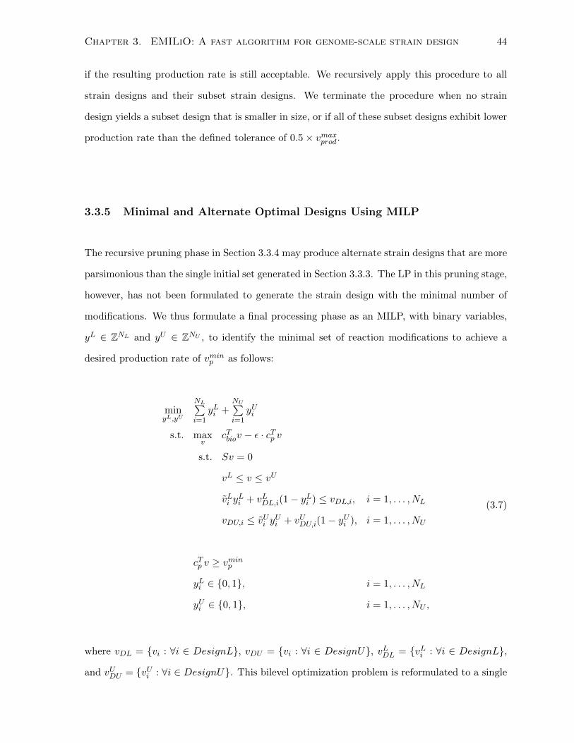
Chapter 3. EMILiO: A fast algorithm for genome-scale strain design 44
if the resulting production rate is still acceptable. We recursively apply this procedure to all
strain designs and their subset strain designs. We terminate the procedure when no strain
design yields a subset design that is smaller in size, or if all of these subset designs exhibit lower
production rate than the defined tolerance of 0.5× vmaxprod.
3.3.5 Minimal and Alternate Optimal Designs Using MILP
The recursive pruning phase in Section 3.3.4 may produce alternate strain designs that are more
parsimonious than the single initial set generated in Section 3.3.3. The LP in this pruning stage,
however, has not been formulated to generate the strain design with the minimal number of
modifications. We thus formulate a final processing phase as an MILP, with binary variables,
yL ∈ ZNL and yU ∈ ZNU , to identify the minimal set of reaction modifications to achieve a
desired production rate of vminp as follows:
minyL,yU
NL∑i=1
yLi +NU∑i=1
yUi
s.t. maxv
cTbiov − ε · cTp v
s.t. Sv = 0
vL ≤ v ≤ vU
vLi yLi + vLDL,i(1− yLi ) ≤ vDL,i, i = 1, . . . , NL
vDU,i ≤ vUi yUi + vUDU,i(1− yUi ), i = 1, . . . , NU
cTp v ≥ vminp
yLi ∈ {0, 1}, i = 1, . . . , NL
yUi ∈ {0, 1}, i = 1, . . . , NU ,
(3.7)
where vDL = {vi : ∀i ∈ DesignL}, vDU = {vi : ∀i ∈ DesignU}, vLDL = {vLi : ∀i ∈ DesignL},
and vUDU = {vUi : ∀i ∈ DesignU}. This bilevel optimization problem is reformulated to a single

Chapter 3. EMILiO: A fast algorithm for genome-scale strain design 45
level MILP as follows:
minv, wS ,
wL, wU ,
ηL, ηU ,
yL, yU
NL∑i=1
yLi +NU∑i=1
yUi
s.t. Sv = 0
vL ≤ v ≤ vU
vLi yLi + vLDL,i(1− yLi ) ≤ vDL,i, i = 1, . . . , NL
vDU,i ≤ vUi yUi + vUDU,i(1− yUi ), i = 1, . . . , NU
(wS)TS + wL − wU + ηL − ηU = cTbio − ε · cTpNL∑i=1
ηLi vLi +
N∑i=1
wLi vLi −
NU∑i=1
ηUi vUi −
N∑i=1
wUi vUi − cTbiov + ε · cTp v = 0
0 ≤ ηLi ≤ KyLi , i = 1, . . . , NL
0 ≤ ηUi ≤ KyUi , i = 1, . . . , NU
0 ≤ wLDL,i ≤ K(1− yLi ), i = 1, . . . , NL
0 ≤ wUDU,i ≤ K(1− yUi ), i = 1, . . . , NU
cTp v ≥ vminp
wL, wU , wLDL, wUDU ≥ 0
yLi ∈ {0, 1}, i = 1, . . . , NL
yUi ∈ {0, 1}, i = 1, . . . , NU ,
(3.8)
where wL ∈ RN and wU ∈ RN are dual variables for lower and upper bounds, respectively,
wLDL = {wLi : ∀i ∈ DesignL}, wUDU = {wUi : ∀i ∈ DesignU}, ηL ∈ RNL and ηU ∈ RNU are
dual variables for the modified lower and upper bounds, respectively, and K = 100. Critical to
note here (for practical application of the algorithm) is that the combinatorial solution space
of this MILP is much smaller than attempting to solve OptKnock or OptReg because we limit
modifications to only those included in each strain design generated in Section 3.3.4. With this
MILP formulation, we can also identify alternate optimal strain designs via integer cuts.

Chapter 3. EMILiO: A fast algorithm for genome-scale strain design 46
3.3.6 Modified OptReg and Local Search
We formulated a modified OptReg (Pharkya and Maranas, 2006), referred to as OptReg’,
to address the following issues: (1) the definition of up- or down-regulation requires splitting
fluxes into forward and reverse components and the strain designs generated by OptReg require
careful interpretation (Pharkya and Maranas, 2006), (2) down-regulation of a reversible reaction
should limit the magnitude of flux in both the forward and reverse directions, since the total
enzyme concentration is decreased, and (3) the definition of up- or down-regulations relative
to a reference flux might not be physiologically realistic and may unneccessarily limit strain
design. We thus modified the definition of up- and down-regulation and eliminated the need to
split reversible reactions into forward and reverse fluxes. A reference flux distribution becomes
irrelevant because we assume that the target reactions chosen by OptReg’ will be fine-tuned
further, regardless of their basal values. These modified definitions also reduced the number
of binary variables required for the algorithm. OptReg’ is fully described below. The modified
implementation of OptReg that we used in this work is as follows, for a maximum of θ total
genetic modifications:
maxvf , wKO,
wL, wU ,
ηDF , ηDR,
ηUF , ηUR,
yKO, yD
yUF , yUR
cTp Tvf (OptReg’)
s.t. vLi ≤ Tivf ≤ vUi , ∀i ∈ Unmod,
vLi yKOi ≤ Tivf ≤ vUj yKOi ,
∀i ∈ KO, j = 1, . . . , NKO,
Tivf ≤ vUDj yDj + vUi (1− yDj ),
∀i ∈ Forward, j = 1, . . . , NFor,
vLDj yDj + vLi (1− yDj ) ≤ Tivf ,
∀i ∈ Reverse, j = 1, . . . , NRev,

Chapter 3. EMILiO: A fast algorithm for genome-scale strain design 47
Tivf ≤ vUUj yURj + vUi (1− yURj ),
∀i ∈ Reverse, j = 1, . . . , NRev,
vLUj yUFj + vLi (1− yUFj ) ≤ Tivf ,
∀i ∈ Forward, j = 1, . . . , NFor,
NKO∑i=1
wKOi TKOi +
N∑i=1
wUi Ti−
N∑i=1
wLi Ti +
NFor∑i=1
ηDFi TFori −
NRev∑i=1
ηDRi TRevi +
NRev∑i=1
ηURi TRevi −
NFor∑i=1
ηUFi TFori = (cTbio − ε · cTp )T,
N∑i=1
wUi vUi −
N∑i=1
wLi vLi +
NDF∑i=1
ηDFi vUDi −
NDR∑i=1
ηDRi vLDi +
NUR∑i=1
ηURi vUUi −
NUF∑i=1
ηUFi vLUi − (cTbio − ε · cTp )Tvf = 0,
NKO∑i=1
yKO +
ND∑i=1
yD +
NUR∑i=1
yUR +
NUF∑i=1
yUF ≤ θ,
−KyKOi ≤ wKOi ≤ KyKOi , i = 1, . . . , NKO,
0 ≤ ηDFi ≤ KyDFi , i = 1, . . . , NFor,
0 ≤ ηDRi ≤ KyDRi , i = 1, . . . , NRev,
0 ≤ ηURi ≤ KyURi , i = 1, . . . , NRev,
0 ≤ ηUFi ≤ KyUFi , i = 1, . . . , NFor,
0 ≤ wUDF,i ≤ K(1− yDF )i, i = 1, . . . , NFor,
0 ≤ wLDR,i ≤ K(1− yDR)i, i = 1, . . . , NRev,
0 ≤ wUUR,i ≤ K(1− yUR)i, i = 1, . . . , NRev,
0 ≤ wLUF,i ≤ K(1− yUF )i, i = 1, . . . , NFor,

Chapter 3. EMILiO: A fast algorithm for genome-scale strain design 48
cTbiov ≥ vminbio ,
wL, wU , ηDL, ηDU , ηUR, ηUF ≥ 0,
yKOi ∈ {0, 1}, i = 1, . . . , NKO,
yDi ∈ {0, 1}, i = 1, . . . , ND,
yURi ∈ {0, 1}, i = 1, . . . , NRev,
yUFi ∈ {0, 1}, i = 1, . . . , NFor,
where, wKO, wU , wL, ηDF , ηDR, ηUR, ηUF are dual variables for the constraints corresonding
to knockouts, unmodified upper and lower bounds, down-regulation of forward fluxes, down-
regulation of reverse fluxes, upregulation of reverse fluxes, and upregulation of forward fluxes,
respectively, yKO, yD, yUR, yUF are binary variables for the constraints corresponding to
knockouts, down-regulation, upregulation of reverse fluxes, and upregulation of forward fluxes,
respectively, and TKO, TFor, TRev are the rows of T corresponding to fluxes in the sets, KO,
Forward, and Reverse, respectively. These sets are defined as follows:
Unmod = {i = 1, . . . , N : flux i cannot be modified},
KO = {i /∈ Unmod : flux i can be knocked out},
Forward = {i /∈ Unmod : vmini ≥ 0, vmaxi > 0},
Reverse = {i /∈ Unmod : vmaxi ≤ 0, vmini < 0},
where vmini and vmaxi are the minimum and maximum values of flux i found using flux variability
analysis (FVA) (Mahadevan and Schilling, 2003). The sets, KO, Forward and Reverse have
NKO, NFor and NRev members, respectively. The modified bounds for up- or down-regulating
forward or reverse fluxes are defined in Table 3.1 and schematically described in Figure 3.1.
3.3.7 Local search implementation of modified OptReg
In order to obtain locally optimal solutions within reasonable computational time, we also
developed a local search version of OptReg’, referred to as OptReg’LS. The local search method
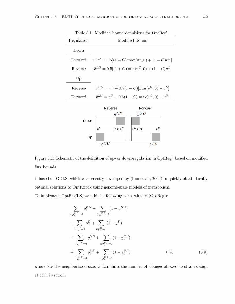
Chapter 3. EMILiO: A fast algorithm for genome-scale strain design 49
Table 3.1: Modified bound definitions for OptReg’
Regulation Modified Bound
Down
Forward vUD = 0.5[(1 + C) max(vL, 0) + (1− C)vU ]
Reverse vLD = 0.5[(1 + C) min(vU , 0) + (1− C)vL]
Up
Reverse vUU = vL + 0.5(1− C)[min(vU , 0)− vL]
Forward vLU = vU + 0.5(1− C)[max(vL, 0)− vU ]
Figure 3.1: Schematic of the definition of up- or down-regulation in OptReg’, based on modified
flux bounds.
is based on GDLS, which was recently developed by (Lun et al., 2009) to quickly obtain locally
optimal solutions to OptKnock using genome-scale models of metabolism.
To implement OptReg’LS, we add the following constraint to (OptReg’):
∑i:yKO
i =0
yKOi +∑
i:yKOi =1
(1− yKOi )
+∑
i:yDi =0
yDi +∑
i:yDi =1
(1− yDi )
+∑
i:yURi =0
yURi +∑
i:yURi =1
(1− yURi )
+∑
i:yUFi =0
yUFi +∑
i:yUFi =1
(1− yUFi ) ≤ δ, (3.9)
where δ is the neighborhood size, which limits the number of changes allowed to strain design
at each iteration.

Chapter 3. EMILiO: A fast algorithm for genome-scale strain design 50
We observed that at any iteration, k, the algorithm might cycle between two solutions. To
prevent cycling, we added the following constraint:
∑i:yKO
k−1,i=0
yKOi +∑
i:yKOk−1,i=1
(1− yKOi )
+∑
i:yDk−1,i=0
yDi +∑
i:yDk−1,i=1
(1− yDi )
+∑
i:yURk−1,i=0
yURi +∑
i:yURk−1,i=1
(1− yURi )
+∑
i:yUFk−1,i=0
yUFi +∑
i:yUFk−1,i=1
(1− yUFi ) ≥ 1 (3.10)
This prevents the algorithm from identifying a new solution for iteration k + 1 from returning
to the solution found previously at iteration k − 1.
At any iteration, the algorithm might terminate if no solution that improves the objective can
be found, subject to the neighborhood size constraint. Hence, for δ = 1, if the MILP solver
cannot find a single change to the current strain design that would improve the objective,
the solver might return the current solution and the algorithm would converge and terminate.
This situation arises when δ is small and the strain design at the current iteration can only be
improved via multiple simultaneous modifications or by first backtracking. Hence, to prevent
premature convergence for small values of δ, we added the following constraint:
∑i:yKO
i =0
yKOi +∑
i:yKOi =1
(1− yKOi )
+∑
i:yDi =0
yDi +∑
i:yDi =1
(1− yDi )
+∑
i:yURi =0
yURi +∑
i:yURi =1
(1− yURi )
+∑
i:yUFi =0
yUFi +∑
i:yUFi =1
(1− yUFi ) ≥ 1 (3.11)
This forces the MILP solver to make at least one change to the current strain design. Hence,
constraints (3.10) and (3.11) force a different solution to be identified at each iteration, without
returning back to the previous solution. If constraints (3.10) and (3.11) make the MILP problem
infeasible, or the new solution has a worse objective, this indicates that no change within the

Chapter 3. EMILiO: A fast algorithm for genome-scale strain design 51
neighborhood size can be made to improve the current solution–hence, the algorithm terminates.
We note that these constraints do not prevent cycles spanning more iterations, such as cycling
back to a solution from two iterations ago. However, we have not experienced such longer cycles
during our simulations.
3.3.8 Determining minimum flux magnitudes
Using EMILiO, we generated almost 200 strains for aerobic or anaerobic succinate production.
To compare the physiology of these strains to each other and to the wild-type, we determined
the minimum flux magnitude of each flux i as follows:
minv,r
r (3.12a)
s.t. Sv = 0, (3.12b)
vi − r ≤ 0, (3.12c)
−vi − r ≤ 0, (3.12d)
vL ≤ v ≤ vU , (3.12e)
r ≥ 0, (3.12f)
where r is a non-negative variable equal to the minimum absolute value of flux, vi, at optimality.
We iteratively solved this linear program for all N fluxes for each mutant and the wild-type.
For anaerobic conditions, the upper and lower bounds of the oxygen uptake flux were set to
zero.
3.4 Results and Discussion
3.4.1 Comparison of the strain design algorithms
We designed succinate-producing E. coli strains grown aerobically on glucose using three algo-
rithms: EMILiO, OptReg’, and OptReg’LS. OptReg’ and OptReg’LS are the global and local
search implementations of a modified OptReg. We modified the definition of up- and down-
regulation such that unbiased exploration of the strain designs could be performed, without the
need for a reference flux distribution (Materials and Methods). We also developed OptReg’LS,

Chapter 3. EMILiO: A fast algorithm for genome-scale strain design 52
a local search implementation of OptReg’ based on GDLS.
EMILiO was able to identify a strain having 100% succinate production, fully coupled to its
100
101
102
103
104
0
20
40
60
80
100
Percent of maximal succinate production (%)
CPU time (min)
EMILiO
OptRegLS’
OptReg’
(Minimum growth rate, Maximal succinate production)
Growth rate (h−1)
Succinate production (mmol/gDW/h)
0 0.1 0.3 0.5 0.7 0.9 1.1 1.30
5
10
15
20
25
30
35
Wild−type
EMILiO
OptReg’LS
OptReg’
Figure 3.2: Comparison of succinate production strains identified by EMILiO, OptReg’LS, and
OptReg’. Succinate production envelopes for OptReg’, OptReg’LS, and EMILiO using the
iAF1260 genome-scale model of E. coli metabolism (top). CPU times for strain design using
EMILiO, OptReg’LS, and OptReg’ (bottom). OptReg’LS converged in two iterations. CPU
time is shown in log scale.
maximum growth rate in 2 minutes (Fig. 3.2). The strain design involved a total of three
modifications: deletion of succinate dehydrogenase (SUCDi) and up-regulation of fumarate re-
ductase (FRD2) and aconitase (see (Yang et al., 2011)). We then examined the network-wide
changes due to these modifications. We first calculated the minimal absolute flux of all reactions

Chapter 3. EMILiO: A fast algorithm for genome-scale strain design 53
under the wild-type genetic background, subject to a minimum growth rate of 0.1 h−1 (Section
3.3.8). This step was implemented to prevent ambiguity arising from alternate optimal flux
distributions. Similarly, we calculated the minimum flux magnitudes for the designed strain
and compared these results with those of the wild-type. We thus identified 75 reactions that
were forced to carry more flux in the designed strain compared to the wild-type. These reac-
tions include isocitrate lyase (ICL), malate synthase (MALS), citrate synthase (CS), isocitrate
dehydrogenase (ICDH), malate synthase (MALS), malate dehydrogenase (MDH), and PPC. In-
cidentally, all of these reactions were shown to have increased activity by succinate-producing
strains of E. coli involving SUCDi knockout, grown aerobically on glucose in chemostats (Lin
et al., 2005).
We next ran OptReg’ and OptReg’LS with a regulatory strength parameter, C = 0.5, which
determines the flux value of reactions that are up- or down-regulated. First, we terminated
OptReg’ after four days and obtained a solution, which was not proven to be globally optimal.
The strain designed by OptReg’, nonetheless, produced succinate at 83.26% of the maximal
rate (Fig. 3.2). The strain involved three modifications: acetate kinase knockout, and over-
expression of PPC and fumarate reductase (FRD3). We investigated why OptReg’, which
was allowed to identify up to three modifications, did not find the superior three-modification
strain found by EMILiO. Upon inspection, we found that a strategy overexpressing fumarate
reductase and aconitase to values determined by C = 0.5 and deleting SUCDi violated the
stoichiometric constraints (Materials and Methods). This result demonstrated that potentially
better solutions might have been missed by OptReg’ and OptReg’LS due to the difficulty of
choosing an appropriate C for all reactions, prior to running the algorithms.
We then ran the local search implementation, OptReg’LS to quickly find locally optimal solu-
tions. Initially, OptReg’LS converged to a solution in three iterations, taking ∼ 4 hours (Fig.
3.2). The identified strain produced 82.13% of maximal production. Thus, OptReg’LS was able
to identify a strain having only 1.4% less production than the global search in four hours rather
than four days. This strain involved only the overexpression of FRD3, which was one of the
three modifications identified by OptReg’.
We investigated why OptReg’LS was unable to identify the three-modification strain designed

Chapter 3. EMILiO: A fast algorithm for genome-scale strain design 54
by OptReg’, since only two more modifications were required. For this, we began with a strain
having only FRD3 overexpression and added each of the two modifications, separately. This
procedure reflects how OptReg’LS was run with a neighborhood size of δ = 1, so only single
changes could be made from the initial strain. We found that adding each modification indi-
vidually could not improve production–only by adding both could production improve. In fact,
adding PPC overexpression to FRD3 overexpression slightly decreased (by 0.035%) succinate
production. This shows that the interactions amongst all possible flux modifications is non-
linear and that a local search method with small neighborhood size may fail to find improved
solutions. Increasing the neighborhood size may overcome this problem; however, we noticed
that a neighborhood size of even δ = 2 made each iteration of OptReg’LS prohibitively long,
thereby undermining the reason for using local search.
3.4.2 Large-scale exploration of the strain design space
The computational efficiency of EMILiO allowed us to use it as an engine for large-scale ex-
ploration of numerous alternate strain designs for succinate production. A substantial body of
literature already exists for succinate overproduction strains. The genetic manipulation strate-
gies in the literature can be categorized as (1) experimentally constructed, (2) computationally
predicted, and (3) computationally predicted and experimentally validated. Here, we have
surveyed a number of strain designs identified by recent computational algorithms, and also a
portion of the experimental literature. We found that while the existing literature on computa-
tional strain designs covered a wide variety of strain designs, some regions of the design space
had not been previously explored. Furthermore, genetically defined experimental strains have
been confined to a small region of the design space (Fig. 3.3).
EMILiO identified distinctly different strain designs for anaerobic and aerobic conditions.
Aerobically, knockout or inhibition of succinate dehydrogenase (SUCDi) and overexpression of
fumarate reductase were predicted to be necessary for achieving 100% of the maximal pro-
duction. Without these two strategies, up to ∼84% maximal production could be achieved.
Anaerobically, however, SUCDi knockout or inhibition was not an important strategy. Fu-

Chapter 3. EMILiO: A fast algorithm for genome-scale strain design 55
PFL
PPPGO
SUCDi
FRD2
ICL
MALS
FUM
PPCSCT
SUCDi
SUCOAS
Aerobic Anaerobic Both
191
4
21
27
1
12
6
EMILiO simulations
Literature:
Experimental
Literature:
Computational
Figure 3.3: Summary of strategies (i.e., the individual reactions being modified) identified by
EMILiO for succinate production and comparison to existing literature. While many strategies
are supported by previous experimental and/or computational literature, many more unval-
idated predictions have been generated in this work. Strategies were identified for aerobic,
anaerobic, or both conditions. Some of the frequently used strategies are annotated. Nodes are
linked if the strategies are used together frequently.
marate reductase was an important strategy for an initial anaerobic strain. However, we found
that strain designs not using fumarate reductase had equivalent succinate production. In these
strains, fumarase or malate dehydrogenase overexpression were the most important modifica-
tions. Another strain having 85% maximal anaerobic succinate production was found, for which
a slight induction of malate synthase was most important. Such relationships amongst the re-
action modifications are mapped in Fig. 3.4.
For each of the 234 strains designed using EMILiO and also the wild-type, we calculated the

Chapter 3. EMILiO: A fast algorithm for genome-scale strain design 56
Figure 3.4: The landscape of strategies for succinate production. Squares indicate modifica-
tions having a large impact on strain performance. Diamonds indicate modifications identified
frequently in the 234 alternate strain designs.

Chapter 3. EMILiO: A fast algorithm for genome-scale strain design 57
minimum magnitude of each flux–again, to avoid ambiguity due to alternate optimal flux distri-
butions. For each strain, we then obtained an n-dimensional vector (n is the number of fluxes)
defined as the deviation in these minimum flux magnitudes, relative to those of the wild-type.
These deviation vectors can thus be used to differentiate amongst the different strain designs.
Also, the set of fluxes whose minimum magnitudes are different from those of the wild-type are
similar to the MUST sets of (Ranganathan et al., 2010). We then clustered the 234 alternate
strain designs based on the similarity of their minimum flux magnitude vectors, using affinity
propagation (AP) (Frey and Dueck, 2007) with damping factor of 0.9. We thus identified 15
distinct clusters of varying sizes (Fig. 3.5). The largest two clusters produced 100% of the
maximal succinate flux, and the cluster centers differed only by one modification: knockout
of methionine adenosyltransferase (METAT) versus increased reverse activity of succinyl-CoA
synthetase (SUCOAS). This resulted in significantly higher fluxes through acetate-CoA ligase
(ACCOAL), propanoyl-CoA: succinate CoA-transferase (PPCSCT), and SUCOAS in the sec-
ond cluster of strains.
We identified flux magnitudes that consistently deviated from those of the wild-type across
many of the 15 clusters (Fig. 3.5). Some of these have been experimentally validated in the
literature (Table 3.2). We also found that, in some cases, a small number of fluxes were suffi-
cient to clearly differentiate one cluster from another. For example, cluster 5 had significantly
higher deviations in glucose-1-phosphate adenylyltransferase (GLGC) and polyphosphate ki-
nase (PPKr) fluxes, compared to those of cluster 1 (Fig. 3.5). PPKr activity was not directly
modified, but the increased production of inorganic diphosphate due to increased GLGC activ-
ity led to high reverse activity of PPKr. The increased GLGC activity more tightly coupled
succinate production to growth. This cluster represented a group of anaerobic strains producing
succinate at 75.72% maximal production.
Strain clusters 8 and 10 provide a case study of the potential utility of the map of strain
design space generated by EMILiO. The respective cluster center strains produced 89.17% and
84.75% maximal succinate. The pattern of absolute flux deviations, relative to wild-type, of
these clusters show distinctly different patterns from the others (Fig. 3.5). In particular, both
clusters have increased activities of acetyl-CoA synthetase (ACS), acetate kinase and phospho-

Chapter 3. EMILiO: A fast algorithm for genome-scale strain design 58
Figure 3.5: The 234 strains grouped into 15 clusters using affinity propagation. (A) Clusters are
formed based on the deviation of minimum flux magnitudes, relative to those of the wild-type.
These deviations represent changes in physiology of each strain. Larger rectangles represent
clusters with a larger number of strain design members. (B) The fluxes that deviate consistently
across the 15 strains are shown in yellow, while those fluxes distinguishing cluster 5 from cluster
1 are shown in magenta.
transacetylase (ACK-PTA). Lin et al. (2006) showed that ACS overexpression could reduce
acetate accumulation during excess glucose fermentation. They also showed that under aerobic
conditions, ACS overexpression could increase the acetyl-CoA pool, and the authors hypothe-
sized that this could potentially improve product formation. Our independent computational
exploration agrees with these experimental results. Cluster 10 represents aerobic succinate
production strains with increased ACS activity. Cluster 8 represents anaerobic strains with
similarly increased ACS activity. Both strains exhibited increased PPC activity. The anaer-
obic cluster is thus consistent with experimental literature, in which the acetyl-CoA pool was
increased, together with PPC overexpression, to improve anaerobic succinate production (Lin
et al., 2004). This cluster also exhibited glyoxylate shunt activity, together with increased ACK-
PTA activity. These strategies have been experimentally implemented to improve anaerobic
succinate production by Sanchez et al. (2005). Finally, although EMILiO predicted that both

Chapter 3. EMILiO: A fast algorithm for genome-scale strain design 59
Table 3.2: Reactions whose minimum flux magnitude (see Section 3.3.8) deviated from that of
the wild-type. Reference is made to experimental evidence.
Reaction Reference(s)
Malic enzyme, NAD (ME1) (Jantama et al., 2008; Stols and Donnelly, 1997)
Methylglyoxal synthase (MGSA) (Jantama et al., 2008)
Propionate kinase (PPAKr) (Jantama et al., 2008)
Phosphoenolpyruvate carboxykinase (PPCK) (Millard et al., 1996)
Acetaldehyde dehydrogenase (ACALD) (Jantama et al., 2008; Sanchez et al., 2006; Yun et al.,
2005)
Acetate kinase (ACKr) (Jantama et al., 2008; Lin et al., 2005; Sanchez et al.,
2006; Yun et al., 2005)
Alcohol dehydrogenase, ethanol (ALCD2x) (Jantama et al., 2008; Sanchez et al., 2006; Yun et al.,
2005)
Aspartate transaminase (ASPTA) (Jantama et al., 2008)
Isocitrate lyase (ICL) (Lin et al., 2005; Sanchez et al., 2006)
D-lactate dehydrogenase (LDH-D) (Chatterjee et al., 2001; Jantama et al., 2008; Millard
et al., 1996; Sanchez et al., 2006; Stols and Donnelly, 1997)
Malate synthase (MALS) (Sanchez et al., 2006)
Pyruvate formate lyase (PFL) (Chatterjee et al., 2001; Jantama et al., 2008; Stols and
Donnelly, 1997)
Phosphoenolpyruvate carboxylase (PPC) (Lin et al., 2005; Millard et al., 1996)
Phosphotransacetylase (PTAr) (Jantama et al., 2008; Sanchez et al., 2006; Yun et al.,
2005)
Succinate dehydrogenase (SUCDi) (Lin et al., 2005)
CO2 uptake (EX-co2(e)) (Zeikus et al., 1999)
PEP:Pyr phosphotransferase system (GLCpt-
spp)
(Chatterjee et al., 2001; Lin et al., 2005)
NADH dehydrogenase (NADH16pp) (Yun et al., 2005)
ACS and ACK-PTA activities could be implemented simultaneously, ACK-PTA has a higher
Km than ACS, which may limit its flux (Lin et al., 2006). Therefore, mechanistic understanding
of the succinate production might be improved by incorporating detailed kinetic constraints for

Chapter 3. EMILiO: A fast algorithm for genome-scale strain design 60
these and related reactions.
3.4.3 Increasing production beyond knockout strains
Previously, Pharkya et al. (2003) explored knockout strains for amino acid production using
OptKnock. Amino acid secretion was coupled to growth but this required fixing certain ex-
change fluxes (e.g., oxygen, ammonia, etc.), in addition to knockouts. This study demonstrated
the difficulty of fundamentally coupling secretion of amino acids to growth using only gene
knockouts. More recently, Feist et al. (2010) computationally explored strains having up to
10 knockouts using OptKnock and OptGene algorithms using the latest genome-scale model
of E. coli metabolism. Strains with high yield were found for certain product-substrate pairs;
however, some products, including L-glutamate and L-serine, could not be coupled to growth.
These studies demonstrated that strictly knockout strategies may be insufficient for growth-
coupled production of certain products. We thus investigated if strains involving fine-tuned
fluxes could be engineered to produce L-glutamate and L-serine.
An initial run of EMILiO generated a strain secreting L-glutamate at 100% of the maximal
flux. This strain design included knockout of glutamate decarboxylase to prevent conversion
of L-glutamate to 4-aminobutanoate and knockout of α-ketoglutarate dehydrogenase to direct
carbon flux towards L-glutamate production. The latter strategy has been experimentally val-
idated (Shirai et al., 2005). The strain also increased reverse activity of glutamate dehydroge-
nase (GLUDy), which would convert AKG to L-glutamate. Computationally, this strategy was
identified because increased reverse activity of GLUDy would directly increase L-glutamate
production. However, increasing in vivo reverse activity of glutamate dehydrogenase would
require a high ratio of AKG to L-glutamate concentrations, which is difficult to directly manip-
ulate. Hence, we ran EMILiO again with GLUDy removed from the list of target reactions, to
encourage the identification of strain designs incorporating a broader scope of manipulations.
The second strain identified by EMILiO secreted L-glutamate at 94% of the maximal rate.
This strain involved two knockouts, four down-regulation and three up-regulation strategies.
In contrast with the first strain, GLUDy flux was decreased, while pentose phosphate pathway
flux significantly increased. This demonstrated that at least two distinct modes of metabolism

Chapter 3. EMILiO: A fast algorithm for genome-scale strain design 61
could be used to overproduce L-glutamate. One of the non-intuitive, necessary modifications
was the removal of inorganic diphosphatase activity (PPA), which catalyzed the conversion of
inorganic diphosphate to inorganic phosphate. This strategy was used in conjunction with over-
expression of glucose-1-phosphate adenylyltransferase, which produced inorganic diphosphate.
The removal of PPA lead to increased reverse polyphosphate kinase (PPKr) activity to consume
inorganic diphosphate while also generating ATP. Hence, the network-wide effects of targeting
the balance of currency metabolites was captured by the algorithm.
Similarly, we generated strains for L-serine production using EMILiO. The first included exper-
imental strategies used by Peters-Wendisch et al. (2005) for C. glutamicum, which were based
on targeted metabolic engineering. These included L-serine dehydratase knockout and over-
expression of 3-phosphoglycerate dehydrogenase. We then looked for alternate strain designs
involving a broader scope of manipulations that would be more difficult to conceive using a
targeted metabolic engineering approach. We thus ran EMILiO again with the reactions close
to L-serine production (PGCD, PSERT, PSER-L, MTHFC, and MTHFD) removed from the
list of target reactions. EMILiO identified an alternate strain that produced 99.65% maximal
L-serine, suggesting that non-intuitive strategies could be identified using the algorithm.
The search for L-glutamate and L-serine production strains demonstrated that EMILiO could
generate both experimentally validated and potentially novel strategies for amino acids, in ad-
dition to central metabolism intermediates.
3.5 Conclusions
We have used a novel computational strain design algorithm (EMILiO) for production of suc-
cinate, L-glutamate, and L-serine using the iAF1260 genome-scale model E. coli metabolism.
EMILiO was shown to be computationally efficient and capable of generating almost two hun-
dred alternate strain designs with high succinate production (≥ 83% maximal production) using
both parallel and orthogonal sequential search methods. Using EMILiO, we rapidly identified
strains producing L-glutamate or L-serine production at 100% of the respective maximal rates.

Chapter 3. EMILiO: A fast algorithm for genome-scale strain design 62
Strains coupling the production of these amino acids to growth could not be identified in a
previous study that investigated up to 10 knockouts using OptKnock and OptGene algorithms
(Feist et al., 2010). This shows that while knockout strategies alone can be insufficient to couple
secretion of some products to growth under certain conditions, fine-tuning fluxes may enable
such coupling. Using previous algorithms, the identification of fine-tuned flux strategies would
be significantly more complicated than solely knockout strategies; however, EMILiO was shown
to generate such strain designs with ease using a genome-scale model of metabolism.
We used EMILiO as an efficient engine for exploring the strain design space of growth-coupled
succinate production using the latest genome-scale model of E. coli metabolism. The resulting
map elucidated interactions amongst over 100 genetic manipulation strategies for succinate pro-
duction. We intend to bring such large-scale, predictive maps of the strain design space closer to
the workbench of metabolic engineers. Owing to the speed of EMILiO, the entire map can then
be re-drawn in the future with incorporation of new experimental data. This can accelerate
both model refinement and elucidation of mechanisms relevant for product formation.

Chapter 4
Genome-scale robust strain design
4.1 Abstract
Cell metabolism is an important platform for sustainable biofuel, chemical and pharmaceutical
production but its complexity presents a major challenge for scientists and engineers. Although
in silico strains have been designed in the past with predicted performances near the theoretical
maximum, their real-world performances are often sub-optimal. We argue that model-based,
genome-scale designs need to consider realistic perturbations for improved performance. Here
we demonstrate, using ∼100 in silico succinate overproduction strains, that predicted yields
vary widely when intracellular and environmental perturbations are included in the model.
We show that mechanisms for improving robustness of naturally evolved organisms can be
identified to help design robust engineered strains. Furthermore, we find that redundancy, a
robustness-enhancing strategy ubiquitous in complex systems, may either improve or undermine
robustness, depending on the magnitude of perturbations. With a deeper understanding and a
more fruitful exploitation of robustness, we believe that more robust strain designs are possible.
4.2 Introduction
Naturally evolved systems exhibit robustness against a variety of perturbations, from intracel-
lular noise in protein translation rates (Becskei and Serrano, 2000) to temporal variations in the
weather (Tilman et al., 2006). By virtue of robust design principles (Morari and Zafiriou, 1989),
63

Chapter 4. Genome-scale robust strain design 64
engineered systems display comparable robustness (Csete and Doyle, 2002; Kitano, 2004). The
finding that biological systems naturally acquire the same robustness-enhancing mechanisms as
those utilized in engineered systems (Yi et al., 2000) suggests that it may be possible to system-
atically design robustness in engineered cells. In particular, robust microbial and mammalian
strains are required for the environmentally sustainable and economically viable production of
chemicals, fuels, and pharmaceuticals.
As with engineered systems, predictive models can accelerate the design of robust biological
systems. Currently, computational models of cell metabolism (Orth et al., 2010), and strain
design algorithms (Burgard et al., 2003; Ranganathan et al., 2010; Kim and Reed, 2010; Yang
et al., 2011) are being developed actively, in order to alleviate the bottlenecks encountered in
traditional approaches to strain design (Chen et al., 2010). However, the prediction of strain
performance in response to perturbations in various environmental and intracellular processes
has been explored only to a limited extent for knockout strains (Cox et al., 2006; Tepper and
Shlomi, 2010). Such studies are even more lacking for strains involving optimal target fluxes,
in which perturbations to intracellular (e.g., transcriptional or post-translation regulation) or
environmental (e.g., substrate and oxygen concentrations) processes can cause in vivo flux of
targeted reactions to deviate from their predicted, optimal levels.
Here, we present a novel computational framework to incorporate the effects of genetic and en-
vironmental perturbations, as well as model parameter uncertainties into computational strain
design. We anticipate that the results of our analysis will generate a new category of in silico
strains: those optimized for balanced performance and robustness against specific perturbations
and uncertainties.
4.3 Robust strain design
We now present our computational framework for designing robust overproduction strains. We
model production rate, or flux, of the target metabolite as a random variable with mean, µ and
standard deviation σ. We desire a high µ and low σ. Thus, we define robustness, R, as
R = 1− σ
µ. (4.1)

Chapter 4. Genome-scale robust strain design 65
R is defined only for non-zero µ. It has a maximum value of 1 under nominal conditions (σ = 0),
and it has an unbounded minimum. The coefficient of variation (σ/µ) contained in this defi-
nition is also termed the stability coefficient in ecology (Tilman et al., 2006), while its inverse
(µ/σ) is termed the signal-to-noise ratio in imaging (McGibney and Smith, 1993). In addition,
σ/µ is related to sensitivity measures used to estimate the change in a variable in response to a
change in a parameter (Saltelli et al., 2000). The simple definition of robustness adopted here
is useful for engineering applications. For an alternative definition of robustness in biological
systems, see (Kitano, 2007).
A system that is robust to one perturbation may not be robust, or may be fragile, to oth-
ers. Thus, we consider the perturbations and uncertainties listed in Table 4.1. To maximize
metabolite production, metabolic engineering often requires targeted genes to be expressed
at optimal levels to control flux through key pathways (Alper et al., 2005; Lee et al., 2007).
However, these fluxes are perturbed by various factors and are known to deviate from their
optimal values, in vivo. At a minimum, gene expression noise results in random perturbations
to these fluxes (Wang and Zhang, 2011); therefore, we have included the random perturbation
of controlled fluxes in all of our simulations. In addition, we consider variations in glucose and
oxygen uptake fluxes, the secretion of byproducts due to these variations, the re-consumption
of these byproducts, and osmotic stress response. These are some of the major perturbations
encountered by engineered strains in industrial-scale bioreactors (Enfors et al., 2001).
Recently, the constraint-based modeling framework has been extended to include additional
Table 4.1: Perturbations and model uncertainties investigated
Perturbations
- Flux variations due to gene expression noise
- Variation in substrate and oxygen uptake fluxes
- Re-consumption of overflow byproducts
- Osmotic stress response
Parameter - Parameters involved in the molecular crowding constraint (Beg et al., 2007)
uncertainties - Parameters involved in the membrane occupancy constraint (Zhuang et al., 2011)
metabolic constraints, including a limit on the total enzyme concentration in the cell (molecular

Chapter 4. Genome-scale robust strain design 66
crowding (Beg et al., 2007)), and a limit on the total concentration of membrane-bound enzymes
(membrane occupancy (Zhuang et al., 2011)). These constraints have been shown to affect key
physiological features including catabolite repression and overflow metabolism. Although these
constraints improve the accuracy of model predictions, they require the estimation of many
additional parameters. Therefore, we assessed the sensitivity of strain design to uncertainty in
these model parameters.
4.4 Materials and Methods
4.4.1 Flux balance analysis, model reduction, and in silico strain design
verification
The distribution of metabolic reaction fluxes was simulated using Flux Balance Analysis (FBA)
(Varma and Palsson, 1994). In FBA, the reaction network stoichiometry is defined in a matrix,
S ∈ Rm×n where the m rows correspond to metabolites and the n columns correspond to fluxes.
The rank, r, of S is less than m; hence, we can separate the free and pivot variables in the
reduced row echelon form of S and formulate a reduced FBA problem as below:
maxv
cT · Tvf = vbio − ε · vprod (4.2a)
s.t. vL ≤ Tvf ≤ vU , (4.2b)
where vf ∈ RN−r are the free flux variables, vL ∈ RN and vU ∈ RN are the vectors of minimum
and maximum fluxes, respectively, and T ∈ RN×(N−r) is defined such that v = Tvf , and c is the
objective vector. Here, ε = 0.001 is used to add a small weighted minimization of the product
flux because alternate optima in the solution of this linear program (LP) might lead to a range
of product flux when growth rate (vbio) is maximized. We implemented this reduced FBA in
EMILiO, as described in (Yang et al., 2010a, 2011).
The core biomass reaction in the iAF1260 model was used to simulate cell growth. We defined
the nominal model to have an uptake rate of 20 mmol/gDW/h for both glucose and oxygen, to
reflect experimentally observed uptake rates (Varma et al., 1993). We computed the nominal
maximum succinate production rate, vmaxprod=32.25 mmol/gDW/h by maximizing succinate flux

Chapter 4. Genome-scale robust strain design 67
subject to these uptake constraints, and a minimum required growth rate of 0.1 h−1. Similarly,
the nominal maximum L-serine production rate was 39.52 mmol/gDW/h.
We reduced the number of target reactions for modification to eliminate target reactions sus-
pected not to be experimentally implementable. Non-gene associated reactions were excluded
from the target reactions based on the gene-protein-reaction mappings in the iAF1260 model.
We also removed reactions that were either essential for or significantly reduced growth. These
reactions are described in (Feist et al., 2010) and include reactions involved in cell enve-
lope biosynthesis, glycerophospholipid metabolism, inorganic ion transport and metabolism,
lipopolysaccharide biosynthesis and recycling, membrane lipid metabolism, murein biosynthe-
sis, murein recycling, inner membrane transport, outer membrane transport, and outer mem-
brane porin transport.
Each strain design identified by EMILiO was verified, in silico, by implementing the strategies
into an FBA simulation. This step was implemented to ensure that numerical difficulties asso-
ciated with solving the large-scale mixed-integer linear program (MILP) problems did not lead
to solutions that violated the constraints of the optimization problems.
All code was implemented in MATLAB (The Mathworks, Inc., Natick, MA). CPLEX 12.1 was
used to solve the LPs and MILPs using the CPLEXINT MATLAB interface. All simulations
were run on AMD Opteron 2.4 GHz processors.
4.4.2 EMILiO
EMILiO is a computational algorithm that couples biochemical production to growth by quan-
titatively optimizing a set of target fluxes (Yang et al., 2010a, 2011). EMILiO is formulated as
the following bilevel optimization problem:
maxvL,vU
cTp · Tvf
s.t. maxvf
cT · Tvf − ε · cTp · Tvf
s.t. vL ≤ Tvf ≤ vU
vbio ≥ vminbio ,
(4.3)

Chapter 4. Genome-scale robust strain design 68
where vminbio is the minimum required growth rate, and the inner optimization is the reduced
FBA formulation (4.2) with the additional objective of minimizing production rate. ε = 0.001
was chosen so that the maximum growth rate was not affected by minimization of production.
Using the Karush-Kuhn-Tucker (KKT) conditions, this bilevel optimization problem is refor-
mulated into a single-level mathematical program with complementarity constraints (MPCC)
(Yang et al., 2008) as follows:
maxx
cTp · Tvf (4.4a)
wLi µLi + wUi µ
Ui = 0, i = 1, . . . , N (4.4b)
Tvf + µU = vU (4.4c)
Tvf − µL = vL (4.4d)
wUT − wLT = cT · T − ε · cTp · T (4.4e)
vbio ≥ vminbio (4.4f)
wL, wU , µL, µU ≥ 0 (4.4g)
where µL ∈ RN and µU ∈ RN are slack variables for the lower and upper bounds, respectively,
and x = [vf , vU , vL, µU , µL, wU , wL]T . This MPCC is solved in three stages as described in
(Yang et al., 2010a, 2011). Briefly, a successive linear program (SLP), or iterative linear program
(ILP) (Baker and Lasdon, 1985; Bullard and Biegler, 1991) is formulated to identify a large set
of reaction modifications. This set is then recursively reduced to subsets using LP. Finally, an
MILP is applied to each of the resulting subsets to find alternate minimal sets.
Once the MPCC above was solved, we implemented a number of post-processing steps to ensure
that the strains were not affected by numerical error. First, EMILiO sometimes found strategies
that optimized fluxes to very low levels. While many of these were valid inhibition strategies,
we asked whether some could be replaced by a knockout instead without reducing production.
If an inhibition can indeed be replaced by a knockout without affecting production, then the
inhibition and knockout are alternate optimal strategies. If the knockout actually improves
production, then we can conclude that EMILiO had converged to a local optimum, whereas if
production decreases, then we must quantify the decrease in production. Then, we must assess

Chapter 4. Genome-scale robust strain design 69
whether the greater ease of genetic manipulation through implementing a knockout instead of
an inhibition justifies the decrease in production. Accordingly, for every strain, we replaced each
manipulation that optimized flux to less than 0.1 mmol/gDW/h with a knockout. If production
increased or remained the same, we kept the knockout modification.
Second, manipulations were sometimes found that increased production by only a small amount.
We thus removed all manipulations from each strain that increased production by less than
0.001% of the maximal flux.
4.4.3 Strain design using EMILiO
Using the EMILiO algorithm (Yang et al., 2010a, 2011), we started by generating a total of
112 alternative strains under nominal conditions (i.e., glucose and oxygen uptake rates of 20
mmol/gDW/h). Initially, 73% of the 112 strains achieved at least 99% maximal succinate yield
under nominal conditions. EMILiO, being a local optimization algorithm, does not guarantee
global optimality. Hence, we implemented an additional step to try and improve the nominal
performance of the thirty strains that did not achieve 99% nominal performance. We used the
sensitivity analysis procedure (see Section Sensitivity analysis of a strain design), with glucose
and oxygen uptake rates fixed to their nominal values. We sampled 1,000 feasible random fluxes
for each controlled reactions in each of the thirty strains with nominal performance below 99%
maximal yield.
The results of random sampling showed that despite being a local optimization algorithm,
EMILiO very often found the globally optimal fine-tuning levels, in addition to identifying the
optimal set of manipulated reactions. Only two of the 30 strains showed improved succinate
production. One strain improved 3% from 89% to 92% maximal succinate flux. This was
achieved by replacing a succinate dehydrogenase (SUCDi) inhibition with a knockout and ad-
justing fine-tuned levels of other reactions appropriately. Another strain improved almost 19%
from 82% to 97% maximal succinate flux. This strain already had SUCDi knockout and fine-
tuning of menaquinone-dependent fumarate reductase (FRD2) and malate synthase (MALS).
The large improvement in succinate flux was achieved solely by further adjusting fine-tuned
levels of FRD2 and MALS. The sensitivity analysis further showed that at maximal nominal
Chapter 4. Genome-scale robust strain design 70
performance, MALS fine-tuning became irrelevant–it was not an active constraint. We then
inquired if MALS fine-tuning, which did not improve nominal performance, could be used to
improve robust performance. We thus constructed another strain consisting only of SUCDi
knockout and FRD2 fine-tuning. After these additional steps, we had a total of 114 alternative
strains with nominal performances ranging from 75% to 100% of the maximum nominal per-
formance.
We found that amongst these strains, some included the inhibition of SUCDi, rather than
its deletion. Initial trials of sensitivity analysis indicated that perturbations to SUCDi levels
severely decreased robustness. Therefore, in all instances of SUCDi inhibition, we replaced the
modification with deletion of SUCDi. We then re-optimized the other controlled fluxes to max-
imize succinate production. After this step, we removed strains that were equivalent. Finally,
we had 98 unique strains. We note that if two strains control different fluxes that are part
of the same set of fully coupled fluxes (Burgard et al., 2004), the strains may be functionally
equivalent.
4.4.4 Escaping from local optima
The first stage of EMILiO involves solution of an SLP, which converges to a solution quickly,
but does not guarantee global optimality. We thus developed a procedure, described below, to
search for potentially better local optima in the vicinity of the solution identified by the SLP.
This procedure is initiated if the SLP converges to a solution that does not satisfy either the
KKT conditions or the metabolite production threshold levels.
First, each bilinear term in (4.4b) is replaced by the McCormick relaxation (McCormick, 1976).
This procedure is achieved by introducing a new variable, say, zLi = wLi µLi , and constraining
zLi as follows:
zLi ≥ (wLi )LµLi + (µLi )LwLi − (wLi )L(µLi )L, (4.5)
zLi ≥ (wLi )UµLi + (µLi )UwLi − (wLi )U (µLi )U ,
zLi ≤ (wLi )UµLi + (µLi )LwLi − (wLi )U (µLi )L,
zLi ≤ (wLi )LµLi + (µLi )UwLi − (wLi )L(µLi )U ,

Chapter 4. Genome-scale robust strain design 71
where (wLi )L, (wLi )U , (µLi )L, (µLi )U are the lower and upper bounds of wLi and µLi , respectively.
Accordingly, the relaxation is a function of the lower and upper bounds on each of the variables.
For different bounds, the optimum of the convex relaxation may differ. Hence, we generated a
set of relaxed problems for each local optimum. Each problem involves different bounds for the
relaxed bilinear constraints. For example,
(wL)Lj = wLk − φj(wLk − (wL)min
),
(wL)Uj = wLk + φj((wL)max − wLk
),
where wLk is the value of wL at the local optimum at iteration k, and (wL)min and (wL)max
are the minimum and maximum values for wL, respectively, calculated using Flux Variability
Analysis (FVA) (Mahadevan and Schilling, 2003). The vector, φ can be of any length including
a random or deterministic sequence of numbers between 0 and 1. In this work, We chose
φ = {0.1, 0.3, 0.5, 0.7, 0.9}. This deterministic sequence was chosen to ensure the reproducibility
of our solutions.
If an improved solution is found, then this procedure is repeated from that solution until the
termination criterion is satisfied. Overall, the procedure terminates under two conditions: (1)
when a solution satisfying KKT and production requirements is found, or (2) when a solution
with a better objective value cannot be found. In the latter case, we conclude that no strain
can be found for the given conditions and terminate this run of EMILiO.
4.4.5 Generating alternate strain designs
We generated alternate strain designs using the following procedure:
1. Obtain the initial solution, which is the optimum to the convex relaxation [4.5] subject
to wild-type flux bounds.
2. Run EMILiO starting from the initial solution found in Step 1 and a set of reactions that
are allowed to be manipulated. This set is initially defined by the user, but automatically
changes in subsequent iterations, as described below.
3. If EMILiO identifies a strain design that meets the production criterion and the KKT

Chapter 4. Genome-scale robust strain design 72
conditions within a tolerance level, save the design and continue. Otherwise, quit the
procedure.
4. Rank each reaction manipulation in the strain design according to its contribution to
production. That is, the reactions that result in a greater reduction in production when
removed from the set of manipulated reactions are ranked higher.
5. Remove the highest ranking reaction manipulation (as determined at step 4), from the
set of reactions available for manipulation.
6. Return to step 1 and continue if the number of iterations has not exceeded the user-defined
maximum.
This procedure was used to efficiently generate 98 different succinate production strains, as
well as three L-serine strains. Of the 98 succinate strains, three were chosen for further anal-
ysis. These three strains consisted of (following the reaction notation in the iAF1260 model)
SUCDi deletion, and one to three additional controlled fluxes. These fluxes were FRD2, MALS,
and AKGDH, which controlled flux through the reductive TCA cycle, glyoxylate shunt, and
oxidative TCA cycle, respectively. The exact flux values for the nominal condition (i.e., no
perturbations) are defined in Appendix A.1, which lists all succinate strain definitions. See
strains 12, 83, and 95, which are referred to as succinate strains I, II, and III, respectively in
this chapter.
4.4.6 Sensitivity analysis of a strain design
Here, we define a robust strain as one that maintains a high production rate despite random
perturbations arising from gene expression noise, industrially-relevant perturbations, and uncer-
tainties in model parameters (Table 4.1). We assume that deleted reactions are not perturbed
since they carry no flux, while the other controlled fluxes (i.e., activated or inhibited) are per-
turbed by gene expression noise.
To assess the sensitivity of production to flux perturbations and model uncertainties, we perform
the following sensitivity analysis for Nsamples random samples:

Chapter 4. Genome-scale robust strain design 73
1. Determine feasible flux ranges for the set of perturbed flux bounds (lower or upper bounds)
by applying flux variability analysis (Mahadevan and Schilling, 2003) to the corresponding
reactions. If robustness against model parameter uncertainty is being assessed, define the
ranges for the uncertain parameters.
2. Set Nfeas = 0.
3. Generate a random vector of the perturbed flux bounds from a uniform random distribu-
tion within the feasible ranges determined at Step 1.
4. If robustness against model parameter uncertainty is being assessed, generate a random
vector of parameter values from a uniform random distribution within the defined range
(determined at Step 1) of parameter values.
5. Define an FBA problem that is subject to the perturbed flux bounds. If a perturbed
flux bound is a lower bound (i.e., for activated forward flux, inhibited reverse flux, or
limitation on nutrient uptake) then fix the lower bound to the randomly sampled value.
If a perturbed flux bound is an upper bound (i.e., for inhibited forward flux, or activated
reverse flux), then fix the upper bound to the randomly sampled value.
6. If robustness against model parameter uncertainty is being assessed, add the appropriate
constraints (i.e., molecular crowding or membrane occupancy) to the FBA problem defined
above. Fix the uncertain parameter values to the random values determined at Step 4.
7. Solve the FBA problem defined above to maximize biomass synthesis flux. Subsequently,
minimize product flux subject to the maximum biomass synthesis flux.
8. If the FBA problem is feasible, keep the solution and set Nfeas = Nfeas + 1. If the FBA
problem is infeasible, then reject the sample.
9. Repeat Steps 3-8 until the desired number of samples is collected (i.e., Nfeas = Nsamples).
The solution space that we sampled is a subspace of the convex space defined only by stoichiom-
etry and flux bounds. The additional constraint of optimal growth and random variations in
the flux bounds themselves make this solution space nonlinear and furthermore, non-convex.

Chapter 4. Genome-scale robust strain design 74
Sampling could thus not be performed using artificial centering hit-and-run (ACHR) (Kaufman
and Smith, 1998)–a popular choice for sampling convex solution spaces in constraint-based
modeling (Schellenberger and Palsson, 2009).
4.4.7 Determining the perturbation size
We define the solution space in which controlled reactions can take on any flux within their
feasible ranges as V = {v ∈ Rn : Sv = 0, vL ≤ v ≤ vU}. We also define φ(ε) = {v ∈ V :
v∗i − ε(v∗i − vLi ) ≤ vi ≤ v∗i + ε(vUi − v∗i ), i ∈ MOD}, where MOD is the set of fluxes that
are controlled. Thus, φ(ε) represents the solution space in which the controlled fluxes deviate
from their optimal values, v∗i , by a fraction, ε. To assess how robust performance changed as a
function of the perturbation size, we defined a metric of perturbation size, δ(ε), as follows:
δ(ε) =vol(φ(ε))
vol(V ). (4.6)
Perturbation size is thus normalized to the most conservative description of perturbation, V ,
where controlled reactions have no bias towards their optimal fluxes. The vol(·) operation cal-
culates the volume. We calculated the volume by randomly sampling the optimal solution space
(with maximizing growth rate as the objective function) and counting the number of feasible
points.
4.4.8 Sensitivity of succinate strains without aerobic fumarate reductase
activity
To account for the inactivation of FRD under aerobic conditions, we calculated nominal perfor-
mances of the 98 strains with inactive FRD. These performances were calculated by removing
FRD activity from the original 98 strains and re-optimizing the fluxes of controlled reactions
to maximize succinate production. We note that, in addition to FRD, we also inactivated
pyruvate dehydrogenase (PDH) in anaerobic strains, as it is normally inhibited by the elevated
NADH levels found in anaerobic conditions (Wang et al., 2010). Anaerobic PDH activity can
be achieved by a mutant PDH that is resistant to NADH inhibition under anaerobic conditions

Chapter 4. Genome-scale robust strain design 75
(Wang et al., 2010).
We then evaluated the performances of the sets of strains with and without aerobic FRD ac-
tivity subject to both intracellular and environmental perturbations. Genetic perturbations
involved deviations of controlled fluxes from their optimal levels, as in previous sections. En-
vironmental perturbations involved deviations of glucose and oxygen uptake rates from their
nominal values of 20 mmol/gDW/h. Both glucose and oxygen uptake were varied between 10
and 20 mmol/gDW/h.
When FRD was inactivated under aerobic conditions, nominal performances of the 98 strains
ranged between 0% and 89% maximal yield, with median of 78% (Fig. 4.9A, C). Robust perfor-
mances had minimum, maximum, and median yields of 0%, 66%, and 42% maximal yield (Fig.
4.9B, D). Additionally, succinate production was correlated with oxygen uptake flux when FRD
was inactive (Fig. 4.10A), while production was insensitive to oxygen uptake when FRD was
active (Fig. 4.10B).
4.4.9 Modeling the metabolic response to osmotic stress
Osmotic stress has a number of physiological consequences, including an increase in ATP main-
tenance (Varela et al., 2004). Thus, the metabolic response to osmotic stress can be modeled
partially by imposing a high ATP drain. We perturbed the non-growth associated maintenance
requirement (NGAM) up to ten times its basal value. Such a large increase has been shown to
be necessary to account for observed reductions in growth rate when modeling osmotic stress
response solely by an ATP drain (Metris et al., 2011). Experimentally, an increase in NGAM of
up to five-fold has been observed (Varela et al., 2004), indicating that additional mechanisms
exist. Although evaluating the detailed mechanisms for modeling osmotic stress response is
beyond the scope of this article, detailed models of osmotic stress response can be readily in-
corporated into our framework as they become available.

Chapter 4. Genome-scale robust strain design 76
4.4.10 Modeling byproduct secretion and re-consumption with molecular
crowding and membrane occupancy constraints
To simulate the secretion of by-products under glucose and oxygen variations, we incorporated
the membrane crowding constraint in our FBA simulations (Zhuang et al., 2011). We imposed
the membrane crowding constraint on fumarate reductase because it is membrane-bound and
any limitations to its activity directly impacts the performance of all three succinate overpro-
duction strains, as defined in Section 4.4.5. We used a nominal, normalized crowding coefficient
value of kFRD = 0.033, which is quantitatively equivalent to the inverse of the maximum FRD
flux predicted by FBA for a ∆sdhAB strain at a growth rate of 0.1 h−1. We assumed parameter
uncertainty of ±50% of the nominal value.
To model co-consumption of the by-products, we incorporated the normalized molecular crowd-
ing constraint (Beg et al., 2007). We used a crowding coefficient of 0.0031, consistent with (Beg
et al., 2007). Simulations were performed with ±50% uncertainty on this value.
4.4.11 Mean-variance portfolio optimization
The optimal combination of fluxes through a collection of metabolic pathways to maximize mean
production for a specified variance (or, to minimize variance for a specified mean production)
can be predicted using mean-variance portfolio optimization. This problem is formulated as a
quadratic program, as below:
maxw∈Rn
rTw − wTΣw (4.7)
s.t.
n∑i=1
wi = 1 (4.8)
w ≥ 0 (4.9)
where w is the vector of weights, r is the vector of mean returns, and Σ is the covariance matrix.
We include the constraint, w ≥ 0, which prevents short-selling in financial portfolios, since the
concept of short-selling is not applicable when modeling cell metabolism. The mean returns
and covariance matrix used in this work were calculated from the 1,000 random samples of

Chapter 4. Genome-scale robust strain design 77
succinate strain III, which uses all three pathways. The values are shown in Tables 4.2 and 4.3,
respectively, and the results of the portfolio optimization are shown in Fig. 4.3.
Table 4.2: Mean and maximum succinate yields through three controlled pathways based on
1,000 random samples
Pathway Mean yield Maximum succinate yield (mol/mol glucose)
Reductive TCA (A) 0.443 1.66
Glyoxylate shunt (B) 0.434 1.50
Oxidative TCA (C) 0.117 1.29
Table 4.3: Covariance matrix for the three controlled pathway fluxes based on 1,000 random
samples
Pathway A B C
Reductive TCA (A) 42.2 -9.36 -10.2
Glyoxylate shunt (B) -9.36 25.1 -9.11
Oxidative TCA (C) -10.2 -9.11 25.5
4.5 Results and Discussion
4.5.1 Computational strain design
In order to investigate the effects of perturbations on strain performance, we first generated
succinate overproduction strains using the iAF1260 genome-scale model of Escherichia coli
(Feist et al., 2007) that performed optimally with no perturbations or parameter uncertainty
present. We chose succinate as it is used in the food, pharmaceutical and agricultural industries,
and has the potential to be used as a substrate for the sustainable production of plastics,
solvents, and commodity chemicals (Zeikus et al., 1999; McKinlay et al., 2007).
To generate these strain designs we used the EMILiO algorithm (Yang et al., 2011), as described
in Section 3.3.2. Briefly, EMILiO is a bilevel optimization algorithm that identifies optimal flux
values for a minimal set of controlled reactions to maximize production of a target metabolite. A

Chapter 4. Genome-scale robust strain design 78
major concern with strain designs involving optimally controlled fluxes, such as those generated
by EMILiO and similar algorithms (Ranganathan et al., 2010), is the potential sensitivity of
strain performance to perturations to the optimal flux values.
In total, we generated 98 different strains with yields ranging between 76% and 100% maximal
yield and median yield of 99% maximal yield (Fig. 4.1). These yields are referred to as the
nominal yields, which are the yields predicted in the absence of perturbations and parameter
uncertainty. Detailed procedures for generating alternative strains using EMILiO, as well as
the selection and refinement steps are outlined in Section 4.4.5.

Chapter 4. Genome-scale robust strain design 79
Figure 4.1: Nominal and mean succinate yields of the 98 strains generated using EMILiO.
(A) Succinate yield of each strain when no perturbations are present (i.e., the nominal yields).
Dashed red line denotes the maximal (nominal) yield at a growth rate of 0.1 h−1, the minimum
required growth rate for the strain designs. The red vertical bars are used to indicate the three
succinate strains referred to as strain I, II, and III in the main text. (B) Succinate yield of
each strain when gene expression noise is present, based on 1,000 random samples for each
strain (see Section 4.4.6 for the procedure). Blue dots show the mean of the 1,000 samples
of succinate yield for each strain, while the red line shows the median. Black lines show the
minimum and maximum succinate yield for each strain, while the minimum and maximum
values in the green area correspond to the 25th and 75th percentiles of succinate yield, for each
strain. Strains are sorted in order of descending mean yield (in (A) as well). (C) Histogram
of succinate yields across the 98 strains when no perturbations are present. (D) Histogram of
mean succinate yields across the 98 strains when gene expression noise is present. 52% of the
98 strains achieved a nominal yield above 99% of the maximum succinate yield. In contrast,
only 1% of strains achieved a mean yield above 99% of the highest mean yield, which was 88%
of the maximal nominal succinate yield.

Chapter 4. Genome-scale robust strain design 80
4.5.2 Pathway diversification improves robustness against flux perturbations
When we perturbed the controlled fluxes of the 98 succinate-producing strains described in the
previous section, we found that some strains clearly outperformed others. One of the most
robust strain designs (strain III) consisted of a knockout (succinate dehydrogenase) and three
optimized pathway fluxes: the reductive branch of the citric acid (TCA) cycle, the glyoxylate
shunt, and the oxidative TCA branch (1, 2, and 3, respectively in Fig. 4.2E). Prior to perturbing
the strains, the use of all three pathways seemed redundant, since we found two other strains,
strains I and II, that performed similarly in terms of their nominal yields, but required only one
(i.e., reductive TCA) and two pathways (i.e., reductive TCA and glyoxylate shunt), respectively
(Fig. 4.2E). Under perturbations with the largest size (see Section 4.4.7 for calculation of
perturbation size), strain III was the most robust, based on the robustness metric, Eq. 4.1
(R = 0.752). Strain II was less robust (R = 0.669), and strain I was the least robust (R = 0.412)
(Fig. 4.2H). Depending on one’s perspective, the apparent robustness of strain III is either
counter-intuitive or obvious: on the one hand, controlling a larger number of fluxes introduces
additional perturbations and should worsen performance. On the other hand, the reduction in
variability resulting from the addition of many independent random variables is a well-known
phenomenon in finance, ecology, and the physical sciences. This phenomenon is termed the
statistical averaging, or “portfolio” effect, and it is responsible for the robustness of many
natural and engineered systems (Vlad et al., 2007).
The effects of pathway diversification are evident in the distribution of succinate yield (Fig.
4.2A), and the controlled fluxes (Fig. 4.2B-D). In strain I, controlled flux variations translate
directly to variations in product yield. Meanwhile, controlled flux variations are mitigated in
strains II and III; therefore, the strain using a larger number of pathways has a higher mean and
lower standard deviation of succinate yield (Fig. 4.2F-G), which results in higher robustness
(Fig. 4.2H).

Chapter 4. Genome-scale robust strain design 81
AKGDH (mol/mol glc)
Relative frequency
D
Strain I 1
3
2oaa
citicit
akg
malfum
succ
glxpep
Glycolysis
succoa
Figure 4.2: Robustness of three succinate strains. (A) Histograms of succinate yield, relative to
glucose uptake flux, for strains I to III. (B-D) histograms of controlled fluxes, relative to glucose
uptake flux. (E) Strains I to III use one to three alternative routes to succinate production,
respectively: the reductive branch of the citric acid (TCA) cycle (1), the glyoxylate shunt
(2), and the oxidative branch of the TCA cycle (3). (F) Mean succinate yield. (G) Standard
deviation of succinate yield. (H) Robustness, R, of succinate yield, calculated according to Eq.
4.1. The simultaneous use of a large number of pathways improves robustness against variations
in the controlled fluxes. FRD2: fumarate reductase, MALS: malate synthase, AKGDH: α-
ketoglutarate dehydrogenase.

Chapter 4. Genome-scale robust strain design 82
While the portfolio effect applies to independent random variables, the sum of negatively
correlated random variables leads to an even more pronounced reduction in variance. Inciden-
tally, the three pathways for succinate production show a weak negative correlation due to the
steady-state mass balance constraints and the fact that they are branching pathways. As with
the optimization of financial portfolios, negatively correlated assets (i.e., metabolic pathways)
can be combined in an optimal manner to maximize return (product yield) for a specified level
of risk (variability) (Fig. 4.3). An important consideration in portfolio optimization is that one
must make a tradeoff between risk and return. Kitano (Kitano, 2010) explored such tradeoffs
in the natural evolution of microbes. Our results suggest that a diversified set of metabolic
pathways leads to more robust strain designs. In the next section, we assess whether improved
robustness is a general consequence of diversification, or if this benefit arises only under specific
conditions.
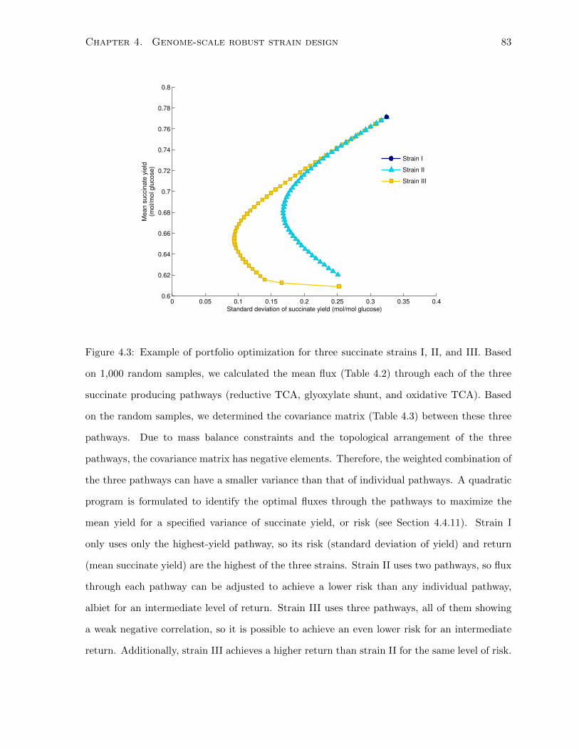
Chapter 4. Genome-scale robust strain design 83
0 0.05 0.1 0.15 0.2 0.25 0.3 0.35 0.40.6
0.62
0.64
0.66
0.68
0.7
0.72
0.74
0.76
0.78
0.8
Standard deviation of succinate yield (mol/mol glucose)
Mean s
uccin
ate
yie
ld(m
ol/m
ol glu
cose)
Strain I
Strain II
Strain III
Figure 4.3: Example of portfolio optimization for three succinate strains I, II, and III. Based
on 1,000 random samples, we calculated the mean flux (Table 4.2) through each of the three
succinate producing pathways (reductive TCA, glyoxylate shunt, and oxidative TCA). Based
on the random samples, we determined the covariance matrix (Table 4.3) between these three
pathways. Due to mass balance constraints and the topological arrangement of the three
pathways, the covariance matrix has negative elements. Therefore, the weighted combination of
the three pathways can have a smaller variance than that of individual pathways. A quadratic
program is formulated to identify the optimal fluxes through the pathways to maximize the
mean yield for a specified variance of succinate yield, or risk (see Section 4.4.11). Strain I
only uses only the highest-yield pathway, so its risk (standard deviation of yield) and return
(mean succinate yield) are the highest of the three strains. Strain II uses two pathways, so flux
through each pathway can be adjusted to achieve a lower risk than any individual pathway,
albiet for an intermediate level of return. Strain III uses three pathways, all of them showing
a weak negative correlation, so it is possible to achieve an even lower risk for an intermediate
return. Additionally, strain III achieves a higher return than strain II for the same level of risk.

Chapter 4. Genome-scale robust strain design 84
4.5.3 Diversity increases sensitivity to small perturbations
Here, we consider perturbations of varying magnitudes and define a metric of perturbation size,
δ (see Section 4.4.7). δ = 1 indicates that every controlled flux is allowed to vary within the full
range of feasible values, as in the previous section. δ < 1 indicates that every controlled flux
remains closer to its nominal value. When controlled fluxes are equal to their nominal values,
then δ = 0.
In the previous section, in which δ = 1, strain III was the most robust to perturbations, due to
pathway diversification, while strain I was the least robust, since it controlled only one flux. In
contrast, when perturbations are small (δ < 0.395), strain I is the most robust, while strain III is
the least robust (Fig. 4.4C). Therefore, pathway diversification appears to improve robustness
only when perturbations are of a certain magnitude, which we now explain how to determine.

Chapter 4. Genome-scale robust strain design 85
0 0.2 0.4 0.6 0.8 10
0.5
1
1.5
Perturbation size (δ)
Mea
n yi
eld
(mol
/mol
glu
cose
)
A
0 0.2 0.4 0.6 0.8 10
0.1
0.2
0.3
0.4
Perturbation size (δ)
Sta
ndar
d de
viat
ion
ofyi
eld
(mol
/mol
glu
cose
)
B
0 0.2 0.4 0.6 0.8 10
0.2
0.4
0.6
0.8
1
Perturbation size (δ)
Rob
ustn
ess
(R)
δ*(2) δ*(3)
C
Strain I
Strain II
Strain III
Figure 4.4: Robustness of three succinate strains as functions of perturbation size. (A) Mean
product yield versus perturbation size. Error bars represent one standard deviation. (B) Stan-
dard deviation of product yield versus perturbation size. (C) Robustness (R) versus perturba-
tion size. Critical perturbation sizes for strains II (δ∗(2) = 0.395) and III (δ∗(3) = 0.415) are
indicated by dotted lines. Strains I, II, and III each use, one, two, and three succinate produc-
tion pathways, respectively. Strain I uses only the highest-yield pathway; therefore, its mean
yield is highest when perturbations are small. However, the robustness of strain I deteriorates
rapidly as perturbation size increases, while strain III is the most robust. Strain II is the most
robust for only a narrow range of perturbation sizes (i.e., for 0.395 ≤ δ ≤ 0.415).

Chapter 4. Genome-scale robust strain design 86
To quantitatively compare robustness between strains at different perturbation sizes, we
introduce the critical perturbation size metric, δ∗(n), with integer n > 1, defined as the per-
turbation size for which a strain using n > 1 pathways is more robust (based on the metric, R)
than the strain using only one pathway. Thus, δ∗(n) represents the perturbation size at which
diversification improves robustness. Furthermore, a small δ∗(n) indicates that diversification
is useful for a wider range of perturbations, while a large δ∗(n) indicates that robustness is
improved only for large perturbations when n pathways are used. Based on the critical per-
turbation size, strain I is the most robust for δ < 0.395 (Fig. 4.4C). Within a narrow interval
of perturbation sizes (0.395 ≤ δ < 0.415), strain II is the most robust. For larger perturba-
tions, δ > 0.415, strain III is the most robust. Thus, the critical perturbation size provides a
metric to quantitatively determine the number of redundant pathways to use for an expected
perturbation size. In this case, strain I or III should be used for small or large perturbations,
respectively. In the following section, we will apply our findings to the study of robust L-serine
overproduction strains.
4.5.4 Enhanced robustness of L-serine production via low-yield pathways
L-serine is an industrially important amino acid that is used in cosmetics, pharmaceuticals, and
as a precursor for a variety of other chemicals (Peters-Wendisch et al., 2005; Stoiz et al., 2007).
In this section, we investigate whether robust L-serine overproduction strains can be designed
using pathway diversification.
In E. coli, two pathways are available for L-serine synthesis (Fig. 4.5A): the phosphoserine
phosphatase (PSP) route, and the glycine hydroxymethyltransferase (GHMT) route. Flux
balance analysis (FBA) simulations show that GHMT yields less L-serine than PSP (2.0 versus
1.15 mol L-serine/mol glucose). Therefore, to maximize nominal yield, the PSP route should
be utilized exclusively. However, to maximize robust production under large perturbations, the
GHMT route, despite its low yield, is shown to play an important role.

Chapter 4. Genome-scale robust strain design 87
��������������������������A�������������BC
�������������������������������������������������
�����������������C���D������������������������������
��������������������������A�������������BC
�����������������������������ECF��
�����������������C���D
��������������������������A�������������BC
�����������������������������ECF���������AC��D
�����������������C���D��������������������������������
���A������BC��D���E��������F�����E�
�B
��������
���
���
���
��
���
�!"
�#����
$�%
&#$
�#��
"%'
��"%# ����� (���� ����� ��)�$
�)�$�� )�"%�
�� ��
���
D�"
��"
*��+"
"��
&+�
&,�
",�
"%�
��)� ������
��"%��+�
� �
� �
�+�
�����
��� ����
����
AB�CD
��������
�E�F��E�B��
��B
$% )& $� )&
����B�����������AB�����CDABED�F
�����������AB�����CDABED��
��������
�E�B�B
Figure 4.5: L-serine production pathways and strains. (A) Two pathways are available for L-
serine production: (1) the PSP route and (2) the GHMT route. (B) We designed three strains
(strains I, II, and III), using one or both of these pathways. In addition, strain III inhibits
NDPK3 and CTPS2 fluxes.

Chapter 4. Genome-scale robust strain design 88
To demonstrate, consider three L-serine strains (Fig. 4.5B). Strain I utilizes only the high-
yield PSP pathway, while strains II and III use both PSP and GHMT. Strain I consistently
had the highest mean yield across all perturbation sizes (Fig. 4.6A). However, its standard
deviation was also the highest (Fig. 4.6B) when perturbations were large, due to the lack of
alternative production routes. Thus, for large perturbations, strains II and III were more robust
than strain I (Fig. 4.6C). This result indicates that even low-yield pathways can be combined
with high-yield ones to improve robustness against large perturbations.

Chapter 4. Genome-scale robust strain design 89
0 0.1 0.2 0.3 0.4 0.5 0.6 0.7 0.8 0.9 10
0.5
1
1.5
2
Perturbation size (δ)
Mea
n yi
eld
(mol
/mol
glu
cose
)
A
0 0.1 0.2 0.3 0.4 0.5 0.6 0.7 0.8 0.9 10
0.2
0.4
0.6
Perturbation size (δ)
Sta
ndar
d de
viat
ion
ofyi
eld
(mol
/mol
glu
cose
)
B
0 0.1 0.2 0.3 0.4 0.5 0.6 0.7 0.8 0.9 10.4
0.6
0.8
1
Perturbation size (δ)
Rob
ustn
ess
(R)
C
Strain I
Strain II
Strain III
Figure 4.6: Robustness of three L-serine strains as functions of perturbation size. (A) Mean
yields of three L-serine strains as functions of perturbation size. Error bars represent one stan-
dard deviation. (B) Standard deviation of L-serine yield for the three strains. (C) Robustness
values of the three L-serine strains as functions of perturbation size. Strain I uses one L-serine
synthesis pathway, while strains II and III use two pathways. Strain III inhibits two addi-
tional reactions, compared to strain II, which results in improved nominal yield but decreased
robustness.
Chapter 4. Genome-scale robust strain design 90
Under small perturbations, strain II was more robust than strain III. Compared with strain
II, strain III involves two additional controlled fluxes: inhibition of nucleoside-diphosphate
kinase (NDPK3) and CTP synthase (CTPS2). Under nominal conditions, these inhibitions
increased yield by 2% over strain II. However, the minute increase in nominal yield does not
appear to justify the decrease in robustness against small perturbations. In general, the opti-
mal tradeoff between product yield and variability will depend on the yield and variability of
individual controlled fluxes, as well as the size of expected perturbations. In silico design, as
described here, should help to accelerate the systematic identification of an optimal tradeoff.
A potential concern with the experimental feasibility of the proposed strategy is whether PSP
and GHMT can simultaneously produce L-serine since GHMT typically consumes L-serine when
PSP is active (Stolz et al., 2007). Possible approaches for simultaneous activity include provid-
ing glycine as a nitrogen source (Newman et al., 1976) or using resting cell systems to reduce
serine degradation (Shen et al., 2010).
4.5.5 Assessing robustness against industrially relevant perturbations
In the previous sections, we showed that robustness can be improved through the control of
redundant pathways. Yet, it may be argued that under a stable environment, such as lab-scale
cultures, efficient strains that use only high-yield pathways are superior to diversified strains
that use redundant pathways, which may have lower-yields.
We hypothesize that diversified strains are more practical than efficient ones because industrial-
scale bioreactors introduce a wide range of environmental perturbations that are not typically
encountered at the lab-scale (Enfors et al., 2001). To test this hypothesis, we assessed the
robustness of the three succinate strains (discussed in previous sections) against representative
environmental perturbations: variations in glucose and oxygen uptake rates, osmotic stress,
secretion of byproducts due to overflow metabolism, and re-consumption of these byproducts.
These perturbations are difficult to control in large-scale bioreactors and deteriorate bioprocess
performance (Enfors et al., 2001).
Controlled flux variation arising from expression noise was included in all of our simulations,
since this intracellular perturbation is inherent to any cell. When glucose uptake rate was also

Chapter 4. Genome-scale robust strain design 91
perturbed, average product yields decreased, since glucose is the sole substrate (Fig. 4.7a–b).
Osmotic stress, which was modeled as increased ATP maintenance requirements (see Section
4.4.9), had similar consequences (Fig. 4.7e–f). Both results were as expected, as both glucose
availability and ATP drain impact production capacity.

Chapter 4. Genome-scale robust strain design 92
−20 −10 00
0.1
0.2
0.3
Glucose
Relative
frequency
a
10 20 300
0.1
0.2
0.3
Succinate
b
−20 −10 00
0.1
0.2
0.3
Oxygen
Relative
frequency
c
10 20 300
0.1
0.2
0.3
Succinate
d
0 40 800
0.1
0.2
0.3
ATPM
Relative
frequency
e
10 20 300
0.1
0.2
0.3
Succinate
f
0 0.050
0.05
0.1
0.15
0.2
kMemFRD
Relative
frequency
g
10 20 300
0.1
0.2
0.3
Succinate
h
0 10 20 300
0.5
1
Acetate
i
0 20 400
0.2
0.4
0.6
Formate
j
0 10 200
0.2
0.4
0.6
0.8
Ethanol
k
0 5
x 10−3
0.05
0.1
0.15
0.2
kVol
Relative
frequency l
10 20 300
0.1
0.2
0.3
Succinate
m
−30 −20 −10 00
0.5
1
Acetate
n
−40 −20 00
0.2
0.4
0.6
Formate
o
−20 −10 00
0.2
0.4
0.6
0.8
Ethanol
p
Strain I
Strain II
Strain III
Perturbation Predicted flux responses (mmol/gDW/h)Expression noise &
Glucose
Dissolvedoxygen
Cells
Figure 4.7: Histograms showing the simulated response of succinate strains to industrially-
relevant perturbations. All controlled fluxes are perturbed due to gene expression noise.
Industrially-relevant perturbations include variations in glucose uptake rate (a-b), oxygen up-
take rate (c-d), osmotic stress (e-f), byproduct secretion due to overflow metabolism (g-k), and
re-consumption of byproducts (l-p). While simulating byproduct secretion, membrane occu-
pancy coefficients were subjected to parameter uncertainty (g). While simulating byproduct
consumption, molecular crowding coefficients were subjected to parameter uncertainty (l). For
oxygen and substrates (glucose, acetate, formate, and ethanol), negative fluxes correspond to
uptake while positive fluxes correspond to secretion. ATPM: non-growth-associated ATP main-
tenance, kMemFRD: membrane crowding coefficient of fumarate reductase, kVol: molecular
crowding coefficient.
Chapter 4. Genome-scale robust strain design 93
In contrast, we found that all three strains were robust against variations in the oxygen
uptake rate (Fig. 4.7c–d). This robustness was due to aerobic FRD activity, which enables
fumarate to be respired, in addition to oxygen (Fig. 4.8). In the absence of aerobic FRD activity,
the maximum aerobic succinate yield became more sensitive to oxygen uptake rates (Fig. 4.9,
4.10). Although FRD is normally repressed under aerobic conditions, aerobic FRD activity can
be achieved through several methods: the regulatory gene, fnr can be overexpressed to activate
frdABCD (Shaw and Guest, 1982); the frd operon copy number can be increased (Cole and
Guest, 1979); or FRD enzymes can be mutated to decrease their sensitivity to oxygen (Iuchi
et al., 1986). In addition, Portnoy et al. (Portnoy et al., 2010) adaptively evolved cytochrome
oxidase mutants of E. coli, which exhibited anaerobic physiology and fumarate respiration under
aerobic conditions. These studies suggest that fumarate respiration via aerobic FRD activity
may be a viable strategy for robust succinate production.

Chapter 4. Genome-scale robust strain design 94
Figure 4.8: Respiration and succinate production. (1) Reductive branch of the citric acid (TCA)
cycle. (2) Glyoxylate shunt. (3) Oxidative branch of the TCA cycle. When fumarate reductase
(FRD) is repressed (A), the quinol-dependent NADH dehydrogenase activity dominates and
oxygen is the terminal electron acceptor. In contrast, when FRD is activated (B), fumarate is
available as an additional terminal electron acceptor. Accordingly, the production of succinate
becomes insensitive to fluctuations in oxygen availability.

Chapter 4. Genome-scale robust strain design 95
0 10 20 30 40 50 60 70 80 900
0.5
1
1.5
Maximal nominal performance
Strain number
Succin
ate
yie
ld (
mol/m
ol glu
cose)
A
0 10 20 30 40 50 60 70 80 900
0.5
1
1.5
Strain number
Succin
ate
yie
ld (
mol/m
ol glu
cose)
B
Mean Median 25th
& 75th
percentiles Min & max
0 0.5 1 1.50
10
20
30
40
50
Yield (mol/mol glucose)
Fre
quency
C
0 0.5 1 1.50
10
20
30
40
50
Mean yield (mol/mol glucose)
Fre
quency
D
Figure 4.9: Nominal and mean succinate yield of 98 strains without aerobic fumarate reductase
(FRD) and anaerobic pyruvate dehydrogenase (PDH) activities. (A) Succinate yield of each
strain when no perturbations are present. All yields were calculated without aerobic FRD and
anaerobic PDH activities. However, to easily compare results with Fig. 1, the dashed red
line denotes the maximal yield at a growth rate of 0.1 h−1 when aerobic FRD and anaerobic
PDH activities are enabled. (B) Succinate yield of each strain when gene expression noise
is present, based on 1,000 random samples for each strain. Blue dots show the mean of the
1,000 samples of succinate yield for each strain, while the red line shows the median. Black
lines show the minimum and maximum succinate yield for each strain, while the minimum and
maximum values in the green area correspond to the 25th and 75th percentiles of succinate
yield, for each strain. Strains are sorted in order of descending mean yield (in (A) as well).
(C) Histogram of succinate yield across the 98 strains when no perturbations are present. (D)
Histogram of mean succinate yield across the 98 strains when gene expression noise is present.
Mean succinate yields ranged from 0% to 66% of the maximal yield, and had a median of 42%
of the maximal yield.

Chapter 4. Genome-scale robust strain design 96
Figure 4.10: Correlation between succinate production and oxygen uptake for strain III. Colors
are proportional to growth rate as shown in the colorbar. When fumarate reductase (FRD)
is active under aerobic conditions, maximum succinate flux is insensitive to changes in oxygen
uptake flux due to the availability of fumarate respiration (A). When FRD is inactive under
aerobic conditions, maximum succinate flux is affected by oxygen uptake rate (B).

Chapter 4. Genome-scale robust strain design 97
To accurately model byproduct secretion and re-consumption in response to variation in
glucose and oxygen uptake rates, we incorporated the molecular crowding (Beg et al., 2007)
and membrane occupancy (Zhuang et al., 2011) constraints (see Section 4.4.10). Simulations
showed that formate and acetate were major byproducts, which is consistent with experimental
observations (Kirkpatrick et al., 2001; Wang et al., 2011), as well as ethanol (Fig. 4.7i–k).
Byproduct secretion led to a general decrease in succinate yield (Fig. 4.7h). Re-consumption
of these products, however, increased succinate flux, as additional substrates became available
(Fig. 4.7m–p).
In addition to these metabolic responses, we assessed the sensitivity of strains to uncertainty
in the parameters introduced by the molecular crowding and membrane occupancy constraints.
Specifically, we considered ±50% uncertainty on the membrane crowding coefficient of FRD
(kFRD), and similar uncertainty on the single molecular crowding coefficient. As expected, pre-
dicted performance of strain I was the most sensitive to uncertainty in kFRD since this strain
uses only FRD to produce succinate (Fig. 4.7g–h). Parameter uncertainty skewed the succi-
nate distribution, which was originally uniformly distributed. This transition is characteristic
of the “anti-portfolio” effect, arising in situations in which a variable is the product of multiple
random factors (Vlad et al., 2007). Indeed, succinate flux is influenced by the product of kFRD
uncertainty and perturbations to FRD flux. The molecular crowding constraints resulted in
decreased production for all three strains (Fig. 4.7l–m). For both the molecular crowding and
membrane occupancy constraints, pathway diversity improved robustness against the combined
effects of parameter uncertainty and byproduct re-consumption.
We then calculated δ∗(n) to quantitatively assess the effect of pathway diversification in the
context of the industrially relevant perturbations (Table 4.4). Compared to the other pertur-
bations, diversification provided the least amount of benefit when expression noise was the sole
perturbation (δ∗(2) = 0.395 and δ∗(3) = 0.415). This scenario is comparable to the environ-
ments of endosymbionts. Incidentally, endosymbionts lose a great deal of metabolic redundancy
and studies have hypothesized that this is due to the lack of a need for robustness in stable
environments (Moran, 2002; Tamas et al., 2002; Mendonca et al., 2011).
When glucose perturbations were added to expression noise, the use of two and three pathways

Chapter 4. Genome-scale robust strain design 98
was more beneficial, as reflected by reductions in δ∗(2) and δ∗(3) of 56% and 54%, respectively.
Addition of oxygen perturbations to expression noise similarly increased the effective range of
diversification.
Osmotic stress, byproduct secretion and re-consumption all increased the benefits of diversifi-
cation greatly. In fact, the more diversified strains were always more robust than the efficient
strain (i.e., δ∗(n) = 0), even for small perturbations. These results suggest that pathway redun-
dancy is more important for improving robustness against environmental perturbations than
against expression noise alone.
Table 4.4: Critical perturbation size, δ∗(n), indicating the perturbation size at which robustness
of diversified strains (with n pathways) exceeds that of the most efficient strain.
Perturbation δ∗(2) δ∗(3)
Expression noise 0.395 0.415
Glucose variation 0.173 0.193
Oxygen variation 0.243 0.183
Osmotic stress 0 0.011
By-product secretion 0 0
By-product consumption 0 0
δ∗ = 0 indicates that the diversified
strain is more robust than the simple
strain for all perturbation sizes.
4.6 Conclusions
In this work, we have developed a procedure for robust strain design that can be employed
immediately using available genome-scale constraint-based models (CBM) of cell metabolism.
First, the CBM is modified to simulate an engineered strain, based on known genetic modifica-
tions, or using a strain design algorithm (Burgard et al., 2003; Ranganathan et al., 2010; Kim
and Reed, 2010; Yang et al., 2011) to identify knockout targets and controlled fluxes. Second,

Chapter 4. Genome-scale robust strain design 99
a set of random perturbations are identified (e.g., see Table 4.1). The relative sizes of these
perturbations are then estimated (see Section 4.5.3). Next, the designed strains are subjected
to these random perturbations and the robustness of each strain is calculated (Eq. 4.1). Strains
that are robust against specific or many perturbations are retained while the sensitive strains
are discarded. Robustness-enhancing strategies are identified by examining the most robust
strains and these strategies are incorporated into the next iteration of strain design to further
improve strain robustness.
In this work, we found that pathway diversification improved robustness against a wide variety
of industrially relevant random perturbations, including variation in substrate and oxygen up-
take rates, osmotic stress, byproduct secretion, and re-consumption of these byproducts (Fig.
4.7). Although pathway diversification improved robustness against large perturbations, it also
increased sensitivity to small perturbations (Fig. 4.4). This tradeoff may have implications
for strain construction. For example, two representative methods for controlling target fluxes
are inducible expression systems and libraries of constitutive promoters (De Mey et al., 2007).
Inducible systems typically exhibit greater variability in the level of protein expression across
individual cells than that of constitutive promoter libraries (Alper et al., 2005). Therefore,
pathway diversification may have a greater effect on improving robustness when using inducible
systems than when using promoter libraries.
Diversification is adopted as a strategy to improve robustness against perturbations by a variety
of artificial and natural systems, ranging from financial portfolios to prairie grasslands (Tilman
et al., 2006). Under constant environments, efficiency may take preference over robustness. For
example, endosymbionts and parasites reside in stable environments, and their genomes reflect
a significant loss of redundant genes and pathways (Moran, 2002; Tamas et al., 2002; Mendonca
et al., 2011). On a faster time-scale, deletion of key enzymes leads to large intracellular pertur-
bations. These perturbations include re-routing of fluxes, amplification of existing pathways,
and the activation of latent pathways, which are eventually deactivated as intracellular condi-
tions stabilize over the course of adaptive evolution (Fong et al., 2006; Cornelius et al., 2011).
Thus, the transient activation and deactivation of latent pathways may be related to changes
in the size of intracellular perturbations over time. Although the mechanisms underlying these

Chapter 4. Genome-scale robust strain design 100
phenomena are not fully understood, they are consistent with the presence of a tradeoff be-
tween robustness against large perturbations versus sensitivity to small perturbations exhibited
by the diversification strategy. Therefore, the characterization of random perturbations during
latent pathway activation and natural selection may help to explain why robustness is acquired
or lost as conditions change over time.
Experimental data related to our results can be found in the literature. For example, in (Son-
ntag et al., 1993), L-lysine is synthesized by Corynebacterium glutamicum via two pathways
that diverge from a common precursor. One pathway involves a single, ammonium-dependent
reaction that contributes 72% to 0% of total L-lysine production. The actual contribution de-
pends strongly on the availability of ammonium, which can vary temporally and spatially in
the bioreactor. The presence of two L-lysine synthesis pathways in C. glutamicum has raised
fundamental questions on their relative functions, since other microbes, including E. coli, Bacil-
lus subtilis, and Bacillus sphaericus use only one of three possible L-lysine synthesis pathways
(Schrumpf et al., 1991). For the purpose of robust strain design, the results in this thesis point
to the use of both pathways as a viable strategy for improving robustness against ammonium
fluctuations.
To provide experimental verification of the design ideas presented here, one could extend the
experiments in (Sonntag et al., 1993) as follows. First, an experimental apparatus is designed
such that perturbations to ammonium or substrate availability are introduced in at least two
different amplitudes. Fluctuations can be introduced in lab-scale culture, as in (Pekkonen et al.,
2011; Suiter et al., 2003; Picket and Bazin, 1980). Second, a set of strains is constructed, based
on the robust strain design framework. The set should include at least one diversified strain,
having diverse pathways towards product formation, and an efficient strain, having only the
highest-yield pathway. Third, the set of strains are cultured under the two different perturba-
tions. By measuring the mean and standard deviation of L-lysine production of the different
strains, the hypothesis that greater diversification improves robustness against large perturba-
tions, at the cost of increased sensitivity to small perturbations would be tested. Additionally,
the experiment would verify whether in silico robust strain design can indeed lead to the de-
velopment of microbial strains that are robust against industrially-relevant perturbations.

Chapter 4. Genome-scale robust strain design 101
The computational framework described here is general for use with any constraint-based model.
Future work may include the incorporation of integrated metabolic and regulatory network
models (Chandrasekaran and Price, 2010) to assess the potential for genetic and pathway re-
dundancy (Mahadevan and Lovley, 2008) and engineering of regulatory networks (Kafri et al.,
2006, 2009) for robust strain design. Furthermore, the predictive design of robust strains using
simple strategies like diversification, with quantifiable effects under a variety of perturbations
(Fig. 4.7) may become important when designing engineered cells from the bottom up, using
cells with minimal metabolic networks (Glass et al., 2006; Henry et al., 2010b) as a platform.
One of the main contributions of this work is to place these considerations within a systematic
framework that is tangible to the designer, rather than leaving the issue of robust performance
to chance, trial, and error.

Chapter 5
Designing Experiments from Noisy
Metabolomics Data to Refine
Constraint-Based Models
This chapter contains material originally published in the conference proceedings below, with
permission from the publisher, the American Automatic Control Council (AACC):
Yang, L., Mahadevan, R. and Cluett, W.R.. (2010b) Designing experiments from noisy metabolomics
data to refine constraint-based models. In: Proceedings of the American Control Conference,
pp. 5143–5148.
5.1 Abstract
Metabolomics is an emerging technology for making high-throughput measurements of metabo-
lites and is useful for the discovery of novel biomarkers of genetic diseases and for metabolic
engineering. The system-wide data can be used to refine predictions made by constraint-based
models of cell metabolism. However, the predictions of important output variables may still
suffer from high variability due to high variance in the data itself, or from suboptimal choice of
measurements in the metabolomics experiment. Here, we present a computational algorithm
102

Chapter 5. Designing experiments using noisy metabolomics data 103
that uses initial metabolomics data to identify a smaller set of metabolites whose precise mea-
surement most reduces variability of model predictions. We first randomly sample fluxes and
concentrations using a new non-convex sampling algorithm that differs from previous approaches
in its ability to sample across disjoint regions of the space and in its parallel implementation.
We then demonstrate our algorithm’s ability to identify a sequence of experiments that succes-
sively refines model predictions using a simplified model of Escherichia coli central metabolism.
5.2 Introduction
Cell metabolism is a complex network consisting of hundreds of biochemical species, or metabo-
lites, interacting through over a thousand chemical reactions. Accurately modeling this sys-
tem is an important challenge for metabolic engineers and health scientists. Metabolomics is
an emerging high-throughput technology to make system-wide concentration measurements of
hundreds of metabolites and has important applications for identifying novel biomarkers of ge-
netic diseases (Buescher et al., 2009; Shlomi et al., 2009). Constraint-based modeling (CBM)
is used to make systems-level predictions of reaction rate, or flux, distributions throughout the
metabolic network (Becker et al., 2007). Recent advances in this field include the develop-
ment of algorithms that can predict both concentration and flux ranges using thermodynamic
information on the free energies of reactions (Henry et al., 2007). Model predictions can be
refined using metabolomics data to constrain the concentrations of metabolites (Bennett et al.,
2009; Mo et al., 2009). Also, the quality of experimental data can be assessed by examining
thermodynamic feasibility of the data within a constraint-based model (Zamboni et al., 2008).
However, important output variables may still suffer from increased uncertainty due to high
variance in the data, or from suboptimal choice of measurements.
The problem of identifiability in metabolic networks has been the subject of several stud-
ies including the identification of optimal flux measurement sets to completely characterize
flux distributions using isotopic metabolic flux analysis experiments (Chang et al., 2008). In
(Savinell and Palsson, 1992), the authors wanted to completely determine flux configurations

Chapter 5. Designing experiments using noisy metabolomics data 104
by measuring some fluxes and computing the others based on network stoichiometry and mass-
balance equations. By estimating the sensitivity of calculated fluxes relative to the uncertainty
in measured fluxes, the fluxes needing precise measurements could be determined. The system
considered by the authors was defined by linear constraints. Hence, they could use properties
of matrix norms to define upper bounds on flux sensitivities. Furthermore, they estimated
actual sensitivities by generating random experimental flux measurements and experimental
uncertainties.
In this thesis, we build upon this idea by estimating the sensitivities of calculated fluxes and
metabolite concentrations, relative to experimental uncertainties of measured concentrations.
Unlike the system in (Savinell and Palsson, 1992), here we consider both fluxes and concen-
trations, which are non-linearly related; therefore, novel methods are developed. For our algo-
rithm we begin with an initial metabolomics dataset consisting of many metabolite concentra-
tions with high variability. This dataset is used to place loose bounds on concentrations in a
constraint-based model, resulting in a reduced solution space relative to the case where arbi-
trarily wide bounds are used. We then generate random samples from the space using a new
non-convex sampling algorithm. We then use these samples to assess sensitivities of calculated
variables to measured concentrations. A schematic of the overall framework is shown in Fig.
5.1. We present the necessary preliminaries in Section 5.3, describe the algorithm for sampling
the non-convex concentration space in Section 5.4, and present our algorithm for identifying
important metabolites in Section 5.5 with an example using a simplified model of Escherichia
coli central metabolism. We present our results in Section 5.6 and conclusions in Section 5.7.
5.3 Preliminaries
5.3.1 Constraint-Based Modeling
Cell metabolism is modeled as a network of biochemical species, or metabolites, that are in-
terconnected through enzyme-catalyzed reactions with defined stoichiometry. The variables of
this system are reaction rates, or fluxes, and metabolite concentrations. Fluxes are defined by

Chapter 5. Designing experiments using noisy metabolomics data 105
Figure 5.1: Metabolomics data serve as the launchpad for iterative model refinement. Our
computational algorithm, outlined in Section 5.5, allows researchers to identify metabolites
needing more precise concentration measurements to make precise predictions of the output
variables of interest.
the following constraints:
Sv =dx
dt(5.1)
vL ≤ v ≤ vU , (5.2)
where v ∈ RN is the vector of fluxes, x ∈ RM is the vector of metabolite concentrations, vL
and vU are lower and upper bound vectors of the fluxes. S is the matrix defining network
stoichiometry with M rows corresponding to metabolites and N columns corresponding to
fluxes.
In Flux Balance Analysis (FBA) (Becker et al., 2007), we assume that metabolic reactions occur

Chapter 5. Designing experiments using noisy metabolomics data 106
much faster than environmental changes. Hence, we assume a quasi-steady state for metabolite
concentrations, so that dxdt = 0. Consequently, flux configurations are calculated by solving the
following linear program (LP):
maxv
cT v (5.3a)
s.t. Sv = 0 (5.3b)
vL ≤ v ≤ vU , (5.3c)
where cT ∈ RN is the vector of flux weights in the objective function, chosen to reflect cell
behavior under its growth condition (e.g., maximize growth yield).
In Thermodynamics-based Metabolic Flux Analysis (TMFA)(Henry et al., 2007), both fluxes
and concentrations are predicted by solving the following mixed-integer linear program:
maxv,x,∆rG′
cT v (5.4a)
s.t. Sv = 0, (5.4b)
0 ≤ vj ≤ zjvmaxj , {j = 1, . . . , N}, (5.4c)
∆rG′j −K(1 + zj) < 0, (5.4d)
{j = 1, . . . , N |∆rG′j◦is known},
∆rG′j◦ +RT
M∑i=1
si,j ln(xi) = ∆rG′j , (5.4e)
{j = 1, . . . , N |∆rG′j◦is known, },
xL ≤ x ≤ xU , (5.4f)
vj ≥ 0, {j = 1, . . . , N}, (5.4g)
zj ∈ {0, 1}, (5.4h)
where ∆rG′j is the reaction Gibbs free energy change of reaction j, ∆rG
′j◦ is the standard
Gibbs free energy change, and zj is a binary variable equal to 1 when the ∆rG′j of reaction j is
negative, thereby allowing flux, and is equal to 0, otherwise. Reactions are split into forward and
reverse so that all fluxes are non-negative, vmaxj denotes the maximum flux through reaction
j, xL and xU are lower and upper concentration bounds, and si,j denotes the element of S
corresponding to the M -th row and N -th column.

Chapter 5. Designing experiments using noisy metabolomics data 107
5.3.2 Randomly Sampling the Solution Space
Optimization-based approaches like FBA and TMFA are effective at predicting flux distribu-
tions for prokaryotes growing in nutrient-limiting conditions where suitable cellular objective
functions have been validated. When an appropriate objective function is not known, or an
unbiased exploration of the solution space is desired, random sampling approaches are used
(Schellenberger and Palsson, 2009).
To sample points uniformly distributed over the solution space X ⊂ RN defined by constraints
(5.3b)-(5.3c), we can use artificial centering hit and run (ACHR) (Kaufman and Smith, 1998).
In ACHR, we first generate a set of Nw warmup points W = {wa : wa ∈ X, a = 1, . . . , Nw}
using hit-and-run sampling. Subsequently, we do the following:
1. Initialize the starting point X0 ∈ X, the center point X = X0 and set t = 0.
2. Choose a random warmup point, wa from W , and set the random direction vector dt =
(wa − X)/||wa − X||2, where || · ||2 is the L-2 norm.
3. Select a random step size, λt, and a new candidate point from the line set Yt = {λt ∈
R|Xt + λtdt ∈ X}.
4. If the set Yt is empty, then go to Step 2.
5. Set Xt+1 = Xt + λtdt and t = t+ 1.
6. Set X = (tX +Xt)/(t+ 1) and go to Step 2.
The ACHR algorithm differs from previous hit-and-run algorithms in that the direction choice
at each iteration is adaptively chosen to improve convergence. Because each direction choice
depends on previous sample points (i.e., warmup points), the sequence does not form a Markov
Chain and the convergence theorems for Markov Chain Monte Carlo do not apply (Kaufman
and Smith, 1998). Nonetheless, the high empirical convergence rate of ACHR has made it a
popular choice for random sampling in the CBM community.

Chapter 5. Designing experiments using noisy metabolomics data 108
5.4 Sampling the non-convex solution space
In this work, we require uniformly distributed sample points from the thermodynamically fea-
sible solution space. Disjoint regions arise in this space due to reversible fluxes and their
corresponding ∆Gr, which are functions of concentrations (see Fig. 5.2). Schellenberger et
al. (Schellenberger et al., 2007) developed a method to sample concentrations by first defin-
ing flux directions based on stoichiometry, environmental constraints and concentration data.
However, this method does not fully explore the combined concentration and flux space when
reversible reactions are present. This is because reversible reactions create disjoint regions in
the thermodynamically feasible solution space that cannot be fully sampled using convex sam-
pling like ACHR that the authors used in (Schellenberger et al., 2007). Here, we use a simple
extension to ACHR to sample the non-convex solution space that includes reversible reactions.
This method also eliminates the need to identify thermodynamically infeasible reaction cycles
(steady state flux through network loops without a thermodynamic driving force) a priori as
in (Price et al., 2006) since the thermodynamic constraints checked at each iteration include a
test for the presence of such cycles. We sample the non-convex solution space, T ⊆ X ⊂ RN ,
defined by constraints (5.4b)-(5.4h) as follows, for each parallel sampling chain, i:
1. Initialize the starting point Xi0 ∈ T, the center point Xi = Xi
0 and set t = 1.
2. Set the random direction vector dit = (Xjt−1 − Xi)/||Xj
t−1 − Xi||2 based on a random
parallel chain, j.
3. Generate a set of K steps sizes, Λit = {λi(k)t ∈ R|Xi
t + λi(k)t dit ∈ X, k = 1, . . . ,K}.
4. Choose a step size, λit from the set of thermodynamically feasible (satisfying constraint
(5.4d)) step sizes, Θit = {λit ∈ Λit|Xi
t + λitdit ∈ T}.
5. If Θit is empty, then choose a feasible point Xi
t = Xjt−1, from a random parallel chain, j
and go to Step 2.
6. Set Xit+1 = Xi
t + λitdit and t = t+ 1.
7. Set Xi = (tXi +Xit)/(t+ 1) and go to Step 2.

Chapter 5. Designing experiments using noisy metabolomics data 109
The sampling algorithm visits disjoint regions of the solution space by generating many candi-
date points for each parallel search direction and assessing thermodynamic feasibility for each
candidate point. We increase the chance of finding feasible points by allowing communication
between the parallel chains in two ways: (a) the direction of a chain at an iteration is based on
the previous feasible points of all parallel chains, and (b) if a chain fails to find a feasible point
at an iteration, it randomly chooses a feasible point from the other chains for that iteration. In
this way, the success rate of finding feasible points in the non-convex solution space is increased.
We performed parallel computations on the Nvidia GeForce GTX 295 graphics processing unit
(GPU), using the Jacket (AccelerEyes, LLC, Austell, GA) interface to MATLAB (The Math-
works, Inc., Natick, MA).
5.5 Identifying Important Metabolites
Our objective is to identify the metabolites needing more precise concentration measurements,
using metabolomics data as the starting point. For our purposes, additional measurements are
of little value if they do not affect the variability of outputs that we predict using the model.
Hence, we identify important metabolites using an approach inspired by the Derivative-based
Global Sensitivity Measures (Kucherenko et al., 2009). Below is an outline of our method
to estimate the change in variability of output yj (either a flux or concentration) relative to
uncertainty in metabolite concentration measurement xi:
1. Generate uniform random samples from the thermodynamically feasible solution space.
2. For each measurable metabolite, i, generate r = 1 . . . Nrand random concentrations, xir
within their feasible concentration bounds.
3. For random concentration r, define small concentration deviations, xir −∆x and xir + ∆x
for a positive ∆x.
4. Obtain K sample points each within the concentration intervals [xir−∆x, xir] and [xir, xir+
∆x], and denote the k-th sampled value of output j for each interval as yak and ybk,
Chapter 5. Designing experiments using noisy metabolomics data 110
respectively.
5. Calculate variances of the samples of output j, with respect to metabolite i within each
interval as
σja =1
K − 1
K∑k=1
(yak − ya)2
and
σjb =1
K − 1
K∑k=1
(ybk − yb)2,
where ya and yb are the means of the output samples ya and yb, respectively.
6. Calculate the gradient of variability in output j with respect to metabolite i at random
concentration xir as
γjr =|σjb − σ
ja|
2∆x.
7. Repeat Steps 2-6 for all Nrand random concentrations of metabolite i.
8. Define the mean sensitivity of output j with respect to metabolite i as
γji =1
Nrand
Nrand∑r=1
γjr .
The algorithm produces γji , which can be used to assess the metabolites that should be measured
if we wish to minimize variability when predicting fluxes or concentrations. Results in this thesis
were generated using the variance of samples as a measure of output variability at Step 5 but
we can also use other measures of variability. For example, if the range of samples is used,
Step 5 is equivalent to finding the minimum and maximum values of the output within the
concentration intervals. Alternatively, if the distribution of samples is highly skewed, we can
use the interquartile range.
5.6 Results
5.6.1 Sampling the Non-Convex Solution Space
We assessed how metabolomics data of varying degrees of variability could refine the thermo-
dynamically feasible solution space (Fig. 5.2). While the amount of refinement in the solution

Chapter 5. Designing experiments using noisy metabolomics data 111
Figure 5.2: The flux and concentration space of a toy reaction cycle. Random samples and
reduction of solution space with (A) no measurements, (B) high-variance measurements, and
(C) precise measurements. Four representative pair-wise scatterplot patterns: disjoint flux and
∆rG′ regions (v < 0 & ∆rG
′ > 0, and v > 0 & ∆rG′ < 0) (D), relation between ∆rG
′ and
metabolite concentrations due to Equation (5.4) (E), correlation between fully coupled fluxes
(Burgard et al., 2004) (F), and non-convex regions between fluxes constrained by thermody-
namics (G). The layout of scatterplots is inspired by the COBRA Toolbox (Becker et al., 2007).
space was clearly greatest using precise measurements (Fig. 5.2C), even metabolomics data
with high variability could considerably refine the solution space (Fig. 5.2B).
Pair-wise cross-correlation scatterplots visualize relations between two variables (Fig. 5.2A-G).
First, we see that thermodynamically infeasible reaction cycles (Price et al., 2006) are elimi-
nated. This is evident in Fig. 5.2A–when the inflow and outflow to the network (fluxes R1
Chapter 5. Designing experiments using noisy metabolomics data 112
and R3) are zero, so are the fluxes through the “cycle” (fluxes R2, R4, and R5). We also see
disjoint regions formed between a flux and its reaction Gibbs free energy due to thermodynamic
reversibility constraints (5.4d) (Fig. 5.2D). Also, the reaction Gibbs free energies are related
to concentrations by (5.4e) (Fig. 5.2E). Two fluxes that are fully-coupled, as defined by (Bur-
gard et al., 2004), show a correlation on the scatterplots (Fig. 5.2F). In Fig. 5.2G, we see a
non-convex space formed by two reversible fluxes. This pattern arises in this simple example
due to the elimination of infeasible reaction cycles as described above. This eliminates flux
distributions in which the inflow and outflow fluxes are less than the internal (R2, R4, and R5)
fluxes and also distributions in which the flux directions between R1 and R2 are opposite.
Finally, while concentrations and ∆rG′ are clearly related according to (5.4e), concentrations
and fluxes do not show strongly quantitative relationships in the scatterplots. This is because,
unlike kinetic models as in (Famili et al., 2005), in TMFA, concentrations affect only flux direc-
tions but not their magnitudes. Nonetheless, all variables, including concentrations, do exhibit
multi-modality in their marginal probability densities. This indicates that the algorithm was
capable of sampling from the non-convex solution space.
5.6.2 Computational Performance of the Sampling Algorithm
We experienced >20X speedup on the GPU over the CPU for the non-convex sampling al-
gorithm (Fig. 5.3). The performance gain on the GPU increased with increasing number of
samples. This indicated that, for the models investigated here, the GPU resources were not
used to their full potential–hence, larger models can potentially be studied using our algorithm
on the GPU. The GPU-specific code was run using half of the processing units of an Nvidia
GeForce GTX 295, while CPU code was run on an Intel Xeon 3.2 GHz processor.
5.6.3 Example: Simplified Model of E. coli Central Metabolism
We illustrate our algorithm using a simplified network model of E. coli central metabolism and
artificially generated metabolite concentration data. The network model consists of 20 reactions
and 11 metabolites as described in (Yang et al., 2008).
We used the algorithm described in Section 5.5 to estimate the sensitivity of output variability

Chapter 5. Designing experiments using noisy metabolomics data 113
2 3 4 5 6 7 8 9 10
x 104
0
20
40
60
80
100
120
140
Number of samples
Tim
e (
se
c)
Hit and Run sampling of central model (short chains are of length 100)
Long CPU chain
Parallel CPU chains
Parallel GPU chains
Figure 5.3: Comparison of computational speed non-convex sampling on the simplified model
of E. coli central metabolism on the CPU and GPU. Parallelized code was more efficient than
a single long chain on the CPU. For the largest number of samples, parallel code on the GPU
was faster than that on the CPU by >20X.
relative to uncertainty in metabolite concentrations. For each metabolite, we first estimated
the mean output sensitivity (γji ) of all unmeasured concentrations and fluxes, initially in the
absence of measurements (Fig. 5.4A). We then summed the sensitivities of all outputs for
each metabolite (Fig. 5.4B). We identified three metabolites whose concentration measure-
ments most affected overall output variability (metabolites 5, 7, and 10). We then provided
high-variance concentration data for these three metabolites and again used our algorithm to
re-assess sensitivities (Fig. 5.4C-D). Overall, two (metabolites 5 and 7) of the three measured
metabolites were now less sensitive, indicating that despite high variability, the measurements
sufficiently constrained these concentrations. Metabolite 10 was still considered sensitive, over-
all, because while some outputs exhibited less variability, others showed increased variability
as the solution space was more narrowly defined by the additional measurements. This result

Chapter 5. Designing experiments using noisy metabolomics data 114
indicates that the sensitivities depend on the region of the solution space that the physical
system resides in.
We then assessed the potential of using our algorithm to design experiments to refine model
A
1 2 3 4 5 6 7 8 9 1011
0
5
10
15
20
25
30
35
0
0.05
0.1
0.15
0.2
0.25
Measured metabolite index
Output variable index
Ave
rag
e g
rad
ien
t o
f o
utp
ut
sta
nd
ard
de
via
tio
n
B1 2 3 4 5 6 7 8 9 10 11
0
0.5
1
1.5
2
2.5
3
3.5
Measured metabolite index
Su
mm
ed
ave
rag
e g
rad
ien
t o
f o
utp
ut
sta
nd
ard
de
via
tio
n
C
1 2 3 4 5 6 7 8 9 1011
0
5
10
15
20
25
30
35
0
0.1
0.2
0.3
0.4
0.5
0.6
0.7
Measured metabolite index
Output variable index
Ave
rag
e g
rad
ien
t o
f o
utp
ut
sta
nd
ard
de
via
tio
n
D1 2 3 4 5 6 7 8 9 10 11
0
1
2
3
4
5
6
7
Measured metabolite index
Su
mm
ed
ave
rag
e g
rad
ien
t o
f o
utp
ut
sta
nd
ard
de
via
tio
n
Figure 5.4: Determining the metabolite concentrations needing precise measurements. The
global sensitivity of the variability of each output prediction was assessed relative to each
metabolite concentration. Without experimental data (top two figures), several metabolite
concentrations require measurements to reduce output variability. Once high-variance data are
provided for metabolites 5, 7, and 10, other metabolite measurements become important for
reducing output variability (bottom two figures).
predictions. We used the simplified model as above and generated 5,000 random points from the
thermodynamically feasible solution space. Each point represents a viable cell phenotype. We

Chapter 5. Designing experiments using noisy metabolomics data 115
then injected 10% noise to simulate high-precision data, where uncertainty would be primarily
due to biological variability. We then generated a more realistic metabolomics dataset by inject-
ing 20% noise to the original points. This uncertainty represents the inclusion of experimental
error. We then ran 10 random in silico experiments, each time choosing a different partial set
of the “omics” dataset. In each experiment we used our algorithm to identify the measurable
metabolites needing precise measurements. We then provided up to three precise measurements
from the ideal dataset (10% variability) for the sensitive metabolites and assessed the variabil-
ity of output predictions (Fig. 5.5, bottom). We compared this experiment design to a purely
random approach, where precise measurements were provided for three metabolites chosen at
random (Fig. 5.5, middle). The designed experiment significantly reduces output prediction
variability (over 10X compared to the random approach), while the random approach barely re-
duces variability for most outputs, compared to predictions based solely on initial high-variance
data (Fig. 5.5, top).
5.7 Conclusions
In this work, we have presented a computational algorithm to estimate the sensitivity of a
calculated flux or concentration relative to the uncertainty in a measured concentration, within
the context of constraint-based modeling. This study builds upon previous work assessing
sensitivity of calculated fluxes to uncertainty in measured fluxes (Savinell and Palsson, 1992).
The system studied here includes non-linear relations between fluxes and concentrations, which
were randomly sampled using a new sampling algorithm (Section 5.4). Our algorithm was able
to estimate sensitivities of fluxes and concentrations in a simplified model of E. coli central
metabolism. We found that these sensitivities depended on the operating region of the system;
therefore, even metabolomics data with high variability served as a valuable first step in the
iterative process of precisely defining cell behaviour within the solution space.
Metabolomics experiments provide crucial information on the end-products of metabolism, but
they are still resource-intensive and can involve much experimental uncertainty. In Section 5.5,
we developed a novel algorithm to address this issue and demonstrated its potential applica-

Chapter 5. Designing experiments using noisy metabolomics data 116
0 5 10 15 20 25 30 350
1
2
3
4x 10
4
Rela
tive e
rror
Only partial noisy dataset
0 5 10 15 20 25 30 350
1
2
3
4x 10
4R
ela
tive e
rror
Partial noisy + few random precise data
0 5 10 15 20 25 30 350
1
2
3
4x 10
4
Rela
tive e
rror
Partial noisy + few designed precise data
Measured state index
Figure 5.5: Comparison of model prediction error when, in addition to a partial set of noisy
data, precise metabolites are unavailable (top), chosen randomly (middle) and chosen by design
using our algorithm (bottom). The relative error in model predictions is reduced over 10X using
the designed experiment compared to the purely random experiment.
bility using simulated data on a simplified model of E. coli central metabolism. The results of
our case study demonstrating experiment design (Section 5.6.3) were consistent with our goal
of directing targeted experiments based on initial, noisy metabolomics data. The next step
in this work is to validate the algorithm using actual experimental data on a more detailed
model of cell metabolism. Although applied to a simplified system, the marked improvement
in model precision by incorporating targeted measurements directed by our algorithm (Fig.
5.5) provides the motivation needed to face the challenge of adapting our algorithm to more
complex models and datasets. Furthermore, the significant improvement in computational ef-
ficiency gained by using GPU technology (Fig. 5.3) suggests a promising avenue for scaling up

Chapter 5. Designing experiments using noisy metabolomics data 117
our analysis. Finally, the results of sampling the thermodynamically feasible flux-concentration
space (Fig. 5.2) demonstrated that the thermodynamic constraints on reaction direction only
loosely coupled fluxes and concentrations. Hence, models that more quantitatively capture the
flux-concentration relations may further improve the utility of our algorithm. For example, the
methods developed here could be extended to kinetic models of metabolism such as the k-cone
analysis (Famili et al., 2005).

Chapter 6
Scalable methods for optimal strain
design using kinetic models
6.1 Abstract
Kinetic models of cell metabolism quantitatively describe the relationship between reaction
fluxes, metabolite concentrations, and enzyme levels through kinetic rate equations. Hence,
these models are potentially more accurate than those based solely on stoichiometry and enable
design strategies that target the enzymes directly; however, optimal strain design algorithms
are more difficult to develop using kinetic models due to the presence of complex nonlinear
terms in the rate equations. While a number of optimal design algorithms have been developed
in the past, their scalability to larger kinetic models may be hindered by a large increase in
complexity with model size. Here, we present an alternative approach that is potentially faster
and more scalable to larger kinetic models. This scalability and computational efficiency was
achieved at the cost of a reduced specificity in the design. We make recommendations on how
to extend the current algorithm to improve design specificity.
118

Chapter 6. Scalable methods for strain design using kinetic models 119
6.2 Introduction
This thesis has focused on the design of microbial strains using genome-scale models of cell
metabolism. One limitation of these models is the lack of a quantitative relationship between
fluxes, metabolite concentrations, and enzyme levels. Kinetic models, consisting of kinetic rate
equations, quantitatively describe these relationships. However, they often require the estima-
tion of many more parameters than a genome-scale model that includes only stoichiometric
and thermodynamic constraints. Furthermore, they often introduce additional nonlinear con-
straints in an optimization problem. Therefore, the development of efficient modeling methods
for large-scale networks of kinetic rate equations, and strain design algorithms that utilize these
models, is useful but challenging. This chapter attempts to extend the optimization methods
developed for strain design in previous chapters to kinetic models of metabolism.
A significant number of optimization-based methods are currently available for the identification
of optimal genetic manipulations to maximize production using kinetic models of metabolism
(Pozo et al., 2011; Nikolaev, 2010; Vital-Lopez et al., 2006a; Visser et al., 2004; Schmid et al.,
2004; Dean and Dervakos, 1998). Here, we wish to explore whether more computationally ef-
ficient methods can be developed, albeit while incurring certain costs (e.g., reduced control of
the design scope). Our goal is to develop computational efficient methods that are potentially
scalable to large-scale kinetic models of metabolism. Accordingly, we apply the techniques
developed by Yang et al. (2011) for the development of an efficient algorithm for identifying
optimal enzyme manipulations using kinetic models of metabolism.
Sections 6.3–6.4.2 describe the algorithm. In Section 6.5, we test the algorithm using a kinetic
model of E. coli metabolism (Chassagnole et al., 2002) for the production of serine. A discussion
of the major findings, and recommendations for future work follow in Section 6.6.
6.3 Design of optimal enzyme manipulations using approxima-
tive kinetic models
Our algorithm involves constructing an approximative model from the original kinetic model
at the reference state, followed by identification of optimal enzyme manipulations using the

Chapter 6. Scalable methods for strain design using kinetic models 120
approximative model. The optimal enzyme manipulations are then implemented in the original
kinetic model to accurately predict the improvement in production. Conceptually, this proce-
dure is inspired by the work of (Vital-Lopez et al., 2006a). In that study, the approximative
model was derived using a generalized linearization, which yielded a linear model. Here, we will
instead approximate the original model using the nonlinear form of the lin-log rate equations
(Section 2.3.3). Therefore, the approximative model used here involves bilinear terms (i.e., the
product of enzyme variables and concentration variables). Thus, our algorithm requires the
solution of a nonlinear program that involves bilinear terms. We have excluded integer vari-
ables from the optimization problem for simplicity. Consequently, the total number of enzymes
that are manipulated is not constrained. We discuss the consequences of this characteristic in
Section 6.6.
The nonlinear program for identifying the optimal enzyme levels for maximizing production
using the lin-log model is as follows, for n reactions and m metabolites:
maxv, lnx′, p, γ
cTp · v
s.t. Sv = 0
vj = v0j pjγj , j = 1, . . . , n
γj = 1 +
m∑i=1
(Ej,i · lnx′i
), j = 1, . . . , n
vL ≤ v ≤ vU
lnx′L ≤ lnx′ ≤ lnx′U
pL ≤ p ≤ pU
(6.1)
where S ∈ Rm×n is the stoichiometric matrix, cTp is the objective vector for maximizing produc-
tion, γ is introduced to concisely define the rate equation, lnx′ = ln(x/x0) ∈ Rm are the natural
logarithm of fold-changes in concentrations from the reference concentrations (x0), v ∈ Rn is
the vector fluxes, p ∈ Rn is the vector of enzyme fold-changes from the reference, bounded by
pL and pU , and E ∈ Rn×m is the matrix of elasticities, as described by Smallbone et al. (2010).
We solved (6.1) using a customized algorithm, which is described in detail in the following sec-
tions. The algorithm consists of both successive linear programming (SLP) and a sub-routine
that makes use of convex relaxations. These methods are described in the following sections.

Chapter 6. Scalable methods for strain design using kinetic models 121
6.4 Methods
6.4.1 Solution using successive linear programming
The problem (6.1) involves bilinear terms that give rise to non-convexity making the problems
challenging to solve for large-scale problems. To solve the problem, we used successive linear
programming (SLP) (Baker and Lasdon, 1985; Bullard and Biegler, 1991; Yang et al., 2011),
similar to Section 3.3.2. The SLP formulation is as follows, for iteration k:
min∆v,∆lnx′,∆p,∆γ
Ka
n∑j=1
sj −KpcTp ·∆v (6.2)
s.t. S∆v = 0 (6.3)
− sj ≤ vkj + ∆vj − v0j (p
kjγ
kj + pkj∆γj + γkj ∆pj) ≤ sj , j = 1, . . . , n (6.4)
∆γj =
m∑i=1
Ej,i∆lnx′i, j = 1, . . . , n (6.5)
vL ≤ vk + ∆v ≤ vU (6.6)
lnx′L ≤ lnx′k + ∆lnx′ ≤ lnx′U (6.7)
pL ≤ pk + ∆p ≤ pU (6.8)
s ≥ 0 (6.9)
where Ka and Kp are weights for emphasizing minimization of bilinear constraint violations
or production, respectively, si ≥ 0 are auxiliary variables for minimizing bilinear constraint
violations, and ∆v = vk+1 − vk, ∆p = pk+1 − pk, ∆lnx′ = lnx′k+1 − lnx′k are deviations of
the fluxes, enzyme levels, and (logarithm of) metabolite concentrations, respectively, from their
values at iteration k. Note that in constraint (6.4), the reference flux (vkj = v0j pkj γ
kj ) cancels out.
Solution of (6.2)–(6.9) generates an optimal step direction to determine the new values of v, p,
lnx′ and γ at the next iteration, k+1. A full step in this direction is not guaranteed to improve
the objective, because the optimal step direction is determined based on a linear approximation
of the bilinear constraints. Accordingly, a line search procedure is used to determine the optimal
step size,
λ∗ = minλ∈[0,1]
Ka
n∑j=1
∣∣∣vkj + λ∆vj − v0j (p
kj + λ∆pj)(γ
kj + λ∆γj)
∣∣∣−KpcTp (vk + λ∆v)
, (6.10)

Chapter 6. Scalable methods for strain design using kinetic models 122
where | · | denotes the absolute value. To determine λ∗, we generate a number of trial step
sizes and evaluate Eq. (6.10) for each trial. The trial step size that minimizes Eq. (6.10) is
chosen to be λ∗. In this work, we used 100 trial steps, evenly distributed between 0 and 1. If
λ∗ = 0, then the SLP has converged since no further improvement of the objective is possible.
If the SLP has converged to a solution that does not satisfy the user-defined tolerances for the
bilinear constraint violations and the production level, then either the SLP must be restarted
at a different initial solution, or a sub-procedure for escaping sub-optimal solutions is initiated,
as described in the next Section (6.4.2). The sub-procedure involves the solution of a linear
relaxation of the original problem, which is formulated using the convex hull (McCormick,
1976). The convex hull is obtained as described in the next section. We note that the initial
solution to the SLP is also obtained by solving this relaxed problem.
6.4.2 Escaping local optima with convex relaxations
The first stage of the algorithm involves solution of an SLP, which converges to a solution
quickly, but does not guarantee global optimality. We thus developed a procedure, described
below, to search for potentially better local optima in the vicinity of the solution identified by
the SLP. This procedure is initiated if the SLP converges to a solution that does not satisfy
either the nonlinear violation tolerance or the metabolite production threshold.
First, each bilinear term is replaced by the McCormick relaxation (McCormick, 1976). This is
achieved by introducing a new variable, say, zi = piγi, and constraining zi as follows:
zi ≥ (pi)Lγi + (γi)
Lpi − (pi)L(γi)
L, (6.11)
zi ≥ (pi)Uγi + (γi)
Upi − (pi)U (γi)
U ,
zi ≤ (pi)Uγi + (γi)
Lpi − (pi)U (γi)
L,
zi ≤ (pi)Lγi + (γi)
Upi − (pi)L(γi)
U ,
where (pi)L, (pi)
U , (γi)L, (γi)
U are the lower and upper bounds of pi and γi, respectively. Ac-
cordingly, the relaxation is a function of the lower and upper bounds on each of the variables.
For different bounds, the optimum of the convex relaxation may differ. Hence, we generated a
series of relaxed “trial” problems for each local optimum. Each trial problem involves different

Chapter 6. Scalable methods for strain design using kinetic models 123
bounds for the relaxed bilinear constraints. In this work, the bounds of p for trial j are defined
as follows:
(p)Lj = pk − φj(pk − (p)min
),
(p)Uj = pk + φj ((p)max − pk) ,
where pk is the value of p at the local optimum at iteration k, (p)min and (p)max are the mini-
mum and maximum values for p, respectively, calculated using Flux Variability Analysis (FVA)
(Mahadevan and Schilling, 2003). The vector, φ can be of any length including a random or
deterministic sequence of numbers between 0 and 1. In this work, we chose to deterministi-
cally explore convex relaxations near the local optimum, with additional relaxations on bounds
of random width. Thus, for Ns sequences, φ = {x, r ∈ RNs/2 : x = 0.01 + 0.04 ∗ i−1Ns/2 , i =
1 . . . Ns/2, 0 ≤ r ≤ 1}, where r is a random number between 0 and 1.
6.5 Result: serine synthesis in E. coli
We tested the algorithm by identifying optimal enzyme manipulation strategies to maximize
serine synthesis (SERS) flux in the kinetic model of E. coli central metabolism developed by
Chassagnole et al. (Chassagnole et al., 2002). To identify the enzyme manipulations, we first
constructed the lin-log, approximative model at the reference state. Accordingly, we calculated
the elasticity matrix using automatic differentiation at the reference state. The values of the
elasticity matrix, reference fluxes, and reference concentrations used in this work are listed in
Appendix B.1.
To limit the discrepancy between the approximative and original kinetic models, we constrained
enzyme manipulations to within 0.5- and 2-fold changes and metabolite concentrations to within
0.1 of the smallest concentration (among all metabolites) and 10-times the largest concentration.
Once the optimal enzyme manipulations were identified using the algorithm, we determined the
SERS flux by performing a dynamic simulation using the original kinetic model, subject to the
optimal enzyme manipulations.
The optimal levels of the 30 enzymes in the model are shown in Fig. 6.1. Essentially, all
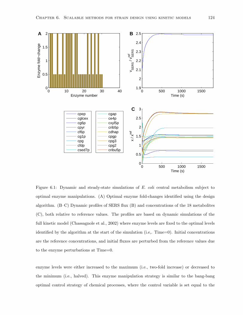
Chapter 6. Scalable methods for strain design using kinetic models 124
0 10 20 30 400
0.5
1
1.5
2
Enzyme number
Enz
yme
fold
−ch
ange
A
0 500 1000 15001.9
2
2.1
2.2
2.3
2.4
2.5
Time (s)
v SE
RS /
vref
SE
RS
B
0 500 1000 15000
0.5
1
1.5
2
2.5
3
Time (s)
x / x
ref
C
cpepcglcexcg6pcpyrcf6pcg1pcpgcfdpcsed7p
cgapce4pcxyl5pcrib5pcdhapcpgpcpg3cpg2cribu5p
Figure 6.1: Dynamic and steady-state simulations of E. coli central metabolism subject to
optimal enzyme manipulations. (A) Optimal enzyme fold-changes identified using the design
algorithm. (B–C) Dynamic profiles of SERS flux (B) and concentrations of the 18 metabolites
(C), both relative to reference values. The profiles are based on dynamic simulations of the
full kinetic model (Chassagnole et al., 2002) where enzyme levels are fixed to the optimal levels
identified by the algorithm at the start of the simulation (i.e,. Time=0). Initial concentrations
are the reference concentrations, and initial fluxes are perturbed from the reference values due
to the enzyme perturbations at Time=0.
enzyme levels were either increased to the maximum (i.e., two-fold increase) or decreased to
the minimum (i.e., halved). This enzyme manipulation strategy is similar to the bang-bang
optimal control strategy of chemical processes, where the control variable is set equal to the

Chapter 6. Scalable methods for strain design using kinetic models 125
lower or upper bound (San and Stephanopoulos, 1983). Bang-bang control is an optimal control
strategy when certain conditions are satisfied by the problem (San and Stephanopoulos, 1983).
An interesting direction for future work is to investigate when, if ever, these conditions are
satisfied in kinetic models, and whether this can lead to simpler optimization problems for
strain design.
The optimal enzyme levels were then implemented in the original kinetic model, and dynamic
simulations were performed. Dynamic simulation of the original kinetic model indicated that the
optimal enzyme manipulations resulted in a 148% (2.48-fold) increase to SERS flux, compared to
the reference flux. As expected, the optimal enzyme levels include the maximum (i.e., two-fold)
increase of the SERS enzyme. A two-fold increase in SERS alone results in an 89% (1.89-fold)
increase of SERS flux, as determined by a dynamic simulation of the full kinetic model. Thus,
the optimal levels of the other 29 enzymes account for the additional 59% increase in SERS flux.
This result indicates that there is value in developing optimization algorithms for identifying
complex enzyme manipulation strategies to maximize production.
6.6 Conclusions
In this chapter, a computationally efficient algorithm was developed for the identification of op-
timal enzyme manipulation strategies using kinetic models of metabolism. A nonlinear kinetic
model (Chassagnole et al., 2002) was approximated around the reference state by representing
the reactions by lin-log rate equations. The elasticity matrix, which forms the only set of kinetic
parameters in the lin-log model, was calculated at the reference state using automatic differ-
entiation of the original nonlinear model. The resulting lin-log kinetic model, while simpler
than the original model, contained bilinear terms. Thus, to use the lin-log model for design-
ing optimal enzyme manipulations, a nonlinear optimization algorithm was developed. This
algorithm uses successive linear programming (SLP) to rapidly identify a local optimum, while
convex relaxations (McCormick relaxation for bilinear terms (McCormick, 1976)) are used to
improve the solution once the SLP has converged. The algorithm was able to identify opti-
mal enzyme manipulation strategies within a minute for a model containing 48 reactions (30

Chapter 6. Scalable methods for strain design using kinetic models 126
enzyme-catalyzed) and 18 metabolites (17 intracellular, one extracellular) (Chassagnole et al.,
2002). The optimal enzyme manipulations were implemented in the original nonlinear model
in order to accurately predict the effects of the enzyme manipulations via dynamic simulations.
The nonlinear model indicated a 2.48-fold increase in the steady state flux of the target reac-
tion, relative to the reference.
These results suggest that this and similar algorithms may be scalable to larger and more com-
plex, kinetic models of cell metabolism. For example, the algorithm can be applied directly
to the genome-scale kinetic model developed by Smallbone et al. (2010), which uses lin-log
rate equations. On the other hand, we found that applying the algorithm (SLP and convex
relaxations) directly to the original kinetic model of Chassagnole et al. (2002), the algorithm
had difficulty identifying satisfactory solutions. This difficulty may be attributed to several
factors. First, in the case of bilinear constraints, the convex hull is given by the McCormick
relaxations. However, for general nonlinear constraints such as those found in the original ki-
netic model, other convex relaxations must be used. The ability of the algorithm to identify
globally optimal solutions is affected by the availability of tight convex relaxations. Currently,
commercial software such as BARON (Tawarmalani and Sahinidis, 2005) is available for global
optimization of MINLPs involving general nonlinear constraints. Alternatively, methods that
formulate tight relaxations that are customized for each type of rate equation may be more
efficient (Pozo et al., 2011).
A limitation that is inherent in our algorithm is the need to constrain the deviation of variables
from the reference such that the approximate model remains valid. Thus, the approximative
model leads to a simpler optimization problem, but the optimal enzyme manipulations may
only be valid for small changes in enzyme levels, fluxes and concentrations. This tradeoff
between computational tractability and model accuracy is inherent in the use of any approxi-
mative model. In future work, it may be possible to employ an iterative procedure, in which
constrained enzyme manipulations are identified, dynamic simulations are performed using
the original model to determine the new steady state, where the approximate model is re-
constructed, followed by another iteration of optimization. This procedure is similar to the
techniques employed for nonlinear model predictive control of chemical processes. We note

Chapter 6. Scalable methods for strain design using kinetic models 127
that the approximate model need not be limited to the lin-log rate equation, which we used in
this work. In particular, the generalized linearization that is based on arbitrary basis functions
(Vital-Lopez et al., 2006a) may be used at each iteration.
In addition, we note that the algorithm developed here is computationally efficient, but at the
cost of decreased control over the design scope. Specifically, while MILP-based methods (Niko-
laev, 2010; Vital-Lopez et al., 2006a) allow the user to limit the number and type of genetic
manipulations through the use of integer variables, our approach does not offer a straightforward
method for such fine control of the design scope without sacrificing computational efficiency.
The tradeoff between computational efficiency and specificity of the design scope will continue
to be challenging as this approach is developed further. One potential extension of this algo-
rithm is to develop subsequent procedures for choosing optimal subsets of the optimal enzyme
manipulations identified using the algorithm. For example, an MILP can be developed to choose
subsets of the enzyme manipulations subject to user-defined thresholds for the production and
number of enzyme manipulations, or to identify (alternative) minimal subsets. Essentially, the
MILP-based procedure is analogous to the third phase employed in the EMILiO algorithm,
which is described in Section 3.3.2. In conclusion, the most practical approach for in silico
strain design is to become familiar with all of the complementary techniques available and to
assess whether one is better suited than another for each individual problem.

Chapter 7
Conclusions
This thesis has explored a number of problems that are central for accurately predicting the
behavior of biological systems, and for effectively engineering them for the cost-effective pro-
duction of chemicals, biofuels, and pharmaceuticals. The major contributions of this thesis are
summarized below:
• Simulation of metabolic networks: Optimization is used to simulate both steady-
state and dynamic cell behavior. Simulation by optimization is appropriate if the cell is
assumed to behave according to a cellular objective, or if unmeasured states are estimated
while minimizing discrepancy with the subset of states that are measured. Linear, mixed-
integer, and nonlinear objectives and constraints have been explored in the literature.
This thesis has made contributions to the simulation of metabolic states through the
development of a method for randomly sampling thermodynamically feasible reaction
fluxes and metabolite concentrations (Chapter 5). This non-convex solution space is
difficult to sample due to an exponential increase in problem size with model dimension.
Hence, the sampling algorithm was implemented on the graphics processing unit (GPU)
to utilize its parallel processing capabilities. The GPU showed a ten-fold improvement in
processing speed over the CPU.
• In silico strain design: Optimal design of cell metabolism for metabolite overproduc-
tion is a rapidly growing area of research. Various linear, mixed-integer, and nonlinear
128

Chapter 7. Conclusions 129
optimization problems have been formulated for this purpose. These problems are chal-
lenging as they typically become exponentially larger as the model becomes more detailed.
The design scope or model size is often reduced to make the design problem tractable.
This thesis has made contributions to the problem of optimal strain design by developing
an efficient strain design algorithm called EMILiO (Chapter 3). EMILiO is based on a
bilevel optimization problem that is reformulated as an MPCC and efficiently solved (to a
local optimum) using successive linear programming (SLP). Subsequent steps in EMILiO
ensure that both minimal and alternative designs are systematically and efficiently iden-
tified.
• Assessing robustness of a strain design: This thesis has explored the potential for
in silico design of strains that are robust against gene expression noise, environmental
perturbations, and model parameter uncertainty (Chapter 4). Diversification of assets
(i.e., metabolic pathways) was shown to be an effective strategy for improving robustness
against all of these perturbations and model uncertainties. A larger number of diversified,
or redundant, pathways improved robustness against large perturbations; however, sen-
sitivity to small perturbations was also increased. Therefore, metabolic engineers should
be mindful of the trade-offs inherent in robust design. Furthermore, future robust strain
design efforts will require accurate characterization of the nature of environmental per-
turbations, including, but not limited to their magnitudes.
• Experiment design using noisy metabolomics data: Experiment design can be
aided by mathematical models to improve the efficiency of time and resource allocation
while maximizing the value of measurements. This thesis has explored the potential
impact of model-based experiment design using metabolomics data (Chapter 5). Accord-
ingly, a method was developed to assess the sensitivity of reaction flux and metabolite
concentration simulations to uncertainty in measurements in a subset of metabolites. This
sensitivity information, which is based on noisy metabolomics data sets, could be used to

Chapter 7. Conclusions 130
efficiently choose a set of metabolite concentrations needing precise measurements.
• Designing optimal enzyme manipulations using kinetic models of metabolism:
The identification of optimal enzyme manipulation strategies using mathematical opti-
mization and kinetic models of metabolism is a challenging problem with practical ap-
plications. A number of optimization methods have been developed for this purpose, as
reviewed in Chapter 2. In Chapter 6, the optimization techniques used in the development
of EMILiO were successfully extended to the design of optimal enzyme manipulations us-
ing kinetic models of metabolism. The algorithm was tested using a kinetic model of E.
coli central metabolism (Chassagnole et al., 2002). The model is used widely for testing
strain design algorithms. It includes 17 intracellular metabolites and 30 enzyme-catalyzed
reactions whose rates are defined using nonlinear kinetic rate equations. The algorithm
developed in Chapter 6 was able to identify optimal enzyme manipulation strategies that
increased serine synthesis flux by 148% (relative to the reference flux) in less than one
minute of CPU time. We found that this computational efficiency came with the cost
of reduced specificity of the design: i.e., the number and types of enzyme manipulations
could not be easily controlled. However, we have encountered a similar tradeoff in Chapter
3. Thus, potential avenues for improvement are discussed in Chapter 8.
Chapter 8
Recommendations for Future Work
• Include additional constraints in the bilevel optimization framework for strain
design: The bilevel optimization framework for strain design (Chapter 3) is not limited
to models of metabolism that include stoichiometric constraints alone. For example,
the optimization techniques used in EMILiO (Chapter 3) may be extended to models of
metabolism that include regulatory constraints. Specifically, the techniques may be used
to extend existing algorithms that identify optimal gene knockout or expression strategies
(Kim and Reed, 2010), to the identification of optimal gene expression levels in mod-
els that describe both metabolic and transcriptional regulatory networks. Furthermore,
strategies for identifying knockout and optimal gene expression levels may be applied
to models that describe transcriptional regulation using quantitative flux bounds, rather
than Boolean rules, such as the PROM model (Chandrasekaran and Price, 2010).
A special case of additional constraints in the constraint-based modeling framework is the
addition of rate equation constraints. These constraints define the reaction rates as func-
tions of concentrations, enzyme levels, and kinetic parameters. We refer to these classes of
models as kinetic models of metabolism, and we found that optimization-based methods
could be applied efficiently for identifying optimal enzyme manipulations (Chapter 6).
Therefore, we recommend continued research in mathematical optimization-based design
using kinetic models of metabolism.
• Continued development of scalable techniques for optimal strain design us-
131

Chapter 8. Recommendations for Future Work 132
ing kinetic models: In Chapter 6, efficient optimization techniques were employed for
strain design using kinetic models of metabolism. The nonlinear kinetic model of E. coli
central metabolism developed by Chassagnole et al. (2002) was approximated as a lin-log
kinetic model (Section 2.3.3). An optimization problem was formulated using this lin-log
model to identify optimal enzyme manipulations for maximizing serine synthesis (Section
6.3). This nonlinear optimization problem was successfully solved using the optimization
techniques developed in Chapter 3.
In future work, this method may be applied directly to large-scale models that use lin-log
rate equations. For example, Smallbone et al. (2010) developed a genome-scale model of
S. cerevisiae, in which reaction rates are described using lin-log rate equations. For the
model of central metabolism used in Chapter 6 (having 30 enzymes and 17 intracellular
metabolites), the optimization problem was solved in under a minute. Accordingly, it
would be interesting to investigate whether the methods developed here are indeed scal-
able to genome-scale models.
• Investigate the tradeoff between efficiency and specificity of designing a strain:
In Chapter 6, optimal enzyme manipulation strategies were found efficiently, but this
efficiency was achieved at the cost of lower specificity of the design scope. That is, control
over the number and types of enzyme manipulations allowed was decreased, and this can
directly influence the practical value of in silico designs. Thus, one avenue for improving
the algorithm is to develop efficient methods for restricting the design scope. In fact,
MILP-based (Vital-Lopez et al., 2006a) or MINLP-based (Nikolaev, 2010) methods have
been developed, which enable finer control over the scope of design. In future work, an
optimal tradeoff may be achieved by extending the current algorithm. For example, an
MILP can be developed to choose subsets of the enzyme manipulations subject to user-
defined thresholds for the production and number of enzyme manipulations, or to identify
(alternative) minimal subsets. Essentially, the MILP-based procedure is analogous to the
third phase employed in the EMILiO algorithm, which is described in Section 3.3.2.
Chapter 8. Recommendations for Future Work 133
• Investigate special conditions for optimal strain design: In Chapter 6, we iden-
tified an optimal enzyme manipulation strategy to maximize serine synthesis using the
kinetic model of E. coli central metabolism (Chassagnole et al., 2002). Essentially, all
enzyme levels were either increased to the maximum (i.e., two-fold increase) or decreased
to the minimum (i.e., halved). This enzyme manipulation strategy is similar to the bang-
bang optimal control strategy of chemical processes, where the control variable is set
equal to the lower or upper bound (San and Stephanopoulos, 1983). Bang-bang control
is an optimal control strategy when certain conditions are satisfied by the problem (San
and Stephanopoulos, 1983). Accordingly, an interesting direction for future work is to
investigate when, if ever, these conditions are satisfied in kinetic models, and whether
this can lead to simpler optimization problems for strain design.
• Optimal strain designs that are robust against model parameter uncertainty:
Kinetic models typically require the estimation of many parameters. These parameters
involve uncertainty (Miskovic and Hatzimanikatis, 2011), which may affect the feasibility
of the optimal strategies identified. Therefore, future work may be directed at adopting
the techniques of robust optimization (Ben-Tal and Nemirovski, 1998) for the identifica-
tion of enzyme manipulation strategies that are robust to model uncertainty.
• Investigate the use of alternative kinetic models: The optimization techniques
developed in this thesis are not limited to only the lin-log rate equations. Alternatively,
other forms of approximate rate equations (Vital-Lopez et al., 2006a), mechanistic rate
equations (Chassagnole et al., 2002), or hybrid models (Bulik et al., 2009) can be used. An-
other promising direction of research is to use large-scale models that describe metabolic
and regulatory interactions as mass action kinetics, as described by Jamshidi and Palsson
(2010). This modeling approach involves a large number of interactions but the terms
will be consistent in terms of their nonlinearities. Specifically, in the formulation of an
optimal enzyme manipulation problem, we can expect trilinear terms arising from the

Chapter 8. Recommendations for Future Work 134
product of two substrates and an enzyme level for each mass action rate equation.
Accordingly, the extension of the scalable optimization methods developed in this thesis
to alternative kinetic models will likely require the concurrent development or adoption
of optimization techniques.
• Investigate improved optimization techniques
In this thesis, the problem of identifying optimal enzyme levels using kinetic models
(Problem (6.1)) was solved through a straightforward application of the optimization
techniques developed for solving the EMILiO problem (in Chapter 3). For the reference
condition considered here, we could find an optimal solution that was comparable in the
rate of serine synthesis with previous studies (Vital-Lopez et al., 2006a), albeit with a
larger number of enzyme manipulations.
In future research, improved optimization techniques will need to be developed. This
conclusion was reached when we applied the optimization method directly to the original,
nonlinear kinetic model developed by Chassagnole et al. (2002). We found that the
optimization technique that worked well in this thesis did not converge to a satisfactory
solution when the original kinetic model was used. This obstacle was likely due to two
reasons.
First, the solution of (6.1) relies on the availability of tight convex underestimators, both
for the identification of good starting solutions, as well as to improve convergence to a
global optimum. For bilinear constraints, the McCormick relaxations are adequate since
they form the convex hull (McCormick, 1976). However, for general nonlinear constraints,
the McCormick relaxations no longer apply and other convex relaxations must be used.
In the area of convex relaxations, interested researchers are suggested to study the works
of Sahinidis et al. (Tawarmalani and Sahinidis, 2005).
Second, the optimization method can be improved. We used a successive (iterative) linear
program with line search (Bullard and Biegler, 1991) in this thesis (Eq. 6.1). While this
technique worked well for problems involving bilinear constraints, it did not work as
well when applied to the original kinetic model that involved more complex, nonlinear
constraints. One direction for improvement is to use a trust-region method rather than

Chapter 8. Recommendations for Future Work 135
the line search (Biegler, 2010). The extra flexibility present in the trust-region method
may enable better approximations of the complex, nonlinear terms present in mechanistic
kinetic models of metabolism.
• Develop scalable software platforms for large-scale kinetic models
An eventual goal of developing scalable algorithms for design using kinetic models is to
apply the algorithms to genome-scale models such as that developed by Smallbone et al.
(2010). An immediate challenge to the use of genome-scale kinetic models is the lack
of software platforms that are capable of handling such large models (Smallbone et al.,
2010). Accordingly, simulation and visualization of genome-scale kinetic models is diffi-
cult. Indeed, while the development of scalable design algorithms may continue to progress
through the development of optimization techniques, there may nonetheless be a lack of
software platforms to simulate and interpret the optimal designs that are generated by
the algorithm. Therefore, a recommendation for future research is to collaborate with
software developers or computer scientists in order to accelerate the development of soft-
ware platforms that are capable of interpreting the results of, and potentially integrating,
optimal strain designs based on large-scale kinetic models. A potentially useful advance
in computational techniques is the use of graphics processing units (GPUs) for low-cost,
parallel computing (see Chapter 5 for the author’s experience with GPUs for modeling
metabolic networks).
• Experimentally validate computationally-generated hypotheses
This thesis has generated a number of hypotheses that may be experimentally validated
in future work. For example, a large number of strategies for succinate production have
been suggested in Chapter 3. Also, in Chapter 4, we have outlined an experimental
procedure based on the experiments of Sonntag et al. (1993) for testing our hypothesis
that diversification improves robustness against large perturbations at the cost of increases
sensitivity to small perturbations. In Chapter 5, we developed a method for designing
experiments to specify a small set of metabolites needing precise measurements in order
to improve model precision. Thus, in future work, the experiment design methodology

Chapter 8. Recommendations for Future Work 136
should be tested using an initial metabolomics dataset, followed by measurement of only
a few important metabolite concentrations. In Chapter 6, we hypothesized that certain
enzymes should be upregulated while others should be inhibited in order to maximize L-
serine production. In future work, a number of these hypotheses can be tested, although
we recommend first reducing the set of enzyme manipulations using pruning methods,
such as those developed in Chapter 3.
• Additional directions for future research
Finally, while not discussed in detail in this thesis, the optimization techniques used for
the design of optimal microbial strains may also be extended to higher organisms. For
example, industrial production of chemicals and therapeutics requires systematic methods
for designing superior and cost-effective growth media. Unlike the microbes studied in
this thesis, the growth media for mammalian cells typically contain a combination of
many substrates and nutrients. The development of accurate models of mammalian cell
metabolism may enable the use of mathematical optimization for cell medium design.
An immediate challenge for the application of CBM to modeling mammalian cells is the
identification of an appropriate objective function, since maximization of growth yield is
typically inaccurate for these systems. Alternatively, kinetic models may be developed.
In this case, effective methods for parameter estimation will be required. An interesting
problem is to design experiments that involve an optimal combination of experimental
data (i.e., metabolomics, fluxomics, proteomics, transcriptomics, steady-state data, or
transient data) with minimal cost in resources and time. To solve these important and
practical problems, the collaboration between experts in mathematical optimization and
experts in experimental techniques will be necessary.

Bibliography
Alper, H., Fischer, C., Nevoigt, E., and Stephanopoulos, G. (2005). Tuning genetic control
through promoter engineering. Proc. Natl. Acad. Sci. USA, 102:12678–12683.
Baker, T. E. and Lasdon, L. S. (1985). Successive linear programming at exxon. Management
Science, 31:264–274.
Becker, S. A., Feist, A. M., Mo, M. L., et al. (2007). Quantitative prediction of cellular
metabolism with constraint-based models: the COBRA Toolbox. Nature Protocols, 2:727–
738.
Becskei, A. and Serrano, L. (2000). Engineering stability in gene networks by autoregulation.
Nature, 405:590–593.
Beg, Q. K., Vazquez, A., Ernst, J., et al. (2007). Intracellular crowding defines the mode and
sequence of substrate uptake by Escherichia coli and constrains its metabolic activity. Proc.
Natl. Acad. Sci. USA, 104:12663–12668.
Ben-Tal, A. and Nemirovski, A. (1998). Robust convex optimization. Mathematics of Operations
Research, 23:769–805.
Bennett, B. D., Kimball, E. H., Gao, M., et al. (2009). Absolute metabolite concentrations
and implied enzyme active site occupancy in Escherichia coli. Nature Chemical Biology,
5:593–599.
Benyamini, T., O., F., Ruppin, E., and Shlomi, T. (2010). Flux balance analysis accounting
for metabolite dilution. Genome. Biol., 11:R43.
137

BIBLIOGRAPHY 138
Biegler, L. T. (2010). Nonlinear programming: concepts, algorithms, and applications to chem-
ical processes. Society for Industrial and Applied Mathematics, Philadelphia, PA.
Buescher, J. M., Czernik, D., Ewald, J. C., Sauer, U., and Zamboni, N. (2009). Cross-Platform
Comparison of Methods for Quantitative Metabolomics of Primary Metabolism. Analytical
Chemistry, 81:2135–2143.
Bulik, S., Grimbs, S., Huthmacher, C., Selbig, J., and Holzhutter, H. G. (2009). Kinetic hybrid
models composed of mechanistic and simplified enzymatic rate laws - a promising method for
speeding up the kinetic modelling of complex metabolic networks. FEBS Journal, 276:410–
424.
Bullard, L. G. and Biegler, L. T. (1991). Iterative linear programming strategies for constrained
simulation. Computers and Chemical Engineering, 15:239–254.
Burgard, A. P., Nikolaev, E. V., Schilling, C. H., and Maranas, C. D. (2004). Flux coupling
analysis of genome-scale metabolic network reconstructions. Genome Research, 14:301–312.
Burgard, A. P., Pharkya, P., and Maranas, C. D. (2003). OptKnock: A bilevel program-
ming framework for identifying gene knockout strategies for microbial strain optimization.
Biotechnol. Bioeng., 84:647–657.
Chandrasekaran, S. and Price, N. D. (2010). Probabilistic integrative modeling of genome-scale
metabolic and regulatory networks in Escherichia coli and Mycobacterium tuberculosis. Proc
Natl Acad Sci USA, 107:17845–17850.
Chang, Y., Suthers, P. F., and Maranas, C. D. (2008). Identification of optimal measurement
sets for complete flux elucidation in metabolic flux analysis experiments. Biotechnology and
Bioengineering, 100:1039–1049.
Chassagnole, C., Noisommit-Rizzi, N., Schmid, J. W., Mauch, K., and Reuss, M. (2002). Dy-
namic modeling of the central carbon metabolism of Escherichia coli. Biotechnol. Bioeng.,
79:53–73.

BIBLIOGRAPHY 139
Chatterjee, R., Millard, C. S., Champion, K., Clark, D. P., and Donnelly, M. I. (2001). Mutation
of the ptsc gene results in increased production of succinate in fermentation of glucose by
Escherichia coli. Appl. Environ. Microbiol., 67:148–154.
Chen, Z., Wilmanns, M., and Zeng, A. P. (2010). Structural synthetic biotechnology: from
molecular structure to predictable design for industrial strain development. Trends Biotech-
nol., 28:534–542.
Cole, S. T. and Guest, J. R. (1979). Amplification and aerobic synthesis of fumarate reductase
in ampicillin-resistant mutants of Escherichia coli k-12. FEMS Microbiol. Lett., 5:65–67.
Cornelius, S. P., Lee, J. S., and Motter, A. E. (2011). Dispensability of Escherichia coli ’s latent
pathways. Proc Natl Acad Sci U.S.A.
Costa, R. S., Machado, D., Rocha, I., and Ferreira, E. C. (2011). Critical perspective on the
consequences of the limited availability of kinetic data in metabolic modeling. IET Systems
Biology, 5:157–163.
Covert, M. W., Knight, E. M., Reed, J. L., Herrgard, M. J., and Palsson, B. O. (2004).
Integrating high-throughput and computational data elucidates bacterial networks. Nature,
429:92–96.
Covert, M. W., Schilling, C. H., and Palsson, B. (2001). Regulation of gene expression in flux
balance models of metabolism. Journal of Theoretical Biology, 213:73–88.
Cox, S. J., Levanon, S. S., Sanchez, A., et al. (2006). Development of a metabolic network
design and optimization framework incorporating implementation constraints: a succinate
production case study. Metab. Eng., 8:46–57.
Csete, M. E. and Doyle, J. C. (2002). Reverse engineering of biological complexity. Science,
295:1664–1669.
De Mey, M., Maertens, J., Lequeux, G. J., Soetaert, W. K., and Vandamme, E. J. (2007).
Construction and model-based analysis of a promoter library for E. coli : an indispensable
tool for metabolic engineering. BMC Biotechnol., 7:34.
BIBLIOGRAPHY 140
Dean, J. P. and Dervakos, G. A. (1998). Redesigning metabolic networks using mathematical
programming. Biotechnol. Bioeng., 58:267–271.
Edwards, J., Covert, M., and Palsson, B. (2002). Metabolic modelling of microbes: the flux-
balance approach. Environmental Microbiology, 4:133–140.
Edwards, J. S., Ibarra, R. U., and Palsson, B. O. (2001). In silico predictions of Escherichia coli
metabolic capabilities are consistent with experimental data. Nat. Biotechnol., 19:125–130.
Enfors, S.-O., Jahic, M., Rozkov, A., et al. (2001). Physiological responses to mixing in large
scale bioreactors. Journal of Biotechnology, 85(2):175 – 185.
Famili, I., Mahadevan, R., and Palsson, B. O. (2005). k-cone analysis: Determining all candidate
values for kinetic parameters on a network scale. Biophysical Journal, 88:1616–1625.
Feist, A. M., Henry, C. S., Reed, J. L., et al. (2007). A genome-scale metabolic reconstruction for
Escherichia coli K-12 MG1655 that accounts for 1260 ORFs and thermodynamic information.
Mol. Syst. Biol., 3:121.
Feist, A. M., Zielinski, D. C., Orth, J. D., et al. (2010). Model-driven evaluation of the produc-
tion potential for growth-coupled products of Escherichia coli. Metab. Eng., 12:173–186.
Fong, S., Nanchen, A., Palsson, B. O., and Sauer, U. (2006). Latent pathway activation and
increased pathway capacity enable Escherichia coli adaptation to loss of key metabolic
enzymes. Journal of Biological Chemistry, 281:8024–8033.
Fong, S. S., Burgard, A. P., Herring, C. D., et al. (2005). In silico design and adaptive evolution
of Escherichia coli for production of lactic acid. Biotechnol. Bioeng., 91:643–648.
Frey, B. J. and Dueck, D. (2007). Clustering by passing messages between data points. Science,
315:972–976.
Glass, J. I., Assad-Garcia, N., Alperovich, N., et al. (2006). Essential genes of a minimal
bacterium. Proc. Natl. Acad. Sci. USA, 103:425–430.

BIBLIOGRAPHY 141
Glover, F. (1975). Improved linear integer programming formulations of nonlinear integer
problems. Manage. Sci., 22:445.
Heijnen, J. J. (2005). Approximative kinetic formats used in metabolic network modeling.
Biotechnol. Bioeng., 91:534–545.
Henry, C. S., Broadbelt, L. J., and Hatzimanikatis, V. (2007). Thermodynamics-Based
Metabolic Flux Analysis. Biophys. J., 92:1792–1805.
Henry, C. S., DeJongh, M., Best, A. A., et al. (2010a). High-throughput generation, optimiza-
tion and analysis of genome-scale metabolic models. Nature Biotechnology, 28:977–U22.
Henry, C. S., Overbeek, R., and Stevens, R. L. (2010b). Building the blueprint of life. Biotechnol.
J., 5:695–704.
Herrgard, M. J., Swainston, N., Dobson, P., et al. (2008). A consensus yeast metabolic network
reconstruction obtained from a community approach to systems biology. Nature Biotechnol-
ogy, 26:1155–1160.
Hoops, S., Sahle, S., Gauges, R., et al. (2006). COPASI–a COmplex PAthway Simulator.
Bioinformatics, 22:3067–3074.
Hua, Q., Joyce, A. R., Fong, S. S., and Palsson, B. O. (2006). Metabolic analysis of adaptive
evolution for in silico-designed lactate-producing strains. Biotechnol. Bioeng., 95:992–1002.
Ibarra, R. U., Edwards, J. S., and Palsson, B. O. (2002). Escherichia coli K-12 undergoes
adaptive evolution to achieve in silico predicted optimal growth. Nature, 420:186–189.
Iuchi, S., Kuritzkes, D. R., and Lin, E. C. C. (1986). Three classes of Escherichia coli mutants
selected for aerobic expression of fumarate reductase. J Bacteriol., 168:1415–1421.
Jamshidi, N. and Palsson, B. O. (2010). Mass action stoichiometric simulation models: incor-
porating kinetics and regulation into stoichiometric models. Biophysical Journal, 98:175–185.
Jantama, K., Haupt, M. J., Svoronos, S. A., et al. (2008). Combining metabolic engineering
BIBLIOGRAPHY 142
and metabolic evolution to develop nonrecombinant strains of Escherichia coli c that produce
succinate and malate. Biotechnol. Bioeng., 99:1140–1153.
Jin, Y. S. and Stephanopoulos, G. (2007). Multi-dimensional gene target search for improving
lycopene biosynthesis in Escherichia coli. Metab. Eng., 9:337–347.
Joyce, A. R. and Palsson, B. O. (2006). The model organism as a system: integrating ’omics’
data sets. Nature Reviews Molecular Cell Biology, 7:198–210.
Kacser, H. and Burns, J. A. (1973). The control of flux. Symp. Soc. Exp. Biol., 27:65–104.
Kafri, R., Levy, M., and Pilpel, Y. (2006). The regulatory utilization of genetic redundancy
through responsive backup circuits. Proc. Natl. Acad. Sci. USA, 103(31):11653–11658.
Kafri, R., Springer, M., and Pilpel, Y. (2009). Genetic Redundancy: New Tricks for Old Genes.
Cell, 136(3):389–392.
Kaufman, D. E. and Smith, R. L. (1998). Direction choice for accelerated convergence in
hit-and-run sampling. Operations Research, 46:84–95.
Kim, J. and Reed, Jennifer, L. (2010). OptORF: Optimal metabolic and regulatory perturba-
tions for metabolic engineering of microbial strains. BMC Syst. Biol., 4:53.
Kirkpatrick, C., Maurer, L., Oyelakin, N., et al. (2001). Acetate and formate stress: Opposite
responses in the proteome of Escherichia coli . J. Bacteriol., 183(21):6466–6477.
Kitano, H. (2004). Biological robustness. Nat. Rev. Genet., 5:826–837.
Kitano, H. (2007). Towards a theory of biological robustness. Mol. Syst. Biol., 3:137.
Kitano, H. (2010). Violations of robustness trade-offs. Mol. Syst. Biol., 6:384.
Kucherenko, S., Rodriguez-Fernandez, M., Pantelides, C., and Shah, N. (2009). Monte carlo
evaluation of derivative-based global sensitivity measures. Reliability Engineering & System
Safety, 94:1135 – 1148.
BIBLIOGRAPHY 143
Lee, K. H., Park, J. H., Kim, T. Y., Kim, H. U., and Lee, S. Y. (2007). Systems metabolic
engineering of Escherichia coli for l-threonine production. Mol. Syst. Biol., 3:149.
Lin, H., Bennett, G. N., and San, K. Y. (2005). Chemostat culture characterization of Es-
cherichia coli mutant strains metabolically engineered for aerobic succinate production: a
study of the modified metabolic network based on metabolic profile, enzyme activity, and
gene expression profile. Metab. Eng., 7:337–352.
Lin, H., Castro, N. M., Bennett, G. N., and San, K. Y. (2006). Acetyl-CoA synthetase over-
expression in Escherichia coli demonstrates more efficient acetate assimilation and lower
acetate accumulation: a potential tool in metabolic engineering. Applied Microbiology and
Biotechnology, 71:870–874.
Lin, H., Vadali, R. V., Bennett, G. N., and San, K. Y. (2004). Increasing the acetyl-coa pool
in the presence of overexpressed phosphoenolpyruvate carboxylase or pyruvate carboxylase
enhances succinate production in Escherichia coli. Biotechnol. Prog., 20:1599–1604.
Lun, D. S., Rockwell, G., Guido, N. J., et al. (2009). Large-scale identification of genetic design
strategies using local search. Mol. Syst. Biol., 5:296.
Mahadevan, R., Burgard, A. P., Famili, I., Van Dien, S., and Schilling, C. H. (2005). Applica-
tions of metabolic modeling to drive bioprocess development for the production of value-added
chemicals. Biotechnol. Bioeng., 10:408–417.
Mahadevan, R., Edwards, J. S., and Doyle, F. J. (2002). Dynamic flux balance analysis of
diauxic growth in Escherichia coli. Biophysical Journal, 83:1331–1340.
Mahadevan, R. and Lovley, D. R. (2008). The degree of redundancy in metabolic genes is linked
to mode of metabolism. Biophys. J., 94:1216–1220.
Mahadevan, R. and Schilling, C. H. (2003). The effects of alternate optimal solutions in
constraint-based genome-scale metabolic models. Metab. Eng., 5:264–276.
McCormick, G. P. (1976). Computability of global solutions to factorable nonconvex programs:
Part I–convex underestimating problems. Math. Program., 10:147–175.

BIBLIOGRAPHY 144
McGibney, G. and Smith, M. (1993). An unbiased signal-to-noise ratio measure for magnetic-
resonance images. Medical Physics, 20(4):1077–1078.
McKinlay, J. B., Vieille, C., and Zeikus, G. J. (2007). Prospects for a bio-based succinate
industry. Appl. Microbiol. Biotechnol., 76:727–740.
Melzer, G., Esfandabadi, M. E., Franco-Lara, E., and Wittmann, C. (2009). Flux design: In
silico design of cell factories based on correlation of pathway fluxes to desired properties.
BMC Systems Biology, 3:120.
Mendes, P. and Kell, D. B. (1998). Non-linear optimization of biochemical pathways: applica-
tion to metabolic engineering and parameter estimation. Bioinformatics, 14:869–883.
Mendonca, A. G., Alves, R. J., and Pereira-Leal, J. B. (2011). Loss of genetic redundancy in
reductive genome evolution. PLoS Comput. Biol., 7:e1001082.
Metris, A., George, S., and Baranyi, J. (2011). Modelling osmotic stress by flux balance analysis
at the genomic scale. Journal of Biotechnology, 104:77–85.
Millard, C. S., Chao, Y. P., Liao, J. C., and Donnelly, M. (1996). Enhanced production
of succinic acid by overexpression of phosphoenolpyruvate carboxylase in Escherichia coli.
Appl. Environ. Microbiol., 62:1808–1810.
Miskovic, L. and Hatzimanikatis, V. (2011). Modeling of uncertainties in biochemical reactions.
Biotechnol. Bioeng., 108:413–423.
Mo, M. L., Palsson, B. O., and Herrgard, M. J. (2009). Connecting extracellular metabolomic
measurements to intracellular flux states in yeast. BMC Systems Biology, 3.
Moran, N. A. (2002). Microbial minimalism: genome reduction in bacterial pathogens. Cell,
108:583–586.
Morari, M. and Zafiriou, E. (1989). Robust Process Control. Prentic Hall, Englewood Cliffs,
New Jersey.

BIBLIOGRAPHY 145
Nakamura, C. E. and Whited, G. M. (2003). Metabolic engineering for the microbial production
of 1,3-propanediol. Current Opinion in Biotechnology, 14:454–459.
Newman, E. B., Batist, G., Fraser, J., et al. (1976). Use of glycine as nitrgen-source by
Escherichia coli -k12. Biochimica et Biophysica Acta, 421(1):97–105.
Nikolaev, E. V. (2010). The elucidation of metabolic pathways and their improvements using
stable optimization of large-scale kinetic models of cellular systems. Metab. Eng., 12:26–38.
Orth, J. D., Thiele, I., and Palsson, B. O. (2010). What is flux balance analysis? Nat.
Biotechnol., 28:245–248.
Patil, K. R., Rocha, I., Forster, J., and Nielsen, J. (2005). Evolutionary programming as a
platform for in silico metabolic engineering. BMC Bioinformatics, 6:308.
Pekkonen, M., Korhonen, J., and Laakso, J. (2011). Increased survival during famine improves
fitness of bacteria in a pulsed-resource environment. Evol. Ecol. Res., 13:1–18.
Peters-Wendisch, P., Stoiz, M., Etterich, H., et al. (2005). Metabolic engineering of Corynebac-
terium glutamicum for l-serine production. Appl. Environ. Microbiol., 71:7139–7144.
Pharkya, P., Burgard, A. P., and Maranas, C. D. (2003). Exploring the overproduction of amino
acids using the bilevel optimization framework optknock. Biotechnol. Bioeng., 84:887–899.
Pharkya, P., Burgard, A. P., and Maranas, C. D. (2004). Optstrain: a computational framework
for redesign of microbial production systems. Genome Research, 14:2367–2376.
Pharkya, P. and Maranas, C. D. (2006). An optimization framework for identifying reaction ac-
tivation/inhibition or elimination candidates for overproduction in microbial systems. Metab.
Eng., 8:1–13.
Picket, A. M. and Bazin, M. J. (1980). Growth and composition of Escherichia coli subjected
to square-wave perturbations in nutrient supply: effect of varying amplitudes. Biotechnol.
Bioeng., 22:1213–1224.

BIBLIOGRAPHY 146
Portnoy, V. A., Scott, D. A., Lewis, N. E., et al. (2010). Deletion of genes encoding cytochrome
oxidases and quinol monooxygenase blocks the aerobic-anaerobic shift in Escherichia coli
K-12 MG1655. Appl. Environ. Microbiol., 76:6529–6540.
Pozo, C., Guillen-Gosalbez, G., Sorribas, A., and Jimenez, L. (2011). A spatial branch-and-
bound framework for the global optimization of kinetic models of metabolic networks. Ind.
Eng. Chem. Res., 50:5225–5238.
Price, N., Thiele, I., and Palsson, B. (2006). Candidate states of Helicobacter pylori’s genome-
scale metabolic network upon application of “loop law” thermodynamic constraints. Bio-
physical Journal, 90:3919–3928.
Purich, D. L. (2010). Enzyme kinetics: catalysis and control. Elsevier/Academic Press, Ams-
terdam, Netherlands; Boston, MA.
Ranganathan, S., Suthers, P. F., and Maranas, C. D. (2010). Optforce: an optimization pro-
cedure for identifying all genetic manipulations leading to targeted overproductions. PLoS
Comput. Biol., 6:e1000744.
Salis, H. M., Mirsky, E. A., and Voigt, C. A. (2009). Automated design of synthetic ribosome
binding sites to control protein expression. Nat. Biotechnol., 27:946–950.
Saltelli, A., Tarantola, S., and Campolongo, F. (2000). Sensitivity analysis as an ingredient of
modeling. Statistical Science, 15:377–395.
San, K. Y. and Stephanopoulos, G. (1983). Optimal-control policy for substrate inhibited
kinetics with enzyme deactivation in an isothermal CSTR. AICHE Journal, 29:417–424.
Sanchez, A. M., Bennett, G. N., and San, K. Y. (2005). Novel pathway engineering design of
the anaerobic central metabolic pathway in Escherichia coli to increase succinate yield and
productivity. Metab. Eng., 7:229–239.
Sanchez, A. M., Bennett, G. N., and San, K. Y. (2006). Batch culture characterization and
metabolic flux analysis of succinate-producing Escherichia coli strains. Metab. Eng., 8:209–
226.
BIBLIOGRAPHY 147
Savinell, J. M. and Palsson, B. O. (1992). Optimal selection of metabolic fluxes for invivo mea-
surement .1. development of mathematical-methods. Journal of Theoretical Biology, 155:201–
214.
Schellenberger, J. and Palsson, B. O. (2009). The use of randomized sampling for analysis of
metabolic networks. Journal of Biological Chemistry, 284:5457–5461.
Schellenberger, J., Tsai, E. A., and Palsson, B. O. (2007). Exploring the concentration space
of genome scale metabolic networks. In Eighth International Conference on Systems Biology,
page H20.
Schmid, J. W., Mauch, K., Reuss, M., Gilles, E. D., and Kremling, A. (2004). Metabolic design
based on a coupled gene expression-metabolic network model of tryptophan production in
Escherichia coli. Metab. Eng., 6:364–377.
Schrumpf, B., Schwarzer, A., Kalinowski, J., et al. (1991). A functionally split pathway for
lysine synthesis in corynebacterium-glutamicum. J. Bacteriol., 173:4510–4516.
Schuetz, R., Kuepfer, L., and Sauer, U. (2007). Systematic evaluation of objective functions
for predicting intracellular fluxes in Escherichia coli. Mol. Syst. Biol., 3:119.
Shaw, D. J. and Guest, J. R. (1982). Amplification and product identification of the fnr gene
of Escherichia coli. J. Gen. Microbiol., 128:2221–2228.
Shen, P., Chao, H., Jiang, C., et al. (2010). Enhancing Production of l-Serine by Increasing
the glyA Gene Expression in Methylobacterium sp MB200. Appl. Biochem. Biotechnol.,
160(3):740–750.
Shirai, T., Nakato, A., Izutani, N., et al. (2005). Comparative study of flux redistribution
of metabolic pathway in glutamate production by two coryneform bacteria. Metab. Eng.,
7:59–69.
Shlomi, T., Cabili, M. N., and Ruppin, E. (2009). Predicting metabolic biomarkers of human
inborn errors of metabolism. Molecular Systems Biology, 5.

BIBLIOGRAPHY 148
Smallbone, K., Simeonidis, E., Swainston, N., and Mendes, P. (2010). Towards a genome-scale
kinetic model of cellular metabolism. BMC Syst. Biol., 4:6.
Sonntag, K., Eggeling, L., De Graaf, A. A., and Sahm, H. (1993). Flux partitioning in the
split pathway of lysine synthesis in Corynebacterium glutamicum: quantification by 13C- and
1H-NMR spectroscopy. Eur. J. Biochem., 213:1325–1331.
Stephanopoulos, G. and Simpson, T. W. (1997). Flux amplification in complex metabolic
networks. Chem. Eng. Sci., 52:2607–2627.
Stoiz, M., Peters-Wendisch, P., Etterich, H., et al. (2007). Reduced folate supply as a key to
enhanced l-serine production by Corynebacterium glutamicum. Appl. Environ. Microbiol.,
73:750–755.
Stols, L. and Donnelly, M. I. (1997). Production of succinic acid through overexpression of
nad(+)-dependent malic enzyme in an escherichia coli mutant. Appl. Environ. Microbiol.,
63:2695–2701.
Stolz, M., Peters-Wendisch, P., Etterich, H., et al. (2007). Reduced folate supply as a key to
enhanced L-serine production by Corynebacterium glutamicum. Appl. Environ. Microbiol.,
73(3):750–755.
Suiter, A. M., Banziger, O., and Dean, A. M. (2003). Fitness consequences of a regulatory
polymorphism in a seasonal environment. Proc. Natl. Acad. Sci. U.S.A, 100:12782–12786.
Tamas, I., Klasson, L., Canback, B., et al. (2002). 50 million years of genomic stasis in en-
dosymbiotic bacteria. Science, 296:2376–2379.
Tawarmalani, M. and Sahinidis, N. V. (2005). A polyhedral branch-and-cut approach to global
optimization. Mathematical Programming, 103:225–249.
Tepper, N. and Shlomi, T. (2010). Predicting metabolic engineering knockout strategies for
chemical production: accounting for competing pathways. Bioinformatics, 26:536–543.
Tilman, D., Reich, P. B., and Knops, J. M. H. (2006). Biodiversity and ecosystem stability in
a decade-long grassland experiment. Nature Letters, 441:629–632.

BIBLIOGRAPHY 149
Varela, C. A., Baez, M. E., and Agosin, E. (2004). Osmotic stress response: quantification of
cell maintenance and metabolic fluxes in a lysine-overproducing strain of Corynebacterium
glutamicum. Appl. Environ. Microbiol., 70:4222–4229.
Varma, A., Boesch, B. W., and Palsson, B. O. (1993). Stoichiometric interpretation of Es-
cherichia coli glucose catabolism under various oxygenation rates. Appl. Environ. Microbiol.,
59:2465–2473.
Varma, A. and Palsson, B. O. (1994). Stoichiometric flux balance models quantitatively predict
growth and metabolic by-product secretion in wild-type Escherichia coli W3110. Appl.
Environ. Microbiol., 60:3724–3731.
Visser, D., Heijden van der, R., Mauch, K., Reuss, M., and Heijnen, S. (2000). Tendency
modeling: a new approach to obtain simplified kinetic models of metabolism applied to
Saccharomyces cerevisiae. Metab. Eng., 2:252–275.
Visser, D. and Heijnen, J. J. (2003). Dynamic simulation and metabolic re-design of a branched
pathway using linlog kinetics. Metab. Eng., 5:164–176.
Visser, D., Schmid, J. W., Mauch, K., Reuss, M., and Heijnen, J. J. (2004). Optimal re-design
of primary metabolism in Escherichia coli using linlog kinetics. Metab. Eng., 6:378–390.
Vital-Lopez, F. G., Armaou, A., Nikolaev, E. V., and Maranas, C. D. (2006a). A computa-
tional procedure for optimal engineering interventions using kinetic models of metabolism.
Biotechnol. Prog., 22:1507–1517.
Vital-Lopez, F. G., Maranas, C. D., and Armaou, A. (2006b). Bifurcation analysis of the
metabolism of E. coli at optimal enzyme levels. In Proceedings of the 2006 American Control
Conference, pages 3439–3444.
Vlad, M. O., Corlan, A. D., Popa, V. T., and Ross, J. (2007). On anti-portfolio effects in sci-
ence and technology with application to reaction kinetics, chemical synthesis, and molecular
biology. Proc Natl Acad Sci U.S.A, 104:18398–18403.

BIBLIOGRAPHY 150
Wang, J., Zhu, J., Bennett, G. N., and San, K.-Y. (2011). Succinate production from different
carbon sources under anaerobic conditions by metabolic engineered Escherichia coli strains.
Metab. Eng., 13:328–335.
Wang, Q., Ou, M. S., Kim, Y., Ingram, L. O., and Shanmugam, K. T. (2010). Metabolic
Flux Control at the Pyruvate Node in an Anaerobic Escherichia coli Strain with an Active
Pyruvate Dehydrogenase. Appl. Environ. Microbiol., 76:2107–2114.
Wang, Z. and Zhang, J. (2011). Impact of gene expression noise on organismal fitness and the
efficacy of natural selection. Proc. Natl. Acad. Sci. USA, 108:E67–E76.
Yang, L., Cluett, W. R., and Mahadevan, R. (2010a). Rapid design of system-wide metabolic
network modifications using iterative linear programming. In Proceedings of the 9th Interna-
tional Symposium on Dynamics and Control of Process Systems, pages 377–382.
Yang, L., Cluett, W. R., and Mahadevan, R. (2011). EMILiO: A fast algorithm for genome-scale
strain design. Metab. Eng., 13:272–281.
Yang, L., Mahadevan, R., and Cluett, W. R. (2008). A bilevel optimization algorithm to identify
enzymatic capacity constraints in metabolic networks. Computers and Chemical Engineering,
32:2072–2085.
Yang, L., Mahadevan, R., and Cluett, W. R. (2010b). Designing experiments from noisy
metabolomics data to refine constraint-based models. In Proceedings of the 2010 American
Control Conference, pages 5143–5148.
Yi, T. M., Huang, Y., Simon, M. I., and Doyle, J. (2000). Robust perfect adaptation in bacterial
chemotaxis through integral feedback control. Proc. Natl. Acad. Sci. USA, 97:4649–4653.
Yim, H., Haselbeck, R., Niu, W., et al. (2011). Metabolic engineering of Escherichia coli for
direct production of 1,4-butanediol. Nature Chemical Biology, 7:445–452.
Yu, C., Cao, Y., Zou, H., and Xian, M. (2011). Metabolic engineering of Escherichia coli for
biotechnological production of high-value organic acids and alcohols. Applied Microbiology
and Biotechnology, 89:573–583.

BIBLIOGRAPHY 151
Yun, N. R., San, K. Y., and Bennett, G. N. (2005). Enhancement of lactate and succinate
formation in adhe or pta-acka mutants of nadh dehydrogenase-deficient Escherichia coli.
Journal of Applied Microbiology, 99:1404–1412.
Zamboni, N., Kuemmel, A., and Heinemann, M. (2008). anNET: a tool for network-embedded
thermodynamic analysis of quantitative metabolome data. BMC Bioinformatics, 9.
Zeikus, J. G., Jain, M. K., and Elankovan, P. (1999). Biotechnology of succinic acid production
and markets for derived industrial products. Appl. Microbiol. Biotechnol., 51:545–552.
Zhuang, K., Goutham, V. N., and Mahadevan, R. (2011). Economics of membrane occupancy
and respiro-fermentation. Mol Syst Biol, 7:500.

Appendix A
The Robust Strain Design
Algorithm
A.1 Succinate overproduction strains
The 98 succinate overproduction strains are defined below.
152

Appendix A. The Robust Strain Design Algorithm 153
Strain 1:
Knockout:
SUCDi
Modified lower bound Lower bound value
ACONTa 6.35178
FRD2 26.0044
Strain 2:
Knockout:
PPCSCT
SUCDi
XAND
Modified lower bound Lower bound value
FRD2 26.0044
MALS 4.78481
Modified upper bound Upper bound value
SUCOAS -1.40702
Strain 3:
Knockout:
SUCDi
Modified lower bound Lower bound value
FRD2 31.2654
ICL 0.0626559
Strain 4:
Knockout:
PPCSCT
SUCDi
UGLYCH
Modified lower bound Lower bound value
FRD2 26.0046
MALS 4.78481
Modified upper bound Upper bound value
SUCOAS -1.40702
Strain 5:
Knockout:
SUCDi
Modified lower bound Lower bound value
FRD2 26.0044
MDH -21.1158
Modified upper bound Upper bound value
ACCOAL 98.593
FUM -25.9006
SUCOAS -100
Strain 6:
Knockout:
SUCDi
Modified lower bound Lower bound value
FRD2 31.2654
ICDHyr 0.16873
Strain 7:
Knockout:
SUCDi
TRDR
Modified lower bound Lower bound value
FRD2 26.0044
ICDHyr 1.56704
MALS 4.78481
Strain 8:
Knockout:
ALLTAMH
SUCDi
Modified lower bound Lower bound value
FRD2 26.0044
MALS 4.78481
Modified upper bound Upper bound value
PPCSCT 98.593
SUCOAS -100
Strain 9:
Knockout:
SUCDi

Appendix A. The Robust Strain Design Algorithm 154
Modified lower bound Lower bound value
AKGDH 1.45951
FRD2 26.0044
MDH -21.1158
Modified upper bound Upper bound value
FUM -25.9006
Strain 10:
Knockout:
SUCDi
XAND
Modified lower bound Lower bound value
FRD2 26.0044
ICDHyr 1.56704
MALS 4.78481
Strain 11:
Knockout:
SUCDi
PPCSCT
UGLYCH
Modified lower bound Lower bound value
FRD3 25.7367
MALS 0.0985183
FRD2 0.0439508
Modified upper bound Upper bound value
SUCOAS -5.9933
Strain 12:
Knockout:
SUCDi
Modified lower bound Lower bound value
FRD2 31.3763
Strain 13:
Knockout:
SUCDi
Modified lower bound Lower bound value
FRD2 26.0044
ICDHyr 1.56704
MDH -21.1158
Modified upper bound Upper bound value
FUM -25.9006
Strain 14:
Knockout:
METOX1s
METSOXR2
SUCDi
THIORDXi
Modified lower bound Lower bound value
FRD2 26.0044
MALS 4.78481
Modified upper bound Upper bound value
PPCSCT 98.593
SUCOAS -100
Strain 15:
Knockout:
PPCSCT
SUCDi
Modified lower bound Lower bound value
FRD2 26.0044
MDH -21.1158
Modified upper bound Upper bound value
FUM -25.9006
SUCOAS -1.40702
Strain 16:
Knockout:
SUCDi
XAND

Appendix A. The Robust Strain Design Algorithm 155
Modified lower bound Lower bound value
FRD3 25.9197
MALS 6.27375
Strain 17:
Knockout:
SUCDi
XAND
Modified lower bound Lower bound value
FRD2 26.0044
MALS 4.78481
Modified upper bound Upper bound value
PPCSCT 98.593
SUCOAS -100
Strain 18:
Knockout:
PFL
SUCDi
Modified lower bound Lower bound value
FRD2 26.0044
MALS 4.78481
Modified upper bound Upper bound value
PDH 11.4641
PSERT 0.171463
TKT1B -100
Strain 19:
Knockout:
SUCDi
UGLYCH
Modified lower bound Lower bound value
FRD2 31.2654
MALS 0.0626855
Strain 20:
Knockout:
SUCDi
Modified lower bound Lower bound value
FRD2 26.0044
MALS 4.78481
Modified upper bound Upper bound value
GLYCL 0.00539765
PPCSCT 98.593
SUCOAS -100
Strain 21:
Knockout:
SUCDi
UGLYCH
Modified lower bound Lower bound value
FRD2 26.0046
MALS 4.78481
Modified upper bound Upper bound value
ACCOAL 98.593
SUCOAS -100
Strain 22:
Knockout:
SUCDi
Modified lower bound Lower bound value
FRD2 26.0044
ICL 4.78474
Modified upper bound Upper bound value
PPCSCT 98.593
SUCOAS -100
Strain 23:
Knockout:
SUCDi
Modified lower bound Lower bound value
FRD2 26.0044
ICL 4.78474
PPAKr 100

Appendix A. The Robust Strain Design Algorithm 156
Modified upper bound Upper bound value
SUCOAS -1.40702
Strain 24:
Knockout:
PFL
SUCDi
Modified lower bound Lower bound value
FRD2 26.0044
MALS 4.78481
Modified upper bound Upper bound value
GLYCL 0.00539765
PDH 11.4641
TKT1 99.98
TKT1B -100
Strain 25:
Knockout:
SUCDi
THIORDXi
METSOXR1
METSOXR2
Modified lower bound Lower bound value
FRD2 31.2654
MALS 0.0626855
Strain 26:
Knockout:
SUCDi
XAND
Modified lower bound Lower bound value
AKGDH 1.45951
FRD2 26.0044
MALS 4.78481
Strain 27:
Knockout:
SUCDi
PPCSCT
UGLYCH
Modified lower bound Lower bound value
FRD3 25.0746
MALS 2.74481
Modified upper bound Upper bound value
SUCOAS -3.92675
Strain 28:
Knockout:
SUCDi
Modified lower bound Lower bound value
FRD2 26.0046
MDH -21.1158
PTA2 100
Modified upper bound Upper bound value
FUM -25.9006
SUCOAS -1.40702
Strain 29:
Knockout:
PPCSCT
SUCDi
Modified lower bound Lower bound value
FRD2 26.0044
ICL 4.78474
Modified upper bound Upper bound value
SUCOAS -1.40702
Strain 30:
Knockout:
SUCDi

Appendix A. The Robust Strain Design Algorithm 157
Modified lower bound Lower bound value
FRD2 26.0044
ICDHyr 1.56704
MALS 4.78481
Modified upper bound Upper bound value
MTHFC 0
Strain 31:
Knockout:
ACCOAL
SUCDi
Modified lower bound Lower bound value
FRD2 26.0044
ICL 4.78474
Modified upper bound Upper bound value
SUCOAS -1.40702
Strain 32:
Knockout:
SUCDi
Modified lower bound Lower bound value
FRD3 25.9197
ICDHyr 6.31332
Strain 33:
Knockout:
METOX1s
METSOXR2
PPCSCT
SUCDi
THIORDXi
Modified lower bound Lower bound value
FRD2 26.0044
MALS 4.78481
Modified upper bound Upper bound value
SUCOAS -1.40702
Strain 34:
Knockout:
SUCDi
Modified lower bound Lower bound value
AKGDH 1.45951
FRD2 26.0044
ICL 4.78474
Strain 35:
Knockout:
SUCDi
Modified lower bound Lower bound value
ACONTb 6.35178
FRD2 26.0044
Strain 36:
Knockout:
SUCDi
PPCSCT
Modified lower bound Lower bound value
FRD3 25.7367
ICL 0.098784
FRD2 0.0436759
Modified upper bound Upper bound value
SUCOAS -5.99483
Strain 37:
Knockout:
ASPT
SUCDi
Modified lower bound Lower bound value
FRD2 26.0046
MDH -21.1158
PPC 27.7601
Modified upper bound Upper bound value
MTHFC 0.0986143
TKT1 99.98
TKT1B -100

Appendix A. The Robust Strain Design Algorithm 158
Strain 38:
Knockout:
SUCDi
XAND
Modified lower bound Lower bound value
FRD2 26.0044
MALS 4.78481
PTA2 100
Modified upper bound Upper bound value
SUCOAS -1.40702
Strain 39:
Knockout:
CITL
SUCDi
Modified lower bound Lower bound value
CS 6.35178
FRD2 26.0044
Strain 40:
Knockout:
SUCDi
Modified lower bound Lower bound value
FRD2 26.0046
MDH -21.1158
Modified upper bound Upper bound value
FUM -25.9006
PPCSCT 98.593
SUCOAS -100
Strain 41:
Knockout:
ACCOAL
SUCDi
Modified lower bound Lower bound value
FRD2 25.5693
Modified upper bound Upper bound value
SUCOAS -6.40932
Strain 42:
Knockout:
SUCDi
Modified lower bound Lower bound value
FRD2 26.0044
ICDHyr 1.56704
ICL 4.78474
Strain 43:
Knockout:
GLYCL
SUCDi
Modified lower bound Lower bound value
FRD2 26.0044
ICDHyr 1.56704
MALS 4.78481
Strain 44:
Knockout:
PPCSCT
SUCDi
TRDR
Modified lower bound Lower bound value
FRD2 26.0044
MALS 4.78481
Modified upper bound Upper bound value
SUCOAS -1.40702
Strain 45:
Knockout:
ASPT
SUCDi
UGLYCH

Appendix A. The Robust Strain Design Algorithm 159
Modified lower bound Lower bound value
FRD2 26.0046
MDH -21.1158
Modified upper bound Upper bound value
ACCOAL 98.593
ADSS 0.029821
SUCOAS -100
Strain 46:
Knockout:
METOX1s
METOX2s
SUCDi
THIORDXi
Modified lower bound Lower bound value
FRD2 26.0044
MALS 4.78481
Modified upper bound Upper bound value
PPCSCT 98.593
SUCOAS -100
Strain 47:
Knockout:
SUCDi
Modified lower bound Lower bound value
FRD2 26.0046
MALS 4.78481
Modified upper bound Upper bound value
FUM -25.9006
PPCSCT 98.593
SUCOAS -100
Strain 48:
Knockout:
ALLTAMH
SUCDi
Modified lower bound Lower bound value
FRD2 26.0044
MALS 4.78481
PPAKr 100
Modified upper bound Upper bound value
SUCOAS -1.40702
Strain 49:
Knockout:
SUCDi
ACCOAL
UGLYCH
Modified lower bound Lower bound value
FRD2 25.0746
MALS 2.74481
Modified upper bound Upper bound value
SUCOAS -3.92675
Strain 50:
Knockout:
SUCDi
Modified lower bound Lower bound value
FRD3 14.096
FRD2 12.6775
PPAKr 24.1691
Modified upper bound Upper bound value
SUCOAS -80.2984
Strain 51:
Knockout:
G6PDH2r
SUCDi
Modified lower bound Lower bound value
FRD2 26.0046
ICDHyr 1.56704
MALS 4.78481
Strain 52:
Appendix A. The Robust Strain Design Algorithm 160
Knockout:
SUCDi
UGLYCH
Modified lower bound Lower bound value
FRD2 26.0046
MALS 4.78481
Modified upper bound Upper bound value
PPCSCT 98.593
SUCOAS -100
Strain 53:
Knockout:
ALLTAMH
SUCDi
Modified lower bound Lower bound value
FRD2 26.0044
MALS 4.78481
Modified upper bound Upper bound value
ACCOAL 98.593
SUCOAS -100
Strain 54:
Knockout:
SUCDi
Modified lower bound Lower bound value
FRD3 31.2654
ICL 0.0626559
Strain 55:
Knockout:
METOX2s
METSOXR1
SUCDi
THIORDXi
Modified lower bound Lower bound value
FRD2 26.0044
ICDHyr 1.56704
MALS 4.78481
Strain 56:
Knockout:
SUCDi
ALLTAMH
Modified lower bound Lower bound value
FRD2 31.2654
MALS 0.0626855
Strain 57:
Knockout:
SUCDi
Modified lower bound Lower bound value
FRD2 17.8535
Modified upper bound Upper bound value
SUCOAS -9.15938
PPCSCT 1.19021
Strain 58:
Knockout:
SUCDi
Modified lower bound Lower bound value
FRD2 28.7877
ICDHyr 0.649545
MALS 2.35202
Strain 59:
Knockout:
ALLTN
PPCSCT
SUCDi
Modified lower bound Lower bound value
FRD2 26.0043
MALS 4.78481
Appendix A. The Robust Strain Design Algorithm 161
Modified upper bound Upper bound value
SUCOAS -1.40702
Strain 60:
Knockout:
SUCDi
TRDR
Modified lower bound Lower bound value
FRD2 31.2654
MALS 0.0626855
Strain 61:
Knockout:
SUCDi
Modified lower bound Lower bound value
FRD2 26.0046
ICL 4.78474
Modified upper bound Upper bound value
ACCOAL 98.593
SUCOAS -100
Strain 62:
Knockout:
PFL
SUCDi
Modified lower bound Lower bound value
FRD2 26.0046
ICL 4.78474
PGI 20
XYLI2 0
Modified upper bound Upper bound value
MTHFD 0
PDH 11.4641
Strain 63:
Knockout:
SUCDi
Modified lower bound Lower bound value
FRD3 31.2654
Strain 64:
Knockout:
SUCDi
Modified lower bound Lower bound value
FRD2 26.0046
MALS 4.78481
PGI 20
PPC 27.7601
XYLI2 0
Modified upper bound Upper bound value
GLYAT 0
GLYCL 0.00539765
PDH 11.4641
Strain 65:
Knockout:
FTHFD
SUCDi
Modified lower bound Lower bound value
FRD2 29.7161
PGI 3.34713
XYLI2 3.33587
Strain 66:
Knockout:
CITL
Modified lower bound Lower bound value
CS 11.26
DHAPT 2.97171
Modified upper bound Upper bound value
FUM -16.0841
PUNP1 -67.6209
Strain 67:

Appendix A. The Robust Strain Design Algorithm 162
Modified upper bound Upper bound value
MDH -66.212
PPC 27.6366
PPCSCT 85.8866
SUCOAS -100
Strain 68:
Modified lower bound Lower bound value
FRD2 56.188
Modified upper bound Upper bound value
PPCSCT 88.9
SUCOAS -100
Strain 69:
Knockout:
PAPSR
PFL
Modified lower bound Lower bound value
ENO 28.4368
GND 33.4575
HSDy -0.0698123
Modified upper bound Upper bound value
DHDPS 0.037098
GRXR 0.0246302
Strain 70:
Knockout:
GRXR
PFL
Modified lower bound Lower bound value
MALS 11.1001
PYAM5PO 14.9525
TPI 19.8992
Modified upper bound Upper bound value
ASPK 0.10691
SUCOAS -100
TRDR 14.9772
Strain 71:
Knockout:
ME1
ME2
OAADC
PPA
PPCK
PPCSCT
Modified lower bound Lower bound value
HSDy -0.0698123
PDH 11.5876
PPC 27.6367
PTAr 99.626
Modified upper bound Upper bound value
SUCOAS -11.1
Strain 72:
Knockout:
ALR2
LALDO2x
PFL
Modified lower bound Lower bound value
AKGDH 11.324
ENO 36.7979
HSDy -0.412738
MGSA 2.96296
PPS 11.2628
Modified upper bound Upper bound value
ADK1 11.4935
ADK3 -100
DHDPRy 0.037098
Strain 73:
Knockout:
CITL

Appendix A. The Robust Strain Design Algorithm 163
Modified lower bound Lower bound value
CS 11.26
PDH 22.6876
Modified upper bound Upper bound value
FUM -16.0841
PUNP1 -67.6209
Strain 74:
Knockout:
CITL
Modified lower bound Lower bound value
CS 11.26
Modified upper bound Upper bound value
FUM -16.0841
ICDHyr 0.160022
PUNP1 -67.6209
Strain 75:
Knockout:
CITL
Modified lower bound Lower bound value
CS 11.26
Modified upper bound Upper bound value
FUM -16.0841
PPC 16.5366
PUNP1 -67.6209
Strain 76:
Knockout:
PAPSR
PFL
Modified lower bound Lower bound value
ENO 28.4368
GND 33.4575
HSDy -0.0698123
Modified upper bound Upper bound value
DHDPS 0.037098
PAPSR2 0.0246302
Strain 77:
Knockout:
PFL
TRDR
Modified lower bound Lower bound value
ENO 28.4368
GND 33.4575
HSDy -0.0698123
Modified upper bound Upper bound value
DHDPS 0.037098
PAPSR2 0.0246302
Strain 78:
Knockout:
GLDBRAN2
PFL
Modified lower bound Lower bound value
GLBRAN2 100
MALS 11.1001
PYAM5PO 14.9525
TPI 19.8992
Modified upper bound Upper bound value
ASPK 0.10691
SUCOAS -100
Strain 79:
Knockout:
GLDBRAN2
PFL

Appendix A. The Robust Strain Design Algorithm 164
Modified lower bound Lower bound value
GLBRAN2 100
ICDHyr 0.160022
MALS 11.1001
TPI 19.8992
Modified upper bound Upper bound value
ASPK 0.10691
PPA 0.315937
Strain 80:
Knockout:
GLDBRAN2
PFL
Modified lower bound Lower bound value
GLBRAN2 100
MALS 11.1001
TPI 19.8992
Modified upper bound Upper bound value
ASPK 0.10691
PPA 0.315937
SUCOAS -100
Strain 81:
Knockout:
GTHOr
ME1
ME2
OAADC
PPCK
PPCSCT
Modified lower bound Lower bound value
HSDy -0.0698123
PDH 11.5876
PPC 27.6367
Modified upper bound Upper bound value
SUCOAS -11.1
TRDR 0.0246302
Strain 82:
Knockout:
ALR2
GTHOr
LALDO2x
PFL
Modified lower bound Lower bound value
AKGDH 11.324
ENO 36.7979
HSDy -0.412738
MGSA 2.96296
Modified upper bound Upper bound value
DHDPRy 0.037098
TRDR 0.0299492
Strain 83:
Knockout:
SUCDi
Modified lower bound Lower bound value
FRD2 31.3763
MALS 0.00365797
Strain 84:
Knockout:
EX-o2-e-
Modified lower bound Lower bound value
FRD2 26.5417
ICL 0.754562
Modified upper bound Upper bound value
PPCSCT 98.593
SUCOAS -100
Strain 85:

Appendix A. The Robust Strain Design Algorithm 165
Knockout:
EX-o2-e-
Modified lower bound Lower bound value
MALS 0.754629
NDPK1 92.8447
PPC 28.2974
XYLI2 8.78917
Modified upper bound Upper bound value
FUM -26.4379
PRPPS -99.9068
Strain 86:
Knockout:
EX-o2-e-
Modified lower bound Lower bound value
MALS 0.754629
NDPK1 92.8447
PPC 28.2974
TPI 19.8992
Modified upper bound Upper bound value
FUM -26.4379
PRPPS -99.9068
Strain 87:
Knockout:
EX-o2-e-
Modified lower bound Lower bound value
MALS 0.754629
NDPK1 92.8447
PPC 28.2974
Modified upper bound Upper bound value
FUM -26.4379
PDH 10.9267
PRPPS -99.9068
Strain 88:
Knockout:
EX-o2-e-
Modified lower bound Lower bound value
MALS 0.754629
NDPK1 92.8447
TPI 19.8992
XYLI2 8.78917
Modified upper bound Upper bound value
FUM -26.4379
PDH 10.9267
PRPPS -99.9068
Strain 89:
Knockout:
EX-o2-e-
Modified lower bound Lower bound value
MALS 0.754629
NDPK1 92.8447
PGI 11.2108
XYLI2 8.78917
Modified upper bound Upper bound value
FUM -26.4379
PDH 10.9267
PRPPS -99.9068
Strain 90:
Knockout:
EX-o2-e-
PFL
Modified lower bound Lower bound value
ICDHyr 1.56704
LDH-D 0
MALS 0.754629

Appendix A. The Robust Strain Design Algorithm 166
Modified upper bound Upper bound value
MDH -25.6833
PDH 10.9267
Strain 91:
Knockout:
EX-o2-e-
PFL
PPCSCT
Modified lower bound Lower bound value
LDH-D 0
MALS 0.754629
Modified upper bound Upper bound value
MDH -25.6833
PDH 10.9267
SUCOAS -1.40702
Strain 92:
Knockout:
EX-o2-e-
PFL
PPCSCT
Modified lower bound Lower bound value
GLGC 99.684
MALS 0.754629
Modified upper bound Upper bound value
ACKr -7.4649
MDH -25.6833
SUCOAS -1.40702
Strain 93:
Knockout:
DRPA
EX-o2-e-
MGSA
PFL
Modified lower bound Lower bound value
GHMT2r 0.105953
GLGC 99.684
MALS 4.00779
Strain 94:
Knockout:
DRPA
EX-o2-e-
GRXR
MGSA
PFL
Modified lower bound Lower bound value
GHMT2r 0.105953
MALS 4.00779
Modified upper bound Upper bound value
TRDR 0.0272472
Strain 95:
Knockout:
SUCDi
Modified lower bound Lower bound value
AKGDH 5.89437
FRD2 26.0795
MALS 0.0440389
Strain 96:
Knockout:
SUCDi
Modified lower bound Lower bound value
FRD2 26.0046
MALS 4.78481
Modified upper bound Upper bound value
FUM -25.9006
SUCOAS -100
Strain 97:

Appendix A. The Robust Strain Design Algorithm 167
Knockout:
SUCDi
Modified lower bound Lower bound value
FRD2 26.0046
MALS 4.78481
Modified upper bound Upper bound value
SUCOAS -100
Strain 98:
Knockout:
SUCDi
Modified lower bound Lower bound value
FRD2 26.0046
MALS 4.78481
Modified upper bound Upper bound value
PPCSCT 98.593
SUCOAS -100

Appendix A. The Robust Strain Design Algorithm 168
A.2 Simple example of the portfolio effect
We demonstrate the portfolio effect in metabolic networks using a simple example. In Fig. A.1,
three networks are shown, each having one, two, and three pathways. The total flux through all
pathways is X. Now, assume that the flux X, is a random variable with mean µ and standard
deviation s. In the case of one pathway, (Fig. A.1A) the standard deviation is assumed to have
a value, σ. In the case of two pathways (Fig. A.1B), the mean value of the total flux remains
the same. However, the standard deviation is now σ/√
2. For three pathways (Fig. A.1C), the
mean of X is again constant; however, the standard deviation is σ/√
3. Thus, in this simple
demonstration of the portfolio effect (Tilman et al., 2006; Vlad et al., 2007), the presence of a
larger number of alternative pathways reduces the variability of total flux.
a b c
a c
d
e
X
Mean
E[X] = μ
Standard deviation
s = σ
Robustness
r = μ/σ
Mean
E[X] = μ
Standard deviation
s = σ/2
Robustness
r = 2 μ/σ
1/2
X
X
X
X/2
X/2
X/3
C
A
B
a b c
d
e
X/3
X/3
X
X
Fre
qu
en
cy
Fre
qu
en
cy
Fre
qu
en
cy
1/2
Mean
E[X] = μ
Standard deviation
s = σ/3
Robustness
r = 3 μ/σ
1/2
1/2
# of pathways, m=1
m=2
m=3
Figure A.1: Simple demonstration of the portfolio effect.

Appendix B
Simulation and Design using Kinetic
Models of Metabolism
B.1 Reference state and elasticity matrix
In Chapter 6 we tested our design algorithm using the kinetic model of E. coli central metabolism
of (Chassagnole et al., 2002). For a given reference state, consisting of n fluxes and m metabolite
concentrations, the elasticity matrix, E ∈ Rn×m is defined as follows:
E(i, j) =∂vi∂xj· xjvi, i = 1 . . . n, j = 1 . . .m, (B.1)
where vi are fluxes and xj are concentrations.
We calculated E using automatic differentiation in MATLAB. The values of E are listed below
in Table B.1. The reference fluxes and concentrations used to generate the results in Chapter
6, as well as to calculate E are listed in Tables B.2 and B.3.
169
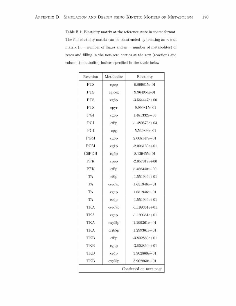
Appendix B. Simulation and Design using Kinetic Models of Metabolism 170
Table B.1: Elasticity matrix at the reference state in sparse format.
The full elasticity matrix can be constructed by creating an n×m
matrix (n = number of fluxes and m = number of metabolites) of
zeros and filling in the non-zero entries at the row (reaction) and
column (metabolite) indices specified in the table below.
Reaction Metabolite Elasticity
PTS cpep 9.999815e-01
PTS cglcex 9.964954e-01
PTS cg6p -3.564447e+00
PTS cpyr -9.999815e-01
PGI cg6p 1.481332e+03
PGI cf6p -1.480573e+03
PGI cpg -5.539836e-01
PGM cg6p 2.008147e+01
PGM cg1p -2.006130e+01
G6PDH cg6p 8.129455e-01
PFK cpep -2.057819e+00
PFK cf6p 5.488340e+00
TA cf6p -1.551946e+01
TA csed7p 1.651946e+01
TA cgap 1.651946e+01
TA ce4p -1.551946e+01
TKA csed7p -1.199361e+01
TKA cgap -1.199361e+01
TKA cxyl5p 1.299361e+01
TKA crib5p 1.299361e+01
TKB cf6p -3.802860e+01
TKB cgap -3.802860e+01
TKB ce4p 3.902860e+01
TKB cxyl5p 3.902860e+01
Continued on next page

Appendix B. Simulation and Design using Kinetic Models of Metabolism 171
Table B.1 – continued from previous page
Reaction Metabolite Elasticity
ALDO cfdp 1.565349e+01
ALDO cgap -1.498767e+01
ALDO cdhap -1.492655e+01
GAPDH cgap 1.003187e+00
GAPDH cpgp -1.001987e+00
TIS cgap -1.618848e+01
TIS cdhap 1.672123e+01
G3PDH cdhap 8.431321e-01
PGK cpgp 1.097577e+02
PGK cpg3 -1.095900e+02
sersynth cpg3 3.067314e-01
rpGluMu cpg3 2.431108e+02
rpGluMu cpg2 -2.430364e+02
ENO cpep -1.737547e+02
ENO cpg2 1.737929e+02
PK cpep 9.888856e-02
PK cfdp 5.507438e-05
pepCxylase cpep 5.897203e-01
pepCxylase cfdp 1.818458e-01
Synth1 cpep 2.609891e-01
Synth2 cpyr 2.724525e-01
DAHPS cpep 1.180329e-03
DAHPS ce4p 2.410126e+00
PDH cpyr 3.565752e+00
PGDH cpg 9.792591e-01
R5PI crib5p -9.568694e+00
Ru5P cxyl5p -9.307892e+00
PPK crib5p 2.024370e-01
G1PAT cg1p 8.383144e-01
Continued on next page

Appendix B. Simulation and Design using Kinetic Models of Metabolism 172
Table B.1 – continued from previous page
Reaction Metabolite Elasticity
G1PAT cfdp 9.313728e-01
G6P cg6p 1
f6P cf6p 1
fdP cfdp 1.000000e+00
GAP cgap 1.000000e+00
DHAP cdhap 1
PGP cpgp 1
PG3 cpg3 1
pg2 cpg2 1.000000e+00
PEP cpep 1.000000e+00
RIB5P crib5p 1
XYL5P cxyl5p 1.000000e+00
SED7P csed7p 1.000000e+00
pyr cpyr 1
PG cpg 1.000000e+00
E4P ce4p 1
GLP cg1p 1
EXTER cglcex -3.967127e-04
Table B.2: Reference flux for the model of E. coli central metabolism (Chassagnole et al., 2002)
vref =[ 3.083759e-03, 7.638286e-02, 2.648023e-03, 1.350352e-01, 9.706682e-02, 3.960809e-02, 3.961367e-02,
3.177509e-02, 4.371100e-04, 1.468660e-01, 3.307102e-01, 1.450466e-01, 1.037000e-03, 1.813584e-03, -7.664090e-02,
1.785526e-02, 3.068128e-01, 3.068026e-01, 3.810352e-02, 4.594254e-02, 1.446010e-02, 5.356195e-02, 7.829968e-03,
1.881657e-01, 2.262700e-03, 1.383618e-01, 4.991527e-02, 7.139249e-02, 1.029097e-02, 2.652691e-03, 9.250426e-05,
1.594627e-05, 9.214241e-06, 6.718378e-06, 5.141066e-06, 2.389480e-07, 6.317756e-05, 1.182871e-05, 7.914956e-05,
3.027655e-06, 1.096343e-05, 3.826403e-06, 6.915745e-06, 7.424102e-05, 2.215697e-05, 2.873981e-06, 1.724254e-05,
3.083453e-03]

Appendix B. Simulation and Design using Kinetic Models of Metabolism 173
Table B.3: Reference concentrations for the model of E. coli central metabolism (Chassagnole
et al., 2002)
xref =[ 2.847107e+00, 4.443915e-02, 3.327491e+00, 2.670540e+00, 5.736069e-01, 6.202351e-01, 7.970132e-01,
3.314475e-01, 2.487678e-01, 2.416683e-01, 1.033806e-01, 1.376404e-01, 3.943680e-01, 1.849304e-01, 8.595251e-03,
2.272574e+00, 4.254930e-01, 1.089085e-01]

Appendix C
Strain design for balanced yield,
titer, and productivity
The strain design algorithms developed in this thesis (Chapters 3 and 4) have used product
yield as the engineering target. However, industrial bioprocesses typically consider additional
objectives; namely, titer and (volumetric) productivity. Therefore, a practical consideration for
in silico strain design is to develop efficient methods that can quantify the tradeoff between the
three objectives (yield, titer, and productivity).
To address the need to design strains that balance yield, titer, and productivity, a novel com-
putational method was developed, called Dynamic Strain Scanning Optimization (DySScO).
Briefly, DySScO involves sampling the production envelope, assuming maximum product flux,
in order to identify the growth rates for which growth-coupled production would best balance
titer, yield, and productivity. These objectives are estimated using dynamic simulations of
a bioreactor that is coupled to flux balance analysis simulations (i.e., the dFBA framework
(Mahadevan et al., 2002)). Then, a strain design algorithm is used to design multiple strains
having growth rates within the range identified in the previous step. If the product yield is not
at the theoretical maximum for the defined growth rate, as is typically the case with knockout
mutants, then the yield, titer, and productivity of these strains are re-assessed. Finally, the
best strains are selected. The DySScO method is compatible with any method of dynamic
simulation and strain design. To maximize the efficiency of DySScO, an efficient strain design
174
Appendix C. Strain design for balanced yield, titer, and productivity 175
algorithm is desired, in order to rapidly generate a large set of strains for screening. Accord-
ingly, we used the GDLS (Lun et al., 2009) algorithm to efficiently identify knockout strains.
This chapter includes the author’s contributions to the development and testing of DySScO,
which was carried out in collaboration with another Doctoral candidate, Kai Zhuang, in the
Department of Chemical Engineering at the University of Toronto.
C.1 Introduction
A large number of computational strain design algorithms have been developed for identifying
optimal metabolic network manipulation strategies constraint-based models of metabolism. Op-
tKnock (Burgard et al., 2003) was the first computational algorithm for systematically designing
knockout strains for growth-coupled production of a biochemical. Growth-coupled production
has been shown to be effective in certain conditions, such in strains that are adaptively evolved
for maximum growth yield (Fong et al., 2005; Hua et al., 2006). In addition to gene knockouts,
the activation (Jin and Stephanopoulos, 2007) and inhibition (Nakamura and Whited, 2003) of
reactions have been shown to enhance biochemical production. OptReg (Pharkya and Maranas,
2006) is a Mixed Integer Linear Program (MILP)-based algorithm that identifies activation and
inhibition targets. Limitations include the need to define activation and inhibition levels for all
reactions prior to the identification of the optimal set of manipulated reactions, and a compu-
tational burden that typically exceeds that of OptKnock.
The computational difficulty of identifying globally optimal solutions to OptKnock has moti-
vated the development of more efficient algorithms. Recently, Lun et al. (Lun et al., 2009)
developed Genetic Design through Local Search (GDLS) to efficiently obtain locally optimal
solutions to OptKnock. The local search constraint is generally applicable to any MILP. Thus,
Yang et al. (2011) developed OptReg’LS, a local search implementation of OptReg,and demon-
strated that the locally optimal strains performed similarly to those identified by the global
OptReg problem, but in only a fraction of the time (Yang et al., 2011). Nonetheless, GDLS
and OptReg’LS still suffer from an exponential increase in complexity with increasing scope

Appendix C. Strain design for balanced yield, titer, and productivity 176
of each local search. This is especially problematic if the product yield cannot be improved
through sequential changes in a small number of reactions.
More recent advances include OptForce, which maximizes product yield by identifying knock-
out, inhibition, and activation targets, relative to a wild-type flux distribution (Ranganathan
et al., 2010); and EMILiO, which rapidly identifies the optimal set of modified reactions and
their optimal fluxes using a successive linear programming procedure (Yang et al., 2011). Alter-
natives to the bilevel optimization-based strain design have also been developed. For example,
evolutionary programming enables the optimization of nonlinear objectives, and, in some cases,
it has been shown to be more efficient for identifying higher-order knockout strategies than
MILP-based formulations (Patil et al., 2005). Other studies used the enumeration of elemen-
tary modes to identify flux modification targets based on their correlation with the product
flux (Melzer et al., 2009). However, this method was applied to condensed versions of the orig-
inal genome-scale models, since the enumeration of elementary modes is still computationally
expensive. Thus, the field of computational strain design is clearly active, and more efficient
algorithms to maximize the yield of overproducing strains is in continued development.
C.2 Results
We tested the capabilities of DySScO using two case studies: the design of succinate and 1, 4-
butanediol (BDO) overproduction strains. We used the iAF1260 genome-scale model of E. coli
metabolism for both case studies. To design BDO overproduction strains, the BDO biosynthesis
pathways described in (Yim et al., 2011) were added to the iAF1260 model.
C.2.1 Succinate strains using GDLS
Many of the strategies for succinate overproduction identified in this work (Table C.1) over-
lapped with those found in the literature. For example, the knockout of competing fermenta-
tion products like formate, ethanol, and lactate is a common experimental strategy (Yu et al.,
2011) and is consistent with the in silico knockout of PFL, ALCD2x, and LDH D. In addition,
knockout of the NADP-dependent malic enzyme (ME2) or glucose-6-phosphate dehydrogenase

Appendix C. Strain design for balanced yield, titer, and productivity 177
(G6PDH2r) is consistent with previously identified in silico strategies (Feist et al., 2010). Es-
sentially, the individual knockout strategies identified in this work have also been identified in
previous computational studies, or have previously been experimentally implemented. The ma-
jor contribution of this work has been to add new value to these well-known knockout strategies
for the model-based improvement of yield, titer and productivity.
Table C.1: Knockout strategies for succinate overproduction identified using GDLS
Succinate strains YZ1 YZ2 YZ3
Growth rate (hr−1) 0.16 0.24 0.21
Product yield (mol/mol glc) 1.27 0.89 0.92
Knockouts ALCD2x F6PA ACALD
GLUDy G6PDH2r F6PA
LDH D ME2 G6PDH2r
PFL MTHFD GLUDy
PPKr PFL ME2
TKT2 PYK PFL
PYK
C.2.2 Butanediol strains using GDLS
The BDO strains identified in this work are listed in Table C.2. The two BDO strains YZ4 and
YZ5 showed similarities in the predicted flux distributions as YIM1260. Namely, all three strains
used pyruvate dehydrogenase and the oxidative TCA cycle, and secreted acetate, all at similar
levels. However, unlike YIM1260, in which malate dehydrogenase (MDH) is deleted, YZ4 and
YZ5 utilize MDH in the reverse direction. Knockout of MDH in YZ5 reduces BDO yield by 97%
while increasing reverse lactate dehydrogenase (LDH) activity. The additional knockout of LDH
leads to YIM1260. Thus, deletion of MDH and LDH eliminate NADH-consuming reactions, such
that excess NADH is channeled to the NADH-consuming BDO synthesis reactions, SSALcoax,
4HBDH, 4HBTALDDH, and BTDP2. While maximizing the channeling of NADH to BDO
synthesis improves BDO yield, this is achieved at the cost of lowered growth rate. Strain YZ5,

Appendix C. Strain design for balanced yield, titer, and productivity 178
through reverse MDH activity, increases growth rate at the cost of lowered product yield. The
DySScO strategy identified YZ5 as the strain that achieves the best tradeoff between yield and
volumetric productivity, whereas previous strain design methods may have discarded YZ5 due
to its lower yield.
Table C.2: Knockout strategies for BDO overproduction identified using GDLS
BDO strains YZ4 YZ5 YIM1260
Growth rate (hr−1) 0.30 0.35 0.30
Product yield (mol/mol glc) 0.52 0.51 0.52
Knockouts ALCD2x ALCD2x ALCD2x
PFL PFL PFL
PGI MDH
TKT2 LDH D
C.3 Methods
The GDLS (Genetic Design through Local Search) algorithm (Lun et al., 2009) was used to
identify knockout strategies for succinate and BDO overproduction in E. coli, using the iAF1260
genome-scale model. For each iteration of GDLS, we used a neighborhood size of 2, and a single
search path. In addition, we implemented constraints to prevent the local search from cycling
back to the previous solution. Each MILP problem (i.e., local search iteration) was given a
timeout threshold of 1,800 seconds. If the MILP problem did reach the timeout threshold, then
GDLS was continued only if a feasible, but not necessarily optimal, solution was identified. In
this work, every local search MILP indeed found a feasible solution even if the timeout threshold
was met.
The MILPs were solved using CPLEX 12.1 using the CPLEXINT interface, with up to 8 parallel
threads using 2.4 GHz AMD Opteron processors.