mathematical theories of turbulent dynamical systemsqidi/turbulence16/theory.pdf · mathematical...
TRANSCRIPT
Mathematical Theories of Turbulent Dynamical Systems
Di Qi, and Andrew J. Majda
Courant Institute of Mathematical Sciences
Fall 2016 Advanced Topics in Applied Math
Di Qi, and Andrew J. Majda (CIMS) Mathematical Theories of Turbulent Systems Nov. 17, 2016 1 / 39
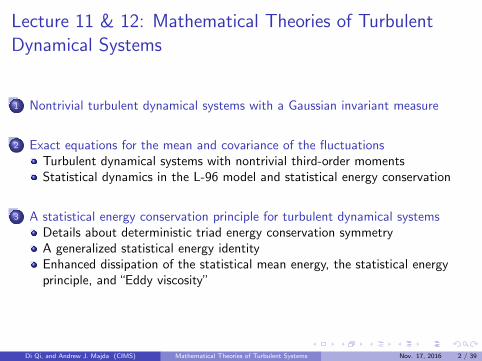
Lecture 11 & 12: Mathematical Theories of TurbulentDynamical Systems
1 Nontrivial turbulent dynamical systems with a Gaussian invariant measure
2 Exact equations for the mean and covariance of the fluctuationsTurbulent dynamical systems with nontrivial third-order momentsStatistical dynamics in the L-96 model and statistical energy conservation
3 A statistical energy conservation principle for turbulent dynamical systemsDetails about deterministic triad energy conservation symmetryA generalized statistical energy identityEnhanced dissipation of the statistical mean energy, the statistical energyprinciple, and “Eddy viscosity”
Di Qi, and Andrew J. Majda (CIMS) Mathematical Theories of Turbulent Systems Nov. 17, 2016 2 / 39
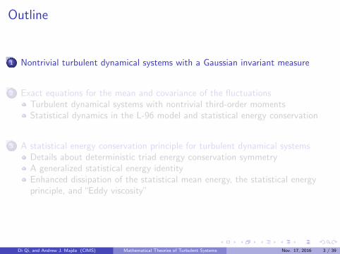
Outline
1 Nontrivial turbulent dynamical systems with a Gaussian invariant measure
2 Exact equations for the mean and covariance of the fluctuationsTurbulent dynamical systems with nontrivial third-order momentsStatistical dynamics in the L-96 model and statistical energy conservation
3 A statistical energy conservation principle for turbulent dynamical systemsDetails about deterministic triad energy conservation symmetryA generalized statistical energy identityEnhanced dissipation of the statistical mean energy, the statistical energyprinciple, and “Eddy viscosity”
Di Qi, and Andrew J. Majda (CIMS) Mathematical Theories of Turbulent Systems Nov. 17, 2016 3 / 39
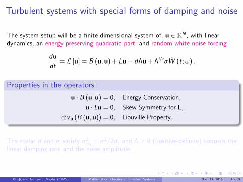
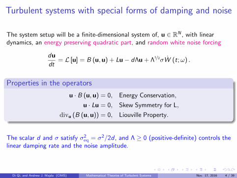
Turbulent systems with special forms of damping and noise
The system setup will be a finite-dimensional system of, u ∈ RN , with lineardynamics, an energy preserving quadratic part, and random white noise forcing
du
dt= L [u] = B (u,u) + Lu− dΛu + Λ
1/2σW (t;ω) .
Properties in the operators
u · B (u,u) = 0, Energy Conservation,
u · Lu = 0, Skew Symmetry for L,
divu (B (u,u)) = 0, Liouville Property.
The scalar d and σ satisfy σ2eq = σ2/2d , and Λ ≥ 0 (positive-definite) controls the
linear damping rate and the noise amplitude.
Di Qi, and Andrew J. Majda (CIMS) Mathematical Theories of Turbulent Systems Nov. 17, 2016 4 / 39
General setup of turbulent systems
du
dt= L [u] = B (u,u) + Lu− dΛu + Λ
1/2σW (t;ω) .
Examples:
I General 3× 3 triad system model;I Truncated Burgers-Hopf (TBH) equation, and inviscid L-96;I Quasi-geostrophic flow with topography, mean flow in pseudo-energy metric;I Inviscid Boussinesq or modified shallow water equation.
Di Qi, and Andrew J. Majda (CIMS) Mathematical Theories of Turbulent Systems Nov. 17, 2016 5 / 39
Gaussian invariant measure
du
dt= L [u] = B (u,u) + Lu− dΛu + Λ
1/2σW (t;ω) . (1)
Proposition
Associated with SDE in (1), with the structural properties, then
(1) has the Gaussian invariant measure defined as in peq;
The invariant measure has equipartition of energy in each component of u,peq = C−1
N exp(− 1
2σ−2eq u · u
), with σ2
eq = σ2/2d.
Proof. The Fokker-Planck Equation for (1), using the properties, is given by
dp
dt= −divu [(B (u, u) + Lu) p] + divu (dΛup) + divu
(Λσ2
2∇p)
= − (B (u, u) + Lu) · ∇p + divu
(dΛup +
Λσ2
2∇p).
Insert peq
dΛupeq +Λσ2
2∇upeq = dΛupeq −
Λσ2
2σ−2eq upeq ≡ 0.
Di Qi, and Andrew J. Majda (CIMS) Mathematical Theories of Turbulent Systems Nov. 17, 2016 6 / 39
Example: a simplified 57-mode testing model12
In the numerical experiments, the truncation |k|2 ≤ Λ, with Λ = 17 are utilizedwith 57 degrees of freedom
dωk
dt=
(∇⊥ψ · ∇q
)k
+ ik1
(β/ |k|2 − V
)ωk − ik1hkV
−dλkωk + σ(
1 + µ/ |k|2)−1/2
λ1/2k Wk,
dV
dt=
∑1≤|k|≤Λ
ik1
|k|2h∗k ωk−dλ0V + σµ−1/2λ
1/20 W0.
The pseudo-energy metric induces
peq (V , ω) = C−1 exp
−µ2σ−2eq
(V − V
)2 −1
2σ−1eq
∑1≤|k|2≤Λ
(1 +
µ
|k|2
)(ωk − ωk)2
.So the steady state large and small scale variables reach the equilibrium mean and variance
V = −β
µ, ψk =
hk
µ+ |k|2, |V ′|2 =
σ2eq
µ, |ψ′|2 =
σ2eq
|k|2(|k|2 + µ
) .1Majda, Timofeyev, and Vanden-Eijnden, JAS, 20032Majda, Franzke, Fischer, and Crommelin, PNAS, 2006
Di Qi, and Andrew J. Majda (CIMS) Mathematical Theories of Turbulent Systems Nov. 17, 2016 7 / 39
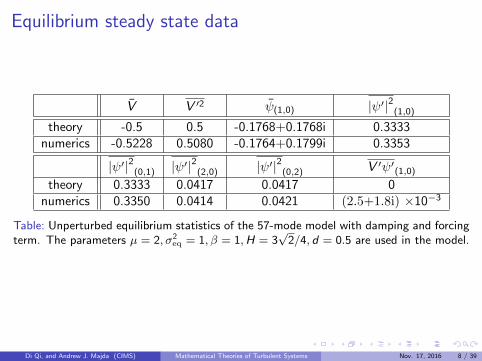
Equilibrium steady state data
V V ′2 ψ(1,0) |ψ′|2(1,0)
theory -0.5 0.5 -0.1768+0.1768i 0.3333numerics -0.5228 0.5080 -0.1764+0.1799i 0.3353
|ψ′|2(0,1) |ψ′|2(2,0) |ψ′|2(0,2) V ′ψ′(1,0)
theory 0.3333 0.0417 0.0417 0numerics 0.3350 0.0414 0.0421 (2.5+1.8i) ×10−3
Table: Unperturbed equilibrium statistics of the 57-mode model with damping and forcingterm. The parameters µ = 2, σ2
eq = 1, β = 1,H = 3√
2/4, d = 0.5 are used in the model.
Di Qi, and Andrew J. Majda (CIMS) Mathematical Theories of Turbulent Systems Nov. 17, 2016 8 / 39
Outline
1 Nontrivial turbulent dynamical systems with a Gaussian invariant measure
2 Exact equations for the mean and covariance of the fluctuationsTurbulent dynamical systems with nontrivial third-order momentsStatistical dynamics in the L-96 model and statistical energy conservation
3 A statistical energy conservation principle for turbulent dynamical systemsDetails about deterministic triad energy conservation symmetryA generalized statistical energy identityEnhanced dissipation of the statistical mean energy, the statistical energyprinciple, and “Eddy viscosity”
Di Qi, and Andrew J. Majda (CIMS) Mathematical Theories of Turbulent Systems Nov. 17, 2016 9 / 39
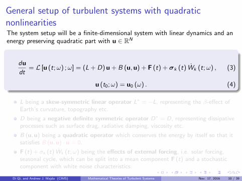
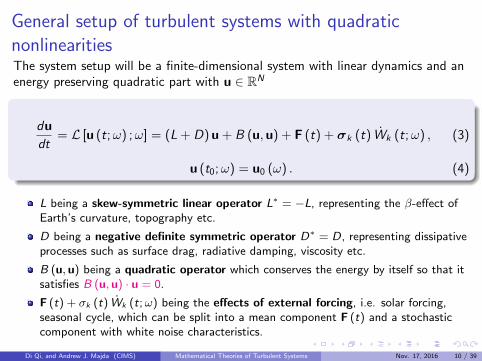
General setup of turbulent systems with quadraticnonlinearitiesThe system setup will be a finite-dimensional system with linear dynamics and anenergy preserving quadratic part with u ∈ RN
du
dt= L [u (t;ω) ;ω] = (L + D) u + B (u,u) + F (t) + σk (t) Wk (t;ω) , (3)
u (t0;ω) = u0 (ω) . (4)
L being a skew-symmetric linear operator L∗ = −L, representing the β-effect ofEarth’s curvature, topography etc.
D being a negative definite symmetric operator D∗ = D, representing dissipativeprocesses such as surface drag, radiative damping, viscosity etc.
B (u, u) being a quadratic operator which conserves the energy by itself so that itsatisfies B (u, u) · u = 0.
F (t) + σk (t) Wk (t;ω) being the effects of external forcing, i.e. solar forcing,seasonal cycle, which can be split into a mean component F (t) and a stochasticcomponent with white noise characteristics.
Di Qi, and Andrew J. Majda (CIMS) Mathematical Theories of Turbulent Systems Nov. 17, 2016 10 / 39
Ideas about Reduced Order Methods (ROMs)
Approach:
Project dynamics onto a finite-dimensional representation of the stochasticfield consisting of fixed-in-time, N-dimensional, orthonormal basis {vi}Ni=1
u (t) = u (t) + u′ (t) , u′ =N∑
i=1
Φi (t;ω) vi ≈s∑
i=1
Φi (t;ω) vi ;
Modeling is restricted to subspace Vs = span {vi}si=1;
Aim is to capture as much of the dynamics as possible with few modes;
Attractive for reduced computational cost.
Di Qi, and Andrew J. Majda (CIMS) Mathematical Theories of Turbulent Systems Nov. 17, 2016 11 / 39
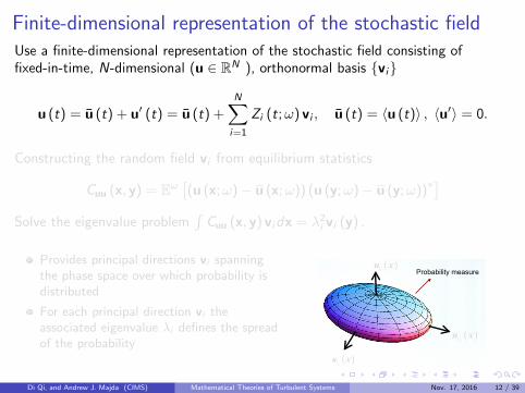
Finite-dimensional representation of the stochastic fieldUse a finite-dimensional representation of the stochastic field consisting offixed-in-time, N-dimensional (u ∈ RN ), orthonormal basis {vi}
u (t) = u (t) + u′ (t) = u (t) +N∑
i=1
Zi (t;ω) vi , u (t) = 〈u (t)〉 , 〈u′〉 = 0.
Constructing the random field vi from equilibrium statistics
Cuu (x, y) = Eω[(u (x;ω)− u (x;ω)) (u (y;ω)− u (y;ω))∗
]
Solve the eigenvalue problem´
Cuu (x, y) vidx = λ2i vi (y) .
Provides principal directions vi spanningthe phase space over which probability isdistributed
For each principal direction vi theassociated eigenvalue λi defines the spreadof the probability
8
Geometrical picture of KL expansion
( ) ( ) ( )2, i i id λ=∫ uuC x y u x x u ySolution of the eigenvalue problem
Probability measure
( )2iu x
( )3iu x
( )1iu x
Provides principal directions of the infinite-dimensional space over which probability is distributed
( )iu x
For each principal direction the associated eigenvalue defines the spread of the probability
( )iu xiλ
For infinite-dimensional probability measures (case of stochastic fields) we have Countable infinity of principal directions
However for most of them (infinite) the spread of the probability measure can be neglected!
For a stochastic field we have ( );ωu x ( ) ( ) ( )( ) ( ) ( )( ), ; ; ; ;T
Eω ω ω ω ω⎡ ⎤= − −⎢ ⎥⎣ ⎦uuC x y u x u x u y u y
Di Qi, and Andrew J. Majda (CIMS) Mathematical Theories of Turbulent Systems Nov. 17, 2016 12 / 39
Development of statistical moment dynamics
u (t) = u (t) + u′ (t) = u (t) +N∑
i=1
Zi (t;ω) vi , 〈u′〉 = 0.
Take expectation on both sides of the equations
du
dt= (L + D) u + B (u,u) + F (t) + σk (t) Wk (t;ω) (5)
Equation for the mean field u�
�d u
dt= (L + D) u + B (u, u) + RijB (vi , vj) + F (t), (6)
where Rij =⟨ZiZ
∗j
⟩,
B (u,u) = B (u + u′, u + u′)
= B (u, u) + B (u,u′) + B (u′, u) + B (u′,u′) ,
〈B (u′,u′)〉 = 〈B (Zivi ,Zjvj)〉 =⟨ZiZ
∗j
⟩B (vi , vj) .
Di Qi, and Andrew J. Majda (CIMS) Mathematical Theories of Turbulent Systems Nov. 17, 2016 13 / 39
Equation for the fluctuation component
du′
dt= (L + D) u′ + B (u,u′) + B (u′, u)
+ B (u′,u′)− RjkB (vj , vk) + σk (t) Wk (t;ω) . (7)
Equations for the stochastic coefficients
dZi
dt= Zj [(L + D) vj + B (u, vj) + B (vj , u)] · vi
+ [B (u′,u′)− RjkB (vj , vk)] · vi + Wkσk · vi . (8)
Equation for the covariance matrix Rij =⟨ZiZ
∗j
⟩
�
�dR
dt= Lv (u) R + RL∗v (u) + QF + Qσ. (9)
Di Qi, and Andrew J. Majda (CIMS) Mathematical Theories of Turbulent Systems Nov. 17, 2016 14 / 39
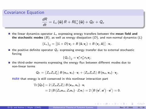
Covariance Equation
dR
dt= Lv (u) R + RL∗v (u) + QF + Qσ
the linear dynamics operator Lv expressing energy transfers between the mean field andthe stochastic modes (B), as well as energy dissipation (D), and non-normal dynamics (L)
{Lv}ij =[(L + D) vj + B
(u, vj
)+ B
(vj , u
)]· vi .
the positive definite operator Qσ expressing energy transfer due to external stochasticforcing
{Qσ}ij = v∗i σ∗k σkvj .
the third-order moments expressing the energy flux between different modes due tonon-linear terms
QF =⟨ZmZnZj
⟩B (vm, vn) · vi + 〈ZmZnZi 〉B (vm, vn) · vj .
note that energy is still conserved in this nonlinear interaction part
Tr [QF ] = 2 〈ZmZnZi 〉B (vm, vn) · vi= 2 〈B (Zmvm,Znvn) · Zivi 〉 = 2
⟨B(u′, u′
)· u′⟩
= 0.
Di Qi, and Andrew J. Majda (CIMS) Mathematical Theories of Turbulent Systems Nov. 17, 2016 15 / 39
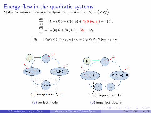
Energy flow in the quadratic systemsStatistical mean and covariance dynamics, u = u + Zivi , Rij =
⟨ZiZ∗j
⟩,
d u
dt= (L + D) u + B (u, u) + RijB
(vi , vj
)+ F (t) ,
dR
dt= Lv (u)R + RL∗v (u) + QF + Qσ .
QF =⟨ZmZnZj
⟩B (vm, vn) · vi + 〈ZmZnZi 〉B (vm, vn) · vj
Figure 3: Energy flow in the L-96 system. Energy flows from the mean field to the linearly unstablemodes and then redistributed through nonlinear, conservative terms to the stable modes. Redarrows denotes dissipation, while the dashed box indicates terms that conserve energy.
4. The stable modes receive energy from the unstable ones through the nonlinear conservativeterms. A portion of this energy is dissipated and the rest is subsequently returned to the meanthrough the modes with negative eigenvalues. All modes including the mean flow dissipateenergy through the negative definite part of the linearized dynamics.
This cycle of energy in the L-96 model is representative of any general model that contains i)unstable linearized modes whose stability depends on the mean field energy level (i.e. that theyabsorb energy from the mean field), ii) stable modes, and iii) nonlinear conservative terms thattransfer energy between the modes and through this transfer the system is reaching an equilibrium.This structure is ubiquitous in turbulent systems in the atmosphere and ocean with forcing anddissipation [26, 22, 1, 2] as well as in fluid flows with lower dimensional attractors [23]. However,there are also examples of idealized truncated geophysical flows without dissipation and forcingwith a Gaussian statistical equilibrium where the linear operator at the climate mean state is stablewhile the system has many positive Lyapunov exponents [19].
7
(a) perfect model Figure 4: Energy flow in the MQG UQ scheme. Energy flows from the mean field to the linearlyunstable modes and then redistributed through empirical, conservative fluxes to the stable modes.Red arrows denotes dissipation, while the dashed box indicates terms that conserve energy.
we substitute the nonlinear conservative mechanism by a conservative pair of positive and negativeenergy fluxes having the form of additional damping for the unstable modes and additive noisefor the stable modes (Figure 4). Note that this additional damping is chosen so that the unstableeigenvalues of the original linearized dynamics are guaranteed to have zero real part in the statisticalsteady state. In that sense this is the minimal amount of additional damping and noise required toachieve marginal stability (non-positive eigenvalues) of the correct steady state statistics. Thus, wehave a minimally changed model compared to the original equation that admits the correct steadystate statistics as a stable equilibrium stage. In the next subsections we will see that for numericalreasons it is required to add a small amount of additional damping (and noise) so that the correctstatistical steady state is not just marginally stable but it is associated with eigenvalues havingpurely negative real part. Moreover, in the transient phase of the dynamics the intensity of thenonlinear energy fluxes should depend on the energy level of the system and to this end we willapply a scaling factor to the additional damping and noise (that represent the nonlinear energyfluxes) which will take into account this dependence.Note that all of the required fluxesQ−F1, Q
+F1 are evaluated explicitly from available information
involving the linear operator, Lv (u1), and the covariance matrix, R1 in a statistical steady state.In addition, since the nonlinear flux model is kept separate from the unmodified linear dynamics, itexpresses an inherent property of the system, a direct link between second and third-order statisticalmoments in the same spirit that Karman-Howarth equation [10] does for isotropic turbulence.
11
(b) imperfect closure
Di Qi, and Andrew J. Majda (CIMS) Mathematical Theories of Turbulent Systems Nov. 17, 2016 16 / 39
Turbulent dynamical systems with non-Gaussian statisticalsteady states
16 3 The Mathematical Theory of Turbulent Dynamical Systems
iii) as well as the energy flux between different modes due to non-Gaussian statistics(or nonlinear terms) modeled through third-order moments
{QF}i j =⌦ZmZnZ j
↵B(vm,vn) ·vi + hZmZnZiiB(vm,vn) ·v j. (3.9)
Note that the energy conservation property of the quadratic operator B is inheritedby the matrix QF since
tr(QF) = 2hZmZnZiiB(vm,vn) ·vi = 2B�u0,u0� ·u0 = 0. (3.10)
The above exact statistical equations will be the starting point for the developmentsin this chapter and subsequent material on UQ methods in Chapter 4 [158, 159, 117].
3.2.1 Turbulent Dynamical Systems with Non-Gaussian StatisticalSteady States and Nontrivial Third Moments
Consider a turbulent dynamical system without noise, s ⌘ 0, and assume it has astatistical steady state so that ueq and Req are time independent. Since d
dt Req = 0,Req necessarily satisfies the steady covariance equation (3.6)
LueqReq +ReqL⇤ueq = �QF,eq, (3.11)
where QF,eq are the third moments from (3.9) evaluated at the statistical steady state.Thus a necessary and sufficient condition for a non-Gaussian statistical steady stateis that the first and second moments satisfy the obvious requirement that the matrix
LueqReq +ReqL⇤ueq 6= 0, (3.12)
so the above matrix has some non-zero entries. This elementary remark can beviewed as a sweeping generalization for turbulent dynamical systems of the Karman-Howarth equation for the Navier-Stokes equation (see Chapter 6 of [47]). The non-trivial third moments play a crucial dynamical role in the L-96 model and for two-layer ocean turbulence [158, 157], and is discussed in later chapters.
In Section 2.1, we have constructed turbulent dynamical systems with a Gaussianinvariant measure and non-zero noise when L 6= 0. There ueq = 0, Req = s2
eqI, andLueq = L with L skew, so LReq +ReqL⇤ ⌘ 0 and the damping, with matrix D =�dL ,exactly balances the stochastic forcing variances; these facts also apply to the casein Section 3.1 for L ⌘ 0 and no dissipation and random forcing where s2
eq can beany non-zero number. This helps illustrate and clarify the source of non-Gaussianitythrough the nontrivial interaction of the linear operator Lueq and the covariance Reqat a statistical steady state. In fact for a strictly positive covariance matrix, Req, thereis a “whitening” linear transformation, T , so that T ReqT�1 = I so the condition in(3.12) for nontrivial third moments is satisfied if the symmetric part of the matrix,T LueqT�1, is non-zero.
So the above matrix has some non-zero entries. The non-trivial third momentsplay a crucial dynamical role in the L-96 model and for two-layer ocean turbulence.
Di Qi, and Andrew J. Majda (CIMS) Mathematical Theories of Turbulent Systems Nov. 17, 2016 17 / 39
Turbulent dynamical systems with non-Gaussian statisticalsteady states
In the system with a Gaussian invariant measure
du
dt= B (u,u) + Lu− dΛu + Λ
1/2σW (t;ω) .
There ueq = 0,Req = σ2eqI , and Lueq
= L with L skew-symmetric, so
LReq + ReqL∗ ≡ 0;
The damping with matrix D = −dΛ exactly balances the stochastic forcingvariance σ2Λ;
For a strictly positive covariance Req, there is a “whitening” lineartransformation, so that TReqT−1 = I . Nontrivial third moments are satisfiedif
TLueqT−1,
is non-zero.
Di Qi, and Andrew J. Majda (CIMS) Mathematical Theories of Turbulent Systems Nov. 17, 2016 18 / 39
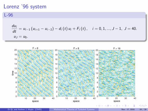
Lorenz ’96 system
L-96
dui
dt= ui−1 (ui+1 − ui−2)− di (t) ui + Fi (t) , i = 0, 1, ..., J − 1, J = 40.
uJ = u0.
8 2 Prototype Examples of Complex Turbulent Dynamical Systems
familiar low-dimensional weakly chaotic behavior associated with the transition toturbulence.
F l1 N+ KS Tcorr
weakly chaotic 6 1.02 12 5.547 8.23
strongly chaotic 8 1.74 13 10.94 6.704
fully turbulent 16 3.945 16 27.94 5.594
Table 2.1 Dynamical properties of L-96 model for weakly chaotic regime (F = 6), strongly chaot-ic regime (F = 8)and fully turbulent regime (F = 16). Here, l1 denotes the largest Lyapunovexponent, N+ denotes the dimension of the expanding subspace of the attractor, KS denotes theKolmogorov-Sinai entropy, and Tcorr denotes the decorrelation time of energy-rescaled time corre-lation function.
F = 6
10 20 30 40space
0
2
4
6
8
10
12
14
16
18
20
time
F = 8
10 20 30 40space
0
2
4
6
8
10
12
14
16
18
20F = 16
10 20 30 40space
0
2
4
6
8
10
12
14
16
18
20
Fig. 2.1 Space-time of numerical solutions of L-96 model for weakly chaotic (F = 6), stronglychaotic (F = 8), and fully turbulent (F = 16) regime.
2.3 Statistical Triad Models, the Building Blocks of ComplexTurbulent Dynamical Systems
Statistical triad models are special three dimensional turbulent dynamical systemswith quadratic nonlinear interactions that conserve energy. For u = (u1,u2,u3)
T 2R3, these equations can be written in the form of (1.5)–(1.7) with a slight abuse ofnotation as
dudt
= L⇥u+Du+B(u,u)+F+sWt , (2.4)
Di Qi, and Andrew J. Majda (CIMS) Mathematical Theories of Turbulent Systems Nov. 17, 2016 19 / 39
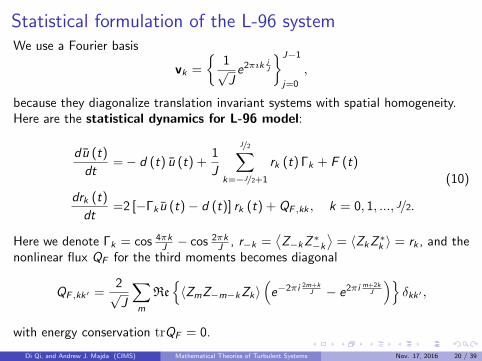
Statistical formulation of the L-96 systemWe use a Fourier basis
vk =
{1√J
e2πık jJ
}J−1
j=0
,
because they diagonalize translation invariant systems with spatial homogeneity.Here are the statistical dynamics for L-96 model:
du (t)
dt=− d (t) u (t) +
1
J
J/2∑
k=−J/2+1
rk (t) Γk + F (t)
drk (t)
dt=2 [−Γk u (t)− d (t)] rk (t) + QF ,kk , k = 0, 1, ..., J/2.
(10)
Here we denote Γk = cos 4πkJ − cos 2πk
J , r−k =⟨Z−kZ∗−k
⟩= 〈ZkZ∗k 〉 = rk , and the
nonlinear flux QF for the third moments becomes diagonal
QF ,kk′ =2√J
∑
m
Re{〈ZmZ−m−kZk〉
(e−2πi 2m+k
J − e2πi m+2kJ
)}δkk′ ,
with energy conservation trQF = 0.
Di Qi, and Andrew J. Majda (CIMS) Mathematical Theories of Turbulent Systems Nov. 17, 2016 20 / 39
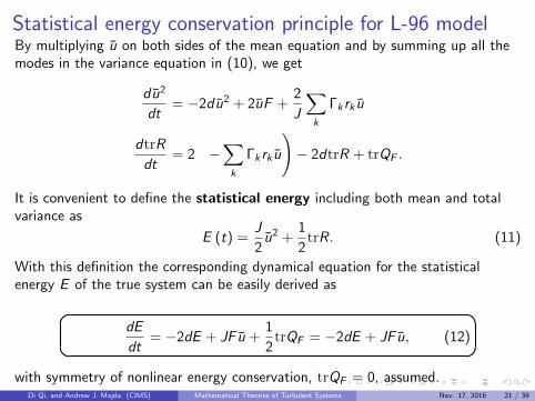
Statistical energy conservation principle for L-96 modelBy multiplying u on both sides of the mean equation and by summing up all themodes in the variance equation in (10), we get
du2
dt= −2du2 + 2uF +
2
J
∑
k
Γk rk u
dtrR
dt= 2
(−∑
k
Γk rk u
)− 2dtrR + trQF .
It is convenient to define the statistical energy including both mean and totalvariance as
E (t) =J
2u2 +
1
2trR. (11)
With this definition the corresponding dynamical equation for the statisticalenergy E of the true system can be easily derived as�
�dE
dt= −2dE + JF u +
1
2trQF = −2dE + JF u, (12)
with symmetry of nonlinear energy conservation, trQF = 0, assumed.Di Qi, and Andrew J. Majda (CIMS) Mathematical Theories of Turbulent Systems Nov. 17, 2016 21 / 39
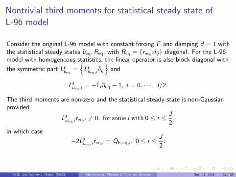
Nontrivial third moments for statistical steady state ofL-96 model
Consider the original L-96 model with constant forcing F and damping d = 1 withthe statistical steady states ueq,Req, with Req = {req,iδij} diagonal. For the L-96model with homogeneous statistics, the linear operator is also block diagonal with
the symmetric part Lsueq =
{Lsueq,i
δij
}and
Lsueq,i = −Γi ueq − 1, i = 0, · · · , J/2.
The third moments are non-zero and the statistical steady state is non-Gaussianprovided
Lsueq,i req,i 6= 0, for some i with 0 ≤ i ≤ J
2,
in which case
−2Lsueq,i req,i = QF ,eq,i , 0 ≤ i ≤ J
2.
Di Qi, and Andrew J. Majda (CIMS) Mathematical Theories of Turbulent Systems Nov. 17, 2016 22 / 39
Nontrivial third moments for statistical steady state ofL-96 mode
14 Predicting Fat-Tailed Intermittent Probability Distributions in Passive Scalar Turbulence
20
third order moments in spectral domain, F = 8
181614
k2
1210820
15
10
20
18
16
14
12
10
8
k1
k3
-4
-2
0
2
4
6
8
10
uk
10 12 14 16 18 20
ul
10
11
12
13
14
15
16
17
18
19
20third order moments in spectal domain, F = 8
-3
-2
-1
0
1
2
3
4
5
(a) third order moments between modes in spectral domain
40
third order moments in physical domain, F = 8
3020
x1
1000
10
20
30
x2
0
10
20
30
40
40
x3
-10
-8
-6
-4
-2
0
2
4
6
ui
0 10 20 30 40
uj
0
5
10
15
20
25
30
35
40third order moments in physical domain, F = 8
-10
-8
-6
-4
-2
0
2
4
6
(b) third order moments between state variables at different physical grid points
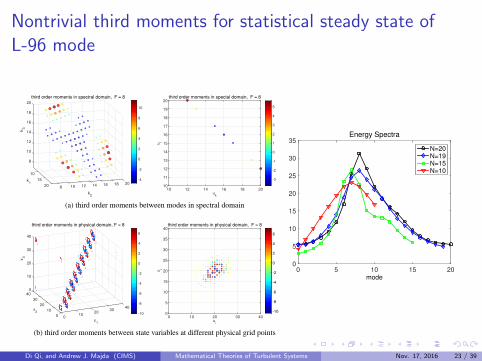
Fig. 2.6: Third order moments of the flow variable u in steady state in both spectral and physical domain in regimeF =8. The left panels show the 3D scatter plot for values of
⌦u0mu0nu0k
↵and
⌦uiu jul
↵; and the right panels display
one cross-section of the third moments of⌦u0mu0nu08
↵and
⌦uiu ju1
↵. The size and color of the dots represent the
values of third order moments and only large values are plotted.
domain and then transfer them to the spectral domain to update the system. See [36, 37] for some applicationsabout this idea, and we will also investigate this further in future researches.
2.3.2. Errors from insufficient ensemble sizeHere we check the other issue about the model performance with changing ensemble size for Monte-Carlo
method. It is useful to estimate the error from insufficient number of particles especially when the high dimen-sionality of the system makes it impossible to run large ensemble members. From central limit theorem (CLT),the i.i.d. Monte-Carlo particles ui with mean µ and variance s2 tend to have a Gaussian distribution as the particlenumber N increases ÂN
i=1 ui�Nµ/p
Ns2!N(0,1). Therefore we can estimate the uncertainty of the statistical meanfrom Monte-Carlo simulation at one time instant as
pvar(u)=
vuutvar
1N
N
Âi=1
ui
!⇠ sp
N. (2.18)
This shows the extremely slow convergence rate and the high computational requirement as the scale of theproblem increases. Table 2.1 and Figure 2.7 below show the model prediction for the mean and total variance withvarying ensemble size. We can see that the time averaged mean and variance can always offer good approximationfor the truth. On the other hand, the uncertainty in the ensemble prediction at one time instant keeps increasing asthe number of particles used decrease. The uncertainty for this ensemble mean at each time step can be estimatedthrough CLT in order O
�N�1/2
�.
3. Gaussian velocity stochastic models for passive tracer statistics
Di Qi and Andrew J. Majda 13
time0 5 10 15 20 25 30 35 40
-1
0
1
2
3
4State of the Mean
K = 20K = 19K = 15K = 10
time0 5 10 15 20 25 30 35 40
0
5
10
15
20
251-point variance
K = 20K = 19K = 15K = 10
(a) Model prediction for the mean and total variancemode
0 5 10 15 200
5
10
15
20
25
30
35Energy Spectra
N=20N=19N=15N=10
(b) Model prediction for energy spectra
Fig. 2.5: Model prediction of the mean state uM (left upper row) and averaged energy trRM/J (or 1-point statisticon each grid point, left lower row) from Galerkin truncated L-96 models in regime F =8 with number of positiveFourier modes K =19,15,10, compared with the true model with total number of modes K =20. The steadystate spectra achieved through these truncated models are compared with the state variables uk from the true L-96system (right).
Therefore the corresponding background flow (2.4) and (2.5) for the cross-sweep U (t) and shearing v(x,t) inGalerkin truncated dynamics becomes
dUdt
=�dU (t)+ Âk2LK
Gk |uk|2(t)+F, (2.16)
duk
dt=�duk +
⇣e2pi k
J �e�2pi 2kJ
⌘U (t)uk
+ Âk+m,k2LK�{0}
uk+mu⇤m⇣
e2pi 2m+kJ �e�2pi m+2k
J
⌘, k=1,··· ,K, (2.17)
with only the first K Fourier modes under consideration in the interaction term between modes. In Figure 2.5, wecompare the model predicted mean uM and single point variance trRM/J under different truncation wavenumberK =10,15,19 (note that the most energetic modes are always contained in LK within these truncation numbers)together with the truth K =N =20. Large model errors appear in all these truncated models even with only oneFourier mode k=20 neglected. Further by checking the steady state energy spectra captured by these truncatedmodels, the prediction skill in the variances of each mode also appears quite poor even with K =19 out of thetotal 20 modes resolved. The reason for the large errors through the truncation models can be explained by thecrucial role in the higher order interactions between the large scale and small scale modes. In the L-96 system,nonlinearity mostly comes from the interaction between modes represented by the second line in equation (2.5).Whereas under the truncated models, only the low frequency mode interactions are included in the dynamics asshown in (2.17). By checking the third order moments in Figure 2.6, it appears obviously that the most importantcontribution of the interactions happens between modes u7,u8 with u20, which is neglected in the truncated model(2.17). This becomes the inherent obstacle that we always need to keep in mind when the truncated methods areapplied to true systems.REMARK 2.3. Third order moments in Figure 2.6 show the possible errors we may face in Galerkin truncationmodels. However rather than the nonlocal third order moments in the spectral domain, the moments in physicaldomain (shown in the second row) are quite localized with major values near the center. Therefore one possiblecorrection for the truncation method is to get the higher order moments locally near the grid points in the physical
Di Qi, and Andrew J. Majda (CIMS) Mathematical Theories of Turbulent Systems Nov. 17, 2016 23 / 39
Outline
1 Nontrivial turbulent dynamical systems with a Gaussian invariant measure
2 Exact equations for the mean and covariance of the fluctuationsTurbulent dynamical systems with nontrivial third-order momentsStatistical dynamics in the L-96 model and statistical energy conservation
3 A statistical energy conservation principle for turbulent dynamical systemsDetails about deterministic triad energy conservation symmetryA generalized statistical energy identityEnhanced dissipation of the statistical mean energy, the statistical energyprinciple, and “Eddy viscosity”
Di Qi, and Andrew J. Majda (CIMS) Mathematical Theories of Turbulent Systems Nov. 17, 2016 24 / 39
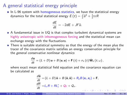
A general statistical energy principleIn L-96 system with homogeneous statistics, we have the statistical energydynamics for the total statistical energy E (t) = J
2 u2 + 12 trR
dE
dt= −2dE + JF u.
A fundamental issue in UQ is that complex turbulent dynamical systems arehighly anisotropic with inhomogeneous forcing and the statistical mean canexchange energy with the fluctuations.There is suitable statistical symmetry so that the energy of the mean plus thetracer of the covariance matrix satisfies an energy conservation principle forthe general conservative nonlinear dynamics
du
dt= (L + D) u + B (u, u) + F (t) + σk (t) Wk (t;ω) ,
where exact mean statistical field equation and the covariance equation canbe calculated as
d u
dt= (L + D) u + B (u, u) + RijB (ei , ej) + F,
dR
dt=LvR + RL∗v + QF + Qσ.
Di Qi, and Andrew J. Majda (CIMS) Mathematical Theories of Turbulent Systems Nov. 17, 2016 25 / 39
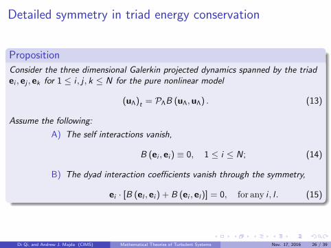
Detailed symmetry in triad energy conservation
Proposition
Consider the three dimensional Galerkin projected dynamics spanned by the triadei , ej , ek for 1 ≤ i , j , k ≤ N for the pure nonlinear model
(uΛ)t = PΛB (uΛ,uΛ) . (13)
Assume the following:
A) The self interactions vanish,
B (ei , ei ) ≡ 0, 1 ≤ i ≤ N; (14)
B) The dyad interaction coefficients vanish through the symmetry,
ei · [B (el , ei ) + B (ei , el)] = 0, for any i , l . (15)
Di Qi, and Andrew J. Majda (CIMS) Mathematical Theories of Turbulent Systems Nov. 17, 2016 26 / 39
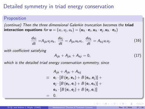
Detailed symmetry in triad energy conservation
Proposition
(continue) Then the three dimensional Galerkin truncation becomes the triadinteraction equations for u = (ui , uj , uk) = (uΛ · ei ,uΛ · ej ,uΛ · ek)
dui
dt=Aijkujuk ,
duj
dt= Ajkiukui ,
duk
dt= Akijuiuj . (16)
with coefficient satisfyingAijk + Ajik + Akji = 0, (17)
which is the detailed triad energy conservation symmetry, since
Aijk + Ajki + Akij
≡ ei · [B (ej , ek) + B (ek , ej)] +
ej · [B (ek , ei ) + B (ei , ek)] +
ek · [B (ei , ej) + B (ej , ei )]
= 0.
Di Qi, and Andrew J. Majda (CIMS) Mathematical Theories of Turbulent Systems Nov. 17, 2016 27 / 39
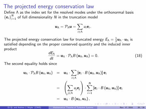
The projected energy conservation lawDefine Λ as the index set for the resolved modes under the orthonormal basis{ei}Ni=1 of full dimensionality N in the truncation model
uΛ = PΛu =∑
i∈Λ
uiei .
The projected energy conservation law for truncated energy EΛ = 12 uΛ · uΛ is
satisfied depending on the proper conserved quantity and the induced innerproduct
dEΛ
dt= uΛ · PΛB (uΛ,uΛ) = 0. (18)
The second equality holds since
uΛ · PΛB (uΛ,uΛ) = uΛ ·∑
i∈Λ
[ei · B (uΛ,uΛ)] ei
=
∑
j∈Λ
ujej
·
N∑
i=1
[ei · B (uΛ,uΛ)] ei
= uΛ · B (uΛ,uΛ) ,
Di Qi, and Andrew J. Majda (CIMS) Mathematical Theories of Turbulent Systems Nov. 17, 2016 28 / 39
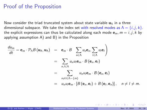
Proof of the Proposition
Now consider the triad truncated system about state variable uΛ in a threedimensional subspace. We take the index set with resolved modes as Λ = {i , j , k}.the explicit expressions can thus be calculated along each mode em,m = i , j , k byapplying assumption A) and B) in the Proposition
dum
dt= em · PΛB (uΛ,uΛ) = em · B
(∑
n∈Λ
unen,∑
l∈Λ
ulel
)
=∑
n,l∈Λ
unulem · B (en, el)
=∑
n 6=l∈Λ−{m}
unulem · B (en, el)
= unulem · [B (en, el) + B (el , en)] , n 6= l 6= m.
Di Qi, and Andrew J. Majda (CIMS) Mathematical Theories of Turbulent Systems Nov. 17, 2016 29 / 39
Proof of the Proposition
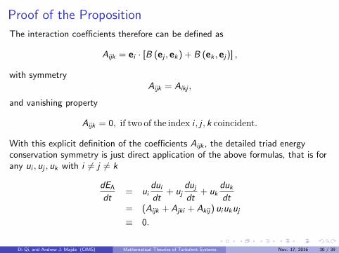
The interaction coefficients therefore can be defined as
Aijk = ei · [B (ej , ek) + B (ek , ej)] ,
with symmetryAijk = Aikj ,
and vanishing property
Aijk = 0, if two of the index i , j , k coincident.
With this explicit definition of the coefficients Aijk , the detailed triad energyconservation symmetry is just direct application of the above formulas, that is forany ui , uj , uk with i 6= j 6= k
dEΛ
dt= ui
dui
dt+ uj
duj
dt+ uk
duk
dt= (Aijk + Ajki + Akij) uiukuj
≡ 0.
Di Qi, and Andrew J. Majda (CIMS) Mathematical Theories of Turbulent Systems Nov. 17, 2016 30 / 39
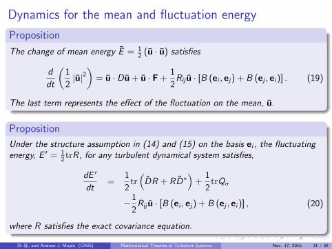
Dynamics for the mean and fluctuation energy
Proposition
The change of mean energy E = 12 (u · u) satisfies
d
dt
(1
2|u|2)
= u · Du + u · F +1
2Rij u · [B (ei , ej) + B (ej , ei )] . (19)
The last term represents the effect of the fluctuation on the mean, u.
Proposition
Under the structure assumption in (14) and (15) on the basis ei , the fluctuatingenergy, E ′ = 1
2 trR, for any turbulent dynamical system satisfies,
dE ′
dt=
1
2tr(
DR + RD∗)
+1
2trQσ
−1
2Rij u · [B (ei , ej) + B (ej , ei )] , (20)
where R satisfies the exact covariance equation.
Di Qi, and Andrew J. Majda (CIMS) Mathematical Theories of Turbulent Systems Nov. 17, 2016 31 / 39
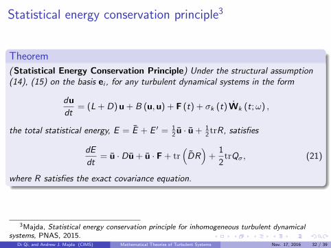
Statistical energy conservation principle3
Theorem
( Statistical Energy Conservation Principle) Under the structural assumption(14), (15) on the basis ei , for any turbulent dynamical systems in the form
du
dt= (L + D) u + B (u,u) + F (t) + σk (t) Wk (t;ω) ,
the total statistical energy, E = E + E ′ = 12 u · u + 1
2 trR, satisfies
dE
dt= u · Du + u · F + tr
(DR)
+1
2trQσ, (21)
where R satisfies the exact covariance equation.
3Majda, Statistical energy conservation principle for inhomogeneous turbulent dynamicalsystems, PNAS, 2015.
Di Qi, and Andrew J. Majda (CIMS) Mathematical Theories of Turbulent Systems Nov. 17, 2016 32 / 39
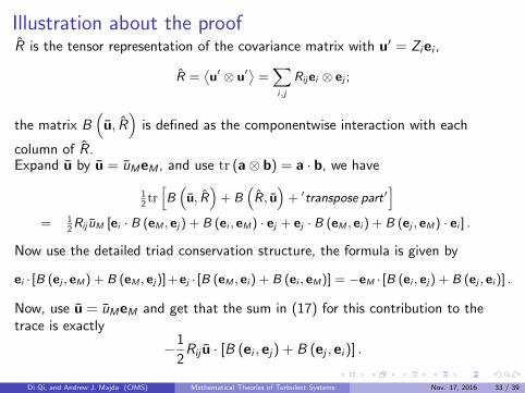
Illustration about the proofR is the tensor representation of the covariance matrix with u′ = Ziei ,
R =⟨u′ ⊗ u′
⟩=∑i,j
Rijei ⊗ ej ;
the matrix B(
u, R)
is defined as the componentwise interaction with each
column of R.Expand u by u = uMeM , and use tr (a⊗ b) = a · b, we have
12tr[B(
u, R)
+ B(R, u
)+ ′transpose part′
]= 1
2Rij uM [ei · B (eM , ej) + B (ei , eM) · ej + ej · B (eM , ei ) + B (ej , eM) · ei ] .
Now use the detailed triad conservation structure, the formula is given by
ei · [B (ej , eM) + B (eM , ej)]+ej · [B (eM , ei ) + B (ei , eM)] = −eM · [B (ei , ej) + B (ej , ei )] .
Now, use u = uMeM and get that the sum in (17) for this contribution to thetrace is exactly
−1
2Rij u · [B (ei , ej) + B (ej , ei )] .
Di Qi, and Andrew J. Majda (CIMS) Mathematical Theories of Turbulent Systems Nov. 17, 2016 33 / 39
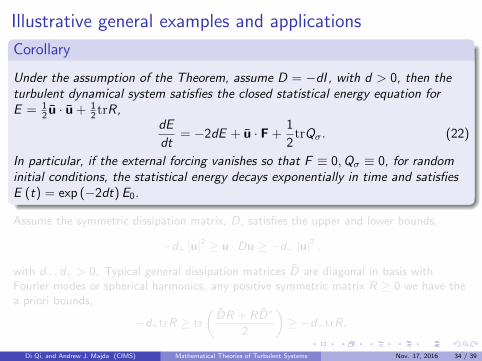
Illustrative general examples and applications
Corollary
Under the assumption of the Theorem, assume D = −dI , with d > 0, then theturbulent dynamical system satisfies the closed statistical energy equation forE = 1
2 u · u + 12 trR,
dE
dt= −2dE + u · F +
1
2trQσ. (22)
In particular, if the external forcing vanishes so that F ≡ 0,Qσ ≡ 0, for randominitial conditions, the statistical energy decays exponentially in time and satisfiesE (t) = exp (−2dt) E0.
Assume the symmetric dissipation matrix, D, satisfies the upper and lower bounds,
−d+ |u|2 ≥ u · Du ≥ −d− |u|2 ,
with d−, d+ > 0. Typical general dissipation matrices D are diagonal in basis withFourier modes or spherical harmonics, any positive symmetric matrix R ≥ 0 we have thea priori bounds,
−d+trR ≥ tr
(DR + RD∗
2
)≥ −d−trR.
Di Qi, and Andrew J. Majda (CIMS) Mathematical Theories of Turbulent Systems Nov. 17, 2016 34 / 39
Illustrative general examples and applications
Corollary
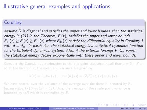
Assume D is diagonal and satisfies the upper and lower bounds, then the statisticalenergy in (21) in the Theorem, E (t), satisfies the upper and lower boundsE+ (t) ≥ E (t) ≥ E− (t) where E± (t) satisfy the differential equality in Corollary 1with d ≡ d±. In particular, the statistical energy is a statistical Lyapunov functionfor the turbulent dynamical system. Also, if the external forcings F ,Qσ vanish,the statistical energy decays exponentially with these upper and lower bounds.
Consider the Gaussian approximation to the one point statistics; recall that u = u + Ziei
so at the location x , the mean and variance are given by
u (x) = uMeM (x) , var (u (x)) = 〈ZjZ∗k 〉 ej (x)⊗ ek (x) .
We have control over the variance of the average over the domain, denoted by Ex
because Exej (x)⊗ ek (x) = δjk I ; thus, the average of the single point variance isbounded by trR which is controlled by E .
Di Qi, and Andrew J. Majda (CIMS) Mathematical Theories of Turbulent Systems Nov. 17, 2016 35 / 39
Illustrative general examples and applications
Corollary
Assume D is diagonal and satisfies the upper and lower bounds, then the statisticalenergy in (21) in the Theorem, E (t), satisfies the upper and lower boundsE+ (t) ≥ E (t) ≥ E− (t) where E± (t) satisfy the differential equality in Corollary 1with d ≡ d±. In particular, the statistical energy is a statistical Lyapunov functionfor the turbulent dynamical system. Also, if the external forcings F ,Qσ vanish,the statistical energy decays exponentially with these upper and lower bounds.
Consider the Gaussian approximation to the one point statistics; recall that u = u + Ziei
so at the location x , the mean and variance are given by
u (x) = uMeM (x) , var (u (x)) = 〈ZjZ∗k 〉 ej (x)⊗ ek (x) .
We have control over the variance of the average over the domain, denoted by Ex
because Exej (x)⊗ ek (x) = δjk I ; thus, the average of the single point variance isbounded by trR which is controlled by E .
Di Qi, and Andrew J. Majda (CIMS) Mathematical Theories of Turbulent Systems Nov. 17, 2016 35 / 39
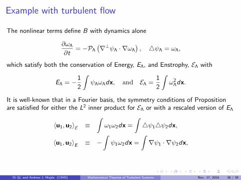
Example with turbulent flow
The nonlinear terms define B with dynamics alone
∂ωΛ
∂t= −PΛ
(∇⊥ψΛ · ∇ωΛ
), 4ψΛ = ωΛ,
which satisfy both the conservation of Energy, EΛ, and Enstrophy, EΛ with
EΛ = −1
2
ˆψΛωΛdx, and EΛ =
1
2
ˆω2
Λdx.
It is well-known that in a Fourier basis, the symmetry conditions of Propositionare satisfied for either the L2 inner product for EΛ or with a rescaled version of EΛ
〈u1,u2〉E ≡ˆω1ω2dx =
ˆ4ψ14ψ2dx,
〈u1,u2〉E ≡ −ˆψ1ω2dx =
ˆ∇ψ1 · ∇ψ2dx,
Di Qi, and Andrew J. Majda (CIMS) Mathematical Theories of Turbulent Systems Nov. 17, 2016 36 / 39
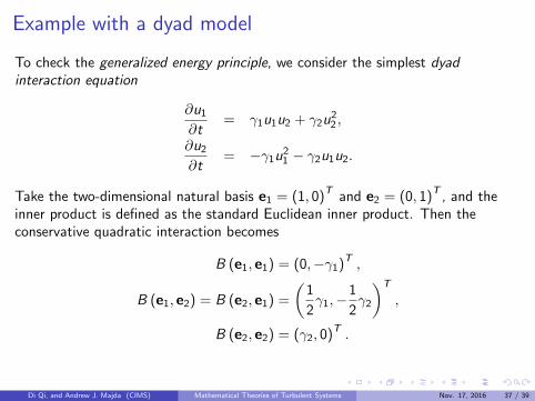
Example with a dyad model
To check the generalized energy principle, we consider the simplest dyadinteraction equation
∂u1
∂t= γ1u1u2 + γ2u2
2 ,
∂u2
∂t= −γ1u2
1 − γ2u1u2.
Take the two-dimensional natural basis e1 = (1, 0)T and e2 = (0, 1)T , and theinner product is defined as the standard Euclidean inner product. Then theconservative quadratic interaction becomes
B (e1, e1) = (0,−γ1)T ,
B (e1, e2) = B (e2, e1) =
(1
2γ1,−
1
2γ2
)T
,
B (e2, e2) = (γ2, 0)T .
Di Qi, and Andrew J. Majda (CIMS) Mathematical Theories of Turbulent Systems Nov. 17, 2016 37 / 39
The energy conservation u · B (u,u) = 0 is satisfied in this model.
Obviously the assumptions in (14) and (15) become non-zero
B (ei , ei ) 6= 0, ei · [B (el , ei ) + B (ei , el)] 6= 0.
On the other hand, the dyad interaction balance is satisfied so that
e1 · B (e1, e2) + e1 · B (e2, e1) + e2 · B (e1, e1) = γ1 − γ1 = 0.
Therefore the statistical energy conservation law is still valid for this dyadsystem
d
dt
[1
2
(u2
1 + u22
)+
1
2
(u′21 + u′22
)]= 0.
Di Qi, and Andrew J. Majda (CIMS) Mathematical Theories of Turbulent Systems Nov. 17, 2016 38 / 39

Questions & Discussions
Di Qi, and Andrew J. Majda (CIMS) Mathematical Theories of Turbulent Systems Nov. 17, 2016 39 / 39