Scuola Internazionale di Studi Superiori Avanzati

International School for Advanced Studies

Mathematics Area

PhD thesis by Giangiacomo Sanna

Rational curves and instantonson the Fano threefold Y5

Supervisors: Ugo Bruzzo SISSAAlexander Kuznetsov Steklov Mathematical Institute

Referees: Daniele Faenzi Universite de BourgogneEmilia Mezzetti Universita di TriesteLudmil Katzarkov Universitat Wien

Academic Year 2013/2014

Abstract

This thesis is an investigation of the moduli spaces of instanton bundles on theFano threefold Y5 (a linear section of Gr(2,5)). It contains new proofs of classicalfacts about lines, conics and cubics on Y5, and about linear sections of Y5.

The main original results are a Grauert–Mulich theorem for the splitting typeof instantons on conics, a bound to the splitting type of instantons on lines and anSL2-equivariant description of the moduli space in charge 2 and 3.

Using these results we prove the existence of a unique SL2-equivariant instan-ton of minimal charge and we show that for all instantons of charge 2 the divisorof jumping lines is smooth. In charge 3, we provide examples of instantons withreducible divisor of jumping lines. Finally, we construct a natural compactificationfor the moduli space of instantons of charge 3, together with a small resolution ofsingularities for it.

Contents

1 Some preliminary facts 81.1 Semi-orthogonal decompositions . . . . . . . . . . . . . . . . . . . . . . . . . 81.2 Beilinson spectral sequence . . . . . . . . . . . . . . . . . . . . . . . . . . . . 121.3 Flatness and families of sheaves . . . . . . . . . . . . . . . . . . . . . . . . . 151.4 Stability of vector bundles . . . . . . . . . . . . . . . . . . . . . . . . . . . . 161.5 The Grauert–Mulich theorem . . . . . . . . . . . . . . . . . . . . . . . . . . 181.6 Koszul complexes . . . . . . . . . . . . . . . . . . . . . . . . . . . . . . . . . . 191.7 Base change . . . . . . . . . . . . . . . . . . . . . . . . . . . . . . . . . . . . . 221.8 Families of subschemes of codimension at least 2 . . . . . . . . . . . . . . . 241.9 Closed embeddings . . . . . . . . . . . . . . . . . . . . . . . . . . . . . . . . . 251.10 A classical fact about (possibly nonreduced) curves in Pn . . . . . . . . . . 26

2 The setting 282.1 The SL2-action on Y . . . . . . . . . . . . . . . . . . . . . . . . . . . . . . . 322.2 Lines in Y . . . . . . . . . . . . . . . . . . . . . . . . . . . . . . . . . . . . . . 372.3 Conics in Y . . . . . . . . . . . . . . . . . . . . . . . . . . . . . . . . . . . . . 432.4 Cubics . . . . . . . . . . . . . . . . . . . . . . . . . . . . . . . . . . . . . . . . 50

3 More on the geometry of Y 513.1 Embeddings of P(A) . . . . . . . . . . . . . . . . . . . . . . . . . . . . . . . . 513.2 Identification with blow up . . . . . . . . . . . . . . . . . . . . . . . . . . . . 583.3 A map from Gr(3, V ) to P(Λ2V ∗/A) . . . . . . . . . . . . . . . . . . . . . . 603.4 Linear sections of Y and the Fourier–Mukai transform ΦBl . . . . . . . . . 65

4 Instantons 694.1 Instantons on Fano 3-folds . . . . . . . . . . . . . . . . . . . . . . . . . . . . 694.2 Instantons on Y . . . . . . . . . . . . . . . . . . . . . . . . . . . . . . . . . . 714.3 Jumping lines and conics . . . . . . . . . . . . . . . . . . . . . . . . . . . . . 74

1

5 Minimal instantons 82

6 Instantons of charge 3 866.1 A map from MI3 to Gr(3, V ) . . . . . . . . . . . . . . . . . . . . . . . . . . 876.2 An embedding of MI3 in a relative Grassmannian . . . . . . . . . . . . . 936.3 Special instantons . . . . . . . . . . . . . . . . . . . . . . . . . . . . . . . . . 966.4 Non-special instantons . . . . . . . . . . . . . . . . . . . . . . . . . . . . . . . 99

7 An example: degenerate theta-characteristics 107

8 A desingularization of MI3 109

2

Introduction

The goal of this thesis is an investigation of instanton vector bundles on a Fano threefoldof index 2 and degree 5, a natural generalization of instanton vector bundles on P3.

Definition. An instanton on P3 is a µ-stable vector bundle E of rank 2 such thatc1(E) = 0 and H1(E(−2)) = 0. Its second Chern class c2(E) is called the charge of E.

The standard approach [AHDM78] (see also [OSS80]) to the description of instantonson P3 and of their moduli space is via the Beilinson spectral sequence. Using thisapproach one can write any instanton E of charge n as the middle cohomology of acomplex

0→ OP3(−1)⊕n → O⊕2n+2P3 → OP3(1)⊕n → 0 (1)

such that the first map is fiberwise injective and the last map is surjective. Such acomplex is usually called a monad for E and is determined by E up to the action of agroup. This leads to a description of the moduli space of instantons as a GIT quotient.This description turns out to be too complicated for large n to provide answers to thenatural questions about the moduli space of instantons: smoothness, irreducibility andrationality. In the end, some of these questions were solved in recent works of Verbitsky,Jardim, Markushevitch and Tikhomirov by a different technique (see [JV11], [MT10],[Tik12]).

On the other hand, for small values of n one can give a more explicit description ofthe moduli space of instantons (see [ES81]) by analyzing the loci of jumping lines.

Definition. A line L is jumping for an instanton E if E restricted to L is not trivial.We will say that a line L is k-jumping for E if E restricted to L is isomorphic toOL(−k)⊕OL(k).

By Grauert–Mulich theorem the locus of jumping lines for an instanton E is a hy-persurface SE of degree n in the Grassmannian Gr(2,4) parameterizing lines in P3. Itcomes with a rank one torsion free sheaf LE and one can show that an instanton Ecan be reconstructed from the pair (SE ,LE). However, it turns out to be quite hard tocharacterize which pairs (SE ,LE) give rise to instantons, at least for higher values ofthe charge. One of the reasons for this is the high dimension of SE and its singularities.

Recently, the definition of instanton bundle was extended from P3 to other Fanothreefolds of Picard number 1.

Definition ([Fae11]). A rank 2 vector bundle E with c1(E) = 0 or 1 on a Fano threefoldX is an instanton if there is a twist E ⊗OX(t) = F such that

F ≅ F ∗ ⊗ ωX , H1(X,F ) = 0

Faenzi proved some general results about instantons on Fano threefolds, such as theexistence of a good component of arbitrary charge (see [Fae11]). On the other hand,Kuznetsov investigated in greater detail the case of Fano threefolds of index 2. In

3

particular, in [Kuz12] the locus of jumping lines DE was defined together with a theta-sheaf LE on it. Moreover, motivated by the Grauert–Mulich theorem, the followingconjecture was suggested.

Conjecture 1 ([Kuz12]). For an instanton E on a Fano threefold of index 2 the genericline is not jumping. An instanton E can be reconstructed from its theta-sheaf LE .

In the case of Fano threefolds of index 2 and degree 4 or 5, [Kuz12] provides moreconcrete descriptions of the moduli spaces of instantons.

Namely, in the case of the degree 4 threefold the moduli spaces of instantons wereshown to be related to the moduli spaces of self dual vector bundles on a curve ofgenus 2. Using this, the first part of conjecture 1 was reinterpreted and the second partwas proved.

The degree 5 case is that of a triple linear section of Gr(2,5).

Definition. The variety Y is the transverse intersection of the Plucker embeddingGr(2,5) ⊂ P9 with a P6.

It turns out that Y is similar to P3 in many respects. For example, both admit anaction of SL2 with an open orbit and both admit a full exceptional collection for theirderived category.

Again in [Kuz12], these similarities with P3 were used to show that every instantonon Y can be represented as the middle cohomology of the monad

0→ U⊕n → O⊕4n+2Y → U∗⊕n → 0,

where U is the restriction of the tautological bundle to Y , in analogy with (1). As acorollary a GIT description of the moduli space of instantons via special nets of quadricswas found, a reinterpretation of the first part of conjecture 1 was given and the secondpart was proved.

The goal of this thesis is an extension of the results of [Kuz12] on moduli spaces ofinstantons on Y and a detailed study of moduli spaces of small charge, namely charge 2(minimal instantons) and charge 3.

We start with an exposition of various facts about the geometry of Y , some of whichare known to experts. The references for these facts are scattered in the literature andsome of them do not explicitly refer to the SL2-structure, so that we prefer providingcomplete proofs for most of them. In particular, we describe several useful exceptionalcollection in Db(Y ), the bounded derived category of coherent sheaves on Y , show thatthe Hilbert scheme of lines on Y identifies with P2 and that the Hilbert scheme of conicson Y identifies with P4. We also write down explicit SL2-equivariant resolutions forthe structure sheaves of lines and conics, discuss the natural stratification of the Hilbertscheme of conics and describe the natural incidence correspondences on the products ofthese Hilbert schemes. Finally, we apply the same methods to cubic curves in Y . In allthese constructions we pay special attention to the induced action of SL2.

4

In section 3 we introduce the following construction of Y : we show that the blowupof the Veronese surface in P4 identifies naturally with the projectivization of the vectorbundle U on Y . This description turns out to be very useful later, when we discuss thegeometry of hyperplane sections of Y and their relation to the Grassmannian of planesin P4. Again, all the results of this section are SL2-equivariant.

In section 4 we start discussing instantons on Y . We remind the necessary definitionsand constructions from [Fae11] and [Kuz12], in particular the monadic description andsome results about jumping lines. We state here the first new result of the thesis, whichwill be of great use in the description of the moduli space of minimal instantons.

Theorem (4.17, 4.18). If E is an instanton of charge n then E has no k-jumping linesfor k ≥ n.

A direct consequence of theorem 4.17 is the following proposition providing an explicitdescription of instantonic theta-characteristics of degree 2.

Proposition (5.2). If E is an instanton of charge 2 then the curve of jumping lines DE

is a smooth conic and the sheaf LE is isomorphic to ODE(−1). In particular, conjecture 1holds true for instantons of charge 2.

We also introduce the notion of a jumping conic for an instanton. Of course one canjust say that a conic C is jumping for E if the restriction of E to C is nontrivial, butit is not clear how to encode nontriviality of E on C in a sheaf on the Hilbert space ofconics. We show that a reducible conic C = L1 ∪L2 (resp. nonreduced conic C = 2L) is ajumping conic for an instanton E if and only if the restriction of E to either of the linesL1 and L2 (resp. to L) is nontrivial. Moreover, we show that

Proposition (4.22). If E is an instanton and C is a conic then C is a jumping conicif and only if H i(C,E ⊗ U ∣C) ≠ 0 for some i.

By means of proposition 4.22, we also show that an analogue of the Grauert–Mulichtheorem holds for conics.

Theorem (4.24, 4.29). For an instanton E of charge n the scheme of jumping conics ofE is a divisor of degree n in P4 which comes with a natural sheaf of rank 2. In particular,the generic conic is non-jumping.

So, in some sense, conics behave better than lines, but as the dimension of the spaceof conics is higher, the information we get is harder to use.

In section 5 we discuss in detail the moduli space of minimal instantons. This modulispace is also known in the literature as the moduli space of aCM bundles (see [BF09]).We show that the moduli space MI2 identifies with an explicit open subset of P5.

Theorem (5.8). The moduli space MI2 of charge 2 instantons on Y can be representedas

MI2 ≅ P(S2C3) ∖ (∆ ∪H),where ∆ is the symmetric determinantal cubic and H is the unique SL2-invariant hy-perplane.

5

A consequence of the description of theorem 5.8 is the following.

Corollary (5.9). There is a unique instanton E0 of charge 2 on Y with an SL2-equivariant structure.

In section 6 we consider the moduli space of instantons of charge 3. We constructa natural map β ∶MI3 → B ∶= Gr(3,5) and show that its flattening stratification onB consists of only two strata: the closed stratum Bs ⊂ B identifies with the image ofthe projective plane parameterizing lines on Y under a special embedding κ ∶ P2 → Bconstructed in section 3, and the open stratum Bn ∶= B ∖Bs is its complement.

After constructing β, we also construct a natural compactificationMI3 ofMI3 anddescribe it.

Theorem (6.23). There is a natural compactification MI3 of MI3 such that the mapβ ∶MI3 → B extends to a regular map β ∶MI3 → B which is a P3-fibration over Bn

and a Gr(2,5)-fibration over Bs.

We show that instantons E such that β(E) ∈ Bs form a divisorial family and havemany special properties (because of this we call them special). One of the characterizingproperties is the following

Proposition (6.24). An instanton E is special if and only if it has a 2-jumping line L.For a special instanton E there is a unique 2-jumping line L and κ(L) = β(E).

In section 7, the results of section 6 are used to show how singular the theta-sheafLE of jumping lines can be for an instanton E of charge 3. While in the case of minimalinstantons the theta-characteristics admit the simple description of corollary 5.2, forc2(E) = 3 we prove the following propositions

Proposition (7.2). The theta-sheaf of E is not locally free if and only if E is special.

Proposition (7.3). If the plane β(E) ⊂ P4 is a generic tangent plane to the Veronesesurface in P4, then the theta-sheaf of E is supported on a reducible curve.

It turns out that the compactified moduli space MI3 is singular on a closed subsetof codimension 3 which is contained in MI3 ∖MI3 and in β−1(Bs).

The last section is devoted to the construction and the description of an explicitdesingularization

π ∶ MI3 →MI3

We construct MI3 by blowing up the (non-Cartier) divisor of special instantons insideMI3 and we identify MI3 with a P3-fibration over the blowup B of B in Bs.

Theorem (8.4). There is a small contraction

π4 ∶ MI3 →MI3

which is a resolution of the singularity of MI3. Moreover, the pushforward of the struc-ture sheaf of MI3 is the structure sheaf of MI3.

6

Acknowledgements

I would like to thank my PhD advisor A. Kuznetsov for introducing me to the topic ofthis thesis, and for teaching me the techniques to play with it. I am extremely gratefulboth to him and to my co-advisor U. Bruzzo for patiently providing me with clearanswers to many questions. Finally, I have been helped in many ways by several peopleboth in SISSA and in Steklov, and I would also like to thank them.

7

1 Some preliminary facts

We work over C. All schemes are assumed to be Noetherian and separated. In thissection we set the notation which we will use for derived categories and we state a fewmore results (Beilinson spectral sequence, Grauert–Mulich theorem, Hoppe’s criterion)to which we will refer in the rest of the thesis.

1.1 Semi-orthogonal decompositions

In any triangulated category T the shift is denoted by [1]. For any two objects F,G of T ,the space Hom(F,G[p]) is denoted by Extp(F,G) and the cohomology of RHom(F,G),that is to say ⊕p Ext

p(F,G)[−p], is denoted by Ext(F,G).We work with triangulated categories T which are Ext-finite, that is to say that for

any pair of objects F,G the graded vector space Ext(F,G) is finite dimensional. In otherwords, Hom(F,G) is always finite dimensional and Hom(F,G[i]) vanishes for almost allintegers i ∈ Z.

We usually think of Ext(F,G) as a non-symmetric scalar product with values in thecategory of graded finite dimensional vector spaces. When a subcategory A ⊂ T is given,the subcategory

A⊥ = T ∈ T s.t. ∀A ∈ A Ext(A,T ) = 0

is called the right orthogonal of A in T . Respectively, the subcategory

⊥A = T ∈ T s.t. ∀A ∈ A Ext(T,A) = 0

is called the left orthogonal of A in T .

Definition 1.1. A full triangulated subcategory A of T is admissible if the inclusionfunctor has a left and a right adjoint.

If the inclusion functor of A has only a left or right adjoint, the category A is calledrespectively left or right admissible. By [Kuz07, sec. 2.2/2.3] (which summarizes resultsand definitions from [Bon90] [BK90] [BVdB03]), in the case T is the derived category ofa smooth variety, the following theorem holds.

Theorem 1.2 ([BK90]). For X smooth projective variety over a field k, any left or rightadmissible subcategory of Db(X) is admissible.

Definition 1.3. A semiorthogonal decomposition of a triangulated category T is anordered set of full triangulated subcategories ⟨A1, . . . ,An⟩ such that the following twoconditions hold:

• For all i > j and all Ai ∈ Ai and Aj ∈ Aj

Hom(Ai,Aj) = 0

8

• For any object T ∈ T there exist objects Ti and maps fi

0 = TnfnÐ→ Tn−1

fn−1ÐÐ→ . . .f2Ð→ T1

f1Ð→ T0 = T

such that the cones of fi ∶ Ti → Ti−1 lie in Ai.

A sequence of maps as in definition 1.3 is usually called a filtration for T .

Definition 1.4. Given an object T in T , a filtration for T is a set of objects Ti andmaps fi such that

0 ≅ TmfmÐ→ Tm−1

fm−1ÐÐÐ→ . . .fn+2ÐÐ→ Tn+1

fn+1ÐÐ→ Tn ≅ T (2)

If we denote by Li[−i] the cone of fi+1, there is an induced sequence in the oppositedirection

0→ LngnÐ→ Ln+1 gn+1ÐÐ→ . . .

gm−2

ÐÐÐ→ Lm−1 → 0 (3)

such that gi+1 gi = 0. Sequences (3) and (2) fit in a diagram

0fm - Tm−1

fm−1 - . . .fn+2 - Tn+1

fn+1 - T

⋆ ⋆ ⋆ ⋆

Lm−1[−m + 1] gm−2

Lm−2[−m + 2]

. . . Ln+1[−n − 1] gn

Ln[−n]

(4)

where all bottom triangles are commutative and those marked with ⋆ are distinguished.Dashed arrows denote maps of degree one. The diagram (4) is usually called Postnikovtower (or Postnikov system). One also usually says that T is the convolution of thePostnikov tower (4).

The following is a simple and classical fact, but it is fundamental.

Theorem 1.5 ([Bon90]). The Postnikov tower induced by a semi-orthogonal decompo-sition is functorial.

Proof. By definition of semi-orthogonal decomposition it is enough to prove the theoremfor a decomposition ⟨A1,A2⟩ and then proceed by induction.

Choose a filtration for each object T in T . Given a map ϕ ∶ S → T we will show thatit extends uniquely to a map of distinguished triangles

S1- S - L - S1[1]

T1

ϕ1

?- T

ϕ

?- M

ψ

?- T1[1]

ϕ1[1]?

The fact that ψ commutes with both ϕ and ϕ1[1] comes from the axiom of triangu-lated category which says that there is at least one such ψ.

Functoriality follows from uniqueness of ϕ1 and ψ.

9

An object E ∈ A is called exceptional if Ext(E,E) = C. A set of exceptional objectsE1, . . . ,En is called an exceptional collection if Extk(Ei,Ej) = 0 for i > j. If moreoverExtk(Ei,Ej) = 0 whenever k ≠ 0 the exceptional collection is called a strong exceptionalcollection.

A way to induce semiorthogonal decompositions is to look for exceptional objectsin T , as the following theorem shows. Note that, when included in a semiorthogonaldecomposition, Ei stands for the category generated by Ei.

Theorem 1.6. Given an exceptional collection E1, . . . ,En in T , there are inducedsemiorthogonal decompositions

⟨E1, . . . ,En,⊥⟨E1, . . .En⟩⟩

and⟨⟨E1, . . .En⟩⊥,E1, . . . ,En⟩

If the left or the right orthogonal of ⟨E1, . . . ,En⟩ (i.e. the minimal triangulated sub-category containing E1, . . .En) is 0, the collection is called a full exceptional collection.In this case both the left and the right orthogonal to ⟨E1, . . . ,En⟩ vanish.

Given a semiorthogonal decomposition, one can obtain other semiorthogonal decom-positions via functors which are called left and right mutations.

Let j ∶ A → T be an admissible subcategory, so that T = ⟨A⊥,A⟩ and ⟨A, ⊥A⟩ aresemiorthogonal decompositions. Denote the left and right adjoint functors to j by j∗ andj!. Denote the embedding functors of ⊥A and A⊥ in T by l and r, and their (respectivelyright and left) adjoint functors by l! and r∗. It is easy to check that for T ∈ T we have

l!(T ) = Cone(T → jj∗T )[−1]

andr∗(T ) = Cone(jj!T → T )

Definition 1.7. The functor ll! ∶ T → T is called right mutation through A and isdenoted by RA. The functor rr∗[−1] ∶ T → T is called left mutation through A and isdenoted by LA.

To spell out definition 1.7, we point out that the left and right mutation functors arecharacterized by the fact that there are distinguished triangles

LA(T ) - jj!T - T - LA(T )[1]

andRA(T )[−1] - T - jj∗T - RA(T )

The functors RA and LA return zero on A, but they are isomorphisms when restrictedto the (respectively right and left) orthogonals. More precisely

l!r = l!RAr ∶ A⊥ → ⊥A

10

andr∗l = r∗LAl ∶ ⊥A→ A⊥

are equivalences of triangulated categories as it is easy to check that the functor l! ⋅r ⋅r∗ ⋅ lis equivalent to the identity of ⊥A and that the functor r∗ ⋅ l ⋅ l! ⋅ r is equivalent to theidentity of A⊥.

A special case of the above setting is when A is Db(k), with k a field. In thiscase j sends k to an exceptional object E, and the functors j∗ and j! are respectivelyExt(−,E)∗ and Ext(E,−). In this case the unit and the counit of the adjunction arerespectively the evaluation and coevaluation maps for E, i.e. the universal

Ext(E,T )⊗E → T

andT → Ext(T,E)∗ ⊗E

Now, let T = ⟨A1, . . . ,An⟩ be a semiorthogonal decomposition into admissible sub-categories. Denote the collection (A1, . . . ,An) by A; we are going to construct twocollections which we will denote by RiA and LiA.

Definition 1.8 (Lemma 2.3 [Kuz06]). Given A = (A1, . . . ,An) semiorthogonal decom-position, assume that each Ai is admissible. Then for each i ∈ [1, n − 1] there is asemiorthogonal decomposition

(RiA)j =⎧⎪⎪⎪⎨⎪⎪⎪⎩

Aj if j ≠ i, i + 1Ai+1 if j = iRAi+1Ai =

⊥⟨A1, . . . ,Ai−1,Ai+1⟩ ∩ ⟨Ai+2, . . . ,An⟩⊥ if j = i + 1.

called the i-th right mutation of A and a semi-orthogonal decomposition

(LiA)j =⎧⎪⎪⎪⎨⎪⎪⎪⎩

Aj if j ≠ i, i + 1LAiAi+1 = ⊥⟨A1, . . . ,Ai−1⟩ ∩ ⟨Ai,Ai+2, . . . ,An⟩⊥ if j = iAi if j = i + 1

called the i-th left mutation of A.

We are now going to introduce two semiorthogonal decompositions related to A: theyare called the left dual and the right dual to A due to the vanishing of the entries of thematrices RHom(∨Ai,Aj) and RHom(Ai,A∨j ) such that i + j ≠ n + 1.

Definition 1.9. The right dual decomposition of A is

A∨ = (L1 . . .Ln−1) . . . (L1L2) (L1)(A)

The left dual decomposition of A is

∨A = (Rn−1 . . .R1) . . . (Rn−1Rn−2) (Rn−1)(A)

11

In the case the categories Ai are generated by an exceptional element, one can refinethe idea of dual decomposition to that of dual collection.

Definition 1.10. Let T = ⟨E1, . . . ,En⟩ be a full exceptional collection for T . Set

E∨

i = LE1LE2⋯LEn−1En−i+1

and∨Ei = REnREn−1⋯REn−i+2En−i+1

The full exceptional collections ⟨E∨

n , . . . ,E∨

1 ⟩ and ⟨∨En, . . . , ∨E1⟩ are called respectivelyright dual collection and left dual collection.

With the above choices, the right and left dual collections are characterized by thefollowing property (see [GK04, sec.2.6]).

Extk(∨Ei,Ej) = Extk(Ei,E∨

j ) = C if i + j = n + 1 and i = k + 10 otherwise

(5)

1.2 Beilinson spectral sequence

Given a filtration for an object A in Db(X), one can construct a spectral sequenceanalogous to the one induced by a filtered complex. Recall that the filtration inducesa Postnikov tower whose convolution is A. In the notation of diagram (4), we have thefollowing proposition.

Proposition 1.11 (e.g. [GM03] ex. IV.2.2). Given a filtration Ti, fi for an object A inDb(X), there is a natural spectral sequence

Ep,q1 =Hq(Lp)

with differential dp =Hq(gp) and converging to Hp+q(A).

Proof. Replace the Li to reduce to the case where fi are actual morphisms of complexes,then use the double complex spectral sequence.

As we will often use proposition 1.11, let us clarify in the following remarks what wemean by natural and what the direction of differentials in the spectral sequence is.

Remark 1.12. By naturality of the induced spectral sequence we mean that given twoPostnikov towers whose convolution is A1 and A2, and given a map between the twotowers (i.e. a collection of maps between the objects in the tower commuting with allmaps in the tower), then there is an induced map of spectral sequences. Moreover, suchmaps of spectral sequences depend functorially on the maps between Postnikov towers.

12

Remark 1.13. The spectral sequence can be thought of as the spectral sequence inducedby a bicomplex whose columns are Li and whose horizontal arrows are gi. Entries Ep,q1

with p ∉ [n,m − 1] vanish.

Hj+1(Ln) Hj+1(gn)- Hj+1(Ln+1)

Hj+1(gn+1)- . . .

Hj+1(gm−2

)

- Hj+1(Lm−1)

Hj(Ln) Hj(gn)- Hj(Ln+1)

Hj(gn+1)- . . .

Hj(gm−2

)

-

d2

-Hj(Lm−1)

Hj−1(Ln) Hj−1(gn)- Hj−1(Ln+1)

Hj−1(gn+1)- . . .

Hj−1(gm−2

)

-

d2

-Hj−1(Lm−1)

It follows that the last non trivial differential is at most at page En−m+1.

A common situation where a filtration for an object in Db(X) is available is whenthere is a semi-orthogonal decomposition of Db(X). The archetype of such a situation isX = Pn: its derived category admits several full exceptional collections, the most notablebeing ⟨OPn(−n), . . . ,OPn⟩. Together with its dual collection, it gives rise to a resolutionof the diagonal inside Pn × Pn.

The point in having a resolution for the diagonal of a scheme X is that one can alwaysrewrite the identity functor of Db(X) as the Fourier–Mukai transform with kernel thestructure sheaf of the diagonal. As on Pn there is such a resolution, one can takeany object A in Db(Pn), pull it back to Pn × Pn, tensor it by the resolution of thediagonal, push it forward to the other copy of Pn and finally recover the initial A. TheGrothendieck spectral sequence is in this case a spectral sequence converging to H(A),which is known as the Beilinson spectral sequence.

Theorem 1.14 ([OSS80]). For any A in Db(Pn) there are spectral sequences

′

Epq1 =Hq(A⊗Ω−p(−p))⊗O(p)

and′′

Epq1 =Hq (A(p))⊗Ω−p(−p)converging to Hp+q(A).

The existence of a Beilinson-type spectral sequence on a variety X is a more generalfact, depending only on the choice of a full exceptional collection on X. As we will needto decompose families of sheaves with respect to a full exceptional collection, we willstate a relative version of the Beilinson spectral sequence.

Assume a scheme X has a full exceptional collection E1, . . . ,En. Then there is aninduced left dual collection ∨E1, . . . ,

∨En and a full exceptional collection for X ×X

Db(X ×X) = ⟨Ei ⊠ (∨Ej)∗⟩i=1...n,j=1...n

The filtration of the diagonal of X with respect to the above exceptional collection takesa very simple form.

13

Theorem 1.15 ([Kuz09]). The structure sheaf of the diagonal ∆∗OX has a filtrationwhose i-th shifted successive cone Li is Ei+1 ⊠ (∨En−i)∗[n − 1].

Remark 1.16. The statement in [Kuz09, Prop. 3.8] only says that the subquotientsbelong to the subcategory generated by Ei+1 ⊠ ∨(En−i)∗. To check that the cones arethe ones in the statement of theorem 1.15, use the filtration of the diagonal to inducea filtration of Ei, and afterwards use the spectral sequence of proposition 1.11 on thefiltration for Ei.

One of the consequences of theorem 1.15 is the following result, which can be seenas an analogue of the Beilinson spectral sequence in a category where a full exceptionaldecomposition is available.

Theorem 1.17. Let X be a smooth projective variety and let Db(X) be generated byan exceptional sequence of pure objects E1, . . . ,En. Then for any A in Db(X) there is aspectral sequence

Ep,q1 = Extn+q−1(∨En−p,A)⊗Ep+1

converging to Hp+q(A).

The statement and its proof can be found both in [GK04, sec 2.7.3] and in [Rud90,cor. 3.3.2]. A more general form can be found in [Boh06, thm 2.1.14].

With theorem 1.17 in mind, we write a spectral sequence for a family of objects inDb(X) parametrized by a scheme S. First, choose a notation for the projections betweenproducts of X and S

X ×X × S p2- X × S

X × S

p1?

q- S

q

?

Next, construct the diagonal of X ×X × S relative to S, namely ∆X × S. Finally, bypulling back the filtration for the diagonal of X ×X to X ×X ×S, we obtain a filtrationfor ∆X × S whose successive cones are Ei ⊠ (∨En−i+1)∗ ⊠OS .

Theorem 1.18. Let X be a projective variety having a full exceptional collection. LetS be any scheme. For any F ∈Db(X × S) there is a spectral sequence

Ep,q1 = Ep+1 ⊠Rn+q−1q∗RHomX×S(∨En−p ⊠OS ,F) (6)

converging to Hp+q(F) which is functorial in F .

Proof. The main step in the proof is rewriting the identity functor of Db(X × S) as thecomposition of the following functors: first pullback via p2, then tensor by the structuresheaf of the relative diagonal ∆X × S, finally pushforward via p1. This is the same assaying that the identity of Db(X × S) is the Fourier–Mukai transform with kernel thestructure sheaf of ∆X × S.

14

Pullback the filtration for O∆Xof theorem 1.15 to get a filtration of the relative

diagonal O∆X×S with successive cones Ei+1 ⊠ (∨En−i)∗ ⊠OS . Then, for any F ∈Db(X ×S) we can tensor the filtration of the relative diagonal by p∗2F to get a filtration ofp∗2F ⊗O∆X×S .

Next, push the filtration for p∗2F ⊗O∆X×S forward via p1. By the first paragraph ofthis proof, the result is a filtration for F . Finally, the spectral sequence (6) is inducedby using 1.11 for the filtration of F which we have just obtained.

The functoriality in F follows from the fact that the Postnikov tower (4) associatedwith a semiorthogonal decomposition is functorial in F by 1.5 and from the fact thatthe spectral sequence associated with a Postnikov tower depends functorially on thePostnikov tower by 1.11.

1.3 Flatness and families of sheaves

We will often need to check flatness of families of sheaves. Most of the times such sheaveswill not be coherent over the base of the family, so that it is useful to state the followingclassical local criterion for flatness [Eis95, thm. 6.8], where M is not assumed to befinitely generated over R.

Theorem 1.19 ([Eis95, thm 6.8]). Suppose (R,m) is a local noetherian ring and let(S,n) be a local noetherian R-algebra such that mS ⊂ n. If M is a finitely generatedS-module, then M is flat over R if and only if TorR1 (R/m,M) = 0.

We will use the following generalization of criterion 1.19. Let

f ∶X → Y

be a finite type flat map of noetherian schemes. Let

Xyj- X

◻

y?

- Y

f

?

be a cartesian diagram where y is a closed point in Y .

Corollary 1.20. Let F ∈D−

coh(X), fix m ∈ Z and assume that for any y → Y the pullbackLj∗F is a sheaf shifted by m. Then F is the shift by m of a coherent sheaf on X whichis flat over Y .

Proof. The statement is invariant under shift, so we assume that m = 0. It is local onthe stalk both in X and Y because taking the cohomology of a complex of sheaves andflatness are so.

We want to check that H i(F) = 0 for i ≠ 0: this can be done locally around closedpoints of X and Y . We also want to check that H0(F) is flat over Y : by flatness of f ,this can be checked locally around closed points of X. As f is of finite type, it sends

15

closed points of X into closed points of Y , so that one can localize at closed points of Yand the mS ⊂ n assumption in theorem 1.19 holds.

In this way the statement reduces to a statement about (S,n) local ring of a closedpoint of X, (R,m) local ring of a closed point of Y and f a map between them sendingthe closed point of X into the closed point of Y . The complex of coherent sheaves Fbecomes a complex of modules F which are finitely generated over S.

There is a spectral sequence whose entries are Lqj∗(Hp(F)) and converging toLp+qj∗(F). Note that H>0(F) = 0, as otherwise the top nonvanishing cohomologycannot be killed by any of the next differentials and would contribute non-trivially toL>0j∗(F), which we assumed is zero. As a consequence, the spectral sequence has apage

. . . H−1(F)⊗S S/mS H0(F)⊗S S/mS 0

. . . TorS1 (H−1(F), S/mS) TorS1 (H0(F), S/mS) 0

. . . TorS2 (H−1(F), S/mS) TorS2 (H0(F), S/mS)

0

(7)

where we have substituted H>0(F) = 0.As we assumed that only L0j∗(F) is non zero, TorS1 (H0(F), S/mS) = 0. As S is flat

over R, there is an isomorphism

TorSi (H0(F), S/mS) = TorRi (H0(F),R/mR) (8)

so that by 1.19 for i = 1, H0(F) is flat over R.Using (8) in the other direction, we get that TorSi (H0(F), S/mS) = 0 for all i > 0.

This in turn implies by spectral sequence (7) that H−1(F) ⊗S S/mS = 0. As F hascoherent cohomology, we can use Nakayama’s lemma and obtain H−1(F) = 0.

Finally, note that if H i(F) = 0 for some i ∈ [i0,−1], by spectral sequence (7) alsoH i0−1(F) = 0, so that by induction we obtain F ≅H0(F).

1.4 Stability of vector bundles

Throughout section 1.4, X will be an integral locally factorial scheme whose Picardgroup is Z. Moreover we always require that the unique ample generator OX(1) hasglobal sections. As there is a unique ample generator of Pic(X), we will talk about thedegree of a line bundle, meaning the degree with respect to OX(1).

Let us recall the definition of normalization of a vector bundle E.

Definition 1.21. The normalization Enorm of a vector bundle E of rank r is its uniquetwist such that −r < c1(Enorm(k)) ≤ 0.

Equivalently, one can also say that Enorm is the unique twist of E with slope

µ(Enorm) = deg c1(E)rank(E)

16

in the interval (−1,0]. The degree of c1(E) is taken with respect to the unique amplegenerator of Pic(X).

The following criterion for Mumford stability goes under the name of Hoppe’s crite-rion. It is proved in [Hop84] for vector bundles on projective spaces, but the same proofworks more generally.

Theorem 1.22 (Hoppe’s criterion, [Hop84]). Assume OX(1) has global sections and letE be a vector bundle of rank r on X such that for each 1 ≤ s ≤ r − 1 the vector bundle(ΛsE)norm has no global sections. Then E is µ-stable.

Proof. Assume E is not Mumford stable, i.e. that there is a sheaf F of rank s < r and asequence

0→ F → E → Q→ 0

with µ(F ) ≤ µ(E) and Q pure. As X is integral, E and Q are torsion free, so that F isreflexive [Har80, prop 1.1].

As X is locally factorial, we can define ΛsF by removing the non-locally free locusof F (which has at least codimension 2), taking the determinant on the remaining opensubset of X and finally extending the line bundle back to X.

As a consequence, we have a section

OX → ΛsE ⊗OX(−c1(F ))

As OX(1) has sections and X is integral, such a section induces non zero sections ofΛsE ⊗OX(−c1(F ) + k) for any k ≥ 0.

Now we check that

(ΛsE)norm ≅ ΛsE ⊗OX(−c1(F ) + k)

for some k ≥ 0. To prove it, it is enough to check that

µ (ΛsE ⊗OX(−c1(F ))) ≤ 0

The left hand side of the above inequality is

s(µ(E) − µ(F )) (9)

As F destabilizes E, (9) is not positive, so that we have constructed sections for a twistof E with non-positive slope. As OX(1) has sections, also the normalized s-th exteriorpower of E has sections.

Again, let X be an integral locally factorial scheme whose Picard is generated byan ample line bundle OX(1). Under these assumptions, the following lemma showsthe equivalence, in the case of rank 2 bundles, of Gieseker–Maruyama stability andMumford–Takemoto stability.

Lemma 1.23. A vector bundle E of rank 2 on X is µ-stable if and only if it is Giesekerstable.

17

Proof. Assuming that E is Gieseker stable, we prove it is µ-stable. It is enough to provethe statement for normalized rank 2 bundles, so we replace E by Enorm. As E has rank2, if it is not µ-stable there is a reflexive rank 1 sheaf which destabilizes it. Assume Ehas a section

0→ OX → E → Q→ 0

If the section vanishes on a codimension 1 subset, as the scheme is locally factorial itvanishes on a Cartier divisor. As OX(1) generates the Picard group, we can factor thesection as

0→ OX(n)→ E

for some positive n, which is impossible by µ-semistability of E.It follows that we have an exact sequence

0→ OX → E → Q∗∗ → F → 0

with F supported in codimension at least 2, showing that c1(Q) = 0. Finally, the reducedHilbert polynomial of E satisfies

pE(n) = pOX (n) − PF (n)/2

which contradicts the Gieseker stability of E.The other direction is standard.

Remark 1.24. As explained in [Har80, sec.3], we have actually proved that the onlystrictly µ-semistable rank 2 vector bundles with µ = 0 are extensions of OX by itself.As H1(OX) is the tangent space to Pic(X) at the identity and as we assumed thatPic(X) = Z, the only extension of OX by itself is OX ⊕OX , which is therefore the onlystrictly µ-semistable rank 2 vector bundle with µ = 0 on X.

1.5 The Grauert–Mulich theorem

When a scheme X contains enough rational curves, one can try to recover a stable vectorbundle E on X by looking at its behaviour on such curves. As all vector bundles onP1 split into a direct sum of line bundles, there is the following standard definition (e.g.[OSS80]).

Definition 1.25. The splitting type of a vector bundle E on a rational curve L ≅ P1 isthe unique sequence of integers a1 ≤ . . . ≤ ar such that

E∣L ≅ OL(a1)⊕ . . .⊕OL(ar)

In this case, we will also write

STL(E) ≅ (a1, . . . , ar)

18

The classical Grauert–Mulich theorem [GM75] says that for a stable vector bundleon Pn the generic splitting type has no gaps. The proof mainly relies on the irreducibilityof the family of lines through a point.

Among the generalizations of the Grauert–Mulich theorem, we are going to stateand use the one proved by Hirschowitz in [Hir81]. Let X be a smooth projective varietyof dimension n with a fixed ample line bundle OX(1). Let Z ⊂ X × S be a non-emptyproper flat family of subvarieties of X of dimension m.

Z

X

p

X × S?

∩

- S

q

-

Denote by TZ/X the relative tangent bundle of Z over X. Denote by [Zs] the class ofthe general fiber of q in H2n−2m(X,Q), i.e. p(q−1(s)) for a general point s in S.

Theorem 1.26 ([Hir81]). Assume the following conditions hold:

1. p is flat out of some set of codimension at least 2 in Z.

2. the generic fiber of p is irreducible.

3. the classes c1(OX(1))n−1 and [Zs].c1(OX(1))m−1 are proportional in H2n−2(X,Q).

Let E ≠ 0 be a torsion free sheaf on X and (µ1 ≥ . . . ≥ µk) the slopes of the Harder–Narasimhan filtration of p∗E restricted to the general fiber of q.

If E is semistable, then

µi − µi+1 ≤ −µmin(TZ/X) for i = 1, . . . , k − 1

where µmin(TZ/X) is the minimal slope in the Harder–Narasimhan filtration of TZ/X

relative to S.

Note that in theorem 1.26 the role of the splitting type is played by the slopes in theHarder-Narasimhan filtration of E restricted to subvarieties of X.

1.6 Koszul complexes

In this section X is a Cohen-Macaulay scheme. Given a section of a vector bundle E∗,the same latter will be used to denote it and to denote the dual map from E to OX .

Let s be a section of a vector bundle E∗ on a scheme X. There is a complex

det(E)→ ⋯→ Λ2E → E sÐ→ OX (10)

where all maps are contractions between exterior powers induced by the section s. Com-plex (10) is called the Koszul complex and is denoted by Kosz(E , s).Remark 1.27. The Koszul complex Kosz(E , s) is a DG-algebra. It follows that also itscohomology has the structure of a DG-algebra.

19

When X is Cohen-Macaulay it makes sense to talk about codimension, as all thelocal rings of X and all associated points of X have the same dimension. In this case, ifthe zero-locus Z of s has codimension equal to the rank r of E , there is an exact sequence

0→ det(E)→ ⋯→ Λ2E → E sÐ→ OX → OZ → 0

showing that Kosz(E , s) is quasi isomorphic to OZ .In the case the codimension of Z is not the expected one, Kosz(E , s) is not anymore

quasi isomorphic to a sheaf. It is nonetheless possible sometimes to describe its coho-mology in terms of exterior powers of an excess bundle related to the conormal bundleof Z in X. Proposition 1.28 shows how to do it.

Assume that Z is a local complete intersection of codimension c inside X, i.e. thatdim(X) − dim(Z) = c and that locally around any point of Z the ideal IZ of Z inX is generated by c elements. Then, as X is Cohen-Macaulay, a minimal set of localgenerators for IZ is a regular sequence, so that the conormal sheaf IZ/I2

Z is locally free(see for example [Ful98, A.6.1, A.7.1]). We will denote it by N ∗

Z/X .

Proposition 1.28. Let X be a Cohen-Macaulay scheme and Z a local complete inter-section of codimension c in X.

There is a vector bundle LZ on Z sitting in an exact sequence

0→ LZ → EZ → N ∗

Z/X → 0

such that the cohomology of the Koszul complex Kosz(E , s) is isomorphic as a DG-algebrato the exterior algebra ΛLZ .

Proof. As the schematic zero-locus of s is Z, the map s factors as

E -- IZ - OX

Restricting to Z surjectivity is preserved and IZ becomes the conormal bundle, so thatwe find an exact sequence

0→ LZ → EZ → N ∗

Z/X → 0 (11)

defining a sheaf LZ . As Z is l.c.i. inside X, N ∗

Z/X is a vector bundle on Z, so that LZis a vector bundle as well.

Trivialize E on an open affine subset U ⊂ X. Possibly after restricting to a smalleropen subset (still denoted by U), we can split sequence (11) and lift the splitting to acommutative diagram

LZ∩U - EZ∩U - N ∗

Z∩U/U

LZ∩U

66

- EU

66

- N ∗

Z∩U/U

66 (12)

where both LZ∩U and N ∗

Z∩U/U are trivial bundles on U . This is possible as the obstruc-

tion to all the liftings we want to find depends only on H1(IZ∩U/U), which vanishes asU is affine.

20

Denote the components of s with respect to the splitting (12) by sL and sN . In thisnotation the splitting (12) induces an isomorphism of DG-algebras

Kosz (EU , s) ≅ Kosz (LZ , sL)⊗Kosz (N ∗

Z/X , sN)

As X is Cohen-Macaulay and sN is locally around any point of Z a system of parametersfor Z, the Koszul complex of sN is quasi isomorphic to OZ∩U . As s and sN restrict to0 on Z ∩U , so does sL. It follows that there is a quasi-isomorphism of DG-algebras

Kosz (EU , s) ≅ Kosz (LZ∩U ,0) ≅ ΛLZ∩U (13)

Now we prove the global statement. We will set

Hi ∶=H−i(Kosz(E , s))First, we prove that H1 ≅ LZ by constructing a morphism and checking locally that itis an isomorphism.

Denote by K the kernel of s, i.e.

0→K → E sÐ→ IZ → 0

is exact. The canonical projection from K to E ∣Z factors via LZ . Moreover, by definitionof K and of LZ , the map from K to LZ is surjective. By the exact sequence

Λ2E ∣Z →K ∣Z →H1∣Z → 0

and as the differentials of Kosz(E , s) restrict to 0 on Z, the surjective map from K ∣Zto LZ factors surjectively via H1∣Z . We have checked locally that the cohomology ofKosz(E , s) is supported on Z, so that H1∣Z ≅ H1. We have therefore constructed asurjective map from H1 to LZ . Note that we know that locally both H1 and LZ are thepushforward of vector bundles on Z of rank equal to rank(E)− codim(Z). It follows themap

H1 → LZis an isomorphism as it is surjective.

Finally, we prove the isomorphism of the rest of the cohomology. The diagram

H1 ⊗ . . .⊗H1- Hk

LZ ⊗ . . .⊗LZ

≅

6

- ΛkLZ

6(14)

can be completed to a commutative square uniquely by the universal property of exteriorpowers, as the multiplication of the cohomology of a DG-algebra is graded commutative.When we restrict to an arbitrary affine subscheme U , the diagram (14) still enjoys theproperty that there is a unique arrow from ΛkLZ ∣U to Hk∣U making it commutative.

The quasi-isomorphism (13) is a map of DG-algebras, so that the induced map incohomology is compatible with multiplication. As a consequence it coincides with therestriction of the dashed arrow of (14) to U , finally proving that

ΛLZ ≅H

as DG-algebras on the whole X.

21

1.7 Base change

Given a commutative square σ

X ′v- X

σ

Y ′

g?

u- Y

f

?(15)

of schemes, there is an induced natural transformation

BCσ ∶ Lu∗Rf∗ → Rg∗Lv∗ (16)

called the base change map. It can be defined as the composition

Lu∗Rf∗Lu∗Rf∗(ηv)ÐÐÐÐÐÐ→ Lu∗Rf∗Rv∗Lv

∗ ≅Ð→ Lu∗Ru∗Rg∗Lv∗εu(Rg∗Lv∗)ÐÐÐÐÐÐ→ Rg∗Lv

∗

where ηv is the counit of the adjunction for Rv∗, Lv∗, while εu is the unit for theadjunction Ru∗, Lu∗.

By interchanging the roles of f and u (and of g and v) we get another naturaltransformation

BC′σ ∶ Lf∗Ru∗ → Rv∗Lg∗

defined analogously.We are interested in diagrams σ such that BCσ is an isomorphism. Theorem 1.31

describes such cartesian diagrams. In order to state it, we will need the following defi-nition.

Definition 1.29. A cartesian diagram σ is Tor-independent if for any pair of pointsy′, x such that u(y′) = f(x) = y one has

TorOy,Y

i (Ox,X ,Oy′,Y ′) = 0

for all i > 0.

Remark 1.30. Any cartesian diagram where u or f is flat is Tor-independent.

Theorem 1.31 ([Lip09, thm 3.10.3]). Assume a cartesian diagram σ is given. Thenthe following properties are equivalent.

1. The natural transformation BCσ is a functorial isomorphism.

2. The natural transformation BC′σ is a functorial isomorphism.

3. The diagram σ is Tor-independent.

22

Remark 1.32. Note that given two adjacent cartesian squares σ and τ

X ′′ - X ′ - X

σ τ

Y ′′

?- Y ′

?- Y?

satisfying any of the equivalent conditions of theorem 1.31, it is easy to see that theouter square also satisfies them.

Next, we provide a class of Tor-independent squares.

Lemma 1.33. Assume X,Y,Y ′ are smooth and irreducible and that the fiber productX ′ has expected dimension. Then diagram (15) is Tor-independent.

Proof. First, we will reduce to the case where f and u are closed embeddings. Considerthe diagram

X ′ ⊂(g,v)- Y ′ ×X pX- X

Y ′

g?⊂

Γu- Y ′ × Y

Y ′×f

?

pY- Y

f

?(17)

where Γu is the graph of u. By remark 1.30 and as pY is smooth, the square on theright is Tor-independent. It follows by remark 1.32 that in order to show that σ isTor-independent it is enough to show that the left square in (17) is so.

Note that

X ′ ⊂(g,v)- Y ′ ×X

Y ′

g?⊂

Γu- Y ′ × Y

Y ′×f

?

has expected dimension if and only if

X ′ ⊂v- X

σ

Y ′

g?⊂

u- Y

f

?

has expected dimension.Repeating the construction with the graph of f we reduce to the case of f, u closed

embeddings of smooth irreducible varieties with intersection of expected dimension. Wenow proceed to the computation of

TorOy,Y

i (Ox,X ,Oy′,Y ′) (18)

which is clearly local on the stalk of X,Y,Y ′.

23

As Y ′ is smooth and as X is integral, the structure sheaf of OX has a Koszul res-olution KoszX/Y by free OY -modules which can be used to compute (18). The tensorproduct

KoszX/Y ⊗OY ′

is itself a Koszul complex with Y ′, which we denote by KoszX′/Y ′ as by definition of fiberproduct it has 0-th cohomology isomorphic to OX′ .

Restrict around a point x′ of X ′. As the fiber product X ′ has expected dimension

dim(Y ) − dim(X) = dim(Y ′) − dim(X ′)

we have that the dim(Y ) − dim(X) generators of the Koszul complex are a system ofparameters for X ′ in Y ′, which is smooth. It follows that KoszX′/Y ′ has non-trivialcohomology only in degree 0, that is to say that all higher Tor groups (18) vanish.

1.8 Families of subschemes of codimension at least 2

As we will work with families of curves inside threefolds, we will need lemma 1.34. Notethat S is not assumed to be reduced.

Let X be smooth and projective of dimension dX . Let Z,W be families of subschemesof X

Z ⊂ϕ- S ×X

S

πS?µS -

W ⊂ψ- S ×X

S

πS?νS -

of dimension dZ , dW and flat over S.

Lemma 1.34. Let Z,W be flat families of subschemes of X. If the ideal sheaves I,Jof Z,W in S ×X are isomorphic to each other as OS×X-modules, then Z and W areisomorphic families.

Proof. We begin by proving that given a diagram

0 - I ⊂ - OS×X - OZ - 0

0 - J

≅

?⊂ - OS×X

t

?- OW

t

?- 0

(19)

one can choose the dashed arrows to make it into a commutative diagram. Note thatfor this purpose it is enough to find t.

By long exact sequence, it is enough to show that

Exti(OZ ,OS×X) = 0

for i = 0,1. For this to happen, it is enough that

R≤1πS∗RHomS×X (ϕ∗OZ ,OS×X) = 0

24

As ϕ is a proper morphism, we can rewrite the above condition as

R≤1µS∗RHomZ (OZ , ϕ!OS×X) = R≤1πS∗ϕ∗RHomZ (OZ , ϕ!OS×X) = 0 (20)

via Grothendieck duality.As X is smooth, π!

SOS = ωX[dX] is a shifted line bundle. As X is smooth and µS isflat, ϕ has finite Tor-dimension, so that ϕ! commutes with tensor product (see [Nee96,Ex. 5.2]). As a consequence, we can rewrite condition (20) as

R≤1−dXµS∗RHomZ (ϕ∗ωX , µ!SOS) = 0

which by Grothendieck duality for the proper map µS is equivalent to

R≤1−dXHomZ(RµS∗ (ϕ∗ωX),OS) = 0

The hypercohomology spectral sequence yields for dimensional reasons that this lastcondition is true whenever dX − dZ > 1, which is one of our hypotheses.

Now that we have lifted the isomorphism between I and J to a morphism t indiagram (19), we want to show that t is an isomorphism. If this is true, then it inducesan isomorphism t from OZ to OW and the lemma is proved.

By snake lemma, the kernel and the cokernel of

t ∶ OZ → OW

are isomorphic respectively to ker(t) and coker(t). We want to check that there are nonon-zero morphisms from OW to coker(t).

Assume on the contrary that there is a morphism

OW → coker(t) (21)

which is non-zero. Then there is an associated point of coker(t) where it is non-zero.This contradicts the fact that all associated points of W have height at least 2, whilethe associated primes of coker(t) have height at most 1.

As coker(t) = 0, also ker(t) has to vanish (as OS×X is locally free), so that t is anisomorphism.

1.9 Closed embeddings

Given a proper map of schemesf ∶ Y →X

we will often use the following criterion in order to determine whether f is a closedembedding or not.

Lemma 1.35. Assume f is proper of relative dimension 0 and assume that the naturalOX → f∗OY is surjective. Then f is a closed embedding.

25

Proof. If f is proper of relative dimension 0, then it is affine by [GD67, prop. 4.4.2]. Asf is affine and as being a closed embedding is local in Y , we reduce to the case of

f ∶ Spec(B)→ Spec(A)

In this case the natural OX → f∗OY becomes A → B. As we assume that OX → f∗OYis surjective, so is A→ B. It follows that f is a closed embedding.

1.10 A classical fact about (possibly nonreduced) curves in Pn

Let Z ⊂ Pn be a closed subscheme such that the Hilbert polynomial PZ(t) of OZ isdZt + c. Then Z has dimension 1. We want to say that we can find a projection

πZ ∶ Pn → Pd

which is an isomorphism out of a finite number of points of Z. If we denote by X thescheme-theoretic image of Z, then this is equivalent to the fact that the adjunction map

OX → π∗OZ

extends to an exact sequence

0→ OX → πZ∗OZ →M → 0

where M is supported in dimension 0.The following proposition is analogous to the classical fact that any reduced curve is

birational to an affine plane curve, but works for possibly non-reduced curves.

Proposition 1.36. Let Z ⊂ Pn be a closed subscheme. Assume that at each genericpoint of Z the tangent space has dimension less or equal than d, with d > 1. Then forthe generic linear projection πZ to Pd there is an exact sequence

0→ OX → πZ∗OZ →M → 0

where M is supported in dimension 0.

Remark 1.37. If the Hilbert polynomial of Z is PZ(t) = dZt + c with dZ ≤ d, then theassumptions of proposition 1.36 are satisfied.

Proof. As the statement we want to prove is up to finitely many points, we can assumethat Z has no components of dimension 0, i.e. it is locally Cohen-Macaulay. We willshow that if n > d then we can find a projection to Pn−1 as in the statement. We willdenote by Zi the components of Z, each of degree di.

First note that there for the general point P in Pn the projection from P satisfiesthe following properties.

1. For each component Zi there is a point Qi such that the line through P and Qidoes not intersect Z in any other point.

26

2. For each component Zi there is a point Q′

i such that the line through P and Q′

i

does not lie in the tangent space to Z at Q′

i.

As for property (1), note that for any point Qi the set of lines through Qi which intersectZ in another point forms a surface. As the components are finitely many and n > d ≥ 2,property (1) holds for the generic point in Pn.

As property (1) holds for any Qi ∈ Zi, we will look for Q′

i among the Qi and we willsuppress the prime in Q′

i. Note that the tangent space TQiZi to Zi at a general pointQi has dimension at most di. It follows that the general di-codimensional linear spaceHi ⊂ Pn containing Qi is transversal to TQiZi inside TQiPn, and that through the generalpoint P ∈ Pn there is such an Hi. Any line contained in Hi is not contained in TQiZi andeach Hi contains lines as di < n. As a consequence, property (2) holds for the generalpoint P ∈ Pn.

Let π be the linear projection from P satisfying properties (1) and (2). It restrictsto a regular map Z → X which in affine coordinates in suitable neighborhoods of eachπ(Qi) becomes

AX → AZ (22)

Note that (22) is injective by definition of schematic image. Moreover, possibly afterrestricting further the affine chart in X, the map Z →X is injective on closed points byproperty (1). Finally, that (22) is surjective can be checked on cotangent spaces at eachclosed point. By property (2) we know that the map is injective on tangent spaces ateach closed point, which is equivalent. It follows that (22) is an isomorphism.

As π is affine, the map (22) is the restriction of

0→ OX → πZ∗OZ →M → 0

around general points of each component of X. It follows that M is not supported onany of the components of X, so that it is supported on points.

Corollary 1.38. Let Z ⊂ Pn be a closed subscheme with PZ(t) = dZt + c. Denote by δthe length of M and by ε the sum of the lengths of the embedded points of X.

1. There is no Z such that dZ = 1 and c < 1. If c = 1, Z is a line.

2. There is no Z such that dZ = 2 and c < 1. If c = 1, Z is a plane conic.

3. There is no Z such that dZ = 3 and c < 0. If c = 0, Z is a plane cubic. If c = 1, thefollowing are equivalent

• Z contains a plane cubic.

• Z has an embedded point.

• h1(OZ) ≠ 0.

Proof. Note that δ = 0 if and only if π is an isomorphism between Z and X.Case (1) is clear as proposition 1.36 gives PZ = t+ 1+ ε+ δ, so that c ≥ 1 and equality

holds if and only if δ = ε = 0.

27

Case (2) is clear as proposition 1.36 gives PZ = 2t+ 1+ ε+ δ. It follows that c ≥ 1 andequality holds if and only if ε = δ = 0.

In case (3) again by 1.36 one has PZ = PX + δ for X ⊂ P3. If the dimension ofthe tangent space to X is greater than 2 at each point, than X is, up to finitely manypoints, a triple spatial line (i.e. cut by the square of the ideal of a line). In this casePZ = 3t + 1 + ε + δ, so that c ≥ 1 and equality holds if and only ε = δ = 0, i.e. if and onlyif both X and Z are triple spatial lines.

If the dimension of the tangent space to X is generically less than 3, project to P2

and obtain PZ = 3t + ε + δ, so that c ≥ 0 with equality if and only if Z is a plane cubic.Finally, assume c = 1. Note that by the above part of the corollary, Z contains an

embedded point if and only if it contains a plane elliptic curve. If Z contains a planeelliptic curve, then h1(OZ) = 1 by long exact sequence. If h1(OZ) ≠ 0, then h0(OZ) > 1,so that there is a non-surjective non-zero section of OZ , which implies that there is anon surjective

ϕ ∶ OZ → OZwith cokernel OW1 . The ideal sheaf of W1 in Z is a quotient of OZ , so that it is also thestructure sheaf of a closed subscheme W2 of Z. By parts (1) and (2) and additivity ofthe Hilbert polynomial, the degree of W1 cannot be 1 or 2. It follows that either W1 orW2 has Hilbert polynomial 3t and is therefore an elliptic plane curve in Z.

Let Y5 be the Fano threefold introduced in the next section. As we are interested inHilbdt+1(Y5), we also give the following corollary.

Corollary 1.39. Let d ∈ 1,2,3, then Hilbdt(Y5) is empty. Any curve Z ⊂ Y5 repre-senting a point in Hilbdt+1(Y5) has no embedded points and satisfies h1(OZ) = 0.

Proof. As for Hilbdt(Y5), the only non-trivial case is d = 3. By part (3) of 1.38, allsubschemes of P6 with Hilbert polynomial 3t are plane cubics. As Y5 is cut by quadrics,if it contains a plane cubic it contains the whole plane which it spans, against Lefschetzhyperplane theorem.

As for Hilbdt+1(Y5), it follows directly from part (3) of 1.38 and from the fact thatY5 contains no plane cubics, as we have just pointed out.

2 The setting

Let V be a complex vector space of dimension 5. Let A ⊂ Λ2V ∗ be a 3-dimensional spaceof 2-forms on V , and let YA denote the triple linear section of Gr(2, V ) cut by A.

The following lemma is classical and its proof can be found for example in [Isk80,ch.II, thm 1.1], where one can find the full classification of Fano threefolds of index 2.The proof which we give here is ad hoc for triple linear sections of Gr(2, V ), but it issimpler.

Lemma 2.1. YA is a smooth threefold if and only if all forms in A have rank 4. Moreoverall smooth threefolds YA are in the same GL(V )-orbit.

28

Proof. For the first part, it is a classical fact that Gr(2, V ∗) ⊂ P(Λ2V ∗) is the projectivedual of Gr(2, V ) ⊂ P(Λ2V ). A very short proof is for example in [Tev05, thm 2.1] and isthe following one.

The action of GL(V ) on P(Λ2V ) and P(Λ2V ∗) has only one closed orbit, i.e. re-spectively Gr(2, V ) and Gr(2, V ∗). As the projective dual is closed and preserved bythe action of GL(V ), the two orbits are projectively dual to each other.

Once we know that Gr(2, V ∗) is the projective dual of Gr(2, V ), it is enough to notethat Gr(2, V ∗) is the locus of forms of rank 2 and that YA is a smooth threefold if andonly if it has 3-dimensional tangent space at any of its points, that is to say if and onlyif all linear sections in A are smooth.

For the second part, note that PSL(V ) has dimension 24, while Gr(3,Λ2V ∗) hasdimension 21, so that for a general point we expect a 3-dimensional stabilizer. Denoteby SLA(V ) the stabilizer of A under the action of SL(V ) on Gr(3,Λ2V ). As theGrassmannian is irreducible, if there are points with a 3-dimensional stabilizer, thenthey all belong to a unique open orbit under the action of PSL(V ). We will prove that,for any smooth YA, SLA(V ) is 3-dimensional. From this fact, it follows that all smooth3-dimensional YA are projectively equivalent.

By its definition SLA(V ) acts on A, so that there is a map

SLA(V )→ SL(A) (23)

As all forms in A have rank 4, define a SLA(V )-equivariant map

AVer2ÐÐ→ S2A

S2

Ð→ S2Λ2V ∗ ∧Ð→ Λ4V ∗ ≅ V

The kernel of the projection from S2A to V is generated by a non-degenerate SLA(V )-invariant quadratic form on A∗, as one can show as follows.

Assume the kernel contains a degenerate quadratic form a1 ⋅a2 ∈ S2A, i.e. a1∧a2 = 0.Fix a basis v1, . . . , v5 for V ∗ such that a1 = v1 ∧ v2 + v3 ∧ v4 and denote the span ofv1, . . . , v4 by V ∗

4 . It follows thata2 ∈ Λ2V ∗

4

As a consequence, the pencil of 2-forms spanned by a1 and a2 inside P(Λ2V ∗

4 ) intersectsGr(2, V ∗

4 ), against the assumption that all forms in A have rank 4.Assume now that the kernel has dimension greater than 1: then there would be a

degenerate quadric in it, as the set of degenerate quadrics is a divisor in P(S2A). Wehave therefore proved that the kernel of the projection from S2A to V is generated by anon-degenerate quadric.

As a consequence, map (23) factors as

SLA(V )→ SLq(A)→ SL(A) (24)

where SLq(A) is the subgroup of SL(A) of transformations fixing a smooth conic, thatis to say SL(2,C).

Finally, note that, as the kernel of the SLA(V )-equivariant projection from S2A toV is non-degenerate, there is a well defined regular map from P(A) to P(V ) factoring via

29

P(S2A). The image of this map is not contained in any hyperplane of P(V ) as the imageof Ver2 is not contained in any hyperplane of P(S2A). As the connected components ofthe fixed locus of an automorphism of P(V ) are linear subspaces, an element of PSLA(V )fixing all points in the image of P(A) in P(V ) has to be the identity of P(V ). It followsthat the kernel of (24) is at most discrete, so that SLA(V ) is at most 3-dimensional.

Lemma 2.1, together with the fact that the generic triple hyperplane section ofGr(2, V ) is smooth by Bertini, justifies the following definition.

Definition 2.2. Y is the unique (up to projective equivalence) smooth threefold ob-tained as the intersection of Gr(2, V ) and P(A⊥) inside P(Λ2V ∗).

While proving lemma 2.1 we have introduced a map which plays an important rolein the geometry of Y . We point it out in the next definition, and explain in a remarkthat it is an embedding.

Definition 2.3. The map σ is the compostion

P(A) Ver2- P(S2A) - P(V )

where the first map is the Veronese embedding of degree 2 and the second one is projec-tivization of the composition

S2A - S2Λ2V ∗∧- Λ4V ∗ ≅ V

Remark 2.4. In 2.1 we have proved that the kernel of the projection from S2A to V isa non-degenerate form. As the variety of bisecants to the image of Ver2 is the variety ofdegenerate quadratic forms, σ is a closed embedding.

The following lemma describes the (co-)homology of Y .

Lemma 2.5. Let M an abelian group, then

Hodd(Y,M) = 0

andH0(Y,M) =H2(Y,M) =H4(Y,M) =H6(Y,M) =M

and the same holds for homology.

Proof. The statement is true for H i(Y,Z) and Hi(Y,Z) when i ≠ 3 by Lefschetz hyper-plane theorem and by Poincare duality over Z. For i = 3, note that by Euler characteristicHi is torsion and by universal coefficients a non-trivial Hi would give a torsion subgroupof H4(Y,Z).

For arbitrary M the statement follows from universal coefficients and from the resultfor M = Z.

30

As a consequence of lemma 2.5, we will often refer to classes of the Chow group ofY as to integers. For example, we will usually say that Chern classes on Y are integers.We will denote the generators of cohomology groups of Y respectively by H (the class ofa hyperplane section), L (the class of a line, which is Poincare dual to H), P (the classof a point).

On a Fano variety X, Kodaira vanishing implies

H i(X,OX) = 0

for i > 0. It follows that the exponential sequence induces an isomorphism

c1 ∶ Pic(X)→H2(X,Z)

As a consequence, Pic(Y ) has a unique ample generator OY (1) induced by the uniqueample generator of Gr(2, V ). As all ample line bundles are positive multiples of OY (1),stability of a sheaf on Y will always mean stability with respect to OY (1).Remark 2.6. As OY (1) comes from the ambient P6 via pullback, it has global sections.Moreover, we have just shown that Pic(Y ) = Z and Y is smooth by definition. Summingup, we have just said that Y satisfies the hypotheses of theorem 1.22 and lemma 1.23.

Vector bundles on Gr(2, V ) induce vector bundles on Y by restriction: we will denotethe rank 2 tautological subbundle by U , so that we have the following exact sequence

0→ U → V ⊗OY → V /U → 0 (25)

and its dual0→ U⊥ → V ∗ ⊗OY → U∗ → 0 (26)

The decomposition of the cohomology of Y is actually a shadow of a more generaldecomposition on Y , that of Db(Y ) into subcategories generated by exceptional vectorbundles. More precisely, there is a semiorthogonal decomposition induced by a fullexceptional collection (see [Orl91]) of the form

Db(Y ) = ⟨U ,U⊥,OY ,OY (1)⟩ (27)

We will see in proposition 2.15 that triangles (25) and (26) compute some of the muta-tions of the above collection, yielding other useful collections.

We will need the Chern polynomials and characters of these bundles, so we writethem in the following lemma for future reference.

Lemma 2.7. The following equalities hold in the cohomology of Y .

ch(U) = 2 −H + L2+ P

6

ch(U⊥) = 3 −H − L2+ P

6

ch(S2U∗) = 3 + 3H + 9L

2− P

6c(U) = 1 −H + 2L

c(U⊥) = 1 −H + 3L − P

(28)

31

Moreover, H3 = 5P and ωY = OY (−2).

Proof. Once the Chern character of U is known, all the other equalities follow fromadditivity of the Chern character or by multiplicativity of the Chern class with respectto exact sequences (25) and (26). On the ambient Gr(2, V ) we have that −c1(U) isthe ample generator of the Picard group, so that the same holds by Lefschetz on Y .Moreover, on Gr(2, V ) we can easily compute c1(U)4c2(U) = 2PGr, where PGr is theclass of a point on Gr(2, V ), so that, by functoriality of Chern classes, on Y we havec1(U)c2(U) = 2P , which implies c2(U) = 2L.

The fact that H3 = 5P follows by the computation of H6Gr on Gr(2, V ). The fact

that ωY = OY (−2) follows from adjunction formula and from ωGr = OGr(−5).

The cohomology of the equivariant bundles in sequences (25) and (26) and the mapsbetween them can be computed using Borel–Bott–Weil on the ambient Gr(2, V ) and theresolution for the structure sheaf of Y inside it.

0→ OGr(−3)→ A∗ ⊗OGr(−2)→ A⊗OGr(−1)→ OGr → OY → 0 (29)

We will compute all of them in lemma 2.14.The natural bundles on Y which we have just introduced are all µ-stable. The proof

is an easy application of Hoppe’s criterion 1.22 and is carried out in 2.16.

2.1 The SL2-action on Y

When working on Y , one should be aware that there is an action of SL2 on Y withan open orbit, as explained for example in [MU83]. The SL2-action can be induced bychoosing a vector space W with dimW = 2, and identifying V with S4W . Then, we geta canonical decomposition

Λ2V ∗ ≅ S2W ⊕ S6W

and we can choose A = S2W . With this choice Gr(2, V ) ∩ P(A⊥) is smooth and thenatural action of SL2(W ) on Λ2V restricts to an action on Gr(2, V ) ∩ P(A⊥), as it isdefined as the intersection of two SL2(W ) invariant varieties.

Lemma 2.8. Let YA = Gr(2, V ) ∩ P(A⊥) where A ⊂ Λ2V ∗ is SL2-equivariant. Then YAis smooth.

Proof. To see that the above SL2-equivariant construction returns a smooth variety, wewill show that all forms in A have rank 4 and then we will use lemma 2.1.

To show that all forms in A have rank 4, consider the SL2-equivariant projection

S2AS2

Ð→ S2Λ2V ∗ ∧Ð→ Λ4V ∗ ≅ V (30)

Note that a form in A has rank 2 if and only if it is in the kernel of (30).By decomposing it into SL2-irreducibles, we find

S4W ⊕C→ S4W

32

It follows that the kernel of (30) is either a line or the whole S2A.If it is a line, then there is at most one degenerate form in P(A), which gives an

irreducible non-trivial SL2-subrepresentation of A.If it is the whole S2A, then all forms in A are degenerate, so that they share a

common kernel, which gives a non-trivial SL2-subrepresentation of V .As V and A are by definition SL2-irreducible, all forms in A have rank 4, so that YA

is smooth.

Remark 2.9. We have proved in 2.1 that for a smooth Gr(2, V ) ∩ P(A⊥) the kernel of(30) is a non-degenerate conic. By lemma 2.8, this holds also for Y constructed in theSL2-equivariant way.

A more direct argument is the following: if the kernel of (30) is degenerate as asymmetric form on A∗, then its kernel (as a form on A∗) is SL2-invariant, against thefact that A is SL2-irreducible.

Remark 2.10. As SL2 acts as a subgroup of GL(V ), sequences (25), (26) and (29) areSL2-equivariant.

One can describe explicitly the vector space A ⊂ Λ2S4W . Let us fix the notation forthe SL2 (and sl2) action. Denote by x, y a basis for W and by xn−iyi a basis for SnW .Then the linear operators

X = x∂y Y = y∂x H = [X,Y ] = x∂x − y∂y

are the standard basis for sl2. In this notation A is spanned by

3x3y ∧ x2y2 − x4 ∧ xy3, 2x3y ∧ xy3 − x4 ∧ y4, 3x2y2 ∧ xy3 − x3y ∧ y4

and A⊥ is spanned by

x4 ∧ x3y, x4 ∧ x2y2, 2x3y ∧ x2y2 + x4 ∧ xy3, 8x3y ∧ xy3 + x4 ∧ y4,

2x2y2 ∧ xy3 + x3y ∧ y4, x2y2 ∧ y4, xy3 ∧ y4

The formx4 ∧ x2y2 + x2y2 ∧ y4 (31)

is decomposable and belongs to A⊥. It follows that it belongs to Y . Under the identifi-cation of A⊥ with S6W , the form (31) corresponds to

xy(x4 − y4)

Note that xy(x4−y4) has 6 distinct roots and that its stabilizer under the action of SL2

is therefore discrete (it is a discrete group of order 48 known as the binary octahedralgroup). The well-known proposition 2.13 is a specialization of the following lemma tothe case f = xy(x4 − y4).

33

Lemma 2.11 ([MU83, lemma 1.5]). Let f be a homogeneous polynomial of degree n intwo variables. If the stabilizer of [f] ∈ P(SnW ) is a finite group and if all the roots off = 0 are distinct, then the closure of the SL2-orbit generated by [f] is decomposed intothe disjoint union of SL2-orbits

(SL2 ⋅ f) ∪ (SL2 ⋅ x5y) ∪ (SL2 ⋅ x6)

Remark 2.12. The 2-dimensional orbit is the span of tangent lines to the rational normalcurve of degree 6. One can check it at the point x6 and then argue by SL2-equivariance.

Proposition 2.13. The action of SL2 on Y has the following orbit decomposition:

• A unique open orbit, isomorphic to SL2/Γ, where Γ is the binary octahedral group.

• A unique 2-dimensional orbit, whose closure is linearly equivalent to 2H. More-over, it is the union of the tangent lines to the 1-dimensional orbit.

• A unique 1-dimensional orbit, which is a rational normal curve of degree 6.

Proof. Using lemma 2.11 and the fact that xy(x4 − y4) has 6 distinct roots one immedi-ately gets the decomposition into orbits, while remark 2.12 provides the description interms of tangent lines.

That the 2-dimensional orbit is linearly equivalent to 2H, it follows from the de-composition into SL2-irreducible representations of H0(OY (2)). The reason is that theSL2-equivariant Koszul complex (29) provides us with an exact sequence

0→ A∗ → A⊗Λ2V ∗ →H0(OY (2))→ 0

which is SL2 isomorphic to

0→ S2W → (. . .)⊕ S0W →H0(OY (2))→ 0

and implies the existence of an SL2-invariant divisor linearly equivalent to 2H. As thereare no SL2-invariant divisors linearly equivalent to H, the zero locus of the SL2-invariantsection of OY (2) is the unique 2-dimensional orbit.

Via Borel–Bott–Weil, Serre duality and the sequences (25), (26) and (29) one candescribe thoroughly the cohomology of the bundles on Y which come from the ambientGrassmannian (see also [Orl91]).

Lemma 2.14. There are canonical SL2-equivariant isomorphisms

• U(1) = U∗

• H(U) =H(U(−1)) =H(U⊥) =H(U⊥(−1)) =H(OY (−1)) = 0;

• H(V /U(−1)) = Hom(U⊥, V /U(−1)) = 0;

• H(V /U) = V and H(U∗) = V ∗;

34

• Hom(U ,U⊥) = A;

• H(OY (1)) = Λ2V ∗/A.

Moreover, under the above identifications the composition pairing

A⊗ V ≅ Hom(U ,U⊥)⊗Hom(U⊥,OY )→ Hom(U ,OY ) ≅ V ∗

is the natural evaluation of a skew form in A on a vector of V .

Proof. The isomorphism of U(1) = U∗ follows from rank(U) = 2 and Λ2U = O(−1). Thevanishing of H(U), H(U(−1)), H(U⊥), H(U⊥(−1)) and H(OY (−1)) comes fromBorel–Bott–Weil and from the Koszul resolution (29). The vanishing of H(V /U(−1))and Hom(U⊥, V /U(−1)) follows from the above vanishings and from the tautologicalsequences (25) and (26).

Again by Borel–Bott–Weil there is an SL2-equivariant isomorphism

HomY (U ,U⊥) = A⊗ Ext1(U(1),U⊥) = A

The long exact sequences of (25) and (26) induce the other two isomorphisms, to-gether with their SL2-equivariance. In the same way, one checks that H(OY (1)) =Λ2V ∗/A.

To compute the composition, note that there is a unique non-zero SL2-equivariantmap from A⊗ V to V ∗ and that the natural pairing is SL2-equivariant. To understandwhy the pairing is non-trivial, note that it can be induced by the diagram

0 - A⊗ U - A⊗ V ⊗OY - A⊗ V /U - 0

0 - U⊥evU?

- V ∗ ⊗OY

a(−,−)?

- U∗evV /U

?- 0

(32)

where it is always possible to draw the dashed arrow as by definition of Y the pairinga(u1, u2) vanishes at any point [U] and for any u1, u2 ∈ U .

In the next proposition we use lemma 2.14 to compute some mutations of the excep-tional collection (27).

Proposition 2.15. The following equalities hold

ROY (U) = V /U , ROY (U⊥) = U∗, RU(V /U(−1)) = U⊥. (33)

The collections

⟨U ,OY ,U(1),OY (1)⟩, ⟨OY , V /U ,U∗,OY (1)⟩ (34)

are full and exceptional.The collection

⟨OY (−1),U ,U⊥,OY ⟩ (35)

is full and exceptional. Its left dual collection is

⟨OY ,U(1),U⊥(1),OY (1)⟩ (36)

35

Proof. By Borel–Bott–Weil and resolution (29), (V /U)∗ = U⊥ is acyclic on Y , that isto say that V /U ∈ ⊥OY . As a consequence, sequence (25) is the mutation sequence ofU through OY , so that ROY (U) = V /U . The dual of a mutation triangle is again amutation triangle, so that ROY (U⊥) = U∗.

As for RU(V /U(−1)) = U⊥, by lemma 2.14 there is an evaluation map

V /U(−1)→ A⊗ U

We are now going to show that the cone of the evaluation map is U⊥. Note that byBorel–Bott–Weil and Serre duality the cone lies in the right orthogonal to OY andOY (1). Moreover, by definition of the evaluation map, it lies in the left orthogonal toU , so that by fullness of the collection (27) it is in ⟨U⊥⟩. It follows that the cone of theevaluation map is a direct sum of shifted copies of U⊥. As there are no maps from U⊥to V /U(−1), the evaluation map is injective and its cokernel is U⊥, that is to say thatthere is an exact sequence

0→ V /U(−1)→ A⊗ U → U⊥ → 0 (37)

showing that RU(V /U(−1)) = U⊥.As a consequence of (33), the collections in (34) are full and exceptional because

they are mutations of (27).The fact that (35) is exceptional follows from the more general fact that every time

that there is a Serre functor S for a triangulated category T and an admissible subcat-egory A is given, there is an isomorphism

S(⊥A) = A⊥

In our setting,

⟨U ,U⊥,OY ⟩⊥ = S(⊥⟨U ,U⊥,OY ⟩) = S(⟨OY (1)⟩) = ⟨OY (−1)⟩

The left dual of collection (35) is characterized by equations (5), which hold forcollections (35) and (36), as one can easily check with the aid of lemma 2.14.

Via Hoppe’s criterion 1.22 and lemma 2.14 we can easily check that all tautologicalbundles we have introduced so far are µ-stable.

Lemma 2.16. The tautological vector bundles U ,U∗,U⊥, V /U are µ-stable.

Proof. By remark 2.6 we can use Hoppe’s criterion 1.22. As rank(U) = 2 and c1(U) = −1,U is a normalized bundle. To prove that U is stable it is enough to check that H0(U) = 0,which is true by lemma 2.14.

The bundle U⊥ has rank 3, so that there is an isomorphism Λ2U⊥ ≅ O(−1) ⊗ V /U .By Hoppe’s criterion, it is enough to check H0(U⊥) ≅ H0(V /U(−1)) = 0, which holdstrue again by lemma 2.14.

As for the other two bundles, it is enough to point out that V /U = (U⊥)∗ and thatthe dual of a µ-stable bundle is µ-stable.

36

2.2 Lines in Y

As Y has a canonical choice of a very ample line bundle OY (1), we will call line anysubscheme L with Hilbert polynomial hL(t) = 1+ t. It is well known that L is an actualline linearly embedded in Pn, without any embedded points. We will need analogousstatements for conics and cubics in Y : they are collected in corollary 1.39.

The Fano scheme of lines in Y is canonically identified with P(A). Before describingthe identification, we characterize the restriction to any line of the tautological bundlescoming from Gr(2, V ).

In order to do it, recall that any vector bundle on P1 splits as a direct sum of linebundles and that we have already defined the splitting type of a vector bundle E on aline L in 1.25.

Lemma 2.17. The splitting types of U , V /U ,U⊥,U∗ on any line L are as follows:

STL(U) = (−1,0)STL(V /U) = (0,0,1)STL(U⊥) = (−1,0,0)STL(U∗) = (0,1)

Proof. Both U and U⊥ embed in a trivial bundle by sequence (25), so that their splittingtype contains no OL(n) with n > 0. As c1(U) = c1(U⊥) = −1 we have the splitting typesin the thesis. The other two splitting types follow by dualization.

Now we are going to describe the identification of the Fano scheme of lines in Y withP(Hom(U ,U⊥)), which by 2.14 is canonically isomorphic to P(A).

Lemma 2.18. The schematic zero locus of v ∈H0(V /U) ≅ V is either a point or a line.It is a line if and only if v = ker(a) for some a ∈ A.

Proof. On the ambient Gr(2, V ), consider the dual map

v ∶ U⊥ → V ∗ ⊗OGrevvÐÐ→ OGr

The zero locus Z of v is isomorphic to P(V /v), where the embedding of P(V /v) intoGr(2, V ) sends w ∈ V to w ∧ v ∈ Gr(2, V ).

Denote by ZY the zero locus of v on Y , and note that it is the intersection of P(V /v)and P(A⊥) inside P(Λ2V ∗), namely

ZY = P(V /v) ∩ P(A⊥) = P(A(v,−)⊥/v)

It follows that if v = ker(a) for some a ∈ A, then A(v,−)⊥ is 3-dimensional and ZY is aline, otherwise A(v,−)⊥ is 2-dimensional and ZY is a point.

Corollary 2.19. Any map a ∶ U → U⊥ is injective and has cokernel isomorphic to theideal of a line.

37

Proof. Any non-zero map from U to U⊥ is injective. Indeed, the two bundles are stableby lemma 2.16 and have slope respectively −1/2 and −1/3, so that, if a non-zero map isnot injective, either the kernel destabilizes U or the image destabilizes U⊥.

Extend the map a to a complex

U a- U⊥ ker(a)- OY - OL (38)

By lemma 2.18

U⊥ ker(a)- OY - OL - 0

is exact. As a ∶ U → U⊥ is injective, the complex (38) is equivalent to the shift of a sheaf.By table (28), the Chern character of (38) vanishes, so that it is an exact sequence.

Not only we can associate a line with any map from U to U⊥, but also the converseis true. Moreover, the correspondence works in families and gives rise to the universalfamily of lines in Y .

Proposition 2.20. P(A), P(Hom(U ,U⊥)) and the Hilbert scheme of lines HilbL(Y ) onY are isomorphic. Moreover, the exact sequence

0→ OP(A)(−3) ⊠ U → OP(A)(−2) ⊠ U⊥ → OP(A)×Y → OL → 0 (39)

is a resolution of the structure sheaf of the universal family L of lines on Y .

Proof. First, we construct a family of lines on P(A) × Y , later on we will prove it is theuniversal family.

By lemma 2.14, over P(A) × Y there is a universal map from U to U⊥

OP(A)(−3) ⊠ U → OP(A)(−2) ⊠ U⊥

The twist by OP(A)(−3) is chosen for compatibility with future notation. The abovemap extends to an SL2-equivariant complex

OP(A)(−3) ⊠ U → OP(A)(−2) ⊠ U⊥ → OP(A)×Y (40)

By corollary 2.19 the restriction of (40) to any point of P(A) is a pure object on Y , sothat by criterion 1.20 the complex (40) is equivalent to a pure object flat over P(A).

As a consequence we have an exact sequence

0→ OP(A)(−3) ⊠ U → O(−2)P(A) ⊠ U⊥ → OP(A)×Y → OL → 0 (41)

where L is a closed subscheme in P(A)×Y flat over P(A). By (38) it is a family of lines.Now, assume a flat family of lines π ∶ L → S over a base S is given. We want to

construct a map f ∶ S → P(A) associated to L. By theorem 1.18 there is a relativeBeilinson spectral sequence

Rqπ∗(OL ⊗ (∨En−p)∗) ⊠Ep+1 Ô⇒ OL

38

with respect to the full exceptional collection OY (−1),U ,U⊥,OY and its left dual collec-tion OY ,U∗,U⊥(1),OY (1) (see proposition 2.15).

We will now discuss the vanishing of most of the entries of the relative Beilinsonspectral sequence. Note that we can substitute R>1π∗(OL ⊗ −) = 0 as the relativedimension of L over S is 1. It follows that the first page of the spectral sequence is

R1π∗OL(−1)⊗OY (−1) - R1π∗V /U(−1)∣L ⊗ U - R1π∗U ∣L ⊗ U⊥ - R1π∗OL ⊗OY

π∗OL(−1)⊗OY (−1) - π∗V /U(−1)∣L ⊗ U - π∗U ∣L ⊗ U⊥ -

d2

-π∗OL ⊗OY

d2

-

(42)As OL(−1) is acyclic, the column p = 0 vanishes. By base change and lemma 2.17,we can use theorem 1.20 on Rπ∗(OL ⊗ V /U(−1)) and deduce that it is equivalent to aline bundle LU . Analogously, Rπ∗(OL ⊗ U) ≅ LU⊥ and Rπ∗(OL) ≅ OS . The spectralsequence (42) becomes

0 0 0 0

0 π∗V /U(−1)∣L ⊗ U - π∗U ∣L ⊗ U⊥ - π∗OL ⊗OY

Altogether, we have an exact sequence

0→LU ⊠ U →LU⊥ ⊠ U⊥ → OS×Y → OL → 0 (43)

on S × Y .Take Hom(U ,−) of the first map of sequence (43) and push it forward to S. The

result is a mapLU → A⊗LU⊥ (44)

As OL is flat over S, when we base change to s × Y the sequence (43) is still exact, sothat the map (39) is an injection of vector bundles, and therefore defines a unique mapf ∶ S → P(A) such that the pullback of the universal

OP(A)(−1)→ A⊗OP(A)

is (44) twisted by L ∗

U⊥.

So far we have constructed two correspondences: one associates a map S → P(A)with a family π ∶ L → S, the other associates a family to a map S → P(A) by pullingback L. We need to check that they are natural and that they are mutually inverse.

The naturality follows easily from their definitions and from the functoriality of theBeilinson spectral sequence, which is discussed in theorem 1.18.

The fact that if we start from a map from S → P(A), pullback the universal L and useit to induce a map from S → P(A), then we recover the initial map is also a consequenceof the functoriality of the Beilinson spectral sequence.

39

The fact that if we start from a family of lines π ∶ L→ S, induce a map S → P(A) andpullback the universal L via this map, then we recover the initial map can be explainedin the following way. By definition of the two correspondences we recover the ideal sheafof the family L ⊂ S ×Y . As codim(L) = 2 and by lemma 1.34, the ideal sheaf determinesthe subscheme L.

Remark 2.21. In proposition 2.20 we have established an SL2-equivariant isomorphismbetween the Hilbert scheme of lines on Y and P(A). Under the action of SL2, P(A) hastwo orbits: the open one and the conic Q which is the zero locus of unique invariantform q ∈ S2A∗.

The lines corresponding to points on Q are known in the literature as special lines,and we will see in proposition 2.27 that they are characterized by the fact that theirnormal bundle in Y is not trivial.

The following definition sets the notation which we are going to use for the identifi-cation of the Hilbert scheme of lines and of P(A).

Definition 2.22. Given an element a ∈ A, denote by La the corresponding line inY . Given a line L in Y , denote by aL any element in A such that L corresponds to[aL] ∈ P(A).

We are now going to state and prove a few consequences of proposition 2.20. We willdenote the projections from the universal line L to P(A) and Y by rA and by rY , as inthe following diagram

L

P(A)

rA

Y

rY-

In what follows, given a point P ∈ Y , UP is the fiber of U at P . All lines in Y ariseby the following simple construction.

Corollary 2.23. Given two points P,Q ∈ Y , there is a line connecting them if and onlyif UP and UQ have non-trivial intersection. In this case the line is given by

P(UP +UQkera

) ⊂ Gr(2, V )

Proof. By proposition 2.20, for P and Q to belong to a line L it is equivalent thatthere exists a ∈ A such that kera = 0 in both V /UP and V /UQ. Therefore, if P and Qbelong to L, the intersection UP ∩UQ is not trivial. In the other direction, if there existsv ∈ UP ∩ UQ, then A(v,UP + UQ) = 0 inside V ∗, so that P((UP + UQ)/v) is a line whichembeds in Y and contains P,Q.

Corollary 2.24. The map rY ∶ L→ Y is a 3 to 1 cover. The multiplicity of preimages is(1,1,1) over the open orbit, (2,1) over the divisorial orbit and (3) over the closed orbit.

40

Proof. It is enough to prove that the family of lines through any point is finite and thatthe rank of rA∗OL is 3.

The family of lines through any point is finite by the following argument. Assumethere are infinitely many lines through P ∈ Y . By proposition 2.20 all lines have aresolution of the form (38), so that each vector in UP is the kernel of some a ∈ A. Itfollows that P(UP ) ⊂ σ(A), against the fact that the σ(A), being a surface of degree 2,does not contain lines.

As for rA∗OL, it is easily computed by pushing forward the resolution (39). Theresulting spectral sequence shows that rA∗OL ≅ O ⊕ U .

By proposition 2.20, the ramification divisor of rY is linearly equivalent to r∗AOP(A)(2).As it is SL2-invariant, it has to be the preimage of special lines r−1

A (Q). For the samereason the ramification type over the 2-dimensional orbit in Y is (2,1).

Finally, lines intersecting the closed orbit span an SL2-invariant divisor, so that bylemma 2.11 and remark 2.12 they are all tangent to the closed orbit.

Remark 2.25. By corollary 2.24, the family of lines through a general point in Y is notconnected, so that condition (2) of theorem 1.26 is not verified.

We will now describe the intersection pairing between lines in Y . Given two distinctlines L1 and L2 with ideals I1 and I2 there are several equivalent ways to check whetherthey intersect or not. We look for a condition which is minimal among the ones whichcut the closure of the locus of intersecting distinct lines inside P(A) × P(A).

Let SL2 act on P(A) × P(A) componentwise. Then the space H0(O(1,1)) containsa unique SL2-invariant line. Indeed, by Littlewood–Richardson it is SL2-isomorphic toA∗⊗A∗ = V ⊕A⊕C. Under the decomposition A∗⊗A∗ ≅ Λ2A∗⊕S2A∗, the SL2-invariantelement is symmetric as Λ2A∗ ≅ A.

As a consequence, we have selected an SL2-invariant effective divisor inside P(A) ×P(A). We will denote it by IQ. Note that, by means of the SL2-invariant quadric q,we can identify A and A∗, so that we find an SL2-equivariantly embedded flag varietyFl(1,2;A) inside P(A) × P(A). Moreover the flag variety is an effective divisor of type(1,1), so that by uniqueness of such a divisor we have

IQ = Fl(1,2;A) ⊂ P(A) × P(A) (45)

Proposition 2.26. IQ is the closure of the locus of distinct intersecting lines.

Proof. The SL2-invariant conic in S2A∗ induces an SL2-invariant section

OP(A)(−2) ⊠OP(A)(−2)→ V ⊠ V → A∗ ⊗OP(A)×P(A) (46)

over P(A) × P(A). The composition of (46) with the SL2-invariant surjection

A∗ ⊗OP(A)×P(A) → OP(A)(1) ⊠OP(A) ⊕OP(A) ⊠OP(A)(1) (47)

vanishes: one can check it fiberwise at (a1, a2), where the composition of (46) and (47)becomes

a21 ⊗ a2

2 ↦ kera1 ⊗ kera2 ↦ kera1 ∧ kera2 ↦ a1(kera1,kera2)⊕ a2(kera1,kera2) = 0

41

As a consequence, map (46) factors via the kernel of (47). This provides us with anSL2-invariant

OP(A)(−2) ⊠OP(A)(−2)→ OP(A)(−1) ⊠OP(A)(−1)

which vanishes at (a1, a2) if and only if A(kera1,kera2) = 0, that is to say if and only ifkera1 ∧ kera2 ∈ Y . By description 2.23 and for a1 ≠ a2, this happens if and only if La1and La2 intersect.

Proposition 2.27. A line L = La has normal bundle OL(−1) ⊕ OL(1) if and only if(a, a) ∈ IQ, otherwise its normal bundle is trivial.

Proof. The derived tensor product

OLL⊗ OL

is equivalent to OL[2]⊕N ∗

L/Y [1]⊕OL. By resolution (43), it is also equivalent to

OL(−1)⊕OL → OL(−1)⊕OL ⊕OL → OL

By removing the Tor0 and Tor2 components, we are left with an exact sequence

0→ OL(−1)→ OL(−1)⊕OL ⊕OL → N ∗

L/Y [1]→ 0

which shows that the normal bundle is nontrivial if and only if the OL(−1) componentof the leftmost map in the above sequence vanishes. By the description of lemma 2.14for the maps from U to U⊥, this condition is equivalent to the fact that

A(κ(a), κ(a)) = 0

Note that this condition is equivalent to the vanishing of the composition

OP(A)(−1)→ A⊗OP(A) → Λ2V ∗ ⊗OP(A) → Λ2κ∗K∗ (48)

Moreover, as A(σ(a), κ(a)) = 0 and σ(a) ∈ κ(a), the composition (48) factors via

OP(A)(1) ≅ Λ2(κ∗K/σ∗OP(V )(−1))∗ → Λ2κ∗K∗

where the isomorphism on the left follows from lemma 3.1. As a consequence, the set oflines with nontrivial normal bundle correspond to the zero-locus of a section of OP(A)(2).As the unique SL2-invariant quadric is IQ, it follows that the normal bundle to La isnon-trivial if and only if (a, a) is in IQ.

Remark 2.28. In other words, two distinct lines intersect if and only if they are polarwith respect to the unique SL2-invariant conic Q ⊂ P(A). Proposition 2.27 says that(a, a) lies on IQ if and only if there is an infinitesimal deformation of La fixing a pointof La.

42

The resolution (43) for the structure sheaf of the universal line allows us to computethe action of the Fourier–Mukai functor

ΦL ∶Db(Y )→Db(P(A))

with kernel the structure sheaf of L. We compute the transforms of a few bundles whichwe will need later.

Lemma 2.29. The following equalities hold

ΦL(U(−1)) = OP(A)(−3)[1], ΦL(U⊥(−1)) = OP(A)(−2)[1] (49)

Moreover,

ΦL ∶ A ≅ Hom(U(−1),U⊥(−1))→ Hom(OP(A)(−3),OP(A)(−2)) ≅ A∗ (50)

is the unique (up to scalar) SL2-equivariant isomorphism.

Proof. Both equalities in (49) are proved by means of the Grothendieck spectral sequenceand using the resolution (43). The entries in the spectral sequence can be computed viaKunneth formula and Borel–Bott–Weil formula and in both cases there is only one non-vanishing entry.

As for the isomorphism (50), apply ΦL on the mutation triangle (37)

0→ V /U(−1)→ A⊗ U evUÐÐ→ U⊥ → 0

By (49) we find a distinguished triangle

ΦL(V /U(−1))[−1]→ A⊗OP(A)(−3)→ OP(A)(−2)

If (50) is zero, then ΦL(V /U(−1)) is the direct sum of two line bundles with differentshifts. As we know by lemma 2.17 and by base change that ΦL(V /U(−1)) restricts to anypoint a ∈ P(A) as C⊕C, this is not possible, so that (50) has to be an isomorphism.

Remark 2.30. Actually, we have also proved that ΦL(V /U(−1)) is ΩP(A)(−2)[1].

2.3 Conics in Y

We will prove in proposition 2.32 that the Hilbert scheme of conics in Y is canoni-cally identified with P(V ∗). By conic on Y we mean any subscheme C ⊂ Y such thatχ(OC(n)) = 2t + 1.

Remark 2.31. Note that the only such subschemes in projective spaces are plane conics(corollary 1.38 part (2)). It follows that they satisfy h1(OC) = 0 and they have noembedded points.

43

When the conic C is smooth, it makes sense to talk about splitting type of a vectorbundle on it. Still, when C is singular the splitting type on components (or on the linesupporting the non-reduced conic) does not characterize uniquely the vector bundle. Inthese cases it is better to have cohomological properties, which in the smooth case allowto recover the splitting type. We pack such properties in the decomposition of OC withrespect to the full exceptional collection (35).

With some help from lemmas 2.36 – 2.39, we prove proposition 2.32, which describesthe universal conic C ⊂ P(V ∗)×Y as the zero locus of a regular section of OP(V ∗)(1)⊠U∗,as PY (U⊥) and as the restriction of Fl(2,4;V ) ⊂ P(V ∗) ×Gr(2, V ) to P(V ∗) × Y .

Proposition 2.32. The Hilbert scheme of conics Hilb2t+1Y is canonically isomorphic to

P(V ∗) ≅ P(H0(U∗)). The universal conic C has a resolution

0→ OP(V ∗)(−2) ⊠OY (−1)→ OP(V ∗)(−1) ⊠ U → OP(V ∗)×Y → OC → 0 (51)

on P(V ∗) × Y . The schemes

C ≅ P(U⊥) ≅ Fl(2,4, V )∣P(V ∗)×Y ⊂ Fl(2,4, V ) ⊂ P(V ∗) ×Gr(2, V ) (52)

are isomorphic as subschemes of P(V ∗) × Y .

Proof. Given a flat family C → S ×Y of conics in Y , take the relative Beilinson spectralsequence 1.18 with respect to the full exceptional collection (35), i.e. O(−1),U ,U⊥,O.

Denote by πS the projection from C → S and by πY the projection C → Y . Asthe relative dimension of πS is 1, when computing the entries of the relative Beilinsonspectral sequence for OC we will restrict to R0πS∗ and R1πS∗.

We start from RπS∗(OC): by remark 2.31, H1(OCs) = 0 for any s ∈ S, so that bybase change R1πS∗(OC) = 0. As a consequence, R0πS∗(OC) is locally free of rank 1. Asit has a never vanishing section induced by the 1 section of OC , it is OS .

The entries in the second column are the cohomology of RπS∗(OC⊗π∗Y U). By lemma2.38, for any conic Cs the cohomology H(Cs,U) vanishes, so that also RπS∗(OC⊗π∗Y U)vanishes.

The entries in the third column are the cohomology of RπS∗(OC ⊗π∗Y V /U(−1)). Bylemma 2.36 and by Serre duality, for any conic Cs

H(V /U(−1)∣Cs) =H(U⊥∣Cs[3])∗

By lemma 2.37, for any conic Cs we find H(Cs, V /U(−1)) = C[−1]. By lemma 1.20,RπS∗(OC ⊗ π∗Y V /U(−1)) is quasi isomorphic to the shift of a line bundle. Denote it byLU .

The entries of the last column are the cohomology of RπS∗(OC(−1)). By lemma2.36 and remark 2.31, for any conic Cs we find H(Cs,OY (−1)) = C[−1]. Again, bylemma 1.20, RπS∗(OC(−1)) is quasi isomorphic to the shift of a line bundle. Denote itby LO(−1).

As the Beilinson spectral sequence 1.18 converges to OC , there is an exact sequence

0→LO(−1) ⊠OY (−1)→LU ⊠ U → OS×Y → OC → 0 (53)

44

Twisting by OY (1) and pushing forward to S, we get an exact sequence

0→LO(−1) →LU ⊗ V ∗ → OS ⊗Λ2V ∗/A→ π∗(OC(1))→ 0 (54)

To get a map from S to P(V ∗) we still need to prove that the first map in (54) is aninjection of vector bundles. To prove it, we base change to s ∈ S by first twisting (53)by OY (1), then restricting the resulting complex to s×Y and finally pushing forward tos. By flatness of OC over S, we find an exact sequence

0→ C→ V ∗ → Λ2V ∗/A→H0(OY (1)∣C)→ 0

which shows thatLO(−1) →LU ⊗ V ∗

is an injection of vector bundles. In the above way, given a family of conics C, we haveconstructed a map from S to P(V ∗)

We will now construct a family which will be the universal family of conics. Thestructure sheaf of the subscheme

PY (U⊥) ⊂ P(V ∗) × Y

is cut by the Koszul complex

0→ OP(V ∗)(−2) ⊠OY (−1)→ OP(V ∗)(−1) ⊠ U → OP(V ∗)×Y

of the SL2-invariant section of OP(V ∗)(1) ⊠ U∗.All fibers of the projection

PY (U⊥)→ P(V ∗)have dimension 1 as there is no map from U to OY vanishing on a divisor. It followsthat PY (U⊥) is flat over P(V ∗) and that therefore

0→ OY (−1)→ U → OY

is exact for each v × Y inside P(V ∗) × Y . By table (28), PY (U⊥) is a family of conics.What is still left to prove is that the two constructions are functorial and that they

are inverse to each other: both facts can be proved in the same way they were provedfor lines in proposition 2.20, again by means of lemma 1.34.

As for the isomorphism of PY (U⊥) and the restriction of the flag variety Fl(2,4, V ) toP(V ∗)× Y , this is a direct consequence of the fact that Fl(2,4, V ) embeds into P(V ∗)×Gr(2, V ) as PGr(U⊥) and that restriction commutes with projectivization.

Note that by proving proposition 2.32 we have also proved the following corollary.

Corollary 2.33. Any section of U∗ is regular and fits in a Koszul complex

0→ OY (−1)→ U → OY → OC → 0 (55)

where C is a conic in Y .

45

Proof. In 2.32 we have shown that given U → OY the cokernel is always a conic, so thatany section of U∗ is regular. Then the Koszul complex is exact.

The following definition sets the notation which we are going to use for the identifi-cation of the Hilbert scheme of conics and of P(V ∗).

Definition 2.34. Given an element w ∈ V ∗, denote by Lw the corresponding conic inY . Given a conic C in Y , denote by wC any element in V ∗ such that C corresponds to[wC] ∈ P(V ∗).

Actually, proposition 2.32 also says that any conic is obtained by choosing a non zerovector v ∈ V ∗ and taking Gr(2,ker v) ∩ P(A⊥) inside P(Λ2V ). Viceversa, every time wechoose v ∈ V ∗ and intersect Gr(2,ker v) embedded via Plucker with P(A⊥), we find aconic in Y , just because Gr(2,4) itself is a quadric in P5.

Corollary 2.35. The zero locus of any section of U∗ is a conic.

Proof. The last map in the resolution (51) is the universal map from U to OY .

Here are the lemmas we have used in the proof of 2.32. Recall that a conic isany subscheme C of Y whose Chern character is 2L − P , or equivalently whose Hilbertpolynomial is 2t + 1.

Lemma 2.36. The canonical bundle of any conic C is the restriction of OY (−1) to C.

Proof. As OY (−1) is the restriction of O(−1) from a projective space, it is enough toprove the same statement for a conic C embedded in Pn. Moreover, any C ∈ Pn factorsvia a P2 spanned by H0(OC(1))∗ by remark 2.31.

A conic in P2 is a Cartier divisor (as it has no embedded points by remark 2.31), sothat by adjunction

ωC ≅ ωP2 ⊗OP2(2)∣C ≅ OP2(−1)∣Cwhich is the thesis.

Lemma 2.37. The following relations hold on Y for any conic C:

χ(U⊥∣C) = 1

h0(U⊥∣C) = 1

h1(U⊥∣C) = 0

χ(U∗∣C) = 4

h0(U∗∣C) = 4

h1(U∗∣C) = 0

Proof. To compute χ(U⊥∣C) use Riemann–Roch.To check h0(U⊥∣C) = 1 it is then enough to check h0(U⊥∣C) ≤ 1. Assume this is not the

case, i.e. that there is B ⊂ H0(U⊥∣C),dim(B) = 2. This implies that C is schematicallycontained in Y ′ = Gr(2,B⊥)∩Y ⊂ Gr(2, V ). As Y is a linear section of Gr(2, V ), Y ′ ⊂ Yis a linear section of Gr(2,B⊥) = P2 linearly embedded in P(Λ2V ∗). Moreover, we knowby Lefschetz that Y contains no P2, so that Y ′ is either a line or a point. As C is a

46

conic and Y ′ is a line or a point, C can’t be a subscheme of Y ′, so that it must beh0(U⊥∣C) ≤ 1.

As for h1(U⊥∣C) = 0, it follows by subtracting the other two results and usingdim(C) = 1 to get the vanishing of higher cohomology.

The results for U∗∣C follow using the defining sequence (26) restricted to C and theresults for U⊥∣C which we have just proved.

Lemma 2.38. The following relations hold on Y for any conic C:

χ(U ∣C) = 0

h0(U ∣C) = 0

h1(U ∣C) = 0

χ(V /U ∣C) = 5

h0(V /U ∣C) = 5

h1(V /U ∣C) = 0

Proof. To compute χ(U ∣C) use Riemann–Roch.To check h0(U ∣C) = 0, assume U ∣C has a section. By remark 2.31 we can think of it

as v ∈ V . Then C embeds in the zero locus of some v ∈ H0(Y,V /U), which by 2.18 iseither a line or a point.

The other results follow as in 2.37.

Lemma 2.39. The following relations hold on Y for any conic C:

ext1(U ,IC) = 0

hom(U ,IC) = 1

Proof. In order to prove ext1(U ,IC) = 0, we will prove the surjectivity of

H0(U∗)→H0(U∗∣C)

Take the diagram

0 U⊥ V ∗ ⊗OY U∗ 0

0 U⊥∣C V ∗ ⊗OC U∗∣C 0

(56)

After applying H0 it becomes

0 - 0 - V ∗≅- H0(U∗) - 0

0 - H0(U⊥∣C)?

- V ∗

1V ∗?-- H0(U∗∣C)

?- 0

where we have used 0 =H1(U⊥∣C) from 2.37, and the rows are exact. Surjectivity followsby commutativity of the diagram.

47

To check hom(U ,IC) = 1 use the long exact sequence of

0→ U∗∣C ⊗ IC → U∗ → U∗∣C → 0

together with h0(U∗∣C) = 4 from 2.37 and with ext1(U ,IC) = 0, which we have justproved.

Now we want to use the above cohomological properties to recover the splitting typeof the tautological bundles on conics.

Corollary 2.40. The splitting types of U , V /U ,U⊥,U∗ on any smooth conic C are asfollows:

STC(U) = (−1,−1)STC(V /U) = (0,1,1)STC(U⊥) = (−1,−1,0)

STC(U∗) = (1,1)

Proof. The vector bundle embedding of U⊥ into V ∗ ⊗ OY implies that U⊥∣C cannothave direct summands of strictly positive degree. Moreover, by lemma 2.37, we haveh1(U⊥∣C) = 0, which yields

STC(U⊥) = (−1,−1,0)

as only possible splitting. Dualizing we also obtain the splitting type of V /U .To compute the splitting of U , recall that by lemma 2.38 U ∣C has no sections, which

impliesSTC(U) = (−1,−1)

Dualize to get the splitting type of U∗.

For any pair of points in P3 there is a line connecting them, and the space of linesthrough each point is irreducible. These properties are used in [OSS80] to prove thatthe splitting type of a stable bundle on a generic line has no gaps. As we would like torecover analogous results for instantons on Y , we prove now some properties for conicsin Y which are analogous to properties of lines in P3 that we have just mentioned.

Recall from proposition 2.32 that the universal conic C has two natural projections

C

P(V ∗)

qA

Y

qY-

which are naturally identified with the projections from PY (U⊥) and from Fl(2,4, V )∣Yto P(V ∗) and Y .

48

This last fact has a few straightforward consequences. Denote by Hilb2t+1Y,P the Hilbert

scheme of conics passing through a point P ∈ Y and by CP the universal conic passingthrough P ∈ Y . There is a cartesian square

Hilb2t+1Y,P

- C

◻

P(V ∗) × P?

∩

- P(V ∗) × Y?

∩

as one can check by comparing the universal properties of the fiber product

C ×P(V ∗)×Y (P(V ∗) × P )

and of Hilb2t+1Y,P .

Corollary 2.41. The Hilbert scheme of conics passing through a point P ∈ Y5 is canon-ically isomorphic to P(U⊥P )→ P(V ∗) under the identification of P(V ∗) and Hilb2t+1

Y .

Proof. By isomorphism (52) and by its definition, Hilb2t+1Y,P is the fiber of P(U⊥), that is

to say P(U⊥P )→ P(V ∗).

Remark 2.42. By corollary 2.41, condition (2) of theorem 1.26 holds for the universalfamily of conics in Y .

Another consequence of 2.32 is the following description of the space of conics throughtwo points.

Corollary 2.43. Given any two points P,Q ∈ Y there is at least one conic C connectingthem. Moreover the conic C is unique if and only if P,Q do not lie on a line.

Proof. The Hilbert scheme of conics through P and Q is by definition the fiber productof P(U⊥P )→ P(V ∗) and P(U⊥Q)→ P(V ∗), that is to say P((UP +UQ)⊥).

By corollary 2.23, P((UP +UQ)⊥) is a point if and only if P and Q do not line on aline. In the case P and Q lie on a line, by the same corollary, there is a P1 of conics viaP and Q. All of them contain the line through P and Q (and are therefore singular) asotherwise there would be a plane elliptic curve. As Y is cut by quadrics, if it contains aplane elliptic curve, it contains the whole plane, which is against Lefschetz hyperplanesection theorem.

The following proposition describes the locus of singular conics.

Proposition 2.44. The locus of singular conics in Y is the image of a degree 2 mapfrom IQ to P(V ). It is a divisor of degree 3 which is singular along a rational normalcurve of degree 4 representing double lines.

Proof. Over the spaceIQ ⊂ P(A) × P(A)

49

of intersecting pairs of lines there is a family of conics. This is clearly true for pointscorresponding to distinct lines, while it follows from the normal bundle description 2.27in the case of points on the diagonal of P(A) × P(A).

This family of lines induces a regular map

IQ→ P(V ∗) (57)

which by proposition 2.26 and corollary 2.41 has degree (1,1). The variety IQ has aninvolution interchanging the two factors, and the map (57) factors through this involu-tion. Keeping this in mind and using projection formula, one can compute the degreeof the image of (57) by intersecting it with a line in P(V ∗).

Finally, one can check that the quotient by the involution of the map (57) is a closedembedding, so that its singular locus is the fixed locus of the involution, namely thecurve of double lines. As there is only one orbit of dimension 1 for the action of SL2 onP(V ∗), the curve of double lines is a rational normal curve of degree 4 in P(V ∗).

We will also discuss the intersection pairing of a line and a conic in lemma 3.5.

2.4 Cubics

The Beilinson spectral sequence approach works in the case of cubics in the same wayas in the cases of lines and conics. As we have dealt with these other two cases in greatdetail in proposition 2.20 and proposition 2.32, we will only sketch the proofs in the caseof cubics.

Remark 2.45. By cubic we mean a subscheme T of Y whose Hilbert polynomial is 3t+1.By corollary 1.39 such subschemes have no embedded points and satisfy h1(OT ) = 0.

Proposition 2.46. The Hilbert scheme of cubics in Y is isomorphic to Gr(2, V ). Theuniversal family of cubics Cub has a resolution

0→ U(−1) ⊠OY (−1)→ OGr(−1) ⊠ V /U(−1)→ OGr ⊠OY → OCub → 0

inside Gr(2, V ) × Y .

Proof. First we construct a family of cubics. Via Borel–Bott–Weil one can construct onGr(2, V ) × Y a complex

U(−1) ⊠OY (−1)→ OGr(−1) ⊠ V /U(−1)→ OGr ⊠OY

where U is as usual the rank 2 tautological bundle on Gr(2, V ). One can then prove thatit has a unique non-vanishing cohomology and that its cohomology is flat over Gr(2, V ).The Chern character computation proves that it is a family of cubics in Y .

Given a family of cubics T ⊂ S ×Y , compute the relative Beilinson spectral sequence1.18 with respect to the dual collections

⟨OY (−1), V /U(1),U ,OY ⟩⟨OY , V /U ,U∗,OY (1)⟩

50

which one can obtain by dualizing collections (35) and (36).From remark 2.45 we can deduce several other vanishings about the tautological

bundles on Y restricted to T , which yield an exact sequence

0→MO(−1) ⊠OY (−1)→LV /U(−1) ⊠ V /U(−1)→ OS ⊠OY → OT → 0

By corollary 1.20 the sheaf MO(−1) is a vector bundle of rank 2, while LV /U(−1) is a linebundle.

The proof that the two correspondences between families of cubics and maps toGr(2, V ) are inverse to each other is analogous to that of lines in proposition 2.20.

Remark 2.47. A more geometric construction for the universal family of cubics is thefollowing. We will see later that there is a diagram

PY (U)≅ Blσ(A)P(V )

Y

P(V )b -

By proposition 3.10, the Fourier–Mukai transform functor with kernel the structure sheafBlσ(A)P(V ) of a line in P(V ) is a cubic in Y . The Koszul complex for the universal line

P(T2) ⊂ Gr(2, V ) × P(V )

yields a resolution

0→ OGr(−1) ⊠ U(−1)→ V /T2 ⊠OY (−1)→ OGr ⊠OY → OCub → 0

One can also obtain the above resolution by using the relative Beilinson spectralsequence with respect to the collection ⟨OY (−1),U(−1),OY ,U⟩.

3 More on the geometry of Y

In this section we rely on the results of section 2 to investigate further the geometry ofY . In 3.1 we construct an embedding of P(A) in Gr(3, V ) and some exact sequencesrelated to it. In 3.2 we show that the projectivization PY (U) is naturally isomorphic toa blow up of P(V ). This leads to the construction of a family of linear sections of Yparametrized by Gr(3, V ), which we describe in 3.3. Finally, in 3.4 we study a Fourier–Mukai transform in relation to the family of linear sections which we constructed.

3.1 Embeddings of P(A)

First, recall that by definition 2.3 and by remark 2.4, the map σ is an embedding ofP(A) in P(V ) associating to a form a ∈ A its unique kernel vector a∧a ∈ Λ4V ∗ ≅ V . Theimage of P(A) via σ is denoted by σ(A).

51

We can also embed P(A) in Gr(3, V ) by mapping a ∈ A to the kernel of the naturalcomposition

V ÐÐ→ A∗ ⊗ V ∗ keraÐÐ→ A∗

which we will denote by A(ker(a),−)⊥. We denote this embedding by κ and the tauto-logical bundle on Gr(3, V ) by K. The proof that κ is an embedding is part of proposition3.6 and is carried out with the help of lemma 3.1. The image of P(A) via κ is denotedby κ(A).

Lemma 3.1. Let K be the tautological bundle on Gr(3, V ). There is an exact sequence

0→ κ∗K → V ⊗OP(A) → A⊗OP(A)(2)→ OP(A)(3)→ 0 (58)

The degree of κ is 3.

Proof. Define the middle map as the dual of the composition

A⊗OP(A)(−2) A⊗σÐÐ→ A⊗ V ⊗OP(A)

evÐ→ V ∗ ⊗OP(A)

Using the fact 2.1 that each form in A has rank 4, the exactness of

0→ OP(A)(−3)→ A⊗OP(A)(−2)→ V ∗ ⊗OP(A)

can be checked pointwise, showing at the same time that the cokernel of

A⊗OP(A)(−2)→ V ∗ ⊗OP(A)

is a vector bundle. The rank 3 quotient bundle of V ∗ ⊗OP(A) induces the map κ fromP(A) to Gr(3, V ). The degree of κ is the degree of −c1(κ∗K): by exact sequence (58)we find deg(κ) = 3.

Under the canonical identification of Gr(3, V ) with Gr(2, V ∗), which is the space ofpencils of conics in Y5, this embedding maps a ∈ P(A) into the unique pencil of conicssharing the line La as a component.

Lemma 3.2. The scheme of conics containing a line L ∶= La is the line in P(V ∗)corresponding to κ(a) ∈ Gr(2, V ∗).

Proof. Let La be the line corresponding to a ∈ A and Cw the conic corresponding tow ∈ V ∗ under the identifications of proposition 2.20 and 2.32. By corollary 2.23, Laembeds in Gr(2, V ) as P(κ(a)/kera), while by proposition 2.32 for any conic Cw wehave

Cw = P(A⊥) ∩Gr(2,kerw) ⊂ P(Λ2V )It follows that La is contained in Cw if and only if κ(a) ⊂ kerw, which means that wbelongs to the line in Gr(2, V ∗) corresponding to the 3-dimensional space κ(a) ⊂ V .

The schematic structure on the scheme of conics containing L is the reduced one asby corollary 2.41 it is the intersection of projective planes in P(V ).

52

Lemma 3.3 also provides us with another description of κ(A) ⊂ Gr(3, V ). Note thata general projective plane P(K) in P(V ) intersects κ(A) in a finite number of points.The locus in Gr(3, V ) where this property fails is κ(A).

Lemma 3.3. The intersection P(K) ∩ σ(A) inside P(V ) is not of expected dimensionif and only if K ∈ κ(A) ⊂ Gr(3, V ).

Proof. Restrict the exact sequence

K⊥ ⊗OP(V )(−1)→ OP(V ) → OP(K) → 0

to P(A) via σ to find

K⊥ ⊗OP(A)(−2)→ OP(A) → OP(K)∩σ(A) → 0 (59)

The intersection P(K)∩σ(A) is not of expected dimension if and only if all conics inthe pencil given by K⊥ share a common component L. This on the other hand happensif and only if the map (59) factors as

K⊥ ⊗OP(A)(−2)→ OP(A)(−1) a∗Ð→ OP(A)

that is to say that there is a commutative diagram

K⊥ - V ∗

A∗

?⊗a∗- S2A∗

?(60)

Note that A∗ ⊗ a∗ is never contained in V ∗, as V ∗ is cut inside S2A∗ by the SL2-equivariant quadric q ∈ S2A and q is non-degenerate. It follows that there is a regularmap from P(A) to Gr(2, V ∗) which sends a∗ to the fiber product of

A∗ ⊗a∗ÐÐ→ S2A∗

and of the canonical injection V ∗ → S2A∗. Moreover, the locus of K⊥ having 1-dimensional intersection with σ(A) is the image of P(A) under that map, so that itis at most 2-dimensional and it is irreducible.

We will prove that all planes in P(V ) corresponding to points of κ(A) have 1-dimensional intersection with σ(A). Given a conic C, the set of lines which intersect itis a conic in P(A). More precisely, by lemma 3.5, the SL2-equivariant linear map fromV ∗ to S2A∗ associates with a conic C the set of lines which intersect it, so that in orderto show that P(K)∩P(A) is not finite it is enough to show that there are infinitely manylines intersecting all conics of the pencil K⊥ ⊂ V ∗. But for K ∈ κ(A) this last fact istrue, as by lemma 3.2 all conics in the pencil contain a fixed line, which by proposition2.26 intersects infinitely many other lines.

Finally, as κ(A) has dimension 2, it is the whole locus of planes which intersect σ(A)in a 1-dimensional scheme.

53

Remark 3.4. What we have actually proved is that if K ∈ κ(A), then the intersection

P(K) ∩ σ(A) ⊂ P(A)

is the extension of the structure sheaf of a line by that of a point. Furthermore, one cancheck that the point and the line are polar with respect to the intersection quadric Q.

Denote by ILC the subvariety of P(A) × P(V ∗) which is the closure of the locus ofpairs L, C where L is a line and C is a conic intersecting L but not containing it.

Lemma 3.5. The varietyILC ⊂ P(A) × P(V ∗)

of intersecting pairs of a line and a conic is cut by the SL2-equivariant

OP(A)(−2) ⊠OP(V ∗)(−1)→ OP(A) ⊠OP(V ∗)

Moreover, ILC is irreducible.

Proof. Given a ∈ A and w ∈ V ∗ let La be the corresponding line and Cw the correspondingconic under the identifications of propositions 2.20 and 2.32. Arguing as in lemma 3.2one gets to

La ∩Cw = P(κ(a)/kera) ∩Gr(2,kerw) ⊂ P(Λ2V )

As the intersection of κ(a) and kerw inside V is always at least 2-dimensional, we findthat La intersects Cw if and only if kera ∈ kerw.

This last condition cuts a divisor inside P(A) × P(V ∗) which is isomorphic to thefollowing zero locus. Restrict the tautological

OP(V )(−1) ⊠OP(V ∗)(−1)→ OP(V ) ⊠OP(V ∗)

to P(A) × P(V ) via (σ × Id) in order to find an SL2 invariant divisor cut by

OP(A)(−2) ⊠OP(V ∗)(−1)→ OP(V ) ⊠OP(V ∗) (61)

The above map vanishes at (a,w) if and only if w(kera) = 0.Note that over P(A) the zero locus of (61) is the projectivization of the rank 4 vector

bundle given by the kernel of the composition

V ∗ ⊗OP(A) → S2A∗ ⊗OP(A) → OP(A)(2)

so that it is clearly irreducible. It follows that the zero locus of (61) is the variety ILCof intersecting pairs of lines and conics.

We can also map P(A) into Gr(3, V ) by sending a ∈ A to the embedded tangentspace Tσ(a)σ(A). We denote this map by τ and the image of P(A) via τ by τ(A).

54

Proposition 3.6. The map κ is an embedding. There are exact sequences

0→ A⊗OP(V )(−3)→ ΩP(V )(−1)→ OP(V ) → Oσ(A) → 0 (62)

0→ OP(V )(−1)⊕OP(V )(−2)→ V ⊗OP(V ) → A∗ ⊗OP(V )(1)→ σ∗OP(A)(3)→ 0 (63)

and

A⊗K d1Ð→ V ∗ ⊗OGr Ð→ κ∗OP(A)(2)→ 0 (64)

Proof. First, note that the exact sequence (63) can also be written as

0→ OP(V )(−2)→ TP(V )(−1)→ A∗ ⊗OP(V )(1)→ σ∗OP(A)(3)→ 0

The above sequence can be obtained dualizing and twisting (62) as the dualizing sheaf ofσ is the determinant of the normal bundle Nσ(A)/P(V ), which has odd degree. It followsthat in order to prove (63) it is enough to prove (62).

We will prove the exactness of (63) by decomposing the ideal Iσ(A) of σ(A) insideP(V ) with respect to the full exceptional collection

⟨OP(V )(−3),ΩP(V )(−1),OP(V )(−2),OP(V ),OP(V )(1)⟩

As both OP(V ) and Oσ(A) lie in the left orthogonal of OP(V )(1), so does Iσ(A). It is alsoclear that the ideal of σ(A) is in the left orthogonal of OP(V ).

In order to check that Iσ(A) is in the left orthogonal of OP(V ) we can argue as follows.Assume there is a quadric in P(V ) containing σ(A), then its pullback to P(S2A) is aquadric containing the image of Ver2. As the ideal of Ver2 does not contain quadrics,so does that of σ(A). Moreover, the defining exact sequence for σ(A) shows thath>1(σ(A)(2)) vanishes and that h1 ≠ 0 if and only if h0 ≠ 0, so that we have provedthat H(σ(A)(2)) = 0.

Summing up we have proved that Iσ(A) belongs to

⟨OP(V )(−3),ΩP(V )(−1)⟩

By Beilinson spectral sequence it follows that OP(V )(−3) and ΩP(V )(−1) can contributenon-trivially only in one degree. As their Chern characters are independent this leavesthe unique possibility of a resolution

0→ A⊗OP(V )(−3)→ ΩP(V )(−1)→ Iσ(A) → 0

which can be extended to (62).The next part of the statement is that κ is an embedding. First, note that as σ is an

embedding also the product map (κ,σ) from P(A) to Gr(3, V )×P(V ) is an embedding.We are now going to prove that the image of (κ,σ) is the zero locus of the composition

A⊗K ⊠OP(V )(−1)→ A⊗ V ⊗OGr(3,V ) ⊠ V ⊗OP(V ) → OGr(3,V ) ⊠OP(V ) (65)

of the tautological subbundles of Gr(3, V ) and P(V ) with the natural pairing betweenA and V ⊗ V . To prove it, we are going to show that the natural projection from

55

Gr(3, V ) ×P(V ) to P(V ) induces an isomorphism between the zero locus Z of (65) andthe degeneracy locus D of the SL2-equivariant

V ⊗OP(V ) → V ⊗ V ⊗OP(V )(1)→ A∗ ⊗OP(V )(1) (66)

The map from Z to D is constructed as follows. By definition of Z, the commutativediagram

K ⊠OP(V )

V ⊗OGr ⊠OP(V )

?

∩

- A∗ ⊗OGr ⊠OP(V )(1)-

(67)

restricts toK∣Z

V ⊗OZ?

∩

- A∗ ⊗OP(V )(1)∣Z

0

-(68)

so that we have a rank 3 subbundle of the kernel of

V ⊗OZ → A∗ ⊗OP(V )(1)∣Z

showing that the map from Z to P(V ) factors via D.The map from D to Z is constructed as follows. First note that over D there is an

exact sequence

0→ KerD → V ⊗OD → A∗ ⊗OD(1)→ CokerD → 0

where OD(1) is the restriction of OP(V )(1). Note moreover that the rank of (66) neverdrops by 2 as the map σ is injective. It follows that CokerD is a line bundle on D, sothat KerD is a rank 3 subbundle of V ⊗OD. We now prove that the induced map fromD to Gr(3, V ) × P(V ) factors via Z. Over Gr(3, V ) × P(V ) there is a diagram

K ⊠OP(V )- V ⊗OGr ⊠OP(V )

A∗ ⊗OGr ⊠OP(V )(1)?-

(69)

encoding both the tautological injection of Gr(3, V ) and that of P(V ). By definition ofthe map from D to Gr(3, V ) × P(V ), the diagram (69) restricts as

KerD - V ⊗OD

A∗ ⊗OD(1)?

0

-(70)

with the diagonal map from KerD to A∗ ⊗OD(1) being the zero map. By definition ofZ, we have a map from D to Z.

56

The two maps between D and Z that we have just constructed are mutually inverse,as we are about to prove. There are commutative diagrams (69) (restricted to Z) and(70) which, under the two maps which we have just defined, pull back one to the other.As a consequence the map Z → D → Z pulls the tautological injection of K ⊂ V ⊗OZback to itself, so that the is IdZ . Analogously, the map D → Z → D pulls the universalKerD back to itself, so that it is IdD.

Now that we know that the schematic zero-locus of (65) is P(A), we can pushforwardKosz(A⊗K⊠OP(V )(−1)) to Gr(3, V ) using proposition 1.28. Note that, by lemma 1.35,in order to prove that P(A) embeds into Gr(3, V ) via κ it is enough to check that κ hasrelative dimension 0 and that OGr(3,V ) → κ∗OP(A) is surjective.

That κ is a finite map is clear for the following reason. As P(A) is proper, it isenough to show that κ has finite fibers. If this is not the case, κ contracts a divisor,which implies in turn that κ is a constant map. As kera ∈ κ(a), if κ(a) is constant thenσ(A) ⊂ κ(a), which is impossible.

The first spectral sequence for the derived pushforward of a complex has second page

RiπGr∗ (Λ−j (A⊗K ⊠OP(V )(−1)))

It might have several non-vanishing entries, but the only ones interfering with the coho-mology in degree 0 are those with −j = i− 1, i, i+ 1. As dimP(V ) = 4, i ranges from 0 to4. As OP(V )(−i) is acyclic for i ∈ [1,4], the cohomology in degree 0 is the cokernel of

Λ5 (A⊗K) d5Ð→ OGr

Note that the composition (65) cuts a 2-dimensional scheme inside the 10-dimensionalscheme Gr(3, V )×P(V ). It follows by proposition 1.28 and by the fact that a smooth sub-variety of a smooth variety is a local complete intersection that Kosz(A⊗K⊠OP(V )(−1))has non vanishing cohomology only in degrees −1 and 0. If we denote by LP(A) the ex-cess bundle from proposition 1.28, then the second page of the other spectral sequencefor the pushforward of Kosz(A⊗K ⊠OP(V )(−1)) is

RiπGr∗ (LP(A)) RiπGr∗ (OP(A)

)

As we have already pointed out in this proof, κ is finite, so that the only non-vanishingentries are

κ∗ (LP(A)) κ∗ (OP(A)

)

with the spectral sequence degenerating at this page. As a consequence the sequence

Λ5 (A⊗K) d5Ð→ OGr Ð→ κ∗OP(A) → 0

is exact and κ is an embedding.The last part of the statement is the sequence (64). Take the Koszul complex of

(65), twist it by OP(V )(1) and push it forward to P(V ). As in the previous step of the

57

proof, we will find two spectral sequences: by comparing them and by Kunneth formulawe find an exact sequence

A⊗K d1Ð→ V ∗ ⊗OGr Ð→ κ∗OP(A)(2)→ 0

which finally proves (64).

3.2 Identification with blow up

The map U → V ⊗OY induces a diagram

PY (U)

Y

pY

P(V )

pV-

In the next lemma we will prove that the above diagram is isomorphic to another naturalcorrespondence between Y and P(V ).

Proposition 3.7. There is an isomorphism

f ∶ PY (U)→ Blσ(A)P(V )

commuting with the natural projections to P(V ).

Remark 3.8. As a consequence of lemma 3.7, from now on we will denote also theprojections in

Blσ(A)P(V )

Y

pY

P(V )

pV- (71)

by pY and pV .

Proof. Over the ambient Grassmannian Gr(2, V ) there are natural identifications

PGr(2,V )(U) ≅ Fl(1,2, V ) ≅ PP(V )(TP(V )(−2))

relative to Gr(2, V ). The last space is by definition

ProjP(V )(Sym(ΩP(V )(2)))

When we restrict to Y , we are intersecting the above space with

ProjP(V )(Sym(A⊗OP(V )))

inside P(V ) × P(Λ2V ).

58

The result is the projectivization of the symmetric algebra of

coker (A⊗OP(V ) → ΩP(V )(2)) (72)

By exact sequence (62) and SL2-equivariance of the whole construction, the cokernel(72) is isomorphic to a twist of the ideal of σ(A) in P(V ), so that its Proj is by definitionthe blowup of P(V ) in σ(A).

Definition 3.9. Denote by H the pullback of the ample generator from Y , by h thepullback of the ample generator from P(V ), and by E the exceptional divisor of theblow-up.

Since the Picard number of PY (U) is 2, we look for a relation between H, h and E.We will use the relative tautological sequence

0→ O(−h)→ p∗Y U → O(H − h)→ 0 (73)

on PY (U).

Proposition 3.10. The relative canonical class of PY (U) over Y is OPY (U)(h − E).Moreover,

H = 3h −E (74)

Proof. Compute the canonical class of PY (U) in two different ways. On one hand, usingthe blow-up description, it is −5h+E. On the other hand, on PY (U) there’s a tautologicalinjection

0→ OPY (U)(−h)→ p∗Y U (75)

which gives as relative cotangent bundle ωpY = OPY (U)(H−2h). Together with ωY = −2Hthis gives ωP(U) = −H − 2h, so that in the end H = 3h −E.

We can use propositions 3.7 and 3.10 to describe how lines transform via the corre-spondence PY (U).

Proposition 3.11. Let L be a line in P(V ), L be its strict transform in P(U) andL+ = pY (L). Then

3 − `(σ(A) ∩L) = deg(L+)

where ` denotes the length of the structure sheaf of a scheme.

Proof. First, note that it makes sense to talk about length, as there is no line insideP(A). Then, by projection formula deg(L+) = H ⋅ L. Moreover H = 3h −E by equation(74), and again by projection formula l(σ(A) ∩L) = l(E ∩ L).

Given a point y ∈ Y , its transform pV p−1Y (y) in P(V ) is a line. More precisely,

the projective bundle PY (U) gives a family of lines in P(V ) parametrized by Y . By

59

proposition 3.11 all lines pV p−1Y (y) are trisecants to σ(A), so that we choose the following

notation for the induced map from Y to Gr(2, V ):

tri ∶ Y - Tri ⊂ Gr(2, V )

y - pV p−1Y (y)

where Tri is the space of trisecant lines to σ(A) ⊂ P(V ). The following corollary wasalready known to Castelnuovo [Cas91].

Corollary 3.12. The map tri is an isomorphism from Y to the space Tri of lines inP(V ) which are trisecant to σ(A).

Proof. The map tri is defined by the family PY (U), so that it is regular. For a line L inP(V ), let L be its strict transform in Blσ(A)(P(V )). Define the inverse of tri as

tri−1 ∶ Tri - Y

L - pY (L)

Note that tri−1 is well defined on Tri by proposition 3.11. Also tri−1 can be defined infamilies, and it is easy to check that the two morphisms are inverse to each other.

3.3 A map from Gr(3, V ) to P(Λ2V ∗/A)

Given P(K) ⊂ P(V ), dim(K) = 3, there are two natural ways to obtain a point inP(Λ2V ∗/A). We define a map α in (76) and we prove in proposition 3.16 that there isanother description for it.

Definition 3.13. The map α is the composition of

Gr(3, V ) ≅- Gr(2, V ∗) ⊂- P(Λ2V ∗) - P(Λ2V ∗/A) (76)

where the second map is the Plucker embedding and the third is the linear projectionfrom P(A).

The map α is regular on Gr(2, V ∗), as P(A)∩Gr(2, V ∗) = ∅ by lemma 2.1. It providesus with a family of linear sections of Y parametrized by Gr(3, V ). As we will often usethe total preimage p−1

V (P(K)), we introduce the following notation.

Definition 3.14. Recall that K denotes the tautological bundle over Gr(3, V ). Thescheme S is the fiber product

S ⊂ - Gr(3, V ) × PY (U)

◻

PGr(3,V )(K)?

⊂ - Gr(3, V ) × P(V )

IdGr×pV?

(77)

We denote the fiber of S over a point K ⊂ V of Gr(3, V ) by SK , and its image pY (SK)by YK .

60

Remark 3.15. We will see in proposition 3.16 that YK is a linear section of Y and that,under the canonical identification of the space of linear sections of Y with P(Λ2V ∗/A),YK corresponds to α(K).

Denote by ΦBl the Fourier–Mukai functor with kernel OBlσ(A)P(V ), that is to say

ΦBl ∶= RpV ∗Lp∗Y ∶Db(P(V ))→Db(Y5) (78)

where pY and pV are the projections from Blσ(A)P(V ) to Y and V , as defined in diagram(71). For K ⊂ V a 3-dimensional subspace, proposition 3.16 shows that ΦBl(OP(K)) isthe structure sheaf of a linear section of Y .

Proposition 3.16. Let K be a 3-dimensional subspace of V . In the notation of definition3.14 and remark 3.15

ΦBl(OP(K)) = OYKMoreover, YK is the linear section of Y corresponding to α(K) under the natural iden-tification of the space of linear sections of Y with P(Λ2V ∗/A).

Proof. First, note that the fiber product (77) has expected dimension because for eachK we have P(K) /⊂ σ(A) and because the relative dimension of pV over P(V ) is 1. Itfollows by lemma 1.33 that the diagram is Tor-independent and that Lp∗VOP(K) ≅ OS .

Now, let K ⊂ V ⊗OGr(3,V ) be the tautological injection. Over PGr(V ⊗OGr) there isa universal Koszul resolution

OP(K) ≅ Λ2K⊥(−2h)→ K⊥(−h)→ OP(V )×Gr(3,V )

for the structure sheaf of PGr(3,V )(K).Pulling back via IdGr × pV we get

OS ≅ Λ2K⊥(−2h)→ K⊥(−h)→ OPY (U)×Gr(3,V ) (79)

As O(h) is the relative O(1) of pY , we can use this resolution to compute Φ(OP(K))as the limit of a spectral sequence. The only page with non vanishing differentials is

det(K⊥) ⊠OY (−H) 0 0

0 0 OGr(3,V )×Y

d2 -

where in order to compute the entries we have used relative Serre duality for the pro-jection from Gr(3, V ) × PY (U) to Gr(3, V ) × Y and the fact that det(U) = O(−H).

Twist d2 by OY (H) and push it forward to Gr(3, V ) to obtain

det(K)→ (Λ2V ∗/A)⊗OGr(3,V ) (80)

where we have substituted det(K) = det(K⊥) and H0(OY (1)) = (Λ2V ∗/A).

61

We will now check that the quotient of (80) is locally free by base-changing to pointsof Gr(3, V ). Let K be a 3-dimensional subspace of V , then diagram (77) restricts to

S ⊂ - PY (U)

◻

P(K)?

⊂ - P(V )

pV?

(81)

Once more, the fiber product has expected dimension, so that Lp∗VOP(K) ≅ p∗VOP(K) andp∗VOP(K) ≅ OS . As a consequence there is a quasi isomorphism between

OY (−H)d2∣[K]×YÐÐÐÐÐ→ OY (82)

and RpY ∗OS . If d2 restricted to [K] × Y were 0, then there would be a nontrivialR−1pY ∗OS . It follows that d2∣[K]×Y ≠ 0 and therefore (80) is an injection of vectorbundles.

Finally, (80) induces a regular map from Gr(3, V ) to P(Λ2V ∗/A) which is SL2-equivariant as ΦBl is SL2-equivariant. We claim that this map is α. By SL2-equivariance,it is enough that the degree of the map which associates ΦBl(OK) with K is 1. This lastfact is a straightforward consequence of (80) and of det(K) = OGr(3,V )(−1).

We are now going to describe the preimage via α of the branching locus of α inP(Λ2V ∗/A). If we think of P(Λ2V ∗/A) as of the space of hyperplane sections of Y , byprojective duality the branching locus of α corresponds to singular hyperplane sectionsof Y . It follows that the preimage via α of the branching locus of α parametrizessubspaces K ⊂ V such that the transform p∗V pY ∗OP(K) is the structure sheaf of a singularhyperplane sections.

Proposition 3.18 is stated in terms of two subschemes of Gr(2, V ): we will denotethem by Dtri and by Dfat.

Definition 3.17. The closed subscheme Dtri ⊂ Gr(3, V ) is the locus of K ⊂ V whichcontain a trisecant to σ(A). The closed subscheme Dfat ⊂ Gr(3, V ) is the locus of K ⊂ Vsuch that the intersection with σ(A) has a non-trivial tangent space.

Note that Dfat contains all K ⊂ V such that the intersection is a non-reduced sub-scheme or is positive dimensional. We have already seen in lemma 3.3 that κ(A) ⊂Dfat.In the proof of 3.3 we have seen that if K ∈ κ(A), then the intersection is the union of aconic and a point lying on the plane spanned by the conic: it follows that κ(A) ⊂Dtri.

Proposition 3.18. The ramification locus of α is linearly equivalent to OGr(3,V )(2).Dtri and Dfat are irreducible divisors in Gr(3, V ). Their union is the preimage via α ofthe branching locus.

Proof. The ramification divisor is linearly equivalent to the relative canonical bundle ofα. As α is a linear projection we have

α∗OP(Λ2V ∗/A)(1) = OGr(3,V )(1)

62

It follows that the relative canonical bundle of α is OGr(3,V )(2).Let K ⊂ V be a vector subspace of dimension 3. The next step we are going to prove

is the following: whenever K ∉Dtri∪Dfat, the linear section of Y corresponding to α(K)is regular.

By proposition 3.16, the structure sheaf of the linear section corresponding to α(K)is OYK = ΦBl(OP(K)). By proposition 3.10, the projection pY from Blσ(A)P(V ) to Yis given by the complete linear system 3h −E. As K ∉ Dfat, the total preimage SK ofP(K) under pV is the blow-up of P(K) in 4 distinct points. As K ∉ Dtri any triple ofblown up points does not lie on a line. It is easy to check that in this case 3h−E is veryample on SK . For example we can first check that 3h −E does not contract curves andafter that, using RpY ∗OSK = ΦBl(OP(K)) = OYK , we can conclude that

pY ∶ SK → YK

is an isomorphism on its image by lemma 1.35. It follows that the preimage via α of thebranch locus is Dtri ∪Dfat.

Now we prove that Dtri and Dfat are distinct irreducible divisors in Gr(3, V ). First,we check that they are distinct.

Given a point y in the open orbit of Y , by corollaries 2.24 and 3.12 we have thattri(y) is a trisecant to σ(A) intersecting it in 3 distinct points, corresponding to the 3distinct lines L1, L2, L3 through y. Call Ka,y the plane spanned by a and tri(y), wherewe choose a ∈ σ(A) such that La does not intersect the 3 lines L1, L2, L3 through y (i.e.the lines in P(V ) through a and any point in tri(y) ∩ σ(A) are not trisecants).

If P(Ka,y) contains tangent vectors to σ(A), then its intersection with σ(A) haslength at least 5 and is therefore 1-dimensional. In this case remark 3.4 says thatP(Ka,y) ∩ σ(A) is the union of a point and of a conic (in P(Ka,y)). But then any line(in P(Ka,y)) through the point is a trisecant, against our choice of a and tri(y) ∩ σ(A).

To show that Dtri is an irreducible divisor, construct the universal space Dtri of pairsgiven by a plane P(K) in P(V ) and a trisecant to σ(A) contained in the plane. As Y isthe space of trisecants to σ(A) (see corollary 3.12), there is a diagram

Dtri

Y

Dtri

ptri

-

Moreover, for each trisecant line to σ(A) there is a P2 of planes in P(V ) containing it.More precisely, Dtri is PY (V /U), which is clearly irreducible and 5-dimensional.

Finally, the generic fiber of ptri is one point, as we are about to show. Take a planeP(K) in P(V ) intersecting σ(A) with expected dimension and containing 2 trisecants.Each one cuts a scheme of length 3 inside P(K) ∩ σ(A), which has length 4. It followsthat the 2 trisecants intersect in a scheme of length at least 2 and that, being lines,they coincide. As a consequence Dtri is 5-dimensional and irreducible, as it is the imageunder the generically finite map ptri of a 5-dimensional irreducible scheme.

63

As for Dfat, construct the universal space Dfat of pairs given by a plane P(K) inP(V ) and a tangent direction contained in the intersection P(K) ∩ σ(A). The space oftangent directions to σ(A) is the projectivization of the tangent bundle to P(A), whichwe denote by PP(A)(TP(A)), so that there is a diagram

Dfat

Dfat

pfat

PP(A)(TP(A))-

The space Dfat is a P2-fibration over PP(A)(TP(A)), so that it is 5-dimensional andirreducible.

Moreover the fiber of pfat over the generic point of Dfat is finite for the followingreason. Assume a plane P(K) has 0-dimensional intersection with σ(A), then if P(K)contains a 1-dimensional family of tangent directions to σ(A) there is a point a inP(K) ∩ σ(A) such that P(K) contains a 1-dimensional family of tangent directions toσ(A) at a. As σ(A) has dimension 2 and is smooth, this is enough to deduce that P(K)is the tangent space to σ(A) at a. The locus of tangent planes to σ(A) and tangentdirections is a 3-dimensional subvariety of Dtri, so that the generic point of Dfat is notcontained in it. It follows that Dfat is 5-dimensional and irreducible as it is the imageunder the generically finite map pfat of a 5-dimensional irreducible scheme.

Remark 3.19. One can also check that the branch locus has degree 10, and that thecomponents of the fiber over its the generic point have multiplicities (2,1,1,1), with thenon-reduced fiber, which corresponds to a ramification point, belonging to Dtri.

We will use the description of the ramification locus of proposition 3.18 to prove thefollowing result about smooth linear sections containing a fixed line.

Lemma 3.20. For any line L and for the generic plane P(K) ⊂ P(V ) containing σ(L),the linear section YK is smooth. Moreover, for any line L in Y , the generic hyperplanesection YK ⊂ Y containing L is smooth.

Proof. The second assertion clearly follows from the first as if σ(L) ∈ P(K) then L ⊂ YK .By proposition 3.18 the set of planes P(K) ⊂ P(V ) inducing singular sections of Y is

the union of Dtri and Dfat. For any L there is a 4-dimensional family of planes in P(V )containing σ(L), namely Gr(2, V /σ(L)) and by smoothness of σ(A) the generic one isnot in Dfat.

We still need to prove that the generic P(K) through σ(L) does not contain anytrisecant. First, we prove that the generic bisecant through σ(L) is not a trisecant.This is true as trisecants through σ(L) correspond via the maps tri and tri−1 of corollary3.12 to points of L, so that there is a one dimensional family of trisecants through σ(L)(corresponding to points in L).

Now, choose two other points L1, L2 ∈ P(A) such that the three bisecants connectingσ(L), σ(L1) and σ(L2) are not trisecants and consider the plane P(K) spanned by σ(L),σ(L1) and σ(L2). Then clearly P(K) ∉Dtri.

64

Lemma 3.21. κ(A) is contained in Dtri.

Proof. By lemma 3.3 if K ∈ κ(A) then the intersection of P(K) with σ(A) is the unionof a conic and a point (possibly lying on the conic). It follows that any line in P(K)passing through the extra point is a trisecant contained in P(K).

3.4 Linear sections of Y and the Fourier–Mukai transform ΦBl

In proposition 3.16 we have given an interpretation of the map α in terms of a Fourier–Mukai transform functor. In this section we use the Fourier–Mukai transform

ΦBl ∶= RpY ∗Lp∗V ∶Db(P(V ))→Db(Y )

to relate the incidence properties of planes in P(V ) and σ(A) with the properties ofcertain sheaves supported on linear sections of Y .

Recall from definition 3.14 that for any K ∈ Gr(3, V ) we denote by SK the totalpreimage of P(K) via pV and that we denote by YK the image of SK via pY , as in thefollowing diagram.

P(K) pK SKpYK- YK

◻

P(V )

iK?

∩

pV

PY (U)

iS?

∩

pY- Y

iYK?

∩

(83)

We will often need to compute the cohomology of sheaves on SK which come by pullbackfrom P(K). This can be easily done via projection formula, provided one has alreadycomputed RpK∗Lp

∗

KOP(K)

Lemma 3.22. The projection pK ∶ SK → P(K) is such that the canonical map

OP(K) → RpK∗OSK (84)

is an isomorphism.

Proof. The map pK is defined via the following cartesian diagram

SKiS- BlP(A)P(V )

P(K)

pK?

iK- P(V )

pV?

(85)

The fiber product in the cartesian diagram (85) has expected dimension and P(K), P(V ),PY (U) are smooth. It follows by lemma 1.33 that the diagram (85) is Tor-independent,so that the base change map is an isomorphism. As a consequence

RpK∗OSK ≅ RpK∗Li∗

SOBlP(A)P(V ) ≅ Li∗KRpV ∗OBlP(A)P(V ) (86)

As the RpV ∗OBlP(A)P(V ) is OP(V ), so that the right hand side of (86) is OP(K).

65

The following lemma holds.

Lemma 3.23. For any K ⊂ V 3-dimensional vector subspace, ΦBl(OP(K)(2h)) is a pureobject concentrated in degree 0. Moreover it is equivalent to

OY → U∗⊕2 → S2U∗ (87)

Proof. By arguing as in 3.16 we get

p∗VOP(K)(2h) ≅ OPY (U) → OPY (U)(h)⊕2 → OPY (U)(2h)

AsOPY (U)(h) is the relativeO(1) of pY , we can use this resolution to get ΦBl (OP(K)(2h))as the limit of a spectral sequence. The page with horizontal differentials is the last onewith non-trivial maps and is

0 - 0 - 0

OY - U∗⊕2 - S2U∗

as pY has relative dimension 1. This shows that R1pY ∗OP(K)(2h) = 0 (i.e. thatΦBl(OP(K)(2h)) is equivalent to a sheaf) and that the sequence

0→ OY → U∗⊕2 → S2U∗ → ΦBl(OP(K)(2h))→ 0 (88)

is exact.

We can use the resolution for ΦBl(OP(K)(2h)) to compute several things about it.Recall that by proposition 3.16 with any K ∈ Gr(3, V ) we associate a linear sectionYK = ΦBlOP(K) of Y .

Lemma 3.24. The following facts about ΦBl(OP(K)(2h)) hold:

(a) ch (ΦBl(OP(K)(2h))) =H + 7L/2 − P /6.

(b) ΦBl(OP(K)(2h)) is the pushforward of the sheaf RpYK∗p∗

KOP(K)(2h) from YK .

(c) ΦBl(OP(K)(2h)) has no associated points of codimension 3.

(d) ΦBl(OP(K)(2h)) has associated points in codimension 2 if and only if K ∈ κ(P(A)).

(e) If K ∉ κ(P(A)) in Gr(3, V ), then ΦBl(OP(K)(2h)) is torsion free on its support YK .

Proof. To check associated primes we check

Torp (OZ ,ΦBl(OP(K)(2h)))

for p = codim(Z) and Z any irreducible closed subset of Y .

(a) Use additivity of the Chern character and formulas (28).

66

(b) For our claim to hold, it is enough to check that the base change map for the leftmostsquare of diagram (83) is an isomorphism. This follows from lemma 1.33 as PY (U),P(K) and P(V ) are smooth and SK has expected dimension.

(c) Any Tor3(ΦBl(OP(K)(2h)),−) vanishes as resolution (87) has length 2.

(d) Each map from OY to U∗ vanishes on a conic, so the first map in (87) vanishes onthe intersection of a pencil of conics, which has codimension 2 if and only if all conicsin the pencil are singular and share a component. By lemma 3.2 this implies thatthere is Tor2 only with OL and if and only if K ∈ κ(P(A)).

(e) The computation of ch(ΦBl(OP(K)(2h))) shows that Supp(ΦBl(OP(K)(2h))) = YS .Moreover, as K ∉ κ(P(A)), all associated primes have codimension 1, so that thesheaf ΦBl(OP(K)(2h)) is torsion free on its support by definition.

The following lemma describes further the correspondence between properties ofP(K) in P(V ) and properties of its transform ΦBl(OP(K)(2h)).

Lemma 3.25. For a plane P(K) ⊂ P(V ) and a point P ∈ Y the following conditions areequivalent

(a) Tor2 (OP ,ΦBl(OP(K)(2))) ≠ 0.

(b) The line p−1Y (P ) is contained in SK .

(c) The line pV p−1Y (P ) is contained in P(K).

(d) All the conics in the pencil corresponding to K ∈ Gr(3, V ) ≅ Gr(2, V ∗) contain P .

Proof. Clearly, condition (b) is equivalent to condition (c). We will show that condition(a) is equivalent to conditions (c) and (d).

By adjunction formula

OP ⊗RpY ∗p∗VOP(K)(2h) ≅ RpY ∗ (Op−1Y (P )⊗ p∗VOP(K)(2h))

The cohomology in degree −2 of the left hand side can be computed via the Grothendieckspectral sequence, so that

Tor2 (OP ,ΦBl(OP(K)(2h))) = 0

if and only if

Tor2 (Op−1Y (P ), p∗VOP(K)(2h)) (89)

has sections. The sheaf (89) can be computed via the Koszul complex for P(K). Theresult is the kernel of

Op−1Y (P )→ (V /K)∗ ⊗Op−1Y (P )

(1)

67

which can be either 0 or Op−1Y (P ). The second case occurs if and only if

pV p−1Y (P ) /⊂ P(K)

so that we have proved the equivalence of conditions (a) and (c).As for the equivalence of conditions (a) and (d), note that in order to compute

Tor2 (OP ,ΦBl(OP(K)(2)))

it is enough to restrict the locally free resolution (88) to P , so that condition (a) isequivalent to the fact that

0→ OY → (V /K)∗ ⊗ U∗

is 0 at P , i.e. that P belongs to all conics in the pencil given by (V /K)∗ ⊂ V ∗.The last part of the statement follows by letting P vary in Y and by corollary

3.12.

In the description of the moduli space of instantons with c2 = 3 we will need the rightadjoint Φ!

Bl to ΦBl. We discuss it in the following lemma.

Lemma 3.26. Let Φ!Bl be the right adjoint to ΦBl. Then the following facts hold.

1. Φ!Bl(−) = RpV ∗(Lp∗Y (−)⊗OPY (U)(h −E)[1])

2. Φ!Bl(OY ) ≅ Iσ(A)(1)[1]

3. There is an exact sequence

0→ Iσ(A)(1)→ Φ!Bl(U)[−1]→ OP(V )(−h)→ 0

Proof. 1. Since ΦBl = RpY ∗ Lp∗V , its right adjoint Φ!Bl is RpV ∗ (Lp∗Y (−)⊗ ωpY )[1].

We have already computed ωpY in 3.10, so by substitution we find

Φ!Bl(−) = RpV ∗(Lp∗Y (−)⊗OPY (U)(h −E)[1])

2. The sequence

0→ OPY (U)(h −E)→ OPY (U)(h)→ OE(h)→ 0

is exact. Pushing it forward to P(V ) we find

Φ!Bl(OY ) = RpV ∗OPY (U)(h −E)[1] = Iσ(A)(1)[1]

3. Recall that by proposition 3.10 on PY (U) there is a tautological extension

0→ OPY (U)(−h)→ p∗Y U → OPY (U)(−2h +E)→ 0

Twisting it by OPY (U)(h −E) and pushing it forward we find that Φ!Bl(U) is con-

centrated in degree 1 and that it sits in an exact sequence

0→ Iσ(A) → Φ!Bl(U)[−1]→ OP(V )(−h)→ 0 (90)

68

Recall from definition 3.14 that we denote by SK the total preimage of P(K) via pV ,and that SK it fits in diagram (83).

Lemma 3.27. For any K ∈ Gr(3, V )

RpYK∗OSK ≅ OYK

Proof. As Lp∗YKOYK ≅ OSK , we only need to compute RpYK∗OSK . Note that in 3.16we have checked that iYK∗RpYK∗OSK and OYK are isomorphic, so that by exactness ofiYK∗ we find that RpYK∗OSK is equivalent to a complex with cohomology concentratedin degree 0 and isomorphic to OYK .

Lemma 3.28. For K ∉Dtri, the map pYK ∶ SK → YK is an isomorphism.

Proof. First, we prove that pYK has relative dimension 0. Clearly, the only irreduciblecurves which pY contracts are the fibers of points of Y . By lemma 3.12 such curves arethe strict transforms of trisecants to σ(A) inside P(V ). As K ∉ Dtri, P(K) does notcontain trisecants, so that SK does not contain the strict transform of any trisecant.

Finally note that pYK is proper as pY is proper and that the canonical map

OYK → pYK∗OSK

is an isomorphism by 3.27. By lemma 1.35, pYK is an isomorphism.

4 Instantons

In section 4.1 we introduce instantons on Fano 3-folds and state the main results thatare already known about them. Section 4.2 is devoted to instantons on Y and does notcontain new results, but it contains a detailed discussion about the description of MInas a geometric quotient of an affine variety. Section 4.3 contains the main new resultsabout the splitting type of instantons on lines and conics.

4.1 Instantons on Fano 3-folds

Let X be a smooth projective variety of dimension dimX. One says that X is Fano whenits anti-canonical class −ωX is ample. Assume that Pic(X) = Z and denote the amplegenerator by OX(1). The index ιX of X is the maximal integer dividing the canonicalclass ωX .

By [KO73], we have ιX ≤ dimX + 1. Moreover, the only Fano variety of indexdimX + 1 is the projective space and the only Fano variety of index dimX is the non-singular quadric hypersurface inside the projective space of dimension dimX + 1. Indimension 3 the classification is complete [Isk80] [MU83]. A list of the deformationclasses of Fano 3-folds can be found for example in [IP99].

In analogy with P3, where the twist by O(−2) is the twist by a square root of thecanonical class, Kuznetsov gives the following definition [Kuz12] of instanton on a Fano3-fold of index 2.

69

Definition 4.1. An instanton E on a Fano 3-fold X of index 2 is a rank 2 µ-stable vectorbundle such that c1(E) = 0 and H1(E(−1)) = 0. The second Chern class c2(E) = n iscalled the charge of E.

Remark 4.2. One can easily check that

ch(E) = 2 − c2(E) = 2 − n ⋅L (91)

Moreover, it follows from the stability (and from the anti-selfduality) of E that

h1(E) = c2(E) − 2 = n − 2

and that h2(E) = h3(E) = 0. It follows that there are no instantons with c2(E) < 2.

In the more general setting of a Fano 3-fold of arbitrary index, Faenzi gives a defini-tion of instanton bundle in [Fae11].

Definition 4.3. An instanton E on a Fano 3-fold X is the normalization of a rank 2Gieseker-stable vector bundle F such that F ≅ F ∗ ⊗ ωX and H1(F ) = 0.

In the next sections we will work on the Fano 3-fold Y defined in section 2, but inthis section we will recall a few results that are already known about instantons on Fano3-folds, starting from the following remark.

Remark 4.4. For Fano 3-folds of index 2 the definitions 4.1 and 4.3 are equivalent. Thisfollows directly from lemma 1.23.

We will denote by MIX,k the moduli space of instantons of charge k on X. Whenworking with X = Y5 = Y we omit the X in the index, so that MIk stands for MIY,k.There are some simple constraints on the values of k and of some discrete parametersof X which guarantee non-emptiness of MIX,k and generic smoothness of at least anirreducible component of it.

Theorem 4.5 ([Fae11]). The emptiness ofMIX,k depends only on k and on discrete in-variants of X. If it is non-empty,MIX,k has a generically smooth irreducible componentof dimension depending only on k and on discrete invariants of X.

A classical result about instantons on P3 is the existence of a monadic descriptionfor them. More precisely, for any instanton E of charge k on P3 there is an anti-selfdualcomplex (called monad)

OP3(−1)⊕n → O⊕2n+2P3 → OP3(1)⊕n

such that the first map is injective, the last is surjective and the middle cohomology isE. From this point of view, the istantonic condition H1(E(−2)) and the stability of Eprovide the orthogonality of E to OP3(2), and the monad is the decomposition of E withrespect to the selfdual semi-orthogonal decomposition for OP3(2)⊥ inside Db(P3).

This point of view generalizes to all X Fano threefolds of Picard number 1 having afull exceptional collection. Such X are completely classified and they are:

70

• P3;

• Q, a smooth quadric inside P4;

• Y ⊂ Gr(2,5), the intersection of 3 linear sections of Gr(2,5)

• X22 ⊂ Gr(3,7), the zero locus of three sections of Λ2U∗3 , where U3 is the rank 3tautological bundle.

For any X in the above list and for any integer k, one can imitate the monadic descriptionon P3. The identification of the moduli spaces of instantons on the above Fano threefoldswith geometric quotients of spaces of linear forms is carried out in [Fae11, thm. B].

In all other cases, only a partial decomposition is available for Db(X). When theindex of X is 2, the derived category of X decomposes as

Db(X) = ⟨BX ,OX ,OX(1)⟩

where BX is called the non-trivial part of Db(X).The instantonic condition H1(E(−1)) and the stability of E imply the orthogonality

of E with respect to OX(1). The projection E of an instanton E to BX sits in an exactsequence

0→ E → E →H1(E)⊗OX → 0 (92)

as the universal extension of OX by E. Conversely, given E with the appropriate Cherncharacter and H0, if E is self dual with respect to a certain anti-autoequivalence of⟨OX ,OX(1)⟩⊥, it is proved in [Kuz12, thm 3.10] that one can reconstruct uniquely aninstanton E such that E is its universal extension.

4.2 Instantons on Y

In the case of instantons on Y , one can write an anti-selfdual monad in terms of theexceptional collection U ,OY ,U∗,OY (1). It is often convenient to work with the decom-position of an instanton with respect to collection (27), that is to say U ,U⊥,OY ,OY (1).

Fix a positive integer n and an n-dimensional vector space H. Recall that A is boththe space of linear sections which cut Y inside Gr(2, V ) and the space of maps from Uto U⊥ by lemma 2.14. As a consequence, given γ ∈ A ⊗ S2H∗ one can associate to it amap γ′ from H ⊗ U to H∗ ⊗ U⊥ and a map γ as in the following definition.

Definition 4.6. Given γ ∈ A⊗ S2H∗, we denote by γ′ the composition

γ′ ∶H ⊗ U γÐ→ A⊗H∗ ⊗ U H∗⊗evÐÐÐÐ→H∗ ⊗ U⊥

and by γ the mapγ ∶H ⊗ V →H∗ ⊗ V ∗

obtained by polarizing γ with respect to V .

71

Remark 4.7. Note that γ = Hom(γ′,OY ) under the canonical isomorphisms Hom(U⊥,OY ) ≅V and Hom(U ,OY ) ≅ V ∗. Moreover, we will often write

γ ∶ A→ S2H∗

by means of the canonical SL2-invariant identification between A∗ and A.

It turns out ([Kuz12], [Fae11]) that every instanton E on Y is isomorphic to themiddle cohomology of a 3-term complex

0→H ⊗ U →H∗ ⊗ U⊥ →H ′ ⊗OY → 0 (93)

with dim(H ′) = dim(H) − 2 = n − 2 and such that the first map is fiberwise injectiveand the last is surjective. Complex (93) is usually called a monad for E. The followingtheorem is an improvement of this description.

Theorem 4.8 ([Fae11], [Kuz12]). Let H∗ be a vector space of dimension n and letG ∶= GL(H)/±1. Denote by Mn(Y ) the set of all γ ∈ A ⊗ S2H∗ which satisfy thefollowing conditions

(i) the map γ′ ∶H ⊗ U →H∗ ⊗ U⊥ is a fiberwise monomorphism of vector bundles,

(ii) the rank of the map γ ∶H ⊗ V →H∗ ⊗ V ∗ equals 4n + 2.

Then the coarse moduli space MIn(Y ) of instantons of charge n on Y is the GIT-quotient Mn(Y )/G.

Remark 4.9 (Scheme structure). More precisely, Mn ∶= Mn(Y ) should be given the fol-lowing scheme structure. Consider the polarized tautological map

OA⊗S2H∗ ⊗H ⊗ V → OA⊗S2H∗ ⊗H∗ ⊗ V ∗ (94)

on A⊗ S2H∗. Take the degeneration locus of rank 4n + 2, i.e. the locus where the map(94) has rank exactly 4n + 2. This is a locally closed subscheme in A⊗ S2H∗.

Next, consider over A⊗ S2H∗ × Y the universal composition

OA⊗S2H∗ ⊗H ⊠ U → OA⊗S2H∗ ⊗H∗ ⊠A⊗ U → OA⊗S2H∗ ⊗H∗ ⊠ U⊥ (95)

It is a map of vector bundles of rank 2n and 3n and it is fiberwise a monomorphism outof a closed subset. As Y is proper, the image of this subset in A⊗S2H∗ is again closed,so that the condition that the map (95) is injective at all points of Y defines an opensubscheme of A⊗ S2H∗.

The intersection of the two subschemes which we have just defined, provides Mn witha natural scheme structure, which is the one used in theorem 4.8.

Remark 4.10 (Geometric quotient). Even though theorem 4.5 says that for each n ≥ 2there is a generically smooth irreducible component of MIn, nothing is known aboutpossible other components when n ≥ 4. It is not even known whether in general Mn isreduced or not.

72

On the other end, in the case n = 2 or n = 3, condition 4.8 (ii) is open. It follows thatM2 and M3 are smooth.

For arbitrary n, it is straightforward to check that the orbits of G in Mn are closedand that all stabilizers are trivial (i.e. that all points of Mn are GIT-stable with respectto the action of G). It suffices to note that if an orbit is not closed, then there aretwo non-isomorphic monads mapping to the same point in the coarse moduli space ofinstantons, which is impossible by the naturality of the Beilinson spectral sequence. Itfollows that MIn is a geometric quotient of Mn by G, so that MI2 and MI3 aresmooth.

Remark 4.11 (Coarse moduli space). Denote by MIn the functor associating with ascheme S the set of families of instantons on Y up to twists by line bundles on S. Inorder to check that Mn/G is the coarse moduli space for MIn one has to check a few facts,namely that there is a natural transformation from MIn to Mn/G which is bijective onclosed points and that it corepresents MIn.

The key point in the proof of the above facts is that over Mn ×Y there is a universalmonad, as we are about to see. Note that over A⊗ S2H∗ there is a map

0→H ⊠ U →H∗ ⊠ U⊥ → 0 (96)

called the universal short monad.By property 4.8 (i), the cohomology of the universal short monad (96) on Mn ⊂

A⊗ S2H∗ is locally free of rank n.By property 4.8 (ii) over Mn there is a universal complex

H ⊠ U →H∗ ⊠ U⊥ → D∗ ⊠OY (97)

where D is a vector bundle of rank n− 2 sitting in an exact anti-selfdual exact sequence

0→ D →H ⊗ V ⊗OA⊗S2H∗ →H∗ ⊗ V ∗ ⊗OA⊗S2H∗ → D∗ → 0 (98)

We will call the object in (97) the universal monad, as its restriction to each point ofA⊗ S2H∗ is isomorphic to

0→H ⊗ U →H∗ ⊗ U⊥ →H ′ ⊗OY → 0 (99)

The universal monad (97) is GL(H)-equivariant but not G-equivariant, as −1 actsnon-trivially on it. When n is odd, one can twist the GL(H) action by the characterdet and make it G-equivariant. When n is even all characters of GL(H) are trivial on−1, so that one cannot use the same method. We will discuss the behaviour for n = 2 inproposition 5.12.

In order to prove that Mn/G is a coarse moduli space, one should first provide anatural transformation from the functor MIn to Mn/G. This can be done in the sameway as in theorem [OSS80, 4.1.12]. Given a family of instantons parametrized by S, usethe Beilinson spectral sequence to get a monad for it, restrict to open subsets Si wherethe bundles in the monad trivialize to get maps from Si to Mn and finally show that theinduced maps to Mn/G are compatible and therefore glue to a map from S to Mn/G.

73

The proof that this natural transformation is bijective on closed points can be carriedout exactly in the same way of [OSS80, 4.1.12].

As we do not know whether Mn is reduced or not, we have to be a bit more carefulwhile proving that Mn/G corepresents MIn. The proof in [OSS80, 4.1.12] uses the factthat the space of monads is reduced, and we want to avoid using it. The main problemis in the construction of a commutative diagram

MInΨ - Hom(−,N)

Hom(−,Mn)

E6

π- Hom(−,Mn/G)

6

once a natural transformation Ψ is given. Here E is the map from Mn to MIn cor-responding to the cohomology of the universal monad (97). Note that it is not clearthat the map Ψ E descends to a map from Mn/G, as the universal E is not necessarilyG-equivariant, but only GL(H)-equivariant.

On the other hand, if we want to check that the diagram

G ×Mn- Mn

Mn

?- N?

(100)

is commutative, we can replace G × Mn by a flat cover. As a flat cover we chooseGL(H) ×Mn, so that by GL(H)-equivariance of E we can deduce the commutativity of

GL(H) ×Mn- Mn

Mn

?- N?

and therefore of (100).In the above way one can avoid referring to closed points and complete the proof of

the fact that Mn/G is a coarse moduli space following the lines of [OSS80, 4.1.12].

4.3 Jumping lines and conics

We are now going to discuss the restriction of E to rational curves in Y . By rationalcurve C we mean a scheme of pure dimension 1 with h1(OC) = 0 and h0(OC) = 1. Letus first recall the following definition.

Definition 4.12. A rational curve C is jumping for an instanton E if E∣C is not trivial.If C is smooth we will say that C is n-jumping for E if E∣C ≅ OC(−n)⊕OC(n). In thiscase we will call n the order of jump of E at C.

74

Recall that in proposition 2.20 and 2.32 we have constructed the universal familiesof lines

L

Y

rY

P(A)

rA- (101)

and of conicsC

Y

qY

P(V ∗)

qV- (102)

Definition 4.13. The Fourier–Mukai transforms from Db(Y ) to Db(P(V ∗)) with kernelOL and OC are denoted by

ΦL ∶= RrA∗Lr∗Y ∶Db(Y )→Db(P(A)) (103)

ΦC ∶= RqV ∗Lq∗Y ∶Db(Y )→Db(P(V ∗)) (104)

Theorem 4.14 and corollary 4.16 clarify the relation between jumping lines and theFourier–Mukai transform ΦL(E(−1)).

Theorem 4.14 ([Kuz12]). Let E be an instanton on Y and

γE ∈ A⊗ S2H∗ ≅ A∗ ⊗ S2H∗

via the canonical identification of A and A∗. Then there is a distinguished triangle

ΦL(E(−1))→H ⊗OP(A)(−3) γEÐ→H∗ ⊗OP(A)(−2)

We include a sketch of a proof of theorem 4.14 different from the one which is givenin [Kuz12].

Proof. First, as OL(−1) is acyclic,

ΦL(E(−1)) = ΦL(E(−1))

where E is the acyclic extension of E defined by (92). By theorem 4.8 we have aresolution

0→H ⊗ U →H∗ ⊗ U⊥ → E → 0

By lemma 2.17, ΦL(U(−1)) and ΦL(U⊥(−1)) are line bundles over P(A) shifted by −1.By means of the resolution for OL given in proposition 2.20 one can check that they areOP(A)(−3) and OP(A)(−2). Finally, by computing ΦL(OL(−1)) one can also check that

ΦL ∶ Hom(U(−1),U⊥(−1))→ Hom(OP(A)(−3),OP(A)(−2))

is an isomorphism.

75

We introduce a shorthand notation for ΦL(E(−1))[1].Definition 4.15. We will call ΦL(E(−1))[1] the object of jumping lines of E and wewill denote it by JLE . If the generic line is not jumping for E, then by theorem 4.14 itis equivalent to a sheaf and we will therefore call it the sheaf of jumping lines of E.

Corollary 4.16. Let L ⊂ Y be a line, then E∣L = (−n,n) if and only if the corank of γEat aL is n.

Proof. The integer n such that E∣L = (−n,n) is the dimension of H1(E(−1)). By flatbase change at the point representing L for the diagram

L - L

aL?- P(A)

?

we have that the derived restriction of ΦL(E(−1)) at aL is the cohomology H(E(−1)).By theorem 4.14 the dimension of H1(E(−1)) is the corank of γE at aL.

In the following theorem we will prove that for an instanton E of charge n the orderof jump at a line is strictly less than n. This theorem is a key step in the description 5.8of instantons of charge 2. It is also useful in higher charge as it shows that the map

γ ∶ A∗ → S2H∗

associated with a monad for an instanton E induces a regular map from P(A∗) toP(S2H∗).Theorem 4.17. Let E be an instanton and

γ′ ∶H ⊗ U →H∗ ⊗ U⊥ (105)

the initial part of a monad for E. Let γ ∶ A∗ → S2H∗ the map associated to the monad.Then γ is injective.

Proof. Assume there is a such that γ(a) = 0. By base change γ(a) is H1 of

γ′∣La ∶H ⊗ U ∣L →H∗ ⊗ U⊥∣Lwhich by lemma 2.17 is isomorphic to

γ′∣La(−1) ∶H ⊗ (OL(−1)⊕OL(−2)) 0Ð→H∗ ⊗ (OL(−1)⊕OL(−1)⊕OL(−2))

As γ′ represents an instanton, by theorem 4.8 it is fiberwise injective, so that it inducesa fiberwise injection

H ⊗OL(−2) 0Ð→H∗ ⊗ (OL(−1)⊕OL(−2)) (106)

which becomes 0 when we apply H1. It follows that the map (106) is a fiberwise injectionfactoring via H∗ ⊗ OL(−1). As there is no fiberwise injection from H ⊗ OL(−2) toH∗ ⊗OL(−1), we conclude that it is impossible to have γ(a) = 0.

76

Corollary 4.18. The order of jump of E at a line L is at most c2(E) − 1.

Proof. By corollary 4.16 the order of jump at a line L is the corank of γ(aL). By theorem4.17 the rank of γ(aL) is at least 1, so that the corank is at most c2(E) − 1.

It is not known whether JLE is supported on the whole P(A) or not (see e.g. [Kuz12,conj. 3.16]. The reason is that the usual Grauert–Mulich theorems, such as theorem1.26, can only be used provided the family of lines through a general point is irreducible.By corollary 2.24 this is clearly not the case for Y .

If we turn our attention to conics, the situation changes completely: by corollary2.41 the family of conics passing through a point of Y is parametrized by P2, so that theassumptions of theorem 1.26 are satisfied.

Recall that by definition 4.12 a conic is jumping for E if and only if E∣C is not trivial.We are now going to construct an analogue of JLE in the case of conics.

Remark 4.19. If L is a line, then the restriction E(−1)∣L is acyclic if and only if L isnot jumping for E. Analogously, by corollary 2.40, if C is a smooth conic, then therestriction E ⊗ U ∣C is acyclic if and only if C is not jumping for E.

The above remark suggests that a possible analogue of JLE in the case of conics couldbe a shift of ΦC(E ⊗ U). We will now check that the restriction of E ⊗ U to singularconics detects whether C is jumping or not for E, that is to say whether E∣C is trivialor not.

Recall that by conic we mean a subscheme C of Y with Hilbert polynomial 2t + 1and that this implies that C has pure dimension 1 and h1(OC) = 0 (see remark 2.31).Let C be a singular conic and denote by L1, L2 its components (in the case C is adouble line, take L1 = L2). Then, we lemma 4.21 and proposition 4.22 provide us witha cohomological way to check whether a conic is jumping or not.

As some conics in Y are non-reduced, we will need the following remark.

Remark 4.20. For each singular conic C (possibly non-reduced) the ideal I1 of L1 in Cis isomorphic to OL2(−1). The reason is that by additivity the Hilbert polynomial of I1

is t, which shows that it is schematically supported on a component of C. Moreover ithas no associated points of dimension 0 because it is a subsheaf of OC . This is enoughto conclude that it is isomorphic to OL2(−1), so that there is an exact sequence

0→ OL2(−1)→ OC → OL1 → 0 (107)

both in the case L1 ≠ L2 and in the case L1 = L2

Lemma 4.21. Let F be a vector bundle of rank r on a singular conic C with (possiblycoinciding) components L1, L2. If F is trivial on L1 and L2 then F is trivial on C.

Proof. As F is trivial on L1, we can choose an isomorphism

s1 ∶ O⊕rL1→ F ∣L1

77

Tensor the exact sequence (107) by F . As F is trivial on L2, the restriction F (−1)∣L2 isacyclic, so that s1 lifts to

s ∶ O⊕rC → F

As O⊕rC and F are vector bundles of the same rank, in order to check that s is anisomorphism it is enough to check that s is surjective. This is equivalent to surjectivity ofs1 and s2 = s∣L2 . As F is trivial on each Li and Li is irreducible, it is enough to check thateach si is surjective at some closed reduced point Pi ∈ Li. Choose P1 = P2 = P ∈ L1 ∩L2,then

s1∣P ≅ s2∣Pand the first one is an isomorphism by definition.

Proposition 4.22. A conic C is jumping for an instanton E if and only if

H(E ⊗ U ∣C) ≠ 0

Proof. Assume E∣C is trivial on C. Then there is an isomorphism between E ⊗ U ∣C andU ∣⊕2C . By lemma 2.38 we have H(E ⊗ U ∣C) = 0.

In the other direction, for C smooth conic, H(E ⊗ U ∣C) = 0 implies E∣C trivial by2.40. For C singular conic, by lemma 4.21 it is enough to prove that H(E ⊗ U ∣C) = 0implies E∣L trivial for L component of C. Tensoring sequence (107) by E ⊗U we find isan injection

H0(E ⊗ U ⊗OL(−1))→H0(E ⊗ U ∣C) = 0

so that also H0(E ⊗ U ⊗OL(−1)) vanishes. By lemma 2.17 and c1(E) = 0 we deducethat E∣L is trivial.

The following remark is analogous to remark 4.19, but concerns also singular conics.

Remark 4.23. By proposition 4.22 a conic C is jumping for E if and only if, in thenotation of definition 2.34, vC ∈ P(V ∗) lies in the support of ΦC(E ⊗ U).

While the family of lines through a point in Y is disconnected, we have proved in2.41 that the family of conics through a point P in Y is an irreducible variety. Thisallows us to use 1.26 in order to state and prove the following theorem.

Theorem 4.24. For an instanton E on Y , the generic conic is not jumping. Moreover,ΦC(E ⊗ U)[1] is the cokernel of an injection

H ⊗ (O(−2)⊕ (A⊗O(−1)) )→H∗ ⊗ ( (A∗ ⊗O(−1))⊕O) (108)

and is equivalent to a sheaf supported on a divisor.

Proof. We will use theorem 1.26 on the family of smooth conics in Y . The flatnesscondition (1) holds as the projection from C to Y is the projection from PY (U⊥) to Y byproposition 2.32. The condition (2) about the irreducibility of the generic fiber followsfrom corollary 2.41. The proportionality condition (3) is always true on Y as each evencohomology group is isomorphic to Z.

78

We are now interested in the splitting type of an instanton E on the generic smoothconic. By theorem 1.26 we have that if STC(E) = (−j, j) with j ≥ 0, then

2j ≤ −µmin (TC/Y /(C/P(V ∗)) (109)

where the right hand side is the minimal slope in the Harder-Narasimhan filtration ofthe relative tangent bundle restricted to the general fiber of C → P(V ∗).

This minimal slope can be computed as follows. First, by proposition 2.32, identifythe universal conic (together with its two projections to Y and P(V ∗)) with PY (U⊥).

It follows that there is a relative Euler exact sequence

0→ OC → U⊥ ⊗ p∗VOP(V ∗)(1)→ TC/Y → 0

which by corollary 2.40 restricts to any smooth conic C as

0→ OC → OC ⊕OC(−1)⊕OC(−1)→ TC/Y ∣C → 0

This is enough to conclude that STC(TC/Y ) = (−1,−1), so that inequality (109) becomes2j ≤ 1, that is to say j = 0.

In order to show that ΦC(E⊗U) is equivalent to a shifted sheaf, note that as ΦC(U) = 0we have

ΦC(E ⊗ U) ≅ ΦC(E ⊗ U)where E is the acyclic extension defined in (92). Moreover, for ΦC(E ⊗ U) we have adistinguished triangle

H ⊗ΦC(U ⊗ U)→H∗ ⊗ΦC(U⊥ ⊗ U)→ ΦC(E ⊗ U)

Via Borel–Bott–Weil and the resolution for OC of proposition 2.32, the above distin-guished triangle becomes

H ⊗ (O(−2)⊕ (A⊗O(−1)) )→H∗ ⊗ ( (A∗ ⊗O(−1))⊕O)→ ΦC(E ⊗ U)[1]

where we write O instead of OP(V ∗) for brevity. By the first part of this proof, ΦC(E⊗U)vanishes at the generic point of P(V ∗), so that the map

H ⊗ (O(−2)⊕ (A⊗O(−1)) )→H∗ ⊗ ( (A∗ ⊗O(−1))⊕O) (110)

is injective at the generic point of P(V ∗). By looking at the determinant of (110), itfollows that ΦC(E ⊗ U)[1] is equivalent to a sheaf supported on a divisor.

In analogy with definition 4.15, we give the following definition.

Definition 4.25. We will call ΦC(E ⊗ U)[1] the sheaf of jumping conics of E and wewill denote it by JCE .

Remark 4.26. By corollary 4.24 the object JCE is equivalent to a sheaf supported on adivisor. By remark 4.23 a point vC ∈ P(V ∗) is in the support of JCE if and only if C isjumping for E.

79

The next corollary is a consequence of 4.22 and 4.24 and allows to translate state-ments about jumping lines into statements about jumping conics. Hopefully, this canbe a step towards a proof of the following conjecture.

Conjecture 4.27. For an instanton E on Y the generic line is not jumping.

Corollary 4.28. For an instanton E the following conditions are equivalent.

1. The generic line is jumping for E.

2. JCE contains the divisor of singular conics.

Proof. To prove that condition 2 implies condition 1 we can argue as follows. Assumethat the generic line is not jumping for E, so that the support of JLE is a curve. Itfollows that JLE × JLE is a surface, while by 2.26 the variety of intersecting lines IQ is3-dimensional. As a consequence, there is at least a pair of intersecting lines L1, L2 suchthat E restricts trivially to both of them. By lemma 4.21, E is trivial on the conic whichis the union of L1 and L2, so that the support of JCE not contain the locus of singularconics.

Condition 1 implies condition 2 by lemma 4.21.

Proposition 4.29. The divisor of jumping conics for an instanton E of charge n hasdegree n (counted with multiplicity).

Remark 4.30. By counted with multiplicity we mean the following. The support of JCEcan be reducible and have many components Ji: n will be the sum of deg(Ji) ⋅Oi whereOi is the order of jump of E at the generic curve of Ji.

If a component Ji is the divisor of reducible conics, then by corollary 4.28 the genericline is jumping for E. In this case Oi is 2k − 1, where k the order of jump of E at thegeneric line.

Proof. By resolution (108), the leading term of the Chern character of JCE is n timesthe class of a quadric in P(V ∗). This shows that the sum

∑i

deg(Ji) ⋅ rank(JCE , Ji) = 2n

where rank(JCE , Ji) is the rank of JCE at the generic point of Ji. Our claim will be thatfor any component J of JCE we have

rank(JCE , Ji) = 2 ⋅Oi

Note that by base change we always have the equality

rank(JCE , Ji) = h1(E ⊗ U ∣C)

where C is a general conic in Ji.

80

Assume now that the generic conic C in Ji is smooth. Then by corollary 2.40 wehave

rank(JCE , Ji) = h1(E ⊗ U ∣C) = 2 ⋅ h1(E∣C) = 2 ⋅OiThe only case which is left is that in which Ji is the divisor of reducible conics. Let

C be a general reducible reduced conic with components L1, L2. By lemma 4.31

h0(E ⊗ U ∣C) = 4k − 2

where k is the order of jump of E at Li. Finally as χ(E ⊗ U ∣C) = 0 we deduce

rank(JCE , Ji) = h1(E ⊗ U ∣C) = 2 ⋅Oi

Lemma 4.31. If the generic line is k-jumping for E, k > 0, then h0(E ⊗ U ∣C) = 4k − 2.

Proof. Denote the intersection point of L1 and L2 by P . Tensor the exact sequence

0→ OC → OL1 ⊕OL2 → OP → 0

by E ⊗ U and take the long exact sequence for sheaf cohomology.

h0(E ⊗ U ∣C) = 4k + 2 − d

where d ∈ [0,4] is the dimension of the image of

H0(E ⊗ U ∣L1)⊕H0(E ⊗ U ∣L2)→H0(E ⊗ U ∣P ) (111)

The following argument shows that d = 4 for the generic pair of intersecting L1 andL2. First, each point P not in the closed orbit lies is the intersection of at least twodistinct lines (lemma 2.24). For each such point P and each pair L1, L2 intersecting atP , we get two vectors e1, e2 in the fiber of E at P : the images of the canonical

OLi(k)→ E∣Li

Note thatU ∣Li(k)→ E ⊗ U ∣Li

is surjective on global sections as k > 0. It follows that the map (111) is actually therestriction

e1 ⊗H0(U ∣L1(k))⊕ e2 ⊗H0(U ∣L2(k))→ EP ⊗UPAs U ∣Li(k) is generated by global sections for k > 0, (111) becomes

(e1 ⊕ e2 → E)⊗UP

so that its image is not 4-dimensional if and only if e1 = e2.

81

Finally, we are going to prove that if for the generic pair of lines the induced e1, e2

are equal, then there is a section of E defined on the complement of a curve.The locus of lines whose order of jump is at least k + 1 is at most a curve, so that its

preimage inside the universal line L is at most a surface SE . On the complement of SEwe can define a section of r∗YE which (by flatness of rY ) descends to a section of E onrY (L ∖ SE), which is an open subvariety of Y as rY is flat.

Note that if Y ∖ rY (L ∖ SE) contains a surface, then its preimage in L is saturatedwith respect to both rY and rA, contradicting the fact that for each two points we canfind a chain of lines connecting them (as for any two lines there is a third one intersectingboth of them by proposition 2.26).

To conclude, note that note that a section of E defined on a complement of a curveextends to a global section of E, contradicting the stability of E.

5 Minimal instantons

In this section we provide a complete description of the moduli space on instantons onY in the case of c2 = 2.

As explained in remark 4.2, for any instanton E we have

h1(E) = c2(E) − 2 = n − 2

As a consequence, there are no instantons with c2(E) < 2.

Definition 5.1. Instantons such that c2(E) takes the minimal possible value, i.e.c2(E) = 2 are called minimal instantons.

The first result that we prove about minimal instantons is the following consequenceof theorem 4.17.

Proposition 5.2. For a minimal instanton E the generic line is not jumping. Moreover,the support of JLE is a smooth conic.

Proof. We prove directly the second part of the statement, which includes the first.From [Kuz12, Prop. 4.10] we know that the support of JLE is γ−1(∆H), where ∆H isthe discriminant inside P(S2H∗) and

γ ∶ A ≅ A∗ → S2H∗

is any preimage of E via the projection from Mn to MI2.By 4.17 γ is injective. In the case of minimal instantons

dim(A) = dim(S2H∗) = 3

so that γ is also surjective. As γ is an isomorphism and ∆H is a smooth conic inP(S2H∗), the jumping divisor of a minimal instanton is a smooth conic.

82

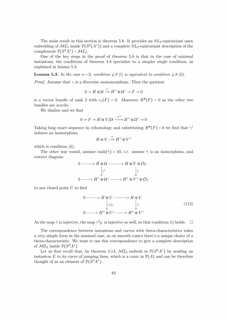
The main result in this section is theorem 5.8. It provides an SL2-equivariant openembedding ofMI2 inside P(S2(A∗)) and a complete SL2-equivariant description of thecomplement P(S2A∗) ∖MI2.

One of the key steps in the proof of theorem 5.8 is that in the case of minimalinstantons, the conditions of theorem 4.8 specialize to a simpler single condition, asexplained in lemma 5.3.

Lemma 5.3. In the case n = 2, condition 4.8 (i) is equivalent to condition 4.8 (ii).

Proof. Assume that γ is a fiberwise monomorphism. Then the quotient

0→H ⊗ U γ′Ð→H∗ ⊗ U⊥ → F → 0

is a vector bundle of rank 2 with c1(F ) = 0. Moreover H(F ) = 0 as the other twobundles are acyclic.

We dualize and we find

0→ F →H ⊗ V /U −γ′∗ÐÐ→H∗ ⊗ U∗ → 0

Taking long exact sequence in cohomology and substituting H(F ) = 0 we find that γ′

induces an isomorphism

H ⊗ V −γÐ→H∗ ⊗ V ∗

which is condition (ii).The other way round, assume rank(γ) = 10, i.e. assume γ is an isomorphism, and

restrict diagram

0 H ⊗ U H ⊗ V ⊗OY

0 H∗ ⊗ U⊥ H∗ ⊗ V ∗ ⊗OY

γ′ γ

to any closed point U to find

0 H ⊗U H ⊗ V

0 H∗ ⊗U⊥ H∗ ⊗ V ∗

γ′∣U γ (112)

As the map γ is injective, the map γ′∣U is injective as well, so that condition (i) holds.

The correspondence between instantons and curves with theta-characteristics takesa very simple form in the minimal case, as on smooth conics there’s a unique choice of atheta-characteristic. We want to use this correspondence to give a complete descriptionof MI2 inside P(S2A∗).

Let us first recall that, by theorem 4.14, MI2 embeds in P(S2A∗) by sending aninstanton E to its curve of jumping lines, which is a conic in P(A) and can be thereforethought of as an element of P(S2A∗).

83

Proof. (Sketch) Given a minimal instanton E one can obtain a conic in P(A) via theorem4.14. Conversely, given a conic C

iC ∶ C → P(A)

which comes from an instanton via theorem 4.14, take the pushforward iC∗OC(−1) anddecompose it with respect to the exceptional collection

⟨OP(A)(−2),OP(A)(−1),OP(A)⟩

This will provide a resolution

0→H ⊗OP(A)(−2)→H∗ ⊗OP(A)(−1)→ iC∗OC(−1)→ 0

Finally, one checks that such a resolution is symmetric in H and recovers in this way anelement in A∗ ⊗ S2H∗ corresponding to an instanton.

In section 2.1 we have discussed an SL(W )-equivariant construction of Y : its firststep is the choice of an SL(W )-invariant 3-dimensional A ⊂ Λ2V ∗. As SL(W ) acts onA, it also acts on A⊗ S2H∗. In the case of minimal instantons there is another copy ofSL2 acting on A⊗ S2H∗, namely SL(H).

As the two actions of SL(W ) and SL(H) on A ⊗ S2H∗ commute, they induce anaction of SL(W )×SL(H). The description of the complement of the locus of instantonicγ in A⊗ S2H∗ involves the two SL(W ) × SL(H)-invariant divisors which we are aboutto introduce.

Definition 5.4. We denote the degree 3 divisor in P(A ⊗ S2H∗) of degenerate mapsfrom A∗ to S2H∗ by Q3.

There is a unique divisor of degree 2 in P(A ⊗ S2H∗) which is invariant under theaction of SL(W ) × SL(H). We denote it by Q2.

Remark 5.5. Let us show that Q2 is well defined. It is easy to determine the irreduciblecomponents of each direct summand of

S2(A∗ ⊗ S2H) = (S2A∗ ⊗ S2S2H)⊕ (Λ2A∗ ⊗Λ2S2H)

with respect to the action of SL(W ) × SL(H). They are all the products of irreduciblecomponents of the factors. It follows that there is only one 1-dimensional SL(W ) ×SL(H) irreducible representation, which shows that Q2 is well defined. Note moreoverthat, as there are clearly no SL(W )×SL(H) invariant elements in A∗⊗S2H, the divisorQ2 is irreducible.

Proposition 5.6. The complement ∂M2 = A⊗ S2H∗ ∖M2 is the union of Q2 and Q3.

Proof. By lemma 5.3 we know that γ ∈ M2 if and only if it satisfies condition (ii). Asγ is a 10 by 10 antisymmetric matrix, it has rank 10 if and only if its Pfaffian does notvanish. As the entries of γ are linear in the coordinates of A ⊗ S2H∗, ∂M2 is cut by a

84

degree 5 equation. Moreover, by 4.17 we know that for γ to be in M2 it is necessary thatit induces an isomorphism from A∗ to S2H∗, so that Q3 is contained in ∂M2.

As Q3 has degree 3, we are left with the task of finding a missing quadric, which weclaim is Q2. To prove it, we use the joint action of SL(W ) and SL(H). The instantonicconditions (i), (ii) are clearly invariant under the action of both copies of SL2, so thatalso the missing quadric has the same property. By remark 5.5, having degree 2 andbeing SL(W )×SL(H)-invariant uniquely determine Q2, so that finally ∂M2 is the unionof Q2 and Q3.

Theorem 5.8 completes the description of MI2 inside P(S2A∗). In order to stateit, we need to choose a notation for two divisors in P(S2A∗). We do it in the followingdefinition.

Definition 5.7. We denote the degree 3 divisor in P(S2A∗) of degenerate conics inP(A) by ∆A.

There is a unique hyperplane in P(S2A∗) which is invariant under the action ofSL(W ). We denote it by Hq as under the canonical S2A∗ ≅ S2A it is cut by q.

Denote by F the rational surjection

F ∶ P(A⊗ S2H∗) P(S2A∗)

sending γ to γ−1(∆H). Note that F has degree 2 and that by the decomposition ofS2(A ⊗ S2H∗) and S2A∗ into SL(W ) × SL(H)-irreducibles it is the unique SL(W ) ×SL(H)-equivariant map of degree 2 from P(A ⊗ S2H∗) to P(S2A∗). Another way todescribe F is to say that

F (γ) = γT ⋅ qH ⋅ γ (113)

where γT is the transpose of γ and qH ∈ S2H∗ is the unique SL(H)-invariant.We are now ready to state and prove theorem 5.8.

Theorem 5.8. The map which associates with an instanton E of charge 2 its conic ofjumping lines is an SL2-equivariant isomorphism

MI2 → P(S2A∗) ∖ (∆A ∪Hq)

where ∆A and Hq are defined in 5.7.

Proof. As F is surjective, it is enough to show that

F −1(Hq) = Q2 F−1(∆A) = Q3

The first one holds as F is SL(H)-equivariant of degree 2 and Hq is SL(W )-equivariant,so that F −1(Hq) is invariant under the action of both SL(W ) and SL(H). By remark5.5, the only such quadric is Q2.

As for the second one, by equation (113) we have

det(F (γ)) = det(γ)2 det(qH)

so that F (γ) is degenerate if and only if γ is degenerate.

85

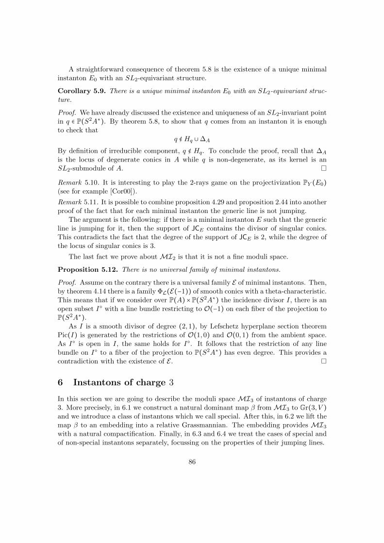
A straightforward consequence of theorem 5.8 is the existence of a unique minimalinstanton E0 with an SL2-equivariant structure.

Corollary 5.9. There is a unique minimal instanton E0 with an SL2-equivariant struc-ture.

Proof. We have already discussed the existence and uniqueness of an SL2-invariant pointin q ∈ P(S2A∗). By theorem 5.8, to show that q comes from an instanton it is enoughto check that

q ∉Hq ∪∆A

By definition of irreducible component, q ∉ Hq. To conclude the proof, recall that ∆A

is the locus of degenerate conics in A while q is non-degenerate, as its kernel is anSL2-submodule of A.

Remark 5.10. It is interesting to play the 2-rays game on the projectivization PY (E0)(see for example [Cor00]).

Remark 5.11. It is possible to combine proposition 4.29 and proposition 2.44 into anotherproof of the fact that for each minimal instanton the generic line is not jumping.

The argument is the following: if there is a minimal instanton E such that the genericline is jumping for it, then the support of JCE contains the divisor of singular conics.This contradicts the fact that the degree of the support of JCE is 2, while the degree ofthe locus of singular conics is 3.

The last fact we prove about MI2 is that it is not a fine moduli space.

Proposition 5.12. There is no universal family of minimal instantons.

Proof. Assume on the contrary there is a universal family E of minimal instantons. Then,by theorem 4.14 there is a family ΦL(E(−1)) of smooth conics with a theta-characteristic.This means that if we consider over P(A)×P(S2A∗) the incidence divisor I, there is anopen subset I with a line bundle restricting to O(−1) on each fiber of the projection toP(S2A∗).

As I is a smooth divisor of degree (2,1), by Lefschetz hyperplane section theoremPic(I) is generated by the restrictions of O(1,0) and O(0,1) from the ambient space.As I is open in I, the same holds for I. It follows that the restriction of any linebundle on I to a fiber of the projection to P(S2A∗) has even degree. This provides acontradiction with the existence of E .

6 Instantons of charge 3

In this section we are going to describe the moduli space MI3 of instantons of charge3. More precisely, in 6.1 we construct a natural dominant map β fromMI3 to Gr(3, V )and we introduce a class of instantons which we call special. After this, in 6.2 we lift themap β to an embedding into a relative Grassmannian. The embedding provides MI3

with a natural compactification. Finally, in 6.3 and 6.4 we treat the cases of special andof non-special instantons separately, focussing on the properties of their jumping lines.

86

6.1 A map from MI3 to Gr(3, V )

It turns out that there is a surjective map fromMI3 to Gr(3, V ), which we will denoteby β. Its fibers are either projective spaces or Grassmannians and it is convenient tostratify Gr(3, V ) with respect to their type. More precisely, there will be two strata andβ will be smooth on each of them. This will correspond to a distinction between twokinds of instantons: the special ones and the non-special ones.

Notation 6.1. We will denote Gr(3, V ) by B. We will also denote κ(A), that is to saythe image of κ in Gr(3, V ), by Bs and its complement B ∖Bs by Bn.

Notation 6.2. When c2(E) = 3, the space H ′ in monad (93) is 1-dimensional. For thisreason we will write

H ⊗ U →H∗ ⊗ U⊥ → OY (114)

for any monad associated with an instanton E of charge 3. The first map in the complex

HγÐ→H∗ ⊗A→ V ∗ (115)

obtained by applying Hom(U ,−) to (114) is denoted by γ.

Lemma 6.3. For a charge 3 instanton the following properties are equivalent

• ext1(U ,E) ≠ 0

• hom(U ,E) ≠ 1

Proof. We can compute both Hom(U ,E) and Ext1(U ,E) using the monad (99): theyare the cohomology of the complex (115). Note that γ is injective as its kernel wouldcontribute to Ext−1(U ,E).

It follows from (115) that

hom(U ,E) − ext1(U ,E) = 1

showing the equivalence of the two conditions.

The above lemma motivates the following definition.

Definition 6.4. An instanton E of charge 3 is special if Ext1(U ,E) ≠ 0. Equivalently,an instanton is non-special if Hom(U ,E) = C.

We will see that special instantons are special in many ways. Essentially by definitionthey do not have a canonical map into U∗, while most of instantons have one. Theyare the only instantons having 2-jumping lines (see proposition 6.24). They are the onlyinstantons whose associated theta-characteristic is not locally free (see proposition 7.3).

We are now going to introduce the main character in the description of MI3.

Definition 6.5. The mapβ ∶MI3 → B

sends E to Ext1(−,E) of the tautological map V ∗ ⊗OY → U∗.

87

So far it is not clear that

Ext1(U∗,E)→ Ext1(V ∗ ⊗OY ,E) ≅ V ⊗H1(E) ≅ V

is a 3-dimensional subspace of V and that β is regular: we prove it in proposition 6.7 bymeans of lemma 6.6.

Lemma 6.6. If E is an instanton with c2(E) ≥ 3, then Hom(U⊥,E) = 0.

Proof. Both E and U⊥ are µ-stable (see lemma 2.16) of slope respectively µ(E) = 0 andµ(U⊥) = −1/3. It follows that there is no map of rank 1 from U⊥ to E, as otherwise

µ(E) > µ(Im) > µ(U⊥)

which contradicts the fact that the slope of the image µ(Im) is an integer.As E is torsion-free, there are no maps of rank 0, so that we only have to check that

there are no maps of rank 2. To prove it, assume there is such a map and complete itto an exact sequence.

0→ L→ U⊥ → E → Q→ 0

Then L is reflexive of rank 1 and therefore it is a line bundle. Moreover, c1(L) ≤ −1 bystability of U⊥ and c1(L) ≥ −1 by stability of E, so that L ≅ O(−1). To conclude theproof, we use equations (28) and (91) to compute ch(Q) and derive a contradiction:

ch(Q) = ch(E) − ch(U⊥) + ch(O(−1))

yieldsch(Q) = (3L − c2(E)) − P

so that the leading term is negative when c2(E) ≥ 3.

The bound in lemma 6.6 is sharp as instantons of charge 2, by monadic description,always have a 2-dimensional space of maps from U⊥.

Proposition 6.7. β is a regular map from MI3 to B.

Proof. By self duality of E, ext1(U∗,E) = ext1(E,U), and by monadic description (93)we have ext1(E,U) = 3. Moreover the kernel of Ext1(U∗,E) → V ⊗H1(E) sits insideHom(U⊥,E), which vanishes by lemma 6.6, so that

Ext1(U∗,E) ⊂ V ⊗H1(E)

gives a point in B.We prove that the map β is regular by constructing it in families. Take any flat

family E of instantons of charge 3 over a base scheme S. Take the tautological mapV ∗ ⊗OY → U∗ and out of it construct

Hom(U∗,E)→ V ⊗Hom(OY ,E)

88

Push it forward to S. By cohomology and base change, we obtain a (shifted by 1)rank 3 subbundle of V ⊗H1(E), where H1(E) is a line bundle. By twisting the subbundleby H1(E)∗ we finally get a rank 3 subbundle of V ⊗OS , which by defining property ofB gives a map from S to B. By the universal property for the coarse moduli space ofinstantons, we induce a unique map from MI3 to B.

Lemma 6.8 and proposition 6.9 deal with different descriptions of β.

Lemma 6.8. β(E) is the 3-dimensional subspace of V given by Ext1(E,−) applied tothe tautological U → V ⊗OY .

Proof. By self-duality of E, there is a functorial isomorphism between Ext1(−,E) andExt1(E,−∗) inducing a commutative square

Ext1(E,V ⊗O) Ext1(E,U)

Ext1(V ∗ ⊗O,E)

≅

? Ext1(U∗,E)

≅

?(116)

Proposition 6.9. Let (114) be a monad for E. β(E) is the image of the injective map

H∗ ≅ Hom(U⊥,H∗ ⊗ U⊥)→ Hom(U⊥,OY ) ≅ V

obtained from (114) by applying Hom(U⊥,−).

Proof. Under the canonical identification of B with the Grassmannian of 2-dimensionalquotients of V , β(E) is the bottom row the the following commutative diagram.

Hom(U⊥,H∗ ⊗ U⊥) ≅- Hom(U⊥, E) 0

0 = Hom(OY , E)

Hom(U⊥,OY )?

≅

-

V ⊗H0(OY )

0?

Ext1(U⊥,E)?

β(E)

V ⊗H1(E)

≅

?

(117)

The upper left triangle is induced by the monad (114), the middle and right column areinduced by the acyclic extension sequence (92). The horizontal maps are induced byU⊥ → V ∗ ⊗OY . The commutativity of (117) shows that

Hom(U⊥,H∗ ⊗ U⊥)→ Hom(U⊥,OY )

is the kernel of β(E).

89

Notation 6.10. By proposition 6.9, for a family of instantons E over a base S we willwrite

H ⊠ U → β∗K ⊠ U⊥ → OS×Y (118)

for its decomposition with respect to the usual collection (35).

Next, we characterize the special instantons in terms of their image under β. Recallthat we have introduced a stratification Bs,Bn for B = Gr(3, V ), and that the closestratum Bs is the image under κ of P(A).

Proposition 6.11. An instanton E is special if and only if β(E) ∈ Bs.

Proof. E is special if and only if in the sequence (115) the map

H∗ ⊗A εÐ→ V ∗

is not surjective. Instead of computing Ext1(−,E) only on U , compute it on the universalmap U → A∗ ⊗ U⊥. The result is a commutative diagram

A⊗H∗

ε- V ∗

A⊗H∗

Id ≅

6

A⊗β(E)

- A⊗ V

a(v,−)6

showing that ε has a cokernel if and only if there is v ∈ V such that A(β(E), v) = 0. Asdimβ(E) = 3, this can happen if and only if dimA(v,−) ≤ 2, which is the case if andonly if there is av ∈ A such that v = kerav. Finally, if v = kerav, there’s a unique choicefor β(E) and it is κ(av).

The following is a more accurate description of the moduli space MIs3 of specialinstantons. Note that so far we have defined what a single special instanton is, but wedo not have a notion of family of special instantons.

Let S be a scheme and denote the projections from Y × S to Y and S respectivelyby πY and πS .

Definition 6.12. We will denote by MIs3 the functor which associates with S the setof families of instantons E such that the schematic support R1πMI3∗Hom(π∗Y U ,E) isthe whole S.

Remark 6.13. The formation of R1πMI3∗Hom(π∗Y U ,E) commutes with arbitrary basechanges T → S. The reason is that by monad (114) all higher pushforwards

R>1πMI3∗Hom(π∗Y U ,E)

vanish.

90

Remark 6.14. Also the formation of the support of R1πMI3∗Hom(π∗Y U ,E) commuteswith arbitrary base change. This is true as the rank of R1πMI3∗Hom(π∗Y U ,E) is nevergreater than 1, so that its the schematic support is the first degeneracy locus of thevector bundle map

A⊗ β∗K → V ∗ ⊗OS (119)

To conclude, note that the formation of the above map commutes with arbitrary basechange by functoriality of the decomposition with respect to a full exceptional collection.

Proposition 6.15. There is a cartesian diagram

MIs3 ⊂- MI3

◻

P(A)

βs

?⊂κ- B

β

?(120)

where the embedding of MIs3 in MI3 is the natural one.

Proof. Given a family of special instantons E on a scheme S, consider its associatedmonad (118). Recall that β(E) is by definition β∗K → V ⊗OS , whose cokernel is, bydefinition of family of special instantons, supported everywhere on S. It follows that themap from S to B factors uniquely via the degeneracy locus of (119), which by proposition3.6 is Bs. As a consequence, we have constructed the maps in (120).

In the other direction, given a family of instantons E over S such that β(E) factorsvia Bs, we clearly have that

R1πMI3∗Hom(π∗Y U ,E)

is supported on the whole S as it comes by pullback from Bs, where by 3.6 it is a linebundle.

By definition 6.4, any non-special instanton has a canonical map E → U∗. By stabilityof E and U∗, this map is injective, so that we have an exact sequence

0→ E → U∗ → QE → 0

where QE is by definition the cokernel of E → U∗. The Chern character computationyields

ch(QE) =H + 7L

2− P

6(121)

so that QE is supported on a linear section of Y . Later on, in theorem 6.34, we willprove that for any non-special E such a QE is always of the form ΦBl (OP(K) (2)). In

view of this, we prove that if QE is isomorphic to ΦBl (OP(K) (2)), then β(E) =K.

Proposition 6.16. For every short exact sequence

0→ E → U∗ → ΦBl (OP(K) (2))→ 0

where E is an instanton and K ∈ B ∖Dtri, it is true that β(E) =K.

91

Proof. We will compute β(E) using the slight modification of definition 6.5 which isdescribed in lemma 6.8.

We need to compute Ext1(E,−) on the tautological sequence

0→ U → V ⊗OY → V /U → 0

As U∗ lies in the left orthogonal to all bundles in the sequence, we get isomorphisms

Ext1(E,−) = Ext2 (ΦBl (OP(K) (2)) ,−) = Ext2(OP(K)(2),Φ!Bl(−)) (122)

Our next goal is to check that the image of

Ext2(OP(K)(2),Φ!Bl(U))→ V ⊗ Ext2(OP(K)(2),Φ!

Bl(OY )) (123)

is K. We will apply Φ!Bl to the tautological injection U → V ⊗OY . In order to do it, recall

the identifications of lemma 3.26. Note also that over PY (U) there is a commutativediagram

OPY (U)(−E)

p∗Y U(h −E) -

V ⊗OPY (U)(h −E)

eV (−E)

?

where the diagonal map is the twisted relative tautological injection on PY (U) and thehorizontal map is the pullback of the tautological injection on Y . If we push the diagramforward to P(V ) we find another commutative diagram

Iσ(A)

Φ!Bl(U)[−1] -

V ⊗Φ!

Bl(OY )[−1]

eV (−E)

?(124)

To find the map (123), apply the functor Ext2(OP(K)(2),−)[1] to the above diagram.By Grothendieck duality

Ext2(OP(K)(2),−)[1] ≅H1P(K)

(Lj∗K(−))

Applying H1P(K)

(Lj∗K(−)) to diagram (124). The result is

H1(Lj∗KIσ(A))

H1(Lj∗KΦ!Bl(U)[−1])

β(E)

-

≅

V ⊗H1(Lj∗KIσ(A)(h))

H1(eV )

?(125)

where the diagonal arrow is an isomorphism as its cokernel is O(−h) is acyclic on P(K).It follows that the image of β(E) coincides with the image of H1(eV ).

92

As we assumed K ∉Dtri, we know by lemma 3.3 and lemma 3.21 that the intersectionof P(K) with σ(A) has expected dimension, so that Iσ(A) pulls back to an ideal sheafon P(K). More precisely, Lj∗KIσ(A) is the ideal of a length 4 subscheme of P(K). Wewill denote P(K) ∩ σ(A) by K4 and its ideal in P(K) by I4, so that the vertical arrowin the diagram (125) becomes

H1P(K)

(eV ) ∶H1(I4)→ V ⊗H1(I4(h)) (126)

Note hat the restriction to P(K) of the Euler map eV factors via the Euler map eKof K:

H1(I4)

K ⊗H1(I4(h))

H1(eK)

?

jK- V ⊗H1(I4(h))

H1(eV )

-

In order to conclude the proof, we only need to check that H1(eK) is an isomorphism.As the cokernel of the Euler map is TP(K), if

H1(TP(K) ⊗ I4) =H2(TP(K) ⊗ I4) = 0 (127)

then H1(eK) is an isomorphism.To check this last vanishing, we use a resolution for I4. Using the fact that P(K) ∉

Dtri, we will prove that K4 is always cut by two conics, so that I4 has a Koszul resolution

0→ O(−4)→ O(−2)⊕2 → I4 → 0

For any scheme of length 4 in P(K) there is at least a pencil of conics containing it. Takea pencil of conics in P(K) containing K4: if they do not have common components, thenthe intersection is K4, otherwise the conics in the pencil share a component. If theyshare a component, K4 is contained in a line with an embedded point, and thereforeintersects the line in a scheme of length at least 3, against the fact that P(K) ∉Dtri.

Finally,H(TP(K)(−2)) =H(TP(K)(−4)) = 0

imply that (127) is true.

6.2 An embedding of MI3 in a relative Grassmannian

The monadic data for the construction of an instanton of charge 3 consist of two maps:one from H ⊗ U to H∗ ⊗ U⊥, the other from H∗ ⊗ U⊥ to OY . When we constructed themap β in section 6.1 we used only the second one. By taking also the first one intoaccount we expect to construct an embedding of MI3.

Recall that we are using notation 6.1, so that B is Gr(3, V ) and Bn,Bs is astratification of B. We will construct a map Γ from MI3 to GrB(3,A ⊗K) which will

93

fit in a commutative diagram

MI3Γ- GrB(3,A⊗K)

B

πB?β -

where πB is the canonical projection.Let E be a family of instantons parametrized by S. Denote by πS and πY the

projections from S ×Y to S and Y . Denote by βE the composition of the map S →MI3

corresponding to E with β. The relative Beilinson spectral sequence provides us with amonad for E :

H ⊠ U γEÐ→ β∗EK ⊠ U⊥ βEÐ→ OS×Y (128)

where K is the tautological bundle on B (see notation 6.2).

Remark 6.17. In order to construct a map Γ fromMI3 to GrB(3,A⊗K) which is relativeto B, it is enough to associate naturally to any family of instantons E a rank 3 subbundleof β∗

EK ⊗A.

Lemma 6.18. Given a family of instantons E parametrized by S,

πS∗Hom(π∗Y U ,H ⊠ U)πS∗Hom(p∗Y U ,γ)ÐÐÐÐÐÐÐÐÐ→ πS∗Hom(π∗Y U , β∗EK ⊠ U⊥) (129)

is a rank 3 subbundle of β∗EK ⊗A.

Proof. First, note that by Kunneth formula the map (129) becomes

H⊗OS → β∗EK ⊗A

Next, let s ∈ S be a closed reduced point and Es the corresponding instanton. By basechange and flatness of pS , it is enough to check that for each closed reduced point of Sthe map

Hom(U ,H ⊗ U)→ Hom(U , β(Es)⊗ U⊥) (130)

is injective. This holds as a non-trivial kernel of (130) contributes to Hom−1(U ,Es),which vanishes.

Definition 6.19. Γ takes a family of instantons E to the rank 3 subbundle (129).

Our next goal is to describe the closure of the image of Γ. Denote by Z3 the zerolocus on GrB(3,A⊗K) of the composition

T rel3 → A⊗K → A⊗ V ⊗OGrB(3,A⊗K) → V ∗ ⊗OGrB(3,A⊗K) (131)

where the first map is the relative tautological injection, the second one is the pullbackof the tautological injection from B tensored by A and the third one is the evaluationof forms in A on V .

First, we describe Z3. By proposition 3.6 there is an exact sequence

0→ Ker→ A⊗K → V ∗ ⊗OB → κ∗ (OP(A)(2))→ 0 (132)

which defines a reflexive sheaf Ker.

94

Definition 6.20. The restriction of Ker to Bn, that is to say the kernel of

A⊗K∣Bn → V ∗ ⊗OBn

is a rank 4 vector bundle over Bn denoted by Kern. The kernel of

A⊗K∣Bs → V ∗ ⊗OBs

is a rank 5 vector bundle over Bs denoted by Kers.

Lemma 6.21. The restriction of Z3 to Bn is PBn(Kern∗). The restriction of Z3 to Bs

is GrBs(3,Kers).

Proof. The formation of zero loci of maps of vector bundles commutes with arbitrarybase change.

Lemma 6.22. Z3 is the zero locus of a regular section of T rel∗3 ⊗ V ∗. Moreover, Z3 isirreducible and Γ factors via Z3.

Proof. Z3 is schematically cut by a section of the rank 15 vector bundle

T rel3 ⊗ V

by its definition in (131). We only need to check that the section is regular, i.e. thatcodim(Z3) = 15. As dim(GrB(3,A⊗K)) = 24, it is enough to check that dim(Z3) ≤ 9.

In the notation of definition 6.20 and by lemma 6.21

Z3 = PBn(Kern∗) ⊔GrBs(3,Kers)

This gives a stratification of Z3 into an open 9-dimensional subscheme and a closed8-dimensional subscheme, so that dim(Z3) ≤ 9.

The 9-dimensional open subscheme is irreducible and its complement is 8-dimensional,so that, if Z3 were reducible, one of its components would be at most 8-dimensional. Thisis impossible as Z3 is cut by 15 equations inside a Cohen-Macaulay scheme of dimension24. It follows that Z3 is irreducible.

Finally, by definition of Γ, the pullback of Hom(U ,−) of

T rel3 → A⊗K → V ∗ ⊗OGrB(3,A⊗K)

is the relative monad (128). As the relative monad is a complex, Γ factors via Z3.

We are now going to prove that the map Γ is an embedding ofMI3 into GrB(3,A⊗K)and to show that the closure of its image is Z3.

Theorem 6.23. Γ is an embedding and the closure of its image is Z3.

95

Proof. Over GrB(3,A⊗K) × Y there are canonical maps

T rel3 ⊠ U → K ⊠ U⊥ → OGrB(3,A⊗K) ⊠OY (133)

The first map is the composition

T rel3 ⊠ U → A⊗K ⊠ U → K ⊠ U⊥

where the first map is the relative tautological injection and the second is the uniqueSL2-equivariant one. The second map is the unique SL2-invariant element of

HomGrB(3,A⊗K)(K ⊠ U⊥,OGrB(3,A⊗K) ⊠OY ) = V ∗ ⊗ V

By definition of Z3 we have that the restriction of (133) to Z3 × Y is a complex. Bytheorem 4.5, the moduli space MI3 is non-empty. Given an instanton E, by definitionof Γ the restriction of (133) to Γ(E)×Y is a monad for E. It follows that on a non-trivialopen subset Zo3 ⊂ Z3, the only non-trivial cohomology of the complex (133) is the middleone, and that it is a family of instantons.

Summarizing, for any family of instantons E over a base S, there is an induced mapto Zo3 given by Γ(E). Conversely, for any map from S to Zo3 the pullback of (133) is afamily of instantons.

6.3 Special instantons

By proposition 6.15, the moduli spaceMIs3 of special instantons embeds in GrBs(3,Kers).In this section we are going to provide an instantonic interpretation for the projectionto Bs and we are going to show that such a projection is surjective.

Proposition 6.24. Given an instanton E and a line L, the order of jump of E at L is2 if and only if β(E) = κ(aL). In particular, E has a 2-jumping line if and only if it isspecial.

Proof. Note that by corollary 4.18 there are no jumping lines of order greater than 2, sothat L is a 2-jumping line for E if and only if H1(E∣L) ≠ 0.

Recall from corollary 2.23 that

L = P (κ(aL)/ker(aL))

so thatU⊥∣L ≅ (A(keraL,−)⊗OL)⊕OL(−1)

It follows that if we restrict a monad (93) for E to L we get

H ⊗ (OL ⊕OL(−1))→ β(E)⊗ (A(keraL,−)⊗OL ⊕OL(−1))→ OL

The only contribution to H1(E∣L) comes from the rightmost term, so that H1(E∣L) isnot zero if and only if the composition

β(E)⊗A(keraL,−)→ V ⊗ V ∗ → C

96

vanishes.As β(E) is 3-dimensional and A(keraL,−) is 2-dimensional, this happens if and only

if κ(aL) = β(E).

Next, we will prove that for each line L there is an instanton E such that β(E) = κ(L).By proposition 6.24 it is enough to show that L is a 2-jumping line for E.

Let L be a line in Y and let K ⊂ V be a 3-dimensional space such that κ(L) ∈ P(K).By lemma 3.20, we can choose K such that YK , the linear section of Y induced by K, issmooth. Note that in this case, by lemma 3.28, YK is the blow up of P(K) in 4 distinctpoints such that no 3 of them lie on a line. Denote the 4 components of the exceptionaldivisor by L,L1, L2, L3. In this notation, the following proposition holds.

Proposition 6.25. Given a surjective map

U → OYK(h − 2L) (134)

denote its kernel by E(−1). Then E is an instanton and L is a 2-jumping line for E.

Proof. We need to prove that H(E(−1)) = 0, that ch(E) = 2−3L, that E is locally freeand that it is µ-stable.

The vanishing of H(E(−1)) follows from 2.17 and from the exact sequence

0→ OYK(−L)→ OYK(h − 2L)→ Oh−L(−1)→ 0

which shows that OYK(h − 2L) is acyclic.The Chern character computation follows from (28) and from the fact that it is easy

to compute the Euler characteristic of several twists of OYK(h − 2L) by means of theidentification of YK with the blow up of P(K) in 4 points such that no 3 of them arecollinear.

The fact that E is locally free follows from the isomorphism

Tori(E,−) ≅ Tori+1(OYK(h − 2L),−)

and from the fact that locally OYK(h− 2L) is the structure sheaf of a Cartier divisor, sothat Tor>1(OYK(h − 2L),−) = 0.

The stability of E can be checked via Hoppe’s criterion 1.22. In order to do it, it isenough to check that H0(E) vanishes. This is equivalent to the fact that

H0(U∗)→H0(OYK(h − 2L)) (135)

is surjective. Note that the restriction map U∗ → UYK is an isomorphism in cohomology,as its kernel U is acyclic, so that the surjectivity of (135) is equivalent to that of

H0(U∗∣YK)→H0(OYK(h − 2L)) (136)

Finally, as U∗YK → OYK(h − 2L) is surjective, its kernel is a line bundle. More precisely,it is determined by its c1, which is

H − h − 2L = 2h +L −L1 −L2 −L3

97

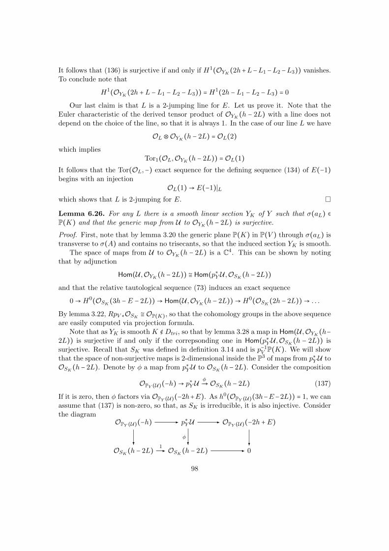
It follows that (136) is surjective if and only if H1(OYK(2h+L−L1 −L2 −L3)) vanishes.To conclude note that

H1(OYK(2h +L −L1 −L2 −L3)) =H1(2h −L1 −L2 −L3) = 0

Our last claim is that L is a 2-jumping line for E. Let us prove it. Note that theEuler characteristic of the derived tensor product of OYK(h − 2L) with a line does notdepend on the choice of the line, so that it is always 1. In the case of our line L we have

OL ⊗OYK(h − 2L) = OL(2)

which impliesTor1(OL,OYK(h − 2L)) = OL(1)

It follows that the Tor(OL,−) exact sequence for the defining sequence (134) of E(−1)begins with an injection

OL(1)→ E(−1)∣Lwhich shows that L is 2-jumping for E.

Lemma 6.26. For any L there is a smooth linear section YK of Y such that σ(aL) ∈P(K) and that the generic map from U to OYK(h − 2L) is surjective.

Proof. First, note that by lemma 3.20 the generic plane P(K) in P(V ) through σ(aL) istransverse to σ(A) and contains no trisecants, so that the induced section YK is smooth.

The space of maps from U to OYK(h − 2L) is a C4. This can be shown by notingthat by adjunction

Hom(U ,OYK(h − 2L)) ≅ Hom(p∗Y U ,OSK(h − 2L))

and that the relative tautological sequence (73) induces an exact sequence

0→H0(OSK(3h −E − 2L))→ Hom(U ,OYK(h − 2L))→H0(OSK(2h − 2L))→ . . .

By lemma 3.22, RpV ∗OSK ≅ OP(K), so that the cohomology groups in the above sequenceare easily computed via projection formula.

Note that as YK is smooth K ∉Dtri, so that by lemma 3.28 a map in Hom(U ,OYK(h−2L)) is surjective if and only if the correpsonding one in Hom(p∗Y U ,OSK(h − 2L)) issurjective. Recall that SK was defined in definition 3.14 and is p−1

V P(K). We will showthat the space of non-surjective maps is 2-dimensional inside the P3 of maps from p∗Y U toOSK(h− 2L). Denote by φ a map from p∗Y U to OSK(h− 2L). Consider the composition

OPY (U)(−h)→ p∗Y UφÐ→ OSK(h − 2L) (137)

If it is zero, then φ factors via OPY (U)(−2h+E). As h0(OPY (U)(3h−E−2L)) = 1, we canassume that (137) is non-zero, so that, as SK is irreducible, it is also injective. Considerthe diagram

OPY (U)(−h) - p∗Y U - OPY (U)(−2h +E)

OSK(h − 2L)?

1- OSK(h − 2L)

φ?

- 0?

98

By snake lemma, the cokernel of φ is isomorphic to the cokernel of

OPY (U)(−2h +E)→ OZ(h − 2L)

where Z is the zero locus of a section of OSK(2h − 2L). It follows that Z contains aP1 ⊂ SK linearly equivalent to h −L. As a consequence, φ factors via OSK(h −L). Onecan finally check that there is a P1 of maps from U to OSK(−L) and that there is a P1

of maps from OSK(−L) to OSK(h− 2L), so that the space of non-surjective maps is theimage of P1 × P1, showing eventually that the generic φ is surjective.

6.4 Non-special instantons

The aim of this section is to construct a family of instantons corresponding to an opendense subset ofMI3. We will also prove that this family is the universal family for non-special instantons. Consistently with notation 6.1 and definition 6.12, we will denotethe moduli space of non-special instantons by MIn3.

Note that, by lemma 6.21 and theorem 6.23, we already have a description of themoduli space of non-special instantons as an open subset of PBn(Kern∗). We want toimprove this description in two ways: by finding the image β(MIn3) inside Bn and bydescribing the complement of MIn3 inside PBn(Kern∗).

In the next proposition we will construct non-special instantons as kernels of surjec-tive maps from U∗ to ΦBl(OP(K)(2h)).

Proposition 6.27. If K ∉ Dtri, then the kernel E of a surjective map from U∗ toΦBl(OP(K)(2h)) is a non-special instanton of charge 3.

Proof. Assume the kernel E of a surjective map from U∗ to ΦBl(OP(K)(2h)) is given.To prove that E is an instanton of charge 3, we need to prove that it is locally free,that it is stable, that H1(E(−1)) = 0 and that ch(E) = 2 − 3L. We will denote the mapU∗ → ΦBl(OP(K)(2h)) by φ. After that, we will check that it is non-special.

E is locally free if and only if the Tor-dimension of E is 0, i.e. if for any i > 0 andany y closed point Tori(Oy,E) = 0 . The defining sequence

0→ E → U∗ φÐ→ ΦBl(OP(K)(2h))→ 0

gives an isomorphism between Tori(Oy,E) and Tori+1(Oy,ΦBl(OP(K)(2h))). We com-pute the latter via resolution (88), so that for i > 1 we always get 0, while for i =1 there might be a non-trivial result. More precisely, by lemma 3.25 the conditionTor2(Oy,ΦBl(OP(K)(2h))) ≠ 0 is equivalent to K ∈ Dtri, so that under the assumptionK ∉Dtri we have that E is locally free.

By Hoppe’s criterion 1.22, E is stable if and only if H0(E) = 0. To check H0(E) = 0,we check that the map

H0(U∗) H0(φ)ÐÐÐ→H0 (ΦBl(OP(K)(2h))) (138)

99

is injective. By the Grothendieck spectral sequence for the composition of two pushfor-wards, we get that the above map is the same as

H0(p∗Y U∗)H0

(φad)ÐÐÐÐÐ→H0 (p∗VOP(K)(2)) (139)

induced by the adjoint map φad to φ, so that it is enough to check that H0(φad) isinjective.

As φ is surjective, so is φad by lemma 6.30. Now we claim that the restriction map

p∗Y U∗ → p∗Y U∗∣SK (140)

is an isomorphism in cohomology. By Koszul resolution (79) this follows if we show thatp∗Y U∗(−2h) and p∗Y U∗(−h) are acyclic. By twisting the tautological sequence

0→ OPY (U)(2h −E)→ p∗Y U∗ → OPY (U)(h)→ 0

by OPY (U)(−2h) we get immediately that p∗Y U∗(−2h) is acyclic. By twisting it byOPY (U)(−h) we get a non trivial extension of OPY (U) by OPY (U)(h−E), so that p∗Y U∗(−h)is acyclic if and only if h1 (OPY (U)(h −E)) = 1 and its other cohomology groups vanish.The short exact sequence

0→ OPY (U)(h −E)→ OPY (U)(h)→ OE(h)→ 0

is SL2-equivariant and induces an SL2-equivariant cohomology long exact sequence

0→H0 (OPY (U)(h −E))→ S4W → S4W ⊕C→H1 (OPY (U)(h −E))→ 0 (141)

so that h1 (OPY (U)(h −E)) = 1. Summing up, we have proved that (140) is an isomor-phism in cohomology.

In order to prove stability of E, we still need to prove that if

p∗Y U∗∣SKφad∣SKÐÐÐÐ→ p∗VOP(K)(2h)

is surjective, then H0(φad∣SK) is injective, that is to say that its kernel has no globalsections. As we have just proved that φad∣SK surjective, its kernel is locally free ofrank one, and is determined by its c1. As c1(U∗) = H = 3h −E, our claim is now thatOSK(h −E) has no global sections. This last fact can be reduced via resolution (79) tosome vanishing in the cohomology of

OPY (U)(−h −E), OPY (U)(−E), OPY (U)(h −E)

It is easy to check that the first two line bundles are acyclic, and that h0(OPY (U)(h−E)),so that finally also OSK(h −E) has no global sections.

The vanishing of H1(E(−1)) follows from

H1(U) = 0, H0(ΦBl(OP(K)(2h))(−H)) = 0

100

While the vanishing of H1(U) is trivial, we check that

H0(ΦBl(OP(K)(2h))(−H)) = 0

Recall that ΦBl(OP(K)(2h)) has a resolution (87). Twist it byOY (−H) and note that theonly nontrivial vanishing is that of H(S2U∗(−H)). On the other hand, the vanishingof the cohomology of S2U∗(−H) is equivalent to the fact that U is exceptional, which isin proposition 2.15. It follows that E(−1) is acyclic.

The Chern character of E is ch(U∗)−ch(ΦBl(OP(K)(2h))). To check that it is 2−3Lit is enough to substitute the Chern characters which are computed in table (28) andlemma 3.24.

Finally, the fact that E is non-special directly follows from proposition 6.16 andcriterion 6.11, which tell us that β(E) =K and that E is special if and only if β(E) ∈ Bs.By assumption β(E) ∉ Dtri, while by lemma 3.21 Bs ⊂ Dtri, so that we have that E isnot special.

Lemma 6.28. For i = 1,2, let Ei be the instanton associated (via proposition 6.27) toφi ∶ U∗ → ΦBl(Ki), Ki ∉Dtri. If E1 ≅ E2, then K1 =K2 and φ1 = φ2 up to rescaling.

Proof. As E1 ≅ E2, we have K1 = β(E1) = β(E2) = K2. As for φ1 and φ2, there is acanonical arrow from E1 ≅ E2 to U∗, so that (up to rescaling f), we can find a diagram

E1- U∗ φ1- ΦBl(K1)

E2

f

?- U∗

1?

φ2- ΦBl(K2)?

showing that φ1 and φ2 have the same kernel.Moreover, by lemma 3.28 and as Ki ∉ Dtri, the sheaf ΦBl(Ki) is a line bundle on

its support. As its support is irreducible, the identity is its only automorphism up torescaling.

We should also check that our construction produces at least one instanton. We willcheck it in lemma 6.31.

The next lemma, together with 6.31, will give us the dimension of the family ofinstantons which we have just constructed.

Lemma 6.29. For any K, there is an exact sequence

0→K∗ → Hom(U∗,ΦBl(OP(K)(2h)))→ C→ 0 (142)

Proof. Let Φ∗ be the left adjoint functor to ΦBl. Then by definition there is a naturalisomorphism

HomY (U∗,ΦBl(OP(K)(2h))) ≅ HomP(V )(Φ∗(U∗),OP(K)(2))

101

As ΦBl = RpY ∗Lp∗V , its left adjoint Φ∗ is RpV ∗(−⊗ωpV )Lp∗Y . Substituting ωpV = O(E)and using the tautological sequence (73) we get a distinguished triangle

RpV ∗OPY (U)(2h)→ Φ∗(U∗)→ RpV ∗O(h +E) (143)

The leftmost term is OP(V )(2h) by projection formula. The rightmost is computed bypushing forward the exact sequence

0→ O(h)→ O(h +E)→ OE(h +E)→ 0 (144)

to P(V ). Note that for every point v in σ(A), the sheaf OE(h + E) is acyclic on thefiber p−1

V (v), as it is isomorphic to Op−1V (v)(−1), so that

RpV ∗O(h +E) ≅ RpV ∗O(h)

In the end, by taking the long exact sequence for (143) we have shown that there is acanonical exact sequence on P(V )

0→ OP(V )(2h)→ Φ∗(U∗)→ OP(V )(h)→ 0 (145)

which after the application of Hom(−,OP(K)(2h)) becomes sequence (142).

Now we want to identify surjective maps inside Hom(U∗,ΦBl(OP(K)(2h))). The nextlemma allows us to do it without discussing the possible singularities of SK and YK . Notethat for any K there is an isomorphism

HomY (U∗,ΦBl(OP(K)(2h)))≅Ð→ HomSK (p∗YKU

∗,OSK(2h)) (146)

given by adjunction with respect to pullback and pushforward via the composition

SKpYKÐÐ→ YK → Y (147)

Lemma 6.30. Let K ∉ Dtri. A map in HomY (U∗,ΦBl(OP(K)(2h))) is surjective the

corresponding one in HomSK (p∗YKU∗,OSK(2h)) via (146) is surjective.

Proof. By lemma 3.28, if K ∉ Dtri then the composition (147) is a closed embedding.Adjunction with respect to pullback and pushforward via closed embeddings clearlypreserves surjectivity.

Lemma 6.31. If K ∉ Dtri, then the general map in HomY (U∗,ΦBl(OP(K)(2h))) issurjective. The locus of non-surjective maps is a union of at most 5 hyperplanes.

Proof. We will classify non-surjective maps and show that they form a divisor insideP (HomY (U ,ΦBl(OP(K)(2h)))). By lemma 6.30, a map in P (HomY (U ,ΦBl(OP(K)(2h)))is surjective if and only if the corresponding one in HomPY (U)(p∗Y U∗, p∗VOP(K)(2h)) issurjective.

102

Take any map f ∈ HomPY (U)(p∗Y U∗, p∗VOP(K)(2h)): the composition with the tauto-logical map OPY (U)(2h − E) → U∗ is either 0 or not. If it vanishes, then f factors viaOPY (U)(h). In this case f vanishes on a linear section of SK , so that it is never surjective.

To check how many such maps there are, we compute hom(OSK(h),OSK(2h)) =h0(OSK(h)). By lemma 3.22, the blow-up projection pK ∶ SK → P(K) is such thatthe coevaluation map (84) is an isomorphism. Therefore, by projection formula for pK ,H(OSK(h)) ≅ H(OP(K)(h)) =K∗, which means that maps factoring via O(h) form ahyperplane.

By lemma 3.3, whenever K ∉ Bs the fiber product SK is irreducible. It follows thatif the composition

OPY (U)(2h −E)→ U∗ fÐ→ p∗VOP(K)(2h)does not vanish, then it is injective. As a consequence, on SK there is a commutativediagram

OPY (U)(2h −E) - p∗Y U∗ - OPY (U)(h)

p∗VOP(K)(2h)?

1- p∗VOP(K)(2h)

f?

- 0?

By the snake lemma, there is an exact sequence

O(h)→ OE(2h)→ Cokerf → 0

As h restricts trivially to E, we have

OE → OE → Cokerf → 0

E might be reducible or non-reduced, but in any case, if Cokerf ≠ 0 then there is a P1

denoted by e such that Cokerf → Oe.We want to show that for each such e there is a P2 of maps from p∗Y U∗ to p∗VOP(K)(2h)

which are not surjective on ei, and thus factor via the twisted ideal Ie(2h) of e in SK .Note that ei might not be a Cartier divisor inside SK , so that we will write Ie instead ofOSK(−e) for the ideal of e. To check hom(p∗Y U∗, Ie(2h)) = 3, use the long exact sequenceinduced by

0→ Ie(2h)→ OSK(2h)→ Oe → 0

We can easily check that hom(p∗Y U∗,Oe) = 1 via the tautological sequence on SK andusing the fact that E restricts to e as -1. Then we need to check that ext1(p∗Y U∗, Ie(2h)) =0. Again by tautological sequence it is enough to show thatH1(Oe(2h−E)) =H1(Oe(h)) =0, which is true as h restricts trivially to e, while E restricts as Oe(−1).

Finally, we have proven that the set of non-surjective maps is a union of at most 5hyperplanes, such that each one represents maps that are non surjective on a divisor.The divisor where surjectivity fails can be either linearly equivalent to h or to one of the(at most 4) irreducible components ei of E on SK .

On the other hand, there are no surjective maps from U∗ to ΦBl(OP(K)(2h)) forK ∈Dtri, as proved in the following lemma.

103

Lemma 6.32. For K ∈Dtri there are no surjective maps from U∗ to ΦBl(OP(K)(2h))

Proof. We will show that if P(K) contains a trisecant L to σ(A), then the fiber ofΦBl(OP(K)(2h)) at the point y ∈ Y correpsonding to the trisecant via 3.12 is 3-dimensional.

By base change and as pY has relative dimension 1, the dimension of the restrictionof ΦBl(OP(K)(2h)) to y is greater than the dimension of

H0 (p−1Y (y), p∗VOP(K)(2h)∣p−1Y (y))

which is isomorphic to H0(OL(2)). As the rank of U∗ is 2, it follows that there are nosurjective maps from U∗ to ΦBl(OP(K)(2h)).

By performing the construction in 6.27 in families, we are now going to construct a9-dimensional family of instantons and to prove that it is the universal family for themoduli space of non special istantons.

First, recall from definition 3.14 that over B, one can construct a universal family Sfor SK .

By lemma 6.29 the pushforward of HomB×Y (U∗,RpY ∗OS(2h)) to B is a rank 4vector bundle. Denote it by G. It turns out that we have already discussed this vectorbundle (or at least its restriction to the complement of Dtri): it is the bundle

Lemma 6.33. There is an isomorphism of vector bundles

KerB∖Dtri ≅ G∗∣B∖Dtri

up to a twist by a line bundle on B ∖Dtri.

Proof. First, note that by Grothendieck duality for the embedding of YK in Y there isan isomorphism

Hom(U∗,OYK(2h)) ≅ Ext1(OYK(h −E),U)

which can be constructed in family, up to a twist by a line bundle on the base of thefamily. Recall also that by lemma 3.28, the map pYK is an isomorphism between SK andYK whenever K ∉Dtri.

Next, compute the decomposition of OYK(h − E) with respect to the collectionU ,U⊥,OY ,OY (H). As H = 3h −E, OYK(h −E) lies in the right orthogonal to OY (H).Also the component with respect to OY is easily computed:

RHom(OY ,OYK(h −E)) = C[−1]

so that there is a non trivial extension

0→ OYK(h −E)→ LOYOYK(h −E)→ OY → 0 (148)

To compute the U⊥ component of LOYOYK(h −E), use the defining sequence (148):

0→ V /U ⊗OYK(h −E)→ V /U ⊗LOYOYK(h −E)→ V /U → 0

104

Note that the connection morphism

V ≅H0(V /U)→H1(V /U ⊗OYK(h −E))

is isomorphic to the second map in the exact sequence

0→H1(U ⊗OYK(h −E))→ V ⊗H1(OYK(h −E))→H1(V /U ⊗OYK(h −E))→ 0

induced by the tautological sequence on Y . Let us now prove that the above sequenceis isomorphic to

0→K → V → V /K → 0

For each component ei of the exceptional locus, get the commutative diagram

H0(Oei)

H1(OYK(−E))?

∩

- V ⊗H1(OYK(h −E))

⊂

-

The diagonal map is the natural injection of a component of the intersection P(K) ∩σ(A) into V , so that as i varies among all components, the images span K ⊂ V . Ash1(OYK(−E)) = 3, we have proved that the mutation ofOYK(h−E) across U⊥,OY ,OY (H)is the cone of

OYK(h −E)→ K ⊗ U⊥ → OY As this last cone is isomorphic to a direct sum of shifts of U , the computation of therank yields the following decomposition for OYK(h −E)

Ker(K ⊗A→ V ∗)⊗ U →K ⊗ U⊥ → OY (149)

Finally, we can use decomposition (149) to show that

Ker(K ⊗A→ V ∗) ≅ Ext1(OYK(h −E),U)

This is clear as the U⊥ and O part of (149) do not contribute to Hom(−,U).The same isomorphisms, performed in families over B ∖Dtri, show that

KerB∖Dtri ≅ G∗∣B∖Dtri

up to a twist by a line bundle on B ∖Dtri.

Our claim is that the moduli space of non-special instantons of charge 3 is the opensubset of PB(G) parametrizing surjective maps from U∗ to OSK . We will denote it byP(G). By lemma 6.32 there are no such maps if K ∈ Dtri, so that the image of P(G)in B does not intersect Dtri. By lemma 6.31 and lemma 6.32, the image of P(G) in Bis exactly the complement of Dtri.

Theorem 6.34. The moduli space MIn3 of non-special instantons of charge 3 is iso-morphic to P(G).

105

Proof. First we prove that P(G) has a natural identification with an open subschemeof MIn3. There is a natural map from P(G) to MIn3 induced by the relative version oflemma 6.27.

The diagramP(G) - MIn3

B

β

?-(150)

is commutative by proposition 6.16. By lemma 6.28 the map is injective on closed points.Moreover the two varieties have the same dimension and are smooth, as explained inremark 4.10 about the GIT construction. It follows from Zariski’s main theorem thatthe map is an open embedding.

Now we prove that the map from P(G) to MIn3 is surjective by proving that everynon-special instanton is the kernel of a surjective map from U∗ to Φ(K) for some K.

First, note that by proposition 6.11 the diagram (150) factors as

P(G) - MIn3

Bn

β?

- (151)

Over Y × (Bn) we can consider the sheaf

ΦBl (OP(K)(2h)) (152)

and think of it as of a family of Gieseker semistable pure sheaves. The fact that thesheaves ΦBl(OP(K)(2h)) are pure follows from lemma 3.24. Their stability follows fromthe fact that they have rank 1 on their support (which is irreducible, by 3.3), so thatthey have no non-trivial saturated subsheaves. It follows that (152) defines a regularmap

Bn →Mch(ΦBl(OP(K)(2h)))

into the moduli space of Giesecker semistable pure sheaves with the same Chern characteras ΦBl(OP(K)(2h)).

One can also define a family of such sheaves overMIn3 by taking the cokernel of thecoevaluation map

0→ E → U∗

Note that this family of cokernels restricts to P(G) as

0→ E ∣P(G) → U∗ → ΦBl(OP(K)(2h))→ 0

where the surjective map is the universal one on P(G) from U∗ to ΦBl(OP(K)(2h)).What we have proved so far is that there is a diagram

P(G) ⊂ - MIn3

Bn?

δ-

β

Mch(ΦBl(OP(K)(2h)))

ck=coker(E→U∗)

?

106

and that the square in it is commutative. As P(G) is an open Zariski dense subvarietyof MIn3 and as the moduli space Mch(ΦBl(OP(K)(2h)))

is separated, the two maps δ βand ck coincide. In particular, for any non-special instanton E of charge 3 we have anexact sequence

0→ E → U∗ → ΦBlOβ(E)(2h)→ 0

that is to say that E is in the image of P(G).

As a corollary, we get the following relation between jumping lines for E and bisecantsto σ(A) contained in P(β(E)).

Corollary 6.35. Given a bisecant L to σ(A) and a non-special instanton E such thatL ⊂ β(E), the image L+ = pY (L) of the strict transform L of L in PY (U) is a 1-jumpingline for E.

Proof. By theorem 6.34 for any non-special instanton there is an exact sequence

0→ E → U∗ → OYβ(E)(2h)→ 0

By twisting it by OY (−H) and restricting it to L+ we get a long exact sequence

0→ Tor1(OYβ(E)(2h −H),OL+)→ E∣L+(−1)→ OL+ ⊕OL+(−1)→ OL+∩Yβ(E)

(2h −H)→ 0(153)

As L+ lies in Yβ(E) and h restricts to L as OL(1), sequence (153) becomes

0→ OL+ → E∣L+(−1)→ OL+ ⊕OL+(−1)→ OL+(1)→ 0 (154)

which shows that L+ is 1-jumping for E

Remark 6.36. For K ∉ Dtri ∪ Dfat there are 6 bisecants to σ(A) contained in P(K),corresponding to lines in P(K) via the 4 points P(K) ∩ σ(A). If K ∈ Dfat ∖Dtri therewill be in general less and less bisecants to σ(A), as long as K ∉ τ(P(A)).

When K ∈ τ(P(A)), i.e. when P(K) is the tangent plane to σ(A) at some pointaL ∈ P(A), there are infinitely many bisecants to σ(A) contained in P(K), namely alllines in P(K) through aL. It follows that for instantons E such that β(E) ∈ τ(P(A))∖Dtri

there is a P1 ⊂ P(A) of jumping lines which is the P1 of lines intersecting L.In other words, corollary 6.35 says that the family of instantons with a fixed β(E)

induces a linear system of cubic plane curves (the supports of the associated thetacharacteristics) whose base locus corresponds in the dual P(A) to the intersection ofP(K) and σ(A).

7 An example: degenerate theta-characteristics

In this section we will discuss the possible singularities of the theta-characteristic asso-ciated with a charge 3 instanton. We will prove that the instantons whose associatedtheta-characteristic is not locally free are the special instantons, and we will provide a

107

geometric description of a family of instantons whose associated theta-characteristic issupported on a reducible curve.

Classically, a theta-characteristic on a smooth curve is a line bundle such that

M⊗M ≅ ωC (155)

Unfortunately, condition (155) forces M to be a line bundle, while a family of smoothcurves with theta-characteristic can degenerate flatly to a singular curve with a torsionsheaf on it. On a Gorenstein curve one can still make sense of the condition

M ≅ RHom(M, ωC) (156)

which in the smooth case is equivalent to (155).

Definition 7.1. A generalized theta-characteristic on a Gorenstein curve C is a sheafM on C such that condition (156) holds.

Generalized theta-characteristics can be not locally free and can have rank greaterthan one (as condition (156) is for example invariant under direct sums). Given aninstanton E and provided that it is trivial on the generic line, theorem 4.14 associatesa theta-characteristic θE with E. Moreover, all theta-characteristics θE arising frominstantons satisfy H0(θE) = 0: such generalized theta-characteristics are called non-degenerate.

There are several open questions about how degenerate can θE be for an instantonE: can the support of θE be singular? Can it be reducible? Can the sheaf θE be notlocally free? It turns out the answer to all the above questions is positive, as it is provedin the next propositions.

Proposition 7.2. Let E be an instanton of charge 3, then θE is not locally free if andonly if E is special.

Proof. By corollary 6.24 an instanton of charge 3 is special if and only if it has a line Lwhere its order of jump is greater than 1. By proposition 4.16 this is equivalent to θEhaving rank 2 at some point of its support, i.e. to the fact that θE is not locally free onits schematic support.

Proposition 7.3. Let E be a non-special instanton such that β(E) ⊂ P(V ) is a tangentplane to σ(A). Then the support of θE is reducible.

Proof. First, note that by 4.17 the support of θE is the intersection of P(A) and of thesymmetric discriminant cubic fourfold ∆H inside P(S2H). More precisely, the sheaf θEis the pullback of the sheaf of cokernels of a symmetric form in H, which is a sheaf ofrank 1 over the generic point of ∆H and of rank 2 over a surface. If P(A) ⊂ ∆H , thenit intersects the locus of corank 2 symmetric forms, so that the rank of θE is 2 at leastat one point of P(A). As the instanton is non-special, this is impossible by proposition6.24, so that the support of θE is not the whole P(A).

108

By corollary 6.35, all tangent lines to σ(A) which are contained in β(E) are jumpinglines for E. As β(E) is a tangent plane to σ(A) at some point a, the P1 of lines in β(E)through a corresponds to a P1 of lines in Y all of them intersecting La. By proposition2.26, the family of lines intersecting La is a line in P(A), so that we have shown thatthe support of θE contains a line.

Remark 7.4. One can construct explicitly a theta-characteristic coming from an instan-ton and supported on a reducible curve. This can be done by taking coordinates x, y, zon P(A) of weight −2,2,0 with respect to the action of SL2. Then the object

OP(A)(−2)⊕3 ΘÐ→ OP(A)(−1)⊕3 (157)

where Θ is given by the matrix

Θ =⎛⎜⎝

0 x y−x y z−y −z 0

⎞⎟⎠

The object (157) is C∗-equivariant, and this fact allows to prove that the conditions oftheorem 4.8 hold for it.

8 A desingularization of MI3

The compactification of MI3 which we have constructed in section 6 is singular on asubvariety of codimension 3. We will show it by constructing a desingularization for it,which we will denote by MI3, and a small contraction from MI3 to MI3.

There is a commutative diagram

FlB(3,4,K ⊗A) π3- GrB(4,K ⊗A)

GrB(3,K ⊗A)

π4?

π3- B

π4?

(158)

On the relative Grassmannians there are relative tautological injections

T rel3 → π∗3K ⊗A (159)

andT rel

4 → π∗4K ⊗A (160)

The bundle K⊗A is a subbundle of V ⊗A⊗OB, so that the natural evaluation of A onV induces a map

K ⊗A→ V ∗ ⊗OB (161)

extending to an exact sequence

0→ Ker→ K ⊗A→ V ∗ ⊗OB → κ∗OP(A)(2)→ 0

which is discussed in proposition 3.6.

109

Lemma 8.1. There is a unique SL2-equivariant line subbundle

OB(−1)→ A⊗K (162)

and it is factors via Ker→ A⊗K.

Proof. Note that K(1) is isomorphic to Λ2K∗. The space of sections of Λ2K∗ is Λ2V ∗

and it contains a unique SL2-invariant subspace of dimension 3. It follows that there isa unique SL2-invariant choice of the map (162).

In order to check that it factors via

Ker→ A⊗K

we check that the composition

OB(−1)→ A⊗K → V ∗ ⊗OBvanishes. This last fact holds because there are no non-zero SL2-invariant elements inV ∗ ⊗Λ2V .

Denote by F the rank 8 vector bundle which is the quotient (162). There is a naturalembedding of relative Grassmannians

GrB(3,F)→ GrB(4,A⊗K)

and a tautological embeddingT relF→ π∗

FF

where T relF

is the rank 3 tautological vector bundle and πF is the canonical projectionto B.

By lemma 8.1 the map (161) factors via the natural projection from A ⊗ K to F .Denote by σF the composition

σF ∶ T relF→ π∗

FF → V ∗ ⊗OB (163)

and its zero locus by ZF . Analogously there are maps

σ3 ∶ T rel3 → V ∗ ⊗O

σ4 ∶ T rel4 → V ∗ ⊗O

over GrB(3,K ⊗A) and GrB(4,K ⊗A), whose zero loci will be denoted by Z3 and Z4.By its definition, MI3 is the zero locus Z3 of σ3. Moreover, we will denote by ZF , Z4

the pullbacks of ZF , Z4 via π3.

Lemma 8.2. The section σF is regular. Its zero locus ZF is irreducible and is isomorphicto BlBsB. The intersection of π−1

4 (Bs) and ZF in GrB(4,A ⊗K) embeds into π−14 (Bs)

asGrBs (3,Kers/OBs(−3)) ⊂ GrBs (4,A⊗K)

and into ZF asE ⊂ BlBsB

where E is the exceptional divisor of the blow up.

110

Proof. First, the zero locus ZF has a stratification into ZsF

and ZnF

induced by pullingback the stratification Bs,Bn. Note that Zn

Fis isomorphic to Bn, as the kernel of

π∗FF → V ∗ ⊗OB (164)

is locally free of rank 3 over Bn. On the other hand, for the same reason, ZnF

is a P3

fibration over Bs, so that its dimension is 5. It follows that ZF is 6-dimensional inside a21-dimensional space where it is cut by a section σF of a rank 15 vector bundle. As theambient space is smooth, the section is regular and ZF is irreducible.

Next, let us construct a map from ZF to the blow up BlBsB. Note that by thedefinition of ZF the map (163) vanishes over ZF , so that there is an induced

F/T relF→ V ∗ ⊗OGrF (165)

By proposition 3.6 its cokernel is a line bundle supported on π−1F

(Bs), so that the rankof (165) drops at most by 1. It follows that the schematic support of the cokernel of(165) is cut by the determinant of (165). This shows that π−1

F(Bs) is a Cartier divisor

and by universal property induces a unique map to the blow up of B in Bs.In the other direction, again by proposition 3.6 and by definition of blow up, the

cokernel of the pullback to BlBsB of (161) is a line bundle supported on a Cartierdivisor. It follows by Tor-dimension that the kernel of the pullback of (161) is a rank 4subbundle of A⊗K. Moreover, by lemma 8.1, the line subbundle

π∗4OB(−1)→ A⊗K

factors via this kernel, inducing a rank 3 subbundle of F such that the composition with

π∗FF → V ∗ ⊗OB

vanishes. By universal property of ZF this induces a map from BlBsB to it.Moreover, by their construction, these two maps are relative to B and are isomor-

phisms out of the preimage of Bs. Note that there is a unique map from BlBsB to itselfwhich is relative to B and it is the identity. It follows that

BlBsB → ZF (166)

is a closed embedding. Note that ZF is generically reduced and that it cannot haveembedded components as it is cut by a regular section. It follows that ZF is reduced, sothat (166) is a closed embedding of irreducible reduced varieties of the same dimension.This is enough to conclude that it is an isomorphism.

As for the embedding statements, they follow directly from the definitions of ZF andof BlBs .

Lemma 8.3. The section σ4 is regular and its zero locus Z4 has 2 components: ZF and

Zv4 ∶= GrBs(3,Kers)

111

Proof. As in lemma 8.2 one can check that σ4 is regular. Clearly there is an inclusionof ZF in Z4 which is an isomorphism out of the preimage of Bs. On the other hand therestriction of Z4 to Bs is by definition GrBs(3,Kers).

Recall that ZF is the result of the fiber product

ZFπ3- ZF

MI3

π4?

π3- B

π4?

(167)

where we abuse the notation of (158) and use the same letters for the restricted projec-tions.

Our next claim is that MI3 is singular on a 6-dimensional locus and that ZF is asmall resolution of singularities for it. We also show that ZF is isomorphic to the blowup of MI3 in the (non-Cartier) divisor MIs3, which is the closure of MIs3 inside MI3.

Theorem 8.4. There is an isomorphism

φ ∶ ZF → BlMI

s3MI3

fitting in a commutative diagram

MI3 ∶= ZFπ3 - BlBsB

∗

BlMI

s3MI3

-

φ -

MI3

π4

?

π3=β-

B

π4=b

?-

(168)

The singular locus of MI3 is

GrBs(2,Kers/OBs(−3)) ⊂ GrBs(3,Kers) ≅MIs3

and the map π4 is a small resolution of singularities for MI3 such that

OMI3

→ Rπ4∗OMI3

is an isomorphism, i.e. the singularity of MI3 is rational.

Proof. First, we construct the map

BlMI

s3MI3 → BlBsB

By universal property of the blow-up, given a map from BlMI

s3MI3 to B it is enough to

show that the pullback of Bs is a Cartier divisor. As the rightmost square is cartesian

112

by proposition 6.15 and as the composition of cartesian squares is cartesian, the outersquare of

BlMI

s3MI3 ×MI3MI

s3

- MIs3 - P(A)

◻ ◻

BlMI

s3MI3

?- MI3

?- B

κ

?(169)

is cartesian. Moreover, by definition of the blow up ofMIs3 ⊂MI3, the leftmost verticalarrow is the embedding of the exceptional divisor, which is always a Cartier divisor.

Now we construct the map

φ ∶ ZF → BlMI

s3MI3

Again, by universal property of blow up we want to check that the leftmost verticalarrow in

ZF ×MI3MIs3

- MIs3 - P(A)

◻ ◻

ZF

?

π4- MI3

?

β- B

κ

?

is the embedding of a Cartier divisor. By commutativity of square (168), this is equiva-lent to the fact that the leftmost vertical arrow in

ZF ×BlBsB E - E - P(A)

◻ ◻

ZF

?

π3- BlBsB

?

b- B

κ

?

is the embedding of a Cartier divisor. This last fact is true as E is a Cartier divisor inBlBsB and as π3 is a dominant map from an irreducible scheme.

Next, we prove commutativity of all triangles in (168). The triangles which arenot marked with ∗ are commutative by construction. The triangle marked with ∗ iscommutative because by universal property of the blow up there is a unique map fromZF to BlBsB which commutes with the projections to B, and both π3 and

ZFφÐ→ Bl

MIs3MI3 → BlBsB

commute with the projections π3 π4 and π4.We still have to prove that φ is an isomorphism. As MI3 is integral, also its blow-

up in MIs3 is integral. As both ZF and BlMI

s3MI3 are integral proper schemes of

dimension 9, so that in order to check that φ is an isomorphism it is enough to checkthat it is a closed embedding. By their definition, the maps π3 and π4 induce a closedembedding

ZF(π3,π4)ÐÐÐÐ→ Gr(3,K ⊗A) ×B Gr(4,K ⊗A)

113

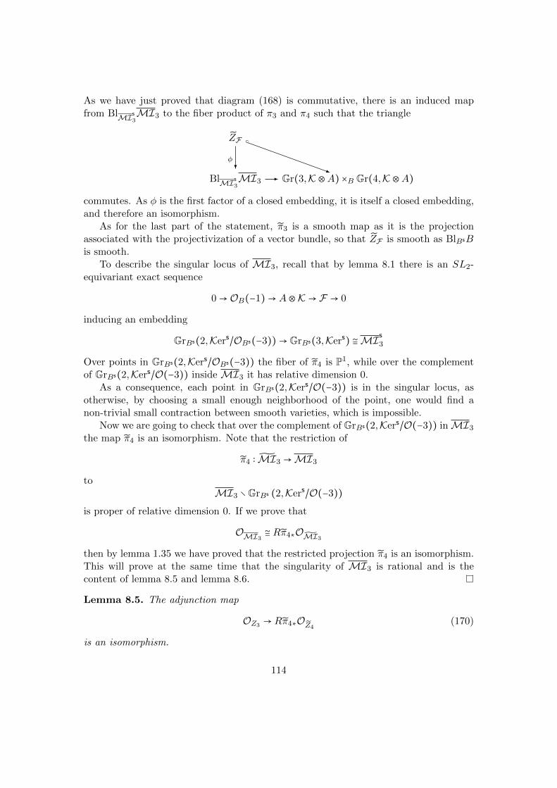
As we have just proved that diagram (168) is commutative, there is an induced mapfrom Bl

MIs3MI3 to the fiber product of π3 and π4 such that the triangle

ZF

BlMI

s3MI3

φ?

- Gr(3,K ⊗A) ×B Gr(4,K ⊗A)

⊂

-

commutes. As φ is the first factor of a closed embedding, it is itself a closed embedding,and therefore an isomorphism.

As for the last part of the statement, π3 is a smooth map as it is the projectionassociated with the projectivization of a vector bundle, so that ZF is smooth as BlBsBis smooth.

To describe the singular locus of MI3, recall that by lemma 8.1 there is an SL2-equivariant exact sequence

0→ OB(−1)→ A⊗K → F → 0

inducing an embedding

GrBs(2,Kers/OBs(−3))→ GrBs(3,Kers) ≅MIs3

Over points in GrBs(2,Kers/OBs(−3)) the fiber of π4 is P1, while over the complementof GrBs(2,Kers/O(−3)) inside MI3 it has relative dimension 0.

As a consequence, each point in GrBs(2,Kers/O(−3)) is in the singular locus, asotherwise, by choosing a small enough neighborhood of the point, one would find anon-trivial small contraction between smooth varieties, which is impossible.

Now we are going to check that over the complement of GrBs(2,Kers/O(−3)) inMI3

the map π4 is an isomorphism. Note that the restriction of

π4 ∶ MI3 →MI3

toMI3 ∖GrBs (2,Kers/O(−3))

is proper of relative dimension 0. If we prove that

OMI3

≅ Rπ4∗OMI3then by lemma 1.35 we have proved that the restricted projection π4 is an isomorphism.This will prove at the same time that the singularity of MI3 is rational and is thecontent of lemma 8.5 and lemma 8.6.

Lemma 8.5. The adjunction map

OZ3 → Rπ4∗OZ4(170)

is an isomorphism.

114

Proof. Take the locally free resolution of OZ4 given by the Koszul complex of

V ⊗ T rel4

σ4Ð→ OGrB(4,K⊗A) (171)

Pull it back via the flat map π3 to find a Koszul resolution for OZ4.

We are now going to pushforward the Koszul resolution for OZ4via π4. Clearly,

Rπ4∗OFlB(3,4,A⊗K) ≅ OGrB(3,A⊗K)

The tautological flag fits in an exact sequence

0→ π∗4T rel3 → π∗3T rel

4 → Oπ4(−1)→ 0 (172)

so thatRπ4∗π

∗

3T rel4 ≅ Rπ4∗π

∗

4T rel3

By projection formulaRπ4∗π

∗

4T rel3 ≅ T rel

3

As the projections π4 and π3 are SL2-equivariant, the SL2-invariant section (171) istransformed into the unique SL2-invariant section

V ⊗ T rel3

σ3Ð→ OGrB(3,K⊗A)

In order to prove (170), it is enough to prove that

Riπ4∗π∗

3 Λi(T rel4 ⊗ V )

vanish for i > 0. The exterior powers

Λi(T rel4 ⊗ V )

admit a filtration (see e.g. [Wey03]) with subquotients

ΣαT rel4 ⊗ΣαT V (173)

where Σα is the Schur functor associated with a Young diagram α such that ∣α∣ = i. Notethat (173) is not zero only when α is contained in a 5-by-4 rectangle, as the ranks ofT rel

4 and V are respectively 4 and 5.The Schur powers of T rel

4 can be rewritten in terms of Schur powers of T rel3 and

Oπ4(−1). This can be done via a natural filtration for

ΣαT rel4

induced by the tautological flag (172). The associated graded object of this naturalfiltration is

⊕β⊆α

(ΣβT rel3 ⊗Σα/βOπ4(−1)) (174)

115

where Σα/β are the skew Schur functors. As α is contained in a 5-by-4 rectangle

Σα/β(Oπ4(−1)) = Oπ4(−j) (175)

for j ∈ [0,5]. As π4 is the projectivization of a rank 6 vector bundle, the line bundleshave vanishing higher pushforward. Finally, by projection formula the pushforward ofsummands of (174) is

ΣβT rel3 ⊗Rπ4∗Oπ4(−j)

which is always concentrated in degree 0.

Lemma 8.6. The adjunction map

OMI3

→ Rπ4∗OZF (176)

is an isomorphism.

Proof. On Z4 there are exact sequences

0→ IZF /Z4→ OZ4

→ OZF → 0

and0→ IZv4∩ZF /Zv4

→ OZv4 → OZv4∩ZF → 0

By lemma 8.5Rπ4∗OZ4

≅ OZ3

so that our claim becomes that Rπ4∗IZF /Z4vanishes, or equivalently

Rπ4∗IZv4∩ZF /Zv4= 0 (177)

We are now going to prove that (177) is an isomorphism. To this purpose, recallthat the intersection of Zv4 and ZF inside GrBs(4,Kers) is described in lemma 8.2 and8.3. As a consequence, the commutative diagram

Zv4 ∩ ZF ⊂ - Zv4

MIs3?-

is isomorphic to the commutative diagram

FlBs(3,OBs(−3) ⊂ 4,Kers) ⊂- FlBs(3,4,Kers)

GrBs(3,Kers)?-

(178)

where the projections are the natural ones to GrBs(3,Kers) and where the upper leftcorner is the flag variety of subbundles of Kers such that the injection (162) restrictedto Bs factors via the 4-dimensional subbundle.

The ideal of the top left corner of diagram (178) is the pullback of O(−1) fromGr(4,Kers) (possibly with a twist by a line bundle on Bs). It follows that it is acyclicon the fibers of the projection to GrBs(3,Kers), so that (177) holds.

116

References

[AHDM78] Michael Francis Atiyah, Nigel James Hitchin, Vladimir Gershonovich Drin-feld, and Yuri Ivanovich Manin. Construction of instantons. Physics LettersA, 65(3):185–187, 1978.

[BF09] Maria Chiara Brambilla and Daniele Faenzi. Moduli spaces of arithmeticallyCohen-Macaulay bundles on Fano manifolds of the principal series. Boll.Unione Mat. Ital. (9), 2(1):71–91, 2009.

[BK90] Alexei I Bondal and Mikhail M Kapranov. Representable functors, serrefunctors, and mutations. Mathematics of the USSR-Izvestiya, 35(3):519,1990.

[Boh06] Christian Bohning. Derived categories of coherent sheaves on rational ho-mogeneous manifolds. Documenta Mathematica, 11:261–331, 2006.

[Bon90] Alexei I Bondal. Representation of associative algebras and coherent sheaves.Mathematics of the USSR-Izvestiya, 34(1):23, 1990.

[BVdB03] Alexei Bondal and Michel Van den Bergh. Generators and representabilityof functors in commutative and noncommutative geometry. Mosc. Math. J,3(1):1–36, 2003.

[Cas91] Guido Castelnuovo. Ricerche di geometria della retta nello spazio a quat-tro dimensioni. Atti del Reale Istituto Veneto di Scienze, Lettere e Arti,7(2):855–901, 1891.

[Cor00] Alessio Corti. Singularities of linear systems and 3-fold birational geometry.2000.

[Eis95] David Eisenbud. Commutative algebra with a view toward algebraic geome-try, volume 27. Springer New York, 1995.

[ES81] Geir Ellingsrud and Stein Arild Strømme. Stable rank-2 vector bundles onP3 with c1 = 0 and c2 = 3. Mathematische Annalen, 255(1):123–135, 1981.

[Fae11] Daniele Faenzi. Even and odd instanton bundles on Fano threefolds of Picardnumber one. Manuscripta Mathematica, pages 1–41, 2011.

[Ful98] William Fulton. Intersection theory, volume 93. Springer Berlin, 1998.

[GD67] A Grothendieck and J Dieudonne. Elements de geometrie algebrique. Publ.math. IHES, 8(24):2–7, 1967.

[GK04] A Gorodentsev and S Kuleshov. Helix theory. Mosc. Math. J, 4(2):377–440,2004.

117

[GM75] Hans Grauert and Gerhard Mulich. Vektorbundel vom Rang 2 uber demn-dimensionalen komplex-projektiven Raum. Manuscripta Mathematica,16(1):75–100, 1975.

[GM03] Sergei Izrailevich Gel’fand and Yuri Manin. Methods of homological algebra.Springer, 2003.

[Har80] Robin Hartshorne. Stable reflexive sheaves. Math. Ann., 254(2):121–176,1980.

[Hir81] Andre Hirschowitz. Sur la restriction des faisceaux semi-stables. In An-nales scientifiques de l’Ecole Normale Superieure, volume 14, pages 199–207.Societe mathematique de France, 1981.

[Hop84] Hans Jurgen Hoppe. Generischer Spaltungstyp und zweite Chernklasse sta-biler Vektorraumbundel vom Rang 4 auf P4. Mathematische Zeitschrift,187(3):345–360, 1984.

[IP99] Vasilii Alekseevich Iskovskikh and Yuri Prokhorov. Fano varieties, algebraicgeometry, v, 1–247. Encyclopaedia Math. Sci, 47, 1999.

[Isk80] Vasilii Alekseevich Iskovskikh. Anticanonical models of three-dimensionalalgebraic varieties. Journal of Mathematical Sciences, 13(6):745–814, 1980.

[JV11] Marcos Jardim and Misha Verbitsky. Trihyperkahler reduction and instantonbundles on P3. arXiv preprint arXiv:1103.4431, 2011.

[KO73] Shoshichi Kobayashi and Takushiro Ochiai. Characterizations of complexprojective spaces and hyperquadrics. Journal of Mathematics of Kyoto Uni-versity, 13(1):31–47, 1973.

[Kuz06] Alexander Kuznetsov. Homological projective duality for grassmannians oflines. arXiv preprint math/0610957, 2006.

[Kuz07] Alexander Kuznetsov. Homological projective duality. Publ. Math. Inst.Hautes Etudes Sci., (105):157–220, 2007.

[Kuz09] Alexander Kuznetsov. Hochschild homology and semiorthogonal decompo-sitions. arXiv preprint arXiv:0904.4330, 2009.

[Kuz12] Alexander Kuznetsov. Instanton bundles on Fano threefolds. Cent. Eur. J.Math., 10(4):1198–1231, 2012.

[Lip09] Joseph Lipman. Foundations of Grothendieck duality for diagrams ofschemes. Number 1960. Springer, 2009.

[MT10] D Markushevich and Alexander S Tikhomirov. Rationality of instantonmoduli. arXiv preprint arXiv:1012.4132, 2010.

118

[MU83] Shigeru Mukai and Hiroshi Umemura. Minimal rational threefolds. In Alge-braic geometry, pages 490–518. Springer, 1983.

[Nee96] Amnon Neeman. The Grothendieck duality theorem via Bousfield’s tech-niques and Brown representability. Journal of the American MathematicalSociety, 9(1):205–236, 1996.

[Orl91] D. O. Orlov. Exceptional set of vector bundles on the variety V5. VestnikMoskov. Univ. Ser. I Mat. Mekh., 5:69–71, 1991.

[OSS80] Christian Okonek, Michael Schneider, and Heinz Spindler. Vector bundles oncomplex projective spaces, volume 3 of Progress in Mathematics. BirkhauserBoston, Mass., 1980.

[Rud90] Alexei N Rudakov. Helices and vector bundles: Seminaire Rudakov, volume148. Cambridge University Press, 1990.

[Tev05] Evgueni A Tevelev. Projective duality and homogeneous spaces, volume 4.Springer, 2005.

[Tik12] Aleksandr S Tikhomirov. Moduli of mathematical instanton vector bundleswith odd c2 on projective space. Izvestiya: Mathematics, 76(5):991, 2012.

[Wey03] Jerzy Weyman. Cohomology of vector bundles and syzygies, volume 149.Cambridge University Press, 2003.

119