mathematics for physicists ii - mathematik.uni-muenchen.depetrakis/script.pdf · chapter 1...
TRANSCRIPT
Mathematics for Physicists II
Iosif Petrakis
Fakultat fur Physik, Ludwig-Maximilians-Universitat MunchenSummer term 2019

i
Acknowledgement
These lecture notes owe a lot to the excellent book of Lang [17]. I would liketo thank Leonid Kolesnikov, Felix Palm, Anne Reif, Jago Silberbauer, ChristianKoke and Florian Ingerl for giving the tutorials of this lecture course and for theircomments and suggestions. Last, but not least, I would like to thank the studentswho followed the course.


Contents
Chapter 1. Introduction: Notions of space and categories 1
Chapter 2. Linear spaces and linear maps 92.1. Linear spaces and linear subspaces 92.2. Finite-dimensional linear spaces 122.3. Existence of a basis 182.4. Linear maps 202.5. Quotient spaces 302.6. The free linear space 372.7. Convex sets 422.8. Caratheodory’s theorem 49
Chapter 3. Matrices 553.1. The linear space of matrices 553.2. The linear map of a matrix 603.3. The matrix of a linear map 64
Chapter 4. Inner product spaces 734.1. The Euclidean inner product space and the Minkowski spacetime 734.2. Existence of an orthogonal basis, the positive definite case 824.3. Existence of an orthogonal basis, the general case 894.4. Sylvester’s theorem 914.5. Open sets in Rn 934.6. Differentiable functions on open sets in Rn 964.7. The dual space of an inner product space 100
Chapter 5. Operators 1035.1. Symmetric and unitary operators 1035.2. Eigenvalues and eigenvectors 1075.3. The simplest ode, but one of the most important 1095.4. Determinants 1135.5. The characteristic polynomial 1175.6. The spectral theorem 119
Chapter 6. Appendix 125
iii
iv CONTENTS
6.1. Some logic 1256.2. Some set theory 1286.3. Some more category theory 131
Bibliography 133

CHAPTER 1
Introduction: Notions of space and categories
There is a big variety of notions of space in mathematics. For example, thereare Hilbert spaces, which are a special case of inner product spaces, Banach spaces,which are a special case of normed spaces, metric spaces, topological spaces, mea-sure spaces, manifolds and many more. Roughly speaking, an S-space, is a pairS := (X;S), where X is a set, which is called the carrier set of S, and S is aspace-structure associated to X. Usually, S is a family of functions associated toX and some fundamental sets in mathematics, like the set of real numbers R. Ifa set X can be equipped with many different space-structures, then X is a very“interesting” set. E.g., if n ≥ 1, the set
Rn := {(x1, . . . , xn) | x1 ∈ R & . . . & xn ∈ R}
of n-tuples of real numbers is the carrier set of a Hilbert space, and hence of aBanach space, of a metric space, and of a topological space, but also of an n-manifold, and of a measure space. All these space-structures, which often areinterconnected, shed a different light in the mathematical “nature” of Rn. A centraltool in the study of S-spaces is the notion of an S-map. Roughly speaking, ifS := (X;S) and T := (Y ;T ) are S-spaces, an S-map is a function f : X → Ythat “preserves” the corresponding space-structures. Let C(S, T ) be the set of allS-maps from S to T . It is expected that the identity map idX on X, where
idX : X → X, x 7→ x,
is an S-map. Moreover, if U := (Z;U) is an S-space, and if f : X → Y is in C(S, T )and g : Y → Z is in C(T ,U), their composition
g ◦ f : X → Z, x 7→ g(f(x)),
is in C(S,U)
X Y Z.f g
g ◦ f
If F(X,Y ) is the set of all functions from X to Y , and f, g ∈ F(X,Y ), then
f = g ⇔ ∀x∈X(f(x) = g(x)
).
1

2 1. INTRODUCTION: NOTIONS OF SPACE AND CATEGORIES
By the definition of composition of functions we have that f ◦ idX = f , or that thefollowing diagram commutes
X X Y ,idX f
f
and that idY ◦ f = f , or that the following diagram commutes
X Y Y .f idY
f
Note that the composition of functions is associative i.e., if
X Y Z W ,f g h
then h ◦ (g ◦ f) = (h ◦ g) ◦ f , or the following outer diagram commutes
X Y Z W .f g h
g ◦ f
h ◦ (g ◦ f)
h ◦ g
(h ◦ g) ◦ f
If f ∈ C(S, T ) and g ∈ C(T ,S) such that the following diagrams commute
X Y X Yf g
f
idX
idY
i.e., g ◦ f = idX and f ◦ g = idY , the corresponding S-spaces are considered to bethe “same” S-spaces. We call then f , or g, an S-isomorphism between S and T ,while the S-spaces S and T are called S-isomorphic. In this case we write S ' T ,and we also write (f, g) : S ' T to express that f and g “prove” S ' T . It is easyto see that if (f, g) : S ' T and (f, g′) : S ' T , then g = g′.
Remark 1.0.1. Let S := (X;S), T := (Y ;T ), and U := (Z;U) be S-spaces.
(i) S ' S.
(ii) If S ' T , then T ' S.
(iii) If S ' T and T ' U , then S ' U .
Proof. Exercise. �
1. INTRODUCTION: NOTIONS OF SPACE AND CATEGORIES 3
An important theme in the study of S-spaces is the construction of new S-spaces from given ones. A notion of an S-space is mathematically fruitful, if manysuch constructions are possible. It is desirable to have a notion of S-subspace,namely, if Y ⊆ X and S := (X;S) is an S-space, an S-space S|Y := (Y ;S|Y ) isdefined. Moreover, if S and T are S-spaces, their S-product S ×T is also expectedto be defined. It is also useful to be able to “glue” together S-spaces, or to addan S-structure on the set C(S, T ) of S-maps from S to T . Usually, some specificS-spaces have a special role among other S-spaces, and they can be used to classifymany other S-spaces. A “classification theorem” for S-spaces determines a largeclass of S-spaces that are S-isomorphic to some distinguished S-space. E.g., in thetheory of linear spaces and linear maps, the linear space Rn has a very special roleamong the so-called finite-dimensional linear spaces. Usually, the set of S-mapsfrom an S-space S to such a distinguished S-space provides information on theoriginal space S. The linear space of linear maps from a linear space V to R is suchan example.
The collection of all S-spaces and S-maps between them forms the category ofS-spaces. The study of categories of mathematical objects and abstract “maps”between them is the subject matter of Category Theory (see e.g. [3]). The theoryof sets (see e.g., [10]), and the category theory are the most popular “dialects” inthe language of modern mathematics.
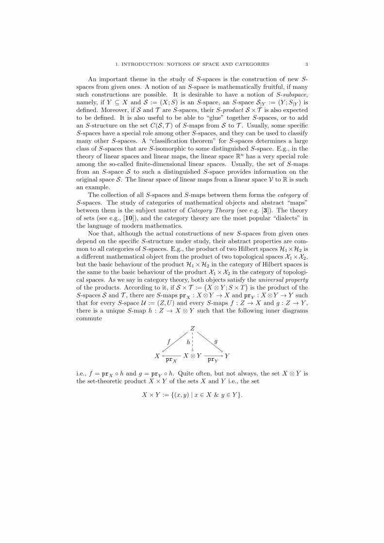
Noe that, although the actual constructions of new S-spaces from given onesdepend on the specific S-structure under study, their abstract properties are com-mon to all categories of S-spaces. E.g., the product of two Hilbert spaces H1×H2 isa different mathematical object from the product of two topological spaces X1×X2,but the basic behaviour of the product H1×H2 in the category of Hilbert spaces isthe same to the basic behaviour of the product X1×X2 in the category of topologi-cal spaces. As we say in category theory, both objects satisfy the universal propertyof the products. According to it, if S × T :=
(X ⊗ Y ;S × T
)is the product of the
S-spaces S and T , there are S-maps prX : X⊗Y → X and prY : X⊗Y → Y suchthat for every S-space U := (Z,U) and every S-maps f : Z → X and g : Z → Y ,there is a unique S-map h : Z → X ⊗ Y such that the following inner diagramscommute
X X ⊗ Y Y
Z
prX prY
f gh
i.e., f = prX ◦ h and g = prY ◦ h. Quite often, but not always, the set X ⊗ Y isthe set-theoretic product X × Y of the sets X and Y i.e., the set
X × Y := {(x, y) | x ∈ X & y ∈ Y }.

4 1. INTRODUCTION: NOTIONS OF SPACE AND CATEGORIES
Definition 1.0.2 (Eilenberg, Mac Lane (1945)). A category C is a structure(C0, C1, dom, cod, ◦,1), where
(i) C0 is the collection of the objects of C,
(ii) C1 is the collection of the arrows of C,
(iii) For every f in C1, dom(f), the domain of f , and cod(f), the codomain of f ,are objects in C0, and we write f : A→ B, where A = dom(f) and B = cod(f),
(iv) If f : A→ B and g : B → C are arrows of C i.e., dom(g) = cod(f), there is anarrow g ◦ f : A→ C, which is called the composite of f and g,
(v) For every A in C0, there is an arrow 1A : A→ A, the identity arrow of A,
such that the following conditions are satisfied:
(a) If f : A→ B, then f ◦ 1A = f = 1B ◦ f .
(b) If f : A→ B, g : B → C and h : C → D, then h ◦ (g ◦ f) = (h ◦ g) ◦ f .
If A,B are in C0, we denote by HomC(A,B), or simply by Hom(A,B), if C is clearfrom the context, the collection of arrows f in C1 with dom(f) = A and cod(f) = B.
The objects of a category are not necessarily sets. E.g., in the next chapter wewill study certain properties of the category of (real) linear spaces LinR, or simplerLin, that has as objects the (real) linear spaces, which are sets equipped with alinear structure. The arrows of Lin are certain functions between the carrier setsof the corresponding linear spaces, which are called linear maps.
Example 1.0.3. If X is not equipped with some S-structure, or, equivalently,if it is equipped with the empty structure, the corresponding category of S-spaces isthe category of sets Set. Its objects are sets, and its arrows are functions betweensets. If A is a set, then 1A := idA, and the composition of arrows is the compositionof functions.
Next we give an example of a category the arrows of which are not functions.
Example 1.0.4. The category Rel has objects sets, and an arrow f : A → Bis any subset of A×B i.e., any binary relation on A,B. If A is a set, let
1A :={
(a, a′) ∈ A×A | a = a′},
while, if R ⊆ A×B and S ⊆ B × C, let
S ◦R :={
(a, c) ∈ A× C | ∃b∈B((a, b) ∈ R & (b, c) ∈ S
)}.
Definition 1.0.5. A partially ordered set, or a poset, is a pair (I,�), where Iis a set, and � ⊆ I × I satisfying the following conditions:
(i) ∀i∈I(i � i
).
(ii) ∀i,j∈I(i � j & j � i⇒ i = j
).
(iii) ∀i,j,k∈I(i � j & j � k ⇒ i � k
).

1. INTRODUCTION: NOTIONS OF SPACE AND CATEGORIES 5
If (J,≤) is any poset, a function m : I → J is called monotone, if
∀i,i′∈I(i � i′ ⇒ m(i) ≤ m(i′)
).
Clearly, (R,≤) is a poset, which is linearly ordered i.e., ∀a,b∈R(a ≤ b ∨ b ≤ a
).
Example 1.0.6. The category Pos has objects posets and an arrow m : I → Jis any monotone function. If (I,�) is a poset, we have 1A := idA, and ◦ in Pos isthe composition of functions.
Categories can be used to describe various physical phenomena (see [8], [9]). Ifwe consider a physical system of some type A (e.g., an electron), and if an operation(e.g., a measurement) is performed on it, which results in a system of some typeB, this situation can be described by an arrow f : A→ B. An operation g on thesystem that follows f can be described by the arrow g : B → C, and g ◦ f denotesthe consecutive application of f and g. The trivial operation of “no operation” ona system of type A is denoted by 1A. For many non-trivial applications of categorytheory to mathematical physics see [21].
Next we define the right notion of “map” between categories.
Definition 1.0.7. Let C and D be categories. A covariant functor, or simplya functor from C to D is a pair F = (F0, F1), where:
(i) F0 maps an object A of C to an object F0(A) of D,
(ii) F1 maps an arrow f : A→ B of C to an arrow F1(f) : F0(A)→ F0(B) of D,
such that the following conditions are satisfied:
(a) For every A in C0 we have that F1(1A) = 1F0(A)
F0(A)
F0(A).
1F0(A) F1(1A)
(b) If f : A→ B and g : B → C, then F1(g ◦ f) = F1(g) ◦ F1(f) i.e., the followingdiagram commutes
F0(A) F0(B) F0(C),F1(f) F1(g)
F1(g ◦ f)
where for simplicity we use the same symbol for the operation of composition inthe categories C and D. In this case we write1 F : C →D.
A contravariant functor from C to D is a pair F := (F0, F1), where:
1In the literature it is often written F (C) and F (f), instead of F0(C) and F1(f).

6 1. INTRODUCTION: NOTIONS OF SPACE AND CATEGORIES
(i) F0 maps an object A of C to an object F0(A) of D,
(ii′) F1 maps an arrow f : A→ B of C to an arrow F1(f) : F0(B)→ F0(A) of D,
such that the following conditions are satisfied:
(a) F1(1A) = 1F0(A), for every A in C0.
(b′) If f : A→ B and g : B → C, then F1(g ◦ f) = F1(f) ◦ F1(g) i.e., the followingdiagram commutes
F0(C) F0(B) F0(A),F1(g) F1(f)
F1(g ◦ f)
In this case we write F : Cop →D.
Example 1.0.8. If C is a category, the identity functor on C is the pairIdC := (IdC
0 , IdC1 ) : C → C, where IdC
0 (X) := X, for every X in C0, and if
f : X → Y , then IdC1 (f) := f .
Example 1.0.9. The pair F := (F0, F1) : Set→ Rel, where F0(X) := X, andif f : X → Y , then F1(f) := {(a, b) ∈ A × B | b = f(a)} := Gr(f), is a covariantfunctor from Set to Rel.
Example 1.0.10. The pair (G0, G1) : Set → Set, where G0(X) := F(X) :={φ : X → R}, and if f : X → Y , then G1(f) : F(Y )→ F(X) is defined by
[G1(f)])(θ) := θ ◦ f
X Y
R,
f
θθ ◦ f
for every θ ∈ F(Y ), is a contravariant functor from Set to Set. If X is a set, then
[G1(idX)])(φ) := φ ◦ idX = φ
and since φ ∈ F(X) is arbitrary, we conclude that G1(idX) = idF(X) := idG0(X). Iff : X → Y and g : Y → Z, then G1(f) : F(Y )→ F(X), G1(g) : F(Z)→ F(Y ) andG1(g ◦ f) : F(Z)→ F(X). Moreover, if η ∈ F(Z), we have that
[G1(g ◦ f)](η) := η ◦ (g ◦ f)
= (η ◦ g) ◦ f:= [G1(f)](η ◦ g)
:= G1(f)([G1(g)](η)
):= [G1(f) ◦G1(g)](η).
1. INTRODUCTION: NOTIONS OF SPACE AND CATEGORIES 7
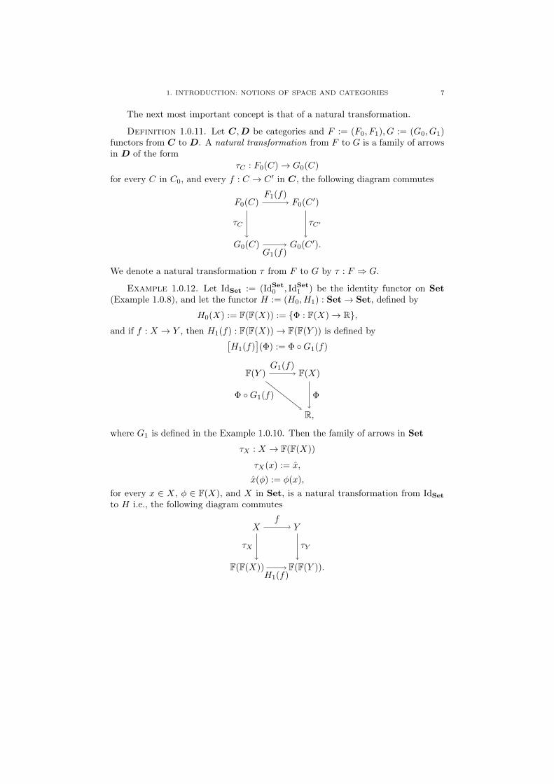
The next most important concept is that of a natural transformation.
Definition 1.0.11. Let C,D be categories and F := (F0, F1), G := (G0, G1)functors from C to D. A natural transformation from F to G is a family of arrowsin D of the form
τC : F0(C)→ G0(C)
for every C in C0, and every f : C → C ′ in C, the following diagram commutes
F0(C) F0(C ′)
G0(C ′).G0(C)
F1(f)
τC′
G1(f)
τC
We denote a natural transformation τ from F to G by τ : F ⇒ G.
Example 1.0.12. Let IdSet := (IdSet0 , IdSet
1 ) be the identity functor on Set(Example 1.0.8), and let the functor H := (H0, H1) : Set→ Set, defined by
H0(X) := F(F(X)) := {Φ : F(X)→ R},and if f : X → Y , then H1(f) : F(F(X))→ F(F(Y )) is defined by[
H1(f)](Φ) := Φ ◦G1(f)
F(Y ) F(X)
R,
G1(f)
ΦΦ ◦G1(f)
where G1 is defined in the Example 1.0.10. Then the family of arrows in Set
τX : X → F(F(X))
τX(x) := x,
x(φ) := φ(x),
for every x ∈ X, φ ∈ F(X), and X in Set, is a natural transformation from IdSet
to H i.e., the following diagram commutes
X Y
F(F(Y )).F(F(X))
f
τY
H1(f)
τX
8 1. INTRODUCTION: NOTIONS OF SPACE AND CATEGORIES
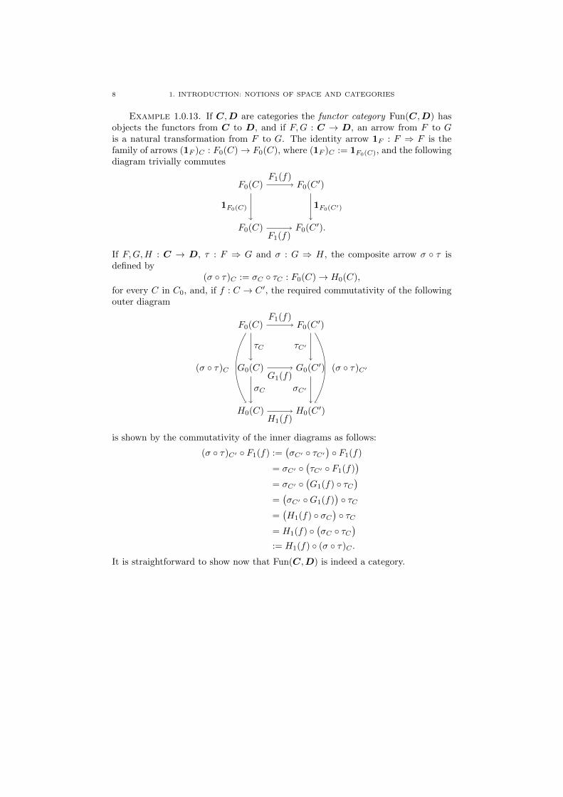
Example 1.0.13. If C,D are categories the functor category Fun(C,D) hasobjects the functors from C to D, and if F,G : C → D, an arrow from F to Gis a natural transformation from F to G. The identity arrow 1F : F ⇒ F is thefamily of arrows (1F )C : F0(C)→ F0(C), where (1F )C := 1F0(C), and the followingdiagram trivially commutes
F0(C) F0(C ′)
F0(C ′).F0(C)
F1(f)
1F0(C′)
F1(f)
1F0(C)
If F,G,H : C → D, τ : F ⇒ G and σ : G ⇒ H, the composite arrow σ ◦ τ isdefined by
(σ ◦ τ)C := σC ◦ τC : F0(C)→ H0(C),
for every C in C0, and, if f : C → C ′, the required commutativity of the followingouter diagram
F0(C) F0(C ′)
G0(C ′)G0(C)
H0(C) H0(C ′)
F1(f)
τC′
G1(f)
τC
σC σC′
H1(f)
(σ ◦ τ)C (σ ◦ τ)C′
is shown by the commutativity of the inner diagrams as follows:
(σ ◦ τ)C′ ◦ F1(f) :=(σC′ ◦ τC′
)◦ F1(f)
= σC′ ◦(τC′ ◦ F1(f)
)= σC′ ◦
(G1(f) ◦ τC
)=(σC′ ◦G1(f)
)◦ τC
=(H1(f) ◦ σC
)◦ τC
= H1(f) ◦(σC ◦ τC
):= H1(f) ◦ (σ ◦ τ)C .
It is straightforward to show now that Fun(C,D) is indeed a category.
CHAPTER 2
Linear spaces and linear maps
In this chapter we study the basic properties of the linear spaces–also calledvector spaces–and of the linear maps between them. A linear space is a set en-dowed with a linear structure, and a linear map between linear spaces is a functionbetween their carrier sets that preserves their linear structure. Both, the innerproduct spaces and the normed spaces, are linear spaces with some extra topo-logical structure. Hence, the linear spaces are instrumental in the mathematicaldescription of physical reality. The linear structure of R3 is a fundamental com-ponent of the geometric representation of the classical physical world. Throughoutthese lecture notes, when we write Rn, we mean that n ≥ 1.
2.1. Linear spaces and linear subspaces
Definition 2.1.1. A linear space, or a vector space, over R is a structureV := (X; +,0, ·), where X is a set, 0 ∈ X, and +, · are functions
+ : X ×X → X, · : R×X → X
(x, y) 7→ x+ y, (a, x) 7→ a · x,such that the following conditions are satisfied:
(LS1) ∀x,y,z∈X((x+ y) + z = x+ (y + z)
).
(LS2) ∀x∈X(x+ 0 = 0 + x = x
).
(LS3) ∀x∈X∃y∈X(x+ y = 0
).
(LS4) ∀x,y∈X(x+ y = y + x
).
(LS5) ∀x,y∈X∀a∈R(a · (x+ y) = a · x+ a · y
).
(LS6) ∀x∈X∀a,b∈R((a+ b) · x = a · x+ b · x
).
(LS7) ∀x∈X∀a,b∈R((ab) · x = a · (b · x)
).
(LS8) ∀x∈X(1 · x = x
).
For simplicity, we may write ax instead of a · x. The triple (+,0, ·) is called thesignature of the linear space V. If, instead of R, we consider any field1 F, the
1A field is a structure (F;+,0, ·,1), where F is a set, 0,1 ∈ F, + : F×F→ F, and · : F×F→ Fsuch that together with (LS1)− (LS4) the following conditions are satisfied:
9

10 2. LINEAR SPACES AND LINEAR MAPS
corresponding structure is called a linear space over F. A linear space over R isalso called a real linear space, and a linear space over the field of complex numbersC is called a complex linear space. If V is a linear space, the elements of X aretraditionally called vectors. A linear space is called non-trivial, if it contains avector x such that x 6= 0. Unless stated otherwise, the linear spaces considered hereare going to be real. When the linear structure on X is clear from the context, weuse for simplicity X to denote the vector space V.
Example 2.1.2. Let the structure Rn := (Rn; +,0, ·), where
Rn := {(x1, . . . , xn) | x1 ∈ R & . . . & xn ∈ R},(x1, . . . , xn) = (y1, . . . , yn)⇔ x1 = y1 & . . . & xn = yn,
(x1, . . . , xn) + (y1, . . . , yn) := (x1 + y1, . . . , xn + yn),
0 := (0, . . . , 0),
a · (x1, . . . , xn) := (ax1, . . . , axn).
Clearly, Rn a linear space over R, and, similarly, Qn := (Qn; +,0, ·) is linear spaceover Q, and Cn := (Cn; +,0, ·) is a linear space over C.
Example 2.1.3. If X is a set, F(X) is the set of all functions f : X → R, and
if we define the functions f + g, 0X
and a · f , where a ∈ R, by
(f + g)(x) := f(x) + g(x),
0X
(x) := 0,
(a · f)(x) := af(x),
for every x ∈ X, then F(X) := (F(X); +, 0X, ·) is a linear space over R.
The Example 2.1.3 shows that a mathematical object can be viewed as a vector,although no immediate geometric intuition is associated with it. If
n := {0, 1, . . . , n− 1}though, an element of Rn can be identified with a function f : n → R, and thenthe Example 2.1.2 is a special case of the Example 2.1.3. If f, g ∈ F(X) and a ∈ R,
f ≤ g ⇔ ∀x∈X(f(x) ≤ g(x)
),
∀x,y,z∈F(x · (y · z) = (x · y) · z
).
∀x,y,z∈F(x · (y+ z) = x · y+ x · z
).
∀x,y∈F(x · y = y · x
).
∀x∈F(1 · x = x
).
∀x∈F(x 6= 0⇒ ∃y∈F(x · y = 1)
).
It is immediate to see that the rational numbers Q, the real numbers R and the complex numbers Chave a field structure. Actually, Q is a subfield of R and R is a subfield of C i.e., the field-signature
(+,0, ·,1) of Q is inherited from the field-signature of R, which, in turn, can be inherited fromthe field-signature of C.
2.1. LINEAR SPACES AND LINEAR SUBSPACES 11
f ≤ a :⇔ f ≤ aX ⇔ ∀x∈X(f(x) ≤ a)
),
where aX(x) := a, for every x ∈ X.
Remark 2.1.4. Let V := (X; +,0, ·) be a linear space, a, b ∈ R, and x, y, z, w ∈X. The following hold:
(i) If z = w and x = y, then z + x = w + y.
(ii) If x = y and a = b, then a · x = b · y.
(iii) If x+ y = x+ z = 0, then y = z.
(iv) 0 · x = 0.
(v) (−1) · x = −x, where, because of case (iii), −x is the unique element y of Xin condition (LS3) such that x+ y = 0.
(vi) If x 6= 0 and a · x = 0, then a = 0.
Proof. Exercise. �
Definition 2.1.5. Let V := (X; +,0, ·) be a linear space, and Y ⊆ X suchthat the following conditions are satisfied:
(i) ∀y,y′∈Y(y + y′ ∈ Y
),
(ii) 0 ∈ Y ,
(iii) ∀y∈Y ∀a∈R(a · y ∈ Y
).
Then the structure
V|Y := (Y,+|Y×Y ,0, ·|R×Y ),
where +|Y×Y is the restriction of + to Y × Y and ·|R×Y is the restrictions of ·to R × Y , is called a linear subspace of V, or, simpler, a subspace of V. We writeV|Y � V to denote that V|Y is a linear subspace of V, although, for simplicity, werefer to a linear subspace V|Y mentioning only the set Y , and we write Y � X. Wedenote by Sub(V) the set of all subspaces of V.
Clearly, {0} and X are linear subspaces of X.
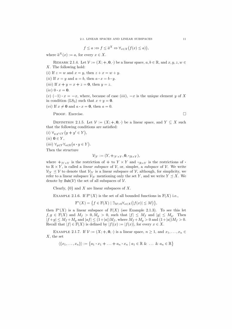
Example 2.1.6. If F∗(X) is the set of all bounded functions in F(X) i.e.,
F∗(X) ={f ∈ F(X) | ∃M>0∀x∈X
(|f(x)| ≤M
)},
then F∗(X) is a linear subspace of F(X) (see Example 2.1.3). To see this letf, g ∈ F(X) and Mf > 0,Mg > 0, such that |f | ≤ Mf and |g| ≤ Mg. Then|f+g| ≤Mf +Mg and |af | ≤ (1+ |a|)Mf , where Mf +Mg > 0 and (1+ |a|)Mf > 0.Recall that |f | ∈ F(X) is defined by |f |(x) := |f(x)|, for every x ∈ X.
Example 2.1.7. If V := (X; +,0, ·) is a linear space, n ≥ 1, and x1, . . . , xn ∈X, the set
〈{x1, . . . , xn}〉 :={a1 · x1 + . . .+ an · xn | a1 ∈ R & . . . & an ∈ R
}

12 2. LINEAR SPACES AND LINEAR MAPS
is a linear subspace of V. We call an elementn∑i=1
aixi := a1 · x1 + . . .+ anxn
of 〈{x1, . . . , xn}〉 a linear combination of x1, . . . , xn, and the space 〈{x1, . . . , xn}〉the linear span of x1, . . . , xn. We may write 〈x1, . . . , xn〉 instead of 〈{x1, . . . , xn}〉.
If e1 := (1, 0), e2 := (0, 1), and (x, y) ∈ R2, we get R2 = 〈e1, e2〉, since
(x, y) := x(1, 0) + y(0, 1) := xe1 + ye2.
Proposition 2.1.8. Let V := (X; +,0, ·) be a linear space, Y ⊆ X, and letU, V � X.
(i) If U + V := {u+ v | u ∈ U & v ∈ V }, then U + V � X.
(ii) If U ∩ V := {x ∈ X | x ∈ U & x ∈ V }, then U ∩ V � X.
(iii) If we define
〈Y 〉 :=⋂{
U � X | Y ⊆ U}
:={x ∈ X | ∀U�X(Y ⊆ U ⇒ x ∈ U)
},
then 〈Y 〉 is well-defined (i.e., the set {U � X | Y ⊆ Y } is non-empty) and it is theleast linear subspace of X that includes Y .
(iv) If Y 6= ∅, then
〈Y 〉 =
{ n∑i=1
aiyi | n ≥ 1 & ∀i∈{1,...,n}(ai ∈ R & yi ∈ Y
)}.
Proof. Exercise. �
Since ∅ ⊆ {0}, we have that 〈∅〉 = {0}. The subspace U + V of X is called thesum of U and V . By Proposition 2.1.8 the linear span 〈x1, . . . , xn〉 of x1, . . . , xn ∈ Xis the least linear space containing x1, . . . , xn. If X = 〈Y 〉, we say that Y generatesthe linear space V (or X), and the elements of Y are called generators of V.
2.2. Finite-dimensional linear spaces
Definition 2.2.1. Let V := (X; +,0, ·) be a linear space, n ≥ 1, and letx1, . . . , xn ∈ X. We say that the vectors x1, . . . , xn are linearly dependent, or thattheir set {y1, . . . , yn} is a linearly dependent subset of X, if
∃a1,...,an∈R(∃i∈{1,...,n}
(ai 6= 0
)&
n∑i=1
aixi = 0
).
We say that x1, . . . , xn are linearly independent, if they are not linearly dependent.A subset Y of X is called linearly dependent, if
∃n≥1∃y1,...,yn∈Y({y1, . . . , yn} is linearly dependent
),

2.2. FINITE-DIMENSIONAL LINEAR SPACES 13
while it is called linearly independent, if it is not a linearly dependent subset of X.
If x1, . . . , xn are linearly dependent, a1x1 + . . .+ anxn = 0, and ai 6= 0, then
xi =
(−a1
ai
)x1 + . . .+
(−ai−1
ai
)xi−1 +
(−ai+1
ai
)xi+1 + . . .+
(−anai
)xn
i.e., xi is a linear combination of a1, . . . , ai−1, ai+1, . . . , an.
Remark 2.2.2. Let X be a linear space and Y,Z ⊆ X.
(i) If x1, . . . , xn ∈ X, then x1, . . . , xn are linearly independent if and only if
∀a1,...,an∈R( n∑i=1
aixi = 0⇒ ∀i∈{1,...,n}(ai = 0)
).
(ii) Y is linearly independent if and only if
∀n≥1∀y1,...,yn∈Y({y1, . . . , yn} is linearly independent
).
(iii) {0} and X are linearly dependent subsets of X.
(iv) If x 6= 0, then {x} is a linearly independent subset of X.
(v) The empty set ∅ is a linearly independent subset of X.
(vi) If Y is linearly dependent and Y ⊆ Z, then Z is linearly dependent.
(vii) If Y is linearly independent and Z ⊆ Y , then Z is linearly independent.
Proof. (i) and (ii) By negating the corresponding defining formulas. E.g., for(i) we use the Corollary 6.1.3 and the Lemma 6.1.1 in the Appendix.(iii) 1 · 0 = 0, and {0} is a linearly dependent subset of X.(iv) It follows immediately by Remark 2.1.4(vi).(v) If we suppose that ∅ is a linearly dependent subset of X i.e.,
∃n≥1∃y1,...,yn(y1 ∈ ∅ & . . . & yn ∈ ∅ & {y1, . . . , yn} is linearly dependent
),
it is immediate that we get a contradiction from it.(vi) and (vii) are immediate to show. �
Example 2.2.3. The following n-vectors in Rn
e1 := (1, 0, . . . , 0), e2 := (0, 1, 0, . . . , 0), . . . , en := (0, . . . , 0, 1)
are linearly independent, since for every a1, . . . , an ∈ R we have thatn∑i=1
aiei = 0⇔ (a1, . . . , an) = 0⇔ a1 = . . . = an = 0.
Example 2.2.4. For every n ≥ 1, the following n-vectors in F(R)
f1(t) := et, . . . , fn(t) := ent
are linearly independent (Exercise).
14 2. LINEAR SPACES AND LINEAR MAPS
Remark 2.2.5. Let V := (X; +,0, ·) be a linear space, n ≥ 1, and x1, . . . , xn ∈X linearly independent. If a1, . . . , an, b1, . . . , bn ∈ R, then
n∑i=1
aixi =
n∑i=1
bixi ⇒(a1 = b1 & . . . & an = bn
).
Moreover, xi 6= 0, for every i ∈ {1, . . . , n}.
Proof. It follows from the Definition 2.2.1 and the equivalence
n∑i=1
aixi =
n∑i=1
bixi ⇔n∑i=1
(ai − bi)xi = 0.
If i ∈ {1, . . . , n} such that xi = 0, then 0x1 + 0xi−1 + 1xi+ 0xi+1 + . . .+ 0xn = 0,which by the hypothesis of linear independence is impossible2. �
Definition 2.2.6. If V := (X; +,0, ·) is linear space, a subset B of X is calleda basis of V (or, for simplicity a basis of X), if B is linearly independent, and〈B〉 = X. If V has a finite basis B, it is called a finite-dimensional linear space,while if it has an infinite basis, it is called infinite-dimensional.
Clearly, the subspace {0} has as a basis the empty set.
Example 2.2.7. The set En := {e1, . . . , en} of the linearly independent ele-ments in Rn that were defined in the Example 2.2.3 is the standard basis of Rn.Hence, Rn is finite-dimensional. It is easy to see that Rn has more than one bases.E.g., B := {(1, 1), (−1, 2)} is another basis of R2.
Example 2.2.8. Since the set E := {ent | n ≥ 1} is a linearly independentsubset of F(R), the set E is a basis of the linear subspace 〈E〉 of F(R), and 〈E〉 isinfinite-dimensional.
Corollary 2.2.9. Let V := (X; +,0, ·) be a linear space, and x ∈ X. IfB := {v1, . . . , vn} is a basis of V, there are unique a1, . . . , an ∈ R such that
x =
n∑i=1
aivi.
Proof. It follows by the definition of a basis and the Remark 2.2.5. �
These unique a1, . . . , an ∈ R are called the coordinates of x with respect to B.
Definition 2.2.10. Let V := (X; +,0, ·) be a linear space, {v1, . . . , vn} ⊆X and m ≤ n. The set {v1, . . . vm} is a maximal subset of linearly independentelements of X, if it is a linearly independent subset of X, and for every k ∈ N,such that m < k ≤ n, the set {v1, . . . , vm, vk} is a linearly dependent subset of X.
2This also follows from the Remark 2.2.2(vii)

2.2. FINITE-DIMENSIONAL LINEAR SPACES 15
Theorem 2.2.11 (Finite basis-criterion I). Let V := (X; +,0, ·) be a linearspace, n ≥ 1, and {v1, . . . , vn} ⊆ X such that X = 〈{v1, . . . , vn}〉. If {v1, . . . , vr}is a maximal subset of linearly independent elements of X, where 1 ≤ r ≤ n, then{v1, . . . , vr} is a basis of V.
Proof. If r = n, then {v1, . . . , vr} is a linearly independent subset generatingX i.e., it is a basis of V. If r < n, by the maximality of {v1, . . . , vr} the sets
{v1, . . . , vr, vr+1}, {v1, . . . , vr, vr+2}, . . . , {v1, . . . , vr, vn}are linearly dependent subsets of X. We show that
vr+1 ∈ 〈{v1, . . . , vr}〉 & vr+2 ∈ 〈{v1, . . . , vr}〉 & . . . & vn ∈ 〈{v1, . . . , vr}〉.We show this only for vr+1, and for vr+2, . . . , vn we proceed similarly. Since{v1, . . . , vn, vr+1} is linearly dependent, there are a1, . . . , ar, ar+1 ∈ R such that
a1v1 + . . .+ arvr + ar+1vr+1 = 0,
and not all of them are equal to 0. If ar+1 = 0, then a1v1 + . . . + arvr = 0,hence a1 = . . . = ar = ar+1 = 0, which is a contradiction. Hence ar+1 6= 0, andhence vr+1 can be written as a linear combination of v1, . . . , vr. Since an elementx of X is a linear combination of v1, . . . , vr, vr+1, . . . , vn and vr+1, . . . , vn are linearcombinations of v1, . . . , vr, then x is a linear combination of v1, . . . , vr. �
Next we show that we can replace any number of elements of a finite basis byan equal number of any linearly independent vectors.
Lemma 2.2.12 (Exchange lemma (Steinitz)). Let n,m ≥ 1, let {v1, . . . vn} bea basis of the linear space V := (X; +,0, ·), and let w1, . . . , wm ∈ X be linearlyindependent.
(i) If m < n, there are um+1, . . . , un ∈ {v1, . . . vn} such that
〈{w1, . . . , wm, um+1, . . . , un}〉 = X.
(ii) If m = n, then 〈{w1, . . . , wn}〉 = X.
Proof. (i) By the definition of a basis there are a1, . . . an ∈ R such that
w1 = a1v1 + . . .+ anvn.
Since by Remark 2.2.5 w1 6= 0, there is some ai 6= 0, where i ∈ {1, . . . , n}. Withoutloss of generality we can take i = 1 (if a1 = 0, we can re-enumerate the elementsof the set {v1, . . . vn} so that the first coefficient in the writing of w1 as a linearcombination of the elements of the set {v1, . . . vn} is non-zero). Hence
a1v1 = w1 −n∑i=2
aivi ⇔ v1 =1
a1w1 −
n∑i=2
aia1vi,
and consequently
v1 ∈⟨{w1, v2, . . . , vn
}⟩,

16 2. LINEAR SPACES AND LINEAR MAPS
and ⟨{w1, v2, . . . , vn
}⟩= X.
By the inductive hypothesis, if 1 ≤ r < m we get (possibly after a re-enumerationof the set {v1, . . . vn}) ⟨
{w1, . . . , wr, vr+1, . . . , vn}⟩
= X.
Hence,wr+1 = b1w1 + . . .+ brwr + cr+1vr+1 + . . .+ cnvn.
Not all the terms cr+1, . . . , cn are equal to 0, since then wr+1 would be a linearcombination of w1, . . . , wr, something that contradicts the hypothesis of linear in-dependence of the vectors w1, . . . , wm. Without loss of generality, let cr+1 6= 0,hence
cr+1vr+1 = wr+1 −[ r∑i=1
biwi +
n∑j=r+2
cjvj]⇔
vr+1 =1
cr+1wr+1 −
r∑i=1
bicr+1
wi −n∑
j=r+2
cjcr+1
vj ,
and consequently
vr+1 ∈⟨{w1, . . . , wr, wr+1, vr+2, . . . , vn
}⟩,
and ⟨{w1, . . . , wr, wr+1, vr+2, . . . , vn}
⟩= X.
After m-number of steps, we get 〈{w1, . . . , wm, um+1, . . . , un}〉 = X.(ii) It follows immediately by (i). �
Theorem 2.2.13. Let 0 < n < m, and let {v1, . . . vn} be a basis of the linearspace V := (X; +,0, ·). If w1, . . . , wm ∈ X, then w1, . . . , wm are linearly dependent.
Proof. Suppose that the vectors w1, . . . , wm are linearly independent. Sincethen the vectors w1, . . . , wn are also linearly independent, by the Lemma 2.2.12(ii)we have that w1, . . . , wn is a basis of X. By the hypothesis of linear indepen-dence we have that wn+1 6= 0, hence it is also a non-trivial linear combinationof w1, . . . , wn. By this contradiction we conclude that the vectors w1, . . . , wm arelinearly dependent. �
Corollary 2.2.14. If B1, B2 are finite bases of a linear space V := (X; +,0, ·),then B1 and B2 have the same number of elements.
Proof. If V is a trivial linear space, then the two bases are equal to theempty set, and |B1| = |B2| = 0, where |I| denotes the number of elements, or thecardinality, of a set I. Let V be non-trivial, and let n,m ≥ 1 such that |B1| = nand |B2| = m. If n < m, then by the Theorem 2.2.13 we have that B2 is linearlydependent, which is a contradiction. Hence n ≥ m. Similarly we get m ≥ n. �
Because of the Corollary 2.2.14 the following concept is well-defined.

2.2. FINITE-DIMENSIONAL LINEAR SPACES 17
Definition 2.2.15. If n ≥ 1 and {v1, . . . , vn} is a basis of a linear space V :=(X; +,0, ·), we call V an n-dimensional space, and we write dim(X) := n. A triviallinear space has dimension 0.
Clearly, dim(Rn) := n.
Corollary 2.2.16. Let n ≥ 1, and let v1, . . . , vn be linearly independent ele-ments of a linear space X.
(i) (Finite basis-criterion II) If their set M := {v1, . . . , vn} is a maximal set oflinearly independent elements of X i.e., for every x ∈ X we have that
x, v1, . . . , vn
are linearly dependent elements of X, then M is a basis of X.
(ii) If dim(X) = n, and w1, . . . , wn are linearly independent elements of X, thenB := {w1, . . . , wn} is a basis of X.
(iii) If Y is a subspace of X with dim(Y ) = dim(X) = n, then Y = X.
(iv) If dim(X) = n, 1 ≤ r < n, and w1, . . . , wr are linearly independent elementsof X, then there are elements vr+1, . . . , vn of X such that the set
{w1, . . . , wr, vr+1, . . . , vn}is a basis of X.
Proof. Exercise. �
Next we show that the existence of a basis of a linear space X implies theexistence of a basis of any subspace of X.
Corollary 2.2.17. Let V := (X; +,0, ·) be a linear space with dim(X) = n.If Y � X, then Y has a basis and dim(Y ) ≤ dim(X).
Proof. If Y := {0}, then ∅ is a basis of Y and dim(Y ) = 0 ≤ dim(X). If Yis non-trivial, then either Y = X, or Y is a proper subspace of X. In the first casewhat we want to show follows trivially. If Y is a proper, non-trivial subspace of X,then there is some y1 ∈ Y such that y1 6= 0, and by the Remark 2.1.4(vi)M1 := {y1}is linearly independent. By the principle of the excluded middle3 (PEM), we havethat M1 is either a maximal set of linearly independent elements of Y , hence bythe Corollary 2.2.16(i) it is also a basis of Y , and hence dim(Y ) = 1, or there isy2 ∈ Y such that M2 := {y1, y2} is linearly independent. Proceeding similarly, wecan repeat the same argument at most (n− 1) number of times, in order to reachthe required conclusion. �
Proposition 2.2.18. If X is a linear space, and Y,Z � X, such that4
∀x∈X∃!y∈Y ∃!z∈Z(x = y + z
),
3See section 6.1 of the Appendix.4The unfolding of a “unique existence”-formula ∃!x∈Xφ(x) is found in the section 6.1 of the
Appendix.

18 2. LINEAR SPACES AND LINEAR MAPS
we write X := Y ⊕ Z. The following are equivalent:
(i) X = Y ⊕ Z.
(ii) X = Y + Z and Y ∩ Z = {0}.
Proof. Exercise. �
Proposition 2.2.19. Let X be a linear space, n ∈ N, and dim(X) = n.
(i) If Y � X, there is some Z � X such that X = Y ⊕ Z.
(ii) If Y, Z � X such that X = Y ⊕ Z, then dim(X) = dim(Y ) + dim(Z).
Proof. Exercise. �
Next we give a condition under which, a linearly independent subset of a linearspace X can be extended to a larger linearly independent subset of X.
Lemma 2.2.20. Let Y be a linearly independent subset of a linear space X, andx0 ∈ X. If x0 /∈ 〈Y 〉, then Y ∪ {x0} is a linearly independent subset of X.
Proof. Exercise. �
2.3. Existence of a basis
A trivial linear space has the empty set as a basis. In this section we show thata non-trivial linear space has always a basis. The proof of this fact requires the useof Zorn’s lemma (see section 6.2 of the Appendix).
Definition 2.3.1. A subset C of a poset (I,�) (see Definition 1.0.5) is calleda chain in I, or a totally ordered subset of I, if
∀c,c′∈C(c � c′ ∨ c′ � c
).
A subset J of I is bounded in I, if there is i0 ∈ I such that ∀j∈J(j � i0
). In this
case i0 is called a bound of J . An element i0 of I is called maximal in I, if
∀i∈I(i0 � i⇒ i = i0
).
A bound i0 of I itself is called the maximum element5 of I. If the poset (I,�) isclear from the context, we just say C is a chain, J is bounded, and i0 is a maximalelement. As usual, for simplicity we say that I is a poset, and we do not write thewhole structure (I,�), when � is clear from the context.
5A maximum element i0 is uniquely determined i.e., if j0 is also bound of I, then j0 = i0.
The maximum element is also a maximal element, while the converse is not generally the case.
2.3. EXISTENCE OF A BASIS 19
The powerset P(I) of a set I is the set of all subsets of I, and it is partiallyordered by the relation A ⊆ B, “the subset A is included in the subset B”,
A ⊆ B :⇔ ∀i∈I(i ∈ A⇒ i ∈ B
).
An infinite, countable chain C in P(X) can take the form
A1 ⊆ A2 ⊆ . . . ⊆ An ⊆ . . . ,
and∞⋃n=1
An :={i ∈ I | ∃n≥1
(i ∈ An)
}is a bound of C. Clearly, X is the maximum element of P(X), and ∅ is the min-imum element of P(X), where the notions of minimal and minimum are dual tothose of maximal and maximum.
Zorn’s lemma (ZL): If I is a non-empty6 poset, such that every chain in I isbounded, then I has a maximal element.
Theorem 2.3.2 (ZL). A non-trivial linear space X has a basis.
Proof. If we define the set
I(X) := {Y ⊆ X | Y is linearly independent},
then ∅ ∈ I(X), hence I(X) is non-empty. If Y,Z ∈ I(X), we define Y � Z :⇔ Y ⊆Z, which is a partial order on I(X). If C ⊆ I(X) is a chain in I(X), then⋃
C := {x ∈ X | ∃A∈C(x ∈ A)}
is a bound of C in P(X), and it is also a bound in I(X) i.e.,⋃C ∈ I(X). To show
this, we use the Remark 2.2.2(ii). Let x1, . . . , xn ∈⋃C, for some n ≥ 1. By the
definition of⋃C there are Y1, . . . , Yn ∈ C such that x1 ∈ Y1 & . . . & xn ∈ Yn.
Since C is a chain there is some i ∈ {1, . . . , n} such that Y1 ⊆ Yi & . . . & Yn ⊆ Yi.Hence, {x1, . . . , xn} ⊆ Yi, and since Yi is linearly independent, {x1, . . . , xn} is alsolinearly independent. Since the set {x1, . . . , xn} is an arbitrary finite subset of⋃C, we conclude that
⋃C is in I(X). Since C is an arbitrary chain in I(X), the
hypothesis of ZL is satisfied. Hence, by ZL the poset I(X) has a maximal elementB. We show that B is a basis of X. Since B ∈ I(X), it is a linearly independentsubset of X. It remains to show that B generates X. Let x ∈ X, and suppose thatx /∈ 〈B〉. By the Lemma 2.2.20 we have that B∪{x} is linearly independent, whichcontradicts the hypothesis of maximality of B. Hence, x ∈ 〈B〉. �
6If I = ∅, then it is easy to show that the rule Efq (see section 6.1 of the Appendix) implies
that if every chain of ∅ is bounded, then ∅ has a maximal element.

20 2. LINEAR SPACES AND LINEAR MAPS
Notice that the previous proof of existence of a basis is very “indirect”, as itprovides no method, or algorithm, to find, or construct a basis. One can show7 thatthe Theorem 2.3.2 implies ZL, hence “the existence of a base of a linear space” andZL are equivalent (over ZF).
One can show similarly the following stronger version of Theorem 2.3.2. Notethat this version generalises the Corollary 2.2.16(iv), without using the hypothesisof the existence of a (finite) basis, while if Y = ∅, it implies the Theorem 2.3.2.
Theorem 2.3.3 (ZL). If Y is a linearly independent subset of a non-triviallinear space X, there is a basis B of X, such that Y ⊆ B.
Proof. Exercise. �
2.4. Linear maps
Definition 2.4.1. If X and Y are linear spaces, a function f : X → Y is calledlinear, or a linear map, if it satisfies the following conditions:
(i) ∀x,x′∈X(f(x+ x′) = f(x) + f(x′)
).
(ii) ∀x∈X∀a∈R(f(a · x) = a · f(x)
).
Moreover, we define the following sets:
L(X,Y ) := {f : X → Y | f is linear},
L(X) := L(X,X) := {f : X → X | f is linear},
X∗ := L(X,R) := {f : X → R | f is linear}.The elements of L(X) are called operators on X, or linear transformations on X,while X∗ is called the dual space of X.
Example 2.4.2. If X is a linear space with dim(X) = n, for some n ≥ 1, andB := {v1, . . . , vn} is a fixed basis of X, then the function fB : X → Rn, defined by
fB(x) := (a1, . . . , an), x =
n∑i=1
aivi,
is a linear map. Moreover, if i ∈ {1, . . . , n}, the function prBi : X → R, defined by
prBi (x) := ai, x =
n∑i=1
aivi,
7For that see [6]. In [19] many statements from classical mathematics are shown to be
equivalent to the axiom of choice.

2.4. LINEAR MAPS 21
X Rn
R
fB
prBipri
is a linear map. If n > m ≥ 1, the function g : Rn → Rm is linear, where
g(a1, . . . , am, am+1, . . . , an) := (a1, . . . , am).
Remark 2.4.3. The set L(X,Y ) is equipped with the following linear structure
(f + g)(x) := f(x) + g(x), x ∈ X,
(a · f)(x) := a · f(x), a ∈ R, x ∈ X,0(x) := 0, x ∈ X.
Proof. If f, g ∈ L(X,Y ), then f + g ∈ L(X,Y ), since if x, x′ ∈ X, then(f + g
)(x+ x′) := f(x+ x′) + g(x+ x′)
=(f(x) + f(x′)
)+(g(x) + g(x′)
)=(f(x) + g(x)
)+(f(x′) + g(x′)
):=(f + g
)(x) +
(f + g
)(x′),
and if b ∈ R, then
(f+g)(b·x) := f(b·x)+g(b·x) = b·f(x)+b·g(x) = b·(f(x)+g(x)
):= b·
[(f+g
)(x)].
If a ∈ R, and f ∈ L(X,Y ), then a · f ∈ L(X,Y ), since
(a · f)(x+ x′) := a · f(x+ x′) = a ·[f(x) + f(x′)
]= a · f(x) + a · f(x′)
:= (a · f)(x) + (a · f)(x′),
and
(a · f)(bx) := a · f(b ·x) = a ·[b · f(x)
]= (ab) · f(x) = b ·
[a · f(x)
]:= b ·
[(a · f)(x)
].
That the function 0 : X → Y , x 7→ 0, is in L(X,Y ) is immediate to show. It istrivial to show that L(X,Y ) satisfies the conditions of a linear space. �
Clearly, X∗ is a subspace of F(X). The dimension of L(X,Y ) for finite-dimensional linear spaces X and Y is determined in the Theorem 2.4.17.
Remark 2.4.4. Let X,Y, Z be linear spaces, f ∈ L(X,Y ) and g ∈ L(Y,Z).
(i) The composite function g ◦ f is in L(X,Z).
(ii) idX ∈ L(X).
(iii) f(0) = 0.
(iv) if x ∈ X, then f(−x) = −f(x).

22 2. LINEAR SPACES AND LINEAR MAPS
(v) If n ≥ 1, a1, . . . an ∈ R, and x1, . . . xn ∈ X, then
f
( n∑i=1
aixi
)=
n∑i=1
aif(xi).
Proof. Exercise. For the inductive proof of the case (vi), use the followingrecursive definition of
∑ni=1 xi, where x1, . . . , xn ∈ X and n ≥ 1:
n∑i=1
xi :=
x1 , n = 1(∑n−1i=1 xi
)+ xn , n > 1
�
By the previous remark the structure with objects the linear spaces and arrowsthe linear maps is a category, which we call the category of (real) linear spaces Lin.
Proposition 2.4.5. Let n ≥ 1, X,Z be linear spaces, Y ⊆ X, and f0 : Y → Z.
(i) If X = 〈Y 〉, there is at most one linear map f : X → Z that extends f0 i.e.,f(y) = f0(y), for every y ∈ Y , or, in other words, the following diagram commutes
Y Z
X.
f0
idY f
(ii) If Y = {v1, . . . , vn} is a basis of X, there is a unique linear map f : X → Zthat extends f0, and hence, if g, h : X → Z are linear maps, we have that8
g|Y = h|Y ⇒ g = h.
(iii) If 1 ≤ m ≤ n, dim(X) = n, and if Y = {v1, . . . , vm} is a linearly independentsubset of X, there is a linear map f : X → Z that extends f0.
Proof. (i) If X is a trivial linear space, then Y = ∅ or Y = X. In the firstcase, f0 is the empty set (as a set of pairs), and the only linear map that extends f0
is the constant zero linear map. If Y = X, the only extension of f0 is f0 itself. If Xis non-trivial, let f, g : X → Z be linear maps such that their restrictions f|Y , g|Yto Y are equal to f0, i.e.,
∀y∈Y(f(y) = f0(y) = g(y)
).
If x ∈ X, let a1, . . . , an ∈ R and y1, . . . yn ∈ Y such that x =∑ni=1 aiyi. By the
Remark 2.4.4(v) we have that
f(x) = f
( n∑i=1
aiyi
)=
n∑i=1
aif(yi) =
n∑i=1
aig(yi) = g
( n∑i=1
aiyi
)= g(x).
8The restriction g|Y of g is the function g|Y : Y → Z, where g|Y (y) := g(y), for every y ∈ Y .
Clearly, if Y is a subspace of a linear space X and f ∈ L(X,Z), then fY ∈ L(Y, Z).

2.4. LINEAR MAPS 23
(ii) If x ∈ X, then x has a unique writing as x =∑n
=1 aivi, for some a1, . . . , an ∈ R.We define f : X → Z by
f
( n∑i=1
aivi
)=
n∑i=1
aif0(vi).
It is easy to check that f is a linear map that extends f0. Since Y generates X, bythe case (i) we get that f is the unique extension of f0. Moreover, if g and h areequal on the basis Y , then they are equal as functions from X to Z, since there isa unique extension of the restriction g|Y of g to Y .(iii) By the Corollary 2.2.16(iv) Y is extended to a finite basis B of X. We canextend f0 to a function f1 : B → Z (e.g., f1 maps every element of B \ Y := {x ∈X | x ∈ B & x /∈ Y } to the zero element of Z). By the case (ii) we get a linearextension f : X → Z of f1. Clearly, f is a linear extension of f0 too. �
Next we show that a linear map preserves linear dependence, but not necessarilylinear independence. The latter holds if a linear map is injective. If it is a bijectioni.e., an injection and a surjection, it sends a basis of its domain to a basis of itscodomain.
Lemma 2.4.6. Let X,Z be linear spaces, Y ⊆ X, f ∈ L(X,Z), and x1, . . . , xn ∈X.
(i) If x1, . . . xn are linearly dependent in X, then f(x1), . . . , f(xn) are linearly de-pendent in Z.
(ii) If Y is a linearly dependent subset of X, then f(Y ) := {f(y) | y ∈ Y } is alinearly dependent subset of Z.
(iii) If x1, . . . xn are linearly independent in X, then there is a linear map g : X → Zsuch that g(x1), . . . , g(xn) are linearly dependent in Z.
(iv) If x1, . . . xn are linearly independent in X, and if f is an injection, thenf(x1), . . . , f(xn) are linearly independent in Z.
(v) If Y is a linearly independent subset of X, and if f is an injection, then f(Y )is a linearly independent subset of Z.
(vi) If X = 〈Y 〉, and if f is a surjection, then Z = 〈f(Y )〉.(vii) If Y is a basis of X, and if f is a bijection, then f(Y ) is a basis of Z.
Proof. (i) Let a1, . . . an ∈ R, where ai 6= 0, for some i ∈ {1, . . . , n} such that∑ni=1 aixi = 0. Then what we want follows from the equalities
0 = f(0) = f
( n∑i=1
aixi
)=
n∑i=1
aif(xi).
(ii) It follows immediately from the case (i).
(iii) For example, we can take g to be the zero map.

24 2. LINEAR SPACES AND LINEAR MAPS
(iv) By the injectivity of f , if a1, . . . , an ∈ R, we have that
n∑i=1
aif(xi) = 0⇔ f
( n∑i=1
aixi
)= f(0)
⇔n∑i=1
aixi = 0
⇔ a1 = . . . = an = 0.
(v) It follows immediately from the case (iv).
(vi) If X is trivial, then Y = ∅ or Y = X. In both cases what we want followsimmediately. Let X be non-trivial, and let z ∈ Z. Then there is x ∈ X such thatf(x) = z. If a1, . . . , an ∈ R and y1, . . . , yn ∈ Y such that x =
∑ni=1 aiyi, then
z = f(x) = f
( n∑i=1
aiyi
)=
n∑i=1
aif(yi) ∈ 〈f(Y )〉.
(vii) By the case (v) we have that f(Y ) is a linearly independent subset of Z, andby the case (vi) we have that Z = 〈f(Y )〉. �
Proposition 2.4.7. If X,Y are linear spaces, and f ∈ L(X,Y ), let
Ker(f) :={x ∈ X | f(x) = 0
},
Im(f) :={y ∈ Y | ∃x∈X
(f(x) = y
)}.
(i) Ker(f) � X and Im(f) � Y .
(ii) Ker(f) = {0} if and only if f is an injection.
Proof. Exercise. �
Theorem 2.4.8. If X,Y are linear spaces, dim(X) = n, for some n ≥ 1, andf ∈ L(X,Y ), then
dim(X) = dim(Ker(f)
)+ dim
(Im(f)
).
Proof. By the Corollary 2.2.17 the subspace Ker(f) of X has a basis B ={v1, . . . , vk}, for some k ≥ 0, such that k ≤ n. By the Corollary 2.2.16(iii) thereare ek+1, . . . , en ∈ X such that the set
B := {v1, . . . , vk, ek+1, . . . , en}
is a basis of X. If y ∈ Im(f), there is x ∈ X and a1, . . . , ak, bk+1, . . . , bn ∈ R with
y = f(x)
= f
( k∑i=1
aivi +
n∑j=k+1
bjej
)
2.4. LINEAR MAPS 25
=
k∑i=1
aif(vi) +
n∑j=k+1
bjf(ej)
= 0 +
n∑j=k+1
bjf(ej)
=
n∑j=k+1
bjf(ej).
Hence, the set {f(ek+1, . . . , f(en)} generates Im(f), and it is also linearly indepen-dent in Y , since the restriction f|〈{ek+1,...,en}〉 of f to the subspace 〈{ek+1, . . . , en}〉 ofX is an injection, and then we use the Lemma 2.4.6(iv). To show that f|〈{ek+1,...,en}is an injection, we suppose that there is x ∈ 〈{ek+1, . . . , en}〉, such that f(x) = 0.In this case there are a1, . . . , ak, bk+1, . . . , bn ∈ R such that
x =
k∑i=1
aivi =
n∑j=k+1
bjej .
If x 6= 0, there is some i ∈ {1, . . . , k} such that ai 6= 0, and some j ∈ {k+ 1, . . . , n},such that bj 6= 0. Hence ej is written as a linear combination of the elementsv1, . . . , vk, ek+1, . . . , ei−1, ei+1, . . . , en of B, which is a contradiction. Hence, x = 0.The required equality dim(X) = dim
(Ker(f)
)+ dim
(Im(f)
)follows immediately
from the fact that B is a basis of X. �
Notice that in the previous result the cases k = 0, and k = n i.e., f is aninjection, and f is the constant map 0, respectively, follow as special cases. A niceconsequence of the previous result is that there is no linear map from R3 to R2,which is an injection!
Proposition 2.4.9. Let X,Y be linear spaces with dim(X) = n and dim(Y ) =m, for some n,m ≥ 1. Let the following linear operations defined on X × Y :
(x, y) + (x′, y′) := (x+ x′, y + y′),
a · (x, y) := (a · x, a · y),
0 := (0,0).
(i) X × Y is a linear space, which we call the product linear space of X and Y .
(ii) If {v1, . . . , vn} is a basis of X and {w1, . . . , wm} is a basis of Y , then{(v1,0), . . . , (vn,0), (0, w1), . . . , (0, wm)
}is a basis of X × Y , and dim(X × Y ) = n+m.
(iii) The projections prX : X × Y → X and prY : X × Y → Y , defined by
prX(x, y) := x & prY (x, y) := y,
are linear maps.

26 2. LINEAR SPACES AND LINEAR MAPS
(iv) X × Y satisfies the universal property of products i.e., for every linear spaceZ, and every linear map f : Z → X, and every linear map g : Z → Y there is aunique linear map h : Z → X × Y such that the following inner diagrams commute
X X × Y Y
Z
prX prY
f gh
i.e., f = prX ◦ h and g = prY ◦ h.
Proof. Exercise. �
The “up to isomorphism”-uniqueness of X × Y is shown in the Appendix (sec-tion 6.3). Next we show that the direct sum Y ⊕ Z of the linear subspaces Y, Z ofa linear space X behaves in a way dual to the product. Notice that the arrows inthe next diagram are opposite to the arrows of the previous one.
Proposition 2.4.10. Let X be a linear space, and Y,Z � X.
(i) The injections inY : Y → Y ⊕ Z and inZ : Z → Y ⊕ Z, defined by
inY (y) := y + 0 = y & inZ(z) := 0 + z = z,
are linear maps.
(ii) Y ⊕ Z satisfies the universal property of coproducts i.e., for every linear spaceW , and every linear map f : Y → W , and every linear map g : Z → W there is aunique linear map h : Y ⊕Z →W such that the following inner diagrams commute
Y Y ⊕ Z Z
W
inY inZ
f gh
i.e., f = h ◦ inY and g = h ◦ inZ .
Proof. Exercise. �
Corollary 2.4.11. If X is a linear space, and n ∈ N, such that dim(X) = n,then if Y � X and Z � X, we have that
dim(Y ) + dim(Z) = dim(Y + Z) + dim(Y ∩ Z).
Proof. Exercise [Hint: use the Proposition 2.4.9 and the Theorem 2.4.8]. �
Notice that the Proposition 2.2.19(ii) is a special case of the Corollary 2.4.11.

2.4. LINEAR MAPS 27
Corollary 2.4.12. If X,Y are linear spaces, n ∈ N, dim(X) = n = dim(Y ),and f ∈ L(X,Y ), the following are equivalent:
(i) Ker(f) = {0}.(ii) Im(f) = Y .
(iii) f is a bijection i.e., f is an injection and a surjection.
Proof. Exercise. �
Definition 2.4.13. If X,Y are linear spaces, an f ∈ L(X,Y ) is a linear iso-morphism between X,Y , if there is g : Y → X with f ◦ g = idY and g ◦ f = idX
X Y X Y .f g
f
idX
idY
In this case, we write (f, g) : X ' Y , or, simpler, f : X ' Y , and we say that thelinear spaces X and Y are (linearly) isomorphic.
If (f, g) : X ' Y , and (f, h) : X ' Y , then g = h. Since f is also a bijection(Exercise sheet 1, Exercise 1(i)), we write g := f−1. The following converse to theCorollary 2.4.12 expresses the “invariance” of the finite dimension of a linear spaceunder an isomorphism.
Remark 2.4.14. Let X,Y be linear spaces, and f ∈ L(X,Y ) a linear isomor-phism.
(i) If (f, g) : X ' Y , then g ∈ L(Y,X).
(ii) If n ∈ N, and dim(X) = n, then dim(Y ) = n.
Proof. Exercise. �
If n ≥ 1, then an n-dimensional linear space is isomorphic to Rn.
Corollary 2.4.15. If X is a linear space, and n ≥ 1, then dim(X) = n if andonly if X is isomorphic to Rn.
Proof. Exercise. �
Now we can determine the dimension of the dual of a finite-dimensional space.
Corollary 2.4.16. If X is a linear space, n ∈ N, and dim(X) = n, thendim(X∗) = n.
Proof. If X is trivial i.e., X := {0}, then X∗ := {f : {0} → R | f is linear}.Hence, X∗ contains only the zero map, and dim(X) = dim(X∗) = 0. If X isnon-trivial and B := {v1, . . . , vn} is a basis of X, let eB : X∗ → Rn defined by
eB(f) :=(f(v1), . . . , f(vn)
),
28 2. LINEAR SPACES AND LINEAR MAPS
for every f ∈ X∗. It is easy to see that eB is a linear map. Moreover, since
eB(f) = 0⇔(f(v1), . . . , f(vn)
)=(0, . . . , 0
)⇔ f(v1) = 0 & . . . & f(vn) = 0,
we have that f(x) = f
(∑ni=1 aivi
)=∑ni=1 aif(vi) = 0, for every x ∈ X, hence
f = 0X
i.e., Ker(eB) = {0}, or eB is an injection. Next we show that eB is asurjection. If (a1, . . . , an) ∈ Rn, we define a function f0 : {v1, . . . , vn} → Rn byf0(v1) := a1 & . . . & f0(vn) := an. By the Proposition 2.4.5(ii) there is a uniquelinear extension f : X → Rn of f0. Moreover, eB(f) :=
(f(v1), . . . , f(vn)
)=(
f0(v1), . . . , f0(vn))
=(a1, . . . , an
). �
The previous corollary is a special case of the following theorem.
Theorem 2.4.17. Let X,Y be linear spaces, m,n ≥ 1, {v1, . . . , vm} a basisof X, and {w1, . . . , wn} a basis of Y . If for every i ∈ {1, . . . ,m} and every j ∈{1, . . . , n} the function fij : X → Y is the unique linear extension of the function9
f0ij : {v1, . . . , vm} → Y
f0ij(vk) := δkiwj ,
δki :=
{1 , k = i0 , k 6= i,
then the set
B :={fij | i ∈ {1, . . . ,m} & j ∈ {1, . . . , n}
}is a basis of L(X,Y ), and dim
(L(X,Y )
)= mn.
Proof. By the definition of fij we have that
fij(vk) =
{wj , k = i0 , k 6= i,
for every k ∈ {1, . . . ,m}. First we show that 〈B〉 = L(X,Y ). Let h ∈ L(X,Y ). Ifk ∈ {1, . . . ,m}, there are ak1, . . . , akn ∈ R such that
h(vk) =
n∑j=1
akjwj .
We show that
h =
m∑i=1
n∑j=1
aijfij =
m n∑i=1,j=1
aijfij ∈ 〈B〉.
9The symbol δki is known as Kronecker’s delta.

2.4. LINEAR MAPS 29
By the Proposition 2.4.5(ii) it suffices to show that the two functions, h and∑mi=1
∑nj=1 aijfij ∈ L(X,Y ), are equal on the given basis of X. If k ∈ {1, . . . ,m},
by the definition of the linear operations on L(X,Y ) we have that( m n∑i=1,j=1
aijfij
)(vk) :=
m n∑i=1,j=1
aijfij(vk)
:=
m n∑i=1,j=1
aijδkiwj
=
n∑j=1
akjwj
= h(vk).
Next we show that the elements of B are linearly independent. If aij ∈ R, wherei ∈ {1, . . . ,m} and j ∈ {1, . . . , n}, then
m n∑i=1,j=1
aijfij = 0⇒ ∀k∈{1,...,m}(( m n∑
i=1,j=1
aijfij
)(vk) = 0
)
⇔ ∀k∈{1,...,m}( m n∑i=1,j=1
aijfij(vk) = 0
)
⇔ ∀k∈{1,...,m}( m n∑i=1,j=1
aijδkiwj = 0
)
⇔ ∀k∈{1,...,m}( n∑j=1
akjwj = 0
)⇔ ∀k∈{1,...,m}
(ak1 = . . . = akn = 0
)⇔ ∀i∈{1,...,m}∀j∈{1,...,n}
(aij = 0
).
Since the cardinality of B is mn, we conclude that dim(L(X,Y )
)= mn. �
The basis of X∗ determined from the proof of the Theorem 2.4.17, if Y = R,is equal to the basis of X∗ determined from the proof of the Corollary 2.4.16 i.e.,the set {e−1
B (e1), . . . , e−1B (em)}, where {e1, . . . , em} is the standard basis of Rm.
According to the proof of the Theorem 2.4.17, X∗ has as bases the m-functionsf11, . . . , fm1, where fi1 is the unique linear extension of f0
i1 : {v1, . . . .vm} → R, and
fi1(vk) =
{1 , k = i0 , k 6= i,
=: δki,
for every k ∈ {1, . . . ,m}. On the other hand, if f1 := e−1B (e1), . . . , fm := e−1
B (em),is the basis of X∗ determined by the proof of the Corollary 2.4.16, then
eB(fi) = ei ⇔(f(v1), . . . , f(vi−1), f(vi), f(vi+1), . . . , f(vn)
)= (0, . . . , 0, 1, 0, . . . , 0)

30 2. LINEAR SPACES AND LINEAR MAPS
i.e., fi(vk) = δki = fi1(vk), and hence fi = fi1, for every i ∈ {1, . . . ,m}.The set of operators L(X) of a linear space X is algebraically more interesting
than L(X,Y ), since a “multiplication”, the composition of functions, is definedbetween its elements.
Definition 2.4.18. If X is a linear space, and T ∈ L(X), we define
Tn :=
{idX , n = 0T ◦ Tn−1 , n > 0.
E.g., T 3 = T ◦ T ◦ T
X X X X.T T T
T 3
Remark 2.4.19. If X is a linear space, and P ∈ L(X), such that P 2 = P , then
X = Ker(P )⊕ Im(P ).
Proof. Exercise. �
Remark 2.4.20. Let X be a linear space, T ∈ L(X), with T 2 = idX , and let
P :=1
2(idX + T ) & Q :=
1
2(idX − T ).
(i) P +Q = idX .
(ii) P 2 = P , and Q2 = Q.
(iii) PQ = QP = 0.
Proof. Exercise. �
2.5. Quotient spaces
A subspace Y of a linear space X generates a new linear space by “identifying”the elements of Y . This identification is done by “quotienting” over Y with respectto some appropriate equivalence relation.
Remark 2.5.1. Let X be a linear space and Y � X. If x, x′ ∈ X, we define
x ∼ x′(modY ) :⇔ x′ − x ∈ Y.Then the relation x ∼ x′(modY ) is an equivalence relation on X i.e., for everyx, x′, x′′ ∈ X the following conditions are satisfied:
(i) x ∼ x(modY ).
(ii) If x ∼ x′(modY ), then x′ ∼ x(modY ).

2.5. QUOTIENT SPACES 31
(iii) If x ∼ x′(modY ) and x′ ∼ x′′(modY ), then x ∼ x′′(modY ).
Moreover, the relation x ∼ x′(modY ) is compatible with the operations of X i.e.,
(a) If x ∼ x′(modY ) and y ∼ y′(modY ), then x+ y ∼ x′ + y′(modY ).
(b) If x ∼ x′(modY ) and a ∈ R, then a · x ∼ a · x′(modY ).
Proof. Exercise. �
Definition 2.5.2. If x ∈ X, the equivalence class [x]∼ of x with respect to theequivalence relation x ∼ x′(modY ) is the set
[x]∼(modY ) :={x′ ∈ X | x′ ∼ x(modY )
}:={x′ ∈ X | x′ − x ∈ Y )
}={x′ ∈ X | ∃y∈Y
(x′ − x = y
)}={x′ ∈ X | ∃y∈Y
(x′ = x+ y
)}={x+ y | y ∈ Y
}=: x+ Y.
The set of all these equivalence classes is denoted by X/Y i.e.,
X/Y := {x+ Y | x ∈ X},and it is called the quotient space, or the factor space of X with respect to Y . Ifx, x′ ∈ X and a ∈ R, and using for simplicity the same symbols to the symbols ofthe signature of X, let
(x+ Y ) + (x′ + Y ) := (x+ x′) + Y,
a · (x+ Y ) := (a · x) + Y,
0 := 0 + Y = Y.
The canonical projection of X onto Y is the surjection
πY : X → X/Y, x 7→ x+ Y, x ∈ X.
By the above definitions we get x+Y = x′+Y ⇔ x ∼ x′(modY )⇔ x−x′ ∈ Y.
Remark 2.5.3. Let X be a linear space and Y � X. If x ∼ x′(modY ) isdefined as above, then the quotient space V/Y := (X/Y ; +,0, ·) is a linear space,the canonical projection πY of X onto Y is a linear map, and this linear structureon X/Y is the unique linear structure on X/Y that makes πY a linear map.
Proof. It is immediate to show that X/Y is a linear space. Next we showthat πY is a linear map. If x, x′ ∈ Y and a ∈ R, we have that
πY (x+ x′) := (x+ x′) + Y := (x+ Y ) + (x′ + Y ) := πY (x) + πY (x′),
πY (ax) := (ax) + Y := a(x+ Y ) := aπY (x).
If (⊕,0,�) is a linear structure on X/Y that makes πY a linear map, then
πY (x+ x′) = πY (x)⊕ πY (x′) :⇔ (x+ x′) + Y = (x+ Y )⊕ (x′ + Y ),
32 2. LINEAR SPACES AND LINEAR MAPS
πY (a · x) = a� πY (x) :⇔ ax+ Y = a� (x+ Y )
i.e., the linear structure (⊕,0,�) on X/Y is the one given in the Definition 2.5.2.�
The quotient space X/X is a trivial linear space, since
x ∼ x′(modX) :⇔ x′ − x ∈ X,
and hence any two elements of X are equivalent, or, the only equivalence class isX itself i.e., X/X = {X}. The quotient space X/{0} is isomorphic to X, since
x ∼ x′(mod{0}) :⇔ x′ − x ∈ {0} ⇔ x′ − x = 0⇔ x′ = x,
and hence x + {0} = {x} ∈ X/{0}. Consequently, the mapping e : X → X/{0},defined by x 7→ {x}, for every x ∈ X, is a linear isomorphism. Next follows a moreinteresting example of a quotient space.
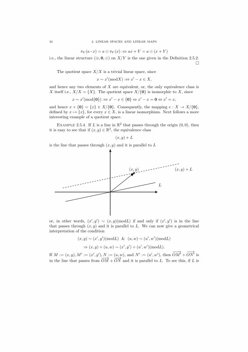
Example 2.5.4. If L is a line in R2 that passes through the origin (0, 0), thenit is easy to see that if (x, y) ∈ R2, the equivalence class
(x, y) + L
is the line that passes through (x, y) and it is parallel to L
L
(x, y) + L(x, y)
or, in other words, (x′, y′) ∼ (x, y)(modL) if and only if (x′, y′) is in the linethat passes through (x, y) and it is parallel to L. We can now give a geometricalinterpretation of the condition
(x, y) ∼ (x′, y′)(modL) & (u,w) ∼ (u′, w′)(modL)
⇒ (x, y) + (u,w) ∼ (x′, y′) + (u′, w′)(modL).
If M := (x, y),M ′ := (x′, y′), N := (u,w), and N ′ := (u′, w′), then−−−→OM ′ +
−−→ON ′ is
in the line that passes from−−→OM +
−−→ON and it is parallel to L. To see this, if L is
2.5. QUOTIENT SPACES 33
represented by the equation y = ax, for some a ∈ R, then
(y′ + w′)− (y + w)
(x′ + u′)− (x+ u)=
(y′ − y) + (w′ − w)
(x′ − x) + (u′ − u)
=a(x′ − x) + a(u′ − u)
(x′ − x) + (u′ − u)
= a(x′ − x) + u′ − u)
(x′ − x) + (u′ − u)
= a.
The following condition is interpreted similarly
(x, y) ∼ (x′, y′)(modL) & λ ∈ R ⇒ λ(x, y) ∼ λ(x′, y′)(modL),
sinceλy′ − λyλx′ − λx
=y′ − yx′ − x
= a.
The quotient space X/L is the set of all equivalence classes (x, y) + L, hence,according to the above geometrical interpretation of (x, y) + L, it is the set of alllines parallel to L. Each such line is determined from the point of its intersectionwith the axis y′y, which is a real number a(x,y)+L, where
y − a(x,y)+L
x− 0= a⇔ a(x,y)+L = y − ax.
It is easy to see that the addition [(x, y) +L] + [(u,w) +L] on X/L corresponds tothe addition a(x,y)+L+a(u,w)+L and the scalar multiplication b · [(x, y)+L] on X/Lcorresponds to the multiplication ba(x,y)+L of reals. In other words, the mapping
e : X/L→ R,
(x, y) + L 7→ a(x,y)+L,
is linear, and it is also a bijection. Hence, even without carrying out the exactcalculations, it is “geometrically” expected that X/L is linearly isomorphic to R.Hence, in this case we have that
dim(R2) = dim(L) + dim(R2/L).
Definition 2.5.5. Let X be a linear space, Y � X and x1, . . . , xn ∈ X.We say that x1, . . . , xn are linearly dependent (modY ), if x1 + Y, . . . , xn + Y arelinearly dependent in X/Y , and x1, . . . , xn are linearly independent (modY ), ifx1 + Y, . . . , xn + Y are linearly independent in X/Y .
One can show that x1, . . . , xn are linearly dependent (modY ) if and only ifthere are n ≥ 1 and a1, . . . , an ∈ R such that ai 6= 0, for some i ∈ {1, . . . , n}, and
∃y∈Y( n∑i=1
aixi = y
),
34 2. LINEAR SPACES AND LINEAR MAPS
and hence, x1, . . . , xn are linearly independent (modY ) if and only if for every n ≥ 1and every a1, . . . , an ∈ R
∃y∈Y( n∑i=1
aixi = y
)⇒ a1 = . . . = an = 0.
Theorem 2.5.6. Let X be a linear space and Y � X. If BY is a basis of Y ,and B := BY ∪ C is a basis of X, where BY ∩ C = ∅, then
C + Y := {c+ Y | c ∈ C}is a basis of X/Y , and dim(X) = dim(Y ) + dim(X/Y ).
Proof. If Z := 〈C〉, then X = Y + Z. To see this let x ∈ X, and letb1, . . . , bm ∈ BY , c1, . . . , cn ∈ C, and λ1, . . . , λm, µ1, . . . , µn ∈ R such that
x =
m∑i=1
λibi +
n∑j=1
µjcj = y + z,
where
y :=
m∑i=1
λibi ∈ Y & z :=
n∑j=1
µjcj ∈ Z.
Clearly, we have that x ∈ Y +Z. Moreover, Y ∩Z = {0}, since, if there was x ∈ Xsuch that x 6= 0 and x ∈ Y ∩ Z i.e.,
x =
m∑i=1
λibi =
n∑j=1
µjcj ,
for some λ1, . . . , λm, µ1, . . . , µn ∈ R, then there would be some µj 6= 0, and conse-quently the vector cj could be written as a linear combination of the rest. SinceBY ∩ C = ∅, this is impossible. Hence, by the Proposition 2.2.19 we have thatX = Y ⊕ Z. Let the function
φ : Z → X/Y, z 7→ z + Y, z ∈ Z,Since φ is the restriction of the canonical projection πY to the subspace Z of X, itis also a linear map. First we show that φ is an injection. If z1, z2 ∈ Z, then
z1 + Y = z2 + Y ⇔ (z1 − z2) ∈ Y ⇔ (z1 − z2) ∈ Y ∩ Z ⇔ (z1 − z2) = 0⇔ z1 = z2.
Next we show that φ is a surjection. Let x+ Y ∈ X/Y . Since there are y ∈ Y andz ∈ Z such that x = y + z, as we described above, we have that
φ(z) := z + Y = (0 + Y ) + (z + Y ) = (y + Y ) + (z + Y ) := (y + z) + Y = x+ Z.
Since C is a basis of Z, by the Lemma 2.4.6(vii) we have that φ(C) = C + Y is abasis of X/Y . Now the equality dim(X) = dim(Y ) + dim(X/Y ) follows10. �
10Since dim(X) = |B| = |BY ∪ C|, we use here the fact that |BY ∪ C| = |BY | + |C|, whenBY ∩C = ∅. This fact about cardinalities of sets is trivial when the related sets are finite, and it
can also be shown in the general case.
2.5. QUOTIENT SPACES 35
For the quotient space of the Example 2.5.4 we have that L := {(x, y) ∈ R2 |y = ax}, for some a ∈ R, BL := {(1, a)} is a basis of L and if C := {(0, 1)}, thenBL ∪ C is a basis of R2, BL ∩ C = ∅, and {(0, 1) + L} is a basis of R2/L.
If X is a finite dimensional space, and f : X → Y is linear, by the Theorem 2.4.8we have that
dim(X) = dim(Ker(f)) + dim(Im(f)),
and by the previous theorem we also have that
dim(X) = dim(Ker(f)) + dim(X/Ker(f)).
Hence, if m = dim(Im(f)) = dim(X/Ker(f)), and since both these spaces are bythe Corollary 2.4.15 isomorphic to Rm, we also have that X/Ker(f) ' Im(f). Nextwe show this fact for any linear space X.
Theorem 2.5.7. If X,Y are linear spaces and f ∈ L(X,Y ), then
X/Ker(f) ' Im(f).
Proof. Let the function φ : X/Ker(f)→ Im(f), defined by
φ(x+ Ker(f) := f(x),
for every x+ ker(f) ∈ X/Ker(f). First we show that φ is indeed a function and aninjection. If x+ ker(f) and x′ + ker(f) are in X/Ker(f), then
x+ ker(f) = x′ + ker(f)⇔ (x− x′) ∈ ker(f)⇔ f(x− x′) = 0⇔ f(x) = f(x′).
Next we show that φ is linear:
φ((x+ ker(f)) + (x′ + ker(f))
):= φ
((x+ x′) + ker(f)
):= f(x+ x′)
= f(x) + f(x′)
:= φ(x+ Ker(f)
)+ φ
(x′ + Ker(f)
),
φ(a(x+ ker(f))
):= φ
(ax+ ker(f)
):= f(ax)
= af(x)
:= aφ(x+ Ker(f)
).
Since φ is, trivially, a surjection, we have that φ is a linear isomorphism. �
From the previous theorem a linear map f : X → Y is written as the composi-tion of an injection (φ) with a surjection (πKer(f))

36 2. LINEAR SPACES AND LINEAR MAPS
X Y
X/Ker(f).
f
πKer(f) φ
Proposition 2.5.8. Let X be a linear space and Y, Z � X.
(i) Y/(Y ∩ Z) ' (Y + Z)/Z.
(ii) If X = Y ⊕ Z, then Y ' X/Z.
(iii) If Z � Y , then (X/Z)/(Y/Z) ' X/Y .
Proof. (i) Let f : Y → (Y +Z)/Z defined by f(y) := y+Z, for every y ∈ Y .Since f is the composition of linear maps
Y Y + Z (Y + Z)/Z,iY πZ
where iY (y) := y = y+ 0 is the linear injection of Y into Y + Z (see also Proposi-tion 2.4.10(i)), or since f is the restriction of the linear map πY to the subspace Yof Y + Z, we have that f is linear. If (y + z) + Z ∈ (Y + Z)/Z, then
f(y) := y + Z = (y + Z) + Z = (y + Z) + (z + Z) := (y + z) + Z
i.e., f is a surjection. Since
y ∈ Ker(f)⇔ f(y) = 0⇔ y + Z = Z ⇔ y ∈ Z ⇔ y ∈ Y ∩ Z,
we have that ker(f) = Y ∩ Z. By the Theorem 2.5.7 we get
Y/Ker(f) ' Im(f)⇔ Y/(Y ∩ Z) ' (Y + Z)/Z.
(ii) If X = Y ⊕ Z, then by the Proposition 2.2.19 we have that Y ∩ Z = {0}, andby the case (i) we get
Y ' Y/{0} ' (Y + Z)/Z = (Y ⊕ Z)/Z = X/Z.
(iii) Exercise. �
Definition 2.5.9. If X,Y are finite-dimensional linear spaces, and f : X → Yis linear, the rank of f is defined by
rank(f) := dim(Im(f)).
By the Theorems 2.5.7 and 2.5.6 we have that
rank(f) = dim(X/Ker(f)) = dim(X)− dim(Ker(f)),
hence f is an injection if and only if rank(f) = dim(X).

2.6. THE FREE LINEAR SPACE 37
2.6. The free linear space
In this section we study the construction of a free object in the category Lin.The methods that we use and the results we prove here are found, in some disguise,in many different contexts in mathematics.
Definition 2.6.1. If X is a set, and f : X → R, the zero set [f = 0] of f is theinverse image of {0} under f , and the cozero set [f 6= 0] of f is the complement11
of f = 0 i.e.,[f = 0] := {x ∈ X | f(x) = 0} = f−1({0}),
[f 6= 0] := {x ∈ X | f(x) 6= 0} = X \ [f = 0].
We denote by εX the set of all real-valued functions on X that are non-zero foronly finitely many elements of X i.e.,
εX :={f ∈ F(X) | [f 6= 0] is finite
}.
If f ∈ εX, we also say that f is almost everywhere 0.
If f ∈ εX, there are n ∈ N and x1, . . . , xn ∈ X such that{f(x) 6= 0 , if x ∈ {x1, . . . , xn}f(x) = 0 , otherwise.
The constant zero function 0X
on X is in εX, since[0X 6= 0
]= ∅, and ∅ is trivially
a finite subset of X. If x ∈ X, the function fx : X → R, defined by
fx(y) :=
{1 , if y = x0 , y 6= x
for every y ∈ X, is also in εX.
Remark 2.6.2. Let f, g ∈ F(X) and a ∈ R.
(i) [(f + g) 6= 0] ⊆ [f 6= 0] ∪ [g 6= 0].
(ii) [(af) 6= 0] ⊆ [f 6= 0].
Proof. (i) Let x ∈ X such that f(x) + g(x) 6= 0, and suppose that f(x) =g(x) = 0 i.e., x ∈ [f = 0]∩ [g = 0]. Then f(x) + g(x) = 0, which is a contradiction,hence x ∈ X \
([f = 0] ∩ [g = 0]
), and consequently12 we get x ∈ [f 6= 0] ∪ [g 6= 0].
(ii) If a = 0, then [(af) 6= 0] = ∅ ⊆ [f 6= 0]. If a 6= 0, and x ∈ X such thataf(x) 6= 0, then f(x) 6= 0. �
It is easy to find f, g ∈ F(X) such that [(f + g) 6= 0] ( [f 6= 0] ∪ [g 6= 0].Moreover, if a = 0, and [f 6= 0] 6= ∅, we have that [(af) 6= 0] = ∅ ( [f 6= 0], and ifa 6= 0, then [(af) 6= 0] = [f 6= 0].
11If Y ⊆ X, its complement X \ Y is defined by X \ Y := {x ∈ X | x /∈ Y }.12If Y and Z are subsets of a set X, then X \ (Y ∩Z) = (X \ Y )∪ (X \Z). Interchanging ∩
and ∪, we get X \ (Y ∪ Z) = (X \ Y ) ∩ (X \ Z).
38 2. LINEAR SPACES AND LINEAR MAPS
Corollary 2.6.3. If X is a given set, then εX, equipped with the linear struc-ture of F(X), is a linear subspace of F(X), which has as basis the set
BX := {fx | x ∈ X},
and the map iX : X → εX, defined by x 7→ fx, for every x ∈ X, is an injection.
Proof. If X = ∅, then ε∅ is the trivial linear space, since
ε∅ := {f : ∅ → R | [f 6= 0] is finite} = {∅},
and B∅ = ∅. The injectivity of i∅ also follows trivially.Let X be a non-empty set. If f, g ∈ εX, then by the Remark 2.6.2(i) we have
that [(f + g) 6= 0] is a subset of the union of two finite sets. Since the union oftwo finite sets is also finite, and since any subset of a finite set is again finite, weconclude that [(f + g) 6= 0] is a finite subset of X, and hence f + g ∈ εX. Similarly,by the Remark 2.6.2(ii) we have that if f ∈ εX and a ∈ R, then af ∈ εX. Since
0X ∈ εX, we conclude that εX is a linear subspace of F(X).
Next we show that 〈BX〉 = εX. Let f ∈ εX. If f = 0X
, then
f = 0fx0 = f(x0)fx0 ,
where x0 ∈ X. If [f 6= 0] = {x1, . . . , xn}, for some x1, . . . , xn ∈ X, then
f =
n∑i=1
f(xi)fxi∈ 〈BX〉.
To show that BX is linearly independent subset of εX, let fx1, . . . , fxn
∈ BX and
a1, . . . , an ∈ R such that a1fx1+ . . .+ anfxn
= 0X
. Since for every k ∈ {1, . . . , n}we have that ( n∑
i=1
aifxi
)(xk) = 0
X(xk)⇔ ak = 0,
we get what we want. Finally, we suppose that x, x′ ∈ X such that fx = fx′ . Since1 = fx(x) = fx′(x), we conclude that x′ = x. �
“Identifying” X with BX , we can view εX as a linear space with X as a basis.If X := 1 := {0}, then
ε1 :={f ∈ F(1) | [f 6= 0] is finite
}:= F(1),
and F(1) has as many elements as the set R of real numbers (why?). We see thatεX can be much larger than X. It turns out that if X is already a linear space,then the linear space εX is very different from X.
Definition 2.6.4. If X is a set, the linear space εX is called the free linearspace generated by X, or the free linear space over X.

2.6. THE FREE LINEAR SPACE 39
The fundamental property of εX is that any function h from X to a linearspace Y generates a linear map from εX to Y that “extends” h. In the proof ofthe following theorem we need to be careful, since εX is not necessarily a finite-dimensional linear space, and we have proved the Proposition 2.4.5(ii) only forfinite-dimensional linear spaces.
Theorem 2.6.5 (The universal property of the free linear space). If X is aset, then for every linear space Y and every function h : X → Y there is a uniquelinear map εh : εX → Y such that “h factors through εX” i.e., the followingdiagram commutes13
X εX
Y .
iX
εhh
Proof. Let f ∈ εX, such that [f 6= 0] = {x1, . . . , xn}, for some n ≥ 1. As wehave seen in the proof of the Corollary 2.6.3, f is written as follows:
f =
n∑i=1
f(xi)fxi .
This writing of f is unique. To show this, let {y1, . . . , ym} ⊆ X such that
m∑j=1
bjfyj = f =
n∑i=1
f(xi)fxi.
Since, for every l ∈ {1, . . . ,m}, we have that
f(yl) =
( m∑j=1
bjfyj
)(yl) =
m∑j=1
bjfyj (yl) = bl,
the previous equalities are written as follows:
m∑j=1
f(yj)fyj = f =
n∑i=1
f(xi)fxi.
If k ∈ {1, . . . , n}, then( m∑j=1
f(yj)fyj
)(xk) = f(xk)⇔
m∑j=1
f(yj)fyj (xk) = f(xk),
13An injection f : A→ B is also denoted by f : A ↪→ B. We use such a “hook right arrow”
in a diagram to indicate that iX is an injection. A dashed arrow, like the arrow corresponding to
εh, in a diagram is used to denote the uniqueness of that arrow.

40 2. LINEAR SPACES AND LINEAR MAPS
which implies that xk = yl for some l ∈ {1, . . . ,m}. Similarly we show that everyyj is equal to some xi, hence m = n and xi = yi, for every i ∈ {1, . . . , n}. Let thefunction h∗ : BX → Y defined by
h∗(fx) := h(x).
By the uniqueness of the writing of some f as above as a linear combination of theelements of BX , the function h∗ has the following unique linear extension εh onεX, where
(εh)(f) := (εh)
( n∑i=1
f(xi)fxi
):=
n∑i=1
f(xi)h(xi).
Notice that if f = 0X
, the writing of f as f(x0)fx0 is not unique, since, for example,
f(x0)fx0= 0
X= f(x1)fx1
, for every x0, x1 ∈ X. Since14
(εh)(0X)
:= (εh)(f(x0)fx0
)= f(x0)h(x0) = 0h(x0) =
= 0 = 0h(x1) = f(x1)h(x1) = (εh)(f(x1)fx1
),
we have though, that the formula of εh applies also on 0X
and gives the expectedvalue 0. Since (εh)
(iX(x)
):= (εh)
(fx))
:= h(x), we get the required commutativityof the above diagram. �
Notice that the importance of εX lies exactly in its universal property. Al-though F(X) is a linear space that can also be considered as “a space generatedby X”, there is no interesting connection between X and F(X). In the case of εXinstead, X “is” the basis of εX, a fact crucial to the previous proof of the universalproperty of εX. Next we show that εX is unique, up to isomorphism, in Lin i.e.,if W is a linear space that satisfies the universal property of the free linear spacegenerated by X, then W is linearly isomorphic to εX.
Theorem 2.6.6 (Uniqueness of the free linear space). Let W be a linear spaceand jX : X → W an injection, such that for every linear space Y and everyfunction h : X → Y there is a unique linear map hW : W → Y such that thefollowing diagram commutes
X W
Y .
jX
hWh
Then W is linearly isomorphic to εX.
Proof. If in the universal property for W we take Y := W and h := jX
14If we write 0X
=∑n
i=1 0X
(xi)fxi , the formula of εh gives similarly that (εh)(0X)
= 0.

2.6. THE FREE LINEAR SPACE 41
X W
W ,
jX
(jX)WjX
then explain why (jX)W = idW . Next we proceed as in the proof of the up toisomorphism-uniqueness of the product (see the section 6.3 of the Appendix). �
Proposition 2.6.7. Let X,Y, Z be sets, and h : X → Y , g : Y → Z functions.
(i) There is a unique linear map εh : εX → εY such that the following diagramcommutes
X Y
εX εY .
h
εh
iX iY
(ii) The following lower outer diagram commutes
X Y
εX εY
Z
εZ
h g
εgεh
iX iY iZ
ε(g ◦ h)
g ◦ h
i.e., ε(g ◦ h) = εg ◦ εh.
(iii) If X is a set, let E0(X) := εX, and, if h : X → Y is a function from the setX to the set Y , let E1(h) := εh : εX → εY is the linear map determined in thecase (i). Then the pair E := (E0, E1) is a covariant functor from the category Setto the category Lin.
Proof. Exercise. �
Proposition 2.6.8. Let X,Y be linear spaces and h : X → Y a function.
(i) There is a unique linear map πX : εX → X such that πX ◦ iX = idX

42 2. LINEAR SPACES AND LINEAR MAPS
X εX
X.
iX
πXidX
(ii) Let the following subset of εX
N(X) :={fλx+µy − λfx − µfy | x, y ∈ X & λ, µ ∈ R
}.
Then 〈N(X)〉 ⊆ Ker(πX).
(iii) Ker(πX) ⊆ 〈N(X)〉.(iv) The function h is a linear map if and only if πY ◦ εh = h ◦ πX
X Y
εX εY .
h
εh
iX iYπX πY
Proof. We describe only the steps to find the algorithm for the proof of the
case (iii). Since 0X ∈ Ker(πX), we only want to show that for every n ≥ 1, and for
every x1, . . . xn ∈ X,
f =
n∑i=1
f(xi)fxi∈ Ker(πX)⇒ f ∈ 〈N(X)〉.
(a) Show that f0 ∈ N(X), and show the case n = 1 i.e., if f = f(x1)fx1∈ Ker(πX),
then f ∈ 〈N(X)〉.(b) Show the case n = 2 i.e., if f = f(x1)fx1
+ f(x2)fx2∈ Ker(πX), then f ∈
〈N(X)〉.(c) Show the case n = 3 i.e., if f = f(x1)fx1
+f(x2)fx2+f(x3)fx3
∈ Ker(πX), thenf ∈ 〈N(X)〉.(d) Show the case n = 4 i.e., if f = f(x1)fx1
+ f(x2)fx2+ f(x3)fx3
+ f(x4)fx4∈
Ker(πX), then f ∈ 〈N(X)〉.The algorithm for the general case is either evident in the proof of this case, or, ifnot, it should be clear in the proof of the case n = 5. �
2.7. Convex sets
In this section we study the notion of a convex set in a linear space, provingsome very first results in the theory of convex sets. The area of “Convex Analysis”is very broad, and we refer to [14] for further reading.

2.7. CONVEX SETS 43
If M,N ∈ Rn, the linear segment [M,M +N ] between M and M +N
N
M +N
M
is the following set
[M,M +N ] :={M + tN | t ∈ [0, 1]
}.
If t := 0, then M +0N = M , and if t := 1, then M +1N = M +N . If, for example,S is the middle point of the segment, then
S =M + (M +N)
2= M +
N
2= M +
1
2N.
Since N = M + (N −M), we have that the linear segment [M,N ] between M andN is the following set:
[M,N ] = [M,M + (N −M)]
={M + t(N −M) | t ∈ [0, 1]
}={tN + (1− t)M | t ∈ [0, 1]
}={sM + (1− s)N | s ∈ [0, 1]
}={t1M + t2N | t1, t2 ∈ [0, 1] & t1 + t2 = 1
}={t1M + t2N | t1, t2 ≥ 0 & t1 + t2 = 1
}.
The next definition is the generalisation of the description of [M,N ] in Rn.
Definition 2.7.1. If X is a linear space and x, y ∈ X, the linear segment [x, y]between x and y is defined by
[x, y] :={tx+ (1− t)y | t ∈ [0, 1]
}.
Clearly, for every x, y ∈ X we have that
[x, y] = [y, x] & [x, x] = {x}.
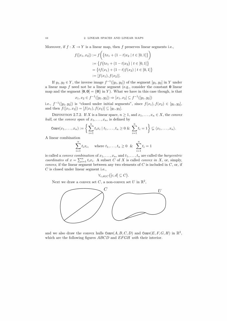
44 2. LINEAR SPACES AND LINEAR MAPS
Moreover, if f : X → Y is a linear map, then f preserves linear segments i.e.,
f([x1, x2]) := f
({tx1 + (1− t)x2 | t ∈ [0, 1]
}):={f(tx1 + (1− t)x2
)| t ∈ [0, 1]
}={tf(x1) + (1− t)f(x2) | t ∈ [0, 1]
}:= [f(x1), f(x2)].
If y1, y2 ∈ Y , the inverse image f−1([y1, y2]) of the segment [y1, y2] in Y undera linear map f need not be a linear segment (e.g., consider the constant 0 linearmap and the segment [0,0] = {0} in Y ). What we have in this case though, is that
x1, x2 ∈ f−1([y1, y2])⇒ [x1, x2] ⊆ f−1([y1, y2])
i.e., f−1([y1, y2]) is “closed under initial segments”, since f(x1), f(x2) ∈ [y1, y2],and then f([x1, x2]) = [f(x1), f(x2)] ⊆ [y1, y2].
Definition 2.7.2. If X is a linear space, n ≥ 1, and x1, . . . , xn ∈ X, the convexhull, or the convex span of x1, . . . , xn, is defined by
Conv(x1, . . . , xn) :=
{ n∑i=1
tixi | t1, . . . , tn ≥ 0 &
n∑i=1
ti = 1
}( 〈x1, . . . , xn〉.
A linear combinationn∑i=1
tixi, where t1, . . . , tn ≥ 0 &
n∑i=1
ti = 1
is called a convex combination of x1, . . . , xn, and t1, . . . , tn are called the barycentriccoordinates of x =
∑ni=1 tixi. A subset C of X is called convex in X, or, simply,
convex, if the linear segment between any two elements of C is included in C, or, ifC is closed under linear segment i.e.,
∀c,d∈C([c, d] ⊆ C
).
Next we draw a convex set C, a non-convex set U in R2,
C U
and we also draw the convex hulls Conv(A,B,C,D) and Conv(E,F,G,H) in R2,which are the following figures ABCD and EFGH with their interior.

2.7. CONVEX SETS 45
A B
D C
Conv(A,B,C,D)
E
F
G
H
Conv(E,F,G,H)
Example 2.7.3. Any subspace Y of a linear space X is convex. Hence, X itselfis convex. There are many convex subsets of X that are not subspaces of X. E.g.,if X is a non-trivial linear space, and x 6= 0, then {x} is convex in X. If x, y ∈ X,then [x, y] is convex in X. If C,D are convex sets in X, their intersection C ∩D isconvex in X (why?).
C D
Similarly, the intersection of any family (Ci)i∈I if convex sets in X is convex. Theempty set ∅ is trivially convex in X, since the defining property of a convex set istrivially satisfied15
∀c,d∈∅([c, d] ⊆ ∅
):⇔ ∀c,d
(c ∈ ∅ & d ∈ ∅ ⇒ [c, d] ⊆ ∅
).
The union of two convex sets, like A and B in R2, is not always a convex set.
A B
15Here we use the logical fact (P ⇒ ⊥) ⇒ (P ⇒ Q), where P,Q are formulas. For the
derivation of this formula we use the logical rules Efq and Modus Ponens.

46 2. LINEAR SPACES AND LINEAR MAPS
Remark 2.7.4. Let X,Y be linear spaces, C,C ′ ⊆ X, and D ⊆ Y .
(i) If C is convex in X, and D is convex in Y , then C ×D is convex in X × Y .
(ii) If C,C ′ are convex, then C + C ′ := {c+ c′ | c ∈ C & c′ ∈ C ′} is convex.
(iii) If C is convex, and a ∈ R, then aC := {a · c | c ∈ C} is convex.
Proof. Exercise. �
Notice that Conv(x1) = {x1}, and Conv(x1, x2) = [x1, x2], while Conv(x1, x2, x3)is the triangle, with its interior, of x1, x2, x3 in X. Generally, more than one convexcombinations correspond to the same vector e.g.,
1
2=
1
2
(3
8
)+
1
2
(5
8
)=
3
4
(7
16
)+
1
4
(11
16
).
Proposition 2.7.5. If X is a linear space, n ≥ 1, and x1, . . . , xn ∈ X, theirconvex hull Conv(x1, . . . , xn) is the least convex set in X that contains x1, . . . , xn.
Proof. First we show that Conv(x1, . . . , xn) is convex in X. Let
x =
n∑i=1
tixi, t1, . . . , tn ≥ 0 &
n∑i=1
ti = 1,
y =
n∑i=1
sixi, s1, . . . , sn ≥ 0 &
n∑i=1
si = 1.
If t ∈ [0, 1], then
tx+ (1− t)y = t
n∑i=1
tixi + (1− t)n∑i=1
sixi
=
n∑i=1
ttixi +
n∑i=1
(1− t)sixi
=
n∑i=1
[tti + (1− t)si]xi.
If ai := tti + (1− t)si, for every i ∈ {1, . . . , n}, and if a, b ∈ R, let
a ∧ b := min{a, b},
then, since a ≥ a ∧ b and b ≥ a ∧ b, we have that
ai ≥ t(ti ∧ si) + (1− t)(ti ∧ si) = [t+ (1− t)](ti ∧ si) = ti ∧ si ≥ 0,
andn∑i=1
ai =
n∑i=1
tti +
n∑i=1
(1− t)si = t
n∑i=1
ti + (1− t)n∑i=1
si = t+ (1− t) = 1.
2.7. CONVEX SETS 47
Next, we show that if C is a convex set in X that contains x1, . . . , xn, thenConv(x1, . . . , xn) ⊆ C. For that we prove inductively the following formula:
∀n≥1
(∀x1,...,xn∈X
(x1 ∈ C & . . . & xn ∈ C ⇒ Conv(x1, . . . , xn) ⊆ C
)).
If n = 1, we show that ∀x1∈X(x1 ∈ C ⇒ Conv(x1) ⊆ C
), which we get immediately
from the equality Conv(x1) = {x1}. Next we suppose that
∀x1,...,xn∈X(x1 ∈ C & . . . & xn ∈ C ⇒ Conv(x1, . . . , xn) ⊆ C
),
and we show that
∀x1,...,xn+1∈X(x1 ∈ C & . . . & xn+1 ∈ C ⇒ Conv(x1, . . . , xn+1) ⊆ C
).
Let x1, . . . , xn, xn+1 ∈ X, such that x1 ∈ C & . . . & xn ∈ C & xn+1 ∈ C, and let
x =
n+1∑i=1
tixi, t1, . . . , tn+1 ≥ 0 &
n+1∑i=1
ti = 1.
If there is some i ∈ {1, . . . , n+1}, such that ti = 0, then by the inductive hypothesison the n-elements x1, . . . , xi−1, xi+1, . . . , xn+1 of X we get
x =
n+1∑j=1,j 6=i
tjxj ∈ C.
If ti 6= 0, for every i ∈ {1, . . . , n+ 1}, then tn+1 6= 1, and hence
x = (1− tn+1)c+ tn+1xn+1,
c :=t1
1− tn+1x1 + . . .+
tn1− tn+1
xn.
Sinceti
1− tn+1≥ 0, i ∈ {1, . . . , n},
andt1
1− tn+1+ . . .+
tn1− tn+1
=1
1− tn+1
(t1 + . . .+ tn
)=
1− tn+1
1− tn+1= 1
we get c ∈ Conv(x1, . . . , xn). By the inductive hypothesis on x1, . . . , xn we havethat c ∈ C, and hence, since C is convex, we get x ∈ C. �
As in the case of the linear span, the notion of the convex hull is generalised to anarbitrary subset Y of a linear space X.
Definition 2.7.6. IfX is a linear space, and Y ⊆ X, the convex hull ConvX(Y ),or simpler Conv(Y ), of Y in X is defined by
Conv(Y ) :=⋂{C ⊆ X | Y ⊆ C & C is convex}.
Clearly, Conv(Y ) is the least convex set including Y . Moreover, since ∅ isconvex, Conv(∅) = ∅ ( {0} = 〈∅〉.

48 2. LINEAR SPACES AND LINEAR MAPS
Proposition 2.7.7. Let X be a linear space, and Y,Z ⊆ X.
(i) Y ⊆ Conv(Y ).
(ii) If Y ⊆ Z, then Conv(Y ) ⊆ Conv(Z).
(iii) Conv(Conv(Y )) = Conv(Y ).
(iv) Conv(Y ∩ Z) ⊆ Conv(Y ) ∩ Conv(Z).
(v) Conv(Y ) ∪ Conv(Z) ⊆ Conv(Y ∪ Z).
(vi) Y is convex if and only if Conv(Y ) = Y .
Proof. Exercise. �
As in the case of linear span, the “top-down” definition of the convex hull ofany subset Y has an equivalent “bottom-up” description.
Proposition 2.7.8. If X is a linear space, and Y ⊆ X, then the convex hullConv(Y ) of Y is equal to all convex combinations of the elements of Y .
Proof. What we need to show amounts to the equality Conv(Y ) = Y , where
Y :=
{ n∑i=1
tiyi | n ≥ 1 & ∀i∈{1,...,n}(ti ≥ 0 & yi ∈ Y
)&
n∑i=1
ti = 1
}.
By the Proposition 2.7.5, and since trivially Y ⊆ Y , to show that Conv(Y ) ⊆ Y , it
suffices to show that Y is convex. Let
x =
n∑i=1
tiyi, y1, . . . , yn ∈ Y & t1, . . . , tn ≥ 0 &
n∑i=1
ti = 1,
x′ =
m∑j=1
sjyj′, y1
′, . . . , ym′ ∈ Y & s1, . . . , sm ≥ 0 &
m∑j=1
sj = 1.
If t ∈ [0, 1], then
tx+ (1− t)x′ =
n∑i=1
(tti)yi +
m∑j=1
(1− t)sjyj ′ ∈ Y ,
since tti ≥ 0, and (1− t)sj ≥ 0, and
n∑i=1
(tti) +
m∑j=1
(1− t)sj = t
( n∑i=1
ti
)+ (1− t)
( m∑j=1
sj
)= t1 + (1− t)1 = 1.
By the definition of Conv(Y ), to show the inclusion Y ⊆ Conv(Y ), it suffices to show
that if C is convex in X, such that Y ⊆ C, then Y ⊆ C. Let x =∑ni=1 tiyi ∈ Y ,
for some n ≥ 1, t1, . . . , tn ≥ 0, such that∑ni=1 ti = 1, and y1, . . . , yn ∈ Y . Hence,
x ∈ Conv(y1, . . . , yn). Since {y1, . . . , yn} ⊆ Y ⊆ C, by Proposition 2.7.5 we getx ∈ Conv(y1, . . . , yn) ⊆ C. �

2.8. CARATHEODORY’S THEOREM 49
Remark 2.7.9. Let X,Y be linear spaces, f ∈ L(X,Y ), C ⊆ X, D ⊆ Y , andZ � X.
(i) If D is convex in Y , then f−1(D) := {x ∈ X | f(x) ∈ D} is convex in X.
(ii) If C is convex in X, then f(C) := {f(x) | x ∈ C} is convex in Y .
(iii) If C is convex in X, then C + Z := {c+ Z | c ∈ C} is convex in X/Z.
(iv) If n ≥ 1, and x1, . . . , xn ∈ X, then
f(Conv(x1, . . . , xn)
)= Conv(f(x1), . . . , f(xn)).
Proof. Exercise. �
Corollary 2.7.10. If X is a linear space, f, g ∈ X∗ := L(X,R), and a ∈ R,then the following sets
[f > a] := {x ∈ X | f(x) > a},[f ≥ a] := {x ∈ X | f(x) ≥ a},[f = a] := {x ∈ X | f(x) = a},[f < a] := {x ∈ X | f(x) > a},[f ≤ a] := {x ∈ X | f(x) ≥ a},[f > g] := {x ∈ X | f(x) > g(x)},[f ≥ g] := {x ∈ X | f(x) ≥ g(x)},[f = g] := {x ∈ X | f(x) = g(x)},
are convex in X.
Proof. Exercise. �
2.8. Caratheodory’s theorem
If y1, y2, y3 ∈ R and x ∈ Conv(y1, y2, y3), it is easy to see that x is in the convexhull of at most two elements of {y1, y2, y3}. If x ∈ {y1, y2, y3}, then it is in theconvex hull of one of them, while if x /∈ {y1, y2, y3}, and supposing, without loss ofgenerality, that y1 < y2 < y3, then the hypothesis x ∈ Conv(y1, y2, y3) implies thatx ∈ [y1, y3], and hence x ∈ [y1, y2] = Conv(y1, y2), or x ∈ [y2, y3] = Conv(y2, y3).
y1 y2 y3
Similarly, if y1, y2, y3, y4 ∈ R2 and x ∈ Conv(y1, y2, y3, y4), it is easy to seethat x is in the convex hull of at most three elements of {y1, y2, y3, y4}. If x ∈{y1, y2, y3, y4}, then it is in the convex hull of one of them, while if x is in the linesegment between two of them, it is in the convex hull of two of them. In any othercase, we can find a triangle with vertices in {y1, y2, y3, y4} in the interior of whichx belongs to.

50 2. LINEAR SPACES AND LINEAR MAPS
y1
y2
y3
y4
x
Caratheodory’s theorem is a generalisation of these intuitive remarks. Accord-ing to it, if Y ⊆ Rn, and x ∈ Conv(Y ), we can find at most (n + 1)-elements in Ysuch that x is in their convex hull.
Theorem 2.8.1 (Caratheodory). If Y ⊆ Rn, then for every x ∈ Conv(Y ) thereis m ∈ N such that 1 ≤ m ≤ n + 1, and there are y1, . . . , ym ∈ Y , such thatx ∈ Conv(y1, . . . , ym).
Proof. If x ∈ Conv(Y ), then by the Proposition 2.7.8 there is k ≥ 1, and thereare y1, . . . , yk ∈ Y , such that
x =
k∑i=1
tiyi, t1, . . . , tk ≥ 0 &
k∑i=1
ti = 1.
If k ≤ n+1, we have nothing to prove. Suppose next that k > n+1⇔ k−1 > n, andsuppose also that t1 > 0 & . . . & tk > 0, since if ti = 0, for some i ∈ {1, . . . , k}, wecan write immediately x as a convex combination of k− 1 elements of Y . Actually,our strategy is to prove that there are k − 1 elements of Y , such that x can bewritten as a convex combination of them. By repeating the same argument at mostk − (n+ 1) number of times, we reach the required conclusion. To find these k − 1elements of Y , we work as follows. Since by the Theorem 2.2.13 the k − 1 > nnumber of vectors in Rn
(y1 − yk), . . . , (yk−1 − yk)
are linearly dependent, there are a1, . . . , ak−1 ∈ R, such that
k−1∑j=1
aj(yj − yk) = 0,
and aj 6= 0, for some j ∈ {1, . . . , k − 1}. If we define
ak := −k−1∑j=1
aj ,
thenk∑i=1
ai = 0 &
k∑i=1
aiyi = 0,

2.8. CARATHEODORY’S THEOREM 51
sincek∑i=1
aiyi =
k−1∑j=1
ajyj + akyk
=
k−1∑j=1
ajyj +
(−k−1∑j=1
aj
)yk
=
k−1∑j=1
ajyj −k−1∑j=1
ajyk
=
k−1∑j=1
aj(yj − yk)
= 0.
We claim that there is some i ∈ {1, . . . , k} such that ai > 0. If there is some j ∈{1, . . . , k−1}, such that aj > 0, we are done. If aj ≤ 0, for every j ∈ {1, . . . , k−1},and since in this case there is some j ∈ {1, . . . , k − 1} with aj < 0, then ak > 0.Hence, by our justified claim, and our hypothesis that each ti > 0, there is somel ∈ {1, . . . , k} such that
max
{a1
t1, . . . ,
aktk
}=altl
:=1
M> 0,
where M := tlal
. We show that x ∈ Conv(y1, . . . , yl−1, yl+1, . . . , yk). If
sj := tj −Maj , j ∈ {1, . . . , l − 1, l + 1, . . . , k},then, for every j ∈ {1, . . . , l − 1, l + 1, . . . , k}, we have that
ajtj≤ 1
M⇒Maj ≤ tj ⇒ sj := tj −Maj ≥ 0,
and since∑ki=1 aiyi = 0, we have that
∑kj=1,j 6=l ajyj = −(alyl), and hence
k∑j=1,j 6=l
sjyj :=
k∑j=1,j 6=l
(tj −Maj)yj
=
k∑j=1,j 6=l
tjyj −Mk∑
j=1,j 6=l
ajyj
=
k∑j=1,j 6=l
tjyj −tlal
[− (alyl)
]=
k∑i=1
tiyi

52 2. LINEAR SPACES AND LINEAR MAPS
= x.
Since∑ki=1 ai = 0, we have that
∑kj=1,j 6=l aj = −al, and hence
k∑j=1,j 6=l
sj :=
k∑j=1,j 6=l
(tj −Maj)
=
k∑j=1,j 6=l
tj −Mk∑
j=1,j 6=l
aj
=
k∑j=1,j 6=l
tj −tlal
[−al]
=
k∑i=1
ti
= 1
i.e., x was written as a convex combination of k − 1 elements of Y . �
By Caratheodory’s theorem, an element x of Conv(Y ), where Y ⊆ Rn can bewritten as
x =
n+1∑i=1
tiyi, t1, . . . tn+1 ≥ 0, y1, . . . , yn+1 ∈ Y,
since, even if the number m in the formulation of Caratheodory’s theorem is smallerthan n + 1, one can consider in the above convex combination any elements of Ymultiplied by 0’s.
If Y is the union of a number of convex sets in Rn, which is smaller than thedimension n of Rn, then, according to the next corollary of Caratheodory’s theorem,we can find a convex combination for the elements of Conv(Y ) even smaller fromthe one determined by Caratheodory’s theorem.
Corollary 2.8.2. If 1 ≤ k ≤ n, and C1, . . . , Ck are convex subsets of Rn,then for every
x ∈ Conv
( k⋃i=1
Ci
)there is m ≤ k, and there are y1, . . . , ym ∈
⋃ki=1 Ci, such that
x ∈ Conv(y1, . . . , ym).
Hint: The case k = 1 is trivial, since by the convexity of C1 we have that
x ∈ Conv
( 1⋃i=1
Ci
)= Conv(C1) = C1 ⇒ x ∈ Conv(x) = {x}.

2.8. CARATHEODORY’S THEOREM 53
It is helpful to work next with two convex sets C1, C2 in R2, and to show thatfor every x ∈ Conv(C1 ∪ C2) there are at most two elements y, y′ ∈ C1 ∪ C2 suchthat x ∈ Conv(y, y′). The proof of the general case uses the trick of the case ofR2 and the method of proof of Caratheodory’s theorem. Namely, we suppose thatthe determined by Caratheodory’s theorem convex combination of x with at most
m ≤ n+ 1 number of elements from⋃ki=1 Ci is larger than k, and we find a convex
combination of x from m − 1 number of vectors from⋃ki=1 Ci. The rest is an
exercise. �


CHAPTER 3
Matrices
3.1. The linear space of matrices
Definition 3.1.1. If m,n ≥ 1, an array of real numbers
A :=
a11 . . . a1n
......
...ai1 . . . ain...
......
am1 . . . amn
=: [aij ].
is called a matrix of m-rows and n-columns. If 1 ≤ i ≤ m, the i-th row of A is thearray
Ai :=[ai1 . . . ain
]:= [aij ]i (∈ Rn),
and we also write A as a column of its rows
A =
A1
...Am
.The row-rank of A is defined by
rRank(A) := dim(〈A1, . . . , Am〉
)and it is the maximum number of linearly independent rows of A. If 1 ≤ j ≤ n,the j-th column of A is the array
Aj :=
a1j
...amj
:= [aij ]j (∈ Rm),
and we also write A as a row of its columns
A = [A1 . . . An].
The column-rank of A is defined by
cRank(A) := dim(〈A1, . . . , An〉
),
55

56 3. MATRICES
and it is the maximum number of linearly independent columns of A. The set ofm × n-matrices is denoted by Mm,n(R), while the set of square matrices Mn,n(R)is also denoted by Mn(R). If [aij ], [bij ] ∈Mm,n(R), and λ ∈ R, we define
[aij ] = [bij ] :⇔ ∀i∈{1,...,m}∀j∈{1,...,n}(aij = bij
).
[aij ] + [bij ] := [aij + bij ],
λ · [aij ] := [λaij ],
0mn := [0],
and if m = n, we denote 0nn by 0n, or, if n is clear from the context, by 0.
If m = n = 2, the above definitions take the form[a bc d
]=
[a′ b′
c′ d′
]⇔ a = a′ & b = b′ & c = c′ & d = d′,[
a bc d
]+
[a′ b′
c′ d′
]=
[a+ a′ b+ b′
c+ c′ d+ d′
],
λ
[a bc d
]=
[λa λbλc λd
], λ ∈ R,
02 :=
[0 00 0
].
Remark 3.1.2. Mm,n(R) is a linear space of dimension mn.
Proof. The fact that Mm,n(R) is a linear space is immediate from the Defini-tion 3.1.1. To determine the dimension of Mm,n(R), we associate to an m×n-matrix
A :=
a11 . . . a1n
......
...ai1 . . . ain...
......
am1 . . . amn
the following element of Rmn(
a11, . . . , a1n, . . . , ai1, . . . , ain, . . . , am1, . . . , amn).
E.g., to the 2× 2-matrix [a bc d
]we associate the 4-tuple
(a, b, c, d).
It is easy to see that this mapping e : Mm,n(R) → Rmn is a linear isomorphism,hence by the Remark 2.4.14(ii) we get dim
(Mm,n(R)
)= dim(Rmn) = mn. �

3.1. THE LINEAR SPACE OF MATRICES 57
Definition 3.1.3. Let the mapping t : Mm,n(R)→Mn,m(R), defined by
[aij ] 7→ [aij ]t,
where
[aij ]t := [bji], bji := aij .
The matrix [aij ]t is called the transpose of [aij ], and it has columns the rows of
[aij ] and rows the columns of [aij ]. If A ∈ Mn(R) with At = A, we say that A issymmetric, and we denote their set by Symn(R). A diagonal matrix in Mn(R) hasthe form
λ1
λ2
. . .
λn
:=
λ1 0 . . . 00 λ2 . . . 0...
.... . .
...0 0 . . . λn
=: Diag(λ1, . . . , λn).
We denote by In the unit matrix in Mn(R), defined by
In :=
1
1. . .
1
=: [δij ],
where1
δij :=
{1 , if i = j0 , if i 6= j.
E.g., if we consider the 2× 3-matrix
A :=
[2 1 01 3 5
],
then its transpose At is the following 3× 2-matrix
At :=
2 11 30 5
.An example of a symmetric matrix is the following:
A =
3 1 −21 5 4−2 4 −8
= At.
Remark 3.1.4. Let A,B ∈Mm,n(R) , C ∈Mn(R), and a ∈ R.
(i) (A+B)t = At +Bt.
(ii) (a ·B)t = a ·Bt.
1The symbol δki is known as Kronecker’s delta.

58 3. MATRICES
(iii)(At)t
= A.
(iii) C + Ct is symmetric.
Proof. Exercise. �
Next we define the multiplication between matrices, an operation which, aswe shall see later, is related to the composition of linear maps. To define themultiplication AB the number of columns of A has to be the number of rows of B!
Definition 3.1.5. If A := [aij ] ∈ Mm,n(R) and B := [bjk] ∈ Mn,l(R), theirproduct AB ∈Mm,l(R) is defined by
AB := [aij ][bjk] := [cik],
cik :=
n∑j=1
aijbjk,
for every 1 ≤ i ≤ m and 1 ≤ k ≤ l. If A ∈Mn(R), let
An :=
{In , n = 0AAn−1 , n > 0
A matrix A ∈Mn(R) is invertible, if there is B ∈Mn(R) such that AB = BA = In.We denote by Invn(R) the set of invertible matrices in Mn(R).
E.g., if
A :=
[2 1 51 3 2
]& B :=
3 4−1 2
2 1
,then
AB :=
[2 1 51 3 2
] 3 4−1 2
2 1
=
[15 154 12
].
It is not always true that AB = BA. E.g.,[3 20 1
] [2 −10 5
]=
[6 70 5
],
and [2 −10 5
] [3 20 1
]=
[6 −30 5
].
If a, b ∈ R, and
A :=
[1 a0 1
]& B :=
[1 b0 1
],
then
AB :=
[1 a+ b0 1
].

3.1. THE LINEAR SPACE OF MATRICES 59
Hence [1 −a0 1
] [1 a0 1
]= I2.
Notice that, in contrast to what happens in R, there are non-zero square ma-trices that are not invertible, like the matrix[
1 11 1
].
Proposition 3.1.6. Let A ∈Mm,n(R), B,C ∈Mn,l(R), and D ∈Ml,s(R).
(i) AIn = A and ImA = A.
(ii) A(B + C) = AB +AC.
(iii) If a ∈ R, then A(a ·B) = a · (AB).
(iv) A(BD) = (AB)D.
(v) The multiplication BtAt is well-defined, and (AB)t = BtAt.
Proof. Exercise. �
Corollary 3.1.7. Let A,B,C ∈Mn(R).
(i) If AB = BA = In = AC = CA, then B = C. We denote the unique matrix Bsuch that AB = BA = In by A−1, and we call it the inverse of A.
(ii) Itn = In.
(iii) If A is invertible, then (A−1)t = (At)−1.
Proof. (i) C = InC = (AB)C = (BA)C = B(AC) = BIn = B.(ii) [δij ]
t := [dij ], where dij := δij , and what we want follows from the obviousequality δij = δji.(iii) By the Proposition 3.1.6(v) and the case (ii) we have that In = Itn = (AA−1)t =(A−1)tAt, and In = Itn = (A−1A)t = At(A−1)t. Since In = (At)−1At = At(At)−1,by the case (i) we get (A−1)t = (At)−1. �
One can show that if A,B ∈Mn(R), then
AB = In ⇒ BA = In,
hence we do not need to check both equalities in order to show that a matrix A isinvertible. Note that this is the case only when the product AB is equal to In. IfA,B ∈ Mn(R) are invertible, then AB is also invertible and (AB)−1 = B−1A−1,since
(AB)(B−1A−1) = A[B(B−1A−1)] = A[(BB−1)A−1] = A[InA−1] = AA−1 = In.
Definition 3.1.8. If A := [aij ] ∈Mn(R), the trace Tr(A) is defined by
Tr(A) :=
n∑i=1
aii.
60 3. MATRICES
It is immediate to see that Tr(At) = Tr(A), and Tr(In) = n.
Remark 3.1.9. Let A,B,C ∈Mn(R) and λ ∈ R.
(i) Tr(A+B) = Tr(A) + Tr(B).
(ii) Tr(λA) = λTr(A).
(iii) Tr(AB) = Tr(BA).
(iv) If B is invertible, then Tr(B−1AB) = Tr(A).
(v) Tr(A(B + C)) = Tr(AB) + Tr(AC).
(vi) Tr((λA)B) = λTr(AB).
(vii) There are no matrices A,B ∈Mn(R) such that
AB −BA = In.
(viii) If A ∈ Mn(R) such that for every B ∈ Mn(R), we have that Tr(AB) = 0,then A = 0n.
Proof. Exercise. �
Proposition 3.1.10. (i) The set of symmetric matrices Symn(R) is a linearsubspace of Mn(R).
(ii) If A ∈ Symn(R), then Tr(AA) ≥ 0.
(iii) If A ∈ Symn(R) and A 6= 0n, then Tr(AA) > 0.
Proof. Exercise. �
As we shall explain later, because of the above properties, the function (A,B) 7→Tr(AB) is an inner product on Symn(R).
3.2. The linear map of a matrix
Matrices can be used to represent linear maps. Let’s see the following charac-teristic example. If θ ∈ R, let the matrix
R(θ) :=
[cos θ − sin θsin θ cos θ
].
Let the map Rθ : R2 → R2 defined by
Rθ(x, y) := R(θ)
[xy
]:=
[cos θ − sin θsin θ cos θ
] [xy
]=
[cos θ − sin θsin θ cos θ
] [r cosφr sinφ
]
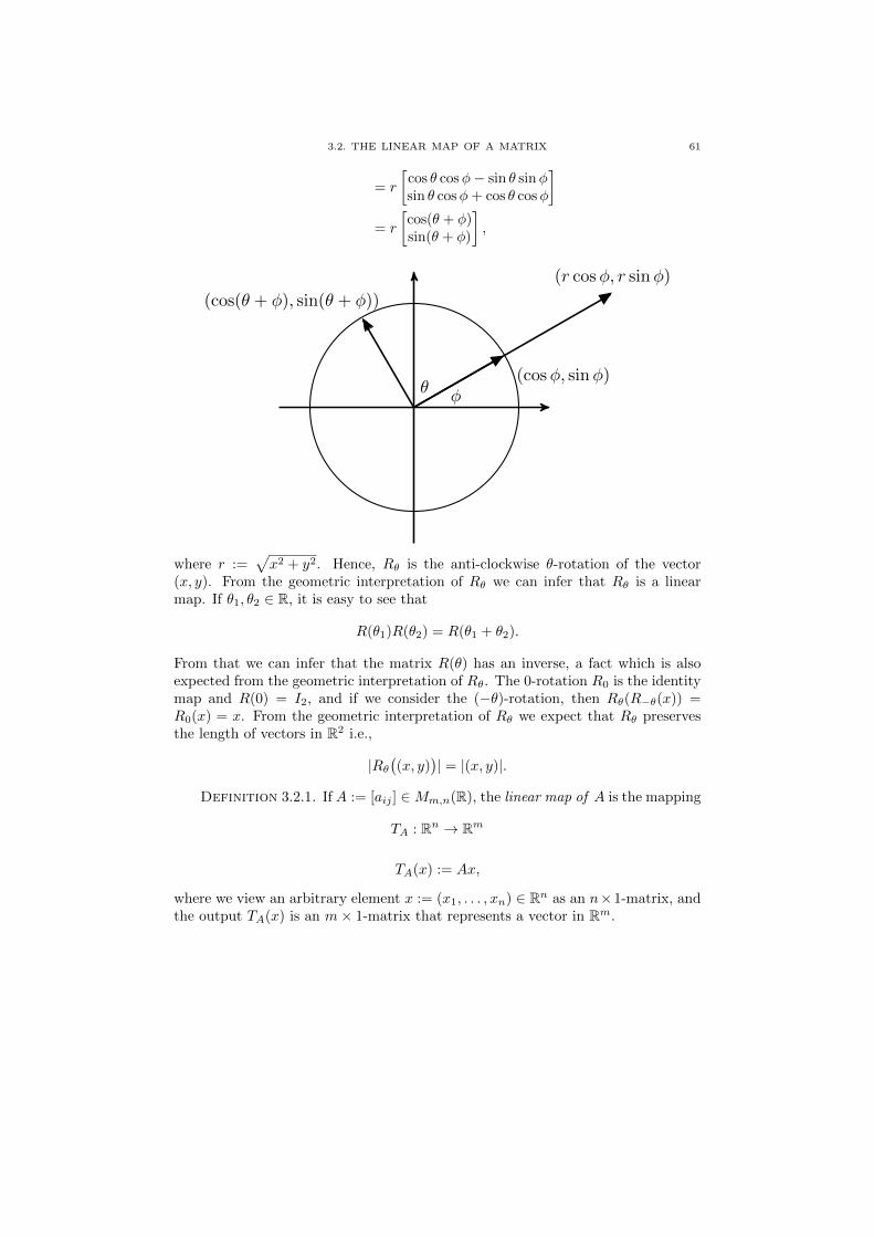
3.2. THE LINEAR MAP OF A MATRIX 61
= r
[cos θ cosφ− sin θ sinφsin θ cosφ+ cos θ cosφ
]= r
[cos(θ + φ)sin(θ + φ)
],
(r cosφ, r sinφ)
(cosφ, sinφ)
(cos(θ + φ), sin(θ + φ))
φθ
where r :=√x2 + y2. Hence, Rθ is the anti-clockwise θ-rotation of the vector
(x, y). From the geometric interpretation of Rθ we can infer that Rθ is a linearmap. If θ1, θ2 ∈ R, it is easy to see that
R(θ1)R(θ2) = R(θ1 + θ2).
From that we can infer that the matrix R(θ) has an inverse, a fact which is alsoexpected from the geometric interpretation of Rθ. The 0-rotation R0 is the identitymap and R(0) = I2, and if we consider the (−θ)-rotation, then Rθ(R−θ(x)) =R0(x) = x. From the geometric interpretation of Rθ we expect that Rθ preservesthe length of vectors in R2 i.e.,
|Rθ((x, y)
)| = |(x, y)|.
Definition 3.2.1. If A := [aij ] ∈Mm,n(R), the linear map of A is the mapping
TA : Rn → Rm
TA(x) := Ax,
where we view an arbitrary element x := (x1, . . . , xn) ∈ Rn as an n×1-matrix, andthe output TA(x) is an m× 1-matrix that represents a vector in Rm.

62 3. MATRICES
If we unfold the above definition, we have that
TA(x) =
TA(x)1
...TA(x)m
:=
a11 . . . a1n
......
...am1 . . . amn
x1
...xn
:=
( n∑j=1
a1jxj , . . . ,
n∑j=1
aijxj , . . . ,
n∑j=1
amjxj
)=(x1a11, . . . , x1am1
)+ . . .+
(xna1n, . . . , xnamn
)= x1
a11
...am1
+ . . . xj
a1j
...amj
+ . . .+ xn
a1n
...amn
= x1A
1 + . . . xjAj + . . .+ xnA
n.
If {e1, . . . , en} is the standard basis of Rn, and j ∈ {1, . . . , n}, then
TA(ej) = 0A1 + . . .+ 0Aj−1 + 1Aj + 0Aj+1 + . . .+ 0An = Aj ,
and hence, for every i ∈ {1, . . . ,m}, we have that
TA(ej)i = aij .
From the linear structure of Mn(R) we get TA ∈ L(Rn,Rm), since
TA(X + Y ) := A(X + Y ) = AX +AY := TAX + TAY,
TA(λX) = A(λX) = λ(AX) := λTAX.
Using the Proposition 3.1.6 we can show the following.
Proposition 3.2.2. If A,B ∈Mm,n(R), and a ∈ R, the following hold:
(i) If TA = 0, then A = 0mn.
(ii) TA+B = TA + TB.
(iii) Ta·A = aTA.
(iv) If TA = TB, then A = B.
(v) TIn = idRnand T0mn
= 0.
(vi) If C ∈Mn,l(R), then TAC = TA ◦ TC
Rl Rn RmTC TA
TAC
3.2. THE LINEAR MAP OF A MATRIX 63
(vii) If m = n and A is invertible, then TA is invertible and T−1A = TA−1 .
(viii) The map T : Mm,n(R)→ L(Rn,Rm), defined by A 7→ TA, is linear.
Proof. Exercise. �
Proposition 3.2.3. If A ∈Mn(R) and A1, . . . , An are the columns of A, thenA is invertible if and only if the vectors A1, . . . , An are linearly independent in Rn.
Proof. Exercise. [Hint: use the fact that if x := (x1, . . . , xn) ∈ Rn, thenTA(x) = x1A
1 + . . .+ xnAn.] �
It is not a surprise now that the matrix[1 11 1
]is not invertible. Matrices can be related to the theory of linear equations.
Proposition 3.2.4. If A := [aij ] ∈ Mm,n(R) and (x1, . . . , xn) ∈ Rn, the fol-lowing are equivalent.
(i) (x1, . . . , xn) is a solution of the following system of linear equations
a11x1 + . . .+ a1nxn = 0
......
...
am1x1 + . . .+ amnxn = 0.
(ii) (x1, . . . , xn) is a solution of the following equation in Rm
x1A1 + . . .+ xnA
n = 0m.
(iii) (x1, . . . , xn) is in Ker(TA).
Proof. The proof is immediate from the above unfolding of TA. �
The system of inhomogeneous equations
a11x1 + . . .+ a1nxn = b1
......
...
am1x1 + . . .+ amnxn = bm
does not always have a solution. Take e.g., the system
3x+ 5y − z = 1,
3x+ 5y − z = 2.
If there is one solution though, then all solutions are obtained from that solutionand the solutions of the corresponding homogeneous system.

64 3. MATRICES
Proposition 3.2.5. Let A := [aij ] ∈Mm,n(R), b = (b1, . . . , bm) ∈ Rm, Sol theset of solutions of the system of linear equations
Ax = b,
and Sol0 the set of solutions of the homogeneous system of linear equations
Ax = 0m,
where in both systems x = (x1, . . . , xn) ∈ Rn. If x0 ∈ Sol, then
Sol = x0 + Sol0.
Proof. Exercise. �
Corollary 3.2.6. If A ∈Mm,n(R), then
Rank(TA) = cRank(A) & dim(Ker(TA)) = n− cRank(A).
Proof. Exercise. �
3.3. The matrix of a linear map
So far we defined a linear map TA : Rn → Rm, given a matrix A ∈ Mm,n(R).Next we define a matrix AT ∈ Mm,n(R), given a linear map T : Rn → Rm. Thetwo constructions are inverse to each other.
Theorem 3.3.1. Let n,m ≥ 1. If T : Rn → Rm is a linear map, there is aunique matrix AT ∈Mm,n(R) such that T = TAT
i.e., for every x ∈ Rn
T (x) = TAT(x) := ATx.
The matrix AT is called the matrix of the linear map T .
Proof. If B := {e1, . . . , en} is the standard basis of Rn, then for every j ∈{1, . . . , n} we write T (ej) as a linear combination of the standard basis of Rm i.e.,
T (ej) :=(T (ej)1, . . . , T (ej)m
).
The matrix AT is formed by taking these m-tuples as its columns i.e., we define
AT :=
T (e1)1 . . . T (en)1
......
...T (e1)i . . . T (en)i
......
...T (e1)m . . . T (en)m
=: [aij ] =[T (ej)i
].
By the Proposition 2.4.5, to show that the linear maps T and TATare equal, it
suffices to show that they are equal on the elements of B. As we have shownafter the Definition 3.2.1, TA(ej) is the j-column Aj of A. Hence, TAT
(ej) is thej-column of AT , which is exactly T (ej) by the definition of AT . The uniqueness
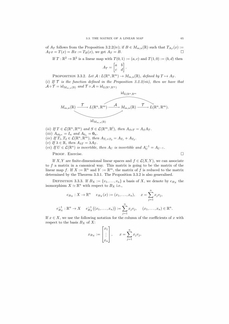
3.3. THE MATRIX OF A LINEAR MAP 65
of AT follows from the Proposition 3.2.2(iv); if B ∈Mm,n(R) such that TAT(x) :=
ATx = T (x) = Bx := TB(x), we get AT = B. �
If T : R2 → R2 is a linear map with T (0, 1) := (a, c) and T (1, 0) := (b, d) then
AT =
[a bc d
].
Proposition 3.3.2. Let A : L(Rn,Rm)→Mm,n(R), defined by T 7→ AT .
(i) If T is the function defined in the Proposition 3.2.2(vii), then we have thatA ◦ T = idMm,n(R) and T ◦ A = idL(Rn,Rm)
Mm,n(R) L(Rn,Rm) Mm,n(R) L(Rn,Rm).T A T
idMm,n(R)
idL(Rn,Rm
(ii) If T ∈ L(Rn,Rm) and S ∈ L(Rm,Rl), then AS◦T = ASAT .(iii) AidRn = In and A0n
= 0n.(iv) If T1, T2 ∈ L(Rn,Rm), then AT1+T2 = AT1 +AT2 .(v) If λ ∈ R, then AλT = λAT .(vi) If U ∈ L(Rn) is invertible, then AU is invertible and A−1
U = AU−1 .
Proof. Exercise. �
If X,Y are finite-dimensional linear spaces and f ∈ L(X,Y ), we can associateto f a matrix in a canonical way. This matrix is going to be the matrix of thelinear map f . If X := Rn and Y := Rm, the matrix of f is reduced to the matrixdetermined by the Theorem 3.3.1. The Proposition 3.3.2 is also generalised.
Definition 3.3.3. If BX := {v1, . . . , vn} a basis of X, we denote by eBXthe
isomorphism X ' Rn with respect to BX i.e.,
eBX: X → Rn eBX
(x) := (x1, . . . , xn), x =
n∑j=1
xjvj ,
e−1BX
: Rn → X e−1BX
((x1, . . . , xn)
):=
n∑j=1
xjvj , (x1, . . . , xn) ∈ Rn.
If x ∈ X, we use the following notation for the column of the coefficients of x withrespect to the basis BX of X:
xBX:=
x1
...xn
, x =
n∑j=1
xjvj ,
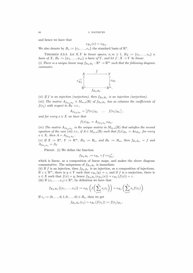
66 3. MATRICES
and hence we have thateBX
(x) = xBX.
We also denote by Bn := {e1, . . . , en} the standard basis of Rn.
Theorem 3.3.4. Let X,Y be linear spaces, n,m ≥ 1, BX := {v1, . . . , vn} abasis of X, BY := {w1, . . . , wm} a basis of Y , and let f : X → Y be linear.
(i) There is a unique linear map fBXBY: Rn → Rm such that the following diagram
commutes
X Y
Rn Rm.
f
fBXBY
e−1BX
eBY
(ii) If f is an injection (surjection), then fBXBYis an injection (surjection).
(iii) The matrix AfBXBY∈ Mm,n(R) of fBXBY
has as columns the coefficients of
f(vj) with respect to BY i.e.,
AfBXBY=[f(v1)BY
. . . f(vn)BY
],
and for every x ∈ X we have that
f(x)BY= AfBXBY
xBX.
(iv) The matrix AfBXBYis the unique matrix in Mm,n(R) that satisfies the second
equation of the case (iii) i.e., if A ∈Mm,n(R) such that f(x)BY= AxBX
, for everyx ∈ X, then A = AfBXBY
.
(v) If X := Rn, Y := Rm, BX := Bn, and BY := Bm, then fBnBm = f andAfBnBn
= Af
Proof. (i) We define the function
fBXBY:= eBY
◦ f ◦ e−1BX,
which is linear, as a composition of linear maps, and makes the above diagramcommutative. The uniqueness of fBXBY
is immediate.(ii) If f is an injection, then fBXBY
is an injection, as a composition of injections.If z ∈ Rm, there is y ∈ Y such that eBY
(y) = z, and if f is a surjection, there isx ∈ X such that f(x) = y, hence fBXBY
(eBX(x)) = eBY
(f(x)) = z.(iii) If (x1, . . . , xn) ∈ Rn, by definition we have that
fBXBY
((x1, . . . , xn)
):= eBY
(f
( n∑j=1
xjvj
))= eBY
( n∑j=1
xjf(vj)
).
If ej := (0, . . . , 0, 1, 0, . . . , 0) ∈ Bn, then we get
fBXBY(ej) = eBY
(f(vj)) := f(vj)BY,
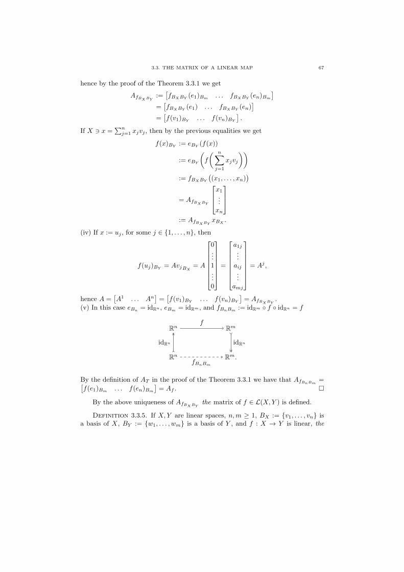
3.3. THE MATRIX OF A LINEAR MAP 67
hence by the proof of the Theorem 3.3.1 we get
AfBXBY:=[fBXBY
(e1)Bm. . . fBXBY
(en)Bm
]=[fBXBY
(e1) . . . fBXBY(en)
]=[f(v1)BY
. . . f(vn)BY
].
If X 3 x =∑nj=1 xjvj , then by the previous equalities we get
f(x)BY:= eBY
(f(x))
:= eBY
(f
( n∑j=1
xjvj
)):= fBXBY
((x1, . . . , xn)
)= AfBXBY
x1
...xn
:= AfBXBY
xBX.
(iv) If x := uj , for some j ∈ {1, . . . , n}, then
f(uj)BY= AvjBX
= A
0...1...0
=
a1j
...aij...
amj
= Aj ,
hence A =[A1 . . . An
]=[f(v1)BY
. . . f(vn)BY
]= AfBXBY
.
(v) In this case eBn= idRn , eBm
= idRm , and fBnBm:= idRm ◦ f ◦ idRn = f
Rn Rm
Rn Rm.
f
fBnBm
idRn idRn
By the definition of AT in the proof of the Theorem 3.3.1 we have that AfBnBm=[
f(e1)Bm. . . f(en)Bm
]= Af . �
By the above uniqueness of AfBXBYthe matrix of f ∈ L(X,Y ) is defined.
Definition 3.3.5. If X,Y are linear spaces, n,m ≥ 1, BX := {v1, . . . , vn} isa basis of X, BY := {w1, . . . , wm} is a basis of Y , and f : X → Y is linear, the

68 3. MATRICES
matrix of f with respect to BX and BY is the matrix AfBXBY∈ Mm,n(R), where
fBXBY:= eBY
◦f ◦e−1BX
. If T : X → X is linear, we use the notation TBX:= TBXBX
X X
Rn Rn.
T
eBXe−1BX
TBX
Corollary 3.3.6. Let X be a linear space, n ≥ 1, BX := {v1, . . . , vn} andCX := {w1, . . . , wn} are bases of X.
(i) If x ∈ X, then xCX= A(idX)BXCX
xBXand
A(idX)BXCX=[(v1)CX
. . . (vn)CX
]X X
Rn Rn.
idX
eCXe−1BX
(idX)BXCX
(ii) (idX)BX= idRn and A(idX)BX
= In
X X
Rn Rn.
idX
eBXe−1BX
(idX)BX
Proof. Exercise. �
If dim(X) = n and dim(Y ) = m, then by the Theorem 2.4.17 we have thatdim(L(X,Y )) = mn and by the Remark 3.1.2 we have that dim(Mm,n(R)) = mn.Hence, by the Corollary 2.4.15 we get L(X,Y ) ' Rmn 'Mmn(R), hence L(X,Y ) 'Mm,n(R). Next we provide a concrete isomorphism between these linear spaces.
Proposition 3.3.7. Let X,Y be linear spaces, n,m ≥ 1, BX := {v1, . . . , vn} abasis of X, BY := {w1, . . . , wm} a basis of Y , and let f, g : X → Y be linear maps.
(i) A(f+g)BXBY= AfBXBY
+AgBXBY.
(ii) If λ ∈ R, then A(λf)BXBY= λAfBXBY
.
(iii) The function eBXBY: L(X,Y ) → Mm,n(R), defined by f 7→ AfBXBY
, for
every f ∈ L(X,Y ), is a linear isomorphism.

3.3. THE MATRIX OF A LINEAR MAP 69
Proof. Exercise. �
The function eBXBYalso preserves the multiplication i.e., it sends the compo-
sition of linear maps to the product of the image-matrices.
Proposition 3.3.8. Let X,Y and Z be linear spaces, n,m, l ≥ 1, BX :={v1, . . . , vn} a basis of X, BY := {w1, . . . , wm} a basis of Y , BZ := {u1, . . . , ul} abasis of Z, and let f : X → Y and g : Y → Z be linear maps.
(i) (g ◦f)BXBZ= gBY BZ
◦fBXBYi.e., the following lower outer diagram commutes
X Y
Rn Rm
Z
Rl.
f g
gBY BZfBXBY
e−1BX
eBY e−1BY
eBZ
(g ◦ f)BXBZ
g ◦ f
(ii) A(g◦f)BXBZ= AgBY BZ
AfBXBY.
Proof. (i) Using the commutativity of the above inner diagrams we get
(g ◦ f)BXBZ:= eBZ
◦ (g ◦ f) ◦ e−1BX
= eBZ◦ [g ◦ idY ◦ f ] ◦ e−1
BX
= eBZ◦ [g ◦ (e−1
BY◦ eBY
) ◦ f ] ◦ e−1BX
= (eBZ◦ g ◦ e−1
BY) ◦ (eBY
◦ f ◦ e−1BX
)
= gBY BZ◦ fBXBY
.
We have that AgBY BZ∈ Ml,m(R) and AfBXBY
∈ Mm,n(R), therefore their multi-
plication is well-defined and belongs in Ml,n(R). Moreover, A(g◦f)BXBZ∈Ml,n(R).
By the Theorem 3.3.4(iii) we have that
A(g◦f)BXBZxBX
:= [g(f(x)]BZ= AgBY BZ
f(x)BY= AgBY BZ
AfBXBYxBX
,
and by the uniqueness in the Theorem 3.3.4(iv) A(g◦f)BXBZ= AgBY BZ
AfBXBY. �
Corollary 3.3.9. Let n ≥ 1, let X be an n-dimensional linear space, and letBX and CX be bases of X.
(i) (idX)BX= (idX)CXBX
◦ (idX)BXCX

70 3. MATRICES
X X
Rn Rn
X
Rn.
idX idX
(idX)CXBX(idX)BXCX
e−1BX
eCX
e−1CX eBX
(idX)BX
idX
(ii) A(idX)BX= A(idX)CXBX
A(idX)BXCX, and the matrices A(idX)CXBX
, A(idX)BXCX
are inverse to each other.
Proof. (i) It follows immediately from the Proposition 3.3.7(i).(ii) The required equality follows immediately from the Proposition 3.3.7(ii). Inter-changing the bases BX and CX we get A(idX)CX
= A(idX)BXCXA(idX)CXBX
. Since
by the Corollary 3.3.6(ii) we have that A(idX)BX= In = A(idX)CX
, the matricesA(idX)CXBX
and A(idX)BXCXare inverse to each other. �
Corollary 3.3.10. Let X,Y, Z and W be linear spaces, n,m, l, s ≥ 1, BX :={v1, . . . , vn} a basis of X, BY := {w1, . . . , wm} a basis of Y , BZ := {u1, . . . , ul} abasis of Z, BW := {ρ1, . . . , ρs} a basis of W , and let f : X → Y , g : Y → Z, andh : Z →W be linear maps.
(i) (h ◦ g ◦ f)BXBW= hBZBW
◦ gBY BZ◦ fBXBY
X Y
Rn Rm
Z W
Rl Rs.
f g h
gBY BZ
fBXBY hBZBW
e−1BX
eBY
e−1BY eBZ
e−1BZ eBW
(h ◦ g ◦ f)BXBW
h ◦ g ◦ f
(ii) A(h◦g◦f)BXBW= AhBZBW
AgBY BZAfBXBY
.
Proof. Exercise. �
Theorem 3.3.11. If n ≥ 1, X is an n-dimensional linear space, BX and CXare bases of X, and T : X → X is a linear map, then there exists an invertible

3.3. THE MATRIX OF A LINEAR MAP 71
matrix B ∈Mn(R) such that
ATCX= B−1ATBX
B.
Proof. By the Corollary 3.3.10 we have that
X X
Rn Rn
X X
Rn Rn
idX T idX
TBX
(idX)CXBX(idX)BXCX
e−1CX
eBX
e−1BX eBX
e−1BX eCX
TCX
T
TCX= (idX)BXCX
◦ TBX◦ (idX)CXBX
and ATCX= A(idX)BXCX
ATBXA(idX)CXBX
.
By the Corollary 3.3.9(ii) A(idX)CXBXand A(idX)BXCX
are inverse to each other. �
Definition 3.3.12. If n ≥ 1, X is an n-dimensional linear space, and T : X →X is a linear map, we say that a basis BX := {v1, . . . , vn} of X diagonalises T , ifATBX
=[T (v1)BX
. . . T (vn)BX
]∈ Mn(R) is a diagonal matrix. We say that T is
diagonalisable, if there exists some basis CX of X such that CX diagonalises T . Amatrix A ∈ Mn(R) is called a diagonalisable matrix, if the linear map TA of A isdiagonalisable.
Theorem 3.3.13. If n ≥ 1, X is an n-dimensional linear space, BX is a basisof X, and T : X → X is a linear map, then T is diagonalisable if and only ifthere exists some invertible matrix B ∈Mn(R) such that B−1ATBX
B is a diagonalmatrix.
Proof. Exercise. �
Definition 3.3.14. If A,A′ ∈ Mn(R), we say that A and A′ are similar, insymbols A ∼ A′, if there is some invertible matrix B ∈ Mn(R) such that A′ =B−1AB.
Remark 3.3.15. The relation A ∼ A′ is an equivalence relation on Mn(R).
Proof. Exercise. �


CHAPTER 4
Inner product spaces
4.1. The Euclidean inner product space and the Minkowski spacetime
Definition 4.1.1. Let X be a linear space. A bilinear map on X is a function〈·, ·〉 : X ×X → R such that for every x, y, z ∈ X and λ ∈ R the following hold:
(i) 〈x+ y, z〉 = 〈x, z〉+ 〈y, z〉 (left additivity).
(ii) 〈x, y + z〉 = 〈x, y〉+ 〈x, z〉 (right additivity).
(iii) 〈λx, y〉 = λ〈x, y〉 (left homogeneity).
(iv) 〈x, λy〉 = λ〈x, y〉 (right homogeneity).
An inner product on X is a symmetric bilinear map i.e., for every x, y ∈ X(v) 〈x, y〉 = 〈y, x〉 (symmetry),
and the pair (X, 〈·, ·〉) is called an inner product space. We call an inner product
(a) non-degenerate, if
∀x∈X(∀z∈X
(〈x, z〉 = 0
)⇒ x = 0
),
(b) positive, if ∀x∈X(〈x, x〉 ≥ 0
),
(c) negative, if ∀x∈X(〈x, x〉 ≤ 0
),
(c) positive definite, if
∀x∈X(x 6= 0⇒ 〈x, x〉 > 0
),
(d) negative definite, if
∀x∈X(x 6= 0⇒ 〈x, x〉 < 0
),
(e) indefinite, if it is neither positive definite nor negative definite.
If 〈·, ·〉 is an inner product on X the quadratic form Q〈·,·〉 associated with 〈·, ·〉 isthe function Q〈·,·〉 : X → R, defined by
Q〈·,·〉(x) := 〈x, x〉,
for every x ∈ X. If the inner product 〈·, ·〉 is clear from the context, we write Q(x)instead of Q〈·,·〉(x). An element x of X is called
(α) lightlike, or null, if Q(x) := 〈x, x〉 = 0,
73
74 4. INNER PRODUCT SPACES
(β) timelike, if Q(x) := 〈x, x〉 < 0,
(γ) spacelike, if Q(x) := 〈x, x〉 > 0,
(δ) unit, if Q(x) := 〈x, x〉 ∈ {1,−1}.
E.g., if C([0, 1]) is the linear space of all continuous, real-valued functions onthe compact interval [0, 1], the function
(f, g) 7→ 〈f, g〉 :=
∫ 1
0
f(t)g(t)dt,
for every f, g ∈ C([0, 1]) is a non-degenerate, positive, inner product on C([0, 1]).As we have already seen in the Remark 3.1.9, the function
(A,B) 7→ Tr(AB)
is a non degenerate, indefinite inner product on Mn(R), and a positive definiteinner product on Symn(R).
Remark 4.1.2. Let (X, 〈·, ·〉) be an inner product space.
(i) Left additivity and left homogeneity imply right additivity and right homogene-ity, and vice versa.
(ii) If x ∈ X, then 〈0, x〉 = 0.
(iii) If 〈·, ·〉 is positive definite, then 〈·, ·〉 is positive, and non-degenerate.
(iv) If 〈·, ·〉 is positive, then −〈·, ·〉, where −〈·, ·〉(x, y) := −〈x, y〉, for every x, y ∈ X,is a negative inner product on X.
(v) For every x, y ∈ X we have that
〈x, y〉 =1
4
(〈x+ y, x+ y〉 − 〈x− y, x− y〉
).
(vi) If 〈〈·, ·〉〉 is an inner product on X such that Q〈·,·〉(x) = Q〈〈·,·〉〉(x), for everyx ∈ X, then 〈〈x, y〉〉 = 〈x, y〉, for every x, y ∈ X.
Proof. Exercise. �
Definition 4.1.3. If x = (x1, . . . , xn) and y = (y1, . . . , yn) are in Rn, theirEuclidean inner product is defined by
〈x, y〉 :=
n∑i=1
xiyi := x1y1 + . . .+ xnyn.
If n = 1, the Euclidean inner product on R is the product on R. The quadraticform of the Euclidean inner product on Rn is given by
Q(x) := 〈x, x〉 :=
n∑i=1
xixi =
n∑i=1
x2i = x2
1 + . . .+ x2n.
The Euclidean inner product is a positive definite inner product on Rn, with 0 asthe only lightlike vector, and with no timelike vectors.

4.1. THE EUCLIDEAN INNER PRODUCT SPACE AND THE MINKOWSKI SPACETIME 75
Definition 4.1.4. If n ≥ 2, x = (x1, . . . , xn−1, s) and y = (y1, . . . , yn−1, t) arein Rn, their Minkowski inner product, or their Lorentz inner product, is defined by
〈x, y〉 :=
n−1∑i=1
xiyi − st = x1y1 + . . .+ xn−1yn−1 − st.
The pair M4 := (R4, 〈·, ·〉), where 〈·, ·〉 is the Minkowski inner product on R4, iscalled the Minkowski spacetime. We call the pair M3 := (R3, 〈·, ·〉), where 〈·, ·〉is the Minkowski inner product on R3, the Minkowski planetime, and the pairM2 := (R2, 〈·, ·〉), where 〈·, ·〉 is the Minkowski inner product on R2, the Minkowskilinetime.
The quadratic forms of the Minkowski inner product on Rn and R4 are
Q(x1, . . . , xn−1, s)
):= 〈(x1, . . . , xn−1, s), (x1, . . . , xn−1, s)〉
:=
n−1∑i=1
x2i − s2 = x2
1 + . . .+ x2n−1 − s2,
Q((x1, x2, x3, s)
):= 〈(x1, x2, x3, s), (x1, x2, x3, s)〉 :=
3∑i=1
x2i −s2 = x2
1 +x22 +x2
3−s2.
The Minkowski spacetime is regarded in [18], p. 1, as “the appropriate arenawithin which to formulate those laws of physics that do not refer specifically to grav-itational phenomena”1. A non-zero vector x in Rn, equipped with the Minkowskiinner product, where x := (x1, . . . , xn−1, 0) is spacelike,
Q((x1, . . . , xn−1, 0)
):= x2
1 + . . .+ x2n−1 − 0 > 0,
while if x := (0, . . . , 0, s), then x is timelike, since
Q((0, . . . , 0, s)
):= 02 + . . .+ 02 − s2 < 0.
Moreover, there are non-zero vectors in R4 that are lightlike e.g.,
Q((1, 1, 0,
√2))
:= 12 + 12 + 02 −√
22
= 0.
If we consider the Minkowski linetime, the lightlike vectors form the lines t = xand t = −x, the timelike vectors are within the cone at the origin (0, 0) formed bythese two lines, and the spacelike vectors are outside the cone.
1See [18] for an elaborated study of the mathematical properties of the Minkowski spacetime.

76 4. INNER PRODUCT SPACES
x
t
t = xt = −x
Q < 0
Q < 0
Q > 0Q > 0
If we consider the Minkowski planetime, then one can show that its lightlike vectors(x, y, t) ∈ R3 form a cone at the origin (0, 0, 0) with equation
x2 + y2 − t2 = 0,
its timelike vectors are inside this cone, and its spacelike vectors are outside thiscone. Next we draw the upper lightcone at the origin (0, 0, 0).
−1
1−1
1
0.5
1
x
y
t
Proposition 4.1.5. The Minkowski inner product is an indefinite and non-degenerate inner product on Rn.
Proof. Exercise. �
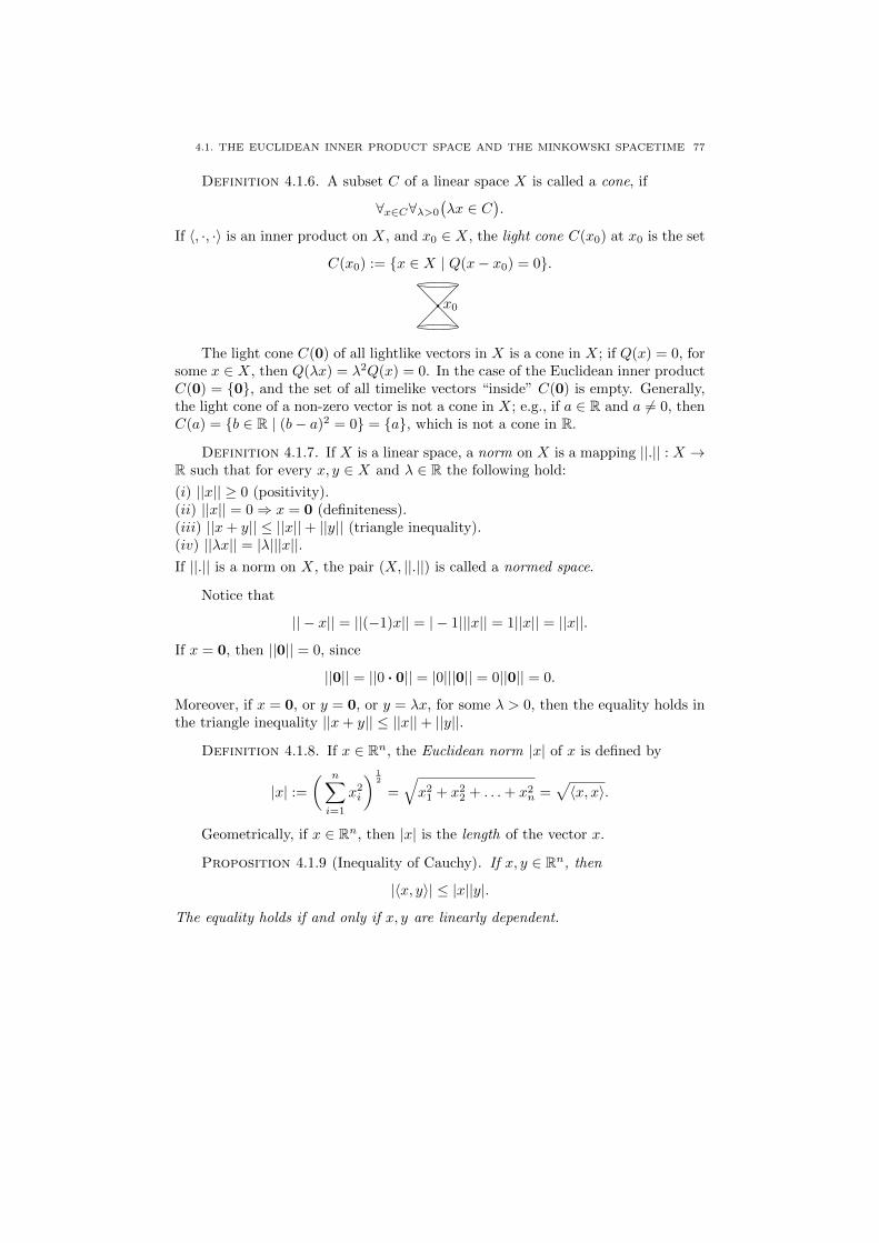
4.1. THE EUCLIDEAN INNER PRODUCT SPACE AND THE MINKOWSKI SPACETIME 77
Definition 4.1.6. A subset C of a linear space X is called a cone, if
∀x∈C∀λ>0
(λx ∈ C
).
If 〈, ·, ·〉 is an inner product on X, and x0 ∈ X, the light cone C(x0) at x0 is the set
C(x0) := {x ∈ X | Q(x− x0) = 0}.
x0
The light cone C(0) of all lightlike vectors in X is a cone in X; if Q(x) = 0, forsome x ∈ X, then Q(λx) = λ2Q(x) = 0. In the case of the Euclidean inner productC(0) = {0}, and the set of all timelike vectors “inside” C(0) is empty. Generally,the light cone of a non-zero vector is not a cone in X; e.g., if a ∈ R and a 6= 0, thenC(a) = {b ∈ R | (b− a)2 = 0} = {a}, which is not a cone in R.
Definition 4.1.7. If X is a linear space, a norm on X is a mapping ||.|| : X →R such that for every x, y ∈ X and λ ∈ R the following hold:
(i) ||x|| ≥ 0 (positivity).(ii) ||x|| = 0⇒ x = 0 (definiteness).(iii) ||x+ y|| ≤ ||x||+ ||y|| (triangle inequality).(iv) ||λx|| = |λ|||x||.If ||.|| is a norm on X, the pair (X, ||.||) is called a normed space.
Notice that
|| − x|| = ||(−1)x|| = | − 1|||x|| = 1||x|| = ||x||.
If x = 0, then ||0|| = 0, since
||0|| = ||0 · 0|| = |0|||0|| = 0||0|| = 0.
Moreover, if x = 0, or y = 0, or y = λx, for some λ > 0, then the equality holds inthe triangle inequality ||x+ y|| ≤ ||x||+ ||y||.
Definition 4.1.8. If x ∈ Rn, the Euclidean norm |x| of x is defined by
|x| :=( n∑i=1
x2i
) 12
=√x2
1 + x22 + . . .+ x2
n =√〈x, x〉.
Geometrically, if x ∈ Rn, then |x| is the length of the vector x.
Proposition 4.1.9 (Inequality of Cauchy). If x, y ∈ Rn, then
|〈x, y〉| ≤ |x||y|.
The equality holds if and only if x, y are linearly dependent.

78 4. INNER PRODUCT SPACES
Proof. By definition we need to show∣∣∣∣ n∑i=1
xiyi
∣∣∣∣ ≤ ( n∑i=1
x2i
) 12( n∑i=1
y2i
) 12
,
which is equivalent to
A :=
( n∑i=1
xiyi
)2
≤( n∑i=1
x2i
)( n∑i=1
y2i
)=: B.
This we get as follows:
B −A =
n∑i=1
x2i
n∑j=1
y2j −
n∑i=1
xiyi
n∑j=1
xjyj
=1
2
n∑i=1
x2i
n∑j=1
y2j +
1
2
n∑j=1
x2j
n∑i=1
y2i −
n∑i=1
xiyi
n∑j=1
xjyj
=
n∑i,j=1
1
2
(x2i y
2j + x2
jy2i − 2xiyixjyj
)=
n∑i,j=1
1
2
(xiyj − xjyi
)2≥ 0.
If y = 0, then 0x + 1y = 0, hence x,0 are linearly dependent, and the equalitytrivially holds. If yj 6= 0, for some j ∈ {1, . . . , n}, then B = A ⇔ x = λy, whereλ :=
xj
yj. Clearly, xj = λyj . If i 6= j, then xi = λyi ⇔ xi− xj
yjyi = 0⇔ xiyj−xjyi =
0. The last condition, for every i, j ∈ {1, . . . , n} such that i 6= j is equivalent toB −A = 0⇔ B = A. �
The inequality of Cauchy is necessary to the proof that (Rn, |.|) is a normedspace; it is used in the proof of the triangle inequality for the Euclidean norm, whilethe rest of the proof is easy. To understand the geometric meaning of the Euclideaninner product we first see that a vector x ∈ Rn is orthogonal to a vector y ∈ Rn,in symbols x⊥y, if and only if 〈x, y〉 = 0. To explain this we work as follows. It iseasy to see geometrically2 that
x⊥y ⇔ |x− y| = |x+ y|,
since the diagonals of the parallelogram are equal only if x is perpendicular to y.
2The following figure also explains why |x+ y| ≤ |x|+ |y|.
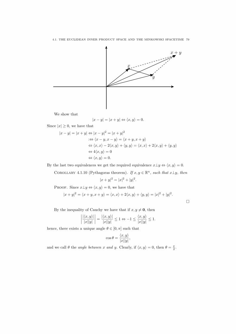
4.1. THE EUCLIDEAN INNER PRODUCT SPACE AND THE MINKOWSKI SPACETIME 79
y
x+ y
x
We show that
|x− y| = |x+ y| ⇔ 〈x, y〉 = 0.
Since |x| ≥ 0, we have that
|x− y| = |x+ y| ⇔ |x− y|2 = |x+ y|2
:⇔ 〈x− y, x− y〉 = 〈x+ y, x+ y〉⇔ 〈x, x〉 − 2〈x, y〉+ 〈y, y〉 = 〈x, x〉+ 2〈x, y〉+ 〈y, y〉⇔ 4〈x, y〉 = 0
⇔ 〈x, y〉 = 0.
By the last two equivalences we get the required equivalence x⊥y ⇔ 〈x, y〉 = 0.
Corollary 4.1.10 (Pythagoras theorem). If x, y ∈ Rn, such that x⊥y, then
|x+ y|2 = |x|2 + |y|2.
Proof. Since x⊥y ⇔ 〈x, y〉 = 0, we have that
|x+ y|2 = 〈x+ y, x+ y〉 = 〈x, x〉+ 2〈x, y〉+ 〈y, y〉 = |x|2 + |y|2.
�
By the inequality of Cauchy we have that if x, y 6= 0, then∣∣∣∣ |〈x, y〉||x||y|
∣∣∣∣ =|〈x, y〉||x||y|
≤ 1⇔ −1 ≤ 〈x, y〉|x||y|
≤ 1.
hence, there exists a unique angle θ ∈ [0, π] such that
cos θ =〈x, y〉|x||y|
,
and we call θ the angle between x and y. Clearly, if 〈x, y〉 = 0, then θ = π2 .
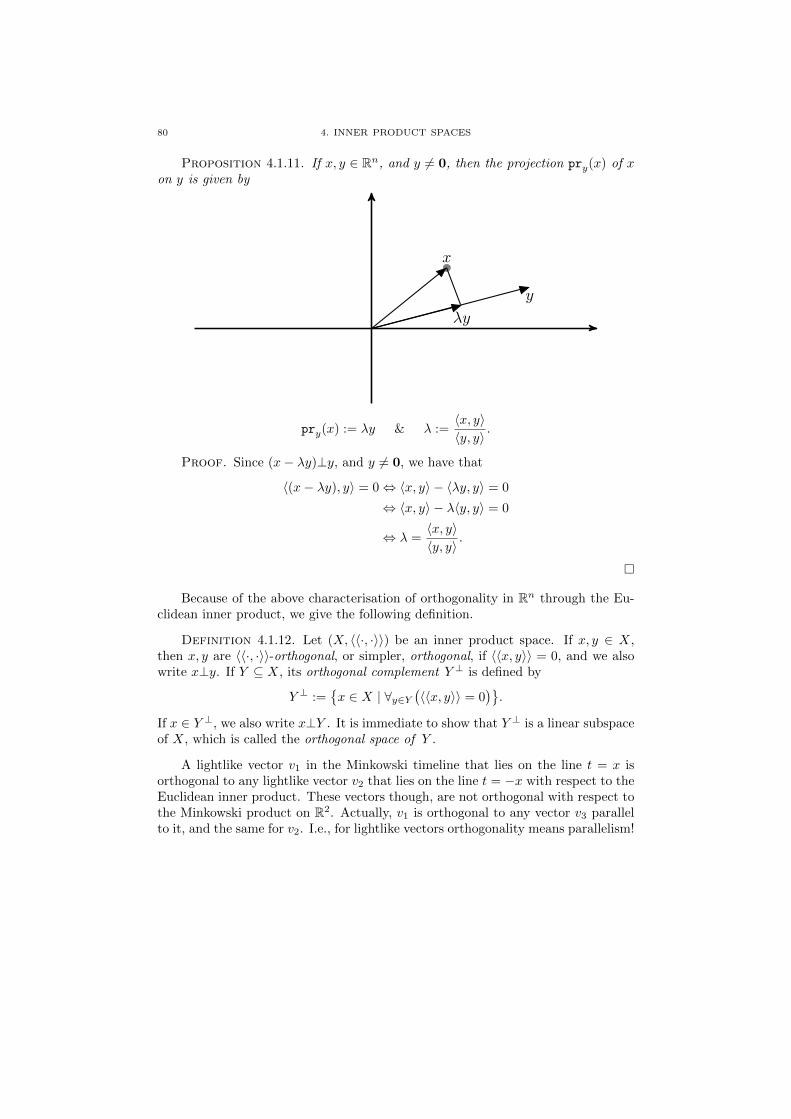
80 4. INNER PRODUCT SPACES
Proposition 4.1.11. If x, y ∈ Rn, and y 6= 0, then the projection pry(x) of xon y is given by
y
x
λy
pry(x) := λy & λ :=〈x, y〉〈y, y〉
.
Proof. Since (x− λy)⊥y, and y 6= 0, we have that
〈(x− λy), y〉 = 0⇔ 〈x, y〉 − 〈λy, y〉 = 0
⇔ 〈x, y〉 − λ〈y, y〉 = 0
⇔ λ =〈x, y〉〈y, y〉
.
�
Because of the above characterisation of orthogonality in Rn through the Eu-clidean inner product, we give the following definition.
Definition 4.1.12. Let (X, 〈〈·, ·〉〉) be an inner product space. If x, y ∈ X,then x, y are 〈〈·, ·〉〉-orthogonal, or simpler, orthogonal, if 〈〈x, y〉〉 = 0, and we alsowrite x⊥y. If Y ⊆ X, its orthogonal complement Y ⊥ is defined by
Y ⊥ :={x ∈ X | ∀y∈Y
(〈〈x, y〉〉 = 0
)}.
If x ∈ Y ⊥, we also write x⊥Y . It is immediate to show that Y ⊥ is a linear subspaceof X, which is called the orthogonal space of Y .
A lightlike vector v1 in the Minkowski timeline that lies on the line t = x isorthogonal to any lightlike vector v2 that lies on the line t = −x with respect to theEuclidean inner product. These vectors though, are not orthogonal with respect tothe Minkowski product on R2. Actually, v1 is orthogonal to any vector v3 parallelto it, and the same for v2. I.e., for lightlike vectors orthogonality means parallelism!
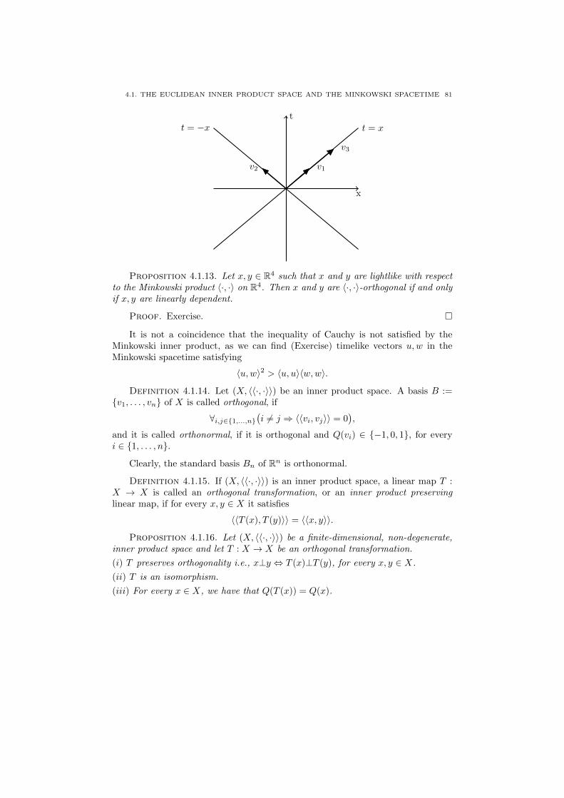
4.1. THE EUCLIDEAN INNER PRODUCT SPACE AND THE MINKOWSKI SPACETIME 81
x
t
t = xt = −x
v1v2
v3
Proposition 4.1.13. Let x, y ∈ R4 such that x and y are lightlike with respectto the Minkowski product 〈·, ·〉 on R4. Then x and y are 〈·, ·〉-orthogonal if and onlyif x, y are linearly dependent.
Proof. Exercise. �
It is not a coincidence that the inequality of Cauchy is not satisfied by theMinkowski inner product, as we can find (Exercise) timelike vectors u,w in theMinkowski spacetime satisfying
〈u,w〉2 > 〈u, u〉〈w,w〉.
Definition 4.1.14. Let (X, 〈〈·, ·〉〉) be an inner product space. A basis B :={v1, . . . , vn} of X is called orthogonal, if
∀i,j∈{1,...,n}(i 6= j ⇒ 〈〈vi, vj〉〉 = 0
),
and it is called orthonormal, if it is orthogonal and Q(vi) ∈ {−1, 0, 1}, for everyi ∈ {1, . . . , n}.
Clearly, the standard basis Bn of Rn is orthonormal.
Definition 4.1.15. If (X, 〈〈·, ·〉〉) is an inner product space, a linear map T :X → X is called an orthogonal transformation, or an inner product preservinglinear map, if for every x, y ∈ X it satisfies
〈〈T (x), T (y)〉〉 = 〈〈x, y〉〉.
Proposition 4.1.16. Let (X, 〈〈·, ·〉〉) be a finite-dimensional, non-degenerate,inner product space and let T : X → X be an orthogonal transformation.
(i) T preserves orthogonality i.e., x⊥y ⇔ T (x)⊥T (y), for every x, y ∈ X.
(ii) T is an isomorphism.
(iii) For every x ∈ X, we have that Q(T (x)) = Q(x).

82 4. INNER PRODUCT SPACES
(iv) If S : X → X is a linear map such that Q(S(x)) = Q(x), for every x ∈ X,then S is an orthogonal transformation.
(v) If BX := {v1, . . . , vn} is an orthonormal basis of X, then its image T (BX) :={T (v1), . . . , T (vn)} under T is an orthonormal basis of X.
(vi) Suppose that X has an orthonormal basis, and let S : X → X be a linear mapsuch that for every orthonormal basis BX := {v1, . . . , vn} of X its image S(BX)under S is an orthonormal basis of X, and for every i ∈ {1, . . . , n}, we have thatQ(S(vi)) = Q(vi). Then S is an orthogonal transformation.
Proof. Exercise. �
The existence of orthogonal and orthonormal bases of an inner product spaceis studied next.
4.2. Existence of an orthogonal basis, the positive definite case
Throughout this section 〈〈·, ·〉〉 is a positive definite inner product on a linearspace X. The properties of (X, 〈〈·, ·〉〉) generalise the properties of Rn equippedwith the Euclidean norm, if we use the following definitions, motivated by theirgeometric interpretation in the case of Rn. Namely, we define
x⊥y :⇔ 〈〈x, y〉〉 = 0
pry(x) := λy(x)y, λy(x) :=〈〈x, y〉〉〈〈y, y〉〉
,
where y 6= 0. Since 〈〈x, x〉〉 ≥ 0, the norm induced by the positive definite innerproduct 〈〈·, ·〉〉 on X is given by
||x|| :=√〈〈x, x〉〉,
for every x ∈ X. We need to show the generalisation of the inequality of Cauchy,in order to prove that ||x|| is a norm on X.
Proposition 4.2.1. Let (X, 〈〈·, ·〉〉) be a positive definite, inner product space,x, y, x1, . . . , xn ∈ X, and let || · || be the norm on X induced by 〈〈·, ·〉〉.(i) (Pythagoras) If x⊥y, then ||x+ y||2 = ||x||2 + ||y||2.
(ii) (Generalised Pythagoras) If xi⊥xj, for every i, j ∈ {1, . . . , n} such that i 6= j,then
||x1 + . . .+ xn||2 = ||x1||2 + . . .+ ||xn||2.(iii) (Parallelogram law) ||x+ y||2 + ||x− y||2 = 2
(||x||2 + ||y||2
).
(iv) (Polarisation identity) 〈〈x, y〉〉 := 14
(||x+ y||2 − ||x− y||2
).
(v) If λ ∈ R, then ||λx|| = λ||x||.(vi) ||x|| = 0⇔ x = 0.

4.2. EXISTENCE OF AN ORTHOGONAL BASIS, THE POSITIVE DEFINITE CASE 83
(vii) If x 6= 0, then ∣∣∣∣∣∣∣∣ x||x||∣∣∣∣∣∣∣∣ = 1.
(viii) (Inequality Cauchy-Schwarz) |〈〈x, y〉〉| ≤ ||x|| ||y||, and the equality holds ifand only if x, y are linearly dependent.
(ix) (Triangle inequality) ||x + y|| ≤ ||x|| + ||y||. The equality holds if and only ifeither x = 0 ∨ y = 0 or there is some λ > 0 such that x = λy.
(x) || · || is a norm on X.
(xi)∣∣||x|| − ||y||∣∣ ≤ ||x− y||.
(xii) ||x|| − ||y|| ≤∣∣||x|| − ||y||∣∣ ≤ ||x+ y||.
Proof. We show only the case (viii), and the rest is an exercise. If y = 0,then both terms of the inequality are equal to 0. If y 6= 0 and ||y|| = 1, then,(x− λy(x))⊥y, hence
(x− λy(x)y)⊥λy(x)y.
By the theorem of Pythagoras we have that
||x||2 = ||(x− λy(x)y) + λy(x)y||2
= ||x− λy(x)y||2 + ||λy(x)y||2
= ||x− λy(x)y||2 +[|λy(x)|||y||
]2= ||x− λy(x)y||2 + λy(x)2,
hence λy(x)2 ≤ ||x||2, and consequently
|λy(x)| :=∣∣∣∣ 〈〈x, y〉〉〈〈y, y〉〉
∣∣∣∣ = |〈〈x, y〉〉| ≤ ||x|| = ||x||1 = ||x||||y||.
If y 6= 0, then by the case (v) and the previous fact we have that∣∣∣∣〈〈x, y
||y||〉〉∣∣∣∣ ≤ ||x|| ⇔ |〈〈x, y〉〉| ≤ ||x|| ||y||.
If x, y are linearly dependent, then the equality holds; if y = 0, it is trivial, and ify 6= 0, then x = λy, for some λ ∈ R, and
|〈〈λy, y〉〉| = |λ||〈〈y, y〉〉| = |λ|||y||2 = |λ|||y||||y|| = ||x|| ||y||.If the equality holds and one of x, y is 0, then x, y are linearly dependent. Sup-pose next that the equality holds and both x 6= 0 and y 6= 0. As it is expectedgeometrically, we have that
||x− λy(x)y||2 = 〈〈x− λy(x)y, x− λy(x)y〉〉= 〈〈x, x〉〉 − 2λy(x)〈〈x, y〉〉+ λy(x)2〈〈y, y〉〉
:= 〈〈x, x〉〉 − 2〈〈x, y〉〉〈〈y, y〉〉
〈〈x, y〉〉+〈〈x, y〉〉2
〈〈y, y〉〉

84 4. INNER PRODUCT SPACES
= 〈〈x, x〉〉 − 〈〈x, y〉〉2
〈〈y, y〉〉
=〈〈x, x〉〉〈〈y, y〉〉 − 〈〈x, y〉〉2
〈〈y, y〉〉= 0,
hence x = λy(x)y. Since x 6= 0 and y 6= 0, we get λy(x) 6= 0, and hence x, y arelinearly dependent. �
Theorem 4.2.2 (Jordan, von Neumann). If (X, ||.||) is a normed space, itsnorm ||.|| is induced by some positive definite inner product 〈〈·, ·〉〉 on X if and onlyif ||.|| satisfies the parallelogram law.
Proof. The satisfiability of the parallelogram law follows from the Proposi-tion 4.2.1(iii). For the converse, we define, due to the polarization identity,
(4.1) 〈〈x, y〉〉 :=1
4
(||x+ y||2 − ||x− y||2
).
It is immediate to show that 〈〈x, y〉〉 is positive definite and symmetric form on X.It is also straightforward to see that
(4.2) 〈〈−x, y〉〉 = −〈〈x, y〉〉.In order to show left additivity, by the parallelogram law and the definition of〈〈x, y〉〉 we have that
4〈〈x+ z, y〉〉 = ||x+ z + y||2 − ||x+ z − y||2
=
∣∣∣∣∣∣∣∣(x+y
2
)+
(z +
y
2
)∣∣∣∣∣∣∣∣2 − ∣∣∣∣∣∣∣∣(x− y
2
)+
(z − y
2
)∣∣∣∣∣∣∣∣2= 2
∣∣∣∣∣∣∣∣x+y
2
∣∣∣∣∣∣∣∣2 + 2
∣∣∣∣∣∣∣∣z +y
2
∣∣∣∣∣∣∣∣2 − ||x− z||2−(
2
∣∣∣∣∣∣∣∣x− y
2
∣∣∣∣∣∣∣∣2 + 2
∣∣∣∣∣∣∣∣z − y
2
∣∣∣∣∣∣∣∣2 − ||x− z||2)= 2
(∣∣∣∣∣∣∣∣x+y
2
∣∣∣∣∣∣∣∣2 − ∣∣∣∣∣∣∣∣x− y
2
∣∣∣∣∣∣∣∣2)
+ 2
(∣∣∣∣∣∣∣∣z +y
2
∣∣∣∣∣∣∣∣2 − ∣∣∣∣∣∣∣∣z − y
2
∣∣∣∣∣∣∣∣2)
= 8〈〈x, y2〉〉+ 8〈〈z, y
2〉〉,
where for the last equality we used the definition of 〈〈x, y〉〉. Hence we get
(4.3) 〈〈x+ z, y〉〉 = 2
(〈〈x, y
2〉〉+ 〈〈z, y
2〉〉).
If in (4.3) we set z = 0, we get for every x, y ∈ X
(4.4) 〈〈x, y〉〉 = 2〈〈x, y2〉〉.
4.2. EXISTENCE OF AN ORTHOGONAL BASIS, THE POSITIVE DEFINITE CASE 85
Consequently, (4.3) becomes
〈〈x+ z, y〉〉 = 2
(〈〈x, y
2〉〉+ 〈〈z, y
2〉〉)
= 〈〈x, y〉〉+ 〈〈z, y〉〉.
The rest of the proof is an exercise. �
In [2] there are around 350 characterizations of when a norm is induced by apositive definite inner product!
Proposition 4.2.3. Let (X, 〈〈·, ·〉〉) be a positive definite, inner product space,and || · || the norm on X induced by 〈〈·, ·〉〉. Let B := {v1, . . . , vn} ⊆ X, such that
(a) vi⊥vj, for every i, j ∈ {1, . . . , n} with i 6= j, and (b) vi 6= 0, for every i ∈{1, . . . , n}. If x ∈ X, let
λi(x) := λvi(x) :=〈〈x, vi〉〉〈〈vi, vi〉〉
& xB :=
n∑i=1
λi(x)vi.
(i) The vectors v1, . . . , vn are linearly independent.
(ii) The vector x− xB is orthogonal to every element of B.
(iii) The vector xB is the closest approximation to x from 〈B〉 i.e., for everya1, . . . , an ∈ R, we have that
||x− xB || :=∣∣∣∣∣∣∣∣x− n∑
i=1
λi(x)vi
∣∣∣∣∣∣∣∣ ≤ ∣∣∣∣∣∣∣∣x− n∑i=1
aivi
∣∣∣∣∣∣∣∣.(iv) Let ||vi|| = 1, for every i ∈ {1, . . . , n}.(α) The following inequality, known as Bessel inequality, holds
n∑i=1
λi(x)2 ≤ ||x||2.
(β) For every x ∈ X we have that
||x||2 =
n∑i=1
λi(x)2
if and only if B is a basis of X.
Proof. (i) Let a1, . . . , an ∈ R such that∑ni=1 aivi = 0. If k ∈ {1, . . . , n}, then
0 =
⟨⟨ n∑i=1
aivi, vk
⟩⟩= ak〈〈vk, vk〉〉 := ak||vk||2,
and by the hypothesis (b) we get ak = 0.(ii) If k ∈ {1, . . . , n}, then⟨⟨
x−n∑i=1
λi(x)vi, vk
⟩⟩= 〈〈x, vk〉〉 −
⟨⟨ n∑i=1
λi(x)vi, vk
⟩⟩

86 4. INNER PRODUCT SPACES
= 〈〈x, vk〉〉 − 〈〈λk(x)vk, vk〉〉= 〈〈x, vk〉〉 − λk(x)〈〈vk, vk〉〉
:= 〈〈x, vk〉〉 −〈〈x, vk〉〉〈〈vk, vk〉〉
〈〈vk, vk〉〉
= 0.
(iii) Since x− xB is orthogonal to B, it is also orthogonal to 〈B〉, hence(x−
n∑i=1
λi(x)vi
)⊥
n∑i=1
(λi(x)− ai
)vi.
By the theorem of Pythagoras we have that∣∣∣∣∣∣∣∣x− n∑i=1
aivi
∣∣∣∣∣∣∣∣2 =
∣∣∣∣∣∣∣∣x− n∑i=1
aivi +
n∑i=1
λi(x)vi −n∑i=1
λi(x)vi
∣∣∣∣∣∣∣∣2=
∣∣∣∣∣∣∣∣(x− n∑i=1
λi(x)vi
)+
n∑i=1
(λi(x)− ai
)vi
∣∣∣∣∣∣∣∣2=
∣∣∣∣∣∣∣∣x− n∑i=1
λi(x)vi
∣∣∣∣∣∣∣∣2 +
∣∣∣∣∣∣∣∣ n∑i=1
(λi(x)− ai
)vi
∣∣∣∣∣∣∣∣2,and the required inequality follows.(iv)(α) Since x− xB is orthogonal to 〈B〉, we have that(
x−n∑i=1
λi(x)vi
)⊥
n∑i=1
λi(x)vi.
By the theorem of Pythagoras and its generalised version we have that
||x||2 =
∣∣∣∣∣∣∣∣(x− n∑i=1
λi(x)vi
)+
n∑i=1
λi(x)vi
∣∣∣∣∣∣∣∣2=
∣∣∣∣∣∣∣∣x− n∑i=1
λi(x)vi
∣∣∣∣∣∣∣∣2 +
∣∣∣∣∣∣∣∣ n∑i=1
λi(x)vi
∣∣∣∣∣∣∣∣2=
∣∣∣∣∣∣∣∣x− n∑i=1
λi(x)vi
∣∣∣∣∣∣∣∣2 +
n∑i=1
||λi(x)vi||2
=
∣∣∣∣∣∣∣∣x− n∑i=1
λi(x)vi
∣∣∣∣∣∣∣∣2 +
n∑i=1
λi(x)2||vi||2
=
∣∣∣∣∣∣∣∣x− n∑i=1
λi(x)vi
∣∣∣∣∣∣∣∣2 +
n∑i=1
λi(x)2,
and the required inequality follows. The proof of (β) is an exercise. Notice that wedo not need to suppose that X is finite-dimensional. �
4.2. EXISTENCE OF AN ORTHOGONAL BASIS, THE POSITIVE DEFINITE CASE 87
Theorem 4.2.4. If (X, 〈〈·, ·〉〉) is a positive definite, inner product space ofdimension n ≥ 1, Y is a proper subspace of X, and BY := {y1, . . . , ym} is anorthogonal basis of Y , there exist vm+1, . . . , vn ∈ X such that
B⊥ := {y1, . . . , ym, vm+1, . . . , vn}is an orthogonal basis of X.
Proof. By the Corollary 2.2.16(iv) there exist um+1, . . . , un ∈ X such thatB := {y1, . . . , ym, um+1, . . . , un} is a basis of X. If Ym+1 := 〈y1, . . . , ym, um+1〉, let
vm+1 := um+1 −m∑j=1
λyj (um+1)yj :=
m∑j=1
〈〈um+1, yj〉〉〈〈yj , yj〉〉
yj .
By the Proposition 4.2.3(ii) we get vm+1⊥{y1, . . . , ym}. Since
um+1 = vm+1 +
m∑j=1
λyj (um+1)yj ,
we get um+1 ∈ 〈y1, . . . , ym, vm+1〉. Moreover, vm+1 6= 0, since if vm+1 = 0, thenum+1 =
∑mj=1 λyj (um+1)yj , and B is not linearly independent. Consequently,
{y1, . . . , ym, vm+1} is an orthogonal basis of Ym+1. Repeating this step m − nnumber of times (actually, an induction takes place here) we reach our conclusion.
�
Corollary 4.2.5. If (X, 〈〈·, ·〉〉) is a positive definite, inner product space ofdimension n ≥ 1, there exists an orthogonal (orthonormal) basis B⊥ (B1
⊥) of X.
Proof. If v1 ∈ X such that v1 6= 0, then {v1} is an orthogonal basis of 〈v1〉,and by the Theorem 4.2.4 there is an orthogonal basis B⊥ of X that extends {v1}.Moreover, if B⊥ := {v1, . . . , vn} is an orthogonal basis of X, then
B1⊥ :=
{v1
||v1||, . . . ,
vn||vn||
}is an orthonormal basis of X. �
Hence, if B := {u1, . . . , un} is a basis of X, and
v1 := u1
v2 := u2 −〈〈u2, v1〉〉〈〈v1, v1〉〉
v1
v3 := u3 −〈〈u3, v2〉〉〈〈v2, v2〉〉
v2 −〈〈u3, v1〉〉〈〈v1, v1〉〉
v1
......
vn := un −〈〈un, vn−1〉〉〈〈vn−1, vn−1〉〉
vn−1 − . . .−〈〈un, v1〉〉〈〈v1, v1〉〉
v1,
88 4. INNER PRODUCT SPACES
then B⊥ := {v1, . . . , vn} is an orthogonal basis of X. The above algorithm forfinding an orthogonal basis of X, given a finite basis of X, is called the Gram-Schmidt orthogonalisation process.
Remark 4.2.6. Let (X, 〈〈·, ·〉〉) be a positive definite, inner product space ofdimension n ≥ 1, BX := {v1, . . . , vn} a basis of X, and
x =
n∑i=1
λivi & y =
n∑i=1
µivi,
where λ1, . . . , λn, µ1, . . . , µn ∈ R. Let aij := 〈〈vi, vj〉〉, for every i, j ∈ {1, . . . , n}.(i) 〈〈x, y〉〉 =
∑ni,j=1 λiµjaij .
(ii) If BX is orthogonal, then 〈〈x, y〉〉 =∑ni=1 λiµiaii.
(iii) If BX is orthonormal, then 〈〈x, y〉〉 =∑ni=1 λiµi.
Proof. Exercise. �
Since the standard basis Bn of Rn is orthonormal, by the Remark 4.2.6(iii) theEuclidean inner product is uniquely determined. Next we see why Y ⊥ is called theorthogonal complement of the subspace Y .
Theorem 4.2.7. If (X, 〈〈·, ·〉〉) is a positive definite, inner product space ofdimension n ≥ 1, and Y is a subspace of X of dimension r, where 0 ≤ r ≤ n, then
X = Y ⊕ Y ⊥,and hence dim(Y ⊥) = n− r.
Proof. Exercise. �
The above decomposition of X does not hold, in general, if the inner producton X is not positive definite. E.g., we can find a subspace Y of the Minkowskilinetime such that {0} ( Y ⊥ ∩ Y and R2 is not equal to Y + Y ⊥ (Exercise). Nextwe add one more equivalent condition to the Proposition 3.2.4.
Proposition 4.2.8. If A := [aij ] ∈ Mm,n(R) and (x1, . . . , xn) ∈ Rn, the fol-lowing are equivalent.
(i) (x1, . . . , xn) is a solution of the following system of linear equations
a11x1 + . . .+ a1nxn = 0
......
...
am1x1 + . . .+ amnxn = 0.
(ii) (x1, . . . , xn) is orthogonal to the row vectors A1, . . . , Am of A.
Proof. Exercise. �
Now we can complete the Corollary 3.2.6.

4.3. EXISTENCE OF AN ORTHOGONAL BASIS, THE GENERAL CASE 89
Corollary 4.2.9. If A ∈Mm,n(R), then
cRank(A) = rRank(A).
Proof. Exercise. �
4.3. Existence of an orthogonal basis, the general case
Theorem 4.3.1. If X is a non-trivial, finite-dimensional linear space and〈〈·, ·〉〉 is an inner product on X, then X has an orthogonal basis.
Proof. We prove the following by induction on n ≥ 1:
∀n≥1∀X∈Lin
(dim(X) = n⇒ X has an orthogonal basis
).
If dim(X) = 1, then if B1 := {v1} is a basis of X, then B1 is orthogonal, sinceaccording to the Definition 4.1.12, the formula
∀i,j∈{1}(i 6= j ⇒ 〈〈vi, vj〉〉 = 0
)holds trivially with the use of the rule Ex falso quodlibet (Efq). Suppose that theformula above is true for n > 1, and we prove it for n + 1. For this we supposethat X is a linear space with dim(X) = n + 1. If for every x ∈ X we have thatQ(x) = 0, then by the polarisation identity (Remark 4.1.2(v)) the inner product〈〈·, ·〉〉 is the constant function 0, and hence any basis of X is trivially orthogonal.Suppose next that there is v1 ∈ X such that Q(v1) 6= 0. If V1 := 〈v1〉, we show that
X = V1 ⊕ V ⊥1 .
First we show that V1 ∩ V ⊥1 ⊆ {0}, hence, since both V1 and V ⊥1 are subspaces ofX, we get V1 ∩ V ⊥1 = {0}. If x ∈ V1 ∩ V ⊥1 , there is some λ ∈ R such that x = λv1,and x⊥V1, hence
〈〈λv1, v1〉〉 = λ〈〈v1, v1〉〉 = 0,
hence, since Q(v1) 6= 0, we get λ = 0, and x = 0. Next we show that X = V1 +V ⊥1 .If x ∈ X, then
x = λv1(x) + (x− λv1(x)),
and since (x − λv1(x))⊥v1, we have that x − λv1(x) ∈ V ⊥1 . Since dim(V ⊥1 ) = n,by the inductive hypothesis on V ⊥1 there is some orthogonal basis {v2, . . . , vn+1} ofV ⊥1 . Since v2, . . . , vn+1⊥v1, we have that
{v1, v2, . . . , vn+1}is an orthogonal basis of X. �
If B⊥ = {v1, . . . , vn} is an orthogonal basis of a finite-dimensional inner productspace X, we assume without loss of generality, otherwise we re-enumerate B⊥accordingly, that B⊥ is of the form
B⊥ ={v1, . . . , vr, vr+1, . . . , vs, vs+1, . . . , vn
},

90 4. INNER PRODUCT SPACES
where
Q(vj) > 0, j ∈ {1, . . . , r},Q(vk) < 0, k ∈ {r + 1, . . . , s},Q(vl) = 0, l ∈ {s+ 1, . . . , n}.
If x ∈ X, there are λ1, . . . , λn ∈ R such that x =∑ni=1 λivi, and hence
Q(x) = Q
( n∑i=1
λivi
)
=
⟨⟨ n∑i=1
λivi,
n∑i=1
λivi
⟩⟩
=
n∑i=1
λ2iQ(vi)
=
r∑j=1
λ2jQ(vj) +
s∑k=r+1
λ2kQ(vk) +
n∑l=s+1
λ2lQ(vl)
=
r∑j=1
λ2jQ(vj) +
s∑k=r+1
λ2kQ(vk).
Corollary 4.3.2. If X is a non-trivial, finite-dimensional linear space and〈〈·, ·〉〉 is an inner product on X, then X has an orthonormal basis.
Proof. By the Theorem 4.3.1, and as we explained above, X has an orthogonalbasis of the form
B⊥ ={v1, . . . , vr, vr+1, . . . , vs, vs+1, . . . , vn
}.
Then
B1⊥ =
{v1√Q(v1)
, . . . ,vr√Q(vr)
,vr+1√−Q(vr+1)
, . . . ,vs√−Q(vs)
, vs+1, . . . , vn
}is an orthonormal basis of X, since it is orthogonal, and
Q
(vj√Q(vj)
)=
⟨⟨vj√Q(vj)
,vj√Q(vj)
⟩⟩= 1,
Q
(vk√−Q(vk)
)=
⟨⟨vk√−Q(vj)
,vk√−Q(vk)
⟩⟩= −1,
for every j ∈ {1, . . . , r} and every k ∈ {r + 1, . . . , s}, respectively, and Q(vl) = 0,for every l ∈ {s+ 1, . . . , n}. �
In the next section we show that the numbers r and s in the above form of anorthogonal basis of X are the same in any orthogonal basis of X.
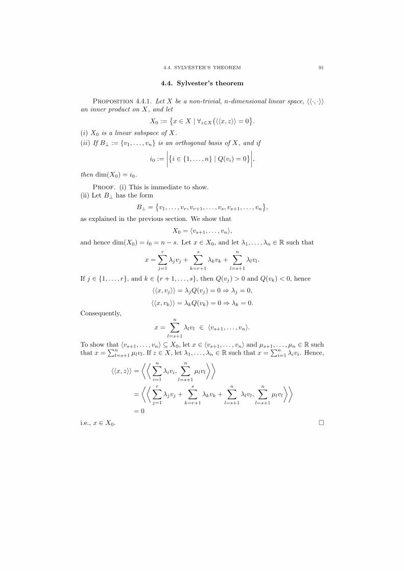
4.4. SYLVESTER’S THEOREM 91
4.4. Sylvester’s theorem
Proposition 4.4.1. Let X be a non-trivial, n-dimensional linear space, 〈〈·, ·〉〉an inner product on X, and let
X0 :={x ∈ X | ∀z∈X
(〈〈x, z〉〉 = 0
}.
(i) X0 is a linear subspace of X.
(ii) If B⊥ := {v1, . . . , vn} is an orthogonal basis of X, and if
i0 :=
∣∣∣∣{i ∈ {1, . . . , n} | Q(vi) = 0}∣∣∣∣,
then dim(X0) = i0.
Proof. (i) This is immediate to show.(ii) Let B⊥ has the form
B⊥ ={v1, . . . , vr, vr+1, . . . , vs, vs+1, . . . , vn
},
as explained in the previous section. We show that
X0 = 〈vs+1, . . . , vn〉,
and hence dim(X0) = i0 = n− s. Let x ∈ X0, and let λ1, . . . , λn ∈ R such that
x =
r∑j=1
λjvj +
s∑k=r+1
λkvk +
n∑l=s+1
λlvl.
If j ∈ {1, . . . , r}, and k ∈ {r + 1, . . . , s}, then Q(vj) > 0 and Q(vk) < 0, hence
〈〈x, vj〉〉 = λjQ(vj) = 0⇒ λj = 0,
〈〈x, vk〉〉 = λkQ(vk) = 0⇒ λk = 0.
Consequently,
x =
n∑l=s+1
λlvl ∈ 〈vs+1, . . . , vn〉.
To show that 〈vs+1, . . . , vn〉 ⊆ X0, let x ∈ 〈vs+1, . . . , vn〉 and µs+1, . . . , µn ∈ R suchthat x =
∑nl=s+1 µlvl. If z ∈ X, let λ1, . . . , λn ∈ R such that x =
∑ni=1 λivi. Hence,
〈〈x, z〉〉 =
⟨⟨ n∑i=1
λivi,
n∑l=s+1
µlvl
⟩⟩
=
⟨⟨ r∑j=1
λjvj +
s∑k=r+1
λkvk +
n∑l=s+1
λlvl,
n∑l=s+1
µlvl
⟩⟩= 0
i.e., x ∈ X0. �
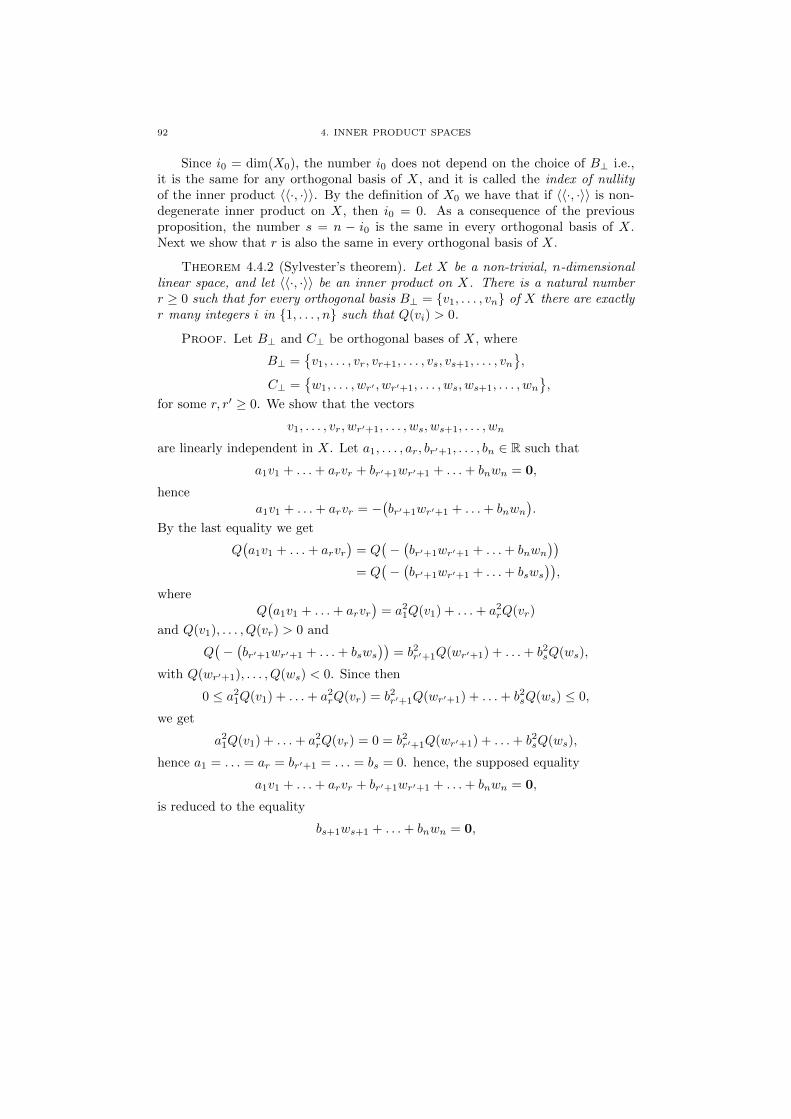
92 4. INNER PRODUCT SPACES
Since i0 = dim(X0), the number i0 does not depend on the choice of B⊥ i.e.,it is the same for any orthogonal basis of X, and it is called the index of nullityof the inner product 〈〈·, ·〉〉. By the definition of X0 we have that if 〈〈·, ·〉〉 is non-degenerate inner product on X, then i0 = 0. As a consequence of the previousproposition, the number s = n − i0 is the same in every orthogonal basis of X.Next we show that r is also the same in every orthogonal basis of X.
Theorem 4.4.2 (Sylvester’s theorem). Let X be a non-trivial, n-dimensionallinear space, and let 〈〈·, ·〉〉 be an inner product on X. There is a natural numberr ≥ 0 such that for every orthogonal basis B⊥ = {v1, . . . , vn} of X there are exactlyr many integers i in {1, . . . , n} such that Q(vi) > 0.
Proof. Let B⊥ and C⊥ be orthogonal bases of X, where
B⊥ ={v1, . . . , vr, vr+1, . . . , vs, vs+1, . . . , vn
},
C⊥ ={w1, . . . , wr′ , wr′+1, . . . , ws, ws+1, . . . , wn
},
for some r, r′ ≥ 0. We show that the vectors
v1, . . . , vr, wr′+1, . . . , ws, ws+1, . . . , wn
are linearly independent in X. Let a1, . . . , ar, br′+1, . . . , bn ∈ R such that
a1v1 + . . .+ arvr + br′+1wr′+1 + . . .+ bnwn = 0,
hencea1v1 + . . .+ arvr = −
(br′+1wr′+1 + . . .+ bnwn
).
By the last equality we get
Q(a1v1 + . . .+ arvr
)= Q
(−(br′+1wr′+1 + . . .+ bnwn
))= Q
(−(br′+1wr′+1 + . . .+ bsws
)),
whereQ(a1v1 + . . .+ arvr
)= a2
1Q(v1) + . . .+ a2rQ(vr)
and Q(v1), . . . , Q(vr) > 0 and
Q(−(br′+1wr′+1 + . . .+ bsws
))= b2r′+1Q(wr′+1) + . . .+ b2sQ(ws),
with Q(wr′+1), . . . , Q(ws) < 0. Since then
0 ≤ a21Q(v1) + . . .+ a2
rQ(vr) = b2r′+1Q(wr′+1) + . . .+ b2sQ(ws) ≤ 0,
we get
a21Q(v1) + . . .+ a2
rQ(vr) = 0 = b2r′+1Q(wr′+1) + . . .+ b2sQ(ws),
hence a1 = . . . = ar = br′+1 = . . . = bs = 0. hence, the supposed equality
a1v1 + . . .+ arvr + br′+1wr′+1 + . . .+ bnwn = 0,
is reduced to the equality
bs+1ws+1 + . . .+ bnwn = 0,

4.5. OPEN SETS IN Rn 93
hence bs+1 = . . . = bn = 0, since ws+1, . . . , wn are linearly independent as elementsof C⊥. Since v1, . . . , vr, wr′+1, . . . , wn are linearly independent, we get
r + (n− r′) ≤ n⇔ r ≤ r′.Working similarly, we show that the vectors
w1, . . . , wr′ , vr+1, . . . , vn
are linearly independent in X, hence
r′ + (n− r) ≤ n⇔ r′ ≤ r.Since r ≤ r′ and r′ ≤ r, we get the required equality r = r′. �
The integer r in Sylvester’s theorem is called the index of positivity of 〈〈·, ·〉〉,and the integer s− r, which is also independent from the choice of the orthogonalbasis, is called the index of negativity of 〈〈·, ·〉〉. If 〈〈·, ·〉〉 is the constant 0 innerproduct, then r = 0, and if 〈〈·, ·〉〉 is the Minkowski inner product on R4, thenr = 3. Of course, the index of negativity of the Euclidean inner product is 0.
Corollary 4.4.3. Let X be a non-trivial, n-dimensional linear space, and let〈〈·, ·〉〉 be an inner product on X. There is a direct sum decomposition
X = X+ ⊕X− ⊕X0
of X, where X0 is defined in the Proposition 4.4.1 and X+ and X− satisfy thefollowing conditions:
∀x∈X+
(x 6= 0⇒ Q(x) > 0
),
∀x∈X−(x 6= 0⇒ Q(x) < 0
).
Proof. Exercise. �
4.5. Open sets in Rn
Definition 4.5.1. If x ∈ Rn, the open ball B(x, ε) with center x and radiusε > 0 is defined by
B(x, ε) := {y ∈ Rn | d(x, y) < ε}:= {y ∈ Rn | |x− y| < ε}
:= {y ∈ Rn |√
(x1 − y1)2 + . . . (xn − yn)2 < ε}.
The closed ball B(x, ε] with center x and radius ε is defined by
B(x, ε] := {y ∈ Rn | d(x, y) ≤ ε}.If U ⊆ Rn, we say that U is an open subset of Rn, if
∀x∈U∃ε>0
(B(x, ε) ⊆ U
).

94 4. INNER PRODUCT SPACES
If F ⊆ Rn, we say that F is a closed subset of Rn, if its complement F c := {y ∈Rn | x /∈ F} is open.
The open ε-ball B(0, ε) at the origin (0, 0) is the open ε-disc around (0, 0)
B(0, ε) ε
and the closed ε-ball B(0, ε] at the origin (0, 0) is the ε-disc around (0, 0) with theε-circle around the origin. The open ε-ball B(x, ε) is an open set, since if we takeany point y in the ball B(x, ε), we can find an ε′ > 0 such that B(y, ε′) ⊆ B(x, ε). Ifε′ := ε− |y − x0|, then ε′ > 0, for y 6= x0. If y = x0, we can take ε′ = ε, and whatwe want follows immediately. Let z ∈ B(y, ε′) i.e., |z − y| < ε′. Then we have that
|z − x0| = |(z − y) + (y − x0)|≤ |z − y|+ |y − x0|< ε′ + |y − x0|= ε− |y − x0|+ |y − x0|= ε.
The closed ε-ball B(0, ε] is not open, since a ball around a point at the ε-circle is notincluded in B(0, ε]. It is clear though, that B(0, ε] is closed. Similarly, the interiorU of the following curve in R2 is open in R2.
U

4.5. OPEN SETS IN Rn 95
Note that the open ε-ball B(0, ε) in R at the origin 0 is the open interval (−ε, ε).
Proposition 4.5.2. Let n ≥ 1.
(i) Rn and ∅ are both open and closed.
(ii) If U ⊆ Rn, then U is open if and only if its complement U c is closed.
(iii) If U, V are open in Rn, then U ∩ V and U ∪ V are open in Rn.
(iv) If F,K are closed in Rn, then F ∩K and F ∪K are closed in Rn.
(v) If (Ui)i∈I is a family of open sets in Rn i.e., Ui is open for every i ∈ I, thentheir union ⋃
i∈IUi :=
{x ∈ Rn | ∃i∈I
(x ∈ Ui
)}is open.
(vi) If (Fi)i∈I is a family of closed sets in Rn i.e., Ui is closed for every i ∈ I, thentheir intersection ⋂
i∈IFi :=
{x ∈ Rn | ∀i∈I
(x ∈ Fi
)}is closed.
Proof. (i) If x ∈ Rn, then B(x, 1) ⊆ Rn, and hence Rn is open. Consequently,∅ is closed, since ∅c = Rn. The implication x ∈ ∅ ⇒ B(x, 1) ⊆ ∅ is trivially true,since its premise is false. Hence ∅ is open, and Rn is closed, since (Rn)c = ∅.(ii) If U is open, then U c is closed, since (U c)c = U is open. If U c is closed, thenby definition (U c)c = U is open.(iii) First we show that U ∩ V is open. If x ∈ U ∩ V , then x ∈ U and x ∈ V . SinceU is open, there is some ε1 > 0 such that B(x, ε1) ⊆ U . Since V is open, there issome ε2 > 0 such that B(x, ε2) ⊆ Y . If ε := min{ε1, ε2}, then
B(x, ε) ⊆ V ∩ U.
To show this, let y ∈ Rn such that |y − x| < ε ≤ ε1. Hence y ∈ U . Similarly,|y − x| < ε ≤ ε2, and hence y ∈ Y . Consequently, y ∈ V ∩ U . Next we show thatU ∪ V is open. If x ∈ U ∪ V , then x ∈ U , or x ∈ V . In the first case we have thatB(x, ε1) ⊆ U ⊆ U ∪ V , and in the second we have that B(x, ε2) ⊆ V ⊆ U ∪ V .(iv) We use the case (iii) and the equalities
(F ∩K)c = F c ∪Kc & (F ∪K)c = F c ∩Kc.
(v) and (vi) Exercise. �
The intersection of a countable family of open sets is not generally open. E.g.,
(0, 1] =⋂n≥1
(0, 1 +
1
n
),

96 4. INNER PRODUCT SPACES
and (0, 1] is not open, as any non-trivial interval around 1 intersects (1,+∞). Theunion of a countable family of closed sets is not generally closed. E.g.,
(0, 1) =⋃n≥2
[1
n, 1− 1
n
],
and (0, 1) is not closed, since its complement (−∞, 0] ∪ [1,+∞) is not open. It isnot hard to see that the cartesian product of open sets in R is an open set in thecorresponding Rn. E.g., the set
(0, 1)× (−1, 1) := {(x, y) ∈ R2 | x ∈ (0, 1) & y ∈ (−1, 1)}
is open in R2. Similarly the set
(0, 1)× (−1, 1)× R := {(x, y, z) ∈ R3 | x ∈ (0, 1) & y ∈ (−1, 1)}
is open in R3.
4.6. Differentiable functions on open sets in Rn
If U is an open subset of Rn, and x = (x1, . . . , xn) ∈ U , then for every i ∈{1, . . . , n}, there are appropriately small values of h ∈ R such that the point
(x1, . . . , xi + h, . . . , xn) ∈ U,
and the following concept is well-defined.
Definition 4.6.1. Let U be an open subset of Rn, x = (x1, . . . , xn) ∈ U , andf : U → R. If the following limit exists
limh→0
f(x1, . . . , xi + h, . . . , xn)− f(x1, . . . , xn)
h,
we let
Dif(x) :=∂f
∂xi(x) := lim
h→0
f(x1, . . . , xi + h, . . . , xn)− f(x1, . . . , xn)
h,
and we call Dif(x), or ∂f∂xi
(x), the i-th partial derivative of f at x.
If Bn := {e1, . . . , ei, . . . , en} is the standard basis of Rn, we have that
Dif(x) = limh→0
f(x+ hei)− f(x)
h.
If for example f : R2 → R is defined by
f(x, y) := x2y3,
then
D1f(x) :=∂f
∂x(x)

4.6. DIFFERENTIABLE FUNCTIONS ON OPEN SETS IN Rn 97
:= limh→0
f(x+ h, y)− f(x, y)
h
= limh→0
(x+ h)2y3 − x2y3
h
= y3 limh→0
(x+ h)2 − x2
h
= y32x
= 2xy3,
where the term 2x is the derivative of the function g(x) = x2. I.e., to calculateD1f(x) we treat y as a constant and we differentiate with respect to x. Similarly,
D2f(x) :=∂f
∂y(x)
:= limh→0
f(x, y + h)− f(x, y)
h
= limh→0
x2(y + h)3 − x2y3
h
= x2 limh→0
(y + h)3 − y3
h
= x23y2
= 3x2y2,
where the term 3y2 is the derivative of the function h(y) = y3. I.e., to calculateD2f(x) we treat x as a constant and we differentiate with respect to y. If f, g :U → R, and x ∈ U such that Dif(x) and Dig(x) exist, then by the properties ofthe derivative of real-valued functions on intervals of R we get
Di(f + g)(x) = Dif(x) +Dig(x),
Di(λf)(x) = λDif(x), λ ∈ R.
Definition 4.6.2. Let U be an open subset of Rn, x; = (x1, . . . , xn) ∈ U , andf : U → R. If the partial derivatives at x
D1f(x) :=∂f
∂x1(x), . . . , Dnf(x) :=
∂f
∂xn(x)
exist, the gradient (gradf)(x) of f at x is the vector
(gradf)(x) :=
(∂f
∂x1(x), . . . ,
∂f
∂xn(x)
):=
(D1f(x), . . . , Dnf(x)
).

98 4. INNER PRODUCT SPACES
E.g., if f : R2 → R is defined as above by f(x, y) := x2y3, then
(gradf)(x) := (2xy3, 3x2y2).
Because of the above linearity of Di, we get immediately that if f, g : U → R, andx ∈ U such that Dif(x) and Dig(x) exist, then
(grad(f + g))(x) = (gradf)(x) + (gradg)(x),
(grad(λf))(x) = λ(gradf)(x),
for every λ ∈ R. If Dif(x) and Dig(x) exist, for every x ∈ U , we get
grad(f + g) = gradf + gradg,
grad(λf) = λgradf,
for every λ ∈ R. Before defining when a function f : U → R, where U is an opensubset of Rn, is differentiable at some point x0 ∈ U , we notice the following fact.
Remark 4.6.3. Let U be an open subset of R, x0 ∈ U and f : U → R. Thefollowing are equivalent:
(i) f is differentiable at x0.
(ii) There are ε > 0, a ∈ R, and a function g : (−ε, ε)→ R such that
f(x0 + h)− f(x0) = ah+ |h|g(h),
for every h ∈ (−ε, ε), and
limh→0
g(h) = 0.
Proof. (i) ⇒ (ii) If f is differentiable at x0, then
a := f ′(x0) := limh→0
f(x0 + h)− f(x0)
h∈ R,
and if h 6= 0, we define
φ(h) =f(x0 + h)− f(x0)
h− f ′(x0),
while if h = 0, we define φ(0) := 0. Clearly,
limh→0
φ(h) = 0,
and for every h in some ε-interval around 0 we have that
f(x0 + h)− f(x0) = f ′(x0)h+ hφ(h).
If we define
g(h) :=
{φ(h) , if h ≥ 0−φ(h) , if h < 0,
we have that
|h|g(h) = hφ(h),

4.6. DIFFERENTIABLE FUNCTIONS ON OPEN SETS IN Rn 99
and we get the required equality
f(x0 + h)− f(x0) = ah+ |h|g(h).
Of course,
limh→0
g(h) = 0.
(ii) ⇒ (i) If h 6= 0, then
f(x0 + h)− f(x0)
h=ah+ |h|g(h)
h= a+
|h|hg(h),
which converges to a, as h converges to 0 i.e., a = f ′(x0). �
Definition 4.6.4. Let U be an open subset of Rn, x0 ∈ U and f : U → R. Wesay that f is differentiable at x0, if
(a) The gradient of f at x0
gradf(x0) :=(D1f(x0), . . . , Dnf(x0)
)=
(∂f
∂x1(x0), . . . ,
∂f
∂xn(x0)
)exists, and
(b) there is a function g defined on a small open ball around the origin 0 such that
lim|h|→0
g(h) = 0,
and
f(x0 + h)− f(x0) =∂f
∂x1(x0)h1 + . . .+
∂f
∂xn(x0)hn + |h|g(h)
:=⟨(gradf)(x0), h
⟩+ |h|g(h).
We say that f is differentiable on U , if it is differentiable at every point of U .
To show that a function f as above is differentiable on U , it suffices to showthat the gradient of f at every point of U exists, and that the partial derivativeson U are continuous functions (the proof is omitted).
Proposition 4.6.5. If U is an open subset of Rn, x0 ∈ U and f : U → R, thenf is differentiable at x0, if all partial derivatives of f at x0 exist in U and for eachi ∈ {1, . . . , n} the function
U 3 x 7→ ∂f
∂xi(x)
is continuous at x0.
Proof. See [16], p. 322. �

100 4. INNER PRODUCT SPACES
4.7. The dual space of an inner product space
In the Definition 2.4.1 we defined the dual space of a linear space as the spaceof functionals on X i.e.,
X∗ := {f : X → R | f is linear}.There are many examples of important functionals from the physical point of view.E.g., the Dirac functional δx0
: C([0, 1])→ R, where x0 ∈ [0, 1], is defined by
δx0(f) := f(x0),
for every f ∈ C([0, 1]). If (X, 〈〈·, ·〉〉) is an n-dimensional inner product space we candescribe in an explicit way the isomorphism between X and X∗ (Corollary 2.4.16).
Theorem 4.7.1. Let (X, 〈〈·, ·〉〉) be a finite-dimensional inner product space,and let x0 ∈ X.
(i) The function Lx0 : X → R, defined by
Lx0(x) := 〈〈x, x0〉〉,for every x ∈ X, is in X∗.
(ii) The function L : X → X∗, defined by
L(x0) := Lx0 ,
for every x0 ∈ X, is a linear map.
(iii) If 〈〈·, ·〉〉 is non-degenerate, then L is an isomorphism between X and X∗.
Proof. (i) and (ii) are immediate to show. Since dim(X) = dim(X∗), to show(iii) it suffices to show that L is an injection i.e., Ker(L) = {0}. If L(x) = 0, then∀y∈X
(Lx(y) = 〈〈y, x〉〉 = 0
), hence, since 〈〈·, ·〉〉 is non-degenerate, x = 0. �
Consequently, if 〈〈·, ·〉〉 is a non-degenerate inner product on X, then for everyfunctional f ∈ X∗ there is a unique x0 ∈ X such that
f = Lx0 ,
and the functional f is represented by the vector x0. The condition (b) in theDefinition 4.6.4 takes the form
f(x0 + h)− f(x0) = L(gradf)(x0)(h) + |h|g(h),
where L(gradf)(x0) : Rn → R is defined by
L(gradf)(x0)(y) := 〈(gradf)(x0), y〉,for every y ∈ Rn. I.e., the differentiability of a function f on an open subset ofRn means that “locally” f is approximated by some linear functional on Rn. Thefunctional L(gradf)(x0) is called the derivative of f at x0.
Recall that if BX := {v1, . . . , vn} is a basis of a linear space X, then
BX∗ := {v∗1 , . . . , v∗n}
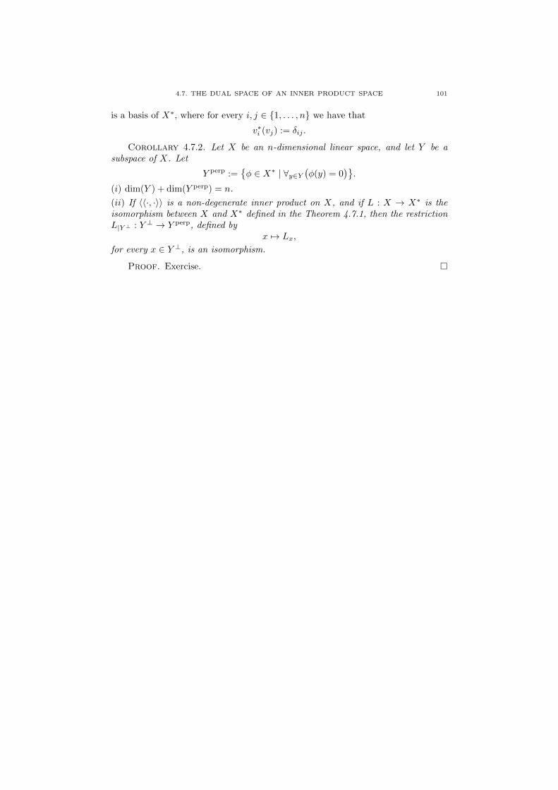
4.7. THE DUAL SPACE OF AN INNER PRODUCT SPACE 101
is a basis of X∗, where for every i, j ∈ {1, . . . , n} we have that
v∗i (vj) := δij .
Corollary 4.7.2. Let X be an n-dimensional linear space, and let Y be asubspace of X. Let
Y perp :={φ ∈ X∗ | ∀y∈Y
(φ(y) = 0
)}.
(i) dim(Y ) + dim(Y perp) = n.
(ii) If 〈〈·, ·〉〉 is a non-degenerate inner product on X, and if L : X → X∗ is theisomorphism between X and X∗ defined in the Theorem 4.7.1, then the restrictionL|Y ⊥ : Y ⊥ → Y perp, defined by
x 7→ Lx,
for every x ∈ Y ⊥, is an isomorphism.
Proof. Exercise. �

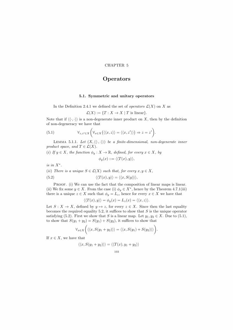
CHAPTER 5
Operators
5.1. Symmetric and unitary operators
In the Definition 2.4.1 we defined the set of operators L(X) on X as
L(X) := {T : X → X | T is linear}.Note that if 〈〈·, ·〉〉 is a non-degenerate inner product on X, then by the definitionof non-degeneracy we have that
(5.1) ∀z,z′∈X(∀x∈X
(〈〈x, z〉〉 = 〈〈x, z′〉〉
)⇒ z = z′
).
Lemma 5.1.1. Let (X, 〈〈·, ·〉〉) be a finite-dimensional, non-degenerate innerproduct space, and T ∈ L(X).
(i) If y ∈ X, the function φy : X → R, defined, for every x ∈ X, by
φy(x) ::= 〈〈T (x), y〉〉,is in X∗.
(ii) There is a unique S ∈ L(X) such that, for every x, y ∈ X,
(5.2) 〈〈T (x), y〉〉 = 〈〈x, S(y)〉〉,
Proof. (i) We can use the fact that the composition of linear maps is linear.(ii) We fix some y ∈ X. From the case (i) φy ∈ X∗, hence by the Theorem 4.7.1(iii)there is a unique z ∈ X such that φy = Lz, hence for every x ∈ X we have that
〈〈T (x), y〉〉 = φy(x) = Lz(x) = 〈〈x, z〉〉.Let S : X → X, defined by y 7→ z, for every z ∈ X. Since then the last equalitybecomes the required equality 5.2, it suffices to show that S is the unique operatorsatisfying (5.2). First we show that S is a linear map. Let y1, y2 ∈ X. Due to (5.1),to show that S(y1 + y2) = S(y1) + S(y2), it suffices to show that
∀x∈X(〈〈x, S(y1 + y2)〉〉 = 〈〈x, S(y1) + S(y2)〉〉
).
If x ∈ X, we have that
〈〈x, S(y1 + y2)〉〉 = 〈〈T (x), y1 + y2〉〉
103

104 5. OPERATORS
= 〈〈T (x), y1〉〉+ 〈〈T (x), y2〉〉= 〈〈x, S(y1)〉〉+ 〈〈x, S(y2)〉〉= 〈〈x, S(y1) + S(y2)〉〉.
Similarly, to show that S(λy) = λS(y), where λ ∈ R, it suffices to show that
∀x∈X(〈〈x, S(λy)〉〉 = 〈〈x, λS(y)〉〉
).
If x ∈ X, we have that
〈〈x, S(λy)〉〉 = 〈〈T (x), λy〉〉= λ〈〈T (x), y〉〉= λ〈〈x, S(y)〉〉= 〈〈x, λS(y)〉〉.
Let S′ ∈ L(X) such that S′ satisfies (5.2). If y ∈ X, then
〈〈x, S′(y)〉〉 = 〈〈T (x), y〉〉 = 〈〈x, S(y)〉〉,
hence by (5.1) we get S′(y) = S(y). Since y ∈ X is arbitrary, we get S′ = S. �
Definition 5.1.2. Let (X, 〈〈·, ·〉〉) be a finite-dimensional, non-degenerate innerproduct space, and T ∈ L(X). The unique S ∈ L(X) satisfying (5.2) is called thetranspose operator of T , and it is denoted by T t. If T t = T , we call T a symmetricoperator.
If T ∈ L(X), where X is as above, then, for every x, y ∈ X, (5.2) becomes
(5.3) 〈〈T (x), y〉〉 = 〈〈x, T t(y)〉〉,
and if T is symmetric, then, for every x, y ∈ X, (5.2) becomes
(5.4) 〈〈T (x), y〉〉 = 〈〈x, T (y)〉〉.
If x = (x1, . . . , xn) ∈ Rn and y = (y1, . . . , yn) ∈ Rn, then
〈x, y〉 :=
n∑i=1
xiyi
=[x1 . . . xn
] y1
...yn
=
x1
...xn
t y1
...yn
= xty,

5.1. SYMMETRIC AND UNITARY OPERATORS 105
if we view x, y as (n× 1)-matrices. If T ∈ L(Rn), then
〈x, T t(y)〉 = 〈T (x), y〉= 〈ATx, y〉
=(ATx
)ty
=(xtAtT
)y
= xt(AtT y
)= 〈x,AtT y〉,
Since x, y are arbitrary, we get T t(y) = AtT y, and since T t(y) = AT ty, we get
AT t = AtT ,
a fact that explains the use of the same notation and terminology for the transposeof an operator as in the case of a transpose of a matrix.
Proposition 5.1.3. Let (X, 〈〈·, ·〉〉) be a finite-dimensional, non-degenerate in-ner product space, S, T ∈ L(X) and λ ∈ R.
(i) (S + T )t = St + T t.
(ii) (λS)t = λSt.
(iii) (S ◦ T )t = T t ◦ St.(iv) (St)t = S.
Proof. We work as in the proof of the Lemma 5.1.1 (exercise). �
In the Definition ?? an orthogonal transformation was defined as an operatorthat was preserving the corresponding inner product. If the inner product is positivedefinite, we use the following special term.
Definition 5.1.4. Let (X, 〈〈·, ·〉〉) be a finite-dimensional, positive definite in-ner product space, and let U ∈ L(X). We call U unitary, if it is inner product-preserving i.e., if for every x, y ∈ X we have that
〈〈U(x), U(y)〉〉 = 〈〈x, y〉〉.
Proposition 5.1.5. Let (X, 〈〈·, ·〉〉) be a finite-dimensional, positive definiteinner product space, and let U ∈ L(X). The following are equivalent.
(i) U is unitary.
(ii) U is norm-preserving i.e., for every x ∈ X we have that
||U(x)|| = ||x||,where ||.|| is the norm on X induced by 〈〈·, ·〉〉.(iii) U sends a unit vector to a unit vector i.e.,
∀x∈X(||x|| = 1⇒ ||U(x)|| = 1
).

106 5. OPERATORS
Proof. (i) ⇒ (ii) If x ∈ X, then we use the following equality
||U(x)||2 = 〈〈U(x), U(x)〉〉 = 〈〈x, x〉〉 = ||x||2.(ii) ⇒ (iii) If x ∈ X such that ||x|| = 1, then ||U(x)|| = ||x|| = 1.
(iii) ⇒ (ii) If x = 0, then U(0) = 0 and the required equality is immediate fromthe fact that ||.|| is a function. If x 6= 0, then∣∣∣∣∣∣∣∣ x||x||
∣∣∣∣∣∣∣∣ = 1,
and by (iii) we have that
1 =
∣∣∣∣∣∣∣∣ x||x||∣∣∣∣∣∣∣∣ =
∣∣∣∣∣∣∣∣U( x
||x||
)∣∣∣∣∣∣∣∣ =
∣∣∣∣∣∣∣∣ 1
||x||U(x)
∣∣∣∣∣∣∣∣ =
∣∣∣∣ 1
||x||
∣∣∣∣||T (x)|| = 1
||x||||U(x)||,
hence ||U(x)|| = ||x||.(ii) ⇒ (i) If x, y ∈ X, using the polarisation identity twice we get
〈〈x, y〉〉 =1
4
(〈〈x+ y, x+ y〉〉 − 〈〈x− y, x− y〉〉
)=
1
4
(||x+ y||2 − ||x− y||2
)=
1
4
(||U(x+ y)||2 − ||U(x− y)||2
)=
1
4
(||U(x) + U(y)||2 − ||U(x)− U(y)||2
)=
1
4
(〈〈U(x) + U(y), U(x) + U(y)〉〉 − 〈〈U(x)− U(y), U(x)− U(y)〉〉
)= 〈〈U(x), U(y)〉〉.
�
Hence, a unitary operator is characterised from the fact that it sends unitvectors to unit vectors, a property that explains the use of the term “unitary”. If
S1(X) := {x ∈ X | ||x|| = 1}is the unit sphere of (X, ||.||), then a unitary operator sends S1(X) to itself i.e.,
U|S1(X) : S1(X)→ S1(X).
By definition, a unitary operator preserves orthogonality since
〈〈x, y〉〉 = 0⇒ 〈〈U(x), U(y)〉〉 = 0.
The converse is not always true i.e., there are operators that preserve orthogonalitybut are not unitary (exercise).
Theorem 5.1.6. If (X, 〈〈·, ·〉〉) is a finite-dimensional, positive definite innerproduct space, and U ∈ L(X), then U is unitary if and only if
U t ◦ U = idX .

5.2. EIGENVALUES AND EIGENVECTORS 107
Proof. Exercise. �
It is easy to see that a unitary operator is invertible and with some more effortthat U−1 = U t (exercise). Moreover, it can be shown (exercise) that if U is unitary,then U t is unitary. It can also be shown that the only unitary operators of R2 arethe linear maps whose matrices are of the form[
cos θ − sin θsin θ cos θ
]or
[cos θ sin θsin θ − cos θ
].
Note that the determinant of the first is 1 and the determinant of the second is −1.
5.2. Eigenvalues and eigenvectors
Definition 5.2.1. Let X be a linear space and T ∈ L(X). An element x of Xis called an eigenvector of T , if
(5.5) ∃λ∈R(T (x) = λx
).
If x 6= 0, and x is an eigenvector of T , then there is a unique1 λ ∈ R satisfying (5.5),which is called an eigenvalue of T that belongs to x. If A ∈Mn(R), an eigenvectorof A is an eigenvector of TA ∈ L(Rn).
If we consider the linear space
C∞(R) :={f ∈ F(R) | f is infinitely differentiable
},
where f : R→ R is infinitely differentiable, if there exist all finite derivatives
f (1) := f ′, f (2) := f ′′, . . . , f (n) :=(f (n−1)
)′, . . . ,the derivative operator is the linear operator
′: C∞(R)→ C∞(R)
f 7→ f ′,
for every f ∈ C∞(R). If λ ∈ R, the function f ∈ C∞(R), defined by
f(t) := eλt,
for every t ∈ R, is an eigenvector of the derivative and λ belongs to f , sincef ′(t) = λf(t), for every t ∈ R. Note that if λ is an eigenvalue of T ∈ L(X) thatbelongs to x ∈ X, then for every a ∈ R, we have that ax is an eigenvector of T thatalso belongs to λ;
T (ax) = aT (x) = a(λx) = λ(ax).
Clearly, the set Xλ(T ) of all eigenvectors of x with λ ∈ R as an eigenvalue
Xλ(T ) :={x ∈ X | T (x) = λx
}1If T (x) = λx = µx, then (λ− µ)x = 0, and since x 6= 0, we get λ = µ.

108 5. OPERATORS
is a subspace of X, and actually
Xλ(T ) = Ker(T − λidX).
We call Xλ(T ) the eigenspace of X belonging to λ.
Theorem 5.2.2. If X is a linear space, T ∈ L(X), and v1, . . . , vm are eigen-vectors of T with eigenvalues λ1, . . . , λm, respectively, such that λi 6= λj for everyi, j ∈ {1, . . . ,m} with i 6= j, then v1, . . . , vm are linearly independent.
Proof. We prove by induction on n ≥ 1 the following formula
∀m≥1
(∀v1,...,vm∈X∀λ1,...,λm∈R
(PWU(λ1, . . . , λm) &
& EIGENT (v1, . . . , vm;λ1, . . . , λm)⇒ LIND(v1, . . . , vm))),
wherePWU(λ1, . . . , λm) :⇔ ∀i,j∈{1,...,m
(i 6= j ⇒ λi 6= λj
),
EIGENT (v1, . . . , vm;λ1, . . . , λm) :⇔ T (v1) = λ1v1 & . . . & T (vm) = λmvm,
LIND(v1, . . . , vm) :⇔ v1, . . . , vm are linearly independent.
If m = 1, and if we fix some v1 ∈ X and λ1 ∈ R, then PWU(λ1) holds trivially,and if EIGENT (v1;λ1), then necessarily v1 6= 0, hence LIND(v1). We suppose thatthe formula for m > 1 and we show it for m + 1. Let v1, . . . , vm+1 ∈ X, andλ1, . . . , λm+1 such that PWU(λ1, . . . , λm+1) and
EIGENT (v1, . . . , vm+1;λ1, . . . , λm+1),
and we show that LIND(v1, . . . , vm+1). For that, let c1, . . . , cm+1 ∈ R such that
(5.6) c1v1 + c2v2 + . . .+ cm+1vm+1 = 0.
Multiplying (5.6) by λ1 we get
(5.7) c1λ1v1 + c2λ1v2 + . . .+ cm+1λ1vm+1 = 0.
Since
0 = T (0)
= T(c1v1 + c2v2 + . . .+ cm+1vm+1
)= c1T (v1) + c2T (v2) + . . .+ cm+1T (vm+1)
= c1λ1v1 + c2λ2v2 + . . .+ cm+1λm+1vm+1,
subtracting (5.7) from the last equality we get
(5.8) c2(λ2 − λ1)v2 + . . .+ cm+1(λm+1 − λ1)vm+1 = 0.
SincePWU(λ1, . . . , λm+1)⇒ PWU(λ2, . . . , λm+1),
andEIGENT (v1, . . . , vm+1;λ1, . . . , λm+1)⇒

5.3. THE SIMPLEST ODE, BUT ONE OF THE MOST IMPORTANT 109
EIGENT ((λ2 − λ1)v2, . . . , (λm+1 − λ1)vm+1;λ2, . . . , λm+1),
by the inductive hypothesis on v2, . . . , vm+1 ∈ X and λ2 − λ1, . . . , λm+1 − λ1 ∈ Rwe get
LIND(v2, . . . , vm+1),
and by (5.8) we get
c2(λ2 − λ1) = . . . = cm+1(λm+1 − λ1) = 0.
since by PWU(λ1, . . . , λm+1) we have that (λ2−λ1) 6= 0 and . . . and (λm+1−λ1) 6=0, we conclude that
c2 = . . . = cm+1 = 0.
Since then (5.7) becomes c1v1 = 0, we get c1 = 0. Since c1, . . . , cm+1 are arbitrary,we get LIND(v1, . . . , vm+1). �
By the Theorem 5.2.2 we get another proof that the functions
f1(t) = eλ1t, . . . , fm(t) = eλmt
where PWU(λ1, . . . , λm), are linearly independent in C∞(R), since
EIGEN(f1, . . . , fm;λ1, . . . , λm).
Corollary 5.2.3. If X is a linear space with dim(X) = n ≥ 1, T ∈ L(X),and v1, . . . , vn are eigenvectors of T with eigenvalues λ1, . . . , λn, respectively, suchthat λi 6= λj for every i, j ∈ {1, . . . , n} with i 6= j, then {v1, . . . , vn} is a basis ofX.
Proof. Exercise. �
Proposition 5.2.4. Let X be a non-trivial finite-dimensional linear space,BX = {v1, . . . , vn} a basis of X, and T ∈ L(X).
(i) BX diagonalises T if and only if v1, . . . , vn are eigenvectors of T .
(ii) T is diagonalisable if and only if there is a basis of X consisting of eigenvectorsof T .
Proof. Exercise (use the Definition 3.3.12). �
Next we describe a space having a basis consisting of eigenvectors.
5.3. The simplest ode, but one of the most important
If a ∈ R and x : J → R is differentiable, where J is an interval of R, one canshow (exercise) that the ordinary differential equation (ode)
(5.9) x′(t) = ax(t)
has as set of solutions the set
Sol(5.9) ={s : J → R | ∃C∈R∀t∈J
(s(t) = Ceat
)}.

110 5. OPERATORS
The equation (5.9) is the simplest ode. If s ∈ Sol(5.9), then s(0) = C. Conversely,there is a unique function s ∈ Sol(5.9) such that s(0) = C. This is a special caseof the existence of a unique s ∈ Sol(5.9) satisfying the initial condition s(t0) = s0,where t0 ∈ J . The parameter a in (5.9) influences dramatically the way the solutioncurve s looks like. If a > 0, then we have the following three cases:
a > 0 C > 0
C < 0
C = 0
If C > 0, then limt−→+∞ Ceat = +∞, and if C < 0, then limt−→+∞ Ceat = −∞.If a = 0, the solution curves are constant functions
a = 0C > 0
C < 0
C = 0
If a < 0, we have the following three cases:
a < 0C > 0
C < 0
C = 0
In this case, if C 6= 0, then
limt−→+∞
Ceat = C limt−→+∞
e−|a|t = C limt−→+∞
1
e|a|t= 0.

5.3. THE SIMPLEST ODE, BUT ONE OF THE MOST IMPORTANT 111
The above graphs reflect the qualitative behavior of the solution curves. If a 6= 0,equation (5.9) is stable in the following sense: If a is replaced by some a′ sufficientlyclose to a, the qualitative behavior of the solution curves does not change. E.g., wehave that
|a′ − a| < |a| ⇒ sign(a′) = sign(a),
since, if a > 0, then |a′ − a| < a⇔ −a < a′ − a < a⇒ 0 < a′ < 2a, while, if a < 0,then |a′ − a| < −a ⇔ a < a′ − a < −a ⇒ 2a < a′ < 0. If a = 0, equation (5.9)is unstable, since the slightest change in the value of a implies a big change in thequalitative behavior of the solution curves. For this reason we say that a = 0 is abifurcation point in the one-parameter family of equations(
x′(t) = ax(t)
)a∈R
.
Let the following system of two odes in two unknown functions:
(5.10)x1′(t) = a1x1(t),
x2′(t) = a2x2(t).
Since there is no relation between x1(t) and x2(t), we have that
Sol(5.10) =
{s : J → R2 | ∃C1,C2∈R∀t∈J
(s(t) =
(C1e
a1t, C2ea2t))}
.
If s1(t) = C1ea1t and s2(t) = C2e
a2t, we get C1 = s1(0) and C2 = s2(0). Theequation (5.10) can be written as
(5.11) x′(t) = Ax(t),
where
A : R2 → R2,
A(x1, x2) := (a1x1, a2, x2)
is a vector field on R2, which geometrically we understand as a function that assignsto each vector x ∈ R2 the directed line segment from x to x+Ax.
x
x(t)
Ax(t)
x(t) +Ax(t)

112 5. OPERATORS
We can write the equation (5.10) using matrices as follows
(5.12)
[x1′(t)
x2′(t)
]=
[a1 00 a2
] [x1(t)x2(t)
].
If J is an interval of R, x1, . . . , xn : J → R are differentiable functions, andaij ∈ R, for every i, j ∈ {1, . . . , n}, let the following system of odes
(5.13)
x1′(t) = a11x1(t) + . . .+ a1nxn(t),
......
...
xi′(t) = ai1x1(t) + . . .+ ainxn(t),
......
...
xn′(t) = an1x1(t) + . . .+ annxn(t).
We can write equation (5.13) using matrices as follows
(5.14)
x1′(t)...
xi′(t)...
xn′(t)
=
a11 . . . a1n
......
...ai1 . . . ain...
......
an1 . . . ann
x1(t)...
xi(t)...
xn(t)
,or, generalizing the simplest ode, we can write it in the form
(5.15) x′(t) = Ax(t),
where
(5.16) A :=
a11 . . . a1n
......
...ai1 . . . ain...
......
an1 . . . ann
=: [aij ].
Proposition 5.3.1. Let the system of odes (5.15), and let λ1, . . . , λn ∈ R suchthat
A = Diag(λ1, . . . , λn).
If Sol is the set of solutions of the system (5.15), then Sol is a linear space and
Sol =⟨[eλ1t
], . . . ,
[eλnt
]⟩,
where [eλ1t
]:=(eλ1t,0, . . . ,0
), . . . ,
[eλnt
]:=(0,0, . . . , eλnt
).
Proof. Exercise. �

5.4. DETERMINANTS 113
5.4. Determinants
Definition 5.4.1. If
A =
[a bc d
]is a 2× 2-matrix, its determinant Det(A) is defined by
Det(A) :=
∣∣∣∣a bc d
∣∣∣∣ := ad− bc.
If
A1 :=
[ac
]& A2 :=
[bd
]are the columns of A, we use the notation
Det(A) = Det(A1, A2).
We have that
Det(I2) :=
∣∣∣∣1 00 1
∣∣∣∣ := 1− 0 = 1.
It is also clear that
Det(A) :=
∣∣∣∣a bc d
∣∣∣∣ := ad− bc =:
∣∣∣∣a cb d
∣∣∣∣ =: Det(At).
Remark 5.4.2. Let the following 2× 1 matrices:
A1 :=
[a1
a2
], C1 :=
[c1c2
], B2 :=
[b1b2
], D2 :=
[d1
d2
].
The following hold.
(i) Det(A1 + C1, B2) = Det(A1, B2) + Det(C1, B2).
(ii) Det(A1, B2 +D2) = Det(A1, B2) + Det(A1, D2).
(iii) If λ ∈ R, then Det(λA1, B2) = λDet(A1, B2) = Det(A1, λB2).
(iv) If A1 = B2, then Det(A1, B2) = 0.
Proof. We prove only (i), and the rest is an exercise.
Det(A1 + C1, B2) :=
∣∣∣∣a1 + c1 b1a2 + c2 b2
∣∣∣∣:= (a1 + c1)b2 − b1(a2 + c2)
= (a1b2 − b1a2) + (c1b2 − b1c2)
:=
∣∣∣∣a1 b1a2 b2
∣∣∣∣+
∣∣∣∣c1 b1c2 b2
∣∣∣∣:= Det(A1, B2) + Det(C1, B2).
�

114 5. OPERATORS
Although one can use the definition of Det(A) to show the following corollary,its proof is simpler, if we use the fundamental properties of the Remark 5.4.2.
Corollary 5.4.3. Let the following 2× 1 matrices:
A1 :=
[a1
a2
], B2 :=
[b1b2
].
The following hold.
(i) If λ ∈ R, then Det(A1 + λB2, B2) = Det(A1, B2).
(ii) If λ ∈ R, then Det(A1, B2 + λA1) = Det(A1, B2).
(iii) Det(A1, B2) = −Det(B2, A1).
Proof. Exercise. �
The determinant of a matrix A provides non-trivial information on vectorsrelated to A. We have seen that Det(I2) = 1 6= 0, and we know that the columnse1 := (1, 0) and e2 := (0, 1) of the matrix I2 are linearly independent elements.This is a special case of the following general fact.
Proposition 5.4.4. Let the following 2× 1 matrices:
A :=
[a1
a2
], B :=
[b1b2
].
The vectors (a1, a2) and (b1, b2) are linearly independent in R2 if and only if
Det(A,B) 6= 0.
Proof. (⇒) Suppose that (a1, a2) and (b1, b2) are linearly independent in R2,and suppose that
Det(A,B) :=
∣∣∣∣a1 b1a2 b2
∣∣∣∣ := a1b2 − b1a2 = 0.
Since then we have that
b2(a1, a2) + (−a2)(b1, b2) = (b2a1 − a2b1, b2a2 − a2b2) = (0, 0),
by the hypothesis of linear independence of (a1, a2) and (b1, b2) we get
b2 = 0 = −a2 = a2.
Hence the two vectors take the form (a1, 0) and (b1, 0). Since they are linearlyindependent, these are non-zero vectors, hence a1 6= 0 and b1 6= 0. Consequently,we have that (a1, 0) = a1
b1(b1, 0) i.e., the vectors (a1, a2) and (b1, b2) are linearly
dependent, which is a contradiction. Hence, Det(A,B) 6= 0.
(⇐) Suppose that Det(A,B) 6= 0, and let λ, µ ∈ R such that
λ(a1, a2) + µ(b1, b2) = (0, 0)⇔ (λa1 + µb1, λa2 + µb2) = (0, 0),
henceλa1 = −µb1 & λa2 = −µb2.

5.4. DETERMINANTS 115
Suppose that λ 6= 0 (if we suppose that µ 6= 0. we proceed similarly). By theRemark 5.4.2 we have that
Det(A,B) =
∣∣∣∣(−µλ )b1 b1(−µλ
)b2 b2
∣∣∣∣=
(−µλ
) ∣∣∣∣b1 b1b2 b2
∣∣∣∣=
(−µλ
)0
= 0,
which is a contradiction. Hence λ = 0 = µ, and the vectors (a1, a2), (b1, b2) arelinearly independent. �
Proposition 5.4.5. Let A,B ∈M2(R).
(i) Det(AB) = Det(A)Det(B).
(ii) A is invertible if and only if Det(A) 6= 0.
Proof. (i) Exercise.(ii) If AA−1 = I2, then by the case (i) we have that
1 = Det(I2) = Det(AA−1) = Det(A)Det(A−1),
hence Det(A) 6= 0, Det(A−1) 6= 0, and
Det(A−1) =1
Det(A).
For the converse let
A =
[a bc d
]and suppose that
Det(A) :=
∣∣∣∣a bc d
∣∣∣∣ := ad− bc 6= 0.
We show that the system [a bc d
] [x yz w
]=
[1 00 1
]⇔
[ax+ bz ay + bwcx+ dz cy + dw
]=
[1 00 1
]⇔
ax+ bz = 1 & cx+ dz = 0,
and
ay + bw = 0 & cy + dw = 1,
116 5. OPERATORS
has a solution. If we multiply the equation ax + bz = 1 by d and the equationcx+ dz = 0 by b and then we subtract them, we get
dax+ dbz − bcx− bdz = d⇔ x =d
ad− bc.
Working similarly, we get
A−1 :=
[x yz w
]=
1
Det(A)
[d −b−c a
].
�
Definition 5.4.6. If
A =
a11 a12 a13
a21 a22 a23
a31 a32 a33
is a 3× 3-matrix, its determinant Det(A) is defined by
Det(A) :=
∣∣∣∣∣∣a11 a12 a13
a21 a22 a23
a31 a32 a33
∣∣∣∣∣∣ := a11
∣∣∣∣a22 a23
a32 a33
∣∣∣∣− a12
∣∣∣∣a21 a23
a31 a33
∣∣∣∣+ a13
∣∣∣∣a21 a22
a31 a32
∣∣∣∣ .As expected, we have that
Det(I3) :=
∣∣∣∣∣∣1 0 00 1 00 0 1
∣∣∣∣∣∣ := 1
∣∣∣∣1 00 1
∣∣∣∣− 0
∣∣∣∣0 00 1
∣∣∣∣+ 0
∣∣∣∣0 10 0
∣∣∣∣ = 1.
More generally, if we consider a matrix in diagonal form, then for the correspondingdeterminant we have that∣∣∣∣∣∣
λ1 0 00 λ2 00 0 λ3
∣∣∣∣∣∣ := λ1
∣∣∣∣λ2 00 λ3
∣∣∣∣− 0
∣∣∣∣0 00 λ3
∣∣∣∣+ 0
∣∣∣∣0 λ2
0 0
∣∣∣∣ = λ1λ2λ3.
All results we showed for the determinant of a matrix in M2(R) hold for thedeterminant of a matrix in Mn(R). To define Det(A), where A ∈Mn(R) and n > 2,we suppose that we have defined Det(B), for every B ∈Mn−1(R), and we let
Det(A) := (−1)i+1ai1Det(Ai1) + . . .+ (−1)i+nainDet(Ain),
where the matrix Aij ∈ Mn−1(R) is obtained from A by crossing out the i-th rowand the j-th column. E.g., if n = 3 and i = 1, we get
Det(A) := (−1)1+1a11Det(A11) + (−1)1+2a12Det(A12) + (−1)1+3a13Det(A13)
= a11Det(A11)− a12Det(A12) + a13Det(A13).
It can be shown that Det : Mn(R) → R is the unique function from Mn(R)to R that satisfies Remark 5.4.2(i)-(iii) and sends In to 1 (see [17] p. 149 and p.171), and it is the unique function from Mn(R) to R that satisfies the followingconditions:

5.5. THE CHARACTERISTIC POLYNOMIAL 117
(D1) Det(AB) = Det(A)Det(B),
(D2) Det(In) = 1,
(D3) Det(A) 6= 0 if and only if A is invertible.
If B is invertible, it is easy to see that
(D4) Det(B−1) = Det(B)−1,
(D5) Det(BAB−1) = Det(A).
From (D3) on shows that if A ∈Mn(R), then
Det(A) 6= 0⇔ Ker(TA) = {0},
and equivalently we have that
Det(A) = 0⇔ {0} ( Ker(TA)⇔ A is not invertible.
5.5. The characteristic polynomial
Proposition 5.5.1. If X is a finite-dimensional linear space, T ∈ L(X) andλ ∈ R, then λ is an eigenvalue of T if and only if T − λidX is not invertible.
Proof. We have that
T − λidX is not invertible ⇔ T is not an injection
⇔ {0} ( Ker(T − λidX)
⇔ ∃x∈X(x 6= 0 & T (x) = λx
)⇔ λ is an eigenvalue of T.
�
Definition 5.5.2. If A ∈Mn(R), the characteristic polynomial of A is
pA(t) := Det(tIn −A) =
∣∣∣∣∣∣∣∣∣t− a11 −a12 . . . −a1n
−a21 t− a22 . . . −a2n
......
......
−an1 −an2 . . . t− ann
∣∣∣∣∣∣∣∣∣ .If T ∈ L(Rn), the characteristic polynomial pT of T is pAT
. If X is an n-dimensionallinear space and T ∈ L(X), the characteristic polynomial pT of T is pATBX
, where
BX is a basis of X.
By the definition of Det(A) we can show inductively that
pA(t) = tn + a polynomial of a degree lower than n.

118 5. OPERATORS
If T ∈ L(X), pT is independent from the choice of the basis BX . For this we usethe Theorem 3.3.11 and the fact that similar matrices have equal characteristicpolynomials; if C = B−1AB, and if t ∈ R, then by the property (D5) of Det we get
Det(tIn −B−1AB) = Det(tB−1B −B−1AB)
= Det(B−1tB −B−1AB)
= Det(B−1(tB −AB))
= Det(B−1(tInB −AB))
= Det(B−1(tIn −A)B)
(D5)= Det(tIn −A).
E.g., if
A =
1 −1 3−2 1 10 1 −1
,pA(t) =
∣∣∣∣∣∣t− 1 1 −3
2 t− 1 −10 −1 t+ 1
∣∣∣∣∣∣ = t3 − t2 − 2t+ 4.
Proposition 5.5.3. If A ∈Mn(R) and λ ∈ R, then λ is an eigenvalue of A ifand only if λ is a root of the characteristic polynomial of A.
Proof. By the Definition 5.2.1 and the Proposition 5.5.1 we have that
λ is an eigenvalue of A :⇔ λ is an eigenvalue of TA
⇔ TA − λidX is not invertible
⇔ λidX − TA is not invertible
⇔ Det(A[λidX−TA]) = 0
⇔ Det(λIn −A) = 0
⇔ pA(λ) = 0.
�
E.g., if
A =
[1 42 3
],
pA(t) =
∣∣∣∣t− 1 −4−2 t− 3
∣∣∣∣ = t2 − 4t− 5 = (t− 5)(t+ 1),
and the eigenvalues of A are 5 and −1. If (x, y) is an eigenvector of A, the system[1 42 3
] [xy
]=
[λxλy
]
5.6. THE SPECTRAL THEOREM 119
takes the form
x+ 4y = λx,
2x+ 3y = λy,
or equivalently
(1− λ)x+ 4y = 0,
2x+ (3− λ)y = 0.
If x = 1, the pair
(1, 2
λ−3
)is an eigenvector of A. If λ = 5, the eigenspace X5 has
as basis the set {(1, 1)}, and if λ = −1, then X−1 has as basis the set {(1,− 1
2
)}.
Proposition 5.5.4. If X is a linear space, T ∈ L(X), n ≥ 1, and BX :={v1, . . . , vn} is a basis of X consisting of eigenvectors of T with distinct eigenvaluesλ1, . . . , λn, respectively, an eigenvector of T is a scalar multiple of some vi ∈ BX .
Proof. Exercise. �
5.6. The spectral theorem
Definition 5.6.1. If A ∈ Mn(R) is symmetric, the quadratic form qA associ-ated with A is the function qA : Rn → R, defined, for every x ∈ Rn, by
qA(x) := 〈x,Ax〉.
If x ∈ Rn, by our remark after the Definition 5.1.2 we have that
qA(x) = xtAx
=[x1 . . . xn
] a11 . . . a1n
......
...an1 . . . ann
x1
...xn
=[x1a11 + . . .+ xnan1 . . . x1a1n + . . . xnann
] x1
...xn
=[∑n
i=1 xiai1 . . .∑ni=1 xiain
] x1
...xn
= x1
n∑i=1
xiai1 + . . .+ xn
n∑i=1
xiain
=
n∑j=1
( n∑i=1
xiaij
)

120 5. OPERATORS
=
n∑j=1,i=1
xjxiaij
=
n∑i,j=1
aijxixj ,
hence, since x ∈ Rn is arbitrary, we get
(5.17) qA =
n∑i,j=1
aijpriprj
Definition 5.6.2. A function f : Rn → Rm is called continuous, if for everyV ⊆ Rm open its inverse image
f−1(V ) := {x ∈ Rn | f(x) ∈ V }
under f is open in Rn. We denote by C(Rn,Rm) the set of continuous functionsfrom Rn to Rm, and we also use the notation C(Rn) := C(Rn,R).
It is easy to see that C(Rn) is a linear space and it is also closed under multi-plication. The composition of continuous functions is also continuous. If G is openin R, we have that
pr−1i (G) = R× . . .× R×G× R . . .× R,
hence pri is a continuous function, and by (5.17) qA ∈ C(Rn).
Definition 5.6.3. A subset B of Rn is called bounded, if there are r > 0 andx0 ∈ Rn such that B ⊆ B(x0, r). A subset K of Rn is called compact, if K is closedand bounded.
Clearly, the unit sphere S1(Rn) of Rn, where
S1(Rn) := {x ∈ Rn | |x| = 1},
is closed and bounded, therefore a compact subset of Rn. One can show that iff ∈ C(Rn), its restriction f|K : K → R to a compact subset K of Rn has amaximum on K i.e., there is some u ∈ K such that
∀x∈K(f(u) ≥ f(x)
).
This fundamental result is a generalisation of the fact that a continuous functionf : [a, b]→ R has a maximum value. For a proof of this see e.g., [11], p. 31.
Theorem 5.6.4. Let A ∈Mn(R) be symmetric, and qA : Rn → R the quadraticform associated with A. If P ∈ S1(Rn) such that qA(P ) is the maximum value ofqA on S1(Rn), then P is an eigenvector of A.
Proof. If we define Y := 〈P 〉⊥, then dim(Y ) = n− 1. Let also
Y1 := Y ∩ S1(Rn) = {y ∈ Y | |y| = 1}.

5.6. THE SPECTRAL THEOREM 121
If Q ∈ Y1, let the curve2 xQ : R→ Rn, defined by
xQ(t) := (cos t)P + (sin t)Q,
for every t ∈ R. Clearly, xQ(0) = P . If t ∈ R, and since Q⊥P , we have that
|xQ(t)| =√〈xQ(t),xQ(t)〉
=√〈(cos t)P + (sin t)Q, (cos t)P + (sin t)Q〉
=√〈(cos t)P, (cos t)P 〉+ 〈(sin t)Q, (sin t)Q〉
=
√(cos2 t)〈P, P 〉+ (sin2 t)〈Q,Q〉
=
√(cos2 t) + (sin2 t)
= 1
i.e., xQ : R→ S1(Rn). Moreover, if t ∈ R, then
xQ′(t) := (− sin t)P + (cos t)Q,
hence xQ′(0) = Q. If g := qA ◦ xQ : R→ R
R Rn
R,
xQ
qAg
then for every t ∈ R we have that
g(t) := qA(xQ(t)) := 〈xQ(t), AxQ(t)〉,
hence using the Leibniz rule for the derivative of the product of two real-valuedfunctions3 and by the symmetry of A we get
g′(t) = 〈xQ′(t), AxQ(t)〉+ 〈xQ(t), AxQ′(t)〉
= 〈xQ′(t), AxQ(t)〉+ 〈AxQ(t),xQ′(t)〉
= 2〈xQ′(t), AxQ(t)〉
2A curve in Rn is a function x : I → Rn, where I is an interval of R. If x(t) =(x1(t), . . . , xn(t)
), for every t ∈ I, we say that x is differentiable on I if the coordinate functions
x1(t), . . . , xn(t) of x are differentiable on I. If x : I → Rn is a differentiable curve, its derivative
is the curve x′ : I → Rn defined, for every t0 ∈ I, by x′(t0) := dxdt
(t0) :=(x1′(t0), . . . , xn′(t0)
):=( dx1
dt(t0), . . . , dxn
dt(t0)
). We call x′(t0) the velocity vector of x(t) at time t0.
3If I is an interval of R and x,y : I → Rn are differentiable curves, then it is easy to showthat the function 〈x,y〉 : I → R satisfies the Leibniz rule: 〈x,y〉′(t) = 〈x′(t),y(t)〉+ 〈x(t),y′(t)〉.
122 5. OPERATORS
for every t ∈ R. Since g(0) = qA(xQ(0)) = qA(P ) is the maximum value of qA onS1(Rn), we have that
0 = g′(0)⇔ 2〈xQ′(0), AxQ(0)〉 = 0
⇔ 〈Q,AP 〉 = 0
⇔ AP⊥Q.
Since Q is an arbitrary element of Y1, we get AP⊥Y1 i.e., AP ∈ Y ⊥1 , hence AP ∈〈P 〉 i.e., there is some λ ∈ R such that AP = λP . �
Theorem 5.6.5. Let (X, 〈〈, 〉〉) be a finite-dimensional, positive definite innerproduct space. If T ∈ L(X) is symmetric, then T has a non-zero eigenvector.
Proof. We use the Theorem 5.6.4 and the fact that AT is symmetric. �
Definition 5.6.6. Let (X, 〈〈·, ·〉〉) be a linear space, Y is a subspace of X andT ∈ L(X). We say that Y is invariant under T , or T -invariant, if T (Y ) ⊆ Y i.e.,
∀y∈Y(T (y) ∈ Y
),
and we write INV(Y ;T ).
Proposition 5.6.7. Let X be a finite-dimensional, positive definite inner prod-uct space, Y a subspace of X, T ∈ L(X) symmetric with respect to 〈〈·, ·〉〉, andx0 ∈ X a non-zero eigenvector of T .
(i) If z ∈ X such that z⊥x0, then T (z)⊥x0.
(ii) If INV(Y ;T ), then INV(Y ⊥;T ).
Proof. (i) If λ ∈ R such that T (x0) = λx0, then by the symmetry of T we get
0 = λ〈〈x0, z〉〉 = 〈〈λx0, z〉〉 = 〈〈T (x0), z〉〉 = 〈〈x0, T (z)〉〉.(ii) If z ∈ Y ⊥, we show that T (z) ∈ Y ⊥. If y ∈ Y , by the symmetry of T we get
〈〈T (z), y〉〉 = 〈〈y, T (z)〉〉 = 〈〈T (y), z〉〉 = 0,
since T (y) ∈ Y and z ∈ Y ⊥. �
Definition 5.6.8. A basis BX of a linear space consisting of eigenvectors ofsome T ∈ L(X) is called a spectral basis for T .
Clearly, a spectral basis for T diagonalises T .
Theorem 5.6.9 (Spectral theorem). Let (X, 〈〈·, ·〉〉) be a non-trivial, finite-dimensional, positive definite inner product space. If T ∈ L(X) is symmetric withrespect to 〈〈·, ·〉〉, then X has an orthogonal spectral basis for T .
Proof. By the Theorem 5.6.5 T has a non-zero eigenvector v1 with eigenvalueλ1 ∈ R. Let Y1 := 〈y1〉. If x = av1 ∈ Y1, for some a ∈ R, then
T (x) = T (av1) = aT (v1) = aλ1v1 = (aλ1)v1 ∈ Y1
5.6. THE SPECTRAL THEOREM 123
i.e., INV(Y1;T ). By the Proposition 5.6.7(ii) we get INV(Y ⊥1 ;T ). Since X =Y1 ⊕ Y ⊥1 , we get dim(Y ⊥1 ) = n − 1 ≥ 0. If n − 1 = 0, then what we want followsimmediately. If n − 1 > 0, we repeat the previous argument for the symmetricoperator
T|Y ⊥1 : Y ⊥1 → Y ⊥1 .
Note that a non-zero eigenvector of T|Y ⊥1 is a non-zero eigenvector of T . After n
number of steps an orthogonal basis of X is formed consisting of eigenvectors ofT . �
If BX is an orthogonal spectral basis for T , then multiplying each element ofBX with the inverse of its norm we get an orthonormal spectral basis for T .
Corollary 5.6.10. Let (X, 〈〈·, ·〉〉) be a non-trivial, finite-dimensional, positivedefinite inner product space, T ∈ L(X) symmetric with respect to 〈〈·, ·〉〉, and v1, v2
eigenvectors of T with eigenvalues λ1, λ2, respectively. If λ1 6= λ2, then v1⊥v2.
Proof. Exercise. �


CHAPTER 6
Appendix
In the appendix we include some material from various areas that is necessaryto the understanding of the main topics of the lecture course.
6.1. Some logic
If P is any formula1, we define its negation ¬P (not P ) by
¬P := P ⇒ ⊥,
where ⊥ is a formula representing an absurdity.
When we prove a formula we use some logical rules, like the following:
[P & (P ⇒ Q)]⇒ Q,
which is called Modus Ponens (MP), or like the following rules for the conjunction“P and Q” (P & Q) of the formulas P,Q:
(P & Q)⇒ P,
(P & Q)⇒ Q.
Conversely, if we have a proof of P and a proof of Q, we get a proof of P & Q. Alogical rule used in classical mathematics2 is the double negation shift (DNS)
(¬¬P )⇒ P.
The principle of the excluded middle (PEM) is the rule
P ∨ (¬P ),
1A comprehensive introduction to first-order logic can be found in [20].2Mathematics can be done also without the use of DNS and of PEM, in a way that does not
contradict classical mathematics i.e., mathematics done with classical logic. This more general
kind of mathematics is called constructive mathematics (see [5] and [4]). The mathematics usedin physics is mainly classical mathematics. There are though, applications of constructive mathe-matics in physics (see [13] and [7]). The logical system generated by excluding DNS, or PEM, is
called intuitionistic logic and its father is the great Dutch topologist L. E. J. Brouwer.
125
126 6. APPENDIX
where P ∨ Q is the disjunction, “P or Q”, of the formulas P,Q. The Ex falsoquodlibet (Efq) - “from falsity anything follows” - is the rule, where P is any formula,
⊥ ⇒ P,
Lemma 6.1.1. If P,Q are formulas, then[¬(P & Q)
]⇔(Q⇒ ¬P
).
Proof. First we show that[¬(P & Q)
]⇒(Q⇒ ¬P
). For that we suppose
¬(P & Q) := (P & Q)⇒ ⊥,and we prove
Q⇒ ¬P := Q⇒ (P ⇒ ⊥).
For that we suppose Q and we show P ⇒ ⊥. Suppose P . Since we already havesupposed a proof of Q, we get a proof of P & Q, and by MP we get ⊥.
Next we show the converse implication(Q ⇒ ¬P
)⇒[¬(P & Q)
]. For that we
supposeQ⇒ ¬P := Q⇒ (P ⇒ ⊥),
and we prove¬(P & Q) := (P & Q)⇒ ⊥.
For that we suppose P & Q and we show ⊥. If we have P & Q, we get Q. Henceby MP with our hypothesis we get P ⇒ ⊥. Similarly, if we have P & Q, we get P ,hence by MP with the hypothesis P ⇒ ⊥ we get ⊥. �
If φ(x) is a formula, we use the following abbreviations:
∃x∈Xφ(x) := ∃x(x ∈ X & φ(x)
),
∀x∈Xφ(x) := ∀x(x ∈ X ⇒ φ(x)
).
Proposition 6.1.2. (i) ¬∃x∈Xφ(x)⇔ ∀x∈X(¬φ(x)
).
(ii) ¬∀x∈Xφ(x)⇔ ∃x(¬φ(x)
).
Proof. (i) First we show that ¬∃x∈Xφ(x) ⇒ ∀x∈X(¬φ(x)
). For that we
suppose
¬∃x∈Xφ(x) :=[∃x∈Xφ(x)
]⇒ ⊥ :=
[∃x(x ∈ X & φ(x)
)]⇒ ⊥,
and we prove
∀x∈X(¬φ(x)
):= ∀x
(x ∈ X ⇒ ¬φ(x)
):= ∀x
(x ∈ X ⇒ (φ(x)⇒ ⊥)
).
Let x such that x ∈ X. We show that φ(x) ⇒ ⊥. For that we suppose φ(x). Butthen we have that ∃x
(x ∈ X & φ(x)
), and by MP we get ⊥.
Next we show that ∀x∈X(¬φ(x)
)⇒ ¬∃x∈Xφ(x). For that we suppose
∀x∈X(¬φ(x)
):=:= ∀x
(x ∈ X ⇒ ¬φ(x)
):= ∀x
(x ∈ X ⇒ (φ(x)⇒ ⊥)
),
and we show that
¬∃x∈Xφ(x) :=[∃x∈Xφ(x)
]⇒ ⊥ :=
[∃x(x ∈ X & φ(x)
)]⇒ ⊥.
6.1. SOME LOGIC 127
Suppose ∃x(x ∈ X & φ(x)
). By our hypothesis instantiated to this x ∈ X we get
φ(x)⇒ ⊥. Since from x ∈ X & φ(x) we get φ(x), by MP we get ⊥.
(ii) Exercise. �
If φ(x, y) is a formula, we use the following abbreviations:
∃x,y∈Xφ(x, y) := ∃x∈X∃y∈Xφ(x, y),
∀x,y∈Xφ(x, y) := ∀x∈X∀y∈Xφ(x, y),
and, generally, if n ≥ 1, and φ(x1, . . . , xn) is a formula, we use the following abbre-viations:
∃x1,...,xn∈Xφ(x1, . . . , xn) := ∃x1∈X . . . ∃xn∈Xφ(x1, . . . , xx),
∀x1,...,xn∈Xφ(x1, . . . , xn) := ∀x1∈X . . . ∀xn∈Xφ(x1, . . . , xx).
Corollary 6.1.3.
(i) ¬(∃x1,...,xn∈Xφ(x1, . . . , xn)
)⇔ ∀x1,...,xn∈X
(¬φ(x1, . . . , xn)
).
(ii) ¬(∀x1,...,xn∈Xφ(x1, . . . , xn)
)⇔ ∃x1,...,xn∈X
(¬φ(x1, . . . , xn)
).
Proof. We prove only (i), and for n = 2. The proof of the inductive step isthe same. For (ii) we work similarly. By the repeated use of the Proposition 6.1.2(i)we get
¬∃x,y∈Xφ(x, y) := ¬∃x∈X∃y∈Xφ(x, y)
:= ¬∃x∈X[∃y∈Xφ(x, y)
]⇔ ∀x∈X¬
[∃y∈Xφ(x, y)
]⇔ ∀x∈X∀y∈X
(¬φ(x, y)
):= ∀x,y∈X
(¬φ(x, y)
)�
Next we write the expression that abbreviates the unique existence of an ele-ment of a set X satisfying a formula φ(x):
∃!x∈X(φ(x)
):⇔ ∃x∈X
(φ(x) & ∀y∈X
(φ(y)⇒ y = x
)).

128 6. APPENDIX
6.2. Some set theory
The theory of sets is a very recent enterprise in the history of mathematics,which was created by Cantor. At the beginning, Cantor used the Full Comprehen-sion Scheme (FCS):
∃u(u = {x | φ(x)}),which guarantees the existence of a set generated by any formula φ that is formedby the symbol of elementhood ∈. Russell, and independently Zermelo, found thatCantor’s principle was contradictory: if φ(x) := x /∈ x, then by FCS we have that
R = {x | x /∈ x}is a set. The contradiction
R ∈ R⇔ R /∈ Ris known as Russell’s paradox. Zermelo’s Restricted Comprehension Scheme (RCS),also known as Separation Scheme,
∃u(u = {x ∈ v | φ(x)})replaced the problematic principle FCS, and Russell’s paradox was avoided. If Vis the universe of all sets i.e.,
V := {x | x = x},then RCS implies that V /∈ V : if V ∈ V , then by RCS we have that u = {x ∈ V |x /∈ x} ∈ V and then u ∈ u ↔ u /∈ u. If FCS was not contradictory, we wouldn’tneed so many axioms to describe our intuition about sets. E.g., the union of twosets would be defined as u ∪ v = {x | x ∈ u ∨ x ∈ v}. The first-order non-logicalaxioms of the Zermelo-Fraenkel set theory ZF in the first-order language of thesymbol ∈ are the following3:
Extensionality : ∀x,y(∀z(z ∈ x⇔ z ∈ y)⇒ x = y
).
Empty set : ∃x∀y(y /∈ x).
Unordered pair : ∀x,y∃z∀w(w ∈ z ⇔ w = x ∨ w = y).
Union: ∀x∃y∀z(z ∈ y ⇔ ∃w(w ∈ x & z ∈ w)
).
Replacement Scheme: If φ(x, y, ~w) is a function formula, then
∀x∃v∀y(y ∈ v ⇔ ∃z(z ∈ x & φ(z, y, ~w))
).
Power-set : ∀x∃y∀z(z ∈ y ⇔ ∀w(w ∈ z ⇒ w ∈ x)
).
Foundation: ∀x(x 6= ∅ ⇒ ∃z
(z ∈ x & ¬∃w(w ∈ z ∧ w ∈ x)
)).
Infinity : ∃x(∅ ∈ x & ∀y(y ∈ x⇒ y ∪ {y} ∈ x)
).
3An introduction to the axiomatic set theory can be found in [10]. A more advanced book
on the subject is [15].

6.2. SOME SET THEORY 129
Unlike the axioms for linear spaces (first came the examples, or models, of linearspaces, and then came the axioms for a linear space) the axioms for sets were givenfirst and then their models were studied! The axioms of ZF are generally “accepted”by the classical mathematicians, and ZF is considered the standard foundation ofclassical mathematics. A function f : x→ y, where x, y are sets in ZF, is defined asan appropriate subset of x× y, where the notion of an ordered pair can be definedthrough the notion of an unordered pair as follows
(a, b) :={{a}, {a, b}
}.
Clearly, {{a}, {a, b}
}={{c}, {c, d}
}⇔ a = c & b = d.
If we add to ZF the axiom of choice, we get the system ZFC, where the axiom ofchoice can be formulated4 as follows.
Axiom of choice (AC): If (Aj)j∈J is a family of non-empty sets indexed by someset J , there is a function
f : J →⋃j∈J
Aj ,
such that f(j) ∈ Aj , for every j ∈ J .
The axiom of choice might be considered trivial, in case I is finite, but as weshow in the next theorem, in conjunction with the classical notion of sets, the AC,even for finite I, has non-trivial consequences. If one considers a constructive notionof set5, then the AC for I finite is not problematic, but the acceptance of the ACwhen J is countable (i.e., when J has as many elements as N) is debatable. The ex-trapolation though, to the case of an arbitrary set J has non-trivial, and sometimesunexpected, consequences even from the point of view of classical mathematics6.
Theorem 6.2.1 (Diaconescu 1975). The AC together with some very smallpart of Zermelo-Fraenkel set theory implies (constructively7) the principle of theexcluded middle PEM.
Proof. Let P be any well-formed formula, 2 := {0, 1}, and let the sets
A0 := {x ∈ 2 | x = 0 ∨ P},
4Another formulation of AC is the following: ∀v∃f :v→V ∀x∈v(x 6= ∅ ⇒ f(x) ∈ x
).
5There is a a constructive theory of sets CZF that uses intuitionistic logic and it is equivalent
to ZF, if PEM is added to it. See [1] for a comprehensive study of CZF.6A consequence of the AC is the Banach-Tarski “paradox”, according to which, given a solid
ball in 3-dimensional space, there exists a decomposition of the ball into a finite number of disjoint
subsets, which can then be put back together in a different way to yield two identical copies of theoriginal ball. Indeed, the reassembly process involves only moving the pieces around and rotating
them without changing their shape. However, the pieces themselves are not solids in the usualsense, but infinite scatterings of points. The reconstruction can work with as few as five pieces.
7I.e., without the use of PEM.
130 6. APPENDIX
A1 := {x ∈ 2 | x = 1 ∨ P}.Since 0 ∈ A0 and 1 ∈ A1, the sets A0 and A1 are non-empty. By AC there is
f : 2→⋃j∈2
Aj = A0 ∪A1 ⊆ 2
such that
f(0) ∈ A0 ⇔ f(0) = 0 ∨ P and
f(1) ∈ A1 ⇔ f(1) = 1 ∨ P.Since f takes values in 2, we consider the following cases. If f(0) = 1, then, sincef(0) ∈ A0, we get P . If f(0) = 0, we consider the two possible cases for f(1). Iff(1) = 0, then, since f(1) ∈ A1, we get P . If f(1) = 1, we show ¬P i.e., we reach acontradiction by supposing P . Suppose P . In this case A0 = A1 = 2. Let the set{A0, A1} and the function f∗ : {A0, A1} → 2, defined by f∗(Aj) := f(j), for everyj ∈ 2. Since A0 = A1 ⇒ f∗(A0) = f∗(A1) ⇔ f(0) = f(1) ⇔ 0 = 1, we get therequired contradiction. Hence, we showed P ∨ ¬P . �
In the previous proof we used the (full) Separation Scheme, and the axioms forthe unordered pair, the empty set, to define 0 and 1, and the extensionality axiom.
Zorn’s lemma (ZL) [1935]: If I is a non-empty poset, such that every chain in Iis bounded, then I has a maximal element.
Theorem 6.2.2. AC⇒ ZL.
Proof. (Sketch) Let (I,�) be a non-empty poset, such that every chain inI is bounded. Let C be a fixed chain in I, where by hypothesis
B(C) := {i ∈ I | i is a bound of C} 6= ∅.
With the use of PEM, either C contains a maximal element of I, or not. In the firstcase, the existence of a maximal element follows immediately. Hence, we supposethat C does not contain a maximal element of I (Hyp1). In this case, we show that
B∗(C) := {i ∈ B(C) | i /∈ C} 6= ∅.
Suppose that B∗(C) = ∅ i.e.,
∀i∈B(C)(i ∈ C) (Hyp2).
Let i0 ∈ B(C). By Hyp2 we get i0 ∈ C. If i ∈ I, such that i0 � i, then i ∈ B(C)too, hence by Hyp2 we have that i ∈ C. Since i0 ∈ B(C), we get i � i0, hence bythe transitivity of � we conclude that i0 = i. Since i is an arbitrary element of I,we have that i0 is a maximal element in I that it is also in C, which contradictsthe hypothesis Hyp1. Let
C :={C ⊆ I | C is a chain in I that contains no maximal element of I
}.
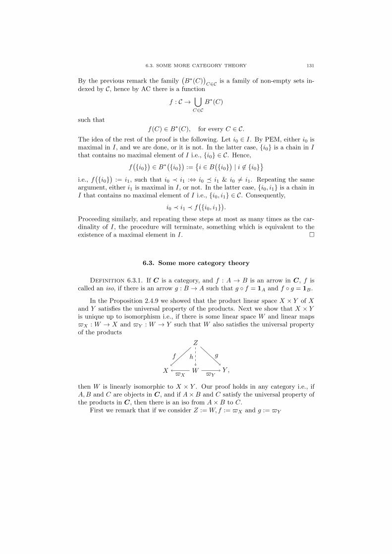
6.3. SOME MORE CATEGORY THEORY 131
By the previous remark the family(B∗(C)
)C∈C is a family of non-empty sets in-
dexed by C, hence by AC there is a function
f : C →⋃C∈C
B∗(C)
such that
f(C) ∈ B∗(C), for every C ∈ C.The idea of the rest of the proof is the following. Let i0 ∈ I. By PEM, either i0 ismaximal in I, and we are done, or it is not. In the latter case, {i0} is a chain in Ithat contains no maximal element of I i.e., {i0} ∈ C. Hence,
f({i0}
)∈ B∗
({i0}
):={i ∈ B
({i0}
)| i 6∈ {i0}
}i.e., f
({i0}
):= i1, such that i0 ≺ i1 :⇔ i0 � i1 & i0 6= i1. Repeating the same
argument, either i1 is maximal in I, or not. In the latter case, {i0, i1} is a chain inI that contains no maximal element of I i.e., {i0, i1} ∈ C. Consequently,
i0 ≺ i1 ≺ f({i0, i1}
).
Proceeding similarly, and repeating these steps at most as many times as the car-dinality of I, the procedure will terminate, something which is equivalent to theexistence of a maximal element in I. �
6.3. Some more category theory
Definition 6.3.1. If C is a category, and f : A → B is an arrow in C, f iscalled an iso, if there is an arrow g : B → A such that g ◦ f = 1A and f ◦ g = 1B .
In the Proposition 2.4.9 we showed that the product linear space X × Y of Xand Y satisfies the universal property of the products. Next we show that X × Yis unique up to isomorphism i.e., if there is some linear space W and linear maps$X : W → X and $Y : W → Y such that W also satisfies the universal propertyof the products
X W Y ,
Z
$X $Y
f gh
then W is linearly isomorphic to X × Y . Our proof holds in any category i.e., ifA,B and C are objects in C, and if A×B and C satisfy the universal property ofthe products in C, then there is an iso from A×B to C.
First we remark that if we consider Z := W, f := $X and g := $Y

132 6. APPENDIX
X W Y ,
W
$X $Y
$X $YidW
then, since idW makes the above inner diagrams commutative, and since the linearmap h is unique, we have that h = idW . Since X × Y and W both satisfy theuniversal property of the products we get from the previous remark that
X W Y
X × Y
X × Y
$X $Y
prX prYh
gprX prY
g ◦ h = idX×Y . Similarly from the commutative diagrams
X X × Y Y
W
W
prX prY
$X $Yg
h$X $Y
we get that h ◦ g = idW , hence X × Y and W are (linearly) isomorphic.
Definition 6.3.2. In a commutative diagram of sets and functions, the arrows
X Yf
X Yf
X Yf
denote an injection, a surjection, and a bijection, respectively.

Bibliography
[1] P. Aczel, M. Rathjen: Constructive Set Theory, book draft, 2010 (available in the internet).[2] D. Amir: Characterizations of inner product spaces, Springer Basel, 1986.
[3] S. Awodey: Category Theory, Oxford University Press, 2010.
[4] A. Bauer: Five stages of accepting constructive mathematics, Bulletin of the American Math-ematical Society, Volume 54, Number 3, 2017, 481-498.
[5] E. Bishop and D. S. Bridges: Constructive Analysis, Grundlehren der math. Wissenschaften
279, Springer-Verlag, Heidelberg-Berlin-New York, 1985.[6] A. Blass: Existence of bases implies the axiom of choice, Contemporary Mathematics, Volume
31, 1984, 31-33.
[7] D. S. Bridges: Can constructive mathematics be applied in physics?, Journal of PhilosophicalLogic 28 (5), 1999, 439-453.
[8] B. Coecke: Kindergarten quantum mechanics-lecture notes, In: Quantum Theory: Reconsid-
erations of the Foundations III. A. Khrennikov, Ed., American Institute of Physics Press.arXiv:quant-ph/0510032, 2005.
[9] B. Coecke: Introducing categories to the practicing physics, arXiv:0808.1032, 2008.[10] H. B. Enderton: Elements of Set Theory, Academic Press, 1977.
[11] O. Forster: Analysis 2, Vieweg+Teubner, 2008.
[12] W. Greub: Linear Algebra, Springer-Verlag, 1975.[13] G. Hellman: Constructive mathematics and quantum mechanics: unbounded operators and
the spectral theorem, Journal of Philosophical Logic 22, 1993, 221-248.
[14] J-B. Hiriart-Urruty, C. Lemarechal: Fundamentals of Convex Analysis, Springer-Verlag,2001.
[15] K. Kunen: Set Theory, Individual author and College Publications, 2013.
[16] S. Lang: Undergraduate Analysis, Springer, 1983.[17] S. Lang: Linear Algebra, Springer-Verlag, 1987.
[18] G. L. Naber: The Geometry of Minkowski Spacetime, An Introduction to the Mathematics
of the Special Theory of Relativity, Springer, 2012.[19] H. Rubin, J. E. Rubin: Equivalents of the axiom of choice II, North-Holland, 1985.[20] H. Schwichtenberg, S. Wainer: Proofs and Computations, Cambridge University Press, 2012.[21] Higher category theory and physics, in https://ncatlab.org/nlab/show/higher+category+the
ory+and+physics
133