mathematics module 5 higher concepts of mathematics textbooks/03... · higher concepts of...

MATHEMATICSModule 5

Higher Concepts of Mathematics

Higher Concepts of Mathematics TABLE OF CONTENTS

TABLE OF CONTENTS

LIST OF FIGURES . . . . . . . . . . . . . . . . . . . . . . . . . . . . . . . . . . . . . . . . . . . . . . . . . . iii

LIST OF TABLES . . . . . . . . . . . . . . . . . . . . . . . . . . . . . . . . . . . . . . . . . . . . . . . . . . . iv

REFERENCES . . . . . . . . . . . . . . . . . . . . . . . . . . . . . . . . . . . . . . . . . . . . . . . . . . . . . v

OBJECTIVES . . . . . . . . . . . . . . . . . . . . . . . . . . . . . . . . . . . . . . . . . . . . . . . . . . . . . . vi

STATISTICS . . . . . . . . . . . . . . . . . . . . . . . . . . . . . . . . . . . . . . . . . . . . . . . . . . . . . . 1

Frequency Distribution. . . . . . . . . . . . . . . . . . . . . . . . . . . . . . . . . . . . . . . . . . . 1The Mean. . . . . . . . . . . . . . . . . . . . . . . . . . . . . . . . . . . . . . . . . . . . . . . . . . . . 2Variability . . . . . . . . . . . . . . . . . . . . . . . . . . . . . . . . . . . . . . . . . . . . . . . . . . . 5Normal Distribution . . . . . . . . . . . . . . . . . . . . . . . . . . . . . . . . . . . . . . . . . . . . . 7Probability . . . . . . . . . . . . . . . . . . . . . . . . . . . . . . . . . . . . . . . . . . . . . . . . . . . 8Summary . . . . . . . . . . . . . . . . . . . . . . . . . . . . . . . . . . . . . . . . . . . . . . . . . . . 10

IMAGINARY AND COMPLEX NUMBERS . . . . . . . . . . . . . . . . . . . . . . . . . . . . . . . 11

Imaginary Numbers. . . . . . . . . . . . . . . . . . . . . . . . . . . . . . . . . . . . . . . . . . . . 11Complex Numbers . . . . . . . . . . . . . . . . . . . . . . . . . . . . . . . . . . . . . . . . . . . . 14Summary . . . . . . . . . . . . . . . . . . . . . . . . . . . . . . . . . . . . . . . . . . . . . . . . . . . 16

MATRICES AND DETERMINANTS . . . . . . . . . . . . . . . . . . . . . . . . . . . . . . . . . . . . 17

The Matrix . . . . . . . . . . . . . . . . . . . . . . . . . . . . . . . . . . . . . . . . . . . . . . . . . . 17Addition of Matrices . . . . . . . . . . . . . . . . . . . . . . . . . . . . . . . . . . . . . . . . . . . 18Multiplication of a Scaler and a Matrix. . . . . . . . . . . . . . . . . . . . . . . . . . . . . . 19Multiplication of a Matrix by a Matrix. . . . . . . . . . . . . . . . . . . . . . . . . . . . . . . 20The Determinant. . . . . . . . . . . . . . . . . . . . . . . . . . . . . . . . . . . . . . . . . . . . . . 21Using Matrices to Solve System of Linear Equation. . . . . . . . . . . . . . . . . . . . . 25Summary . . . . . . . . . . . . . . . . . . . . . . . . . . . . . . . . . . . . . . . . . . . . . . . . . . . 29

Rev. 0 Page i MA-05

TABLE OF CONTENTS Higher Concepts of Mathematics

TABLE OF CONTENTS (Cont)

CALCULUS . . . . . . . . . . . . . . . . . . . . . . . . . . . . . . . . . . . . . . . . . . . . . . . . . . . . . . 30

Dynamic Systems. . . . . . . . . . . . . . . . . . . . . . . . . . . . . . . . . . . . . . . . . . . . . 30Differentials and Derivatives. . . . . . . . . . . . . . . . . . . . . . . . . . . . . . . . . . . . . . 30Graphical Understanding of Derivatives. . . . . . . . . . . . . . . . . . . . . . . . . . . . . . 34Application of Derivatives to Physical Systems. . . . . . . . . . . . . . . . . . . . . . . . . 38Integral and Summations in Physical Systems. . . . . . . . . . . . . . . . . . . . . . . . . . 41Graphical Understanding of Integral. . . . . . . . . . . . . . . . . . . . . . . . . . . . . . . . . 43Summary . . . . . . . . . . . . . . . . . . . . . . . . . . . . . . . . . . . . . . . . . . . . . . . . . . . 46

MA-05 Page ii Rev. 0

Higher Concepts of Mathematics LIST OF FIGURES

LIST OF FIGURES

Figure 1 Normal Probability Distribution. . . . . . . . . . . . . . . . . . . . . . . . . . . . . . . 7

Figure 2 Motion Between Two Points. . . . . . . . . . . . . . . . . . . . . . . . . . . . . . . . . 31

Figure 3 Graph of Distance vs. Time. . . . . . . . . . . . . . . . . . . . . . . . . . . . . . . . . 31



Figure 6 Slope of a Curve. . . . . . . . . . . . . . . . . . . . . . . . . . . . . . . . . . . . . . . . . 36

Figure 7 Graph of Velocity vs. Time. . . . . . . . . . . . . . . . . . . . . . . . . . . . . . . . . 41

Figure 8 Graph of Velocity vs. Time. . . . . . . . . . . . . . . . . . . . . . . . . . . . . . . . . 44

Rev. 0 Page iii MA-05

Higher Concepts of Mathematics REFERENCES

REFERENCES

Dolciani, Mary P., et al., Algebra Structure and Method Book 1, Atlanta: Houghton-Mifflin, 1979.

Naval Education and Training Command, Mathematics, Vol:3, NAVEDTRA 10073-A,Washington, D.C.: Naval Education and Training Program Development Center, 1969.

Olivio, C. Thomas and Olivio, Thomas P., Basic Mathematics Simplified, Albany, NY:Delmar, 1977.

Science and Fundamental Engineering, Windsor, CT: Combustion Engineering, Inc., 1985.

Academic Program For Nuclear Power Plant Personnel, Volume 1, Columbia, MD:General Physics Corporation, Library of Congress Card #A 326517, 1982.

Standard Mathematical Tables, 23rd Edition, Cleveland, OH: CRC Press, Inc., Library ofCongress Card #30-4052, ISBN 0-87819-622-6, 1975.

Rev. 0 Page v MA-05

OBJECTIVES Higher Concepts of Mathematics

TERMINAL OBJECTIVE

1.0 SOLVE problems involving probability and simple statistics.

ENABLING OBJECTIVES

1.1 STATE the definition of the following statistical terms:a. Meanb. Variancec. Mean variance

1.2 CALCULATE the mathematical mean of a given set of data.

1.3 CALCULATE the mathematical mean variance of a given set of data.

1.4 Given the data,CALCULATE the probability of an event.

MA-05 Page vi Rev. 0

Higher Concepts of Mathematics OBJECTIVES

TERMINAL OBJECTIVE

2.0 SOLVE for problems involving the use of complex numbers.

ENABLING OBJECTIVES

2.1 STATE the definition of an imaginary number.

2.2 STATE the definition of a complex number.

2.3 APPLY the arithmetic operations of addition, subtraction, multiplication, anddivision to complex numbers.

Rev. 0 Page vii MA-05

OBJECTIVES Higher Concepts of Mathematics

TERMINAL OBJECTIVE

3.0 SOLVE for the unknowns in a problem through the application of matrix mathematics.

ENABLING OBJECTIVES

3.1 DETERMINE the dimensions of a given matrix.

3.2 SOLVE a given set of equations using Cramer’s Rule.

MA-05 Page viii Rev. 0

Higher Concepts of Mathematics OBJECTIVES

TERMINAL OBJECTIVE

4.0 DESCRIBE the use of differentials and integration in mathematical problems.

ENABLING OBJECTIVES

4.1 STATE the graphical definition of a derivative.

4.2 STATE the graphical definition of an integral.

Rev. 0 Page ix MA-05

Higher Concepts of Mathematics STATISTICS

STATISTICS

This chapter will cover the basic concepts of statistics.

EO 1.1 STATE the definition of the following statistical terms:a. Meanb. Variancec. Mean variance

EO 1.2 CALCULATE the mathematical mean of a given set ofdata.

EO 1.3 CALCULATE the mathematical mean variance of agiven set of data.

EO 1.4 Given the data, CALCULATE the probability of anevent.

In almost every aspect of an operator’s work, there is a necessity for making decisions resultingin some significant action. Many of these decisions are made through past experience with othersimilar situations. One might say the operator has developed a method of intuitive inference:unconsciously exercising some principles of probability in conjunction with statistical inferencefollowing from observation, and arriving at decisions which have a high chance of resulting inexpected outcomes. In other words, statistics is a method or technique which will enable us toapproach a problem of determining a course of action in a systematic manner in order to reachthe desired results.

Mathematically, statistics is the collection of great masses of numerical information that issummarized and then analyzed for the purpose of making decisions; that is, the use of pastinformation is used to predict future actions. In this chapter, we will look at some of the basicconcepts and principles of statistics.

Frequency Distribution

When groups of numbers are organized, or ordered by some method, and put into tabular orgraphic form, the result will show the "frequency distribution" of the data.

Rev. 0 Page 1 MA-05

STATISTICS Higher Concepts of Mathematics

Example:

A test was given and the following grades were received: the number of studentsreceiving each grade is given in parentheses.

99(1), 98(2), 96(4), 92(7), 90(5), 88(13), 86(11), 83(7), 80(5), 78(4), 75(3), 60(1)

The data, as presented, is arranged in descending order and is referred to as an orderedarray. But, as given, it is difficult to determine any trend or other information from thedata. However, if the data is tabled and/or plotted some additional information may beobtained. When the data is ordered as shown, a frequency distribution can be seen thatwas not apparent in the previous list of grades.

GradesNumber of

OccurrencesFrequency

Distribution

9998969290888683807875

111111111111 111111111111 11111 11111111 11111 111111 111111111111111

12475131175431

In summary, one method of obtaining additional information from a set of data is to determinethe frequency distribution of the data. The frequency distribution of any one data point is thenumber of times that value occurs in a set of data. As will be shown later in this chapter, thiswill help simplify the calculation of other statistically useful numbers from a given set of data.

The Mean

One of the most common uses of statistics is the determination of the mean value of a set ofmeasurements. The term "Mean" is the statistical word used to state the "average" value of a setof data. The mean is mathematically determined in the same way as the "average" of a groupof numbers is determined.

MA-05 Page 2 Rev. 0


The arithmetic mean of a set of N measurements, Xl, X2, X3, ..., XN is equal to the sum of themeasurements divided by the number of data points, N. Mathematically, this is expressed by thefollowing equation:

x1n

n

i 1xi

where

= the meanxn = the number of values (data)x1 = the first data point,x2 = the second data point,....xi = the ith data pointxi = the ith data point,x1 = the first data point,x2 = the second data point, etc.

The symbol Sigma (∑) is used to indicate summation, andi = 1 to n indicates that the values ofxi from i = 1 to i = n are added. The sum is then divided by the number of terms added,n.

Example:

Determine the mean of the following numbers:

5, 7, 1, 3, 4

Solution:

x 1n

n

i 1xi

15

5

i 1xi

where

= the meanxn = the number of values (data) = 5x1 = 5, x2 = 7, x3 = 1, x4 = 3, x5 = 4

substituting

= (5 + 7 + 1 + 3 +4)/5 = 20/5 = 4

4 is the mean.

Rev. 0 Page 3 MA-05


Example:

Find the mean of 67, 88, 91, 83, 79, 81, 69, and 74.

Solution:

x 1n

n

i 1xi

The sum of the scores is 632 andn = 8, therefore

x 6328

x 79

In many cases involving statistical analysis, literally hundreds or thousands of data points areinvolved. In such large groups of data, the frequency distribution can be plotted and thecalculation of the mean can be simplified by multiplying each data point by its frequencydistribution, rather than by summing each value. This is especially true when the number ofdiscrete values is small, but the number of data points is large.

Therefore, in cases where there is a recurring number of data points, like taking the mean of aset of temperature readings, it is easier to multiply each reading by its frequency of occurrence(frequency of distribution), then adding each of the multiple terms to find the mean. This is oneapplication using the frequency distribution values of a given set of data.

Example:

Given the following temperature readings,

573, 573, 574, 574, 574, 574, 575, 575, 575, 575, 575, 576, 576, 576, 578

Solution:

Determine the frequency of each reading.

MA-05 Page 4 Rev. 0


Frequency Distribution

Temperatures Frequency (f) (f)(xi)

573

574

575

576

578

2

4

5

3

1

15

1146

2296

2875

1728

578

8623

Then calculate the mean,

x 1n

n

i 1

xi

x 2(573) 4(574) 5(575) 3(576) 1(578)15

x 862315

x 574.9

Variability

We have discussed the averages and the means of sets of values. While the mean is a useful toolin describing a characteristic of a set of numbers, sometimes it is valuable to obtain informationabout the mean. There is a second number that indicates how representative the mean is of thedata. For example, in the group of numbers, 100, 5, 20, 2, the mean is 31.75. If these datapoints represent tank levels for four days, the use of the mean level, 31.75, to make a decisionusing tank usage could be misleading because none of the data points was close to the mean.

Rev. 0 Page 5 MA-05


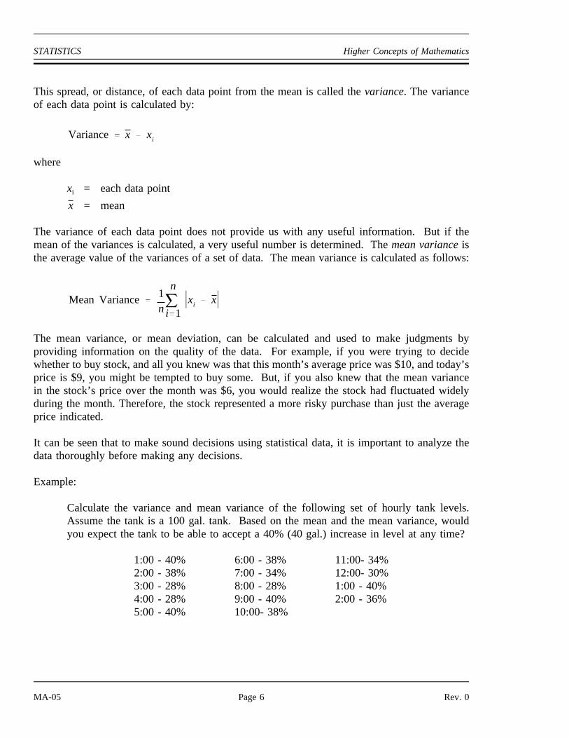
This spread, or distance, of each data point from the mean is called thevariance. The varianceof each data point is calculated by:

Variance x xi

where

xi = each data point

= meanx

The variance of each data point does not provide us with any useful information. But if themean of the variances is calculated, a very useful number is determined. Themean varianceisthe average value of the variances of a set of data. The mean variance is calculated as follows:

Mean Variance 1n

n

i 1xi x

The mean variance, or mean deviation, can be calculated and used to make judgments byproviding information on the quality of the data. For example, if you were trying to decidewhether to buy stock, and all you knew was that this month’s average price was $10, and today’sprice is $9, you might be tempted to buy some. But, if you also knew that the mean variancein the stock’s price over the month was $6, you would realize the stock had fluctuated widelyduring the month. Therefore, the stock represented a more risky purchase than just the averageprice indicated.

It can be seen that to make sound decisions using statistical data, it is important to analyze thedata thoroughly before making any decisions.

Example:

Calculate the variance and mean variance of the following set of hourly tank levels.Assume the tank is a 100 gal. tank. Based on the mean and the mean variance, wouldyou expect the tank to be able to accept a 40% (40 gal.) increase in level at any time?

1:00 - 40% 6:00 - 38% 11:00- 34%2:00 - 38% 7:00 - 34% 12:00- 30%3:00 - 28% 8:00 - 28% 1:00 - 40%4:00 - 28% 9:00 - 40% 2:00 - 36%5:00 - 40% 10:00- 38%

MA-05 Page 6 Rev. 0


Solution:

The mean is

[40(4)+38(3)+36+34(2)+30+28(3)]/14= 492/14 = 35.1

The mean variance is:

114

40 35.1 38 35.1 28 35.1 ...36 35.1

114

(57.8) 4.12

From the tank mean of 35.1%, it can be seen that a 40% increase in level will statistically fit intothe tank; 35.1 + 40 <100%. But, the mean doesn’t tell us if the level varies significantly overtime. Knowing the mean variance is 4.12% provides the additional information. Knowing themean variance also allows us to infer that the level at any given time (most likely) will not begreater than 35.1 + 4.12 = 39.1%; and 39.1 + 40 is still less than 100%. Therefore, it is a goodassumption that, in the near future, a 40% level increase will be accepted by the tank without anyspillage.

Normal Distribution

The concept of a normal distribution curve is used frequently in statistics. In essence, a normaldistribution curve results when a large number of random variables are observed in nature, andtheir values are plotted. While this "distribution" of values may take a variety of shapes, it isinteresting to note that a very large number of occurrences observed in nature possess afrequency distribution which is approximately bell-shaped, or in the form of a normaldistribution, as indicated in Figure 1.

Figure 1 Graph of a Normal Probability Distribution

Rev. 0 Page 7 MA-05


The significance of a normal distribution existing in a series of measurements is two fold. First,it explains why such measurements tend to possess a normal distribution; and second, it providesa valid basis for statistical inference. Many estimators and decision makers that are used to makeinferences about large numbers of data, are really sums or averages of those measurements.When these measurements are taken, especially if a large number of them exist, confidence canbe gained in the values, if these values form a bell-shaped curve when plotted on a distributionbasis.

Probability

If E1 is the number of heads, and E2 is the number of tails, E1/(E1 + E2) is an experimentaldetermination of the probability of heads resulting when a coin is flipped.

P(El) = n/N

By definition, the probability of an event must be greater than or equal to 0, and less than orequal to l. In addition, the sum of the probabilities of all outcomes over the entire "event" mustadd to equal l. For example, the probability of heads in a flip of a coin is 50%, the probabilityof tails is 50%. If we assume these are the only two possible outcomes, 50% + 50%, the twooutcomes, equals 100%, or 1.

The concept of probability is used in statistics when considering the reliability of the data or themeasuring device, or in the correctness of a decision. To have confidence in the values measuredor decisions made, one must have an assurance that the probability is high of the measurementbeing true, or the decision being correct.

To calculate the probability of an event, the number of successes (s), and failures (f), must bedetermined. Once this is determined, the probability of the success can be calculated by:

ps

s f

where

s + f = n = number of tries.

Example:

Using a die, what is the probability of rolling a three on the first try?

MA-05 Page 8 Rev. 0


Solution:

First, determine the number of possible outcomes. In this case, there are 6 possibleoutcomes. From the stated problem, the roll is a success only if a 3 is rolled. There isonly 1 success outcome and 5 failures. Therefore,

Probability = 1/(1+5)= 1/6

In calculating probability, the probability of a series of independent events equals the product ofprobability of the individual events.

Example:

Using a die, what is the probability of rolling two 3s in a row?

Solution:

From the previous example, there is a 1/6 chance of rolling a three on a single throw.Therefore, the chance of rolling two threes is:

1/6 x 1/6 = 1/36

one in 36 tries.

Example:

An elementary game is played by rolling a die and drawing a ball from a bag containing3 white and 7 black balls. The player wins whenever he rolls a number less than 4 anddraws a black ball. What is the probability of winning in the first attempt?

Solution:

There are 3 successful outcomes for rolling less than a 4, (i.e. 1,2,3). The probability ofrolling a 3 orless is:

3/(3+3) = 3/6 = 1/2 or 50%.

Rev. 0 Page 9 MA-05


The probability of drawing a black ball is:

7/(7+3) = 7/10.

Therefore, the probability of both events happening at the same time is:

7/10 x 1/2 = 7/20.

Summary

The important information in this chapter is summarized below.

Statistics Summary

Mean - The sum of a group of values divided by the numberof values.

Frequency Distribution - An arrangement of statistical data that exhibits thefrequency of the occurrence of the values of a variable.

Variance - The difference of a data point from the mean.

Mean Variance - The mean or average of the absolute values of eachdata point’s variance.

Probability of Success - The chances of being successful out of a number oftries.

sP =

s+f

MA-05 Page 10 Rev. 0

Higher Concepts of Mathematics IMAGINARY AND COMPLEX NUMBERS

IMAG INARY AND COMPLEX NUMBERS

This chapter will cover the definitions and rules for the application ofimaginary and complex numbers.

EO 2.1 STATE the definition of an imaginary number.

EO 2.2 STATE the definition of a complex number.

EO 2.3 APPLY the arithmetic operations of addition, subtraction,and multiplication, and division to complex numbers.

Imaginary and complex numbers are entirely different from any kind of number used up to thispoint. These numbers are generated when solving some quadratic and higher degree equations.Imaginary and complex numbers become important in the study of electricity; especially in thestudy of alternating current circuits.

Imaginary Numbers

Imaginary numbers result when a mathematical operation yields the square root of a negativenumber. For example, in solving the quadratic equation x2 + 25 = 0, the solution yields x2 = -25.

Thus, the roots of the equation are x = + . The square root of (-25) is called an imaginary 25number. Actually, any even root (i.e. square root, 4th root, 6th root, etc.) of a negative numberis called an imaginary number. All other numbers are called real numbers. The name"imaginary" may be somewhat misleading since imaginary numbers actually exist and can beused in mathematical operations. They can be added, subtracted, multiplied, and divided.

Imaginary numbers are written in a form different from real numbers. Since they are radicals,

they can be simplified by factoring. Thus, the imaginary number equals , 25 (25) ( 1)

which equals . Similarly, equals , which equals . All imaginary5 1 9 (9) ( 1) 3 1numbers can be simplified in this way. They can be written as the product of a real number and

. In order to further simplify writing imaginary numbers, the imaginary unit i is defined as 1

. Thus, the imaginary number, , which equals , is written as 5i, and the 1 25 5 1

imaginary number, , which equals , is written 3i. In using imaginary numbers in 9 3 1electricity, the imaginary unit is often represented by j, instead of i, since i is the commonnotation for electrical current.

Rev. 0 Page 11 MA-05

IMAGINARY AND COMPLEX NUMBERS Higher Concepts of Mathematics

Imaginary numbers are added or subtracted by writing them using the imaginary unit i and thenadding or subtracting the real number coefficients of i. They are added or subtracted like

algebraic terms in which the imaginary unit i is treated like a literal number. Thus, and 25 9are added by writing them as 5i and 3i and adding them like algebraic terms. The result is 8i

which equals or . Similarly, subtracted from equals 3i subtracted8 1 64 9 25

from 5i which equals 2i or or . 2 1 4

Example:

Combine the following imaginary numbers:

Solution:

16 36 49 1

16 36 49 1 4i 6i 7i i

10i 8i

2i

Thus, the result is 2i 2 1 4

Imaginary numbers are multiplied or divided by writing them using the imaginary unit i, and thenmultiplying or dividing them like algebraic terms. However, there are several basic relationshipswhich must also be used to multiply or divide imaginary numbers.

i2 = (i)(i) = = -1( 1 ) ( 1 )

i3 = (i2)(i) = (-1)(i) = -ii4 = (i2)(i2) = (-1)(-1) = +1

Using these basic relationships, for example, equals (5i)(2i) which equals 10i2.( 25) ( 4 )But, i2 equals -1. Thus, 10i2 equals (10)(-1) which equals -10.

Any square root has two roots, i.e., a statement x2 = 25 is a quadratic and has roots

x = ±5 since +52 = 25 and (-5) x (-5) = 25.



Similarly,

25 ±5i

4 ±2iand

25 4 ±10.

Example 1:

Multiply and . 2 32

Solution:

( 2 ) ( 32 ) ( 2 i) ( 32 i)

(2) (32) i2

64 ( 1)

8 ( 1)

8

Example 2:

Divide by . 48 3

Solution:



Complex Numbers

Complex numbers are numbers which consist of a real part and an imaginary part. The solutionof some quadratic and higher degree equations results in complex numbers. For example, theroots of the quadratic equation, x2 - 4x + 13 = 0, are complex numbers. Using the quadraticformula yields two complex numbers as roots.

x b ± b2 4ac2a

x 4 ± 16 522

x 4 ± 362

x 4 ± 6i2

x 2 ± 3i

The two roots are 2 + 3i and 2 - 3i; they are both complex numbers. 2 is the real part; +3i and -3i are the imaginary parts. The general form of a complex number is a + bi, in which "a"represents the real part and "bi" represents the imaginary part.

Complex numbers are added, subtracted, multiplied, and divided like algebraic binomials. Thus,the sum of the two complex numbers, 7 + 5i and 2 + 3i is 9 + 8i, and 7 + 5i minus 2 + 3i, is5 + 2i. Similarly, the product of 7 + 5i and 2 + 3i is 14 + 31i +15i2. But i2 equals -1. Thus,the product is 14 + 31i + 15(-1) which equals -1 + 31i.

Example 1:

Combine the following complex numbers:

(4 + 3i) + (8 - 2i) - (7 + 3i) =

Solution:

(4 + 3i) + (8 - 2i) - (7 + 3i) = (4 + 8 - 7) + (3 - 2 - 3)i= 5 - 2i



Example 2:

Multiply the following complex numbers:

(3 + 5i)(6 - 2i)=

Solution:

(3 + 5i)(6 - 2i) = 18 + 30i - 6i - 10i2

= 18 + 24i - 10(-1)= 28 + 24i

Example 3:

Divide (6+8i) by 2.

Solution:

6 8i2

62

82

i

3 4i

A difficulty occurs when dividing one complex number by another complex number. To getaround this difficulty, one must eliminate the imaginary portion of the complex number from thedenominator, when the division is written as a fraction. This is accomplished by multiplying thenumerator and denominator by theconjugateform of the denominator. Theconjugateof acomplex number is that complex number written with the opposite sign for the imaginary part.For example, the conjugate of 4+5i is 4-5i.

This method is best demonstrated by example.

Example: (4 + 8i) ÷ (2 - 4i)

Solution:

4 8i2 4i

2 4i2 4i

8 32i 32i 2

4 16i 2

8 32i 32( 1)4 16( 1)

24 32i20

65

85

i



Summary

The important information from this chapter is summartized below.

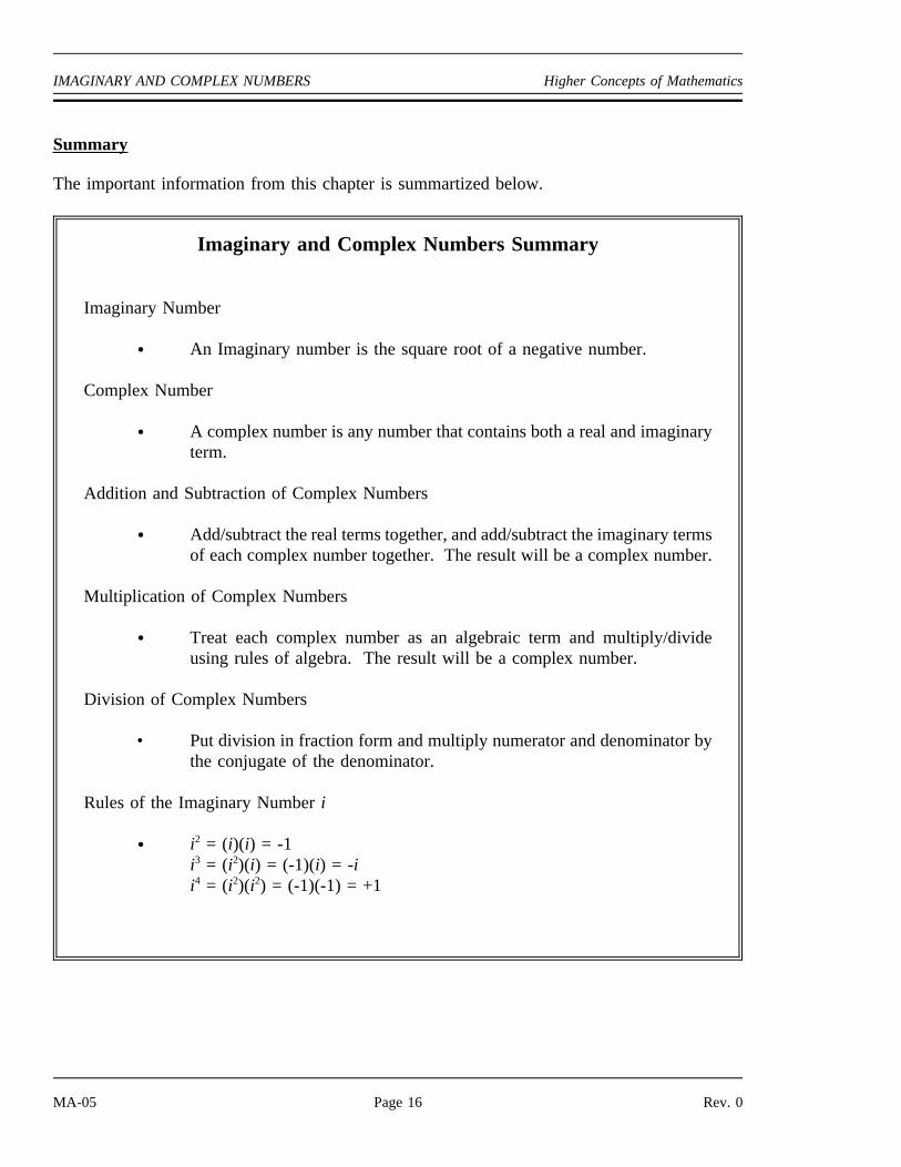
Imaginary and Complex Numbers Summary

Imaginary Number

An Imaginary number is the square root of a negative number.

Complex Number

A complex number is any number that contains both a real and imaginaryterm.

Addition and Subtraction of Complex Numbers

Add/subtract the real terms together, and add/subtract the imaginary termsof each complex number together. The result will be a complex number.

Multiplication of Complex Numbers

Treat each complex number as an algebraic term and multiply/divideusing rules of algebra. The result will be a complex number.

Division of Complex Numbers

• Put division in fraction form and multiply numerator and denominator bythe conjugate of the denominator.

Rules of the Imaginary Numberi

i2 = (i)(i) = -1i3 = (i2)(i) = (-1)(i) = -ii4 = (i2)(i2) = (-1)(-1) = +1


Higher Concepts of Mathematics MATRICES AND DETERMINANTS

MATRICES AND DETERMINANTS

This chapter will explain the idea of matrices and determinate and the rulesneeded to apply matrices in the solution of simultaneous equations.

EO 3.1 DETERMINE the dimensions of a given matrix.

EO 3.2 SOLVE a given set of equations using Cramer’s Rule.

In the real world, many times the solution to a problem containing a large number of variablesis required. In both physics and electrical circuit theory, many problems will be encounteredwhich contain multiple simultaneous equations with multiple unknowns. These equations can besolved using the standard approach of eliminating the variables or by one of the other methods.This can be difficult and time-consuming. To avoid this problem, and easily solve families ofequations containing multiple unknowns, a type of math was developed called Matrix theory.

Once the terminology and basic manipulations of matrices are understood, matrices can be usedto readily solve large complex systems of equations.

The Matrix

We define a matrix as any rectangular array of numbers. Examples of matrices may be formedfrom the coefficients and constants of a system of linear equations: that is,

2x - 4y = 73x + y = 16

can be written as follows.

2 4 7

3 1 16

The numbers used in the matrix are called elements. In the example given, we have threecolumns and two rows of elements. The number of rows and columns are used to determine thedimensions of the matrix. In our example, the dimensions of the matrix are 2 x 3, having 2 rowsand 3 columns of elements. In general, the dimensions of a matrix which havem rows andncolumns is called anm x n matrix.


MATRICES AND DETERMINANTS Higher Concepts of Mathematics

A matrix with only a single row or a single column is called either a row or a column matrix.A matrix which has the same number of rows as columns is called a square matrix. Examplesof matrices and their dimensions are as follows:

1 7 6

2 4 82 x 3

1 7

6 2

3 5

3 x 2

3

2

1

3 x 1

We will use capital letters to describe matrices. We will also include subscripts to give thedimensions.

A2×3

1 3 3

5 6 7

Two matrices are said to be equal if, and only if, they have the same dimensions, and theircorresponding elements are equal. The following are all equal matrices:

0 1

2 4

0 1

2 4

0 11

63

4

Addition of Matrices

Matrices may only be added if they both have the same dimensions. To add two matrices, eachelement is added to its corresponding element. The sum matrix has the same dimensions as thetwo being added.



Example:

Add matrix A to matrix B.

A

6 2 6

1 3 0B

2 1 3

0 3 6

Solution:

A B

6 2 2 1 6 3

1 0 3 3 0 6

8 3 9

1 0 6

Multiplication of a Scalar and a Matrix

When multiplying a matrix by a scalar (or number), we write "scalarK times matrixA." Eachelement of the matrix is multiplied by the scalar. By example:

K 3 and A

2 3

1 7

then

3 x A 3

2 3

1 7

2 3 3 3

1 3 7 3

6 9

3 21



Multiplication of a Matrix by a Matrix

To multiply two matrices, the first matrix must have the same number of rows (m) as the secondmatrix has columns (n). In other words,m of the first matrix must equaln of the second matrix.For example, a 2 x 1matrix can be multiplied by a 1 x 2matrix,

x

ya b

ax bx

ay by

or a 2 x 2 matrix can be multiplied by a 2 x 2. If anm x n matrix is multiplied by ann x pmatrix, then the resulting matrix is anm x p matrix. For example, if a 2 x 1 and a 1 x 2 aremultiplied, the result will be a 2 x 2. If a 2 x 2 and a 2 x 2 are multiplied, the result will be a2 x 2.

To multiply two matrices, the following pattern is used:

A

a b

c dB

w x

y z

C A B

aw by ax bz

cw dy cx dz

In general terms, a matrix C which is a product of two matrices, A and B, will have elementsgiven by the following.

cij = ai1b1j + aj2b2j + + + . . . + ainbnj

where

i = ith rowj = jth column

Example:

Multiply the matricesA x B.

A

1 2

3 4B

3 5

0 6



Solution:

A B

(1x3) (2x0) (1x5) (2x6)

(3x3) (4x0) (3x5) (4x6)

3 0 5 12

9 0 15 24

3 17

9 39

It should be noted that the multiplication of matrices is not usually commutative.

The Determinant

Square matrixes have a property called a determinant. When a determinant of a matrix is written,it is symbolized by vertical bars rather than brackets around the numbers. This differentiates thedeterminant from a matrix. The determinant of a matrix is the reduction of the matrix to a singlescalar number. The determinant of a matrix is found by "expanding" the matrix. There areseveral methods of "expanding" a matrix and calculating it’s determinant. In this lesson, we willonly look at a method called "expansion by minors."

Before a large matrix determinant can be calculated, we must learn how to calculate thedeterminant of a 2 x 2 matrix. By definition, the determinant of a 2 x 2 matrix is calculated asfollows:

A =



Example: Find the determinant of A.

A =6 2

1 3

Solution:

A (6 3) ( 1 2)18 ( 2)18 220

To expand a matrix larger than a 2 x 2 requires that it be simplified down to several 2 x 2matrices, which can then be solved for their determinant. It is easiest to explain the process byexample.

Given the 3 x 3matrix:

1 3 1

4 1 2

5 6 3

Any single row or column is picked. In this example, column one is selected. The matrix willbe expanded using the elements from the first column. Each of the elements in the selectedcolumn will be multiplied by its minor starting with the first element in the column (1). A lineis then drawn through all the elements in the same row and column as 1. Since this is a 3 x 3matrix, that leaves a minor or 2 x 2 determinant. This resulting 2 x 2 determinant is called theminor of the element in the first row first column.



The minor of element 4 is:

The minor of element 5 is:

Each element is given a sign based on its position in the original determinant.

The sign is positive (negative) if the sum of the row plus the column for the element is even(odd). This pattern can be expanded or reduced to any size determinant. The positive andnegative signs are just alternated.



Each minor is now multiplied by its signed element and the determinant of the resulting 2 x 2calculated.

1

1 2

6 31 (1 3) (2 6) 3 (12) 9

4

3 1

6 34 (3 3) (1 6) 4 9 6 12

5

3 1

1 25 (3 2) (1 1) 5 6 1 25

Determinant = (-9) + (-12) + 25 = 4

Example:

Find the determinant of the following 3 x 3 matrix, expanding about row 1.

3 1 2

4 5 6

0 1 4



Solution:

Using Matrices to Solve System of Linear Equation (Cramer’s Rule)

Matrices and their determinant can be used to solve a system of equations. This method becomesespecially attractive when large numbers of unknowns are involved. But the method is stilluseful in solving algebraic equations containing two and three unknowns.

In part one of this chapter, it was shown that equations could be organized such that theircoefficients could be written as a matrix.

ax + by = cex + fy = g

where:

x andy are variablesa, b, e, andf are the coefficientsc andg are constants



The equations can be rewritten in matrix form as follows:

a b

e f

x

y

c

g

To solve for each variable, the matrix containing the constants (c,g) is substituted in place of thecolumn containing the coefficients of the variable that we want to solve for (a,e or b,f ). Thisnew matrix is divided by the original coefficient matrix. This process is call "Cramer’s Rule."

Example:

In the above problem to solve forx,

c b

g fx =

c b

g f

and to solve fory,

a c

e gy =

a b

e f

Example:

Solve the following two equations:

x + 2y = 4-x + 3y = 1



Solution:

4 2

1 3x =

1 2

1 3

1 4

1 1y =

1 2

1 3

solving each 2 x 2 for itsdeterminant,

x [ (4 3) (1 2) ][ (1 3) ( 1 2) ]

12 23 2

105

2

y [ (1 1) ( 1 4) ][ (1 3) ( 1 2) ]

1 43 2

55

1

x 2 and y 1

A 3 x 3 is solved by using the same logic, except each 3 x 3 must be expanded by minors tosolve for the determinant.

Example:

Given the following three equations, solve for the three unknowns.

2x + 3y - z = 2x - 2y + 2z = -103x + y - 2z = 1



Solution:

2 3 1

10 2 2

1 1 2x =

2 3 1

1 2 2

3 1 2

2 2 1

1 10 2

3 1 2y =

2 3 1

1 2 2

3 1 2

2 3 2

1 2 10

3 1 1z =

2 3 1

1 2 2

3 1 2

Expanding the top matrix forx using the elements in the bottom row gives:

1

3 1

2 2( 1)

2 1

10 2( 2)

2 3

10 2

1 (6 2) ( 1) (4 10) ( 2) ( 4 30)

4 6 52 42



Expanding the bottom matrix forx using the elements in the first column gives:

2

2 2

1 2( 1)

3 1

1 23

3 1

2 2

2 (4 2) ( 1) ( 6 1) 3 (6 2)

4 5 12 21

This gives:

x 4221

2

y andz can be expanded using the same method.

y = 1z = -3

Summary

The use of matrices and determinants is summarized below.

Matrices and Determinant Summary

The dimensions of a matrix are given asm x n, wherem = number of rows andn = number of columns.

The use of determinants and matrices to solve linear equations is done by:

placing the coefficients and constants into a determinant format.

substituting the constants in place of the coefficients of the variable to besolved for.

dividing the new-formed substituted determinant by the originaldeterminant of coefficients.

expanding the determinant.


CALCULUS Higher Concepts of Mathematics

CALCULUS

Many practical problems can be solved using arithmetic and algebra; however,many other practical problems involve quantities that cannot be adequatelydescribed using numbers which have fixed values.

EO 4.1 STATE the graphical definition of a derivative.

EO 4.2 STATE the graphical definition of an integral.

Dynamic Systems

Arithmetic involves numbers that have fixed values. Algebra involves both literal and arithmeticnumbers. Although the literal numbers in algebraic problems can change value from onecalculation to the next, they also have fixed values in a given calculation. When a weight isdropped and allowed to fall freely, its velocity changes continually. The electric current in analternating current circuit changes continually. Both of these quantities have a different valueat successive instants of time. Physical systems that involve quantities that change continuallyare called dynamic systems. The solution of problems involving dynamic systems often involvesmathematical techniques different from those described in arithmetic and algebra. Calculusinvolves all the same mathematical techniques involved in arithmetic and algebra, such asaddition, subtraction, multiplication, division, equations, and functions, but it also involves severalother techniques. These techniques are not difficult to understand because they can be developedusing familiar physical systems, but they do involve new ideas and terminology.

There are many dynamic systems encountered in nuclear facility work. The decay of radioactivematerials, the startup of a reactor, and a power change on a turbine generator all involvequantities which change continually. An analysis of these dynamic systems involves calculus.Although the operation of a nuclear facility does not require a detailed understanding of calculus,it is most helpful to understand certain of the basic ideas and terminology involved. These ideasand terminology are encountered frequently, and a brief introduction to the basic ideas andterminology of the mathematics of dynamic systems is discussed in this chapter.

Differentials and Derivatives

One of the most commonly encountered applications of the mathematics of dynamic systemsinvolves the relationship between position and time for a moving object. Figure 2 represents anobject moving in a straight line from positionP1 to positionP2. The distance toP1 from a fixedreference point, point 0, along the line of travel is represented byS1; the distance toP2 frompoint 0 byS2.


Higher Concepts of Mathematics CALCULUS

Figure 2 Motion Between Two Points

If the time recorded by a clock, when the object is at positionP1 is t1, and if the time when theobject is at positionP2 is t2, then the average velocity of the object between pointsP1 and P2

equals the distance traveled, divided by the elapsed time.

(5-1)Vav

S2 S1

t2 t1

If positions P1 and P2 are close together, the distance traveled and the elapsed time are small.The symbol∆, the Greek letter delta, is used to denote changes in quantities. Thus, the averagevelocity when positionsP1 andP2 are close together is often written using deltas.

(5-2)Vav

∆S∆t

S2 S1

t2 t1

Although the average velocity is

Figure 3 Displacement Versus Time

often an important quantity, inmany cases it is necessary to knowthe velocity at a given instant oftime. This velocity, called theinstantaneous velocity, is not thesame as the average velocity,unless the velocity is not changingwith time.

Using the graph of displacement,S, versus time,t, in Figure 3, wewill try to describe the concept ofthe derivative.



Using equation 5-1 we find the average velocity from S1 to S2 is . If we connect the S2 S1

t2 t1

points S1 and S2 by a straight line we see it does not accurately reflect the slope of the curvedline through all the points between S1 and S2. Similarly, if we look at the average velocitybetween time t2 and t3 (a smaller period of time), we see the straight line connecting S2 and S3

more closely follows the curved line. Assuming the time between t3 and t4 is less than betweent2 and t3, the straight line connecting S3 and S4 very closely approximates the curved line betweenS3 and S4.

As we further decrease the time interval between successive points, the expression more ∆ S∆ t

closely approximates the slope of the displacement curve. As approaches the∆ t →0, ∆ S∆ t

instantaneous velocity. The expression for the derivative (in this case the slope of the

displacement curve) can be written . In words, this expression would be dSdt

lim∆ t →o

∆ S∆ t

"the derivative of S with respect to time (t) is the limit of as ∆t approaches 0." ∆ S∆ t

(5-3)V dsdt

lim∆ t→0

∆ s∆ t

The symbols ds and dt are not products of d and s, or of d and t, as in algebra. Each representsa single quantity. They are pronounced "dee-ess" and "dee-tee," respectively. Theseexpressions and the quantities they represent are called differentials. Thus, ds is the differentialof s and dt is the differential of t. These expressions represent incremental changes, where dsrepresents an incremental change in distance s, and dt represents an incremental change in timet.

The combined expression ds/dt is called a derivative; it is the derivative of s with respect tot. It is read as "dee-ess dee-tee." dz/dx is the derivative of z with respect to x; it is read as"dee-zee dee-ex." In simplest terms, a derivative expresses the rate of change of one quantitywith respect to another. Thus, ds/dt is the rate of change of distance with respect to time.Referring to figure 3, the derivative ds/dt is the instantaneous velocity at any chosen pointalong the curve. This value of instantaneous velocity is numerically equal to the slope of thecurve at that chosen point.

While the equation for instantaneous velocity, V = ds/dt, may seem like a complicatedexpression, it is a familiar relationship. Instantaneous velocity is precisely the value given bythe speedometer of a moving car. Thus, the speedometer gives the value of the rate of changeof distance with respect to time; it gives the derivative of s with respect to t; i.e. it gives thevalue of ds/dt.



The ideas of differentials and derivatives are fundamental to the application of mathematics todynamic systems. They are used not only to express relationships among distance traveled,elapsed time and velocity, but also to express relationships among many different physicalquantities. One of the most important parts of understanding these ideas is having a physicalinterpretation of their meaning. For example, when a relationship is written using a differentialor a derivative, the physical meaning in terms of incremental changes or rates of change shouldbe readily understood.

When expressions are written using deltas, they can be understood in terms of changes. Thus,the expression ∆T, where T is the symbol for temperature, represents a change in temperature.As previously discussed, a lower case delta, d, is used to represent very small changes. Thus,dT represents a very small change in temperature. The fractional change in a physical quantityis the change divided by the value of the quantity. Thus, dT is an incremental change intemperature, and dT/T is a fractional change in temperature. When expressions are written asderivatives, they can be understood in terms of rates of change. Thus, dT/dt is the rate ofchange of temperature with respect to time.

Examples:

1. Interpret the expression ∆V /V, and write it in terms of adifferential. ∆V /V expresses the fractional change of velocity.It is the change in velocity divided by the velocity. It can bewritten as a differential when ∆V is taken as an incrementalchange.

may be written as ∆ VV

dVV

2. Give the physical interpretation of the following equation relatingthe work W done when a force F moves a body through adistance x.

dW = Fdx

This equation includes the differentials dW and dx which can beinterpreted in terms of incremental changes. The incrementalamount of work done equals the force applied multiplied by theincremental distance moved.



3. Give the physical interpretation of the following equation relatingthe force,F, applied to an object, its massm, its instantaneousvelocity v and timet.

F mdvdt

This equation includes the derivativedv/dt; the derivative of thevelocity with respect to time. It is the rate of change of velocitywith respect to time. The force applied to an object equals themass of the object multiplied by the rate of change of velocity withrespect to time.

4. Give the physical interpretation of the following equation relatingthe accelerationa, the velocityv, and the timet.

a dvdt

This equation includes the derivativedv/dt; the derivative of thevelocity with respect to time. It is a rate of change. Theacceleration equals the rate of change of velocity with respect totime.

Graphical Understanding of Derivatives

A function expresses a relationship between two or more variables. For example, the distancetraveled by a moving body is a function of the body’s velocity and the elapsed time. When afunctional relationship is presented in graphical form, an important understanding of the meaningof derivatives can be developed.

Figure 4 is a graph of the distance traveled by an object as a function of the elapsed time. Thefunctional relationship shown is given by the following equation:

s = 40t (5-4)

The instantaneous velocityv, which is the velocity at a given instant of time, equals thederivative of the distance traveled with respect to time,ds/dt. It is the rate of change ofs withrespect tot.



The value of the derivativeds/dt for the case

Figure 4 Graph of Distance vs. Time

plotted in Figure 4 can be understood byconsidering small changes in the two variabless and t.

∆s∆t

(s ∆s) s(t ∆t) t

The values of (s + ∆s) ands in terms of (t +∆t) and t, using Equation 5-4 can now besubstituted into this expression. At timet, s= 40t; at time t + ∆t, s + ∆s = 40(t + ∆t).

∆s∆t

40(t ∆t) 40t(t ∆t) t

∆s∆t

40t 40(∆t) 40tt ∆t t

∆s∆t

40(∆t)∆t

∆s∆t

40

The value of the derivativeds/dt in the case plotted in Figure 4 is a constant. It equals 40 ft/s.In the discussion of graphing, the slope of a straight line on a graph was defined as the changein y, ∆y, divided by the change inx, ∆x. The slope of the line in Figure 4 is∆s/∆t which, in thiscase, is the value of the derivativeds/dt. Thus, derivatives of functions can be interpreted interms of the slope of the graphical plot of the function. Since the velocity equals the derivativeof the distances with respect to timet, ds/dt, and since this derivative equals the slope of the plotof distance versus time, the velocity can be visualized as the slope of the graphical plot ofdistance versus time.

For the case shown in Figure 4, the velocity is constant. Figure 5 is another graph of thedistance traveled by an object as a function of the elapsed time. In this case the velocity is notconstant. The functional relationship shown is given by the following equation:

s = 10t2 (5-5)



The instantaneous velocity again equals the

Figure 5 Graph of Distance vs. Time

value of the derivativeds/dt. This value ischanging with time. However, theinstantaneous velocity at any specified timecan be determined. First, small changes ins and t are considered.

∆s∆t

(s ∆s) s(t ∆t) t

The values of (s + ∆s) ands in terms of(t + ∆t) and t using Equation 5-5, can thenbe substituted into this expression. At timet, s = 10t2; at time t + ∆t, s + ∆s = 10(t +∆t)2. The value of (t + ∆t)2 equals t2 +2t(∆t) + (∆t)2; however, for incrementalvalues of∆t, the term (∆t)2 is so small, itcan be neglected. Thus, (t + ∆t)2 = t2 +2t(∆t).

∆s∆t

10[t2 2t(∆t)] 10t2

(t ∆t) t

∆s∆t

10t2 20t(∆t)] 10t2

t ∆t t

Figure 6 Slope of a Curve

∆s∆t

20t

The value of the derivativeds/dt in the caseplotted in Figure 5 equals 20t. Thus, at timet = 1 s, the instantaneous velocity equals 20ft/s; at time t = 2 s, the velocity equals 40ft/s, and so on.

When the graph of a function is not a straightline, the slope of the plot is different atdifferent points. The slope of a curve at anypoint is defined as the slope of a line drawntangent to the curve at that point. Figure 6shows a line drawn tangent to a curve. Atangent line is a line that touches the curve atonly one point. The lineAB is tangent to the



curvey = f(x) at pointP.

The tangent line has the slope of the curvedy/dx, where, θ is the angle between the tangent lineAB and a line parallel to the x-axis. But, tanθ also equals∆y/∆x for the tangent lineAB, and∆y/∆x is the slope of the line. Thus, the slope of a curve at any point equals the slope of the linedrawn tangent to the curve at that point. This slope, in turn, equals the derivative ofy withrespect tox, dy/dx, evaluated at the same point.

These applications suggest that a derivative can be visualized as the slope of a graphical plot.A derivative represents the rate of change of one quantity with respect to another. When therelationship between these two quantities is presented in graphical form, this rate of changeequals the slope of the resulting plot.

The mathematics of dynamic systems involves many different operations with the derivatives offunctions. In practice, derivatives of functions are not determined by plotting the functions andfinding the slopes of tangent lines. Although this approach could be used, techniques have beendeveloped that permit derivatives of functions to be determined directly based on the form of thefunctions. For example, the derivative of the functionf(x) = c, wherec is a constant, is zero.The graph of a constant function is a horizontal line, and the slope of a horizontal line is zero.

f(x) = c

(5-6)d[f(x)]dx

0

The derivative of the functionf(x) = ax + c (compare to slopem from general form of linearequation, y =mx + b), wherea and c are constants, isa. The graph of such a function is astraight line having a slope equal toa.

f(x) = ax + c

(5-7)d[f(x)]dx

a

The derivative of the functionf(x) = axn, wherea andn are constants, isnaxn-1.

f(x) = axn

(5-8)d[f(x)]dx

naxn 1

The derivative of the functionf(x) = aebx, wherea andb are constants ande is the base of naturallogarithms, isabebx.



f(x) = aebx

(5-9) d [f(x)]dx

abebx

These general techniques for finding the derivatives of functions are important for those whoperform detailed mathematical calculations for dynamic systems. For example, the designers ofnuclear facility systems need an understanding of these techniques, because these techniques arenot encountered in the day-to-day operation of a nuclear facility. As a result, the operators ofthese facilities should understand what derivatives are in terms of a rate of change and a slopeof a graph, but they will not normally be required to find the derivatives of functions.

The notation d[f(x)]/dx is the common way to indicate the derivative of a function. In some

applications, the notation is used. In other applications, the so-called dot notation is usedf (x)to indicate the derivative of a function with respect to time. For example, the derivative of the

amount of heat transferred, Q, with respect to time, dQ/dt, is often written as . Q

It is also of interest to note that many detailed calculations for dynamic systems involve not onlyone derivative of a function, but several successive derivatives. The second derivative of afunction is the derivative of its derivative; the third derivative is the derivative of the secondderivative, and so on. For example, velocity is the first derivative of distance traveled withrespect to time, v = ds/dt; acceleration is the derivative of velocity with respect to time, a = dv/dt.Thus, acceleration is the second derivative of distance traveled with respect to time. This iswritten as d2s/dt2. The notation d2[f(x)]/dx2 is the common way to indicate the second derivative

of a function. In some applications, the notation is used. The notation for third, fourth,f (x)and higher order derivatives follows this same format. Dot notation can also be used for higherorder derivatives with respect to time. Two dots indicates the second derivative, three dots thethird derivative, and so on.

Application of Derivatives to Physical Systems

There are many different problems involving dynamic physical systems that are most readilysolved using derivatives. One of the best illustrations of the application of derivatives areproblems involving related rates of change. When two quantities are related by some knownphysical relationship, their rates of change with respect to a third quantity are also related. For

example, the area of a circle is related to its radius by the formula . If for some reasonA πr2

the size of a circle is changing in time, the rate of change of its area, with respect to time forexample, is also related to the rate of change of its radius with respect to time. Although theseapplications involve finding the derivative of function, they illustrate why derivatives are neededto solve certain problems involving dynamic systems.



Example 1:

A stone is dropped into a quiet lake, and waves move in circles outward from thelocation of the splash at a constant velocity of 0.5 feet per second. Determine therate at which the area of the circle is increasing when the radius is 4 feet.

Solution:

Using the formula for the area of a circle,

A πr2

take the derivative of both sides of this equation with respect to time t.

dAdt

2πr drdt

But, dr/dt is the velocity of the circle moving outward which equals 0.5 ft/s anddA /dt is the rate at which the area is increasing, which is the quantity to bedetermined. Set r equal to 4 feet, substitute the known values into the equation,and solve for dA /dt.

dAdt

2πr drdt

dAdt

(2) (3.1416) (4 ft) 0.5 ft/s

dAdt

12.6 ft2/s

Thus, at a radius of 4 feet, the area is increasing at a rate of 12.6 square feet persecond.

Example 2:

A ladder 26 feet long is leaning against a wall. The ladder starts to move suchthat the bottom end moves away from the wall at a constant velocity of 2 feet persecond. What is the downward velocity of the top end of the ladder when thebottom end is 10 feet from the wall?

Solution:

Start with the Pythagorean Theorem for a right triangle:a2 = c2 - b2



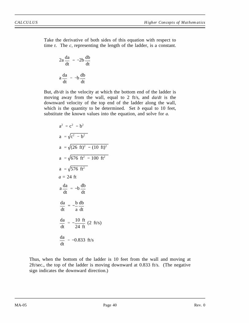
Take the derivative of both sides of this equation with respect totime t. The c, representing the length of the ladder, is a constant.

2a dadt

2b dbdt

a dadt

b dbdt

But, db/dt is the velocity at which the bottom end of the ladder ismoving away from the wall, equal to 2 ft/s, and da/dt is thedownward velocity of the top end of the ladder along the wall,which is the quantity to be determined. Set b equal to 10 feet,substitute the known values into the equation, and solve for a.

a2 c2 b2

a c2 b2

a (26 ft)2 (10 ft)2

a 676 ft2 100 ft2

a 576 ft2

a = 24 ft

a dadt

b dbdt

dadt

ba

dbdt

dadt

10 ft24 ft

(2 ft/s)

dadt

0.833 ft/s

Thus, when the bottom of the ladder is 10 feet from the wall and moving at2ft/sec., the top of the ladder is moving downward at 0.833 ft/s. (The negativesign indicates the downward direction.)



Integrals and Summations in Physical Systems

Differentials and derivatives arose in physical systems when small changes in one quantity wereconsidered. For example, the relationship between position and time for a moving object led tothe definition of the instantaneous velocity, as the derivative of the distance traveled with respectto time, ds/dt. In many physical systems, rates of change are measured directly. Solvingproblems, when this is the case, involves another aspect of the mathematics of dynamic systems;namely integral and summations.

Figure 7 is a graph of the instantaneous velocity of an object as a function of elapsed time. Thisis the type of graph which could be generated if the reading of the speedometer of a car wererecorded as a function of time.

At any given instant of time, the velocity

Figure 7 Graph of Velocity vs. Time

of the object can be determined byreferring to Figure 7. However, if thedistance traveled in a certain interval oftime is to be determined, some newtechniques must be used. Consider thevelocity versus time curve of Figure 7.Let's consider the velocity changesbetween times tA and tB. The firstapproach is to divide the time interval intothree short intervals , and to(∆ t1,∆ t2,∆ t3)assume that the velocity is constant duringeach of these intervals. During timeinterval ∆t1, the velocity is assumedconstant at an average velocity v1; duringthe interval ∆t2, the velocity is assumedconstant at an average velocity v2; duringtime interval ∆t3, the velocity is assumedconstant at an average velocity v3. Thenthe total distance traveled is approximately the sum of the products of the velocity and theelapsed time over each of the three intervals. Equation 5-10 approximates the distance traveledduring the time interval from ta to tb and represents the approximate area under the velocity curveduring this same time interval.

s = v1∆t1 + v2∆t2 + v3∆t3 (5-10)



This type of expression is called a summation. A summation indicates the sum of a series ofsimilar quantities. The upper case Greek letter Sigma, , is used to indicate a summation.Generalized subscripts are used to simplify writing summations. For example, the summationgiven in Equation 5-10 would be written in the following manner:

(5-11)S 3

i 1

vi∆ ti

The number below the summation sign indicates the value of i in the first term of thesummation; the number above the summation sign indicates the value of i in the last term of thesummation.

The summation that results from dividing the time interval into three smaller intervals, as shownin Figure 7, only approximates the distance traveled. However, if the time interval is dividedinto incremental intervals, an exact answer can be obtained. When this is done, the distancetraveled would be written as a summation with an indefinite number of terms.

(5-12)S ∞

i 1

vi∆ ti

This expression defines an integral. The symbol for an integral is an elongated "s" . Usingan integral, Equation 5-12 would be written in the following manner:

(5-13)S

tB

tA

v dt

This expression is read as S equals the integral of v dt from t = tA to t = tB. The numbers belowand above the integral sign are the limits of the integral. The limits of an integral indicate thevalues at which the summation process, indicated by the integral, begins and ends.

As with differentials and derivatives, one of the most important parts of understanding integralsis having a physical interpretation of their meaning. For example, when a relationship is writtenas an integral, the physical meaning, in terms of a summation, should be readily understood.In the previous example, the distance traveled between tA and tB was approximated by equation5-10. Equation 5-13 represents the exact distance traveled and also represents the exact areaunder the curve on figure 7 between tA and tB.

Examples:

1. Give the physical interpretation of the following equation relatingthe work, W, done when a force, F, moves a body from positionx1 to x2.



W

x2

x1

F dx

The physical meaning of this equation can be stated in terms of asummation. The total amount of work done equals the integral ofF dx from x = x1 to x = x2. This can be visualized as taking theproduct of the instantaneous force, F, and the incremental changein position dx at each point between x1 and x2, and summing allof these products.

2. Give the physical interpretation of the following equation relatingthe amount of radioactive material present as a function of theelapsed time, t, and the decay constant, λ.

N1

N0

dNN

λt

The physical meaning of this equation can be stated in terms of asummation. The negative of the product of the decay constant, λ,and the elapsed time, t, equals the integral of dN/N from N = N0

to n = n1. This integral can be visualized as taking the quotientof the incremental change in N, divided by the value of N at eachpoint between N0 and N1, and summing all of these quotients.

Graphical Understanding of Integral

As with derivatives, when a functional relationship is presented in graphical form, an importantunderstanding of the meaning of integral can be developed.

Figure 8 is a plot of the instantaneous velocity, v, of an object as a function of elapsed time, t.The functional relationship shown is given by the following equation:

v = 6t (5-14)

The distance traveled, s, between times tA and tB equals the integral of the velocity, v, withrespect to time between the limits tA and tB.

(5-15)s

tB

tA

v dt



The value of this integral can be determined for

Figure 8 Graph of Velocity vs. Time

the case plotted in Figure 8 by noting that thevelocity is increasing linearly. Thus, the averagevelocity for the time interval between tA and tB isthe arithmetic average of the velocity at tA andthe velocity at tB. At time tA, v = 6tA; at time tB,v = 6tB. Thus, the average velocity for the time

interval between tA and tB is which 6tA 6tB2

equals 3(tA + tB). Using this average velocity, thetotal distance traveled in the time intervalbetween tA and tB is the product of the elapsedtime tB - tA and the average velocity 3(tA + tB).

s = vav∆t

s = 3(tA + tB)(tB - tA) (5-16)

Equation 5-16 is also the value of the integral of the velocity, v, with respect to time, t, betweenthe limits tA -tB for the case plotted in Figure 8.

tB

tA

vdt 3(tA tB) (tB tA)

The cross-hatched area in Figure 8 is the area under the velocity curve between t = tA and t =tB. The value of this area can be computed by adding the area of the rectangle whose sides aretB - tA and the velocity at tA, which equals 6tA - tB, and the area of the triangle whose base is tB - tA and whose height is the difference between the velocity at tB and the velocity at tA, whichequals 6tB - tA.

Area [(tB tA) (6tA)]

12(tB tA) (6tb 6tA)

Area 6tA tB 6t2A 3t2B 6tA tB 3t2A

Area 3t2B 3t2A

Area 3(tB tA) (tB tA)



This is exactly equal to the value of the integral of the velocity with respect to time betweenthe limits tA and tB. Since the distance traveled equals the integral of the velocity with respectto time, vdt, and since this integral equals the area under the curve of velocity versus time, thedistance traveled can be visualized as the area under the curve of velocity versus time.

For the case shown in Figure 8, the velocity is increasing at a constant rate. When the plot ofa function is not a straight line, the area under the curve is more difficult to determine.However, it can be shown that the integral of a function equals the area between the x-axis andthe graphical plot of the function.

f(x)dx = Area between f(x) and x-axis from x1 to x2

X2

X1

The mathematics of dynamic systems involves many different operations with the integral offunctions. As with derivatives, in practice, the integral of functions are not determined byplotting the functions and measuring the area under the curves. Although this approach couldbe used, techniques have been developed which permit integral of functions to be determineddirectly based on the form of the functions. Actually, the technique for taking an integral is thereverse of taking a derivative. For example, the derivative of the function f(x) = ax + c, wherea and c are constants, is a. The integral of the function f(x) = a, where a is a constant, is ax +c, where a and c are constants.

f(x) = a

(5-17) f(x)dx ax c

The integral of the function f(x) = axn, where a and n are constants, is , where an 1

xn 1 c

c is another constant.

f(x) = axn

(5-18) f(x)dx a

n 1xn 1 c

The integral of the function f(x) = aebx, where a and b are constants and e is the base of natural

logarithms, is , where c is another constant. aebx

b c



f(x) = aebx

(5-19) f(x)dx a

bebx c

As with the techniques for finding the derivatives of functions, these general techniques forfinding the integral of functions are primarily important only to those who perform detailedmathematical calculations for dynamic systems. These techniques are not encountered in theday-to-day operation of a nuclear facility. However, it is worthwhile to understand that takingan integral is the reverse of taking a derivative. It is important to understand what integral andderivatives are in terms of summations and areas under graphical plot, rates of change, andslopes of graphical plots.

Summary

The important information covered in this chapter is summarized below.

Derivatives and Differentials Summary

The derivative of a function is defined as the rate of change of one quantitywith respect to another, which is the slope of the function.

The integral of a function is defined as the area under the curve.


mathematics module 5 higher concepts of mathematics textbooks/03... · higher concepts of...

Documents