matlab

19

The Use of Matlab in Advanced Design of Bonded and Welded Joints

Paolo Ferro University of Padova

Italy

1. Introduction

From a mathematical viewpoint, welding can be considered as a transient boundary problem in which the thermal input varies in space and time. Thermal coefficients involved with heat lost by convection and radiation, are usually temperature-dependent; displacement constraint conditions are also imposed on the geometry. Temperature and stress development in the material are steered by the well know differential equations of heat exchange and elasto-plastic equilibrium. Two complications in the models are due to the microstructure transformations (which influence the mechanical behaviour of the joint), and to the filler metal (which influences also the chemical composition of the parent metal and the temperature distribution). It should be noted that coupled phenomena are involved because the latent heat of phase transformation influences the temperature distribution due to the welding source. Moreover, the constitutive relations which connect stresses to strains are both temperature and phase dependent. The development of new models for joint planning is of great importance in the industrial and research fields. The prediction of residual stresses, temperature distributions, phase transformations, asymptotic stress fields near the weld toe or near the interface between the matrix and the adhesive in bonded joints, may be of fundamental importance for a good joining plan and operation. In this chapter, some models developed for bonded and welded joints and solved by means of Matlab program, are presented. In the first part, models for temperture ditributions and phase transformations diagrams are considered with particular attention, referred both to conventional and innovative welding precesses, such as laser and friction stir welding. In the second part, mechanical models are described with particolar attention put on residual stress calculation and advanced joints planning methodologies. Only analytical or semi-analyitical models are taken into account due to their efficiency compared to Finite Element models. As a matter of fact, by using analytical models for temperature distributions prediction it is possible to optimize the process parameters such as power source, welding speed and pre-heating temperature, with low effort in terms of time and cost. Such models offer also the possibility to predict the fusion zone (FZ) and heat affected zone (HAZ) extension and, finally, to perform a parametric sudy of welding. In this work, the Rosenthl solution (Rosenthal, 1941; Rosenthal and Shamerber, 1938) of the welding thermal problem, will be described. Moving point source, linear source or combinations of the last two are used to reproduce the fusion zone shape of the joint,

www.intechopen.com

Applications of MATLAB in Science and Engineering

388

leading to good results in a very short time. Referring to the residual stresses calcualtion, the ‘’rod model“ by Cañas et al. will be presented. In this model, the equations referred to the problem under consideration, are written in matrix notation and advantageously used in an efficient algorithm solved with Matlab. As refers to phase transformations, the possibility to calculate the Time-Temperature Transformation (TTT) and Continuous Cooling Transformation (CCT) diagrams of steels with use of the Kirkaldy model is also proved. In the matter of advanced joint planning, it was shonwn that better predictions of static and fatigue resitance are possible if the intensity of the asymptotic stress fields is taken into account. Dealing with the fatigue strength of welded joints, such local approach models the weld toe region as a sharp, zero radius, V-shaped notch. Under these conditions, the intensity of asymptotic stress distribuions, obeying Williams’ solution, are quantified by means of the notch stress intensity factors (NSIFs). The formulation of this method is completed analytically and the resulting set of ordinary differential equations is solved numerically by means of Matlab. In this chapter it is described with a particular attention put on bonded joints.

2. Thermo-metallurgical analysis

The thermal history induced by a welding process can be calculated by solving the fundamental equation of heat transfer (1):

( )p ij iji j

C T k T L T p

(1)

where ρ is the material density, Cp is the specific heat capacity of the material (weighted according to proportions of various phases), k is the thermal conductivity of material (weighted according to proportions of various phases), T is the temperature, T is the temperature rate (Newton’s notation is used for the time derivative of a function), Lij(T) is the latent heat (at temperature T) of the i→j transformation, pij is the phase proportion of i-th phase which is transformed into j-th phase in the time unit, and

1 2 31 2 3x x x

i i i

is the 3D gradient vector operator. The heat transfer boundary conditions of the problem are

q k T

(2)

where q is the heat flux at the boundary which, in the welding process, consists of a prescribed function of the time and space (heat source), convective and radiative heat loss, and zero flux in a symmetry plane. The Rosenthal solution of Eq. (1) is described both for fusion and friction stir welding with some guidelines put on its practical use in welding process plan.

2.1 Temperature distribution and cooling rate in fusion welding

The analytical solution of Eq. (1) was given by Rosenthal (1941), who considered a point source moving on a semi-infinite plate under steady-state conditions, with temperature-independent material properties, at convective and radiative heat loss and phase

www.intechopen.com


389

transformations neglected. In a reference system linked to the source, this solution is given by the following equation:

02

vRvQ e

T T ek R

(3)

where T0 is the reference temperature, R=(ξ2 + y2 + z2)1/2 is the radial distance of a point of the plate from the source axis, v is the welding speed, t is the time, ξ = x – vt is a moving co-ordinate, λ = 1/(2α) (where α is the diffusivity), and Q is the effective thermal power absorbed by the material. In the case of a line source in a plate of thickness H, the relation (3) becomes:

00

( )

2v K vrQ

T T ek H

(4)

where K0 is the modified Bessel function of the second kind and zero order. In the case of arc welding, the effective thermal power equals to

Q VI (5)

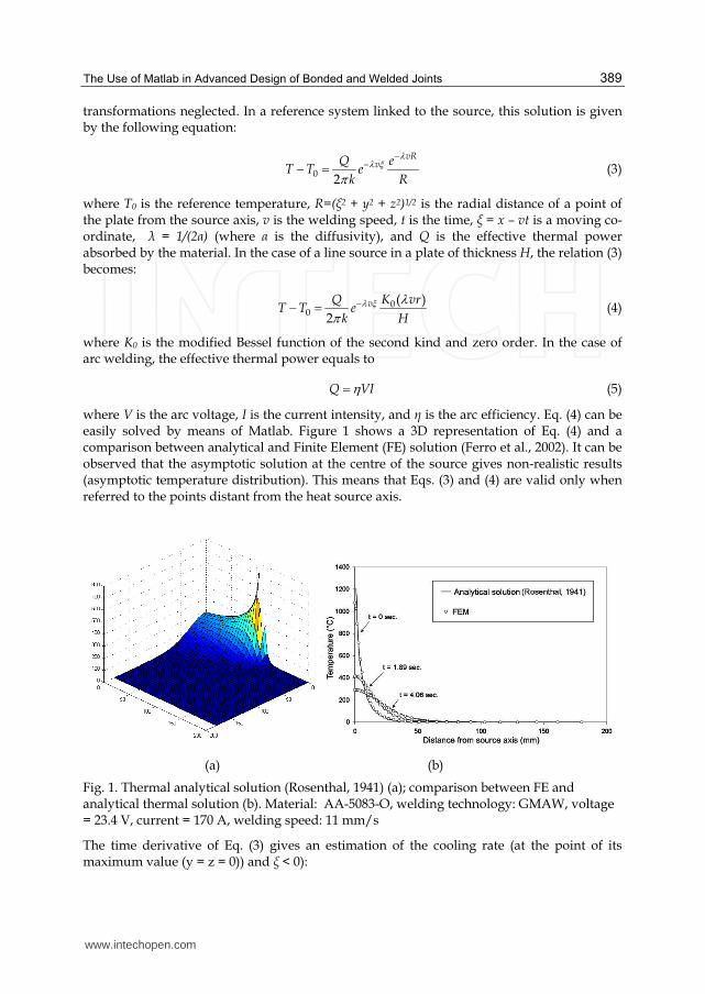
where V is the arc voltage, I is the current intensity, and η is the arc efficiency. Eq. (4) can be easily solved by means of Matlab. Figure 1 shows a 3D representation of Eq. (4) and a comparison between analytical and Finite Element (FE) solution (Ferro et al., 2002). It can be observed that the asymptotic solution at the centre of the source gives non-realistic results (asymptotic temperature distribution). This means that Eqs. (3) and (4) are valid only when referred to the points distant from the heat source axis.

(a) (b)

Fig. 1. Thermal analytical solution (Rosenthal, 1941) (a); comparison between FE and analytical thermal solution (b). Material: AA-5083-O, welding technology: GMAW, voltage = 23.4 V, current = 170 A, welding speed: 11 mm/s

The time derivative of Eq. (3) gives an estimation of the cooling rate (at the point of its maximum value (y = z = 0)) and ξ < 0):

www.intechopen.com


390

20

2( )

T kv T T

t Q

(6)

Equation (6) shows the strong (squared) dependence of the pre-heating (T-T0) on cooling rate compared to the others process parameters such as welding speed and power. It means that pre-heating is the most efficient variable, in the case of steel welding, which can be modified in order to obtain sound welds. Knowing the critical cooling rate of the steel, it is possible to estimate, by using Eq. (6), the pre-heating value needed to avoid a martensitic microstructure in the weld bead.

2.2 Temperature distribution in Friction Stir Welding

The main difficulty in the formulation of any model for friction stir welding (FSW) is due to the high coupling between thermal and mechanical phenomena. Thus, in Ferro et al. (2010), the solution of the formulated equation was obtained by a numerical routine written in Matlab code under the simplification of isothermal condition at the matrix/tool interface. The formulation of heat flow is based on Rosethal’s solution, while the heat generation is described as a surface flux, which depends on the variation of the shear yield stress with temperature.

2.2.1 Governing equations

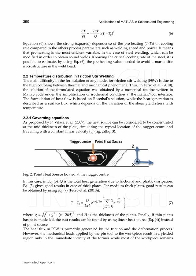
As proposed by P. Vilaca et al. (2007), the heat source can be considered to be concentrated at the mid-thickness of the plate, simulating the typical location of the nugget centre and travelling with a constant linear velocity (v) (fig. 2)(Eq. 3).

Fig. 2. Point Heat Source located at the nugget centre.

In this case, in Eq. (3), Q is the total heat generation due to frictional and plastic dissipation. Eq. (3) gives good results in case of thick plates. For medium thick plates, good results can be obtained by using eq. (7) (Ferro et al. (2010)):

/2 20

1

2

ivi r

v

ii

QT T e e

k r

(7)

where 2 2 2( 2 )ir y z iH and H is the thickness of the plates. Finally, if thin plates

has to be modelled, the best results can be found by using linear heat source (Eq. (4)) instead

of point-source. The heat flux in FSW is primarily generated by the friction and the deformation process. However, the mechanical loads applied by the pin tool to the workpiece result in a yielded region only in the immediate vicinity of the former while most of the workpiece remains

www.intechopen.com


391

unyielded. Thus, idealizing the localized yielded region as being coincident with the tool surface and treating the workpiece as a rigid matter, the heat generation originated from both frictional and plastic dissipation, can be modelled via surface flux boundary condition at tool/matrix interface (Schmidt et al., 2008, Perivilli et al., 2008). It can be found (Ferro et al., 2010) that the heat generated is expressed by the formula:

3 3 3 20

2 *1 ( )(1 tan ) 3

3workpiece sh p p p p

M

TQ R R R R H

T (8)

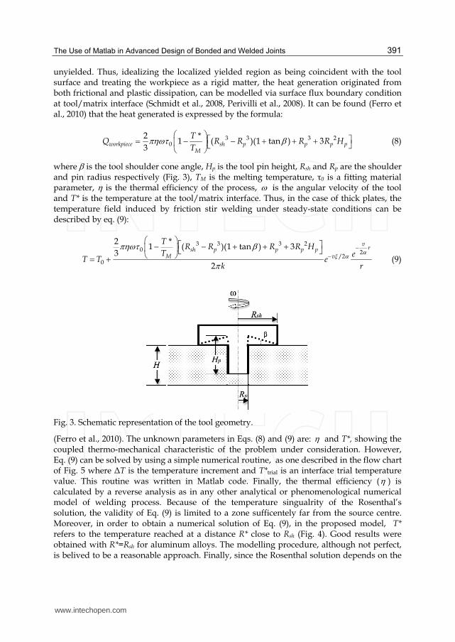
where is the tool shoulder cone angle, Hp is the tool pin height, Rsh and Rp are the shoulder and pin radius respectively (Fig. 3), TM is the melting temperature, τ0 is a fitting material parameter, is the thermal efficiency of the process, is the angular velocity of the tool and T* is the temperature at the tool/matrix interface. Thus, in the case of thick plates, the temperature field induced by friction stir welding under steady-state conditions can be described by eq. (9):

3 3 3 20 2

/20

2 *1 ( )(1 tan ) 3

3

2

vrsh p p p p

M v

TR R R R H

T eT T e

k r

(9)

Fig. 3. Schematic representation of the tool geometry.

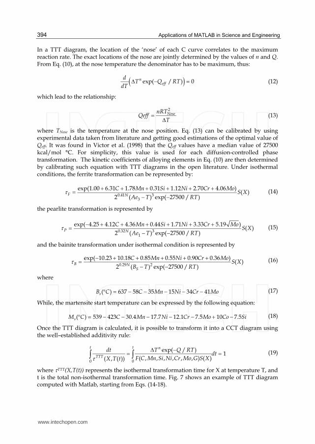
(Ferro et al., 2010). The unknown parameters in Eqs. (8) and (9) are: and T*, showing the coupled thermo-mechanical characteristic of the problem under consideration. However, Eq. (9) can be solved by using a simple numerical routine, as one described in the flow chart of Fig. 5 where ΔT is the temperature increment and T*trial is an interface trial temperature value. This routine was written in Matlab code. Finally, the thermal efficiency ( ) is calculated by a reverse analysis as in any other analytical or phenomenological numerical model of welding process. Because of the temperature singualrity of the Rosenthal’s solution, the validity of Eq. (9) is limited to a zone sufficentely far from the source centre. Moreover, in order to obtain a numerical solution of Eq. (9), in the proposed model, T* refers to the temperature reached at a distance R* close to Rsh (Fig. 4). Good results were obtained with R*=Rsh for aluminum alloys. The modelling procedure, although not perfect, is belived to be a reasonable approach. Finally, since the Rosenthal solution depends on the

www.intechopen.com


392

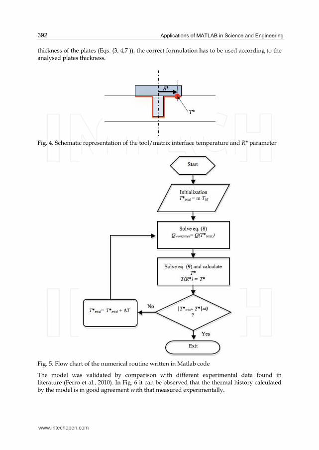
thickness of the plates (Eqs. (3, 4,7 )), the correct formulation has to be used according to the analysed plates thickness.

Fig. 4. Schematic representation of the tool/matrix interface temperature and R* parameter

Fig. 5. Flow chart of the numerical routine written in Matlab code

The model was validated by comparison with different experimental data found in literature (Ferro et al., 2010). In Fig. 6 it can be observed that the thermal history calculated by the model is in good agreement with that measured experimentally.

www.intechopen.com


393

Fig. 6. Variation of transient temperature at different locations of the thermocouples for

rotational speed of 240 rpm, welding speed 3.32 mm/s (=0.5, R*=Rsh, 0=51.56 MPa) (lines: Semi-analytical solution, symbols: test data (Chao et al. (2003)))

2.3 TTT and CCT diagrams calculation

The Time-Temperature Transformation (TTT) and Continuous Cooling Transformation (CCT) diagrams are useful tools in thermomechanical processing of steels. Such diagrams depend on a so great number of variables that it is impossible to produce enough experimental diagrams for generalised use. For this reason, significant work has been undertaken to develop models that can calculate TTT and CCT diagrams for steels. Starting from Kirkaldy’s model, the general formulation of TTT diagrams is described by the relation (10):

( , , , , , , )

( , ) ( )exp( / )n

eff

F C Mn Si Ni Cr Mo NX T S X

T Q RT (10)

where is the time needed to transform X volume fraction of austenite, T is the temperature, F is a function of steel composition (expressed in wt%), N is the prior austenite grain size

(ASTM number), T is the undercooling, Qeff is the effective activation energy for diffusion, and the exponent n is an empirical constant, determined by the effective diffusion mechanism; n = 2 for volume and n = 3 for boundary diffusion. S(X) is the reaction rate term, which approximates the sigmoidal effect of phase transformation. In the work of Victor Li at al. (1998), S(X) is expressed as follows:

0.4(1 ) 0.4

0

( )(1 )

X

X X

dXS X

X X (11)

www.intechopen.com


394

In a TTT diagram, the location of the ‘nose’ of each C curve correlates to the maximum reaction rate. The exact locations of the nose are jointly determined by the values of n and Q. From Eq. (10), at the nose temperature the denominator has to be maximum, thus:

exp( / ) 0neff

dT Q RT

dT (12)

which lead to the relationship:

2NosenRT

QeffT

(13)

where TNose is the temperature at the nose position. Eq. (13) can be calibrated by using experimental data taken from literature and getting good estimations of the optimal value of Qeff. It was found in Victor et al. (1998) that the Qeff values have a median value of 27500 kcal/mol °C. For simplicity, this value is used for each diffusion-controlled phase transformation. The kinetic coefficients of alloying elements in Eq. (10) are then determined by calibrating such equation with TTT diagrams in the open literature. Under isothermal conditions, the ferrite transformation can be represented by:

0.41 3

3

exp(1.00 6.31 1.78 0.31 1.12 2.70 4.06 )( )

2 ( ) exp( 27500 / )F N

C Mn Si Ni Cr MoS X

Ae T RT (14)

the pearlite transformation is represented by

0.32 3

1

exp( 4.25 4.12 4.36 0.44 1.71 3.33 5.19 )( )

2 ( ) exp( 27500 / )P N

C Mn Si Ni Cr MoS X

Ae T RT (15)

and the bainite transformation under isothermal condition is represented by

0.29 2

exp( 10.23 10.18 0.85 0.55 0.90 0.36 )( )

2 ( ) exp( 27500 / )B N

S

C Mn Ni Cr MoS X

B T RT (16)

where

( ) 637 58 35 15 34 41sB C C Mn Ni Cr Mo (17)

While, the martensite start temperature can be expressed by the following equation:

( ) 539 423 30.4 17.7 12.1 7.5 10 7.5sM C C Mn Ni Cr Mo Co Si (18)

Once the TTT diagram is calculated, it is possible to transform it into a CCT diagram using the well–established additivity rule:

0 0

exp( / )1

( , , , , , , ) ( )( , ( ))

t t n

TTT

dt T Q RTdt

F C Mn Si Ni Cr Mo G S XX T t (19)

where TTT(X,T(t)) represents the isothermal transformation time for X at temperature T, and t is the total non-isothermal transformation time. Fig. 7 shows an example of TTT diagram computed with Matlab, starting from Eqs. (14-18).

www.intechopen.com


395

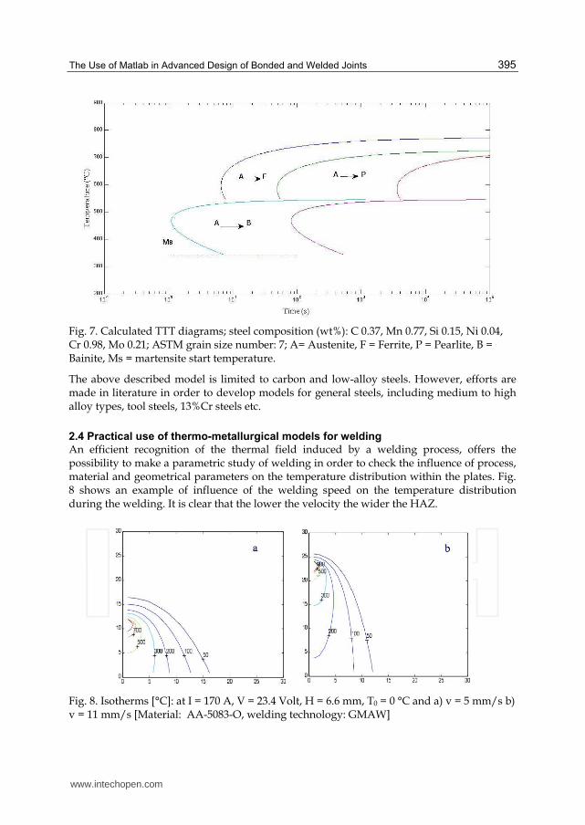
Fig. 7. Calculated TTT diagrams; steel composition (wt%): C 0.37, Mn 0.77, Si 0.15, Ni 0.04, Cr 0.98, Mo 0.21; ASTM grain size number: 7; A= Austenite, F = Ferrite, P = Pearlite, B = Bainite, Ms = martensite start temperature.

The above described model is limited to carbon and low-alloy steels. However, efforts are made in literature in order to develop models for general steels, including medium to high alloy types, tool steels, 13%Cr steels etc.

2.4 Practical use of thermo-metallurgical models for welding

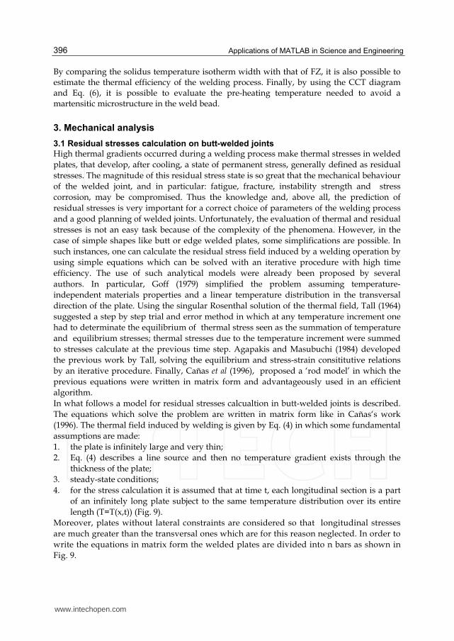
An efficient recognition of the thermal field induced by a welding process, offers the possibility to make a parametric study of welding in order to check the influence of process, material and geometrical parameters on the temperature distribution within the plates. Fig. 8 shows an example of influence of the welding speed on the temperature distribution during the welding. It is clear that the lower the velocity the wider the HAZ.

Fig. 8. Isotherms [°C]: at I = 170 A, V = 23.4 Volt, H = 6.6 mm, T0 = 0 °C and a) v = 5 mm/s b) v = 11 mm/s [Material: AA-5083-O, welding technology: GMAW]

www.intechopen.com


396

By comparing the solidus temperature isotherm width with that of FZ, it is also possible to estimate the thermal efficiency of the welding process. Finally, by using the CCT diagram and Eq. (6), it is possible to evaluate the pre-heating temperature needed to avoid a martensitic microstructure in the weld bead.

3. Mechanical analysis

3.1 Residual stresses calculation on butt-welded joints

High thermal gradients occurred during a welding process make thermal stresses in welded

plates, that develop, after cooling, a state of permanent stress, generally defined as residual

stresses. The magnitude of this residual stress state is so great that the mechanical behaviour

of the welded joint, and in particular: fatigue, fracture, instability strength and stress

corrosion, may be compromised. Thus the knowledge and, above all, the prediction of

residual stresses is very important for a correct choice of parameters of the welding process

and a good planning of welded joints. Unfortunately, the evaluation of thermal and residual

stresses is not an easy task because of the complexity of the phenomena. However, in the

case of simple shapes like butt or edge welded plates, some simplifications are possible. In

such instances, one can calculate the residual stress field induced by a welding operation by

using simple equations which can be solved with an iterative procedure with high time

efficiency. The use of such analytical models were already been proposed by several

authors. In particular, Goff (1979) simplified the problem assuming temperature-

independent materials properties and a linear temperature distribution in the transversal

direction of the plate. Using the singular Rosenthal solution of the thermal field, Tall (1964)

suggested a step by step trial and error method in which at any temperature increment one

had to determinate the equilibrium of thermal stress seen as the summation of temperature

and equilibrium stresses; thermal stresses due to the temperature increment were summed

to stresses calculate at the previous time step. Agapakis and Masubuchi (1984) developed

the previous work by Tall, solving the equilibrium and stress-strain consititutive relations

by an iterative procedure. Finally, Cañas et al (1996), proposed a ‘rod model’ in which the

previous equations were written in matrix form and advantageously used in an efficient

algorithm.

In what follows a model for residual stresses calcualtion in butt-welded joints is described.

The equations which solve the problem are written in matrix form like in Cañas‘s work

(1996). The thermal field induced by welding is given by Eq. (4) in which some fundamental

assumptions are made:

1. the plate is infinitely large and very thin;

2. Eq. (4) describes a line source and then no temperature gradient exists through the

thickness of the plate;

3. steady-state conditions;

4. for the stress calculation it is assumed that at time t, each longitudinal section is a part

of an infinitely long plate subject to the same temperature distribution over its entire

length (T=T(x,t)) (Fig. 9).

Moreover, plates without lateral constraints are considered so that longitudinal stresses

are much greater than the transversal ones which are for this reason neglected. In order to

write the equations in matrix form the welded plates are divided into n bars as shown in

Fig. 9.

www.intechopen.com


397

L

x

y

2B

b The seam

di

Nyi

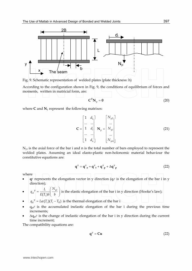
Fig. 9. Schematic representation of welded plates (plate thickness: h)

According to the configuration shown in Fig. 9, the conditions of equilibrium of forces and moments, written in matricial form, are:

y TC N 0 (20)

where C and Ny represent the following matrixes:

11

... ...

1

... ...

1

i

n

d

d

d

C

1

...

...

y

yiy

yn

N

N

N

N (21)

Nyi is the axial force of the bar i and n is the total number of bars employed to represent the

welded plates. Assuming an ideal elasto-plastic non-holonomic material behaviour the

constitutive equations are:

y y y y y e t p pq q q q q (22)

where

qy represents the elongation vector in y direction (qiy is the elongation of the bar i in y direction);

( )

yiyei

i

NLq

E T h b

is the elastic elongation of the bar i in y direction (Hooke’s law);

0( )( )yti i iq L T T T is the thermal elongation of the bar i

qpiy is the accumulated inelastic elongation of the bar i during the previous time increments;

qpiy is the change of inelastic elongation of the bar i in y direction during the current time increment;

The compatibility equations are:

y q Cu (22)

www.intechopen.com


398

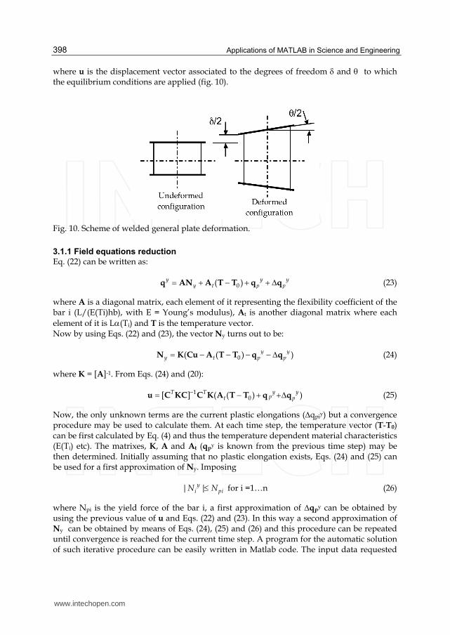
where u is the displacement vector associated to the degrees of freedom and to which the equilibrium conditions are applied (fig. 10).

Fig. 10. Scheme of welded general plate deformation.

3.1.1 Field equations reduction

Eq. (22) can be written as:

0( )y y yy t p p q AN A T T q q (23)

where A is a diagonal matrix, each element of it representing the flexibility coefficient of the bar i (L/(E(Ti)hb), with E = Young’s modulus), At is another diagonal matrix where each

element of it is L(Ti) and T is the temperature vector. Now by using Eqs. (22) and (23), the vector Ny turns out to be:

0( ( ) )y yy t p p N K Cu A T T q q (24)

where K = [A]-1. From Eqs. (24) and (20):

10[ ] ( ( ) )y yT T

pt p u C KC C K A T T q q (25)

Now, the only unknown terms are the current plastic elongations (qpiy) but a convergence procedure may be used to calculate them. At each time step, the temperature vector (T-T0) can be first calculated by Eq. (4) and thus the temperature dependent material characteristics (E(Ti) etc). The matrixes, K, A and At (qp

y is known from the previous time step) may be then determined. Initially assuming that no plastic elongation exists, Eqs. (24) and (25) can be used for a first approximation of Ny. Imposing

| |yi piN N for i =1…n (26)

where Npi is the yield force of the bar i, a first approximation of qpy can be obtained by

using the previous value of u and Eqs. (22) and (23). In this way a second approximation of Ny can be obtained by means of Eqs. (24), (25) and (26) and this procedure can be repeated until convergence is reached for the current time step. A program for the automatic solution of such iterative procedure can be easily written in Matlab code. The input data requested

www.intechopen.com


399

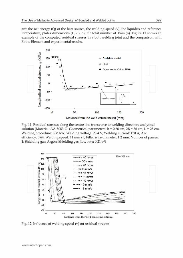
are: the net energy (Q) of the heat source, the welding speed (v), the liquidus and reference temperature, plates dimensions (L, 2B, h), the total number of bars (n). Figure 11 shows an example of the computed residual stresses in a butt welding joint and the comparison with Finite Element and experimental results.

Fig. 11. Residual stresses along the centre line transverse to welding direction: analytical solution (Material: AA-5083-O. Geometrical parameters: h = 0.66 cm, 2B = 36 cm, L = 25 cm. Welding procedure: GMAW; Welding voltage: 23.4 V; Welding current: 170 A; Arc efficiency: 0.64; Welding speed: 11 mm s-1; Filler wire diameter: 1.2 mm; Number of passes: 1; Shielding gas: Argon; Shielding gas flow rate: 0.21 s-1)

Fig. 12. Influence of welding speed (v) on residual stresses

www.intechopen.com


400

The analytical model is very cost-effective in its computer implementation. Therefore, it allows for a series of parametric analyses to be performed and the relative importance of various parameters to be easily investigated. Fig. 12 shows, for example, the influence of welding speed on the residual stress field in welded plate without lateral constraints. Because of the heat input reduction, a decrement of plastic zone when welding speed increases is found.

3.2 Asymptotic stress distributions in welded and bonded joints

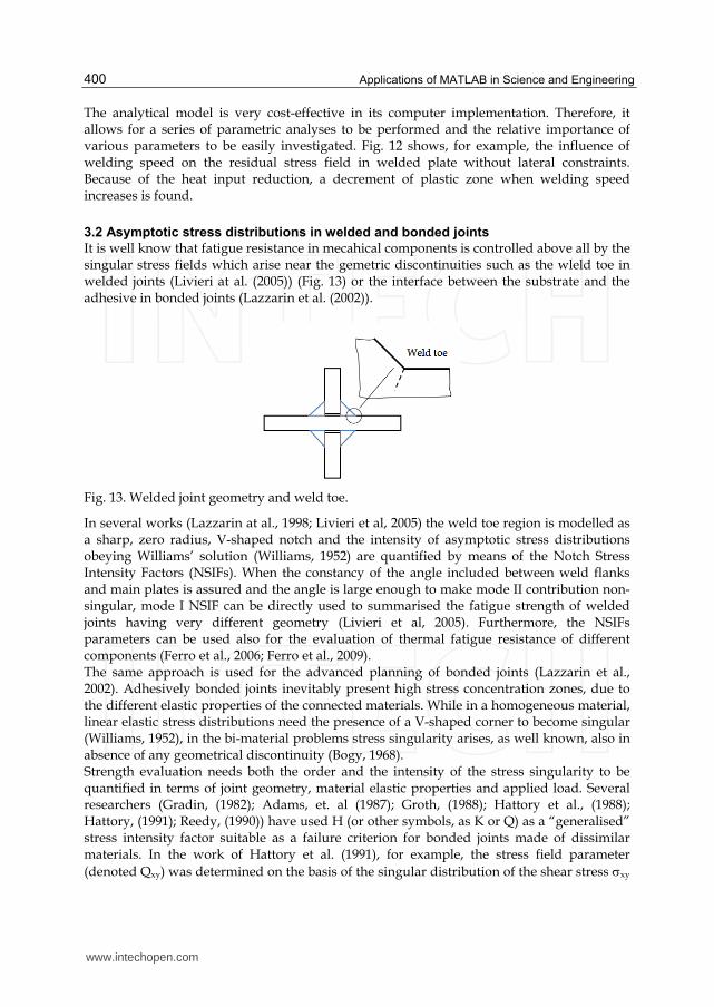
It is well know that fatigue resistance in mecahical components is controlled above all by the singular stress fields which arise near the gemetric discontinuities such as the wleld toe in welded joints (Livieri at al. (2005)) (Fig. 13) or the interface between the substrate and the adhesive in bonded joints (Lazzarin et al. (2002)).

Fig. 13. Welded joint geometry and weld toe.

In several works (Lazzarin at al., 1998; Livieri et al, 2005) the weld toe region is modelled as a sharp, zero radius, V-shaped notch and the intensity of asymptotic stress distributions obeying Williams’ solution (Williams, 1952) are quantified by means of the Notch Stress Intensity Factors (NSIFs). When the constancy of the angle included between weld flanks and main plates is assured and the angle is large enough to make mode II contribution non-singular, mode I NSIF can be directly used to summarised the fatigue strength of welded joints having very different geometry (Livieri et al, 2005). Furthermore, the NSIFs parameters can be used also for the evaluation of thermal fatigue resistance of different components (Ferro et al., 2006; Ferro et al., 2009). The same approach is used for the advanced planning of bonded joints (Lazzarin et al., 2002). Adhesively bonded joints inevitably present high stress concentration zones, due to the different elastic properties of the connected materials. While in a homogeneous material, linear elastic stress distributions need the presence of a V-shaped corner to become singular (Williams, 1952), in the bi-material problems stress singularity arises, as well known, also in absence of any geometrical discontinuity (Bogy, 1968). Strength evaluation needs both the order and the intensity of the stress singularity to be quantified in terms of joint geometry, material elastic properties and applied load. Several researchers (Gradin, (1982); Adams, et. al (1987); Groth, (1988); Hattory et al., (1988); Hattory, (1991); Reedy, (1990)) have used H (or other symbols, as K or Q) as a “generalised” stress intensity factor suitable as a failure criterion for bonded joints made of dissimilar materials. In the work of Hattory et al. (1991), for example, the stress field parameter

(denoted Qxy) was determined on the basis of the singular distribution of the shear stress xy

www.intechopen.com


401

present at the interface of Large Scale Integrated (LSI) electronic circuit devices subjected to thermal stresses. The critical value of Qxy (able to provoke delamination in the components)

was plotted against the order of the singularity . Different values of were obtained by using various configurations of epoxy/Fe-Ni blocks bonded together. Previously, Qxy had already been used by Gradin (1982), by introducing his static criterion for brittle edge-bonded bi-material bodies. More recently, a H-based approach has also been used by Lefrebvre and Dillard (1999) to predict the fatigue crack initiation in epoxy-aluminium wedge specimens, in a manner similar to the use of the Notch Stress Intensity Factors in welded structures (Lazzarin at al., 1998). In view of the use of stress fields and stress intensity factors to predict the fatigue life at crack initiation, it is important to have the complete and correct description of the stress field very near to the apex. A method for the evaluation of the singular stress field in bonded joints of different geometry is presented and solved with Matlab; the stress distributions are represented by a two terms stress expansion, under the hypothesis that both first and second terms are in the variable separable form and therefore each term can be represented by a radial component with unknown exponent (eigenvalue) and an angular function also unknown. The resulting analytical formulation of the stress distributions can be given as:

(0) (1)0 1( , ) ( ) ( )s t

ij ij ijr H r f H r f (27)

The method is based on the numerical solution of the ordinary differential equation (ODE) system that, under the hypothesis of plane strain state, derives from the equilibrium and compatibility equations of a bonded joint or, more generally, of a bi-material body. The capability of the formulation to account for the actual elastic properties of the substrates, allows us to obtain the accurate description of the stress field even in the case of joints made of materials with comparable elastic properties. It is worth noting that the “stress function approach” (where the formulation is completed analytically and the resulting set of equations is solved numerically) has already been used successfully by many researchers, mainly engaged with in-plane crack and notch problems in materials obeying a power-hardening law (Lazzarin et al., 2001).

3.2.1 Analytical frame

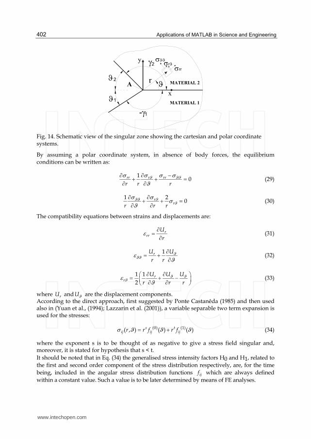
Let us consider the problem of the elastic equilibrium in a bi-material joint, in presence of a V-shaped corner with an opening angle 1 2( ) as shown in Figure 14. Both materials are thought of as homogeneous and isotropic and subjected to plane strain conditions. Under linear elastic hypothesis, strains components are:

1 m m

ij ij kk ijm mE E

(28)

where subscript m =1, 2 denotes the material, ij is the Kroneker delta, and summation convention is used for repeated indexes. In writing the problem of the elastic equilibrium we can now consider separately the two materials and later find the solution by applying the boundary conditions at the traction free surfaces and at the interface. It is possible therefore to omit, from now on and until not differently evidenced, the material subscript m, being the equations valid for the both substrates.

www.intechopen.com


402

-

A

MATERIAL 1

x

r y

MATERIAL 2

rr

1

1

2

2 r

Fig. 14. Schematic view of the singular zone showing the cartesian and polar coordinate systems.

By assuming a polar coordinate system, in absence of body forces, the equilibrium conditions can be written as:

1

0rr r rr

r r r

(29)

1 2

0rr

r r r

(30)

The compatibility equations between strains and displacements are:

rrr

U

r (31)

1rU U

r r

(32)

1 1

2r

r

U U U

r r r

(33)

where rU andU are the displacement components. According to the direct approach, first suggested by Ponte Castanêda (1985) and then used also in (Yuan et al., (1994); Lazzarin et al. (2001)), a variable separable two term expansion is used for the stresses:

(0) (1)( , ) ( ) ( )s tij ij ijr r f r f (34)

where the exponent s is to be thought of as negative to give a stress field singular and, moreover, it is stated for hypothesis that s < t.

It should be noted that in Eq. (34) the generalised stress intensity factors H0 and H1, related to

the first and second order component of the stress distribution respectively, are, for the time

being, included in the angular stress distribution functions ijf which are always defined

within a constant value. Such a value is to be later determined by means of FE analyses.

www.intechopen.com


403

Substitution of Eq. (34) into (28) gives the following expressions for strains:

(0) (1)( , ) ( ) ( )s tij ij ijr r r (35)

where:

(0) (0) (0)1( ) ( ) ( )ij ij kk ijf f

E E

(36)

(1) (1) (1)1( ) ( ) ( )ij ij kk ijf f

E E

(37)

The relevant displacement components are:

(0) (1)1 1( , ) ( ) ( )s ti i iU r r U r U (38)

As it is known, the exponents depend on the combination of the material elastic properties. In the close neighbourhood of the singularity point (r which tends towards zero), the first term of the stress distribution becomes dominant. Let us consider, therefore, in the stress and strain expansions only the leading-order term, s being the relevant exponent. Substitution of Eqs. (34), (35) and (38) into Eqs. (29) to (33), together with the plane strain conditions

(0)(0) (0)( ) [ ( ) ( )]z rrf f f (39)

gives the following system:

(0) (0) (0),

(0) (0),

(0) (0) (0) (0)

(0) (0) (0) (0) (0),

( 1) ( ) ( ) ( ) 0

( ) ( 2) ( ) 0

1( 1) ( ) ( ) [ ( )(1 ) ( )(1 )] 0

1( ) ( ) ( ) [ ( )(1 ) ( )(1 )] 0

1

2

rr r

r

r rr rr

r rr

s f f f

f s f

s U f f fE E

U U f f fE E

(0) (0) (0),

1[ ( ) ( )] ( ) 0r rU sU f

E

(40)

where ,f and ,U mean f

and

U

, respectively.

The boundary conditions, at the traction free surface and at the interface between the two materials, are as follows:

.1 .21 2

.1 .21 2

.1 .2

.1 .2

.1 .2

.1 .2

( ) ( ) 0

( ) ( ) 0

(0) (0)

(0) (0)

(0) (0)

(0) (0)

mat mat

mat matr r

mat mat

mat matr r

mat mat

mat matr r

f f

f f

f f

f f

U U

U U

(41)

www.intechopen.com


404

By using the third equation of the system 40 to eliminate the (0)( )rU , the problem gives

four differential equations for the material 1 and four differential equations for the material

2. The angular stress and displacement components f , rf , rrf and U are the

eigenfunctions of the problem, which will be given to within a constant value, as the

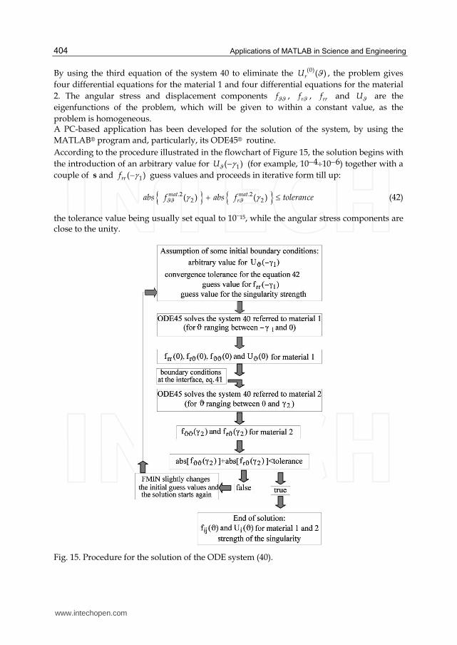
problem is homogeneous. A PC-based application has been developed for the solution of the system, by using the

MATLAB® program and, particularly, its ODE45® routine.

According to the procedure illustrated in the flowchart of Figure 15, the solution begins with

the introduction of an arbitrary value for 1( )U (for example, 104106) together with a

couple of s and 1( )rrf guess values and proceeds in iterative form till up:

.2 .22 2( ) ( )mat mat

rabs f abs f tolerance (42)

the tolerance value being usually set equal to 1015, while the angular stress components are close to the unity.

Fig. 15. Procedure for the solution of the ODE system (40).

www.intechopen.com


405

To obtain the solution, the MATLAB® FMIN® function can, automatically, slightly modify the guessed values and restart the procedure. In cases where the convergence is not reached within a certain number of iterations, substantially different guessed values have to be chosen and the solution to be restarted. As the stress expansion is in a variable separable form, and due also to the hypothesis of linear elastic behaviour, if we consider, in the stress and strain expansions, only the second term and the associated t order exponent, the system solution provides the related eigenfunctions. Once the solution of the ODE system (40) is completed, the eigenfunctions, that is the angular stress and displacement distribution functions, and also the singularity strength for both the leading and second order term and for material 1 and 2 are available.

For the complete description of the stress field, according to Eq. (27), the generalised stress intensity factors H0 and H1 have still to be determined and this can be done through FE analyses, by minimising, for a generic * direction (arbitrarily chosen on the steel side), the following error function:

,max

(0) (1)0 1 0 1

,min

. .( , ) .[ ( *) ( *) ( )]r

s tij ij ij

r

E F H H abs H r f H r f FE (43)

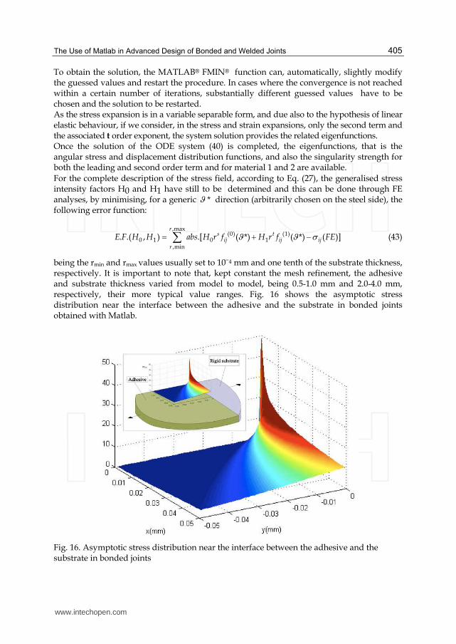
being the rmin and rmax values usually set to 104 mm and one tenth of the substrate thickness, respectively. It is important to note that, kept constant the mesh refinement, the adhesive and substrate thickness varied from model to model, being 0.5-1.0 mm and 2.0-4.0 mm, respectively, their more typical value ranges. Fig. 16 shows the asymptotic stress distribution near the interface between the adhesive and the substrate in bonded joints obtained with Matlab.

Fig. 16. Asymptotic stress distribution near the interface between the adhesive and the substrate in bonded joints

www.intechopen.com


406

4. Conclusion

Different thermal and mechanical models solved with Matlab were presented which are very useful for a good planning of welded or bonded joints. About the thermal and residual stress fields predictions, some limitations are due to the geometry and material properties, but, compared to the finite element models, they are more user friendly and more efficient in terms of computational time; thus they can be used both for a rapid check of the thermal and stress filed induced by welding and for a parametric study of the process. The ‘stress field approach’ for fatigue resistance prediction of welded and bonded joints was also presented. In particular, an analytical method for the description of the singular stress distributions on bonded joints of different geometry has been developed. The stress distributions near the singularity have been assumed to be represented by a power series expansion in the variable separable form as usually done in the elastoplastic analyses; under the further hypothesis of plane strain state, applying the equilibrium and compatibility conditions results in a ordinary differential equation system, which has been numerically solved by using a “shooting” technique.

5. References

Rosenthal, D. (1941). Mathematical theory of heat distribution during welding and cutting, Weld. J. Res. Supp., 20, 220s.

Rosenthal, D. and Shamerber, H. (1938). Thermal study of Arc Welding. Experimental Verification of Theoretical Formulas. The Welding Journal Res. Suppl., Vol. 17, No. 4, pp. 2-8.

Ferro, P., Tiziani, A., Bonollo, F. (2002). Analisi numerica e teorica del campo di tensioni residue indotte dal processo di saldatura in piastre in lega leggera. Proceedings of XXXI AIAS Conference, Parma, Italy, September 18-21, 2002.

Ferro, P., Bonollo, F. (2010). A Semianalytical Thermal Model for Friction Stir Welding. Metallurgical and Material transaction A, Vol. 41A, pp. 440 -449.

Vilaca, P., Quintino, L., dos Santos, J.F., Zettler, R., Sheikhi, S. (2007). Quality assessment of friction stir welding joints via an analytical thermal model, iSTIR’. Materials Science and Engineering A, 445-446 pp. 501-508.

Victor Li, M., Niebuhr, V., Meekisho, L., Atteridge, G. (1998). A Computational Model for the Prediction of Steel Hardenability. Metallurgical and Materials Transactions B, Vol. 29B, pp. 661-672.

Schmidt, H.B.,. Hattel. J.H. (2008). Thermal modelling of friction stir welding’. Scripta Materialia, Vol 58, pp. 332-337.

Perivilli, S., Peddieson, J., Cui, J. (2008). Simplified Two-Dimensional Analytical Model for Friction Stir Welding heat Transfer. Journal of Heat Transfer, Vol. 130, pp 1-9.

Goff, R. F. D. Porter. (1979). A Simplified Analysis of the Residual Longitudinal Stresses and Strains Due to the Gas-Cutting and Welding of Thin Steel Plate. Int. J. Mech. Sci. Vol. 21, pp. 287-300.

Chao, Y.J., Qi, X., Tang., W. (2003). Heat Transfer in Friction Stir welding - experimental and Numerical Studies. Transaction of ASME, Vol 125, pp 138-145.

Tall, L. (1964). Residual Stresses in Welded plates – a Theoretical Study. Weld. J. Res. Supp. Vol. 43, 10s.

www.intechopen.com


407

Agapakis, J. E., Masubuchi, K. (1984). Analytical Modeling of Thermal Stress Relieving in Stainless and High Strength Steel Weldments”, Weld J. Res. Suopp. 36, 187s.

Cañas, J., Picòn, R., París, F., Blazquez A., Marín, J. C. (1996). A Simplified Numerical Analysis of Residual Stresses in Aluminium Welded Plates, Computers & Structures, Vol. 58 No. 1, pp. 59-69

Cañas, J., Picòn, R., París F., Del Río, J. I. (1996). A One-Dimensional Model for the Prediction of Residual Stress and its Relief in Welded Plates, Int. J. Mech. Sci. Vol. 38, pp. 735-751.

Lazzarin, P., Quaresimin, M., Ferro, P. (2002). A two terms stress function approach to evaluate stress distributions in bonded joints of different geometry, Journal of Strain Analysis for Engineering Design, Vol 37 No 5, pp. 385-398

Livieri, P., Lazzarin, P. (2005). Fatigue strength of steel and aluminium welded joints based on generalised stress intensity factors and local energy values, International Journal of Fracture, Vol. 133, pp. 247-276

Williams, M.L. (1952). Stress singularities resulting from various boundary conditions in angular corners of plates in exstension. Journal of Applied Mechanics, Vol 19, pp. 526-528

Bogy, D.B. (1968) Edge-bonded dissimilar orthogonal elastic wedges under normal and shear loading. J. Appl. Mechanics, Vol 35, pp. 460-466

Gradin, P.A. (1982). A fracture criterion for edge-bonded bi-material bodies. J. Composite Mater., Vol. 16, pp. 448-456

Adams, R.D. and Harris, J.A., (1987). The influence of local geometry on the strength of adhesive joints. Int. J. Adhes. Adhes., Vol. 7, pp. 69-80

Groth, H.L. (1988). Stress singularities and fracture at interface corners in bonded joints, Int. J. Adhes. Adhes., , Vol. 8, pp. 107-113

Hattory, T., Sakata, S., Hatsuda, T. and Murakami, G. (1988). A stress singularity parameter approach for evaluating adhesives strength. JSME Int. J., Series I, Vol. 31, pp. 718-723

Hattory T. (1991). A stress singularity parameter approach for evaluating the adhesives strength of single lap joint. JSME. Int. J., Series I, Vol. 34 , pp. 326-331

Reedy, Jr E.D. (1990). Intensity of stress singularity at the interface-corner between a bonded elastic and rigid layer. Engng Fracture Mechanics, Vol. 36, pp. 575-583

Lefebvre, D.R. and Dillard, D.A. (1999). A stress singularity approach for the prediction of fatigue crack initiation in adhesive bonds. PART 1: Theory. J. Adhesion, Vol. 70, pp. 119-138

Lazzarin, P. and Tovo, R. (1998). A Notch Stress Intensity Factor Approach to the Stress Analysis of Welds. Fatigue Fracture Engng Mater. Structs, Vol. 21, pp. 1089-1104

Lazzarin, P., Zambardi, R. and Livieri, P. (2001). Plastic Notch Stress Intensity Factors for Large V-Shaped Notches under Mixed Load Conditions. Int. J. Fracture, Vol. 107, pp. 361-377

Ponte Castañeda, P. (1985). Asymptotic fields in steady crack growth with linear strain-hardening. J. Mech. Phys. Solids, Vol. 35, pp. 227-268

Yuan, H. and Lin, G. (1994). Analysis of elastoplastic sharp notches. Int. J. Fracture, , Vol. 67, pp. 187-216

www.intechopen.com


408

Ferro, P., Petrone, N. (2009). Asymptotic Thermal and Residual Stress Distributions due to Transient thermal Loads. Fatigue and Fracture of Engineering Materials and Structures. Vol. 32, pp. 936-948

Ferro, P., Berto, F., Lazzarin, P. (2006). Generalized stress intensity factors due to steady and transient thermal loads with applications to welded joints. Fatigue Fract. Engng. Mater. Struct, Vol. 29, pp. 440-453.

www.intechopen.com

Applications of MATLAB in Science and EngineeringEdited by Prof. Tadeusz Michalowski

ISBN 978-953-307-708-6Hard cover, 510 pagesPublisher InTechPublished online 09, September, 2011Published in print edition September, 2011

InTech EuropeUniversity Campus STeP Ri Slavka Krautzeka 83/A 51000 Rijeka, Croatia Phone: +385 (51) 770 447 Fax: +385 (51) 686 166www.intechopen.com

InTech ChinaUnit 405, Office Block, Hotel Equatorial Shanghai No.65, Yan An Road (West), Shanghai, 200040, China

Phone: +86-21-62489820 Fax: +86-21-62489821

The book consists of 24 chapters illustrating a wide range of areas where MATLAB tools are applied. Theseareas include mathematics, physics, chemistry and chemical engineering, mechanical engineering, biological(molecular biology) and medical sciences, communication and control systems, digital signal, image and videoprocessing, system modeling and simulation. Many interesting problems have been included throughout thebook, and its contents will be beneficial for students and professionals in wide areas of interest.

How to referenceIn order to correctly reference this scholarly work, feel free to copy and paste the following:

Paolo Ferro (2011). The Use of Matlab in Advanced Design of Bonded and Welded Joints, Applications ofMATLAB in Science and Engineering, Prof. Tadeusz Michalowski (Ed.), ISBN: 978-953-307-708-6, InTech,Available from: http://www.intechopen.com/books/applications-of-matlab-in-science-and-engineering/the-use-of-matlab-in-advanced-design-of-bonded-and-welded-joints

matlab

Documents

welding source

analytical models

mechanical models

welding thermal problem

welding speed

development of new models

innovative welding

semianalyitical models