matlab - arizona state universityplato.asu.edu/mat420/files/chap1.pdf · 2 introduction to matlab...
TRANSCRIPT

MATLABr Laboratory Manual
with SIMULINKr examples
Bruno D. Welfert
to accompany
Fundamentals of
Differential EquationsSixth Edition
and
Fundamentals of
Differential Equationsand
Boundary Value ProblemsFourth Edition
Nagle Saff Snider
i

MATLABr and SIMULINKr are registered trademarks of The MathWorks, Inc.MAPLEr is a registered trademark of Waterloo Maple, Inc.
c©2003 B. Welfert
ii

Contents
Preface v
1 Introduction to MATLAB 1
The MATLAB Environment . . . . . . . . . . . . . . . . . . . . . . . . . . . . . . . . . . . . . . 1Basics and Help . . . . . . . . . . . . . . . . . . . . . . . . . . . . . . . . . . . . . . . . . . . . . 1Plotting with MATLAB . . . . . . . . . . . . . . . . . . . . . . . . . . . . . . . . . . . . . . . . 5Scripts and Functions . . . . . . . . . . . . . . . . . . . . . . . . . . . . . . . . . . . . . . . . . 10Matrices and Linear Algebra . . . . . . . . . . . . . . . . . . . . . . . . . . . . . . . . . . . . . 12MATLAB Programming and Debugging . . . . . . . . . . . . . . . . . . . . . . . . . . . . . . . 15Exercises . . . . . . . . . . . . . . . . . . . . . . . . . . . . . . . . . . . . . . . . . . . . . . . . 17
2 Ordinary Differential Equations
with MATLAB 19
Numerical Differentiation and Solution of the IVP . . . . . . . . . . . . . . . . . . . . . . . . . 19Direction Fields and Graphical Solutions . . . . . . . . . . . . . . . . . . . . . . . . . . . . . . . 20First-Order Scalar IVP . . . . . . . . . . . . . . . . . . . . . . . . . . . . . . . . . . . . . . . . . 24
Basic ode45 Usage . . . . . . . . . . . . . . . . . . . . . . . . . . . . . . . . . . . . . . . . 24Error Plot, Improving the Accuracy . . . . . . . . . . . . . . . . . . . . . . . . . . . . . . 26Integration . . . . . . . . . . . . . . . . . . . . . . . . . . . . . . . . . . . . . . . . . . . . 29Parameter-Dependent ODE . . . . . . . . . . . . . . . . . . . . . . . . . . . . . . . . . . . 29
Higher-Order and Systems of IVPs . . . . . . . . . . . . . . . . . . . . . . . . . . . . . . . . . . 31
3 MATLAB sessions 35
Laboratory 1: First-Order Differential Equations, Graphical Analysis . . . . . . . . . . . . . . . 38Direction fields . . . . . . . . . . . . . . . . . . . . . . . . . . . . . . . . . . . . . . . . . . 38Additional Problems . . . . . . . . . . . . . . . . . . . . . . . . . . . . . . . . . . . . . . . 41
Laboratory 2: Numerical Solutions (Euler, Improved Euler) for Scalar Equations . . . . . . . . 42Euler’s Method . . . . . . . . . . . . . . . . . . . . . . . . . . . . . . . . . . . . . . . . . . 42Improved Euler’s Method . . . . . . . . . . . . . . . . . . . . . . . . . . . . . . . . . . . . 46Additional Problems . . . . . . . . . . . . . . . . . . . . . . . . . . . . . . . . . . . . . . . 47
Laboratory 3: Solution Sensitivity . . . . . . . . . . . . . . . . . . . . . . . . . . . . . . . . . . 49Dependence of IVP Solution on IC . . . . . . . . . . . . . . . . . . . . . . . . . . . . . . . 50Existence and Uniqueness . . . . . . . . . . . . . . . . . . . . . . . . . . . . . . . . . . . . 52Additional Problems . . . . . . . . . . . . . . . . . . . . . . . . . . . . . . . . . . . . . . . 54
Laboratory 4: Picard Iteration . . . . . . . . . . . . . . . . . . . . . . . . . . . . . . . . . . . . 56Picard iteration . . . . . . . . . . . . . . . . . . . . . . . . . . . . . . . . . . . . . . . . . . 56Numerical Picard Iteration . . . . . . . . . . . . . . . . . . . . . . . . . . . . . . . . . . . 57Additional problems . . . . . . . . . . . . . . . . . . . . . . . . . . . . . . . . . . . . . . . 59
Laboratory 5: Applications of First-Order Differential Equations . . . . . . . . . . . . . . . . . 61Population Growth . . . . . . . . . . . . . . . . . . . . . . . . . . . . . . . . . . . . . . . . 61Problems . . . . . . . . . . . . . . . . . . . . . . . . . . . . . . . . . . . . . . . . . . . . . 62Other Models, Parameter Estimation . . . . . . . . . . . . . . . . . . . . . . . . . . . . . . 63
Laboratory 6: Further Applications of First-Order Differential Equations . . . . . . . . . . . . 66
iii
The Snowplow Problem . . . . . . . . . . . . . . . . . . . . . . . . . . . . . . . . . . . . . 66Aircraft Guidance . . . . . . . . . . . . . . . . . . . . . . . . . . . . . . . . . . . . . . . . 67Heating and Cooling of Buildings . . . . . . . . . . . . . . . . . . . . . . . . . . . . . . . . 68
Laboratory 7: Implementing Higher-Order Differential Equations . . . . . . . . . . . . . . . . . 72Reducing a Higher-Order ODE . . . . . . . . . . . . . . . . . . . . . . . . . . . . . . . . . 72MATLAB Implementation . . . . . . . . . . . . . . . . . . . . . . . . . . . . . . . . . . . . 72Additional Considerations . . . . . . . . . . . . . . . . . . . . . . . . . . . . . . . . . . . . 73
Laboratory 8: The Mass-Spring System . . . . . . . . . . . . . . . . . . . . . . . . . . . . . . . 78Mass-Spring System without Damping . . . . . . . . . . . . . . . . . . . . . . . . . . . . . 78Mass-Spring System with Damping . . . . . . . . . . . . . . . . . . . . . . . . . . . . . . . 80The GUI spring.m . . . . . . . . . . . . . . . . . . . . . . . . . . . . . . . . . . . . . . . . 81
Laboratory 9: The Pendulum . . . . . . . . . . . . . . . . . . . . . . . . . . . . . . . . . . . . . 83The Undamped Case . . . . . . . . . . . . . . . . . . . . . . . . . . . . . . . . . . . . . . . 83The Linearized Case . . . . . . . . . . . . . . . . . . . . . . . . . . . . . . . . . . . . . . . 86With Damping Present . . . . . . . . . . . . . . . . . . . . . . . . . . . . . . . . . . . . . . 86The Poe pendulum . . . . . . . . . . . . . . . . . . . . . . . . . . . . . . . . . . . . . . . . 88
Laboratory 10: Forced Equations and Resonance . . . . . . . . . . . . . . . . . . . . . . . . . . 89The Amplitude of Forced Oscillations . . . . . . . . . . . . . . . . . . . . . . . . . . . . . 89Resonance . . . . . . . . . . . . . . . . . . . . . . . . . . . . . . . . . . . . . . . . . . . . . 92Beats . . . . . . . . . . . . . . . . . . . . . . . . . . . . . . . . . . . . . . . . . . . . . . . 92Additional Problem . . . . . . . . . . . . . . . . . . . . . . . . . . . . . . . . . . . . . . . 93
Laboratory 11: Analytical and Graphical Analysis of Systems . . . . . . . . . . . . . . . . . . . 94An Example . . . . . . . . . . . . . . . . . . . . . . . . . . . . . . . . . . . . . . . . . . . . 94Multiple Eigenvalue . . . . . . . . . . . . . . . . . . . . . . . . . . . . . . . . . . . . . . . 97Complex Eigenvalues . . . . . . . . . . . . . . . . . . . . . . . . . . . . . . . . . . . . . . . 99Additional Problems . . . . . . . . . . . . . . . . . . . . . . . . . . . . . . . . . . . . . . . 101
Laboratory 12: Additional Numerical Techniques . . . . . . . . . . . . . . . . . . . . . . . . . . 102Taylor and Runge-Kutta Methods . . . . . . . . . . . . . . . . . . . . . . . . . . . . . . . 102Application to a System of ODEs . . . . . . . . . . . . . . . . . . . . . . . . . . . . . . . . 104Additional Problems . . . . . . . . . . . . . . . . . . . . . . . . . . . . . . . . . . . . . . . 105
Laboratory 13: Introduction to SIMULINK . . . . . . . . . . . . . . . . . . . . . . . . . . . . . 107An Example SIMULINK Model: spring1.mdl . . . . . . . . . . . . . . . . . . . . . . . . 107Building a Mass-Spring SIMULINK Model . . . . . . . . . . . . . . . . . . . . . . . . . . . 109Alternate SIMULINK Implementations . . . . . . . . . . . . . . . . . . . . . . . . . . . . . 111
Laboratory 14: Laplace transform, application to linear IVPs . . . . . . . . . . . . . . . . . . . 114Laplace transform . . . . . . . . . . . . . . . . . . . . . . . . . . . . . . . . . . . . . . . . 114Inverse Laplace transform . . . . . . . . . . . . . . . . . . . . . . . . . . . . . . . . . . . . 116Applications to the solution of IVPs . . . . . . . . . . . . . . . . . . . . . . . . . . . . . . 122
4 Additional Project Descriptions 127
Note to the Instructor: Group Projects . . . . . . . . . . . . . . . . . . . . . . . . . . . . . . . 127P1. Design your Own Project . . . . . . . . . . . . . . . . . . . . . . . . . . . . . . . . . . . . 129P2. The ODE of World-Class Sprint . . . . . . . . . . . . . . . . . . . . . . . . . . . . . . . . . 130P3. Consecutive Reactions for Batch Reactors . . . . . . . . . . . . . . . . . . . . . . . . . . . 132P4. Normal T-Cells . . . . . . . . . . . . . . . . . . . . . . . . . . . . . . . . . . . . . . . . . . 133P5. T-Cells in the Presence of HIV . . . . . . . . . . . . . . . . . . . . . . . . . . . . . . . . . 135P6. Design of an Electrical Network . . . . . . . . . . . . . . . . . . . . . . . . . . . . . . . . . 138P7. The Dynamics of Love . . . . . . . . . . . . . . . . . . . . . . . . . . . . . . . . . . . . . . 140P8. Hypergeometric Functions . . . . . . . . . . . . . . . . . . . . . . . . . . . . . . . . . . . . 142
5 References 145
Bibliography . . . . . . . . . . . . . . . . . . . . . . . . . . . . . . . . . . . . . . . . . . . . . . 145Appendix: MATLAB Quick Reference . . . . . . . . . . . . . . . . . . . . . . . . . . . . . . . . 146
iv

Preface
This manual is designed to accompany the new edition of Fundamentals of Differential Equations (andBoundary Value Problems) by Nagle, Saff and Snider and its format was mostly inspired by the com-panion Maple Technology Manual written by Kenneth Pothoven. The usefulness of this manual shouldhowever extend well beyond this specific association.
MATLAB is a “high-performance language for technical computing which now integrates computa-tion, visualization, and programming in an easy-to-use environment where problems and solutions areexpressed in familiar mathematical notation” (excerpt from The MathWorks website). MATLAB standsfor MATrix LABoratory and was originally written to provide easy access to matrix software developedby the LINPACK and EISPACK projects.
MATLAB has become “a standard instructional tool for introductory and advanced courses in Math-ematics, Engineering, and Science. In industry, MATLAB is now the tool of choice for high-productivityresearch, development, and analysis.” This manual explores the use of MATLAB in solving differentialequations and visualizing and interpreting their solutions. The main objectives are:
1. familiarize students with basic MATLAB programming to solve differential equations of varyingcomplexity,
2. provide a platform for testing and experimenting with fundamental aspects of numerical compu-tations of solutions of differential equations, and
3. present simple ways to visualize the numerical solutions.
The use of the MATLAB Symbolic Toolbox was limited to short examples with the functions laplace
and ilaplace in Laboratory 14. Custom functions which do not use this toolbox were used to illustratethe numerical evaluation of these transforms. An introduction to SIMULINK is given in Laboratory13. SIMULINK provides a tool for building and testing models using the power of MATLAB withoutrequiring the specific knowledge of the MATLAB language necessary to implement these models.
The versions of MATLAB and SIMULINK used are MATLAB 6.0 and SIMULINK 4, respectively(Release 12). Changes made in Release 13 (the last available as of June 2003) have no bearing on thecontent of this manual.
This manual includes two introductory chapters on MATLAB: the first one shows how to startMATLAB and how to use and organize basic commands. It explains in particular how to save groupsof commands in a file, which is important in creating programs that implement a whole problem. Thesecond chapter is more specific to differential equations. It goes over how to implement initial valueproblems and how to visualize the solution(s), using complete examples. Students are encouraged toread these two chapters and execute the listed commands before moving to the laboratory section.
Following is the main part of this manual which comprises 14 laboratory sessions covering generalnumerical implementation and execution issues when solving differential equations. This is done inthe context of specific applications, many of which are similar to the ones presented in the MAPLEcompanion manual. As noted there, these laboratory sessions vary in length and difficulty, and areincluded to demonstrate the use of MATLAB as well as to involve students through exploratory exercises.Instructors should feel free to modify the sessions at their own discretion.
Additional project ideas are included in the last chapter. These projects represent different kindsof applications from various disciplines including chemical, civil, electrical, and mechanical engineering,including most of the projects ideas (sometimes radically changed though) from the Maple companion
v

book by K. Pothoven. A project idea coming from an actual project carried out in a DifferentialEquations with MATLAB course I have been teaching is also included. Each project is briefly describedat the beginning of the chapter.
As always when using a computer software the user should be careful to respect the correct syntaxneeded for proper execution. In my experience this represents the most significant hurdle for studentswithout any background in computer programming. This manual is designed to help in this regard, byincluding simple examples and templates that students can conveniently use as a starting point for theirown applications. Ultimately, some effort must however be made by the student in order to assimilate theproper ways of using MATLAB by practicing with the examples included in this manual and adaptingthem to new problems.
The manuscript was prepared using the LATEX document preparation system. PostScript figureswere created using MATLAB or converted from screen capture in Jpeg format using jpeg2ps 1.9 byThomas Herz. The cover picture was created from the original book cover of the new (sixth) edition of theNagle, Saff and Snider text with a mask based on the MATLAB logo using PhotoShop. The MATLABgraphical user interfaces dfield6.m and pplane6.m by John Polking and David Arnold were briefly usedin this manual. A detailed description is available in their book Ordinary Differential Equations UsingMATLAB. Many of the MATLAB and SIMULINK programs used in this manual are available online athttp://math.asu.edu/∼bdw/PUBLIC. Partial funding for this work was provided by a grant to improveundergraduate education from the College of Liberal Arts and Sciences at Arizona State University.
Bruno WelfertArizona State UniversitySeptember 2003
vi

Chapter 1
Introduction to MATLAB
MATLAB is a computer software commonly used in both education and industry to solve a wide rangeof problems.
This chapter provides a brief introduction to MATLAB, and the tools and functions that help youto work with MATLAB variables and files.
The MATLAB Environment
⋆ To start MATLAB double-click on the MATLAB shortcut icon or type matlab & at theprompt (Unix). The MATLAB desktop opens.
On the right side of the desktop you find the Command Window, where commands are entered atthe prompt >>.
On the left side you will generally find the Launch Pad and Workspace windows, and the CommandHistory and Current Directory windows. For all practical purposes we have in mind I recommend closingthe Launch Pad, Workspace, and Command History windows, if opened. It is convenient to keep theCurrent Directory window opened to check for files you create and use in the Command Window.
Note that windows within the MATLAB desktop can be resized by dragging the separator bar(s). Atypical MATLAB desktop is shown in Fig. 1.1.⋆ To exit MATLAB do one of the following:
• Click on the close box at the top right of the MATLAB Desktop.
• Select File > Exit from the desktop File menu.
• Type quit or exit at the Command Window prompt >>.
Basics And Help
Commands are entered in the Command Window.⋆ Basic operations are +, -, *, and /. The sequence
>> a=2; b=3; a+b, a*b,
ans =
5
ans =
1

2 Introduction to MATLAB
Figure 1.1: A typical MATLAB desktop
6
defines variables a and b and assigns values 2 and 3, respectively, then computes the sum a+b and productab. Each command ends with , (output is visible) or ; (output is suppressed). The last command on aline does not require a ,.⋆ Standard functions can be invoked using their usual mathematical notations. For example
>> theta=pi/5;
>> cos(theta)^2+sin(theta)^2
ans =
1
verifies the trigonometric identity sin2 θ + cos2 θ = 1 for θ = π
5 . A list of elementary math functions canbe obtained by typing help elfun in the Command window:
>> help elfun
Elementary math functions.

Introduction to MATLAB 3
Trigonometric.
sin - Sine.
sinh - Hyperbolic sine.
asin - Inverse sine.
asinh - Inverse hyperbolic sine.
cos - Cosine.
cosh - Hyperbolic cosine.
acos - Inverse cosine.
acosh - Inverse hyperbolic cosine.
tan - Tangent.
tanh - Hyperbolic tangent.
atan - Inverse tangent.
atan2 - Four quadrant inverse tangent.
atanh - Inverse hyperbolic tangent.
sec - Secant.
sech - Hyperbolic secant.
asec - Inverse secant.
asech - Inverse hyperbolic secant.
csc - Cosecant.
csch - Hyperbolic cosecant.
acsc - Inverse cosecant.
acsch - Inverse hyperbolic cosecant.
cot - Cotangent.
coth - Hyperbolic cotangent.
acot - Inverse cotangent.
acoth - Inverse hyperbolic cotangent.
Exponential.
exp - Exponential.
log - Natural logarithm.
log10 - Common (base 10) logarithm.
log2 - Base 2 logarithm and dissect floating point number.
pow2 - Base 2 power and scale floating point number.
sqrt - Square root.
nextpow2 - Next higher power of 2.
Complex.
abs - Absolute value.
angle - Phase angle.
complex - Construct complex data from real and imaginary parts.
conj - Complex conjugate.
imag - Complex imaginary part.
real - Complex real part.
unwrap - Unwrap phase angle.
isreal - True for real array.
cplxpair - Sort numbers into complex conjugate pairs.
Rounding and remainder.
fix - Round towards zero.
floor - Round towards minus infinity.
ceil - Round towards plus infinity.
round - Round towards nearest integer.
mod - Modulus (signed remainder after division).

4 Introduction to MATLAB
rem - Remainder after division.
sign - Signum.
⋆ To obtain a description of the use of a particular function type help followed by the name of thefunction. For example
>> help cosh
COSH Hyperbolic cosine.
COSH(X) is the hyperbolic cosine of the elements of X.
⋆ To get a list of other groups of MATLAB programs already available enter help:
>> help
HELP topics:
matlab\general - General purpose commands.
matlab\ops - Operators and special characters.
matlab\lang - Programming language constructs.
matlab\elmat - Elementary matrices and matrix manipulation.
matlab\elfun - Elementary math functions.
matlab\specfun - Specialized math functions.
matlab\matfun - Matrix functions - numerical linear algebra.
matlab\datafun - Data analysis and Fourier transforms.
matlab\audio - Audio support.
matlab\polyfun - Interpolation and polynomials.
matlab\funfun - Function functions and ODE solvers.
matlab\sparfun - Sparse matrices.
matlab\graph2d - Two dimensional graphs.
matlab\graph3d - Three dimensional graphs.
matlab\specgraph - Specialized graphs.
matlab\graphics - Handle Graphics.
matlab\uitools - Graphical user interface tools.
matlab\strfun - Character strings.
matlab\iofun - File input/output.
matlab\timefun - Time and dates.
matlab\datatypes - Data types and structures.
matlab\verctrl - Version control.
matlab\winfun - Windows Operating System Interface Files (DDE/ActiveX)
matlab\demos - Examples and demonstrations.
toolbox\local - Preferences.
matlabR12\work - (No table of contents file)
For more help on directory/topic, type "help topic".
⋆ Another way to obtain help is through the desktop Help menu, Help > MATLAB Help, or byconnecting to the Mathworks web site at www.mathworks.com.⋆ MATLAB is case-sensitive. For example
>> theta=1e-3, Theta=2e-5; ratio=theta/Theta
theta =

Introduction to MATLAB 5
0.0010
Theta =
2.0000e-005
ratio =
50
⋆ The quantities Inf (∞) and NaN (Not a Number) also appear frequently. Compare
>> c=1/0
Warning: Divide by zero.
c =
Inf
with
>> d=0/0
Warning: Divide by zero.
d =
NaN
Plotting with MATLAB
⋆ To plot a function you have to create two arrays (vectors): one containing the abscissae, the other thecorresponding function values. Both arrays should have the same length. For example, consider plottingthe function
y = f(x) =x2 − sin(πx) + ex
x − 1
for 0 ≤ x ≤ 2. First choose a sample of x values in this interval:
>> x=[0,.1,.2,.3,.4,.5,.6,.7,.8,.9,1, ...
1.1,1.2,1.3,1.4,1.5,1.6,1.7,1.8,1.9,2]
x =
Columns 1 through 4
0 0.1000 0.2000 0.3000
Columns 5 through 8
0.4000 0.5000 0.6000 0.7000
Columns 9 through 12

6 Introduction to MATLAB
0.8000 0.9000 1.0000 1.1000
Columns 13 through 16
1.2000 1.3000 1.4000 1.5000
Columns 17 through 20
1.6000 1.7000 1.8000 1.9000
Column 21
2.0000
or simply
>> x=0:.1:2
x =
Columns 1 through 4
0 0.1000 0.2000 0.3000
Columns 5 through 8
0.4000 0.5000 0.6000 0.7000
Columns 9 through 12
0.8000 0.9000 1.0000 1.1000
Columns 13 through 16
1.2000 1.3000 1.4000 1.5000
Columns 17 through 20
1.6000 1.7000 1.8000 1.9000
Column 21
2.0000
Try also
>> x=linspace(0,2,21)
x =
Columns 1 through 4
0 0.1000 0.2000 0.3000

Introduction to MATLAB 7
Columns 5 through 8
0.4000 0.5000 0.6000 0.7000
Columns 9 through 12
0.8000 0.9000 1.0000 1.1000
Columns 13 through 16
1.2000 1.3000 1.4000 1.5000
Columns 17 through 20
1.6000 1.7000 1.8000 1.9000
Column 21
2.0000
⋆ Note that an ellipsis ... was used to continue a command too long to fit in a single line.⋆ The output for x can be suppressed (by adding ; at the end of the command) or condensed by enteringformat compact:
>> format compact
>> x
Columns 1 through 4
0 0.1000 0.2000 0.3000
Columns 5 through 8
0.4000 0.5000 0.6000 0.7000
Columns 9 through 12
0.8000 0.9000 1.0000 1.1000
Columns 13 through 16
1.2000 1.3000 1.4000 1.5000
Columns 17 through 20
1.6000 1.7000 1.8000 1.9000
Column 21
2.0000
From now on we shall use such format for all output.To evaluate the function f simultaneously at all the values contained in x, type
>> y=(x.^2-sin(pi.*x)+exp(x))./(x-1)
Warning: Divide by zero.
y =
Columns 1 through 4
-1.0000 -0.8957 -0.8420 -0.9012
Columns 5 through 8
-1.1679 -1.7974 -3.0777 -5.6491
Columns 9 through 12
-11.3888 -29.6059 Inf 45.2318
Columns 13 through 16
26.7395 20.5610 17.4156 15.4634
Columns 17 through 20
8 Introduction to MATLAB
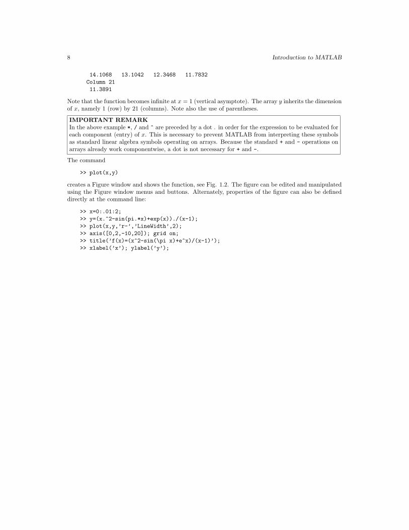
14.1068 13.1042 12.3468 11.7832
Column 21
11.3891
Note that the function becomes infinite at x = 1 (vertical asymptote). The array y inherits the dimensionof x, namely 1 (row) by 21 (columns). Note also the use of parentheses.
IMPORTANT REMARK
In the above example *, / and ^ are preceded by a dot . in order for the expression to be evaluated foreach component (entry) of x. This is necessary to prevent MATLAB from interpreting these symbolsas standard linear algebra symbols operating on arrays. Because the standard + and - operations onarrays already work componentwise, a dot is not necessary for + and -.
The command
>> plot(x,y)
creates a Figure window and shows the function, see Fig. 1.2. The figure can be edited and manipulatedusing the Figure window menus and buttons. Alternately, properties of the figure can also be defineddirectly at the command line:
>> x=0:.01:2;
>> y=(x.^2-sin(pi.*x)+exp(x))./(x-1);
>> plot(x,y,’r-’,’LineWidth’,2);
>> axis([0,2,-10,20]); grid on;
>> title(’f(x)=(x^2-sin(\pi x)+e^x)/(x-1)’);
>> xlabel(’x’); ylabel(’y’);

Introduction to MATLAB 9
Figure 1.2: A Figure window
0 0.2 0.4 0.6 0.8 1 1.2 1.4 1.6 1.8 2−10
−5
0
5
10
15
20
x
y
f(x)=(x2−sin(π x)+ex)/(x−1)
Figure 1.3: The function y = f(x) = x2−sin(πx)+e
x
x−1 .
10 Introduction to MATLAB
The number of x-values has been increased for a smoother curve (what is the new size of x?). Thecurve now appears wider and in red. The range of x and y values has been reset (always a good ideain the presence of vertical asymptotes). A title and labels have been added. The resulting new plot isshown in Fig. 1.3. For more options type help plot in the Command Window.
Scripts and Functions
⋆ Files containing MATLAB commands are called m-files and have a .m extension. They are two types:
1. A script is simply a collection of MATLAB commands gathered in a single file. The value of thedata created in a script is still available in the Command Window after execution.
2. A function is similar to a script, but can accept and return arguments. Unless otherwise specifiedany variable inside a function is local to the function and not available in the Workspace. Afunction invariably starts with the command
function output = function_name(input)
and should contain one or several commands defining the output.
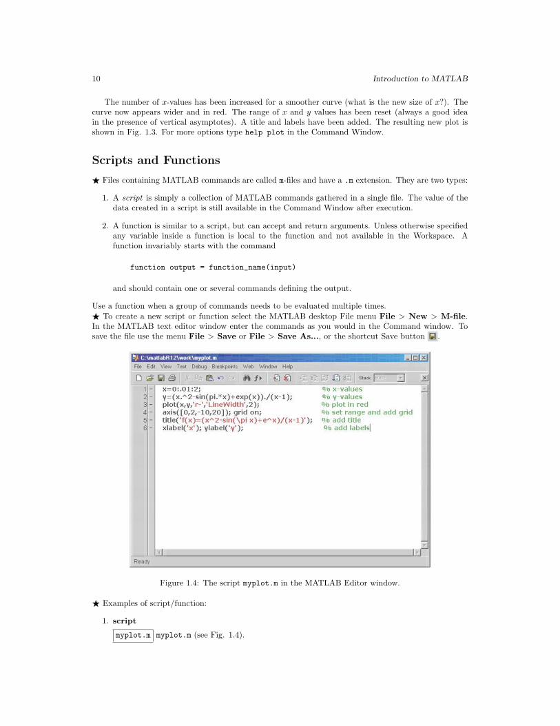
Use a function when a group of commands needs to be evaluated multiple times.⋆ To create a new script or function select the MATLAB desktop File menu File > New > M-file.In the MATLAB text editor window enter the commands as you would in the Command window. Tosave the file use the menu File > Save or File > Save As..., or the shortcut Save button .
Figure 1.4: The script myplot.m in the MATLAB Editor window.
⋆ Examples of script/function:
1. script
myplot.m myplot.m (see Fig. 1.4).

Introduction to MATLAB 11
x=0:.01:2; % x-values
y=(x.^2-sin(pi.*x)+exp(x))./(x-1); % y-values
plot(x,y,’r-’,’LineWidth’,2); % plot in red
axis([0,2,-10,20]); grid on; % set range and add grid
title(’f(x)=(x^2-sin(\pi x)+e^x)/(x-1)’); % add title
xlabel(’x’); ylabel(’y’); % add labels
2. script+function (two separate files)
myplot2.m (driver script)
x=0:.01:2; % x-values
y=feval(@myfunction,x); % evaluate myfunction at x
plot(x,y,’r-’,’LineWidth’,2); % plot in red
axis([0,2,-10,20]); grid on; % set range and add grid
title(’f(x)=(x^2-sin(\pi x)+e^x)/(x-1)’); % add title
xlabel(’x’); ylabel(’y’); % add labels
myfunction.m (function)
function y=myfunction(x) % defines function
y=(x.^2-sin(pi.*x)+exp(x))./(x-1); % y-values
3. script+function (one single file)
myplot1.m (driver script converted to function + function)
function myplot1
x=0:.01:2; % x-values
y=feval(@myfunction,x); % evaluate myfunction at x
plot(x,y,’r-’,’LineWidth’,2); % plot in red
axis([0,2,-10,20]); grid on; % set range and add grid
title(’f(x)=(x^2-sin(\pi x)+e^x)/(x-1)’); % add title
xlabel(’x’); ylabel(’y’); % add labels
%-----------------------------------------
function y=myfunction(x) % defines function
y=(x.^2-sin(pi.*x)+exp(x))./(x-1); % y-values
In case 2 myfunction.m can be used in any other m-file (just as other predefined MATLAB functions).In case 3 myfunction.m can be used by any other function in the same m-file (myplot1.m) only. Use 3when dealing with a single project and 2 when a function is used by several projects.⋆ It is convenient to add descriptive comments into the script file. Anything appearing after % on anygiven line is understood as a comment (in green in the MATLAB text editor).⋆ To execute a script simply enter its name (without the .m extension) in the Command Window, e.g.,
>> myplot;
in case 1,
>> myplot2;
in case 2 and
>> myplot1;
in case 3 above. The function myfunction can also be used independently if implemented in a separatefile myfunction.m:

12 Introduction to MATLAB
>> x=2; y=myfunction(x)
y =
11.3891
A script can be called from another script or function (in which case it is local to that function).If any modification is made, the script or function can be re-executed by simply retyping the script
or function name in the Command Window (or use the up-arrow on the keyboard to browse throughpast commands).
IMPORTANT REMARK
By default MATLAB saves files in the Current Directory (folder). When entering MATLAB theCurrent Directory is the Work Directory (e.g., C:\matlabR12\work). Make sure the file is savedwhere you want it. To change directory use the Current Directory window or the Current Directorybox on top of the MATLAB desktop.
⋆ A function file can contain a lot more than a simple evaluation of a function f(x) or f(t, y). But insimple cases f(x) or f(t, y) can simply be defined using the inline syntax. Compare
>> ...
>> slope = feval(@f,2,1) % note use of @. Try also slope=f(2,1)
slope =
3
where f.m is the file containing
function dydt = f(t,y)
dydt = t^2-y;
to
>> ...
>> f = inline(’t^2-y’,’t’,’y’)
f =
Inline function:
f(t,y) = t^2-y
>> slope = feval(f,2,1) % note no @
slope =
3
However, an inline function is only available where it is used and not to other functions. It is notrecommended when the function implemented is too complicated or involves too many statements.
Matrices and Linear Algebra
We have used one-dimensional 1× 21 arrays x and y in previous examples. MATLAB can handle higherdimensional arrays. Two-dimensional arrays (matrices) are commonly used in many situations.⋆ Matrices can be constructed in MATLAB in different ways. For example the 3 × 3 matrix A =
8 1 63 5 74 9 2
can be entered as
>> A=[8,1,6;3,5,7;4,9,2]
A =
8 1 6
3 5 7
4 9 2
or

Introduction to MATLAB 13
>> A=[8,1,6;
3,5,7;
4,9,2]
A =
8 1 6
3 5 7
4 9 2
or defined as the concatenation of 3 rows
>> row1=[8,1,6]; row2=[3,5,7]; row3=[4,9,2]; A=[row1;row2;row3]
A =
8 1 6
3 5 7
4 9 2
or 3 columns
>> col1=[8;3;4]; col2=[1;5;9]; col3=[6;7;2]; A=[col1,col2,col2]
A =
8 1 6
3 5 7
4 9 2
Note the use of , and ;. Concatenated rows/columns must have the same length. Larger matrices canbe created from smaller ones in the same way:
>> C=[A,A] % Same as C=[A A]
C =
8 1 6 8 1 6
3 5 7 3 5 7
4 9 2 4 9 2
The matrix C has dimension 3 × 6 (“3 by 6”). On the other hand smaller matrices (submatrices) canbe extracted from any given matrix:
>> A(2,3) % coefficient of A in 2nd row, 3rd column
ans =
7
>> A(1,:) % 1st row of A
ans =
8 1 6
>> A(:,3) % 3rd column of A
ans =
6
7
2
>> A([1,3],[2,3]) % keep coefficients in rows 1 & 3 and columns 2 & 3
ans =
1 6
9 2
⋆ Some matrices are already predefined in MATLAB:
>> I=eye(3) % the Identity matrix
I =
1 0 0
0 1 0

14 Introduction to MATLAB
0 0 1
>> magic(3)
ans =
8 1 6
3 5 7
4 9 2
(what is magic about this matrix?)⋆ Matrices can be manipulated very easily in MATLAB (unlike Maple). Here are sample commandsto exercise with:
>> A=magic(3);
>> B=A’ % transpose of A, i.e, rows of B are columns of A
B =
8 3 4
1 5 9
6 7 2
>> A+B % sum of A and B
ans =
16 4 10
4 10 16
10 16 4
>> A*B % standard linear algebra matrix multiplication
ans =
101 71 53
71 83 71
53 71 101
>> A.*B % coefficientwise multiplication
ans =
64 3 24
3 25 63
24 63 4
Try A*A, A^2, A.^2.⋆ Two MATLAB commands are especially relevant when studying the solution of linear systems ofdifferentials equations:
1. x=A\b determines the solution x = A−1b of the linear system Ax = b. The array b must have asmany rows as the matrix A.
2. [S,D]=eig(A) determines the eigenvectors of A (columns of S) and associated eigenvalues (diagonalcoefficients of D) (note that the eig function has one input and two output arguments).
As an example consider the matrix A =magic(3) again and x =
123
:
>> A=magic(3)
A =
8 1 6
3 5 7
4 9 2
>> x=[1,2,3]’ % same as x=[1;2;3]
x =
1
2
3

Introduction to MATLAB 15
>> b=A*x
b =
28
34
28
>> A\b % this is x!
ans =
1
2
3
>> inv(A)*b % less efficient and accurate
ans =
1.0000
2.0000
3.0000
>> [S,D]=eig(A)
S =
-0.5774 -0.8131 -0.3416
-0.5774 0.4714 -0.4714
-0.5774 0.3416 0.8131
D =
15.0000 0 0
0 4.8990 0
0 0 -4.8990
>> A*S(:,1)-D(1,1)*S(:,1) % test 1st eigenvector-eigenvalue pair
ans =
1.0e-014 *
-0.1776
0.3553
-0.3553
Note the multiplicative factor 10−14 in the last computation. MATLAB performs all operations usingstandard IEEE double precision.
MATLAB Programming and Debugging
Several constructs are used in MATLAB:
1. repetitive loops (fixed number of times)
for <expression>
<list of commands>
end
2. repetitive loops (indefinite number of times)
while <expression>
<list of commands>
end
3. conditional branching
if expression
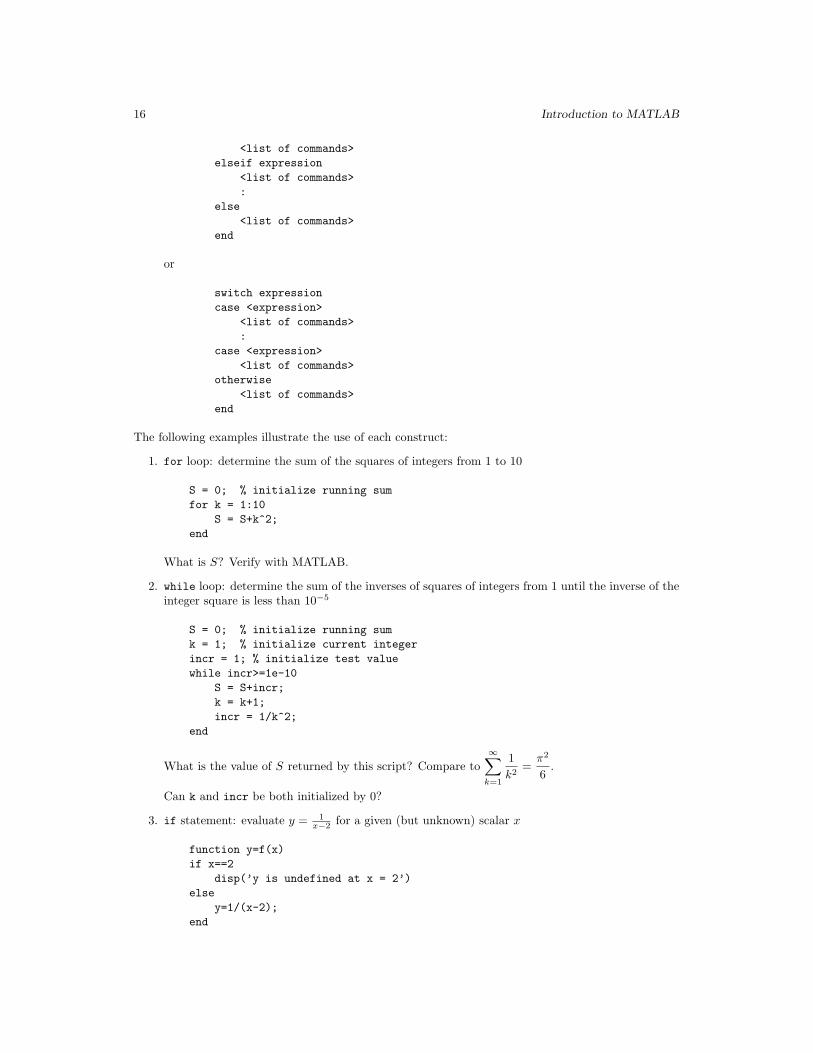
16 Introduction to MATLAB
<list of commands>
elseif expression
<list of commands>
:
else
<list of commands>
end
or
switch expression
case <expression>
<list of commands>
:
case <expression>
<list of commands>
otherwise
<list of commands>
end
The following examples illustrate the use of each construct:
1. for loop: determine the sum of the squares of integers from 1 to 10
S = 0; % initialize running sum
for k = 1:10
S = S+k^2;
end
What is S? Verify with MATLAB.
2. while loop: determine the sum of the inverses of squares of integers from 1 until the inverse of theinteger square is less than 10−5
S = 0; % initialize running sum
k = 1; % initialize current integer
incr = 1; % initialize test value
while incr>=1e-10
S = S+incr;
k = k+1;
incr = 1/k^2;
end
What is the value of S returned by this script? Compare to∞∑
k=1
1
k2=
π2
6.
Can k and incr be both initialized by 0?
3. if statement: evaluate y = 1x−2 for a given (but unknown) scalar x
function y=f(x)
if x==2
disp(’y is undefined at x = 2’)
else
y=1/(x-2);
end

Introduction to MATLAB 17
or with switch statement:
function y=f(x)
switch x
case 2
disp(’y is undefined at x = 2’)
otherwise
y=1/(x-2);
end
Try f(1), f(2). Modify the example to allow for arrays as input.
⋆ Whenever possible all these construct should be avoided and available MATLAB functions used toimprove efficiency. In particular lengthy do loops introduce a substantial overhead. Compare
>> tic; S=0; for k=1:1000000; S=S+1/k^2; end; toc; S
elapsed_time =
1.8830
S =
1.6449
and
>> tic; S=sum(1./(1:1000000).^2); toc; S
elapsed_time =
0.0800
S =
1.6449
⋆ Programming with MATLAB is fairly easy. Still a script or function may not execute properly dueto some programming error. In this case MATLAB returns an error indicating where it stopped andwhy. Most of the time this is sufficient to find out the error and correct it, especially when you get usedto it. But keep in mind that even non-fatal mistakes may eventually force a program to later crash.Debugging tools are available in the MATLAB editor to force the execution to stop at specific placeswithin a script or function(s) and access the current state of available variables.
Write a script or function with the MATLAB editor and position the cursor on a selected line. Thentry the buttons and in the editor window before executing the file in the Command Window.Observe what happens. Check the value of variables. To continue and eventually exit the debugger pressreturn.
Exercises
Now that you have been through the essential elements of MATLAB relevant in this text, a good exerciseis to go through the commands and change values, functions, and problems to familiarize yourself withthe MATLAB syntax and commands introduced in this chapter.